ABCDEFG

UNIVERS ITY OF OULU P.O.B . 7500 F I -90014 UNIVERS ITY OF OULU F INLAND

A C T A U N I V E R S I T A T I S O U L U E N S I S

S E R I E S E D I T O R S

SCIENTIAE RERUM NATURALIUM

HUMANIORA

TECHNICA

MEDICA

SCIENTIAE RERUM SOCIALIUM

SCRIPTA ACADEMICA

OECONOMICA

EDITOR IN CHIEF

PUBLICATIONS EDITOR

Senior Assistant Jorma Arhippainen

Lecturer Santeri Palviainen

Professor Hannu Heusala

Professor Olli Vuolteenaho

Senior Researcher Eila Estola

Director Sinikka Eskelinen

Professor Jari Juga

Professor Olli Vuolteenaho

Publications Editor Kirsti Nurkkala

ISBN 978-951-42-9856-1 (Paperback)ISBN 978-951-42-9857-8 (PDF)ISSN 0355-3213 (Print)ISSN 1796-2226 (Online)

U N I V E R S I TAT I S O U L U E N S I SACTAC

TECHNICA

U N I V E R S I TAT I S O U L U E N S I SACTAC

TECHNICA

OULU 2012

C 423

Johanna Ketonen

EQUALIZATION AND CHANNEL ESTIMATION ALGORITHMS AND IMPLEMENTATIONS FOR CELLULAR MIMO-OFDM DOWNLINK

UNIVERSITY OF OULU GRADUATE SCHOOL;UNIVERSITY OF OULU, FACULTY OF TECHNOLOGY, DEPARTMENT OF COMMUNICATIONS ENGINEERING;CENTRE FOR WIRELESS COMMUNICATIONS;INFOTECH OULU

C 423

ACTA

Johanna Ketonen

C423etukansi.kesken.fm Page 1 Monday, May 28, 2012 12:28 PM

A C T A U N I V E R S I T A T I S O U L U E N S I SC Te c h n i c a 4 2 3

JOHANNA KETONEN

EQUALIZATION AND CHANNEL ESTIMATION ALGORITHMS AND IMPLEMENTATIONS FOR CELLULAR MIMO-OFDM DOWNLINK

Academic dissertation to be presented with the assent ofthe Doctoral Training Committee of Technology andNatural Sciences of the University of Oulu for publicdefence in OP-sali (Auditorium L10), Linnanmaa, on 27June 2012, at 1 p.m.

UNIVERSITY OF OULU, OULU 2012

Copyright © 2012Acta Univ. Oul. C 423, 2012

Supervised byProfessor Markku JunttiDocent Joseph R. Cavallaro

Reviewed byAssociate Professor Mark C. ReedAssociate Professor Ahmed Eltawil

ISBN 978-951-42-9856-1 (Paperback)ISBN 978-951-42-9857-8 (PDF)

ISSN 0355-3213 (Printed)ISSN 1796-2226 (Online)

Cover DesignRaimo Ahonen

JUVENES PRINTTAMPERE 2012

Ketonen, Johanna, Equalization and channel estimation algorithms andimplementations for cellular MIMO-OFDM downlink.University of Oulu Graduate School; University of Oulu, Faculty of Technology, Department ofCommunications Engineering; Centre for Wireless Communications; Infotech Oulu, P.O. Box4500, FI-90014 University of Oulu, FinlandActa Univ. Oul. C 423, 2012Oulu, Finland

Abstract

The aim of the thesis is to develop algorithms and architectures to meet the high data rate, lowcomplexity requirements of the future mobile communication systems. Algorithms, architecturesand implementations for detection, channel estimation and interference mitigation in the multiple-input multiple-output (MIMO) orthogonal frequency division multiplexing (OFDM) receivers arepresented. The performance-complexity trade-offs in different receiver algorithms are studied andthe results can be utilized in receiver design as well as in system design.

Implementation of detectors for spatial multiplexing systems is considered first. The linearminimum mean squared error (LMMSE) and the K-best list sphere detector (LSD) are comparedto the successive interference cancellation (SIC) detector. The SIC algorithm was found toperform worse than the K-best LSD when the MIMO channels are highly correlated. Theperformance difference diminishes when the correlation decreases. With feedback to thetransmitter, the performance difference is even smaller, but the full rank transmissions still requirea more complex detector. A reconfigurable receiver, using a simple or a more complex detector asthe channel conditions change, would achieve the best performance while consuming the leastamount of power in the receiver.

The use of decision directed (DD) channel estimation is also studied. The 3GPP long termevolution (LTE) based pilot structure is used as a benchmark. The performance and complexity ofthe pilot symbol based least-squares (LS) channel estimator, the minimum mean square error(MMSE) filter and the DD space-alternating generalized expectation-maximization (SAGE)algorithm are studied. DD channel estimation and MMSE filtering improve the performance withhigh user velocities, where the pilot symbol density is not sufficient. With DD channel estimation,the pilot overhead can be reduced without any performance degradation by transmitting datainstead of pilot symbols.

Suppression of co-channel interference in the MIMO-OFDM receiver is finally considered.The interference and noise spatial covariance matrix is used in data detection and channelestimation. Interference mitigation is applied for linear and nonlinear detectors. An algorithm toadapt the accuracy of the matrix decomposition and the use of interference suppression isproposed. The adaptive algorithm performs well in all interference scenarios and the powerconsumption of the receiver can be reduced.

Keywords: channel estimation, detection, interference mitigation, LSD, MIMO, OFDM

Ketonen, Johanna, Korjain- ja kanavaestimointialgoritmit ja niiden toteutuksetMIMO-OFDM-solukkoalalinkissä. Oulun yliopiston tutkijakoulu; Oulun yliopisto, Teknillinen tiedekunta, Tietoliikennetekniikanosasto; Centre for Wireless Communications; Infotech Oulu, PL 4500, 90014 Oulun yliopistoActa Univ. Oul. C 423, 2012Oulu

Tiivistelmä

Tämän väitöskirjatyön tavoitteena on kehittää vastaanotinalgoritmeja ja -arkkitehtuureja, jotkatoteuttavat tulevaisuuden langattomien tietoliikennejärjestelmien suuren datanopeuden ja pienenkompleksisuuden tavoitteet. Työssä esitellään algoritmeja, arkkitehtuureja ja toteutuksia ilmai-suun, kanavaestimointiin ja häiriönvaimennukseen monitulo-monilähtötekniikkaa (multiple-input multiple-output, MIMO) ja ortogonaalista taajuusjakokanavointia (orthogonal frequencydivision multiplexing, OFDM) yhdistäviin vastaanottimiin. Algoritmeista saatavaa suorituskyky-hyötyä verrataan vaadittavaan toteutuksen monimutkaisuuteen. Työn tuloksia voidaan hyödyntääsekä vastaanotin- että järjestelmäsuunnittelussa.

Lineaarista pienimmän keskineliövirheen (minimum mean square error, MMSE) ilmaisinta jalistapalloilmaisinta (list sphere detector, LSD) verrataan peräkkäiseen häiriönpoistoilmaisimeen(successive interference cancellation, SIC). SIC-ilmaisimella on huonompi suorituskyky kuinLSD-ilmaisimella radiokanavan ollessa korreloitunut. Korrelaation pienentyessä myös ilmai-simien suorituskykyero pienenee. Erot suorituskyvyissä ovat vähäisiä silloinkin, jos järjestel-mässä on takaisinkytkentäkanava lähettimelle. Tällöinkin korkean signaali-kohinasuhteen olo-suhteissa LSD-ilmaisimet mahdollistavat tilakanavoidun, suuren datanopeuden tiedonsiirron.Radiokanavan muuttuessa uudelleenkonfiguroitava vastaanotin toisi virransäästömahdollisuu-den vaihtelemalla kompleksisen ja yksinkertaisen ilmaisimen välillä.

Kanavaestimointialgoritmeja ja niiden toteutuksia vertaillaan käyttämällä lähtökohtananykyisen mobiilin tiedonsiirtostandardin viitesignaalimallia. Tutkittavat algoritmit perustuvatpienimmän neliösumman (least squares, LS) ja pienimmän keskineliövirheen menetelmään, sekäpäätöstakaisinkytkettyyn (decision directed, DD) kanavaestimointialgoritmiin. DD-kanavaesti-maattori ja MMSE-suodatin parantavat vastaanottimen suorituskykyä korkeissa käyttäjän nope-uksissa, joissa viitesignaaleiden tiheys ei ole riittävä. DD-kanavaestimoinnilla datanopeutta voi-daan nostaa viitesignaaleiden määrää laskemalla vaikuttamatta suorituskykyyn.

Työssä tarkastellaan myös saman kanavan häiriön vaimennusta. Häiriöstä ja kohinasta koos-tuvaa kovarianssimatriisia käytetään ilmaisuun ja kanavaestimointiin. Työssä esitetään adaptiivi-nen algoritmi matriisihajoitelman tarkkuuden ja häiriön vaimennuksen säätämiseen. Algoritmimahdollistaa hyvän suorituskyvyn kaikissa häiriötilanteissa vähentäen samalla virrankulutusta.

Asiasanat: häiriön vaimennus, ilmaisin, kanavaestimointi, LSD, MIMO, OFDM

Preface

The research for this thesis has been carried out at the Centre for Wireless Communica-tions (CWC) and the Department of Communications Engineering, University of Oulu,Finland. First of all, I want to thank Professor Matti Latva-aho, and Lic. Tech. AriPouttu, the directors of CWC during my stay, for giving me the opportunity to work inthe inspiring working environment.

I would also like to thank my supervisor, Professor Markku Juntti, for his invaluableguidance and support and for the possibility to start my postgraduate research which hasgreatly benefitted from his technical precision and high research standards. I would alsolike to thank Professor Joseph R. Cavallaro for his supervision and for the opportunity togo on research visits to Rice University, USA. I would like to express my gratitude tothe reviewers of this thesis Associate Professor Ahmed Eltawil from the Universityof California, Irvine, USA and Associate Professor (Adjunct) Mark Reed from theAustralian National University, Canberra, Australia. Their comments significantlyimproved the quality of the thesis. Dr. Pertti Väyrynen is acknowledged for proofreadingthe manuscript as well.

The work presented in this thesis was carried out in the MIMO Techniques for3G System and Standard Evolution (MITSE) and Cooperative MIMO Techniquesfor Cellular System Evolution (CoMIT) projects. I would like to thank the projectmanager of these projects, Lic. Tech Visa Tapio, and my colleagues in those projects.I would also like to thank the technical steering group members of the projects fortheir helpful comments. I am grateful to my co-authors Dr. Markus Myllylä, Dr. JariYlioinas, Dr. Janne Janhunen, Dr. Juha Karjalainen and Tuomo Hänninen for thefruitful co-operation. I would also like to thank my colleagues for the traveling companyand for the discussions and inspiring working environment. Special thanks go to EssiSuikkanen, my office mate for six years, for her friendship and support in the researchwork. The administrative support of Antero Kangas, Elina Komminaho, Sari Luukkonen,Kirsi Ojutkangas, Eija Pajunen, Hanna Saarela, Jari Sillanpää and Timo Äikäs is alsoappreciated.

The research for this thesis has been financially supported by Infotech Oulu DoctoralProgram during 2010-2012. Funding through the projects was provided by the FinnishFunding Agency for Technology and Innovation, Elektrobit, Nokia, Nokia Siemens

9

Networks, Texas Instruments, Renesas Mobile Europe, Uninord, Xilinx and the Academyof Finland, which is gratefully acknowledged. I was privileged to receive personalgrants for Doctoral studies from the following Finnish foundations: Nokia Foundation,Oulun yliopiston tukisäätiö and Tauno Tönningin säätiö. These acknowledgementsencouraged me to go on with my research work and they are gratefully recognized.

My deepest gratitude goes to my parents Maarit and Kari for their support andencouragement. I would also like to thank my baby for the figurative and literal kickstowards completing the thesis. My warmest thanks belong to my husband Ilkka for hislove and companionship.

Oulu, June, 2012 Johanna Ketonen

10

Symbols and Abbreviations

| · | absolute value(·)∗ complex conjugate(·) estimate of variable|| · || Euclidean norm(·)H Hermitian transpose(·)−1 inverse(·)+ Moore-Penrose pseudo-inverse(·)† pseudo-inverse√(·) square root⊗ Kronecker productd(·) distancedet(·) determinantdiag(·) diagonal values of matrixE(·) expectation of the argumentei(·) PED on the ith level in SSFEexp(·) exponent functionIm· imaginary part of the argumentjacln(·) Jacobian logarithm of the argumentJ0(·) the zeroth-order Bessel function of the first kindln(·) natural logarithmlog2(·) base 2 logarithmmax(x,y) maximum of the argumentsmin(x,y) minimum of the argumentsp(·) likelihood functionPr(·) probabilityr(·) a refinement termRe· or ·re real part of the argument

C complex planeδm m dominant eigenvaluesε metric for constellation point selection in SSFE

11

Γ diagonal matrix with noise variance estimatesγ j instantaneous SINRγk metric for layer selection in SIC detectionγmR noise variance estimate on mRth receive antennaηc noise vectorκ ratio of the maximum eigenvalue to the sum of all eigenvaluesΛ LLR bit metricλ wave lengthΩ set of all possible transmitted symbolsΨ reduced covariance matrixρi signal-to-interference-noise ratio on the ith streamρ(n−n′) temporal correlation between the channel taps at times n and n′

R real planeΣ diagonal matrix from SVDΣ−1hLS

mR,mT ,lthe cross-covariance matrix between hmR,mT ,l(n) and hLS

mR,mT ,l

ΣHmR,mT ,l auto-covariance matrix of hmR,mT ,l(n)

Σw noise covariance matrixσ2 noise varianceςi ith singular value

B bandwidthB f length of MMSE filtering windowB diagonal matrix for removing LMMSE biasBd the off-diagonal elements of Db transmitted binary vectorBk,±1 the set of 2NQ−1 bit vectors having bk =±1bk the kth transmitted bitb[k] subvector of b without its kth elementbp binary vector on pth subcarrier corresponding to the transmitted symbolc speed of lightC channel capacityC0 sphere radiusCRX receiver spatial correlation matrixCT X transmitter spatial correlation matrix

12

d distanceDdet latency of the detectorDdec latency of the decoderDrec latency of the receiverD diagonal matrix of eigenvaluesDR diagonal matrix with diagonals of RDU diagonal matrix with squared diagonals of REs power spectral density of received signalEx symbol expectationF the DFT matrixFk kth row of the truncated Fourier matrixF NP×NL matrix from the DFT matrixfc center frequencyfclock clock frequencyfd Doppler frequencyG matrix to be inverted in LMMSE filter calculationH channel matrix on any subcarrierH extended channel matrixH channel estimateHe equivalent channel matrixHk matrix H with the vectors from previously detected layers removedHp channel matrix on pth subcarrierhk kth vector from matrix Hhi ith column of matrix Hh(i)mT ,mR,l

(n) channel estimate on the ith iteration for lth tap and mT ,mRth antennas

hLSmR

(n) LS channel estimate for the mRth receive antenna at time index n

hLSmR,mT ,l

the LS channel estimate for the lth tap and mT ,mRth antennas

hMMSEmR,mT ,l

(n) MMSE channel estimate for the mRth receive antenna at time index n

hmR the time domain channel vector from the transmit antennas to the mRth receive antennaIM identity matrix with dimensions of number of receive antennasIN identity matrix with dimensions of number of transmit antennasimR vector containing interference plus identically distributed complex white Gaussian noisek Boltzmann’s constantK the list size of the tree search detectorL length of the channel impulse response

13

L list of candidatesLk,±1 subset of Bk,±1 where bk =±1LA the a priori informationLA1 the a priori information at the detector inputLA2 the a priori information at the decoder inputLA,[k] LA values corresponding to b, excluding the value for bk

LD the a posteriori informationLD1 the a posteriori information at the detector outputLD2 the a posteriori information at the decoder outputLE the extrinsic informationLE1 the extrinsic information after the detectorLE2 the extrinsic information after the decoderLF free space path lossLLRk log-likelihood ratio if bit k

M number of receive antennasm SSFE node spanning vectormR receive antenna indexmT transmit antenna indexN number of transmit antennasNiter number of receiver iterationsN0 power spectral density of the AWGN processNcand size of the output list of a list sphere detectorNP number of OFDM symbols with pilot symbols in an MMSE filtering windowNR receiver noise floorNr number of pilot symbolsNs number of RAM bits used by a state machineo time domain received signalP number of subcarriersQ number of bits per symbolQ matrix with orthogonal columnsQi spatial covariance matrix of interferenceQA matrix result from SGRQ extended matrix with orthogonal columnsqi ith column of matrix QR upper triangular matrix with positive diagonal elements

14

R upper triangular matrix with positive diagonal elements from QRD with extended matrixri, j i, j element of matrix Rr received signal vectorS constellation point in symbol expectation calculationSi number of SAGE iterationsT temperatureTB OFDM symbol durationt pc throughput clock cyclesTr training periodU unitary matrix from SVDUR upper triangular matrix from SGRv velocityV unitary matrix from SVDVm eigenvectors for m dominant eigenvaluesW LMMSE filter coefficient matrixWmR,mT ,l(n) the MMSE filter for the lth tap from the mT th transmit antenna to the mRth receive antennaw circularly symmetric complex Gaussian distributed noiseX(n) transmitted signal over P subcarriers and N transmit antennasx transmitted signal on any subcarrierxl lth constellation point in Ω

xp transmitted signal on pth subcarrierx2N

i the last 2N− i+1 components of vector xx estimate of the transmitted signalX−1

k,λ subset of hypersymbols x for which the λ th bit of label b is i

xML ML estimatexMMSE LMMSE equalized symbol estimatey received signaly extended received signalyp received signal on pth subcarrierymR

(n) received signal over all subcarriers on the mRth receive antenna at discrete time index n

z complete data in SAGE estimator

cc clock cycledB decibel degrees

15

Gb/s gigabits per secondGHz gigahertzHz hertzk thousandkbit kilo bitkHz kilohertzkm/h kilometers per hourMbps megabits per secondMHz megahertzmm2 square millimetersµs microsecondmW milliwattnJ nano Joulens nanoseconds second

2G second generation3G third generation3GPP third generation partnership project4G fourth generationADC analog to digital converterAMC adaptive modulation and codingAoA angle of arrivalAoD angle of departureAPP a posteriori probabilityARQ automatic repeat requestASIC application-specific integrated circuitASIP application-specific instruction set processorAWGN additive white Gaussian noiseB3G beyond third generationBER bit error rateBICM bit-interleaved coded modulationBLAST Bell Laboratories layered space-timeBRAM block RAMBS base station

16

CCI co-channel interferenceCDMA code-division multiple accessCIR channel impulse responseCMOS complementary metal oxide semiconductorCoMP coordinated multi-pointCORDIC coordinate rotation digital computerCP cyclic prefixCQI channel quality indicatorCSI channel state informationDA data aidedD-BLAST diagonal Bell Laboratories layered space-timeDD decision directedDDCE decision directed channel estimationDFT discrete Fourier transformDSP digital signal processingED Euclidean distanceEM expectation maximizationEVD eigenvalue decompositionFD frequency domainFEC forward error controlFER frame error rateFFT fast Fourier transformFM fade marginFPGA field programmable gate arrayGPRS general packet radio servicesGE gate equivalentGS Gram-SchmidtGSM Groupe spécial mobileIEEE Institute of electrical and electronics engineersH-BLAST horizontal Bell Laboratories layered space-timeHDL hardware description languageHLS high level synthesisHSPA high speed packet accessICI intercarrier interferenceIFFT inverse fast Fourier transform

17

IMT-A international mobile telecommunications-advancedIN-SCM interference and noise spatial covariance matrixIR-LSD increasing radius list sphere detectorISI intersymbol interferenceITU International Telecommunication UnionLA link adaptationLLR log-likelihood ratioLMMSE linear minimum mean square errorLOS line-of-sightLR lattice reductionLS least squaresLSD list sphere detectorLTE long term evolutionLTE-A long term evolution advancedLUT lookup tableMAC multiply and accumulateMAP maximum a posteriori

MCS modulation and coding schemeMIMO multiple-input multiple-outputMISO multiple-input single-outputML maximum likelihoodMMSE minimum mean square errorMS mobile stationMSE mean square errorNLOS non line-of-sightNMT Nordic mobile telephonyOFDM orthogonal frequency-division multiplexingOFDMA orthogonal frequency division multiple accessOSIC ordered serial interference cancellationPAPR peak-to-average power ratioPCCC parallel concatenated convolutional codePED partial Euclidean distancePIC parallel interference cancellationPMI precoding matrix indicatorQAM quadrature amplitude modulation

18

QoS quality of serviceQPSK quadrature phase shift keyingQRD QR decompositionRAM random access memoryRLS recursive least squaresRTL register transfer levelRX receiverSAGE space-alternating generalized expectation-maximizationSC-FDMA single-carrier frequency division multiple accessSD sphere decodingSEE Schnorr Euchner enumerationSGR squared Givens rotationsSIC successive interference cancellationSIMO single-input multiple-outputSINR signal-to-interference-noise ratioSIR signal-to-interference ratioSISO single-input single-outputSM spatial multiplexingSNR signal-to-noise ratioSQRD sorted QR decompositionSSFE selective spanning with fast enumerationSTC space-time codeSTBC space-time block codeSTTC space-time trellis codeSVD singular value decompositionTD time domainTDMA time division multiple accessTX transmitterTU typical urbanUMTS Universal Mobile Telecommunications ServicesV-BLAST Vertical Bell laboratories layered space-timeVHDL very high speed integrated circuit hardware description languageVLSI very-large-scale integrationWiMAX worldwide interoperability for microwave accessWLAN wireless local are network

19

ZF zero-forcing

20

Contents

AbstractTiivistelmäPreface 9Symbols and Abbreviations 111 Introduction 25

1.1 Mobile communication systems . . . . . . . . . . . . . . . . . . . . . . . . . . . . . . . . . . . . . . . 25

1.2 Multiple antenna communications . . . . . . . . . . . . . . . . . . . . . . . . . . . . . . . . . . . . . 26

1.3 Multicarrier communications and cellular systems . . . . . . . . . . . . . . . . . . . . . . . 28

1.4 Aims, outline and author’s contribution . . . . . . . . . . . . . . . . . . . . . . . . . . . . . . . . 30

2 Literature review 352.1 Detection in MIMO systems . . . . . . . . . . . . . . . . . . . . . . . . . . . . . . . . . . . . . . . . . . 35

2.1.1 Linear detection and interference cancellation . . . . . . . . . . . . . . . . . . . . 35

2.1.2 Tree search algorithms . . . . . . . . . . . . . . . . . . . . . . . . . . . . . . . . . . . . . . . . . 36

2.1.3 Optimizations and implementations . . . . . . . . . . . . . . . . . . . . . . . . . . . . . 38

2.2 Channel estimation in OFDM . . . . . . . . . . . . . . . . . . . . . . . . . . . . . . . . . . . . . . . . . 39

2.2.1 Data aided channel estimation . . . . . . . . . . . . . . . . . . . . . . . . . . . . . . . . . . 40

2.2.2 Decision directed channel estimation . . . . . . . . . . . . . . . . . . . . . . . . . . . . 42

2.3 Interference mitigation . . . . . . . . . . . . . . . . . . . . . . . . . . . . . . . . . . . . . . . . . . . . . . . 44

2.4 Design methodology . . . . . . . . . . . . . . . . . . . . . . . . . . . . . . . . . . . . . . . . . . . . . . . . . 45

3 System, signal and channel models 473.1 System model . . . . . . . . . . . . . . . . . . . . . . . . . . . . . . . . . . . . . . . . . . . . . . . . . . . . . . . 47

3.2 Signal model for detection . . . . . . . . . . . . . . . . . . . . . . . . . . . . . . . . . . . . . . . . . . . . 48

3.3 Signal model for channel estimation and interference mitigation . . . . . . . . . . 50

3.4 Channel model . . . . . . . . . . . . . . . . . . . . . . . . . . . . . . . . . . . . . . . . . . . . . . . . . . . . . . .51

4 Detection in MIMO-OFDM systems 554.1 ML and MAP detection. . . . . . . . . . . . . . . . . . . . . . . . . . . . . . . . . . . . . . . . . . . . . . .56

4.2 Linear detection and interference cancellation. . . . . . . . . . . . . . . . . . . . . . . . . . .58

4.2.1 LMMSE detection . . . . . . . . . . . . . . . . . . . . . . . . . . . . . . . . . . . . . . . . . . . . . 58

4.2.2 The SIC algorithm . . . . . . . . . . . . . . . . . . . . . . . . . . . . . . . . . . . . . . . . . . . . . 63

4.3 Tree search algorithms . . . . . . . . . . . . . . . . . . . . . . . . . . . . . . . . . . . . . . . . . . . . . . . 65

4.3.1 The K-best LSD algorithm . . . . . . . . . . . . . . . . . . . . . . . . . . . . . . . . . . . . . 66

21

4.3.2 Selective spanning with fast enumeration . . . . . . . . . . . . . . . . . . . . . . . . 684.3.3 Tree search with interference cancellation . . . . . . . . . . . . . . . . . . . . . . . . 70

4.4 Numerical throughput examples . . . . . . . . . . . . . . . . . . . . . . . . . . . . . . . . . . . . . . . 714.4.1 Simulation model . . . . . . . . . . . . . . . . . . . . . . . . . . . . . . . . . . . . . . . . . . . . . . 714.4.2 2 × 2 MIMO system. . . . . . . . . . . . . . . . . . . . . . . . . . . . . . . . . . . . . . . . . . . 724.4.3 4 × 4 MIMO system. . . . . . . . . . . . . . . . . . . . . . . . . . . . . . . . . . . . . . . . . . . 744.4.4 Preprocessing, enhanced tree search and LLR calculation . . . . . . . . . . 764.4.5 Performance comparison of K-best and SSFE . . . . . . . . . . . . . . . . . . . . 784.4.6 Performance with AMC . . . . . . . . . . . . . . . . . . . . . . . . . . . . . . . . . . . . . . . . 80

4.5 Implementation results . . . . . . . . . . . . . . . . . . . . . . . . . . . . . . . . . . . . . . . . . . . . . . . 844.5.1 Preprocessing . . . . . . . . . . . . . . . . . . . . . . . . . . . . . . . . . . . . . . . . . . . . . . . . . 854.5.2 K-best LSD . . . . . . . . . . . . . . . . . . . . . . . . . . . . . . . . . . . . . . . . . . . . . . . . . . . 884.5.3 Soft interference cancellation . . . . . . . . . . . . . . . . . . . . . . . . . . . . . . . . . . . 954.5.4 Latency and receiver comparison . . . . . . . . . . . . . . . . . . . . . . . . . . . . . . . . 984.5.5 SSFE and K-best comparison . . . . . . . . . . . . . . . . . . . . . . . . . . . . . . . . . . 1044.5.6 Receiver adaptation . . . . . . . . . . . . . . . . . . . . . . . . . . . . . . . . . . . . . . . . . . . 107

4.6 Discussion . . . . . . . . . . . . . . . . . . . . . . . . . . . . . . . . . . . . . . . . . . . . . . . . . . . . . . . . . 1115 Channel estimation in MIMO-OFDM systems 117

5.1 Channel estimation algorithms . . . . . . . . . . . . . . . . . . . . . . . . . . . . . . . . . . . . . . . 1185.1.1 LS channel estimation . . . . . . . . . . . . . . . . . . . . . . . . . . . . . . . . . . . . . . . . 1185.1.2 MMSE channel estimation . . . . . . . . . . . . . . . . . . . . . . . . . . . . . . . . . . . . 1195.1.3 SAGE channel estimation . . . . . . . . . . . . . . . . . . . . . . . . . . . . . . . . . . . . . 120

5.2 Performance comparison . . . . . . . . . . . . . . . . . . . . . . . . . . . . . . . . . . . . . . . . . . . . 1215.3 Complexity reduction in channel estimation . . . . . . . . . . . . . . . . . . . . . . . . . . . 129

5.3.1 SAGE feedback reduction . . . . . . . . . . . . . . . . . . . . . . . . . . . . . . . . . . . . . 1305.3.2 Latency-performance trade-off . . . . . . . . . . . . . . . . . . . . . . . . . . . . . . . . .132

5.4 Implementation of LS, MMSE and SAGE channel estimation . . . . . . . . . . . 1345.4.1 Architecture and memory requirements . . . . . . . . . . . . . . . . . . . . . . . . . 1345.4.2 Implementation results . . . . . . . . . . . . . . . . . . . . . . . . . . . . . . . . . . . . . . . . 137

5.5 Discussion . . . . . . . . . . . . . . . . . . . . . . . . . . . . . . . . . . . . . . . . . . . . . . . . . . . . . . . . . 1406 Interference mitigation in MIMO-OFDM systems 143

6.1 Receiver algorithms . . . . . . . . . . . . . . . . . . . . . . . . . . . . . . . . . . . . . . . . . . . . . . . . . 1446.1.1 Channel and noise variance estimation. . . . . . . . . . . . . . . . . . . . . . . . . .1446.1.2 Detection . . . . . . . . . . . . . . . . . . . . . . . . . . . . . . . . . . . . . . . . . . . . . . . . . . . . 1456.1.3 Interference estimation and processing . . . . . . . . . . . . . . . . . . . . . . . . . 146

22

6.2 Performance examples . . . . . . . . . . . . . . . . . . . . . . . . . . . . . . . . . . . . . . . . . . . . . . 1486.3 Implementation results . . . . . . . . . . . . . . . . . . . . . . . . . . . . . . . . . . . . . . . . . . . . . . 1556.4 Discussion . . . . . . . . . . . . . . . . . . . . . . . . . . . . . . . . . . . . . . . . . . . . . . . . . . . . . . . . . 158

7 Conclusions and future work 161References 167

23

24

1 Introduction

During the last few decades, wireless communication systems have been under majordevelopment. The requirements have shifted from the low data rate voice services toreal time video transmissions. Support for higher data rates has become more essentialand the development towards more advanced wireless systems is still ongoing. Multipleantennas are currently included in many of the wireless standards to achieve the requireddata rates. This increases the complexity of signal processing algorithms in the receiver.However, the complexity and power consumption of the wireless device should bemoderate. This poses challenges in developing algorithms and architectures for themobile receiver.

The goal of this thesis is to develop receiver algorithms and architectures to meet thehigh data rate and low complexity requirements of the forthcoming wireless systems.Furthermore, many of the system features are considered when evaluating the suitabilityof different algorithms for the wireless systems. The work in the thesis concentrateson signal detection, channel estimation and interference mitigation algorithms andtheir implementation requirements. The evolution of mobile communication systems isreviewed in Section 1.1 and multiple antenna communications are discussed in Section1.2. The aims and outline of the thesis, including the author’s contribution, are coveredin Section 1.4.

1.1 Mobile communication systems

The evolution of mobile communication systems has progressed rapidly. The firstinternational cellular networks were deployed in the 1980s, while national car phonesystems were employed during the previous decades. The Nordic mobile telephony(NMT) system was the first cellular network used in the Nordic countries [1]. It wasbased on analog cellular technology, as well as the systems deployed shortly afterNMT in North America and Japan. The second generation (2G) cellular systems werepioneered by the Groupe Spécial Mobile (GSM) with a European cellular standard nowknown globally as the Global Systems for Mobile Communications [2]. The GSM is adigital system using time division multiple access (TDMA) with frequency hopping andfrequency shift keying [3]. Simultaneously, TDMA based 2G standards were developed

25

in the USA and Japan. General packet radio services (GPRS) were included in theGSM standard to enable data transfer and the operating bandwidth was tripled with theintroduction of the enhanced data-rates for global evolution (EDGE) [4].

The third generation (3G) mobile communication standards were first being devel-oped by the International Telecommunication Union (ITU) and they were based onwideband code division multiple access (WCDMA) [2]. The standardization was laterunified to be performed under the Third Generation Partnership Project (3GPP). The 3Gsystems further increased the data rates from 2G and added the number of availableservices [1]. A 3G network was first launched in Japan and shortly after that in Europe,where it was known as Universal Mobile Telecommunications Services (UMTS). The3GPP 3G system was later further improved with high speed packet access (HSPA) andmultiple antennas [5–7].

As the need for higher data rates and a better quality of service (QoS) increased,the 3GPP started the development of the long term evolution (LTE) standard in 2005.LTE uses orthogonal frequency-division multiplexing (OFDM) as the downlink accessscheme and single-carrier frequency division multiple access (SC-FDMA) in the uplink[8]. The peak data rates for LTE were defined to be 100 Mbps for downlink and 50Mbps for uplink [9]. Other requirements for LTE included a scalable bandwidth up to 20MHz and an increased performance at the cell edge. The evolution of cellular systems isstill ongoing. ITU defined the targets for the fourth generation (4G) international mobiletelecommunications-advanced (IMT-A) technologies. The LTE-advanced (LTE-A) [10]and the 802.16m mobile worldwide interoperability for microwave access (WiMAX) 2.0standard from the Institute of Electrical and Electronics Engineers (IEEE) have filled therequirements for IMT-A. The WiMAX 2.0 standard, also known as WirelessMAN-Advanced, reaches the 1 Gb/s data rate requirements with the use of multiple antennasand orthogonal frequency division multiple access (OFDMA) [11–13]. OFDMA isalso the access scheme for the LTE-A downlink where up to eight antennas are used toachieve the high data rate requirements [14, 15].

1.2 Multiple antenna communications

Multiple antennas can be used in the transmitter, receiver or both to improve thereliability of the transmission or to increase the data rates. Spatial diversity allowsmultiple antenna systems to utilize multipath propagation by taking advantage of fadingand the channel delay spread [16]. Due to the multiple paths for a signal, combining

26

them in the receiver can restore and improve the received signal quality. The diversityorder increases with the number of spatial streams. Single-input multiple-output (SIMO)antenna configurations can be used for array gain, i.e. enhancing the signal at thereceiver by combining the signals from the transmit antennas [17]. SIMO transmissioncan also be utilized to obtain receive diversity and the diversity order is equal to thenumber of receive antennas. Multiple-input single-output (MISO) channels can beexploited to achieve transmit diversity [18]. Assuming independently faded streams, thediversity order in the MISO system is equal to the number of transmit antennas [17].

Multiple-input multiple-output (MIMO) schemes can also be used to obtain adiversity gain or an array gain, but unlike in the MISO and SIMO systems, MIMOsystems offer also spatial multiplexing (SM) gain [19]. The capacity increase providedby spatial multiplexing is achieved by demultiplexing the data onto different transmitantennas. The capacity grows linearly with the number of transmit and receive antennapairs in spatial multiplexing MIMO systems if the channel can be estimated in thereceiver and the channel paths are independent [20, 21]. Given independently fadingMIMO streams, the diversity order of a MIMO system is the product of the number oftransmit and receive antennas.

The Bell Labs Layered Space Time (BLAST) architecture demultiplexes the encodeddata stream onto separate transmit antennas [20]. The method of dividing a streaminto vertical vectors to be transmitted on the antenna array is also known as thevertical BLAST (V-BLAST) architecture [22]. Horizontal transmission, also knownas H-BLAST, can also be applied [23]. The streams are then encoded separately foreach transmit antenna. The V-BLAST scheme can offer a higher coding gain overthe H-BLAST scheme, but the H-BLAST has the advantage of retransmitting onlythe failed streams [23]. The diagonal BLAST (D-BLAST) architecture [20] applieshorizontal encoding after which the codewords are spread over the transmit antennas.The D-BLAST architecture leads to an ideal performance, but the efficiency suffersfrom the wasted blocks in the beginning and end of the transmission [23].

Transmit diversity in MIMO systems can be achieved with space-time codes (STC)[16]. Using channel coding combined with multiple transmit antennas to achieve diver-sity was proposed in [24], but space-time codes for multiple antenna communicationswere introduced in [25], where trellis codes were used to achieve a diversity and codinggain. Space-time trellis codes (STTC) provide a diversity corresponding to the numberof transmit antennas but require complex receiver processing. Space-time block codes(STBC) were proposed in [26] for two transmit antennas and were shown to provide a

27

diversity gain in the order of twice the number of receive antennas and require onlysimple linear processing at the receiver. STBC for multiple transmit antennas wasintroduced in [27]. If channel knowledge at the transmitter is available, beamformingcan be used to obtain a diversity gain [28, 29].

Both diversity and spatial multiplexing gain can be achieved simultaneously inMIMO communications, but there is a tradeoff between the error probability anddata rate [30]. With feedback from the receiver to the transmitter, the transmissioncan be adapted to perform either spatial multiplexing or to use a diversity mode [31].Spatial multiplexing can be used in good channel conditions and diversity schemes inpoor channels to obtain a good performance in different channel conditions [2]. Themodulation can also be adjusted according to the channel conditions [32]. Adaptation ofthe transmission scheme can be combined with modulation and coding adaptation toapproximate the link capacity [33]. Adaptation can be performed by adjusting the rateor power of the transmission [1, 34]. In power adaptation, the transmit power is adjustedto maintain a target error rate and in rate adaptation, the transmission rate is adjusted tothe channel conditions. Rate control is more commonly used and more efficient [35, 36].Link adaptation (LA) and adaptive modulation and coding (AMC) have been extensivelystudied in the literature [37–40].

1.3 Multicarrier communications and cellular systems

The fading channels exploited by MIMO systems can cause intersymbol interference (ISI)[19]. OFDM suppresses the ISI and it is therefore combined with MIMO transmissionsin many communication systems, such as the 3GPP LTE and LTE-A and the WiMAXsystems [41]. The idea of OFDM was proposed by Chang in the 1960s [42] andthe performance of the OFDM system was considered in [43]. The discrete Fouriertransform (DFT) based time-limited multi-tone system was described in [44]. OFDMfor mobile communications was proposed in [45], where the results showed significantimprovements in performance.

OFDM is a multicarrier (MC) technique where the frequency band is divided intoseveral narrow-band subcarriers which are transmitted in parallel. The duration of eachsymbol can then be increased, which reduces ISI if the delay spread of the channel issmaller than the duration of the symbol [46]. A MIMO-OFDM transmission systemis illustrated in Figure 1. The transmission from each antenna can be reflected frombuildings or other structures and arrive at the receiver with delay and attenuation. Due to

28

the delay in the reflected paths, interference from the previous OFDM symbol is added tothe received symbol. Therefore, a cyclic prefix (CP), which contains replicated symbolsfrom the end of the block, is added to the beginning of each block. This eliminatesthe ISI if the length of the CP is larger than that of the channel [47]. Equalizationin the receiver also becomes simpler as ISI is not present. To prevent interferencefrom adjacent subcarriers and to improve the spectral efficiency by overlapping thesubcarriers, orthogonality between the carriers is applied [43].

CP

removal+

OFDM

demod.

(FFT)

OFDM

mod.

(IFFT)

+CP

...

CP

Channel

Time

Power

Fig. 1. The wireless MIMO-OFDM transmission system.

The idea of efficient implementation of the DFT by the fast Fourier transform (FFT)[48, 49] motivated the use of OFDM in communication systems [2]. The modulation inOFDM is then performed with an inverse FFT (IFFT) and the demodulation with theFFT. Interleaving and channel coding is often combined with OFDM to increase therobustness of the system [50]. Interleaving the code words over time and frequencyprevents a set of contiguous symbols from being exposed to deep fades. If channel stateinformation (CSI) at the transmitter is available, the data and power assigned to eachsubcarrier can be adapted based on the quality of the subchannel [51].

A high peak-to-average power ratio (PAPR) is one of the drawbacks of OFDM dueto the linear combination of the transmitted subcarriers. The peak and average valuesshould be close to each other for an efficient use of the power amplifier [2]. Therefore,high PAPR leads to an increased cost and power consumption in the power amplifiers.Methods to reduce the PAPR, such as clipping and filtering, dummy sequence insertion,selected mapping and pre-coding, can be applied [1, 41]. Another problem in OFDMis the time and frequency offset in the receiver [52]. It can be caused by mismatched

29

oscillator frequencies in the transceiver or by Doppler spread and can cause ISI andintercarrier interference (ICI) [41]. These offsets can lead to a high error rate, but theycan be estimated in the receiver [53]. The frequency offset caused by Doppler spreadcan change over time and may be more difficult to mitigate. In a scenario with multipleusers, orthogonal frequency division multiple access (OFDMA) can be used to allocate asubset of subcarriers from the entire bandwidth to different users. OFDMA can increasethe capacity of the system with reasonable subcarrier allocation, but synchronization ofthe transmissions from different users becomes an issue [41].

The combination of MIMO transmissions and OFDM has gained a great deal ofattention from the early combination of MIMO systems and multitone transmission [54]to MIMO-OFDM field trials [55]. MIMO-OFDM in a multiuser scenario has also leadto new problems in optimizing the transmission. MIMO-OFDM is currently adopted inwireless standards, including the 3GPP LTE [8], LTE-A [10] and WiMAX [56].

As the cellular networks consist of cells formed by the transmission range ofthe base station, transmissions from neighboring cells can cause interference. Co-channel interference (CCI) is a key limiting factor in the forthcoming communicationsystems. The interference from another cell may be prohibitive for the cell edgeuser. It may be combatted with interference alignment [57] or scheduling of thetime or frequency resources [58]. Schemes such as coordinated multi-point (CoMP)transmission, where the base stations co-operate when transmitting to a user at the celledge, are currently considered for future wireless systems [59]. Joint processing andcoordinated beamforming are the two main considered downlink CoMP transmissionschemes [60]. In the joint processing schemes, a resource block is assigned to onlyone cell edge user from the coordinates cells. In this scheme, the user receives thetransmission from multiple cells or only from its own cell, while the other cells are nottransmitting on the resource block. Beamforming weights which reduce interference tousers in other cells can be used with the coordinated beamforming schemes and allowsimultaneous transmission to users in neighboring cells. Both schemes increase the celledge throughput, but the joint transmission schemes are even more effective than thecoordinated beamforming schemes [60].

1.4 Aims, outline and author’s contribution

In the future wireless systems, the data rate requirements have increased, but the needfor power efficient and low complexity solutions still exists. The goal of this thesis

30

is to develop algorithms and architectures to meet these requirements. Algorithms,architectures and implementations for detection, channel estimation and interferencemitigation in MIMO systems are presented. The performance-complexity trade-offswith realistic system setup and scenarios are obtained through computer simulations andhardware synthesis results. The outcome of the thesis can be used in the mobile receiverdesign, but the results can also be utilized in system design.

Transmission of independent data streams from different antennas in spatial multi-plexing MIMO systems usually causes inter-antenna interference. Advanced receiversare essential in coping with the interference. An optimal detector would be the maxi-mum a posteriori probability (MAP) symbol detector which provides soft outputs orlog-likelihood ratio (LLR) values to the forward error control (FEC) decoder. Sincethe computational complexity of the MAP detector is exponential with the numberof spatial channels and modulation symbol levels, several suboptimal solutions areconsidered. The performance-complexity tradeoff of various soft-output MIMO-OFDMdetectors is analyzed for application in the evolving next generation cellular standards.Both the information transmission rate and the hardware detection rate combined withthe complexity and power consumption are considered when comparing the differentdetection algorithms. The impact of transmission adaptation on the performance ofdifferent detection algorithms is also studied to see if a simpler detector could be usedwhen the transmission is tuned to the channel conditions.

Channel estimation for MIMO-OFDM is also considered. The reference signals usedin channel estimation are placed in the OFDM time-frequency grid at certain intervals inmost forthcoming systems [61]. The interval may not be sufficiently short when the uservelocity is high and the channel is fast fading. The high mobility scenario, which isincluded in the LTE-A requirements, calls for the use of spatial multiplexing when thechannel state information (CSI) at the transmitter becomes outdated for transmissionadaptation. Furthermore, the pilot overhead increases with the number of MIMO streams.Additionally, channel estimation based on only pilot symbols does not utilize the channelinformation available in the data decisions. Decision directed (DD) channel estimationcan be used to improve the performance by exploiting the information on the non-pilotsymbols or to reduce the pilot overhead by transmitting data symbols instead of pilotsymbols. The performance and complexity of channel estimation algorithms is studiedusing the LTE pilot symbol structure as a benchmark. Two throughput decreasing issuesare addressed, namely the fast fading or high mobility scenario with insufficient pilotsymbol density and the high pilot overheads from the MIMO pilot symbols. Several

31

algorithms for channel estimation in high velocity scenarios have been proposed inthe literature. However, the actual implementation cost or a performance-complexitycomparison of the algorithms has not been previously discussed. Thus, this is the scopeof the work in this thesis.

The CoMP schemes may not be able to adapt to the frequently changing channelconditions in high velocity scenarios and their functionality and performance requirefurther study. However, the CCI may be suppressed at the receiver for improvedperformance and a more efficient use of resources. The complexity and performance ofinterference suppression combined with two different detection algorithms are presented.

The outline of the thesis is as follows: Chapter 2 consists of the literature reviewon MIMO receiver algorithms containing previous and parallel work. The systemmodels for the remainder of the thesis are introduced in Chapter 3. The work ondetection is discussed first, followed by topics on channel estimation and interferencemitigation. MIMO detection algorithms are addressed in Chapter 4. The work presentedtherein has been previously published in part in [62–66]. Different suboptimal detectionalgorithms are presented and their performance is compared via computer simulations.The performance is compared in fixed modulation and code rate scenarios, after whichthe scope is shifted to systems with adaptive modulation and coding. The complexitiesof the algorithms are compared via the presented implementation results.

Chapter 5 focuses on channel estimation algorithms for MIMO-OFDM. The workhas been in part published in [67] and submitted in [68, 69]. The performance of theleast-squares (LS), minimum mean square error (MMSE) and the space-alternatinggeneralized expectation-maximization (SAGE) channel estimation algorithms is studied.The theoretical complexity of the channel estimation algorithms is presented and somecomplexity-performance trade-off aspects of the algorithms are considered as well. Thearchitecture and implementation results in gate counts and power consumption for thepilot symbol based LS, MMSE and the DD SAGE channel estimators are presentedfor the 2×2 and 4×4 antenna systems. For a more energy efficient solution, a longerlatency for the channel estimator is considered. The impact of generating a timelychannel estimate for the detector on the performance and complexity is then discussed.

Chapter 6 includes topics on interference mitigation for MIMO-OFDM. The resultshave been submitted for publication in [70, 71]. The interference and noise spatialcovariance matrix measured on the pilot subcarriers is used in data detection and channelestimation. Linear and nonlinear detectors are considered. The impact of the accuracyof the matrix decomposition on the structure of the covariance matrix is studied. An

32

algorithm to adapt the accuracy of the matrix decomposition and the use of interferencesuppression is proposed. The different interference mitigation methods are implementedand the performance-complexity tradeoffs are presented. Finally, conclusions and drawnand future work is discussed in Chapter 7.

The thesis is written as a monograph, but part of the results in Chapters 4 and5 have been published in one journal paper [62] and five conference papers [63–67]. Furthermore, the work done in Chapters 5 and 6 has been submitted to twodifferent journals. The author was the main contributor in all of the papers. The otherauthors provided help and comments. The novel SSFE-SIC algorithm or the SSFEimplementation results from Chapter 4 have not been previously published. Additionalsimulation results were added to Chapters 5 and 6 that were not included in the journalsubmissions.

The simulation software was originally developed by Dr. Markus Myllylä andDr. Nenad Veselinovic and the turbo coding and decoding used in the simulator byDr. Mikko Vehkaperä. The channel models used in the simulations were generatedwith the channel simulator from Dr. Esa Kunnari and the original Matlab code for theSAGE channel estimator was produced by Dr. Jari Ylioinas. The author made extensivechanges to the simulator before generating the results shown in this thesis.

In summary, the main contributions of the thesis are:

– A performance-complexity comparison of selected detection algorithms for MIMO-OFDM

– The performance of an implemented algorithm defined as goodput, which is acombination of information transmission rate and hardware detection rate

– Evaluation of the detection algorithms, also in a system with adaptive transmission– Implementation of data aided and decision directed channel estimation algorithms– Evaluation of the applicability of the channel estimation algorithms for mobile

MIMO-OFDM systems with different pilot symbol densities– Finding the complexity and performance of co-channel interference mitigation– An adaptive algorithm for CCI mitigation to obtain a good performance with possibil-

ity for power savings.

33

34

2 Literature review

Receiver algorithms for spatial multiplexing MIMO transmissions are discussed in thischapter. The literature containing previous and parallel work in MIMO detection isreviewed in Section 2.1. Linear detectors and interference cancellation are covered first,followed by tree search algorithms and some implementation related optimizations.Channel estimation is discussed in Section 2.2, where pilot allocation and differentchannel estimation methods are covered. Section 2.3 includes methods for co-channelinterference suppression.

2.1 Detection in MIMO systems

2.1.1 Linear detection and interference cancellation

Minimum mean square error (MMSE) or zero forcing (ZF) equalization principles canbe straightforwardly applied in MIMO detection [17, 72]. The ZF equalizer is given by

WZF = (HHH)−1HH = H†, (1)

where H is the channel matrix and (·)† is the pseudo-inverse [73] of the matrix. The ZFreceiver suppresses the interference between the MIMO streams, but it enhances thenoise and the performance is far from optimal. The MMSE equalizer minimizes themean square error (MSE), i.e.,

argminW

E||Wy−x||2, (2)

where W is the MMSE filter, y is the received signal, x is the transmitted signal andtakes the noise term into account [74]. It outperforms the ZF receiver, but at highsignal-to-noise ratios (SNR) the performance is equal to that of the ZF receiver. Thediversity order for the ZF and MMSE equalizers is only M−N +1, where M is thenumber of receive antennas and N is the number of transmit antennas [17]. After theequalizer, a decision on the transmitted symbol vector is made either by quantizationor by calculating the log-likelihood ratios (LLR) of the transmitted bits by takinginto account the residual channel and interference plus noise covariance matrix afterequalization [75].

35

The linear detectors can suffer a significant performance loss in fading channels, inparticular with spatial correlation between the antenna elements [76]. The nulling andcancelling or interference cancellation methods consider the other layers as interferencewhile detecting the desired layer [22]. The nulling of each layer can be performed with aZF or an MMSE equalizer. In successive interference cancellation (SIC), the nulling andcancelling of each layer is performed in a serial matter. The SIC receiver can suffer fromerror propagation if an incorrectly detected layer is used in the cancellation. Therefore,the ordered serial interference cancellation (OSIC) was proposed in the original papersconsidering the Bell Laboratories layered space-time (BLAST) architecture [22, 77, 78].There, the strongest layer, i.e. the layer with the highest signal-to-interference-plus-noiseratio (SINR), is detected first and its interference is cancelled from the other streams.Without error propagation, each cancellation step increases the diversity [17]. In parallelinterference cancellation (PIC), all the layers are detected simultaneously and thencancelled from each other followed by another stage of detection [79]. PIC was proposedto reduce the latency from SIC but has a higher computational complexity.

The linear ZF detector is optimal if the channel matrix is orthogonal. However, sincethis is not usually the case in practice, lattice reduction (LR) can be used to transformthe channel matrix to a more orthogonal matrix after which ZF or MMSE filters canbe applied [80]. Using LR aided linear equalization can improve the performancesignificantly [81].

2.1.2 Tree search algorithms

Uncoded systems

The maximum likelihood (ML) detector performs an exhaustive search over all possibletransmitted symbol vectors. The complexity of the ML detector is exponential in thenumber of states (N), but it is the optimal detector for finding the transmitted symbolvector [17]. Sphere detectors (SD) calculate the ML solution by taking into accountonly the lattice points that are inside a sphere of a given radius [82]. Sphere detectionalgorithms are based on the QR decomposition (QRD) of the channel matrix, whichallows for the tree based search of the lattice points. The choice of the sphere radius hasan impact on the performance and complexity. It can be adjusted according to the noisevariance [83]. The Pohst enumeration strategy for ML detection, also known as theViterbo-Boutros (VB) algorithm [83], can be thought of the classical sphere detection

36

algorithm where the natural spanning of the nodes is applied. The Schnorr-Euchnerenumeration (SEE) [84] spans the nodes in a zig-zag order, making the search processfaster [85]. Improvements to the VB and Schnorr-Euchner based algorithms wereproposed in [86].

The spanning of the tree can be performed in a depth-first, breadth-first or metric-firstmanner [87]. The VB and SEE are considered to be depth-first algorithms where thetree search is performed one branch at a time from the top of the tree to the last leafnode or until a threshold value is reached. The breadth-first tree search is performed byexpanding the nodes on each level of the tree before moving to their leaf nodes. If thenumber of nodes to continue from each level is limited, sorting has to be performedto find the nodes with the smallest Euclidean distances. In this case, the result maynot be the exact ML solution. The M-algorithm [87] and the K-best algorithm [88]are examples of the breadth-first approach. The metric-first or best-first algorithmsextend the path with the best metric while maintaining a list of path metrics [89].The metric-first algorithms can be more efficient than the depth-first and breadth-firstalgorithms and they find the ML solution [90]. The ever-increasing radius spheredetector (IR-SD) [91] increases the sphere radius during the tree search, which leads tofinding the ML solution faster while requiring less storage for the path metrics [92].

Coded systems

In a system with FEC, the optimal method for finding the transmitted symbols is tojointly perform the symbol detection and data decoding [93]. However, the method isinfeasible in practice, since the complexity grows exponentially in the dimensions of thesearch space. The joint detection and decoding method is then usually approximatedby separating the detection and decoding problems and exchanging soft informationbetween the detector and decoder. The turbo principle used in decoding [94] can beused to perform detection and decoding iteratively [95, 96]. The MAP detector [97] isthe optimal detector for providing the a posteriori probabilities (APP) for the decoder.However, its complexity may also be prohibitive. Suboptimal techniques such as MMSEbased turbo equalization [98–101] where interference cancellation is performed basedon the soft bit decisions from the turbo decoder have been considered.

The MAP detector can be approximated by a list sphere detector (LSD), whichprovides the log-likelihood ratios (LLR) as APPs for the decoder [102]. The spheredetector algorithms can be modified to provide a list of candidate symbols for the LLR

37

calculation instead of just one solution. The breadth-first tree search based K-best LSDalgorithm is a modification of the K-best algorithm [103]. The a priori LLRs from thedecoder can be used to reduce the number of visited nodes in the K-best detector [104].The depth-first [105–107] and metric-first [108, 109] sphere detectors have also beenmodified to perform well in coded systems.

2.1.3 Optimizations and implementations

As MIMO detection is a complex problem, several implementation friendly modificationsto the detection algorithms have been proposed. Sorted QRD (SQRD) can be used in theMMSE based BLAST detection to reduce the computational complexity with no impacton performance [110]. Modifications to the soft output calculation of the detector andthe soft symbol calculation from the decoder in a SIC receiver were proposed in [111].Even lower complexity for the soft output calculation from the ZF or MMSE equalizercan be achieved with the approximate LLR approach [112]. MMSE based preprocessingcan also be used for the tree search detectors to improve the performance [113].

Several implementations of the MMSE equalizer can be found from the literature. Adirect matrix inversion algorithm is applied for the MMSE filter calculation in [114]. AQR decomposition based matrix pseudo inverse calculation for MMSE-VBLAST isimplemented in [115]. An architecture and implementation for an MMSE detector in[116] utilizes Strassen’s algorithms in the matrix inversion. The implementations of theQRD based MMSE detector via the coordinate rotation digital computer (CORDIC) andsquared Givens rotation (SGR) algorithms were compared in [117]. A modified Gram-Schmidt based sorted QRD implementation was presented in [118], where the QRD canbe used for SIC or as preprocessing for tree search algorithms. Further implementationsof the QR decomposition can be found in [119–121]. An ASIC implementation of aSISO detector for iterative MIMO decoding utilizing an MMSE-PIC algorithm wasdiscussed in [122].

The silicon complexity analysis of ML detection in [123] concluded that MLdetection can be applied for low order modulation, but sphere detection can be appliedto achieve performance close to that of ML detection. An implementation of the K-bestalgorithm with a large list size was reported in [124]. A simplified norm calculationand pre-sorted metric computations for the K-best algorithm were used in [125]. Amodification to the M-algorithm was proposed in [126], where the number of nodesextended in each level can be adjusted. Optimizations of a hard-output K-best detector

38

were presented in [127] and a radius adaptive K-best detector and its implementationwere reported in [128]. An architecture and implementation for the K-best algorithmwhere the nodes are expanded on demand were presented in [129]. An algorithmcombining the depth-first and breadth-first approaches in order to reduce the complexityand achieve a close to ML performance was introduced in [130]. The depth-first spheredetector was implemented in [131]. The throughput of the sphere detector was notconstant and depended on the SNR as the depth-first tree search approach was utilized.A bounded search for the sphere detector was proposed in [132], which reduces thelatency and hardware cost compared to the unbounded sphere detector while maintaininggood performance. A flexible implementation of a sphere detector, which could adapt tothe antenna configuration and modulation was presented in [133]. Switching betweenPIC and LSD in an iterative receiver can reduce the required list size and number ofiterations [134].

Several tree search algorithms, other than sphere detectors, have been proposedto allow a parallel implementation with fixed complexity and latency. The selectivespanning with fast enumeration (SSFE) algorithm [135] and the flex-sphere algorithm[136] use SEE to expand a fixed number of nodes on each level. The fixed spheredecoder in [137] has also similar functionality. The SSFE algorithm does not includesorting and is suitable for programmable platforms. The layered orthogonal latticedetector (LORD) was proposed in [138]. It consists of performing QR decompositionand a SSFE type tree search for different orderings of the channel matrix. An iterativeversion of the LORD algorithm was proposed in [139].

Comparison of implementations of the different detection algorithms presented inthe literature is difficult as the design methods and platforms vary and the performanceresults are obtained in different scenarios. Therefore, different detection algorithms arecompared through a unified simulation and design process in this thesis in order toobtain comparable results.

2.2 Channel estimation in OFDM

Coherent or synchronized transmission [140] is applied in most wireless systems. Forcoherent detection of the transmitted signal, the channel has to be known or estimated atthe receiver [141]. Differential modulation techniques can be used to avoid channelestimation, but the performance degradation is high. In OFDM, channel estimation canbe performed with a blind or a non-blind technique [142]. The blind channel estimation

39

method does not require the use of training sequences or pilot symbols and enablesa more efficient use of the available bandwidth. The channel estimates are obtainedusing the statistical properties of the received data which is collected over a certain timeperiod [143]. A noise subspace method for blind channel estimation for MIMO-OFDMwas presented in [143], where the accurate channel estimation results were found byincreasing the length of the observation block. With the blind channel estimationmethods, decreased performance can be observed in fast fading scenarios. Pilot symbolscan be used to improve the channel estimation accuracy of blind channel estimation,resulting in a semi-blind channel estimation scheme [144]. In [144], a subspace basedsemi-blind channel estimator was presented which is able to track slow variations in thechannel. Given the large memory requirements of blind channel estimation and theinability to track fast channel variations, non-blind channel estimation is used in most ofthe current wireless transmission systems. Pilot aided transmission is used in most ofthe wireless transmission systems and it will be discussed in more detail. The non-blindchannel estimation methods can be divided into two groups, namely the data aided (DA)or decision directed (DD) methods.

2.2.1 Data aided channel estimation

Pilot allocation

A training sequence or pilot symbols known at the receiver are used in estimating thechannel with the DA methods. The training sequence is usually inserted in the beginningof the transmission with no simultaneous data transmission. With pilot symbol assistedmodulation [145], known symbols are inserted periodically among the data symbols andthe peak-to-average power ratio or pulse shape is not affected. Pilot assisted transmissionis used widely in wireless communication systems as the periodically transmitted pilotsymbols enable more frequent channel estimation in fading channels [146]. The impactof training on the capacity of a fading channel was considered in [147]. It was foundthat optimal results can be obtained in high signal-to-noise ratios (SNR), but the trainingschemes are suboptimal at low SNRs. A higher number of pilot symbols leads to betterchannel estimation accuracy, but since the pilot symbols replace the data symbols, thetransmission rate is decreased. Therefore, the placement of the pilot symbols should bedesigned as a compromise between a good channel estimate and a high transmissionrate.

40

In OFDM, the pilot symbols are usually placed in a time-frequency grid of subcarriers.The pilot symbols placing should be dense enough in frequency domain so that thechannel variations are captured accurately. The spacing of the pilot subcarriers thendepends on the coherence frequency [142]. Similar criteria for pilot symbol spacingshould be applied in the time domain in order to capture the channel variationsdepending on the Doppler spread. The optimal pilot sequence in MIMO-OFDM shouldbe equispaced, equipowered and phase shift orthogonal in order to obtain the minimummean square error (MSE) of the least squares (LS) channel estimate [148]. Furthermore,the pilot symbols should be spaced with the maximum distance to prevent the wasting ofresources and they should be placed on different subcarriers over consecutive OFDMsymbols. In [149], a placement of the pilot symbols that maximizes the capacityassuming a minimum mean square error (MMSE) channel estimate was found. The pilotsymbols should then be placed periodically in frequency. The training sequence can alsobe designed to simplify the channel estimation [150]. Pilot symbol assisted modulationis used in most of the current and upcoming wireless MIMO-OFDM transmissionsystems, such as the WiMAX, LTE and LTE-A. The pilot symbols are placed at certainintervals in time and frequency. In a MIMO system, when a pilot is transmitted for oneantenna, the other antennas transmit nothing [61].

Channel estimation

The channel estimates for the pilot positions are most commonly obtained by maximumlikelihood (ML) or MMSE based estimators. Maximum likelihood (ML) channelestimation is equivalent to LS estimation with additive white Gaussian noise when thenumber of pilot symbols is larger than the channel length [151]. The ML estimatorassumes that the channel impulse response (CIR) is deterministic and that there is noknowledge of the channel statistics or the SNR. The CIR is assumed to be randomin the MMSE estimation where the SNR and prior information on the channel areexploited. The recursive LS (RLS) algorithm can be used to enhance the channelestimation performance, but it is most suitable for slow fading channels [148]. TheMMSE estimator minimizes the MSE of the channel estimates, but the complexity ishigh compared to the ML or LS estimators. The ML and MMSE methods were comparedin [151] and [152] for OFDM systems and the MMSE was found to outperform the MLin low SNRs. The calculation of the MMSE estimate requires a large matrix inversion. Alow-complexity approximation of the MMSE estimator was proposed in [153], where the

41

singular value decomposition (SVD) was used to reduce the complexity. The complexityof the MMSE estimator can also be reduced by considering only the high energy channeltaps [152]. The same modification can be extended to the LS estimator.

When the channel is estimated only on the set of pilot subcarriers, the estimatesfor the data carriers can be obtained through interpolation. The performance of thepiecewise constant and piecewise linear interpolation techniques were compared in[154]. In constant interpolation, the channel is assumed to be constant on the subcarriersadjacent to the pilot carriers. In linear interpolation, the channel frequency response isassumed to change linearly between pilot subcarriers. The performance was found toimprove with linear interpolation from the constant interpolation to the extent that thenumber of pilots could be decreased. Higher order polynomial fitting can be used toobtain the channel estimates for the data subcarriers when a priori information on thefrequency selectivity of the channel is available [142]. Transform domain techniquesmay also be used for obtaining the channel estimates for the whole bandwidth. The fastFourier transform (FFT) is widely used due to its low complexity. The inverse FFTtransforms the channel frequency response into time domain where the low power tapscan be eliminated and the noise reduced channel can be transformed back to frequencydomain with the FFT [142]. MMSE filtering can also be used to predict the channel ofthe current OFDM symbol based on channel estimates from previous symbols [155],i.e. time and frequency domain correlation of the channel frequency response, canbe exploited in the channel estimation. For improved performance in MIMO-OFDMsystems, the spatial correlation can be included in the MMSE channel estimation [156].

2.2.2 Decision directed channel estimation

The decision directed channel estimation (DDCE) method uses the detected data symbolsand the channel estimates from previous OFDM symbols in calculating the currentchannel estimate. The performance of the DDCE can degrade if the data symbols aredetected incorrectly or if the channel estimate used for initialization is incorrect oroutdated due to a fast fading environment. With either of the impairments present, theerrors in DDCE will propagate to the following channel estimates. Therefore, the correctinitialization is important in DDCE. The performance can be improved by sending pilotsymbols more frequently, using prediction algorithms to predict the channel for the nextOFDM symbol, filtering the channel estimates with the transform domain techniques orthe MMSE filter and using channel coding to improve the data symbol estimates [142].

42

Iterative channel estimator which utilizes the preamble, pilot symbols and data symbolswas proposed in [157].

The expectation maximization (EM) algorithm [158] has been considered widely forDDCE. It can be used to calculate the maximum likelihood (ML) estimate iteratively,avoiding the matrix inversion. It uses the probabilities of the transmitted symbols fromthe decoder, which makes the EM algorithm attractive for coded OFDM transmissionsystems [142]. The EM algorithm includes a maximization and an expectation step. Thechannel is estimated with the maximization step and the expectation step estimates thecomponent of the transmitted signal. The steps are alternated iteratively to obtain acorrect channel estimate. The channel estimate converges to the ML estimate whena high enough number of iterations is performed. The DDCE can be used togetherwith pilot aided channel estimation to improve the estimation accuracy in fast fadingscenarios.

The space-alternating generalized expectation-maximization (SAGE) algorithm[159] updates the parameters sequentially instead of simultaneously as in the classicalEM algorithm. This leads to a faster convergence with the SAGE algorithm. Twodifferent EM algorithms were introduced for channel estimation in OFDM in [160]. TheEM and SAGE algorithms were compared and the SAGE was found to converge fasterand have a lower complexity. The SAGE algorithm has been considered for channelestimation jointly with detection and decoding in [161] and for MIMO-OFDM in [162].

Implementation of channel estimation algorithms

Implementations of channel estimation algorithms have not been reported in theliterature as extensively as the implementations of detection algorithms. In fact, mostof the reported implementations deal with the ML or filtering type solutions. Animplementation of an OFDM receiver with a transform domain channel estimatorwas presented in [163]. A modification to the maximum likelihood estimator andits implementation can be found in [164]. An implementation for an approximatelinear MMSE channel estimator was reported in [165] and in [166] a singular valuedecomposition (SVD) based MMSE channel estimator for MIMO-OFDM systems waspresented. Data carriers are used in channel estimation for calculating channel variationsin [167]. However, implementation results for a decision directed channel estimatorhave not been presented in the literature. Furthermore, a performance or complexitycomparison of different types of channel estimators has not been previously carried out.

43

2.3 Interference mitigation

Signals from base station in other cells can cause interference on the desired signal in anOFDM system. The co-channel interference can be measured on the pilot subcarriersand the interference-plus-noise correlation matrix [168] can be used in both channelestimation and in whitening the received signal for detection. The interference can besynchronous or asynchronous. With synchronous interference, the interferers cyclicprefix (CP) is aligned with the desired signals CP [142]. Channel estimation algorithmsfor channels in the presence of co-channel interference were presented in [169]. If theinterference is synchronous, a structured model for the covariance can be used with fewparameters.

CCI suppression for receive diversity schemes have been considered in the literatureas the degrees of freedom can be used for eliminating the interference [170]. In ascheme with a higher number of receive than transmit antennas, each additional receiveantenna can be used to eliminate an interfering signal. The suppression of asynchronousinterference was considered in [171] and [172]. It was shown in [172] that the circular-convolution methods can fully suppress the asynchronous interference only if the numberof receive antennas is higher than that of channel paths. It was then proposed to exploitthe CP with a semi-blind asynchronous interference suppressor, which was found tosuppress both the synchronous and asynchronous interference. A suppression methodfor asynchronous CCI for MIMO-OFDM was discussed in [171], where the interferencespatial covariance matrix was exploited. With asynchronous interference, the channel ofthe interfering signal cannot be measured on the subcarriers, and thus, the conventionalinterference cancellation cannot be applied effectively. Therefore, the covariance of theinterference was obtained by measuring the interference on the subcarriers, after whichCholesky decomposition and low-pass smoothing was applied.

A semi-structured interference suppression method for OFDM was presented in[173]. A low-rank model for the CCI part of the spatial covariance matrix was applied in[174]. The structured covariance model leads to a fewer number of estimated parameterswhich could have errors. Therefore, the total number of errors in the estimates can bedecreased. The low-rank model can be obtained from an eigenvalue decompositionof the spatial covariance matrix which can then be used in the ML detection of thereceived signal. A model averaged interference mitigation method for MIMO-OFDMwas proposed in [175], where the interference and noise spatial covariance matrix(IN-SCM) was parameterized via a number of low rank models. A low complexity

44

maximum a posteriori receiver was derived to regulate the log-likelihood ratio (LLR)values. In addition, a probability for the number of interferers was obtained and used inthe LLR calculation.

Implementations for the aforementioned interference mitigation methods havenot been presented in the literature to the best of our knowledge. However, someimplementations of the SVD can be found. The SVD can be used for the matrixdecomposition needed in the nonlinear detection and matrix structuring when suppressingthe interference. In the case of a covariance matrix, the SVD can be replaced with amore simple eigenvalue decomposition (EVD). Coordinate rotation digital computer(CORDIC) algorithms are often used in the calculation of the SVD [176]. A very-large-scale integration (VLSI) implementation of the SVD was presented in [177].Implementations combining the QRD and SVD were presented in [178, 179] andfield programmable gate array (FPGA) implementations of the SVD were reportedin [180, 181]. Nevertheless, the performance-complexity trade-offs of interferencemitigation methods have not been discussed in the literature.

2.4 Design methodology

High level synthesis (HLS) is used to obtain the implementation results in this thesis.Even though HLS tools have been developed for decades, only the tools developed inthe last decade have gained a more widespread interest. The main reasons for this arethe use of an input language, such as C, familiar to most designers, the good quality ofresults and their focus on digital signal processing (DSP) [182]. HLS tools are especiallyinteresting in the context of rapid prototyping where they can be used for architectureexploration and to produce designs with different parameters [183].

The design process starts with a high level description of the functionality of theblock. In this work, C code is used as the input language to the HLS tool. Bit-accurateor fixed point data types are assigned to the variables in the design. The word lengthsfor the fixed point variables are found by performing computer simulations with thefixed length variables and comparing the performance to that obtained with floatingpoint variables. The high level description may have to be modified before beingsuitable for the HLS tool. In general, HLS tools first compile the input description, afterwhich they allocate hardware resource and schedule the design before generating theregister transfer level (RTL) implementation [184]. Without any timing and allocationconstraints in the input file, the generation of different architectures by changing the

45

parameters in the tool is possible. After obtaining the RTL with the desired timing andcomplexity results, synthesis is performed with application-specific integrated circuit(ASIC) or field programmable gate array specific tools to obtain the final complexityresults.

The benefits of using a HLS tool include a more unified design flow, low designeffort, reduced verification burden and more generic designs [185]. The unified designflow allows the designer to return to the specifications and generate a new architecturewithout a time consuming design process. Without the need to manually design thearchitecture or scheduling, the chance of errors is reduced. With generic designs,the implementation can be easily modified by making minor changes to the inputor constraints. However, using HLS requires knowledge of hardware design andarchitecture exploration, familiarity with the tool specific options and the generation of asuitable input code to the tool. Thus, the learning curve for using HLS can be lengthy.Also, the resulting RTL from a HLS tool may not be as optimized as a correspondinghand written RTL. HLS tools have been used in the implementation of MIMO detectionalgorithms on FPGA [109, 186] and ASIC [187]. Despite their many advantages, HLStools have not yet been extensively utilized in the implementations presented in theliterature.

Catapult r C Synthesis tool [188] was used in the implementation of the receiveralgorithms in this thesis. It synthesizes algorithms written in ANSI C++ and SystemCinto high-performance, concurrent hardware. This single source methodology allowsdesigners to pick the best architecture for a given performance/area/power specificationwhile minimizing design errors and reducing the overall verification burden. Whilethe results may not always be as optimal as with hand-coded HDL, the tool allowsexperimenting with different architectures in a short amount of time and the comparisonof different algorithms can be made, provided they are implemented with the same tool.The complexity results can be close to the hand-coded ones with small designs [186].There can be a higher difference with large designs.

46

3 System, signal and channel models

The system model, signal models for detection and channel estimation and the usedchannel model are presented in this chapter. A common system model for the remainderof the thesis is presented in Section 3.1. As the notations in the signal models differfor the detection and channel estimation related work, the signal model for detectionis introduced in Section 3.2 and for channel estimation in Section 3.3. Transmissionadaptation is also briefly described in Section 3.3 and the reference symbol structureis discussed in Section 3.3. The channel models used in computer simulations arepresented in Section 3.4.

3.1 System model

An OFDM based MIMO transmission system with N transmit (TX) and M receive(RX) antennas, where N ≤M, is considered. A layered space-time architecture withhorizontal encoding is applied. The cyclic prefix of an OFDM symbol is assumed to belong enough to eliminate the intersymbol interference. The system model is illustratedin Figure 2. The blocks with solid lines are common for all scenarios throughout thethesis. The blocks with dashed lines are used in parts of the thesis. Precoding andCQI calculation are used only in part of the results in Chapters 4 and 6 and channelestimation is used in Chapters 5 and 6.

The LTE standard specifies a maximum of two separately encoded data streams[189]. Therefore, two streams of data bits are encoded separately in the transmitter, afterwhich they are interleaved. Two separately encoded streams are also used in the 4×4antenna system. Each separate stream is then multiplexed onto two transmit antennas.The bit streams are modulated onto quadrature amplitude modulation (QAM) symbols.Precoding is performed when transmission adaptation is used before transforming thesymbols to time domain with the IFFT. In the receiver, the symbols are transformedinto frequency domain with the FFT. The soft detector provides soft output LLRs forthe decoder. Feedback from the decoder can be used in the detector. The soft symbolestimates from the decoder can also be used in the channel estimation or only thereceived symbols with the known pilot symbols may be utilized. The channel qualityindicator (CQI) is calculated when transmission adaptation is used.

47

Channel

estimation

Symbol

estim.

...

...

y1

yM

X1

XN

Soft

detection

Deinter-

leavingDecoding

Channel

hInter-

leaving

FFT

EncodingInter-

leaving

Pre-

codingModul-

ationIFFT

CQI

...

...

Fig. 2. The MIMO-OFDM system model.

The received frequency domain signal vector y(n) at a discrete time index n after thediscrete Fourier transform (DFT) can be described as

y(n) = X(n)Fh(n)+w(n), (3)

where X(n) = [X1, ...,XN ] ∈ CP×NP is the transmitted signal over P subcarriers and N

transmit antennas, y = [y1, ..,yP] ∈ CP×M , w ∈ CP×M contains circularly symmetriccomplex Gaussian distributed noise with variance σ2, F = IN⊗F is a NP×NL matrixfrom the DFT matrix with [F]u,s = 1√

Pe− j2πus/P, u = 0, ...,P−1, s = 0, ...,L−1, L is

the length of the channel impulse response and h ∈ CNL×M is the time domain channelmatrix.

Parallel concatenated convolutional coding (PCCC) is used in the turbo encoding asspecified in [190] for LTE. The encoder consists of two 8-state constituent encodersand one turbo code internal interleaver. The rate of the constituent encoders is 1/2.Encoding is performed over one OFDM symbol. The turbo decoder consists of two MAPdecoders and an interleaver [97]. Eight iterations in the turbo decoder are performed.The log-likelihood ratios in the decoder are calculated with the soft-input soft-outputAPP module [191].

3.2 Signal model for detection

The received frequency domain (FD) signal on the pth subcarrier at discrete time indexn can be described with the equation

yp(n) = Hp(n)xp(n)+ηp(n), p = 1,2, . . . ,P, (4)

48

where P is the number of subcarriers, xp ∈CN is the transmitted signal on pth subcarrier,yp ∈ CM is the pth vector from y, ηp ∈ CM is a vector containing circularly symmetriccomplex Gaussian distributed noise with variance σ2 and Hp ∈ CM×N is the frequencydomain channel matrix containing complex Gaussian fading coefficients. Bit-interleavedcoded modulation (BICM) is applied. The entries of xp are drawn from a complex QAMconstellation Ω and |Ω|= 2Q, where Q is the number of bits per symbol. The set ofpossible transmitted symbol vectors is ΩN . The binary vector bp corresponding to xp

has elements b j, where j = (k−1)Q, ...,kQ−1 with the kth element of xp. The timeindex n will be omitted in the sequel in the detection related work.

A real valued system model is sometimes assumed for simpler processing in thesphere detector. The real valued received signal can then be expressed as[

ReypImyp

]=

[ReHp −ImHpImHp ReHp

][RexpImxp

]+

[Reη pImη p

], (5)

where Re· and Im· denote the real and imaginary parts of the signal. The dimensionsof the real valued signals are then twice of those of the complex valued signals.

Transmission adaptation

Feedback from the receiver to the transmitter can be used to improve the performance ofthe system. Several metrics for the channel quality and transmission adaptation havebeen used in the literature, but the channel capacity was chosen for the metric in thiswork as the aim is to study the impact of adaptation on different receiver algorithms andnot to optimize the adaptation. The channel capacity or signal-to-interference-noiseratio (SINR) based channel quality indicator is calculated in the receiver and then sentback to the transmitter. The CQI includes the indices to adapt modulation, code rate andtransmission rank for the downlink transmission. A suitable precoding matrix from apredefined codebook is also informed in the form of a precoding matrix indicator (PMI)[189]. The channel capacities with different precoding matrices are calculated in thereceiver and the highest capacity achieving precoding matrix is selected. A lookup tableis used to select the best modulation, code rate and transmission rank combination forthe calculated capacity while maintaining the target frame error rate (FER).

The Shannon capacity on a subcarrier p with no CSI at the transmitter and perfectCSI at the receiver can be calculated as [141]

C = log(det(I+Es

σ2MHH

P Hp)) (6)

49

and it can be summed over all the subcarriers in the frame to obtain the threshold used inthe modulation and coding scheme (MCS) selection. Different MCS can be applied forblocks of subcarriers to achieve a better performance in a frequency selective channel. Ifprecoding is used, H in (6) is replaced by PH and the P with the largest capacity isselected. The instantaneous SINR can also be used in the MCS selection and it can becalculated for the jth stream as

γ j =1

[(I+ Esσ2M HH

p Hp)−1] j j. (7)

The capacity based MCS selection is assumed here. The subscript p will be omitted forclarity in the sequel.

3.3 Signal model for channel estimation and interferencemitigation

The received frequency domain signal vector y(n) on the mRth receive antenna at adiscrete time index n after the discrete Fourier transform (DFT) can be described as

ymR(n) = X(n)FhmR(n)+ imR(n), (8)

where ymR= [ymR,1, ..,ymR,P]

T ∈ CP and hmR ∈ CNL is the time domain channel vectorfrom the transmit antennas to the mRth receive antenna. In the system model for Chapter6, imR ∈ CP contains interference plus identically distributed complex white Gaussiannoise with the spatial covariance Qi and in Chapter 5, it is assumed that imR containsonly noise. The entries of the diagonal matrix XmT ∈ CP×P are from a complex QAMconstellation Ω and mT = 1, ...,N and mR = 1, ...,M.

The cell-specific reference signal or pilot symbol positions in LTE resource elementsare illustrated in Fig. 3, where the downlink slot consist of OFDM symbols i, wherei = 0, ..,6 for the normal cyclic prefix [61]. Each element in the grid corresponds to aresource element. Reference signals are transmitted in the first, second and fifth OFDMsymbols. The reference signals in the first antenna port are illustrated with black, in thesecond with vertical stripes, in the third with horizontal stripes and in the fourth portwith diagonal stripes. Nothing is transmitted on the other antenna ports when a referencesignal is transmitted on one antenna port. The reference signals for each antenna portare mapped to every 6th resource element in frequency. Quadrature phase shift keying(QPSK) modulated reference signals are assumed.

50

The pilot overhead in the 2×2 MIMO is roughly 9.5% and in the 4×4 MIMO14%. With 8×8 MIMO, the pilot overhead is more than 20% when the demodulationreference signals are used. In LTE-A, user specific or demodulation reference signalsare specified to support up to eight transmit antennas [61]. With spatial multiplexing,demodulation reference signals can be transmitted for all antennas in the last two OFDMsymbols in a slot. Reference signals for up to four antennas can be transmitted in thesame subcarrier and orthogonal cover codes are used to achieve time and frequencydomain orthogonality. The demodulation reference signals can be used with precoding,so that the channel estimate obtained from the reference signals corresponds to theprecoded channel. The demodulation reference signals are not considered in this work.

i=0 i=0Even slots Odd slots

Antenna port 0

Antenna port 1

Antenna port 2

Antenna port 3

i=6i=6... ...

...

...

Fig. 3. The LTE pilot structure ([67], published by permission of IEEE).

3.4 Channel model

Several MIMO channel models have been proposed to account for the spatial correlationand frequency selectivity found in many propagation environments [192]. The modelscan be divided into narrowband and wideband channel and time-varying and time-invariant channels. The models can also be divided into physical models and analyticalmodels [192]. Physical models characterize the wave propagations, while analyticalmodels characterize the channel impulse response mathematically. The physical modelsmay not describe the channel accurately with a low number of parameters, however

51

[193]. The analytical models can be accurate, but only for the specified scenario.Nevertheless, physical models seem to have gained more interest. Two different physicalchannel models were used in the generation of simulation results in this thesis. Astochastic small-scale fading model [194] is used for the majority of the thesis. Thegeometry-based stochastic Winner channel model [195] is employed to verify thechannel estimation results in Chapter 5. The Winner model was also used in [65] tocompare different detection algorithms.

The typical urban (TU) channel [194, 196] with base station (BS) azimuth spread of2 or 5 degrees was applied in most of the work. The simulator for the MIMO fadingchannel model was introduced in [194] and it includes temporal, spatial and spectralcorrelation. The TU channel parameters are shown in Table 1. Slightly different pathdelays and powers were used for the generated channels in Chapters 4 and 5. The spatialcorrelation matrix for the receiver can be written as

CRX =

1 −0.7+0.34 j 0.49−0.36 j −0.38+0.34 j

−0.7+0.34 j 1 −0.7+0.34 j 0.49−0.36 j

0.49−0.36 j −0.7+0.34 j 1 −0.7+0.34 j

−0.38+0.34 j 0.49−0.36 j −0.7+0.34 j 1

, (9)

where each element corresponds to the correlation between the first antenna and eachof the next four antennas. For a 2× 2 antenna case, the first two elements of thematrix are used. The spatial correlation matrix for the transmitter depends on the BSazimuth spread. For BS azimuth spread of 2 degrees, the first row of the matrix is[1;0.8+0.3 j;0.42+0.44 j;0.14+0.39 j], and for BS azimuth spread of 5 degrees, thefirst row is [1;0.46+0.2 j;0.13+0.15 j;0.03+0.09 j]. The correlation matrix CT X forthe transmitter can be formed from the vectors in a similar manner as in CRX . Thechannel spatial correlation model can be obtained from CT X ⊗CRX , where ⊗ is theKronecker product. The channel with BS azimuth spread of 2 degrees is denoted as acorrelated channel and with 5 degrees as a moderately correlated channel. In addition, aspatially uncorrelated channel is considered as well. The base station antenna separationis 4 λ and the mobile station (MS) antenna separation is λ/2.

The Winner channel model [195] was used for part of the results in Chapter 5. Thechannel parameters are presented in Table 2. The Winner C1 suburban macro-cellchannel with no line-of-sight (NLOS) components and a line-of-sight (LOS) componentwere used. The Winner channel models are based on channel measurements. Thesuburban macro-cell mobile stations are outdoors and the base stations are aboverooftops. The model generates more taps for the LOS channel than the NLOS channel

52

Table 1. TU channel model parameters.

Chapter 4 Chapters 5,6

Number of paths 6 6

Path delays (ns) [0,200,500,1600,2300,5000] [0,310,710,1090,1730,2510]

Path power −[3,0,2,6,8,10] dB −[0,1,9,10,15,20] dB

BS antenna spacing 4 λ 4 λ

MS antenna spacing λ/2 λ/2

BS average AoD 50 50

MS average AoA 67.5 67.5

BS azimuth spread 2 / 5 2 / 5

MS azimuth spread 35 35

as the delays are longer and the number of clusters is higher.

Table 2. Winner C1 channel model parameters.

LOS NLOS

Number of clusters 15 14

Path delays (ns) [0,...,960] [0,...,770]

Path power −[0,...,32.6] dB −[3,...,22.4] dB

BS antenna spacing 4 λ 4 λ

MS antenna spacing λ/2 λ/2

Cluster departure azimuth spread 5 2

Cluster arrival azimuth spread 5 10

53

54

4 Detection in MIMO-OFDM systems

Different detection algorithms and their implementations for MIMO-OFDM systems arepresented in this chapter. The performance of the algorithms is compared via computersimulations. The performances are compared both with a fixed modulation and codingscheme and in schemes with adaptive transmission. Perfect CSI at the receiver isassumed in this chapter. The complexities of the detector algorithms are obtained viavery-large-scale integration (VLSI) implementations.

The communication system performance is characterized by frame error rate, whichis usually transformed to data transmission throughput. The frame is defined to beerroneous when it contains erroneous bits. Given an ideal automatic repeat request(ARQ) procedure, the transmission throughput is decreased with every re-transmission.The transmission throughput is then defined to be equal to the nominal informationtransmission rate of information bits times (1-FER). In other words, the throughputmeasure characterizes the rate and the reliability. However, in real systems, the numberof ARQ re-transmissions would be limited. The latency of the implementation is alsoanalyzed, and reflected as a detection rate of a particular implementation. The detectionrate refers to the nominal rate by which the algorithm can make data decisions, but it tellsnothing about the reliability of the decisions. When both the throughput and detectionrate are considered, the performance of the algorithm can be evaluated more reliably.Even though the transmission throughput of an algorithm can be high, the detector maynot be able to process the data with the required speed. The definition for goodput inthis work differs from the one generally used in network theory for application levelthroughput [197]. The minimum of the detection rate and transmission throughput isreferred to as goodput in this chapter. When combined with the complexity and powerconsumption of the algorithm, the cost and performance of different algorithms can becompared.

The main contributions of this chapter are provision of a performance-complexitycomparison of selected detection algorithms for MIMO-OFDM and evaluation of thedetection algorithms, also in a system with adaptive transmission. A modification to theK-best tree search is presented and an algorithm combining a tree search algorithm andinterference cancellation is introduced.

The chapter is organized as follows: the system model was presented in Section

55

3.1, where transmission adaptation is also briefly addressed. Section 4.1 presents theoptimal ML and MAP detection methods. LMMSE and interference cancellation arediscussed in Section 4.2 and tree search detection algorithms are introduced in Section4.3. Performance of different types of detectors is compared in Section 4.4 and theirimplementation complexities are presented in Section 4.5. Finally, the results arediscussed in Section 4.6. The chapter contains some previously published material.The simulation results from Sections 4.4.2, 4.4.3 and 4.4.4 were published in [62] andpart of the results from Section 4.4.6 was published in [63]. The algorithm descriptionin 4.3.3 or the related simulation results in 4.4.5 have not been previously published,however. The implementation results in Section 4.5 were generated for this thesis, butthe architecture descriptions and similar results have been published [62, 63] with theexception of the tree search comparison in Section 4.5.5.

4.1 ML and MAP detection

The ML detection method minimizes the average error probability and it is the optimalmethod for finding the closest lattice point [17]. The ML detector calculates theEuclidean distances (EDs) between the received signal vector y and lattice points Hx,and returns the vector x with the smallest distance, i.e. it minimizes

xML = arg minx∈ΩN

||y−Hx||2. (10)

The ML detector performs an exhaustive search over all possible lattice points and thecomplexity is exponential in N.

The ML detector is optimal for uncoded systems, but for coded systems, as pointedout in Section 2.1.2, APPs for the decoder are required. The optimal receiver wouldperform detection and decoding jointly, but its complexity would be prohibitive as itdepends on the length of the code block [102]. The optimal receiver is then approximatedwith an iterative receiver [96]. A structure of such a receiver is presented in Figure 4.The detector calculates a posteriori soft output values LD1 using the a priori informationLA1. The contribution of the a priori information is subtracted from LD1 to obtain theextrinsic information LE1. The soft in soft out (SISO) decoder uses the de-interleavedLE1 as a priori information LA2 to produce the a posteriori values LD2. The extrinsicinformation LE2 is again obtained by subtracting the a priori values from the a posteriori

values. The interleaved LE2 can then be used as a priori information for the detector.The MAP detector provides the optimal APPs or LLRs [95] for the decoder. The a

56

Soft output

detector

Deinter-

leaver

SISO

Decoder

Inter-

leaver

LA2LD1

+

+

-

-

LA1 LE2

LE1

LD2

Fig. 4. The iterative receiver.

posteriori LLR LD(bk) for the transmitted bit k is

LD(bk|y) = lnPr(bk =+1|y)Pr(bk =−1|y)

. (11)

Given the interleaving of b, the bits are approximately statistically independent andLD(bk|y) can be written as [102]

LD(bk|y) = LA(bk)+ ln

∑b∈Bk,+1

p(y|b)exp(12

bT[k]LA,[k])

∑b∈Bk,−1

p(y|b)exp(12

bT[k]LA,[k])︸ ︷︷ ︸

LE (bk|y)

, (12)

where Bk,a is the set of 2NQ−1 bit vectors having bk = a,a ∈ −1,1, b[k] is a subvectorof b without bk and vector LA,[k] includes all LA values except for bk. The likelihoodfunction p(y|b) can be written as

p(y|b) = exp(− 12σ2 ||y−Hx||2) (13)

when the noise in the system is white Gaussian. The complexity of (12) can be reducedby only considering a subset of Bk,a. With (12) and (13), LE(bk|y) can be rewritten as

LE(bk|y) = ln

∑b∈Lk,+1

exp(− 12σ2 ||y−Hx||2 + 1

2bT[k]LA,[k])

∑b∈Lk,−1

exp(− 12σ2 ||y−Hx||2 + 1

2bT[k]LA,[k])

, (14)

where Lk,+1⋂Bk,+1 is a list of candidate points x. The list L can be obtained by

neglecting the insignificant elements in B such that the K candidate points in L include

57

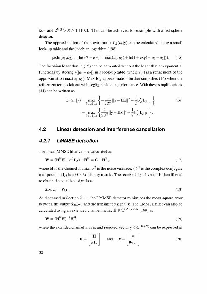
xML and 2MQ > K ≥ 1 [102]. This can be achieved for example with a list spheredetector.

The approximation of the logarithm in LE(bk|y) can be calculated using a smalllook-up table and the Jacobian logarithm [198]

jacln(a1,a2) := ln(ea1 + ea2) = max(a1,a2)+ ln(1+ exp(−|a1−a2|)). (15)

The Jacobian logarithm in (15) can be computed without the logarithm or exponentialfunctions by storing r(|a1−a2|) in a look-up table, where r(·) is a refinement of theapproximation max(a1,a2). Max-log approximation further simplifies (14) when therefinement term is left out with negligible loss in performance. With these simplifications,(14) can be written as

LE(bk|y) = maxb∈Lk,+1

− 1

2σ2 ||y−Hx||2 + 12

bT[k]LA,[k]

(16)

− maxb∈Lk,−1

1

2σ2 ||y−Hx||2 + 12

bT[k]LA,[k]

.

4.2 Linear detection and interference cancellation

4.2.1 LMMSE detection

The linear MMSE filter can be calculated as

W = (HHH+σ2IM)−1HH = G−1HH, (17)

where H is the channel matrix, σ2 is the noise variance, (·)H is the complex conjugatetranspose and IM is a M×M identity matrix. The received signal vector is then filteredto obtain the equalized signals as

xMMSE = Wy. (18)

As discussed in Section 2.1.1, the LMMSE detector minimizes the mean square errorbetween the output xMMSE and the transmitted signal x. The LMMSE filter can also becalculated using an extended channel matrix H ∈ C(M+N)×N [199] as

W = (HHH)−1HH, (19)

where the extended channel matrix and received vector y ∈ C(M+N) can be expressed as

H =

[H

σIN

]and y =

[y

0N×1

](20)

58

and 0N×1 denotes a vector of zeros. The equalized signals can then be obtained from

xMMSE = H+y, (21)

where (·)+ denotes the Moore-Penrose pseudo-inverse of the matrix [200]. The biasin the LMMSE filter can be removed by W = BG−1HH [112], where B is a diagonalmatrix with i, ith element

Bi,i =ρi +1

ρi. (22)

The SINR on stream i can be calculated as [17]

ρi =1

σ2G−1i,i−1. (23)

Matrix inversion

The matrix inversion required in the LMMSE filter calculation can be calculated withdifferent approaches. The direct approach is used for the 2×2 antenna system in thiswork. The direct matrix inversion is calculated as

G−1 =1|G|

[g2,2 −g1,2

−g2,1 g1,1

]. (24)

The positive semi-definite nature of the matrix G in (17) simplifies the calculation of thematrix inverse. The determinant |G| is a real valued and no complex division is required.

The direct approach can, however, be too complex for large matrices. The QRdecomposition can be utilized in the matrix inversion. Two methods are used to calculatethe LMMSE filter in this work. The squared Givens rotations (SGR) [201] are used forcalculating the inverse of G. The modified Gram-Schmidt algorithm [200] is employedto perform a QR decomposition on the extended channel matrix H = QR, whereR ∈ C(M+N)×N has orthonormal columns and R ∈ CN×N is an upper triangular matrix.The LMMSE filter is then obtained from

W = R−1QH. (25)

The modified Gram-Schmidt algorithm is described as Algorithm 1. The factorizationcan also be performed with sorting in order to obtain an optimal detection order [202].The sorted QRD (SQRD) can be used as a basis for interference cancellation in a

59

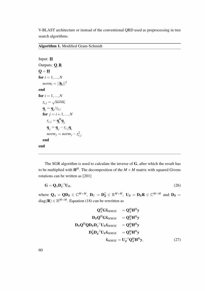
V-BLAST architecture or instead of the conventional QRD used as preprocessing in treesearch algorithms.

Algorithm 1. Modified Gram-Schmidt

Input: HOutputs: Q,RQ = Hfor i = 1, ...,N

normi = ||hi||2

endfor i = 1, ...,N

ri,i =√

normi

qi = qi/ri,i

for j = i+1, ...,Nri, j = qH

i q j

q j = q j− ri, jqi

norm j = norm j− r2i, j

endend

The SGR algorithm is used to calculate the inverse of G, after which the result hasto be multiplied with HH. The decomposition of the M×M matrix with squared Givensrotations can be written as [201]

G = QAD−1U UR, (26)

where QA = QDR ∈ CM×M , DU = D2R ∈ RM×M , UR = DRR ∈ CM×M and DR =

diag(R) ∈ RM×M . Equation (18) can be rewritten as

QHA GxMMSE = QH

A HHy

DRQHGxMMSE = QHA HHy

DRQHQDRD−1U URxMMSE = QH

A HHy

D2RD−2

R URxMMSE = QHA HHy

xMMSE = U−1R QH

A HHy, (27)

60

where QA and UR are obtained with the SGR. Since UR is an upper triangular matrix, itsinversion can be obtained through back substitution or with an algorithm presented in[203]. The latter was used in this work and the algorithm is presented as Algorithm 2.

Algorithm 2. Inversion of triangular matrix

Input: UR

Output: U−1R

A = 0M×M

for i = 1, ...,MAi,i =

1U Ri,i

endfor i = 1, ...,M−1

for j = i+1, ...,Mt = 0for k = 1, ..., j−1

t = t +Ai,kURk, j

endAi, j =−tA j, j

endendU−1

R = A

LLR calculation

The log-likelihood ratios for the FEC decoder can be calculated with a soft demodulatorwhich takes as input the LMMSE equalizer outputs xMMSE , the equivalent channelHe = diag(WH) and the covariance of the residual interference N0 = He−HeHH

e . Theprocess of producing LLRs with the soft demodulator is described as Algorithm 3.

61

Algorithm 3. Soft demodulation

Inputs: He,N0, xMMSE

Output: LLRfor k = 1, ...,N

for i = 1, ...,Qs1 = s0 =−∞

for j = 1, ...,Ωd = xMMSEk −Hekx j

di = |d|2

lm =−di/N0k

if bi, j = 1s1 = maxx(s1, lm)

elses0 = maxx(s0, lm)

endendLLRki = s1− s0

endendFunction c = maxx(a,b)

if a > b

c = a+ log(1+ e−|a−b|)

elsec = b+ log(1+ e−|a−b|)

end

The LLRs can be calculated from the LMMSE equalizer outputs xMMSE as presentedin [112] by using an approximate log-likelihood criterion. Instead of calculating theEuclidean distance between the LMMSE equalizer output and the possible transmittedsymbols as in Algorithm 3, Gray labeling of the signal points is exploited. Thisreduces the latency and complexity but was shown to have only a minor impact on theperformance. The bit-metric approximations L(b j|x,W) in [112] are calculated as

62

ρkΛ(b j, x) = minxk∈X−1

k, j

|xk− xk|2− minxk∈X1

k, j

|xk− xk|2, (28)

where k = b j/Qc+1, X= xk : b j = i is the subset of hypersymbols x for whichthe jth bit of label b is i and ρk is the SINR of layer k. Λ(b j, x) can be simplified byconsidering xk in only one quadrature dimension given by j. The symbol mapping ofreal symbols to LLR values with 64-QAM is shown in Figure 5. For example, the firstbit is one in the positive side of the axis and zero on the negative size. The LLR thengrows based on how far the symbol value is from zero. The same process applies to theimaginary parts of the symbols.

−8 −6 −4 −2 0 2 4 6 8−80

−60

−40

−20

0

20

40

60

80

Re(x)/Im(x)

LL

R

LLR mapping

LLR(1)

LLR(2)

LLR(3)

Constellation point

110 111 101 100010011001000

Fig. 5. The mapping of symbols to LLRs.

4.2.2 The SIC algorithm

Instead of jointly detecting signals from all the antennas, the strongest signal can bedetected first and its interference is cancelled from each received signal in the SICreceiver. Then, the second strongest signal is detected and cancelled from the remainingsignals, and so on. The detection method is called successive nulling and interference

63

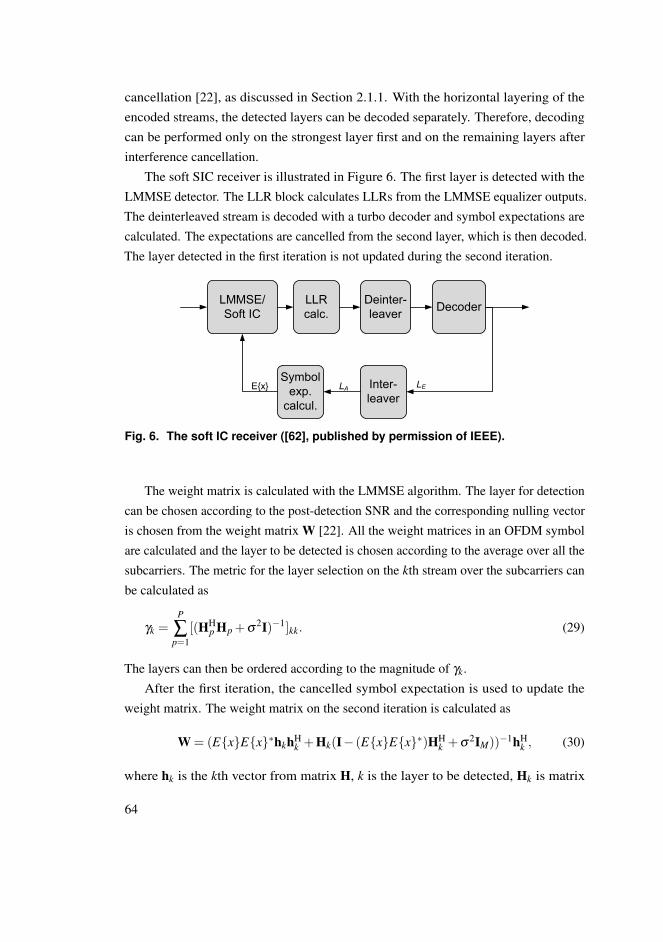
cancellation [22], as discussed in Section 2.1.1. With the horizontal layering of theencoded streams, the detected layers can be decoded separately. Therefore, decodingcan be performed only on the strongest layer first and on the remaining layers afterinterference cancellation.

The soft SIC receiver is illustrated in Figure 6. The first layer is detected with theLMMSE detector. The LLR block calculates LLRs from the LMMSE equalizer outputs.The deinterleaved stream is decoded with a turbo decoder and symbol expectations arecalculated. The expectations are cancelled from the second layer, which is then decoded.The layer detected in the first iteration is not updated during the second iteration.

LMMSE/

Soft IC

Deinter-

leaverDecoder

Inter-

leaverLA

LLR

calc.

Symbol

exp.

calcul.

Ex LE

Fig. 6. The soft IC receiver ([62], published by permission of IEEE).

The weight matrix is calculated with the LMMSE algorithm. The layer for detectioncan be chosen according to the post-detection SNR and the corresponding nulling vectoris chosen from the weight matrix W [22]. All the weight matrices in an OFDM symbolare calculated and the layer to be detected is chosen according to the average over all thesubcarriers. The metric for the layer selection on the kth stream over the subcarriers canbe calculated as

γk =P

∑p=1

[(HHp Hp +σ

2I)−1]kk. (29)

The layers can then be ordered according to the magnitude of γk.After the first iteration, the cancelled symbol expectation is used to update the

weight matrix. The weight matrix on the second iteration is calculated as

W = (ExEx∗hkhHk +Hk(I− (ExEx∗)HH

k +σ2IM))−1hHk , (30)

where hk is the kth vector from matrix H, k is the layer to be detected, Hk is matrix

64

H with the vectors from previously detected layers removed and Ex is the symbolexpectation.

The detected layer is decoded and symbol expectations from the soft decoder outputsare calculated as [204]

Ex= (12)Q

∑xl∈Ω

xl

Q

∏i=1

(1+bi,l tanh(LA(bi)/2)), (31)

where LA(bi) are the LLRs of coded bits corresponding to x and bi,l are bits correspondingto constellation point xl . The expectation calculation in (31) can be simplified to theform

Exre = sgn(LA(bi))S|tanh(LA(bi+2))|. (32)

The constellation point S is chosen from 1,3,5,7 depending on the signs of LA(bi+1)

and LA(bi+2).

4.3 Tree search algorithms

The search over the lattice points can be performed with a tree structure due to the QRdecomposition applied on the channel matrix. The sphere detector is a well known andcommonly used tree search based algorithm for MIMO detection. The SD algorithmssolve the ML solution with a reduced number of considered candidate symbol vectors asstated in Section 2.1.2. They take into account only the lattice points that are inside asphere of a given radius. The condition that the lattice point lies inside the sphere can bewritten as

||y−Hx||2 ≤C0. (33)

After QR decomposition of the channel matrix H in (69), it can be rewritten as

||y′−Rx||2 ≤C′0, (34)

where C′0 =C0−||(Q′)Hy||2, y′ = QHy, R ∈ CN×N is an upper triangular matrix with

positive diagonal elements, Q ∈ CM×N and Q′ ∈ CM×(M−N) are orthogonal matrices.The squared partial Euclidean distance (PED) of xN

i , i.e. the square of the distancebetween the partial candidate symbol vector and the partial received vector, can becalculated as

d(xNi ) =

N

∑j=i

∣∣∣∣∣y′j− N

∑l= j

r j,lxl

∣∣∣∣∣2

, (35)

65

where i = N . . . ,1, y′j is the jth element of y′, r j,l is the j, lth element of the matrix

R, xl is the lth element of the candidate vector xNi and xN

i denotes the last N− i+1components of vector x [86].

List sphere detectors can be used to approximate the MAP detector and to providesoft outputs for the decoder [102]. A list of candidates L and their Euclidean distancesare used to calculate the a posteriori probabilities LD of the coded bits in bp.

A LSD structure is presented in Figure 7. The channel matrix H is first decomposedas H = QR in the QR-decomposition block. The Euclidean distances between thereceived signal vector y and the possible transmitted symbol vectors are calculated inthe LSD block. The candidate symbol list L from the LSD block is demapped to abinary form. The LSD block can be substituted with any tree search algorithm thatproduces a list of candidate symbols. The log-likelihood ratios are calculated from thelist of Euclidean distances in the LLR block. Limiting the range of LLRs reduces therequired list size [205].

QRD LSDDe-map

LLRH Q

R

y

L

d²(L)

b

LA

Fig. 7. The list sphere detector ([62], published by permission of IEEE).

4.3.1 The K-best LSD algorithm

The tree search can be performed in a breadth-first, depth-first or metric-first manner,as discussed in Section 2.1.2. The breadth-first approach is considered in this thesisbecause it can be easily pipelined and parallelized and provides a fixed detection rate.The breadth-first K-best LSD can also be more easily implemented and provide thehigh and constant detection rates required in the LTE. The K-best algorithm [88] is abreadth-first search based algorithm, which keeps the K nodes which have the smallestaccumulated Euclidean distances at each level. If the PED is larger than the squaredsphere radius C0, the corresponding node will not be expanded. No sphere constraint isassumed, i.e. C0 = ∞, but a set the value for K is used instead, as is common with theK-best algorithms. The K-best algorithm without the sphere constraint can also be seenas the M-algorithm [87]. The K-best LSD algorithm description is given as Algorithm 4.

66

The main loop of the algorithm runs from i = 1, ...,2N in a real valued system.

Algorithm 4. The K-best LSD algorithm

Inputs: Q,R,y, C′0, K, P (modulation used, P-QAM)Preprocessing:

Calculate: y′

Algorithm:for i = 1, ...,N1. Denote the partial candidate by xN

i+1.1.1 Determine all admissible candidate child nodes xi with given C′0

and calculate the corresponding PEDs d(xNi ).

1.2 Store the partial candidates and their PEDs to a temporary stack memory.2. Sort the partial candidates according to their PEDs and store the K smallest PEDsand the corresponding symbol vectors to the final list stack memory.endGive the candidates and their EDs as outputs.

The K-best tree search with no sphere constraint is illustrated in Figure 8. A listsize of two is assumed. The tree search proceeds level by level, expanding all the childnodes of each parent node. If the number of child nodes exceeds the list size, sortingis performed to find the K nodes with the smallest partial Euclidean distances. Thetree search starts from the top of the tree on the first level in the figure. Both nodes arespanned, and on the second level, all the child nodes are spanned as well. Sorting isperformed to find the two nodes with the smallest PEDs. The tree search continues untilthe fourth level is reached and the two leaf nodes with the smallest Euclidean distancesare given as output.

Enhanced tree search

The breadth-first tree search can be modified to decrease the latency. With the novelsearch strategy [64], two or more PEDs can be calculated in parallel and the largest onesare discarded. With 64-QAM, instead of having to sort 64 PEDs, there are only 32 PEDsto be sorted on each level when two PEDs are calculated in parallel. On the first level,the PEDs are calculated as with the original breadth-first search, as shown in Figure 9.

67

1.

2.

3.

4.

Sort

Sort

Fig. 8. The K-best tree search.

On subsequent levels, half the nodes are discarded before sorting, as shown in the figure,as lighter nodes.

...

...

...

7 -7 5 3 1-5 -3 -1

7 -7 5 3 1-5 -3 -1 7 -7 5 3 1-5 -3 -1

7 -7 5 3 1-5 -3 -1 7 -7 5 3 1-5 -3 -1

...

Fig. 9. The modified tree search ([62], published by permission of IEEE).

4.3.2 Selective spanning with fast enumeration

The selective spanning with fast enumeration algorithm [135] can also be thought ofas a breadth-first tree search algorithm. The algorithm spans each level of the treebased on the node spanning vector m = [m1, ...,mM]. The number of spans for eachnode on a level is specified with the element of m corresponding to that level. As thespanned nodes are not discarded, the length of the final candidate list can be obtained bymultiplying the elements of m. For example, in a 2×2 antenna and 64-QAM system,

68

the vector m = [64,8] would lead to a final candidate list of 512. For the same realvalued system, the vector m = [8,8,8,8] would lead to a final list size of 4,096. Inpractice, smaller list sizes should be aimed at. In this work, a real valued system model isused. Such a system model simplifies the Euclidean distance calculation and the slicingoperation as the closest constellation point selection can be done on a one dimensionalaxis.

The PED on each level of the tree search can be calculated as

di(xi) = di+1(xi+1)+∥∥ei(xi)

∥∥2, (36)

where di+1(xi+1) is the PED from the previous level and i = N, ...,1. The slicer unitselects a set of closest constellation points xi, minimizing

∥∥ei(xi)∥∥2

=

∥∥∥∥∥∥∥∥∥∥∥y′i−

M

∑j=i+1

ri, jx j︸ ︷︷ ︸bi+1(xi+1)

−ri,ixi

∥∥∥∥∥∥∥∥∥∥∥

2

. (37)

Minimizing∥∥ei(xi)

∥∥2 is equivalent to the minimization of ‖ei(xi)/rii‖2

∥∥∥∥ei(xi)

ri,i

∥∥∥∥2

=

∥∥∥∥∥∥bi+1(xi+1)/ri,i︸ ︷︷ ︸ε

−xi

∥∥∥∥∥∥2

. (38)

The closest constellation points based on ε are selected in the slicer unit.The real valued axis for 64-QAM is shown in Figure 10. The slicing order given

ε is also depicted. If five constellation points are sliced, the slicer would select theconstellation points in the order of 5,3,7,1,−1. The process is similar to the Schnorr-Euchner enumeration (SEE). The SSFE algorithm could then be thought of as theM-algorithm combined with SEE. The SSFE algorithm does not require sorting, whichmakes it more attractive for implementation than the M-algorithm or the K-best detector.The SSFE algorithm is summarized as Algorithm 5.

69

1-1 3 5 7-3-5-7ε

1.2.

3.

4.

5.

Fig. 10. The slicing operation in SSFE with 64-QAM.

Algorithm 5. The SSFE algorithm

Inputs: Q,R,y, m, P (modulation used, P-QAM)Preprocessing:

Calculate: y′

Calculate: hi = 1/Ri,i

Algorithm:for i = 1, ...,N1. Calculate ε for each candidate in xi

2. Slice the mi closest points3. Calculate the PEDs to the sliced lattice pointsendGive the candidates and their EDs as outputs.

4.3.3 Tree search with interference cancellation

A system with two separately encoded streams in the 4×4 antenna case is assumed.If MMSE-SIC is used, two strongest layers are cancelled from the other two layersand only MMSE is used in separating the two strongest or weakest layers. This candegrade the performance, especially in low rank channels. A tree search algorithm canbe used to separate the streams, which were not used for interference cancellation. Inthe SSFE-SIC algorithm, the strongest stream is detected with the SSFE detector. TheLLRs are calculated from the final list and decoding is performed. The tree search has tobe performed for the whole received symbol vector in the first iteration to achieve asufficiently good performance. Symbol expectations can be calculated from the outputsof the decoder as in (31). The symbol expectations are cancelled from the receiversymbol vector with r = y−HEx. A partial tree search is performed on r in order toseparate the final two streams.

70

4.4 Numerical throughput examples

4.4.1 Simulation model

The communication system, i.e. the transmission throughput performance of the SICdetector, is compared to that of the K-best LSD and the LMMSE detectors. Thesimulation parameters are based on the LTE standard [189] and are summarized in Table3. In the horizontally encoded system, two data streams are encoded separately and thenmapped onto different layers. The strongest layer can be detected and decoded firstand then cancelled from the remaining layer. In the 4×4 antenna system, each of thetwo streams is multiplexed onto two antennas; the first stream is multiplexed onto thefirst and second antenna and the second stream onto the third and fourth antenna. Themost recent versions of the 3GPP LTE specifications also include the 2×2 verticallyencoded case, where a single code word is multiplexed onto two layers. In this scenario,decoding of the layers cannot be performed separately.

The transmission throughput is calculated as the nominal information transmissionrate of information bits times (1−FER). A 5 MHz bandwidth was assumed in thesimulations. The signal-to-noise ratio represents Es/N0, where Es is the symbol energy.Each SNR point includes transmission of 1,000 frames. Perfect channel state informationwas assumed in the receiver. The number of turbo decoder iterations in the simulationswas eight. The typical urban (TU) channel [194, 196] with base station (BS) azimuthspread of 2 or 5 degrees was applied. The channel with BS azimuth spread of 2 degreesis denoted as a correlated channel and with 5 degrees as the moderately correlatedchannel, as explained in Section 3.4. A spatially uncorrelated channel was considered aswell. Parameters of the used channel models were shown in Table 1.

Table 3. Simulation parameters.

Coding Turbo coding with 1/2 code rate

Channel model Typical urban

User velocity 30, 120 km/h

Number of subcarriers 512 (300 used)

Bandwidth 5 MHz

Symbol duration 71.4 µs

71

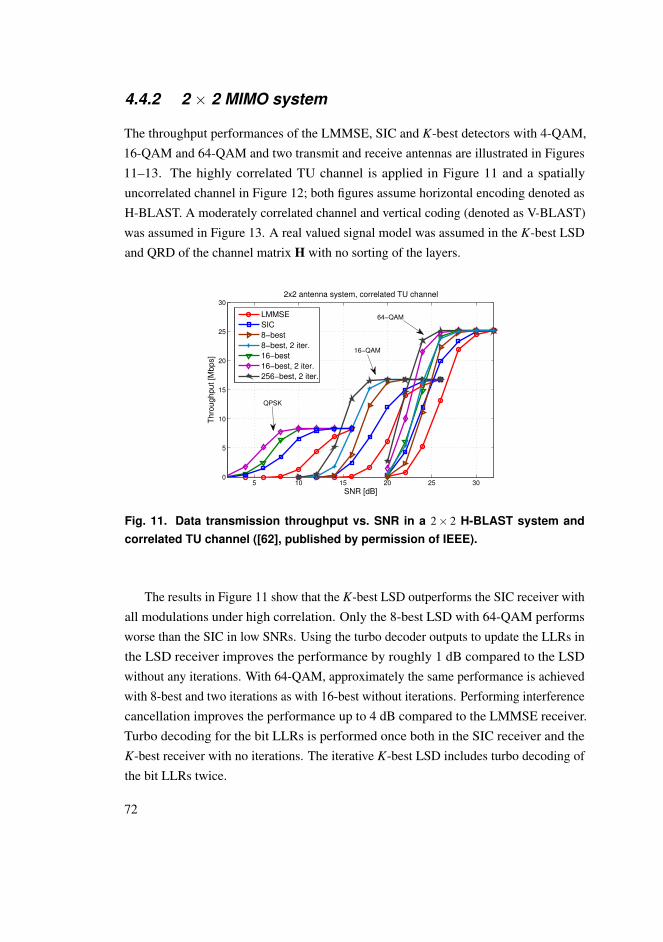
4.4.2 2 × 2 MIMO system

The throughput performances of the LMMSE, SIC and K-best detectors with 4-QAM,16-QAM and 64-QAM and two transmit and receive antennas are illustrated in Figures11–13. The highly correlated TU channel is applied in Figure 11 and a spatiallyuncorrelated channel in Figure 12; both figures assume horizontal encoding denoted asH-BLAST. A moderately correlated channel and vertical coding (denoted as V-BLAST)was assumed in Figure 13. A real valued signal model was assumed in the K-best LSDand QRD of the channel matrix H with no sorting of the layers.

5 10 15 20 25 300

5

10

15

20

25

30

SNR [dB]

Thro

ughput [M

bps]

2x2 antenna system, correlated TU channel

LMMSE

SIC

8−best

8−best, 2 iter.

16−best

16−best, 2 iter.

256−best, 2 iter.

QPSK

16−QAM

64−QAM

Fig. 11. Data transmission throughput vs. SNR in a 2× 2 H-BLAST system andcorrelated TU channel ([62], published by permission of IEEE).

The results in Figure 11 show that the K-best LSD outperforms the SIC receiver withall modulations under high correlation. Only the 8-best LSD with 64-QAM performsworse than the SIC in low SNRs. Using the turbo decoder outputs to update the LLRs inthe LSD receiver improves the performance by roughly 1 dB compared to the LSDwithout any iterations. With 64-QAM, approximately the same performance is achievedwith 8-best and two iterations as with 16-best without iterations. Performing interferencecancellation improves the performance up to 4 dB compared to the LMMSE receiver.Turbo decoding for the bit LLRs is performed once both in the SIC receiver and theK-best receiver with no iterations. The iterative K-best LSD includes turbo decoding ofthe bit LLRs twice.

72

0 5 10 15 200

5

10

15

20

25

30

SNR [dB]

Thro

ughput [M

bps]

2x2 antenna system, Uncorrelated channel

LMMSE

SIC

8−best

8−best, 2 iter.

16−best

16−best, 2 iter.

256−best, 2 iter.

QPSK

16−QAM

64−QAM

Fig. 12. Data transmission throughput vs. SNR in a 2× 2 H-BLAST system anduncorrelated channel ([62], published by permission of IEEE).

0 5 10 15 20 250

5

10

15

20

25

30

SNR [dB]

Thro

ughput [M

bps]

2x2 antenna system, V−BLAST, moderately correlated TU channel

LMMSE

8−best

8−best, 2 iter.

16−best

16−best, 2 iter.

256−best, 2 iter.

16−QAM

64−QAM

QPSK

Fig. 13. Data transmission throughput vs. SNR in a 2× 2 V-BLAST system andmoderately correlated channel ([62], published by permission of IEEE).

The SIC receiver also outperforms the K-best LSD when the channel has nocorrelation, as presented in Figure 12. With highly correlated channels, the initialdecisions in the SIC receiver are more likely to be incorrect, which is found to lead toerror propagation.

The SIC receiver improves the performance of the LMMSE receiver only verymarginally in the vertically encoded system, as illustrated in Figure 13. This is

73

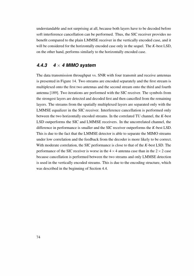
understandable and not surprising at all, because both layers have to be decoded beforesoft interference cancellation can be performed. Thus, the SIC receiver provides nobenefit compared to the plain LMMSE receiver in the vertically encoded case, and itwill be considered for the horizontally encoded case only in the sequel. The K-best LSD,on the other hand, performs similarly to the horizontally encoded case.

4.4.3 4 × 4 MIMO system

The data transmission throughput vs. SNR with four transmit and receive antennasis presented in Figure 14. Two streams are encoded separately and the first stream ismultiplexed onto the first two antennas and the second stream onto the third and fourthantenna [189]. Two iterations are performed with the SIC receiver. The symbols fromthe strongest layers are detected and decoded first and then cancelled from the remaininglayers. The streams from the spatially multiplexed layers are separated only with theLMMSE equalizer in the SIC receiver. Interference cancellation is performed onlybetween the two horizontally encoded streams. In the correlated TU channel, the K-bestLSD outperforms the SIC and LMMSE receivers. In the uncorrelated channel, thedifference in performance is smaller and the SIC receiver outperforms the K-best LSD.This is due to the fact that the LMMSE detector is able to separate the MIMO streamsunder low correlation and the feedback from the decoder is more likely to be correct.With moderate correlation, the SIC performance is close to that of the K-best LSD. Theperformance of the SIC receiver is worse in the 4×4 antenna case than in the 2×2 casebecause cancellation is performed between the two streams and only LMMSE detectionis used in the vertically encoded streams. This is due to the encoding structure, whichwas described in the beginning of Section 4.4.

74

5 10 15 20 25 300

10

20

30

40

50

60

SNR [dB]

Thro

ughput [M

bps]

4x4 antenna system, correlated TU channel

LMMSE

SIC

16−best

16−best, 2 iter.

8−best

8−best, 2 iter.

256−best, 2 iter.

QPSK

16−QAM

64−QAM

(a)

0 5 10 15 20 25 300

10

20

30

40

50

60

SNR [dB]

Thro

ughput [M

bps]

4x4 antenna system, moderately correlated TU channel

LMMSE

SIC

16−best

16−best, 2 iter.

8−best

8−best, 2 iter.

256−best, 2 iter.

QPSK

16−QAM

64−QAM

(b)

0 5 10 15 20 250

10

20

30

40

50

60

SNR [dB]

Thro

ughput [M

bps]

4x4 antenna system, uncorrelated channel

LMMSE

SIC

8−best

8−best, 2 iter.

16−best

16−best, 2 iter.

256−best, 2 iter.

QPSK

64−QAM

16−QAM

(c)

Fig. 14. Data transmission throughput vs. SNR in a 4× 4 system in (a) a highlycorrelated (b) moderately correlated and (c) uncorrelated channel ([62], publishedby permission of IEEE).

75

4.4.4 Preprocessing, enhanced tree search and LLRcalculation

Different methods for the QRD in the tree search algorithms can be applied. Thebasic QRD decomposes the channel matrix H, while the MMSE-QRD performs QRdecomposition on the extended channel matrix H. The MMSE-SQRD improves theperformance by including the noise term in the preprocessing. The sorted QRD sorts thechannel matrix according to its column norms while performing the QRD [110]. Thisapproach leads to an improved tree search order where the best layer is expanded first.The SQRD can also be performed on the extended channel matrix to further improve theperformance. The FER performances of the different preprocessing approaches arepresented in Figure 15 in a 4×4 16-QAM case. The K-best LSD with the list sizes of 4,8 and 16 was used as the tree search algorithm. Including the noise variance in thepreprocessing has a high impact on the performance. It can be seen from the fact thatthe highest performance gain is obtained by the extended channel matrix. Sorting in theQRD brings only a little additional gain. Also, the larger the list size, the lower theimpact of the preprocessing. With more complex preprocessing, even small list sizes canbe used.

16 18 20 22 24 26 2810

−3

10−2

10−1

100

Es/N0 [dB]

FE

R

4x4 16−QAM, correlated TU channel, 100 km/h

8−best, QRD

8−best, SQRD

8−best, MMSE−SQRD

8−best, MMSE−QRD

4−best, QRD

4−best, SQRD

4−best, MMSE−SQRD

4−best, MMSE−QRD

16−best, QRD

16−best, MMSE−SQRD

Fig. 15. FER vs. SNR in a 4×4 system in a highly correlated channel with differentQRD preprocessors.

76

The impact of the enhanced tree search described in Section 4.3.1 on the performancein a 2×2 64-QAM case is shown in Figure 16. It can be seen that the performancedegradation is minimal, but the detection rate will be doubled. The new strategy is themost beneficial with high order modulations, when the nodes have several branches.When a lower order modulation is used, the performance degrades more with the newstrategy because a smaller amount of bit combinations is included in the LLR calculation.

20 22 24 26 28 30 320

5

10

15

20

25

30

SNR [dB]

Thro

ughput [M

bps]

2x2 64−QAM, correlated TU channel

8−best

16−best

Mod. 16−best

Mod. 8−best

Fig. 16. Data transmission throughput vs. SNR in a 2× 2 system in a highly cor-related channel with the modified tree search ([62], published by permission ofIEEE).

The LLR calculation in the K-best LSD is simplified from (15) by leaving outthe refinement part from (15). The impact of using the simplified LLR calculationis presented in Figure 17. The simplification has again only a small impact on theperformance. Comparison of implementation estimations showed that the complexity isreduced approximately four times with the simplified LLR calculation. Also the SICreceiver is simplified from using soft demodulation presented as Algorithm 3 for LLRcalculation compared to using the approximate log-likelihood criterion. The symbolexpectations are also calculated with (32).

77

20 22 24 26 28 30 320

5

10

15

20

25

30

SNR [dB]

Thro

ughput [M

bps]

2x2 64−QAM, correlated TU channel

16−best, exact LLR

16−best, appr. LLR

SIC, soft demod.

SIC, simplified LLR

Fig. 17. Data transmission throughput vs. SNR in a 2×2 system in a highly corre-lated channel with the simplified LLR calculation ([62], published by permissionof IEEE).

4.4.5 Performance comparison of K-best and SSFE

The performances of the tree search algorithms with different list sizes are compared inFigures 18 and 19. The performance of the SSFE-SIC algorithm from Section 4.3.3 isalso shown. The SSFE node spanning vector m is shown in the figure for the first fourlevels of the real valued tree search. In the last four levels, only one node is expanded.The last value of m corresponds to the first level in the tree. A 4×4 antenna systemwith 16-QAM and a correlated channel is assumed in Figure 18. There, the K-best withthe list size of 16 and 8-best with two iterations perform best. The performance of theSSFE-SIC is degraded by the incorrect symbol decisions from the decoder feedback.SSFE with one global iteration and a final list size of 12 has a performance difference ofalmost 2 dB compared to the 8-best. The SSFE may not always find the best brancheson each level, but the K-best detector goes through all the child branches on a level andfinds the ones with the smallest distances. The SSFE detector also goes through onlyone branch in the bottom levels of the tree.

A 4× 4 antenna system with 64-QAM and a moderately correlated channel isassumed in Figure 19. The difference in performance is smaller than in the correlated

78

16 18 20 22 24 26 28 300

5

10

15

20

25

30

35

Es/N0 [dB]

Thro

ughput [M

bps]

4x4 16−QAM, correlated TU channel, 120 km/h

8−best

SSFE[2,2,3,3]−SIC

8−best, 2 global it.

SSFE [1,2,2,3], 2 it.

MMSE

16−best

SSFE[1,2,2,3]

SSFE [1,2,2,3], 3 it.

Fig. 18. Data transmission throughput vs. SNR of K-best and SSFE in a correlatedchannel with 4×4 16-QAM.

channel. The best performance is obtained with the SSFE-SIC algorithm with asufficiently large tree search size. Updating of the LLRs gives a good performancewith both K-best and SSFE. Even though the SSFE might be better suitable forimplementation, the performance of the SSFE is still worse than that of the K-best.Therefore, as the K-best algorithm gives the most constant performance in most scenarios,it will be the main tree search algorithm considered in the remainder of the thesis.Nevertheless, detailed complexity comparisons are provided in Section 4.5.5.

79

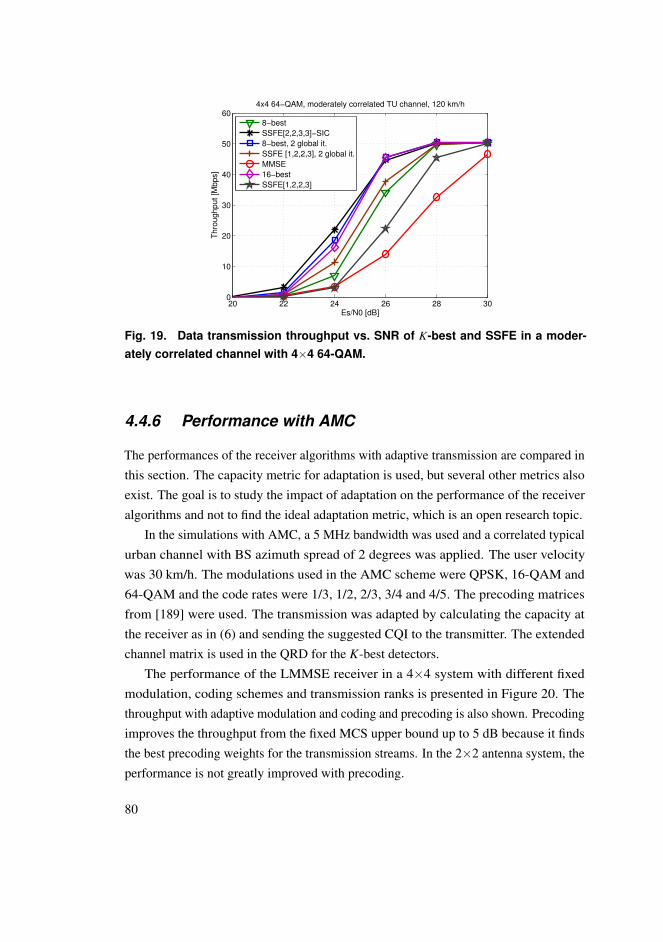
20 22 24 26 28 300

10

20

30

40

50

60

Es/N0 [dB]

Thro

ughput [M

bps]

4x4 64−QAM, moderately correlated TU channel, 120 km/h

8−best

SSFE[2,2,3,3]−SIC

8−best, 2 global it.

SSFE [1,2,2,3], 2 global it.

MMSE

16−best

SSFE[1,2,2,3]

Fig. 19. Data transmission throughput vs. SNR of K-best and SSFE in a moder-ately correlated channel with 4×4 64-QAM.

4.4.6 Performance with AMC

The performances of the receiver algorithms with adaptive transmission are compared inthis section. The capacity metric for adaptation is used, but several other metrics alsoexist. The goal is to study the impact of adaptation on the performance of the receiveralgorithms and not to find the ideal adaptation metric, which is an open research topic.

In the simulations with AMC, a 5 MHz bandwidth was used and a correlated typicalurban channel with BS azimuth spread of 2 degrees was applied. The user velocitywas 30 km/h. The modulations used in the AMC scheme were QPSK, 16-QAM and64-QAM and the code rates were 1/3, 1/2, 2/3, 3/4 and 4/5. The precoding matricesfrom [189] were used. The transmission was adapted by calculating the capacity atthe receiver as in (6) and sending the suggested CQI to the transmitter. The extendedchannel matrix is used in the QRD for the K-best detectors.

The performance of the LMMSE receiver in a 4×4 system with different fixedmodulation, coding schemes and transmission ranks is presented in Figure 20. Thethroughput with adaptive modulation and coding and precoding is also shown. Precodingimproves the throughput from the fixed MCS upper bound up to 5 dB because it findsthe best precoding weights for the transmission streams. In the 2×2 antenna system, theperformance is not greatly improved with precoding.

80

−5 0 5 10 15 20 25 300

5

10

15

20

25

30

35

40

45

Es/N0 [dB]

Thro

ughput [M

bps]

4x4 antenna system, correlated TU channel, 30 km/h used velocity, 5 MHz bandwidth

1/3

1/2

2/3

3/4

4/5

AMC &PrecodingFixed

MCSupperbound

Fig. 20. Data transmission throughput vs. SNR with fixed MCSs and AMC withprecoding ([63], published by permission of IEEE).

The performance of the receiver algorithms with AMC is presented in Figure 21 in a2×2 antenna case. The transmission was adapted to use mostly rank 1 transmission inthe lower SNRs. When rank 2 transmission is used, the K-best LSD receiver with alist size of 8 performs the best and the LMMSE receiver has the worst performance.Updating the LLRs from the decoder improves the performance of the K-best by 1 dB.Since the transmission is already adapted to the channel, a better receiver does not give ahigh gain in performance.

−5 0 5 10 15 20 25 30 35 400

5

10

15

20

25

30

35

40

45

Es/N0 [dB]

Th

rou

gh

pu

t [M

bp

s]

2x2 H−BLAST, correlated TU channel, 30 km/h user velocity, 5 MHz bandwidth

LMMSE

8−best

SIC

8−best, 2 iter.

4−best

Fig. 21. Data transmission throughput vs. SNR in a correlated 2×2 channel ([63],published by permission of IEEE).

81

The performance of the algorithms in a channel with less correlation than in Figure21 is shown in Figure 22. The difference in performance is smaller when the channelconditions are improved. The same was seen in the fixed modulation and code rate casesearlier in the chapter. With lower correlation in the channel and transmission adaptedto the channel conditions, a simpler receiver also succeeds in separating the MIMOstreams.

−5 0 5 10 15 20 25 30 35 400

5

10

15

20

25

30

35

40

45

Es/N0 [dB]

Th

rou

gh

pu

t [M

bp

s]

2x2 H−BLAST, moderately correlated TU channel, 30 km/h user velocity, 5 MHz bandwidth

LMMSE

8−best

8−best, 2i iter.

SIC

Fig. 22. Data transmission throughput vs. SNR in a moderately correlated 2× 2

channel ([63], published by permission of IEEE).

The performance in a 4×4 antenna system is shown in Figure 23. The transmissionrank of the precoding matrix was one, two or four. The performances of the algorithmsare similar with rank one transmissions as in the 2×2 antenna system. With higherSNRs and transmission rank, the performance improves with the more complex receivers.The SIC receiver does not improve the performance much from the LMMSE in the highSNRs when rank 4 transmission is used. This is partly due to the encoding structureand the two strongest streams are cancelled from the other streams and only MMSEis used to separate the remaining streams. However, the LSD receivers improve theperformance greatly with rank 4 transmission since a more advanced detector is neededto separate the streams.

The performance difference of LMMSE and K-best in a 4×4 antenna system withall the ranks from one to four is illustrated in Figure 24. The performance differencebetween the receivers is smaller from Figure 23 when the additional rank is utilized in

82

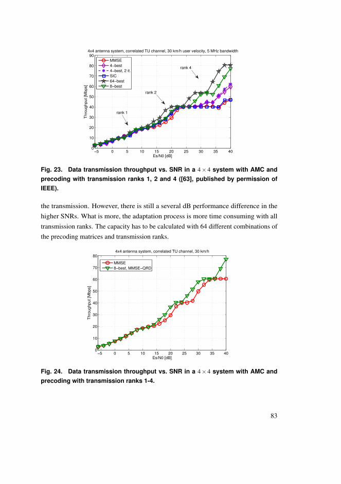
−5 0 5 10 15 20 25 30 35 400

10

20

30

40

50

60

70

80

90

Es/N0 [dB]

Th

rou

gh

pu

t [M

bp

s]

4x4 antenna system, correlated TU channel, 30 km/h user velocity, 5 MHz bandwidth

MMSE

4−best

4−best, 2 it.

SIC

64−best

8−best

rank 1

rank 2

rank 4

Fig. 23. Data transmission throughput vs. SNR in a 4× 4 system with AMC andprecoding with transmission ranks 1, 2 and 4 ([63], published by permission ofIEEE).

the transmission. However, there is still a several dB performance difference in thehigher SNRs. What is more, the adaptation process is more time consuming with alltransmission ranks. The capacity has to be calculated with 64 different combinations ofthe precoding matrices and transmission ranks.

−5 0 5 10 15 20 25 30 35 400

10

20

30

40

50

60

70

80

Es/N0 [dB]

Th

rou

gh

pu

t [M

bp

s]

4x4 antenna system, correlated TU channel, 30 km/h

MMSE

8−best, MMSE−QRD

Fig. 24. Data transmission throughput vs. SNR in a 4× 4 system with AMC andprecoding with transmission ranks 1-4.

83

4.5 Implementation results

The theoretical complexity of the receivers with M = N is presented in Table 4, wherethe number of multiplication and addition operations is specified. In the squaredGivens rotations (SGR) and the Gram-Schmidt based QRD, the division and squareroot were approximated with additions and shifts [206]. The largest term in the SGRcomes from matrix multiplications and in the QRD from multiple iterations of vectormultiplications. The number of operations in the K-best algorithm depends on the listsize K. If K is larger than

√|Ω|(l−1), it is used as K. In the first level l, the number of

multiplications is 2√|Ω| and additions

√|Ω|. The LLR calculation operations for the

linear receivers depend on the modulation. The constant multiplications with a power of2 were calculated as shifts. The number of multiplications is lower in the K-best LSDthan in the SIC with 4×4 QPSK. The number of multiplications in the K-best algorithmincreases with the list size and modulation. The modulation order does not have a majorimpact on the complexity with the SIC receiver. The impact of this can be seen later inthe implementation results. The SIC receiver includes more multiplications than theK-best algorithm with 4×4 QPSK and the implementation gate count is also higher.With 64-QAM, the number of multiplications and gates is higher with the K-best.

As discussed in Section 2.4, the implementation results were generated with theCatapult C HLS tool. The FPGA complexity results are presented in slices and dedicateddigital signal processing (DSP) slices. The DSP slices include an 18×18-bit multiplier.The VHDL from Catapult C was synthesized to a Xilinx Virtex-5 FPGA with MentorGraphics Precision Synthesis. The ASIC results are presented in gate equivalents(GE) and power consumption estimates. The Synopsys Design Compiler was used insynthesizing the VHDL along with the UMC 0.18 µm complementary metal oxidesemiconductor (CMOS) technology.

Simulations were performed to confirm that the used word lengths did not resultin performance degradation compared to the floating point word lengths. The mostcritical part in terms of word lengths in the detector is the preprocessing, i.e. the QRD orLMMSE. Figure 25 includes simulation results for both the LMMSE detector and theK-best LSD with the list size of 16. In the K-best, the word lengths in the tree searchand LLR calculation are 16 bits. The word lengths in the QRD are from 18 to 20 bits.The LMMSE filter calculation was performed with the extended channel matrix as in(19). The need to increase the word lengths in the LMMSE filter increases with theSNR. The 26 bit word length in the division and square root operations and the 24 bit

84

Table 4. The theoretical complexity of the receivers as numbers of arithmetic op-erations ([62], published by permission of IEEE).

Block Multiplications Additions

(HHH+σ2IM) 4M3

SGR (Q,R) 4M3+4.5M2+7.5M-12

MMSE-QRD (Q,R) 2M(16M3−6M2 +M+5) 32M4−20M3 +62M2 +86M

R inverse ∑M−1j=1 j2

R−1QH 8M3

Detection 4M2 3M2−M

LLR (MMSE/SIC) [2|8|16]M MQ/4

Expectation calc. 4M

SIC 2M2 +4M 4M2−M

QRD 2M(8M3−2M2 +3M+1) 16M4−12M3 +66M2 +86M

Matrix-vector mult. 4M2 4M2−2M

K-best LSD2M

∑l=2

K√|Ω|(l +1) K

2M

∑l=2

√|Ω|(l +1)

LLR (K-best) K QM+32

word length in the matrix elements is enough for the lower SNRs, but higher wordlengths are required for the higher SNRs. However, the high SNRs may not be feasiblein the LMMSE detector and a compromise can be used to lower the complexity of theLMMSE filter while maintaining a good performance in the lower SNRs.

4.5.1 Preprocessing

Preprocessing of the channel matrix is utilized in every detector type in this thesis. TheLMMSE and SIC detectors require the LMMSE filter calculation and the tree searchdetectors need the results from the QR decomposition of the channel matrix. Twopreprocessing methods were considered in Section 4.2. The SGR based QRD is used forthe LMMSE coefficient calculation and the Gram-Schmidt algorithm is employed toperform the QRD on the channel matrix. The Gram-Schmidt process is also utilized inthe LMMSE filter calculation for the extended channel matrix.

A simplified architecture for the SGR based LMMSE filter calculation is presentedin Figure 26. The dashed rectangle represents M/2(M−1) iterations with the operations

85

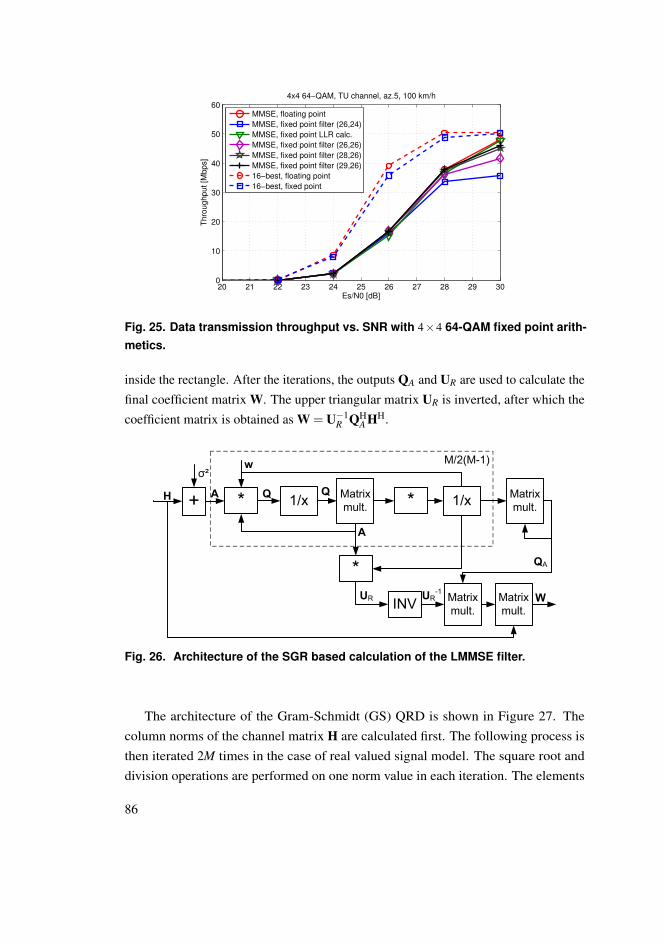
20 21 22 23 24 25 26 27 28 29 300

10

20

30

40

50

60

Es/N0 [dB]

Thro

ughput [M

bps]

4x4 64−QAM, TU channel, az.5, 100 km/h

MMSE, floating point

MMSE, fixed point filter (26,24)

MMSE, fixed point LLR calc.

MMSE, fixed point filter (26,26)

MMSE, fixed point filter (28,26)

MMSE, fixed point filter (29,26)

16−best, floating point

16−best, fixed point

Fig. 25. Data transmission throughput vs. SNR with 4×4 64-QAM fixed point arith-metics.

inside the rectangle. After the iterations, the outputs QA and UR are used to calculate thefinal coefficient matrix W. The upper triangular matrix UR is inverted, after which thecoefficient matrix is obtained as W = U−1

R QHA HH.

+H 1/x *Q

σ²

Matrix

mult.* 1/xA

A

Q

w

Matrix

mult.

QA*

INVUR Matrix

mult.

Matrix

mult.W

M/2(M-1)

UR-1

Fig. 26. Architecture of the SGR based calculation of the LMMSE filter.

The architecture of the Gram-Schmidt (GS) QRD is shown in Figure 27. Thecolumn norms of the channel matrix H are calculated first. The following process isthen iterated 2M times in the case of real valued signal model. The square root anddivision operations are performed on one norm value in each iteration. The elements

86

of matrix R and columns of matrix Q are updated with the multiply and accumulate(MAC) operations. The number of MAC operations is 2M with the channel matrix Hand 4M with the extended channel matrix H. The updating of R and Q is iterated asj = i+1, ...,2M for each outer iteration i. The iterations increase the latency of the GSQRD unless several intermediate registers are added and the architecture is copied intoseveral stages. If the architecture is used for the LMMSE filter calculation, a matrixmultiplication and an inversion of R is added.

NormsH √‾ 1/x * MAC MAC MAC

Q

R

2Mi=1,...,2M

2M

Q

j=i+1,...,2M

Fig. 27. Architecture of the Gram-Schmidt based QRD.

The implementation results for the 4×4 antenna system preprocessing are shownin Table 5. The table includes implementation results for the Gram-Schmidt QRDin the 8×8 real valued channel matrix and the 8×16 real valued extended channelmatrix cases and for the SGR QRD of the complex valued 4×4 channel matrix. Also,the blocks for inversion of the upper triangular matrices and matrix multiplicationsare included. The word lengths in the GS QRD are from 18 to 20 bits and from 20to 26 bits for the extended channel matrix. The high word length requirement andincreased number of iterations in the extended GS QRD double the power consumptioncompared to the QRD with the regular channel matrix. The word lengths for the SGRare from 18 to 20 bits as in [187], but some scaling is assumed. However, the numericalaccuracy is more problematic with the SGR LMMSE filter and the GS method is utilizedin the sequel. When the implementation latencies are roughly the same, the powerconsumption of the GS LMMSE is higher. A faster SGR was also implemented in thecase of the need to calculate all the coefficient matrices before starting the SIC detection.However, it is assumed in the sequel that only a portion of the LMMSE coefficientmatrices are needed to determine the SIC detection order and that the order remainsthe same for a few channel coherence periods. Thus, the GS based QRD is used forpreprocessing in the LMMSE, SIC and K-best detectors.

87

Table 5. The 4×4 preprocessing ASIC implementation results.

Block Gates Power Clock Latency Throughput

GS QRD 248.7 k 210.5 mW 125 MHz 175 cc 176 cc

GS QRD 380 k 237 mW 124 MHz 85 cc 40 cc

GS QRD ext. 350.3 k 440 mW 97 MHz 505 cc 504 cc

R−1 38.3 k 41.2 mW 100 MHz 455 cc 456 cc

Matrix mult. 26.4 k 39.9 mW 140 MHz 258 cc 256 cc

SGR QRD 443 k 260 mW 137 MHz 404 cc 400 cc

SGR U−1R QH

A HH 26.2 k 36.3 mW 140 MHz 258 cc 256 cc

SGR QRD 399.5 k 550 mW 124 MHz 63 cc 40 cc

SGR U−1R QH

A HH 84.7 k 126.2 mW 140 MHz 45 cc 40 cc

Total: GS LMMSE 415 k 522 mW 97 MHz 1218 cc 504 cc

Total: SGR LMMSE 469.2 k 296 mW 137 MHz 662 cc 400 cc

Total: SGR LMMSE 484 k 676 mW 124 MHz 108 cc 40 cc

4.5.2 K-best LSD

The K-best LSD receiver includes the QRD block, the K-best LSD block and the LLRcalculation block. The QR decomposition block is based on the modified Gram-SchmidtQRD algorithm from [110]. Ordering of the channel matrix is not utilized in thearchitecture. The top level architecture of the K-best LSD for a 2×2 antenna system isshown in Figure 28. The 4×4 antenna system LSD is based on the same architecture,but four more PED calculation blocks and sorters are added to the design.

The K-best LSD architecture is modified from [66]. A 2×2 and a 4×4 antennasystem with a real signal model [207] is assumed. The received signal vector y ismultiplied with matrix Q in the matrix multiplication block. Matrix R is multipliedwith the possible transmitted symbols after the QRD is performed, i.e. when thechannel realization changes. Partial Euclidean distances between the last symbol invector y′ and possible transmitted symbols are calculated in block PED1 in a 2× 2antenna system with d(x2

4) = ||y′4− r

′4,4||2. The resulting lists of symbols and PEDs

are not sorted at the first stage. The distances are added to the partial Euclideandistances d(x2

3) = ||y′3− (r

′3,3 + r

′3,4)||2 calculated in the PED2 block. The lists are

sorted and K partial symbol vectors with the smallest PEDs are kept. PED3 block

88

calculates d(x22) = ||y

′2− (r

′2,2 + r

′2,3 + r

′2,4)||2, which are added to the previous distance

and sorted. The last PED block calculates the partial Euclidean distances d(x21) =

||y′1− (r′1,1 + r

′1,2 + r

′1,3 + r

′1,4)||2. After adding the previous distances to d(x2

1), the listsare sorted and the final K symbol vectors are demapped to bit vectors and their Euclideandistance is used in the LLR calculation.

Matrixmult.

PED

1

PED

2

y

Q

y'(4)

R(4)

d²(L)

LL

H SortPED

3

PED

4Sort Sort

L L L L L

d²(L) d²(L) d²(L) d²(L) d²(L) d²(L)

R(3) R(2) R(1)

y'(3) y'(2) y'(1)

Fig. 28. The top level architecture of the 2× 2 K-best LSD ([62], published by per-mission of IEEE).

The modified K-best LSD tree search was used in the implementation in most ofthe 64-QAM results. The architecture of the second stage parallel Euclidean distancecalculation and insertion sorting is illustrated in Figure 29. Two PEDs are calculated inparallel and the smallest one is added to the list. The latency of each stage is then halvedfrom that of the original K-best tree search.

+

+

+

+

+

R3x1i

R4xicand

-

-

>

x1i

x2i

y’3

y’3

d²(L)i*

*

>

>

...

...

>clk

resetctr

I, CT=0Ī, 2, →>

SRG8PED2 Sorter

R3x2i

Fig. 29. Parallel PED calculation and sorting ([62], published by permission ofIEEE).

The 2×2 FPGA implementation results are shown in Table 6 for the preprocessing,Table 7 for the K-best tree search and Table 8 for the LLR calculation. The 4×4 FPGAimplementation results are presented in Table 9 for the preprocessing, Table 10 for thetree search and Table 11 for the LLR calculation. Seven 18 Kbit BRAMs are needed tostore the results of the QRD in a 5 MHz bandwidth. In the iterative 2×2 64-QAM16-best LSD, additional 9 BRAMs are needed to store the list and LLRs from the

89

previous iteration. The ASIC implementation results are shown in Table 12 for the 2×2preprocessing, Table 13 for the K-best tree search and Table 14 for the LLR calculation.The 4×4 ASIC implementation results are presented in Tables 15, 16 and 17.

The latency and throughput of each block is expressed in clock cycles (cc). Thethroughput cycles express the number of cycles after which the block can take a newinput, i.e. the pipelined throughput of the block. The QRD was scheduled to beperformed in the channel coherence time so that 1,200 subcarriers would be processedduring the coherence period. Assuming that the preprocessing can be performed at adifferent clock frequency than the detection, the maximum velocity for the 2×2 FPGAresults would be almost 300 km/h. The velocity can be calculated as

v =3.6 fclockc

P fct pc, (39)

where fclock is the clock frequency, c is the speed of light, P is the number of subcarriers,fc is the center frequency and t pc is the number of throughput cycles. The maximumvelocity in the 4× 4 FPGA case would then be 95 km/h. The velocities for thepreprocessing implemented with the ASIC technology would be 312 km/h in the 2×2case and 213 km/h in the 4×4 case given a 100 MHz clock frequency. However, theQRD could be clocked at a higher clock frequency.

The word lengths for the K-best LSD and LLR calculation are mainly 16 bits andcomputer simulations have been performed to confirm that there is no performancedegradation [64]. The sorters are insertion sorters. The list size values of 16 and 8 areused in the implementation. The sorters have 16 or 8 registers in which the smallestEuclidean distances are kept during the sorting depending on the list size. A full list isused in the 2×2 QPSK case and no sorting is required. This decreases the complexityof the detector. The LSD is the timing bottleneck in the receiver. The QRD has thehighest latency, but it is performed only once in the channel coherence time. The listL from the first iteration is used in calculating the LLRs in the second iteration. Thenon-iterative LLR block has the same latency as the K-best block.

The LLR calculation block was designed both for the iterative and non-iterativereceiver. Using the decoder soft outputs in calculating the LLRs adds to the complexity.An iterative receiver would include both the LLR block and the iterative LLR block. Theiterative LLR block was designed to have the same latency as the LLR block withoutiterations. However, the latency of the decoder would reduce the data rate of the iterativereceiver. If extra iterations are not needed, only one LLR block would be included in thereceiver.

90

Table 6. The 2×2 Preprocessing FPGA implementation results.

Block Slices DSPs Clock Latency Throughput

QRD 1136 5 139 MHz 174 cc 175 cc

1/σ2 45 1 157 MHz 27 cc 28 cc

4-QAM Rx 151 5 159 MHz 10 cc 11 cc

16-QAM Rx 351 6 137 MHz 23 cc 25 cc

64-QAM Rx 652 6 136 MHz 47 cc 49 cc

Table 7. The 2×2 K-best FPGA implementation results.

Modulation K Slices DSPs Clock Latency Throughput

4-QAM 16 372 12 206 MHz 22 cc 16 cc

16-QAM 16 771 5 189 MHz 151 cc 32 cc

64-QAM 8 1080 15 189 MHz 320 cc 32 cc

64-QAM 16 2427 15 194 MHz 293 cc 64 cc

Table 8. The 2×2 LLR FPGA implementation results.

Modulation K Slices DSPs Clock Latency Throughput

Non-iter.

4-QAM 16 171 1 206 MHz 35 cc 16 cc

16-QAM 16 247 1 194 MHz 48 cc 32 cc

64-QAM 8 330 1 194 MHz 48 cc 32 cc

64-QAM 16 346 1 195 MHz 125 cc 64 cc

Iter.

4-QAM 16 196 1 209 MHz 35 cc 16 cc

16-QAM 16 284 1 216 MHz 49 cc 32 cc

64-QAM 8 403 1 194 MHz 49 cc 32 cc

64-QAM 16 425 1 209 MHz 126 cc 64 cc

91

Table 9. The 4×4 Preprocessing FPGA implementation results.

Block Slices DSPs Clock Latency Throughput

QRD 2243 14 96 MHz 377 cc 378 cc

1/σ2 45 1 157 MHz 27 cc 28 cc

4-QAM Rx 568 17 137 MHz 36 cc 37 cc

16-QAM Rx 1242 1 93 MHz 73 cc 75 cc

64-QAM Rx 2319 36 104 MHz 40 cc 40 cc

Table 10. The 4×4 K-best FPGA implementation results.

Modulation K Slices DSPs Clock Latency Throughput

4-QAM 8 1800 12 192 MHz 177 cc 16 cc

16-QAM 16 2131 12 183 MHz 315 cc 32 cc

16-QAM 16 3909 12 129 MHz 564 cc 64 cc

64-QAM 8 3016 24 180 MHz 320 cc 32 cc

64-QAM 16 7116 22 220 MHz 607 cc 64 cc

Table 11. The 4×4 LLR FPGA implementation results.

Modulation K Slices DSPs Clock Latency Throughput

Non-iter.

4-QAM 8 233 1 211 MHz 34 cc 16 cc

16-QAM 8 412 1 194 MHz 48 cc 32 cc

16-QAM 16 423 1 170 MHz 124 cc 64 cc

64-QAM 8 485 1 184 MHz 53 cc 32 cc

64-QAM 16 594 1 211 MHz 125 cc 64 cc

Iter.

4-QAM 8 233 1 183 MHz 34 cc 16 cc

16-QAM 8 517 1 183 MHz 49 cc 32 cc

16-QAM 16 542 1 190 MHz 126 cc 64 cc

64-QAM 8 750 1 157 MHz 49 cc 32 cc

64-QAM 16 788 1 149 MHz 126 cc 64 cc

92

Table 12. The 2×2 Preprocessing ASIC implementation results.

Block Gates Power Clock Latency Throughput

QRD 39.5 k 36.1 mW 150 MHz 119 cc 120 cc

1/σ2 3 k 5 mW 150 MHz 30 cc 31 cc

4-QAM Rx 6.5 k 8.3 mW 100 MHz 10 cc 11 cc

16-QAM Rx 13.7 k 15.4 mW 100 MHz 21 cc 23 cc

64-QAM Rx 24 k 37.1 mW 100 MHz 35 cc 37 cc

Table 13. The 2×2 K-best ASIC implementation results.

Modulation K Gates Power Clock Latency Throughput

4-QAM 16 33.8 k 162 mW 280 MHz 19 cc 16 cc

16-QAM 8 97 k 341 mW 280 MHz 304 cc 32 cc

16-QAM 8 125 k 454 mW 280 MHz 180 cc 16 cc (P)

64-QAM 8 150 k 551.4 mW 280 MHz 311 cc 32 cc (P)

64-QAM 16 217.2 k 717.3 mW 280 MHz 592 cc 64 cc

Table 14. The 2×2 LLR ASIC implementation results.

Modulation K Gates Power Clock Latency Throughput

Non-iter.

4-QAM 16 10.9 k 43.7 mW 280 MHz 37 cc 16 cc

16-QAM 8 11.3 k 44.7 mW 280 MHz 65 cc 32 cc

64-QAM 8 14.4 k 57.4 mW 280 MHz 65 cc 32 cc

64-QAM 16 17 k 66 mW 280 MHz 129 cc 64 cc

Iter.

4-QAM 16 10.8 k 42.2 mW 280 MHz 37 cc 16 cc

16-QAM 8 12.5 k 53.5 mW 280 MHz 69 cc 32 cc

64-QAM 8 15.9 k 71.3 mW 280 MHz 66 cc 32 cc

64-QAM 16 18.8 k 78.3 mW 280 MHz 130 cc 64 cc

93

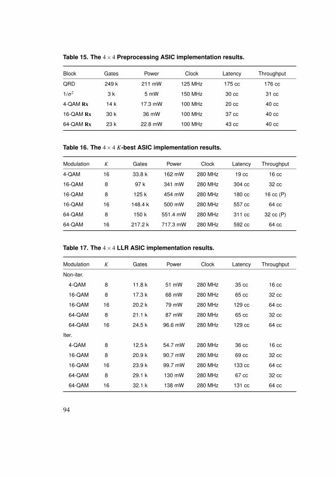
Table 15. The 4×4 Preprocessing ASIC implementation results.

Block Gates Power Clock Latency Throughput

QRD 249 k 211 mW 125 MHz 175 cc 176 cc

1/σ2 3 k 5 mW 150 MHz 30 cc 31 cc

4-QAM Rx 14 k 17.3 mW 100 MHz 20 cc 40 cc

16-QAM Rx 30 k 36 mW 100 MHz 37 cc 40 cc

64-QAM Rx 23 k 22.8 mW 100 MHz 43 cc 40 cc

Table 16. The 4×4 K-best ASIC implementation results.

Modulation K Gates Power Clock Latency Throughput

4-QAM 16 33.8 k 162 mW 280 MHz 19 cc 16 cc

16-QAM 8 97 k 341 mW 280 MHz 304 cc 32 cc

16-QAM 8 125 k 454 mW 280 MHz 180 cc 16 cc (P)

16-QAM 16 148.4 k 500 mW 280 MHz 557 cc 64 cc

64-QAM 8 150 k 551.4 mW 280 MHz 311 cc 32 cc (P)

64-QAM 16 217.2 k 717.3 mW 280 MHz 592 cc 64 cc

Table 17. The 4×4 LLR ASIC implementation results.

Modulation K Gates Power Clock Latency Throughput

Non-iter.

4-QAM 8 11.8 k 51 mW 280 MHz 35 cc 16 cc

16-QAM 8 17.3 k 68 mW 280 MHz 65 cc 32 cc

16-QAM 16 20.2 k 79 mW 280 MHz 129 cc 64 cc

64-QAM 8 21.1 k 87 mW 280 MHz 65 cc 32 cc

64-QAM 16 24.5 k 96.6 mW 280 MHz 129 cc 64 cc

Iter.

4-QAM 8 12.5 k 54.7 mW 280 MHz 36 cc 16 cc

16-QAM 8 20.9 k 90.7 mW 280 MHz 69 cc 32 cc

16-QAM 16 23.9 k 99.7 mW 280 MHz 133 cc 64 cc

64-QAM 8 29.1 k 130 mW 280 MHz 67 cc 32 cc

64-QAM 16 32.1 k 138 mW 280 MHz 131 cc 64 cc

94

4.5.3 Soft interference cancellation

The SIC receiver consists of a LMMSE detector, a LLR calculation block, a symbolexpectation calculation block and an interference cancellation block, as presented inFigure 6. The top level architecture of the LMMSE detector for a 2×2 antenna systemis presented in Figure 30. The channel matrix H is first multiplied by its complexconjugate transpose and the noise variance σ2 is added to the diagonal elements. Theresulting 2×2 matrix G is positive definite and symmetric. This simplifies the matrixinversion, which is performed by dividing the elements with the determinant, switchingthe diagonals and negating the off-diagonal elements. The determinant is real valuedand the off-diagonal elements are complex conjugates. Therefore, fewer operations areneeded.

H*H´H

σ²

*W

*

*

*- /

*

G

G11_re

G22_re

G12_re

G12_im

+

1

*

*

*

G22_re

G11_re

-G12_re

-G12_im

Fig. 30. The top level architecture of the 2×2 LMMSE detector ([62], published bypermission of IEEE).

The architecture for the real part of the symbol expectation calculation in the16-QAM case is presented in Figure 31. The imaginary part is calculated in parallel inthe same manner from LLRs LA(bi) and LA(bi+2) from the decoder. The lookup table(LUT) is used to find the tanh value.

>0LA(bi+1)

LUT1/√10 Exre*>0

1-1

LA(bi+3)

3/√10

Fig. 31. The architecture of the symbol expectation calculation ([62], published bypermission of IEEE).

95

The complexity of the SIC receiver for a 2×2 system is presented in Table 18 withan FPGA implementation and in Table 20 using ASIC technology. The word lengthswere determined with computer simulations. In symbol expectation and LLR calculationblocks, the word lengths range from 6 to 16 bits. In the LMMSE block, word lengths upto 22 bits were used. In addition, four 18-kbit block RAMs are used to store the channelmatrix H and the received symbol vector y and a BRAM is used in the interleaver. TheLLR calculation block also includes detection, i.e. multiplying the received signal withthe weight matrix W and another block for only LLR calculation in the SIC receiver.The clock frequency in the ASIC implementation is 100 MHz and the minimum clockfrequency is 126 MHz in the FPGA implementation. The clock frequency on FPGA islimited by the used implementation tools. Higher clock frequencies could be obtainedon FPGAs with some optimization.

The complexity of the SIC receiver for a 4×4 system is presented in Table 19 forthe FPGA implementation and in Table 21 for the ASIC implementation. The LMMSEdetector is the most complex part of the receiver taking 94 percent of the slices andalmost 69 percent of the gates. The LMMSE detector is based on the Gram-SchmidtQRD of the extended channel matrix and the LMMSE filter is obtained as in (25). Thenumber of BRAMs needed to store the channel matrix, the weight matrix W and thereceived signal is eleven. There are two LLR calculation blocks in the receiver in orderto perform the first and second iteration in parallel. The decoder is not included in thetotal complexity.

The LLR calculation block produces Q(N/2) bit LLRs in the given latency period.N/2 symbol expectations for a subcarrier are calculated in the given period. Thelatencies in the ASIC implementation were set to achieve the detection rates needed toprocess the data according to LTE time frames in a 20 MHz bandwidth. 20 MHz is themaximum bandwidth in LTE, but lower bandwidths, such as the 5 MHz bandwidth usedin the simulations, are also possible.

96

Table 18. The 2×2 SIC FPGA implementation results.

Block Modulation Slices DSPs Clock Latency Throughput

LMMSE - 698 13 126 MHz 62 cc 63 cc

LLR 4-QAM 23 12 238 MHz 2 cc 1 cc

LLR 16-QAM 41 26 165 MHz 4 cc 1 cc

LLR 64-QAM 106 40 155 MHz 5 cc 1 cc

Symbol exp. 4-QAM 3 2 100 MHz 1 cc 1 cc

Symbol exp. 16-QAM 8 2 100 MHz 2 cc 1 cc

Symbol exp. 64-QAM 27 2 138 MHz 3 cc 1 cc

SIC - 48 16 135 MHz 2 cc 1 cc

Table 19. The 4×4 SIC FPGA implementation results.

Block Modulation Slices DSPs Clock Latency Throughput

LMMSE - 8509 43 139 MHz 2074 cc 982 cc

LLR 4-QAM 72 40 180 MHz 2 cc 1 cc

LLR 16-QAM 112 66 148 MHz 4 cc 1 cc

LLR 64-QAM 243 96 155 MHz 5 cc 1 cc

Symbol exp. 4-QAM 11 4 704 MHz 2 cc 1 cc

Symbol exp. 16-QAM 29 4 347 MHz 2 cc 1 cc

Symbol exp. 64-QAM 53 20 138 MHz 3 cc 1 cc

SIC - 165 43 149 MHz 3 cc 1 cc

97

Table 20. The 2×2 SIC ASIC implementation results.

Block Modulation Gates Power Clock Latency Throughput

LMMSE - 48 k 40 mW 100 MHz 60 cc 40 cc

LLR 4-QAM 12.4 k 30 mW 100 MHz 6 cc 3 cc

LLR 16-QAM 18.6 k 33 mW 100 MHz 11 cc 3 cc

LLR 64-QAM 30.3 k 45 mW 100 MHz 9 cc 3 cc

Symbol exp. 4-QAM 488 0.58 mW 100 MHz 1 cc 2 cc

Symbol exp. 16-QAM 1335 1.2 mW 100 MHz 2 cc 2 cc

Symbol exp. 64-QAM 3521 3.2 mW 100 MHz 2 cc 2 cc

SIC - 17.5 k 22.3 mW 100 MHz 5 cc 3 cc

Table 21. The 4×4 SIC ASIC implementation results.

Block Modulation Gates Power Clock Latency Throughput

LMMSE - 415 k 522 mW 134 MHz 1218 cc 504 cc

LLR 4-QAM 35.9 k 82.6 mW 100 MHz 6 cc 3 cc

LLR 16-QAM 45.8 k 91 mW 100 MHz 12 cc 3 cc

LLR 64-QAM 72.6 k 114 mW 100 MHz 7 cc 3 cc

Symbol exp. 4-QAM 664 0.56 mW 100 MHz 1 cc 1 cc

Symbol exp. 16-QAM 2346 1.2 mW 100 MHz 1 cc 1 cc

Symbol exp. 64-QAM 3146 2.2 mW 100 MHz 1 cc 1 cc

SIC - 59 k 72 mW 100 MHz 5 cc 3 cc

4.5.4 Latency and receiver comparison

The processing latency of a receiver can be expressed as

Drec = Ddet +(DLLR +Ddec)Niter, (40)

where Ddet is the latency of the detector, DLLR is the latency of LLR calculation, Ddec isthe latency of the decoder and Niter is the number of iterations. LLR calculation anddecoding can be performed simultaneously and in a pipelined manner with detectionand their latency does not have to be included in the throughput latency. In an iterative

98

receiver, the throughput latency is determined by the minimum of Ddet and DLLR +Ddec.The detection rate of a receiver can be calculated as

QNDrec

, (41)

where Q is the number of bits per symbol and N is the number of transmit antennas.The timing of the K-best receiver is shown in Figure 32. The detector and the LLR

calculation are pipelined and have the same throughput period. The iterative LLRcalculation can begin after the code block has been decoded. It can be performedsimultaneously with the detection of the next code block. A code block size of 6,144bits was assumed in the latency calculations.

LSD

LSD

LLR

LLR

1. subcarrier

2. subcarrier

......

304 cc32 cc

65 cc

LSD LLRPth subcarrier Dec

LSD LLR1. subcarrier

LLRi

LLRi

...

Fig. 32. The timing and latencies in the K-best receiver with 4×4 16-QAM.

The timing of the SIC receiver is illustrated in Figure 33, where the block latenciesare presented in clock cycles. The throughput period is shown as the time after processingof the next subcarrier can begin. The weight matrices are calculated when the channelrealization changes, i.e. once in the channel coherence time. It is assumed that not allthe weight matrices have to be included in the decision on the layer to be detected andthat the layer order will remain the same for several channel realizations. The latency ofthe LMMSE receiver does not depend on the modulation. The latency of turbo decodingis included in the total latency estimate and it is calculated from the results given in[208], where the decoding rate is 1.28 Gb/s. The turbo decoder limits pipelining inthe SIC receiver in a way that all the subcarriers have to be decoded before movingto the symbol expectation calculation. The LLR1 block includes detection and LLRcalculation and it can start to process the next OFDM symbol while the second layer inthe previous symbol is being calculated.

A summary of the implementation results on FPGA is presented in Table 22 fora 2× 2 antenna system and in Table 23 for a 4× 4 system. The detection rate of

99

MMSE

MMSE

...

Decoder

Decoder

40 166

LLR1

LLR1

LLR2SICEx

LLR2Ex

...

1. OFDM

symbol

2. OFDM

symbol

3. OFDM

symbol

...

1. subcarrier

2. subcarrier

1. subcarrier

2. subcarrier

2. subcarrier

1. subcarrier

...1

SIC

5

1 3

10

LLR1 LLR2SICEx

LLR2Ex

1 SIC

5

1

4

LLR1

LLR1

Fig. 33. The timing and latencies in the SIC receiver with 4×4 16-QAM ([62], pub-lished by permission of IEEE).

each detector and the required rate for an LTE system are also presented. In the LTEspecifications, a 0.5 ms slot has been allocated for 7 or 6 (depending on the length ofthe cyclic prefix length) OFDM symbols [189]. In a 20 MHz bandwidth, each OFDMsymbol contains 1,200 subcarriers. A part of the subcarriers is reserved for pilot symbolsthat do not have to be detected. In a 2×2 system, roughly 10 percent of the subcarriersin a slot are pilot symbols and in a 4×4 system, more than 16 percent of the subcarrierscontain pilot symbols. The required detection rates are then calculated from the datasubcarriers. Any other control signal or other overhead is not included in the requiredrates. The FPGA results were generated to take full advantage of the platform and theclock frequencies and detection rates are as high as possible with the given platform andalgorithm. The K-best detection rate is restricted by the sorting in the algorithm. TheLMMSE and SIC receivers have a higher detection rate than necessary. Several K-bestdetectors could be used in parallel to achieve the required detection rate.

100

Table 22. The 2×2 receiver FPGA complexity and throughput.

Modulation Slices DSPs Clock Det. rate Req. rate

LMMSE 4-QAM 713 23 126 MHz 252 Mbps 60 Mbps

SIC 4-QAM 772 43 126 MHz 210 Mbps 60 Mbps

16-best 4-QAM 1875 24 206 MHz 51.5 Mbps 60 Mbps

LMMSE 16-QAM 722 30 126 MHz 504 Mbps 121 Mbps

SIC 16-QAM 795 65 126 MHz 361 Mbps 121 Mbps

8-best 16-QAM 2550 18 189 MHz 47.3 Mbps 121 Mbps

8-best iter. 16-QAM 2762 18 189 MHz 45.5 Mbps 121 Mbps

LMMSE 64-QAM 755 37 126 MHz 756 Mbps 182 Mbps

SIC 64-QAM 879 79 126 MHz 476 Mbps 182 Mbps

8-best 64-QAM 3243 28 180 MHz 67.5 Mbps 182 Mbps

16-best 64-QAM 4606 28 194 MHz 36.4 Mbps 182 Mbps

Available 8160 288

Table 23. The 4×4 receiver FPGA complexity and throughput.

Modulation Slices DSPs Clock Det. rate Req. rate

LMMSE 4-QAM 8566 79 139 MHz 612 Mbps 115 Mbps

SIC 4-QAM 8758 130 139 MHz 406 Mbps 115 Mbps

8-best 4-QAM 4889 52 192 MHz 96 Mbps 115 Mbps

LMMSE 16-QAM 8589 92 139 MHz 1.2 Gbps 230 Mbps

SIC 16-QAM 8815 156 139 MHz 615 Mbps 230 Mbps

8-best 16-QAM 6073 29 183 MHz 91.5 Mbps 230 Mbps

8-best iter. 16-QAM 6516 29 183 MHz 85.4 Mbps 230 Mbps

16-best 16-QAM 7863 29 129 MHz 32.3 Mbps 230 Mbps

LMMSE 64-QAM 8655 107 138 MHz 1.6 Gbps 345 Mbps

SIC 64-QAM 5970 202 138 MHz 721 Mbps 345 Mbps

8-best 64-QAM 8108 76 180 MHz 135 Mbps 345 Mbps

8-best iter. 64-QAM 8782 76 157 MHz 107.8 Mbps 345 Mbps

16-best 64-QAM 12317 74 211 MHz 79 Mbps 345 Mbps

Available 8160 288

101

The ASIC implementation results are summarized in Table 24 for the 2×2 antennasystem and in Table 25 for the 4×4 case. The LMMSE and SIC receiver were designedto have a 100 MHz clock frequency. They achieve the required detection rates in mostcases. Based on the synthesis results, the SIC receiver could be easily clocked with ahigher frequency in order to achieve the required rates. The K-best detector has a 280MHz clock frequency, but it achieves the required rates only with the lower modulationorders. In the other cases, the number of tree search and LLR blocks would have to bedoubled to achieve the required rates. The (P) in the table denotes the parallel K-bestdetector presented in Section 4.3.1. The iterative K-best receivers include two LLRcalculation blocks. One block calculates the LLRs on the first iteration and the otherblock uses the feedback from the decoder. Decoding latency of two code words isincluded in detection rate results of the iterative K-best. The SIC receivers include thedecoding latency of one code block in the detection rate results. The complexities ofthe different receivers do not differ greatly, but the power consumption of the K-bestdetector can be higher due to the higher clock frequency.

102

Table 24. The 2×2 receiver ASIC complexity and throughput.

Modulation Gates Power Clock Det. rate Req. rate

LMMSE 4-QAM 57.2 k 61.3 mW 100 MHz 66.7 Mbps 60 Mbps

SIC 4-QAM 78.3 k 92.6 mW 100 MHz 63.3 Mbps 60 Mbps

16-best 4-QAM 93.6 k 254 mW 280 MHz 70 Mbps 60 Mbps

LMMSE 16-QAM 60.2 k 64.3 mW 100 MHz 133 Mbps 121 Mbps

SIC 16-QAM 85.4 k 96.7 mW 100 MHz 120.7 Mbps 121 Mbps

8-best 16-QAM 105 k 238 mW 280 MHz 70 Mbps 121 Mbps

8-best iter. 16-QAM 112 k 273 mW 280 MHz 68.1 Mbps 121 Mbps

8-best (P) 16-QAM 116 k 287 mW 280 MHz 140 Mbps 121 Mbps

LMMSE 64-QAM 65.9 k 72.5 mW 100 MHz 200 Mbps 182 Mbps

SIC 64-QAM 99.3 k 110.6 mW 100 MHz 172.9 Mbps 182 Mbps

8-best (P) 64-QAM 137.5 k 326 mW 280 MHz 105 Mbps 182 Mbps

16-best (P) 64-QAM 161 k 404 mW 280 MHz 52.5 Mbps 182 Mbps

Table 25. The 4×4 receiver ASIC complexity and throughput

Modulation Gates Power Clock Det. rate Req. rate

LMMSE 4-QAM 444.5 k 587 mW 100 MHz 133 Mbps 115 Mbps

SIC 4-QAM 511 k 662 mW 100 MHz 120.7 Mbps 115 Mbps

8-best 4-QAM 367.3 k 604 mW 280 MHz 140 Mbps 115 Mbps

LMMSE 16-QAM 451 k 598 mW 100 MHz 266.7 Mbps 230 Mbps

SIC 16-QAM 522 k 686 mW 100 MHz 220.7 Mbps 230 Mbps

8-best 16-QAM 397 k 661 mW 280 MHz 140 Mbps 230 Mbps

8-best iter. 16-QAM 400.3 k 684 mW 280 MHz 126 Mbps 230 Mbps

LMMSE 64-QAM 459 k 607 mW 100 MHz 400 Mbps 345 Mbps

SIC 64-QAM 550 k 710 mW 100 MHz 304.7 Mbps 345 Mbps

8-best (P) 64-QAM 448 k 877 mW 280 MHz 210 Mbps 345 Mbps

16-best (P) 64-QAM 518.4 k 1052 mW 280 MHz 105 Mbps 345 Mbps

The performance, complexity and power consumption of the LMMSE, SIC andK-best are further illustrated in Figures 34 and 35. The goodput was defined to be thelesser of the detection rate and transmission throughput. Even though the information

103

transmission rate of the K-best detector is higher than that of the SIC or LMMSE,the hardware detection rate of a single detector is lower. The number of detectorswas increased to achieve the required rates, but this resulted also in an increase in thecomplexity and power consumption. The results in Figures 34 and 35 are very similar.In some cases, the SIC detector achieves a higher goodput with a lower amount of powerconsumption than the K-best detector. The complexity, however, can be very close tothat of the 8-best detector. This can also be calculated from the theoretical complexity inTable 4. The power consumption results may differ from the theoretical results due tothe different clock frequencies. The LMMSE has the lowest power consumption, but itmay not achieve any goodput in difficult channel conditions. It can be seen that the16-best detector has a very high complexity and power consumption, while the goodputis at the same level as with the 8-best. The 8-best provides a fair amount of goodput inall scenarios.

400 500 600 700 800 900 1000 1100 1200 1300 14000

20

40

60

80

100

120

140

160

180

Complexity [k gates]

Go

od

pu

t [M

bp

s]

4x4 system, Goodput vs. Complexity

16−QAM, corr. channel at 26 dB

16−QAM, mod. corr. channel at 20 dB

64−QAM, corr. channel at 30 dB

64−QAM, mod. corr. channel at 26 dB

LMMSE

LMMSE

16−best

16−best8−best, 2 it.

8−best

8−best

8−best, 2 it.

SIC

8−best

SIC

LMMSE

SIC

Fig. 34. Complexity-performance trade-off in a 4×4 antenna system.

4.5.5 SSFE and K-best comparison

The complexity and performance of two tree search algorithms are compared. Theperformance of the algorithms was discussed in Section 4.4.5. The complexity resultsfor the SSFE and K-best detectors are presented in Table 26 in the 16-QAM case and inTable 27 in the 64-QAM case. The SSFE list size is 12 and the node spanning vectoris [3,2,2,1,1,1,1,1] as in the simulation results. The clock frequency of the detectors

104

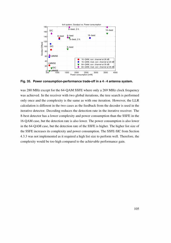
500 1000 1500 2000 2500 3000 3500 40000

20

40

60

80

100

120

140

160

180

Power consumption [mW]

Go

od

pu

t [M

bp

s]

4x4 system, Goodput vs. Power consumption

16−QAM, corr. channel at 26 dB

16−QAM, mod. corr. channel at 20 dB

64−QAM, corr. channel at 30 dB

64−QAM, mod. corr. channel at 26 dB

8−best

SIC 16−best8−best, 2 it.

SIC

LMMSE

LMMSE

LMMSE

SIC

8−best

8−best

8−best, 2 it.

16−best

Fig. 35. Power consumption-performance trade-off in a 4×4 antenna system.

was 280 MHz except for the 64-QAM SSFE where only a 269 MHz clock frequencywas achieved. In the receiver with two global iterations, the tree search is performedonly once and the complexity is the same as with one iteration. However, the LLRcalculation is different in the two cases as the feedback from the decoder is used in theiterative detector. Decoding reduces the detection rate in the iterative receiver. The8-best detector has a lower complexity and power consumption than the SSFE in the16-QAM case, but the detection rate is also lower. The power consumption is also lowerin the 64-QAM case, but the detection rate of the SSFE is higher. The higher list size ofthe SSFE increases its complexity and power consumption. The SSFE-SIC from Section4.3.3 was not implemented as it required a high list size to perform well. Therefore, thecomplexity would be too high compared to the achievable performance gain.

105

Table 26. Implementation results with 4×4 16-QAM.

Receiver Gates Power Detection rate

Tree search LLR Tree search LLR

SSFE 135.2 k 19 k 488.9 mW 79 mW 186 Mbps

SSFE, 2 it. 135.2 k 34.6 k 488.9 mW 158 mW 163 Mbps

8-best 97 k 17.3 k 341.5 mW 68.3 mW 140 Mbps

8-best, 2 it. 97 k 33.1 k 341.5 mW 140.5 mW 126 Mbps

16-best 148.4 k 20.2 k 499.6 mW 79.2 mW 70 Mbps

Table 27. Implementation results with 4×4 64-QAM.

Receiver Gates Power Detection rate

Tree search LLR Tree search LLR

SSFE 177.4 k 25.7 k 568.6 mW 110.5 mW 269 Mbps

SSFE, 2 it. 177.4 k 50.4 k 568.6 mW 236.7 mW 222 Mbps

8-best 183.7 k 21.5 k 551.4 mW 87 mW 210 Mbps

8-best, 2 it. 183.7 k 45.2 k 551.4 mW 197.9 mW 180 Mbps

16-best 217.2 k 24.5 k 717.3 mW 96.6 mW 105 Mbps

The complexity-performance trade-off is illustrated in Figure 36. The goodput i.e.the minimum of the transmission throughput and hardware detection rate of informationbits in a 20 MHz bandwidth with a 1/2 code rate, is compared to the hardware complexity.The K-best with list size of 16 has a high complexity and low goodput. The goodputof the SSFE with two global iterations is close to that of the 8-best with one iterationwith 16-QAM, but has a higher complexity. With 64-QAM, SSFE with two iterationsachieves the highest goodput. Extra iterations do not bring any benefit with the K-besttree search as the detection rate is low. Even though the SSFE algorithm does notinclude sorting, the slicing operation induces extra complexity compared to the K-bestalgorithm and the difference between the two tree search algorithms remains small.

106

100 150 200 25030

40

50

60

70

80

90

100

110

120

Complexity [k gates]

Go

od

pu

t [M

bp

s]

4x4 system, Goodput vs. Complexity

16−QAM, mod. corr. channel at 18 dB

16−QAM, corr. channel at 22 dB

64−QAM, mod. corr. channel at 26 dB

16−bestSSFE

16−best

SSFE

SSFE,2 it.

8−best,2 it.

SSFE,2 it.

8−best

8−best,2 it.

8−best

Fig. 36. Complexity-performance trade-off in a 4×4 antenna system.

4.5.6 Receiver adaptation

Architecture

The architecture of the QRD and MMSE calculation for an N×N MIMO system ispresented in Figure 37. The QRD of the matrix is calculated with an algorithm whichproduces a unitary matrix Q. The input matrix is either the extended channel matrix H orthe matrix used in the capacity and SINR calculations. The same QRD architecture canbe used for both matrices. For example, the Gram-Schmidt process [209] presented inSection 4.2 without column reordering can be used for the QRD. Part of the multiplierscan be turned off when calculating capacity because the input matrix is smaller than theextended channel matrix. Another option is to extend the capacity/SINR matrix withzeros and then the QRD architecture can be used in exactly the same way as with theextended channel matrix. The capacity is obtained by multiplying the diagonal elementsof R and taking the logarithm from the product. The SINR for stream n is found bycalculating the inverse of the diagonal element (n,n) of matrix W.

The decision on the modulation and coding scheme can be obtained by summing theSINR or capacity of the subcarriers in an OFDM symbol and using a lookup table toselect the modulation, code rate and transmission rank based on the sum. The calculationof QRD and capacity can be time interleaved as they are not performed in each framebut in the channel coherence time. If precoding is used, multiplying the channel matrix

107

with different precoding matrices is added to the left side of the architecture. A separateblock can be added to calculate the rank 1 and 2 capacities as matrix inversion is notnecessary.

QRD

MMSE/

Capacity

MMSE/

CapacityH

HxHH

Hx

1/Nσ²

Concat

Iσ

inv

x

R

QH

W

/

1stream

SINR

x log2Capacity

I

Fig. 37. Architecture of the capacity and MMSE/QRD calculation ([63], publishedby permission of IEEE).

Implementation results

The LMMSE, SIC and K-best LSD receivers were designed to operate with an adaptivemodulation scheme in a 2×2 and a 4×4 antenna system. Therefore, the receivers can beused with QPSK, 16-QAM and 64-QAM. The decoder is not included in the complexityresults, but a high throughput turbo decoder [208, 210] can be used to achieve the LTEdecoding rate requirement.

The complexities in gate equivalents of the preprocessing, detection and LLRcalculation are presented in Table 28 for the 2×2 system and Table 29 for the 4×4system. The clock frequency was 280 MHz with the K-best LSD and 100 MHz with theother receivers and preprocessing. In the 2×2 case, the MMSE was calculated with thedirect matrix inversion and the QRD with the Gram-Schmidt algorithm. The QRD wasthe most complex block. The latency of the block is the time after which processing ofthe next input can start. The preprocessing latency can be higher than the detectionlatency as it has to be performed when the channel realization changes. In the 4×4system, the QRD is one of the most complex blocks. An 8×16 real valued extendedchannel matrix is used as an input to the QRD. As the direct matrix inversion for MMSEweight matrix calculation would be more complex in the 4×4 system, the QRD of theextended channel matrix is used to calculate the weight matrix as presented in (19). The

108

word lengths of the different receivers are mostly 16 bits. In the QRD, some larger innerword lengths were used and if the QRD is used for capacity calculation, the inputs arescaled as the capacity values are larger than the channel values.

Table 28. The 2×2 implementation results for adaptive receiver.

Receiver Block Complexity Power Latency

(Gates) (mW) ns

QRD (Gram-Schmidt) 66.6 k 35.1 400

MMSE (direct matrix inversion) 48 k 40 400

Detection and LLR 17.1 k 12.8 10

SIC 19.6 k 24.5 40

4-best LSD 31.7 k 120.6 114

8-best LSD 51.3 k 198 114

LLR for 4-best 12.6 k 50 114

LLR for 8-best 14.4 k 57.4 114

LLR it. for 8-best 18.7 k 79.6 114

Table 29. The 4×4 implementation results for adaptive receiver.

Receiver Block Complexity Power Latency

(Gates) (mW) ns

QRD (Gram-Schmidt) 179.8 k 116 4480

R−1 (for MMSE) 43.5 k 31.9 3420

Matrix mult. (for MMSE) 29 k 31.4 3200

Detection and LLR 31 k 33.7 50

SIC 86.3 k 88.7 40

4-best LSD 78.3 k 322.8 114

8-best LSD 126.6 k 496 114

LLR for 4-best 18.2 k 74.5 114

LLR it. for 4-best 41.4 k 216.9 114

LLR for 8-best 21 k 86.2 114

109

The total complexity and power consumption of the receivers are presented inTables 30 and 31. The K-best LSD has the highest complexity. In the 2×2 system, thecomplexity of the SIC receiver is much lower even though the performance is close tothat of the K-best LSD.

Table 30. Complexity and decoding rate of 2×2 adaptive receivers.

Receiver Complexity Power consumption Max. det. rate

(Gates) (mW) (Mbps)

LMMSE 59.5 k 52.4 600

SIC 84.7 k 77.3 134

4-best 130 k 229 105

8-best 151.7 k 314 105

8-best, 2 it. 156 k 368 97

The difference in complexity between the receivers is smaller in the 4×4 case thanin the 2×2 case. Calculating the MMSE weight matrix W takes almost 90 percent of thegate equivalents in the LMMSE receiver in the 4×4 case. The 2×2 system allowedsome simplifications in the implementation and cannot be straightforwardly scaled to allother antenna configurations. The 4×4 implementation could be also scaled to largerantenna configurations.

Table 31. Complexity and decoding rate of 4×4 adaptive receivers.

Receiver Complexity Power consumption Max. det. rate

(Gates) (mW) (Mbps)

LMMSE 283.3 k 213 240

SIC 369.6 k 302 202

4-best 305 k 538 210

4-best, 2 it. 329 k 681 180

8-best 356.5 k 723 210

If precoding is used, the complexity of the receiver is increased. The capacity hasto be calculated for the sixteen possible precoding matrices in LTE with the differentprecoding matrix ranks. For rank 4 transmission, the capacity is the same for all

110

precoding matrices and it has to be calculated only once. The QRD can be used tocalculate the determinant, as shown in Figure 37. The matrix multiplications and the lowrank determinant calculations add still another 82 k gates to the complexity, as shown inTable 32. Without precoding, the capacity calculations are simpler and most of thecomplexity comes from the HHH matrix multiplication.

Table 32. Complexity of precoding in a 4×4 system ([63], published by permissionof IEEE).

Block Complexity Power

(Gates) (mW)

Capacity with precoding 81.9 k 39.2

Capacity without precoding 32 k 36

4.6 Discussion

The theoretical complexities of the algorithms were presented. The complexity of theK-best algorithm is close to that of the SIC algorithm with low order modulations, butthe difference is greater with higher modulations. The implementation results in Section4.5 support the theoretical results in Table 4: the receivers have similar complexitieswith low order modulations, but the complexity of the K-best LSD increases withthe modulation order. The LMMSE calculation was implemented as a direct matrixinversion in the 2× 2 case, which made the SIC less complex even with low ordermodulations.

Comparison of both performance and implementation to literature can be difficultas the used channel models, methods and the implementation technologies may bedifferent. Many of the implementations in the literature consider an uncoded system oran uncorrelated channel, where also simple receivers perform well, which can lead todifferent parameters in the implementation. Also, the word length requirements mayvary with different system setups. The parameters used may have even a higher impacton the preprocessing, i.e. the LMMSE filter or the QRD. Depth-first sphere detectorimplementations in the literature usually report an SNR dependent throughput, whichmakes the implementation comparison more challenging. The use of a HLS tool in thiswork also results in an unfavorable comparison to hand-coded results.

111

The Givens rotation based QRD in [120] uses smaller word lengths than the QRDimplementation in this work. The complexity is roughly 100 k gates smaller, but thepower consumption is higher by 100 mW. The latency of the QRD is, however, muchsmaller than that in this work. An MMSE receiver was implemented in [116]. Thecomplexity and power consumption are much higher than those in this work, however,the detection rate is also higher. Nevertheless, a lower detection rate was aimed for inthis work.

The hard-output l2-norm K-best detectors in [211] have a lower complexity, but wereimplemented with different list sizes and CMOS technology from our work. Other normswere also used in [211] for the Euclidean distance calculation to avoid the squaringoperation in the l2-norm, yet since they were not used in this work as they also have animpact on performance, their implementation is not comparable. The complexity of thereceiver increases by roughly 30 percent both in [211] and this work when the list size isdoubled. However, the detection rate decreases almost five times in [211], whereas it isonly halved in our work. An implementation of a radius adaptive K-best detector waspresented in [128]. The complexities of the 64-QAM K-best detectors are similar tothose in this work, yet the power consumption is much lower. This can also be due to thedifferent implementation technology. The hard-output K-best detector with on demandnode expansion was implemented in [129]. A different implementation technologywas used, but the gate count and power consumption were smaller than those in thiswork. The soft output K-best implementation in [103] with a list size of 5 in a 4×416-QAM system has almost a three times lower throughput and half the complexityof our implementation with a list size of 8. A soft output K-best detector is presentedin [124]. It achieves a 50 Mb/s throughput with 4×4 64-QAM, list size of 256 and asilicon area of 20 mm2. In conclusion, numerous existing detection implementationscan be found, but a meaningful quantitative comparison in terms of performance andcomplexity is difficult. Therefore, the performance and complexity of several detectionalgorithms was compared in this work.

The performance-complexity trade-off of the ASIC implementations in a 2× 216-QAM in a correlated channel is summarized in Table 33 and in the 4×4 16-QAMcase in Table 34. The detection rates of the receivers are almost the same and enough toreach 121 Mbps in the 2×2 case and 230 Mbps in the 4×4 case. Even though thedetection rate of the LMMSE receiver is high, the performance degradation in terms ofreliable transmission throughput is considerable, in particular at the cell edge, where theavailable SNR is often low. The term goodput was defined to be the minimum of the

112

hardware detection rate times the 1/2 code rate and the transmission rate of informationbits over the 20 MHz bandwidth times (1−FER).

The LMMSE receiver would require almost 10 dB more transmit power in order toachieve the goodput of the K-best LSD, but the power consumption is much higher withthe K-best LSD. The SIC receiver does not achieve the goodput of the K-best LSD, buthas a much lower complexity. In the 4×4 antenna case, the SIC and LMMSE receiversdo not give much goodput at lower SNRs, yet all the receivers have a high goodputwhen the SNR is high enough. If the channel is less correlated, the receivers have amore similar performance and less transmit power is needed to achieve a high goodput.The SIC receiver produces the most bits per gate equivalent in the 2×2 antenna system,but in the 4×4 system, the K-best LSD is the most efficient. A part of the performancedegradation of the SIC receiver in the 4×4 antenna system is due to the encoding ofthe streams, which leads to interference cancellation being performed between twolayer pairs and the two layer pairs being separated only by the LMMSE equalizer. TheSIC receiver would still provide a higher goodput than the LMMSE receiver with alower power consumption than the K-best LSD, thus, offering a compromise betweenperformance and complexity.

Table 33. The performance-complexity trade-off with 2×2 16-QAM.

Receiver Complexity Power Goodput Goodput

(Gates) mW at 16 dB at 20 dB

LMMSE 60 k 64 0.3 Mb/s 15.7 Mb/s

SIC 85 k 97 6.2 Mb/s 49.4 Mb/s

8-best 170 k 274 17.4 Mb/s 67.3 Mb/s

8-best, 2 iter. 173 k 458 32.4 Mb/s 69.8 Mb/s

113

Table 34. The performance-complexity trade-off with 4×4 16-QAM.

Receiver Complexity Power Goodput Goodput

(Gates) mW at 24 dB at 28 dB

LMMSE 451 k 598 0.1 Mb/s 84.4 Mb/s

SIC 522 k 686 20.6 Mb/s 133.7 Mb/s

8-best 545 k 1112 113.4 Mb/s 140 Mb/s

8-best, 2 iter. 576 k 1257 128 Mb/s 140 Mb/s

As a final illustration of the performance-complexity trade-off, the required transmitpower to satisfy the rate and quality requirements is considered in a simple example case.As the LMMSE and SIC receivers reach their maximum throughput at higher SNRsthan the K-best receiver, the transmit power needs to be higher to obtain the highestdata rates. The following example case illustrates the distance at which the maximumdata rates can be achieved with the different receivers. The power efficiency of thetransmitter in transmit power/transmission rate in a 4×4 antenna system with a 20 MHzbandwidth is presented in Figure 38. The needed transmit power was obtained fromLF +NR +SNR+FM, where LF is the free space path loss 20log(4πd/λ ), NR is thereceiver noise floor (kT B + receiver noise figure of 6 dB) and FM is a 30 dB fade margin(λ is the wavelength, d is the distance from the base station, k is Boltzmann’s constant,T is the temperature [K] and B is the bandwidth). The SNR is the signal strength at thereceiver required to achieve the maximum goodput. A simple path loss model withoutshadowing or reflections was chosen for simplicity. The required transmit power of theLMMSE receiver is at least twice of that of the K-best LSD. The transmit energy perbit grows with the modulation order and is the same with 64-QAM K-best LSD and16-QAM LMMSE. The K-best LSD can receive data reliably from a higher distancethan the SIC or LMMSE receiver with a fixed transmit power. With 4×4 64-QAM,the LMMSE receiver can receive data at only very short distances with a reasonabletransmit power. Therefore, a more complex receiver is needed to receive data from alsolarger distances.

The previous performance-complexity trade-off results assumed that there is nochannel state information at the transmitter. With full or partial transmitter channel stateinformation, low mobility appropriate feedback schemes combined with transmitterprecoding could change the conclusions. Therefore, the impact of adaptive modulation

114

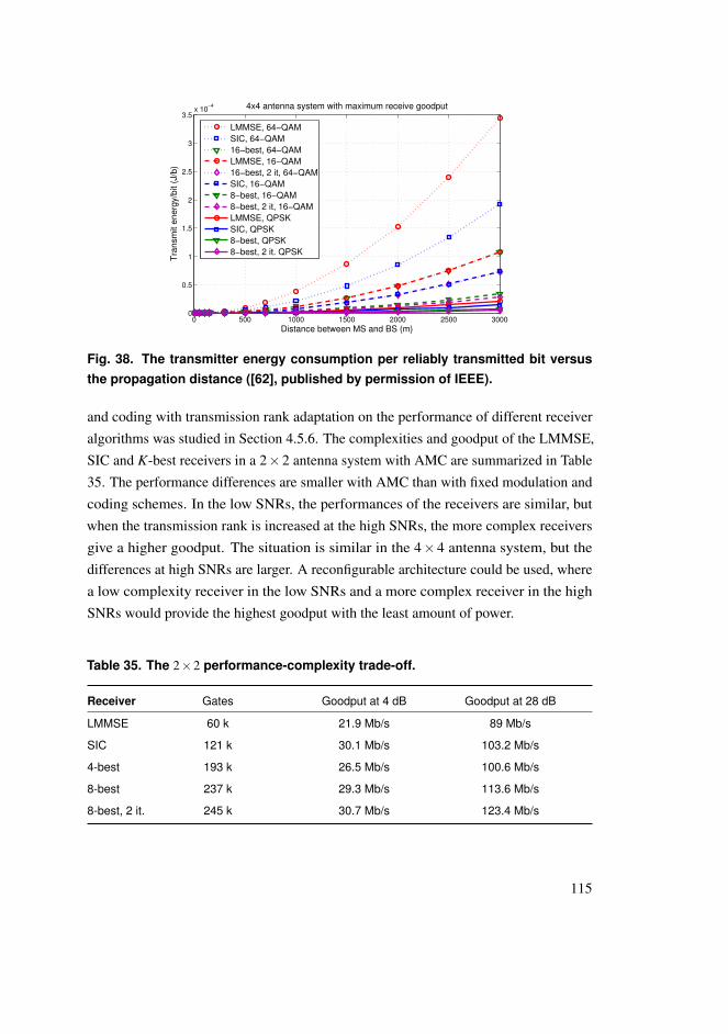
0 500 1000 1500 2000 2500 30000

0.5

1

1.5

2

2.5

3

3.5x 10

−4

Distance between MS and BS (m)

Tra

nsm

it e

nerg

y/b

it (

J/b

)

4x4 antenna system with maximum receive goodput

LMMSE, 64−QAM

SIC, 64−QAM

16−best, 64−QAM

LMMSE, 16−QAM

16−best, 2 it, 64−QAM

SIC, 16−QAM

8−best, 16−QAM

8−best, 2 it, 16−QAM

LMMSE, QPSK

SIC, QPSK

8−best, QPSK

8−best, 2 it. QPSK

Fig. 38. The transmitter energy consumption per reliably transmitted bit versusthe propagation distance ([62], published by permission of IEEE).

and coding with transmission rank adaptation on the performance of different receiveralgorithms was studied in Section 4.5.6. The complexities and goodput of the LMMSE,SIC and K-best receivers in a 2×2 antenna system with AMC are summarized in Table35. The performance differences are smaller with AMC than with fixed modulation andcoding schemes. In the low SNRs, the performances of the receivers are similar, butwhen the transmission rank is increased at the high SNRs, the more complex receiversgive a higher goodput. The situation is similar in the 4×4 antenna system, but thedifferences at high SNRs are larger. A reconfigurable architecture could be used, wherea low complexity receiver in the low SNRs and a more complex receiver in the highSNRs would provide the highest goodput with the least amount of power.

Table 35. The 2×2 performance-complexity trade-off.

Receiver Gates Goodput at 4 dB Goodput at 28 dB

LMMSE 60 k 21.9 Mb/s 89 Mb/s

SIC 121 k 30.1 Mb/s 103.2 Mb/s

4-best 193 k 26.5 Mb/s 100.6 Mb/s

8-best 237 k 29.3 Mb/s 113.6 Mb/s

8-best, 2 it. 245 k 30.7 Mb/s 123.4 Mb/s

115

116

5 Channel estimation in MIMO-OFDM systems

In this chapter, performance of the LS, MMSE and SAGE channel estimation algorithmsis studied using the LTE pilot symbol structure as a benchmark. The fast fadingor high mobility scenario with insufficient pilot symbol density and the high pilotoverheads from the MIMO pilot symbols are the two main issues considered. The SAGEchannel estimator is used in the iterative receiver to improve the performance whenthe pilot symbol density is too low, i.e. in high velocity cases. MMSE filtering is alsoused in between pilot symbols to improve the channel estimates and the performanceis compared to that of the SAGE estimator. The throughput can be increased byreplacing some of the pilot symbols with data symbols and using the SAGE algorithmto compensate for the performance loss caused by the decreased pilot density. Thetheoretical complexity of the channel estimation algorithms is presented and somecomplexity-performance trade-off aspects of the SAGE algorithm are considered. Thearchitecture and implementation results in gate counts and power consumption for thepilot symbol based LS, MMSE and the DD SAGE channel estimators are presentedfor the 2×2 and 4×4 antenna systems. For a more energy efficient solution, a longerlatency for the channel estimator is considered. The impact of generating a timelychannel estimate for the detector on the performance and complexity is then discussed.

The main contributions of this chapter are the implementation of data aided anddecision directed channel estimation algorithms and evaluating the applicability ofthe channel estimation algorithms for mobile MIMO-OFDM systems with differentpilot symbol densities. Although different channel estimation algorithms have beenproposed, only few implementations of channel estimation algorithms can be found inthe literature. Furthermore, the latency of decision directed channel estimation has notbeen previously considered. Thus, these are the main themes of this chapter.

The channel estimation algorithms are introduced in Section 5.1. The performancesof the algorithms with different channel models are compared in Section 5.2 and somecomplexity reducing alterations and latency issues are discussed in Section 5.3. Theimplementation results are presented in Section 5.4 and Section 5.5 includes discussionon the results. The performances of the LS and SAGE algorithms were compared in[67], where the latency of the SAGE estimator was also discussed. The implementationresults and the simulation results presented in Section 5.2 have not been previously

117

published.

5.1 Channel estimation algorithms

The system model was introduced in Section 3.1 and the signal model for channelestimation in Section 3.3. The receiver structure is presented in Figure 39. The LSchannel estimator is used in calculating the channel estimates from pilot symbols. Thereceived signal vector is transformed into frequency domain before the LS channelestimation. The LS channel estimate can be filtered with an MMSE filter. The channelimpulse response result from the LS or MMSE estimator has to be transformed intofrequency domain for the detector with the second fast Fourier transform (FFT). TheDD SAGE channel estimator can be used in addition to the LS estimator. The pilotbased LS estimator provides initial channel estimates for the SAGE algorithm. Thesoft symbols are calculated from the decoder outputs as in (31) in Chapter 4 and aretransformed into time domain for the SAGE channel estimator. The SAGE channelestimator also takes the time domain received signal as input. The hard outputs fromthe decoder are not considered for channel estimation as the soft information betterrepresents the reliability of the decision.

Detection π-1

Decoding

πSoft

decisionsIFFT

FFT LS FFT

SAGEĥ

o

Optional decision directed addition

Ĥ

MMSE

Fig. 39. The receiver structure.

5.1.1 LS channel estimation

The LS estimate of the channel can be calculated as

hLSmR

(n) = (FHXH(n)X(n)F)−1FHXH(n)ymR(n), (42)

where X contains the pilot symbols or if used in a DD mode, the symbol decisions. Thecalculation of the LS channel estimate from the pilot symbols is simple as the matrix

118

inversion can be calculated in advance and the only calculation to be performed in realtime is multiplication with the received signal. When using the LS estimator in a DDmode, the NL×NL matrix inversion induces a high computational complexity.

5.1.2 MMSE channel estimation

In order to exploit the time domain correlation of the channel and to take into accountthe impact of the noise, the LS channel estimate can be filtered with an MMSE filter [74]

hMMSEmR,mT ,l(n) = WH

mR,mT ,l(n)hLSmR,mT ,l , (43)

where the LS channel estimate vector for the lth tap from the mT th transmit antenna tothe mRth receive antenna

hLSmR,mT ,l = [hLS

mR,mT ,l(n1)...hLSmR,mT ,l(nNP)]

T ∈ CNP×1 (44)

contains the LS channel estimates from the duration of the filtering window. NP is thenumber of OFDM symbols with pilot symbols in a filtering window and mT = 1, ...,Nand mR = 1, ...,M are the transmit and receive antenna indices. The MMSE filteringvector WmR,mT ,l(n) is [156]

WmR,mT ,l(n) = Σ−1hLS

mR,mT ,lΣ

HmR,mT ,l , (45)

where the cross-covariance matrix between hmR,mT ,l(n) and hLSmR,mT ,l

is

ΣmR,mT ,l = [ρ(n−n1)...ρ(n−nNP)]Σhl (46)

and the auto-covariance matrix is

ΣhLSmR,mT ,l

=

ρ(n1−n1) · · · ρ(n1−nNP)

.... . .

...ρ(nNP −n1) · · · ρ(nNP −nNP)

ΣhmR ,mT ,l +Σw. (47)

The noise covariance matrix Σw = σ2I ∈ RNP×NP , ΣhmR,mT ,l = E(h∗mR,mT ,lhmR,mT ,l) andρ(n−n′) is the temporal correlation between the channel taps, which depends on the lagn−n′ between time indices n and n′ [156]. In order to avoid the calculation of the spatialcorrelation Σhl , it can be left out from (46) and (47). This only has a minor impact on theperformance, as presented in Section 5.2. It also enables the use of precalculated MMSE

119

filter coefficients, where the predetermined values for σ2 and user velocity are used.The coefficients can be calculated for a set of σ2 and velocity values and the coefficientsclosest to the estimated values can be used. Since ρ(n−n) = 1 and Σw contains σ2 onits diagonal, the precalculated coefficients can be obtained by substituting the knownvalues in (45). The MMSE filter coefficients can be then precalculated as

1+σ2 · · · ρ(n1−nNP)...

. . ....

ρ(nNP −n1) · · · 1+σ2

−1

ρ(n−n1)...

ρ(n−nNP)

, (48)

where the temporal correlation is distributed according to Jakes’ model and can bewritten as

ρ(n−n′) = J0(2π fd(n−n′)TB) (49)

and J0 denotes the zeroth-order Bessel function of the first kind, fd is the Dopplerfrequency and TB is the OFDM symbol duration.

5.1.3 SAGE channel estimation

The EM algorithms consist of an expectation and a maximization step. The "complete"data is estimated in the expectation step and the channel estimate is updated in themaximization step. The frequency domain SAGE algorithm provides an iterativesolution of the decision directed LS estimate in (55). The time domain SAGE algorithm[212] can be used to avoid the matrix inversion required with non-constant envelopemodulations in FD SAGE channel estimator. The time domain received signal o isviewed as the "incomplete" data and z as the "complete" data, which is iterativelyupdated along with the channel estimate hmT ,mR,l(n). The time domain SAGE algorithmcalculates the channel estimates with iterations

z(i)mT ,mR,l= z(i)mT ,mR,l +[omR −

MT

∑m′T=1

L−1

∑l′=0

z(i)m′T ,mR,l′] (50)

h(i+1)mT ,mR,l

(n) =xH

mT ,l z(i)mT ,mR(n)

xHmT ,l

xmT ,l(51)

z(i+1)mT ,mR,l(n) = xmT,l h

(i+1)mT ,mR,l

(52)

120

z(i+1)m′′T ,mR,l′′

(n) = z(i)m′′T ,mR,l′′. (53)

The channel estimator is initialized with the channel estimate h(0)mT ,mR,lfrom the previous

OFDM symbol as

z(0)mT ,mR,l(n) = xmT,l h(0)mT ,mR,l

. (54)

5.2 Performance comparison

The simulation parameters are presented in Table 36 and the vehicular channel modelparameters [213] in Table 1 in Section 3.4. Alternatively, a Winner channel model wasused [195]. The Winner channel parameters were presented in Table 2. The detectorused in the simulations is a K-best list sphere detector [88] with the list size of 8 in the2×2 antenna system and 16 in the 4×4 antenna system. The user velocities of 50 km/hand 100 km/h were assumed, where the corresponding Doppler frequencies were 111Hz and 222 Hz.

Mitigation of inter-carrier interference (ICI) caused by very high mobile velocitiesis out of the scope of this work. The remaining frequency offset after frequencysynchronization may be modeled with increased noise at the receiver [214]. Furthermore,the algorithms considered in this thesis are not among the most suitable algorithms forvery high velocities where the ICI would be the most dominant.

The throughput can be increased by using half of the LTE reference signals alongwith the decision directed channel estimation. The pilot symbols are then transmittedonly in the first OFDM symbol in a slot and data is transmitted instead of pilot symbols inthe other OFDM symbols which is denoted in the figures as 1 pilot. Channel estimationcan be performed over several slots, but this degrades the performance in high velocityscenarios.

In the following simulation results, LS channel estimation is used on the OFDMsymbols with pilot symbols and the SAGE algorithm is used on the OFDM symbolswithout reference signals. The performance of the SAGE algorithm with transmitteddata as the feedback, i.e. genie aided SAGE algorithm, is also shown in the figures.With the genie aided mode, pilots are transmitted in one OFDM symbol per slot wherethe LS estimator is used in estimating the channel. The MMSE channel estimator isprecalculated with the velocity of 70 km/h and the SNR of 26.5 dB in the 4×4 antennasystem and 16.5 dB in the 2×2 antenna case as they were found to be suitable for mostof the simulation cases. MMSE filtering is performed over one slot with the LTE pilot

121

structure and over two slots with pilots in only one OFDM symbol as the MMSE filterneeds at least two channel estimates to perform well. The filtering window is shiftedwhen a new channel estimate is available from the LS estimator in order to obtain themost current estimates. This also decreases the latency from the case where channelestimation is performed on the whole slot before detection. Increasing the size of thefiltering window with LTE pilot structure does not improve the performance.

The performances of the LS, the precalculated MMSE and the SAGE algorithmsare presented and compared in the following figures. First, the results with 2× 2antenna system with 16-QAM and 100 km/h user velocity are presented in Figure40 followed by the 4×4 16-QAM results with a 50 km/h user velocity in Figures 41and 42. Then, results for 4× 4 MIMO with 16-QAM, different channel types and100 km/h user velocity in Figure 43 are discussed. After that, the performance of thealgorithms is illustrated in Figure 45 for 4×4 64-QAM and a 50 km/h user velocity,including comparisons of the MMSE estimator with known velocity and SNR andthe precalculated MMSE filter with constant velocity and SNR. Spatial correlation isnot used in the MMSE filter with the exception of the results with the known spatialcorrelation in Figure 44. The impact of estimated tap delays is presented in Figure 46and the performances with the Winner channel model are shown in Figures 47 and 48.The performance with the LMMSE and K-best detectors combined with MMSE andSAGE channel estimators in an uncorrelated channel are compared in Figure 49. Thetypical urban channels are moderately correlated with base station (BS) azimuth spreadof 5 degrees except for the channels in Figures 43 and 49.

Table 36. Simulation parameters.

Coding Turbo coding with 1/2 code rate

Carrier frequency 2.4 GHz

Modulation scheme 16-QAM, 64-QAM

Number of subcarriers 512 (300 used), 5 MHz bandwidth

Symbol duration 71.4 µs

The performance of the channel estimation algorithms is presented in Figure 40 in a2×2 antenna system. The communication system performance is usually characterizedby frame error rate. The transmission throughput is defined to be equal to the nominalinformation transmission rate of information bits times (1−FER). The throughput

122

increases when half of the LTE reference symbols are used along with the decisiondirected channel estimation. However, the MMSE estimator performs nearly as wellas the SAGE estimator in the 2×2 antenna system. The pilot symbol density is nothigh enough for the LS estimator to perform well since the channel changes too rapidlybetween the OFDM symbols containing pilot symbols.

10 12 14 16 18 20 22 24 260

2

4

6

8

10

12

14

162x2 16−QAM, TU channel, 8−best LSD, 100 km/h

Es/N0 [db]

Thro

ughput [M

bps]

LS+genie SAGE, 1 pilot

LS+SAGE, 1 pilot

LS+SAGE, LTE pilots

LS+MMSE, LTE pilots

LS, LTE pilots

LS, 1 pilot

Fig. 40. 2× 2 16-QAM data transmission throughput vs. SNR with different pilotdensities and 100 km/h user velocity.

The same can be seen in Figure 41 with a 4×4 antenna system, where the decisiondirected channel estimation increases the throughput more than in the 2×2 antenna casealready with the LTE pilot symbols. With pilot symbols in one OFDM symbol in aslot, denoted as 1 pilot, pilot symbols for all antennas are transmitted in the 1st OFDMsymbol. The MMSE and SAGE estimators are able to compensate for the performanceloss from the decreased pilot symbol density, unlike the LS estimator. The performanceof the MMSE estimator is almost as good as with the SAGE estimator with the LTE pilotstructure, but when the pilot density is decreased, the performance difference is larger.

The simulated mean square error of channel estimation is presented in Figure 42 inthe same scenario as in Figure 41. The performance of the SAGE channel estimator ishighly dependent on the quality of the data decisions. This can be seen in the MSE assaturation when the data decisions are reliable. The MSE of the LS or MMSE channelestimators does not depend on the data decisions.

The performance with a 100 km/h user velocity is shown in Figure 43 and the MSE

123

16 18 20 22 24 26 28 300

5

10

15

20

25

30

35

Es/N0 [dB]

Thro

ughput [M

bps]

4x4 16−QAM, TU channel, 16−best LSD, 50 km/h

Genie SAGE, 1 pilot

SAGE, 1 pilot

MMSE, 1 pilot

SAGE, LTE pilots

MMSE, LTE pilots

LS, LTE pilots

LS, 1 pilot

Fig. 41. 4× 4 16-QAM data transmission throughput vs. SNR with different pilotdensities and 50 km/h user velocity.

0 5 10 15 20 25 3010

−4

10−3

10−2

10−1

100

Es/N0 [dB]

MS

E

4x4 16−QAM, TU channel, 16−best LSD, 50 km/h

LS, LTE pilots

MMSE, LTE pilots

Genie SAGE, LTE pilots

SAGE, LTE pilots

LS, 1 pilot

MMSE, 1 pilot

SAGE, 1 pilot

Genie SAGE, 1 pilot

Fig. 42. 4×4 16-QAM MSE vs. SNR with different pilot densities and 50 km/h uservelocity.

results for the same scenario in Figure 44. Figure 44 includes performance results ofthe MMSE filter with the known velocity, SNR and spatial correlation. The differencein performance of the MMSE filter with the known parameters is small compared tothat of the MMSE filter with fixed parameters. Channels with different amounts ofcorrelation were used. The highly correlated channel is generated with the BS azimuthspread of 2 degrees and the moderately correlated channel with an azimuth spread of

124

5 degrees. The average channel condition number is 90 for the correlated channel,30 for the moderately correlated channel and 10 for the uncorrelated channel. Thecondition number can be calculated as the ratio of the maximum and minimum singularvalue ς1/ςN , where the singular values are obtained from the diagonal matrix Σ withthe singular value decomposition of the channel matrix H = UΣVH. The performanceis poor in the correlated channel. This is mostly due to the fact that the detector doesnot perform well in the highly correlated channel. This also has an impact on theperformance of the SAGE algorithm as the quality of feedback from the detector isnot high. The benefit obtained with the SAGE algorithm increases in the moderatelycorrelated and uncorrelated channels.

10 12 14 16 18 20 22 24 26 28 300

5

10

15

20

25

30

354x4 16−QAM, TU channel, 16−best LSD,100 km/h, pilots in 1 OFDM symbol/slot

Es/N0 [dB]

Thro

ughput [M

bps]

Genie SAGE,Uncorr.

SAGE, Uncorr.

MMSE, Uncorr.

LS, Uncorr.

SAGE, mod. corr.

MMSE, mod. corr.

LS, mod. corr.

SAGE, high corr.

MMSE, high corr.

LS, high corr.

uncorr.

mod. corr. high corr.

Fig. 43. 4× 4 16-QAM data transmission throughput vs. SNR with different chan-nels and 100 km/h user velocity.

Transmitting pilot symbols for all four antennas in the 1st OFDM symbol in aslot improves the SAGE estimator performance, especially with high user velocitiesbecause there is no need to combine the channel estimate of the two antennas in thecurrent OFDM symbol with the channel estimate of the other two antennas from theprevious OFDM symbol. The SAGE estimator also gets a better initial guess of thechannel when all pilot symbols are transmitted in the same slot and is able to estimatethe channel well in the decision directed mode. With the LTE pilots, the MMSE filterperforms well. However, the performance of the MMSE estimator degrades when thepilot symbol density decreases, i.e. the MMSE estimator needs a sufficient pilot symboldensity to perform well. The MMSE estimator cannot be used effectively to improve the

125

0 5 10 15 20 25 3010

−4

10−3

10−2

10−1

100

Es/N0 [dB]

MS

E

4x4 16−QAM, TU channel, 16−best LSD, 100 km/h, pilots in 1 OFDM symbol/slot

LS, all channel corr.

MMSE, all channel corr.

Genie SAGE, all channel corr.

SAGE, highly corr.

SAGE, uncorrelated

SAGE, mod corr.

MMSE, known, all channel corr.

Fig. 44. 4× 4 16-QAM MSE vs. SNR with different channels and 100 km/h uservelocity.

throughput by transmitting less pilots as the SAGE channel estimator.The performance in a 4×4 antenna system and 64-QAM is presented in Figure 45.

Simulations were performed with both precalculated MMSE filter coefficients and withthe MMSE filter from (45) using the actual SNR and user velocity. It can be seen thatleaving out the spatial correlation Σhl from (46) and (47) and using fixed values for theSNR and user velocity has only a minor impact on the performance. Furthermore, thethroughput can be increased by decreasing the pilot symbol density and using the SAGEchannel estimator.

The channel length and the delays of the taps were assumed to be known in theprevious simulation results. However, in practice, they would have to be estimated.Figure 46 shows the performance with estimated channel tap delays where only fivetaps were estimated when the number of channel taps was six. The tap delays wereestimated by calculating a LS estimate h for 20 taps and using the diagonal valuesPLS = diag(hHh) to determine the strongest paths. Five paths from the estimated pathswere used in channel estimation in Figure 46. The genie aided SAGE estimator also usesonly five channel taps. The performance degrades with the estimated taps compared tothe known tap delays in Figure 41, but the performance difference between the channelestimation algorithms does not change.

Simulations were also performed with an alternative channel model. The Winnersuburban macro-cell channel with no line-of-sight (NLOS) was used to generate the

126

24 25 26 27 28 29 30 31 32 33 340

5

10

15

20

25

30

35

40

45

504x4 64−QAM, TU channel, 16−best LSD, 50 km/h

Es/N0 [dB]

Thro

ughput [M

bps]

Genie SAGE,1 pilot

SAGE, 1 pilot

MMSE (precalc.),LTE pilots

MMSE, LTE pilots

MMSE, 1 pilot

MMSE (precalc.),1 pilot

LS, LTE pilots

Fig. 45. 4× 4 64-QAM data transmission throughput vs. SNR with different pilotdensities and 50 km/h user velocity.

16 18 20 22 24 26 28 300

5

10

15

20

25

30

35

Es/N0 [dB]

Thro

ughput [M

bps]

4x4 16−QAM, TU channel, 16−best LSD, 50 km/h, 5/6 taps estimated

LS, LTE pilots

MMSE, LTE pilots

SAGE, LTE pilots

LS, 1 pilot

MMSE, 1 pilot

SAGE, 1 pilot

SAGE, genie, 1 pilot

Fig. 46. 4×4 16-QAM data transmission throughput vs. SNR with estimated chan-nel tap delays and 50 km/h user velocity.

results in Figure 47 and a line-of-sight (LOS) channel was used for the results in 48. TheWinner channel models are based on channel measurements. The suburban macro-cellmobile stations are outdoors and the base stations are above rooftops [195]. The modelgenerates more taps for the LOS channel than the NLOS channel. Even though theLOS channel has a stronger first tap, the NLOS channel has effectively three taps and

127

the LOS channel has seven taps. The performances of the MMSE and SAGE channelestimators are similar in the NLOS channel, but the SAGE algorithm performs better inthe LOS channel with a higher number of taps.

10 12 14 16 18 20 22 24 26 28 300

5

10

15

20

25

30

35

Es/N0 [dB]

Thro

ughput [M

bps]

4x4 16−QAM, Winner C1 Suburban macro−cell NLOS channel, 100 km/h

LS, LTE pilots

MMSE, LTE pilots

SAGE, LTE pilots

LS, 1 pilot

MMSE, 1 pilot

SAGE, 1 pilot

Genie SAGE, 1 pilot

Fig. 47. 4× 4 16-QAM data transmission throughput vs. SNR with the WinnerNLOS channel.

16 18 20 22 24 26 28 300

5

10

15

20

25

30

35

Es/N0 [dB]

Thro

ughput [M

bps]

4x4 16−QAM, Winner C1 Suburban macro−cell LOS channel, 100 km/h

LS, LTE pilots

MMSE, LTE pilots

SAGE, LTE pilots

LS, 1 pilot

MMSE, 1 pilot

SAGE, 1 pilot

Genie SAGE, 1 pilot

Fig. 48. 4×4 16-QAM data transmission throughput vs. SNR with the Winner LOSchannel.

128

The performance of the MMSE and SAGE channel estimators with the LMMSEand K-best detectors are compared in Figure 49 in an uncorrelated channel. In suchchannels, the performance difference between the LMMSE and K-best detectors issmaller than in a correlated channel, as discussed in Chapter 4. The more low complexityLMMSE detector could be used with the SAGE channel estimator to achieve a similarperformance as with the K-best detector and MMSE channel estimator. With a reducedpilot symbol density, SAGE estimator combined with LMMSE detection performs evenbetter than the MMSE estimator with K-best detection. The low complexity of thedetector would then balance the complexity difference in the receiver when comparingthe SAGE and MMSE channel estimators.

10 12 14 16 18 20 22 240

5

10

15

20

25

30

35

Es/N0 [dB]

Thro

ughput [M

bps]

Pilots in 1 OFDM symbol/slot

10 12 14 16 18 20 22 240

5

10

15

20

25

30

Es/N0 [dB]

Thro

ughput [M

bps]

4x4 16−QAM, Uncorrelated channel, 50 km/h, LTE pilots

LMMSE detection, MMSE channel estimator

LMMSE detection, SAGE channel estimator

8−best detection, MMSE channel estimator

8−best detection, SAGE channel estimator

Fig. 49. 4× 4 16-QAM data transmission throughput vs. SNR with uncorrelatedchannel.

5.3 Complexity reduction in channel estimation

The complexity of an algorithm can be measured, at least to some extent, by thenumber multiplications and additions performed during a certain processing time. Thecomplexity of the time domain SAGE algorithm in the number of multiplications isP(8LNMSi +4N) and in the number of additions P((2NL+7)LNMSi +2N), where P

is the number of subcarriers, L is the length of the channel and Si is the number ofSAGE iterations; 2N divisions are also needed. The number of multiplications in the LS

129

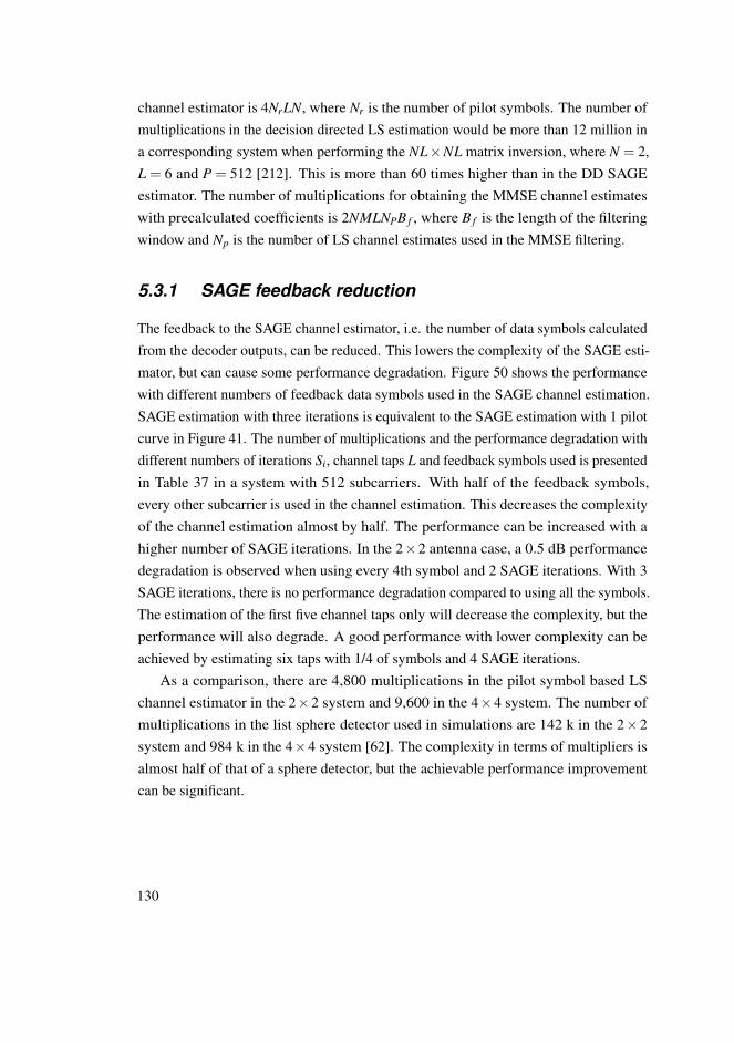
channel estimator is 4NrLN, where Nr is the number of pilot symbols. The number ofmultiplications in the decision directed LS estimation would be more than 12 million ina corresponding system when performing the NL×NL matrix inversion, where N = 2,L = 6 and P = 512 [212]. This is more than 60 times higher than in the DD SAGEestimator. The number of multiplications for obtaining the MMSE channel estimateswith precalculated coefficients is 2NMLNPB f , where B f is the length of the filteringwindow and Np is the number of LS channel estimates used in the MMSE filtering.

5.3.1 SAGE feedback reduction

The feedback to the SAGE channel estimator, i.e. the number of data symbols calculatedfrom the decoder outputs, can be reduced. This lowers the complexity of the SAGE esti-mator, but can cause some performance degradation. Figure 50 shows the performancewith different numbers of feedback data symbols used in the SAGE channel estimation.SAGE estimation with three iterations is equivalent to the SAGE estimation with 1 pilotcurve in Figure 41. The number of multiplications and the performance degradation withdifferent numbers of iterations Si, channel taps L and feedback symbols used is presentedin Table 37 in a system with 512 subcarriers. With half of the feedback symbols,every other subcarrier is used in the channel estimation. This decreases the complexityof the channel estimation almost by half. The performance can be increased with ahigher number of SAGE iterations. In the 2×2 antenna case, a 0.5 dB performancedegradation is observed when using every 4th symbol and 2 SAGE iterations. With 3SAGE iterations, there is no performance degradation compared to using all the symbols.The estimation of the first five channel taps only will decrease the complexity, but theperformance will also degrade. A good performance with lower complexity can beachieved by estimating six taps with 1/4 of symbols and 4 SAGE iterations.

As a comparison, there are 4,800 multiplications in the pilot symbol based LSchannel estimator in the 2×2 system and 9,600 in the 4×4 system. The number ofmultiplications in the list sphere detector used in simulations are 142 k in the 2×2system and 984 k in the 4×4 system [62]. The complexity in terms of multipliers isalmost half of that of a sphere detector, but the achievable performance improvementcan be significant.

130

16 18 20 22 24 26 28 300

5

10

15

20

25

30

35

Es/N0 [dB]

Thro

ughput [M

bps]

4x4 16−QAM, TU channel, 16−best LSD, 50 km/h, pilots in 1 OFDM symb./slot

SAGE, 3 it.

SAGE, 3 it., 1/2 feedback

SAGE, 4 it., 1/4 feedback

SAGE, 3 it., 1/4 feedback

LS

Fig. 50. 4× 4 16-QAM data transmission throughput vs. SNR with different num-bers of used symbols and 50 km/h user velocity.

Table 37. Number of multiplications with different parameters ([67], published bypermission of IEEE).

Symbols Si L Performancedegradation

Multiplications

2×2

512 2 6 - 200704

256 2 6 +-0 dB 100352

128 3 6 +-0 dB 74752

128 2 6 -0.5 dB 50176

4×4

512 2 6 - 794624

256 3 6 +-0 dB 593920

256 2 6 -[2-4] dB 397312

256 3 5 -[1-2] dB 495616

128 3 6 -[3-5] dB 296960

128 4 6 -0.5 dB 395264

131

5.3.2 Latency-performance trade-off

The LS channel estimation from the pilot symbols can be performed before detection inorder to have a more timely channel estimate. However, the latency requirement of thechannel estimator is less strict if channel estimation can be performed during detection.This can also have a major impact on the complexity. The alternative latencies in thereceiver are presented in Figure 51. In the top part of the figure, the channel estimatorshave a latency of one OFDM symbol. Pilot symbols are received in the first OFDMsymbol. The LS estimator then calculates the channel estimate during the detection ofall data symbols in the first OFDM symbol. The LS channel estimate is used in thedetection of the second OFDM symbol and as an input to the MMSE estimator or theSAGE estimator. The SAGE channel estimation can be performed when the decoding ofthe code word has finished. The data decisions of the first OFDM symbol are used tocalculate the SAGE channel estimate while detecting the second OFDM symbol. Thechannel estimate is then used in the detection of the third symbol. Thus, the channelestimate used in the estimation is an estimate of the channel experienced two OFDMsymbols ago. The other alternative is to use the result from the decision directed channelestimation in the detection of the next symbol, as shown in the bottom part of the figure.The channel estimate used in detection corresponds to the channel experienced in theprevious OFDM symbol. The MMSE estimator can be used to predict a more currentchannel estimate from the delayed LS estimates as the coefficients can be adjustedaccording to the delay of the LS estimate.

132

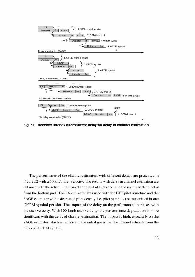
LS1. OFDM symbol (pilots)

2. OFDM symbol

3. OFDM symbol

Delay in estimates (SAGE)

H

Detector Dec

SAGE

Detector Dec

Detector Dec

Detector Dec

H

4. OFDM symbol

...

LS1. OFDM symbol (pilots)

2. OFDM symbol

3. OFDM symbol

Delay in estimates (MMSE)

H

Detector Dec

Detector Dec

Detector Dec

H

...

MMSE

MMSE

SAGE

SAGE

LS

...

1. OFDM symbol (pilots)

No delay in estimates (MMSE)

Detector Dec

Detector Dec

Detector Dec

H2. OFDM symbol

3. OFDM symbol

MMSE

MMSE

LS

...

1. OFDM symbol (pilots)

No delay in estimates (SAGE)

Detector Dec

Detector Dec SAGE

Detector Dec SAGE

H 2. OFDM symbol

3. OFDM symbol

IFFT

Fig. 51. Receiver latency alternatives; delay/no delay in channel estimation.

The performance of the channel estimators with different delays are presented inFigure 52 with a 50 km/h user velocity. The results with delay in channel estimation areobtained with the scheduling from the top part of Figure 51 and the results with no delayfrom the bottom part. The LS estimator was used with the LTE pilot structure and theSAGE estimator with a decreased pilot density, i.e. pilot symbols are transmitted in oneOFDM symbol per slot. The impact of the delay on the performance increases withthe user velocity. With 100 km/h user velocity, the performance degradation is moresignificant with the delayed channel estimation. The impact is high, especially on theSAGE estimator which is sensitive to the initial guess, i.e. the channel estimate from theprevious OFDM symbol.

133

16 18 20 22 24 26 28 300

5

10

15

20

25

30

35

Es/N0 [dB]

Thro

ughput [M

bps]

4x4 16−QAM, TU channel, 16−best LSD, 50 km/h

SAGE, no delay, 1 pilot

SAGE, delay, 1 pilot

MMSE, no delay, LTE pilots

MMSE, delay, LTE pilots

LS, no delay, LTE pilots

LS, delay, LTE pilots

Fig. 52. 4×4 16-QAM data transmission throughput vs. SNR with different delaysand 50 km/h user velocity.

5.4 Implementation of LS, MMSE and SAGE channelestimation

5.4.1 Architecture and memory requirements

The LS channel estimator includes complex multiplications of the LS coefficients andthe received data symbols when performed from the pilot symbols. The calculation ofeach LNM channel coefficient includes P/N complex multiplications, after which theresults are added together. For a 2×2 antenna system, there are 80 channel coefficientsto be calculated. If the channel estimate can be obtained with the delay of one OFDMsymbol, the latency for the calculation of one channel coefficient is 0.88 µs.

The MMSE channel estimator consists of multiplications of the LS channel estimateswith real valued coefficients. Each MMSE channel estimate coefficient hMMSE

mR,mT ,lis a

composite of the NP LS estimates from the filtering period. With the 4×4 system,NP = 3 and the filtering period is 7 OFDM symbols. The MMSE channel estimatorthen performs six multiplications and four additions for each complex valued channelcoefficient.

The architecture of the SAGE channel estimator for a 2× 2 antenna system ispresented in Fig 53. Each block corresponds to (50)–(54). The elements of xmT in each

134

stream are squared and the results are added together in the symbol multiplication part.The inverses of the results are multiplied with xmT . These calculations from (51) can beperformed separately from the iterative channel tap calculations. For each channel tap,Nc iterations are performed. The channel tap iterations are initialized by multiplying thesymbol decisions xmT with the channel taps from the previous OFDM symbol in theblock corresponding to (52). In later iterations, the channel taps from previous iterationsare used. L multiplication results from N layers corresponding to the channel to eachreceive antenna are added together and subtracted from the received symbol from eachreceive antenna. The result is then added to the first xmT hmT mR multiplication result inthe block corresponding to (50) and multiplied with x−1

i in the block corresponding to(51). A channel tap is obtained by adding together the results from the Nc iterations. Thetotal number of iterations in calculating all the channel taps is MNLSiNc.

Complex mult + inv x Xi-1

Complex mult

Complex mult

Xi

Xi+1

ĥi

ĥi+1

+

+-+

oi

+ Complex mult + ĥ

Xi

XiSymbol mult. (11)

ti di

xp

(12)

Zi

Zi

(10) (11)

Fig. 53. The architecture of the SAGE channel estimator.

The precision of the variables required to sustain the performance close to that of thefloating point variables were determined. The minimum word lengths for the channelestimators are presented in Table 38 in (word length, integer length, sign) format. Theword lengths were determined with computer simulations using the same parameters asthose in Section 5.2. The performance of the fixed point channel estimators compared tothose of the floating point estimators are presented in Figure 54. Some performancedegradation is allowed in the fixed point estimators in order to keep the complexity lowas reaching the floating point performance may require a considerable increase in theword lengths.

The total number of bits required in the variables, the bits out of the word lengthused for the integer part and if the variable is signed or unsigned are shown in the table.

135

10 12 14 16 18 20 22 24 260

2

4

6

8

10

12

14

16

Es/N0 [dB]

Thro

ughput [M

bps]

2x2 16−QAM, TU channel, 8−best LSD, 100 km/h, LTE pilots

LS, floating point

LS, fixed point

SAGE, floating point

SAGE, fixed point

MMSE, floating point

MMSE, fixed point

Fig. 54. 2× 2 16-QAM data transmission throughput vs. SNR with fixed wordlengths.

The variables in the SAGE channel estimator correspond to those in Figure 53 and thecorresponding block is denoted by (10)-(12). The LS coefficients are the precalculatedresults of (FHXH(n)X(n)F)−1FHXH(n) from pilot symbols. The received signal vectory is in frequency domain in the LS estimator and yi is in time domain in the SAGEchannel estimator. The MMSE coefficients are precalculated and real valued.

Table 38. Word lengths in channel estimation.

SAGE LS MMSEVariable (Wl , Il ,Sl ) Variable (Wl , Il ,Sl ) Variable (Wl , Il ,Sl )Xi (11) (8,3,1) y (FD) (16,4,1) MMSE coeff. (13,2,1)X−1

i (11) (12,2,1) LS coeff. (12,2,1) hMMSE (14,2,1)xp (11) (17,13,0) hLS (13,2,1)1/xp (11) (17,1,0)hi (11),(12) (18,4,1)ti (10) (12,5,1)

zi (12) (12,4,1)oi (TD) (10) (8,4,1)di (10) (12,4,1)

The amount of memory required to store the LS coefficients precalculated from thepilot symbols is 14.4 Kbit assuming that the pilot symbols are the same in each OFDMsymbol. The highest amount of memory in the MMSE filter is needed in storing the

136

LS channel estimates from NP OFDM symbols. The required amount of memory is17.5 Kbit in the 4×4 antenna system. In the SAGE channel estimator, the memoryrequirement for the symbol expectations xi is 16.4 Kbit in the 2×2 antenna systemand 32.8 Kbit in the 4× 4 antenna system. The highest amount of memory in theSAGE estimator would be the 1.2 Mbit for storing the interim results for zi but this ispartly included in the following implementation results unlike the previously discussedmemory requirements for the LS and MMSE filters.

5.4.2 Implementation results

Catapult r C Synthesis tool [188] was used in the implementation of the receivers. TheSynopsys Design Compiler was used in synthesizing the VHDL along with the UMC0.18 µm CMOS technology. The FFTs are not included in the complexity estimations.The complexity and power consumption of each channel estimator is comparableonly to other channel estimators presented in this work as the results depend on theused implementation method and library. However, a few other channel estimationimplementations from the literature will be briefly discussed.

The implementation results for the LS channel estimator and MMSE filter arepresented in Table 39 with different processing times. The estimators were implementedfor 2×2 and 4×4 antenna systems and for a 5 MHz bandwidth. The processing time of71 µs corresponds to the case of delay in channel estimates and the shorter processingtime corresponds to the no delay case shown in the bottom part of Figure 51. Thecorresponding performance results were presented in Figure 52. The detector latencywas assumed to be half from the 71 µs OFDM symbol duration, but the detector itselfis not included in the complexity estimates. The LS estimator latency can then be 38µs in the 2×2 antenna system and 33 µs in the 4×4 antenna system. The decoderlatency [210] is also included in the latency calculations and each codeword is assumedto be mapped to a single slot and not interleaved over multiple slots. The gate countincreases with the bandwidth in the LS estimator and the results can be scaled tohigher bandwidths. The longer processing delay does not have a major impact on thecomplexity, but the power consumption can be decreased. This is due to the reducedclock frequencies in the case of the longer processing delay.

137

Table 39. Synthesis results for the LS and MMSE channel estimators with differentlatencies.

No delay DelayLS MMSE LS MMSE

2×2Processing time 38 µs 38 µs 71 µs 71 µsClock frequency 95 MHz 95 MHz 51 MHz 51 MHzEquivalent gates 3763 3213 3730 3213Power consumption 8.3 mW 5.2 mW 4.8 mW 2.8 mW

4×4Processing time 33 µs 33 µs 71 µs 71 µsClock frequency 146 MHz 146 MHz 102 MHz 68 MHzEquivalent gates 3759 4549 3763 4375Power consumption 13.2 mW 10.2 mW 8.9 mW 4.6 mW

The implementation results for the SAGE channel estimator are presented in Table40. There are two target processing times for the SAGE estimator. The SAGE channelestimator has 31 µs in the no delay case to calculate the channel estimates in the 2×2antenna system when the detector latency, the decoder latency of 5 µs, the symbolexpectation latency of 1 µs and the IFFT [215] latency of 1 µs is subtracted from theOFDM symbol time. The symbol expectation calculation was implemented with thearchitecture from [62] and the gate count of 5.5 k gates was added to the SAGE estimatorcomplexity in Table 40. In the 4×4 antenna system, the decoder and IFFT have higherlatencies and the processing time for SAGE channel estimation is only 25 µs.

The longer processing times of 64 µs and 59 µs correspond to the case when channelestimation is performed during the detection of the following OFDM symbol. TheIFFT complexity was not considered in the total complexity. An IFFT block couldbe added to the receiver or the FFT with scaling could be reused, timing permitting.The LS estimator would be included in the receiver with SAGE channel estimator andthe complexity and power estimates would have to be added together to get the totalcomplexity of the SAGE channel estimator.

138

Table 40. Synthesis results for the SAGE channel estimator with different laten-cies.

Delay No delay2×2

Processing time 64 µs 31 µsSymbols, Si 1/2, 3 1/2, 4Clock frequency 144 MHz 165 MHzEquivalent gates 34.6 k 58.2 kPower consumption 93 mW 189 mW

4×4Processing time 59 µs 25 µsSymbols, Si 1/4, 4 1/4, 4Clock frequency 104 MHz 147 MHzEquivalent gates 113.4 k 210 kPower consumption 257 mW 604 mW

Implementation results for MIMO channel estimators have not been presentedextensively in the literature; this is particularly true for decision-directed algorithms.Quantitative comparison to existing work in terms of performance and complexity canbe difficult as the simulation setups and system models differ from the ones in thiswork. Therefore, a thorough performance-complexity comparison to other work isunfeasible and it is one of the reasons different channel estimation algorithms werecompared in this work. Comparison in terms of complexity has additional challenges,such as different implementation technologies and methods used. However, a fewimplementations are briefly introduced.

The approximate linear MMSE channel estimator from [165] uses the noise andcorrelation in calculating the coefficients. The implementation cost is 49 k gates, but thealgorithm is different from the MMSE filter in this work making a comparison difficult.Data carriers are exploited in channel estimation for calculating channel variationsin [167]. The algorithm provides better performance in fast fading scenarios, but thecomplexity of the channel estimator is 1,901 k gates. Furthermore, the implementationwas done for a wireless local area network (WLAN) system. An implementation of adecision feedback channel estimator for space-time block code system was introducedin [216]. However, the performance is not comparable to the spatial multiplexing systemin this work and the complexity for the one receive antenna implementation of [216] ishigher than that of the SAGE estimator implementation for four antennas in this work.

139

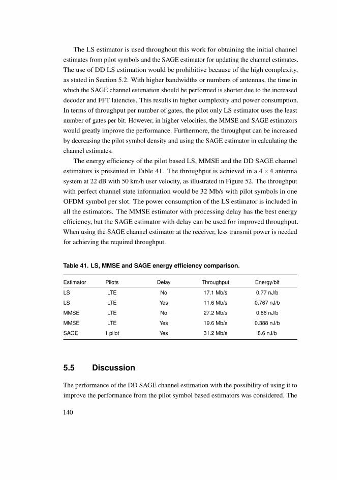
The LS estimator is used throughout this work for obtaining the initial channelestimates from pilot symbols and the SAGE estimator for updating the channel estimates.The use of DD LS estimation would be prohibitive because of the high complexity,as stated in Section 5.2. With higher bandwidths or numbers of antennas, the time inwhich the SAGE channel estimation should be performed is shorter due to the increaseddecoder and FFT latencies. This results in higher complexity and power consumption.In terms of throughput per number of gates, the pilot only LS estimator uses the leastnumber of gates per bit. However, in higher velocities, the MMSE and SAGE estimatorswould greatly improve the performance. Furthermore, the throughput can be increasedby decreasing the pilot symbol density and using the SAGE estimator in calculating thechannel estimates.

The energy efficiency of the pilot based LS, MMSE and the DD SAGE channelestimators is presented in Table 41. The throughput is achieved in a 4× 4 antennasystem at 22 dB with 50 km/h user velocity, as illustrated in Figure 52. The throughputwith perfect channel state information would be 32 Mb/s with pilot symbols in oneOFDM symbol per slot. The power consumption of the LS estimator is included inall the estimators. The MMSE estimator with processing delay has the best energyefficiency, but the SAGE estimator with delay can be used for improved throughput.When using the SAGE channel estimator at the receiver, less transmit power is neededfor achieving the required throughput.

Table 41. LS, MMSE and SAGE energy efficiency comparison.

Estimator Pilots Delay Throughput Energy/bit

LS LTE No 17.1 Mb/s 0.77 nJ/b

LS LTE Yes 11.6 Mb/s 0.767 nJ/b

MMSE LTE No 27.2 Mb/s 0.86 nJ/b

MMSE LTE Yes 19.6 Mb/s 0.388 nJ/b

SAGE 1 pilot Yes 31.2 Mb/s 8.6 nJ/b

5.5 Discussion

The performance of the DD SAGE channel estimation with the possibility of using it toimprove the performance from the pilot symbol based estimators was considered. The

140

least squares estimator was used in obtaining the channel estimates from pilot symbols.Time domain correlation of the channel estimates was exploited in the MMSE filterwhen calculating estimates for symbols with no pilots. The theoretical complexity of theSAGE algorithm and some complexity reducing modifications were presented. Theimplementation results for the pilot based LS estimator, the SAGE channel estimatorand the MMSE filter were presented.

The complexity and power consumption of the LS and MMSE estimators are low.The delay after which the channel estimates from the SAGE estimator are available fordetection has a high impact on the complexity and performance. The complexity andpower consumption can be high when using the SAGE estimator with a short processingdelay. A good performance-complexity trade-off can be achieved by allowing a longerprocessing delay for the SAGE estimator.

The MMSE filter and the SAGE estimator improve the pilot symbol based LSestimator performance with high user velocities when the channel changes frequentlybetween pilot symbols. The throughput can be increased by decreasing the pilot symboldensity and transmitting data instead of pilot symbols. The SAGE estimator can then beused in calculating channel estimates when pilot symbols are not transmitted. The SAGEchannel estimator would be a good choice for systems where training is performed inthe beginning of the transmission or less frequently. The MMSE estimator is suitable forsystems with high pilot densities as it has a low complexity and it is able to sustainacceptable performance.

141

142

6 Interference mitigation in MIMO-OFDMsystems

In this chapter, the performance and the complexity of suppressing CCI at the downlinkreceiver are considered. The main focus is on the 2× 4 system where two MIMOstreams are transmitted. Interference mitigation is beneficial also in other MIMO casesand the 2× 2 and 4× 4 schemes are also studied. The LTE standard specifies fourantennas in the terminal. The extra degrees of freedom could be used for interferencesuppression, making the 2×4 system a case of interest. The base station can have morethan two transmit antennas, which could be used for multi-user MIMO in the cell or fortransmit diversity. However, the suppression of interference from neighboring cells isstudied in this work and the aforementioned schemes are not included here. An OFDMsystem is assumed, but the interference suppression methods could also be extended touplink where a 2×4 would be even more relevant.

The interference is measured on the pilot subcarriers and the IN-SCM is used inchannel estimation and data detection. Noise power level estimation is also performed inthe receiver. Both the linear minimum mean square error and the nonlinear maximumlikelihood based detector are considered. The received data is whitened before nonlineardetection by using the result of an eigenvalue decomposition. The accuracy of the EVDhas an impact on the structure of the covariance matrix. Both the unstructured andstructured model for the covariance matrix with different degrees of accuracy are appliedand the complexity-performance trade-off is compared. Eigenspace tracking is alsoused to reduce the complexity of the EVD. Furthermore, an adaptive algorithm for theinterference suppression and EVD calculation is proposed in order to achieve a goodperformance in all interference scenarios.

This chapter discusses the complexity and performance of co-channel interferencemitigation since the combination has not been considered in the literature. Differentmethods and their implementation complexities are compared. Another contributionof the chapter is an adaptive algorithm for CCI mitigation, which obtains a goodperformance with the possibility for power savings.

The rest of the chapter is organized as follows. The receiver algorithms, includinginterference mitigation and detection, are introduced in Section 6.1 and some perfor-mance results are presented in Section 6.2. The complexities of the different interference

143

suppression methods are compared in Section 6.3, where the VLSI implementationresults are presented. Section 6.4 includes discussion on the results. The resultspresented in this chapter have not been previously published but a part of the results hasbeen submitted as a journal publication.

6.1 Receiver algorithms

The receiver structure is presented in Fig. 55. The LS channel estimator is used incalculating the channel estimates from pilot symbols. The received signal vector istransformed into frequency domain before the LS channel estimation. The result ofthe LS estimator is in time domain as shown in (55) and it has to be transformed intofrequency domain for the detector with the second FFT. The MMSE filter can be usedto filter the LS channel estimates in high velocity scenarios [156]. The CCI blockcalculates the IN-SCM and the noise variance from the channel estimates, pilot symbolsand received signal vectors. Results with decoder feedback are not reported in this workdue to the latency and error propagation issues.

Detection π-1

DecodingFFT LS FFTo

Ĥ

MMSE CCI

Fig. 55. The receiver structure.

6.1.1 Channel and noise variance estimation

The LS estimate of the channel can be calculated as [74]

hmR(n) = (FHXH(n)X(n)F)−1FHXH(n)ymR(n), (55)

where X contains the pilot symbols. The calculation of the LS channel estimate from thepilot symbols is simple as the matrix inversion can be calculated in advance and the onlycalculation to be performed in real time is multiplication with the received signal, asdiscussed in Chapter 5.

Maximum likelihood channel estimation based on pilot symbols is equivalent to theLS estimation in additive white Gaussian noise when the number of pilot symbols islarger than the channel length. The IN-SCM can be included in the channel estimation.

144

The ML channel estimates, which can be also seen as weighted LS estimates, can thenbe calculated as [74, 175]

hmR(n) = (P

∑k=1

FHk Q−1

ikFk)−1

P

∑k=1

FHk Q−1

ikymR

(n)xHk (n), (56)

where Qi is the IN-SCM, Fk is fk⊗ IM, fk is the kth row of the P×L truncated Fouriermatrix and xk(n) is the transmitted pilot signal on the kth pilot subcarrier. The calculationof the channel estimate requires a ML×ML matrix inversion.

The unbiased noise variance estimate on a receive antenna can be calculated as

γmR =1

Nr−1

Nr

∑k=1|(yk(n)− Hk(n)xk(n))mR −µ|2, (57)

where the variance is calculated over all the pilot subcarriers Nr and µ is the average ofthe values (yk(n)− Hk(n)xk(n))mR , k = 1, ...,Nr. The noise variance can be averagedover the receive antennas, as well as over consecutive subframes.

6.1.2 Detection

The spatial covariance matrix is needed both in a linear MMSE detector and ML baseddetector for improved performance. The LMMSE filter can be calculated as

W = (HHH+Qi)

−1HH, (58)

where the covariance matrix is used instead of the noise variance matrix σ2I. If thecovariance matrix is not available, the LMMSE filter can be approximated using thenoise variance estimates as

W = (HHH+Γ)−1HH, (59)

where Γ is a diagonal matrix containing the noise variance estimates γmR . The receivedsignal is filtered with the LMMSE filter and the log-likelihood ratios (LLR) can becalculated with a soft demodulator or as bit metric approximations [112], as explainedin Section 4.2.

The IN-SCM is needed in the LLR calculation in the nonlinear detector. Thelog-likelihood ratio L(bk) for the transmitted bit k can be determined as

LD(bk|y) = lnPr(bk =+1|y)Pr(bk =−1|y)

, (60)

145

as presented in (11) in Chapter 4. The likelihood function (13) on any subcarrier can becalculated using the covariance matrix as

p(y|b) = 1|Qi|

exp(−||Q−1/2i (y− Hx)||2). (61)

6.1.3 Interference estimation and processing

The interference can be measured on the pilot subcarriers by subtracting the estimatedchannel from the received signal. The IN-SCM on a subcarrier is defined as

Qi = E[(y−Hx)(y−Hx)H], (62)

where H is the channel matrix in frequency domain and x contains the transmitted pilotsymbol. The IN-SCM estimate

Qi =1Tr

Tr

∑n=1

(y(n)− H(n)x(n))(y(n)− H(n)x(n))H (63)

is obtained by averaging over a training period Tr.A structured model for the covariance can be applied in order to improve the accuracy

of the estimation [174]. The IN-SCM can be modeled as

Qi = Ψ+ σ2I, (64)

where Ψ has the EVD as Ψ = Vm(δm− σ2Im)VHm, the eigenvectors Vm and the eigen-

values δm correspond to the m dominant eigenvalues and σ2 is the average of the lastM−m eigenvalues.

The whitening of the channel matrix and the received signal vector in the detectorcan be performed by multiplying them with the inverse square root of the covariancematrix estimate Qi as presented in (61). The inverse square root of a Hermitian matrixcan be calculated from its eigenvalue decomposition Qi = VDVH as

Q−1/2i = VD−1/2VH, (65)

where D is a diagonal matrix containing the eigenvalues of Qi and V contains thecorresponding eigenvectors.

The EVD can be calculated by row-cyclic Jacobi sweeping [73] where left andright side transformations are applied. The input matrix is diagonalized iteratively by

146

applying the transformations on submatrices. The rotations can be calculated withcoordinate rotation digital computer (CORDIC) iterations. A more accurate result canbe obtained by applying several sweeps of the algorithm. Each sweep makes the inputmatrix more diagonal and results in more accurate eigenvalues. If the interference levelor signal-to-noise ratio is low, the unstructured covariance matrix may give a betterperformance when the EVD for (65) is calculated with only one sweep. The off-diagonalvalues are discarded and only the diagonal values are used. The covariance matrix afterone sweep can be written as

Qi = VH(D−Bd)V, (66)

where Bd contains the off-diagonal elements of D. With one sweep of the algorithm, themost significant eigenvalues are obtained, which leads to Q−1/2

i close to that calculatedwith the structured covariance matrix.

The accuracy of the EVD with a low number of sweeps may be improved by trackingof eigenspaces [217]. The covariance matrix Qi can be multiplied from both sideswith the previous eigenvector matrix V before performing the EVD. This makes thecovariance matrix more diagonal, which results in the need for fewer sweeps in theEVD. The new covariance matrix before the EVD can be calculated as

Qi(n+1) = VH(n)Qi(n+1)V(n) (67)

and the eigenvector matrix after the EVD is obtained from

V(n+1) = V(n)V(n+1). (68)

CCI mitigation adaptation

In order to adapt the CCI calculation, the eigenvalue ratio can be used. The ratio of themaximum eigenvalue to the sum of all eigenvalues

κ = δmax/M

∑i=1

δi, (69)

where δmax is the largest eigenvalue and ∑Mi=1 δi is the sum of all eigenvalues with

different numbers of interferers is presented in Figure 56. The values for κ wereobtained after performing one Jacobi sweep in the EVD. A 2×4 MIMO system wasassumed, resulting in a 4× 4 covariance matrix. The values do not depend on the

147

modulation scheme of the interference or the desired signal. With low SNR and highsignal-to-interference ratio (SIR), the eigenvalue ratio is small. With a low eigenvalueratio, the interference is not dominating and interference mitigation brings no gain.With high SNR and low SIR, the ratio is close to one when there is only one interferingsignal. The ratio decreases when the number of interferers increases. When there is nointerference, the ratio is close to 0.5 regardless of the SNR.

0.5 0.55 0.6 0.65 0.7 0.75 0.8 0.85 0.9 0.950

0.5

1

1.5

2

2.5

3

3.5

Eigenvalue ratio

Ni

Number of interferers vs. eigenvalue ratio

SNR/SIR

24/014/0

24/014/010/04/04/8

24/8

24/014/010/0

6/0

4/8

Fig. 56. Eigenvalue ratios with different numbers of interferers.

The proposed adaptation algorithm starts by determining the number of sweeps inthe EVD. After the first sweep of the algorithm, the need for an additional sweep can bedetermined by calculating the eigenvalue ratio. If the ratio indicates more than oneinterferer being present, i.e. it is within a certain limit, another sweep is performed.With multiple strong interferers, the ratio is within certain limits, as can be seen inFigure 56. The other condition for continuing with the second sweep is a thresholdformed by scaling the largest eigenvalue with the noise variance. The second step of thealgorithm decides whether interference mitigation is performed. If κ is below a limit,interference is not suppressed.

6.2 Performance examples

The simulation parameters are the same as those used in Chapter 5 and the channelparameters were presented in Table 1. The nonlinear detector used in the simulations isa K-best list sphere detector with the list size of 8 and the LS estimator was used for

148

channel estimation. As earlier, the transmission throughput is defined to be equal to theinformation transmission rate of information bits times (1−frame error rate). Decodingwas performed over one OFDM symbol in the simulations. The signal-to-interferenceratio of 0 dB was assumed in the simulations. With high SIR, the interference can beseen as noise and interference suppression has no major impact on the performance. Theestimated IN-SCM from (63) is used in the interference mitigation and the structuredmodel from (64) is fixed to m−1 dominating eigenvalues. The EVDs are calculatedwith transformations using six CORDIC rotations.

The performance with one interferer with SIR of 0 dB is shown in Figure 57. Theuser velocity is 3 km/h. The interferer is present with probability of one. There is nothroughput without interference mitigation. Similar performance is achieved with thestructured model, the unstructured model with two sweeps, the adaptive algorithmand the unstructured model with one sweep and eigenspace tracking. The adaptivealgorithm does not fully achieve the one sweep EVD performance in the low SNRs, butthe performance difference in negligible. The performance improves at high SNRs withthe algorithms using more iterations because the estimated covariance matrices are moreaccurate. At low SNRs, better performance is achieved when just one eigenvalue is usedfor the covariance matrix.

10 15 20 25 300

5

10

15

Es/N0 [dB]

Th

rou

gh

pu

t [M

bp

s]

2x4 16−QAM, 1 interferer, SIR=0 dB

Unstructured, 1 sweep

Unstructured, 2 sweeps

Unstructured, 1 sweep, tracking

Unstructured, adaptive

No mitigation

Structured, m=3, 2 sweeps

Fig. 57. 2×4 16-QAM data transmission throughput vs. SNR with one interferer.

The performance with one interferer present with the probability of 0.5, user velocityof 3 km/h and SIR of 0 dB is presented in Figure 58. In this case, the interference is

149

either present in all the subcarriers in an OFDM symbol or there is no interferencein any of the subcarriers. The structured model has the best performance while theunstructured model with one sweep leads to roughly 2 dB performance degradation. Thetwo sweep case has the worst performance. The eigenspace tracking does not improvethe performance. The adaptive algorithm performs well, i.e. no interference mitigationis performed in low SNRs and a one sweep EVD is performed in the high SNRs.

0 2 4 6 8 10 120

1

2

3

4

5

6

7

8

Es/N0 [dB]

Th

rou

gh

pu

t [M

bp

s]

2x4 QPSK, 1 interferer with prob. 0.5, SIR=0 dB

No mitigation

Unstructured, 1 sweep

Unstructured, 2 sweeps

Unstructured, 1 sweep, tracking

Unstructured, adaptive

Structured,m=2, 2 sweeps

Fig. 58. 2× 4 QPSK data transmission throughput vs. SNR with max. one inter-ferer.

The performance with maximum of two interferers with a probabilities of 1 and0.2 and SIR of 0 dB is presented in Figure 59. The user and interference velocity is50 km/h. The MMSE filter is used to filter the LS channel estimates for improvedperformance in the high velocity case. The lower velocity cases do not benefit fromMMSE filtering. The structured model gives the best performance and the adaptivealgorithm and unstructured model perform also well. The performance is poor withoutinterference mitigation.

The structured model or the number of sweeps in the EVD does not have an impacton performance in a 2× 2 antenna case, as can be seen in Figure 60. The use ofeigenspace tracking does not improve the performance either, as the 2×2 covariancematrix does not require additional accuracy. However, interference mitigation doesimprove the performance compared to the case of no mitigation. The difference inperformance is larger in the 4×4 system. There, the unstructured model with one sweep

150

4 6 8 10 12 14 16 18 20 22 240

0.5

1

1.5

2

2.5

3

3.5

4

4.5

Es/N0 [dB]

Th

rou

gh

pu

t [M

bp

s]

2x4 QPSK, 50 km/h, 2 interferers with prob. [1, 0.2], SIR=0 dB

No mitigation

Unstructured, 1 sweep

Unstructured, 2 sweeps

Unstructured, 1 sweep, tracking

Structured,m=2, 2 sweeps

Unstructured, adaptive

Structured,m=3, 2 sweeps

Fig. 59. 2×4 QPSK data transmission throughput vs. SNR with max. two interfer-ers.

performs better than the two-sweep case and the adaptive algorithm performs also well.The structured model has the best performance, but the choice of wrong m can degradethe performance.

10 12 14 16 18 20 22 24 26 28 300

5

10

15

Es/N0 [dB]

Thro

ughput [M

bps]

QPSK, 1 interferer, SIR=0 dB

2x2, No mitigation

2x2, Unstructured, 1 sweep

2x2, Unstructured, 2 sweeps

2x2, Unstructured, adaptive

2x2, Structured, m=2, 2 sweeps

4x4, No mitigation

4x4, Unstructured, 1 sweep

4x4, Unstructured, 2 sweeps

4x4, Unstructured, adaptive

4x4, Structured, m=2, 2 sweeps

4x4, Structured, m=3, 2 sweeps

Fig. 60. 2× 2 and 4× 4 QPSK data transmission throughput vs. SNR with oneinterferer.

The performance with a linear MMSE detector is illustrated in Figure 61. Oneinterfering signal is present with a SIR of 0 dB. The interfering signal has a velocity of50 km/h, while the user velocity is 3 km/h. Using the noise variance estimate from (57)

151

improves the performance from the no mitigation case where the known SNR is used.The structuring of the covariance matrix with the EVD improves the performance fromusing the covariance matrix directly in (58). The use of the covariance matrix in theLMMSE filter calculation could have an impact on the complexity due to the possibleincrease in word lengths.

0 5 10 15 200

1

2

3

4

5

6

7

8

Es/N0 [dB]

Th

rou

gh

pu

t [M

bp

s]

2x4 QPSK, 1 interferer, SIR=0 dB, MMSE detection

No mitigation

IN−SCM in MMSE

1 sweep IN−SCM in MMSE

2 sweep IN−SCM in MMSE

Adaptive sweep IN−SCMin MMSE

MMSE with var. estimate

Fig. 61. 2×4 QPSK data transmission throughput vs. SNR with one interferer andMMSE detection.

The structured model leads to a good performance in the presented scenarios.However, the number of dominant interferers has to be estimated. This can be done forexample with the rank estimation method from [174], but it will add extra complexity tothe receiver and may not perform as well as applying a fixed value for the rank. Thestructured model may not provide a gain compared to the unstructured model when thenumber of interferers is larger than the difference between the number of transmit andreceive antennas. The extra degrees of freedom are helpful in interference mitigationand without them, the structuring of the covariance matrix may not be successful. Theunstructured model with one sweep performs well if the interference cannot be estimatedaccurately, such as in the case of low SNR and multiple interferers.

The impact of including the IN-SCM in the channel estimation as in (56) is presentedin Figure 62. The user and interference velocities are 3 and 50 km/h. The channelestimation was performed with the true IN-SCM as well with the estimated covariancematrix. The largest difference in performance can be seen in high SNRs with the

152

known IN-SCM. However, the calculation of the channel estimate with (56) requires anML×ML matrix inversion and the interference would be the strongest in the lowerSNRs. There, the performance may even suffer from using the estimated IN-SCM inchannel estimation. Therefore, the complexity cost of including the IN-SCM in thechannel estimation is high compared to the achievable performance gain.

0 5 10 15 20 25 300

5

10

15

Es/N0 [dB]

Th

rou

gh

pu

t [M

bp

s]

2x4 QPSK, 1 interferer, SIR=0 dB, MMSE detection with estimated covariance

QPSK, No mitigation

QPSK, No IN−SCM in channel est.

QPSK, Known IN−SCM in channel est.

QPSK, Estim. IN−SCM in channel est.

16−QAM, No mitigation

16−QAM, No IN−SCM in channel est.

16−QAM, Known IN−SCM in channel est.

16−QAM, Estim. IN−SCM in channel est.

Fig. 62. Impact of IN-SCM in channel estimation on the performance in a 2× 4

system.

A comparison of the LMMSE and K-best detectors with one interferer with SIRof 0 dB is given in Figure 63. The K-best detector performs better regardless of theinterference mitigation method. Without interference mitigation, the performance withboth detectors is poor. Structuring the covariance matrix with one sweep of the EVDimproves the performance also in the LMMSE detector.

The results with adaptive modulation and coding are presented in Figure 64. Thesame setup as in Section 4.4.6 is used with the exception of all the transmission ranksfrom one to four are possible. The K-best and LMMSE detectors are compared in acase with no interference and one interferer with SIR of 0 dB. LS channel estimation isused. The K-best detector performs better than the LMMSE detector when there is nointerference and the SNR is high enough for higher transmission ranks. The results aresimilar to those in Section 4.4.6, where the channel was assumed to be known in thereceiver. With interference from a neighboring cell, the performance of the detectors issimilar. The transmission rank in this case is more probably lower even in the high

153

0 2 4 6 8 10 12 140

1

2

3

4

5

6

7

82x4 QPSK, 1 interferer with 50 km/h velocity, TU channel, az.5

Es/N0 [dB]

Th

rou

gh

pu

t [M

bp

s]

No mitigation, MMSE

No mitigation, 8−best

IN−SCM in MMSE

Unstructured, 2 sweeps, 8−best

1 sweep IN−SCM in MMSE

1 sweep IN−SCM in 8−best

Fig. 63. 2×4 QPSK data transmission throughput vs. SNR with one interferer and8-best and MMSE detection.

SNRs than in the case of no interference.

0 5 10 15 20 25 300

10

20

30

40

50

60

Es/N0 [dB]

Th

rou

gh

pu

t [M

bp

s]

4x4 AMC, TU channel, 3 km/h, LS channel estimation

MMSE, no interference

8−best, no interference

MMSE, 1 interferer, SIR=0 dB

8−best, 1 interferer, SIR=0 dB

Fig. 64. AMC data transmission throughput vs. SNR with one interferer and 8-bestand MMSE detection.

154

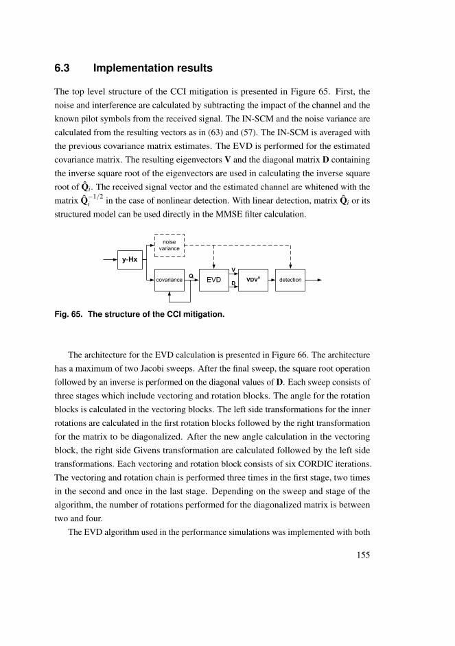
6.3 Implementation results

The top level structure of the CCI mitigation is presented in Figure 65. First, thenoise and interference are calculated by subtracting the impact of the channel and theknown pilot symbols from the received signal. The IN-SCM and the noise variance arecalculated from the resulting vectors as in (63) and (57). The IN-SCM is averaged withthe previous covariance matrix estimates. The EVD is performed for the estimatedcovariance matrix. The resulting eigenvectors V and the diagonal matrix D containingthe inverse square root of the eigenvectors are used in calculating the inverse squareroot of Qi. The received signal vector and the estimated channel are whitened with thematrix Q−1/2

i in the case of nonlinear detection. With linear detection, matrix Qi or itsstructured model can be used directly in the MMSE filter calculation.

y-Hx

noise

variance

covariance EVD VDVH

detection

V

D

Qi

Fig. 65. The structure of the CCI mitigation.

The architecture for the EVD calculation is presented in Figure 66. The architecturehas a maximum of two Jacobi sweeps. After the final sweep, the square root operationfollowed by an inverse is performed on the diagonal values of D. Each sweep consists ofthree stages which include vectoring and rotation blocks. The angle for the rotationblocks is calculated in the vectoring blocks. The left side transformations for the innerrotations are calculated in the first rotation blocks followed by the right transformationfor the matrix to be diagonalized. After the new angle calculation in the vectoringblock, the right side Givens transformation are calculated followed by the left sidetransformations. Each vectoring and rotation block consists of six CORDIC iterations.The vectoring and rotation chain is performed three times in the first stage, two timesin the second and once in the last stage. Depending on the sweep and stage of thealgorithm, the number of rotations performed for the diagonalized matrix is betweentwo and four.

The EVD algorithm used in the performance simulations was implemented with both

155

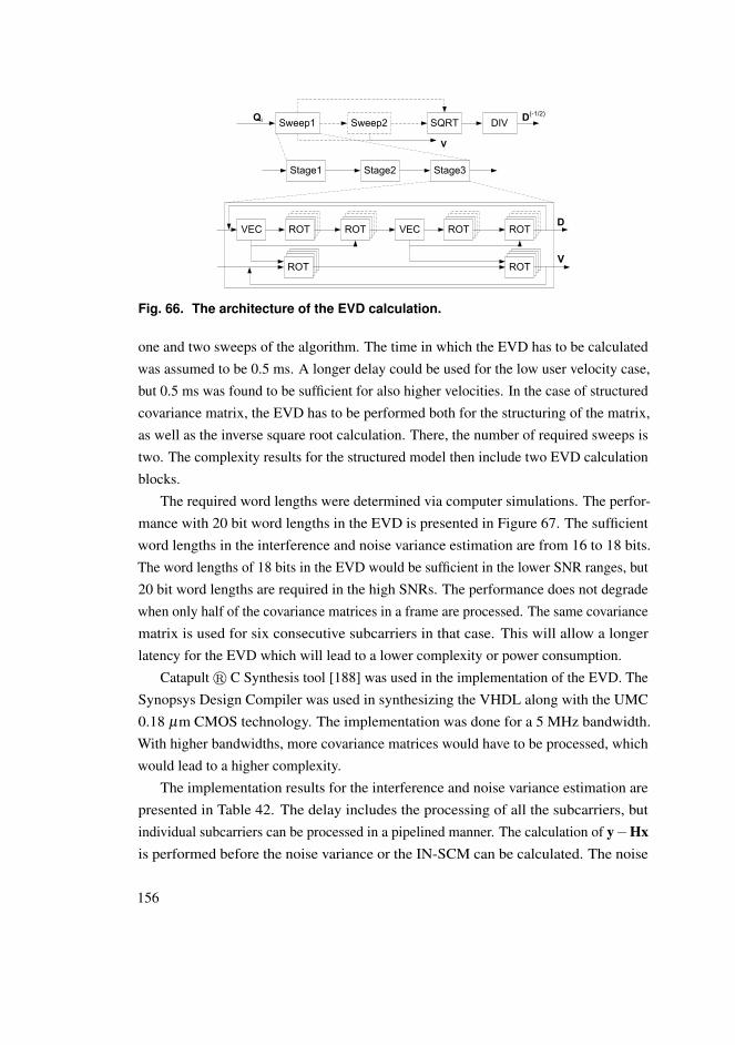
VEC VECROT

SQRT

ROT

ROT ROT ROT

ROT

Stage1 Stage2 Stage3

Sweep1 Sweep2

V

D

DIVQi D

(-1/2)

V

Fig. 66. The architecture of the EVD calculation.

one and two sweeps of the algorithm. The time in which the EVD has to be calculatedwas assumed to be 0.5 ms. A longer delay could be used for the low user velocity case,but 0.5 ms was found to be sufficient for also higher velocities. In the case of structuredcovariance matrix, the EVD has to be performed both for the structuring of the matrix,as well as the inverse square root calculation. There, the number of required sweeps istwo. The complexity results for the structured model then include two EVD calculationblocks.

The required word lengths were determined via computer simulations. The perfor-mance with 20 bit word lengths in the EVD is presented in Figure 67. The sufficientword lengths in the interference and noise variance estimation are from 16 to 18 bits.The word lengths of 18 bits in the EVD would be sufficient in the lower SNR ranges, but20 bit word lengths are required in the high SNRs. The performance does not degradewhen only half of the covariance matrices in a frame are processed. The same covariancematrix is used for six consecutive subcarriers in that case. This will allow a longerlatency for the EVD which will lead to a lower complexity or power consumption.

Catapult r C Synthesis tool [188] was used in the implementation of the EVD. TheSynopsys Design Compiler was used in synthesizing the VHDL along with the UMC0.18 µm CMOS technology. The implementation was done for a 5 MHz bandwidth.With higher bandwidths, more covariance matrices would have to be processed, whichwould lead to a higher complexity.

The implementation results for the interference and noise variance estimation arepresented in Table 42. The delay includes the processing of all the subcarriers, butindividual subcarriers can be processed in a pipelined manner. The calculation of y−Hxis performed before the noise variance or the IN-SCM can be calculated. The noise

156

0 2 4 6 8 10 12 140

1

2

3

4

5

6

7

8

Es/N0 [dB]

Th

rou

gh

pu

t [M

bp

s]

2x4 QPSK, 1 interferer, SIR=0 dB

No mitigation

1 sweep EVD

1 sweep EVD, half of IN−SCM

1 sweep EVD, 1/4 of IN−SCM

Adaptive, half of IN−SCM

Adaptive sweeps

Adaptive, fixed point 20−bits

Fig. 67. The impact of complexity reduction and word lengths on the performance.

variance estimator has to process all the subcarriers before the noise estimate is obtained.The covariance calculation block calculates the IN-SCM matrices. The calculationof VDVH is performed after the EVD to form the inverse square root matrix. Theimplementation results do not include the use of the IN-SCM in detection.

Table 42. Implementation results for the interference estimation.

Delay (cycles) Delay (µs) Gates Power

y−Hx 627 12.5 7424 11 mW

Noise var. est. 1704 34 7117 4 mW

Covariance 3151 63 11.3 k 8.4 mW

VDVH 2850 92 44 k 33.5 mW

The implementation results for the EVD are presented in Table 43 with differentnumbers of sweeps of the algorithm. The complexity of the algorithm with one or twosweeps is roughly the same, but the clock frequency is higher with the two sweep case.The structured model consists of two EVDs with two sweeps.

157

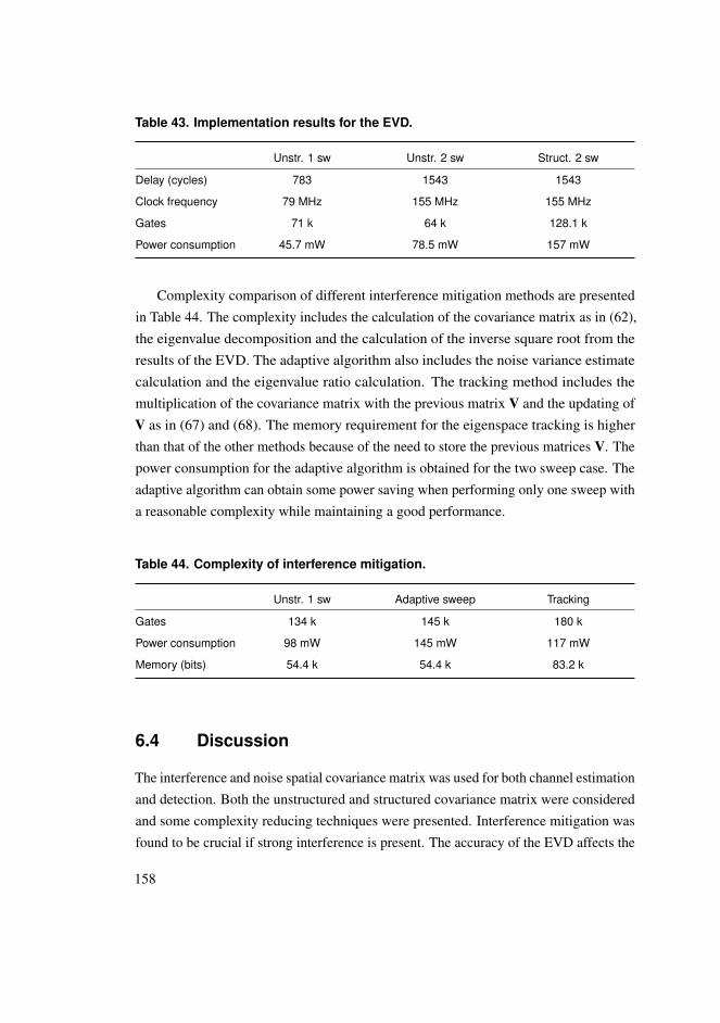
Table 43. Implementation results for the EVD.

Unstr. 1 sw Unstr. 2 sw Struct. 2 sw

Delay (cycles) 783 1543 1543

Clock frequency 79 MHz 155 MHz 155 MHz

Gates 71 k 64 k 128.1 k

Power consumption 45.7 mW 78.5 mW 157 mW

Complexity comparison of different interference mitigation methods are presentedin Table 44. The complexity includes the calculation of the covariance matrix as in (62),the eigenvalue decomposition and the calculation of the inverse square root from theresults of the EVD. The adaptive algorithm also includes the noise variance estimatecalculation and the eigenvalue ratio calculation. The tracking method includes themultiplication of the covariance matrix with the previous matrix V and the updating ofV as in (67) and (68). The memory requirement for the eigenspace tracking is higherthan that of the other methods because of the need to store the previous matrices V. Thepower consumption for the adaptive algorithm is obtained for the two sweep case. Theadaptive algorithm can obtain some power saving when performing only one sweep witha reasonable complexity while maintaining a good performance.

Table 44. Complexity of interference mitigation.

Unstr. 1 sw Adaptive sweep Tracking

Gates 134 k 145 k 180 k

Power consumption 98 mW 145 mW 117 mW

Memory (bits) 54.4 k 54.4 k 83.2 k

6.4 Discussion

The interference and noise spatial covariance matrix was used for both channel estimationand detection. Both the unstructured and structured covariance matrix were consideredand some complexity reducing techniques were presented. Interference mitigation wasfound to be crucial if strong interference is present. The accuracy of the EVD affects the

158

performance. The less accurate EVD performs better in scenarios where the quality ofthe covariance matrix is low. There, a lower number of estimated parameters leadsto fewer erroneous parameters. An adaptive algorithm was proposed to control theinterference suppression and the number of iterations performed in the EVD. Noisevariance estimation was included in the adaptive algorithm. The algorithm performswell in all interference scenarios. Eigenspace tracking was also applied to lower thecomplexity of the EVD and was found to perform well in some scenarios.

The EVD required for the structuring of the covariance matrix, as well as forthe inverse square root calculation was implemented with a high level synthesis toolto obtain the complexity numbers. The use of the structured model leads to a goodperformance at the expense of high complexity. Eigenspace tracking performs well, buthas a higher complexity and memory requirements than the adaptive algorithm, whichcan be used to achieve a good performance while obtaining power savings.

159

160

7 Conclusions and future work

The thesis concentrated on finding feasible algorithms for a MIMO mobile receiver whileimproving the error rate performance and throughput. Data detection, channel estimationand interference mitigation were considered. The aim was to develop algorithms andarchitectures to meet the high performance and low power consumption requirements ofthe future mobile communication systems, as stated in Chapter 1. The performance ofthe algorithms was studied through computer simulation and the complexity and powerconsumption results were obtained via VLSI implementations. The previous and parallelwork on detection, channel estimation and interference mitigation was introduced inChapter 2. The system, signal and channel models for detection and channel estimationwere presented in Chapter 3.

The performances and implementation complexities of the LMMSE, SIC, non-iterative and iterative K-best LSD receivers for MIMO–OFDM communications werecompared in Chapter 4. The emphasis was on LTE specific system parameters andlatency requirements. The SIC receiver was shown to outperform the K-best LSD withhorizontal encoding in channels with low spatial correlation, but the result is reversed inchannels with significant spatial correlation; the SIC receiver is not practically suitablefor vertically encoded MIMO communications. Soft information feedback from theFEC decoder to the K-best LSD stage was also considered as a strategy to improvethe performance. It provides up to 2 dB performance improvement. The choice of thereceiver algorithm is emphasized when the number of antennas increases and the channelcondition number is high. There, the nonlinear ML or MAP based receivers clearlyoutperform the linear receivers, but the price is remarkably increased computationalcomplexity and power consumption.

The considered receivers were synthesized to an FPGA and an ASIC to get a solidground for implementation complexity comparison. A modification on the tree search ofthe K-best LSD was presented to simplify its implementation with no compromise inits error rate performance. Thus, it can achieve double detection rate compared to theoriginal K-best algorithm. On the selected FPGA, the SIC receiver is fast enough toprocess the number of subcarriers defined in the LTE standard for 20 MHz bandwidthwith all modulations and 2× 2 and 4× 4 antenna configurations. The K-best LSDsuffers from the timing bottleneck caused by the sorter, but the required detection rates

161

can be achieved by utilizing multiple detection blocks in parallel.ASIC implementation results were also provided. The receivers were designed to

have a detection rate, which would be enough for the LTE 20 MHz bandwidth. TheK-best LSD was found to be more than twice as complex as the SIC receiver in the 2×2antenna case, but in the 4×4 case, the complexity difference was smaller. The latencyof the SIC receiver does not depend on the used modulation and it can be employed withhigher order modulations. The latency of the K-best LSD increases with the modulationand the list size in both FPGA and ASIC implementations.

The detectors with the highest goodput and the lowest complexity on ASIC withcorrelated, moderately correlated and uncorrelated channels with a given SNR arepresented in Table 45. It can be seen that the simpler LMMSE and SIC receivers can beused in the uncorrelated channel, but in the correlated channel, the K-best LSD gives thebest goodput. The detector and the modulation order could be changed adaptively withthe channel conditions and SNR in order to achieve the best possible goodput with theleast amount of receive power.

Table 45. The detector with the best goodput (QAM constellation Ω) ([62], pub-lished by permission of IEEE).

SNR Correlated Mod. correlated Uncorrelated

2×2 system

2 dB it. 16-best (4) it. 16-best (4) it. 16-best (4)

10 dB 16-best (4) 16-best (4) LMMSE (4)

15 dB SIC (4) SIC (16) SIC (16)

20 dB it. 8-best (16) SIC (64) SIC (64)

4×4 system

10 dB it. 8-best (4) 8-best (4) LMMSE (4)

15 dB 8-best (4) LMMSE (4) SIC (16)

20 dB LMMSE (4) 8-best (16) SIC (64)

25 dB it. 8-best (16) LMMSE (16) LMMSE (64)

To obtain an insight of the impact of transmitter channel state information into theperformance of the detector algorithms, the LMMSE, SIC and K-best detectors werefurther evaluated in a system with adaptive modulation and coding. The capacity metricwas considered here, but the idea was to study the impact of adaptation on the receiver.

162

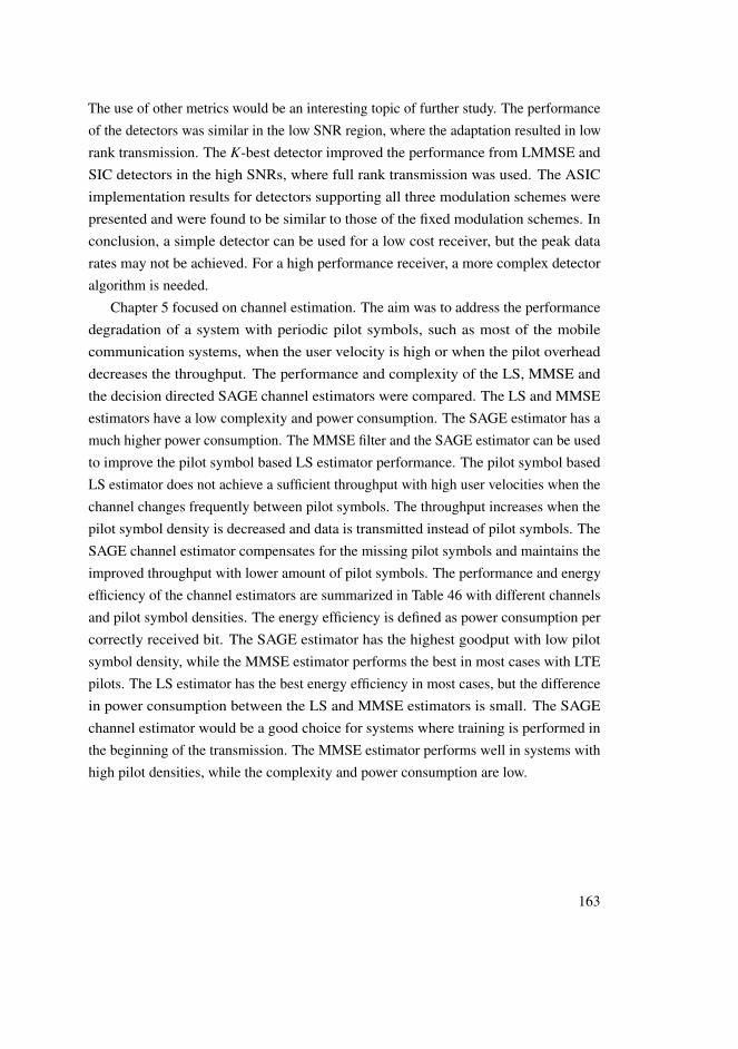
The use of other metrics would be an interesting topic of further study. The performanceof the detectors was similar in the low SNR region, where the adaptation resulted in lowrank transmission. The K-best detector improved the performance from LMMSE andSIC detectors in the high SNRs, where full rank transmission was used. The ASICimplementation results for detectors supporting all three modulation schemes werepresented and were found to be similar to those of the fixed modulation schemes. Inconclusion, a simple detector can be used for a low cost receiver, but the peak datarates may not be achieved. For a high performance receiver, a more complex detectoralgorithm is needed.

Chapter 5 focused on channel estimation. The aim was to address the performancedegradation of a system with periodic pilot symbols, such as most of the mobilecommunication systems, when the user velocity is high or when the pilot overheaddecreases the throughput. The performance and complexity of the LS, MMSE andthe decision directed SAGE channel estimators were compared. The LS and MMSEestimators have a low complexity and power consumption. The SAGE estimator has amuch higher power consumption. The MMSE filter and the SAGE estimator can be usedto improve the pilot symbol based LS estimator performance. The pilot symbol basedLS estimator does not achieve a sufficient throughput with high user velocities when thechannel changes frequently between pilot symbols. The throughput increases when thepilot symbol density is decreased and data is transmitted instead of pilot symbols. TheSAGE channel estimator compensates for the missing pilot symbols and maintains theimproved throughput with lower amount of pilot symbols. The performance and energyefficiency of the channel estimators are summarized in Table 46 with different channelsand pilot symbol densities. The energy efficiency is defined as power consumption percorrectly received bit. The SAGE estimator has the highest goodput with low pilotsymbol density, while the MMSE estimator performs the best in most cases with LTEpilots. The LS estimator has the best energy efficiency in most cases, but the differencein power consumption between the LS and MMSE estimators is small. The SAGEchannel estimator would be a good choice for systems where training is performed inthe beginning of the transmission. The MMSE estimator performs well in systems withhigh pilot densities, while the complexity and power consumption are low.

163

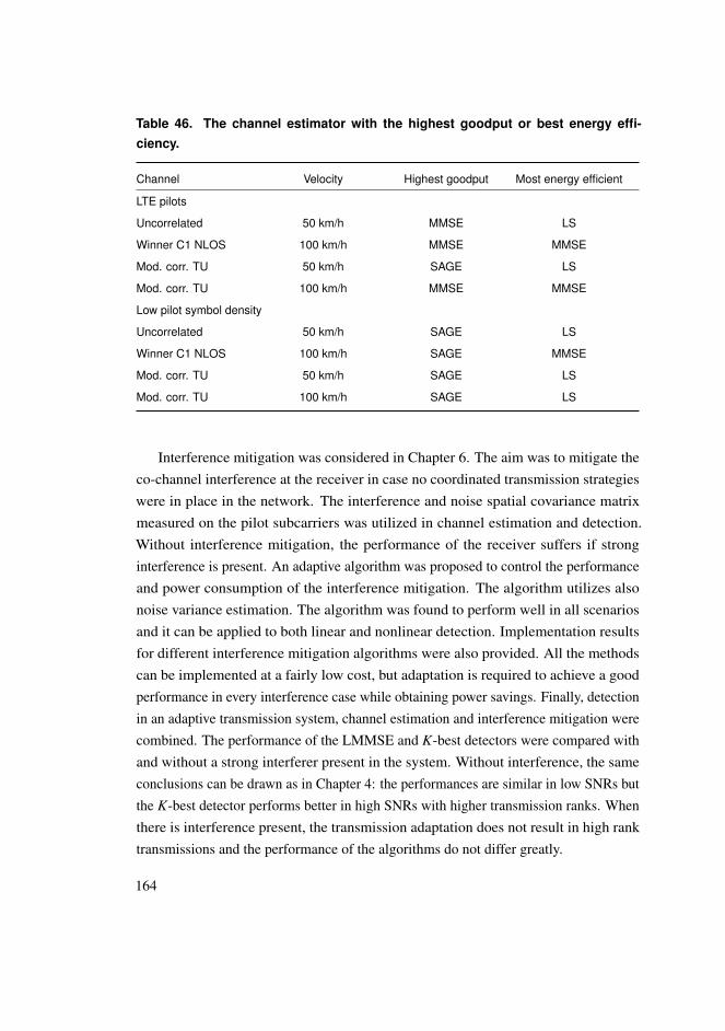
Table 46. The channel estimator with the highest goodput or best energy effi-ciency.

Channel Velocity Highest goodput Most energy efficient

LTE pilots

Uncorrelated 50 km/h MMSE LS

Winner C1 NLOS 100 km/h MMSE MMSE

Mod. corr. TU 50 km/h SAGE LS

Mod. corr. TU 100 km/h MMSE MMSE

Low pilot symbol density

Uncorrelated 50 km/h SAGE LS

Winner C1 NLOS 100 km/h SAGE MMSE

Mod. corr. TU 50 km/h SAGE LS

Mod. corr. TU 100 km/h SAGE LS

Interference mitigation was considered in Chapter 6. The aim was to mitigate theco-channel interference at the receiver in case no coordinated transmission strategieswere in place in the network. The interference and noise spatial covariance matrixmeasured on the pilot subcarriers was utilized in channel estimation and detection.Without interference mitigation, the performance of the receiver suffers if stronginterference is present. An adaptive algorithm was proposed to control the performanceand power consumption of the interference mitigation. The algorithm utilizes alsonoise variance estimation. The algorithm was found to perform well in all scenariosand it can be applied to both linear and nonlinear detection. Implementation resultsfor different interference mitigation algorithms were also provided. All the methodscan be implemented at a fairly low cost, but adaptation is required to achieve a goodperformance in every interference case while obtaining power savings. Finally, detectionin an adaptive transmission system, channel estimation and interference mitigation werecombined. The performance of the LMMSE and K-best detectors were compared withand without a strong interferer present in the system. Without interference, the sameconclusions can be drawn as in Chapter 4: the performances are similar in low SNRs butthe K-best detector performs better in high SNRs with higher transmission ranks. Whenthere is interference present, the transmission adaptation does not result in high ranktransmissions and the performance of the algorithms do not differ greatly.

164

One promising topic for further study would be the design and implementation of areconfigurable overall architecture which would adaptively switch using a simple or amore complex detector depending on the transmission requirements, available SNR,channel properties, etc. This architecture could provide the best performance in alltransmission scenarios while minimizing the power consumption. The receiver could bealso further optimized for interference scenarios. Also, the combination of detection,channel estimation and interference mitigation from Chapters 4-6 could be optimized toobtain area and power savings. In conclusion, it can be seen that the wireless systemsare designed with a simple receiver in mind, but more complex receiver algorithms arestill needed to achieve the high data rates in difficult environments. Furthermore, sinceeven higher data rates are planned for the future wireless systems, the use of simplereceiver algorithms may not suffice.

165

166

References

1. Dahlman E, Parkvall S, Sköld J & Beming P (2008) 3G Evolution HSPA and LTE forMobile Broadband. Academic Press, 2nd edition.

2. Goldsmith A (2005) Wireless Communications. Cambridge University Press, New York,USA.

3. 3rd Generation Partnership Project (3GPP); Technical Specification Group GSM/EDGERadio Access Network (2005) Physical layer on the radio path; general description (release4). Technical report, 3rd Generation Partnership Project (3GPP).

4. De Vriendt J, Laine P, Lerouge C & Xu X (2002) Mobile network evolution: a revolution onthe move. IEEE Commun. Mag. 40(4): 104–111.

5. 3rd Generation Partnership Project (3GPP); Technical Specification Group Radio Ac-cess Network (2002) High speed downlink packet access: Physical layer aspects (3G TS25.858 version 5.0.0). Technical report, 3rd Generation Partnership Project (3GPP).

6. 3rd Generation Partnership Project (3GPP); Technical Specification Group Radio Ac-cess Network (2004) FDD enhanced uplink; overall description; stage 2 (3G TS 25.309version 6.1.0). Technical report, 3rd Generation Partnership Project (3GPP).

7. Juntti M, Vehkaperä M, Leinonen J, Zexian V, Tujkovic D, Tsumura S & Hara S (2005)MIMO MC-CDMA communications for future cellular systems. IEEE Commun. Mag.43(2): 118–124.

8. 3rd Generation Partnership Project (3GPP); Technical Specification Group Radio Ac-cess Network (2007) Evolved universal terrestrial radio access E-UTRA; term evolution (lte)physical layer; general description (release 8) TS 36.201 (version 8.0.0). Technical report.

9. 3rd Generation Partnership Project (3GPP); Technical Specification Group Radio Ac-cess Network (2006) Requirements for evolved UTRA (E-UTRA) and evolved UTRAN(E-UTRAN) (TR 25.913 version 7.3.0 (release 7)). Technical report, 3rd GenerationPartnership Project (3GPP).

10. 3rd Generation Partnership Project (3GPP); Technical Specification Group Radio Ac-cess Network (2010) Evolved universal terrestrial radio access E-UTRA; lte physical layer;general description (release 10) TS 36.201 (version 10.0.0). Technical report.

11. IEEE 80216 Broadband Wireless Access Working Group (2010). IEEE 802.16m systemdescription document.

12. Wang F, Ghosh A, Sankaran C, Fleming P, Hsieh F & Benes S (2008) Mobile WiMAXsystems: performance and evolution. IEEE Commun. Mag. 46(10): 41 –49.

13. Fu IK, Chen YS, Cheng P, Yuk Y, Y Kim R & Kwak JS (2010) Multicarrier technology for4G WiMax system [WiMAX/LTE Update]. IEEE Commun. Mag. 48(8): 50–58.

14. Mogensen P, Koivisto T, Pedersen K, Kovacs I, Raaf B, Pajukoski K & Rinne M (2009)LTE-advanced: The path towards gigabit/s in wireless mobile communications. Proc. Int.Conf. on Wireless. Aalborg, Denmark, 147–151.

167

15. Lunttila T, Kiiski M, Hooli K, Pajukoski K, Skov P & Toskala A (2009) Multi-antennatechniques for LTE-advanced. Proc. Int. Symp. Wireless Pers. Multimedia Commun. Sendai,Japan.

16. Gesbert D, Shafi M, Shiu D, Smith PJ & Naguib A (2003) From theory to practice: Anoverview of MIMO space-time coded wireless systems. IEEE J. Select. Areas Commun.21(3): 281–302.

17. Paulraj A, Nabar RD & Gore D (2003) Introduction to space-time wireless communications.Cambridge University Press, Cambridge, U.K.

18. Winters JH, Salz J & Gitlin RD (1994) The impact of antenna diversity on the capacity ofwireless communication systems. IEEE Trans. Commun. 42(2/3/4).

19. Bölcskei H (2006) MIMO-OFDM wireless systems: Basics, perspectives, and challenges.IEEE Trans. Commun. 13(4): 31–37.

20. Foschini G (1996) Layered space–time architecture for wireless communication in a fadingenvironment when using multi-element antennas. Bell Labs Tech. J. 1(2): 41–59.

21. Telatar IE (1995) Capacity of multi-antenna Gaussian channels. Technical report, BellLaboratories. Internal Tech.Memo, pp. 1–28.

22. Wolniansky PW, Foschini GJ, Golden GD & Valenzuela RA (1998) V-BLAST: Anarchitecture for realizing very high data rates over the rich-scattering wireless channel.International Symposium on Signals, Systems, and Electronics (ISSSE). Pisa, Italy, 295–300.

23. Foschini G, Chizhik D, Gans M, Papadias C & Valenzuela R (2003) Analysis and perfor-mance of some basic space-time architectures. IEEE J. Select. Areas Commun. 21(3):303–320.

24. Seshadri N & Winters JH (1993) Two signaling schemes for improving the error performanceof frequency-division-duplex (FDD) transmission systems using transmitter antenna diversity.Proc. IEEE Veh. Technol. Conf. Secaucus, USA, 508–511.

25. Tarokh V, Seshadri N & Calderbank AR (1998) Space-time codes for high data rate wirelesscommunication: Performance criterion and code construction. IEEE Trans. Inform. Theory44(2): 744–765.

26. Alamouti S (1998) A simple transmit diversity technique for wireless communications.IEEE J. Select. Areas Commun. 16(8): 1451–1458.

27. Tarokh V, Jafarkhani H & Calderbank AR (1999) Space-time block codes from orthogonaldesigns. IEEE Trans. Inform. Theory 45(5): 1456–1467.

28. Rashid-Farrokhi F, Liu KJR & Tassiulas L (1998) Transmit beamforming and power controlfor cellular wireless systems. IEEE J. Select. Areas Commun. 16(8): 1437–1450.

29. Visotsky E & Madhow U (1999) Optimum beamforming using transmit antenna arrays.Proc. IEEE Veh. Technol. Conf. Houston, TX, vol. 1, 851 – 856.

30. Zheng L & Tse DNC (2003) Diversity and multiplexing: A fundamental tradeoff inmultiple-antenna channels. IEEE Trans. Inform. Theory 49(5): 1073–1096.

31. Heath RW Jr & Love D (2005) Multimode antenna selection for spatial multiplexing systemswith linear receivers. IEEE Trans. Signal Processing 53(8): 3042–3056.

32. Cavers JK (1972) Variable-rate transmission for rayleigh fading channels. IEEE Trans.Commun. COM-20(1): 15–22.

33. Jungnickel V, Haustein T, Pohl V & von Helmolt C (2003) Link adaptation in a multi-antennasystem. Proc. IEEE Veh. Technol. Conf. Jeju, Korea, vol. 2, 862–866.

34. Hayes JF (1968) Adaptive feedback communications. IEEE Trans. Commun. Technol.COM-16(1): 29–34.

168

35. Goldsmith A & Varaiya P (1997) Capacity of fading channels with channel side information.IEEE Trans. Inform. Theory 43(6): 1986–1992.

36. Goldsmith A (1997) The capacity of downlink fading channels with variable rate and power.IEEE Trans. Veh. Technol. 46(3): 569–580.

37. Catreux S, Erceg V, Gesbert D & Heath RW Jr (2002) Adaptive modulation and MIMOcoding for broadband wireless data networks. IEEE Commun. Mag. 40(6): 108–115.

38. Choi YS & Alamouti SM (2008) A pragmatic PHY abstraction technique for link adaptationand MIMO switching. IEEE J. Select. Areas Commun. 26(6): 960–971.

39. Chae CB, Forenza A, Heath RW Jr, McKay MR & Collings IB (2010) Adaptive MIMOtransmission techniques for broadband wireless communication systems. IEEE Commun.Mag. 48(5): 112–118.

40. Forenza A, McKay MR, Pandharipande A, Heath RW Jr & Collings IB (2007) AdaptiveMIMO transmission for exploiting the capacity of spatially correlated channels. IEEE Trans.Veh. Technol. 56(2): 619–630.

41. Hwang T, Yang C, Wu G, Li S & Ye Li G (2009) OFDM and its wireless applications: Asurvey. IEEE Trans. Veh. Technol. 58(4): 1673–1694.

42. Chang RW (1966) Synthesis of band-limited orthogonal signals for multichannel datatransmission. Bell Syst. Tech. J. 45: 1775–1797.

43. Saltzberg B (1967) Performance of an efficient parallel data transmission system. IEEETrans. Commun. Technol. 15(6): 805–811.

44. Weinstein SB & Ebert PM (1971) Data transmission by frequency division multiplexingusing the discrete Fourier transform. IEEE Transactions on Communication Technology19(5): 628–634.

45. Cimini LJ (1985) Analysis and simulation of a digital mobile channel using orthogonalfrequency division multiplexing. IEEE Trans. Commun. 33(7): 665–675.

46. Chuang J (1987) The effects of time delay spread on portable radio communicationschannels with digital modulation. IEEE J. Select. Areas Commun. 5(5): 879–889.

47. Wang Z & Giannakis GB (2000) Wireless multicarrier communications. IEEE SignalProcessing Mag. 17(3): 29–48.

48. Cooley JW & Tukey JW (1965) An algorithm for the machine calculation of complexFourier series. Math. Comp. 19(90): 297–301.

49. Duhamel P (1990) Algorithms meeting the lower bounds on the multiplicative complexityof length-2n DFTs and their connection with practical algorithms. IEEE Trans. Acoust.,Speech, Signal Processing 38(9): 1504–1511.

50. Kaiser S (1999) Performance of multi-carrier CDM and COFDM in fading channels. Proc.IEEE Global Telecommun. Conf. Rio de Janeireo , Brazil, vol. 1b, 847–851.

51. Willink TJ & Wittke PH (1997) Optimization and performance evaluation of multicarriertransmission. IEEE Trans. Inform. Theory 43(2): 426–440.

52. Warner W & Leung C (1993) OFDM/FM frame synchronization for mobile radio datacommunication. IEEE Trans. Veh. Technol. 42(3): 302–313.

53. van de Beek J, Sandell M & Borjesson P (1997) ML estimation of time and frequency offsetin OFDM systems. IEEE Trans. Signal Processing 45(7): 1800–1805.

54. Raleigh GG & Cioffi JM (1998) Spatio-temporal coding for wireless communication. IEEETrans. Commun. 46(3): 357–366.

169

55. Sampath H, Talwar S, Tellado J, Erceg V & Paulraj A (2002) A fourth-generation MIMO-OFDM broadband wireless system: Design, performance, and field trial results. IEEECommun. Mag. 40(9): 143–149.

56. IEEE Standard 80216 (2004). IEEE standard for local and metropolitan area networks part16: Air interface for fixed broadband wireless access systems.

57. Caire G, Ramprashad S, Papadopoulos H, Pepin C & Sundberg CE (2008) MultiuserMIMO downlink with limited inter-cell cooperation: Approximate interference alignment intime, frequency and space. Proc. Annual Allerton Conf. Commun., Contr., Computing.Urbana-Champaign, Illinois, USA, 730–737.

58. Jungnickel V, Schellmann M, Thiele L, Wirth T, Haustein T, Koch O, Zirwas W & Schulz E(2009) Interference-aware scheduling in the multiuser MIMO-OFDM downlink. IEEECommun. Mag. 47(6): 56–66.

59. 3rd Generation Partnership Project (3GPP); Technical Specification Group Radio Access Net-work (2011) Feasibility study for further advancements for E-UTRA (LTE-advanced)(release 10). Technical report.

60. Sawahashi M, Kishiyama Y, Morimoto A, Nishikawa D & Tanno M (2010) Coordinatedmultipoint transmission/reception techniques for LTE-advanced [coordinated and distributedMIMO]. IEEE Wireless Commun. Mag. 17(3): 26–34.

61. 3rd Generation Partnership Project (3GPP); Technical Specification Group Radio Ac-cess Network (2010) Evolved universal terrestrial radio access E-UTRA; physical channelsand modulation (release 10) TS 36.211 (version 10.0.0). Technical report.

62. Ketonen J, Juntti M & Cavallaro J (2010) Performance-complexity comparison of receiversfor a LTE MIMO-OFDM system. IEEE Trans. Signal Processing 58(6): 3360–3372.

63. Ketonen J, Juntti M & Cavallaro JR (2009) Receiver implementation for MIMO-OFDMwith AMC and precoding. Proc. Annual Asilomar Conf. Signals, Syst., Comp. PacificGrove, USA, 1268–1272.

64. Ketonen J, Myllylä M, Juntti M & Cavallaro JR (2008) ASIC implementation comparison ofSIC and LSD receiver for MIMO-OFDM. Proc. Annual Asilomar Conf. Signals, Syst.,Comp. Pacific Grove, USA, 1881–1885.

65. Ketonen J, & Juntti M (2008) Performance comparisons of SIC and K-best LSD receivers fora MIMO-OFDM system. Proc. Int. Symp. Wireless Pers. Multimedia Commun. Saariselkä,Finland, 1–5.

66. Ketonen J & Juntti M (2008) SIC and K-best LSD receiver implementation for a MIMO-OFDM system. Proc. European Sign. Proc. Conf. Lausanne, Switzerland, 1–5.

67. Ketonen J, Juntti M & Ylioinas J (2010) Decision directed channel estimation for reducingpilot overhead in LTE-A. Proc. Annual Asilomar Conf. Signals, Syst., Comp. Pacific Grove,USA, 1503–1507.

68. Ketonen J, Juntti M, Ylioinas J & Cavallaro J (2012) Decision-directed channel estimationimplementation for spectral efficiency improvement in mobile MIMO-OFDM. IEEE Trans.Circuits Syst. I, submitted .

69. Ketonen J, Juntti M, Ylioinas J & Cavallaro JR (2012) Implementation of LS, MMSE andSAGE channel estimators for mobile MIMO-OFDM. Proc. Annual Asilomar Conf. Signals,Syst., Comp., submitted.

70. Ketonen J & Juntti M (2012) Adaptive receiver for co-channel interference suppression inMIMO-OFDM. Signal Processing, Elsevier, submitted .

170

71. Ketonen J & Juntti M (2012) Receiver implementations for co-channel interferencesuppression in MIMO-OFDM. Proc. Annual Asilomar Conf. Signals, Syst., Comp.,submitted.

72. Lupas R & Verdú S (1989) Linear multiuser detectors for synchronous code-divisionmultiple-access channels. IEEE Trans. Inform. Theory 34(1): 123–136.

73. Golub GH & Loan CFV (1996) Matrix Computations, 3rd ed. The Johns Hopkins UniversityPress, Baltimore.

74. Kay SM (1993) Fundamentals of Statistical Signal Processing: Estimation Theory. Prentice-Hall, Englewood Cliffs, NJ, USA.

75. Vehkaperä M, Tujkovic D, Li Z & Juntti M (2005) Receiver design for spatially layereddownlink MC-CDMA system. IEEE Trans. Veh. Technol. 54(3): 1042–1055.

76. Artes H, Seethaler D & Hlawarsch F (2003) Efficient detection algorithms for MIMOchannels: A geometrical approach to approximate ML detection. IEEE Trans. SignalProcessing 51(11): 2808–2820.

77. Foschini GJ & Gans MJ (1998) On limits of wireless communications in a fading environ-ment when using multiple antennas. Wireless Pers. Commun., Kluwer 6: 311–335.

78. Golden GD, Foschini CJ, Valenzuela RA & Wolniansky PW (1999) Detection algorithm andinitial laboratory results using V-BLAST space-time communication architecture. IEEElectron. Lett. 35(1): 14–16.

79. Chin W, Constantinides A & Ward D (2002) Parallel multistage detection for multipleantenna wireless systems. Electronics Letters 38(12): 597 –599.

80. Wübben D, Seethaler D, Jalden J & Matz G (2011) Lattice reduction: A survey withapplications in wireless communications. IEEE Signal Processing Mag. 28(3): 70–91.

81. Ma X & Zhang W (2008) Performance analysis for MIMO systems with lattice-reductionaided linear equalization. IEEE Trans. Commun. 56(2): 309 –318.

82. Fincke U & Pohst M (1985) Improved methods for calculating vectors of short length in alattice, including a complexity analysis. Math. Comput. 44(5): 463–471.

83. Viterbo E & Bouros J (1999) A universal lattice code decoder for fading channels. IEEETrans. Inform. Theory 45(5): 1639–1642.

84. Schnorr CP & Euchner M (1994) Lattice basis reduction: Improved practical algorithms andsolving subset sum problems. Math. Programming 66(2): 181–191.

85. Agrell E, Eriksson T, Vardy A & Zeger K (2002) Closest point search in lattices. IEEETrans. Inform. Theory 48(8): 2201–2214.

86. Damen MO, Gamal HE & Caire G (2003) On maximum–likelihood detection and the searchfor the closest lattice point. IEEE Trans. Inform. Theory 49(10): 2389–2402.

87. Anderson J & Mohan S (1984) Sequential coding algorithms: A survey and cost analysis.IEEE Trans. Commun. 32(2): 169–176.

88. Wong K, Tsui C, Cheng RK & Mow W (2002) A VLSI architecture of a K-best latticedecoding algorithm for MIMO channels. Proc. IEEE Int. Symp. on Circuits and Systems.Scottsdale, AZ, vol. 3, 273–276.

89. Mohan S & Anderson J (1984) Computationally optimal metric-first code tree searchalgorithms. IEEE Trans. Commun. 32(6): 710 – 717.

90. Murugan A, Gamal HE, Damen M & Caire G (2006) A unified framework for tree searchdecoding: rediscovering the sequential decoder. IEEE Trans. Inform. Theory 52(3):933–953.

171

91. Xu W, Wang Y, Zhou Z & Wang J (2004) A computationally efficient exact ML spheredecoder. Proc. IEEE Global Telecommun. Conf. vol. 4, 2594–2598.

92. Zhao W & Giannakis GB (2005) Sphere decoding algorithms with improved radius search53(7): 1104–1109.

93. Vikalo H & Hassibi B (2006) On joint detection and decoding of linear block codes onGaussian vector channels. IEEE Trans. Signal Processing 54(9): 3330 –3342.

94. Berrou C, Glavieux A & Thitimajshima P (1993) Near Shannon limit error correcting codingand decoding: Turbo codes. Proc. IEEE Int. Conf. Commun. Geneva, Switzerland, vol. 2,1064–1070.

95. Hagenauer J, Offer E & Papke L (1996) Iterative decoding of binary block and convolutionalcodes. IEEE Trans. Inform. Theory 42(2): 429–445.

96. Hagenauer J (1997) The turbo principle: Tutorial introduction and state of the art. Proc. Int.Symb. on Turbo Codes. Brest, France.

97. Bahl LR, Cocke J, Jelinek F & Raviv J (1974) Optimal decoding of linear codes forminimizing symbol error rate. IEEE Trans. Inform. Theory 20(2): 284–287.

98. Tüchler M, Singer A & Koetter R (2002) Minimum mean squared error equalization using apriori information. IEEE Trans. Signal Processing 50(3): 673–683.

99. Wautelet X, Dejonghe A & Vandendorpe L (2004) MMSE-based fractional turbo receiverfor space-time BICM over frequency-selective MIMO fading channels. IEEE Trans. SignalProcessing 52(6): 1804–1809.

100. Sellathurai M & Haykin S (2002) TURBO-BLAST for wireless communications: Theoryand experiments. IEEE Trans. Signal Processing 50(10): 2538–2546.

101. Reed MC (1999) Iterative Receiver Techniques for Coded Multiple Access CommunicationSystems. Ph.D. thesis, The University of South Australia, Australia.

102. Hochwald B & ten Brink S (2003) Achieving near-capacity on a multiple-antenna channel.IEEE Trans. Commun. 51(3): 389–399.

103. Guo Z & Nilsson P (2006) Algorithm and implementation of the K-best sphere decoding forMIMO detection. IEEE J. Select. Areas Commun. 24(3): 491–503.

104. Wang L, Xu L, Chen S & Hanzo L (2008) Apriori-LLR-threshold-assisted K-best spheredetection for MIMO channels. Proc. IEEE Veh. Technol. Conf. Singapore, 867–871.

105. Studer C, Burg A & Bolcskei H (2008) Soft-output sphere decoding: algorithms and VLSIimplementation. IEEE J. Select. Areas Commun. 26(2): 290–300.

106. Mennenga B, Fritzsche R & Fettweis G (2009) Iterative soft-in soft-out sphere detection forMIMO systems. Proc. IEEE Veh. Technol. Conf. Barcelona, Spain.

107. Zhao M, Shi Z & Reed M (2008) The performance of sphere decoders for iterative spatialmultiplexing MIMO receiver. Proc. Int. Symb. on Turbo Codes. Lausanne, Switzerland,113–117.

108. Hagenauer J & Kuhn C (2007) The list-sequential (LISS) algorithm and its application.IEEE Trans. Commun. 55(5): 918 –928.

109. Myllylä M, Juntti M & Cavallaro J (2009) Architecture design and implementation of theincreasing radius - list sphere detector algorithm. Proc. IEEE Int. Conf. Acoust., Speech,Signal Processing. Taipei, Taiwan, 553–556.

110. Wübben D, Böhnke R, Kühn V & Kammeyer K (2003) MMSE extension of V-BLASTbased on sorted QR decomposition. Proc. IEEE Veh. Technol. Conf. Orlando, Florida,vol. 1, 508–512.

172

111. Bittner S, Zimmermann E & Fettweis G (2006) Low complexity soft interference cancellationfor MIMO-systems. Proc. IEEE Veh. Technol. Conf. Melbourne, Australia, vol. 4, 1993–1997.

112. Collings I, Butler M & McKay M (2004) Low complexity receiver design for MIMObit-interleaved coded modulation. Proc. IEEE Int. Symp. Spread Spectrum Techniques andApplications. Sydney, Australia, 1993–1997.

113. Zimmermann E & Fettweis G (2006) Unbiased MMSE tree search detection for multipleantenna systems. Proc. Int. Symp. Wireless Pers. Multimedia Commun. San Diego, USA.

114. Burg A, Haene S, Perels D, Luethi P, Felber N & Fichtner W (2006) Algorithm and VLSIarchitecture for linear MMSE detection in MIMO-OFDM systems. Proc. IEEE Int. Symp.on Circuits and Systems. Kos, Greece.

115. Khan Z, Arslan T, Thompson J & Erdogan A (2006) Area power efficient VLSI architecturefor computing pseudo inverse of channel matrix in a MIMO wireless system. Proc. IEEE Int.Conf. on VLSI Design. Hyderabad, India.

116. Yoshizawa S, Yamauchi Y & Miyanaga Y (2008) A complete pipelined MMSE detectionarchitecture in a 4x4 MIMO-OFDM receiver. Proc. IEEE Int. Symp. on Circuits andSystems. Seattle, USA.

117. Myllylä M, Juntti M, Limingoja M, Byman A & Cavallaro JR (2006) Performance evaluationof two LMMSE detectors in a MIMO-OFDM hardware testbed. Proc. Annual AsilomarConf. Signals, Syst., Comp. Pacific Grove, USA, 1161–1165.

118. Luethi P, Studer C, Duetsch S, Zgraggen E, Kaeslin H, Felber N & Fichtner W (2008)Gram-Schmidt-based QR decomposition for MIMO detection: VLSI implementation andcomparison. Proc. of IEEE Asia Pacific Conference on Circuits and Systems. Macao, 830–833.

119. Wang JY, Lai RH, Clien CM, Ting PA & Huang YH (2010) A 2×2 - 8×8 sorted QRdecomposition processor for MIMO detection. IEEE Asian Solid State Circuits Conference.Beijing, China, 1–4.

120. Huang ZY & Tsai PY (2011) Efficient implementation of QR decomposition for gigabitMIMO-OFDM systems. IEEE Trans. Circuits Syst. I 58(10): 2531–2542.

121. Patel D, Shabany M & Gulak P (2009) A low-complexity high-speed QR decompositionimplementation for MIMO receivers. Proc. IEEE Int. Symp. on Circuits and Systems. Taipei,Taiwan, 33–36.

122. Studer C, Fateh S & Seethaler D (2011) ASIC implementation of soft-input soft-outputMIMO detection using MMSE parallel interference cancellation. IEEE J. Solid-StateCircuits 46(7): 1754 –1765.

123. Garrett D, Davis L, ten Brink S, Hochwald B & Knagge G (2004) Silicon complexityfor maximum likelihood MIMO detection using spherical decoding. IEEE J. Solid-StateCircuits 39(9): 1544–1552.

124. Chen S, Zhang T & Xin Y (2005) Breadth-first tree search MIMO signal detector design andVLSI implementation. Proc. IEEE Military Commun. Conf. Atlantic City, USA, 1470–1476.

125. Wenk M, Zellweger M, Burg A, Felber N & Fichtner W (2006) K-best MIMO detectionVLSI architectutes achieving up to 424 mbps. IEEE Trans. Commun. : 1151–1154.

126. Milliner D & Barry J (2007) A layer-adaptive M algorithm for multiple-input multiple-outputchannel detection. Proc. IEEE Works. on Sign. Proc. Adv. in Wirel. Comms. Helsinki,Finland, 1 –5.

173

127. Mondal S, Eltawil A & Salama K (2009) Architectural optimizations for low-power K-bestMIMO decoders. IEEE Trans. Veh. Technol. 58(7): 3145–3153.

128. Shen CA & Eltawil A (2010) A radius adaptive K-best decoder with early termination:Algorithm and VLSI architecture. IEEE Trans. Circuits Syst. I 57(9): 2476–2486.

129. Shabany M & Gulak PG (2012) A 675 mbps, 4 × 4 64-QAM K-best MIMO detector in 0.13µm CMOS. IEEE Trans. VLSI Syst. 20(1): 135 –147.

130. Shen CA, Eltawil A, Mondal S & Salama K (2010) A best-first tree-searching approach forML decoding in MIMO system. Proc. IEEE Int. Symp. on Circuits and Systems. Paris,France, 3533–3536.

131. Burg A, Borgmann M, Wenk M, Zellweger M, Fichtner W & Bölcskei H (2005) VLSIimplementation of MIMO detection using the sphere decoding algorithm. IEEE J. Solid-StateCircuits 40(7): 1566–1577.

132. Radosavljevic P & Cavallaro J (2006) Soft sphere detection with bounded search forhigh-throughput MIMO receivers. Proc. Annual Asilomar Conf. Signals, Syst., Comp.Pacific Grove, USA, 1175–1179.

133. Yang CH & Markovic D (2009) A flexible DSP architecture for MIMO sphere decoding.IEEE Trans. Circuits Syst. I 56(10): 2301 –2314.

134. Yang T, Yuan J, Shi Z & Reed M (2008) Convergence behavior analysis and detectionswitching for the iterative receiver of MIMO-BICM systems. IEEE Trans. Veh. Technol.57(4): 2642–2648.

135. Li M, Bougart B, Lopez E & Bourdoux A (2008) Selective spanning with fast enumeration:A near maximum-likelihood MIMO detector designed for parallel programmable basebandarchitectures. Proc. IEEE Int. Conf. Commun. Beijing, China, 737 – 741.

136. Amiri K, Cavallaro JR, Dick C & Rao RM (2009) A high throughput configurable SDRdetector for multi-user MIMO wireless systems. J Sign. Process. Syst. .

137. Bhagawat P, Dash R & Choi G (2009) Systolic like soft-detection architecture for 4x464-QAM MIMO system. Design, Automation and Test in Europe Conference and Exhibition.Nice, France, 870–873.

138. Siti M & Fitz M (2006) A novel soft-output layered orthogonal lattice detector for multipleantenna communications. Proc. IEEE Int. Conf. Commun. Istanbul, Turkey, 1686 –1691.

139. Tomasoni A, Siti M, Ferrari M & Bellini S (2007) Turbo-LORD: A MAP-approachingsoft-input soft-output detector for iterative MIMO receivers. Proc. IEEE Global Telecommun.Conf. Washington, DC, USA, 3504–3508.

140. Meyr H, Moeneclaey M & Fechtel SA (1998) Digital Communication Receivers: Synchro-nization, Channel Estimation and Signal Processing. John Wiley and Sons, New York,USA.

141. Tse D & Viswanath P (2005) Fundamentals of Wireless Communication. CambridgeUniversity Press, Cambridge, UK.

142. Ozdemir MK & Arslan H (2007) Channel estimation for wireless OFDM systems. IEEECommunications Surveys & Tutorials 9(2): 18–48.

143. Shin C, Heath RW & Powers EJ (2007) Blind channel estimation for MIMO-OFDM systems.IEEE Trans. Veh. Technol. 56: 670–685.

144. Zhou S, Muquet B & Giannakis GB (2002) Subspace-based (semi-) blind channel estimationfor block precoded space-time OFDM. IEEE Trans. Signal Processing 50(5): 1215–1228.

145. Cavers JK (1991) An analysis of pilot symbol assisted modulation for Rayleigh fadingchannels. IEEE Trans. Veh. Technol. 40(4): 686–693.

174

146. Tong L, Sadler BM & Dong M (2004) Pilot-assisted wireless transmissions: general model,design criteria, and signal processing. IEEE Signal Processing Mag. 21(6): 12–25.

147. Hassibi B & Hochwald BM (2003) How much training is needed in multiple–antennawireless links? IEEE Trans. Inform. Theory 49(4): 951–963.

148. Barhumi I, Leus G & Moonen M (2003) Optimal training design for MIMO–OFDM systemsin mobile wireless channels. IEEE Trans. Signal Processing 51(6): 1615–1624.

149. Adireddy S, Tong L & Viswanathan H (2002) Optimal placement of training for frequencyselective block–fading channels. IEEE Trans. Inform. Theory 48(8): 2338–2353.

150. Li Y (2002) Simplified channel estimation for OFDM systems with multiple transmitantennas. IEEE Trans. Wireless Commun. 1(1): 67–75.

151. Morelli M & Mengali U (2001) A comparison of pilot-aided channel estimation methods forOFDM systems. IEEE Trans. Signal Processing 49(12): 3065–3073.

152. van de Beek JJ, Edfors O, Sandell M, Wilson S & Borjesson P (1995) On channel estimationin OFDM systems. Proc. IEEE Veh. Technol. Conf. Chicago, IL, USA, vol. 2, 815–819.

153. Edfors O, Sandell M, van de Beek JJ, Wilson S & Börjesson P (1998) OFDM channelestimation by singular value decomposition. IEEE Trans. Commun. 46(7): 931–939.

154. Rinne J & Renfors M (1996) Pilot spacing in orthogonal frequency division multiplexingsystems on practical channels. IEEE Trans. Consumer Electron. 42(3): 959–962.

155. Li Y, Cimini LJ & Sollenberger NR (1998) Robust channel estimation for OFDM systemswith rapid dispersive fading channels. IEEE Trans. Commun. 46(7): 902–915.

156. Miao H & Juntti M (2005) Space-time channel estimation and performance analysis forwireless MIMO-OFDM systems with spatial correlation. IEEE Trans. Veh. Technol. 54(6):2003–2016.

157. Zhao M, Shi Z & Reed M (2008) Iterative turbo channel estimation for OFDM system overrapid dispersive fading channel. IEEE Trans. Wireless Commun. 7(8): 3174 –3184.

158. Dempster AP, Laird NM & Rubin DB (1977) Maximum likelihood from incomplete datavia the EM algorithm. J. Royal Stat. Soc. 39(1): 1–38.

159. Fessler J & Hero A (1994) Space-alternating generalized expectation-maximization algo-rithm. IEEE Trans. Signal Processing 42(10): 2664–2677.

160. Xie Y & Georghiades CN (2003) Two EM–type channel estimation algorithms for OFDMwith transmitter diversity. IEEE Trans. Commun. 51(1): 106–115.

161. Panayirci E, Senol H & Poor H (2010) Joint channel estimation, equalization, and datadetection for OFDM systems in the presence of very high mobility. IEEE Trans. SignalProcessing 58(8): 4225–4238.

162. Ylioinas J & Juntti M (2009) Iterative joint detection, decoding, and channel estimation inturbo coded MIMO-OFDM. IEEE Trans. Veh. Technol. 58(4): 1784–1796.

163. Zou H & Daneshrad B (2004) VLSI implementation for a low power mobile OFDMreceiver ASIC. Proc. IEEE Wireless Commun. and Networking Conf. Atlanta, USA, vol. 4,2120–2124.

164. Haene S, Burg A, Felber N & Fichtner W (2008) OFDM channel estimation algorithmand ASIC implementation. European Conf. Circuits and Systems for Communications.Bucharest, Romania, 270–275.

165. Simko M, Wu D, Mehlfuehrer C, Eilert J & Liu D (2011) Implementation aspects of channelestimation for 3GPP LTE terminals. Proc. European Wireless Conf. Vienna, Austria.

175

166. Löfgren J, Mehmood S, Khan N, Masood B, Awan M, Khan I, Chisty N & Nilsson P (2009)Hardware implementation of an SVD based MIMO OFDM channel estimator. NORCHIP.Trondheim, Norway, 1–4.

167. Sun MF, Juan TY, Lin KS & Hsu TY (2009) Adaptive frequency-domain channel estimatorin 4×4 MIMO-OFDM modems. IEEE Trans. VLSI Syst. 17(11): 1616 –1625.

168. Winters JH (1984) Optimum combining in digital mobile radio with cochannel interference.IEEE J. Select. Areas Commun. 2(4): 528–539.

169. Jeremic A, Thomas TA & Nehorai A (2004) OFDM channel estimation in the presence ofinterference. IEEE Trans. Signal Processing 52(12): 3429–3439.

170. Dai H, Molisch AF & Poor HV (2004) Downlink capacity of interference-limited MIMOsystems with joint detection. IEEE Trans. Wireless Commun. 3(2): 442 – 453.

171. Li Q, Zhu J, Guo X & Georghiades C (2007) Asynchronous co-channel interferencesuppression in MIMO OFDM systems. Proc. IEEE Int. Conf. Commun. Glasgow, Scotland,5744–5750.

172. Thomas TA & Vook FW (2003) Asynchronous interference suppression in broadbandcyclic-prefix communications. Proc. IEEE Wireless Commun. and Networking Conf. NewOrleans, USA, vol. 1, 568–572.

173. Larsson EG (2003) Semi-structured interference suppression for orthogonal frequencydivision multiplexing. Proceedings of IEEE ISSPIT. Darmstadt, Germany, 435–438.

174. Jöngren G, Astely D & Ottersten B (2000) Structured spatial interference rejection combining.Proc. European Sign. Proc. Conf. Tampere, Finland.

175. Raghavendra M, Juntti M & Myllylä M (2009) Co-channel interference mitigation for 3GLTE MIMO-OFDM systems. Proc. IEEE Int. Conf. Commun. 1 –5.

176. Cavallaro JR & Luk FT (1988) CORDIC arithmetic for an SVD processor. Journal ofParallel and Distributed Computing 5(3): 271–290.

177. Cavallaro J, Keleher M, Price R & Thomas G (1989) VLSI implementation of a CORDICSVD processor. University/Government/Industry Microelectronics Symposium. Westbor-ough, MA, USA, 256–260.

178. Studer C, Blosch P, Friedli P & Burg A (2007) Matrix decomposition architecture for MIMOsystems: Design and implementation trade-offs. Proc. Annual Asilomar Conf. Signals,Syst., Comp. Pacific Grove, CA, USA, 1986–1990.

179. Dickson K, Liu Z & McCanny J (2004) QRD and SVD processor design based on anapproximate rotations algorithm. IEEE Workshop on Signal Processing Systems. Austin,TX, USA, 42–47.

180. Ahmedsaid A, Amira A & Bouridane A (2003) Improved SVD systolic array and imple-mentation on FPGA. IEEE Int. Conf. Field-Programmable Technology. Tokyo, Japan,35–42.

181. Szecowka P & Malinowski P (2010) CORDIC and SVD implementation in digital hardware.Int. Conf. Mixed Design of Integrated Circuits and Systems. Warsaw, Poland, 237–242.

182. Martin G & Smith G (2009) High-level synthesis: Past, present, and future. Design Test ofComputers, IEEE 26(4): 18–25.

183. Casseau E, Gal L, Bomel P, Jego C, Huet S & Martin E (2005) C-based rapid prototypingfor digital signal processing. Proc. European Sign. Proc. Conf. Antalya, Turkey.

184. Coussy P, Gajski D, Meredith M & Takach A (2009) An introduction to high-level synthesis.Design Test of Computers, IEEE 26(4): 8–17.

185. Fingeroff M (2010) High-Level Synthesis Blue Book. Xlibris Corporation.

176

186. Cong J, Liu B, Neuendorffer S, Noguera J, Vissers K & Zhang Z (2011) High-level synthesisfor FPGAs: From prototyping to deployment. IEEE Trans. Computer-Aided Design ofIntegrated Circuits and Systems 30(4): 473–491.

187. Myllylä M (2011) Detection algorithms and architectures for wireless spatial multiplexingin MIMO-OFDM systems, vol. C380 of Acta Universitatis Ouluensis, Doctoral thesis.

188. Mentor Graphics (2012). Catapult C Synthesis Overview, Tech. Rep.,http://www.mentor.com/esl/catapult/overview.

189. 3rd Generation Partnership Project (3GPP); Technical Specification Group Radio Ac-cess Network (2008) Evolved universal terrestrial radio access E-UTRA; physical channelsand modulation (release 8) TS 36.211 (version 8.5.0). Technical report.

190. 3rd Generation Partnership Project (3GPP); Technical Specification Group Radio Ac-cess Network (2011) Evolved universal terrestrial radio access E-UTRA; multiplexing andchannel coding (release 10) TS 36.212 (version 10.3.0). Technical report.

191. Benedetto S, Divsalar D, Montorsi G & Pollara F (1997) A soft-input soft-output maximumAPP module for iterative decoding of concatenated codes. IEEE Commun. Lett. 1(1):22–24.

192. Almers P, Bonek E, Burr A, Czink N, Debbah M, Degli-Esposti V, Hofstetter H, Kyösti P,Laurenson D, Matz G, Molisch AF, Oestges C, & Özcelik H (2007) Survey of channel andradio propagation models for wirelessmimo systems. EURASIP J. Wireless Comm. andNetw. : 1–19.

193. Yu K & Ottersten B (2002) Models for MIMO propagation channels, a review. Wirelesscommunications and mobile computing : 1–14.

194. Kunnari E & Iinatti J (2007) Stochastic modelling of Rice fading channels with temporal,spatial and spectral correlation. IET Communications 1(2): 215–224.

195. Hentilä L, Kyösti P, Käske M, Naradzic M & Alatossava M (2007) MATLAB implementationof the WINNER phase II channel model. Technical report, Available: https://www.ist-winner.org/phase_2_model.html.

196. 3rd Generation Partnership Project (3GPP); Technical Specification Group Radio Ac-cess Network (2002) Radio transmission and reception (3G TS 45.005 version 5.4.0 (release5)). Technical report, 3rd Generation Partnership Project (3GPP).

197. Qiao D, Choi S & Shin KG (2002) Goodput analysis and link adaptation for IEEE 802.11awireless LANs. IEEE Trans. Mobile Comput." 1(4): 278–292.

198. Robertson P, Villebrun E & Hoeher P (1995) A comparison of optimal and sub-optimalMAP decoding algorithms operating in the log domain. Proc. IEEE Int. Conf. Commun. :1009–1013.

199. Hassibi B (2000) A fast square-root implementation for BLAST. Proc. Annual AsilomarConf. Signals, Syst., Comp. Asilomar, USA, vol. 2, 1255–1259.

200. Golub GH & Loan CFV (1989) Matrix Computations, 2nd edn. The Johns HopkinsUniversity Press, Baltimore.

201. Döhler R (1991) Squared Givens rotation. IMA Journal of Numerical Analysis 11: 1–5.202. Wübben D, Böhnke R, Kühn V & Kammeyer KD (2003) MMSE extension of V-BLAST

based on sorted QR decomposition. Proc. IEEE Veh. Technol. Conf. Orlando, Florida, USA,vol. 1, 508–512.

203. El-Amawy A & Dharmarajan K (1989) Parallel VLSI algorithm for stable inversion ofdense matrices. Computers and Digital Techniques, IEE Proceedings E 136(6): 575–580.

177

204. Tüchler M, Singer AC & Koetter R (2002) Minimum mean squared error equalisation usinga priori information. IEEE Trans. Signal Processing 50(3): 673–683.

205. Myllylä M, Antikainen J, Juntti M & Cavallaro J (2007) The effect of LLR clipping to thecomplexity of list sphere detector algorithms. Proc. Annual Asilomar Conf. Signals, Syst.,Comp. Pacific Grove, USA, 1559–1563.

206. Parhami B (2000) Computer Arithmetic: Algorithms and Hardware Designs. OxfordUniversity Press, New York, USA.

207. Myllylä M, Juntti M & Cavallaro JR (2007) Implementation aspects of list sphere detectoralgorithms. Proc. IEEE Global Telecommun. Conf. Washington, D.C., USA, 3915–3920.

208. Sun Y & Cavallaro J (2011) Efficient hardware implementation of a highly-parallel 3GPPLTE/LTE-advance turbo decoder. Elsevier Integration, the VLSI journal 44(4): 305–315.

209. Wübben D, Böhnke R, Rinas J, Kühn V & Kammeyer KD (2001) Efficient algorithm fordecoding layered space-time codes. IEE Electronic Letters 37(22): 1348–1349.

210. Sun Y, Zhu Y, Goel M & Cavallaro J (2008) Configurable and scalable high throughput turbodecoder architecture for multiple 4G wireless standards. IEEE Int. Conf. on Application-specific Systems, Architectures and Processors (ASAP). Leuven, Belgium, 209–214.

211. Burg A (2006) VLSI Circuits for MIMO Communication Systems. Ph.D. thesis, ETHZurich, Switzerland.

212. Ylioinas J, Raghavendra MR & Juntti M (2009) Avoiding matrix inversion in DD SAGEchannel estimation in MIMO-OFDM with M-QAM. Proc. IEEE Veh. Technol. Conf.Anchorage, USA, 1–5.

213. 3rd Generation Partnership Project (3GPP); Technical Specification Group Radio Ac-cess Network (2003) Spatial channel model for multiple input multiple output (MIMO)simulations (3G TS 25.996 version 6.0.0 (release 6)). Technical report, 3rd GenerationPartnership Project (3GPP).

214. Lee J, Lou HL, Toumpakaris D & Cioffi J (2006) SNR analysis of OFDM systems in thepresence of carrier frequency offset for fading channels. IEEE Trans. Wireless Commun.5(12): 3360–3364.

215. Babionitakis K, Manolopoulos K, Nakos K & Chouliaras V (2006) A high performanceVLSI FFT architecture. IEEE International Conference on Electronics, Circuits and Systems.Nice, France, 810–813.

216. Chen HY, Ku ML, Jou SJ & Huang CC (2010) A robust channel estimator for high-mobilitySTBC-OFDM systems. IEEE Trans. Circuits Syst. I 57(4): 925–936.

217. Schäfer F, Stege M, Michalke C & Fettweis G (2003) Efficient tracking of eigenspaces andits application to MIMO-systems. Proc. IST Mobile & Wireless Telecommun. Summit.Aveiro, Portugal.

178

A C T A U N I V E R S I T A T I S O U L U E N S I S

Book orders:Granum: Virtual book storehttp://granum.uta.fi/granum/

S E R I E S C T E C H N I C A

408. Rajala, Hanna-Kaisa (2011) Enhancing innovative activities and tools for themanufacturing industry: illustrative and participative trials within work systemcases

409. Sinisammal, Janne (2011) Työhyvinvoinnin ja työympäristön kokonaisvaltainenkehittäminen – tuloksia osallistuvista tutkimus- ja kehittämisprojekteista sekäasiantuntijahaastatteluista

410. Berg, Markus (2011) Methods for antenna frequency control and user effectcompensation in mobile terminals

411. Arvola, Jouko (2011) Reducing industrial use of fossil raw materials : Techno-economic assessment of relevant cases in Northern Finland

412. Okkonen, Jarkko (2011) Groundwater and its response to climate variability andchange in cold snow dominated regions in Finland: methods and estimations

413. Anttonen, Antti (2011) Estimation of energy detection thresholds and errorprobability for amplitude-modulated short-range communication radios

414. Neitola, Marko (2012) Characterizing and minimizing spurious responses inDelta-Sigma modulators

415. Huttunen, Paavo (2012) Spontaneous movements of hands in gradients of weakVHF electromagnetic fields

416. Isoherranen, Ville (2012) Strategy analysis frameworks for strategy orientationand focus

417. Ruuska, Jari (2012) Special measurements and control models for a basic oxygenfurnace (BOF)

418. Kropsu-Vehkaperä, Hanna (2012) Enhancing understanding of company-wideproduct data management in ICT companies

419. Hietakangas, Simo (2012) Design methods and considerations of supplymodulated switched RF power amplifiers

420. Davidyuk, Oleg (2012) Automated and interactive composition of ubiquitousapplications

421. Suutala, Jaakko (2012) Learning discriminative models from structured multi-sensor data for human context recognition

422. Lorenzo Veiga, Beatriz (2012) New network paradigms for future multihopcellular systems

C423etukansi.kesken.fm Page 2 Monday, May 28, 2012 12:28 PM

ABCDEFG

UNIVERS ITY OF OULU P.O.B . 7500 F I -90014 UNIVERS ITY OF OULU F INLAND

A C T A U N I V E R S I T A T I S O U L U E N S I S

S E R I E S E D I T O R S

SCIENTIAE RERUM NATURALIUM

HUMANIORA

TECHNICA

MEDICA

SCIENTIAE RERUM SOCIALIUM

SCRIPTA ACADEMICA

OECONOMICA

EDITOR IN CHIEF

PUBLICATIONS EDITOR

Senior Assistant Jorma Arhippainen

Lecturer Santeri Palviainen

Professor Hannu Heusala

Professor Olli Vuolteenaho

Senior Researcher Eila Estola

Director Sinikka Eskelinen

Professor Jari Juga

Professor Olli Vuolteenaho

Publications Editor Kirsti Nurkkala

ISBN 978-951-42-9856-1 (Paperback)ISBN 978-951-42-9857-8 (PDF)ISSN 0355-3213 (Print)ISSN 1796-2226 (Online)

U N I V E R S I TAT I S O U L U E N S I SACTAC

TECHNICA

U N I V E R S I TAT I S O U L U E N S I SACTAC

TECHNICA

OULU 2012

C 423

Johanna Ketonen

EQUALIZATION AND CHANNEL ESTIMATION ALGORITHMS AND IMPLEMENTATIONS FOR CELLULAR MIMO-OFDM DOWNLINK

UNIVERSITY OF OULU GRADUATE SCHOOL;UNIVERSITY OF OULU, FACULTY OF TECHNOLOGY, DEPARTMENT OF COMMUNICATIONS ENGINEERING;CENTRE FOR WIRELESS COMMUNICATIONS;INFOTECH OULU

C 423

ACTA

Johanna Ketonen

C423etukansi.kesken.fm Page 1 Monday, May 28, 2012 12:28 PM