out-of-core simplification with appearance …eprints.utm.my/id/eprint/4407/1/75166.pdf ·...
TRANSCRIPT

VOT 75166
OUT-OF-CORE SIMPLIFICATION WITH APPEARANCE
PRESERVATION
FOR COMPUTER GAME APPLICATIONS
Project Leader
Abdullah Bade
Researcher
Assoc. Prof. Daut Daman
Mohd Shahrizal Sunar
Research Assistant
Tan Kim Heok
RESEARCH MANAGEMENT CENTER
UNIVERSITI TEKNOLOGI MALAYSIA
2006
OUT-OF-CORE SIMPLIFICATION WITH APPEARANCE
PRESERVATION
FOR COMPUTER GAME APPLICATIONS
PROJECT REPORT
Author
Abdullah Bade
RESEARCH MANAGEMENT CENTER
UNIVERSITI TEKNOLOGI MALAYSIA
2006

i
Acknowledgement
Special thanks are dedicated to the management and staff of Research
Management Center (RMC), Universiti Teknologi Malaysia Malaysia for their
supports, commitments and motivations. We would like to express our appreciation
to those who have assisted us directly or indirectly in making this project a success.

ii
Abstract
Drastic growth in computer simulations’ complexity and 3D scanning technology has
boosted the size of geometry data sets. Before this, conventional (in-core)
simplification techniques are sufficient in data reduction to accelerate graphics
rendering. However, powerful graphics workstation also unable to load or even
generates the smooth rendering of these extremely large data. In this thesis, out-of-
core simplification algorithm is introduced to overcome the limitation of
conventional technique. Meanwhile, preservation on surface attributes such as
normals, colors and textures, which essential to bring out the beauty of 3D object, are
also discussed. The first process is to convert the input data into a memory efficient
format. Next, datasets are organized in an octree structure and later partitioned
meshes are kept in secondary memory (hard disk). Subsequently, submeshes are
simplified using a new variation of vertex clustering technique. In order to maintain
the surface attributes, a proposed vertex clustering technique that collapses all
triangles in every leaf node using the generalized quadric error metrics is introduced.
Unlike any other vertex clustering methods, the knowledge of neighbourhood
between nodes is unnecessary and the node simplification is performed
independently. This simplification is executed recursively until a desired levels of
detail is achieved. During run-time, the visible mesh is rendered based on the
distance criterion by extracting the required data from the previously generated
octree structure. The evaluated experiments show that the simplification is greatly
controlled by octree’s subdivision level and end node size. The finer the octree, thus
the finer mesh will be generated. Overall, the proposed algorithm is capable in
simplifying large datasets with pleasant quality and relatively fast. The system is run
efficiently on low cost personal computer with small memory footprint.
iii
Abstrak
Perkembangan drastik dalam simulasi komputer dan teknologi pengimbasan 3D telah
meningkatkan saiz data geometri. Sebelum ini, teknik simplifikasi tradisional (in-
core) mampu mengurangkan saiz data untuk mempercepatkan visualisasi grafik.
Walau bagaimanapun, stesen kerja grafik yang berspesifikasi tinggi juga tidak
mampu memuat data yang terlalu besar ini apatah lagi menjana visualisasi yang licin.
Dalam thesis ini, algoritma simplifikasi out-of-core telah diperkenalkan untuk
mengatasi kekurangan teknik tradisional. Sementara ini, pengekalan ciri-ciri
permukaaan seperti normal, warna dan tekstur yang menunjukkan kecantikan objek
3D telah dibincangkan. Proses pertama ialah menukarkan data input kepada format
yang ramah memori. Kemudian, data disusun dalam struktur octree dan data yang
siap dibahagikan disimpan dalam memori sekunder (cakera keras). Selepas ini,
permukaan bagi setiap nod diringkaskan dengan teknik pengumpulan verteks. Untuk
mengekalkan attribut-attribut permukaan, teknik pengumpulan vertex yang
menggantikan segitiga-segitiga dalam setiap nod dengan menggunakan kaedah
“generalized quadric error metrics” dicadangkan. Berbeza dengan teknik-teknik lain,
pengetahuan antara nod jiran tidak diperlukan dan simplifikasi nod dilakukan secara
individu. Proses simplifikasi ini dijalankan secara rekursif sehingga bilangan
resolusi yang dikehendaki dicapai. Semasa perlaksaan sistem, permukaan yang
boleh dinampak divisualisasikan berdasarkan aspek jarak dengan mengekstrak data
berkenaan dari struktur octree yang dihasilkan. Eksperimen yang dianalisa
menunjukkan bahawa simplifikasi banyak dikawal oleh aras pembahagian octree dan
saiz nod akhir. Semakin banyak octree dibahagikan, semakin tinggi resolusi
permukaan yang dihasilkan. Secara keseluruhan, algoritma cadangan adalah
berpotensi dalam simplifikasi data besar dengan kualiti yang memuaskan dan agak
cepat. Sistem ini telah dilaksanakan secara effektif pada komputer berkos rendah
dengan penggunaan memori yang kecil.
iv
Table of Contents
CHAPTER TITLE PAGE
Acknowledgement i
Abstract ii
Abstrak iii
Table of Contents iv
1 INTRODUCTION 1
1.1 Introduction 1
1.2 Background Research 2
1.3 Motivations 5
1.4 Problem Statement 6
1.5 Purpose 6
1.6 Objectives 6
1.6 Research Scope 7
2 LITERATURE REVIEW 8
2.1 Introduction 8
2.2 Level of Detail Framework 9
2.2.1 Discrete Level of Detail 9
2.2.2 Continuous Level of Detail 10
2.2.3 View-Dependent Level of Detail 11
2.3 Level of Detail Management 11
2.4 Level of Detail Generation 15
2.4.1 Geometry Simplification 16
2.4.1.1 Vertex Clustering 16
2.4.1.2 Face Clustering 17
2.4.1.3 Vertex Removal 18
2.4.1.4 Edge Collapse 19
v
2.4.1.5 Vertex Pair Contraction 21
2.4.2 Topology Simplification 21
2.5 Metrics for Simplification and Quality Evaluation 23
2.5.1 Geometry-Based Metrics 23
2.5.1.1 Quadric Error Metrics 23
2.5.1.2 Vertex-Vertex vs Vertex-Plane
vs Vertex-Surface vs Surface-
Surface Distance
24
2.5.2 Attribute Error Metrics 25
2.6 External Memory Algorithms 25
2.6.1 Computational Model 27
2.6.2 Batched Computations 27
2.6.2.1 External Merge Sort 27
2.6.2.2 Out-of-Core Pointer
Dereferencing
28
2.6.2.3 The Meta-Cell Technique 29
2.6.3 On-Line Computations 30
2.7 Out-of-Core Approaches 31
2.7.1 Spatial Clustering 32
2.7.2 Surface Segmentation 34
2.7.3 Streaming 36
2.7.4 Comparison 38
2.8 Analysis on Out-of-Core Approach 39
2.8.1 Advantages and Disadvantages 39
2.8.2 Comparison: In-core and Out-of-Core
Approach
39
2.8.3 Performance Comparison: Existing
Simplification Techniques
41
2.9 Appearance Attribute Preservation 46
2.10 Summary 48
3 METHODOLOGY 51
3.1 Introduction 51
vi
3.2 Algorithm Overview 52
3.3 Data Processing 54
3.31 Data File Structure 55
3.4 Proposed Octree Construction 57
3.5 Proposed Out-of-Core Simplification 59
3.5.1 New Vertex Clustering 60
3.5.2 Generalized Quadric Error Metrics 61
3.5.2 Simplification on Internal Nodes 63
3.6 Run Time Rendering 64
3.7 Summary 65
4 IMPLEMENTATION 66
4.1 Introduction 66
4.2 Data Processing 67
4.2.1 Input Data Reading 67
4.2.2 Triangle Soup Mesh Generation 68
4.2.2.1 Calculation of Triangle’s
Dimension and Sorting Index
69
4.2.2.2 External Sorting on Sorting
Index
71
4.2.2.3 Dereferencing on Sorting Indices 72
4.3 Octree Construction 73
4.4 Out-of-Core Simplification 76
4.4.1 Simplification on Leaf Nodes 76
4.4.2 Simplification on Internal Nodes 76
4.5 Run Time Rendering 77
4.6 Summary 78
5 RESULTS AND DISCUSSIONS 79
5.1 Introduction 79
5.2 Octree Construction Analysis 80
5.3 Out-of-Core Simplification Analysis 81
5.3.1 Proposed Out-of-Core Simplification
vii
Analysis 82
5.3.2 Relationships between Simplification and
Octree Construction
85
5.3.3 Surface-Preserving Simplification
Analysis
89
5.3.4 Comparison on Out-of-Core
Simplifications
91
5.4 Summary 93
6 CONCLUSIONS 94
6.1 Summary 94
6.2 Summary of Contributions 95
6.3 Future Works 97
REFERENCES 99
Appendices A - B 112
CHAPTER 1
INTRODUCTION
1.1 Introduction
A 3D interactive graphics application is an extremely computational
demanding paradigm, requiring the simulation and display of a virtual environment
at interactive frame rates. It is significant in real time game environment. Even with
the use of powerful graphics workstations, a moderately complex virtual
environment can involve a vast amount of computation, inducing a noticeable lag
into the system. This lag can detrimentally affect the visual effect and may therefore
severely compromise the diffusion of the quality of graphics application.
Therefore, a lot of techniques have been proposed to overcome the delay of
the display. It includes motion prediction, fixed update rate, visibility culling,
frameless rendering, Galilean antialiasing, level of detail, world subdivision or even
employing parallelism. Researches have been done and recovered that the fixed
update rates and level of detail technique are the only solutions which enable the
application program balances the load of the system in real-time (Reddy, 1997). Of
these solutions, concentration is focused on the notion of level of detail.
Since the mid nineteen-seventies, programmers have used Level of Detail
(LOD) management to improve the performance and quality of their graphics
systems. The LOD approach involves maintaining a set of representations of each
polygonal object, each with varying levels of triangle resolution. During the

2
execution of the animation, object deemed to be less important is displayed with a
low-resolution representation. Where as object of higher importance is displayed
with higher level of triangle resolution.
The drastic growth in scanning technology and high realism computer
simulation complexity has lead to the increase of dataset size. Only super computer
or powerful graphics workstation are capable to handle these massive datasets. For
this reason, problem of dealing with meshes that are apparently larger than the
available main memory exists. Data, which has hundreds, million of polygons are
impossible to fit in any available main memory in desktop personal computer.
Because of this memory shortage, conventional simplification methods, which
typically require reading and storing the entire model in main memory, cannot be
used anymore. Hence, out-of-core approaches are gaining its attention widely.
As commonly known, graphics applications always desire high realism scene
yet smooth scene rendering. Smooth rendering can be achieved by reducing the
number of polygons to a suitable level of detail using the simplification technique. It
saves milliseconds of execution time that help to improve performance. However, in
order to obtain a nice simplified mesh, surface attributes other than geometry
information are essential to be preserved as well. Eye catching surface appearance
certainly will increase the beauty of the scene effectively.
1.2 Background Research
Traditionally, polygonal models have been used in computer graphics
extensively. Till this moment, large variety of applications is using this fundamental
primitive to represent three dimensional objects. Besides, many graphics hardware
and software rendering systems support this data structure. In addition, all virtual
environment systems employ polygon renderers as their graphics engine.
In reality, many computational demanding systems desire smooth rendering
of these polygonal meshes. To optimize the speed and quality of graphics rendering,

3
level of details has been used widely to reduce the complexity of the polygonal mesh
using level of detail technique. In short, a process which takes an original polygon
description of a three dimensional object and creates another such description,
retaining the general shape and appearance of the original model, but containing
fewer polygons.
Recent advances in scanning technology, simulation complexity and storage
capacity have lead to an explosion in the availability and complexity of polygonal
models, which often consist of millions of polygons. Because of the memory
shortage in dealing with meshes that are significantly larger than available main
memory, conventional methods, which typically require reading and storing the
entire model in main memory during simplification process, cannot solve the
dilemma anymore. Thus, out-of-core approaches are introduced consequently.
Out-of-core algorithms are also known as external algorithms or secondary
memory algorithms. Out-of-core algorithms keep the bulk of the data on disk, and
keep in main memory (or so called in-core) only the part of the data that’s being
processed. Lindstrom (Lindstrom, 2000a) is the pioneer in out-of-core simplification
field. He created a simplification method; called OoCS which is independent of
input mesh size. However, the output size of the mesh must be smaller than the
available main memory. Later on, other researchers carried out similar approaches.
Especially in out-of-core simplification, a large number of research have been
done on level of detail’s construction and management for use in interactive graphics
applications, mostly in medical visualization, flight simulators, terrain visualization
systems, computer aided design and computer games. For instance, simplification is
used broadly in medical and scientific visualization. It always involves a lot of
processing on high resolution three dimensional data sets. The data is mainly
produced by those high technology scanners, such as CT or MRI scanners. The
simplification process may need to extract volumetric data at different density levels.
If the accuracy is not that critical, one may only process on its isosurfaces. Anyhow,
these data simplification require a lot of processing time and it is mainly run daily on
supercomputers worldwide.

4
Graphics applications, which demand high accuracy in simplification
development is critical. It is essential to maintain the high quality and good frame
rates at the same time. For example, medical visualization and terrain visualization
is crucial in maintaining a good visual fidelity. Anyway, in many real time systems,
the quality of data visualization has to be degraded in order to retain superior
rendering time. For instance, an excellent frame rate is vital in game environment
without doubt. Thus, the quality of simplified model has to be sacrificed sometimes.
Rendering the large models at interactive frame rates is essential in many
areas, includes entertainment, training, simulation and urban planning. Out-of-core
techniques are required to display large models at interactive frame rates using low
memory machines. Hence, it needs new solution or further improvement such as
prefetching, geomorphing, appearance preservation, parallelization, visibility pre-
computing, geometry caching, image-based rendering, and etc.
To avoid the last minute data fetching when needed, prefetching, visibility
pre-computing and geometry caching are imperative. Although the changes from
frame to frame are regularly small, however, they are occasionally large, so,
prefetching technique is needed. This technique predicts or speculates which part of
the model are likely to become visible in the next few frames then prefetch them
from disk ahead of time. Correa et al. (2002) showed that prefetching can be based
on from-point visibility algorithms. Visibility can be pre-computed using from-
region visibility or from-point visibility. Whilst geometry caching exploits the
coherence between frames, thus keeping geometry cache in main memory and update
the cache as the viewing parameters changes.
Above and beyond, parallelization and image-based rendering enhance the
frame rates as well. Parallelization (Correa et al., 2002) uses a few processors to run
different tasks at the same time. Or, it can make use of multithreading concept in a
single-processor machine too. On the other hand, image-based rendering techniques
(Wilson and Monacha, 2003) such as texture-mapped impostors can be used to
accelerate the rendering process. These texture-mapped impostors are generated
either in a preprocessing step or at runtime (but not every frame). These techniques
are suitable for outdoor models.
5
The geomorphing and surface preserving are potential in pleasant scene
rendering. An unfortunate side effect of rendering with dynamic levels of detail is
the sudden visual ‘pop’ that occurs when triangles are inserted or removed from the
mesh. Geomorphing allows smooth transitions between the approximations
(Levenberg, 20002; Erikson, 2000; Hoppe, 1998a). In virtual environments or three
dimensional game engines, the surface attributes play an important role to make the
object looks attractive. Therefore, these surface attributes like colors and textures
should be maintained after simplification process.
1.3 Motivations
Why do we care about visualization of large datasets? Due to the advances in
scanning technology and complexity of computer simulation, the size of the datasets
grows rapidly these years. The data is vital because it has application in many areas,
such as computer design and engineering, visualization of medical data, modeling
and simulation of weapons, exploration of oil and gas, virtual training and many
more.
These massive data can only be rendered on high end computer system. If it
is needed to run on personal computer, it may be an impossible mission, or even it
can, the output is jagged or ungraceful. Therefore, to run it on expensive high end
graphics machine, it is very cost ineffective and not user friendly. There is a need to
display the data in low cost PC with high quality output.
Surface attributes, for example, normal, curvature, color and texture values
are important to make the rendered objects looks attractive. It can increase the
realism of a virtual environment. It shows the details of an object, such as its
illumination, lighting effect and material attributes. Without it, the rendered scene
will become dull and bored.

6
1.4 Problem Statement
The datasets are getting enormous in size. However, even the well
implemented in-core methods no more able to simplify these massive datasets. This
is mainly because in-core approach loads the whole full resolution mesh into main
memory during simplification process. Besides, we cannot keep relying on high end
graphics machine as it is expensive and not everyone has the chance to use it.
Therefore, when the datasets bigger than the main memory, the datasets cannot be
simplified.
Geometry aspects like vertex position always retained after simplification
process whether in in-core simplification or out-of-core simplification. However,
work in preserving the surface appearance, e.g. surface normal, curvature and color
or even texture attributes in the original mesh is not common in out-of-core
simplification approach. The lost surface attributes will greatly reduce the realism of
virtual environment.
1.5 Purpose
To render the massive datasets in 3D real-time environment and preserve its
surface appearance during simplification process using commodity personal
computer.
1.6 Objectives
1. To develop an out-of-core simplification technique.
2. To preserve the surface attributes on the out-of-core model based on
error metrics.

7
1.7 Research Scope
a) Only triangular polygonal mesh is considered, other data
representation is not investigated here.
b) The simplification is for only static polygonal objects, dynamic object
is not covered here.
c) Only vertex positions, normals, colors and texture coordinates are
preserved after simplification process.
d) Application is run on commodity personal computer. Commodity in
this content means low cost PC with not more than 2GB RAM and not
any kind of SGI machine.
e) Graphics card of the PC is assumed capable in handling real time
rendering.
f) Only simple level of detail management system is applied by using
distance criterion.
g) Secondary memory used here is the hard disk, other secondary
memory devices are not investigated its cons and pros.
h) The size of the datasets mustn’t larger than the size of secondary
memory owned by the machine.
i) No other enhancement techniques such as geomorphing, prefetching,
caching, parallelization and no disk usage reduction are investigated.

CHAPTER 2
LITERATURE REVIEW
2.1 Introduction
Mesh simplification reduces storage requirements and computational
complexity. For these reason, the scene rendering frame rate also becomes faster. In
order to make the simplification suits into real time application, there are a few
processes to go through. First, determine the level of detail framework to be used.
Each LOD framework has its cons and pros. It is chosen based on application needs.
Next, work on level of detail management to choose suitable or appropriate selection
criteria. Then, to generate each level of detail for an object, simplification method is
taken into account. For sure, metrics for simplification and quality evaluation is
required as well.
The large datasets cannot be simplified using the ordinary in-core
simplification methods as discussed before. It is inadequate. The large dataset
simplification needs more mechanisms to make it run able in real time on low cost
personal computer. First of all, the large dataset need to be loaded into system using
external memory algorithm. Then, then data shall be organized into suitable
structure, which facilitate and accelerate the real time rendering. Last but not least, it
has to be simplified using out-of-core simplification algorithm.
Here, the essential algorithms in making out-of-core simplification success in
graphics application are discussed in a few sections. In Section 2.2, the level of

9
detail framework is discussed. Following it, Section 2.3 shows the level of detail
management implemented so far. Then, researches that had been done in simplifying
object are explained in Section 2.4. Next, the error metrics for simplification and
evaluation are revealed in Section 2.5. Then, external memory management (Section
2.6) and out-of-core approaches (Section 2.7) are carried out. Later on, several
comparisons carried out to differentiate all of the existing techniques (Section 2.8).
Next, the appearance preservation is discussed in Section 2.9. Last but not least, this
work is concluded in last section.
2.2 Level of Detail Framework
Currently, there are three different kinds of LOD framework, which are
discrete LOD, continuous LOD and view-dependent LOD. Discrete LOD is the
traditional approach, which is being used since 1976. Continuous LOD was
developed in year 1996, while view-dependent LOD was created in the following
year.
2.2.1 Discrete Level of Detail
Discrete level of detail creates several discrete versions of the object during a
pre-process time. During run-time, it picks the most appropriate level of detail to
represent the object according to some particular selection criteria. Many works
select the appropriate level of detail using the distance aspect (Funkhouser and
Sequin, 1993; Garland and Heckbert, 1997; Erikson et al., 2001). Since levels of
detail are created offline at fixed resolutions, so it is called discrete level of detail or
static polygonal simplification.
Discrete level of detail has its advantages and disadvantages. The most
significant advantage is it is the simplest model to be programmed. Simply, the level
of detail creation does not encounter any real-time constraints, as it is computed
10
offline. It imposes very little overhead during run-time process. Secondly, it fits the
modern graphics hardware well. It is easily to compile each level of detail into
triangle strips, display list, vertex array and so on. Hence, it may accelerate the
rendering process compared to unorganized list of polygons.
Even the implementation of discrete LOD is straightforward, popping
artifacts may occur during level of detail switching. Besides, it is unsuitable for
large datasets simplification if the whole simplified mesh is loaded during run-time
without taking any viewing aspect into consideration.
2.2.2 Continuous Level of Detail
Continuous LOD is a departure from the traditional discrete approach.
Discrete LOD creates individual levels of detail in a pre-process. Contrast to this,
continuous LOD creates data structure, which enables desired level of detail can be
extracted during run time.
Continuous LOD has better fidelity. The level of detail is specified exactly,
not chosen from a few pre-created options. Thus objects use no more unnecessary
polygons, which free up polygons for other objects. Therefore, it has better resource
utilization and leads to better overall fidelity. By using continuous LOD, transition
between approximations is smoother (Lindstrom et al., 1996; Xia et al., 1997; El-
Sana and Varshney, 1998). This is because continuous LOD can adjust detail
gradually and incrementally, subsequently reduces visual pops. To further eliminate
visual pops, geomorphing technique can be applied. Additionally, it supports
progressive transmission (Hoppe, 1996). However, it is inappropriate to use it in
real-time massive data simplification.
11
2.2.3 View-Dependent Level of Detail
View-dependent LOD uses current view parameters to select best
representation for the current view. A single object may span several levels of detail.
It is a selective refinement of continuous LOD. It shows nearby portions of object at
higher resolution than distant portions (Hoppe, 1997; Luebke and Erikson, 1997; El-
Sana and Varshney, 1999, Lindstrom, 2003b). Silhouette regions of an object may
appear at a higher resolution than interior regions. View-dependent LOD can also
take into account the user peripheral vision.
View-dependent LOD has better granularity than continuous LOD do. This
is because it allocates polygons where they are most needed, within as well as among
objects. For instance, one may consider a situation where only a part of object is
near to viewer whilst the rest are not. If discrete LOD or continuous LOD is used,
one may either use the high detail mesh or low detail mesh. It is rather unpractical as
using the high detail mesh creates the unacceptable frame rates and the low detail
mesh creates terrible fidelity.
The obvious disadvantage of view-dependent LOD is the increased loading
time in choosing and extracting the appropriate LOD. If the system is run in real-
time or CPU bound, this extra work will decrease the frame rate and subsequently
induce lag artifacts.
2.3 Level of Detail Management
Level of detail management is an important process to choose the best level
of detail for the object representation in different conditions. In deciding the most
appropriate level of detail, different criteria have been developed to optimize the
level of detail selection.
Traditionally, the system assigns levels of detail in a range of distances
(Kemeny, 1993; Vince, 1993, Chrislip and Ehlert Jr., 1995, Carey and Bell, 1997).

12
Basically a corresponding level of detail is applied based on the object’s distance to
the user viewpoint. It may create visual ‘pop’ and does not maintain constant frame
rate. The correct switching distance may vary with field of view, resolution and etc.
However, it is extremely simple to understand and to implement.
A more sophisticated level of detail management is required to enhance the
level of detail selection. Here, other implemented levels of detail selection
techniques are encapsulated as below:
a) Size
An object’s LOD is based upon its pixel size on the display device. It can
overcome the weakness of distance selection criterion (Wernecke, 1993).
b) Eccentricity
An object’s LOD is based upon the degree to which it exists in the periphery
of the display (Funkhouser and Sequin, 1993; Ohshima et al., 1996; Reddy,
1995; Watson et al., 1995). It is generally assumed that the user will be
looking towards the centre of the display if suitable eye tracking system is
absent. Thus, objects are degraded in relation to their displacement from this
point.
c) Velocity
An object’s LOD is based upon its velocity relative to the user, e.g. its
velocity across the display device or the user’s retina (Ohshima et al., 1996;
Funkhouser and Sequin, 1993). Funkhouser and Sequin (1993) acknowledge
that the objects moving quickly across the screen appear blurred, or can be
seen only for only a short period of time, and hence the user may not be able
to see them clearly.
However, different idea comes from Brown et al. (2003a), which is visual
importance-biased image synthesis animation. He extends the ideas by
incorporating temporal changes into the models and techniques developed.
This research indicates that motion is a strong attractor of visual attention. It
also shows that high correlation of points between viewers when observing

13
images containing movement. This is probably point to slow moving object
but not a fast moving object.
d) Fixed Frame Rate
Distinct from others, fixed frame rate concerns computational optimization
rather than perceptual optimization. An object’s LOD is modulated in order
to achieve a prescribed update rate. The refresh of screen must be in certain
speed even sometimes the realism of scene has to be sacrificed.
Time-critical rendering ensures guaranteed frame rates even on scenes with
very high complexity (Zach et al., 2002). This presented time-critical
rendering approach that combines discrete and continuous LOD selection and
demonstrated its benefits in a terrain flyover application. The rendering
process of every frame has to meet strict timing constraints to attain the best
visual quality with the available rendering time.
e) Human Eyes Limitation
Resolution of element depends upon the depth of field focus of the user’s
eyes. For example, objects out with the fusional area appear in lower detail.
Highest sensitivity to spatial detail at fovea, other area is less sensitive.
Another weakness of human eye is saccade. A saccade is a rapid reflex
movement of the eye to fixate a target onto the fovea. Human do not appear
to perceive detail during saccade.
Change Blindness (Cater et al., 2003), a major side effect of brief visual
disruptions, including an eye saccade, a flicker or a blink, where portions of
the scene that have changed simultaneously with the visual disruption go
unnoticed to the viewer. Without automatic control, attention is controlled
entirely by slower, highly-level mechanisms in the visual system, that search
the scene, object by object, until attention finally focuses on the object that is
changing. Once attention has latched onto the appropriate object, the change
is easy to see, but this occurs only after exhaustive serial inspection of the
scene.
14
There are two major influences on human visual attention: bottom-up and
top-down processing. Bottom-up processing is the automatic direction of
gaze to lively or colourful objects as determined by low-level vision. In
contrast, top-down processing is consciously directed attention in the pursuit
of predetermined goals or tasks. This technique demonstrated the principle of
Inattentional Blindness (Cater, 2002), a major side effect of top-down
processing, where portions of the scene that unrelated to the specified task are
unnoticed.
f) Environment Conditions
Slacken level of detail thresholds through the use of fog, haze, clouds, smoke,
and etc. This is because these effects make the scene blur and hard to
perceive the actual detail.
g) Attention-Directed
This concept works out on where the user is likely to be looking at by using
models of visual attention. Or, control where the user looks through the
dramatic content of your scenes.
Visual attention-based technique allocates polygons to objects in a scene
according their visual importance (Brown et al., 2003b). Every object is
assigned an object importance value by considering the size, position, motion
and luminance of the object. Then, a suitable level of detail will be taken for
each object.
h) Shader LOD
Procedural shaders can adjust their detail as well. For example, convert
bump map to texture map, texture map or noise function to single color, multi
textures to one texture or using BRDF approximations.
15
2.4 Level of Detail Generation
Automatic generation of various levels of detail is essential. Without this
ability, multiresolution of meshes have to be generated manually. Such activity
would be a tedious and laborious process. Hence, a variety of level of detail
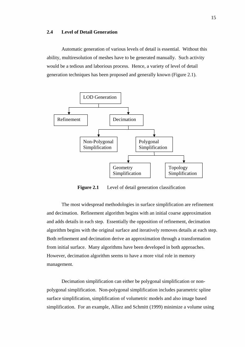
generation techniques has been proposed and generally known (Figure 2.1).
Figure 2.1 Level of detail generation classification
The most widespread methodologies in surface simplification are refinement
and decimation. Refinement algorithm begins with an initial coarse approximation
and adds details in each step. Essentially the opposition of refinement, decimation
algorithm begins with the original surface and iteratively removes details at each step.
Both refinement and decimation derive an approximation through a transformation
from initial surface. Many algorithms have been developed in both approaches.
However, decimation algorithm seems to have a more vital role in memory
management.
Decimation simplification can either be polygonal simplification or non-
polygonal simplification. Non-polygonal simplification includes parametric spline
surface simplification, simplification of volumetric models and also image based
simplification. For an example, Alliez and Schmitt (1999) minimize a volume using
LOD Generation
Refinement Decimation
Non-Polygonal Simplification
Polygonal Simplification
Geometry Simplification
Topology Simplification

16
the gradient-based optimization algorithm and finite-element interpolation model.
Nooruddin and Turk (2003) also use voxel-based method with 3D morphological
operators in their simplification. Practically, mostly all virtual environment systems
employ polygon renderer as their graphics engine. Therefore, it is common to
convert any other model types into polygonal surfaces before rendering. Hence, the
polygonal model is ubiquitous. Pragmatically, the focus falls on polygonal model.
Polygon simplification can be categorized into geometry simplification and
topology simplification. Geometric simplification reduces the number of geometric
primitives such as vertices, edges, and triangles. Meanwhile, topology simplification
deducts the number of holes, tunnels and cavities. Simplification that changes the
geometry and topology of the original mesh is called aggressive simplification.
Another idea from Erikson (1996) is that polygonal simplification can be separated
into geometry removal (decimation), sampling and adaptive subdivision (refinement).
Sampling is an algorithm that samples a model’s geometry and then attempts to
generate a simplified model that closely fits the sampled data.
2.4.1 Geometry Simplification
2.4.1.1 Vertex Clustering
The initial vertex clustering approach, proposed by Rossignac and Borrel
(1993), is performed by building uniform grid of rectilinear cells, and then merging
all the vertices within a cell, also can be call a cluster to a representative vertex for
the cell. All the triangles and edges that stay completely in a cell are collapsed to a
single point. Consequently, all these triangles and edges are discarded. Here by, the
simplified mesh is generated.
The quality of vertex clustering could be improved by using some simple
heuristics in finding the optimal vertex. Other than the work of Rossignac and Borrel
(1993), Low and Tan (1997) proposed a slight variation on this heuristic motivated
by a more thorough geometric reasoning. Their contribution is the making use of
17
“floating cell”. This floating cell algorithm dynamically picks the most important
vertex as the center of a new cell, thus the quality is better.
Regularly, vertex clustering technique is fast and simple to implement. By
recursively merging the clusters, the supercluster can be created. At the same time, it
can be organized in a tree-like manner, allowing selective refinement of view-
dependent simplification.
2.4.1.2 Face Clustering
Face clustering is similar to vertex clustering as both also group a number of
vertices into a cluster. However, face clustering is less popular than vertex clustering.
The algorithm starts by partitioning the original faces into superface patches (Kalvin
and Taylor, 1996). Then, the interior vertices in each cluster are removed, and the
cluster boundaries are simplified. In a final phase, the resulting non-planar
superclusters are triangulated, thus creates a simplified model.
Garland (1999) creates multiple levels of detail for radiositized models by
simplifying them in regions of near constant color. He uses the quadric error metric
in simplifying the mesh’s dual graph.
Simplified mesh generated by face clustering has poorer quality compared to
other operators. It is because the choice in choosing a right region to be a superface
is already a tiresome and difficult work. Therefore, it is hard to create clusters that
collectively provide an optimal partitioning to retain the important features. Some
more, the geometry of the mesh is rarely optimized.

18
2.4.1.3 Vertex Removal
Vertex removal method iteratively keeps taking away a vertex in each time,
and its incident triangles are removed. In doing it, holes may be created and thus
triangulation is needed. Perhaps this is one of the most natural approaches. The first
vertex removal method was foremost introduced by Schroeder et al. (1992). They
remove the vertex based on the distance between the vertex and the plane by fitting a
plane to the vertices surrounding the vertex being considered for removal. Vertices
in high curvature regions have the higher priority to be retained compared to the
vertices in flatter regions during simplification process. This is because eliminating
the vertex in high curvature regions induces more error.
Same like Schroeder et al. do, other works also make use of the error metrics.
Simplification envelops (Cohen et al., 1996) algorithm removes the vertices
randomly as long as the simplified surface lies within the envelopes. It is ensuring
the simplified mesh stays within a specified deviation from the original mesh. Klein
et al. (1996) also coarsen the model using vertex removal technique with maximum
error bounds guaranty.
Figure 2.2 Local simplification operations (Lindstrom, 2003a)

19
2.4.1.4 Edge Collapse
Edge collapse is the most popular simplification operator, invented by Hoppe
et al. (1993). This operator collapses an edge to a single vertex, continuously
deleting the collapsed edge and its incident triangles. It is similar to vertex removal
as it takes away a vertex at a time, yet, the choice of the vertex to be taken away is
different. Also unlike vertex removal, no triangulation action is required because the
resulting connectivity is uniquely defined
Progressive mesh (Hoppe, 1996) is the most famous work in existing edge
collapse algorithms. A coarse mesh is keep adding details into it, explicitly, keep
refining the mesh until a desired level of refined mesh is produced. It is done by
performing the vertex split actions on the original mesh. This algorithm is wholly
beneficial as the original coarser mesh can be obtained back by using the information
used in vertex splitting process.
Edge collapse algorithm need to choose the order of edges to be collapse and
also the optimal vertex to replace the discarded edge. Generally, these decisions are
made by specifying an error metrics that depends on the positions of the substitute
vertex. The sequence of the edges collapses usually is ordered from the cheapest to
the most expensive action. In choosing the right replacement vertex, the lowest error
metrics is used. Anyway, there are other factors may involve in these processes,
including topological constraints, geometry constraints and handling of degenerate
cases.
An identical edge collapse algorithm from Ronfard and Rossignac (1996)
determine the edge collapsing sequence based on the maximum distance from the
new optimal vertex to its supporting planes. A variation of this work, Garland and
Heckbert (1997) perform the edge collapses by minimizing aggregate quadric error
metrics, which is the sum of squared distances to the supporting planes. Whenever
an edge is collapsed, the new vertex inherits the sum of quadric matrices of the
edge’s vertices.
20
Haibin and Quiqi (2000) present a simple, fast and effective polygon
reduction algorithm based on edge collapse by utilizing the “minimal cost” method
to create multiresolution in real time 3D virtual environment development. Franc
and Skala (2001) propose the parallel triangular mesh decimation using the edge
contraction. The system is fast even sorting is not implemented. Its strength is
proved according to the number of processors and the data size they used for testing.
Lindstrom and Turk (1998) create memoryless simplification using edge
collapse, where geometric history in simplification is not retained. Then, the work
was evaluated by Lindstrom and Turk (1999). Besides, memoryless polygonal
simplification (Sourthen et al., 2001) applies vertex split operations in their level of
detail generation.
Danovaro et al. (2002) compare two types of multiresolution representation:
one is tetrahedron bisection (HT) and another one is based on vertex split (MT).
Their work shows that HT can only deal with structured datasets whilst MT can work
on unstructured and structured mesh. At the same time, based on their experiments,
HT is more economic and the extracted mesh is lower in size.
An easier edge collapse method, commonly referred as half-edge collapse
reduces an edge to one of its vertices. Hence, it generally produces in lower quality
meshes than formal edge collapse since it allows no freedom in optimizing the mesh
geometry. Anyway, as it allows the geometry to be fixed up-front, therefore it
enables the polygon transferring and caching on the graphics card done efficiently.
Besides, it is good in doing the view-dependent dynamic level of detail management.
In addition, it is more concise and faster compared to edge collapse. This makes it
suitable for progressive compression.
Another potential coarsening operation is called triangle collapse, which
merges the three vertices of a triangle to an optimal vertex. It was used by Hamann
(1994) and Gieng et al. (1997) for simplification. Since this operation is equivalent
to perform two consecutive edge collapses, thus it also requires optimization of the
substitute vertex. It has little bit faster computational time than the general edge
collapse.
21
2.4.1.5 Vertex Pair Contraction
Vertex pair contraction is a variation of edge collapse that merges any pair of
vertices from a virtual edge. There’s possibility to merge disconnected components
of a model by allowing topologically disjoint vertices to be collapsed. Not every pair
of vertices can be collapsed, basically the subsets of pairs, which are spatially close
to each other, are considered. Different strategies have been introduced and the
selection of the virtual edge is usually orthogonal to the simplification method itself,
including Delaunay edges (1997) and static thresholding (1997).
The work of Erikson and Manocha (1999) is the most notable for its dynamic
selection of virtual edges, which allows increasingly larger gaps between pieces of a
model to be merged. According to the work of Garland and Heckbert (1997), the
vertex pair contraction can be generalized to a single atomic merge of any number of
vertices. Thus, vertex pair contraction is considered the primitive generation of the
edge collapse and vertex clustering simplification method.
2.4.2 Topology Simplification
Topology refers to the connected polygonal mesh’s structure. Whilst, local
topology of a primitive such as a vertex, edge or face is the connectivity of the
primitive to their immediate neighborhood. If the local topology of a mesh is
everywhere equivalent to a disc, then it is known as 2D manifold mesh.
Research on simplifying the topology of models with complex topological
structure is gaining its attention. For large models with a large number of connected
components and holes, such as mechanical part assemblies and large structures such
as a building, it may need to merge the geometrically close pieces into larger
individual pieces to allow further simplification (Erikson, 2000).
During topology simplification, it has to determine whether the manifold of
mesh is required to be preserved or else. Topology preserving algorithm does not

22
close the holes in a mesh and hence the simplification is limited. Opposite to it,
topology modifying algorithm aggregates separate components into assemblies, thus
allows drastic simplification.
By default, the vertex pair contraction and vertex clustering are the
simplification operators that modify the topology of models. These operators are not
purposely designed to do so, but it is a byproduct of the geometry coarsening process.
Anyway, these operators may introduce non-manifold mesh after simplification takes
place.
Schroeder (1997) keeps on coarsening the mesh using vertex splits when the
half edge collapse is limited during the manifold preserving coarsening process.
However, only limited topological simplification is allowed, for example,
disconnected parts cannot be merged. The method proposed by El-Sana and
Varshney (1997) is able to detect and remove small holes or bumps.
Nooruddin and Turk (2003) implement a new topology-altering
simplification, which able to handle holes, double walls and intersecting parts.
Meanwhile, their work preserves the surface attributes and manifold of mesh at the
same time. Liu et al. (2003) present a manifold-guaranteed out-of-core
simplification of large meshes with controlled topological type by utilizes a set of
Hermite data as an intermediate model representation. The topological controls
include manifoldness of the simplified meshes, toleration of non-manifold mesh data
input, topological noise removal, topological type control and sharp features and
boundary preservation.
In many real-time applications, surface’s manifoldness is less important.
Hence, the vertex pair contraction and its derivatives are sufficient for topology
simplification and it is significantly simpler to implement. Anyway, topology should
be preserved well if the visual fidelity is crucial.
23
2.5 Metrics for Simplification and Quality Evaluation
Geometric error metrics is a measurement of geometric deviation between
two surfaces during simplification. Because of the simplified mesh is rarely identical
to the original, therefore metrics is used to check how similar the two models are.
For graphics applications that produce raster image or the visual quality of the model
is highly important, thus the image metric is more suitable at this moment.
2.5.1 Geometry-Based Metrics
Besides evaluating the quality of the simplified mesh, metrics is determining
the way of simplification works. This mathematical definition of metrics is
responsible in calculating the representative vertex and also determining the order of
the coarsening operations. Anyway, each metrics has different ways in choosing its
best manner for object simplification. On the other hand, the quality of the metrics is
hardly to be evaluated in a precise way.
Typically simplification algorithms are using different kinds of metrics.
Though, many of them are inspired by the well-known symmetric Hausdorff distance.
This metric is defined using the Euclidean distance, which uses the shortest distance
between a point and a set of points. In next sections, the well known metrics will be
given away.
2.5.1.1 Quadric Error Metrics
The mathematical computation in metrics generation is usually reduced its
complexity in order to make the simplification faster. There are many ways in
calculating error metrics. For metrics based on maximum error, they are more
conservative and fast. Meanwhile, the mean error metric is done locally on a small
portion of the surface (Hoppe et al., 1993).

24
Quadric error metrics (Garland and Heckbert, 1997) is based on weighted
sums of squared distances. The distances are measured with respect to a collection
of triangle planes associated with each vertex. This algorithm proceeds by iteratively
merging pairs of vertices, which need not to be connected edge. Its major
contribution is a new way to represent error using a sequence of vertex merge
operations.
Quadric error metrics efficiently represents the metrics by using matrix.
Anyhow, it only supports wholly geometry simplification. Garland and Heckbert
(1998) extends the metrics to more than four dimensions to support surface attributes
preservation other than geometry information. The matrix’s dimension is based on
how many attributes does a vertex own. It is particularly robust and fast. Besides, it
produces good fidelity mesh even for drastic polygon reduction.
Quadric error metrics is fast, simple and guide simplification with minor
storage costs. The visual fidelity is relatively high at the same time. In addition, it
does not require manifold topology. That is, it allows drastic simplification as it lets
holes to be closed and components to be merged.
2.5.1.2 Vertex-Vertex vs Vertex-Plane vs Vertex-Surface vs Surface-Surface
Distance
Vertex-vertex distance measures the maximum distance traveled by merging
vertices. While vertex-plane distance stores set of planes with each vertex, then
errors are calculated based on distance from vertex to plane. Similarly, vertex-
surface distance is distance between vertex and surface. It maps point set to closest
points to simplified surface. Maximum distance between input and simplified
surfaces is used to measure surface-surface distance.

25
2.5.2 Attribute Error Metrics
Quality evaluation can be done on image instead of model’s geometry.
Image metrics have been adopted in a number of different graphics applications.
Therefore, the quality of the simplified mesh can be measured by evaluating the
difference before and after the simplification happens. Some image metrics are quite
simple. Probably the traditional metrics for comparing images is the Lp pixel-wise
norm. Nonetheless, recently there are quite a number of researches focus on
humans’ psychology and vision to develop the computational models. In doing it,
image processing and human visual perception is exploited.
Image processing techniques such as Fourier transform (Rushmeier et al.,
1995) or wavelet transforms (Jacobs et al., 1995) can be used for this purpose.
Besides, contrast sensitivity function also can be employed to guide the
simplification process. It measures contrast and spatial frequency of changes induces
by operation.
Human visual perception is utilized by Watson et al. (2000) by conducting a
survey on the human’s ability in identifying simplified models using different
metrics. The durations of time spent to distinguish the different between the images
for different metrics are analyzed. The results show that image metrics generally
performed somewhat better than the geometry-based metrics used by Metro.
Nevertheless, its robustness is uncertain.
2.6 External Memory Algorithms
The external memory algorithms are required in handling the data, which
larger than the main memory. Because of the main memory cannot fit all the data,
thus there is an external memory dilemma. As the speed of the data set is growing
much faster than the RAM size. Therefore, these algorithms are essential to make
the massive data sets loadable and run able in graphics applications. The initial work
of external memory is proposed by Aggarwal and Vitter (1988). Later on, some
26
other fundamental paradigms for external memory algorithms are introduced. Until
now, researches on external memory are continuous and never end.
There are two fundamental external memory concepts used in visualization
and graphics applications, including batch computation and on-line computation.
Batch computation has no preprocessing process and the whole set of data is
processed. The way to make the data loadable is stream in the data in a few passes.
Thus, only the portion of the data, which is smaller than the workstation’s memory,
is filled at one time and processed. Whilst on-line computation conducts preprocess
to organize the data into a more manageable data structure in advance. This
preprocess actually is a batch computation. Therefore, during runtime, only the
needed portion of data is read into main memory by performing query on the well
built data structure.
To accelerate the graphics rendering, geometry caching or prefetching
techniques can be combined with the explained paradigms. It avoids the last minute
data retrieval when the part of the data required to be displayed on screen. Else, it
may slow down the rendering process as it needs to find the right portion of data
from the data structure and then throw the required data to graphics card. Hence, if
the part of the data, which is possible visible in the next frame is predicted, and put
into cache first, consequently rendering will be speeded up.
In following section, discussion on computational model (Aggarwal and
Vitter, 1988) is carried out. Then, batched computations, including external merge
sort (Aggarwal and Vitter, 1988), out-of-core pointer de-referencing (Chiang and
Silva, 1997), and the meta-cell technique (Chiang et al., 1998) are discussed. Next,
on-line computation (Bayer and McCeight, 1972; Comer, 1979) is investigated too.

27
2.6.1 Computational Model
Disk access is two times longer than main memory access (Aggarwal and
Vitter, 1988). In order to optimize the disk accessing time, a large block of
contiguous data is loaded in one time. In handling large data sets, the size of input
data (N) and the available main memory size (M) have to be found out.
Continuously, the size of the data item (B) has to be determined. It is the size of
memory used for every pass of data reading or data processing.
The performance of external memory algorithms is based on the total of the
I/O operations (Aggarwal and Vitter, 1988). This I/O complexity is calculated by
dividing the size of input data by size of the data item (N/B). The data size of
scanned data may be reaching a few hundreds million of triangles. For instance,
LLNL isosurface datasets used in work of Correa (2003) is 473 million triangles.
2.6.2 Batched Computations
2.6.2.1 External Merge Sort
Sorting is the primary practice in large data management. This is because
sorting eliminates the need of randomly searching on a wanted value lies in the large
dataset. External merge sort is a k-way merge sort, that is, k is M/B. k is the
maximum number of disk block that can fit in main memory. The data is required to
be loaded into main memory portion by portion in its contiguous place.
K-way merge sort has to load the whole data set with size N. If the current
list L to be read is small enough to fit into main memory, then the data can be read
into system in one time then sort it and put it back into its contiguous place. Else, L
list is required to be spilt into k sub-lists, where each of them is equal in size. Then
for each sub-list, the sorting is performed. There are lots of sorting algorithms
nowadays, including bubble sort, quick sort, selection sort, tag sort and etc. After all
the sub-lists are sorted, these sub-lists are merged.
28
Basically, merging is made by comparing the values from different lists. For
example, like in two-way merge sort, two lists of data will be merged into a single
data list. These two lists are read from beginning, and then compare the first
elements from both lists. Whichever smaller element is put into output list and the
array pointer is incremented. Continue checking on the following elements in both
lists until all data elements are completely sorted.
A memory insensitive technique (Lindstrom, 2000a; Lindstrom and Silva,
2001) practically use the external merge rsort written by Linderman (2000) It is a
combination of radix and merge sort technique, which the keys are compare
lexicographically.
The way of the sorted k sub-lists of the entire data (N) to be merged in good
I/O complexity is important. These k sorted-lists are merged and output these sorted
items to disk in units of blocks. When the previous buffer finished its process, then
the next block of the corresponding sub-list is read into main memory to fill up the
allocated buffer. This process is repeated until all k sub-lists are merged successfully.
2.6.2.2 Out-of-Core Pointer Dereferencing
Usually data used in visualization or graphics applications is in indexed
format. The triangular indexed mesh has a list of vertex coordinates and a list of
triangles indices pointing to its relevant vertex coordinates. This data format is
compact and save memory space as every vertex value is only stored once.
Using indexed mesh needs full searching on the vertex list to find its
belonged vertices. If the data is small, then it is not noticeably memory inefficient.
However, probably the vertex list or the triangles’ indices or both of them are not fit
able in main memory. Hence, pointer dereferencing is essential to generate a triangle
soup instead of using the indexed mesh. Subsequently, it avoids the random accesses
on disk. Random access is a must avoided task because single vertex retrieval may
29
need several block by block data readings (B) from the entire input data (N). It
would require (N) I/O’s in the worst case, which is extremely ineffective.
In order to make the massive data reading I/O efficient, thus the pointer
dereferencing is used to replace the triangle indices by its corresponding vertices.
Because of each triangle contains three vertices, so the pointer dereferencing also has
three passes. In first pass, sort the first vertex using external merge sort technique.
After all of the first vertices from triangle list are sorted, now the vertex list can be
read in sequence. Keep replacing the vertex 1 with first vertex from vertex list,
vertex 2 with second vertex from vertex list and so on. At that moment, all of the
first triangle indices are filled with its equivalent vertices. In the second pass, sort
the second vertices in the triangle list, and then dereference their equivalent vertices.
Same works are acted upon the third vertices. Finally, triangle soup mesh is
generated with every triangle indices are filled with its corresponding vertices.
This technique is applied in Lindstrom’s (2000b) first out-of-core data
simplification. Same with others’ opinion, his work also avoids random access by
using triangle soup mesh instead of indexed mesh. This data representation is two to
three times more space consuming, but typically increase simplification speed by a
factor of 15-20 (Lindstrom, 2000b). This process has also been used in (Chiang and
Silva, 1997; Chiang et al., 1998; El-Sana and Chiang, 2000; Lindstrom and Silva,
2001). These direct vertex information make the I/O complexity better.
2.6.2.3 The Meta-Cell Technique
The out-of-core pointer dereferencing technique is I/O efficient, but it is not
suitable for final data representation in real time applications. Additionally, the
vertices are duplicated quite many times. It causes the disk space overhead is bulky.
To optimize both disk access and disk-space requirement, Chiang et al. (1998)
proposed a technique called meta-cell technique. It is an I/O efficient partition
scheme for irregular mesh. This technique has been adopted in out-of-core
30
isosurface extraction (Chiang et al., 1998; Chiang et al., 2001) and out-of-core
volume rendering (Farias and Silva, 2001).
Basically the meta-cell technique divides the data into cells, which are equal
in volume. Each meta-cell has own information and is normally loaded the whole
from disk to main memory. The cell data is in indexed representation, called index
cell set (ICS) by Chiang et al. (1998). This data representation contains a local
vertex list and a local cell list, which point to the local vertex list. Hence, the vertex
duplications are reduced compared to out-of-core pointer de-referencing technique.
Only the vertices that fall into two different meta-cells are kept twice. Anyway, the
more the meta-cells, the more the duplicated vertices it creates. However, it means
each meta-cell is more refined and contains less information. Subsequently, the disk
reading is faster. Therefore, there is always trade-off between query time and disk
space.
The meta-cell technique has been extended for view-dependent simplification
(El-Sana and Chiang, 2000). The meta-node tree is not only used in simplification
but also accelerate the run time data query. At the same time, they also employ some
additional features, such as prefetching, buffer management and also parallel
processing.
2.6.3 On-Line Computations
A more efficient data searching probably is the tree based data structures for
real time applications. The data in tree based data structures are well sorted and
queries can be done faster. For external memory usage, the most famous tree based
structure is the multiway B-tree by Bayer and McCreight (1972). Each end node
holds B items. The branching factor is defined as the number of children of each
internal node, except root node. This framework has been adopted in the works of
Edelsbrunner (1983), El-Sana and Chiang (2000) and El-Sana and Varshney (1999).
This algorithm is robust and capable to facilitate in many out-of-core visualization
and graphic domains.

31
Tree based data structure significantly reduce the I/O complexity compared to
direct data searching on the external memory mesh. Usually binary tree or even
octree with branching factor two or eight can be used. Anyway, it still requires
accessing a certain number of items in order to get the demanded item. Therefore, it
is better to externalize the data structure to B-tree-like data structure. It can be done
by increasing the branching factor for the internal node. Automatically, the tree’s
height is decreased while the number of items in each node is increased. As a result,
it can trim down the data searching time.
2.7 Out-of-Core Approaches
One of the reason why out-of-core simplification approaches exist is the
majority of the previous methods for in-core simplification are ill-suited in out-of-
core setting. The prevailing approach to in-core simplification is to iteratively
perform a sequence of local mesh coarsening operations (Section 2.4.1) that locally
simplify the mesh by removing a primitive geometry at one time. The order of
operations performed relies on the error metrics they use, which discard a simplex
according to their visual importance. In any case, manipulating the order of
coarsening operations from lowest error to highest error impose a certain number of
memory and computational time.
In order to make the massive mesh able to be simplified, usually the mesh
need to be partitioned until it is suitable to be simplified in available main memory.
Therefore, it is common to group the mesh into clusters. Basically those triangles,
whose vertices belong to three different clusters, are remained during the
simplification process. Ideally the partitioning is done to minimize the given error
measurement and the representative vertex is chosen based on certain error metrics.
Most of the in-core methods use indexed mesh representation, where the
triangles are specified as indices and their corresponding vertices are referred. For
out-of-core simplification to be viable, random accesses must be avoided at all costs.
As a result, many out-of-core methods make use of a triangle soup mesh
32
representation, where each triangle is represented independently as a triplet of vertex
coordinated. The triangle soup can be generated by using the previously discussed
external memory algorithms.
Varadhan and Manocha (2002) proposed an external memory algorithm for
fast display of large and complex geometric environment. This algorithm uses a
parallel approach to render the scene as well as fetch objects from the disk in a
synchronous manner. Besides, novel prioritized prefetching technique that takes into
account LOD switching and visibility-based events. Correa et al. (2002) also present
an out-of-core preprocessing algorithm, which uses multiple threads to overlap
rendering, visibility computation and disk operation. Besides, from-point
prefetching method is implemented. Crack prevention is introduced by Guthe et al.
(2003) by appropriately shades the cut using fat borders in their hierarchical levels of
details algorithm.
Borodin et al. (2003) also propose an out-of-core simplification with
guaranteed error tolerance. The algorithm consisted three processes, includes
memory insentive cutting, hierarchical simplification and memory insensitive
stitching. Vertex contraction is their simplification operator as they claimed it
produces better quality but slower computation time. Shaffer and Garland (2001)
also propose an adaptive simplification of massive meshes, which can generate
progressive transmission. It uses edge contraction in simplification process.
There are three distinct approaches to out-of-core simplification techniques:
spatial clustering, surface segmentation and streaming (Lindstrom, 2003b). For each
approach, uniform and adaptive partitioning will be distinguished.
2.7.1 Spatial Clustering
Clustering decisions is based on either connectivity or geometry of the mesh,
or both. Because of computing and maintaining the connectivity of a large mesh out-
of-core is difficult, perhaps the simplest approach is partitioning the vertices spatially.
33
Determining cell containment performs vertex clustering. No topological constraints
are considered.
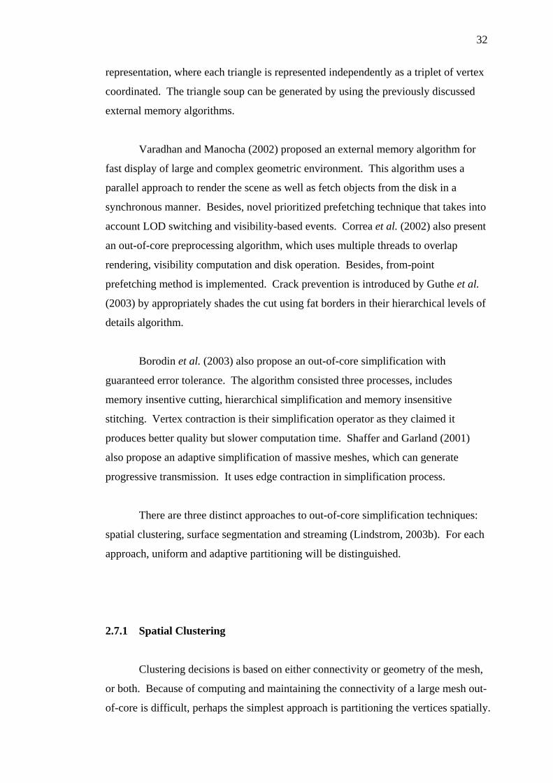
Spatial clustering’s main idea is to partition the space that the surface is
embedded into simple convex 3D regions. Next, merge the vertices in the same cell.
Because the mesh geometry is often specified in a Cartesian coordinate system, a
rectilinear grid gives the most straightforward space partitioning. It is similar to
vertex clustering algorithms (Section 2.4.1.1). Figure 2.3 illustrates the how the
spatial clustering works.
Figure 2.3 Spatial Clustering process (Lindstrom, 2003a)
Uniform spatial clustering is simplest partitioning, which partitions the space
into grid equally. It sparse the data structure represents occupied cells. By
minimizing the quadric error, the representative vertex can be calculated. The
triangles whose vertices fall in three different cells are kept at last. These processes
are practically done by Lindstrom (2000) in his out-of-core simplification (OOCS).
Later on, memory insensitive clustering (OOCSx) approach, which is independent on
simplified mesh’s size, is introduced (Lindstrom and Silva, 2001). It first scans the
triangles, and then computes the plane equation, saves the cluster ID and plane
equation for each vertex and saves the non-degenerated triangles to triangle file. Sort
plane equation file on cluster ID then compute cluster quadrics and output optimal
vertices. Then, re-indexing process take place to sort the triangle file, scan and
replace the cluster ID with vertex ID, repeat to every vertex field. This work is
extended to run-time view-dependent rendering by preserving some surface attributes
(Lindstrom, 2003c).

34
For uneven triangles distributed mesh, where many triangles may fall in a
region whilst the other part may have very little number of triangles, it is impractical
to use the uniform clustering. It is because the uniform spatial clustering technique
doesn’t adapt to surface features nicely. It does not imply well-shaped clusters.
Besides, it may create many uneven or disconnected surface patches. On the other
hand, the fixed-resolution limits the maximum simplification. To overcome these
weaknesses, adaptive spatial clustering technique is proposed.
In adaptive clustering, the cell geometry is adapted to surface condition. For
example, uses smaller cells in detailed regions. Garland and Shaffer (2002) present a
BSP tree technique in space partitioning. Firstly, the quadrics on uniform grid are
accumulated. Secondly, the PCA of primal/dual quadrics is used to a suitable space
partitioning condition. In second pass, the mesh is reclustered. Fei et al. (2002)
propose an adaptive sampling scheme, called the balanced retriangulation (BT).
They use Garland’s quadric error matrix to analyze the global distribution of surface
details. Based on this analysis, a local retriangulation achieves adaptive sampling by
restoring detailed areas with cell split operation while further simplifying smooth
areas with edge collapse operations.
2.7.2 Surface Segmentation
Fundamentally, spatial clustering partitions the space that the surface lies in.
This method partitions the surface into patches so that they can be further processed
independent in-core. Then, every patch is simplified to a desired level of detail using
in-core simplification operator. For instance, one can simplify the triangles in the
patch using the edge collapse. After simplification, the patches are stitched back.
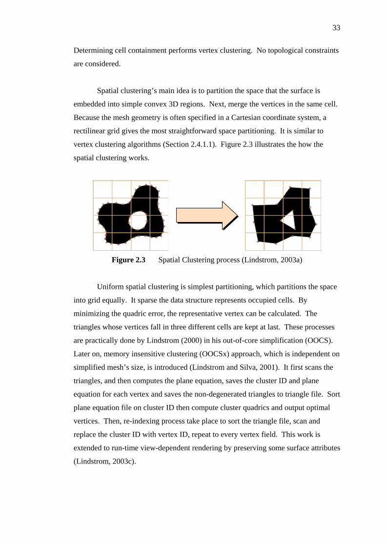
As in spatial clustering, surface segmentation could be uniform by
partitioning the surface over uniform grid, or adaptive by cutting the surface along
feature line. Figure 2.4 shows the diagram of process flow in surface segmentation
method.
35
Figure 2.4 Block-based simplification using uniform surface segmentation and
edge collapse (Hoppe, 1998b)
Bernardini et al. (2002) propose a uniform surface segmentation algorithm
with constraints that the boundary intact to allow future merging. It is quite easy to
implement and have higher quality than spatial clustering simplification method. But,
it is two times slower than spatial clustering method. Additionally, the output of the
simplified mesh can’t span a few level of detail.
An adaptive surface segmentation algorithm is proposed, named OEMM
(Cignoni et al., 2003c). It uses octree-based external memory mesh data structure.
The grid is rectilinear and the data structure is unspecific that not only created for
simplification purpose. It is similar to Bernardini et al. (2002), but the octree adapts
in suitable resolution to match better surface detail, the edges can be collapsed across
patch boundaries and the output is a progressive mesh.
Another adaptive approach, which is fully depends on error-driven surface
segmentation is introduced by El-Sana and Chiang (2000). This technique can
preserve the correct collapsing order and thus ensure the run-time image quality.
Besides, features like prefetching, implicit dependencies and parallel processes are
implemented. It computes mesh connectivity, initialize priority queue on disk. Then,
for each bath of lower-error edges, dequeue the edge and load incident faces into
RAM, collapse edges whenever possible, recomputed error then write back to disk.
It repeats until desired accuracy is achieved.
36
Prince (2000) uses octree partitioning and edge collapse like OEMM do. He
is able to create and view progressive mesh representation of large models. He uses
octree partition, edge collapse simplification operator but need to frozen the path’s
boundary. There is another adaptive surface segmentation method is by Choudhury
and Watson (2002) whose propose a simplification in reserve. It is an enhancement
of RSimp (Brodsky and Watson, 2000) to become VMRSimp. Brodsky and Watson
use refinement based on vector quantization. Their work is generally believed faster
as the refinement is take shorter time than simplification does. Anyway, it has
poorer quality as refinement leads to lower quality result.
2.7.3 Streaming
Streaming treats a mesh as a sequenced stream of triangles. For each time,
read a triangle, process it then write it in a single pass. Later on, in finite in-core
stream buffer, indexed submesh is built up. For the triangles that loaded into buffer,
in-core simplification is performed. In order to make sure buffer contains
sufficiently large and connected mesh patches, it requires coherent linear layout of
mesh triangles.
In stream buffer properties, there are processed region, buffered region and
unprocessed region. One or more loops of edges that divide mesh into processed and
unprocessed regions. Indexed triangles read from input boundary and write to output
boundary. The stream boundary sweeps continuously over mesh. Therefore, no
stitching is needed unlike conventional surface segmentation method. Figure 2.5
shows the stream boundaries.

37
Figure 2.5 Streaming properties (Lindstrom, 2003a)
A new approach in out-of-core mesh processing technique can be adapted to
perform computation based on new processing sequence (Isenburg and Gumhold,
2003; Isenburg et al., 2003a) paradigm. Processing sequence for large mesh
simplification (Isenburg et al., 2003b) represents a mesh as a particular interleaved
ordering of indexed triangles and vertices. This representation allows streaming very
large meshes through main memory while maintaining information about the
visitation status of edges and vertices. Stream-based edge collapse (Wu and Kobbelt,
2003) reads the input from a data stream and writes the output to another stream. It
is good because it doesn’t have stitching artifacts, but its geometry hashing overhead
and cannot differentiate stream boundary from surface boundary.
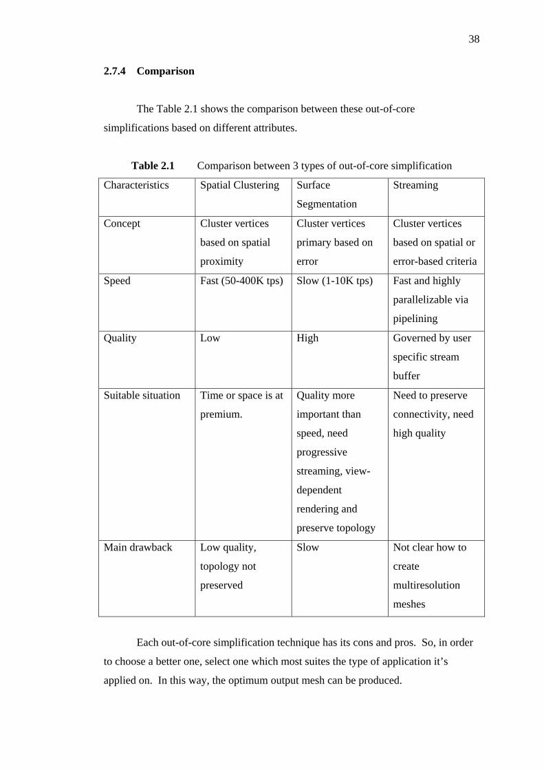
38
2.7.4 Comparison
The Table 2.1 shows the comparison between these out-of-core
simplifications based on different attributes.
Table 2.1 Comparison between 3 types of out-of-core simplification
Characteristics Spatial Clustering Surface
Segmentation
Streaming
Concept Cluster vertices
based on spatial
proximity
Cluster vertices
primary based on
error
Cluster vertices
based on spatial or
error-based criteria
Speed Fast (50-400K tps) Slow (1-10K tps) Fast and highly
parallelizable via
pipelining
Quality Low High Governed by user
specific stream
buffer
Suitable situation Time or space is at
premium.
Quality more
important than
speed, need
progressive
streaming, view-
dependent
rendering and
preserve topology
Need to preserve
connectivity, need
high quality
Main drawback Low quality,
topology not
preserved
Slow Not clear how to
create
multiresolution
meshes
Each out-of-core simplification technique has its cons and pros. So, in order
to choose a better one, select one which most suites the type of application it’s
applied on. In this way, the optimum output mesh can be produced.

39
2.8 Analysis on Out-of-Core Approach
2.8.1 Advantages and Disadvantages
Nowadays, models are well beyond most core memories can be handled. The
sizes of these datasets rise drastically from range 107 to 109 faces. The out-of-core
approaches apparently solved simplification problems on datasets, which are larger
than main memory. These out-of-core techniques use virtual memory to put the data
that are not used into hard disk and then put in the portion of data needed for
rendering into main memory. Therefore, it makes the display of extremely large
datasets possible.
Besides, out-of-core approaches could speed up development. For example,
Lindstrom (2000) presents an extremely fast simplification model that can process
400K triangles per second on desktop PC. It is the nearly impossible achieved by
other in-core simplification methods. On the other hand, it could handle highly
variable level of detail, even extreme close-ups revealing new detail.
Even though out-of-core approaches contributed a lot in making the rendering
of massive datasets possible, it has its weakness. That’s it; random access on must
be avoided. This is because the disk access is slow and hence need to minimize this
process. It is unlike main memory access, which is fast and convenient.
2.8.2 Comparison: In-Core and Out-of-Core Approach
In-core simplification and out-of-core simplification have their similarities
and differences. When looking into the purpose of simplification, they have a same
ambition, that’s to simplify the input mesh to a certain level of detail. They both
discard degenerated triangles. Their quality determined by the degree of similarity
between simplified mesh and original mesh. However, they have few differences as
well (refer Table 2.2).

40
Table 2.2 Comparison between in-core approach and out-of-core approach
Characteristics In-core Out-of-core
Type of Memory Main memory. Use secondary memory for unused
data, main memory for data, which
will be displayed.
Size of datasets Must smaller than main
memory.
Can be larger than main memory,
maximum data size depends on
algorithm’s strategy. For example,
Lindstrom (2000) depends on output
mesh size whilst Lindstrom and Silva
(2001) is independent of the available
memory on computer.
Simplification
operators
Local simplification,
such as vertex removal,
edge collapse, triangle
collapse, vertex
clustering, vertex pair
contraction, etc.
Can be categorized in three groups,
which are spatial clustering, surface
segmentation and streaming. Internal
operation can be done by in-core
simplification operator, for example:
edge collapse in OEMM (Cignoni et
al., 2002) and vertex clustering
(Lindstrom, 2000).
How it works? Directly place the mesh
into main memory and
simplify it. For
example, edge collapse
and vertex clustering.
Convert mesh into a data structure in
preprocess and store it on disk, then
extract the portion of data that is being
used to main memory during run-time.
Speed Depends on size of
input mesh.
Depends on algorithm. But eventually
faster than in-core method.
Quality Depends on
simplification operator.
Depends on simplification method.

41
2.8.3 Performance Comparison: Existing Simplification Techniques
For comparison between a few implemented simplification techniques, a
comparison can be made between in-core and out-of-core simplification. The basis
for many out-of-core simplifications, Out-of-Core Simplification (OOCS) by
(Lindstrom, 2000) is the initial work in out-of-core simplification. It can simplify
400K triangles per second and require 63-72 bytes to represent a triangle.
Nevertheless, its quality is quite low as no connectivity is remained. Table 2.3
compare the OOCS (Lindstrom, 2000) to two in-core simplification techniques,
QSlim (Garland and Heckbert, 1997) and memoryless simplification (Lindstrom and
Turk, 1998). QSlim is one of the fastest vertex merge algorithm (Brodsky and
Watson, 2000). While memoryless simplification is an efficient simplification that
no needs to retain history of simplified mesh in memory.
Table 2.3 Simplification results of running QSlim, memoryless simplification
(Mless) and OOCS. All results were gathered on a 195 MHz R 10000 SGI Origin
with 4GB of RAM and a standard SCSI disk drive (Lindstrom, 2000)
RAM (MB) Time (h:m:s) Model Tout
QSlim Mless OOCS QSlim Mless OOCS
244,562 213 134 28 5:31 11:59 0:16
113,090 214 134 11 5:55 14:12 0:12
Dragon
T=871,306
47,228 214 134 7 6:06 15:21 0:10
204,750 250 166 26 7:13 16:58 0:17Buddha
T=1,087,716 62,354 251 166 8 7:35 19:19 0:12
Blade
T=28,246,208
507,104 - 3,185 63 - 12:37:25 5:02
Statue
T=386,488,573
3,122,226 - - 366 - - 1:59:20
From Table 2.3, we can see that RAM usages in-core approaches (QSlim and
Memoryless Simplification) are depends on the size of the input mesh. When the
RAM usage is bigger than 4GB, blade cannot be process by QSlim method.
However, it still can be process by memoryless simplification because memoryless

42
simplification doesn’t retain the history of simplified mesh free up some space for
this process. Nevertheless, statue with input size 400 millions of triangles cannot be
processed by memoryless simplification anymore as it cannot be fit into limited
RAM memory. It is not a problem for OOCS as it doesn’t depend on input mesh’s
size. OOCS can process any mesh with constraint that the size of the output mesh
mustn’t larger than RAM size. While being much more memory efficient, this out-
of-core simplification technique also orders of magnitude faster.
OOCS is fast, but the quality is looser because it doesn’t perform adaptive
sampling. Further, since OOCS does not reply on connectivity information, it has no
way of detecting boundary edges (or non-manifold edge). To make the quality better,
hybrid approach could be considered, that is, first, perform OOCS on a large model,
then follow by slower but accurate in-core simplification (Lindstrom, 2000a).
Even though OOCS can display lots of massive data, however, it encounters
problem when dealing with the output size, which is larger than available main
memory. Referring Table 2.4, OOCS is faster than OOCSx (Lindstrom and Silva,
2001) between two to five times when output mesh remains smaller than RAM size.
But, in one case, for simplification of blade, OOCSx is faster than OOCS. The
reason is OOCS ran out of memory, and numerous page faults occurred. Another
case is 15.5MB RAM even is not enough for OOCS to simplify the fluid. Memory
usage of OOCSx depends on size of the input mesh, whereas memory usage for
OOCS is proportional to size of output mesh. Additionally, OOCSx only use
arbitrary little main memory (5MB or 8MB RAM in this simplification process).
Contrary, OOCS use all available main memory for displaying the output mesh.
In (Lindstrom, 2003c), Lindstrom has improved insensitive algorithm
(Lindstrom and Silva, 2001), which is remarkable fast and yields an effective triangle
processing rate of roughly 20K to 60K triangles per second. The system is view-
dependent. Other than that, he also pointed out that El-Sana and Chiang (2000) can
simplify at 5,300 triangles per second with input mesh 1.2 million triangles. But,
their method will steadily reject the input mesh when it grows larger. Prince (2000)
can produce a 1000 triangles per second on 11.4 million triangles’ mesh, however, it
requires more than 512MB RAM to do it.

43
Table 2.4 Run-time performance of OOCS and OOCSx. Blade were computed
on Linux PC with 512MB RAM and two 800 MHz Pentium III processor. Statue
and fluid are simplified on SGI Onyx2 with forth-eight 250MHz R10000 processor
and 15.5GB RAM. (Lindstrom and Silva, 2001)
RAM:disk (MB) Time (h:m:s) Model Tin Tout
OOCS OOCSx OOCS OOCSx
507,104 49:0 5:4,850 2:46 13:14
1, 968,172 160:0 5:4,899 3:11 14:30
Blade 28,246,208
7,327,888 859:0 5:4,993 19:14 17:04
3,012,996 261:0 8:64,004 44:22 2:7:24Statue 372,963,401
21,506,180 3,407:0 8:64,256 51:23 2:49:30
6,823,739 588:0 8:80,334 55:56 3:11:48
26,086,125 3,427:0 8:80,510 1:08:48 3:23:42
Fluid 467,614,855
94,054,242 - 8:80,345 - 4:19:09
Simplification using Octree-based External Memory Mesh (OEMM) by
(Cignoni et al., 2003c) eventually faster than in-core simplification method: QSlim
and RAM-QEM (implementation of QEM in main memory) and their RMS errors
are quite similar. However, it is much slower than OOCS even though the error
metrics is much smaller (higher quality) than OOCS. Besides, Cignoni et al. (2003c)
can produce up to 13K triangles per second, but the output is not directly usable in
view-dependent refinement. Table 2.5 shows the simplification of a Happy Buddha
(1,087, 716 faces) on PIII 800MHz PC with 128MB RAM.
Table 2.5 Simplification on Happy Buddha using four different codes (Cignoni
et al., 2003c)
Code Simpl.
faces
RAM
(MB)
Time (s) Tps rate RMS err
QSlim v2.0 18,338 195 60 17.4K 0.0131
RAM-QEM 18,338 160 58 18K 0.0125
- 4 58 - -OEMM-QEM (Preprocess)
OEMM-QEM (Simplify) 18,338 60 48 21.7K 0.0129
OOCS 19,071 36 15 69.5K 0.0245

44
An approach making the out-of-core simplification with a guaranteed error
tolerance (Borodin et al., 2003) is implemented using vertex contraction technique
instead of vertex clustering. Even the error is minimized until lower than QSlim
(Garland and Heckbert, 1997) and output’s quality is high, the simplification time is
relatively slow. Plus, their work doesn’t show the statistics of simplified mesh with
size larger than 35K triangles (See Table 2.6).
Table 2.6 Reduction and performance rates for four standard models using a
1.8GHz Pentium IV PC with 512MB main memory (Borodin et al., 2001)
Model Tin Tout Error Simplifcation
time (h:m:s)
Rate
(tps)
Armadillo 345 944 33 780 0.129 0:05:06 826
Happy Buddha 1 087 716 32 377 0.170 0:19:28 728
David 2mm 8 254 150 25 888 0.178 2:22:02 762
Lucy 28 055 742 26 772 0.163 8:03:57 779
A multiphrase approach (Garland and Shaffer, 2002), which operates by
combining an initial out-of-core uniform clustering phase with a subsequent in-core
iterative edge contraction phase performs very well in simplification process. This
technique produces higher quality, better distribution of triangles than uniform
spatial clustering. But, higher grid resolution needed in the first pass causing the
more memory is consumed. Besides, it is still output sensitive. They have compared
their results with OOCS (Lindstrom, 2000), adaptive out-of-core clustering (Shaffer
and Garland, 2001), and QSlim (Garland and Heckbert, 1997). Results show that it
is able to simplify polygonal mesh of arbitrary size, like OOCS, but it is able to
generate much higher quality approximations at moderate to small output sizes.
Indeed, it consistently produces approximations of quality comparable to QSlim, but
using considerably less running time and memory, both asymptotically and in
practice.
Guthe et al. (2003) propose a very efficient hierarchical level of details on
complex environment and filling cracks created during simplification process by
using shaded fat borders. This algorithm is run on a 1.8GHz Pentium 4 PC with
512MB memory and ATI Radeon 9700Pro and the results are tremendously good.
45
Their work is compared with out-of-core algorithm without crack filling and in-core
rendering. The frame rates that it produced are adequate to generate an excellent
real-time application probably due to the good VGA card they used.
Correa (2003) proposes a new algorithm in out-of-core simplification,
consisting two phrases of work as well, which is preprocessing and runtime. In
building the octree, a finer tree creates a more precise view-frustum. Coarser
granularity reduces traversal time, decreases vertex replication but increases
possibility of fetching and rendering of invisible geometry. LoD generations are
created by vertex clustering technique. Besides, occlusion culling and sort-first
parallel rendering are also implemented.
For preprocessing step, 2.4 GHz Pentium IV computer with 512 MB of RAM,
250 GB IDE disk and a NVIDIA GeForce Quadro FX 5200 Graphics card is used.
During octree generation, based on his thesis’s figure, granularity of 15K vertices per
leaf needs roughly six minutes to generate it. Whilst LOD generation for the original
data and four simplified models needs approximately eight minutes of time with
additional data size of 268MB. This algorithm is fairly good in its speed aspect.
Nevertheless, due to his implementation constructs static LOD, while Lindstrom
(2003c) generates view-dependent LOD, and hence comparison is hard to be made
between these algorithms. Besides, no figures on simplification time are shown.
Subsequently, it is difficult to compare its efficiency with other existing algorithms.
Comparison between performance of adaptive and uniform clustering
methods have been carried out by Shaffer and Garland (2001). Tool Metro (Cignoni
et al., 1998) is used to measure error metrics. The results show that error in coarse
approximation is reduced about 20%. At the same time, finer resolution is dropped
around 10% too. This shows that adaptive gives better quality approximation.
However, the time consuming to simplify the mesh is varied from around 2.5 to 3
times as much as that required for uniform clustering. As a short conclusion,
adaptive clustering induces better quality mesh but slower than uniform clustering do.
In streaming simplification approach, it generates higher quality than spatial
clustering and surface segmentation simplification techniques with low memory

46
requirement. Most recent work by Isenburg et al. (2003b) enables full connectivity
and geometry information is available for the active elements of the traversal even
the mesh access is restricted to a fixed traversal order. This provides seemless and
highly efficient out-of-core access to very large meshes for algorithms that can adapt
their computations to this fixed ordering. Some models simplified using this
algorithm by using 800MHz Linux PC. This is suitable to make a comparison to
works of (Wu and Kobbelt, 2003; Lindstrom and Silva, 2001; Cignoni et al., 2003c)
as their works are run on 800MHz Pentium 3 with 880MB RAM. The quality of this
approach is apparently compatible with other out-of-core approaches. Anyway, the
neighbour triangles have to be grouped together.
From all these recently published algorithms, the findings show that the
multiphrase approach (Garland and Shaffer, 2002), Efficient View-Dependent Out-
of-Core Visualization (Guthe et al., 2003), Out-of-Core Visualization of Large
Datasets (Correa, 2003 ) and large mesh simplification using Sequence Processing
(Isenburg et al, 2003b) give an appropriate good quality as the same time a pleasant
processing time as well. OOCS (Lindstrom, 2000) would be the greatest if the
simplification time is the most vital element instead of quality.
2.9 Appearance Attribute Preservation
Many simplification algorithms simplify geometry data but pay no attention
to surface preservation. For sure, geometry simplification is vital in reducing the
gigantic data size. However, appearance-preserving also important to retain the
surface attributes after simplification process. Normally, the surfaces attributes need
to be preserved during mesh simplification include surface position, normal, surface
curvature, color attributes and texture attributes.
From beginning, surface preservation is often done separately with geometry
simplification. In accomplishing this, decouples the sampling rates of the surface
attributes by storing the object’s color and normal vectors in texture and normal
maps respectively. Then make sure the bounds on both the surface and texture
47
deviations by filtering the model’s surface position. Meanwhile, the color and
normal attributes are filtered during rendering time. Thus, it guarantees the surface
attributes are sampled appropriately within certain error tolerance.
The mapping algorithm presented in (Bajaj and Schikore, 1996) allows the
preservation of arbitrary scalar fields across a surface. The scalar fields are linearly
interpolated across the mesh’s triangles. They track geometric and attribute errors in
mesh’s faces to obtain error-bounded simplification of meshes with attributes.
Hughes et al. (1996) investigated the simplification on colored Gouraud-
shaded meshes produced by global illumination algorithms. They transform the
vertex colors into a more perceptually linear space before simplification takes place.
Certain et al. (1996) added surface color to a wavelet-based multiresolution
framework for surface subdivision (DeRose et al., 1993). They generate two lists of
wavelet coefficients for geometry and color data. Surface parameterization is also
used to store colors in texture maps to render as textured triangles during rendering
process.
Hoppe (1996) explicitly includes surface attributes in the error metric of
Hoppe et al. (1993). The scalar deviation is measured as a sum of squared Euclidean
distances in the attribute space. However, it doesn’t show the impact after
incorporating the attributes preservation in the final appearance of simplified object.
Erikson and Manocha (1998) present a point-wise quadric error method to
measure the maximum attribute deviation in Euclidean attribute spaces. Associated
with each vertex is an attribute volume for each measured attribute. Each attribute
volume is initially a point in the attribute space. As vertex pairs are merged, the
attribute volumes grow to contain the volumes of both vertices.
Cohen et al. (1998) develop an algorithm, which is capable to reparameterize
texture maps as a surface is simplified. By tracking parametric instead of geometry
correspondence, their method bounds the displacement of a vertex on the mesh with
any given texture coordinate, which is the right metric for texture mapped surfaces.
48
Unlike the method mentioned previously, the surface attributes’
simplification is possible to be completed successfully using a single metric. As
discussed in the section of quadric error metric (Section 2.5.1.1), extended quadric
error metric (Garland and Heckbert, 1998) is proficient in retaining surface attributes
during simplification development. In conjunction, Hoppe (1999) continue
enhancing this metric by using a wedge-based mesh data structure to capture the
attribute discontinuities, such as surface creases and material boundaries. Besides,
he permits simultaneous optimization of these multiple attributes vectors.
Similar to Garland and Heckbert (1998) and Hoppe (1999), Lindstrom (2000a)
has extended the vertex representation from three dimensions to multiple dimensions.
He is using the concept of utilizing single metric in geometry and attributes
simplification. Anyhow, Lindstrom (2000a) creates the texture coordinates himself
by choosing the most suitable texture coordinates based on the given vertex positions.
2.10 Summary
This chapter has covered mostly all the critical topics in level of detail field.
Mostly all the main processes involved in developing a full simplification model
have been discussed in depth, whether for in-core simplification or out-of-core
simplification.
This literature review surveyed the main processes in developing an in-core
simplification application, which are LOD framework, LOD management, LOD
generation and error metrics. First, we need to determine which type of LOD
framework that we are planning to use. Every LOD framework has its pros and cons.
Suitable LOD has to be chosen based on the type of application it applies in. View-
dependent offer higher fidelity as no extra polygons are rendered based on viewing
perspective. However, it needs more calculation on the viewing perception.
Contrary, discrete LOD may offer less accuracy, but its computation is less. Anyway,
using any of these LOD frameworks brings cons and pros. Hence, good care is
needed in handling its weakness.

49
Even though many ideas developed so far in LOD management, but, there are
still no criterion can be said is the most optimum technique. Distance or screen
space size is the traditional way in LOD management, whilst visual perception is the
most up to date LOD management criterion. There’s always trade in between precise
level of detail selection with the high computation time and high cost in eye tracking
device.
Geometry simplification reduces number of polygons. To eliminate the holes
and cracks created, topology simplification must be applied. Many simplification
operators invented and enhanced so far. Same concept goes to this area, higher
quality mesh always need more computation time than others do. Edge collapse
creates nice output mesh, whereas the vertex clustering is fairly fast.
To measure the error metrics, there are a few methods in doing it. This is to
compare how accurate the simplified object with the original object. Either it is
geometry-based metrics or attributes error metrics. Among these metrics, quadric
error metrics is the robust and well-known error metrics.
Out-of-core approach needs more works than in-core do. That is, here,
external memory management and out-of-core simplification methods are considered
necessary. Before the data going through the simplification, external memory
management is making sure that it is loadable into main memory first. Later on, out-
of-core simplification is carried out. It partitions the space using spatial data
structure or subdivides the space uniformly first. Then, it uses the existing
simplification operator to simplify the mesh in every partitioned space. The process
is pretty tricky and need extra care to make sure it runs without causing any memory
leaking problem.
In addition, a full analysis has been carried out to investigate its cons and pros,
to compare between in-core and out-of-core methods and to study the performance
distinctions between existing out-of-core algorithms.
Last but not least, the well-known surface preservation techniques have been
revealed. At starting, simplification on geometry and attributes are made separately.

50
Later on, simplification on geometry and surface attributes is performed on each
vertex by using single metrics. These recent methods are simple and straightforward
to be implemented.

CHAPTER 3
METHODOLOGY
3.1 Introduction
Rapid technology growth in modern 3D scanning technology and the high
complexity of computer simulations has led to a boost in the size of geometry
datasets. Even the most powerful graphics hardware also cannot handle the
rendering of the extremely massive data, especially in real-time application. Besides,
in many applications, surface attributes are important to show the details of the mesh.
Therefore, automatic simplification on massive datasets while preserving its surface
attributes is proposed.
This out-of-core simplification starts with data processing. Continuously,
data is represented in an octree structure and then the model is simplified using a new
variation of vertex clustering technique. During run-time, the portion of the visible
mesh is rendered based on distance aspect. This approach is fairly simple and
efficient.
The methodology is organized in a few sections. First, the algorithm
framework is employed. Next, the preprocess performing the data processing, octree
construction and simplification is given. Lastly, the run-time rendering is discussed
and finally a short conclusion is brought.
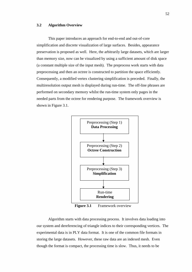
52
3.2 Algorithm Overview
This paper introduces an approach for end-to-end and out-of-core
simplification and discrete visualization of large surfaces. Besides, appearance
preservation is proposed as well. Here, the arbitrarily large datasets, which are larger
than memory size, now can be visualized by using a sufficient amount of disk space
(a constant multiple size of the input mesh). The preprocess work starts with data
preprocessing and then an octree is constructed to partition the space efficiently.
Consequently, a modified vertex clustering simplification is preceded. Finally, the
multiresolution output mesh is displayed during run-time. The off-line phrases are
performed on secondary memory whilst the run-time system only pages in the
needed parts from the octree for rendering purpose. The framework overview is
shown in Figure 3.1.
Figure 3.1 Framework overview
Algorithm starts with data processing process. It involves data loading into
our system and dereferencing of triangle indices to their corresponding vertices. The
experimental data is in PLY data format. It is one of the common file formats in
storing the large datasets. However, these raw data are an indexed mesh. Even
though the format is compact, the processing time is slow. Thus, it needs to be
Preprocessing (Step 2) Octree Construction
Preprocessing (Step 3) Simplification
Run-time Rendering
Preprocessing (Step 1) Data Processing

53
further processed before proceeding to simplification process. Hence, by using data
dereferencing, a list of triangle is pointed to its vertices so that a triangle soup mesh
is generated.
Secondly, an octree is constructed to divide the loaded data into spatial space.
The purpose is to make sure the data become easier and neater. By using it, the
simplification and data extraction processes become simpler. Most important is it
can accelerate the data query during rendering process later on. The triangular mesh
is subdivided into its appropriate location. Because of the datasets size is too large to
the available main memory size on commodity computer; hence the data in each
octree node is kept in its end node file. The end node files size is small enough to fit
in main memory and are stored in an organized directory format. Thus, the file
searching is easier to be performed.
At this stage, the end node files can be simplified independently. This step is
taken by modifying the existing vertex clustering technique from Rossignac and
Borrel (1993). As the mesh is already partitioned in previous stage, this input mesh
does not need any further space partitioning. If simplification is done separately in
every node, cracks and holes may be produced. In order to make sure that the whole
input mesh looks good after joining back all of the node’s simplified mesh, this
portion of mesh should retain its boundary edges. Meanwhile, all the vertices inside
the mesh are collapsed to an optimal vertex.
Inspired by OOCS algorithm (Lindstrom, 2000b), optimal vertex for the
discarded vertices can be found by using single error metrics. In this case, the
generalized quadric error metrics (Garland and Heckbert, 1998) is used to find the
optimal representation vertex so that the normal, color or texture attributes of the
geometry can be retained as well. This vertex clustering alike simplification operator
introduces non-manifold vertices and edges. However, the quality is good enough
and suitable for real-time application. Between, it is simple, robust and fast
compared to other simplification operators. The nature of traversing the mesh once
is practically inducing good I/O complexity. The output of this stage is a set of files
with multiple resolutions for each node.

54
As the simplified meshes are pre-computed, hence, the framework is referred
as discrete level of detail framework. This framework is chosen as it is fast, better
suited for current hardware and imposes less computational time during run-time
than dynamic LODs do. During the run-time phrase, the data for visible nodes are
extracted from octree. Each of them is considered as active nodes and the triangle
information is loaded into a dynamic data structure. The active nodes are expanded
and collapsed based on viewing perception criteria.
3.3 Data Processing
PLY data file has header and follow by its vertex list, finally its face list. The
file header starts with PLY and end with END_HEADER. Following is the general
PLY file’s header structure:
ply
format ascii 1.0
comment …
element vertex num_of_vertices
property float32 x
property float32 y
property float32 z
element face num_of_faces
property list uint8 int32 vertex_index
end_header
Subsequently, a vertex list, which total up has num_of_vertices of vertices
and a triangle list, which total up has num_of_faces of triangles are listed. It is in
indexed format. The details of the file format are enclosed in Section 3.3.1. Even
this format is extremely space efficient. Nevertheless, it slows down the processing
time. Therefore, this indexed triangle list have to be converted to triangle soup style
even though it needs bigger storage space.

55
After reading in the PLY file portion by portion, the header of the PLY file is
discarded as the other information is no need any longer. Only the number of
vertices and number of triangles are retained. Besides, the datasets type is also
recorded. Subsequently, two files are created, one storing the vertex values and
another one storing the indexed indices for triangles.
To make the indexed mesh become a triangle soup mesh, external sorting is
essential. External sorting is mandatory because the massive datasets cannot directly
be loaded into main memory due to resource limitations. External sorting loads the
portion of data, which fit into main memory, then sorts it and lastly output it to a file
again. Here, merge sort is used for this purpose. Sorting the triangle indices
involves the quicksort technique due of its advantage in sorting speed compared to
other sorting algorithms. As mentioned, the data is read part by part. Therefore,
merging is required to unite each sorted portions of data. The merging scheme used
in this project is the two-way-merge sort.
By using the merge sort technique, firstly, sort the first indices of all the
triangles. Then, each index is read sequentially. At the same time, the vertex values
are read in sequentially as well. Now, dereference each triangle index to its
corresponding vertex value. Because of the data is sorted in sequence, hence the
dereferencing process is generally faster. Repeat these steps until all of the triangle’s
first indices are dereferenced.
Taking account of each face is in triangle shape, each triangle has three
vertices. Thus, the merge sort and dereferencing processes are considered necessary
to run three times in order to create a complete triangle soup mesh.
3.3.1 Data File Structure
PLY file is a simple and easy file format to store graphical objects, which are
represented by a set of polygons. It is a common data format in scanning technology.
Only one object is described in a PLY file. It is a collection of vertices, faces and

56
other elements such as color, surface normal, texture coordinates and so on. It is
either an ASCII representation or binary version for compact storage and fast I/O
processing. The PLY format is not intended to be a general scene description
language, a shading language or a catch-all modeling format. Hence, it has no
transformation matrices, object instantiation, modeling hierarchy or object sub-parts.
Figure 3.2 Main structure of PLY file
As mentioned before, PLY file (Figure 3.2) has a header, follow by a vertex
list next, then a face list. It may has other elements that declared by users. One can
ignore the unwanted information and only remain the needed data. The header
includes the description of every element type, including the element’s name, how
many of such elements are in the object and a list of various properties associated
with the element. The header also tells whether the file is ASCII format or binary
format and some comments maybe. Figure 3.3 is a PLY file example.
From Figure 3.3, it illustrates the element is in this structure:
element <element_name> <number_in_file>
property <data_type> <property_name1>
property <data_type> <property_name1>
…………….…
The property is listed in sequential order after its element. The property may have
scalar, list and also list type. The above format is scalar type. The list type is
structured as:
property list <numerical_type> <numerical_type> <property_name>
Header Vertex List Face List (List of other elements)
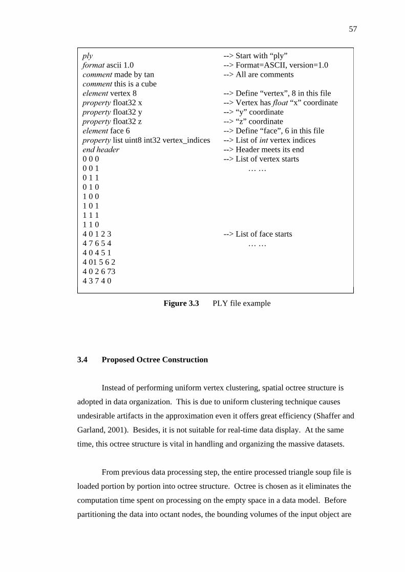
57
Figure 3.3 PLY file example
3.4 Proposed Octree Construction
Instead of performing uniform vertex clustering, spatial octree structure is
adopted in data organization. This is due to uniform clustering technique causes
undesirable artifacts in the approximation even it offers great efficiency (Shaffer and
Garland, 2001). Besides, it is not suitable for real-time data display. At the same
time, this octree structure is vital in handling and organizing the massive datasets.
From previous data processing step, the entire processed triangle soup file is
loaded portion by portion into octree structure. Octree is chosen as it eliminates the
computation time spent on processing on the empty space in a data model. Before
partitioning the data into octant nodes, the bounding volumes of the input object are
ply format ascii 1.0 comment made by tan comment this is a cube element vertex 8 property float32 x property float32 y property float32 z element face 6 property list uint8 int32 vertex_indices end header 0 0 0 0 0 1 0 1 1 0 1 0 1 0 0 1 0 1 1 1 1 1 1 0 4 0 1 2 3 4 7 6 5 4 4 0 4 5 1 4 01 5 6 2 4 0 2 6 73 4 3 7 4 0
--> Start with “ply” --> Format=ASCII, version=1.0 --> All are comments --> Define “vertex”, 8 in this file --> Vertex has float “x” coordinate --> “y” coordinate --> “z” coordinate --> Define “face”, 6 in this file --> List of int vertex indices --> Header meets its end --> List of vertex starts … … --> List of face starts … …

58
essential for efficiency. The information includes the width and center point of the
bounding box that covers the whole mesh.
At each time, the space is divided into eight cubes recursively until the tree is
fully subdivided. It partitions the input mesh adaptively. This is because it only
breaks down the node into children nodes when the node has more triangles than it is
allowed to. Each internal node stores their directory path, so that every node’s file
searching becomes easier. The leaf nodes only need to hold the filename, which is
storing the partitioned triangle list.
Since the datasets could not fit into main memory, the vertices in each leaf
node are written into every end node file. The file is small and is kept in an
organized directory structure. Each child node is contained in their parents’ node
directory (previous parents’ directory). Hence, the tracking of every end node file is
simpler and organized better.
Different with others (Correa, 2003), this octree structure does not create any
triangle replication. Whenever the triangle has existed in previous visited nodes,
then the triangle would not be stored in any other node. This cause the boundary
triangle is kept only once. One may question that it may create artifacts during
rendering later. The artifacts occur whenever triangles inside a visible node does not
be kept if it is already kept in its neighbour node. However, this artifact is rarely
happened based on experiments.
By using the constructed octree as our spatial data structure, it makes
simplification easier and perceptual rendering faster in general. It contains the whole
world information. Every sub mesh in each leaf node is small and stored in its end
node file, thus making the simplification can be performed easily. However, the
octree need to be revised during simplification process if more than one level of
detail is demanded.
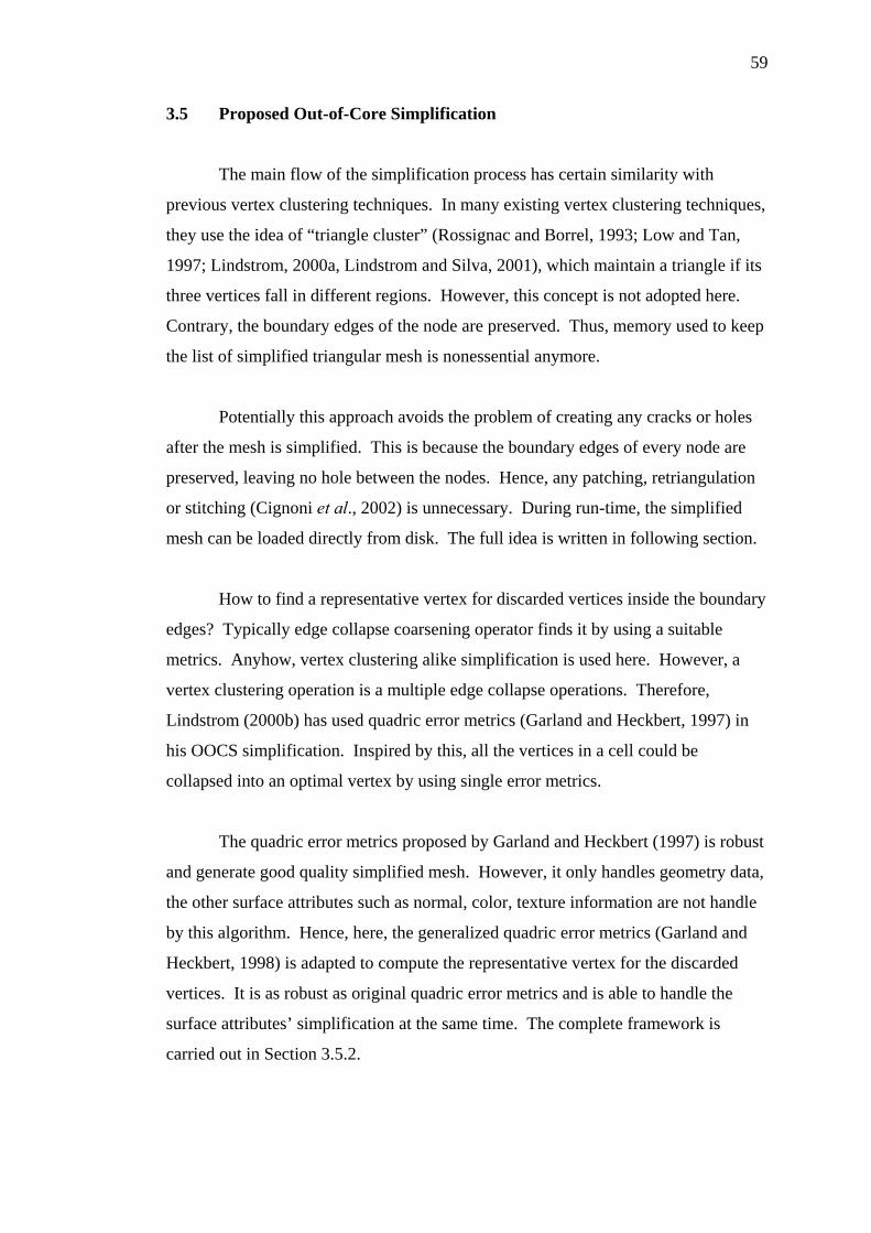
59
3.5 Proposed Out-of-Core Simplification
The main flow of the simplification process has certain similarity with
previous vertex clustering techniques. In many existing vertex clustering techniques,
they use the idea of “triangle cluster” (Rossignac and Borrel, 1993; Low and Tan,
1997; Lindstrom, 2000a, Lindstrom and Silva, 2001), which maintain a triangle if its
three vertices fall in different regions. However, this concept is not adopted here.
Contrary, the boundary edges of the node are preserved. Thus, memory used to keep
the list of simplified triangular mesh is nonessential anymore.
Potentially this approach avoids the problem of creating any cracks or holes
after the mesh is simplified. This is because the boundary edges of every node are
preserved, leaving no hole between the nodes. Hence, any patching, retriangulation
or stitching (Cignoni et al., 2002) is unnecessary. During run-time, the simplified
mesh can be loaded directly from disk. The full idea is written in following section.
How to find a representative vertex for discarded vertices inside the boundary
edges? Typically edge collapse coarsening operator finds it by using a suitable
metrics. Anyhow, vertex clustering alike simplification is used here. However, a
vertex clustering operation is a multiple edge collapse operations. Therefore,
Lindstrom (2000b) has used quadric error metrics (Garland and Heckbert, 1997) in
his OOCS simplification. Inspired by this, all the vertices in a cell could be
collapsed into an optimal vertex by using single error metrics.
The quadric error metrics proposed by Garland and Heckbert (1997) is robust
and generate good quality simplified mesh. However, it only handles geometry data,
the other surface attributes such as normal, color, texture information are not handle
by this algorithm. Hence, here, the generalized quadric error metrics (Garland and
Heckbert, 1998) is adapted to compute the representative vertex for the discarded
vertices. It is as robust as original quadric error metrics and is able to handle the
surface attributes’ simplification at the same time. The complete framework is
carried out in Section 3.5.2.

60
As the data is completely partitioned, therefore every single end node’s
triangle data is ready to be simplified. The process is totally independent as
simplification can take place without knowing its neighbours’ information. By
repeating the simplification on every leaf node, it generates first level of
simplification on the original input mesh. Every simplified triangular mesh is stored
on disk separately. This level of detail is the finest mesh among the simplified mesh.
To obtain coarser resolutions of the mesh, further simplification on internal nodes
(Section 3.5.3) is required.
3.5.1 New Vertex Clustering
Vertex clustering can also be called spatial clustering as it partitions the space
that the surface is embedded into simple convex 3D regions. Because triangular
mesh is always represented in Cartesian coordinate system, the easiest way is to do
rectilinear space partitioning or partition the space using spatial data structure such as
BSP, octree, kd-tree and etc. In this project, the space is partitioned adaptively using
octree because it suits the mesh’s condition better. In every leaf node, the new
approach on vertex clustering technique is applied to simplify the mesh. It does not
need any neighbour nodes’ information or any mesh stitching.
This new variation of vertex clustering technique is a fully independent
simplification process. It is claimed an independent process because it does not need
to know the triangles that fall into three different regions like other vertex clustering
methods do. Instead, it preserves the triangles, which has the boundary edges for
every node (Figure 3.4). Triangles that stay in internal area of the node are thrown
away. The discarded vertices are represented by a new generated optimal vertex
using the generalized quadric error metrics (Garland and Heckbert, 1998).
To find the boundary edges, every triangle in the node have to be tested its
edges. Every triangle has three edges. Every edge is considered as boundary edge at
starting and is stored as boundary edges. Whenever the triangle’s edge is found exist
in the boundary edges list, thus the edge is considered no more a boundary edge.

61
Else, the edge is set as boundary edge. The process keep repeated until every edge is
checked. Finally, a list of boundary edges is produced. At the same time, the
representative vertex is calculated. Hence, the non-degenerate triangles are produced,
which every triangle consists of two vertices of a boundary edge and the
representative vertex.
Figure 3.4 New vertex clustering
There’s maybe occurrence that the substitute vertex is lie far outside from the
node. The situation happens when a cell contains two nearly parallel surface sheets.
Hence, the quadric may suggest a solution that is close to the intersection of both
planes. Thus, the substitute vertex has to be clamped back to its cell. Here, the
proposed vertex clustering technique pulls the optimal vertex to the center of the cell
when it is lying too far away from cell.
3.5.2 Generalized Quadric Error Metrics
This generalized quadric (Garland and Heckbert, 1998) is improved from the
original quadric error metrics (Garland and Heckbert, 1997). The original quadric
error metrics only handles geometry primitives (vertex position) in mesh
simplification. Although it is extended from previous quadric error metric, it cannot
be generated solely by using the normal of the plane for a triangle. Instead, it needs
two orthonormal unit vectors e1 and e2 to compute the error metrics. The unit vectors
are shown in Figure 3.5.
Before After
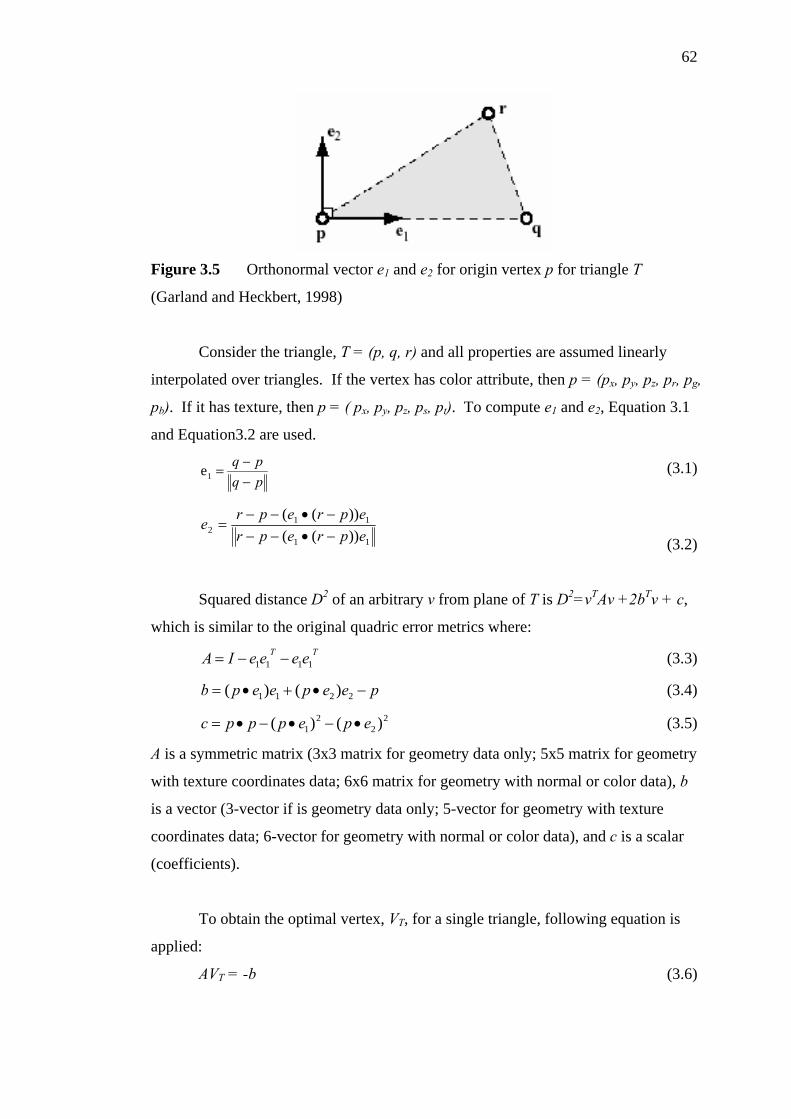
62
Figure 3.5 Orthonormal vector e1 and e2 for origin vertex p for triangle T
(Garland and Heckbert, 1998)
Consider the triangle, T = (p, q, r) and all properties are assumed linearly
interpolated over triangles. If the vertex has color attribute, then p = (px, py, pz, pr, pg,
pb). If it has texture, then p = ( px, py, pz, ps, pt). To compute e1 and e2, Equation 3.1
and Equation3.2 are used.
pqpq
−−
=1e (3.1)
11
112 ))((
))((eprepreprepre
−•−−−•−−
= (3.2)
Squared distance D2 of an arbitrary v from plane of T is D2=vTAv +2bTv + c,
which is similar to the original quadric error metrics where: TT eeeeIA 1111 −−= (3.3)
peepeepb −•+•= 2211 )()( (3.4) 2
22
1 )()( epepppc •−•−•= (3.5)
A is a symmetric matrix (3x3 matrix for geometry data only; 5x5 matrix for geometry
with texture coordinates data; 6x6 matrix for geometry with normal or color data), b
is a vector (3-vector if is geometry data only; 5-vector for geometry with texture
coordinates data; 6-vector for geometry with normal or color data), and c is a scalar
(coefficients).
To obtain the optimal vertex, VT, for a single triangle, following equation is
applied:
AVT = -b (3.6)

63
By solving Equation 3.6, the optimal vertex with its simplified surface attributes for a
triangle is computed. To simplify different types of mesh, refer Table 3.1 for each
dimension it uses.
Table 3.1 Space Requirement (Garland and Heckbert, 1998)
Model type Vertex A Unique coefficients
Geometry only [x y z]T 3x3 10
Geometry + 2D texture [x y z s t]T 5x5 21
Geometry + color [x y z r g b]T 6x6 28
Geometry + normal [x y z a b c]T 6x6 28
In order to get the optimal vertex for a cluster of triangles, VN , add up all
matrices A of every triangle and add up all vectors b of every triangle. For now, the
solution formula becomes as Equation 3.7.
∑AVN = - ∑b (3.7)
Solving this equation gives the representative vertex for all of the collapsed triangles
in a single cell.
3.5.3 Simplification on Internal Nodes
First level of detail is generated on all leaf nodes. This is the finest simplified
mesh. To get a coarser mesh, further simplification is essential to be performed on
internal nodes. The process starts from root node.
Starting from the root node, its children nodes is kept checking on. The data
in internal node is simplified whenever all of its children nodes are simplified in
previous level. The simplification is again using the new vertex clustering technique
(Section 3.5.1) and also the generalized quadric error metrics (Section 3.5.2) to
obtain the substitute vertex. Thus, after the simplification done on all of the children
nodes for the current node, set the node as it already been simplified. The output
64
triangle list is written into the current node’s directory. The searching is stopped.
Else, don’t simplify it and the searching continues recursively.
The octree is traversed every time generating a new coarser mesh. The
process is repeating until a desired number of simplified meshes are generated. As
an alternative, the simplification will stop whenever the first level children nodes of
the root node are simplified before.
3.6 Run Time Rendering
The rendering is based on the visibility criterion. During rendering, the
boundaries of a node to the view-frustum planes are tested. If it is visible, expands
the node, else, collapse it. If a node is visible, then compare the threshold based on
distance aspect. If the object is far off the viewpoint, use less resolution mesh.
Otherwise, the higher resolution mesh is loaded.
This process is performing the on-demand paging on the external data. The
visible nodes in frustum are loaded initially. That is, load in the data from files,
which generated in octree and simplification processes previously. It frees up more
main memory by avoiding unnecessary data storage. From frame to frame, new
visible nodes are loaded as necessary. At the same time, the loaded nodes but
invisible for quite a time is thrown away from memory.
As commonly known, creation of a few resolution of mesh during the
preprocess phrase is a discrete level of detail framework. Consequently, it may
produce undesired popping artifacts. In order to resolve this trouble, adequate
number of simplified mesh is generated. Thus, when the changes between the levels
of detail switching are less, subsequently the popping problem could be minimized.

65
3.7 Summary
The initial framework has been proposed to carry out the out-of-core large
mesh simplification with surface attributes preserved on commodity personal
computer. This method is some sort of hybrid method and a new variation on
previous simplification method to solve the stated issues. The implementation is
explained in next chapter.
CHAPTER 4
IMPLEMENTATION
4.1 Introduction
The methodology has been revealed in previous chapter. Consequently, the
details of the pseudo code and step-by-step algorithm are discussed here. As a brief
review, this system involves two main processes, which are preprocessing phrase and
run-time phrase. Preprocessing phrase performs data processing, octree construction
and mesh simplification. Whilst run-time phrase executes the real-time rendering on
simplified mesh based on the viewing criteria.
During data processing, input datasets are loaded in portion by portion. Then,
external sorting and dereferencing process is carried on. In simplification process,
new variation of vertex clustering algorithm is used to simplify the input mesh and a
hierarchy of mesh is generated. Meanwhile, a generalized quadric error metric is
used to calculate the representative vertex. This metric preserves the vertex position,
normal, color and texture information after the simplification process. Then, the data
is visualized subsequently.

67
4.2 Data Processing
4.2.1 Input Data Reading
The input file, PLY has header and list of the declared elements. It can store
any polygonal information, for example storing the vertex, edge and also face list.
At the same times, it can keep a lot of information such as vertex coordinates,
normals, range data confidence and other different properties. Besides, the
polygonal faces may in triangular shape, tetrahedral shape or rectangle shape.
However, for this project, only triangular and appropriate data information is
remained after the file reading. Unused data is neglected.
In this approach, the header information is not kept except the element
information. The preserved elements are the “vertex” and “face” elements only. For
the properties, the vertex coordinates (x, y, z), surface normals, colors and texture
coordinates under the “vertex” element are retained. In no doubt, the “face” element,
which consists of the number of indices for the face and list of the vertex indices, is
preserved.
Figure 4.1 Data Structure for different type of vertex element
typedef struct Vertex { float x, y, z } Vertex; typedef struct NVertex { float x, y, z float nx, ny, nz } NVertex; typedef struct CVertex { float x, y, z; unsigned char red, green, blue } CVertex; typedef struct TVertex { float x, y, z; float u, v } TVertex;

68
After surveying on the existing PLY files, the data type for the each of the
needed elements and properties is noticed has its similarity. Figure 4.1 is the data
structure used to store the data.
To read the PLY file, the pseudo code is as below:
1. Read the PLY file header and take note of number of vertices and number of
triangles in this PLY model.
2. For every element,
a. If it is “vertex”,
i. Check the suitable data type whether it is only vertex
coordinates or it has normal, color and texture coordinates.
ii. Discard the other property (if found any).
iii. Load in the data portion by portion, the maximum records can
be loaded is depends on the allocated available main memory.
Then write the data into vertex file. Repeat until all data have
been written.
b. If it is “face”,
i. Set the data structure (as it has only one case).
ii. Discard other property (if found any).
iii. Load in the data portion by portion, the maximum records can
be loaded is depends on the allocated available main memory.
Then write the data into triangle file. Repeat until all data
have been written
c. If it is “other” element, ignore it.
3. Now the vertex file and triangle file is generated.
4.2.2 Triangle Soup Mesh Generation
Triangle soup file is mandatory to speed up the simplification and rendering
process, which performs later on. Involving algorithms are the external sorting and
data dereferencing processes. The concepts of two-way merge sort and data
69
dereferencing functions are well explained previously. At this point, the main flow
of the works is described in a pseudo code chart:
1. From previous step, two files, which are vertex file and triangle file, are
generated. Besides, the kind of data, whether it is vertex coordinates only or
has surface normal, color or texture coordinates attributes are known.
Besides, the number of vertices and number of triangle are identified. In
addition, the buffer size is set. All these information is needed in this process.
2. In three passes (every triangle has three vertices),
a. Calculate triangle’s dimension and the index that will be sorted. First
pass is the first index for every triangle, and so on.
b. Externally sorts the current sorting indices.
c. Dereference its corresponding vertex.
3. The triangle soup file is successfully generated.
4.2.2.1 Calculation of Triangle’s Dimension and Sorting Index
By considering the data type for each triangle, the current record’s dimension
and sorting index for every pass in external sorting process can be determined. The
following chart illustrates how to calculate it in three passes (Figure 4.2). The
example is a data type, which only has vertex coordinates information. In first pass,
the first index of a triangle is the sorting index (box in gray). Of course, the record’s
dimension is three as every triangle has three vertices. Now, the vertex is
dereferenced into from the vertex list. Hence, first triangle’s index is replaced by
three corresponding vertex values, (x1, y1, z1). The process is repeated for all of the
first indices in the triangle list. In this calculation, the sorting index starts from zero,
but not one. For every data type, the record’s dimension and sorting index is listed in
Table 4.1.
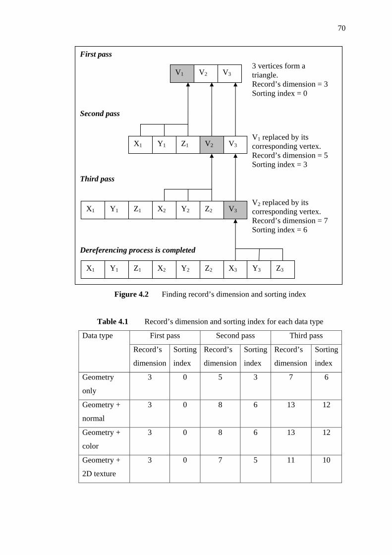
70
Figure 4.2 Finding record’s dimension and sorting index
Table 4.1 Record’s dimension and sorting index for each data type
First pass Second pass Third pass Data type
Record’s
dimension
Sorting
index
Record’s
dimension
Sorting
index
Record’s
dimension
Sorting
index
Geometry
only
3 0 5 3 7 6
Geometry +
normal
3 0 8 6 13 12
Geometry +
color
3 0 8 6 13 12
Geometry +
2D texture
3 0 7 5 11 10
V1 V2 V3
First pass 3 vertices form a triangle. Record’s dimension = 3 Sorting index = 0
X1 Y1 Z1 V2
V3
Second pass
V1 replaced by its corresponding vertex. Record’s dimension = 5 Sorting index = 3
X1 Y1 Z1 X2 Y2 Z2
V3
Third pass
V2 replaced by its corresponding vertex. Record’s dimension = 7 Sorting index = 6
Y1 Z1 X2 Y2 Z2 X1 X3 Y3 Z3
Dereferencing process is completed
71
4.2.2.2 External Sorting on Sorting Indices
The sorting process is needed before the indexed indices are dereferenced. It
is to speed up the data referring. Else, it may affect the I/O operation slower as the
random access is a must avoided operation. By applying the sorting algorithm, the
I/O operation can be done in sequence. Because the data is larger than memory size,
merge sort is used to sort these massive data. Quicksort and two-way merge sort
algorithms are applied here. The flow of the process is described as below:
1. Calculate the number of times the data loading must be performed.
number_of_times = Dataset’s size / available memory size
// start performing sorting action
2. Load the portion of data, which is smaller than the available buffer size.
3. Perform quicksort() on the loaded data.
4. Output to a temporary output file.
5. Repeat step 2 – 4 for number_of_times.
// start performing merging action
6. If the number_of_generated_files = 1, rename the file as output file.
7. Else if the number_of_generated_files = 2, merge the two files as output file.
8. Else (number_of_generated_files > 2),
a. Divide the number_of_generated_files by 2, merge the pair of files
b. If left a, odd file, rename it.
c. Remove the unused files.
d. Now, get the new number_of_generated_files.
e. Repeats this step (step 8) until all files is merged.
9. The large data is well sorted in its current sorting index and merged into a
single file.

72
4.2.2.3 Dereferencing on Sorting Indices
The sorted file and the vertex file are the input for dereferencing process.
The following flowchart in Figure 4.3 shows its algorithm flow.
Figure 4.3 Dereferencing process
Begin
Vertex data type, sort index and max_record is known
Read a vertex, vert_id=0
Read a triangle, tri_id=0
Read triangle success?
Write the remaining triangle data to file
End tri_id= vert_id?
Read next triangle, vert_id++
Dereference the vertex and save it into buffer tri_id++
tri_id = max_record?
Write the data in buffer to output file tri_id=0
Yes
No
Yes
No
Yes
No

73
4.3 Octree Construction
The fundamental concept of octree is to partition the space into eight smaller
cube recursively to become an easier handled data structure. Initially, the width and
center point of the cube, which coats the whole object, must be found. Later on, the
octree is built by recursively subdivide the cube. The node is subdivided into eight
directions (Figure 4.4). The data members and its constraint parameters in octree
class are given away in Figure 4.5.
Figure 4.4 Sub nodes in an octree node
Figure 4.5 Data member and parameters in COctree class
Top_Left_Back Top_Right_Back
Top_Left_Front Top_Right_Front
Bottom_Right_Back Bottom_Left_Back
Bottom_Left_Front Bottom_Right_Front
// node’s information float width; float center; bool is_subdivided; int tri_count; // node’s data location char* nodeDirectory; char* endNodeFilename; COctree* octreeNodes[8]; // node’s simplification information bool * is_simplified; char* simpFilename; int simp_tri_count;
int max_tri int max_subdivision;
Octree class member Octree’s controller parameters

74
The works is simplified in following pseudo code:
1. Calculate width and center point for boundary cube, GetDimension().
a. Center vertex, center = (total up of all the vertices’ values) / total
number of vertices
b. Width, width is obtained by:
i. Compute the width of x, y and z direction by subtracting the
current width with center point.
ii. Multiply the width by two (full width).
iii. Compare the width in x, y and z direction. Take the greatest
value as the cube width.
2. Octree generation, CreateLargeNode()
a. If the current_num_tri > max_tri and current_subdivision <
max_subdivision
i. Set directory path, nodeDirectory.
ii. Create eight temporary files to store triangle values for every
child node.
iii. Set the subdivision status, is_subdivided = true;
iv. Load the data portion by portion which can be fit in main
memory
v. For each loaded triangle, find its location in current octree
node.
vi. Write the data into the node’s file based on their location.
vii. Repeat step (iv) to (vi) until all triangles are entirely divided.
viii. After the mesh is fully subdivided, create eight new octree
children nodes (CreateNewLargeNode()).
b. Else, just rename the input file as end node file.
3. Discard all existing non-end node files. Keeping only the end node files on
disk.
To create the new octree nodes (CreateNewLargeNode()) in previous Step 2
(viii), it is described as below:
1. Create a new child node by naming it octreeNodes[node position].
2. Set node directory path, nodeDirectory.
3. Compute new center node and new width, ComputeNewDimension().
75
4. Call the function CreateLargeNode() in Step 2 (Octree Generation) to
generate an octree.
To create the new center and new width in previous Step 3
(ComputeNewDimension()) in creating the new octree nodes, it is describe as
following:
1. Using the parents’ center vertex, center and parents’ width, width, the new
center point for the child node is obtained.
a. If Top_Left_Front, new_center.x = center.x –width/4
new_center.y = center.y + width/4
new_center.z = center.z + width/4
b. Else if Top_Left_Back, new_center.x = center.x – width/4
new_center.y = center.y + width/4
new_center.z = center.z - width/4
c. Else if Top_Right_Back, new_center.x=center.x + width/4
new_center.y = center.y + width/4
new_center.z = center.z - width/4
d. Else if Top_Right_Front, new_center.x=center.x + width/4
new_center.y = center.y + width/4
new_center.z = center.z + width/4
e. Else if Bottom_Left_Front, new_center.x=center.x - width/4
new_center.y = center.y - width/4
new_center.z = center.z + width/4
f. Else if Bottom_Left_Back, new_center.x=center.x - width/4
new_center.y = center.y - width/4
new_center.z = center.z - width/4
g. Else if Bottom_Right_Back, new_center.x=center.x +- width/4
new_center.y = center.y - width/4
new_center.z = center.z - width/4
h. Else if Bottom_Right_Front, new_center.x=center.x + width/4
new_center.y = center.y - width/4
new_center.z = center.z + width/4
2. New width for the child node, new_width = width/2

76
4.4 Out-of-Core Simplification
4.4.1 Simplification on Leaf Nodes
As the data was completely subdivided, therefore every single end node’s
triangle data is now ready to be simplified independently. The steps are as below:
1. Load in the data.
2. For each input triangle,
a. Calculate triangle’s quadric, QT and add it into node’s quadric, QN.
b. For each edge,
i. If it is not stored in edge list, add it into edge list and initially
set its status as a boundary edge.
ii. Else, set the edge’s status as a non-boundary edge.
3. For each edge in the edge list,
a. If its status is a boundary edge, save it into boundary edge list.
4. Calculate node’s optimal vertex, VN using node’s quadric, QN.
a. If VN is lie too far from node, set its value the center of node.
5. For each input triangle,
a. Check every boundary edge. If the edge is a boundary edge, add it
into output triangle list and set this boundary edge not a boundary
edge anymore. The triangle is consisted of two vertices from the
boundary edge and the calculated optimal vertex.
6. Write the output triangle list into a file, which named using the node’s
directory path with its level of detail indication number.
This simplification is performed on all of the leaf nodes. Therefore, first
level of detail in octree subdivided mesh is generated.
4.4.2 Simplification on Internal Nodes
After obtaining the first LOD (level-0), higher level of detail (level>0) is
produced by repeating the pseudo code until desired level of detail is achieved. The

77
simplification for every level of detail starts by examining the root node. The
process is encapsulated as below:
1. Initially set the is_simplified[level] status as true and examining all children
nodes of the current node.
a. If all children nodes’ is_simplified [level-1] true, get the data from all
of the children nodes.
b. Else, set node’s is_simplified [level] status false and stop checking on
other children nodes.
2. Check for is_simplified [level] status,
a. If is_simplified [level] is true, simplify the data obtained previously
using the explained simplification algorithm (Section 4.4.1), then save
it to file named level.LOD in node’s directory.
b. Else continue check on the children nodes.
4.5 Run-Time Rendering
For each frame, only the nodes inside view frustum are being rendered. First
of all, the projection matrix and model matrix are extracted from current graphics
world. Hence, the clipping planes can be created. During rendering process, every
bounding cube, which bound every octree node, is then checked its eight points at the
corner. If the point is in frustum, load the node’s triangle list into our system.
After the previous simplification has been carried out, the mesh is simplified
into a few versions. Though, there are multiresolution meshes are available for the
graphics rendering. To decide which resolution of the mesh to be loaded, the
distance of the object to viewing point is the key in making decision on it. Whenever
the object is near to view point, extract the higher resolution node mesh. Else, use
the less resolution mesh for rendering.
After determining whether a node is inside or outside the frustum and also the
node’s level of detail, afterward the triangles inside the node is extracted from its
directory. If the normal, color or texture coordinates is provided, then this attribute is
78
loaded with its geometric information. By using the OpenGL functions, these
triangles can be drawn subsequently.
To reduce disk access and speed up the rendering, the triangles for visible
nodes are kept in main memory after loading. Hence, the same data no need be
obtained from disk every frame if it is inside frustum for several continuous frames.
Whenever the loaded data is no longer falls in the frustum for a period of time, then
the data is obsolete and thrown from main memory to make the space available for
other visible nodes.
4.6 Summary
As this methodology have to deal with variety of massive datasets, hence the
implementation is very critical in memory management. The memory allocation has
to be handled with cares and has to be released from time to time. It is critical to
avoid memory leaking problem. Anyhow, the framework has been successfully
implemented to overcome the stated problems. In next chapter, the efficiency and
robustness of the framework is evaluated. Hence, the results is analyzed and
discussed in following chapter.
CHAPTER 5
RESULTS AND DISCUSSIONS
5.1 Introduction
To evaluate the proposed methodology in large data simplification with
surface preservation, the Buddha model, which is larger than mostly all low cost
computer’s main memory is analyzed and discussed in following experiments.
Buddha model has 1, 087, 716 triangles. This out-of-core simplification is run on
one CPU of a 2.4GHz Pentium IV with 512MB of RAM and NVIDIA GeForce FX
5200 graphics card.
At one time, the maximum main memory assigned for data storage and
processing for the experiments is restricted to 12MB of RAM only. It is to making
sure almost all of the low cost personal computers nowadays can perform this system
without any memory shortage and memory leaking problems. Besides, it is designed
so that main memory can be allocated in rendering or any other process.
First is the analysis on octree’s performance based on the octree’s depth and
leaf node’s size. Secondly, out-of-core simplification is evaluated carefully. To
compare the algorithm with other out-of-core simplification techniques, out-of-core
simplification (OOCS) by Lindstrom (2000b) is preferred. Meanwhile, the accuracy
of simplified mesh is measured by using Metro tool like other algorithms always do.
The quality and speed of this simplification method are revealed in numerical tables.
Besides, the qualities of simplified models are visually shown in images.
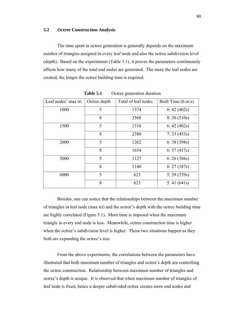
80
5.2 Octree Construction Analysis
The time spent in octree generation is generally depends on the maximum
number of triangles assigned in every leaf node and also the octree subdivision level
(depth). Based on the experiments (Table 5.1), it proves the parameters continuously
affects how many of the total end nodes are generated. The more the leaf nodes are
created, the longer the octree building time is required.
Table 5.1 Octree generation duration
Leaf nodes’ max tri Octree depth Total of leaf nodes Built Time (h:m:s)
5 1374 6: 42 (402s) 1000
8 3568 8: 30 (510s)
5 1316 6: 42 (402s) 1500
8 2380 7: 33 (453s)
5 1262 6: 38 (398s) 2000
8 1654 6: 57 (417s)
5 1127 6: 26 (386s) 3000
8 1140 6: 27 (387s)
5 623 5: 39 (339s) 6000
8 623 5: 41 (641s)
Besides, one can notice that the relationships between the maximum number
of triangles in leaf node (max tri) and the octree’s depth with the octree building time
are highly correlated (Figure 5.1). More time is imposed when the maximum
triangle in every end node is less. Meanwhile, octree construction time is higher
when the octree’s subdivision level is higher. These two situations happen as they
both are expanding the octree’s size.
From the above experiments, the correlations between the parameters have
illustrated that both maximum number of triangles and octree’s depth are controlling
the octree construction. Relationship between maximum number of triangles and
octree’s depth is unique. It is observed that when maximum number of triangles of
leaf node is fixed, hence a deeper subdivided octree creates more end nodes and

81
finally enforces more octree building time (Refer Table 5.1). Similarly, when
octree’s depth is fixed, then the smaller node assignation will create a bigger tree. In
Table 1, octrees with 3000 and 6000 maximum number of triangles have full control
on the octree generation. This is mainly because both of them created tree that less
the 5 level of subdivision. Hence, the assigned octree’s depth has no impact on
octree generation.
Figure 5.1 Octree building time versus (a) maximum number of triangles and (b)
octree subdivision depth
The maximum number of triangles or subdivision level shouldn’t be assigned
an extremely large or extremely small figure. Whenever either the maximum
number of triangles or octree subdivision depth is set too high, then the other party
will lose its full identity in controlling an octree construction. Let’s say the octree is
only allowed to be subdivided three times at most, thus setting the maximum number
of triangles to a small number will only have a little impact to the octree and
probably produce an unbalance tree.
5.3 Out-of-Core Simplification Analysis
In simplification analysis, some experiments in a few perspectives have been
carried out. First is the analysis on the multiresolution simplified meshes, which are
generated using the proposed out-of-core vertex clustering technique. Next, the
Time
Leaf node’s max tri
Time
Octree’s depth
(a) (a)

82
simplified models are applied in a variety of distances to show its quality based on
viewing perception. Besides, this proposed simplification technique is compared
with Out-of-Core Simplification (OOCS) by Lindstrom (2000b). Lastly, the
relationship between simplification and octree construction is revealed.
5.3.1 Proposed Out-of-Core Simplification Analysis
From Figure 5.2, different resolutions of Buddha model, which simplified
using the proposed out-of-core vertex clustering technique, are given away. The
models are simplified at the first level of detail, which means each simplification is
done on leaf nodes only. The quality distortion is hardly to be perceived even after a
drastic simplification from 1, 087, 7106 triangles to 383, 619 triangles. The Buddha
model starts obviously losing its detail when the mesh is reduced to approximate 60K
polygons (Figure 5.2e).
In controlling the level of detail, the maximum number of triangles assigned
to octree’s leaf nodes plays an important role. That is, all of the triangles inside a
node will be simplified using the new variation of vertex clustering technique with
the constraint that the number of triangles it has must less than the assigned
maximum number of triangles. Like in Figure 5.2a, the maximum number of
triangles for node simplification is 200, thus creating a smoother looks simplified
Buddha as fewer polygons are simplified once. Whilst for Buddha in Figure 5.2.e, a
total of 6000 polygons are reduced to a few hundreds polygons to obtain this 60K
polygon mesh. This drastic polygon reduction certainly creates poorer quality mesh.
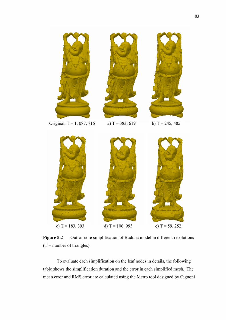
83
Figure 5.2 Out-of-core simplification of Buddha model in different resolutions
(T = number of triangles)
To evaluate each simplification on the leaf nodes in details, the following
table shows the simplification duration and the error in each simplified mesh. The
mean error and RMS error are calculated using the Metro tool designed by Cignoni
e) T = 59, 252
a) T = 383, 619 b) T = 245, 485 Original, T = 1, 087, 716
d) T = 106, 993 c) T = 183, 393
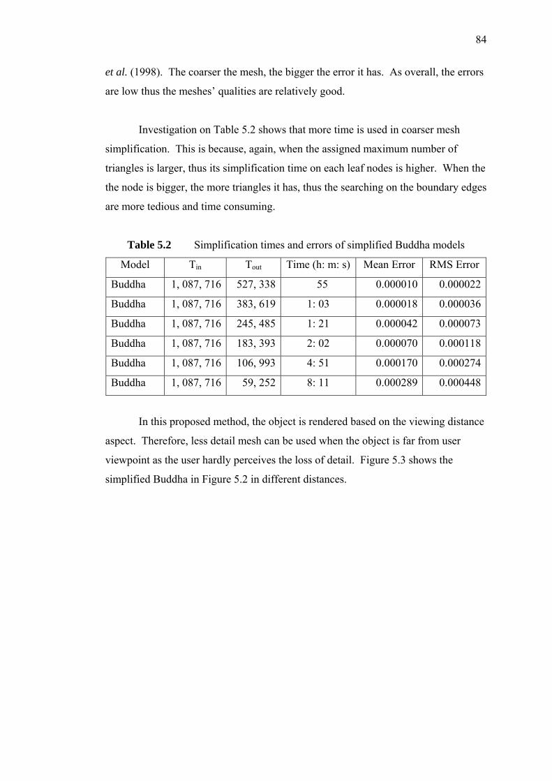
84
et al. (1998). The coarser the mesh, the bigger the error it has. As overall, the errors
are low thus the meshes’ qualities are relatively good.
Investigation on Table 5.2 shows that more time is used in coarser mesh
simplification. This is because, again, when the assigned maximum number of
triangles is larger, thus its simplification time on each leaf nodes is higher. When the
the node is bigger, the more triangles it has, thus the searching on the boundary edges
are more tedious and time consuming.
Table 5.2 Simplification times and errors of simplified Buddha models
Model Tin Tout Time (h: m: s) Mean Error RMS Error
Buddha 1, 087, 716 527, 338 55 0.000010 0.000022
Buddha 1, 087, 716 383, 619 1: 03 0.000018 0.000036
Buddha 1, 087, 716 245, 485 1: 21 0.000042 0.000073
Buddha 1, 087, 716 183, 393 2: 02 0.000070 0.000118
Buddha 1, 087, 716 106, 993 4: 51 0.000170 0.000274
Buddha 1, 087, 716 59, 252 8: 11 0.000289 0.000448
In this proposed method, the object is rendered based on the viewing distance
aspect. Therefore, less detail mesh can be used when the object is far from user
viewpoint as the user hardly perceives the loss of detail. Figure 5.3 shows the
simplified Buddha in Figure 5.2 in different distances.

85
Figure 5.3 Multiresolution of Buddha model in different distances
5.3.2 Relationships between Simplification and Octree Constructions
Our out-of-core simplification is in sequence and continuous (Figure 5.4).
This means the simplification on next level of detail is based on the previously
simplified mesh. It is much faster than simplifying the original mesh every time a
new level of detail is required as the data reading on out-of-core data is memory
inefficient. Anyway, it will produce a little less quality mesh compared to the
simplification directly referring to the original mesh.
a) 384K
b) 245K
e) 59K
c) 183K
d) 107K
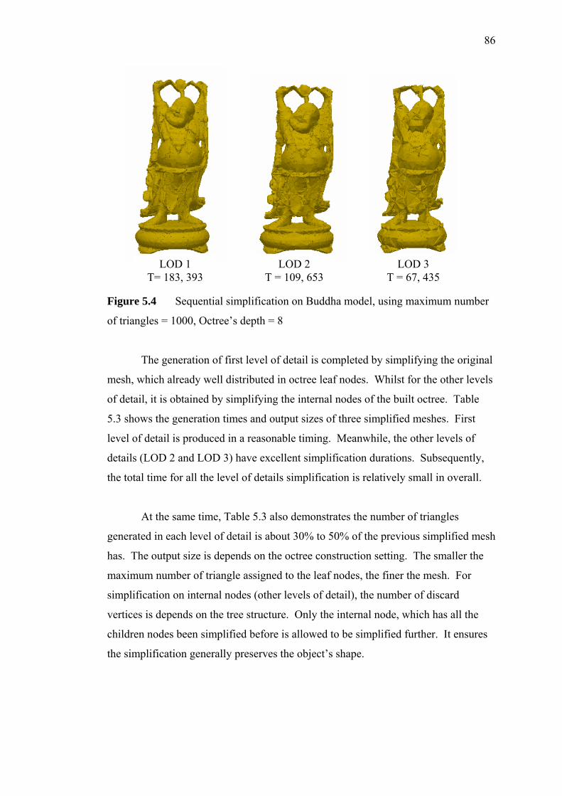
86
Figure 5.4 Sequential simplification on Buddha model, using maximum number
of triangles = 1000, Octree’s depth = 8
The generation of first level of detail is completed by simplifying the original
mesh, which already well distributed in octree leaf nodes. Whilst for the other levels
of detail, it is obtained by simplifying the internal nodes of the built octree. Table
5.3 shows the generation times and output sizes of three simplified meshes. First
level of detail is produced in a reasonable timing. Meanwhile, the other levels of
details (LOD 2 and LOD 3) have excellent simplification durations. Subsequently,
the total time for all the level of details simplification is relatively small in overall.
At the same time, Table 5.3 also demonstrates the number of triangles
generated in each level of detail is about 30% to 50% of the previous simplified mesh
has. The output size is depends on the octree construction setting. The smaller the
maximum number of triangle assigned to the leaf nodes, the finer the mesh. For
simplification on internal nodes (other levels of detail), the number of discard
vertices is depends on the tree structure. Only the internal node, which has all the
children nodes been simplified before is allowed to be simplified further. It ensures
the simplification generally preserves the object’s shape.
LOD 2 T = 109, 653
LOD 3 T = 67, 435
LOD 1 T= 183, 393
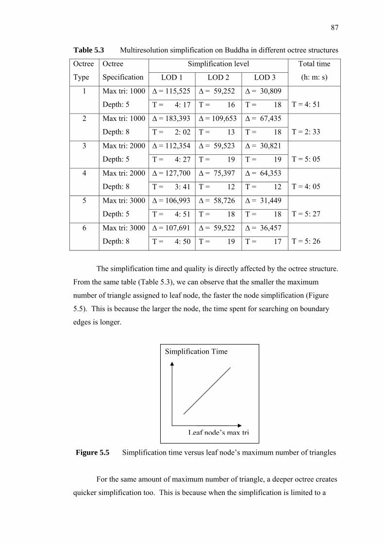
87
Table 5.3 Multiresolution simplification on Buddha in different octree structures
Simplification level Octree
Type
Octree
Specification LOD 1 LOD 2 LOD 3
Total time
(h: m: s)
∆ = 115,525 ∆ = 59,252 ∆ = 30,809 1 Max tri: 1000
Depth: 5 T = 4: 17 T = 16 T = 18
T = 4: 51
∆ = 183,393 ∆ = 109,653 ∆ = 67,435 2 Max tri: 1000
Depth: 8 T = 2: 02 T = 13 T = 18
T = 2: 33
∆ = 112,354 ∆ = 59,523 ∆ = 30,821 3 Max tri: 2000
Depth: 5 T = 4: 27 T = 19 T = 19
T = 5: 05
∆ = 127,700 ∆ = 75,397 ∆ = 64,353 4 Max tri: 2000
Depth: 8 T = 3: 41 T = 12 T = 12
T = 4: 05
∆ = 106,993 ∆ = 58,726 ∆ = 31,449 5 Max tri: 3000
Depth: 5 T = 4: 51 T = 18 T = 18
T = 5: 27
∆ = 107,691 ∆ = 59,522 ∆ = 36,457 6 Max tri: 3000
Depth: 8 T = 4: 50 T = 19 T = 17
T = 5: 26
The simplification time and quality is directly affected by the octree structure.
From the same table (Table 5.3), we can observe that the smaller the maximum
number of triangle assigned to leaf node, the faster the node simplification (Figure
5.5). This is because the larger the node, the time spent for searching on boundary
edges is longer.
Figure 5.5 Simplification time versus leaf node’s maximum number of triangles
For the same amount of maximum number of triangle, a deeper octree creates
quicker simplification too. This is because when the simplification is limited to a
Simplification Time
Leaf node’s max tri

88
certain subdivision level, some nodes will be imposed a number of triangles, which is
greater than the assigned maximum number of triangles. Based on the testing of
octree with maximum number of triangles is 200 each node, the maximum depth of
octree can reach is seven subdivision levels for the simplified mesh with 383K
triangles. Meanwhile, the simplification with assigned 1000 or 2000 maximum
number of triangles can reach maximum depth of six subdivision levels. Thus, when
the octree’s depth is limited to five levels, some nodes will be assigned a greater
number of triangles than they are supposed to have. So on, the bigger node creates
slower processing time as explained before. For simplification with assigned 3000
maximum number of triangles, its maximum depth is less than five levels. Hence,
the simplification time and output size for both depths with level five or level eight
are almost the identical.
The assignations of maximum number of triangles and octree’s depth
shouldn’t go into extreme values. Assigning an extremely small maximum number
of triangles in leaf node is discouraging. This is because very little of triangles can
be eliminated in one node simplification. In the meantime, a too large maximum
number of triangles also has disadvantage in introducing poor simplification.
Basically an extremely low octree subdivision may create poor simplification
as well. Based on the experiments, subdivision level of octree is rarely exceeding
level ten. Hence, the octree won’t expand too large. To control the simplification on
the nodes, the best way is to set the maximum subdivision level to a relatively big
number (level eight or level ten). Accordingly, the node simplification is fully
controlled by the maximum number of triangles in every leaf node.
One may question when the levels of detail generation will end? It can be set
to desired levels of detail. Anyway, octree’s depth also plays a role in controlling the
levels of detail generations. The simplification will stop when it’s approaching the
root node even the levels of detail generation haven’t finished.

89
5.3.3 Surface-Preserving Simplification Analysis
The surface preservation is including attribute preservation on normal, color
and texture attributes. Anyway, existing massive PLY data sets are not provided
these attributes. For small PLY model with color, its RGB is all set to 255, 255, 255.
Therefore, the preservation is hard to be shown. Anyway, the Generalized Quadric
Error Metric (Garland and Heckbert, 1998) had proved their robustness in surface
preservation.
Due to the memory problem, large mesh is not able to be texture mapped.
However, as a proof to attributes preservation, a simplified Buddha has been texture
mapped (spherical texture mapping) using 3D modeling software (3D Max Studio)
and then further simplified using the proposed algorithm. The simplification on
textured object is revealed in Figure 5.6. Due to the generalized quadric error metric
is assuming the mesh is continuous. Thus, we can see the discontinuous joint at the
boundary of the texture.
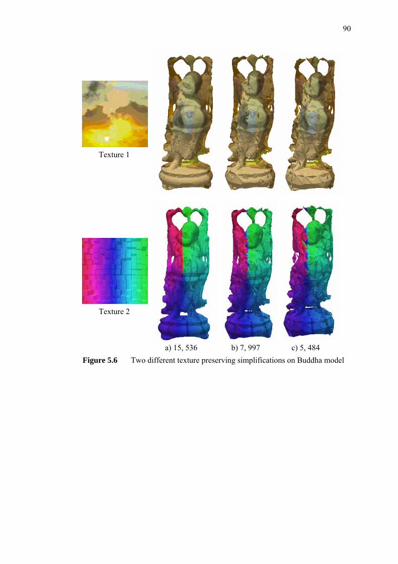
90
Figure 5.6 Two different texture preserving simplifications on Buddha model
a) 15, 536 b) 7, 997 c) 5, 484
Texture 1
Texture 2

91
5.3.4 Comparison on Out-of-Core Simplifications
Comparison is made between our algorithm and Out-of-Core Simplification
(OOCS) by Lindstrom (2000b). This is because OOCS is among the fastest
simplification method and also uses the vertex clustering operator like our
methodology. Moreover, the quality of OOCS technique is also good in general.
Following diagram (Figure 5.7) illustrates the Buddha simplified by OOCS and our
simplification algorithm. For the same amount of triangles both simplified mesh
from both algorithms, OOCS uses more space partitioning than our do. Thus, OOCS
produces slightly higher quality mesh than our do. In fact, fewer end nodes are used
in our case yet more triangles are retained in each node because of the preservation
on boundary edges.
Figure 5.7 Simplified Buddha with 90K triangles using OOCS (Lindstrom,
2000b) and the proposed method
In term of simplification time, our algorithm is faster than OOCS for a large
simplified mesh (90K triangles or more). Unfortunately, for drastic simplified mesh
with 50K or less triangles, the OOCS is much faster. OOCS is faster as the
rectilinear cells are less. While for us, collapsing a very large node is more time
OOCS Time = 7: 23
72 x 180 x 72 cellsOriginal Buddha
Proposed method Time = 6: 02
976 end nodes

92
consuming because the involving boundary edges searching is longer when the node
contains more triangles. Table 5.4 shows the processing time of OOCS.
Table 5.4 Simplification on Buddha model using OOCS (Lindstrom, 2000b)
Output Size (Tout) Cell dimension Time (h: m: s)
95340 72 x 180 x 72 7: 37
68028 57 x 150 x 57 2: 28
31564 38 x 100 x 38 57
8104 20 x 50 x 20 50
Anyhow, our simplification technique has its pros as it can overcome some
other problems. First of all, simplification on single node evades unnecessary action
in getting to know the neighbouring information. Moreover, the simplification on
well partitioned octree nodes avoids repartitioning of mesh for more than one level of
detail generations. Additionally, the simplified mesh is ready for query extraction
during run-time rendering.
A big difference between OOCS and ours is, whenever several levels of detail
are required, our simplification is faster by comparing the total time needed for few
levels of detail generation. The scenario is explained in Section 5.2.2 previously.
Moreover, OOCS can’t generate output, which its size larger than available
main memory. Opposite to it, ours can do so because we are exploiting the disk
usage in keeping the simplified mesh. Furthermore, the node simplification is
definitely can be performed without memory shortage dilemma due to the small sub
mesh is kept in every leaf node.
On the whole, the speed of our proposed method is compatible with the
others as they are at least 10 times slower than OOCS do (Comparisons based on
Chapter 2). These algorithms created extremely good fidelity mesh but extremely
time-consuming.

93
5.4 Summary
From the experiments, it is proved that proposed methodology is capable in
simplifying large datasets with surface preservation. An obvious finding is that
octree construction greatly affects the simplification process. That is, the level of
detail generation is guided by the octree structure. Letting leaf node size to control
the simplification process generally can guarantee the creation of a desired output
mesh. Besides, results showed that the octree subdivision level shouldn’t go
extremely deep to avoid extended construction time.
More experiments and brief discussion are carried out in Appendix A and
Appendix B. The same testing environment is used for the experiments in
appendices. Appendix A shows the results of Dragon model with 871, 414 triangles
whilst Appendix B shows the results of Blade model with 1, 765, 388 triangles.
CHAPTER 6
CONCLUSIONS
6.1 Summary
This project has presented a novel out-of-core simplification with small
memory allocation for computer games. In this project, the objectives of the study
are
(1) To perform out-of-core simplification in low end personal computer
(2) To preserve surface attributes in simplification process
In order to make it a success mission, the methodology starts with preprocess
and follows by run-time process.
The first objective is to process and simplify massive datasets so that it can be
visualized during run-time. To ensure the data is loadable into limited main memory,
the data is loaded part by part into main memory. Input data is converted into
triangle soup representation for memory efficiency. Then, to make the data suitable
for run time data accessing, the data is organized in an octree data structure, which is
exploiting on disk storage. Subsequently, the mesh in every octree node is simplified
independently using the proposed new vertex clustering technique. Finally, the
suitable portion of mesh is extracted and rendered based on viewing perspective.
Reviewing the results in Chapter 5, it is proved that the proposed
methodology is capable in simplifying the large data sets. The statistics show that
the proposed simplification technique generated relatively pleasant output with small
95
simplification time. Small memory footprint has been exploited, as only a few
megabytes of main memory are required. Anyhow, the simplification quality is
constrained by octree condition and its quality could be futher improved.
In the second objective, the surface attributes are important in bringing out
the beauty of an object. To do this, the generalized quadric error metrics, which
formally used in vertex pair contraction has been adjusted and applied into the
proposed vertex clustering technique. By using it, the best optimal vertex and the
surface attributes are retained after simplification process. The metrics is robust yet
easy.
As conclusion, the proposed methodology has successfully simplified and
displayed massive datasets, which preserves surface attributes, such as positions,
normals, colors and texture coordinates for graphics application. The invention on
modifying the vertex clustering coarsening operator and adopting the suitable
algorithms into this out-of-core framework has made the research goals are
accomplished. This algorithm is a practical and scalable system that allows the
inexpensive PCs to visualize datasets in computer games, which is formally an
impossible task.
6.2 Summary of Contributions
The main research contributions are:
a) New simplification operator
The simplification technique is a new variation of vertex clustering
coarsening operator. The proposed vertex clustering algorithm does not
retain the triangle that fall into three different cells, but performs the
simplification on single node by preserving its node’s boundary. As the
neighborhood of nodes is unnecessary, the node simplification is fully
independent. Besides, it has made the node simplification performable in
96
main memory as the subdivided meshes are small enough to fit in available
main memory.
b) Unique octree construction
The octree has been exploiting the file and directory system on disk in an
organized scheme. By keeping the file path of every node, the node’s mesh is
always easy to be achieved. The children nodes are always contained in their
parents’ directory. Thus, in each directory, no more than eight children
nodes’ files are saved. This ensures the file searching is faster and systematic.
The memory used to keep all the data is eliminated, thus making sure even
large data also loadable into this octree structure.
Usually in octree generation, if a triangle’s vertices fall into different nodes,
the triangle is kept in its corresponding nodes. Subsequently, it creates
replicate triangles. Here, a triangle is only being saved in one of the node that
it falls. Thus, no data replication caused. The side effect of it may create
artifacts during rendering is rare. This is because neighbour nodes are always
fall into viewing frustum during rendering time.
c) Preserved surface attributes in large data simplification
The surface attributes are preserved by combining the generalized quadric
error metrics (Garland and Heckbert, 1998) into the proposed out-of-core
simplification. This metrics is originally designed for edge collapse
coarsening operators. Here, the metrics is adjusted to be applicable into the
proposed vertex clustering simplification operator.
In many out-of-core simplification algorithms, the surface attributes, such as
normal and color are frequently preserved but not the texture attributes.
Contrast to them, the texture coordinates are preserved in this proposed out-
of-core simplification framework.
d) Novel out-of-core simplification
The proposed methodology so far has not been exploited by previous
researches. By adopting the appropriate existing techniques and modifying
some existing algorithms, it is proved that the proposed method is able to

97
handle the massive data simplification. In addition, the way of
implementations of simplification and octree structure are significantly novel
and suitable for many graphics application.
6.3 Future Work
The proposed framework showed a promising result. Nevertheless, it is not a
conclusive study. In fact, improvement could be applied to this method to enhance
the quality and also the speed for the simplification and rendering process. There are
few possible venues for future work. First of all, the system could be improved if the
main memory that an inexpensive computer has is known. That is, the maximum
main memory assigned to system may not always set to a fixed value of 12MB.
Instead, we can use more main memory when a higher main memory is detected on
the computer. It can speed up the data processing.
Besides, there are rooms to enhance the proposed vertex clustering method.
If the boundary edges could be further simplified, thus it can reduce more triangles at
one time. However, caution must to be taken to avoid cracks or holes that may be
generated after the simplification on boundary edges. One can adopt weighted error
metric in computing the optimal vertex for the discarded vertices. This is because it
generally produces better quality simplified mesh. For simplification with texture
preservation, the generalized quadric error metrics could be extended to handle the
discontinuous mesh.
On the other hand, try to apply other higher quality simplification operators
like edge collapse to the node simplification may produce more outstanding result.
To improve the quality of simplified mesh, other coarsening operators could be
inserted into the current system by forming a new hybrid framework. As an opinion,
one may simplify original mesh to a level of detail, which it is the highest quality
mesh for the run-time rendering based on the main memory that a PC has. This
avoid excessive data storage that a system may not afford to render even it is fit able
into system.

98
From the experimental results, the optimal values for both maximum number
of triangles and subdivision level in octree construction for different kind of models
are found. The optimal values are found if it creates same output triangles with less
computation time. However, it is more practical if the optimal values can be
represented by using a formula instead of doing the try and error experiments. The
formula should illustrate the relationship between the data size with the maximum
number of triangles in every end node and subdivision depth.
A better real time rendering speed is desired. Due to this out-of-core
framework exploits a lot of disk usage, thus the data fetching could to be improved to
avoid too much of disk accessing during rendering time. For these reasons, a full
prefetching technique is eagerly sought. Besides, a good geometry caching is also
very welcome to be appended in this methodology.
Exploiting the OpenGL functions to fully utilities the graphics card’s memory
is a good idea in accelerating the rendering. Besides, changing the triangular mesh to
triangle strips structure may help the rendering speed as well. In the proposed vertex
clustering technique, the simplified mesh can be easily converted to triangle strips if
the input mesh is a manifold mesh. Else, more works have to done to process the
mesh to be manifold before hand. Besides, this methodology is looking forward to
be extended to other domains, such as medical visualization or virtual geographic
information system (GIS).
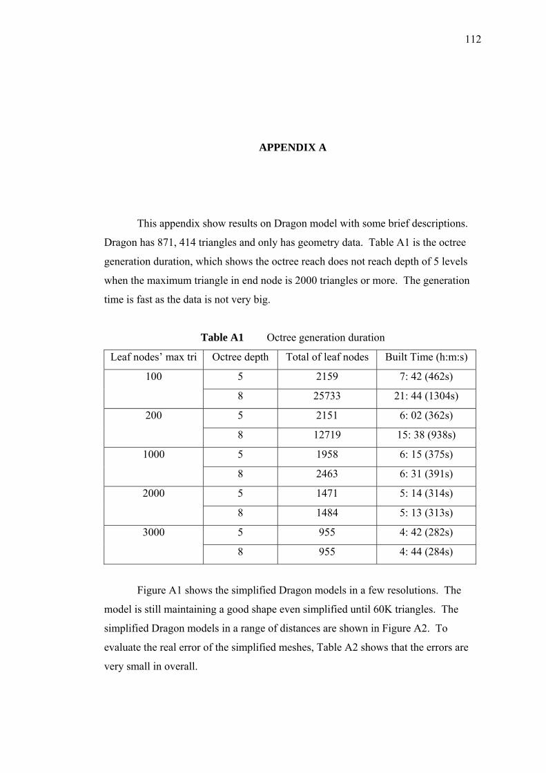
112
APPENDIX A
This appendix show results on Dragon model with some brief descriptions.
Dragon has 871, 414 triangles and only has geometry data. Table A1 is the octree
generation duration, which shows the octree reach does not reach depth of 5 levels
when the maximum triangle in end node is 2000 triangles or more. The generation
time is fast as the data is not very big.
Table A1 Octree generation duration
Leaf nodes’ max tri Octree depth Total of leaf nodes Built Time (h:m:s)
5 2159 7: 42 (462s) 100
8 25733 21: 44 (1304s)
5 2151 6: 02 (362s) 200
8 12719 15: 38 (938s)
5 1958 6: 15 (375s) 1000
8 2463 6: 31 (391s)
5 1471 5: 14 (314s) 2000
8 1484 5: 13 (313s)
5 955 4: 42 (282s) 3000
8 955 4: 44 (284s)
Figure A1 shows the simplified Dragon models in a few resolutions. The
model is still maintaining a good shape even simplified until 60K triangles. The
simplified Dragon models in a range of distances are shown in Figure A2. To
evaluate the real error of the simplified meshes, Table A2 shows that the errors are
very small in overall.

113
Figure A1 Out-of-core simplification of Dragon model in different resolutions
(Tri = number of triangles, Time = simplification time)
Original, Tri = 871, 414 a) Tri = 425, 531 Time = 37 s
b) Tri = 298, 266 Time = 39 s
c) Tri = 136, 144 Time = 94 s
d) Tri = 107, 633 Time = 148 s
e) Tri = 64, 428 Time = 226 s

114
Figure A2 Multiresolution of Dragon model in different distances
Table A2 Simplification times and errors of simplified Dragon models
Model Tin Tout Time (h: m: s) Mean Error RMS Error
Dragon 871, 414 425, 531 0: 37 0.000011 0.000022
Dragon 871, 414 298, 266 0: 39 0.000021 0.000040
Dragon 871, 414 136, 144 1: 34 0.000085 0.000140
Dragon 871, 414 107, 633 2: 28 0.000136 0.000226
Dragon 871, 414 62, 428 3: 46 0. 000198 0. 000320
A few levels of detail may be generated in an octree structure, an example of
the sequential simplification is revealed in Figure A3. Besides, Table A3 shows the
simplification time for different octree structures. As mentioned before, the
simplification is depends on octree structure. Additionally, the octree subdivision
level is not reaching level 5 when the maximum triangle in every node is 2000
triangles or more. Thus, the simplification times for octree with maximum triangles
of 2000 triangles and 3000 triangles are same for depth of 5 levels and 8 levels.
a) 426K
b) 298K
c) 136K
d) 107K
e) 64K

115
Figure A3 Sequential simplification on Dragon model, using maximum number
of triangles = 200, Octree’s depth = 8
LOD 1 Tri = 298, 266 Time = 39 s
LOD 2 Tri = 179, 586 Time = 13 s
LOD 3 Tri = 143, 803
Time = 9 s
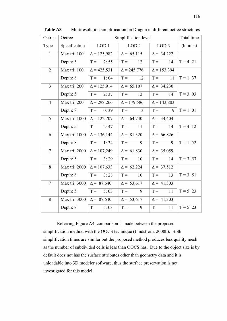
116
Table A3 Multiresolution simplification on Dragon in different octree structures
Simplification level Octree
Type
Octree
Specification LOD 1 LOD 2 LOD 3
Total time
(h: m: s)
∆ = 125,982 ∆ = 65,115 ∆ = 34,222 1 Max tri: 100
Depth: 5 T = 2: 55 T = 12 T = 14
T = 4: 21
∆ = 425,531 ∆ = 245,776 ∆ = 153,394 2 Max tri: 100
Depth: 8 T = 1: 04 T = 12 T = 11
T = 1: 37
∆ = 125,914 ∆ = 65,107 ∆ = 34,230 3 Max tri: 200
Depth: 5 T = 2: 37 T = 12 T = 14
T = 3: 03
∆ = 298,266 ∆ = 179,586 ∆ = 143,803 4 Max tri: 200
Depth: 8 T = 0: 39 T = 13 T = 9
T = 1: 01
∆ = 122,707 ∆ = 64,740 ∆ = 34,404 5 Max tri: 1000
Depth: 5 T = 2: 47 T = 11 T = 14
T = 4: 12
∆ = 136,144 ∆ = 81,320 ∆ = 66,826 6 Max tri: 1000
Depth: 8 T = 1: 34 T = 9 T = 9
T = 1: 52
∆ = 107,249 ∆ = 61,830 ∆ = 35,059 7 Max tri: 2000
Depth: 5 T = 3: 29 T = 10 T = 14
T = 3: 53
∆ = 107,633 ∆ = 62,224 ∆ = 37,512 8 Max tri: 2000
Depth: 8 T = 3: 28 T = 10 T = 13
T = 3: 51
∆ = 87,640 ∆ = 53,617 ∆ = 41,303 7 Max tri: 3000
Depth: 5 T = 5: 03 T = 9 T = 11
T = 5: 23
∆ = 87,640 ∆ = 53,617 ∆ = 41,303 8 Max tri: 3000
Depth: 8 T = 5: 03 T = 9 T = 11
T = 5: 23
Referring Figure A4, comparison is made between the proposed
simplification method with the OOCS technique (Lindstrom, 2000b). Both
simplification times are similar but the proposed method produces less quality mesh
as the number of subdivided cells is less than OOCS has. Due to the object size is by
default does not has the surface attributes other than geometry data and it is
unloadable into 3D modeler software, thus the surface preservation is not
investigated for this model.
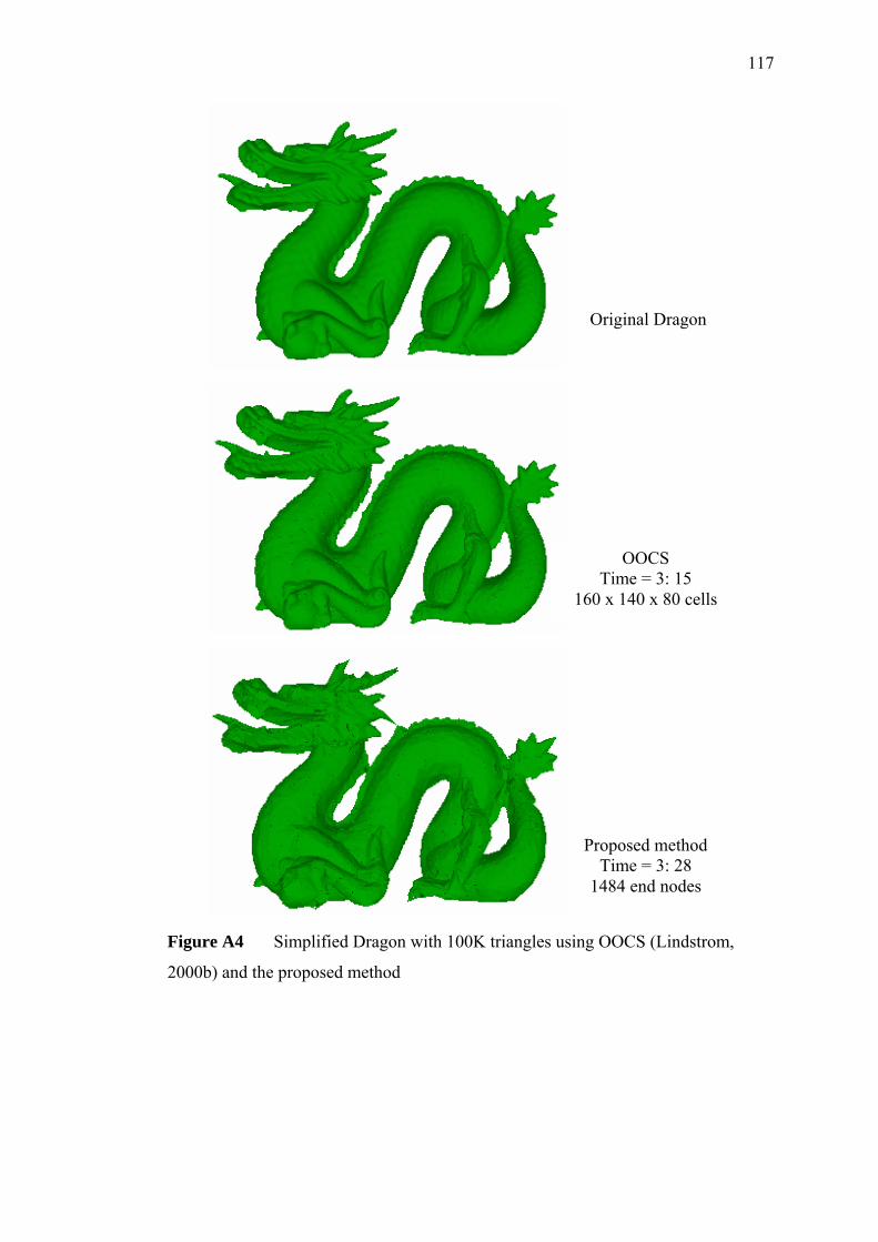
117
Figure A4 Simplified Dragon with 100K triangles using OOCS (Lindstrom,
2000b) and the proposed method
OOCS Time = 3: 15
160 x 140 x 80 cells
Proposed method Time = 3: 28
1484 end nodes
Original Dragon
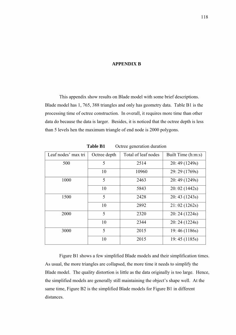
118
APPENDIX B
This appendix show results on Blade model with some brief descriptions.
Blade model has 1, 765, 388 triangles and only has geometry data. Table B1 is the
processing time of octree construction. In overall, it requires more time than other
data do because the data is larger. Besides, it is noticed that the octree depth is less
than 5 levels hen the maximum triangle of end node is 2000 polygons.
Table B1 Octree generation duration
Leaf nodes’ max tri Octree depth Total of leaf nodes Built Time (h:m:s)
5 2514 20: 49 (1249s) 500
10 10960 29: 29 (1769s)
5 2463 20: 49 (1249s) 1000
10 5843 20: 02 (1442s)
5 2428 20: 43 (1243s) 1500
10 2892 21: 02 (1262s)
5 2320 20: 24 (1224s) 2000
10 2344 20: 24 (1224s)
5 2015 19: 46 (1186s) 3000
10 2015 19: 45 (1185s)
Figure B1 shows a few simplified Blade models and their simplification times.
As usual, the more triangles are collapsed, the more time it needs to simplify the
Blade model. The quality distortion is little as the data originally is too large. Hence,
the simplified models are generally still maintaining the object’s shape well. At the
same time, Figure B2 is the simplified Blade models for Figure B1 in different
distances.

119
Figure B1 Out-of-core simplification of Blade model in different resolutions (Tri
= number of triangles, Time = simplification time)
b) Tri = 440, 608 Time = 3: 17
d) Tri = 247, 448 Time = 7: 30
e) Tri = 227, 934 Time = 8: 24
Original, Tri = 1, 765, 388 a) Tri = 622, 868 Time = 2: 34
c) Tri = 325, 774 Time = 5: 13
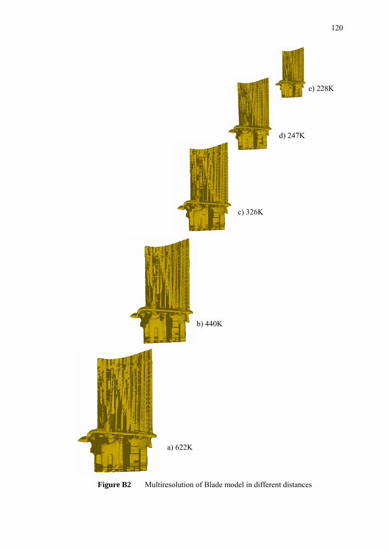
120
Figure B2 Multiresolution of Blade model in different distances
a) 622K
b) 440K
c) 326K
d) 247K
e) 228K

121
As the quality between these simplified meshes is hard to be distinguished
visually, Table B2 is created to show the errors of the simplified models. The error
is acceptable. For example, the error for simplified Blade with 623K triangles is
relatively small.
Table B2 Out Simplification times and errors of simplified Blade models
Model Tin Tout Time (h: m: s) Mean Error RMS Error
Blade 1, 765, 388 622, 868 2: 34 0.080685 0.195153
Blade 1, 765, 388 440, 608 3: 17 0.169567 0.345696
Blade 1, 765, 388 325, 774 5: 13 0.290001 0.526541
Blade 1, 765, 388 247, 448 7: 30 0.465160 0.764213
Blade 1, 765, 388 227, 934 8: 24 0.504452 0.816460
The multiresolution Blade models are simplified in a sequential way.
Example of a sequential simplification is shown in Figure B3. Table B3 shows the
generation of three levels of detail using different octree setting. The simplification
time is less when the node size is smaller.
Referring Figure B4, comparison is made between the proposed
simplification method with the OOCS technique (Lindstrom, 2000b). As mentioned
previously, the simplification is limited using OOCS (Lindstrom, 2000b). Hence
100K triangles simplified meshes are compared between his algorithm with the
proposed algorithm. Due to the object size is by default does not has the surface
attributes other than geometry data and it is unloadable into 3D modeler software,
thus the surface preservation is not investigated for this model.
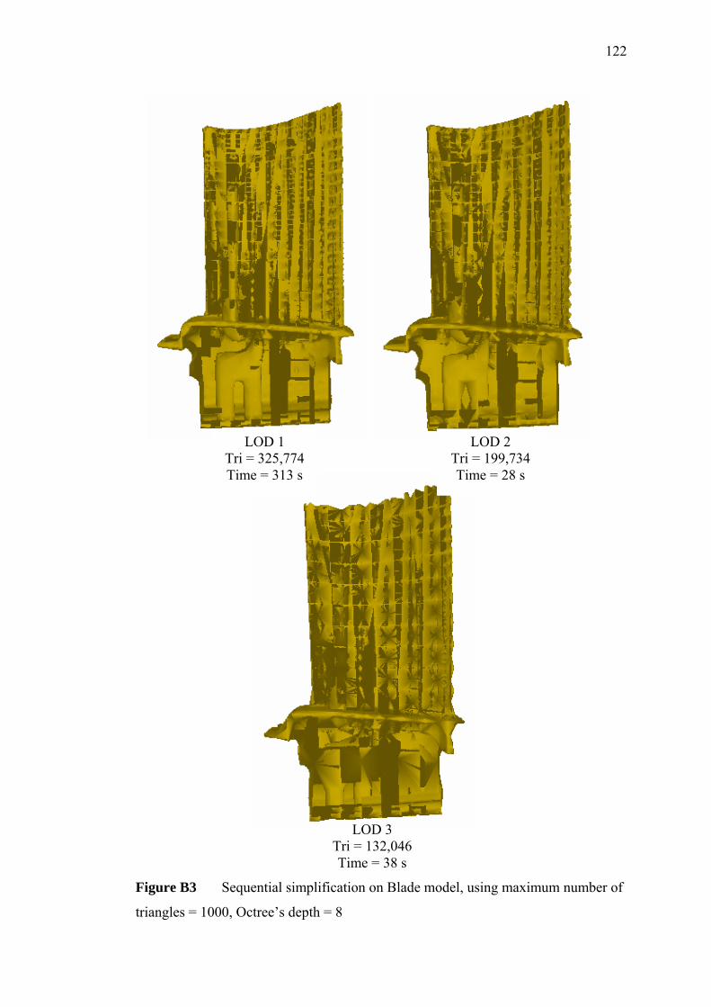
122
Figure B3 Sequential simplification on Blade model, using maximum number of
triangles = 1000, Octree’s depth = 8
LOD 1 Tri = 325,774 Time = 313 s
LOD 2 Tri = 199,734 Time = 28 s
LOD 3 Tri = 132,046 Time = 38 s

123
Table B3 Multiresolution simplification on Blade in different octree structures
Simplification level Octree
Type
Octree
Specification LOD 1 LOD 2 LOD 3
Total time
(h: m: s)
∆ = 233,920 ∆ = 118,864 ∆ = 55,622 1 Max tri: 500
Depth: 5 T = 8: 05 T = 44 T = 54
T = 9: 43
∆ = 440,608 ∆ = 234,106 ∆ = 133,180 2 Max tri: 500
Depth: 10 T = 3: 17 T = 41 T = 46
T = 4: 44
∆ = 232,780 ∆ = 118,832 ∆ = 55,654 3 Max tri: 1000
Depth: 5 T = 8: 06 T = 43 T = 54
T = 9: 43
∆ = 325,774 ∆ = 199,734 ∆ = 132,046 4 Max tri: 1000
Depth: 10 T = 5: 13 T = 28 T = 38
T = 6: 19
∆ = 231,632 ∆ = 118,822 ∆ = 55,654 5 Max tri: 1500
Depth: 5 T = 8: 10 T = 43 T = 54
T = 9: 47
∆ = 247,448 ∆ = 140,646 ∆ = 102,050 6 Max tri: 1500
Depth: 10 T = 7: 30 T = 36 T = 44
T = 8: 50
∆ = 226,904 ∆ = 118,550 ∆ = 55,894 7 Max tri: 2000
Depth: 5 T = 8: 27 T = 42 T = 54
T = 10: 03
∆ = 227,934 ∆ = 120,450 ∆ = 61,230 8 Max tri: 2000
Depth: 10 T = 8: 24 T = 41 T = 53
T = 9: 58
Figure B4 Simplified Blade with 100K triangles using OOCS (Lindstrom, 2000b)
and the proposed method
Original Dragon OOCS
Time = 9: 02 100 x 160 x 80 cells
Proposed method Time = 8: 48
1536 end nodes

99
REFERENCES
Aggarwal, A., and Vitter, J. S. (1988). The Input/Output Complexity of Sorting and
Related Problems. Communications of the ACM. 31(9):1116–1127.
Alliez, P. and Schmitt, F. (1999). Mesh Approximation using a Volume-Based
Metric. Proceeding of Pacific Graphics ’99 Conference Proceedings. 1999. 292-
301.
Bajaj, C., and Schikore, D. (1996). Error-bounded Reduction of Triangle Meshes
with Multivariate Data. SPIE. 2656: 34-45.
Bayer, R. and McCreight, E. (1972). Organization of Large Ordered Indexes. Acta
Inform., 1:173–189.
Bernardini, F., Rushmeier, H., Martin, IM, Mittleman, J. and Taubin, G. (2002).
Building a Digital Model of Michelangelo’s Florentine Pietà. Computer Graphics
and Applications. 22(1): 59-67.
Borodin, P., Guthe, M. and Klein, R. (2003). Out-of-Core Simplification with
Guaranteed Error Tolerance. Vision, Modeling and Visualization 2003. 19-21
November 2003. Munich, Germany: 309-316.
Brodsky, D. and Watson, B. (2000). Model Simplification though Refinement. In:
Mackenzie, I.S. and Stewart, J. eds. Graphics Interface 2000. Montreal, Canada:
Morgan Kaufmann Publishers. 211-228.

100
Brown, R., Pham, B. and Maeder, A. (2003a). Visual Importance-biased Image
Synthesis Animation. Proceedings of the 1st international conference on
Computer graphics and interactive techniques in Austalasia and South East Asia.
2003. New York, USA: ACM Press. 63-70.
Brown, R., Cooper, L. and Pham, B. (2003b). Visual Attention-Based Polygon Level
of Detail Management. Proceedings of the 1st international conference on
Computer graphics and interactive techniques in Austalasia and South East Asia.
2003. New York, USA: ACM Press. 55-62.
Cater, K. (2002). Selective Quality Rendering by Exploiting Inattentional Blindness:
Looking but not Seeing. Proceedings of the ACM symposium on Virtual reality
software and technology. 2002. New York, USA: ACM Press. 17-24.
Cater, K., Chalmers, A. and Dalton, C. (2003). Varying Rendering Fidelity by
Exploiting Human Change Blindness. Proceedings of the 1st international
conference on Computer graphics and interactive techniques in Austalasia and
South East Asia. 2003. New York, USA: ACM Press. 39-46.
Certain, A., Popovic, J., DeRose, T., Duchamp, T., Salesin, D. and Stuetzle, W.
(1996). Interactive Multiresolution Surface Viewing. Proceedings of SIGGRAPH
96. 91-98.
Chhugani, J. and Kumar, S. (2003). Budget Sampling of Parametric Surface Patches.
Proceedings of the 2003 symposium on Interactive 3D graphics. 2003. New York,
USA: ACM Press. 131-138.
Chiang, Y. J., Farias, R., Silva, C. and Wei, B. (2001). A Unified Infrastructure for
Parallel Out-Of-Core Isosurface Extraction and Volume Rendering of
Unstructured Grids’. Proc. IEEE Symposium on Parallel and Large-Data
Visualization and Graphics. 59–66.
101
Chiang, Y. J., Goodrich, M. T., Grove, E. F., Tamassia, R., Vengroff, D. E. and J. S.
Vitter. (2000). External-Memory Graph Algorithms. Proc. ACM-SIAM Symp. on
Discrete Algorithms. 139–149.
Chiang, Y. J. and Silva, C. T. (1997). I/O Optimal Isosurface Extraction. IEEE
Visualization 97. 293–300.
Chiang, Y. J. and Silva, C. T. (1999). External Memory Techniques for Isosurface
Extraction in Scientific Visualization. External Memory Algorithms and
Visualization, DIMACS Series. 50:247–277.
Chiang, Y. J., Silva, C. T. and Schroeder, W. J. (1998). Interactive Out-Of-Core
Isosurface Extraction. IEEE Visualization 98. Oct. 1998. 167–174,.
Choudhury, P. and Watson, B. (2002). Completely Adaptive Simplification of
Massive Meshes. Northwestern University: Tech. Report CS-02-09, 2002.
Chrislip, C. A. and Ehlert Jr., J. F. (1995). Level of Detail Models for Dismounted
Infantry. Naval Posgraduate School, Monterey, CA.: Master’s Thesis.
Cignoni, P., Ganovelli, F., Gobbetti, E., Marton, F., Federico, P., and Scopigno, R.
(2003a). BDAM - Batched Dynamic Adaptive Meshes for High Performance
Terrain Visualization. Computer Graphics Forum. 22(3): 505-514.
Cignoni, P., Ganovelli, F., Gobbetti, E., Marton, F., Federico, P., and Scopigno, R.
(2003b). Planet-Sized Batched Dynamic Adaptive Meshes (P-BDAM).
Proceedings IEEE Visualization. October 2003. Italy: IEEE Computer Society
Press, 147-155.
Cignoni, P., Montani, C., Rocchini, C. and Scopigno, R. (2003c). External Memory
Management and Simplification of Huge Meshes. Visualization and Computer
Graphics, IEEE Transactions. 9(4): 525-537.

102
Cignoni, P., Rocchini, C., Scopigno, R. (1998). Metro: Measuring Error on
Simplified Surfaces. Computer Graphics Forum. 17(2): 37-54.
Cohen, J., Olano, M. and Manocha, D. (1998). Appearance-Preserving Simplification.
Proceedings of SIGGRAPH 98 in Computer Graphics Annual Conference, ACM
SIGGRAPH. 19-24 July 1998. Orlando, Florida: ACM SIGGRAPH, ?.
Cohen, J., Varshney, A., Manocha, D., Turk, G., Weber, H., Agarwal, P. Brooks, Jr.
F. P. and Wright, W. (1996). Simplification envelopes. In: Rishmeier, H. ed.
Proceedings of SIGGRAPH 96. New Orleans, Louisianna: Addison Wesley. 119-
128.
Cohen, J., Luebke, D., Duca, N. and Schubert, B. (2003). GLOD: Level of Detail for
The Masses. The Johns Hopkins University and the University of Virginia:
Technical Report.
Comer, D. (1979). The Ubiquitous B-Tree. ACM Comput. Surv. 11:121–137.
Correa, W. T, Klosowski, J.T and Silva, C. T. (2002). iWalk: Interactive Out-of-Core
Rendering of Large Models. Princeton University, 2002: Technical Report TR-
653-02.
Danovaro, E., Floriani, L. D., Lee, M. and Samet, H. (2002). Multiresolution
Tetrahedra Meshes: an Analysis and a Comparison. Shape Modeling
International 2002 (SMI’02). 17-22 May 2002. Banff, Canada: IEEE, 83.
DeHaemer, J. M. and Zyda, M. J. (1991) Simplification of Objects Rendered by
Polygonal Approximations. Computers & Graphics. 15(2):175-184.
DeRose, T.D., Lounsbery, M. and Warren, J. (1993). Multiresolution Analysis for
Surfaces of Arbitrary Topology Type. Department of Computer Science,
University of Washington: Technical Report TR 93-10-05.

103
Edelsbrunner, H. (1983). A New Approach to Rectangle Intersections, Part I.
Internat. J. Comput. Math. 13: 209–219.
El-Sana, J. and Chiang, Y. J. (2000). External Memory View-Dependent
Simplification. Computer Graphics Forum. 19(3): 139–150.
El-Sana, J. and Varshney, A. (1997). Controlled Simplification of Genus for
Polygonal Models. In: Yagel, R. and Hagen, H. eds. IEEE Visualization ’97.
Phoenix, Arizona: IEEE. 403-412.
El-Sana, J. and Varshney, A. (1998). Topology Simplification for Polygonal Virtual
Environments. IEEE Transaction on Visualization and Computer Graphics. 4(2):
133-144.
El-Sana, J. and Varshney, A. (1999). Generalized View-Dependent Simplification.
Computer Graphics Forum. 18(3): 83–94.
Erikson, C. (1996). Polygonal Simplification: An Overview. Department of Computer
Science, University of North Carolina, Chapel Hill, NC: UNC Technical Report
No. TR96-016.
Erikson, C. (2000). Hierarchical Levels of Detail to Accelerate the Rendering of
Large Static and Dynamic Polygonal Environments. University of North
Carolina at Chapel Hill: Ph.D. Thesis.
Erikson, C. and Manocha, D. (1998). Simplification Culling of Static and Dynamic
Scene Graphs. Department of Computer Science, University of North Carolina at
Chapel Hill: Technical Report TR98-009.
Erikson, C. and Manocha, D. (1999). GAPS: General and Automatic Polygonal
Simplification. In: Hodgins, J. and Foley, J. D. eds. ACM symposium on
Interactive 3D Graphics. Atlanta, Georgia: ACM SIGGRAPH. 79-88.
104
Erikson, C., Monacha, D. and Baxter, W. V. III. (2001). HLODs for Faster Display
of Large Static and Dynamic Environments. 2001 ACM Symposium on
Interactive 3D Graphics. 111-120.
Farias, R. and Silva, C. T. (2001). Out-Of-Core Rendering of Large, Unstructured
Grids. IEEE Computer Graphics & Applications. 21(4): 42–51.
Fei, G. Z., Guo, B. N., Wu, E. H., Cai, K. Y. (2002). An Adaptive Sampling Scheme
for Out-of-Core Simplification. Computer Graphics Forum. 21(2): 111-119.
Franc, M. and Skala, V. (2001). Parallel Triangular Mesh Decimation without
Sorting. 17th Spring Conference on Computer Graphics (SCCG '01). April 2001.
Budmerice,Slovakia: IEEE, 22-29.
Funkhouser, T. A. and Sequin, C. H. (1993). Adaptive Display Algorithm for
Interactive Frame Rates During Visualization of Complex Virtual Environment.
Proceedings of the 20th annual conference on Computer graphics and interactive
techniques. 1993. New York, USA: ACM Press. 247-254.
Garland, M. (1999). Quadric–Based Polygonal Surface Simplification. Carnegie
Mellon University: Ph.D. Thesis.
Garland, M. and Heckbert, P. S. (1997). Surface Simplification Using Quadric Error
Metrics. In: Whitted, T. ed. Proceedings of SIGGRAPH 97. Los Angeles,
California: ACM Press. 209-216.
Garland, M. and Heckbert, P.S. (1998). Simplifying Surface with Color and Texture
Using Quadric Error Metrics. IEEE Visualization ’98 Conference Proceeding.
IEEE, 263-270.
Garland, M. and Shaffer, E. (2002). A Multiphase Approach to Efficient Surface
Simplification. Visualization ’02. Washington, DC, USA: IEEE Computer
Society, 117-124.

105
Gieng, T. S., Hamann, B. Joy, K. I., Schlussmann, G. L. And Trotts, I. J. (1997).
Smooth Hierarchical Surface Traingulations, In: Yagel, R. and Hagen, H. eds.
IEEE Visualization ’97. Phoenix, Arizona: IEEE. 379-386.
Guthe, M., Borodin, P. and Klein, R. (2003). Efficient View-Dependent Out-of-Core
Visualization. Proceeding of The 4th International Conference on Virtual Reality
and Its Application in Industry (VRAI’2003). October 2003.
Haibin, W. and Quiqi, R. (2000). Fast Rendering of Complex Virtual Environment.
Proceedings of ICSP2000. 1395-1398.
Hamann, B. (1994). A data Reduction Scheme for Triangulated Surfaces. Computer
Aided Geometric Design. 11(20): 197-214.
Hoppe, H. (1996). Progressive Mesh. In: Rushmeier, H. ed. Proceeding of
SIGGRAPH 96. Computer Graphics Proceedings, Annual Conference Series.
New Orleans, Louisiana: Addison Wesley. 99-108.
Hoppe, H. (1997). View-dependent Refinement of Progressive Meshes. Proceedings
of the 24th Annual Conference on Computer Graphics and Interactive Techniques.
August 1997. ACM: 189-198
Hoppe, H. (1998a). Efficient Implementation of Progressive Meshes. Computer
Graphics. 22(1): 27-36.
Hoppe, H. (1998b). Smooth View-Dependent Level-of-Detail Control and Its
Application to Terrain Rendering. IEEE Visualization ’98. October 1998. North
Carolina: IEEE, 25-42.
Hoppe, H. (1999). New Quadric Metric for Simplifying Meshes with Appearance
Attributes. IEEE Visualization ’99. October 1999. San Francisco, California:
IEEE, 59-66.
106
Hoppe, H., DeRose, T., Duchamp, T., McDonald, J. and Stuetzle, W. (1993). Mesh
Optimization. In: Kajiya, J. T. ed. Proceeding of SIGGRAPH 93. Anaheim,
California: Addison Wesley. 19-26.
Hughes, M., Lastra, A. A. and Saxe, E. (1996). Simplification of Global-Illumination
Meshes. Proceedings of Eurographics '96, Computer Graphics Forum. 15(3):
339-345.
Isenburg, M. and Gumhold, S. (2003). Out-of-Core Compression for Gigantic
Polygon Meshes. ACM Transaction on Graphics. 22(3): 935-942.
Isenburg, M., Gumhold, S. and Snoeyink,J. (2003a). Processing Sequence: A New
Paradigm for Out-of-Core Processing on Large Meshes.
Isenburg, M., Lindstrom, P., Gumhold, S. and Snoeyink, J. (2003b). Large Mesh
Simplification using Processing Sequences. Proceedings of Visualization 2003.
19-24 October 2003. Seattle, Washington: IEEE, 465-472.
Jacob, C. E., Finkelstein, A. and Salesn, D. H. (1995). Fast Multiresolution Image
Querying. In: Cook, R. ed. Proceeding of SIGGRAPH 95, Computer Graphics
Proceedings, Annual Conference Series. Los Angeles, California: Addison
Wesley. 277-286.
Kalvin, A. D. and Taylor, R. H. (1994). Superfaces: Polygonal Mesh Simplification
with Bounded Error. IBM Research Division, T. J. Watson Research CEntre,
Yorktown Heights, NY: Technical Report RC 19828 (#87702).
Kalvin, A.D. and Taylor, R. H. (1996). Superfaces: Polygonal Mesh Simplification
with Bounded Error. IEEE Computer Graphics & Applications. 16(3):64-77.
Klein, R., Liebich, G. ad Straber, W. (1996). Mesh Reduction With Error Control. In:
Yagel, R. and Nielson, G. M. eds. IEEE Visualization ’96. San Francisco,
Carlifornia: IEEE. 311-318.
107
Levenberg, J. (2002). Fast View-Dependent Level-of-Detail Rendering Using
Cached Geometry. IEEE Visualization 2002. October 2002. Boston, MA, USA:
IEEE. 259-265.
Linderman, J., (2000). rsort and fixcut man page, Apr 1996. (revised June 2000).
Lindstrom, P. (2000a). Model Simplification using Image and Geometry-Based
Metrics. Georgia Institute of Technology: Ph.D Thesis.
Lindstrom, P. (2000b). Out-of-Core Simplification of Large polygonal Models. ACM
SIGGRAPH 2000. July 2000. 259-262.
Lindstrom, P. (2003a). Out-of-Core Surface Simplification. California: University of
California, Davis, lectures on "Multiresolution Methods" February 2003.
Lindstrom, P. (2003b). Out-of-Core Construction and Visualization of
Multiresolution Surfaces. Symposium on Interactive 3D Graphics. April 2003.
ACM, 93-102, 239.
Lindstrom, P. (2003c). Out-of-core Construction and Visualization of
Multiresolution Surfaces. Proceedings of the 2003 Symposium on Interactive 3D
Graphics. 28-30 April 2003. Monterey, California: ACM Press,
Lindstrom, P., Koller, D., Ribarsky, W., Hughes, L. F., Faust, N. and Turner, G.
(1996). Real-Time, Continuous Level of Detail Rendering of Height Fields. ACM
SIGGRAGH 96. 109-118.
Lindstrom, P., and Pascucci, V. (2001). Visualization of Large Terrains Made Easy.
IEEE Visualization 2001. October 2001. San Diego, California: IEEE, 363–370.
Lindstrom, P. and Silva, C. (2001). A Memory Insensitive Technique for Large
Model Simplification. IEEE Visualization 2001. October 2001. IEEE, 121-126.

108
Lindstrom, P. and Turk, G. (1998). Fast and Memory Efficient Polygonal
Simplification. In: Ebert, D., Hagen, H. and Rushmeier, H. eds. IEEE
Visualization ’98. Research Triangle Park, North Carolina: IEEE. 279-286.
Lindstrom, P. and Turk, G. (1999). Evaluation of Memoryless Simplification. IEEE
Transactions on Visualization and Computer Graphics. 5(2): 98-115.
Liu, Y. J., Yuen, M. F. and Tang, K. (2003). Manifold-Guaranteed Out-of-Core
Simplification of Large Meshes with Controlled Topological Type. The Visual
Computer (2003). 19(7-8): 565-580.
Low, K. L. and Tan T. S. (1997). Model Simplification using vertex-clustering. In:
Cohen, M. and Zeltzer, D. eds. 1997 ACM Symposium on Interactive 3D
Graphics. Phode Island: ACM SIGGRAPH. 75-82.
Luebke, D. and Erikson, C. (1997). View-Dependent Simplification of Arbitrary
Polygonal Environments. ACM SIGGRAPH 97. 199–208.
Nooruddin, F. S. and Turk, G. (2003). Simplification and Repair of Polygonal
Models using Volumetric Techniques. IEEE Transactions on Visualization and
Computer Graphics. 9(2): 191-205.
Ohshima, T., Yamamoto, H. and Tamura, H. (1996). Gaze-Directed Adaptive
Rendering for Interacting with Virtual Space. Proceedings of the IEEE Virtual
Reality Annual International Symposium (VRAIS). 30 March – 03 April 1996.
IEEE, 103-110.
Prince, C. (2000). Progressive Meshes for Large Models of Arbitrary Topology.
University of Washington: Master’s Thesis.
Reddy, M. (1995). Musings on Volumetric Level of Detail for Virtual Environments.
Virtual Reality: Research, Development and Application. 1(1): 49-56.
Reddy, M. (1997). Perceptually Modulated Level of Detail for Virtual Environment.
University of Edinburgh: Ph.D Thesis.

109
Ronfard, R. and Rossignac, J. (1996). Full-Range Approximations for Triangulated
Polyhedra. Computer Graphics Forum. 15(3): 67-76;
Rossignac, J. and Borrel, P. (1992). Multi-resolution 3D Approximations for
Rendering Complex Scenes. NY: Technical Report RC 17697.
Rossignac, J. and Borrel, P. (1993). Multi-resolution 3d Approximations for
Rendering Complex Scenes. In: Falciendo, B. and Kunii, T. L. eds. Modeling in
Computer Graphics. Springer-Verlag. 455-465.
Rushmeier, H., Larson, G. W., Piatko, C., Sanders, P. and Rust, B. (1995).
Comparing Real and synthetic Images: Some Ides about Metrics. In: Hanrahan, P.
and Purgathofer, W. eds. Eurographics Rendering Workshop 1995. Dublin,
Ireland: Springer-Verleg. 82-91.
Schmitt, F. J. M., Barsky, B. A. And Du, W. H. (1986). An Adaptive Subdivision
Method for Surface-Fitting From Sample Data. Computer Graphics. 20(4): 179-
188.
Schroeder, W. J. (1997). A Topology Modifying Progressive Decimation Algorithm.
In: Yagel, R. and Hagen, H. eds. IEEE Visualization ’97. Phoenix, Arizona: IEEE.
205-212.
Schroeder, W. J., Zarge, J. A. And Lorensen W. E. (1992). Decimation of Triangle
Meshes. In: Catmull, E. E. ed. Computer Graphics (Proceeding of SIGGRAPH
92). Chicago: Illinois. 65-70.
Shaffer, E. and Garland M. (2001). Efficient Simplification of Massive Meshes. 12th
IEEE Visualization 2001 Conference (VIS 2001). 24-26 October 2001. San Diego,
CA: IEEE.
Silva, C.T., Chiang, Y. J., El-Sana, J. and Lindstrom, P. (2002). Out-Of-Core
Algorithms for Scientific Visualization and Computer Graphics. IEEE
Visualization Conference 2002. October 2002. Boston, MA: IEEE, 217-224.
110
Southern, R., Marais, P. and Blake, E. (2001). Generic Memoryless Polygonal
simplification. ACM Afrigraph. ACM, 7-15.
Trotts, I. J., Hamann, B., Joy, K. I. (1999). Simplification of Tetrahedra Meshes with
Error Bounds. IEEE Transaction on Visualization and Computer Graphics. 5(3):
224-237.
Varadhan, G. and Manocha, D. (2002). Out-of-Core Rendering of Massive
Geometric Environments. IEEE Visualization 2002. Oct 27 – Nov 1. Boston:
IEEE, 69-76.
Vince, J. (1993). Virtual Reality Techniques in Flight Simulation. In A.A. Earnshaw,
M.A. Gigante and H.Jones eds. Virtual Reality Systems. Academic Press Ltd.
Watson, B., Friedman, A. and McGaffey, A. (2000). Using Naming Time to Evaluate
Quality Predictors for Model Simplification. Proceeding of the CHI 2000
Conference on Human Factors in Computing Systems. April 2000. The Hague,
The Netherlands: Addison Wesley. 113-120.
Watson, B., Walker, N. and Hodges, L.F. (1995). A User Study Evaluating Level of
Detail Degradation in the Periphery of Head-Mounted Displays. Proceedings of
the FIVE ’95 Conference. UK: University of London, 203-212.
Wernecke, J. (1993). The Inventor Mentor: Programming Object-Oriented 3D
Graphics with Open Inventor (TM). Release 2, 1st Edison. Boston, MA, USA:
Addison-Wesley.
Wilson, A. and Manocha, D. (2003). Simplifying Complex Environments Using
Incremental Textured Depth Meshes. ACM Transactions on Graphics (TOG).
July 2003. New York, USA: ACM Press. 678-688.
Wu, J. and Kobbelt, L. (2003). A Stream Algorithm for the Decimation of Massive
Meshes. Graphics Interface ‘03. 185-192.

111
Xia, J. C., El-Sana, J. and Varshney, A. (1997). Adaptive Real-Time Level-of-Detail-
Based Rendering for Polygonal Models. IEEE Transactions on Visualization and
Computer Graphics. 3(2): 171-183.
Zach, C, Mantler, S. and Karner, K. (2002). Time-critical Rendering of Discrete and
Continuous Levels of Detail. Proceedings of the ACM symposium on Virtual
reality software and technology. 2002. New York, USA: ACM Press.

R & D FINAL REPORT 2nd. OPTION FORMAT IP SCREENING & TECHNOLOGY ASSESSMENT FORM END OF PROJECT BENEFIT OF REPORT BORANG PENGESAHAN LAPORAN AKHIR TITLE PAGE (as 1st option report) ABSTRACT(B. INGGERIS) ABSTRAK(B. MELAYU) ACKNOWLEDGEMENT TABLE OF CONTENTS CHAPTER 1 INTRODUCTION
GENERAL PROBLEM STATEMENT OR STATE OF THE ART OBJECTIVE AND SCOPE OF STUDY
CHAPTER 2 (related technical paper published – results of project : format as paper published) TITLE ABSTRACT INTRODUCTION EXPERIMENTAL RESULTS AND DISCUSSION CONCLUSION CHAPTER 3 (related technical paper published –results of project) CHAPTER 4 (related technical paper published –results of project)

1
UTM/RMC/F/0014 (1998)
UNIVERSITI TEKNOLOGI MALAYSIA Research Management Centre
PRELIMINARY IP SCREENING & TECHNOLOGY ASSESSMENT FORM
(To be completed by Project Leader submission of Final Report to RMC or whenever IP protection arrangement is required) 1. PROJECT TITLE IDENTIFICATION :
OUT-OF-CORE SIMPLIFICATION WITH APPEARANCE PRESERVATION
FOR COMPUTER GAME APPLICATIONS Vote No: 75166
2. PROJECT LEADER :
Name : ABDULLAH BIN BADE
Address: FAKULTI SAINS KOMPUTER DAN SISTEM MAKLUMAT, UNIVERSITI TEKNOLOGI
MALAYSIA, 81310 SKUDAI JOHOR
Tel : 07-5532324 Fax : 07-5565044 e-mail : [email protected]
3. DIRECT OUTPUT OF PROJECT (Please tick where applicable)
4. INTELLECTUAL PROPERTY (Please tick where applicable)
Not patentable Technology protected by patents
Patent search required Patent pending
Patent search completed and clean Monograph available
Invention remains confidential Inventor technology champion
No publications pending Inventor team player
No prior claims to the technology Industrial partner identified
Scientific Research Applied Research Product/Process Development Algorithm Method/Technique Product / Component Structure Demonstration / Process Prototype Data Software
Other, please specify Other, please specify Other, please specify ___________________ __________________ ___________________________ ___________________ __________________ ___________________________ ___________________ __________________ ___________________________
√
√
Lampiran 13

2
UTM/RMC/F/0014 (1998)
5. LIST OF EQUIPMENT BOUGHT USING THIS VOT
1. Computer (HP) 2. Laser Jet Printer
6. STATEMENT OF ACCOUNT
a) APPROVED FUNDING RM : 28,000.00
b) TOTAL SPENDING RM : …………………………
c) BALANCE RM : ………………………… 7. TECHNICAL DESCRIPTION AND PERSPECTIVE
Please tick an executive summary of the new technology product, process, etc., describing how it works. Include brief analysis that compares it with competitive technology and signals the one that it may replace. Identify potential technology user group and the strategic means for exploitation. a) Technology Description
A 3D interactive graphics application is an extremely computational demanding paradigm, requiring the simulation
and display of a virtual environment at interactive frame rates. It is significant in real time game environment. Even
with the use of powerful graphics workstations, a moderately complex virtual environment can involve a vast amount
of computation, inducing a noticeable lag into the system. This lag can detrimentally affect the visual effect and may
therefore severely compromise the diffusion of the quality of graphics application. Therefore, a lot of techniques have
been proposed to overcome the delay of the display. It includes motion prediction, fixed update rate, visibility
culling, frameless rendering, Galilean antialiasing, level of detail, world subdivision or even employing parallelism. In
this project, we strive to render a massive dataset in 3D real-time environment and preserve its surface appearance
during simplification process using commodity personal computer. By using our out-of-core simplification technique
and preserve the surface attributes on the out-of-core model based on error metrics, we can prove that our proposed
methodology is capable in simplifying the large datasets with surface attributes preservation, such as positions,
normals, colors and texture coordinates for graphics application. The invention on modifying the vertex clustering
coarsening operator and adopting the suitable algorithms into this out-of-core framework has made the research goals
are accomplished. This algorithm is a practical and scalable system that allows the inexpensive PCs to visualize
datasets in computer games, which is formally an impossible task.
b) Market Potential
The output gathered from this study is useful for the industry of computer games particularly on handling and
manipulating massive datasets during run-time rendering. By keeping the bulk of the data on disk and retain in main
memory (or so called core) only the part of the data that’s being processed, visualizing massive datasets are now
possible.

3
c) Commercialisation Strategies
In order to commercialize this research, the prototype and technique of out-of-core simplification with appearance
preservation should be promoted to the industry of computer games in Malaysia through the Development and
Creative Application Center, Multimedia Development Corporation Sdn Bhd (MDC).
8. RESEARCH PERFORMANCE EVALUATION
a) FACULTY RESEARCH COORDINATOR Research Status ( ) ( ) ( ) ( ) ( ) ( ) Spending ( ) ( ) ( ) ( ) ( ) ( ) Overall Status ( ) ( ) ( ) ( ) ( ) ( ) Excellent Very Good Good Satisfactory Fair Weak
Comment/Recommendations : _____________________________________________________________________________
____________________________________________________________________________
_____________________________________________________________________________
_____________________________________________________________________________
_____________________________________________________________________________
____________________________________________________________________________
………………………………………… Name : ………………………………………
Signature and stamp of Date : ……………………………………… JKPP Chairman
UTM/RMC/F/0014 (1998)

4
RE
b) RMC EVALUATION
Research Status ( ) ( ) ( ) ( ) ( ) ( ) Spending ( ) ( ) ( ) ( ) ( ) ( ) Overall Status ( ) ( ) ( ) ( ) ( ) ( ) Excellent Very Good Good Satisfactory Fair Weak
Comments :- ________________________________________________________________________
__________________________________________________________________________
_________________________________________________________________________
_________________________________________________________________________
_________________________________________________________________________
_____________________________________________________________________________
Recommendations :
Needs further research
Patent application recommended
Market without patent
No tangible product. Report to be filed as reference
………………………………………………..
Name : ……………………………………………
Signature and Stamp of Dean / Deputy Dean Date : …………………………………………… Research Management Centre
UTM/RMC/F/0014 (1998)

1
Lampiran 20
UTM/RMC/F/0024 (1998)
UNIVERSITI TEKNOLOGI MALAYSIA
BORANG PENGESAHAN LAPORAN AKHIR PENYELIDIKAN
TAJUK PROJEK : OUT-OF-CORE SIMPLIFICATION WITH APPEARANCE
PRESERVATION FOR COMPUTER GAME APPLICATIONS
Saya ABDULLAH BADE (HURUF BESAR) Mengaku membenarkan Laporan Akhir Penyelidikan ini disimpan di Perpustakaan Universiti Teknologi Malaysia dengan syarat-syarat kegunaan seperti berikut :
1. Laporan Akhir Penyelidikan ini adalah hakmilik Universiti Teknologi Malaysia 2. Perpustakaan Universiti Teknologi Malaysia dibenarkan membuat salinan untuk tujuan rujukan sahaja. 3. Perpustakaan dibenarkan membuat penjualan salinan Laporan Akhir Penyelidikan ini bagi kategori TIDAK
TERHAD 4. * Sila tandakan ( / )
SULIT (Mengandungi maklumat yang berdarjah keselamatan atau Kepentingan Malaysia seperti yang termaktub di dalam AKTA RAHSIA RASMI 1972)
TERHAD (Mengandungi maklumat TERHAD yang telah ditentukan oleh Organisasi/badan di mana penyelidikan dijalankan)
TIDAK TERHAD ____________________________________________ TANDATANGAN KETUA PENYELIDIK ____________________________________________ Nama & Cop Ketua Penyelidik Tarikh : ________________
√