out-of-sample performance of mutual fund predictorschristoj/pdf/jones_mo.pdfout-of-sample...
TRANSCRIPT

Out-of-sample performance of mutual fund predictors∗
Christopher S. Jones Haitao Mo
Marshall School of Business Ourso College of Business
University of Southern California Louisiana State University
[email protected] [email protected]
January 2016
∗We are grateful to the participants of seminars at the University of Southern California. Data on hedgefund assets under management were kindly provided by Matti Suominen. All errors remain our own.

Out-of-sample performance of mutual fund predictors
Abstract
This study analyzes the out-of-sample performance of a variety of variables
shown in prior work to forecast future mutual fund alphas. Overall, we find that
the degree of predictability, as measured by alpha spreads from quintile sorts
of by cross-sectional regression slopes, falls by at least half following the end of
the sample and perhaps by 75% after publication. This decline is not driven
by changes in fund flows or expenses, suggesting that it is not explained by the
model of Berk and Green (2004). Rather, we find that the shrinking of alpha
spreads is associated with higher levels of arbitrage activity, and that this largely
explains the out-of-sample decline.
Keywords: mutual funds, out-of-sample performance, market efficiency

1 Introduction
A central question in the mutual fund literature is whether funds with positive alpha, net of
fees and costs, can be distinguished, ex ante, from those with negative alpha. An affirmative
answer to the question requires that some variable in the investor’s information set be asso-
ciated with future alphas. To this end, a number of studies have investigated the ability of
various theoretically or intuitively motivated variables to predict future fund alphas, and a
modest number of variables that appear to do so have now been found. Whether these alpha
predictors continue to perform outside of their original samples is a question we answer in
this paper.
In the model of Berk and Green (2004), the alphas that investors perceive given available
information is zero. Alphas that are above zero are eliminated by higher fees and disec-
onomies of scale resulting from fund inflows. If the alpha predictors we study are part of the
investor’s information set, at least after the studies that propose them are published, then
their effectiveness should be expected to decline out of sample.
In addition to highlighting limitations of the Berk and Green hypothesis, continued per-
formance of alpha predictors out of sample would also allow us to rule out the possibility of
data mining as the explanation of mutual fund alpha prediction. Academic studies would
then appear to offer some potential in guiding mutual fund investors towards better perfor-
mance.
To the extent that performance does decline out of sample, then an analysis of this
decline may help us to understand the forces that cause apparent mispricing to disappear
over time, one possibility being that alphas converge to zero in the manner that Berk and
Green suggest. An alternative is that a steady increase in arbitrage activity over the last
several decades has made stock markets more efficient, and that alpha generation has become
more difficult for mutual fund manager.
Chordia et al. (2014) investigate how the returns to asset pricing anomalies (momentum,
value, accruals, etc.) are related to various measures of arbitrage activity. Across a number of
anomalies, they find that the average return is reduced substantially by an increase in short
interest, the assets under management of hedge funds, and aggregate share turnover. We
1

follow their work by analyzing how these arbitrage activity proxies are related to abnormal
fund returns.
We find that alpha predictors largely fail, out of sample, to replicate their in-sample
success. At least half of the alpha spread generated by predictors proposed in the literature
disappears out of sample. In some specification, that number rises to 75%. Thus, to a
potential mutual fund investor, advice from the academic literature on mutual funds is at
best moderately useful, though in the brief window between the end of the sample period
and the date of publication the situation is somewhat more positive. In this window, which
lasts around four years on average, the power of the average alpha predictor falls only by
30-40%.
The finding that alpha predictability declines gradually rather than immediately following
the end of the original sample makes it unlikely that data mining is a primary explanation
for in-sample predictability. Another possibility, discussed above, is that academic studies
foster learning by mutual fund investors and management. The resulting changes in beliefs
about fund manager skill trigger fund flows and fee adjustments that, according to Berk
and Green (2004), should be expected to cause alphas to shrink to zero. We investigate
the relation between alpha predictors and flows and find a significant positive relation that
does not change out-of-sample. The relation between alpha predictors and fees is generally
negative, becoming significantly more negative out-of-sample. This is the opposite of what
the Berk and Green model would imply, suggesting that the decline in alpha predictability
is not driven by investor learning.
Finally, we examine the relation between alphas and arbitrage activity. Here we find
strong evidence that higher levels of arbitrage are associated with smaller alpha spreads.
Part of this effect is consistent with the view that market efficiency has in general increased
over the sample we examine as the result of a trend towards greater arbitrage activity. How-
ever, the relation between arbitrage and alphas also holds for detrended arbitrage activity
measures, suggesting cyclical variation in arbitrage forces are important as well. When we
include both out-of-sample and arbitrage effects within the same specification, it is arbitrage
activity that most often retains significance. This suggests to us that poor out-of-sample
performance is at least mostly the result of an overall trend towards greater market efficiency
2

over our sample.
Our paper relates to several strands of the finance literature. Most clearly, we follow a
significant literature on mutual fund performance prediction, which we review in Section II.
Our paper is also closely related to work on the persistence of asset pricing anomalies. In
addition to the work of Chordia et al. (2014), a number of studies have explored how the ex-
pected returns of anomaly strategies have held up since the original papers documenting their
existence. Schwert (2003) shows, for example, that the size anomaly largely faded following
its discovery in the early 1980s. Jones and Pomorski (2015) analyze several anomalies from
the perspective of a Bayesian investor, finding that out-of-sample investment performance
is improved by allowing, ex ante, for the possibility that the anomaly return may diminish
over time. Finally, in a study closely related to the current one, McLean and Pontiff (2015)
examine the out-of-sample performance of 97 variables shown to predict equity returns and
find a substantial decline relative to in sample averages.
This paper is also related to work seeking to characterize the distribution of mutual
fund managers. This work has generally found that the average fund alpha, net of fees and
expenses, is negative, but there is substantial disagreement over the fraction of managers
that do provide positive alphas. In the Bayesian framework of Jones and Shanken (2005) and
the bootstrap analysis of Kosowski et al. (2006), a substantial minority of funds do appear to
outperform. In contrast, Fama and French (2010) conclude that funds with positive alphas
are highly unusual, while Chen and Ferson (2015) find that they are largely nonexistent.
Interestingly, in a similar study, Barras et al. (2010) find a substantial fraction of funds with
positive alphas prior to 1996, but find that almost no positive alphas existed by 2006. Our
finding that arbitrage activity is associated with declining alpha spreads is consistent with
this observation.
In the following section we discuss the measurement of mutual fund alpha and the repli-
cation of mutual fund alpha predictors. In Section 3 we assess the out-of-sample performance
of these predictors. We test the hypotheses on flows and expenses in Section 4 and examine
the relation between alphas and arbitrage activity in Section 5. Section 6 concludes.
3

2 Mutual fund alpha predictors
A variety of variables have been found to predict future fund performance. Most of the
papers that document this predictability were published following the introduction of the
CRSP Survivor-Bias-Free US Mutual Fund database, which first appeared in the work of
Carhart (1997). The only predictor that predates this database is the lagged one-year return,
which Hendricks et al. (1993) showed to forecast future returns.
Carhart’s 1997 paper contained a number of results that were new to the literature
and that we analyze here. He showed, for instance, that expense ratios and turnover were
negatively related to future fund performance. While confirming the results of Hendricks
et al. (1993), Carhart found that past alphas from his own four-factor model were more
useful in forecasting future risk-adjusted performance.
There is also some evidence that fund size is related to future performance. Chen et al.
(2004) find that larger funds perform worse, particularly for small-cap funds, while fund
family size is positively related to performance. While the interpretation of this evidence is
somewhat controversial (see Pastor et al. (2015)) in that it is not clear whether performance
is an accurate reflection of managerial skill, the empirical relation between alphas and funds
size appears relatively strong.
The tendency of mutual funds to deviate from benchmark indexes also appears be related
to future performance. These deviations can be measured from fund holdings, as in the active
share measure of Cremers and Petajisto (2009). They can also be measured from the R2
of the fund’s returns on one or more benchmarks, as in Amihud and Goyenko (2013). In
both cases, funds that deviate more from their benchmarks perform better, suggesting that
the greater “conviction” of managers who make larger stock-specific bets is associated with
ability.
Several other measures are designed to identify managers that are more likely to display
ability in stock selection. Kacperczyk et al. (2005) argue that fund managers may have
informational advantages only in some industries, so that industry concentration indicates
investment skill. Kacperczyk and Seru (2007) find that managers who appear to rely more
on public information when making portfolio decisions tend to perform worse. Christoffersen
4

and Sarkissian (2009) find evidence that funds in larger cities, where private information may
be more accessible and knowledge spillovers are more likely, perform better than funds in
smaller cities. Finally, funds whose holdings resemble other funds with strong performance
records have been shown by Cohen et al. (2005) to offer superior performance.
Several performance measures have been derived by comparing the actual performance
of the mutual fund to the performance of the portfolio formed on the basis of the most
recent quarter-end fund holdings. The so called “return gap,” proposed by Kacperczyk et al.
(2008), is defined as the difference between the actual fund returns and the holdings-based
returns. A measure of risk shifting can be obtained, as in Huang et al. (2011), by computing
the difference between the volatility of the fund’s actual returns to that of the holdings-based
portfolio. These studies show that a higher return gap is positively related to future fund
returns, while funds that exhibit greater risk shifting perform poorly. Both results are of a
magnitude that is economically important and highly significant.
Other performance predictors are based on asset market liquidity. Da et al. (2010) find
that funds that trade stocks with a high likelihood of informed trading (the PIN measure of
Easley et al., 1996) perform better than those that do not. Liquidity at the aggregate level
also appears to be important. Cao et al. (2013) find that funds that appear to time market
liquidity by increasing market beta prior to periods of high liquidity on average perform
better.
Finally, several performance measures do not use additional fund-level characteristics
but seek to predict future fund performance as a result of improvements in methodology.
Mamaysky et al. (2007) show how back testing can be used to better identify funds with
nonzero alphas. Kacperczyk et al. (2014) propose a skill index that combines both market
timing and stock picking abilities and show that it strongly forecasts future fund returns.
In total, we find 20 different predictors from 17 papers. These 20 predictors represent
the starting point of our analysis.
2.1 Mutual fund sample
We obtain mutual fund returns (monthly) and fund characteristics such as expenses, total
net assets (TNA), fund portfolio turnovers, and investment styles, from Center for Research
5
in Security Prices Mutual Fund (CRSP MF) database, from January 1961 to January 2013.
Fund returns are net of expenses but not of loads. Quarterly fund equity holdings data
from 1980 to 2012 are from Thomson Reuters and, when we merge it with CRSP MF we
use MFLINK. We exclude fixed income, international, money market, sector, index, and
balanced funds, focusing on active US equity funds.1 We subject the fund data to a number
of screens to mitigate omission bias (Elton et al., 2002) and incubation and back-fill bias
(Evans, 2010). We exclude observations prior to the first offer dates of funds, those for which
the names of the funds are missing in the CRSP MF database, and those before the fund’s
TNA reaches $15 million. To prevent the impact of outliers when holdings data are used, we
require a fund to hold at least 10 stocks to be eligible in our sample. We combine multiple
share classes for each fund, focusing on the TNA-weighted aggregate share class.
To construct various fund predictors, we obtain additional data: CRSP stock price data,
constituents of nineteen indices from three families (S&P/Barra, Russell, and Wilshire) as
used in Cremers and Petajisto (2009), daily fund returns data from CRSP MF, analysts’
recommendation data from IBES, and monthly/daily data of Fama-French-Carhart four
factors from Kenneth French’s website. For example, we need the data of index constituents
to construct active shareness (Cremers and Petajisto, 2009), the analysts’ recommendation
data to construct reliance on public information (Kacperczyk and Seru, 2007), and the daily
fund returns to construct R-square (Amihud and Goyenko, 2013) and risk shifting (Huang
et al., 2011).
There are 3514 unique funds in our final sample from January 1961 to January 2013 and
the average number of months for a fund in our sample is 128.
1 We identify and remove index funds both by CRSP index fund flag and by searching the funds’ nameswith key words “exchange-traded|exchange traded|etf|dfa|index|inde|indx|inx|idx|dow jones|ishare|s&p|s&p|s& p|s & p|500|WILSHIRE|RUSSELL|RUSS|MSCI.” US equity funds are defined as those with pol-icy code CS; Weisenberger objective codes G, G-I, GCI, LTG, MCG, SCG, IEQ, I, I-G, SCG, AGG, G, G-S,S-G, GRO, LTG, I, I-S, IEQ, ING, GCI, G-I, G-I-S, G-S-I, I-G, I-G-S, I-S-G, S-G-I, S-I-G, GRI, MCG;SI objective codes AGG, GMC, GRI, GRO, ING, SCG; Lipper class codes EIEI, G, I, GI, LCCE, LCGE,LCVE, MCCE, MCGE, MCVE, MLCE, MLGE, MLVE, SCCE, SCGE, SCVE; or an average equity holdingbetween 80% and 105% in the fund asset.
6

2.2 Computing alpha spreads
The ultimate object of interest in our study is mutual fund alpha. In order to control for
standard risk exposures and to allow alphas to vary over time, we follow Carhart (1997)
by computing alphas based on rolling window estimates of factor betas. Specifically, for
each fund at each date, we use the previous 36 months to estimate the betas on the Fama
and French (1993) and Carhart factors. We then use those betas to risk-adjust the current
month’s excess return. Given the lagged nature of the risk adjustment, we refer to the result
as the “ex post alpha.” We label this quantity for fund i and time t as αit.
A large part of our analysis is focused on the behavior of spreads in mutual fund alphas.
These are formed by measuring the relation between fund alphas and some fund-level pre-
dictor xijt, where the i subscript denotes the fund and j the predictor. For compactness
of notation we specify the date as t but note that the predictor is always known as of the
end of month t − 1. In all cases, the predictor variable is defined such that high values are
associated with good performance and low values with bad performance. This determination
is made on the basis of the original paper in which the predictor was proposed, and we find
no cases in which the sign of the prediction changes when we replicate the original paper’s
results.
We measure alpha spreads in two ways, by sorting and by cross-sectional regression.
Sort-based alphas are computed by sorting on xijt and computing the difference between the
equal weighted average alphas in the top and bottom quintiles. For shorthand we denote
this spread as “Q5-Q1.” We also use cross-sectional regression to produce alpha spreads. In
this approach, we simply run univariate monthly regressions of fund alphas on the predictor.
The slope coefficients of these regressions constitute the “CSR” alpha spread.
We feel that including both types of alpha spread is potentially important. Cross-sectional
regression maximizes dispersion in the predictor, which potentially allows funds with very
large or very small values of the predictor to have more influence on the spread. This
is appropriate if we believe that those funds are more heavily affected by whatever force
underlies the effectivenes of that predictor. This is undesirable, however, if the relation
between predictor and alpha is nonlinear. In this case, computing spreads based on extreme
7
quintiles makes more sense. Given no guidance to choose one approach or the other, we
include them both.
2.3 Criteria for including predictors
As discussed in Section 2, we have identified 20 predictors that have been found in the mutual
fund literature to forecast future fund performance. Unfortunately, four are impossible to
replicate given that they rely on proprietary or hand collected data.2 This leaves us with 16
predictors that we were able to analyze.
Since our goal is to understand the out-of-sample performance of these predictors, we
must first document in-sample performance. We follow McLean and Pontiff (2015) in re-
quiring that predictors exhibit a degree of success in-sample that falls somewhat short of
statistical significance. Specifically, we require that the average in-sample alpha spread have
a t-statistic above 1.4.3 For the extreme quintile (Q5-Q1) results, this t-statistic is computed
on the basis of in-sample Q5-Q1 spreads. For the cross-sectional regression (CSR) results,
the t-statistic is based on CSR spreads.
Out of the 16 predictors we consider, 10 exceed the t-statistic threshold for both Q5-Q1
and CSR. Two predictors meet the criteria for Q5-Q1 but not CSR, and two meet the criteria
for CSR but not Q5-Q1. Two predictors have t-statistics below 1.4 for both Q5-Q1 and CSR.
It is important to keep in mind that a failure to obtain a t-statistic of 1.4 or more does
not indicate that the original study is incorrect, as many studies employ methods that are
different than the ones we use here. In some studies, for instance, predictors are shown to
be significant only in the context of regressions in which other control variables are include.
In addition, the data on which we base our analysis can be different from that used in prior
work. The CRSP Mutual Fund Database, for example, has undergone several significant
revisions.
Table 1 summarizes the process of in-sample replication. On average, the Q5-Q1 sort
produces an in-sample alpha spread of 1.96% per year, with an average t-statistic of 2.28.
2 In these cases obtaining data from the authors of the original studies does not help us since the datasetsneed to be extended beyond the original sample periods.
3 McLean and Pontiff (2015) require a t-statistic of 1.5 or more. We use a slightly lower cutoff so thattwo more predictors can be included.
8

The predictors included in the Q5-Q1 analysis have an average of 160 months of data past
the end of their sample period and 135 months of data after their date of publication.
The interpretation of CSR-based alpha spreads is not as straightforward. Recall that the
CSR-based alpha spread is the slope of a cross-sectional regression. Because slopes computed
in this way would not be comparable, for this table we normalize predictors to have zero
mean and unit standard deviation. The average CSR alpha spread is the average coefficient
on these normalized predictors, multiplied by 12. The 1.13 value implies, approximately,
that a one standard deviation increase in a predictor increases average fund alpha by 1.13%
per year.
3 Post-sample performance
The central question we answer in this paper is whether mutual fund alpha predictors con-
tinue to work out of sample. We address this question in several ways. We first follow
McLean and Pontiff (2015) by analyzing how alpha spreads change following the end of the
in-sample period. We then consider a new framework for analyzing predictability in a panel
of mutual funds.
3.1 Predictor-level averages
Given the alpha spread corresponding to each predictor in each month, we can analyze the
out-of-sample behavior of alpha spreads simply by dividing the average out-of-sample spread
by the average in-sample spread of the same predictor. The first column of Table 2 contains
the results of doing so. For the Q5-Q1 method, the average scaled spread is just 0.218,
indicating that the out-of-sample spread in alphas is only about 22% of the average in-
sample spread. For the CSR-based method, the average out-of-sample spread is only 13.5%
of its in-sample value. Both of these results suggest that the out-of-sample performance of
mutual fund alpha predictors is at best marginal.
Hypothesis testing for these averages is somewhat suspect. Standard errors are computed
simply by examining the dispersion across the 12 scaled spreads divided by the square root of
12. This measure ignores differences in the volatilities of different spreads, the length of the
9

different out-of-sample periods, and any cross-sectional correlation between alpha spreads
formed on the basis of different predictors. For these reasons, we follow McLean and Pontiff
(2015) by examining similar results in more reliable panel regression setting below, but with
the above caveats in mind we simply note that we cannot reject the null hypothesis that the
ratio of out-of-sample to in-sample alpha spreads is on average zero. We can strongly reject
reject the null hypothesis that the ratio is equal to one.
Table 2 also describes the behavior of alpha spreads following the publication of the
paper on which each predictor is based. If the publication of the paper leads to learning
by mutual fund investors or management companies about which funds are likely to be
better performers, then it is possible that publication may be more closely associated with a
decline in performance. In the Berk and Green (2004) model, this could be accomplished by
investors increasing their holdings of funds with favorable predictors and decreasing holdings
of funds with unfavorable predictors. The model would also predict that as fund companies
are better able to identify which funds are likely to offer superior performance, they alter
fund expense ratios to be more aligned with those assessments.
We find that the performance of the alpha predictors deteriorates further in the post-
publication period, with ratios of out-of-sample to in-sample alpha spreads that are close to
and insignificantly different from zero.
Finally, Table 2 examines the period in between the end of the sample and the date
of publication. While this period is typically short, on average only around 44-48 months,
it paints a much different picture than the other two subsamples. For both methods, the
average alpha spread prior to publication but still out of sample is around 60% of its in-
sample value. This spread is significantly different from zero and insignificantly different
from one.
It is somewhat hazardous to draw strong conclusions given the questionable assumptions
involved in the hypothesis testing thus far, but our tentative findings suggest two interesting
possibilities. One is that out-of-sample performance is poor, which is consistent with fund
investors or management companies learning about how to better predict performance. The
other is that this poor performance is unlikely to be explained, at least primarily, as the
result of data mining, since the magnitude of alpha spreads remains reasonably high at least
10

for a short time out of sample.
3.2 Predictor panel
Given the limitations of the previous analysis, we follow McLean and Pontiff (2015) by
reassessing the out-of-sample performance of mutual fund predictors in a panel regression
setting where all predictors are analyzed jointly. To do so, first define Ajt as the time-t alpha
spread corresponding to predictor j. The dependent variable in the regression is then set
equal to Ajt/Aj, where Aj is the average value of Ajt over the in-sample period of predictor
j.4
The top panel of Table 3 shows the result of regressing this variable on the indicator
variable Djt, which takes the value of one if predictor j is out of sample as of month t.
In the bottom panel of the table we include separate indicators for the out-of-sample but
pre-publication period and for the post-publication period, both of which differ for each
predictor. The table reports coefficient estimates for these indicator variables as well as
t-statistics that are computed with clustering both by date and by predictor.
In short, results are similar to those from Table 2but are slightly more muted. For
both the Q5-Q1 and CSR methods, the coefficient on the out-of-sample indicator variable is
around -0.6, which implies that the alpha spread shrinks by about 60% on average following
the end of the sample. In this specification, we can easily test the hypothesis of no dete-
rioration in out-of-sample performance (coefficient equal to zero) as well as the hypothesis
of complete disappearance of out-of-sample performance (coefficient equal to -1). We reject
both hypotheses.
In the lower panel of Table 3 we consider the out-of-sample but pre-publication and post-
publication periods separately. We find that, in the window between the end of the sample
period and the publication date, the size of the alpha spread appears to shrink by 30-40%,
with the Q5-Q1 method suggesting a greater decrease in predictability. For both methods,
we cannot reject the null hypothesis of no decline in alpha spreads, and we do reject the null
of complete disappearance.
4 As in McLean and Pontiff (2015), one result of this definition is that the intercept of this regression isexactly equal to 1.
11
Post-publication, alpha spreads decrease further on average. Using the Q5-Q1 approach,
post-publication alphas are, on average, just 37% of their in-sample values. Using the CSR
approach, they are only 26% of the in-sample value on average. For both methods, we can
strongly reject the null that post-publication alpha spreads are as large as in-sample spreads.
Only for the Q5-Q1 results can we reject the null that any alpha spread remains following
publication.
Overall, these results reinforce the interpretation of Table 2. Out-of-sample spreads
in alphas, particularly over the post-publication period, are much smaller than in-sample
counterparts, suggesting that the economic value of the average predictor is modest at best.
At the same time, in-sample alpha predictability is clearly not merely the result of data
mining, as we see significant evidence that predictors continue to generate spreads in alphas
in the out-of-sample periods, particularly prior to publication.
3.3 Fund panel
We also analyze the out-of-sample and post-publication predictability of mutual fund alphas
in a mutual fund-level panel regression. We do so for several reasons. One is that individual
funds are likely to display substantial variation in alpha predictors relative to fund averages,
such as those created as the result of a quintile sort. With larger variation in expected
alpha, we may better be able to detect when realized alphas fall short of expected alphas,
for instance due to a publication effect. In examining individual funds, we will also find
cases where a fund displays multiple characteristics associated with good performance. This
will also increase predicted alpha and again give us the best chance to detect any changes in
the relationship between predicted and realized alphas. A final reason to pursue a fund-level
analysis is that it will allow us to examine fund expense ratios and asset growth in a natural
way. We leave that analysis for Section 4.
To understand our fund-level regressions, first imagine the regression that we would run
if we were using just a single alpha predictor:
αit = a+ bSit + cSitDt + εit
In this regression, St represents a score computed based on fund i’s date-t value of the
12
predictor (which is assumed known prior to date t). As an example, the score might take
the value +1 if the fund was in the bottom quintile based on the predictor and -1 if it was
in the top quintile, The variable Dt is an indicator variable that takes the value 1 if t is
past the end of the original sample used in the paper where the predictor was first proposed.
Thus, c = 0 corresponds to the case in which the out-of-sample impact of the predictor is
unchanged from its in-sample impact. If b + c = 0, then the predictor ceases to have any
ability to forecast ex post alpha out of sample.
With multiple predictors, we must make an assumption about how predictability aggre-
gates. We do so by simply assuming that alphas are related to the average score across all
predictors. If there are N predictors, we assume that
αit = a+ b1
N
N∑j=1
Sijt + c1
N
N∑j=1
SijtDjt + εit, (1)
where the j coefficient denotes the predictor. Under this specification, it remains true that
c = 0 implies no deterioration in predictive ability out of sample, and that b+ c = 0 implies
that no predictability can result from any predictor following the end of that predictor’s
original sample period.
We consider two different specifications of the score variable Sijt. One is the extreme
quintile score described above, where funds in the top predictor quintile receive a score of
+1 and funds in the bottom quintile receive a score of -1. This corresponds roughly to the
Q5-Q1 approach in our earlier results. The other score is equal to the percentile of the
predictor of a given fund, rescaled to lie between -1 and +1, within the contemporaneous
cross section. This is more related to, but not analogous to, the earlier CSR results. We
have experimented with other definitions of the score and find little effect on our results.
The results, shown in Table 4, are mixed. When we do not include fund fixed effects, the
overall effect of higher average scores is large and significant, but no significant out-of-sample
or post-publication declines are detected. For example, in the first column of Panel A, the
3.11 coefficient on the average score implies that a fund whose predictors are all in the 75th
percentile (with a score of 0.5) will on average have an alpha that is 3.11% higher than
a fund whose predictors are all in the 25th percentile (with a score of -0.5). In the second
column, this coefficient rises with the introduction of the interaction term included to capture
13

declining out-of-sample predictability. This interaction term is insignificant, however, both
for out-of-sample and post-publication effects, a result that is unchanged when we instead
base scores on extreme quintiles. When we examine the sum of the direct and interacted
effects (denoted as “sum of coefficients”) we find positive and significant values, consistent
with continued predictability out of sample.
Only after adding fund fixed effects do we see a significant decrease in predictive ability in
the out-of-sample or post-publication periods. In doing so, however, we lose the significance
of the baseline average score variable, presumably because average score does not vary enough
over time within each fund to identify its direct effect.
In all, we view this evidence as generally consistent with the prior results based on a
panel of predictors rather than funds. Results here are weaker than anticipated for reasons
that are unknown at this point.
4 Flows and expenses
The previous section showed strong evidence that variables that forecast future mutual fund
alphas lose much of their predictive ability out of sample. The decline, however, takes some
time to occur. In particular, in the typically short interval between the end of the original
sample period and the date of publication, most of the predictive power, perhaps 30-40%,
remains intact. Only after publication does the decay in predictive ability reach its terminal
level.
The continued performance of predictors out of sample would seem to rule out data
mining as a primary explanation of in-sample predictability. The apparently larger decay
post-publication suggests the possibility that fund investors, managers, or management com-
panies may be learning about the distribution of fund alphas based on the results of published
studies.
The idea that learning may affect expected return has been discussed in several papers
investigating asset pricing anomalies, most recently Jones and Pomorski (2015) and McLean
and Pontiff (2015). In these papers, the mechanism of how learning affects asset prices is well
understood – learning from an academic study that a set of securities offers positive alpha
14

induces greater investment to those securities, which raises their prices and eliminates the
alpha. In the mutual fund setting, the effects of learning are likely not as straightforward.
One set of predictions is implied by the model of Berk and Green (2004). In that model, an
increase in the predicted fund alpha would either drive the fund to increase its management
fee or investors to increase their holdings of the fund. The former directly reduces alphas,
which are measured net of expenses. The latter does so indirectly as the result of assumed
diseconomies of scale. Either way, if learning causes all parties to conclude that a fund has
positive alpha, then the future performance of that fund (net of fees) should be expected to
decrease.
While the effects of raising fees are straightforward, there is some disagreement in the
literature about whether fund inflows are likely to have a significant effect on the typical
fund’s alpha generation ability. Pastor et al. (2015) find inconclusive evidence and summarize
conflicting results found elsewhere in the literature. Thus, a finding that the out-of-sample
decay in alpha is associated with changing flow behavior would provide new support for a
somewhat unsubstantiated hypothesis.
It is also possible that learning may affect predictability through a channel unrelated to
Berk and Green (2004). If the publication of academic research does affect mutual fund flows
or allow some managers to raise fees, then fund managers may use that research to better
mimic fund types that have been shown to offer better performance on average. For example,
a fund manager with a low “active share,” which Cremers and Petajisto (2009) show signals
to have poor performance, may decide to switch to a high active share strategy, even though
his ability to generate good performance is unchanged. By doing so, this and other managers
corrupt the active share measure, reducing its predictive power. Since they only have an
incentive to do so if it generates inflows or allows them to raise fees, this hypothesis may be
observationally equivalent to the one based on the Berk and Green model.
We first investigate the relation between flows and alpha predictors in a framework that
is similar to the fund panel analyzed in Section 3.3. We define new money growth (NMGit)
as the net inflows to the fund within a month divided by the total net assets of the fund at
the end of the prior month. We regress this on the average score variable, the average score
15

interacted with out-of-sample indicators, and the average score interacted with a time trend:
NMGit = a+ b1
N
N∑j=1
Sijt + c1
N
N∑j=1
SijtDjt + d t1
N
N∑j=1
SijtDjt + εit (2)
Results for this and restricted specifications are shown in Table 5. As in the previous fund-
level panel regression, we include results both with and without fund fixed effects.
Table 5 is easily summarized. There is a strong and significant tendency for mutual
funds with higher average scores, whose alphas are more likely to be positive, to have higher
inflows. This result is obtained for both scoring methods, regardless of whether fixed effects
are included.
We find little else beyond that result. In some of the specifications the interaction of the
average score with a time trend approaches statistical significance, suggesting that flows may
have become more responsive to alpha predictors over time. We find no evidence that flows
are more or less responsive to alpha predictors out-of-sample. If we examine post-publication
effects rather than out-of-sample effects, none of these results changes meaningfully.
We next examine mutual fund expense ratios in the same regression framework, where
fees are defined as annual expense ratios charged (CRSP MF item exp ratio, decimal format).
For better readability of estimates, we rescale the expense ratios by 1000 before applying in
the regressions Here we obtain a somewhat richer set of results, which are shown in Table 6.
The first result from this analysis is that fees are on average lower for funds with high
average predictor scores, which is not dependent on the scoring method or whether fixed
effects are included. For example, the coefficient of -8.11 from the first column of Panel B
implies that a fund with all zero scores (no predictor in the top or bottom quintile) would
on average have an annual expense ratio that is 0.811 percent higher than a fund with all
predictors in the top quintile (Sijt = 1 for all j). This result suggests that part of the reason
that alpha predictors work is that they are correlated with fund fees.
The second result is that this negative relation between alpha predictors and fees is
significantly stronger in the out-of-sample period.5 This is important because it effectively
negates the possibility that rising fees are responsible for disappearing alpha predictability.
Funds with high average scores on average have positive alphas. Under the Berk and Green
5 As with new money growth, specifications using post-publication indicators result in similar findings.
16

(2004) hypothesis, a fund that is believed to have positive alpha will have a tendency to
increase fees. To the extent that academic work identifying alpha predictors affects the
beliefs of mutual fund investors and management companies, the impact appears to be the
opposite.
Table 6 also reports the results of specifications in which a time trend is interacted with
the average score. These are included because out-of-sample indicators are also increasing
over time and could therefore possibly capture a trend in alpha predictability rather than
a shift at the end of the sample. While the time trend interaction term has different signs
depending on the specification, including it does not change earlier conclusions about the
sign and significance of the out-of-sample term.
Overall, we believe that the results in Tables 5 and 6 suggest that learning about expected
fund performance is not a likely explanation of the decline of alpha predictability. Funds with
higher predicted alphas do not experience higher inflows and in fact have a strong tendency
to charge lower fees. Thus, while our results do not preclude the possibility that the Berk
and Green (2004) model may receive support elsewhere, it does not appear to describe the
dynamics in alphas that we observe.
5 Time-varying arbitrage activity
An alternative explanation for diminished out-of-sample alpha spreads is that increases in the
level of market efficiency over time have made alpha generation (either positive or negative)
more and more difficult. This is the conclusion of Chordia et al. (2014), who show that
measures of the intensity of arbitrage activity are inversely correlated with the profitability
of many of the best-known asset pricing anomalies. Out of the 12 anomalues they consider,
11 are decreasing in the amount of hedge fund assets under management, 10 are decreasing
in the level of aggregate short interest, and 11 are decreasing in aggregate share turnover.
In this section we follow Chordia et al. by examining the relation between arbitrage activity
and market efficiency, but where we measure the latter based on the spread of alphas.
17

5.1 Arbitrage activity proxies
Following Chordia et al. (2014), we consider three different proxies of market-level arbitrage
activity – aggregate short interest, aggregate share turnover, and aggregate hedge fund asset
size. Aggregate short interest is the value-weighted monthly short interest scaled by the
previous month’s outstanding shares. Stock short interest data is from Compustat, and our
final aggregate short interest spans from January 1973 to December 2012. Aggregate share
turnover is the monthly value-weighted share turnover using the market capitalization at
the end of the previous year as the weight. Monthly share turnover is share trading volume
scaled by shares outstanding, which are all from CRSP. Our final aggregate share turnover
spans from January 1961 to December 2012. Aggregate hedge fund asset size is hedge fund
monthly assets under management (AUM) scaled by the market capitalization for NYSE
and AMEX stocks in the previous month. Hedge fund monthly AUM from March 1977 to
December 2010 are from Jylha and Suominen (2011). We extend this series through 2012
using annual AUM data from Hedge Fund Research. Our final aggregate hedge fund asset
size therfore spans from March 1977 to December 2012.
In Chordia et al. (2014), each of the arbitrage activity proxies is detrended by regressing
the measure on a time trend prior to its inclusion in a regression. We believe that detrended
measures are useful in that they potentially identify effects that cannot be explained by a
simple trend towards market efficiency. At the same time, if markets have become more effi-
cient over time as the result of an overall positive trend in arbitrage activity, then detrending
will remove some of the variation driving alpha dynamics. Without a strong rationale to
choose one over the other, we consider both detrended and non-detrended series.
In addition, we create composite arbitrage activity series by first normalizing each mea-
sure and then averaging across the three measures. One average is computed for detrended
arbitrage proxies, and one average is computed for non-detrended proxies.
5.2 Arbitrage and alpha
Our first set of results on arbitrage activity follows the predictor panel approach used in
Section 3.2. For each predictor, we compute an alpha spread either using the Q5-Q1 or
18

CSR approach and run a panel regression of those alpha spreads on some arbitrage proxy.
A negative coefficient indicates that greater arbitrage activity reduces the ability of the
predictors to generate spreads in mutual fund alphas.
Table 7 contains the results of this analysis. In short, with few exceptions, greater
arbitrage activity appears to be inversely and significantly related to mutual fund alpha
spreads. Results are slightly stronger for the Q5-Q1 results, but even for the CSR results we
find that non-detrended arbitrage variables are highly significant, with detrended variables
somewhat more marginal.
The coefficients on the two composite measures vary from -0.28 to -0.41. The -0.36
coefficient for the Q5-Q1 results implies that if all three arbitrage proxies increased by one
standard deviation, then the average alpha spread would fall by 36 basis points. Given the
intercept estimates, which are all close to 0.8, the results imply that all spreads disappear
when arbitrage proxies are a little more than two standard deviations below their respective
means.
Next, we investigate the role of arbitrage activity within the fund panel framework de-
scribed in Section 3.3. In this approach, we compute the average score,
Avg.Sit =1
N
N∑j=1
Sijt,
for each fund i at each time t and run the regression
αit = a+ bAvg.Sit + cZtAvg.Sit + εit,
where Zt, known at the start of date t, is one of the arbitrage activity proxies or composite
measures discussed above. As in Table 4, this regression is run both with and without fund
fixed effects. T-statistics are always clustered by date.
The results for scores computed based on predictor percentiles are contained in 8A. They
mirror those from Table 7 but are in fact even stronger. In all cases, heavier arbitrage activity
reduces the predictability of fund alphas, in that predictors are significantly less positively
related to fund alphas when arbitrage activity is high.
Table 8B repeats this analysis when scores are instead based on extreme quintiles. Arbi-
trage activity proxies continue to have a significant depressive effect on alpha predictability.
19

Differences with the percentile-based results are small in statistical and economic terms.
5.3 The out-of-sample effect revisited
In this section we ask whether it is possible that the declining out-of-sample predictabil-
ity is consistent with time-varying arbitrage activity. To answer this question we consider
specifications that include both out-of-sample indicators and measures of arbitrage activity.
We also include time trends in some regressions. As noted above, out-of-sample indicator
variables and non-detrended arbitrage proxies are all, to some extent, trending upwards over
time. By including time trends we hope to distinguish these effects from generic trends.
We first consider the issue within the panel of mutual fund alpha predictors. To limit the
number of results, we only include the composite arbitrage activity proxies, both detrended
and non-detrended. Regressions using individual arbitrage proxies are slightly weaker but
very consistent with the regressions that we include here.
The results, shown in Table 9, are somewhat mixed. In the Q5-Q1 results, in which alpha
spreads are computed based on the extreme quintiles of sorts on the predictors, the out-of-
sample effect is significant in only one out of four specifications. In that specification, which
does not include a time trend, the arbitrage proxy is also significant. Out of the three other
Q5-Q1 specifications, the arbitrage proxy is significant in two. Overall, including a time trend
eliminates the significance of the out-of-sample effect and also weakens the significance of
the arbitrage activity measure if that measure is not already detrended. Detrended arbitrage
activity is unaffected by the inclusion of a trend and is highly significant.
For the CSR-based alpha spreads, as in earlier sections, results are weaker. The out-of-
sample effect is significant in one specification and the arbitrage effect is significant in one
other.
We next consider the mutual fund panel in Table 10. We estimate full and restricted
versions of the specification
αit = a+ b1
N
N∑j=1
Sijt + c1
N
N∑j=1
SijtDjt + dZt1
N
N∑j=1
Sijt + e t1
N
N∑j=1
Sijt + εit, (3)
As before, the b coefficient captures the baseline relation between average predictor scores
and alpha, c measures the out-of-sample effect, d captures the relation with arbitrage activity,
20

and e measures how the impact of alpha predictors is affected by a time trend.
Results in the fund panel are somewhat more clear cut. The out-of-sample effect is never
statistically significant though most point estimates remain negative. Arbitrage activity
has a negative affect on alpha prediction in all 16 specifications, and it is significant in
14. Interestingly, including a time trend seems to strengthen the significance of the non-
detrended arbitrage activity proxy, the opposite of its effect in Table 9. It also strengthens
the out-of-sample effect, though not enough for that variable to reach significance. As with
earlier results, computing predictor scores based on percentiles or extreme quintiles does not
have a material effect.
6 Summary
Whether academic finance research is useful or not in practice largely rests on whether or
not its findings continue to hold out of sample. In the case of variables shown in the finance
literature to forecast future mutual fund alphas, we find that the out-of-sample performance
is somewhat disappointing. Using several different econometric approaches, we find that
most of the predictability in fund alphas disappears following the end of the sample. The
post-publication decline appeared to be even larger.
One possible explanation for these results was that academic studies represent a source
for learning by mutual fund investors and management companies. Any change in the
expectation of future performance should lead to changes in equilibrium fees and fund sizes.
A fund newly perceived as being a good likely performer will have an incentive to raise fees,
thereby decreasing future performance. Higher inflows can also worsen performance if, as in
the model of Berk and Green (2004), funds face diseconomies of scale. Alternatively, if funds
do see greater inflows as the result of investors learning that a certain fund characteristic is
associated with good future performance, then unskilled fund managers will have an incentive
to mimic the favored characteristic. This would lead to a corruption of that characteristic,
causing it to deteriorate as a predictor of fund alpha even if the alpha of each fund was
unchanged.
When we analyze fund fees and flows, however, we find no shift out-of-sample or post-
21

publication that would suggest that any of these dynamics are at play. Flows are positively
related to alpha predictors, but this relation does not change out-of-sample. Fund fees are
negatively related to predicted alpha, and this relation only gets stronger out-of-sample,
which is the opposite of the prediction above.
We find instead that a more consistent explanation is that an upward trend in arbitrage
activity over our sample period has increased market efficiency, causing all fund alphas to
shrink towards zero. These arbitrage activity variables, aggregate measures of short interest,
share turnover, and hedge fund AUM, have been shown by Chordia et al. (2014) to be
associated with shrinking alphas on asset pricing anomalies like size and momentum. We
find that these variables are correlated with mutual fund alphas as well and largely explain
the decline in mutual fund alpha generation ability.
Key questions remain. Are the same forces causing the attenuation of all mutual fund
alpha predictors, or does the strength of different predictors depend on different forces?
What is the channel by which arbitrage activity affects mutual fund performance? Can
arbitrage activity in one market segment affect mutual fund performance in another? We
leave these questions for future work.
22

References
Amihud, Yakov and Ruslan Goyenko (2013), “Mutual fund’sR2 as predictor of performance.”
Review of Financial Studies, 26, 667–694.
Barras, Laurent, Olivier Scaillet, and Russ Wermers (2010), “False discoveries in mutual fund
performance: Measuring luck in estimated alphas.” Journal of Finance, 65, 179–216.
Berk, Jonathan B. and Richard Green (2004), “Mutual fund flows and performance in ra-
tional markets.” Journal of Political Economy, 112, 1269–1295.
Cao, Charles, Timothy T. Simin, and Ying Wang (2013), “Do mutual fund managers time
market liquidity?” Journal of Financial Markets, 16, 279–307.
Carhart, Mark M. (1997), “On persistence in mutual fund performance.” Journal of finance,
52, 57–82.
Chen, Joseph, Harrison Hong, Ming Huang, and Jeffrey D. Kubik (2004), “Does fund size
erode mutual fund performance? the role of liquidity and organization.” American Eco-
nomic Review, 94, 1276–1302.
Chen, Yong and Wayne Ferson (2015), “How many good and bad funds are there, really?”
working paper.
Chordia, Tarun, Avanidhar Subrahmanyam, and Qing Tong (2014), “Have capital market
anomalies attenuated in the recent era of high liquidity and trading activity?” Journal of
Accounting and Economics, 58, 41–58.
Christoffersen, Susan and Sergei Sarkissian (2009), “City size and fund performance.” Jour-
nal of Financial Economics, 92, 252–275.
Cohen, Randolph B., Joshua D. Coval, and L’ubos Pastor (2005), “Judging fund managers
by the company they keep.” Journal of Finance, 60, 1057–1096.
Cremers, Martijn and Antti Petajisto (2009), “How active is your fund manager? a new
measure that predicts performance.” Review of Financial Studies, 22, 3329–3365.
23

Da, Zhi, Pengjie Gao, and Ravi Jagannathan (2010), “Impatient trading, liquidity provision,
and stock selection by mutual funds.” Review of Financial Studies, 24, 675–720.
Easley, David, Nicholas M. Kiefer, Maureen O’Hara, and Joseph B. Paperman (1996), “Liq-
uidity, information, and infrequently traded stocks.” Journal of Finance, 51, 1405–1436.
Elton, Edwin J., Martin J. Gruber, and Christopher R. Blake (2002), “A first look at the ac-
curacy of the CRSP mutual fund database and a comparison of the CRSP and Morningstar
mutual fund databases.” 56, 2415–2430.
Evans, Richard B. (2010), “Mutual fund incubation.” The Journal of Finance, 65, 1581–
1611.
Fama, Eugene F and Kenneth R French (1993), “Common risk factors in the returns on
stocks and bonds.” Journal of financial economics, 33, 3–56.
Fama, Eugene F. and Kenneth R. French (2010), “Luck versus skill in the cross-section of
mutual fund returns.” Journal of Finance, 65, 1915–1947.
Hendricks, Darryll, Jayendu Patel, and Richard Zeckhauser (1993), “Hot hands in mutual
funds: Short-run persistence of relative performance, 1974-1988.” Journal of Finance,
93–130.
Huang, Jennifer, Clemens Sialm, and Hanjiang Zhang (2011), “Risk shifting and mutual
fund performance.” Review of Financial Studies, 2575–2616.
Jones, Christopher S. and Lukasz Pomorski (2015), “Investing in disappearing anomalies.”
Review of Finance.
Jones, Christopher S. and Jay Shanken (2005), “Mutual fund performance with learning
across funds.” Journal of Financial Economics, 78, 507–552.
Jylha, Petri and Matti Suominen (2011), “Speculative capital and currency carry trades.”
Journal of Financial Economics, 99, 60–75.
Kacperczyk, Marcin, Stijn Van Nieuwerburgh, and Laura Veldkamp (2014), “Time-varying
fund manager skill.” Journal of Finance, 69, 1455–1484.
24

Kacperczyk, Marcin and Amit Seru (2007), “Fund manager use of public information: New
evidence on managerial skills.” Journal of Finance, 62, 485–528.
Kacperczyk, Marcin, Clemens Sialm, and Lu Zheng (2005), “On the industry concentration
of actively managed equity mutual funds.” Journal of Finance, 60, 1983–2011.
Kacperczyk, Marcin, Clemens Sialm, and Lu Zheng (2008), “Unobserved actions of mutual
funds.” Review of Financial Studies, 21, 2379–2416.
Kosowski, Robert, Allan Timmermann, Russ Wermers, and Hal White (2006), “Can mutual
fund “stars” really pick stocks? new evidence from a bootstrap analysis.” Journal of
finance, 61, 2551–2595.
Mamaysky, Harry, Matthew Spiegel, and Hong Zhang (2007), “Improved forecasting of mu-
tual fund alphas and betas.” Review of Finance, 11, 359–400.
McLean, R. David and Jeffrey Pontiff (2015), “Does academic research destroy stock return
predictability?” Journal of Finance, 1, 1–999.
Pastor, L’ubos, Robert F. Stambaugh, and Lucian A. Taylor (2015), “Scale and skill in
active management.” Journal of Financial Economics, 116, 23–45.
Schwert, G. William (2003), “Anomalies and market efficiency.” In Handbook of the Eco-
nomics of Finance (Milton Harris Constantinides, George and Rene M. Stulz, eds.), chap-
ter 15, 939–974, North-Holland.
25

Number of predictors
found in the literature 20
unable to replicate based on data unavailability 4
Predictors included based on extreme quintiles (Q5-Q1) 12
Number of predictors with t-statistic ≥ 1.4 12
Number of predictors with out-of-sample data 12
Number of predictors with post-publication data 10
Average number of out-of-sample months 160
Average number of post-publication months 135
Average number of out-of-sample but pre-publication months 48
Average in-sample alpha spread (annual %) 1.96
Average in-sample t-statistic 2.28
Predictors included based on cross-sectional regression (CSR) 12
Number of predictors with t-statistic ≥ 1.4 12
Number of predictors with out-of-sample data 12
Number of predictors with post-publication data 11
Average number of out-of-sample months 154
Average number of post-publication months 121
Average number of out-of-sample but pre-publication months 44
Average in-sample alpha spread (annualized CSR coefficient in %) 1.13
Average in-sample t-statistic 2.21
This table summarizes the predictors considered in the paper. Predictors are included in
the analysis if we are able to replicate the sign of the relation between alpha and the
predictor reported in the original paper and obtain a t-statistic of at least 1.4 using the
original sample period.
Table 1
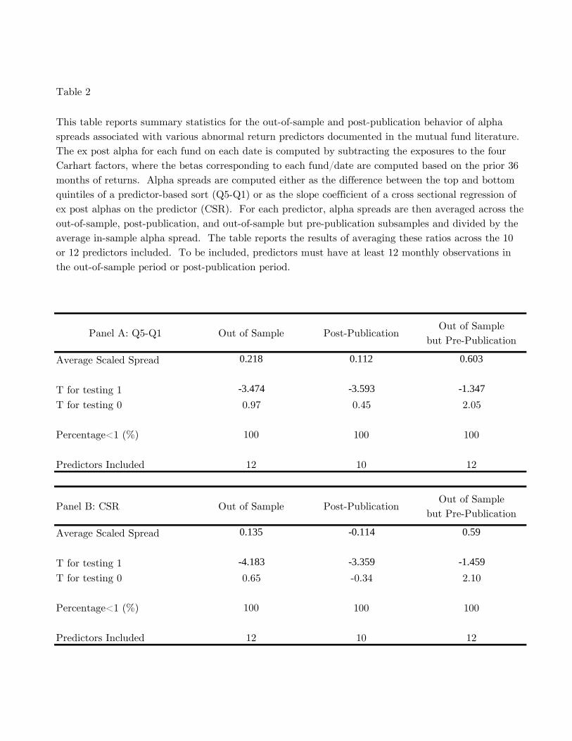
Table 2
Panel A: Q5-Q1 Out of Sample Post-PublicationOut of Sample
but Pre-Publication
Average Scaled Spread 0.218 0.112 0.603
T for testing 1 -3.474 -3.593 -1.347
T for testing 0 0.97 0.45 2.05
Percentage<1 (%) 100 100 100
Predictors Included 12 10 12
Panel B: CSR Out of Sample Post-PublicationOut of Sample
but Pre-Publication
Average Scaled Spread 0.135 -0.114 0.59
T for testing 1 -4.183 -3.359 -1.459
T for testing 0 0.65 -0.34 2.10
Percentage<1 (%) 100 100 100
Predictors Included 12 10 12
This table reports summary statistics for the out-of-sample and post-publication behavior of alpha
spreads associated with various abnormal return predictors documented in the mutual fund literature.
The ex post alpha for each fund on each date is computed by subtracting the exposures to the four
Carhart factors, where the betas corresponding to each fund/date are computed based on the prior 36
months of returns. Alpha spreads are computed either as the difference between the top and bottom
quintiles of a predictor-based sort (Q5-Q1) or as the slope coefficient of a cross sectional regression of
ex post alphas on the predictor (CSR). For each predictor, alpha spreads are then averaged across the
out-of-sample, post-publication, and out-of-sample but pre-publication subsamples and divided by the
average in-sample alpha spread. The table reports the results of averaging these ratios across the 10
or 12 predictors included. To be included, predictors must have at least 12 monthly observations in
the out-of-sample period or post-publication period.
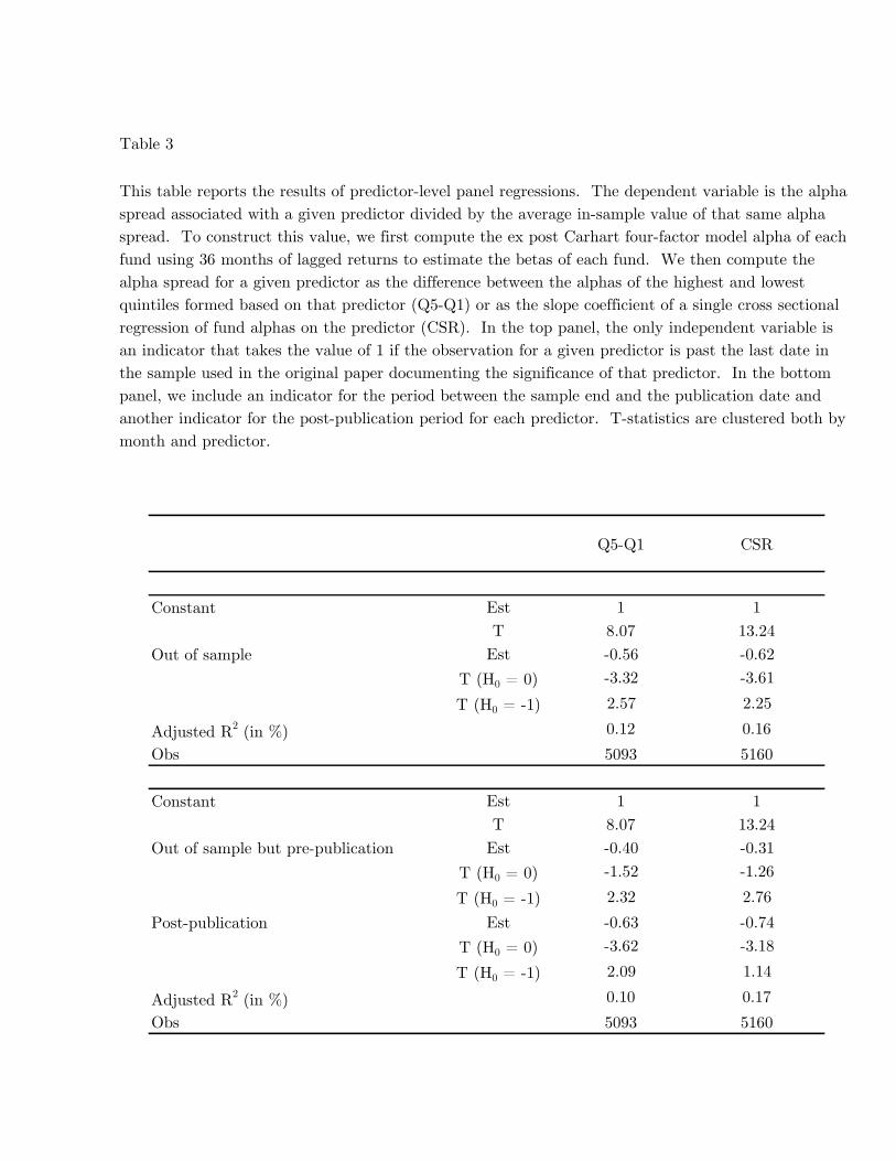
Table 3
Q5-Q1 CSR
Constant Est 1 1
T 8.07 13.24
Out of sample Est -0.56 -0.62
T (H0 = 0) -3.32 -3.61
T (H0 = -1) 2.57 2.25
Adjusted R2 (in %) 0.12
%
0.16
%Obs 5093 5160
Constant Est 1 1
T 8.07 13.24
Out of sample but pre-publication Est -0.40 -0.31
T (H0 = 0) -1.52 -1.26
T (H0 = -1) 2.32 2.76
Post-publication Est -0.63 -0.74
T (H0 = 0) -3.62 -3.18
T (H0 = -1) 2.09 1.14
Adjusted R2 (in %) 0.10
%
0.17
%Obs 5093 5160
This table reports the results of predictor-level panel regressions. The dependent variable is the alpha
spread associated with a given predictor divided by the average in-sample value of that same alpha
spread. To construct this value, we first compute the ex post Carhart four-factor model alpha of each
fund using 36 months of lagged returns to estimate the betas of each fund. We then compute the
alpha spread for a given predictor as the difference between the alphas of the highest and lowest
quintiles formed based on that predictor (Q5-Q1) or as the slope coefficient of a single cross sectional
regression of fund alphas on the predictor (CSR). In the top panel, the only independent variable is
an indicator that takes the value of 1 if the observation for a given predictor is past the last date in
the sample used in the original paper documenting the significance of that predictor. In the bottom
panel, we include an indicator for the period between the sample end and the publication date and
another indicator for the post-publication period for each predictor. T-statistics are clustered both by
month and predictor.
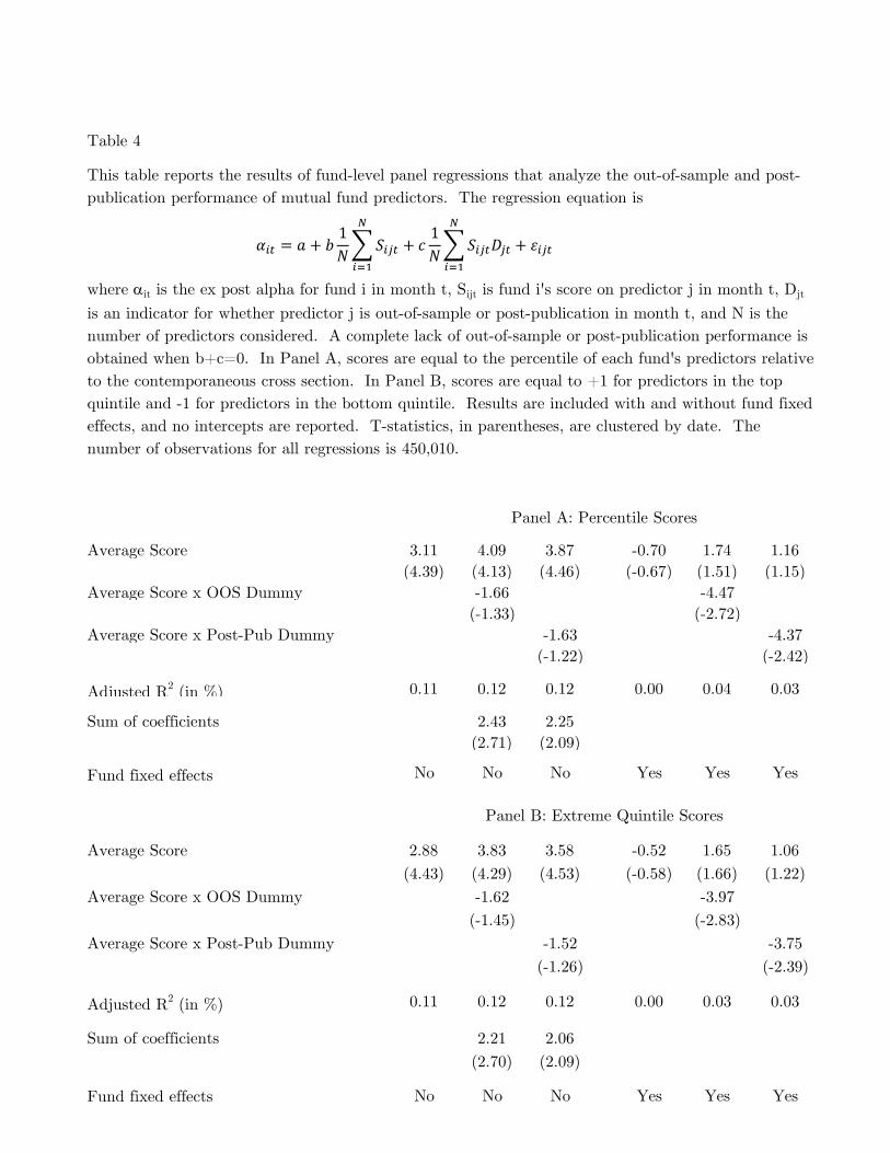
Table 4
Average Score 3.11 4.09 3.87 -0.70 1.74 1.16
(4.39) (4.13) (4.46) (-0.67) (1.51) (1.15)
Average Score x OOS Dummy -1.66 -4.47
(-1.33) (-2.72)
Average Score x Post-Pub Dummy -1.63 -4.37
(-1.22) (-2.42)
Adjusted R2 (in %) 0.11 0.12 0.12 0.00 0.04 0.03
Sum of coefficients 2.43 2.25
(2.71) (2.09)
Fund fixed effects No No No Yes Yes Yes
Average Score 2.88 3.83 3.58 -0.52 1.65 1.06
(4.43) (4.29) (4.53) (-0.58) (1.66) (1.22)
Average Score x OOS Dummy -1.62 -3.97
(-1.45) (-2.83)
Average Score x Post-Pub Dummy -1.52 -3.75
(-1.26) (-2.39)
Adjusted R2 (in %) 0.11
%
0.12
%
0.12
%
0.00
%
0.03
%
0.03
%Sum of coefficients 2.21 2.06
(2.70) (2.09)
Fund fixed effects No No No Yes Yes Yes
Panel B: Extreme Quintile Scores
Panel A: Percentile Scores
This table reports the results of fund-level panel regressions that analyze the out-of-sample and post-
publication performance of mutual fund predictors. The regression equation is
where ait is the ex post alpha for fund i in month t, Sijt is fund i's score on predictor j in month t, Djt
is an indicator for whether predictor j is out-of-sample or post-publication in month t, and N is the
number of predictors considered. A complete lack of out-of-sample or post-publication performance is
obtained when b+c=0. In Panel A, scores are equal to the percentile of each fund's predictors relative
to the contemporaneous cross section. In Panel B, scores are equal to +1 for predictors in the top
quintile and -1 for predictors in the bottom quintile. Results are included with and without fund fixed
effects, and no intercepts are reported. T-statistics, in parentheses, are clustered by date. The
number of observations for all regressions is 450,010.
𝛼𝑖𝑡 = 𝑎 + 𝑏1
𝑁
𝑖=1
𝑁
𝑆𝑖𝑗𝑡 + 𝑐1
𝑁
𝑖=1
𝑁
𝑆𝑖𝑗𝑡𝐷𝑗𝑡 + 𝜀𝑖𝑗𝑡
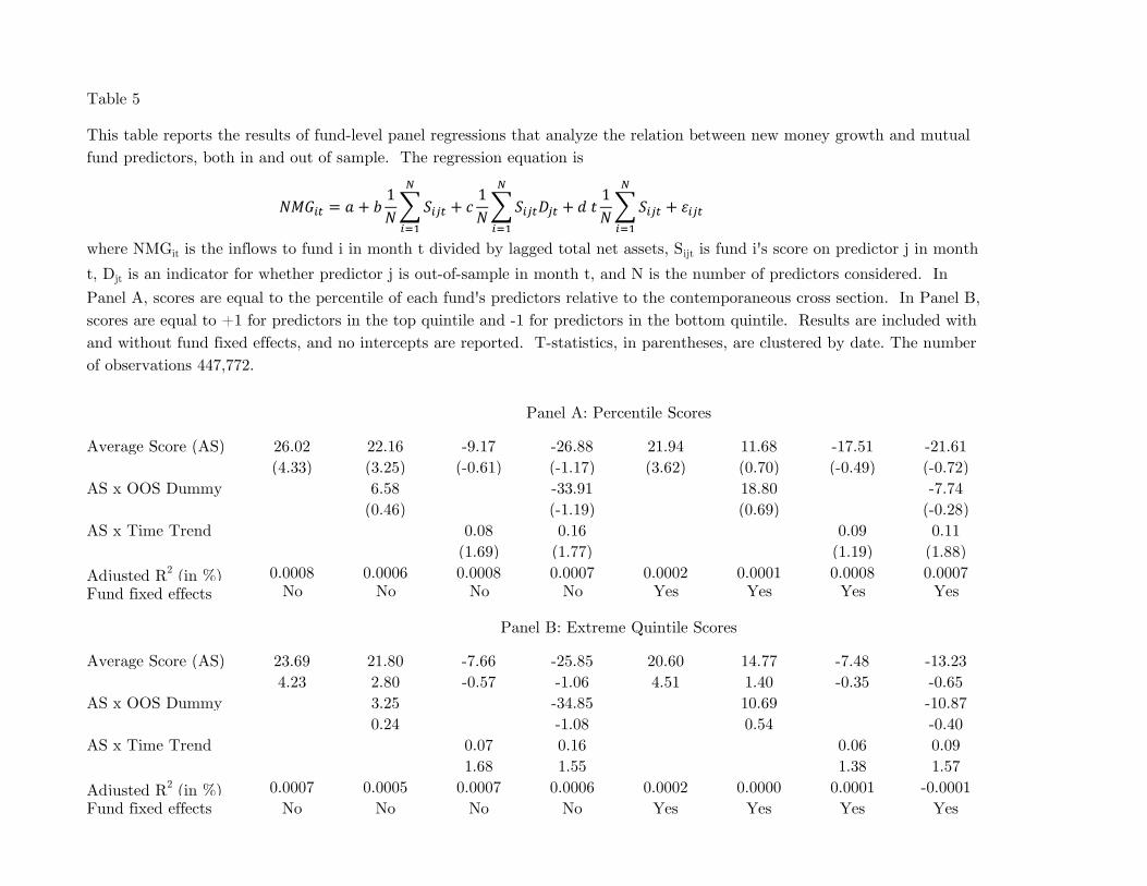
Table 5
Average Score (AS) 26.02 22.16 -9.17 -26.88 21.94 11.68 -17.51 -21.61
(4.33) (3.25) (-0.61) (-1.17) (3.62) (0.70) (-0.49) (-0.72)
AS x OOS Dummy 6.58 -33.91 18.80 -7.74
(0.46) (-1.19) (0.69) (-0.28)
AS x Time Trend 0.08 0.16 0.09 0.11
(1.69) (1.77) (1.19) (1.88)
Adjusted R2 (in %) 0.0008 0.0006 0.0008 0.0007 0.0002 0.0001 0.0008 0.0007
Fund fixed effects No No No No Yes Yes Yes Yes
Average Score (AS) 23.69 21.80 -7.66 -25.85 20.60 14.77 -7.48 -13.23
4.23 2.80 -0.57 -1.06 4.51 1.40 -0.35 -0.65
AS x OOS Dummy 3.25 -34.85 10.69 -10.87
0.24 -1.08 0.54 -0.40
AS x Time Trend 0.07 0.16 0.06 0.09
1.68 1.55 1.38 1.57
Adjusted R2 (in %) 0.0007 0.0005 0.0007 0.0006 0.0002 0.0000 0.0001 -0.0001
Fund fixed effects No No No No Yes Yes Yes Yes
This table reports the results of fund-level panel regressions that analyze the relation between new money growth and mutual
fund predictors, both in and out of sample. The regression equation is
where NMGit is the inflows to fund i in month t divided by lagged total net assets, Sijt is fund i's score on predictor j in month
t, Djt is an indicator for whether predictor j is out-of-sample in month t, and N is the number of predictors considered. In
Panel A, scores are equal to the percentile of each fund's predictors relative to the contemporaneous cross section. In Panel B,
scores are equal to +1 for predictors in the top quintile and -1 for predictors in the bottom quintile. Results are included with
and without fund fixed effects, and no intercepts are reported. T-statistics, in parentheses, are clustered by date. The number
of observations 447,772.
Panel A: Percentile Scores
Panel B: Extreme Quintile Scores
𝑁𝑀𝐺𝑖𝑡 = 𝑎 + 𝑏1
𝑁
𝑖=1
𝑁
𝑆𝑖𝑗𝑡 + 𝑐1
𝑁
𝑖=1
𝑁
𝑆𝑖𝑗𝑡𝐷𝑗𝑡 + 𝑑 𝑡1
𝑁
𝑖=1
𝑁
𝑆𝑖𝑗𝑡 + 𝜀𝑖𝑗𝑡
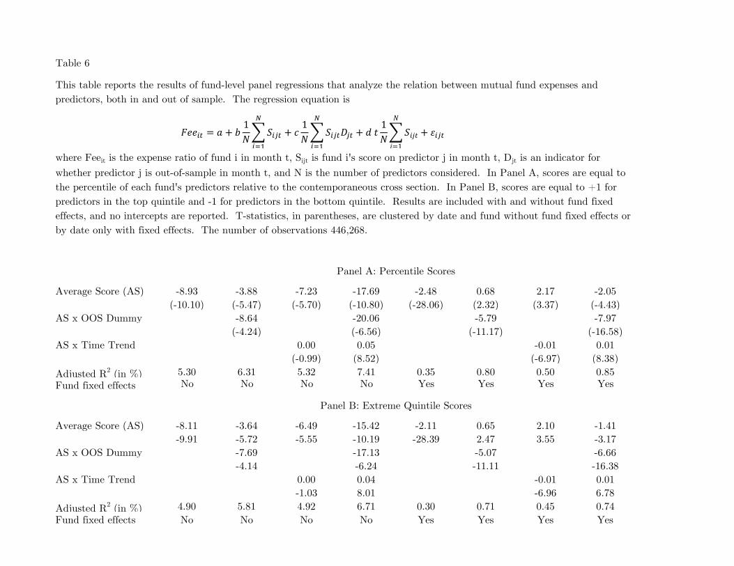
Table 6
Average Score (AS) -8.93 -3.88 -7.23 -17.69 -2.48 0.68 2.17 -2.05
(-10.10) (-5.47) (-5.70) (-10.80) (-28.06) (2.32) (3.37) (-4.43)
AS x OOS Dummy -8.64 -20.06 -5.79 -7.97
(-4.24) (-6.56) (-11.17) (-16.58)
AS x Time Trend 0.00 0.05 -0.01 0.01
(-0.99) (8.52) (-6.97) (8.38)
Adjusted R2 (in %) 5.30 6.31 5.32 7.41 0.35 0.80 0.50 0.85
Fund fixed effects No No No No Yes Yes Yes Yes
Average Score (AS) -8.11 -3.64 -6.49 -15.42 -2.11 0.65 2.10 -1.41
-9.91 -5.72 -5.55 -10.19 -28.39 2.47 3.55 -3.17
AS x OOS Dummy -7.69 -17.13 -5.07 -6.66
-4.14 -6.24 -11.11 -16.38
AS x Time Trend 0.00 0.04 -0.01 0.01
-1.03 8.01 -6.96 6.78
Adjusted R2 (in %) 4.90 5.81 4.92 6.71 0.30 0.71 0.45 0.74
Fund fixed effects No No No No Yes Yes Yes Yes
This table reports the results of fund-level panel regressions that analyze the relation between mutual fund expenses and
predictors, both in and out of sample. The regression equation is
where Feeit is the expense ratio of fund i in month t, Sijt is fund i's score on predictor j in month t, Djt is an indicator for
whether predictor j is out-of-sample in month t, and N is the number of predictors considered. In Panel A, scores are equal to
the percentile of each fund's predictors relative to the contemporaneous cross section. In Panel B, scores are equal to +1 for
predictors in the top quintile and -1 for predictors in the bottom quintile. Results are included with and without fund fixed
effects, and no intercepts are reported. T-statistics, in parentheses, are clustered by date and fund without fund fixed effects or
by date only with fixed effects. The number of observations 446,268.
Panel A: Percentile Scores
Panel B: Extreme Quintile Scores
𝐹𝑒𝑒𝑖𝑡 = 𝑎 + 𝑏1
𝑁
𝑖=1
𝑁
𝑆𝑖𝑗𝑡 + 𝑐1
𝑁
𝑖=1
𝑁
𝑆𝑖𝑗𝑡𝐷𝑗𝑡 + 𝑑 𝑡1
𝑁
𝑖=1
𝑁
𝑆𝑖𝑗𝑡 + 𝜀𝑖𝑗𝑡
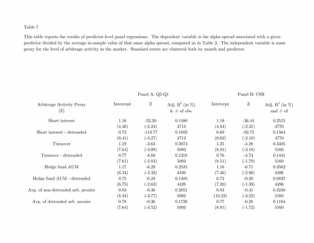
Table 7
Arbitrage Activity Proxy
(Z)
Intercept Z Adj. R2 (in %)
& # of obs.
Intercept Z Adj. R2 (in %)
and # of
observationsShort interest 1.16 -32.20 0.1480 1.19 -36.44 0.2515
(4.46) (-2.24) 4713 (4.84) (-2.31) 4770
Short interest - detrended 0.72 -113.77 0.1892 0.69 -92.75 0.1564
(6.41) (-3.27) 4713 (6.62) (-2.10) 4770
Turnover 1.19 -3.63 0.2074 1.25 -4.28 0.3405
(7.64) (-3.99) 5093 (8.01) (-3.10) 5160
Turnover - detrended 0.77 -4.88 0.1318 0.76 -4.74 0.1441
(7.61) (-2.83) 5093 (8.51) (-1.79) 5160
Hedge fund AUM 1.17 -6.29 0.2531 1.16 -6.71 0.3562
(6.34) (-3.33) 4439 (7.46) (-2.96) 4496
Hedge fund AUM - detrended 0.75 -0.28 0.1485 0.72 -0.20 0.0837
(6.75) (-2.63) 4439 (7.20) (-1.39) 4496
Avg. of non-detrended arb. proxies 0.83 -0.36 0.2051 0.83 -0.41 0.3240
(8.34) (-3.77) 5093 (10.23) (-3.22) 5160
Avg. of detrended arb. proxies 0.78 -0.36 0.1726 0.77 -0.28 0.1184
(7.64) (-3.52) 5093 (8.81) (-1.72) 5160
Panel A: Q5-Q1 Panel B: CSR
This table reports the results of predictor-level panel regressions. The dependent variable is the alpha spread associated with a given
predictor divided by the average in-sample value of that same alpha spread, computed as in Table 2. The independent variable is some
proxy for the level of arbitrage activity in the market. Standard errors are clustered both by month and predictor.
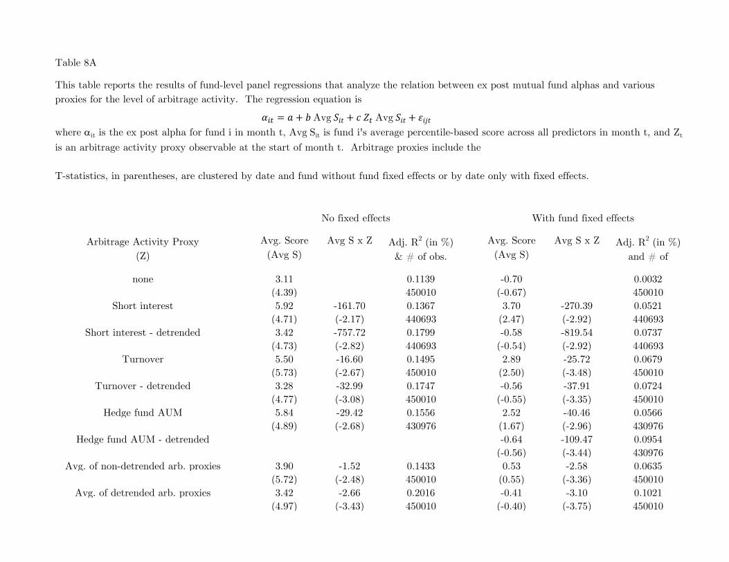
Table 8A
Arbitrage Activity Proxy
(Z)
Avg. Score
(Avg S)
Avg S x Z Adj. R2 (in %)
& # of obs.
Avg. Score
(Avg S)
Avg S x Z Adj. R2 (in %)
and # of
observationsnone 3.11 0.1139 -0.70 0.0032
(4.39) 450010 (-0.67) 450010
Short interest 5.92 -161.70 0.1367 3.70 -270.39 0.0521
(4.71) (-2.17) 440693 (2.47) (-2.92) 440693
Short interest - detrended 3.42 -757.72 0.1799 -0.58 -819.54 0.0737
(4.73) (-2.82) 440693 (-0.54) (-2.92) 440693
Turnover 5.50 -16.60 0.1495 2.89 -25.72 0.0679
(5.73) (-2.67) 450010 (2.50) (-3.48) 450010
Turnover - detrended 3.28 -32.99 0.1747 -0.56 -37.91 0.0724
(4.77) (-3.08) 450010 (-0.55) (-3.35) 450010
Hedge fund AUM 5.84 -29.42 0.1556 2.52 -40.46 0.0566
(4.89) (-2.68) 430976 (1.67) (-2.96) 430976
Hedge fund AUM - detrended -0.64 -109.47 0.0954
(-0.56) (-3.44) 430976
Avg. of non-detrended arb. proxies 3.90 -1.52 0.1433 0.53 -2.58 0.0635
(5.72) (-2.48) 450010 (0.55) (-3.36) 450010
Avg. of detrended arb. proxies 3.42 -2.66 0.2016 -0.41 -3.10 0.1021
(4.97) (-3.43) 450010 (-0.40) (-3.75) 450010
This table reports the results of fund-level panel regressions that analyze the relation between ex post mutual fund alphas and various
proxies for the level of arbitrage activity. The regression equation is
where ait is the ex post alpha for fund i in month t, Avg Sit is fund i's average percentile-based score across all predictors in month t, and Zt
is an arbitrage activity proxy observable at the start of month t. Arbitrage proxies include the
T-statistics, in parentheses, are clustered by date and fund without fund fixed effects or by date only with fixed effects.
No fixed effects With fund fixed effects
𝛼𝑖𝑡 = 𝑎 + 𝑏 Avg 𝑆𝑖𝑡 + 𝑐 𝑍𝑡 Avg 𝑆𝑖𝑡 + 𝜀𝑖𝑗𝑡

Table 8B
Arbitrage Activity Proxy
(Z)
Avg. Score
(Avg S)
Avg S x Z Adj. R2 (in %)
& # of obs.
Avg. Score
(Avg S)
Avg S x Z Adj. R2 (in %)
and # of
observationsnone 2.88 0.1092 -0.52 0.0021
(4.43) 450010 (-0.58) 450010
Short interest 5.44 -147.23 0.1299 3.25 -231.39 0.0431
(4.68) (-2.13) 440693 (2.41) (-2.79) 440693
Short interest - detrended 3.15 -679.71 0.1680 -0.42 -727.13 0.0642
(4.75) (-2.72) 440693 (-0.45) (-2.79) 440693
Turnover 5.09 -15.35 0.1432 2.63 -22.55 0.0591
(5.82) (-2.73) 450010 (2.57) (-3.49) 450010
Turnover - detrended 3.04 -30.34 0.1668 -0.40 -33.88 0.0647
(4.82) (-3.14) 450010 (-0.45) (-3.36) 450010
Hedge fund AUM 5.44 -27.51 0.1504 2.33 -35.51 0.0490
(4.97) (-2.75) 430976 (1.74) (-2.93) 430976
Hedge fund AUM - detrended -0.44 -97.70 0.0852
(-0.45) (-3.41) 430976
Avg. of non-detrended arb. proxies 3.61 -1.40 0.1372 0.55 -2.24 0.0543
(5.77) (-2.52) 450010 (0.66) (-3.32) 450010
Avg. of detrended arb. proxies 3.17 -2.43 0.1909 -0.26 -2.75 0.0907
(5.02) (-3.43) 450010 (-0.30) (-3.70) 450010
This table reports the results of fund-level panel regressions that analyze the relation between ex post mutual fund alphas and various
proxies for the level of arbitrage activity. The regression equation is
where ait is the ex post alpha for fund i in month t, Avg Sit is fund i's average extreme quintile-based score across all predictors in month t,
and Zt is an arbitrage activity proxy observable at the start of month t. Arbitrage proxies include the
T-statistics, in parentheses, are clustered by date and fund without fund fixed effects or by date only with fixed effects.
No fixed effects With fund fixed effects
𝛼𝑖𝑡 = 𝑎 + 𝑏 Avg 𝑆𝑖𝑡 + 𝑐 𝑍𝑡 Avg 𝑆𝑖𝑡 + 𝜀𝑖𝑗𝑡
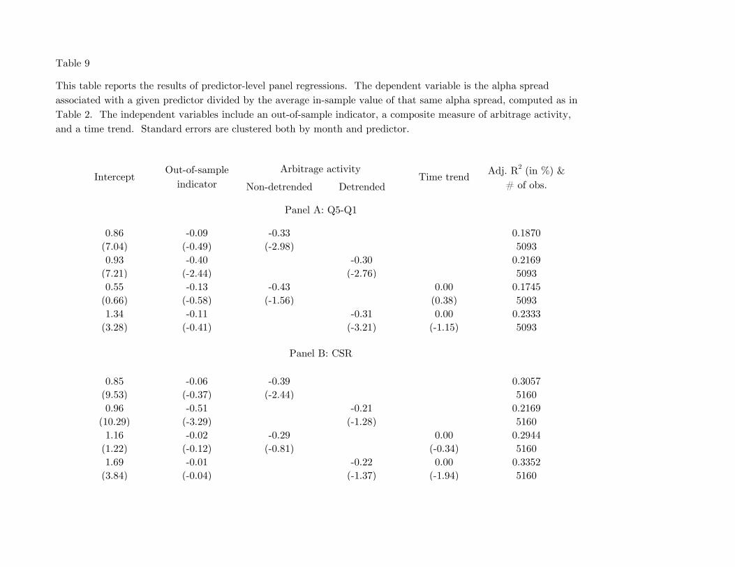
Table 9
Non-detrended Detrended
0.86 -0.09 -0.33 0.1870
(7.04) (-0.49) (-2.98) 5093
0.93 -0.40 -0.30 0.2169
(7.21) (-2.44) (-2.76) 5093
0.55 -0.13 -0.43 0.00 0.1745
(0.66) (-0.58) (-1.56) (0.38) 5093
1.34 -0.11 -0.31 0.00 0.2333
(3.28) (-0.41) (-3.21) (-1.15) 5093
0.85 -0.06 -0.39 0.3057
(9.53) (-0.37) (-2.44) 5160
0.96 -0.51 -0.21 0.2169
(10.29) (-3.29) (-1.28) 5160
1.16 -0.02 -0.29 0.00 0.2944
(1.22) (-0.12) (-0.81) (-0.34) 5160
1.69 -0.01 -0.22 0.00 0.3352
(3.84) (-0.04) (-1.37) (-1.94) 5160
Panel A: Q5-Q1
Panel B: CSR
InterceptOut-of-sample
indicator
Arbitrage activity
This table reports the results of predictor-level panel regressions. The dependent variable is the alpha spread
associated with a given predictor divided by the average in-sample value of that same alpha spread, computed as in
Table 2. The independent variables include an out-of-sample indicator, a composite measure of arbitrage activity,
and a time trend. Standard errors are clustered both by month and predictor.
Time trendAdj. R
2 (in %) &
# of obs.

Table 10
2.99 (2.21) 2.14 (0.78) -2.21 (-1.75) 0.1480 No
3.33 (3.28) 0.16 (0.12) -2.69 (-3.24) 0.2015 No
-7.16 (-2.51) -0.69 (-0.22) -4.83 (-3.22) 0.03 (3.12) 0.1882 No
2.08 (1.08) -0.85 (-0.28) -2.70 (-3.31) 0.00 (0.49) 0.2028 No
0.53 (0.38) -0.01 (-0.00) -2.58 (-2.11) 0.0633 Yes
0.86 (0.76) -2.37 (-1.53) -2.81 (-3.41) 0.1104 Yes
-8.69 (-2.86) -2.69 (-0.90) -4.80 (-3.08) 0.03 (2.63) 0.0907 Yes
0.42 (0.23) -2.72 (-0.93) -2.81 (-3.40) 0.00 (0.18) 0.1103 Yes
2.93 (2.45) 1.65 (0.68) -1.93 (-1.71) 0.1404 No
3.15 (3.44) 0.02 (0.02) -2.43 (-3.21) 0.1907 No
-6.52 (-2.56) -0.84 (-0.31) -4.39 (-3.23) 0.03 (3.26) 0.1794 No
1.86 (1.09) -1.00 (-0.37) -2.45 (-3.30) 0.00 (0.57) 0.1924 No
0.71 (0.61) -0.40 (-0.18) -2.11 (-2.02) 0.0542 Yes
0.89 (0.92) -2.15 (-1.61) -2.49 (-3.33) 0.0988 Yes
-7.84 (-2.90) -2.71 (-1.12) -4.22 (-3.02) 0.02 (2.78) 0.0811 Yes
0.12 (0.08) -2.74 (-1.15) -2.49 (-3.32) 0.00 (0.38) 0.0990 Yes
Fund FE
Panel B: Extreme quintile scores
Panel A: Percentile scores
This table reports the results of fund-level panel regressions of full and restricted versions of
where ait is the ex post alpha for fund i in month t, Sijt is fund i's score on predictor j in month t, Djt is an indicator for whether
predictor j is out-of-sample in month t, and Zt is a composite measure of arbitrage activity. Results are included with and
without fund fixed effects, and no intercepts are reported. T-statistics, in parentheses, are clustered by date and fund without
fund fixed effects or by date only with fixed effects. The number of observations for all regressions is 450,010.
Avg. score
Time trendDetrendedNon-detrended
Avg. score Arbitrage activityAvg. score
Out-of-sampleAvg. score
Adj. R2
(in %)
𝛼𝑖𝑡 = 𝑎 + 𝑏1
𝑁
𝑖=1
𝑁
𝑆𝑖𝑗𝑡 + 𝑐1
𝑁
𝑖=1
𝑁
𝑆𝑖𝑗𝑡𝐷𝑗𝑡 + 𝑑 𝑍𝑡1
𝑁
𝑖=1
𝑁
𝑆𝑖𝑗𝑡 + 𝑒 𝑡1
𝑁
𝑖=1
𝑁
𝑆𝑖𝑗𝑡 + 𝜀𝑖𝑗𝑡