Outdoor Motion Capturing of Ski Jumpers using Multiple Video Cameras

Atle Nes

atle.nes@hist.no

Faculty of Informatics and e-Learning Trondheim University College

Department of Computer and Information ScienceNorwegian University of Science and Technology

General description

Task: Create a cheap and portable video camera system

that can be used to capture and study the 3D motion of ski jumping during take-off and early flight.

Goals:: More reliable, direct and visual feedback More reliable, direct and visual feedback More effective outdoor trainingMore effective outdoor trainingLonger ski jumps!Longer ski jumps!

2D3D solution

Multiple video cameras have been placed strategically around in the ski jumping hill capturing image sequences from different views synchronously.

Allows us to reconstruct 3D coordinates if the same physical point is detected in at least two camera views.

Camera equipment

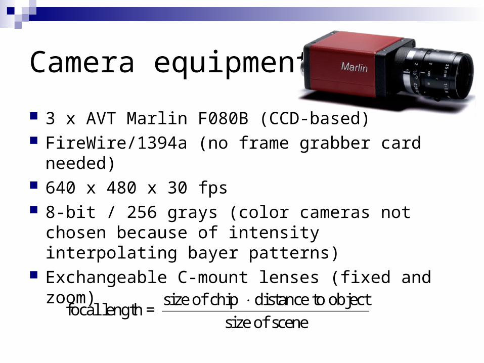
3 x AVT Marlin F080B (CCD-based) FireWire/1394a (no frame grabber card needed) 640 x 480 x 30 fps 8-bit / 256 grays (color cameras not chosen

because of intensity interpolating bayer patterns) Exchangeable C-mount lenses (fixed and zoom)

size of chip distance to object focal length =

size of scene

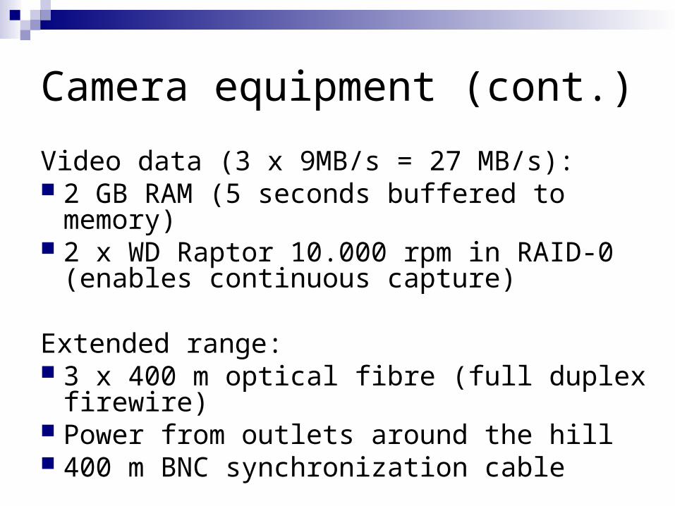
Camera equipment (cont.)

Video data (3 x 9MB/s = 27 MB/s): 2 GB RAM (5 seconds buffered to memory) 2 x WD Raptor 10.000 rpm in RAID-0

(enables continuous capture)

Extended range: 3 x 400 m optical fibre (full duplex firewire) Power from outlets around the hill 400 m BNC synchronization cable

Camera setup

Video data + Control signals

Synch pulse

Direct Linear Transformation

XY

Z

object pointO (x, y, z)

image point I (u, v, 0)

projection centreN (u0, v0, d) (x0, y0, z0)

principal point P (u0, v0, 0)

object space(X, Y, Z)

image plane(U, V)

image space(U, V, W)

W

U

V

- Based on the pinhole model- Linear image formation

DLT: Fundamentals

Classical collinearity equations

Standard DLT equations (aka 11 parameter solution)

11 0 12 0 13 00

31 0 32 0 33 0

21 0 22 0 23 00

31 0 32 0 33 0

( ) ( ) ( )

( ) ( ) ( )

( ) ( ) ( )

( ) ( ) ( )

r x x r y y r z zu u d

r x x r y y r z z

r x x r y y r z zv v d

r x x r y y r z z

1 2 3 4

9 10 11

5 6 7 8

9 10 11

1

1

L x L y L z Lu

L x L y L z

L x L y L z Lv

L x L y L z

Abdel-Aziz and Karara 1971

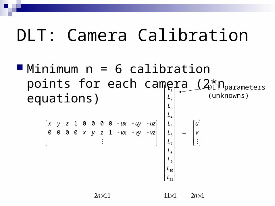
DLT: Camera Calibration

Minimum n = 6 calibration points for each camera (2*n equations)

1

2

3

4

5

6

7

8

9

10

11

1 0 0 0 0

0 0 0 0 1

2 11 11 1 2 1

L

L

L

L

x y z ux uy uz uL

x y z vx vy vz vL

L

L

L

L

L

n n

DLT parameters(unknowns)

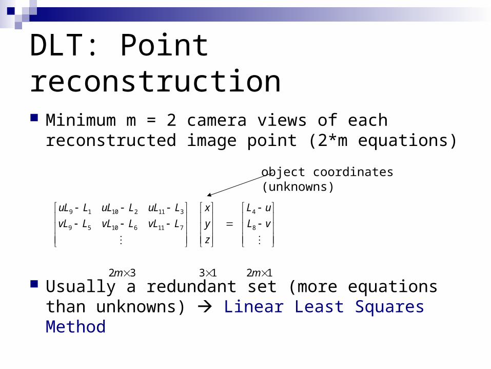
DLT: Point reconstruction

Minimum m = 2 camera views of each reconstructed image point (2*m equations)

Usually a redundant set (more equations than unknowns) Linear Least Squares Method

9 1 10 2 11 3 4

9 5 10 6 11 7 8

2 3 3 1 2 1

uL L uL L uL L x L u

vL L vL L vL L y L v

z

m m

object coordinates(unknowns)

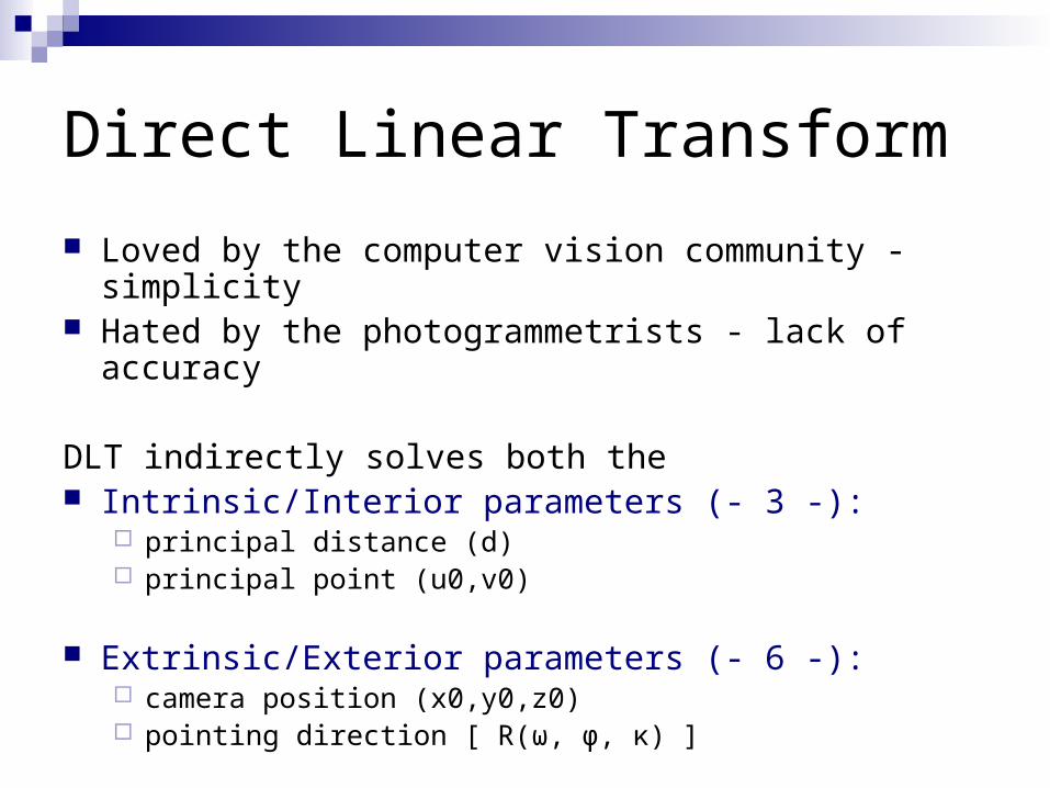
Direct Linear Transform

Loved by the computer vision community - simplicity Hated by the photogrammetrists - lack of accuracy

DLT indirectly solves both the Intrinsic/Interior parameters (- 3 -):

principal distance (d) principal point (u0,v0)

Extrinsic/Exterior parameters (- 6 -): camera position (x0,y0,z0) pointing direction [ R(ω, φ, κ) ]

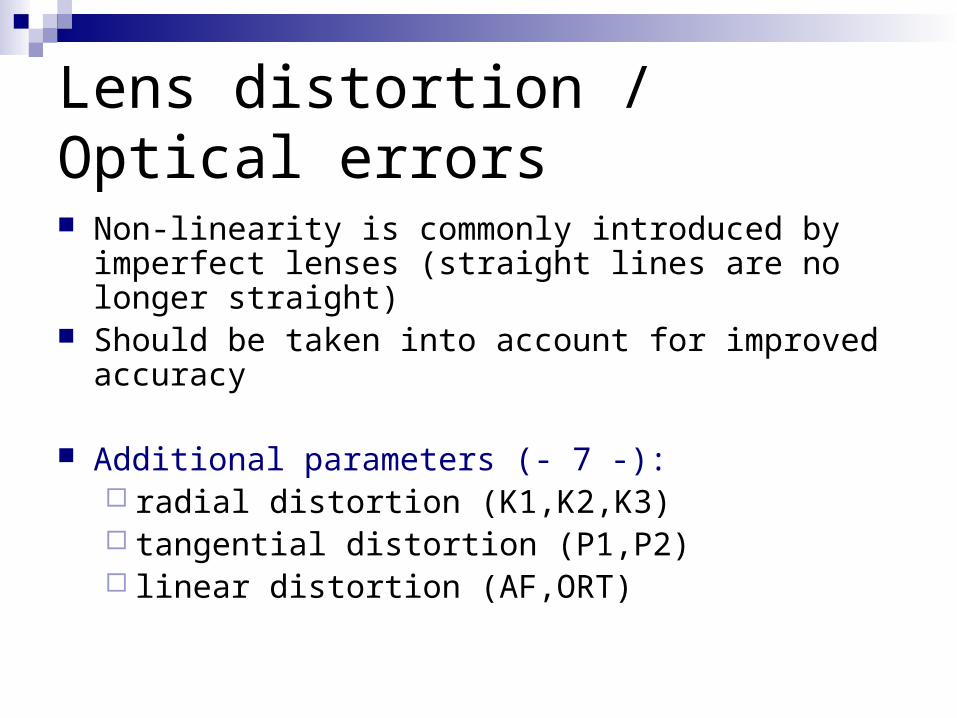
Lens distortion / Optical errors

Non-linearity is commonly introduced by imperfect lenses (straight lines are no longer straight)

Should be taken into account for improved accuracy

Additional parameters (- 7 -): radial distortion (K1,K2,K3) tangential distortion (P1,P2) linear distortion (AF,ORT)

Radial distortion (symmetric)

Barrel distortion

No distortion Pincusion distortion

U U

V V V

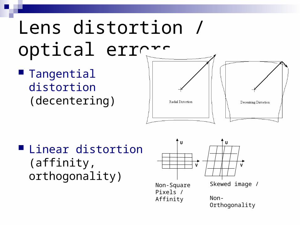
Lens distortion / optical errors

Tangential distortion (decentering)

Linear distortion (affinity, orthogonality)

Non-Square Pixels / Affinity

Skewed image / Non-Orthogonality

U U

V V

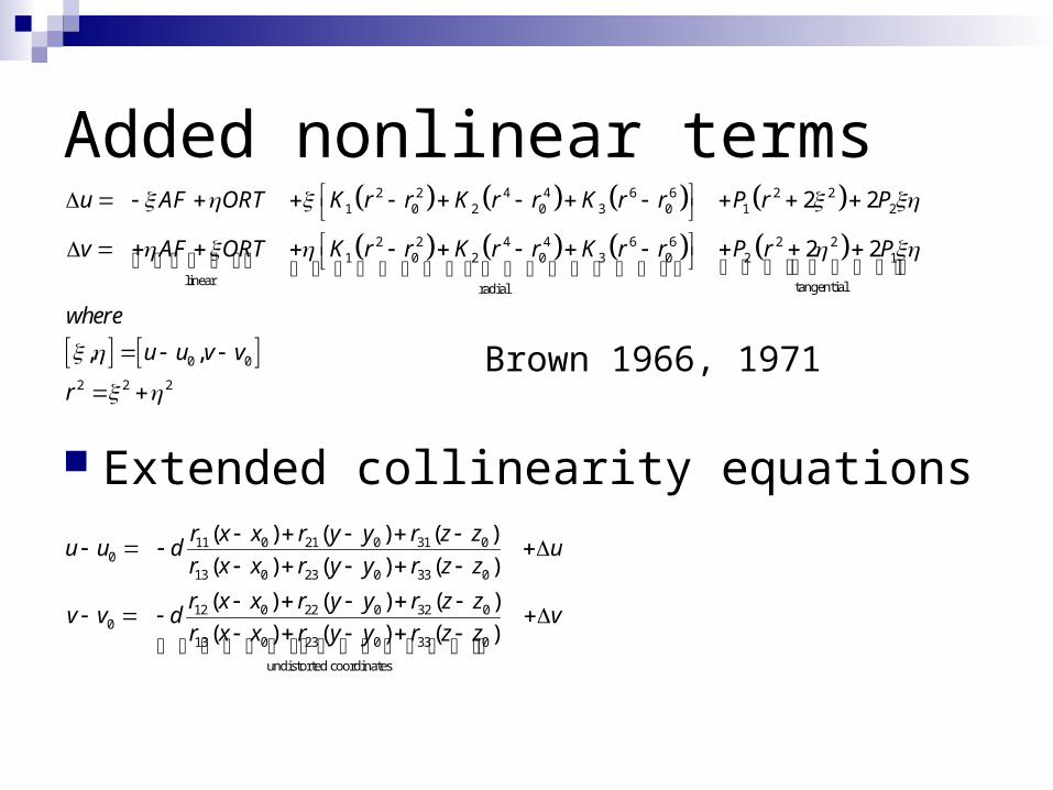
Added nonlinear terms

Extended collinearity equations

2 2 4 4 6 6 2 21 0 2 0 3 0 1 2

2 2 4 4 6 6 2 21 0 2 0 3 0 2 1

linear tangentialradial

0 0

2 2

2 2

2 2

, ,

u AF ORT K r r K r r K r r P r P

v AF ORT K r r K r r K r r P r P

where

u u v v

r

2

11 0 21 0 31 00

13 0 23 0 33 0

12 0 22 0 32 00

13 0 23 0 33 0

undistorted coordinates

( ) ( ) ( )

( ) ( ) ( )

( ) ( ) ( )

( ) ( ) ( )

r x x r y y r z zu u d u

r x x r y y r z z

r x x r y y r z zv v d v

r x x r y y r z z

Brown 1966, 1971

Bundle Adjustment

Requires a good initial parameter guess (for instance from a DLT Calibration)

Non-linear search - Iterative solution using the Levenberg Marquardt Method

Basically: Update one parameter, keep the rest stable, see what happens …Do this systematically

Calibration points and intrinsic/extrinsic parameters can be separated blockwise

The matrix has a sparse structure which can be exploited for lowering the computation time

Detection of outliers

Calibration points with the largest errors are removed automatically/manually resulting in a more stable geometry.

Both image and object point coordinates are considered.

Overview

Direct Linear Transformation is used to estimate the initial intrinsic and extrinsic parameter values for the 2D3D mapping.

Bundle Adjustment is used to refine the parameters and geometry iteratively, including the additional parameters.

Intrinsic & Additional parameters off-site (focal length, principal point, lens distortion)

Extrinsic parameters on-site (camera position & direction)

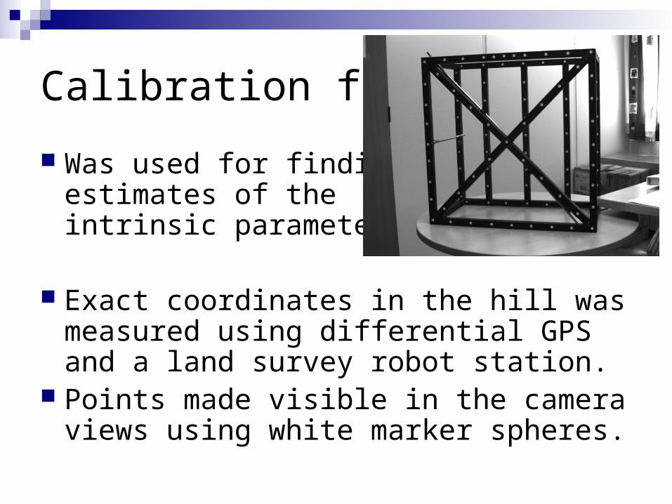
Calibration frame

Was used for finding estimates of theintrinsic parameters.

Exact coordinates in the hill was measured using differential GPS and a land survey robot station.

Points made visible in the camera views using white marker spheres.

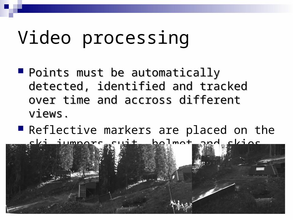
Video processing

Points must be automatically detected, identified Points must be automatically detected, identified and tracked over time and accross different and tracked over time and accross different views.views.

Reflective markers are placed on the ski jumpers suit, helmet and skies.

Video processing (cont.)

Blur caused by fast moving jumpers (100 km/h) is avoided by tuning aperture and integration time.

Three cameras gives a redundancy in case of occluded/undetected points (epipolar lines).

Also possible to use information about the structure of human body to identify relative marker positions.

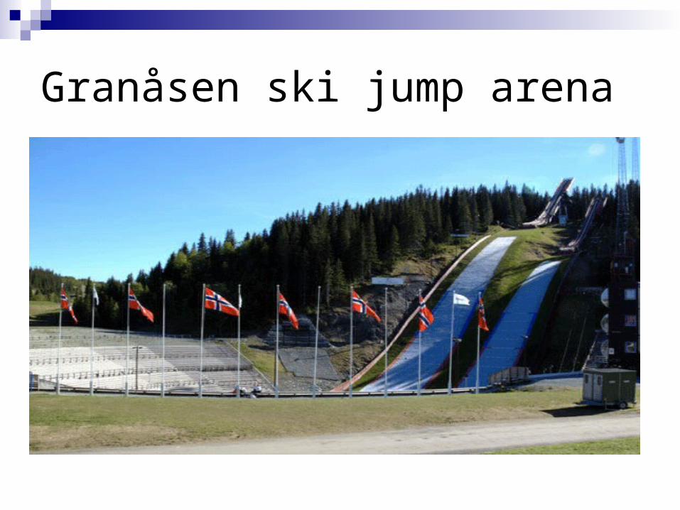
Granåsen ski jump arena

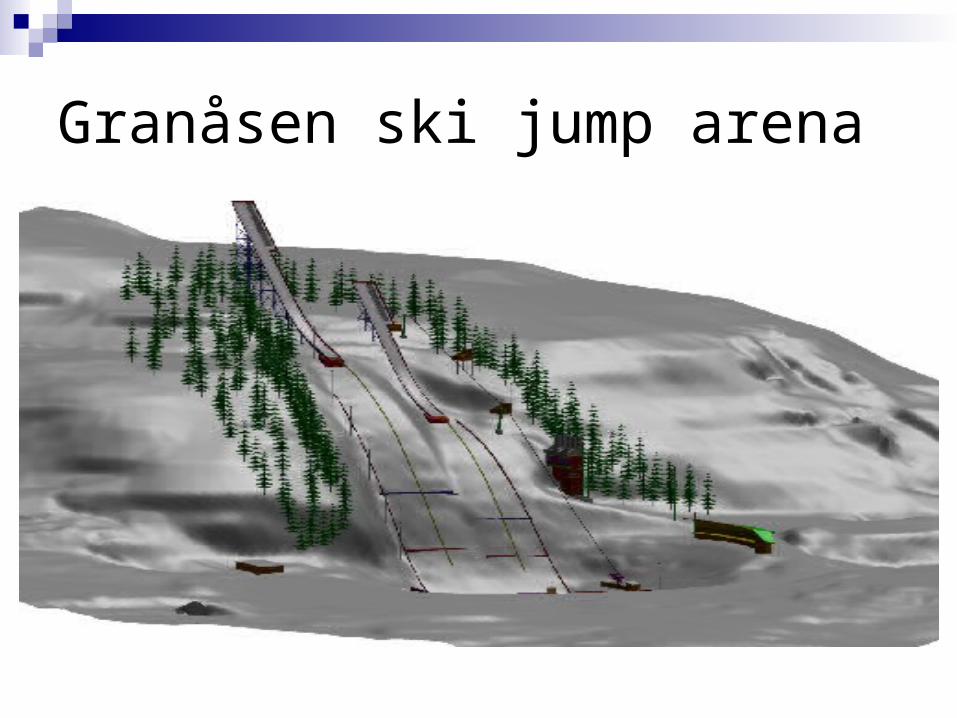
Granåsen ski jump arena

Visualization

Moving feature points are connected back onto a dynamic 3D model of a ski jumper.

Model is allowed to be moved and controlled in a large static model of the ski jump arena.

Results

Reconstruction accuracy: Distance: 30-40 meters

Points in the hill: ~3 cm xyz Points on the ski jumper: ~5 cm xyzD

Future work

Real-Time Capturing and Visualization: Direct Feedback to the Jumpers Time Efficient Algorithms Linear & Closed-Form Solutions

Questions?