outsourcing in the danish fashion · pdf fileusing the economist intelligence unit’s...
TRANSCRIPT
Outsourcing in the Danish FashionIndustry
Christina Valentin Fabritius Eskebaek
Master of Engineering Thesis
Department of Informatics and Mathematical Modelling
Technical University of Denmark
Kongens Lyngby 2007
Technical University of Denmark
Informatics and Mathematical Modelling
Building 321, DK-2800 Kongens Lyngby, Denmark
Phone +45 45253351, Fax +45 45882673
www.imm.dtu.dk
i
Abstract
Purpose Improve the competitive performance of Danish fashion companieswith tools for profit analysis, cost estimates, and supplier comparisons.Suggest management decision support tools for outsourcing through sce-nario analyses.
Design/methodology/approach Use of statistical analysis, operations re-search methodologies, and reviews of trends in global sourcing patterns.
Findings We see a trend towards increased Freight-On-Board production ratherthan Cut-Make-Trim. Macro-economic qualitative measures can be quan-tified to better support outsourcing decisions. Operations research haverelevance to the fashion industry; it provides more profitable suggestionsfor decision-making companies of all sizes.
Research limitations/implications Access to more data than available forthis report could lead to an interesting analysis for matching competitivegoals and supplier types. Confirmation lacks on the precision of quanti-fying macro-economic impacts on sourcing decisions, using the BusinessEnvironment Ranking (developed by the Economist Intelligence Unit).No comparison between model recommendations and the judgement of anexperienced, sourcing professional.
Practical implications The simple tools put forward in this report are sug-gested for inclusion in daily business routines to support outsourcing andpurchasing decisions. Fashion companies are advised to investigate newsuppliers, under the consideration of macro costs, indirect costs, and directcosts in that order.
Originality/value This report examines global fashion business practices froma Danish perspective. Using the Economist Intelligence Unit’s BusinessEnvironment Ranking, the impact of macro-economic perspectives are in-cluded in an outsourcing-decision evaluation. Methods are proposed forestimating costs of delays, errors, wrong deliveries, etc. Price quote struc-tures in the fashion business leave great opportunities for cost savings.
Keywords Sourcing, outsourcing strategies, operations research, Danish fash-ion, master’s thesis, engineering, linear programming, integer program-ming, sourcing, fashion, apparel, clothing, garment, Denmark, compara-tive analyses, economies of production, macro costs, indirect costs, sup-plier comparison, business environment ranking.
Paper type Engineering approach

ii
Executive Summary
Abstract
This is an executive summary of the report based on the M. Sc. Thesis “Out-sourcing in the Danish Fashion Industry”, carried out at the Department ofInformatics and Mathematical Modelling at the Technical University of Den-mark.
This paper outlines the reason for the M.Sc. project and introduces a tool forsupporting management decisions in outsourcing. The tool may be used in thefashion industry to support a more profitable business conduct.
Tests on data sets indicated that there are significant cost advantages to obtainusing this tool, especially for small and mid-sized fashion companies, who aretypical less cost efficient than their large-sized colleagues.
Introduction
The Danish fashion industry is dominated by three large fashion groups within asegment of very price-oriented consumers for whom design is also important. Inthe higher-priced segment, design and branding becomes increasingly important;price remains a factor, though not the primary one. A densely populated groupof fashion players compete in this segment and they account for the majority ofDanish fashion businesses. As these players mainly compete on the local market

iv Executive Summary
but at the same time iconify the Danish self-perception as an internationalfashion nation, the ambition of the industry to turn Copenhagen into a fashioncapital is faced with a dilemma. This is further highlighted by the fact thatthese companies struggle to even yield a profit.
Danish fashion companies all outsource their production, which therefore estab-lishes their main costs. For this reason the report focuses on identifying sourcingmodels and analytical tools to increase company profits.
The development of such tools are inspired by fashion industry consultant, DavidBirnbaum who argues that additional costs are of vital importance when evalu-ating suppliers. It is important to include considerations of macro costs (macroeconomic factors, quota charges, and tariffs) and indirects costs (damaged gar-ments, delays, wrong lot deliveries, and quantity minimums).
The main purpose for this paper is not to give a complete summary of the M.Sc.thesis, “Outsourcing in the Danish Fashion Industry”, but rather to present thetool and methods developed during the project and show the relevance of thetool to the fashion industry.
Project achievements
A tool for supporting management decisions in outsourcing is developed. It isdivided into three steps: strategy, tactics, and operations:
Strategy A method developed and proposed for evaluation on which suppliercollaboration, Freight-on-Board (FOB) or Cut-Make-Trim (CMT), best matchesa company’s competitive profile. The method is versatile enough to include othercollaboration types as well.
Tactics An method is developed for supplier comparison analyses, which in-cludes estimates of macro costs, indirect costs, and supplier price quotations.Furthermethods were developed to perform the cost estimates, and the more interestingare mentioned below:
• Estimating costs of business environmentan experimental meth-ods is suggested for estimating the macro cost of business environment.The method is based on the Business Environment Ranking from the
v
Economist Business Intelligence Unit, but may work for any ranking sys-tem.
• Estimating cost of delays The method include considerations to delaytime and the fashion company’s tolerance towards delays.
• Damaged garments With steady error percentages, this percentage canthen be automatically included in cost comparisons
Operations Methods are developed to increase a company’s profitability buyweeding out low profit styles and include surplus lot ordering to attain costadvantages due to price quotation structures.
The components of the decision tool
In this section the three-step process of the decision tool is briefly sketched:
Strategy: FOB vs. CMT collaborations
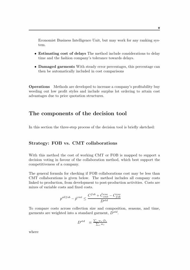
With this method the cost of working CMT or FOB is mapped to support adecision voting in favour of the collaboration method, which best support thecompetitiveness of a company.
The general formula for checking if FOB collaborations cost may be less thanCMT collaborations is given below. The method includes all company costslinked to production, from development to post-production activities. Costs aremixes of variable costs and fixed costs.
pallfob − pcmt ≤Cfob + Ccoo
cmt − Ccoofob
Dstd
To compare costs across collection size and composition, seasons, and time,garments are weighted into a standard garment, Dstd.
Dstd ≡P
sws·Ds
P
s ws
where
vi Executive Summary
Dstd number of ’standard’ garmentsDs the quantity of garment style Ds, e.g. DAW146 is an order of
520 skirts of style #AW146.ws weighted value ws of one piece of garment style Ds, e.g. wAW146
is the added value €14 for each skirt of style #AW146
Tactics: Supplier comparison analysis
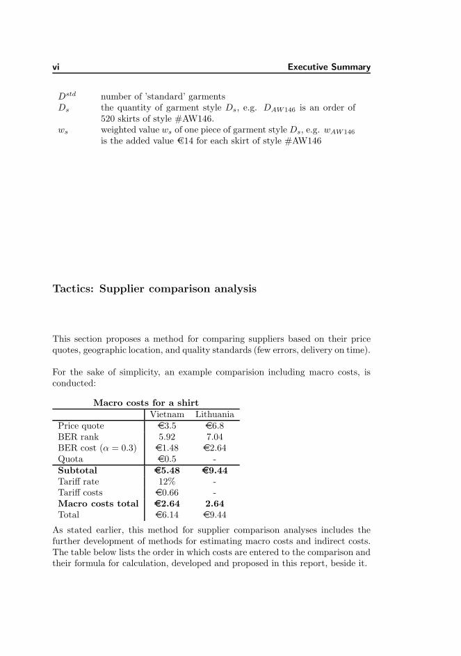
This section proposes a method for comparing suppliers based on their pricequotes, geographic location, and quality standards (few errors, delivery on time).
For the sake of simplicity, an example comparision including macro costs, isconducted:
Macro costs for a shirtVietnam Lithuania
Price quote e3.5 e6.8BER rank 5.92 7.04BER cost (α = 0.3) e1.48 e2.64Quota e0.5 -Subtotal e5.48 e9.44Tariff rate 12% -Tariff costs e0.66 -Macro costs total e2.64 2.64Total e6.14 e9.44
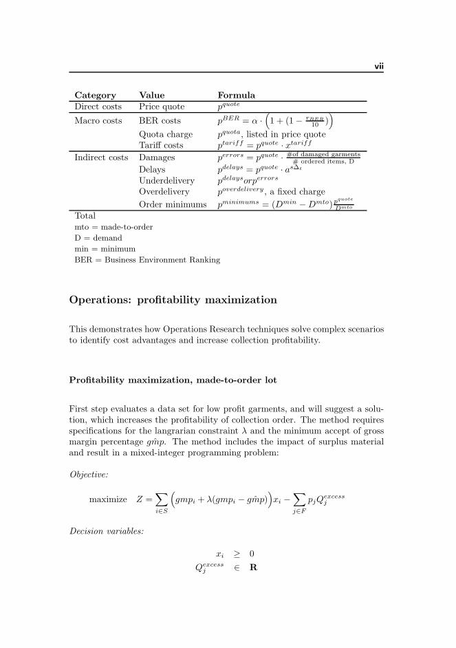
As stated earlier, this method for supplier comparison analyses includes thefurther development of methods for estimating macro costs and indirect costs.The table below lists the order in which costs are entered to the comparison andtheir formula for calculation, developed and proposed in this report, beside it.
vii
Category Value FormulaDirect costs Price quote pquote
Macro costs BER costs pBER = α ·(
1 + (1 − rBER
10 ))
Quota charge pquota, listed in price quoteTariff costs ptariff = pquote · xtariff
Indirect costs Damages perrors = pquote · #of damaged garments# ordered items, D
Delays pdelays = pquote · as∆t
Underdelivery pdelaysorperrors
Overdelivery poverdelivery , a fixed charge
Order minimums pminimums = (Dmin − Dmto)pquote
Dmto
Totalmto = made-to-order
D = demand
min = minimum
BER = Business Environment Ranking
Operations: profitability maximization
This demonstrates how Operations Research techniques solve complex scenariosto identify cost advantages and increase collection profitability.
Profitability maximization, made-to-order lot
First step evaluates a data set for low profit garments, and will suggest a solu-tion, which increases the profitability of collection order. The method requiresspecifications for the langrarian constraint λ and the minimum accept of grossmargin percentage ˆgmp. The method includes the impact of surplus materialand result in a mixed-integer programming problem:
Objective:
maximize Z =∑
i∈S
(
gmpi + λ(gmpi − ˆgmp))
xi −∑
j∈F
pjQexcessj
Decision variables:
xi ≥ 0
Qexcessj ∈ R
viii Executive Summary
Constraints:
xi ≤ Di , ∀i
Qexcessj ≥ 0 , ∀j
Qexcessj +
∑
i∈S
qij
∑
k=0
(d(i,k)y(i,k) + x(i,k)) ≥ Qminj , ∀j
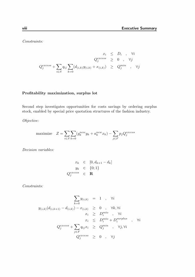
Profitability maximization, surplus lot
Second step investigates opportunities for costs savings by ordering surplusstock, enabled by special price quotation structures of the fashion industry.
Objective:
maximize Z =∑
i∈S
∑
k=0
(gnewk yk + anew
k xk) −∑
j∈F
pjQexcessj
Decision variables:
xk ∈ [0, dk+1 − dk]
yk ∈ {0; 1}
Qexcessj ∈ R
Constraints:
∑
k=0
y(i,k) = 1 , ∀i
y(i,k)(d(i,k+1) − d(i,k)) − x(i,k) ≥ 0 , ∀k, ∀i
xi ≥ Dmtoi , ∀i
xi ≤ Dmtoi + D
surplusi , ∀i
Qexcessj +
∑
j∈F
qijxi ≥ Qminj , ∀j, ∀i
Qexcessj ≥ 0 , ∀j
ix
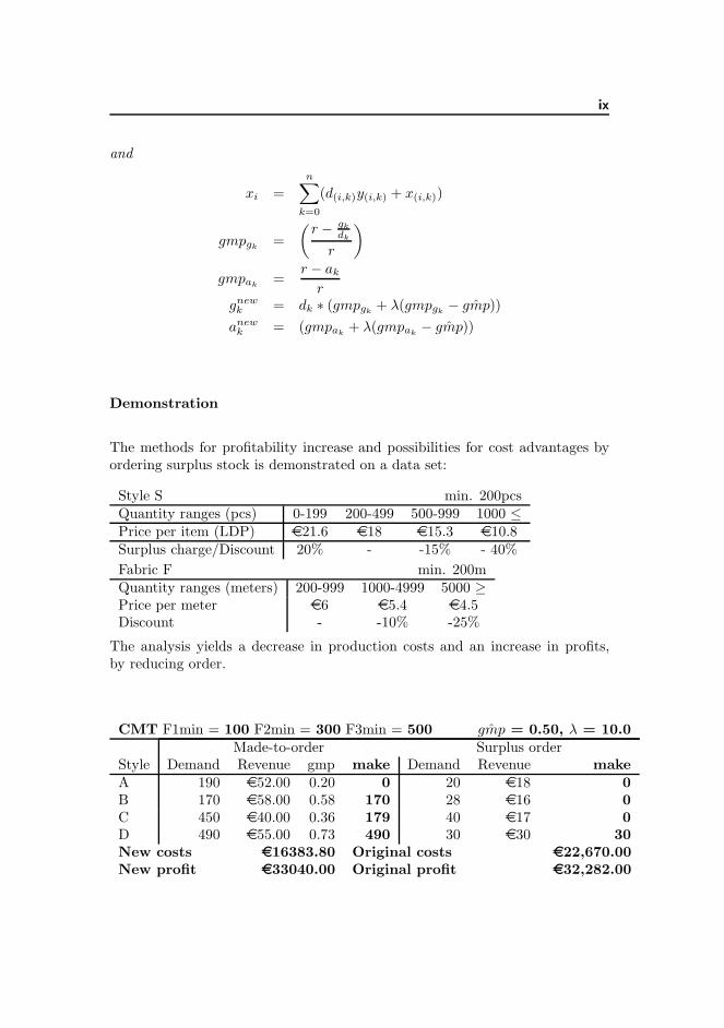
and
xi =
n∑
k=0
(d(i,k)y(i,k) + x(i,k))
gmpgk=
(
r − gk
dk
r
)
gmpak=
r − ak
r
gnewk = dk ∗ (gmpgk
+ λ(gmpgk− ˆgmp))
anewk = (gmpak
+ λ(gmpak− ˆgmp))
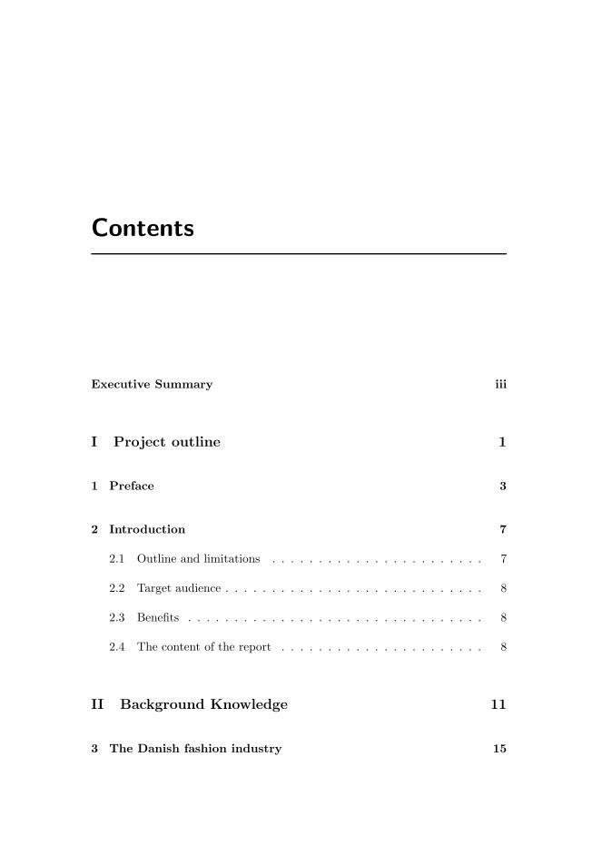
Demonstration
The methods for profitability increase and possibilities for cost advantages byordering surplus stock is demonstrated on a data set:
Style S min. 200pcsQuantity ranges (pcs) 0-199 200-499 500-999 1000 ≤Price per item (LDP) e21.6 e18 e15.3 e10.8Surplus charge/Discount 20% - -15% - 40%
Fabric F min. 200mQuantity ranges (meters) 200-999 1000-4999 5000 ≥Price per meter e6 e5.4 e4.5Discount - -10% -25%
The analysis yields a decrease in production costs and an increase in profits,by reducing order.
CMT F1min = 100 F2min = 300 F3min = 500 ˆgmp = 0.50, λ = 10.0Made-to-order Surplus order
Style Demand Revenue gmp make Demand Revenue makeA 190 e52.00 0.20 0 20 e18 0B 170 e58.00 0.58 170 28 e16 0C 450 e40.00 0.36 179 40 e17 0D 490 e55.00 0.73 490 30 e30 30New costs e16383.80 Original costs e22,670.00New profit e33040.00 Original profit e32,282.00

x Executive Summary
Contents
Executive Summary iii
I Project outline 1
1 Preface 3
2 Introduction 7
2.1 Outline and limitations . . . . . . . . . . . . . . . . . . . . . . . 7
2.2 Target audience . . . . . . . . . . . . . . . . . . . . . . . . . . . . 8
2.3 Benefits . . . . . . . . . . . . . . . . . . . . . . . . . . . . . . . . 8
2.4 The content of the report . . . . . . . . . . . . . . . . . . . . . . 8
II Background Knowledge 11
3 The Danish fashion industry 15
xii CONTENTS
3.1 Characteristics . . . . . . . . . . . . . . . . . . . . . . . . . . . . 15
3.2 Key figures . . . . . . . . . . . . . . . . . . . . . . . . . . . . . . 17
3.3 Competitive factors . . . . . . . . . . . . . . . . . . . . . . . . . . 18
3.4 Business Conduct . . . . . . . . . . . . . . . . . . . . . . . . . . . 19
3.5 Vision: Copenhagen as a fashion capital . . . . . . . . . . . . . . 22
4 Fashion business management 25
4.1 An introduction to D. Birnbaum’s ideas . . . . . . . . . . . . . . 25
4.2 Evaluating Birbaum . . . . . . . . . . . . . . . . . . . . . . . . . 31
4.3 Limitations of Birnbaum . . . . . . . . . . . . . . . . . . . . . . . 36
5 Commen business practice 37
5.1 Cost management . . . . . . . . . . . . . . . . . . . . . . . . . . 39
5.2 Outsourcing practices and country evaluations . . . . . . . . . . 43
5.3 Optimization techniques with operations research . . . . . . . . . 47
III Methods and analyses 49
6 FOB vs. CMT collaborations 53
6.1 Method . . . . . . . . . . . . . . . . . . . . . . . . . . . . . . . . 53
6.2 Results interpreted . . . . . . . . . . . . . . . . . . . . . . . . . . 63
7 Supplier comparison analysis 65
7.1 Quantifying Macro Costs . . . . . . . . . . . . . . . . . . . . . . 65
CONTENTS xiii
7.2 Identifying and Including Indirect Costs . . . . . . . . . . . . . . 70
7.3 Supplier comparison . . . . . . . . . . . . . . . . . . . . . . . . . 74
8 Optimizations with Operations Research 77
8.1 Production Cost Minimization . . . . . . . . . . . . . . . . . . . 77
8.2 Profitability maximization . . . . . . . . . . . . . . . . . . . . . . 87
8.3 Implementation details . . . . . . . . . . . . . . . . . . . . . . . . 94
8.4 Sensitivity analysis . . . . . . . . . . . . . . . . . . . . . . . . . . 94
8.5 Expanding the models . . . . . . . . . . . . . . . . . . . . . . . . 96
8.6 Findings . . . . . . . . . . . . . . . . . . . . . . . . . . . . . . . . 96
9 Outsourcing decision tool 99
IV Evaluation and conclusions 103
10 Evaluation and future work 107
11 Conclusions 109
V Appendices 111
A Cost accounting 113
B Investment Analysis 117
C Case stories 119
xiv CONTENTS
D Glossary 125
E Company data collection 127
F Sensitivity analysis 137
F.1 Testing fabric minimums . . . . . . . . . . . . . . . . . . . . . . . 137
F.2 Testing revenues for mto and surplus lots . . . . . . . . . . . . . 139
F.3 Testing ˆgmp . . . . . . . . . . . . . . . . . . . . . . . . . . . . . . 141
F.4 Testing λ . . . . . . . . . . . . . . . . . . . . . . . . . . . . . . . 142
F.5 Testing λ and ˆgmp combined . . . . . . . . . . . . . . . . . . . . 144
List of Figures
3.1 Collection, styles, variants, and production lot . . . . . . . . . . . 16
3.2 Competive factors, price and design . . . . . . . . . . . . . . . . 18
3.3 The development process in 5 steps . . . . . . . . . . . . . . . . . 20
3.4 An example of estimated cost distributions in a Danish fashioncompany . . . . . . . . . . . . . . . . . . . . . . . . . . . . . . . . 21
5.1 Concept of distributing fixed costs for full costing (left) and ABC(right) . . . . . . . . . . . . . . . . . . . . . . . . . . . . . . . . . 42
6.1 Supplier collaboration type and cost structure . . . . . . . . . . . 57
7.1 Different examples for constraint functions . . . . . . . . . . . . . 68
8.1 Stepwise decreasing item prices, illustrated . . . . . . . . . . . . 79
8.2 All b-values are 0 . . . . . . . . . . . . . . . . . . . . . . . . . . . 79
8.3 Stepwise decreasing prices, continuous price curve . . . . . . . . . 80

xvi LIST OF FIGURES
8.4 Material costs rise as more garments are produced . . . . . . . . 82
E.1 Illustration of the data collected from companies and the inter-relationship between the data blocks. . . . . . . . . . . . . . . . . 129
List of Tables
3.1 The clothing industry, figures of 2006 [8][10] . . . . . . . . . . . . 17
4.1 Example of macro cost analysis: Quota restrictions [3] . . . . . . 28
4.2 Example of macro cost analysis: EU added costs [3] . . . . . . . 28
4.3 Example of macro cost analysis: Tariff costs . . . . . . . . . . . . 28
4.4 Minimum quantities reflects in the indirect costs . . . . . . . . . 29
4.5 Example of indirect cost analysis: . . . . . . . . . . . . . . . . . . 29
4.6 Example of cost comparison . . . . . . . . . . . . . . . . . . . . . 30
4.7 FVCA analysis . . . . . . . . . . . . . . . . . . . . . . . . . . . . 31
4.8 Distribution of fixed costs . . . . . . . . . . . . . . . . . . . . . . 35
5.1 Accumulating costs for a shirt . . . . . . . . . . . . . . . . . . . . 41
5.2 Price quote comparisons, as benchmark for negotiations . . . . . 46
7.1 The raking model suggested by Jones . . . . . . . . . . . . . . . 66
xviii LIST OF TABLES
7.2 Overdelivery and underdelivery on the same order . . . . . . . . 73
7.3 The cost elements of a supplier comparison, ordered by calcula-tion procedure . . . . . . . . . . . . . . . . . . . . . . . . . . . . 74
8.1 Stepwise decreasing prices for a garment style . . . . . . . . . . . 78
8.2 Fabric purchase, with quantity discounts. . . . . . . . . . . . . . 78
8.3 Style specifications . . . . . . . . . . . . . . . . . . . . . . . . . . 84
8.4 Fabric specifications . . . . . . . . . . . . . . . . . . . . . . . . . 84
8.5 Results of FOB cost minimization . . . . . . . . . . . . . . . . . 86
8.6 Manufacturing cost curves . . . . . . . . . . . . . . . . . . . . . . 86
8.7 Results of FOB cost minimization . . . . . . . . . . . . . . . . . 86
8.8 Compounded cost curves . . . . . . . . . . . . . . . . . . . . . . . 87
8.9 Collection overview for styles and material linkage . . . . . . . . 89

Part I
Project outline

Chapter 1
Preface
Motivation
While working with the fashion industry in Denmark I began searching for infor-mation to understand the strategic challenges of setting up a fashion companyin an already overflowed market. I came across the books of David Birnbaum,a fashion professional, who after working in the fashion industry for years, hasnow become a strategic consultant for countries anxious to build a stable fash-ion industry or large companies who wish to improve their competitiveness byworking more profitably.
In a world with quota restrictions, declines in the work force of countries withwell-developed fashion industries and frequent pessimistic forecasts for fashionbusinesses make the outlook for fashion businesses in the western world mayseem pretty gloomy.
I was intrigued by Birnbaum’s optimistic forecasts for companies willing to em-brace challenges and changes. His refreshingly positive analysis of the dynamicsof the global fashion industry certainly leaves the impression that there is workto be done. His arguments have inspired me to investigate his ideas in a Danishfashion industry context.
4 Preface
A Danish perspective
In Denmark there is a strong conception of having a particular fashion identity.However, this notion is not echoed internationally, and political initiatives tosupport the industry’s ambition for recognition are virtually non-existent. Thedensely populated market of small creative fashion companies plays a significantrole in the Danish fashion epos, but in reality profits are low and the numberof names making an international breakthrough continue to be modest. Thefashion industry’s economic contribution to Denmark is mainly provided bythree fashion companies, BTX group, Bestseller, and IC Company’s, all of themrun sound professional businesses. If the rest of the Danish fashion world wishto rise to this level, they need more than a good story and creative designs: theyneed capital and management.
The authors background
I have studied software engineering at the Technical University of Denmarksince August 2000. My academic focus set off in computer graphics with specialemphasis on garment simulation and virtually tailored garments. This interestwas spurred on by studying automatic pattern-making for the garment industryat the Hong Kong University of Science and Technology for two semesters in2002 and 2005, respectively, in the mechanics department under Prof. MatthewYuen. My bachelor’s thesis used optimization techniques from Operations Re-search, to aid the development of large tree structures by using a 3D graphicalrepresentation. Courses at Copenhagen Business School in the Fall of 2005 pro-vided me with insights to luxury industries, as well as global and local brandingstrategies.
Since August 2005, running parallel with my studies, I have worked as a produc-tion agent and sales agent for minor Danish fashion companies. As a sales agentI have established sales channels and direct sales on the Danish, English andSwedish markets. Through responsibilities in outsourcing entire collections toEast-Europe and Asia, I developed easy tools to support good outsourcing de-cisions. My pre-university education as a garment pattern-developer was usefulduring this period.
5
Quantitative methods
In this report, I suggest the use of certain analytical tools to enhance sup-port measures for outsourcing decisions in fashion companies. Techniques fromoperations research are applied to develop profit optimization and cost mini-mization models. Statistics and accounting methods are used for comparingcosts of sourcing collaborations, and basic math is used in cost estimates.
Acknowledgements
I would like to thank my supervisor professor Jens Clausen of the TechnicalUniversity of Denmark for his guidance on this report and help issues within op-erations research. Thanks are also due to Thomas Ernfeldt from IC Company’sfor contributing valuable insights into the fashion industry, John Eskebaek forinformation on practices in the food industry, as well as Jan Fabritius for inputto financial codes of conduct, and intensive help with structuring the analysis inchapter 6. I am very grateful to Jeanny Fabritius for extensively proofreadingmy English.

6 Preface
Chapter 2
Introduction
2.1 Outline and limitations
This report seeks to develop methods to support outsourcing decisions in theDanish fashion industry on both strategic, tactical, and operational levels. Threemethods must be developed to use as one tool:
Strategy Create method to investigate which supplier type, Cut-Make-Trimor Freight-on-Board, enhances the competitiveness of a fashion company.
Tactic Present method to compare suppliers including direct costs, indirectcosts, and macro costs. Develop methods for estimates none exist already.
Operation Construct method to support purchasing decisions at to increasingprofits or profitability, making the most of the fashion industry’s pricestructures.
The first two methods are developed from the basis of author, David Birnbaumwho’s views and recommendations are investigated in a Danish context.
8 Introduction
2.2 Target audience
The aim of this report is two-fold. As an engineering masters thesis, this reportwill demonstrate my analytical skills in approaching a subject - in this casethe fashion industry. The setting for my application of academic ideas hasbeen determined by my intention to brief the non-fashion professional readerabout the nature of the fashion industry, and its characteristics in Denmark inparticular.
For fashion professionals with a more usage-oriented approach, I attempt todemonstrate the usefulness of available analytical and mathematical tools, whichcould benefit profits and support sourcing decisions.
2.3 Benefits
Fashion professionals will learn about specific tools in order to gain better in-sights into sourcing scenarios and their outcome. They will be able to identifyopportunities for cost savings within the costs structures of their industry. Fur-thermore, they will obtain tools to quantify qualitative measures so as to makea better choice when evaluating sourcing opportunities. Other readers stand togain interesting insights into learnings from the fashion industry. Applicationsof mathematical tools and logical analysis may inspire readers from other indus-tries, especially in terms of best practices and recommendations for outsourcinganalyses.
2.4 The content of the report
Outcome:
• A tool for supporting outsourcing decisions on strategic, tactical, opera-tional levels.
• A method for analysing and comparing the costs of two main suppliercollaboration types, Freight-On-Board and Cut-Make-Trim.
• A method for estimating macro costs using a country ranking system whichincludes weights on political climate, educational level, and trade barriers,etc. Macro costs also include quota restrictions and import tariffs.
2.4 The content of the report 9
• A method for calculating indirect costs in of delays, damaged goods, andwrong deliveries.
• A method for comparing suppliers based on price quotations, quantityminimum’s, macro costs, and indirect costs.
• A method for profit maximization in purchasing decisions, by discardinglow-profit products and purchasing surplus stock to gain quantity dis-counts. Profits were increased on a test data set with 5%.
• Investigation of David Birnbaum’s views in a Danish context
Given the mixed target audience of this thesis, I will begin by introducing thereader to the main characteristics of the Danish fashion industry, some featuresof which will be shared with fashion businesses worldwide. The reader willlearn about the relative size and competitive landscape of Denmark as opposedto other markets, as well as Denmark’s frequently stated vision of becoming theworld’s fifth fashion capital; a title fiercely challenged by other aspiring citiesworldwide, e.g. Antwerp, Tokyo, and Los Angeles. The highly competitiveenvironment of Denmark leaves too little a profit to the take on heavy brandingand marketing resources needed to funnel an international breakthrough for afashion company. Denmark would need quite a few of these breakthroughs to beable to successfully claim the title as a, generally acknowledged, fashion capital.
In the interest of identifying qualified management tools to increase the profitmargin of Danish fashion companies, I wanted to compile the existing literatureon the subject. Sources turned out to be quite scarce. However, for the purposeof Chapter 4 the works of D. Birnbaum claim a prominent position and his toolsand ideas are presented in a summarized form to the reader. Birnbaum suggestshow companies may sort their costs into three categories (macro costs, indirectcosts and direct costs) to obtain a better understanding of which decisions willprovide the most profitable outcome. Birnbaum’s suggested methodology formaking costs comparisons between different suppliers is accounted for, and cri-tique is given to his less than direct-deployable model. Subsequently, his claimsand views are evaluated in the light of additional literature on the fashion in-dustry and trends.
The next chapter discuss methods and techniques of improving profitability inoutsourcing decisions. General best practises for management conduct are validin all industries. No additional learnings are found in industries that sharecharacteristics with the fashion industry.
With knowledge acquired from previous chapters, a method is proposed to eval-uating which outsourcing method is the more profitable to a fashion company.
10 Introduction
Due to limited data access the chapter is mainly based on theory while suggest-ing a method to challenge the claim that Freight-On-Board sourcing is moreprofitable than Cut-Make-Trim sourcing.
Following Birnbaum’s suggestion to compare suppliers and thus finding the leastexpensive, work is conducted to measure macro costs and indirect costs. Toaccount for macro costs I develop a macro cost factor, in chapter 7 using a widelyacknowledged ranking system. Suggestions are put forward on how to adjustthe macro cost factor to suit fashion industry specifics. It is also concretizedhow to include tariff and quota costs in comparative analyses, as well as howto identify, quantify, and include indirect costs. A small data set is produced inan attempt to demonstrate how to perform full-scale analyses.
Chapter 8 presents a method for further increase in profitability, using tech-niques from the operations research (OR). The simplified model of cost min-imizations serve to illustrate the concept and deployment of OR methods. Amethod is given to identify cost saving opportunities by ordering surplus stock,taking advantage of price quote structures on materials and production, as wellas quantity minimums. The model is extended into a profit maximization model,to suggest letting go of low-profit products and to advance qualified recommen-dations for purchasing surplus stock. A demonstration is provided using realisticdata extended and the models tested for stability and strength.
Chapter 9 combines the tree methods of the previous chapters into one toolfor supporting manager’s sourcing decisions. Perspectives and evaluations ofthis report alert the reader to new trends in competitive factors, which may bebetter facilitated with Cut-Make-Trim production.
In conclusion the report lists the primary findings of the work presented.

Part II
Background Knowledge

13
In this part..
This part contains three chapters with background knowledge for to understandthe settings for the work presented in this report.
First chapter provides a sketch of the fashion industry and it’s outline in Den-mark especially. Logic and premises of the fashion industry are introducedincluding definitions of industry terms to be used interchangeably throughoutthe rest of the report.
The second chapter deals with the tools and ideas of David Birnbaum, whoinspired this thesis. Birnbaum’s claims and ideas are summarized and thenchallenged using related literature. The relevance of his recommendations in aDanish context is confirmed.
Finally, focus on management methods and guidelines in general. The chap-ter investigates methods for cost and profit analyses. Based on a report fromThe Confederation of Danish Industries, recommendations for good outsourc-ing practices are given. Furthermore, a brief introduction on operations research(OR) techniques is given as OR can help companies in decision analysis.

14

Chapter 3
The Danish fashion industry
The chapter aims at giving the reader background knowledge of the fashionindustry in general and in Denmark particularly, with information on maincharacteristics, key figures, and competitive factors. Key terms will be explainedand important structures in business logic introduced as well as information onbusiness conduct and decision processes will be described. The Danish visionto proclaim Copenhagen a fashion capital and the prerequisites to do so, isdiscussed.
This chapter main basis in interviews with case companies, as well as sources[15], [29], [24], [11], [22]
3.1 Characteristics
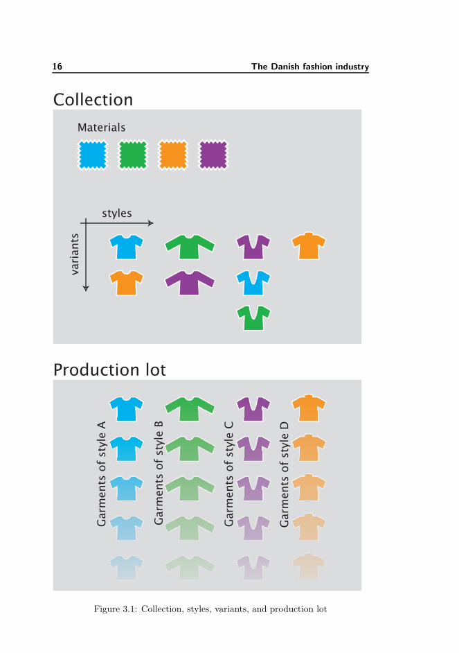
The Danish fashion industry is populated by small and medium-sized businesses.Each season fashion products are gathered in new style collections, available inmultiple colour variants (see figure 3.1. A small fashion company will develop 50-1,000 new styles a year, distributed over two to four seasons, and a medium-sizedcompany may develop up to 5,000 new styles a year for as many as eight seasons.In Denmark most companies work with two primary seasons and occasionally
16 The Danish fashion industry
CollectionGarments of style A
Garments of style B
Garments of style C
Garments of style D
Materials
variants
styles
Production lot
Figure 3.1: Collection, styles, variants, and production lot
3.2 Key figures 17
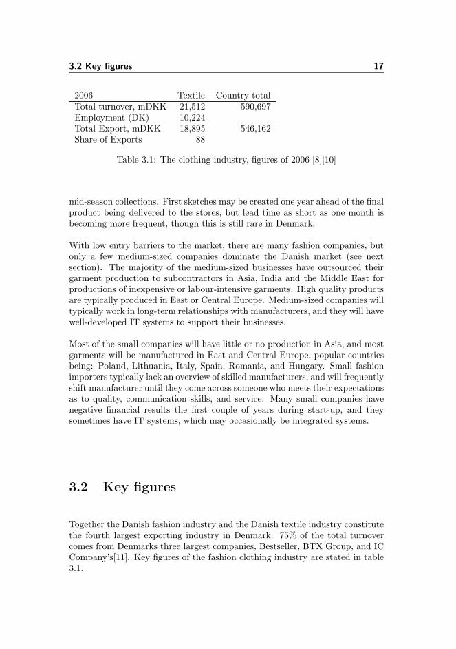
2006 Textile Country totalTotal turnover, mDKK 21,512 590,697Employment (DK) 10,224Total Export, mDKK 18,895 546,162Share of Exports 88
Table 3.1: The clothing industry, figures of 2006 [8][10]
mid-season collections. First sketches may be created one year ahead of the finalproduct being delivered to the stores, but lead time as short as one month isbecoming more frequent, though this is still rare in Denmark.
With low entry barriers to the market, there are many fashion companies, butonly a few medium-sized companies dominate the Danish market (see nextsection). The majority of the medium-sized businesses have outsourced theirgarment production to subcontractors in Asia, India and the Middle East forproductions of inexpensive or labour-intensive garments. High quality productsare typically produced in East or Central Europe. Medium-sized companies willtypically work in long-term relationships with manufacturers, and they will havewell-developed IT systems to support their businesses.
Most of the small companies will have little or no production in Asia, and mostgarments will be manufactured in East and Central Europe, popular countriesbeing: Poland, Lithuania, Italy, Spain, Romania, and Hungary. Small fashionimporters typically lack an overview of skilled manufacturers, and will frequentlyshift manufacturer until they come across someone who meets their expectationsas to quality, communication skills, and service. Many small companies havenegative financial results the first couple of years during start-up, and theysometimes have IT systems, which may occasionally be integrated systems.
3.2 Key figures
Together the Danish fashion industry and the Danish textile industry constitutethe fourth largest exporting industry in Denmark. 75% of the total turnovercomes from Denmarks three largest companies, Bestseller, BTX Group, and ICCompany’s[11]. Key figures of the fashion clothing industry are stated in table3.1.
18 The Danish fashion industry
price price/design design
Europe
Denmark
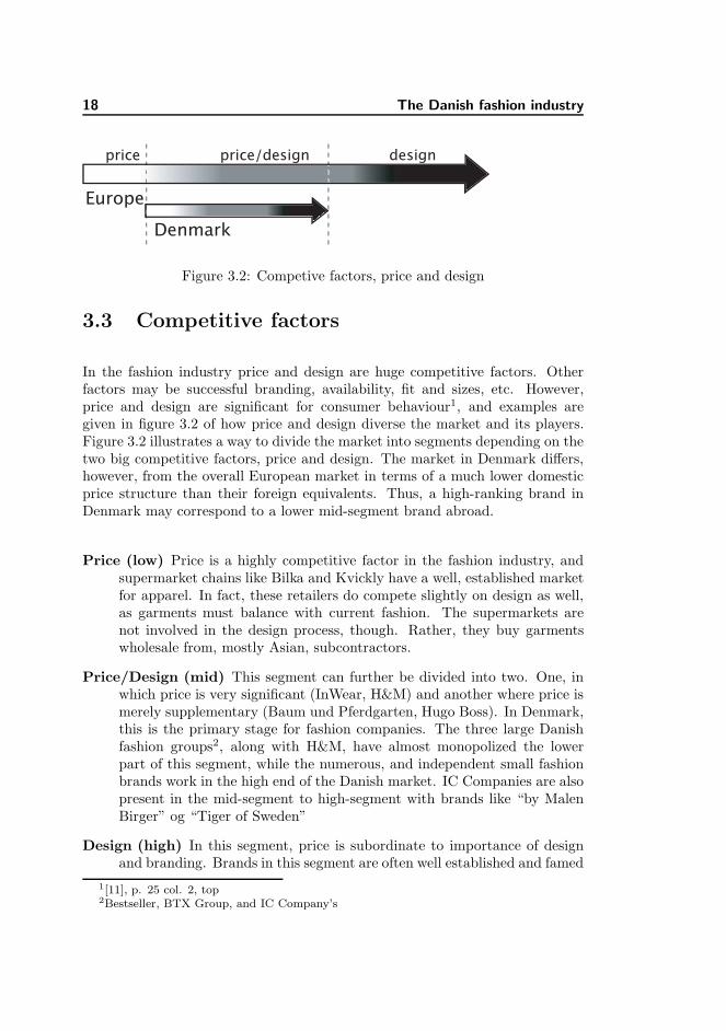
Figure 3.2: Competive factors, price and design
3.3 Competitive factors
In the fashion industry price and design are huge competitive factors. Otherfactors may be successful branding, availability, fit and sizes, etc. However,price and design are significant for consumer behaviour1, and examples aregiven in figure 3.2 of how price and design diverse the market and its players.Figure 3.2 illustrates a way to divide the market into segments depending on thetwo big competitive factors, price and design. The market in Denmark differs,however, from the overall European market in terms of a much lower domesticprice structure than their foreign equivalents. Thus, a high-ranking brand inDenmark may correspond to a lower mid-segment brand abroad.
Price (low) Price is a highly competitive factor in the fashion industry, andsupermarket chains like Bilka and Kvickly have a well, established marketfor apparel. In fact, these retailers do compete slightly on design as well,as garments must balance with current fashion. The supermarkets arenot involved in the design process, though. Rather, they buy garmentswholesale from, mostly Asian, subcontractors.
Price/Design (mid) This segment can further be divided into two. One, inwhich price is very significant (InWear, H&M) and another where price ismerely supplementary (Baum und Pferdgarten, Hugo Boss). In Denmark,this is the primary stage for fashion companies. The three large Danishfashion groups2, along with H&M, have almost monopolized the lowerpart of this segment, while the numerous, and independent small fashionbrands work in the high end of the Danish market. IC Companies are alsopresent in the mid-segment to high-segment with brands like “by MalenBirger” og “Tiger of Sweden”
Design (high) In this segment, price is subordinate to importance of designand branding. Brands in this segment are often well established and famed
1[11], p. 25 col. 2, top2Bestseller, BTX Group, and IC Company’s
3.4 Business Conduct 19
for their high quality luxury products. The only Danish example is BirgerChristensen (fur apparel). Internationally, we find brands such as Hermes,Chanel, and Christian Dior in the high-end.
3.4 Business Conduct
Brief Product Development flow overview
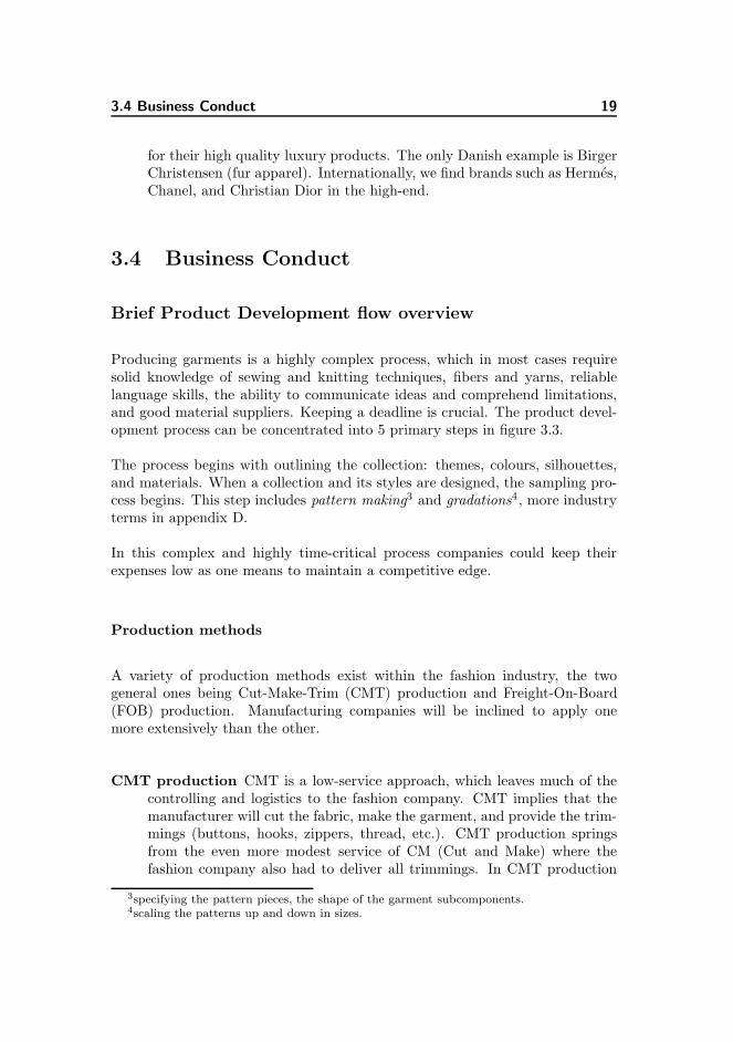
Producing garments is a highly complex process, which in most cases requiresolid knowledge of sewing and knitting techniques, fibers and yarns, reliablelanguage skills, the ability to communicate ideas and comprehend limitations,and good material suppliers. Keeping a deadline is crucial. The product devel-opment process can be concentrated into 5 primary steps in figure 3.3.
The process begins with outlining the collection: themes, colours, silhouettes,and materials. When a collection and its styles are designed, the sampling pro-cess begins. This step includes pattern making3 and gradations4, more industryterms in appendix D.
In this complex and highly time-critical process companies could keep theirexpenses low as one means to maintain a competitive edge.
Production methods
A variety of production methods exist within the fashion industry, the twogeneral ones being Cut-Make-Trim (CMT) production and Freight-On-Board(FOB) production. Manufacturing companies will be inclined to apply onemore extensively than the other.
CMT production CMT is a low-service approach, which leaves much of thecontrolling and logistics to the fashion company. CMT implies that themanufacturer will cut the fabric, make the garment, and provide the trim-mings (buttons, hooks, zippers, thread, etc.). CMT production springsfrom the even more modest service of CM (Cut and Make) where thefashion company also had to deliver all trimmings. In CMT production
3specifying the pattern pieces, the shape of the garment subcomponents.4scaling the patterns up and down in sizes.

20 The Danish fashion industry
Designing, fabric selection,
evalutation(often takes place in collaboration with
designer, manufacturer, product rep. and sales
rep.)
Sampling(the process of creating the pattern, deciding
on the correct fabric, fittings, until final
salesman samples are ready.)
Production Planning(order fabric and trimmings, final alterations,
setting up line plans, shipment, quota handling,
transportation, optimization of quantities and
fabric)
Production(cutting, manufacturing, quality assurance,
packing, documenting, shipping)
Post production(claims handling, evalution, discard of surplus
materials, stock handling)
Figure 3.3: The development process in 5 steps
fashion companies, are responsible for selecting the fabric, logistics, ne-gotiations with material suppliers, pattern making, prototype samplingetc.
CM(T) production collaborations were among the first production meth-ods to be used when outsourcing was new. Today, many newly startedcompanies collaborate with this type of production suppliers as it allowsthem to keep in control of the final design of a garment (fabric, fittingsand pattern, buttons etc.), or because they lack the knowledge or networkto choose other collaborational forms. Fashion companies relying heavily
on technical textiles (e.g. GoreTex®) may also prefer CM(T) production.
FOB production FOB is a high-service approach, where manufacturers willsupply not only CMT services, but also pattern making, prototype sam-pling, material sourcing etc. This relieves the fashion company of manyof these cumbersome tasks, and even solves cash-flow issues related todisbursements for materials and others. The design of the garments is acollaborative effort between the fashion company and the manufacturer.The manufacturing company will handle all production and product de-velopment tasks until the order exits the factory.
Accounts of profitability
The fashion industry holds a unique status being among the first industries tooutsource the greater part of their business activities. Production was moved

3.4 Business Conduct 21
Design
Materials
Production
Sales
Marketing
Logistics
Administration
Legal
Taxes
20%
20%
20%10%
9%
10%
11%
5%8%
Figure 3.4: An example of estimated cost distributions in a Danish fashioncompany
abroad, as early as the 1950’s, due to cost advantages offered by lower-wagecountries. No other industries work with this extreme a combination of shortproduct life-cycles, short time-to-market, and rate of new product developmentin such a densely populated market. In order to make profit, companies couldfocus on both increasing sales and cutting expenses. Earlier times’ focus on theimportance of low wages and material costs are yet perceived as a key factorto cost-effective garments. More recent observers of the fashion industry claim,however, that this one-sided view misleads fashion companies into focusing onless efficient cost-saving initiatives. The distribution of a company’s expensesvary greatly with the size of the company, and the competitive strategy of thebrand, see one example of a company’s cost distribution in figure 3.4.
Outsourcing patterns
Suppliers are investigated and selected by the sourcing offices, whether by ownstaff or external agents. These suppliers are found through recommendationsby associate, previous collaborations, unsolicited applications, or third partyintroductions. The process of selecting suppliers are not as extensive as theone suggested in this report. Among larger companies it is common practise todouble-source5 items on a regular basis, before supplier evaluations.
5the process of collecting price quotes and production/salesman samples from two or moresuppliers.
22 The Danish fashion industry
Professional Management
Managers in the fashion industry have a wide variety of education, managerialtraining and experience. The presence of experienced management is moreprominent in large companies and companies with professional investors. Thereare indications that where experienced management is present, more focus isgiven to cost and profitability analyses.
3.5 Vision: Copenhagen as a fashion capital
Danes often pride themselves of living in a fashion-famed culture. But the truthis that in the global market, Copenhagen is merely one of many cities worldwidehoping to be acknowledged as a fashion capital next after Paris, Milan, Londonand New York. Achieving this goal is, however, is by no means a simple taskand will require a collaborative effort within the industry itself and backing frompolitical quarters. Newly formed associations such as Modekonsortiet (MOKO)and Danish Fashion Institute (DAFI) work together to consolidate Denmark’sposition in the fashion landscape.
For Danish fashion companies struggling to succeed abroad, these are frequentchallenges6:
1. Once established in a small and low-priced market as Denmark, companiesdo not have the resources to promote themselves abroad.
2. Finding financial backing from investors is challenging, because few in-vestors are accustomed to investments in the fashion industry.
3. Lack professional management: Most Danish fashion companies are foundedand controlled by people with a design background instead of a professionalmanagement team which may lead to focus on areas of interest rather thanareas of need.
4. Old-fashioned production and product development methods: surprisinglymany companies in Denmark still develop their products in a traditionalway through CMT collaborations rather than testing opportunities in col-laborating with FOB suppliers, as a more recent approach. This approachkeep key competences on design and marketing in-house but oursourcemost of the traditional production development processes to the supplier.
6[11] p. 48, middle.
3.5 Vision: Copenhagen as a fashion capital 23
FOB production is standard in the three leading fashion groups in Den-mark.
This report discusses some of the issues mentioned above, contributing obser-vations and identifying tools for companies hoping to achieve a more profitablebusiness conduct.
The next chapter is dedicated to literature on fashion industry management.As primary source of information, David Birnbaum’s views will be summarizedand challenged with related literature.

24 The Danish fashion industry
Chapter 4
Fashion business management
The previous chapter outlined the fashion industry characteristics with Denmarkin focus. This chapter seeks out literature on business management in thefashion industry, with emphasis on analyses and tactics in processes for globaloutsourcing. The works of David Birnbaum is interesting and have served asinspiration to this report. Birnbaum’s work is examined for concurrence withother authors and his relevance to a Danish setting concluded upon. The lack ofadditional, elaborate literature to support fashion business mangement, identifyde facto standards of the industry, and recommended codes of conduct, leavesBirnbaum as the only author with this prominent a position on fashion businessmanagement.
4.1 An introduction to D. Birnbaum’s ideas
David Birnbaum is a fashion professional, who after working in the fashionindustry for years has now become a strategic consultant for countries, whowhish to build a stable fashion industry or large fashion companies, who wishto improve their competitiveness by working more profitably.
26 Fashion business management
The challenge of the fashion industry
Birnbaum argues that the fashion industry players are at war. He claims thatthe number of garment manufacturers, material suppliers, as well as fashionimporters and designers, has increased steadily while we see a decrease in theamount of money consumers spend on clothing: the market is shrinking. Com-panies should improve their competitiveness or they will become extinct. Hesees the primary parameters of competition as quality, delivery, and price. Fur-thermore, he believes that these factors will become even more important overtime.
Tools and results from Birnbaum
One way for companies to improve competitiveness is to focus on their costs.Birnbaum claims that few fashion businesses know the actual costs of theiractivities and the financial impact of their sourcing decisions. According tohim, many companies focus primarily on direct production costs, instead ofminimizing their true burden: indirect costs so. In order to stay competitive,companies should know their costs so that they may reduce them, and focus onquality, delivery, and price of their products.
Based on a definition of three costs: macro costs, indirect costs, and direct costs,Birnbaum demonstrates his tool ”Full Value Cost Analysis” which supposedlyunveils the true costs of a company’s production related activities.
Birnbaum opposes the conventional perception that low manufacturing costs areequal to the least expensive outsourcing. He also argues that quota restrictionsdamage fashion businesses everywhere. He suggests that factories upgrade theirservice as much as possible and recommends fashion importers to work withhigh-service factories, if possible. Consequently, both parties will gain from thisapproach.
Birnbaum’s cost analysis
Through carefully planned strategic and tactic decision-making, companies canimprove their profitability by including cost analysis, in comparative studiesbetween suppliers worldwide. Too many companies focus only on direct costswhen they make decisions about where to produce their garments, which con-trasts Birnbaum’s main arguments that indirect costs are more significant for a
4.1 An introduction to D. Birnbaum’s ideas 27
company’s profitability. His cost analysis yields three costs that should influencefashion importers sourcing decisions, in order of importance:
1. Macro costs - critically important. Macro costs should indicate where toproduce. Macro costs imply:
(a) Education (there must be sufficiently educated people managing fac-tories)
(b) Infrastructure (roads, electricity, communication must work well)
(c) Government policy (work towards supporting their industries)
(d) Human rights (proper working hours, no child-labour, rights to unions)
(e) The politics of trade (import/export quotas, taxes/tariffs)
2. Indirect costs - very important. Indirect costs should indicate which man-ufacturer to work with. Indirect costs include:
(a) Letter of credits, credit # of days
(b) Quality Assurance, Communication skills,
(c) Delivery, Reliability
(d) Order minimums
3. Direct costs - least important:
(a) CMT (Cut, Make, Trim)
(b) Materials: fabric and trimmings
(c) Time-to-market
Quantifying the macro costs
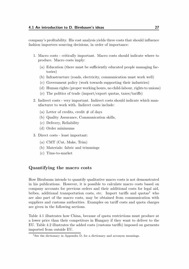
How Birnbaum intends to quantify qualitative macro costs is not demonstratedin his publications. However, it is possible to calculate macro costs based oncompany accounts for previous orders and their additional costs for legal aid,bribes, additional transportation costs, etc. Import tariffs and quotas1 whoare also part of the macro costs, may be obtained from communication withsuppliers and customs authorities. Examples on tariff costs and quota chargesare given in the following sections.
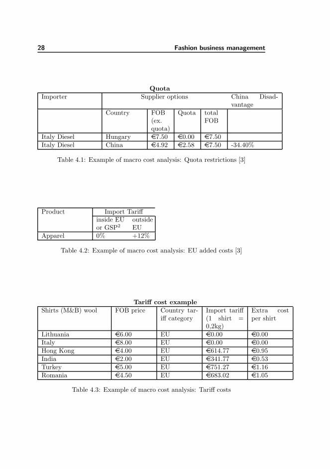
Table 4.1 illustrates how China, because of quota restrictions must produce ata lower price than their competitors in Hungary if they want to deliver to theEU. Table 4.2 illustrates the added costs (customs tariffs) imposed on garmentsimported from outside EU.
1See the dictionary in Appendix D, for a dictionary and acronym meanings.
28 Fashion business management
QuotaImporter Supplier options China Disad-
vantageCountry FOB
(ex.quota)
Quota totalFOB
Italy Diesel Hungary e7.50 e0.00 e7.50Italy Diesel China e4.92 e2.58 e7.50 -34.40%
Table 4.1: Example of macro cost analysis: Quota restrictions [3]
Product Import Tariffinside EUor GSP2
outsideEU
Apparel 0% +12%
Table 4.2: Example of macro cost analysis: EU added costs [3]
Tariff cost exampleShirts (M&B) wool FOB price Country tar-
iff categoryImport tariff(1 shirt =0,2kg)
Extra costper shirt
Lithuania e6.00 EU e0.00 e0.00Italy e8.00 EU e0.00 e0.00Hong Kong e4.00 EU e614.77 e0.95India e2.00 EU e341.77 e0.53Turkey e5.00 EU e751.27 e1.16Romania e4.50 EU e683.02 e1.05
Table 4.3: Example of macro cost analysis: Tariff costs

4.1 An introduction to D. Birnbaum’s ideas 29
Shirt FOB price Quantity Minimums CostsIndia e2.08 1,200 2,500 e5,200Hong Kong e4.45 1,200 1,000 e5,340Lithuania e7.00 1,200 300 e8,400
Table 4.4: Minimum quantities reflects in the indirect costs
Shirts Quantity Minimums Costs Dispatchsurplusstock (unitcost: e1.2)
Total
India 1,200 2,500 e5,200 e1560 e6760Hong Kong 1,200 1,000 e5,340 e0 e5340Lithuania 1,200 300 e8,400 e0 e8400
Table 4.5: Example of indirect cost analysis:
Indirect costs analysis
Manufacturers often have minimum quantities on each garment style. If a com-pany is only able to sell 1200 styles of a garment, but must order 3000 items,they consequently must sell the surplus stock at a discount or dump it. Thisis reflected in table 4.4. The final mark-up illustrates that an Indian manufac-turer is favourable to work with, if one considers direct production costs andminimums only. It is most likely, however, that other cost factors will reducethe advantage held by India according to this table.
If the company can only sell 1,200 items, then its is more profitable order theproduction in Hong Kong even though unit prices are lower in India. Table 4.5illustrates how additional costs for dispatching surplus stock further decreasesthe competitiveness of the Indian manufacturer in the previous example. Thisis an example of indirect costs’ impact on total costs.
Finally, an example on comparing bank costs (see example below). The con-ditions for payment set by the supplier also impact the final costs of an order,especially if a bank guarantee is supplied through a letter of credit, which freezesthe money on the fashion company’s account to ensure sufficient funding whenproduction must be payed for.
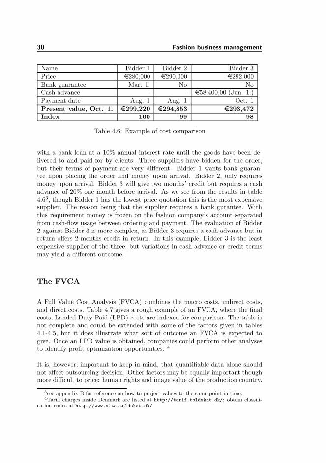
Example: see table 4.6A production batch should be ordered in early March for delivery in July, thecosts of production are approximately e300,000. This expense must be financed
30 Fashion business management
Name Bidder 1 Bidder 2 Bidder 3Price e280,000 e290,000 e292,000Bank guarantee Mar. 1. No NoCash advance - - e58.400,00 (Jun. 1.)Payment date Aug. 1 Aug. 1 Oct. 1Present value, Oct. 1. e299,220 e294,853 e293,472Index 100 99 98
Table 4.6: Example of cost comparison
with a bank loan at a 10% annual interest rate until the goods have been de-livered to and paid for by clients. Three suppliers have bidden for the order,but their terms of payment are very different. Bidder 1 wants bank guaran-tee upon placing the order and money upon arrival. Bidder 2, only requiresmoney upon arrival. Bidder 3 will give two months’ credit but requires a cashadvance of 20% one month before arrival. As we see from the results in table4.63, though Bidder 1 has the lowest price quotation this is the most expensivesupplier. The reason being that the supplier requires a bank gurantee. Withthis requirement money is frozen on the fashion company’s account separatedfrom cash-flow usage between ordering and payment. The evaluation of Bidder2 against Bidder 3 is more complex, as Bidder 3 requires a cash advance but inreturn offers 2 months credit in return. In this example, Bidder 3 is the leastexpensive supplier of the three, but variations in cash advance or credit termsmay yield a different outcome.
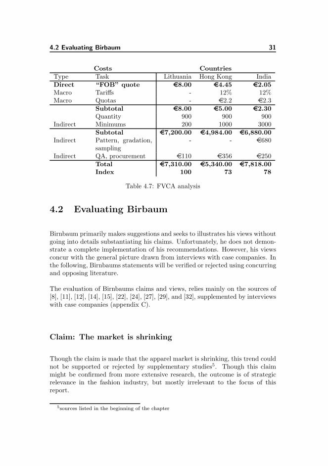
The FVCA
A Full Value Cost Analysis (FVCA) combines the macro costs, indirect costs,and direct costs. Table 4.7 gives a rough example of an FVCA, where the finalcosts, Landed-Duty-Paid (LPD) costs are indexed for comparison. The table isnot complete and could be extended with some of the factors given in tables4.1-4.5, but it does illustrate what sort of outcome an FVCA is expected togive. Once an LPD value is obtained, companies could perform other analysesto identify profit optimization opportunities. 4
It is, however, important to keep in mind, that quantifiable data alone shouldnot affect outsourcing decision. Other factors may be equally important thoughmore difficult to price: human rights and image value of the production country.
3see appendix B for reference on how to project values to the same point in time.4Tariff charges inside Denmark are listed at http://tarif.toldskat.dk/; obtain classifi-
cation codes at http://www.vita.toldskat.dk/
4.2 Evaluating Birbaum 31
Costs CountriesType Task Lithuania Hong Kong IndiaDirect “FOB” quote e8.00 e4.45 e2.05Macro Tariffs - 12% 12%Macro Quotas - e2.2 e2.3
Subtotal e8.00 e5.00 e2.30Quantity 900 900 900
Indirect Minimums 200 1000 3000Subtotal e7,200.00 e4,984.00 e6,880.00
Indirect Pattern, gradation,sampling
- - e680
Indirect QA, procurement e110 e356 e250Total e7,310.00 e5,340.00 e7,818.00Index 100 73 78
Table 4.7: FVCA analysis
4.2 Evaluating Birbaum
Birnbaum primarily makes suggestions and seeks to illustrates his views withoutgoing into details substantiating his claims. Unfortunately, he does not demon-strate a complete implementation of his recommendations. However, his viewsconcur with the general picture drawn from interviews with case companies. Inthe following, Birnbaums statements will be verified or rejected using concurringand opposing literature.
The evaluation of Birnbaums claims and views, relies mainly on the sources of[8], [11], [12], [14], [15], [22], [24], [27], [29], and [32], supplemented by interviewswith case companies (appendix C).
Claim: The market is shrinking
Though the claim is made that the apparel market is shrinking, this trend couldnot be supported or rejected by supplementary studies5. Though this claimmight be confirmed from more extensive research, the outcome is of strategicrelevance in the fashion industry, but mostly irrelevant to the focus of thisreport.
5sources listed in the beginning of the chapter
32 Fashion business management
View: The challenge of the fashion industry
As Birnbaum’s view on the challenge of the fashion industry is partly based onthe claim that the market is shrinking his conclusions has not been sufficientlybacked by literature used for evaluation. However, his views on quality, delivery,and price as important competitive factors concur with the the description ofthe fashion industry in chapter 3, which is based on sources [25], [11], and [24],as well as interviews with fashion companies. In a densely populated market, itis most likely that profitable businesses will outlast those yielding losses, thoughnew start-up companies are in constant supply. Whether the many players ofthe fashion industry are cannibalizing on each other is a subject for furtherstudies outside of this report.
Claim: Companies focus on direct production costs
The claim that companies focus on direct production costs is only partly sup-ported by Gibbon and Thomsen [29]. However, case company interviews in-dicated some concurrence with Birnbaum’s claim for small fashion companies.Once businesses have attained a certain size, with the experience following thisposition they will most likely have identified a business conduct, which is bothprofitable and adjusted according to main macro costs and indirect costs. Con-sequently, the attention given to direct costs is justifiable. The cost focus ofmid-sized companies depends on management experiences and personalities.
Concurring literature
Gibbon and Thomsen somewhat confirms Birnbaum’s claim, documenting thatScandinavian fashion companies find price of vital importance to their sourcingdecisions. Countries like China, India and Bangladesh are preferred over HongKong and East-Europe in the price discussion. However, Scandinavian coun-tries are at the same time, slow to investigate new and potentially less costlymanufacturers. They maintain low expectations to their suppliers’ potential foradding value to design and materials [29]. Conclusively, it would seem thatScandinavian fashion companies are more likely to focus on direct cost savings,rather than cost-savings in a greater perspective.
4.2 Evaluating Birbaum 33
Opposing literature
In the UK Gibbon and Thomsen observed a different pattern amongst fashioncompanies. Whether it is a conscious decision or not to investigate cost-savingsoutside direct production costs, UK companies tend to demand higher-servicesuppliers because of their added value to their businesses.
View: The importance of macro costs, indirect costs, anddirect costs, respectively
Whilst no other authors than Birnbaum’s directly state why sound (and of-ten market leading) companies choose, presumably, more expensive high-servicesuppliers, literature concludes that this is in fact the case.
Concurring literature
Most available literature supporting Birnbaum’s view, focus on the businesschallenges of manufacturers rather than fashion companies. The conclusion isnever the less crystal clear: supplier price is not the single most competitivefactor, but also logistics, material sourcing, and qualified customer service havebecome vital.
Literature further concludes that many truly low-wage countries like e.g. manyAfrican nations, have little or no part in the global garment manufacture dueto poor infrastructures and an unstable political climates ([15]). These sameissues are addressed in Birnbaum’s emphasis on the importance of macro costs.Furthermore, other authors point out that trade barriers or favoured nationsagreements heavily affects the sourcing patterns of the EU and the USA. Thenatural competitiveness of countries and manufacturers are distorted by thesepolitical agreements, making room for less than competitive manufacturing en-vironments in, e.g., Italy or Mauritius.
Opposing literature
No opposing literature was found which questions the reasoning behind evaluat-ing macro-economic aspects before considering candidate countries for outsourc-ing. Whether focus on direct costs should be prioritized higher than indirectcosts has not been articulated.
34 Fashion business management
Claim: High-service manufacturers are more profitable towork with
Gibbon and Thomsen describes how many UK companies have high serviceexpectations of their suppliers. UK fashion companies insist that their suppli-ers ’bring something to the table’ whereas this was only the case for 50% ofthe Scandinavian fashion companies. Also Scandinavian countries meet theirsuppliers with lower expectations regarding the value they could bring to theircompany: design suggestions, material sourcing, etc.
Concurring literature
Much of the literature, recommends manufacturing companies to upgrade theirservice-level, and consequently increasing competitiveness. This increase in de-mand for high-service manufacturers indicates that customers experience bettervalue.
Opposing literature
In the report by Gibbon and Thomsen some Danish companies claim that CMTallows them to order smaller production quantities, a prerequisite for their busi-ness existence. Whether this is the most profitable choice is not necessarilyinvestigated, though.
The latest trend towards fast fashion may challenge Birnbaum’s claims in thefuture6. They iconify the new world of lean retailing which likely will providenew opportunities and threads to the fashion industry [30],[31].
6Fast fashion is an industry term for meeting consumer demands instantly, yielding quickcollection turnovers. Spanish fashion company and retail chain Zara have experienced atremendous success with fast fashion. Zara currently serves as a model example for the fastfashion movement. Its organisation structure is a vertical platform, from yarn dying and spin-ning to retailing and customer feedback loops. Much of Zara’s production is done in-house orlinked closely to manufacturers working according to the CM concept. They produce in smallproduction batches, waiting for the market to respond to their products. Based upon themarket feedback they either discontinues a style, increase production or design new versions.
4.2 Evaluating Birbaum 35
Job function Annualsalary
DaysWorkedper Year
Days toMake Unit
Cost perUnit
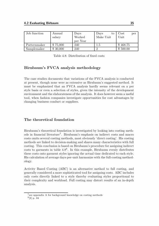
Patternmaker $ 75,000 240 1.5 $ 468.75Samplemaker $ 30,000 240 2 $ 500.00
Table 4.8: Distribution of fixed costs
Birnbaum’s FVCA analysis methodology
The case studies documents that variations of the FVCA analysis is conductedat present, though none were as extensive as Birnbaum’s suggested method. Itmust be emphasized that an FVCA analysis hardly seems relevant on a perstyle basis or even a selection of styles, given the intensity of the developmentenvironment and the elaborateness of the analysis. It does however seem a usefultool, when fashion companies investigate opportunities for cost advantages bychanging business conduct or suppliers.
The theoretical foundation
Birnbaum’s theoretical foundation is investigated by looking into costing meth-ods in financial literature7. Birnbaum’s emphasis on indirect costs and macrocosts omits several costing methods, most obviously ’direct costing’. His costingmethods are linked to decision-making and shares many characteristics with fullcosting. This conclusion is based on Birnbaum’s procedure for assigning indirectcosts to garments in table 4.88. In this example, Birnbaum evenly distributesthese costs onto garment styles ignoring the actual time dedicated to each style.His calculation of average days-per-unit harmonize with the full-costing method-ology.
Activity Based Costing (ABC) is an alternative method to full costing, andgenerally considered a more sophisticated tool for assigning costs. ABC includesonly costs directly linked to a style thereby evaluating styles proportional totheir complexity and workload. Full costing may distort results of an in-depthanalysis.
7see appendix A for background knowledge on costing methods8[3] p. 84

36 Fashion business management
4.3 Limitations of Birnbaum
It seems that Birnbaum offers interesting lessons to fashion professionals, whomight not investigate the palette of outsourcing opportunities and benefits. Thissaid, Birnbaum offers little advice to fashion companies, who already follows hisrecommendations on business conduct. Companies already collaborating withhigh-service suppliers may merely be advised to monitor outsourcing trendsamong colleagues as well as global developments in manufacturing prices. Birn-baum offers no methods for quantifying qualitative macro-costs for analysispurposes, nor does he demonstrate a complete and adequate indirect costinganalysis.
Birnbaum’s literature helps the reader adopt a different mind-set and attentionto other important costs in outsourcing. This report attempts to follow-up withhands-on tools to implement Birnbaum’s recommendations.
In the next chapter, will describe general business practices for outsourcing andcost management in a practical perspective. Furthermore, it will introduce theusability of operations research for decision analysis when high profitability isthe goal.
Chapter 5
Commen business practice
Upon the insights gained into the fashion industry is practical and theoreticalsettings, this chapter aims to identify common business practices valid acrossindustries. Focus remains on managerial tools for production related activitiessuch as cost management and outsourcing. The chapter is further extendedwith a section on how techniques from operations research are used in decisionanalysis.
Industries who where identified as related in character to the fashion industryare first examined for relevant business practices:
The mobile telephone industry This industry operates in a fashion sensi-tive market, where product life cycles are very short (1-3 years approx.).The competition is intensive between the few large mobile producers oninnovation in both design and technology. Each vendor launches newproducts fast and often. The majority of consumers are price sensitive.In some countries, consumer purchases are linked with telecommunicationcompanies offering the telephone network.
The industry shares some characteristics with the fashion industry in termsof short time to market, harsh competition, a fashion sensitive market, agenerally price sensitive market, and many new products developed eachyear.
38 Commen business practice
The food industry The food industry is characterized by short product lifecycles, many competitors, market layers which resemble price, and price/designsensitive consumers. To differentiate between fairly (functionally) identi-cal products, branding becomes increasingly important.
Exploring various industries’ codes of conduct with regards to outsourcing strate-gies, and cost structures made it clear that tools outside the related industriesmay prove equally relevant for the fashion industry to learn from. In fact, soundways to work with outsourcing decisions and cost analyses seems consistentacross industries. Whether a company works analytically with its outsourcingstrategy and costs, apparently depends more on personal qualifications of themanagement than its industry characteristics.
Conclusively an overview good practices in general was sought within: out-sourcing, supplier evaluation and price comparisons, and costing methods; us-ing industry reports. Numerous practices in business conduct exist and may bedeployed with equally good results. This report do not attempt to identify andevaluate on all of them, but rather familiarize the reader with some hands-onmethods that have proven both relevant and powerful.
To attain practical and pragmatic knowledge on common practices, two finan-cial managers where interviewed, both with extensive experience in productionmanaging financial analyses and business turnarounds. These interviews con-tributed with valuable insights which serve as the basis for this chapter.
Manager A Works as a consultant in the food industry, primarily involvedwith learning ex-state-owned companies, now privately held, how to adapttheir business to the more open competitive landscape. Much effort is putinto implementing costing methodologies to support profitability analysesas a primary tool, to decide on strategies and tactics.
Manager B Has extensive experience in turnarounds and strategies in indus-tries as variable as medical care, oil, cargo, shipyards, steel production,plastic moulding, and others. Furthermore, a resume of establishing newmarkets, investment analyses and strategies. Manager B is routinely work-ing with investment analysis, supplier evaluation and cost-benefit analysesin outsourcing scenarios.
5.1 Cost management 39
5.1 Cost management
All companies delivering products, either being physical or services, must man-age their costs in a sensible manner. For companies operating in highly competi-tive markets cost control is essential to stay competitive. A dissatisfied customermay easily turn to a competitor, regardless of the brand value and the actualdesign qualities of the original company products.
Even so, small fashion companies rarely have procedures for cost analyses sincethis is not the primary interest of the designer who typically runs the business.As an exception, Case Company C stands out as their CEO has an economiceducation with high focus on cost control.
The skill of strong cost management seems to depend more on individual man-agement, than characteristics of a specific industry. Thus the fashion industrymay include general methods for cost management, and benefit from it.
In general, companies in business for profit offer a product range to a targetmarket. To stay in business companies composition their product ranges toensure their continuous existence and finance their drive towards expansion,shareholder pay-outs, and research alike. Products typically have a life-cycle,which requires a continuous update of the product range to maintain a relevantvalue proposition to the market and a profitable operation for the company.Product ranges must be updated, new products developed, and obsolete itemsweeded out. The condition of doing so wisely, implies that decision-makers canmap their cost and profit landscape of individual products, product families, aswell as value interchange in the product range. This requires the means of costanalysis and profitability analysis.
Cost distribution
Costing is by far a trivial task and requires that analysts use the data in astructured and consistent way. Computational power has increased during the20th century and along with it accounting software has emerged facilitatingmultiple ways to track and analyze costs. In previous days, where computationswhere done by hand, costing for internal purposes where often done using tablesof standard costs instead of tracking the actual costs, which would be tediousand quickly render obsolete in the time it took to finish calculations. Withcomputer systems, we have the means to make accurate costing and a muchgreater range of methodologies to choose from, which we must do carefully.
40 Commen business practice
Often companies will use a mix of different costing methodologies, each fordifferent purposes. Costs are roughly divided into variable costs and fixed costs.Examples of variable costs are materials and hired labour. Examples of fixedcosts are: staff salaries, administration, buildings and equipment.
A typical method for evaluating products on their costs and profitability, in-cludes distributing fixed costs on the product range, so each product may includeboth variable costs and fixed costs. By assigning costs to products, managementwill gain insight into on what terms they are making profit, and which productsare more profitable than others. The method for distributing fixed costs can bedone in a variety of ways, full costing or Activity-based costing being some ofthe more commonly known [1].
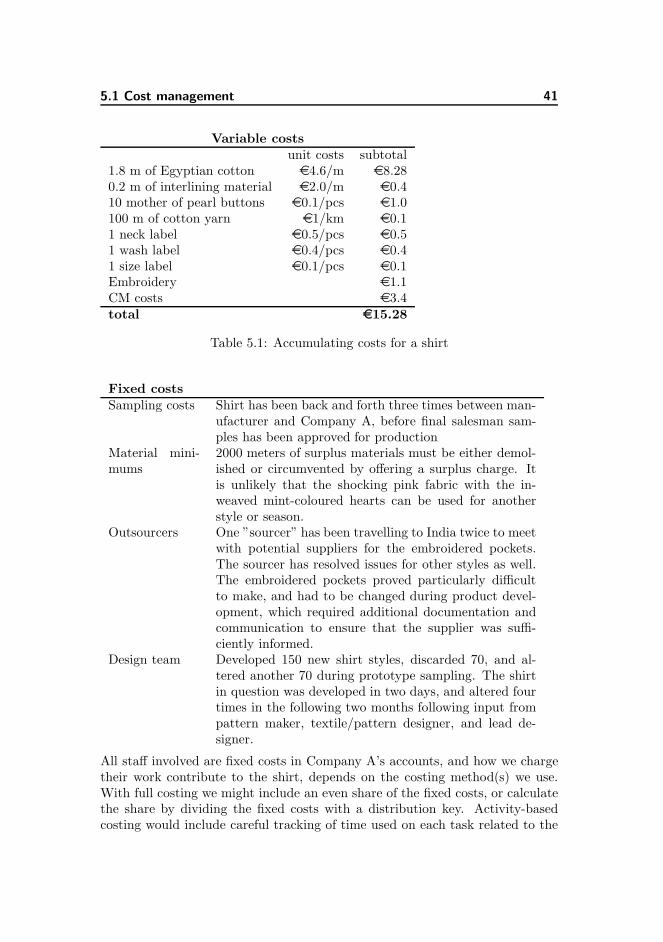
Example: Making a shirt The shirt is part of Company A’s half-annualfashion range. Next season it will be replaced with a freshly designed item. Adesign team is dedicated to developing new products for this fashion range. Theshirt has hand-stitched ornaments on the breast pocket, which required Com-pany A’s outsourcing team to find a manufacturer, capable of hand-stitchingthe pockets and ship them off to Company A’s usual shirt manufacturer whothen assemble the shirt and apply the pockets. Means must be taken to ensurethat pockets and assembled shirts come from the same fabric roll so colours willmatch precisely1. Fabric comes from a textile mill with an exquisite quality ofEgyptian cotton. Company A only needs 3000 m of fabric, but the textile millrequires a minimum purchase of 5000m. Table 5.1 shows how the variable costsfrom making a shirt are accumulated.
Assigning fixed costs to an item is, however, much harder and requires somerule for the distribution of fixed costs.
1Slight colour variations occur from roll to roll, often because the fabric or yarns has beendyed in different batches.
5.1 Cost management 41
Variable costsunit costs subtotal
1.8 m of Egyptian cotton e4.6/m e8.280.2 m of interlining material e2.0/m e0.410 mother of pearl buttons e0.1/pcs e1.0100 m of cotton yarn e1/km e0.11 neck label e0.5/pcs e0.51 wash label e0.4/pcs e0.41 size label e0.1/pcs e0.1Embroidery e1.1CM costs e3.4total e15.28
Table 5.1: Accumulating costs for a shirt
Fixed costsSampling costs Shirt has been back and forth three times between man-
ufacturer and Company A, before final salesman sam-ples has been approved for production
Material mini-mums
2000 meters of surplus materials must be either demol-ished or circumvented by offering a surplus charge. Itis unlikely that the shocking pink fabric with the in-weaved mint-coloured hearts can be used for anotherstyle or season.
Outsourcers One ”sourcer” has been travelling to India twice to meetwith potential suppliers for the embroidered pockets.The sourcer has resolved issues for other styles as well.The embroidered pockets proved particularly difficultto make, and had to be changed during product devel-opment, which required additional documentation andcommunication to ensure that the supplier was suffi-ciently informed.
Design team Developed 150 new shirt styles, discarded 70, and al-tered another 70 during prototype sampling. The shirtin question was developed in two days, and altered fourtimes in the following two months following input frompattern maker, textile/pattern designer, and lead de-signer.
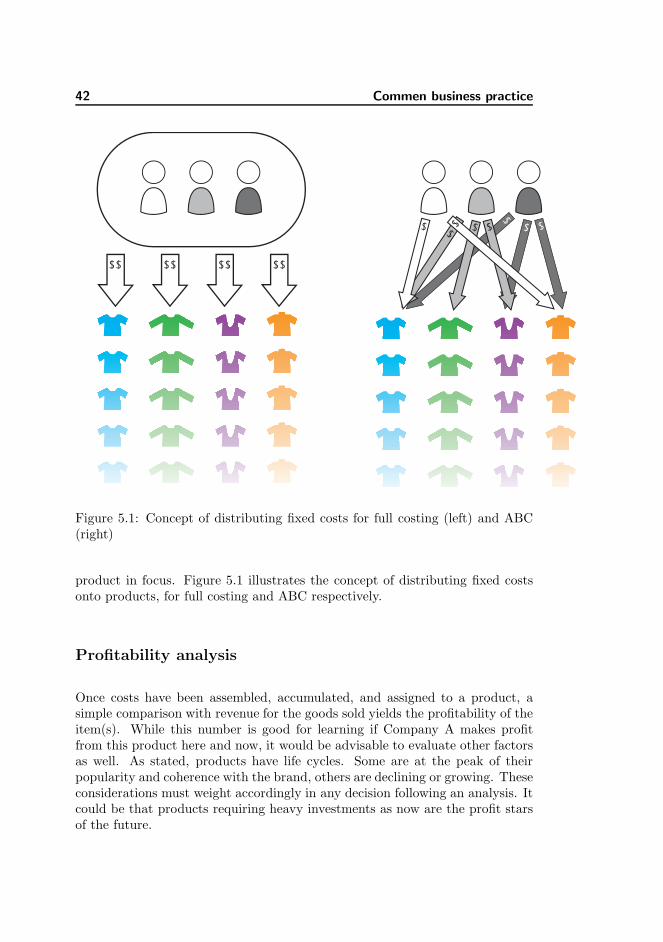
All staff involved are fixed costs in Company A’s accounts, and how we chargetheir work contribute to the shirt, depends on the costing method(s) we use.With full costing we might include an even share of the fixed costs, or calculatethe share by dividing the fixed costs with a distribution key. Activity-basedcosting would include careful tracking of time used on each task related to the
42 Commen business practice
$$$$$$$$
$ $$
$ $
Figure 5.1: Concept of distributing fixed costs for full costing (left) and ABC(right)
product in focus. Figure 5.1 illustrates the concept of distributing fixed costsonto products, for full costing and ABC respectively.
Profitability analysis
Once costs have been assembled, accumulated, and assigned to a product, asimple comparison with revenue for the goods sold yields the profitability of theitem(s). While this number is good for learning if Company A makes profitfrom this product here and now, it would be advisable to evaluate other factorsas well. As stated, products have life cycles. Some are at the peak of theirpopularity and coherence with the brand, others are declining or growing. Theseconsiderations must weight accordingly in any decision following an analysis. Itcould be that products requiring heavy investments as now are the profit starsof the future.
5.2 Outsourcing practices and country evaluations 43
5.2 Outsourcing practices and country evalua-tions
This section is heavily based on a report from The Confederation of Danish In-dustries (DI) on outsourcing practises [28], and from interviews with case com-panies. The report includes many considerations on establishing own productionfacilities and offices abroad as well as outsourcing some tasks to subcontractors.The Danish fashion industry is mainly characterised by purchasing productionservices from subcontractors though larger companies may have own sourcingdepartments abroad. A pattern of frequent supplier shifts was observed amongthe small and young case companies. Whereas outsourcing may be a new dis-cipline to some industries, it has been common practice in the fashion industryfor decades. Fashion companies rarely consider if they should be outsourcingbut rather where to next. That said, many good practices are relevant acrossindustries and the fashion industry could benefit from learning how to analyzeand compare their existing and potential market of suppliers.
Why do companies outsource? Outsourcing may benefit companies in avariety of ways. These are some of the common reasons for outsourcing:
• To save money
• Speed to market
• Proximity to market
• To get better products
• To enter new markets
• To focus on their key competences
What do companies outsource? Surprisingly many tasks are candidatesfor outsourcing:
• Time consuming or simple tasks
• Logistics
• Services, e.g. support, supervision
• Test and analyses
44 Commen business practice
• Accounting
The fact that many of these tasks are very complex and requires educatedlabour could be an eye-opener to companies hesitant to outsourcing more thanthe simpler tasks of their business. Suppliers worldwide have sophisticated skillsto embrace a variety of advanced tasks and even contribute to their continuousimprovement.
Best codes of conduct: This section summarizes the report on outsourcingfrom DI. Regardless of whether outsourcing implies establishing the companyin another country or merely purchasing products or services from a supplierabroad, criteria apply on how to select an appropriate location and outsourcingmodel.
The majority of fashion companies will purchase production services from sup-pliers, rather than manufacturing themselves. Some will buy additional servicesof organizing production with a production agent, others keep this tasks in-house or in offices abroad. Thus, considerations of establishing own productionunits abroad will be omitted in this chapter.
Know your own costs remember to include indirect costs and consider whichparts of the business could be outsourced even further. Having a goodunderstanding of own costs enables later comparing with results from out-sourcing and conclusions on the success of the action. This way existingcosts may be compared with opportunities abroad.
Decide on the outsourcing model With knowledge of the opportunities foroutsourcing, identify which part of the business to outsource. Decide whichcriteria suppliers must meet to take on these tasks.
Geographic location The choice of geographic location will have heavy im-pact on the results. Carefully evaluate which countries to consider foroutsourcing. Some will have tradition for specific types of production witha sub-industry to support these activities. Vast differences apply betweencountries in taxes, political climates, and jurisdictions. This may be vitalto the economic success of an outsourcing decision. Proximity may ben-efit time-to-market and customer service offerings. Make a comparativeanalysis of the countries subject to consideration.
Seek out suppliers Look for suppliers that match the criteria set up previ-ously. To seek out candidate suppliers ask colleagues, embassies, tradecouncils, unsolicited contacts, look on the internet, etc. Visit potential
5.2 Outsourcing practices and country evaluations 45
suppliers and verify that they have the means to facilitate your business.They must be technically capable of delivering the right product(s), un-dertaking quality control, providing the financial backing, facilitating pro-duction and product improvements, handling logistics, and possessing themanagerial competences to meet future challenges. Long term relation-ships will benefit all parties involved.
Gradual outsourcing Start by outsourcing only part of the production, oroutsource the simpler tasks first. Establish success with this before in-creasing volume and/or complexity of products. Assign resources enoughto facilitate the shift. In any new collaboration there will be errors; expectthem and be prepared to solve them.
Evaluate results Ask questions like: Are the results as good as expected?What went right or wrong? Any improvements or restrictions? Theseevaluations will be valuable to future outsourcing decisions.
Be prepared to move Keep and eye out for changes in the world around andbe prepared to move. Seek out new opportunities, and allow for inspirationby the actions of other companies. Monitor outsourcing trends. Make sureyou did not put all eggs in a single supplier basket.
These codes of good conduct apply to all industries. The fashion business isfurther stressed by the fact that decisions and evaluations must be made muchmore frequently than in other industries. Many of the recommendations concurwith Birnbaum’s focus on macro costs and supplier evaluation.
Best practices for performing comparative studeise between potential supplierswill be dealt with next.
Supplier comparisons
Whereas there are plenty of literature on comparative studies, there is onlyvery little documentation on best practices from the industries. Interviews withmanagers A and B, and authors of the DI report, revealed that the majority ofcompanies do not have any the structured procedures for these analyses.
Often, sourcing decisions are conducted by filtering potential suppliers down toa list of candidate suppliers who meet all primary requirements. Considerationsas to extraordinary costs from the sourcing decision are rarely included afterthis stage. Each candidate is asked to submit detailed price quotes, breakingdown their offer into subtasks. Knowledge of these costs can be used in price
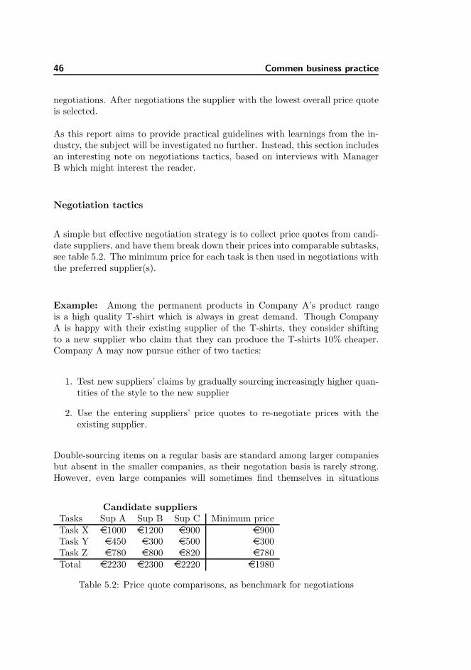
46 Commen business practice
negotiations. After negotiations the supplier with the lowest overall price quoteis selected.
As this report aims to provide practical guidelines with learnings from the in-dustry, the subject will be investigated no further. Instead, this section includesan interesting note on negotiations tactics, based on interviews with ManagerB which might interest the reader.
Negotiation tactics
A simple but effective negotiation strategy is to collect price quotes from candi-date suppliers, and have them break down their prices into comparable subtasks,see table 5.2. The minimum price for each task is then used in negotiations withthe preferred supplier(s).
Example: Among the permanent products in Company A’s product rangeis a high quality T-shirt which is always in great demand. Though CompanyA is happy with their existing supplier of the T-shirts, they consider shiftingto a new supplier who claim that they can produce the T-shirts 10% cheaper.Company A may now pursue either of two tactics:
1. Test new suppliers’ claims by gradually sourcing increasingly higher quan-tities of the style to the new supplier
2. Use the entering suppliers’ price quotes to re-negotiate prices with theexisting supplier.
Double-sourcing items on a regular basis are standard among larger companiesbut absent in the smaller companies, as their negotation basis is rarely strong.However, even large companies will sometimes find themselves in situations
Candidate suppliersTasks Sup A Sup B Sup C Minimum priceTask X e1000 e1200 e900 e900Task Y e450 e300 e500 e300Task Z e780 e800 e820 e780Total e2230 e2300 e2220 e1980
Table 5.2: Price quote comparisons, as benchmark for negotiations

5.3 Optimization techniques with operations research 47
where the supplier has the upper hand in negotiations, when the special craftingskills or techniques of the supplier are in demand.
5.3 Optimization techniques with operations re-search
Operations research (OR), a branch of mathematics, enables us to articulateand analyze complex scenario, for decision analysis purposes, profit maximiza-tion, resource allocation and much more. Several industries benefit from thisdiscipline. Within logistics, operations research is used for complex planning,plotting optimal routes for carriers, or placing logistic centres etc. In the foodindustry examples are found on how to maximize profit with limited capacitiesand uncertain and unstable demand.
Though the field of research originated during World War II and shortly afterfound usage in the industries, deployment of OR is limited to mainly large firmswith the economic and human resources to articulate and solve OR challenges.
The evolution in computational resources within the past half-century, have onlyrecently gained OR popularity among the wider business community. Possibly,graphical user interfaces for management make it easier to gather data and ar-ticulate optimization problems. With visual feedback to variations in scenarios,it might be easier to trust the analyses results. The preconditions for widelyadaptation of OR in routine business procedures are only just evolving by ORsoftware integrations with enterprise resource planning (ERP) systems. Yet,even small companies may benefit from OR techniques. e.g for product mixanalyses and decision analyses.
The potential application of OR is unlimited, but some examples are givenbelow:
Transportation and Assignment problems Airline companies may use ORto make flight plans which minimizes airport costs.
Resource allocation With limited machinery capacity, production resourcescan be allocated to, e.g., maximize profits.
Decision analysis Decide for one plan among a selection of plans for investinga fixed sum of money.
We have learned that general business practices apply across industries, and
48 Commen business practice
may be part of business procedures in fashion companies as well. Routine costmanagement and analysis is present, where companies strive to understand theprofitability of their operations. Outsourcing practises are less systematic inpractical applications, but guidelines on good outsourcing practices have beenlisted based on the recommendations of The Confederation of Danish Industries.Applications of methods from operations research in other industries, indicatethat OR methodologies could prove valuable to the fashion industry.
This chapter concludes part II, which provides background knowledge requiredto understand the preliminaries for the work presented in this report. Thoughoutsourcing is a vital part of Danish fashion companies’ business conduct, thereseem to lack structured methods for outsourcing evaluations and decisions. Itis possible, a tool for outsourcing evaluations may benefit fashion companies.
Part III focus on developing such a method, and investigate if it indeed hasbenefits to offer.
Part III
Methods and analyses

51
In this part..
This part is dedicated to the development of an analysis tool to support, forstrategic, tactic, and operational outsourcing decisions.
A company could choose which type of manufacturer, Cut-Make-Trim (CMT)or Freight-on-Board (FOB), they want to work with as part of a strategy. Thefirst chapter presents a method for comparing FOB and CMT costs, so com-panies may individually decide which collaboration model best enhances theircompetitiveness and establish supplier collaborations accordingly.
The second chapter is dedicated to the tactical decision of selecting particularsuppliers to work with from a range of candidates. A method is suggested forcomparing suppliers with respect to price quotations, estimates of macro costs,and indirect costs. Techniques for estimating macro costs and indirect costs aresuggested. The comparison of three fictional suppliers is demonstrated.
The first two chapters are in coherence with the views and recommendationsof David Birnbaum, accounted for in Chapter 4. The third and final chaptercontinues the pursuit of cost advantages and profits increase beyond Birnbaum’ssuggestions. By using operations research techniques methods are presented forincreasing profitability after a fashion company has decided which suppliers touse. The methods are intended for use in daily operations.
The last chapter gathers the methods of the previous three chapters and adviceon their proper usage as a combined management decision support tool foroutsourcing as well as interpretations of results.

52
Chapter 6
FOB vs. CMT collaborations
This chapter presents a method for comparing FOB and CMT costs across col-lections and garment types. The objective is to obtain a method for manystrategic decisions on which supplier collaborations may be established to in-crease profitability.
The method presented in this chapter have been developed by the author withinput and guidance from Jan Fabritius.
6.1 Method
Though each garment carries its own cost in terms of material consumption,labour costs, etc., it is part of a collection of styles linked to each other throughshared materials, design, and season. Thus, garments will be viewed as insepa-rable entities as a basis for the method developed.
An entire collection is linked together through shared materials, colours, stylesand branding. A collection is evaluated as a whole and customers (retailersand end-consumers) will respond in the same way. A collection often consistsof basic styles, modified and updated bestsellers from previous seasons, exper-imental styles, and signature styles. The fundamental economic transaction
54 FOB vs. CMT collaborations
links with the entire collection rather than the individual garment. As a resultthe economic benefits of a sound outsourcing strategy will be reflected in theprofitability of the collection (and the company) as a whole.
Design costs relate to the collection rather than the individual piece of garments,as externals apply, i.e.: the initial work in defining a collection style is a one-time effort, the marginal design work for an individual piece of garment is thenmuch less.
Because many styles share the same fabric, splitting the production lot betweentwo different suppliers entails more complicated and expensive logistics. There-fore, it may be reasonable to choose the manufacturer with the combined lowestprice, even though lower prices for individual styles can be found among othercandidate suppliers.
A model is built in three iterations, starting with a single style and a single can-didate supplier, ending with numerous styles and numerous candidate suppliers.The analysis will refer to a fictive fashion company, “Company A”. The term’Manufacturers’ denote the collective name for all companies in the business ofmanufacturing garments. ’Suppliers’ on the other hand, are manufacturers wholive up to Company A’s standard and collaborate with Company A. ’Candidatesuppliers’ are suppliers which Company A contemplates as suppliers. Suppliersspecialize in either CMT or FOB services, which will label the ’Supplier type’.
Assumptions
The method presented in the following is based on a number of assumptions.A set of assumptions reflect a simplified reality, however, for which a givenproblem can be defined and solved. Making assumptions carries a risk of over-simplifying the original problem which in turn yields inapplicable solutions. Foreach assumption, implications of accepting them is set out below.
Assumption 1 The method focuses only on design and production related ac-tivities, plus related staff costs.Consequence: The method heavily depends on qualified measures of staffcosts and production related activities. Failing to do so may yield inac-curate results. Upon evaluation of the analysis results one may benefit tokeep these consequences in mind to fully enjoy the recommendations ofthe analyses.
Assumption 2 There is no correlation between outsourcing decisions, and out-side costs such as sales force costs and management costs.
6.1 Method 55
Consequence: Outsourcing decisions may affect which fabric minimumsCompany A faces. It might prove more profitable to order surplus stockwhich in turn must be dumped (see Chapter 8), requiring involvement ofother departments.
Assumption 3 Company A may need only internal management and key de-signers purchasing additional product development and production ser-vices at suppliers’.Consequence: This assumption may result in organisational restructures,if the company has previously been organized around a different productdevelopment structure.
Assumption 4 Garment quality does not change from one supplier or produc-tion collaboration method to another. There is a certain quality standard,which candidate suppliers match.Consequence: The assumption that garment qualities and fabric rangesare identical between suppliers is a bold simplification. It may be ratifiedif candidate suppliers chosen for comparison have been carefully nomi-nated based on this requirement. If this assumption fails, it may heavilyaffect the resulting products and customer perception of the brand.
Assumption 5 Fabric supplies are identical from one candidate supplier toanother.Consequence: This is mostly attainable with supplier proximity to a largetextile industry. Should this assumptions fail, it may put restraint styledesigns.
Designers may feel too restricted if the range of materials and productioncapabilities are too tight, yielding a less appealing product range. Conse-quently, the result of the analysis may point to a more costly solution.
Assumption 6 The additional macro costs or macro cost estimates have al-ready been included in the candidate supplier price quotes during datacollection for the analyses1.Consequence: The use of macro cost estimates is only valid if the esti-mates have been made to carefully reflect reality. Otherwise results of theinvestigation may be completely arbitrary. Failing to project cost mea-sures to the same moment in time may yield inaccurate results. Sincecountries and political agreements are constantly changing, resulting inchanged trade conditions. That said, precise macro costs estimates andhigh data quality will render very probable results.
Assumption 7 All comparative data has been projected to the same momentin time, see appendix B.
1more on this in Chapter 7, which presents a method to estimate macro costs.
56 FOB vs. CMT collaborations
Consequence: Costs from different years does not include currency infla-tions or changes in political agreements. Likewise, different compositionsof collection complexities and changing fashion may disrupt an accuratecomparison.
Developing the method
For the analysis, Company A’s activities are divided into 20 categories, see figure6.1.
The cost structure of Company A is influenced by supplier collaboration. Pur-chases are a variable cost per garment. For CMT services, this covers functions10-13; FOB includes functions 2-15 as well. In addition, Company A have addi-tional variable and fixed costs regardless of supplier type. For the analysis, wedefine the following variables:
pcmt price quoted by the candidate supplier per garment for functions10-13
pallfob price quoted by the candidate supplier per garment for functions2-14
Cmat Company A’s procurement and logistics cost of material, i.e.functions 5-9
Cfob Company A’s cost for FOB services when co-operating with aCMT supplier
Ccoo Company A’s cost of collaboration with a particular supplier,i.e. functions 15, 16, and 18
Cother the costs of non-FOB functions, i.e. functions 1, 17, 19, and 20
Company A’s general annual or seasonal cost functions looks like this:
Ctotal ≡ Cfixed + Cvariable + Purchasevariable (6.1)
where Purchase refers to purchases only from the supplier, and C are pur-chases from other suppliers or Company A’s own cost. The actual calculationsdiffer depending on the type of supplier collaboration and assumptions prior tosupplier selection.
The analysis has been broken into three steps, starting with the simplest case:one company, one garment type, and one supplier. Though it is highly unlikelythat a fashion company will place only one of its items with one supplier, thisprocedure will demonstrate the methodology, before we move on to increasinglycomplex scenarios.
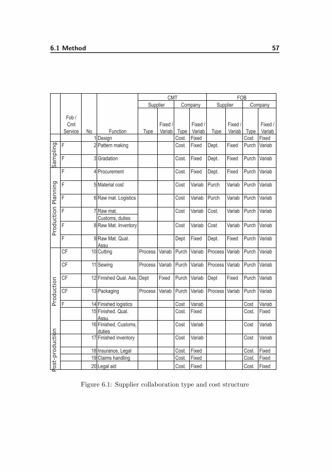
6.1 Method 57
Type
Fixed /
Variab Type
Fixed /
Variab Type
Fixed /
Variab Type
Fixed /
Variab
1 Design Cost. Fixed Cost. Fixed
F 2 Pattern making Cost. Fixed Dept. Fixed Purch Variab
F 3 Gradation Cost. Fixed Dept. Fixed Purch Variab
F 4 Procurement Cost. Fixed Dept. Fixed Purch Variab
F 5 Material cost Cost Variab Purch Variab Purch Variab
F 6 Raw mat. Logistics Cost Variab Purch Variab Purch Variab
Raw mat.
Customs, duties
F 8 Raw Mat. Inventory Cost Variab Cost Variab Purch Variab
F 9 Raw Mat. Qual.
Assu
Dept Fixed Dept. Fixed Purch Variab
CF 10 Cutting Process Variab Purch Variab Process Variab Purch Variab
CF 11 Sewing Process Variab Purch Variab Process Variab Purch Variab
CF 12 Finished Qual. Ass. Dept Fixed Purch Variab Dept Fixed Purch Variab
CF 13 Packaging Process Variab Purch Variab Process Variab Purch Variab
F 14 Finished logistics Cost Variab Cost Variab
15 Finished. Qual.
Assu.
Cost. Fixed Cost. Fixed
16 Finished. Customs,
duties
Cost Variab Cost Variab
17 Finished inventory Cost Variab Cost Variab
18 Insurance, Legal Cost. Fixed Cost. Fixed
19 Claims handling Cost. Fixed Cost. Fixed
20 Legal aid Cost. Fixed Cost. Fixed
Pro
duction
Purch Variab
Sam
pling
Pro
duction P
lannin
g
Cost Variab Cost. VariabF 7
FOB
Supplier Company Supplier Company
Fob /
Cmt
Service No Function
CMT
Post-
pro
duction
Figure 6.1: Supplier collaboration type and cost structure
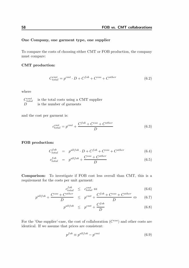
58 FOB vs. CMT collaborations
One Company, one garment type, one supplier
To compare the costs of choosing either CMT or FOB production, the companymust compare:
CMT production:
Ccmttotal = pcmt · D + Cfob + Ccoo + Cother (6.2)
where
Ccmttotal is the total costs using a CMT supplier
D is the number of garments
and the cost per garment is:
ccmttotal = pcmt +
Cfob + Ccoo + Cother
D(6.3)
FOB production:
Cfobtotal = pallfob · D + Cfob + Ccoo + Cother (6.4)
cfobtotal = pallfob +
Ccoo + Cother
D(6.5)
Comparison: To investigate if FOB cost less overall than CMT, this is arequirement for the costs per unit garment:
cfobtotal ≤ ccmt
total ⇔ (6.6)
pallfob +Ccoo + Cother
D≤ pcmt +
Cfob + Ccoo + Cother
D⇔ (6.7)
pallfob ≤ pcmt +Cfob
D(6.8)
For the ’One supplier’-case, the cost of collaboration (Ccoo) and other costs areidentical. If we assume that prices are consistent:
pfob ≡ pallfob − pcmt (6.9)
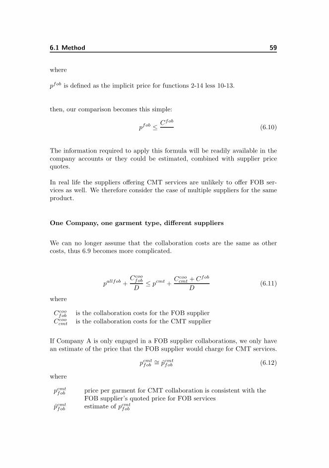
6.1 Method 59
where
pfob is defined as the implicit price for functions 2-14 less 10-13.
then, our comparison becomes this simple:
pfob ≤Cfob
(6.10)
The information required to apply this formula will be readily available in thecompany accounts or they could be estimated, combined with supplier pricequotes.
In real life the suppliers offering CMT services are unlikely to offer FOB ser-vices as well. We therefore consider the case of multiple suppliers for the sameproduct.
One Company, one garment type, different suppliers
We can no longer assume that the collaboration costs are the same as othercosts, thus 6.9 becomes more complicated.
pallfob +Ccoo
fob
D≤ pcmt +
Ccoocmt + Cfob
D(6.11)
where
Ccoofob is the collaboration costs for the FOB supplier
Ccoocmt is the collaboration costs for the CMT supplier
If Company A is only engaged in a FOB supplier collaborations, we only havean estimate of the price that the FOB supplier would charge for CMT services.
pcmtfob
∼= pcmtfob (6.12)
where
pcmtfob price per garment for CMT collaboration is consistent with the
FOB supplier’s quoted price for FOB servicespcmt
fob estimate of pcmtfob
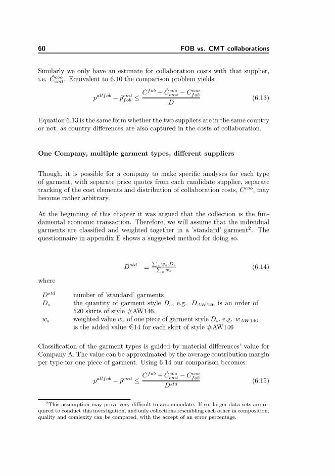
60 FOB vs. CMT collaborations
Similarly we only have an estimate for collaboration costs with that supplier,i.e. Ccoo
cmt. Equivalent to 6.10 the comparison problem yields:
pallfob − pcmtfob ≤
Cfob + Ccoocmt − Ccoo
fob
D(6.13)
Equation 6.13 is the same form whether the two suppliers are in the same countryor not, as country differences are also captured in the costs of collaboration.
One Company, multiple garment types, different suppliers
Though, it is possible for a company to make specific analyses for each typeof garment, with separate price quotes from each candidate supplier, separatetracking of the cost elements and distribution of collaboration costs, Ccoo, maybecome rather arbitrary.
At the beginning of this chapter it was argued that the collection is the fun-damental economic transaction. Therefore, we will assume that the individualgarments are classified and weighted together in a ’standard’ garment2. Thequestionnaire in appendix E shows a suggested method for doing so.
Dstd ≡P
sws·Ds
P
sws
(6.14)
where
Dstd number of ’standard’ garmentsDs the quantity of garment style Ds, e.g. DAW146 is an order of
520 skirts of style #AW146.ws weighted value ws of one piece of garment style Ds, e.g. wAW146
is the added value €14 for each skirt of style #AW146
Classification of the garment types is guided by material differences’ value forCompany A. The value can be approximated by the average contribution marginper type for one piece of garment. Using 6.14 our comparison becomes:
pallfob − pcmt ≤Cfob + Ccoo
cmt − Ccoofob
Dstd(6.15)
2This assumption may prove very difficult to accommodate. If so, larger data sets are re-quired to conduct this investigation, and only collections resembling each other in composition,quality and comlexity can be compared, with the accept of an error percentage.
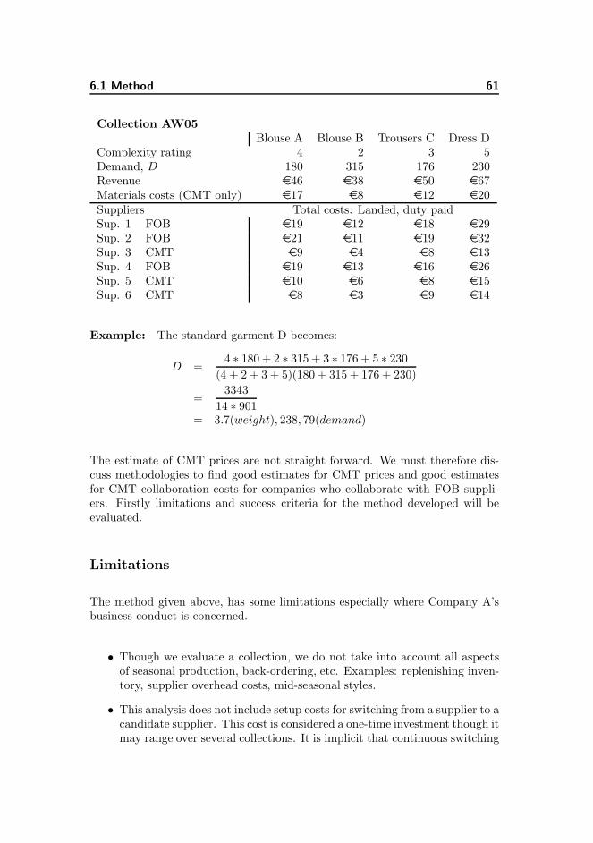
6.1 Method 61
Collection AW05Blouse A Blouse B Trousers C Dress D
Complexity rating 4 2 3 5Demand, D 180 315 176 230Revenue e46 e38 e50 e67Materials costs (CMT only) e17 e8 e12 e20Suppliers Total costs: Landed, duty paidSup. 1 FOB e19 e12 e18 e29Sup. 2 FOB e21 e11 e19 e32Sup. 3 CMT e9 e4 e8 e13Sup. 4 FOB e19 e13 e16 e26Sup. 5 CMT e10 e6 e8 e15Sup. 6 CMT e8 e3 e9 e14
Example: The standard garment D becomes:
D =4 ∗ 180 + 2 ∗ 315 + 3 ∗ 176 + 5 ∗ 230
(4 + 2 + 3 + 5)(180 + 315 + 176 + 230)
=3343
14 ∗ 901= 3.7(weight), 238, 79(demand)
The estimate of CMT prices are not straight forward. We must therefore dis-cuss methodologies to find good estimates for CMT prices and good estimatesfor CMT collaboration costs for companies who collaborate with FOB suppli-ers. Firstly limitations and success criteria for the method developed will beevaluated.
Limitations
The method given above, has some limitations especially where Company A’sbusiness conduct is concerned.
• Though we evaluate a collection, we do not take into account all aspectsof seasonal production, back-ordering, etc. Examples: replenishing inven-tory, supplier overhead costs, mid-seasonal styles.
• This analysis does not include setup costs for switching from a supplier to acandidate supplier. This cost is considered a one-time investment though itmay range over several collections. It is implicit that continuous switching
62 FOB vs. CMT collaborations
to cheaper candidate suppliers, will be less profitable than establishinglonger relations to existing suppliers, who already understand the designand quality requirements of Company A.
• Company A must be willing to use the material available to it’s FOB sup-pliers. We assume that all candidate FOB suppliers can offer a wide rangeof fabrics, qualities, and patterns which will match Company A’s stan-dards. Company A for its part, is open to selecting among the availablefabrics, and not locked on to one specific textile manufacturer.
Estimating CMT collaboration costs with FOB suppliers
Proper estimates of CMT collaboration costs are important to conduct the anal-ysis. However, evaluating on techniques for doing so is outside the scope of thisreport.
Converting collection garments into a standard garmentsmeasure, Dstd
Equation 6.14 can be calculated with weights depending on Company A’s prefer-ences. The weighting can be carried out with alternative factors of importance,e.g.:
• The mark-up value for a garment (net. unit revenue)
• Complexity degree
• Novelty value
• Brand value
It is the authors belief collection styles may be weighted into a standard garmentin a satisfying way, though it requires qualitative and consistent evaluation foreach style to yield good results. This report suggest using complexity degree asweight. The weight can be based on a rating as suggested in the questionnaireof appendix E.
6.2 Results interpreted 63
Data collection
To use the method presented in this chapter, data must be collected prior toanalysis. The collection of data may be automated, granted all measures havebeen collected through an ERP system.
6.2 Results interpreted
A method has been presented for comparing cost of FOB and CMT collab-orations, buy including all activities of the production process. To comparecollections of different style compositions and complexities a method for weight-ing these variations into a standard garment is presented. The comparison ofFOB and CMT collaboration costs may be useful for identifying which suppliercollaboration model is most profitable for a fashion company. The method issuggested for use in strategic considerations.
The following chapter suggest a method for comparing suppliers based on theirprice quotations, geographic location and quality standards.

64 FOB vs. CMT collaborations
Chapter 7
Supplier comparison analysis
This chapter is dedicated to improving the information outsourcing decisionsare based upon, and consequently select suppliers, which are least expensiveoverall. A method for comparing suppliers, with considerations to direct costs,indirects costs, and macro costs is given. To make proper estimates for macrocosts a method is developed based on a ranking system. Methods for costingindirect costs are also provided. The objective is to create an easy-to-use com-pounded method for supporting tactical decisions, which can be incorporatedinto business routines for managers and sourcers.
All methods presented in this chapter is developed by the author. The inspi-ration for including additional costs in supplier comparisons comes from DavidBirnbaum (see chapter 4).
7.1 Quantifying Macro Costs
Before deciding to collaborate with a supplier in a given country it would bewise to consider macro-factors (political climate, infrastructures, trade barriers,etc.) facilitating or obstructing collaboration across borders, or in more generalterms: the business environment. To compare the data of different candidate
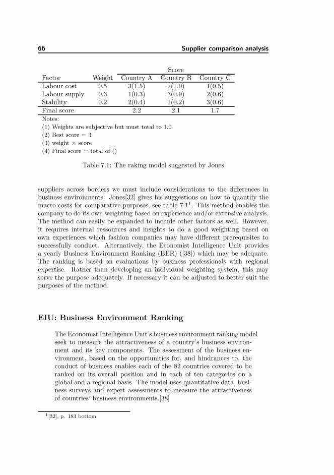
66 Supplier comparison analysis
ScoreFactor Weight Country A Country B Country CLabour cost 0.5 3(1.5) 2(1.0) 1(0.5)Labour supply 0.3 1(0.3) 3(0.9) 2(0.6)Stability 0.2 2(0.4) 1(0.2) 3(0.6)Final score 2.2 2.1 1.7Notes:
(1) Weights are subjective but must total to 1.0
(2) Best score = 3
(3) weight × score
(4) Final score = total of ()
Table 7.1: The raking model suggested by Jones
suppliers across borders we must include considerations to the differences inbusiness environments. Jones[32] gives his suggestions on how to quantify themacro costs for comparative purposes, see table 7.11. This method enables thecompany to do its own weighting based on experience and/or extensive analysis.The method can easily be expanded to include other factors as well. However,it requires internal ressources and insights to do a good weighting based onown experiences which fashion companies may have different prerequisites tosuccessfully conduct. Alternatively, the Economist Intelligence Unit providesa yearly Business Environment Ranking (BER) ([38]) which may be adequate.The ranking is based on evaluations by business professionals with regionalexpertise. Rather than developing an individual weighting system, this mayserve the purpose adequately. If necessary it can be adjusted to better suit thepurposes of the method.
EIU: Business Environment Ranking
The Economist Intelligence Unit’s business environment ranking modelseek to measure the attractiveness of a country’s business environ-ment and its key components. The assessment of the business en-vironment, based on the opportunities for, and hindrances to, theconduct of business enables each of the 82 countries covered to beranked on its overall position and in each of ten categories on aglobal and a regional basis. The model uses quantitative data, busi-ness surveys and expert assessments to measure the attractivenessof countries’ business environments.[38]
1[32], p. 183 bottom
7.1 Quantifying Macro Costs 67
The BER yields a single country score based on both quantitative data andqualitative data within 10 different categories, (see listing below). The ratingdoes not include tariffs and quota costs, which are prevalent in the fashionindustry. These variable costs are, however, well known and can be includedseparately in an final FVCA analysis. The categories are:
1. Political environment
2. Macroeconomic environment
3. Market opportunities
4. Policy towards private enterprise and competition
5. Policy and attitudes towards foreign investment
6. Foreign trade and exchange regimes
7. Tax regime
8. Financing
9. Labour market and skills
10. Infrastructure
In total, a questionnaire of 95 questions, quantify the qualitative data. Foreach question the respondent gives a ranking between 1-5. Quantitative data islikewise divided into five subdivisions. Finally, the aggregate category scores areweighted together, and several incremental steps finally yields a country scoreon a scale ranging from one to ten.
During the research previous to this report no examples were found on using therankings as explicitly as suggested here. Rather, the rankings seem to be usedmainly for briefing purposes. The attempt to use this score to include macrocosts in a price quote evaluation must be considered experimental.
Method of inclusion
We decide that a candidate supplier price quote, Pquote, must be weighted withthe macro costs factor, xBER, to reveal the business environment cost pBER tothe fashion company.
pBER = pquote · xBER (7.1)

68 Supplier comparison analysisp
en
alt
y c
ha
rge
share in collected
consumption
even
soft constrainthard constraint
proportional
accelerated
100%50%
custom-made
Figure 7.1: Different examples for constraint functions
The key is to develop xBER to ensure increase with decreasing values of therank. To achieve this, xBER is converted into an inversely proportial functionof the BER, with the convertion formula f(r) and adjust it with a. The resultsis:
xBER = α · f(rBER) (7.2)
where
rBER is the BER ratingf(r) is the conversion function, converting rBER into a percentage
The function, f(r), can be defined however we prefer. An initial linear con-version function is defined:
f(r) =(
1 + (1 −rBER
10))
(7.3)
As we gain more experience with using these parameters in comparative studiesand compare our forecasts with reality, a and f(r) may need adjustments. Thefunction f(r) may be modelled with soft or hard contraints (see figure 7.1)towards the extremeties of the BER to avoid considerations of suppliers in verylow BER rated countries.
To verify the model and parameters, companies can develop cost forecasts fora collection from a previous season for immediate comparison with the actualoutcome, granted all data is available. If not, procedures for data collectionmust be extended to facilitate these types of analysis on future collections.
7.1 Quantifying Macro Costs 69
After carefully testing the model for different values of a and f(r), the forecaststill fails to deliver satisfactory results, changes on the BER might be necessary.
Modifying the BER for fashion business purposes.
Changing the BER to better suit fashion businesses requires careful analysisof the data feedback from earlier models and a clear understanding of how theBER rate is calculated. Below, a procedure for modifying the BER is suggested.
1. Compare supplier price quotes and estimated total costs with xBER, withactual costs2. Observe any patterns in differences. Graphics might beuseful for identifying the patterns, or statistic correlation between countrycosts and error fluctuations.
2. Analyze which factors cause the fluctuations and to which BER categoriesthey belong, consequently discovering which factors of the BER could beweighted differently.
3. Study exactly how the BER has been generated. The tool has been cre-ated by skilled analysts and their method may provide good guidelines.Consider consulting a statistics analyst.
4. Use Jones’ (table 7.1) example as a guideline to adjust the ranking.
5. Evaluate on the new country scores by comparing against older data.
If modifications to the BER still yields inaccurate results, the model may berejected to seek new approaches to estimate the impact of macro costs.
The next section focus on tariff an quota costs.
Tariff and quotas
Tariffs and quotas are part of the trade barriers, which are setup between coun-tries or regions. Tariffs relate to the costs of bringing goods into a country andthey apply regardless of where the production is from3. Quotas set a physicallimit to how many items can be imported into a country or region, and they
2 The actual costs must be carefully analyzed to give a true indicator. Methods withinActivity Based Costing may be relevant
3Inside the EU internal trade is tariff-free, though.
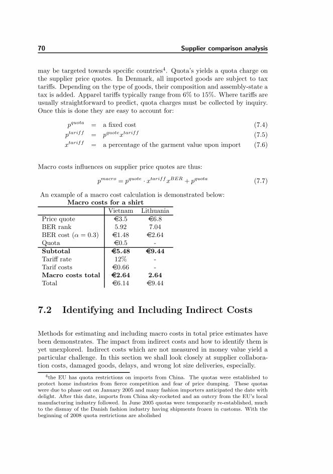
70 Supplier comparison analysis
may be targeted towards specific countries4. Quota’s yields a quota charge onthe supplier price quotes. In Denmark, all imported goods are subject to taxtariffs. Depending on the type of goods, their composition and assembly-state atax is added. Apparel tariffs typically range from 6% to 15%. Where tariffs areusually straightforward to predict, quota charges must be collected by inquiry.Once this is done they are easy to account for:
pquota = a fixed cost (7.4)
ptariff = pquotextariff (7.5)
xtariff = a percentage of the garment value upon import (7.6)
Macro costs influences on supplier price quotes are thus:
pmacro = pquote · xtariffxBER + pquota (7.7)
An example of a macro cost calculation is demonstrated below:Macro costs for a shirt
Vietnam LithuaniaPrice quote e3.5 e6.8BER rank 5.92 7.04BER cost (α = 0.3) e1.48 e2.64Quota e0.5 -Subtotal e5.48 e9.44Tariff rate 12% -Tarif costs e0.66 -Macro costs total e2.64 2.64Total e6.14 e9.44
7.2 Identifying and Including Indirect Costs
Methods for estimating and including macro costs in total price estimates havebeen demonstrates. The impact from indirect costs and how to identify them isyet unexplored. Indirect costs which are not measured in money value yield aparticular challenge. In this section we shall look closely at supplier collabora-tion costs, damaged goods, delays, and wrong lot size deliveries, especially.
4the EU has quota restrictions on imports from China. The quotas were established toprotect home industries from fierce competition and fear of price dumping. These quotaswere due to phase out on January 2005 and many fashion importers anticipated the date withdelight. After this date, imports from China sky-rocketed and an outcry from the EU’s localmanufacturing industry followed. In June 2005 quotas were temporarily re-established, muchto the dismay of the Danish fashion industry having shipments frozen in customs. With thebeginning of 2008 quota restrictions are abolished
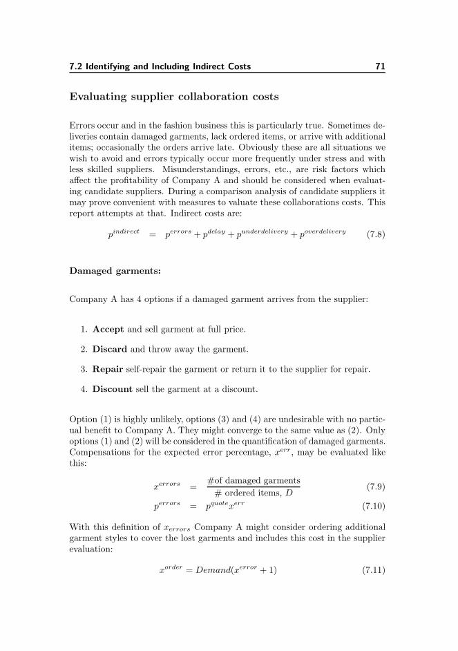
7.2 Identifying and Including Indirect Costs 71
Evaluating supplier collaboration costs
Errors occur and in the fashion business this is particularly true. Sometimes de-liveries contain damaged garments, lack ordered items, or arrive with additionalitems; occasionally the orders arrive late. Obviously these are all situations wewish to avoid and errors typically occur more frequently under stress and withless skilled suppliers. Misunderstandings, errors, etc., are risk factors whichaffect the profitability of Company A and should be considered when evaluat-ing candidate suppliers. During a comparison analysis of candidate suppliers itmay prove convenient with measures to valuate these collaborations costs. Thisreport attempts at that. Indirect costs are:
pindirect = perrors + pdelay + punderdelivery + poverdelivery (7.8)
Damaged garments:
Company A has 4 options if a damaged garment arrives from the supplier:
1. Accept and sell garment at full price.
2. Discard and throw away the garment.
3. Repair self-repair the garment or return it to the supplier for repair.
4. Discount sell the garment at a discount.
Option (1) is highly unlikely, options (3) and (4) are undesirable with no partic-ual benefit to Company A. They might converge to the same value as (2). Onlyoptions (1) and (2) will be considered in the quantification of damaged garments.Compensations for the expected error percentage, xerr, may be evaluated likethis:
xerrors =#of damaged garments
# ordered items, D(7.9)
perrors = pquotexerr (7.10)
With this definition of xerrors Company A might consider ordering additionalgarment styles to cover the lost garments and includes this cost in the supplierevaluation:
xorder = Demand(xerror + 1) (7.11)

72 Supplier comparison analysis
Alternatively, Company A might charge a cost proportional to the profit con-tribution value5 of this garment to the collection.
perrors = pquote ·
pprofits
Pprofitcollection · Demands · xerrors
(7.12)
where s refers to a specific style. It is up to Company A to decide how they willrespond to and valuate errors.
Delays
Occasionally orders are not delivered at the agreed date. Companies have verydifferent ways to handle delays in delivery. The case studies indicate that mostcompanies tolerate some delay but grow increasingly intolerant of prolongeddelays. Intolerance peaks, when delays result in a complete refusal of the entiredelivery. Delays must be a function of time and might look like:
pdelays = pquote · xdelay (7.13)
xdelay(t) = as∆t , for t ∈ [0 − q] (7.14)
xdelay(t) = 10.000% , for t > q (7.15)
where
∆t time, measured in days, ∆t ∈ Ia weight of cost, defined by Company As parameter to accelerate or deccelerate the curve, defined by Company Aq maximum accepted delay time, measured in days
The final value of xdelay depends on the individual supplier’s ability to deliveron time.
Observations from case company interviews indicated that decreasing size offashion companies would increase their tolerance to delays. This may be linkedto the fact, that larger companies may work towards more frequent collectionturnover, and smaller fashion companies have a greater share of their total ordertied up with each supplier.
Wrong lot size
Overdelivery and underdelivery cause different inconveniences to companies.Furthermore both situations may occur simultaneously.
5or any other scalar value suitable to reflect the costs of unsaleable items
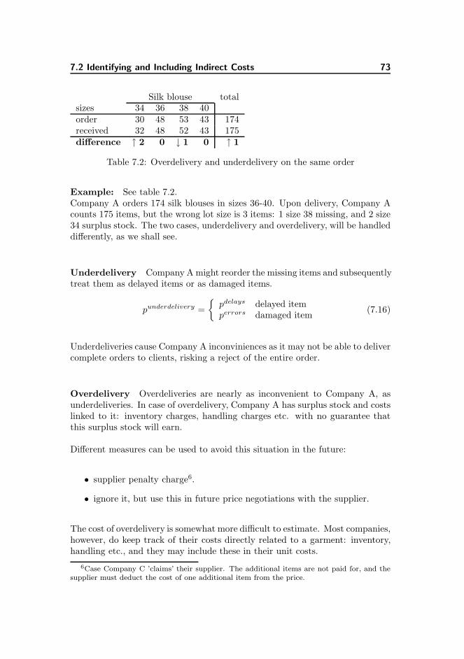
7.2 Identifying and Including Indirect Costs 73
Silk blouse totalsizes 34 36 38 40order 30 48 53 43 174received 32 48 52 43 175difference ↑ 2 0 ↓ 1 0 ↑ 1
Table 7.2: Overdelivery and underdelivery on the same order
Example: See table 7.2.Company A orders 174 silk blouses in sizes 36-40. Upon delivery, Company Acounts 175 items, but the wrong lot size is 3 items: 1 size 38 missing, and 2 size34 surplus stock. The two cases, underdelivery and overdelivery, will be handleddifferently, as we shall see.
Underdelivery Company A might reorder the missing items and subsequentlytreat them as delayed items or as damaged items.
punderdelivery =
{
pdelays delayed itemperrors damaged item
(7.16)
Underdeliveries cause Company A inconviniences as it may not be able to delivercomplete orders to clients, risking a reject of the entire order.
Overdelivery Overdeliveries are nearly as inconvenient to Company A, asunderdeliveries. In case of overdelivery, Company A has surplus stock and costslinked to it: inventory charges, handling charges etc. with no guarantee thatthis surplus stock will earn.
Different measures can be used to avoid this situation in the future:
• supplier penalty charge6.
• ignore it, but use this in future price negotiations with the supplier.
The cost of overdelivery is somewhat more difficult to estimate. Most companies,however, do keep track of their costs directly related to a garment: inventory,handling etc., and they may include these in their unit costs.
6Case Company C ’claims’ their supplier. The additional items are not paid for, and thesupplier must deduct the cost of one additional item from the price.
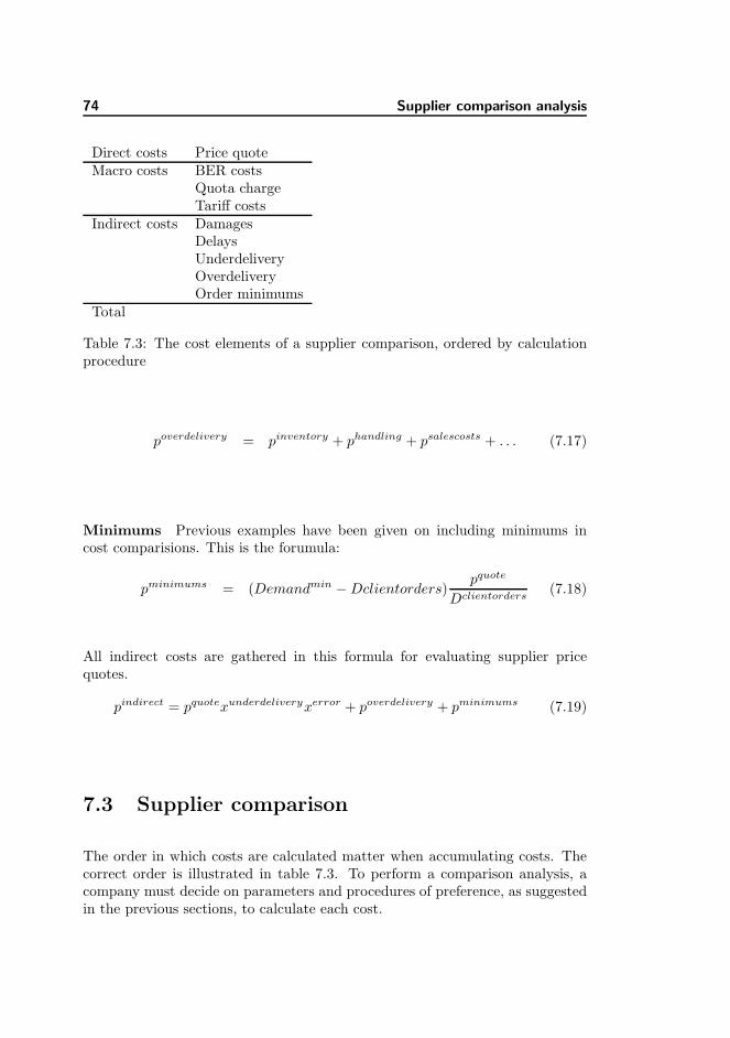
74 Supplier comparison analysis
Direct costs Price quoteMacro costs BER costs
Quota chargeTariff costs
Indirect costs DamagesDelaysUnderdeliveryOverdeliveryOrder minimums
Total
Table 7.3: The cost elements of a supplier comparison, ordered by calculationprocedure
poverdelivery = pinventory + phandling + psalescosts + . . . (7.17)
Minimums Previous examples have been given on including minimums incost comparisions. This is the forumula:
pminimums = (Demandmin − Dclientorders)pquote
Dclientorders(7.18)
All indirect costs are gathered in this formula for evaluating supplier pricequotes.
pindirect = pquotexunderdeliveryxerror + poverdelivery + pminimums (7.19)
7.3 Supplier comparison
The order in which costs are calculated matter when accumulating costs. Thecorrect order is illustrated in table 7.3. To perform a comparison analysis, acompany must decide on parameters and procedures of preference, as suggestedin the previous sections, to calculate each cost.
7.3 Supplier comparison 75
This chapter presented various methods for estimating macro costs and indirectcosts, which could be used in price comparisons of different suppliers. In totalthe chapter presents a method to include these costs to uncover the financialconsequences of selecting a given supplier. The tool can be integrated withaccounting systems and in business routines, and provide supportive analysisfor tactical decisions.
Next, we consider how techniques from Operations Research may be used indaily operations, to discover cost advantages as a consequence of price structuresin the fashion industry.

76 Supplier comparison analysis

Chapter 8
Optimizations with
Operations Research
Even after a careful consideration of supplier type, and candidate supplier com-parisons, further cost advantages are still obtainable once Company A has de-cided which supplier wins the order. This chapter demonstrates how fashioncompanies may benefit from using Operations Research methods to performcost minimization and profit maximization analyses as a means to support pur-chasing decisions that will increase company profitability.
8.1 Production Cost Minimization
To illustrate the relevance of a cost minimization model this section put forwardan example:
Example: For each garment style s in the collection, Company A have pre-booked orders Ds as a result of the sales team efforts. The costs of meetingthe demand for all collection styles can be minimized, using operations researchmethodologies as will be demonstrated, in this section.
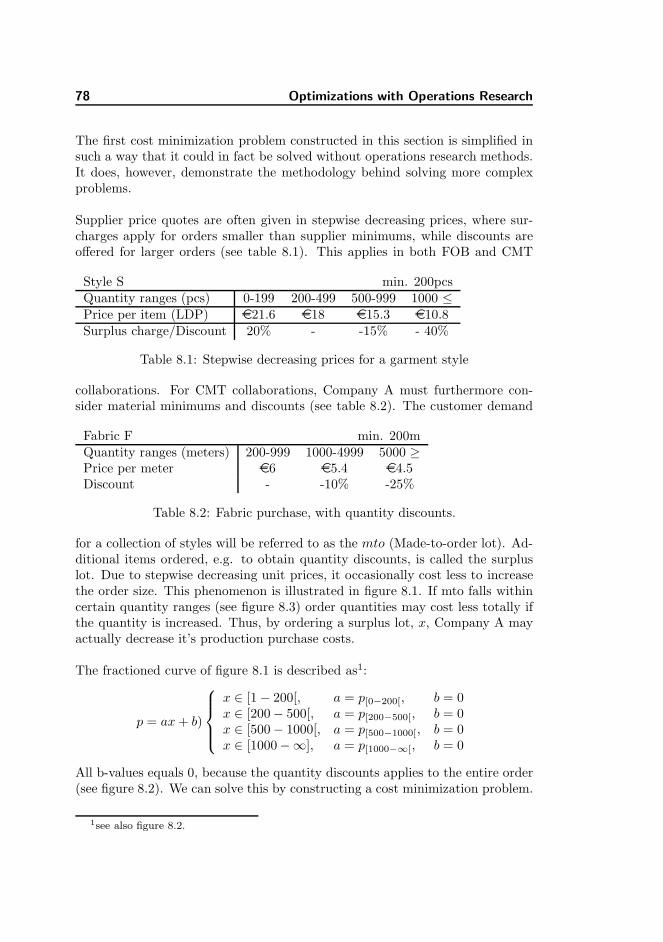
78 Optimizations with Operations Research
The first cost minimization problem constructed in this section is simplified insuch a way that it could in fact be solved without operations research methods.It does, however, demonstrate the methodology behind solving more complexproblems.
Supplier price quotes are often given in stepwise decreasing prices, where sur-charges apply for orders smaller than supplier minimums, while discounts areoffered for larger orders (see table 8.1). This applies in both FOB and CMT
Style S min. 200pcsQuantity ranges (pcs) 0-199 200-499 500-999 1000 ≤Price per item (LDP) e21.6 e18 e15.3 e10.8Surplus charge/Discount 20% - -15% - 40%
Table 8.1: Stepwise decreasing prices for a garment style
collaborations. For CMT collaborations, Company A must furthermore con-sider material minimums and discounts (see table 8.2). The customer demand
Fabric F min. 200mQuantity ranges (meters) 200-999 1000-4999 5000 ≥Price per meter e6 e5.4 e4.5Discount - -10% -25%
Table 8.2: Fabric purchase, with quantity discounts.
for a collection of styles will be referred to as the mto (Made-to-order lot). Ad-ditional items ordered, e.g. to obtain quantity discounts, is called the surpluslot. Due to stepwise decreasing unit prices, it occasionally cost less to increasethe order size. This phenomenon is illustrated in figure 8.1. If mto falls withincertain quantity ranges (see figure 8.3) order quantities may cost less totally ifthe quantity is increased. Thus, by ordering a surplus lot, x, Company A mayactually decrease it’s production purchase costs.
The fractioned curve of figure 8.1 is described as1:
p = ax + b)
x ∈ [1 − 200[, a = p[0−200[, b = 0x ∈ [200 − 500[, a = p[200−500[, b = 0x ∈ [500 − 1000[, a = p[500−1000[, b = 0x ∈ [1000−∞], a = p[1000−∞[, b = 0
All b-values equals 0, because the quantity discounts applies to the entire order(see figure 8.2). We can solve this by constructing a cost minimization problem.
1see also figure 8.2.
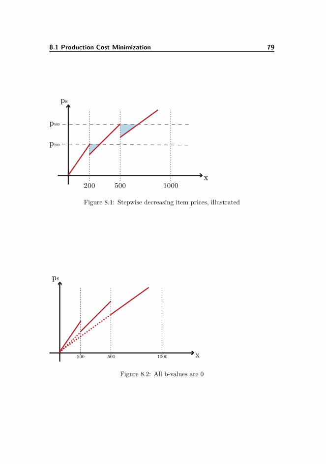
8.1 Production Cost Minimization 79
x
ps
200 500 1000
p200
p500
Figure 8.1: Stepwise decreasing item prices, illustrated
x
ps
200 500 1000
Figure 8.2: All b-values are 0
80 Optimizations with Operations Research
x
ps
yk+2yk+1yk
dk
dk
+1
dk
+2
gk, gk+1
gk+2, ...
ak
ak+1
Figure 8.3: Stepwise decreasing prices, continuous price curve
Cost Minimization Problem, Mixed Integer Programming
The overall objective is to minimize the production costs, and still meet thedemand, D. The fractioned curve of figure 8.1 has been replaced with a contin-uous equivalent in 8.3 . This equivalent curve illustrates that where demand,D, exceeds the quantity di for some intervals production costs are lowest whenordering di+1 items. Naturally, Company A would place their order accordingly.
This can be articulated as a simple minimization problem:
Objective:
min Z =∑
k=0
(gkyk + akxk) (8.1)
Decision variables:
xk ∈ [0, dk+1 − dk]
yk ∈ {0, 1}
Constraints:∑
k=0
yk = 1
yk(dk+1 − dk) − xk ≥ 0 , ∀k∑
k=0
(dkyk + xk) ≥ D
where
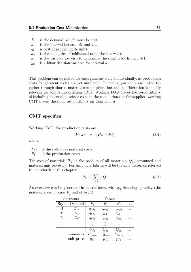
8.1 Production Cost Minimization 81
D is the demand, which must be metk is the interval between dk and dk+1
gk is cost of producing dk unitsak is the unit price of additional units the interval k
xk is the variable we wish to determine the surplus lot from, x ∈ Iyk is a binar decision variable for interval k
This problem can be solved for each garment style s individually, as productioncosts for garment styles are yet unrelated. In reality, garments are linked to-gether through shared material consumption, but this consideration is mainlyrelevant for companies ordering CMT. Working FOB places the responsibilityof including material purchase costs in the calculations on the supplier; workingCMT places the same responsibility on Company A.
CMT specifics
Working CMT, the production costs are:
PCMT = (PM + PS) (8.2)
where
PM is the collection material costsPS is the production costs
The cost of materials PM is the product of all materials, Qf , consumed andmaterial unit prices pf . For simplicity fabrics will be the only materials referredto henceforth in this chapter.
PM =∑
j∈F
pjQj (8.3)
An overview can be generated in matrix form, with qij denoting quantity (thematerial consumption Fj and style Si):
Garments FabricStyle Demand F1 F2 F3 . . .
A DA qaf1qaf2
qaf3. . .
B DB qbf1qbf2
qbf3. . .
C DC qcf1qcf2
qcf3. . .
......
......
.... . .
Qf1Qf2
Qf3. . .
minimums F1minF3min
F3min. . .
unit price pf1pf2
pf3. . .

82 Optimizations with Operations Research
x
ps
yi+1 yi+4yi
di
di+
1
di+
3
di+
2
gi, gi+1
gi+2
gi+3
... ..
ai+1
ai
sew
ing co
sts
sew
iiingg
costt
s
material c
osts
pf * F_min
...
sew
in
g + m
ateria
l cos
ts
ai+4
Figure 8.4: Material costs rise as more garments are produced
and fabric consumption costs PM costs:
PM =∑
i∈S
Di
∑
j∈F
pj · qij (8.4)
As Company A cannot always meet fabric minimums we must include this costof additional material somehow.
Example: only 367m of fabric is needed, but factory minimums are 500m. Theadditional 133m also carries costs which must be distributed on the garments.
For CMT collaborations, ordering surplus lots becomes increasingly complex,because of fabric minimums. As long as fabric minimums are not met we mayview the production of a surplus lot as free of fabric costs.
Furthermore, if fabric minimums are not met, Company A might consider dis-carding the entire fabric and the style variants using this fabric, with resultingimage loss due to incomplete order delivery. Yet, this is not an option if thedemand, D, must be met. We shall return to this debate, however, in section8.2 concerning profit maximization.
Balancing all expenses and cost saving opportunities is challenging but withoperations research methods the problem becomes much easier. We articulatethe mininimization problem for the collection as a whole, including surchargesfor excess materials.
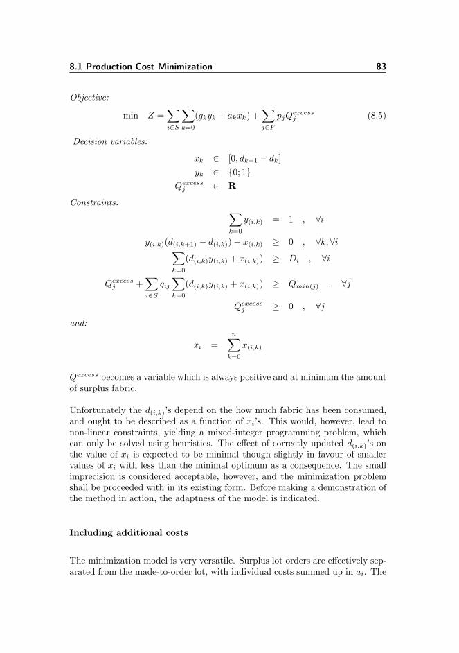
8.1 Production Cost Minimization 83
Objective:
min Z =∑
i∈S
∑
k=0
(gkyk + akxk) +∑
j∈F
pjQexcessj (8.5)
Decision variables:
xk ∈ [0, dk+1 − dk]
yk ∈ {0; 1}
Qexcessj ∈ R
Constraints:∑
k=0
y(i,k) = 1 , ∀i
y(i,k)(d(i,k+1) − d(i,k)) − x(i,k) ≥ 0 , ∀k, ∀i∑
k=0
(d(i,k)y(i,k) + x(i,k)) ≥ Di , ∀i
Qexcessj +
∑
i∈S
qij
∑
k=0
(d(i,k)y(i,k) + x(i,k)) ≥ Qmin(j) , ∀j
Qexcessj ≥ 0 , ∀j
and:
xi =
n∑
k=0
x(i,k)
Qexcess becomes a variable which is always positive and at minimum the amountof surplus fabric.
Unfortunately the d(i,k)’s depend on the how much fabric has been consumed,and ought to be described as a function of xi’s. This would, however, lead tonon-linear constraints, yielding a mixed-integer programming problem, whichcan only be solved using heuristics. The effect of correctly updated d(i,k)’s onthe value of xi is expected to be minimal though slightly in favour of smallervalues of xi with less than the minimal optimum as a consequence. The smallimprecision is considered acceptable, however, and the minimization problemshall be proceeded with in its existing form. Before making a demonstration ofthe method in action, the adaptness of the model is indicated.
Including additional costs
The minimization model is very versatile. Surplus lot orders are effectively sep-arated from the made-to-order lot, with individual costs summed up in ai. The

84 Optimizations with Operations Research
value ai may contain additional handling costs and inventory costs for surpluslot items which does not apply to made-to-order items. Material quantity dis-counts are included initially in the model, as intervals and costs are defined.As long as the values ai and gi are kept constant within an interval, this min-imization model applies to a range of cost scenarios and can be solved as amixed integer problem. In the next section the minimization problem will beincluded in a new objective function with additional decision variables. First ademonstration, though, of cost minimization on a data set.
Demonstration
To demonstrate the results obtained with the cost minimization model we con-duct the analysis on some realistic data.
quantity ranges, unit pricesStyle Demand ≤ 200 201-500 501-1000 1000 <
A 51 e11.4 e9.5 e8.1 e5.7B 105 e4.8 e4 e3.4 e2.4C 150 e15.6 e13 e11.1 e7.8D 167 e9.6 e8 e6.8 e4.8
Table 8.3: Style specifications
F1 minimum: 100mQuantity ranges (meters) 100-500 501-1000 1000 <
Price per meter e12 e10.2 e7.8Discount - -15% -35%
F2 minimum: 300mQuantity ranges (meters) 300-1000 1001-3000 3000 <
Price per meter e6 e5.4 e4.5Discount - -10% -25%
F3 minimum: 500mQuantity ranges (meters) - 500-5000 5000 <
Price per meter - e4.5 e3.0Discount - -20%
Table 8.4: Fabric specifications
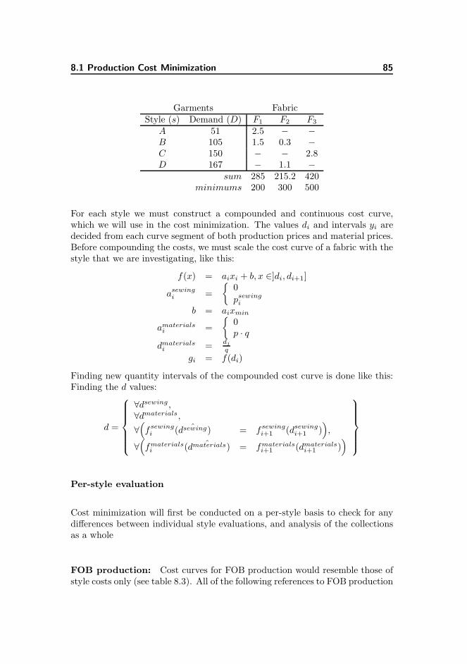
8.1 Production Cost Minimization 85
Garments FabricStyle (s) Demand (D) F1 F2 F3
A 51 2.5 − −B 105 1.5 0.3 −C 150 − − 2.8D 167 − 1.1 −
sum 285 215.2 420minimums 200 300 500
For each style we must construct a compounded and continuous cost curve,which we will use in the cost minimization. The values di and intervals yi aredecided from each curve segment of both production prices and material prices.Before compounding the costs, we must scale the cost curve of a fabric with thestyle that we are investigating, like this:
f(x) = aixi + b, x ∈]di, di+1]
asewingi =
{
0
psewingi
b = aixmin
amaterialsi =
{
0p · q
dmaterialsi =
dj
q
gi = f(di)
Finding new quantity intervals of the compounded cost curve is done like this:Finding the d values:
d =
∀dsewing ,
∀dmaterials,
∀(
fsewingi ( ˆdsewing) = f
sewingi+1 (dsewing
i+1 ))
,
∀(
fmaterialsi ( ˆdmaterials) = fmaterials
i+1 (dmaterialsi+1 )
)
Per-style evaluation
Cost minimization will first be conducted on a per-style basis to check for anydifferences between individual style evaluations, and analysis of the collectionsas a whole
FOB production: Cost curves for FOB production would resemble those ofstyle costs only (see table 8.3). All of the following references to FOB production
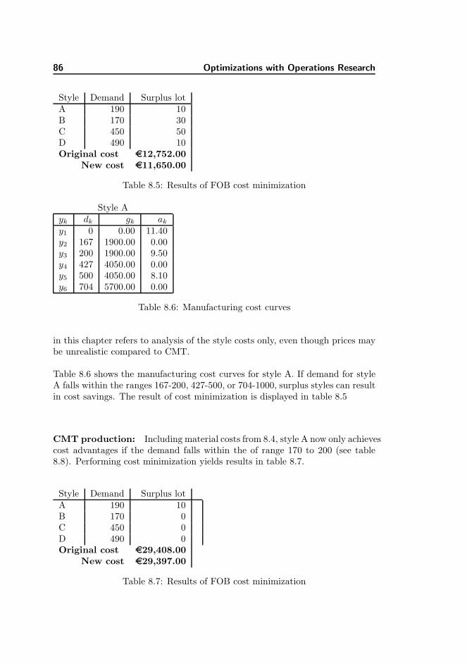
86 Optimizations with Operations Research
Style Demand Surplus lotA 190 10B 170 30C 450 50D 490 10Original cost e12,752.00
New cost e11,650.00
Table 8.5: Results of FOB cost minimization
Style Ayk dk gk ak
y1 0 0.00 11.40y2 167 1900.00 0.00y3 200 1900.00 9.50y4 427 4050.00 0.00y5 500 4050.00 8.10y6 704 5700.00 0.00
Table 8.6: Manufacturing cost curves
in this chapter refers to analysis of the style costs only, even though prices maybe unrealistic compared to CMT.
Table 8.6 shows the manufacturing cost curves for style A. If demand for styleA falls within the ranges 167-200, 427-500, or 704-1000, surplus styles can resultin cost savings. The result of cost minimization is displayed in table 8.5
CMT production: Including material costs from 8.4, style A now only achievescost advantages if the demand falls within the of range 170 to 200 (see table8.8). Performing cost minimization yields results in table 8.7.
Style Demand Surplus lotA 190 10B 170 0C 450 0D 490 0Original cost e29,408.00
New cost e29,397.00
Table 8.7: Results of FOB cost minimization

8.2 Profitability maximization 87
Style Ayk dk gk ak
y1 0 0.00 41.40y2 167 6910.00 30.00y3 170 700.00 0.00y4 200 700.00 35.00y5 427 14,938.50 25.5y6 500 16,800.00 33.60y7 704 23,652.0 25.50y8 1000 31,200.00 25.50
Table 8.8: Compounded cost curves
Cost minimization for the collection as a whole:
Evaluating on surplus stock ordering on a per-style basis may be suitable forillustrative purposes, but for decision-making analyzing the collection as a wholeseems more appropriate.
FOB production In the case of FOB production, there are no differencesbetween evaluating on styles individually and the collection, since the styles inthe model only linked through their material consumption. In FOB productionthis relatedness is absolved. CMT production is another story.
CMT production: Performing cost minimization for the CMT productionand the collection as a whole, yields the same results as the per-style evaluationon this data set.
Though cost minimization is important in any well-run business it is nothingwithout successful sales, which is the key to making a profit. In fact, the overallobjective for focusing on costs may prove more valuable if shifted to focussingon profits. This includes additional dimensions to the minimization problem ofsection 8.2.
8.2 Profitability maximization
Companies may have large turnovers and focus on costs minimizations, withoutmaking the most profitable decisions for their company. Profit maximizations is
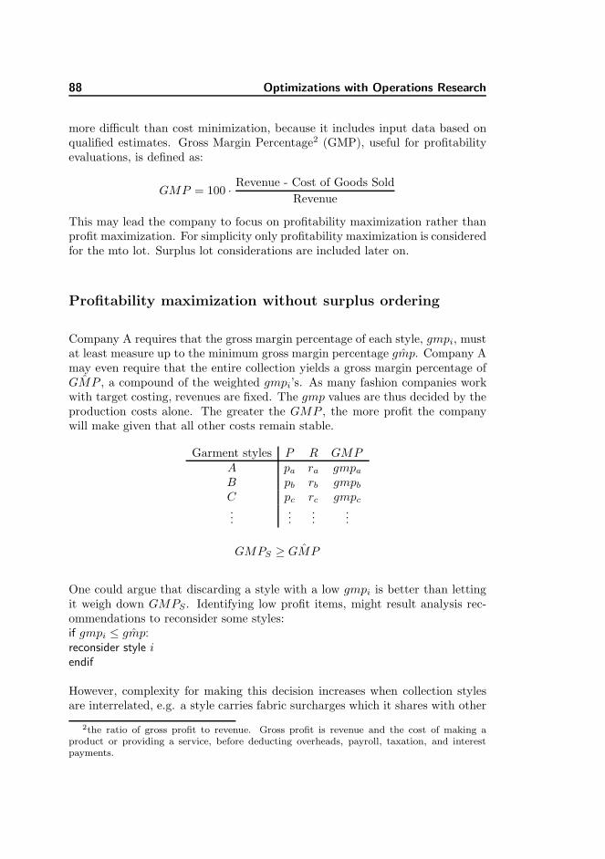
88 Optimizations with Operations Research
more difficult than cost minimization, because it includes input data based onqualified estimates. Gross Margin Percentage2 (GMP), useful for profitabilityevaluations, is defined as:
GMP = 100 ·Revenue - Cost of Goods Sold
Revenue
This may lead the company to focus on profitability maximization rather thanprofit maximization. For simplicity only profitability maximization is consideredfor the mto lot. Surplus lot considerations are included later on.
Profitability maximization without surplus ordering
Company A requires that the gross margin percentage of each style, gmpi, mustat least measure up to the minimum gross margin percentage ˆgmp. Company Amay even require that the entire collection yields a gross margin percentage of
ˆGMP , a compound of the weighted gmpi’s. As many fashion companies workwith target costing, revenues are fixed. The gmp values are thus decided by theproduction costs alone. The greater the GMP , the more profit the companywill make given that all other costs remain stable.
Garment styles P R GMP
A pa ra gmpa
B pb rb gmpb
C pc rc gmpc
......
......
GMPS ≥ ˆGMP
One could argue that discarding a style with a low gmpi is better than lettingit weigh down GMPS . Identifying low profit items, might result analysis rec-ommendations to reconsider some styles:if gmpi ≤ ˆgmp:
reconsider style i
endif
However, complexity for making this decision increases when collection stylesare interrelated, e.g. a style carries fabric surcharges which it shares with other
2the ratio of gross profit to revenue. Gross profit is revenue and the cost of making aproduct or providing a service, before deducting overheads, payroll, taxation, and interestpayments.
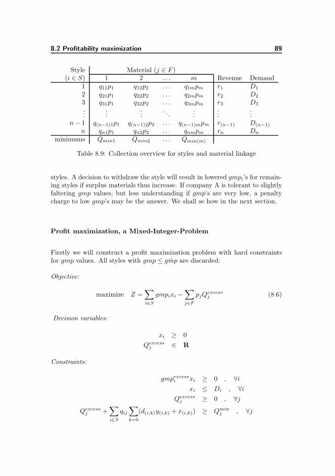
8.2 Profitability maximization 89
Style Material (j ∈ F )(i ∈ S) 1 2 . . . m Revenue Demand
1 q11p1 q12p2 . . . q1mpm r1 D1
2 q21p1 q22p2 . . . q2mpm r2 D2
3 q31p1 q32p2 . . . q3mpm r3 D3
......
.... . .
......
...n − 1 q(n−1)1p1 q(n−1)2p2 . . . q(n−1)mpm r(n−1) D(n−1)
n qn1p1 qn2p2 . . . qnmpm rn Dn
minimums Qmin1 Qmin2 . . . Qmin(m)
Table 8.9: Collection overview for styles and material linkage
styles. A decision to withdraw the style will result in lowered gmpi’s for remain-ing styles if surplus materials thus increase. If company A is tolerant to slightlyfaltering gmp values, but less understanding if gmp’s are very low, a penaltycharge to low gmp’s may be the answer. We shall se how in the next section.
Profit maximization, a Mixed-Integer-Problem
Firstly we will construct a profit maximization problem with hard constraintsfor gmp values. All styles with gmp ≤ ˆgmp are discarded:
Objective:
maximize Z =∑
i∈S
gmpixi −∑
j∈F
pjQexcessj (8.6)
Decision variables:
xi ≥ 0
Qexcessj ∈ R
Constraints:
gmpexcessi xi ≥ 0 , ∀i
xi ≤ Di , ∀i
Qexcessj ≥ 0 , ∀j
Qexcessj +
∑
i∈S
qij
∑
k=0
(d(i,k)y(i,k) + x(i,k)) ≥ Qminj , ∀j
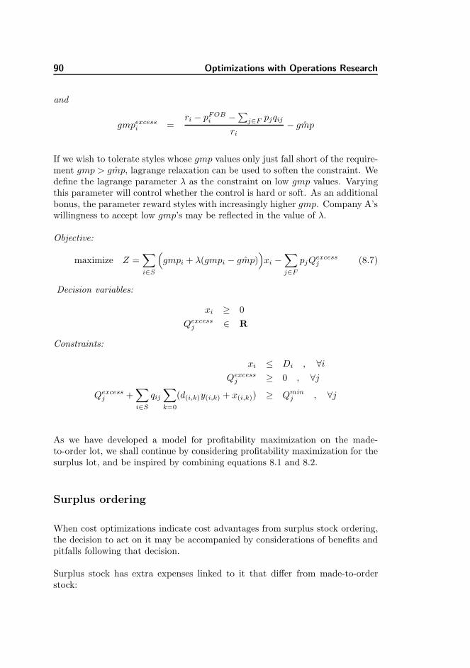
90 Optimizations with Operations Research
and
gmpexcessi =
ri − pFOBi −
∑
j∈F pjqij
ri
− ˆgmp
If we wish to tolerate styles whose gmp values only just fall short of the require-ment gmp > ˆgmp, lagrange relaxation can be used to soften the constraint. Wedefine the lagrange parameter λ as the constraint on low gmp values. Varyingthis parameter will control whether the control is hard or soft. As an additionalbonus, the parameter reward styles with increasingly higher gmp. Company A’swillingness to accept low gmp’s may be reflected in the value of λ.
Objective:
maximize Z =∑
i∈S
(
gmpi + λ(gmpi − ˆgmp))
xi −∑
j∈F
pjQexcessj (8.7)
Decision variables:
xi ≥ 0
Qexcessj ∈ R
Constraints:
xi ≤ Di , ∀i
Qexcessj ≥ 0 , ∀j
Qexcessj +
∑
i∈S
qij
∑
k=0
(d(i,k)y(i,k) + x(i,k)) ≥ Qminj , ∀j
As we have developed a model for profitability maximization on the made-to-order lot, we shall continue by considering profitability maximization for thesurplus lot, and be inspired by combining equations 8.1 and 8.2.
Surplus ordering
When cost optimizations indicate cost advantages from surplus stock ordering,the decision to act on it may be accompanied by considerations of benefits andpitfalls following that decision.
Surplus stock has extra expenses linked to it that differ from made-to-orderstock:
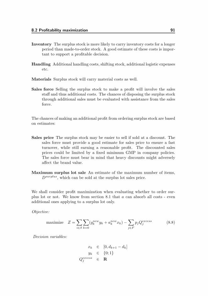
8.2 Profitability maximization 91
Inventory The surplus stock is more likely to carry inventory costs for a longerperiod than made-to-order stock. A good estimate of these costs is impor-tant to support a profitable decision.
Handling Additional handling costs, shifting stock, additional logistic expensesetc.
Materials Surplus stock will carry material costs as well.
Sales force Selling the surplus stock to make a profit will involve the salesstaff and thus additional costs. The chances of disposing the surplus stockthrough additional sales must be evaluated with assistance from the salesforce.
The chances of making an additional profit from ordering surplus stock are basedon estimates:
Sales price The surplus stock may be easier to sell if sold at a discount. Thesales force must provide a good estimate for sales price to ensure a fastturnover, while still earning a reasonable profit. The discounted salesprices could be limited by a fixed minimum GMP in company policies.The sales force must bear in mind that heavy discounts might adverselyaffect the brand value.
Maximum surplus lot sale An estimate of the maximum number of items,Dsurplus, which can be sold at the surplus lot sales price.
We shall consider profit maximization when evaluating whether to order sur-plus lot or not. We know from section 8.1 that a can absorb all costs - evenadditional ones applying to a surplus lot only.
Objective:
maximize Z =∑
i∈S
∑
k=0
(gnewk yk + anew
k xk) −∑
j∈F
pjQexcessj (8.8)
Decision variables:
xk ∈ [0, dk+1 − dk]
yk ∈ {0; 1}
Qexcessj ∈ R
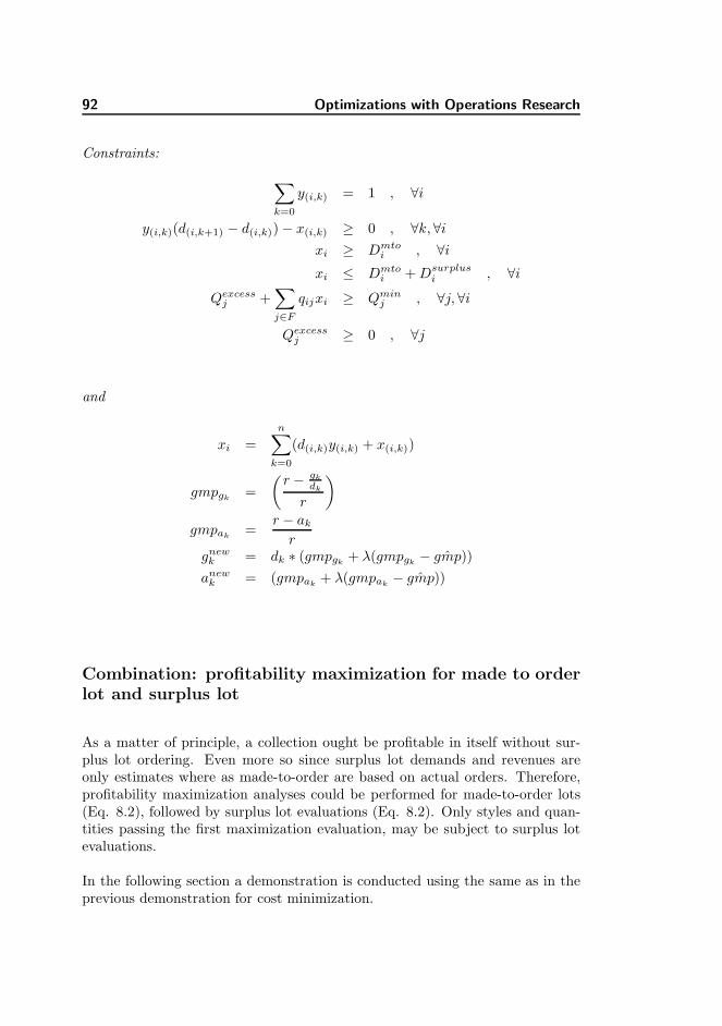
92 Optimizations with Operations Research
Constraints:
∑
k=0
y(i,k) = 1 , ∀i
y(i,k)(d(i,k+1) − d(i,k)) − x(i,k) ≥ 0 , ∀k, ∀i
xi ≥ Dmtoi , ∀i
xi ≤ Dmtoi + D
surplusi , ∀i
Qexcessj +
∑
j∈F
qijxi ≥ Qminj , ∀j, ∀i
Qexcessj ≥ 0 , ∀j
and
xi =
n∑
k=0
(d(i,k)y(i,k) + x(i,k))
gmpgk=
(
r − gk
dk
r
)
gmpak=
r − ak
r
gnewk = dk ∗ (gmpgk
+ λ(gmpgk− ˆgmp))
anewk = (gmpak
+ λ(gmpak− ˆgmp))
Combination: profitability maximization for made to orderlot and surplus lot
As a matter of principle, a collection ought be profitable in itself without sur-plus lot ordering. Even more so since surplus lot demands and revenues areonly estimates where as made-to-order are based on actual orders. Therefore,profitability maximization analyses could be performed for made-to-order lots(Eq. 8.2), followed by surplus lot evaluations (Eq. 8.2). Only styles and quan-tities passing the first maximization evaluation, may be subject to surplus lotevaluations.
In the following section a demonstration is conducted using the same as in theprevious demonstration for cost minimization.
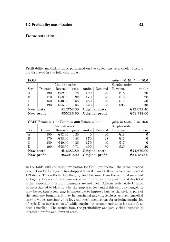
8.2 Profitability maximization 93
Demonstration
Profitability maximization is performed on the collections as a whole. Resultsare displayed in the following table:
FOB ˆgmp = 0.50, λ = 10.0Made-to-order Surplus order
Style Demand Revenue gmp make Demand Revenue makeA 190 e52.00 0.78 190 20 e18 20B 170 e58.00 0.92 170 28 e16 28C 450 e40.00 0.68 450 60 e17 50D 490 e55.00 0.85 490 30 e30 30New costs e12752.00 Original costs e12,031.40New profit e55216.60 Original profit e51,938.00
CMT F1min = 100 F2min = 300 F3min = 500 ˆgmp = 0.50, λ = 10.0Made-to-order Surplus order
Style Demand Revenue gmp make Demand Revenue makeA 190 e52.00 0.20 0 20 e18 0B 170 e58.00 0.58 170 28 e16 0C 450 e40.00 0.36 179 40 e17 0D 490 e55.00 0.73 490 30 e30 30New costs e16383.80 Original costs e22,670.00New profit e33040.00 Original profit e32,282.00
In the table with collection evaluation for CMT production, the recommendedproduction lot for style C has dropped from demand 450 items to recommended179 items. This reflects that the gmp for C is lower than the required ˆgmp andambiguity follows: It rarely makes sense to produce only part of a styles totalorder, especially if fabric minimums are not met. Alternatively, style C mustbe investigated to identify why the gmp is so low and if this can be changed. Itmay be so, that a low gmp is impossible to improve but, as the style is part ofthe company branding, it may be continued anyway. Style A as been cancelledas gmp values are simply too low, and recommendations for ordering surplus lotof style D as increased to 30 while surplus lot recommendations for style A asbeen cancelled. The results from the profitability analyses yield substantiallyincreased profits and lowered costs.
94 Optimizations with Operations Research
8.3 Implementation details
The implementation of the methods presented in this chapter used tools to solvedemonstration scenarios that were written in the programming language Python(v.2.3), using the libraries PyCplex3, MatplotLib4 and the proprietary programCPLEX5.
Readers wanting to implement the models put forward in this chapter must haveaccess to a software library able to solve mixed-integer programming problems.
8.4 Sensitivity analysis
Before accepting the models, they will be validated by conducting a sensitivityanalysis to ensure the models are robust enough in use and as a mean to gainconfidence in the results from using the model. By varying the input data, weshall observe how these changes affect the results, and thus gain insights intowhich parameters and variations the model is sensitive towards. Variables ˆgmp
and λ are expected impact the results as well as variations in demands andrevenues. Appendix F shows the results from variation in these parameters.
Variations in revenue Obviously the model is sensitive to variations in rev-enue data. We see a clear indication that style A is not profitable due tohigh production costs. Only if the sales revenue for this style is high, e.g.e92.00, is it recommendable for production. Style D appears to be a prof-itable style. Variations in recommendations for styles B and C are evidentlogical with changes in revenue. Also note that, as revenues increase forthe surplus lot, recommendations rocket upwards for ordering additionalstyles.
Variations in ˆgmp Sensitivity towards variations in ˆgmp is also apparent yetreveils no surprising results. When selecting ˆgmp for analytical purposes,the company need have a clear understanding of why ˆgmp is chosen, andit would be wise to comply with the actual level of gmp’s in the company.So that ˆgmp only rules out significant low gmp’s. The ˆgmp values barelyaffect the surplus stock recommendations, but that may be due to lowrevenues in the first place, as we have seen the changes previously forvariations in surplus stock revenues.
3python interface to CPLEX library, http://www.cs.toronto.edu/∼darius/software/pycplex/4open source matlab clone, http://matplotlib.sourceforge.net/5http://www.ilog.com/products/cplex/
8.4 Sensitivity analysis 95
Variations in λ Variations in λ shows that low values clearly increase recom-mendations for surplus stock and effect the made-to-order lot recommen-dations steadily as well. Higher values of lambda will have effects on themade-to-order lot and smoothly rule out lower gmp’s. Where λ = 0.15,gmp values for B and C are listed as the same, but we must assume somedifferences in lower decimals, since recommendations are different for styleB and C.
Variations in λ and ˆgmp combined An interesting thing happens where bothλ and ˆgmp are low: purchasing surplus stock for style A is now recommend-able, which did not occur when the two parameters were tested separately.Low values of λ will increase tolerance towards low gmp’s even if ˆgmp ishigh. Where λ is high and ˆgmp is low changes apply mainly to the surplusstock.
Variations in fabric minimums With increasingly higher fabric minimums,there is a tendency to accept styles with small gmp’s, where we would havediscarded them previously. But the main affect is on surplus stock recom-mendations, which are used to compensate for the greater fabric expenses.More worryingly, styles are not discarded when fabric minimumsincrease. Moreover, gmp values do not change with increasing fabricminimums as they are calculated from a fabric unit price with no concernsto fabric minimums. Since the model for discarding styles is built aroundgmp values styles are never discarded even though fabric minimums willcannibalize all profits as illustrated in the test table.
As expected the results respond to the input data, in a robust and reasonableway. None of the outcomes are very surprising but behaves very much in bal-ance with expectations. Naturally, the balance between revenue from sales andproduction costs are the important factor to which the parameters will respondaccordingly. The model attract the analyst’s attention towards styles with lowgmp’s and point out cost advantages from surplus stock ordering. Focus mustbe given to profits as well, especially to identify destructive fabric minimums.
Following the recommendations will, in some cases, decrease the total revenuefrom the starting point, but considering the risks run by producing a low prof-itable style, this may be acceptable. Evaluations will follow on how to avoidlow-profitable styles in the future, or at least ensure that they do not become themajority of a collection. If some of these styles are signature styles of the brand,and thus important for the image of the brands, management could considerbalancing this costs with some high-profit products to finance the branding.Knowledge of which styles are good for the bottomline, could prove valuablewhen planning collections ahead.
96 Optimizations with Operations Research
8.5 Expanding the models
The model is complete for cost and profit analysis for collection evaluation, butcould be extended in several useful ways to shed light on more aspects presentin deciding.
Use fabric minimums As we have seen in the sensitivity analysis, the modeldoes not respond to high fabric minimums, giving no indications thatfabric minimums jeopardize the profitability of the entire collection. Itwould be useful to incorporate considerations to high fabric minimums,e.g. by requiring a collection ˆGMP , or other means to inform analysts ofthe disadvantages of proceeding based on the current data.
Updating intervals As previously stated, di values marking the intervals forgi and ai values in surplus stock evaluations ought in fact be updated assurplus quantities are defined. This update has previously been discarded,as it would complicate optimizations procedures greatly and likely requirea heuristic to solve. For simplification purposes it was discarded, butimplementing and testing such a consideration may yield surprising resultsor merely confirm the reason in discarding it in the first place.
Surplus stock scenarios In the analysis, surplus stock recommendations arebased on estimates on revenues and demands. Managers may prefer view-ing the outcome from different scenarios by displaying results for differentestimates of demands and revenues. This can be done by implementing astochastic model to determine the optimal order of surplus stock, whichminimizes costs and maximize profits when demand is unknown.
8.6 Findings
This chapter demonstrates the relevance of operations research techniques tosupport purchasing and ordering decisions for fashion companies at all levels6.
Two two robust models have been presented for cost minimization and profitabil-ity maximization respectively, taking advantage of the price quotation charac-teristics of the fashion industry. These models provide a tool on low-profit styles,or cost-saving opportunities, which management may use for evaluations beforemaking important decisions based on quantitative insights.
6In fact the software developer ILOG behind CPLEX has products aimed towards man-ufacturing companies, and facilitates integration with the widely used software system SAP,http://www.ilog.com/industries/manufacturing
8.6 Findings 97
Firstly, a cost minimization model was developed to take advantage of the pricequotation characteristics of the fashion industry, leaving room for cost savingsby purchasing surplus stock items up to a certain limit. The knowledge ofthese surplus lot order suggestions may be used by management, either to orderthe recommended quantities or negotiate prices with suppliers. A demonstra-tion of using the model is given, and satisfying recommendations for surpluslot orderings are obtained. By following the recommendations of the analysisthe company can actually obtain cost savings from ordering the needed items.Secondly, the cost minimization model is extended into a profitability maximiza-tion model, in which sales revenues and tolerances towards low profit marginsare incorporated. Buy using langrarian relaxation, companies are able to weedout dramatically poor-profit products, while accepting low-profit products withsome restrictions. Choosing appropriate parameters for this analysis it vital, andbest utized with consideration to the company characteristics. The maximiza-tion model is demonstrated and proves robust in use, with recommendations toincrease company profitability. Occasionally this yields a decrease in companyprofits, but only if the collection includes styles with low profit margins. Therecommendations of the model is not intended for implicted application, butused as a managerial tool to make better informed decisions. Especially resultswhere styles with less-than-desirable profit margins are at present, may resultin lowered made-to-order quantity recommendations from the original data in-put. These evaluations could spur management to investigate the styles ratherthan following the literal interpretation of the results. The following sensitivityanalysis tests the models with variations in input data and decision parametersespecially. The test confirms that the model is robust to data variations, butrequires better methods for responding to high fabric minimums.
The models are expected to work well for companies at all levels. Larger com-panies may gain the ability to monitor development in collections and styles, tosupport fast, well-informed decisions. Smaller companies may gain a strongerinsight into which activities and styles are providing them with the means forfuture growth. Companies with IT systems can relatively easy incorporate theseanalyses in their business routine, facilitating informed decisions without muchextra time invested in conducting them. Access to a software library for solvingmixed-integer programming problems is required.
This chapter demonstrates that fashion companies can make use of the pricestructures in the industry to obtain cost savings by ordering surplus stock.It is possible to use operations research to discard low-profit products whilestill striving towards profitability maximization, and gain very good results.The methods of this chapter yields a decision-tool for managers to supportoperational decisions in a more complete and informed way, increasing profitseven after a specific supplier has been decided upon.

98 Optimizations with Operations Research
The following chapter links the first three chapters of part III and advices ontheir proper usage.

Chapter 9
Outsourcing decision tool
This chapter illustrates how to link the methods of the previous three chap-ters together and use them as one tool, to gain a detailed view on availableoutsourcing options and their economic consequences.
The methods presented in the previous chapters are intended for use in a com-bined tool, aiding fashion professionals in strategic, tactic, and operational deci-sions, in that order. Here follows advice on the intended usage of each method:
Step 1: Strategy A fashion company should decide which type manufactur-ing services they desire from their suppliers. The level of service affects thecompany’s organisational structure, work force compositions, and businessprocedures. The type of supplier collaboration should be selected to in-crease the company’s competitiveness, whether that be in speed of serviceor higher mark-up. This analysis might be conducted with regular inter-vals, e.g. bi-annually, with considerations to latest outsourcing patternsin the industry or evolving competitive factors of the market.
Step 2: Tactic The choice of collaboration type impacts which candidate sup-pliers are considered as suppliers. At this stage, costs and qualitativemeasures on delivery is of high importance. Both criteria may be joinedinto one method for comparison allowing for different weights on their im-portance balanced with company guidelines. The method presents ways

100 Outsourcing decision tool
to estimate additional costs from an outsourcing decision, such as macrocosts and indirect costs. Using this method, decision makers gain detailedinsights to the full costs of collaboration with suppliers, and may choosesuppliers, which benefits the fashion company most. The methods foranalysis can be automated. Thus, an analysis can be conducted each timea selection of candidate suppliers are considered, providing managers witha stronger base for decisions.
Step 3: Operate When suppliers have been selected, it is possible on an op-erational level to work towards further benefits for the fashion company.With methods from operations research, the methods proposes solutionscenarios to conduct mainly profitable activities, while making most useof cost savings available for profit maximization purposes. The methodssuggested may conducted automatically with data from the company’s ITsystem and included for evaluation in daily business routines. By view-ing automatically created scenarios decision-makers may base purchasingorders on output recommendations, and investigate low-profit productsbrought to their attention by the analysis.
The three steps join together in a single tool to make the most of outsourcingdecisions. Each step does not affect the results of the next, but sets the stage ofwhat is subject to analysis. Their combined usage will reflect on the financialresult. The candidate suppliers subject to comparison are gathered accordingto company strategy guidelines on preferred supplier types. But the outcomeof the analysis is only given by the single supplier comparison analysis methodalone.
The selection of supplier, will set the stage for which data is analysed for in-creased profitability and costs savings, but does not affect the outcome of theanalysis. However, as surplus stock quantities are ordered, and styles eitheraccepted, discarded, or re-considered, the profit yielded in the last method isstill subject to additional costs identified in the supplier comparison. The profitwill decrease with indirect costs and macro costs and they best financial resultattainable, is in turn a condition of the supplier type selected.
This chapter concludes part III, in which a tool is suggested to aid fashioncompanies in their outsourcing decisions. The tool is assembled from threemethods presented in the previous chapters, who may be used with differentfrequency. Combined, the three methods contribute with a more detailed viewon outsourcing options and their economic consequences. As outsourcing isgenerally the pre-requisite for Danish fashion companies, using the tool maycontribute with alternative decisions for outsourcing yielding additional profits.

101
Part IV which follows, is dedicated to evaluation of the report and its sugges-tions.

102 Outsourcing decision tool

Part IV
Evaluation and conclusions


105
In this part..This part rounds off the report with suggestions for further work and con-clusions on the work presented. Furthermore, new trends in competition andpresumptions for the fashion industry is described. Finally, results of the workpresented concludes the report.

106
Chapter 10
Evaluation and future work
Much of the work in this report is conducted on the assumption that priceis an important competitive factor in the Danish market. The current trendof successful fashion companies suggest that FOB production collaborationsmay be superior to CMT in increasing company profits. However, since the1990’s, large retail chains such as H&M and Zara have proven that fast marketresponse, high flexibility in client services and speedy delivery are increasinglyimportant as competitive parameters in future. Zara has set new standardsfor product development cycles and speed, based heavily on in-house CM andCMT production or closely linked CM supplier collaborations. This indicativeof opportunities not to be missed. Fashion companies is well advised to monitorthis trend and to conduct the analyses recommended in this report.
Knowledge of the benefits and disadvantages in production collaborations andgeographic locations of suppliers, may lead to a more profitable sourcing strategyfor the individual companies; especially, if combined with awareness of valueproposition
The methods developed in this report may seem too elaborate for small busi-nesses. It is advisable to conduct analyses in balance with a company’s size andtarget audience, yet acknowledge that companies of all sizes may benefit withadditional insights and profit opportunities proposed by methods presented inthis report.

108 Evaluation and future work
It would be very interesting, to conduct a national investigation of competitivefactors and which supplier collaboration methods best support them.
The method of using a ranking systems to estimate macro costs, would benefitfrom evaluations on the result it yields on real data.
Chapter 11
Conclusions
This report presents a tool for supporting management decisions in outsourcing.The objective is to increase the competitiveness of Danish fashion companies,and thus increase chances of export and growth. The tool combines three meth-ods, corresponding to strategical, tactical and operational decisions.
The first method, suggests how to evaluate which type of supplier best facilitatesthe competitiveness of a fashion company. Based on the outcome of the analysis,managers may decide which suppliers to seek out. The method may also be usedto match supplier collaborations types with competitive parameters.
The second method is designed for comparing suppliers based on their pricequotations, geographic locations, and additional information on qualitative mea-sures. This method requires means to estimate macro costs and indirect costs.
A technique for estimating macro costs is suggested, which makes use of theBusiness Environment Ranking, regularly released by the Economist BusinessIntelligence Unit. Guidelines are suggested for including quota costs and tariffs.
To estimate indirect costs, techniques are developed for measuring the costsof delays, damaged goods, and wrong deliveries. The importance and size ofeach costs can be weighted individually in accordance with company guidelines.Using this method, decision-makers may have a better understanding of the
110 Conclusions
costs following the selection of a supplier.
The last method aids decision-makers in ensuring that mainly profitable activ-ities and purchases are carried out, and cost advantages are made the most of.This is done with operations research techniques for profit maximization, whichwill suggest a purchasing scenario indicating if any styles should be discardedor reconsidered. The method may further recommend purchases of surplus gar-ments if they facilitate increased profits or lowered total costs.
The three methods combined may improve the overall profitability of a companyintegrating these analyses in business procedures.

Part V
Appendices

Appendix A
Cost accounting
The methodology of dividing costs into categories of direct, indirect, and macrocosts, is only one of many cost accounting (a.k.a. costing) approaches thatmay be used to analyze a company’s operational costs. Most companies willoften utilize a mix of different costing methodologies depending on the scopeof the outcome. Some costing methods are relevant for long-term managerialdecisions, others for making profit analyses of single products or for identifyingbottlenecks in generating profits, etc. The type of products may also affectwhich costing system is more appropriate, e.g. oil refinement and a consultantproject within marketing are two widely different products and they requirevery different costing systems.
Overall, cost accounting systems can be split into two parts:
• Controlling
• Decision support.
Costing methods from controlling and decision making may be combined andused together. Both components are required for running a business.
114 Cost accounting
Controlling
Control costing systems provides numerous ways to motivate production flowsin a desired direction. Three main costing systems are represented: Standardcosting, Throughput costing, and Backflush costing.
Standard Costing
A control method involving the preparation of detailed cost and salesbudgets. Such budgets are then compared with the actual resultsfor a specific account period and any significant variances betweenthe actual and the budgeted results are investigated.1
Standard costing was invented in the early 20th century, before computers madecalculations less tedious and time consuming. The methodology is obsolete inmany of today’s scenarios but can still be useful with some modification inothers. Standard costing can be useful for, e.g., the pricing of projects. Itis not relevant for short-lived products or environments subject to continuousimprovement.
Throughput Costing
Focus on identifying financial bottlenecks in a production, e.g. the least prof-itable product in a product series or the least profitable customer order. Through-put costing can be used to prioritize which orders to process first, thereby en-suring that the company always works on the most profitable task. Throughputcosting is most relevant to industries working with batch productions and con-tinuously serving customers with the same product.
Backflush Costing
A costing method that applies costs based on the output of a process. Themethodology is generally associated with repetitive manufacturing. It uses abill of material or a bill of activities to draw quantities from inventory throughwork in process, to finished goods; at any intermediate stage, using the outputquantity as the basis. These quantities are generally costed using standard
1(http://wps.pearsoned.co.uk/wps/media/objects/1065/1090612/glossary.html )
115
costs. The process assumes that the bill of material (or bill of activities) andthe standard costs at the time of backflushing represent the actual quantitiesand resources used in the manufacture of the product. This is important sinceno shop orders are usually maintained to collect costs.
Decision Making
Costing methods within this category centers around production costs. Tradi-tionally there was Full costing and Variable costing. Activity Based Costing(ABC) joined the two around 1990.
Variable costing
Also known as direct costing, or marginal costing. The methodology focusonly on direct costs, and is suited only for short-term decision making, sinceit ignores all other costs. Among other uses, the methodology is applicablefor profitability modeling. Naturally, the neglect of indirect costs make thedirect costing unsuitable for long-term decision making, but most companieswill regularly find use for the method.
Full costing
Alternatively: absorption costing. A method of costing that assigns all man-ufacturing costs to products or other cost objects. The costs assigned includethose that vary with the level of activity performed and those that do not. Fullcosting may be better known by its’ two sub-methods: job costing and processcosting:
Job costing Projects or production development is broken into appropriatebatches, inside which all resources consumed are registered: materials, labor,overhead, machine time, etc. Job costing is well suited for production or profes-sional service companies, in other industries, such as retailing (service industry)it has little relevance.
116 Cost accounting
Activity Based Costing (ABC)
A methodology that measures the cost and performance of activities,resources, and cost objects. Resources are assigned to activities, thenactivities are assigned to cost objects based on their use. Activity-based costing recognizes the causal relationships of cost drivers toactivities.2
The methodology can, if not carefully managed, consume more resources thancan be justified by the gains. If managed well, however, it provides managerswith valuable insight to base their decisions upon. Activity Based Costing wasdeveloped as productions became more complex, and automation moved directcosts to indirect costs making it more difficult to spot the cost drivers in aproduction.
A.0.0.1 Target Costing
In Target costing one decides for the finished product value in the market,with the question: ”What are the consumers willing to pay for this item?”.Then the company decides for a minimum markup on the price, which yieldsthe earning on the product. Using these values the company backtracks to adesired target production price. If this price cannot be met, the item will notbe put into production. Target costing is convenient for companies working inhighly competitive markets with many players.
2(strategicsourcing.navy.mil/reference documents/defs.cfm)
Appendix B
Investment Analysis
It is outside the scope of this project to demonstrate advanced knowledge ineconomics. Rather, it is my intention to utilize financial tools, which are cur-rently available to solve real-life problems resonably well. Some novice financialtools are presented.
Current value/Present value
This method is used to compare values across time, with consideration givento currency inflation. In order to compare values, one must make sure that thevalues are considered at the same period of time. If the values are from differenttime periods they must all be projected to the same point in time (either backor forth). The equations for projecting forward in time 1 are:
Single sum: KN = K0(1 + R)N (B.1)
Multiple sums: KN =∑N
t=0 NBt(1 + R)N−t (B.2)
Multiple sums are used, e.g. when a bankloan is paid in mortgages, where eachamount must have correct current value in a comparison analysis.
1(source: investeringsteori s. 191)

118 Investment Analysis
Return on Investment analysis
One can view activities in a fashion company from an investment point of view.Finding new manufacturers to take over part of the production requires funds:finding costs for locating new manufacturers and evaluating their potential assubcontractors and start-up costs while the manufacturer and the fashion com-pany learns to communicate and interpret each other’s answers correctly. Fur-thermore, it will take a while before the manufacturer understands all require-ments in relation to design, quality etc. The money already invested in the oldmanufacturer will be lost, if all collaboration ceas.
Letter of Credit
Manufacturers often require a Letter of Credit (LOC) from the company whenan order is placed.
A letter of credit is an irrevocable payment undertaking of an issuingbank issued to a beneficiary upon request of an applicant for sup-ply of goods, services or performance with documents stated in theletter of credit presented to the issuing bank, a nominated bank orconfirming bank, if any, within the expiry date of the letter of creditor within a stated number of days after shipment, where applica-ble, in full compliance with the terms and conditions of the letter ofcredit, the applicable UCP and international standard banking prac-tice. It is a legally enforceable obligation or undertaking on the partof the issuing bank and is not a contract (although it is sometimesmistakenly referred to as such). [36]
An LOC freezes this sum from the company’s funds, and prevents possibleintermediate investments of the money, further straining the company’s budget.If, on the contrary the manufacturer was willing to work with open accounts,the company could save money.
Appendix C
Case stories
Each case company is described by background, their LPD and GMP calcu-lation, process for selecting suppliers, and evaluation procedures for supplierperformance.
Company 2
Background
Company 2 is part of a larger group and serves the Danish mid segment. TheCompany 2 targets a lower price segment than the other case companies, butmay share consumers. This brand differs from the other ones, by having asignificantly larger turnover, and a larger organization. Company 2 main pur-pose is to contrast the other case companies and juxtapose their differences inproduction expenses.
Company 2 often reuses styles from previous seasons, changing mainly detailsor fabric. Since choice of fabric and details affect the manufacturer selectedfor production, Company 2 has found it more expedient to develop their ownpatterns, and share them with the manufacturer as required. Let it be stated
120 Case stories
that the manufacturer is responsible for adjusting the pattern to the specificdesign and create additional pattern pieces, required in the production of thegarment.
Organization
Surrounding the design department, and the technical designers, are the sourcersin charge of selecting manufacturers. The sourcers run the dialogue sourcingoffices, the agents and manufacturers selected for production.
The process of choosing manufacturer
LPD comparisons based on offers for initial designs and fabric selections.
When the garment design is completed, a final price of production is negoti-ated. After the sales period, prices are negotiated once more. Conclusively, ifthe designer makes radical changes to the garment, e.g., adding labor-intensivedetails, there is a chance that production prices could have been lower withanother manufacturer. However, Company 2 will stick with the previously cho-sen manufacturer. Occasionally, Company 2 will double-source1 an item, toevaluate new manufacturer candidates.
Evaluation of manufacturers
Based on claims, short deliveries or delays, manufacturers are evaluated byCompany 2’s sourcers. Input is also received from the sourcing offices or sourcingagents.
1collects price quotes from two or more manufacturers, by producing a salesman samplefrom each, ensure that the quality is equivalent, and compare prices before selecting supplier.
121
Company 3
Background
The company brand is in the Danish high-end, and has existed for little over adecade. The company has recently received investment capital and consequentlyorganisational restructuring. Professional management has been added, as wellas new colleagues with intense industry experience. Company 3 works with amix of FOB and CMT production. Simpler styles are produced FOB, wherevery complicated styles or styles using a particular fabric is produced CMT.
LPD analysis and gross margin calculation
No analysis of this nature was identified during interviews.
Manufacturers
Sourcing is done mainly inside the EU.
Company 1
This company is owned by a fashion group which supplies distribution, soft-ware solutions, financial support, financial data analysis, and sourcing officeservices. Sharing this administrative platform with sister companies under thesame parent company, Company 1 benefits to some extent from economies ofscale. Company 1 is entirely responsible for its own product development, salesand marketing, and production planning (incl. choosing sourcing office or man-ufacturer). The company works solely with FOB production, performs targetcosting before selecting suppliers or negotiating with suppliers. From their targetcosting they find their target LDP values, and these serve as a basis for negotia-tions with suppliers. Top management has an economic educational backround.
Not all costs are considered, however, in a final profitability analysis. Mostlybecause the remaining costs are either difficult to price tag or these future similarcosts are eliminated in the evaluation process of manufacturers - without usingexpensive time on analyzing the exact cost spent.

122 Case stories
Background
Company 1 is less than five years old, founded with investment capital for thepurpose of creating a mid-high, fast-growing brand.
The company must develop an indentity, acquire market shares, all sufficientlybacked by investments to pursue these goals. It has a CEO with a strong foun-dation in finance and, an experienced designer, and a trained team of employees.The CEO a close eye on the development of Company 1 and is heavily involvedin the sourcing process.
LPD analysis and gross margin calculation
1. Estimated sales price made → leads to target production price. Grossmargin 1 calculated.
2. Production prices gathered. Compare with target price. Some productsare skipped. Gross margin 2 calculated.
3. Sales period ended. Products ordered, and new prices negotiated. Grossmargin 3 calculated
4. Production. Gross margin 4 calculated
The process of choosing manufacturer
Manufacturers are chosen from a pool of potential candidates, most of whichhas been used before. This pool is continually updated with new manufacturersand the exclusion of others, based on multi-yearly evaluation runs conducted byCEO, Designer, and Head Sourcer.
A specific manufacturer may be chosen for production of a particular garmentbased on either criteria:
• The manufacturer sources the fabric chosen for the style
• The manufacturer is geographically close to the textile supplier for thegarment
• Other garments sharing the same textile, are produced with this manu-facturer
123
• A similar garment was produced satisfactorily at this manufacturer in aprevious season
• The garment requires specific work skills
• Production quality is tested using a new manufacturer
Designers chooses material, and based on collection designs the Designer makesthe sourcing decision.
Manufacturers are further evaluated based on their communication skills, errorpercentage, shortage percentage, and transportation time.
Company 4
Work on a CMT basis, partly FOB within knits and dresses. Patterns aredeveloped in DK. For CMT production, gradation takes place on manufacturer’slocation.
Background
Very small organization: two persons + two to four internships. Company 4works primarily on a CMT basis, but with pattern assistance from manufac-turers to implement pattern modifications and gradation. Company 4 has nolong-term relations to their manufacturers, and production has previously beensuffering heavily from late deliveries. Company 4 is searching for more stablecollaboration partners and will most likely settle with at slightly higher directproduction costs, if service quality in terms of stability, proneness to errors willimprove correspondingly.
LPD analysis and gross margin calculation
Currently Company 4 makes no data mining, nor does it perform LPD analyses,and any such analyses would contribute to a better understanding of the indirectcosts and macro costs included in a production batch.

124 Case stories
Choosing manufacturers and evaluation of performance
Based on previous bad experience, Company 4 will attempt to spread the risk,by using multiple manufacturers, and evaluations of their performance will becompared with data from previous collections as with a subjective interpreta-tion.
Appendix D
Glossary
Terminology and acronyms
CMT, Cut-Make-Trim The process of Cutting, Making (sewing) and addingTrims to a garment, given fabrics, findings and cutting marker from cus-tomer.
FOB, Freight on Board Originally a term used solely for products that aretransporated by boat. Now, it is generally used as a term for the totalprice of a product from production start till it has been packed etc. andpicked up by a courier.[9]
LPD, Landed, Duty Paid A term invented by David Birnbaum. Used todescribe the complete cost of a garment from initial designing till deliveryin the customers’ target country.
Total cost of ownership
MFN Most favoured nations
Apparel garments, clothes
Double-sourcing The Collect price quotes from two or more manufacturers,by producing a salesman sample from each, ensure that the quality isequivalent, and compare prices before selecting supplier

126 Glossary
Claims An item which has been discarded or returned to the deliverer for somereason. The buyer claims the seller for this item.
Sourcer Employee in charge of collaborating with the manufacturing company.
Pattern making
Appendix E
Company data collection
The material in this chapter, has been used to collect data from case companies.
Confidentiality
The data requested is recognized as being highly sensitive to your company,and will be treated with utmost respect and confidentiality. Enclosed withthis document is a confidentiality agreement from The Technical Universityof Denmark, which I suggest we agree upon before exchanging any sensitiveinformation. Company sensitive information in the final thesis will be keptconfidential.
Collaboration outcome:
Three analyses are conducted:
• Which production method is most profitable, FOB or CMT?
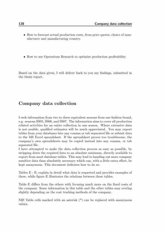
128 Company data collection
• How to forecast actual production costs, from price quotes, choice of man-ufacturer and manufacturing country.
• How to use Operations Research to optimize production profitability.
Based on the data given, I will deliver back to you my findings, submitted inthe thesis report.
Company data collection
I seek information from two to three equivalent seasons from one fashion brand,e.g. seasons SS05, SS06, and SS07. The information aims to cover all productionrelated activities for an entire collection in one season. Where extensive datais not avaible, qualified estimates will be much appreciated. You may exporttables from your databases into any comma or tab separated file or submit datato the MS Excel spreadsheet. If the spreadsheet proves too troublesome, thecompany’s own spreadsheets may be copied instead into any comma, or tabseparated file.I have attempted to make the data collection process as easy as possible, bystripping down the required data to an absolute minimum, directly available toexport from most database tables. This may lead to handing out more companysensitive data than absolutely necessary which can, with a little extra effort, bekept anonymous. This document indicates how to do so.
Tables E - E, explain in detail what data is requested and provides examples ofthese, while figure E illustrates the relations between these tables.
Table E differs from the others with focusing much more on the fixed costs ofthe company. Some information in this table and the other tables may overlapslightly depending on the cost tracking methods of the company.
NB! Table cells marked with an asterisk (*) can be replaced with anonymousvalues.
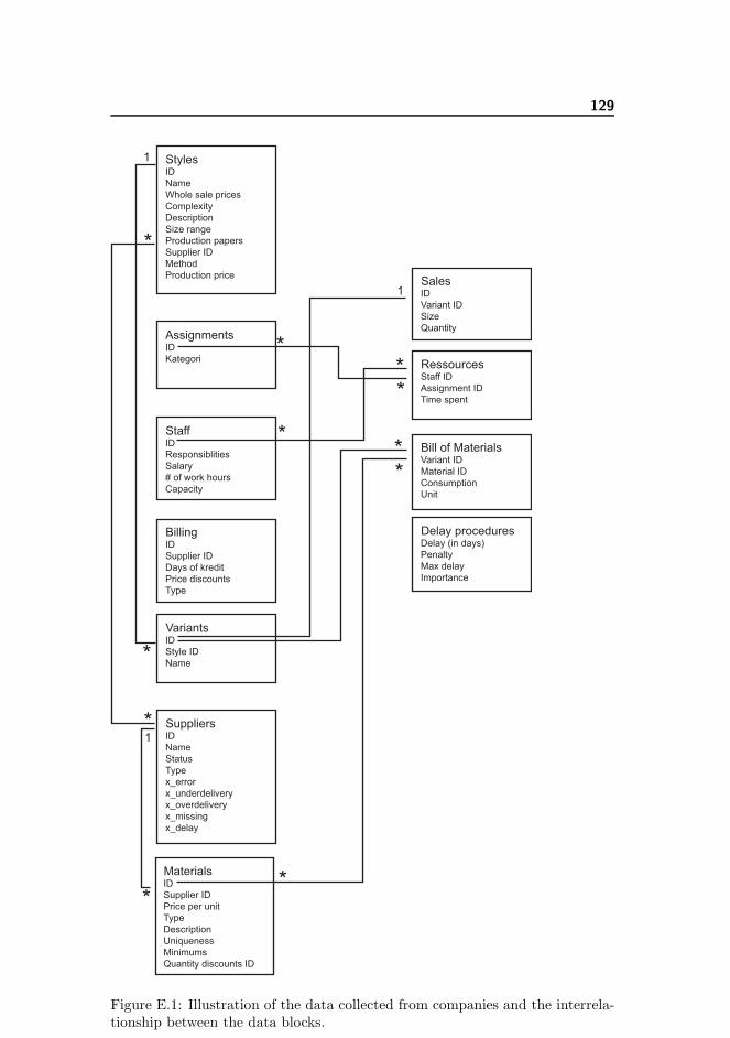
129
AssignmentsID
KategoriRessourcesStaff ID
Assignment ID
Time spent
StaffID
Responsiblities
Salary
# of work hours
Capacity
StylesID
Name
Whole sale prices
Complexity
Description
Size range
Production papers
Supplier ID
Method
Production price
VariantsID
Style ID
Name
Bill of MaterialsVariant ID
Material ID
Consumption
Unit
SalesID
Variant ID
Size
Quantity
SuppliersID
Name
Status
Type
x_error
x_underdelivery
x_overdelivery
x_missing
x_delay
BillingID
Supplier ID
Days of kredit
Price discounts
Type
Delay proceduresDelay (in days)
Penalty
Max delay
Importance
MaterialsID
Supplier ID
Price per unit
Type
Description
Uniqueness
Minimums
Quantity discounts ID
1
1
**
**
*
*
*
*
1
*
*
*
Figure E.1: Illustration of the data collected from companies and the interrela-tionship between the data blocks.
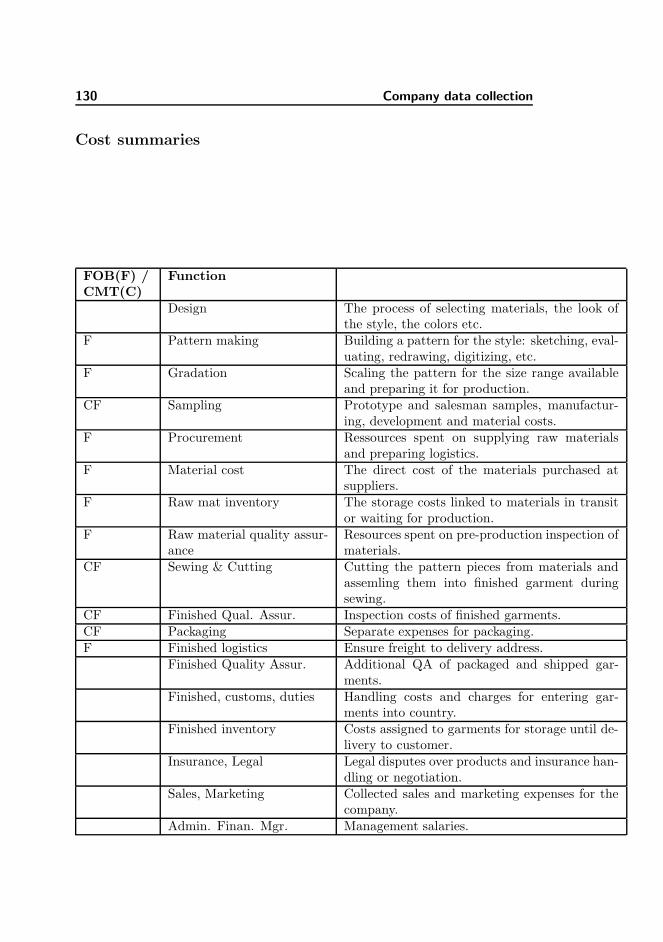
130 Company data collection
Cost summaries
FOB(F) /CMT(C)
Function
Design The process of selecting materials, the look ofthe style, the colors etc.
F Pattern making Building a pattern for the style: sketching, eval-uating, redrawing, digitizing, etc.
F Gradation Scaling the pattern for the size range availableand preparing it for production.
CF Sampling Prototype and salesman samples, manufactur-ing, development and material costs.
F Procurement Ressources spent on supplying raw materialsand preparing logistics.
F Material cost The direct cost of the materials purchased atsuppliers.
F Raw mat inventory The storage costs linked to materials in transitor waiting for production.
F Raw material quality assur-ance
Resources spent on pre-production inspection ofmaterials.
CF Sewing & Cutting Cutting the pattern pieces from materials andassemling them into finished garment duringsewing.
CF Finished Qual. Assur. Inspection costs of finished garments.CF Packaging Separate expenses for packaging.F Finished logistics Ensure freight to delivery address.
Finished Quality Assur. Additional QA of packaged and shipped gar-ments.
Finished, customs, duties Handling costs and charges for entering gar-ments into country.
Finished inventory Costs assigned to garments for storage until de-livery to customer.
Insurance, Legal Legal disputes over products and insurance han-dling or negotiation.
Sales, Marketing Collected sales and marketing expenses for thecompany.
Admin. Finan. Mgr. Management salaries.
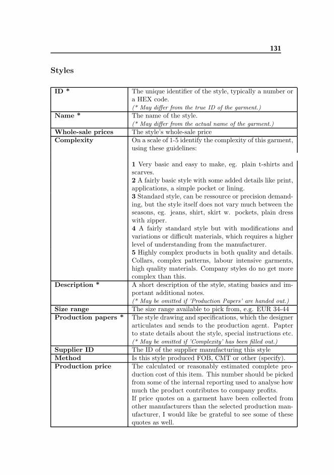
131
Styles
ID * The unique identifier of the style, typically a number ora HEX code.(* May differ from the true ID of the garment.)
Name * The name of the style.(* May differ from the actual name of the garment.)
Whole-sale prices The style’s whole-sale priceComplexity On a scale of 1-5 identify the complexity of this garment,
using these guidelines:
1 Very basic and easy to make, eg. plain t-shirts andscarves.2 A fairly basic style with some added details like print,applications, a simple pocket or lining.3 Standard style, can be ressource or precision demand-ing, but the style itself does not vary much between theseasons, eg. jeans, shirt, skirt w. pockets, plain dresswith zipper.4 A fairly standard style but with modifications andvariations or difficult materials, which requires a higherlevel of understanding from the manufacturer.5 Highly complex products in both quality and details.Collars, complex patterns, labour intensive garments,high quality materials. Company styles do no get morecomplex than this.
Description * A short description of the style, stating basics and im-portant additional notes.(* May be omitted if ’Production Papers’ are handed out.)
Size range The size range available to pick from, e.g. EUR 34-44Production papers * The style drawing and specifications, which the designer
articulates and sends to the production agent. Papterto state details about the style, special instructions etc.(* May be omitted if ’Complexity’ has been filled out.)
Supplier ID The ID of the supplier manufacturing this styleMethod Is this style produced FOB, CMT or other (specify).Production price The calculated or reasonably estimated complete pro-
duction cost of this item. This number should be pickedfrom some of the internal reporting used to analyse howmuch the product contributes to company profits.If price quotes on a garment have been collected fromother manufacturers than the selected production man-ufacturer, I would like be grateful to see some of thesequotes as well.
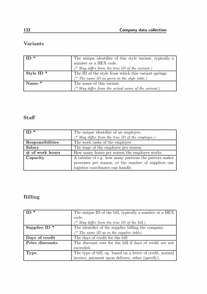
132 Company data collection
Variants
ID * The unique identifier of this style variant, typically anumber or a HEX code.(* May differ from the true ID of the variant.)
Style ID * The ID of the style from which this variant springs.(* The same ID as given in the style table.)
Name * The name of this variant.(* May differ from the actual name of the variant.)
Staff
ID * The unique identifier of an employee.(* May differ from the true ID of the employee.)
Responsibilities The work tasks of the employeeSalary The wage of the employee per season.# of work hours How many hours per season the employee worksCapacity A tabular of e.g. how many patterns the pattern maker
processes per season, or the number of suppliers onelogistics coordinater can handle.
Billing
ID * The unique ID of the bill, typically a number or a HEXcode.(* May differ from the true ID of the bill.)
Supplier ID * The identifier of the supplier billing the company.(* The same ID as in the supplier table)
Days of credit The days of credit for the billPrice discounts The discount rate for the bill if days of credit are not
exceeded.Type The type of bill, eg. based on a letter of credit, normal
invoice, payment upon delivery, other (specify).
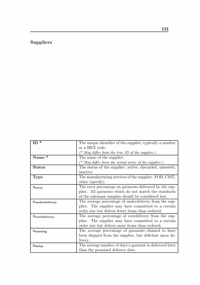
133
Suppliers
ID * The unique identifier of the supplier, typically a numberor a HEX code.(* May differ from the true ID of the supplier.)
Name * The name of the supplier.(* May differ from the actual name of the supplier.)
Status The status of the supplier: active, discarded, untestetl,inactive
Type The manufacturing services of the supplier: FOB, CMT,other (specify).
xerror The error percentage on garments delivered by the sup-plier. All garments which do not match the standardsof the salesman samples should be considered lost.
xunderdelivery The average percentage of underdelivery from the sup-plier. The supplier may have committed to a certainorder size but deliver fewer items than ordered.
xoverdelivery The average percentage of overdelivery from the sup-plier. The supplier may have committed to a certainorder size but deliver more items than ordered.
xmissing The average percentage of garments claimed to havebeen shipped from the supplier, but deficient upon de-livery.
xdelay The average number of days a garment is delivered laterthan the promised delivery date.

134 Company data collection
Materials
ID * The unique identifier of the material, typically a numberor a HEX code.(* May differ from the true ID of the material.)
Supplier ID * The ID of the supplier supplying the material.(* The same ID as in the supplier table)
Price per unit The unit price of the material, e.g. meters of fabrics,number of buttons.
Type The type of material, eg. fabric, button, zipper.Description * A description of the material, e.g. notes for handling of
the material.(* May be omitted if irrelevant.)
Uniqueness On a scale of 1-5, using the guidelines herunder, howeasily can the supplier of the material be shifted?1 The material can easily come from numerous othersuppliers2 The material is quite common but there is a limitednumber of suppliers.3 The material has qualities and design elements de-sired, but these can be replaced by an equivalent yetnot similar item from another supplier.4 It is unlikely that the material can come from anyother supplier, e.g. due to code of conduct in the busi-ness, or the supplier provides favourable trade relations.5 The material cannot be found with any other sup-plier, may be due to the complexity of the material orcopyrights.
Minimums The minimum order of the materialQuantity discountsID
Possible discounts or surcharges for the material de-pending on order quantity
Sales
ID * The unique identifier of the sales summary, typically anumber or a HEX code.(* May differ from the true ID of the sales summary.)
Variant ID * The ID of the style variant sold.(* The same ID as in the variants table)
Size The garment size soldQuantity The total quantity of the variant sold.
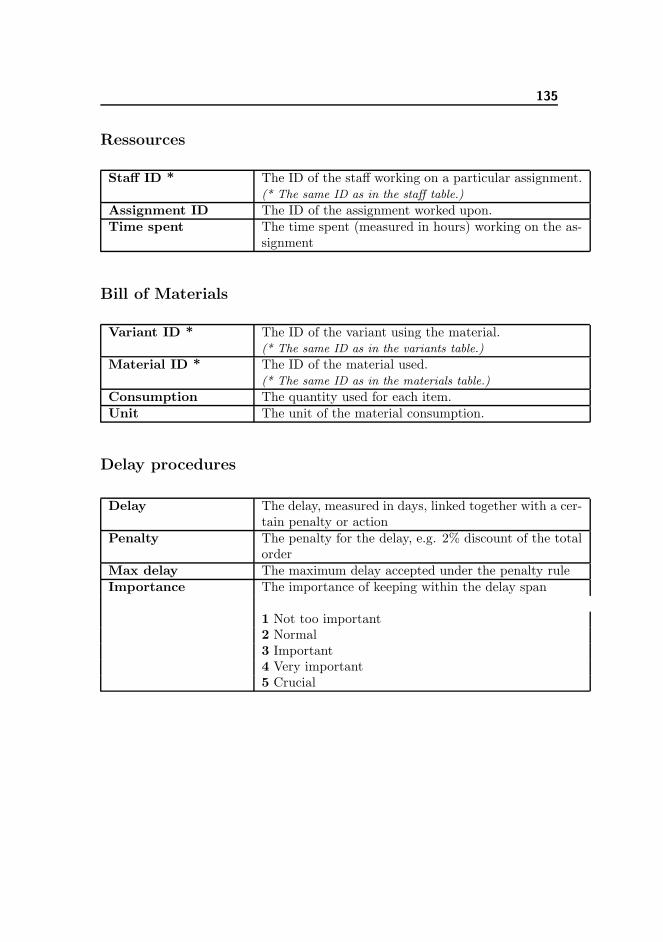
135
Ressources
Staff ID * The ID of the staff working on a particular assignment.(* The same ID as in the staff table.)
Assignment ID The ID of the assignment worked upon.Time spent The time spent (measured in hours) working on the as-
signment
Bill of Materials
Variant ID * The ID of the variant using the material.(* The same ID as in the variants table.)
Material ID * The ID of the material used.(* The same ID as in the materials table.)
Consumption The quantity used for each item.Unit The unit of the material consumption.
Delay procedures
Delay The delay, measured in days, linked together with a cer-tain penalty or action
Penalty The penalty for the delay, e.g. 2% discount of the totalorder
Max delay The maximum delay accepted under the penalty ruleImportance The importance of keeping within the delay span
1 Not too important2 Normal3 Important4 Very important5 Crucial

136 Company data collection
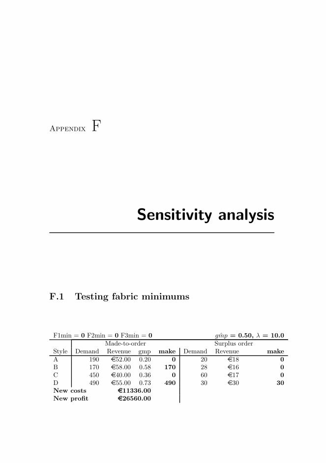
Appendix F
Sensitivity analysis
F.1 Testing fabric minimums
F1min = 0 F2min = 0 F3min = 0 ˆgmp = 0.50, λ = 10.0Made-to-order Surplus order
Style Demand Revenue gmp make Demand Revenue makeA 190 e52.00 0.20 0 20 e18 0B 170 e58.00 0.58 170 28 e16 0C 450 e40.00 0.36 0 60 e17 0D 490 e55.00 0.73 490 30 e30 30New costs e11336.00New profit e26560.00

138 Sensitivity analysis
F1min = 50 F2min = 200 F3min = 100 ˆgmp = 0.50, λ = 10.0Made-to-order Surplus order
Style Demand Revenue gmp make Demand Revenue makeA 190 e52.00 0.20 0 20 e18 0B 170 e58.00 0.58 170 28 e16 0C 450 e40.00 0.36 36 60 e17 0D 490 e55.00 0.73 490 30 e30 30New costs e12351.20New profit e33040.00
F1min = 300 F2min = 400 F3min = 300 ˆgmp = 0.50, λ = 10.0Made-to-order Surplus order
Style Demand Revenue gmp make Demand Revenue makeA 190 e52.00 0.20 18 20 e18 10B 170 e58.00 0.58 170 28 e16 0C 450 e40.00 0.36 108 60 e17 0D 490 e55.00 0.73 490 30 e30 30New costs e15126.80New profit e36559.00
F1min = 700 F2min = 800 F3min = 800 ˆgmp = 0.50, λ = 10.0Made-to-order Surplus order
Style Demand Revenue gmp make Demand Revenue makeA 190 e52.00 0.20 178 20 e18 10B 170 e58.00 0.58 170 28 e16 0C 450 e40.00 0.36 286 60 e17 0D 490 e55.00 0.73 490 30 e30 30New costs e26026.80New profit e35497.00
F1min = 1000 F2min = 1200 F3min = 2000 ˆgmp = 0.50, λ = 10.0Made-to-order Surplus order
Style Demand Revenue gmp make Demand Revenue makeA 190 e52.00 0.20 190 20 e18 20B 170 e58.00 0.58 170 28 e16 28C 450 e40.00 0.36 450 60 e17 60D 490 e55.00 0.73 490 30 e30 30New costs e38432.00New profit e29595.60

F.2 Testing revenues for mto and surplus lots 139
F1min = 2000 F2min = 2000 F3min = 5000 ˆgmp = 0.50, λ = 10.0Made-to-order Surplus order
Style Demand Revenue gmp make Demand Revenue makeA 190 e52.00 0.20 190 20 e18 20B 170 e58.00 0.58 170 28 e16 28C 450 e40.00 0.36 450 60 e17 60D 490 e55.00 0.73 490 30 e30 30New costs e43952.00New profit e24075.60
F.2 Testing revenues for mto and surplus lots
F1min = 100 F2min = 300 F3min = 500 ˆgmp = 0.50, λ = 10.0Made-to-order Surplus order
Style Demand Revenue gmp make Demand Revenue makeA 190 e22.00 -0.88 40 20 e5 10B 170 e18.00 -0.37 -0 28 e5 0C 450 e12.00 -1.13 0 60 e8 0D 490 e35.00 0.58 490 30 e10 0New costs e8810.00New profit e7226.00
F1min = 100 F2min = 300 F3min = 500 ˆgmp = 0.50, λ = 10.0Made-to-order Surplus order
Style Demand Revenue gmp make Demand Revenue makeA 190 e43.00 0.04 1 20 e16 10B 170 e31.00 0.21 65 28 e15 0C 450 e25.00 -0.02 179 60 e16 0D 490 e45.00 0.68 490 30 e28 30New costs e13842.20New profit e18529.00
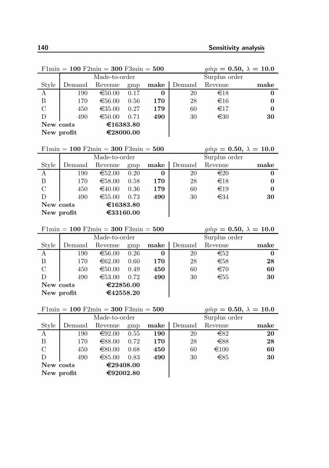
140 Sensitivity analysis
F1min = 100 F2min = 300 F3min = 500 ˆgmp = 0.50, λ = 10.0Made-to-order Surplus order
Style Demand Revenue gmp make Demand Revenue makeA 190 e50.00 0.17 0 20 e18 0B 170 e56.00 0.56 170 28 e16 0C 450 e35.00 0.27 179 60 e17 0D 490 e50.00 0.71 490 30 e30 30New costs e16383.80New profit e28000.00
F1min = 100 F2min = 300 F3min = 500 ˆgmp = 0.50, λ = 10.0Made-to-order Surplus order
Style Demand Revenue gmp make Demand Revenue makeA 190 e52.00 0.20 0 20 e20 0B 170 e58.00 0.58 170 28 e18 0C 450 e40.00 0.36 179 60 e19 0D 490 e55.00 0.73 490 30 e34 30New costs e16383.80New profit e33160.00
F1min = 100 F2min = 300 F3min = 500 ˆgmp = 0.50, λ = 10.0Made-to-order Surplus order
Style Demand Revenue gmp make Demand Revenue makeA 190 e56.00 0.26 0 20 e52 0B 170 e62.00 0.60 170 28 e58 28C 450 e50.00 0.49 450 60 e70 60D 490 e53.00 0.72 490 30 e55 30New costs e22856.00New profit e42558.20
F1min = 100 F2min = 300 F3min = 500 ˆgmp = 0.50, λ = 10.0Made-to-order Surplus order
Style Demand Revenue gmp make Demand Revenue makeA 190 e92.00 0.55 190 20 e82 20B 170 e88.00 0.72 170 28 e88 28C 450 e80.00 0.68 450 60 e100 60D 490 e85.00 0.83 490 30 e85 30New costs e29408.00New profit e92002.80
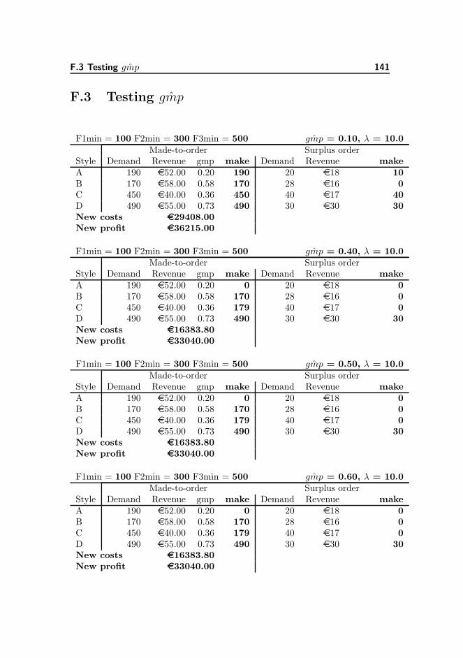
F.3 Testing ˆgmp 141
F.3 Testing ˆgmp
F1min = 100 F2min = 300 F3min = 500 ˆgmp = 0.10, λ = 10.0Made-to-order Surplus order
Style Demand Revenue gmp make Demand Revenue makeA 190 e52.00 0.20 190 20 e18 10B 170 e58.00 0.58 170 28 e16 0C 450 e40.00 0.36 450 40 e17 40D 490 e55.00 0.73 490 30 e30 30New costs e29408.00New profit e36215.00
F1min = 100 F2min = 300 F3min = 500 ˆgmp = 0.40, λ = 10.0Made-to-order Surplus order
Style Demand Revenue gmp make Demand Revenue makeA 190 e52.00 0.20 0 20 e18 0B 170 e58.00 0.58 170 28 e16 0C 450 e40.00 0.36 179 40 e17 0D 490 e55.00 0.73 490 30 e30 30New costs e16383.80New profit e33040.00
F1min = 100 F2min = 300 F3min = 500 ˆgmp = 0.50, λ = 10.0Made-to-order Surplus order
Style Demand Revenue gmp make Demand Revenue makeA 190 e52.00 0.20 0 20 e18 0B 170 e58.00 0.58 170 28 e16 0C 450 e40.00 0.36 179 40 e17 0D 490 e55.00 0.73 490 30 e30 30New costs e16383.80New profit e33040.00
F1min = 100 F2min = 300 F3min = 500 ˆgmp = 0.60, λ = 10.0Made-to-order Surplus order
Style Demand Revenue gmp make Demand Revenue makeA 190 e52.00 0.20 0 20 e18 0B 170 e58.00 0.58 170 28 e16 0C 450 e40.00 0.36 179 40 e17 0D 490 e55.00 0.73 490 30 e30 30New costs e16383.80New profit e33040.00
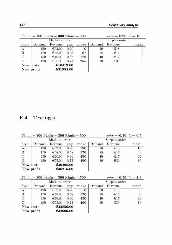
142 Sensitivity analysis
F1min = 100 F2min = 300 F3min = 500 ˆgmp = 0.90, λ = 10.0Made-to-order Surplus order
Style Demand Revenue gmp make Demand Revenue makeA 190 e52.00 0.20 0 20 e18 0B 170 e58.00 0.58 67 28 e16 0C 450 e40.00 0.36 179 40 e17 0D 490 e55.00 0.73 255 30 e30 0New costs e10419.00New profit e31954.00
F.4 Testing λ
F1min = 100 F2min = 300 F3min = 500 ˆgmp = 0.50, λ = 0.5Made-to-order Surplus order
Style Demand Revenue gmp make Demand Revenue makeA 190 e52.00 0.20 190 20 e18 10B 170 e58.00 0.58 170 28 e16 0C 450 e40.00 0.36 450 40 e17 40D 490 e55.00 0.73 490 30 e30 30New costs e29408.00New profit e36215.00
F1min = 100 F2min = 300 F3min = 500 ˆgmp = 0.50, λ = 1.0Made-to-order Surplus order
Style Demand Revenue gmp make Demand Revenue makeA 190 e52.00 0.20 0 20 e18 0B 170 e58.00 0.58 170 28 e16 0C 450 e40.00 0.36 450 40 e17 40D 490 e55.00 0.73 490 30 e30 30New costs e22856.00New profit e32696.00

F.4 Testing λ 143
F1min = 100 F2min = 300 F3min = 500 ˆgmp = 0.50, λ = 5.0Made-to-order Surplus order
Style Demand Revenue gmp make Demand Revenue makeA 190 e52.00 0.20 0 20 e18 0B 170 e58.00 0.58 170 28 e16 0C 450 e40.00 0.36 179 40 e17 0D 490 e55.00 0.73 490 30 e30 30New costs e16383.80New profit e33040.00
F1min = 100 F2min = 300 F3min = 500 ˆgmp = 0.50, λ = 10.0Made-to-order Surplus order
Style Demand Revenue gmp make Demand Revenue makeA 190 e52.00 0.20 0 20 e18 0B 170 e58.00 0.58 170 28 e16 0C 450 e40.00 0.36 179 40 e17 0D 490 e55.00 0.73 490 30 e30 30New costs e16383.80New profit e33040.00
F1min = 100 F2min = 300 F3min = 500 ˆgmp = 0.50, λ = 15.0Made-to-order Surplus order
Style Demand Revenue gmp make Demand Revenue makeA 190 e52.00 0.20 0 20 e18 0B 170 e58.00 0.58 170 28 e16 0C 450 e40.00 0.36 179 40 e17 0D 490 e55.00 0.73 490 30 e30 30New costs e16383.80New profit e33040.00
F1min = 100 F2min = 300 F3min = 500 ˆgmp = 0.50, λ = 20.0Made-to-order Surplus order
Style Demand Revenue gmp make Demand Revenue makeA 190 e52.00 0.20 0 20 e18 0B 170 e58.00 0.58 170 28 e16 0C 450 e40.00 0.36 179 40 e17 0D 490 e55.00 0.73 490 30 e30 30New costs e16383.80New profit e33040.00
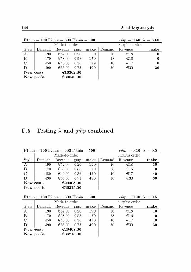
144 Sensitivity analysis
F1min = 100 F2min = 300 F3min = 500 ˆgmp = 0.50, λ = 80.0Made-to-order Surplus order
Style Demand Revenue gmp make Demand Revenue makeA 190 e52.00 0.20 0 20 e18 0B 170 e58.00 0.58 170 28 e16 0C 450 e40.00 0.36 178 40 e17 0D 490 e55.00 0.73 490 30 e30 30New costs e16362.80New profit e33040.00
F.5 Testing λ and ˆgmp combined
F1min = 100 F2min = 300 F3min = 500 ˆgmp = 0.10, λ = 0.5Made-to-order Surplus order
Style Demand Revenue gmp make Demand Revenue makeA 190 e52.00 0.20 190 20 e18 10B 170 e58.00 0.58 170 28 e16 0C 450 e40.00 0.36 450 40 e17 40D 490 e55.00 0.73 490 30 e30 30New costs e29408.00New profit e36215.00
F1min = 100 F2min = 300 F3min = 500 ˆgmp = 0.40, λ = 0.5Made-to-order Surplus order
Style Demand Revenue gmp make Demand Revenue makeA 190 e52.00 0.20 190 20 e18 10B 170 e58.00 0.58 170 28 e16 0C 450 e40.00 0.36 450 40 e17 40D 490 e55.00 0.73 490 30 e30 30New costs e29408.00New profit e36215.00
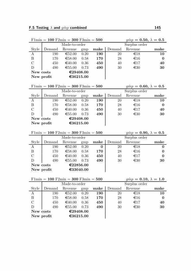
F.5 Testing λ and ˆgmp combined 145
F1min = 100 F2min = 300 F3min = 500 ˆgmp = 0.50, λ = 0.5Made-to-order Surplus order
Style Demand Revenue gmp make Demand Revenue makeA 190 e52.00 0.20 190 20 e18 10B 170 e58.00 0.58 170 28 e16 0C 450 e40.00 0.36 450 40 e17 40D 490 e55.00 0.73 490 30 e30 30New costs e29408.00New profit e36215.00
F1min = 100 F2min = 300 F3min = 500 ˆgmp = 0.60, λ = 0.5Made-to-order Surplus order
Style Demand Revenue gmp make Demand Revenue makeA 190 e52.00 0.20 190 20 e18 10B 170 e58.00 0.58 170 28 e16 0C 450 e40.00 0.36 450 40 e17 40D 490 e55.00 0.73 490 30 e30 30New costs e29408.00New profit e36215.00
F1min = 100 F2min = 300 F3min = 500 ˆgmp = 0.90, λ = 0.5Made-to-order Surplus order
Style Demand Revenue gmp make Demand Revenue makeA 190 e52.00 0.20 0 20 e18 0B 170 e58.00 0.58 170 28 e16 0C 450 e40.00 0.36 450 40 e17 0D 490 e55.00 0.73 490 30 e30 30New costs e22856.00New profit e33040.00
F1min = 100 F2min = 300 F3min = 500 ˆgmp = 0.10, λ = 1.0Made-to-order Surplus order
Style Demand Revenue gmp make Demand Revenue makeA 190 e52.00 0.20 190 20 e18 10B 170 e58.00 0.58 170 28 e16 0C 450 e40.00 0.36 450 40 e17 40D 490 e55.00 0.73 490 30 e30 30New costs e29408.00New profit e36215.00

146 Sensitivity analysis
F1min = 100 F2min = 300 F3min = 500 ˆgmp = 0.40, λ = 1.0Made-to-order Surplus order
Style Demand Revenue gmp make Demand Revenue makeA 190 e52.00 0.20 190 20 e18 10B 170 e58.00 0.58 170 28 e16 0C 450 e40.00 0.36 450 40 e17 40D 490 e55.00 0.73 490 30 e30 30New costs e29408.00New profit e36215.00
F1min = 100 F2min = 300 F3min = 500 ˆgmp = 0.50, λ = 1.0Made-to-order Surplus order
Style Demand Revenue gmp make Demand Revenue makeA 190 e52.00 0.20 0 20 e18 0B 170 e58.00 0.58 170 28 e16 0C 450 e40.00 0.36 450 40 e17 40D 490 e55.00 0.73 490 30 e30 30New costs e22856.00New profit e32696.00
F1min = 100 F2min = 300 F3min = 500 ˆgmp = 0.60, λ = 1.0Made-to-order Surplus order
Style Demand Revenue gmp make Demand Revenue makeA 190 e52.00 0.20 0 20 e18 0B 170 e58.00 0.58 170 28 e16 0C 450 e40.00 0.36 450 40 e17 0D 490 e55.00 0.73 490 30 e30 30New costs e22856.00New profit e33040.00
F1min = 100 F2min = 300 F3min = 500 ˆgmp = 0.90, λ = 1.0Made-to-order Surplus order
Style Demand Revenue gmp make Demand Revenue makeA 190 e52.00 0.20 0 20 e18 0B 170 e58.00 0.58 170 28 e16 0C 450 e40.00 0.36 179 40 e17 0D 490 e55.00 0.73 490 30 e30 30New costs e16383.80New profit e33040.00
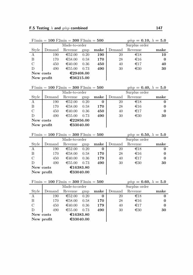
F.5 Testing λ and ˆgmp combined 147
F1min = 100 F2min = 300 F3min = 500 ˆgmp = 0.10, λ = 5.0Made-to-order Surplus order
Style Demand Revenue gmp make Demand Revenue makeA 190 e52.00 0.20 190 20 e18 10B 170 e58.00 0.58 170 28 e16 0C 450 e40.00 0.36 450 40 e17 40D 490 e55.00 0.73 490 30 e30 30New costs e29408.00New profit e36215.00
F1min = 100 F2min = 300 F3min = 500 ˆgmp = 0.40, λ = 5.0Made-to-order Surplus order
Style Demand Revenue gmp make Demand Revenue makeA 190 e52.00 0.20 0 20 e18 0B 170 e58.00 0.58 170 28 e16 0C 450 e40.00 0.36 450 40 e17 0D 490 e55.00 0.73 490 30 e30 30New costs e22856.00New profit e33040.00
F1min = 100 F2min = 300 F3min = 500 ˆgmp = 0.50, λ = 5.0Made-to-order Surplus order
Style Demand Revenue gmp make Demand Revenue makeA 190 e52.00 0.20 0 20 e18 0B 170 e58.00 0.58 170 28 e16 0C 450 e40.00 0.36 179 40 e17 0D 490 e55.00 0.73 490 30 e30 30New costs e16383.80New profit e33040.00
F1min = 100 F2min = 300 F3min = 500 ˆgmp = 0.60, λ = 5.0Made-to-order Surplus order
Style Demand Revenue gmp make Demand Revenue makeA 190 e52.00 0.20 0 20 e18 0B 170 e58.00 0.58 170 28 e16 0C 450 e40.00 0.36 179 40 e17 0D 490 e55.00 0.73 490 30 e30 30New costs e16383.80New profit e33040.00
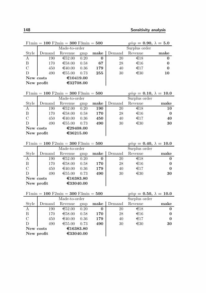
148 Sensitivity analysis
F1min = 100 F2min = 300 F3min = 500 ˆgmp = 0.90, λ = 5.0Made-to-order Surplus order
Style Demand Revenue gmp make Demand Revenue makeA 190 e52.00 0.20 0 20 e18 0B 170 e58.00 0.58 67 28 e16 0C 450 e40.00 0.36 179 40 e17 0D 490 e55.00 0.73 255 30 e30 10New costs e10419.00New profit e32708.00
F1min = 100 F2min = 300 F3min = 500 ˆgmp = 0.10, λ = 10.0Made-to-order Surplus order
Style Demand Revenue gmp make Demand Revenue makeA 190 e52.00 0.20 190 20 e18 10B 170 e58.00 0.58 170 28 e16 0C 450 e40.00 0.36 450 40 e17 40D 490 e55.00 0.73 490 30 e30 30New costs e29408.00New profit e36215.00
F1min = 100 F2min = 300 F3min = 500 ˆgmp = 0.40, λ = 10.0Made-to-order Surplus order
Style Demand Revenue gmp make Demand Revenue makeA 190 e52.00 0.20 0 20 e18 0B 170 e58.00 0.58 170 28 e16 0C 450 e40.00 0.36 179 40 e17 0D 490 e55.00 0.73 490 30 e30 30New costs e16383.80New profit e33040.00
F1min = 100 F2min = 300 F3min = 500 ˆgmp = 0.50, λ = 10.0Made-to-order Surplus order
Style Demand Revenue gmp make Demand Revenue makeA 190 e52.00 0.20 0 20 e18 0B 170 e58.00 0.58 170 28 e16 0C 450 e40.00 0.36 179 40 e17 0D 490 e55.00 0.73 490 30 e30 30New costs e16383.80New profit e33040.00
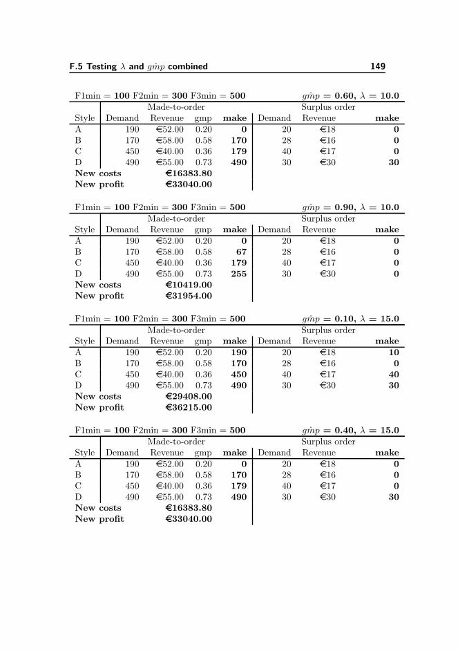
F.5 Testing λ and ˆgmp combined 149
F1min = 100 F2min = 300 F3min = 500 ˆgmp = 0.60, λ = 10.0Made-to-order Surplus order
Style Demand Revenue gmp make Demand Revenue makeA 190 e52.00 0.20 0 20 e18 0B 170 e58.00 0.58 170 28 e16 0C 450 e40.00 0.36 179 40 e17 0D 490 e55.00 0.73 490 30 e30 30New costs e16383.80New profit e33040.00
F1min = 100 F2min = 300 F3min = 500 ˆgmp = 0.90, λ = 10.0Made-to-order Surplus order
Style Demand Revenue gmp make Demand Revenue makeA 190 e52.00 0.20 0 20 e18 0B 170 e58.00 0.58 67 28 e16 0C 450 e40.00 0.36 179 40 e17 0D 490 e55.00 0.73 255 30 e30 0New costs e10419.00New profit e31954.00
F1min = 100 F2min = 300 F3min = 500 ˆgmp = 0.10, λ = 15.0Made-to-order Surplus order
Style Demand Revenue gmp make Demand Revenue makeA 190 e52.00 0.20 190 20 e18 10B 170 e58.00 0.58 170 28 e16 0C 450 e40.00 0.36 450 40 e17 40D 490 e55.00 0.73 490 30 e30 30New costs e29408.00New profit e36215.00
F1min = 100 F2min = 300 F3min = 500 ˆgmp = 0.40, λ = 15.0Made-to-order Surplus order
Style Demand Revenue gmp make Demand Revenue makeA 190 e52.00 0.20 0 20 e18 0B 170 e58.00 0.58 170 28 e16 0C 450 e40.00 0.36 179 40 e17 0D 490 e55.00 0.73 490 30 e30 30New costs e16383.80New profit e33040.00
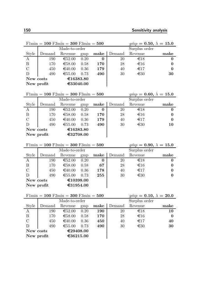
150 Sensitivity analysis
F1min = 100 F2min = 300 F3min = 500 ˆgmp = 0.50, λ = 15.0Made-to-order Surplus order
Style Demand Revenue gmp make Demand Revenue makeA 190 e52.00 0.20 0 20 e18 0B 170 e58.00 0.58 170 28 e16 0C 450 e40.00 0.36 179 40 e17 0D 490 e55.00 0.73 490 30 e30 30New costs e16383.80New profit e33040.00
F1min = 100 F2min = 300 F3min = 500 ˆgmp = 0.60, λ = 15.0Made-to-order Surplus order
Style Demand Revenue gmp make Demand Revenue makeA 190 e52.00 0.20 0 20 e18 0B 170 e58.00 0.58 170 28 e16 0C 450 e40.00 0.36 179 40 e17 0D 490 e55.00 0.73 490 30 e30 10New costs e16383.80New profit e32708.00
F1min = 100 F2min = 300 F3min = 500 ˆgmp = 0.90, λ = 15.0Made-to-order Surplus order
Style Demand Revenue gmp make Demand Revenue makeA 190 e52.00 0.20 0 20 e18 0B 170 e58.00 0.58 67 28 e16 0C 450 e40.00 0.36 178 40 e17 0D 490 e55.00 0.73 255 30 e30 0New costs e10398.00New profit e31954.00
F1min = 100 F2min = 300 F3min = 500 ˆgmp = 0.10, λ = 20.0Made-to-order Surplus order
Style Demand Revenue gmp make Demand Revenue makeA 190 e52.00 0.20 190 20 e18 10B 170 e58.00 0.58 170 28 e16 0C 450 e40.00 0.36 450 40 e17 40D 490 e55.00 0.73 490 30 e30 30New costs e29408.00New profit e36215.00

F.5 Testing λ and ˆgmp combined 151
F1min = 100 F2min = 300 F3min = 500 ˆgmp = 0.40, λ = 20.0Made-to-order Surplus order
Style Demand Revenue gmp make Demand Revenue makeA 190 e52.00 0.20 0 20 e18 0B 170 e58.00 0.58 170 28 e16 0C 450 e40.00 0.36 179 40 e17 0D 490 e55.00 0.73 490 30 e30 30New costs e16383.80New profit e33040.00
F1min = 100 F2min = 300 F3min = 500 ˆgmp = 0.50, λ = 20.0Made-to-order Surplus order
Style Demand Revenue gmp make Demand Revenue makeA 190 e52.00 0.20 0 20 e18 0B 170 e58.00 0.58 170 28 e16 0C 450 e40.00 0.36 179 40 e17 0D 490 e55.00 0.73 490 30 e30 30New costs e16383.80New profit e33040.00
F1min = 100 F2min = 300 F3min = 500 ˆgmp = 0.60, λ = 20.0Made-to-order Surplus order
Style Demand Revenue gmp make Demand Revenue makeA 190 e52.00 0.20 0 20 e18 0B 170 e58.00 0.58 170 28 e16 0C 450 e40.00 0.36 179 40 e17 0D 490 e55.00 0.73 490 30 e30 10New costs e16383.80New profit e32708.00
F1min = 100 F2min = 300 F3min = 500 ˆgmp = 0.90, λ = 20.0Made-to-order Surplus order
Style Demand Revenue gmp make Demand Revenue makeA 190 e52.00 0.20 0 20 e18 0B 170 e58.00 0.58 67 28 e16 0C 450 e40.00 0.36 178 40 e17 0D 490 e55.00 0.73 255 30 e30 0New costs e10398.00New profit e31954.00
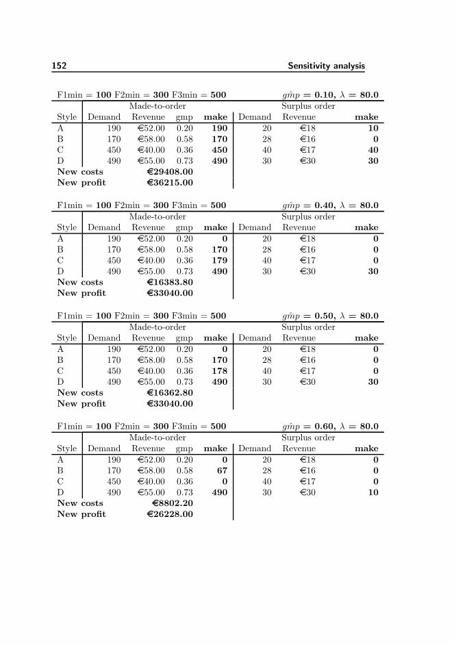
152 Sensitivity analysis
F1min = 100 F2min = 300 F3min = 500 ˆgmp = 0.10, λ = 80.0Made-to-order Surplus order
Style Demand Revenue gmp make Demand Revenue makeA 190 e52.00 0.20 190 20 e18 10B 170 e58.00 0.58 170 28 e16 0C 450 e40.00 0.36 450 40 e17 40D 490 e55.00 0.73 490 30 e30 30New costs e29408.00New profit e36215.00
F1min = 100 F2min = 300 F3min = 500 ˆgmp = 0.40, λ = 80.0Made-to-order Surplus order
Style Demand Revenue gmp make Demand Revenue makeA 190 e52.00 0.20 0 20 e18 0B 170 e58.00 0.58 170 28 e16 0C 450 e40.00 0.36 179 40 e17 0D 490 e55.00 0.73 490 30 e30 30New costs e16383.80New profit e33040.00
F1min = 100 F2min = 300 F3min = 500 ˆgmp = 0.50, λ = 80.0Made-to-order Surplus order
Style Demand Revenue gmp make Demand Revenue makeA 190 e52.00 0.20 0 20 e18 0B 170 e58.00 0.58 170 28 e16 0C 450 e40.00 0.36 178 40 e17 0D 490 e55.00 0.73 490 30 e30 30New costs e16362.80New profit e33040.00
F1min = 100 F2min = 300 F3min = 500 ˆgmp = 0.60, λ = 80.0Made-to-order Surplus order
Style Demand Revenue gmp make Demand Revenue makeA 190 e52.00 0.20 0 20 e18 0B 170 e58.00 0.58 67 28 e16 0C 450 e40.00 0.36 0 40 e17 0D 490 e55.00 0.73 490 30 e30 10New costs e8802.20New profit e26228.00

F.5 Testing λ and ˆgmp combined 153
F1min = 100 F2min = 300 F3min = 500 ˆgmp = 0.90, λ = 80.0Made-to-order Surplus order
Style Demand Revenue gmp make Demand Revenue makeA 190 e52.00 0.20 0 20 e18 0B 170 e58.00 0.58 0 28 e16 0C 450 e40.00 0.36 0 40 e17 0D 490 e55.00 0.73 0 30 e30 0New costs e0.00New profit e0.00

154 Sensitivity analysis
Bibliography
[1] Reeve, James M.: Readings and Issues in Cost Management, Second Edi-tion, 2000, South-Western College Publishing, ISBN: 0-324-02298-0
[2] Birnbaum, David: Birnbaum’s Global Guide to Material Sourcing 2005,The FashionIndex, Inc., ISBN: 0-9741011-3-3
[3] Birnbaum, David: The Great Garment War
[4] Bragg, Stephen M.: Controller’s Guide to Costing 2005, John Wiley &Son’s, Inc. ISBN: 0-471-71394-5
[5] Bukh, Per N. Activity Based Costing - Dansk Økonomistyring under for-vandling 2004, Jurist- og Økonomforbundets forlag, ISBN: 87-574-1015-1
[6] Lyngaard, Peter: Driftsøkonomi 2002, Handelshøjsskolens Forlag, ISBN:87-629-0198-2
[7] http://www.mcgrawhill.ca/college/garrison5/student/olc/5mag
gloss 07.html
[8] Federation of Danish Textile & Clothing: Forecasting for the textile & cloth-ing industry 2007
[9] http://instruct1.cit.cornell.edu/Courses/cuttingedge/glossary.html
[10] Danmarks Statistik www.dst.dk
[11] Riegels Mechior, Marie & Olsen Rule, Nikolina: Dansk mode - Historie, De-sign, Identitet 2006 Danmarks Designskole Printcenter, ISBN: 87-985478-3-6
156 BIBLIOGRAPHY
[12] Christopher, Martin; Lowson, Robert; Peck, Helen: Creating agile sup-ply chains in the fashion industry 2004, International Journal of Retail &Distribution Management, Vol. 32, Number 8 pp. 367-376, ISSN 0959 0552
[13] R.P. Rollins, K. Porter, D. Little: Modelling the changing apparel supplychain International Journal of Clothing Science and Technology, Vol. 15No. 2, 2003, ISSN 0955 6222
[14] Ian M. Taplin, Jonathan Winterton: The European clothing industry - Met-ting the competitive challange Journal of Fashion Marketing and Manage-ment, Vol. 8 No. 3, 2004
[15] Gary Gereffi: International trade and industrial upgrading in the apparelcommodity chain Journal of International Economics, volume 48, Issue 1,June 1999
[16] Fu-Shiung Hsieh: An evolutionary approach for self-organization of contractmanufacturing supply chains 0-7803-7087-2/01
[17] S.D. Mokashi, A.C.Kokossis: Application of dispersion alogirthms to supplychain optimisation Computers & Mechanical Engineering 27, 2003, ISSN0098 1354
[18] Soundouss Bouhia, Frederick H. Abernathy: Sceduling and ordering pro-duction policies in a Limited Capacity Manufacturing System - the MultipleReplenishment Products Case
[19] Andrew Hughes: ABC/ABM - activity-based costing and activity-basedmanagement. Journal of Fashion Marketing and Management, 2005, 9, 1
[20] Sergio Maturana, Juan-Carlos Ferrer, Francisco Baranao: Design and im-plementation of an optimization-based decision support system generatorEuropean Journal of Operational Research 154, 2004
[21] Andrew J. Newman, Darshika Patel: The marketing directions of two fash-ion retailers European Journal of Marketing Vol. 38 No. 7, 2004
[22] Frederick H. Abernathy, Anthonyh Volpe, David Weil: The Future of theApparel and Textile Industries: Prospects and Choices for Public and Pri-vate Actors Harvard Center for Textile and Apparel Research, Dec. 22 2005
[23] Vækstfonden: Dansk Design - en god forretning? www.vf.dk, 10. August2007, pdf-document
[24] TEKO: TEKO analysen 2005 - Mode og livstilsbranchen www.teko.dk
[25] Danish Fahion Institute: ‘Arsberetning 2005 www.dafi.dk, 10 August 2007,pdf-document
BIBLIOGRAPHY 157
[26] Stig Ørskov: Mens vi venter paerhvervslivet 12 July 2005, DesignMattersno. 09
[27] Peter Doeringer, Sarah Crean: Can fast fashion save the US apparel indus-try? Socio-Economic Review(2006) 4, Advanced Access publication March12, 2006
[28] Dansk Industri: Guide til outsourcing og etablering Oktober 2004,www.di.dk
[29] Peter Gibbon, Lotte Thomsen: Scandinavian Cloth-ing Retailers’ Global Sourcing Patterns and Prac-tices CDR Working Paper 02.14, November 2002http://www.diis.dk/graphics/CDR%5FPublications/cdr%5Fpublications/working%5Fpap
[30] The future of fast fashion. Economist, 6/18/2005, Vol. 375 Issue 8431
[31] Amanda Craig, Charlese Jones, Martha Nieto: ZARA: Fashion Follower,Industry Leader Business of Fashion Case Study Competition, PhiladelphiaUniversity April 2, 2004
[32] Richard M. Jones: The Apparel Industry Blackwell, 2006, 2nd. ed., ISBN:9781405135993
[33] Business environment rankings methodologya330.g.akamai.net/7/330/25828/20060515192601/graphics.eiu.com/files/ad
pdfs/CF PDF.pdf, 2007/09/26methodology:http://www.alacra.com/wdata/help/forecastmethodology.htm
[34] Morten Crone: Designerduo kvalt i vækst 2006/06/11,http://www.business.dk/article/20060711/nyhedsoversigt/107110292/
[35] David Tarp: Tœjdesign og ledelse er en darlig cocktail 2006/08/07,http://www.business.dk/article/20060807/nyhedsoversigt/108070297/
[36] Wikipedia, http://en.wikipedia.org/wiki/Letter of credit
[37] Wikipedia, Lagrarian Relaxation http://en.wikipedia.org/wiki/Lagrangian
relaxation, 24/10-2007
[38] http://www.finfacts.com/irelandbusinessnews/publish/article
1011625.shtml
[39]