Outsourcing, Product Quality, and Contract

Enforcement

Yi Lua, Travis Ngb, and Zhigang Taoc

a National University of Singapore

b Chinese University of Hong Kong

c University of Hong Kong

This Version: March 2011

Abstract

Does outsourcing compromise product quality? Does sound contract enforcement

alleviate this concern? We offer a simple model to illustrate how outsourcing leads

to lower product quality and how contract enforcement helps mitigate this problem.

These theoretical predictions are borne out of a survey of 2,400 firms in China con-

ducted by the World Bank in 2003.

Keywords: Outsourcing; Product Quality; Quality Guarantee; Contract Enforcement

JEL Codes: D23, L23, L15, K0

1

1 Introduction

Over the past several decades, firms have been increasingly disintegrating their production

processes and becoming more vertically specialized along with the trend of globalization

(Feenstra, 1998; Hummels, Ishii, and Yi, 2001). While the benefits of outsourcing (most

notably, lower production cost) are well recognized, there has been an increasing awareness

of the potential costs associated with outsourcing.1 Anecdotal evidence suggests that out-

sourcing leads to problems in product quality. For example, the massive pet food recalls

in both the US and Canada in 2007 exposed a serious hazard of outsourcing: the product

quality of the concerned pet food companies was compromised due to their outsourcing of

key ingredients to domestic suppliers.2 In the largest product recall in China in 2008, the

baby formula of Sanlu (the largest company in the industry by volume) was found to contain

melamine originated from contaminated milk supply outsourced to local farmers. This raises

the question of whether outsourcing has a negative impact on product quality.

Outsourcing involves contracting with external suppliers for the delivery of parts and

components with pre-specified quality levels. Enforcement of those contracts, especially

regarding the quality levels of parts and components is, however, far from perfect even in

some developed countries. To the extent that the quality of a final product depends on

the quality of its parts and components, product quality thus depends on the effectiveness

of contract enforcement. Given that the effectiveness of contract enforcement varies across

industries and regions, there is a further question for those firms pursuing the outsourcing

strategy, namely, how contract enforcement interacts with the impact of outsourcing on

product quality.

Despite their importance, there are few systematic studies on these issues.3 This paper

attempts to fill this void. We first offer a theoretical model to illustrate how outsourcing

1The opposite arrangement is called vertical integration.2Specifically, Menu Foods Ltd. of Ontario, Canada was the supplier responsible for the faulty production

of the key ingredients.3To the best of our knowledge, the exceptions are two theoretical studies by Hart, Shleifer, and Vishny

(1997) and Economides (1999).

2

may lead to low product quality and how contract enforcement may alleviate this problem.

We then test the theoretical predictions using data from China.4

In our theoretical analysis, a firm contracts the production of its components to a supplier,

whose effort stochastically determines the quality of the components and, consequently,

the quality of the final product. The quality of the components is observable to the two

contracting parties, but not perfectly verifiable by a third party such as the court. In the

case of a dispute regarding the quality of components, there is a non-zero probability that

the court may make a mistake in its ruling. For instance, when the supplier fails to deliver

high-quality components and the firm sues the supplier, the court may fail to rule against

the supplier. Such a probability captures the degree of imperfection of contract enforcement.

Under this setting, we show that product quality is lower under outsourcing compared to

that under vertical integration. Moreover, when contract enforcement becomes less effective

(i.e., courts are more likely to make mistakes in its ruling), the gap in product quality between

vertical integration and outsourcing widens.

To bring the theoretical predictions to empirical tests, in which quality guarantee is used

as an indirect measure of product quality, we explicitly establish a link between product qual-

ity and the offering of quality guarantee. We incorporate information asymmetry between

a producer and a consumer regarding the underlying product quality. A producer can be of

two types (i.e., carrying either a high-quality product or a low-quality one) and two possible

strategies (i.e., offering quality guarantee or not). There are three possible equilibria: a

pooling equilibrium in which neither type offers quality guarantee; a separating equilibrium

in which a high-quality producer offers quality guarantee but not for a low-quality producer;

and a pooling equilibrium in which both types offer quality guarantee. The likelihood of

offering quality guarantee is shown to be lower under outsourcing compared to that under

vertical integration. However, the negative impact of outsourcing on quality guarantee is

again mitigated by the effectiveness of contract enforcement.

4Our theoretical model can be extended to the setting of international outsourcing. However, due to datalimitations, the empirical analysis focuses on domestic outsourcing in China instead.

3

Our empirical study uses a survey of firms in China conducted by the World Bank in

2003. Although China is a unitary state with uniform de jure laws across the country, there

are substantial variations in the effectiveness of contract enforcement across its regions (Du,

Lu, and Tao, 2008; World Bank, 2008; Lu and Tao, 2009a). For example, in some coastal

cities, it takes an average of 230 days to resolve an uncomplicated commercial dispute, but

a much lengthy 363 days in the northeastern part of China (World Bank, 2008). Thus, the

dataset offers an ideal setting for investigating the impact of outsourcing on product quality,

and the role of the effectiveness of contract enforcement.

The dependent variable for the empirical analysis is the percentage of products or services

for which a firm offers quality guarantees. The measure of outsourcing is constructed based

on the reply to the survey question on the percentage of inputs purchased from external

suppliers. The measure of the effectiveness of contract enforcement is constructed based on

the reply to the survey question regarding the likelihood that the legal system would uphold

contract and property rights in business disputes.

The ordinary-least-squares (OLS) estimation results show that outsourcing reduces the

likelihood of offering quality guarantees, and that poor contract enforcement would further

exacerbate this negative impact of outsourcing. Given the positive correlation between prod-

uct quality and quality guarantees, our results imply that outsourcing compromises product

quality, but the negative impact of outsourcing on product quality is mitigated by the effec-

tiveness of contract enforcement. These estimation results could be biased, however, due to

the omitted variables problem. To address this concern, we include a list of control variables

capturing firm characteristics, CEO characteristics, industry and city dummies in a stepwise

fashion. Our results remain robust.

To further deal with the possible endogeneity issue, we use the two-step Generalized

Method of Moments (GMM) estimation. Following the recent literature on empirical indus-

trial organization (e.g., Berry, Levinsohn, and Pakes, 1995; Nevo, 2000, 2001), we use the

average extent of outsourcing among firms in the same industry but located in other cities

4

as the instrumental variable for the firm-level measure of outsourcing. Similarly, we use the

average effectiveness of contract enforcement among firms in other industries but located

in the same city as an instrument for the effectiveness of contract enforcement at the firm

level. The two-step GMM estimations reinforce our early findings about the negative impact

of outsourcing on product quality and the mitigating role of the effectiveness of contract

enforcement.

Our study is related to a growing literature on the determinants of outsourcing in the con-

text of the global economy. For example, Antras (2003), Grossman and Helpman (2003), and

Antras and Helpman (2004) examine when multinationals produce the components in-house

in the foreign countries (i.e., foreign direct investment) and when they outsource the com-

ponent production to foreign suppliers (i.e., global outsourcing). Furthermore, Acemoglu,

Antras, and Helpman (2007), Nunn (2007), Antras and Helpman (2008), and Acemoglu,

Johnson, and Mitton (2009) investigate the impact of contract enforcement on the extent

of outsourcing. The departure of our study from this literature is its emphasis on the im-

pact, rather than the determinants, of outsourcing. Moreover, we investigate how contract

enforcement mitigates the impact of outsourcing, rather than how it determines the extent

of outsourcing.

This study is one of the first few studies documenting costs of outsourcing, specifically,

low product quality. It should be pointed out, however, that there are certainly benefits from

outsourcing. For example, it has been widely accepted that outsourcing offers an advantage

in production costs. Indeed, Lu and Tao (2009b) find that firms adopting an outsourcing

strategy have a bigger scale of production and higher production efficiency. Taken together,

these studies suggest there is a trade-off for firms in using the outsourcing strategy. The

optimal choice of the vertical boundary of a firm (i.e., the extent of outsourcing) thus depends

on the relative importance of product quality vis-a-vis production efficiency, and ultimately

on the strategic positioning of the firm.

The remainder of the paper is structured as follows. Section 2 offers a theoretical model,

5

while Section 3 presents the empirical analysis. We conclude in Section 4.

2 Theoretical Analysis

This section first offers a simple model to illustrate how outsourcing may lead to low product

quality and how contract enforcement may alleviate this problem. We then link product

quality to the propensity to offer quality guarantee.

2.1 Outsourcing and Product Quality

Firm B contemplates the sourcing strategy for its key component. The component can be

made in-house (i.e., vertical integration I) or outsourced to an external supplier S (i.e.,

outsourcing O). For simplicity, it is assumed that there are two types of component, a high-

quality one and a low-quality one. Following Economides (1999), the model assumes that

the quality of the component fully determines the quality of the final product; that is, a

high-quality component leads to a high-quality final product while a low-quality component

leads to a low-quality final product. The probability of having a high-quality component is x

and that of having a low-quality component is 1−x, where x is the level of precautions taken

by the component maker.5 The cost of taking precautions, c(x), has the standard properties

(i.e., c (x) is twice continuously differentiable, c (0) = 0, c (1) = ∞, c′(0) = 0, c′ (x) > 0 for

x > 0, c′′ (x) > 0 for x > 0, and c′ (1) = ∞). The benefit of a high-quality component to

firm B is denoted by Vh while that of a low-quality component is Vl, with Vh > Vl. Without

loss of generality, in this sub-section, Vh and Vl are normalized to 1 and 1− α respectively,

with α ∈ (0, 1).6

5Note that the investment x made by the component maker only affects the probability of having a high-or a low-quality component and hence a high- or low-quality final product. It does not affect the qualitylevel of the respective final product, specifically, in terms of the probability of product break down (to beformally introduced in the next sub-section).

6The actual values of Vh and Vl are determined by how much firm B can charge consumers in the finalproduct market. Specifically, in the next sub-section, we introduce information asymmetry between firm Band consumers regarding the quality of the final product, as a result of which these two values are determinedby the probability of product break down as well as the likelihood of having quality guarantee. Nonetheless,

6

In the case of outsourcing, firm B signs a contract with supplier S, stipulating a payment

T from B to S for the delivery of the high-quality component. Once produced, the quality of

the component is observable by both B and S, but not perfectly verifiable by a third party

such as the court.7

If there is no disagreement on the quality of the component, B will give S the payment

stipulated in the contract; otherwise, B and S may go to the court to resolve their dispute.

Assume that the court will make a correct ruling with probability θ ∈ (1/2, 1].8 This

assumption captures the imperfection of contract enforcement. It could arise because the

jury may not have the expertise to evaluate the quality of the component, which often

involves highly complicated proprietary technologies. Specifically, if S indeed fails to deliver

a high-quality component and B sues S in the court, there is only a probability of θ that

the court rules against S. Similarly, if S delivers a high-quality component but B claims

otherwise, there is a probability of θ that the court rules against B. Whenever the court

rules against S (i.e., with the judgment that the component is of low-quality), the supplier

needs to pay a damage of α to the buyer.9 Without loss of generality, the cost of litigation

is assumed to be the same for B and S, and is denoted by k. With perfect information on

the expected outcome of the court litigation and with costless renegotiation, the two parties

will renegotiate the terms of the transaction using the court litigation as the default, rather

than settle their dispute in court.

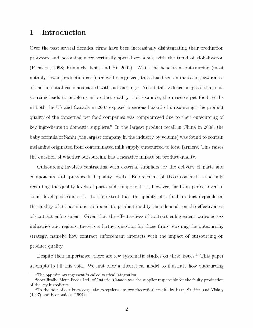
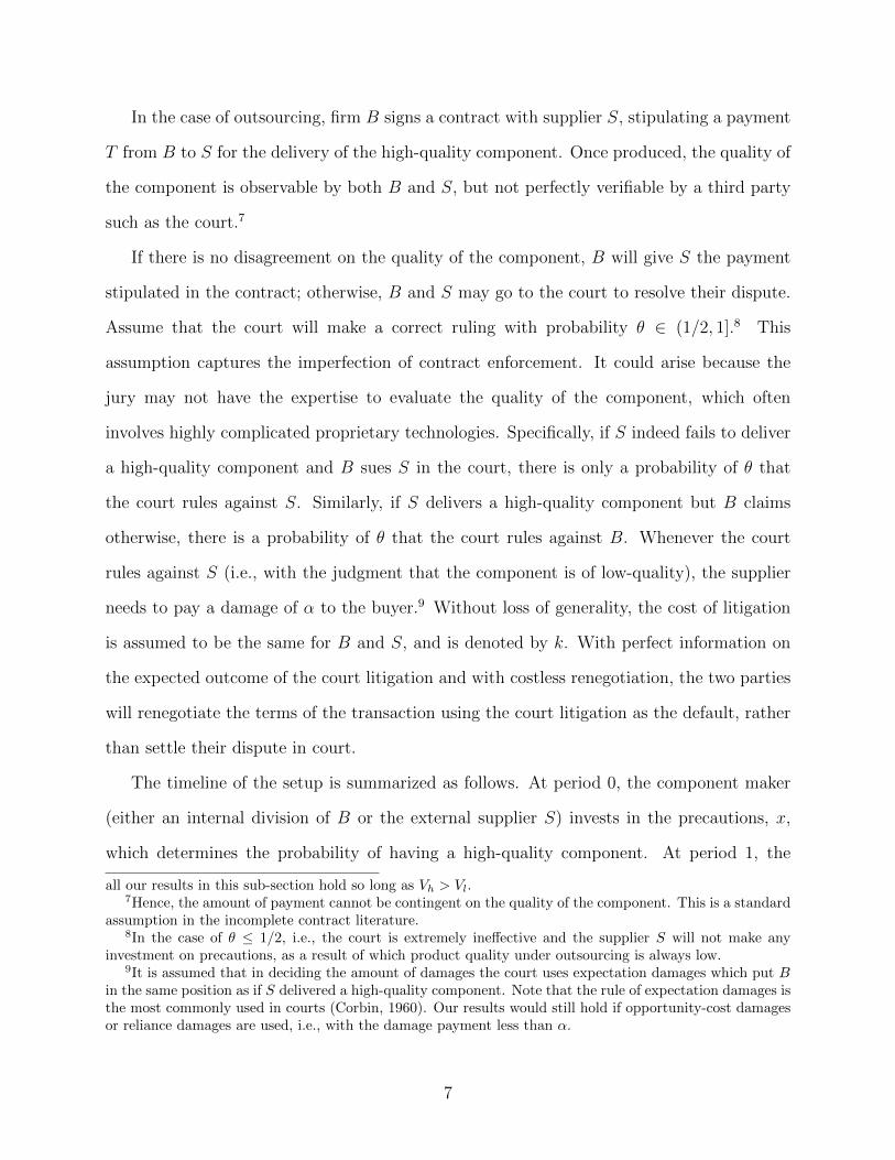
The timeline of the setup is summarized as follows. At period 0, the component maker

(either an internal division of B or the external supplier S) invests in the precautions, x,

which determines the probability of having a high-quality component. At period 1, the

all our results in this sub-section hold so long as Vh > Vl.7Hence, the amount of payment cannot be contingent on the quality of the component. This is a standard

assumption in the incomplete contract literature.8In the case of θ ≤ 1/2, i.e., the court is extremely ineffective and the supplier S will not make any

investment on precautions, as a result of which product quality under outsourcing is always low.9It is assumed that in deciding the amount of damages the court uses expectation damages which put B

in the same position as if S delivered a high-quality component. Note that the rule of expectation damages isthe most commonly used in courts (Corbin, 1960). Our results would still hold if opportunity-cost damagesor reliance damages are used, i.e., with the damage payment less than α.

7

Period 0 Period 1

Take precautions

High-quality or low-quality?

Renegotiate for settlement?

Quality dispute

Court ruling

Time

Outsource

Figure 1: Timeline of the game in the case of outsourcing

component is delivered. In the case of vertical integration, the transaction is carried out

without any friction, and the game ends. In the case of outsourcing, the buyer and the

external supplier may have a dispute on the quality of the component upon delivery, in

which case they will renegotiate the terms of the transaction and complete the transaction.

Figure 1 summarizes the game for the case of outsourcing in a timeline.

In the case of vertical integration, firm B chooses the level of precautions x to maximize

the expected profit, i.e.,

max0≤x≤1

x+ (1− x)(1− α)− c (x) . (1)

and the associated first-order condition is

α = c′ (x∗I) , (2)

where x∗I is the optimal level of precautions under vertical integration.

To solve the equilibrium product quality under outsourcing, we use backward induction.

First, consider the subgame in which S delivers a low-quality component and B sues S. With

probability θ the court will rule against S, under which S is required to pay B the damage

α; otherwise, S does not need to pay any damages. The expected payoff for S is T − θα− k,

and that for B is (1− α)− T + θα− k. With perfect information on the expected litigation

outcome and costless renegotiation, B and S will settle their dispute without actually going

to the court. Assume that the renegotiation takes the form of Nash bargaining and that

the two parties have equal bargaining power. Let the settlement price that S will pay B be

8

pl. The expected payoffs for S and B are T − pl and (1 − α) − T + pl, respectively. The

settlement price pl is the solution to the following optimization problem

maxpl

{[T − pl

]− [T − θα− k]

} 12{[

(1− α)− T + pl]− [(1− α)− T + θα− k]

} 12

⇒

pl = θα. (3)

Second, consider the subgame in which S delivers a high-quality component but B claims

otherwise. With probability 1 − θ, the court will rule against S, under which S is required

to pay B the damage α; otherwise, S does not need to pay any damages. The expected

payoff for S is T − (1− θ)α− k, and that for B is 1− T + (1− θ)α− k. Again, with perfect

information on the litigation outcome and costless renegotiation, B and S will settle their

dispute without actually going to court. Let the settlement price from S to B be ph. Then,

the expected payoffs for S and B are T − ph and 1 − T + ph, respectively. The settlement

price ph is the solution to the following optimization problem

maxpl

{[T − ph

]− [T − (1− θ)α− k]

} 12{[

1− T + ph]− [1− T + (1− θ)α− k]

} 12

⇒

ph = (1− θ)α. (4)

Going back to Period 0, S is to choose x to maximize its expected profit, i.e.,

max0≤x≤1

T − xph − (1− x) pl − c (x) ,

and the associated first-order condition is

(2θ − 1)α = c′ (x∗O) (5)

9

where x∗O is the optimal investment level under outsourcing.

Comparing Equation (2) with Equation (5), it is clear that x∗O ≤ x∗I because c′′ (x) > 0

and θ ≤ 1. This implies that the quality of the component under outsourcing is lower

than that under vertical integration. Furthermore, we can show that the negative impact

of outsourcing on the component quality (i.e., x∗I − x∗O) becomes smaller as the effectiveness

of contract enforcement (i.e., θ) increases. In particular, when the contract enforcement is

perfect (θ = 1), there is no difference in the component quality between outsourcing and

vertical integration. Recalling that the quality of the component determines the quality of

the final product, we then have the following proposition:

Proposition 1. Product quality is lower under outsourcing compared to that under vertical

integration. However, the negative impact of outsourcing on product quality is mitigated by

the effectiveness of contract enforcement.

Here we would like to compare our theoretical analysis with two existing theoretical stud-

ies in the literature. Economides (1999) constructs a model of two vertically related monop-

olies in which each of them makes investment for the quality of its respective component and

the quality of the final product depends on the lower quality of the two components. Without

vertical integration, the two independent monopolies have the typical double-marginalization

problem; each independent monopoly has a lower incentive to invest in quality because it

has to share the benefits with the other monopoly. However, this problem could be avoided

in the case of vertical integration as the positive externality of the investment would be fully

internalized.

Hart, Shleifer, and Vishny (1997) construct a multi-task model in which a supplier has

self investment (i.e., cost reduction) and cooperative investment (i.e., product improvement).

In the case of outsourcing where the supplier owns the assets, he enjoys the full benefit from

the self investment, but needs to share the benefit from the cooperative investment with

the buyer because of the incompleteness of the ex ante supply contract. As a result, the

supplier’s incentive is skewed toward self investment. In the case of vertical integration,

10

the supplier does not own the assets and has a lower but balanced incentive for both self

investment and cooperative investment. When the self investment causes too much damage

on product quality, product quality is compromised under outsourcing.

Our model shares with these two models in explaining the negative impact of outsourcing

on product quality. Our model differs from these two models in incorporating the role of

contract enforcement and showing explicitly that the lower product quality under outsourcing

is due to the imperfection of contract enforcement.

2.2 Product Quality and Quality Guarantee

Taking the model to the data involves an inherent challenge: the underlying product qual-

ity is neither observable nor systematically measured across firms. We therefore rely on

other observable proxies that systematically correlate with the underlying product quality.

Whether firms offer quality guarantee is a natural candidate because intuitively it is cheaper

for firms of high-quality products to offer quality guarantee than for those of low-quality

products. We explicitly establish the link between the underlying product quality and the

likelihood of offering quality guarantee in this subsection.

We extend the model in Section 2.1 to the next stage in which a final good producer (firm

B) sells its product to a representative consumer. A consumer buys either one or zero unit

of the product. His utility of consuming the product is v − p if the product does not break

down, but drops to v− p−h if it does, where p is the price the consumer pays, v is the gross

utility from consuming the product, and h corresponds to the harm the consumer incurs in

the case of breakdown. Without loss of generality, it is assumed that there are numerous

consumers so that the producer can extract all the net benefit from the consumers through

pricing of the product.

There is information asymmetry between the consumer and the producer about the qual-

ity of the final product. The producer knows the underlying product quality, but the con-

sumer only knows a producer can be of two types: a producer of a high-quality final product

11

(H-type) or a producer of a low-quality final product (L-type). A high-quality product is

less likely to break down. Specifically, H-type and L-type break down with probabilities qh

and ql, respectively, with 0 < qh < ql < 1. The consumer has a prior belief that λ percentage

of products will have a product defect where qh < λ < ql.10

As a strategy for alleviating information asymmetry, the producer could offer quality

guarantee. Specifically, the guarantee promises a free repair of a defective product to the

extent that the consumer suffers no harm (in the sense, his net benefit is brought back to

v− p from v− p− h). The cost of repairing a defective product is εh, where ε draws from a

distribution of G(ε) and ε ∈ [0,∞).

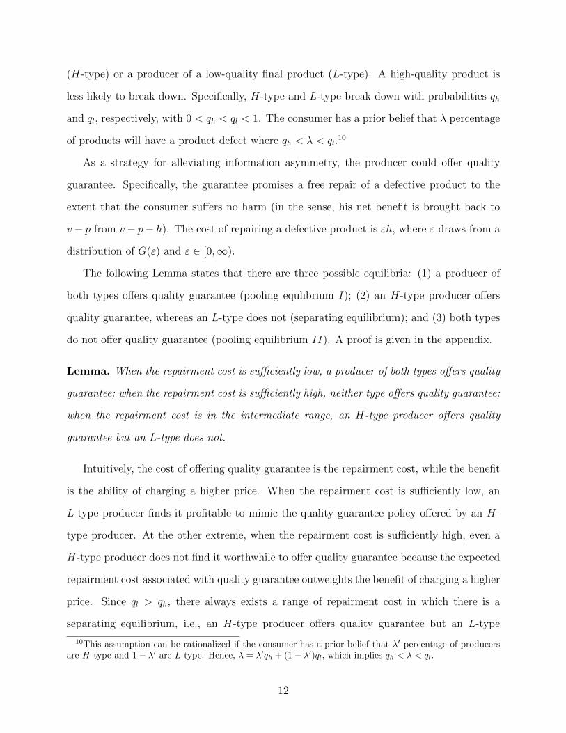
The following Lemma states that there are three possible equilibria: (1) a producer of

both types offers quality guarantee (pooling equlibrium I); (2) an H-type producer offers

quality guarantee, whereas an L-type does not (separating equilibrium); and (3) both types

do not offer quality guarantee (pooling equilibrium II). A proof is given in the appendix.

Lemma. When the repairment cost is sufficiently low, a producer of both types offers quality

guarantee; when the repairment cost is sufficiently high, neither type offers quality guarantee;

when the repairment cost is in the intermediate range, an H-type producer offers quality

guarantee but an L-type does not.

Intuitively, the cost of offering quality guarantee is the repairment cost, while the benefit

is the ability of charging a higher price. When the repairment cost is sufficiently low, an

L-type producer finds it profitable to mimic the quality guarantee policy offered by an H-

type producer. At the other extreme, when the repairment cost is sufficiently high, even a

H-type producer does not find it worthwhile to offer quality guarantee because the expected

repairment cost associated with quality guarantee outweights the benefit of charging a higher

price. Since ql > qh, there always exists a range of repairment cost in which there is a

separating equilibrium, i.e., an H-type producer offers quality guarantee but an L-type

10This assumption can be rationalized if the consumer has a prior belief that λ′ percentage of producersare H-type and 1− λ′ are L-type. Hence, λ = λ′qh + (1− λ′)ql, which implies qh < λ < ql.

12

producer does not.

The Lemma is thus important in linking Proposition 1 to the empirical analysis because it

identifies an outcome in which a high-quality producer differentiates itself from a low-quality

producer by means of quality guarantee. This corresponds to the empirical observation that

a producer with a product-quality product has a higher propensity to offer quality guarantee

than a producer with a low-quality product.

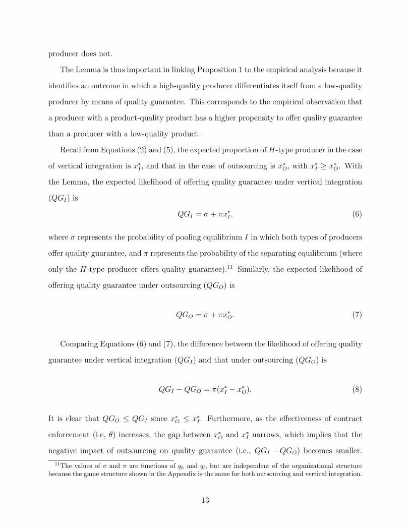
Recall from Equations (2) and (5), the expected proportion ofH-type producer in the case

of vertical integration is x∗I , and that in the case of outsourcing is x∗O, with x∗I ≥ x∗O. With

the Lemma, the expected likelihood of offering quality guarantee under vertical integration

(QGI) is

QGI = σ + πx∗I , (6)

where σ represents the probability of pooling equilibrium I in which both types of producers

offer quality guarantee, and π represents the probability of the separating equilibrium (where

only the H-type producer offers quality guarantee).11 Similarly, the expected likelihood of

offering quality guarantee under outsourcing (QGO) is

QGO = σ + πx∗O. (7)

Comparing Equations (6) and (7), the difference between the likelihood of offering quality

guarantee under vertical integration (QGI) and that under outsourcing (QGO) is

QGI −QGO = π(x∗I − x∗O). (8)

It is clear that QGO ≤ QGI since x∗O ≤ x∗I . Furthermore, as the effectiveness of contract

enforcement (i.e, θ) increases, the gap between x∗O and x∗I narrows, which implies that the

negative impact of outsourcing on quality guarantee (i.e., QGI −QGO) becomes smaller.

11The values of σ and π are functions of qh and ql, but are independent of the organizational structurebecause the game structure shown in the Appendix is the same for both outsourcing and vertical integration.

13

Hence, we have the following proposition:

Proposition 2. The likelihood of offering quality guarantee is lower under outsourcing com-

pared to that under vertical integration. However, the negative impact of outsourcing on

quality guarantee is mitigated by the effectiveness of contract enforcement.

Finally, with this full-fledged model, we can write down the actual values of the respective

benefits (i.e., Vh and Vl) of a high- and low-quality component to firm B. Specifically,

Vh = σ [v(1− qh) + (v − εh)qh] + π [v(1− qh) + (v − εh)qh]

+(1− σ − π) (v − λh)

Vl = σ [v(1− ql) + (v − εh)ql] + π (v − qlh)

+(1− σ − π) (v − λh)

.

It can be shown that Vh > Vl as ε ≤ qlqh

under the separating equilibrium.

3 Empirical Analysis

3.1 Data and Variables

Our data come from a survey of firms in China, conducted by the World Bank in cooperation

with the Enterprise Survey Organization of China in early 2003.12 The World Bank selected

a total of 18 cities from five supra-regions of China for balance of representation: 1) Benxi,

Changchun, Dalian, and Haerbin in the Northeast; 2) Hangzhou, Jiangmen, Shenzhen, and

Wenzhou along the coastal area; 3) Changsha, Nanchang, Wuhan, and Zhengzhou in Central

China; 4) Chongqing, Guiyang, Kunming, and Nanning in the Southwest; and 5) Lanzhou

and Xi’an in the Northwest. In each city, the World Bank randomly sampled 100 or 150

firms from the following nine manufacturing industries and five service industries: garment

and leather products, electronic equipment, electronic parts making, household electronics,

12The data set has been used by Cull and Xu (2005) and Dong and Xu (2009).

14

auto and auto parts, food processing, chemical products and medicine, biotech products and

Chinese medicine, metallurgical products, transportation services, information technology,

accounting and non-banking financial services, advertisement and marketing, and business

services. The total number of surveyed firms is 2,400.

The survey consists of two parts. One is a general questionnaire directed at the senior

management seeking information about the firm, innovation, product certification, market-

ing, relations with suppliers and customers, access to markets and technology, relations with

government, labor, infrastructure, international trade, finance and taxation, and the CEO

and board of directors. The other questionnaire is directed at the accountant and personnel

manager, covering ownership, various financial measures, and labor and training.

To measure the quality of products or services, we use the reply to the survey question

regarding the percentage of products or services for which a firm offers quality guarantees,

and construct a variable called Guarantee accordingly. This measure is an indirect measure

of product quality. As shown in Section 2.2, there is a positive correlation between quality

guarantees and underlying product quality. Table 1 provides the summary statistics.

One key explanatory variable in this study is the extent of outsourcing, i.e., the fraction

of parts purchased from external suppliers. In the survey, there is a question regarding the

percentage of a firm’s parts, in terms of its value, that are produced within the firm.13 The

key explanatory variable, Outsourcing, is constructed as one minus the reply to this question.

The other key explanatory variable in this study is the effectiveness of contract en-

forcement. According to North (1991), contract enforcement concerns about the horizontal

relations between transacting parties. To measure the effectiveness of contract enforcement,

we follow the approach of Johnson, McMillan, and Woodruff (2002), Acemoglu and Johnson

(2005), and Cull and Xu (2005). Specifically, in the survey, there is a question addressed to

the senior management regarding their perceived likelihood that the legal system will uphold

13Measuring the extent of outsourcing at the firm level has always been a challenging problem because ofdata limitation. As a result, indirect measures have been used in the literature (for example, Hortacsu andSyverson, 2007; Acemoglu, Johnson, and Mitton, 2009). In contrast, our dataset offers a direct measure ofthe extent of outsourcing.

15

the contract and property rights in business disputes.14 Accordingly, we construct a variable

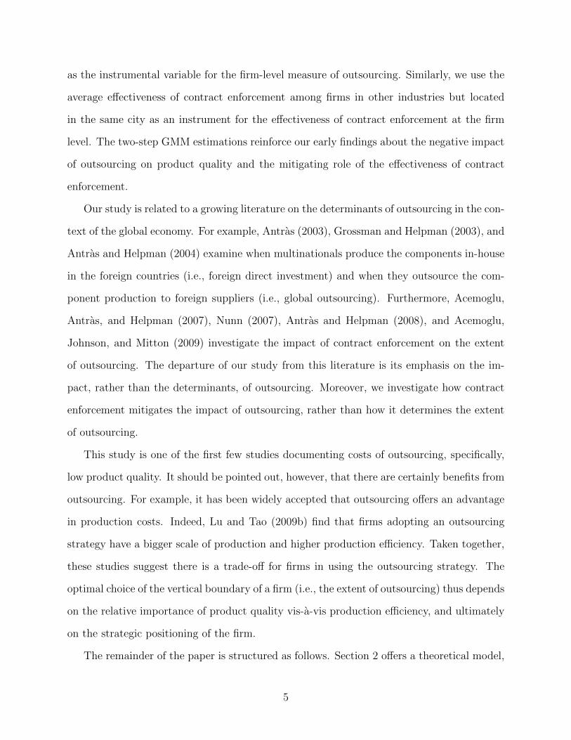
called Contract Enforcement, with values varying from 0% to 100%. As shown in Panel A of

Table 2, there are substantial variations in the effectiveness of contract enforcement across

cities. This is further confirmed by the regression results reported in Panel B of Table 2.

Such city-level variations could be attributed to the fact that much of the de facto effec-

tiveness of contract enforcement in China hinges upon the interpretation and enforcement

of laws and national ordinances by the local governments, despite the fact that China is a

unitary state with uniform laws and national ordinances.

In the empirical analysis, we also control for other factors that may affect product qual-

ity. Variables related to firm characteristics include: Firm Size (measured by the logarithm

of total employment), Firm Age (measured by the logarithm of years of establishment),

Private Ownership Percentage (measured by the share of equity owned by parties other

than government agencies), R&D Intensity (measured by the ratio of R&D expenditures to

sales), Capital Labor Ratio (measured by the logarithm of total assets over employment), and

Skilled Labor Ratio (measured by the ratio of skilled labor in the total employment). Vari-

ables concerning CEO characteristics are:15 his/her human capital – CEO Education (years

of schooling), CEO Tenure (years of being CEO) and Deputy CEO Previously (a dummy

variable indicating whether the CEO was the firm’s deputy CEO before he became CEO),

and his/her political capital – Government Cadre Previously (a dummy variable indicating

whether the CEO was a government official before he became CEO), and Party Member (a

dummy variable indicating whether the CEO is a member of the Chinese Communist Party).

Finally, we include industry dummies and city dummies to account for the industry fixed

effects and city fixed effects.

14Cull and Xu (2005) also use the same measure of the effectiveness of contract enforcement. The authorsshow that this measure is comparable to other measures of contract enforcement used in the literature.

15To the extent that more capable CEOs are also those who are more capable of delivering rigorousquality control, we need to control for variables related to CEO’s human capital. Meanwhile, CEOs withmore political capital are able to navigate through the imperfect legal systems in China and secure bettercontract enforcement, hence the control for CEO’s political capital.

16

3.2 The Impact of Outsourcing on Product Quality

To investigate the impact of outsourcing on product quality, we estimate the following equa-

tion:

Guaranteefic = α + β ·Outsourcingfic + εfic (9)

where Guaranteefic is an indirect measure of product quality for firm f in industry i and city

c; Outsourcingfic is the extent of outsourcing; and εfic is the error term. Standard errors are

clustered at the industry-city level to deal with the possible heteroskadasticity problem.16

The OLS estimation results are presented in Column 1 of Table 3. We find that Out-

sourcing has a negative and statistically significant impact on Guarantee, measured by the

percentage of products or services for which a firm offers quality guarantees, which suggests

a decrease in product quality. To gauge the economic significance of this result, we calcu-

late that a one standard deviation increase in the extent of outsourcing is associated with a

decrease of 0.386 x 0.098 = 0.038 in the percentage of products or services for which a firm

offers quality guarantees or 9.8% relative to the mean of Guarantee.

One may, however, concern that the estimate could be biased owing to the omission of

relevant variables. To the extent that we can find a comprehensive list of controls, Xfic, such

that the residual error term, ηfic ≡ εfic −X ′

ficγ, is not correlated with Outsourcingfic, then

we can isolate the causal impact of Outsourcing on Guarantee (Goldberger, 1972; Barnow

et al., 1980). Accordingly, the new estimation specification becomes:

Guaranteefic = α + β ·Outsourcingfic +X′

ficγ + ηfic. (10)

Specifically, we include industry dummies, firm characteristics (i.e., Firm Size, Firm Age,

Private Ownership Percentage, R&D Intensity, Capital Labor Ratio, Skilled Labor Ratio,

16The standard errors for micro-level data need to be adjusted for the possibility that error terms couldbe correlated within a cluster (Liang and Zeger, 1986). However, when the number of clusters is small(specifically, fewer than 42), the clustered standard errors could be misleading (e.g., Wooldridge, 2003, 2006;Angrist and Pischke, 2009). As our study includes just 18 cities and 14 industries, we can not use thestandard errors clustered at the city level or industry level. Instead, we use the standard errors clustered atthe industry-city level.

17

and Contract Enforcement), CEO characteristics (i.e., his/her human capital and political

capital), and city dummies in a stepwise fashion. As shown in Columns 2-5 of Table 3,

Outsourcing still cast a negative and statistically significant impact on Guarantee in all these

specifications. In terms of economic significance, the negative impact drops substantially

when industry dummies are included, implying that there are significant differences across

industries.

Despite the long list of control variables included in the regression analysis, one may still

argue that the OLS estimation results are biased due to the endogeneity problem associated

with the extent of outsourcing, i.e., omitted variables and reverse causality. To address this

potential endogeneity issue, we use the two-step GMM estimation. Specifically, following

the recent literature on empirical industrial organization (e.g., Berry, Levinsohn, and Pakes,

1995; Nevo, 2000, 2001), we use the average extent of outsourcing among firms in the same

industry but located in other cities as the instrumental variable for the firm-level measure

of outsourcing.17

Note that with the inclusion of industry and city dummies, the only possible remaining

omitted variables are at the industry-city level or individual firm-level. Thus, the average

extent of outsourcing among firms in the same industry but located in other cities should not

be correlated with the industry-city level or individual firm-level characteristics, implying

the satisfaction of the exclusion restriction condition for the two-step GMM estimation.

Meanwhile, the average extent of outsourcing among firms in the same industry but

located in other cities should be negatively correlated with the firm-level measure of out-

sourcing. This is because, with the industry dummies controlling for the absolute extent of

outsourcing across different industries, these two variables represent deviations away from the

17For example, in estimating the price elasticity for a brand, Nevo (2000, 2001) uses the average price inother cities as an instrument for the price in the concerned city. The rationale proposed is that with theinclusion of city dummies, the only possible omitted variables are at the within-city level. Thus, the averageprice in other cities is not expected to be correlated with those within-city characteristics. Moreover, theaverage price in other cities reflects the same underlying features of firms, for example, their productiontechnologies and costs, and is thus expected to be positively correlated with the price in the concerned city.

18

industry averages (proxied by the industry dummies) and should be negatively correlated.18

Thus, the relevance condition for the two-step GMM estimation is satisfied.

The two-step GMM estimation results are presented in Table 4. We include all control

variables used earlier – firm characteristics, CEO characteristics, industry dummies, and city

dummies. Regarding the relevance condition for a valid instrument, the correlation between

the instrument and the extent of outsourcing is negative and highly significant, consistent

with the intuition presented above. Meanwhile, the Anderson canonical correlations LR

statistic and the Cragg-Donald Chi-statistic provide further support for the satisfaction of

the relevance condition, and the large Shea partial R-squared and the F-test of excluded

instruments rule out the concern of weak instrument.19

With respect to the central issue, the coefficient of outsourcing, instrumented by the

average extent of outsourcing among firms in the same industry but located in other cities,

is negative and statistically significant. The coefficient is almost six times larger than the

corresponding OLS estimate (Column 5 of Table 3).20 Correspondingly, the estimated impact

of a one standard deviation decrease in Outsourcing on Guarantee is 14.2% relative to the

mean of Guarantee.

We then perform two sensitivity checks. First, for firms with many lines of businesses, the

extent of outsourcing could vary from one business to another. Thus, our outsourcing mea-

sure may have reflected the average extent of outsourcing across various lines of businesses,

which may bias our estimates of the impact of outsourcing on quality guarantee. To address

this concern, we focus on the sub-sample of firms with a focused business (defined as firms

18Intuitively, the extent of outsourcing is determined by the external environment, say, the number ofexternal suppliers. As the industry dummies control for the total number of external suppliers across differentindustries, the inter-city difference within an industry reflects the allocation of external suppliers acrossdifferent cities. Thus, given the total number of external suppliers, it seems reasonable that more externalsuppliers clustered in other cities imply fewer external suppliers located in the concerned city. In otherwords, the instrumental variable is expected to be negatively correlated with the endogenous explanatoryvariable.

19The F-test value for our regressions is significantly above the value of 10, which is considered as thecritical value by Staiger and Stock (1997).

20Apparently, any bias due to endogeneity serves to bias the coefficient of outsourcing downward ratherthan upward. Another possibility is that there are measurement errors which drive the OLS estimatesdownward to zero.

19

whose main business contributes more than 50% of their total sales). Our results shown in

Columns 1-2 of Table 5 suggest that our main findings remain robust to this sub-sample.

Second, China’s state-owned enterprises are legacies of the central planning system.

These enterprises tend to be more vertically integrated because of the government pres-

sure for hiring surplus workers and fulfilling social responsibilities. Meanwhile, state-owned

enterprises are generally required to provide quality products or services as part of their social

responsibilities. To rule out the possibility that our results are driven by these state-owned

enterprises, we take out these enterprises and only focus on the sub-sample of private firms.

As shown in Columns 3-4 of Table 5, our main findings remain robust to this sub-sample.

3.3 The Role of Contract Enforcement

To investigate the role of the effectiveness of contract enforcement, we estimate the following

equation:

Guaranteefic = α + β ·Outsourcingfic + λ · Contract Enforcementfic (11)

+θ ·Outsourcingfic · Contract Enforcementfic +X ′ficγ + ηfic.

Column 1 of Table 6 reports the OLS results. Consistent with our early findings, outsourc-

ing has a negative and statistically significant coefficient.21 More importantly, it is found

that the estimated coefficient for the interaction term between outsourcing and contract en-

forcement is positive and statistically significant. These results imply that more outsourcing

is associated with poorer product quality as in the last section, but it is less so when contract

enforcement is more effective. In other words, outsourcing compromises product quality, but

this negative impact is mitigated by the effectiveness of contract enforcement.

To address the concern of the endogeneity problems associated with both the extent

21Note that the coefficient of contract enforcement is negative. However, the net impact of ContractEnforcement on Guarantee remains positive because the coefficient for the interaction term is dominant.This is consistent with the results in Table 3, where contract enforcement has a positive and statisticallysignificant coefficient.

20

of outsourcing and the effectiveness of contract enforcement, we use the two-step GMM

estimation. As in Section 3.2, we use the average extent of outsourcing among firms in the

same industry but located in other cities as an instrument for the measure of outsourcing

at the firm level. Following the same logic, we use the average effectiveness of contract

enforcement among firms in other industries but located in the same city as an instrument

for the measure of contract enforcement at the firm level.22 The interaction term between

outsourcing and contract enforcement is instrumented by the interaction term of the above

two instruments.

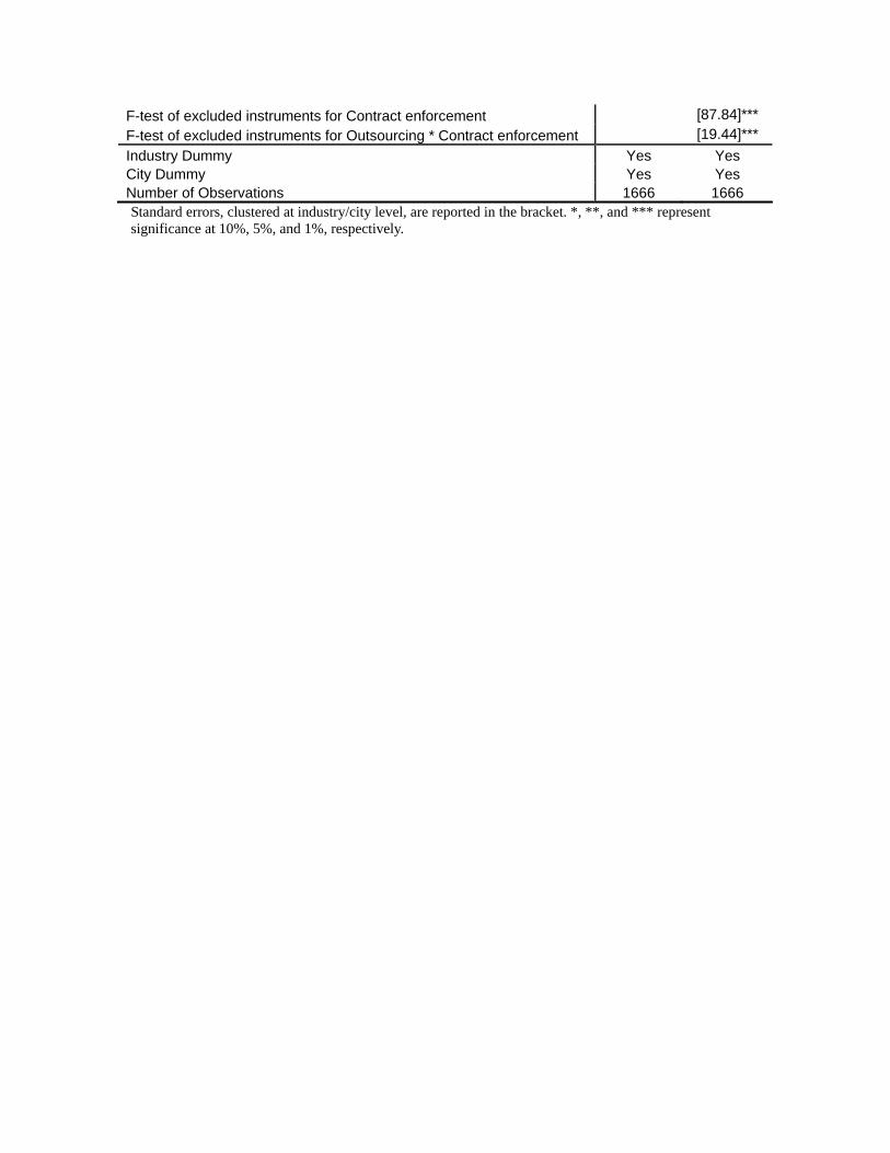
Column 2 of Table 6 reports the second-stage results of the two-step GMM estimation.23

Similar to the OLS results, the interaction term between Outsourcing and Contract En-

forcement continues to exert a positive impact on Guarantee. The various tests for the

instrumental variables suggest that our two-step GMM estimation is valid.

Taken together, the results from Tables 3-6 suggest that outsourcing does compromise

product quality, but such a negative impact can be mitigated by the effectiveness of contract

enforcement.

4 Conclusion

While outsourcing along with the trend of globalization has led to considerable benefits

such as cost reduction, increasing attention has been drawn toward product quality issues

that are often associated with outsourcing. Meanwhile, product quality under outsourcing

22The rationale for using this instrument is as follows. With the city dummies controlling for the averageeffectiveness of contract enforcement across different cities, the instrumental variable and the endogenousexplanatory variable represent deviations away from the city averages (proxied by the city dummies) andshould be negatively correlated. Intuitively, the effectiveness of contract enforcement reflects the behaviorsof government officials and judges, for example, the more time or efforts put by government officials andjudges in one industry results in better contract enforcement for this industry. As the city dummies controlfor the total amount of time or efforts put on contract enforcement across different cities, the inter-industrydifference within a city reflects the allocation of time or efforts by government officials and judges acrossdifferent industries. Thus, given the total amount of time or efforts, it is expected that the more time orefforts government officials and judges put in other industries implies less time or efforts in the concerned in-dustry. In other words, the instrumental variable is expected to be negatively correlated with the endogenousexplanatory variable.

23The three first-stage results are not reported to save space and are available upon request.

21

depends critically on the enforcement of contracts between suppliers and buyers. This leads

to questions of whether product quality is better under vertical integration than that under

outsourcing, and whether effective contract enforcement enhances product quality under

outsourcing. Despite the importance of these issues, there have been few systematic studies

on the impacts of outsourcing on product quality and the role of contract enforcement.

We first offer a simple model of outsourcing and product quality where there is imperfect

contract enforcement, namely, the court may make wrong rulings when there is a dispute

on the component quality. Under these circumstances, the independent supplier under out-

sourcing has lower incentive to take precautions to ensure the component quality. However,

the gap in component quality between outsourcing and vertical integration narrows as con-

tract enforcement becomes more effective; intuitively, the product quality gap completely

disappears when contract enforcement is perfect.

Using data from a survey of firms in China conducted by the World Bank, we find that

outsourcing decreases the percentage of products or services for which a firm offers qual-

ity guarantees, and that poor contract enforcement would further exacerbate this problem.

Given a positive correlation between product quality and quality guarantees, our results im-

ply that outsourcing compromises product quality, but the negative impact of outsourcing

on product quality is mitigated by the effectiveness of contract enforcement. These empirical

findings are robust to the control for the endogeneity issues associated with the extent of

outsourcing and the effectiveness of contract enforcement.

Our study suggests that there are costs (e.g., poor product quality) as well as benefits

(e.g., low costs of production) of outsourcing. For firms that differentiates themselves by

means of product quality, quality control is of paramount importance. They should seriously

consider the cost of outsourcing. If outsourcing is the strategy to take, a careful examination

of the effectiveness of contract enforcement is called for.

22

References

[1] Acemoglu, Daron, and Simon Johnson. 2005. “Unbundling Institutions.” Journal of

Political Economy, 113(5): 949-995.

[2] Acemoglu, Daron, Pol Antras, Elhanan Helpman. 2007. “Contracts and Technology

Adoption.” American Economic Review, 97(3): 916-943.

[3] Acemoglu, Daron, Simon Johnson, and James A. Robinson. 2002. “Reversal of Fortune:

Geography and Institutions in the Making of the Modern World Income Distribution.”

Quarterly Journal of Economics, 117(4): 1231-1294.

[4] Acemoglu, Daron, Simon Johnson, and Todd Mitton. 2009. “Determinants of Vertical

Integration: Financial Development and Contracting Costs.” Journal of Finance, 64(3):

1251-1290.

[5] Angrist, Joshua, and Jorn-Steffen Pischke. 2009. Mostly Harmless Econometrics. Prince-

ton, NJ: Princeton University Press.

[6] Antras, Pol. 2003. “Firms, Contracts, And Trade Structure.” Quarterly Journal of Eco-

nomics, 118(4): 1375-1418.

[7] Antras, Pol, and Elhanan Helpman. 2004. “Global Sourcing.” Journal of Political Econ-

omy, 112(3): 552-580.

[8] Antras, Pol, and Elhanan Helpman. 2008. “Contractual Frictions and Global Sourcing.”

In The Organization of Firms in a Global Economy, ed. E. Helpman, D. Marin, and T.

Verdier, 9-54. Cambridge, MA: Harvard University Press.

[9] Barnow, Burt S., Glen G. Cain, and Arthur S. Goldberger. 1980. “Issues in the analysis

of selectivity bias.” In Evaluation Studies Review Annual, ed. E. Stromsdorfer and G.

Farkas, Vol 5, 43-59. Beverly Hills: Sage Publications.

23

[10] Berry, Steven, James Levinsohn, and Ariel Pakes. 1995. “Automobile Prices in Market

Equilibrium.” Econometrica, 63(4): 841-90.

[11] Corbin, Arthur Linton. 1960. Corbin on Contracts: A Comprehensive Treatise on Work-

ing Rules of Contract Law, Vol. 3A. St Paul: West Publishing.

[12] Cull, Robert, and Lixin Colin Xu. 2005. “Institutions, Ownership, and Finance: the

Determinant of Profit Reinvestment among Chinese Firms.” Journal of Financial Eco-

nomics, 77(1): 117-146.

[13] Du, Julan, Yi Lu, and Zhigang Tao. 2008. “Economic Institutions and FDI Location

Choice: Evidence from US Manufacturing Firms in China.” Journal of Comparative

Economics, 36(3): 412-429.

[14] Dong Xiao-yuan, and Lixin Colin Xu. 2009. “Labor Restructuring in China: Toward a

Functioning Labor Market.” Journal of Comparative Economics, 37(2): 287-305.

[15] Economides, Nicholas. 1999. “Quality Choice and Vertical Integration.” International

Journal of Industrial Organization, 17(6): 903-914.

[16] Feenstra, Robert C. 1998. “Integration of Trade and Disintegration of Production in

the Global Economy.” Journal of Economic Perspectives, 12(4): 31-50.

[17] Gibbons, Robert. 1992. Game Theory for Applied Economists. Princeton, NJ: Princeton

University Press.

[18] Goldberger, Arthur S. 1972. “Structural Equation Methods in the Social Sciences.”

Econometrica, 40(6): 979-1001.

[19] Grossman, Gene M., and Elhanan Helpman. 2003. “Outsourcing Versus FDI in Industry

Equilibrium.” Journal of the European Economic Association, 1(2-3): 317-327.

24

[20] Hart, Oliver, Andrei Shleifer, and Robert W. Vishny. 1997. “The Proper Scope of Gov-

ernment: Theory and an Application to Prisons.” Quarterly Journal of Economics,

112(4): 1127-1161.

[21] Hortacsu, Ali, and Chad Syverson. 2007. “Cementing Relationships: Vertical Integra-

tion, Foreclosure, Productivity, and Prices.” Journal of Political Economy, 115(2): 250-

301.

[22] Hummels, David, Jun Ishii, and Kei-Mu Yi. 2001. “The Nature and Growth of Vertical

Specialization in World Trade.” Journal of International Economics, 54(1): 75-96.

[23] Johnson, Simon, John McMillan, and Christopher Woodruff. 2002. “Property Rights

and Finance.” American Economic Review, 92(5): 1335-1356.

[24] Liang, Kung-Yee, and Scott L. Zeger. 1986. “Longitudinal Data Analysis Using Gener-

alized Linear Models.” Biometrika, 73(1): 13-22.

[25] Lu, Yi, and Zhigang Tao. 2009a. “Contract Enforcement and Family Control of Business:

Evidence from China.” Journal of Comparative Economics, 37(4): 597-609.

[26] Lu, Yi, and Zhigang Tao. 2009b. “Vertical Integration and Firm Performance.” Working

paper.

[27] Nevo, Aviv. 2000. “A Practitioner’s Guide to Estimation of Random-Coefficients Logit

Models of Demand.” Journal of Economics and Management Strategy, 9(4): 513-548.

[28] Nevo, Aviv. 2001. “Measuring Market Power in the Ready-to-Eat Cereal Industry.”

Econometrica, 69(2): 307-42.

[29] North, Douglass C. 1991. “Institutions.” Journal of Economic Perspectives, 5(1): 97-

112.

[30] Nunn, Nathan. 2007. “Relationship-Specificity, Incomplete Contracts, and the Pattern

of Trade.” Quarterly Journal of Economics, 122(2): 569-600.

25

[31] Staiger, Douglas and James Stock. 1997. “Instrumental Variables Regression with Weak

Instruments.” Econometrica, 65(3): 557-586.

[32] Wooldridge, Jeffrey M. 2003. “Cluster-Sample Methods in Applied Econometrics.”

American Economic Review, 93(2): 133-138.

[33] Wooldridge, Jeffrey M. 2006. “Cluster Sample Methods in Applied Econometrics: An

Extended Analysis.” Working paper.

[34] World Bank. 2008. Doing Business in China 2008. Beijing, China: Social Science Aca-

demic Press.

26

v − p− qhh

p

Buy

N

S

S

S

S

S

S

B

B

B

B

BuyBuy

Buy

Not buy

Not buyNot buy

Not buy

Offer

Offer

Not Offer

Not Offer

High quality (λ′)

Low quality (1 − λ′) v − p− qlh

p

00

00

p− qhεh

v − p[φ]

[1− φ]

[δ]

[1− δ]

p

pp

p

v − p

p− qlεh

00

00

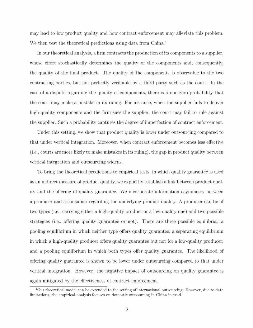
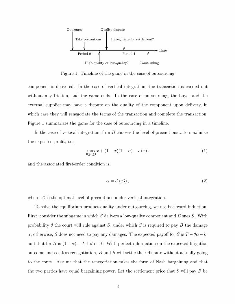
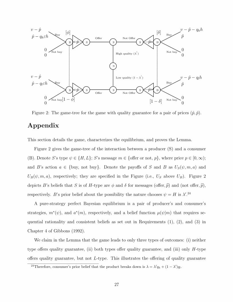
Figure 2: The game-tree for the game with quality guarantee for a pair of prices (p, p).

Appendix

This section details the game, characterizes the equilibrium, and proves the Lemma.

Figure 2 gives the game-tree of the interaction between a producer (S) and a consumer

(B). Denote S’s type ψ ∈ {H,L}; S’s message m ∈ {offer or not, p}, where price p ∈ [0,∞);

and B’s action a ∈ {buy, not buy}. Denote the payoffs of S and B as US(ψ,m, a) and

UB(ψ,m, a), respectively; they are specified in the Figure (i.e., US above UB). Figure 2

depicts B’s beliefs that S is of H-type are φ and δ for messages (offer, p) and (not offer, p),

respectively. B’s prior belief about the possibility the nature chooses ψ = H is λ′.24

A pure-strategy perfect Bayesian equilibrium is a pair of producer’s and consumer’s

strategies, m∗(ψ), and a∗(m), respectively, and a belief function µ(ψ|m) that requires se-

quential rationality and consistent beliefs as set out in Requirements (1), (2), and (3) in

Chapter 4 of Gibbons (1992).

We claim in the Lemma that the game leads to only three types of outcomes: (i) neither

type offers quality guarantee, (ii) both types offer quality guarantee, and (iii) only H-type

offers quality guarantee, but not L-type. This illustrates the offering of quality guarantee

24Therefore, consumer’s prior belief that the product breaks down is λ = λ′qh + (1− λ′)ql.

27

as a good proxy for the underlying quality of the firm. The rest of the section proves this

claim.

Proof of the Lemma. We prove this Lemma through establishing three claims.

Claim 1: Other types of separating equilibria other than the one that involves an H-type

producer offering quality guarantee and an L-type not offering do not exist.

Proof. The type of separating equilibria that involves L-type offering quality guarantee and

an H-type not offering (i.e., m∗(L) = (offer, pL) and m∗(H) = (not offer, pH) for some

pL < pH) cannot be equilibrium because if it were optimal for the L-type to offer quality

guarantee, it would not have been optimal for the H-type not to mimic the L-type by offering

quality guarantee too. With a lower probability of breakdown, H-type’s expected cost of

offering quality guarantee is lower than that of L-type. The benefit is that H-type would

have charged the same price as what L-type is charging. Such a profitable deviation renders

this type of separating equilibria impossible.

Another type of separating equilibria involves both types having the same quality guar-

antee policy (i.e., both offering, or both not offering) but charging different prices (i.e.,

m∗(L) = (offer, pL) and m∗(H) = (offer, pH) for some pL 6= pH , or m∗(L) = (not offer, pL)

and m∗(H) = (not offer, pH) for some pL 6= pH). Given any consistent belief of the consumer,

it would have been always profitable for the type that charges a lower price to deviate by

charging a price equal to the price the other type charges.

Claim 2: When the repairment cost is in the intermediate range, there exists a separating

equilibrium that involves an H-type producer offering quality guarantee and an L-type not

offering.

Proof. The strategy profile is: (i) m∗(H) = (offer, v) and m∗(L) = (not offer, v − qlh). (ii)

a∗(offer, p) =

buy if p ≤ v

not buy if p > vand a∗(not offer, p)

28

=

buy if p ≤ v − qlh

not buy if p > v − qlh. (iii) on-the-equilibrium-path beliefs: µ(H|offer, v) = 1 and

µ(H|not offer, v − qlh) = 0, (iv) off-the-equilibrium-path beliefs: µ(H|not offer, p) = 0 for

any p > v − qlh. There is no restriction on any other off-the-equilibrium-path beliefs.

B’s on-the-equilibrium-path belief is consistent with m∗(ψ). Given the belief µ(ψ|m),

both a∗(offer, p) and a∗(not offer, p) are obviously sequentially rational. We now give con-

ditions whereby both m∗(H) = (offer, v) and m∗(L) = (not offer, v − qlh) are sequentially

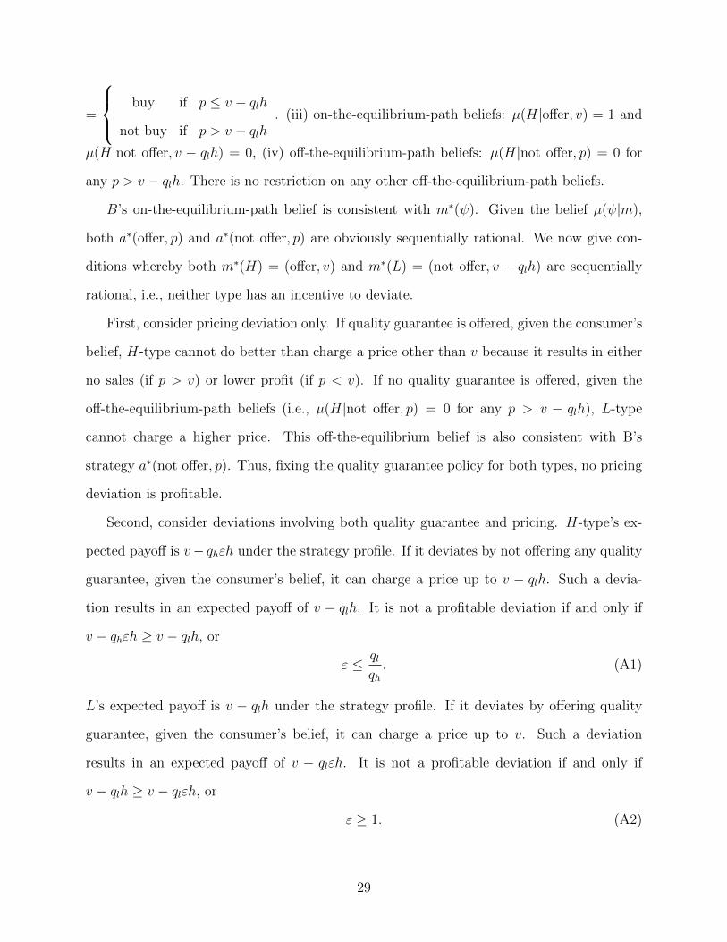
rational, i.e., neither type has an incentive to deviate.

First, consider pricing deviation only. If quality guarantee is offered, given the consumer’s

belief, H-type cannot do better than charge a price other than v because it results in either

no sales (if p > v) or lower profit (if p < v). If no quality guarantee is offered, given the

off-the-equilibrium-path beliefs (i.e., µ(H|not offer, p) = 0 for any p > v − qlh), L-type

cannot charge a higher price. This off-the-equilibrium belief is also consistent with B’s

strategy a∗(not offer, p). Thus, fixing the quality guarantee policy for both types, no pricing

deviation is profitable.

Second, consider deviations involving both quality guarantee and pricing. H-type’s ex-

pected payoff is v− qhεh under the strategy profile. If it deviates by not offering any quality

guarantee, given the consumer’s belief, it can charge a price up to v − qlh. Such a devia-

tion results in an expected payoff of v − qlh. It is not a profitable deviation if and only if

v − qhεh ≥ v − qlh, or

ε ≤ qlqh. (A1)

L’s expected payoff is v − qlh under the strategy profile. If it deviates by offering quality

guarantee, given the consumer’s belief, it can charge a price up to v. Such a deviation

results in an expected payoff of v − qlεh. It is not a profitable deviation if and only if

v − qlh ≥ v − qlεh, or

ε ≥ 1. (A2)

29

Thus, this strategy profile is a pure-strategy perfect Bayesian equilibrium if

1 ≤ ε ≤ qlqh. (A3)

Thus, this separating equilibrium exists when the repairment cost is in an intermediate range.

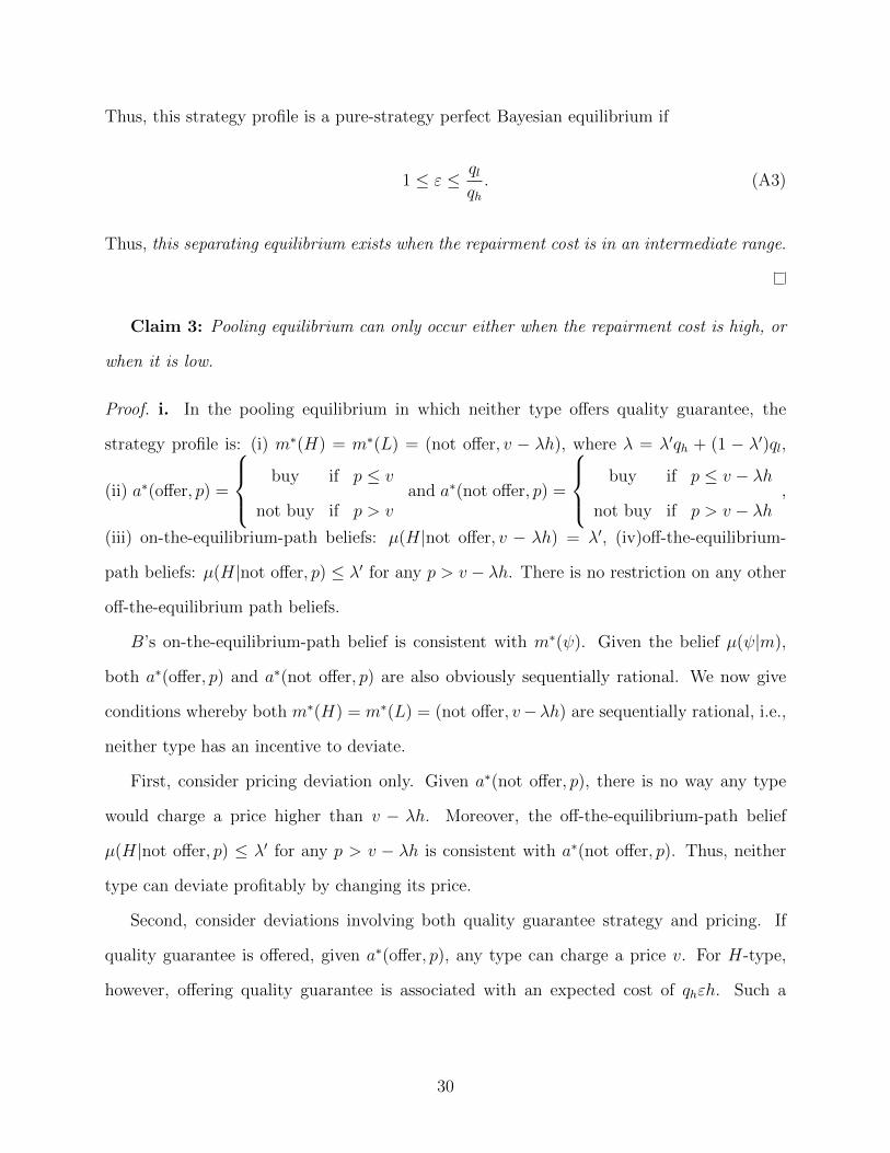
Claim 3: Pooling equilibrium can only occur either when the repairment cost is high, or

when it is low.

Proof. i. In the pooling equilibrium in which neither type offers quality guarantee, the

strategy profile is: (i) m∗(H) = m∗(L) = (not offer, v − λh), where λ = λ′qh + (1 − λ′)ql,

(ii) a∗(offer, p) =

buy if p ≤ v

not buy if p > vand a∗(not offer, p) =

buy if p ≤ v − λh

not buy if p > v − λh,

(iii) on-the-equilibrium-path beliefs: µ(H|not offer, v − λh) = λ′, (iv)off-the-equilibrium-

path beliefs: µ(H|not offer, p) ≤ λ′ for any p > v − λh. There is no restriction on any other

off-the-equilibrium path beliefs.

B’s on-the-equilibrium-path belief is consistent with m∗(ψ). Given the belief µ(ψ|m),

both a∗(offer, p) and a∗(not offer, p) are also obviously sequentially rational. We now give

conditions whereby both m∗(H) = m∗(L) = (not offer, v−λh) are sequentially rational, i.e.,

neither type has an incentive to deviate.

First, consider pricing deviation only. Given a∗(not offer, p), there is no way any type

would charge a price higher than v − λh. Moreover, the off-the-equilibrium-path belief

µ(H|not offer, p) ≤ λ′ for any p > v − λh is consistent with a∗(not offer, p). Thus, neither

type can deviate profitably by changing its price.

Second, consider deviations involving both quality guarantee strategy and pricing. If

quality guarantee is offered, given a∗(offer, p), any type can charge a price v. For H-type,

however, offering quality guarantee is associated with an expected cost of qhεh. Such a

30

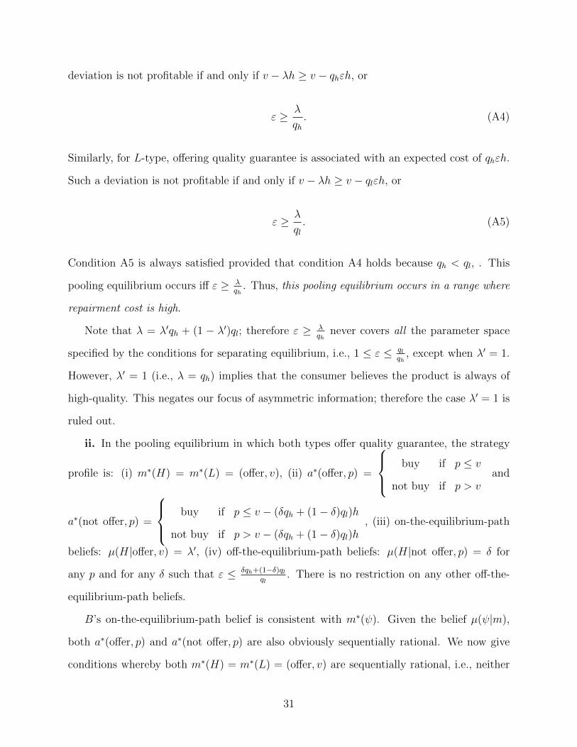
deviation is not profitable if and only if v − λh ≥ v − qhεh, or

ε ≥ λ

qh. (A4)

Similarly, for L-type, offering quality guarantee is associated with an expected cost of qhεh.

Such a deviation is not profitable if and only if v − λh ≥ v − qlεh, or

ε ≥ λ

ql. (A5)

Condition A5 is always satisfied provided that condition A4 holds because qh < ql, . This

pooling equilibrium occurs iff ε ≥ λqh

. Thus, this pooling equilibrium occurs in a range where

repairment cost is high.

Note that λ = λ′qh + (1 − λ′)ql; therefore ε ≥ λqh

never covers all the parameter space

specified by the conditions for separating equilibrium, i.e., 1 ≤ ε ≤ qlqh

, except when λ′ = 1.

However, λ′ = 1 (i.e., λ = qh) implies that the consumer believes the product is always of

high-quality. This negates our focus of asymmetric information; therefore the case λ′ = 1 is

ruled out.

ii. In the pooling equilibrium in which both types offer quality guarantee, the strategy

profile is: (i) m∗(H) = m∗(L) = (offer, v), (ii) a∗(offer, p) =

buy if p ≤ v

not buy if p > vand

a∗(not offer, p) =

buy if p ≤ v − (δqh + (1− δ)ql)h

not buy if p > v − (δqh + (1− δ)ql)h, (iii) on-the-equilibrium-path

beliefs: µ(H|offer, v) = λ′, (iv) off-the-equilibrium-path beliefs: µ(H|not offer, p) = δ for

any p and for any δ such that ε ≤ δqh+(1−δ)qlql

. There is no restriction on any other off-the-

equilibrium-path beliefs.

B’s on-the-equilibrium-path belief is consistent with m∗(ψ). Given the belief µ(ψ|m),

both a∗(offer, p) and a∗(not offer, p) are also obviously sequentially rational. We now give

conditions whereby both m∗(H) = m∗(L) = (offer, v) are sequentially rational, i.e., neither

31

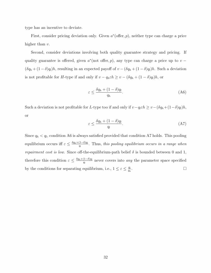
type has an incentive to deviate.

First, consider pricing deviation only. Given a∗(offer, p), neither type can charge a price

higher than v.

Second, consider deviations involving both quality guarantee strategy and pricing. If

quality guarantee is offered, given a∗(not offer, p), any type can charge a price up to v −

(δqh + (1− δ)ql)h, resulting in an expected payoff of v− (δqh + (1− δ)ql)h. Such a deviation

is not profitable for H-type if and only if v − qhεh ≥ v − (δqh + (1− δ)ql)h, or

ε ≤ δqh + (1− δ)qlqh

. (A6)

Such a deviation is not profitable for L-type too if and only if v−qlεh ≥ v−(δqh+(1−δ)ql)h,

or

ε ≤ δqh + (1− δ)qlql

. (A7)

Since qh < ql, condition A6 is always satisfied provided that condition A7 holds. This pooling

equilibrium occurs iff ε ≤ δqh+(1−δ)qlql

. Thus, this pooling equilibrium occurs in a range when

repairment cost is low. Since off-the-equilibrium-path belief δ is bounded between 0 and 1,

therefore this condition ε ≤ δqh+(1−δ)qlql

never covers into any the parameter space specified

by the conditions for separating equilibrium, i.e., 1 ≤ ε ≤ qlqh

.

32

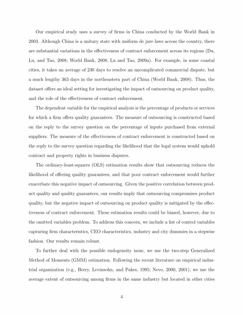
Table 1: Summary statistics

Variable Obs Mean Std. Dev. Min Max Guarantee 2274 0.893 0.274 0.000 1.000 Outsourcing 2055 0.730 0.386 0.000 1.000 Contract enforcement 2068 0.640 0.389 0.000 1.000 Outsourcing * Contract enforcement 1831 0.465 0.405 0.000 1.000 Firm size 2396 4.850 1.491 0.000 11.159 Firm age 2400 2.430 0.799 1.099 3.970 Private ownership percentage 2399 0.781 0.402 0.000 1.000 R&D intensity 2373 0.006 0.030 0.000 0.705 Capital labor ratio 2320 3.376 1.663 -3.466 11.437 Skilled labor ratio 2358 0.038 0.087 0.000 1.000 CEO education 2382 15.643 2.394 0.000 19.000 CEO tenure 2371 5.771 4.255 1.000 33.000 Deputy CEO previously 2378 0.274 0.446 0.000 1.000 Government cadre previously 2378 0.060 0.237 0.000 1.000 Party member 2351 0.668 0.471 0.000 1.000

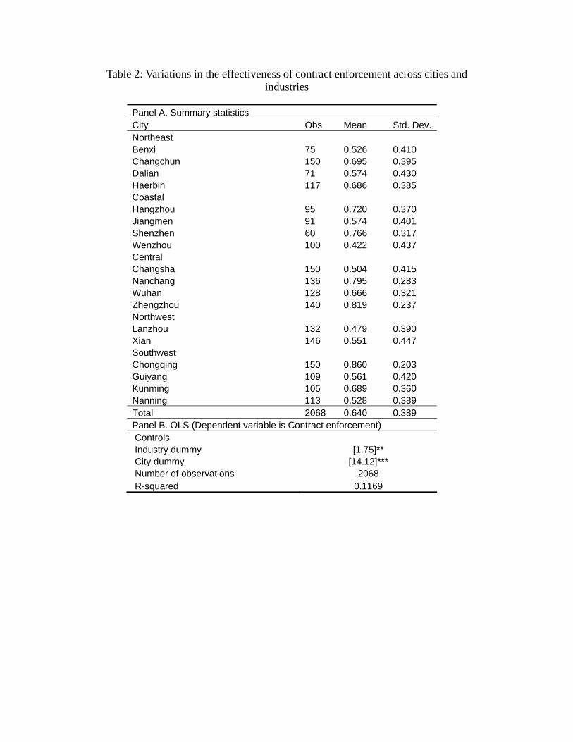
Table 2: Variations in the effectiveness of contract enforcement across cities and industries

Panel A. Summary statistics City Obs Mean Std. Dev. Northeast Benxi 75 0.526 0.410 Changchun 150 0.695 0.395 Dalian 71 0.574 0.430 Haerbin 117 0.686 0.385 Coastal Hangzhou 95 0.720 0.370 Jiangmen 91 0.574 0.401 Shenzhen 60 0.766 0.317 Wenzhou 100 0.422 0.437 Central Changsha 150 0.504 0.415 Nanchang 136 0.795 0.283 Wuhan 128 0.666 0.321 Zhengzhou 140 0.819 0.237 Northwest Lanzhou 132 0.479 0.390 Xian 146 0.551 0.447 Southwest Chongqing 150 0.860 0.203 Guiyang 109 0.561 0.420 Kunming 105 0.689 0.360 Nanning 113 0.528 0.389 Total 2068 0.640 0.389 Panel B. OLS (Dependent variable is Contract enforcement) Controls Industry dummy [1.75]** City dummy [14.12]*** Number of observations 2068 R-squared 0.1169

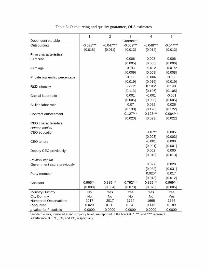
Table 3: Outsourcing and quality guarantee, OLS estimates

Standard errors, clustered at industry/city level, are reported in the bracket. *, **, and *** represent significance at 10%, 5%, and 1%, respectively.

1 2 3 4 5 Dependent variable Guarantee Outsourcing -0.098*** -0.047*** -0.052*** -0.048*** -0.044*** [0.018] [0.011] [0.013] [0.014] [0.013] Firm characteristics Firm size 0.006 0.003 0.006 [0.005] [0.005] [0.006] Firm age -0.014 -0.012 -0.015* [0.009] [0.009] [0.008] Private ownership percentage -0.008 -0.006 -0.008 [0.019] [0.019] [0.019] R&D intensity 0.221* 0.196* 0.140 [0.113] [0.106] [0.105] Capital labor ratio 0.001 -0.001 -0.001 [0.005] [0.005] [0.005] Skilled labor ratio 0.07 0.059 0.026 [0.130] [0.126] [0.122] Contract enforcement 0.127*** 0.123*** 0.084*** [0.023] [0.023] [0.022] CEO characteristics Human capital CEO education 0.007** 0.005 [0.003] [0.003] CEO tenure -0.001 0.000 [0.001] [0.001] Deputy CEO previously 0.002 0.000 [0.013] [0.013] Political capital Government cadre previously 0.027 0.028 [0.032] [0.031] Party member 0.025* 0.017 [0.013] [0.012] Constant 0.965*** 0.885*** 0.792*** 0.825*** 0.969*** [0.008] [0.054] [0.073] [0.075] [0.085] Industry Dummy No Yes Yes Yes Yes City Dummy No No No No Yes Number of Observations 2017 2017 1724 1666 1666 R-squared 0.020 0.111 0.141 0.145 0.189 p-value for F-statistic 0.0000 0.0000 0.0000 0.0000 0.0000

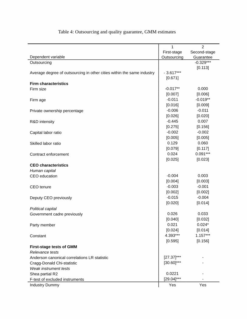
Table 4: Outsourcing and quality guarantee, GMM estimates

1 2 First-stage Second-stage Dependent variable Outsourcing Guarantee Outsourcing -0.329*** [0.113] Average degree of outsourcing in other cities within the same industry - 3.617*** [0.671] Firm characteristics Firm size -0.017** 0.000 [0.007] [0.006] Firm age -0.011 -0.019** [0.016] [0.009] Private ownership percentage -0.006 -0.011 [0.026] [0.020] R&D intensity -0.445 0.007 [0.275] [0.156] Capital labor ratio -0.002 -0.002 [0.005] [0.005] Skilled labor ratio 0.129 0.060 [0.079] [0.117] Contract enforcement 0.024 0.091*** [0.025] [0.023] CEO characteristics Human capital CEO education -0.004 0.003 [0.004] [0.003] CEO tenure -0.003 -0.001 [0.002] [0.002] Deputy CEO previously -0.015 -0.004 [0.020] [0.014] Political capital Government cadre previously 0.026 0.033 [0.040] [0.032] Party member 0.021 0.024* [0.024] [0.014] Constant 4.393*** 1.157*** [0.595] [0.156] First-stage tests of GMM Relevance tests Anderson canonical correlations LR statistic [27.37]*** - Cragg-Donald Chi-statistic [30.60]*** - Weak instrument tests Shea partial R2 0.0221 - F-test of excluded instruments [29.04]*** - Industry Dummy Yes Yes

Standard errors, clustered at industry/city level, are reported in the bracket. *, **, and *** represent significance at 10%, 5%, and 1%, respectively.

City Dummy Yes Yes Number of Observations 1666 1666

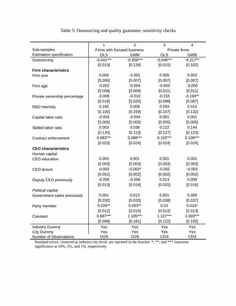
Table 5: Outsourcing and quality guarantee, sensitivity checks

Standard errors, clustered at industry/city level, are reported in the bracket. *, **, and *** represent significance at 10%, 5%, and 1%, respectively.

1 2 3 4 Sub-samples Firms with focused business Private firms Estimation specification OLS GMM OLS GMM Outsourcing -0.041*** -0.358*** -0.048*** -0.217** [0.013] [0.126] [0.015] [0.102] Firm characteristics Firm size 0.006 -0.001 0.005 0.002 [0.006] [0.007] [0.007] [0.007] Firm age -0.002 -0.004 -0.009 -0.009 [0.008] [0.009] [0.011] [0.011] Private ownership percentage -0.008 -0.010 -0.155 -0.194** [0.019] [0.020] [0.098] [0.087] R&D intensity 0.165 0.008 0.093 0.014 [0.100] [0.159] [0.107] [0.132] Capital labor ratio -0.003 -0.004 0.001 0.001 [0.005] [0.005] [0.005] [0.005] Skilled labor ratio 0.003 0.038 0.122 0.144 [0.120] [0.113] [0.127] [0.123] Contract enforcement 0.083*** 0.088*** 0.102*** 0.108*** [0.023] [0.024] [0.024] [0.024] CEO characteristics Human capital CEO education 0.003 0.001 0.001 0.001 [0.003] [0.003] [0.003] [0.003] CEO tenure -0.002 -0.003* -0.002 -0.003 [0.001] [0.002] [0.002] [0.002] Deputy CEO previously -0.005 -0.006 0.013 0.009 [0.013] [0.014] [0.015] [0.016] Political capital Government cadre previously 0.001 0.013 0.001 0.000 [0.030] [0.033] [0.038] [0.037] Party member 0.026** 0.033** 0.02 0.024* [0.012] [0.015] [0.012] [0.013] Constant 0.697*** 1.185*** 1.107*** 1.003*** [0.099] [0.161] [0.122] [0.192] Industry Dummy Yes Yes Yes Yes City Dummy Yes Yes Yes Yes Number of Observations 1526 1526 1316 1316

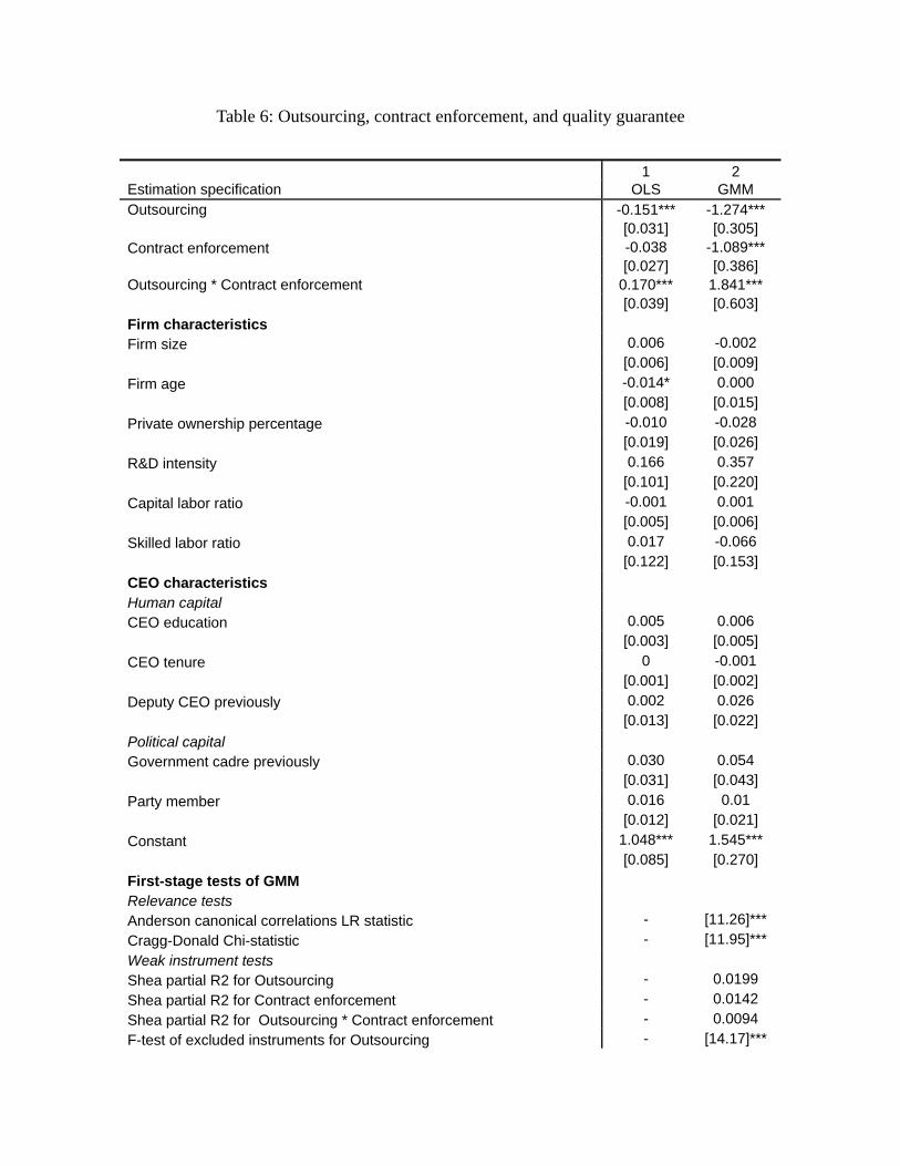
Table 6: Outsourcing, contract enforcement, and quality guarantee

1 2 Estimation specification OLS GMM Outsourcing -0.151*** -1.274*** [0.031] [0.305] Contract enforcement -0.038 -1.089*** [0.027] [0.386] Outsourcing * Contract enforcement 0.170*** 1.841*** [0.039] [0.603] Firm characteristics Firm size 0.006 -0.002 [0.006] [0.009] Firm age -0.014* 0.000 [0.008] [0.015] Private ownership percentage -0.010 -0.028 [0.019] [0.026] R&D intensity 0.166 0.357 [0.101] [0.220] Capital labor ratio -0.001 0.001 [0.005] [0.006] Skilled labor ratio 0.017 -0.066 [0.122] [0.153] CEO characteristics Human capital CEO education 0.005 0.006 [0.003] [0.005] CEO tenure 0 -0.001 [0.001] [0.002] Deputy CEO previously 0.002 0.026 [0.013] [0.022] Political capital Government cadre previously 0.030 0.054 [0.031] [0.043] Party member 0.016 0.01 [0.012] [0.021] Constant 1.048*** 1.545*** [0.085] [0.270] First-stage tests of GMM Relevance tests Anderson canonical correlations LR statistic - [11.26]*** Cragg-Donald Chi-statistic - [11.95]*** Weak instrument tests Shea partial R2 for Outsourcing - 0.0199 Shea partial R2 for Contract enforcement - 0.0142 Shea partial R2 for Outsourcing * Contract enforcement - 0.0094 F-test of excluded instruments for Outsourcing - [14.17]***

Standard errors, clustered at industry/city level, are reported in the bracket. *, **, and *** represent significance at 10%, 5%, and 1%, respectively.

F-test of excluded instruments for Contract enforcement [87.84]*** F-test of excluded instruments for Outsourcing * Contract enforcement [19.44]*** Industry Dummy Yes Yes City Dummy Yes Yes Number of Observations 1666 1666