Ov erc o mmunic a tio n a nd B o unded R a tio na lity in Stra te g ic

Info rma tio n T ra nsmissio n G a mes: A n Ex p e rimenta l Inv e stig a tio n∗

Ho ngbin Ca i†

D epa rtment o f E co no mics, UCL A

Jo seph T a o -Y i W a ng

D epa rtment o f E co no mics, UCL A

O cto ber 2 0 0 3

Abstract

Since Crawford and Sob el (1982), th e th eory of strategic inform ation transm ission h as

fou nd a wid e range of ap p lications and h as b ecom e increasingly im p ortant in th e literatu re.

In th is p ap er we cond u ct lab oratory ex p erim ents to test th is th eory . O u r ex p erim ental resu lts

strongly su p p ort th e b asic insigh t of th e th eory , nam ely , th at less inform ation is transm itted

wh en p references of th e send er and th e receiv er d iv erge. M oreov er, th e av erage p ay off s for

th e send ers, th e receiv ers, and th e ov erall su b ject p op u lation are v ery close to th ose p red icted

b y th e m ost inform ativ e eq u ilib riu m . Howev er, th e ev id ence sh ows th at su b jects consistently

ov ercom m u nicate in th at th e send ers’ m essages are m ore inform ativ e ab ou t th e tru e states

of th e world and th at th e receiv ers rely m ore on th e send ers’ m essages in ch oosing actions,

com p ared with wh at th e th eory allows in th e m ost inform ativ e eq u ilib riu m . T h ese fi nd ings

are rob u st to certain v ariations of p ay off p aram eters and noisy signals. In ad d ition, we d o not

fi nd any clear learning eff ect in ou r d ata. T o u nd erstand th e ov ercom m u nication p h enom enon,

we u se two p op u lar ap p roach es of b ou nd ed rationality : b eh av ior ty p e analy sis and q u antal

resp onse eq u ilib riu m , to analy ze su b jects’ b eh av ior in ou r ex p erim ent d ata.

∗We are grateful to Dav id L ev ine for his encouragem ent, support and adv ice. We also thank V incent C raw ford,

T hom as P alfrey , and L eeat Y ariv for v ery helpful com m ents. A ll rem aining errors are our ow n.

†C orresponding author: Departm ent of E conom ic s, U C L A , 405 H ilgard A v e, L os A ngeles, C A 90095-1477. T el:

310-794-6495. F ax : 310-825-9528. e-m ail: cai@ econ.uc la.edu

1

1 Intro ductio n

In many real world situations decision mak ers have to rely on others for information needed to

mak e good decisions, who often have preferences different from the decision mak ers’ and hence

may act strategically in communicating their information to the decision mak ers. F ollowing the

seminal work of Crawford and Sobel (1982), the literature on strategic information transmis-

sion has grown rapidly, with a wide range of applications in economics and many related fields

such as political science (e.g., congress committee decisions), finance (e.g., stock analysts), and

organization theory (e.g., managers versus subordinates or consultants). G iven its increasing im-

portance in the literature, it is natural to ask whether and to what extent the theoretical insights

of Crawford and Sobel and the subsequent work s hold out empirically. However, aside from the

standard limitations of field data (e.g., no controlled environments, too much noise), this theory

is very diffi cult to test by field data, because its k ey variables (e.g., communication, preference

differences) are inherently unobservable. E xperiments are well suited to test the theory by pro-

viding controlled environments and by allowing experimenters choose the variables unobservable

in field data (e.g., preference differences).

In this paper, we conduct laboratory experiments to test the theory of strategic information

transmission. W e are interested in whether and to what extent the main insights of the theory

are supported by experimental data. In the model of Crawford and Sobel (1982), one player

(the sender) communicates his private information about the state of the world to a decision

mak er (the receiver). They show that messages are partitions of the state space in all equilibria.

Moreover, in the most informative equilibrium, less information can be transmitted as the pref-

erence difference between the two players increases. W ith non-trivial preference differences, little

information can be communicated even in the most informative equilibrium, that is, the finest

partition in equilibrium is quite coarse.1 W e design a relatively simple game of strategic informa-

tion transmission with discrete states, messages and actions. The most informative equilibrium

of this game ranges from the completely informative equilibrium (truth-telling by the sender and

fully-trusting by the receiver), to partially informative equilibria, to the completely uninforma-

tive equilibrium (“babbling” equilibrium), as the preference difference between the sender and

the receiver increases. W e run a series of experiments with varying preference differences, and

find evidence that strongly supports the theoretical comparative statics predictions. Specifically,

the experimental results clearly show that as the preference difference increases, less information

is transmitted from the senders and utilized by the receivers, in the sense that correlations be-

tween states and messages, between messages and actions, and between states and actions all

1In the canonical example in which the state is uniformly distributed on [0, 1] and utility functions are q uadratic,

there can be at most two partitions (less than or greater than 1/4) when the preference diff erence between the two

players is only 1/8.

2

decrease in preference difference. Moreover, the average payoffs for the senders, the receivers, and

the overall subject population are very close to the equilibrium payoffs predicted by the theory.

These findings suggest that the subjects not only understand the game and behave strategically

(and hence become less “trusting” when their partner’s preference is more different from theirs),

but also seem to be playing according to the most informative equilibrium.

A closer look at the subjects’ behavior in the data, however, clearly rejects the conclusion

that the subjects as a whole play according to equilibrium. In fact, the data show that there is

a robust tendency for the subject population to communicate more than what the theory allows

in the most informative equilibrium. In the case of large preference differences, correlations

between states and messages, between messages and actions, and between states and actions are

all significantly positive, while the theory predicts that they should all be zero. R egression results

on individual subject data further confirm that messages, states and actions are all positively

correlated with each other, rejecting strongly the babbling equilibrium hypothesis. We then

examine distributions of states conditional on messages, distributions of actions conditional on

messages, and distributions of actions conditional on states. In all cases, the experimental data

clearly show that these conditional distributions (frequencies) are not consistent with theory

predictions: messages are informative about the states, and actions rely on messages and hence

are correlated with states. For example, in our game with the state space of {1, 3, 5, 7, 9}, in the

case of large preference difference in which the babbling equilibrium is the unique equilibrium

of the game, for the message of 5, the empirical distribution of states is: s = 1 (43.75% ), s = 3

(16.25% ), s = 5 (28.75% ), s = 7 (6.25% ), s = 9 (5.00% ), with an average state of 3.25. Compared

with the uniform distribution with an expected state of 5 predicted by the theory, this empirical

distribution contains a substantial amount of information about the true state of the world.

To test the robustness of these results, we run experiments with modified designs. It turns

out that the experimental results from the baseline sessions are very robust to variations of pa-

rameter values that change the subjects’ payoff sensitivity and to variations of message space the

senders are allowed to use. Furthermore, we run experiments in which the senders are only given

noisy signals about the true states of the world. The results show that the noisiness of signals

does not have noticeable effects on experimental outcomes, suggesting that the overcommuni-

cation phenomenon is not due to a simple “trusting-the-expert” mentality by the subjects. We

also investigate the possible effects of subjects learning on the experimental results. R egression

analysis on payoffs and correlations using data from a session of experiment with 31 rounds of

play find no clear time trend and no convergence to equilibrium predictions, suggesting that there

is no clear learning effect at least up to 31 rounds in the experiments.

These findings raise two questions. First, why are the average payoffs so close to the equi-

librium predictions while at the same time subjects’ individual behavior is clearly different from

equilibrium strategies? Second, what are the possible explanations for the subjects’ behavior? In

3

particular, what are the reasons behind the overcommunication phenomenon? Two approaches

of bounded rationality, behavior type analysis and quantal response equilibrium, are commonly

used in the existing literature to explain non-equilibrium phenomena in experimental data. To

understand the overcommunication phenomenon in our experiment, we apply both approaches

to analyze our data.

The behavior type analysis approach is developed by a number of scholars, e.g., Nagel (1995),

Stahl and Wilson (1995), Ho, Camerer and Weigelt (1998), and Costa-Gomes, Crawford and

B roseta (2001, 2002). They demonstrate that subjects in their experiments (in particular,

“beauty contest” games) consistently behave in a specific bounded rational way: subjects of

different levels of sophistication have the non-equilibrium belief that other subjects are one level

lower than themselves in sophistication and best response to that belief.2 To apply this approach

in communication games, Crawford (2003) cites earlier experiment evidence (e.g., B lume, De-

Jong, K im and Sprinkle, 2001) and argues that the system of subject types should be anchored on

the “truster” type of senders and the “believer” type of receivers.3 In our data, there are indeed

senders who always tell the truth (the truster type) and receivers who always believe the senders

(the believer type). So we follow Crawford (2003) to define the system of behavior types for our

game.4 We then follow the classification methodology of Costa-Gomes et al (2001, 2002) to clas-

sify subjects whose actions can be consistently identified as fitting into one of the behavior types.

About 75% of the subjects in our experiments can be classified. We calculate the expected payoffs

and correlations generated by the distribution of behavior types combined with some random

noise. The results match the actual data quite well. This suggests the following interpretation of

our experimental results. Subjects of lower levels of sophistication overcommunicate, resulting in

more communication than what the theory predicts. However, since the subjects are randomly

paired, a sender of a certain type can be matched with possibly many types of receivers in a given

round. Some of these matches are equilibrium-alike, others (“mismatches”) give rise to outcomes

quite different from equilibrium. Combined with some noise, these mismatches tend to offset the

payoff gains and losses (relative to the equilibrium predictions), leading to average payoffs close

2See Crawford (1997) and Camerer (2002) for comprehensive surveys and further references.

3In other games it is standard to specify the lowest level of sophistication to behave completely randomly (choos-

ing every available strategy with equal probability). However, complete randomization is the sender’s equilibrium

strategy in the babbling equilibrium of communication games (which always exists). Thus, the system of behavior

types in communication games cannot be anchored on complete randomization. Similarly, it is not straightforward

to apply the cognitive hierarchy theory of Camerer, Ho, and Chong (2002) to communication games.

4The next level of sophistication is for the senders to send messages identical to their most preferred actions to

best response to the believer type receivers (the liar type of senders), and for the receivers to best response to the

liar senders by taking actions equal to messages minus the preference differences (the inverter type of receivers.

The system of behavior types can be constructed in this iterative way.

4

to the equilibrium predictions.

An alternative approach to bounded rationality is the “quantal response equilibrium” pro-

posed by McKelvey and P alfrey (1995, 1998), in which players have correct beliefs about their

opponents but do not maximize their payoffs perfectly given the beliefs. One advantage of this

approach is that it explicitly takes into account noisy behavior of subjects. One advantage of

this approach is that Q RE explicitly takes into account noisy behavior by subjects. To apply this

approach to our experiment data, we follow McKelvey and P alfrey (1998) to solve for the logit-

agent quantal response equilibrium (logit-AQ RE) for our game, and do the maximum likelihood

estimation using our data. The results suggest that the logit-AQ RE explains the communication

patterns in our experimental data pretty well.

In the existing literature there are very few experimental works testing the theory of strategic

information transmission. Closest to our paper is Dickhaut, McCabe and Mukherji (1995),

who pioneered direct experimental testing of the theory of strategic information transmission.

Their experimental results also confirm the comparative statics predictions of the theory. Our

experimental design is similar to theirs, but differ in several aspects. First, our experimental

design allows sharper tests of the theory. Dickhaut, et al, use a game in which both the state

space and the action space are {1, 2, 3, 4}. In this game the receiver is often indifferent between

two actions, which makes outcomes of different equilibria not sharply distinguishable.5 Moreover,

we control for repeated game effects while Dickhaut, et al, let each pair of subjects play three

rounds of the game in sessions with 4 pairs of subjects. Despite the differences in design, it

is comforting that their findings are broadly confirmed in our experiments. However, we go

beyond confirming the comparative statics predictions of the theory. We find similarities between

average payoffs and equilibrium-predicted payoffs, and more importantly, the overcommunication

phenomenon. We establish the robustness of these findings along several dimensions. Lastly, we

analyze the possible reasons behind the non-equilibrium behavior of subjects and what results in

payoffs being so close to the equilibrium predicted payoffs.

Blume, DeJong, Kim and Sprinkle (1998, 2001) also conduct a series of experiments on

strategic information transmission games. Their experimental results clearly indicate an over-

communication tendency by the subjects, see, e.g., Tables V-VII of Blume et al (2001). They also

do a quite thorough investigation into whether such non-equilibrium phenomenon is consistent

with several different solution concepts. However, their experimental design does not directly

correspond to the game of Crawford and Sobel (1982). Moreover, since they are mainly interested

in the evolution of meanings of messages, subjects interacted with each other many times and

5For example, in the babbling equilibrium the receiver is supposed to choose either 2 or 3 and the sender

should purely randomize among 1, 2, 3 or 4. If the receiver’s tie-breaking leans toward matching the sender (i.e.,

choosing 2 for message 2, and 3 for message 3), this babbling equilibrium is indistinguishable with the completely

informative equilibrium 50% of time.

5

summary history about other subject pairs was revealed at the end of each period. Our focus

and experimental design are different from theirs.

There is a very active literature, both theoretical and experimental, on pre-game communi-

cation when players try to communicate to their opponents their intentions to play the game

in a particular way, e.g., see Farrell and Rabin (1996).6 Due to space limit, we will not discuss

the relationships between such pre-game communication and strategic information transmission

(where players communicate their private information to their opponents). Crawford (1988) of-

fers an excellent overview of the theoretical connections and distinctions between these two types

of cheap talk games as well as the related experimental literature.

Several theoretical models, e.g., Eyster and Rabin (2000), Ottaviani and Squintani (2002),

and Crawford (2003), predict that under certain conditions players communicate their private

information more than the standard Bayesian Nash equilibrium allows. We will discuss the

relations of these papers with our study in Section 7.

The rest of the paper is organized as follows. Section 2 presents the theoretical model and its

predictions, and Section 3 discusses our experiment design. Then we present the experimental

results of the baseline sessions in Section 4 and the results of robustness tests in Section 5. In

Section 6 we examine possible learning effects. The next two sections use two approaches of

bounded rationality to interpret our data. Section 7 analyzes the data using the behavior type

analysis approach mentioned above, and Section 8 applies quantal response equilibrium to the

data. Concluding remarks are contained in Section 9.

2 Theore tical Mode l and P redictions

In our experiments, subjects are paired to play the following specific game of strategic information

transmission. One player in each pair is the sender and the other is the receiver. The sender is

informed about the state of the world, which is a number uniformly drawn from the state space

S = {1, 3, 5, 7, 9}. The receiver knows the distribution of s, but not its realization. The sender

then chooses to send a message to the receiver, where the feasible message space is any subset

of M = {1, 3, 5, 7, 9}. After receiving a message from the sender, the receiver chooses an action

from the action space of A = {1, 2, 3, 4, 5, 6, 7, 8, 9}. The true state of the world and the receiver’s

action determine the two players’ payoffs in points according to the following pre-specified formula

uR = 110 − 10 · |s − a|k

uS = 110 − 10 · |s + d − a|k

6Palfrey and R osenthal (1991) study a model in which players have private information about their costs

of contributing to a public project and also can announce their intentions (whether to contribute) before the

contribution stage. They obtain mixed experimental results regarding communication in the cheap talk stage.

6

where uR and uS are the payoffs for the receiver and the sender, respectively, s is the true state

of the world, a is the receiver’s action, d is the preference difference between the sender and the

receiver, and k is a positive parameter. Thus, the receiver’s ideal action is to match the true

state of the world, while the sender’s is the true state of the world plus d.

In games of strategic information transmission, it is well known that there exists a babbling

equilibrium in which the sender always sends a purely uninformative message (message not

correlated with his information about the true state of the world) and the receiver always ignores

the sender’s message and makes decisions based on her own prior knowledge about the state of

the world. In the babbling equilibrium, no information is transmitted from the informed sender

to the receiver. Naturally the focus of research is on the most informative equilibrium, that is,

how much information can be possibly transmitted in any equilibrium. Informativeness can be

measured by the correlation between actions and the true states of the world. The correlation

is zero in the babbling equilibrium, and takes the maximum value of one if actions perfectly

match the states of the world. In addition, the informativeness of the sender’s messages can be

measured by the correlation between the true states of the world and the messages he sends;

and how “trusting” the receiver is can be measured by the correlation between the messages she

receives and the actions she takes.

In the game used in our experiments, as the preference difference varies, the most informative

equilibria can be characterized as follows.

Proposition 1 For k ≥ 1, the m ost in form ative equ ilibria of the gam e (for diff eren t d’s) are

(i) the separating (completely informativ e) equilibrium if d ≤ 1, in w hich for every

state of the w orld s, the sen der alw ay s tells the tru th (m(s) = s), an d the receiver alw ay s

chooses the action accordin g to the (tru thfu l) m essage (a(m) = m);

(ii) the partial pooling equilibrium if 1 < d ≤ 1.5, in w hich the sen der sen ds a sam e

m essage for states 1 an d 3, an d an other m essage for states 5, 7, an d 9 ( m(s = 1) = m(s =

3) = {13}; m(s = 5) = m(s = 7) = m(s = 9) = {579}),7 an d the receiver chooses 2 or 7

accordin g to a(m = {13}) = 2 an d a(m = {579}) = 7;

(iii) the partial pooling equilibrium if 1.5 < d ≤ 2.5, in w hich the sen der chooses m(s =

1) = 1 an d pools for states 3, 5, 7, an d 9 ( m(s = 3) = m(s = 5) = m(s = 7) = m(s =

9) = {3579}, w hile the receiver chooses 1 if m = 1 (a(m = 1) = 1) an d 6 otherw ise

(a(m = {3579}) = 6);

(iv) the babbling equilibrium if d > 2.5, in w hich the sen der pools for states 1, 3, 5, 7, an d

9(for all s, m(s) = {13579}), an d the receiver alw ay s chooses 5 ( for all m, a(m) = 5).

7{13} means pooling of states 1 and 3, {579} means pooling of states 5, 7, and 9, etc.

7

Our experiments have four treatments with d1 = 0.5, d2 = 1.2, d3 = 2, and d4 = 4, corre-

sponding to the four cases in Proposition 1. We choose a value of 1.4 for parameter k in our

baseline sessions, so that payoffs are sensitive to the choices subjects make (the receiver’s payoffs

range from 110 to -73.79 and the sender’s earning can range from 110 to - 214.23 when d = 4),

but not too high that subjects may suffer from a loss in one round too large to recover in the

experiment (for example, for k = 2 and d = 4, the sender could get payoffs of -1330 in one

round). Besides, it is not desirable for one or few abnormal rounds to have too large an impact

on the payoffs and to potentially affect subjects’ behavior in latter rounds. In our experiments

with k = 1.4 and d = 4, subjects sometimes got negative point payoffs in some rounds but all

recovered their losses and got positive total payoffs by the end of the experiments. For robustness

analysis, we also conduct experiments with different values of k, which will be discussed later in

Section 5.

The properties of the most informative equilibria are presented in Table 1 below.

Table 1: Properties of the Most Informative Equilibria

d Equilibrium Equil. Senders’ Receivers’ O verall Corr. Corr. Corr.Messages Actions Payoffs Payoffs Payoffs† (S,M)‡ (M,A) (S,A)

0.5 {1},{3},{5},{7},{9} 1,3,5,7,9 106.21 ( 0.00) 110.00 ( 0.00) 108.11 ( 1.89) 1.000 1.000 1.000

1.2 {13},{579} 2, 7 89.52 (18.06) 95.44 (10.33) 92.48 (15.01) 0.750 0.866 0.866

2 {1},{3579} 1, 6 72.37 (31.77) 87.38 (19.88) 79.88 (27.54) 0.500 0.707 0.707

4 {13579} 5 29.46 (66.32) 71.59 (27.26) 50.52 (54.90) 0.000 0.000 0.000

No tes: Nu m b ers in sid e th e p a re n th e sis a re th e sta n d a rd d e v ia tio n s o f th e c o rresp o n d in g p a y o ffs.

† T h is is th e a v e ra g e o f th e se n d e r’s a n d re c e iv e r’s p a y o ffs. T h is m e a su re is u se fu l b e c a u se o u r e x p e rim e n ts ra n d o m ly a ssig n

a su b je c t’s ro le a s th e se n d e r o r re c e iv e r a t th e b e g in n in g o f e a ch ro u n d .

‡ Wh en c a lc u la tin g th e c o rre la tio n s in v o lv in g m e ssa g e s, w e in te rp re t th e m e ssa g e s a s m ix in g a c ro ss th e p o ssib le sta tes. In

o th e r w o rd s, {13} w o u ld b e m ix in g b e tw e e n 1 a n d 3, a n d so o n .

The main insight of Crawford and Sobel is clearly shown in Table 1. As the preference

difference d between the sender and the receiver increases, less information can be transmitted

in the most informative equilibrium. Specifically, as d increases, the sender’s message becomes

less informative as he pools more. As a result, as d increases from 0.5, to 1.2, to 2, and to 4,

the correlation between the true state and the sender’s message decreases from 1, to 0.75, to 0.5,

all the way down to 0. Correspondingly, as d increases, the receiver trusts the sender less as her

actions are less correlated with his messages. For d = 0.5, 1.2, 2, 4, the correlation between the

sender’s messages and the receiver’s actions decreases from 1, to 0.866, to 0.707, all the way down

to 0. Consequently, as a measure of how much information is refl ected in the receiver’s decisions,

the correlation between actions and the true states decreases as d increases.8 Accordingly, both

8N ote that the correlation between messages and actions is identical to the correlation between states and

8

the sender’s and the receiver’s payoffs decrease in d, with the sender’s payoff suffering a much

greater reduction than the receiver’s as d increases from 0.5 to 4. The following hypotheses

summarize the theoretical predictions of the model.

Hypothesis 1 As the preferences of the sender and the receiver diverge, less information is

transmitted by the sender and utilized by the receiver: the correlations between states and mes-

sages, between messages and actions, and between states and actions all decrease.

Hypothesis 2 As the preferences of the sender and the receiver diverge, both the sender’s and

the receiver’s payoffs decrease.

3 Experiment Design

The experiment was conducted in the California Social Science Experimental Laboratory (CAS-

SEL) located at UCLA, and programmed with the software z-Tree (Fischbacher, 1999). Typically,

sessions lasted from 1.5 to 2.5 hours, and subjects were predominantly UCLA undergraduate

students, with few graduate students. As is standard, subjects interacted with each other only

through computer terminals during the experiments. Subjects are paid a $5 show-up fee plus

whatever they earn from playing the games; their dollar earnings are converted from point payoffs

using a pre-specified exchange rate.9

In each experiment session, 2N subjects were matched into N pairs. Pairing was done in such

a way that two subjects would play against each other at most once; and this is made known

and clear to all subjects to avoid problems of repeated interactions.10 In each round, within each

pair one player was randomly chosen to be the sender and the other to be the receiver. For each

pair, the computer program generated a number uniformly from {1, 3, 5, 7, 9}, and revealed the

number to the sender. After knowing this number, the sender chose a message to send to the

receiver. Besides one of the five possible states, the sender was also allowed to randomize over

the state space. For example, the sender could instruct the computer to send “3 or 5 or 7”, and

the computer program would generate a number uniformly from the set the sender specified and

actions. Since we treat pooling of states as an explicit mixing of these states (done by the computer program),

the distribution of the realized messages is the same as the distribution of states. For example, when d = 1.2, the

sender will mix between 1 and 3 equally for states s = 1 and s = 3 (each with probability of 1

5· 1

2+ 1

5· 1

2= 0.2),

leading to the realized message of m = 1 or m = 3 each with a probability of 0.2. Moreover, the receiver will

take an action of 2 when seeing messages 1 or 3, which corresponds to states 1 or 3. Therefore, the correlation of

actions with states is the same with messages.

9Excluding the $5 show-up fee, average dollar earning ranges from about $10.30 to $32.11 from the lowest payoff

session to the highest payoff session.

10The Appendix contains a sample of instructions for one of the sessions.

9

sent it to the receiver. Once the receiver got the sender’s message, she chooses an action from

{1, 2, 3, 4, 5, 6, 7, 8, 9}. The even numbers were included in the action space so that the receiver

could make better decisions if she tried to maximize her expect payoff and her beliefs led to

the expected state being one of the even numbers (e.g., the state being either 1 or 3 with equal

probabilities). Payoff functions and parameters were publicly announced to the subjects, while

possible values of payoffs are presented in tables to the subjects so they do not have to do the

calculations. For example, when the true state of the world is 7, the sender’s and the receiver’s

payoffs in points for the four treatments d = 0.5, 1.2, 2, 4, are as shown in Table 2.

Table 2: Payoffs When True State s = 7 (k=1.4)

Actions action 1 action 2 action 3 action 4 action 5 action 6 action 7 action 8 action 9

member B -12.86 14.82 40.36 63.44 83.61 100.00 110.00 100.00 83.61

A (d=0.5) -27.43 1.23 27.87 52.23 73.93 92.36 106.21 106.21 92.36

A (d=1.2) -48.59 -18.63 9.44 35.43 59.04 79.84 97.09 108.95 102.68

A (d= 2 ) -73.79 -42.45 -12.86 14.82 40.36 63.44 83.61 100.00 110.00

A (d= 4 ) -141.19 -106.74 -73.79 -42.45 -12.86 14.82 40.36 63.44 83.61

Notes: The sender is called “ member A” , and the receiver “ member B” in the experiments. The receiver’s payoff depends

on the state and her action, and is invariant to d.

In the experiments, the tables of payoffs as functions of the true state of the world and the

receiver’s action were presented to the subjects as shown in the following screen shots. The

preference difference d was shown in a box in the upper right corner of each player’s screen (in

the example, d = 4). The payoff table was presented on the left side of the screen for each

player. The first column was titled “Secret number”, which represents the state of the world

in the experiments. Subjects needed to click on the button of a number in the first column to

view the payoffs for both players (which depend on member B’s actions) if the true value of the

secret number was that number. In the example, member A clicked on buttons of “1”, “3”, “5”,

and not (yet) on “7” or “9”, while member B clicked all the buttons except “7”. On the right

side of member A’s screen, member A could find the true value of the secret number (“5” in

this example) and was asked to choose a message in the box below. In this example, member

A chose “5 or 7 or 9”, which meant that the computer program would generate a number from

among the three with equal probability. The number turned out to be “9” in this case, which

the computer sent to member B. The right side box of member B’s screen told her that member

A sent a message “The number I received is 9”, where she was also reminded that “This message

could come from a random draw”.11 Member B was then asked to choose an action from the

11We restrict the language protocol to “The number I received is” to ensure that both subjects communicate in

a common language. We do not deal with issues of evolution of meanings of messages that Blume, DeJong, K im

and Sprinkle (1998, 2001) study.

10

Figure 1: Sender’s (Member A’s) Screen.

action space. At the end of each round, a summary table revealed all the relevant information

to both players, including the true state of the world, the sender’s message, the receiver’s action,

and each player’s payoff.

We ran three sessions using our base design with the payoff parameter k set at 1.4. S ession

1 w as cond u cted w ith 28 su b jects and a total of 21 rou nd s, fi v e rou nd s each for d = 0.5, 1.2, 2

and six rou nd s for d = 4, resu lting in 70 ob serv ations for each of the fi rst three cases and 84 for

the last. S ession 2 w as ru n w ith 32 su b jects and a total of 31 rou nd s, all w ith d = 4, resu lting

in 496 ob serv ations. S ession 3 w as ru n w ith 32 su b jects and a total of 20 rou nd s, all w ith d = 2,

resu lting in 320 ob serv ations. T he resu lts from these three sessions tu rned ou t to b e v ery c lose,

so w e grou p ed them together as a single sam p le.

11

Figure 2: Receiver’s (M ember B ’s) Screen.

12

4 Experimental Results

In this section we present the experimental results of the three baseline sessions.

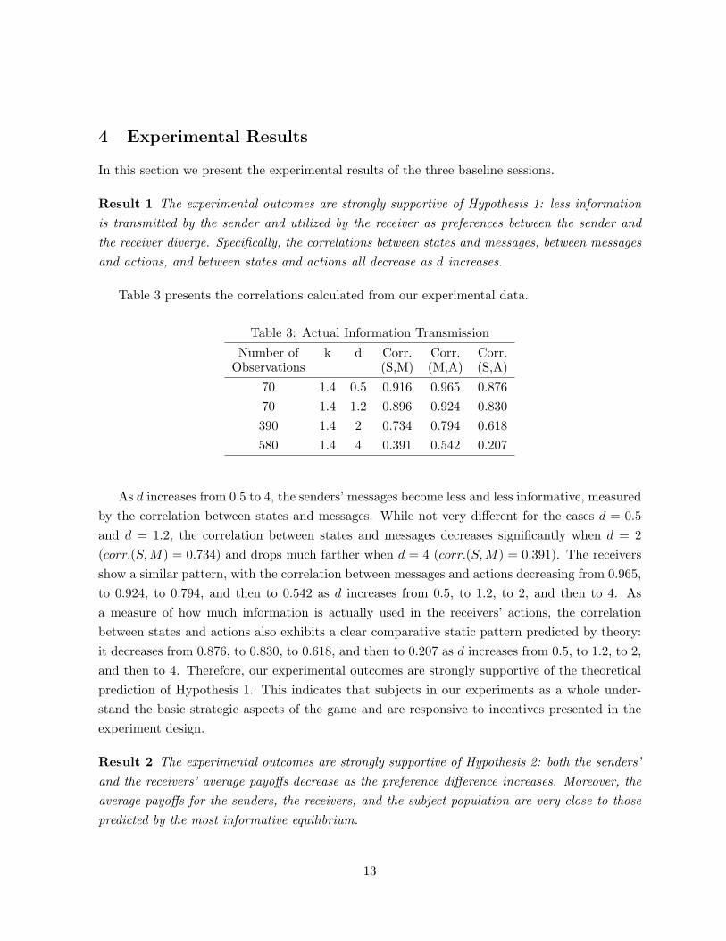
Result 1 The experim ental ou tcom es are strongly su pportive of H ypothesis 1: less inform ation

is transm itted by the sender and u tilized by the receiver as preferences betw een the sender and

the receiver diverge. S pecifi cally , the correlations betw een states and m essages, betw een m essages

and actions, and betw een states and actions all decrease as d increases.

Table 3 presents the correlations calculated from our experimental data.

Table 3: Actual Information Transmission

Number of k d C orr. C orr. C orr.O bservations (S,M) (M,A) (S,A)

70 1.4 0.5 0.916 0.965 0.876

70 1.4 1.2 0.896 0.924 0.830

390 1.4 2 0.734 0.794 0.618

580 1.4 4 0.391 0.542 0.207

As d increases from 0.5 to 4, the senders’ messages become less and less informative, measured

by the correlation between states and messages. W hile not very diff erent for the cases d = 0.5

and d = 1.2, the correlation between states and messages decreases significantly when d = 2

(c o r r.(S , M) = 0.734) and drops much farther when d = 4 (c o r r.(S , M) = 0.391). The receivers

show a similar pattern, with the correlation between messages and actions decreasing from 0.965,

to 0.924, to 0.794, and then to 0.542 as d increases from 0.5, to 1.2, to 2, and then to 4. As

a measure of how much information is actually used in the receivers’ actions, the correlation

between states and actions also exhibits a clear comparative static pattern predicted by theory:

it decreases from 0.876, to 0.830, to 0.618, and then to 0.207 as d increases from 0.5, to 1.2, to 2,

and then to 4. Therefore, our experimental outcomes are strongly supportive of the theoretical

prediction of Hypothesis 1. This indicates that subjects in our experiments as a whole under-

stand the basic strategic aspects of the game and are responsive to incentives presented in the

experiment design.

Result 2 The experim ental ou tcom es are strongly su pportive of H ypothesis 2: both the senders’

and the receivers’ average payoff s decrease as the preference diff erence increases. M oreover, the

average payoff s for the senders, the receivers, and the su bject popu lation are very close to those

predicted by the m ost inform ative equ ilibriu m .

13

We calculate the average payoffs for the senders, the receivers, and the whole subject popula-

tion, for each value of preference difference d = 0.5, 1.2, 2, 4. Table 4 presents the results, as well

as the eq uilibrium predicted payoffs (from Table 1) for comparison. It is clear from Table 4 that

the actual payoffs exhibit strong monotonic patterns as preferences between the senders and the

receivers diverge, just as theory predicts. In particular, as d increases from 0.5, to 1.2, to 2, and

then to 4, the average payoff for the senders decreases from 99.08, to 88.76, to 75.03, and then

to 36.89; the average payoff for the receivers decreases from 101.79, to 93.54, to 83.69, and then

to 65.84; and accordingly the average payoff for the subject population decreases from 100.44, to

91.15, to 79.36, and then to 51.37. These results lend strong support for the comparative static

prediction of the Crawford and Sobel (1982).

Table 4: Theoretical vs. Actual P ayoffs

# of Senders’ P ayoffs Receivers’ P ayoffs Averageobs. d P redicted Actual P redicted Actual P redicted Actual

(s.d.) (s.d.) (s.d.) (s.d.) (s.d.) (s.d.)

70 0.5 106.21 99.08∗ 110.00 101.79∗∗ 108.11 100.44∗

( 0.00) (24.16) ( 0.00) (25.82) ( 1.89) (24.95)

70 1.2 89.52 88.76 95.44 93.54 92.48 91.15(18.06) (18.10) (10.33) (19.97) (15.01) (19.14)

390 2 72.37 75.03 87.38 83.69∗ 79.88 79.36(31.77) (37.28) (19.88) (32.69) (27.54) (35.30)

580 4 29.46 36.89∗∗ 71.59 65.84∗∗ 50.52 51.37(66.32) (68.38) (27.26) (42.72) (54.90) (58.80)

∗ T-test sh o w s a c tu a l p a y o ffs d iffer fro m e q u ilib riu m p a y o ffs sig n ifi c a n tly a t th e 5 -p e rc e n t le v e l o f c o n fi d e n c e .

∗∗ T-test sh o w s a c tu a l p a y o ffs d iffer fro m e q u ilib riu m p a y o ffs sig n ifi c a n tly a t th e 1 -p e rc e n t le v e l o f c o n fi d e n c e .

Another finding from Table 4 is that the actual payoffs are very close to their corresponding

payoffs predicted by the most informative eq uilibrium, given how noisy experimental data usually

are. For d = 0.5, the most informative eq uilibrium is the separating (completely informative)

outcome in which both the sender and the receiver get deterministic payoffs. In this case one

expects that some subjects in the experiments make errors sometimes or just want to try other

strategies (e.g., trying to learn), thus leading to somewhat lower payoffs. From Table 4, the

senders and the receivers on average get 7.13 and 8.21 points less, respectively, than their eq ui-

librium payoffs when d = 0.5. For the cases of d = 1.2 and d = 2, actual payoffs and eq uilibrium

payoffs are very close for both the senders and the receivers and for the population average. In

fact, in most instances, they are almost identical, e.g., 89.52 (eq uilibrium) and 88.76(actual),

95.44 (eq uilibrium) and 93.54 (actual), 79.88 (eq uilibrium) and 79.36 (actual). For d = 4, the

actual payoffs for the senders and the receivers are still q uite close to the corresponding eq uilib-

14

rium payoffs, but not as close as in the cases of d = 1.2 and d = 2. The actual average population

payoff (51.37) for d = 4 is very close to the equilibrium payoff (50.52), since the senders’ gain

relative to equilibrium (36.89−29.46 = 7.43 points) is largely offset by the receivers’ loss relative

to equilibrium (71.59 − 65.84 = 5.75). Note also that even the standard deviations calculated

from our experimental data come very close to those predicted by the theory, with the case of

d = 0.5 being the obvious exception. Finally, we perform t-statistic tests to determine whether

actual payoffs differ from equilibrium payoffs in a statistically significant way. For the cases of

d = 1.2 and d = 2, actual payoffs are not statistically different from the corresponding equilib-

rium payoffs at the 5-percent level of confidence, except for the receivers’ average payoff when

d = 2. Since the sample size is large for d = 4, it is easy to get significant values of the t-statistics

and reject the null hypothesis that the actual payoff equals the equilibrium payoff.12 However,

even when the t-test is significant, all it says is that statistically the actual payoff is not equal

to the equilibrium payoff. The differences between theoretical and actual payoffs in those cases

are still small given how noisy experimental data usually are. In sum, the evidence in Table 4

indicates that the actual payoffs in our experiments are very close to those predicted by theory.

Does this mean that subjects play according to the most informative equilibrium? The results

on payoffs suggest a positive answer. However, after examining the data in more detail, we find

that this is not the case.

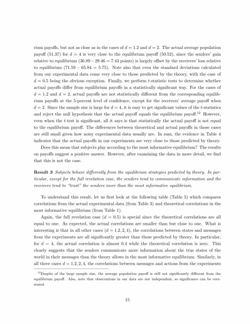
Result 3 Subjects behave differently from the equilibrium strategies predicted by theory. In par-

ticular, except for the full revelation case, the senders tend to communicate information and the

receivers tend to “ trust” the senders more than the most informative equilibrium.

To understand this result, let us first look at the following table (Table 5) which compares

correlations from the actual experimental data (from Table 3) and theoretical correlations in the

most informative equilibrium (from Table 1).

Again, the full revelation case (d = 0.5) is special since the theoretical correlations are all

equal to one. As expected, the actual correlations are smaller than but close to one. What is

interesting is that in all other cases (d = 1.2, 2, 4), the correlations between states and messages

from the experiments are all significantly greater than those predicted by theory. In particular,

for d = 4, the actual correlation is almost 0.4 while the theoretical correlation is zero. This

clearly suggests that the senders communicate more information about the true states of the

world in their messages than the theory allows in the most informative equilibrium. Similarly, in

all three cases d = 1.2, 2, 4, the correlations between messages and actions from the experiments

12Despite of the large sam ple size, the av erage population pay off is still not significantly diff erent from the

eq uilibrium pay off . A lso, note that observ ations in our data are not independent, so significance can be ov er-

stated.

15

Table 5: Theoretical vs. Actual Information Transmission

Number of d Correlation(S,M) Correlation(M,A) Correlation(S,A)Observations Predicted Actual Predicted Actual Predicted Actual

70 0.5 1.000 0.916 1.000 0.965 1.000 0.876

70 1.2 0.750 0.896 0.866 0.924 0.866 0.830

390 2 0.500 0.734 0.707 0.794 0.707 0.618

580 4 0.000 0.391 0.000 0.542 0.000 0.207

are all greater than those predicted by theory, especially when d = 4 (the actual correlation is

0.542, compared to zero for the theoretical correlation). At least in the case of a large preference

difference (d = 4), the evidence strongly suggests that the receivers tend to trust the senders much

more than theory allows. Compared with equilibrium strategies, both senders and receivers in our

experiments show an overcommunication tendency for cases with large preference differences.13

Surprisingly, the overcommunication tendency by both senders and receivers does not neces-

sarily imply that information actually used in the decisions is than the theory predictions. Table

5 shows that the correlation between states and actions from the experiments is actually lower

than that predicted by theory in all cases except d = 4. In particular, despite the fact that both

senders and receivers overcommunicate when d = 1.2 and d = 2, the actual correlations between

states and actions are lower than the equilibrium predictions: 0.830 (actual) versus 0.866 (equi-

librium) for d = 1.2, and 0.618 (actual) versus 0.707 (equilibrium) for d = 2. For the case of

d = 4, even though the actual correlation between states and actions (0.207) is still significantly

greater than the equilibrium correlation of zero, its magnitude is much smaller compared with

the strong overcommunication tendency of senders and receivers.

To further investigate these correlations, we perform statistical tests to see if the actual

correlations are significantly different from the predicted ones. Consider a linear regression

Y = a + bX + ε. Then

b =sY

sX

· C orr(X, Y )

where sX , sY are the sample standard deviation of X and Y , and C orr(X, Y ) is the sample

correlation between X and Y . To test the null hypothesis H0 : C orr(X, Y ) = σXY , where σXY

is the correlation between X and Y predicted by theory, we can regress

(Y − rXY · X) = α + β X + ε

13Note that since senders and receivers communicate more than w hat is allow ed in the most informative equi-

librium, their behavior is even further aw ay from the less informative equilibria of the game.

16

where

rXY =sY

sX

· σXY

The t-test on β would tell us if β is statistically different from zero, or equivalently, if Corr(X, Y )

(the actual correlation between X and Y ) is statistically different from σXY (the theoretical

correlation). We run the regressions with (Y, X) being one of the three pairs (Message, State),

(Action, Message) and (Action, State). The results of these regressions are presented in Table 6.

Consistent with our casual observation above, for the correlation between states and messages,

we find the t-test significant for all but the case of d = 0.5 (where the actual correlation is

0.916), indicating that the actual correlations 0.896(d = 1.2), 0.734(d = 2), and 0.391(d = 4)

are statistically higher than the predicted ones, 0.75, 0.5, and 0, respectively. Also, for the

correlation between messages and actions, the t-test is significant for d = 2 (0.794 vs. 0.707)

and d = 4 (0.542 vs. 0), but not significant for d = 0.5 (0.924 vs. 0.866) and d = 1.2 (0.965

vs. 1). Interestingly, for the correlation between states and actions, the t-test is significant for

d = 0.5, as well as d = 2, 4, but not for d = 1.2. In fact, the β’s are negative for all but the case

of d = 4, meaning that actual correlations are lower than the predicted ones and indicating some

mismatch given the overcommunication tendency shown in the other correlations. However, the

correlations of the aggregate data cannot reveal what kind of mismatch there is. To gain insights

about this question, we need to look into the finer details of the experimental data.

As a first step, we examine the frequencies of actions taken by the receivers conditional on the

true states of the world. For this and the other conditional frequencies discussed later, we focus

on the observations for the case of d = 4, because the actual correlations in this case differ from

equilibrium predictions the most and also because we have the most observations for this case.

For d = 4, the only equilibrium is the babbling equilibrium, in which the receiver should choose

action 5 regardless of the messages she receives and hence regardless of the true states of the

world. The experimental results are presented in Table 7. For simplicity, we group actions into

three groups: “actions 1 to 3”, “actions 4 to 6”, and “actions 7 to 9”. For the 580 observations

we have on d = 4, the frequencies of the five states (s = 1, 3, 5, 7, 9) are very close to uniform.

Several observations can be made of Table 7. First, for each of the 5 states, only about half of

the time actions 4 to 6 are chosen. That is, only about half of the observations can be considered

broadly consistent with equilibrium. Secondly, as the state becomes larger, the frequency weights

switch from the small actions to the large actions. Specifically, as the state increases, while the

frequencies of actions 4 to 6 remain more or less constant, the frequencies of small actions 1

to 3 decreases (s = 7 poses a minor exception)14 and the frequencies of large actions 7 to 9

increases. Comparing states 1 and 9, the frequency of small actions 1 to 3 decreases from almost

14This is because some receivers simply subtract 4 from 7, resulting in many 3’s. See Section 6 for further

ex planations.

17

Table 6: Regression Tests for Correlations

Correlations d N Predicted Actual α β R2 F{Regression} Corr. Corr. (s.e.) (s.e.) (p-value)

0.5 70 1.000 0.916 0.489 -0.085 0.04 2.963(0.272) (0.049) (0.090)

Corr(S,M) 1.2 70 0.750 0.896 1.949∗∗ 0.137∗∗ 0.10 7.403(0.292) (0.050) (0.008)

{(M − rSM · S) 2 390 0.500 0.734 2.308∗∗ 0.230∗∗ 0.11 45.958= α + βS + ε}† (0.184) (0.034) (0.000)

4 580 0.000 0.391 5.466∗∗ 0.347∗∗ 0.15 104.483(0.193) (0.034) (0.000)

0.5 70 1.000 0.965 0.303 -0.033 0.02 1.197(0.173) (0.030) (0.278)

Corr(M,A) 1.2 70 0.866 0.924 -0.508 0.060 0.02 1.574(0.322) (0.048) (0.214)

{(A − rMA · M) 2 390 0.707 0.794 0.912∗∗ 0.081∗∗ 0.02 7.928= α + βM + ε} (0.180) (0.029) (0.005)

4 580 0.000 0.542 2.138∗∗ 0.481∗∗ 0.29 240.771(0.236) (0.031) (0.000)

0.5 70 1.000 0.876 0.797∗ -0.121∗ 0.06 4.480(0.316) (0.057) (0.038)

Corr(S,A) 1.2 70 0.866 0.830 1.341∗∗ -0.035 0.00 0.283(0.379) (0.065) (0.596)

{(A − rSA · S) 2 390 0.707 0.618 2.464∗∗ -0.081∗ 0.01 4.938= α + βS + ε} (0.198) (0.037) (0.027)

4 580 0.000 0.207 4.786∗∗ 0.163∗∗ 0.04 25.879(0.182) (0.032) (0.000)

† rSM =sM

sS· σSM , where sM , sS are the standard deviations of Message M and S tate S, respectively, and σSM is the

theoretical correlation between M and S. S imilarly, rMA =sA

sM· σMA and rSA =

sA

sS· σSA.

∗ T-test shows significant difference from zero at the 5-percent level of confidence.

∗∗ T-test shows significant difference from zero at the 1-percent level of confidence.

18

30% to just 10% , while the frequency of large actions 7 to 9 increases from below 20% to about

43% . Thirdly, the average action clearly exhibits an increasing trend as the state becomes larger.

These observations strengthen the claim that the experimental outcomes are not consistent with

the babbling equilibrium predictions.

Table 7: Frequencies of Actions Conditional on States (d=4)

State # of obs. Actions 1,2,3 Actions 4,5,6 Actions 7,8,9 Average χ2(8) Statistics

(% ) (% ) (% ) Action (p-value†)

1 115 34 59 22 4.670 19.48(29.75% ) (51.30% ) (19.13% ) (0.012)

3 122 24 58 40 5.516 28.38(19.67% ) (47.54% ) (32.79% ) (0.000)

5 118 16 61 41 5.746 38.76(13.56% ) (51.69% ) (34.75% ) (0.000)

7 113 19 47 47 5.973 46.10(16.81% ) (41.59% ) (41.59% ) (0.000)

9 112 12 52 48 6.071 48.29(10.71% ) (46.43% ) (42.86% ) (0.000)

† The confidence level (p-value) is reported for the χ2 test against the null hypothesis that Action 5 is the intended

equilibrium play while all other actions are errors made with equal probability. To do so, we adjust the error

probabilities so that the predicted frequency of Action 5 equals the actual frequency observed.

For a more formal analysis, we perform χ2 tests to see if the empirical distribution of actions

conditional on each state is consistent with the theory. If the theory prediction is interpreted

literally, namely, the distribution of actions should be the degenerate one with all the probability

mass on action 5, the test is trivially rejected by our data. We use a stronger test by postulating

that subjects “tremble hands” while choosing the equilibrium strategy and that the observed

choices of action 5 are all equilibrium plays while all other actions result from erroneous plays

with equal probabilities. Since action 5 is observed less than 50% of the time, our test is very

strong in that it allows noisy plays more than 50% of the time. The last column of Table 7

presents the χ2 test results. For every state s = 1, 3, 5, 7, 9, the test results strongly reject the

null hypothesis of equilibrium play with errors at the 2-percent level of confidence. In other

words, with very high probabilities the observed frequencies of actions conditional on each state

are not consistent with the babbling equilibrium hypothesis, even if a large amount of errors are

allowed.

To analyze more closely the senders’ behavior, we compute the frequencies of the true states

conditional on the senders’ messages, which are presented in Table 8. The empirical frequencies

of states conditional on messages indicate how informative each message (s = 1, 3, 5, 7, 9) is about

19

Table 8: Frequencies of States Conditional on Messages (d=4)

Message # of State 1 State 3 State 5 State 7 State 9 Average χ2(4) Statistics

obs. (%) (%) (%) (%) (%) State (p-value†)

1 31 19 4 2 3 3 2.871 33.35(61.29%) (12.90%) ( 6.45%) ( 9.68%) ( 9.68%) (0.000)

3 53 14 21 6 8 4 3.755 18.04(26.42%) (39.62%) (11.32%) (15.09%) ( 7.55%) (0.001)

5 80 35 13 23 5 4 3.250 42.75(43.75%) (16.25%) (28.75%) ( 6.25%) ( 5.00%) (0.000)

7 84 22 25 15 14 8 4.071 10.88(26.19%) (29.76%) (17.86%) (16.67%) ( 9.52%) (0.028)

9 332 25 59 72 83 93 5.964 41.92( 7.53%) (17.77%) (21.69%) (25.00%) (28.01%) (0.000)

† The confidence level (p-value) is reported for the χ2 test against the null (babbling equilibrium) hypothesis that messages

are completely uninformative so that all states are possible with equal probability conditional on each message.

the true state of the world. In the babbling equilibrium, the sender’s message should be com-

pletely uninformative, namely, the distribution of states conditional on any message should still

be uniform over {1, 3, 5, 7, 9}, so that the receiver cannot draw any inference from the messages

she receives. In the 580 observations with d = 4, the frequencies of messages are very skewed:

message 1 was sent only 31 times while message 9 was sent 332 times. The fact that messages

are concentrated on 9 does not itself reject the hypothesis that messages are uninformative, since

senders in different states could all pool at a same message. However, the frequencies of states

conditional on messages clearly rejects the hypothesis that messages are uninformative. For mes-

sage 1, with more than 60% probability the state is one, and with more than 80% probability

the state is less than or equal to 5. If a receiver is shown Table 8, her optimal action upon

receiving a message of 1 is to choose the average state conditional on message 1, which is 2.87,

far from the equilibrium action 5. Similar patterns are observed for messages 3 and 5, where

the frequency weights are predominantly placed on small states 1, 3, and 5, and the conditional

average state is much smaller than the equilibrium prediction of 5.15 The conditional frequencies

of states is closest to the uniform distribution for message 7, except that the frequency weights

are surprisingly still skewed towards small states,16 leading to a conditional average state of only

about 4. On the other hand, the conditional frequencies of states for message 9 are clearly skewed

15Interestingly, the average state when the message is 5 is lower than that when the message is 3. This is because

some receivers simply subtract 4 from 5, resulting in a probability of 43.75% that Action 1 is chosen when the

message is 5. See Section 6 for further explanations.

16This can be attributed to the fact that some receivers would subtract 4 from 7, resulting in a probability of

29.76% that Action 3 is tak en when the message is 7.

20

towards large states 5, 7, and 9, resulting in a conditional average state of almost 6. To sum up,

the evidence here strongly indicates that the senders’ messages are informative about the true

states of the world, and that they overcommunicate compared with the theoretical prediction.

The last column of Table 8 presents the results of χ2 tests for each message s = 1, 3, 5, 7, 9.

The null hypothesis (babbling equilibrium) is that the senders’ messages are uninformative so

that conditional on messages the states are uniformly distributed. The test results strongly reject

the uniform distribution of state hypothesis at the 0.1-percent level of confidence for all messages

except for m = 7, in which case the null hypothesis is rejected at the 3-percent level of confidence.

Clearly, messages are informative about the states, hence the senders overcommunicate compared

with the babbling equilibrium prediction.

Table 9: Frequencies of Actions Conditional on Messages (d=4)

Message # of Actions 1,2,3 Actions 4,5,6 Actions 7,8,9 Average χ2(8) Statistics

obs. (%) (%) (%) Action (p-value†)

1 31 20 11 0 2.774 44.13(64.52%) (35.48%) ( 0.00%) (0.000)

3 53 22 25 6 4.094 28.90(41.51%) (47.17%) (11.32%) (0.000)

5 80 23 49 8 4.288 20.07(28.75%) (61.25%) (10.00%) (0.010)

7 84 31 36 17 4.786 81.83(36.90%) (42.86%) (20.27%) (0.000)

9 332 9 156 167 6.611 257.13( 2.71%) (46.99%) (50.30%) (0.000)

† The confidence level (p-value) is reported for the χ2 test against the null hypothesis that Action 5 is the intended

equilibrium play while all other actions are errors made with equal probability. To do so, we adjust the error

probabilities so that the predicted frequency of Action 5 is equal to the actual frequency observed.

The receivers’ overcommunication tendency can be seen from Table 9, which presents the

frequencies of actions conditional on messages. Again, in the babbling equilibrium, the receiver

should choose action 5 regardless of the message she receives. This is clearly not the case in our

experiments. Actions 4 to 6 are taken less than 50% of the time except for message 5. Receivers

are far more likely to take small actions 1 to 3 for small messages 1 or 3 than large messages 5,

7, and (especially) 9, and are also far more likely to take large actions 7 to 9 for large messages

7 or 9 than small messages 1,3, and 5. The average action exhibits a clear monotonic trend as

the message increases.

Again, we perform χ2 tests to see if the receivers ignore the messages sent by the senders. We

use the stronger test as before by postulating that receivers play the equilibrium strategy with

21

errors of equal probabilities and that the observed choices of action 5 are all equilibrium plays.

From the results in the last column of Table 9, the babbling equilibrium hypothesis is rejected at

the 1-percent level of confidence for all messages. The evidence clearly indicates that receivers’s

actions vary with the senders’ messages, hence they “over-trust” the senders compared with the

babbling equilibrium prediction.

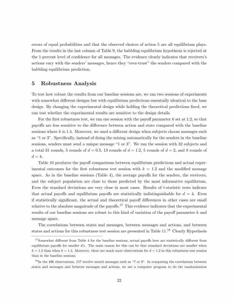
5 Robustness A naly sis

To test how robust the results from our baseline sessions are, we ran two sessions of experiments

with somewhat different designs but with equilibrium predictions essentially identical to the base

design. By changing the experimental design while holding the theoretical predictions fixed, we

can test whether the experimental results are sensitive to the design details.

For the first robustness test, we ran one session with the payoff parameter k set at 1.2, so that

payoffs are less sensitive to the difference between action and state compared with the baseline

sessions where k is 1.4. Moreover, we used a different design when subjects choose messages such

as “1 or 3”. Specifically, instead of doing the mixing automatically for the senders in the baseline

sessions, senders must send a unique message “1 or 3”. We ran the session with 32 subjects and

a total 31 rounds, 5 rounds of d = 0.5, 13 rounds of d = 1.2, 5 rounds of d = 2, and 8 rounds of

d = 4.

Table 10 produces the payoff comparisons between equilibrium predictions and actual exper-

imental outcomes for the first robustness test session with k = 1.2 and the modified message

space. As in the baseline sessions (Table 4), the average payoffs for the senders, the receivers,

and the subject population are close to those predicted by the most informative equilibrium.

E ven the standard deviations are very close in most cases. Results of t-statistic tests indicate

that actual payoffs and equilibrium payoffs are statistically indistinguishable for d = 4. E ven

if statistically significant, the actual and theoretical payoff differences in other cases are small

relative to the absolute magnitude of the payoffs.17 This evidence indicates that the experimental

results of our baseline sessions are robust to this kind of variation of the payoff parameter k and

message space.

The correlations between states and messages, between messages and actions, and between

states and actions for this robustness test session are presented in Table 11.18 Clearly Hypothesis

17Somewhat different from Table 4 for the baseline sessions, actual payoffs here are statistically different from

equilibrium payoffs for smaller d’s. The main reason for this can be that standard deviations are smaller when

k = 1.2 than when k = 1.4. Moreover, there are much more observations for d = 1.2 in this robustness test session

than in the baseline sessions.

18In the 496 observations, 157 involve mixed messages such as “7 or 9”. In computing the correlations between

states and messages and between messages and actions, we use a computer program to do the randomization

22

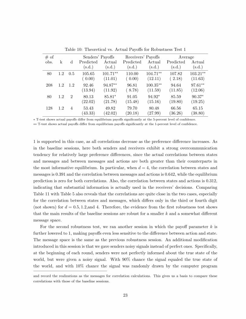
Table 10: Theoretical vs. Actual Payoffs for Robustness Test 1

# of Senders’ Payoffs Receivers’ Payoffs Averageobs. k d Predicted Actual Predicted Actual Predicted Actual

(s.d.) (s.d.) (s.d.) (s.d.) (s.d.) (s.d.)

80 1.2 0.5 105.65 101.71∗∗ 110.00 104.71∗∗ 107.82 103.21∗∗

( 0.00) (11.01) ( 0.00) (12.11) ( 2.18) (11.63)

208 1.2 1.2 92.46 94.87∗∗ 96.81 100.35∗∗ 94.64 97.61∗∗

(13.94) (11.92) ( 8.78) (11.59) (11.85) (12.06)

80 1.2 2 80.13 85.81∗ 91.05 94.92∗ 85.59 90.37∗

(22.02) (21.78) (15.48) (15.16) (19.80) (19.25)

128 1.2 4 53.43 49.82 79.70 80.48 66.56 65.15(43.33) (42.02) (20.18) (27.99) (36.26) (38.80)

∗ T-test shows actual payoffs differ from equilibrium payoffs significantly at the 5-percent level of confidence.

∗∗ T-test shows actual payoffs differ from equilibrium payoffs significantly at the 1-percent level of confidence.

1 is supported in this case, as all correlations decrease as the preference difference increases. As

in the baseline sessions, here both senders and receivers exhibit a strong overcommunication

tendency for relatively large preference differences, since the actual correlations between states

and messages and between messages and actions are both greater than their counterparts in

the most informative equilibrium. In particular, when d = 4, the correlation between states and

messages is 0.391 and the correlation between messages and actions is 0.642, while the equilibrium

prediction is zero for both correlations. Also, the correlation between states and actions is 0.312,

indicating that substantial information is actually used in the receivers’ decisions. Comparing

Table 11 with Table 5 also reveals that the correlations are quite close in the two cases, especially

for the correlation between states and messages, which differs only in the third or fourth digit

(not shown) for d = 0.5, 1.2,and 4. Therefore, the evidence from the first robustness test shows

that the main results of the baseline sessions are robust for a smaller k and a somewhat different

message space.

For the second robustness test, we ran another session in which the payoff parameter k is

further lowered to 1, making payoffs even less sensitive to the difference between action and state.

The message space is the same as the previous robustness session. An additional modification

introduced in this session is that we gave senders noisy signals instead of perfect ones. Specifically,

at the beginning of each round, senders were not perfectly informed about the true state of the

world, but were given a noisy signal. With 90% chance the signal equaled the true state of

the world, and with 10% chance the signal was randomly drawn by the computer program

and record the realizations as the messages for correlation calculations. This gives us a basis to compare these

correlations with those of the baseline sessions.

23

Table 11: Theoretical vs. Actual Information Transmission for Robustness Test 1

# of k d Correlation(S,M) Correlation(M,A) Correlation(S,A)obs. Predicted Actual Predicted Actual Predicted Actual

80 1.2 0.5 1.000 0.916 1.000 0.955 1.000 0.923

208 1.2 1.2 0.750 0.897 0.866 0.912 0.866 0.895

80 1.2 2 0.500 0.837 0.707 0.850 0.707 0.755

128 1.2 4 0.000 0.391 0.000 0.642 0.000 0.312

uniformly from {1, 3, 5, 7, 9}. The reason for introducing noisy signals is the following: One

possible explanation for overcommunication is that the receivers tend to trust the senders “too

much” because they believe that the senders are more “powerful” due to their knowledge about

the state of the world (in applications the senders are usually experts of some sort). If this is a

force behind overcommunication, one expects its effect will diminish with noisy signals since the

senders are less knowledgable and hence less powerful. We ran the session with 48 subjects and

a total 20 rounds, 5 rounds for each of the four cases d = 0.5, 1.2, 2, 4.

Table 12 presents the payoff comparisons between equilibrium predictions and actual experi-

mental outcomes for the second robustness test session with k = 1.0 and noisy signals. Note that

the equilibrium predicted payoffs are quite different from those in the baseline sessions (Table 4)

when preference difference is large (d = 2, 4). Also note that with noisy signals, the equilibrium

predicted payoffs have substantial variances even in the perfectly separating equilibrium when

d = 0.5. Again, just like in the baseline sessions, Table 12 clearly shows that the average payoffs

for the senders, the receivers, and the subject population match very well with those predicted by

the most informative equilibrium. This claim can be strongly supported by the results of t-tests.

Except for d = 0.5, the actual payoffs are not different from the equilibrium predictions at the

5-percent level of confidence in all but one case (the senders’ payoffs when d = 2). In many of

these cases the difference between actual and theoretical payoffs is within one point. The fact

that signals are noisy (and hence the senders may not be perceived as authoritative as in the

case of perfect signals) does not seem to have any effect on the experimental outcomes.

Let us now examine information transmission in the second robustness test. Table 13 presents

the correlations between signals and messages, messages and actions, and between signals and

actions.19 Since the senders only get the signals but do not observe the states, we use the correla-

tions with respect to signals, for they refl ect more closely how much information is communicated

than correlations with respect to states. The equilibrium predictions about the correlations with

19As in the first robustness test, we use simulations to treat messages such as “7 or 9” in calculating the

correlations regarding messages.

24

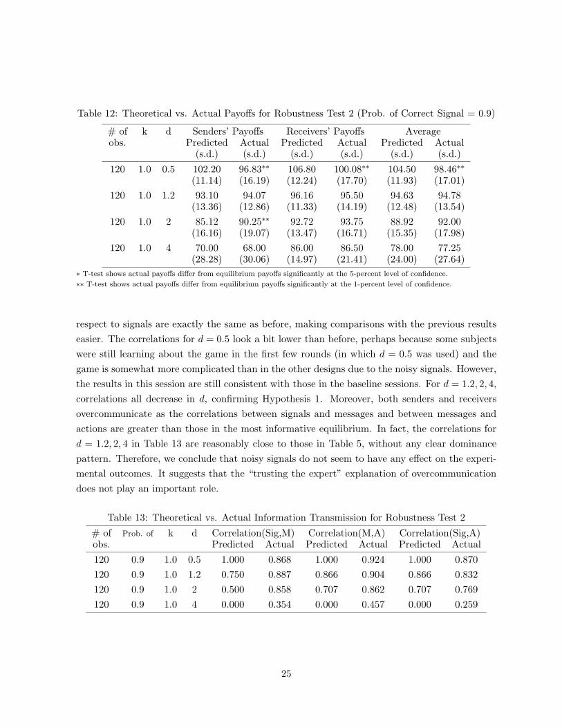
Table 12: Theoretical vs. Actual Payoffs for Robustness Test 2 (Prob. of Correct Signal = 0.9)

# of k d Senders’ Payoffs Receivers’ Payoffs Averageobs. Predicted Actual Predicted Actual Predicted Actual

(s.d.) (s.d.) (s.d.) (s.d.) (s.d.) (s.d.)

120 1.0 0.5 102.20 96.83∗∗ 106.80 100.08∗∗ 104.50 98.46∗∗

(11.14) (16.19) (12.24) (17.70) (11.93) (17.01)

120 1.0 1.2 93.10 94.07 96.16 95.50 94.63 94.78(13.36) (12.86) (11.33) (14.19) (12.48) (13.54)

120 1.0 2 85.12 90.25∗∗ 92.72 93.75 88.92 92.00(16.16) (19.07) (13.47) (16.71) (15.35) (17.98)

120 1.0 4 70.00 68.00 86.00 86.50 78.00 77.25(28.28) (30.06) (14.97) (21.41) (24.00) (27.64)

∗ T-test shows actual payoffs differ from equilibrium payoffs significantly at the 5-percent level of confidence.

∗∗ T-test sh o w s a c tu a l p a y o ffs d iffer fro m e q u ilib riu m p a y o ffs sig n ifi c a n tly a t th e 1 -p e rc e n t le v e l o f c o n fi d e n c e .

respect to signals are ex actly th e sam e as b efore, m ak ing com parisons w ith th e prev iou s resu lts

easier. T h e correlations for d = 0.5 look a b it low er th an b efore, perh aps b ecau se som e su b jects

w ere still learning ab ou t th e gam e in th e fi rst few rou nd s (in w h ich d = 0.5 w as u sed ) and th e

gam e is som ew h at m ore com plicated th an in th e oth er d esigns d u e to th e noisy signals. How ev er,

th e resu lts in th is session are still consistent w ith th ose in th e b aseline sessions. F or d = 1.2, 2, 4,

correlations all d ecrease in d, confi rm ing Hy poth esis 1. M oreov er, b oth send ers and receiv ers

ov ercom m u nicate as th e correlations b etw een signals and m essages and b etw een m essages and

actions are greater th an th ose in th e m ost inform ativ e eq u ilib riu m . In fact, th e correlations for

d = 1.2, 2, 4 in T ab le 13 are reasonab ly close to th ose in T ab le 5, w ith ou t any clear d om inance

pattern. T h erefore, w e conclu d e th at noisy signals d o not seem to h av e any eff ect on th e ex peri-

m ental ou tcom es. It su ggests th at th e “tru sting th e ex pert” ex planation of ov ercom m u nication

d oes not play an im portant role.

T ab le 13: T h eoretical v s. Actu al Inform ation T ransm ission for Rob u stness T est 2

# of Prob. of k d C orrelation(S ig,M ) C orrelation(M ,A) C orrelation(S ig,A)ob s. P red icted Actu al P red icted Actu al P red icted Actu al

120 0.9 1.0 0.5 1.000 0.868 1.000 0.924 1.000 0.870

120 0.9 1.0 1.2 0.750 0.887 0.866 0.904 0.866 0.832

120 0.9 1.0 2 0.500 0.858 0.707 0.862 0.707 0.769

120 0.9 1.0 4 0.000 0.354 0.000 0.457 0.000 0.259

25

6 Learning E ff e cts

Another possible explanation for subjects’ overcommunication tendency observed in our experi-

ments is learning. The game used in our experiments is not a trivial one for people without game

theory training, so it may take a while for subjects to learn to play the equilibrium strategies.20

To examine this learning hypothesis, we ran a session using our base design (Session 2 as de-

scribed in the end of Section 3) in which 32 subjects played 31 rounds of the game with preference

difference d = 4. B y holding the design (including preference difference) fixed throughout the

session, we can compare outcomes in early rounds with those in later rounds to see if subjects

behave differently after gaining experience playing the game. W e focus on the case of d = 4 to

test the learning effect for two reasons. O ne reason is that among the four difference preferences,

deviations from equilibrium predictions are the largest for d = 4. Hence, if learning leads to

convergence to equilibrium, then its effect will be strongest for d = 4. Another reason we focus

on d = 4 is that in this case subjects should have the strongest incentives to learn to play the

equilibrium strategies, because it is most costly for subjects to be outguessed by their opponent.

In trying to increase the subjects’ incentives to learn, we use a generous exchange rate of points

to dollars ($1=50 points) in this session. The session lasted less than 2.5 hours, the highest payoff

was $45.1 and the lowest was $12.7 (excluding the $5 show-up fee).

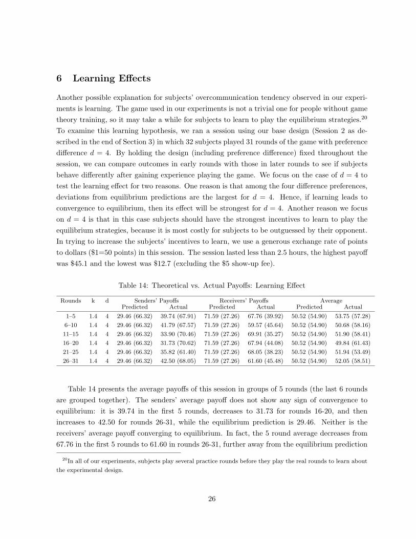
Table 14: Theoretical vs. Actual Payoffs: Learning E ffect

Rounds k d Senders’ Pay off s Receiv ers’ Pay off s A v eragePredicted A ctual Predicted A ctual Predicted A ctual

1–5 1.4 4 29.46 (66.32) 39.74 (67.91) 71.59 (27.26) 67.76 (39.92) 50.52 (54.90) 53.75 (57.28)

6–10 1.4 4 29.46 (66.32) 41.79 (67.57) 71.59 (27.26) 59.57 (45.64) 50.52 (54.90) 50.68 (58.16)

11–15 1.4 4 29.46 (66.32) 33.90 (70.46) 71.59 (27.26) 69.91 (35.27) 50.52 (54.90) 51.90 (58.41)

16–20 1.4 4 29.46 (66.32) 31.73 (70.62) 71.59 (27.26) 67.94 (44.08) 50.52 (54.90) 49.84 (61.43)

21–25 1.4 4 29.46 (66.32) 35.82 (61.40) 71.59 (27.26) 68.05 (38.23) 50.52 (54.90) 51.94 (53.49)

26–31 1.4 4 29.46 (66.32) 42.50 (68.05) 71.59 (27.26) 61.60 (45.48) 50.52 (54.90) 52.05 (58.51)

Table 14 presents the average payoffs of this session in groups of 5 rounds (the last 6 rounds

are grouped together). The senders’ average payoff does not show any sign of convergence to

equilibrium: it is 39.74 in the first 5 rounds, decreases to 31.73 for rounds 16-20, and then

increases to 42.50 for rounds 26-31, while the equilibrium prediction is 29.46. Neither is the

receivers’ average payoff converging to equilibrium. In fact, the 5 round average decreases from

67.76 in the first 5 rounds to 61.60 in rounds 26-31, further away from the equilibrium prediction

20In all of our ex perim ents, subjects play sev eral practice rounds before they play the real rounds to learn about

the ex perim ental design.

26

of 71.59. The population average payoff is close to the equilibrium prediction, but shows no time

trend. Overall, the evidence on average payoffs does not indicate any significant learning effect.

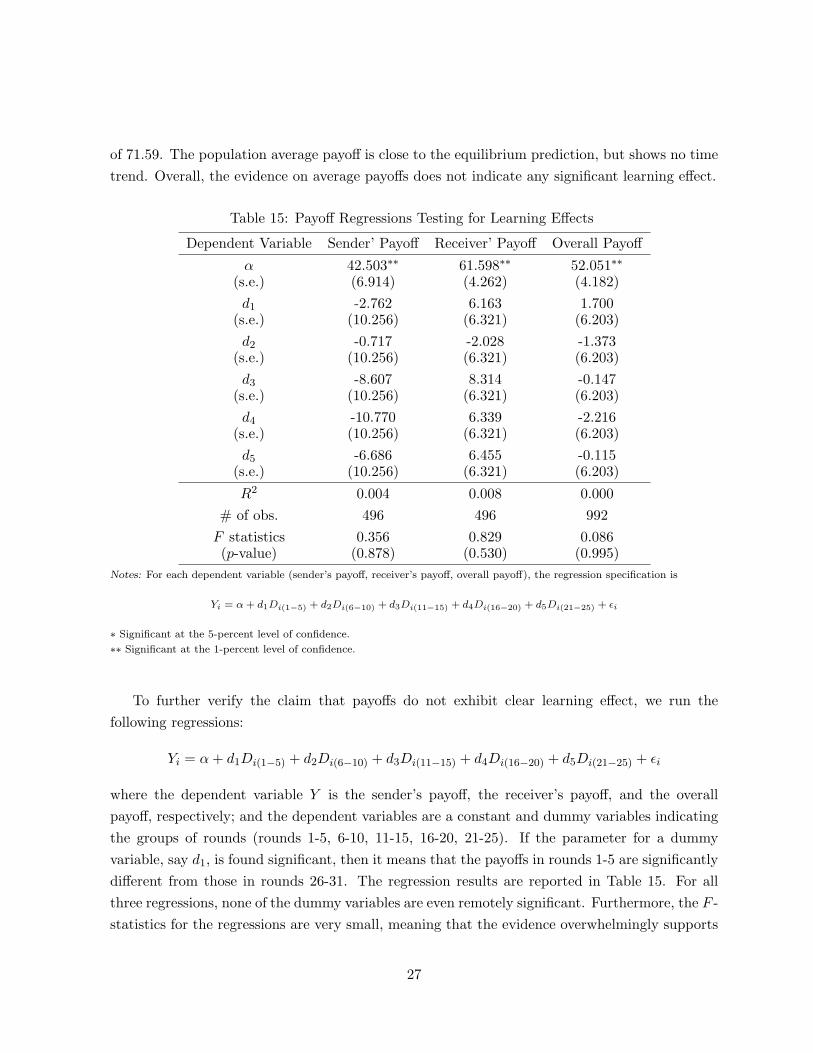
Table 15: Payoff Regressions Testing for Learning Effects

Dependent V ariable Sender’ Payoff Receiver’ Payoff Overall Payoff

α 42.503∗∗ 61.598∗∗ 52.051∗∗

(s.e.) (6.914) (4.262) (4.182)

d1 -2.762 6.163 1.700(s.e.) (10.256) (6.321) (6.203)

d2 -0.717 -2.028 -1.373(s.e.) (10.256) (6.321) (6.203)

d3 -8.607 8.314 -0.147(s.e.) (10.256) (6.321) (6.203)

d4 -10.770 6.339 -2.216(s.e.) (10.256) (6.321) (6.203)

d5 -6.686 6.455 -0.115(s.e.) (10.256) (6.321) (6.203)

R2 0.004 0.008 0.000

# of obs. 496 496 992

F statistics 0.356 0.829 0.086(p-value) (0.878) (0.530) (0.995)

No tes: F or each dependent variable (sender’s payoff, receiver’s payoff, overall payoff), the regression specification is

Yi = α + d1Di(1−5) + d2Di(6−10) + d3Di(11−15) + d4Di(16−20) + d5Di(21−25) + εi

∗ S ignificant at the 5-percent level of confidence.

∗∗ S ignificant at the 1-percent level of confidence.

To further verify the claim that payoffs do not exhibit clear learning effect, we run the

following regressions:

Yi = α + d1Di(1−5) + d2Di(6−10) + d3Di(11−15) + d4Di(16−20) + d5Di(21−25) + εi

where the dependent variable Y is the sender’s payoff, the receiver’s payoff, and the overall

payoff, respectively; and the dependent variables are a constant and dummy variables indicating

the groups of rounds (rounds 1-5, 6-10, 11-15, 16-20, 21-25). If the parameter for a dummy

variable, say d1, is found significant, then it means that the payoffs in rounds 1-5 are significantly

different from those in rounds 26-31. The regression results are reported in Table 15. For all

three regressions, none of the dummy variables are even remotely significant. Furthermore, the F -

statistics for the regressions are very small, meaning that the evidence overwhelmingly supports

27

the null hypothesis that all other groups of rounds are no different from the last 6 rounds. Thus,

the evidence on payoffs strongly indicates that there is no clear learning effect in our data.

Examining the table of correlations also reveals the same picture. From Table 16, one can see

that none of the three correlations exhibit a clear time trend, let alone convergence to equilibrium.

For example, the correlation between states and messages and the correlation between messages

and actions both are greater in the last 6 rounds than in the first 5 rounds after some ups and

downs in between.

Table 16: Theoretical vs. Actual Information Transmission: Learning Effect

Rounds k d Correlation(S,M) Correlation(M,A) Correlation(S,A)Predicted Actual Predicted Actual Predicted Actual

1–5 1.4 4 0.000 0.244 0.000 0.500 0.000 0.139

6–10 1.4 4 0.000 0.351 0.000 0.530 0.000 0.091

11–15 1.4 4 0.000 0.434 0.000 0.449 0.000 0.329

16–20 1.4 4 0.000 0.470 0.000 0.566 0.000 0.175

21–25 1.4 4 0.000 0.439 0.000 0.627 0.000 0.245

26–31 1.4 4 0.000 0.344 0.000 0.557 0.000 0.133

To test rigorously any learning effect in the correlations, we run the following three regressions:

Yi = α + βXi + d1Di(1−5)Xi + d2Di(6−10)Xi + d3Di(11−15)Xi + d4Di(16−20)Xi + d5Di(21−25)Xi + εi

where (Y, X) is one of the three pairs (Message, State), (Action, Message) and (Action, State).

Also included as dependent variables in the regressions are the product terms of dummy variables

and X. Since the parameter β is proportional to the correlation between (Y, X) for rounds 26-31,

a non-significant β will support the babbling equilibrium prediction. On the other hand, if the

parameter for a dummy variable, say d1, is found to be significant, it means that the correlation

between (Y, X) in rounds 1-5 are significantly different from that in rounds 26-31. Table 17

reports the regression results.

The first thing to note from Table 17 is that β is significant in all three regressions, indi-

cating that all three correlations are significantly different from zero—the babbling equilibrium

prediction for rounds 26-31. Moreover, all the parameters d1 to d5 are not significant in all three

regressions, except for d1 in the regression of message on state. Aside from the exception, the

results show that the correlations are not significantly different across rounds, suggesting no clear

learning effect. In fact, the F -tests of di = 0 for all i are not significant, except for (X, Y ) =

(Message, State) since its d1 is significant.21 Note that the sign of d1 in the regression of message

21The F tests of β = 0 and di = 0 for all i are all significant, because β is significant in all regressions.

28

Table 17: Correlation Regressions Testing for Learning Effect

Regression Message on State[ Action on Message† Action on State‡

α 5.556∗∗ 2.387∗∗ 4.958∗∗

(s.e.) (0.208) (0.245) (0.189)

β 0.380∗∗ 0.461∗∗ 0.159∗∗

(s.e.) (0.053) (0.038) (0.048)

d1 -0.191∗∗ 0.009 -0.049(s.e.) (0.063) (0.037) (0.057)

d2 -0.051 0.023 0.002(s.e.) (0.062) (0.035) (0.056)

d3 -0.058 -0.062 -0.057(s.e.) (0.061) (0.035) (0.056)

d4 -0.046 -0.027 -0.056(s.e.) (0.061) (0.035) (0.055)

d5 0.006 0.001 0.013(s.e.) (0.060) (0.034) (0.054)

# of obs. 496 496 496

R2 0.163 0.295 0.040

F statistics 15.852 34.034 3.415(p-value) (0.000) (0.000) (0.003)

F statistics 2.825 1.343 0.770di = 0 ∀i

(p-value) (0.016) (0.245) (0.572)

[ Mi = α + β Si + d1Di(1−5)Si + d2Di(6−10)Si + d3Di(11−15)Si + d4Di(16−20)Si + d5Di(21−25)Si + εi

†Ai = α + β Mi + d1Di(1−5)Mi + d2Di(6−10)Mi + d3Di(11−15)Mi + d4Di(16−20)Mi + d5Di(21−25)Mi + εi

‡Ai = α + β Si + d1Di(1−5)Si + d2Di(6−10)Si + d3Di(11−15)Si + d4Di(16−20)Si + d5Di(21−25)Si + εi

∗ Significant at the 5-percent level of confidence.

∗∗ Significant at the 1-percent level of confidence.

29

on state is negative, meaning that the correlation between message and state is smaller in rounds

1-5 than in rounds 26-31. So even if there is a time trend in the correlation between messages

and states, it is moving further away from equilibrium. Therefore, the results of the correlation

regressions indicate that there is no clear learning effect.

To conclude this section, we do not find any clear time trend in our data that can suggest

learning plays a significant role in the experimental outcomes. Of course, this is not to say that

learning definitely will not lead to convergence to equilibrium. There are 31 rounds in this session

of our experiment, and there does not appear to be any significant time trend. It is possible

that it takes much longer for subjects to learn and eventually learning results in convergence

to equilibrium. But we have to leave it to future research to investigate this possibility. It

is interesting to note that, in contrast to our result here, Blume et al (2001) report evidence

indicating significant learning effects: senders became more “sophisticated” (e.g., revealing their

types less often) and receivers became less gullible. Because Blume et al are interested in the

evolution of messages, their experimental design facilitates possible subject learning much more

than ours. In their experiments, there were 60 rounds of play and subjects were randomly paired

with 6 opponents and thus interacted with an opponent about 10 periods. Moreover, summary

history about other subject pairs was revealed to all subjects at the end of each period. In our

experiments, opportunities for subjects to learn are more limited since they played 31 rounds,

interacted with any other subject only once, and only knew the outcomes of the games they

played in.

7 Bounded Rationality : Behav ior T y p e A naly sis

Our experimental results show that on the aggregate level subjects understand the basic strategic

elements of the game (hence the comparative statics hypotheses 1 and 2 are strongly confirmed),

but both senders and receivers tend to overcommunicate relative to what theory allows in the

most informative equilibrium. So the following questions naturally arise. What accounts for

the non-equilibrium behavior? Why are the actual average payoffs so close to the equilibrium

predictions? In order to answer these questions, we need to examine the subjects’ individual

behavior to figure out what kinds of non-equilibrium behavior the subjects exhibit. In this

section, we apply one approach of bounded rationality, behavior type analysis, to our experiment

data to understand the overcommunication phenomenon. To identify behavior patterns, we need

a non-trivial number of plays of the same game for each subject. For this reason, we use the data

from Session 2 of the base design, in which there are 31 rounds of play with preference difference

d = 4. With 31 rounds of play, each subject on average plays 15-16 rounds as the sender and

15-16 rounds as the receiver.

Using earlier experiment evidence (e.g., Blume, DeJong, K im and Sprinkle, 2001) on com-

30

munication games, Crawford (2003) defines the system of behavior types that is anchored on

the “truster” type of senders and the “believer” type of receivers. We follow Crawford (2003) to

define the system of behavior types for our game with d = 4. The definitions are listed in Table

18. A sender of the lowest level of sophistication, type L0 or the truster type, simply sends the

truthful message all the time. In response to the type L0 sender, the type L0 or the believer

type receiver completely trusts the sender and always chooses the action identical to the sender’s

message. The next level sender, type L1 or liar type, believes that the receiver is of the L0 type,

and hence incorporates his policy bias (d = 4) into his messages. In response to the type L1

sender, the type L1 or the inverted type receiver will choose action 1 for a message of 5, action

3 for a message of 7, and action 7 for a message 9 (since it is equally likely from an L1 sender

in states 5, 7, 9). Messages 1 and 3 would be “out-of-equilibrium” for an L1 sender; we assign

the belief of state 1 for the L1 receiver. An L2 sender best responses to an L1 receiver and will

always send a message of 9 regardless of the true state.22 An L2 receiver best responses to an

L2 sender and hence will always choose action 5. In equilibrium the sender should randomize

and hence any message will be consistent, so it is not meaningful to identify an equilibrium type

sender. On the other hand, an equilibrium type receiver will always choose action 5 regardless

of the message she receives, which coincides with the L2 type. Finally, a sophisticated type

sender maximizes his payoffs given the empirical distribution of the receivers’ behavior, while a

sophisticated type receiver best responses to the empirical distribution of the senders’ behavior.

Their optimal strategies are given in the last row of Table 18.

Table 18: Type Classification Definition(d=4)

Type Sender’s Message (given S) Receiver’s Action (given M)

Name S=1 S=3 S=5 S=7 S=9 M=1 M=3 M=5 M=7 M=9

L0 1 3 5 7 9 1 3 5 7 9

L1 5 7 9 9 9 1 1 1 3 7

L2 9 9 9 9 9 5 5 5 5 5

Eq any any any any any 5 5 5 5 5

Sop 7 9 9 9 9 2 3 3 4 6

We then follow the classification methodology of Costa-G omes et al (2001, 2002) to classify

subjects whose actions can be consistently identified as fitting into one of the behavior types.

In applying the type definitions to classify the 32 subjects, we allow for errors of plus or minus

22In state 1, an L 2 sender is indifferent betw een sending a message of 7 and a message of 9 to an L 1 receiver,

and w e break the tie tow ards 9. The results are not significantly affected by this tie-breaking choice.

31

1.23 Then we count how many times a subject’s choices are consistent with one of the types as a

sender and as a receiver separately. Subjects are classified into a particular type if their behavior

is consistent with that type for more than 60% of the time (e.g., at least 10 out of 16 times). If

a subject is consistent with more than one type by the 60% rule, we classify him or her as the

type he or she is most consistent with. If there is a tie between two or more types, we classify

that subject to the lowest type of sophistication.24 Table 19 presents the classification results for

the senders.

Table 19: Type Classifications Results: Senders

Type Count Subject Number (% of consistency)

L0 2 18(80% ), 22(90.9% )

L1 8 1(83.3% ), 2(66.7% ), 12(71.4% ), 14(69.2% ), 16(60% ), 23(76.9% ), 29(63.2% ),

32(64.7% )

L2 10 3(78.9% ), 4(100% ), 6(100% ), 9(62.5% ), 11(85.7% ), 17(86.7% ), 20(82.4% ),

25(81.3% ), 27(72.2% ), 31(64.7% )

Sop 4 5(94.4% ), 8(88.2% ), 19(100% ), 30(100% )

N/A 8 7, 10, 13, 15, 21, 24, 26, 28

Among the 32 subjects, 24 can be classified as one of the behavior types. Two can be classified

as the L0 type, 8 the L1 type, 10 the L2 type, and 4 the sophisticated type.

The classification results for the receivers is presented in Table 20. Among the 32 subjects,

26 can be classified as one of the behavior types. Three can be classified as the L0 type, 3 the

L1 type, 11 the L2 or Equilibrium type, and 9 the sophisticated type.

The fact that about 75% of the subject population fits into the behavior types seems to

indicate that this approach of bounded rationality is reasonably successful in describing the

behavior of a majority of subjects. Moreover, it is interesting to note that some subjects, such as

18 and 22, are highly consistent as the truster type L0 senders and believer type L0 receivers; and

quite a many subjects are highly consistent as either the liar type L1 senders or the inverter type

L1 receivers.25 This suggests roughly the following interpretation of our data. Those subjects of

23Note that this has no effect on classification of the senders, since their messages differ from each other by 2.

24There are three subjects (20, 29, 31) who are tied for two or more types as senders and five subjects (5, 8, 15,

19, 24) who are tied for two or more types as receivers. U sing alternative tie-breaking rules does not have much

effect on the analysis below.

25E xamining these low type subjects’ individual behavior, we do not find indication of learning over time, that

is, they do not become more rational over time. This is q uite remarkable for the L0 types, since the potential

gain from becoming more rational is rather significant. By our calculation, given the empirical distribution of the

32

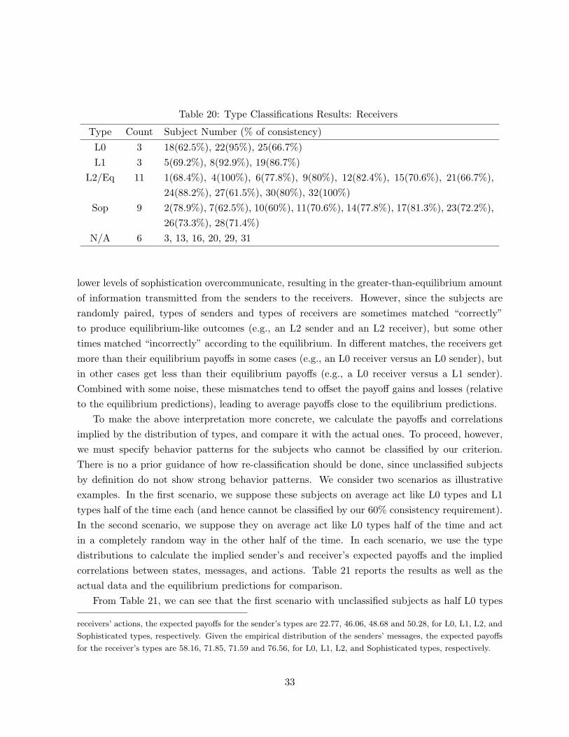
Table 20: Type Classifications Results: Receivers

Type Count Subject Number (% of consistency)

L0 3 18(62.5%), 22(95%), 25(66.7%)

L1 3 5(69.2%), 8(92.9%), 19(86.7%)

L2/Eq 11 1(68.4%), 4(100%), 6(77.8%), 9(80%), 12(82.4%), 15(70.6%), 21(66.7%),

24(88.2%), 27(61.5%), 30(80%), 32(100%)

Sop 9 2(78.9%), 7(62.5%), 10(60%), 11(70.6%), 14(77.8%), 17(81.3%), 23(72.2%),

26(73.3%), 28(71.4%)

N/A 6 3, 13, 16, 20, 29, 31

lower levels of sophistication overcommunicate, resulting in the greater-than-equilibrium amount

of information transmitted from the senders to the receivers. However, since the subjects are

randomly paired, types of senders and types of receivers are sometimes matched “correctly”

to produce equilibrium-like outcomes (e.g., an L2 sender and an L2 receiver), but some other

times matched “incorrectly” according to the equilibrium. In different matches, the receivers get

more than their equilibrium payoffs in some cases (e.g., an L0 receiver versus an L0 sender), but

in other cases get less than their equilibrium payoffs (e.g., a L0 receiver versus a L1 sender).

Combined with some noise, these mismatches tend to offset the payoff gains and losses (relative

to the equilibrium predictions), leading to average payoffs close to the equilibrium predictions.

To make the above interpretation more concrete, we calculate the payoffs and correlations

implied by the distribution of types, and compare it with the actual ones. To proceed, however,

we must specify behavior patterns for the subjects who cannot be classified by our criterion.

There is no a prior guidance of how re-classification should be done, since unclassified subjects

by definition do not show strong behavior patterns. We consider two scenarios as illustrative

examples. In the first scenario, we suppose these subjects on average act like L0 types and L1

types half of the time each (and hence cannot be classified by our 60% consistency requirement).

In the second scenario, we suppose they on average act like L0 types half of the time and act

in a completely random way in the other half of the time. In each scenario, we use the type

distributions to calculate the implied sender’s and receiver’s expected payoffs and the implied

correlations between states, messages, and actions. Table 21 reports the results as well as the

actual data and the equilibrium predictions for comparison.

From Table 21, we can see that the first scenario with unclassified subjects as half L0 types

receivers’ actions, the expected payoffs for the sender’s types are 22.77, 46.06, 48.68 and 50.28, for L0, L1, L2, and

Sophisticated types, respectively. G iven the empirical distribution of the senders’ messages, the expected payoffs

for the receiver’s types are 58.16, 71.85, 71.59 and 76.56, for L0, L1, L2, and Sophisticated types, respectively.

33

Table 21: Estimation Results of Nash Equilibrium, Type Analysis and AQ RE (d = 4)

Actual Nash Type Type Crawford Q RE

Scenario 1 Scenario 2 Equilibrium (λ = 2.0042)

Senders’ uS 37.37 29.46 40.54 35.82 50.24 23.53

Receivers’ uR 65.67 71.59 72.86 67.85 79.75 66.27

Corr(S,M) 0.376 0.000 0.531 0.388 0.630 0.328

Corr(M,A) 0.534 0.000 0.631 0.517 0.829 0.403

Corr(S,A) 0.183 0.000 0.361 0.222 0.608 0.180

and half L1 types overestimates communication (all three correlations are greater than those of

actual data) and the senders’ and receivers’ expected payoffs. On the other hand, the second

scenario (that all unclassified subjects are supposed to act randomly half of the time and act

according to L0 types) does a very good job matching up with the actual data in terms of both

correlations and expected payoffs. This shows that at least with some reasonable adjustments

the behavior type analysis can explain our experimental data quite well, predicting both the

degree of overcommunication and the players’ expected payoffs. Having said that, we offer a

word of caution. The main issue is that subjects of higher levels of sophistication in our games

are not very distinguishable from each other, for example, L2 and sophisticated senders only

differ in state 1, while L2 and equilibrium senders and receivers are not distinguishable at all

(Table 18). Moreover, several subjects are tied with two or three higher types on both the sender

and receiver sides. Even though the tie-breaking rule does not have important effects on our

result, it is possible that the type classification may not be robust in other somewhat different

environments. Thus, the results from the behavior type analysis in this section are not conclusive.

Models and experimental designs that allow sharper distinction of subject types are needed for

further investigation.

A related, but slightly different way to interpret our experiment data is to explain the data as

some equilibrium in a model in which some subjects are rational and others are of some behavior

types. Crawford (2003) studies a cheap talk model with a zero-sum underlying game in which

players can be rational or the L0 and L1 types (i.e., truster and liar senders, believer and inverter

receivers). In equilibrium, rational type players best response to their opponents, taking into

account that their opponents can be one of the three types. He characterizes the equilibrium

of the game and shows how it changes as the initial type distribution changes. Even though

the underlying game in our study is quite different from that in Crawford (2003), it is easy to

apply his method here, because subjects of L2 and Equilibrium types in our games are not very

distinguishable from the sophisticated types (Table 18). As a result, in the classification quite a

34

many subjects classified as L2 types are equally (or very close to be) consistent with sophisticated

types. More precisely, if L2 type is ruled out, 8 out of 10 L2 type senders in Table 19 can be re-

classified as sophisticated type, and 5 out of 11 L2 type receivers in Table 20 can be re-classified

as sophisticated type. Reclassifying those unclassified subjects so that they on average act like

L0 type half of the time and L1 type in the other half of the time, we arrive at a type distribution

roughly as follows: the senders are L0, L1 and sophisticated with proportions (20%, 40%, 40%),

and the receivers are L0, L1 and sophisticated with proportions (30%, 30%, 40%). With these type

distributions, it can be verified that in equilibrium the sophisticated type sender sends a message 7

when the state is 1, and 9 in all other states, which coincides with the behavior of the sophisticated

sender who best responses to the empirical distribution of the receivers’ actions (Table 18). In

equilibrium, the sophisticated type receiver will choose 1 in state 1, choose 3 in states 3, 5,

7, and choose 7 in state 9. Compared with the behavior of the sophisticated receiver who

best responses to the empirical distribution of the senders’ actions (Table 18), the theoretically

sophisticated receiver’s strategy is very close but not identical in states 1, 7, 9. We compute

the correlations and expected payoffs in this equilibrium. The results are in Table 21, under

the column titled “Crawford Equilibrium”. Evidently, the Crawford equilibrium substantially

overestimates communication and expected payoffs. The reason for the overestimation by the

Crawford equilibrium and by the non-equilibrium type simulation of scenario 1 above (with half

L0 types and half L1 types for unclassified subjects) is the same. In our experiment data, there

is much noise in subjects’ behavior, which is not taken into account by either interpretation. The

second scenario (with half L0 types and half complete randomization) matches the data very

well, because it introduces complete randomness into the subject population.

8 Bounded Rationality: Quantal Response Eq uilibrium

An alternative explanation for non-equilibrium behavior in experimental data is the concept of

Quantal Response Equilibrium (QRE) introduced in McKelvey and Palfrey (1995, 1998). In

Quantal Response Equilibrium, players have correct beliefs about their opponents’ behavior, but

they either make mistakes while trying to maximizing their payoffs or their preferences over

different strategies are stochastic. Unlike the rational approach and the behavior type analysis,

QRE explicitly takes into account noisy behavior of subjects. McKelvey and Palfrey (1995, 1998)

demonstrate that QRE can be very useful in organizing and interpreting experimental data for

a variety of experiments. In this section we apply the concept of QRE to our experiment data

to shed light on the overcommunication phenomenon.

Specifically, following McKelvey and Palfrey (1998), we solve for the logit agent quantal

35

response equilibrium (logit-AQRE) for our game.26 Let u(a, s) and v(a, s) be the utilities of the

sender and receiver, respectively, when the state is s and the receiver chooses an action a. Then

in the logit-AQRE with a parameter λ, the sender in state s sends a message m ∈ {1, 3, 5, 7, 9}

with probability psm = P r(m|s):

psm =eλus(m)

∑5,7,9j=1,3, e

λus(j,)

where us(m) =∑9

a=1 qmau(a, s) is the sender’s expected payoff from sending a message m in state

s; the receiver chooses an action a upon receiving a message m with probability qma = P r(a|m):

qma =eλvm(a)

∑9j=1 eλvm(j)

where vm(a) =∑5,7,9

s=1,3 r(s|m)v(a, s) is the receiver’s expected payoff from choosing an action a

upon the receipt of message m and r(s|m) = psm/∑9

i=1 pim is her posterior belief about the

states.

Hence, P = (psm)5×5 and Q = (qma)5×9 represent the sender’s and receiver’s mixed strategies,

respectively, in the logit-AQRE. For any given λ, to solve for the seventy variables from the system

of seventy equations, we iterate by starting with an initial P0 and obtaining the new Q1 and

P1 using the above equations. We perform this procedure iteratively until P and Q converge to

a fixed point. We then calculate the likelihood for this λ and obtain the maximum likelihood

estimator by maximizing the likelihood function.27

Similar to the issue of choosing the right anchor for the behavior type analysis, choosing a

proper initial point P0 is important in applying the logit-AQRE to strategic information trans-

mission games. In these games, since the sender’s strategies (namely, their messages) do not

directly affect payoffs (thus the term “cheap talk”), there are many payoff-equivalent equilibria

but with different equilibrium strategies. For example, in the d = 4 case, while babbling is the

only equilibrium outcome, there are in fact many babbling equilibria, in each of which the sender

sends a particular message in all states. So if we choose a complete random strategy for the

sender as the initial P0, the iteration process quickly settles on a babbling equilibrium. To avoid

this problem, we use the truth-telling strategy for the senders as the initial P0 (i.e., identity

matrix).

For the ease of comparison, the result of the logit-AQRE estimation is displayed in the last

column of Table 21. As shown in Table 21, the maximum likelihood estimator of λ is 2.0042. In

the estimated AQRE, the correlation between state and action is very close to the actual data,

26For details of the solution concept and its applications, see McK elvey and Palfrey (1998).

27W e use the golden section method in the estimation since λ is one dimension and L(λ) is unimodal according

to our grid search.

36

the correlations between state and message and between message and action are fairly close to

the actual data. Hence the logit-AQRE provides a good interpretation for the communication

patterns in our experimental data. In terms of payoffs, the receiver’s expected payoff in the

estimated AQRE is very close to that of actual data, while the sender’s is somewhat lower. This

may suggest that the logit-AQRE incorporates all kinds of noisy actions, while subjects in the

data do not make mistakes (especially the very bad mistakes) to the extent the logit-AQRE

postulates.28

9 Conclusion

In this paper we conduct laboratory experiments to test the theory of strategic information

transmission originated by Crawford and Sobel (1982). Our main findings are the following.

First, our experimental results strongly support the basic insight of the theory, namely, less

information is transmitted when preferences of the sender and the receiver diverge. Secondly, the

evidence shows that subjects consistently overcommunicate in that the senders’ messages are more

informative about the true states of the world and the receivers utilize the senders’ messages more

in choosing actions, compared with what the theory allows in the most informative equilibrium.

Thirdly, these results are robust to certain variations of payoff parameters and noisy signals, and

are robust to subjects’ learning. Fourthly, we use both the behavior type analysis and quantal

response equilibrium to analyze subjects’ behavior in our experiment data. Both approaches

have some success in interpreting our data. In particular, with each of the two approaches, we

generate the kinds of correlations (overcommunication) and average payoffs (close to equilibrium

payoffs) observed in the experimental data.

While we have some success in explaining our experimental results (in particular, overcom-

munication and near equilibrium payoffs) using the two bounded rationality approaches, the test

may not be very “powerful” in the sense that for large preference differences, messages and ac-

tions tend to cluster toward the highest state (state 9), as the sender’s bias is in one direction. In

future work, it is desirable to develop models such that biases are symmetric so that clustering

does not arise. Questions about what the underlying motives for the L0 types are naturally

arise. Subjects 18 and 22 are highly consistent as L0 senders and L0 receivers in that they send

truthful messages and choose actions blindly following the messages. Are they driven by social

preferences (e.g., trust)? Where do their beliefs come from? These questions all await for further

investigation.

28To be sure, the Q RE requires that players make worse mistakes less often. In our game, the sender suffers

more than the receiver in their respective worst payoff cases: when the state is 1 and the action is 9, the loss to

the sender is 214.23 and the loss to the receiver is 73.79. So this may explain why the sender’s expected payoff is

under-estimated by the logit-AQ RE.

37

References

[1] Banks, Jeffrey, Colin Camerer and David Porter, 1994, Experimental Tests of Nash Refine-

ments in Signaling Games, Games an d E con omic B eh av ior, 6:1-31.

[2] Brandts, Jordi and Charles Holt, 1992, An Experimental Test of Equilibrium Dominance in

Signaling Games, American E con omic Rev iew , 82:1350-1365.

[3] Brandts, Jordi and Charles Holt, 1993, Adjustment Patterns and Equilibrium Selection in

Experimental Signaling Games, In tern ation al Journ al of Game T h eory , 22:279-302.

[4] Blume, Andreas, Douglas V. DeJong, Y ong-Gwan Kim and Geoffrey B. Sprinkle, 1998,

Experimental Evidence on the Evolution of Meaning of Messages in Sender-Receiver Games,

American E con omic Rev iew , 88:1323-1340.

[5] Blume, Andreas, Douglas V. DeJong, Y ong-Gwan Kim and Geoffrey B. Sprinkle, 2001,

Evolution of Communication with Partial Common Interest, Games an d E con omic B eh av ior,

37:79-120.

[6] Camerer, Colin, 2002, Behavior G am e T heory : E xperim ents on S trategic Interaction, Prince-

ton University Press, Princeton, NJ.

[7] Camerer, Colin, Teck-Hua Ho, and Juin Kuan Chong, 2002, A cognitive hierarchy theory of

one-shot games, Caltech working paper.

[8] Costa-Gomes, Miguel, Vincent Crawford, and Bruno Broseta, 2001, Cognition and Behavior

in Normal-Form Games: An Experimental Study, E con ometrica, 69:1193-1235.

[9] Costa-Gomes, Miguel and Vincent Crawford, 2002, Cognition and Behavior in Two-Person

Guessing Games: An Experimental Study, UCSD Working Paper.

[10] Crawford, Vincent, 1997, Theory and Experiment in the Analysis of Strategic Interaction,

in Ad van ces in E con omic s an d E con ometric s: T h eory an d Ap p lication s, S ev en th W orld

C on gress, eds. Kreps, David and Ken Wallis, Cambridge University Press, Cambridge, UK.

[11] Crawford, Vincent, 1998, A Survey of Experiments on Communication via Cheap Talk,

Journ al of E con omic T h eory , 78:286-298.

[12] Crawford, Vincent, 2003, Lying for Strategic Advantage: Rational and Roundedly Rational

Misrepresentation of Intentions, American E con omic Rev iew , 93:133-149.

[13] Crawford, Vincent and Joel Sobel, 1982, Strategic Information Transmission, E con ometrica,

50:1431-1451.

38

[14] Dickhaut, John, Kevin A. McCabe and Arijit Mukherji, 1995, An Experimental Study of

Strategic Information Transmission, Economic Theory, 6:389-403.

[15] Eyster, Erik and Matthew Rabin, 2000, Cursed Equilibrium, working paper, UC Berkeley.

[16] Farrell, Joseph and Matthew Rabin, 1996, Cheap Talk, Journal of Economic P erspectives,

10:103-118.

[17] Fischbacher, Urs, 1999, z-Tree: Toolbox for Readymade Economic Experiments, IEW Work-

ing paper 21, University of Zurich.

[18] Ho, Teck Hua, Colin Camerer and Keith Weigelt, 1998, Iterated Dominance and Iterated

Best Response in Experimental “p-Beauty Contests”, American Economic Review, 39:649-

660.

[19] Kagel, John and Alvin Roth, 1995, Handbook of Experimental Economics, eds, Princeton

University Press: Princeton, NJ.

[20] McKelvey, Richard and Thomas Palfrey, 1998, Quantal Response Equilibria in Normal Form

Games, Games and Economic Behavior, 10:6-38.

[21] McKelvey, Richard and Thomas Palfrey, 1995, Quantal Response Equilibria in Extensive

Form Games, Ex perimental Economics, 1:9-41.

[22] Nagel, Rosemarie, 1995, Unraveling in Guessing Games: An Experimental Study, American

Economic Review, 85:1313-1326.

[23] Ottaviani, Marco and Francesco Squintani, 2002, Not Fully Strategic Information Transmis-

sion, working paper, London Business School.

[24] Palfrey, Thomas and Howard Rosenthal, 1991, Testing for Effects of Cheap Talk in a Public

Goods Game with Private Information, Games and Economic Behavior, 3:183-220.

[25] Stahl, Dale and Paul Wilson, 1995, On Players’ Models of Other Players: Theory and

Experimental Evidence, Games and Economic Behavior, 10:218-254.

39

Last Updated: 10/7/2003 1

�������������� ������������������������ ��� ���������� ���� ����������������� ������� �������!��"#���$�������%��&���'� ��(�)��"����������������� ������������(������*����������+��(�� ������,(�����������������"��(�� ������,(�����(������������������+���� ����������������� �(� �-������(������ ��(���������� ����+���� ����.��

���������������������������������������������� ���!�

�/��������#���� ��������������� ������������ ����������� ���& �0��"����������,����#������� +���������������������� ����� (�� ���*������ ��� �(�� ���� �+� �(�� ������ ���.� )(��� ���� ����� ������ � ������� ��� ����� ���� ��� �� ������� ��� �(������ ��� � �+� ��(�� �� ����������� ��� �(����.� ���� �� ������++� ���� ��"�� � ���� ��������� �(��� � ��,.� ���� �� ��� �� �������"�� ��(�������(�*�������������(���� �����.��%(��������������� ����,������0���������(���"(��� ��������� ���� ����������������������#��,��������,������0���������(���"(��(���� ����� .�1��� �� ���������(��������������0�����������,������������ ��������,��(���(�������������� ������"��(�������� �������� � ����+����#���(�������� �����.��)��,���� �����,��(���#���+��� ���������������.������"��(���� ��������������������,����#��"�*������� ����������+��(�� ����+������ ��+� �(�������� ��������,����#�� (�,��(�,� ���� �� �(���� ����� .� 1+�����(�*������2�� ���� ������"� �(� ������������ �������(�������������2�� �����,����#���� ,����� ���*�����������(���.�����"����"#��$����"#�

�3�����������*�����������������(��������� (������ ���.��/���,����� ���(� � (�������������������������+�����������" .��/������ �������� #���� ��(���� #���+����,��"�4���56�,��������������� ������.��)������������ �������� �������� #�������(�� (���.��7��������� (��������� �+�������8�����,����������������(�������+��(�� � ������������*���������� ���.��������� ������������������������������������������9�� �(� � �� ��� ���� �� ����� ���� �(�� ��*���� � �(��� �������� ���� +�� � ����� ���"(#�� .� �����"� �(�� ���� �� �+� �(� ������� ��������� ����+�����+�� ����0��"�,��(���������"(#�� .��������������� ������ �����#�������0�����(��-5��+�1���.��%(� �,����#���"���������(��-5��+�,���� �� �����.���9����(��������2�� ���� :���������������!� �����"���������#$���������"�$������%&!������$'������(�������� ����������$��)���$$����������$�� ��*��+&,+-, .,++���������/&!����0�������%(�������� ������������������������"������� � � ��+����� #����+������ .��9���(�������+��(��+����������������,����#��� 0��� ��� +���� ���� ��2�� ���������� ����"�������� �(�� ������ � ����� ����(�*������ ������������"� �(�� ���� ���+� �(�� � ��������������������(��;<� (�,&���+��.���*���#����,����#�������������*�����+���� (�,��"��(��������� (���.��/�����������������#��"����������������(�� �(�,� ��(�����������.���������"� �(�� ������ ���� ���� �(�� ������" � ���� ���� ������� ��� =�9>$�.� � /���� ������� ������" � ��� �(�� ���� �+� �(�������� ������������� �����#���(��=�9>$�;����(��"��������� ��������(��#���������(��+���������#��0��+��(����� .�%(� ����(��"�������� ��2��������.���;��=�9>$�.�%(���+�����<��=�9>$�������2��*���������;.�������������$"�#�

�)��,����#�"����(�������� ������,.��%(�������� ������� � � ��+����������������� ����������������� .��1���(������������ �� �,������������� ����� ���(��� �����������.� �/���,��������#�� ���(���,��(� �(�� � ��������� +�� ����*��� ������ ��(���"(�����(��������������� ���.��%(� ���(�� ���(��"�� ��������� ��(���,����(����(������ ��� ����� �0�������������������(�������++�����(������ ��� ��+������������,����#�� ���(���,��(��������������� .����=�� ���,������"���"��������(���������������� %���$��"&��'����������$"�#����"���'���"(�)(#�$"����(�$�������� ��� ��� #�%� � /��� ���� ���� ����� +��� �(�� ��������� ����� 8� ��� � � ?� �� +��� ���� ��� +� ������-�� ���� ��+� ,��(� �(�������� ���������(���� ���������"�� .���������������&� ������1��������2+&,+-, .,++���������/&!������9�� �(�� #�"�����"� �+� ���(� ������� ���� ,���� #�� ����� ��� ?������ ,��(� ����(��� ������������ ��� +�� � �� ����.� � 3��������������� ��� ���(� ����� � � ����� ��� �(� ��� ��� #�� � #��� 9�� ���� �(�� ��(��� � #��� @.� � =�� � ����� �� ������

Appendix: Instructions

Last Updated: 10/7/2003 2

������� ���� ,���� +���� ����� ����� A � #��� 9� ��� � #��� @B� ��� �(�� ������ ���� �(�� ���+������� ��++������� #��,���� � #���9����� � #���@���(�� �����"��+�,(��(�,����#�� ���������������.���������������3���%(� � � � �(�� � �� �������#��� +��� � #���@.� �>���� �(��� �(���"(���� �(�������� ����� �(�����+���������++������� � ���,�� �C.���������������4���1�����(���������(���� ���������"�� �"������� ��� �������� #����(���� ������ ������,��+�� ��(�� ���D���<���EF�+����*��������.��%(���� ������,���� �����(�� �������� #������G� #���9.��9+���������*��"��(���� #���� � #���9�,���� ������ � �"����� � #���@�������(��� � #���@�,�����(�� �����������.��@��(� � #���9�����@H �������" ������������(��*������+��(�� �������� #������� � #���@H �������.���������������.��1�������������� � #���@H �������" �,����#���� ��� ����� � ��(���� ������#��,�����(�� �������� #��������(��������� �(� ��� #�� � #��� @� ��� �(�� ��,��� .C.� � G� #��� 9H � ������" �,���� #�� �� ��� � �� �� � � �(�� �� ������#��,����4�(�� �������� #������ ������+���������++������6������(����������(� ���#�� � #���@�����(����,���.C.��/������������������,������#�����(� ������������� ������(���� ������,����������+������.���������������-��%(��"���(����+����� (�, ��(���� �#���������" �,(����(�� �������� #���� ��.��%(����������� (�, ��(��������" ��+� � #���@�"�*�����++�������������(����� (���(�� � 8��(��#��������� (�, ��(��������" ��+� � #���9�"�*�����++�������������@��(�� � .��>�����(��� � #���@H �������" ������(��(�"(� ��,(����(���������� �������������"�,��(��(�� �������� #���A�B.��G� #���9H �������" ������(��(�"(� ��,(����(���������� ����,(��(�� ��(�� �������� #���A�B���� ��(�����+���������++�������ACB.��%(�����0��+� � #���9H �������" �A�B������(�����0��+� � #���@H �������" �A�B�(� �����++��������+�C��,(��(�� ��(�����+���������++���������.�������������5��1�� �(� � "���(�� �(�� ������ �� #��� � � .� � !������ � #���@� "�� � �(�� (�"(� �� ������" �,(��� �(�� ������� � � �� ���� � #���9�"�� ��(��(�"(� ��������" �,(����(���������� �<��,(��(�� ����� ��(�����+���������++��������C.�������������6��3�� ����� ������� ����,���� ��� �(�� ��#��� �+� ���� �� �#��� ������" .� � =��� �(�� ��� ���� (�,� ��� +������ �(�����+���������++��������� � �C�� �(�� �������� #������� �(����������(� �������#��(��� �(��� � #���@H �������" ������������ � #���9H �������" �����C�.������+������"� � #���@H ����0�����(�����*��� �"���(.��1+��(���������� �<�� � #���@H �������" �������,�C�.�������� � #���9H �������" �����������+������"� � #���9H ����0�����(�����*��� �"���(.��9����(��������2�� ���� :����9+����������"��(����+�� �������������� ���������� ��(������#������ ����"��4��� ���������.6��%(���� � #���9�,���������*�� �(�� ������ �� #���� ,(��(� � � ���������� ��� �(�� ���� ��"(�� �+� �(�� �����.� %(�� �� �#��� ������" � +��� �*���� ��������������� ����������(����+�.��������������� +���1+��������� � #���9��������������0�����(������#����� ����������"��(���� �#���*���� ��+��(�� �������� #������*��,��(�� ������" � ���� ���� � #��� @� �"(�� "��� �+� �(��� ,���� �(�� ����� *����.� � %(�� ��#��� �+� �� �#��� ������" � "�*�����++������ ������ � �(� ��� #�� � #��� @� (�, � ��.� � >���� �(��� ����� ������" � ���� (�,�� ��� *��� ���� �(�� ��(��� � #��H �������" ����� (�,����� *���.��������������� ���/��� �������0������++������#����� ���� ���������" ������(��� ������� .��/��� �����0��������� ����������0�� � ������ � �� �����,�����#����� � #����(�����(�������������� �����,�����".��������������� !���1���(����� �������?������ ����(�� ��������(�����+���������++������� � �C�������(���� #��� � #���9������*��� � �<.��!������ � #���9H �������" �� ���A�(��(�"(� �B��+�9������E�,�����(� ���#�� � #���@��,(���� � #���@H �������" �� ���A�(��(�"(� �B��+�9������<�,�����(� ���#�� � #���@.��������������� &��G� #���9�,������,� ������ � �"����� � #���@.��%(�� � �"��#���� �����(����"(�� �����+��(�� �����.��/��������(�� ������(��0������+��(���(��0#��� �����+�� ��� � �"�����������"��(��*�����������"���+��(���� #��������*��.��

Last Updated: 10/7/2003 3

1+�����,�������0����� ���#��,�����,����� ����*���� �� � �����(��0������+��(��*���� �����,������� ���#��,���.��'� ���� � #��� ��� �(��0� �(�� 4��6� #��� ��� +����� �+� �(� � ��� ���+�� .� � �+� (�$� �'��#� !��� �'"� �"� ,�$-� �'���!�$���.�����"��!�(��'��#��"��+��'�,�$#�.��'�/$�����00����(�"��#"��������!!0�� %��=������ �������� �(�� ������ (�,��(����� � #���9��(�� � � �(�� � �"��� 4%(���� #��� 1� �����*��� � � <���������E.6��!�������(���� ������,�����(�������� ����(�� ������ #���+�� �D<�����EF������ ���������� � #���@.��>�����(������� ����� ���(�� ����� ������ � �"�� ����"��4����(��"�6�,��(�����(��0��"�������(���#��� .� �%(� � � � �(�� � ��� ��(�� ��"�4���������<���������E�6������(���� ������,���� ������� � #���@�������� ������,���� #���+�� �D�����<�����EF.������������� � �"������,�������0����� �������������0�437.6����������������� 3� ����� �����$����$�� ���$������������$����!� ��*�������� � � #���9�+��� (���(� (��� � �"�:��1 ��(��������2�� ������#�����(�� � �"�� �����"������ :����>�,����� � � #���@H ����������(�� �����������.��'� ����0���(�����*��� � ��������(�� � �"�� ����#�� � #���9�� �����(����"(�� �����+��(�� ������������� �#���������" ���������(�� ��+�.��/�����������0������ �#���*���� ��+��(�� �������� #��� ��� *��,� �(�� ������" � ���� ���� � #��� 9� �"(�� "��� �+� �(��� ,���� �(�� ����� *����.� � �� � #��� �(��� �����������" �������� *���������(����(��� � #��H �������" �������� *���.��������������� 4���>�����(����+� � #���9� ������ � �"���(������ � � ��+� �����(�������*���� ���(���� ������,��������� ������0������+��(� ������� ����� ����������� �����.��!������ ����"���4�6��������� ������������ �����(��� � #���9� ��������4%(�� �� #��� 1� �����*��� � � �6� ��� �(��� � #��� 9� ���� ���� �� ����� � �"�� ,��(� �� � � ���� �� �#��� *����.� =������ ��������������#���(��� � #���9� ��������4����(��"�6������(���� ���������,�4�6������+��(�������D�����<�����EF.��=�������(������ ������ �� ����?����������(�� ����������(��"(� � #���9����*��� ����(� ����(�� � �"��4<���������E�6� � #���@������*� ��(���� #���4E�6�,(��(�� ������ ������,��+�� �<���������E.�G� #���@���,�,�����(�� ������������� ��"���������C��<��������I������E.��%��������(��������������(�� ����������0�4376��������������(� ������.������������� .� ����� �������������$�� ���$������������$����9���(�������+��(����������(�� �������� #���� ���*����������������������" ���������� �������������"��.��9� � �����+� �(� � ������ �������� ������������ �(��*������+� �(�� �������� #���� �(���� #��� � #���9������*���� �(�� � �"�� � #���9���������� ������(�� � �"��@������*�����(����������(� ���#�� � #���@�����������������" �#��(�����(� ������������� ������� ����(��������� � ���.���������(� � � �?� ��������������������������� �������������" ����� �����-���.��9����(��������2�� ���� :������������� -���$���0�4376�����������������(����(����������������� .��1���(� ���������������������,����"������(��������������(����(�������.��1.�.��+�����,���� � #���9�����(�����*��� ������������,������,�#�� � #���@������*����*�� �.��/��� ��� ��������(�� ������ � �"����������������(� ���������������.���������$"�#��)�� ,���� ��,� ����� �(�� ����� ����� .� � /��� ,���� ��,� ����� �� A��� �B� ����� �� ���(� ������ ������� ,��(� �� ��++�����������������.������ � #����/���,��������#�� ���(���,��(��(�� � ���������+�� ����*��� ������ ��(���"(�����(��������������� ���.��!��������������� ��� ������������������(�������++�����(������ ��� ��+��(�������������,���������,��(����+����������� .��'�#��#�"����������1�(�$�.����0����2���$���0�4�06����������������(������������ .������ �������������� �0��������(���� .����3�.����%(� � � ��(�������+��(�������� ���.�3������� ����������,���� ����������"�#��� ���������"������=�9>$��������" �+����(� � � ���.���������7��$���������2+&,+-, .,++�8��$���������������8������� �� +���� ��� ����� +�� �� �� ��� �� �� �� ��� �?����,(��(�������������� ����"������ ������(�������#��0"�����.� %(������� �4376.��/���,����#���������������"��.����%(�������� ����(� ������.��3������� ����������,���� ����������"�#������������"������������������" �+����(��������������� ���.������ �� �0�� ����������������(�������������++���������������� (���.�����%�0�� �(� � (���� ��� �(�� �������� +��� ��� ���.� %(� � (����,���� #�� ���(��� ������� �� ������ ��������� �+� �� ��� � +������ ���.��/������� ��� �,����#�����������������(������� ��2������.��%(��0�����+���������������������.���