overreactions, momentum, liquidity, and price bubbles in ...caginalp/pub72.pdf · shares, plus...

Overreactions, Momentum, Liquidity, and Price Bubbles inLaboratory and Field Asset Markets

Gunduz Caginalp, David Porter, and Vernon L. Smith

Laboratory asset markets provide an experimental setting in which to observe investorbehavior. Over more than a decade, numerous studies have found that participants inlaboratory experiments frequently drive asset prices far above fundamental value, af-ter which the prices crash. This bubble-and-crash behavior is robust to variations in anumber of variables, including liquidity (the amount of cash available relative to thevalue of the assets being traded), short-selling, certainty or uncertainty of dividendpayments, brokerage fees, capital gains taxes, buying on margin, and others.

This paper attempts to model the behavior of asset prices in experimental settingsby proposing a “momentum model” of asset price changes. The model assumes thatinvestors follow a combination of two factors when setting prices: fundamental value,and the recent price trend. The predictions of the model, while still far from perfect,are superior to those of a rational expectations model, in which traders consider onlyfundamental value. In particular, the momentum model predicts that higher levels ofliquidity lead to larger price bubbles, a result that is confirmed in the experiments. Thesimilarity between laboratory results and data from field (real-world) markets sug-gests that the momentum model may be applicable there as well.

What drives stock prices? Certainly earnings—ormore generally, fundamental value—play a role. Inves-tor behavior, however, is increasingly considered as an-other important factor. Unfortunately, it is difficult toobservemostof the importantvariables inactual tradingbehavior. Experimental asset markets seek to overcomethis limitation by observing traders in a controlled set-ting, where fundamental value is a known quantity (animpossibility in field markets), and where other sourcesof uncertainty can be eliminated as well.

In a typical laboratory experiment, a group of sub-jects participates in a trading session lasting approxi-mately twohours.Eachsubject isgivenacertainamountof cash and stock with which to trade. Trading is con-ducted by computer over a local network, and the ses-sion is divided into fifteen periods. In each period, bidsand offers are matched and the trades clear simulta-neously. The subjects are told at the beginning that theirshares will pay a dividend each period. The amount ofeach dividend is not known in advance, but the subjectsare told what distribution the dividend payments are

drawn from. For example, there may be a one in fourprobability of either 60 cents, 28 cents, 8 cents, or zero.The average (expected) dividend would then come outto 24 cents per period. This means that the fundamentalvalue of each share is $3.60 for the full fifteen periods.After each period, the value drops by 24 cents. The par-ticipants are told this at the beginning, so they know thefundamental value of their shares.

In laboratory experiments, no assumptions are maderegarding traders’ decision-making processes. This canbe compared to rational expectations theory, for exam-ple, where there are very definite assumptions that in-vestorsareunbiasedprocessorsof information. Ineithercase, there are two important variables: the informationthat bears on fundamental value, and investor behavior.In field markets, information is incomplete, and it is notalways clear whether fundamental value or investor be-havior is themost importantdeterminantofstockprices,because both tend to be highly uncertain. Traditionally,finance theory and research have, in effect, treated in-vestorbehaviorasknownand fixed,while taking funda-mental value to be the only source of uncertainty. Byobserving traders in a laboratory market setting, we canturn this situation around and control for variations anduncertainty in fundamental value, thus allowing for arelatively clear observation of investor behavior.

We begin by examining the database of laboratoryexperiments in which full information on the dividenddistribution (including the calculated value of expecteddividend value each period) is provided to all subjects(second through fourth sections). The effects of a large

24

The Journal of Psychology and Financial Markets Copyright © 2000 by2000, Vol. 1, No. 1, 24–48 The Institute of Psychology and Markets

Gunduz Caginalp is Professor of Mathematics at the Universityof Pittsburgh.

David Porter is Senior Research Scientist at the Economic Sci-ence Laboratory of the University of Arizona.

Vernon L. Smith is Regents’ Professor of Economics and Re-search Director of the Economic Science Laboratory at the Univer-sity of Arizona.

Requests for reprints should be sent to Gunduz Caginalp, Depart-ment of Mathematics, University of Pittsburgh, Thackeray 506, Pitts-burgh, PA 15260. E-mail: [email protected].

number of treatments, subject pools, subject experi-ence, and institutional variations (brokerage fees, cap-ital gains taxes, short-selling, margin buying, futurescontracting, limit price change rules—circuit break-ers—and call market organization) are provided.Subject experience, subject sophistication, and fu-tures contracting are the only treatments that materi-ally dampen the robust tendency of the stock marketsin these environments to produce price bubbles andcrashes relative to fundamental value.

In the fifth and sixth sections, we articulate math-ematically a “momentum” model that modifies therational expectations approach by postulating thatinvestor sentiment is of two types: 1) fundamentalistswhose purchases are positively (negatively) related tothe discount (premium) of price relative to intrinsicvalues; and 2) momentum traders whose purchases arepositively related to the percentage rate of change inprice. The laboratory research findings and the modelare then used to interpret field data sets, including twoexamples of bubbles in closed-end funds (where fun-damental value is known, and this information iswidely available), two funds with identical portfolios,and the frequency of crashes in the Standard & Poor’sindex.

The seventh section then compares various meth-ods of predicting laboratory stock market prices. Inparticular, we compare the momentum model, experttrader forecasts, time series forecasts, and a price ad-justment process in which price changes are a linearfunction of the excess bids (bids versus asks—similarto a Walrasian price adjustment process where priceadjusts in the direction of excess demand).

Finally, in the last section, we interpret the momen-tum model parametrically in terms of a measure ofmarket liquidity, which can be controlled in the labora-tory as a treatment variable, and report a series of ex-periments based on the liquidity interpretation of themomentum model. Contrary to the rational expecta-tions model, this model predicts that asset prices willbe an increasing function of the aggregate ratio of cashto share endowments, a result that is corroborated bythe liquidity experiments.

Basic Bubble Experiments

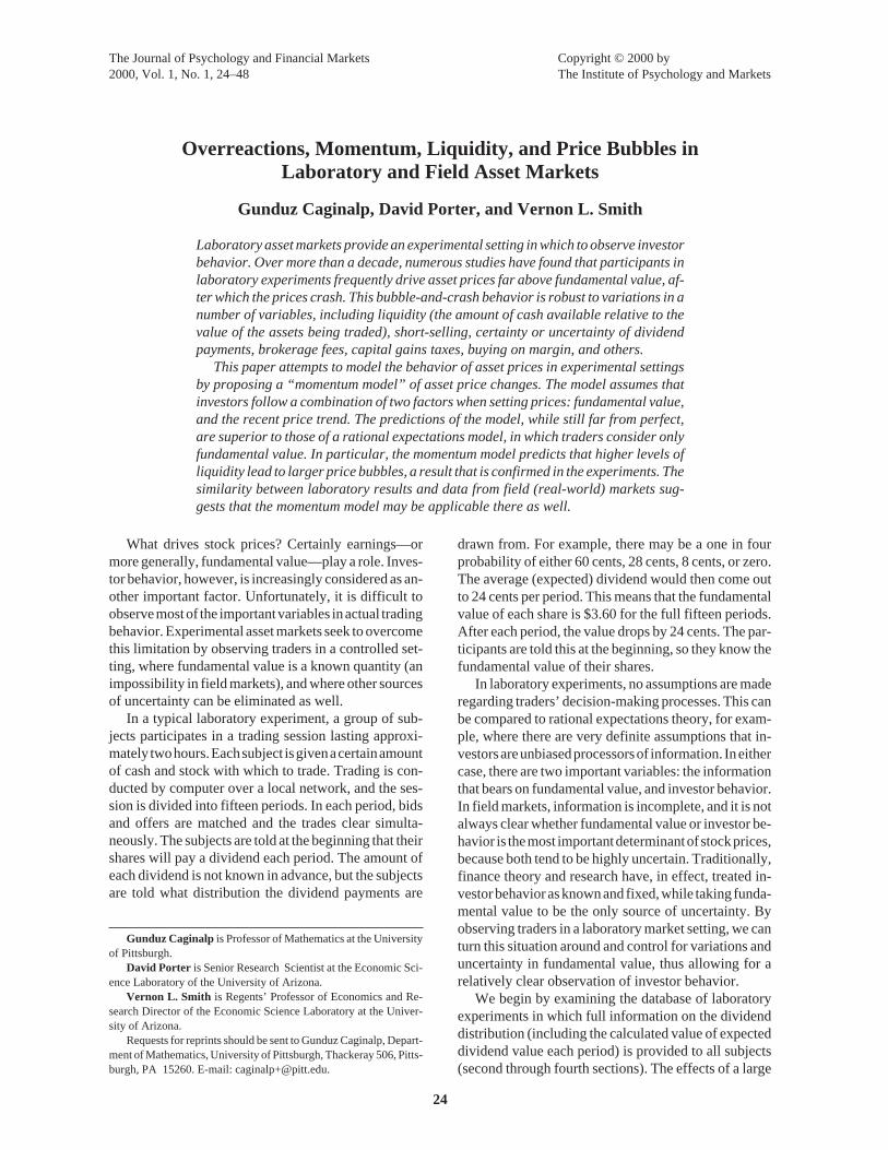
An experimental design for studying the temporalevolution of asset trading prices was introduced bySmith,Suchanek, and Williams (SSW) [1988]). Figure 1

25

LAB AND FIELD ASSET MARKETS

FIGURE 1Baseline Asset Market Experiment Parameters

illustrates one of their experimental environments. Eachof the twelve traders receives an initial portfolio of cashand shares of a security with a fixed life of fifteen tradingperiods. Before each trading period, t = 1, 2, …, 15, theexpected dividend value of a share,1 $0.24(15 – t + 1), iscomputed and reported to all subjects to guard againstany misunderstanding. This situation is like that of astock mutual fund, whose net asset value is reported to in-vestors daily or weekly. Each trader is free to trade sharesof the security using double auction trading rules (seeWilliams [1980] for details of these rules), which are sim-ilar to those used on major stock exchanges. At the end ofthe experiment, a sum equal to all dividends received onshares, plus initial cash, plus capital gains, minus capitallosses, is paid in U.S. currency to each trader.

The rational expectations model predicts that pricestrack the fundamental value line (see Figure 1). Behav-iorally, however, inexperienced traders produce highamplitude2 bubbles that can rise two to three timesabove fundamental value. In addition, the span of aboom tends to be of longduration(ten to eleven peri-ods), with a largeturnoverof shares (five to six timesthe outstanding stock of shares over the fifteen-periodexperiment). In nearly all cases, prices crashed to fun-damental value by period 15.

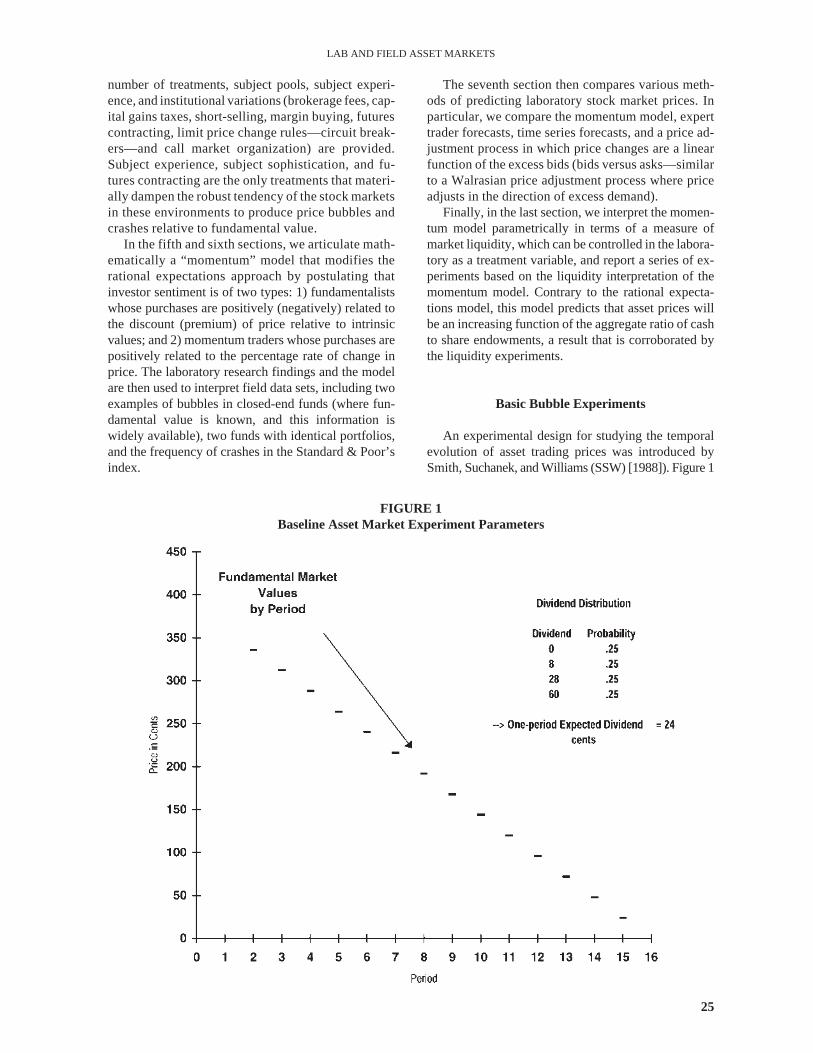
Figure 2 contrasts the mean contract prices and vol-ume for inexperienced traders with those for experi-enced traders in two laboratory asset markets. The datapoints plot the mean price for each period and the num-bers next to the prices show the number of contractsmade in that period. With inexperienced traders, bub-bles and crashes are standard fare, but this phenome-non disappears as traders become experienced. That is,traders twice experienced in trading in a laboratory as-

set market will trade at prices that deviate little fromfundamental value.

The robustness of the bubble/crash phenomenonhas led several researchers to examine changes in thebasic trading environment and rules to see if suchchanges can reduce or eliminate this large systematicprice deviation from fundamental value. We describebelow the research testing various hypotheses thatmight contribute to, or retard, the formation of pricebubbles (for a survey of the literature on asset tradingexperiments, see Sunder [1995]).

Changes in the Economic Environment

Recall that in the baseline experiments individualtraders were endowed with different initial portfolios(see footnote 1). A common characteristic of first-pe-riod trading is that buyers tend to have low share en-dowments, while sellers have relatively high share en-dowments. Based on conventional utility theory, risk-averse tradersmightbeusing themarket toacquiremorebalanced portfolios. If diversification preferences ac-count for the low initial prices, which in turn leads to ar-bitrage that creates expectations of further priceincreases, making the initial trader endowments equalacross subjects would dampen bubbles. However,ob-servations from four experiments with inexperiencedtraders show no significant effect of equal endowmentson bubble characteristics(see King, Smith, Williams,and Van Boening (KSWV) [1992]). Thus, the conjec-ture that initial portfolio rebalancing depresses prices,with subsequent price increases leading to expectationsof capital gains, cannot be substantiated.

26

CAGINALP, PORTER, & SMITH

FIGURE 2Mean Contract Price and Total Volume

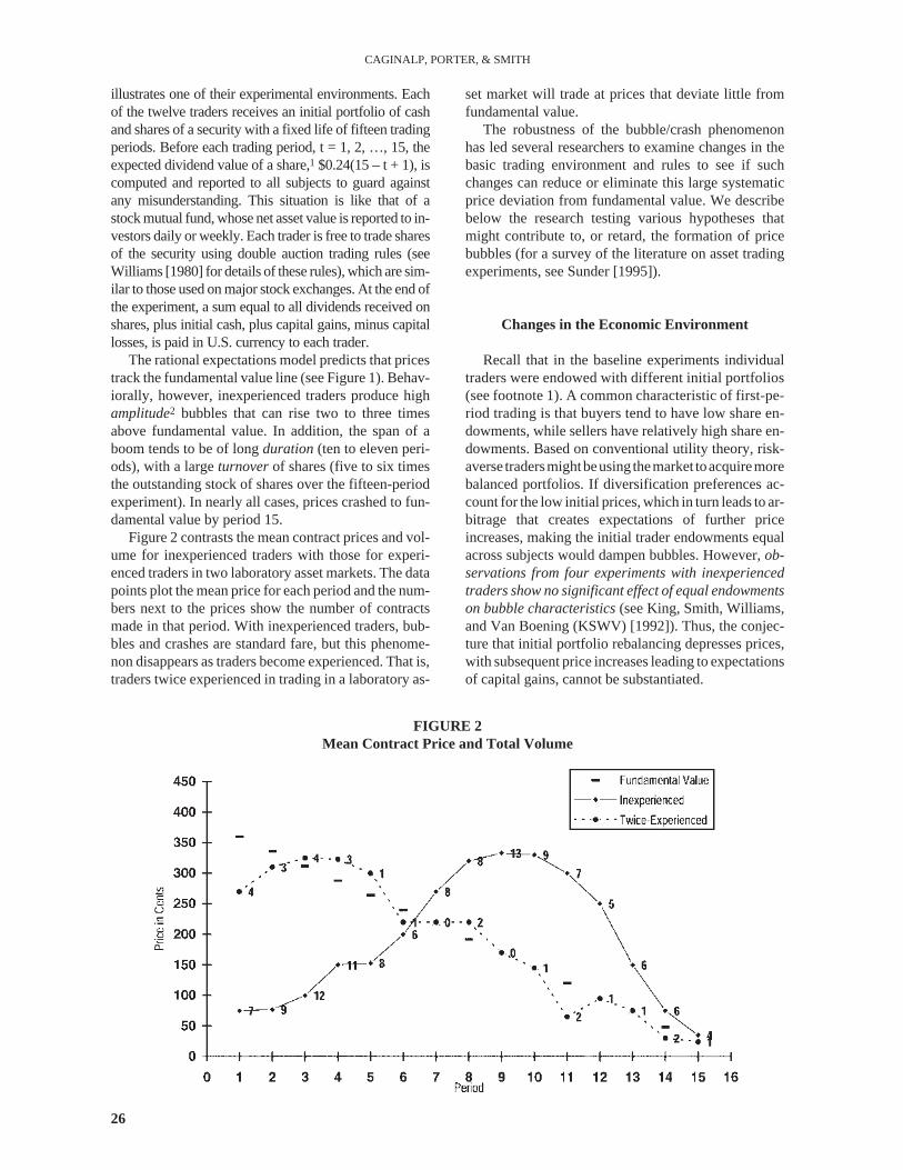
Asecondconjecturebasedon riskaversiondealswithprice expectations due to dividend uncertainty. In thiscase, itmaybe thatadivergenceofexpectationsconcern-ing dividends can cause price increases in early periodswhenthecumulativedividendvariance is largest (thesin-gle-period variance is 26.73 cents, so the variance of thesumofdividendsatperiodt is [15–(t–1)]×26.73cents).Theeliminationofsuchuncertaintyshould reduce these-verity of bubbles if this conjecture is true.

Experiments by Porter and Smith (PS) [1995] showthat the elimination of dividend uncertainty is not asufficient condition to eliminate bubbles (see Figure 3for an example). In particular,when the dividend draweach period is set equal to the one-period expected div-idend value, so that the asset dividend stream is cer-tain, bubbles still occur and are not significantlydifferent from the case with dividend uncertainty.Thisis consistent with the hypothesis that an important fac-tor in the occurrence of bubbles is traders’ uncertaintyabout the behavior of other traders. The bubble is allbut eliminated, however, when dividends are certainand subjects are more experienced, which suggests thatdividend certainty assists traders in achieving commonexpectations of value.

Lei, Noussair, and Plott [1998] investigate the capi-tal gains expectation motivation for bubbles through aseries of experiments that try to eliminate this motiva-tion. In one treatment, they restrict the trading mecha-nism by not allowing reselling, so that the ability tocapture capital gains is eliminated. They restrict therole of each subject to that ofeithera buyer or a seller;

this artificial restriction eliminates the ability of anysubject to buy for the purpose of resale. They find thatthey are able to reproduce the empirical patterns ofprevious bubble experiments.

Rational expectations theory predicts that anyoneaware of the tendency of traders to overreact in thesemarkets could engage in profitable arbitrage. Thus,knowledgeable traders will take advantage of these op-portunities, thus dampening the price volatility in thesemarkets. KSWV test this hypothesis by creating a set of“insider” traders. Specifically, three graduate studentsread the SSW paper, and were given data on the perfor-mance of a group of inexperienced undergraduates, whoreturned for a second session as uninformed but experi-enced subjects. The graduate students then participatedin this session as informed “insiders” and were givensummary information on the number of bids and offersentered at the end of each period (SSW showed that theexcess number of bids over offers in a period was posi-tively correlated with the change in mean price from thecurrent to the next period; see section VIIB). These in-formed subjects participated in markets with six or nineuninformed traders recruited as above. In addition tohaving the same share endowments as the uninformedtraders, the informed traders each had a capacity to sellshares borrowed from the experimenters. These shortsales had to be repurchased and returned to the experi-menter before the close of period 15. While the resultsprovide support forthe rational expectations predictionwhen the uninformed subjects are experienced, as de-scribed above, when the uninformed traders are inexpe-

27


FIGURE 3Mean Contract Price and Total Volume: Certain Dividend

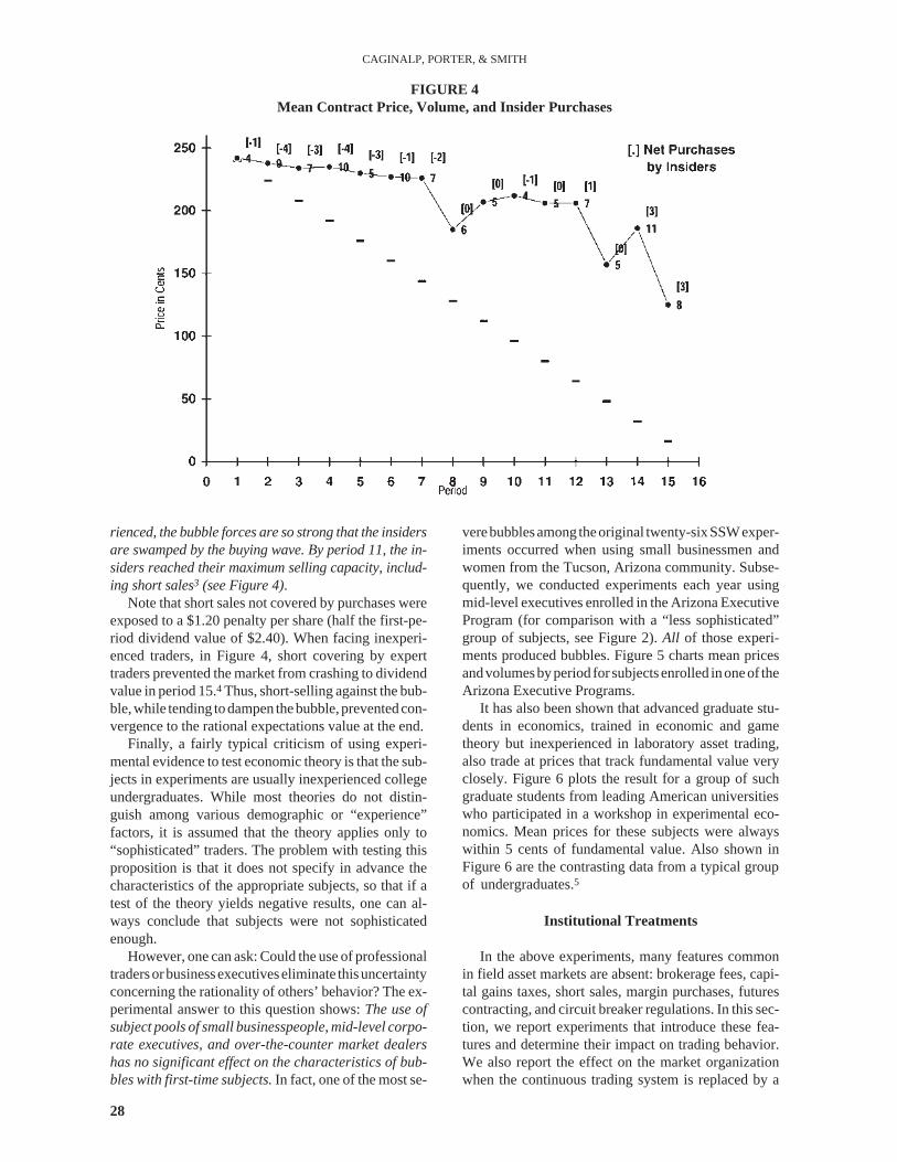
rienced, the bubble forces are so strong that the insidersare swamped by the buying wave. By period 11, the in-siders reached their maximum selling capacity, includ-ing short sales3 (see Figure 4).

Note that short sales not covered by purchases wereexposed to a $1.20 penalty per share (half the first-pe-riod dividend value of $2.40). When facing inexperi-enced traders, in Figure 4, short covering by experttraders prevented the market from crashing to dividendvalue in period 15.4 Thus, short-selling against the bub-ble,while tending todampen thebubble,preventedcon-vergence to the rational expectations value at the end.

Finally, a fairly typical criticism of using experi-mental evidence to test economic theory is that the sub-jects in experiments are usually inexperienced collegeundergraduates. While most theories do not distin-guish among various demographic or “experience”factors, it is assumed that the theory applies only to“sophisticated” traders. The problem with testing thisproposition is that it does not specify in advance thecharacteristics of the appropriate subjects, so that if atest of the theory yields negative results, one can al-ways conclude that subjects were not sophisticatedenough.

However, one can ask: Could the use of professionaltradersorbusinessexecutiveseliminate thisuncertaintyconcerning the rationality of others’ behavior? The ex-perimental answer to this question shows:The use ofsubject pools of small businesspeople, mid-level corpo-rate executives, and over-the-counter market dealershas no significant effect on the characteristics of bub-bles with first-time subjects.In fact, one of the most se-

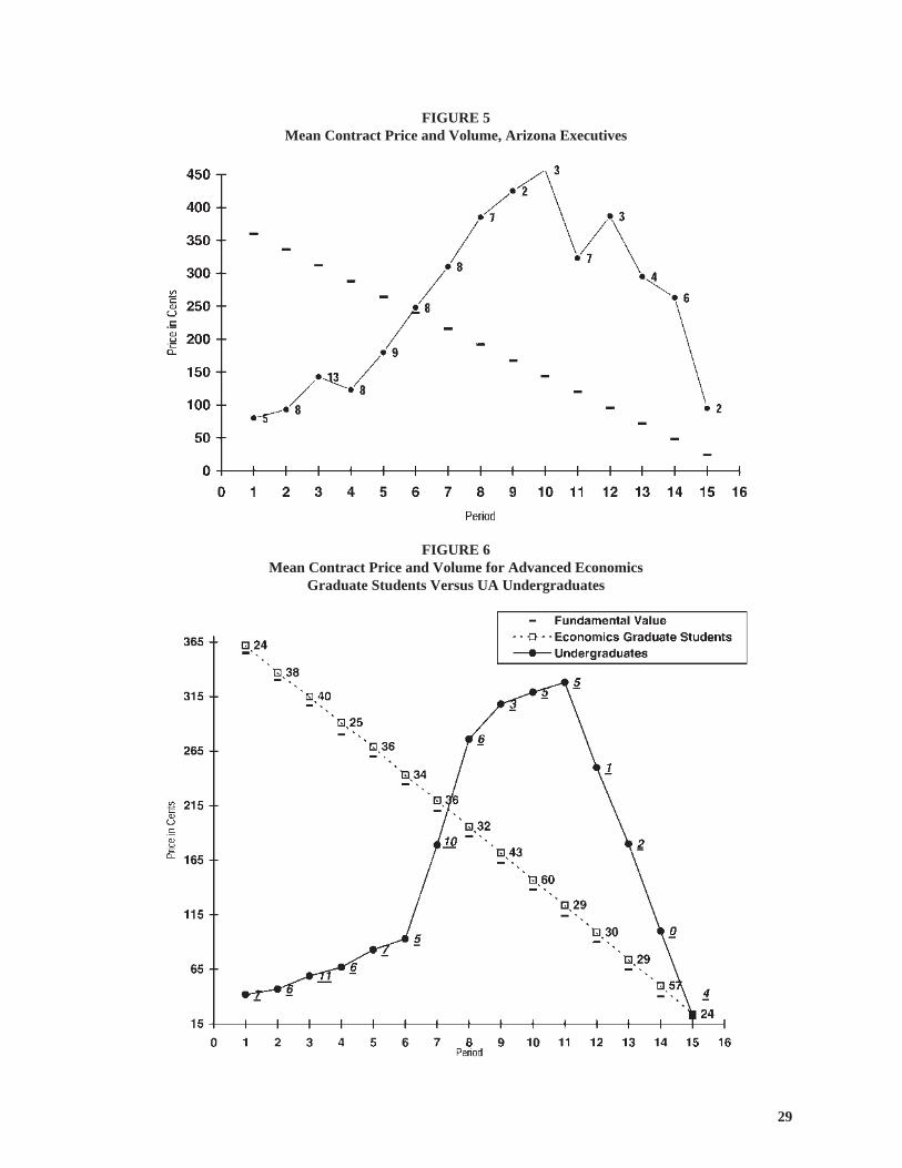
verebubblesamongtheoriginal twenty-sixSSWexper-iments occurred when using small businessmen andwomen from the Tucson, Arizona community. Subse-quently, we conducted experiments each year usingmid-level executives enrolled in the Arizona ExecutiveProgram (for comparison with a “less sophisticated”group of subjects, see Figure 2).All of those experi-ments produced bubbles. Figure 5 charts mean pricesandvolumesbyperiod forsubjectsenrolled inoneof theArizona Executive Programs.

It has also been shown that advanced graduate stu-dents in economics, trained in economic and gametheory but inexperienced in laboratory asset trading,also trade at prices that track fundamental value veryclosely. Figure 6 plots the result for a group of suchgraduate students from leading American universitieswho participated in a workshop in experimental eco-nomics. Mean prices for these subjects were alwayswithin 5 cents of fundamental value. Also shown inFigure 6 are the contrasting data from a typical groupof undergraduates.5

Institutional Treatments

In the above experiments, many features commonin field asset markets are absent: brokerage fees, capi-tal gains taxes, short sales, margin purchases, futurescontracting, and circuit breaker regulations. In this sec-tion, we report experiments that introduce these fea-tures and determine their impact on trading behavior.We also report the effect on the market organizationwhen the continuous trading system is replaced by a

28


FIGURE 4Mean Contract Price, Volume, and Insider Purchases

29

FIGURE 5Mean Contract Price and Volume, Arizona Executives

FIGURE 6Mean Contract Price and Volume for Advanced Economics

Graduate Students Versus UA Undergraduates

call market in which all orders are aggregated at the be-ginning of a period and all trades are made at the callwith one market clearing price. We conducted experi-ments on each of these features individually. We didnot conduct any experiments that included all thechanges (transaction costs, certain dividend, futures,short-selling, insider, and so on). From the data, wesuspect that futures, short-selling, and insiders have astrong effect on reducing the magnitude of the bubble,while the effect of the others is neutral, and marginbuying only makes things “worse.”

Brokerage Fees/Capital Gains Taxes

The market used to trade assets in these experimentshas low participation costs of trading, since subjectsonly have to touch a button to accept standing bids orasks (the same is essentially true now of trading via on-line brokers). This, coupled with the conjecture thatlaboratory subjects may believe they are expected totrade, may result in price patterns that deviate from ra-tional expectations equilibrium. One way to test thetransactions cost hypothesis is to impose a fee on eachexchange. The addition of this brokerage fee has verylittle effect on bubble characteristics. In particular,a20 cent fee on each trade (10 cents each on the buyerand seller) had no significant effect on the amplitude,duration, or share turnover.

In addition to transaction fees, bubbles may formdue to capital gains expectations and the “greater fool”theory. To dampen this form of price expectations for-mation, Lei, Noussair, and Plott [LNP] [1998] imposea capital gains tax of 50% on all traders.They find thatthe capital gains tax does not reduce the tendency forbubbles to occur. Either other factors account for bub-bles, or capital gains expectations are strong enoughto overcome reductions in their profitability.

Contracting Forms (Short Sales,Margin Buying, and Futures)

If individual traders could take a position on eitherside of the market and leverage their sales by sellingborrowed shares (taking a short position), or leveragetheir purchases by buying with borrowed funds (mar-gin buying), it is conjectured that traders who believeprices should be at fundamental value can offset theoverreaction of other traders. KSWV conducted sev-eral experiments in which subjects were given a zerointerest loan, with principal repaid at the end of the ex-periment so that margin buying was possible. In addi-tion, subjects were also given the ability to sellborrowed shares that had to be returned by the end ofthe experiment. Neither condition, margin funds or theability to sell short, is sufficient to reduce bubble char-

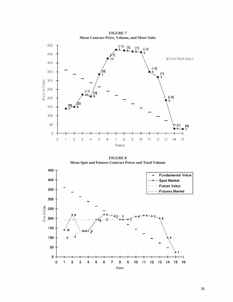
acteristics; in the case of margin buying, the bubble be-comes worse.Margin buying opportunities cause asignificant increase in the amplitude of bubbles for in-experienced traders. Short-selling does not signifi-cantly diminish the amplitude and duration of bubbles,but the volume of trade is increased significantly. Fig-ure 7 provides an example.

Figure 7 highlights the problem of the timing ofshort sales. In periods 6, 7, and 10, net short sales arenegative, indicating net purchases to cover short posi-tions. In period 13, net short sales are zero. All thesecovering purchases are at prices near the peak of thebubble, and therefore tend to exacerbate the bubble.But the traders could not know this, and behaved as ifprices would continue upward.

One major criticism of the contracting form usedin the original experiments of SSW is that traderscan-not obtain information about potential future pricesthrough the market. Specifically, traders must formprice expectations internally, without any marketmeans to calibrate their expectations. In the field,traders have access to prices in futures markets to helpthem hedge risks and to get a market reading on futureprice expectations. A futures market could provideimmediate feedback to traders who can see that thebubble is not likely to persist, and thus allow ebullientexpectations to unravel.

To test this hypothesis, PS ran two sequences oftwo experiments with subjects who were first trainedin the mechanics of a futures market. In the trainingsequences, subjects participated in a series of two-pe-riod markets, with futures contracts in period 1 ma-turing in period 2. In this manner, subjects learnedthat a futures contract is equivalent to a cash contractin the period in which it expires, and should trade atthe same price. In the new treatment experiments, afutures contract expiring in period 8 was used, andagents could trade both the spot and the period 8 fu-tures contracts in periods 1–8; after period 8, only thespot market was active. This contracting regime pro-vides observations (futures’ contract prices) on thegroup’s period 8 expectations during the first sevenperiods of the market.

Figure 8 shows the results of one of these futuresmarket experiments (the other experiment did not con-verge to dividend value in period 8, but produced asmaller bubble than is common without a futures mar-ket). In particular,futures markets dampen, but do noteliminate, bubbles by speeding up the process by whichtraders form common expectations. Note that the spotmarket trades at mean prices less than fundamentalvalue for the first seven periods, while the futures mar-ket trades at, or under, the period 8 share value for thefirst seven periods. But the trades are minimally ratio-nal in the sense that spot shares trade at prices abovethe futures prices (spot shares have higher dividendvalues than a future on period 8).

30


31

FIGURE 7Mean Contract Price, Volume, and Short Sales

FIGURE 8Mean Spot and Futures Contract Prices and Total Volume

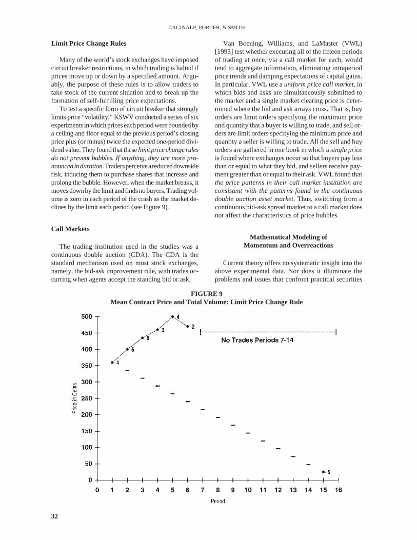
Limit Price Change Rules

Many of the world’s stock exchanges have imposedcircuit breaker restrictions, in which trading is halted ifprices move up or down by a specified amount. Argu-ably, the purpose of these rules is to allow traders totake stock of the current situation and to break up theformation of self-fulfilling price expectations.

To test a specific form of circuit breaker that stronglylimits price “volatility,” KSWV conducted a series of sixexperiments inwhichpriceseachperiodwereboundedbya ceiling and floor equal to the previous period’s closingprice plus (or minus) twice the expected one-period divi-dend value. They found that theselimit price change rulesdo not prevent bubbles. If anything, they are more pro-nouncedinduration.Tradersperceiveareduceddownsiderisk, inducing them to purchase shares that increase andprolong the bubble. However, when the market breaks, itmovesdownby the limitand findsnobuyers.Tradingvol-ume is zero in each period of the crash as the market de-clines by the limit each period (see Figure 9).

Call Markets

The trading institution used in the studies was acontinuous double auction (CDA). The CDA is thestandard mechanism used on most stock exchanges,namely, the bid-ask improvement rule, with trades oc-curring when agents accept the standing bid or ask.

Van Boening, Williams, and LaMaster (VWL)[1993] test whether executing all of the fifteen periodsof trading at once, via a call market for each, wouldtend to aggregate information, eliminating intraperiodprice trends and damping expectations of capital gains.In particular, VWL use auniform price call market,inwhich bids and asks are simultaneously submitted tothe market and a single market clearing price is deter-mined where the bid and ask arrays cross. That is, buyorders are limit orders specifying the maximum priceand quantity that a buyer is willing to trade, and sell or-ders are limit orders specifying the minimum price andquantity a seller is willing to trade. All the sell and buyorders are gathered in one book in which asingle priceis found where exchanges occur so that buyers pay lessthan or equal to what they bid, and sellers receive pay-ment greater than or equal to their ask. VWL found thatthe price patterns in their call market institution areconsistent with the patterns found in the continuousdouble auction asset market. Thus, switching from acontinuous bid-ask spread market to a call market doesnot affect the characteristics of price bubbles.

Mathematical Modeling ofMomentum and Overreactions

Current theory offers no systematic insight into theabove experimental data. Nor does it illuminate theproblems and issues that confront practical securities

32


FIGURE 9Mean Contract Price and Total Volume: Limit Price Change Rule

trading and marketing. In particular, the prolonged de-viations from fundamental value (or dividend value inthe experiments), large price movements in the ab-sence of significant news, and sudden unexpectedcrashes are puzzling in terms of classical theories.These theories assume unlimited arbitrage capital andunbounded rationality, which would restore prices to re-alistic value before deviations became large. In 1998,both of these assumptions were severely strained by thedemise of Long Term Capital Management, whose pri-mary investment strategy was to conduct option arbi-trage based on the Black-Scholes model (see Frantzand Truell [1998]).

The inability of current theories to explain, evenqualitatively, some key features of experiments andpractical experience has led to an examination of thesetheoriesandtheextent towhichtheyneedtobemodifiedto be compatible with the observations. Classical eco-nomics focuses primarily on equilibrium phenomena.Modern theories that explain the time evolution towardequilibrium have often used differential equations, usu-allywithaprobabilisticorstochasticcomponent.Acen-tral assumption has involved the dependence of thechangeofpriceon thedeviation of theprice fromfunda-mental value. This precludes any overshooting of theprice through that fundamental value, and is thereforeincapable of describing overreactions and oscilla-tions in the market (except through random or sto-chastic factors). In mathematical terms, the role ofprice change history (or in trading terminology, thetrend) is neglected.

A second concept key to the traditional theories isthe assumption of infinite capital that is available toeliminate market inefficiencies. In practice (as in theexperiments), the pool of money available is limited.Underwriters, for example, are keenly aware that ifthey bring too much supply to the marketplace, theprice of the asset will suffer, even though the valuationmay be sound.

We discuss next a theoretical development based onmaking these two important changes (i.e., incorporat-ing price trend and the finiteness of cash and assets)within a differential equations framework that relatesthe change in price to the underlying microeconomicmotivations for buying and selling, similarly to themodern theories of price adjustment.

In addition to these issues, a large body of research,known as technical analysis, attempts to identify pat-terns on price charts that may indicate whether a trendis likely to continue or terminate. Of course, such apossibility is ruled out by the (weak) efficient markethypothesis, which maintains that prices alone have nopredictive value. Many academicians are quite skepti-cal of these ideas, while some practitioners use themroutinely in trading and marketing securities.

Modern theories of price adjustment (see, e.g.,Watson and Getz [1981]) stipulate that relative price

change occurs in order to restore a balance betweensupply,s, and demandd, each of which depend onprice:

wherep(t) is the price of a share at timet,andd(p)/s(p)–1 is excess demand (normalized by supply). Equation(5.1) implies that the relative change in price dependsupon a function,F, of demand and supply at that price,p. This function,F, must have the property that whensupply and demand are equal there is no change inprice. On the other hand, when demand exceeds supply,so thatd(p)/s(p) > 1, prices rise, and conversely, whensupply exceeds demand, so thatd(p)/s(p) < 1, pricesfall.

The larger the ratio of demand to supply, the morerapidly prices rise.

In mathematical terms, this means that the functionF has the properties

With the standard assumptions thatd(p) ands(p) aremonotonic, condition (5.2) ensures that this equilib-rium point is unique.

Thevastmajorityof thephenomenadiscussedprevi-ously cannot be explained on the basis of this formula-tion. In Caginalp and Ermentrout [1990] and Caginalpand Balenovich [1994], the basic theories were general-ized by preserving as much of the foundation as possi-ble, e.g., the structure of the price equation, whilemodifying some of the concepts that are in clear conflictwith the experiments. Studies showed that in laboratoryexperiments such as PS (see Figure 3), current priceswere strongly influenced by previous prices. This trenddependence would be difficult to explain with supplyand demand depending on price alone.

The next step in specifying the detailed form of theequations is to determine a functional form ofd ands.The comments above justify the dependence of de-mand and supply on price trend as well as price itself.This is expressed generally as

We need to specify the dependence of demand, d, andsupply,s,on the price,p, and price derivative,p´. Thisdependence is achieved through an investor sentimentfunction,ζ, that includes all motivations for purchasingthe asset. The investor sentiment determines an indexor flow function,k, which measures the flow from cashto the asset. One can regardk probabilistically as thelikelihood that a unit of cash will be submitted for a pur-chase order of the asset. Consequently,k must take on

33


( ) ( )( )

( )( )

−= = =

1log (5.1)

d p s p d pd dpp G F

dt p dt s p s p

( )= >′1 0 and 0 (5.2)F F

( ) ( )( )

′= ′

,log (5.3)

,

d p pdp F

dt s p p

values between 0 and 1. When k is close to 1, investorsare eager to buy the asset, and whenk is near 0, theyhave little interest. Sinceζ can take on any value, weneed a transformation fromζ to k. This is achievedthrough a smooth function, such as that seen in (5.5) inthe Appendix. In principle, this sentiment function,ζ,can depend on a variety of factors that influence inves-tor decisions. We focus on two factors: the price trend,ζ1 , and fundamental valuation,ζ2.

As discussed in the Appendix, Equations (5.6´) and(5.7´) express the simplest mathematical expressionfor these ideas. Equation (5.6´) expressesζ1 as the rela-tive price change multiplied by a factor,q1, which indi-cates the weighting that the investor group places uponthe trend. Equation (5.7´) stipulates thatζ2 is a weight-ing factor,q2, times the relative discount of the pricefrom the fundamental value,pa(t). At a deeper level,we can expressζ in terms of its dependence on theprice changes in the past with the more recent eventsweighted most strongly. This leads to (5.6). A similardelay effect in terms of recognizing undervaluation isexpressed by (5.7).

Thus, Equations (5.3)-(5.7) constitute a system ofdifferential equations (the momentum model) that canbe studied computationally upon specifying the pa-rameters such asq1 and q2. These constants are notknown but can be evaluated experimentally for a par-ticular investor group. Then, one can use the computercalculations for the differential equations to predictprice behavior in subsequent experiments.

We derive a system of differential equations withina general class represented by (5.3) next (see the ap-pendix for a derivation and exposition of these equa-tions). Generally, we denote flow demand rates (adesired rate of accumulation of asset shares) and flowsupply rates (a desired rate of accumulation of cash)using lower-case symbols as above in Equation (5.1),while upper-case symbols are used to denote finitesupplies of shares or cash.

We describe a mathematical model that involves aclosed system (i.e., a fixed number of shares of a singleasset plus a fixed amount of cash). This is ideallysuited for studying the asset market experiments. Themathematical system can also be generalized to incor-porate influxes or outflows of cash or shares into theexperiment.

We begin by stating some stock flow identities,then introduce the equations representing the behav-ioral assumptions that underpin the sentiments gov-erning the supply and demand rates. We analyze aclosed system containingM dollars andSshares. Thedemand,d, for shares is expressed as the availablecash multiplied by the rate,k (normalized so that it as-sumes values between 0 and 1), that investors desireto accumulate shares (place purchase orders) . A simi-lar description applies to the desire to accumulatecash (place sell orders). If we letB be the fraction of

the total value of assets held in the form of shares (1 –B is the fraction held in cash), thenB = pS/(pS + M),and thestock-flowidentitiesweusecanbewrittenas:

All the behavioral features of this system will be de-fined in terms ofk, wherek can be thought of as the ve-locity (turnover) of the stock of money required toexpress the demand for shares in this closed system.Similarly,1 – kis the velocity of the stock of shares re-quired to express the supply of shares.

To develop the behavioral hypotheses concerningmarket decisions, letpa(t) denote the fundamentalvalue of a share at timet. If k depended only onpa(t),we would have a generalization of the theory of priceadjustment written in terms of thefinitenessof assetsand delay in taking action. However, if the ratek isspecified throughinvestor sentiments,the desire to ac-cumulate shares, or preference for shares over cash,then price can adjust based on investor perceptions.

To understand the dependence of investor senti-ment on the history of price change, consider the moti-vation of an investor who owns the security as it isundervalued but still declining. The choice available tothis investor is to either sell or to wait in the expecta-tion that those with cash will see the opportunity toprofit by purchasing the undervalued security. The is-sue of distinguishing between self-maximizing behav-ior and reliance on optimizing behavior of others isconsidered in the experiments of Beard and Beil[1994] on the Rosenthal conjecture [1981] that showedthe unwillingness of many agents to rely on others’ op-timizing behavior. Not everyone assumes that otherswill automatically act in their immediate self-interest.

The dynamical system is closed by relating twotypes of investor sentiment into trading motivations. Inparticular, the total investor sentiment or preferencefunction is expressed as thesumof the price trend andthe price deviation from fundamental value.6 In eachcase, the basic motivation is summed with a weightingfactor that declines as elapsed time increases. In thecase of the trend, this means that recent price changeshave a larger influence than older ones. For the funda-mental component, it means that there is some lag timebetween an undervaluation and investor action. Theweighting factors are assumed to be exponentials, sothat there is a gradual decline in the influence of a par-ticular event.

In general, when price is below fundamentals, valueinvestors start buying shares, thereby moving the pricehigher. This provides a signal that draws trend-basedbuyers into the market, precipitating a further increasein the rate of price change, which further fuels the priceincreases. As prices rise above fundamentals, value in-vestors start to sell, increasing their liquidity and re-

34


( ) ( ) −= − = − = ⋅−

11 , 1 , and (5.4)

1

d k Bd k B s k B

s k B

ducing the liquidity of trend-based investors. As thetrend reverses, the momentum traders continue thesell-off until prices drop to (or below) fundamentalvalue.

The numerical computations of the model confirmthat if thetrend-basedcoefficient issufficientlysmall, thepriceevolves rapidly towardpa(t)with littleornooscilla-tion. This corresponds to a classical rational expectationmodel (seeTirole [1982]). If trend-basedmotivationsareincreased further, the price oscillations increase in mag-nitude and frequency. As the trend-based motivationsare increased, they reach a point where the price oscilla-tions become unstable in the sense that they increase inmagnitude without bound. Behavior in this model is re-flected in an increased (or decreased) desire to accumu-late shares, but of course it is impossible for the marketas a whole to acquire more shares, the quantity of whichis fixed. So autonomous changes in the desire to accu-mulate shares alter the price by precisely the amount re-quired to induce a desire in the market as a whole to holdthe existing stock. But the relative holdings of that stockby different types of investors will change over time aspart of the equilibrating process. The equilibrium is notthat of rational expectations theory unless there are nomomentum traders and all investors are motivated byfundamentals.

What is the extent to which these equations can pre-dict the price evolution in experiments? In principle,once one knows the dividend structure and the tradingprice of period 1, the rest of the trading prices can bepredicted if the parameters have already been esti-mated from previous experiments. This out-of-sampleprediction approach has been implemented and com-pared with other methods (see Caginalp, Porter, andSmith [1999]), and is discussed in Section VIII.

Applying Principles From theLaboratory to Field Data

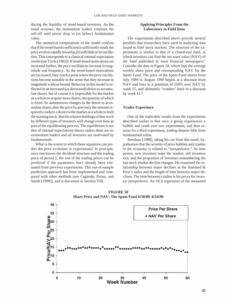
The experiments described above provide severalparallels that researchers have used in analyzing datafound in field stock markets. The structure of the ex-periments is similar to that of a closed-end fund, inwhich investors can find the net asset value (NAV) ofthe fund published in most financial newspapers.7

Consider the data in Figure 10, which lists the averageweekly share price and corresponding NAV for theSpain Fund. The price of the Spain Fund shares fromJuly 1989 to August 1990 begins at a discount fromNAV and rises to a premium of 250% over NAV byweek 15, and ultimately “crashes” back to a discountby week 61.8

Trader Experience

One of the replicable results from the experimentsdescribed earlier is that once a group experiences abubble and crash over two experiments, and then re-turns for a third experiment, trading departs little fromfundamental value.

Renshaw [1988], taking his cue from this result, hy-pothesizes that the severity of price bubbles and crashesin the economy is related to “inexperience.” As timepasses, new investors enter the market, old investorsexit, and the proportion of investors remembering thelast stock market decline changes. He examined the re-lationship between major declines in the Standard &Poor’s index and the length of time between major de-clines. The time between crashes is his proxy for inves-tor inexperience. An OLS regression of the measured

35


FIGURE 10Share Price and NAV: The Spain Fund 6/30/89–8/24/90

extent of the index’s decline,Y, on the time since theprevious decline,X, yields the estimate:

The greater the magnitude of a crash in prices, the lon-ger it will be before its memory fades and we observethe termination of a new bubble-crash cycle. This anal-ysis, unlike the replication of laboratory experiments,cannot distinguish between events that are spaced farapart in time because they are rare events, and thecausal effect hypothesized by the regression. Hence,this relationship may be suspect.

Time Series Methods as LinkBetween the Laboratory and the Field

Differential equations are a powerful modelingtool, because they incorporate specific postulatedforms of behavior and impose physical constraints likethe conservation of cash and shares. On the other hand,the assumptions used to derive the equations may becontroversial. We address this point by applying non-parametric statistical tests of the predictions of the dif-ferential equations to data from experiments in whichwe control variables such as dividend value and the in-ventory of cash and shares.

Another approach to modeling is standard time se-ries analysis, which addresses two key questions. First,can one identify momentum and the extent to which itinfluences price movements in world markets, andthen use this information to make out-of-sample pre-dictions? Second, can one use these procedures tomake a quantitative link between the phenomena ob-served in laboratory experiments and world marketdata?

A very simple model for understanding asset pricesis the random walkmodel, which relates the price attimet, denotedy(t), to the price one time unit ago in thefollowing way:

wherew(t) is a sequence of independent random distur-bances with zero means and equal variances (seeShumway [1988, p. 129]). This is the simplest of theBox-Jenkins or ARIMA models, which can be summa-rized as follows.

The basic ARIMA models involve componentsthat are autoregressive (AR), meaning they link thepresent observation componentsy(t) with those up toh times earlier,{y(t – 1),…,y(t – h)}, and the movingaverages (MA) of the error terms experienced in theprevious q members of the time series,{ε(t – 1), …,ε(t – q)}. The observations, y(t), can be differenced

(denoted∆) so that if the original series is non-sta-tionary, the methods are applied to the sequencew(t):=∆y(t), which is the sequence{y(t)} differencedvtimes. The general (ARIMA(h, v, q) model can thenbe written as:

in terms of the coefficients or “process parameters”φandθ. In particular, ARIMA (0, 1, 0), i.e.,h = 0, v = 1, q= 0, is just ordinary random walk, while ARIMA (0, 1,1) is simply an exponential smoothing scheme.

Analyzing market data is generally difficult, as itis influenced by many random unknown changes infundamentals. To control for this, Caginalp andConstantine [1995] used data on two closed-endfunds, the Future Germany Fund (FGF) and the Ger-many Fund (GF), consisting of thesame portfolioand having the same manager. Closed-end fundstrade like ordinary stocks, and may have a premiumor discount to the net asset value (NAV). The funda-mental changes are identical for the two stocks sothat the ratio of the price of the two funds should notchange during the time period. They define

and analyzed the time series of closing prices from theinception of the latter fund (FGF) until the 1,149th day.The efficient market hypothesis, which would predictthat y(t) would fluctuate randomly around a value ofunity, was tested using the “sign test” and the “turningpoint test” (see, for example, Krishnaiah and Sen[1984]).

For the entire data, the number of runs deviated by29 standard deviations from that expected from thenull hypothesis of constant value plus noise. Similarly,the turning point test deviated by 6.8 standard devia-tions from the null hypothesis. The standard deviationof a data set is a measure of its dispersion, so a largestandard deviation corresponds to a high probabilitythat a particular measurement will fall far from itsmean, while a small standard deviation means it willlikely be close to its mean. If a set of measurements de-viates by two or more standard deviations from themean, it is very unlikely to be a result of randomness.

Once the null hypothesis has been rejected, theBox-Jenkins procedure can be applied. Applyingthis procedure to the entire data, they found thatv=1 is necessary and sufficient. Examination of theautocorrelation function resulted inh = 1 andq = 1,as the correlations drop dramatically in the next or-der. The emergence of a particular ARIMA model,i.e., (1, 1, 1), rather than the (0, 1, 0) associatedwith random walk, further confirmed the existence

36


( )= + =

=

25.5 0.90 ; 0.98

15.1

Y X R

t

( ) ( ) ( )= − +1 (6.1)y t y t w t

( ) ( ) ( ) ( )( ) ( )1 2

0 1

1 2

(6.2)

v

q

w t w t w t w t h

t t q

= φ − + φ − + + φ − +

ε +θ −θ − −θ ε −

…

…

( )=Price of

(6.3)Price of

t

t

FGFy t

GF

of trend-based (momentum) components in thedata. The ARIMA model selected by the data usingthis procedure was found to be

The coefficients 0.5 and 0.8 are 9.6 and 21.6 standarddeviations, respectively, away from null hypothesisvalues of 0, in which yesterday’s price is the best pre-dictor of today’s price.

Consequently, the concept of a lagged differencestructure emerged quite naturally from the data, asEquation (6.4) is a relation between today’s rate ofchange,y(t) – y(t – 1),compared with yesterday’s,y(t –1) – y(t – 2).Thus, the ARIMA procedure leads to theconclusion that the best predictor of prices is very farfrom a random perturbation from yesterday’s price.

The results suggest a very basic motivation in trad-ing. In the absence of any change in fundamentalvalue, there are two simple views possible about pricemovement: 1) that price will be essentially unchangedfrom the day before, and 2) that today’s pricechangewill be essentially unchanged from yesterday’s. Thecoefficient 0.5 in Equation (6.4) effectively interpo-lates between the two strategies and indicates that theinvestors who generated this data set were equally in-clined to be influenced by yesterday’s price change asthey were by the price itself.

In financial forecasting, the use of “out-of-sample”predictions is a valuable test to ensure that there is no“overfitting” of the data. Caginalp and Constantine[1995] used the first-quarter data (the first sixty-fourdays) to predict this quotient during the next ten dayswithout updating the coefficients. The actual values fordays 65 to 74 were well within the 95% confidenceregions.

In a more extensive test, they also used the ARIMA(1, 1, 1) model to forecast with updated coefficients byusing the firstN days in order to estimate the coeffi-cients and to forecast the(N + 1)th day’s quotient. Be-ginning with the first sixty-four days, they predicted thenext quarter’s price quotients on a day-by-day basis.The predictions were again within the 95% confidenceintervals and were better than both the random walk pre-diction and the constant ratio (efficient market) predic-tions by three standard deviations, as measured by theWilcoxon matched pairs signed ranks test or binomialdistribution comparisons.

Such statistical methods can potentially establish aquantitative link between the laboratory experimentsand the world markets. Toward this end, the ARIMAmodel and coefficients constructed using the firstquarter of the FGF/GER data are used to forecast theexperiments done by PS. In the set of experimentsconsidered, the participants traded a financial instru-

ment that pays 24 cents during each of fifteen peri-ods. Hence, the fundamental values of the instrumentare given by

We let P(t) denote the experimental values of price,Pa(t) the fundamental value determined by summingthe expected dividends at that time, and define

We can apply the same time series framework used fory(t) = FGF/GER. The time seriesy(t)andx(t)both pos-sess the key property that the temporal changes in theirfundamental value have been eliminated. Conse-quently, the efficient market hypothesis predicts thesame value (in time) for both.

We would like to examine the extent to which datafrom world markets can be used to predict experi-ments and vice versa. If this can be done success-fully, it would provide considerable evidence that themechanism underlying price dynamics is similar inboth cases. It would also lend support to the conceptof searching for microeconomic mechanisms forprice change in the absence of fundamental changesin valuation.

Toward this end, Caginalp and Constantine [1995]used the ARIMA(1, 1, 1) model with the coefficientsobtained from the FGF/GER data to make predictionson the experiments. These predictions were then com-pared with the null hypothesis, namely, thatx(t) = 1 forall t.

The Wilcoxon paired difference test confirms thatthe ARIMA(1, 1, 1) with the original coefficients al-lows rejection of the null hypothesis thatx(t) = 1, witha statistical significance ofp = 0.007. In other words,the probability that the ARIMA model’s superior pre-dictions are attributable to chance is less than 1%. Thisresult is remarkable because not only the model, butthe coefficients as well, have been determined entirelyfrom New York Stock Exchange data.

We believe this is a promising direction for futureresearch in that it allows us to interpret quantitativelythe results of experiments in terms of world markets,and vice versa. It offers the possibility that one can useexperiments to make statements that go beyond quali-tative conclusions and to examine the extent of thatparticular mechanism, because price dynamics are uni-versal across different investor populations.

Testing the MomentumModel: Experiments

If the parameters of the system of differential equa-tions were estimated, it would be possible to predict

37


( )= −3.60 .24 (6.5)aP t t

( ) ( ) ( )=: (6.6)ax t P t P t

( ) ( ) ( ) ( ){ } ( )( )

0.5 1 2

0.8 1 (6.4)

y t y t y t y t t

t

− = − − − + ε +

ε −

the entire price path if we knew the opening priceP(0).Thus, if one could control the opening period price,this model would predict the entire price path. This isthe motivation for the opening period price control ex-periments we discuss next.

Using Price Controls toInitialize the Model

Caginalp, Porter, and Smith (CPS1) [1999] esti-mated, using ordinary least squares, the two parame-ters representing the strength of trend-based (q1) andfundamental value-based (q2) investing from a set ofbaseline experiments in which the opening price is un-constrained. These parameters were then used to deter-mine the price predictions when the opening price isrestricted to trade in a specified range. We used pricecontrols so that we could replicate experiments withidentical opening prices, i.e., we control for the open-ing price. The price controls were always below theinitial $3.60 expected value, and ranged from a controlinterval of [$1.40, $1.60] to [$2.90, $3.10].

Two types of price control experiments were con-ducted. The first set used the standard $0.24 dividend,while the second set doubled the dividend distribution($0.48 in experiment money) and cash, but made theconversion rate of experiment money into U.S. cur-rency one-half, so that there would be no difference inreal money space. Figure 11 provides the momentum

model predictions under the different price controltreatments.

Figures 12 and 13 show the ratioΦt = Pa(t)/Pm(t),wherePa(t) is the actual mean contract price in pe-riod t andPm(t) is the prediction from the momentummodel, for each of the opening price control treat-ments. Thus ifΦt = 1, there is a perfect match be-tween the actual mean price and the momentumprediction for periodt; if Φt > 1, the momentummodel prediction is less than the actual price for pe-riod t; if Φt < 1, the momentum model prediction isgreater than the actual price for periodt. The datasuggest thatthe momentum model underestimatesthe mean contract price in the early trading periodsand overestimates the price in the later trading peri-ods. The data appear to imply that there is an asym-metry between the bull and bear phases of a bubblethat is not captured by the model.

While the momentum model is not predictivewithin 5%, it does have some qualitative propertiesthat can be exploited. Recall that in the momentummodel, when prices are belowPa(t), there is a tendencyfor buy orders to increase due to the expected return.As prices approach fundamental value, the momentumis higher due to increasing prices. Thus, if we considerpositive price differences from one trading period tothe next, the momentum model would predict that thesum of these differences would be greatest when theinitial undervaluation is greatest. The following re-gression was estimated:

38


FIGURE 11Momentum Model Predictions for Various Initial Price Controls

39

FIGURE 12Actual Prices/Momentum Predicted Price ($0.24 Dividend Case)

FIGURE 13Actual Prices/Momentum Predicted Price ($0.48 Dividend Case)

where i indexes the experiment. The prediction is thatβ> 0. CPS1find a larger initial undervaluation producesa larger positive price movement.

It is not surprising that the momentum model didnot accurately predict the entire price path, becausethe momentum model predicts fifteen periods in ad-vance and is independent of the characteristics of thegroup that is trading. Updating, based on current andpast trading activity, would provide a better cali-brated model. In CPS1, we use the previousj – 1 ex-periments to obtain optimal values of the investorsentiment parameters for each of the experiments andaverage these values to get new parameter estimates.This updated calibration method allows the parame-ters to adjust dependent on the most recent informa-tion from the market.

Price Forecasting Models

While the original momentum model does not havehigh predictive powers for large times, it may havebetter predictive power relative to other price forecast-ing models. In CPS1, the momentum model was pittedagainst the following forecasting methods to deter-mine which method predicts best.9

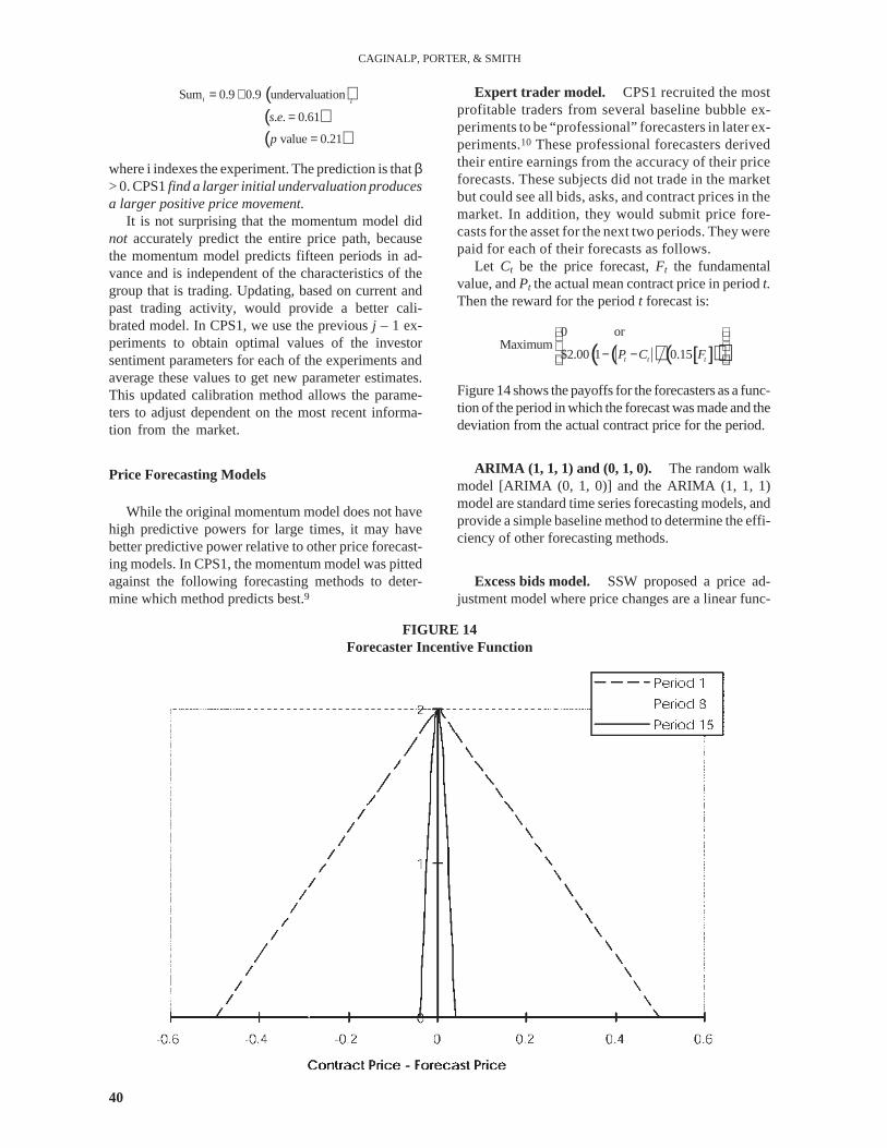
Expert trader model. CPS1 recruited the mostprofitable traders from several baseline bubble ex-periments to be “professional” forecasters in later ex-periments.10 These professional forecasters derivedtheir entire earnings from the accuracy of their priceforecasts. These subjects did not trade in the marketbut could see all bids, asks, and contract prices in themarket. In addition, they would submit price fore-casts for the asset for the next two periods. They werepaid for each of their forecasts as follows.

Let Ct be the price forecast,Ft the fundamentalvalue, andPt the actual mean contract price in periodt.Then the reward for the periodt forecast is:

Figure 14 shows the payoffs for the forecasters as a func-tion of the period in which the forecast was made and thedeviation from the actual contract price for the period.

ARIMA (1, 1, 1) and (0, 1, 0). The random walkmodel [ARIMA (0, 1, 0)] and the ARIMA (1, 1, 1)model are standard time series forecasting models, andprovide a simple baseline method to determine the effi-ciency of other forecasting methods.

Excess bids model. SSW proposed a price ad-justment model where price changes are a linear func-

40


( ) [ ]( )( ) − −

0 orMaximum

$2.00 1 0.15t t tP C F

FIGURE 14Forecaster Incentive Function

( )( )( )

Sum 0.9 0.9 undervaluation

. . 0.61

value 0.21

i i

s e

p

= +

=

=

tion of the excess bids (bids tendered over asks ten-dered). The excess bid variable provides a proxy for theexcess demand for the asset. This is similar to aWalrasianpriceadjustmentmodel,whichstipulates thatprice responds in the direction of the excess demand fortheasset.SSWusethedifferencebetweenthenumberofbids and number of asks submitted as a proxy for excessdemand. In particular, they estimate the following ordi-nary least squares model:11

wherePt is the mean price in periodt,α is minus the one-period expected dividend value (adjusted for any riskaversion),β is adjustment speed,Bt – 1 is the number ofbids tobuytendered inperiodt–1,andOt–1is thenumberof offers to sell tendered in periodt – 1. Price change inthis model has three components: 1) the risk-adjusted perperiod expected dividend payout, 2) an increase (de-crease) due to excess demand arising from homegrowncapital gains (losses) expectations (a Walrasian measureof which is excess bids,Bt – 1–Ot – 1), and 3) unexplainednoise,εt . Forecasting in the experiments uses a leastsquares regression that is updated across all previous ex-periments to obtain the parameter estimate$α and $β. Inparticular, theforecastedpriceinperiodt+1isgivenby:

The results of the forecasting experiments show:

(i) The momentum model and professional fore-casters’ price predictions have similar absoluteerrors.

(ii) The momentum model has superior two-periodahead forecasts relative to the other forecast-ing models.

(iii) The ARIMA models are relatively the worstforecast models.

(iv) The professional forecasters update price pre-dictions based on a forecast surprise.

(v) The excess bids model has a slightly better one-period forecast than the momentum model.

This last result suggests that it may be desirable toincorporate other market information into the momen-tum model in order to update the price path. In particu-lar, the momentum model could incorporate excessbids and forecast surprises into its framework alongwith market conditions (cash and share holdings in themarket).

Liquidity and Price Formation

Rational expectations theory proposes a uniquevalue for a financial instrument that reflects all infor-

mation among the participants as to its worth. Anytemporary moves away from this value will be quicklyarbitraged. However, it is generally recognized by in-vestment houses and traders that a large supply ofstock in the marketplace has a significant and perhapslasting effect on stock prices. Portfolio managers rou-tinely submit large orders slowly over time andthrough various brokers so that they will not causelarge movements of a stock’s price against them asthey seek to change their position. Thus, there is a splitbetween theory and the beliefs that drive practice.Practitioners constantly talk about market “liquidity”as an indication of the ability of stocks to absorb pulsesin the order flow or to maintain a price level or trend.

In this section, we introduce a notion of liquidity thatcanbe interpreted in termsof themomentummodel,andused as a treatment in designing experiments.

Modeling Liquidity Value

Both the experimental evidence and computationsbased on the differential equations suggest that theamount of available cash in relation to shares is a po-tentially important factor in price movement.12 Withinthe realm of rational expectations, there is no mecha-nism for an excess of cash or of the asset to induce de-viations from fundamental value. Any addition to cashbalances will be held in idle accounts if the availableshares are priced at their fundamental value. But this isnot generally true for the momentum model, where anincreased supply of cash may increase purchases ofshares by momentum traders who would like to buy inproportion to the percentage increase in price, but arecash-constrained. We saw in section IVB that when weallowed margin purchases there was a significant in-crease in the amplitude of bubbles. The momentummodel predicts this will occur if any momentumtrader’s purchases are constrained by his cash position.Borrowing allows that constraint to be loosened.

Caginalp and Balenovich [1999] reinterpret theoriginal differential equations to define and analyze li-quidity in a precise manner, as follows. Consider aclosed market containingSshares of an income-gener-ating asset, andM dollars distributed arbitrarily amongparticipants at the outset and subject to change overtime.

Let the price of the single asset be denoted again byp(t) and define liquidity as the ratio of cash to shares,L=M/S, which is measured in dollars per share. Giventhat the relative price changes linearly with excess de-mand we have:

for a time scaleτ0. Thus, from the definitions in (5.4),we find

41


( )+ − −= + α +β −1 1 1ˆˆ

t t t tP P B O

( )− − −− = α +β − + ε1 1 1t t t t tP P B O

τ= −0 1 (8.1)

dp d

p dt s

so thatB-1(1-B)p = L is time-invariant. Equation (8.3)leads to the derivative identity

Note that there is no need for a time scale in this equa-tion. Given the two types of investor sentiment as de-scribed in section V, and the assumption that the transi-tion ratek is a weighted sum of the current derivativeand the valuation discount, we obtain:

where q1 is the coefficient representing trend-basedmotivations andq2 is the coefficient representing fun-damental value motivations.

Using (5.4) and (8.3) in the price equation (8.1) re-sults in

Note that the liquidity value, L, which represents thenominal value of all money in the system divided by thetotal number of shares, is a fundamental scale for price.In particular,p/L is the ratio of asset value to liquidityvalue. Thus, for any givenp, asL increases the rate ofprice change increases.

Experiments Testing Liquidity

This model shows that the liquidity value obtainedby dividing the total cash available by the total numberof shares is a significant counterpart to the fundamen-tal value. We test this hypothesis by conducting experi-ments with a spectrum of liquidity values (cash tostock ratio) ranging from $1.80 to $7.20, i.e., half asmuch cash as stock value to twice as much cash tostock value, in an environment with stock dividendvalue $3.60.

A series of twelve experiments used a sealed bid-of-fer (SBO) one-price clearing mechanism in each trad-ing period (see Van Boening [1991] for auctionmethods). At the end of the fifteenth and final period, asingle payout with expectation value of $3.60 is real-ized (25% probability each for $2.60 and $4.60; 50%probability of $3.60). We used a payout at the last pe-

riod to keep liquidity constant during the experiment.The traders, all first-time participants in an asset mar-ket study, were informed of the expected dividend atthe start of the experiment.

The experiments differ only in liquidity,L, definedto be the (total) initial cash distributed to all partici-pants divided by the total number of shares distributed.Thus, an experiment for which liquidity isL = $7.20begins with twice as much cash as stock value. Usingthe terminology cash-rich and asset-rich forL > $3.60andL < $3.60, respectively, we find, as in earlier ex-periments (see Caginalp, Porter, and Smith [1998]),that cash-rich experiments result in a higher meanprice. A Mann-Whitney test shows that the central ten-dencies of cash-rich experiments (median = $3.73,mean = $3.75) are higher than those of the asset-rich(median =$2.90, mean = $2.83), which is statisticallysignificant at 0.0081. The two-sampleT-test for meansresults in an even stronger statistical significance of0.0007.

Examining a particular period of all experiments,the correlation between price,P(t), and liquidity, L,across all twelve experiments in periodt is given by

Period (t)

1 2 3 4 5 6 7 8 9 10 11 12 13 14 15

.51 .69 .80 .80 .80 .70 .51 .42 .34 .63 .54 .64 .37 .67 .44

Correlation

The data indicate that the influence of liquidity is stron-gest in the first four periods, during which shares andcash move into different participant accounts, and thatit diminishes gradually as the experiment nears the end.To study this, we divide the periods into early (periods1–4), middle (periods 5–11), and late (periods 12–15).A linear regression of price on liquidity results in thefollowing for the three time intervals, respectively:

Thus, an increase of $1 per share of extra cash in themarket means there is a 29 cent increase in the averageprice per share during the first four periods. Near theend of the experiment, the effect is reduced to abouthalf, at 15 cents per dollar of liquidity, but remains sig-nificant. The diminishing role of liquidity is supersededby the fundamental value ($3.60) and culminates in ahigher constant in the later periods.

A more subtle issue is the extent to which pricechanges can be predicted. In particular, does either ofthe quantities

42


( )( )

1 021 2 2 1 (8.5)

1 a

p tqk dpq

k p dt p t

τ= + + − −

( )0 1 (8.6)

1

dp k L

p dt k p

τ= −

−

⋅= − =⋅ + ⋅ +

, 1 (8.2)S p M

B BS p M S p M

(8.3)1

B S p p

B M L

⋅= =−

( )11 (8.4)

dB dpB B

dt p dt= −

( ) 1.92 0.289 (9.1a)P t L= +

( ) 2.74 0.194 (9.1b)P t L= +

( ) 2.84 0.146 (9.1c)P t L= +

predict the next price change,∆P(t) = P(t) - P(t-1) dur-ing any of these time intervals? As the regressionsabove, and Table 1 and Figure 1 indicate, the key pricemovements are in the early periods. Performing sepa-rate linear regressions for∆L and∆P(t-1), we obtain inthe early periods (1–4) the results:

Thus, in the early trading periods, momentum and li-quidity have positive effects on price movements, butthese positive effects cease to be statistically significantin later periods.

We use both statistical and differential equationsmodels to understand the underlying mechanism forthese observations. We list for each time period of eachexperiment the price, the previous two-period prices,and the liquidity value. Sorting the periods, we per-form a regression on each period separately and esti-mate the following statistical model:

Hence, at timet-1 the derivative of the price,∆P(t-1),the deviation from liquidity value∆L and the devia-tion from fundamental value (emerging through the

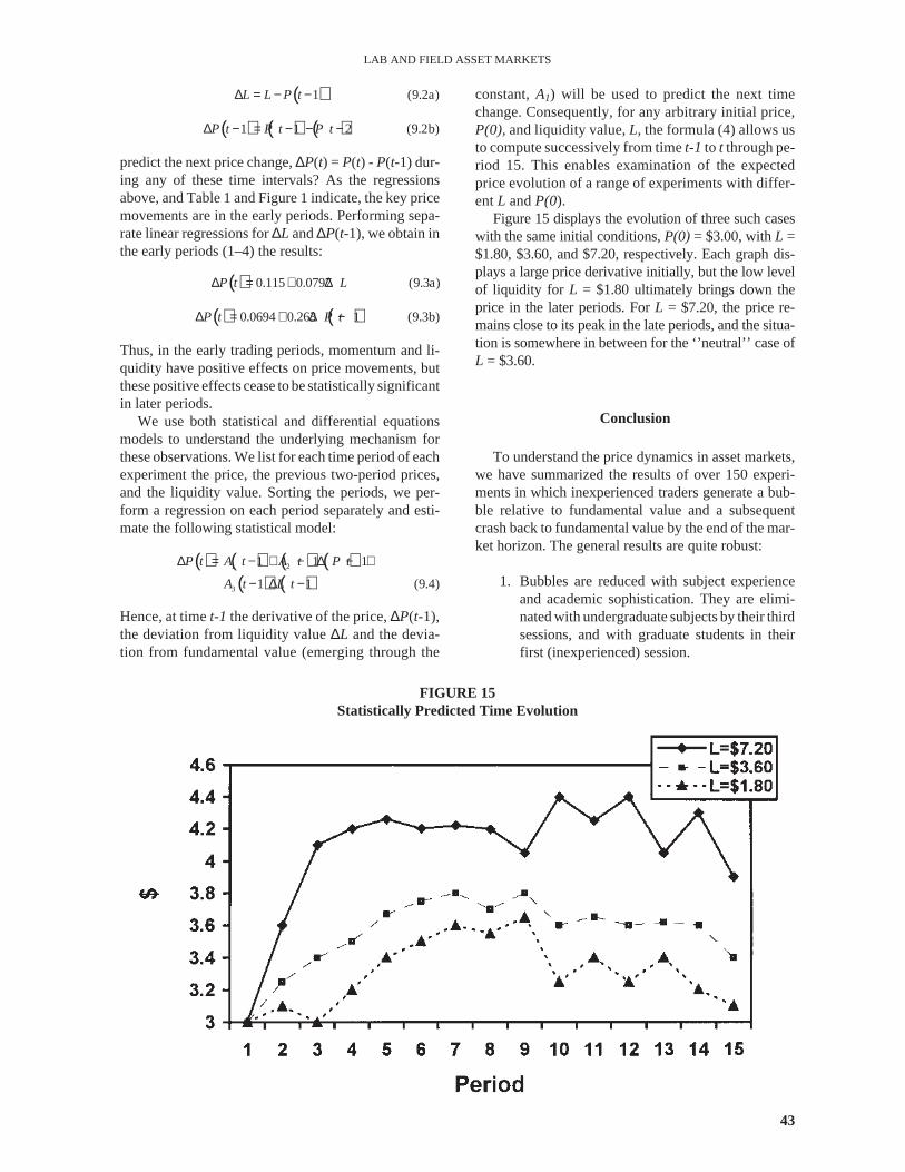
constant,A1) will be used to predict the next timechange. Consequently, for any arbitrary initial price,P(0),and liquidity value,L, the formula (4) allows usto compute successively from timet-1 to t through pe-riod 15. This enables examination of the expectedprice evolution of a range of experiments with differ-entL andP(0).

Figure 15 displays the evolution of three such caseswith the same initial conditions,P(0)= $3.00, withL =$1.80, $3.60, and $7.20, respectively. Each graph dis-plays a large price derivative initially, but the low levelof liquidity for L = $1.80 ultimately brings down theprice in the later periods. ForL = $7.20, the price re-mains close to its peak in the late periods, and the situa-tion is somewhere in between for the ‘’neutral’’ case ofL = $3.60.

Conclusion

To understand the price dynamics in asset markets,we have summarized the results of over 150 experi-ments in which inexperienced traders generate a bub-ble relative to fundamental value and a subsequentcrash back to fundamental value by the end of the mar-ket horizon. The general results are quite robust:

1. Bubbles are reduced with subject experienceand academic sophistication. They are elimi-nated with undergraduate subjects by their thirdsessions, and with graduate students in theirfirst (inexperienced) session.

43


( ) ( ) ( ) ( )( ) ( )

1 2

3

1 1 1

1 1 (9.4)

P t A t A t P t

A t L t

∆ = − + − ∆ − +

− ∆ −

FIGURE 15Statistically Predicted Time Evolution

( )1 (9.2a)L L P t∆ = − −

( ) ( ) ( )1 1 2 (9.2b)P t P t P t∆ − = − − −

( ) 0.115 0.0797 (9.3a)P t L∆ = + ∆

( ) ( )0.0694 0.263 1 (9.3b)P t P t∆ = + ∆ −

2. Futures markets, dividend certainty, and low li-quidity tend to dampen the bubble.

3. Margin buying and limit price change rules tendto exacerbate the bubble.

4. All other treatments examined (e.g., short-sell-ing, capital gains taxes, brokerage fees, and callmarkets) were neutral in their effect on thebubble.

Current finance theory offers no systematic insightinto the experimental data we report. Thus, we create adynamical system to model momentum and over-reactions. The model results in a system of differentialequations that allows for a wide variety of possibleprice patterns based on the relative strengths of funda-mental-based trade and trend-based motivations. Thebasic feature of the model is that when price is belowfundamentals, value investors start buying shares, thuscausing a positive rate of change in stock prices. Thissignals trend-based buyers to enter the market, precipi-tating a further increase in the rate of price change,which further fuels the price increases. As prices riseabove fundamentals, value investors start to sell, in-creasing their liquidity (cash balances) and reducingthe liquidity of trend-based investors. As the trend re-verses, the momentum traders continue the sell-off un-til prices drop to fundamental value. The prices mayeven drop below fundamental value due to selling bymomentum traders, in which case the stage is set for arecovery, as value investors again start to buy.

Using data from experiments, the parameters of themodel are calibrated and then tested in a new set of ex-periments. The main result is thatthe momentum modelunderestimates the mean contract price in the earlytrading periods and overestimates it in the later tradingperiods.We then look at the effectiveness of the mo-mentum model relative to other forms of price forecast-ing (time series analysis, expert forecasters, and excessbids). The results of these experiments suggest that:

1. The momentum model and professional fore-casters have similar predictive power.

2. The momentum model has superior two-periodahead forecasts relative to the other forecast-ing methods.

3. The ARIMA models are relatively the worstforecast methods.

The differential equation model is a closed system thatinvolves the conservation of cash and shares. The inter-action of these two forms of investment leads to a nat-ural measurement of the liquidity of the market (M/S,the ratio of total cash to total shares in the market). Weinvestigate the effect on prices by varying this liquid-ity measure and find:The central tendency of prices incash-rich experiments is significantly higher thanprices in asset-rich experiments.

The results of our experiments and modeling sug-gest that we should:

1. Allow traders to see the entire limit book in alow-liquidity environment to determine if morecomplete information will dampen expecta-tions of price increases.

2. Allow for significant infusions of cash (accu-mulated dividends) or shares (accumulatedstock dividends) into the market to determine ifliquidity can rekindle momentum or stifle bur-geoning bubbles.

3. Introduce another security into the model to seehow momentum across markets affects theprice dynamics.

The time series results of empirical data and labora-tory data confirm the importance of momentum, whichis often difficult to isolate in field data due to many fac-tors that are difficult to quantify. The result that thepredictive capacity of the momentum model is compa-rable to those of the best traders, and considerablybetter than the time series methods, is strong evidencethat the basic concepts of momentum and liquidityhave been incorporated into the model in a useful way.

The model can be further augmented by includinginformation such as excess bids, which will likely re-sult in better forecasts. For the portfolio manager, us-ing such a model would be possible by postulating afundamental value function of time and fitting the bestparameters for a recent time period. The momentummodel would then make some predictions for the nearfuture that may be useful.

Notes

1. The initial distribution of shares and cash identified portfoliotypes as follows:

2. We calculate amplitude as the difference between the highestdeviation of mean contract price from its fundamental valueand the lowest deviation of mean contract from its fundamentalvalue. This value is then normalized by 360, the expected divi-dend value over fifteen periods.

3. Evidence with the capacity to short sell in this environment canbe found in the section titled “Contracting Forms (Short Sales,Margin Buying, and Futures)” on page 30. Also, note that inFigure 4, the one-period expected dividend is only $0.16. Thisexpected dividend is derived from a uniform distribution overthe dividend values of ($0.00, $0.08, $0.16, $0.40).

4. Note that the nine public traders were endowed with twenty-one shares in total, while the “insiders” were endowed withseven owned shares plus a capacity to borrow up to twelve forshort sales. Hence, the insiders’ total selling capacity wasnineteen shares, or 47.5% of the floating supply. Summing thenet purchases by insiders (shown in brackets in figure 4)

44


across periods, we see that by period 11 insiders had sold allnineteen shares and thus had to become buyers to cover theirshort sells.

5. Although the advanced graduate students are “rational” in thesense of exhibiting common expectations that prices will reflectfundamental value, they fail to follow the dictates of “rational”behavior in two-person extensive bargaining (see McCabe andSmith [1999]). Consequently, we cannot say that training in ra-tional theory predicts behavior consistent with the theory in allcircumstances.

6. TheWall Street Journal(see Ip [1999]) reported that the 1998–1999 record-setting rise in blue-chip stock prices amid interestrate uncertainty, according to market analysts, can be traced toprice momentum. In fact, more than 40% of fund managers useprice and earnings momentum in their investment style.

7. Closed-end funds, unlike open-ended mutual funds, do notstand ready to redeem shares. The funds operate with a fixednumber of shares outstanding and do not regularly issue newshares of stock. The stocks of these closed-end funds are ac-tively traded in secondary markets.

8. In a commentary on a presentation of this example along withdata from the laboratory, a discussant objected that the SpainFund was a case of disequilibrium, and that it was also hard toobtain shares to sell short. But finding a sufficient supply ofshares that can be borrowed for making short sales is a ubiqui-tous problem for any stock. Brokers limit the availability ofshares for lending to short-sellers because those shares comefrom the floating stock held to cover shares purchased by theircustomers. These stocks are drained by sales to customers ofother brokers, and hence limiting the potential demand willconstrain the broker’s short sales and reduce his risk. But thatrisk mounts as momentum traders bid up share prices. Hencethe availability of borrowed shares is tightest when short-sellersmost want them.

9. These experiments used a uniform price call market as the pric-ing mechanism (see Van Boening et al. [1993]. This mecha-nism was used because it has a single price prediction, as op-posed to the double auction in which averages or closing priceswould have to be selected.

10. SSW conducted some experiments in which subjects wereasked to forecast the mean price for the next period with a mon-etary reward for the best forecaster across all periods. The con-sensus (mean) forecast results reveal that: 1) bullish capitalgains expectations arise early in these experiments; 2) the meanforecast always fails to predict price jumps and turning points;and 3) the mean forecasts are highly adaptive, i.e., jumps in themean price and turning points are only reflected in forecasts af-ter a one-period lag. Also, individual forecasting accuracy waspositively and significantly correlated with profits earned.These observations parallel the performance of professionalforecasters, whose forecasts are reasonably accurate only whenthe forecasted measure does not change much, and who are no-toriously inaccurate at forecasting turning points when youneed them most (Zarnowitz [1986]).

11. For their experiments, SSW findR2values ranging from 0.04 to0.63. In addition, the variances in the estimates ofα are large, sothat α is almost never significantly different than minus theone-period expected dividend.

12. The Wall Street Journal (Browning [1999]) reports that liquid-ity (defined as retirement savings) is a major factor in currentstock price movements.

References

Aczel, J. and Dhombres, J.Functional Equations Containing SeveralVariables. Cambridge: Cambridge University Press, 1989.

Anderson, S. and J. Born.Closed-End Investment Companies: Issuesand Answers. Boston: Kluwer, 1992.

Blume, L., D. Easley, and M. O’Hara. “Market Statistics and Techni-cal Analysis: The Role of Volume.”Journal of Finance, 69,(1994), 153–181.

Beard T. and R. Beil. “Do People Rely on the Self–Interested Maxi-mization of Others? An Experimental Test.”Management Sci-ence, 40, (1994), 252–262.

Brock, W.A. ‘’Distinguishing Random and Deterministic Systems.’’Journal of Economic Theory, 40, (1986), 168–195.

Brock, W.A., and B. LeBaron. “Simple Technical Trading Rules andStochastic Properties of Stock Returns.”Journal of Finance,47,(1992).

Browning, E. “New Forces Are Powering Surging Stocks.” The WallStreet Journal,, C1, (1999).

Caginalp, G. and D. Balenovich. “Market Oscillations Induced by theCompetition Between Value-Based and Trend-Based Invest-ment Strategies.” Applied Mathematical Finance, (1994), 129–164.

Caginalp, G., and D. Balenovich. “Trend Based Asset Flow in Tech-nical Analysis and Securities Marketing.”Psychology and Mar-keting, 13, (1996), 407–444.

Caginalp, G., and D. Balenovich. ‘’Asset Flow and Momentum: De-terministic and Stochastic Equations.”Proc. Royal Soc., to ap-pear, 1999.

Caginalp, G. and G. Constantine. “Statistical Influence and Modelingof Momentum in Stock Prices.”Applied Mathematical Finance,2, (1995), 225–242.

Caginalp, G. and Ermentrout. “A Kinetic Thermodynamic Approachto the Psychology of Fluctuations in Financial Markets.”Ap-plied Mathematics Letters, Vol. 4, 1990.

Caginalp, G. and Ermentrout. “Numerical Studies of DifferentialEquations Related to Theoretical Financial Markets.”AppliedMathematics Letters,Vol. 4, 1991.

Caginalp, G., D. Porter and V.L. Smith. “Initial Cash/Asset Ratio andAsset Prices: An Experimental Study.”Proc. Nat. Acad. Sci.,95, (1995), 756–761.

Caginalp, G., D. Porter and V.L. Smith. “Momentum and Overreac-tion in Experimental Asset Markets.”International Journal ofIndustrial Organization,to appear, 1998.

Chen, N., R. Kan, and M. Miller. “Are the Discounts on Closed-EndFunds a Sentiment Index?”Journal of Finance, 48, (1993), 795–800.

Chopra, N., C. Lee, A. Shleifer, and R. Thaler. “Yes, Discounts onClosed-End Funds are a Sentiment Index.” Journal of Finance,48, (1993), 801–808.

Coddington, E. and N. Levinson. Theory of Ordinary DifferentialEquations. New York: McGraw-Hill, 1995.

Fama, E. “Efficient Capital Markets: A Review of Theory and Empir-ical Work.” Journal of Finance, 25, (1970), 383–417.

Forsythe, R., T. Palfrey, and C. Plott. “Asset Valuation in an Experi-mental Market.”Econometrica, 50, (1982), 537–567.

Frantz, D. and P. Truell. “Long-Term Capital: A Case of Marketsover Minds,” The New York Times, 1998.

Griliches, Z. and M. Intriligator, eds,Handbook of EconometricsNorth Holland, Amsterdam, 1994.

Grinblatt, M., S. Titman, and R. Wermers. “Momentum InvestmentStrategies, Portfolio Performance, and Herding: A Study of Mu-tual Fund Behavior.”American Economic Review, 85, (1996),No. 5.

Grossman, S., and J. Stiglitz. “On the Impossibility of In-formationally Efficient Markets.”Am. Economic Rev., 70,(1980), 393–407.

Guth, W., J. Krahnen and C. Rieck. “Financial Markets withAsymmetric Information: A Pilot Study Focusing on InsiderAdvantages.”Journal of Economic Psychology, 18, (1997),235–258.

Harvey, Andrew. Time Series Models. Cambridge, MIT Press, 1994.

45


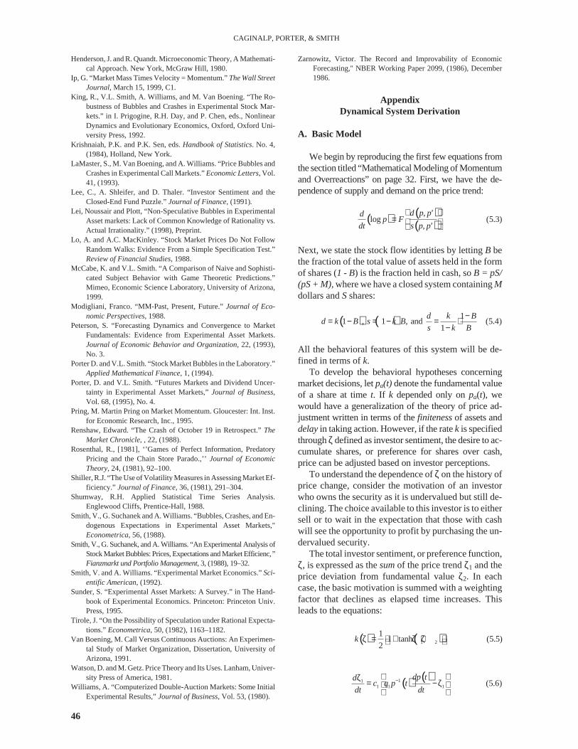
Henderson, J. and R. Quandt. Microeconomic Theory, A Mathemati-cal Approach. New York, McGraw Hill, 1980.

Ip, G. “Market Mass Times Velocity = Momentum.”The Wall StreetJournal,March 15, 1999, C1.

King, R., V.L. Smith, A. Williams, and M. Van Boening. “The Ro-bustness of Bubbles and Crashes in Experimental Stock Mar-kets.” in I. Prigogine, R.H. Day, and P. Chen, eds., NonlinearDynamics and Evolutionary Economics, Oxford, Oxford Uni-versity Press, 1992.

Krishnaiah, P.K. and P.K. Sen, eds.Handbook of Statistics. No. 4,(1984), Holland, New York.

LaMaster, S., M. Van Boening, and A. Williams. “Price Bubbles andCrashes in Experimental Call Markets.”Economic Letters, Vol.41, (1993).

Lee, C., A. Shleifer, and D. Thaler. “Investor Sentiment and theClosed-End Fund Puzzle.”Journal of Finance,(1991).

Lei, Noussair and Plott, “Non-Speculative Bubbles in ExperimentalAsset markets: Lack of Common Knowledge of Rationality vs.Actual Irrationality.” (1998), Preprint.

Lo, A. and A.C. MacKinley. “Stock Market Prices Do Not FollowRandom Walks: Evidence From a Simple Specification Test.”Review of Financial Studies, 1988.

McCabe, K. and V.L. Smith. “A Comparison of Naive and Sophisti-cated Subject Behavior with Game Theoretic Predictions.”Mimeo, Economic Science Laboratory, University of Arizona,1999.

Modigliani, Franco. “MM-Past, Present, Future.”Journal of Eco-nomic Perspectives, 1988.

Peterson, S. “Forecasting Dynamics and Convergence to MarketFundamentals: Evidence from Experimental Asset Markets.Journal of Economic Behavior and Organization, 22, (1993),No. 3.

Porter D. and V.L. Smith. “Stock Market Bubbles in the Laboratory.”Applied Mathematical Finance, 1, (1994).

Porter, D. and V.L. Smith. “Futures Markets and Dividend Uncer-tainty in Experimental Asset Markets,”Journal of Business,Vol. 68, (1995), No. 4.

Pring, M. Martin Pring on Market Momentum. Gloucester: Int. Inst.for Economic Research, Inc., 1995.

Renshaw, Edward. “The Crash of October 19 in Retrospect.”TheMarket Chronicle, , 22, (1988).

Rosenthal, R., [1981], ‘’Games of Perfect Information, PredatoryPricing and the Chain Store Parado.,’’Journal of EconomicTheory, 24, (1981), 92–100.

Shiller, R.J. “The Use of Volatility Measures in Assessing Market Ef-ficiency.” Journal of Finance, 36, (1981), 291–304.

Shumway, R.H. Applied Statistical Time Series Analysis.Englewood Cliffs, Prentice-Hall, 1988.

Smith, V., G. Suchanek and A. Williams. “Bubbles, Crashes, and En-dogenous Expectations in Experimental Asset Markets,"Econometrica, 56, (1988).

Smith, V., G. Suchanek, and A. Williams. “An Experimental Analysis ofStock Market Bubbles: Prices, Expectations and Market Efficienc,”Fianzmarkt und Portfolio Management, 3, (1988), 19–32.

Smith, V. and A. Williams. “Experimental Market Economics.”Sci-entific American, (1992).

Sunder, S. “Experimental Asset Markets: A Survey.” in The Hand-book of Experimental Economics. Princeton: Princeton Univ.Press, 1995.

Tirole, J. “On the Possibility of Speculation under Rational Expecta-tions.” Econometrica, 50, (1982), 1163–1182.

Van Boening, M. Call Versus Continuous Auctions: An Experimen-tal Study of Market Organization, Dissertation, University ofArizona, 1991.

Watson, D. and M. Getz. Price Theory and Its Uses. Lanham, Univer-sity Press of America, 1981.

Williams, A. “Computerized Double-Auction Markets: Some InitialExperimental Results,”Journal of Business, Vol. 53, (1980).

Zarnowitz, Victor. The Record and Improvability of EconomicForecasting," NBER Working Paper 2099, (1986), December1986.

AppendixDynamical System Derivation

A. Basic Model

We begin by reproducing the first few equations fromthe section titled “Mathematical Modeling of Momentumand Overreactions” on page 32. First, we have the de-pendence of supply and demand on the price trend:

Next, we state the stock flow identities by lettingB bethe fraction of the total value of assets held in the formof shares (1 - B) is the fraction held in cash, soB = pS/(pS + M), where we have a closed system containingMdollars andSshares:

All the behavioral features of this system will be de-fined in terms ofk.

To develop the behavioral hypotheses concerningmarket decisions, letpa(t) denote the fundamental valueof a share at timet. If k depended only onpa(t), wewould have a generalization of the theory of price ad-justment written in terms of thefinitenessof assets anddelayin taking action. However, if the ratek is specifiedthroughζ defined as investor sentiment, the desire to ac-cumulate shares, or preference for shares over cash,price can be adjusted based on investor perceptions.

To understand the dependence ofζ on the history ofprice change, consider the motivation of an investorwho owns the security as it is undervalued but still de-clining. The choice available to this investor is to eithersell or to wait in the expectation that those with cashwill see the opportunity to profit by purchasing the un-dervalued security.

The total investor sentiment, or preference function,ζ, is expressed as thesumof the price trendζ1 and theprice deviation from fundamental valueζ2. In eachcase, the basic motivation is summed with a weightingfactor that declines as elapsed time increases. Thisleads to the equations:

46


( ) ( )( )

,log (5.3)

,

d p pdp F

dt s p p

′= ′

( ) ( ) −= − = − = ⋅−

11 , 1 , and (5.4)

1

d k Bd k B s k B

s k B

( ) ( )1 2

11 tanh (5.5)

2k ζ = + ζ +ζ

( ) ( )111 1 1 (5.6)

dp tdc q p t

dt dt− ζ = −ζ

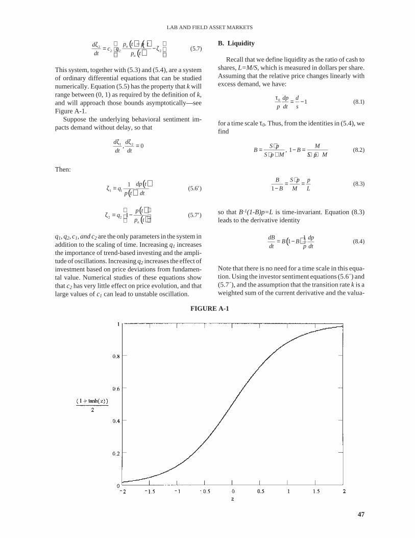
This system, together with (5.3) and (5.4), are a systemof ordinary differential equations that can be studiednumerically. Equation (5.5) has the property thatk willrange between (0, 1) as required by the definition ofk,and will approach those bounds asymptotically—seeFigure A-1.

Suppose the underlying behavioral sentiment im-pacts demand without delay, so that

Then:

q1, q2, c1, and c2 are the only parameters in the system inaddition to the scaling of time. Increasingq1 increasesthe importance of trend-based investing and the ampli-tude of oscillations. Increasingq2 increases the effect ofinvestment based on price deviations from fundamen-tal value. Numerical studies of these equations showthatc2 has very little effect on price evolution, and thatlarge values ofc1 can lead to unstable oscillation.

B. Liquidity

Recall that we define liquidity as the ratio of cash toshares,L=M/S, which is measured in dollars per share.Assuming that the relative price changes linearly withexcess demand, we have:

for a time scaleτ0. Thus, from the identities in (5.4), wefind

so thatB-1(1-B)p=L is time-invariant. Equation (8.3)leads to the derivative identity

Note that there is no need for a time scale in this equa-tion. Using the investor sentiment equations (5.6´) and(5.7´), and the assumption that the transition ratek is aweighted sum of the current derivative and the valua-

47


FIGURE A-1

( )( )2 2 1 (5.7 )

a

p tq

p t

ζ = − ′

( ) ( )( )

22 2 2 (5.7)a

a

p t p tdc q

dt p t

−ζ = −ζ

1 2, 0d d

dt dt

ζ ζ =

( )( )

1 1

1(5.6 )

dp tq

p t dtζ = ′

0 1 (8.1)dp d

p dt s

τ= −

⋅= − =⋅ + ⋅ +

, 1 (8.2)S p M

B BS p M S p M

(8.3)1

B S p p

B M L

⋅= =−

( )11 (8.4)

dB dpB B

dt p dt= −

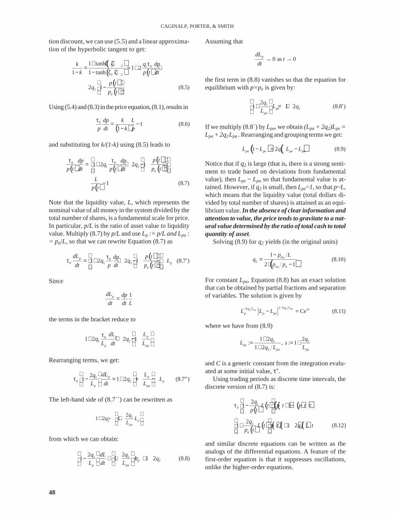
tion discount, we can use (5.5) and a linear approxima-tion of the hyperbolic tangent to get:

Using (5.4)and(8.3) in thepriceequation, (8.1), results in

and substituting fork/(1-k)using (8.5) leads to

Note that the liquidity value, L, which represents thenominal value of all money in the system divided by thetotal number of shares, is a fundamental scale for price.In particular,p/L is the ratio of asset value to liquidityvalue. Multiply (8.7) byp/Land useLp := p/L and Lpa := pa/L, so that we can rewrite Equation (8.7) as

Since

the terms in the bracket reduce to

Rearranging terms, we get:

The left-hand side of (8.7´´) can be rewritten as

from which we can obtain:

Assuming that

the first term in (8.8) vanishes so that the equation forequilibrium withp=pe is given by:

If we multiply (8.8´) byLpa, we obtain(Lpa+ 2q2)Lpe=Lpa+ 2q2Lpa. Rearranging and grouping terms we get:

Notice that ifq2 is large (that is, there is a strong senti-ment to trade based on deviations from fundamentalvalue), thenLpe ~ Lpa so that fundamental value is at-tained. However, ifq2 is small, thenLpe~1,so thatp~L,which means that the liquidity value (total dollars di-vided by total number of shares) is attained as an equi-librium value.In the absence of clear information andattention to value, the price tends to gravitate to a nat-ural value determined by the ratio of total cash to totalquantity of asset.

Solving (8.9) forq2 yields (in the original units)

For constantLpa, Equation (8.8) has an exact solutionthat can be obtained by partial fractions and separationof variables. The solution is given by

where we have from (8.9)

andC is a generic constant from the integration evalu-ated at some initial value,τ*.

Using trading periods as discrete time intervals, thediscrete version of (8.7) is:

and similar discrete equations can be written as theanalogs of the differential equations. A feature of thefirst-order equation is that it suppresses oscillations,unlike the higher-order equations.

48


( )( )

00 1 21 2 2 1 (8.7 )p

pa

dL p tdpq q L

dt p dt p t

ττ = + + − − ′

1pdL dp

dt dt L=

01 21 2 2 1p p

p pa

dL Lq q

L dt L

τ+ + −

10 2

21 1 2 1 (8.7 )p p

pp pa

dL Lqq L

L dt L

τ − = + − − ′′

22

21 2 p

pa

qq L L

L

+ − +

1 22

2 21 1 1 2 (8.8)p

p pa

q qdLL q

L dt L

− + + = +

0 as 0pdLt

dt→ →

22

21 1 2 (8.8 )pe

pa

qL q

L

+ = + ′

( ) ( )21 2 (8.9)pa pe pe paL L q L L− = −

( )( ) ( )

( )( )

1 2 1 0

1 2

2

1 tanh1 2

1 1 tanh

2 1 (8.5)a

qk dp

k p t dt

p tq

p t

+ ζ +ζ τ= ≈ + +

− − ζ +ζ

−

( )0 1 (8.6)

1

dp k L

p dt k p

τ= −

−

( ) ( )( )( )

( )

0 01 21 2 2 1

1 (8.7)

a

p tdp dpq q

p t dt p t dt p t

L

p t

τ τ= + + − ⋅

−

( )2

1(8.10)

2 1eq

eq a

p Lq

p p

−=

⋅ −

111 22 Ce (8.11)

pepeq Lq L s

p p peL L L−− τ− =

2 2

2

1 2 2: , : 1

1 2pepa pa

q qL s

q L L

+= = ++

( ) ( ) ( ) ( )( )

( ) ( ) ( ) ( ) ( )

10

22

21 1

21 1 2 (8.12)

a

qL t p t p t

p t

qL t p t q L t

p t

τ − + − =

+ + +

overreactions, momentum, liquidity, and price bubbles in ...caginalp/pub72.pdf · shares, plus...

Documents