Overview of 3D Computer Graphics

Aknowledgements: to my best knowledges, these slides originally come from University of Washington, and subsequently are adapted by colleagues.

Overview

• Modeling of 3D objects– Polygonal representation (geometry)– Parametric represenation (curves and surfaces)

• Rendering: – (lighting and illumination models)– on-line graphics pipeline– off-line global illumination methods: ray-tracing

and radiosity

Graphics pipeline

• 2D and 3D Euclidean transformations• Hierarchical modeling• Introduction to projective geometry• (real) camera modeling from vision• (synthetic) camera for graphics: projective

transformation• Hiden surface removal

Polygonal representation

• Hierarchical data structure– An object is surfaces– A surface is polygons– A polygon is vertices

• Mannually designed• Automatic from scanning of real objects• Automatically generated from other descriptions

(implicit)

Rendering Triangles

• Developer specifies in OpenGL/DirectX– Rendering state

(transformation matrices, texture mapping, etc…)– Triangles and vertices

(with colors, etc…)

• Graphics card processing– Vertex processing

(model, view, projection transformation)– Triangle scan-conversion – Pixel processing

(value set to Gouraud-interpolated colors)

Rendering Triangles

• Developer specifies in OpenGL/DirectX– Rendering state

(transformation matrices, texture mapping, etc…)– Triangles and vertices

(with colors, etc…)

• Graphics card processing– Vertex processing

(model, view, projection transformation)– Triangle scan-conversion – Pixel processing

(value set to Gouraud-interpolated colors)

Fully programmable!

Transform and Lighting Background

• GPU Transform and Lighting of vertices – available on consumer graphics cards circa 1999

– Also called fixed function pipeline– Previously normally done on CPU

• Forced the use of Gouraud / Phong lighting

– Other variations couldn’t be handled by the graphics hardware

Fixed Function PipelineVertex Data

(Model space)

Fixed Function Transform and

Lighting

Clipping and Viewport Mapping

Texture Stages

Fog, Alpha, Stencil Depth Testing

Geometry Stage

Rasterizer Stage

Open GL

• OpenGL (Open Graphics Library) is a standard specification defining a cross-language cross-platform API for writing applications that produce 3D computer graphics (and 2D computer graphics as well).

• The interface consists of over 250 different function calls which can be used to draw complex three-dimensional scenes from simple primitives. OpenGL was developed by Silicon Graphics Inc. (SGI) in 1992[1] and is popular in the video games industry where it competes with Direct3D on Microsoft Windows platforms (see Direct3D vs. OpenGL).

• OpenGL is widely used in CAD, virtual reality, scientific visualization, information visualization, flight simulation and video game development.

• OpenGL is a low-level, procedural API, requiring the programmer to dictate the exact steps required to render a scene.

• the red book: http://www.rush3d.com/reference/opengl-redbook-1.1/

2D Transformations

Reading

Required:• Hearn & Baker, 5.1-5.5

Optional:• Foley, et al., 5.1-5.5.• David F. Rogers and J. Alan Adams, Mathematical

Elements for Computer Graphics, 2nd ed., McGraw-Hill, New York, 1990, Chapter 2.

• Linear algebra: Gilbert Strang

prod.dot with nn AE nA

nR

Naturally everything starts from the known vector space

• add two vectors• multiply any vector by any scalar• zero vector – origin • finite basis

Intuitive introduction

• Vector space to affine: isomorph, one-to-one

• vector to Euclidean as an enrichment: scalar prod.

Pts, lines, parallelism

Angle, distances, circles

Points versus vectors(geometry vs. algebra)

Point• A location in space• Its coordinate values

depend on the choice of coordinate system

• P+Q is not defined P is not defined, but is defined if

Vector• Has direction and

magnitude• Free to move anywhere

(free vectors)• v + w is defined v is defined

•Both can be represented as a list of coordinates•The distinction enables us to check validity of geometric operations.

iiP 1i

(linear) algebra:Geometry:

• An affine space is similar to a vector space, only viewed differently

• An affine space is a vector space if we fix one pt as the origin.

• A vector space is an affine space if we ‘forget’ the ‘zero’.

• Affine geometry reduces to linear algebra

Geometric transformations

Geometric transformations map points in one space to points in another space: (x’, y’, z’) = f(x, y, z)

These transformations can be very simple, such as scaling each coordinate, or complex, such as non-linear twists and bends.

We’ll focus on transformations that can be represented easily with matrix operations: linear transformations.

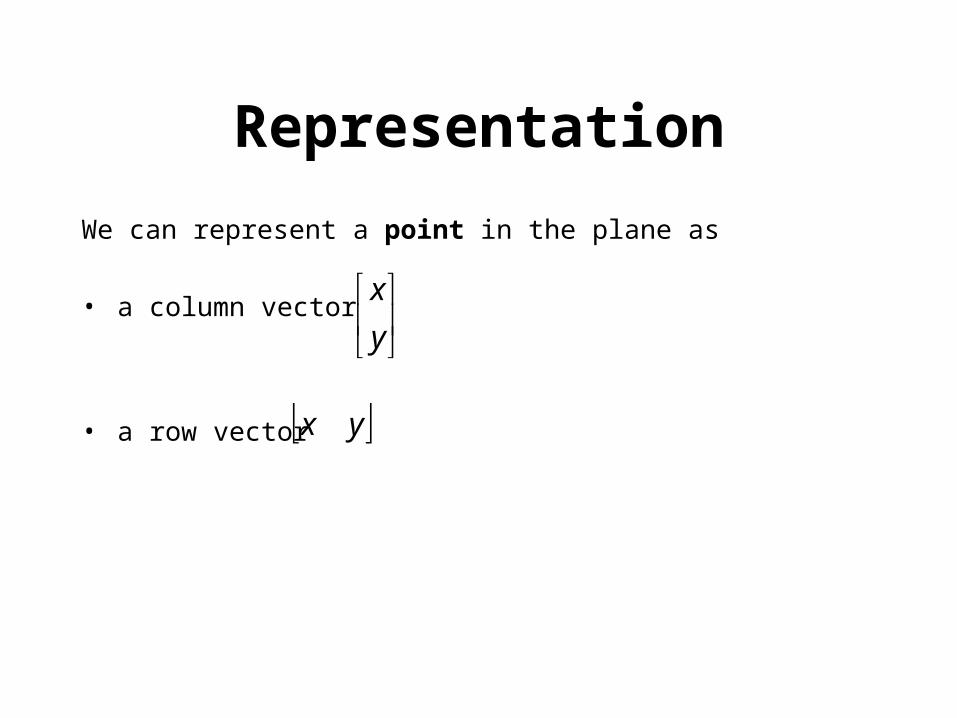
Representation

We can represent a point in the plane as

• a column vector

• a row vector

y

x

yx

Representation, cont.We can represent a 2D transformation M by a matrix

If p is a column vector, then M goes on the left:

If p is a row vector, then MT goes on the right:

We will use column vectors.

dc

baM

y

x

dc

ba

y

x

Mpp

db

cayxyx

M Tpp

2D Transformations

Here’s all you get with a 2x2 transformation matrix M:

So:

y

x

dc

ba

y

x

dycxy

byaxx

Identity

Suppose we choose a=d=1, b=c=0:

• Gives the identity matrix:

• Doesn’t move the points at all

10

01

Scaling

Suppose we set b=c=0, but let a and d take on any positive value:

• Gives a scaling matrix:

• Provides differential scaling in x and y:

d

a

0

0

dyy

axx

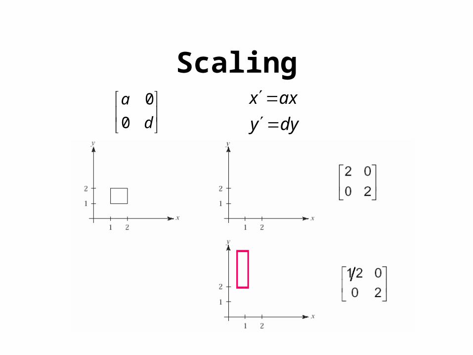
Scaling

d

a

0

0

dyy

axx

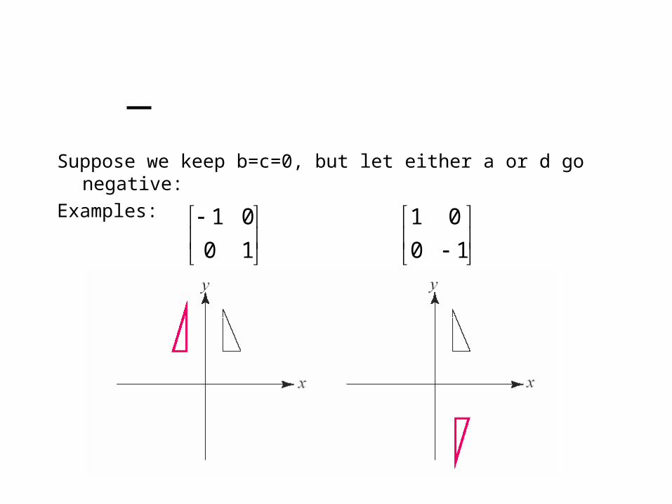
Suppose we keep b=c=0, but let either a or d go negative:Examples:

10

01

10

01

Now let’s leave a=d=1 and experiment with b ….The matrix

gives:

10

1 b

yy

byxx

Effect on unit square

Let’s see how a general 2x2 transformation M affects the unit square:

ddcc

bbaa

dc

ba

dc

ba

0

0

1100

0110

srqpsrqp

Effect on unit square, cont.

Observe:• Origin invariant under M• M can be determined just by knowing how the corners

(1,0) and (0,1) are mapped• a and d give x- and y-scaling• b and c give x- and y-shearing

Rotation

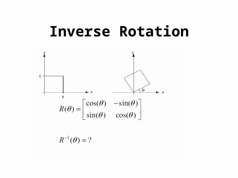
Inverse Rotation

Limitations of the 2x2 matrix

A 2x2 matrix allows• Scaling• Rotation• Reflection• Shearing

Q: What important operation does that leave out?

Homogeneous coordinates,just as a convenient tool!

Idea is to loft the problem up into 3-space, adding a third component to every point:

And then transform with a 3x3 matrix:

1

y

x

y

x

1100

10

01

y

x

t

t

w

y

x

y

x

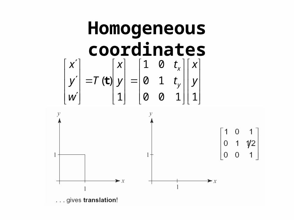
Homogeneous coordinates

1100

10

01

1

)( y

x

t

t

y

x

T

w

y

x

y

x

t

Rotation around arbitrary point

With homogeneous coordinates, we can specify rotations about any point p with a matrix

1. Translate object so that pivot is at origin

2. Rotate object3. Translate so that pivot is

back to original position

Order is important!

Affine transformations

• All of the transformations we have looked at so far are examples of affine transformations

• Some properties of affine transformations:– Lines map to lines– Parallel lines remain parallel– Midpoints map to midpoints (in fact, ratios are

always preserved)

Affine versus Euclidean Geometry

Affine geometry• Operations for vectors: v w, v • Operations for points: P – Q, P v• No concepts of length and angle

Eucliean geometry• Add one operation to affine geometry: inner product• Thus introduce angles and distances• Concepts defined: length of vector, normalize a vector,

distance between points, angle between vectors, orthogonality, orthogonal projection

Angle

• Angle between u and v = where are unit vectors

u

v

)ˆˆ(cos 1 vu

0

0

900

vu

vu

vu

vu ˆ,ˆ

Orthogonal projection

• Orthogonal projection of a given vector u onto is

u

unit vector

vvu ˆ)ˆ( v̂

v̂

Summary

What you should take away from this lecture:• The meaning of all the boldfaced terms• How points and transformations are represented• What all the elements of a 2x2 transformation matrix do• What homogeneous coordinates are and how they work

for affine transformations• How to concatenate transformations• Properties of affine transformations

3D Transformations

Reading

Required:• Hearn & Baker, 5.9-5.15

Optional• Hill 5.1-5.4

Basic 3D transformations: scaling

Some of the 3D transformations are just like 2D ones. For example, scaling

Scaling

Translation in 3D

Rotation in 3DRotation now has more possibilities in 3D:

Rotation in 3DWhat about the inverses of 3D rotations?

Rotation around an axis by an angle …

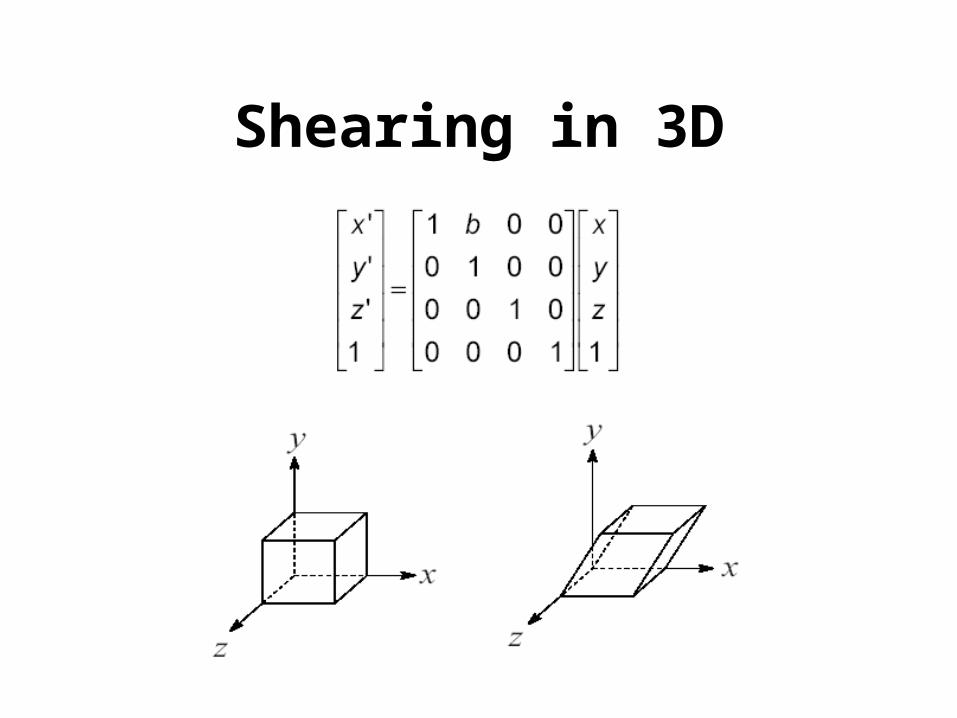
Shearing in 3D

Compositing multiple transformations

• Expressed as matrix multiplications: p’ = M1 M2 p

means apply transformation M2 first, followed by M1

Historically, the vectors in graphics were row vectors,but columns are more popular.

Compositing multiple transformations

3 steps1) T(-2, -3)2) R(30)3) T(2, 3)

q’=T(2,3) R(30) T(-2,-3) q

Change of the coordinate frame, Change of basis

Let’s first look at a 2D example

• p=(2, 1)T, what are the coordinates of p with respect to the new basis (coordinate system)?

p

Specify: an origin, and two vectors

• Linear dependence or independence• Spanning a space or a subspace, ‘generators’• Basis for a space or a subspace (a set of vectors)• Dimension of a subspace (a number)

• A basis for V is a set of vectors: linearly independent (not too many) and span the space V (not too few)

• Basis is not unique, coordinates are, when the basis is fixed.

p

• New basis: O=(4,3)T, e0=(-1,0)T, e1=(0,-1)T

1

1

0

1

0

10

1100

1

1100

1

1

001

1

0

oy

ox

py

px

eeOp

Let coordinates of p in new basis be (0, 1)T

• New basis: O=(4,3)T, e0=(-1,0)T, e1=(0,-1)T

• Represent as homogeneous coordinates:

O=(4,3,1)T, e0=(-1,0,0)T, e1=(0,-1,0)T

• For vectors, last component of homogeneous coordinates is 0, for convenience only for the time being.

TT 1,1)0,( B 1,1)0,(

• Basis change: e’_i = B e_i• Pt change, x’ = A x• x=\sum x_i e_i,• x=\sum x_i B^{-1} e’

= \sum B^{-1} x_i e’

• x’ = B^{-1} x

Change of basis in 3Done origine, three vectors

3D case

• Given an orthonormal basis (O, e0, e1, e2)

– e0, e1, e2 are unit length vectors

– e0, e1, e2 are mutually orthogonal

• To change basis, need matrix M=(e0 e1 e2 O)

• It is easy to find the inverse of such a matrix

100023222120

13121110

03020100

mmmm

mmmm

mmmm

M

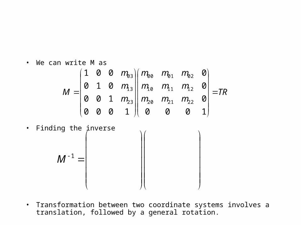
• We can write M as

• Finding the inverse

• Transformation between two coordinate systems involves a translation, followed by a general rotation.

TRmmm

mmm

mmm

m

m

m

M

1000

0

0

0

1000

100

010

001

222120

121110

020100

23

13

03

1M

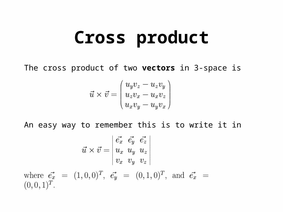
Cross product

The cross product of two vectors in 3-space is

An easy way to remember this is to write it in the form

Cross product: define coordinate system

• Given two vectors u and v (not parallel)• Define a coordinate system such that

– One of the axis is in the direction of u– Another axis is perpendicular to both u and v

• Solution:

– Direction of x-axis: e0 = u

– Direction of z-axis: e2 = u x v

– Direction of y-axis: e1 = e2 x e0 (note: e0 x e2 )

• The Gram-Shmidt process

Cross product: normal

Find the normal of a triangle

OpenGL Transformation functions

OpenGL • OpenGL maintains a matrix stack called Modelview• Transformations are accumulated by

postmultiplication with the top-of-the-stack matrix M• glLoadIdentity() M I glTranslatef(tx, ty, tz) M MT glRotatef(theta, x, y, z) M MR glScalef(sx, sy, sz) M MS

• Points are multiplied to the top-of-the-stack matrix during drawing

glMatrixMode( GL_MODELVIEW ); /* Subsequent matrix commands will affect the modelview matrix */ glLoadIdentity(); /* Initialise the modelview to identity */ glTranslatef( 0, 0, -3 ); /* Translate the modelview 3 units along the Z axis */

We issue a polygon – a green square oriented in the xy plane.

glBegin( GL_POLYGON ); /* Begin issuing a polygon */ glColor3f( 0, 1, 0 ); /* Set the current color to green */ glVertex3f( -1, -1, 0 ); /* Issue a vertex */ glVertex3f( -1, 1, 0 ); /* Issue a vertex */ glVertex3f( 1, 1, 0 ); /* Issue a vertex */ glVertex3f( 1, -1, 0 ); /* Issue a vertex */ glEnd(); /* Finish issuing the polygon */

Summary

What you should take away from this lecture:• The meaning of all the boldfaced terms• How transformations are generalized from 2D to 3D• How to concatenate transformations• How to define a coordinate system from two given

vectors• How to change basis• How to represent points and vectors in homogeneous

coordinates• How OpenGL matrix stack works