HAL Id: hal-02190170https://hal.archives-ouvertes.fr/hal-02190170

Submitted on 22 Jul 2019

HAL is a multi-disciplinary open accessarchive for the deposit and dissemination of sci-entific research documents, whether they are pub-lished or not. The documents may come fromteaching and research institutions in France orabroad, or from public or private research centers.

L’archive ouverte pluridisciplinaire HAL, estdestinée au dépôt et à la diffusion de documentsscientifiques de niveau recherche, publiés ou non,émanant des établissements d’enseignement et derecherche français ou étrangers, des laboratoirespublics ou privés.

Distributed under a Creative Commons Attribution| 4.0 International License

Overview of GeoLifeCLEF 2019: plant species predictionusing environment and animal occurrences

Christophe Botella, Maximilien Servajean, Pierre Bonnet, Alexis Joly

To cite this version:Christophe Botella, Maximilien Servajean, Pierre Bonnet, Alexis Joly. Overview of GeoLifeCLEF2019: plant species prediction using environment and animal occurrences. Working Notes of CLEF2019 - Conference and Labs of the Evaluation Forum, Sep 2019, Lugano, Switzerland. �hal-02190170�

Overview of GeoLifeCLEF 2019: plant speciesprediction using environment and animal

occurrences

Botella Christophe1,2,3, Servajean Maximilien5, Bonnet Pierre3,4, Joly Alexis1

1 INRIA Sophia-Antipolis - ZENITH team, LIRMM - UMR 5506 - CC 477, 161 rueAda, 34095 Montpellier Cedex 5, France.

2 INRA, UMR AMAP, F-34398 Montpellier, France.3 AMAP, Univ Montpellier, CIRAD, CNRS, INRA, IRD, Montpellier, France.

4 CIRAD, UMR AMAP, F-34398 Montpellier, France.5 LIRMM, Universite Paul Valery, University of Montpellier, CNRS, Montpellier,

France

Abstract. The GeoLifeCLEF challenge aim to evaluate location-basedspecies recommendation algorithms through open and perennial datasetsin a reproducible way. It offers a ground for large-scale geographic speciesprediction using cross-kingdom occurrences and spatialized environmen-tal data. The main novelty of the 2019 campaign over the previous oneis the availability of new occurrence datasets: (i) automatically identifiedplant occurrences coming from the popular Pl@ntnet platform and (ii)animal occurrences coming from the GBIF platform. This paper presentsan overview of the resources and assessment of the GeoLifeCLEF 2019task, synthesizes the approaches used by the participating groups andanalyzes the main evaluation results. We highlight new successful ap-proaches relevant for community modeling like models learning to pre-dict occurrences from many biological groups and methods weightingoccurrences based on species infrequency.

Keywords: LifeCLEF, biodiversity, environmental data, species recommenda-tion, evaluation, benchmark, Species Distribution Models, methods comparison,presence-only data, model performance, prediction, predictive power

1 Introduction

The automatic prediction of the species most likely to be observed at a givenlocation is an important issue for many areas such as biodiversity conservation,land management or environmental education. First, it could improve speciesidentification processes and tools by reducing the list of candidate species observ-able at a given site (whether automated, semi-automatic or based on traditional

Copyright c© 2019 for this paper by its authors. Use permitted under Creative Com-mons License Attribution 4.0 International (CC BY 4.0). CLEF 2019, 9-12 Septem-ber 2019, Lugano, Switzerland.

field guides or flora). More generally, it could facilitate biodiversity inventoriesand compliance with regulatory obligations for the environmental integration ofdevelopment projects. Finally, it could be used for educational purposes throughbiodiversity discovery applications offering functionalities such as contextualizededucational pathways.

In the context of LifeCLEF evaluation campaign 2019 [6], the objective ofthe GeoLifeCLEF challenge is to evaluate the state of the art of species predic-tion methods over the long term and with a view to reproducibility. To achievethis, the challenge freely provides researchers with large-scale, documented andaccessible data sets over the long term. Concretely, the aim of the challenge isto predict the list of species that are the most likely to be observed at a givenlocation. Therefore, we provide a large training set of species occurrences and aset of environmental rasters that characterize the environment in a quantitativeand qualitative way at any position in the territory. Indeed, it is usually notpossible to learn a species distribution models directly from spatial positionsbecause of the limited number of occurrences and the sampling bias. What isusually done in ecology is to predict the distribution of species based on a repre-sentation in environmental space, typically a characteristic vector composed ofclimatic variables (mean temperature at that location, precipitation, etc.) andother variables such as soil type, land cover, distance to water, etc. GeoLife-CLEF’s originality is to encourage the extension of this approach to learning amore complex representation space that takes into account various input datasuch as environmental descriptors, their spatial structure and the known bioticcontext. Therefore, we provide tools to facilitate the extraction of environmentaltensors that can be easily used as input data to models such as convolutionalneural networks.

In 2019, the provided data was significantly enriched and several methodolog-ical improvements have been made. In more details, the new features introducedare as follows:

1. Pl@ntNet occurrences: to increase the amount of plant occurrences in thetraining set, we completed the publicly available data from the GBIF6 withuser-generated observations of the Pl@ntNet mobile application [1]. Thesedata are clearly noisier and more biased than conventional occurrence databut they can be filtered by the confidence level of the taxonomic automaticclassifier used in the app and they have the advantage of being produced inhuge quantities.

2. Occurrences of other kingdoms: to investigate how knowledge of the presenceof non-plants organisms can help predict the presence of plants species, weprovided a large training set of occurrences from other kingdoms comingfrom the GBIF platform.

3. A better quality test set: to ensure the reliability of our evaluation, theoccurrence data of the test set were restricted to expert data with the highestspecies identification certainty and high geographical accuracy (lower than 50m). Last but not least, the test occurrences were sampled in order to avoid, as

6 https://www.gbif.org/

much as possible, biases of spatial coverage and in the species representation.By this way, it contributes to give relatively more importance to rare speciesand scarce areas.

In the following sections, we describe in more details the data produced andthe evaluation methodology used. We then present the results of the evaluationand the analysis of these results.

2 Dataset

2.1 Train occurrences

Pl@ntNet raw data. (PL complete) This data is directly pulled from [4]. Pl@ntNet7

is a smartphone app using machine learning to identify plant species from pic-tures submitted by a broad public of users. For each submission, also calleda query, the Pl@ntNet algorithm answers a distribution of probability valuesacross the targeted taxonomic referential. If the users allows it, the query’s ge-olocation is also stored. In the provided training data, we used all accuratelygeolocated queries (with maximum 30 meters uncertainty) in France from thebeginning of 2017 to the end of October 2018. Each geolocated occurrence islabelled with the species of higher identification probability. This dataset is thusvery heterogeneous in species identification quality, due to the high variability ofthe image quality submitted by users. The confidence score is provided to Geo-LifeCLEF participants as specific field in this dataset, who can use it to accountfor identification uncertainty in their models. This data set contains 2,377,610occurrences covering 3,906 plant species.

Pl@ntNet filtered data. (PL filtered) We proposed a filtered version of theprevious dataset based on species identification quality. We only kept the occur-rences for which the first species probability value was above 0.98. This scorehas been determined by expert to give a reasonable degree of identification con-fidence. This set of 237,087 occurrences covers 1,364 species.

GeoLifeClef 2018. (GBIF) Train and test occurrences datasets from the pre-vious year edition [5] were merged to feed the current challenge. Those plantsoccurrences were extracted from the Global Biodiversity Information Facility 8.This set of occurrences is around ten times smaller than the Pl@ntNet dataset,as shown in Figure 1. Within this dataset, occurrences are often aggregatedon a same geographic point, which denotes uncertain or degraded geolocation.However, the geolocation certainty field is often missing. It contains 281, 952occurrences covering 3, 231 plant species.

7 https://plantnet.org8 https://www.gbif.org/

Occurrences of other kingdoms. (GBIF) This data source is made of species thatare not plants, but may interact somehow with plants (e.g. trophic, pollination,symbiosis, use of plant as habitat or shelter), and are thus likely to carry in-teresting correlations with plant species presences. None of those species are inthe list of species to predict in the test set (which are only plant species). Thoseoccurrences have also been extracted from the GBIF; based on the following fil-ters: { Basis of record: Human, Location : include coordinates, Country or area: France }. We extracted occurrences from 7 non-plant taxonomic groups:

– Chordata/ Aves (8,000,000).– Chordata/ Mammalia (1,300,000)– Chordata/ Amphibia (300,000)– Chordata/ Reptilia (200,000)– Arthropoda/ Insecta (3,250,000)– Arthropoda/ Arachnida (70,000)– Fungi/ Basidiomycota (50,000)

It contains 10,618,839 occurrences in total covering 23,893 taxa.

Taxonomic and geographic filters applied to all datasets. Because scientists donot name species by the same way in all regions of the world, many official lists ofspecies names, called referentials, co-exist. There are no exact matching betweenthem (in particular because of the new scientific knowledge acquired during theperiod between the creation of two separate lists) except those suggested by thescientific latin names themselves. In our case, the distinct data sources don’t usethe same referentials. Furthermore, distinct species names might be consideredas redundant (synonyms) in some referentials. GBIF uses its own referentialmade from several taxonomic referentials, and GBIF occurrences may not beat the species taxonomic level, but at sub-species, or genus, etc. Pl@ntNet dataincludes occurrences from several plants taxonomic referentials (like The PlantList9, GRIN10, the French National plant list, etc.).Thus, for attributing species identifiers in GeoLifeCLEF, it was important tofirst match all occurrences names to a single taxonomic referential adapted forthe French Flora. We chose to use Taxref v12 11 referential. We only kept namesmatching Taxref v12 according to an exact matching algorithm (R script pro-vided on Github 12). Some true species might have been lost due to distinctspelling between the GBIF taxonomy and Taxref.We only kept points falling inside the French territory (Polygon from GADM13)or inside a 30 meters buffer zone, to account for geolocation uncertainty. Finally,occurrences were randomly shuffled to avoid any bias introduced by their orderof use.9 http://www.theplantlist.org/

10 https://www.ars-grin.gov/11 https://inpn.mnhn.fr/programme/referentiel-taxonomique-taxref?lg=en12 https://github.com/maximiliense/GLC19/blob/master/GITHUB_taxonomic_and_

spatial_filtering.R13 https://gadm.org/

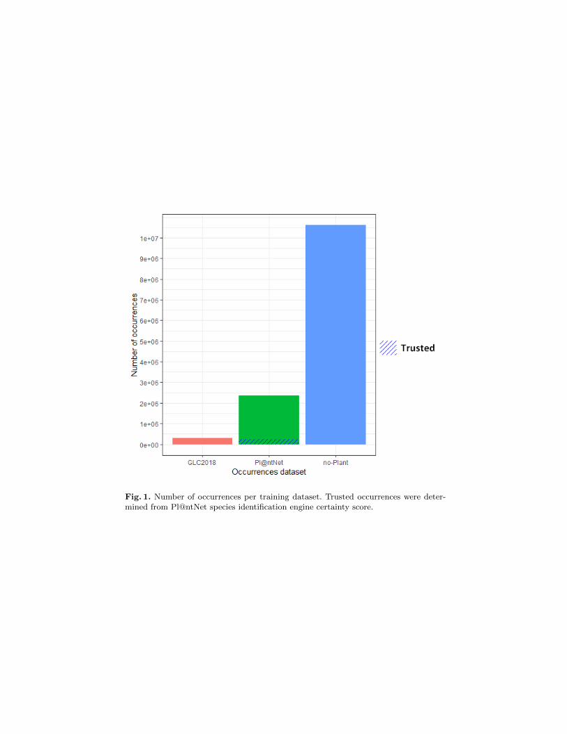
Fig. 1. Number of occurrences per training dataset. Trusted occurrences were deter-mined from Pl@ntNet species identification engine certainty score.

2.2 Environmental data

Geographic rasters. The geographic and environmental data proposed to par-ticipants are a compilation of geographic rasters. The variables represented areoften used for the purpose of species distribution modelling, especially for plants.The nature of values stored in the rasters are quantitative (bioclimatic, topo-logical, hydrographical and evapo-transpiration variables), ordinal (pedologicalvariables) or categorical (land cover). The rasters are extracted from the datarepository of Botella [3], where readers can find a detailed description.

Fig. 2. Patch extracted at the city of Brest, France.

Tensors extraction. To facilitate the learning of representations taking into ac-count the spatial structure of the environment, we provided a Python toolbox14

allowing to extract local environmental tensors from any position in the rasters.By default, it extracts for each raster a 64x64 pixels patch centered on the targetposition and aggregate the patches from all rasters in the form of a tensor of sizenx64x64 where n is the number rasters.

2.3 Test data

We have chosen an independent and unpublished source dataset of occurrencesfor the test set. It is extracted from the SILENE database maintained by theConservatoire Botanique Mediterraneen 15. Those observations come from vari-ous providers including the conservatory himself, but also national parks, botan-ical associations or impact study consultants. We removed species (i) that werenot present in the train set, (ii) vulnerable species according to the SINP referen-tial “especes sensibles” 16, (iii) and species that are at least vulnerable accordingto the IUCN red list 17. This dataset has a high degree of identification certaintybecause only botanical experts contribute to it. Its geolocation certainty is un-der 50 meters. We used random weighted selection scheme to draw 25,000 testoccurrences among the 700,000 of the initial set noted S. We compute, for eachoccurrence si in S a weight wi:

wi = 1/(ni × ri)

Where ri is the number of species in the neighborhood of si defined by acircle of radius d. ni is the total number of occurrences in the neighborhood. Wedefine the spatial scale d = 2 kilometers. With these weights and the followingalgorithm, we guaranty that (i) test occurrences are uniformly distributed in thegeographic space at scale 2d, (ii) there is as many occurrences of each presentspecies on neighborhoods of radius 2d. We then draw the test occurrences fromS without replacement, through the following algorithm:

– Initialize the bag of test occurrences S′ := S and the test set T = ∅.– Randomly draw an occurrence in S′, say i.– Draw a scalar z ∼ U(0,max(w1, ..., w|S|)).– If z < wi, remove i from S′ and add it to T , otherwise leave it in S′.– Stop if |T | = 25000, otherwise we go back to step (1).

3 Task description

For every occurrence of the test set, the evaluated systems must return a listof 50 species maximum, ranked without ex-aequo. The main evaluation metric

14 https://github.com/maximiliense/GLC1915 http://flore.silene.eu/index.php?cont=accueil16 http://www.naturefrance.fr/languedoc-roussillon/

referentiel-des-donnees-sensibles17 https://uicn.fr/liste-rouge-flore/

used is the top 30 accuracy (TOP30). We provide its expression hereafter:

TOP30 :1

Q

Q∑q=1

1rankq≤30

where Q is the total number of query occurrences xq in the test set and rankqis the rank of the correct species y(xq) in the ranked list of species predicted bythe evaluated method for the occurrence xq.A secondary metric is the Mean Reciprocal Rank (MRR), a statistic measurefor evaluating any process that produces a list of possible responses to a sampleof queries ordered by probability. The reciprocal rank of a query response is themultiplicative inverse of the rank of the correct answer. We provide its expressionhereafter :

MRR :1

Q

Q∑q=1

1

rankq

The MRR was used as main metric during last year edition. We compute itthis year, in order to enable comparisons between two campaigns.

4 Participants and methods

61 participants registered to the challenge through the online platform, amongwhich 5 participants managed to submit runs in times. A total of 44 runs weresubmitted. All participants runs methods are characterized by their types ofmodel architecture, the occurrences and input data they used in table 6. In thefollowing paragraph, we describe in more details the methodology of each team.

LIRMM, Inria, Univ. Paul Valery, Univ. Montpellier, France, 4 runs, [10] :This team used a single deep convolutional neural network architecture derivedin four models. All models take as input the default environmental tensors ex-tracted by the provided python toolbox (see section 2.1), with a one-hot encodingtransformation for each category of the land cover variables (clc), inducing 77layers images in the input of the model. The chosen architecture was an Incep-tion V3 ([13]). Models were trained as classifiers, using a softmax output anda cross-entropy loss (also known as multinomial logistic regression). Model ofrun 27006 was trained on all occurrences of PL complete and glc18 datasets,while models 27004 used PL complete with identification score ≥ 0.7, and 27005used PL complete with identification score ≥ 0.98 (filtered dataset). Further-more, runs 27004 and 27005 were only trained on a subset of the occurrences:a sample of around 30K occurrences was drawn according to the same selectionprocedure as for the test set. Thus, all those models predicted only plant species.On the contrary, model 27007 was trained on all occurrences datasets includingPL complete, glc18 and also noPlants. This one was trained to predict plantspecies and many animal species.

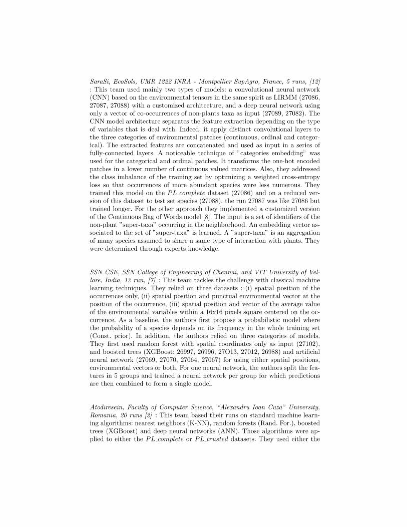
SaraSi, EcoSols, UMR 1222 INRA - Montpellier SupAgro, France, 5 runs, [12]: This team used mainly two types of models: a convolutional neural network(CNN) based on the environmental tensors in the same spirit as LIRMM (27086,27087, 27088) with a customized architecture, and a deep neural network usingonly a vector of co-occurrences of non-plants taxa as input (27089, 27082). TheCNN model architecture separates the feature extraction depending on the typeof variables that is deal with. Indeed, it apply distinct convolutional layers tothe three categories of environmental patches (continuous, ordinal and categor-ical). The extracted features are concatenated and used as input in a series offully-connected layers. A noticeable technique of ”categories embedding” wasused for the categorical and ordinal patches. It transforms the one-hot encodedpatches in a lower number of continuous valued matrices. Also, they addressedthe class imbalance of the training set by optimizing a weighted cross-entropyloss so that occurrences of more abundant species were less numerous. Theytrained this model on the PL complete dataset (27086) and on a reduced ver-sion of this dataset to test set species (27088). the run 27087 was like 27086 buttrained longer. For the other approach they implemented a customized versionof the Continuous Bag of Words model [8]. The input is a set of identifiers of thenon-plant ”super-taxa” occurring in the neighborhood. An embedding vector as-sociated to the set of ”super-taxa” is learned. A ”super-taxa” is an aggregationof many species assumed to share a same type of interaction with plants. Theywere determined through experts knowledge.

SSN CSE, SSN College of Engineering of Chennai, and VIT University of Vel-lore, India, 12 run, [7] : This team tackles the challenge with classical machinelearning techniques. They relied on three datasets : (i) spatial position of theoccurrences only, (ii) spatial position and punctual environmental vector at theposition of the occurrence, (iii) spatial position and vector of the average valueof the environmental variables within a 16x16 pixels square centered on the oc-currence. As a baseline, the authors first propose a probabilistic model wherethe probability of a species depends on its frequency in the whole training set(Const. prior). In addition, the authors relied on three categories of models.They first used random forest with spatial coordinates only as input (27102),and boosted trees (XGBoost: 26997, 26996, 27O13, 27012, 26988) and artificialneural network (27069, 27070, 27064, 27067) for using either spatial positions,environmental vectors or both. For one neural network, the authors split the fea-tures in 5 groups and trained a neural network per group for which predictionsare then combined to form a single model.

Atodiresein, Faculty of Computer Science, “Alexandru Ioan Cuza” University,Romania, 20 runs [2] : This team based their runs on standard machine learn-ing algorithms: nearest neighbors (K-NN), random forests (Rand. For.), boostedtrees (XGBoost) and deep neural networks (ANN). Those algorithms were ap-plied to either the PL complete or PL trusted datasets. They used either the

spatial coordinates or the environmental punctual values of a selection of 29environmental variables, or the concatenation of coordinates and variables. Allcombinations of algorithms, occurrences data and input data were evaluated ona validation set and the best of them were submitted. They also carried ensemblepredictions from those models (runs 26969, 26970, 26958, 27062, 26960, 26971,26961, 26964, 26968). A partial explanation of the low performances of their runsis that they only answered a short list of species (maximum 5) for each test oc-currences, which lowers down performances a lot, especially for the top30 metric.

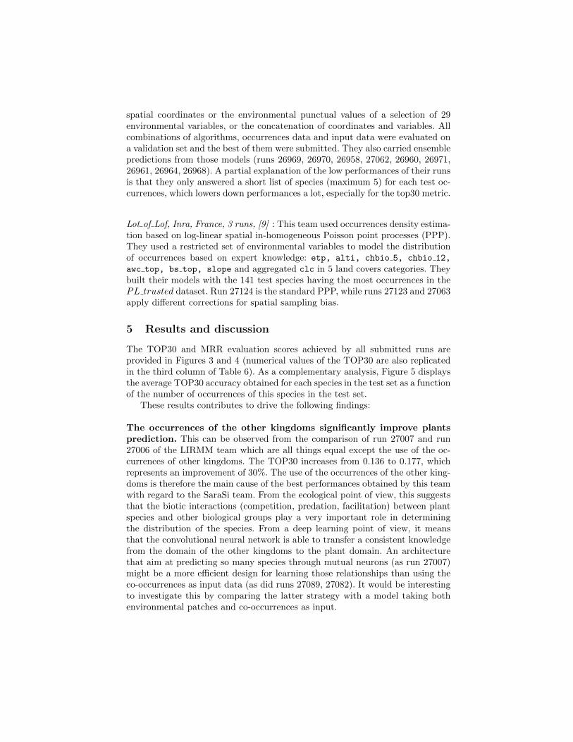
Lot of Lof, Inra, France, 3 runs, [9] : This team used occurrences density estima-tion based on log-linear spatial in-homogeneous Poisson point processes (PPP).They used a restricted set of environmental variables to model the distributionof occurrences based on expert knowledge: etp, alti, chbio 5, chbio 12,

awc top, bs top, slope and aggregated clc in 5 land covers categories. Theybuilt their models with the 141 test species having the most occurrences in thePL trusted dataset. Run 27124 is the standard PPP, while runs 27123 and 27063apply different corrections for spatial sampling bias.

5 Results and discussion

The TOP30 and MRR evaluation scores achieved by all submitted runs areprovided in Figures 3 and 4 (numerical values of the TOP30 are also replicatedin the third column of Table 6). As a complementary analysis, Figure 5 displaysthe average TOP30 accuracy obtained for each species in the test set as a functionof the number of occurrences of this species in the test set.

These results contributes to drive the following findings:

The occurrences of the other kingdoms significantly improve plantsprediction. This can be observed from the comparison of run 27007 and run27006 of the LIRMM team which are all things equal except the use of the oc-currences of other kingdoms. The TOP30 increases from 0.136 to 0.177, whichrepresents an improvement of 30%. The use of the occurrences of the other king-doms is therefore the main cause of the best performances obtained by this teamwith regard to the SaraSi team. From the ecological point of view, this suggeststhat the biotic interactions (competition, predation, facilitation) between plantspecies and other biological groups play a very important role in determiningthe distribution of the species. From a deep learning point of view, it meansthat the convolutional neural network is able to transfer a consistent knowledgefrom the domain of the other kingdoms to the plant domain. An architecturethat aim at predicting so many species through mutual neurons (as run 27007)might be a more efficient design for learning those relationships than using theco-occurrences as input data (as did runs 27089, 27082). It would be interestingto investigate this by comparing the latter strategy with a model taking bothenvironmental patches and co-occurrences as input.

Fig. 3. Average Top30 accuracy per run and participant. It was computed over the25,000 test occurrences. This was the official ranking metric for the task.

Fig. 4. Mean Reciprocal Rank per run and participant. It was computed over the25,000 test occurrences.

Weighting the loss by species is better for predicting rare species.The CNN models learnt by the SaraSi team were based on a weighted cross-entropy loss penalizing the classes with more samples as a way to compensateclass imbalance. Interestingly, it can be seen in Figure 5 that this significantlyincreased the ability of the model 27086 to predict the species having few oc-currences compared to the winner CNN (run 27007) from LIRMM. Run 27086is better than 27007 for more than 80% of the species. LIRMM team gave equalweights to all occurrences in the loss for training model 27007. It also shows howthe most represented species hide the performances on the majority of species,which rarely occur. Giving more balanced weights across species is certainly im-portant to achieve more robust predictions because the observation preferencesacross species vary a lot from one biodiversity dataset to another, as it is thecase here between Pl@ntNet, the GBIF and SILENE.

The more complex the model, the better the prediction. The analysisof the column ”model” of Table 6 suggests that, at least models using environ-mental inputs, can be ranked according to their performance as: (i) Convolu-tional Neural Network (CNN), (ii) Boosted trees (XGboost), (iii) Deep NeuralNetwork (ANN), (iv) Poisson point processes, (v) K-Nearest Neighbors. Thisclearly shows a gradient from the models that integrate the most complex in-put data (CNN having the most complex with many channels of environmentalimages) and the most flexible architectures (CNN, XGBoost and ANN can fitvery complex functions of their input data), to the models that are the mostconstrained by their input data (environmental vectors only) and with simplearchitectures (log-linear model of PPP, no optimized parameters for K-NN). Thisshows that the size of the available datasets and the complexity of the problemgive a real advantage to complex statistical learning methods. More specifically,once again CNN results far exceeded those of the other methods which reinforcesthe results obtained in the last edition of the challenge. The CNN are likely toextract complex features of spatio-environmental patterns in their highest levelneurons which are more suited to describe species habitats than environmentalvariables designed by experts. They may also captures spatial configurations ofhabitats that favor certain dispersion mechanisms, e.g. source-think coloniza-tion, or detect signatures of particular trophic assemblages.

The training of CNN can fail. Although the best models were basedon CNNs, not all CNNs obtained so good results. Indeed, some runs based onCNNs were even worst than the prior ranking of species according to their globalabundance (see 27004 ≤ 26821). Furthermore, non-submitted CNN models men-tioned in a participant working note did perform less in validation than simplerapproaches (see [7] 3.4). Model design (architecture, selection of environmentalchannels, management of categorical variables), regularization (optimization al-gorithm, use of dropout, learning rate and stopping rule policy), training data(especially size, see runs 27004 and 27005) and occurrence weighting scheme de-

termine jointly the implementation success.

Fig. 5. Top30 accuracy averaged per species abundance class for the two best CNNmodels. Species were ranked by decreasing number of occurrences in the test set andthen aggregated in 14 classes of abundances. For run 27086, each occurrence is weightedinversely proportional to the abundance of its species in the loss function.

Results of the MRR show that performances were globally lower than lastyear. Indeed, last year average MRR of the ten best runs was 0.039 while it is0.024 this year. This large global performance gap is probably due to the diffi-culty of the test set, given that last year dataset was included in the trainingdata. We note that the test set was not identically distributed, firstly because itwas located on the Mediterranean region only, but also because the occurrenceswere sampled to avoid spatial and species biases. We know that all models pre-dict less well rare species and under-sampled areas. Thus, this drop in overallperformance supports the idea that the new test set has succeeded in givinggreater importance to rare species and sub-sampled areas.In absolute terms, the best run gives the good answer 20% of the times in its top-30. Thus, roughly speaking, even the best model gives generally a large majorityof wrong species in its top-30 list. To give an order of comparison, the databaseSophy [11] contains more than 35,000 exhaustive plant species inventories onplots generally not exceeding 400m2, and covers a wide range of environmentsin France. According to it, the species diversity in such plots is 25 in average

and rarely exceeds 70. There is thus large room for improvement in automatedpredictions.

6 Conclusion and perspectives

We now come back on the main outcomes of this task and discuss its perspec-tives.LIRMM best CNN successfully integrated many non-plants species occurrencesin their models predictions to better extract spatio-environmental patterns thatmore robustly predict plants species. It suggests that the global biotic assemblagehighly determine the plant assemblage through underlying species interactions,and the multi-species prediction proved again to be a good deep learning strategyto account for it. This is the main new outcome of this year’s edition. However,there should be significant room for improvement in the implementation of thisapproach. Indeed, LIRMM indicated that the winning model training couldn’t befinished for time constraints reasons. Furthermore, light and customized modelsarchitectures accounting for the different variables natures seem more adaptedto the problem than heavily parameterized state-of-the-art image classificationarchitectures. Indeed, SaraSi customized CNN architecture has performed betterthan the related LIRMM Inception V3 CNN with the same output. Merging thestrengths of both strategies promises good improvements in the future.A rich source of information that remains unexploited for this task is the highresolution satellite images data. For example, today, 50 cm resolution satelliteimages are freely available for research all over the french territory through theNational Institute of Geography (IGN) 18. Including such images as input in thecurrent models would inform them about very local land cover type and thusgive much finer resolution prediction, if one can efficiently handle the size of thisdata.The philosophy of the evaluation was to favor models that are more robust tobiases in the training data, especially the imbalance of species representationand the heterogeneous spatial coverage, both consequences of the reporting pro-cess heterogeneity. We can say that it is a success concerning species imbalancerepresentation. Indeed, SaraSi achieved remarkably stable performances even forrare species through a per class weighting scheme in the cost function. A nextstep would be to account for spatial sampling heterogeneity, as we have seenthat all methods still struggle a lot with scarcely reported areas.Regarding the evaluation process on this problem globally, we put an effortthis year in the quality of the occurrences identification, and corrected for thespecies imbalance bias and heterogeneous spatial coverage (due to the reportingheterogeneity). Our new evaluation strategy was quite discriminant across themethods, and lowered globally the computed results. In absolute terms, we havealso seen that even the best model tends to rank a lot of relevant species (i.e.probably absent from the surroundings) before the good one. The problem ofspatial prediction of plant species lists is objectively far from being solved. Still,

18 https://geoservices.ign.fr/documentation/geoservices/

with the new areas of improvements that the task results pointed out, we areoptimistic about the future methodological advances on the problem of locationbased species prediction.

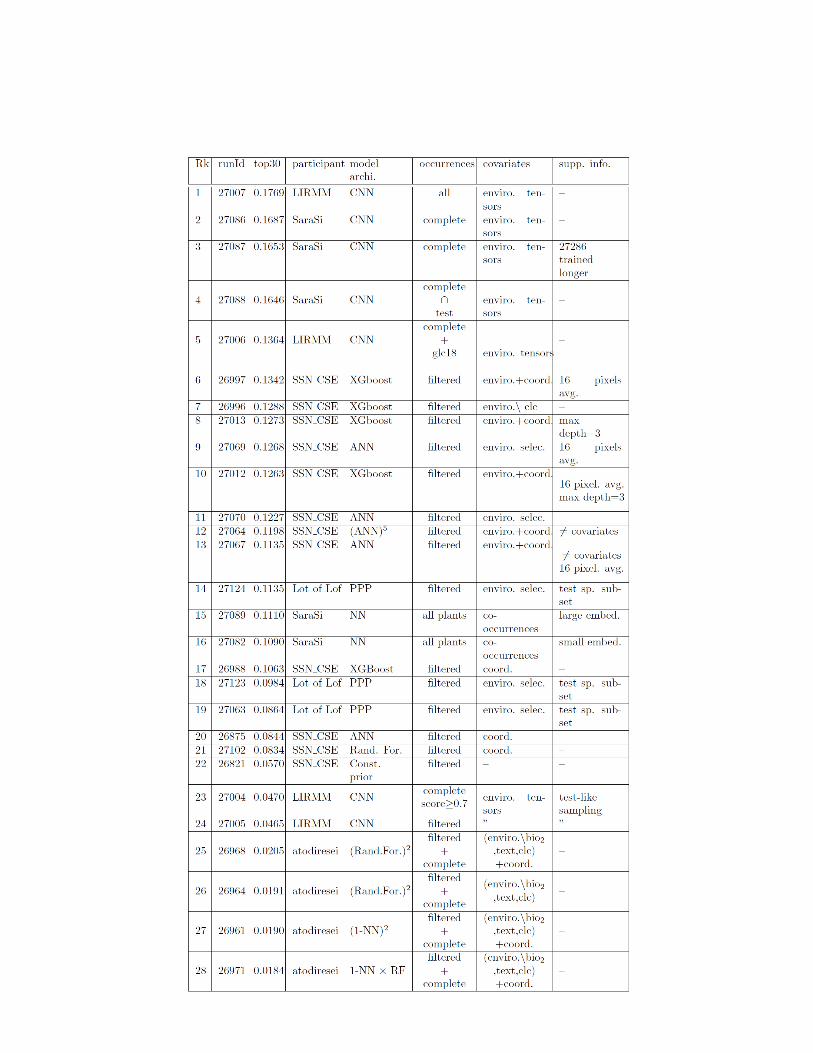
Table 1. Results and summarized methodology description of all runs submitted to Ge-oLifeCLEF 2019. Symbols and abbreviations: A+B means that variables/data B wasadded to A. A\B means that variables/data B where removed from A. complete∩ testmeans that only test species occurrences from the complete dataset were used. Products(×) and exponent notations in column ”model archi.” decompose an ensemble methodswith its different models. Occurrences: complete=PL complete,filtered=PL filtered,all plants=PL complete + PL filtered + glc18, all=PL complete + PL filtered +glc18 + nonP lants. Covariates in model input: ”enviro. tensors”=environmental ten-sors with spatial neighborhood”, ”enviro.”=punctual values of environmental variables,”coord.”= spatial coordinates.

Bibliography

[1] Affouard, A., Goeau, H., Bonnet, P., Lombardo, J.C., Joly, A.: Pl@ ntnetapp in the era of deep learning. In: ICLR 2017-Workshop Track-5th Inter-national Conference on Learning Representations. pp. 1–6 (2017)

[2] Atodiresei, Costel-Sergiu, I.A.: Location-based species recommendation -geolifeclef 2019 challenge. proceedings of CLEF 2019 (2019)

[3] Botella, C.: A compilation of environmental geographic rasters for sdm cov-ering france (version 1) [data set]. Zenodo (2019), http://doi.org/10.

5281/zenodo.2635501

[4] Botella, C., Bonnet, P., Joly, A., Lombardo, J.C., Affouard, A.: Pl@ntnetqueries 2017-2018 in france. Zenodo (2019), http://doi.org/10.5281/

zenodo.2634137

[5] Botella, C., Bonnet, P., Munoz, F., Monestiez, P., Joly, A.: Overview of geo-lifeclef 2018: location-based species recommendation. In: CLEF 2018 (2018)

[6] Joly, A., Goeau, H., Botella, C., Kahl, S., Poupard, M., Servajean, M.,Glotin, H., Bonnet, P., Vellinga, W.P., Planque, R., Schluter, J., Stoter,F.R., Muller, H.: Lifeclef 2019: Biodiversity identification and predictionchallenges. In: Azzopardi, L., Stein, B., Fuhr, N., Mayr, P., Hauff, C., Hiem-stra, D. (eds.) Advances in Information Retrieval. pp. 275–282. SpringerInternational Publishing, Cham (2019)

[7] Krishna, Nanda, K.P.K.R.M.P.A.C.J.S.: Species recommendation using ma-chine learning - geolifeclef 2019. proceedings of CLEF 2019 (2019)

[8] Mikolov, T., Chen, K., Corrado, G., Dean, J.: Efficient estimation of wordrepresentations in vector space. arXiv preprint arXiv:1301.3781 (2013)

[9] Monestiez, Pascal, B.C.: Location-based species recommendation - geolife-clef 2019 challenge. proceedings of CLEF 2019 (2019)

[10] Negri, Mathilde, S.M.J.A.: Plant prediction from cnn model trained withother kingdom species (geolifeclef 2019: Lirmm team). proceedings of CLEF2019 (2019)

[11] Ruffray, P., B.H.G.r.G.H.M.: “sophy”, une banque de donnees phyto-sociologiques; son interet pour la conservation de la nature. Actes du col-loque “Plantes sauvages et menacees de France: bilan et protection”, Brest,8-10 octobre 1987 pp. 129–150 (1989)

[12] Si-Moussi, Sara, G.E.H.M.D.T.T.W.: Species recommendation using envi-ronment and biotic associations. proceedings of CLEF 2019 (2019)

[13] Szegedy, C., Vanhoucke, V., Ioffe, S., Shlens, J., Wojna, Z.: Rethinking theinception architecture for computer vision. In: Proceedings of the IEEE con-ference on computer vision and pattern recognition. pp. 2818–2826 (2016)