overview on the cosmo-model system ulrich schättler deutscher wetterdienst bu research and...
Post on 21-Dec-2015
222 views
TRANSCRIPT
Overview on the COSMO-Model System
Ulrich Schättler
Deutscher Wetterdienst
BU Research and Development
Department for Numerical Modelling
02.-06.03.2009 COSMO/CLM Training Course 2
Contents
• The Model System
• Development History
• Components of the COSMO-Model
• Preprocessing: PEP and INT2LM

02.-06.03.2009 COSMO/CLM Training Course 3
The Model System
• The COSMO-Model System is a nonhydrostatic limited-area atmospheric prediction system.
• It can be used for regional numerical weather prediction (NWP) and regional climate modelling (RCM).
• The COSMO Community runs the system for daily production of (numerical) weather forecasts.
• The CLM Community deployed it for the IPCC runs and for various scientific purposes.
• The software package of the COSMO-Model system is available (freely) for scientific purposes (only!).

02.-06.03.2009 COSMO/CLM Training Course 4
COSMO-Model(s)
DWD (Offenbach, Germany):NEC SX-9
MeteoSwiss:Cray XT4: COSMO-7 and COSMO-2 use 800+4 MPI-Tasks on 402 out of 448 dual core AMD nodes
ARPA-SIM (Bologna, Italy):IBM pwr5: up to 160 of 512 nodes at CINECA
COSMO-LEPS (at ECMWF):running on ECMWF pwr5 as member-state time-critical application
HNMS (Athens, Greece):IBM pwr4: 120 of 256 nodes
IMGW (Warsawa, Poland):SGI Origin 3800:uses 88 of 100 nodes
ARPA-SIM (Bologna, Italy):Linux-Intel x86-64 Cluster for testing (uses 56 of 120 cores)
USAM (Rome, Italy):HP Linux Cluster XEON biproc quadcoreSystem in preparation
Roshydromet (Moscow, Russia), NMA (Bucharest, Romania):Still in planning / procurement phase
02.-06.03.2009 COSMO/CLM Training Course 5
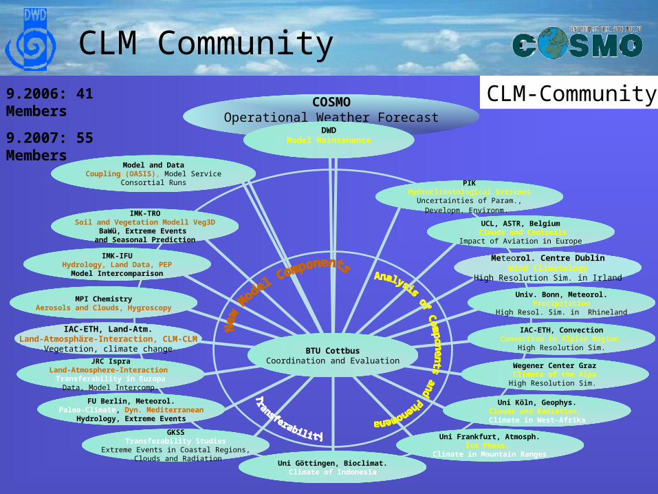
BTU CottbusCoordination and Evaluation
COSMOOperational Weather Forecast
Model and DataCoupling (OASIS), Model Service
Consortial Runs
IMK-TROSoil and Vegetation Modell Veg3D
BaWü, Extreme Events and Seasonal Prediction
IMK-IFUHydrology, Land Data, PEP
Model Intercomparison
MPI ChemistryAerosols and Clouds, Hygroscopy
JRC IspraLand-Atmosphere-Interaction
Transferability in EuropaData, Model Intercomp.
FU Berlin, Meteorol.Paleo-Climate, Dyn. Mediterranean
Hydrology, Extreme Events
GKSSTransferability Studies
Extreme Events in Coastal Regions, Clouds and Radiation
Uni Göttingen, Bioclimat.Climate of Indonesia
Uni Frankfurt, Atmosph.Ice Phase,
Climate in Mountain Ranges
Uni Köln, Geophys.Clouds and Radiation, Climate in West-Afrika
Wegener Center GrazClimate of the Alps
High Resolution Sim.
IAC-ETH, ConvectionConvection in Alpine Region
High Resolution Sim.
Univ. Bonn, Meteorol.Precipitation
High Resol. Sim. in Rhineland
UCL, ASTR, Belgium Clouds and Contrails
Impact of Aviation in Europe
PIKHydroclimatological Extremes
Uncertainties of Param.,Developm. Environm.
DWDModel Maintenance
Meteorol. Centre DublinWind Climatology
High Resolution Sim. in Irland
IAC-ETH, Land-Atm.Land-Atmosphäre-Interaction, CLM-CLM
Vegetation, climate change
9.2006: 41 Members
9.2007: 55 Members
CLM-Community
CLM Community

02.-06.03.2009 COSMO/CLM Training Course 6
The Model System (II)
• Software / data necessary to run the system: – External parameters to describe the earth´s surface:
• constant data, e.g.: orography, land-sea-mask, soil type• (not so constant) data, e.g.: plant characteristics
These data can be provided by EXTPAR (DWD) or PEP (CLM)
– INT2LM: Interpolation program which reads data from a driving model to prepare initial and boundary conditions for the COSMO-Model
– COSMO-Model: The forecast model itself – Postprocessing tools
• Visualization of results• Verification • Evalutation of climate runs
02.-06.03.2009 COSMO/CLM Training Course 7
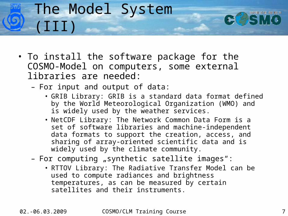
The Model System (III)
• To install the software package for the COSMO-Model on computers, some external libraries are needed:– For input and output of data:
• GRIB Library: GRIB is a standard data format defined by the World Meteorological Organization (WMO) and is widely used by the weather services.
• NetCDF Library: The Network Common Data Form is a set of software libraries and machine-independent data formats to support the creation, access, and sharing of array-oriented scientific data and is widely used by the climate community.
– For computing „synthetic satellite images“:• RTTOV Library: The Radiative Transfer Model can be used to
compute radiances and brightness temperatures, as can be measured by certain satellites and their instruments.
02.-06.03.2009 COSMO/CLM Training Course 8
The Model System (IV)
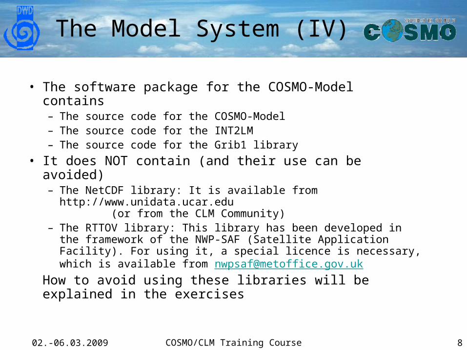
• The software package for the COSMO-Model contains– The source code for the COSMO-Model– The source code for the INT2LM– The source code for the Grib1 library
• It does NOT contain (and their use can be avoided)– The NetCDF library: It is available from http://www.unidata.ucar.edu (or from the CLM Community)
– The RTTOV library: This library has been developed in the framework of the NWP-SAF (Satellite Application Facility). For using it, a special licence is necessary, which is available from [email protected]
How to avoid using these libraries will be explained in the exercises
02.-06.03.2009 COSMO/CLM Training Course 9
History
• DWD developed the nonhydrostatic Local Model during 1996-1999 and started operational runs on 1 December 1999.
• The development did not start from the scratch! The former system EM/DM of DWD was used as a basis.
• In Summer 1999, the Consortium for Small-Scale Modelling was founded by the national weather services of Germany, Switzerland, Italy and Greece, which took over the Local Model
• Later on, Poland (in 2001) and Romania (in 2007) joined. Russia applied for membership (in 2007).
• In 2006 it was decided to use COSMO as the common model name
02.-06.03.2009 COSMO/CLM Training Course 10
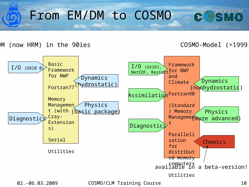
From EM/DM to COSMO
Basic Framework for NWP
Fortran77
Memory Management (with Cray-Extensions)
Serial
Utilities
I/O (GRIB 0)
Diagnostics
Dynamics (hydrostatic)
Physics(basic package)
I/O (Grib1, NetCDF, Restart)
Diagnostics
Dynamics (nonhydrostatic)
Physics(more advanced)
Assimilation
Framework for NWP and Climate
Fortran90 (Standard) Memory Management
Parallelizationfor distributed memory computers
Utilities
Chemics
available in a beta-version!
EM/DM (now HRM) in the 90ies COSMO-Model (>1999)

02.-06.03.2009 COSMO/CLM Training Course 11
COSMO-Model Components
In the following, we will give • an overview on the available components• some basic explanations (more details will be
given during the week for dynamics and physics)• some basic namelist variables (for a more
detailed listing see the „Tutorial“ and for a complete reference the User Guides for the COSMO-Model and the INT2LM)

02.-06.03.2009 COSMO/CLM Training Course 12
Basic Framework
• The basic organization of the COSMO-Model is done in the main program lmorg.F90. The first task is the setup, to define the configuration (CALL organize_setup in module src_setup.f90)– namelist input for the setup– definition of the model domain– memory management– parallelization– computation of basic constants and fields
• The relevant namelist groups are– /LMGRID/– /RUNCTL/

02.-06.03.2009 COSMO/CLM Training Course 13
Basic Framework: /LMGRID/
startlat_tot,startlon_tot
Rotated latitude and longitude of lowerleft grid point
dlat, dlon Resolution (grid spacing) in degrees
pollat, pollon Geographical latitude / longitude ofrotated north pole
ie_tot, je_tot Horizontal grid size (in grid points)
ke_tot Number of vertical levels
Definition of model domain:
02.-06.03.2009 COSMO/CLM Training Course 14
Basic Framework: /RUNCTL/
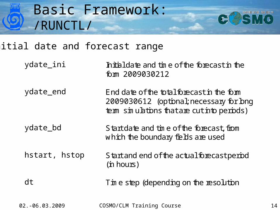
ydate_ini Initial date and time of the forecast in the form 2009030212
ydate_end End date of the total forecast in the form 2009030612 (optional; necessary for long term simulations that are cut into periods)
ydate_bd Start date and time of the forecast, from which the boundary fields are used
hstart, hstop Start and end of the actual forecast period (in hours)
dt Time step (depending on the resolution
Initial date and forecast range
02.-06.03.2009 COSMO/CLM Training Course 15
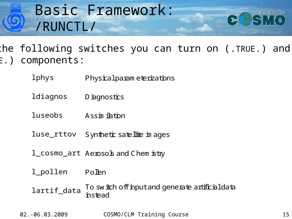
Basic Framework: /RUNCTL/
lphys Physical parameterizations
ldiagnos Diagnostics
luseobs Assimilation
luse_rttov Synthetic satellite images
l_cosmo_art Aerosols and Chemistry
l_pollen Pollen
lartif_data To switch off input and generate artificial data instead
With the following switches you can turn on (.TRUE.) and off(.FALSE.) components:

02.-06.03.2009 COSMO/CLM Training Course 16
Basic Framework: /RUNCTL/
nprocx, nprocy, Number of processors in east-westand south-north
nprocio Number of additional IO processors(usually 0)
nboundlines =2 for Leapfrog dynamics=3 for Runge-Kutta dynamics
lreproduce Ensures computation of reproducibleresults, but needs morecommunication
Parallel Execution:
There are also some „machine-dependent“ variables, like ldatatypes, ncomm_type. For them, all settings should work on any computer, but could give a different performance. NOTE: Only ldatatypes=.TRUE. is NOT working on machineswith 64-bit addressing (like the NEC at DWD )
02.-06.03.2009 COSMO/CLM Training Course 17
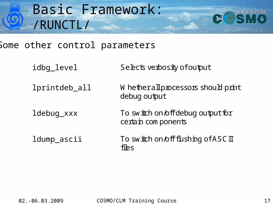
Basic Framework: /RUNCTL/
idbg_level Selects verbosity of output
lprintdeb_all Whether all processors should printdebug output
ldebug_xxx To switch on/off debug output forcertain components
ldump_ascii To switch on/off flushing of ASCIIfiles
Some other control parameters
02.-06.03.2009 COSMO/CLM Training Course 18
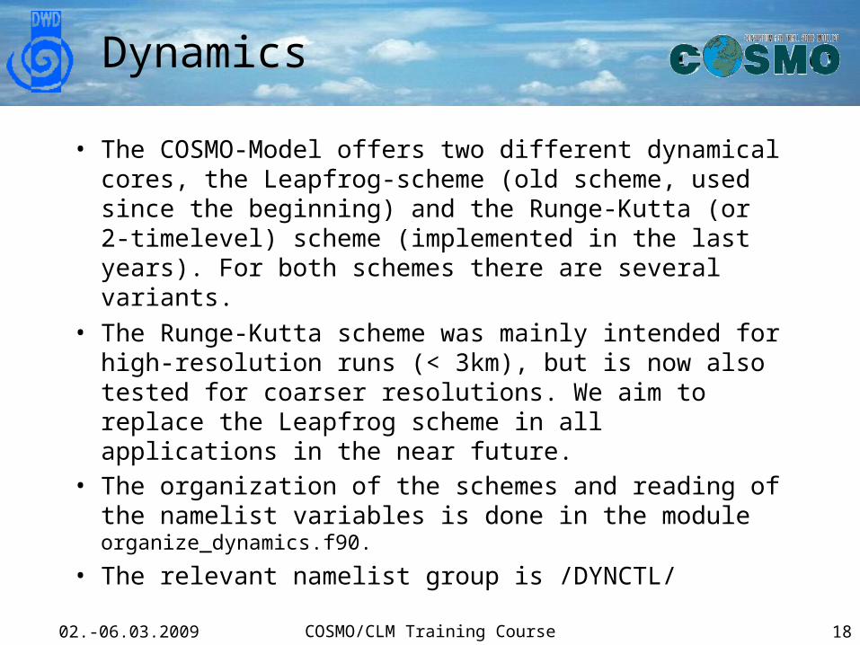
Dynamics
• The COSMO-Model offers two different dynamical cores, the Leapfrog-scheme (old scheme, used since the beginning) and the Runge-Kutta (or 2-timelevel) scheme (implemented in the last years). For both schemes there are several variants.
• The Runge-Kutta scheme was mainly intended for high-resolution runs (< 3km), but is now also tested for coarser resolutions. We aim to replace the Leapfrog scheme in all applications in the near future.
• The organization of the schemes and reading of the namelist variables is done in the module organize_dynamics.f90.
• The relevant namelist group is /DYNCTL/
02.-06.03.2009 COSMO/CLM Training Course 19
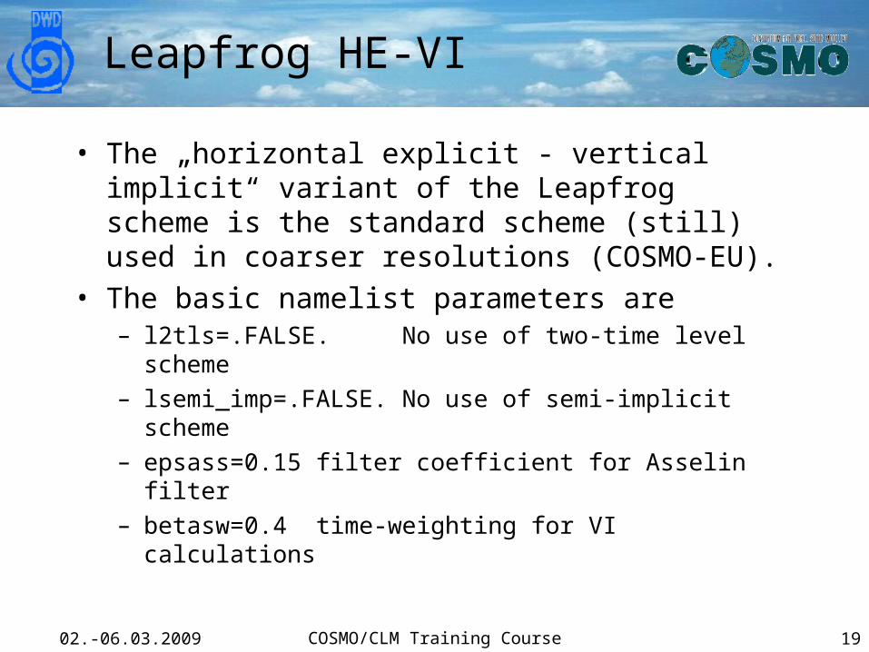
Leapfrog HE-VI
• The „horizontal explicit - vertical implicit“ variant of the Leapfrog scheme is the standard scheme (still) used in coarser resolutions (COSMO-EU).
• The basic namelist parameters are– l2tls=.FALSE. No use of two-time level
scheme– lsemi_imp=.FALSE. No use of semi-implicit scheme– epsass=0.15 filter coefficient for Asselin filter– betasw=0.4 time-weighting for VI calculations
02.-06.03.2009 COSMO/CLM Training Course 20
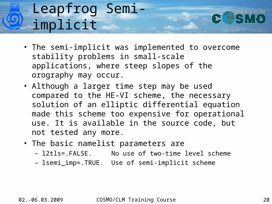
Leapfrog Semi-implicit
• The semi-implicit was implemented to overcome stability problems in small-scale applications, where steep slopes of the orography may occur.
• Although a larger time step may be used compared to the HE-VI scheme, the necessary solution of an elliptic differential equation made this scheme too expensive for operational use. It is available in the source code, but not tested any more.
• The basic namelist parameters are– l2tls=.FALSE. No use of two-time level
scheme– lsemi_imp=.TRUE. Use of semi-implicit scheme
02.-06.03.2009 COSMO/CLM Training Course 21
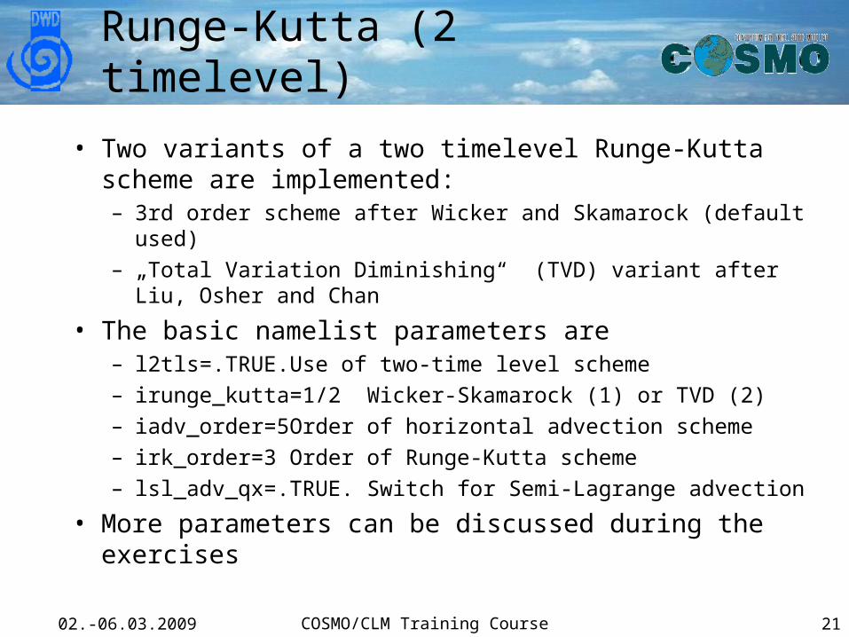
Runge-Kutta (2 timelevel)
• Two variants of a two timelevel Runge-Kutta scheme are implemented:– 3rd order scheme after Wicker and Skamarock (default used)– „Total Variation Diminishing“ (TVD) variant after Liu, Osher and
Chan
• The basic namelist parameters are– l2tls=.TRUE. Use of two-time level scheme– irunge_kutta=1/2 Wicker-Skamarock (1) or TVD (2)– iadv_order=5 Order of horizontal advection
scheme– irk_order=3 Order of Runge-Kutta scheme– lsl_adv_qx=.TRUE. Switch for Semi-Lagrange advection
• More parameters can be discussed during the exercises

02.-06.03.2009 COSMO/CLM Training Course 22
Physics
• The COSMO-Model uses several sub-components for the physical parameterizations. For most sub-components, different variants are offered.
• Note: Not all variants are fully tested!• The sub-components are:
– Microphysics– Radiation– Moist convection– Turbulent diffusion and parameterization of surface fluxes– Soil Processes– Subgrid Scale Orography Scheme
• The organization of the schemes and reading of the namelist group /PHYCTL/ is done in the module organize_physics.f90, if lphys=.TRUE. in the setup.
02.-06.03.2009 COSMO/CLM Training Course 23
Microphysics
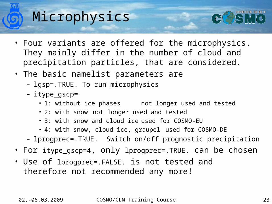
• Four variants are offered for the microphysics. They mainly differ in the number of cloud and precipitation particles, that are considered.
• The basic namelist parameters are– lgsp=.TRUE. To run microphysics– itype_gscp=
• 1: without ice phases not longer used and tested• 2: with snow not longer used and tested• 3: with snow and cloud ice used for COSMO-EU• 4: with snow, cloud ice, graupel used for COSMO-DE
– lprogprec=.TRUE. Switch on/off prognostic precipitation
• For itype_gscp=4, only lprogprec=.TRUE. can be chosen• Use of lprogprec=.FALSE. is not tested and therefore not
recommended any more!
02.-06.03.2009 COSMO/CLM Training Course 24
Radiation
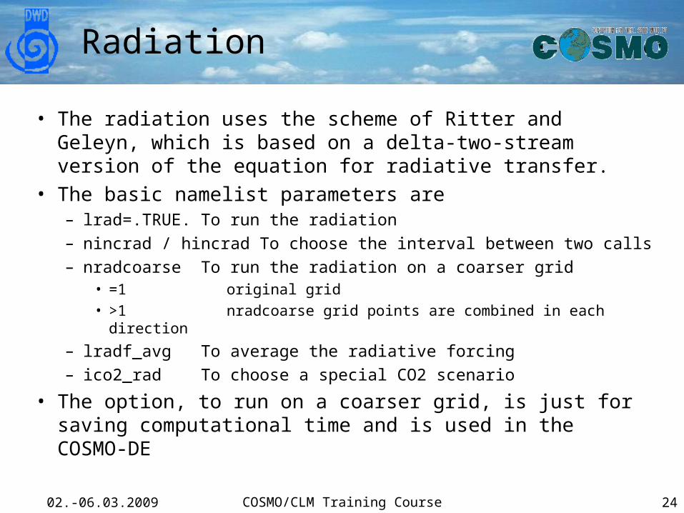
• The radiation uses the scheme of Ritter and Geleyn, which is based on a delta-two-stream version of the equation for radiative transfer.
• The basic namelist parameters are– lrad=.TRUE. To run the radiation– nincrad / hincrad To choose the interval between two calls– nradcoarse To run the radiation on a coarser grid
• =1 original grid• >1 nradcoarse grid points are combined in each
direction
– lradf_avg To average the radiative forcing– ico2_rad To choose a special CO2 scenario
• The option, to run on a coarser grid, is just for saving computational time and is used in the COSMO-DE
02.-06.03.2009 COSMO/CLM Training Course 25
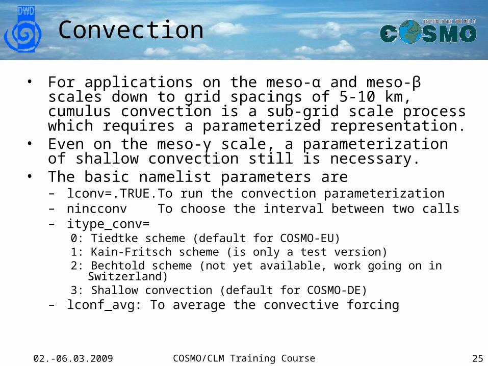
Convection
• For applications on the meso-α and meso-β scales down to grid spacings of 5-10 km, cumulus convection is a sub-grid scale process which requires a parameterized representation.
• Even on the meso-γ scale, a parameterization of shallow convection still is necessary.
• The basic namelist parameters are– lconv=.TRUE. To run the convection parameterization– nincconv To choose the interval between two calls– itype_conv=
0: Tiedtke scheme (default for COSMO-EU)1: Kain-Fritsch scheme (is only a test version)2: Bechtold scheme (not yet available, work going on in Switzerland)3: Shallow convection (default for COSMO-DE)
– lconf_avg: To average the convective forcing
02.-06.03.2009 COSMO/CLM Training Course 26
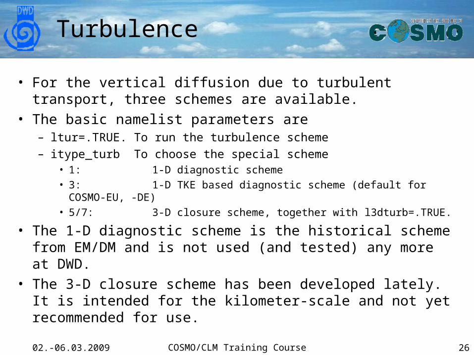
Turbulence
• For the vertical diffusion due to turbulent transport, three schemes are available.
• The basic namelist parameters are– ltur=.TRUE. To run the turbulence scheme– itype_turb To choose the special scheme
• 1: 1-D diagnostic scheme• 3: 1-D TKE based diagnostic scheme (default for COSMO-
EU, -DE)• 5/7: 3-D closure scheme, together with l3dturb=.TRUE.
• The 1-D diagnostic scheme is the historical scheme from EM/DM and is not used (and tested) any more at DWD.
• The 3-D closure scheme has been developed lately. It is intended for the kilometer-scale and not yet recommended for use.
02.-06.03.2009 COSMO/CLM Training Course 27
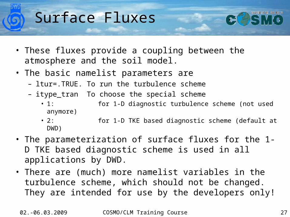
Surface Fluxes
• These fluxes provide a coupling between the atmosphere and the soil model.
• The basic namelist parameters are– ltur=.TRUE. To run the turbulence scheme– itype_tran To choose the special scheme
• 1: for 1-D diagnostic turbulence scheme (not used anymore)
• 2: for 1-D TKE based diagnostic scheme (default at DWD)
• The parameterization of surface fluxes for the 1-D TKE based diagnostic scheme is used in all applications by DWD.
• There are (much) more namelist variables in the turbulence scheme, which should not be changed. They are intended for use by the developers only!
02.-06.03.2009 COSMO/CLM Training Course 28
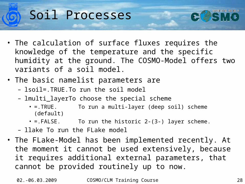
Soil Processes
• The calculation of surface fluxes requires the knowledge of the temperature and the specific humidity at the ground. The COSMO-Model offers two variants of a soil model.
• The basic namelist parameters are– lsoil=.TRUE. To run the soil model– lmulti_layer To choose the special scheme
• =.TRUE. To run a multi-layer (deep soil) scheme (default)
• =.FALSE. To run the historic 2-(3-) layer scheme.
– llake To run the FLake model
• The FLake-Model has been implemented recently. At the moment it cannot be used extensively, because it requires additional external parameters, that cannot be provided routinely up to now.
02.-06.03.2009 COSMO/CLM Training Course 29
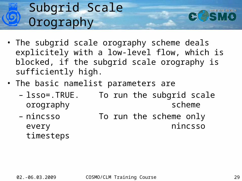
Subgrid Scale Orography
• The subgrid scale orography scheme deals explicitely with a low-level flow, which is blocked, if the subgrid scale orography is sufficiently high.
• The basic namelist parameters are– lsso=.TRUE. To run the subgrid scale orography
scheme– nincsso To run the scheme only every
nincsso timesteps

02.-06.03.2009 COSMO/CLM Training Course 30
Input / Output
• For practical simulations, it is necessary to get data into and out of the model. For idealized test cases, input can be switched off.
• The COSMO-Model supports three different data formats:– Grib, Version 1– NetCDF– Binary data (only for Restarts)
• It is planned to implement Grib, Version 2, „in the near future“ (may take 1-2 years!)
• It would be better to have the restart files in NetCDF, to be machine independent.
• The organization of I/O and reading of the 3 namelist groups is done in the module organize_data.f90.
02.-06.03.2009 COSMO/CLM Training Course 31
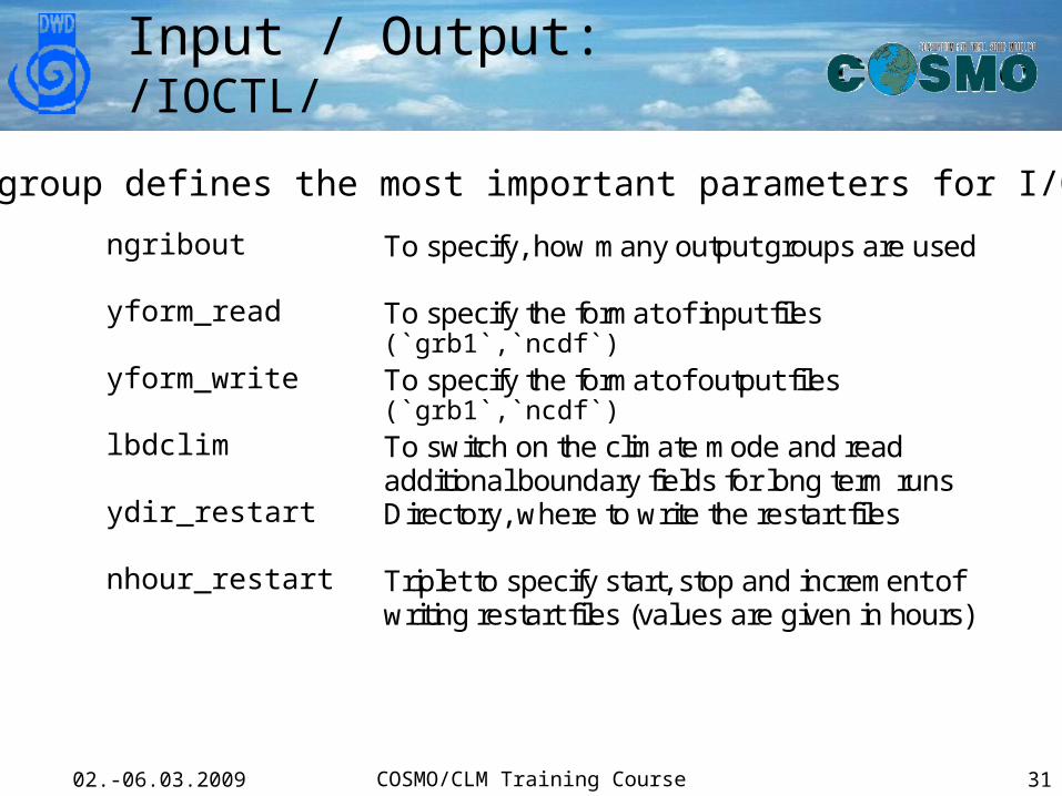
Input / Output: /IOCTL/
ngribout To specify, how many output groups are used
yform_read To specify the format of input files (`grb1`,`ncdf`)
yform_write To specify the format of output files (`grb1`,`ncdf`)
lbdclim To switch on the climate mode and read additional boundary fields for long term runs
ydir_restart Directory, where to write the restart files
nhour_restart Triplet to specify start, stop and increment of writing restart files (values are given in hours)
This group defines the most important parameters for I/O
02.-06.03.2009 COSMO/CLM Training Course 32
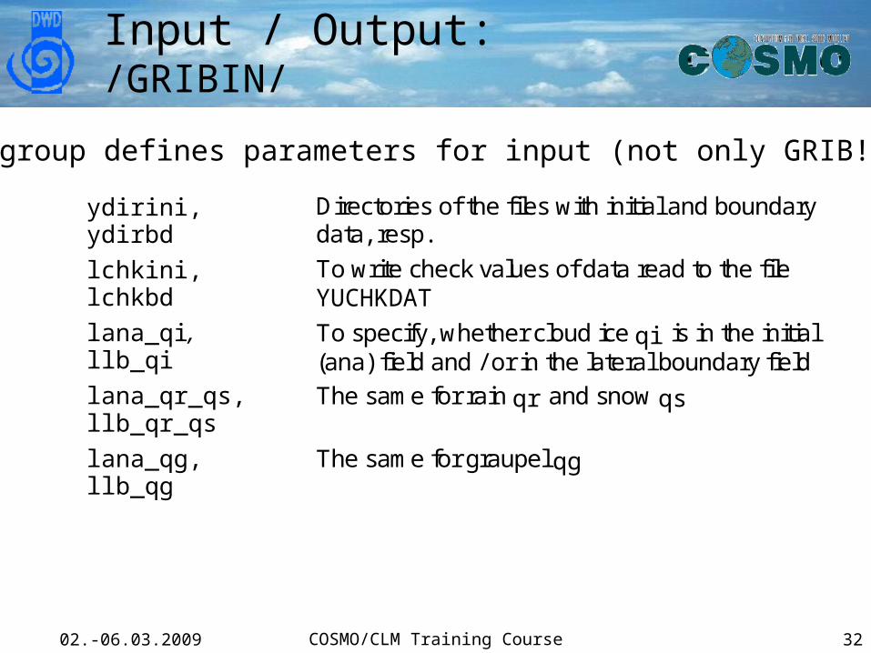
Input / Output: /GRIBIN/
ydirini,ydirbd
Directories of the files with initial and boundarydata, resp.
lchkini,lchkbd
To write check values of data read to the fileYUCHKDAT
lana_qi,llb_qi
To specify, whether cloud ice qi is in the initial(ana) field and / or in the lateral boundary field
lana_qr_qs,llb_qr_qs
The same for rain qr and snow qs
lana_qg,llb_qg
The same for graupel qg
This group defines parameters for input (not only GRIB!)
02.-06.03.2009 COSMO/CLM Training Course 33
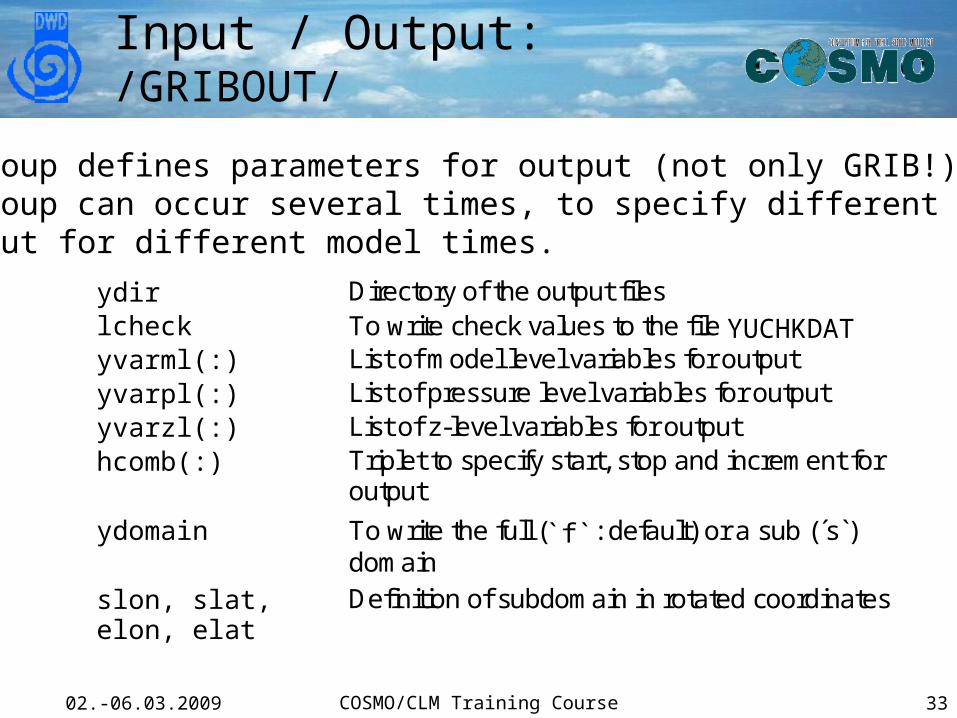
Input / Output: /GRIBOUT/
ydir Directory of the output fileslcheck To write check values to the file YUCHKDATyvarml(:) List of model level variables for outputyvarpl(:) List of pressure level variables for outputyvarzl(:) List of z-level variables for outputhcomb(:) Triplet to specify start, stop and increment for
output
ydomain To write the full (`f`: default) or a sub (´s`)domain
slon, slat,elon, elat
Definition of subdomain in rotated coordinates
This group defines parameters for output (not only GRIB!)This group can occur several times, to specify different kind of output for different model times.

02.-06.03.2009 COSMO/CLM Training Course 34
Preprocessing
•To run the COSMO-Model, several fields have to be provided (Note: Some of them are depending on Namelist switches)
– External parameters: Constant or slowly varying fields for :• HSURF (FIS), FR_LAND, SOILTYP, Z0, FR_LAKE, DEPTH_LK,
• FOR_E, FOR_D, constant• PLCOV, LAI, ROOTDP, annual cycle• VIO3, HMO3 annual cycle
– Initial fields:• Atmosphere: U, V, W, T, PP, QV, QC, QI, QR, QS, QG• Soil and surface: T_SNOW, W_SNOW, W_I, QV_S, T_S, T_SO, W_SO, FRESHSNW, RHO_SNOW, (T_M, T_CL, WG_1, WG_2, W_CL)
– Boundary fields:• Atmosphere: U, V, W, T, PP, QV, QC, QI, QR, QS, QG• Soil and surface: T_SNOW, W_SNOW, QV_S, (T_S, T_M, WG_1, WG_2)
02.-06.03.2009 COSMO/CLM Training Course 35
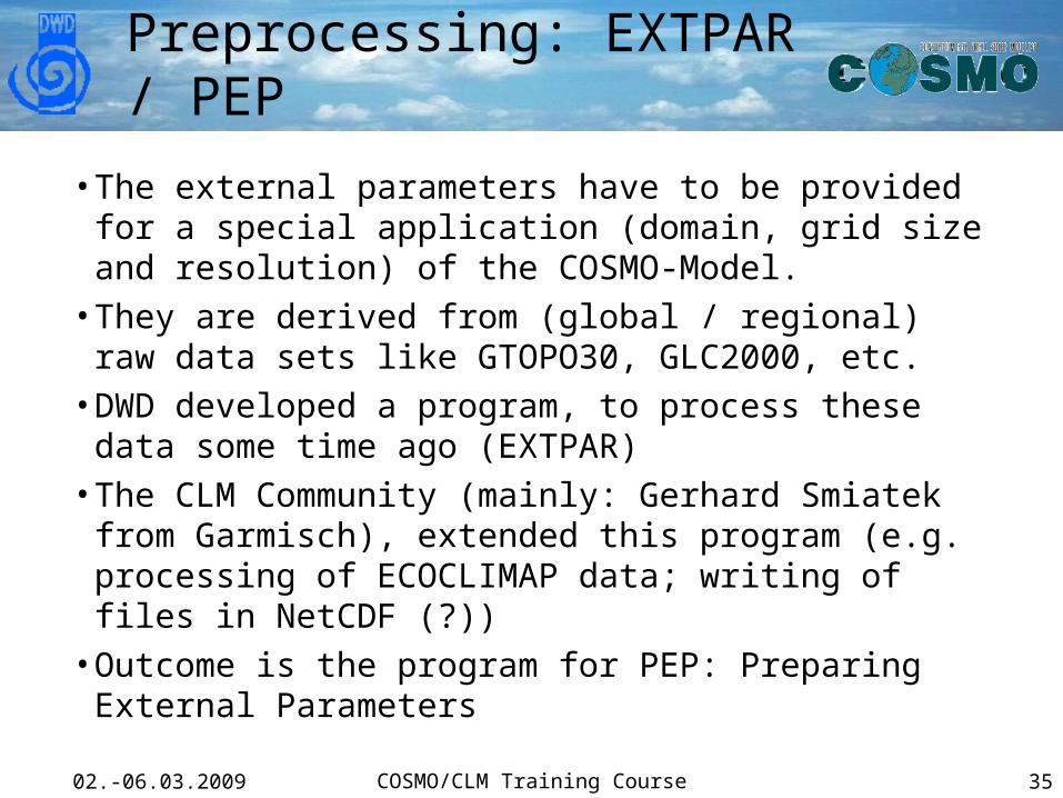
Preprocessing: EXTPAR / PEP
• The external parameters have to be provided for a special application (domain, grid size and resolution) of the COSMO-Model.
• They are derived from (global / regional) raw data sets like GTOPO30, GLC2000, etc.
• DWD developed a program, to process these data some time ago (EXTPAR)
• The CLM Community (mainly: Gerhard Smiatek from Garmisch), extended this program (e.g. processing of ECOCLIMAP data; writing of files in NetCDF (?))
• Outcome is the program for PEP: Preparing External Parameters
02.-06.03.2009 COSMO/CLM Training Course 36
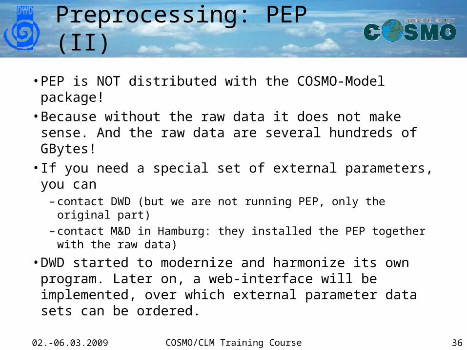
Preprocessing: PEP (II)
• PEP is NOT distributed with the COSMO-Model package!• Because without the raw data it does not make sense.
And the raw data are several hundreds of GBytes!• If you need a special set of external parameters, you can
– contact DWD (but we are not running PEP, only the original part)– contact M&D in Hamburg: they installed the PEP together with the
raw data)
• DWD started to modernize and harmonize its own program. Later on, a web-interface will be implemented, over which external parameter data sets can be ordered.
02.-06.03.2009 COSMO/CLM Training Course 37
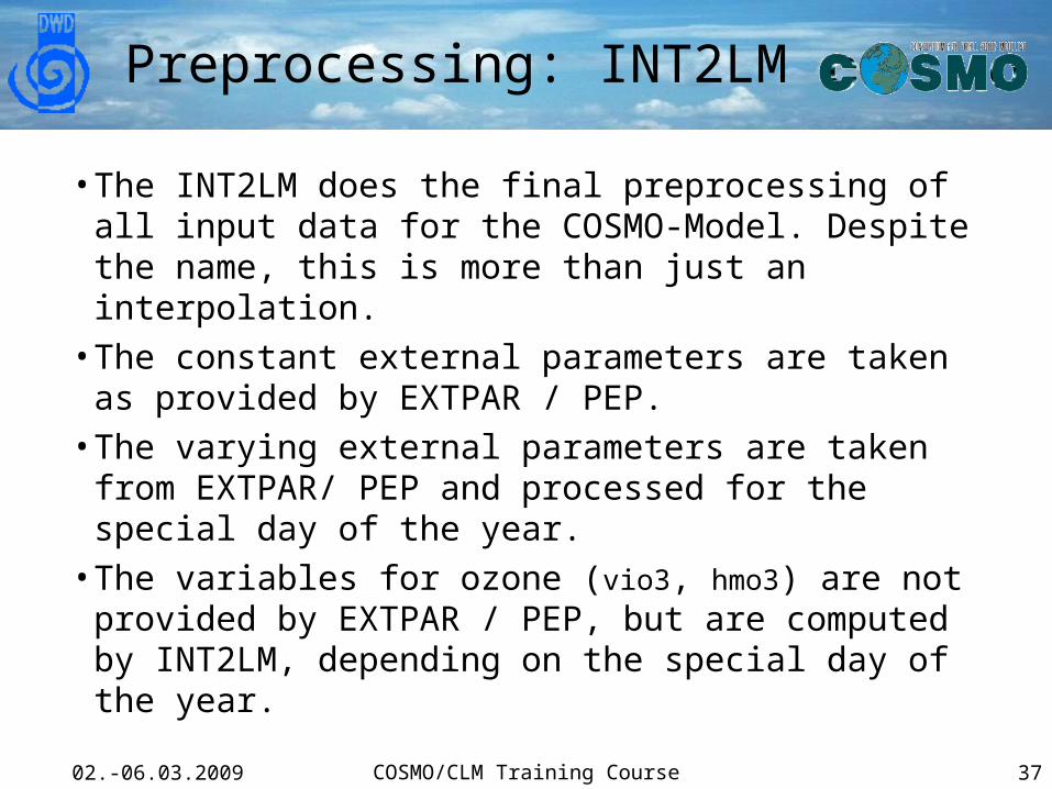
Preprocessing: INT2LM
• The INT2LM does the final preprocessing of all input data for the COSMO-Model. Despite the name, this is more than just an interpolation.
• The constant external parameters are taken as provided by EXTPAR / PEP.
• The varying external parameters are taken from EXTPAR/ PEP and processed for the special day of the year.
• The variables for ozone (vio3, hmo3) are not provided by EXTPAR / PEP, but are computed by INT2LM, depending on the special day of the year.

02.-06.03.2009 COSMO/CLM Training Course 38
Preprocessing: INT2LM (II)
• All other initial and boundary fields are taken from a coarse grid model and processed for the COSMO-Model domain.
• This involves (mainly) a horizontal interpolation, a vertical interpolation and a special treatment in the boundary layer.
• Running the INT2LM is controlled by several Namelist groups.

02.-06.03.2009 COSMO/CLM Training Course 39
INT2LM: /CONTRL/
ydate_ini,ydate_bd
Initial date and time of the forecast and ofthe forecast from the boundaries
hstart, hstop,hincbound
Start and end of the forecast and incrementfor providing boundaries (in hours)
lgme2lm, lec2lm,llm2lm, lcm2lm
To specify the input model that provides(initial and) boundary data
linitial,lboundaries
To specify, whether initial and / or boundarydata should be computed
lbdclim To provide the boundaries for the climatemode
lfilter_oro To do a filtering of the orography foravoiding numerical problems
Basic control:

02.-06.03.2009 COSMO/CLM Training Course 40
INT2LM: /GRID_IN/
ni_gme, i3e_gme Resolution and vertical grid size for GME
ie_in_tot,je_in_tot,ke_in_tot
Grid specifications for other models thanGME
startlat_in_tot,startlon_in_tot
dlon_in, dlat_in
pollat_in,pollon_in
This group specifies the characteristics of the input model:

02.-06.03.2009 COSMO/CLM Training Course 41
INT2LM: /LMGRID/
startlat_tot,startlon_tot
Rotated latitude and longitude oflower left grid point
dlat, dlon Resolution (grid spacing) indegrees
pollat, pollon Geographical latitude / longitudeof rotated north pole
ielm_tot,jelm_totkelm_tot
Horizontal and vertical grid size (ingrid points)
Definition of model domain (same as in the COSMO-Model):
02.-06.03.2009 COSMO/CLM Training Course 42
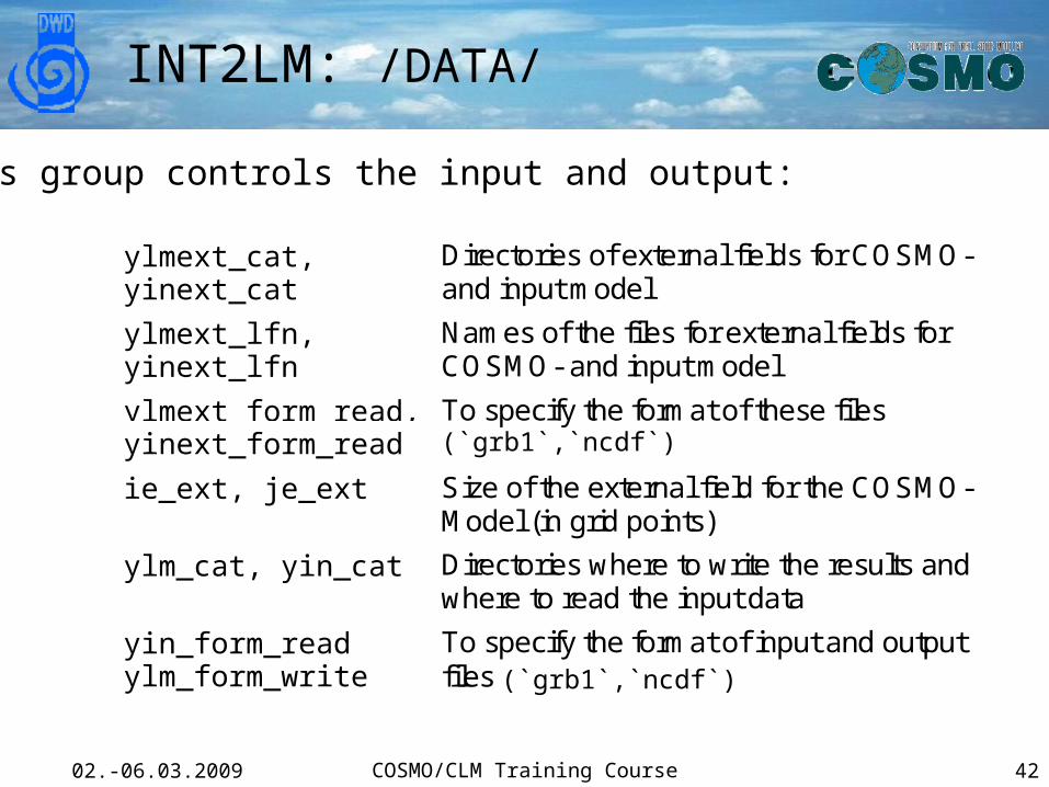
INT2LM: /DATA/
ylmext_cat,yinext_cat
Directories of external fields for COSMO-and input model
ylmext_lfn,yinext_lfn
Names of the files for external fields forCOSMO- and input model
ylmext_form_read,yinext_form_read
To specify the format of these files(`grb1`,`ncdf`)
ie_ext, je_ext Size of the external field for the COSMO-Model (in grid points)
ylm_cat, yin_cat Directories where to write the results andwhere to read the input data
yin_form_readylm_form_write
To specify the format of input and outputfiles (`grb1`,`ncdf`)
This group controls the input and output:

02.-06.03.2009 COSMO/CLM Training Course 43
Coming to an END
• This presentation should have given you an overview on the different parts and components of the COSMO-Model System.
• During this week you will learn more on the theoretical aspects for the dynamics, physics and additional components.
• You will also get some practical experience for installing the source code and running the necessary programs during the „Tutorials“.
• We are happy to take your comments and suggestions!