owen christopher geduldt dissertation
TRANSCRIPT

THE IMPACT OF HARMONIC DISTORTION ON POWER
TRANSFORMERS OPERATING NEAR THE THERMAL LIMIT
by
OWEN CHRISTOPHER GEDULDT
DISSERTATION
submitted in fulfilment
of the requirements for the degree
MASTER OF ENGINEERING
in
ELECTRICAL AND ELECTRONIC ENGINEERING
in the
FACULTY OF ELECTRICAL AND ELECTRONIC ENGINEERING
at the
UNIVERSITY OF JOHANNESBURG
SUPERVISOR: PROF I HOFSAJER
OCTOBER 2005

I hereby declare that this dissertation, submitted for the Master of Engineering degree to the University
of Johannesburg, apart from the help recognised, is my own work and has not previously been
submitted to another university or institution of higher education for a degree.
………………….
O.C. Geduldt

I dedicate this work to my wife Leilani Benita Geduldt for her patience and support in the completion of
this work.

“Whatever exists has already been named, and what man is has been known.” Eccl 6: 10
“We therefore avail ourselves of the labours of the mathematicians, and retranslate their results from the
language of the calculus into the language of dynamics, so that our words may call up the mental image,
not of some algebraical process, but of some property of moving bodies.” James Clerk Maxwell

ABSTRACT
The study looks into the impact of harmonic distortion on power-plant equipment in general, and then
focuses on the impact it has on power transformers operating near the thermal limit. The feasibility of
the study is firstly evaluated and then the theory on harmonics and transformer losses is analysed. The
study had been narrowed down to power transformers due to the high numbers of failures nationally and
internationally attributed to unknown causes. A transformer model is then developed through theoretical
considerations. Finally, a case study is done on the capability of a fully loaded transformer under
harmonics conditions evaluated through transformer capability calculations and the proposed
transformer model. Thereafter the transformer model developed is verified with measured results.
The main impact of harmonic current distortion on power transformers is an increase in the rated power
losses that results in a temperature rise inside the power transformer. The heat build-up can lead to
degradation of insulation, which can shorten the transformer’s life and lead to eventual breakdown. The
harmonic current distortion impacts transformer losses – namely, ohmic losses, the winding eddy
current losses and other stray losses. All of these harmonic effects on transformer losses are verified
theoretically, mathematically and practically.
The harmonic impact on the transformer capability is then evaluated through a numerical example of a
transformer feeding a harmonic load. The transformer capability is determined via two methods –
namely, harmonic capability calculations in the standard “IEEE Recommended Practice for Establishing
Transformer Capability when Supplying Nonsinusoidal Load Currents”, [11] and a proposed
transformer model derived from theoretical and mathematical analysis. The results show that an
increase in the winding eddy current losses can decrease the maximum permissible nonsinusoidal load
current substantially. If the load current of the transformer is derated accordingly it translates into a loss
of the output power capacity of the power transformer. The standard recommended capability
calculations for winding eddy current losses are conservative and not satisfactorily accurate. This results
in a large loss of power capacity. The proposed transformer model includes a parameter that estimates
the winding eddy current loss in the transformer that results in a smaller loss in power capacity.
Furthermore, it was shown that the harmonic current distortion levels could exceed the permissible
levels although the harmonic voltage distortion levels are within acceptable levels. The proposed
transformer equivalent model is thereafter practically verified with experimental results of papers
published by M.A.S. Masoum, E.F. Fuchs and D.J. Roesler, [19], [20] and [29].

LIST OF KEYWORDS: harmonics, winding eddy current losses, other stray losses, nonsinusoidal,
transformer, transformer capability.

ACKNOWLEDGEMENTS
Thanks to my friend Vincent Jaffa for writing the proposal for this completed work. I thank Prof. Ivan
Hofsajer, my study leader, for his invaluable suggestions and guidance. I give thanks to the people that
helped with the editing of this dissertation. To Eskom Transmission I give special thanks for their
financial support. Moreover, I cannot cease to give thanks to my Father God and His Son, Jesus
Khristos, to whom all the glory and praise belongs.

CONTENTS Page no.
CHAPTER 1: INTRODUCTION 1
Introduction 1
1.1 Harmonic effects on power-plant equipment 2
1.1.1 Resonances 4
Parallel resonance 4
Series resonance 6
1.1.2 Transmission system 7
1.1.3 Capacitor banks 9
1.1.4 Transformers 11
1.2 Failure statistics on power transformers 13
Conclusion 15
CHAPTER 2: HARMONIC THEORY, STANDARDS AND SOURCES 16
Introduction 16
2.1 Harmonic definition 17
2.2 Total harmonic distortion, power and power factor 18
2.3 Harmonic sources 20
2.3.1 Thyristor switches 20
Thyristor-controlled inductors [6] 21
2.3.2 Arc furnaces [10] 24
2.3.3 Static converters [6] 26
Single-phase two-way converter 27

Three-phase two-way converter 29
2.3.4 Three-phase inverters [6], [3] 31
2.3.5 Transformer magnetisation non-linearities [6], [8], [9] 34
2.4 Harmonic standards and recommended guidelines 37
2.4.1 Voltage harmonics compatibility levels and assessments 37
Voltage harmonics compatibility levels 37
Voltage assessment method 39
2.4.2 Apportioning procedures for harmonics 40
2.4.3 Harmonic current distortion limits recommended in IEEE 519-1991 42
2.4.4 Transformer heating considerations 44
Conclusion 45
CHAPTER 3: THEORY OF TRANSFORMER LOAD AND NO-LOAD LOSSES 46
Introduction 46
Recommended practice for establishing transformer capability-Transformer losses 46
3.1 Load losses 47
3.1.1 Ohmic losses (I2R) in transformer windings 48
3.1.2 Eddy current losses in windings 51
Skin effect in winding 52
Proximity effect 55
3.1.3 Other stray losses in transformers (POSL) 64

3.2 No-load loss (Excitation losses) 66
3.2.1 Hysteresis losses 66
3.2.2 Eddy current losses in the core 68
3.2.3 Empirical expression for total core loss 73
3.3 Harmonic impact on top oil temperature rise and winding temperature rise 74
3.4 Transformer capability calculations 76
3.5 Recommended procedure for evaluating existing transformers 78
3.5.1 Transformers capability equivalent for power transformers using design data 78
3.5.2 Temperature capability calculations for transformers using design data 79
Conclusion 80
CHAPTER 4: THE TRANSFORMER MODEL DEVELOPMENT 81
Introduction 81
4.1 Transformer theory 81
4.1.1 Basic ideal transformer magnetic theory 81
4.1.2 Non-ideal transformer equivalent model 83
4.2 Leakage flux or self inductance: Leakage inductance 88
4.3 The dc resistance 89
4.4 Mutual flux or magnetising flux: Magnetising inductance 90
4.4.1 Linear magnetising inductance expression 90
4.4.2 Non-linear magnetising inductance expression 92
4.5 Core resistance expression 93

4.6 Winding eddy current loss circuit parameter 94
4.7 Other stray loss resistance 95
4.8 The complete transformer simulation model based on theoretical discussions 96
4.8.1 The complete transformer non-linear model formulated 96
Conclusion 99
CHAPTER 5: EVALUATE THE TRANSFORMER MODEL UNDER HARMONIC LOADING
CONDITIONS 100
Introduction 100
5.1 The simulation program Intusoft SPICE used to simulate the non-linear transformer
model 100
5.2 The general transformer data derived for recommended capability calculations 101
5.3 Recommended capability calculations, [12] and results for the 1kVA transformer 103
5.4 The transformer data calculated for the transformer model in Intusoft SPICE 109
5.5 Transformer model results compared to the recommend capability calculations 112
5.6 Analysis of the transformer model results compared to the NRS and IEEE Standards 116
Conclusion 118
CHAPTER 6: VERIFICATION OF THE TRANSFORMER SIMULATION MODEL 120
Introduction 120
6.1 Evaluate the practical core loss curves with empirical estimations 121
6.1.1 Epstein core loss curves and empirical estimation comparison 121
6.1.2 Epstein core loss curves used to estimate core resistance 122

6.1.3 The magnetisation or B-H curves and relative permeability curve 123
6.2 Evaluate the transformer excitation practical results with non-linear transformer model 125
6.2.1 Measured and simulated excitation curve verification 125
6.3 Experimental verification of non-linear fully loaded transformer model under harmonic
supply 127
Conclusion 130
CHAPTER 7: CONCLUSIONS AND RECOMMENDATIONS 131
CONCLUSIONS 131
RECOMMENDATIONS 135
REFERENCES 136

LIST OF APPENDIXES
APPENDIX A
Transformer Data
Figure A.1 Measured dimensions of 1kVA single-phase transformer in mm. [19]
APPENDIX B
The simulated programming results and circuit in Intusoft SPICE for the nonlinear transformer model
under full load and harmonic loaded conditions.
APPENDIX C
The simulated programming results and circuit simulated in Intusoft SPICE for the nonlinear
transformer model under rated no-load conditions.
APPENDIX D
The simulation programming results and circuit simulated in Intusoft SPICE for the nonlinear
transformer model under full-load rated conditions, and for four cases under full load and superimposed
harmonic supply conditions.

LIST OF SYMBOLS
AΩ is the cross-section of the wire.
Aw is the area the flux density cuts through the winding due to the proximity effect.
Aair is the area the leakage flux cuts through.
Ac is the cross-section of the core.
Aair,1 is the area the primary leakage flux cuts through.
Aair,2 is the area the secondary leakage flux cuts through.
B is the flux density.
BSAT is the magnitude of the saturation flux density.
Bmax is the maximum magnitude of the ac flux density.
H is the magnetic field.
J is the current density.
E is the electric field.
ℑ or mmf is the magnetomotive force.
F is the skin-effect factor.
FHL is the harmonic loss factor for winding eddy current losses.
FHL-STR is the harmonic loss factor for other stray losses.
Gr is the proximity effect factor.
Φ is the main flux that circulates in the transformer core.
Φmax is the maximum magnitude of the main flux that circulates in the transformer core.
Φ1 is the total flux in the primary coil.
Φ2 is the total flux in the secondary coil.
Φm is the magnetising flux, confined to the core.
Φl1 is the primary leakage flux, which cuts through the air.
Φec,1 is the primary winding flux, which cuts through the secondary winding.
Φosl,1 is the primary ‘other structural parts’ flux, which cuts through the structural part or tank of the
transformer.
Φl2 is the secondary leakage flux, which cuts through the air.

Φec,2 is the secondary winding flux, which cuts through the secondary winding.
Φosl,2 is the secondary ‘other structural parts’ flux, which cuts through the structural part or tank of the
transformer.
lm is the magnetic path length.
ld is the mean length of the winding turn.
l1 is the leakage path length of the transformer for the primary side.
l2 is the leakage path length of the transformer for the secondary side.
lw is the total length of the winding or wire.
ll is the winding length or breadth, bw for the leakage inductance.
iS(t) is the time-varying source current.
i1(t) is the fundamental current component of the source current.
ih(t) is the time-varying harmonic current component at harmonic order h.
Is1 is the magnitude of the fundamental current supplied from source vs.
Ish is the magnitude of the current harmonic components generated by the harmonic load.
Ih(pu) is the per unit harmonic current at harmonic order h.
Ih is the magnitude of harmonic current at harmonic order h.
is1 is the time-varying fundamental current of the source current.
Is is the rms magnitude of the source current.
iL is the time-varying load current.
I is the rms magnitude of the load current.
Ip is the magnitude of the real current component.
Iq is the magnitude of the reactive current component.
iL1 is the time-varying fundamental load current.
IL is the rms magnitude of the load current.
id is the time-varying dc supply current.
Id is the magnitude of the dc current.
ia is the phase a supply current.
ib is the phase b supply current.
ic is the phase c supply current.

iripple is the ripple current.
Is0 is the dc current component of the Fourier series.
ISC is the maximum short-circuit current magnitude at point of common coupling (PCC).
IL,max is the maximum demand load current magnitude (fundamental frequency component) at PCC.
Ih,p is the allowable apportioned harmonic current of number h at the PCC (Ampere).
I1 is the rms magnitude of the primary current.
I2 is the rms magnitude of the secondary current.
IA is the rms magnitude of the actual measured current.
IL is the rms magnitude of the load current.
iec(pu) is the time-varying eddy current per unit.
IR-p,1 is the peak magnitude of the primary current.
IR-p,2 is the peak magnitude of the secondary current.
IR,1 is the rated rms magnitude of the primary winding eddy current.
IR,2 is the rated rms magnitude of the secondary winding eddy current.
Imax is the rms magnitude of the maximum permissible current for dry-type transformers.
Imax(pu) is the per unit rms magnitude of the nonsinusoidal load current.
i1 is the time-varying primary current of the transformer.
i2 is the time-varying secondary current of the transformer.
I1 is the rms magnitude of the primary current of the transformer.
I2 is the rms magnitude of the secondary current of the transformer.
iC is the core current.
im is the magnetising current.
MLT is the mean length turn of the winding.
N is turns of the winding.
N1 is the primary turns of the transformer.
N2 is the secondary turns of the transformer.
Zs is the source impedance.
Zp is the impedance of the parallel combination of impedances.
S is the apparent power.

Q is the reactive power.
pf is the power factor.
φ is the phase angle between the voltage, vs and load current, is.
φh is the harmonic phase angle between the harmonic -voltage and -current of harmonic order h.
φ1 is the phase angle between the source voltage and the fundamental time-varying current.
cosφ is the power factor in linear circuits.
α is the thyristor delay angle.
δ is the tan angle.
w is the energy absorbed.
PTL is the total losses.
PLL is the total load loss of the transformer.
PEC is the winding eddy current losses.
PEC-Max is the maximum winding eddy current loss.
POSL is the other stray losses.
Ph is the total harmonic losses.
Pc is the total core loss.
P=I2R is the ohmic losses.
PAV is the average power or real power.
PNL is the no-load losses.
PTSL is the total stray losses.
PEC-O is the winding eddy current losses at the measured current.
PEC-R is the rated total winding eddy current loss.
PEC-R,1 is the rated primary winding eddy current loss.
PEC-R,2 is the rated secondary winding eddy current loss.
POSL-R is the rated other stray losses.
POSL-R,1 is the rated primary other stray losses.
POSL-R,2 is the rated secondary other stray losses.
POSL-h is the other stray loss taking into account the harmonic contribution.
Pec is the total winding eddy current loss.

PΩ (T1) is the ohmic loss (Watts) at temperature T1, ˚C.
PΩ (T2) is the ohmic loss (Watts) at temperature T2, ˚C.
Pec (Tm) is the winding eddy current loss (Watts) at temperature Tm, ˚C.
Pec (T) is the winding eddy current loss (Watts) at temperature T, ˚C.
PLL-R (pu) is the per unit rated load losses of the transformer or local loss density.
PEC-R(pu) is the per unit rated winding eddy current loss at rated current.
POSL-R(pu) is the other stray losses at rated current.
PΩ-h is the ohmic losses impacted by harmonic currents.
1lℜ is the primary reluctance of the leakage paths.
2lℜ is the secondary reluctance of the leakage paths.
Cℜ is the reluctance of the core.
Rh is the power line or cable resistance as a function of frequency.
Rdc is the conduction resistance at dc and low frequencies.
Rdc(T1) is the dc resistance (Ohms) at temperature T1, ˚C.
Rdc(T2) is the dc resistance (Ohms) at temperature T2, ˚C.
Rdc,1 is the primary resistance.
Rdc,2 is the secondary resistance.
Rac is the resistance taking into account the skin effect with the dc resistance.
Rse is the skin-effect resistance.
REC-R,1 is the rated primary winding eddy current loss resistance.
REC-R,2 is the rated secondary winding eddy current loss resistance.
ROSL,1 is the primary other stray loss resistance.
ROSL,2 is the secondary other stray loss resistance.
RC is the core resistance.
RC-R is the rated core resistance.
θg is the winding hot spot conductor rise over top oil temperature rise.
θg-R is the rated winding hot spot conductor rise over top oil temperature rise.
θTO is the top oil temperature rise.
θTO-R is the rated top oil temperature rise.

Tk is the temperature constant for a specific metal or conductor, ˚C.
∆T is the temperature rise.
Ta is the ambient temperature.
LS is the source inductance.
Ls is the source inductance.
Ll is the leakage inductance.
Ll1 is the leakage inductance for the primary coil.
Ll2 is the leakage inductance for the secondary coil.
Lm is the magnetising inductance.
C is the capacitance.
XS is the inductive reactance.
XC is the capacitive reactance.
Xsc is the short circuit reactance at the substation.
Xc is the capacitive reactance at fundamental frequency.
Xch is the capacitive reactance at harmonic frequency at harmonic order, h.
Xh is the maximum supply impedance of number h at the PCC for any normal operating condition (Ohms).
MVAsc is the MVA short circuit rating at the point of study.
MVArcap is the capacitor rating at the system voltage.
THDi is the total harmonic distortion of the current.
THDv is the total harmonic distortion of the voltage.
TDD is the total demand distortion (TDD): is the percentage of the ratio of the rms root-sum-square harmonic distortion to the rms maximum demand load current over a 15 or 30 min demand.
DPF is the displacement power factor ( αφ coscos 1 ==DPF ).
µ is the permeability.
µ0 is the free space permeability.
µi is the initial relative permeability.
σ is the conductivity of a material.
ρ is the resistivity of a material.
d is the diameter or thickness of the conductor.

δd is the skin-effect ratio.
δ is the penetration depth of the conductor
=
ωµσδ
1.
k, n and m are the coefficients for the core loss empirical expression that depend upon the properties of the particular material.
m is the core mass in kg.
b and c is the empirical constants for the Frolic equation.
ah and bh are the Fourier coefficients.
hr is the resonant frequency as multiple of the fundamental frequency.
ωh is the angular frequency at harmonic order h.
ssRCωδ =tan is the loss factor for the series equivalent.
ppRCωδ
1tan = is the loss factor for the parallel equivalent.
vs is the source voltage.
Vh is the magnitude of the harmonic voltage at harmonic order h.
V1 is the rms magnitude of the primary voltage.
V2 is the rms magnitude of the secondary voltage.
Vs0 is the dc voltage magnitude.
Vs1 is the magnitude of the fundamental voltage component.
Vsh is the magnitude of the harmonic voltage at harmonic order h.
vt is the terminal voltage.
Vt is the terminal voltage.
vAn is the phase a time-varying to neutral voltage.
Un is the nominal ac voltages.
vd is the rectified dc supply voltage.
Vh,p is the percentage magnitude of the harmonic voltage emission of number h at the PCC allocated to the new customer (Volt).
vec is the winding eddy current voltage.
v1 is the primary ac voltage of the transformer.

v2 is the secondary ac voltage of the transformer.
Vrms is the rms magnitude of the winding voltage.
VR,rms is the rms magnitude of the rated voltage.
vec,1 is the primary winding eddy current potential difference due to the flux that cuts through the winding.
vec,2 is the secondary winding eddy current potential difference due to the flux that cuts through the winding.
vosl,1 is the primary other stray losses potential difference that is due to flux that cuts through the other structural parts of the transformer.
vosl,2 is the secondary other stray losses potential difference that is due to flux that cuts through the other structural parts of the transformer.
vm is the magnetising voltage.
Vl,1 is the rms magnitude of the primary leakage voltage.
Vl,2 is the rms magnitude of the secondary leakage voltage.
LV (Low Voltage) – the nominal ac voltages of 1000V and lower.
MV (Medium Voltage) – the nominal ac voltage levels are in the range of 1kV< Un ≤ 44 kV.
HV (High Voltage) – the nominal ac voltages levels are in the range of 44kV< Un ≤ 110 kV.
EHV (Extra High Voltage) – the nominal ac voltages levels are in the range of 110kV< Un ≤ 400 kV.

1
CHAPTER 1: INTRODUCTION
Introduction
Chapter one deals with some of the issues of the harmonic effects on power-plant equipment and the
scope of the study. First the current practice of harmonics in South Africa is explained and then the
harmonic presence on the power system is confirmed by harmonic current measurements. The effect of
harmonics on power-plant equipment is mathematically analysed and discussed. It comments on the
research that has been done, the effects of harmonics on power transformers and the statistics of power
transformer failures nationally and internationally. The percentage of unknown failures on power
transformers nationally and internationally has been extracted to indicate that research on power
transformer failures requires attention. This brief survey was done to place this dissertation in
perspective on the impact of harmonic distortion of power transformers operating near the thermal
limit.
1.1 Harmonic effects on power-plant equipment
The introduction of harmonic sources on the power system is a worldwide occurrence. Harmonic
distortion impacts loads and the power-plant equipment so harmonic impact studies become invaluable
as power quality is becoming a major role-player in the power industry.
Detailed research had been done in the past twenty years on the effects of harmonics on the power
system. Harmonic standards and guidelines have been put in place at power utilities so that power-plant
equipment is not pushed beyond its compatibility limits. The Quality of Supply division of Eskom
Transmission deals with the harmonic issues and monitors the voltage harmonics levels and the total
harmonic distortion voltage in the power system according to the NRS harmonic standards. It is good
practice to monitor the harmonic voltages levels in the power system. The harmonic voltage content
does not however give us a good indication of the prevalence and magnitude of harmonic currents in
the power system. Harmonic voltage and harmonic currents can do similar damage to power-plant
equipment, as will be explained in more detail in the following subsections.

2
The utility waveforms can be distorted due to harmonic currents injected in the utility grid. The
problem is illustrated by considering the current harmonics generated from a power electronic load as
shown in the block diagram of Figure 1.1. The voltage waveform at the point of common coupling to
the other loads will become distorted, which may cause loads not to function properly. In addition to
voltage waveform distortion, other main effects due to voltage and current harmonics are i) harmonic
levels that can be amplified due to series and parallel resonances, ii) current harmonics that can reduce
the efficiency in power generation, transmission and utilisation, and iii) ageing of the insulation of
electrical plant components and thus shortening of their useful life. [3]
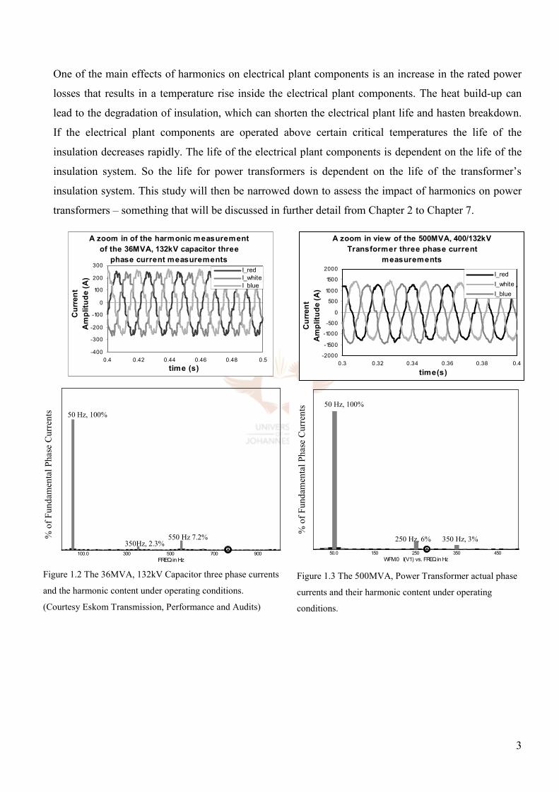
Several occurrences of harmonic currents in
capacitor and power transformer line currents in
Eskom Sub Transmission were reported. [32] This
had been determined by spot measurements of
harmonic currents at strategic points. The
harmonic currents’ presence in the line currents of
the capacitor is shown in Figure 1.2. The
harmonic currents could activate resonance,
which normally occurs between a capacitor and a
power transformer. The resonance usually results in capacitor nuisance tripping or the blow of
capacitor fuses. The presence of harmonic currents is a fact, especially in the Sub Transmission and
Distribution networks. Figure 1.3 indicates the harmonic current occurrences in the phase currents of a
500MVA, 400/132kV power transformer. The effects on, and consequences for, harmonic currents in
power transformers have not received much attention in the past. Utilities are not yet able to predict
with certainty the effects and take corrective action.
The effects of harmonic distortion on power-plant equipment like power lines and cables, capacitors,
reactors and power transformers and the influences of harmonics in series and parallel resonance in the
power system will be briefly discussed in this Chapter. This shows the research already done on power-
plant equipment and the damage harmonic distortion can do to power-plant equipment. Additionally it
indicates that the impact of harmonic currents on power transformers needs further research.
Figure 1.1 Utility interface.
LS vs
Utility source
Harmonic
Load
v
Other Loads
∑+= )()(1
)( thititsi
Point of common
coupling
3
One of the main effects of harmonics on electrical plant components is an increase in the rated power
losses that results in a temperature rise inside the electrical plant components. The heat build-up can
lead to the degradation of insulation, which can shorten the electrical plant life and hasten breakdown.
If the electrical plant components are operated above certain critical temperatures the life of the
insulation decreases rapidly. The life of the electrical plant components is dependent on the life of the
insulation system. So the life for power transformers is dependent on the life of the transformer’s
insulation system. This study will then be narrowed down to assess the impact of harmonics on power
transformers – something that will be discussed in further detail from Chapter 2 to Chapter 7.
050.0 150 250 350 450
WFM.0 I(V1) vs. FREQ in Hz
1.35K
1.05K
750
450
150
FFT of Phase Currents
350 Hz, 3% 250 Hz, 6%
50 Hz, 100%
% of Fundamental Phase Currents
Figure 1.3 The 500MVA, Power Transformer actual phase
currents and their harmonic content under operating
conditions.
Figure 1.2 The 36MVA, 132kV Capacitor three phase currents
and the harmonic content under operating conditions.
(Courtesy Eskom Transmission, Performance and Audits)
50 Hz, 100%
350Hz, 2.3% 550 Hz 7.2%
0100.0 300 500 700 900
FREQ in Hz
270
210
150
90.0
30.0% of Fundamental Phase Currents
A zoom in of the harmonic measurement
of the 36MVA, 132kV capacitor three
phase current measurements
-400
-300
-200
-100
0
100
200
300
0.4 0.42 0.44 0.46 0.48 0.5
time (s)
Current
Amplitude (A)
I_red
I_white
I_blue
A zoom in view of the 500MVA, 400/132kV
Transformer three phase current
measurements
-2000
-1500
-1000
-500
0
500
1000
1500
2000
0.3 0.32 0.34 0.36 0.38 0.4
time(s)
Current
Amplitude (A)
I_red
I_white
I_blue
4
1.1.1 Resonances
The presence of capacitors in the power system such as those used for power factor correction and
voltage regulation can result in local system resonances which can lead to excessive currents with
subsequent damage to such capacitors. [3] The two types of resonances, namely parallel and series
resonances, are discussed next.
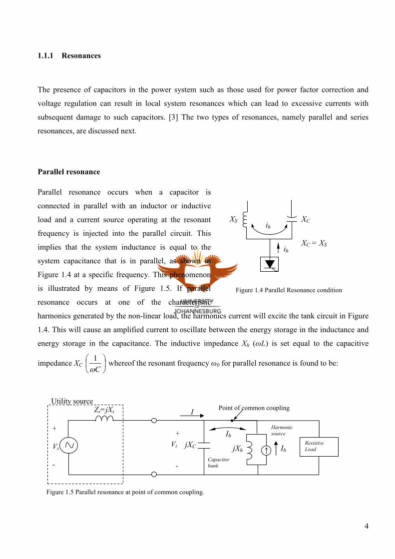
Parallel resonance
Parallel resonance occurs when a capacitor is
connected in parallel with an inductor or inductive
load and a current source operating at the resonant
frequency is injected into the parallel circuit. This
implies that the system inductance is equal to the
system capacitance that is in parallel, as shown in
Figure 1.4 at a specific frequency. This phenomenon
is illustrated by means of Figure 1.5. If parallel
resonance occurs at one of the characteristic
harmonics generated by the non-linear load, the harmonics current will excite the tank circuit in Figure
1.4. This will cause an amplified current to oscillate between the energy storage in the inductance and
energy storage in the capacitance. The inductive impedance Xh (ωL) is set equal to the capacitive
impedance XC
Cω1 whereof the resonant frequency ω0 for parallel resonance is found to be:
Utility source
Vt
+
-
I Zs=jXs
+
-
Vs
Figure 1.5 Parallel resonance at point of common coupling.
Capacitor bank
Harmonic source
Resistive Load Ih
Point of common coupling
jXh jXC
Ih
ih
ih
XS XC
XC = XS
Figure 1.4 Parallel Resonance condition

5
LC
10 =ω (1-1)
The harmonic resonance frequency can also be calculated in terms of MVA short-circuit rating at the
point of study, MVAr of the capacitance at system voltage or in terms of the short-circuit reactance at
the substation and capacitive reactance of the capacitor bank at fundamental frequency. [10]
sc
c
cap
scr X
X
MVAr
MVAh == (1-2)
where hr is the resonant frequency as a multiple of the fundamental frequency;
MVAsc is the MVA short circuit rating at the point of study;
MVArcap is the capacitor rating at the system voltage;
Xsc is the short circuit reactance at the substation;
XC is the capacitive reactance of the capacitor bank at fundamental frequency.
The high oscillating current can cause voltage distortion in the distribution circuit as well as telephone
interference if telephone circuits are in close physical proximity. It can also damage the capacitor if the
oscillating current exceeds the current limit of 135% of the rated current for capacitors [25]. The most
common symptom of resonance is fuse-blowing due to over current flow in the capacitor. Most of the
resonance problems can be avoided by choosing a capacitor size that will not result in resonance near
to the characteristic harmonic frequencies.
Similar damage may occur in the transformer or reactor with which the capacitor resonates. The
transformer or reactor connecting the customer to the utility system should not be subjected to
individual harmonic currents in excess of 5% of the transformer’s rated current [10]. This will ensure
that transformer insulation is not being stressed beyond design limits. Transformer heating is discussed
at length in section 2.3 in Transformer Heating Considerations.
6
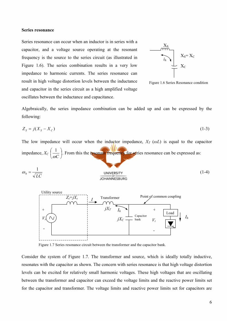
Series resonance
Series resonance can occur when an inductor is in series with a
capacitor, and a voltage source operating at the resonant
frequency is the source to the series circuit (as illustrated in
Figure 1.6). The series combination results in a very low
impedance to harmonic currents. The series resonance can
result in high voltage distortion levels between the inductance
and capacitor in the series circuit as a high amplified voltage
oscillates between the inductance and capacitance.
Algebraically, the series impedance combination can be added up and can be expressed by the
following:
)( CSS XXjZ −= (1-3)
The low impedance will occur when the inductor impedance, XT (ωL) is equal to the capacitor
impedance, XC
Cω1. From this the resonant frequency for series resonance can be expressed as:
LC
10 =ω (1-4)
Consider the system of Figure 1.7. The transformer and source, which is ideally totally inductive,
resonates with the capacitor as shown. The concern with series resonance is that high voltage distortion
levels can be excited for relatively small harmonic voltages. These high voltages that are oscillating
between the transformer and capacitor can exceed the voltage limits and the reactive power limits set
for the capacitor and transformer. The voltage limits and reactive power limits set for capacitors are
Figure 1.6 Series Resonance condition
ih
XS
XC
XS= XC
Utility source
Vt
-
I Zs=jXs
+
-
Vs
Figure 1.7 Series resonance circuit between the transformer and the capacitor bank.
Capacitor
bank
Load
Point of common coupling
Ih
Transformer
jXC
Ih jXT +

7
equal to 110% peak voltage, 110% rms voltage and 135% kVAr rating according to the IEEE Std. 18-
1991. The transformer voltage limits states in IEC 60076-8 that a transformer shall be capable of
continuous service without damage with 5% over-voltage at rated load and at no load the voltage limit
is 110% rated voltage without exceeding the guaranteed temperature rise. Above these voltage limits
the transformer could run into over-excitation, which results in high excitation currents and which can
in turn eventually lead to transformer breakdown. More detailed discussion will be continued in
Chapter 2 on the impact of harmonics on power transformers.
1.1.2 Transmission system
The flow of harmonics in a transmission system produces two main effects, namely a) the increase of
the rms value of current and b) voltage drops.
The first effect is the increase of the rms value of current generated by the harmonic load expressed as:
21
1
22
1 )( ∑≠
+=h
shsS III (1-5)
where Is1 is the fundamental current supplied from source vs and Ish is the current harmonic component
generated by the harmonic load. Consequently, the harmonics generated can increase the transmission
power loss in the power lines or cables, i.e.
∑∞
=
=1
2
hlhshhloss RIP (1-6)
where Rlh is the power line or cable resistance as a function of frequency. The resistance as a function
of frequency is due to the skin and proximity effects that are functions of frequency. The harmonics
generated can increase the skin and proximity effects contribution to the total resistance. The causes
thereof can increase power losses in the transmission line or cable. A further detailed discussion on the
skin effect is given in Chapter 3.
The second effect is that the harmonic current flow creates harmonic voltage drops across the circuit
impedances at the point of common coupling. This effect is illustrated in Figure 1.8. This means in
effect that a weak system (low fault level and large amount of impedance) will result in greater voltage

8
disturbances than a stiff system with a high fault level and low impedance. The voltage waveform at
the point of common coupling to the other loads will become distorted for sufficient harmonic current
flow into a weak system. This may cause other loads to malfunction due to the finite source impedance
of the power system represented by a source inductance, line inductance and line resistance as a
function of frequency as depicted in Figure 1.8.
Utility source Zs=jXs
+
-
Vs
Figure 1.8 A transmission line fed a harmonic source.
Harmonic
source
jXh
Rlh Llh
Is + Ish1
Power Line
∑Ish Is1 vt
-
+
Other loads
Point of common coupling

9
1.1.3 Capacitor banks
Harmonics affect power capacitors more than any other equipment. Harmonics cause additional heating
(higher current) and higher dielectric stresses on capacitors. Heating in capacitors is caused by two
main effects, namely conduction losses and dielectric losses. The conduction losses are the losses in the
plates and conductors of the capacitor. In the case of dielectric losses an understanding of the dipole
alignment of dielectrics is needed. The dielectric consists of dipoles on a molecular level. [26] When an
alternating voltage is applied to the dielectric, the dipoles vibrate to the frequency through polarity
reversals, resulting in the heating of the dielectric due to friction. The presence of the dielectric losses
and conduction losses can be represented by a resistor in series or in parallel with the capacitor. A
nonsinusoidal voltage waveform or voltage waveform that contains harmonics produces power losses
due to conduction and dielectric losses. These power losses are expressed as:
∑ ∑ ∞
=
∞
= =
= 1
2
1
2 tan
h ch h
h C ch h loss V
c Cω
X
R V Cω P δ
(1-7)
where
C is the capacitance,
ωh is the angular frequency at harmonic order h,
Vh is the harmonic voltage at harmonic order h,
δ is the tan angle between the resistance and capacitance,
ssRCωδ =tan is the loss factor for the series equivalent and,
ppRCωδ
1tan = is the loss factor for the parallel equivalent.
It can be seen from equation (1-7) that the total loss of the capacitor is frequency-dependent and that
harmonic voltages high in magnitude lead to large power losses. The increase in power losses can
result in overheating of the capacitors and can often lead to thermal breakdown. Limits on the current
loading are therefore imposed on capacitors to prevent thermal overloading. The rms current limit for
capacitors of 135% could be exceeded if supply voltage contains harmonics of appreciable magnitude.
10
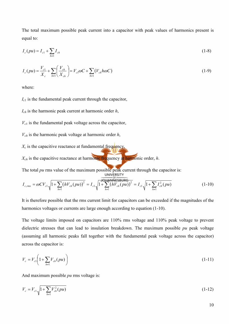
The total maximum possible peak current into a capacitor with peak values of harmonics present is
equal to:
∑≠
+=1
1)(h
chcc IIpuI (1-8)
( )∑∑≠≠
+=
+=
1
1
1
1)(h
chch ch
ch
c
cc ChVCV
X
V
X
VpuI ωω (1-9)
where:
Ic1 is the fundamental peak current through the capacitor,
Ich is the harmonic peak current at harmonic order h,
Vc1 is the fundamental peak voltage across the capacitor,
Vch is the harmonic peak voltage at harmonic order h,
Xc is the capacitive reactance at fundamental frequency,
Xch is the capacitive reactance at harmonic frequency at harmonic order, h.
The total pu rms value of the maximum possible peak current through the capacitor is:
( ) ( ) ∑∑∑≠≠≠
+=+=+=1
2
1
1
2
1
1
2
1, )(1)(1)(1h
chch
chch
chcrmsc puIIpuhVIpuhVCVI ω (1-10)
It is therefore possible that the rms current limit for capacitors can be exceeded if the magnitudes of the
harmonics voltages or currents are large enough according to equation (1-10).
The voltage limits imposed on capacitors are 110% rms voltage and 110% peak voltage to prevent
dielectric stresses that can lead to insulation breakdown. The maximum possible pu peak voltage
(assuming all harmonic peaks fall together with the fundamental peak voltage across the capacitor)
across the capacitor is:
+= ∑≠1
1 )(1h
chcc puVVV (1-11)
And maximum possible pu rms voltage is:
∑≠
+=1
2
1 )(1h
chcc puVVV (1-12)

11
1.1.4 Transformers
The main impact of harmonics on power transformers is an increase in the rated power losses that
results in temperature rise inside the power transformer. The heat build-up can lead to degradation of
insulation, which can shorten the transformer’s life and lead to eventual breakdown. The contributing
factors that cause the increase in transformer losses due to harmonics are an increase in rms current, an
increase in the winding eddy currents caused by proximity effect, and an increase in other stray losses.
The increase in the rms current translates into an increase in conduction losses (I2R). The impact of
harmonic distortion on winding eddy current losses and the other stray losses is explained in more
detail in Chapter 3. The harmonic currents or voltages impact conduction losses (P=I2R), eddy current
losses (PEC), other stray losses (POSL) and core losses (Pc) whereof the total power losses are:
cOSLECTL PPPPP +++= Ω (1-13)
The increase of total power losses due to harmonics can give rise to overheating. Overheating is
detrimental to the transformer as it affects both the oil and paper insulation system whereas the copper
and iron losses are relatively unaffected. However, power is dissipated in the copper and iron, and from
the copper and iron heat is transferred to the insulation system. If the transformer is operated above the
critical temperatures the life of the transformer decreases rapidly. The life of the transformer is
therefore dependent on both the life of the oil and paper insulation system. Fortunately, most modern
transformers have cooling systems that prevent transformers from overheating. Nevertheless, thermal
runaway can still occur if the cooling system is not designed for the harmonic current content. In
addition to this, a transformer’s permissible load current can decrease for an increase in transformer
losses, which means the transformer is derated. A decrease in permissible load current translates into a
decrease in the power capacity of the transformer.
°∠03aI
In3
°∠03cI
°∠03bI
Power
Transformer
Triplen
harmonic load
Figure 1.9 A star connected transformer supplying a triplen harmonic generating load.
12
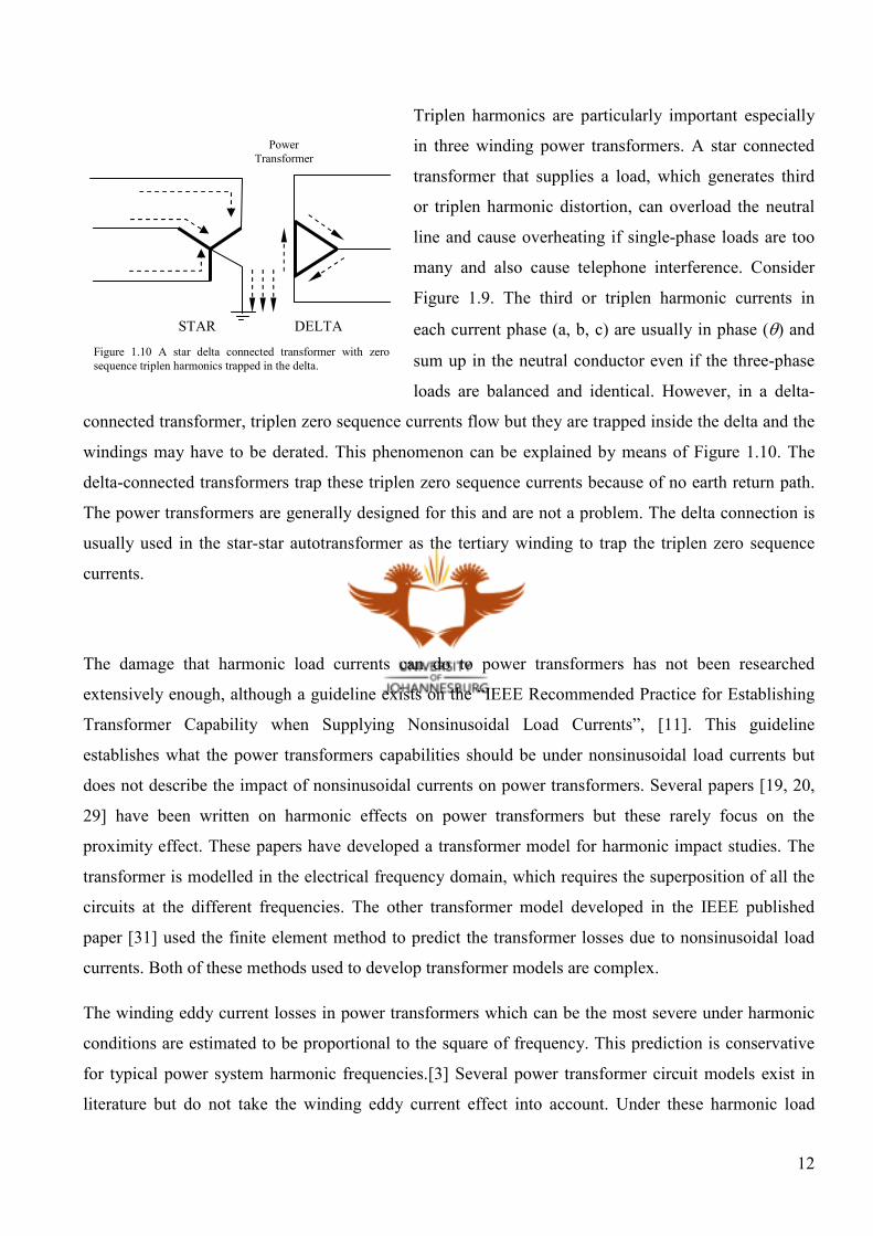
Triplen harmonics are particularly important especially
in three winding power transformers. A star connected
transformer that supplies a load, which generates third
or triplen harmonic distortion, can overload the neutral
line and cause overheating if single-phase loads are too
many and also cause telephone interference. Consider
Figure 1.9. The third or triplen harmonic currents in
each current phase (a, b, c) are usually in phase (θ) and
sum up in the neutral conductor even if the three-phase
loads are balanced and identical. However, in a delta-
connected transformer, triplen zero sequence currents flow but they are trapped inside the delta and the
windings may have to be derated. This phenomenon can be explained by means of Figure 1.10. The
delta-connected transformers trap these triplen zero sequence currents because of no earth return path.
The power transformers are generally designed for this and are not a problem. The delta connection is
usually used in the star-star autotransformer as the tertiary winding to trap the triplen zero sequence
currents.
The damage that harmonic load currents can do to power transformers has not been researched
extensively enough, although a guideline exists on the “IEEE Recommended Practice for Establishing
Transformer Capability when Supplying Nonsinusoidal Load Currents”, [11]. This guideline
establishes what the power transformers capabilities should be under nonsinusoidal load currents but
does not describe the impact of nonsinusoidal currents on power transformers. Several papers [19, 20,
29] have been written on harmonic effects on power transformers but these rarely focus on the
proximity effect. These papers have developed a transformer model for harmonic impact studies. The
transformer is modelled in the electrical frequency domain, which requires the superposition of all the
circuits at the different frequencies. The other transformer model developed in the IEEE published
paper [31] used the finite element method to predict the transformer losses due to nonsinusoidal load
currents. Both of these methods used to develop transformer models are complex.
The winding eddy current losses in power transformers which can be the most severe under harmonic
conditions are estimated to be proportional to the square of frequency. This prediction is conservative
for typical power system harmonic frequencies.[3] Several power transformer circuit models exist in
literature but do not take the winding eddy current effect into account. Under these harmonic load
Power
Transformer
Figure 1.10 A star delta connected transformer with zero
sequence triplen harmonics trapped in the delta.
STAR DELTA
13
conditions the winding eddy current effect can be substantial. The transformer models that are proven
accurate in most published papers are based on complicated iterative algorithms that are cumbersome.
This study concentrates on the development of a complete electrical transformer model that takes into
account the winding eddy current loss, non-linear magnetising curve and the total core losses which
can be used especially for harmonic impact studies. A winding eddy current parameter developed in the
time domain will make harmonic impact studies on power transformers simpler. Power transformer
behaviour under harmonic effects can thus be simulated and forecasted simpler under harmonic
loading.
The reason the study focuses on power transformers is because of their high failure rates and high
unknown causes to these failures, as will be expanded on in the following section. Therefore a
thorough theoretical and practical investigation is done on how harmonic loading impacts on the power
losses of the transformer and heating as the transformer is operated near the thermal limit.
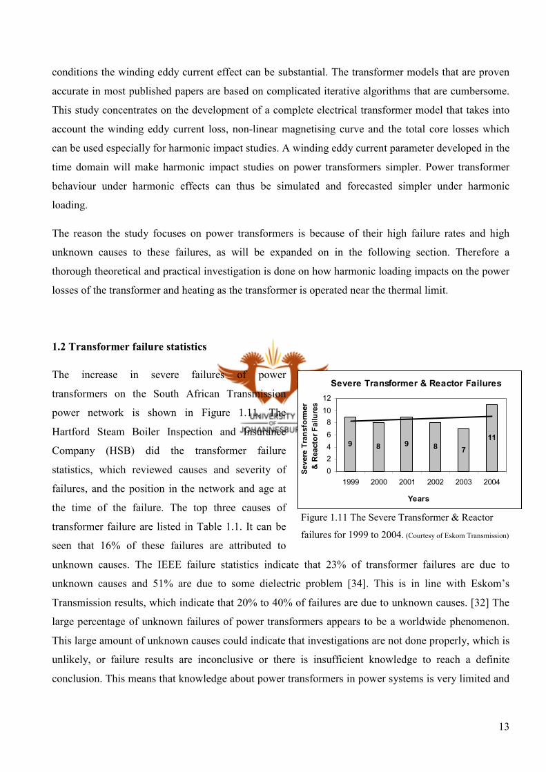
1.2 Transformer failure statistics
The increase in severe failures of power
transformers on the South African Transmission
power network is shown in Figure 1.11. The
Hartford Steam Boiler Inspection and Insurance
Company (HSB) did the transformer failure
statistics, which reviewed causes and severity of
failures, and the position in the network and age at
the time of the failure. The top three causes of
transformer failure are listed in Table 1.1. It can be
seen that 16% of these failures are attributed to
unknown causes. The IEEE failure statistics indicate that 23% of transformer failures are due to
unknown causes and 51% are due to some dielectric problem [34]. This is in line with Eskom’s
Transmission results, which indicate that 20% to 40% of failures are due to unknown causes. [32] The
large percentage of unknown failures of power transformers appears to be a worldwide phenomenon.
This large amount of unknown causes could indicate that investigations are not done properly, which is
unlikely, or failure results are inconclusive or there is insufficient knowledge to reach a definite
conclusion. This means that knowledge about power transformers in power systems is very limited and
Severe Transformer & Reactor Failures
9 8 9 8 7
11
0
2
4
6
8
10
12
1999 2000 2001 2002 2003 2004
Years
Severe Transform
er
& Reactor Failures
Figure 1.11 The Severe Transformer & Reactor
failures for 1999 to 2004. (Courtesy of Eskom Transmission)

14
that research into this field is not extensive. Feasible explanations have to be found for the large
percentage of unknown causes so that corrective measures can be taken.
Table 1.1 The top percentage categories of failures of power transformers done by HSB [33]
The HV and EHV power transformers are amongst the most expensive power-plant equipment on the
network and such high failure rates is costly. In addition to this, large power transformers (HV and
EHV) have delivery times of more than 4 months. Power transformers are critical power-plant
equipment and finding causes to transformer failures will be invaluable to any utility worldwide. The
fact remains that harmonic currents are prevalent on the power system and could be one of the reasons
for the failures in power transformers that are unaccounted for.
In summary, the power utility in South Africa will start to operate plants at maximum capacity because
of increasing load demands. Harmonics loads and sources will start to increase due to the expansion of
industries that use smelters, power converters, switching devices etc. The increase of harmonics in the
power system can therefore push power-plant equipment into thermal breakdown. The extent to which
harmonics affect power transformers will be investigated to determine the impact on power
transformers operated near the thermal limit. The replacement or refurbishment of power transformers
is expensive to power utilities and can cost these organisations millions of rand if power transformer
failures can be prevented or minimised. The impact of harmonic distortion might be one of the possible
causes of the unknown power transformer failures.
Cause % of Failure
Insulation Failure 26
Manufacturing Problems 24
Unknown 16

15
Conclusion
The presence of harmonic currents in the power system or in power-plant equipment has been
confirmed by measurements of harmonic currents through a capacitor bank and power transformer.
This Chapter proposed that harmonic effects on the power-plant equipment can cause damage to the
equipment. The IEEE recommended practices and papers published show that harmonics do impact
power transformers and there is a need to develop a simplified but accurate power transformer model
for harmonic impact studies. The research on the harmonic effects on power transformers is lacking
and the published papers and the standards that evaluate the harmonic impact on power transformers
have complex and cumbersome models. Furthermore, knowledge on the causes of power transformer
failures is lacking. This is proven by the large number of severe failures nationally and the high
numbers of failures nationally and internationally that are attributed to unknown causes. Power
transformers also make up some of the most expensive equipment in utilities, especially in the
transmission and distribution networks. For these reasons, research into the harmonic impact of power
transformers operating near the thermal limit is highly worthwhile.
The second chapter introduces reader to harmonic sources, theory and standards to evaluate the past
work done on harmonics. The theory on transformer no-load and load losses is examined to assess the
impact of harmonic distortion transformer losses in the third chapter. In the fourth chapter a
transformer model for harmonic impact studies is developed through the transformer theory. The
transformer model is then used to determine the harmonic impact on a transformer in the fifth chapter.
This is done through a numerical example of a transformer feeding a harmonic load. Finally, in the
sixth chapter, the new transformer model is practically verified with the experimental results of papers
published by M.A.S. Masoum, E.F. Fuchs and D.J. Roesler, [19], [20] and [29]. Chapter seven
concludes the study and provides recommendations.

16
CHAPTER 2: HARMONIC SOURCES, THEORY AND STANDARDS
Introduction
This chapter firstly introduces the reader to the fundamental theory of harmonics and the basic
calculations relevant to harmonics. The harmonics sources generally found in power systems are then
considered. It then discusses the NRS guidelines and specifications, and IEEE-recommended practices
and requirements for harmonic voltage and current distortion limits that set the minimum standards for
the quality of the electricity supply for utilities to the end customers.
The total harmonic distortion formula is defined and how harmonics impact power and the power
factor is briefly discussed. These calculations form the basis of the study of the impact of harmonics on
power-plant equipment.
The harmonic spectrums or harmonic currents and voltages generated from the switching equipment
(harmonic sources) are either tabulated, figuratively shown or mathematically calculated. And it is
briefly explained how harmonic waveforms are created through the operation of this switching
equipment. The switching equipment given in this Chapter do exist on the power system and shows
that harmonics do occur in the power system.
The NRS national standards were developed mainly from the IEC European standards. The harmonic
voltage compatibility levels are tabulated and the procedure to establish the harmonic voltage levels for
different voltage levels is outlined according to NRS practices and IEEE practices. The IEEE practices
establish a detailed layout of harmonic distortion current levels whereas the NRS standards look at a
detailed layout of harmonic voltage distortion levels. The harmonic standards were reviewed to show
that the presence of harmonic voltage and currents in power systems does pose dangers to power-plant
equipment. Finally, the transformer heating considerations are briefly discussed in subsection 2.3.4.

17
2.1 Harmonic definition
A harmonic voltage or current frequency is an integer multiple of the fundamental frequency. The
harmonic sources have non-linear characteristics and these harmonic sources result in multiples of the
fundamental frequency or system frequency. The fundamental component is the first harmonic or the
power system frequency. The electrical generator produces this fundamental frequency. The second
harmonic is two times the frequency of the fundamental; the third harmonic is three times the
fundamental, and so on (shown in Figure 2.1). So with a fundamental of 50 Hz, the second harmonic is
100 Hz, the third is 150 Hz, the fourth is 200 Hz, etc. The harmonic-producing loads that are the
sources for these harmonic multiples are discussed in section 2.3.
These voltage and current harmonics are generated in power systems by harmonic-producing loads.
Switching equipment used in industrial production processes or electrical industry cause harmonic-
producing loads. These switching equipment are controlled by power electronic equipment, which is
made up of various combinations of silicon diodes and silicon-controlled rectifiers.
=⇒ 1f Fundamental frequency
HarmonicSecondf ⋅=⇒ 2
HarmonicThirdf3 =⇒
=++=⇒ 321 ffff Total
Figure 2.1 The harmonic series description.

18
2.2 Total harmonic distortion, power and power factor
The harmonic sources that existed on the power system were a cause of concern. Therefore
performance parameters were established to deal with these harmonic problems. The section deals with
the different harmonic performance parameters and definitions that define the levels of compatibility
for the power system in terms of voltage and current magnitudes, total harmonic distortion, the
apparent power, real power, reactive power and power factor. For a distorted supply current, Is and
voltage, Vs waveforms the rms magnitudes for nonsinusoidal waveforms can be expressed as (for the
derivation see [6]):
∑=
+=1
22
0
hshs III s (2-1)
and
∑=
+=1
22
0
hshs VVVs (2-2)
where Is0 is the rms magnitude of the dc component of the current, Vs0 is the rms magnitude of the dc
value of the voltage, Vsh is the rms magnitude of the harmonic current component at the h harmonic
frequency and Ish is the rms magnitude of the harmonic current component at the h harmonic
frequency.
These equations are used to calculate the total harmonic distortion that is used to evaluate if the
harmonic levels are within acceptable limits (something that is discussed in more detail in section 2.3).
In most ac waveforms for voltage and current the average values or dc values are zero (Vs0 = 0 and Is0 =
0). The total harmonic distortion (THD) formulas for voltage and current are defined as:
∑≠
×=
1
2
1
100%h s
shi
I
ITHD for current waveforms, and (2-3)
∑≠
×=
1
2
1
100%h s
shv
V
VTHD for voltage waveforms. (2-4)
The average power (P) delivered to the load with a sinusoidal supply voltage (vs) and a nonsinusoidal
current (is) waveform according to reference [6] is:
1111111
00
1 cos)sin(2sin211
ϕϕ ssss
TT
ss IVdttwItwVT
dtivT
P =−⋅== ∫∫ (2-5)
where Vs1 is the rms magnitude of the sinusoidal supply voltage, Is1 is the rms magnitude of the
fundamental current component of the nonsinusoidal current, is and φ1 is the phase angle between the
19
voltage, vs and fundamental current, is1. The current components at harmonic frequencies do not
contribute to the real average power drawn from the source or infinite bus.
The apparent power S is the product of the rms voltage Vs and the rms current Is, [6]:
ss IVS = (2-6)
In this case, the harmonic components with high magnitudes do affect the rms magnitude of the
apparent power because it increases the reactive power components. The reactive power is the cross
products of voltage and current at a given harmonic frequency multiplied by the sine of the phase angle
between the voltage and current at the particular harmonic frequency.
∑=h
hhh IVQ ϕsin (2-7)
where Vh is the rms harmonic voltage, Ih is the rms harmonic current at the h harmonic frequency and
φh is the phase angle between the voltage, Vh and current, Ih.
The power factor (pf) is therefore defined and reduces to:
S
Ppf =
1
111 coscos
ϕϕ
s
s
ss
ss
I
I
IV
IVpf == (2-8)
Note that a distorted current waveform Is results in a low s
s
I
I 1 value and hence a low power factor. In
linear circuits with sinusoidal voltages and currents the power factor is equal to cosφ. In non-linear
circuits with harmonic currents and voltages the power factor is not equal to cosφ. In these circuits the
cosφ1 is called the displacement power factor. The true power factor given in eq. (2-8) is therefore a
true indication of the size of the power system to supply a given load.

20
2.3 Harmonic sources
Non-linear loads create harmonic sources. A non-linear load is created when the load current is not
proportional to the instantaneous voltage. Non-linear currents can be nonsinusoidal, even when the
source voltage is a clean sine wave. A non-linear load can also distort the voltage wave, making the
current wave nonsinusoidal [4].
The non-linear loads that produce harmonics on the power system are static converters, rectifiers, arc
furnaces, static var compensators, inverters for dispersed generation, electronic phase control,
cycloconvertors, switch mode power supplies, transformer magnetisation non-linearities, rotating
machines, fluorescent lighting, pulse width modulated drives etc. A brief discussion follows on several
of the harmonic sources mentioned that have significant effects on the power system.
2.3.1 Thyristor switches
In the electric utility it is desirable to regulate the voltage within a narrow range of its nominal value.
Static var compensators are used to provide quick control over reactive power, thereby regulating the
voltage within a narrow range of its nominal value. Thyristor switches or controllable switches are
mainly used to control these static var compensators. This type of switching is also used in applications
of long-time constant loads (e.g. temperature control in electric ovens). Firstly the static var
compensators will be discussed using the thyristor-controlled type inductors which are used frequently
on the power system.

21
Thyristor-controlled inductors [6]
The thyristor controlled inductors (TCI) act as variable inductors where the inductive vars supplied can
be varied very quickly. The system may require either inductive or capacitive vars, depending on the
system conditions. This requirement is met by paralleling TCIs with a capacitor bank.
Consider the single per-phase system
equivalent circuit shown in Figure 2.2 in
conjunction with the Figure 2.3 An ac
system Thevenin equivalent with purely
inductive impedance is assumed. The
system may require inductive or capacitive
vars depending on the system conditions. A
capacitor is connected in parallel with TCIs
to meet this requirement.
The current is equal to I = Ip + jIq, which lags the terminal voltage Vt sketched in Figure 2.3. The
terminal voltage is at its nominal voltage. The load absorbs an increase in lagging vars (reactive power)
caused by industrial loads such as arc furnaces or air conditioners. This increase in lagging vars causes
the reactive current component to increase Iq+∆Iq while Ip is assumed to be unchanged. The magnitude
of the system voltage is assumed to be unchanged. The increase in the lagging reactive power causes a
Vt
+
-
I Zs=jXs
+
-
vs
Figure 2.2 The basic Thyristor Controlled Inductor (TCI) principle.
AC system
P + jQ
Thyristor Controlled Inductors (TCIs)
iL LOAD
Static VAR Compensator
Vs jXsI
Vt
I
Vt’
Vs’ jXsI’
I’
Iq
Iq’ ∆Iq
Ip
∆∆∆∆Vt
Radius=Vs=Vs’
Reference
Figure 2.3 The phasor diagram for a lagging power factor
load P + jQ.

22
drop in the terminal voltage by a change of ∆Vt shown by the phasor diagram. In this case even the real
power will decrease because Ip remains constant and Vt decreases.
In this situation the static var compensator come into play and delivers more capacitive vars to
compensate for the increase in reactive vars. To accomplish this, the thyristor-controlled inductors in
Figure 2.4 are then switched out to increase the capacitance, and therefore deliver more capacitive vars
to the load. This in turn increases the terminal voltage to its nominal value to deliver optimum real
power. These static var controllers are used to decrease annoying voltage flickers and compensate for
the harmonic distortion caused by industrial loads such as arc furnaces, which cause very rapid changes
in reactive power and also introduce a fluctuating load imbalance between the three phases. The other
uses are to provide a dynamic voltage regulation to enhance the stability of the interconnection between
two ac systems.
In the case where more inductive vars are required from the power system, the thyristor-controlled
inductor banks are switched in. The inductor current waveform, iL (shown in Figure 2.5), is analysed
per phase to explain the basic principle of how an inductor is switch into circuit. The current waveform
α = 90º
0
0
0
α = 110º
α = 135º
1LL ii =
vs
iL iL1
iL iL1
δ
δ
b)
c)
d)
Figure 2.5 A TCI, basic principle; a) per-phase TCI; b) 0 < α < 90º ; c) α = 110º ; d)
α = 135º
ωt
ωt
ωt
+
-
a)
iL
vs

23
iL is nonsinusoidal due to the thyristor delay angle, α and contains harmonics. This waveform can be
expressed as:
( )
( )
+−
−−
=
δ
δ
coscos2
0
coscos2
)(
wtI
wtI
wti
L
L
L
πδπδπδ
δ
≤≤−
−≤≤
≤≤
wt
wt
wt
)(
)(
0
(2-9)
The coefficients of the rms inductor current, iL, are derived from Fourier analysis to:
−+
−−
−−+++
−−−= −+ hhhLh h
h
h
h
h
Ia 11 )1(1
)1(
)1sin()1(1
)1(
)1sin()(1
sinhcos2 δδδδπ
, 1>h (2-10)
[ ]δδπ
22sin2
1 −= LIa (2-11)
0=hb (2-12)
The magnitudes with respect to the fundamental of the harmonic current components are given in Table
2.1.
Table 2.1: The harmonic spectrum of the inductor current, iL.
The inductor current, iL, is investigated here to show where the harmonics of the static var compensator
(SVC) are generated from. These harmonics currents, if generated, will also be drawn by the power
system, which could be excessive due to the thyristor delay or firing angle, α, which can be seen by
Table 2.1. The greater the thyristor delay angle the greater the percentage of harmonic currents
magnitude with reference to the fundamental inductor current. Therefore the harmonic filters are
Harmonic
1a
ah
α = π- δ α = π- δ α = π- δ
h δ= 60 ° δ = 45 ° δ= 30 °
2 0.0000 0.0000 0.0000
3 0.3525 0.5840 0.7967
4 0.0000 0.0000 0.0000
5 -0.0705 0.1168 0.4780
6 0.0000 0.0000 0.0000
7 -0.0252 -0.0834 0.1707
8 0.0000 0.0000 0.0000
9 0.0353 -0.0389 -0.0266
10 0.0000 0.0000 0.0000
24
closely connected to SVCs to sink all the harmonic currents and prevent excessive harmonic flow into
the power system. The harmonic filters in power systems are used to absorb or trap all undesired
frequencies that may be created by harmonic sources on the network and therefore can minimise
excessive harmonic flow into the power system.
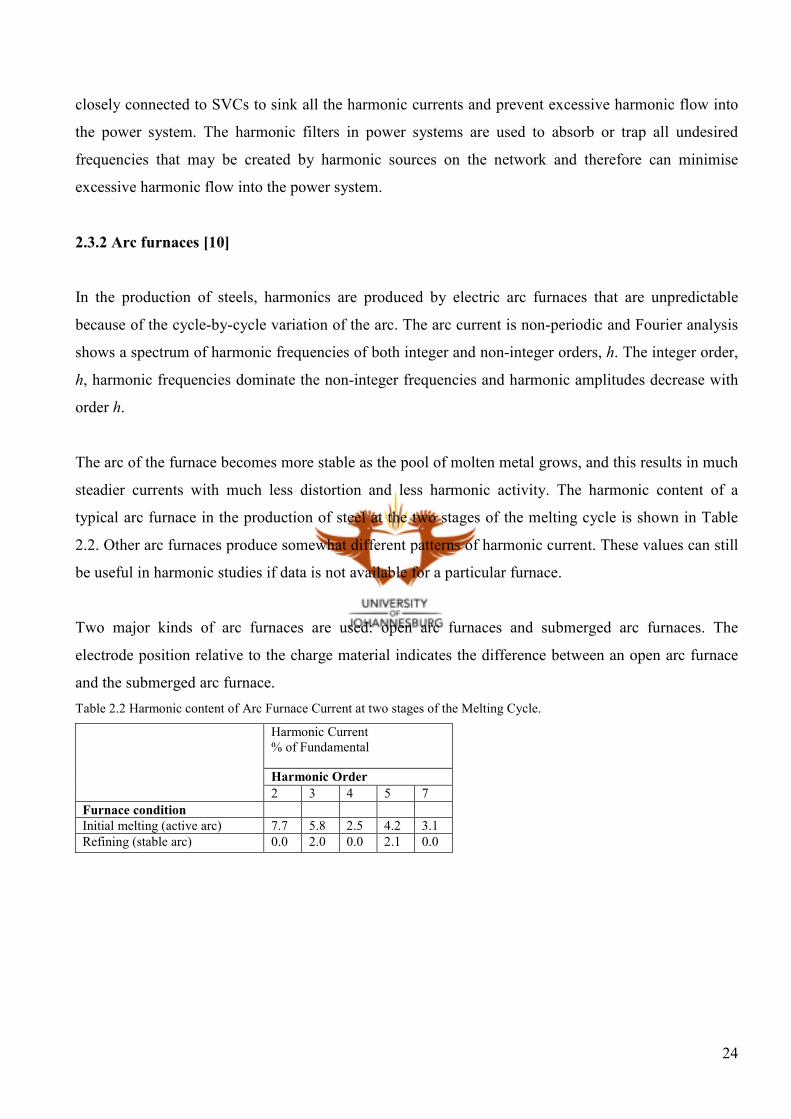
2.3.2 Arc furnaces [10]
In the production of steels, harmonics are produced by electric arc furnaces that are unpredictable
because of the cycle-by-cycle variation of the arc. The arc current is non-periodic and Fourier analysis
shows a spectrum of harmonic frequencies of both integer and non-integer orders, h. The integer order,
h, harmonic frequencies dominate the non-integer frequencies and harmonic amplitudes decrease with
order h.
The arc of the furnace becomes more stable as the pool of molten metal grows, and this results in much
steadier currents with much less distortion and less harmonic activity. The harmonic content of a
typical arc furnace in the production of steel at the two stages of the melting cycle is shown in Table
2.2. Other arc furnaces produce somewhat different patterns of harmonic current. These values can still
be useful in harmonic studies if data is not available for a particular furnace.
Two major kinds of arc furnaces are used: open arc furnaces and submerged arc furnaces. The
electrode position relative to the charge material indicates the difference between an open arc furnace
and the submerged arc furnace.
Table 2.2 Harmonic content of Arc Furnace Current at two stages of the Melting Cycle.
Harmonic Current
% of Fundamental
Harmonic Order
2 3 4 5 7
Furnace condition
Initial melting (active arc) 7.7 5.8 2.5 4.2 3.1
Refining (stable arc) 0.0 2.0 0.0 2.1 0.0

25
Open arc furnace
Open arc furnaces are one of the largest sources of
harmonics and produce unpredictable harmonics due
the cycle-by-cycle variation of the arc. A typical
harmonic distribution for the average harmonic
distortion current as a percentage of its fundamental
for a whole arc furnace production cycle, which
includes the melting and refining period, is illustrated
in Table 2.3 (extracted from references [3], [22] and
[23]).
Submerged arc furnace
The submerged arc furnace generally operates in a
stable fashion, and harmonic levels generated are
fairly low. If an arc furnace operates in the presence of
capacitor banks, the unbalanced operation can amplify
harmonic levels. The harmonic currents as a
percentage of the fundamental for three large
submerged arc furnaces during balanced and
unbalanced furnace operation are given in Table 2.4.
[24]
Harmonic
order
h
Average harmonic current as a
percentage (%) of fundamental
Ref. [3] Ref. [22] Ref. [23]
2
3
4
5
6
7
8
9
10
3.2%
4.0%
1.1%
3.2%
0.6%
1.3%
0.4%
0.5%
> 0.5%
4.1%
4.5%
1.8%
2.1%
1.0%
1.0%
0.6%
> 0.5%
4.5%
4.7%
2.8%
4.5%
1.7%
1.6%
1.1%
1.0%
> 1.0%
Harmonic current as a percentage (%) of
fundamental
Harmonic
order
h Balance operation Unbalance operation
2
3
4
5
6
7
0.7-1.7%
0.5-1.0%
0.1-1.0%
0.8-1.0%
0.3-0.6%
0.1-0.9%
Same
1.0-4.0%
Same
Same
0.4 -1.0%
Same
Table 2.4 The harmonic distortion current as a percentage
of fundamental for three large submerged arc furnaces
during balance and unbalance furnace operation. [24]
Table 2.3 The average harmonic distortion current as a
percentage of the fundamental current.

26
2.3.3 Static converters [6]
Application
These converters are increasingly being used in HVDC power transmission, some in dc motor drives,
or in ac motor drives with regenerative capabilities. In these applications, it is necessary to control
power-flow in both directions between the ac and dc sides.
The converters are a source of current harmonics on the ac side and a source of voltage harmonics on
the dc side. In this study, we only look into large power converters that have significant effects on the
HV and MV power networks. Full bridge converters for single and three-phase utility inputs will be
discussed to indicate how harmonic voltages and currents are created on the dc side and ac side of these
converters.
Single-phase two-way converter
The circuit drawn in Figure 2.6 is an ideal single-phase converter with supply voltage vs that is a purely
sinusoidal waveform. The thyristors T1 and T2 could turn on when the supply voltage, vs, is positive
and thyristors T3 and T4 could turn on when the supply voltage, vs, goes negative. This type of
thyristor-switching results in an input line current, is, shown in Figure 2.6 as a square waveform in the
idealised case that (almost) lags the supply voltage vs with an angle of φ. The dc side voltage vd is the
supply voltage that is rectified as the average load voltage. The load is modelled as an ideal current
source; therefore there is no ripple. Id is the average load current. For the purposes of this study it
concentrates on the ac-side effects of harmonics on the electric utility or power system.
The supply current, is, is estimated to be a square waveform (idealised case) defined as (see Figure 2.7):
+<<+−
+<<+=
22
2)(
πα
πα
παα
wtI
wtIwti
d
d
s (2-14)

27
for even values of h and
Using Fourier analysis the fundamental and the harmonic components can be expressed as:
0=ha , ∫ ==π
ππ0
4)sin(
2
h
IdwthwtIb d
dh (2-15)
∑∑≠≠
−+−=+=11
1 )sin(4
)sin(4
)()()(h
dd
hshss hwt
h
Iwt
Itititi α
πα
π (2-16)
The rms values for these harmonic components can be expressed as:
dd
rmssh Ihh
II 2
2
2
4, ππ
==
=
h
I rmss ,1
0
(2-17)
The source current, is can be expressed in terms of its Fourier components as:
[ ] [ ] K+−+−+−= )5(sin2)3(sin2)sin(2)( 531 ααα wtIwtIwtIwti ssss (2-18)
where only odd harmonics are present.
vs
Id vd
+
-
is
Figure 2.6 Single-phase thyristor converter with
source inductance, Ls = 0 and a constant dc current
T1
T3
T4
T2
for odd values of h
== ddrmss III 9.02π
2,1
for odd values for h
for odd values for h

28
The rms value of is is equal to the dc current, Id deduce from the basic rms definition:
∫=T
srmss dtiT
I0
,
1
∫∫ +=T
Td
T
d dtIdtIT
2
2
0
1 (2-19)
ds II = (2-20)
The total harmonic distortion (THDi) for the ac current given in eq. (2-18) is simplified by substitution
of eq. (2-17) and eq. (2-20):
2
1
2
1
2
100%s
ss
I
IITHD
−×=
−=∑
≠
2
1
2
1
2
ssh
sh III (2-21)
d
dd
I
II
9.0
)9.0(100
22 −×=
%43.48=
The TDD (Total Demand Distortion) is the THDi measured over a 15 or 30 min demand. The THDi
value for the single-wave two-way converters is greater than the TDD maximum values for all cases
tabulated in Table 2.7 in section 2.7.3. This means that preventative measures have to be put into place
to reduce the THDi value to the acceptable recommended values indicated in Table 2.7.
The displacement power factor (DPF) is expressed as:
αϕ coscos 1 ==DPF (2-22)
where α is the delay angle or thyristor firing angle. The real power absorbed by the converter is:
11 cosϕss IVP = (2-23)
Vs is is
φ1 = α
√1Is1
Figure 2.7 The ac-side quantities in the converter.
29
Substituting eq. (2-17) and eq. (2-22) into eq. (2-23) the power yields:
αcos9.0 ds IVP = (2-24)
The power factor (pf) is then simplified to:
αϕ cos9.0cos 1
1 ==s
s
I
Ipf (2-25)
It can thus be clearly seen that the converter draws 10% less than the potential real power because of
the distorted current waveform that has a high harmonic content.
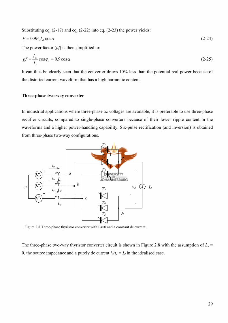
Three-phase two-way converter
In industrial applications where three-phase ac voltages are available, it is preferable to use three-phase
rectifier circuits, compared to single-phase converters because of their lower ripple content in the
waveforms and a higher power-handling capability. Six-pulse rectification (and inversion) is obtained
from three-phase two-way configurations.
The three-phase two-way thyristor converter circuit is shown in Figure 2.8 with the assumption of Ls =
0, the source impedance and a purely dc current id(t) = Id in the idealised case.
Id vd
+
-
ia
ib
ic
a
b
c
n
T1
T3
T5
T4
T2
T6
P
N
Figure 2.8 Three-phase thyristor converter with Ls=0 and a constant dc current.
Ls
Ls
Ls
30
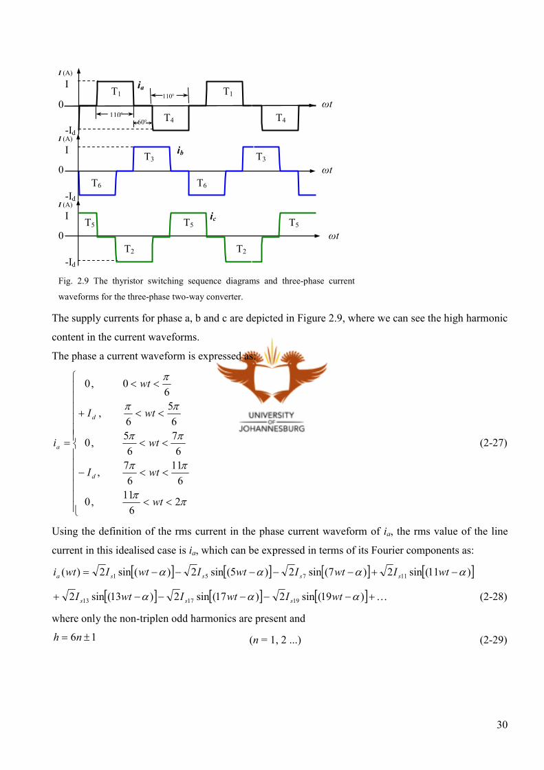
The supply currents for phase a, b and c are depicted in Figure 2.9, where we can see the high harmonic
content in the current waveforms.
The phase a current waveform is expressed as:
<<
<<−
<<
<<+
<<
=
ππ
ππ
ππ
ππ
π
26
11,0
6
11
6
7,
6
7
6
5,0
6
5
6,
60,0
wt
wtI
wt
wtI
wt
i
d
d
a (2-27)
Using the definition of the rms current in the phase current waveform of ia, the rms value of the line
current in this idealised case is ia, which can be expressed in terms of its Fourier components as:
[ ] [ ] [ ] [ ])11(sin2)7(sin2)5(sin2)(sin2)( 11751 αααα −+−−−−−= wtIwtIwtIwtIwti ssssa
[ ] [ ] [ ] K+−−−−−+ )19(sin2)17(sin2)13(sin2 191713 ααα wtIwtIwtI sss (2-28)
where only the non-triplen odd harmonics are present and
16 ±= nh (n = 1, 2 ...) (2-29)
0
0
0
T1 T1
T4 T4
T3 T3
T6 T6
T5 T5
T2 T2
T5
ia
ib
ic I
-Id
I
-Id
I
-Id 60°
110º
110°
Fig. 2.9 The thyristor switching sequence diagrams and three-phase current
waveforms for the three-phase two-way converter.
ωt
ωt
ωt
I (A)
I (A)
I (A)

31
for even values of h
The rms values for these harmonic components can be expressed as:
The rms value of the fundamental frequency component is Is1 = 0.78Id, which is much less than the rms
value of the fundamental frequency component of the single-phase two-way converter. The total rms
current from the ia waveform can be calculated as:
dds III 816.03
2== (2-31)
The THDi can therefore be calculated as:
( ) ( )%07.30
78.0
78.0816.0100
22
1
2
1
2
=−
=−
×=d
dd
s
ssi I
II
I
IITHD (2-32)
This means THDi and total rms current of the three-phase converter is a lower than the single-phase
two-way converter. Overall, the three-phase converter harmonic distortion is lower and better due to
the absence of triplen current harmonics in the line current is. But the three-phase converter’s THDi is
still higher than all the recommended TDD in Table 2.7, and there is still a need to minimise the THDi
level.
2.3.4 Three-phase inverters [6], [3]
Three-phase inverters are most frequently used to supply three-phase loads, in HV dc transmission
systems, for interconnection of renewable
energy sources and energy storage systems,
and a component in variable-frequency
converter classifications.
id
Vd
-
+
T3 T1 T5
T2 T4 T6
A
A B
B
C
C
n
N
Fig. 2.10 Three phase inverter connected to three-phase load.
R R
R
L L
L
for odd values of h
== ddrmss III 78.0
3
23,1 π
(2-30)
=
h
I rmss ,1
0
ππ h
II
hI d
drmssh
6
3
23, ==

32
The three-phase inverter in Figure 2.10 is operated in the square-wave mode and supplies a three-phase
load. It is assumed to supply a three-phase ac motor load. In the square-wave mode of operation the
inverter itself cannot control the magnitude of the output ac voltages. Therefore the dc input voltage
must be controlled in order to control the output in magnitude. The load voltage, vAn, and load current,
iA, waveforms that contain harmonics are depicted in Figure 2.11.
The harmonic spectrums for the phase-to-neutral voltage vAn and the ripple current iripple are shown in
Figure 2.12 and Figure 2.13 respectively; the harmonic spectrums were determined through the Intusoft
SPICE software program. The harmonic components present for the phase to neutral voltage vAn are
non-triplen odd harmonics (h = 5, 7, 11, 13, 17, 19…). The harmonics present in the ripple current iripple
are even (h = 1, 4, 8, 10, 14, 16…) and non-triplen odd harmonics.
ωt
iripple,
0
Peak
Figure 2.11 Phase-to-load-neutral variables of a three-phase square wave inverter: (a) Phase-neutral voltage (vAn); (b) the
ripple current (iripple) in the phase to neutral current; (c) the phase A current iA waveform.
ωt
vAn
0
dV
3
2
dV
3
1
(a)
(b)
ωt
iA
iA1
(c)
vAn1 vA

33
100 300 500 700 900 VAn vs. Frequency in Hz
100
90
50
20
10
Magnitude of V
Ah as a percentage of fundamental
VA1 per unit Volts (V
)
30
40
80
70
60
50 Hz, 100%
150 Hz, 19% 350 Hz, 14%
650 Hz, 7% 950 Hz, 4%
850 Hz, 4.4% 550 Hz, 8%
Figure 2.12 The harmonic spectrum for the phase to neutral voltage (vAn).
100 300 500 700 900 iripple vs. Frequency in Hz
90
70
50
30
10
100
150 Hz, 80%
50 Hz, 100%
100 Hz, 16%
100 Hz, 8,4%
350 Hz, 41%
550 Hz, 14%
850 Hz, 6% 650 Hz, 11%
950 Hz, 5% 500 Hz, 3% 400 Hz, 4%
800 Hz, 1.8% 700 Hz, 1%
20
40
60
80
0
Magnitude of I
sh as a percentage of fundamental
I s1 in Amps(A)
Figure 2.13 The harmonic spectrum for ripple current (iripple).

34
2.3.5 Transformer magnetisation non-linearities [8], [9]
In transformers magnetic materials are used to maximise the coupling between windings as well as to
lower the excitation current required for transformer operation. Ferromagnetic materials are used for
this purpose. Ferromagnetic materials are composed of a large number of magnetic domains.
In an unmagnitised ferromagnetic material, the domain magnetic moments are randomly oriented, and
the net resulting magnetic flux in the material is zero. Now when unmagnitised ferromagnetic material
is placed in a magnetic field parallel to one of the directions of easy magnetisation, then domain
magnetic moments tend to align with the applied magnetic field. The dipole magnetic moments add to
the applied magnetic field (H), resulting in a much larger value of flux density (B) than would exist due
to the applied magnetic field alone. Therefore the effective permeability µ, equal to the ratio of the total
magnetic flux density (B) to the applied magnetic field (H), is large compared with the permeability of
free space µ0.
When the applied magnetic field is increased until all magnetic moments domains align with applied
magnetic field, they can no longer contribute to increasing magnetic
flux density and the ferromagnetic material is said to be fully
saturated. When the applied magnetic field reduces to zero, the
magnetic dipole moments will no longer be totally random in their
orientation; they will retain a net magnetisation component along the
applied field direction. This is the effect responsible for the
phenomenon known as magnetic hysteresis. The saturation and
hysteresis effects give rise to the non-linear relationship between the magnetic field (H) and the flux
density (B). The B-H curve is depicted in Figure 2.14 with the initial magnetisation curve and the
hysteresis loop. Further explanation is done by means of a practical example in the next paragraphs.
Consider a single-phase transformer with two coils
that are magnetically coupled at no load (shown in
Figure 2.15). The supply voltage v1 to the primary
coil is sinusoidal and equates to Faraday’s induction
law:
e1 e2
Φ
+ +
- -
N1 N2 vs
Figure 2.15 Cross-section of a single-phase
transformer
Fig. 2.14 The initial magnetisation curve
and hysteresis loop
Φ,B
im,H

35
dt
dNwtEev m
Φ=−=−= 111 sin (2-33)
The main flux (Φ) that circulates in the core can be obtained through integration of eq. (2-33) to the
following assuming zero remanence flux:
wtwtwN
Edt
N
em
m coscos11
1 Φ==−=Φ ∫ (2-34)
The sinusoidal primary voltage produces a sinusoidal flux at no load. The primary current is not purely
sinusoidal because the flux is not linearly proportional to the magnetising current (this will be
explained next).
For an ideal core without hysteresis loss the flux Φ and the magnetising current im are related to each
other by the magnetisation curve of the magnetic material as shown in Figure 2.16. In Figure 2.16 the
flux Φ produced by the applied primary voltage vs is plotted against time and for each value of flux Φ
the magnetising current is extrapolated from the magnetising curve. The magnetising current then
results in a nonsinusoidal waveform.
When the hysteresis effect is included, the magnetising current is no longer symmetrical about its
maximum value (see Figure 2.17). In the same way as in transformer magnetisation without hysteresis,
the magnetising current can be extrapolated from the flux. The arrows as shown Figure 2.14 depict the
hysteresis loop direction.
Fig. 2.16 Transformer magnetisation (without hysteresis): Magnetisation curve
(B-H curve), flux and magnetisation current waveforms.
ωt
im
Φ,B
im,H ωt
Φ
180º
180°
360°
360º°

36
Figures 2.16 and 2.17 illustrate the distortion in the magnetising current im that mainly contains triplen
harmonics and predominately the third.
Φ,B
im,H ωt
ωt
Φ
im
180°
180°
360°
360°
Fig. 2.17 Transformer magnetisation (with hysteresis):
Magnetisation curve, flux and magnetisation current waveforms.

37
2.4 Harmonic standards and recommended guidelines
Power electronic equipment and other harmonic sources produce distortions in the ac supply voltage
and/or current waveforms of the power system that have an undesired impact on the power system or
power-plant equipment. Therefore standards were established to limit the adverse effects of harmonic
distortion on power-plant equipment of utilities and their customers. The standards will then be used to
determine if the harmonic voltage and current levels of the numerical example of the transformer
feeding a harmonic load in the fifth chapter are within the allowable harmonic levels. This section
discusses the NRS guidelines and specifications, and IEEE-recommended practices and requirements
for harmonic current distortion limits that set the minimum standards for the quality of the electricity
supply for utilities to end customers. The minimum standards of the NRS guidelines and specifications
deal with the voltage compatibility levels, voltage assessment levels and voltage assessment method
that specify the maximum harmonic requirements for harmonic voltages and currents. And the
application guidelines for utilities suggest a technical procedure for the connection of a new customer
and the evaluation of an existing customer regarding harmonics. The technical procedure used a tool
called the apportioning technique, and this will be briefly discussed.
2.4.1 Voltage harmonics compatibility levels and assessments
Definitions
Low voltage (LV) – The nominal ac voltages of 1000V and lower.
Medium voltage (MV) – The nominal ac voltage levels are in the range of 1kV< Un ≤ 44 kV.
High Voltage (HV) – The nominal ac voltages levels are in the range of 44kV< Un ≤ 110 kV.
Extra High Voltage (EHV) – The nominal ac voltages levels are in the range of 110kV< Un ≤ 400 kV.
Voltage harmonics compatibility levels
The compatibility levels are defined as the specified disturbance level at which an acceptable, high
probability of electromagnetic compatibility must exist. The compatibility levels for harmonics on LV
and HV networks are given in the Table 2.5; these set the minimum standards for customers supplied at
LV and MV. The maximum allowable total voltage harmonic distortions (THDv) for LV and MV
networks are eight percent (8%).

38
The customers supplied at HV and EHV will have compatibility levels written into contracts based on
recommended planning levels given in Table 2.5, unless the utility has established its own
recommended planning levels. Table 2.5 indicates the recommended planning levels for non-multiple
odd harmonics, multiple odd harmonics, and even harmonics. The total voltage harmonic distortion
(THDv) in HV and EHV networks is recommended to be smaller than three percent (3%). The
Application Guideline for Utilities [7] recommends apportioning procedures that can be followed to
assess the contractual emission levels (to be discussed in the apportioning procedures subsection).
Table 2.5- The NRS Compatibility levels for LV and MV harmonic voltages and recommended planning levels for MV, HV
and EHV harmonic voltages (as a percentage of the rated voltage of the power systems) [7]
The harmonic voltage distortion limits according to the IEEE-recommended practices are listed in
Table 2.6: these should be used as system design values for the worst case for normal operation
(conditions lasting longer than one hour). These limits may be exceeded by 50% for shorter periods
than an hour during start-ups or unusual conditions.
Odd harmonics (non-multiples of 3) Odd harmonics (multiples of 3) Even harmonics
Order Harmonic voltage (%) Order Harmonic voltage (%) Order Harmonic voltage (%)
Compatibility
levels Recommended planning levels
Compatibility
levels
Recommended
planning levels Compatibility
levels
Recommended
planning levels
h LV /MV MV HV/EHV h LV/MV MV HV/
EHV h LV/MV MV
HV/
EHV
5
7
11
13
17
19
23
25
>25
6
5
3.5
3
2
1.5
1.5
1.5
h
253.12.0 ×+
5.0
4.0
3.0
2.5
1.6
1.2
1.2
1.2
0.2+
h
255.02.0 ×+
2.0
2.0
1.5
1.5
1.0
1.0
0.7
0.7
0.2+
h
255.02.0 ×+
3
9
15
21
>21
5
1.5
0.3
0.2
0.2
4.0
2.0
0.3
0.2
0.2
2.0
2.0
0.3
0.2
0.2
2
4
6
8
10
12
>12
2
1
0.5
0.5
0.5
0.2
0.2
1.6
1.0
0.5
0.4
0.4
0.2
0.2
1.5
1.0
0.5
0.4
0.4
0.2
0.2
NOTE:
Total harmonic distortion (THD) compatibility levels: < 8% in LV and MV power systems.
Total harmonic distortion (THD) recommended planning levels: < 6.5% in MV networks and < 3% in HV and EHV
networks.

39
Table 2.6 The Harmonic Voltage Distortion Limits in IEEE 519-1992, [10]
Voltage assessment method
Firstly the measuring instrument must comply with the requirements of quasi-stationary measurements
and with accuracy class B specified in NRS 048-5.
All phases of the supply voltage must be monitored. The assessment period must be at least 7
continuous days on each phase of the supply voltage. The measuring instrument samples and records
each harmonic voltage at intervals of 3 s or less. These samples are summated over each 10 min root-
mean-square values, V10,h over each period of 14 h (00:00 to 14:00), expressed as:
N
VV
N
hhs
h
∑== 1
2
,
,10 (2-35)
where Vs,h is the measured rms harmonic voltage at 3 s intervals during the 10 min period, N is the
number of rms voltage measurements within the measured 10 min period, and h is the harmonic
number.
In the case where more than one sample is taken every 3 s, the value Vs,h is calculated as:
N
VV
N
hho
hs
∑== 1
2
,
, (2-36)
Bus Voltage Maximum Individual Harmonic
Voltage Distortion (%)
2
1
100
×
sV
shV
Maximum THD (%)
∑≠
×
1100
2
1h s
sh
V
V
69 kV and below
69.001kV to 161kV
Above 161.001 kV
3%
1.5%
1.0%
5%
2.5%
1.5%

40
where Vo,h is the value of each sample in a time window between 80 ms and 500 ms. Gaps between the
windows are allowed.
The 10 min root-mean-square values, which are not exceeded for 95% of the time of each 14-hour day
(00:00 to 14:00), are recorded for each phase for each harmonic value and total harmonic distortion
(THDv) calculation. The highest recorded values on each phase must be then retained as the daily
assessed values. The highest of the daily assessed values over the full assessment period (7 continuous
days) will be compared with the compatibility levels. The number of days in the assessment period that
the THD level exceeds the planning level in Table 1.1 must also be recorded. Under normal operating
conditions, the assessed levels must be less than the planning levels given in Table 1.1.
2.4.2 Apportioning procedures for harmonics
This section shows that the allowable harmonic current levels are specified for voltage levels greater
than 132kV and that the monitoring of harmonic currents is required for HV and EHV voltage levels. A
large load connected to the HV network can have a larger effect on a specific group of customers than a
smaller load connected closer to a group of customers at MV or LV voltage level. The emission levels
need then to be co-ordinated from the high voltage busbar to the low voltage busbar. The compatibility
levels are then defined at the point of common coupling (PCC) for the different voltage levels. The
point of common coupling is where more than one customer is connected to one voltage level. See
Figure 2.18.
EHV
HV
MV
LV Emission levels
Figure 2.18 Emission co-ordination from EHV to LV displaying the
contribution at each voltage level to the total LV level.
Compatibility levels
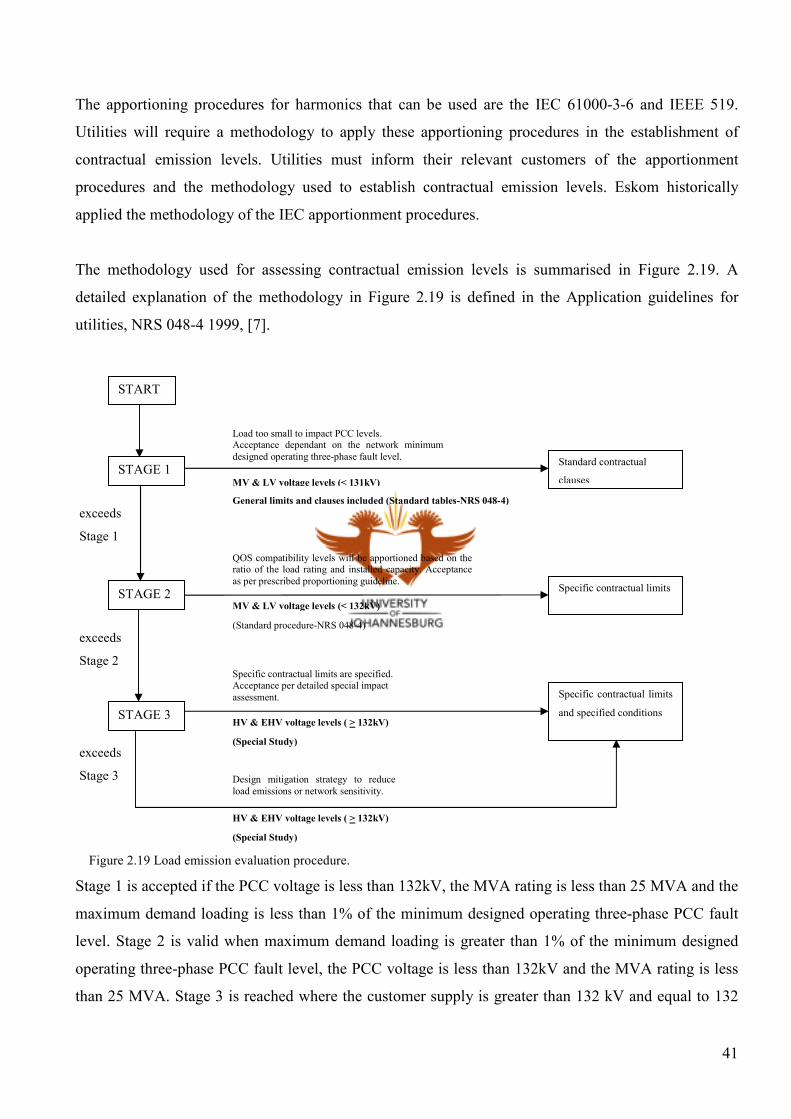
41
The apportioning procedures for harmonics that can be used are the IEC 61000-3-6 and IEEE 519.
Utilities will require a methodology to apply these apportioning procedures in the establishment of
contractual emission levels. Utilities must inform their relevant customers of the apportionment
procedures and the methodology used to establish contractual emission levels. Eskom historically
applied the methodology of the IEC apportionment procedures.
The methodology used for assessing contractual emission levels is summarised in Figure 2.19. A
detailed explanation of the methodology in Figure 2.19 is defined in the Application guidelines for
utilities, NRS 048-4 1999, [7].
Stage 1 is accepted if the PCC voltage is less than 132kV, the MVA rating is less than 25 MVA and the
maximum demand loading is less than 1% of the minimum designed operating three-phase PCC fault
level. Stage 2 is valid when maximum demand loading is greater than 1% of the minimum designed
operating three-phase PCC fault level, the PCC voltage is less than 132kV and the MVA rating is less
than 25 MVA. Stage 3 is reached where the customer supply is greater than 132 kV and equal to 132
STAGE 1
STAGE 2
STAGE 3
Standard contractual
clauses
Specific contractual limits
Specific contractual limits
and specified conditions
START
Load too small to impact PCC levels. Acceptance dependant on the network minimum
designed operating three-phase fault level.
General limits and clauses included (Standard tables-NRS 048-4)
QOS compatibility levels will be apportioned based on the ratio of the load rating and installed capacity. Acceptance
as per prescribed proportioning guideline.
(Standard procedure-NRS 048-4)
Specific contractual limits are specified.
Acceptance per detailed special impact
assessment.
MV & LV voltage levels (< 131kV)
MV & LV voltage levels (< 132kV)
HV & EHV voltage levels ( > 132kV)
Design mitigation strategy to reduce
load emissions or network sensitivity.
HV & EHV voltage levels ( > 132kV)
(Special Study)
(Special Study)
exceeds
Stage 1
exceeds
Stage 2
exceeds
Stage 3
Figure 2.19 Load emission evaluation procedure.

42
kV (HV and EHV), or the size of the customer load is bigger than 15 MVA a linear supply impedance
cannot be assumed. The apportioning procedures for stage 2 and stage 3 are outlined as a fix procedure
in the NRS048-4:1999, Part 4: Application guidelines for utilities. The actual system impedance is then
obtained through system simulation studies. The allowable current injection levels are calculated from
these.
h
phph X
VI ,
, = (2-37)
where Ih,p is the allowable apportioned harmonic current of number h at the PCC (Ampere);
Vh,p is the percentage harmonic voltage emission of number h at the PCC allocated to the new customer
(Volt), and;
Xh is the maximum supply impedance of number h at the PCC for any normal operating condition
(Ohms).
However, a linear supply impedance in power systems cannot be assumed, as the harmonic voltages are
not linear to the harmonic currents in most scenarios. Thus the monitoring of harmonic voltage levels
as well as harmonic current levels is required.
2.4.3 Harmonic current distortion limits recommended in IEEE 519-1992
A single consumer that causes harmonic distortion should be limited to an acceptable current level at
any point in the system. The entire system should be operated without substantial harmonic distortion
anywhere in the system. The IEEE Std. 519-1992 [10] recommends the harmonic distortion limits to
establish the maximum allowable current distortion for a consumer in Table 2.7. The performance
index used for recommended current distortion in % of maximum demand load current is:
TDD: Total demand distortion (TDD) is the percentage of the ratio of the rms root-sum-square
harmonic distortion to the rms maximum demand load current over a 15 or 30 min demand. Instead of
using the measured fundamental current as in the THD, the maximum demand current for calculating
the harmonic current injection in % TDD is used.
Table 2.7 is applicable to six-pulse rectifiers and general distortion situations. In cases where phase-
shift transformers or converters with pulse numbers (q) higher than six are used, the limits for the
characteristic harmonic orders are increased by a factor of6
q. This is only if the amplitudes of non-
characteristic harmonic orders are less than 15% of the limits specified in the tables.
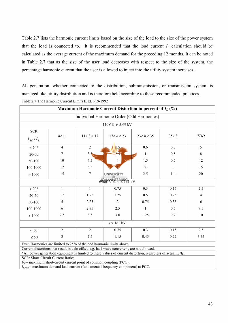
43
Table 2.7 lists the harmonic current limits based on the size of the load to the size of the power system
that the load is connected to. It is recommended that the load current IL calculation should be
calculated as the average current of the maximum demand for the preceding 12 months. It can be noted
in Table 2.7 that as the size of the user load decreases with respect to the size of the system, the
percentage harmonic current that the user is allowed to inject into the utility system increases.
All generation, whether connected to the distribution, subtransmission, or transmission system, is
managed like utility distribution and is therefore held according to these recommended practices.
Table 2.7 The Harmonic Current Limits IEEE 519-1992
Maximum Harmonic Current Distortion in percent of IL (%)
Individual Harmonic Order (Odd Harmonics)
110V≤ v ≤ 69 kV
SCR
LSC II h<11 11< h < 17 17< h < 23 23< h < 35 35< h TDD
< 20*
20-50
50-100
100-1000
> 1000
4
7
10
12
15
2
3.5
4.5
5.5
7
1.5
2.5
4
5
6
0.6
1
1.5
2
2.5
0.3
0.5
0.7
1
1.4
5
8
12
15
20
69001V ≤ v ≤ 161 kV
< 20*
20-50
50-100
100-1000
> 1000
1
3.5
5
6
7.5
1
1.75
2.25
2.75
3.5
0.75
1.25
2
2.5
3.0
0.3
0.5
0.75
1
1.25
0.15
0.25
0.35
0.5
0.7
2.5
4
6
7.5
10
v > 161 kV
< 50
≥ 50
2
3
2
2.5
0.75
1.15
0.3
0.45
0.15
0.22
2.5
3.75
Even Harmonics are limited to 25% of the odd harmonic limits above.
Current distortions that result in a dc offset, e.g. half-wave converters, are not allowed.
*All power generation equipment is limited to these values of current distortion, regardless of actual Isc/IL.
SCR: Short-Circuit Current Ratio;
ISC= maximum short-circuit current point of common coupling (PCC); IL,max= maximum demand load current (fundamental frequency component) at PCC.

44
2.4.4 Transformer heating considerations
The harmonic current distortion limits, as outlined in Table 2.3, are only permissible provided that the
transformer connecting the customer to the utility system will not be subjected to harmonic currents in
excess of 5% of the transformer’s rated current stated in IEEE C57.12.00-1987. [10] The installation of
a larger transformer unit should be considered if the transformer connecting to the customer will be
subjected to harmonic current levels in excess of 5%. The heating effect in the transformer should be
evaluated applying analysis contained in IEEE C57.110-1998 [11] when harmonic current flowing
through the transformer is more than the design level of 5% of the rated current. This will ensure that
transformer insulation is not being stressed beyond design limits.

45
Conclusion
The harmonic sources show that harmonics presence in the power system proves to be true and is a
threat if there is an increase of this switching equipment. The fundamental harmonic concepts were
described with the effects they have on power and power factor. This shows that harmonics do not
affect the real power drawn from the power system but can increase the reactive power of the power
system. This can then result in a lower power factor, which lowers the size of the power system to
supply a given load. Due to the presence of harmonics and their adverse effects on the power system,
standards have been put in place to ensure that the magnitudes of the harmonics are within acceptable
limits.
The NRS harmonic standards provide a detailed layout of the harmonic voltage levels that need to be
monitored and calculate the allowable harmonic current distortion levels only when the maximum
demand loading is greater than 1% of the minimum designed operating three-phase point of common
coupling fault level. The IEEE practices, on the other hand, give attention to harmonic voltages and
provide a detailed outlook on the harmonic distortion current levels. This NRS standards and IEEE
practices confirm that harmonic voltages as well as harmonic currents need to be monitored on the
power system. A linear supply impedance thus cannot be assumed in power systems because harmonic
voltages are not linear to harmonic currents in general. This effect is true when a harmonic load is
supplied by a transformer which is not a linear device under all operating conditions. In the transformer
heating considerations section it has been predicted that if harmonic currents cause transformer line
currents to exceed the design level of 5% of the rated current, they can stress the insulation beyond its
design limits.
This chapter confirms the presence of harmonics on the network and shows that they can affect the
power system adversely. However, if harmonic standards are put in place this could limit the impact of
harmonic distortion. The harmonic standards show that both the harmonic voltages and currents need to
be monitored, as linear supply impedance cannot be assumed.

46
CHAPTER 3: THEORY OF TRANSFORMER LOAD AND NO-LOAD LOSSES
Introduction
This Chapter discusses the theory and effects of harmonics on power transformer losses, which are the
main cause of heating in the transformer. The thermal breakdown is a direct consequence of the amount
of heating, and consequently the temperature the transformer is exposed to. The recommended practice
for establishing transformers’ capability under nonsinusoidal conditions is also evaluated together with
the impact it has on transformer losses. Thus, to study the impact of harmonics on transformers the
causes of transformer losses need to be evaluated together with the temperature rise in the transformer.
Recommended practice for establishing transformer capability transformer losses
The damage to any equipment can be described by means of a damage curve, which shows the point
from which thermal breakdown occurs. The damage curve is the energy as a function of time, which
describes the equipment’s thermal limits or thermal breakdown. Therefore the transformer capability is
established through transformer losses which define the transformer thermal limits.
Lower losses will increase the lifetime of the transformer. Low loss transformers increase reliability
due to the reduced internal heating if there is no external cooling mechanism. Fortunately, most modern
transformers have cooling systems that prevent transformers from overheating.
The thermal power generated in a transformer is undesirable but an unavoidable by-product of normal
transformer operation. Transformer losses are electric power generated by the source converted to
thermal power in the transformer that has to be dissipated. Transformer losses are categorised as no-
load losses and load losses. The total loss is classified as the sum of the no-load loss and the load loss
which are considered separately in the design and operation of the transformer. But the separate losses
are jointly considered in respect of the dissipation of the thermal power generated in the transformer.
The effect of harmonics on transformers is twofold: current harmonics cause an increase in copper
losses and stray flux losses, and voltage harmonics cause an increase in iron losses [10]. The overall
effect is an increase in the transformer heating, as compared to purely sinusoidal (fundamental)
operation [10]. The transformer losses accounted for are no-load losses and load losses which will be
discussed in detail in following sections. The total transformer losses are then given as:

47
LLNLTL PPP += (3-1)
where PNL is the no-load losses and PLL is the load losses.
3.1 Load losses
The losses associated with load currents include a) ohmic losses (I2R) in the conductors as for direct
current, b) the eddy current losses in the conductors or windings caused by alternating leakage flux in
the conductors and other stray losses or eddy currents in the tank clamps, and core plates caused by
leakage flux cutting them.
OSLECLL PPPP ++= Ω (3-2)
where PLL is the total load loss of the transformer and P the I2R losses of the transformer.
Stray losses are of special importance when evaluating the added heating due to the effect of a
nonsinusoidal current waveform. Stray losses are eddy-current losses due to stray electromagnetic flux
in the windings, core, and core clamps, magnetic shields, tank wall, and other structural parts of the
transformer. Thus, the stray loss is subdivided into winding stray loss and stray loss in components
other than the windings (POSL). The winding stray loss includes winding conductor strand eddy-current
loss and the loss due to circulating currents between strands or parallel winding circuits. All of this loss
may be considered to constitute winding eddy-current loss, PEC. This loss will rise in proportion to the
square of the load current and the square of the frequency.

48
3.1.1 Ohmic losses (I2R) in transformer windings
The conductor windings of transformers are made mostly from copper because of its high conductivity.
Although copper has a high conductivity it has a finite conductivity. This conductivity gives rise to a
finite resistance value derived from Ohm’s law.
EJ σ= (3-3)
where σ is the conductivity, J the current density and E the electric field. This equation (3-3) can be
further simplified to the resistance:
Ω
=A
lR w
dc σ (3-4)
where lw is the total length of the winding or wire and AΩ the cross-section of the wire. The path of
integration, lw, is along the current flow-path of the conductor (shown in Figure 3.1). At dc or low
frequencies, current (I) uniformly distributed over cross-section AΩ of the conductor, which can vary
with position. The dc resistance, Rdc, is actually the ohmic resistance at dc and/or low frequencies.
In ordinary conductors, such as copper and aluminium, the highest energy electrons are readily
detached from their atoms by an applied electric field and are free to migrate. The atoms, however,
remain fixed in the conductor’s lattice so only the electrons have mobility. [9] As the temperature
increases, the mobility and density of the electrons in the conductors decreases, hence a decrease in
conductivity (increase in dc resistance). The conductivity of any material is dependent on the
temperature of the material. The conductivity of the most frequently used materials is usually tabulated
for a specific temperature mostly at 20˚C.
E
I
l
σρ1
= ρ = resistivity
σ = conductivity
Figure 3.1 The current flow through the conductor.
AΩ
49
The dc resistance of a conductor or material is therefore dependent on its temperature. The dc
resistance at a specific temperature can be determined by:
2
1
2
1
)(
)(
TT
TT
TR
TR
k
k
dc
dc
+
+= (3-5)
where: Rdc(T1) is the dc resistance (Ohms) at temperature T1, ˚C,
Rdc(T2) is the dc resistance (Ohms) at temperature T2, ˚C,
Tk is 234.5 ºC for copper,
Tk is 225 ºC for aluminium.
Tk is the temperature constant for a specific metal or conductor, ˚C. Therefore, for an increase in
temperature there is an increase in dc resistance Rdc thus an increase in I2R losses. The same formula
given in eq. (3-5) can be written in terms of ohmic power losses instead of dc resistance. The same
result for dc resistance is true for the ohmic loss. Further discussion around the temperature in
transformers occurs in section 3.3.
The resistance value calculation at higher frequencies can become more complex because of the effects
of changing magnetic fields on currents within the conductor. The current distribution over the cross-
section AΩ are consequently non-uniform and the particular path of the current along the cross-section
of the conductor must then be redefined. This phenomenon is called the skin effect, which will be
explained in the next section in more detail.
The dc resistance gives rise to real power losses in the transformer. The total power losses or average
power is the current squared times the resistance. So an increase in resistance increases the power
losses. The ohmic losses (I2R) of load losses for transformers are expressed as:
2,
2
22,
2
1
2
dcdcdc RIRIRIP +==Ω (3-6)
where I1 is the primary current, I2 is the secondary current, Rdc,1 is the primary resistance and Rdc,2 is the
secondary resistance. The losses in the windings can be referred to one winding of a single-phase
transformer and equals referred to the primary side:
×
+==Ω 2
2
2
11
2
1
2 RNNRIRIP dc (3-7)
or referred to the secondary side equals:
50
+
==Ω sec2
sec
2
sec
2 R
NN
RIRIP
prim
prim (3-8)
If harmonic components increase the rms value of the load current, the ohmic losses (I2R) will increase
according to [11] and [3]. This result can be explained by the following derived formula:
dc
h
hrmshdcA RIRIP ×
=×= ∑
=Ω
max
1
2
,
2 (3-9)
Now if the IA, the magnitude of the actual measured rms load current is greater than the magnitude of
the rms rated load current, IL (= I1), the load absorbs, the ohmic losses will definitely increase according
to equation (3-9). This proves that the average power or real power loss can increase as a result of the
harmonic content in the current or voltage waveform.
The average power or real power (ohmic losses) is expressed as:
∫=t
AV pdtT
P1
( )∫ ⋅=t
dtivT
1
∫=t
dc dtiRT
21 (3-10)
The current waveform i can be expressed in terms of harmonic components as:
∑=
+=max
1
)sin(h
hhh thIi ϕω (3-11)
The average power can then be calculated by substituting eq. (3-11) in eq. (3-10).
( )∫ ∑
+=
=
T h
hhh
dcAV dtthI
T
RP
0
2
1
max
sin ϕω (3-12)
( ) ( ) ( )( )∫ ++++++=T
dcAV dttItItI
T
RP
0
3
22
32
22
21
22
1 ...3sin2sinsin ϕωϕωϕω (3-13)
The cross terms in eq. (3-13) result in zero after integration because the cross terms are orthogonal. The
average power or real power due to the ohmic losses reduces to:
2
...)( 2
4
2
3
2
2
2
1 ++++== Ω
IIIIRPP dcAV (3-14)
...)( 2
,4
2
,3
2
,2
2
,1 ++++= rmsrmsrmsrmsdc IIIIR (3-15)

51
∑=
=max
1
2
,
h
hdcrmsh RI (3-16)
The equation (3-16) indicates that harmonic loading can increase the average power loss. This is
especially true if the magnitude of the fundamental current, I1 of the harmonic load current, iL is equal
to the rated load current, IL,R. This result supports the recommended practice that applies only to two
winding transformers covered by IEEE. Std.C57.12.00-1993: IEEE Std C57.12.01-1998 and NEMA
ST20-1992. [10] The I2R losses will increase if harmonic components increase the rms value of the
load current. Therefore a harmonic factor had been established for current
=∑≠
1
1
max
I
Ih
hh
which
according to the IEEE Std C57.12.00-2000 shall not exceed 0.05 per unit. This means that the load
current of the transformer should not exceed 1.05 per unit.
3.1.2 Eddy current losses in windings
There are two effects that can cause increase in winding eddy current losses in windings, namely the
skin effect and the proximity effect. The winding eddy current loss (PEC) in the power frequency
spectrum tends to be proportional to the square of the load current and the square of frequency which
are due to both the skin effect and proximity effect. [11]
22 fIPEC ×∝ (3-17)
This winding eddy current loss proportionality to the frequency will then be confirmed through detailed
theoretical analysis. Now the eddy current losses in the windings are broken down into the skin effect
and the proximity effect, which will be discussed separately in the sections to follow.

52
Skin effect in windings
The skin effect will be explained by means of Figure 3.2. The current i(t) in the conductor illustrated in
Figure 3.2 a) generates a magnetic field which generates a flux density through the wire (Amperes
Law). The flux density through the wire in turn generates circulating eddy currents (Faraday’s law).
These eddy currents flow in the opposite direction to the applied current in the interior of the wire. This
shields the interior of the conductor from the applied current resulting magnetic field. The current
density is then distributed in the conductor as shown in Figure 3.2 c).
The ac resistance of the conductor then needs to be revaluated for the skin effect in the conductor.
According to reference [13] and Butterworth experiments there are two ways the ac resistance has been
evaluated. Firstly the ac resistance was defined in terms of the dc resistance, which is multiplied with a
factor.
c) Current distribution through conductor. b) The eddy currents generated by the
resulting magnetic field.
a) Isolated copper conductor
carrying a current i(t).
H
i(t) J(t) J(t)
0 x
Cross-section of conductor.
i(t)
B(t)
Iec(t)
Figure 3.2 A current-carrying conductor.

53
The ac resistance, Rac, of a conductor is:
)1(dc
sedcsedcac R
RRRRR +=+=
)1( FRdc += Ω (3-18)
where Rse is the skin-effect resistance and F is the skin-effect factor. The skin-effect factor is
proportional to δd where d is the diameter or thickness of the conductor and δ is the penetration depth.
The penetration depth is expressed as:
ωµσδ
1= (3-19)
where µ is the absolute permittivity of conductor and
σ is the conductivity of the conductor.
Butterworth did measurements on how the skin-effect
factor varies with the ratio δd. These results are given
in Figure 3.3. It can be clearly seen in Figure 3.3 when
δd is smaller than 2 that the skin-effect factor is
smaller than 0.01 and can be disregarded. The skin
effect increases rapidly as δd increases and when
δd is
greater than 5 the ac resistance factor is:
)1(4
11 +≅+
δd
F (for δd
> 5) (3-20)
When δd is very large, 1+F approximates to
δ4d and
the ac resistance:
ωµσσπδ c
dcsedcac d
dldRRRR
24=≅+= (3-21)
σδππσµ
d
lf
d
l== (3-22)
Figure 3.3 Skin-effect factor F and proximity effect
factor G, as functions of δd(
∆=d) for round
conductors, based on figures given by Butterworth
[10, 11].

54
An increase in diameter will increase the ratio of the Rac to Rdc but will reduce the actual value of ac
resistance, Rac. Hence the ac resistance of a conductor or winding is frequency-dependent due to the
skin effect. The loss tangent due to the skin effect in an inductor is:
L
FRdcse ω
δ =tan (3-23)
For a more accurate evaluation of the curves in Figure 3.3 the following is derived. F is proportional to
4
δdfor low values of
δd according to the factor F in Figure 3.3 and it is therefore proportional to f2.
Thus at low frequencies tanδse is proportional to f2. These proportionalities are only valid at low values
of frequencies and at value 6≅δd
. Thereafter they stabilise as F becomes approximately proportional to
2
1
f and tanδse approaches proportionality to 2
1−
f . [13]
However, this applies only to a straight isolated conductor. In a closed packed winding the current
fields of adjacent conductors will tend to cancel and this significantly reduces the skin effect in
inductor windings. In practice the diameter, d, of the conductor is chosen much smaller than the
penetration depth, δ, for the operating frequency therefore avoiding the skin-effect contribution at
operating frequency. The skin effect can then be disregarded if skin-effect factor δd is smaller than 2.
But the skin effect can still come into play if frequencies injected into the conductor are high enough to
cause the diameter, d, of the conductor to become more than two times greater than the penetration
depth, δ, of the conductor at a higher frequency. The conductor can then be designed for worst
frequency conditions injected into the power system (possibly as high as 1000 Hz). Conductors and
windings are generally designed for a skin-effect factor smaller than 2 and for the highest possible
Front view Right hand view
coil i
B
i
B
i
coil
Figure 3.4 A closed packed winding that reduces the skin effect in inductor windings

55
frequency so that the skin effect can be disregarded. Therefore the impact of lower-order harmonics on
the skin effect is negligible in the transformer windings. The skin-effect contribution will not be
considered in the winding eddy current losses considering all these design practices for windings and
conductors to minimise the skin effect.
Proximity effect
The proximity effect contribution to the winding eddy current loss is defined as follows. Consider
Figure 3.5. The HV winding produces a flux density, B, due to a changing current, i. The flux density,
B, cuts through the LV winding and core. The flux density that cuts the LV winding induces an emf that
produces circulating currents or eddy currents. These eddy currents oppose the current flow of the
inductor on the left-hand side of the conductor strip as shown in Figure 3.5 b) and reduce the current
density on the left side of the conductor. But these eddy currents on the right-hand side have an
additive effect on the total current that causes an increase on the total current. So a greater current
density is developed on the right-hand side of the conductor. The trend for the current density (J)
against the distance (x) of strip conductor is given in Figure 3.5 b). This effect is called the proximity
effect, which is caused by a current-carrying conductor or magnetic fields that induce eddy currents in
other conductors in close proximity to the other current-carrying conductor or magnetic fields. These
eddy currents will dissipate power, Pec, and contribute to the electrical loss in the windings in addition
HV LV
B
I
Figure 3.5 Illustration of the development of eddy currents due to the proximity effect.
b) Eddy current distribution in the conductor. a) The HV winding flux cut through the LV winding.
Core I
B
Iec
I
J(t)
0 x
Iec
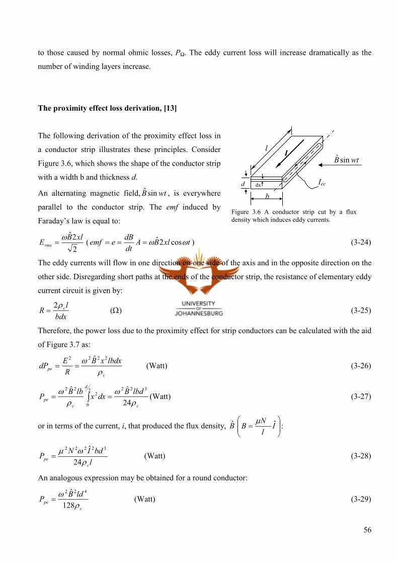
56
to those caused by normal ohmic losses, PΩ. The eddy current loss will increase dramatically as the
number of winding layers increase.
The proximity effect loss derivation, [13]
The following derivation of the proximity effect loss in
a conductor strip illustrates these principles. Consider
Figure 3.6, which shows the shape of the conductor strip
with a width b and thickness d.
An alternating magnetic field, wtB sinˆ , is everywhere
parallel to the conductor strip. The emf induced by
Faraday’s law is equal to:
2
2ˆ xlBErms
ω= ( txlBA
dt
dBeemf ωω cos2ˆ=== ) (3-24)
The eddy currents will flow in one direction on one side of the axis and in the opposite direction on the
other side. Disregarding short paths at the ends of the conductor strip, the resistance of elementary eddy
current circuit is given by:
bdx
lR cρ2
= (Ω) (3-25)
Therefore, the power loss due to the proximity effect for strip conductors can be calculated with the aid
of Figure 3.7 as:
cpe
lbdxxB
R
EdP
ρω 2222 ˆ
== (Watt) (3-26)
c
d
cpe
lbdBdxx
lbBP
ρω
ρω
24
ˆˆ 3222
0
222
== ∫ (Watt) (3-27)
or in terms of the current, i, that produced the flux density, B
= I
l
NB ˆµ
:
l
bdINP
cpe ρ
ωµ24
ˆ 32222
= (Watt) (3-28)
An analogous expression may be obtained for a round conductor:
cpe
ldBP
ρω128
ˆ 422
= (Watt) (3-29)
d
b
l
dx Iec
wtB sinˆ I
Figure 3.6 A conductor strip cut by a flux
density which induces eddy currents.

57
At higher frequencies, or with larger
conductor diameters such that the ratio δd
becomes larger than unity and field due to
these eddy currents, the flux density inside the
conductor is significantly reduced and
associated current distribution becomes non-
linear (as shown by the broken line in Figure
3.7).
Butterworth [14, 15] calculated the eddy
current loss in round conductors taking this
eddy current screening into account. The
results are expressed by introducing a
proximity effect factor, Gr, into eq. (36).
rc
pe GldB
Pρ
ω128
ˆ 422
= (W) (3-30)
or in terms of current I:
rc
pe Gl
dINP
ρωµ
128
ˆ 42222
= (W) (3-31)
where I is the peak current that flows through the winding or coil.
As shown in Figure 3.3, 1→rG as δd decreases to unity and when
δd is increasing beyond 4,
−
→ 132
4 δ
δ
d
dGr (3-32)
The proximity effect can be reduced through a reduction of conductor diameter, d. Reducing the
conductor diameter will increase the value of dc resistance, Rdc and will result in greater overall loss
(A
lRdc
ρ= ). The method used to combat proximity effect is to use bunched conductors of n insulated
wires of diameter or thickness d. At each end of the winding the wires or strands are soldered together
and have an effective area at low frequencies of 4
2dnπ or nbd (b is width and d is thickness).
The conductor is twisted so that, in its simplest form, each strand follows an approximate helical path.
In Figure 3.8 a) and b) a side-view of two strands and a conductor with several insulated and
Figure 3.7 A more detailed illustration of the
circulating eddy currents
l Iec
wtB sinˆ
b
2
d
x
dx

58
transposed wires is shown. The induced emf in each half-twist is cancelled out by those next (as shown
in Figure 3.8 a)). The circulating currents or eddy currents oppose each other and cancel out.
Thus equation (3-31) may be applied to the strands or wires of the conductor, d refers to the diameter
or thickness of the wire and ld refers to the mean length of the winding turn i.e. Nld and 4
2dnπ or
nbd is the total area of conductor. Equation (3-31) is written in a form that is more general for round
conductors in terms of the number of conductor strands n, the strand diameter, d and the total length in
terms of the mean length, lm.
rdc
pe Gl
ndINP
ρωµ128
ˆ 4222
= (3-33)
The proximity effect loss for strip conductors or rectangular conductors can be expressed as:
rdc
pe Gl
nbdINP
ρωµ24
ˆ 3222
= (3-34)
The proximity expressions (3-33) and (3-34) substantiate the statement made in reference [11] that the
winding eddy current losses is directly proportional to the square of the load current and square of the
frequency. The power loss expression for the proximity effect on conductors for nonsinusoidal currents
can be rewritten in terms of harmonic components in a more general form as:
∑=
− =max
1
22h
hhhhpe IkP ω (3-35)
B (flux density)
Iec Iec wires
5
4
3
2
1
1
2
3
4
5
6
7
a) Twisted strands
b) Conductor with several insulated
and transposed wires.
Figure 3.8 The cancellation of eddy current emfs
induced in twisted strands of bunched conductors by
transverse flux.

59
or the proximity effect or eddy current losses in terms of per unit harmonic current values used more
often in power systems as:
)(max
1
22 puIhPPh
hhRpepe ∑
≠−= (3-36)
The result in equations (3-35) and (3-36) is the theoretical proof that proximity effect loss or winding
eddy current loss is proportional to the square of the frequency. A proximity effect parameter expressed
in the time domain is much more useful, especially in the simulations of a transformer model in SPICE
(computed in the next section).
The computation of the proximity effect parameter by electromagnetic theory
The behaviour of electromagnetic time-varying fields into “good conductors” in reference [28], is used
to derive a generic formula for time-varying electric fields in good conductors. The electromagnetic
theory is used to develop a proximity effect parameter in terms of voltage and current defined in the
time domain as opposed to the frequency domain. Such a parameter can be used in time domain
circuits, as opposed to the frequency domain parameter that can only be used at a specific frequency
after which superposition has to be applied. This is proof of the proximity effect parameter in the time
domain. The conductors satisfy Ohm’s law,
EJ σ= (3-37)
The generalised Ampere’s law, including Maxwell’s displacement current term, states that the line
integral of magnetic field about closed path (magnetomotive) is equal to the total current (conduction
and displacement) flowing through the path which equals:
∫∫ ∫ ⋅∂∂
+⋅=⋅SS
dSDt
dSJdlH (3-38)
or in terms of the curl of the magnetic field:
t
DJH
∂∂
+=×∇ (3-39)
Or in terms of electric field,
t
EEH
∂∂
+=×∇ εσ (3-40)
To derive the differential equation that determines the penetration of the fields into the conductor, we
first take the curl of the Maxwell curl equation for electric field (Faraday’s law),

60
( )t
H
t
H
t
BE
∂×∇∂
−=∂∂
×∇=∂∂
×∇=×∇×∇ µµ
∂∂
−=×∇t
BE (3-41)
Further reduction of eq. (3-41), with substitution of eq. (3-40),
( )t
E
t
EEE
∂∂
−∂∂
−=∇−⋅∇∇2
2 µεµσ (3-42)
For metals and other good conductors, it is found that displacement current is negligible in comparison
with conduction current for microwave frequencies and millimetre frequencies, and in fact is not
measurable until frequencies are well into the infrared. [28] This means that at power frequencies and
power system harmonics the displacement current is also negligible. Therefore, the displacement
current is disregarded and the divergence of the electric field is zero )0( =⋅∇ E , and we find
t
EE
∂∂
=∇ µσ2 (3-43)
The differential equation is considered for a plane conductor of finite depth with no field variations
along the width or length dimension. The winding illustrated in Figure 3.9 b) that is round is assumed
to be straightened out as shown; then it can be presented in the z-x plane. For the uniform field
situations shown in Figure 3.9 a) with the electric field vector in the z direction, we assume no
variations with y or z and eq. (3-43) becomes:
E0 z
x
y
Figure 3.9 a) Plane solid illustrating decay of current into conductor due to the magnetic field that penetrates the
conductor and b) the secondary winding produces a flux density, B due to a changing current, i and the flux density,
B(t) cuts through the primary winding which induces an electric field, E0 in the primary winding.
windings Secondary
Primary
Flux density, B(t)
x
z
y
z
x y
Windings
straightened
a) b)
Secondary
Primary
B

61
dt
dE
dx
Ed zz µσ=2
2
(3-44)
Now eq. (3-44) can be presented in terms of the proximity effect voltage induced in the conductor by
the magnetic field that penetrates the conductor.
dt
dvu
dx
vd pepe σ=2
2
(3-45)
where wpe Adt
dBv = of which the flux density is assumed to penetrate the complete composite winding
area that is next to the flux producing winding. The proximity effect voltage, vpe, in terms of the
leakage voltage, vl1, that is:
wair
lwpe A
dt
di
AN
LA
dt
dBv
== 1
1
(3-46)
or
dt
dikv pe
11= (3-47)
The proximity effect voltage in terms of the primary current in eq. (3-47) is then substituted in eq. (3-
45):
2
1
2
12
2
dt
idk
dx
vd pe µσ= (3-48)
After double integration of eq. (3-48) with distance, assuming the current i1 is not a function of distance
and the flux is in one direction, the proximity effect voltage result is expressed as:
2
1
2
2 dt
idkv pe = (3-49)
or in terms of the winding eddy current, ipe.
2
1
2
2
dt
id
l
kA
r
vi
wec
wpepe
−
==ρ
(3-50)
2
1
2
dt
idki pe = (3-51)
2
1
2
1
2
2
2
21
2
1,
1)(
ωpRRpe
Idt
id
dtiddt
id
pui−
×== (3-52)
62
It is assumed in this study that the skin effects are negligible and the main contributor to the winding
eddy current losses is the proximity effect. The winding eddy current and voltage is then assumed to be
equal to the proximity effect voltage and currents.
peec ii = ,
)()( 1,1, puipui peec = and
peec vv = (3-53)
The winding eddy current voltage, vec can then be expressed i.t.o. the winding eddy current resistance,
REC-R,1, at rated voltage as potential difference in series with the leakage inductance and dc resistance of
the transformer as:
1,1,1, )( RECpRecec RIpuiv −− ×⋅=
= −
− 2
1,
1,
1,
R
RECREC I
PR (3-54)
The winding eddy current loss parameter is expressed in the time domain which will simplify harmonic
impact studies on power transformers. The winding eddy current losses, PEC, can then be calculated
from the eddy current per unit, iec(pu), the rated peak to peak current, IR,1, and the rated eddy current
resistance, REC-R,1.
( )∫−− ⋅
=t
ecRECppR
EC dtpuiT
RIP 2
1,
1,
2
1,)( (3-55)
The rated winding eddy current resistance REC-R for the primary and secondary side is calculated
through the following process from eq. (3-56) to eq. (3-62) only if the rated winding eddy current
losses are not given for a transformer. Firstly the total stray loss is calculated, then the total winding
eddy current loss, after which the primary and secondary winding eddy current losses are calculated
respectively. Finally the expression for the rated winding eddy current loss resistance in terms of
winding eddy current loss and rated current is expressed.
-The total stray loss, PTSL can be calculated as follows:
( ) ( )22
21
2
1, RIRIPP RRmeasRLLTSL ×+×−= −−− (3-56)
-The winding eddy current loss is then calculated by assumption 2) in 6.2 of ref. [11] for dry type
transformers.
TSLOEC PP ×=− 67.0 (3-57)
-The winding eddy current loss is then calculated by assumption 2) in 6.2 of ref. [11] for oil-filled
transformers.
TSLOEC PP ×=− 33.0 (3-58)

63
The division of eddy current loss between the windings for transformers having a maximum self-
cooled current rating of less than 1000 A (regardless of turns ratio) are 60% in the inner winding and
40% in the outer winding [11]. The primary voltage (outer winding) winding eddy current loss, PEC-R,1,
at rated current is:
RECREC PP −− ×= 4.01, (outer winding) (3-59)
The secondary voltage (inner winding) winding eddy current loss at rated current is:
RECREC PP −− ×= 6.02, (inner winding) (3-60)
Finally the winding eddy current loss resistance, REC, for the primary and secondary side in terms of
winding eddy current loss, PEC-R, at rated current can be derived from the winding eddy current loss
and rated current:
2
1,
1,
1,
R
ECREC I
PR =− (3-61)
2
2,
2,
2,
R
ECREC I
PR =− (3-62)
This section derives a time-domain winding eddy current voltage parameter, vec, which can be used in a
transformer model to evaluate the harmonic effects. It also gives a calculation procedure to estimate the
rated winding eddy current losses for the transformer for the primary and secondary side. Thereby the
rated winding eddy current resistance, REC, for the primary and secondary side is calculated.

64
3.1.3 Other stray losses in transformers (POSL)
The other stray losses (POSL) in the core, clamps and structural parts will also increase at a rate
proportional to the square of the load current but not at a rate proportional to the square of the
frequency as in winding losses. Studies have shown that eddy current losses in busbars, connections
and structural parts increase by a harmonic factor of 0.8 or less. Stray losses occur in ferromagnetic
material (core-steel or structural steel) and the penetration is a non-linear phenomenon. Stray losses in
mechanical parts are of importance in large special converter transformers and liquid-filled
transformers and usually do not play any great part when a small conventional transformer is used.
The rated load current produces a magnetic field, which is directly proportional to the load current. The
magnetic field, which cuts through the core, windings, clamps and tank, is shown in Figure 3.9. Each
metallic conductor linked by the electromagnetic flux experiences an internally induced voltage that
causes eddy currents to flow in that ferromagnetic material. The eddy currents produce losses that are
dissipated in the form of heat, producing an additional temperature rise in the metallic parts over its
surroundings. The stray losses or eddy current losses outside the windings are the other stray losses
(POSL). [11]
Experiments were done by Deniz Yildrim and Ewald F. Fuchs on a 25kVA liquid-filled (oil)
transformer (7200/240 V) to find the change of other stray losses (POSL) with frequency given in
published paper [16]. The results shown that the ac resistance (Rac) of the other stray losses (POSL) at
low frequencies is equal to (0 – 360 Hz):
Core surface
Clamp
LV
winding HV
winding
Tank
Figure 3.9 Electromagnetic field produced by load current in a transformer.

65
8.0
1
29.1
=
f
fR hlf
OSL [mΩ] (3-63)
and at high frequencies (420-1200Hz) the ac resistance is:
9.0
1
59.029.9
−=
f
fR hhf
OSL [mΩ] (3-64)
The paper concludes that the other stray losses increase with power of 0.8 at low frequencies (0-360Hz)
and decrease at high frequency with power of 0.9. These results are confirmed with those given in
reference [11], which states that the other stray losses in the core, clamps and the other structural parts
are proportional to the square of the load current and the frequency to the exponent factor 0.8.
8.02 fIPOSL ×∝ (3-65)
Or the other stray losses can be effectively written in per unit form as:
)(max
1
28.0 puIhPPh
hhROSLOSL ∑
≠−= (3-66)
The other stray losses can be represented in a transformer circuit as an additional series resistor with
the dc resistor that can be called other stray loss resistance, ROSL, and can be calculated as follows (the
other stray loss, POSL, is then calculated as the remainder of the total stray loss):
ECTSLOSL PPP −= (3-67)
The percentage division between the inner winding and outer winding for the other stray losses is
assumed to be the same as the winding eddy current loss divisions. The primary (outer winding) other
stray losses, POSL-1,1, at rated current is:
ROSLROSL PP −− ×= 4.01, (outer winding) (3-68)
The secondary (inner winding) other stray losses, POSL-1,2, at rated current is:
ROSLROSL PP −− ×= 6.02, (inner winding) (3-69)
and other stray losses, POSL-h in terms of harmonic loss factor, FHL-STR for the secondary winding is:
ROSLSTRHLhOSL PFP −−− ×= 6.01, (3-70)
The other stray loss resistance, ROSL, for the primary and secondary side in terms of other stray loss,
POSL-R, at rated current can be derived from the other stray loss, POSL, and rated current as such:
2
1,
1,
1,
R
OSLOSL I
PR = (3-71)
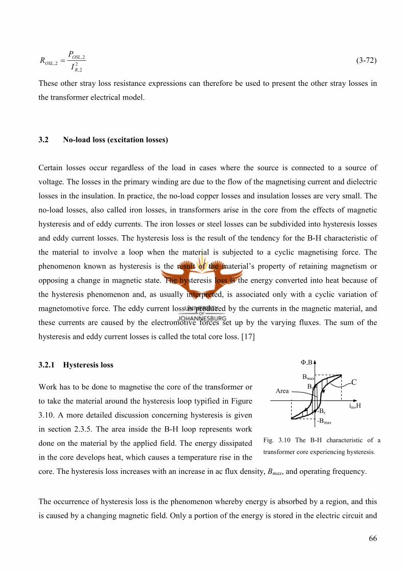
66
2
2,
2,
2,
R
OSLOSL I
PR = (3-72)
These other stray loss resistance expressions can therefore be used to present the other stray losses in
the transformer electrical model.
3.2 No-load loss (excitation losses)
Certain losses occur regardless of the load in cases where the source is connected to a source of
voltage. The losses in the primary winding are due to the flow of the magnetising current and dielectric
losses in the insulation. In practice, the no-load copper losses and insulation losses are very small. The
no-load losses, also called iron losses, in transformers arise in the core from the effects of magnetic
hysteresis and of eddy currents. The iron losses or steel losses can be subdivided into hysteresis losses
and eddy current losses. The hysteresis loss is the result of the tendency for the B-H characteristic of
the material to involve a loop when the material is subjected to a cyclic magnetising force. The
phenomenon known as hysteresis is the result of the material’s property of retaining magnetism or
opposing a change in magnetic state. The hysteresis loss is the energy converted into heat because of
the hysteresis phenomenon and, as usually interpreted, is associated only with a cyclic variation of
magnetomotive force. The eddy current loss is produced by the currents in the magnetic material, and
these currents are caused by the electromotive forces set up by the varying fluxes. The sum of the
hysteresis and eddy current losses is called the total core loss. [17]
3.2.1 Hysteresis loss
Work has to be done to magnetise the core of the transformer or
to take the material around the hysteresis loop typified in Figure
3.10. A more detailed discussion concerning hysteresis is given
in section 2.3.5. The area inside the B-H loop represents work
done on the material by the applied field. The energy dissipated
in the core develops heat, which causes a temperature rise in the
core. The hysteresis loss increases with an increase in ac flux density, Bmax, and operating frequency.
The occurrence of hysteresis loss is the phenomenon whereby energy is absorbed by a region, and this
is caused by a changing magnetic field. Only a portion of the energy is stored in the electric circuit and
Fig. 3.10 The B-H characteristic of a
transformer core experiencing hysteresis.
Φ,B
im,H
Bmax
-Bmax
Br
-Br
C Area

67
recoverable from the region when magnetomotive force (mmf) is removed. The rest of the energy is
converted into heat because of work done on the material in the medium when it responds to the
magnetisation. The energy absorbed is the area enclosed shown in Figure 3.10.
Theoretically, the energy absorbed is given by:
∫ ×=loop
VolHdBw (3-73)
where Vol is the volume of the core. Empirically, Steinmetz found from the results of a large number of
measurements that the area of the normal hysteresis loop of specimens of various irons and steels
commonly used in the construction of electromagnetic apparatus of his day had been approximately
proportional to the 1.6th power of the maximum flux density, throughout the range of flux densities
from about 0.1 to 1.2 Teslas. [12] The exponent 1.6 fails nowadays to give the area of the loops with a
sufficient degree of accuracy to be useful. The empirical expression for the total hysteresis energy loss
in a volume in which the flux density is everywhere uniform and varying cyclically at a frequency of f
cycle per second can then be expressed as:
nh Bw maxη= [J.m
-3.cycle
-1] (3-74)
where η and n have values that depend on the material. The value of n may range between 1.5 and 2.5
for present-day materials. [17] The power loss per cycle is:
nh fBVolP max⋅=η [W] (3-75)
Equation (3-75) can be further reduced by substitution of the following:
l
NI
fN
E µ==Φ
44.4max (3-76)
and can be further rewritten to:
l
NI
fNA
EB
c
µ==
44.4max (3-77)
The power loss expression results in:
n
c
n
ch NA
LIVf
fNA
EfVolP
=
⋅= maxmax
44.4ηη (3-78)
where N is turns and Ac is the core cross-section.
The assumptions made in the derivation of the hysteresis-loss terms in eq. (3-75) are [17]:
a) Each lamination is homogeneous magnetically; that is, each element of its volume has the same
magnetic characteristics.

68
b) The flux density is uniform throughout each lamination; that is, the effect of the eddy currents on
the flux distribution is negligible.
c) The hysteresis loop is of the normal symmetrical shape with no re-entrant loops. Provided this
condition is satisfied no restriction is placed on the manner in which B varies with time throughout
a cycle of magnetisation.
d) The material, the range of maximum flux density and the manner of flux density variations are such
that an empirical exponent n can be used with reasonable accuracy.
3.2.2 Eddy current losses in the core
Whenever the magnetic flux in a medium changes, an electric field is induced within the medium
because of the changing flux. When the medium is conducting, a current is induced by the induced emf
( ∫∫ = dSdt
dEdl
abcd
Bn ). These currents are called eddy currents, Iec. These eddy currents cause eddy
current losses, RI ec2 , which give rise to power losses. The energy absorbed from the circuit that sets up
the field is dissipated as heat in the medium. This loss is significant in determining the efficiency, the
temperature rise, and hence the rating of electromagnetic apparatus in which the flux density varies.
J(t)
0 x
Φ
iec
a b
c d
a) b)
Fig. 3.11 Cross-section of a core lamination showing the current path. [17]
τ
iec

69
A thin metal slab shown in Figure 3.11 is considered to illustrate the conditions typical of those that
occur in an iron core. An alternating flux Φ is assumed to permeate the thin metal slab. The
electromotive force e induced around a boundary abcda of an area through which a flux is changing
given by:
dt
deemf
Φ−== (3-79)
The voltage acting around the circuit abcda causes a current, Iec, to circulate around the boundary and
set up a magnetomotive force ( lu
BHlNimmf ====ℑ ) in such a direction as to oppose any change
in flux, Φ. These eddy currents, Iec, screen or shield the material from the flux, Φ, and bring about a
smaller flux density near the centre of the slab rather than at the surface. As can be seen in Figure 3.11,
the flux density or total flux tends to be crowded toward the surface of the slab. This phenomenon is
also known as the crowding effect.
The simpler analysis of eddy current loss is given below together with a criterion for more accurate
analysis. The simpler analysis is developed for a thin transformer lamination having a thickness dt, as
shown in Figure 3.12. A uniform magnetic field distribution and the magnetomotive forces of eddy
currents have negligible effects on the flux distribution. An emf is induced in the slab according to
Faraday’s induction law, to the path abcda in the xy plane (Figure 3.12).
∫ ∫ ⋅−=abcda S
x ndSBdt
ddlE (3-80)
or
AreatBdt
dtv ×= )()( (3-81)
a b c d
x
x
dx
l
w
Eddy current flow path (Iec))
B sin(wt)
z
y
x
Figure 3.12 Eddy currents generated in a thin transformer lamination by an applied time-varying magnetic field.

70
xwdt
tdB2
)(×= (3-82)
If the conducting material or the core has a resistivity ρ, the current along abcda is equal to:
w
ldxtv
r
tvti
ρ2)()(
)( == [Resistance: ldx
wr
ρ2= ] (3-83)
or
ρlxdx
dt
tdBti
)()( = (3-84)
The instantaneous power dissipated in the thin loop in Figure 3.12 is given by:
rtitp )()( 2=δ
ρdxlwx
dt
tdB 222)(
= (3-85)
Assume the flux density is wtBtB sin)( max= . The instantaneous power dissipated is then further
reduced to:
core
dxlwxtBtp
ρωω
δ2222 2cos
)(×⋅
= (3-86)
Integrating over the volume of the lamination to obtain the total time-average eddy current power, Pec,
dissipated in the lamination gives:
dxlwxtB
dVtpP
d
coreec ∫∫
⋅==
2
0
2222
2cos
)(ρ
ωωδ (3-87)
core
Bwld
ρω
24
223
= (3-88)
The specific eddy current loss, Pec,sp (loss per unit volume), is given by:
corespec
BdP
ρω24
222
, = (3-89)
Note that Pec,sp varies with the square of the lamination thickness, dt. This is the reason that cores are
made up of laminations to reduce the eddy current losses in the core.
The Pec,sp estimate represents an optimistic minimum in the eddy current loss: if the magnetic flux were
inclined at some angle to the plane of the lamination (yz plane), the loss would be considerably large.
[13] Most magnetic steels, especially those used in power transformer applications (50/60 Hz), have a
small percentage of silicon added to the iron to increase the resistivity of the material and thus increase
71
the skin depth and reduce the effects of eddy currents. However, the addition of a few percent silicon
reduces the magnetic properties such as the saturation flux. Hence, a reasonable compromise for
transformers for 50/60 Hz applications is iron alloy of 97% iron, 3% silicon and a lamination thickness
of approximately of 0.3mm.
Further reduction of equation (3-88) by substitution of fNA
EB
44.4max = reduces to:
223
44.424
=
fNA
EwldP
coreec ρ
ω (3-90)
The core loss expression gives correct eddy current loss regardless of the waveform provided the
frequencies involved in the nonsinusoidal wave are not high enough to produce a considerable
crowding effect. When the flux is made up of components, each of these components induces eddy
currents in the core. The eddy current loss produced by each harmonic component in the flux is
proportional to the square of the same harmonic components of the emf generated in the winding. Then
if E1, E2, E3 and E4 are the effective values of the fundamental and harmonic components of generated
emf the total eddy current loss is equal to:
...][ 2
4
2
3
2
2
2
1 ++++= EEEEKPe (3-91)
where ( )2
23
44.424 fNA
wLdK
coreρω
= .
However, the sum of 2
1E ,2
2E ,2
3E , 2
4E , … equals the square of the effective value E of the generated
electromotive force.
2KEPe = (3-92)
Note that the eddy-current loss, when expressed in terms of E (the rms voltage induced in the coil), is
independent of frequency. But the voltage is proportional to the frequency of the flux density or
current.
The theoretical analysis behind eq. (3-88) is found in “The Theory of Transmission Lines, Waveguides
and Antennas”. The assumptions made in the derivation of the eddy current expressions are [17]:
a) The material is magnetically and electrically homogeneous. In practice, this condition is not
perfectly fulfilled, since such factors as grain size, the direction of the grain produced by rolling,
72
and the relatively poorer magnetic properties of the surface layers have an appreciable effect,
especially in thin laminations.
b) The thickness of the laminations is constant and very small compared with their other dimensions.
This condition is usually realised in practice.
c) The flux density is uniform throughout the thickness of the lamination; that is, the eddy current
magnetomotive force is negligible compared with the magnetising magnetomotive force acting on
the core.
d) The volume of core involved is subjected to uniform field so that at any given instant the flux
density is the same in the different laminations.
e) The laminations are perfectly insulated from each other. This assumption is seldom fulfilled in
commercial apparatus because of the considerable pressures under which the laminations are
clamped together.
f) The flux density undergoes a sinusoidal time variation and is always directed parallel to the plane
of the lamination. The assumption of a sinusoidal time variation is not a restriction, however, since
it was shown that the factor ( )2maxfB can be replaced by E2 that is the rms voltage induced in a coil
linked by the alternating core flux which may have any waveform.

73
The total core loss from theory
The total core loss per unit volume is the sum of the hysteresis loss and eddy current loss that is equal
to:
ρπ
η6
2
max
222
max
BdffBppp n
ehc +=+= (3-93)
where the symbols of significance are given previously. Equation (3-93) is based on several
assumptions that are in practice not true and yield numerical results that are too small, sometimes by a
factor of 2 or more. These equations are used not so much to calculate loss but to show the functional
relation between loss and the variables. These expressions serve then merely as guides to the analysis
of experimental data and possibly to modify the loss. These statements are given in [17]. Therefore to
calculate the total core loss a much more accurate expression needs to be produced.
3.2.3 Empirical expression for total core loss
Where precise knowledge of core loss is necessary for core loss calculations, the only reliable data is
obtained experimentally on samples of actual material to be used. Thus, an expression for total core
losses (Pcore in Watts) per kg is of the form:
mnechc BkfPPP max=+= (3-94)
It is the experimental expression for core loss Pc where k, n and m depend upon the properties of the
particular material. The coefficients k, n and m are derived using a three-dimensional least square fit
law from the digitised data. These curves include silicon, nickel-iron, ferrites, powdered iron and
Metglas. The coefficients for the different materials used are referenced in the Magnetic Core Selection
for Transformers and Inductors, 13th Edition and other transformer literature.
The total core loss expression indicates that the frequency plays a fundamental role in the core loss
magnitude. Thus for an increase in frequency of the flux density distributed or voltage induced the total
core loss will definitely increase accordingly.
The core loss expression of equation (3-94) can be presented in the transformer equivalent circuit as a
resistor. The core resistance, RC, can be estimated from this empirical core loss expression as:

74
mnrms
c
rmsC Bmkf
V
mP
VR
max
22
== Ω (3-95)
where the variable Vrms is the winding voltage and m is the core mass in kg. The core resistance, RC, is
therefore non-linear due to the non-linear core loss expression. The harmonic voltages applied to the
transformer play a significant role in the operation and impact of transformers, as can be examined by
the core resistance expression. The greater the frequency of applied terminal voltage the smaller the
core resistance; therefore more current will flow through the core resistance. Eventually it will cause
the core losses to increase due to increased current flow and the temperature will also increase if there
is no cooling system in the transformer. The harmonic current impact on the core resistance is therefore
not substantial according to the core loss expression, unless the harmonic currents injected into the
transformer increase the magnitude of the voltage applied to the transformer to a magnitude of
significance. The core loss expression in eq. (3-94) is used to calculate the core resistance for the
transformer model to evaluate the impact of harmonic distortion on core losses.
3.3 Harmonic impact on top oil temperature rise and winding temperature rise [18]
Not all input power, Pin, from the transformer is delivered to the load the Pout (output power). Part of
the input power is converted into no-load losses and load losses, as discussed in previous sections. The
core and coil assembly heat up from both the load and no-load losses as they emit heat to the
surrounding insulating coolant such as oil and air. The heat produced in transformers due to load and
no-load losses must be limited or transmitted away to prevent excessive rise of temperature and
damage to the insulation. The heat generated by the transformer losses produces a temperature rise,
which must be controlled to prevent damage or failure of the windings and breakdown of the wire
insulation at elevated temperatures. The thermal limit of the transformer is therefore reached when the
transformer’s rated VA rating is reached or is fully loaded provided the transformer has no cooling
system.
The life of dry-type transformers and liquid-filled transformers is dependent on the temperature at
which the transformer operates. The maximum safe working temperature of the winding and iron is
much higher than the insulation and oil temperature. Therefore the operating temperature of a
transformer is limited by its insulation and oil where the insulation materials are classified according to
their maximum safe working temperature given in IEC 60076-11:2004. Therefore the life of the
transformer is the life of the insulation and oil – but the transformer oil or fluid can be reclaimed, not

75
the insulation. So the life of the transformer is directly dependent on the life of the insulation. The
majority of transformer breakdowns are attributable to the failure of the insulating system.
The oil-immersed or synthetic-liquid-insulated transformers mostly use 105 ºC or class A insulation
where 105 ºC is the maximum permissible temperature of the insulation or the ultimate winding
temperature. The thermal characteristics of the transformer are the most important factor in the
transformer but other factors such as the mechanical strength and moisture resistance are also required
for the successful use of insulating materials. And the cellulosic insulation (class A insulation) and
mineral oil still form the strongest known electrical-mechanical insulating system for liquid-immersed
power and distribution transformers. The average temperature rise limits for oil-filled transformers are
referred to steady state under continuous rated power. The temperature rise limits for top oil
temperature rise is 60 ºC, according to the IEC 76-2: 1993 International Standard, and the average
winding temperature rise is 65 ºC at rated kVA, according to the IEEE Std C57.12.00-2000. The
maximum winding temperature or hot spot temperature rise shall not exceed 80 ºC at rated kVA under
usual operating conditions.
An increase in temperature results in an increase in conduction losses and the inverse is also true [27].
2
1
2
1
)(
)(
TT
TT
TP
TP
k
k
+
+=
Ω
Ω (3-96)
PΩ (T1) is the ohmic or conduction loss (Watts) at temperature T1, ˚C,
PΩ (T2) is the ohmic or conduction loss (Watts) at temperature T2, ˚C,
If the temperature limits are exceeded, the life of the transformer is shortened. If the temperature rise
limit is exceeded far beyond its thermal limits, the transformer can go into thermal runaway.
Harmonics currents can therefore increase conduction losses, as explained in section 3.1.1, hence cause
an increase in the temperature.
In contrast to conduction losses, where the conduction losses are directly proportional to the
temperature as defined in eq. (3-96), the winding eddy current losses are inversely proportional to
temperature. Thus the winding eddy current loss analytical formula is described as [27]:
+
+=
TT
TTTPTP
k
mkmecec )()( (3-97)
Pec (Tm) is the winding eddy current loss (Watts) at temperature Tm, ˚C,
Pec (T) is the winding eddy current loss (Watts) at temperature T, ˚C,

76
The equation states that for an increase in temperature the winding eddy current decreases, but the
inverse is not necessarily true. The top oil temperature rise (θTO) will also increase as the total load
losses increase with harmonic loading, especially for liquid-filled transformers. The increase of other
stray loss (POSL) will increase the top oil temperature rise.
Most dry-type transformers or air-insulated transformers use a 220 ºC insulation, where the 220 ºC
represents an ultimate winding temperature that is the summation of the maximum permissible winding
rise (150 ºC), the hot spot winding temperature allowance (30 ºC), and the ambient allowance of 40 ºC.
Although the coils are wound with class 220 ºC insulation, the same insulation is designed to operate at
80 ºC temperature rise. [30]
This heat dissipated from the exposed surfaces of the transformer can be calculated by a combination
of radiation and convection. The dissipation is therefore dependent upon the total exposed surface area
of the core windings.
3.4 Transformer capability calculations, [11]
The recommended practice IEEE 57.110-1998 applies only to two winding transformers covered by
IEEE Std.C57.12.00-1993, IEEE Std C57.12.01-1998 and NEMA ST20-1992. [11] This standard does
cover three-phase and single-phase two-winding power transformers as well but do not cover rectifier
transformers. The loss density in the windings is considered on a per unit basis for the transformer
operating under harmonic load conditions. This section derives the total load losses and harmonic loss
factors for the winding eddy current loss and other stray losses under harmonic loading conditions. The
equation that applies to rated load conditions is:
)()(1)( puPpuPpuP ROSLRECRLL −−− ++= (3-98)
where PLL-R is the rated load losses of the transformer, one is the conduction or ohmic losses, PEC-R is
the winding eddy current loss at rated current and POSL is the other stray losses at rated current. The
base of eq. (3-98) is the I2R or PΩ loss.
The eddy current power losses due to nonsinusoidal conditions or load currents are:
∑∞
=−
=
1
2
2
n R
hRECEC h
I
IPP Watts (3-99)

77
where PEC-R is the rated winding eddy current losses, Ih is the harmonic current component magnitude,
h is the harmonic component and IR is the transformer rated current. But the rated transformer current
for the eddy current winding loss is seldom taken at rated currents of the transformer. Therefore the
eddy winding current loss, PEC, can be expressed in terms of the fundamental current I1.
∑=
−
=
max
1
2
2
1
h
n
hOECEC h
I
IPP (3-100)
The equation for the nonsinusoidal rms load currents to the fundamental current, I, in per unit form is:
∑=
=max
1
2)()(
h
hh puIpuI (3-101)
The harmonic loss factor for winding eddy currents is derived as:
∑
∑
=
=
−
==max
1
2
max
1
22
h
hh
h
hh
OEC
ECHL
I
hI
P
PF
)(
)(
2
1
22max
puI
hpuIF
h
hh
HL
∑== (3-102)
where PEC-O is the winding eddy current losses at the measured current because it seldom happens that
application currents are taken at rated currents of the transformer.
Although the heating due to other stray losses is usually not a consideration for dry-type transformers,
it can have substantial effect on liquid-filled transformers. The harmonic loss factor for other stray
losses is expressed in a similar form as for the winding eddy currents.
∑
∑
∑
∑
=
=
=
=
−−
=
==max
1
2
1
max
1
8.0
2
1
max
1
2
max
1
8.0
2
h
h
h
h
h
h
h
h
h
h
h
h
OOSL
OSLSTRHL
I
I
hI
I
I
I
hI
I
P
PF
)(21
8.02max
puI
hIF
h
hh
STRHL
∑=
= = (3-103)
where the harmonic currents can be normalised to the rms current or fundamental current.
Power losses for harmonic loading in equation (3-98) can be multiplied by the square of the
nonsinusoidal rms load current per unit in dry-type transformers:

78
(3-104)
This equation assumes the other stray losses, POSL, are zero. Now substitute eq. (3-102) in eq. (3-104)
for dry type transformers yields to:
(3-105)
In liquid-filled transformers the total power losses due to harmonic loading yields:
×
+
×
+
×= −
=−
==∑∑∑ )()()()()()(1)()(maxmaxmax
1
8.02
1
22
1
2 puPpuhpuIpuPpuhpuIpuIpuP ROSL
h
hhREC
h
hh
h
hhLL
(3-106)
and reduce to:
[ ])()(1)()( 2 puPFpuPFpuIpuP ROSLSTRHLRECHLLL −=− ×+×+×= (3-107)
Equations (3-105) and (3-107) will then be used to calculate the maximum permissible current of the
transformer.
3.5 Recommended procedure for evaluating existing transformers
3.5.1 Transformers’ capability equivalent for power transformers using design data
Here the maximum permissible current formula is calculated to specify the transformer capability. The
maximum permissible current is calculated by setting PLL(pu) equal to PLL-R(pu) in equation (3-105) in
section 3.4. Thus the permissible current for dry-type transformers is equal to:
pupuPF
puPpuI
RECHL
RLL
)(1
)()(max
−
−
×+= (3-108)
where ∑=
=max
1
2
max )()(h
hh puIpuI .
In addition, the permissible current for liquid-filled transformers is expressed as:
[ ] [ ]pupuPFpuPF
puPpuI
ROSLSTRHLRECHL
RLL
)()(1
)()(max
−−−
−
×+×+= (3-109)
The permissible current can then be derived for equations (3-108) or (3-109) to find the transformer
capability and the transformer can be derated accordingly.
) ( ) ( 1 ) ( ) ( max max
1
2 2
1
2 pu P h pu I pu I pu P R EC
h
h h
h
h h LL −
= = ×
+ × = ∑ ∑
[ ] [ ] ) ( 1 ) ( ) ( 1 ) ( ) ( 2
1
2 max P F pu I pu P F pu I pu R EC HL R EC HL
h
h h LL − −
= + × = + ×
= ∑ P pu

79
3.5.2 Temperature capability calculations for transformers using design data
In the liquid-filled transformers, stray losses are taken into consideration, but in dry-type transformers
generally not. The top oil temperature rise is proportional to the exponent 0.8 and can be estimated for
harmonic losses as (equations defined in IEEE Std C57.91-1995):
CPP
PP
NLRLL
NLLLRTOTO °
+
+×=
−−
8.0
θθ (3-110)
where θTO-R is the rated top oil temperature rise and PNL is the no-load losses. The total load losses, PLL,
are equal to:
( ) ( )ROSLSTRHLRECHLhLL PFPFPpuP −=−−Ω ×+×+=)( (3-111)
where PΩ-h is the ohmic losses impacted by harmonic currents. The winding hot spot conductor
temperature rise over top oil temperature is proportional to the load losses to the 0.8 exponent and is
calculated as follows:
CpuP
puP
RLL
LLRgg °
×=
−−
8.0
)(
)(θθ (3-112)
and can be written as:
( ) [ ][ ]
CpuP
puPFpuI
REC
RECHLRTORgTOg °
+
+×−=
−
−−−−
8.02
)(1
)(1)(θθθ (3-113)
where θg-R is the rated winding hot spot conductor temperature rise over top oil temperature rise. The
hot spot conductor temperature rise over ambient is expressed as:
TOTOgg θθθ += − (3-114)
So the winding hot spot temperature can be estimated for a given harmonic distribution. This can then
be used to verify that the hot spot winding temperature is within the specified temperature limits.
80
Conclusion
This enquiry into the effects of harmonic distortion on transformer losses concludes that the
nonsinusoidal load currents can cause an increase in conduction losses, and that these losses are
increased if the fundamental magnitude of the load current is equal to the rated magnitude of the load
current. The other load losses are attributed to stray losses, of which the impact of harmonic currents
or nonsinusoidal currents is of greater importance. The stray losses are divided into two types of losses,
namely the winding eddy current losses and the other stray losses. The other stray losses in the core,
clamps and the other structural parts are found to be proportional to the square of the load current and
the frequency to the exponent factor 0.8 at low harmonic frequencies. The winding eddy currents are
caused by two types of effects: the skin effect and the proximity effect. It had been found that the skin
effect is negligible when the skin-effect factor is smaller than two – for which windings and conductors
are generally designed. The proximity effect therefore accounts for the largest contribution to winding
eddy currents under harmonic load currents. The statement that the winding eddy current losses are
directly proportional to the square of the load current and square of the frequency was empirically
proven throughout this chapter.
The recommended practice for assessing the capability of transformers gives per unit calculations to
derive other stray loss factors and winding eddy current loss factors for transformers. These factors are
in the frequency domain but require superposition of the entire harmonic frequencies in the load
current. Therefore, a mathematical expression for the proximity effect in the real-time domain was
developed so that simulations of the transformer model under harmonic load conditions can be run in
this domain. So it requires no superposition of harmonic frequencies, which contribute to the
transformer losses or frequency domain circuit analysis. Finite element analysis is therefore also not
required.
The study of recommended capability calculations shows that an increase of winding eddy current
losses due to harmonic load currents can reduce the maximum allowable magnitude of the transformer
load current. The chapter rounds off with a discussion of the temperature rise of the windings and top
oil to which the other stray losses are directly proportional. It concludes that for an increase of others
stray losses the temperature can rise substantially inside liquid-filled transformers given by the
empirical formulas. The effect of other stray losses on the dry-type transformers is assumed to be
minimal or negligible. Although increased temperatures cause higher conduction losses, the literature
shows that the winding eddy current losses tend to decrease with an increase in temperature.
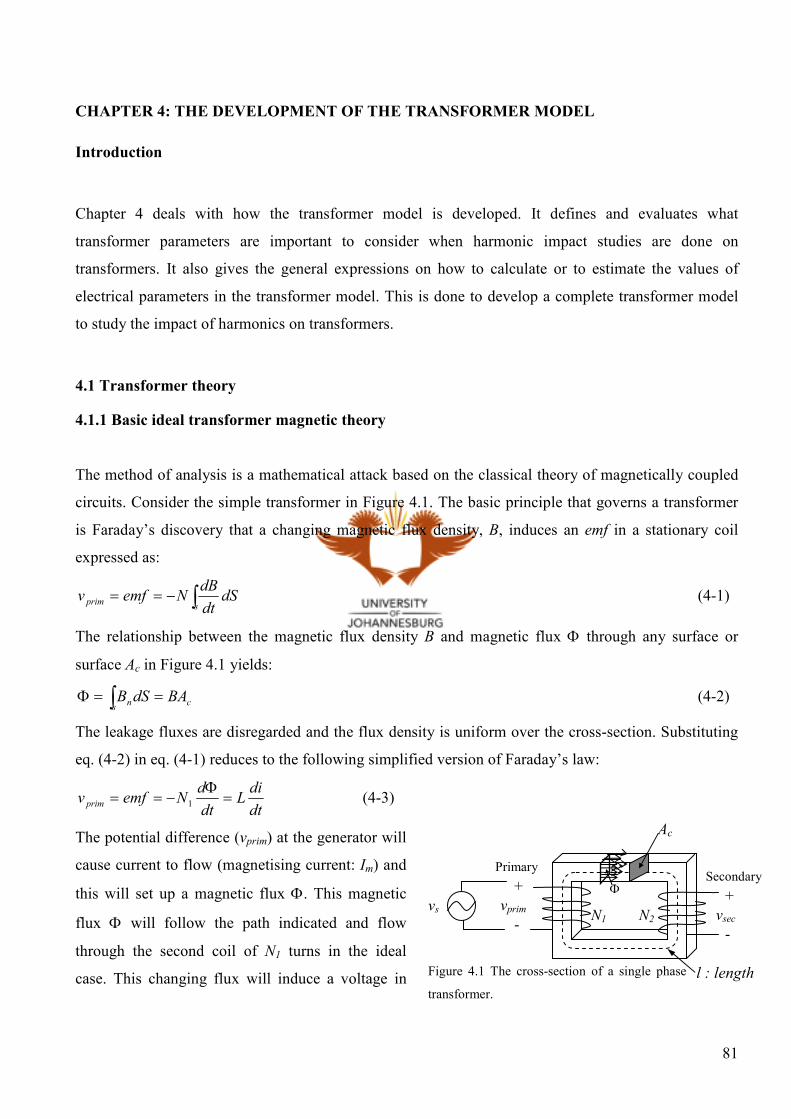
81
CHAPTER 4: THE DEVELOPMENT OF THE TRANSFORMER MODEL
Introduction
Chapter 4 deals with how the transformer model is developed. It defines and evaluates what
transformer parameters are important to consider when harmonic impact studies are done on
transformers. It also gives the general expressions on how to calculate or to estimate the values of
electrical parameters in the transformer model. This is done to develop a complete transformer model
to study the impact of harmonics on transformers.
4.1 Transformer theory
4.1.1 Basic ideal transformer magnetic theory
The method of analysis is a mathematical attack based on the classical theory of magnetically coupled
circuits. Consider the simple transformer in Figure 4.1. The basic principle that governs a transformer
is Faraday’s discovery that a changing magnetic flux density, B, induces an emf in a stationary coil
expressed as:
∫−==sprim dSdt
dBNemfv (4-1)
The relationship between the magnetic flux density B and magnetic flux Φ through any surface or
surface Ac in Figure 4.1 yields:
∫ ==Φs cn BAdSB (4-2)
The leakage fluxes are disregarded and the flux density is uniform over the cross-section. Substituting
eq. (4-2) in eq. (4-1) reduces to the following simplified version of Faraday’s law:
dt
diL
dt
dNemfv prim =
Φ−== 1 (4-3)
The potential difference (vprim) at the generator will
cause current to flow (magnetising current: Im) and
this will set up a magnetic flux Φ. This magnetic
flux Φ will follow the path indicated and flow
through the second coil of N1 turns in the ideal
case. This changing flux will induce a voltage in
vprim vsec
Φ + +
- -
N1 N2 vs
Figure 4.1 The cross-section of a single phase
transformer.
l : length
Ac
Primary Secondary

82
the second coil vsec with a negative polarity (Lenz’s Law) or similarly.
dt
dNv
Φ−= 2sec (4-4)
Now consider a sinusoidal supply voltage vs (vs = vprim= V1 sin wt); then after integration eq. (4-3)
assuming zero remanence flux reduces to:
wtwtwN
Vdt
N
v primcoscos max
1
1
1
Φ−=−=−=Φ ∫ (4-5)
The rms voltage V1,rms is reduced to:
max1
max1
,1 44.42
2Φ=
Φ= fN
fNV rms
π (4-6)
The voltage across the secondary coil, vsec, is calculated by substituting eq. (4-5) in eq. (4-4).
tfNv ωπ sin2 max2sec Φ−= (4-7)
The rms voltage value, V2, for the voltage vsec is:
max2
max2
,244.4
2
2Φ=
Φ−= fN
fNV rms
π (4-8)
Therefore substituting eq. (4-8) into eq. (4-6), the well-known voltage-winding relationship drops out:
1
2
1
2
N
N
V
V−= (4-9)
Suppose the second coil is supplying a load or a resistor is connected between the second coil’s
terminals. The induced voltage v2 will produce a circulating current I2. The current I2 will set up the
magnetomotive force (mmf).
22 INHlHdlmmf ∫ ====ℑ (4-10)
The magneto motive force (mmf) or magnetic field (H) of this current will change but the relationship
between the emf, v1 and the magnetic flux Φ remains unchanged. In the first coil a current I1 has to flow
to the supply to counterbalance to the mmf, assuming a zero magnetising current or zero reluctance or
infinite permeability (c
mC uA
l=ℜ ). The formula that expresses this condition is expressed as:
2211 ININ ==ℑ (4-11)
or similarly the input power (Pin = V1I1) is equal to the output power (Pout = V2I2).
2211 IVIV = (4-12)
In the ideal case of transformers the magnetising current Im is disregarded. Moreover, equations (4-9),
(4-11) and (4-12) can be written as:

83
Turns ratio: 2
1
1
2
1
2
I
I
V
V
N
N== (4-13)
And the impedance ratio is:
2
1
2
1
2
=
N
N
Z
Z (4-14)
The basic theory of power transformers has been reviewed and forms the basis of the development of
the transformer model developed.
4.1.2 Non-ideal transformer equivalent model
The ideal transformer theory was developed in section 4.1 from the classic magnetic theory without
taking into account the effects of winding resistances, magnetic leakage, fluxes and finite exciting
current. A more complete analysis will consider the mentioned effects. In some instances capacitances
of the windings also have important effects. Problems involving transformer behaviour at frequencies
above the audio range, or during rapidly changing transient conditions as those encountered in power
transformers as a result of voltage surges caused by lighting or switching transients, are not considered.
Therefore the capacitance is assumed negligible for the harmonic impact study. The method of analysis
is the equivalent-circuit technique based on physical reasoning. In Figure 4.2 the flux distribution in the
core-type and shell-type transformers is shown to illustrate the differences of typical transformers and
how the leakage and mutual fluxes is set up in the transformers. The three-phase two-winding power
transformers that are larger than 50 MVA are generally the shell type for the reason that the
transformer model analysis is based on a single-phase shell-type transformer. The three-phase two-
Fig 4.2 Schematic view of mutual and leakage fluxes in a transformer.
S S P P
Primary leakage flux Secondary leakage flux
Resultant mutual flux, Φ Primary
windings
Core
a) Core-type transformer
S S P P S S P P
Core Secondary and Primary
leakage flux
b) Shell-type transformer
Front view Side view
Resultant mutual flux, Φ
Primary
windings
Secondary
windings

84
winding transformers are generally modelled in their
single-phase equivalent that is similar to the single-
phase two-winding transformers.
Consider the single-phase shell-type transformer in
Figure 4.3. The total flux linking the primary coil is
the sum of the magnetising flux, Φm, confined to the
iron core, the primary leakage flux, Φl1, which links
only the primary coil, the primary winding flux, Φec,1
that cuts through the secondary winding and the primary other structural parts flux, Φosl,1 that cuts
through the structural part or tank of the transformer. The total flux Φ1 in primary coil is then expressed
as:
1,1,11 oslecml Φ+Φ+Φ+Φ=Φ (4-15)
The total flux, Φ2, in the secondary coil is given as with the aid of Figure 4.3:
2,2,22 oslecml Φ−Φ−Φ−Φ−=Φ (4-16)
where:
Φm is the magnetising flux confined to the iron core;
Φl2 is the secondary leakage flux, which links only the secondary coil;
Φec,2 is the secondary winding flux, which cuts through the secondary winding and;
Φosl,2 is the secondary ‘other structural parts’ flux, which cuts through the structural part or tank of the
transformer.
Suppose the second coil is supplying a load or a resistance is connected between its terminals. The
resultant mutual flux Φm links both the primary and secondary windings and is created by their
combined mmfs expressed as:
NiHdlmmf ===ℑ ∫
miNiNiNmmf 12211 =+==ℑ (4-17)
The secondary current direction is into the transformer for this
winding configuration, and this secondary current has a negative
polarity with reference to the current polarity in Figure 4.4. The
magnetic field H produced by the magnetising current yields:
Figure 4.3 The cross-section of a single phase shell
type transformer.
Φm
v2
Φl1
Φl2
v1 +
-
+
- P S PS
Φec,1
Φec,2 Φosl,2
Φolp,1
Tank
Core
Windings
N1 : N2
i1
e2 +
-
i2
e1 -
+
Fig. 4.4 Transformer voltage
polarities and current direction.

85
miNHl 1=
l
iNH m1= (4-18)
The flux density can then be expressed as:
l
iuNB m1= [ ]uHB = (4-19)
The mmf of primary current component i1 would exactly counteract the mmf of secondary current i1.
The supply voltage induces the resultant mutual flux Φm in the core that brings about the magnetising
current. This flux in the core can be expressed as:
C
m
Cm
iNiNiN
ℜ=
ℜ
+=Φ 12211
Φ=
AB m (4-20)
where c
mC uA
l=ℜ is the reluctance of the core where lm is the magnetic path length, Ac is the core area
and µ is the permeability. In eq. (4-20) the winding eddy current flux and other structural transformer
parts flux contribution to the magnetising flux is not considered in this study.
The magnetising current from equation (4-17) results in:
2
1
21 i
N
Niim += (4-21)
The secondary current direction in Figure 4.4 is in the opposite direction according to the shell-type
transformer configuration shown in Figure 4.3. Then the leakage fluxes are given by:
1
111
ll
iN
ℜ=Φ (4-22)
2
222
ll
iN
ℜ−=Φ (4-23)
where
1,0
11
airl A
l
µ=ℜ and
2,0
22
airl A
l
µ=ℜ are the reluctance paths of the leakage paths in air shown in
Figure 2.2. The leakage flux paths are a non-negligible part of the total coil fluxes in transformers.
These leakage fluxes must be accounted for in any transformer description. The winding fluxes, Φec,
which cut through the windings, and the ‘other structural parts’ flux, Φosl, which cuts through the tank
of the transformer that give rise to series inductance in the transformer is considered negligible under
usual operating conditions. So the total flux Φ1 in the primary coil and total flux Φ2 in the secondary
coil, rewritten in terms of current, turns and reluctance, work out to:

86
C
m
l
ml
iNiN
ℜ+
ℜ=
Φ+Φ=Φ
1
1
11
11
(4-24)
C
m
l
ml
iNiN
ℜ−
ℜ=
Φ−Φ=Φ
1
2
22
22
(4-25)
Also ohmic losses Rdc have to be accounted for in transformer windings caused by the finite resistivity
(ρ) of the conductors with further clarification hereof in section 3.1.1. The winding fluxes, Φec, and the
‘other structural parts’ fluxes, Φosl, in the transformer can result in eddy current losses (sum of winding
eddy current losses and other stray losses), which is considerable under harmonic impact studies which
is noted in ref. [11]. The winding eddy current losses due to the flux that cuts through the winding can
be presented as a potential difference, vec, for the primary and secondary side in series. The other stray
losses that are due to flux that cuts through the other structural parts of the transformer can also be
presented as a potential difference, vosl, for the primary and secondary side in series. Taking into
account ohmic losses, other stray losses, winding eddy current losses and the voltage induced through
the total flux through the coil, the primary voltage, v1, and secondary voltage, v2, at the terminals of the
transformer are given in terms of Ohm’s and Faraday’s law:
dt
dNiviviRv oslecdc
1111,11,11,1 )()(
Φ+++= (4-26)
dt
dNiviviRv oslecdc
2222,22,22,2 )()(
Φ−−−−= (4-27)
The polarity of voltage v1 is set as positive but the current leaves the terminal of primary coil, which is
the reason for the negative polarity for voltage, v2. The voltages v1 and v2 can be expressed in currents
by substitution of eq. (4-24) into eq. (4-26) and eq. (4-25) into eq. (4-27).
dt
diN
dt
diNiviviRv m
Closlecdc ℜ
+ℜ
+++=2
11
1
2
111,11,11,1 )()( (4-28)
dt
diNN
dt
diNiviviRv m
Closlecdc ℜ
+ℜ
−−−−= 212
2
2
222,22,22,2 )()( (4-29)
where 1
2
1
l
N
ℜand
2
2
2
l
N
ℜinductances are equal to the leakage inductances of the primary coil Ll1, and
secondary coil, Ll2, respectively and C
N
ℜ
2
1 inductance is equal to the magnetising inductance Lm. The
voltage v1 in eq. (4-28) can be further reduced to:
11
111,11,11,1
111,11,11,1 )()()()( edt
diLiviviR
dt
diL
dt
diLiviviRv loslecdc
mmloslecdc ++++=++++= (4-30)

87
where dt
diL mm is equal to the induced emf e1 in the primary coil. The voltage v2 in the secondary coil
reduces to:
1
1
22222,22,22,
1
2
2
12222,22,22,2
)()(
)()(
eN
N
dt
diLiviviR
dt
di
N
NN
dt
diLiviviRv
loslecdc
m
closlecdc
+−−−−=
ℜ+−−−−=
(4-31)
where 1
1
2 eN
N is equal to the induced emf e2 in the secondary
coil. Using the voltage equation (4-30) and voltage equation
(4-31) the equivalent transformer circuit can be rendered as in
Figure 4.6. Transformers with cores have a B-H characteristic
with hysteresis such as shown in Figure 4.5. Hence the time-
varying flux Φ in the core will dissipate power in the core. The
core loss resistance, Rc, is shunted with the inductance, Lm,
which is also included in the equivalent transformer model to account for these core losses as well as
the eddy currents in the core. In this model the capacitance is not considered due to the negligible
effects of lower-order harmonics on power transformer capacitances. A more detailed discussion on the
cause and effect of the equivalent circuit components in Figure 4.6 occurs in the following sections.
The transformer model circuit parameters are the series resistor that represents the transformer load
losses of the transformer, the core resistor that represents the no-load losses, the magnetising or mutual
flux that give rise to the magnetising inductance and the leakage flux that give rise to the leakage
inductance. The parameters that constitute the transformer model in Figure 4.6 will now be analysed to
establish accurate expressions of circuit parameters extracted from the literature.
Figure 4.5 The B-H characteristic of
transformer core having hysteresis.
Φ,B
im,H
+
-
vs
Figure 4.6 The equivalent transformer circuit.
Ll2 Rdc,1 Ll1
Lm N1 N2 e1
+
-
e2
+
-
Rc
Rdc,2
v2
+
- im ic
iϕ
i1 i2 i1’=i1 - iϕ
Ideal
transformer
v1
+
-
+ - + - + - + -
v,ec,1 vosl,1 vec,2 vosl,2

88
4.2 Leakage flux or self inductance: Leakage inductance
The leakage flux is part of the flux that cuts through the air as can be seen in Figures 4.2 a) and b). The
leakage inductance is one of the most important parameters in a transformer because it determines its
load voltage regulation and short circuit current. The reactance is controllable and predictable within
certain practical limitations of transformer size, voltage and
winding/core configurations. The leakage inductances of small
and large power transformers are usually well tabulated. The
general form for the total leakage inductance, Ll, referred to the
primary side as in Figure 4.7, is given as:
l
airl l
ANL 0
2
1 µ= (4-32)
where µ0 is the free space permeability
ll the winding length or breadth, bw
Aair the area the leakage flux cuts through
N1 the number of turns of the primary winding
The total leakage inductance, Ll, represents the primary inductance plus the secondary inductance. If
nameplate or test values are not available, the leakage inductance for a transformer winding can be
calculated with the following formula [13] with the aid of Figure 4.7:
∆+
+= − h
hh
b
lNL
w
ml
3104 212
1
4π µH (4-33)
The length lm is the mean length turn (MLT) of the winding and the lengths are in mm. The derivation
for the leakage inductance is available in reference [13]. The leakage inductance determines the
magnitude of the total series inductance of the transformer, which is equal to:
LX L ω= (4-34)
The frequency of the applied currents is directly proportional to the inductive impedance. Thus for a
high harmonic current the impedance increases and limits the magnitude of harmonic current flow
through transformer. The leakage inductance is therefore advantageous to the transformer as it limits
the magnitude of the harmonic currents.
h1 h1
∆h
bw P S
Figure 4.7 The transformer winding
layout for leakage inductance.
Core
Windings
89
4.3 The dc resistance
The total dc resistance of the power transformers is mostly available from the technical specifications
of the supplier under general data. The total dc resistance is the sum of the secondary dc resistance and
primary dc resistance. The standard dc resistance values for large power transformers for different
voltage ratings can also be determined from standard curves available in literature. But if the dc
resistance values of transformers are not available they can be determined by the dimensions and the
conductivity of the winding. The dc resistance can then be calculated by this general expression:
Ω
=A
lR w
dc σ (4-35)
where lw is the total length of the winding or wire, σ the conductivity and AΩ the cross-section of the
wire. At dc and low frequencies, current I is uniformly distributed over cross-section AΩ of the
conductor, which can vary with position. The dc resistances of the secondary and primary windings can
be calculated if the dimensions and the winding material used are available. Usually the resistance or
parameters of the transformer need to be referenced to one side of the transformer for ease of
calculation. The secondary dc resistance to the primary side can be defined as:
2,
2
2
12, dcdc R
N
NR
=′ (4-36)
Furthermore, the primary dc resistance referred to the secondary side of transformer can be calculated
as:
1,
2
1
21, dcdc R
N
NR
=′ (4-37)
The dc resistance represents the conduction losses in the transformer, which are discussed in detail in
Chapter 3.

90
4.4 Mutual flux or magnetising flux: Magnetising inductance
4.4.1 Linear magnetising inductance expression
The magnetising inductance determines the magnitude and the waveform of the transformer exciting
current. The inrush current and saturation effects of the transformer are a direct consequence of the
magnetising inductance. The magnetising inductance is a non-linear parameter and therefore if driven
into saturation the excitation current waveform is nonsinusoidal and high in magnitude. This can be
detrimental to the transformer and for this reason the magnetising inductance is an important parameter
in impact studies of the transformer.
The mathematical derivation for the linear magnetising inductance, Lm, is as follows. The resultant
mutual flux, Φm, links both the primary and secondary windings and is created by their combined
mmfs. The primary current must meet two requirements of the magnetic circuit: it must counteract the
demagnetising effect of the secondary current and produce sufficient mmf to create the resultant mutual
flux, Φm. This effect is described in the following expression:
miNiNiNmmf 12211 =−==ℑ (4-38)
The mmf is then in turn equal to the magnetic field, H, times the magnetic path length, lm, according to
Ampere’s law.
mHlmmf =
µmBl
= [ ]HB µ=
c
mm
A
l
µΦ
= [ ]cm BA=Φ (4-39)
The mutual flux, Фm, as the subject of the equation gives:
C
m
m
mcm
Ni
l
NiA
ℜ==Φ
µ (4-40)
The emf for the mutual flux according to the induction law (Faraday) is equal to:
dt
dNvemf m
m
Φ==
dt
diL
dt
di
l
AN mm
m
m
c ==µ2
(4-41)

91
The linear magnetising inductance can then be extracted from equation (4-41) and expressed as:
m
cm l
ANL
µ2= H (4-42)
where lm is the magnetic path length for the magnetic field, m; µ the permeability, H/m and Ac the
transformer core area, m2. The magnetising inductance, Lm, can also be expressed in term of reluctance,
ℜ which gives a general outcome.
Cm
NL
ℜ=
2
(4-43)
The total core reluctance for an E core type of transformer shown in Figure 4.8a) can be derived from a
magnetic circuit analysis. The core reluctance is then calculated by simple circuit analysis and
simplified core reluctance is expressed as:
( ) ( )( )( ) CCoregap
gapRBCoreRTCoreLBCoreLTCore
gapRBCoreRTCoregapLBCoreLTCoreC −
−−−−
−−−− ℜ+ℜ+ℜ×+ℜ+ℜ+ℜ+ℜ
ℜ+ℜ+ℜ⋅ℜ+ℜ+ℜ=ℜ
2 (4-44)
where the reluctances in the equation are arranged according to Figure 4.8b). The reluctance is related
to the physical parameters of the core and air part through which the flux penetrates. The physical
parameters for reluctance are length, area and permeability of the material the flux flows through. The
general equation for the reluctance is therefore equal to:
A
l
µ=ℜ (4-45)
The magnetising inductance in ferromagnetic core transformers is a non-linear parameter instead of a
linear one due to hysteresis and saturation effects. The linear magnetising inductance therefore does not
simulate the mutual flux accurately for high values of magnetic flux density. A more accurate
gapℜ gapℜ gapℜ
LBCore−ℜ
RTCore−ℜ LTCore−ℜ
CCore−ℜ LBCore−ℜ
excℑ ∝
a) b)
Figure 4.8 a) The E core type physical configuration for a transformer and b) the magnetic circuit
equivalent for the E core transformer.

92
magnetising expression therefore needs to be determined, especially for high flux or voltage impact
studies.
4.4.2 Non-linear magnetising inductance expression
The non-linear magnetising effect can be expressed in a B-H relationship format. An applied magnetic
field to a ferromagnetic core gives rise to hysteresis and saturation effects. A non-linear relationship
between the flux density, B, and magnetic field, H, is formed. Therefore the permeability, µ, of the core
is not constant and is equal to the slope of the hysteresis curve, dHdB . However, the Frolic equation,
[21] can empirically express the non-linear relationship between the flux density, B, and magnetic field,
H.
Hbc
HB
+= (4-46)
The empirical b and c constants are calculated as follows:
0
1
µµ i
c = (4-47)
SAT
i
Bb
µ
11−
= (4-48)
where µi is the initial relative permeability, µ0 free space permeability and BSAT the saturation flux
density. The Frolic equation expresses the magnetising inductance in terms of the relationship between
the flux density, B, and the magnetic field, H. The Frolic equation can be expressed in terms of voltage
and current for simulation purposes. The magnetising voltage expression in terms of current is derived
as follows:
dt
dBNAv cm =
+
×=
m
m
m
c
il
bNc
i
dt
d
l
AN 2
=
m
m
l
NiH
2
2
+
×=
m
m
m
c
il
bNc
dtdi
l
cAN (4-49)

93
where N is turns of the winding, im the magnetising current in A and lm the magnetic path length in m,
Ac the area of the core through which the flux is penetrating in m2. The economic design of the power
transformer requires that transformer core be worked at the curved part of the saturation curve. So it
plays an important role in the impact of faults or abnormal system conditions that could drive the
transformer into saturation. This voltage expression is used to simulate a transformer core that saturates
under voltage conditions higher than the knee-point voltage and will be used in the simulations that
follow. The Frolic equation corresponds to practical measurements reasonable accurately at the
operating point of the power transformer. This will be discussed and proven in Chapter 6. The effect of
voltage harmonics can be detrimental to the transformer due to the B-H curve or the magnetisation
characteristics of the transformer. A higher flux gives rise to a higher voltage, which can drive the
transformer into saturation – and this can lead to transformer breakdown. The impact of harmonic
currents in the load on the magnetisation curve is minor in contrast to the impact of voltage harmonics.
This is true provided that the harmonic currents do not impact the magnitude of the load voltage
applied to the transformer significantly.
4.5 Core resistance expression
The no-load losses in the transformer can be presented by the core resistance. The no-load losses can
be divided generally in core eddy current losses and hysteresis losses but these losses can be expressed
through an empirical power loss expression calculated for different power transformers. The core loss
expression can therefore be represented in the transformer model as a resistor. The core resistance, RC,
can be estimated from this empirical core loss expression as:
mnrms
c
rmsC
Bmkf
V
mP
VR
max
22
== Ω (4-50)
where the variable Vrms is the winding voltage, m is the core mass in kg and Pcore total core losses (in
Watts) per kg. The other parameters are defined in section 3.2.3. The core resistance, RC, is therefore
non-linear due to the non-linear core loss expression. The harmonic voltages applied to the transformer
play a significant role in the operation and impact of transformers, as can be seen by the core resistance
expression. The greater the frequency of applied terminal voltage the smaller the core resistance;
therefore more current will flow through the core resistance. Eventually it will cause the core losses to
increase due to increased current flow and the temperature will also increase if there is no cooling
system in the transformer. The harmonic current impact on the core resistance is therefore not great
according to the core loss expression except if the harmonic currents injected increase the magnitude of

94
the voltage applied to the transformer to a great extent. The core loss expression will then be used to
calculate the core resistance for the transformer model to be simulated. But in transformer harmonic
current impact studies the core resistance can be estimated in terms of rated voltage and rated core loss,
which can be found through the technical data of the power transformer:
Rc
rmsRC P
VR
−
=2
, (4-51)
The core resistance can be placed at the secondary or primary side depending on what reference
voltage is used in the core resistance calculation.
4.6 Winding eddy current loss circuit parameter
In the literature a time domain parameter for the winding eddy current loss in transformers is not
defined; it is described instead in the frequency domain – as shown in section 3.1.2 under Proximity
effect in eq. (3-36). In Chapter 3, section 3.1.2, subsection “The computation of the proximity effect
parameter by electromagnetic theory”, the winding eddy current per unit, iec, is estimated for a
transformer as:
2
1
2
2
2
2
2
2
1)(
ωpR
L
R
L
ecIdt
id
dtiddt
id
pui−
×== (4-52)
The winding eddy current voltage can then be calculated in the general form for transformers as:
RECpRecec RIpuiv −− ×⋅= )( (4-53)
The winding eddy current voltage, vec, for the secondary or primary side referred to is shown in Figure
4.6. The winding eddy current loss resistance, REC, for the primary and secondary side in terms of
winding eddy current loss, PEC, and rated current is expressed as:
2
1,
1,
1,
R
ECREC
I
PR =− (4-54)
2
2,
2,
2,
R
ECREC I
PR =− (4-55)
The primary winding eddy current voltage, vec,1, can then be expressed i.t.o. the winding eddy current
resistance, REC-R,1, at rated fundamental voltage, the rated peak to peak current, IR-pp, of the transformer
and the winding eddy current per unit, iec(pu).

95
1,1,1,1, )( RECpRecec RIpuiv −− ×⋅=
= −
− 2
1,
1,
1,
R
RECREC I
PR (4-56)
2
1
2
2
11,
1,1,
1, )(dt
id
I
RIpuv
pR
RECpRec ×
×=
−
−−
ω (4-57)
2
1
2
1,1, )(dt
idkpuv ecec = (4-58)
The secondary winding eddy current loss, vec,1, can be expressed similarly.
2,2,2,2, )( RECpRecec RIpuiv −− ×⋅=
= −
− 2
2,
2,
2,
R
RECREC I
PR (4-59)
2
2
2
2
12,
2,2,
2, )(dt
id
I
RIpuv
pR
RECpRec ×
×=
−
−−
ω (4-60)
2
2
2
2,2, )(dt
idkpuv ecec = (4-61)
4.7 Other stray loss resistance
The other stray loss will be represented as a resistance in series with dc resistance of the transformer.
The other stray loss resistance, ROSL, can then be estimated in terms of the rated other stray loss, POSL,
and rated primary or secondary current. The other stray loss resistance, ROSL, for the primary and
secondary side can be derived from the other stray loss, POSL, and rated current as such:
2
1,
1,
1,
R
OSLOSL
I
PR = (4-62)
2
2,
2,
2,
R
OSLOSL
I
PR = (4-63)
The other stray loss resistance represents the other stray losses under harmonic currents fairly well, for
it does not increase the other stray losses significantly under harmonic loading, although it is known
that other stray losses increase with frequency to the power 0.8 at low frequencies.

96
4.8 The complete transformer model developed based on theoretical discussions
4.8.1 The complete non-linear transformer model formulated
Figure 4.9 shows the proposed transformer model with the proximity effect loss represented as a
potential difference defined as the second derivative of the load current and the other stray losses
represented as resistor in series with the leakage inductance. The core loss is represented as a non-
linear core resistor and the magnetising shunt branch is represented as a non-linear magnetising
inductance. The primary and secondary leakage inductances and dc resistances values are frequently
given values for power transformers.
The modified transformer parameters are summarised and defined for the circuit in Figure 4.9 as
follows.
The winding eddy current parameters
The voltage for the winding eddy current on the LV side of the transformer as represented in Figure 4.9
is:
LVRECppRecec RIpuiv ,2,2,2, )( −− ×⋅= (4-64)
The winding eddy current, iec, given in eq. (4-52) of section 4.6 is redefined as:
2
12,
2
2
2
22,
2
22
2
2,
1)(
ωpRRec
Idt
id
dtid
dtid
pui−
×== (4-65)
-
v2
i2
1i′
Figure 4.9 The complete transformer equivalent circuit proposed from the theoretical analysis.
+
-
vs
Ll2 R’dc,1
L’l1
Lm 1e
+
-
RC
Rdc,2
+
im ic
iϕ
ϕiii −′= 12
i’ =i - i
1v′
+
2
1
2
1, dt
idkec
′′
2
2
2
2,dt
idkec
R’osl,1 Rosl,2
-
+ - + -

97
The LV winding eddy current voltage, vec,2(pu), can be further reduced by substitution of eq. (4-65)
into eq. (4-64).
2
2
2
2
12,
,2,
2, )(dt
id
I
RIpuv
pR
LVRECpRec ×
×=
−
−−
ω (4-66)
2
2
2
2,2, )(dt
idkpuv ecec = (4-67)
The HV voltage for the winding eddy current referred to the LV side of the transformer as represented
in Figure 4.9 is:
HVRECpRecec RIpuiv ,1,1,1, '')('' −− ×⋅= (4-68)
The winding eddy current, iec, given in eq. (4-52) of section 4.6 is:
2
11,
2
1
2
2
2
21
2
1,'
1'
'
'
)('ωpRR
ecIdt
id
dtid
dtid
pui−
×== (4-69)
The HV winding eddy current voltage, v’ec,1(pu), can be further reduced by substitution of eq. (4-69)
into eq. (4-68).
2
1
2
2
11,
,1,
1,
'
'
'')('
dt
id
I
RIpuv
pR
LVRECpRec ×
×=
−
−−
ω (4-70)
2
1
2
1,1,
'')('
dt
idkpuv ecec = (4-71)
The other stray loss resistance
The other stray loss resistance, ROSL, for the primary and secondary side in terms of other stray loss,
POSL-O, at measured fundamental current or rated current can be derived from the other stray loss, POSL,
and rated current as such:
2
1,
1,
1,
R
OSLOSL
I
PR
′=′ (4-72)
2
2,
2,
2,
R
OSLOSL
I
PR = (4-73)

98
The non-linear magnetising inductance
The non-linear magnetising inductance, Lm, as seen in Figure 4.9 can be represented as a magnetising
voltage, vm, in terms of the magnetising current, im, derived from the Frolic equation (discussed in
section 4.4.2).
2
2
+
×=
m
m
m
il
bNc
dtdi
l
AcNv (4-74)
The core resistance
Finally, the non-linear core resistance, RC, is defined according to equation (4-50) in section 4.5 as:
mnrms
c
rmsC
Bmkf
V
mP
VR
max
22
== or (4-75)
If the empirical constants and mass of the power transformer are not available the core resistance can
be reduced to:
Rc
rmsRC P
VR
−
=2
, (4-76)

99
Conclusion
The chapter concludes with a complete transformer model that can be used for harmonic impact studies
on power transformers in particular. This model includes all generic parameters such as the leakage
inductances and dc resistances. It also includes the non-linear parameters that model the non-linear
magnetising characteristics, the core resistance expression for the core loss, the proximity effect
parameter and the other stray loss effect of the transformer. The methods developed used to calculate
the stray loss resistances and winding eddy current loss parameters for single-phase two-winding power
transformers can also be used for three-phase two-winding power transformers. So this transformer
model can be used to represent three-phase power transformers modelled in the single-phase equivalent
transformer model.
100
CHAPTER 5: EVALUATE THE TRANSFORMER MODEL UNDER HARMONIC LOADING
CONDITIONS
Introduction
This chapter deals with how harmonic currents can impact the transformer destructively. Firstly a two-
winding shell-type power transformer (1kVA) loaded with harmonic currents is evaluated with the
recommended capability calculations discussed in Chapter 3 and extracted in ref. [11]. The parameters
that are required to do the recommended capability calculations are first extracted and calculated. The
results for the recommended transformer capability calculations are then tabulated and the outcomes
are discussed. Lastly the transformer model developed in Chapter 4 is simulated using the Intusoft
SPICE simulation program. The transformer parameters used to simulate the transformer model are
calculated and extracted. The functionality on how the simulation program Intusoft SPICE is used is
briefly discussed to give the reader an insight into the software package. Finally, the Intusoft SPICE
simulation program models the 1kVA power transformer supplying a single-phase load with the same
harmonic distribution of a typical three-phase static 12 pulse power converter load. The results of the
recommended capability calculations and the transformer model simulated are compared and
conclusions are drawn.
5.1 The simulation program Intusoft SPICE used to simulate the non-linear transformer model
The Intusoft SPICE is circuit analysis program similar to PSPICE but can simulate in addition most
types of functions or non-linear circuit parameters. The Intusoft SPICE program has four program
environments: the Text Editor, Launch IsSpice, Launch Scope and Launch Spicenet. The Text Editor
and the Launch Spicenet can be used to simulate a circuit.
In the Text Editor all the parameters need to be typed in, and this can be very time-consuming.
However, it is much more flexible than the Launch Spicenet. In the Launch Spicenet program a circuit
model can be created with blocks or equivalent circuit parameters which are much more interactive. In
the study the Launch Spicenet was used to model a non-linear transformer model given in Figure 4.9.
The Launch Scope and Launch IsSpice programs are used to analyse the circuit voltages, currents etc.
after the Launch Spicenet or Text Editor runs a simulation or compiles a simulation. In this study the
101
transient simulation was run to analyse the time domain non-linear transformer model under harmonic
loading conditions. The Intusoft SPICE simulation program successfully simulated the non-linear
transformer model with very complicated non-linear circuit parameters.
The programming text or simulated circuits for the Text Editor and Launch Spicenet programs, and the
simulation output results of the Launch Scope and Launch IsSpice graph simulators, for the transformer
under harmonic loading are given in Appendix B, Appendix C and Appendix D.
5.2 The general transformer data derived for recommended capability calculations
The general data for the 1kVA transformer used is summarised in this section. The 1kVA transformer
data is used due to the availability of the required transformer data. Therefore the transformer can be
analysed with reasonable accuracy. There is not much difference between how a three-phase
transformer and single-phase two-winding transformer are analysed. The three-phase two-winding
transformer is usually analysed in single phase for ease of calculation. The electrical circuit parameters
that constitute a 1kVA power transformer are the same for large three-phase power transformers larger
than 1 kVA. So the transformer theoretical analysis expanded upon in Chapter 4 for small power
transformers and large power transformers remains the same. High voltage power transformers use oil
for insulation purposes but for lower voltage levels air is the cheaper solution. So for the evaluation of
the considered range of harmonic frequencies, the insulation of the transformer which represents the
capacitance in the transformer model is disregarded and is assumed negligible under these harmonic
conditions.
The power transformer used is the shell type, air insulated (dry type); it consists of two windings and is
single phase (its physical dimensions and physical layout are given in Appendix A). The transformer
data for the dry-type single-phase transformer and the mathematical analysis based on the capability
calculations discussed in Chapter 3 are given below. [19]
-High-voltage winding (HV)
480V, N1= 480 turns
HV Leakage inductance, Ll,1 = 8.5mH
HV Copper Resistance, Rdc,1 Ω= 263.4
-Low-voltage winding (LV)
240V, N2=255 turns
LV Leakage inductance, Ll,2 = 1.1mH

102
LV Copper Resistance, Rdc,2 Ω= 8942.0
-Rated capacity
1 kVA, single-phase
-Total losses: PTL = 76.7 W for a full resistive load at VLV-R = 240V rms Volts.
PTL = 74.3 W for a full capacitive load at VLV-R = 240V rms Volts.
- No-load losses: 29.27=−RNLP W at rated voltage, VLV-R = 240 V rms;
34=NLP W at voltage, VLV-R = 266.86 V rms.
-Values for I1-R and I2-R
I1-R = 1.0833 A,
I2-R = 4.167 A,
-Values for the HV and LV leakage voltages, Vl,1 and Vl,2
676.62044.30833.21,11, =×=×= − lRl XIV V, 77.390478.0167.41, =×=′lV V
728.14147.0167.42,22, =×=×= − lRl XIV V.
The total load loss, PLL-R, is calculated to derive the total stray loss.
NLTLmeasLL PPP −=,
The no-load losses at VLV-R = 266.86 V rms are used because of the measurement data available. The
measured and rated load losses are given as:
347.76, −=measLLP and 29.277.76, −=− measRLLP
9.42, =measLLP W and 41.49, =− measRLLP W
-The total stray loss, PTSL, can be calculated as follows:
( ) ( )2,2
,21,
2
,1, dcRdcRmeasLLTSL RIRIPP ×+′×′−=
( )[ ] ( )[ ] 42.369.428942.0167.4203.1167.49.4222 −=×+×−=TSLP
The measured and rated total stray losses are given as:
42.369.42 −=TSLP and 42.3641.49 −=−RTSLP
5.648.6 ≈=TSLP W and 13=−RTSLP W
-The winding eddy current loss is then calculated by assumption 2) in 6.2 of ref. [11]. The measured
and rated total winding eddy current losses are given as:
36.45.667.0 =×=ECP W and 71.81367.0, =×=RECP W
The division of eddy current loss between the windings for transformers having a maximum self-
cooled current rating of less than 1000 A (regardless of turns ratio) are 60% in the inner winding and
40% in the outer winding [11]. The measured and rated low voltage winding eddy current losses are:
103
744.136.44.0, =×=LVECP W (outer winding) and 484.371.84.0, =×=− LVRECP W (outer winding)
616.236.46.0, =×=HVECP W (inner winding) and 226.571.86.0, =×=− HVRECP W (inner winding)
-The other stray loss, POSL, is then the remainder of the total stray loss.
ECTSLOSL PPP −=
The measured and rated other stray losses are given as:
14.236.45.6 ≈−=OSLP W and 29.471.813 ≈−=−ROSLP W
The percentage division between the inner winding and outer winding is assumed to be the same as the
winding eddy current loss divisions.
The temperature rise, ∆T, for the transformer at full load is 62 ºC measured. The temperature had been
measured using thermocouples in the transformer. The temperature measured is Ts = 85.3 ºC at a full
resistive load, with an ambient temperature of Ta = 23.3 ºC and a LV voltage of VLV, p-p = 377.4 V. The
load resistance, RL, is 65Ω.
5.3 Recommended capability calculations [11] and results for the 1kVA transformer
The harmonic distribution for a typical three-phase static 12-pulse power converter is given in Table
5.1. The rms harmonic load current, the harmonic multipliers for the eddy current loss and other stray
loss are calculated using this. This harmonic distribution is very common, as shown in Chapter 1, as the
power transformer has been subjected to similar harmonics components. The IEEE 519 standard used
this harmonic current distribution for its application examples, which is usually very common at
transmission voltage levels. Harmonic current sources are put in parallel with the load to model the
harmonic loading for harmonic distribution given in Table 5.1. The maximum permissible
nonsinusoidal load current is calculated using two methods as explained in the following paragraphs.
In the subsection “The maximum permissible nonsinusoidal load current using rated winding eddy
current loss”, the ‘total power loss’ per unit is calculated using the ‘rated winding eddy current loss’
and the ‘eddy current harmonic multiplier’ determined from the harmonic distribution in Table 5.1. The
maximum permissible load current is then calculated from the rated winding eddy current loss and
harmonic multiplier for given harmonic distribution.
In the subsection “The maximum permissible nonsinusoidal load current using maximum winding eddy
current loss”, the maximum winding eddy current loss is estimated according to the recommended

104
practice calculations. The total power losses per unit and the maximum permissible load current are
then calculated using the maximum winding eddy current losses and the eddy current harmonic
multiplier.
Finally, the breakdown in losses for the given transformer and harmonic distribution is calculated and
tabulated for the rated transformer losses and corrected losses under given harmonic load conditions.
Harmonic
order
H 1I
I h 2
1
I
I h
h2 2
2
1
hI
I h
h0.8 8.0
2
1
hI
I h
1 1.000 1.000 1 1.000 1.000 1.000
5 0.192 0.037 25 0.922 3.624 0.134
7 0.132 0.017 49 0.854 4.743 0.083
11 0.073 0.005 121 0.645 6.809 0.036
13 0.057 0.003 169 0.549 7.783 0.025
∑ 1.063 3.9693
1.278
Table 5.1 Harmonic Distribution for a transformer load current supplying a typical three phase static
12 pulse power converter [10].

105
The maximum permissible nonsinusoidal load current using rated winding eddy current loss
The calculation of normal local loss density, PL,, given in eq. (3-105) in section 3.4 for the
nonsinusoidal current is calculated as:
0116.2)239.0734.31(063.1)( =×+×=puPLL pu
The other stray losses can be disregarded for dry-type transformers. Thus, the rms value of the
maximum permissible nonsinusoidal load current with the given harmonic composition and for normal
local loss density, from equation (3-108) in section 3.4.1, is
85.0239.0734.31
357.1)(max =
×+=puI pu
or
417.3167.485.0max =×=I A
where the rated local loss density is:
357.1)()(1 =++= −−− puPpuPP ROSLRECRLL pu
In this case, the transformer capability with the given nonsinusoidal load current harmonic composition
and maximum local loss density is approximately 85% of its sinusoidal load current capability.

106
The maximum permissible nonsinusoidal load current using maximum winding eddy-current
loss
The maximum eddy-current loss density is determined according to eq. 16 or 17 in Std. IEEE C57.110-
1998, which is:
2
2
2
8.2)(
RIK
PpuP
R
RECMaxEC ××
×=
−
−− pu (5-1)
K = 1 for single-phase transformers
= 1.5 for three-phase transformers
The maximum winding eddy current loss is:
5704.153.151
71.88.2)( =
××
=− puP MaxEC pu
The maximum local loss density, PLL-R (pu), from equation (5-1) where PEC-R (pu) is 1.5704 pu can also
be produced by the nonsinusoidal load current in the region of the highest eddy-current loss is:
298.7)5707.1734.31(063.1)( =×+×=puP LL pu
Thus, the rms value of the maximum permissible nonsinusoidal load current with the given harmonic
composition and maximum local loss density, from equation (3-108) in section 3.4.1, is
612.05707.1734.31
5704.2)(max =
×+=puI pu
or
55.2167.4612.0max =×=I A
In this case, the transformer capability with the given nonsinusoidal load current harmonic composition
and maximum local loss density is approximately 60% of its sinusoidal load current capability.
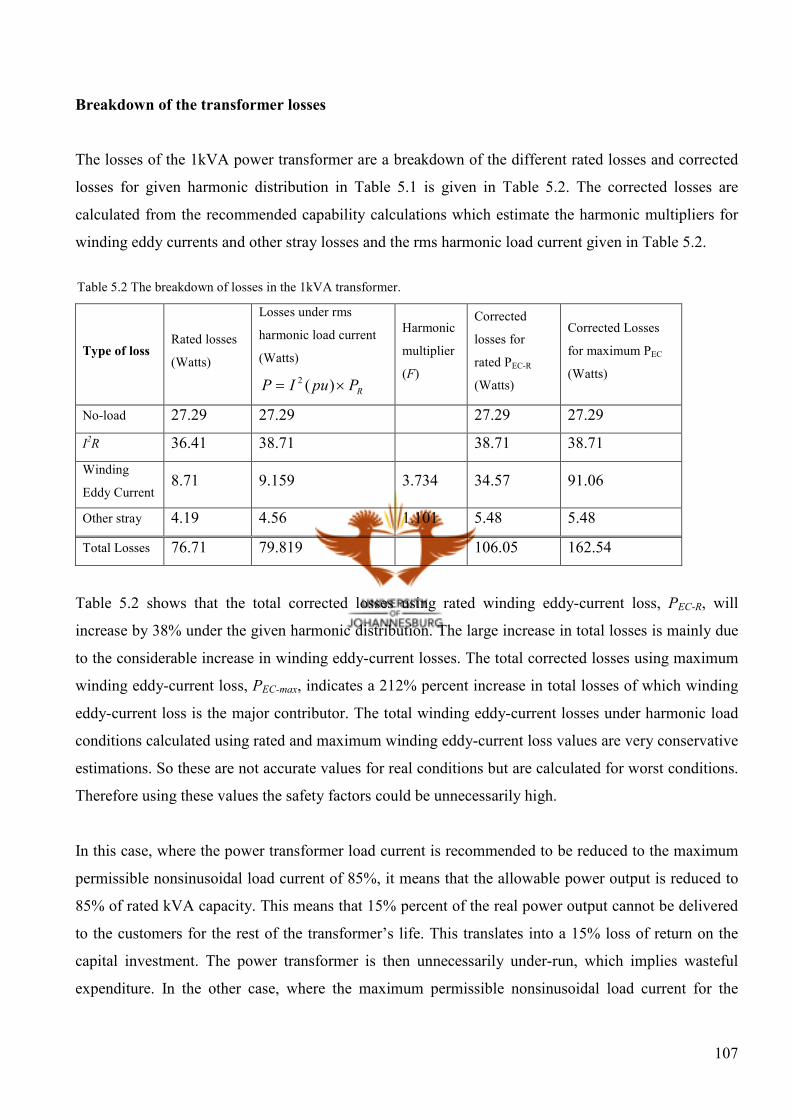
107
Breakdown of the transformer losses
The losses of the 1kVA power transformer are a breakdown of the different rated losses and corrected
losses for given harmonic distribution in Table 5.1 is given in Table 5.2. The corrected losses are
calculated from the recommended capability calculations which estimate the harmonic multipliers for
winding eddy currents and other stray losses and the rms harmonic load current given in Table 5.2.
Type of loss Rated losses
(Watts)
Losses under rms
harmonic load current
(Watts)
RPpuIP ×= )(2
Harmonic
multiplier
(F)
Corrected
losses for
rated PEC-R
(Watts)
Corrected Losses
for maximum PEC
(Watts)
No-load 27.29 27.29 27.29 27.29
I2R 36.41 38.71 38.71 38.71
Winding
Eddy Current 8.71 9.159 3.734 34.57 91.06
Other stray 4.19 4.56 1.101 5.48 5.48
Total Losses 76.71 79.819 106.05 162.54
Table 5.2 shows that the total corrected losses using rated winding eddy-current loss, PEC-R, will
increase by 38% under the given harmonic distribution. The large increase in total losses is mainly due
to the considerable increase in winding eddy-current losses. The total corrected losses using maximum
winding eddy-current loss, PEC-max, indicates a 212% percent increase in total losses of which winding
eddy-current loss is the major contributor. The total winding eddy-current losses under harmonic load
conditions calculated using rated and maximum winding eddy-current loss values are very conservative
estimations. So these are not accurate values for real conditions but are calculated for worst conditions.
Therefore using these values the safety factors could be unnecessarily high.
In this case, where the power transformer load current is recommended to be reduced to the maximum
permissible nonsinusoidal load current of 85%, it means that the allowable power output is reduced to
85% of rated kVA capacity. This means that 15% percent of the real power output cannot be delivered
to the customers for the rest of the transformer’s life. This translates into a 15% loss of return on the
capital investment. The power transformer is then unnecessarily under-run, which implies wasteful
expenditure. In the other case, where the maximum permissible nonsinusoidal load current for the
Table 5.2 The breakdown of losses in the 1kVA transformer.

108
maximum winding eddy-current loss is calculated to be 60% of the rated load current, this translates
into a 40% loss of power capacity. This leads to a 40% loss of income on the asset in use, which is
definitely unacceptable. So whether these recommended capability calculations are implemented or
not, the results show that harmonic load currents can be detrimental to the power transformer and the
permissible values estimated can be too conservative. So better calculations or estimations are required
to calculate the winding eddy-current losses in power transformers. The recommended capability
calculation for the winding eddy-current loss is too conservative and is a major contributor in power
losses under harmonic loading conditions.
109
5.4 The transformer data calculated for transformer model for SPICE simulation
In section 5.2 the general transformer data was given and used for the transformer recommended
capability calculations of ref. [11]. In this section the parameters required to simulate the transformer
model developed are given and calculated. The parameters for the 1kVA transformer are calculated for
the proposed transformer model and given as follows:
The leakage inductance, Ll, for the HV and LV side of the transformer is given as:
HV Leakage inductance referred to the LV side, 4.2'
1, =lL mH
LV Leakage inductance, Ll,2 = 1.1 mH
The dc resistance, Rdc for the HV and LV side of the transformer is given as:
HV Copper Resistance referred to the LV side, Ω= 203.1'
1,dcR
LV Copper Resistance, Rdc,2 Ω= 8942.0
At a load resistance of 59 Ω the transformer’s a rated power output of approximately 1000 Watts is
reached. The load resistance at full load is calculated as 59 Ω used in this simulation at the low voltage
side.
The winding eddy-current resistance, REC, which can be derived from the winding eddy-current loss
and rated current at measured applied fundamental voltage or at rated voltage, is:
1.0)167.4(
744.122
,
,
, ===−LVR
LVECLVOEC
I
PR Ω or
( )2.0
167.4
484.322
,
,
, ===−HVR
LVECLVREC
I
PR Ω
( )15.0
167.4
616.222'
,
,
,0 ===′ −HVR
HVECHVEC
I
PR Ω or
( )3.0
167.4
226.522'
,
,
, ===′ −HVR
HVECHVREC
I
PR Ω
According to the winding eddy-current exposition in Chapter 4, the winding eddy-current per unit, iec,
is:
2
26
2
1
2
2
10194.11
)(dt
id
Idt
idpui
pR
ec ××=×= −
− ω
The time-varying winding eddy current per unit is then used to approximate the induced winding eddy-
current voltage on the winding for the HV and LV side,
LVRECpRecLVec RIpuiv ,1,2,, )( −− ×⋅=
2
2
26
2,2,2, 10407.1)(1785.12.0893.5)(dt
idpuipuiv ececec
′×=×=×⋅= −

110
And the winding eddy-current HV voltage referred to the LV side is
HVRECpRecHVec RIpuiv ,1,1,, )( −− ′×′⋅′=′
2
1
26
1,1,1, 1011.2)('76777.13.0893.5)('dt
idpuipuiv ececec
−×=×=×⋅=′
The other stray loss resistance, ROSL, can be derived from the other stray losses and rated current at
measured applied fundamental voltage and at rated voltage.
( )0493.0
167.4
856.022
,
,
, ===LVR
LVOSLLVOSL
I
PR Ω and
( )0988.0
167.4
716.122
,
,
, === −−
LVR
LVROSLLVROSL
I
PR Ω
( )0739.0
167.4
284.122'
,
,
, ===HVR
HVOSLHVOSL I
PR Ω and
( )148.0
167.4
574.222'
,
,
, === −−
HVR
HVROSLHVROSL
I
PR Ω
The core resistance, RC, can therefore be calculated using the core loss expression for different flux
densities with reasonable accuracy. The rated core resistance, RC-R, can then be calculated for the rated
ac voltage as:
( )66.2110
29.27
24022
===−
−
Rc
RrmsC P
VR Ω
The core resistance calculated here is an important parameter as it influences directly the magnitude of
the winding eddy-current losses in the circuit. It shows that for a core resistance of 2110.66 Ω the total
winding eddy-current losses amount to 14.3 W.
According to the loss density curve in Figure 6.1 and Table 6.1, there is approximately a 5% error for
the core loss calculated value at a flux density, Bmax, of 1.48 Teslas at rated voltage. In this case the
coefficients of the core material used were not known and a curve fitting was done on the measured
core loss curve. Accurate core resistances can be calculated for accurate core loss values with the
coefficients for the different core materials that are referenced in the Magnetic Core Selection for
Transformers and Inductors, 13th Edition and other transformer handbook resources. This 5% error
gives rise to a lower calculated core resistance, RC, which can be corrected by this 5% approximate
error as:
19.221666.211005.1)( =×=correctedRC Ω
The core resistance is corrected to 2216.19 Ω, which results in a total winding eddy-current loss 17.29
W which shows an 18% increase compared to the core resistance calculated in eq. (5-11). It therefore
shows that the core resistance has a direct impact on the magnitude of the winding eddy-current losses.
For this reason the corrected core resistance value was used to give a more accurate result for winding

111
eddy-current losses so that a more accurate evaluation can be done on the transformer under
investigation.
The linear magnetising inductance, Lm, can be calculated as given in section 4.4.1 if the physical
dimensions of the transformer core and the transformer core’s permeability are available. The linear
magnetising inductance can be calculated in terms of the applied magnetising voltage and magnetising
current or excitation current. A good estimation for the E core-type transformer is given as:
51.1596.0602
2402
2
2
,
,1max, =××
×===
ππω pexc
rms
m
mm fI
V
I
VL H [ mexc II ≈ , IC is negligible compared Iexc]
where Iexc is the excitation current, Im is the magnetising current and IC is the core resistance current.
The excitation current, Iexc, at rated voltage is acquired from Table 6.2 in Chapter 6. The linear
magnetising inductance in this case is used to verify the linear part of the non-linear magnetising
expression that is translated in the following paragraph and used to verify that the linear part of the
non-linear magnetising curve is correct.
In this transformer model the non-linear magnetising inductance, Lm, is represented as the magnetising
voltage, vm, across the core resistance according to Frolic’s formula in section 4.5.1.
( )22
2
32.554682.113
406.76709
m
m
m
m
mi
i
il
bNc
dtdi
l
AcNv
+
′×=
+
×=
These calculated transformer parameters are then substituted into the transformer model of Figure 5.1.
This transformer model is then simulated and the load power losses for the dc resistance, winding
eddy-current losses and other stray losses are determined through simulations.
-
Iload
I5 I7 I11 I13 v2
i2
1i′
Figure 5.1 The complete transformer equivalent circuit with harmonic loading.
+
-
vs
Ll2 R’dc,1
L’l1
Lm 1e
+
-
RC
Rdc,2
+
im ic
iϕ
ϕiii −′= 12
i’ =i - i
1v′
+
2
1
2
1, dt
idkec
′′
2
2
2
2,dt
idkec
R’osl,1 Rosl,2
-
+ - + -
LV

112
5.5 Transformer model results compared to the recommended capability calculations
The local loss density of the transformer is important to calculate as it determines the transformer
capability as in section 5.3. The permissible load current is then formulated from the local loss density
calculations.
The rated local loss density is:
357.1)()(1 =++= −−− puPpuPP ROSLRECRLL pu
The load power losses due to load harmonics, PLL-HL, for maximum winding eddy-current loss
estimation determined by the transformer model simulation yields:
41.634767.4948.20982.37 =++=++= Ω− OSLECHLLL PPPP W
Now the per unit load losses or normal local loss density due to harmonics, PLL, are calculated to
determine the new maximum permissible load current for these simulated load losses.
ECsimHLLL
LL KpuIP
PpuP )(742.1
41.36
41.63)( 2, ====
Ω
−
639.1063.1
742.1==ECK
Thus, the rms value of the maximum permissible nonsinusoidal load current with the given harmonic
composition and for normal local loss density, from equation (3-108) in section 3.5.1, is:
91.0639.1
357.1)()(max === − pu
K
puPpuI
EC
RLL pu
or
79.3167.491.0max =×=I A
In this case, the transformer capability with the given nonsinusoidal load current harmonic composition
and maximum local loss density is approximately 91% of its sinusoidal load current capability
according to the proposed transformer model results. This transformer model approximation is 6%
better than the maximum permissible load current of 85% of the IEEE recommended practice. This
shows a 6% saving of power delivered that can be supplied to customers.

113
Breakdown of transformer losses compared
The total transformer losses according to the transformer model simulations in Figure 5.1 are tabulated
in Table 5.3.
a: Harmonic current peaks fall negative to the fundamental peak current (IL,rms= 4.1709). b: Harmonic current peaks fall together with the fundamental peak current (IL,rms= 4.177).
The measured results in Table 5.3 for the rated losses compare reasonably well with the transformer
model results that are simulated. This indicates that the proposed simulation transformer model is a
fairly accurate model to simulate transformers for impact studies – except for impact studies where the
winding and inter-turn capacitances will play a significant role.
The harmonic impact on the transformer losses are tabulated in Table 5.3 for a transformer feeding a
resistive load with a harmonic distribution of a typical three-phase static 12-pulse power converter
tabulated in Table 5.1. The simulated programming results and circuit in Intusoft SPICE for the
transformer equivalent model under full load and harmonic loaded conditions are in Appendix B and
under rated full loading conditions in Appendix D. The difference between the average of the
instantaneous input power (PIN) and average of the instantaneous output power (POUTT) shown in Figure
5.2 was calculated to determine the total transformer losses tabulated in Table 5.3. The measured rated
loss values and rated IEEE capability calculations are used as a reference to the percentage values of
the transformer model simulated results.
PLOSS-R PLOSS-HL
Harmonic loading
Simulated-Watts Type of loss
(PLOSS) Measured
Watts
IEEE
Capability Calc.
Watts
PLOSS-R
Simulated
Watts Out of
phasea In phase
b
PLOSS-HL
Harmonic loading
IEEE Capability Calc.
Watts
No-load 27.29 27.708 27.508 27.482 27.29
I2R 36.41 36.86 37.92 37.917 38.71
Winding Eddy 8.71 7.95 20.948 20.074 34.57
Other stray 4.19 4.346 4.4688 4.469 5.48
Total Losses 76.71 76.86 90.84 89.942 106.05
Table 5.3 The rated losses and harmonic losses of the proposed transformer model compared to
the measured losses at rated supply and the IEEE recommended capability calculations, [11].

114
The transformer model results compared to the rated values show a 4% increase in the conduction
losses, PΩ-HL, and a 7% increase in other stray losses, POSL-HL. In contrast, the harmonic impact results
for the IEEE capability calculations show a 6% increase for the conduction losses, PΩ-HL, to the
measured rated conduction losses and a 31% increase for the other stray losses compared to the rated
measured losses.
The rated winding eddy-current loss, PEC-R, of the transformer is 10% lower than the calculated
estimate according to the recommended practices under rated conditions [11]. The transformer model’s
winding eddy-current losses, PLOSS-HL, estimated under the specified harmonic distribution, are 163%
more than the rated winding eddy-current losses, PEC-R, irrespective of the phase shifts of harmonic
currents with respect to the fundamental current. The winding eddy-current loss, PEC-HL, according to
the IEEE capability calculations under the harmonic load, is nearly 200% more than the rated winding
eddy-current loss, PEC-R value. And according to the recommended practice the calculation is very
conservative and not reasonably accurate.
The peak value of the nonsinusoidal load current exceeds 20% of the rated peak load current, as shown
in Figure 5.3. The rms nonsinusoidal load current, IL, shows a 2% increase in the fundamental rms load
Figure 5.2 The power graphs for the input power and output power for the transformer under
harmonic loading for maximum total transformer losses where all the peaks of the harmonic
currents are negative reference to the fundamental current.
12
288.0M 298.0M 308.0M 318.0M 328.0M
WFM.2 PIN vs. TIME in Secs
2.120K
1.560K
1.000K
440.0
-120.0
PIN in Volts
2.120K
1.560K
1.000K
440.0
-120.0
POUTT in Volts
POUTT
……. PIN
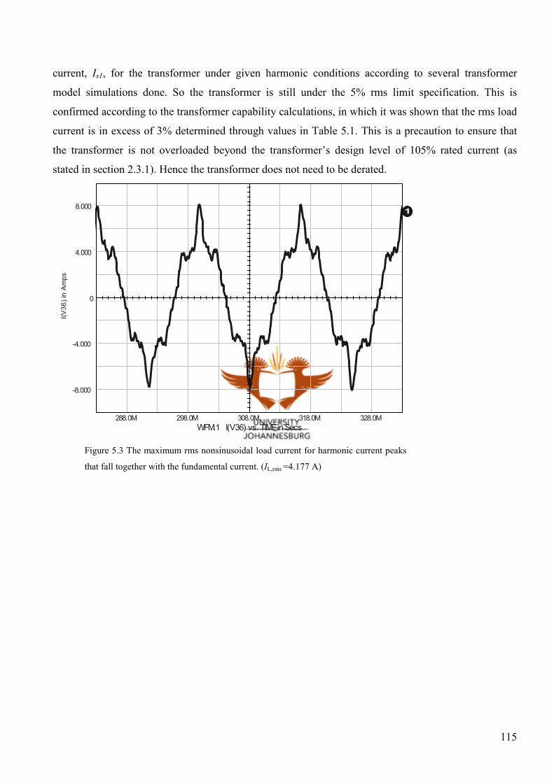
115
current, Is1, for the transformer under given harmonic conditions according to several transformer
model simulations done. So the transformer is still under the 5% rms limit specification. This is
confirmed according to the transformer capability calculations, in which it was shown that the rms load
current is in excess of 3% determined through values in Table 5.1. This is a precaution to ensure that
the transformer is not overloaded beyond the transformer’s design level of 105% rated current (as
stated in section 2.3.1). Hence the transformer does not need to be derated.
1
288.0M 298.0M 308.0M 318.0M 328.0M
WFM.1 I(V36) vs. TIME in Secs
8.000
4.000
0
-4.000
-8.000
I(V36) in Amps
Figure 5.3 The maximum rms nonsinusoidal load current for harmonic current peaks
that fall together with the fundamental current. (IL,rms =4.177 A)
116
5.6 Analysis of the transformer model results compared to the NRS and IEEE standards
The first objective is to determine the total harmonic distortion (THD) for the voltage and current for
the case study. The Fourier calculation of the Intusoft SPICE was used to determine per unit harmonic
current components of the secondary voltage with the fundamental voltage as base. This harmonic per
unit components of the secondary voltage is used to calculate the voltage THDv and to determine if
voltage harmonic components are below the maximum allowable harmonic voltages. The same process
was followed to determine the harmonic current component per unit levels in the nonsinusoidal load
current to calculate the THDi. This harmonic current per unit components is also used to determine if
the harmonic current levels are below maximum allowable harmonic current levels according to the
NRS and IEEE standards.
∑≠
×=
1
2
1
100%h s
sh
V
Vv
THD
1
)()()()(100
2
13
2
11
2
7
2
5 puVpuVpuVpuV +++×=
( ) ( )2.5
1
)022.0()023.0(029.003.01
2222
=+++
=∑≠h %
The actual voltage THDv is lower than the NRS standards-recommended compatibility levels of 8% for
LV voltage levels. Furthermore, the actual voltage THDv is equal to the maximum allowable voltage
THDv for IEEE 519 standard of 5%. This shows that the actual voltage THDv would not alert utilities to
the dangers thereof because it is still within allowable limits. The voltage THDv does not give a good
indication of the harmonic current levels through the power transformer.
∑≠
×=
1
2
1
100%h s
shi
I
ITHD
1
)()()()(100
2
13
2
11
2
7
2
5 puIpuIpuIpuI +++×=
( ) ( )6.20
1
)0479.0()058.0(1033.0162.01
2222
=+++
=∑≠h %
The actual current THDi is a little bit higher than the recommended TDD levels, which range from 5%
to a maximum of 20% depending on the short circuit to load demand ratio according to IEEE 519-
1992. The per unit harmonic current levels used to calculate the THDi and for Table 5.4 are determined

117
from the nonsinusoidal load current waveform in the simulation of the transformer model. So the
current THDi needs to be minimised accordingly.
The individual harmonic magnitudes of the secondary voltage and nonsinusoidal load current will be
compared to the NRS and IEEE standards individual harmonic levels. This is to ensure that individual
harmonic levels do not exceed the allowable levels according to the NRS and IEEE standards.
Table 5.4 Comparison between the actual individual harmonic voltage and current distortion levels, and
the NRS and IEEE standards recommended levels.
The individual harmonic voltage distortion in % The individual harmonic current
distortion in %
Harmonic
order
h
Actual harmonic
(%
1s
sh
V
V)
NRS Standards
(%
1s
sh
V
V)
Max. Individual
Harmonic Voltage
Distortion
(%
1s
sh
V
V)
Actual
harmonic
(%
1s
sh
I
I)
Max. Individual Harmonic
Current Distortion (IEEE 519)
(%
1s
sh
I
I)
5 3 6 3 16.2 4 -15
7 2.9 5 3 10.33 4 -15
11 2.3 3.5 3 5.8 2 - 7
13 2.2 3 3 4.79 2 - 7
The individual harmonic voltage distortion levels for the transformer at its load are still within
acceptable limits compared to the NRS and IEEE standards-recommended levels seen in Table 5.4. The
actual individual harmonic current distortion level for the transformer load current for the 5th harmonic
is out of the recommended level specification for all short circuit current ratios. But for 7th, 11
th and
13th the harmonic distortion is within acceptable levels for high short circuit ratios in the range of 100
and above. This transformer’s short current ratio is estimated to be 22. This indicates that all the actual
individual harmonic current levels of the transformer load current are above the recommended
harmonic current levels specified by the IEEE standards. This is a classic demonstration of the
phenomenon that the voltage harmonic levels and the voltage THDv can be within acceptable limits
while the harmonic current levels and the current THDi are far beyond acceptable or recommended
levels.

118
Furthermore, it was seen that the harmonic currents subjected to the power transformer do not affect
the load voltage (secondary) substantially. So the voltage is not the only measurement that should be
done to monitor the harmonic levels. The harmonic current effects can still be substantial although the
voltage shows a low voltage THDv and low individual harmonic voltage percentages below
recommended levels.
Conclusion
It was shown that, next to conduction losses, the winding eddy-current losses according to the
recommended capability calculations in section 5.3 are one of the major contributors to load losses for
the power transformer under harmonic loading conditions. The winding eddy-current losses were
calculated for harmonic load conditions using rated eddy-current loss density and maximum eddy-
current loss density. The total winding eddy-current losses under harmonic load conditions calculated
using rated and maximum winding eddy-current loss values are very conservative estimations. Using
these values, the safety factor for derating the load current could be unnecessarily high.
An 85% permissible load current translates into a 15% loss on return on the capital investment. The
power transformer could then be unnecessarily under-run, which suggests wasteful expenditure. In the
other case where the maximum permissible nonsinusoidal load current for the maximum winding eddy-
current loss is calculated to be 62% of the rated load current, this translates into a 38% real power loss
of delivering capacity. This leads to a 38% loss of income on the asset in use, which is definitely
unacceptable. So whether this recommended capability calculations is implemented or not the results
shows that harmonic load currents can be detrimental to the power transformer and the permissible load
currents estimations can be too conservative.
A more accurate transformer model was developed to determine the winding eddy-current losses in
power transformers. In this transformer model, the transformer capability is 91% with the given
nonsinusoidal load current harmonic composition and maximum local loss density. This transformer
model approximation is 6% better than the recommended capability calculation of which the maximum
permissible load current is 85%. This shows a 6% saving of power that could be delivered to
customers.

119
The harmonic impact on the transformer model operated under full-load conditions on the ohmic losses
and stray losses is very small (less than 6%) compared to the winding eddy-current losses for the non-
linear transformer model. The impact of harmonics on the transformer model operated under full-load
conditions shows a maximum increase of 163% in winding eddy-current losses.
And the peak value of the nonsinusoidal load current exceeds 20% of the rated peak load current.
According to the different load simulations, the harmonic currents cause a constant increase of
approximately 2% in the rms nonsinusoidal load current over the fundamental rms load current, where
the recommended capability calculations show a 3% increase. The permissible increase in rated load
losses is in excess of 5%, This shows that the rms nonsinusoidal load current is within specification.
The harmonic currents that the transformer is subjected to in this example do not affect the rms
nonsinusoidal current appreciably but can exceed the rated peak load current significantly according to
transformer model simulations.
Finally it had been shown that the harmonic currents that the power transformer is subjected to do not
affect the load voltage (secondary) substantially. So the voltage is not the only measurement that
should be done to monitor the harmonic levels. The case study shows that the harmonic current
distortion levels could be above allowable levels, while the voltage indicates that the voltage THDv and
individual voltage harmonic distortion are within acceptable levels.

120
CHAPTER 6: VERIFICATION OF THE TRANSFORMER MODEL
Introduction
This chapter focuses on the verification of the transformer model. It compares the transformer model
results with measured results to verify the transformer model developed. The conclusions drawn from
the case study in Chapter 5 are then validated. The practical transformer results are extracted from
papers [19], [20] and [29]. The transformer model will now be tested and verified with measurements
done on a 1kVA transformer from references [19], [20] and [29].
Firstly the total core loss expression is verified with the Epstein frame core loss measurements to
calculate the core resistance of the transformer. The initial permeability and saturated flux density are
calculated and determined through the B-H curves measurements.
The first experimental setup is done on a transformer with no load to verify the transformer model at no
load. The measured results of the magnetisation or B-H curves are then plotted and verified with the
transformer model that is simulated in Intusoft SPICE, which uses the Frolic expression to model the
magnetising curvature or non-linear magnetising inductance.
The last experimental setup is done on the power transformer on full load with the voltage supply
superimposed on harmonic voltage for several scenarios. Finally the loss and temperature
measurements were obtained of the 1kVA transformer with the voltage supply superimposed on third
and fifth harmonic voltage respectively that have magnitudes of approximately 20%. The transformer
model simulated was built in a similar fashion to the experimental setup. The simulated or calculated
losses were then compared to the measured losses to test and verify the complete transformer model.
The accuracy of the transformer model developed will then be determined so that the case study
conclusions in Chapter 6 are verified. Furthermore, the transformer model is verified to validate the use
of the transformer model for low order harmonic impact studies on power transformers. It should be
noted in this chapter’s experiments that the supply voltage of the transformer is from the LV side and
the HV side becomes the load side of transformer. This means that the LV side becomes the primary
side and the HV side becomes the secondary side of the transformer.
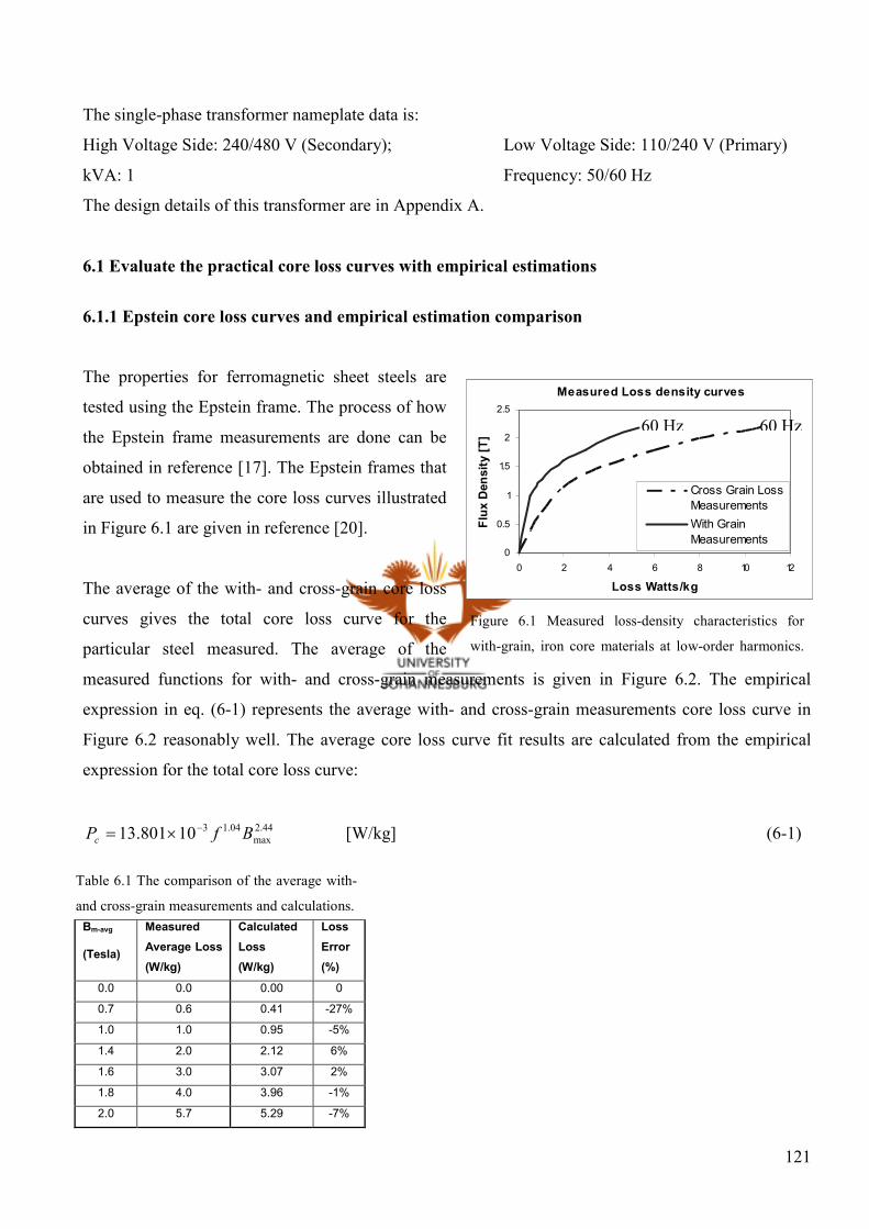
121
The single-phase transformer nameplate data is:
High Voltage Side: 240/480 V (Secondary); Low Voltage Side: 110/240 V (Primary)
kVA: 1 Frequency: 50/60 Hz
The design details of this transformer are in Appendix A.
6.1 Evaluate the practical core loss curves with empirical estimations
6.1.1 Epstein core loss curves and empirical estimation comparison
The properties for ferromagnetic sheet steels are
tested using the Epstein frame. The process of how
the Epstein frame measurements are done can be
obtained in reference [17]. The Epstein frames that
are used to measure the core loss curves illustrated
in Figure 6.1 are given in reference [20].
The average of the with- and cross-grain core loss
curves gives the total core loss curve for the
particular steel measured. The average of the
measured functions for with- and cross-grain measurements is given in Figure 6.2. The empirical
expression in eq. (6-1) represents the average with- and cross-grain measurements core loss curve in
Figure 6.2 reasonably well. The average core loss curve fit results are calculated from the empirical
expression for the total core loss curve:
44.2
max
04.1310801.13 BfPc−×= [W/kg] (6-1)
Bm-avg
(Tesla)
Measured
Average Loss
(W/kg)
Calculated
Loss
(W/kg)
Loss
Error
(%)
0.0 0.0 0.00 0
0.7 0.6 0.41 -27%
1.0 1.0 0.95 -5%
1.4 2.0 2.12 6%
1.6 3.0 3.07 2%
1.8 4.0 3.96 -1%
2.0 5.7 5.29 -7%
Table 6.1 The comparison of the average with-
and cross-grain measurements and calculations.
Figure 6.1 Measured loss-density characteristics for
with-grain, iron core materials at low-order harmonics.
Measured Loss density curves
0
0.5
1
1.5
2
2.5
0 2 4 6 8 10 12
Loss Watts/kg
Flux Density [T]
Cross Grain Loss
Measurements
With Grain
Measurements
60 Hz 60 Hz
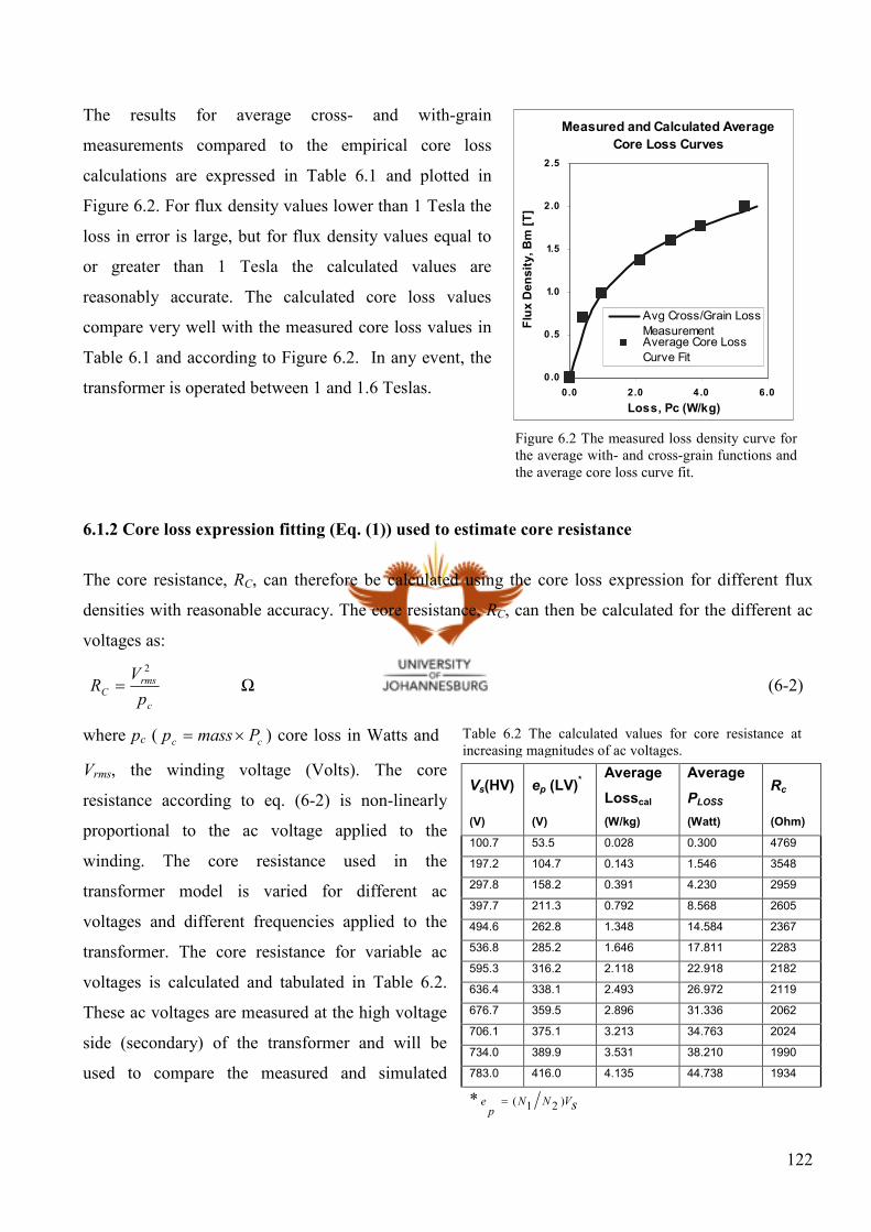
122
Table 6.2 The calculated values for core resistance at
increasing magnitudes of ac voltages.
The results for average cross- and with-grain
measurements compared to the empirical core loss
calculations are expressed in Table 6.1 and plotted in
Figure 6.2. For flux density values lower than 1 Tesla the
loss in error is large, but for flux density values equal to
or greater than 1 Tesla the calculated values are
reasonably accurate. The calculated core loss values
compare very well with the measured core loss values in
Table 6.1 and according to Figure 6.2. In any event, the
transformer is operated between 1 and 1.6 Teslas.
6.1.2 Core loss expression fitting (Eq. (1)) used to estimate core resistance
The core resistance, RC, can therefore be calculated using the core loss expression for different flux
densities with reasonable accuracy. The core resistance, RC, can then be calculated for the different ac
voltages as:
c
rmsC p
VR
2
= Ω (6-2)
where pc ( cc Pmassp ×= ) core loss in Watts and
Vrms, the winding voltage (Volts). The core
resistance according to eq. (6-2) is non-linearly
proportional to the ac voltage applied to the
winding. The core resistance used in the
transformer model is varied for different ac
voltages and different frequencies applied to the
transformer. The core resistance for variable ac
voltages is calculated and tabulated in Table 6.2.
These ac voltages are measured at the high voltage
side (secondary) of the transformer and will be
used to compare the measured and simulated
Vs(HV) ep (LV)*
Average
Losscal
Average
PLOSS Rc
(V) (V) (W/kg) (Watt) (Ohm)
100.7 53.5 0.028 0.300 4769
197.2 104.7 0.143 1.546 3548
297.8 158.2 0.391 4.230 2959
397.7 211.3 0.792 8.568 2605
494.6 262.8 1.348 14.584 2367
536.8 285.2 1.646 17.811 2283
595.3 316.2 2.118 22.918 2182
636.4 338.1 2.493 26.972 2119
676.7 359.5 2.896 31.336 2062
706.1 375.1 3.213 34.763 2024
734.0 389.9 3.531 38.210 1990
783.0 416.0 4.135 44.738 1934
* sVNNp
e )21(=
Figure 6.2 The measured loss density curve for
the average with- and cross-grain functions and
the average core loss curve fit.
Measured and Calculated Average
Core Loss Curves
0.0
0.5
1.0
1.5
2.0
2.5
0.0 2.0 4.0 6.0
Loss, Pc (W/kg)
Flux Density, Bm [T]
Avg Cross/Grain Loss
MeasurementAverage Core Loss
Curve Fit

123
excitation curves simulated at different core resistances.
6.1.3 The magnetisation or B-H curves and relative permeability curve
The magnetisation curves were
calculated from measured flux
linkage and magnetomotive
force data given in references
[19] and [20]. In Table 6.3 all
the measured and calculated
(transformer model) data are
given for B-H and relative
permeability curves.
The mmf, Fexc, is the measured
value whereby the magnetic
field, Hm, is calculated.
m
excm l
FH = [A-t] (6-3)
where lm is the magnetic path length, m.
The flux density, Bm, can again be derived
from the flux linkage, λp, by the following
formula:
c
pm NA
Bλ
= [Teslas] (6-4)
Ac is the transformer core area, m2;
N is the turns of the applicable winding.
The B-H curve can then be drawn from the
measured and calculated data in Table 6.3 and
is shown in Figure 6.3. The secondary and the
primary B-H curves are sketched. The
Fexc ( mmf) Iexc LV
calp,λλλλ HV
meass,λλλλ Hm Bm-sec HV Bm-prim LV µr
(A-t) (A) (Wb-t) (Wb-t) (A/m) (Tesla) (Tesla)
7.192 0.028 0.267 0.2043 31 0.23 0.23 5931
10.7 0.042 0.523 0.304 46 0.46 0.50 7809
15.95 0.063 0.79 0.4383 69 0.69 0.72 7913
25.56 0.100 1.055 0.6564 111 0.92 0.93 6594
55.19 0.216 1.312 1.128 239 1.14 1.17 3798
79.09 0.310 1.424 1.354 343 1.24 1.27 2876
118.4 0.464 1.579 1.575 513 1.37 1.39 2131
152.1 0.596 1.688 1.692 659 1.47 1.47 1773
196.9 0.772 1.795 1.798 853 1.56 1.56 1456
236 0.925 1.873 1.8605 1023 1.63 1.62 1268
280.4 1.100 1.947 1.9155 1215 1.69 1.69 1109
417 1.635 2.077 2.0145 1808 1.81 1.85 796
Table 6.3 The measured flux linkage, λ and mmf, Fexc data with derived magnetic
field, H, flux density, B and relative permeability, µr data.
Figure 6.3 The B-H curves for the measured and simulated
results on the LV and HV side.
The Magnetisation B-H Curve
0.0
0.2
0.4
0.6
0.8
1.0
1.2
1.4
1.6
1.8
2.0
0 500 1000 1500 2000
H (A/m)
B (T)
Bm-sec HV (measured)Bm-sec HV (cal)Bm-prim LV (measured)Bm-prim LV (cal)

124
calculated (transformer model) data for the B-H curve approximates is not good for values of cyclic ac
flux densities less than 1.2 Teslas against the measured values. But for cyclic ac flux densities values
greater than 1.2 Teslas the calculated values are reasonable accurate compared to the measured values.
In any case, the transformer is operated at values greater than 1.2 Teslas, which is the most important
part of the B-H curve. The saturated flux density, Bsat, of the core material is approximated from the B-
H curve that is estimated to be 1.97 Teslas. The relative permeability, µr, curvature against the
magnetic field, H, is plotted in Figure 6.4. The relative permeability, µr, is derived from the following
expression:
H
Br
0µµ = [ 7
0 104 −×= πµ ]
(6-5)
The initial permeability, µi, can then be
derived from Figure 6.4 and is estimated as an
average between the first two relative
permeabilities, µr values in Table 6.3, which
gives a value of approximately 7000 Gauss.
Figure 6.4 The relative permeability against the magnetic
field applied to the 1kVA transformer.
Relative permeability, u r
0
2000
4000
6000
8000
0 300 600 900 1200 1500 1800
H (A/m)
Relative perm
eability (ur)
Secondary-HV
side

125
6.2 Evaluate the transformer excitation practical results with non-linear transformer simulation
model
6.2.1 Measured and simulated excitation curve verification
Figure 6.5 illustrates the experimental setup that was used to test the transformer. An ammeter was put
in series with the supply to monitor the LV current. The voltage meter was put in parallel with the
secondary voltage (HV) to monitor and measure the secondary voltage. The transformer was energised
from the low voltage side (primary side) with no load switched in. The voltage at secondary winding
and the primary excitation current were measured to plot the excitation curve in Figure 6.6. The
experimental test setup is given in more detail in reference [19].
The measured and calculated values for peak flux linkage, peak excitation, peak voltages and peak
currents for the secondary and primary side are tabulated in Table 6.4. The peak flux linkage value for
a certain voltage is calculated as follows:
f
V peakpeak
πλ
2= (6-6)
The magnetomotive force (Fexc) is calculated for the measured peak excitation current as:
excexc NIF = (6-7)
The transformer model setup for simulations was similar to the measurement test setup. The
transformer model is composed of the dc resistance, winding eddy-current parameter, leakage
inductance, non-linear core resistance and the non-linear magnetising impedance. The transformer
V
Figure 6.5 The complete transformer model used for measurements and simulations.
Ideal transformer
A
LV HV
21 NN Rdc,1
Ll1
Lm 1e Rc
im ic
iϕ
ϕiii −=′ 11
i’ =i - i
1v
+
2
1
2
1, dt
idkec′ Rosl,1
+ -
-
v2
i1 Ll2
+
-
Rdc,2
+
2
2
2
2,dt
idkec
Rosl,2
+ -
1i +
-
vs
-Primary Secondary

126
model was simulated for the LV primary voltages in Table 6.4. The HV secondary voltages, LV
primary voltages and the LV primary excitation currents were then extracted from the output data after
the simulation for each ac LV voltage injected on the low voltage side. The simulated programming
results and transformer circuit simulated in Intusoft SPICE for the non-linear transformer model under
rated no-load conditions are given in Appendix C. The peak values for the ac injected primary voltages,
secondary voltages and excitation currents are then
tabulated in Table 6.4. The excitation or mmf, core
resistance, RC, and primary and secondary flux
linkages, λ, are then calculated from the ac injected
primary voltages, secondary voltages and excitation
currents. The peak magnitudes for the primary and
secondary ac flux linkages errors are the difference
between the peak magnitudes for the calculated and
measured ac flux linkages tabulated.
The ac flux linkage errors for the low values of ac
excitation current are not accurate for the transformer
model used. The ac flux linkage for the measured
values increases much more quickly for small values
Fexc
(A-t)
LV
excI (A)
cal
CR
(Ω)
HV
meass,λλλλ(Wb-t)
HV
cals,λλλλ(Wb-t)
HV
sλλλλ∆Error
(%)
HV
meassV ,
(V)
HV
calsV ,
(V)
HV
meassV ,
Referred to LV, (V)
LV
calp ]27[,,λλλλ (Wb-t)
LVcalp,λλλλ
(Wb-t)
LVpλλλλ∆
Error (%)
LV
calpV]27[,,
(V)
LV
calpV ,
(V)
7 0.028 4769 0.267 0.2043 -23% 100.66 77.02 53.47 0.1390 0.1087 -21.8% 52.40 41
11 0.042 3548 0.523 0.304 -42% 197.17 114.61 104.74 0.3070 0.161 -47.6% 115.74 60
16 0.063 2959 0.790 0.4383 -45% 297.82 165.24 158.22 0.4390 0.2332 -46.9% 165.50 88
26 0.100 2605 1.055 0.6564 -38% 397.73 247.46 211.29 0.5690 0.3492 -38.6% 214.51 133
55 0.216 2367 1.312 1.128 -14% 494.61 425.25 262.76 0.7140 0.6002 -15.9% 269.17 226.8
79 0.310 2283 1.424 1.354 -5% 536.84 510.45 285.19 0.7740 0.7207 -6.9% 291.79 272
118 0.464 2182 1.579 1.575 0% 595.27 593.76 316.24 0.8470 0.8375 -1.1% 319.31 316.33
152 0.596 2119 1.688 1.692 0% 636.36 637.87 338.07 0.8980 0.9 0.2% 338.54 339.95
197 0.772 2062 1.795 1.798 0% 676.70 677.83 359.50 0.9500 0.9562 0.7% 358.14 361.2
236 0.925 2024 1.873 1.8605 -1% 706.10 701.39 375.12 0.9910 0.99 -0.1% 373.60 374.05
280 1.100 1990 1.947 1.9155 -2% 734.00 722.13 389.94 1.0290 1.019 -1.0% 387.92 385
417 1.635 1934 2.077 2.0145 -3% 783.01 759.45 415.97 1.1270 1.072 -4.9% 424.87 405.2
Figure 6.6 The measured and simulated fluxlinkage
plots against the mmf for LV and HV side.
Fluxlinkage Primary and Secondary
Curves
0.0
0.5
1.0
1.5
2.0
2.5
0 100 200 300 400 500
Peak Excitation, Fexc = N Iexc (A-t)
Peak Flux Linkages (Wb-t)
HV Fluxlinkage
Measured
LV Fluxlinkage Cal
o f ref[3]
HV Fluxlinkage
Calculated
LV Fluxlinkage
Calculated
Table 6.4 The comparison between measured and calculated values of voltage and flux linkages for the primary and secondary
side of the transformer.

127
of current than the ac flux linkage of the transformer model. This is not so bad since current values are
overestimated for voltages far below rated voltage. In any case, the transformers are not usually
operated at these low voltages but are operated at the curvature part of the saturation curve (as seen in
Figure 6.6).
In Table 6.4 it is clear that for voltages close to rated voltage the accuracy of the transformer simulation
model is excellent. And the accuracy remains stable for higher ac voltages that are applied. These
effects are excellently illustrated in Figure 6.6, which gives the primary and secondary, measured and
calculated λ-i characteristic for the transformer under test. The transformer simulation model proposed
can therefore be used for impact studies on transformers and will give results with reasonable accuracy.
6.3 Experimental verification of non-linear fully loaded transformer model under harmonic
supply
The method of calculation or the non-linear transformer model as developed in this dissertation is
supported by the verification of measured results with the transformer model results. The experimental
setup for these conditions is given in Figure 6.7. The primary and secondary voltages and currents were
measured and used to calculate the losses, which are illustrated by means of ammeters and voltage
meters in Figure 6.7.
The transformer model used in Chapter 5 is supported and verified through these measurements. As
explained in the paper [29], an adjustable phase lock circuit drives a power amplifier such that any
harmonic with selected amplitude and phase shift can be superimposed on the fundamental voltage.
The two methods for measuring the thermal impact of harmonics on single-phase transformers are
presented:
Primary Secondary
V
Ideal transformer
A
LV HV
21 NN Rdc,1
Ll1
Lm 1e Rc
im ic
iϕ
ϕiii −=′ 11
i’ =i - i
1v
+
2
1
2
1, dt
idkec Rosl,1
+ -
-
v2
i2 Ll2
+
-
Rdc,2
+
2
2
2
2,dt
idkec
Rosl,2
+ -
1i
- -
A
RL
Figure 6.7 The experimental setup for 1kVA transformer with harmonic supply and full resistive load.
+
-
vs
vh +
V

128
1. Temperature measurements are measured using thermocouples where the losses are assumed to be
proportional to the temperature rise of transformer;
2. Power measurements are calculated using measured nonsinusoidal input and output voltages and
currents.
The losses are defined as:
[ ]dttitvtitvT
PT
loss ∫ −=0
2211 )()()()(1
(6-8)
or by way of this expression, depending on which one is the most accurate:
[ ]∫ +=T
loss dttptpT
P0
21 )()(2
1 (6-9)
where p1 and p2 are:
[ ][ ])()()()()( 22121 tititvtvtp +−= ( [ ])()( 12 tvtv − and [ ])()( 12 titi + is measured simultaneously);
and
[ ][ ])()()()()( 12122 tititvtvtp −+= ( [ ])()( 12 tvtv + and [ ])()( 12 titi − is measured simultaneously).
The above methods were used to measure losses of the transformer. The measured transformer results
are obtained from the Elsevier published paper [29]. The method of measurements for the power
measurements, the adjustment of the phase shift of the harmonic supply and the temperature are further
outlined in reference [29].
Figure 6.8 is the transformer model setup that is utilised to verify the transformer model under
harmonic and load conditions with a few additions. A harmonic voltage supply is superimposed on the
mains supply, as shown in Figure 6.8. The transformer supplies a resistive load 65 Ω. The calculated
losses shown in Table 6.5 are then obtained from the simulations on the transformer model.
RLO
-
Iload
v2
i1 2i′
Figure 6.8 The complete transformer model with harmonic supply and full resistive load (RL= 65Ω).
+
-
vs
Ll1 R’dc,2
L’l2
Lm 2'e
+
-
Rc
Rdc,1
+
im ic
iϕ
ϕiii −=′ 11
i’ =i - i
2v′
+
2
1
2
1, dt
idkec R’
osl,2
-
+ - + -
vh +
-
2
2
2
2, dt
idkec
′′ Rosl,1
Primary or LV side
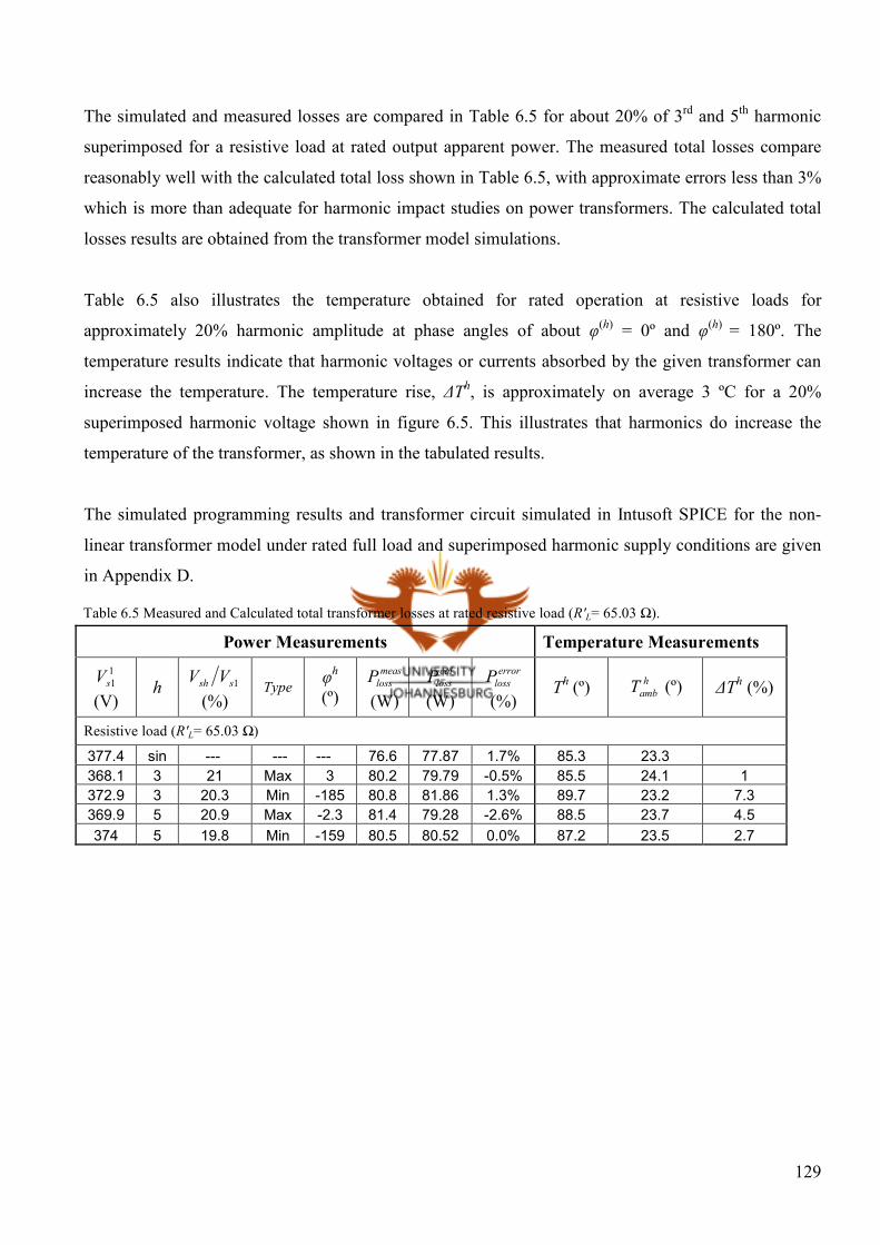
129
The simulated and measured losses are compared in Table 6.5 for about 20% of 3rd and 5
th harmonic
superimposed for a resistive load at rated output apparent power. The measured total losses compare
reasonably well with the calculated total loss shown in Table 6.5, with approximate errors less than 3%
which is more than adequate for harmonic impact studies on power transformers. The calculated total
losses results are obtained from the transformer model simulations.
Table 6.5 also illustrates the temperature obtained for rated operation at resistive loads for
approximately 20% harmonic amplitude at phase angles of about φ(h) = 0º and φ(h) = 180º. The
temperature results indicate that harmonic voltages or currents absorbed by the given transformer can
increase the temperature. The temperature rise, ∆Th, is approximately on average 3 ºC for a 20%
superimposed harmonic voltage shown in figure 6.5. This illustrates that harmonics do increase the
temperature of the transformer, as shown in the tabulated results.
The simulated programming results and transformer circuit simulated in Intusoft SPICE for the non-
linear transformer model under rated full load and superimposed harmonic supply conditions are given
in Appendix D.
Power Measurements Temperature Measurements
1
1sV
(V) h 1ssh VV
(%) Type
φh
(º)
measlossP
(W)
callossP
(W)
errorlossP
(%) Th (º)
hambT (º) ∆Th (%)
Resistive load (R'L= 65.03 Ω)
377.4 sin --- --- --- 76.6 77.87 1.7% 85.3 23.3
368.1 3 21 Max 3 80.2 79.79 -0.5% 85.5 24.1 1
372.9 3 20.3 Min -185 80.8 81.86 1.3% 89.7 23.2 7.3
369.9 5 20.9 Max -2.3 81.4 79.28 -2.6% 88.5 23.7 4.5
374 5 19.8 Min -159 80.5 80.52 0.0% 87.2 23.5 2.7
Table 6.5 Measured and Calculated total transformer losses at rated resistive load (R'L= 65.03 Ω).

130
Conclusion
The core loss estimation expression compares reasonably well with the measured Epstein loss curves
that provide a good estimate for calculating the core resistance. The measured and calculated B-H
curve shows that for low ac flux density values the simulated results are inaccurate but for high values
of ac flux density the simulated results are reasonably accurate. The saturated flux density can then be
estimated from the B-H curves. The initial permeability, µi, can then be derived from the relative
permeability, µr curvature, and is estimated to be an average between the first two relative
permeabilities, µr values. The saturated flux density and initial permeability are used to calculate the
magnetising voltage Frolic expression for the transformer model.
The non-linear transformer model is then verified with the measured data under no-load conditions.
The simulated and measured flux linkage plots for the HV and LV side of the transformer are plotted
against the mmf to determine the accuracy of the transformer simulated model. The plots show
inaccuracies for low values of ac flux linkage but are accurate for high values of ac flux linkage, at
which the transformer is usually operated. The Frolic expression to model the non-linear magnetising
characteristic of the transformer can thus be safely used at operating voltages. Fortunately, the power
transformer is operated at high ac flux linkage values where the accuracy is required.
Finally the non-linear transformer model is verified with the experimental results under a superimposed
harmonic supply with the main supply and full-load conditions. The temperature measurements show
that harmonics do increase the temperature of the transformer, which can be detrimental to
transformers. The transformer power loss measurements compared to the power losses of the
transformer model simulated indicate approximate errors less than 3%. It illustrates that the non-linear
transformer model is accurate under normal transformer operating conditions and can be used to do
harmonic impact studies and transformer modelling.

131
CHAPTER 7: CONCLUSIONS AND RECOMMENDATIONS
CONCLUSIONS
The presence of harmonics on the power system is a fact and poses a threat to power-plant equipment.
Past research shows that harmonics do affect power transformers negatively but the mathematical
models to simulate the harmonic effects on power transformers is complex. The high number of severe
failures of power transformers per year and large number of power transformer failures attributed to
unknown causes proves that the knowledge and research in power transformers is inadequate. Power
transformers are also among the most expensive equipment and make up the most critical plant
equipment in electric utilities, especially in the Transmission and Distribution networks. This strongly
suggests that a study of the harmonic impact of power transformers is both necessary and desirable.
The increase of switching equipment on the power system network will definitely increase the presence
and magnitudes of harmonics on the power system. Harmonic prevalence on the power system can
lower the power-delivering capacity to loads. Harmonics standards are put in place that specify the
allowable voltage and current harmonic distortion levels. Some utilities only monitor voltage
harmonics on the power system. All power-plant equipment is not linear, so a linear supply impedance
cannot be assumed. This means that voltage harmonics are generally not directly proportional to the
harmonic currents in power systems. It stresses the importance of monitoring the harmonic current
levels on the power system. A non-linear supply, for example, can be a power transformer that supplies
a harmonic load. Harmonic currents that cause transformer line currents to exceed more than 5% of the
rated current can stress the power transformer insulation beyond design limits.
The theory proves that conduction losses on power transformers can increase due to the harmonics
absorbed by the power transformer. The other stray losses in the core, clamps and the other structural
parts are found to be proportional to the square of the load current and the frequency to the exponent
factor 0.8 at low harmonic frequencies proven empirically. The winding eddy-current losses are
directly proportional to the square of the load current and square of the frequency that is proven
theoretically and empirically through literature.
The recommended practice for capability calculations on winding eddy-current losses results is too
conservative. The harmonic impact these have on winding eddy-current losses and other stray losses

132
has not been presently realised in the form of time domain parameters. The expression for winding
eddy-current loss resistance can be defined in the frequency domain or in terms of resistance. The
winding eddy-current loss presented in the frequency domain requires superposition (summation of the
contributions of the frequency components). The winding eddy-current loss modelled as a time domain
parameter will not necessitate superposition in the transformer simulations. A harmonic factor for the
winding eddy-current resistance is determined through capability calculations which are conservative
and not reasonably accurate. Finally, a time domain winding eddy-current loss parameter was derived
in relation to which no superposition or conservative harmonic factors are required.
The recommended capability calculations show that an increase of winding eddy-current losses due to
harmonic load currents can reduce the maximum allowable magnitude of the transformer load current.
So the harmonic currents absorbed by the transformer do increase the winding eddy-current losses that
reduce the permissible transformer load currents. It was found that the temperature rise in the
transformer is proportional to other stray losses. It can be concluded that for an increase of other stray
losses the temperature can rise for liquid-filled transformers. This has been substantially proven
through the empirical formulas presented in published papers. The effect of other stray losses on the
dry-type transformers is assumed to be minimal or negligible. Although higher temperatures do
increase conduction losses, the winding eddy-current losses tend to decrease with an increase in
temperature, as has been demonstrated in the literature.
A power transformer model was developed out of theoretical analysis, and can be used to do harmonic
impact studies on power transformers. The transformer model takes into account the leakage
inductance, the dc resistance, the other stray loss parameter, the winding eddy-current loss parameter,
the non-linear magnetising inductance and the core resistance. The parameters were developed and
calculated for a single-phase, shell-type and two-winding power transformer that could also be used to
model three-phase two-winding power transformers which can be presented in the single-phase
equivalent form.
The case study of the power transformer under harmonic loading conditions indicated that, according to
the recommended capability calculations, winding eddy-current losses constitute one of the major
contributors to load losses. The recommended capability calculations estimates for winding eddy-
current loss are shown to be conservative and inaccurate. A winding eddy-current loss that is high in

133
magnitude results in a lower permissible load current which translates into a lower power capacity for
the power transformer. The lower power capacity due to the lower permissible load current results in a
loss of return on capital investment. Therefore a more accurate estimate on winding eddy-current loss
was determined for the power transformer, which shows a saving on power capacity. The case study
also revealed that the harmonic impact on conduction losses and other stray losses is minimal but the
harmonic impact on winding eddy-current losses is significant.
The effect of harmonic currents on the load current was not appreciable in the case study. Only the
peak value of the nonsinusoidal load current was much higher than the rated peak load current. It was
noted for numerous load simulations for the given harmonic distribution that there was a constant
increase of 2% for the rms nonsinusoidal load current over the rms fundamental load current. The
constant increase for the rms nonsinusoidal load current over the rms fundamental load current
calculated through transformer model simulations is smaller then the recommended capability
calculations of 3% and permissible allowance of 5%. The harmonic currents subjected to the
transformer do not affect the rms nonsinusoidal current appreciably but can exceed the rated peak load
current significantly according to the transformer model simulations. The case study revealed a classic
case of the voltage harmonic levels and the voltage THDv being within acceptable limits while the
harmonic current levels and the current THDi were far out of their acceptable or recommended levels. It
was seen that the harmonic currents to which the power transformer was subjected do not affect the
load voltage (secondary) substantially. The monitoring of harmonic current levels on the power system
is becoming a requirement as they can exceed allowable limits.
Finally, the transformer model was verified through measurements done on a small power transformer.
Firstly the core resistance expression was verified. The core loss estimation expression compares
reasonably well with the measured Epstein loss curves, which provide a good estimate for calculating
the core resistance. The saturated flux density used was estimated from the B-H curves. The initial
permeability, µi, is derived from the relative permeability, µr curvature.
The no-load transformer model was then verified with the measured data under a no-load transformer
setup. The flux linkage was plotted against the mmf to compare the transformer model simulation
results with the measured data obtained. The plots show inaccuracies for low values of ac flux densities
but are accurate for high values of ac flux densities, at which the transformer is usually operated.

134
Fortunately the power transformer is operated at the high ac flux density values or the curved part of
the saturation curve where the accuracy of the transformer model is reasonable.
Finally, the transformer model simulated results were verified with the experimental results under a
superimposed harmonic supply with the main supply and full-load conditions. The temperature
measurements show that harmonics do increase the temperature of the transformer, which can be
detrimental to transformers. The power losses of the transformer model simulated compare reasonably
well with the measured transformer power loss measurements. The verification results illustrate that the
non-linear transformer model is accurate under normal transformer operating conditions and can be
used to do harmonic impact studies and transformer modelling.
The study concludes that harmonic voltages as well as harmonic currents need to be monitored. The
supply impedance cannot be assumed to be linear, for the power system consists of power-plant
equipment that has non-linear characteristics such as power transformers. A reasonably accurate non-
linear power transformer model was developed from the theoretical and practical considerations. The
non-linear transformer model accuracy compares reasonably well with practical results. The case study
on the dry-type transformer model under full-load conditions and harmonic loading revealed the
minimal impact it has on the conduction losses, core losses and other stray losses. But the harmonic
current impact on the winding eddy-current losses caused by the proximity effect is considerably high
under harmonic loading conditions. The increase in the rms load current can cause an eventual increase
in the conduction losses of the transformer but the harmonic currents do not increase the rms load
current appreciably. According to the recommended capability calculations, the increase of winding
eddy-current losses decreases the maximum permissible rms load current. Thus the rated load current
of the transformer needs to be derated to the maximum permissible load current, which in turn reduces
the delivering power capacity of the power transformer. Thus, using the proposed transformer model,
as opposed to the recommended capability calculations, will result in a lower loss in power capacity.

135
RECOMMENDATIONS
Firstly it is recommended that utilities should not only monitor harmonic voltages but also monitor
harmonic currents according to the harmonic current limits proposed in the “IEEE Recommended
Practices and Requirements for Harmonic Control in Electrical Power Systems, [10]”. The utilities
should implement the “IEEE Recommended Practice for Establishing Transformer Capability when
Supplying Nonsinusoidal Load Currents [11]”, as power system harmonics can be damaging to power
transformers. The proposed transformer model can be utilised for a more accurate impact study on the
harmonic effects on power transformers. This non-linear transformer model in this study disregards the
effects of capacitance and dielectric losses. So a more complete transformer model can be built taking
into account capacitance and dielectric losses. The research and knowledge base on large power
transformers electrically is limited and research on large power transformers needs to be further
encouraged.
136
REFERENCES
[1] General Electric Company, Transmission Line Reference Book- 345kV and Above, 2nd ed. (Palo
Alto, CA. Electric Power Research Institute, 1982).
[2] Glover, Sarma, Power System analysis and Design, 2nd ed. Boston, PWS Publishing Company,
1987.
[3] Arrillaga, J.,Bradley, D.A., and Bodger, P.S., Power System Harmonics, John Wiley & Sons Ltd.,
New York, 1985.
[4] Odendal, E.J, Prof., “Power Electronics Course notes”, Durban, University of Natal, pg. 8.36.
[5] Whitaker, Jerry C., AC Power Systems Handbook, 2nd Ed., pp. 13-15, CRC Press LLC, 1999.
[6] Mohan, Undeland and Robbins, Power Electronics, 2nd Ed., pp. 41, John Wiley & Sons, Inc., 1995.
[7] NRS 048-4:1999, Electricity Supply - Quality of Supply- Part 4: Application guidelines for utilities.
[8] Kraus and Fleisch, Electromagnetics with Applications, 5th Ed., McGraw-Hill Companies, Inc.,
1999.
[9] Fitzgerald, A.E., Kingsley Jr., C. and Umans, S.D., Electric Machinery, 5th Ed., McGraw-Hill
Companies, Inc., 1990.
[10] IEEE Std. 519-1992, IEEE Recommended Practices and Requirements for Harmonic Control in
Electrical Power Systems, IEEE Publications, 445 Hoes Lane, P.O. Box 1331, Piscataway, NJ 08855-
1331, USA.
[11] IEEE Std C57.110-1998, IEEE Recommended Practice for Establishing Transformer Capability
when Supplying Nonsinusoidal Load Currents, IEEE Publications, 445 Hoes Lane, P.O.Box 1331,
Piscataway, NJ 08855-1331, USA.

137
[12] Bishop, M.T., and Gilker, C., "Harmonic caused transformer heating evaluated by a portable PC-
controlled meter,” 37th Annual Rural Electric Power Conference, 1993.
[13] Snelling, E.C., Soft Ferrites, 2nd Ed., Butterworths, England, Seven Oaks, 1988.
[14] Butterworth, S, “Effective resistance of inductance coils at radio frequencies”, Expl. Wireless, 3,
203 (1926)
[15] Butterworth, S, “Eddy current losses in cylindrical conductors with special applications o the
alternating current resistance of short coils”, Phil. Trans. R. Soc. A222, 57 (1922).
[16] Yildrim, D, Fuchs, E, “Transformer derating and comparison with Harmonic Loss Factor (FHL)
Approach”, IEEE TRANS. PD, VOL 15, No. 1, January 2000.
[17] Members of Staff of Dept. EE, MIT, Magnetic circuits and transformers, 7th, 1950, John Wiley &
Sons Inc., New York.
[18] Mclyman, Colonel Wm., T., Transformer and Inductor Design Handbook, 7th, 1978, Marcel
Dekker Inc., New York.
[19] Fuchs, E.F., Masoum, M.A.S., Roesler, D.J., “Large Signal Nonlinear Model of Anisotropic
Transformers for Nonsinusoidal Operation, Part I: λ-I Characteristic”, IEEE TRANS PD, Vol. 6, No. 1,
January 1991.
[20] Masoum, M.A.S., Fuchs, E.F., Roesler, D.J., “Large Signal Nonlinear Model of Anisotropic
Transformers for Nonsinusoidal Operation, Part II: λ-I Characteristic, IEEE TRANS PD”, Vol. 6, No.
4, October 1991.
[21] Zocholl, S.E., Guzman, A., Hou, D., “Transformer modelling as applied to differential protection”,
SEL, Pullman, Washington
[22] Bendat J.S, Piersol A.G, Engineering application of correlation and spectral analysis, John Wiley
and Sons, 1985.
138
[23] Cavallo A, Setola R, Vasca F, A practical approach using Matlab Simulink and control system
toolbox, The Mathworks Inc. The Matlab curriculum series, Prentice Hall Europe, 1996.
[24] Pretorius R.E, Guide to the generation, evaluation and control of harmonics in industrial and
mining power systems, 1987.
[25] IEEE Std. 18-1991, IEEE Standard for Shunt Power Capacitors, IEEE Publications, 445 Hoes
Lane, P.O.Box 1331, Piscataway, NJ 08855-1331, USA.
[26] Holtzhausen, J., P, High Voltage Engineering, University of Stellenbosch, Electrical and
Electronic Engineering.
[27] IEEE C57.12.91-2001, IEEE Standard Test Code for Dry Type Distribution and Power
Transformers, IEEE Publications, 445 Hoes Lane, P.O.Box 1331, Piscataway, NJ 08855-1331, USA.
[28] Ramo, S., Whinnery, J.R., Van Duzer, T., Fields and Waves in Communication Electronics, 3rd
ed., 1993, John Wiley & Sons, Inc., New York.
[29] Masoum, M.A.S., Fuchs, E.F., “Derating of Anisotropic Transformers under Nonsinusoidal
Operating Conditions”, 2002, Elsevier Science Ltd., Electrical Power and Energy Systems 25 (2003)1-
12.
[30] IEC 60076-11-2004-05, 1st Ed., Power Transformers-PART 11: Dry-type transformers,
International Electrotechnical Commission, 3, rue de Varembe’, P.O.Box 131, CH-1211 Geneva 20,
Switzerland.
[31] M.S. Hwang, W.M. Grady, H.W. Sanders, Jr., “Distribution Transformer Winding Losses due to
Nonsinusoidal Currents”, IEEE TRANS PD”, Vol. 2, No. 1, January 1987.
[32] O.C. Geduldt, I.W. Hofsajer, V. Jaffa, “The Impact and Consequences of Power System
Harmonics on Power Plant Equipment Operating at Thermal Limits”, SAUPEC Conference, January
2003.
[33] Bartley, William H., P.E, “Analysis of Transformer Failures”, Presented at the International
Association of Engineering Insurers 36th Annual Conference, Stockholm, 2003, IMA WG 33(03).

139
[34] Wellard, Allan, “Transformer Study Committee 12 report back on the 39th Paris session of the
International Conference, Cigre Large HV Electric Systems 8th Open Seminar, 2002.

APPENDIX A
Transformer data:
N1 = 480,
N2 = 255,
A = 0.002394 m2
lm = 230.7 mm (Magnetic Path Length/
Mean core length)
Ll,1 = 8.5 mH (HV side Leakage inductance)
Rdc,1 = 4.263 (HV side ohmic resistance)
Ll,2= 1.1 mH (LV side Leakage inductance)
Rdc,2 = 0.8942 Ω (LV side ohmic resistance)
µi,r = 7000 (2
max,ri µµ +,Estimation from B-H curves)
Bsat = 1.97 Tesla (Estimation from B-H curves)
ACu,p =1.875x10⁻⁶ m2 (LV winding)
ACu,s =5.781x10⁻⁷ m2 (HV winding)
dLV = 1.545 mm (Diameter of LV winding)
dHV = 0.85794 mm (Diameter of HV winding)
c = 113.681
b = 0.5015
68.3
Figure A.1 Measured dimensions of 1kVA single-
phase transformer in mm.[20]
89.54
67.4
95.9
117..9
20 90.8
36 0.7
10
13
130.8
60
1
110
117.9
66.5
2 14
0.7 0.7
L L L
L
L H H H H
H
AIR
AIR CORE
CORE
CORE
CORE
CORE
AIR
AIR
BOX

APPENDIX B
The simulated programming results and circuit in Intusoft SPICE for the nonlinear transformer
model under full load and harmonic loaded conditions.
Conditions set for simulations on the nonlinear transformer mode; under harmonic loading is
simulated for two cases:
CASE 1: All peaks of the harmonic currents negative peak to the fundamental current with a slew rate
of 9.13k positive and negative.
CASE 2: All peaks of harmonic current fall together with peaks of the fundamental current for a slew
rate of 12.9k positive and negative.
V(34)V(35)I-HARM
V(38)
GAINK*SK*S GAIN
V(39)
GAINV(1)
L91.1M
V31SIN
I(V33)I_EXC
I(V32)I_M
I(V31)I_LV
V(55)VPRI_HV'
I(V34)I_R
V(49)
L102.4M
I(V35)
V(63)
V(50)
V(65)POUTL
V(66)POUTTV(64)
PCORE
R201.203
R210.8942
V(70)PEC
V(71)PCU
V(72)PCU
R222216.9
V(73)PEC
K*S
I13SIN
I14SIN
I15SIN
I16SIN
V(78)PIN
I(V36)
R230.148
R240.0988
I(V37) I(V38) I(V39) I(V40)
V(85)POSL
V(86)POSL
V(7)V(14)I-HARM V(26)
GAIN
V(91)
K*SK*S Slew Rate
Slew Rate
V(6)
34 35 38
6
36 39
1
47 4849
50
51
59 55
60
62
64
65
66
58 68 69
70
7172
56 73
63
747576 77
78
7967
85
86
7 14 26 9127
Figure B1 The Intusoft SPICE non linear transformer equivalent simulation circuitry modelled for case 1 and case 2.

1
695.41M 702.24M 709.07M 715.89M 722.72M
WFM.1 I(V35) vs. TIME in Secs
7.9880
3.9940
0
-3.9940
-7.9880
I(V35) in Amps
1
695.37M 702.10M 708.83M 715.56M 722.29M
WFM.1 I_EXC vs. TIME in Secs
695.28M
347.64M
0
-347.64M
-695.28M
I_EXC in Amps
1
695.32M 701.95M 708.59M 715.22M 721.86M
WFM.1 V(49) vs. TIME in Secs
373.34
186.67
0
-186.67
-373.34
V(49) in Volts
1
695.37M 702.10M 708.83M 715.56M 722.29M
WFM.1 VPRI_HV' vs. TIME in Secs
398.83
199.42
0
-199.42
-398.83
VPRI_HV' in Volts
2
695.41M 702.24M 709.07M 715.89M 722.72M
WFM.2 I(V36) vs. TIME in Secs
7.7732
3.8866
0
-3.8866
-7.7732
I(V36) in Amps
The Harmonic Loaded Transformer simulated graphic results: CASE 1
( Harmonic current peaks fall negative w.r.t fundamental current peak)
Fig. B2 The HV voltage referred to the LV side. Fig. B3 The LV voltage feeding the load.
Fig. B4 The excitation current seen from the LV side. Fig. B5 The harmonic load current seen from the LV side.
Fig. B6 The full load current seen from the LV side drawn
by full load resistance.

1
695.37M 702.10M 708.83M 715.56M 722.29M
WFM.1 PCU vs. TIME in Secs
39.093
29.320
19.546
9.7731
-51.498U
PCU in Volts1
695.37M 702.10M 708.83M 715.56M 722.29M
WFM.1 PCU vs. TIME in Secs
61.378
46.034
30.689
15.344
-106.81U
PCU in Volts
1
695.32M 701.95M 708.59M 715.22M 721.86M
WFM.1 PIN vs. TIME in Secs
2.3294K
1.7470K
1.1647K
582.33
-6.5918M
PIN in Volts
2
695.80M 702.43M 709.07M 715.70M 722.34M
WFM.2 POUTT vs. TIME in Secs
2.2086K
1.6565K
1.1043K
552.15
-13.794M
POUTT in Volts
1
695.37M 702.10M 708.83M 715.56M 722.29M
WFM.1 POSL vs. TIME in Secs
5.2192
3.7280
2.2368
745.60M
-745.60M
POSL in Volts
1
695.12M 701.37M 707.62M 713.87M 720.12M
WFM.1 POSL vs. TIME in Secs
8.8644
5.9096
2.9548
-21.935U
-2.9548
POSL in Volts
1
695.32M 701.95M 708.59M 715.22M 721.86M
WFM.1 PEC vs. TIME in Secs
205.66
102.83
0
-102.83
-205.66
PEC in Volts
1695M 702M 709M 716M 723M
WFM.1 PEC vs. TIME in Secs
113
56.4
0
-56.4
-113
PEC in Volts
The instantaneous power loss curves for the different transformer losses
Fig. B8 The instantaneous input power curve for the harmonic loaded transformer. Fig. B9 The instantaneous total output power curve for the harmonic loaded transformer.
Fig. B10 The instantaneous HV copper power loss curve for the harmonic loaded
transformer.
Fig. B12 The instantaneous HV other stray power loss curve for the
harmonic loaded transformer
Fig. B11 The instantaneous LV copper power loss curve for the harmonic loaded
transformer
Fig. B13 The instantaneous LV other stray power loss curve for the
harmonic loaded transformer
Fig. B14 The instantaneous HV eddy current power loss curve for the
harmonic loaded transformer
Fig. B15 The instantaneous HV eddy current power loss curve for the
harmonic loaded transformer

1
420M 427M 433M 440M 447M
WFM.1 V(49) vs. TIME in Secs
528
264
0
-264
-528
V(49) in Volts
1
421M 427M 434M 440M 447M
WFM.1 VPRI_HV' vs. TIME in Secs
528
264
0
-264
-528
VPRI_HV' in Volts
1
420M 427M 434M 441M 447M
WFM.1 I_EXC vs. TIME in Secs
768M
384M
0
-384M
-768M
I_EXC in Amps
1
420M 427M 434M 441M 447M
WFM.1 I(V35) vs. TIME in Secs
7.12
3.56
0
-3.56
-7.12
I(V35) in Amps
1
420M 427M 434M 441M 448M
WFM.1 I(V36) vs. TIME in Secs
12.9
6.44
0
-6.44
-12.9
I(V36) in Amps
The Harmonic Loaded Transformer simulated graphic results: CASE 2
( Harmonic current peaks fall positive w.r.t fundamental current peak)
The Graphic window range for the graph plots: 0.417s to 0.450s
Fig. B2 The HV voltage referred to the LV side. Fig. B3 The LV voltage feeding the load.
Fig. B4 The excitation current seen from the LV side. Fig. B5 The harmonic load current seen from the LV side.
Fig. B6 The full load current seen from the LV side drawn by
full load resistance.

1
420M 427M 434M 440M 447M
WFM.1 PIN vs. TIME in Secs
3.31K
2.48K
1.66K
828
0
PIN in Volts
1
420M 427M 434M 440M 447M
WFM.1 POUTT vs. TIME in Secs
2.83K
2.12K
1.41K
708
1.68
POUTT in Volts
1
420M 427M 434M 440M 447M
WFM.1 PCU vs. TIME in Secs
109
72.9
36.5
80.9M
-36.3
PCU in Volts
2
420M 427M 434M 440M 447M
WFM.2 PCU vs. TIME in Secs
68.7
49.1
29.4
9.82
-9.80
PCU in Volts
1
420M 427M 434M 441M 447M
WFM.1 POSL vs. TIME in Secs
11.8
8.27
4.77
1.27
-2.23
POSL in Volts 1
421M 428M 434M 441M 448M
WFM.1 POSL vs. TIME in Secs
7.07
5.30
3.53
1.77
1.70M
POSL in Volts
1
420M 427M 434M 441M 447M
WFM.1 PEC vs. TIME in Secs
383
230
76.6
-76.6
-230
PEC in Volts
1
420M 427M 434M 441M 447M
WFM.1 PEC vs. TIME in Secs
184
111
36.9
-36.9
-111
PEC in Volts
The Instantaneous Power Loss curves for the different Transformer Losses
Fig. B8 The instantaneous input power curve for the harmonic loaded transformer. Fig. B9 The instantaneous total output power curve for the harmonic loaded transformer.
Fig. B10 The instantaneous HV copper power loss curve for the harmonic loaded
transformer.
Fig. B12 The instantaneous HV other stray power loss curve for the
harmonic loaded transformer
Fig. B11 The instantaneous LV copper power loss curve for the harmonic
loaded transformer
Fig. B13 The instantaneous LV other stray power loss curve for the
harmonic loaded transformer
Fig. B14 The instantaneous HV eddy current power loss curve for the
harmonic loaded transformer Fig. B15 The instantaneous HV eddy current power loss curve for the
harmonic loaded transformer

1
1. The simulated programming results and circuit in Intusoft SPICE for the transformer
equivalent model for under full load and harmonic loaded conditions for case 1.
CASE 1
All peaks of the harmonic currents negative peak to the fundamental current with a slew rate of 9.13k
positive and negative.
FILENAME: THL1.CIR
D:\Spice LIB\THL1.CIR
*SPICE_NET
.MODEL DIFF_002 d_dt(out_offset=0.0E+000 gain=450.16U out_lower_limit=-10.0 out_upper_limit=
+ 10.0 limit_range=1.0E-030)
.MODEL DIFF_003 d_dt(out_offset=0.0E+000 gain=450.16U out_lower_limit=-10.0 out_upper_limit=
+ 10.0 limit_range=1.0E-030)
.MODEL SLEW_003 slew(rise_slope=9.13K fall_slope=9.13K )
*INCLUDE DEVICE.LIB
*INCLUDE SYS.LIB
.TRAN 0.0001 0.375 0.2083 0.0001 UIC
.OPTION VNTOL=1E-9 ABSTOL=1E-12 ITL4=100 ACCT METHOD=GEAR RELTOL=0.001
*INCLUDE AD5.LIB
*INCLUDE SWITCH.LIB
*INCLUDE CM1.LIB
*INCLUDE SCN.LIB
.CONTROL
VIEW TRAN I(V36)
TRAN 0.0001 0.375 0.2083 0.0001 UIC
.ENDC
*ALIAS V(35)=I-HARM
*ALIAS I(V33)=I_EXC
*ALIAS I(V32)=I_M
*ALIAS I(V31)=I_LV
*ALIAS V(55)=VPRI_HV'
*ALIAS I(V34)=I_R
*ALIAS V(65)=POUTL
*ALIAS V(66)=POUTT
*ALIAS V(64)=PCORE
*ALIAS V(70)=PEC
*ALIAS V(71)=PCU
*ALIAS V(72)=PCU
*ALIAS V(73)=PEC

2
*ALIAS V(78)=PIN
*ALIAS V(85)=POSL
*ALIAS V(86)=POSL
*ALIAS V(14)=I-HARM
.PRINT TRAN V(38) I(V33) I(V31) V(55)
.PRINT TRAN I(V34) V(49) I(V35) V(50)
.PRINT TRAN V(65) V(66) V(64) V(70)
.PRINT TRAN V(71) V(72) V(73) V(78)
.PRINT TRAN I(V36) I(V37) I(V38) I(V39)
.PRINT TRAN I(V40) V(85) V(86) V(91)
.PRINT TRAN V(6)
X7 6 38 GAIN K=6.944437
A5 35 36 DIFF_002
A6 34 35 DIFF_003
X8 38 39 GAIN K=1
X9 6 1 GAIN K=5.893
L9 47 48 1.1M
V31 0 49 SIN 0 -360.62 60 -0.0041666667
V32 50 51 0
V33 47 50 0
V34 50 56 0
L10 58 59 2.4M
V35 55 60 0
B39 51 0 V=(76709.406*V(63))/(113.682 + (554.32*ABS(I(V32))))^2
B40 62 0 V=I(V32)
B41 60 0 I=V(55)/59
B42 64 0 V=I(V34)*V(50)
B43 65 0 V=V(55)*I(V35)
B44 66 0 V=V(55)*I(V36)
R20 67 58 1.203
R21 68 69 0.8942
B45 70 0 V=I(V31)*(V(59)-V(47))
B46 71 0 V=I(V36)*(V(68)-V(69))
B47 72 0 V=(V(67)-V(58))*I(V31)
R22 56 0 2216.9
B48 73 0 V=I(V36)*(V(48)-V(68))
X10 62 63 SDIFF K=1
I13 74 0 SIN 0 0.765 420 0.00058267
I14 75 0 SIN 0 0.423 660 0.0004029
I15 76 0 SIN 0 0.3305 780 0.0003428

3
I16 77 0 SIN 0 1.113 300 0.00078903
B49 78 0 V=V(49)*I(V31)
V36 69 79
R23 49 67 0.148
R24 79 55 0.0988
B50 47 59 V=V(91)
V37 55 76
V38 55 75
V39 55 74
V40 55 77
B51 68 48 V=V(38)
B52 85 0 V=I(V36)*(V(79)-V(55))
B53 86 0 V=(V(49)-V(67))*I(V31)
B54 7 0 V=I(V31)
X11 10 91 GAIN K=10.41668
A13 14 94 DIFF_002
A14 7 14 DIFF_003
X14 10 3 GAIN K=5.893
A15 94 10 SLEW_003
A18 36 6 SLEW_003
B36 34 0 V=I(V36)
.END

4
2. The simulated programming results and circuit in Intusoft SPICE for the transformer
equivalent model for under full load and harmonic loaded conditions for case 2.
CASE 2
All peaks of harmonic current fall together with peaks of the fundamental current with a slew rate of 12.9k positive and
negative.
FILENAME: THL1.CIR
D:\Spice LIB\THL1
*SPICE_NET
.MODEL DIFF_002 d_dt(out_offset=0.0E+000 gain=450.16U out_lower_limit=-10.0 out_upper_limit=
+ 10.0 limit_range=1.0E-030)
.MODEL DIFF_003 d_dt(out_offset=0.0E+000 gain=450.16U out_lower_limit=-10.0 out_upper_limit=
+ 10.0 limit_range=1.0E-030)
.MODEL SLEW_003 slew(rise_slope=12.9K fall_slope=12.9K )
*INCLUDE DEVICE.LIB
*INCLUDE SYS.LIB
.TRAN 0.0001 0.375 0.2083 0.0001 UIC
.OPTION VNTOL=1E-9 ABSTOL=1E-12 ITL4=100 ACCT METHOD=GEAR RELTOL=0.001
*INCLUDE AD5.LIB
*INCLUDE SWITCH.LIB
*INCLUDE CM1.LIB
*INCLUDE SCN.LIB
.CONTROL
VIEW TRAN I(V36)
TRAN 0.0001 0.375 0.2083 0.0001 UIC
.ENDC
*ALIAS V(35)=I-HARM
*ALIAS I(V33)=I_EXC
*ALIAS I(V32)=I_M
*ALIAS I(V31)=I_LV
*ALIAS V(55)=VPRI_HV'
*ALIAS I(V34)=I_R
*ALIAS V(65)=POUTL
*ALIAS V(66)=POUTT
*ALIAS V(64)=PCORE
*ALIAS V(70)=PEC
*ALIAS V(71)=PCU
*ALIAS V(72)=PCU
*ALIAS V(73)=PEC
*ALIAS V(78)=PIN

5
*ALIAS V(85)=POSL
*ALIAS V(86)=POSL
*ALIAS V(14)=I-HARM
.PRINT TRAN V(38) I(V33) I(V31) V(55)
.PRINT TRAN I(V34) V(49) I(V35) V(50)
.PRINT TRAN V(65) V(66) V(64) V(70)
.PRINT TRAN V(71) V(72) V(73) V(78)
.PRINT TRAN I(V36) I(V37) I(V38) I(V39)
.PRINT TRAN I(V40) V(85) V(86) V(91)
.PRINT TRAN V(6)
X7 6 38 GAIN K=6.944437
A5 35 36 DIFF_002
A6 34 35 DIFF_003
X8 38 39 GAIN K=1
X9 6 1 GAIN K=5.893
L9 47 48 1.1M
V31 0 49 SIN 0 -360.62 60 -0.0041666667
V32 50 51 0
V33 47 50 0
V34 50 56 0
L10 58 59 2.4M
V35 55 60 0
B39 51 0 V=(76709.406*V(63))/(113.682 + (554.32*ABS(I(V32))))^2
B40 62 0 V=I(V32)
B41 60 0 I=V(55)/59
B42 64 0 V=I(V34)*V(50)
B43 65 0 V=V(55)*I(V35)
B44 66 0 V=V(55)*I(V36)
R20 67 58 1.203
R21 68 69 0.8942
B45 70 0 V=I(V31)*(V(59)-V(47))
B46 71 0 V=I(V36)*(V(68)-V(69))
B47 72 0 V=(V(67)-V(58))*I(V31)
R22 56 0 2216.9
B48 73 0 V=I(V36)*(V(48)-V(68))
X10 62 63 SDIFF K=1
I13 74 0 SIN 0 -0.765 420 0.00058267
I14 75 0 SIN 0 -0.423 660 0.0004029
I15 76 0 SIN 0 -0.3305 780 0.0003428
I16 77 0 SIN 0 -1.113 300 0.00078903

6
B49 78 0 V=V(49)*I(V31)
V36 69 79
R23 49 67 0.148
R24 79 55 0.0988
B50 47 59 V=V(91)
V37 55 76
V38 55 75
V39 55 74
V40 55 77
B51 68 48 V=V(38)
B52 85 0 V=I(V36)*(V(79)-V(55))
B53 86 0 V=(V(49)-V(67))*I(V31)
B54 7 0 V=I(V31)
X11 10 91 GAIN K=10.41668
A13 14 94 DIFF_002
A14 7 14 DIFF_003
X14 10 3 GAIN K=5.893
A15 94 10 SLEW_003
A18 36 6 SLEW_003
B36 34 0 V=I(V36)
.END

APPENDIX C
The simulated programming results and circuit simulated in Intusoft SPICE for the nonlinear
transformer model under rated no load conditions.
L11.1M
I(V2)I_EXC
I(V1)I_MI(V3)
I_R
L22.4M
V(12)FLUXL_HV
V(11)FEXC
V(14)
B4V=I(V3)*
V(16)
V(2)
V(17)POUT V(18)
PIN
V(15)PCORE
R11.203
R20.8942
V(22)PEC
V(23)PCU
V(24)PCU
V(25)PEC
K*S
K/S
V(20)
V(4)
V(26)V(27)I-HARM V(28)
V(29)POSL
R32014.4
GAIN
V(30)
K*SK*S
R40.148
R50.0988
V(35)POSL
Slew Rate
V(36)V(37)I-HARM V(5)
GAIN
V(39)
K*SK*S Slew Rate
V(33)I_LV
I(V4)I(V5)
V(32)
K/S
V(45)
V(46)
1 4
2
36
8 9
10
11
12
13 14
15
16
17 18
19 20 21
22
2324
25
26 27 28
29
3031
32 33
35
36 37 5 3940
43
45
46
Figure C1 The Intusoft SPICE non linear transformer equivalent simulation circuitry modelled for under no load conditions.

The No Load Transformer Simulation Graphical results
The transformer was loaded with LV voltage of 405V at no load. The HV flux linkage was then plotted
against the excitation, mmf and the LV fluxlinkage was plotted against the excitation, mmf that results in
the B-H curve.
3
2
1
-320 -120 80.0 280 480
WFM.1 V(45) vs. FEXC in Volts
2.00
1.00
0
-1.00
-2.00
V(45) in Volts
2.00
1.00
0
-1.00
-2.00
V(45) in Volts
3
21
-320 -120 80.0 280 480
WFM.1 FLUXL_HV vs. FEXC in Volts
4.00
2.00
0
-2.00
-4.00
FLUXL_HV in Volts
4.00
2.00
0
-2.00
-4.00
FLUXL_HV in Volts
Figure C2 The LV fluxlinkage plot against the excitation, mmf that results in the hysteresis curve (equivalent to
B-H curve) on the LV side.
Figure C3 The HV fluxlinkage plot against the excitation, mmf that results in the hysteresis curve (equivalent to
B-H curve) on the HV side.

The excitation current, HV and LV voltage plots at 405V
1
218M 238M 258M 278M 298M
WFM.1 V_LV vs. TIME in Secs
800
400
0
-400
-800
V_LV in Volts
Figure C4 The LV input voltage for the no load
1
218M 238M 258M 278M 298M
WFM.1 V(46) vs. TIME in Secs
800
400
0
-400
-800
V(46) in Volts
Figure C5 The HV output voltage for the no load transformer.
1
218M 238M 258M 278M 298M
WFM.1 I_EXC vs. TIME in Secs
2.00
1.00
0
-1.00
-2.00
I_EXC in Amps
Figure C6 The excitation current for the no load

1
FILENAME: VTrfSim.CIR
D:\Spice LIB\VTrfSim
*SPICE_NET
.MODEL DIFF_001 d_dt(out_offset=0.0E+000 gain=450.16U out_lower_limit=-10.0 out_upper_limit=
+ 10.0 limit_range=1.0E-030)
.MODEL DIFF_002 d_dt(out_offset=0.0E+000 gain=2.65258M out_lower_limit=-10.0 out_upper_limit=
+ 10.0 limit_range=1.0E-030)
.MODEL SLEW_004 slew(rise_slope=100.0 fall_slope=100.0 )
.TRAN 0.0002 0.3083 0.2083 0.0002 UIC
.OPTION VNTOL=1E-9 ABSTOL=1E-12 ITL4=100 ACCT
.OPTION RELTOL=0.001 METHOD=GEAR MAXORD=6
*INCLUDE DEVICE.LIB
*INCLUDE SYS.LIB
*INCLUDE AD5.LIB
*INCLUDE SWITCH.LIB
*INCLUDE CM1.LIB
*ALIAS I(V2)=I_EXC
*ALIAS I(V1)=I_M
*ALIAS I(V3)=I_R
*ALIAS V(12)=FLUXL_HV
*ALIAS V(11)=FEXC
*ALIAS V(17)=POUT
*ALIAS V(18)=PIN
*ALIAS V(15)=PCORE
*ALIAS V(22)=PEC
*ALIAS V(23)=PCU
*ALIAS V(24)=PCU
*ALIAS V(25)=PEC
*ALIAS V(27)=I-HARM
*ALIAS V(29)=POSL
*ALIAS V(35)=POSL
*ALIAS V(37)=I-HARM
*ALIAS V(33)=I_LV
.PRINT TRAN I(V2) I(V1) I(V3) V(12)
.PRINT TRAN V(11) V(14) V(16) V(2)
.PRINT TRAN V(17) V(18) V(15) V(22)
.PRINT TRAN V(23) V(24) V(25) V(20)
.PRINT TRAN V(4) V(26) V(27) V(28)
.PRINT TRAN V(29) V(30) V(35) V(36)
.PRINT TRAN V(37) V(5) V(39) V(33)

2
.PRINT TRAN I(V4) I(V5) V(32) V(45)
.PRINT TRAN V(46)
V1 2 3 0
V2 1 2 0
V3 2 6 0
L2 8 9 2.4M
B1 10 0 V=V(46)
B2 11 0 V=255*I(V2)
B3 13 0 V=I(V1)
B4 15 0 V=I(V3)*V(2)
B5 16 0 V=V(33)
B6 17 0 V=V(32)*I(V5)
B7 18 0 V=V(33)*I(V4)
R1 19 8 1.203
R2 20 21 0.8942
B8 22 0 V=I(V5)*(V(19)-V(32))
B9 23 0 V=I(V4)*(V(21)-V(20))
B10 24 0 V=I(V5)*(V(8)-V(19))
B11 25 0 V=(V(20)-V(4))*I(V4)
X1 13 14 SDIFF K=1
X2 10 12 SINT K=1
B12 26 0 V=I(V4)
B13 29 0 V=I(V5)*(V(1) - V(9))
R3 6 0 2014.4
B14 3 0 V=(76709.406*V(14))/(113.682 + (554.32*ABS(I(V1))))^2
B15 9 1 V=V(39)
X3 28 30 GAIN K=1.1785
A1 27 31 DIFF_002
A2 26 27 DIFF_001
B16 4 20 V=V(30)
R4 32 19 0.148
R5 21 33 0.0988
B17 35 0 V=I(V4)*(V(33)-V(21))
A3 31 28 SLEW_004
B18 36 0 V=I(V5)
X5 5 39 GAIN K=1.76777
A4 37 40 DIFF_002
A5 36 37 DIFF_001
A6 40 5 SLEW_004
V4 0 33 SIN 0 -377.4 60 -0.0041666667
V5 32 43 0
X7 16 45 SINT K=1
X8 46 0 43 0 XFMR RATIO=0.53125

3
L1 1 4 1.1M
.END

APPENDIX D
The simulation programming results and circuit simulated in Intusoft SPICE for the nonlinear
transformer model under full load rated conditions and, four cases under full load and
superimposed harmonic supply conditions.
.
L61.1M
I(V21)I_EXC
I(V20)I_M
V(133)I_LV
V(127)VPRI_HV'
I(V22)I_R
I(V42)
L72.4M
I(V23)
V(141)FLUXL_HV
V(140)FEXC V(143)
B29V=I(V22)
V(128)
V(171)PIN V(172)
POUT
V(162)PCORE
R181.203
R190.8942
V(185)PEC
V(187)PCU
V(188)PCU
V(190)PEC
K*SK/S
V(126)
V(590)
V(348)V(349)I-HARM V(10)
V42SIN
V(1221)POSL
R522216.9
GAIN
V(1629)
K*SK*S
R560.148
R570.0988
V(1712)POSL
Slew Rate
V(1705)V(1706)I-HARM V(1707)
GAIN
V(1709)
K*SK*S Slew Rate
593 590
128
300
133 127
134
136 1215
137
139 140141 142 143
162
171 172
174 126 1677
185
187188
190
348 349 10
1221
16292
1712
1705 1706 1707 17091714
Figure D1 The Intusoft SPICE non linear transformer equivalent simulation circuitry modelled for mains supply
under rated mains supply and full load conditions.

1
225M 259M 293M 326M 360M
WFM.1 I_LV vs. TIME in Secs
390
195
0
-195
-390
I_LV in Volts
1
225M 258M 292M 325M 359M
WFM.1 VPRI_HV' vs. TIME in Secs
389
194
0
-194
-389
VPRI_HV' in Volts
1
225M 258M 292M 325M 359M
WFM.1 I_EXC vs. TIME in Secs
760M
380M
0
-380M
-760M
I_EXC in Amps
1
225M 258M 292M 325M 359M
WFM.1 I(V23) vs. TIME in Secs
7.12
3.56
0
-3.56
-7.12
I(V23) in Amps
1
225M 259M 293M 326M 360M
WFM.1 I_R vs. TIME in Secs
179M
89.4M
0
-89.4M
-179M
I_R in A
mps
1
225M 258M 292M 325M 359M
WFM.1 I_M vs. TIME in Secs
756M
378M
0
-378M
-756M
I_M in A
mps
The Transformer simulated under rated load conditions graphic results
The Graphic window range for the graph plots: 0.2083s to 0.37497s
Fig. B2 The HV voltage referred to the LV side. Fig. B3 The LV voltage feeding the load.
Fig. B4 The excitation current seen from the LV side. Fig. B5 The harmonic load current seen from the LV side.
Fig. B6 The core resistance current seen from the LV side. Fig. B7 The magnetising current seen from the LV side.

1
1
225M 258M 292M 325M 359M
WFM.1 PCU vs. TIME in Secs
62.3
44.5
26.7
8.89
-8.91
PCU in Volts
1
225M 258M 292M 325M 359M
WFM.1 PIN vs. TIME in Secs
2.95K
2.11K
1.26K
422
-420
PIN in Volts
1
225M 259M 293M 326M 360M
WFM.1 POUT vs. TIME in Secs
2.90K
2.07K
1.24K
413
-415
POUT in Volts
1
225M 258M 292M 325M 359M
WFM.1 PCU vs. TIME in Secs
32.6
23.3
14.0
4.65
-4.67
PCU in Volts
1
225M 258M 292M 325M 359M
WFM.1 POSL vs. TIME in Secs
3.64
2.73
1.82
910M
0
POSL in Volts
1
225M 259M 293M 326M 360M
WFM.1 POSL vs. TIME in Secs
5.50
4.13
2.75
1.38
0
POSL in Volts
The Power Loss instantaneous curves for the different Transformer
Losses
under rated load conditions.
Fig. B8 The instantaneous input power curve for transformer under
rated load conditions.
Fig. B9 The instantaneous total output power curve for transformer under
rated load conditions.
Fig. B10 The instantaneous HV copper power loss curve for transformer
under rated load conditions.
Fig. B12 The instantaneous HV other stray power loss curve for
transformer under rated load conditions.
Fig. B11 The instantaneous LV copper power loss curve for transformer
under rated load conditions.
Fig. B13 The instantaneous LV other stray power loss curve for
transformer under rated load conditions.

Fig. B14 The instantaneous HV eddy current power loss curve for
transformer under rated load conditions.
Fig. B15 The instantaneous LV eddy current power loss curve for
transformer under rated load conditions.
1
225M 258M 292M 325M 359M
WFM.1 PEC vs. TIME in Secs
11.7
8.36
5.02
1.68
-1.66
PEC in V
olts
1
225M 259M 293M 326M 360M
WFM.1 PEC vs. TIME in Secs
6.61
4.96
3.31
1.65
-1.94M
PEC in V
olts
1
223M 256M 290M 323M 357M
WFM.1 PCORE vs. TIME in Secs
55.0
41.2
27.5
13.7
0
PCORE in Volts
The Instantaneous Power Loss curves for the different Transformer
Losses
under rated load conditions.
Fig. B16 The instantaneous core power loss curve for the transformer
under rated load conditions.

L131.1M
I(V55)I_EXC
I(V54)I_MI(V56)
I_R
L142.4M
V(1862)FLUXL_HV
V(1861)FEXC V(1864)
B90V=I(V56)
B91V=I(V59)
V(1866)
V(1806)
V(1867)POUT
V(1868)PIN
V(1869)
V(1865)PCORE
R661.203
R670.8942
V(1873)PEC
V(1874)PCU
V(1875)PCU
V(1876)PEC
K*S
K*SK/S
V(1871)
V(1891)
V(1877)V(1878)I-HARM V(1879)
V(1880)POSL
R682014.4
GAIN
V(1881)
K*SK*S
R690.148
R700.0988
GAIN
V(1883)
V(1884)POSL
Slew Rate
V(1885)V(1886)I-HARM V(1887)
GAIN
V(1888)
K*SK*S
GAIN
V(1890)
Slew Rate
V(1852)I_LV
I(V59)
V(1850)VPRI_HV'
I(V60)
V(1905)
V(1906)
1786 1891
1806
18481853
1856 1859
1860 18611862 1863 1864
1865
1866
1867
1868
1869
1870 1871 1872
1873
18741875
1876
1877 1878 1879
1880
18811882
1850 1852
1883
1884
1885 1886 1887 18881889
1890
19051855
1906
Figure D2 The Intusoft SPICE non linear transformer equivalent simulation circuitry modelled for mains supply
under voltage harmonic superimposed.

Fig. B4 The excitation current seen from the LV side.
1
223M 257M 292M 326M 360M
WFM.1 VPRI_HV' vs. TIME in Secs
314
157
0
-157
-314
VPRI_HV' in Volts
1
225M 258M 292M 325M 359M
WFM.1 V_LV vs. TIME in Secs
314
157
0
-157
-314
V_LV in Volts
1
225M 258M 291M 324M 357M
WFM.1 I_EXC vs. TIME in Secs
1.06
484M
-91.7M
-668M
-1.24
I_EXC in Amps
1
225M 258M 291M 324M 357M
WFM.1 I_R vs. TIME in Secs
145M
72.6M
0
-72.6M
-145M
I_R in Amps
1
225M 258M 291M 324M 357M
WFM.1 I_M vs. TIME in Secs
1.10
548M
0
-548M
-1.10
I_M in Amps
Fig. B2 The HV voltage referred to the LV side. Fig. B3 The LV voltage feeding the load.
Fig. B5 The LV supply voltage and harmonic supply
voltage seen from the LV side.
Fig. B6 The core resistance current seen from the LV side. Fig. B7 The magnetising current seen from the LV side.
The Transformer Model Verified with Harmonic loaded supply under rated
load conditions CASE 1. The graphic window range is: 0.2083s to 0.37497s
2
1
213.96M 225.88M 237.81M 249.73M 261.65M
WFM.1 V(1905) vs. TIME in Secs
80.000
40.000
0
-40.000
-80.000
V(1905) in Volts
398.62
199.31
0
-199.31
-398.62
V(1906) in Volts

Fig. B8 The instantaneous input power curve for transformer under
rated load conditions.
Fig. B9 The instantaneous total output power curve for transformer under
rated load conditions.
Fig. B10 The instantaneous HV copper power loss curve for transformer
under rated load conditions.
Fig. B12 The instantaneous HV other stray power loss curve for
transformer under rated load conditions.
Fig. B11 The instantaneous LV copper power loss curve for transformer
under rated load conditions.
Fig. B13 The instantaneous LV other stray power loss curve for
transformer under rated load conditions.
The Instantaneous Power Loss curves for the different Transformer Losses
under rated load conditions.
1
225M 259M 293M 326M 360M
WFM.1 PIN vs. TIME in Secs
1.60K
1.20K
807
411
15.0
PIN
in V
olts
1
225M 259M 293M 326M 360M
WFM.1 POUT vs. TIME in Secs
1.46K
1.10K
731
365
-1.38
POUT in Volts
1
225M 258M 292M 325M 359M
WFM.1 PCU vs. TIME in Secs
28.4
21.3
14.2
7.09
-8.34M
PCU in Volts
1
225M 258M 292M 325M 359M
WFM.1 PCU vs. TIME in Secs
20.5
15.4
10.2
5.12
3.05M
PCU in Volts
1
225M 259M 293M 326M 360M
WFM.1 POSL vs. TIME in Secs
3.33
2.49
1.66
831M
-1.20M
POSL in Volts
1
226M 260M 293M 326M 359M
WFM.1 POSL vs. TIME in Secs
2.39
1.79
1.20
606M
12.0M
POSL in Volts

The Instantaneous Power Loss curves for the different Transformer Losses
under rated load conditions.
Fig. B14 The instantaneous HV eddy current power loss curve for
transformer under rated load conditions.
Fig. B15 The instantaneous LV eddy current power loss curve for
transformer under rated load conditions.
Fig. B16 The instantaneous core power loss curve for the transformer
under rated load conditions.
1
227M 261M 295M 328M 362M
WFM.1 PEC vs. TIME in Secs
19.6
13.0
6.43
-150M
-6.73
PEC in Volts
1
225M 260M 295M 329M 364M
WFM.1 PEC vs. TIME in Secs
14.6
9.48
4.34
-800M
-5.94
PEC in Volts
1
225M 259M 293M 326M 360M
WFM.1 PCORE vs. TIME in Secs
49.3
38.0
26.7
15.4
4.14
PCORE in Volts

1
224.92M 258.77M 292.62M 326.46M 360.31M
WFM.1 VPRI_HV' vs. TIME in Secs
372.50
186.25
0
-186.25
-372.50
VPRI_HV' in V
olts
1
224.54M 257.62M 290.69M 323.77M 356.85M
WFM.1 V_LV vs. TIME in Secs
506.68
253.34
0
-253.34
-506.68
V_LV in Volts
1
2
217.23M 235.69M 254.15M 272.62M 291.08M
WFM.2 V(1906) vs. TIME in Secs
368.53
184.27
0
-184.27
-368.53
V(1906) in Volts
80.000
40.000
0
-40.000
-80.000
V(1905) in Volts
1
222.81M 256.27M 289.73M 323.19M 356.65M
WFM.1 I_EXC vs. TIME in Secs
628.12M
314.06M
0
-314.06M
-628.12M
I_EXC in Amps
1
226.46M 259.54M 292.62M 325.69M 358.77M
WFM.1 I_R vs. TIME in Secs
205.36M
102.68M
0
-102.68M
-205.36M
I_R in Amps
1
224.73M 258.19M 291.65M 325.12M 358.58M
WFM.1 I_M vs. TIME in Secs
596.96M
298.48M
0
-298.48M
-596.96M
I_M in Amps
Fig. B2 The HV voltage referred to the LV side. Fig. B3 The LV voltage feeding the load.
Fig. B4 The excitation current seen from the LV side. Fig. B5 The LV supply voltage and harmonic supply
voltage seen from the LV side.
Fig. B6 The core resistance current seen from the LV side. Fig. B7 The magnetising current seen from the LV side.
The Transformer Model Verified with Harmonic loaded supply under rated
load conditions CASE 2. The graphic window range is: 0.2083s to 0.37497s
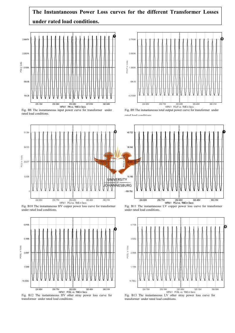
1
225.12M 259.35M 293.58M 327.81M 362.04M
WFM.1 PIN vs. TIME in Secs
2.8847K
2.2021K
1.5195K
836.88
154.26
PIN in Volts
1
224.92M 258.77M 292.62M 326.46M 360.31M
WFM.1 POUT vs. TIME in Secs
2.7760K
2.0820K
1.3880K
694.00
-4.2725M
POUT in Volts
1
224.92M 258.77M 292.62M 326.46M 360.31M
WFM.1 PCU vs. TIME in Secs
51.354
38.515
25.677
12.838
0
PCU in Volts
1
224.92M 258.77M 292.62M 326.46M 360.31M
WFM.1 PCU vs. TIME in Secs
40.722
30.542
20.361
10.180
-169.75U
PCU in Volts
1
224.92M 258.77M 292.62M 326.46M 360.31M
WFM.1 POSL vs. TIME in Secs
6.9195
5.1896
3.4597
1.7299
-10.252U
POSL in Volts
1
224.73M 258.19M 291.65M 325.12M 358.58M
WFM.1 POSL vs. TIME in Secs
4.7136
3.5352
2.3568
1.1784
14.782U
POSL in Volts
Fig. B8 The instantaneous input power curve for transformer under
rated load conditions.
Fig. B9 The instantaneous total output power curve for transformer under
rated load conditions.
Fig. B10 The instantaneous HV copper power loss curve for transformer
under rated load conditions.
Fig. B12 The instantaneous HV other stray power loss curve for
transformer under rated load conditions.
Fig. B11 The instantaneous LV copper power loss curve for transformer
under rated load conditions.
Fig. B13 The instantaneous LV other stray power loss curve for
transformer under rated load conditions.
The Instantaneous Power Loss curves for the different Transformer Losses
under rated load conditions.

1
225.12M 259.35M 293.58M 327.81M 362.04M
WFM.1 PEC vs. TIME in Secs
31.349
22.392
13.435
4.4784
-4.4784
PEC in Volts
1
224.54M 257.62M 290.69M 323.77M 356.85M
WFM.1 PEC vs. TIME in Secs
20.122
13.415
6.7075
81.539U
-6.7073
PEC in Volts
1
226.46M 259.54M 292.62M 325.69M 358.77M
WFM.1 PCORE vs. TIME in Secs
90.281
67.711
45.141
22.571
1.3046M
PCORE in Volts
The Instantaneous Power Loss curves for the different Transformer Losses
under rated load conditions.
Fig. B14 The instantaneous HV eddy current power loss curve for
transformer under rated load conditions.
Fig. B15 The instantaneous LV eddy current power loss curve for
transformer under rated load conditions.
Fig. B16 The instantaneous core power loss curve for the transformer
under rated load conditions.

1
223M 256M 290M 323M 357M
WFM.1 VPRI_HV' vs. TIME in Secs
544
272
0
-272
-544
VPRI_HV' in Volts
1
223M 258M 293M 327M 362M
WFM.1 V_LV vs. TIME in Secs
548
274
0
-274
-548
V_LV in Volts
1
2
216M 233M 250M 267M 284M
WFM.2 V(1905) vs. TIME in Secs
66.4
33.2
0
-33.2
-66.4
V(1905) in Volts
400
200
0
-200
-400
V(1906) in Volts
1
225M 259M 293M 326M 360M
WFM.1 I_EXC vs. TIME in Secs
1.18
588M
0
-588M
-1.18
I_EXC in Amps
1
225M 259M 293M 326M 360M
WFM.1 I_R vs. TIME in Secs
236M
118M
0
-118M
-236M
I_R in Amps
1
225M 259M 293M 326M 360M
WFM.1 I_M vs. TIME in Secs
1.17
584M
0
-584M
-1.17
I_M in Amps
The Transformer Model Verified with Harmonic loaded supply under rated
load conditions CASE 3. The graphic window range is: 0.2083s to 0.37497s
Fig. B2 The HV voltage referred to the LV side. Fig. B3 The LV voltage feeding the load.
Fig. B4 The excitation current seen from the LV side.
Fig. B5 The LV supply voltage and harmonic supply
voltage seen from the LV side.
Fig. B6 The core resistance current seen from the LV side. Fig. B7 The magnetising current seen from the LV side.

1
225M 259M 293M 326M 360M
WFM.1 PCU vs. TIME in Secs
54.0
40.5
27.0
13.5
7.00M
PCU in Volts
1
223M 257M 292M 326M 360M
WFM.1 PCU vs. TIME in Secs
44.2
31.6
19.0
6.32
-6.32
PCU in Volts
1
225M 258M 292M 325M 359M
WFM.1 POSL vs. TIME in Secs
6.04
4.53
3.02
1.51
0
POSL in Volts
1
225M 259M 293M 326M 360M
WFM.1 POSL vs. TIME in Secs
4.73
3.55
2.36
1.18
0
POSL in Volts
Fig. B8 The instantaneous input power curve for transformer under
rated load conditions.
Fig. B9 The instantaneous total output power curve for transformer under
rated load conditions.
Fig. B10 The instantaneous HV copper power loss curve for transformer
under rated load conditions.
Fig. B12 The instantaneous HV other stray power loss curve for
transformer under rated load conditions.
Fig. B11 The instantaneous LV copper power loss curve for transformer
under rated load conditions.
Fig. B13 The instantaneous LV other stray power loss curve for
transformer under rated load conditions.
The Instantaneous Power Loss curves for the different Transformer Losses
under rated load conditions.
1
225M 259M 293M 326M 360M
WFM.1 PIN vs. TIME in Secs
3.47K
2.60K
1.73K
868
1.80
PIN in Volts
1
225M 258M 292M 325M 359M
WFM.1 POUT vs. TIME in Secs
2.92K
2.19K
1.46K
730
0
POUT in Volts

1
225M 259M 293M 326M 360M
WFM.1 PEC vs. TIME in Secs
46.2
27.7
9.23
-9.23
-27.7
PEC in Volts
1
223M 257M 292M 326M 360M
WFM.1 PEC vs. TIME in Secs
31.4
18.8
6.28
-6.28
-18.8
PEC in Volts
1
229M 262M 296M 329M 362M
WFM.1 PCORE vs. TIME in Secs
95.1
67.9
40.7
13.5
-13.7
PCORE in Volts
Fig. B14 The instantaneous HV eddy current power loss curve for
transformer under rated load conditions.
Fig. B15 The instantaneous LV eddy current power loss curve for
transformer under rated load conditions.
Fig. B16 The instantaneous core power loss curve for the transformer
under rated load conditions.
The Instantaneous Power Loss curves for the different Transformer
Losses under rated load conditions.

1
227M 260M 294M 327M 360M
WFM.1 VPRI_HV' vs. TIME in Secs
492
246
0
-246
-492
VPRI_HV' in Volts
1
225M 259M 293M 326M 360M
WFM.1 V_LV vs. TIME in Secs
452
226
0
-226
-452
V_LV in Volts
1
2
218M 238M 258M 278M 298M
WFM.2 V(1906) vs. TIME in Secs
456
228
0
-228
-456
V(1906) in Volts
80.0
40.0
0
-40.0
-80.0
V(1905) in Volts
1
225M 258M 292M 325M 359M
WFM.1 I_EXC vs. TIME in Secs
1.08
540M
0
-540M
-1.08
I_EXC in Amps
1
225M 258M 292M 325M 359M
WFM.1 I_R vs. TIME in Secs
220M
110M
0
-110M
-220M
I_R in Amps
1
226M 258M 291M 323M 355M
WFM.1 I_M vs. TIME in Secs
984M
492M
0
-492M
-984M
I_M in Amps
Fig. B2 The HV voltage referred to the LV side. Fig. B3 The LV voltage feeding the load.
Fig. B4 The excitation current seen from the LV side. Fig. B5 The LV supply voltage and harmonic supply
voltage seen from the LV side.
Fig. B6 The core resistance current seen from the LV side. Fig. B7 The magnetising current seen from the LV side.
The Transformer Model Verified with Harmonic loaded supply under rated
load conditions CASE 4 The graphic window range is: 0.2083s to 0.37497s
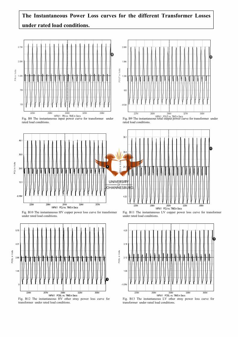
1
225M 258M 292M 325M 359M
WFM.1 PIN vs. TIME in Secs
2.73K
2.08K
1.43K
780
130
PIN in Volts
1
227M 260M 294M 327M 360M
WFM.1 POUT vs. TIME in Secs
2.66K
1.99K
1.33K
663
-813M
POUT in V
olts
1
225M 258M 291M 324M 357M
WFM.1 PCU vs. TIME in Secs
49.1
36.8
24.6
12.3
-8.16M
PCU in Volts
1
225M 258M 292M 325M 359M
WFM.1 PCU vs. TIME in Secs
39.1
30.4
21.7
13.0
4.33
PCU in V
olts
1
224M 257M 290M 322M 355M
WFM.1 POSL vs. TIME in Secs
5.75
4.31
2.88
1.44
0
POSL in Volts
1
225M 259M 293M 326M 360M
WFM.1 POSL vs. TIME in Secs
4.25
3.18
2.12
1.06
-1.07M
POSL in Volts
Fig. B8 The instantaneous input power curve for transformer under
rated load conditions.
Fig. B9 The instantaneous total output power curve for transformer under
rated load conditions.
Fig. B10 The instantaneous HV copper power loss curve for transformer
under rated load conditions.
Fig. B12 The instantaneous HV other stray power loss curve for
transformer under rated load conditions.
Fig. B11 The instantaneous LV copper power loss curve for transformer
under rated load conditions.
Fig. B13 The instantaneous LV other stray power loss curve for
transformer under rated load conditions.
The Instantaneous Power Loss curves for the different Transformer Losses
under rated load conditions.

1
225M 259M 293M 326M 360M
WFM.1 PEC vs. TIME in Secs
38.2
22.9
7.64
-7.64
-22.9
PEC in Volts
1
225M 259M 294M 328M 362M
WFM.1 PEC vs. TIME in Secs
29.6
17.7
5.91
-5.91
-17.7
PEC in Volts
1
225M 259M 293M 326M 360M
WFM.1 PCORE vs. TIME in Secs
97.5
73.9
50.3
26.7
3.10
PCORE in Volts
The Instantaneous Power Loss curves for the different Transformer Losses
under rated load conditions.
Fig. B14 The instantaneous HV eddy current power loss curve for
transformer under rated load conditions.
Fig. B15 The instantaneous LV eddy current power loss curve for
transformer under rated load conditions.
Fig. B16 The instantaneous core power loss curve for the transformer
under rated load conditions.
1
This circuit file covers all the cases with minor changes to the amplitudes, phase shifts and
frequency shown on page three of which the different supply configurations are defined.
FILENAME: TrfmHL.CIR
D:\SPICE4\TrfmHL
*SPICE_NET
.MODEL DIFF_001 d_dt(out_offset=0.0E+000 gain=450.16U out_lower_limit=-10.0 out_upper_limit=
+ 10.0 limit_range=1.0E-030)
.MODEL DIFF_002 d_dt(out_offset=0.0E+000 gain=2.65258M out_lower_limit=-10.0 out_upper_limit=
+ 10.0 limit_range=1.0E-030)
.MODEL SLEW_004 slew(rise_slope=350.0 fall_slope=350.0 )
.MODEL SLEW_005 slew(rise_slope=4.2K fall_slope=4.2K )
.MODEL DIFF_004 d_dt(out_offset=0.0E+000 gain=1.0 limit_range=1.0U)
.MODEL SLEW_003 slew(rise_slope=700.0 fall_slope=700.0 )
*INCLUDE DEVICE.LIB
*INCLUDE SYS.LIB
.TRAN 0.0001 0.37497 0.2083 0.0001 UIC
.OPTION VNTOL=1E-9 ABSTOL=1E-12 ITL4=100 ACCT
*INCLUDE AD5.LIB
*INCLUDE SWITCH.LIB
*INCLUDE CM1.LIB
.OPTION RELTOL=0.001
*ALIAS I(V55)=I_EXC
*ALIAS I(V54)=I_M
*ALIAS I(V56)=I_R
*ALIAS V(1862)=FLUXL_HV
*ALIAS V(1861)=FEXC
*ALIAS V(1867)=POUT
*ALIAS V(1868)=PIN
*ALIAS V(1865)=PCORE
*ALIAS V(1873)=PEC
*ALIAS V(1874)=PCU
*ALIAS V(1875)=PCU
*ALIAS V(1876)=PEC
*ALIAS V(1878)=I-HARM
*ALIAS V(1880)=POSL
*ALIAS V(1884)=POSL
*ALIAS V(1886)=I-HARM
*ALIAS V(1852)=I_LV
*ALIAS V(1850)=VPRI_HV'

2
.PRINT TRAN I(V55) I(V54) I(V56) V(1861)
.PRINT TRAN V(1867) V(1868) V(1865) V(1873)
.PRINT TRAN V(1874) V(1875) V(1876) V(1871)
.PRINT TRAN V(1891) V(1880) V(1881) V(1884)
.PRINT TRAN V(1888) V(1852) I(V59) V(1850)
.PRINT TRAN I(V60) V(1905)
V54 1806 1848 0
V55 1786 1806 0
V56 1806 1853 0
L14 1856 1859 2.4M
B87 1860 0 V=V(1850)
B88 1861 0 V=255*I(V55)
B89 1863 0 V=I(V54)
B90 1865 0 V=I(V56)*V(1806)
B91 1866 0 V=I(V59)
B92 1867 0 V=V(1850)*I(V60)
B93 1868 0 V=V(1852)*I(V59)
R66 1870 1856 1.203
R67 1871 1872 0.8942
B94 1873 0 V=I(V60)*(V(1786)-V(1859))
B95 1874 0 V=I(V59)*(V(1872)-V(1871))
B96 1875 0 V=I(V60)*(V(1856)-V(1870))
B97 1876 0 V=(V(1871)-V(1891))*I(V59)
X67 1866 1869 SDIFF K=1
X68 1863 1864 SDIFF K=1
X69 1860 1862 SINT K=1
B99 1877 0 V=I(V59)
B100 1880 0 V=I(V60)*(V(1870) - V(1850))
R68 1853 0 2014.4
B101 1848 0 V=(76709.406*V(1864))/(113.682 + (554.32*ABS(I(V54))))^2
B102 1859 1786 V=V(1888)
X70 1879 1881 GAIN K=1.1785
A51 1878 1882 DIFF_002
A52 1877 1878 DIFF_001
B103 1891 1871 V=V(1881)
R69 1850 1870 0.148
R70 1872 1852 0.0988
X71 1879 1883 GAIN K=5.8926
B104 1884 0 V=I(V59)*(V(1852)-V(1872))
A53 1882 1879 SLEW_005

3
B105 1885 0 V=I(V60)
X72 1887 1888 GAIN K=1.76777
A54 1886 1889 DIFF_002
A55 1885 1886 DIFF_001
X73 1887 1890 GAIN K=5.8926
A56 1889 1887 SLEW_005
[V59 1905 1852 SIN 0 -368 60 -0.0041666667: CASE 1] OR [V59 1905 1852 SIN 0 -372.9 60 -0.0041666667: CASE 2]
OR
[V59 1905 1852 SIN 0 -369.9 60 -0.0041666667: CASE 3] OR [V59 1905 1852 SIN 0 -374 60 -0.0041666667: CASE 4]
V60 1850 1855 0
B106 1855 0 I=V(1850)/65.03
[V66 0 1905 SIN 0 -77.309 300 -0.004273: CASE1] OR [V66 0 1905 SIN 0 -77.309 300 -0.004273: CASE2] OR [V66 0
1905 SIN 0 -77.309 300 -0.004273: CASE 3] OR [V66 0 1905 SIN 0 -77.309 300 -0.004273: CASE 4]
B126 1906 0 V=V(1852)-V(1905)
L13 1786 1891 1.1M
*ALIAS I(V21)=I_EXC
*ALIAS I(V20)=I_M
*ALIAS V(133)=I_LV
*ALIAS V(127)=VPRI_HV'
*ALIAS I(V22)=I_R
*ALIAS V(141)=FLUXL_HV
*ALIAS V(140)=FEXC
*ALIAS V(171)=PIN
*ALIAS V(172)=POUT
*ALIAS V(162)=PCORE
*ALIAS V(185)=PEC
*ALIAS V(187)=PCU
*ALIAS V(188)=PCU
*ALIAS V(190)=PEC
*ALIAS V(349)=I-HARM
*ALIAS V(1221)=POSL
*ALIAS V(1712)=POSL
*ALIAS V(1706)=I-HARM
.PRINT TRAN I(V21) I(V20) V(133) V(127)
.PRINT TRAN I(V22) I(V42) I(V23) V(140)
.PRINT TRAN V(143) V(128) V(171) V(172)
.PRINT TRAN V(162) V(185) V(187) V(188)
.PRINT TRAN V(190) V(126) V(590) V(348)
.PRINT TRAN V(349) V(10) V(1221) V(1629)
.PRINT TRAN V(1712) V(1705) V(1706) V(1707)

4
.PRINT TRAN V(1709)
V20 128 300 0
V21 593 128 0
V22 128 134 0
L7 136 1215 2.4M
V23 127 137 0
B24 139 0 V=V(133)
B25 140 0 V=255*I(V21)
B27 142 0 V=I(V20)
B29 162 0 V=I(V22)*V(128)
B37 171 0 V=V(133)*I(V42)
B38 172 0 V=V(127)*I(V23)
R18 174 136 1.203
R19 126 1677 0.8942
B40 185 0 V=I(V42)*(V(1215)-V(593))
B42 187 0 V=I(V23)*(V(126)-V(1677))
B43 188 0 V=I(V42)*(V(174)-V(136))
B44 190 0 V=(V(590)-V(126))*I(V23)
X14 142 143 SDIFF K=1
X16 139 141 SINT K=1
B46 137 0 I=V(127)/59
B49 348 0 V=I(V23)
V42 0 133 SIN 0 -360.62 60 -0.0041666667
B60 1221 0 V=I(V42)*(V(133) - V(174))
R52 134 0 2216.9
B64 300 0 V=(76709.406*V(143))/(113.682 + (554.32*ABS(I(V20))))^2
B67 593 1215 V=V(1709)
X53 10 1629 GAIN K=1.1785
A32 349 2 DIFF_002
A33 348 349 DIFF_001
B68 126 590 V=V(1629)
R56 133 174 0.148
R57 1677 127 0.0988
B74 1712 0 V=I(V23)*(V(1677)-V(127))
A43 2 10 SLEW_003
B86 1705 0 V=I(V42)
X64 1707 1709 GAIN K=1.76777
A47 1706 1714 DIFF_002
A48 1705 1706 DIFF_001
A50 1714 1707 SLEW_003

5
L6 593 590 1.1M
.END