ownership structure, bank performance, and … · dr. asri laksmi riani, se.ms, the head of...

i

OWNERSHIP STRUCTURE, BANK PERFORMANCE, AND RISK:

SOME INDONESIAN EVIDENCE

THESIS

Presented In A Partial Fullfilment Of Requirements For The Master Degree In

Master Of Management

Majoring in:

Financial Management

By:

YOHANA TAMARA

S411508020

POSTGRADUATE PROGRAM

MASTER OF MANAGEMENT

SEBELAS MARET UNIVERSITY

SURAKARTA

2017

ii

APPROVAL

OWNERSHIP STRUCTURE, BANK PERFORMANCE, AND

RISK: SOME INDONESIAN EVIDENCE

Prepared and Compiled by:

Yohana Tamara

NIM: S411508020

Approved by Advisor

On: 28th

February 2017

Advisor

Irwan Trinugroho S.E., M.Sc,. Ph.D

NIP. 198411062009121004

The Head of Magister Management Program

Sebelas Maret University

Prof. Dr. Asri Laksmi Riani, MS

NIP. 195901301986012001

iii

LEGITIMATION FROM THE BOARD OF EXAMINERS

OWNERSHIP STRUCTURE, BANK PERFORMANCE, AND

RISK: SOME INDONESIAN EVIDENCE

Compiled by

YOHANA TAMARA

S 411508020

This theses has been defended and examined by the Board of Examiners

On 31 March 2017

Board of Examiners Name Signature

Chairman :Prof. Dr. Asri Laksmi Riani, SE, M.Si

NIP. 195901301968012001

Examiner : Dr. Bambang Hadi Nugroho, M.Si

NIP. 195905081986011001

Advisor : Irwan Trinugroho, SE, M.Si, Ph.D

NIP. 198411062009121004

Director of PPS UNS Head of Magister

Management Program

Prof. Dr. M. Furqon Hidayatullah, M.Pd Prof. Dr. Asri Laksmi Riani, MS

NIP. 196007271987021001 NIP. 195901301968012001

iv

PRONOUNCEMENT

Name : Yohana Tamara

NIM : S 411508020

This is to certify that I wrote this thesis entitled “OWNERSHIP STRUCTURE,

BANK PERFORMANCE, AND RISK: SOME INDONESIAN EVIDENCE”. It

is not a plagiarism or made by others. Anything related to other’s work is written in

quotation, the source of which is listed in bibliography. If then this pronouncement

proves wrong. I am ready to accept any academic punishment, including withdrawal

or cancellation of my academic degree.

Surakarta, April 2017

Declared by,

Yohana Tamara

S. 411508020

v

MOTTO

“For nothing will be impossible with God”

-Luke 1 : 37-

“I can do all things through Christ who strengthens me”

-Philipians 4 : 13-

“God is my strength and power, and He makes my way perfect”

-2 Samuel 22:33-

“Family is not an important thing. It’s everything”

-Unknown-

vi

DEDICATION

Tuhan Yesus Kristus

For loving me perfectly, completely, and unconditionally,

Mr. and Mrs. Sabaradi

As the greatest gift from God,

Yohanes Prasetya Adi

My super handsome brother,

Mr. IrwanTrinugroho, SE, M.Si, Ph.D

My super advisor,

Magister Management Program Batch 45

vii

ACKNOWLEDGMENT

All praise and honor be to my beloved Jesus Christ who always gives bless,

mercy, love, grace and joy to the writer, so that the writer can finish the thesis with

the title : “OWNERSHIP STRUCTURE, BANK PERFORMANCE, AND RISK:

SOME INDONESIAN EVIDENCE” as a partial fullfilment of requirements for the

master degree in Master of Management program. Then the writer would like to

express her special gratitude to:

1. Prof Dr. Muhammad Furqon Hidayatullah, M.Pd, the Director of

Postgraduate Program of Universitas Sebelas Maret for giving permission to

conduct this research.

2. Dr. Hunik Sri Runing, the Dean of Economics and Business Faculty of

Universitas Sebelas Maret for giving permission to conduct this study.

3. Prof. Dr. Asri Laksmi Riani, SE.MS, the head of Magister Management

Program of Universitas Sebelas Maret who has given her recommendation

and opportunity to write this thesis.

4. Irwan Trinugroho, SE, M.Si. Ph. D, as Advisor for this research, for his

valuable insight, guidance and assistance during the whole process of this

thesis writing.

5. My colleagues at Magister Management Program batch 45, for the solidarity

and friendship during our course time.

6. The writer’s parent Daniel Sabaradi, S.E. and Rini Apriliawati S.E. as the

loveliest grace of God who always give prayers, support, and encouragement.

viii

7. My beloved brother, Yohanes Prasetya Adi, S.E. for the never ending support.

The writer accepts every comment and suggestion to make this thesis even

better, where it can be sent to the writer’s email address [email protected]

Hopefully, this thesis can gives benefit for future educational research.

The writer

Yohana Tamara

mailto:[email protected]

ix

TABLE OF CONTENT

Page

TITLE ...................................................................................................................... i

APPROVAL ............................................................................................................ ii

LEGITIMATION FROM THE BOARD OF EXAMINERS ................................. iii

PRONOUNCEMENT ............................................................................................. iv

MOTTO .................................................................................................................. v

DEDICATION ........................................................................................................ vi

ACKNOWLEDGEMENT ...................................................................................... vii

TABLE OF CONTENT .......................................................................................... ix

LIST OF TABLES .................................................................................................. xi

LIST OF FIGURE .................................................................................................. xii

ABSTRAK (INDONESIAN) .................................................................................. xiii

ABSTRACT (ENGLISH) ....................................................................................... xiv

CHAPTER I INTRODUCTION .......................................................................... 1

A. Research Background ......................................................................................... 1

B. Introduction to Problem Definition ................................................................... 6

C. Problem Definition and Research Question ...................................................... 9

D. Research Objectives .......................................................................................... 11

E. Research Contribution ....................................................................................... 12

F. Thesis Structure .................................................................................................. 13

G. Research Originality .......................................................................................... 14

CHAPTER II LITERATURE REVIEW ........................................................... 16

A. Ownership Structure .......................................................................................... 16

1. Stated- Owned Banks ................................................................................... 16

2. Regional Development Banks ...................................................................... 20

3. Private-Owned Banks ................................................................................... 20

4. Foreign Banks ............................................................................................... 23

B. Research Model And Hypothesis Development ............................................... 24

1. Foreign Banks ............................................................................................... 25

x

2. Bank Performance and Bank Risk Taking .................................................... 27

CHAPTER III METHODOLOGY ................................................................ 30

A. Data And Sample ............................................................................................... 30

B. Data Sources ....................................................................................................... 30

C. Variable Measurement ...................................................................................... 30

1. Dependent Variables ..................................................................................... 30

2. Independent Variables .................................................................................. 31

3. Control Variable ........................................................................................... 32

D. Data Analysis .................................................................................................... 32

1. Descriptive Statistics .................................................................................. 32

2. Classical assumption Tests ......................................................................... 33

3. Hypothesis Test .......................................................................................... 33

4. Robustness Check ...................................................................................... 34

CHAPTER IV DATA ANALYSIS ..................................................................... 36

A. Descriptive Statistics ......................................................................................... 36

B. Classical Assumption Tests ............................................................................... 38

1. Autocorrelation Test ..................................................................................... 38

2. Multicollinearity Test ................................................................................... 38

3. Heteroscedasticity Test ................................................................................. 39

C. Empirical Results .............................................................................................. 40

D. Robustness Check .............................................................................................. 45

E. Discussion ......................................................................................................... 49

1. State-Owned Banks ...................................................................................... 49

2. Regional Development Banks ...................................................................... 49

3. Foreign Banks ............................................................................................... 50

4. Robustness Check ......................................................................................... 52

CHAPTER V CONCLUSION, LIMITATION, AND SUGGESTION ........ 53

A. Conclusion ......................................................................................................... 53

B. Limitation And Suggestion ............................................................................... 55

REFERENCES ........................................................................................................ 56

xi

LIST OF TABLES

Page

Table 1.1The Map of Indonesian Banks Ownership Structures 2006-2015 ......... 3

Table 3.1 Table 3.1 Research Control Variables ................................................. 32

Table 4.1 Descriptive Statistics ............................................................................ 37

Table 4.2 Autocorrelation Test Results ................................................................ 38

Table 4.3 Multicollinearity Test Results I ........................................................... 39

Table 4.4 Multicollinearity Test Results II .......................................................... 39

Table 4.5 Regression Test Results Dependent Variable Profitability .................. 41

Table 4.6 Regression Test Results Dependent Variable Risk Taking ................. 44

Table 4.7 Robustness Check Results Dependent Variable Profitability ............... 46

Table 4.8 Robustness Check Results Dependent Variable Risk Taking .............. 48

xii

LIST OF FIGURE

Page

Figure 2.1 Research Model .................................................................................. 25

xiii

STRUKTUR KEPEMILIKAN, KINERJA BANK, DAN RISIKO: SEJUMLAH

BUKTI DI INDONESIA

Oleh :

Yohana Tamara

NIM S. 411508020

ABSTRAK

Penelitian ini bertujuan untuk secara empiris memeriksa kembali perbedaan

kinerja dan pengambilan risiko perbankan Indonesia pada berbagai struktur

kepemilikan. Struktur kepemilikan bank di Indonesia dibagi ke dalam lima kategori

utama, seperti: bank milik negara, bank pembangunan daerah, bank asing dan

campuran, bank domestik yang dimiliki oleh lembaga asing, dan bank domestik yang

dimiliki oleh institusi lokal. Kinerja Bank diukur dengan Return on Assets (ROA)

dan Return on Equity (ROE). Sementara pengambilan risiko bank diukur dengan nilai

Z-Score, yang dikembangkan oleh Boyd dan Graham (1986). Analisis dalam

penelitian ini juga mempertimbangkan karakteristik bank sebagai variabel kontrol,

meliputi: ukuran Bank, leverage Bank, dan loan to deposit ratio (LDR). Pengamatan

dalam penelitian ini melibatkan 110 bank komersial di Indonesia selama periode

2005-2013 dalam dataset bulanan. Metode analisis dalam penelitian ini menggunakan

metode Panel Least Square.

Beberapa hasil dapat disimpulkan dari analisis data: Pertama, kepemilikan

pemerintah Negara berpengaruh negatif terhadap profitabilitas bank yang diukur

dengan Return on Equity dan berpengaruh negative terhadap risiko bank yang diukur

dengan Z-Score ROA. Kedua, kepemilikan pemerintah daerah secara positif

mempengaruhi profitabilitas bank, baik ROE dan ROA; dan secara negatif

mempengaruhi pengambilan risiko bank yang diukur dengan Z-Score ROA.

Kepemilikan asing dan joint venture secara positif mempengaruhi profitabilitas bank,

baik Return on Equity (ROE) dan Return on Asset (ROA) dan juga berpengaruh

positif terhadap pengambilan risiko yang diukur dengan Z-Score ROE. Robustness

check juga telah dilakukan dalam penelitian ini yang menyimpulkan bahwa

kepemilikan asing secara keseluruhan lebih baik dari kepemilikan pemerintah secara

keseluruhan dalam hal kinerja dan pengambilan risiko.

Kata kunci: Struktur kepemilikan, Kinerja, Pengambilan Risiko, Return on Asset,

Return on Equity, Z-Score.

xiv

OWNERSHIP STRUCTURE, BANK PERFORMANCE, AND RISK: SOME

INDONESIAN EVIDENCE

By:

Yohana Tamara

NIM S. 411508020

ABSTRACT

This study aims to empirically re-examine the performance and risk taking

differences of Indonesian banks across ownership structure. The ownership structures

of Indonesian banks are disentangled into five main categories, such as: State-owned

banks, regional development banks, foreign and joint venture banks, domestic banks

owned by foreign institutions, and domestic banks owned by local institutions. Bank

performance is measured by Return on Assets (ROA) and Return on Equity (ROE).

While the risk-taking of banks is measured by the value of Z-Score, proposed by

Boyd and Graham (1986). The analysis in this study is also considering the

characteristics of the bank as a control variable, includes: bank size, bank leverage,

and loan to deposit ratio (LDR). The observation in this study involved 110

commercial banks in Indonesia over the period of 2005 to 2013 in monthly dataset.

The method of analysis in this study is using Panel Least Square method.

Several results can be concluded from the data analysis: First, state-ownership

negatively affects banks profitability as measured by Return on Equity and negatively

affects bank risk taking measured by Z-Score ROA. Second, regional government

ownership positively affects banks profitability, both ROE and ROA; and negatively

affects bank risk taking measured by Z-Score ROA. Foreign banks and joint venture

banks, positively affect banks profitability, both Return on Equity (ROE) and Return

on Asset (ROA) and also positively affects bank risk-taking as measured by Z-Score

ROE. Robustness test have also been performed in this study which concluded that

foreign ownership as a whole are better than government ownership as a whole in

terms of performance and risk taking.

Keywords: Ownership structure, Performance, Risk Taking, Return on Asset, Return

on Equity, Z-Score

1

CHAPTER I

INTRODUCTION

A. Research Background

Banking sector is one of the most vital sectors that form the economic

structure of a country. Banks and the banking industry, as a major player in

economic sector, have function as an intermediary institution in financial

sector that has an important role in the economy of the State. In micro level,

banks functioning channel funds from the client who have excess funds to

businesses and individuals who need funds in order to facilitate the efforts of

the parties concerned. The function of the banking industry on micro level in

Indonesia is stated in Undang- Undang No. 10 tahun 1998 about Banking, in

which commercial banks are defined as "Bank conducting conventional

business or based on sharia principles, which in its activities providing

services in payment transactions, including credit." In addition, the banking

sector also plays a role in control mechanism of the firms, as the party which

monitors the performance of the firm, and plays an important role in corporate

governance through the enforcement of contracts and the support of the

payment system (Levine, 1997). At the macro level, the banking industry

serves as a source of financing for economic development and as a tool in the

implementation of monetary policy.

The banking industry is growing rapidly in developing countries, such

as Indonesia. Especially the impact of post-crisis monetary policy in 1997-

2

1998 resulted major changes on the banking conditions in Indonesia. There

are at least three policies implemented by Indonesian Government along with

Bank Indonesia to strengthen the banking sector in Indonesia: First, a policy

related to the privatization conducted by the government for the private banks

which follows the restructuring program and the provision of bail out funds

thus many private banks belong to the government. Second, the policy stated

in Peraturan Pemerintah Nomor 29 Tahun 1999 which regulates about

Purchase of Shares in Commercial Bank, in which foreign investors can take

control of up to 99% stake in Indonesian bank, thus it can attract many

foreign investors to invest in Indonesia's banking sector. Third, the policy of

the Central Bank (Bank Indonesia) associated with the increase in the

minimum capital of banks, so the banks with limited capital will face two

choices: raising capital or selling its shares to investors. All these policies

affect the composition of ownership in Indonesian banks. There are a large

number of banks in Indonesia, with varying ownership structures. In general,

the ownership structures of Indonesian banks are divided into five categories:

State-owned banks, regional development banks, foreign and joint venture

banks, domestic banks owned by foreign institutions, and domestic banks

owned by local institutions. Based on the Statistik Perbankan Indonesia (SPI)

issued by the Otoritas Jasa Keuangan (OJK), a map of Indonesian banks

ownership structures for 10 years (in 2006-2015) are as follows:

3

Table 1.1The Map of Indonesian Banks Ownership Structures 2006-2015

OWNERSHIP

2006 2007 2008 2009 2010 2011 2012 2013 2014 2015

State-Owned Banks 5 5 5 5 4 4 4 4 4 4

Regional Development

Banks

26 26 26 26 26 26 26 26 26 26

Foreign-Owned Banks 11 11 10 10 10 10 10 10 10 10

Joint Venture Banks 17 17 15 16 15 14 14 14 12 11

Domestic Private-Foreign 35 35 32 34 36 36 36 36 38 38

Domestic Private-Non

Foreign

36 36 36 31 31 30 30 30 29 27

TOTAL BANKS 130 130 124 121 122 120 120 120 119 118

Source : Statistik Perbankan Indonesia (2006-2015)

4

The issue of ownership structure is very important for the banking

industries because several factors interact with and alter governance, such as

the quality of bank regulation and supervision. Moreover, as an intermediary

institution, bank in its operations use more funds from the public compared to

their own capital or capital raised from shareholders. These conditions

encourage related parties involved in the banking sector conduct an

assessment of the health of banks. One of the main indicators that can be used

as the basis of assessment is the bank's financial statements. By using various

financial ratios obtained from the financial statements of banks, both public

and investors can determine the performance and the level of risk of the bank,

so that the security guarantees for the funds invested can be measured.

Profitability is an appropriate indicator to measure the financial

performance of a bank. Generally, profitability is the company's ability to earn

income from its business activities. Profitability measurement that is generally

used in banking industry is Return on Assets (ROA) and Return on Equity

(ROE). Return on Asset (ROA) refers to the measurement of the bank's

efficiency and effectiveness in generating profits through the utilization of the

assets owned. Bank Indonesia and many previous researches attach more on

the assessing of Return on Asset (ROA) compared with Return on Equity

(ROE), for the calculation of the profitability by ROA measured through

assets, which mostly come from public funds deposits.

5

Another parameter that can be appropriately used to measure the

financial strength of banks is the bank's risk assessment. Based on Peraturan

Dewan Gubernur Bank Indonesia BI No. 11/8/PDG/2009 about Risk Based

on Bank Supervision, risk is defined as the potential occurrence of an event

that causes damage to the bank. Bank risks arise as a result of the occurrence

of events that are negative and undesirable. An indicator that can be properly

used to measure the risk of bank is calculating the value of the Z-Score (Boyd

and Graham, 1986). Z- Score, is one form of financial analysis, which used to

predict the probability of failure of the banks. Higher values of Z-Score imply

lower probabilities of banks failure. The calculation of Z- Score in this

research is using the average and standard deviation of banks profitability,

which are measured by Return on Asset (ROA) and Return on Equity (ROE).

This study aims to empirically re-examine the performance and risk

taking differences of Indonesian banks across ownership structure. The

ownership structure of Indonesian banks are disentangled into five main

categories such as State-owned banks, regional development banks, foreign

and joint venture banks, domestic banks owned by foreign institutions, and

domestic banks owned by local institutions. Bank performance is measured by

Return on Assets (ROA) and Return on Equity (ROE). While the risk-taking

of banks is measured by the value of Z-Score, proposed by Boyd and Graham

(1986). The analysis in this study is also considering the characteristics of the

6

bank as a control variable, includes: bank size, bank leverage, and loan to

deposit ratio (LDR).

Ownership structure is an important component that determines the

success of an institution. Therefore, the ownership structure becomes an

important topic for academic explorations and policy making. Several

previous studies that support this research is conducted by Alejandro Micco

(2007) concerning Bank Ownership and Performance, which focused

observations on profitability at state banks and private banks, where the

ownership of private banks is divided into two categories : foreign-owned

banks and local investors-owned banks. Furthermore, other literature that

supports this research was conducted by Boubakri et al. (2005) about

Privatization and Bank Performance in Developing Country, which focuses

observation on profitability, efficiency, credit risk, and capital adequacy at the

bank with the ownership structure divided into four categories: The

Government, Foreign, Industrial Groups, and Individual. Based on this

background, the researcher took the research titled: “OWNERSHIP

STRUCTURE, BANK PERFORMANCE, AND RISK: SOME

INDONESIAN EVIDENCE”

B. Introduction to Problem Definition

The banking sector, which is a major player in economic sector, is one

of the most vital sectors that form the economic structure of a country. The

banking industry is growing rapidly in a country with the characteristics of an

7

emerging economy, like Indonesia. There are a large number of banks in

Indonesia, particularly as a result of post-crisis monetary policies in 1997-

1998 which bring a profound impact on the banking conditions in Indonesia.

Based on the data stated above, there are major changes in banks ownership

structure as a result of those policies. Privatization has minimized the number

of banks owned by the government and encouraged the growing of private

banks, both owned by local and foreign institutions. Besides, foreign and joint

venture banks are also growing rapidly in Indonesia.

Boubakri (2005) stated that privatization of the banking sector,

particularly in countries characterized by emerging economies, are often

accompanied by a process called "Financial Liberalization" that

fundamentally change the way financial sector managed. Those process can

affect the value of the bank, the growth opportunities, risk exposure of banks,

and hence the performance of banks. If the privatization process is

unsuccessful, it can result in a loss to many parties, especially the depositor,

which eventually will lead to financial crisis. As already known, bank is an

intermediary institution, which in its operations use more funds from the

public compared to their own capital or capital raised from shareholders.

These conditions encourage related parties involved in the banking sector

conduct an assessment of the health of banks.

Ownership structure in banking sector becomes an interesting and

important topic for academic explorations and policy making, especially when

it is associated with performance and risk taking differences across many

8

kinds of ownership structures. Several previous studies with various results

have concerned about ownership structures. First, previous research

conducted by Linqiang Huang and Sheng Xiao (2012), explained about how

government ownership affects firm performance. This study concluded that

the profitability of the firm, as measured by Return on Sales (ROS) is

negatively affected by the government ownership. This research stated that

privatization, which lower the government ownership can improve firm’s

performance as a result.

This study result is supported by another prior study conducted by

Alejandro Micco (2007) concerning Bank Ownership and Performance, which

focused observations on profitability at the government-owned banks and

private banks, which the ownership of private banks is divided into two

categories: foreign-owned banks and local investors-owned bank. This study

concluded several results: First, State-Owned Bank located in developing

countries tend to have profitability (measured by Return on Asset) much

lower (0.9% lower) than domestic privately owned bank. Second, foreign

bank located in developed countries tend to be more profitable (0.37% higher)

than private domestic bank.

Previous study conducted by Boubakri (2005) provides a contrast view

for this topic. This study is about Privatization and Bank Performance in

Developing Country, which focuses observation on profitability, efficiency,

credit risk, and capital adequacy at the bank with the ownership structure

divided into four categories: The Government, Foreign, Industrial Groups,

9

and Individual. Several results are concluded: First, privatization is not

significantly improved bank performance, because when the government

relinquishes control, profitability gains are lower. Second, foreign control in

ownership is not significantly affected profitability, and the result associated

with bank risk-taking, the credit risk (measured by Non-Performing Loans

Ratio) in foreign-owned banks is lower than domestic private banks.

A wide range of variations of the previous study results about this

issue make it more interesting to analyze, particularly in the context of the

banking sector in Indonesia. This study provides better insight for the

development of topics related to ownership structure of the bank. In addition

to comprehensively divided bank ownership structure into five main

categories (state-owned banks, regional development banks, foreign and joint

venture banks, domestic banks owned by foreign institutions, and domestic

banks owned by local institutions), this study focuses not only on the

profitability differences across the ownership structure (as measured by ROA

and ROE), but also focuses on the risk taking of each ownership structure,

which measured by the value of Z-Score, as proposed by Boyd and Graham

(1986), which indicates the probability of failure of a given bank. This study

also concern bank characteristics as a control variable include: bank size, bank

leverage, and loan to deposit ratio (LDR).

C. Problem Definition and Research Question

The majority of previous studies regarding with the relationship

between the ownership structure on bank performance and risk taking shows

10

varying results. Research conducted by Linqiang Huang and Sheng Xiao

(2012), about how government ownership affects firm performance,

concluded that the profitability of the firm, as measured by Return on Sales

(ROS) is negatively affected by the government ownership. This study result

is supported by another prior study by Alejandro Micco (2007) regarding

Bank Ownership and Performance, which concluded several results : First,

State-Owned Bank located in developing countries tend to have profitability

(measured by Return on Asset) much lower (0,9% lower) than domestic

privately owned bank. Second, foreign bank located in developed countries

tend to be more profitable (0.37% higher) than private domestic bank.

Another prior study by Rafael La Porta (2002) regarding with

Government Ownership of Banks also stated that higher government

ownership is associated with slower financial development, lower growth of

per capita income, and productivity. Related with bank risk taking, two prior

studies, conducted by Mahmud Hossain (2013) and Alejandro Micco (2006)

reported similar results: state-owned bank plays “smoothing” role. Public

bank managers are lack of incentives to make profit, so they do not

aggressively look for lending opportunities and tends to act to minimize the

risk. This study shows that state-owned bank lending is less responsive to

macroeconomic shocks than the lending of private banks (both domestically

and foreign-owned banks).

In contrast, prior study conducted by Boubakri (2005) about

Privatization and Bank Performance in Developing Country, concluded

11

several result: First, privatization is not significantly improved bank

performance, because when the government relinquish control, profitability

gain is lower. Second, foreign control in ownership is not significantly

affected profitability, and the result associated with bank risk-taking, the

credit risk (measured by Non-Performing Loans Ratio) in foreign-owned

banks is lower than domestic private banks. Hence, based on the discussion

above, the formulation of the research problem is:

What is the effect of bank ownership structure, which divided into five

categories: State-owned banks, regional development banks, foreign and joint

venture banks, domestic banks owned by foreign institutions and domestic

banks owned by local institution on bank performance and risk taking in

Indonesia?

D. Research Objectives

First, this study is aimed to present cross sectional data to provide

better insight about the effect of Ownership Structure on Bank Performance,

which is measured by Return on Asset (ROA) and Return on Equity (ROE) in

Indonesian Commercial Banks. Bank characteristics are concerned as control

variables, include: bank size, bank leverage, and loan to deposit ratio (LDR).

Secondly, this study is aimed to improve the understanding on the

effect of Ownership Structure on Risk Taking, which is measured by the value

of Z-Score (Z-Score ROA and also Z-Score ROE), reflecting the probability

of failure in Indonesian Commercial Banks. Bank characteristics are

12

concerned as control variables, including: bank size, bank leverage, and loan

to deposit ratio (LDR).

Thirdly, this study is meant to provide better insight for the policy-

maker associated with the establishment of the optimal ownership structure, to

improve the banking sector in Indonesia.

E. Research Contribution

Ownership structure is an important component that determines the

success of an institution. Therefore, the ownership structure becomes an

important topic for academic explorations and policy making. The current

study contributes to improve understanding of how bank ownership structure

could affect bank performance and also bank risk-taking. Specifically in

Indonesian context where the impact of post-crisis monetary policy in 1997-

1998 resulting major changes on the banking conditions in Indonesia. The

financial liberalization policy in Indonesia impacts on the large number of

banks in Indonesia with varying ownership structures. Hence, it is important

to develop a literature that provides an understanding associated with

comparison of various types of bank ownership structure in Indonesia. This

study extends previous research in examining how bank ownership structure,

which divided into five categories: State-owned banks, regional development

banks, domestic banks owned by foreign institutions, domestic banks owned

by local institutions, foreign banks and joint venture banks can affect bank

performance and bank risk-taking. Furthermore, this study provides empirical

13

evidence and more insight related to the type of banks ownership structure in

Indonesia which is the best in terms of performance and risk-taking.

This research also contributes in managerial practice, specifically to

improve the condition of banking sector in Indonesia. With the results

presented in this study, government and managers can be helped in making

decisions related to the establishment of optimal ownership structure. The

results showed that foreign ownership is the best type of ownership structure,

in terms of profitability and risk taking. Therefore, bank needs to consider the

entry of foreign investors to improve various aspects of the bank's policy, in

order to improve the overall performance of the bank. The presence of foreign

investor may improve the quality and availability of financial services and the

adoption of modern banking skills and technology (Levine, 1997).

Particularly for state-owned banks, which this research and also the previous

researches have proven that state government ownership is the least optimal

type of ownership; need to consider to reduce the dominance of government

ownership and increase the foreign ownership.

F. Thesis Structure

The second chapter of this thesis consists of a number of literature

studies and previous researches regarding ownership structure on bank

performance and risk taking. This chapter is also including the theoretical

framework of this study along with the short introduction and hypotheses

development.

14

Chapter three of this study contains the research design, which

includes conceptual framework model, methodology, data collection

techniques, variables measurement, and data analysis techniques.

Afterward, the fourth chapter shows the research study. This chapter

consists of the descriptive study, classical assumption tests, and logistic

regression analysis on the variables. Last but not least, chapter five presents

the conclusion, research limitation, and recommendations for future

researches.

G. Research Originality

Although some previous studies have paid special attention to this

topic, this research provides insight for the development of topics related to

ownership structure of the bank. First, this study divides the ownership

structure of banks into five comprehensive detailed categories. Government-

owned banks are divided into two categories: State-owned banks (Bank

Pemerintah) and regional development banks (Bank Pembangunan Daerah).

Domestic private banks are divided into two categories: domestic banks

owned by foreign institutions, and domestic banks owned by local

institutions; Also there are foreign and joint venture banks. Second, the

observations in this study not only focuses on variable performance of the

bank as measured by Return on Assets (ROA) and Return on Equity, but also

observes banks risk taking in various ownership structure as measured by the

value of Z-Score, proposed by Boyd and Graham (1986) which divided into

Z-Score ROA and Z-Score ROE to describe the probability of failure. Third,

15

this study involved bank characteristics as aspects to be considered as a

control variable, include bank size, bank leverage, and loan to deposit ratio

(LDR). Furthermore, the study is using 110 commercial banks in Indonesia

over the period of 2005-2013.

16

CHAPTER II

LITERATURE REVIEW

A. OWNERSHIP STRUCTURE

It is clearly known that institutions evolve to capture economic gains.

A way that institutions do to maximize their economic benefit is through the

ownership structure, thus it becomes an essential component of economic and

political institutions. Ownership structure is a reflection of good corporate

governance which refers to the process and structure used to direct and

manage the company's business activities in order to enhance shareholder

value and wealth.

1. Stated- Owned Banks

Micco (2007) defined state-owned banks as banks with government

ownership exceed 50%. Post-crisis policies made by Government along

with Bank Indonesia in 1997- 1998 provided dramatic changes in

Indonesian banking sector. This policy led to the development of

privatization, both by domestic institutions and foreign institutions, which

is identical to financial liberalization in the banking sector (Boubakri,

2005). Surprisingly, despite the financial liberalization policy has been

widely adopted, government ownership of banks remained prominent in

many countries, especially in countries characterize with developing

economies. Previous study stated that countries in Asia-Pacific region are

17

known for higher government intervention in economy and particularly in

the banking sector. (Hossain, et al. 2013)

Several previous researches have focused the observations on state-

owned banks provided various results. Previous study conducted by

Linqiang Huang and Sheng Xiao (2012), explained about how government

ownership affects firm performance. This study concluded that the

profitability of the firm, as measured by Return on Sales (ROS) is

negatively affected by the government ownership. This research stated

that privatization, which lower the government ownership can improve

firm’s performance as a result.

Results concluded by Linqiang Huang (2012) is supported by another

prior study conducted by Alejandro Micco (2007) concerning Bank

Ownership and Performance, which focused observations on profitability

at the government-owned banks and private banks. This study concluded

that state-owned bank located in developing countries tend to have

profitability (measured by Return on Asset) much lower (0,9% lower)

than domestic privately owned bank. Paolo Sapienza (2004) argued that

profitability is not enough be used as a measurement of the success of

banks, because in addition to gain profit, state-owned banks aim to

maximize broader social objectives.

Another study conducted by Allen, et al. (2009) regarding Bank

Ownership and Efficiency in China concluded several findings: First, state

owned banks, in the context of the central government bank which holds a

18

majority market share in China (The Chinese Big Four State Owned

Banks) have the lowest level of proft efficiency compared to other types

of banks. Second, in terms of cost efficiency, state owned banks are the

most cost efficient banks, since state owned banks spend less on loans

monitoring activities and the process of screening and investigating

potential borrowers. That's why, state owned banks are considered as the

most efficient bank, but has the highest level of credit risk, as measured by

NPL.

Related with bank risk taking, two prior studies, conducted by

Mahmud Hossain (2013) and Alejandro Micco (2006) reported similar

results: state-owned bank plays “smoothing” role. Public bank managers

are lack of incentives to make profit, so they do not aggressively look for

lending opportunities and tends to act to minimize the risk. This study

shows that state-owned bank lending is less responsive to macroeconomic

shocks than the lending of private banks (both domestically and foreign-

owned banks). Paolo Sapienza (2004) reported that state-owned banks

charge lower interest rate than foreign-owned banks in terms of risk

minimizing (44 basis points lower). Based on these studies, state-owned

banks play “smoothing” role and stabilize their lending policy over the

following reasons:

a. The principal (states) obtained multiple benefits of a more stable

macroeconomic environment.

19

b. The implementation of stable lending policies will be able to minimize

the risk of bank failures that are more likely happened during

recessions.

c. Public bank managers are lack of incentives to make profit, so they do

not aggressively look for lending opportunities and tends to act to

minimize the risk.

d. There is a possibility of political influence in the lending policy in

state-owned banks.

(Alejandro Micco, Ugo Panizza, 2006)

In contrast, there is prior study conducted by Boubakri (2005) about

Privatization and Bank Performance in Developing Country, which

focuses observation on profitability, efficiency, credit risk, and capital

adequacy at the bank, with the ownership structure divided into four

categories: The Government, Foreign, Industrial Groups, and Individual.

This study concluded privatization is not significantly improved bank

performance, which is measured by Return on Equity (ROE) because

when the government relinquished control, profitability gain is lower.

Second, government control in ownership is associated with low risk-

taking policies, compared with private control in ownership, because the

management is focused on bank survival.

20

2. Regional Development Banks

If the state- owned banks are government banks within the scope of

central government, regional development banks are banks with the scope

of local (regional) area. Capital stock of regional development banks

majority owned by the local government. According to Undang-Undang

Nomor 13 tahun 1962, regional development banks are banks established

to assist the central government in financing national development efforts,

functioning to help the implementation of economic development evenly

distributed throughout all regions in Indonesia. Regional development

banks work as regional economic development and enhance the local

economic development, to improve people's lives as well as provide

financing in regional financial development, raise funds, carry out and

save the local treasury, in addition to run the banking services. Several

previous researches about government bank focused observations on

government bank in a country level. This study divides government

ownership into two categories, at the level of state government and local

governments and also aims to see the difference between both categories.

3. Private-Owned Banks

Micco (2007) classified private-owned banks as those banks more than

50% of the shares owned by private sector, both domestic and foreign

institutions. Privatization of the banking sector is a mechanism that

emerged in developing countries, such as Indonesia, especially since the

post-crisis policy in 1997-1998. Boubakri (2005) stated that privatization

21

of the banking sector, particularly in countries characterized by emerging

economies, is often accompanied by a process called "Financial

Liberalization" that fundamentally change the way financial sector

managed. Those process can affect the value of the bank, the growth

opportunities, risk exposure of banks, and hence the performance of

banks. If the privatization process is unsuccessful, it can result in a loss to

many parties, especially the depositor, which eventually will lead to

financial crisis.

Previous literatures have provided various results regarding with

privately owned banks. Prior study conducted by Alejandro Micco (2007)

concerning Bank Ownership and Performance, focused observations on

profitability at the government-owned banks and private banks, which the

ownership of private banks is divided into two categories: foreign-owned

banks and local investors-owned bank. This study concluded several

results: First, State-Owned Bank located in developing countries tend to

have profitability (measured by Return on Asset) much lower (0.9%

lower) than domestic privately owned bank. Second, foreign bank located

in developed countries tend to be more profitable (0.37% higher) than

private domestic bank. These results indicate that in order to maximize the

profitability of private banks, the selection of the ownership structure,

foreign versus local investors play important role.

Another prior study conducted by Boubakri (2005) about Privatization

and Bank Performance in Developing Country, which focuses observation

22

on profitability, efficiency, credit risk, and capital adequacy at the bank,

with the ownership structure divided into four categories: The

Government, Foreign, Industrial Groups, and Individual. This study

concluded several results: First, privatization is not significantly improved

bank performance, which is measured by Return on Equity (ROE) because

when the government relinquished control, profitability gain is lower.

Second, foreign control in ownership is not significantly affected

profitability, and the result associated with bank risk-taking, the credit risk

(measured by Non-Performing Loans Ratio) in foreign-owned banks is

lower than domestic private banks. This study also concluded that banks

with local institutional ownership control have the highest risk exposure,

especially related with credit risk and interest rate.

In order to measure the performance and risk taking of private banks,

the ownership structure of private bank (owned by foreign institutions or

domestic) play an important role. Previous research conducted by Allen et

al. (2009) related to Bank Ownership and Efficiency in China divided

bank ownership structure into four categories: The Big Four State Owned

Banks, State Owned Banks Non-Big Four, Majority Private Domestic

Banks, Majority Private Foreign Banks. This study concluded that: First,

foreign banks have the highest level of profit efficiency followed by

private domestic banks in the second rank. Second, adding a minority

foreign ownership can improve profit and cost efficiency, both on state

owned banks and the domestic private banks. For example, when the state

23

owned bank added minority foreign ownership, the profit efficiency level

increased by 20% and the cost efficiency level increased by 30%. This

study suggested management to reduce state ownership and increase

foreign ownership.

4. Foreign Banks

Previous study by Enrica and Poonam (2006) defined foreign banks

as: “Banks with fully owned subsidiaries of foreign institutions or

domestic banks in which a foreign institution holds a controlling share”.

As a result of financial liberalization in banking industry, foreign banks

have a great opportunity to develop, particularly in countries characterized

with emerging market. Levine (1997) also argued that financial

liberalization which allows the entry of foreign banks may bring multiple

benefits:

a) The presence of foreign banks may improve the quality and

availability of financial services and the adoption of modern banking

skills and technology.

b) Foreign banks may stimulate the development of a bank supervisory

and legal framework.

c) It may help to enhance a country’s access to international capital.

In line with Levine (1997), study conducted by Enrica and Poonam (2006)

concluded that foreign banks performed significantly better (in terms of

24

profitability and Net Interest Margin) than domestic banks. This due to

several reasons:

1. Foreign banks are more profitable and efficient than domestic banks

because they have to deal with more intense competition in the global

market. This condition encourages foreign banks to apply better

regulation and supervision mechanisms than the domestic bank with a

narrower scope of competition.

2. Foreign banks are better capitalized because it is easier for them to

raise capital and liquid funds from international financial markets.

Furthermore, it is easier for the foreign banks to raise capital fund

from their parent bank.

3. Foreign banks operating in a wide international scope so that they are

considered to be more reputable.

4. Foreign banks tend to implement more sophisticated risk management

technique and better system of internal control.

5. Foreign banks may be less amenable to political pressure.

B. RESEARCH MODEL AND HYPOTHESIS DEVELOPMENT

This study aimed to identify the effect of ownership structure on the

performance and risk taking of Indonesian banks. The bank's performance in

this study was measured by Return on Assets (ROA) and Return on Equity

(ROE). Brigham (2006) defined Return on Asset (ROA) as the measurement

of the bank's efficiency and effectiveness in generating profits through the

25

utilization of the assets owned. Meanwhile, Return on Equity (ROE) refers to

the measurement the bank's ability to generate profits through equity capital

owned. Figure 2.1 below shows the research model of this thesis:

Figure 2.1 Research Model

1. Bank Ownership on Bank Performance

Previous study regarding bank ownership structure and bank

performance is conducted by Alejandro Micco (2007), which focused

observations on profitability at state banks and private banks, where the

ownership of private banks is divided into two categories: foreign-owned

banks and local investors-owned banks. This study concluded that state-

owned bank located in developing countries tend to have profitability

(measured by Return on Asset) much lower (0.9% lower) than domestic

OWNERSHIP

STRUCTURES

1. State Owned Banks

2. Regional Development

Banks

3. Foreign and Joint

Venture Banks

4. Domestic Banks By

Local Institution

5. Domestic Banks by

Local Institution

BANK RISK

1. Z-Score ROA

2. Z-Score ROE

BANK

PERFORMANCE

1. Return on Asset

2. Return on Equity

CONTROL

VARIABLES:

1. Bank Size

2. EQTA

3. LDR

26

privately owned bank. Another previous study conducted by Linqiang

Huang and Sheng Xiao (2012), explained about how government

ownership affects firm performance. This study concluded that the

profitability of the firm, as measured by Return on Sales (ROS) is

negatively affected by the government ownership.

Another study conducted by Allen, et al. (2009) regarding Bank

Ownership and Efficiency in China also concluded that state owned

banks, in the context of the central government bank which holds a

majority market share in China (The Chinese Big Four State Owned

Banks) have the lowest level of proft efficiency compared to other types

of banks.

Meanwhile, if the state- owned banks are government banks within the

scope of central government, regional development banks are banks with

the scope of local (regional) area. Several previous researches about

government bank focused observations on government bank in a country

level. This study divides government ownership into two categories, at the

level of state government and local governments and also aims to see the

difference between both categories.

Previous study conducted by Alejandro Micco (2007) also concluded

that private foreign bank located in developed countries tend to be more

profitable (0.37% higher) than private domestic bank. In order to measure

the performance and risk taking of private banks, the ownership structure

of private bank (owned by foreign institutions or domestic) play an

27

important role. Previous research conducted by Allen et al. (2009) related

to Bank Ownership and Efficiency in China divided bank ownership

structure into four categories: The Big Four State Owned Banks, State

Owned Banks Non-Big Four, Majority Private Domestic Banks, and

Majority Private Foreign Banks. This study concluded that: First, foreign

banks have the highest level of profit efficiency followed by private

domestic banks in the second rank. Second, adding a minority foreign

ownership can improve profit and cost efficiency, both on state owned

banks and the domestic private banks. For example, when the state owned

bank added minority foreign ownership, the profit efficiency level

increased by 20% and the cost efficiency level increased by 30%. In line

with Allen et al. (2009) study conducted by Enrica and Poonam (2006)

concluded that foreign banks performed significantly better (in terms of

profitability and Net Interest Margin) than domestic banks

Therefore:

H1 : Different ownership structures imply different levels of

profitability as measured by Return on Asset and Return on

Equity.

2. Bank Performance and Bank Risk Taking

An indicator that can be properly used to measure the risk of bank is

calculating the value of the Z-Score (Boyd and Graham, 1986). Z- Score,

28

is one form of financial analysis, which used to predict the probability of

failure of the banks. Higher values of Z-Score imply lower probabilities of

banks failure. The calculation of Z- Score proposed by Boyd and Graham

(1986) is using the average and standard deviation of banks profitability,

which are measured by Return on Asset (ROA) and Return on Equity

(ROE).

Related with bank risk taking, two prior studies, conducted by

Mahmud Hossain (2013) and Alejandro Micco (2006) reported similar

results: state-owned bank plays “smoothing” role. Public bank managers

are lack of incentives to make profit, so they do not aggressively look for

lending opportunities and tends to act to minimize the risk. This study

shows that state-owned bank lending is less responsive to macroeconomic

shocks than the lending of private banks (both domestically and foreign-

owned banks). Paolo Sapienza (2004) reported that state-owned banks

charged lower interest rate than foreign-owned banks in terms of risk

minimizing (44 basis points lower).

In line with Paolo Sapienza (2004), in terms of cost efficiency, Allen

et al (2009) concluded that state owned banks are the most cost efficient

banks, since state owned banks spend less on loans monitoring activities

and the process of screening and investigating potential borrowers. That's

why, state owned banks are considered as the most efficient bank, but has

the highest level of credit risk. Another prior study conducted by Boubakri

(2005) about Privatization and Bank Performance in Developing Country

29

developed a conclusion associated with bank risk-taking, the credit risk

(measured by Non-Performing Loans Ratio) in foreign-owned banks is

lower than domestic private banks. This study also concluded that banks

with local institutional ownership control have the highest risk exposure,

especially related with credit risk and interest rate.

Therefore :

H2 : Different ownership structures imply different levels of risk as

measured by the value of Z-Score.

30

CHAPTER III

METHODOLOGY

A. Data And Sample

The subjects of this research are all commercial banks in Indonesia over the

period of 2005-2013. The overall numbers of samples in this study were 110

commercial banks, which the ownership structure is disentangled into five

categories: State-owned banks, regional development banks, foreign and joint

venture banks, domestic banks owned by foreign institutions and domestic

banks owned by local institutions.

B. Data Sources

This research uses secondary data as a whole, gathered from Laporan Bank

Umum (LBU), which consist of financial data of 110 commercial banks in

Indonesia, over the period of 2005-2013 in a monthly dataset. Finally, it

results in 10,996 observations.

C. Variable Measurement

1. Dependent Variables

The dependent variable can be defined as a variable which is affected

by other variables. This study used Bank Performance and Risk Taking as

dependent variables. Bank performance is measured by Return on Asset

(ROA) and Return on Equity (ROE). Return on Asset (ROA) refers to the

measurement of the bank's efficiency and effectiveness in generating

profits through the utilization of the assets owned. Return on Equity

31

(ROE) refers to the measurement the bank's ability to generate profits

through equity capital owned. Data associated with ROA and ROE are

obtained from Laporan Bank Umum (LBU) in a monthly dataset.

1.

(Source : Brigham and Houston, 2009)

2.

(Source : Brigham and Houston, 2009)

The second dependent variable is Risk Taking which is

measured by the value of Z-Score proposed by Boyd and Graham

(1986), which indicates the probability of failure of a given bank. The

higher value of Z-Score indicates the lower probabilities of failure.

The data needed to calculate the value of Z-Score are obtained from

Laporan Bank Umum (LBU) in a monthly dataset.

3.

(Source : Boyd and Graham, 1986)

4.

(Source : Boyd and Graham, 1986)

2. Independent Variables

This study used bank ownership structure as independent variable. The

ownership structure is divided into five categories: State-owned banks,

regional development banks, foreign and joint venture banks, domestic

banks owned by foreign institutions and domestic banks owned by local

32

institutions. Data associated Indonesian Commercial Banks ownership

structure is obtained from Laporan Bank Umum (LBU) in a monthly

dataset. The ownership structure variable was analyzed with dummy

variable.

3. Control Variable

Control Variable is an unchangeable variable which is able to impact

values. The analysis in this study is also considering the characteristics of

the bank as a control variable, includes: bank size, bank leverage, and loan

to deposit ratio.

Table 3.1

Research Control Variables

NO CONTROL VARIABLES MEASUREMENT

1 Bank Size Natural Logarithm of Total Asset (LTA)

2 EQTA Equity to Total Asset Ratio

3 Loan to Deposit Ratio (LDR) Total Credit / Total Deposits

Sources : Brigham, Houston, 2009

D. Data Analysis

Data analysis was needed to test the hypotheses. Data analysis in this

research performed with several stages:

1. Descriptive Statistics

The descriptive analysis includes descriptive statistics of the

characteristics of the sampled banks and the descriptive statistics for the

variables. Descriptive statistics is used to explain the data distribution of

33

each variable. This consists of measurements such as: mean, median,

minimum, maximum, and standard deviation.

2. Classical assumption Tests

This study includes several classic assumption tests:

1. Autocorrelation Test

Autocorrelation test is performed to determine any indication of

correlation in a time series observations. Autocorrelation test is done

by calculating the value of Durbin-Watson in every regression model.

Autocorrelation test criteria used in this study is explained in table

below:

DURBIN-WATSON SCORE CONCLUSION

DW < 1.686 Autocorrelation

DW 1.687-1.851 No Conclusion

DW 1.852-2.148 No Autocorrelation

DW 2.149-2.314 No Conclusion

DW MORE THAN 2.314 Autocorrelation

2. Multicollinearity Test

Multicollinearity test is conducted to identify whether there is a strong

correlation between two or more independent variables or not. When

the correlation score is 0.90 or above, the variable might suffer the

multicollinearity problem.

34

3. Hypothesis Test

Hypothesis testing is conducted to identify the effect of banks ownership

structure on banks performance and banks risk taking. The hypothesis test

used Panel Least Square method provided by EViews8 for Windows.

Regression test is conducted with three approaches: common effect, fixed

effect and random effect. Furthermore, Hausman test is performed to

select the best model used in conclusion making. To determine whether

the hypotheses are supported or not, can be seen from the t statistics and

the p-value of the coefficient of independent variables. It is significant

when the p-value are less than the significance level which usually 10%,

5%, or 1%.

4. Robustness Check

This study uses two types of robustness check. First, by testing the

regression model into three testing instruments: common effect, fixed

effect, and also random effect. Second, by combining the ownership

structure dummy variables: SOELOC, for the state and regional

government ownership banks, to identify the government ownership as a

whole; and VENFOR, for the foreign and joint venture banks to identify

foreign ownership as a whole.

The following is to sum up the full model:

a. Bank Performance = ƒ (State-owned banks, regional development banks,

foreign and joint venture banks, domestic banks owned by foreign

35

institutions and domestic banks owned by local institutions, bank size,

bank leverage, and Loan To Deposit Ratio). The logistic regression model

is specified as :

b. Risk Taking = ƒ (State-owned banks, regional development banks,

foreign and joint venture banks, domestic banks owned by foreign

institutions and domestic banks owned by local institutions, bank size,

bank leverage, and Loan To Deposit Ratio).

The logistic regression model is specified as:

c. This research also developed several models for robustness tests :

Where SOELOC is the composite of state owned banks and regional

development banks, and VENFOR is the composite of joint venture banks

and foreign banks.

36

CHAPTER IV

DATA ANALYSIS

This research investigates the effect of bank ownership structure on bank

performance and bank risk taking. Bank ownership structure is divided into five

comprehensive detailed categories: State-owned banks, regional development

banks, domestic banks owned by foreign institutions, and domestic banks owned

by local institutions; Also there are foreign and joint venture banks. The subjects

of this research are all commercial banks in Indonesia over the period of 2005-

2013. The overall numbers of samples in this study were 110 commercial banks.

The data needed for this research gathered from Laporan Bank Umum (LBU) for

the period 2005-2013 in monthly dataset.

A. DESCRIPTIVE STATISTICS

Descriptive statistics is used to explain the data distribution of each

variable. The descriptive statistics consists of measurements such as: mean,

median, minimum, maximum, and standard deviation. Table 4.1 below

presents the descriptive statistics for the variables in this research. The

dependent variable ROA has a mean of 1.521421, median of 0.956197, with

the maximum value 17.02348 and the minimum value of -9.668127. Another

proxy for bank profitability, Return on Equity (ROE) has a mean of 18.70751,

median of 13.09164, with the maximum value 470.4082 and the minimum

value of -874.7. The second dependent variable, bank risk taking which

37

measured by two proxies : First, Z-Score ROA has a mean of 1442.485,

median of 678.039, with the maximum value of 216580.5 and the minimum

value of 6.4569; and second, Z-Score ROE has a mean of 314.921, median of

80.478, with the maximum value of 245589.4 and the minimum value of -

16.493.

This study also uses three control variables: First LNTA, as a

measurement of bank size has a mean of 15.91588, median of 15.75541, with

the maximum value 20.28809 and the minimum value of 11.10509. Second,

equity-to-total asset (EQTA) has a mean of 11.15929, median of 8.587983,

with the maximum value 99.04926 and the minimum value of -1.584381. And

the last, Loan to Deposit (LDR) Ratio has a mean of 85.88932, median of

79.97784, with the maximum value 726.7294 and the minimum value of

4.586926.

Table 4.1 Descriptive Statistics

OBSERVATION MEAN MEDIAN MAX MIN STDEV

ROA 6596 1.521421 0.956197 17.02348 -9.668127 2.160081

ROE 6596 18.70751 13.09164 470.4082 -874.7 30.52736

Z-ROA 6596 1442.485 678.039 216580.5 6.4569 5274.674

Z-ROE 6596 314.921 80.478 245589.4 -16.493 4018.873

SOE 6596 0.05169 0 1 0 0.221433

LOCAL 6596 0.230594 0 1 0 0.421245

FOREIGN 6596 0.06413 0 1 0 0.245003

VENTURE 6596 0.127502 0 1 0 0.333559

SOELOC 6596 0.282292 0 1 0 0.450149

VENFOR 6596 0.191631 0 1 0 0.393614

LNTA 6596 15.91588 15.75541 20.28809 11.10509 1.73599

EQTA 6596 11.15929 8.587983 99.04926 -1.584381 10.04908

LDR 6596 85.88932 79.97784 726.7294 4.586926 52.86504

Source: Processed Data

38

B. CLASSICAL ASSUMPTION TESTS

This study includes several classic assumption tests:

1. Autocorrelation Test

Autocorrelation test is performed to determine any indication of

correlation in a time series observations. Autocorrelation test is done by

calculating the value of Durbin-Watson in every regression model:

Table 4.2 Autocorrelation Test Results

DURBIN-WATSON SCORE Conclusion

MODEL 1 0.281 Autocorrelation




ROBUST 1 0.271 Autocorrelation



ROBUST 4 1.124 Autocorrelation Source: Processed Data

Autocorrelation normally occurs in the time series data, including the data

used in this study.

2. Multicollinearity Test

Multicollinearity test is conducted to identify whether there is a strong

correlation between two or more independent variables or not. The table

below shows the results of multicollinearity test for both regression

models:

39

Table 4.3 Multicollinearity Test Results I

ROE SOE LOCAL FOREIGN VENTURE LNTA EQTA LDR

ROE 1

SOE -0.11461 1

LOCAL 0.09893 -0.12805 1

FOREIGN 0.19757 -0.06418 -0.14773 1

VENTURE 0.03181 -0.08813 -0.20284 -0.10167 1

LNTA 0.085716 0.44413 -0.03024 0.111204 0.057519 1

EQTA -0.07509 -0.07475 -0.18237 -0.20563 0.008002 -0.42899 1

LDR -0.00538 -0.05173 -0.19606 0.199326 0.16873 -0.06309 0.199686 1


Table 4.4 Multicollinearity Test Results II

ROE SOELOC VENFOR LNTA EQTA LDR

ROE 1

SOELOC 0.03533 1

VENFOR 0.15373 -0.30371 1

LNTA 0.085716 0.19271 0.11954 1

EQTA -0.07509 -0.20743 -0.12575 -0.42899 1

LDR -0.00538 -0.20876 0.26506 -0.06309 0.19686 1


When the correlation score is 0.90 or above, the variable might be

suffers the multicollinearity problem. From the table above, it can be

concluded that this research do not have multicollinearity effect.

3. Heteroscedasticity Test

Heteroscedasticity test in this study was not done separately, but rather

included as a factor considered in the regression test.

40

C. EMPIRICAL RESULTS

Hypothesis testing is conducted to identify the effect of banks

ownership structure on banks performance and banks risk taking. The

hypothesis test used Panel Least Square method provided by EViews8 for

Windows. Regression test is conducted with three approaches: common

effect, fixed effect and random effect. Furthermore, Hausman test is

performed to select the best model used in conclusion making. For the

robustness check, this study combined the ownership structure dummy

variables: SOELOC, for the state and regional government ownership banks,

to identify the government ownership as a whole; and VENFOR, for the

foreign and joint venture banks to identify foreign ownership as a whole.

Table 4.4 below shows the results of regression test, to identify the

relationship between banks ownership structure and banks profitability as

measured by Return on Equity (ROE) and Return on Assets (ROA). Hausman

test shows that the best model chosen is Fixed Effect (with the p-value <

0.05). Regression test results indicate that simultaneously, ownership structure

affects banks profitability, as showed by the p-value of the F test is 0.000, for

both profitability proxies. The value of adjusted R-Square is 9.2% for Return

on Equity (ROE), and 3.3% for Return on Asset (ROA). Partially, regression

test showed several results:

41

Table 4.5 Regression Test Results Dependent Variable Profitability

Dependent Variable PROFITABILITY

ROE ROA

FIXED EFFECT FIXED EFFECT

SOE -3.465*** 1.755*

-32.623 0.110

LOCAL 17.899*** 14.257***

17.397 1.185

FOREIGN 12.183*** 4.916***

47.959 0.435

VENTURE 11.412*** 9.790***

11.513 1.163

LNTA 7.336*** 7.673***

4.207 0.203

EQTA 4.113*** 4.649***

0.253 0.035

LDR -5.539*** -1.655*

-0.056 -0.001

CONS -6.126*** -4.743***

-56.849 -2.455

F-STAT 7.739 33.146

PROB (F STAT) 0.000 0.000

R-SQUARED 0.106 0.340

ADJUSTED R-SQUARED 0.092 0.330

DURBIN-WATSON 0.281 0.075


Notes:

***indicate significant at 1%,

** indicate significant at 5%, and

* indicate significant at 10%

From the table above, it can be seen that partially, regression test

showed several results:

1. State-ownership negatively affects banks profitability as measured by

Return on Equity, with the p-value 0.0004 (significant at 1%). Coefficient

value is -32.623, indicating that the increase in state-ownership can lower

42

banks Return on Equity by -32.623. Meanwhile, state-ownership can

positively affects banks profitability as measured by Return on Asset, with

the p-value 0.0793 (significant at 10%). Coefficient value is 0.10964,

indicating that the increase in state-ownership can increase banks Return

on Asset by 0.10964. State-ownership actually reduce bank's Return on

Equity and despite the positive impact on ROA, state ownership can only

increase a small number of Return on Assets.

2. Regional government ownership positively affects banks profitability as

measured by Return on Equity, with the p-value 0.0000 (significant at

1%). Coefficient value is 17.397, indicating that the increase in regional

government ownership can increase banks Return on Equity by 17.397.

Meanwhile, regional government ownership can positively affect banks

profitability as measured by Return on Asset, with the p-value 0.000

(significant at 1%). Coefficient value is 1.185, indicating that the increase

in state-ownership can increase banks Return on Asset by 1.185.

3. Foreign ownership, which is divided into two categories: Foreign banks

and joint venture banks, positively affects banks profitability, both Return

on Equity (ROE) and Return on Asset (ROA). For the Return on Equity,

foreign banks resulted p-value 0.000 (significant at 1%) with the

coefficient value 47.959 and the joint venture banks resulted p-value 0.000

(significant at 1%) with the coefficient value 11.513. Meanwhile, for the

Return on Asset, foreign banks resulted p-value 0.000 (significant at 1%)

with the coefficient value 0.435 and the joint venture banks resulted p-

43

value 0.000 (significant at 1%) with the coefficient value 1.163. Foreign

ownership as a whole is the most profitable type of bank ownership.

Table 4.5 below shows the results of regression test, to test the hypothesis

related to the relationship between banks ownership structure and banks risk

taking as measured by the value of Z-Score. The value of Z-Score is

calculated with two approaches, either with Return on Assets or with Return

on Equity. Hausman test shows that the best model chosen for Z-Score ROE

is Random Effect (with the p-value > 0.05) and the best model for the Z-Score

ROA is Fixed Effect (with the p-value < 0.05). Regression test results indicate

that simultaneously, ownership structure affects banks risk, as showed by the

p-value of the F test is 0.000, for both risk proxies. The value of adjusted R-

Square is 3.1% for Z-Score ROE and 3.5% for Z-Score ROA.

44

Table 4.6 Regression Test Results Dependent Variable Risk Taking

Dependent Variable Z-SCORE

Z-ROE Z-ROA

RANDOM EFFECT FIXED EFFECT

SOE 1.0709 -1.59797

85.782 -198.5230

LOCAL -4039 -8.9147***

-35.373 -1183.736

FOREIGN 2,4191** -0.747268

441.499 -185.1281

VENTURE -1.9933** -1.416469

-61.9136 -319.2727

LNTA -0.778291 -4.1337***

-31.453 -236.1114

EQTA 3.131*** 2.00738**

71.695 56.629

LDR -3.3241*** -4.9987***

-3.0289 -6.24113

CONS 0.3138 5.114634***

252.3624 5446.546

F-STAT 32.08619 3.382

PROB (F STAT) 0.000 0.000

R-SQUARED 0.032 0.049

ADJUSTED R-SQUARED 0.031 0.035

DURBIN-WATSON 1.552 1.125

Source: Processed Data Notes:




From the table above, it can be seen that partially, regression test

showed several results:

a. State-ownership does not affect bank risk taking, both measured by Z-

Score ROE, and Z-Score ROA.

45

b. Regional government ownership does not affect bank risk taking measured

by Z-Score ROE, but it negatively affects bank risk taking measured by Z-

Score ROA. The resulting p-value is 0.000 (significant at 1%), with the

coefficient value -1183.736, indicating that the increase in regional

government ownership can lower the value of Z-Score ROA by -1183.736.

c. Foreign ownership in a form of foreign banks, positively affects bank risk-

taking as measured by Z-Score ROE. The resulting p-value is 0.0156

(significant at 5%), with the coefficient value 441.499. Meanwhile, foreign

ownership does not affects bank risk taking as measured by Z-Score ROA.

In a form of joint venture banks, foreign ownership negatively affects the

value of Z-Score ROE, with the resulting p-value 0.0463 (significant at

5%) and coefficient value -61.913.

D. ROBUSTNESS CHECK

This study uses two types of robustness check. First, by testing the

regression model into three testing instruments: common effect, fixed effect,

and also random effect. Second, by combining the ownership structure

dummy variables: SOELOC, for the state and regional government ownership

banks, to identify the government ownership as a whole; and VENFOR, for

the foreign and joint venture banks to identify foreign ownership as a whole.

The table below shows the results of the robustness check:

46

Table 4.7 Robustness Check Results Dependent Variable Profitability

Dependent Variable ROBUSTNESS CHECK

ROE ROA

COMMON FIXED RANDOM COMMON FIXED RANDOM

SOELOC 4.814*** 4.786*** 4.814*** 16.139*** 21.568*** 20.017***

8.870 8.846 8.870 0.955 1.042 1.016

VENFOR 14.842*** 15.113*** 14.842*** 8.534*** 13.571*** 11.672***

25.125 24.770 25.125 0.730 0.963 0.901

LNTA 4.334*** 3.814*** 4.334*** 9.720*** 9.089*** 9.310***

1.380 1.198 1.380 0.188 0.138 0.154

EQTA -1.712* -2.039** -1.712* 9.811*** 9.995*** 9.569***

-0.073 -0.090 -0.073 0.043 0.033 0.036

LDR -3.929*** -5.124*** -3.929*** -7.261*** -1.975** -3.347***

-0.034 -0.052 -0.034 -0.004 -0.001 -0.002

CONS -1.913* -1.092 -1.913* -6.325*** -5.436*** -4.034***

-10.535 -5.895 -10.535 -2.000 -1.389 -1.119

F-STAT 50.292 4.379 50.292 99.759 32.074 116.012

PROB (F STAT) 0.000 0.000 0.000 0.000 0.000 0.000

R-SQUARED 0.035 0.062 0.035 0.067 0.329 0.077

ADJUSTED R-SQUARED 0.034 0.048 0.034 0.067 0.318 0.077

DURBIN-WATSON 0.264 0.271 0.264 0.082 0.074 0.069


Notes:




Hausman test shows that the best model chosen is Fixed Effect (with

the p-value < 0.05) for both proxies of banks profitability. Regression test

results indicate that simultaneously, ownership structure affects banks

profitability, as showed by the p-value of the F test is 0.000, for both ROE and

ROA. The value of adjusted R-Square is 4.8% for Return on Equity (ROE),

and 3.18 % for Return on Asset (ROA).

47

Partially, government ownership as a whole, positively affects banks

profitability, both ROE and ROA. For the Return on Equity, government

banks resulted p-value 0.000 (significant at 1%) with the coefficient value

8.8457. Thus, it can be concluded that the increase in government ownership

as a whole can improve ROE by 8.8457. For the Return on Asset, government

banks resulted p-value 0.000 (significant at 1%) with the coefficient value

1.0424. This shows that the increase in government ownership as a whole can

improve ROA by 1.0424.

Foreign ownership as a whole positively affects banks profitability for

both proxies. For the Return on Equity, foreign banks resulted p-value 0.000

(significant at 1%) with the coefficient value 24.7699. Thus, it can be

concluded that the increase in government ownership as a whole can improve

ROE by 24.7699. For the Return on Asset, foreign banks resulted p-value

0.000 (significant at 1%) with the coefficient value 0.9634. Generally, it can

be concluded that foreign banks are more profitable than government banks.

The table below shows the robustness check results for dependent

variable Risk Taking. Hausman test shows that the best model chosen for Z-

Score ROE is Random Effect (with the p-value > 0.05) and the chosen model

for Z-Score ROA is Fixed Effect (with the p-value < 0.05). Regression test

results indicate that simultaneously, ownership structure affects banks risk

taking, as showed by the p-value of the F test is 0.000, for both proxies. The

value of adjusted R-Square is 2.2% for Z-Score ROE and 3 % for Z-Score

ROA.

48

Table 4.8 Robustness Check Results Dependent Variable Risk Taking

Dependent Variable ROBUSTNESS CHECK

Z-SCORE ROE Z-SCORE ROA

COMMON FIXED RANDOM COMMON FIXED RANDOM

SOELOC -0.3607 -0.400 -0.3608 -9.715*** -9.642*** -9.717***

-24.510 -27.374 -24.510 -1045.99 -1042.53 -1045.08

VENFOR 1.3303 1.28743 1.3304 -1.8427* -1.657* -1.794*

87.337 87.9324 87.337 -331.199 -307.105 -324.734

LNTA -0.7535 -0.9263 -0.7535 -3.3127*** -3.844*** -3.447***

-23.0333 -28.963 -24.033 -149.24 -176.325 -155.38

EQTA 3.1851*** 3.140*** 3.185*** 2.3299** 2.216** 2.312**

70.2851 70.672 70.285 61.607 59.925 61.246

LDR -3.3238*** -3.281*** -3.324*** -4.979*** -4.953*** -5.019***

-2.8226 -3.3157 -2.823 -5.213 -6.042 -5.401

CONS 0.2094 0.397 0.2094 4.297*** 5.0464*** 4.425***

139.475 256.519 139.475 3945.62 4460.14 4058.50

F-STAT 43.967 2.785 43.967 41.08 3.376 41.48

PROB (F STAT) 0.000 0.000 0.000 0.000 0.000 0.000

R-SQUARED 0.032 0.041 0.032 0.029 0.049 0.030

ADJUSTED R-SQUARED 0.031 0.027 0.031 0.028 0.034 0.029

DURBIN-WATSON 1.551 1.553 1.551 1.112 1.124 1.112

Source: Processed Data Notes:


** indicate significant at 5%, and * indicate significant at 10%

Partially, government ownership as a whole, does not affect banks risk

taking measured by the value of Z-Score ROE, but government ownership can

negatively affect banks risk taking as measured by Z-Score ROA. The

resulting p-value is 0.000 (significant at 1%) with the coefficient value -

1042.532. Meanwhile, foreign ownership as a whole does not affect banks

risk taking measured by the value of Z-Score ROE, but it can negatively affect

banks risk taking as measured by Z-Score ROA. The resulting p-value is

49

0.0976 (significant at 10%) with the coefficient value -307.105. In general, it

can be concluded that in terms of bank risk taking, although both types of

ownership lower the value of the Z-Score, government banks are riskier than

foreign bank.

E. DISCUSSION

1. State-Owned Banks

Regression test results indicate that state-ownership negatively affects

banks profitability as measured by Return on Equity, with the p-value

0.0004 (significant at 1%) and the resulted coefficient value is -32.623,

indicating that the increase in state-ownership can lower banks Return on

Equity by -32.623. This result is consistent with previous studies

conducted by Linqiang Huang and Sheng Xiao (2012) which stated that

the profitability of the firm, as measured by Return on Sales (ROS) is

negatively affected by the government ownership. These results are also in

line with another prior study conducted by Alejandro Micco (2007) which

concluded that state-owned bank located in developing countries tend to

have profitability much lower than domestic privately owned bank.

Regarding with bank risk taking, State-ownership does not affect bank

risk taking, both measured by Z-Score ROE, and Z-Score ROA.

2. Regional Development Banks

From the hypothesis test we can conclude that regional government

ownership positively affects banks profitability as measured by Return on

Equity (ROE), with the p-value 0.0000 (significant at 1%) and the resulted

50

coefficient value is 17.397. Meanwhile, regional government ownership

also positively affects banks profitability as measured by Return on Asset,

with the p-value 0.000 (significant at 1%) and the resulted coefficient

value is 1.185. Although both are involving government ownership,

regional development bank is more profitable than stated-owned bank.

Regarding with bank risk taking as measured with the value of Z-

Score (Boyd and Graham, 1986), regional government ownership does not

affect bank risk taking measured by Z-Score ROE, but it negatively affects

bank risk taking measured by Z-Score ROA. The resulting p-value is

0.000 (significant at 1%), with the coefficient value -1183.736, indicating

that the increase in regional government ownership can lower the value of

Z-Score ROA by -1183.736.

3. Foreign Banks

Foreign ownership, which is divided into two categories: Foreign

banks and joint venture banks, positively affects banks profitability, both

Return on Equity (ROE) and Return on Asset (ROA). For the Return on

Equity, foreign banks resulted p-value 0.000 (significant at 1%) with the

coefficient value 47.959 and the joint venture banks resulted p-value 0.000

(significant at 1%) with the coefficient value 11.513. Meanwhile, for the

Return on Asset, foreign banks resulted p-value 0.000 (significant at 1%)

with the coefficient value 0.435 and the joint venture banks resulted p-

value 0.000 (significant at 1%) with the coefficient value 1.163. Foreign

ownership as a whole is the most profitable type of bank ownership.

51

This results were supported by previous study conducted by Alejandro

Micco (2007), which concluded that foreign bank located in developed

countries tend to be more profitable than private domestic bank. Previous

study by Allen et al. (2009) also stated that foreign banks have the highest

level of profit efficiency followed by private domestic banks in the second

rank. ). In line with this research, study conducted by Enrica and Poonam

(2006) also concluded that foreign banks performed significantly better (in

terms of profitability and Net Interest Margin) than domestic banks.

Concerning with bank risk taking, foreign ownership in a form of

foreign banks, positively affects bank risk-taking as measured by Z-Score

ROE. The resulting p-value is 0.0156 (significant at 5%), with the

coefficient value 441.499. Meanwhile, foreign ownership does not affects

bank risk taking as measured by Z-Score ROA. In a form of joint venture

banks, foreign ownership negatively affects the value of Z-Score ROE,

with the resulting p-value 0.0463 (significant at 5%) and coefficient value

-61.913.

Through these results, we can conclude that in terms of bank risk

taking, foreign ownership is the best type of ownership among all types of

bank ownership structures. This result is supported by previous study

conducted by Enrica and Poonam (2006), which stated that foreign banks

performed significantly better than domestic banks because foreign banks

tend to implement more sophisticated risk management technique and

better system of internal control. In line with these results, another prior

52

study conducted by Boubakri (2005) also stated that associated with bank

risk-taking, risk in foreign-owned banks is lower than domestic private

banks.

4. Robustness Check

Robustness check results show that government ownership as a whole,

does not affect banks risk taking measured by the value of Z-Score ROE,

but government ownership can negatively affect banks risk taking as

measured by Z-Score ROA. The resulting p-value is 0.000 (significant at

1%) with the coefficient value -1042.532. Meanwhile, foreign ownership

as a whole does not affect banks risk taking measured by the value of Z-

Score ROE, but it can negatively affect banks risk taking as measured by

Z-Score ROA. The resulting p-value is 0.0976 (significant at 10%) with

the coefficient value -307.105. In general, it can be concluded that in

terms of bank risk taking, although both types of ownership lower the

value of the Z-Score, government banks are riskier than foreign bank.

53

CHAPTER V

CONCLUSION, LIMITATION, AND SUGGESTION

After presenting the data analysis and also the results of this study in the previous

section, several conclusions of this study and its contribution to the literature and

managerial practice will be provided in this chapter. Furthermore, a study limitation

and future research suggestions will also be indicated in the last section.

A. CONCLUSION

Based on the statistical analysis results regarding the effect of bank ownership

structure on bank performance and bank risk taking, several following

conclusions can be drawn:

1. Regression test results indicate that state-ownership negatively affects

banks profitability as measured by Return on Equity. Regarding with bank

risk taking, State-ownership does not affect bank risk taking, both

measured by Z-Score ROE, and Z-Score ROA.

2. From the hypothesis test we can conclude that regional government

ownership positively affects banks profitability as measured by Return on

Equity (ROE). Meanwhile, regional government ownership also positively

affects banks profitability as measured by Return on Asset. Although both

are involving government ownership, from the coefficient value, can be

concluded that regional development bank is more profitable than stated-

owned bank. Regarding with bank risk-taking, regional government

54

ownership does not affect bank risk taking measured by Z-Score ROE, but

it negatively affects bank risk taking measured by Z-Score ROA.

3. Foreign ownership, which is divided into two categories: Foreign banks

and joint venture banks, positively affects banks profitability, both Return

on Equity (ROE) and Return on Asset (ROA). From the regression

results, can be concluded that foreign ownership as a whole is the most

profitable type of bank ownership.

4. Concerning with bank risk taking, foreign ownership in a form of foreign

banks, positively affects bank risk-taking as measured by Z-Score ROE.

Meanwhile, foreign ownership does not affect bank risk taking as

measured by Z-Score ROA. In a form of joint venture banks, foreign

ownership negatively affects the value of Z-Score ROE. Through these

results, we can conclude that in terms of bank risk taking, foreign

ownership is the best type of ownership among all types of bank

ownership structures.

5. Robustness test have also been performed in this study :

First, in terms of bank profitability, government ownership as a whole,

positively affects banks profitability, both ROE and ROA. Foreign

ownership as a whole also positively affects banks profitability for both

proxies. Generally, from the coefficient value, it can be concluded that

foreign banks are more profitable than government banks.

Second, in terms of bank risk taking, government ownership as a

whole, does not affect banks risk taking measured by the value of Z-Score

55

ROE, but government ownership can negatively affect banks risk taking

as measured by Z-Score ROA. Meanwhile, foreign ownership as a whole

does not affect banks risk taking measured by the value of Z-Score ROE,

but it can negatively affect banks risk taking as measured by Z-Score

ROA. In general, it can be concluded that in terms of bank risk taking,

although both types of ownership lower the value of the Z-Score, a foreign

bank is better than government banks

B. LIMITATION AND SUGGESTION

The current study serves as a valuable discussion on how bank

ownership structure affects bank performance and bank risk-taking. However,

as like other research that not all variables can be included, this study is

subject to a number of potential limitations. First, related to the availability of

data. Observations in this study conducted in the monthly period, however

some banks do not provide the data needed in full, especially in monthly

dataset. Thus, researchers (and also future researchers) can use the long period

of observation for more robust research results. Second, regarding the

research related to state-owned banks, Paolo Sapienza (2004) argued that

profitability is not enough be used as a measurement of the success of banks,

because in addition to gain profit, state-owned banks aim to maximize broader

social objectives. Hence, further research needs to consider various aspects in

measuring the performance of state-owned banks.

56

REFERENCES

Amadou, Thierno and Tarazi, Amine, 2010. Ownership structure and risk in

publicly held and privately owned banks. Journal of Banking and

Finance, xxx.

Andrianova, Svetlana, and Demetriades, Panicos, 2008. Government

Ownership Of Banks, Institutions, and Financial Development.

Journal of Development Economics 85, 218–252

Berger, Allen and Hasan, Iftekhar, 2009. Bank Ownership And Efficiency In

China: What Will Happen In The World’s Largest Nation?. Journal of

Banking & Finance 33, 113–130.

Boubakri, Narjess, Cosset, Jean-Claude, and Klaus, Fischer, 2005.

Privatization and Bank Performance In Developing Countries. Journal

of Banking & Finance 29, 2015–2041

Boyd and Graham, 1986. Risk, Regulation, and Bank Holding Company

Expansion into Nonbanking. Federal Reserve Bank of Minneapolis

Quarterly Review, Vol. 10, No.2.

Brigham and Houston, 2009. Fundamentals of Financial Management.

Jakarta : Salemba Empat.

Chalid, Dony Abdul, 2013. Kepemilikan dan Kinerja Perbankan di Indonesia.

Research and Policy Insigt FEUI No.3.

Chiang Lee, Chien, Hsieh, Meng-Fen, 2011. How Does Foreign Bank

Ownership In The Banking Sector Affect Domestic Bank Behaviour?

A Dynamic Panel Data Analysis. Bulletin of Economic Research,

0307-3378.

Detragiache, Enrica and Gupta, Poonam, 2006. Foreign Banks In Emerging

Market Crises: Evidence From Malaysia. Journal of Financial

Stability 2, 217–242.

Detragiache, Enrica And Tressel ,Thierry, 2009. Foreign Banks In Poor

Countries: Theory And Evidence. The Journal Of Finance, Vol.

LXIII, NO. 5

Hossain, Mahmud, Jain, Pankaj and Mitra, Santanu, 2013.., State Ownership

and Bank Equity in The Asia-Pacific Region. Pacific-Basin Finance

Journal 21, 914–931

57

Huang, Linqiang and Xiao, Sheng. 2012. How Does Government Ownership

Affect Firm Performance? A Simple Model Of Privatization In

Transition Economies. Economic Letters, 116, 480-482.

La Porta, Rafael, Silanes, Florencio and Shleifer, Andrei, 2002. Government

Ownership of Bank. The Journal of Finance, Vol. 57, No. 1, 265-

301.

Levine, R., 1997. Financial development and economic growth: View and

agenda. Journal of Economic Literature 35, 688–726.

Micco, Alejandro and Panizza, Ugo, 2006. Bank Ownership And Lending

Behavior. Economics Letters, 93, 248–254.

Micco, Alejandro and Panizza, Ugo, 2007. Bank Ownership and

Performance. Does Politics Matter?. Journal of Banking & Finance

31, 219–241

Okuda, Hidenobu and Rungsomboon, Suvadee, 2006. Comparative Cost

Study Of Foreign And Thai Domestic Banks In 1990–2002: Its Policy

Implications For A Desirable Banking Industry Structure. Journal of

Asian Economics 17, 714–737.

Sapienza, Paolo, 2004. The Effects Of Government Ownership On Bank

Lending. Journal of Financial Economics 72 , 357–384

Statistik Perbankan Indonesia, 2006-2015. Otoritas Jasa Keuangan

58

APPENDIX A INDONESIAN BANKS OWNERSHIP STRUCTURES

a. State-Owned Banks

NO BANK NAME

1 PT BANK RAKYAT INDONESIA (PERSERO), Tbk

2 PT BANK MANDIRI (PERSERO), Tbk

3 PT BANK NEGARA INDONESIA (PERSERO), Tbk

4 PT BANK TABUNGAN NEGARA (PERSERO), Tbk

a. Regional Development Banks

NO BANK NAME

5 PT BPD JAWA BARAT DAN BANTEN, Tbk

6 PT BPD DKI

7 BPD YOGYAKARTA

8 PT BPD JAWA TENGAH

9 PT BPD JAWA TIMUR

10 PT BPD JAMBI

11 PT BANK ACEH

12 PT BPD SUMATERA UTARA

13 PT BPD SUMATERA BARAT

14 PT BPD RIAU DAN KEPULAUAN RIAU

15 PT BPD SUMATERA SELATAN DAN BANGKA BELITUNG

16 PT BPD LAMPUNG

17 PT BPD KALIMANTAN SELATAN

18 PT. BPD KALIMANTAN BARAT

59

19 BPD KALIMANTAN TIMUR

20 PT. BPD KALIMANTAN TENGAH

21 PT. BPD SULAWESI SELATAN DAN SULAWESI BARAT

22 PT. BPD SULAWESI UTARA

23 PT. BPD NUSA TENGGARA BARAT

24 PT BPD BALI

25 PT BPD NUSA TENGGARA TIMUR

26 PT BPD MALUKU

27 PT BPD PAPUA

28 PT BPD BENGKULU

29 PT BPD SULAWESI TENGAH

30 BPD SULAWESI TENGGARA

b. Foreign Banks

NO BANK NAME

31 CITIBANK N.A.

32 JP. MORGAN CHASE BANK, N.A.

33 BANK OF AMERICA, N.A

34 THE BANGKOK BANK COMP. LTD

35 THE HONGKONG AND SHANGHAI BANKING CORP

36 THE BANK OF TOKYO MITSUBISHI UFJ LTD

37 STANDARD CHARTERED BANK

38 THE ROYAL BANK OF SCOTLAND N.V.

60

39 DEUTSCHE BANK AG.

40 BANK OF CHINA

c. Joint Venture Banks

NO BANK NAME

41 PT BANK UOB INDONESIA

42 PT BANK SUMITOMO MITSUI INDONESIA

43 PT BANK DBS INDONESIA

44 PT BANK RESONA PERDANIA

45 PT BANK MIZUHO INDONESIA

46 PT BANK CAPITAL INDONESIA, Tbk

47 PT BANK BNP PARIBAS INDONESIA

48 PT BANK KEB INDONESIA

49 PT BANK ANZ INDONESIA

50 PT BANK WOORI INDONESIA

51 PT BANK RABOBANK INTERNATIONAL INDONESIA

52 PT BANK AGRIS

53 PT BANK CHINA TRUST INDONESIA

54 PT BANK COMMONWEALTH

61

d. De Novo Banks

NO BANK NAME

55 PT BANK DANAMON INDONESIA, Tbk

56 PT BANK PERMATA, Tbk

57 PT BANK CENTRAL ASIA, Tbk

58 PT BANK INTERNASIONAL INDONESIA, Tbk

59 PT BANK CIMB NIAGA, Tbk

60 PT BANK EKONOMI RAHARJA, Tbk

61 PT BANK NUSANTARA PARAHYANGAN,Tbk

62 PT BANK OF INDIA INDONESIA, Tbk

63 PT BANK QNB KESAWAN, Tbk

64 PT BANK TABUNGAN PENSIUNAN NASIONAL, Tbk

62

APPENDIX B DATA ANALYSIS RESULTS

1. MODEL 1

COMMON EFFECT Dependent Variable: ROA

Method: Panel Least Squares

Date: 02/03/17 Time: 05:31

Sample: 2005M09 2013M12

Periods included: 100

Cross-sections included: 110

Total panel (unbalanced) observations: 6919

White diagonal standard errors & covariance (d.f. corrected) Variable Coefficient Std. Error t-Statistic Prob. SOE 0.440582 0.127912 3.444419 0.0006

LOCAL 1.017239 0.059078 17.21855 0.0000

FOREIG -0.114875 0.071365 -1.609669 0.1075

VENT 1.110783 0.109399 10.15349 0.0000

LNTA 0.220852 0.023050 9.581282 0.0000

EQTA 0.039545 0.004250 9.304398 0.0000

LDR -0.003014 0.000517 -5.829624 0.0000

C -2.509472 0.375425 -6.684355 0.0000 R-squared 0.081878 Mean dependent var 1.564191

Adjusted R-squared 0.080948 S.D. dependent var 2.278151

S.E. of regression 2.183999 Akaike info criterion 4.401348

Sum squared resid 32964.45 Schwarz criterion 4.409259

Log likelihood -15218.46 Hannan-Quinn criter. 4.404076

F-statistic 88.04624 Durbin-Watson stat 0.083810

Prob(F-statistic) 0.000000

63

FIXED EFFECT

Dependent Variable: ROA


Date: 02/03/17 Time: 05:35

Sample: 2005M09 2013M12




White cross-section standard errors & covariance (d.f. corrected)

WARNING: estimated coefficient covariance matrix is of reduced rank Variable Coefficient Std. Error t-Statistic Prob. SOE 0.109647 0.062475 1.755061 0.0793

LOCAL 1.184705 0.083094 14.25748 0.0000

FOREIG 0.434977 0.088490 4.915529 0.0000

VENT 1.162901 0.118791 9.789514 0.0000

LNTA 0.203441 0.026514 7.672973 0.0000

EQTA 0.034546 0.007431 4.649026 0.0000

LDR -0.000560 0.000338 -1.654820 0.0980

C -2.454528 0.517539 -4.742696 0.0000 Effects Specification Period fixed (dummy variables) R-squared 0.340271 Mean dependent var 1.564191







64

RANDOM EFFECT


Method: Panel EGLS (Period random effects)

Date: 02/03/17 Time: 05:36

Sample: 2005M09 2013M12




Swamy and Arora estimator of component variances

White cross-section standard errors & covariance (d.f. corrected) Variable Coefficient Std. Error t-Statistic Prob. SOE 0.234728 0.061342 3.826567 0.0001

LOCAL 1.116751 0.079845 13.98656 0.0000

FOREIG 0.221784 0.072285 3.068187 0.0022

VENT 1.146233 0.117988 9.714836 0.0000

LNTA 0.212106 0.030053 7.057729 0.0000

EQTA 0.036398 0.007383 4.929910 0.0000

LDR -0.001541 0.000336 -4.583825 0.0000

C -2.110500 0.484389 -4.357032 0.0000 Effects Specification

S.D. Rho Period random 0.331267 0.0306

Idiosyncratic random 1.864740 0.9694 Weighted Statistics R-squared 0.089792 Mean dependent var 0.929757


S.E. of regression 1.978616 Sum squared resid 27056.03


Prob(F-statistic) 0.000000 Unweighted Statistics R-squared 0.048361 Mean dependent var 1.564191

Sum squared resid 34167.88 Durbin-Watson stat 0.080688

65

HAUSMAN TEST

Correlated Random Effects - Hausman Test

Equation: Untitled

Test period random effects

Test Summary Chi-Sq. Statistic Chi-Sq. d.f. Prob.

Period random 879.699836 7 0.0000

Period random effects test comparisons:

Variable Fixed Random Var(Diff.) Prob. SOE 0.109647 0.234728 0.000053 0.0000

LOCAL 1.184705 1.116751 0.000010 0.0000

FOREIG 0.434977 0.221784 0.000069 0.0000

VENT 1.162901 1.146233 0.000005 0.0000

LNTA 0.203441 0.212106 0.000005 0.0001

EQTA 0.034546 0.036398 0.000000 0.0000

LDR -0.000560 -0.001541 0.000000 0.0000

Period random effects test equation:



Date: 02/03/17 Time: 05:38

Sample: 2005M09 2013M12



Total panel (unbalanced) observations: 6919 Variable Coefficient Std. Error t-Statistic Prob. C -2.454528 0.277236 -8.853567 0.0000

SOE 0.109647 0.120152 0.912573 0.3615

LOCAL 1.184705 0.058299 20.32103 0.0000

FOREIG 0.434977 0.097518 4.460459 0.0000

VENT 1.162901 0.072677 16.00102 0.0000

LNTA 0.203441 0.016609 12.24862 0.0000

EQTA 0.034546 0.002676 12.91155 0.0000

LDR -0.000560 0.000471 -1.189043 0.2345 Effects Specification Period fixed (dummy variables) R-squared 0.340271 Mean dependent var 1.564191







66

UJI MULTIKOLINIERITAS Covariance Analysis: Ordinary

Date: 02/03/17 Time: 05:42

Sample: 2005M09 2013M12

Included observations: 6919

Balanced sample (listwise missing value deletion) Correlation

Probability ROA SOE LOCAL FOREIG VENT LNTA EQTA LDR

ROA 1.000000

-----

SOE 0.072819 1.000000

0.0000 -----

LOCAL 0.128503 -0.125909 1.000000

0.0000 0.0000 -----

FOREIG -0.090828 -0.063114 -0.150049 1.000000

0.0000 0.0000 0.0000 -----

VENT 0.119635 -0.086701 -0.206126 -0.103323 1.000000

0.0000 0.0000 0.0000 0.0000 -----

LNTA 0.121206 0.448694 -0.028238 0.112390 0.058426 1.000000

0.0000 0.0000 0.0188 0.0000 0.0000 -----

EQTA 0.054979 -0.070496 -0.184102 -0.208000 0.008685 -0.424032 1.000000

0.0000 0.0000 0.0000 0.0000 0.4701 0.0000 -----

LDR -0.060651 -0.055481 -0.200196 0.192210 0.166985 -0.064263 0.200163 1.000000

0.0000 0.0000 0.0000 0.0000 0.0000 0.0000 0.0000 -----

66

67

2. MODEL 2

COMMON EFFECT

Dependent Variable: ROE


Date: 02/03/17 Time: 05:46

Sample: 2005M09 2013M12




White diagonal standard errors & covariance (d.f. corrected) Variable Coefficient Std. Error t-Statistic Prob. SOE -34.91916 9.833694 -3.550970 0.0004

LOCAL 17.65290 1.032951 17.08977 0.0000

FOREIG 47.98128 3.954481 12.13340 0.0000

VENT 11.37340 1.004632 11.32096 0.0000

LNTA 4.604634 0.550796 8.359965 0.0000

EQTA 0.291852 0.060801 4.800088 0.0000

LDR -0.044345 0.009664 -4.588657 0.0000




Sum squared resid 20054497 Schwarz criterion 10.80542




68

FIXED EFFECT



Date: 02/03/17 Time: 05:47

Sample: 2005M09 2013M12





LOCAL 17.39728 0.971990 17.89862 0.0000

FOREIG 47.95872 3.936558 12.18291 0.0000

VENT 11.51349 1.008867 11.41230 0.0000

LNTA 4.207000 0.573462 7.336145 0.0000

EQTA 0.252622 0.061420 4.113018 0.0000

LDR -0.056094 0.010128 -5.538722 0.0000








69

RANDOM EFFECT



Date: 02/03/17 Time: 05:48

Sample: 2005M09 2013M12






LOCAL 17.65290 1.032951 17.08977 0.0000

FOREIG 47.98128 3.954481 12.13340 0.0000

VENT 11.37340 1.004632 11.32096 0.0000

LNTA 4.604634 0.550796 8.359965 0.0000

EQTA 0.291852 0.060801 4.800088 0.0000

LDR -0.044345 0.009664 -4.588657 0.0000





S.E. of regression 53.47920 Sum squared resid 20054497



Sum squared resid 20054497 Durbin-Watson stat 0.275695

70

HAUSMAN TEST Correlated Random Effects - Hausman Test

Equation: Untitled



Period random 123.555871 7 0.0000 ** WARNING: estimated period random effects variance is zero.


Variable Fixed Random Var(Diff.) Prob. SOE -32.623413 -34.919156 0.124062 0.0000

LOCAL 17.397281 17.652901 0.022284 0.0868

FOREIG 47.958721 47.981279 0.149389 0.9535

VENT 11.513491 11.373396 0.010096 0.1632

LNTA 4.207000 4.604634 0.010010 0.0001

EQTA 0.252622 0.291852 0.000053 0.0000

LDR -0.056094 -0.044345 0.000006 0.0000




Date: 02/03/17 Time: 05:49

Sample: 2005M09 2013M12




SOE -32.62341 3.318640 -9.830355 0.0000

LOCAL 17.39728 1.655407 10.50937 0.0000

FOREIG 47.95872 2.776625 17.27231 0.0000

VENT 11.51349 2.068915 5.564991 0.0000

LNTA 4.207000 0.469411 8.962292 0.0000

EQTA 0.252622 0.075438 3.348717 0.0008








71

UJI MULTIKOLINIERITAS

Covariance Analysis: Ordinary

Date: 02/03/17 Time: 08:20

Sample: 2005M09 2013M12



Probability ROE SOE LOCAL FOREIG VENT LNTA EQTA LDR

ROE 1.000000

-----

SOE -0.114611 1.000000

0.0000 -----

LOCAL 0.098932 -0.128056 1.000000

0.0000 0.0000 -----

FOREIG 0.197574 -0.064188 -0.147732 1.000000

0.0000 0.0000 0.0000 -----

VENT 0.031810 -0.088135 -0.202846 -0.101678 1.000000

0.0077 0.0000 0.0000 0.0000 -----

LNTA 0.085716 0.444136 -0.030242 0.111204 0.057519 1.000000

0.0000 0.0000 0.0113 0.0000 0.0000 -----

EQTA -0.075093 -0.074750 -0.182365 -0.205632 0.008002 -0.428994 1.000000

0.0000 0.0000 0.0000 0.0000 0.5026 0.0000 -----

LDR -0.005383 -0.051730 -0.196062 0.193260 0.168731 -0.063098 0.196866 1.000000

0.6520 0.0000 0.0000 0.0000 0.0000 0.0000 0.0000 -----

71

72

3 MODEL 3 .

COMMON EFFECT

Dependent Variable: ZROA


Date: 04/08/17 Time: 06:33

Sample (adjusted): 2005M11 2013M12




White cross-section standard errors & covariance (d.f. corrected) Variable Coefficient Std. Error t-Statistic Prob. SOE -335.1519 114.8261 -2.918777 0.0035

LOCAL -1164.337 134.1178 -8.681449 0.0000

FOREIG -213.8540 246.3730 -0.868009 0.3854

VENT -347.7715 218.4239 -1.592187 0.1114

LNTA -198.9152 57.00862 -3.489212 0.0005

EQTA 58.88419 27.81809 2.116759 0.0343

LDR -5.339616 1.077702 -4.954632 0.0000

C 4761.189 1117.346 4.261161 0.0000 R-squared 0.030041 Mean dependent var 1453.144



Sum squared resid 2.12E+11 Schwarz criterion 20.10413




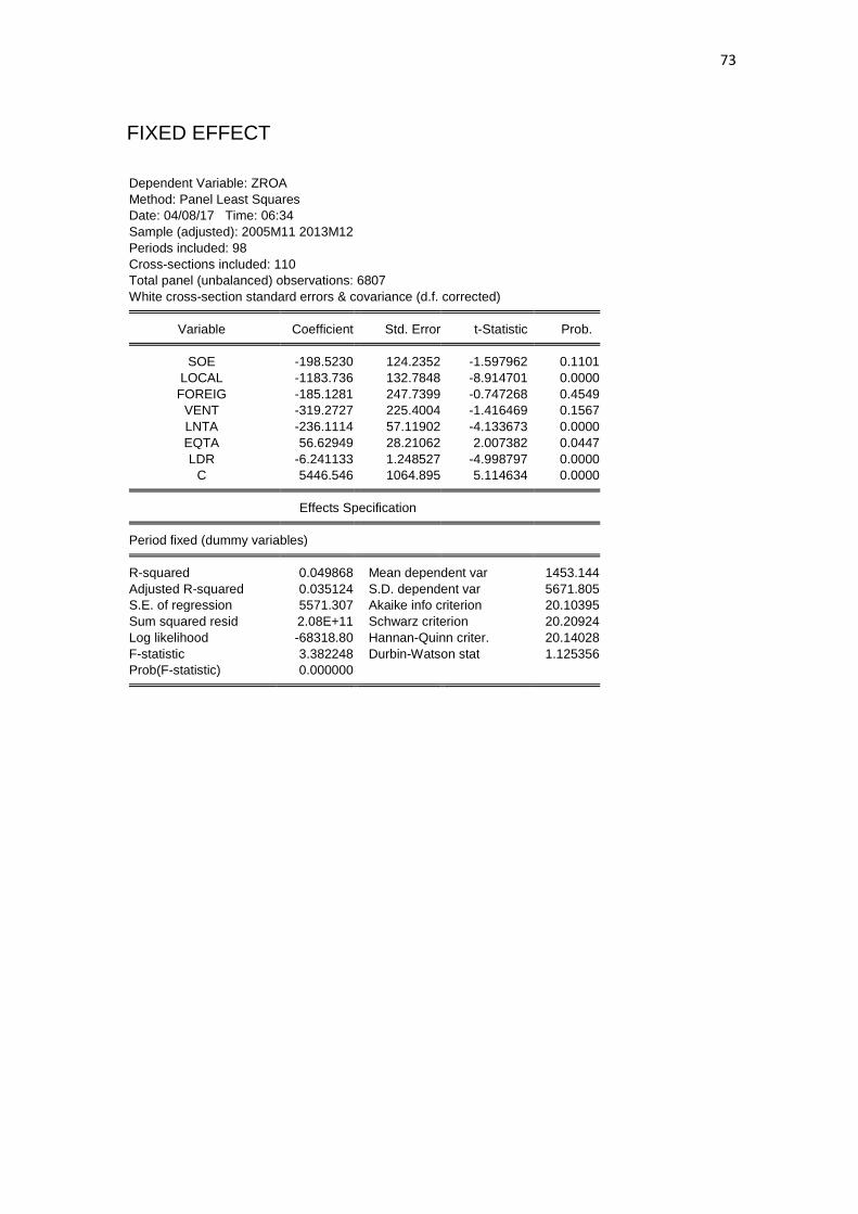
73

FIXED EFFECT



Date: 04/08/17 Time: 06:34






LOCAL -1183.736 132.7848 -8.914701 0.0000

FOREIG -185.1281 247.7399 -0.747268 0.4549

VENT -319.2727 225.4004 -1.416469 0.1567

LNTA -236.1114 57.11902 -4.133673 0.0000

EQTA 56.62949 28.21062 2.007382 0.0447

LDR -6.241133 1.248527 -4.998797 0.0000

C 5446.546 1064.895 5.114634 0.0000 Effects Specification Period fixed (dummy variables) R-squared 0.049868 Mean dependent var 1453.144







74

RANDOM EFFECT



Date: 04/08/17 Time: 06:35







LOCAL -1168.237 133.6464 -8.741251 0.0000

FOREIG -204.6624 247.2963 -0.827600 0.4079

VENT -340.6741 219.5710 -1.551544 0.1208

LNTA -207.3995 56.92989 -3.643069 0.0003

EQTA 58.39151 27.83794 2.097552 0.0360

LDR -5.545252 1.107670 -5.006231 0.0000

C 4912.933 1113.670 4.411480 0.0000 Effects Specification




S.E. of regression 5578.371 Sum squared resid 2.12E+11



Sum squared resid 2.12E+11 Durbin-Watson stat 1.112933

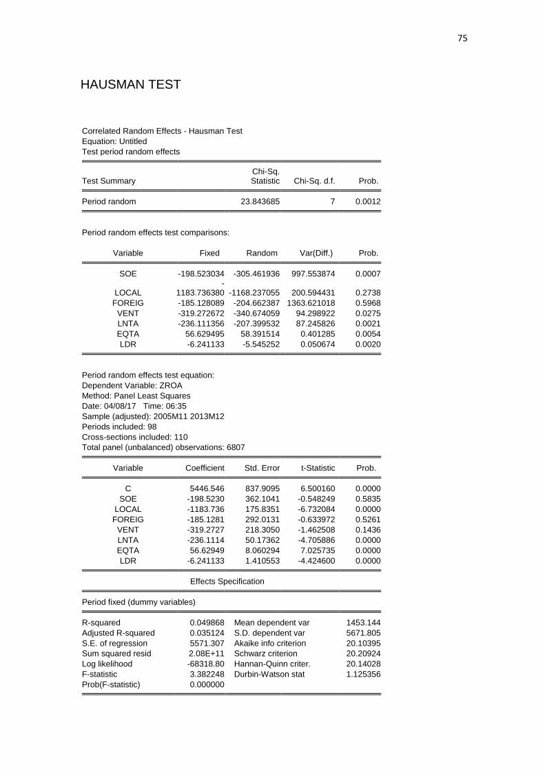
75

HAUSMAN TEST


Equation: Untitled



Period random 23.843685 7 0.0012


Variable Fixed Random Var(Diff.) Prob. SOE -198.523034 -305.461936 997.553874 0.0007

LOCAL -

1183.736380 -1168.237055 200.594431 0.2738

FOREIG -185.128089 -204.662387 1363.621018 0.5968

VENT -319.272672 -340.674059 94.298922 0.0275

LNTA -236.111356 -207.399532 87.245826 0.0021

EQTA 56.629495 58.391514 0.401285 0.0054

LDR -6.241133 -5.545252 0.050674 0.0020




Date: 04/08/17 Time: 06:35




Total panel (unbalanced) observations: 6807 Variable Coefficient Std. Error t-Statistic Prob. C 5446.546 837.9095 6.500160 0.0000

SOE -198.5230 362.1041 -0.548249 0.5835

LOCAL -1183.736 175.8351 -6.732084 0.0000

FOREIG -185.1281 292.0131 -0.633972 0.5261

VENT -319.2727 218.3050 -1.462508 0.1436

LNTA -236.1114 50.17362 -4.705886 0.0000

EQTA 56.62949 8.060294 7.025735 0.0000








76



Date: 04/08/17 Time: 06:38


Included observations: 6807 after adjustments


Probability ZROA SOE LOCAL FOREIG VENT LNTA EQTA LDR

ZROA 1.000000

-----

SOE -0.031589 1.000000

0.0091 -----

LOCAL -0.086951 -0.125776 1.000000

0.0000 0.0000 -----

FOREIG -0.031684 -0.063563 -0.151129 1.000000

0.0089 0.0000 0.0000 -----

VENT -0.010975 -0.086998 -0.206846 -0.104534 1.000000

0.3653 0.0000 0.0000 0.0000 -----

LNTA -0.107707 0.449289 -0.025377 0.111018 0.056229 1.000000

0.0000 0.0000 0.0363 0.0000 0.0000 -----

EQTA 0.138910 -0.070286 -0.185162 -0.208949 0.008822 -0.425963 1.000000

0.0000 0.0000 0.0000 0.0000 0.4668 0.0000 -----

LDR -0.011431 -0.055100 -0.201220 0.191988 0.165927 -0.067318 0.201389 1.000000

0.3457 0.0000 0.0000 0.0000 0.0000 0.0000 0.0000 -----

76

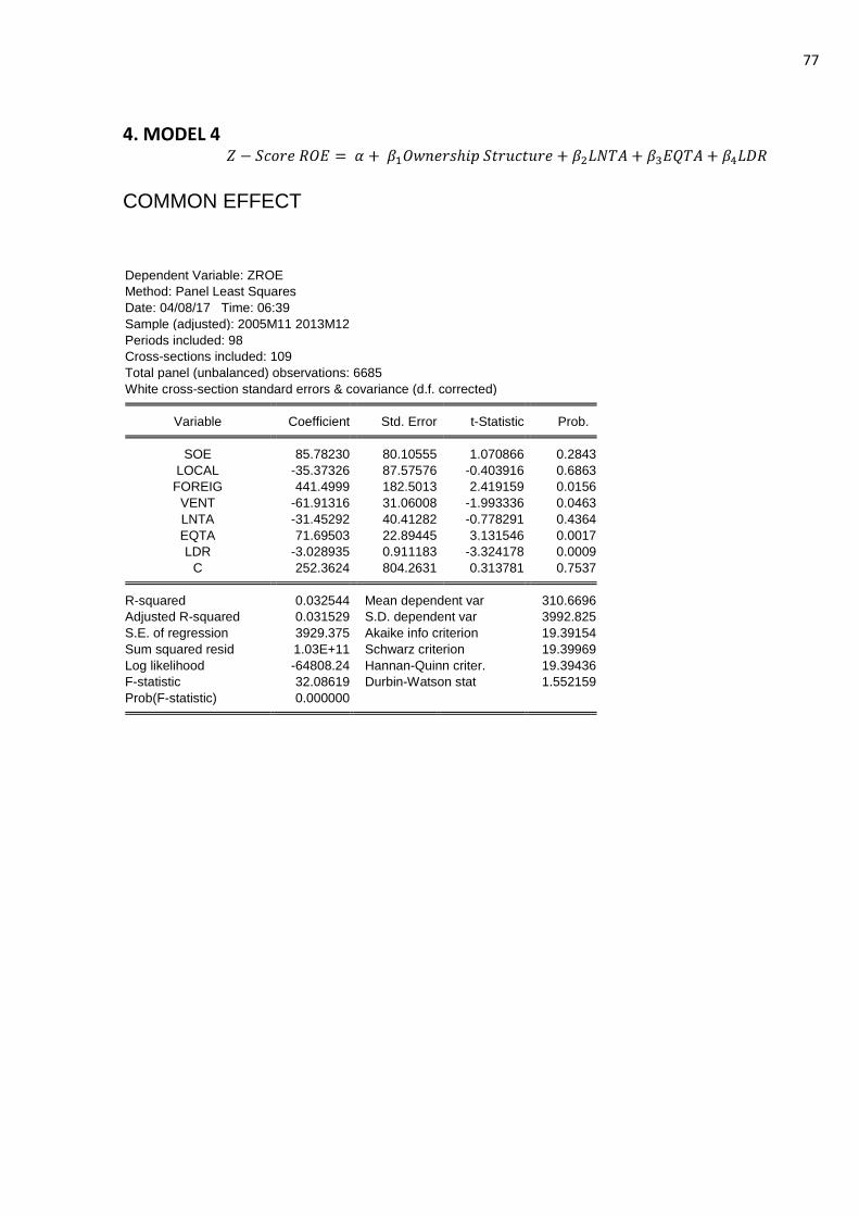
77

4. MODEL 4

COMMON EFFECT

Dependent Variable: ZROE


Date: 04/08/17 Time: 06:39






LOCAL -35.37326 87.57576 -0.403916 0.6863

FOREIG 441.4999 182.5013 2.419159 0.0156

VENT -61.91316 31.06008 -1.993336 0.0463

LNTA -31.45292 40.41282 -0.778291 0.4364

EQTA 71.69503 22.89445 3.131546 0.0017

LDR -3.028935 0.911183 -3.324178 0.0009








78

FIXED EFFECT



Date: 04/08/17 Time: 06:40







LOCAL -48.99209 87.56276 -0.559508 0.5758

FOREIG 436.6229 179.4491 2.433129 0.0150

VENT -52.36990 34.47856 -1.518912 0.1288

LNTA -42.24877 39.87978 -1.059403 0.2895

EQTA 71.64262 23.16919 3.092150 0.0020

LDR -3.517518 1.073700 -3.276071 0.0011










Date: 04/08/17 Time: 06:40







LOCAL -48.99209 87.56276 -0.559508 0.5758

FOREIG 436.6229 179.4491 2.433129 0.0150

VENT -52.36990 34.47856 -1.518912 0.1288

LNTA -42.24877 39.87978 -1.059403 0.2895

EQTA 71.64262 23.16919 3.092150 0.0020

LDR -3.517518 1.073700 -3.276071 0.0011








79

RANDOM EFFECT



Date: 04/08/17 Time: 06:41







LOCAL -35.37326 87.57576 -0.403916 0.6863

FOREIG 441.4999 182.5013 2.419159 0.0156

VENT -61.91316 31.06008 -1.993336 0.0463

LNTA -31.45292 40.41282 -0.778291 0.4364

EQTA 71.69503 22.89445 3.131546 0.0017

LDR -3.028935 0.911183 -3.324178 0.0009









80

HAUSMAN TEST


Equation: Untitled





Variable Fixed Random Var(Diff.) Prob. SOE 147.154983 85.782298 590.813012 0.0116

LOCAL -48.992092 -35.373258 138.292531 0.2468

FOREIG 436.622906 441.499853 906.524834 0.8713

VENT -52.369896 -61.913160 51.340459 0.1829

LNTA -42.248773 -31.452918 50.612005 0.1291

EQTA 71.642622 71.695026 0.239396 0.9147

LDR -3.517518 -3.028935 0.029801 0.0047




Date: 04/08/17 Time: 06:41





SOE 147.1550 248.9213 0.591171 0.5544

LOCAL -48.99209 125.6336 -0.389960 0.6966

FOREIG 436.6229 217.3420 2.008921 0.0446

VENT -52.36990 155.1950 -0.337446 0.7358

LNTA -42.24877 35.76384 -1.181326 0.2375

EQTA 71.64262 5.679194 12.61493 0.0000








81



Date: 04/08/17 Time: 06:43




Probability ZROE SOE LOCAL FOREIG VENT LNTA EQTA LDR

ZROE 1.000000

-----

SOE -0.013825 1.000000

0.2584 -----

LOCAL -0.032896 -0.130022 1.000000

0.0071 0.0000 -----

FOREIG -0.015436 -0.062188 -0.141234 1.000000

0.2070 0.0000 0.0000 -----

VENT -0.013872 -0.090769 -0.206143 -0.098595 1.000000

0.2568 0.0000 0.0000 0.0000 -----

LNTA -0.084084 0.447764 -0.031244 0.108845 0.050073 1.000000

0.0000 0.0000 0.0106 0.0000 0.0000 -----

EQTA 0.174813 -0.076607 -0.187139 -0.188161 0.006243 -0.430402 1.000000

0.0000 0.0000 0.0000 0.0000 0.6098 0.0000 -----

LDR 0.002843 -0.052272 -0.195358 0.184514 0.171400 -0.072572 0.204869 1.000000

0.8162 0.0000 0.0000 0.0000 0.0000 0.0000 0.0000 -----

81

82

5. ROBUSTNESS CHECK 1

COMMON EFFECT



Date: 02/03/17 Time: 18:09

Sample: 2005M09 2013M12




White diagonal standard errors & covariance (d.f. corrected) Variable Coefficient Std. Error t-Statistic Prob. SOELOC 0.954839 0.059162 16.13942 0.0000

VENFOR 0.730470 0.085599 8.533609 0.0000

LNTA 0.188185 0.019361 9.719767 0.0000

EQTA 0.042615 0.004344 9.810799 0.0000

LDR -0.003577 0.000493 -7.261437 0.0000








83

FIXED EFFECT



Date: 02/03/17 Time: 18:09

Sample: 2005M09 2013M12





VENFOR 0.963480 0.070994 13.57135 0.0000

LNTA 0.137777 0.015159 9.088693 0.0000

EQTA 0.033373 0.003339 9.995408 0.0000

LDR -0.000994 0.000503 -1.975254 0.0483








84

RANDOM EFFECT



Date: 02/03/17 Time: 18:10

Sample: 2005M09 2013M12






VENFOR 0.900747 0.077173 11.67180 0.0000

LNTA 0.153500 0.016487 9.310497 0.0000

EQTA 0.035906 0.003752 9.568793 0.0000

LDR -0.001738 0.000519 -3.346536 0.0008





S.E. of regression 1.959295 Sum squared resid 26537.88



Sum squared resid 35108.25 Durbin-Watson stat 0.078550

85

HAUSMAN TEST


Equation: Untitled



Period random 577.579287 5 0.0000


Variable Fixed Random Var(Diff.) Prob. SOELOC 1.042425 1.015556 0.000005 0.0000

VENFOR 0.963480 0.900747 0.000009 0.0000

LNTA 0.137777 0.153500 0.000003 0.0000

EQTA 0.033373 0.035906 0.000000 0.0000

LDR -0.000994 -0.001738 0.000000 0.0000




Date: 02/03/17 Time: 18:10

Sample: 2005M09 2013M12




SOELOC 1.042425 0.055776 18.68960 0.0000

VENFOR 0.963480 0.064143 15.02087 0.0000

LNTA 0.137777 0.014911 9.239833 0.0000

EQTA 0.033373 0.002613 12.77393 0.0000








86



Date: 02/03/17 Time: 18:13

Sample: 2005M09 2013M12



Probability ROA SOELOC VENFOR LNTA EQTA LDR

ROA 1.000000

-----

SOELOC 0.155842 1.000000

0.0000 -----

VENFOR 0.041207 -0.306703 1.000000

0.0006 0.0000 -----

LNTA 0.121206 0.191784 0.121184 1.000000

0.0000 0.0000 0.0000 -----

EQTA 0.054979 -0.206815 -0.126860 -0.424032 1.000000

0.0000 0.0000 0.0000 0.0000 -----

LDR -0.060651 -0.214593 0.263177 -0.064263 0.200163 1.000000

0.0000 0.0000 0.0000 0.0000 0.0000 -----

86

87


COMMON EFFECT



Date: 02/03/17 Time: 18:14

Sample: 2005M09 2013M12





VENFOR 25.12474 1.692864 14.84156 0.0000

LNTA 1.380421 0.318474 4.334483 0.0000

EQTA -0.073133 0.042725 -1.711709 0.0870

LDR -0.034489 0.008777 -3.929239 0.0001








88

FIXED EFFECT



Date: 02/03/17 Time: 18:14

Sample: 2005M09 2013M12





VENFOR 24.76992 1.638931 15.11346 0.0000

LNTA 1.197608 0.314034 3.813625 0.0001

EQTA -0.090156 0.044224 -2.038626 0.0415

LDR -0.051767 0.010103 -5.123961 0.0000








89

RANDOM EFFECT



Date: 02/03/17 Time: 18:15

Sample: 2005M09 2013M12






VENFOR 25.12474 1.692864 14.84156 0.0000

LNTA 1.380421 0.318474 4.334483 0.0000

EQTA -0.073133 0.042725 -1.711709 0.0870

LDR -0.034489 0.008777 -3.929239 0.0001





S.E. of regression 54.86100 Sum squared resid 21110239



Sum squared resid 21110239 Durbin-Watson stat 0.264149

90

HAUSMAN TEST


Equation: Untitled





Variable Fixed Random Var(Diff.) Prob. SOELOC 8.845740 8.869920 0.012429 0.8283

VENFOR 24.769919 25.124736 0.034004 0.0543

LNTA 1.197608 1.380421 0.009195 0.0566

EQTA -0.090156 -0.073133 0.000073 0.0456

LDR -0.051767 -0.034489 0.000006 0.0000




Date: 02/03/17 Time: 18:16

Sample: 2005M09 2013M12




SOELOC 8.845740 1.601033 5.525022 0.0000

VENFOR 24.76992 1.853824 13.36152 0.0000

LNTA 1.197608 0.429879 2.785919 0.0054

EQTA -0.090156 0.074896 -1.203750 0.2287








91

UJI MULTIKOLINEARITAS Covariance Analysis: Ordinary

Date: 02/03/17 Time: 18:17

Sample: 2005M09 2013M12



Probability ROE SOELOC VENFOR LNTA EQTA LDR

ROE 1.000000

-----

SOELOC 0.035339 1.000000

0.0031 -----

VENFOR 0.153738 -0.303710 1.000000

0.0000 0.0000 -----

LNTA 0.085716 0.192713 0.119544 1.000000

0.0000 0.0000 0.0000 -----

EQTA -0.075093 -0.207428 -0.125750 -0.428994 1.000000

0.0000 0.0000 0.0000 0.0000 -----

LDR -0.005383 -0.208762 0.265061 -0.063098 0.196866 1.000000

0.6520 0.0000 0.0000 0.0000 0.0000 -----

91

92


COMMON EFFECT



Date: 04/08/17 Time: 06:44





White cross-section standard errors & covariance (d.f. corrected) Variable Coefficient Std. Error t-Statistic Prob. SOELOC -1045.999 107.6676 -9.715079 0.0000

VENFOR -331.1990 179.7330 -1.842729 0.0654

LNTA -149.2378 45.05044 -3.312681 0.0009

EQTA 61.60741 26.44190 2.329916 0.0198

LDR -5.213054 1.047109 -4.978521 0.0000








93

FIXED EFFECT



Date: 04/08/17 Time: 06:45






VENFOR -307.1048 185.3789 -1.656633 0.0976

LNTA -176.3252 45.86168 -3.844718 0.0001

EQTA 59.92538 27.04384 2.215861 0.0267

LDR -6.042511 1.219877 -4.953375 0.0000








94

RANDOM EFFECT



Date: 04/08/17 Time: 06:46







VENFOR -324.7336 181.0268 -1.793842 0.0729

LNTA -155.3761 45.08033 -3.446649 0.0006

EQTA 61.24646 26.49029 2.312034 0.0208

LDR -5.401130 1.076156 -5.018908 0.0000









95

HAUSMAN TEST


Equation: Untitled



Period random 21.273750 5 0.0007


Variable Fixed Random Var(Diff.) Prob.

SOELOC -

1042.531695 -1045.082386 133.261211 0.8251

VENFOR -307.104773 -324.733621 268.592700 0.2821

LNTA -176.325215 -155.376077 78.328763 0.0179

EQTA 59.925379 61.246460 0.603205 0.0889

LDR -6.042511 -5.401130 0.052318 0.0050




Date: 04/08/17 Time: 06:47





SOELOC -1042.532 166.8964 -6.246579 0.0000

VENFOR -307.1048 191.0094 -1.607799 0.1079

LNTA -176.3252 44.71165 -3.943608 0.0001

EQTA 59.92538 7.805622 7.677207 0.0000








96



Date: 04/08/17 Time: 06:48




Probability ZROA SOELOC VENFOR LNTA EQTA LDR

ZROA 1.000000

-----

SOELOC -0.096844 1.000000

0.0000 -----

VENFOR -0.029634 -0.308362 1.000000

0.0145 0.0000 -----

LNTA -0.107707 0.194699 0.118648 1.000000

0.0000 0.0000 0.0000 -----

EQTA 0.138910 -0.207695 -0.127760 -0.425963 1.000000

0.0000 0.0000 0.0000 0.0000 -----

LDR -0.011431 -0.215358 0.262427 -0.067318 0.201389 1.000000

0.3457 0.0000 0.0000 0.0000 0.0000 -----

96

97


COMMON EFFECT



Date: 04/08/17 Time: 06:48






VENFOR 87.33739 65.64943 1.330360 0.1834

LNTA -24.03338 31.89377 -0.753545 0.4511

EQTA 70.28515 22.06656 3.185143 0.0015

LDR -2.822602 0.849206 -3.323813 0.0009








98

FIXED EFFECT



Date: 04/08/17 Time: 06:49






WARNING: estimated coefficient covariance matrix is of reduced rank Variable Coefficient Std. Error t-Statistic Prob. SOELOC -27.37391 68.41834 -0.400096 0.6891

VENFOR 87.93238 68.30070 1.287430 0.1980

LNTA -28.96345 31.26662 -0.926338 0.3543

EQTA 70.67239 22.50701 3.140017 0.0017

LDR -3.315657 1.010537 -3.281084 0.0010








99

RANDOM EFFECT



Date: 04/08/17 Time: 06:50







VENFOR 87.33739 65.64943 1.330360 0.1834

LNTA -24.03338 31.89377 -0.753545 0.4511

EQTA 70.28515 22.06656 3.185143 0.0015

LDR -2.822602 0.849206 -3.323813 0.0009









100

HAUSMAN TEST


Equation: Untitled





Variable Fixed Random Var(Diff.) Prob. SOELOC -27.373909 -24.510284 75.753149 0.7421

VENFOR 87.932378 87.337386 165.300996 0.9631

LNTA -28.963453 -24.033384 49.105098 0.4817

EQTA 70.672389 70.285151 0.347948 0.5115

LDR -3.315657 -2.822602 0.030134 0.0045




Date: 04/08/17 Time: 06:50





SOELOC -27.37391 118.4309 -0.231138 0.8172

VENFOR 87.93238 137.2656 0.640600 0.5218

LNTA -28.96345 31.98748 -0.905462 0.3653

EQTA 70.67239 5.518347 12.80680 0.0000










Date: 04/08/17 Time: 06:51




Probability ZROE SOELOC VENFOR LNTA EQTA LDR

ZROE 1.000000

-----

SOELOC -0.037618 1.000000

0.0021 -----

VENFOR -0.021346 -0.302712 1.000000

0.0810 0.0000 -----

LNTA -0.084084 0.196048 0.110082 1.000000

0.0000 0.0000 0.0000 -----

EQTA 0.174813 -0.212978 -0.111702 -0.430402 1.000000

0.0000 0.0000 0.0000 0.0000 -----

LDR 0.002843 -0.208401 0.259882 -0.072572 0.204869 1.000000

0.8162 0.0000 0.0000 0.0000 0.0000 -----

101

57

APPENDIX C DESCRIPTIVE STATISTICS

ZROA ZROE SOE LOCAL FOREIG VENT SOELOC VENFOR LNTA EQTA LDR ROA ROE

Mean 1442.485 314.9214 0.051682 0.230676 0.064110 0.127463 0.282358 0.191573 15.91537 11.15728 85.88476 1.521421 18.70751

Median 678.0386 80.47757 0.000000 0.000000 0.000000 0.000000 0.000000 0.000000 15.75468 8.585423 79.97784 0.956197 13.09164

Maximum 216580.5 245589.4 1.000000 1.000000 1.000000 1.000000 1.000000 1.000000 20.28809 99.04926 726.7294 17.02348 470.4082

Minimum 6.456966 -16.49225 0.000000 0.000000 0.000000 0.000000 0.000000 0.000000 11.10509 -1.584381 4.586926 -9.668127 -874.7000

Std. Dev. 5274.674 4018.873 0.221402 0.421297 0.244968 0.333516 0.450181 0.393569 1.735998 10.04824 52.86016 2.160081 30.52736

Skewness 25.16431 45.15813 4.050120 1.278643 3.559018 2.234168 0.966981 1.567452 0.166910 3.826754 6.309137 1.432370 -4.601939

Kurtosis 849.0902 2412.099 17.40347 2.634928 13.66661 5.991505 1.935053 3.456907 2.621885 22.93141 56.61391 10.17987 179.7193

Jarque-Bera 1.98E+08 1.60E+09 75072.57 1834.516 45208.13 7949.249 1340.033 2759.172 69.94075 125317.3 834007.2 16423.28 8606244.

Probability 0.000000 0.000000 0.000000 0.000000 0.000000 0.000000 0.000000 0.000000 0.000000 0.000000 0.000000 0.000000 0.000000

Sum 9517518. 2077852. 341.0000 1522.000 423.0000 841.0000 1863.000 1264.000 105009.6 73615.73 566667.6 10035.29 123394.7

Sum Sq. Dev. 1.84E+11 1.07E+11 323.3763 1170.911 395.8813 733.8037 1336.967 1021.851 19881.31 666080.7 18433316 30771.95 6146010.

Observations 6598 6598 6598 6598 6598 6598 6598 6598 6598 6598 6598 6596 6596

102

ownership structure, bank performance, and … · dr. asri laksmi riani, se.ms, the head of...

Documents