P-15 The Projection of Northern Hemisphere Flow

Regime Transitions Using Integrated Enstrophy.

Emily M. Klaus1, Anthony R. Lupo1, Michael J. Bodner2, and Joshua S. Kastman2,3, Patrick S. Market1

1Department of Soil, Environmental, and Atmospheric Science

302 E Anheuser Busch Natural Resources Building

University of Missouri, Columbia, MO 65211

2Weather Prediction Center

5830 University Research Court

College Park, MD 20740

3Cooperative Institute for Research in Environmental Science

University of Colorado

Boulder, CO 80309

Introduction

• The work of Lorenz (1963) implied the Northern Hemisphere (NH) flow

vascillates between two quasi-equilibrium states. Charney and DeVore

(1979) postulated the NH flow may possess multi-equilibria, including

those that represent blocking.

• Dymnikov et al. (1992) introduces a quantity called integrated Enstrophy

(IE), which in a barotropic atmosphere correlates highly to the positive

Lyapunov exponent in the NH.

• Jensen et al. (2017) and references therein show that IE may be useful for

identifying block onset and decay, as well as flow regime transition.

Motivation/Objective/Goal

• Ensemble models have been used to improve model performance and

mitigate the issue of sensitive dependence on initial conditions.

• It may be possible to use IE to anticipate a change in the prevailing NH

flow regime and/or the onset or decay of blocking.

• Thus, IE in conjunction with ensemble modelling may be used to improve

local and/or regional weather prediction in the 6-21 day time frame.

http://weather.missouri.edu/naefs/IRE-NAEFS-MU.html

Data and Methods

• The 500 hPa daily height (m) provided by the National Centers for Environmental Prediction (NCEP) / North American

Ensemble Forecast System (NAEFS) and the Global Ensemble Forecast System (GEFS) were used for the period of August

2018 to March 2019.

• The observed four-times daily 500 hPa re-analyses provided by the NCEP / National Center for Atmospheric Research

(NCAR) were also used.

• The 500 hPa height for each ensemble member is used to calculate geostrophic vorticity which is integrated across the NH to

70o N. The IE is:

• 𝐼𝑛𝑡𝑒𝑔𝑟𝑎𝑡𝑒𝑑 𝐸𝑛𝑠𝑡𝑟𝑜𝑝ℎ𝑦 𝐼𝐸 = 𝐴 𝜁𝑔2𝑑𝐴 (1)

Summary and Conclusions

Acknowledgements

• Thanks to Missouri EPSCOR for partially funding this work, NSF Award IIA-1355406.

Any opinions, findings, and conclusions or recommendations expressed in this material are

those of the author(s) and do not necessarily reflect the views of NSF.

• An automated system has been developed to download the 500

hPa height for the GEFS and NAEFS ensemble information for

the NH, and is used to calculate IE.

• The ensemble mean IE is used to display day-by-day forecast

values in 24-h increments out to 10 days. Daily forecasts are

shown in order to check for model consistency.

• This system has been in place since February 2018, and the

NH flow was examined here to demonstrate the efficacy of the

IE method used in conjunction with ensemble models.

• The IE has utility in identifying regime transition as well as

block onset and termination (see Jensen et al. 2017). Block

onsets and terminations were identified for April and May

2018.

• The ability of the model to anticipate flow regime transition

shows promise even out to 10 days. If all days are used the

POD was greater than the number of FAR, and this was

significant at greater than 80% confidence.

• When examining a MISS case, we can demonstrate that the

weather regime in the Midwest USA was similar before and

after the miss.

• When examining a HIT case, the weather regime before and

after the regime change was significantly different.

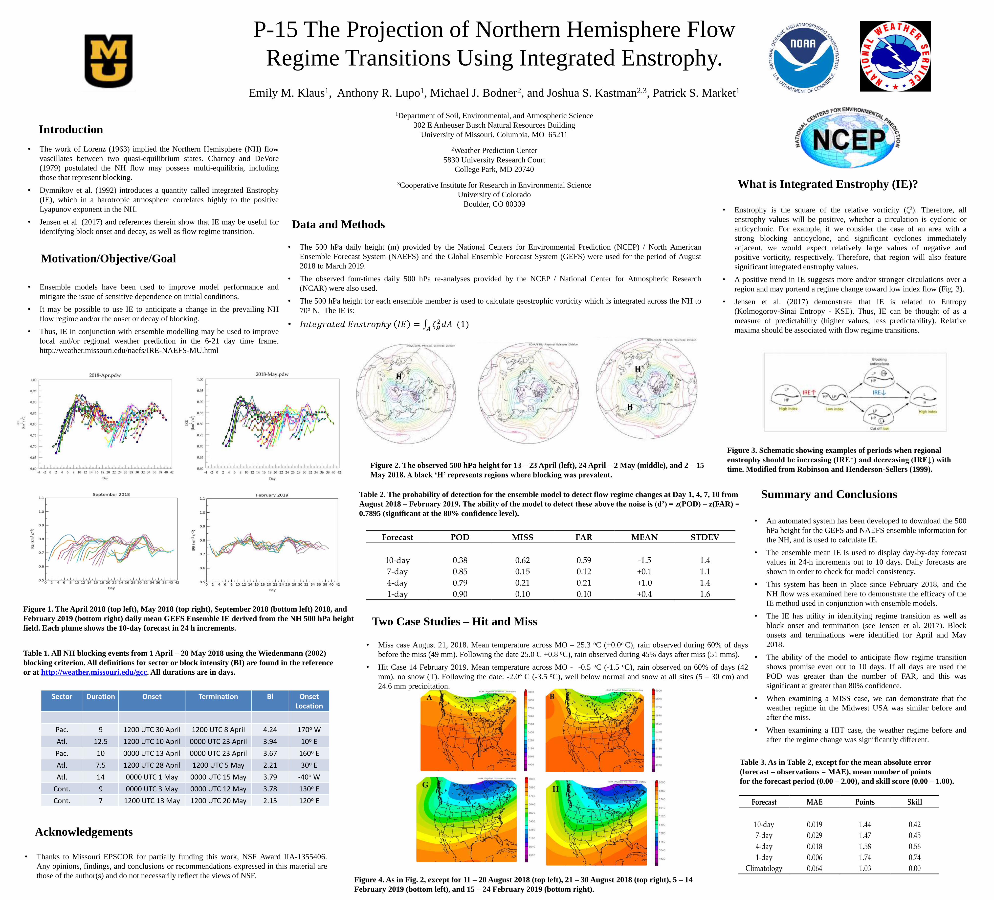
Figure 1. The April 2018 (top left), May 2018 (top right), September 2018 (bottom left) 2018, and

February 2019 (bottom right) daily mean GEFS Ensemble IE derived from the NH 500 hPa height

field. Each plume shows the 10-day forecast in 24 h increments.

Figure 2. The observed 500 hPa height for 13 – 23 April (left), 24 April – 2 May (middle), and 2 – 15

May 2018. A black ‘H’ represents regions where blocking was prevalent.

H

Table 1. All NH blocking events from 1 April – 20 May 2018 using the Wiedenmann (2002)

blocking criterion. All definitions for sector or block intensity (BI) are found in the reference

or at http://weather.missouri.edu/gcc. All durations are in days.

Sector Duration Onset Termination Bl Onset Location

Pac. 9 1200 UTC 30 April 1200 UTC 8 April 4.24 170o W

Atl. 12.5 1200 UTC 10 April 0000 UTC 23 April 3.94 10o E

Pac. 10 0000 UTC 13 April 0000 UTC 23 April 3.67 160o E

Atl. 7.5 1200 UTC 28 April 1200 UTC 5 May 2.21 30o E

Atl. 14 0000 UTC 1 May 0000 UTC 15 May 3.79 -40o W

Cont. 9 0000 UTC 3 May 0000 UTC 12 May 3.78 130o E

Cont. 7 1200 UTC 13 May 1200 UTC 20 May 2.15 120o E

What is Integrated Enstrophy (IE)?

• Enstrophy is the square of the relative vorticity (ζ2). Therefore, all

enstrophy values will be positive, whether a circulation is cyclonic or

anticyclonic. For example, if we consider the case of an area with a

strong blocking anticyclone, and significant cyclones immediately

adjacent, we would expect relatively large values of negative and

positive vorticity, respectively. Therefore, that region will also feature

significant integrated enstrophy values.

• A positive trend in IE suggests more and/or stronger circulations over a

region and may portend a regime change toward low index flow (Fig. 3).

• Jensen et al. (2017) demonstrate that IE is related to Entropy

(Kolmogorov-Sinai Entropy - KSE). Thus, IE can be thought of as a

measure of predictability (higher values, less predictability). Relative

maxima should be associated with flow regime transitions.

Figure 3. Schematic showing examples of periods when regional

enstrophy should be increasing (IRE↑) and decreasing (IRE↓) with

time. Modified from Robinson and Henderson-Sellers (1999).

Table 2. The probability of detection for the ensemble model to detect flow regime changes at Day 1, 4, 7, 10 from

August 2018 – February 2019. The ability of the model to detect these above the noise is (d’) = z(POD) – z(FAR) =

0.7895 (significant at the 80% confidence level).

Figure 4. As in Fig. 2, except for 11 – 20 August 2018 (top left), 21 – 30 August 2018 (top right), 5 – 14

February 2019 (bottom left), and 15 – 24 February 2019 (bottom right).

Two Case Studies – Hit and Miss

• Miss case August 21, 2018. Mean temperature across MO – 25.3 oC (+0.0o C), rain observed during 60% of days

before the miss (49 mm). Following the date 25.0 C +0.8 oC), rain observed during 45% days after miss (51 mms).

• Hit Case 14 February 2019. Mean temperature across MO - -0.5 oC (-1.5 oC), rain observed on 60% of days (42

mm), no snow (T). Following the date: -2.0o C (-3.5 oC), well below normal and snow at all sites (5 – 30 cm) and

24.6 mm precipitation.

Forecast POD MISS FAR MEAN STDEV

10-day 0.38 0.62 0.59 -1.5 1.4

7-day 0.85 0.15 0.12 +0.1 1.1

4-day 0.79 0.21 0.21 +1.0 1.4

1-day 0.90 0.10 0.10 +0.4 1.6

1

Table 3. As in Table 2, except for the mean absolute error

(forecast – observations = MAE), mean number of points

for the forecast period (0.00 – 2.00), and skill score (0.00 – 1.00).

Forecast MAE Points Skill

10-day 0.019 1.44 0.42

7-day 0.029 1.47 0.45

4-day 0.018 1.58 0.56

1-day 0.006 1.74 0.74

Climatology 0.064 1.03 0.00

1