Part II

Information Theory Concepts

Chapter 2 Source Models and Entropy

� Any information-generating process can be viewed as

a source:

{ emitting a sequence of symbols

{ symbols from a �nite alphabet

� text: ASCII symbols

� computer program in executed form: binary 0

and 1

� n-bit image: 2n symbols

1

Discrete Memoryless Sources (DMS)

� successive symbols statistically independent

� S = fs1; s2; : : : ; sng

� fp(s1); p(s2); : : : ; p(sn)g

� I(si), the information revealed by the occurrence of a

certain source symbol, is de�ned as

I(si) = log21

p(si)

� Average Information per source symbol, entropyH(s) =Pp(si)I(si) = �

Pp(si) log2 p(si) bits/symbol

2

Extensions of a Discrete Memoryless Source

� DMS S with an alphabet of size n

� the output of the source grouped into blocks of N

symbols

� SN with an alphabet of size nN : the Nth extension

of the source S

� For a memoryless source, the probability of a symbol

�i = (si1; si2; : : : ; siN) from SN is given by

p(�i) = p(si1)p(si2) : : : p(siN )

H(SN) = NH(S)

3

Markov Sources

� DMS too restrictive

� In general, the previous part of a message in uences

the probabilities for the next symbol, the source has

memory.

� In English text, the letter Q is almost always followed

by the letter U.

� In digital images, the probability of a given pixel tak-

ing on a particular code value is dependent on the

surrounding pixel values.

4

� Such a source can be modeled as a Markov source.

� An mth-order Markov source:

p(sijsj1; : : : ; sjm)

sj1; : : : ; sjm preceding to sii; jk (k = 1; 2; : : : ;m) = 1; 2; : : : ; n

(sj1; : : : ; sjm): a state for themth-order Markov source,

a total of nm states

� For an ergodic Markov source, 9 a unique probabil-

ity distribution over the set of states: stationary or

equilibrium distribution.

5

�

H(Sjsj1; : : : ; sjm) = �P

i p(sijsj1; : : : ; sjm)�

log p(sijsj1; : : : ; sjm)

H(S) =P

SmH(Sjsj1; : : : ; sjm)�

p(sj1; : : : ; sjm)

= �P

Sm+1 p(sj1; : : : ; sjm)p(sijsj1; : : : ; sjm)�

log p(sijsj1; : : : ; sjm)

= �P

Sm+1 p(sj1; : : : ; sjm; si)�

log p(sijsj1; : : : ; sjm)

6

p(1|0,0)=0.2

p(0|1,0)=0.5

p(1|0,1)=0.5

p(1|1,0)=0.5 p(0|1,1)=0.2

p(0|0,1)=0.5

0,0

1,0 0,1

1,1

p(0|0,0)=0.8

p(1|1,1)=0.8

�p(0; 0) = p(1; 1) = 514, p(0; 1) = p(1; 0) = 2

14

H(S) = 0:801 bit/symbol

7

Extensions of a Markov Source and Adjoint

Sources

� The Nth extension of a Markov source, SN , is a �th-

order Markov source with symbols de�ned as blocks

of N symbols from the original source, where � =

dm=Ne

� As in the case of a DMS,

H(SN) = NH(S)

8

� The Nth extension of a Markov source, SN , with

source symbols f�1; �2; : : : ; �nNg and stationary prob-

abilities fp(�1); p(�2);

� � � ; p(�nN )g: a DMS with the same alphabet and the

same symbol probabilities is called the adjoint source

of SN and denoted by �SN .

{ The adjoint source ignores the conditional proba-

bilities which describe the dependence between the

extended symbols.

{ H( �SN) � H(SN)

{ HN(S) =H( �SN )N

! H(S)

9

� The Noiseless Source Coding Theorem

{ S an ergodic source with an alphabet of size n and

an entropy H(S)

{ encoding blocks ofN source symbols at a time into

binary codewords

{ For any � > 0, it is possible, by choosing N large

enough, to construct a code so that the average

number of bits per original source symbol, �L, sat-

is�es

H(S) � �L � H(S) + �

10

Chapter 3 Variable-Length Codes

� Variable-length codes with source extensions to achieve

the entropy of a source

{ a DMS S = fs1; s2; s3; s4;

p(s1) = 0:60, p(s2) = 0:30, p(s3) = 0:05, p(s4) =

0:05g

{ each codeword in the sequence is instantaneously

decodeable without reference to the succeeding code-

words i� no codeword be a pre�x of some other

codeword (called by a pre�x condition code)

11

{ entropy H(S) =Pni=1 p(si)I(si)

with I(si) = � log2 p(si)

{ average codeword length or average length of the

code, �L =Pni=1 p(si)L(si) with L(si) being the

length of the codeword for si

{ To have �L � H(S), we needL(si) � � log2 p(si) =

log21

p(si)bits

or L(si) = dlog21

p(si)e (bits)

{ Shannon-Fano coding

12

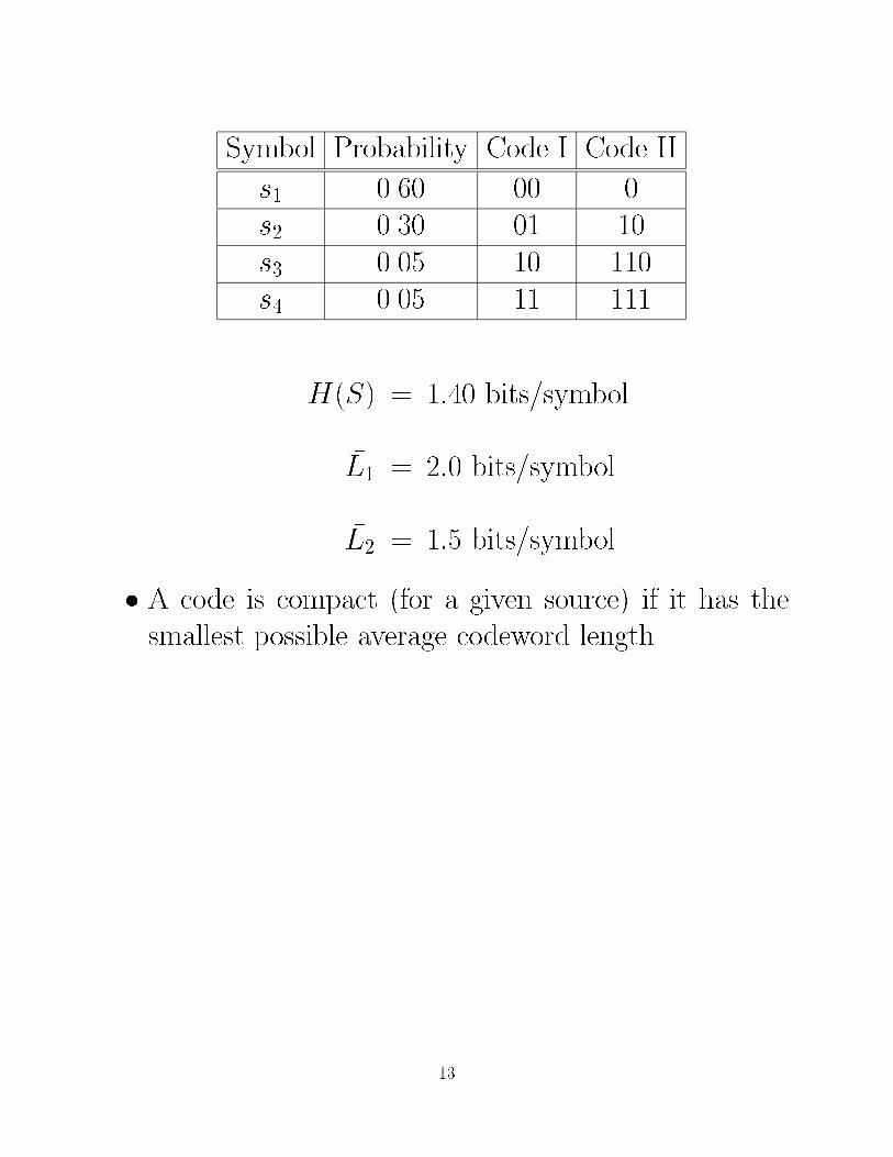
Symbol Probability Code I Code II

s1 0.60 00 0

s2 0.30 01 10

s3 0.05 10 110

s4 0.05 11 111

H(S) = 1:40 bits/symbol

�L1 = 2:0 bits/symbol

�L2 = 1:5 bits/symbol

� A code is compact (for a given source) if it has the

smallest possible average codeword length.

13

� Code E�ciency and Source Extensions

{ Code II compact on S, its average codeword length

is still far greater than H(S)

{ the code e�ciency:

� =H(S)�L

� Code II: � = 1:41:5

= 0:93

{ Extension to S2 of 16 symbols formed as pairs of

symbols from S.

� Table 3.2 shows a compact code of S2, �L = 2:86

bits/extended symbol

14

= 1:43 bits/original source symbol

� = 1:401:43

= 0:98

� Hu�man Codes for constructing compact codes

{ The Hu�man code for a source fs1; s2g has trivial

codewords \0" and \1".

{ Consider S = fs1; s2; : : : ; sng (n > 2)

Let sn�1; sn be least probable symbols of this source.

15

Let Hu�man code for

fs1s2; � � � ; sn�2; fsn�1; sngg

be constructed and the codeword for fsn�1; sng be

w. Then Hu�man code for fs1; � � � ; sn�1; sng will be

Hu�man code for s1; � � � ; sn�2 and w0 for sn�1, w1

for sn.

understanding Fig. 3

16

� Modi�ed Hu�man Codes

{ Frequently, most of symbols in a large symbol set

have very small probabilities.

{ Lump the less probable symbols into a symbol

called \Else" and design a Hu�man code for the

reduced symbol set: the modi�ed Hu�man code.

{ Whenever a symbol in the ELSE category needs to

be encoded, the encoder transmits the codeword

for ELSE followed

17

by extra bits needed to identify the actual message

within the ELSE category.

� the loss in coding e�ciency very small

� the storage requirements and the decoding com-

plexity substantially reduced

� Group 3 international digital facsimile coding stan-

dards:

{ each binary image scan line:

a sequence of alternating black and white runs

which are encoded with separable variable-length

code tables

{ A run is the number of times a particular value

occurs consecutively along a scanline.

18

{ 1728 pixels for each scanline

{ each Hu�man table should have 1728 entries

{ greatly simpli�ed by taking advantage of the fact

that the longer runs are highly improbable

{ The �rst 64 entries in each table represent the Hu�-

man code for runs 0 to 63

{ All other runs 64N +M (1 � N � 27, 0 �M �

64):

entries for 64 to 90 encode N

entries for 0 to 63 encode M

19

{ a run of 213: N = 3 and M = 21 its Hu�man

code

the entry 67(64 + 3) for N = 3

the entry 21 for M = 21

{ simplifying the search for decoding

� Limitations of Hu�man Coding

{ The ideal binary codeword length for a source sym-

bol si from a DMS is � log2 p(si), this condition is

met only if p(si) =12k.

20

{ Otherwise, direct encoding of the individual source

symbols may result in poor code e�ciency.

� p(s1) � 1, p(s2) = : : : = p(sn) � 0

H(S) = �p(s1) log2 p(s1)�P

k�2 p(sk)

log2 p(sk)

� �(n� 1)p(s2) log2 p(s2)

= �(n� 1)(1�p(s1))(n�1)

log2(1�p(s1))(n�1)

= �(1� p(s1)) log2(1�p(s1))(n�1)

�! 0 as p(s1) ! 1

� �L � 1 since the shortest codeword length for

each individual symbol is one

21

{ S = f0; 1g

The Hu�man codewords for \0" and \1" are \0"

and \1", thus �L = 1, regardless of the symbol

probabilities.

{ Encoding an extended source may improve the cod-

ing e�ciency, but convergence to the source en-

tropy could be slow.

{ The number of entries in the Hu�man code table

grows exponentially with the block size.

22

{ For an mth order Markov source, the conditional

probabilities p(sijsi1; : : : ; sim) vary as the state

(si1; : : : ; sim) changes. Thus, a separable Hu�man

table is needed for each state.

{ The coding e�ciency may still be low if the sym-

bol conditional probabilities deviate from the ideal

case.

{ Using an extended source and encoding the ad-

joint, its entropy HN may get close to the entropy

H of the Markov source but the block size must

be large.

23

{ The Hu�man coding cannot e�ciently adapt to

changing source statistics

{ Arithmetic coding is more complex than Hu�man

coding, but it can overcome the limitations of Hu�-

man coding

24