p m c a (mca) using spad 1 version 6.5)

PERFORMING MULTIPLE CORRESPONDENCE ANALYSIS

(MCA) USING SPAD1 (VERSION 6.5)

Brigitte le Roux2, Mikael Börjesson3, Philippe Bonnet4

1. GENERALITIES............................................................................................................................. 1

1.1. Main Window ........................................................................................................................ 1 1.2. Choice of options ................................................................................................................... 1 1.3. Adding chains to “favorite chains”........................................................................................... 2

2. IMPORTING DATABASES with DataXchange ........................................................................... 4 2.1. New types of databases.......................................................................................................... 4 2.2. Importing an SPSS database .................................................................................................. 6 2.3. Verification of the importated SPAD database (sba)............................................................. 9

3. STANDARD MCA....................................................................................................................... 11 3.1. Performing a Standard MCA ............................................................................................... 11 3.2. Results of MCA ................................................................................................................... 13 3.3. Eigenvalues and modified rates ........................................................................................... 14 3.4. Interpretation of axes using contributions............................................................................ 14 3.5. Graph for Interpretation of Axes.......................................................................................... 16

• • Choosing the preferences for graphs ................................................................................. 16 • • Construction of graph for interpreting an axis................................................................... 17

3.6. Graph of the Cloud of Individuals ....................................................................................... 20 4. STORING PRINCIPAL COORDINATES AND PARTITIONS ................................................. 24 5. APPENDIX ................................................................................................................................... 25

5.1. Generalities on the graph editor ........................................................................................... 25 • The toolbar of the graph editor ............................................................................................ 25 • The fundamental rule for formating a graph........................................................................ 26

5.2. Interface SPAD/SPSS using SPAD editor ........................................................................... 26 • To Import SPSS databases: *.sav (SPSS) → *.sba (SPAD)................................................ 28 • To Export SBA databases: *.sba (SPAD) → *.sav (SPSS) ................................................. 30 • Rules for converting SPAD to SPSS.................................................................................... 30

1 SPAD WEB address : www.SPAD.eu Contact: Plilippe Pleuvret: [email protected] 2 Université René Descartes PARIS. www.math-info.univ-paris5.fr/~lerb e-mail: [email protected] 3 Uppsala University – e-mail: [email protected] 4 Université René Descartes PARIS. e-mail: [email protected]

Performing MCA using SPAD — B. Le Roux, M. Börjesson, P. Bonnet (October 2006) 1/2

1. GENERALITIES

1.1. Main Window The main window of SPAD (which opens when you start the program) is composed of three main elements:

1. the toolbar with six menus (Dataset, Chain, Tools, Options, Window and Help), 2. the Methods window with 9 groups of methods (rolling menu): descriptive statistics, factorial

analysis, etc., 3. the Chain window which manages the linked sequence of methods applied to the chosen

database that form a chain.5

1.2. Choice of options 1. Create the directories databases and chains in your own working directory (for example in

C:/…/My Documents/SPAD/). 2. Open the menu Options and choose General parameters.

3. The window General parameters opens.

5 A SPAD chain is a graphical representation of the computations to be performed. At the top of a chain is the Base icon representing the database that SPAD uses for computation. The Base icon is followed by the Method icons that represent the requested computations. After the programming of methods and execution of the chains, the results will appear as icons on the right of the method icons.

Extension of a SPAD database: *.sba Extension of a SPAD chain: *.fil

1

3

2


a) Choose as default directory: Dataset SPAD and Chains those created in your working directory, see above 1.1.

b) Click on

1.3. Adding chains to “favorite chains”

To add Specific MCA to favorite chains: • open the Chain menu in the toolbar; • choose Predefined chains and proceed as indicated hereafter.


4- Write the name “Specific MCA” (name of the new chain) and click on .

Do the same for: “Standard MCA” (Factorial Analyses and Multiple Correspondence Analysis). “Standard MCA + AHC” (Factorial Analyses and Cluster Analysis and Multiple Correspondence Analysis) “Specific MCA + AHC” (Factorial Analyses and Cluster Analysis and Multiple Correspondence Analysis with Choice of Active Categories).

3- Click on Add to favorites

2- Select a method within its group

1- Select a group of methods


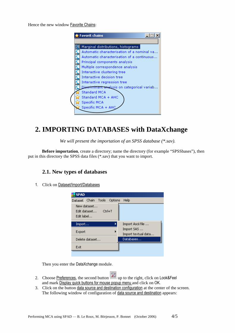
Hence the new window Favorite Chains:

2. IMPORTING DATABASES with DataXchange

We will present the importation of an SPSS database (*.sav).

Before importation, create a directory; name the directory (for example “SPSSbases”), then put in this directory the SPSS data files (*.sav) that you want to import.

2.1. New types of databases

1. Click on Dataset/Import/Databases

Then you enter the DataXchange module.

2. Choose Preferences, the second button up to the right, click on Look&Feel and mark Display quick buttons for mouse popup menu and click on OK.

3. Click on the button data source and destination configuration at the center of the screen. The following window of configuration of data source and destination appears:


4. Use the button (add new source) at the top of the window, and a new window will open,

which will permit to specify what type of database to import 5. Choose SPSS files in the rolling menu:

6. Then, click on 7. Write in the field name: “SPSS data” 8. and in the field description: “SPSS data” 9. and then search for the folder (“SPSSbases”, see above) where the SPSS dataset you want to

analyze is located

10. click on and a new window will open (see window on the following page) 11. Double click, in the window labeled Destinations, on my SBA data to choose the directory in

your working directory where you want to place the SPAD database and click on


2.2. Importing a SPSS database After defining the source in the previous step under the window source, open SPAD DataXchange again, click on Begin new import/export project. You then obtain the window below:

1. Window Sources: double-click on SPSS databases to select the database to import (culture.sav);

2. Window Destinations: double-click on my SBA data and thereafter on new to give a name (culture) to the SPAD database (with the extension * .SBA: thus culture.SBA).

3. Double click on the name of the SPSS database to import (culture.sav) to obtain a list of variables in the SPSS database.


4. Select the variables to export to SPAD;

• transfer the selected variables to the right window. • The type of the variables is undefined:

a) make an automatic typing, by selecting the variables and then click on the button .

Each variable is associated with one of the four following types6:

libel (identifying variable)7 nominal (categorical variable) text (text variable) continu (numerical variable)

b) To change the type for a variable, double-click on the type for this variable and a new window appears that allows modifying the type of the variable (change the variable Z to nominal and id_spadn to libel).

5. For ordinal variables, verify that the order of the modalities is correct8.

6 The types of variables are in French: nominal=categorized; libel=label; continu=numerical. 7 There can only be one identifying variable. 8 In the last version of DataXchange (October 2006), modalities are listed according to the order of the SPSS file. In the preceding version, the import is made according to the alphabetical order of the labels of the modalities (categories).


• For example, for age, double-click on QS3, and the following window appears

4.5. Then click on ok twice.

6. Click on the button Deploy , you will return to the initial window. 7. Click on the button Launch the import/export, then click on No, and the database culture.sba will

be created in the folder Bases in your working directory.

4.1. Click on enter categories

4.2a. Click on ok.

4.4. to change the order, choose the mode manual

4.2b. Click on no

4.3. Select search all categories (maximum) then click on ok.


2.3. Checking of the imported SPAD database (sba)

Check that the imported data corresponds to the initial SPSS database, for instance by comparing the frequencies of the two files. Choose Marginal distributions, histograms in the window Favorite chains. You obtain the following window Chain:

The icons are grey, which means that the methods are not parameterized (that is, the options are not specified)9. To select the database culture.sba:

1. double-click on the icon BASE 2. in the list of databases, double-click on culture.sba

You obtain:

The parameter window is structured in different sheets, each sheet groups the different parameters of the method.

9 Colors of icons inform about their state: grey: the method is not parametrized. yellow: the method is parametrized.

The name of the database associated to the chain appears with its full path.

3. Double-click on the icon for parameters of Stats method.


3. Click on the sheet Marginal distributions and in order to transfer all the variables to the button

window click on , and then click on

4. Click on the icon STATS with the right button of the mouse and on Execute the method (it is

first required to save the chain).

5. Results.

To obtain the frequency tables as a text file, click on , and as an Excel file, click on .


3. STANDARD MCA

3.1. Performing a Standard MCA Choose the chain “Standard MCA” in the window Favorite chains, and choose the database by double-

clicking on the icon and choose culture.sba. You obtain the following window:

It is then necessary to set the parameters for the Cormu and Defac methods. • Setting parameters for Cormu

Double-click on the icon . The window of parameters for the Standard MCA has 4 sheets: Variables, Cases, Weighting, Parameters.

1. Click on the sheet Variables, in order to select the active questions (variables) and the supplementary questions (variables). 1.a. Select the active questions (rolling menu: Variable selection: Active categorical variables): and

transfer the first six variables below by using the button with one arrow . 1.b. Do the same for the supplementary questions (Supplementary categorical variables).


2. Click on the sheet Cases to choose the active individuals (cases) and the supplementary individuals (cases). Choose All.

3. Click on the sheet Weighting.

4. Click on the sheet Parameters.

Dans la méthodologie de l’AGD, on ne ventile pas les modalités de faible effectif : on effectue une ACM spécifique.

In GDA methodology, use specific MCA putting rare modalities as passive ones.

By default, the coordinates of the individuals are not included in the output.


• Running MCA

Click on the right button of the mouse on the icon and choose the Run method.

3.2. Results of MCA You obtain the following icons:

Verify the frequencies and the choice of active and supplementary questions and active individuals in the text file.

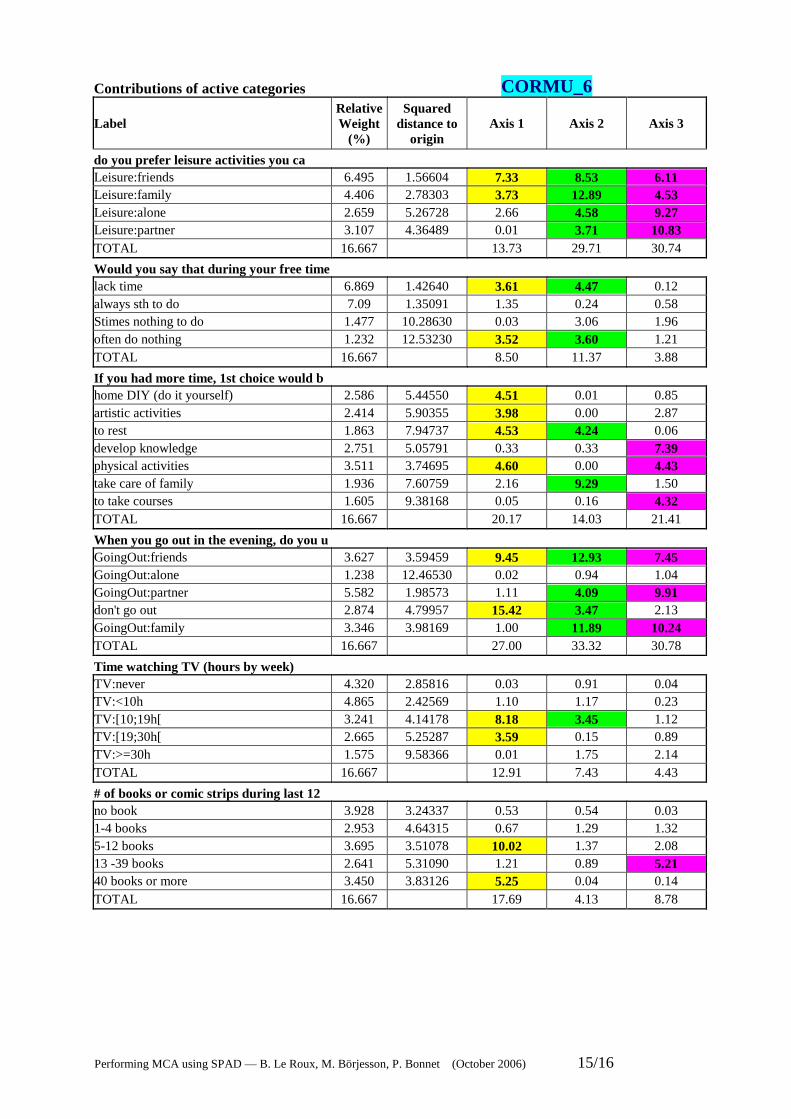
The results in the Excel document are the following: Cormu-1: marginal distributions of active variables Cormu-4: control panel of eigenvalues Cormu-5: loadings [coordinates] of active categories [modalities] Cormu-6: contributions of active categories [modalities] Cormu-7: squared cosines of active categories [modalities] Cormu-8: loadings [coordinates] of active and supplementary categories [modalities] Cormu-9: test-values of active and supplementary categories [modalities]

Results in the form of a text file

Results in the Excel format

Graph editor


To interpret axes, we will essentially use the Cormu-4 and Cormu-6 sheets and then construct graphs of modalities for the interpretation of the axes.

3.3. Eigenvalues and modified rates We use Cormu-4 complemented with modified rates. To calculate the modified rates, make the following calculations:

1) Modified values (column E) for the eigenvalues inferior to the average eigenvalue (that is 1/Q, where Q is the number of active variables, in this case: 1/6= 0.1666),

2) Modified rates (modified values divided by the sum of all modified values specified in column E).

3) Cumulated modified rates.

3.4. Interpretating axes using contributions The interpretation of the axes is based upon the contributions of the categories [mdalities] (given in sheet cormu-6). For each axis, one marks the categories [modalities] whose contributions are above average contribution, that is, 100/30=3.3% (here one has 30 active categories). See the following table, in which the most contributing modalities are highlighted.

E4=(B4-1/6)^2

Sum of modified values of eigenvalues inferior to 1/Q=1/6=0.1666 E28=SUM(E24:E27) (cell $E$28)

F4=E4/$E$28

G4=SUM($F$4:F4)


Contributions of active categories CORMU_6

Label Relative Weight

(%)

Squared distance to

origin Axis 1 Axis 2 Axis 3

do you prefer leisure activities you ca Leisure:friends 6.495 1.56604 7.33 8.53 6.11 Leisure:family 4.406 2.78303 3.73 12.89 4.53 Leisure:alone 2.659 5.26728 2.66 4.58 9.27 Leisure:partner 3.107 4.36489 0.01 3.71 10.83 TOTAL 16.667 13.73 29.71 30.74

Would you say that during your free time lack time 6.869 1.42640 3.61 4.47 0.12 always sth to do 7.09 1.35091 1.35 0.24 0.58 Stimes nothing to do 1.477 10.28630 0.03 3.06 1.96 often do nothing 1.232 12.53230 3.52 3.60 1.21 TOTAL 16.667 8.50 11.37 3.88

If you had more time, 1st choice would b home DIY (do it yourself) 2.586 5.44550 4.51 0.01 0.85 artistic activities 2.414 5.90355 3.98 0.00 2.87 to rest 1.863 7.94737 4.53 4.24 0.06 develop knowledge 2.751 5.05791 0.33 0.33 7.39 physical activities 3.511 3.74695 4.60 0.00 4.43 take care of family 1.936 7.60759 2.16 9.29 1.50 to take courses 1.605 9.38168 0.05 0.16 4.32 TOTAL 16.667 20.17 14.03 21.41

When you go out in the evening, do you u GoingOut:friends 3.627 3.59459 9.45 12.93 7.45 GoingOut:alone 1.238 12.46530 0.02 0.94 1.04 GoingOut:partner 5.582 1.98573 1.11 4.09 9.91 don't go out 2.874 4.79957 15.42 3.47 2.13 GoingOut:family 3.346 3.98169 1.00 11.89 10.24 TOTAL 16.667 27.00 33.32 30.78

Time watching TV (hours by week) TV:never 4.320 2.85816 0.03 0.91 0.04 TV:<10h 4.865 2.42569 1.10 1.17 0.23 TV:[10;19h[ 3.241 4.14178 8.18 3.45 1.12 TV:[19;30h[ 2.665 5.25287 3.59 0.15 0.89 TV:>=30h 1.575 9.58366 0.01 1.75 2.14 TOTAL 16.667 12.91 7.43 4.43

# of books or comic strips during last 12 no book 3.928 3.24337 0.53 0.54 0.03 1-4 books 2.953 4.64315 0.67 1.29 1.32 5-12 books 3.695 3.51078 10.02 1.37 2.08 13 -39 books 2.641 5.31090 1.21 0.89 5.21 40 books or more 3.450 3.83126 5.25 0.04 0.14 TOTAL 16.667 17.69 4.13 8.78


3.5. Graph for Interpretating Axes

• Choosing the preferences for graphs

To enter the graph editor, double-click on the icon

Define the Preferences/ Style for the page


Define the Preferences for the active categories (style for the groups), define one color and a symbol for the active category (for example a red filled circle), a size that is proportional to the weight and long labels as indicated below.

Choose the maximum size for the symbols: Drawing/Adjust the proportionality

• Construction of graph for interpreting an axis

1. Select Graph/New, which gives you the following window:

Maximal size of the symbols in 10 pixels


2. Select the active questions by marking active categorical variables.

3. If preferred, redraw the graph symmetrically to the horizontal axis, by using 4. In order not to show more than 14 out of the 30 (46%) categories that contribute the most to

axis 1: a) Select all points (Selection/Of all points) (the selected points becomes purple )

b) Then Selection/Statistical filtering of the selection


Choose axis 1 as the first and also as the last axis (put axis 1 also as the last axis).

c) Show the labels by clicking on the button ;

d) Unselect the points by using the icon . You then obtain a graph like this:

To interpret axis 2, perform the same steps as for axis 1: use contributions to axis 2 as the statistical criteria for selecting the modalities and drawing the graph. Do the same for axis 3.


3.6. Graph of the Cloud of Individuals

To obtain the cloud of individuals with point sizes proportional to superposition:

1. Parameters of proportionality: Drawing/Adjust the proportionality and choose Maximal size of the symbols in pixels (for example 8).

2. Select all the points (Selection/Of all points), and go to the menu Format/Colours, symbols,… and check the item Proportional size: Superposition.

3. Make a Total unselection

4. If you wish to redraw the graph symmetrically to the horizontal axis, use

You then obtain, in the plane of axes 1-2, the following graph:


Let us now study the cloud of individuals structured by age. Select Graph/new: check Active cases and Supplementary categorical variables

and select the variable Age which will function as structuring factor, by clicking on variables selection.

(If you wish to redraw the graph symmetrically to the horizontal axis, use ), Parameters of proportionality: Drawing/Adjust the proportionality and choose Maximal size of the symbols in pixels (for example 6). Choose Selection/Of Groups/Supplementary Categories and then Format/Colours, Symbols,…: Choose for example Red and empty squares.

Then Total unselection

To join the categories of age, click on , choose Age, and click OK. To trace the 6 ellipses: Format/Cases by a categorical variable or a partition and click on Age…


… and check ellipses in the following window:

Then put all the points as “ghosts” and click on Total unselction , you get the following graph:


To draw only the ellipses for the young and the old, put the other categories as ghosts (Click on the

category 35-45 and then on , etc.

The result is the following graph:

With a click on the right button of the mouse you can modify “by hand” the ellipses, the modality mean points of the categories , or the labels in the graph.


4. STORING PRINCIPAL COORDINATES AND PARTITIONS

To recover the principal axes [factorial axes] or the partitions in a SPAD Database, insert the method Storing factorial axes and partitions into the desired location in your chain, then parameterize it and finally execute it.

You have two tabs to choose from:

1. The principal coordinates (factorial coordinates) and the partitions to store.


2. The parameter settings for archiving. 3.

The storage parameters have default values.

Click on the button New database to give a name to the new BASE and on OK

Then run the method. You obtain the following pictogram. In the text file, you can see the name of the variables in the new file and the name of this new file.

5. APPENDIX

5.1. Generalities on the graph editor

• The toolbar of the graph editor

The initial pre-selection for a new graph is important, it is necessary to pre-select the variables and the individuals you think you will be interested in analyzing in the graph.

Select axes

Point by point selection

Total deselection

Selection by framing

Display labels

Remove labels

Display as ghosts

Back to normal

Information on points

Refresh

Symmetries

Symbol size proportional to criterion


• The fundamental rule for formating a graph

Selection /Format (action) / Unselection

One starts with selecting a point or a group of points, then one formats them, and finally one makes a total unselection, and the chain of procedures can continue.

The “Selection” menu permits to effectuate a selection of points, either by groups of points, or point by point. The selection can be accomplished either by using the “Selection” menu or by the buttons on the toolbar.

The “Format” menu (or the buttons on the toolbar) permits to format the selected points.

Because certain operations, for example the replacement of labels, are resource demanding, the graph can be imperfect with double labels or blank spots. It is thus advisable to Refresh the graph. Either

click on the icon on the toolbar or use the menu: Drawing/Refresh.

5.2. Interface SPAD/SPSS using SPAD editor This option allows you to import a file in SPSS format and transform it into a SPAD database, or conversely, to export a SPAD database towards a file in SPSS format. Identifier of observations In SPSS, there is no specific variable identifying the observations (cases) as such, only an internal variable named $casenum.

In SPAD, there is a specific variable identifying the observations (cases). In order to allow SPAD to identify the cases of an SPSS database (*.sav), it is necessary to create the variable id_spadn, which is a chain of characters recognized by SPAD as the variable defining the cases.

Before importing an SPSS database, create the variable id_spadn with the help of the following SPSS syntax: STRING id_spadn (A4). COMPUTE id_spadn = STRING($casenum,F4) . VARIABLE LABELS id_spadn 'Identifier SPAD' . EXECUTE .


Management of variables types. In SPAD, there are two types of variables, NOMINALS (categorical variables) and CONTINOUS (numerical variables).10 When editing an SPSS database in the data editor of SPAD, the program automatically determines the type of variable according to the following rules: All numerical variables in SPSS with a range of values between 1 and 300 are automatically ascribed as "nominal variables". All other numeric variables in SPSS are automatically typed as "continuous variables". Warning: All SPSS variables with at least one “0” is automatically typed as "continuous variables". Management of missing values. The missing values (by default or specified) in the SPSS database are in the SPAD data editor represented by an empty cell. The program uses respectively the value “0” for categorical variables and 999999 for numerical variables. Management of labels and variable names. For the variables that are automatically typed as "nominal variables", the labels associated with the values (in the SPSS database) are copied into SPAD in the same order. If there are no labels for certain values between the minimum and the maximum value, the program automatically labels the value 'category n° x'. The labels are visible in the window values. Warning: To avoid having a long list of “empty” labels of the type 'category n° x', make sure to code the initial data without gaps. Do not for instance code the variable sex as following, 1 ‘men’, 2 ‘women’ 99 ‘NR’, but 1 ‘men’, 2 ‘women’ 3 ‘NR’. In SPSS it is possible to “pack” the values by using the automatic recode function. In the Variable window, the short identifier of a variable is constituted by the first 4 characters of the name of the variable in the SPSS database. The variable label of SPSS is also imported, which makes it easy to identify the variables. Also the initial order of variables in the SPSS database is preserved. Management of string variables. . However, the string variables in the SPSS database can’t be imported directly into SPADIt is thus necessary to first transform the string variables into numeric variables in SPSS and then to import them as nominal variables. This can be done by using the automatic recode function (menu Transformation) in SPSS. Use the following syntax to automatically recode, for example, the variable “S” to the new variable “SUJ”: AUTORECODE VARIABLES=S /INTO suj /PRINT. This function creates a numerical variable which starts at 1 and whose values are arranged in alphabetical order based on the original string variable.

10 There is also a third type, TEXT (text or string variables), but it is not relevant in the context of importing SPSS databases, see below.


• To Import SPSS databases: *.sav (SPSS) → *.sba (SPAD) 1. In the main window of SPAD, chose Dataset and New database to enter the SPAD database editor.

2. In the menu File in the data editor, click on Open

3. Select Files of type: SPSS file in the list of file types.


4. Then search for and select the SPSS database (*.sav) you want to import (here Culture.sav)

The SPSS database is automatically opened in the SPAD data editor.

To create an SPAD file, chose Save as and select the SPAD file type (.sba) in the list of file types. Name the database (here Culture). Warning: Sometimes in the box for the name, the file extension *.sav appears. It is then necessary to erase this and change it to *.sba, otherwise the initial SPSS database will be overwritten with the SPAD file!


The file culture.sba which now is created is the database for SPAD.

Important remark:The database is not modifiable in SPAD. In case of problem with the import, make the corrections in SPSS and redo the import SAV → SBA.

• To Export SBA databases: *.sba (SPAD) → *.sav (SPSS) To export a SPAD database to a file in the SPSS format, select the option Edit Dataset in the Dataset menu, then File-Open.

� Select the base to export and it will be opened in the Database editor.

� Select the option Save as in the File menu.

� Select the SPSS file type (*.sav) and enter the name of the file to create (by selecting the extension .sav), then click on Save.

• Rules for converting SPAD to SPSS SPSS identifies the variables by their name. The conversion of SPAD to SPSS follows the rules described below. • Categorical variables.

The categorical variables are copied into SPAD with their labels and values identifier, with the value 0 for the missing data. • Numerical variables.

The continuous variables are copied with their labels, and the value 999999 for the missing data. • The variable names are the short identifiers. The labels (view variables) are copied to the ‘variable tag’ in SPSS. • Identification of cases.

The content of the label column of cases is sent to SPSS in the form of a character string with the name id_spadn. • Duplicates of variable names.

In the SPAD database editor, the short identifier is the string containing the first four characters of the label. In the case of these duplicates, the name of the variable in SPSS is created by attaching to the short identifier an index position of the variable in the SPAD file.Variable names must begin with a letter.