P

Predicting Inadequate Capitalization:Early Warning System for Bank Supervision

Julapa A. JagtianiJames W. Kolari

Catharine M. LemieuxG. Hwan Shin

Emerging Issues SeriesSupervision and Regulation Department

Federal Reserve Bank of ChicagoSeptember 2000 (S&R-2000-10R)

1

Predicting Inadequate Capitalization:Early Warning System for Bank Supervision

Julapa A. JagtianiSenior Financial Economist, Supervision and Regulation

Federal Reserve Bank of Chicago

James W. KolariChase Professor of Finance, Finance Department

Texas A&M University

Catharine M. LemieuxDirector, Policy and Emerging Issues, Supervision and Regulation

Federal Reserve Bank of Chicago

G. Hwan ShinVisiting Professor

University of Texas at Pan American

September 27, 2000

_______________________The authors thank Carlos Gutierrez, Loretta Kujawa and Alan Montgomery for their researchassistance, and thank Ken Spong for his assistance related to the regulatory issues. Pleaseaddress correspondence to: James W. Kolari, Finance Department, Texas A&M University,College Station, TX 77843-4218 Office phone: 979-845-4803 Fax: 979-845-3884 Email: j-kolari@tamu.edu. Requests for additional copies should be directed to the Public InformationCenter, Federal Reserve Bank of Chicago, P.O. Box 834, Chicago, Illinois 60690-0834, ortelephone (312) 322-5111. The Federal Reserve Bank of Chicago's Web site can be accessed at:http://www.frbchi.org/regulation/regulation.html.

The views expressed in this paper are those of the authors and do not necessarily reflect theviews of the Federal Reserve Bank of Chicago or Federal Reserve System.

2

Predicting Inadequate Capitalization:Early Warning System for Bank Supervision

Abstract

This paper seeks to examine the efficacy of early warning systems (EWSs) with respect to

predicting incipient financial distress of banking institutions. A sample of banks with total assets

between $300 million and $1 billion is gathered, financial and economic data for individual

banks are collected, and EWSs that have been applied in banking studies are tested. Rather than

attempting to predict bank failure as in previous banking literature, we classify banks as capital

adequate or capital inadequate and seek to predict inadequately capitalized banks one year prior

to the initial decline of the capital ratio. The EWS models developed in this paper could identify

capital inadequate banks with a reasonable degree of accuracy. Thus, our models could be

potentially useful as effective EWSs for purposes of supervisory action.

3

Predicting Inadequate Capitalization:Early Warning System for Bank Supervision

I. Introduction

Capital adequacy is central to regulatory oversight of safety and soundness in the U.S.

banking system. From a regulatory perspective, inadequate capital reflects financial distress that

often leads to failure. Regulators' ability to predict bank capital deficiency would greatly enhance

the effectiveness of the supervisory process, thereby affording regulators additional time to closely

monitor potential problem banks and impose sanctions (on dividend payments, asset growth, new

business activities, salaries, deposit rates, etc.) to facilitate institutional recovery.

Because inadequate capitalization is a pre-condition to bank failure, it has been the subject

of widespread study.1 It is well documented in the literature that financial distress is a prolonged

process that normally takes place over an extended period of time. Previous work on financial

distress attempts to predict bank failure or closure by regulatory authorities.2 These studies

examine the endpoint in the timeline of financial distress, which extends from the early stage of

inability to earn competitive profits to a period of financial turmoil and ultimate failure. As

pointed out by Coats and Fant (1993), “At this point, there is little practical use for a predictive

algorithm since the distressed nature of the firm is obvious to virtually all of the firm’s

1 See Altman (1964); Altman and McGough (1974); Altman, Haldeman, and Narayanan (1977);Ohlson (1980); Zmijewski (1984); Fydman, Altman, and Kao (1985); Zavgren (1985); Lau(1987); DeAngelo and DeAngelo (1990); Platt and Platt (1990); Coats and Fant (1993); Ward(1994); and Johnsen and Melicher (1994).2 See Meyer and Pifer (1970); Sinkey (1975); Santomero and Vinso (1977); Bovenzi, Marino, andMcFadden (1983); Korobrow and Stuhr (1985); West (1985); Maddala (1986); Lane, Looney, andWansley (1986); Whalen and Thomson (1988); Espahbodi (1991); Thomson (1993); Kolari,Caputo, and Wagner (1996); and Kolari, Glennon, Shin, and Caputo (2000).

4

stakeholders …” (1993, p. 147).3 Consistent with this reasoning, Gilbert, Meyer, and Vaughn

(1999) attempt to predict banks that are likely to develop financial problems in the near future --

predicting a CAMELS downgrade from a safe level (rated 1 or 2) to a watchlist level (rated 3, 4,

or 5).4 Using a logit analysis, Gilbert, Myer, and Vaughn found a simple equity to asset ratio to be

one of the important predictors for a CAMELS downgrade.

Extending work by Coats et al. and Gilbert et al., this paper develops EWSs to predict

incipient financial distress of banking institutions as reflected in declining capital ratios. We apply

both logit analysis as well as trait recognition analysis (TRA), a neural network-like method, to the

financial and economic data for the period 1988 to 1990. We classify banks as capital adequate or

capital inadequate and seek to predict bank capital falling below a specified adequate level one

year ahead of time. The empirical results indicate that both of the EWS models could predict

incipient capital deficiencies a year ahead with a reasonable degree of accuracy. The models

could potentially be incorporated into the supervisory process to allocate examination resources

towards troubled institutions and to effectively monitor banks for capital requirement standards.

The next section reviews relevant literature, Section III describes the methodology, Section

IV discusses the data and empirical results, and Section V summarizes and concludes the paper.

II. Literature on Predicting Financial Distress

There are two branches of literature on financial distress – the multinomial choice

approach and the survival time approach.

3 In their study, auditors’ reports were employed to define financially-troubled firms versus viablefirms, and a neural network early warning system (EWS) was developed and tested on a sample ofcorporate firms.4 After an on-site examination, commercial banks receive CAMEL ratings on a scale of 1(strongest) to 5 (weakest) from their chartering agency (the Federal Reserve for state memberbanks, state bank commissioner for state non-member banks, or the Comptroller of the Currency

5

In multinomial choice models, a number of states of the firm are hypothesized to exist. For

example, some studies define five possible states -- financial stability, omitting or reducing

dividend payments, default on loan payments, protection from Chapter X or XI of the Bankruptcy

Act, and bankruptcy and liquidation.5 Some studies define a continuum of financial distress.6

Others collapse these five states into nonbankrupt, financially weak, and bankrupt firms.7 In most

of these studies, an ordinal logistic regression (OLGR) technique is employed, where the response

variable is multinomial (as opposed to binomial), and explanatory variables are used to estimate

the cumulative probability that a firm is a member of the response states.

In general, these studies found that accounting information can detect incipient financial

distress of nonfinancial firms, and that different firm states on the financial distress continuum

appear to be independent of one another. That is, significant predictors vary across states and,

therefore, depend on the particular state of financial health. This suggests that EWS models

previously developed to predict the late state of regulatory closure or bankruptcy of commercial

banks will likely differ from those seeking to predict an early stage of financial distress, such as

deterioration in capital ratios.

Another branch of financial distress, survival time research, predicts the probable time to

failure using financial, economic, managerial, and regulatory factors.8 Using Cox proportional

hazards models, as well as split-population survival time models, previous studies measure

survival time relative to bank closure or failure. In general, the empirical results support the

for national banks), where C = capital adequacy, A = asset quality, M = management,E = earnings,L = liquidity, and S = market sensitivity.5 See DeAngelo and DeAngelo (1990), Giroux and Wiggins (1984), and Lau (1987).6 See Ward (1994).7 See Johnsen and Melicher (1994).8 See Altman and McGough (1974); Kalbfleisch and Prentice (1980); Altman (1983); andYamaguchi (1991) for discussion of nonfinancial firms; and Cole and Gunther (1995); Lane,Looney, and Wansley (1986); and Whalen (1991) for banking firms.

6

notion that financial distress is a dynamic process that can be predicted using financial, economic,

and other explanatory variables. Catanach and Perry (1996) applied a survival time model with

time-varying predictors to savings and loan (S&L) institutions. Interestingly, the authors noted

that, among numerous studies attempting to predict S&L failure, only one variable was significant

in all such studies – the equity capital ratio. Relevant to our purpose, they also observed that:

“Barth et al. (1989) indicate that the importance of the net worth ratio is not surprising since it is

the variable that regulators use in closing institutions. Consequently, capital ratios may better

represent dependent variables than independent variables in distress studies for financial

institutions.” (1996, p. 12).

Our study attempts to close this gap in the literature by using the equity capital ratio as the

dependent variable to reflect an early stage of financial distress. Our objective is to develop a

model that predicts one of two states -- capital-adequate versus capital-inadequate -- where the

latter state represents incipient financial distress to be predicted by bank supervisors. An

advantage of our study over previous studies, which predict legal or regulatory failure, is that our

financial distress event is not biased by regulatory actions that typically take place prior to bank

closure or technical insolvency.9

III. The Methodology -- EWS Models

Two different EWS models are utilized in this paper – the logit model and trait recognition

analysis (TRA).

Logit Model

Logit analysis is the most commonly employed EWS methodology applied in business

academic studies as well as bank regulatory practice, especially in detecting potential failure risk.

7

According to this parametric method, the posterior probability of an event (i.e., capital inadequacy

in the present context) can be derived from the following logit specification:

log[Pi/(1-Pi)] = a + b1Xi1 + b2Xi2 + … + bnXin, (1)

where Pi = the probability of bank i’s failure, and b = (b1, …, bn) is a vector of regression

coefficients for explanatory variables Xj (j = l, …, n). The logit model has the advantages of not

assuming multivariate normality among the independent variables, thus being computationally

more tractable (see Espahbodi (1991, p. 56)).

As discussed in the next section, our logit analysis employs 48 explanatory variables. A

stepwise logistic regression analysis is performed to select a subset of independent variables that

are most important in terms of discriminatory power.10 In view of work by Aldrich and Nelson

(1984) and Stone and Rasp (1991) on miscalibration problems related to degrees of freedom and

disparate sample sizes of the response groups, we infer that our sample sizes (to be discussed

shortly) are sufficient to obtain efficient estimates of the logit parameters (i.e., the cumulative

distribution of the error terms in the regression relationship approximates a logistic function).

Despite the widespread popularity of a logit model as an effective EWS approach, it does

have some drawbacks in terms of the information that it produces. For example, it is not possible

to determine from the parameter estimates generated by logit models which variables are most

useful in predicting capital-inadequate banks (or alternatively capital-adequate banks). The results

only indicate the effectiveness of each variable’s ability to discriminate between the two groups of

banks. While the logit methods seek to minimize classification errors, they do not provide any

9 It is reasonable to assume that most banks become capital deficient prior to regulatory actionssuch as cease and desist orders and supervisory agreements.10 To enhance the predictive power of the logit models, we lowered the threshold for adding variables tothe model by decreasing the (default) significance level from 10 percent to 30 percent.

8

information about how each variable affects Type I and II errors per se. In addition, logit models

are not well suited to examining interactions between variables.

Trait Recognition Analysis (TRA) Model

Trait recognition analyses (TRA) is a nonparametric pattern recognition technique that

relies upon computer-intensive methods to identify systematic patterns in the data. Originally

developed in the hard sciences, and unlike logit analysis, TRA is most closely associated with

neural network models in that it seeks to exploit information contained in complex interactions of

the independent variable set.11 However, in neural network models, variable interactions are

contained in a so-called hidden or latent layer that cannot be observed by the researcher. Unlike

the neural network model, TRA identifies and documents all variable interactions.

Variable interactions in TRA are combinations of variables that are formed to be consistent

with the logic of a financial analyst (e.g., low profitability and high credit risk is an unfavorable

combination for a bank), rather than simple cross products of variables as in neural network

models. Further details of TRA and comparisons with other EWS models are discussed in

Appendix I.

The fact that logit and trait recognition methods are grounded in different types of

mathematical algorithms and yield different results implies that regulatory practice should

consider applying both methods to gain as much information as possible about sample banks’

potential future capital adequacy. One model may dominate the other model for any individual

bank in terms of identifying pending capital adequacy problems. By applying a double screen, the

11 See Bongard et al. (1966); Gelfand et al. (1976); Briggs and Press (1977); Briggs, Press, andGuberman (1977); Caputo et al. (1980); Benavidez and Caputo (1988).

9

total effectiveness of EWS efforts can be improved and information about individual banks can be

enhanced.

IV. Data and Empirical Results

Samples and Independent Variables

Financial data for U.S. commercial banks with total assets between $300 million and $1

billion were collected from the Call Reports of Income and Condition for year-end 1988, 1989,

and 1990.12 The reasons for selecting these years, rather than more recent period, is to obtain a

sufficient number of troubled banks in the sample. Not surprisingly, most banks were well

capitalized during the economic prosperity of the 1990s. We define adequately capitalized

institutions as those banks with at least 5.5 percent primary capital to total assets ratio for the

whole sample period.13 This ratio coincides for the most part with the regulatory standard for

adequate capitalization during the sample period.14

We recognize that the risk-based capital standard, which was announced in July 1988, was

implemented for the first time on December 31, 1990.15 However, our framework attempts to forecast an

12 Since most troubled banks are small (with total assets of less than $1 billion), we focus on thesebanks in our study.13 Primary capital includes common and perpetual stock, surplus and undivided profits,contingency and other capital reserves, mandatory convertible debt instruments (up to 20% ofprimary capital exclusive of such instruments), allowance for loan and lease losses, net worthcertificates, and minority interests in consolidated subsidiaries. Intangible assets and goodwillwere excluded.14 As of December 31, 1990, bank holding companies and state member banks could chooseto conform to either the old 5.5 percent primary capital and 6 percent total capital standards orthe new 7.25 percent minimum risk-based capital standard (see Federal Reserve RegulatoryServices Manual Section 12 CFR 225 titled "Capital Adequacy Guidelines for Bank HoldingCompanies and State Member Banks: Leverage Measure").15 Risk-based capital standards are based on credit risk differences among different kinds ofbank assets and off-balance sheet activities. Minimum capital requirements were establishedfor Tier 1 (equity) capital and Tier 2 (long-term debt and reserves) capital. In 1998 risk-basedcapital rules were amended for market risk related to securities investments. More recently,

10

economic event, as opposed to a legal or regulatory event. In other words, the objective of our analysis is

not to investigate banks' regulatory compliance, but rather to capture an early stage of financial distress,

which may include a variety of indicators such as profitability, leverage ratios, etc. Estrella, Park, and

Peristiani (2000) examined the relationship between different capital ratios and bank failure, and found

that the simple capital to assets ratio (leverage ratio) predicts bank failure as well as more complex risk-

weighted capital ratios over one-year or two-year horizons. In addition, Estrella et al. recommended

using the simple capital ratio as a tool to provide a timely signal of the need for supervisory action. Thus,

our choice of a 5.5 percent primary capital to asset ratio is a suitable proxy for an early stage of financial

distress.16

Our research methodology is implemented in two steps. First, for the original sample

using year-end 1989 data, each sample bank was assigned a dummy value of 1 (capital-adequate)

if the ratio of primary capital to total assets equal to or greater than 5.5 percent, and 0 (capital-

inadequate) otherwise. Financial and economic data are assembled for the original sample one-

year prior to the capital inadequacy event or year-end 1988, and the logit and TRA models are

developed. Second, the data for 1990 holdout sample was then coded as 0 or 1 based on the 5.5

percent primary capital ratio as of year-end 1990. One-year prior (year-end 1989) data (i.e., the

independent variables) for these banks were passed through the logit and TRA models. As such,

the BASEL committee has discussed the possibility of implementing further changesconcerning more refined estimation of credit risk via banks’ internal models.16 It should be noted that the primary capital ratio had the advantage of potentially providing anearlier warning system than institutional closure, assisted merger or acquisition, or liquidation byregulators. The latter discrete conditions typically occur after a prolonged period of financialdistress and represent the endpoint in the distress continuum. Predicting banks that will becomecapital deficient in the near future is tantamount to identifying incipient financial distress, asopposed to the final stage of financial distress. In addition to primary capital, the Federal ReserveBoard established capital zones based on simple capital ratios to flag risky banks (see Spong(1985) for more detail on the capital zones).

11

the holdout sample allows us to observe the predictive ability of the EWS models with data that

was not employed in their development.

After dropping some institutions due to missing data, the following sample sizes were

obtained for the original and holdout samples:

Capital adequate Capital inadequate TotalOriginal samples (1989):

One-year prior (1988) 451 71 522

Holdout sample (1990):One-year prior (1989) 461 77 538

Our explanatory variables for predicting banks that will become capital inadequate include

a wide variety of on- and off-balance sheet bank risks -- profitability, loan risk, operational risk,

liquidity risk, interest rate gap, bank size, derivatives exposure, loan commitments, years in the

banking business, and changes in loan compositions. We also include some control variables that

reflect economic conditions -- information on business and non-business bankruptcy filings in the

state in the past year, rural versus urban location of the bank, and income per capita and permits

per capita in the state where the banks are located.

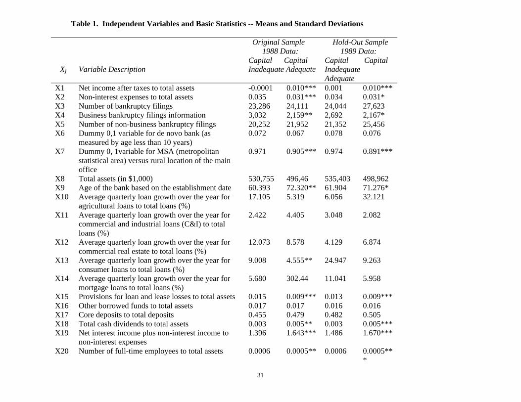
Table 1 lists the independent variables and provides basic statistics for the original and

holdout samples. The t-statistics in Table 1 test the null hypothesis of no significance difference

between capital-adequate versus capital-inadequate banks. Asterisks indicate a failure to accept

the null hypothesis and acceptance of the alternate hypothesis that there was a significant

difference between the levels of the respective variable between the two response groups. In the

original one-year prior (1988) sample, 24 out of 48 independent variables are significantly

different in the two response groups, while 22 out of 48 independent variables are significantly

12

different in the holdout one-year prior (1989) sample. In most cases, significant variables in the

original sample are also significant in the holdout sample.

Generally speaking, capital deficient banks tended to have lower profitability, higher risk,

and higher levels of expenses than other banks. These results suggest that banks pending capital

deficiency have financial profiles that substantially differ from well-capitalized banks. Also,

banks that were capital inadequate tended to be located in states with higher business bankruptcy

filings and in urban region as opposed to rural regions. The numerous significant differences

between capital-adequate versus capital-inadequate banks suggest that it would be appropriate for

our variables to be used as predictors of capital deficiency in EWS models.

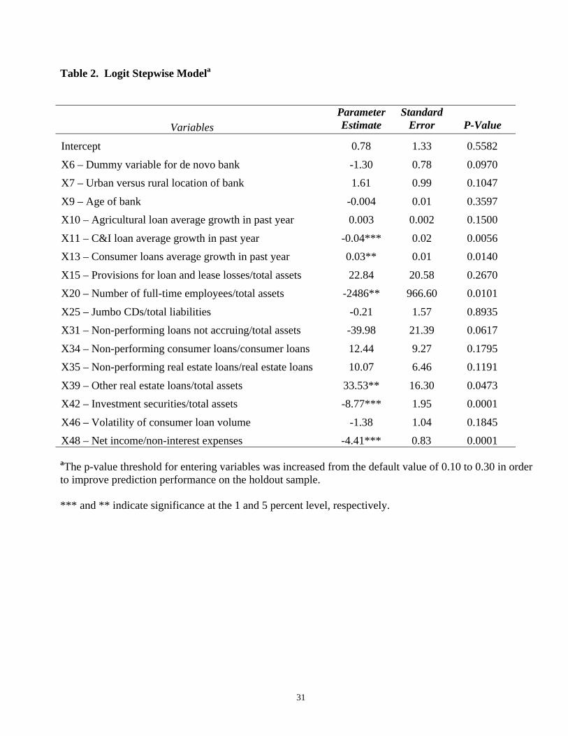
Tables 2 and 3 provide further details of the logit and TRA models, respectively,

developed with the original sample. The classification accuracy of the logit model well exceeded

chance. Taking into account the desire to minimize Type II errors and, at the same time, achieve

good overall classification accuracy, the prior probability of 0.16 yielded 80.7 percent correct

overall classification and 34.0 percent Type II errors (i.e. misclassification of capital inadequate

banks to be adequate).17

From the results of logit analysis in Table 2, 16 out of 48 variables were retained in the

one-year prior logit model, and only six variables are significant at the 5 percent level or better.

Out of these 16 variables, 13 were significant in the univariate t-tests using the same 1988 data

(Table 1) -- thus, both the univariate and multivariate statistical analyses seem to identify the same

significant predictors for the most part. In a multivariate context, each of these significant

variables contributes unique discriminatory information not available from the other variables.

17 Lowering Type II errors by decreasing the prior probability of capital adequacy tends toincrease Type I errors (i.e., misclassification of capital adequate banks to be inadequate). Becausethe tradeoff between Type I and II errors is critical to evaluating EWS models, we report theseresults for the holdout sample to summarize the predictive power of the EWS models.

13

Numerous variables are highly significant (at the 5 percent level or better) in terms of

discriminatory ability between capital-adequate versus capital-inadequate banks. Specifically,

these variables include the average growth rates of commercial and industrial and consumer loans,

average growth rate of consumer loans, number of full-time employees, other real estates loans

(OREO), investment securities to total assets, and net income to non-interest expenses (a measure

of efficiency).

Banks that expanded their consumer lending rapidly tended to significantly add risk to

their portfolio, which subsequently resulted in losses and deterioration in the capital ratio. No

doubt these banks attracted many marginally creditworthy customers. In contrast, a rapid

expansion of C&I loans (rather than consumer loans) tended to lead to profitability and reduced

the likelihood that the capital ratio would fall below our threshold limit. Business customers pay

higher loan fees and often buy other investment and payment services for which the banks charge

fees -- thus, increasing fee income and profitability more than if the loan growth is in consumer

lending.18

Other results indicate that banks with higher proportions of assets invested in investment

securities had a greater cushion against bad lending decisions and, consequently, were less likely

to encounter financial distress. Likewise, more efficient banks with greater net income to non-

interest expenses ratio tended to have a lower probability of financial distress in the near future.

18 Another possible explanation may be related to policies for dealing with problem loans inthese two types of portfolios. For consumer loans, it is customary to charge-off problem loansvery quickly due to their generally short-term nature. For C&I loans, however, banks are morelikely to work with C&I borrowers for a longer period of time; thus, it takes longer for problemC&I loans to be placed on nonaccrual status. As long as interest is still accruing, C&I loangrowth would contribute to reported income, reducing the likelihood of a decline in capitalratios. This difference between C&I and consumer loans is, however, likely to decrease if thetime horizon is longer than one year.

14

Finally, the likelihood of financial distress was reduced by a higher bank age and lower ratio of

non-performing loans not accruing to total assets (i.e., both significant at the 10 percent level).

It is important to note that these variables, when considered in isolation, do not necessarily

provide a complete picture of the early stages of financial distress in banking institutions. For

example, DeYoung (1999) has observed that de novo banks hold relatively higher capital ratios

than other banks but their capital base can rapidly deteriorate, thereby increasing their likelihood

of failure. While logit is not well suited to investigating such variable interactions, the TRA

model identifies interactions between variables that are associated with "safe" and "unsafe" bank

characteristics.

Table 3 lists the distinctive features of one of the TRA models, which performed well on

the holdout sample. Panel A lists the "safe features" for this one-stage TRA model, while panel B

catalogues the "unsafe features".19 Banks with "safe features" are less likely to encounter a

financial distress in the near future, whereas banks with "unsafe features" are those whose capital

ratios are likely to fall below an adequate level within a one-year timeframe. The cutpoints for

defining each of the variables into low (L), low to medium (LM), or high (H) are provided in

Appendix II. Unlike the logit model, most of the 48 predicting variables were included in the

TRA model. Indeed, 37 out of 48 variables are employed in the TRA features. 20 This evidence

implies that capital adequacy is a broad concept that requires review of a wide array of different

kinds of financial and economic variables.

19 Except for one feature that represented a two variable interaction among the safe features, all ofthe safe and unsafe features (i.e., 114 and 150, respectively) are constructed from three variableinteractions.20 The only variables not entering the features list in the TRA model are X5, X8, X9, X21, X22,X30, X38, X43, X44, X45, and X47. Only one of these variables, or X9, entered the logit model.Thus, variables important in the logit model tended to be useful in the TRA model also.

15

Some examples of "safe features" listed in panel A of Table 3 include the following

combinations of variables: X1(U) X6(L) X13(L) – a bank with high profitability that has been in

business for more than 10 years (not a de novo bank) and has slow growth in consumer lending;

and X11(U)X39(L)X48(U) -- a bank with high growth in C&I lending but is less active in other

real estate lending and is cost efficient (i.e., high net income to non-interest expenses ratio).

Overall, there are 114 different interactions that are classified by the model as being "safe

features". Of these 114 interactions, 49 are associated with high profitability, 45 are associated

with low levels of problem loans (X30-X35), and 51 are associated with loan growth. Economic

variables were included in 15 of the 114 interactions for "safe features".

Panel B of Table 3 lists various "unsafe features" that would be of particular interest to

bank supervisors assessing potential capital inadequacy. Some examples of unsafe features are as

follows: X1(L)X2(U)X16(L) -- a bank with low profitability, low efficiency (with high non-

interest expense to assets), and low reliance on borrowed funds; X1(L)X11(L)X48(L) -- a bank

with low profitability, slow growth in C&I lending, and low efficiency; X6(L)X16(L)X17(LM) –

a 10-year or older bank (not a de novo bank) with low reliance on borrowed funds and a normal

(low to medium) ratio of core deposits to total deposits; and X6(L)X19(L)X20(L) -- a non-de

novo bank (older than 10 years) that is less efficient (with low ratio of net income to non-interest

expenses) and has small number of full-time employees. Overall, 150 interactions were reported

as "unsafe features". Of these 150 interactions, 76 are associated with low levels of returns to

assets, 32 are associated with low profitability in conjunction with slow growth, and 49 are

associated with problem loans (mostly agricultural loans due to the economic time period).

Economic variables are included in 18 of the 150 "unsafe features".

16

Comparing these TRA results with those of the logit model, the findings suggest that

interactions between different financial and economic variables are important in identifying banks

with deficient capital. No single variable entered the TRA features list, which means that more

complex interaction variables dominated individual variables in terms of discriminating between

capital-adequate versus capital-inadequate banks. Based on information contained in interaction

variables, the overall classification accuracy of the TRA models was relatively strong in the range

of 95 percent to 100 percent.

Figure 1 graphically shows the 1990 holdout sample prediction results using the logit and

TRA models. The tradeoff between Type I and Type II errors provides a comprehensive view of

overall performance (i.e., the results are based on incrementing the prior probability of capital

inadequacy in the logit model from 0.02 to 0.98, while 25 different TRA models are reported with

different parameter specifications). The logit and TRA models performed very similarly, with

their lines almost tracing one another in the figures. The TRA model was somewhat better than

the logit model in reducing Type II errors but not for the Type I errors. The convexity to the

origin of the lines, as opposed to being a diagonal line connecting 1.00 of the two axes, suggests

that both EWS models performed better than chance. The inflection point of the curves is at about

25 percent Type I and II errors. At the inflection points of the curves, the overall accuracy of

prediction is about 75 percent in both adequately and inadequately capitalized banks.

Overall, both the logit and TRA models developed in this paper would enable bank

supervisors to identify capital inadequate banks a year ahead of time with a reasonable degree of

accuracy. Moreover, the TRA model provides insights into safe and unsafe interactions of

variables that bank supervisors should monitor. We infer that our EWS models could be useful in

17

the supervisory process as effective EWSs for purposes of forecasting impending capital

deficiency.

V. Summary and Conclusions

This paper has sought to empirically test the efficacy of EWS models as prediction tools in

identifying incipient capital inadequacy in U.S. commercial banks. Our sample includes all

insured U.S. banks with total assets in the range of $300 million to $1 billion from year-end 1988

to year-end 1990. Banks are sorted into two response groups on the basis of their primary capital

to total assets ratio. Numerous financial and economic variables are gathered for the sample

banks, which are used to develop logit and the trait recognition analysis (TRA) models as

computer-based EWSs. A holdout sample is used to test the prediction accuracy of the models.

Our results demonstrate that capital deficient banks are much different from other banks in

terms of their financial health. We find that capital adequacy is a broad concept that requires

review of a wide array of different kinds of financial and economic variables. In addition, the

TRA results highlight the importance of complex interaction variables in identifying banks with

deficient capital.

Consistent with these univariate results, multivariate logit and TRA models are able to

correctly predict a decline below a threshold primary capital ratio of 5.5 percent with 75 percent

accuracy. Importantly, both Type I and II errors can be reduced to about 25 percent. Our EWS

models could detect the early onset of financial distress in commercial banks one year in advance

with a reasonable degree of accuracy. By implication, the EWS models can be used to provide a

timely signal of impending bank problems to supervisory agencies.

18

References

Aldrich, J. H. and F. D. Nelson. 1984. Probability, Logit & Probit Models. QuantitativeApplications in the Social Sciences Series: No. 07-045. Sage Publications: BeverlyHills, CA.

Altman, E. 1968. Financial ratios, discriminant analysis and the prediction of corporateBankruptcy. Journal of Finance 23: 589-609.

Altman, E. I. and T. P. McGough. 1974. Evaluation of a company as a going concern. Journalof Accounting: 50-57.

Altman, E., R. Haldeman, and P. Narayanan. 1977. ZETA analysis: A new model to identifybankruptcy risk of corporations. Journal of Banking and Finance 1: 29-54.

Altman, E. I. 1983. Corporate Distress: A Complete Guide to Predicting, Avoiding, andDealing with Bankruptcy. John Wiley & Sons, Inc.: New York, NY.

Barth, J., D. Brumbaugh, Jr., D. Sauerhaft, and G. Wang. 1985. Thrift institution failures:Estimating the regulator’s closure rule. Research in Financial Services 1: 1-23.

Benavidez, A., and M. Caputo. 1988. Pattern recognition of earthquake prone areasin the Andrean Region. Studie Ricerche, University of Bologna: 141-163.

Bongard, M. M., M. I. Vaintsveig, S. A. Guberman, and M. L. Izvekova. 1966. Theuse of self learning programs in the detection of oil containing layers.Geology Geofiz 6: 96-105.

Bovenzi, J. F., J. A. Marino, and F. E. McFadden. 1983. Commercial bank failure predictionModels. Economic Review, Federal Reserve Bank of Atlanta: 186-195.

Briggs, P., and F. Press. 1977. Pattern recognition applied to uranium prospecting.Nature 268: 125-127.

Briggs, P., F. Press, and S. A. Guberman. 1977. Pattern recognition applied toearthquake epicenters in California and Nevada. Geological Society of AmericaBulletin 88: 161-173.

Caputo, M., V. Keilis Borok, E. Oficerova, E. Ranzman, I. I. Rotwain, and A. Solovieff.1980). Pattern recognition of earthquake areas in Italy. Physics Earth and PlanetaryInteriors 21: 305-320.

Catanach, Jr., A. H. and S. E. Perry. 1996. Identifying consistent predictors of financial distressusing survival time models. Working paper. University of Virginia: Charlottesville,VA.

19

Coats, P. K. and L. F. Fant. 1993. Recognizing financial distress patterns using a neuralnetwork tool. Financial Management 22: 142-155.

Cole, R. and J. Gunther. 1995. Separating the likelihood and timing of bank failure. Journal ofBanking and Finance 19:

DeAngelo, H. and L. DeAngelo. 1990. Dividend policy and financial distress: An empiricalinvestigation of NYSE firms. Journal of Finance 45: 1415-1431.

DeYoung, R. 1999. Birth, Growth, and Life or Death of Newly Chartered Banks. FederalReserve bank of Chicago: Economic Perspectives. Third Quarter: 18-35.

Eisenbeis, R. A. 1977. Pitfalls in the application of discriminant analysis in business,finance, and economics. Journal of Finance 30: 875-900.

Espahbodi, P. 1991. Identification of problem banks and binary choice models.Journal of Banking and Finance 15: 53-71.

Estrella, A., S. Park, and S. Peristiani. 2000. Capital Ratios as Predictors of Bank Failure.Economic Policy Review, Federal Reserve Bank of New York (July): 33-52.

Frydman, H., E. I. Altman, and D. Kao. 1985. Introducing recursive partitioning for financialclassification: The case of financial distress. Journal of Finance 40: 269-291.

Gelfand, I. M., Sh. A. Guberman, M. L. Izvekova, V. I. Keilis Borok, L. Knopoff, E.Ranzman, F. Press, E. Ranzman, M. Rotwain, and A. M. Sadowsky. 1976.Pattern recognition applied to earthquake epicenters in California. Physics of the Earthand Planetary Interiors 11: 227-283.

Gilbert, R A., A. P. Meyer, and M. D. Vaughn. 1999. The role of supervisory screens andeconometric models in off-site surveillance. Review, Federal Reserve Bank of St.Louis (November/December): 31-56.

Giroux, G. A. and C. E. Wiggins. 1984. An events approach to corporate bankruptcy. Journalof Bank Research 5: 179-187.

Johnsen, T. and r. W. Melicher. 1994. Predicting corporate bankruptcy and financial distress:Information value added by multinomial logit models. Journal of Economics andBusiness 46: 269-286.

Kalbfleisch, J. and R. Prentice. 1980. The Statistical Analysis of Failure Time Data. JohnWiley & Sons, Inc.: New York, NY.

Kolari, J., M. Caputo, and D. Wagner. 1996. Trait recognition: An alternativeapproach to early warning systems in commercial banking. Journal ofBusiness, Finance and Accounting 23: 1415-1434.

20

Kolari, J., D. Glennon, H. Shin, and M. Caputo. 2000. Predicting large U.S.commercial bank failures. Working Paper No. 2000-1, U.S. Comptroller of theCurrency (Washington, D.C.).

Korobrow, L. and D. Stuhr. 1985. Performance measurement of early warning models:Comments on West and other weakness/failure prediction models. Journal of Bankingand Finance 9: 267-273.

Lane, W. R., S. W. Looney, and J. W. Wansley. 1986. An application of the Cox proportionalhazards model to bank failure. Journal of Banking and Finance 10: 511-531.

Maddala, G. 1986. Econometric issues in the empirical analysis of thrift institutions’ insolvencyand failure. Working Paper No. 56, Federal Home Loan Bank Board.

Meyer, P. and H. Pifer. 1970. Prediction of bank failures. The Journal of Finance 25:853-868.

Ohlson, J. 1980. Financial ratios and the probabilistic prediction of bankruptcy. Journal ofAccounting Research 18: 109-131.

Platt, H. D., and M. B. Platt. 1990. Development of a class of stable predictive variables: Thecase of bankruptcy prediction. Journal of Business, Finance and Accounting 17: 31-51.

Thomson, J. B. 1991. Predicting bank failures in the 1980s. Economic Review, Federal ReserveBank of Cleveland: 9-20.

Santomero, A. and J. Vinso. 1977. Estimating the probability of failure for firms in the bankingSystem. Journal of Banking and Finance 1: 185-206.

Sinkey, J. E., Jr. 1975. A multivariate statistical analysis of the characteristics of problemBanks. Journal of Finance 20: 21-36.

Spong, K. 1985. Banking Regulation: Its Purposes, Implementation, and Effects. SecondEdition. Federal Reserve Bank of Kansas City, Division of Bank Supervision andStructure.

Stone, M. and J. Rasp. 1991. Tradeoffs in the choice between logit and OLS for accountingchoice studies. The Accounting Review 66: 170-187.

Ward, T. J. 1994. An empirical study of the incremental predictive ability of Beaver’s naïveoperating cash flow measure using four-state ordinal models of financial distress. Journalof Business Finance and Accounting 21: 547-561.

West, R. C. 1985. A factor-analytic approach to bank condition. Journal of Banking andFinance 9: 253-266.

21

Whalen, G. and J. B. Thomson. 1988. Using financial data to identify changes in bankCondition. Economic Review, Federal Reserve Bank of Cleveland: 17-26.

Yamaguchi, K. 1991. Event History Analysis. Sage Publications: Newbury Park.

Zavgren, C. 1985. Assessing the vulnerability to failure of American industrial firms: Alogistic analysis. Journal of Business, Finance and Accounting 12: 19-45.

Zmijewski, M. 1984. Methodological issues related to the estimation of financialdistress prediction models. Journal of Accounting Research (Supplement) 22:59-82.

22

Appendix IComparison of TRA with Other EWS Models

Unlike other discriminatory EWS methods, TRA recodes continuous data into binary

codes that simplify the data. This coding enables as many as 16 different interactions between

any two variables to be constructed. Other methods typically do not consider such a large

number of interactions due to related loss of degrees of freedom in the model estimation. Next,

TRA produces a list of both good and bad aspects (traits) for the sample of observations under

study, which can be single variables or interaction variables. By contrast, in other discriminatory

models it is not possible to determine if a variable is valuable in identifying failing banks (or the

control group under investigation) versus nonfailing banks (or the other control group). In this

regard, TRA also generates a list of good and bad traits for each observation. Other EWS

methods typically produce a single score (or probability) but do not provide guidance for each

observation concerning its particular strengths and weaknesses. Finally, unlike most other

discriminatory methods (especially parametric models), TRA performs well with small sample

sizes.21

It is important to point out that in TRA researcher judgement plays an important

role in the model development process. Upon inspecting plots of observations for each variable,

decisions must be made about what level is low, normal, or high for each variable. The rules for

determining whether a variable (or trait) is good or bad in the context of observations under study

must be input into the model. And, rules for classifying banks as safe or unsafe must be specified

21 Indeed, if a large sample size is being employed, it is recommended to run TRA in stages, withthe first stage model classifying observations that are fairly easy to identify and a second (orthird) stage model classifying a smaller set observations that are difficult to identify.

23

by the researcher. This heuristic procedure is ad hoc in nature but is advantageous in designing

EWSs to fit specific sample data.

TRA Coding Procedure

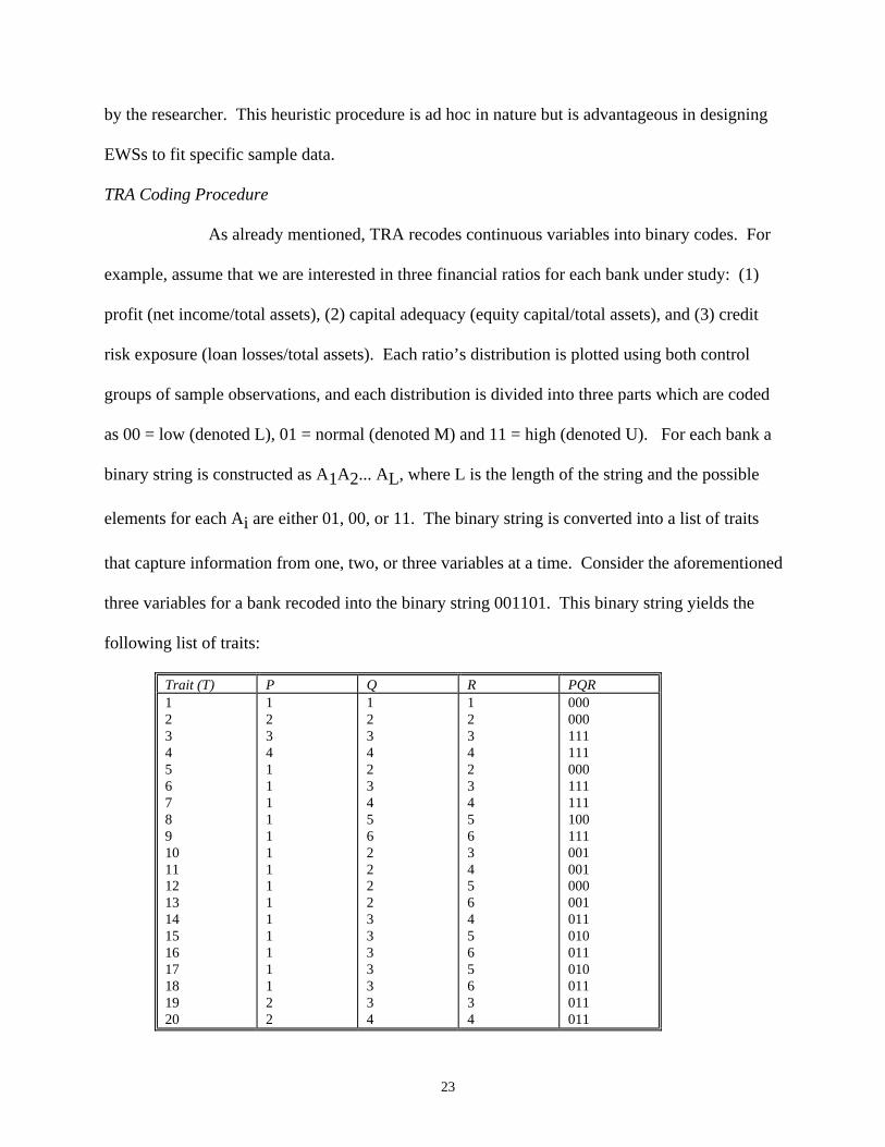
As already mentioned, TRA recodes continuous variables into binary codes. For

example, assume that we are interested in three financial ratios for each bank under study: (1)

profit (net income/total assets), (2) capital adequacy (equity capital/total assets), and (3) credit

risk exposure (loan losses/total assets). Each ratio’s distribution is plotted using both control

groups of sample observations, and each distribution is divided into three parts which are coded

as 00 = low (denoted L), 01 = normal (denoted M) and 11 = high (denoted U). For each bank a

binary string is constructed as A1A2... AL, where L is the length of the string and the possible

elements for each Ai are either 01, 00, or 11. The binary string is converted into a list of traits

that capture information from one, two, or three variables at a time. Consider the aforementioned

three variables for a bank recoded into the binary string 001101. This binary string yields the

following list of traits:

Trait (T) P Q R PQR1234567891011121314151617181920

12341111111111111122

12342345622223333334

12342345634564565634

000000111111000111111100111001001000001011010011010011011011

24

2122232425262728293031323334

22222333334445

56333456445656

56456456565666

000011011010011111100111110111100111101011

In general, as shown in the table above, each trait (T) has six integers: T = p, q, r, P, Q,

R; where p = 1, 2, ..., L; q = p, p+1, ..., L; r = q, q+1, ..., L; P = 0 or 1; Q = 0 or 1; and R = 0

or 1. If q = r, then Q = R; if p = q = r, then P = Q = R; if q = p, then Q = P. The letters p, q, and

r are pointers to positions in the binary string, while P, Q, and R give the values of the binary

code at these respective positions. Thus, trait pqrPQR = 123001 points to positions 1, 2, and 3 in

the 6-digit binary string for a bank, which in the above example has the values of 0, 0, and 1 at

these respective positions. Notice that this trait contains interaction information about profit and

capital adequacy ratios. Casual inspection of the list of traits indicates that they capture all

possible interactions between the variables taken one, two, and three at a time.

Interaction Variables in TRA

Interaction variables in TRA are measured in a different way than normally calculated.

Rather than multiplying together two or more variables (i.e., cross products) to get interaction

variables, interactions between regions of different variables are measured in TRA. For

example, interactions between low and high regions (i.e., the second digit of a two-digit variable

is 0 and the first digit of a two-digit variable is 1, respectively) are possible between any two or

three variables, as well as interactions between low to normal and normal to high regions (i.e.,

25

the first digit is 0 and the second digit is 1, respectively). Thus, interactions between variables

document the performance of a particular bank with respect to more than one variable at a time.

Furthermore, TRA captures information about combinations of financial ratios in a way

that is consistent with common logic applied by practitioners. For example, a low level of capital

and high level of profitability would suggest that the bank’s capital position will improve in the

near future. However, if a cross product of these ratios were calculated, it would not be possible

to determine if the resultant multiplicand is due to normal levels of both ratios, high capital and

low profitability, or vice versa. Thus, the common method of multiplying together two or more

variables eliminates information about the individual variables and causes the interaction

variables to be ambiguous in terms of their information content. By mimicking a financial

analyst’s approach to interpreting combinations of variables, TRA yields results that are not

available in other EWS models.

In TRA the definition of what is low, normal, of high for each financial ratio is controlled

by selecting an approach to dividing the distribution of sample banks into these three regions.

One approach is to let the TRA program automatically generate cutpoints that are plus or minus

one standard deviation from the mean ratio level (i.e., the approach taken in this paper).

Alternatively, graphs of the distributions of the financial ratios can be produced by TRA and

inspected by the researcher for manual selection of each financial ratio’s cutpoints.

If there are numerous variables under study, due to the large number of interactions

explored by TRA, a very large matrix of traits is produced for each bank. Consequently, TRA

culls the traits and retains only those that are useful in discriminating between under versus

adequately capitalized banks. Such traits are known as features, which are defined by specifying

how frequent the trait must be found in these two different groups of banks. Safe features are

26

frequently (infrequently) found in adequately (inadequately) capitalized banks, whereas unsafe

features are frequently (infrequently) found in inadequately (adequately) capitalized banks. As an

example, if a trait is present in 75 percent (10 percent) of the inadequately (adequately)

capitalized banks, it could be specified as a feature of incapitalized banks. We will refer to

adequately capitalized bank features as "safe" features and inadequately capitalized bank features

as "unsafe" features. A routine in the TRA program drops features that are redundant in the sense

of classifying observations in the same way.

Lastly, the safe and unsafe distinctive features are used to “vote” on each bank in the

sample for the purpose of classification in a voting matrix. The voting matrix is simply a two

dimensional grid with number of safe votes on one axis and number of unsafe votes on the other

axis. For each bank the number of safe and unsafe votes are counted and it is placed in the

appropriate cell in the voting matrix. If the number of safe votes is greater than the number of

unsafe votes, the cell is classified as safe, and vice versa for unsafe cells. Cells with equal

numbers of safe and unsafe cells are classified as safe or unsafe based on the number of these

respective observations that fall in them. In this regard, there is an option in TRA wherein each

cell can be manually assigned as safe or unsafe but this option was not invoked here.

With larger sample sizes it is useful to apply an iterative process to TRA model building.

A first stage TRA model is used to classify all observations except those that fall in mixed cells

with both safe and unsafe observations. These observations may be considered to be gray area or

difficult to classify observations and, as such, are employed in a second stage model. Normally,

at least 20 observations in mixed cells are needed to run a second (or third) stage model. This

iterative method can increase the prediction accuracy of the TRA model.

27

Appendix IICutpoint for Each of the Predicting Variables

Values less than or equal to the left cutpoint are defined as low (L); values between the leftcutpoint and right cutpoint are defined as normal (LM or low to medium); and values greaterthan or equal to the right cutpoint are defined as high (H).

Variable Left Cutpoint Right Cutpoint

X1 -0.24 0.07X2 -0.27 0.49X3 -0.68 0.30X4 -0.30 2.26X5 -0.33 0.30X6 0.00 0.01X7 0.00 0.01X8 -0.27 0.01X9 -0.43 0.01X10 -0.11 0.34X11 -0.45 0.32X12 -0.19 0.36X13 -0.05 0.36X14 -0.03 0.01X15 -0.06 0.16X16 -0.17 0.34X17 0.00 0.02X18 -0.41 0.03X19 -0.26 0.02X20 -0.69 0.51X21 0.00 0.22X22 -0.21 0.18X23 -0.27 0.01X24 -0.04 0.42X25 -0.03 0.36X26 -0.05 0.61X27 -0.06 0.19X28 -0.03 0.01X29 -0.06 0.73X30 -0.01 0.28X31 0.00 0.021X32 -0.10 0.54X33 0.00 0.65X34 0.00 0.23X35 -0.23 0.17X36 -0.03 0.03

28

X37 -0.18 1.93X38 -0.06 0.04X39 -0.06 0.62X40 -0.75 1.32X41 -0.18 0.01X42 -0.75 0.11X43 -0.54 0.12X44 -0.04 0.29X45 -0.22 0.22X46 -0.02 0.53X47 -0.11 0.21X48 -0.30 0.02

31

Table 1. Independent Variables and Basic Statistics -- Means and Standard Deviations

Xj Variable Description

Original Sample 1988 Data:Capital CapitalInadequate Adequate

Hold-Out Sample 1989 Data:Capital CapitalInadequateAdequate

X1 Net income after taxes to total assets -0.0001 0.010*** 0.001 0.010***X2 Non-interest expenses to total assets 0.035 0.031*** 0.034 0.031*X3 Number of bankruptcy filings 23,286 24,111 24,044 27,623X4 Business bankruptcy filings information 3,032 2,159** 2,692 2,167*X5 Number of non-business bankruptcy filings 20,252 21,952 21,352 25,456X6 Dummy 0,1 variable for de novo bank (as

measured by age less than 10 years)0.072 0.067 0.078 0.076

X7 Dummy 0, 1variable for MSA (metropolitanstatistical area) versus rural location of the mainoffice

0.971 0.905*** 0.974 0.891***

X8 Total assets (in $1,000) 530,755 496,46 535,403 498,962X9 Age of the bank based on the establishment date 60.393 72.320** 61.904 71.276*X10 Average quarterly loan growth over the year for

agricultural loans to total loans (%)17.105 5.319 6.056 32.121

X11 Average quarterly loan growth over the year forcommercial and industrial loans (C&I) to totalloans (%)

2.422 4.405 3.048 2.082

X12 Average quarterly loan growth over the year forcommercial real estate to total loans (%)

12.073 8.578 4.129 6.874

X13 Average quarterly loan growth over the year forconsumer loans to total loans (%)

9.008 4.555** 24.947 9.263

X14 Average quarterly loan growth over the year formortgage loans to total loans (%)

5.680 302.44 11.041 5.958

X15 Provisions for loan and lease losses to total assets 0.015 0.009*** 0.013 0.009***X16 Other borrowed funds to total assets 0.017 0.017 0.016 0.016X17 Core deposits to total deposits 0.455 0.479 0.482 0.505X18 Total cash dividends to total assets 0.003 0.005** 0.003 0.005***X19 Net interest income plus non-interest income to

non-interest expenses1.396 1.643*** 1.486 1.670***

X20 Number of full-time employees to total assets 0.0006 0.0005** 0.0006 0.0005***

32

X21 Short-term interest rate gap (as measured by short-term assets minus short-term liabilities) to totalassets

0.138 0.117 0.164 0.100***

X22 Income per capita, as measured by personalincome to labor force at the state level

34.294 33.030 38.557 36.482***

X23 Loans made to insider to total assets 0.002 0.003 0.003 0.002X24 Insured deposits to total liabilities 0.655 0.720*** 0.730 0.734X25 Jumbo CDs to total assets 0.158 0.123*** 0.154 0.123***X26 Short-term assets to short-term liabilities 2.212 5.773 1.599 3.441X27 Total loans to core deposits 2.380 16.212 1.596 9.168X28 Total loans to total deposits 0.798 3.672 0.758 7.707X29 Average maturity of assets (years) 3.809 4.461** 3.562 4.501***X30 Non-performing loans past due more than 90 days

and still accruing to total assets0.004 0.003* 0.005 0.003***

X31 Non-performing loans past due more than 90 daysand not accruing to total assets

0.018 0.006*** 0.016 0.006***

X32 Agricultural non-performing loans to totalagricultural loans

0.014 0.014 0.014 0.014

X33 Commercial and industrial (C&I) non-performingloans to total commercial and industrial loans

0.034 0.019*** 0.032 0.021**

X34 Consumer non-performing loans to total consumerloans

0.010 0.006* 0.008 0.007

X35 Real estate non-performing loans to total loanssecured by real estate

0.048 0.014*** 0.039 0.014***

X36 Foreign exchange transactions to total assets 0.001 0.015 0.001 0.011X37 Off-balance sheet interest rate risk (as measured by

all foreign exchange derivatives and futures,forward, and options contracts) to total assets

0.017 0.010 0.013 0.013

X38 Off-balance sheet loan commitments (as measuredby standby letters of credit) to total assets

0.128 0.117 0.126 0.110

X39 Other real estate loans to total assets 0.010 0.003*** 0.007 0.038**X40 Number of permits per capita, as measured by

housing permits issued to labor force in the state0.011 0.011 0.010 0.010

X41 Provision to loan and lease losses to TA 0.011 0.004*** 0.009 0.004***X42 Investment securities (as measured by the book

value of investment securities) to total assets0.138 0.217*** 0.129 0.217***

X43 Volatility of agricultural loan volume (as measuredby the maximum minus the minimum over the past

0.482 0.407 0.381 0.389

33

four quarters to the average over the past year)X44 Volatility of commercial and industrial (C&I) loan

volume0.238 0.199 0.200 0.187

X45 Volatility of commercial real estate loan volume 0.369 0.251* 0.246 0.208X46 Volatility of consumer loan volume 0.273 0.206** 0.210 0.215X47 Volatility of residential mortgage loan volume 0.292 0.201** 0.133 0.382X48 Net income to non-interest expenses -0.017 0.379*** 0.336 -

0.100***

31

Table 2. Logit Stepwise Modela

VariablesParameterEstimate

StandardError P-Value

Intercept 0.78 1.33 0.5582

X6 – Dummy variable for de novo bank -1.30 0.78 0.0970

X7 – Urban versus rural location of bank 1.61 0.99 0.1047

X9 – Age of bank -0.004 0.01 0.3597

X10 – Agricultural loan average growth in past year 0.003 0.002 0.1500

X11 – C&I loan average growth in past year -0.04*** 0.02 0.0056

X13 – Consumer loans average growth in past year 0.03** 0.01 0.0140

X15 – Provisions for loan and lease losses/total assets 22.84 20.58 0.2670

X20 – Number of full-time employees/total assets -2486** 966.60 0.0101

X25 – Jumbo CDs/total liabilities -0.21 1.57 0.8935

X31 – Non-performing loans not accruing/total assets -39.98 21.39 0.0617

X34 – Non-performing consumer loans/consumer loans 12.44 9.27 0.1795

X35 – Non-performing real estate loans/real estate loans 10.07 6.46 0.1191

X39 – Other real estate loans/total assets 33.53** 16.30 0.0473

X42 – Investment securities/total assets -8.77*** 1.95 0.0001

X46 – Volatility of consumer loan volume -1.38 1.04 0.1845

X48 – Net income/non-interest expenses -4.41*** 0.83 0.0001

aThe p-value threshold for entering variables was increased from the default value of 0.10 to 0.30 in orderto improve prediction performance on the holdout sample.

*** and ** indicate significance at the 1 and 5 percent level, respectively.

32

Table 3. Features in the Best Trait Recognition Model

A. "Safe Features": Variables Used in Features (and Region of Their Distribution) X1(U) X4(L) X6(L) X1(U) X4(L) X16(L) X1(U) X4(L) X28(LM) X1(U) X4(L) X39(L) X1(U) X4(L) X48(U) X1(U) X6(L) X13(L) X1(U) X6(L) X31(L) X1(U) X6(L) X35(L) X1(U) X6(L) X37(LM) X1(U) X6(L) X39(L) X1(U) X10(L) X13(L) X1(U) X10(L) X31(L) X1(U) X10(L) X35(L) X1(U) X11(U) X1(U) X11(U) X16(L) X1(U) X11(U) X28(LM) X1(U) X11(U) X39(L) X1(U) X11(U) X48(U) X1(U) X13(L) X28(LM) X1(U) X13(L) X31(L) X1(U) X13(L) X39(L) X1(U) X14(L) X15(L) X1(U) X14(L) X31(L) X1(U) X14(L) X35(L) X1(U) X14(L) X40(U) X1(U) X14(L) X40(L) X1(U) X14(L) X41(L) X1(U) X15(L) X16(L) X1(U) X15(L) X39(L) X1(U) X15(L) X48(U) X1(U) X16(L) X31(L) X1(U) X16(L) X33(L) X1(U) X16(L) X35(L) X1(U) X16(L) X41(L) X1(U) X28(LM) X31(L)X1(U) X28(LM) X33(L)X1(U) X28(LM) X35(L)

X1(U) X28(LM) X40(L)X1(U) X28(LM) X46(L)X1(U) X31(L) X35(L)X1(U) X33(L) X39(L)X1(U) X33(L) X48(U)X1(U) X35(L) X39(L)X1(U) X37(LM) X39(L)X1(U) X39(L) X40(U)X1(U) X39(L) X42(L)X1(U) X39(L) X46(L)X1(U) X40(U) X48(U)X1(U) X41(L) X48(U)X3(U) X14(L) X48(U)X4(L) X13(L) X31(L)X4(L) X35(L) X48(U)X4(L) X39(L) X42(U)X4(L) X39(L) X48(U)X6(L) X15(L) X48(U)X6(L) X31(L) X48(U)X6(L) X35(L) X48(U)X6(L) X39(L) X42(U)X6(L) X41(L) X48(U)X6(L) X46(L) X48(U)X7(U) X13(L) X32(L)X10(L) X31(L) X48(U)X10(L) X39(L) X42(U)X10(L) X46(L) X48(U)X11(U) X16(L) X48(U)X11(U) X28(LM) X48(U)X11(U) X31(L) X35(L)X11(U) X39(L) X46(L)X11(U) X39(L) X48(U)X11(L) X13(L) X31(L)X13(L) X15(L) X35(L)X13(L) X15(L) X35(L)X13(L) X31(LM) X32(LM)X13(L) X31(L) X33(L)

33

X13(L) X31(L) X35(L)X13(L) X31(L) X37(LM)X13(L) X31(L) X39(L)X13(L) X31(L) X41(L)X13(L) X31(L) X48(U)X13(L) X33(L) X35(L)X13(L) X33(L) X48(U)X13(L) X35(L) X48(U)X13(L) X48(U) X48(U)X13(L) X34(L) X41(L)X13(L) X34(L) X42(U)X13(L) X34(L) X44(L)X13(L) X34(L) X48(U)X14(L) X15(L) X26(LM)X14(L) X48(U) X48(U)X14(L) X31(L) X31(L)X14(L) X48(U) X48(U)X14(L) X48(U) X48(U)X15(L) X42(U) X42(U)X15(L) X31(L) X35(L)

X15(L) X31(L) X41(L)X15(L) X39(L) X48(U)X16(L) X31(L) X48(U)X16(L) X41(L) X48(U)X31(MU) X31(L) X36(U)X26(L) X31(L) X42(U)X26(L) X33(L) X42(U)X26(L) X35(L) X42(U)X26(L) X39(L) X42(U)X26(L) X41(L) X42(U)X28(LM) X31(L) X48(U)X28(LM) X46(L) X48(U)X31(L) X35(L) X46(L)X31(L) X35(L) X48(U)X31(L) X39(L) X46(L)X31(L) X41(L) X48(U)X32(L) X39(L) X42(U)X36(LM) X39(L) X42(U)X39(L) X41(L) X48(U)X39(L) X46(L) X48(U)

B. "Unsafe Features": Variables Used in Features (and Region of Their Distribution)

X1(L) X2(U) X16(L)X1(L) X2(U) X27(LM)X1(L) X6(L) X7(U)X1(L) X6(L) X10(L)X1(L) X6(L) X12(L)X1(L) X6(L) X16(L)X1(L) X6(L) X19(LM)X1(L) X6(L) X29(L)X1(L) X6(L) X32(L)X1(L) X6(L) X40(L)X1(L) X7(U) X10(L) X1(L) X7(U) X11(L) X1(L) X7(U) X12(L)

X1(L) X7(U) X16(L) X1(L) X7(U) X26(LM) X1(L) X7(U) X32(L) X1(L) X7(U) X36(LM) X1(L) X7(U) X40(L) X1(L) X7(U) X48(L) X1(L) X10(L) X11(L) X1(L) X10(L) X12(L) X1(L) X10(L) X16(L)X1(L) X10(L) X27(LM)X1(L) X10(L) X29(L)X1(L) X10(L) X32(L)X1(L) X10(L) X36(LM)

34

X1(L) X10(L) X48(L)X1(L) X11(L) X14(LM)X1(L) X11(L) X16(L)X1(L) X11(L) X29(L)X1(L) X11(L) X32(L)X1(L) X11(L) X37(L)X1(L) X11(L) X48(L)X1(L) X12(L) X18(L)X1(L) X12(L) X19(L)X1(L) X12(L) X28(LM)X1(L) X12(L) X29(L)X1(L) X12(L) X32(LM)X1(L) X12(L) X32(L)X1(L) X12(L) X36(LM)X1(L) X12(L) X37(L)X1(L) X12(L) X29(L)X1(L) X12(L) X32(L)X1(L) X12(L) X48(L)X1(L) X12(L) X19(LM)X1(L) X12(L) X40(L)X1(L) X16(L) X42(L)X1(L) X18(L) X23(L)X1(L) X18(L) X29(L)X1(L) X18(L) X32(LM)X1(L) X18(L) X48(L)X1(L) X19(L) X23(L) X1(L) X19(L) X29(L) X1(L) X19(L) X32(L) X1(L) X19(L) X40(L)

X1(L) X19(L) X48(L) X1(L) X23(L) X32(LM) X1(L) X23(L) X48(L) X1(L) X24(L) X48(L) X1(L) X26(LM) X29(L) X1(L) X26(LM) X32(L) X1(L) X26(LM) X48(L) X1(L) X27(LM) X32(L) X1(L) X27(LM) X48(L) X1(L) X29(L) X32(L) X1(L) X29(L) X36(LM) X1(L) X29(L) X37(LM) X1(L) X29(L) X40(L) X1(L) X32(LM) X48(L) X1(L) X32(L) X36(LM) X1(L) X32(L) X40(L) X1(L) X36(LM) X40(L) X1(L) X36(LM) X48(L) X1(L) X37(L) X48(L) X1(L) X42(L) X48(L) X2(U) X29(L) X48(L) X2(U) X32(L) X48(L) X6(L) X12(L) X48(L) X6(L) X16(L) X17(LM) X6(L) X19(L) X20(L) X6(L) X32(LM) X48(L) X7(U) X12(L) X48(L) X7(U) X16(U) X19(LM) X7(U) X16(U) X41(U)

35

X7(U) X19(L) X20(L)X7(U) X19(L) X42(L)X7(U) X24(L) X48(L)X7(U) X28(L) X41(L)X7(U) X32(LM) X48(L)X7(U) X32(L) X41(U)X7(U) X42(L) X48(L)X10(LM)X14(LM) X48(L)X10(L) X12(L) X48(L)X10(L) X32(LM) X48(L)X11(L) X29(L) X48(L)X11(L) X32(LM) X48(L)X12(L) X29(L) X48(L)X12(L) X32(LM) X48(L)X12(L) X32(L) X48(L)X14(LM)X19(L) X20(L)X14(LM)X19(L) X42(L)X14(LM)X24(L) X48(L)X14(LM)X42(L) X48(L)X16(L) X18(L) X42(L)X16(L) X19(LM) X32(L)X16(L) X19(LM) X48(L)X16(L) X19(L) X24(L)X16(L) X19(L) X42(L) X16(L) X19(L) X48(L) X16(L) X24(L) X48(L) X16(L) X32(L) X48(L) X18(L) X24(L) X28(L)X18(L) X29(L) X42(LM)X19(L) X20(L) X27(LM)X19(L) X20(L) X29(L)X19(L) X20(L) X32(L)

X19(L) X20(L) X36(LM) X19(L) X20(L) X37(L) X19(L) X24(L) X29(L) X19(L) X24(L) X32(L) X19(L) X27(LM) X42(L) X19(L) X27(L) X42(L) X19(L) X28(LM) X42(L) X20(L) X29(L) X48(L) X20(L) X32(L) X48(L) X23(L) X29(L) X48(L) X23(L) X32(LM) X48(L) X23(L) X32(L) X48(L) X24(L) X27(LM) X48(L) X24(L) X28(LM) X48(L) X24(L) X28(L) X48(L) X24(L) X29(L) X48(L) X24(L) X32(LM) X48(L) X24(L) X32(L) X48(L) X24L) X36(LM) X48(L) X26(LM)X29(L) X48(L) X26(LM)X32(L) X48(L) X27(LM)X42(L) X48(L) X28(LM)X42(L) X48(L) X29(L) X32(LM) X48(L) X29(L) X32(L) X48(L) X29(L) X37(LM) X48(L) X29(L) X40(L) X48(L) X29(L) X42(L) X48(L) X32(L) X40(L) X48(L) X32(L) X42(L) X48(L) X36(LM)X42(L) X48(L) X37(L) X42(L) X48(L)