Abstract

Cato� Gavin Richard� Partitioning and Scheduling DSP Algorithms for Parallel

Execution Using the Order Graph Method� �Under the direction of Dr� Douglas S�

Reeves and Dr� Winser E� Alexander��

Recent e�orts to speed up signal and image processing algorithms have focused on

executing them in parallel on multiprocessor systems� An important issue in achieving

the maximum parallelism is how to automatically partition and schedule algorithms

onto the individual processors� In this research� we present the Order Graph Method

�OGM� as an e�ective technique for parallel task scheduling and implement OGM in

a scheduling tool to highlight the method�s e�ectiveness�

OGM is developed as a methodology to automatically partition and schedule hier�

archical� fully speci�ed ow graphs for parallel computing while considering interpro�

cessor communication and network topology� Using OGM� Digital Signal Processing

�DSP� algorithms may be scheduled to optimize the processing rate for a speci�ed

number of processors� to optimize the number of processors for a speci�ed processing

rate� or to optimize both the processing rate and the number of processors� The

use of hierarchical ow graphs allows OGM to exploit �ne to coarse�grained paral�

lelism while minimizing the scheduling time by partitioning algorithms at the highest

possible level in the hierarchy� The reduction of inter�processor communication by

preprocessing the ow graphs minimizes the need for bi�directional communication�

In turn� the lower level of bi�directional communication reduces the probability of con�

ii

tention on the network topology� Validating schedules against hardware limitations

within individual processors and on the network topology guarantees the e�ective�

ness of the schedules during physical implementation� In addition� OGM guarantees

a parallel computing schedule by supporting two potential schedules � parallel execu�

tion and software pipelining� For either schedule� OGM balances the workload of the

individual processors�

We have implemented OGM in a scheduling program named Calypso�� Using

Calypso� a variety of signal processing and matrix operations algorithms are scheduled

onto a multi�processor system called the Block Data Parallel Architecture �BDPA��

Results for scheduling a �nd order IIR �lter� a �th order FIR �lter� a �th order

lattice �lter� a �nd order ��D IIR �lter� LU Decomposition� and QR Factorization are

presented� For each algorithm a variety of hierarchical speci�cations demonstrates

OGM�s ability to e�ectively handle hierarchy during the scheduling process� Insights

into the e�ects of hierarchy on scheduling image processing algorithms are identi�ed

and incorporated into OGM� Runtime results and potential schedules for all of the

algorithms are presented� In addition� some standard benchmarks are proposed for

comparing methods of parallel task scheduling�

Partitioning and Scheduling DSP Algorithms

for Parallel Execution Using the

Order Graph Method

byGavin Richard Cato

A dissertation submitted to the Graduate Faculty ofNorth Carolina State University

in partial ful�llment of therequirements for the Degree of

Doctor of Philosophy

Department ofElectrical and Computer Engineering

Raleigh� NC

May ���

Computer Engineering

Approved By�

Co�chair of Advisory Committee Co�chair of Advisory Committee

ii

Biography

Gavin Richard Cato was born in Palo Alto� California on April �� ���� He

received his B�S� degree in Electrical Engineering from Duke University in ��� and

his M�S� degree in Electrical Engineering from Duke University in �� �

In ��� he was commissioned into the United States Army as a �LT and was

promoted to LT in ����

His main research interests are in parallel processing� digital signal processing�

virtual reality� and multimedia� His hobbies include wrestling� scuba diving� snow

skiing� and ying airplanes�

iii

Acknowledgements

I would like to thank Dr� Douglas S� Reeves for his support throughout my

research and the writing of my dissertation� His insightful comments and constructive

suggestions have been useful and sincerely appreciated� I would also like to thank

the other members of my committee Dr� Winser E� Alexander� Dr� Clay Gloster� Dr�

Dharma Agrawal� and Dr� Rex Dwyer who have generously o�ered their advice and

help�

I would also like to thank my sister Lauren E� Cato for her words of encouragement

throughout my graduate career� She has always brought a ray of sunshine to my life�

Finally� I would like to thank my parents Mr� Richard W� and Emily D� Cato�

Their unfailing love and constant support have helped me through the obstacles

and challenges in my life� Their guidance and encouragement have made everything

possible� Words are not enough to express my deepest appreciation� I dedicate this

work to them�

Contents

List of Figures vi

List of Tables ix

� Introduction �

� Previous Work on DSP Task Scheduling �

�� Programming Languages� Compilers� and Loop Optimization � � � � � �

��� Mathematical Approaches � � � � � � � � � � � � � � � � � � � � � � � � ��

��� Heuristic Techniques � � � � � � � � � � � � � � � � � � � � � � � � � � � ��

��� Graph�Based Methods � � � � � � � � � � � � � � � � � � � � � � � � � � ��

� The Order Graph Method ��

�� Overview � � � � � � � � � � � � � � � � � � � � � � � � � � � � � � � � � � ��

��� Preprocessing Step � Handling Feedback � � � � � � � � � � � � � � � � ��

��� Partitioning Step � Generating Candidate Partitionings � � � � � � � � ��

��� Validating and Scheduling Steps � Incorporating Communication � � � ��

���� Communication Concerns � � � � � � � � � � � � � � � � � � � � ��

����� Modeling Contention Due To Communication � � � � � � � � � ��

��� Contributions of the Order Graph Method � � � � � � � � � � � � � � � ��

� Hierarchical FSFGs ��

�� Motivation � � � � � � � � � � � � � � � � � � � � � � � � � � � � � � � � � ��

��� Hierarchical Speci�cation � � � � � � � � � � � � � � � � � � � � � � � � � ��

��� Modi�cations for Scheduling � � � � � � � � � � � � � � � � � � � � � � � ��

���� Preprocessing � � � � � � � � � � � � � � � � � � � � � � � � � � � ��

����� Partitioning � � � � � � � � � � � � � � � � � � � � � � � � � � � � ��

����� Validating and Scheduling � � � � � � � � � � � � � � � � � � � � ��

��� Summary � � � � � � � � � � � � � � � � � � � � � � � � � � � � � � � � � ��

v

� Evaluation of CALYPSO �

�� Overview of the BDPA � � � � � � � � � � � � � � � � � � � � � � � � � � ��

��� Implementation and Experimental Conditions � � � � � � � � � � � � � �

��� Filters � � � � � � � � � � � � � � � � � � � � � � � � � � � � � � � � � � � ��

���� �nd Order IIR Filter � � � � � � � � � � � � � � � � � � � � � � � ��

����� �th Order FIR Filter � � � � � � � � � � � � � � � � � � � � � � ��

����� �th Order Lattice Filter � � � � � � � � � � � � � � � � � � � � � �

����� ��D Filtering � � � � � � � � � � � � � � � � � � � � � � � � � � � ��

��� Matrix Operations � � � � � � � � � � � � � � � � � � � � � � � � � � � � ��

���� LU Decomposition � � � � � � � � � � � � � � � � � � � � � � � � ��

����� QR Factorization � � � � � � � � � � � � � � � � � � � � � � � � � ��

��� Conclusions � � � � � � � � � � � � � � � � � � � � � � � � � � � � � � � � �

� Summary and Future Research ��

�� Summary � � � � � � � � � � � � � � � � � � � � � � � � � � � � � � � � � �

��� Future Research � � � � � � � � � � � � � � � � � � � � � � � � � � � � � � ��

Bibliography ���

List of Figures

� Challenges presented by the U�S� government High Performance Com�puting Initiative in the ����s � � � � � � � � � � � � � � � � � � � � � � �

�� Flow graph for a �D �nd order IIR �lter � � � � � � � � � � � � � � � � �

��� SISAL representation for a �D �nd order IIR �lter � � � � � � � � � � �

��� Sample code with the component a�nity graph � � � � � � � � � � � � �

��� �a� Example loop and the corresponding iteration space representation�b� with skewing of one � � � � � � � � � � � � � � � � � � � � � � � � � � �

��� Example loop transformation matrices � � � � � � � � � � � � � � � � � �

��� Wavefront transformation matrix � � � � � � � � � � � � � � � � � � � � �

��� Wavefronts for Figure ��b� � � � � � � � � � � � � � � � � � � � � � � � �

��� Coarse�grained execution for Figure ��b� � � � � � � � � � � � � � � � � �

��� Geometric representation of the canonical linear transform y � A � x � ��

�� � Geometric representation of the Leiserson and Kung transform � � � � ��

�� Representation of the Leiserson and Kung task schedule � � � � � � � � ��

�� � Example �a� processor graph and �b� task graph for DFBN � � � � � � ��

�� � FSFG for a �D �nd order IIR �lter � � � � � � � � � � � � � � � � � � � ��

�� � Example of a non�iterative FSFG with an early schedule and a lateschedule � � � � � � � � � � � � � � � � � � � � � � � � � � � � � � � � � � ��

�� � Example of combining an early schedule and a late schedule to form ascheduling�range chart � � � � � � � � � � � � � � � � � � � � � � � � � � �

�� � �D �nd order IIR �lter for RGM � � � � � � � � � � � � � � � � � � � � ��

�� � RGM scheduling steps for a �D �nd order IIR �lter � � � � � � � � � � ��

�� � Data movement for an example partitioning of a �nd order IIR �lter � ��

�� � Basic Example for � processor system executing FSFG of �D �ndOrder IIR FSFG� �a� Cycling vector �b� Period matrix �c� Six iterationperiods for �a� and �b� � � � � � � � � � � � � � � � � � � � � � � � � � � ��

���� Schedule Transformations� �a� original period matrix and cycling vec�tor �b� rows � and � of the period matrix are exchanged �c� columnsof the period matrix are rotated left by one �d� rows � and � of theperiod matrix are spliced to rows and � respectively �e� rows and� of the cycling vector are exchanged � � � � � � � � � � � � � � � � � � ��

vii

�� Flow Chart for the Order Graph Method � � � � � � � � � � � � � � � � �

��� �a� Cycling vector for parallel execution �b� Period matrix � � � � � � ��

��� �a� Cycling vector for software pipelining �b� Period matrix � � � � � � ��

�� Hierarchical FSFG for a ��D �nd order IIR of a ���x��� image usingeach row as an input � � � � � � � � � � � � � � � � � � � � � � � � � � � ��

��� Hierarchical FSFG for a �rd order lattice �lter � � � � � � � � � � � � � ��

��� Example Hierarchical FSFG � � � � � � � � � � � � � � � � � � � � � � � ��

��� Potential FSFG hierarchical speci�cation for the �nd order IIR �lter�IIR�� � � � � � � � � � � � � � � � � � � � � � � � � � � � � � � � � � � � ��

��� Sample input �les for the hierarchical speci�cation of a �nd order IIR�lter �IIR�� � � � � � � � � � � � � � � � � � � � � � � � � � � � � � � � � ��

�� Block Diagram of the BDPA � � � � � � � � � � � � � � � � � � � � � � � ��

��� Flow graph for a �nd order IIR �lter �IIR � � � � � � � � � � � � � � � ��

��� Potential FSFG hierarchical speci�cation for the �nd order �D IIR�lter �IIR�� � � � � � � � � � � � � � � � � � � � � � � � � � � � � � � � � ��

��� Potential FSFG hierarchical speci�cation for the �nd order �D IIR�lter �IIR�� � � � � � � � � � � � � � � � � � � � � � � � � � � � � � � � � ��

��� Potential FSFG hierarchical speci�cation for the �nd order �D IIR�lter �IIR�� � � � � � � � � � � � � � � � � � � � � � � � � � � � � � � � � ��

��� FSFG for the �nd�order �D IIR �lter� with a software pipelining� rateand processor optimal schedule generated by Calypso using the OrderGraph Method with tc � � � � � � � � � � � � � � � � � � � � � � � � � ��

��� FSFG for the �th order FIR �lter �FIR � � � � � � � � � � � � � � � � ��

��� Potential FSFG hierarchical speci�cation for a �th order FIR �lter�FIR�� � � � � � � � � � � � � � � � � � � � � � � � � � � � � � � � � � � � ��

��� FSFG for the �th order FIR �lter� with a software pipelining and par�allel execution schedule generated by Calypso using the Order GraphMethod for Pd � �� Td � �� and tc � � � � � � � � � � � � � � � � � � ��

�� � FSFG for the �th order FIR �lter� with a software pipelining and par�allel execution schedule generated by Calypso using the Order GraphMethod for Pd � �� Td � �� tc � � and not splitting atomic nodesacross processors � � � � � � � � � � � � � � � � � � � � � � � � � � � � � �

�� FSFG for a �th order lattice �lter �LAT � � � � � � � � � � � � � � � � �

�� � Potential FSFG hierarchical speci�cation for a �th order lattice �lter�LAT�� � � � � � � � � � � � � � � � � � � � � � � � � � � � � � � � � � � � ��

�� � FSFG for a �th order lattice �lter� with a software pipelining� rateand processor optimal schedule generated by Calypso using the OrderGraph Method with tc � � � � � � � � � � � � � � � � � � � � � � � � � ��

�� � FSFG of the computational primitive equations for the �nd order ��DIIR Filter ��DIIR � � � � � � � � � � � � � � � � � � � � � � � � � � � � � ��

viii

�� � FSFG for the �nd order ��D IIR �lter�s computational primitive equa�tions� with a software pipelined schedule generated by Calypso usingthe Order Graph Method for Pd � �� Td � �� and tc � � � � � � � � � ��

�� � Potential FSFG hierarchical speci�cation of the computational primi�tive for the �nd order ��D IIR Filter ��x � ��DIIR�� � � � � � � � � � � ��

�� � Potential FSFG hierarchical speci�cation of the computational primi�tive for the �nd order ��D IIR Filter ��x�� ��DIIR�� � � � � � � � � � � ��

�� � FSFG of the computational primitive for the �nd order ��D IIR Filter��x��� with a software pipelining schedule generated by Calypso usingthe Order Graph Method for Pd � �� Td � ��� and tc � � � � � � � �

�� � FSFG of the computational primitive for the �nd order ��D IIR Filter��x��� with a parallel execution schedule generated by Calypso usingthe Order Graph Method for Pd � �� Td � ��� and tc � ��� � � � � � ��

���� FSFG for LU Decomposition of a � X � matrix �LUD � � � � � � � � � ��

��� Potential FSFG hierarchical speci�cation for LU Decomposition of a �X � matrix �LUD�� � � � � � � � � � � � � � � � � � � � � � � � � � � � � ��

���� FSFG for LU Decomposition of a �X� matrix� with a software pipelin�ing and parallel execution schedule generated by Calypso using theOrder Graph Method for Pd � �� Td � ��� and tc � � � � � � � � � � ��

���� FSFG for QR Factorization of a �X� matrix �QR � � � � � � � � � � � �

���� Potential FSFG hierarchical speci�cation for QR Factorization of a�X� matrix �QR�� � � � � � � � � � � � � � � � � � � � � � � � � � � � � �

���� FSFG for QR Factorization of a �X� matrix with a software pipeliningand parallel execution schedule generated by Calypso using the OrderGraph Method for Pd � �� Td � ��� and tc � � � � � � � � � � � � � � �

List of Tables

�� List of symbols used to detail the Order Graph Method � � � � � � � � ��

��� Comparison of RGM� CRM� and OGM � � � � � � � � � � � � � � � � � ��

�� Summary of Calypso�s results for scheduling hierarchical FSFGs of a�nd order IIR �lter with tc � � � � � � � � � � � � � � � � � � � � � � ��

��� Summary of Calypso�s results for scheduling hierarchical FSFGs of a�nd order IIR �lter for parallel execution with tc � � � � � � � � � � ��

��� Summary of Calypso�s results for scheduling hierarchical FSFGs of a �th order FIR �lter � � � � � � � � � � � � � � � � � � � � � � � � � � � ��

��� Summary of Calypso�s results for scheduling hierarchical FSFGs of a�th order lattice �lter � � � � � � � � � � � � � � � � � � � � � � � � � � � ��

��� Summary of Calypso�s results for scheduling the computational prim�itive equations� FSFG for a ��D �nd order IIR �lter with tc � � � � ��

��� Summary of Calypso�s results for scheduling the computational prim�itive equations� FSFG for a ��D �nd order IIR �lter with tc � � andno shifting in the partitioning strategy � � � � � � � � � � � � � � � � � ��

��� Summary of Calypso�s results for scheduling hierarchical FSFGs of a��D �nd order IIR �lter � � � � � � � � � � � � � � � � � � � � � � � � � � ��

��� Summary of Calypso�s results for scheduling hierarchical FSFGs forLU Decomposition with tc � � � � � � � � � � � � � � � � � � � � � � � ��

��� Summary of Calypso�s results for scheduling hierarchical FSFGs forQR Factorization with tc � � � � � � � � � � � � � � � � � � � � � � � � �

Chapter �

Introduction

As computer technology develops� demands for high processing rates are increas�

ing dramatically� Research and development of high�performance computing systems

has continuously advanced processing rates for commercial systems� However� the

U�S� government challenged researchers with several computationally intensive ap�

plications in its High Performance Computing Initiative in the ����s� Applications

requiring processing rates as high as TFLOP are presented as goals for future imple�

mentation �See Figure � � taken from � ��� Motivated by the high costs of hardware�

early research e�orts focused on the reduction of an algorithm�s computational re�

quirements in order to achieve e�ective real�time processing� Even with these e�orts�

single processor systems will not be able to meet the initiative�s required processing

rates in the near future�

During the past decade� the focus of research has changed as several trends have

been established with advances in VLSI technology ����

� Decreased cost of hardware

� Increased processing rates

� Decreased size of individual processors

� Increased integration of multiple processors

�

Vision, Human Genome

Climate Model, Ocean Circulation

Fluid Turbulence, Viscous Flow

Quantum Chromodynamics

Superconductor Model

Vehicle Dynamics

72 hr Weather

Financial Model

48 hr Weather Prediction

2D Plasma Model

Oil Reservoir Model

Structural Biology

Chemical Dynamics

Designer Drugs

3D Plasma

Airfoil Model

1 GFLOP 10 GFLOPS 100 GFLOPS 1 TFLOP100 MFLOPSprocessing rates

10GW

1GW

100MW

10MW

1MW

mem

ory

Figure � � Challenges presented by the U�S� government High Performance Comput�ing Initiative in the ����s

� Increased inter�processor communication bandwidth

Taking advantage of these trends� researchers are increasingly using multiprocessing

systems to provide real�time execution for computationally intensive applications�

Attempts to develop these multiprocessor systems has lead to a variety of ar�

chitectures� some of which are now commercially available� Architectures are often

designed around a particular set of applications as e�ective general purpose mul�

tiprocessor systems are increasingly di�cult to achieve� In this research we target

distributed�memory multiprocessor systems for implementation of high performance

real�time applications� To fully utilize the processing capabilities of the system� an ef�

�

fective methodology for scheduling algorithms onto a multiprocessor system is needed�

The task assignment problem requires the assignment of tasks from a user�de�ned al�

gorithm onto multiple processors� in a manner which increases the throughput of

the system� This is accomplished by balancing the computational load among the

processors in the system while ensuring that the communication time requirements

do not exceed the computational time� This creates the need to balance competing

goals� increased distribution of tasks versus minimized interprocessor communication�

Increasing the distribution of tasks results in an increase of interprocessor commu�

nication� Over distributing the tasks produces a multiprocessor schedule in which

the time required for communication exceeds the computation time� In this case� the

schedule becomes communication bound and does not achieve the maximum through�

put rate� Task scheduling to satisfy these conicting objectives is well known as an

NP�complete problem ���� For a good general overview of the task assignment problem

refer to ��� �� ���

Years of research has proved that automatic identi�cation of parallelism is di��

cult� Fortunately� digital signal processing algorithms are easier to parallelize due to

their simplicity and regularity� DSP algorithms may be partitioned to exploit paral�

lelism during the processing of a single sample �intra�iteration�� as well as partitioned

to exploit the parallelism in the processing of multiple input samples �inter�iteration��

Techniques for partitioning and scheduling DSP algorithms onto multiprocessor sys�

tems can be divided into four categories� language and compiler methods� mathemat�

ical approaches� heuristic techniques� and graph�based methods� There are several

factors which may limit the performance of parallel execution on applications� These

challenges include�

� Uneven load balancing across processors

� The need to synchronize processors during parallel execution

�

� The time required for interprocessor communication

� Contention for shared hardware resources� such as communication links

Research at North Carolina State University has introduced the Block Data Flow

Paradigm �BDFP� as a methodology to achieve high processing rates for DSP algo�

rithms ��� �� ��� Using the Block Data Parallel Architecture �BDPA�� the BDFP has

been used to map and simulate a variety of DSP algorithms� Current goals for this

research group include building the BDPA system� and developing techniques for map�

ping algorithms onto the system� The research presented in this dissertation focuses

on the development and implementation of an e�ective task scheduling methodology

for the BDPA system� To be e�ective for the BDPA� the method must be able to

automatically partition algorithms to optimize the system�s throughput and�or the

number of processors� During this process� communication and contention must be

considered� We wish to automate this process such that the user of the BDPA does

not need to know the details of its architecture�

We will present the Order Graph Method �OGM� as a new methodology for

automatically partitioning and scheduling digital processing algorithms for parallel

computing� OGM accepts algorithms speci�ed by hierarchical fully speci�ed ow

graphs �FSFGs� and generates schedules for parallel execution and software pipelin�

ing� Exploiting �ne to coarse�grained parallelism� OGM schedules algorithms to meet

user�de�ned goals for the processing rate or the number of processors� The e�ect of

inter�processor communication and the network topology are considered during the

scheduling process� In addition� we will introduce �Calypso� as a tool which imple�

ments OGM� Using Calypso� we will show the exibility and e�ectiveness of the OGM

methodology by scheduling a variety of hierarchical FSFGs�

This dissertation is organized as follows� In the next chapter� we discuss previous

research for DSP task scheduling� focusing on the characteristics necessary for e�ective

�

implementation of DSP algorithms on the BDPA� Examples from each of the four

categories of task scheduling methods are highlighted� Chapter � introduces the Order

Graph Method and details the process used to partition and schedule algorithms

with consideration for communication and network topology� Chapter � presents

a method for algorithm speci�cation using hierarchical fully speci�ed ow graphs�

The e�ects of hierarchy on task scheduling and the OGM process are described� In

Chapter �� an evaluation of Calypso� a tool which implements OGM for hierarchical

ow graphs� is presented with results for scheduling various �ltering algorithms and

matrix operations� Chapter � concludes with a summary of the research and o�ers

some goals for future e�orts�

Chapter �

Previous Work on DSP Task Scheduling

The methodologies for producing multiprocessor schedules from an algorithm spec�

i�cation vary widely� Methods based on programming languages include pure lan�

guages ��� �� � �� ��� extensions to existing languages � ��� integrated environ�

ments� parallelizing compilers � �� �� �� ��� and loop optimization methods � �

�� ��� � � ��� ���� Mathematical methods have generally been probabilistic tech�

niques ���� or manipulations of recurrence equations for scheduling onto systolic ar�

rays ���� ��� ��� ��� ���� Heuristic methods have included both work�greedy and non�

work�greedy assignment schemes� some of which consider communication costs ����

� � ��� ��� ���� Graph�based techniques include graph minimization through critical

path identi�cation ����� the range�graph method ����� and the cyclostatic realization

method ���� ��� ���� as well as others ���� � � ���� Good recent reviews of many of

theses methods may be found in ���� ��� ��� ��� ���� While an analysis of all available

methodologies is impractical� we will discuss important examples from each of the

general categories� with particular attention to graph�based mapping techniques�

Considering the diversity of these methodologies and the complexity of the task

scheduling problem �NP�complete�� benchmarks should be used to compare di�er�

ent methodologies� Unfortunately� no clear benchmarks have been established which

cover the diverse methods of task scheduling� In the absence of such benchmarks�

�

we propose the use of several criteria for measuring the e�ectiveness of partition�

ing�scheduling methods�

� Use of a familiar and convenient algorithm speci�cation technique

� Requirements for the user to explicitly indicate potential parallelism

� Scalability up to large problem instances

� Level of parallelism supported � coarse� medium� and�or �ne grained paral�

lelism

� Intra�iteration �during processing of a single sample� and�or inter�iteration

�during processing of multiple samples� parallelism exploited

� Consideration of communication overhead and the network topology

� Consideration of input�output communication bandwidth and distribution

� Optimization of the processing time and�or the number of processors

� Automated� semi�automatic� and�or interactive optimization

� Suitability for use on multiple parallel architectures

� Practicality of implementation

� Acceptable running time

Through the remainder of this chapter we identify key methodologies and discuss

them with respect to these criteria� The representative methods are chosen based

on their justi�cation and their promise for application to the BDPA� We begin with

a look at programming languages� compilers� and loop optimization techniques for

multiprocessing systems�

�

��� Programming Languages� Compilers� and Loop

Optimization

Over the last decade� parallel processing languages have received considerable atten�

tion� The research e�orts have developed a wide array of languages which target par�

allel processing systems � ��� They include� SISAL� Linda� Occam� Id� Lucid� Silage�

Lustre� Signal� Gabriel� Aachen� Ptolemy� Schedule� Hense� Crystal� C�� Fortran D�

Kali� and DINO �among others�� Included in the list are pure parallel languages such

as SISAL� Linda� and Occam as well as language extensions such as Schedule and C��

Each of the numerous languages has a di�erent basis for data input� a unique manner

for specifying algorithms� and independent compilers for partitioning and scheduling

of tasks� Most of these languages target single�program multiple�data systems where

the same program is executed on each processor using di�erent data samples� For

many of the programming languages� there is no clear explanation of the mapping

methodology used to partition and schedule algorithms for parallel execution� This

is because research in the development of parallel programming languages tends to

focus on the representation of input data streams and the algorithm speci�cation

method of individual languages� Details of the mapping process are left to compiler

development for the individual languages� While not all languages can be discussed�

we will focus on one of the more e�ective and widely accepted parallel programming

languages � SISAL�

SISAL was developed by Lawrence Livermore National Laboratory for several

multiple�program multiple�data architectures including the Encore Multimax� Se�

quent Balance� Sun� CRAY Y�MP� and the IBM RS����� ����� In many parallel

processing languages� elements of the same data type �including input data elements�

are represented by streams� The SISAL project has developed a language with strict

semantics for representation and execution on the streams� An important capabil�

ity of SISAL is its ability to execute computations on a portion of a data stream

�

before the stream is completely input� This allows SISAL to execute algorithms on

unbounded input streams� Streams are de�ned by the data type of the variable �type

int stream � stream�int��� To manipulate these streams� SISAL provides a set of

operations� Some primitive operations include ���� ����

Create de�nes a new stream

Append adds a value to the end of the stream

Head�Tail selects the item at the front�back of the stream

Empty clears a stream

Concatenate adds one stream to the end of another stream

To pass data between functions� SISAL provides pipelines which connect the output

of one stream operation to one or more input operations� For example� the �nd order

IIR �lter in Figure �� can be speci�ed as shown in Figure ���� Once the algorithm

++ *

+ *

*

+

*

-1Z

Z-1

1

2 4

3 7

8 9

10

5

6

Figure �� � Flow graph for a �D �nd order IIR �lter

is speci�ed� the Optimizing SISAL Compiler �OSC� partitions and schedules the al�

gorithm for parallel execution� The code OSC produces is highly optimized with

data streams implemented as circular bu�ers ���� ���� During code generation� OSC

allows users to set a group of parameters which e�ect optimization� The number

of processors� the size of circular bu�ers between tasks� and the wake�up threshold

�

define IIR

type st � stream�real�

function multiply�stream �operand� � real� operand � st returns stfor i in operand

returns stream of i�operand�end for

end function

function initialize�stream � n � integer returns streturns stream of n

end function

function delay�stream �not�delayed � st returns st ���function add�stream �operand� operand � st returns st ���

function IIR �a� a b� b � real� in�stream � st returns stlet

s� � add�stream�in�stream multiply�stream�a s�s� � add�stream�multiply�stream�a� s� s��s� � add�stream�multiply�stream�b� s� multiply�stream�b s�s � delay�stream�s��s� � delay�stream�s��

inadd�streams�s� s�

end letend function

Figure ���� SISAL representation for a �D �nd order IIR �lter

�determines how full�empty the circular bu�er will be when interleaving the bu�er�s

consumer�producer� are all determined by the user� The e�ciency of the code pro�

duced depends on the setting of these values� Experiments have shown that code

performance consistently increased with the size of the bu�er� that e�ective wake�up

thresholds are about one�half the size of the bu�er� and that bu�er sizes of one result

in demand�driven execution�

While SISAL permits the use of high�level parallel constructs� it is incompatible

with accepted sequential programming languages and may be di�cult to learn �par�

ticularly for non�programmers�� Advanced capabilities of SISAL allow C programs

and libraries to interface with SISAL code and permit conversion from C to SISAL�

However� the C language was developed for sequential computer systems and does

not naturally support parallelism� Thus� a programmer must generate additional C

code to incorporate synchronization� communication parameters� and consideration

for race�conditions within the description of the algorithm� Extensions to existing

languages �C� Pascal� Fortran� and LISP� o�er an attractive alternative to experi�

enced programmers� however� it usually remains up to the programmer to identify

parallelism in algorithms� A tool for parallelizing SISAL programs has been developed

for the iPSC���� ����� however� parallelism must be speci�ed in terms of a directed

acyclic graph �DAG�� Thus� the tool will not be e�ective in exploiting �ne�grained

parallelism within iterative digital signal processing algorithms� Due to the nature

of SISAL� scalability to algorithm size is not a problem� Portability is limited to the

architectures supported by OSC �Encore Multimax� Sequent Balance� Sun� CRAY Y�

MP� and the IBM RS������� however� there are no inherent reasons preventing SISAL

from being ported to other architectures� Unlike most parallel languages� OSC recog�

nizes and supports �to some degree� parallelism during processing of a single sample

as well as parallelism during execution on multiple samples ����� Detection of the

�ne and medium�grained parallelism is semi�automatic with users identifying poten�

tial parallelisms through stream declarations� In addition� the e�ciency of the code

depends on the user�de�ned parameters ����� The network topology and required

communication messages are considered by the OSC compiler� OSC has an accept�

able running time� but there are currently some open issues with the OSC compiler

concerning the appropriate uses for stream operations ���� ����

With the increasing use of multiprocessor systems� parallelizing compilers have ex�

perienced an increase in attention from the research community� A signi�cant amount

of the research has focused on the automatic generation of communication messages

between processors� In this case� the recognition of an algorithm�s parallelism is still

up to the programmer� Thus� the data partitioning and the allocation of tasks to

processors are not handled by the compiler� The compiler simply uses the partition�

�

ing de�ned by the programmer to identify and generate the required communication�

Although a di�cult task� automatic parallelization of sequential code has become the

goal of some research e�orts in parallelizing compilers� Because the data partitioning

problem is NP�complete� a common method for developing parallelizing compilers is

to narrow the focus to a speci�c problem� Among the problems addressed are � ���

� data partitioning for individual loops and strongly connected components �

� data partitioning for individual loops arranged in a sequential order

� tools for evaluating the performance of di�erent data partitioning solutions

� communication between processors resulting from distributed arrays which

cross reference one another

� data partitioning based on identi�cation of loop constraints

Detection and scheduling of parallelism is restricted to loops� non�loop parallelism is

not exploited�

One approach of particular interest is a constraint�based approach to automatic

data partitioning � ��� This method was chosen for discussion based on favorable

comparisons to other methodologies and a broad scope of application to data arrays

and loops� De�ned for the Intel iPSC�� hypercube� the NCUBE and the WARP sys�

tolic machine using Parafrase��� the concepts remain applicable to any programming

languages similar to Fortran� The compiler analyzes every loop in a program and

determines constraints on the data structures being referenced� The constraints on

the data distribution represent requirements that should be met� but are not required

�A FSFG is a directed graph �digraph� G � �V�E� where V is the set of all nodes and E is theset of all edges� A digraph G is strongly connected if for each pair of vertices v� w � V thereis a directed path from v to w and a directed path from w to v as well� A strongly connectedcomponent �strong component� of a digraph is a maximal strongly connected subgraph �G� suchthat there is no pair of vertices v � V and w �� V with a directed path from v to w and a directedpath from w to v�

�

to be met� There are essentially two types of constraints� Parallelization constraints

are de�ned to execute loops with an even distribution across as many processors as

possible� Communication constraints are identi�ed such that input data elements

for an operation reside on the same processor which holds the output data element

�attempting to reduce interprocessor communication�� In order to e�ectively identify

data reference patterns and the data constraints� the compiler limits its focus to loops

containing assignments to arrays� Constraints on data structures are assigned quality

measures based on the structure�s importance to the program�s performance� Qual�

ity measures for parallelization constraints are determined by estimating the time

for sequential execution and the potential speedup� For communication constraints�

quality measures are determined from referencing a library of communication pat�

terns with previously de�ned communication costs � ��� Using the quality measures�

the compiler combines constraints if it reduces the execution time of the program�

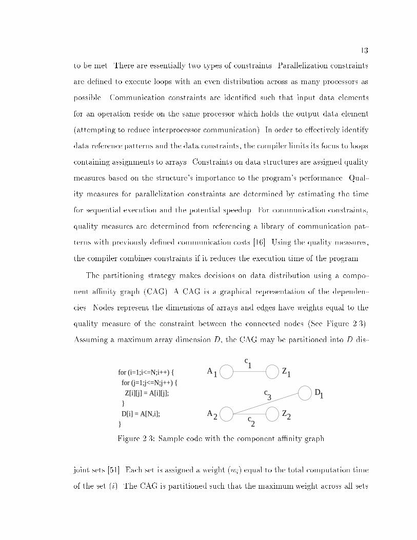
The partitioning strategy makes decisions on data distribution using a compo�

nent a�nity graph �CAG�� A CAG is a graphical representation of the dependen�

cies� Nodes represent the dimensions of arrays and edges have weights equal to the

quality measure of the constraint between the connected nodes �See Figure �����

Assuming a maximum array dimension D� the CAG may be partitioned into D dis�

for (i=1;i<=N;i++) {

for (j=1;j<=N;j++) {

Z[i][j] = A[i][j];

}

D[i] = A[N,i];

}

A

2

3

1

2

c

c

cA Z

1Z

D

1

1

2

Figure ���� Sample code with the component a�nity graph

joint sets �� �� Each set is assigned a weight �wi� equal to the total computation time

of the set �i�� The CAG is partitioned such that the maximum weight across all sets

�

�maxwi � i � � � i � D� is minimized� For each of the D sets� array dimensions

may or may not provide speedup when distributed on multiple processors � ��� Array

dimensions which will not produce speedup are sequentialized to save communica�

tion costs without sacri�cing potential speedup� Other dimensions are analyzed for

contiguous or cyclic distribution using the constraints�

Consider the following loop which imposes constraints on the �rst dimension of A

�A � with the second dimension of B �B���

for �i���i��N�i��� �

A�i��c��� � A�i��c��� � m � B�c���i��

�

The constraints are based on the use of variable i in A and B�� and require

B�c���i� to be available when A�i��c�� is used� The loop also suggests sequentialization

of A� and B to allow software pipelining� Using software pipelining� an input sample

is completely processed by a single processor� Subsequent input samples are processed

on adjacent processors by skewing the time at which the subsequent input samples

begin execution� For example� assume a processor Pi operates on a data item dj

beginning at time tk� The next data item dj�� would begin execution on processor

Pi�� at time tk�c where c is a constant greater than �

Now consider another loop which requires the cyclic distribution of A due to the

inner loop�s index j being �xed by the outer loop�s index i�

for �i���i��N�i��� �

for �j���j��i�j��� �

sum � sum � A�i��j��

�

�

�

This would allocate A�i��j� � j � � j � i to a processor i� The combination of

constraints results in the cyclic distribution of A along dimension � Thus� the dis�

tribution attempts to minimize the interprocessor communication while maximizing

speedup�

Conicts in the determination of the distribution are resolved using the quality

measures � ��� Scheduling maps nodes onto a processor grid of dimension D according

to the decisions made on distribution� If the user wishes to restrict scheduling to a

two dimensional network topology and D � �� additional array dimensions may be

sequentialized to reduce D to � � ��� In this manner� the method may be used to

generate a suggested network topology or to map an algorithm onto a given instance

of a processor array� The number of processors for each dimension of the processor

array is determined according to the distribution decisions and the size of the array

dimensions� Using this partitioning strategy there is no guarantee that the schedule

produced is optimal � ���

Medium grained parallelism is exploited through the automatic recognition of par�

allelism in loops with data array assignments� The method may be adapted for use

with familiar speci�cation techniques and is practical for implementation on other

systems� However� for parallelism to be exploited� the user must represent available

parallelism in terms of data arrays manipulated within loops� Thus� parallelism be�

tween samples is exercised� but parallelism within processing of a single sample is not

exploited� Communication is considered during partitioning via the communication

constraints� but input�output bandwidth is not taken into account� Complete opti�

mization of processing time and�or the number of processors is not guaranteed� The

nature of loops allows varied problem sizes some of which have been used as bench�

mark programs � tred�� dgefa� trfd� mdg� and o�� � ��� The benchmark programs

have shown favorable results� however� the method assumes that the compiler knows

�

the probabilities of executing conditional branches � ��� Currently the user must

supply this information� Running time for task scheduling has not been published�

Yet another area of extensive research is loop optimization� Existing paralleliz�

ing compilers make extensive use of loop optimization techniques to achieve a higher

system throughput� Many of these compilers apply a set of transformations to loops

through a series of steps� In each step� the compiler must determine that the transfor�

mation is legal and will improve the overall performance� However� there are several

methods to determine the order of these transformations� Some methodologies even

test all possible orderings and combinations of the transformations ����� Another

method is based on matrix transformations which models loop interchange� reversal�

and skewing transformations as linear transformations ����� A new approach by Wolf

and Lam combines the advantages of these techniques to provide a uni�ed method�

ology� The Wolf and Lam method was chosen based on the mathematical rigor and

generality of its application�

Their method determines valid and desirable transformations which will maximize

a desired level of parallelism ��ne to coarse grained�� While a brief explanation of

the methodology follows� we refer the reader to ���� for the details not discussed�

Developed for the CMU Warp and the Intel iWarp� Wolf and Lam�s methodology

represents a set of nested loops by a �nite convex polyhedron� Each node in a poly�

hedron represents an iteration in one of the loops and is identi�ed by an index vector

�p � �p�� p�� � � � � pn�T where pi is the ith loop index beginning from the outermost loop

�p�� to the innermost loop �pn�� Edges represent dependencies between iterations

and are de�ned by dependence vectors �d � �d�� d�� � � � � dn� such that �p� � �p� � �d

if iteration �p� must be executed before �p�� The set of all dependence vectors for a

loop is de�ned as D� In nested sequential loops� index vectors are executed in lexi�

cographic order� therefore� dependencies are represented by a set of lexicographically

positive vectors ����� A vector �d is lexicographically positive if �i � �di � � and

�

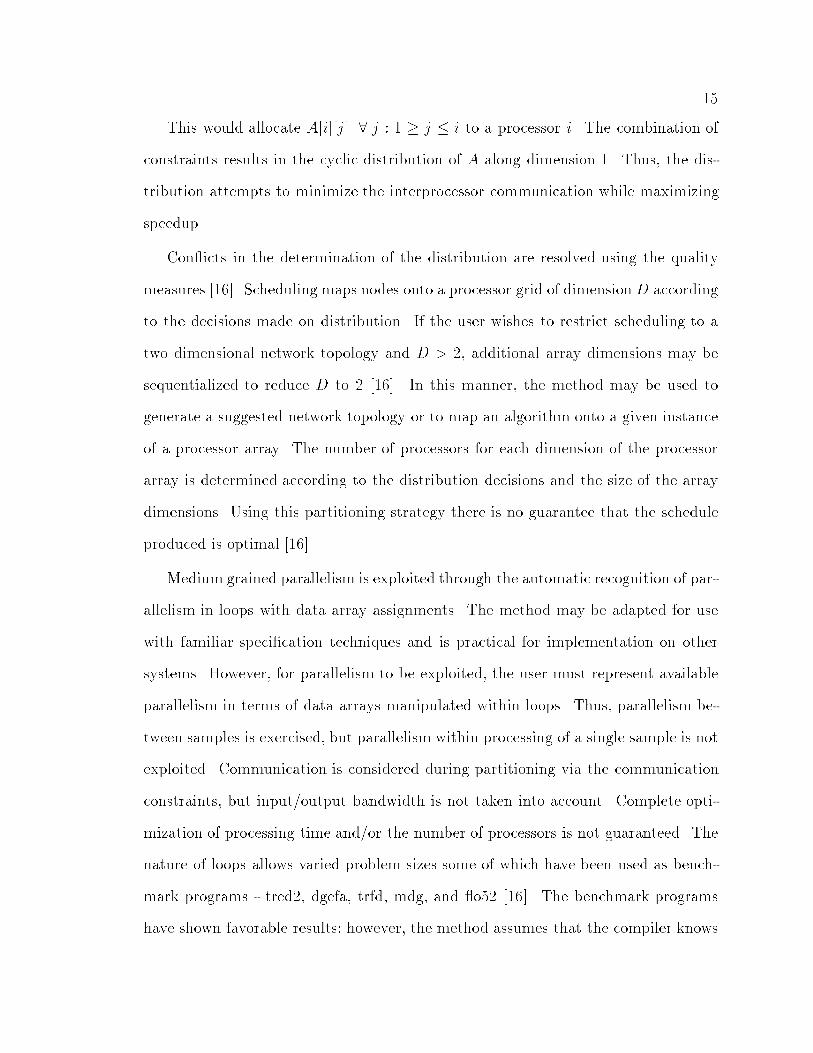
� j � i � dj � �� ����� An example of a loop and the corresponding iteration space

representation are shown in Figure ��� �a� �taken from ������

�a

for I := 0 to 5 do

for I := 0 to 6 do a[I ] := 1/3 * (a[I ] + a[I +1] + a[I +2]);

1

2

2 2 22

D = {(0,1),(1,0),(1,-1)}

1

2

I

I

�b

T= 1 0

1 1

D = TD = {(0,1),(1,1),(1,0)}

1

2

2

2

for I := 0 to 5 do

for I := I to 6+I do

a[I -I +1] + a[I -I +2];2

1

1 a[I -I +1] := 1/3 + a[I -I ]+1

1 2 1

2r

1r

Figure ���� �a� Example loop and the corresponding iteration space representation�b� with skewing of one

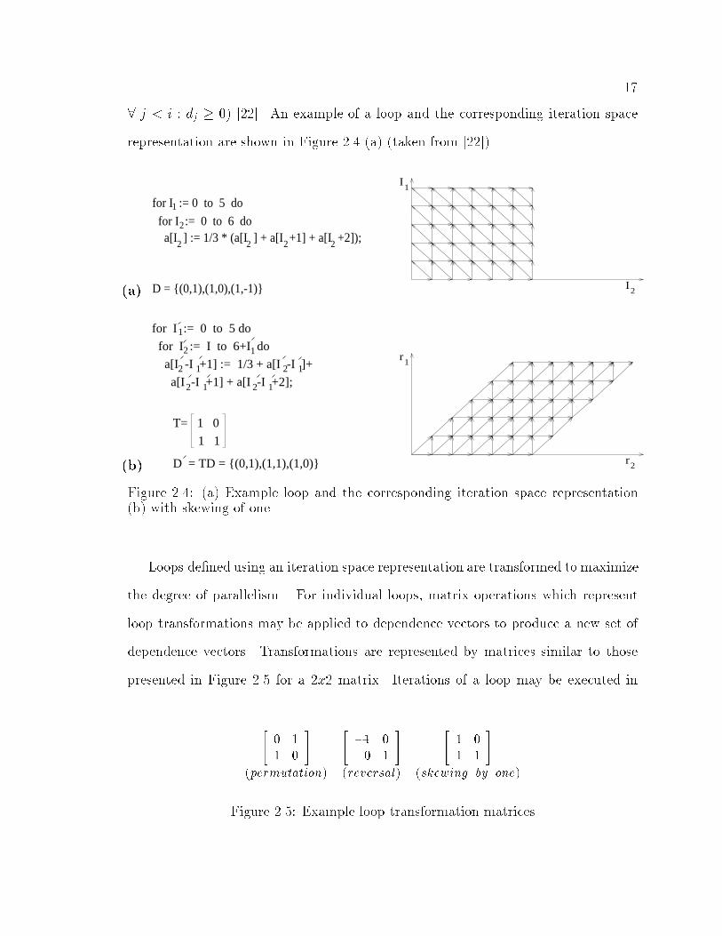
Loops de�ned using an iteration space representation are transformed to maximize

the degree of parallelism � For individual loops� matrix operations which represent

loop transformations may be applied to dependence vectors to produce a new set of

dependence vectors� Transformations are represented by matrices similar to those

presented in Figure ��� for a �x� matrix� Iterations of a loop may be executed in

�� �� �

�

�permutation�

��� �� �

�

�reversal�

�� �� �

�

�skewing by one�

Figure ���� Example loop transformation matrices

�

parallel if there are no dependences within the loop �commonly know as a DOALL

loop�� Transformations are applied to an iteration space representation to minimize

the dependencies which in turn maximizes the number of DOALL loops� Given a

loop nest �I�� � � � � In� with lexicographically positive dependences �d � D� Ii is paral�

lelizable if and only if � �d � D� �d�� � � � � di��� � �� or di � � ����� With n nested loops

and no dependencies between iterations� there are n degrees of parallelism� However�

if dependencies exist� transformations may be executed to achieve at least n de�

grees of parallelism by skewing the innermost loop ����� An example application of

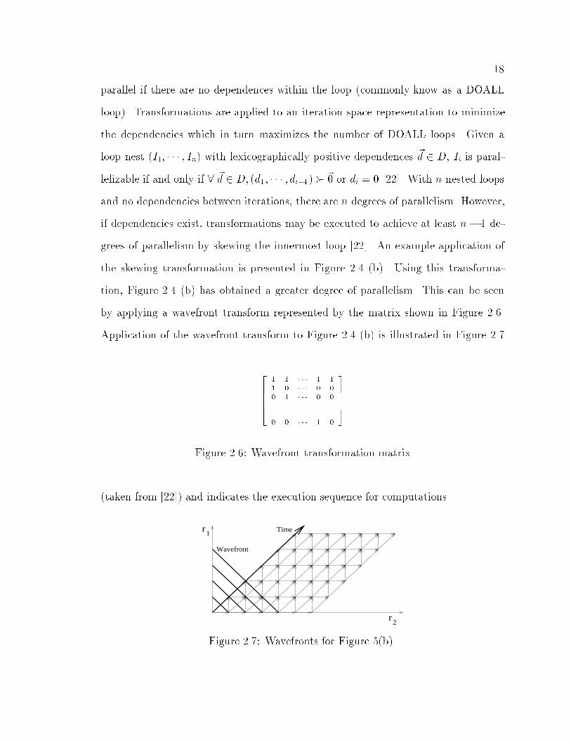
the skewing transformation is presented in Figure ��� �b�� Using this transforma�

tion� Figure ��� �b� has obtained a greater degree of parallelism� This can be seen

by applying a wavefront transform represented by the matrix shown in Figure ����

Application of the wavefront transform to Figure ��� �b� is illustrated in Figure ���

�����

� � � � � � �� � � � � � �� � � � � � ����

� � ����

� � � � � � �

�����

Figure ���� Wavefront transformation matrix

�taken from ����� and indicates the execution sequence for computations�

2r

1r Time

Wavefront

Figure ���� Wavefronts for Figure ��b�

�

Combinations of the transformations are represented by the product of the elemen�

tary matrices� Assuming iterations in a sequential loop are executed in lexicographic

order according to their index� a transformation which produces lexicographically

positive dependence vectors is legal� Thus� maximizing parallelism is simply a matter

of �nding the transformation matrix which maximizes the available parallelism� To

obtain �ne�grained parallelism� the nested loops are skewed and then wavefronted

which is always legal� To wavefront the nested loops� independent iterations of loops

with similar dependencies are identi�ed and assigned to a single wavefront� Thus�

each operation along a wavefront is executed on a di�erent processor during the same

time period� Coarse�grained parallelism can be obtained by grouping together local

operations across wavefronts as seen in Figure ��� �taken from ������ In this case�

each group of operations across a wavefront is executed on a di�erent processor� In

1II’

2II’

Figure ���� Coarse�grained execution for Figure ��b�

either case� the resulting code is optimized and allows parallelism to be exploited in

up to �ve levels of loop nesting�

Wolf and Lam�s method� exploits �ne to coarse�grained parallelism to optimize

processing time and the number of processors for execution of nested loops� The spec�

i�cation technique is familiar and convenient but requires that available parallelism be

de�ned in terms of nested loops� Parallelism between samples as well as parallelism

during processing of a single sample is exploited� Due to the nature of loops� the

��

method is scalable to large problem instances� However� during the transformation

process� potential communication costs are not considered including interprocessor

communication and the input�output bandwidth� As a result� the compiler �which

uses this loop optimization technique� will need to recursively call the loop optimizing

code when interprocessor communication exceeds computation time� The complexity

of the algorithm is O�n�d� where n is the number of nested loops and d is the number

of dependencies� Thus� the running time should be acceptable� There are no inherent

reasons which would limit the portability of this methodology to other systems�

In summary� the research into languages� compilers� and loop optimization is and

continues to be extensive� However� techniques developed in individual research ef�

forts must be incorporated into a single methodology� Languages are e�ective but

usually require users to explicitly de�ne available parallelism� Parallelizing compilers

e�ectively partition their target code� but often fail to recognize all of an algorithm�s

available parallelism� When used in parallelizing compilers� loop optimization tech�

niques provide excellent parallelism� but require users to write programs using loops

and arrays within the scope of the methodology� Mathematical approaches o�er alter�

native techniques to language and compiler task scheduling� We now describe some

of theses mathematical techniques�

��� Mathematical Approaches

Mathematical approaches to task scheduling are based on recurrence equations or

probabilistic modeling� Research into recurrence equations focuses on systolic arrays

and provides methodologies which go beyond basic partitioning and scheduling� Many

of the methodologies will also suggest how many processors are needed and what net�

work topology should be used� Cappello and Steiglitz�s method is one method of

task scheduling using recurrence equations which has proven e�ective and has been

�

referenced frequently ����� Their method provides a geometric representation for

recurrence equations and generation of mapping solutions� Although we will not dis�

cuss probabilistic methods in this paper� we will note that Lin and Yang present a

promising probabilistic method� Their probabilistic method provides e�ective load

balancing by simultaneously reducing the standard deviation of each processor�s ex�

ecution time and increasing the correlation coe�cient between every two processors�

execution times �����

Cappello and Steiglitz�s method de�nes an algorithm in the form of a system

of recurrence equations to be mapped onto a systolic array� From the recurrence

equations� a canonical representation may be formed by adding an additional index to

represent time� Each index in the canonical equations is representative of a dimension

in geometric space� Points may be de�ned in space to represent the sets of indices

where the equations are de�ned� The location of the points in space is determined by

interpreting the indices on the left�hand side of the recurrence equations as coordinate

locations� Each of the de�ned points is associated with a primitive computation

�i�e� the equation on the right�hand side of the equation�� The result is a geometric

representation of the recurrence equations� Using the geometric representation� static

data and communication requirements are identi�able� Individual nodes which require

the same static data element are connected by a solid line� Therefore� each static data

element is represented by a solid line and the points on the line represent locations

which require the data element� Similarly� individual nodes which use the same

variable data element are connected by a dashed line� Thus� dashed lines are used

to identify communication paths for variable data elements� Movement of the data

along the paths is determined by lexicographic order of the indices within time�

By applying matrix transformations representing geometrical transformations �such

as those presented in Figure ����� a geometric representation can be transformed into

a variety of potential mappings ����� A geometrical projection in a single dimension

��

�other than the dimension which represents time� directly maps the primitive compu�

tations onto processors in a systolic array� Nodes which are projected onto the same

point are assigned to the same processor with the number of projected points deter�

mining the size of the systolic array� The timing and data ow are determined from

the geometric space representation by maintaining precedence relations� Thus� the

geometrical representation enables users to easily visualize the systolic array during

algorithm transformations and partitioning�

For example� y � A � x can be expressed yi �Pn

j�� ai�j � xj where n is the size of

vector x� De�ning the initial values� the recurrence equations can be written

yi�� �

yi�j � yi�j�� � ai�j � xjyi yi�n

A canonical representation is formed by adding a time index�

yi�j�t � yi�j���t � ai�j � xj t � � ��� �

Figure ��� �taken from ����� illustrates a geometric representation ��� of Equation ��

for n � �� Using this �gure� the equation y����� � y������a��� �x� occurs at coordinates

� � � ��� Thus� a��� and x� must be de�ned at location � � � during time t � ��

Solid lines in the graph represent the required locations for x� while dashed lines

identify communication paths used to pass yi�j�t for addition� Using the geometric

representation� various mappings of individual algorithms can be investigated� For

example� a transformation suggested by Leiserson and Kung to schedule y � A � x�shown in Figure ���� results in the potential mapping ����

� � T �R��� where R �

��� �

�� �

��� and T �

��� � �

� � � �

���

��

i

jt

Figure ���� Geometric representation of the canonical linear transform y � A � x

i

jt

Figure �� �� Geometric representation of the Leiserson and Kung transform

with � shown in Figure �� � �taken from ������ Projecting � onto the t axis �note

that with the transformation t no longer represents time� yields the task schedule

shown in Figure �� �taken from ������

Cappello and Steiglitz�s methodology targets �ne grained parallelism for systolic

arrays� Available parallelism in algorithms must be speci�ed in terms of recurrence

��

x1x21y

11a

33a

22a

32a23a

12a 21a

13a 31a

Figure �� � Representation of the Leiserson and Kung task schedule

equations which are familiar but not always convenient� The method results in a

combination of parallelism during processing of a single sample and between samples�

however� both types of parallelism cannot be fully exploited simultaneously� Com�

munication patterns are accounted for during mapping to the systolic arrays� but

communication costs and input�output bandwidth are not considered� Scalability

is provided by the indices in the recurrence equations� The concepts are limited to

systolic arrays which are special purpose architectures with rigid synchronization�

In general� they are now out of favor except for low�level repetitive operations� Es�

sentially� Cappello and Steiglitz have provided a visual framework for considering

transformations� but do not identify a method to obtain the ideal transformation�

The process of applying various transformations can be automated� but running time

is potentially unbounded� We now move on to describe some heuristic techniques for

task scheduling�

��

��� Heuristic Techniques

We refer to a paper by Manoharan and Topham for a good comparison of heuristic

techniques which consider communication costs ����� The most promising heuris�

tic identi�ed is a non�work�greedy assignment scheme Depth First Breadth Next

�DFBN� ���� ���� While work�greedy assignment methodologies attempt to keep all

processors busy as long as there is a task capable of being executed� non�work�greedy

schemes do not keep processors busy as a main goal� DFBN attempts to assign inde�

pendent tasks across multiple processors while assigning dependent tasks onto a single

processor� This is done in an e�ort to balance the goals of maximum parallelism and

minimum interprocessor communication�

Unlike many task scheduling methodologies� DFBN allows the user to specify the

target architecture with a processor graph� Nodes in the processor graph represent

the processors with the edges identifying the communication paths� Values are asso�

ciated with each edge to represent the link capacity� Algorithms are speci�ed in the

form of a task graph� In the task graph� nodes identify a task and edges represent

dependencies between tasks� Tasks are de�ned to be a portion of an algorithm which

must be executed sequentially� Values which de�ne the sequential execution time are

assigned to nodes� Edges are assigned values to represent the volume of interprocessor

communication� The task graph is assumed to be acyclic�

Task graphs may be partitioned into chains of nodes using a combination of depth�

�rst and breadth��rst search algorithms ����� The chains are developed such that the

nodes in a chain are dependent� Thus� nodes in di�erent chains will be independent�

To determine which chains to schedule �rst� priorities are assigned to individual nodes�

A critical factor is de�ned for each node �task� such that

CFi �maxj���n �LCT j ECT j� �LCT i ECT i�

��

where ECT i and LCT i are the earliest and latest completion times for task Ti �����

ECT and LCT are initially estimates� exact values are calculated when task assign�

ments are done� The priorities are set through the equation

pi � w��CFi�� � w�� � w�

XTj�succ�Ti

vi�j � w�

XTj�succ�Ti

� w

XTj�succ�Ti

�j � w�si

where w�s are empirical weights� � � �to emphasize CF �� �i is the execution

time of Ti� succ�Ti� identi�es the successors of task Ti� vi�j is the volume of the

communication between Ti and Tj� and si is the memory requirements of Ti �����

The order of available processors is determined by choosing the processor with the

best overall link capacity and then ordering the other processors according to their

distance from the chosen processor� The distance between two connected processors

Pi and Pj is de�ned as �ci�j

where ci�j is the link capacity between Pi and Pj � For

processors not directly connected� the distance equals the sum of the distances along

the shortest path �using Dijkstra�s algorithm�� Task chains are assigned in order of

priority to the best available processor�

For the example processor graph and task graph in Figure �� � �taken from ������

the resulting assignment is

0P

1P

2P

3PT0(6)

T1(8)

T2(7)

T3(10)

T7(6)

T9(7)

T8(8)

T5(12)

T6(9)

T4(8)2

1 1

2

11

1

1

1

1

2

2

2

23

3

3

(a) (b)

Figure �� �� Example �a� processor graph and �b� task graph for DFBN

��

P� � �� � �� �� �� �P� � �� �P� � P� � �� �

While the partitioning obtained by the DFBN assignment scheme is not guaran�

teed to be optimal� DFBN is shown to consistently produce partitionings close to

optimal for acyclic task graphs ����� Note that optimality for acyclic task graphs is

determined by minimizing the throughput delay� the number of processors� and the

interprocessor communication� The speci�cation method is familiar and convenient

using task graphs and processors graphs� The heuristic automatically identi�es and

exploits available �ne�grained parallelism speci�cation of the algorithm in the task

graph� without requiring the user to specify available parallelism� However� the task

graph is acyclic� allowing only parallelism during processing of a single sample to be

exploited� This method will not work e�ectively for iterative algorithms� The cost of

interprocessor communication is considered during the evaluation of priorities� how�

ever� �nal communication patterns are not validated and input�output bandwidth is

not considered� Assuming that the task graph is able to contain non�atomic nodes�

the methodology is scalable and a variety of architectures may be supported� Per�

haps the biggest drawback to this methodology �for DSP algorithms� is its failure

to support feedback loops for iterative algorithms� The algorithm�s complexity is

O��n �m� logm� e� where n is the number of tasks� m is the number of processors�

and e is the number of edges in the task graph� Thus� the running time should be

acceptable�

Graphical algorithm speci�cation methods provide yet another challenge for re�

search in parallel task scheduling� In the next section� we discuss three graph�based

methodologies for scheduling DSP algorithms for parallel execution�

��

��� Graph�Based Methods

Graph�based task scheduling techniques begin with the user de�ning an algorithm

in the form of a ow graph� Flow graphs can be in one of several forms� We begin

by describing fully speci�ed ow graphs �FSFGs� as a speci�cation method which

e�ectively represents both computation and communication properties of algorithms�

A FSFG is a ow graph with computational nodes� communication edges and ideal

delays� Figure �� � �taken from ����� presents an FSFG for a �D �nd order IIR

�lter� Nodes represent an atomic arithmetic or logic function taking place� with

++ *

+ *

*

+

*

-1Z

Z-1

1

2 4

3 7

8 9

10

5

6

Figure �� �� FSFG for a �D �nd order IIR �lter

a �xed computational delay� An edge indicates dependence of one node on data

produced by another node� An ideal delay is represented by block labeled Z���

and denotes a delay in time when a signal passes through the block �representative

of hardware registers and memory�� Using FSFGs� computational information is

completely captured in the atomic nodes of the ow graph� while the communication

is contained entirely in the directed edges� Once the order of these atomic nodes

is de�ned� the FSFG has already bound the computation and communication pretty

tightly to a particular model of execution� As a result� the initial de�nition of a FSFG

tends to limit the possible mappings for a given algorithm�

Fundamental bounds to multiprocessor performance are de�ned to determine how

well a FSFG might be executed ���� ��� ���� The Iteration Period Bound �IPB� is

��

one performance bound of interest for FSFGs with feedback for iterative execution�

The IPB is de�ned as

Tv �maxl�L

Dl

nl

�����

where Dl is the computational delay of all nodes in loop l � L and nl is the number

of ideal delays in loop l � L� The set of all computational loops �L� may be found

by tracing directed edges which form a loop without re�using a directed edge when

de�ning a single loop l� The IPB ensures that the period between inputs is long enough

to process all the computational loops in the FSFG� A FSFG which is executed at an

iteration period equal to Tv takes a new input every Tv time units and is said to be

rate optimal� For the purposes of this research� we assume it takes one time unit for

an addition and two time units for multiplication� Using these assumptions� Tv � �

for the example FSFG shown in Figure �� ��

Once an algorithm has been speci�ed by a FSFG� the nodes of the FSFG may

be scheduled for execution on a multiprocessor system� One basic technique for ob�

taining a multiprocessor schedule is through the identi�cation of critical paths in

the FSFG ����� However� this method does not attempt to optimize the number

of processors or to consider communication costs� Another graphical approach� the

Range�Graph Method �RGM�� partitions algorithms with the goal of �nding an op�

timal position for scheduling individual nodes within a scheduling window ����� This

method is discussed on the basis of favorable comparisons with other graph�based

scheduling methods� RGM de�nes

critical path path containing a set of nodes with a mobility of zero

scheduling window the length of the critical path

scheduling range the time interval an operation can start its execution within the

scheduling window

��

mobility the length of the scheduling range

scheduling range chart display of the scheduling range and the mobility for all

operations

An early schedule for a FSFG de�nes the schedule in which nodes are executed as

soon as possible within the scheduling window� Similarly� a late schedule identi�es a

schedule in which nodes are executed as late as possible within the scheduling window�

Combining the early and late schedules yields a scheduling range chart� Figure �� �

�taken from ����� presents an example of a non�iterative FSFG� an early schedule�

and a late schedule� Figure �� � illustrates the combination of an early schedule

and a late schedule to form a scheduling�range chart� RGM provides two types

*

*

*

+

6C

7C 8C

9C

+ +*1C 2C 3C 4C 5C

* +

+ +*1C 2C 3C 4C 5C

* +

76543210

t(TU)4

3

2

1

P#

early schedule

1 1 2 3 4 4 5

6 6 8

77

9 9

76543210

t(TU)4

3

2

1

P#

1 1 2 3 4 4 5

8

99

7766

out1

in3

in2

in1

durationin TU’sOp

12*

+

Critical Path

late schedule

Figure �� �� Example of a non�iterative FSFG with an early schedule and a lateschedule

of scheduling� non�iterative and iterative� Non�iterative scheduling de�nes a �nite

�

i

i

C

C

765321

t(TU)

C i

t(TU)

4

0 1 2 3 4 5 6 7

0 76543210

t(TU)

late schedule

scheduling-range chart

mobility

duration

notation

1

2

3

4

5

6

7

9

8

1

2

3

4

5

6

7

9

8

early schedule

1

2

3

4

5

6

7

9

8

Figure �� �� Example of combining an early schedule and a late schedule to form ascheduling�range chart

scheduling range determined by the iteration period bound �set by the critical path��

For a non�iterative schedule� the critical path is scheduled and then other nodes are

scheduled in order of increasing mobility� Heuristics are used to choose processors

based on the availability of a time slot which matches the duration of the node to be

scheduled �with consideration of mobility�� Iterative scheduling requires an in�nite

scheduling range� therefore� a reference node is used to �x the schedule in time� The

reference node is chosen from the nodes in the critical loop and is scheduled �rst�

The iteration period bound is used to �x the schedule range around the reference

node with the critical loop identifying the critical path� Other nodes in the FSFG

are scheduled with respect to the reference node in order of increasing mobility ��

�A threshold scheduling technique similar to RGM has been developed for use with SISAL �����Parallelism between operations is represented by a directed acyclic graph and schedules are computed for each possible threshold between the early and late schedules�

��

For example� consider the �D �nd order IIR �lter presented in Figure �� � �taken

from ������ the critical loop can be identi�ed as c � c� � d�� Choosing c� as the

++ *

+

1C 3C

4C2C

5C

7C 6C

8C

*

*

2D

1D

durationin TU’sOp

12

+*

Z-1

-1Z

+ *

Figure �� �� �D �nd order IIR �lter for RGM

reference node� the scheduling steps are illustrated in Figure �� �� The scheduling

range chart in Figure �� � �a� is developed by �xing node c� in time� obtaining early

and late schedules� and combining the early and late schedules to form the range

0 21 0 1 0 1 2

8

2

6

2

13

4

3

4

8

C i

8

7

6

5

4

3

2

1

7 7

5

1

1 2 2 21 100C i

0 1 2

0 1 2

1 2 2 21 100C i

8

7

6

5

4

3

2

1

0

1

2

21 10C i

8

7

6

5

4

3

2

1

1 2 2 21 100C i

8

7

6

5

4

3

2

1

1 2 2 21 100C i

8

7

6

5

4

3

2

1

210

1

2

3

4

5

6

7

8

iC

(a)

t(TU)

2 2 0

0 0 11 2221

4 4 4422

88

7 7

2

13

4

3

4

88

7 76

2

13

4

3

4

1 2 2 21 100

t(TU)

0

2

1

4 4 2

13

4

3

4

8

7

6

5

4

3

2

1

1 3 3

7 7

t(TU)

(e)

t(TU)

(f) (g)

t(TU)t(TU)

(d)(c)

t(TU)

(b)

Figure �� �� RGM scheduling steps for a �D �nd order IIR �lter

��

chart� Arrows pointing forward in time indicate an in�nite scheduling range for the

late schedule� In Figure �� � �a� node c� is scheduled as the reference node followed

by the scheduling of node c which has zero mobility� In Figure �� � �b� and �c� nodes

c� and c� are scheduled in order of increasing mobility� Nodes c�� c � c�� and c� are

scheduled into empty time slots to complete the multiprocessor schedule�

RGM provides automatic scheduling for �ne�grained parallelism by exploiting par�

allelism during processing of a single sample and between samples� However� interpro�

cessor communication time is assumed to be negligible with respect to computation�

and may result in unacceptable schedules� In addition� the input�output commu�

nication bandwidth is not considered� Familiar and convenient FSFGs are used to

specify algorithms� but scalability to larger problems may prove problematic with

requirements for large FSFGs and large range charts� RGM is capable of optimizing

processing time and�or the number of processors without requiring users to identify

potential parallelism� RGM is suitable and practical for use on multiple parallel archi�

tectures �which do not use wormhole routing� with published running times of under

one CPU second for FSFGs up to �� nodes� Scheduled algorithms include FIR� IIR�

lattice� Jaumann and elliptic �lters�

Another graph�based approach of particular interest is the work being done on

optimal� periodic multiprocessor scheduling for fully speci�ed ow graphs� which we

term the cyclostatic realization method �CRM� ���� ��� ���� This method combines

the familiarity of a ow graph speci�cation technique with the concise representation

of matrix theory to provide a exible� generalized mapping methodology�

The cyclostatic realization method attempts to schedule the FSFG to meet given

bounds and has been widely published and referenced� Barnwell et� al� developed

a theory of algorithm mapping whose goal is to simplify the handling of the FSFG

during the mapping process while obtaining the performance bounds� While a detailed

description of CRM can be found in ���� ��� ���� we will provide a brief overview�

��

Using CRM� the problem is modeled by a period matrix and a cycling vector� The

period matrix has one row for each processor used for computing the FSFG and

one column for each time unit in the iteration period� The elements of the period

matrix are computational time units in the FSFG� Each of the nodes in the FSFG

is numbered and placed in the period matrix with a single node entry appearing in

the period matrix once for each time unit it takes to execute that node� The cycling

vector has a single column and one row for each row of the period matrix� The

entries of the cycling vector are integers to r where r is the number of rows of the

period matrix� A cycling vector determines the movement of the rows of the period

matrix between iterations� Superscripts in the period matrix represent which samples

are being processed in parallel in di�erent partitions� If some �arbitrary� partition is

de�ned as processing the current� input sample� a superscript of i denotes concurrent

processing of the ith sample after this �or before this� if the superscript is negative��

An example partitioning for Figure �� � is illustrated in Figure �� �� This partitioning

is represented by the cycling vector and period matrix shown in Figure �� ��

++ *

*+

*

+

*

-1Z

Z-1

1

2 4

3 7

8 9

10

5

6

3P

P4P2

1P

++ *

+ *

*

+

*

-1Z

Z-1

1

2 4

3 7

8 9

10

5

6

3P

P4P

P2

1

Figure �� �� Data movement for an example partitioning of a �nd order IIR �lter

Specifying an algorithm in an intermediate form using matrices allows di�erent

multiprocessor schedules to be obtained by modifying the matrices� The period matrix

and the cycling vector may be manipulated by exchanging rows and columns to yield

di�erent multiprocessor schedules� Manipulations of the period matrix include the

��

�����

��a�

�� � � � � � �

��� ��� ���

��� ��� ��

�� �� ����

��

�b��� � � � � � �

��� ��� ���

��� ��� ��

�� �� ����

���

�� � � � � � �

� � � � � �

��� ��� ��

�� �� ����

���

�� � � � � � �

� � � � � �

� � � � �

�� �� ����

����

��

�� �� �� ��

�� �� ��

�� �� �

� � ���

����� �� �� ��

�� �� ��

�� �� �

� � ���

����� �� �� ��

�� �� ��

�� �� �

� � ���

��

�c�

Figure �� �� Basic Example for � processor system executing FSFG of �D �nd OrderIIR FSFG� �a� Cycling vector �b� Period matrix �c� Six iteration periods for �a� and�b�

exchange of rows� the rotations of the columns� and the slicing and splicing of rows�

The cycling vector can be manipulated using an exchange of rows to obtain any

ordering of the vector�s elements� Resulting periodic schedules must be checked for

viability against a set of admissibility conditions presented in ���� ���� The precedence

condition states that nodes in the FSFG must be calculated in the order that they

occur from the input to the �rst delay� between delays� and from the last delay to

the output� In other words� each node must have the necessary inputs in order to be

scheduled� The nonpreemption condition states that once a node of the FSFG has

been scheduled on the processor� that node can not be preempted by the scheduling

of another node�

To �nd an optimal mapping� the methodology enumerates all possible sets of trans�

formations of the period matrix and the cycling vector� �Figure ���� shows several

possible manipulations of the period matrix and the cycling vector for Figure �� ���

The resulting periodic schedules are checked against the admissibility criteria and

the performance bounds� If the periodic schedule is both permissible and optimal�

the periodic schedule is accepted as a valid mapping� Depending on the size and

complexity of the period matrix� the process of �nding all possible transformations

��

�� �

��

���� � � � � � �

�� �� ���

��� ��� ��

�� ��� ����

��

�a

�� �

��

���� � � � � � �

�� �� ���

�� ��� ����

��� ��� ��

��

�b

�� �

��

���� � � � � �

�� ��� ���

��� �� ��

��� ���� ��

��

�c

h��

i h� � � � � � � � � �

��� ��� �� �� ��� ����

i�d

�� �

��

���� � � � � � �

�� �� ���

��� ��� ��

�� ��� ����

��

�e

Figure ����� Schedule Transformations� �a� original period matrix and cycling vector�b� rows � and � of the period matrix are exchanged �c� columns of the period matrixare rotated left by one �d� rows � and � of the period matrix are spliced to rows and � respectively �e� rows and � of the cycling vector are exchanged

could take an amount of time which is exponential in the problem size�

CRM is a convenient� powerful method for partitioning and scheduling parallel

computations� CRM automatically identi�es parallelism within processing of a single

sample and between samples to produce parallel processing schedules� CRM generates

schedules to meet the optimal processing time and the optimal number of processors�

and does not allow schedule generation for non�optimal solutions� It is worth not�

ing that there are some FSFGs which can not be scheduled at the optimal iteration

period on the optimal number of processors� Interprocessor communication costs

and input�output bandwidth limitations are not explicitly considered �although a re�

cent paper has mentioned that consideration of interprocessor communication costs

is possible ������ In general� CRM assumes an interconnection network which is a

crossbar switch with unlimited bandwidth� This assumption is clearly unrealistic�

Algorithms are speci�ed in the form of FSFGs which limit scalability to the practical

size for non�hierarchical FSFGs� CRM has been developed in C to permit a high

degree of portability and is suitable for scheduling algorithms onto a variety of par�

allel architectures� Running times are unpublished� but are noted to be acceptable�

Practicality for implementation should be determined by running a set of standard�

realistic benchmarks�

��

All of the methods presented have characteristics bene�cial to the task schedul�

ing problem� however� none of the methods are totally e�ective� The focus of this

research is to provide an e�ective methodology to schedule DSP algorithms onto the

BDPA� Some of the major hurdles include continuous input data� high throughput

requirements� feedback loops� communication costs� and a need for a user friendly

system� Programming languages in combination with their compilers are e�ective

when the target system �ts in the mold of the language�s development system� A

compiler must exist for the target system and users must have experience with the

language to achieve optimal parallelism when scheduling an algorithm� Mathematical

approaches are geared toward systolic arrays and would be unable to take full advan�

tage of the BDFP� Heuristic approaches have shown promise� however� even the best

heuristic� DFBN� approaches the task scheduling problem assuming an acyclic FSFG�

Graph�based methods are perhaps the friendliest for users of the BDPA� The RGM

handles feedback loops well but does not consider communication costs in producing

a parallel schedule� CRM provides the best representation for parallel processing

schedules� however� the partitioning and scheduling algorithm does not handle the

communication costs associated with the partitioning of feedback loops� In addition�

CRM�s generation of all possible cycling vectors and period matrices is computation

time intensive and cannot guarantee a schedule�

In the following chapter we introduce the Order Graph Method �OGM� as an

e�ective alternative to existing parallel task scheduling techniques� OGM provides

a user�friendly task scheduling methodology for scheduling algorithms speci�ed by

hierarchical FSFGs� Feedback loops� communication costs� and the network topology

are considered during the scheduling process to guarantee an e�ective� valid schedule�

Chapter �

The Order Graph Method

��� Overview

The Order Graph Method begins with some basic assumptions about the multipro�

cessor system�s architecture�

� processors are non�pipelined general purpose processors

� a processor is capable of communicating �receiving and transmitting

no more than tc units of data per clock cycle

� a link in the network topology is capable of transmitting no more

than tn units of data per clock cycle

� communications and computations are overlapped with the overall

execution time determined by the larger of the two

� each processor is capable of communicating directly with system

input�output devices

These assumptions are based on the use of additional hardware to handle communi�

cation independently of computation ��

�The Texas Instruments TMS��� C � processor has separate hardware for communication andcomputation� Thus communication and computation can be overlapped�

��

The goal of the Order Graph Method is to produce a multiprocessor schedule for a

user�de�ned FSFG which achieves a desired iteration period �Td� ���� ���� This serves

two purposes� There is no need to attempt to schedule the algorithm with a faster

iteration period than necessary� Therefore� the execution time for the scheduling

process is reduced as Td becomes greater than the iteration period bound �Tv�� In

addition� by scheduling to Td� OGM minimizes the cost of the system by using the

minimum number of processors necessary to execute the FSFG� It should be noted

that the OGM also permits scheduling to a speci�c number of processors �Pd� by

using the total computational time in the FSFG �CN� to identify Td for the system�

Thus� OGM requires two inputs � the FSFG to be scheduled and either Td or Pd with

the relationship�

Td �CN

Pd

The notation used to detail the Order Graph Method� is shown in Table �� �

In general� OGM has four major steps�

� Preprocess the FSFG to minimize interprocessor communication

� Generate candidate partitionings for the graph using heuristics to balance the

workload across processors

� Generate schedules for the candidate partitionings

� Validate schedules against the interprocessor communication limitations� the

link capacity� Td� and Pd

Figure �� presents an outline for the algorithm used in the OGM� OGM accepts

hierarchical FSFGs as input with a user speci�ed target for scheduling in the form

of a target iteration period� a target number of processors� or the goal to optimize

both the iteration period and the number of processors� OGM will output a schedule

��

Symbol De�nition

Ci total amount of communications into and out of processor i during Td clock cyclesCN total computational time for a FSFGdi�n� member of the set Di�n�

Di�n�set of all ideal delays for communications between node n on processor i to node n�soutputs on other processors

Dl total computational delay of nodes in loop lE set of all edges in a digraphE� set of all edges in a directed acyclic graph

fisubgraph of a directed acyclic graph consisting of the nodes to be executed on processori

Fi set of nodes in a FSFG to be executed on processor iG directed graphG� directed acyclic graphIi indegree of a subgraphl particular loop in a graphlx set of links required to support the communication due to the nodes in set xL set of all loops in a graph

Lji

number of communications over the link between processor i and processor j in a network topology

Mn set of all output nodes for node nn number of nodes in a FSFGnl number of ideal delays in loop l

nn�m number of ideal delays along a directed path between node n and m in a graphoi�n� member of the set Oi�n�Oi outdegree of a subgraph

Oi�n� set of all processors which contain the output nodes for node n on processor iP poset for a FSFGPd desired number of processorsr number of processors for a candidate partitioning

rminminimum number of processors for all validated candidate partitionings at the desirediteration period

tnumber of linear extensions which satisfy a set of precedence conditions �the size of aposet�

tc maximum number of communications into and out of a processor during a clock cycle

tnmaximum number of communications across a link in the network topology during aclock cycle

Td desired iteration periodTv iteration period boundv node in a digraphv� node in a directed acyclic graphV set of all nodes in a digraphV � set of all nodes in a directed acyclic graphw node in a digraphw� node in a directed acyclic graphwk weight of node kXi number of communications between processor i and input�output devices

Table �� � List of symbols used to detail the Order Graph Method

�

min

Strong ComponentsIdentify and Reduce

Compare Weights to T d

Remove Feedback Edge

<

Partitioning and r

<

>

>

d

min

d

<

<

>

passdoes not pass

passdoes not pass

Store Linear Extension

exhaustedGenerate Linear Extension

Partition

Compare Shifted WeightsTo T

Compare r to rShift Partition ForNetwork Topology

Compare r to P

Stored Linear ExtensionPartitioning

Done - Output r andmin

Done - Output r and CurrentLinear Extension Partitioning

>

Check Network Topology

Check Communication

v dCalculate T , P

dINPUT - FSFG, T

Scheduling

Partitioning

Preprocessing

Validating

2

3

4 Expand Strong Components

6

5

7

8

9

10

11

12

13

14

15

1

16

17

Admissibility Condition

Admissibility Condition

Figure �� � Flow Chart for the Order Graph Method

��

which assigns the nodes in the FSFG to processors and determines when nodes are

executed on the processors� OGM begins by calculating Tv and Pd if the user inputs

Td as the scheduling goal� If Pd is presented as the goal� Tv and Td are calculated by

OGM� Feedback conditions are handled through the identi�cation and manipulation

of strong components� Nodes within a strong component are merged into a single

node in an e�ort to represent each feedback loop as a single node� Removing the

feedback loops �cycles�� the FSFG is reduced to a directed acyclic graph �DAG�� If

Td � Tv� interleaving is used to lower the iteration period below the IPB� Using the

partially ordered set �poset� denoted by the DAG� linear extensions are generated to

identify a speci�c ordering of the nodes in the poset� The linear extensions are then

partitioned into sets with computational weights less than Td� In this dissertation� an

individual set is called a partition� Together these sets de�ne a candidate partitioning

which can be assigned to a set of processors to form a multiprocessor schedule� Thus�

each linear extension is partitioned according to the desired iteration period �Td� into

r partitions with each partition �Fi� containing a set of nodes to be executed on

processor i� The set of all these Fi partitions determines the candidate partitioning�

The candidate partitioning is a potential schedule to be validated against a set of

communications and network topology admissibility conditions� A valid candidate

partitioning is one that has passed both the communication and network topology

admissibility conditions� Through the enumeration of a FSFG�s linear extensions

and the linear extensions� candidate partitionings� a valid multiprocessor schedule is

obtained�

In order to incorporate the communication and network topology admissibility

conditions into multiprocessor scheduling� OGM necessarily iterates� At any time in

the scheduling process� the lowest value of r for any validated candidate partitioning

is held in rmin� Therefore� candidate partitionings with r � rmin do not need to be

validated against the admissibility conditions� A better valid schedule already has

��

been produced with rmin� When a linear extension can no longer produce unique

candidate partitionings� it is eliminated from consideration and another linear exten�

sion is generated for partitioning and validation� Candidate partitionings which pass

all admissibility conditions are checked for processor optimality� For a given Td the

optimal processor utilization occurs with Pd � dCNTde where CN is the total compu�

tational time for the FSFG� Once rmin achieves the target number of processors Pd�

a processor optimal schedule has been found and the scheduling process stops� In

the event that unique linear extensions are exhausted without being able to schedule

the FSFG an iteration period of Td on the optimal number of processors �Pd�� the

best valid schedule is presented as a schedule with an iteration period of Td on rmin

processors�

We now describe some of the important details in OGM � beginning with a de�

scription of the preprocessing stage which handles feedback in FSFGs�

��� Preprocessing Step � Handling Feedback

When determining scheduling for multiprocessor systems� feedback loops in the FSFG

require particular attention� If feedback loops must be split across two separate pro�

cessors� there becomes a need for bi�directional communication between processors�

Thus� the communication time increases for any processors involved in the communi�

cation of the feedback loop� In addition� the potential for contention in the network

topology increases� Therefore� OGM prevents unnecessary divisions of feedback loops

on multiple processors by preprocessing the FSFG�

To prevent the unnecessary splitting of feedback loops� OGM identi�es the feed�

back requirements and attempts to contain each feedback loop in a single node� A

FSFG is a directed graph �digraph� G � �V�E� where V is the set of all nodes and E

is the set of all edges� A digraph G is strongly connected if for each pair of vertices

��

v�w � V there is a directed path from v to w and a directed path from w to v as

well� A strongly connected component �strong component� of a digraph is a maximal

strongly connected subgraph �G� such that there is no pair of vertices v � V and

w � V with a directed path from v to w and a directed path from w to v� Thus� a

strong component will contain either a single node or the set of all the nodes involved

in a feedback loop� The nodes in the strong component of a digraph can be merged

into a single node producing a digraph� G� � �V �� E��� with no cycles �directed acyclic

graph � DAG�� OGM merges the nodes in each strong component into a single node�

The weight of the single node equals the sum of the computational times for the nodes

in the strong component� During the process of identifying the strong components in

the FSFG� the iteration period bound is found by analyzing each strong component

for loops� For each loop� the computational delay and the number of ideal delays is

used to �nd the maximum iteration period �Td�� OGM uses a strong component al�

gorithm by Tarjan which requires O�j V jj E j� time ����� Johnson�s algorithm is used

to identify loops in the strong components and requires O��j V j � j E j��j L j � ��

time where L is the number of loops in a strong component �����

In order to e�ectively schedule the nodes of the resulting DAG� the weight of any

node v� � V � must not be greater than Td� If the weight of v� is greater than Td� v� must

be split to a set of nodes with weights less than Td� This is accomplished by splitting

v� back into the nodes of its strong component� removing a feedback edge� identifying

the new strong components� and merging the nodes of the new strong components

into composite nodes� To remove a feedback edge from the strong component� an

edge adjacent to a delay node is removed from the cycle having the lowest iteration

period� For each loop l � L of the strong component� the computational delay Dl

and the number of ideal delays nl have been identi�ed during the calculation of Tv�

Thus� the feedback edge of loop l is removed from the cycle where Dl

nlis the lowest�

Once the correct cycle is found� additional checks ensure that the removed edge is

��

adjacent to a delay node and is shared by the fewest number of cycles in the strong

component� These checks ensure that the minimum number of loops �but at least

one� within the strong component are broken� In addition� this heuristic ensures that

the FSFG�s critical path is contained within a strong component� This is done in an

e�ort to schedule the critical path on a single processor�

The strong components for the remaining digraph are represented by composite

nodes� and the digraph is reduced to a DAG in the same manner as before� This

process of merging and splitting nodes from digraphs to DAGs continues until all the

weights in the DAG are less than Td �See Figure �� �� If strong components are split

into more than one node� the iteration period will remain equal to the IPB because

the feedback loop still exists across multiple processors� However� by interleaving

independent streams of data� the average iteration period can be reduced ���� ����

Although the DAG no longer captures the exact precedence constraints in the original

FSFG� it can be used to generate linear extensions which minimize the probability

that feedback loops will be split across multiple processors� If the exact dependencies

are needed� the original FSFG is used�

For example� consider the FSFG for the �nd order IIR �lter shown in Figure �� ��

Preprocessing begins by identifying the nodes in the strong component � f � �� �� �� �� �g�These nodes are represented by a composite node �C�� with a weight of �� A compar�

ison to Td � �� indicates that this composite node is too big to schedule in a single

partition and must be split� Analyzing the loops for the strong component� loop �A�

� � � has an iteration period equal to � and loop �B� � � � � has an

iteration period equal to �� Edge � � is an edge from loop �B� which is adjacent to

a delay node and is not shared with loop �A�� This edge is removed� The remaining

strong component � � � is collapsed back into a composite node �C�� with a

weight of �� This time� a comparison of the nodes in the DAG to Td validates the

DAG fC�� � �� �� �� �� �g which is then forwarded to the partitioning stage�

��

The DAG produced by the preprocessing stage is used by the partitioning stage

to generate candidate partitionings� This stage determines� to a great degree� the

amount of time the scheduling process will require� We now describe the generation

of these candidate partitionings�

��� Partitioning Step � Generating Candidate Par�

titionings

The partitioning stage generates a complete set of candidate partitionings for valida�

tion and scheduling� In order to schedule the DAG on a set of processors� an ordering

for the execution of the nodes must be determined� For execution on a single proces�

sor� an order which preserves the precedence constraints may be obtained by listing

all of the possible orderings �linear extensions� and picking the best one� Execution

on multiple processors requires either parallel processing of the linear extension or

pipelining of the linear extension �with each processor executing a portion of the

linear extension�� In either case� it is necessary to identify a valid linear extension�

For the purposes of OGM� each unique linear extension can produce one or more

candidate partitionings to be validated against a set of admissibility conditions� In

many cases� the generation of these linear extensions begins with a partially ordered

set �poset��

Essentially a poset �P � is a method of ordering nodes of a graph in a way which

preserves the data dependencies of the individual nodes� Thus� the DAG is simply

a representation for the poset� Using the precedence constraints identi�ed from the

DAG� we represent the poset in the form of a relations matrix� For a node w� in

the DAG which requires an output from node v�� the relations matrix contains a

�TRUE� entry for v�� w�� In addition� the poset contains an initial ordering for the

nodes in the DAG which maintains precedence� This initial ordering can be found

��

using a depth��rst search from each input node until all nodes in the graph have been

covered� The generation of all linear extensions from a poset has been addressed in

several research e�orts � Pruesse and Ruskey �� � ���� Kalvin and Varol ����� Varol and

Rotem ����� Varol and Rotem accomplish the enumeration of the linear extensions

with complexity O�j V j t� where t is the number of linear extensions which satisfy

the precedence constraints� The algorithm is very simple and has been e�ciently

used in practice� A faster �but more complicated� algorithm for generating linear

extensions from a poset was developed by Gara Pruesse and Frank Ruskey �� �� Using

this methodology� a complete set of linear extensions is generated in O�t� time with

O�j V j�� time for pre�processing� For example� a graph G� with V � � f � �� �� �� �gand E� � f � �� � � �� � � �� � � �� � � �g� the list of linear extensions includes

� � �� �� �� ��� ��� � �� �� ��� � � �� �� �� ��� ��� � �� �� ��� and ��� �� � �� ��� Using Varol and

Rotem�s algorithm� the linear extensions are generated from the poset �This occurs

in the Generate Linear Extension block of Figure �� ��

Each linear extension produced may be executed on a single processor� however�

execution on multiprocessor systems requires that the linear extension be partitioned

for scheduling� OGM greedily partitions a linear extension into r partitions such

that the weight of any partition does not exceed Td� The set of all r partitions

is a candidate partitioning� Let us de�ne the linear extension to be a sequence of

entries v�k � k � n� Each v�k is associated with a weight wk representing the

computational time requirements� The linear extension is greedily partitioned into

sets Fi �maintaining order� such that the sum of the weights in Fi � Td � i� That is�

Fi � fv�j� � � � � v�kg j wj � � � �� wk � Td�h

�wj � � � �� wk � wk��� � Td�k � n

i

Assume that each node in the linear extension � � �� �� �� �� has a computational weight

of and Td � �� the greedy partitioning is F� � f � �g� F� � f�� �g� and F� � f�gThe goal of this heuristic is to create the minimum number of partitions �Fi� with a

��

balanced computational delay across all Fi� Each Fi partition de�nes a set of nodes

to be executed on the ith processor� Thus� this goal results in the minimum number

of processors required for parallel execution of a set of partitions and in a balanced

workload for the processors�

Adding to the exibility of this heuristic is the ability to consider network topolo�

gies with known point to point interconnections� Because the interconnections are

known� the partitioning process can begin with any node in the linear extension� Par�

titioning of the linear extension moves from left to right using a wraparound from the

end of the extension to the start of the extension� The �rst partitioning of a linear

extension begins with the leftmost node and forms the �rst candidate partitioning for

a linear extension� Subsequent candidate partitionings are generated from the same

linear extension by shifting the starting point one node to the right� Duplicate can�

didate partitionings are formed once the starting point has been shifted to the right

over nodes with a total computational weight greater than or equal to Td� Thus� the

maximum number of candidate partitions produced by a single linear extension is

determined by the number of members in F� for the �rst candidate partitioning� By

adding this exibility� OGM provides a greater number of candidate partitionings to

be considered for validation and scheduling�

OGM identi�es the number of processors used for a particular candidate parti�

tioning �r� and maintains the best valid candidate partitioning with the minimum

r �referred to as rmin� at any point in time� Therefore� candidate partitionings are

immediately rejected when they require more partitions than rmin� Linear extensions

are exhaustively enumerated until an extension is partitioned and a candidate parti�

tioning is validated with Pd sets or until there are no more unique linear extensions

to be generated�

When a candidate partitioning needs to be validated� OGM represents the candi�

date partitioning in terms of a cycling vector and period matrix� The period matrix

��

is formed from the Fi partitions by assigning the elements of Fi to row i of the period

matrix in order of precedence� Each element of Fi appears wk times where wk is the

weight of the element� As in CRM� the cycling vector determines the movement of

the rows of the period matrix between iteration periods� OGM supports two potential

cycling vectors � one for parallel execution and one for software pipelining� The cy�

cling vector for parallel execution is de�ned by � � � � � � r� with the software pipelining

cycling vector de�ned by �r� � � � � � r �T � A software pipelining cycling vector will

result in a single processor executing all of a FSFG�s nodes for a single set of inputs�

Subsequent sets of inputs are processed by adjacent processors by skewing the start

times for execution of the FSFG� Thus� all processors execute the same operations

on di�erent data sets� Parallel processing cycling vectors schedule a portion of the

FSFG to be executed on a processor� Each processor executes a di�erent portion of

the FSFG and every processor will execute their portion of the FSFG for each data

set�

OGM�s partitioning stage refers the cycling vectors and the period matrix to the

validation and scheduling stages of OGM to check for communication requirements

and for processor optimality� The validation stage incorporates the communication

and network topology admissibility conditions while the scheduling stage determines

processor optimality� Successful completion of the validation and scheduling stages

produces a valid multiprocessor schedule for the FSFG� Failure in either stage results

in the partitioning stage generating another candidate partitioning� We now describe

the validation and scheduling stages�

��

��� Validating and Scheduling Steps � Incorpo�

rating Communication

����� Communication Concerns

Successful scheduling of the period matrix may require more than simply meeting

the precedence and non�preemption conditions� Frequently� communication process�

ing and contention in the communication network may result in an iteration period

where communication actually takes longer than computation� This results in the

need to schedule an iteration period with enough time to allow communication� as

well as computation� to be completed� In addition to the communication time� two

other communication concerns need to be addressed� The �rst is the e�ect of the

network topology� A fully connected topology provides the most exibility but is

expensive to build� The second concern is contention occurring in the links of the

interconnection network and within the processors� memory� If two processors try

to communicate with one processor� Pi� simultaneously� processor Pi may not have

enough resources to allow memory access to both communicating processors� Addi�

tionally� if the two communication signals attempt to use the same physical link in

the network at the same instant in time� a contention will result within the network�

In order to absolutely deal with the e�ects of communication� a communication ad�

missibility condition and a network topology admissibility condition are incorporated

into OGM�

����� Modeling Contention Due To Communication

The communication admissibility condition is introduced using the same communica�

tions assumptions presented in Section ���� � The goal is to ascertain whether there

is enough time for each processor to perform the necessary communications within

�

an iteration period� Using the cycling vector and period matrix provided by the par�

titioning stage of OGM� the validation stage inspects the potential parallel execution

and software pipelining schedules for communication requirements� This process can

be complicated by the assignment of multiple partitions to a single processor �by

using other permutations of the cycling vector� to form a combination of a parallel

execution and software pipelining schedule� In this section� we will focus on the two

potential schedules � a strictly parallel schedule and a fully pipelining schedule� De�

tails for analyzing communication for schedules which combine the two can be found

in �����

Strictly Parallel Schedules

We begin by forming subgraphs fi within G� which contain the nodes to be executed

on processor i� The nodes for subgraph fi are easily identi�ed from either row i of

the period matrix or from the set Fi� To represent system input�output devices� an

additional node is added to G�� fr�� is a subgraph containing only this node� Edges

within G� which represent system inputs�outputs will originate�terminate to this

node� An edge in graph G� from subgraph fi to subgraph fj indicates data which must

be communicated from one processor to another if fi and fj are scheduled on di�erent

processors� For a strictly parallel schedule� the required communications are identi�ed

from the subgraphs fi� To accomplish this� we temporarily �only while checking

communications for parallel execution� remove duplicate edges which originate from

a node n in fi and terminate to the same subgraph fj� The purpose of removing

these edges is to prevent the validation process from considering communications due

to fan�out from a node n to multiple nodes on the same processor� We denote the

indegree of subgraph fi as Ii� and the outdegree as Oi� If an atomic node is split

between subgraphs� a communication occurs between the subgraphs� and Ii or Oi is

incremented accordingly�

��

For example� a graph G� with V � � f � �� �g and E� � f � �� � � �g has a linear

extension � � �� ��� If nodes and � have a weight of and node � has a weight of �� a

partition with Td � � is F� � f � �g and F� � f�� �g� Assume that node receives a

system input and node � produces a system output� The indegree and outdegree of

the subgraphs f� and f� are I� � � O� � � I� � � and O� � �

The total number of communications into and out of processor i is de�ned by

Ci � Ii � Oi ��� �

where Ci represent the number of inter�processor communications for processor i

�including communications from�to input�output devices�� This allows us to check

whether the communication for processor i can take place in the time available �Td��

Denote tc as the maximum number of communications for a processor during a sin�

gle clock cycle� Any communication overhead associated with initiating the data

transfer should be incorporated into the value of tc� The admissibility condition for

communication is then

Ci

tc� Td � i � � i � r �����

If this admissibility condition holds� there is enough time during the iteration period

Td to complete the necessary communications� For a strictly parallel schedule� this

applies for both synchronous and asynchronous systems�

Example ����� Assuming Td � �� the partitioning stage of OGM may produce the

following Fi partitions for Figure ���

F� � f�� g F� � f�� �g F� � f�� �g F � f�� �� �g

The validation stage of OGM receives these partitions in form of a period matrix

and cycling vector� Figure � identi�es the cycling vector and period matrix for

parallel execution� For a parallel execution schedule� the indegree and outdegree of the

��

�� �

��

��

�a

�� � � �

�� � � ��

��

�b

Figure ���� �a� Cycling vector for parallel execution �b� Period matrix

subgraphs fi are

I� � � I� � I� � I � �O� � O� � � O� � � O �

Thus� the total communication requirements for each processor is equal to

C� � � C� � � C� � � C � �

Assuming tc � and Td � ��

Td � � � C��

� ��

Td � � � C��

� �

Td � � � C�� � �

� Td � � � C�� �

�

the parallel execution schedule fails the communication admissibility condition for

processors � and �� For the assumption tc � � with Td � ��

Td � � � C��

� ��

Td � � � C��

� �

Td � � � C��

� ��

Td � � � C��

� �

and the parallel execution schedule passes the communication admissibility condition�

The connection network has the potential to reduce or improve the e�ectiveness

of communication between processors� For each communication path shared� the

potential for contention on a particular link increases� In addition� communication

between processors may require a number of hops �intermediate processor communi�

cations� through the connection network� thereby� increasing the time for processor

to processor communication �as compared to a fully connected network�� The goal

��

to understanding network topology is to identify communication requirements due to

the physical network topology and to determine link utilization�

In order to consider the routing path used� the structure of the network� and the

contention on the network� we focus our attention on topologies which contain de�ned

point to point communications� For a communication from processor i to processor j�

we assume that there one unique routing path� such that the set of processors involved

in the communication is known� One such topology is the ring topology� Because

there is a de�ned path between each pair of processors� we can compute exactly how

much communication exists on a link and ensure that there is enough time for the

communication to occur�

For parallel execution� we consider all the communication from a processor Pi for

node n� and identify the links used to support this communication� We begin by

placing the processors which contain the output nodes for node n in fi into a set

Oi�n�� The set Oi�n� represents the required inter�processor communication for node

n� We denote a member of Oi�n� by a set oi�n� with a single member� For each oi�n��

communication from Pi to Poi�n may involve several links in the network topology�

We represent a link in the network topology from processor i to processor j as Lji �

and identify the set of links used for communication from Pi to Poi�n by loi�n� The

set of links used to support communication due to Oi�n� equals

lOi�n �

�oi�n�Oi�n

loi�n �����

Communications due to members of Oi�n� for each node n in fi and each processor �Pi�

must be considered to identify all of the communication over the network topology�

Thus� communications are determined for all Lji by adding one communication to

each link in We now introduce a variable tn �similar to tc� to represent the number

of communications a single link on the network topology can handle per time unit�

��

Overhead for data transfers in the network topology are incorporated into the value

of tn� Using tn� the network topology admissibility condition is

Lji

tn� Td � i � � i � r �����

If this condition holds� there is enough time during the iteration period Td to allow the

network topology to complete the necessary communications for parallel execution on

both synchronous and asynchronous systems�

Changes in the amount of inter�processor communications� a�ect the inter�processor

communication used in the communication admissibility condition� For parallel pro�

cessing and software pipelining� the number of input inter�processor communications

for Pi on both synchronous and asynchronous systems becomes

Ii � Lji�� � j �����

The number of inter�processor communications resulting from outputs for Pi is now

Oi � Lji � j �����

Thus� the total communications for Pi for parallel execution becomes

Ci � Ii � Oi � Xi �����

with the admissibility conditions remaining unchanged�

In addition to a network topology admissibility condition� the network topology

requires modi�cation of the linear extension partitioning strategy� Taking advantage

of a network topology which allows system input�output to any processor and com�

munications between processor P� and Pr� the partitioning of the linear extension

may be shifted to allow processing of the �rst and last nodes in the linear extension

on the same processor� Thus� consideration of the network topology will provide sev�

eral di�erent mappings for each linear extension and increase the number of potential

��

mappings from the FSFG to a multiprocessor schedule� Modifying the partitioning

algorithm� the partitioning of each linear extension may begin with any vj as long as

Td �j��Xi��

wj

This condition ensures that duplicate partitionings are not considered�

Example ����� For the purposes of this example� we assume a unidirectional ring

topology with links occurring from Pi to Pi��mod r� Incorporating this network topol

ogy into Example ���� the link utilization for a strictly parallel schedule is found

beginning with the identi�cation of communications due to node n�

O�� � � f�g O���� � f � �� �g O���� � f�g O���� � f�g

The links supporting communication for each Oi�n� is de�ned by

lO��� � fL��g lO��� � fL�

�� L�� L

�g lO��� � fL

�g lO�� � fL�g

Calculating the number of communications on each Lji link results in

L�� � L�

� � L� � � L�

�

Assuming tn � with Td � ��

Td � � � L��� � �

� Td � � � L��� � �

�

Td � � � L��� � �

� Td � � � L��� � �

�

Adjusting the inter processor communication for network topology

I� � I� � I� � I� � �O� � O� � O� � � O� �

With communications due to input�output devices remaining the same� the total re

quired communication �with consideration for the network topology� is

C� � � C� � � C� � � C � �

��

Assuming tc � with Td � ��

Td � � � C��

� ��

Td � � � C��

� ��

Td � � � C��

� �

Td � � � C��

� ��

and the communication admissibility condition fails for processors � and �� Assuming

tc � � with Td � ��

Td � � � C��

� ��

Td � � � C��

� ��

Td � � � C��

� �

Td � � � C��

� ��

Therefore� the parallel execution schedule is not valid for tc � � tn � � and Td � ��

however� it is admissible if tc � �� tn � �� and Td � ��

Software Pipelining Schedules

A completely software pipelined schedule requires additional consideration of delay

nodes� For this type of schedule� delay nodes determine inter�processor communica�

tion� We identify m as an output node for node n� For each node n in fi� we de�ne

nn�m as the number of ideal delays between node n and node m� The ideal delays

which result in inter�processor communication for node n are placed in a set Di�n�

such that

Di�n� �n fnn�m mod rg

o f�g �m � m �Mn �����

where Mn is the set of all n�s output nodes� In addition� we represent the number

of communications between fi and fr�� by Xi� Thus� Xi contains the number of

communications from Pi to input�output devices� For software pipelining� the total

number of communications into and out of each processor can now be determined by

C� � �rX

i��

Xn�fi

jDi�n�j�rXi�i

Xi �����

with each processor having C� communications� For software pipelining� communica�

tions may occur over TdPd clock cycles� Thus� we de�ne a communication admissibility

��

condition for software pipelining as

C�

tc� TdPd ��� ��

If this admissibility condition holds� there is enough time to complete the necessary

communications on either a synchronous or an asynchronous systems�

Example ����� Assuming Td � �� the partitioning stage of OGM may produce the

following Fi partitions for Figure ���

F� � f�� g F� � f�� �g F� � f�� �g F � f�� �� �g

The validation stage of OGM receives these partitions in form of a period matrix and

cycling vector� Figure � identi�es the cycling vector and period matrix for parallel

execution� For a software pipelining schedule� the number of ideal delays between

�� �

��

��

�a

�� � � �

�� � � ��

��

�b

Figure ���� �a� Cycling vector for software pipelining �b� Period matrix

individual nodes is identi�ed as

n��� � � n�� � n��� � � n�� �

with

M� � f�� �� �� �� �g

The delay nodes which have an e�ect on inter processor communication are placed in

a set

D���� � f � �g

��

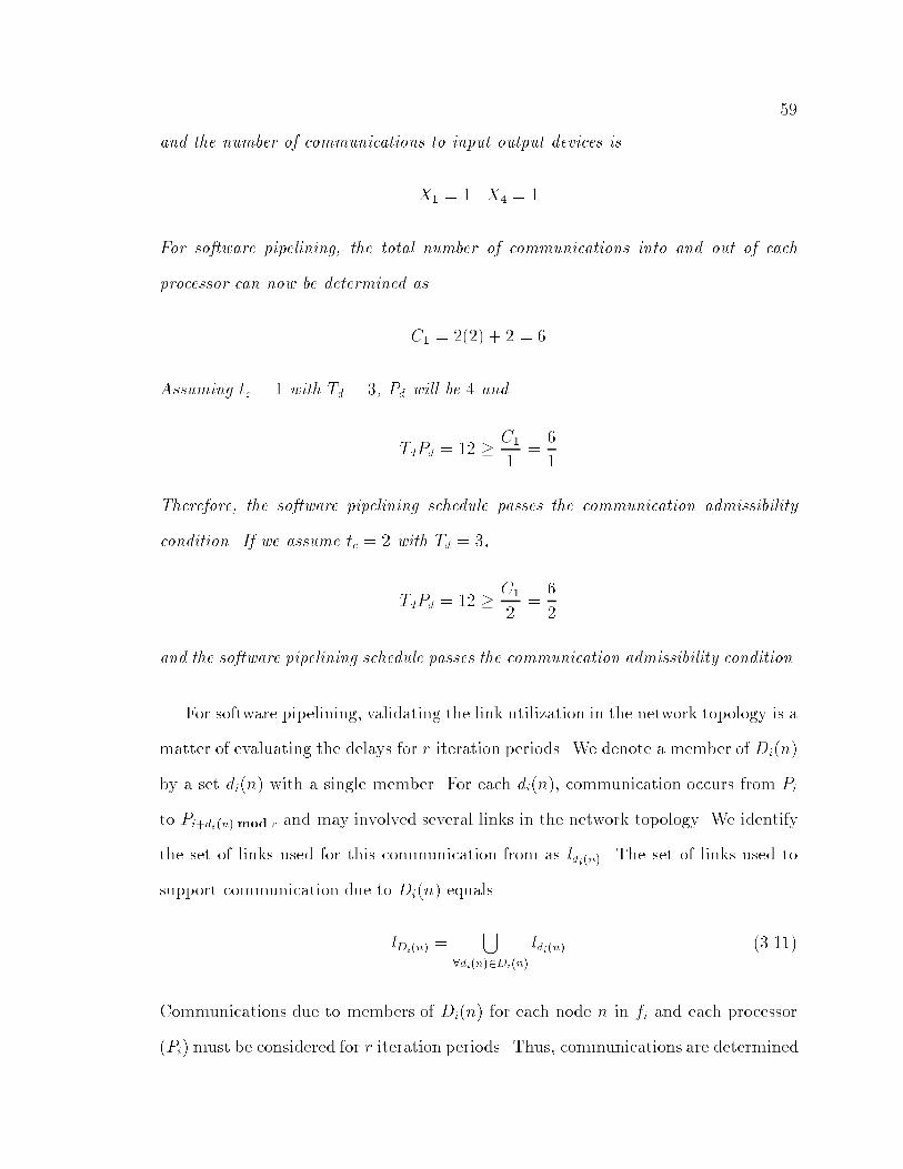
and the number of communications to input output devices is

X� � X �

For software pipelining� the total number of communications into and out of each

processor can now be determined as

C� � ���� � � � �

Assuming tc � with Td � �� Pd will be � and

TdPd � � � C�

�

�

Therefore� the software pipelining schedule passes the communication admissibility

condition� If we assume tc � � with Td � ��

TdPd � � � C�

��

�

�

and the software pipelining schedule passes the communication admissibility condition�

For software pipelining� validating the link utilization in the network topology is a

matter of evaluating the delays for r iteration periods� We denote a member of Di�n�

by a set di�n� with a single member� For each di�n�� communication occurs from Pi

to Pi�di�nmod r and may involved several links in the network topology� We identify

the set of links used for this communication from as ldi�n� The set of links used to

support communication due to Di�n� equals

lDi�n �

�di�n�Di�n

ldi�n ��� �

Communications due to members of Di�n� for each node n in fi and each processor

�Pi� must be considered for r iteration periods� Thus� communications are determined

��

for all Lji by adding one communication to each link in lDi�n � n � fi� � i � � i � r

for r iteration periods� The network topology admissibility condition for software

pipelining is

Lji

tn� TdPd � i � � i � r ��� ��

If this condition holds� there is enough time to allow the network topology to com�

plete the necessary communications for software pipelining on both synchronous and

asynchronous systems�

Adjusting the communication admissibility condition for the changes in the inter�

processor communication� the number of input inter�processor communications for Pi

on both synchronous and asynchronous systems becomes

Ii � Lji�� � j ��� ��

The number of output inter�processor communication for Pi is now

Oi � Lji � j ��� ��

The total communications for Pi using software pipelining becomes

Ci � Ii � Oi � Xi ��� ��

with the admissibility conditions remaining unchanged�

Example ����� We incorporate the unidirectional ring topology into Example ���

by reversing the direction of communication to better support the pipelined schedule�

The link utilization for a software pipelining schedule is found beginning with the

identi�cation of communications due to node n� For the �rst iteration period�

lD��� � fL��� L

�g

�

The second� third� and fourth iteration periods produce communications over the links

in

lD��� � fL�� L

�g lD��� � fL�

� L��g lD��� � fL�

�� L��g

The number of communications on a link in the ring topology is de�ned by

L�� � � L�

� � � L� � � L�

� �

Assuming tn � with Td � ��

Td � � � L��� � �

� Td � � � L��� � �

�

Td � � � L���

� ��

Td � � � L���

� ��

Adjusting the inter processor communication for software pipelining using the ring

topology

I� � � I� � � I� � � I � �O� � � O� � � O� � � O � �

With communications due to input�output devices remaining the same� the total re

quired communication �with consideration for the network topology� is

C� � � C� � � C� � � C � �

Assuming tc � with Td � ��

TdPd � � � C��

� ��

TdPd � � � C��

� ��

TdPd � � � C�� � �

� TdPd � � � C�� � �

�

Assuming tc � � with Td � ��

TdPd � � � C�� � �

� TdPd � � � C�� � �

�

TdPd � � � C�� � �

� TdPd � � � C�� � �

�

Therefore� the software pipelining schedule is valid for tn � � and Td � � with tc �

or tc � ��

��

In this section we have increased the exibility and e�ectiveness of OGM by in�

corporating the communication admissibility condition� the network topology admis�

sibility condition� and the e�ects of network topology on the partitioning strategy�

We now summarize the characteristics of OGM which lead to an e�ective partitioning

and scheduling process�

��� Contributions of the Order Graph Method

The order graph method currently supports the automatic partitioning of FSFGs for

�ne�grained parallelism exploiting parallelism during processing of a single sample

and between samples� FSFGs are used as a convenient and familiar method for OGM

algorithm speci�cation without requiring users to explicitly de�ne available paral�

lelism� OGM considers interprocessor communication and input�output bandwidths

during the scheduling process� In addition� support is provided for ring topologies

such as the BDPA� OGM allows users to optimize processing time and�or the number

of processors for a given FSFG� Similar to CRM and the RGM� scalability is limited

by the acceptable size for a non�hierarchical FSFG� However� the introduction of

hierarchy to OGM in Chapter � extends the scalability for OGM� Implemented in

C� OGM is practical for implementation on multiple parallel architectures �although

support for individual network topologies must be developed�� Running time has

been acceptable for FSFGs of up to ���� nodes with schedules generated for both

parallel and software pipelined implementations�

Considering the diversity of methodologies and the complexity of the task schedul�

ing problem �NP�complete�� benchmarks should be used to compare di�erent method�

ologies� Unfortunately� no accepted standardized benchmarks have been established

which cover the diverse methods� In the absence of such benchmarks� we have eval�

uated the two methods closest to OGM using several criteria� Table ��� presents a

��

comparison of OGM with respect to other key graph�based mapping methodologies

highlighting the advantages of OGM� In the table� � indicates that there is some

formal support for consideration of communication� In addition� � indicates that

there is the ability to support communication� however� the support has not been

presented formally�

Characteristic RGM CRM OGM

FSFG Speci�cation Y Y Y

Parallelism Not Explicitly De�ned Y Y Y

Scalable To Large Problems Y

Level Of Parallelism �ne�grained �ne�grained �ne�grainedto

coarse�grained

Parallelism Processing Single Sample Y Y Y

Parallelism Processing Multiple Samples Y Y Y

Considers Interprocessor Communication � � Y

Considers Network Topology Y

Considers Input�Output Bandwidth Y

Set T Optimize P Y Y

Set P Optimize T Y Y

Optimize T and P Y Y Y

Automated Schedule Generation Y Y Y

Suitable For BDPA Y Y Y

Acceptable Running Time Y � nodes� unpublished � Y ���� nodes�

Software Pipelining Support Y Y

Table ���� Comparison of RGM� CRM� and OGM

We now extend the Order Graph Method to add support for hierarchical FSFGs�

This permits OGM to be scalable to larger problems while reducing the running time

for algorithms speci�ed using hierarchy�

�Recent research e�orts have developed a multiprocessor integer programming based optimal compiler �MULTIPROC�� Developed from some basic concepts in CRM MULTIPROC runs on anIBM RS����� Model ��� and has scheduled FSFGs with less than � nodes� Published run timesaverage approximately �� minutes� however one runtime for a FSFG with �� nodes requirednearly �� hours� ����

Chapter �

Hierarchical FSFGs

��� Motivation

This research presents the Order Graph Method as a new methodology for task

scheduling on parallel processing systems� OGM has been implemented in a tool

called Calypso� to allow experimentation with parallel signal processing� To en�

hance OGM and Calypso� we have added support for hierarchical FSFGs� The need

for hierarchical FSFGs is immediately apparent when attempting to specify the ow

graph for a ��D �nd order IIR �lter of a � �x� � image� Assuming that each row of

the image serves as an input to the ow graph� the complete FSFG would contain

a total of ������ nodes� If a single pixel is used as an input� the example owgraph

would contain ��������� nodes Using a attened ow graph is not a realistic solution

since the graph would have an excessive number of nodes� A attened graph would

make the FSFG impossible to visualize and result in unrealistic scheduling times�

Practical experience has shown that a majority of applications use hierarchical

constructs which can be translated directly to FSFGs� To support this translation�

the de�nition of an algorithm�s hierarchical FSFG must include nodes which can be

used at any level of the hierarchy� Nodes may be simple nodes which identify the

execution of a single operation such as multiplication� They may also be composite

nodes which represent the execution of another level of the hierarchy �i�e� another

��

FSFG�� Thus� a FSFG at any particular level l of the hierarchy may be limited to

a reasonable number of nodes by introducing a series of composite nodes� These

composite nodes are de�ned by another FSFG at level l in the hierarchy� For

example� the FSFG for a ��D �nd order IIR �lter on a ���x��� image �assuming each

row is an input� may be represented by the FSFGs in Figure �� � In FSFG � A� each

of the nodes represents the execution of FSFG � B� Edges in FSFG � A represent

the input and output communications for FSFG � B� Similarly� nodes in FSFG � B

identify the execution of FSFG � C� and edges identify the communication due to

FSFG � C�

��� Hierarchical Specication

We begin the introduction of hierarchical FSFGs to OGM by de�ning a method for

hierarchical speci�cation of an algorithm� This technique must address several issues

which determine the limitations for an algorithm schedule�

� An algorithm speci�cation technique must include a method for de�ning com�

posite nodes which identify the execution of another FSFG�

� When a composite node is used at level l in the hierarchy� the technique must

include a method for de�ning a composite node�s e�ect at level l �i�e� what

happens inside the composite node�� Hierarchical speci�cation must enable

OGM to recognize feedback loops� input�output paths� and the total amount

of computation within a composite node�

� The speci�cation technique must enable OGM to identify input�output com�

munications for a composite node at level l and l in the hierarchy� At

level l in the hierarchy� precedence conditions must be established using the

communications patterns of composite nodes� In addition� inputs to a com�

posite node at level l must be tied to the inputs of the FSFG which de�ne the

��

BB B

B

B

B B

B

B B

B

B B

B

B

B C

C

C

C

C C C

C C C

C C C

C C C

FSFG � A FSFG � B

-1Z

-1Z

b0,0

a 1,1 b1,1

b1,2

a 1,2

a 1,3 b1,3

b1,4

a 1,4

a 1,5 b1,5

b1,6

a 1,6

b2,2

a 2,2

a 2,1 b2,1

*+*

+*

+**

+*+

q (n ,n -1)2,2 1 2

q (n ,n -1)2,1 21

g(n ,n )21q (n -1,n )1,1 1 2

q (n -1,n )1 21,2

q (n -1,n )1 21,4

q (n -1,n )1 21,6

q (n -1,n )1 21,5

q (n -1,n )1 21,3q (n ,n )

1 22,1

q (n ,n )12,2 2

f(n ,n )1 2

+*

+

*+*

*+*

+

*+*

++

*+*

+*

+*

-1Z

-1Z

-1Z

-1Z

-1Z

-1Z

q (n -1,n )1 21,2

q (n -1,n )1,1 1 2

q (n -1,n )1 21,4

q (n -1,n )1 21,6

q (n -1,n )1 21,5

q (n -1,n )1 21,3

2

2

FSFG � C

Figure �� � Hierarchical FSFG for a ��D �nd order IIR of a ���x��� image using eachrow as an input

��

composite node at level l � Similarly� the outputs from a composite node at

level l must be identi�ed with the outputs from the composite node�s de�ning

FSFG at level l � This guarantees that potential feedback loops which span

multiple levels of a hierarchical FSFG do not go unrecognized�

� Inputs and outputs between levels of the hierarchy must be distinguished from

inputs and outputs to system I�O devices�

These issues are identi�ed in the hierarchical FSFG presented in Figure ���� While

B+ * + B

Z-1

C C

FSFG � A FSFG � B

Z-1

+ * +

+

1 2 3

4 5

FSFG � C

Figure ���� Hierarchical FSFG for a �rd order lattice �lter

FSFG � C does not have any internal feedback loops� the paths � � � � � � and

� � � � � � combine to complete the feedback loop in FSFG � B� It should

be noted that the reverse is not always true� An apparent loop at level l in the

hierarchy does not necessarily mean that a feedback loop exists� Edges in level l

of the hierarchy may break the loop �See Figure ����� Thus� there is the potential

for a composite node at level l to contain an input�output path at level l which

forms part of a feedback loop at level l� In this case� all potential input�output

paths for a composite node�s de�nition at level l must be identi�ed and tied to

��

CB*+ *

+

FSFG � A FSFG � B FSFG � C

Figure ���� Example Hierarchical FSFG

the communication edges at level l where the composite node is used� Thus� the

speci�cation technique must relate the two input and two output communications in

FSFG � C of Figure ��� to the composite node�s communications in FSFG � B� In

addition� consideration for communication to system I�O devices must distinguish

the output g�n�� n�� �a system output� from the output q����n�� n�� �an output to the

next level of the hierarchy� in FSFG � C of Figure �� �

The Order Graph Method incorporates a method for hierarchical algorithm spec�

i�cation which maintains the inherent exibility of a hierarchy� We de�ne OGM�s

hierarchical speci�cation technique as follows�

FSFG �� edgeedge �� fromnode tonode data�intopt

fromnode �� nodename instance j innode instance fsfgname instancetonode �� nodename instance j outnode instance fsfgname instance

int �� �� � � ����nodename �� �a� � � z�� j INPUT j OUTPUT

innode �� inputoutnode �� output

fsfgname �� �a� � � z��instance �� int

For example� the hierarchical �nd order IIR �lter shown in Figure ��� may be

de�ned by the input �les in Figure ����

��

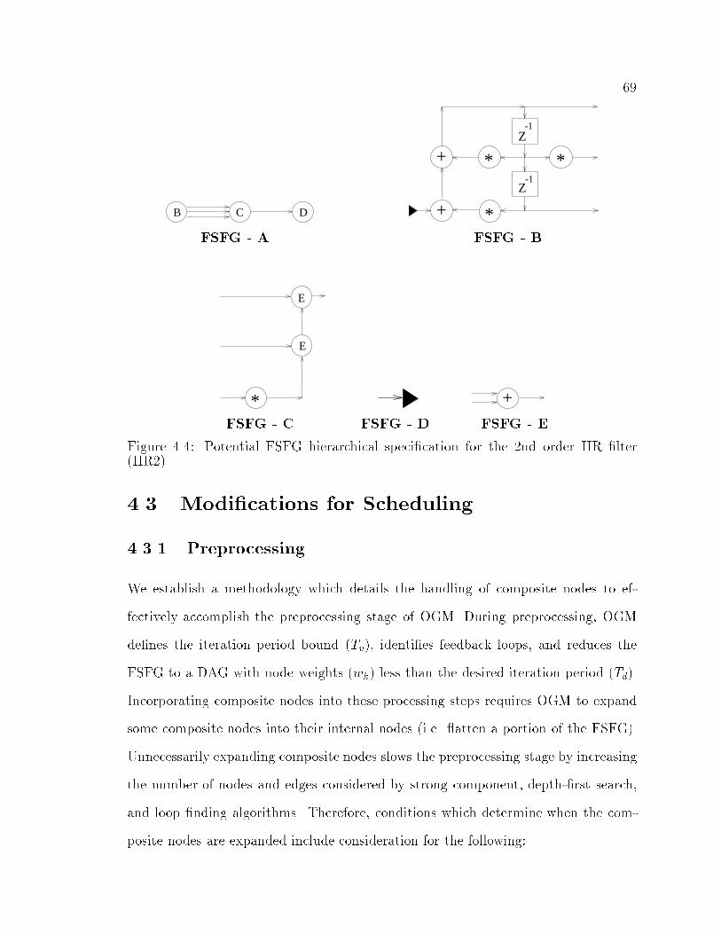
B C D

+ *

+ *

*Z

-1

-1Z

FSFG � A FSFG � B

*

E

E

+

FSFG � C FSFG � D FSFG � E

Figure ���� Potential FSFG hierarchical speci�cation for the �nd order IIR �lter�IIR��

��� Modications for Scheduling

����� Preprocessing

We establish a methodology which details the handling of composite nodes to ef�

fectively accomplish the preprocessing stage of OGM� During preprocessing� OGM

de�nes the iteration period bound �Tv�� identi�es feedback loops� and reduces the

FSFG to a DAG with node weights �wk� less than the desired iteration period �Td��

Incorporating composite nodes into these processing steps requires OGM to expand

some composite nodes into their internal nodes �i�e� atten a portion of the FSFG��

Unnecessarily expanding composite nodes slows the preprocessing stage by increasing

the number of nodes and edges considered by strong component� depth��rst search�

and loop �nding algorithms� Therefore� conditions which determine when the com�

posite nodes are expanded include consideration for the following�

��

filename� hiir�

��������������������������������output� hiir�a�� input� hiir�b��output� hiir�a�� input� hiir�b��output� hiir�a�� input� hiir�b��output� hiir�b�� input� hiir�c��

filename� hiir�a

��������������������������������INPUT� add�add� add�add� output� delay�multiply� add� data��multiply� data�� add�delay� multiply� multiply� data�� delay�delay� data�� output� multiply�multiply� output�

filename� hiir�b

��������������������������������input� input� sum�� data��input� input� sum��input� multiply�output� sum�� input� sum��multiply� input� sum��output� sum�� output�

filename� hiir�c

��������������������������������input� OUTPUT�

filename� sum

��������������������������������input� add�input� add�add� output�

Figure ���� Sample input �les for the hierarchical speci�cation of a �nd order IIR�lter �IIR��

� Is the computational delay of the composite node known! The computational

delay for the node must be identi�ed for comparison to the desired iteration

period and the calculation of strong component weights�

� Is the composite node involved in a feedback loops! This must be determined

at the level of the hierarchy which uses an instance of the composite node and

at the level of the hierarchy which de�nes the composite node�

�

� Is the desired iteration period less than the computational time of the com�

posite node! If so� the node must be expanded to permit partitioning of the

DAG�

� Is the composite node a member of a strong component which must be ex�

panded to reduce the strong component�s weight less than the desired itera�

tion period! When expanding a strong component� composite nodes within a

strong component should be expanded prior to removing an edge in the strong

component�

� Has the composite node previously been expanded! If so� the required in�

formation should already be available without requiring further analysis of

the composite node� If the composite node is not expanded� data should be

available for each instance of the composite node without repetitive analysis�

For example� FSFG � C in Figure ��� should only be expanded once when analyzing

the potential feedback loop in FSFG � B� Under these conditions composite nodes

will only be expanded when absolutely necessary allowing �ne�grained parallelism to

be exploited with a minimum amount of processing time�

OGM determines a composite node�s total computational weight and associates

the weight with each instance of the composite node� During the process of reading

a hierarchical FSFG�s nodes into Calypso� OGM determines the total computational

time for each FSFG� Once all of the FSFG nodes have been input� OGM establishes

the edges within each level of the hierarchy� While assigning edges to an instance

of a composite node� the total computational time is also assigned� As long as the

composite node remains unexpanded� OGM will reference this total weight� Once

expanded� OGM will reference the weights of the composite node�s internal nodes�

Composite nodes will e�ect the determination of feedback loops on two levels of

the hierarchy� the level which uses an instance of the composite node and the level

��

which de�nes the composite node� We begin by discussing feedback loops which

incorporate a composite node� Assume a level l of the hierarchy uses an instance

of a composite node within a feedback loop� OGM uses the input�output paths

within the composite node to determine if the feedback loop truly exists� For each

composite node� all input�output paths to other levels of the hierarchy are identi�ed

by performing depth��rst searches from intermediate input nodes� OGM executes

these depth��rst searches immediately after de�ning the FSFG�s edges� It should be

noted that the process of de�ning FSFG edges and input�output paths begins with

the lowest level of the hierarchy and ends with the highest level of the hierarchy� By

doing this� OGM is able to handle composite nodes which are used within a potential

input�output path of another composite node �i�e� composite nodes within composite

nodes�� Using the composite node�s input�output paths at level l � OGM checks

for a connection between the input and output nodes at level l� If a path exists

between the input and output nodes on level l of the hierarchy� the feedback loop

is considered valid� If not� the potential feedback loop is considered to be invalid�

For the hierarchical FSFG in Figure ���� the input�output paths for FSFG � B would

validate the feedback loop in FSFG � A� While� the input�output paths for FSFG � B

and FSFG � C in Figure ��� would invalidate the potential feedback loop in FSFG � A�

A second way composite nodes may be involved with feedback loops is if the iter�

ation period bound must be identi�ed to produce a rate optimal schedule� Allowing

embedded delays in the hierarchy permits feedback loops to be embedded within

composite nodes� In order to identify the iteration period bound for the digraph� any

feedback loops which exist within the digraph�s composite nodes must be identi�ed�

This will only occur once in the preprocessing stage and prior to the reduction of the

digraph to a DAG� For a composite node which has not been expanded internal loops

are identi�ed using a modi�ed version of Johnson�s algorithm ����� Because a com�

posite node can occur within a composite node� this may involve analyzing composite

��

nodes on multiple levels of the hierarchy� As before� a composite node �y� within a

composite node �x� is not expanded to evaluate potential loops within x� Instead�

input�output paths for y are used to validate potential loops within x� In addition�

OGM will evaluate a composite node�s internal loops only once and will not perform

a loop search for each instance of the composite node� Using the loops from both

expanded and unexpanded composite nodes� the iteration period bound Tv may be

found using Equation ����

Using the feedback information� preprocessing identi�es strong components and

reduces the digraph to a DAG� With hierarchical speci�cation� the DAG can consist

of atomic nodes� composite nodes which identify a strong component� and composite

nodes from the original digraph �which do not identify a strong component�� In

keeping with the goals of the preprocessing stage� composite nodes with a weight

greater than the desired iteration period must be expanded� Expanding composite

nodes which do not identify a strong component is handled by expanding the DAG to

include the internal nodes of the composite node� Depending on the number of levels

of the hierarchy within the composite node� this process may need to be repeated

recursively�

Without hierarchical speci�cation� a composite node which identi�es a strong

component is expanded by considering internal nodes� identifying loops� removing

an edge from a loop� and collapsing the remaining strong component back into a

composite node� To incorporate hierarchy� OGM must determine if a member of the

strong component is a composite node� Before removing an edge from the strong

component� any composite nodes within the strong component must be expanded�

The purpose of this step is to ensure that edges of the graph are not unnecessarily

removed� Composite nodes within a strong component may contain internal nodes

which are not members of the strong component� Because the composite node is not

expanded� these nodes add to the weight of the strong component� By expanding the

��

composite node� the strong component will contain the minimum number of nodes

and will have the minimum weight� Therefore� if composite nodes are found within a

strong component� one of the composite nodes is expanded and the remaining strong

component is reduced back into a composite node� A strong component which does

not contain composite nodes is still expanded by removing an edge from the loop with

the lowest iteration period�

During preprocessing� OGM prevents the analysis of a composite node more than

once by maintaining data for each composite node and recognizing multiple occur�

rences of the node� OGM evaluates an instance of a composite node by determining

if the data is available from another instance of the composite node� The absence of

the necessary data from other instances indicates that the composite node has not

been evaluated� For example� identi�cation of input�output paths for a composite

node is done once and re�used for each instance of the composite node� In addition�

OGM reduces the requirement for composite node analysis by determining a com�

posite node�s representative data during the loading of the FSFG� Details such as

the computational delay for a composite node are determined during the loading of

individual nodes within the composite node�

����� Partitioning

During the partitioning stage� OGM develops a set of candidate partitionings from the

DAG provided by the preprocessing stage� This is accomplished through the use of a

relations matrix to generate linear extensions which produce candidate partitionings�

Entries in the relations matrix are representative of data dependencies between nodes

in the DAG� Because nodes in the DAG can consist of composite nodes� embedded

delays will play a key role in determination of data dependencies for the relations ma�

trix� If a delay exists between node x and node y� then there is no data dependency

in the relations matrix� The absence of a delay results in the entry of xRy �where x

��

is related to y� in the relations matrix� Thus� it is necessary to determine if outputs

from a composite node originate at a delay or from some other element� If they orig�

inate from a delay� there is not a data dependency on the composite node� Similarly�

input communications which terminate at a composite node are identi�ed as termi�

nating at a delay or some other element� Consider FSFG C in Figure �� � all output

communications originate at delay elements and do not result in data dependencies

across composite nodes in FSFG B�

Finally� OGM incorporates a methodology for dealing with the partitioning in�

herently de�ned by the hierarchy� Using a hierarchy� di�erent levels of parallelism

are available ��ne to coarse�grained parallelism�� OGM deals with the inherent par�

titioning by allowing the desired iteration period to determine the required level of

parallelism� If the desired iteration period is greater than the composite nodes� com�

putational time� coarse�grained parallelism is exploited and the composite nodes are

not expanded� In this case� the initial de�nition of the composite nodes will essen�

tially determine the operations which are performed on an individual processor� It

is possible that the user has not developed the hierarchical FSFGs with an e�ective

partitioning in mind� Thus� the coarse�grained implementation may not be e�cient

in reducing excessive communication� However� this is acceptable if the goal is to

produce a valid parallel processing or software pipelining schedule which meets the

admissibility conditions �including communication and network topology admissibil�

ity conditions�� If the desired iteration period is less than the weights of the composite

nodes� �ne�grained parallelism will be exploited� With a lower iteration period� the

composite nodes will be expanded to allow partitioning of the internal nodes� The

partitioning of the internal nodes will result in a schedule which exploits parallelism

between a smaller set of operations� These ideas are illustrated by examples in Chap�

ter ��

��

����� Validating and Scheduling

There are no hierarchical issues which e�ect the validation of communication and

network topology or the scheduling of the cycling vector and period matrix�

��� Summary

In summary� the major issues handled by OGM during task scheduling of hierarchical

FSFGs includes�

� Providing an e�ective speci�cation technique for hierarchical FSFGs�

� Recognizing feedback loops within and across levels of the hierarchy� and pre�

venting the unnecessary partitioning of a feedback loop�

� Avoiding unnecessary attening the hierarchical FSFG during the scheduling

process�

� Preserving the freedom to partition the hierarchical FSFG to achieve the de�

sired iteration period bound and�or the number of processors�

Methodologies to handle these issues include�

� The exibility of the hierarchy is maintained by using nodenames and instances

to de�ne atomic and composite nodes in the hierarchical FSFG�

� Key information about a composite node is stored to prevent repetitive analy�

sis� Input�output paths� internal loops� and the total computational delay for

composite nodes is maintained�

� Composite nodes are initially analyzed for input�output paths to enable the

validation of feedback loops which incorporate composite nodes� This prevents

a attening of the hierarchy to determine feedback loops�

��

� Composite nodes are analyzed for internal feedback loops if the iteration period

bound must be determined� If this must occur� the input�output paths are

used to prevent a complete attening of the hierarchy when composite nodes

occur within composite nodes�

� Strong components are expanded by expanding any composite nodes within

the strong component prior to removing a feedback edge� This ensures that

the largest possible strong component will be retained to minimize the number

of nodes generated in a candidate partitioning�

� After ensuring all strong components have a computational delay less than

the desired iteration period� all composite nodes with a weight greater than

the desired iteration period are expanded� This ensures that the partitioning

process will be able to partition the linear extension using the desired iteration

period without splitting composite nodes across multiple processors�

With these issues addressed� Calypso has been developed to accept hierarchical

FSFGs� Incorporating the methodology to handle these FSFGs� Calypso produces

optimized schedules for hierarchical FSFGs with basic consideration for interprocessor

communication and ring topologies�

Chapter �

Evaluation of CALYPSO

The results of the previous chapters suggest a methodology to increase processing

rates for DSP multiprocessor systems� Research at North Carolina State University

has developed a high performance DSP architecture� termed the Block Data Paral�

lel Architecture �BDPA� ��� �� ���� which may bene�t from this scheduling theory�

The current BDPA system is continually being developed to support a wide array

of real�time signal processing problems� Several algorithms have been successfully

mapped to the BDPA including a ��D digital IIR �lter� a ��D digital FIR �lter� LU

Decomposition� and a ��D discrete cosine transform ��� �� �� ���� For each of these

algorithms� an e�ective mapping was obtained based on insight into the problem and

the architecture� The mapping theory presented in this dissertation will automate

this process for the BDPA� as well as other multiprocessor architectures�

In this chapter� we demonstrate the e�ectiveness of our mapping technique on the

the BDPA for a variety of applications� Due to the complexity of the task scheduling

problem� we present performance data for several benchmark applications to estab�

lish the usability and exibility of OGM for hierarchical FSFGs� Well known as an

NP�complete problem� scheduling time determines to a great extent the usability

of a mapping methodology ���� Therefore� results for scheduling several benchmark

algorithms are presented� including FIR �lters� IIR �lters� lattice �lters� LU Decom�

position and QR Factorization� For each of the algorithms� a variety of hierarchical

��

speci�cations have been used to determine the e�ects of the initial hierarchy on the

resulting multiprocessor schedule and on the scheduling time� The next section briey

describes the BDPA�

��� Overview of the BDPA

The BDPA system consists of three major components� an Input Module �IM�� a

Processor Module Array �PMA�� and an Output Module �OM� as depicted in Fig�

ure �� � In general� the IM acts as a bu�er for incoming data from an input device

PROCESSOR ARRAY

ICM

OCM

OUTPUT DEVICE

INPUT DEVICE

Figure �� � Block Diagram of the BDPA

and splits up the input stream into blocks of data� The blocks of data are then

transferred to di�erent processors in the PMA by the IM� Similarly� the OM serves

as a bu�er between the PMA and the output device� It receives data from the dif�

ferent processors in the PMA and routes the data to the output device� The PMA

consists of a number of identical processors each executing the same program� In

order to prevent communication contention� interprocessor communication is limited

to local unidirectional communication only� This forms the basis of the BDPA system

with the processors executing whenever all the required data elements for the next

operation become available�

��

The block�data ow characteristic of the system emphasizes interaction of commu�

nication and computation� Data ow permits the elimination of lock�step operation

synchronized by a global clock� The concept allows a processor to receive data into

bu�ers and then execute as long as the data required for the next operation is avail�

able in the bu�ers� The block concept reduces the communication time within the

system by eliminating the handshaking between processors for each data element�

Using block�data ow� processors setup for communication and then pass a block of

data elements before closing the communication channel� The characteristics of the

BDPA system may be summarized as follows�

� block data processing and the block data ow paradigm

� globally asynchronous and locally synchronous data transmission protocol

� linear array topology and skew� operations among processors

� local data transmission in only one direction

� overlap of data movement and interprocessor communication with data computa�

tions

One key feature of the BDPA is the ring topology� The interconnections among

the BDPA processors impose a basic limitation on the scheduling of a FSFG� To

handle this limitation� a scheduling algorithm should attempt to restrict a processor�s

dependence to data from processors which proceed it in the ring topology� Any

cut in a feedback loop requires bi�directional communication� For a unidirectional

ring topology� this translates to communication through each processor all the way

around the ring� Thus� the e�ort to limit a processor�s dependence helps avoid a

parallel execution schedule which generates excessive communications to support a

partitioned feedback loop� If a feedback loop has a total computational time greater

than Td� software pipelining may be used to reduce the required communications for

execution at Td by scheduling the feedback loop on a single processor� While the

�

unidirectional communication may be a disadvantage when dealing with feedback

loops� it prevents contention from occurring on the ring topology and increases the

e�ectiveness of skew� operations� If data can be skewed to permit processing of

several elements of a single data stream� dependent as well as independent data

streams may often be interleaved �����

Using OGM� the BDPA�s features can be incorporated into the scheduling process

for hierarchical ow graphs� Calypso has been used on a set of benchmark algorithms

to produce parallel computing schedules for execution on the BDPA� The next section

describes the experimental conditions and assumptions used to obtain the scheduling

data for the benchmark algorithms�

��� Implementation and Experimental Conditions

Calypso is currently implemented in C using approximately ���� lines of code and

consists of three executable �les� The main program executes the OGM mapping

methodology and calls the other two programs to verify communications and network

topology admissibility� Therefore� Calypso can be implemented for another architec�

ture by replacing the network topology executable with another architecture speci�c

executable�

The results presented in this dissertation were obtained on a personal computer

with an Intel ���DX����MZ processor and �MB of memory� The target multiproces�

sor system was assumed to have generalized processors which perform a multiplication

in � computational time units� an addition in time unit� a divide in � time units�

and a square root in �� time units� The network topology is assumed to be a ring

topology with each link transmitting no more than unit of data per time unit�

Results for Calypso are presented in Tables �� to ���� In the tables� column

HFSFG identi�es the initial speci�cation of the algorithm� Nodes indicates the num�

��

ber of nodes in the initial speci�cation� including system input�output nodes� inter�

mediate input�output nodes and delay nodes� Column Levels is the number of levels

in the initial speci�cation�s hierarchy� Pd and Td identify the number of processors

and the iteration period for the scheduled HFSFG� These values are the result of the

scheduling process and may di�er from the initial target values �� The average pro�

cessor utilization for Td and Pd is shown in column Avg� Proc� Util�� The number of

linear extensions considered �during the partitioning stage of OGM� before obtaining

a valid schedule is indicated by Linear Extensions� The running time for Calypso to

obtain a schedule for the HFSFG is shown in CPU time� To ensure the accuracy of the

CPU time� the measurements for running time are the average of � runs on Calypso�

SP and PE indicate whether a valid schedule was found for software pipelining and

parallel execution respectively� The amount of communication allowed per time unit

is shown by tc� The value of tc is for tables which do not have a tc column� In the

tables� bold entries for Td indicate a rate optimal schedule for the value of tc� Bold

entries for an entire row in the tables indicates that the HFSFG is communication

bound at the initial target value for Td� Therefore� Calypso has identi�ed the best

possible schedule under the conditions imposed by tc�

We now present the results for scheduling the benchmark algorithms with Calypso

using the Order Graph Method� For each algorithm� we briey describe the algorithm�

illustrate non�hierarchical and hierarchical FSFGs� present Calypso�s scheduling re�

sults� and illustrate a potential schedule for parallel computing� We begin with �lter

algorithms for digital signal processing�

�Calypso will attempt to meet a user speci�ed target for Td or Pd� During partitioning Calypsomay be able produce a schedule which improves on these values� In addition there are some casesin which a schedule cannot be produced for the target values� In these cases Calypso identi�esand outputs the best possible schedule�

��

��� Filters

For edge enhancement and noise removal during image processing� a variety of �l�

ters may be used ����� In this section� we present some of these �lters and potential

schedules produced by Calypso� For each of the �lters� di�erent hierarchical speci��

cations are used to highlight Calypso�s features and to provide insight into the e�ects

of hierarchy� We begin with a look at the �nd order IIR Filter�

����� �nd Order IIR Filter

The transfer function for a N th order IIR �lter is de�ned as

H�Z� �

PNn�� b�n�Z�n

�PN

n�� a�n�Z�n

with a �nd order IIR equal to

H�Z� �b� � b�Z

�� � b�Z��

� a�Z�� � a�Z��

Four di�erent ways of specifying a �nd order IIR are shown in Figures ���� ����

���� and ���� We refer to these four speci�cations as IIR � IIR�� IIR�� and IIR�

respectively� IIR is non�hierarchical while IIR�� IIR�� and IIR� use hierarchy�

++ *

+ *

*

+

*

-1Z

Z-1

1

2 4

3 7

8 9

10

5

6

Figure ���� Flow graph for a �nd order IIR �lter �IIR �

A badly speci�ed hierarchy �IIR�� demonstrates Calypso�s ability to manipulate a

��

B C D

+ *

+ *

*Z

-1

-1Z

FSFG � A FSFG � B

*

E

E

+

FSFG � C FSFG � D FSFG � E

Figure ���� Potential FSFG hierarchical speci�cation for the �nd order �D IIR �lter�IIR��

+*

+

*

B

+ *

Z-1

C

FSFG � A FSFG � B

+ *

-1Z

FSFG � C

Figure ���� Potential FSFG hierarchical speci�cation for the �nd order �D IIR �lter�IIR��

��

*

*

B

D

+ *

Z-1

C

FSFG � A FSFG � B

+ *

-1Z

+

+

FSFG � C FSFG � D

Figure ���� Potential FSFG hierarchical speci�cation for the �nd order �D IIR �lter�IIR��

speci�cation�s inherent partitioning to produce an optimal schedule� IIR� identi�es

strong components in terms of composite nodes and will reduce the amount of time the

preprocessing stage initially spends identifying strong components� Additionally� IIR�

groups nodes which are not members of a strong component into a composite node�

This bene�ts the partitioning stage by reducing the number of nodes for consideration

during the generation of linear extensions�

Results for scheduling these hierarchical FSFGs are shown in Table �� � With the

relatively small size of the �nd order IIR �lter� the di�erences in the CPU times for

scheduling the various speci�cations is negligible� However� these results illustrate the

ability of OGM to e�ectively handle di�erent hierarchical speci�cations� Even with

smaller graphs� the e�ects of the hierarchy can be seen� For IIR and IIR� with Td � ��

the same number of linear extensions was generated� but the running time was greater

for IIR�� This is due to the composite nodes within the linear extension� During

the greedy partitioning of the linear extension for IIR�� the partitioning algorithm

��

HFSFG Nodes Levels Pd Td Linear Avg� Proc� CPU time SP PEExtensions Util� ��� �sec �

IIR� �� � � �� � ��� � � Y Y

� � � ��� � �� Y Y

� � ��� � � Y N

� � ��� � �� Y N

IIR� �� � � �� � ��� � �� Y Y

� � � ��� � � Y Y

� � ��� � �� Y N

� � ��� � �� Y N

IIR� �� � � �� � ��� � �� Y Y

� � � ��� � � Y Y

� � ��� � � Y N

� � ��� � Y N

IIR �� � � �� � ��� � �� Y Y

� � � ��� � �� Y Y

� � ��� � � Y N

� � ��� � �� Y N

Table �� � Summary of Calypso�s results for scheduling hierarchical FSFGs of a �ndorder IIR �lter with tc �

attempted to split IIR� which resulted in more than Pd partitions� Taking advantage

of the network topology� the starting point for the partitioning algorithm was shifted

and another attempt was made to partition the same linear extension� For IIR��

the second attempt to partition the linear extension was successful while IIR was

successful on the �rst attempt�

In general� Calypso will terminate execution as soon as a valid schedule is found�

Because of communication costs� valid software pipelining schedules tend to be found

prior to schedules for parallel execution� If we force Calypso to produce a sched�

ule for parallel execution� additional linear extensions are considered until a potential

candidate partitioning passes communication and network topology admissibility con�

ditions for parallel execution� Results for the same �nd order IIR �lter FSFGs are

shown in Table ���� A key result from forcing a parallel execution schedule with

��

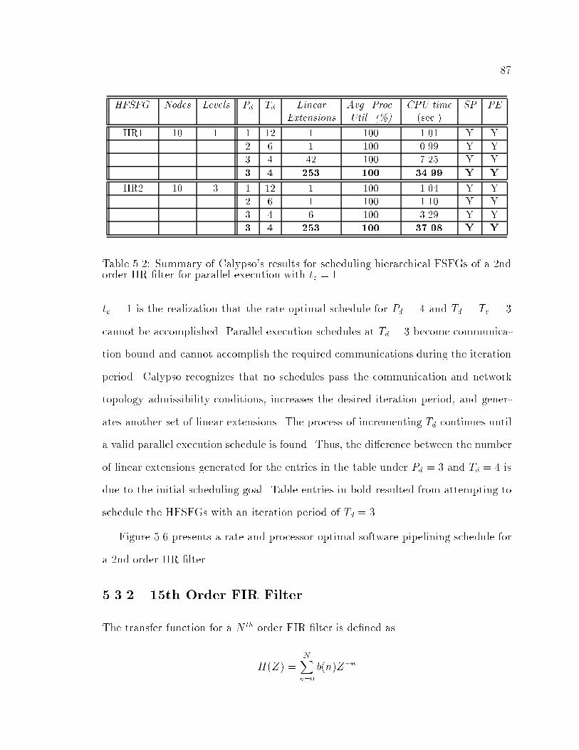
HFSFG Nodes Levels Pd Td Linear Avg� Proc� CPU time SP PEExtensions Util� ��� �sec �

IIR� �� � � �� � ��� � �� Y Y

� � � ��� � �� Y Y

� � ��� � � Y Y

� � ��� ��� ����� Y Y

IIR� �� � � �� � ��� � � Y Y

� � � ��� � �� Y Y

� � ��� � �� Y Y

� � ��� ��� ��� Y Y

Table ���� Summary of Calypso�s results for scheduling hierarchical FSFGs of a �ndorder IIR �lter for parallel execution with tc �

tc � is the realization that the rate optimal schedule for Pd � � and Td � Tv � �

cannot be accomplished� Parallel execution schedules at Td � � become communica�

tion bound and cannot accomplish the required communications during the iteration

period� Calypso recognizes that no schedules pass the communication and network

topology admissibility conditions� increases the desired iteration period� and gener�

ates another set of linear extensions� The process of incrementing Td continues until

a valid parallel execution schedule is found� Thus� the di�erence between the number

of linear extensions generated for the entries in the table under Pd � � and Td � � is

due to the initial scheduling goal� Table entries in bold resulted from attempting to

schedule the HFSFGs with an iteration period of Td � ��

Figure ��� presents a rate and processor optimal software pipelining schedule for

a �nd order IIR �lter�

����� ��th Order FIR Filter

The transfer function for a N th order FIR �lter is de�ned as

H�Z� �NXn��

b�n�Z�n

��

2

1

8

10 7

4

6

512

P

P

P

P

1

2

3

4

9

Z-1

-1Z

+ *

*+ *

*

+

+

Figure ���� FSFG for the �nd�order �D IIR �lter� with a software pipelining� rateand processor optimal schedule generated by Calypso using the Order Graph Methodwith tc �

with a �th order FIR equal to

H�Z� � b� � b�Z�� � b�Z

�� � � � �� b��Z���

If the coe�cients are symmetric� the FSFG for a �th order FIR is shown in Figure ���

�FIR �� A potential hierarchical speci�cation which takes advantage of the FIR�s

repetitive nature of this ow graph is shown in Figure ����FIR��� Results for

Z-1

Z-1

+

*

+

Z-1

Z-1

+

*

+

Z-1

Z-1

+

*

+

Z-1

Z-1

+

*

+

Z-1

Z-1

+

*

+

Z-1

Z-1

+

*

+

Z-1

Z-1

+

*

Z-1

+

*

+

Figure ���� FSFG for the �th order FIR �lter �FIR �

scheduling these FSFGs are shown in Table ����

In the case of the FIR �lter� there is not a feedback loop to restrict the iteration

period to Tv� Therefore� the iteration period for a potential schedules becomes limited

��

Z-1

Z-1

+

*

B B B B B B Z-1

+

*

+

Z-1

Z-1

+

*

+

FSFG � A FSFG � B

Figure ���� Potential FSFG hierarchical speci�cation for a �th order FIR �lter�FIR��

HFSFG Nodes Levels Pd Td Linear Avg� Proc� CPU time SP PE tcExtensions Util� ��� �sec��

FIR� �� � � �� � ��� ���� Y Y �� �� � ���� ���� Y Y �� �� � ���� ���� Y Y � � � ���� ���� Y Y �� � � ���� ���� Y Y �� � ���� ��� Y N ��� � � ���� ���� Y N ��� � � ���� ���� Y N �� � � ���� ���� Y N ��� �� � ���� ���� Y N ���

FIR� �� � � �� � ��� ���� Y Y �� �� � ���� ���� Y Y �� �� � ���� ��� Y Y � � � ���� ���� Y Y �� � � ���� ���� Y Y �� � ���� ���� Y N ��� � � ���� ���� Y N ��� � � ���� ���� Y N �� � � ���� ���� Y N ��� �� � ���� ���� Y N ���

Table ���� Summary of Calypso�s results for scheduling hierarchical FSFGs of a �thorder FIR �lter

��

by the communication requirements� For example� a schedule for parallel execution

with one atomic node per processor requires a minimum of � communications� Thus�

the preprocessing stage determines that the desired iteration period must be greater

than �tc

� If Calypso is forced to obtain a schedule for parallel execution� an attempt

will be made to partition and schedule the algorithm with Td � �tc

� If a valid schedule

does not exist� Td will be increased by one and Calypso will begin the partitioning

and scheduling process again� This process continues until a valid schedule is found�

For the �th order FIR �lter in Figure ��� with tc � � Calypso obtains a parallel

execution schedule with Td � � and Pd � � and a rate optimal software pipelining

schedule at Td � � and Pd � �� Changing the value for tc changes the admissibility

of communications for individual schedules and results in di�erent optimal schedules�

Figure ��� illustrates a potential partitioning generated by Calypso for an optimal par�

allel execution schedule allowing atomic nodes to be split across processors� Choosing

not to split atomic nodes across processors� Calypso produces the schedule depicted

in Figure �� ��

7

6

5

1P

2P

3P

4P

P

P

P*

+

Z-1

Z-1

+

*

+

Z-1

Z-1

+

*

+

Z-1

Z-1

+

*

+

Z-1

Z-1

+

*

+

Z-1

Z-1

+

*

Z-1

+

*

+

+

-1Z

-1Z

+

*

+

-1Z

-1Z

Figure ���� FSFG for the �th order FIR �lter� with a software pipelining and parallelexecution schedule generated by Calypso using the Order Graph Method for Pd � ��Td � �� and tc �

�

7

6

5

1P

2P

3P

4P

P

P

P*

+

Z-1

Z-1

+

*

+

Z-1

Z-1

+

*

+

Z-1

Z-1

+

*

+

Z-1

Z-1

+

*

+

Z-1

Z-1

+

*

Z-1

+

*

+

+

-1Z

-1Z

+

*

+

-1Z

-1Z

Figure �� �� FSFG for the �th order FIR �lter� with a software pipelining andparallel execution schedule generated by Calypso using the Order Graph Method forPd � �� Td � �� tc � � and not splitting atomic nodes across processors

����� �th Order Lattice Filter

In this section� we introduce another IIR �lter structure called the lattice �lter or the

lattice realization� Used extensively in digital speech processing and in the imple�

mentation of adaptive �lters� the lattice �lter is derived from the di�erence equations

for an IIR �lter ����� The FSFG for a �th order lattice �lter is shown in Figure ��

with a potential hierarchy �using the repetitive nature of the lattice �lter�s design�

+ * +

Z-1+

+ * +

Z-1+

+ * +

Z-1+

+ * +

Z-1

Figure �� � FSFG for a �th order lattice �lter �LAT �

shown in Figure �� ��

This �lter highlights Calypso�s ability to deal with multiple feedback loops across

levels of the hierarchy during preprocessing and the identi�cation of Tv� In the �th

order lattice �lter� there are over �� loops to evaluate in order to determine Tv for

��

+ * +

Z-1

B BB

+ * +

Z-1+

FSFG � A FSFG � B

Figure �� �� Potential FSFG hierarchical speci�cation for a �th order lattice �lter�LAT��

rate optimal schedules� The initial reduction of strong components into composite

nodes will produce a graph with � nodes � an INPUT� a composite� and an OUT�

PUT� For the FSFG in Figure �� � the composite node will contain other composite

nodes internally� During preprocessing� reducing the composite node�s weight to less

than Td will require the composite node to be expanded and reduced multiple times�

Therefore� the preprocessing stage of OGM will require more time than the �nd order

IIR and �th order FIR�

Results for scheduling these hierarchical FSFGs are shown in Table ���� An im�

portant aspect of the results present in Table ��� is the slight increase in running time

between LAT and LAT�� During the preprocessing stage of OGM� an attempt is

made to contain a feedback loops within a composite node� For the case of the lattice

�lter� the composite node repeatedly exceeds the maximum computational delay and

must be repeatedly expanded and reduced until the computation weight is less than

Td� In this case� composite nodes resulted in the process taking a longer amount of

time� This is due to the requirement to expand composite nodes within the composite

node prior to removing any edges from the graph�

Lowering the value of tc for the lattice �lter results in the parallel computing

schedule becoming communication bound� Attempts to schedule the LAT and LAT�

with Td � � and tc � ��� fails the communication admissibility condition� As a result�

OGM increases the value of Td and attempts to produce a valid candidate partitioning

��

HFSFG Nodes Levels Pd Td Linear Avg� Proc� CPU time SP PE tcExtensions Util� ��� �sec��

LAT� �� � � �� � ��� ���� Y Y �� �� � ���� ���� Y Y �� � � ���� ���� Y N �� �� � ��� ���� Y Y ���� �� � ���� ���� Y Y ���� � � ���� ��� Y N ���� �� � ��� ���� Y Y ���� �� �� ���� ������ Y N ���� �� ��� ��� ���� Y N ��

LAT� �� � � �� � ��� ���� Y Y �� �� � ���� ���� Y Y �� � � ���� ���� Y N �� �� � ��� ���� Y Y ���� �� � ���� �� � Y Y ���� � � ���� �� � Y N ���� �� � ��� ���� Y Y ���� �� �� ���� ����� Y N ���� �� ��� ��� ����� Y N ��

Table ���� Summary of Calypso�s results for scheduling hierarchical FSFGs of a �thorder lattice �lter

from the same set of linear extensions� Similar to IIR and IIR�� this process continues

until a valid candidate partitioning is found�

Figure �� � illustrates the rate and processor optimal software pipelining schedule

obtained by Calypso for the �th order lattice Filter�

2

3P

P

P1+ * +

Z-1+

+ * +

-1+

+ * +

Z-1 + -1

Z

+*+

Z

Figure �� �� FSFG for a �th order lattice �lter� with a software pipelining� rate andprocessor optimal schedule generated by Calypso using the Order Graph Method withtc �

��

����� ��D Filtering

The transfer function for the ��D IIR �lter is given by

H�Z�Z�� �

PNn��

P�m�� b�n�m�Z�n

� Z�m�

�PN

n��n�m��

P�m�� a�n�m�Z�n

� Z�m�

The BDPA currently implements the �nd order ��D IIR �lter with a � stage pipeline�

computational primitive� The equations for the pipeline are derived from the state

space representation for the ��D system

y�n�� n�� � q����n� � n�� � q����n�� n� �g�n�� n�� � b���f�n�� n�� � y�n�� n��q����n�� n�� � b���f�n�� n�� � a���y�n�� n�� � q����n� � n��q����n�� n�� � b���f�n�� n�� � a���y�n�� n��q����n�� n�� � b���f�n�� n�� � a���y�n�� n�� � q���n� � n��q���n�� n�� � b��f�n�� n�� � a��y�n�� n��q����n�� n�� � b���f�n�� n�� � a���y�n�� n�� � q����n� � n��q����n�� n�� � b���f�n�� n�� � a���y�n�� n��q����n�� n�� � b���f�n�� n�� � a���y�n�� n�� � q����n� � n�� � q����n�� n� �q����n�� n�� � b���f�n�� n�� � a���y�n�� n�� � q����n� � n��

where q��x�n�� n�� are horizontal state variables� q��x�n�� n�� are the vertical state

variables� and g�n�� n�� is the output �for details see ��� �� ���� These equations can

be represented by the FSFG in Figure �� �� Using Calypso� the �nd order ��D IIR

�lter�s computational primitive equations can be mapped to an execution sequence

requiring � cycles for a single iteration� However� a feedback loop will be split across

multiple processors unless software pipelining is used� Results for scheduling the

computational primitive equations� FSFG are shown in Table ����

Results in Table ��� show a fairly consistent running time with a greater number

of linear extensions generated by Calypso for Td � �� �� and �� The higher number

of linear extensions for the lower values of the iteration period are attributed to

Calypso�s insistence that the communication due to feedback loops be minimized and

��

b0,0

a 1,1 b1,1

b1,2

a 1,2

a 1,3 b1,3

b1,4

a 1,4

a 1,5 b1,5

b1,6

a 1,6

b2,2

a 2,2

a 2,1 b2,1

*+*

+*

+**

+*+

q (n -1,n )1,1 1 2

*+*

+*

+*

+*

+

*+*

*+*

+

*+*

++

f(n ,n )1 2

g(n ,n )21

q (n ,n )12,2 2

q (n ,n )1 22,1

q (n ,n )1 21,6

q (n ,n )1 21,5

q (n ,n )1 21,3

q (n ,n )1 21,1

q (n ,n )1 21,4

q (n ,n )1 21,2

q (n -1,n )1 21,4

q (n -1,n )1 21,2

q (n -1,n )1 21,6

q (n ,n -1)2,2 1 2

q (n ,n -1)2,1 21

q (n -1,n )1 21,5

q (n -1,n )1 21,3

Figure �� �� FSFG of the computational primitive equations for the �nd order ��DIIR Filter ��DIIR �

HFSFG Nodes Levels Pd Td Linear Avg� Proc� CPU time SP PEExtensions Util� ��� �sec �

�DIIR� � � � � � ��� � � Y Y

� � � ��� � �� Y Y

� �� � �� � � � Y Y

�� � �� � � �� Y Y

�� � ��� � �� Y N

� � � �� � � � Y N

� � �� �� � � �� Y N

� � �� �� � � �� Y N

�� � � ��� � �� Y N

Table ���� Summary of Calypso�s results for scheduling the computational primitiveequations� FSFG for a ��D �nd order IIR �lter with tc �

��

that split feedback loops be scheduled on adjacent processors� In the case of the

�DIIR FSFG� the feedback loop has a computational weight of �� Therefore� when

the desired iteration period is �� multiple linear extensions are generated in order to

schedule the feedback loop on a single processor� With a desired iteration period less

than �� the feedback loop must be split into a composite node and two atomic nodes�

Multiple linear extensions are produced before a candidate partitioning which keeps

the three nodes �which comprise the feedback loop� on adjacent processors�

Another major result was produced using the �DIIR FSFG by turning o� Ca�

lypso�s ability to shift the starting point for partitioning a linear extension� For each

linear extension� multiple candidate partitionings can be produced by allowing the

starting position for the partitioning algorithm to change� When this feature �shown

in block � of Figure �� � is turned o�� there is a one to one relationship between

the linear extension and the candidate partitioning which can be produced� For the

�DIIR � the results are shown in Table ����

HFSFG Nodes Levels Pd Td Linear Avg� Proc� CPU time SP PEExtensions Util� ��� �sec �

�DIIR� � � � � � ��� � � Y Y

� � � ��� � �� Y Y

� �� � �� � � � Y Y

�� �� � � �� Y Y

�� ������ ��� � �� Y N

� � � �� � � � Y N

� � �� �� � � �� Y N

� � �� �� � � �� Y N

�� � ���������� ��� ������ � Y N

Table ���� Summary of Calypso�s results for scheduling the computational primitiveequations� FSFG for a ��D �nd order IIR �lter with tc � � and no shifting in thepartitioning strategy

The results in Table ��� are highlighted by the � hours of CPU time to schedule

the primitive equations at Td � Tv � �� This can be explained with a detailed

��

look at the partitioning stage for the �DIIR FSFG� The partitioning stage generates

linear extensions based on the dependencies between nodes in the DAG� From a

linear extension� the candidate partitionings are determined� For the �DIIR FSFG�

candidate partitionings are valid only if there are � partitions and the feedback loop

is split across adjacent partitions� In addition� the partitioning algorithm requires

that the composite node cannot be split across multiple partitions� Therefore� when

an attempt is made to split the composite node� the number of partitions increases by

one with the composite node being placed in the partition� This results in candidate

partitionings which exceed the goal of � partitions and other candidate partitionings

must be considered� With the shifting for the network topology turned o�� a new

candidate partitioning can only be generated from another new linear extension� In

the case of the �DIIR with Td � � and Pd � �� the feedback loop is comprised

of a composite node with a weight of � and two atomic nodes� In the initial linear

extension� the composite node happens to be positioned where OGM will continually

attempt to split it� Therefore� the candidate partitionings are invalid and additional

linear extensions must be produced�

Another factor in the the generation of the large number of linear extensions for

the �DIIR is the low mobility of the composite node within the linear extension�

In this case� ��" of the nodes in the graph are constrained by the composite node�

Subsequent linear extensions are more likely to swap two atomic nodes than to swap

an atomic node with the composite node� Therefore� the position of the composite

node in the linear extension changes infrequently and linear extensions are rejected

for having more than � partitions� For the �DIIR FSFG� the location of the com�

posite node within the initial candidate partitioning and the reduced mobility of the

other nodes� translates to approximately ���� �" of the linear extensions being valid

for the number of partitions� This percentage is then reduced even further by the

requirement that the nodes which denote the feedback loop be scheduled on adja�

��

cent processors� As a result� numerous linear extensions are generated before a valid

candidate partitioning can be found to begin checking admissibility conditions for

communications and the network topology�

One potential software pipelining schedule for the computational primitive equa�

tions with Pd � � and Td � � is shown in Figure �� ��

P

P

P

P

P

P

7

6

5

4

3

2

1

P

21,2

q (n ,n )21

q (n ,n )

1,4

21,3

q (n ,n )1

1

1,2

q (n ,n )

2

21,1

q (n ,n )1 21,5

q (n ,n )1 21,6

1

1 21,5

q (n ,n )

1

q (n -1,n )

2,1

q (n ,n )12,2 2

21

2,1

q (n -1,n )

211,6q (n -1,n )

1,3 21q (n -1,n )

1,4 21q (n -1,n )

q (n ,n -1)212,2

q (n ,n -1)

2,2a

1,6a1,6b

1,4b

1,3b

1,2a

1,1b1,1a

0,0

b2,2

++

**

+*a 2,1

++

*b2,1

* +*

* ++

*+

**a 1,5 b1,5

a 1,4

++*

+

*

*

++

+b1,2

**a 1,3

*+

*211,1q (n -1,n )

21f(n ,n )

1 2g(n ,n )

1 2

b

Figure �� �� FSFG for the �nd order ��D IIR �lter�s computational primitive equa�tions� with a software pipelined schedule generated by Calypso using the Order GraphMethod for Pd � �� Td � �� and tc �

To achieve the ��D aspect for this �lter� the FSFG for the computational primitive

equations is repeated three times with the values of q����n�� n� � and q����n�� n� �

being passed between the instances of the FSFG� Using a row of data as input into the

��

FSFG� horizontal state variables are not passed between the instances of the FSFG�

Figures �� � and �� � present potential hierarchical speci�cations for the ��D aspect

of this �lter� Each composite node in Figure �� � takes a row of data from an image

B

B

B

6

2

2

2

2

6

6 6

6

6

FSFG � A

Figure �� �� Potential FSFG hierarchical speci�cation of the computational primitivefor the �nd order ��D IIR Filter ��x � ��DIIR��

as input� In Figure �� �� composite nodes take a single pixel as input� In this case�

the horizontal state variables are passed between instances of the FSFG which process

pixels from the same row� Therefore� FSFG � B for Figure �� � �shown in Figure �� ��

is modi�ed to change the horizontal state values from system input�outputs to inter�

mediate input�outputs� Results for scheduling these hierarchical FSFGs are shown

in Table ����

In general� Calypso is able to minimize the amount of scheduling time for hier�

archical FSFGs� During the partitioning stage� Calypso generates linear extensions

based on the composite nodes derived from the hierarchy� When all of the composite

nodes have a weight equal to Td� the linear extension is guaranteed to generate the

optimal number of partition �Pd�� Thus� scheduling simply requires the generation

��

B

B

B B

B

BB

B

B

6

2

2 2

2 2

2

222

2 2 2

6

6 6

6

6 6

6

6 6

6

6

FSFG � A

Figure �� �� Potential FSFG hierarchical speci�cation of the computational primitivefor the �nd order ��D IIR Filter ��x�� ��DIIR��

HFSFG Nodes Levels Pd Td Linear Avg� Proc� CPU time SP PE tcExtensions Util� ��� �sec��

�DIIR� ��� � � �� � ��� ��� Y Y ��x� � �� � ��� ���� Y Y ���

� �� � ��� ���� Y Y ����

�DIIR� ��� � � ��� � ��� ���� Y Y ��x� � ��� � ��� ��� Y Y ���

� ��� � ��� ��� Y N ���� ��� � ��� ����� Y Y ���

�DIIR ��� � ��� � ��� ���� Y Y � x ��� � ��� ���� Y Y ���

��� � ��� ���� Y Y ���� ��� � ��� ��� Y N ���

�DIIR� ��� � �� � ��� ���� Y Y ��x� � �� � ��� ���� Y Y ���

� �� � ��� ��� Y Y ����� �� � ��� ���� Y N ���

Table ���� Summary of Calypso�s results for scheduling hierarchical FSFGs of a ��D�nd order IIR �lter

�

of a candidate partitioning which passes the communication and network topology

admissibility conditions� In addition� the time between the generation of successive

linear extensions is minimized because the minimum number of nodes has been used

to represent the FSFG� The e�ciency of this representation within OGM is apparent

in the running times for scheduling the �DIIR�� �DIIR�� and �DIIR� FSFGs� There is

not a great deal of di�erence in the running times for the FSFGs despite the increase

in the number of nodes scheduled� In this case� the increase in the running time can

be attributed to the validation stage of OGM� With the increase in the number of

nodes per processor and the number of processors� the number of communications

between processors increased� Therefore� the validation stage required more time to

check the communications and network topology admissibility conditions�

Figures �� � and �� � present schedules obtained for a �DIIR� with Pd � � and

tc � ���� Figure �� � illustrates the �rst valid schedule found by Calypso � a software

2

1

P

P

P

3

B

B

B

6

2

2 2

2 2

2

222

2 2

B

2

6

6 6

6

6 6

6

6 6

6

6

B

BB

B

B

Figure �� �� FSFG of the computational primitive for the �nd order ��D IIR Filter��x��� with a software pipelining schedule generated by Calypso using the OrderGraph Method for Pd � �� Td � ��� and tc �

pipelining schedule� Figure �� � depicts the result for the same hierarchical FSFG if

��

2

1

P

P

P

3

B

B

B

6

2

2 2

2 2

2

222

2 2

B

2

6

6 6

6

6 6

6

6 6

6

6

B

BB

B

B

Figure �� �� FSFG of the computational primitive for the �nd order ��D IIR Filter��x��� with a parallel execution schedule generated by Calypso using the Order GraphMethod for Pd � �� Td � ��� and tc � ���

Calypso is forced to obtain a schedule for parallel execution� The di�erence between

these schedules is due to the communication costs associated with parallel execution�

For the schedule in Figure �� �� software pipelining communication validates while

parallel execution communication requirements do not pass the communication and

network topology admissibility conditions� When a schedule �produced from a can�

didate partitioning� fails to pass communication or network topology admissibility

conditions� Calypso continues to search for a candidate partitioning with lower com�

munication costs� It is interesting to note that the parallel schedule produced by

Calypso allows a row of data from an image to be processed by a single processor �as

shown in Figure �� ���

��

��� Matrix Operations

����� LU Decomposition

LU decomposition is a method widely used in solving sets of linear algebraic equations

and in single value decomposition for digital �lter design� A square matrix� A� is

factored into two triangular matrices� L and U � where L is a lower triangular matrix

with diagonal elements equal to one� and U is an upper triangular matrix�

A � LU

where A� L� and U are n by n matrices� Thus�

Ax � b

is equivalent to

LUx � b

Using forward substitution to solve for y in the following

Ly � b

and then backward substitution in the following

Ux � y

obtains the solution x�

For example� the following matrix A is factored into L and U matrices�

A �

�����

� � �� � � �� �� �� ��

� � �� ��

�����

��

Using row one and eliminating the values in column one of the following rows obtains�

�����

� � �� � � �� � � �� � � �

����������

� � �� � � �� �� � �� � � �

������

�����

� � �� � � �� �� � �� � � �

�����

where the matrix to the right represents the storage of both L and U matrices as a

single matrix �the diagonal of L is omitted because it will be all s�� Using row two

and eliminating the values in column two of the following rows obtains�

�����

� � �� � �� � � �� � � �

����������

� � �� � � �� � � � � � �

������

�����

� � �� � � �� � � � � � �

�����

Using row three and eliminating the values in column three of the following rows

obtains� �����

� � �� � �� � �� � � �

����������

� � �� � � �� � � � � � �

������

�����

� � �� � � �� � � � � � �

�����

Using row four as the pivot row obtains�

LU �

�����

� � �� � �� � �� � �

����������

� � �� � � �� � � � � � �

����� �

�����

� � �� � � �� �� �� ��

� � �� ��

����� � A

A FSFG representation of the LU Decomposition algorithm for a � X � matrix is

shown in Figure ���� with a potential hierarchical FSFG shown in Figure ��� �

Similar to the FIR �lter� the iteration period is limited by the communication

requirements of any particular schedule� Results for scheduling the LU Decomposition

FSFGs are shown in Table ���� Figure ���� shows the schedule for LUD� for Pd � �

and Td � ��� and tc � �

��

HFSFG Nodes Levels Pd Td Linear Avg� Proc� CPU time SP PEExtensions Util� ��� �sec �

LUD� � � � �� � ��� � �� Y Y

X � �� � �� � � �� Y Y

� � ��� � �� Y Y

� � �� � � �� Y Y

� �� � �� � � �� Y N

� � � ��� � �� Y N

�� � � �� � � �� Y N

�� � ��� � �� Y N

� � �� � � �� Y N

� � ��� � � Y N

�� � � �� � � � Y N

LUD� � � � �� � ��� � �� Y Y

X � �� � �� � � �� Y Y

� � ��� � �� Y Y

� � �� � � �� Y Y

� �� � �� � � �� Y N

� � � ��� � �� Y N

�� � � �� � � �� Y N

�� � ��� � �� Y N

� � �� � � �� Y N

� � ��� � � Y N

�� � � �� � � �� Y N

LUD� ��� � � ��� � ��� �� Y Y

�X� � �� � ��� �� Y Y

� � � �� � � Y Y

�� � ��� �� Y Y

� � � ��� �� Y N

�� �� � �� � �� Y N

�� � � �� � �� Y N

� � ��� �� Y N

�� � ��� �� Y N

� � � �� � �� Y N

�� � � ��� �� Y N

Table ���� Summary of Calypso�s results for scheduling hierarchical FSFGs for LUDecomposition with tc �

��

/

/

/

/

/

* * +

* * +

* * +

* * +

* * +

* * +

1,2UA 1,3

L3,2

U2,2

* * +

* * + /

* * +

* * +

* * +

* * +

* * + /

1,1 AA

A

1,2

3,1

4,1

A

A

1,1 1,3UU

U2,3

2,32,3

L

3,1LA

AL

A

A

A

L

2,1A

2,1

4,1

2,2

3,2

4,24,2

3,3

4,3

L

A

U

U

A

UA

UA

U

1,41,4

2,42,4

3,4

4,4

3,4

4,4

3,3

4,3

Figure ����� FSFG for LU Decomposition of a � X � matrix �LUD �

��

B B B

C

C

C

D

B

E F

G

D D

F

GE

/FSFG � A FSFG � B FSFG � C

* * + /* * +

FSFG � D FSFG � E

* * +

* * +

* * +

* * +

/

FSFG � F FSFG � G

Figure ��� � Potential FSFG hierarchical speci�cation for LU Decomposition of a �X � matrix �LUD��

��

4

3

2

1P

P

P

P* * +

* * +

* * +

* * +

* * +

* * +

* * +

* * +

/

* * +

* +

* * +

* * +

* * +

/

/

/

/

/

*

/

Figure ����� FSFG for LU Decomposition of a �X� matrix� with a software pipeliningand parallel execution schedule generated by Calypso using the Order Graph Methodfor Pd � �� Td � ��� and tc �

��

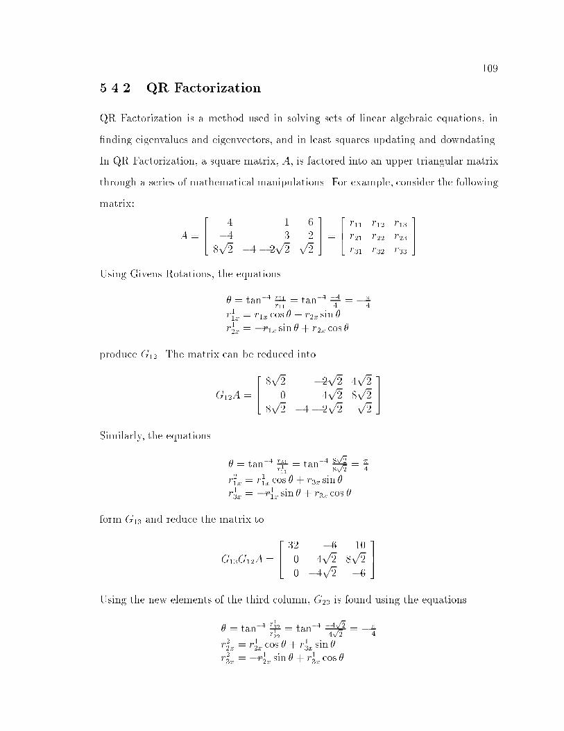
����� QR Factorization

QR Factorization is a method used in solving sets of linear algebraic equations� in

�nding eigenvalues and eigenvectors� and in least squares updating and downdating�

In QR Factorization� a square matrix� A� is factored into an upper triangular matrix

through a series of mathematical manipulations� For example� consider the following

matrix�

A �

���

� �� � �

�p

� � �p

�p

�

��� �

��� r�� r�� r��r�� r�� r��r�� r�� r��

���

Using Givens Rotations� the equations

� � tan�� r��r��

� tan�� �

� �

r��x � r�x cos � � r�x sin �r��x � r�x sin � � r�x cos �

produce G��� The matrix can be reduced into

G��A �

���

�p

� �p

� �p

�

� �p

� �p

�

�p

� � �p

�p

�

���

Similarly� the equations

� � tan�� r��r���

� tan�� p�

p�

� �

r��x � r��x cos � � r�x sin �r��x � r��x sin � � r�x cos �

form G�� and reduce the matrix to

G��G��A �

���

�� � �

� �p

� �p

�

� �p

� �

���

Using the new elements of the third column� G�� is found using the equations

� � tan�� r���r���

� tan�� �p�

p�

� �

r��x � r��x cos � � r��x sin �r��x � r��x sin � � r��x cos �

�

and the matrix is factored such that

QTA � G��G��G��A �

���

�� � �

� � � � �p

�

� � � �p

�

��� � R

The matrix can be factored without the use of trigonometry functions in the

following manner�

A �

���

� �� � �

�p

� p�p

�

���

Using the modi�ed equations

r��x � r�xr��pr����r

���

� r�xr��pr����r

���

r��x � r�x r��pr����r

���

� r�xr��pr����r

���

to de�ne G��� the matrix can be reduced to

G��A �

���

�p

� p� �p

�

� �p

� �p

�

�p

� p�p

�

���

Likewise� the equations

r��x � r��xr���p

�r�����r���

� r�xr��p

�r�����r���

r��x � r��x r��p�r���

��r���� r�x

r���p�r���

��r���

form G�� and reduce the matrix to

G��G��A �

���

� � �

� �p

� �p

�� �

���

Once again� using the new elements of the third column in the equations

r��x � r��xr���p

�r������r���

�� r��x

r���p�r���

���r����

r��x � r��x r���p�r���

���r����

� r��xr���p

�r������r���

�

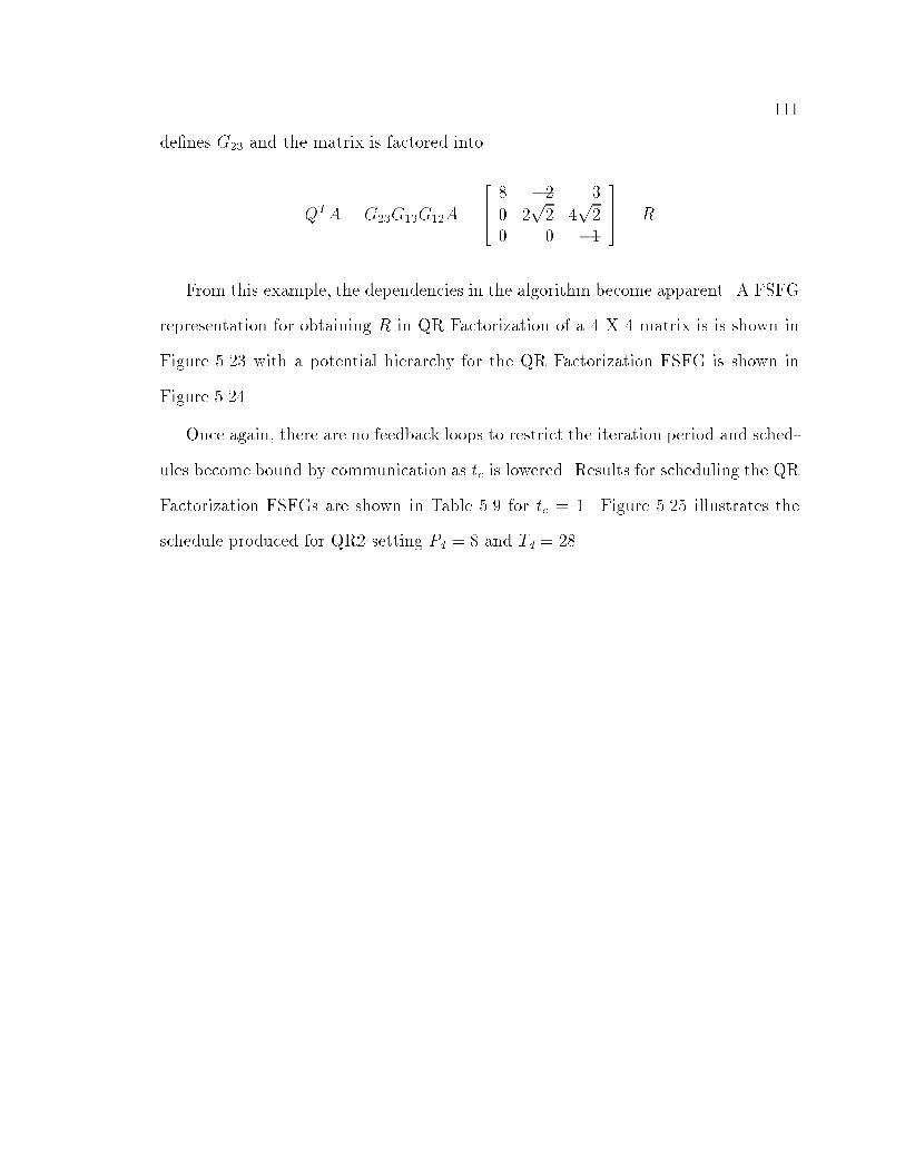
de�nes G�� and the matrix is factored into

QTA � G��G��G��A �

���

� � �

� �p

� �p

�� �

��� � R

From this example� the dependencies in the algorithm become apparent� A FSFG

representation for obtaining R in QR Factorization of a � X � matrix is is shown in

Figure ���� with a potential hierarchy for the QR Factorization FSFG is shown in

Figure �����

Once again� there are no feedback loops to restrict the iteration period and sched�

ules become bound by communication as tc is lowered� Results for scheduling the QR

Factorization FSFGs are shown in Table ��� for tc � � Figure ���� illustrates the

schedule produced for QR� setting Pd � � and Td � ���

�

2,3

1,2

2,2

R

1,1A

A

A

A

A

3,1

3,3

3,2

2,1A A

A

A

1,3

1,2

1,1

R

R

2,1 3,1

3,2

3,2

1,3

R

R

R

R

RR

2,2

3,3

*

*

*

*

*

** +

** +

** +

* +

**

/ /

+

** +

*

** +

** +

** +

** +

** +

**

/ /

+

*

*+

** +

** +

** +

** +

** +

/ /

+

Figure ����� FSFG for QR Factorization of a �X� matrix �QR �

�

B

C

B

+

** +

*

** +

**

** +

** +

** +

**

/ /

+

FSFG � A FSFG � B

*

+

+

** +

**

** +

** +

**

/ /

FSFG � C

Figure ����� Potential FSFG hierarchical speci�cation for QR Factorization of a �X�matrix �QR��

�

2,2

1,2

A 1,1

A

A 2,3

A

3,3

3,2

3,1

A

A

A

A

1,3

1,2

A 2,1

R

R

1,3

1,1

3,12,1 RR

2,2

3,2

3,2

3,3

R

R

R

R

R

8

6

5

1

4

3

2

P

P

P

P

P

P

P

P

7

** +

* *+

** +

**

/ /

+

** +

+

* +

** +

** +

*

*

*

+

** +

**

/ /

+

**

**

*

*

*

*

+

*

** +

** +

** +

** +

** +

/ /

+

Figure ����� FSFG for QR Factorization of a �X� matrix with a software pipeliningand parallel execution schedule generated by Calypso using the Order Graph Methodfor Pd � �� Td � ��� and tc �

�

HFSFG Nodes Levels Pd Td Linear Avg� Proc� CPU time SP PEExtensions Util� ��� �sec �

QR� �� � � ��� � ��� � �� Y Y

� ��� � �� � �� Y Y

� � � �� � �� Y Y

� � �� � � �� Y Y

� �� � �� � � �� Y Y

�� � � �� � � �� Y N

�� � � �� � � �� Y N

� �� � � � Y N

� � �� � � �� Y N

� � � �� � Y N

��� � � �� � �� Y N

QR� �� � � ��� � ��� � �� Y Y

� ��� � �� � �� Y Y

� � � �� � �� Y Y

� � �� � � �� Y Y

� �� � �� � � �� Y Y

�� � � �� � � � Y N

�� � � �� � � � Y N

� �� � � � Y N

� � �� � � Y N

� � � �� � � Y N

��� � � �� � � Y N

Table ���� Summary of Calypso�s results for scheduling hierarchical FSFGs for QRFactorization with tc �

�

��� Conclusions

Results from the previous sections suggest that speci�cation of an algorithm in the

form of a hierarchy has an e�ect on the preprocessing and partitioning stages of the

OGM� The preprocessing stage does most of the work to handle hierarchical speci�

�cation in dealing with composite node representations of hierarchical levels� Parti�

tioning becomes a�ected during the initial identi�cation of the relations matrix� the

generation of linear extensions� and the generation of valid candidate partitionings�

As shown in Table ���� many of the hierarchy�s e�ects are bene�cial in reducing the

amount of processing time needed to obtain a multiprocessor schedule� In the case of

the �DIIR�� �DIIR�� and �DIIR�� the partitioning stage did not deal with the atomic

nodes individually and the scheduling time was minimized�

An increase of composite nodes in the partitioning stage can potentially increase

the amount of time it takes to identify a valid candidate partitioning� In the case

of the �DIIR FSFG for Td � �� turning the shifting for the network topology o�

demonstrated that a composite node may result in a series of linear extensions which

can not be e�ectively partitioned� Because OGM does not distinguish between com�

posite nodes which are formed from hierarchical levels and from strong components�

a user�de�ned hierarchy has the potential to produce a composite node with the same

e�ect� OGM could recognize user�de�ned composite nodes and inspect the internal

nodes to determine if the composite node can be split� However� this increases the

complexity of the partitioning stage and defeats the concept of composite nodes�

Partitioning is also a�ected by hierarchical speci�cation in terms of limiting the

mobility of nodes within a linear extension� A composite node with multiple outputs

often result in multiple nodes depending on the execution of the composite node�

This results in a decrease of the composite node�s mobility within linear extensions�

In the case of the �nd order ��D IIR computational primitive equations with out

�

shifting for network topology� a decrease of nodes� mobility due to a composite node

added to the problems which prevented a valid candidate partitioning from being

identi�ed quickly� Allowing for shifting� the composite node was easily positioned into

a partition which allowed a valid candidate partitioning to be produced� Hierarchical

speci�cation only increases the probability that composite nodes will hinder valid

candidate partitionings from being found quickly� However� as demonstrated by the

results for the hierarchical FSFG speci�cations in this section� the exibility of OGM

during the partitioning stage helps keep this probability low�

Judging from the results presented in the previous sections� there are some guide�

lines for de�ning a hierarchical speci�cation� Failure to follow these guidelines will

not prevent OGM from �nding a parallel computing schedule� however� the number

of linear extensions �and thus the execution time� may be e�ected� When de�ning

a hierarchical speci�cation for OGM� users should attempt to meet the following

conditions�

� The computational weight of the nodes in the lowest level in the hierarchy

should not be greater than the desired iteration period� This minimizes the

number of nodes within linear extensions and the time to generate successive

linear extensions during the partitioning stage of OGM�

� The hierarchy should be de�ned to minimize the number of communications

into or out of each hierarchical level� This increases the mobility of composite

nodes within linear extensions and increases the number of linear extensions

which can be considered for a poset�

� A hierarchical level �l� should be de�ned to minimize the number of edges

�the distance� between any node v � l and its nearest neighbor w � l� If the

hierarchical level l is reduced to a composite node �x� during the partitioning

�

stage� a greater distance between nodes increases the probability that other

nodes will rely on x�s execution� If more nodes rely on x�s execution� the

mobility of nodes within the linear extension will be reduced� In turn� this

decreases the number of linear extensions which can be considered for a poset�

In addition to providing insight into hierarchical speci�cation� the results in Sec�

tions ��� and ��� demonstrate the usability and e�ectiveness of OGM and Calypso�

The average running time for OGM �with all it features on� is under � seconds with

��" of the schedules produced in under � seconds� There are no restrictions on the

hierarchical speci�cation which allows the maximum freedom to de�ne algorithms for

execution on Calypso using OGM� The results illustrate OGM�s ability to specify a

desired iteration period and optimize the number of processors� specify a desired num�

ber of processors and optimize the iteration period� or optimize the iteration period

and the number of processors� For any target iteration period or number of proces�

sors� the results show OGM�s ability to maximize the e�ciency of the system �often

times improving on the speci�ed target�� Variables for identifying the amount of data

which processors and links in the network topology can communicate per unit of time

increase the usability of OGM� Additionally� the exibility of OGM and Calypso was

exercised by preventing the splitting of atomic nodes and forcing the generation of

parallel execution schedules� Together� the experimental results demonstrate OGM

and Calypso�s ability to schedule hierarchical FSFGs for parallel computing using

software pipelining and parallel execution schedules�

We now conclude with a summary of the research presented in this dissertation

and some ideas for future research�

Chapter �

Summary and Future Research

�� Summary

In this research� we present the Order Graph Method �OGM� as a new methodology

for automatically partitioning and scheduling digital signal processing algorithms for

parallel computing� OGM accepts algorithms speci�ed in the form of hierarchical

Fully Speci�ed Flow Graphs �FSFGs� and produces balanced schedules for parallel

execution and software pipelining which exploit �ne to coarse�grained parallelism�

OGM schedules algorithms for rate and processor optimal execution or to meet user�

speci�ed bounds on the rate or the number of processors� In addition� OGM con�

siders the e�ect of inter�processor communication and the network topology� OGM

attempts to minimize inter�processor communication and validates schedules against

restrictions placed on inter�processor communication due to memory limitations and

contention on the network topology� We have evaluated the performance of OGM

with other graph�based methodologies and have shown that OGM provides better

support for scheduling issues� Scalability to larger problems� consideration of com�

munication and network topology� support for software pipelining� and user�speci�ed

iteration period and processor bounds are some of OGM�s advantages�

We implemented OGM in a tool called Calypso� to allow experimentation with

digital signal processing algorithms� Using Calypso� we demonstrated that OGM is

��

e�ective and exible in producing schedules of DSP algorithms for parallel execution�

Algorithms scheduled include a �nd order IIR �lter� a �th order FIR �lter� a �th order

lattice �lter� a �nd order ��D IIR �lter� LU Decomposition� and QR Factorization�

For each of these algorithms a variety of hierarchical speci�cations highlights OGM�s

ability to e�ectively deal with the hierarchy and produce optimized schedules with a

high average processor utilization� Runtime results for each of the algorithms shows

that OGM performs well with varying algorithm sizes� In addition� the hierarchy

is shown to increase OGM�s e�ectiveness if the iteration period is greater than the

computational weight of the lower levels in the hierarchy�

�� Future Research

While this research has contributed to our understanding of multiprocessor imple�

mentations for signal processing algorithms� application of the parallel computing

schedules produced by Calypso onto the BDPA would provide additional insight into

scheduling issues and the BDPA� Due to the exibility of OGM�s scheduling method�

ology� additional stages may be added to re�ne the parallel computing schedules as

new insights are obtained� Some additional issues to consider include�

� The generation of linear extensions could be re�ned to recognize why partic�

ular candidate partitionings are not valid� There may be a way to identify

composite nodes which are positioned where the partitioning algorithm will

continually attempt to split the composite node� By identifying a problematic

composite node� the mobility of other nodes could be targeted toward moving

the problem node into a new position within the candidate partitioning� Sub�

sequent linear extensions could then be intelligently generated to overcome the

reasons previous candidate partitionings were rejected�

�

� Combinations of parallel execution and software pipelined schedules could be

considered� OGM�s communication model has been developed to support this

combination� however� an investigation is needed to determine when combining

the two scheduling techniques is bene�cial�

� Additional support could be added for other network topologies �such as the

hypercube�� If the network topology has a basic interconnection network� re�

placing the program which checks the network topology admissibility condition

may be all that is needed� However� a more complex topology with variations

in the interconnection network will require modifying the partitioning and

scheduling stages of OGM to consider how a partitioning should be assigned

on the network topology� Some potential considerations� include how the dis�

tance and communication bandwidth between processors e�ects the scheduling

of a partition with unbalanced communication�

� Di�erent architectures could be investigated and incorporated into OGM and

Calypso� A closer look at how pipelined processors� loosely coupled processors�

and non�overlapped communication and computation e�ects OGM is needed�

It may be possible to assign communications a weight using tc and change

the partitioning strategy to consider the communication weight during the

formation of the fi sets�

� A closer look is needed to determine the memory requirements for OGM and

Calypso� It is possible that larger FSFGs will present memory problems for

Calypso if composite nodes need to be expanded during the preprocessing

stage� There may be a way to store a level of the hierarchy in memory and

just reference the same memory location whenever an instance of the level is

partitioned�

��

� Parameterization of FSFGs is another feature which may bene�t OGM� A

FSFG may be able to have parameters assigned to indicate multiple occur�

rences of the same graph� This would increase the usability of OGM by mak�

ing it easier to de�ne recursive algorithms� The preprocessing and partitioning

stages could be rewritten to recognize the parameters and identify the prece�

dence conditions necessary to obtain an initial ordering for the linear extension�

� A front end tool could be developed to optimize the FSFG before being sched�

uled by OGM� Potential issues include the elimination of duplicate calculations�

retiming to eliminate node dependencies� reducing broadcast communications�

and manipulating the hierarchical speci�cation to reduce inter�level commu�

nications� Integration with a CAD tool which supports hierarchical algorithm

speci�cation could enhance the usability of Calypso by making the interface

user�friendly�

� Additional work can be done to use Calypso�s output schedules to generate

code which can be compiled and run on multiprocessor systems� If the com�

munication is synchronous� the communications program would need to be

modi�ed to schedule communications on processors in a speci�c sequence� It

may be possible to use the candidate partitionings to determine the required

sequence� However� when the network topology is incorporated� the commu�

nications schedule may need to compensate for data which must propagate

through multiple processors� Asynchronous communications may not require

this type of schedule� If communications are bu�ered� OGM�s schedules could

be used to generate code which communicates an output in the �rst available

time slot and begins execution whenever data arrives at a processor� Be�

cause the network topology admissibility condition currently checks for the

ring topology� the BDPA would be a prime candidate�

��

� Support for conditional branching should be investigated for integration into

OGM and Calypso� For algorithms such as LU Decomposition with pivoting

and LU Decomposition of a sparse matrix� conditional branching may signi��

cantly simplify the algorithm speci�cation� In addition� this would allow OGM

to be used for a more generic set of algorithms beyond digital signal processing�

� Additional communication and processing constraints may be incorporated

into OGM and Calypso� For example� bounds on latency� communication

bu�ers� system input�output connections� and broadcasting limits could be

considered�

For future research� the next logical step is to use Calypso to map a variety of

signal processing and matrix operations algorithms onto the BDPA to demonstrate

the system�s performance characteristics�

Bibliography

� � K� Hwang� Advanced Computer Architecture With Parallel Programming�McGraw�Hill� San Francisco� CA� ����

��� W�E� Alexander� S�T� Alexandre� and D�S� Reeves� Parallel execution of mul�tidimensional DSP algorithms using the block data ow architecture� InternalResearch Paper N�C� State University� ����

��� M�R� Garey and D�S� Johnson� Computers and Intractability� A Guide to theTheory of NP Completeness� W�H� Freeman� San Francisco� CA� ����

��� S�Y� Kung� VLSI Array Processors� Prentice�Hall International� EnglewoodCli�s� CA� ����

��� E�W� Mayr� Basic parallel algorithms in graph theory� Computer Suppl�� ����#� � ����

��� D�I� Moldovan and J�A�B� Fortes� Partitioning and mapping of algorithms into�xed size systolic arrays� IEEE Transactions on Computers� ��� �� # �� January ����

��� S�M� Park� W�E� Alexander� J�H� Kim� W�E� Batchelor� and W�T� Krakow� Anovel VLSI architecture for the real�time implementation of ��D signal processingsystems� In Proceedings of IEEE International Conference Computer Design�VLSI in Computers and Processors� October ����

��� Hongyu Xu� BDFA A Block Data Flow Architecture for Real Time SignalProcessing and Matrix Operations� PhD thesis� North Carolina State University�Dept of Electrical and Computer Engineering� �� �

��� E� Barros and A� Sampaio� Towards probably correct hardware�software par�titioning using OCCAM� In Proceedings of the rd International Workshop onHardware�Software Codesign� pages � �#� �� ����

� �� G� Bilsen� M� Engels� R� Lauwereins� and J�A� Peperstraete� Development ofa load balancing tool for the GRAPE rapid prototyping environment� In Pro ceedings of the �th International Workshop on Rapid System Prototyping� pages�# �� ����

��

� � J�T� Buck� Dynamic dataow model suitable for e�cient mixed hardware andsoftware implementations of DSP applications� In Proceedings of the rd Inter national Workshop on Hardware�Software Codesign� pages ��# ��� ����

� �� D�D� Hills� Visual languages and computing survey� Data ow visual program�ming languages� Journal of Visual Languages and Computing� ����# � � ����

� �� E�A� Lee� Multidimensional streams rooted in dataow� In Proceedings of theWorkshow on Architectures and Compilation Techniques for Fine and MediumGrain Parallelism� pages ���#���� ����

� �� P� Moore and P�G� O�Donoghue� Developing transputer�based systems usinghood and parallel c� Information and Software Technology� ���������#���� June ����

� �� M�C� Chen� Y� Choo� and J� Li� Compiling parallel programs by optimizingperformance� Journal of Supercomputing� �� � #���� October ����

� �� M� Gupta and P� Banerjee� Demonstration of automatic data partitioning tech�niques for parallelizing compilers on multicomputers� IEEE Transactions onParallel and Distributed Systems� ����� ��# ��� March ����

� �� P�H� Hartel� H� Glaser� and J�M� Wild� Compilation of functional languagesusing ow graph analysis� Software Practice and Experience� ������ ��# ���February ����

� �� J� Ramanujam� Compile�time techniques for data distribution in distributedmemory machines� IEEE Transactions on Parallel and Distributed Systems���������#���� October �� �

� �� F� Gasperoni and U� Schwiegelshohn� Scheduling loops on parallel processors� Asimple algorithm with close to optimum performance� Lecture Notes In ComputerScience� ���������#���� ����

���� K�K� Parhi and D�G� Messerschmitt� Static rate�optimal scheduling of iterativedata�ow programs via optimum unfolding� IEEE Transactions on Computers���� ��# ��� February �� �

�� � C�M� Wang and S�D� Wang� E�cient processor assignment algorithms and looptransformations for executing nested parallel loops on multiprocessors� IEEETransactions on Parallel and Distributed Systems� �� ��� #��� January ����

���� M�E� Wolf and M�S� Lam� A loop transformation theory and an algorithm tomaximize parallelism� IEEE Transactions on Parallel and Distributed Systems���������#�� � October �� �

���� M� Wolfe� Automatic vectorization� data dependence� and optimizations forparallel computers� Parallel Processing For Super Computers and Arti�cial In telligence� pages ���#���� ����

��

���� W�M Lin and B� Yang� Load balancing technique for parallel search with statis�tical model� In Proceedings of the ��� IEEE �th Annual International PheonixConference on Computers and Communications� pages ��#��� March ����

���� M�C Chen and C�E� Mead� Concurrent algorithm as space�time recursion equa�tions� In Proceedings of the USC Workshop VLSI Modern Signal Processing�pages � #��� November ����

���� V� Van Dongen and P� Quinton� The mapping of linear recurrence equations onregular arrays� Journal VLSI Signal Processing� ���# �� ����

���� L� Johnsson and D� Cohen� A mathematical approach to modelling the owof data and control in computational networks� In CMU Conference on VLSISystems and Computers� pages ���#���� October �� �

���� W�L� Miranker and A� Winkler� Spacetime representations of computationalstructures� Computing� �����# �� ����

���� P� Quinton� Automatic synthesis of systolic arrays from uniform recurrence equa�tions� In Proceedings of the th Annual International Symposium on ComputerArchitecture� pages ���#� �� ����

���� R� Cole and U� Vishkin� Approximate and exact parallel scheduling with ap�plications to list� tree� and graph problems� In Proceedings of the ��th AnnualSymposium on Foundations of Computer Science� pages ���#�� � New York� NY� ����

�� � P� Eades� M� Hickey� and R�C� Read� Some hamilton paths and a minimal changealgorithm� JACM� � � �#��� ����

���� K� Efe� Heuristic models of task assignment scheduling in distributed systems�IEEE Computer� pages ��#��� June ����

���� S�H� Huang and J�M� Rabaey� Maximizing the throughput of high performanceDSP applications using behavioral transformations� In Proceedings of the Euro pean Design and Test Conference� pages ��#��� ����

���� W� Shen and D� Sweeting� Heuristic algorithms for task assignment and schedul�ing in a processor network� Parallel Computing� ��� �� # �� January ����

���� M� Renfors and Y� Neuvo� The maximum sampling rate of digital �lters underspeed constraints� IEEE Transactions on Circuits and Systems� ��� ��#���� �� �

���� Sonia M� Heemstra de Groot� Sabih H� Gerez� and Otto E� Herrmann� Range�chart�guided iterative data�ow graph scheduling� IEEE Transactions on Cir cuits and Systems� �������� #���� May ����

��

���� T�P� Barnwell III� V�K� Madisetti� and S�J�A� McGrath� The Georgia Tech digi�tal signal multiprocessor� IEEE Transactions on Signal Processing� � ������� #����� July ����

���� Bryce A� Curtis and Vijay K� Madisetti� Rapid prototyping on the GeorgiaTech digital signal multiprocessor� IEEE Transactions on Signal Processing����������#���� March ����

���� P�R� Gelabert and T�P� Barnwell III� Optimal automatic periodic multiprocessorscheduler for fully speci�ed ow graphs� IEEE Transactions on Signal Process ing� � �������#���� February ����

���� P� Evripidou and J��L� Gaudiot� Block scheduling of iterative algorithms andgraph�level priority scheduling in a simulated data�ow multiprocessor� IEEETransactions on Parallel and Distributed Systems� ��������#� �� April ����

�� � K� Hwang� Y�H� Cheng� F�D� Angers� and C�Y� Lee� Scheduling precedencegraphs in systems with interprocessor communication� SIAM Journal of Com puting� �����#���� ����

���� M� Potkonjak and J�M� Rabaey� Scheduling algorithms for hierarchical datacontrol ow graphs� International Journal of Circuit Theory and Applications����� �#���� ����

���� S� Dandamudi� A comparison of task scheduling strategies for multiprocessorsystems� In Proceedings of the rd IEEE Symposium on Parallel and DistributedProcessing� pages ���#���� �� �

���� K� Konstantinides� R�T� Kaneshiro� and J�R� Tani� Task allocation and schedul�ing models for multiprocessor digital signal processing� IEEE Transactions onSignal Processing� ��� ��� December ����

���� C�S�R� Krishnan� D�A�L� Piriyakumar� and C�S�R� Murthy� Task allocation andscheduling models for multiprocessor digital signal processing� IEEE Transac tions on Signal Processing� ���������#���� March ����

���� S� Manoharan and N�P� Topham� An assessment of assignment schemes fordependency graphs� Parallel Computing� � � ����# ��� January ����

���� C�L� McCreary� A�A� Khan� J�J� Thompson� and M�E� McArdle� A comparisonof heuristics for scheduling dags on multiprocessors� In Proceedings of the �thInternational Parallel Processing Symposium� pages ���#�� � ����

���� A�L� Wendelborn and H� Garsden� Exploring the stream data type in SISAL andother languages� In Proceedings of the IFIP WG�� Working Conference on Ar chitectures and Compilation Techniques for Fine and Medium Grain Parallelism�pages ���#���� ����

��

���� J�T� Feo� D�C� Cann� and R�R� Oldehoeft� A report on the sisal language project�Journal of Parallel and Distributed Computing� December ����

���� S� Pande� D�P� Agrawal� and J� Mauney� Scalable scheduling scheme for func�tional parallelism on distributed memory multiprocessor systems� IEEE Trans actions on Parallel and Distributed Systems� ��������#���� April ����

�� � J� Li and M� Chen� Index domain alignment� Minimizing cost of cross�referencingbetween distributed arrays� In Frontiers��� rd Symposium of Frontiers Mas sively Parallel Computation� pages ���#���� ����

���� R� Allen and K� Kennedy� Automatic translation of FORTRAN programs tovector form� ACM Transactions On Programming Languages And Systems�������� #���� April ����

���� J�A�B� Fortes and D�I� Moldovan� Parallelism detection and transformation tech�niques useful for VLSI algorithms� Journal of Parallel and Distributed Comput ing� �����#�� � ����

���� P�R� Cappello� Unifying VLSI array designs with geometric transformations� InProceedings of the �� IEEE International Conference on Parallel Processing�pages ���#���� ����

���� C�E� Leiserson and H�T� Kung� Algorithms for VLSI Processor Arrays� Addison�Wesley� Reading� PA� ����

���� S� Manoharan and P� Thanisch� Assigning dependency graphs onto processornetworks� Parallel Computing� �� ����#��� April �� �

���� Gavin R� Cato and Douglas S� Reeves� Parallel task scheduling using the or�der graph method� In Proceedings of the ��� IEEE �th Annual InternationalPheonix Conference on Computers and Communications� pages ��#��� March ����

���� Gavin R� Cato and Douglas S� Reeves� Parallel task scheduling for the blockdata ow architecture� In Proceedings of Southeastcon� March ����

���� R� Tarjan� Depth��rst search and linear graph algorithms� SIAM Journal ofComputing� ���� ��# ��� ����

���� D�B� Johnson� Finding all the elementary circuits of a directed graph� SIAMJournal of Computing� �� ����#��� ����

�� � Gara Pruesse and Frank Ruskey� Generating the linear extensions of certainposets by transpositions� SIAM Journal of Discrete Mathematics� August �� �

���� Gara Pruesse and Frank Ruskey� Generating linear extensions fast� SIAM Jour nal on Computing� ���������#���� April ����

��

���� A�D� Kalvin and Y�L� Varol� On the generation of all topological sortings� Jour nal of Algorithms� �� ��# ��� ����

���� Y�L� Varol and D� Rotem� An algorithm to generate all topological sortingarrangements� Computer Journal� �����#��� �� �

���� V�K� Madisetti and B�A� Curtis� A quantitative methodology for rapid prototyp�ing and high�level synthesis of signal processing algorithms� IEEE Transactionson Signal Processing� ��� ��� ��#����� November ����

���� W�E� Alexander� D�S� Reeves� and C�S� Gloster� Parallel image processing withthe block data parallel architecture� Accepted for publication in Proceedings ofIEEE� ����

���� D�E� Dudgeon and R�M� Mersereau� Multidimensional Digital Signal Processing�Prentice�Hall� Englewood Cli�s� NJ� ����

���� John G� Proakis and Dimitris G� Manolakis� Introduction to Digital Signal Pro cessing� Macmillan Publishing Company� New York� NY� ����