p series, sp ecial f boundary v problems - nus uavuav.ece.nus.edu.sg/~bmchen/courses/ee2462.pdf ·...

EE 2462 Engineering Math III, Part 1

Power Series, Special Functions & Boundary Value Problems

Ben M. Chen, Ph.D.

OÆce: E4-6-07; Phone: 874-2289; Email: [email protected]

URL: http://www.ee.nus.edu.sg/~bmchen

Copyright c Ben M. Chen, 1995-1998

EE2462 Lecture Notes, Part 1, Prepared by Ben M. Chen 1

Course Outline:

Power Series: Sequences and Series; Convergence and Divergence; A Test for Divergence;

Comparison Tests for Positive Series; The Ratio Test for Positive Series; Absolute Convergence;

Power Series.

Special Functions: Bessel's Equation and Bessel's Functions; The Gamma Function; So-

lution of Bessel's Equation in Terms of the Gamma Function; Modi�ed Bessel's Equations;

Applications of Bessel's Functions; Legendre's Equation and Legendre Polynomials.

Partial Di�erential Equations: Boundary Value Problems in Partial Di�erential Equa-

tions; Wave Equation; Heat Equation; Laplace's Equation; Poisson's Equation; Dirichlet and

Neumann Problems.

Textbooks:

1. P. V. O'Neil, Advanced Engineering Mathematics, PWS-Kent Publishing Company,

4th Edition, 1995.

2. E. Kreyszig, Advanced Engineering Mathematics, John Wiley, 7th Edition, 1995.

Lecture Notes and Tutorial Sets:

PDF �les of the lecture notes & tutorial sets of this part can be downloaded from my home

page at http://www.ee.nus.edu.sg/~bmchen. Tutorial starts on the fourth week!


1. Sequences and Series

If a set of numbers is so arranged that there is a �rst, a second, a third, and so on, it constitutes

a sequence. We indicate a sequence by the general term in braces, ff(n)g. As examples of

sequences we have

fung : u1; u2; � � � ; un; � � � ; (1.1)

�1

2n

�:1

2;1

4; � � � ; 1

2n; � � � ; (1.2)

�1

n

�: 1;

1

2; � � � ; 1

n; � � � � (1.3)

With any sequence fung we can associate an array

Xun = u1 + u2 + u3 + � � �+ un + � � � ; (1.4)

called a series. If all but a �nite number of terms, say, those with n > N , are equal to zero,

then the array takes the form

NXi=1

ui = u1 + u2 + u3 + � � �+ uN : (1.5)

This has a sum in the ordinary sense. And this sum is called the value of the �nite series.

1.1. Convergence and Divergence

The n-th partial sum of the in�nite series

Xun = u1 + u2 + u3 + � � �+ un + � � � ; (1.6)

sn, is de�ned as the sum of its �rst n terms. That is

sn =nXi=1

ui = u1 + u2 + u3 + � � �+ un: (1.7)

The partial sum form a new sequence fsng. If, as n increases and tends to in�nity the sequence

of numbers sn approaches a �nite limit L, the series

Xun = u1 + u2 + u3 + � � �+ un + � � � ; (1.8)

converges. And we write

limn!1

sn = L: (1.9)

We say that the in�nite series converges to L and that L is the value, or sum, of the series.

If the sequence does not approach a limit, then the series is divergent and we do not assign

any value to it.


1.2. A Test for Divergence

Suppose that the series

Xun = u1 + u2 + u3 + � � �+ un + � � � ; (1.10)

converges. Then, since (n� 1)!1 when n!1, we have

limn!1

sn = L and limn!1

sn�1 = L: (1.11)

But sn = sn�1 + un, or un = sn � sn�1. Hence, as n!1,

limn!1

un = limn!1

(sn � sn�1) = limn!1

sn � limn!1

sn�1 = L� L = 0: (1.12)

Hence, as n!1, un ! 0 in any convergent series. Thus, we have established the following

result:

If un does not tend to zero as n becomes in�nite, the series

Xun = u1 + u2 + u3 + � � �+ un + � � � ; (1.13)

is divergent.

Example 1. Show that the series with

un =n

2n+ 1; (1.14)

that is, the series1

3+

2

5+

3

7+ � � �+ n

2n + 1+ � � � ; (1.15)

diverges.

solution. Here

limn!1

un = limn!1

1

2 + 1=n=

1

26= 0: (1.16)

Hence, it diverges.

Example 2. Show that the series with odd terms n+1n

and even terms 1=n, namely, the series

2 +1

2+

4

3+

1

4+ � � �+ m

m� 1+

1

m+m + 2

m + 1+ � � � ; (1.17)

diverges.

solution. Here, for large n, there are (odd) terms, 1 + 1=n, near 1, and also (even) terms,

1=n, near 0. Thus, no limit is approached by un; the terms near 1 show that we cannot have

un ! 0.


1.3. Comparison Tests for Positive Series

A positive series is one with each un � 0. We have the following results:

1. LetPvn be a positive series known to converge. If 0 � un � vn for all n, then the

seriesPun converges.

2. LetPVn be a positive series known to diverge. If un � Vn for all n, then the seriesP

un diverges.

1.4. The Ratio Test for Positive Series

For a positive seriesPun, let us de�ne the test ratio

tn =un+1

un: (1.18)

Suppose that, as n!1, tn ! T . Then the ratio test asserts the following:

For a positive seriesPun, with

limn!1

un+1

un= T; (1.19)

the series converges if T < 1. And the series diverges if T > 1. For the value T = 1, no

conclusion can be drawn.

Example 1. Test the series with

un =(n� 1)!

nn�1(1.20)

for convergence. (note that u1 = 1, since 0! = 1.)

solution. The test ratio is

tn =un+1

un=

n!

(n+ 1)nnn�1

(n� 1)!(1.21)

Since n! = n(n� 1)!, we have

tn =

�n

n + 1

�n=

1

(1 + 1=n)n! 1

e� 1

2:7< 1: (1.22)

Hence, the series converges.

1.5. Absolute Convergence

Consider a series with general term un, which may be positive, zero, or negative. Then, withPun, we associate the positive series

P junj, obtained by taking absolute values. If this latter

series converges, the �rst series is said to converge absolutely. We have the following result:


IfP junj converges, then Pun converges.

Since the series of absolute values is a positive series, its convergence can be tested by the

comparison or ratio test.

If the series of absolute values diverges, the original series may still converge, and in this

case it is said to converge conditionally.

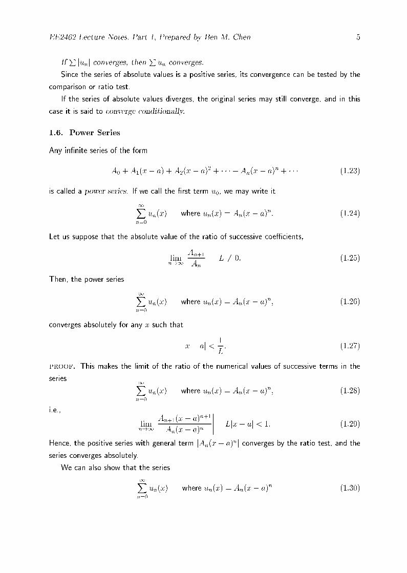
1.6. Power Series

Any in�nite series of the form

A0 + A1(x� a) + A2(x� a)2 + � � �+ An(x� a)n + � � � (1.23)

is called a power series. If we call the �rst term u0, we may write it

1Xn=0

un(x) where un(x) = An(x� a)n: (1.24)

Let us suppose that the absolute value of the ratio of successive coeÆcients,

limn!1

��An+1

An

�� = L 6= 0: (1.25)

Then, the power series

1Xn=0

un(x) where un(x) = An(x� a)n; (1.26)

converges absolutely for any x such that

jx� aj < 1

L: (1.27)

proof. This makes the limit of the ratio of the numerical values of successive terms in the

series1Xn=0

un(x) where un(x) = An(x� a)n; (1.28)

i.e.,

limn!1

��An+1(x� a)n+1

An(x� a)n

�� = Ljx� aj < 1: (1.29)

Hence, the positive series with general term jAn(x� a)nj converges by the ratio test, and the

series converges absolutely.

We can also show that the series

1Xn=0

un(x) where un(x) = An(x� a)n (1.30)


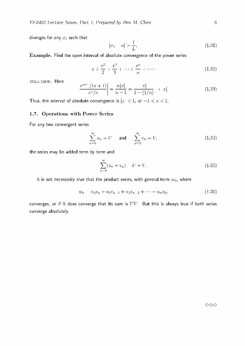
diverges for any x1 such that

jx1 � aj > 1

L: (1.31)

Example. Find the open interval of absolute convergence of the power series

x+x2

2+x3

3+ � � �+ xn

n+ � � � � (1.32)

solution. Here ��xn+1=(n+ 1)

xn=n

�� = njxjn+ 1

=jxj

1 + (1=n)! jxj: (1.33)

Thus, the interval of absolute convergence is jxj < 1, or �1 < x < 1.

1.7. Operations with Power Series

For any two convergent series

1Xn=0

un = U and1Xn=0

vn = V; (1.34)

the series may be added term by term and

1Xn=0

(un + vn) = U + V: (1.35)

It is not necessarily true that the product series, with general term wn, where

wn = u0vn + u1vn�1 + u2vn�2 + � � �+ unv0; (1.36)

converges, or if it does converge that its sum is UV . But this is always true if both series

converge absolutely.

333


2. Bessel's Equation and Bessel Functions of the 1st Kind

The di�erential equation

x2y00 + xy0 + (x2 � v2)y = 0 (2.1)

is called Bessel's equation of order v with v � 0. The following is the so-called Frobenius

Solution (or Method of Frobenius) to the above Bessel's equation: De�ne a Frobenius Series

y(x) =1Xn=0

cnxn+r (2.2)

where cn and r are unknown constants to be determined. We have

y0(x) =1Xn=0

cn(n+ r)xn+r�1 (2.3)

y00(x) =1Xn=0

cn(n + r)(n+ r � 1)xn+r�2 (2.4)

Substituting Equations (2.2), (2.3) and (2.4) into the Bessel's Equation in (2.1), we have

1Xn=0

cn(n+ r)(n+ r � 1)xn+r +1Xn=0

cn(n+ r)xn+r

+1Xn=0

cnxn+r+2 �

1Xn=0

cnv2xn+r = 0

+1Xn=0

cn(n+ r)2xn+r +1Xn=2

cn�2xn+r �

1Xn=0

cnv2xn+r = 0

+

c0r2xr + c1(r + 1)2xr+1 � c0v

2xr � c1v2xr+1

+1Xn=2

hcn(n+ r)2 + cn�2 � cnv

2ixn+r = 0

+

(r2 � v2)c0xr + [(r + 1)2 � v2]c1x

r+1 +1Xn=2

hcn(n+ r)2 + cn�2 � cnv

2ixn+r = 0

Let the coeÆcient of each power of x be zero. Also, assume that c0 6= 0, we �nd from the

above derivation that the coeÆcient of xr is:

F (r) = r2 � v2 = 0

This equation has two solutions, r = v and r = �v.


Case 1: First, let us take the solution r = v. Substituting this solution into the

coeÆcient of xr+1, we get

(2v + 1)c1 = 0

Since v � 0, this equation implies that

c1 = 0

From the coeÆcient of xn+r, we obtain the recurrence relation:

n(n+ 2v)cn + cn�2 = 0

for n = 2; 3; 4; � � �+

cn = � 1

n(n + 2v)cn�2; n = 2; 3; 4; � � �

Since c1 = 0, the recurrence relation above gives

c3 = 0; c5 = 0; � � �

In general cn = 0 with n being odd positive integers.

For even number of n = 2m, we have

c2m = � 1

2m(2m+ 2v)c2m�2

= � 1

22m(m + v)c2m�2

= � 1

22m(m + v)

�1

22(m� 1)(m+ v � 1)c2m�4

=c2m�4

24m(m� 1)(m+ v)(m+ v � 1)

= � � � � � �

=(�1)mc0

22m � [m(m� 1) � � �1] � [(m+ v)(m+ v � 1) � � � (v + 1)]

This gives us one solution of Bessel's equation of order v, i.e.,


y1(x) = c0

1Xm=0

(�1)mx2m+v

22mm!(m+ v)(m + v � 1) � � � (v + 1)

+

y1(x) = c0

1Xn=0

(�1)nx2n+v

22nn!(n+ v)(n+ v � 1) � � � (v + 1)

We will re-written the above solution in terms of the Gamma function. But, �rst of all let us

introduce this Gamma function and examine its properties.

The Gamma Function

For x > 0, de�ne a so-called Gamma Function

�(x) =Z1

0tx�1e�tdt

If x > 0, then �(x + 1) = x �(x). 2

Proof:

�(x+ 1) =

Z1

0txe�tdt

= �txe�t��10+

Z1

0xtx�1e�tdt

= xZ1

0tx�1e�tdt

= x �(x)

Q.E.D.

For any positive integer n,

�(n+ 1) = n �(n) = n(n� 1) �(n� 1)

= � � � � � �

= n(n� 1)(n� 1) � � � (n� n+ 1) �(1)

= n! �(1)


Observing that

�(1) =

Z1

0e�tdt = �e�t

��10= 1

Hence

�(n+ 1) = n!

If v � 0, but v is not necessarily an integer, a similar property holds:

�(n+ v + 1) = (n+ v) �(n+ v)

= (n+ v)(n+ v � 1) �(n+ v � 1)

= � � � � � �

= (n+ v)(n+ v � 1) � � � (n+ v � n+ 1) �(v + 1)

= (n+ v)(n+ v � 1) � � � (v + 1) �(v + 1)

which implies

(n + v)(n+ v � 1) � � � (v + 1) =�(n+ v + 1)

�(v + 1)

This is known as the factorial property of the Gamma function.

Although the improper integral de�ning �(x) converges only if x > 0, it is possible to de�ne

�(x) if x is negative (but not an integer). We can write

�(x) =1

x�(x+ 1)

This holds for all x > 0. Now, if �1 < x < 0, then 0 < x + 1 < 1 and �(x + 1) is properly

de�ned. We can therefore de�ne �(x) for �1 < x < 0, e.g.,

�

��1

2

�=

1

�12

�

��1

2+ 1

�= �2 �

�1

2

�

Having de�ned �(x) on (�1; 0), suppose now that �2 < x < �1, then �1 < x + 1 < 0, we

can again follow the same procedure to de�ne �(x) for �2 < x < �1, e.g.,

�

��3

2

�=

1

�32

�

��3

2+ 1

�= �2

3�

��1

2

�= +

4

3�

�1

2

�

Clearly, we can continue on this process forever by moving to the left over the real line and

de�ning �(x) on every interval (k � 1; k) once it has been de�ned on the interval (k; k + 1)

for any negative integer k.


−4 −3 −2 −1 0 1 2 3 4−20

−15

−10

−5

0

5

10

15

20

The Gamma Function

The Gamma Function Over Interval (�4; 4).


Solution of Bessel's Equation in Terms of the Gamma Function

Recall that the �rst solution we have obtained for the Bessel's equation, i.e.,

y1(x) = c0

1Xn=0

(�1)nx2n+v

22n � n! � (n+ v)(n+ v � 1) � � � (v + 1)

= c0

1Xn=0

(�1)n�(v + 1)x2n+v

22n � n! � �(n+ v + 1)

The second expression is true because

(n + v)(n+ v � 1) � � � (v + 1) =�(n+ v + 1)

�(v + 1)

If we choose

c0 =1

2v�(v + 1)

we obtain

y1(x) = Jv(x) =1Xn=0

(�1)nx2n+v

22n+v � n! � �(n+ v + 1)

Jv(x) is called a Bessel Function of the 1st kind of order v. This series converges for all x

(show it).

Exercise Problems: Show that

1. J 0v(x) =

1

2[Jv�1(x)� Jv+1(x)]

2. vJv(x) =x

2[Jv�1(x) + Jv+1(x)]

3.d

dt[tvJv(t)] = tvJv�1(t)

333

Solutions to the Exercise Problems

1) To verify

J 0v(x) =

1

2[Jv�1(x)� Jv+1(x)]

Note that

Jv(x) =1Xn=0

(�1)nx2n+v

22n+vn! �(n+ v + 1)

+


J 0v(x) =

1Xn=0

(2n+ v)(�1)nx2n+v�1

22n+vn! �(n + v + 1)

+

Jv�1(x) =1Xn=0

(�1)nx2n+v�1

22n+v�1n! �(n+ v)=

1Xn=0

2(n+ v)(�1)nx2n+v�1

22n+vn! �(n+ v + 1)

The second equality holds because �(n+ v + 1) = (n+ v)�(n+ v). Therefore, we have

J 0v(x)� 1

2Jv�1(x) =

1Xn=0

n(�1)nx2n+v�1

22n+vn! �(n+ v + 1)

= 0 +1Xn=1

(�1)nx2n+v�1

22n+v(n� 1)! �(n+ v + 1)

=1Xn=0

(�1)n+1x2n+v+1

22n+v+2n! �(n+ v + 2)

= �1

2

1Xn=0

(�1)nx2n+v+1

22n+v+1n! �(n+ v + 2)

= �1

2Jv+1(x)

That is

J 0v(x) =

1

2[Jv�1(x)� Jv+1(x)]

Q.E.D.

2) To verify

vJv(x) =x

2[Jv�1(x) + Jv+1(x)]

First note that

Jv(x) =1Xn=0

(�1)nx2n+v

22n+vn! �(n+ v + 1)

andx

2Jv�1(x) =

1Xn=0

(�1)nx2n+v

22n+vn! �(n+ v)

Then we have

vJv(x)� x

2Jv�1(x) =

1Xn=0

[v � (n + v)](�1)nx2n+v

22n+vn! �(n+ v + 1)

=1Xn=0

(�n)(�1)nx2n+v

22n+vn! �(n + v + 1)


= 0 +1Xn=1

(�1)n�1x2n+v

22n+v(n� 1)! �(n+ v + 1)

=1Xn=0

(�1)nx2n+2+v

22n+2+vn! �(n + v + 2)

=x

2

1Xn=0

(�1)nx2n+v+1

22n+v+1n! �(n + v + 2)

=x

2Jv+1(x)

That is,

vJv(x) =x

2[Jv�1(x) + Jv+1(x)]

Q.E.D.

3) To verifyd

dt[tvJv(t)] = tvJv�1(t)

We let

y = tvJv(t)

= tv1Xn=0

(�1)nt2n+v

22n+vn! �(n+ v + 1)

=1Xn=0

(�1)nt2n+2v

22n+vn! �(n+ v + 1)

Then we have

dy

dt=

1Xn=0

(2n+ 2v)(�1)nt2n+2v�1

22n+vn! �(n+ v + 1)

=1Xn=0

(�1)nt2n+2v�1

22n+v�1n! �(n+ v)

= tv1Xn=0

(�1)nt2n+v�1

22n+v�1n! �(n+ v)

= tvJv�1(t)


Again, we have used the factorial property of the Gamma function in the above derivation.

That is

�(n + v + 1) = (n+ v) �(n+ v)

Q.E.D.

We have considered the case in which v is any nonnegative number. We will now consider the

problem of �nding a second, linearly independent solution of Bessel's equation. Recall that

F (r) = r2 � v2 = 0

has two roots r1 = v and r2 = �v.Case 1: v is not an integer.

Theorem: If v is not an integer, then two linearly independent solutions of Bessel's equation

of order v are Jv and J�v, where

Jv(x) =1Xn=0

(�1)nx2n+v

22n+vn! �(n+ v + 1)

Thus, the general solution of Bessel's equation of order v, where v is not an integer, is

y(x) = �1Jv(x) + �2J�v(x)

where �1 and �2 are real scalars.

Case 2: v is an integer.

If v is an integer, say v = k, then Jv(x) and J�v(x) are solutions of Bessel's equation of

order v, but they are NOT linearly independent. This fact can be veri�ed from the following

arguments: First note that

J�v(x) =1Xn=0

(�1)nx2n�v

22n�vn! �(n� v + 1)

Observing the values of Gamma function at 0;�1;�2; � � � � � �, they go to in�nity. Thus we

have

�(n� v + 1)!1 or1

�(n� v + 1)! 0

as v ! k for n = 0; 1; 2; � � � ; k � 1. Hence

J�k(x) =1Xn=k

(�1)nx2n�k

22n�kn! �(n� k + 1)


In this, let the variable of summation be changed from n to m by the substitution n = m+ k.

Then

J�k(x)=1X

m=0

(�1)m+kx2(m+k)�k

22(m+k)�k(m + k)! �(m + k � k + 1)

=1X

m=0

(�1)m(�1)kx2m+k

22m+k(m+ k)! �(m+ 1)

=(�1)k1X

m=0

(�1)mx2m+k

22m+k(m + k)! �(m+ 1)=(�1)k

1Xm=0

(�1)mx2m+k

22m+k(m + k)!m!

=(�1)k1X

m=0

(�1)mx2m+k

22m+k �(m+ k + 1)m!=(�1)kJk(x)

Thus, we need to search for another linearly independent solution of Bessel's equation. The is

the subject of the next topic.

3. Bessel Function of the 2nd Kind

For the Bessel's equation of order v:

x2y00 + xy0 + (x2 � v2)y = 0

in which v � 0, the general solution is

y(x) = �1Jv(x) + �2J�v(x)

if v is not an integer. Now, in the case in which v is a nonnegative integer, say v = k, for some

nonnegative k, we have one solution Jk(x) of Bessel's equation but have not yet derived a

second, linearly independent solution. In what follows, we will try to �nd this second solution.

A Second Solution of Bessel's Equation for the Case v = k = 0

Let us try a solution of the following format

y2(x) = y1(x) ln(x) +1Xn=1

c�nxn

where

y1(x) = J0(x) =1Xn=0

(�1)nx2n

22n(n!)2

Then we have

y2(x) = J0(x) ln(x) +1Xn=1

c�nxn


+

y02(x) = J 00(x) ln(x) +1

xJ0(x) +

1Xn=1

nc�nxn�1

+

y002(x) = J 000 (x) ln(x) +2

xJ 00(x)�

1

x2J0(x) +

1Xn=1

n(n� 1)c�nxn�2

Substituting the above equations into Bessel's equation of order 0, i.e.,

xy002 + y02 + xy2 = 0

we have

0 = xJ 000 (x) ln(x) + 2J 00(x)�1

xJ0(x) +

1Xn=1

n(n� 1)c�nxn�1

+ J 00(x) ln(x) +1

xJ0(x) +

1Xn=1

nc�nxn�1

+ xJ0(x) ln(x) +1Xn=1

c�nxn+1

+

0 = ln(x) [xJ 000 (x) + J 00(x) + xJ0(x)]

expression inside [�] = 0 because J0(x) is a solution

+1Xn=2

n(n� 1)c�nxn�1 +

1Xn=1

nc�nxn�1

+1Xn=1

c�nxn+1 + 2J 00(x)

+

2J 00(x) + c�1 +1Xn=2

n2c�nxn�1 +

1Xn=1

c�nxn+1 = 0

Noting that

J 00(x) =1Xn=1

(�1)nx2n�1

22n�1n!(n� 1)!

we have1Xn=1

(�1)nx2n�1

22n�2n!(n� 1)!+ c�1 +

1Xn=2

n2c�nxn�1 +

1Xn=1

c�nxn+1 = 0


+1Xn=1

(�1)nx2n�1

22n�2n!(n� 1)!+ c�1 + 4c�2x +

1Xn=3

n2c�nxn�1 +

1Xn=3

c�n�2x

n�1 = 0

+1Xn=1

(�1)nx2n�1

22n�2n!(n� 1)!+ c�1 + 4c�2x +

1Xn=3

[n2c�n+ c�

n�2]xn�1 = 0

+c�1 = 0

Also, note that the only even powers of x appearing on the left hand side of the equation occur

in the last series, when n is odd.

The coeÆcient of these powers of x must be zero and hence must satisfy

n2c�n+ c�

n�2 = 0; n = 3; 5; 7; � � � � � �

+

c�n= � 1

n2c�n�2; n = 3; 5; 7; � � � � � �

i.e.,

c�3 = �1

9c�1 = 0

c�5 = � 1

25c�3 = 0

c�7 = � 1

49c�5 = 0 � � � � � �

Thus, in general,

c�2m+1 = 0 for m = 0; 1; 2; � � � � � �We will now determine the even-indexed coeÆcients. First, we replace n by 2j in the second

summation (note that n2c�n� c�

n�2 = 0 for n = 3. Thus, the second summation can start from

n = 4, which implies that j can start from 2), and n = j in the �rst summation, i.e.,

1Xj=1

(�1)jx2j�1

22j�2j!(j � 1)!+ 4c�2x +

1Xj=2

[4j2c�2j + c�2j�2]x2j�1 = 0

+

(4c�2 � 1)x+1Xj=2

"(�1)j

22j�2j!(j � 1)!+ 4j2c�2j + c�2j�2

#x2j�1 = 0


Equating the coeÆcients of each power of x to zero, we have

c�2 =1

4

c�2j =(�1)j+1

22jj2j!(j � 1)!� 1

4j2c�2j�2

With j = 2,

c�4 =�1

24222� 1

22224=�1

2242

�1 +

1

2

�

With j = 3,

c�6 =1

26326 � 2 +1 + 1

2

4 � 322242 =1

224262

�1 +

1

2+

1

3

�

In general, we �nd that

c�2j =(�1)j+1

2242 � � � (2j)2"1 +

1

2+

1

3+ � � �+ 1

j

#

+

c�2j =(�1)j+1

22j(j!)2 (j)

where

(j) = 1 +1

2+

1

3+ � � �+ 1

j

A second solution of Bessel's equation of order zero may be written as

y2(x) = J0(x) ln(x) +1Xn=1

(�1)n+1

22n(n!)2 (n)x2n

for x > 0.

Because of the logarithm term, this second solution is linearly independent from the �rst

solution, J0(x).

Instead of y2(x) for a second solution, it is customary to use a particular linear combination of

J0(x) and y2(x), denoted Y0(x) and de�ned by

Y0(x) =2

�

ny2(x) +

h � ln(2)

iJ0(x)

o

in which is called Euler's constant and given by,

= limn!1

[ (n)� ln(n)] = 0:577215664901533 � � �

Since Y0(x) is a sum of constants times solutions of Bessel's equation of order 0, it is also a

solution. Furthermore, Y0(x) is linearly independent from J0(x). Thus, the general solution of

Bessel's equation of order 0 is given by

y(x) = �1J0(x) + �2Y0(x)


In terms of the series derived above for y(x),

Y0(x) =2

�

(J0(x) ln(x) +

1Xn=1

(�1)n+1

22n(n!)2 (n)x2n + [ � ln(2)]J0(x)

)

=2

�

(J0(x)

�ln(

x

2) +

�+

1Xn=1

(�1)n+1

22n(n!)2 (n)x2n

)

Y0(x) is a Bessel's function of the second kind of order zero; with this choice of constants,

Y0(x) is also called Neumann's Function of Order Zero.

A Second Solution of Bessel's Equation of Order v if v is a Positive Integer.

If v is a positive integer, say v = k, then a similar procedure as in the k = 0 case, but more

involved calculation leads us to the following second solution of Bessel's equation of order

v = k,

Yk(x) =2

�

(Jk(x)

�ln

�x

2

�+

��

k�1Xn=0

(k � n� 1)!

22n�k+1n!x2n�k

+1Xn=0

(�1)n+1[ (n) + (n + k)]

22n+k+1n!(n+ k)!x2n+k

); (0) = 0

Yk(x) and Jk(x) are linearly independent for x > 0, and the general solution of Bessel's

equation of order k is given by

y(x) = �1Jk(x) + �2Yk(x)

Although Jk(x) is simple Jv(x) for the case v = k, our derivation of Yk(x) does not suggest

how Yv(x) might be de�ned if v is not a nonnegative integer. However, it is possible to de�ne

Yv(x), if v is not an integer, by letting

Yv(x) =1

sin(v�)[Jv(x) cos(v�)� J�v(x)]

This is a linear combination of Jv(x) and J�v(x), two solutions of Bessel's equation of order

v, and hence is also a solution of Bessel's equation of order v.

It can be shown (very complicated!) that one can obtain Yk(x), for k a nonnegative integer,

from the above de�nition by taking the limit,

Yk(x) = limv!k

Yv(x)

Yv(x) is called Neumann's Bessel's function of order v. It is linearly independent from Jv(x)

and hence the general solution of Bessel's equation of order v can be written as

y(x) = �1Jv(x) + �2Yv(x)

which holds regardless v is an integer or not.


0 1 2 3 4 5 6 7 8 9 10−0.5

0

0.5

1

x−axis

y−ax

is

J2

J1

J0

0 1 2 3 4 5 6 7 8 9 10−3

−2.5

−2

−1.5

−1

−0.5

0

0.5

1

x−axis

y−ax

is

Y0

Y1

Y2

The Bessel Functions of the First and Second Kinds.


4. Modi�ed Bessel Functions

Sometimes modi�ed Bessel functions are encountered in modeling physical phenomena. First,

note that

y(x) = �1J0(kx) + �2Y0(kx)

is the general solution of the di�erential equation

y00 +1

xy0 + k2y = 0

Let k = i, where i =p�1, which implies k2 = i2 = �1. Then

y(x) = �1J0(ix) + �2Y0(ix)

is the general solution of

y00 +1

xy0 � y = 0

This di�erential equation is called a modi�ed Bessel's equation of order zero, and J0(ix) is a

modi�ed Bessel function of the �rst kind of order zero. Usually we denote

I0(x) = J0(ix)

Since i2 = �1, substitution of ix for x in the series for J0 yields:

I0(x) = 1 +1

22x2 +

1

2242x4 +

1

224262x6 + � � � � � �

Usually Y0(ix) is not used. Instead we use the function

K0(x) = [ln(2)� ]I0(x)� I0(x) ln(x) +1

4x2 + � � � � � �

K0(x) is called a modi�ed Bessel function of the second kind of order zero. The quantity is

as usual the Euler's constant.

We now write the general solution of the di�erential equation

y00 +1

xy0 � y = 0

as

y(x) = �1I0(x) + �2K0(x)

Homework:

Show that the general solution of the di�erential equation

y00 +1

xy0 � b2y = 0


0 0.5 1 1.5 2 2.5 30

0.5

1

1.5

2

2.5

3

3.5

4

4.5

5

x−axis

y−ax

is

Ko

Io

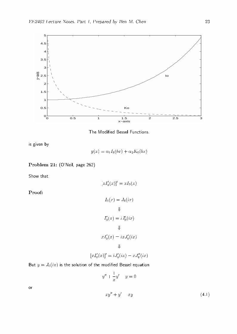
The Modi�ed Bessel Functions.

is given by

y(x) = �1I0(bx) + �2K0(bx)

Problem 21: (O'Neil, page 262)

Show that

[xI 00(x)]0 = xI0(x)

Proof:

I0(x) = J0(ix)

+I 00(x) = iJ 00(ix)

+xI 00(x) = ixJ 00(ix)

+[xI 00(x)]

0 = iJ 00(ix)� xJ 000 (ix)

But y = J0(ix) is the solution of the modi�ed Bessel equation

y00 +1

xy0 � y = 0

or

xy00 + y0 = xy (4.1)


Also, note that

y = J0(ix) =) y0 = iJ 00(ix) =) y00 = �J 000 (ix)Substituting into (4.1) above, we have

�xJ 000 (ix) + iJ 00(ix) = xJ0(ix)

That is

[xI 00(x)]0 = xI0(x)

Q.E.D.

Problem 10: (O'Neil page 262)

Show that y1(x) = xaJn(bxc) and y2(x) = xaYn(bx

c) are solutions of

y00 ��2a� 1

x

�y0 +

b2c2x2c�2 +

a2 � n2c2

x2

!y = 0

for any constants a, b and c, and any nonnegative integer n.

Proof:

y1 = xaJn(bxc)

+y01 = xaJ 0

n(bxc)bcxc�1 + axa�1Jn(bx

c) = bcxa+c�1J 0n(bxc) + axa�1Jn(bx

c)

+

y001 = bcxa+c�1J 00n(bxc)bcxc�1 + bc(a + c� 1)xa+c�2J 0

n(bxc)

+axa�1J 0n(bxc)bcxc�1 + a(a� 1)xa�2Jn(bx

c)

= b2c2xa+2c�2J 00n(bxc) + bc(2a + c� 1)xa+c�2J 0

n(bxc)

+a(a� 1)xa�2Jn(bxc)

Substituting into the given di�erential equation, we get

b2c2 xa+2c�2J 00n+ bc(2a + c� 1)xa+c�2J 0

n+ a(a� 1)xa�2Jn

� (2a� 1)bcxa+c�2J 0n� a(2a� 1)xa�2Jn + a2xa�2Jn

+ b2c2xa+2c�2Jn � n2c2xa�2Jn


= b2c2xa+2c�2J 00n+ bc2xa+c�2J 0

n+ b2c2xa+2c�2Jn � n2c2xa�2Jn

= c2xa�2�b2x2cJ 00

n+ bxcJ 0

n+ (b2x2c � n2)Jn

�

The factor inside f� � �g is equivalent to the left-hand side of the di�erential equation

z2y00 + zy0 + (z2 � n2)y = 0

when we substitute z = bxc and y = Jn(z). Thus,�b2x2cJ 00

n+ bxcJ 0

n+ (b2x2c � n2)Jn

�= 0

That is: y1(x) = xaJn(bxc) is the solution of the given di�erential equation. For the other

solution, y2(x), follow the same procedure above and try to do it yourself.

Q.E.D.

5. Applications of Bessel Functions

Displacement of a Suspended Chain

?

� -x y

Suppose we have a heavy exible chain. The chain is �xed at the upper end and free at the

bottom.

We want to describe the oscillations caused by a small displacement in a vertical plane from

the stable equilibrium position.

We will assume that each particle of the chain oscillates in a horizontal straight line.

Let m be the mass of the chain per unit length, L be the length of the chain, and y(x; t) be

the horizontal displacement at time t of the particle of chain whose distance from the point of

suspension is x.


Consider an element of chain of length �x. If the forces acting on the ends of this element are

T and T +�T , the horizontal component in Newton's Second Law of Motion (force equals to

the rate of change of momentum with respect to time) is:

m(�x)@2y

@t2=

@

@x

T@y

@x

!�x

(For those who are interested in the derivation of the above equation, please

read Section 11.2 & 12.8 of the Reference Book by Wylie)

+

m@2y

@t2=

@

@x

T@y

@x

!

The weight of the chain below x where T acts, is:

T = mg(L� x)

Substituting into the above di�erential equation, we get

@2y

@t2= �g @y

@x+ g(L� x)

@2y

@x2

This is a partial di�erential equation. However, we can reduced the problem of solving it to a

problem involving only an ordinary di�erential equation. Let z = L�x and u(z; t) = y(L�z; t).Then

@2y

@t2=@2u

@t2

@y

@x=@u

@z

@z

@x= �@u

@z

@2u

@z2= � @

@z

@y

@x

!= � @

@x

@y

@x

!@x

@z=@2y

@x2

+@2u

@t2= g

@u

@z+ gz

@2u

@z2

This is still a partial di�erential equation, which can be solved using p.d.e. method. Since we

anticipate the oscillations to be periodic in t, we will attempt a solution of the form

u(z; t) = f(z) cos(!t� Æ)

Substituting into the partial di�erential equation, we get

�!2f(z) cos(!t� Æ) = gf 0(z) cos(!t� Æ) + gzf 00(z) cos(!t� Æ)


Dividing this equation by gz cos(!t� Æ), we get

f 00(z) +1

zf 0(z) +

!2

gzf(z) = 0

Fortunately, we have shown that that

xaJn(bxc) and xaYn(bx

c)

are solutions of the di�erential equation

y00 ��2a� 1

x

�y0 +

b2c2x2c�2 +

a2 � n2c2

x2

!y = 0

Now, let

2a� 1 = �1 =) a = 0

2c� 2 = �1 =) c =1

2+

b2c2 =!2

g=) b =

2!pg

+a2 � n2c2 = 0 =) n = 0

Thus, the general solution is in terms of Bessel functions of order zero:

f(z) = �1J0

2!

sz

g

!+ �2Y0

2!

sz

g

!

Now, from we know (see �gure on page 22) that

Y0

2!

sz

g

!! �1

as z ! 0+ (that is, as x ! L, i.e., at the bottom end of the chain). We must therefore

choose �2 = 0 in order to have a bounded solution, as we expect from the physical setting of

the problem. This leave us with

f(z) = �1J0

2!

sz

g

!

Thus,

u(z; t) = f(z) cos(!t� Æ) = �1J0

2!

sz

g

!cos(!t� Æ)

Hence,

y(x; t) = �1J0

2!

sL� x

g

!cos(!t� Æ)


The frequencies of the normal oscillations of the chain are determined by using this general

form of the solution for y(x; t) together with condition that the upper end of the chain is �xed

and therefore does not move. For all t, we must have

y(0; t) = 0

Assume that �1 6= 0. This requires that we have to choose ! such that

J0

2!

sL

g

!= 0

This gives values of ! which can be frequencies of the oscillations.

To �nd these admissible values of !, we must consult a table of zeros of J0. From a table of

values of zeros of Bessel functions, we �nd that the �rst �ve positive solutions of J0(�) = 0

are approximately 2:405, 5:520, 8:654, 11:792, 14:931. (These values can also be found

using commercially available software package such as MATLAB. Check out

function bessel in MATLAB). Using the these zeros, we obtain

2!1

sL

g= 2:405 =) !1 = 1:203

rg

L

2!2

sL

g= 5:520 =) !2 = 2:760

rg

L

2!3

sL

g= 8:645 =) !3 = 4:327

rg

L

2!4

sL

g= 11:792 =) !4 = 5:896

rg

L

2!5

sL

g= 14:931 =) !5 = 7:466

rg

L

All these are admissible values of !, and they represent approximate frequencies of the normal

modes of oscillation.

The approximate period Tj associated with !j is

Tj =2�

!j

Special Remarks:

There are two features in the solution of this type of problems:

1. Change of variables was used to write solutions in terms of Bessel functions.


(0,0)

P

x

(L,0)

Q

2. Much of information about the motion of the system was obtained from zeros of a Bessel

function.

The Critical Length of a Vertical Rod

Suppose we have a thin elastic rod of uniform density. This rod is clamped in a vertical position

Intuitively, if the rod is \too long" and the upper end is displaced slightly, the rod will remain

in the displaced position after being released.

On the other hand, if the rod is \short enough", it will return to the vertical position after

being released.

We would like to know where the transition occurs between being too long and short enough.

That is, we want the minimum length at which the rod remains bent after being released.

This length is called the Critical Length of the rod and of course will depend on the material

of the rod.

To derive a mathematical model from which we can solve for this critical length, let L be the

length of the rod and a be the radius of its cross-sectional circular. Let w be the weight per

unit length and E be the Young's modulus for the rod. Note that E depends on the material

of the rod. We should expect that this will in uence the critical length. Finally, the moment

of inertia about a diameter is I = �a4=4.

Now, assume that the rod is in equilibrium and is displaced slightly from the vertical. The

origin is as shown, and the x-axis is vertical, with downward as positive. Let P (x; y) be a point

on the rod, and let Q(�; �) be a point slight above P .

The moment about P of the weight of an element w�x at Q is given by

w�x[y(�)� y(x)]


Assume from the theory of elasticity the fact that the moment of the elastic forces about P is

EId2y

dx2

Since the part of the rod above P is in equilibrium, we have

EId2y

dx2=

Zx

0w[y(�)� y(x)]d�

Di�erentiate this equation with respect to x to get

EId3y

dx3= w[y(x)� y(x)]�

Zx

0wy0(x)d� = �wxdy

dx

This yields a third order di�erential equation

EId3y

dx3+ wx

dy

dx= 0

ord3y

dx3+

w

EIxdy

dx= 0

Let u =dy

dxto obtain a second order di�erential equation:

d2u

dx2+

w

EIxu = 0

Recall your tutorial problem (also Problem 1 on page 253 of O'neil): Use the fact that Jv is a

solution of Bessel's equation of order v to show that xaJv(bxc) is a solution of the di�erential

equation

y00 ��2a� 1

x

�y0 +

b2c2x2c�2 +

a2 � v2c2

x2

!y = 0

Compare with the above di�erential equation:

2a� 1 = 0 =) a =1

2+

a2 � v2c2 = 0 =) v =1

3*

2c� 2 = 1; =) c =3

2+

b2c2 =w

EI=) b =

2

3

rw

EI


The general solution of the di�erential equation is given by

u =dy

dx= �1x

1

2J 1

3

�2

3

rw

EIx

3

2

�+ �2x

1

2J�

1

3

�2

3

rw

EIx

3

2

�

There is no bending moment at the upper end of the rod. Thus,

d2y

dx2

��x=0

= 0

This condition requires that we have to choose �1 = 0. Otherwise,

�pxJ1=3

�2

3

rw

EIx3=2

��0

=

(�2

3

rw

EI

��1=3 �23

rw

EIx3=2

�1=3

J1=3

�2

3

rw

EIx3=2

�)0

=

�2

3

rw

EI

��1=3 nt1=3J1=3(t)

o0

rw

EIx1=2 (change from x to t)

=

�2

3

rw

EI

��1=3 nt1=3J 1

3�1(t)

or w

EIx1=2 (see problem 3 on page 12)

= xJ�

2

3

�2

3

rw

EIx3=2

�rw

EI! �1 as x! 0+

Therefore, we have to choose a solution having the following format

dy

dx= �2

pxJ�1=3

�2

3

rw

EIx3=2

�

Furthermore, the lower end of the rod is clamped and so does not move; then

dy

dx

��x=L

= 0

In order to satisfy this condition with �2 6= 0, we must have

J�1=3

�2

3

rw

EIL3=2

�= 0

The critical length is the smallest positive number L which satis�es the above equation.

We �nd from the table or using software tools that the smallest positive zero of J�1=3 is

approximately 1:8663. Thus, the critical length L is determined approximately by

2

3

rw

EIL2=3 = 1:8663

+


L =

0@1:8663� 3

2

sEI

w

1A

2=3

= 1:9863

�EI

w

�1=3

Alternating Current in a Circular Wire: the Skin E�ect

Consider an alternating current of period 2�=!, given by D cos(!t). Let R be the radius of

the wire, � be its speci�c resistance, � be the permeability, x(r; t) be the current density at

radius r and at time t, and H(r; t) be the magnetic intensity at radius r from the centre of

the wire at time t.

To derive an equation for the current density x(r; t), we will need two laws of electromagnetic

�eld theory. Ampere's Law states that the line integral of the electric force around a closed

path equals to 4� times the integral of electric current through the path. Faraday's Law

states that the line integral of the electric force around a closed path equals to the negative of

the partial derivative with respect to time of the magnetic induction through the path.

Now consider a circular path of radius r within the wire, centred about the midpoint of the

wire.

By Ampere's Law,

2�rH = 4�Z

r

02�rxdr

Di�erentiating with respect to r, we get

@

@r(rH) = 4�rx (5.1)

Consider a closed rectangular path in the wire, with two sides along the axis of the cylinder

and of length L, and the other sides of length r.

By Faraday's Law,

�L[x(0; t)� x(r; t)] = � @

@t

Zr

0�LHdr

Di�erentiating w.r.t. r, we get

�@x

@r= �

@H

@t(5.2)

We want to eliminate H from these equations to obtain an equation for x alone. To do that,

we multiply Equation (5.2) by r and di�erentiate the resulting equation w.r.t. r. We obtain

�@

@r

r@x

@r

!= �

@

@r

r@H

@t

!= �

@

@r

@

@t[rH]

!(5.3)


because @r=@t = 0. Assume that we can reverse the order of the di�erentiation on the

right-hand side of the above equation, we obtain

�@

@r

r@x

@r

!= �

@

@t

@

@r[rH]

!

From Equation (5.1), we have1

r

@

@r

r@x

@r

!=

4��

�

@x

@t(5.4)

To solve this equation, we will employ a device which is quite standard in mathematical treat-

ments of electricity and magnetism. Let

z(r; t) = x(r; t) + iy(r; t)

and then replace x with z in Equation (5.4) to get

1

r

@

@r

r@z

@r

!=

4��

�

@z

@t(5.5)

Now recall Euler's formula. We can write

cos(!t) + i sin(!t) = ei!t

Anticipating periodic dependence of the current density on time, we will attempt a solution of

Equation (5.5) of the form,

z(r; t) = f(r)ei!t

Substituting this expression for z into Equation (5.5), we get

1

r

@

@r

hrf 0(r)ei!t

i=

4��

�i!f(r)ei!t

+1

r

@

@r[rf 0(r)] = i

4��!

�f(r)

+

f 00(r) +1

rf 0(r)� i

4��!

�f(r) = 0 (5.6)

Now let

k =1 + ip

2

s4��!

�=) k2 = i

4��!

�

Equation (5.6) becomes

f 00(r) +1

rf 0(r)� k2f(r) = 0


This is a modi�ed Bessel's equation with general solution

f(r) = c1I0(kr) + c2K0(kr)

In order for f(r) to remain �nite as r ! 0+, we must have c2 = 0. Thus, f(r) is of the form

c1I0(kr), with I0 the modi�ed Bessel function of �rst kind of order zero. Then z(r; t) has the

form

z(r; t) = c1I0(kr)ei!t

The current density x(r; t) is the real part of the above expression.

We have not yet used the initial assumption that the alternating current in the wire is given by

D cos(!t).

Note that D cos(!t) is the real part of Dei!t. Since Dei!t represents the total current, we

have

Dei!t =Z

R

02�rzdr = 2�c1

ZR

0rI0(kr)e

i!tdr

Upon dividing by ei!t, we have

D =

ZR

02�rzdr = 2�c1

ZR

0rI0(kr)dr

Recall that D is known. Thus, we obtain the constant c1, which is given by

c1 =D

2�RR

0 rI0(kr)dr(5.7)

Note that (see e.g., page 23) �xI 00(x)

�0

= xI0(x);

which implies

rI0(kr) =r

k2I 00(kr)

and hence ZR

0rI0(kr)dr =

R

k2I 00(kR) (5.8)

Substituting this into Equation (5.7), we get

c1 =Dk2

2�RI 00(kR)

and hence

z(r; t) =Dk2

2�RI 00(kR)I0(kr)e

i!t

The current density x(r; t) is the real part of the expression. Note that both k and k2 are not

real numbers. There is no simple way to separate the above expression into real and imaginary

parts.


The Skin E�ect:

We will now apply this analysis to a mathematically derivation of the skin e�ect:

It has been observed that, for suÆciently high frequencies, the current owing through a

circular wire at radius r is small compared with the total current, even for r nearly equal

to R. This means that \most" of the current in a cylindrical wire ows through a thin

layer at the outer surface, i.e., at the \skin" of the wire.

To derive this e�ect from the model, begin with the solution for z. The total current through

a cylinder of radius r is given by

Zr

02�z(r; t)dr =

Dk2

2�RI 00(kR)

Zr

02�rI0(kr)e

i!tdr

=Dk2

RI 00(kR)ei!t

Zr

0rI0(kr)dr

By Equation (5.8), with r in place of R we haveZr

0rI0(kr)dr =

r

k2I 00(kr)

Thus, the total current through a cylinder of radius r is

Dei!t� r

R

I 00(kr)

I 00(kR)+ +

total current ratio of the current in cylinder

in the wire of radius r to the total current

We want to know this ratio behaves for large k, which is proportional top!. It can be shown

that for large x, I0(x) can be approximated by

I0(x) � Aexpx

for some constant A. Hence, for large x,

I 00(x) �Aexpx

+ Aex��1

2x�3=2

�=Aexpx

�1� 1

2x

�� Aexp

x

Thus, if ! is large, which implies that k is large in magnitude, we have

r

R

I 00(kr)

I 00(kR)� r

R

ekrpr

pR

ekR=

rr

Re�k(R�r)

Given any r < R, e�k(R�r) can be made as small in magnitude as we like by choosing appropriate

(large) ! (or k). Thus, for large k, the ratio of the current in the cylinder of radius r to the

total current ! 0, and this is the so-called skin e�ect.


In fact, we can choose r as close as we like to R, and this conclusion continues to hold, for

suÆciently large frequencies.

333


6. Legendre's Equation and Legendre Polynomials

The di�erential equation

(1� x2)y00 � 2xy0 + �(�+ 1)y = 0

in which � is a constant, is called Legendre's Equation.

It occurs in a variety of problems involving quantum mechanics, astronomy and analysis

of heat conduction, and is often seen in settings in which it is natural to use spherical

coordinates.

Write Legendre's equation as

y00 ��

2x

1� x2

�y0 +

(�(� + 1)

1� x2

)y = 0

The coeÆcient functions are analytic at every point except x = 1 and x = �1. In

particular, both functions have Maclaurin series expansions in (�1; 1).

Since zero is an ordinary point of Legendre's equation, there are two linearly independent

solutions which are analytic in (�1; 1) and which can be found by the power series method.

Let

y(x) =1Xn=0

anxn

Substituting into Legendre's Equation, we have

1Xn=2

n(n� 1)anxn�2 �

1Xn=2

n(n� 1)anxn �

1Xn=1

2nanxn +

1Xn=0

�(�+ 1)anxn = 0

The �rst summation can be written as

1Xn=0

(n+ 2)(n+ 1)an+2xn

+1Xn=0

(n+ 2)(n+ 1)an+2xn �

1Xn=2

n(n� 1)anxn �

1Xn=1

2nanxn +

1Xn=0

�(� + 1)anxn = 0

Combining summations from n = 2 onwards and writing terms for n = 0 and n = 1 separately,

we have

h2a2 + �(�+ 1)a0

i+h6a3 � 2a1 + �(�+ 1)a1

ix

+1Xn=2

n(n+ 2)(n+ 1)an+2 � [n2 + n� �(� + 1)]an

oxn = 0


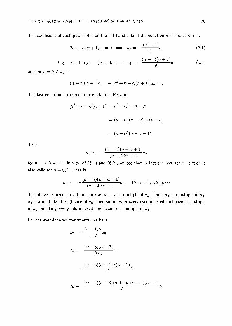
The coeÆcient of each power of x on the left-hand side of the equation must be zero, i.e.,

2a2 + �(�+ 1)a0 = 0 =) a2 = ��(� + 1)

2a0 (6.1)

6a3 � 2a1 + �(� + 1)a1 = 0 =) a3 = �(�� 1)(�+ 2)

6a1 (6.2)

and for n = 2; 3; 4; � � �

(n+ 2)(n+ 1)an+2 � [n2 + n� �(�+ 1)]an = 0

The last equation is the recurrence relation. Re-write

[n2 + n� �(� + 1)] = n2 � �2 + n� �

= (n� �)(n+ �) + (n� �)

= (n� �)(n+ � + 1)

Thus,

an+2 = �(�� n)(n+ � + 1)

(n + 2)(n+ 1)an

for n = 2; 3; 4; � � �. In view of (6.1) and (6.2), we see that in fact the recurrence relation is

also valid for n = 0; 1. That is

an+2 = �(�� n)(n + � + 1)

(n + 2)(n+ 1)an; for n = 0; 1; 2; 3; � � �

The above recurrence relation expresses an+2 as a multiple of an. Thus, a2 is a multiple of a0;

a4 is a multiple of a2 (hence of a0); and so on, with every even-indexed coeÆcient a multiple

of a0. Similarly, every odd-indexed coeÆcient is a multiple of a1.

For the even-indexed coeÆcients, we have

a2 = �(� + 1)�

1 � 2 a0

a4 = �(� + 3)(�� 2)

3 � 4 a2

= +(� + 3)(�+ 1)�(�� 2)

4!a0

a6 = �(� + 5)(� + 3)(�+ 1)�(�� 2)(�� 4)

6!a0


In general, we have

a2n = (�1)n(�+2n�1)(�+2n�3) � � � (�+1)�(��2) � � � (��2n+2)

(2n)!a0

and

a2n+1 = (�1)n(�+2n)(�+2n�2) � � � (�+2)(��1)(��3) � � � (��2n+1)

(2n+ 1)!a1

We can obtain two linearly independent solutions of Legendre's equation by making choice for

a0 and a1.

If we choose a0 = 1 and a1 = 0, we get one solution:

y1(x) = 1+1Xn=1

(�1)n(�+2n�1) � � � (�+1)�(��2) � � � (��2n+2)

(2n)!x2n

= 1� (� + 1)�

2x2 +

(� + 3)(�+ 1)�(�� 2)

24x4

� (� + 5)(�+ 3)(� + 1)�(�� 2)(�� 4)

720x6 + � � �

By letting a0 = 0 and a1 = 1, we obtain a second solution:

y2(x) = x+1Xn=1

(�1)n(�+2n) � � � (�+2)(��1)(��3) � � � (��2n+1)

(2n+ 1)!x2n+1

= x� (� + 2)(�� 1)

6x3 +

(�+ 4)(� + 2)(�� 1)(�� 3)

120x5 � � � �

These power series converge for all x 2 (�1; 1).

Note that for some �, one or the other of these series solutions is a polynomial. For example,

if � = 2, then a4 = 0; and hence a6 = a8 = � � � = 0. Thus, y1 is just a second degree

polynomial, i.e.,

y1(x) = 1� 3x2

If � = 3, then a5 = 0; so a7 = a9 = � � � = 0; and hence y2 is a third degree polynomial, i.e.,

y2(x) = x� 5

3x3

In fact, whenever � is a nonnegative integer, the power series for either y1(x) (if � is even) or

y2(x) (if � is odd) reduces to a �nite series, and we obtain a polynomial solution of Legendre's


equation. Such polynomial solutions are useful in many applications, including methods for

approximating solutions of equations f(x) = 0.

In such applications, it is helpful to standardize speci�c polynomial solutions so that their values

can be tabulated. The convention is to multiply y1 or y2 for each term by a constant which

makes the value of the polynomial 1 at x = 1.

The resulting polynomials are called Legendre polynomials and are denoted by Pn(x), i.e.,

Pn(x) is the solution of Legendre's equation with � = n.

The �rst few Legendre polynomials are

P0(x) = 1; P1(x) = x

P2(x) =1

2(3x2 � 1); P3(x) =

1

2(5x3 � 3x)

P4(x) =1

8(35x4 � 30x2 + 3); P5(x) =

1

8(63x5 � 70x3 + 15x)

Although these polynomials are de�ned for all x, they are solutions of Legendre's equation only

for �1 < x < 1 and for appropriate �.

It can be shown that � must be chosen as a nonnegative integer in order to obtain non-

trivial solutions of Legendre's equation which are bounded on [�1; 1]. This is particularly

important in models of phenomena in physics and engineering, where boundedness of the

solution is a natural expectation.

Theorem 6.1. If m and n are distinct nonnegative integer, then

Z 1

�1Pm(x)Pn(x)dx = 0

Proof: Pn and Pm are solutions of Legendre's di�erential equations with � = n and � = m,

respectively. Hence, we have

(1� x2)P 00n� 2xP 0

n+ n(n+ 1)Pn = 0

(1� x2)P 00m� 2xP 0

m+m(m+ 1)Pm = 0


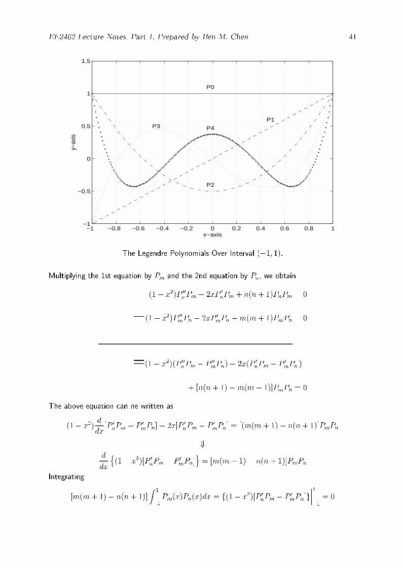
−1 −0.8 −0.6 −0.4 −0.2 0 0.2 0.4 0.6 0.8 1−1

−0.5

0

0.5

1

1.5

x−axis

y−ax

is

P1

P0

P2

P3 P4

The Legendre Polynomials Over Interval (�1; 1).

Multiplying the 1st equation by Pm and the 2nd equation by Pn, we obtain

(1� x2)P 00nPm � 2xP 0

nPm + n(n + 1)PnPm = 0

�(1� x2)P 00mPn � 2xP 0

mPn +m(m + 1)PmPn = 0

=(1� x2)(P 00nPm � P 00

mPn)� 2x(P 0

nPm � P 0

mPn )

+ [n(n + 1)�m(m + 1)]PmPn = 0

The above equation can ne written as

(1� x2)d

dx[P 0

nPm � P 0

mPn]� 2x[P 0

nPm � P 0

mPn] = [(m(m + 1)� n(n + 1)]PmPn

+d

dx

n(1� x2)[P 0

nPm � P 0

mPn]

o= [m(m + 1)� n(n+ 1)]PmPn

Integrating

[m(m + 1)� n(n+ 1)]

Z 1

�1Pm(x)Pn(x)dx = f(1� x2)[P 0

nPm � P 0

mPn]g

��1�1

= 0


Since m 6= n, we have Z 1

�1Pm(x)Pn(x)dx = 0

Q.E.D.

Exercise Problems: (Problem 2 O'Neil pg 237): Show that

Pn(x) =[n=2]Xk=0

(�1)k(2n� 2k)!xn�2k

2nk!(n� k)!(n� 2k)!

in which [n=2] = largest integer � n=2. Use this formula to compute P0(x) through P5(x).

(Problem 3 O'Neil pg 237): Rodrigue's formula states that

Pn(x) =1

2nn!

dn

dxn[(x2 � 1)n]

for n = 1; 2; 3; � � �. Prove this formula, assuming the formula for Pn(x) from Problem 2. Use

Rodrigue's formula to compute P0(x) through P5(x).

7. Properties of the Legendre Polynomials

Generating Function for Legendre Polynomials

The generating function for Legendre Polynomials is

P (x; r) = (1� 2xr + r2)�1=2

To see why this is called a generating function function, recalled the binomial expansion

(1� z)�1=2 = 1 +1

2z +

1

2!

1

2

3

2z2 +

1

3!

1

2

3

2

5

2z3 + � � �

If we let z = 2xr � r2, we have

P (x; r) = 1 +1

2(2xr � r2) +

3

8(2xr � r2)2 +

5

16(2xr � r2)3 + � � �

Rewrite this series in ascending powers of r to give

P (x; r) = 1 + xr +

��1

2+

3

2x2�r2 +

��3

2x +

5

2x3�r3 + � � �

= P0(x) + P1(x)r + P2(x)r2 + P3(x)r

3 + � � �

Thus, the coeÆcient of rn in the series for P (x; r) is exactly Pn(x), i.e.,

P (x; r) =1Xn=0

Pn(x)rn


Theorem 7.1. (Recurrence Relation for Legendre Polynomial). For each positive

integer n,

(n+ 1)Pn+1(x)� (2n+ 1)xPn(x) + nPn�1(x) = 0

for all �1 � x � 1.

Proof: Di�erentiating the generating function

P (x; r) = (1� 2xr + r2)�1=2

w.r.t. r, we obtain

@P

@r= �1

2(1� 2xr + r2)�3=2(�2x + 2r)

= (1� 2xr + r2)�3=2(x� r)

+

(1� 2xr + r2)@P

@r= (1� 2xr + r2)�1=2(x� r)

+

(1� 2xr + r2)@P

@r� (x� r)P (x; r) = 0

Note that from the property of the generating function, i.e.,

P (x; r) =1Xn=0

Pn(x)rn

We have@P

@r=

1Xn=0

nPn(x)rn�1 =

1Xn=1

nPn(x)rn�1

+

(1� 2xr + r2)1Xn=1

nPn(x)rn�1 � (x� r)

1Xn=0

Pn(x)rn = 0

+

1Xn=1

nPn(x)rn�1 �

1Xn=1

2xnPn(x)rn +

1Xn=1

nPn(x)rn+1 �

1Xn=0

xPn(x)rn

+1Xn=0

Pn(x)rn+1 = 0

+


1Xn=0

(n + 1)Pn+1(x)rn +

1Xn=1

(�2xn)Pn( x )rn +

1Xn=2

(n� 1)Pn�1(x)rn

�1Xn=0

xPn(x)rn +

1Xn=1

Pn�1(x)rn = 0

+

0 = P1(x) + 2P2(x)r � 2xP1(x)r � xP0(x)� xP1(x)r + P0(x)r

+1Xn=2

f(n+1)Pn+1(x)�2xnPn(x) + (n�1)Pn�1(x)�xPn(x)+Pn�1(x)g rn

+�P1(x)� xP0(x)

�+

�(1 + 1)P2(x)� (2 + 1)xP1(x) + P0(x)

�r

+1Xn=2

�(n+ 1)Pn+1(x)� (2n+ 1)xPn(x) + nPn�1(x)

�rn = 0

+P1(x)� xP0(x) = 0

(1 + 1)P2(x)� (2 + 1)xP1(x) + P0(x) = 0

and, for n = 2; 3; 4; � � �

(n+ 1)Pn+1(x)� (2n+ 1)xPn(x) + nPn�1(x) = 0

This completes the proof of the recurrence relation. Q.E.D.

Theorem 7.2. The coeÆcient of xn in Pn(x) is

1 � 3 � 5 � � � (2n� 1)

n!

Proof: Let cn be the coeÆcient of xn in Pn(x), and consider the recurrence relation

(n+ 1)Pn+1(x)� (2n+ 1)xPn(x) + nPn�1(x) = 0

The coeÆcient of xn+1 in (n + 1)Pn+1(x) is equal to (n + 1)cn+1: The coeÆcient of xn+1

in �(2n + 1)xPn(x) is equal to �(2n + 1)cn: There is no other xn+1 term in the recurrence

relation. Thus the coeÆcient of xn+1 is

(n+ 1)cn+1 � (2n+ 1)cn = 0


+

cn+1 =2n+ 1

n+ 1cn

Working backwards, we have

cn =2n� 1

ncn�1

=2n� 1

n

2n� 3

n� 1cn�2

=2n� 1

n

2n� 3

n� 1

2n� 5

n� 2cn�3

= � � �

=(2n� 1)(2n� 3)(2n� 5) � � � (1)

n(n� 1)(n� 2) � � � (1) c0

But c0 is the coeÆcient of x0 in P0(x) = 1. ) c0 = 1

+

cn =1 � 3 � 5 � � � (2n� 1)

n!

Q.E.D.

Theorem 7.3. For each positive integer n,

nPn(x)� xP 0n(x) + P 0

n�1(x) = 0

Proof: Given the generating function:

P (x; r) = (1� 2xr + r2)�1=2

Di�erentiating it w.r.t. x, we obtain

@P

@x= �1

2(�2r)(1� 2xr + r2)�3=2

+

(1� 2xr + r2)@P

@x= r(1� 2xr + r2)�1=2

+

(1� 2xr + r2)@P

@x� rP (x; r) = 0


+

(1� 2xr + r2) =

�rP (x; r)

�=@P

@x(7.1)

Recall the earlier result by di�erentiating P (x; r) w.r.t. r, i.e.,

(1� 2xr + r2)@P

@r� (x� r)P (x; r) = 0 (7.2)

Equations (7.1) and (7.2) implies that

r@P

@r� (x� r)

@P

@x= 0

Note that by the property of the generating function, i.e.,

P (x; r) =1Xn=0

Pn(x)rn

we have@P

@r=

1Xn=1

nPn(x)rn�1

@P

@x=

1Xn=0

P 0n(x)rn

+1Xn=1

nPn(x)rn �

1Xn=0

xP 0n(x)rn +

1Xn=0

P 0n(x)rn+1 = 0

+1Xn=1

nPn(x)rn �

1Xn=0

xP 0n(x)rn +

1Xn=1

P 0n�1(x)r

n = 0

+

�xP 00(x) +1Xn=1

�nPn(x)� xP 0

n(x) + P 0

n�1(x)

�rn = 0

Hence (because the fact that P0(x) = 1)

nPn(x)� xP 0n(x) + P 0

n�1(x) = 0

Q.E.D.

Theorem 7.4. For each positive integer n,

nPn�1(x)� P 0n(x) + xP 0

n�1(x) = 0


Proof: We had in the previous proof the following equality

rP (x; r) = (1� 2xr + r2)@P

@x

r@P

@r� (x� r)

@P

@x= 0

+

r@P

@r= (x� r)

@P

@x

Note that

r@

@r[rP (x; r)] = rP + r2

@P

@r

+

r@

@r[rP (x; r)] = (1� 2xr + r2)

@P

@x+ r(x� r)

@P

@x= (1� rx)

@P

@x

+

r@

@r[rP (x; r)]� (1� rx)

@P

@x= 0

Also note that

P (x; r) =1Xn=0

Pn(x)rn

+@P

@x=

1Xn=0

P 0n(x)rn

and

rP (x; r) =1Xn=0

Pn(x)rn+1

+

r@

@r[rP (x; r)] =

1Xn=0

(n+ 1)Pn(x)rn+1

+

0 = r@

@r[rP ]� (1� rx)

@P

@x

=1Xn=0

(n + 1)Pn(x)rn+1 �

1Xn=0

P 0n(x)rn +

1Xn=0

xP 0n(x)rn+1

+1Xn=1

nPn�1(x)rn �

1Xn=0

P 0n(x)rn +

1Xn=1

xP 0n�1(x)r

n = 0

+


1Xn=1

�nPn�1(x)� P 0

n(x) + xP 0

n�1(x)

�rn � P 00(x) = 0

+nPn�1(x)� P 0

n(x) + xP 0

n�1(x) = 0

Q.E.D.

Orthogonal Polynomials

We have shown that if m and n are distinct nonnegative integers, then

Z 1

�1Pn(x)Pm(x)dx = 0

In view of this, we can say that the Legendre polynomials are Orthogonal to each other on

the interval [�1; 1]. We also say that the Legendre polynomials form a set of Orthogonal

Polynomials on the interval on [�1; 1].

The orthogonal property can be used to write many functions as series of Legendre polyno-

mials. This will be important in solving certain boundary value problems in partial di�erential

equations.

For now, we will see how to write any polynomial as such a series. Let q(x) be a polynomial

of degree m. We will see how to choose numbers �0, �1, �2, � � �, �m such that

q(x) =mXk=0

�kPk(x) for �1 � x � 1

Multiply the above equation by Pj(x), where j is any integer from 0 to m inclusive, i.e.,

q(x)Pj(x) = �0P0(x)Pj(x) + �1P1(x)Pj(x) + � � �+ �mPm(x)Pj(x)

Integrating both sides of the above equation from �1 to 1, we have

Z 1

�1q(x)Pj(x)dx = �0

Z 1

�1P0(x)Pj(x)dx+ �1

Z 1

�1P1(x)Pj(x)dx

+ � � �+ �m

Z 1

�1Pm(x)Pj(x)dx (7.3)

Because of the relation

Z 1

�1Pn(x)Pm(x)dx = 0 for m 6= n

+


Z 1

�1Pk(x)Pj(x)dx

on the right hand side of the equation (7.3) is zero, except for that one integral in which k = j.

This leaves us with Z 1

�1q(x)Pj(x)dx = �j

Z 1

�1[Pj(x)]

2dx

+

�j =

Z 1

�1q(x)Pj(x)dxZ 1

�1[Pj(x)]

2dx

for j = 0; 1; 2; � � �m

These numbers can be computed because we know each Pj(x) and we are given q(x). Using

these numbers, we can write q(x) as a series of Legendre polynomials.

For example,

x2 =2

3P2(x) +

1

3P0(x)

x3 =2

5P3(x) +

3

5P1(x)

1� 4x2 + 2x3 = P0(x)� 4

�2

3P2(x) +

1

3P0(x)

�+ 2

�2

5P3(x) +

3

5P1(x)

�

= �1

3P0(x) +

6

5P1(x)� 8

3P2(x) +

4

5P3(x)

Any Polynomial can be Written as a Finite Series of Legendre Polynomials.

Theorem 7.5. Let m and n be nonnegative integers, with m < n. Let q(x) be any

polynomial of degree m. Then

Z 1

�1q(x)Pn(x)dx = 0

That is, the integral, from �1 to 1, of a Legendre polynomial multiplied by any polynomial

of lower degree, is zero.

Proof: We have shown that for any polynomial q(x) of degree m, there exist scalar �0, �1,

� � �, �m such that

q(x) = �0P0(x) + �1P1(x) + � � �+ �mPm(x)


Then Z 1

�1q(x)Pn(x)dx = �0

Z 1

�1P0(x)Pn(x)dx + �1

Z 1

�1P1(x)Pn(x)dx

+ � � �+ �m

Z 1

�1Pm(x)Pn(x)dx

and each of the integrals on the right hand side is zero by the property thatZ 1

�1Pj(x)Pn(x)dx = 0

for j = 0; 1; 2; � � � ; m < n. Q.E.D.

Theorem 7.6. Z 1

�1[Pn(x)]

2dx =2

2n+ 1

for n = 0; 1; 2; � � �

Proof: Let cn be coeÆcient of xn in Pn(x) and also let the coeÆcient of xn�1 in Pn�1(x) be

cn�1. De�ne

q(x) = Pn(x)� cn

cn�1xPn�1(x)

The xn term in Pn(x) is cancelled by the xn term in � cn

cn�1xPn�1(x). Thus, q(x) has degree

n� 1 or lower.

We therefore have

Pn(x) =cn

cn�1xPn�1(x) + q(x)

in which q(x) has degree less than or equal to n� 1.

+

[Pn(x)]2 = Pn(x)

"cn

cn�1xPn�1(x) + q(x)

#=

cn

cn�1xPn�1(x)Pn(x) + q(x)Pn(x)

Integrating this equation from �1 to 1, we haveZ 1

�1[Pn(x)]

2dx =cn

cn�1

Z 1

�1xPn�1(x)Pn(x)dx+

Z 1

�1q(x)Pn(x)dx

=cn

cn�1

Z 1

�1xPn�1(x)Pn(x)dx+ 0

Now use the recurrence relation,

(n+ 1)Pn+1(x)� (2n+ 1)xPn(x) + nPn�1(x) = 0


+

xPn(x) =n+ 1

2n+ 1Pn+1(x) +

n

2n+ 1Pn�1(x)

+Z 1

�1[Pn(x)]

2dx =cn

cn�1

Z 1

�1

n+ 1

2n+ 1Pn�1(x)Pn+1(x)dx

+cn

cn�1

Z 1

�1

n

2n+ 1[Pn�1(x)]

2dx

= 0 +cn

cn�1

Z 1

�1

n

2n + 1[Pn�1(x)]

2dx

+Z 1

�1[Pn(x)]

2dx =cn

cn�1

n

2n+ 1

Z 1

�1[Pn�1(x)]

2dx

Recall from Theorem 7.2 that

cn =1 � 3 � � � � (2n� 1)

n!

Then

cn�1 =1 � 3 � � � � (2n� 3)

(n� 1)!

+cn

cn�1=

2n� 1

n

+Z 1

�1[Pn(x)]

2dx =2n� 1

n

n

2n+ 1

Z 1

�1[Pn�1(x)]

2dx =2n� 1

2n+ 1

Z 1

�1[Pn�1(x)]

2dx

We can work backwards,

Z 1

�1[Pn(x)]

2dx =2n� 1

2n+ 1

Z 1

�1[Pn�1(x)]

2dx

=(2n� 1)(2n� 3)

(2n+ 1)(2n� 1)

Z 1

�1[Pn�2(x)]

2dx

=(2n� 1)(2n� 3)(2n� 5)

(2n+ 1)(2n� 1)(2n� 3)

Z 1

�1[Pn�3(x)]

2dx

= � � � � � � � � �

=(2n� 1)(2n� 3)(2n� 5) � � �3 � 1(2n+ 1)(2n� 1)(2n� 3) � � �5 � 3

Z 1

�1[P0(x)]

2dx


=1

2n + 1

Z 1

�1[P0(x)]

2dx

=2

2n + 1

Q.E.D.

Finally, we can write any polynomial of degree m as a �nite series of Legendre

polynomials,

q(x) =mXk=0

�kPk(x) for �1 � x � 1

with

�k =

Z 1

�1q(x)Pk(x)dxZ 1

�1[Pk(x)]

2dx

=2k + 1

2

Z 1

�1q(x)Pk(x)dx

for k = 0; 1; 2; � � �m.

333


8. Boundary Value Problems in Partial Di�erential Equations

A partial di�erential equation is an equation containing one or more partial derivatives, e.g.,

@u

@t=@2u

@x2

We seek a solution u(x; t) which depends on the independent variables x and t.

A solution of a partial di�erential equation is a function which satis�es the equation.

For example,

u(x; t) = cos(2x)e�4t

is a solution of the above mentioned di�erential equation since

@u

@t= �4 cos(2x)e�4t

@2u

@x2= �4 cos(2x)e�4t

Occasionally, a partial di�erential equation may be solved by inspection. For example, consider

@u

@x= �4

@u

@y

There may be many solutions of this equation, but we can guess one by reasoning as follows:

If@u

@xand

@u

@ywere both constants, we could �nd a solution easily. Try

u(x; y) = Ax +By

with A and B constants. Then

@u

@x= A and

@u

@y= B

Substituting them into the partial di�erential equation, we �nd that the proposed u(x; y) is a

solution for the given di�erential equation if and only if

A = �4B

Therefore, any function de�ned by

u(x; y) = B(�4x + y)

with B being a constant, is a solution of the partial di�erential equation.


Order of a Partial Di�erential Equation

A partial di�erential equation (p.d.e.) is said to be of order n if it contains an nth order partial

derivative but none of higher order. For example, the following so-called Laplace equation

r2u =@2u

@x2+@2u

@y2+@2u

@z2= 0

is of order 2. The p.d.e.@2u

@x2=@5u

@t5� @u

@t

is of order 5.

Linear Case

The general linear �rst order p.d.e. in two variables (with u as a function of the independent

variables x and y) is

a(x; y)@u

@x+ b(x; y)

@u

@y+ f(x; y)u+ g(x; y) = 0

The general second order linear p.d.e. in two variables has the form

a(x; y)@2u

@x2+ b(x; y)

@2u

@x@y+ c(x; y)

@2u

@y2+ d(x; y)

@u

@x

+ e(x; y)@u

@y+ f(x; y)u+ g(x; y) = 0

Most of the equations we encounter will be in one of these two forms.

In both cases, the equation is said to be homogeneous if g(x; y) = 0 for all (x; y) under

consideration and nonhomogeneous if g(x; y) 6= 0 for some (x; y).

We will devote most of our time to equations governing vibration and heat conduction phe-

nomena.

Main Tools:

Fourier series, integrals, transforms and Laplace transform.


y(x,t)

Lxx-axis

y

0

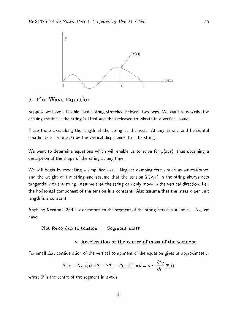
9. The Wave Equation

Suppose we have a exible elastic string stretched between two pegs. We want to describe the

ensuing motion if the string is lifted and then released to vibrate in a vertical plane.

Place the x-axis along the length of the string at the rest. At any time t and horizontal

coordinate x, let y(x; t) be the vertical displacement of the string.

We want to determine equations which will enable us to solve for y(x; t), thus obtaining a

description of the shape of the string at any time.

We will begin by modelling a simpli�ed case. Neglect damping forces such as air resistance

and the weight of the string and assume that the tension T (x; t) in the string always acts

tangentially to the string. Assume that the string can only move in the vertical direction, i.e.,

the horizontal component of the tension is a constant. Also assume that the mass � per unit

length is a constant.

Applying Newton's 2nd law of motion to the segment of the string between x and x+�x, we

have

Net force due to tension = Segment mass

� Acceleration of the centre of mass of the segment

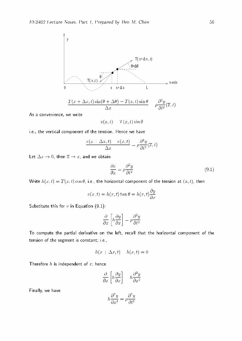
For small �x, consideration of the vertical component of the equation gives us approximately:

T (x+�x; t) sin(� +��)� T (x; t) sin � = ��x@2y

@t2(x; t)

where x is the centre of the segment in x-axis.

+


Lx-axis

y

0

θ+∆θ

θ

x+ ∆ x

Τ( x+ ∆ x , t)

Τ( x ,t )

x

T (x+�x; t) sin(� +��)� T (x; t) sin �

�x= �

@2y

@t2(x; t)

As a convenience, we write

v(x; t) = T (x; t) sin �

i.e., the vertical component of the tension. Hence we have

v(x+�x; t)� v(x; t)

�x= �

@2y

@t2(x; t)

Let �x! 0, then x! x, and we obtain

@v

@x= �

@2y

@t2(9.1)

Write h(x; t) = T (x; t) cos �, i.e., the horizontal component of the tension at (x; t), then

v(x; t) = h(x; t) tan � = h(x; t)@y

@x

Substitute this for v in Equation (9.1):

@

@x

"h@y

@x

#= �

@2y

@t2

To compute the partial derivative on the left, recall that the horizontal component of the

tension of the segment is constant; i.e.,

h(x +�x; t)� h(x; t) = 0

Therefore h is independent of x; hence

@

@x

"h@y

@x

#= h

@2y

@x2

Finally, we have

h@2y

@x2= �

@2y

@t2


Let a2 =h

�, we obtain a so-called 1-D wave equation,

@2y

@t2= a2

@2y

@x2

The motion of the string will be in uenced by both the initial position and the initial velocity

of the string. Therefore we must specify initial conditions:

y(x; 0) = f(x) initial position

@y

@t(x; 0) = g(x) initial velocity

with f(x) and g(x) given functions de�ned on [0; L]. The initial conditions must hold for

0 � x � L.

Next, we consider the boundary conditions. Since the ends of the string are �xed, we have

y(0; t) = y(L; t) = 0 t � 0

The wave equation, together with initial and boundary conditions is an example of a boundary

value problem.

To be more clear, we can put all of them together, i.e.,

@2y

@t2= a2

@2y

@x2(0 < x < L; t > 0)

y(0; t) = y(L; t) = 0 (t > 0)

y(x; 0) = f(x) (0 < x < L)

@y

@t(x; 0) = g(x) (0 < x < L)

We expect on physical grounds that this problem will have a unique solution.

We can also include in the model additional forces acting on the string. For example, if an

external force of magnitude F units per unit length acts parallel to the y axis, the wave equation

must be adjusted by addition of a term F=�, i.e.,

@2y

@t2= a2

@2y

@x2+

1

�F 0 < x < L; t > 0

Note that if F is the weight of the string, then set F = �g in the above p.d.e..

In two dimensions, we might have a membrane covering region R in the plane and �xed on

a frame forming the boundary R. The membrane is set in motion, with vibrations occuring

vertical to the plane of the membrane.


If z(x; y; t) is the vertical coordinate at time t of the particle at point (x; y) in the membrane,

the p.d.e. for z is:@2z

@t2= a2

"@2z

@x2+@2z

@y2

#

for (x; y) in R. This is the 2-D wave equation.

To determine z uniquely, we must �rst include conditions, which specify the initial positions

and velocity of the membrane.

z(x; y; 0) = f(x; y) for (x; y) 2 R@z

@t(x; y; 0) = g(x; y) for (x; y) 2 R

Finally, the condition that the membrane is �xed to the frame means that points on the border

of the membrane do not move, i.e.,

z(x; y; t) = 0

for all t > 0 and (x; y) on the boundary of R.

10. The Heat Equation

This is to study temperature distribution in a straight, thin bar under simple circumstances.

Suppose we have a straight, thin bar of constant density � and constant cross-sectional area

A placed along the x-axis from 0 to L.

Assume that the sides of the bar are insulated and so not allow heat loss and that the temper-

ature on the cross-section of the bar perpendicular to the x-axis at x is a function u(x; t) of x

and t, independent of y.

Let the speci�c heat of the bar be c, and let the thermal conductivity be k, both constant.

Now consider a typical segment of the bar between x = � and x = �.

By the de�nition of speci�c heat, the rate at which heat energy accumulates in this segment

of the bar is: Z�

�

c�A@u

@tdx

By Newton's law of cooling, heat energy ows within this segment from the warmer to the

cooler end at a rate equal to k times the negative of the temperature gradient.

Therefore, the net rate at which heat energy enters the segment of bar between � and � at

time t is:

kA@u

@x(�; t)� kA

@u

@x(�; t)


0 Lβα

u

x

u(x,t)

In the absence of heat production within the segment, the rate at which heat energy accumulates

within the segment must balance the rate at which heat energy enters the segment. Hence,

Z�

�

c�A@u

@tdx = kA

@u

@x(�; t)� kA

@u

@x(�; t)

Note that the right hand side of the above equation can be written as:

kA@u

@x(�; t)� kA

@u

@x(�; t) = kA

Z�

�

@2u

@x2dx

Therefore the whole equation can be written in the following form:

Z�

�

"c�A

@u

@t� kA

@2u

@x2

#dx = 0

This must hold for every � and � with 0 � � < � � L. If

c�A@u

@t� kA

@2u

@x2

were nonzero for any t > 0 and some x0 2 [0; L], we could choose an interval [�; �] about x0

in which

c�A@u

@t� kA

@2u

@x2

is strictly positive or strictly negative, and we would then have

Z�

�

"c�A

@u

@t� kA

@2u

@x2

#dx 6= 0

This is a contradiction.

Thus, we conclude that

c�A@u

@t� kA

@2u

@x2= 0

for all x 2 [0; L] and t > 0.


This is the heat equation, which is more customary written as:

@u

@t= a2

@2u

@x2

where a2 = k=(c�) is called the thermal di�usivity of the bar.

To determine u uniquely, we need boundary conditions (information at the ends of the bar)

and initial conditions (temperature throughout the bar at time zero). The p.d.e., together with

these pieces of information, constitutes a boundary value problem for the temperature function

u.

Example 1:@u

@t= a2

@2u

@x2(0 < x < L; t > 0)

u(0; t) = u(L; t) = T (t > 0)

u(x; 0) = f(x) (0 < x < L)

This boundary value problem models the temperature distribution in a bar of length L, whose

ends are kept at constant temperature T , and the initial temperature in the cross-section at x

is a given function f(x).

Example 2:

A perfectly insulated bar, in which we replace the boundary conditions

u(0; t) = u(L; t) = T

of the �rst example with the conditions

@u

@x(0; t) =

@u

@x(L; t) = 0 (t > 0)

i.e., there is no heat ows across the ends of the bar.

Example 3:

Free radiation (convection): The bar loses heat by radiation from the ends into the surrounding

medium, which is assumed to be maintained at a constant temperature Ta. In this case, the

boundary conditions are@u

@x(0; t) = A[u(0; t)� Ta]

@u

@x(L; t) = �A[u(L; t)� Ta]


for t > 0 with A being a positive constant. Note that if the bar is hotter than the surrounding

medium, the heat ow (change in temperature per unit length, or@u

@x) must be positive at the

left end of the bar and negative at the right end.

We can also have a combination of these di�erent types of conditions occurring in a boundary

value problem. For example, suppose we have a bar with its left end maintained at a constant

temperature T1 and its right end radiating into a medium of temperature T2, with an initial

temperature distribution given by f(x). The boundary value problem modelling the above

temperature distribution is:

@u

@t= a2

@2u

@x2(0 < x < L; t > 0)

u(0; t) = T1 (t > 0)

@u

@x(L; t) = �A[u(L; t)� T2] (t > 0)

u(x; 0) = f(x) (0 < x < L)

In two dimensions, the heat equation is:

@u

@t= a2

"@2u

@x2+@2u

@y2

#

In three dimensions,@u

@t= a2

"@2u

@x2+@2u

@y2+@2u

@z2

#

Corresponding boundary and initial conditions must be speci�ed to determine unique solutions

of these partial di�erential equations.

11. Laplace's Equation; Poisson's Equation; Dirichlet Problem

and Neumann Problem

Laplace's Equation

Laplace's equation in 2-D:@2u

@x2+@2u

@y2= 0

Laplace's equation in 3-D:@2u

@x2+@2u

@y2+@2u

@z2= 0


Laplace's equation is also called the steady-state heat equation, i.e., it is the heat equation

when@u

@t= 0

It has important applications in heat conduction, uid ow, study of electrical �eld poten-

tials.

It is often written as

r2u = 0

A function satisfying r2u = 0 is called a harmonic function.

Dirichlet Problem

The Dirichlet problem is to �nd a function which is harmonic in a given set M and takes on

predetermined values on the boundary ofM . For example, in 3-D, we could have the boundary

value problem

r2u = 0 in M

u(x; y; z) = f(x; y; z) for (x; y; z) on �;

where � is a piecewise-smooth surface bounding M and f is a given function.

A typical Dirichlet problem in the 2-D plane would be:

r2u = 0 in D

u(x; y) = g(x; y) for (x; y) on C

where C is a piecewise-smooth curve bounding the set D in the plane.

Neumann Problem

A Nuemann problem in 3-D consists of �nding a function u such that r2u = 0 for (x; y; z) in

a region M , subject to the condition that the normal derivative of u takes on prescribed values

on the boundary of the region, i.e.,

r2u = 0 in M

@u

@�= f(x; y; z) for (x; y; z) on �

where � is the surface bounding M and@u

@�denotes the directional derivative in the direction

of the normal to �.


Poisson's Equation (Applicable to Potential for Electrical Fields)

The following equation is called Poisson's equation,

r2u = f

with f being a given function. When f is identically zero, Poisson's equation becomes Laplace's

equation.

Laplace's Equation in Cylindrical and Spherical Coordinates

Cylindrical coordinates (r; �; z)

x = r cos �; y = r sin �; z = z

where

r =qx2 + y2

� = tan�1�y

x

�if x 6= 0

Here the value of � is determined by the signs of x and y. For example, if x and y are both

negative, (x; y) is in the 3rd quadrant, so we must have � < � < 3�=2, even though the ratio

y=x is positive.

Now suppose that u is a function of (x; y; z) and that u and its �rst and second partial

derivatives are continuous throughout some set M of 3-D space.

Since x, y and z are functions of r, � and z, we may think of u also as a function of r, � an

dz.

By the chain rule,

@u

@x=@u

@r

@r

@x+@u

@�

@�

@x+@u

@z

@z

@x

=@u

@r

xpx2 + y2

+@u

@�

� y

x2 + y2

!+ 0

=x

r

@u

@r� y

r2@u

@�(11.1)

By a similar calculation,

@u

@y=y

r

@u

@r+x

r2@u

@�(11.2)


To calculate second derivatives, di�erentiate equation (11.1) with respect to x:

@2u

@x2=@u

@r

@

@x

�x

r

�� @u

@�

@

@x

�y

r2

�+x

r

@

@x

@u

@r

!� y

r2@

@x

@u

@�

!

Applying the chain rule again, we obtain

@2u

@x2=y2

r3@u

@r+

2xy

r4@u

@�+x2

r2@2u

@r2� 2xy

r3@2u

@r@�+y2

r4@2u

@�2

If we di�erentiate equation (11.2) with respect to y, we get

@2u

@y2=x2

r3@u

@r� 2xy

r4@u

@�+y2

r2@2u

@r2+

2xy

r3@2u

@r@�+x2

r4@2u

@�2

+

r2u =@2u

@r2+

1

r

@u

@r+

1

r2@2u

@�2+@2u

@z2

+Laplace's equation in cylindrical coordinates is

@2u

@r2+

1

r

@u

@r+

1

r2@2u

@�2+@2u

@z2= 0

For Laplace's equation in polar coordinates, simply omit the z-dependency:

@2u

@r2+

1

r

@u

@r+

1

r2@2u

@�2= 0

Spherical Coordinates

Spherical coordinates are related to rectangular coordinates by

x = � cos(�) sin('); y = � sin(�) sin('); z = � cos(')

where � is the magnitude of the vector P = (x; y; z), and � and ' are respectively the angles

from x-axis and z-axis to P . The Laplacian in spherical coordinates is then given by

r2u =@2u

@�2+

2

�

@u

@�+

1

�2 sin2(')

@2u

@�2+

1

�2@2u

@'2+

cot(')

�2@u

@'

The Laplace's equation in spherical coordinates is r2u = 0.


12. Fourier Series Solution of the Wave Equation

Recall the wave equation of an initially displaced vibrating string with zero initial velocity,

@2y

@t2= a2

@2y

@x2(0 < x < L; t > 0)

y(0; t) = y(L; t) = 0 (t > 0)

y(x; 0) = f(x); (0 < x < L)

@y

@t(x; 0) = 0 (0 < x < L)

This boundary value problem models the vibration of an elastic string of length L, fastened at

the ends, picked up at time zero to assume the shape of the graph of y = f(x) and released

from rest.

The Fourier method or method of separation of variables is to �nd a solution of the form

y(x; t) = X(x)T (t) (12.1)

with appropriate X(x) and T (t) that solves the above mentioned boundary value problem.

At time t, y(x; t) is the vertical displacement of the particle of string having coordinate x. We

attempt a solution of (12.1). Substitute it into the p.d.e. to get

XT 00 = a2X 00T

+X 00

X=

T 00

a2T

We have \separated" x and t; the left hand side is a function of x alone, and the right hand

side is a function of t. Since x and t are independent, we can �x the right hand side by choosing

t = t0, and the left hand side must be equal to

T 00(t0)

a2T (t0)for all x in (0; L)

ThusX 00

Xmust be constant. But the

T 00

a2Tmust be equal to the same constant.

Denote this constant �� (it is also called separation constant), then

X 00

X=

T 00

a2T= ��

+


X 00 + �X = 0

T 00 + �a2T = 0

These are two ordinary di�erential equations for X and T .

Next, look at the boundary conditions for y(x; t) and relate them to X and T . From the

condition that the left end of the string is �xed, we have

y(0; t) = X(0)T (t) = 0

for t > 0. Since T (t) cannot be zero for all t > 0 (if the string is to move), X(0) = 0.

Similarly,

y(L; t) = X(L)T (t) = 0

for t > 0 implies that X(L) = 0.

Next, initial condition@y

@t(x; 0) = 0

requires that

X(x)T 0(0) = 0

for 0 < x < L. Therefore T 0(0) = 0.

At this point, we have two problems for X and T , namely

X 00 + �X = 0

X(0) = X(L) = 0

and

T 00 + �a2T = 0

T 0(0) = 0

A value for � for which the above problem, either the problem associated with X or T ,

has a nontrivial solution (nonzero at some points) is called eigenvalue of this problem. For

such a �, any nontrivial solution for X or for T is called eigenfunction.

We will consider di�erent cases on �. We assume that � is real, as we expect from the physics

of the problem.

Case 1: � = 0


Then X 00 = 0, so X(x) = cx + d for some constants c and d. Then the condition X(0) = 0

implies d = 0 and X(L) = cL = 0 implies c = 0.

+

The solution X(x) = 0 for 0 � x � L, and we will have y(x; t) = 0 as the solution. This is

the case if f(x) = 0 for 0 � x � L because then the string was not displaced initially and

simply remain stationary. If, however, f(x) 6= 0 for some x, X(x) cannot be identically zero,

and we must discard this case.

Case 2: � < 0.

For this case, we write � = �k2 with k > 0. The equation for X is the given by

X 00 � k2X = 0

with general solution

X(x) = cekx + de�kx

Since X(0) = 0 = c+ d ) d = �c and

X(x) = c(ekx � e�kx) = 2c sinh(kx)

Then

X(L) = 2c sinh(kL) = 0

Since k and L are both positive, sinh(kL) > 0, and we conclude that c = 0 and hence

d = �c = 0.

As in Case 1, we obtain X(x) = 0 for 0 � x � L. This case does not yield a solution unless

again the string was not moved initially.

Case 3: � > 0

We can write � = k2 with k > 0. Then

X 00 + k2X = 0

has a general solution

X(x) = c cos(kx) + d sin(kx)

Since X(0) = c = 0, ) X(x) = d sin(kx). We also require that X(L) = d sin(kL) = 0. In

order to choose d 6= 0, we must have sin(kL) = 0. This holds if kL is positive integer multiple

of �, i.e.,

kL = n�; n = 1; 2; 3; � � �


(Recall that k and L are positive). Then

� = k2 =n2�2

L2

for n = 1; 2; 3; � � �. Corresponding to each positive integer n, we therefore have a solution for

X:

Xn(x) = dn sin

�n�

Lx

�

Now look at the problem for T : With � =n2�2

L2, we have

T 00 +n2�2a2

L2T = 0 ; T 0(0) = 0

The general solution for T is given by

T (t) = � cos

�n�a

Lt

�+ � sin

�n�a

Lt

�

Since

T 0(0) = �(n�a=L) = 0 =) � = 0

For each positive integer n, we have a solution for T :

Tn(t) = �n cos

�n�a

Lt

�

We now have, for each positive integer n, a function

yn(x; t) = Xn(x)Tn(t) = An sin

�n�

Lx

�cos

�n�a

Lt

�

in which An = dn�n is a constant yet to be determined.

Each of these functions satis�es the wave equation

@2y

@t2= a2

@2y

@x2; (0 < x < L; t > 0)

together with the boundary conditions

y(0; t) = y(L; t) = 0

for t > 0. The yn's also satisfy one initial condition

@y

@t(x; 0) = 0 (0 < x < L)

We must choose n and An to satisfy the remaining condition,

y(x; 0) = f(x)


Depending on f(x), this may be possible. For example, if

f(x) = 8 sin(5�x=L)

we can choose n = 5 and An = 8. The solution of the boundary value problem for this initial

displacement function f is

y(x; t) = 8 sin(5�x=L) cos(5�at=L)

However, if f(x) is NOT a constant multiple of a sine function, we cannot choose any one

integer n and constant An so that y(x; 0) = f(x).

In this event, we attempt an in�nite superposition of the yn's and write

y(x; t) =1Xn=1

yn(x; t) =1Xn=1

An sin

�n�

Lx

�cos

�n�a

Lt

�

The condition y(x; 0) = f(x) requires that

f(x) =1Xn=1

An sin

�n�

Lx

�

Note that this equation is the Fourier sine expansion of f(x) on [0; L]. We should choose the

An's as the Fourier coeÆcients in this expansion, i.e.,

An =2

L

ZL

0f(x) sin

�n�

Lx

�dx

With this choice of the constants, we have the formal solution

y(x; t) =2

L

1Xn=1

"ZL

0f(�) sin

�n�

L�

�d�

#sin

�n�

Lx

�cos

�n�a

Lt

�

The integral in [� � � � � �] is part of the Fourier coeÆcients, and � is used as the dummy variable

of integration to avoid confusion with x.

Example

Suppose that initially the string is picked up L=2 units at its centre point and then release from

the rest.

The initial position function is

f(x) =

8><>:x 0 � x � L=2

L� x L=2 � x � L


0 L/2 L

y

x

L/2

Then we have

An =2

L

ZL

0f(x) sin

�n�

Lx

�dx

=2

L

"ZL=2

0x sin

�n�

Lx

�dx+

ZL

L=2(L� x) sin

�n�

Lx

�dx

#

=2

L

"�Lxn�

cos

�n�x

L

� ��L=20

+L

n�

ZL=2

0cos

�n�x

L

�dx

� L(L� x)

n�cos

�n�x

L

� ��LL=2

� L

n�

ZL

L=2cos

�n�x

L

�dx

#

=2

L

"� L2

2n�cos

�n�

2

�+

�L

n�

�2

sin

�n�x

L

� ��L=20

+L2

2n�cos

�n�

2

��L

n�

�2

sin

�n�x

L

� ��LL=2

#

=2

L

"�L

n�

�2

sin

�n�

2

�+

�L

n�

�2

sin

�n�

2

�#=

4L

n2�2sin

�n�

2

�

+

y(x; t) =4L

�2

1Xn=1

1

n2sin

�n�

2

�sin

�n�x

L

�cos

�n�at

L

�

Since

sin

�n�

2

�=

8><>:

0 if n is even

(�1)k+1 if n = 2k � 1

we have

A2n = 0

A2n�1 =4L

(2n� 1)2�2(�1)n+1


for n = 1; 2; 3; � � � � � � and hence the solution can also be re-written as

y(x; t) =4L

�2

1Xn=1

(�1)n+1

(2n� 1)2sin

"(2n� 1)�

Lx

#cos

"(2n� 1)�a

Lt

#

The number � = n2�2=L2 are eigenvalues, and the functions sin(n�x=L), or nonzero

multiple thereof, are eigenfunctions.

The eigenvalues carry information about the frequencies of the individual sine waves which

are superimposed to form the �nal solution.

The Wave Equation with Zero Initial Displacement

Now let us consider the case in which the string is released from its horizontal stretched position

(zero initial displacement) but with a nonzero initial velocity. The boundary value modelling

this phenomenon is@2y

@t2= a2

@2y

@x2(0 < x < L; t > 0)

y(0; t) = y(L; t) = 0 (t > 0)

y(x; 0) = 0 (0 < x < L)

@y

@t(x; 0) = g(x) (0 < x < L)

Up to a point the analysis is the same as in the preceding problem. Set y(x; t) = X(x)T (t) to

get

X 00 + �X = 0

X(0) = X(L) = 0

and

T 00 + �a2T = 0

The problem for X is the same as that encountered previously, so the eigenvalues are

� =n2�2

L2

for n = 1; 2; 3; � � � and corresponding eigenfunctions are

Xn(x) = sin

�n�x

L

�

Now, however, we come to the di�erence between this problem and the preceding one. Here

y(x; 0) = X(x)T (0), so T (0) = 0. Since we know the values of �, the problem for T can be

re-written as

T 00 +n2�2a2

L2T = 0; T (0) = 0


The general solution of this di�erential equation for T is

Tn(t) = cn cos

�n�at

L

�+ dn sin

�n�at

L

�

Since T (0) = 0 = cn,

Tn(t) = dn sin

�n�at

L

�

For each positive integer n, we now have

yn(x; t) = dn sin

�n�x

L

�sin

�n�at

L

�

Each of these functions satis�es the wave equation, the boundary conditions, and yn(x; 0) = 0.

To satisfy the initial velocity condition, write a superposition

y(x; t) =1Xn=1

dn sin

�n�x

L

�sin

�n�at

L

�

+@y

@t=

1Xn=1

n�a

Ldn sin

�n�x

L

�cos

�n�at

L

�

So we must choose the coeÆcients to satisfy

@y

@t(x; 0) = g(x) =

1Xn=1

n�a

Ldn sin

�n�x

L

�

Note that this is a Fourier sin expansion of g(x) on [0; L]. By choosing

n�a

Ldn =

2

L

ZL

0g(�) sin

n��

L

!d�

or

dn =2

n�a

ZL

0g(�) sin

n��

L

!d�

we obtain the solution

y(x; t) =2

�a

1Xn=1

1

n

"ZL

0g(�) sin

n��

L

!d�

#sin

�n�x

L

�sin

�n�at

L

�

Example

We consider the same wave equation as in the preceding one but with zero initial displacement

and a initial velocity

g(x) =

8><>:x 0 � x � L=4

0 L=4 < x � L


Compute ZL

0g(�) sin

n��

L

!d� =

ZL=4

0� sin

n��

L

!d�

=L2

n2�2sin

�n�

4

�� L2

4n�cos

�n�

4

�

The solution for the above problem is then given by

y(x; t) =2L2

�2a

1Xn=1

�1

n2�sin

�n�

4

�� 1

4ncos

�n�

4

��sin

�n�x

L

�sin

�n�at

L

�

The Wave Equation with Initial Displacement and Velocity

Consider the boundary value problem

@2y

@t2= a2

@2y

@x2(0 < x < L; t > 0)

y(0; t) = y(L; t) = 0 (t > 0)

y(x; 0) = f(x) (0 < x < L)

@y

@t(x; 0) = g(x) (0 < x < L)

This models a vibrating string in which we have possibly nonzero initial displacement and

velocity function.

Instead of solving this problem directly, we can solve two problem separately, namely,

Problem 1: Zero velocity problem

@2y

@t2= a2

@2y

@x2(0 < x < L; t > 0)

y(0; t) = y(L; t) = 0 (t > 0)

y(x; 0) = f(x) (0 < x < L)

@y

@t(x; 0) = 0 (0 < x < L)

Problem 2: Zero displacement problem

@2y

@t2= a2

@2y

@x2(0 < x < L; t > 0)

y(0; t) = y(L; t) = 0 (t > 0)

y(x; 0) = 0 (0 < x < L)

@y

@t(x; 0) = g(x) (0 < x < L)

We have the following theorem.


Theorem 12.1. Let y1 be the solution of Problem 1 and y2 be the solution of Problem

2. Then y = y1 + y2 is the solution of the entire problem with initial displacement and

velocity.

We will not give any proof for this theorem. Instead we will illustrate this in the following

example.

Example: Consider the wave equation with usual boundary and with

f(x) =

8><>:x 0 � x � L=2

L� x L=2 � x � L

and initial velocity

g(x) =

8><>:x 0 � x � L=4

0 L=4 < x � L

Then it follows from the above theorem and the previous examples, the solution to the above

problem is given by

y(x; t) =4L

�2

1Xn=1

1

n2sin

�n�

2

�sin

�n�x

L

�cos

�n�at

L

�

+2L2

�2a

1Xn=1

�1

n2�sin

�n�

4

�� 1

4ncos

�n�

4

��sin

�n�x

L

�sin

�n�at

L

�

13. Fourier Series Solution of the Heat Equation

In what follows, we will apply the separation of variables method to the typical boundary

value problems associated with the heat equation.

End of the Bar Kept at Zero Temperature

We want to determine the temperature distribution u(x; t) in a thin homogeneous bar of length

L, given the initial temperature distribution throughout the bar at time t = 0, if the ends are

maintained at zero temperature for all time.

The boundary value problem is

@u

@t= a2

@2u

@x2(0 < x < L; t > 0)

u(0; t) = u(L; t) = 0 (t > 0)


u(x; 0) = f(x) (0 < x < L)

We will apply the separation of variables method and seek a solution

u(x; t) = X(x)T (t)

Substitute this into the heat equation

XT 0 = a2X 00T

+T 0

a2T=X 00

X

Since x and t are independent variables, both sides of this equation must be equal to the same

constant.

For some �,T 0

a2T=X 00

X= ��

Then we have

X 00 + �X = 0 and T 0 + �a2T = 0

Note that the condition that u(0; t) = 0 implies that X(0)T (t) = 0 for t > 0, and hence that

X(0) = 0, assuming that T (t) is not identically zero.

Similarly, u(L; t) = 0 implies that X(L)T (t) = 0 and hence X(L) = 0.

+

X 00 + �X = 0 and T 0 + �a2T = 0 X(0) = X(L) = 0

Unlike the wave equation, this equation for T is of �rst order, with no boundary condition.

The boundary value problem for X, however, is identical with that encountered with the wave

equation, so we have eigenvalues

�n =n2�2

L2

and the corresponding eigenfunctions

Xn(x) = dn sin

�n�x

L

�

for n = 1; 2; 3; � � � The constant dn will be determined later. With the values we have for �,

the di�erential equation for T is

T 0 +a2n2�2

L2T = 0


with general solution

Tn(t) = �ne�n2�2a2t=L2

for n = 1; 2; 3; � � �

Now let

un(x; t) = Xn(x)Tn(t) = An sin

�n�x

L

�e�n

2�2a2t=L

2

; An = dn�n

Each un(x; t) satis�es the heat equation and both boundary conditions:

u(0; t) = u(L; t) = 0

There remains to satisfy the initial condition

u(x; 0) = f(x) (0 < x < L)

If we can choose some positive integer n and a constant An such that un(x; 0) = f(x), we

will have the solution.

For example, if f(x) = 4 sin(3�x=L), we can choose n = 3 and An = 4 to obtain the solution

u(x; t) = u3(x; t) = 4 sin

�3�x

L

�e�9�

2a2t=L2

Usually, we cannot choose any n and An such that un(x; 0) = f(x), and we should attempt

an in�nite superposition

u(x; t) =1Xn=1

un(x; t) =1Xn=1

An sin

�n�x

L

�e�n

2�2a2t=L2

The condition u(x; 0) = f(x) requires that

u(x; 0) = f(x) =1Xn=1

An sin

�n�x

L

�

This is the Fourier series expansion of f on [0; L]. Hence, choose the An's as the Fourier

coeÆcients:

An =2

L

ZL

0f(x) sin

�n�x

L

�dx =

2

L

ZL

0f(�) sin

n��

L

!d�

+

u(x; t) =2

L

1Xn=1

"ZL

0f(�) sin

n��

L

!d�

#sin

�n�x

L

�e�n

2�2a2t=L2

Example


Suppose that the bar has length L = � and the initial temperature function is f(x) = 2 for

0 < x < �.

Compute

Z�

02 sin(n�)d� = � 2

ncos(n�)

��0

= � 2

n[cos(n�)� 1] =

2

n[1� (�1)n]

The proposed solution is

u(x; t) =2

�

1Xn=1

2

n[1� (�1)n] sin(nx)e�n

2a2t

=8

�

1Xn=1

1

2n� 1sin[(2n� 1)x]e�(2n�1)

2a2t

It can be shown that this solution is also unique, as might be expected from the physical

setting of the problem.

For solutions to the heat equations with (1) Temperature in a Bar with Insulated Ends

and (2) Temperature Distribution in a Bar with Radiating End, please read through pages

786 to 792 of O'Neil's text.

3333

p series, sp ecial f boundary v problems - nus uavuav.ece.nus.edu.sg/~bmchen/courses/ee2462.pdf ·...

Documents