p436 lect 13 - university of illinois at...

UIUC Physics 436 EM Fields & Sources II Fall Semester, 2015 Lect. Notes 13 Prof. Steven Errede

© Professor Steven Errede, Department of Physics, University of Illinois at Urbana-Champaign, Illinois 2005-2015. All Rights Reserved

1

LECTURE NOTES 13

ELECTROMAGNETIC RADIATION

In P436 Lect. Notes 4-10.5 (Griffiths ch. 9-10}, we discussed the propagation of macroscopic EM waves, but we have not yet discussed how macroscopic EM waves are created. Using what we learned in P436 Lect. Notes 12, we can now discuss how macroscopic EM waves are created.

“Encrypted” into Maxwell’s equations:

1) ,, tot

o

r tE r t

3) ,

,B r t

E r tt

2) , 0B r t 4) ,

, ,o tot o o

E r tB r t J r t

t

is the physics associated with radiation of electromagnetic waves/electromagnetic energy, arising from the acceleration {and/or deceleration} of electric charges (and/or electric currents).

In the P436 Lecture Notes #12, we derived the retarded electromagnetic fields associated with a moving point charge q from the retarded Liénard-Wiechert potentials:

r

1,

4 o

qV r t

r where: rrc t c t t r , rr t r t

r

rr ,

4o

v tqA r t

r and: r r1 1ˆ ˆv t c t r r = “retardation” factor

With: r r r, ,A r t t V r t c

r rt v t c

and: 2 1 o oc

We also derived the corresponding retarded electric and magnetic fields associated with a moving point electric charge q:

rr r

,, ,

A r tE r t V r t

t

term for generalized term for radiation/Coulomb field/velocity field acceleration field

2 2r r r r r3,

4 o r

qE r t c v t u t u t a t

u t

r rr

r r, ,B r t A r t

where: r rˆu t c v t

r and: r r

1, ,ˆB r t E r t

c

r

term for generalized term for radiation/Coulomb field/velocity field acceleration field

2 2r r r r r3

r

1,

4ˆ

o

qB r t c v t u t u t a t

c u t

r r rr



2

Microscopically:

The acceleration {and/or deceleration} of electric charges q and/or time-varying electric

current densities . . ; ~e g J nqv J t nq v t nqa

“converts” (a portion of the) virtual

photons (associated with the “static” Coulomb field, which individually have zero total energy/zero-frequency) to real photons (which individually have finite total energy/finite frequency f ), which then freely propagate outward/away from the source of time-varying electric charge and/or electric current at the speed of light, c {in vacuum / free space}.

Since real photons individually carry energy/linear momentum/angular momentum, macroscopic EM waves carry energy/linear momentum angular momentum away from the source, in an irreversible manner – these EM waves propagate away from the source time. Energy/momentum must be input to the charged particle for this to happen – energy/momentum are {both} conserved in the radiation process.

{Note also that we can reverse the arrow of time t t in this process and thus learn about the absorption of energy/linear momentum/angular momentum by electric charges/currents from incoming/incident EM waves. . . .}

The total instantaneous power r ,P r t

associated with radiation of EM waves from a source

(assumed to be localized) is obtained by integrating the retarded Poynting’s vector r ,S r t

over

a large spherical shell of radius r a = characteristic dimension of a localized source – this is known as the “far-field” limit, when r :

r r r r

1, , , ,

S So

P r t S r t da E r t B r t da

The instantaneous power radiated is the limit of r ,P r t

as r : r rlim ,rad

rP t P r t

The physical reason for this definition is simple. In the so-called “near-zone”, when r a

, the (generalized) Coulomb field(s) (microscopically consisting of virtual photons) are dominant

in this region – thus, time-varying but non-radiating and E B

fields are present in proximity to the source. The near-zone EM fields fall off/decrease/diminish as 2~ 1 r from the source.

In reality, for finite r , there is always a mixture of radiating and non-radiating EM fields present that is associated with any source. Expressed in a graphical manner in terms of r a :

r a . . . . 10-4 10-3 10-2 10-1 100 10 100 103 104 105. . . . .

=1

“near-zone” regime: “far-zone” regime

1r

a

1r

a

Generalized Coulomb field(s) Radiation/acceleration field(s) dominant (virtual photons) dominant (freely propagating real photons)



3

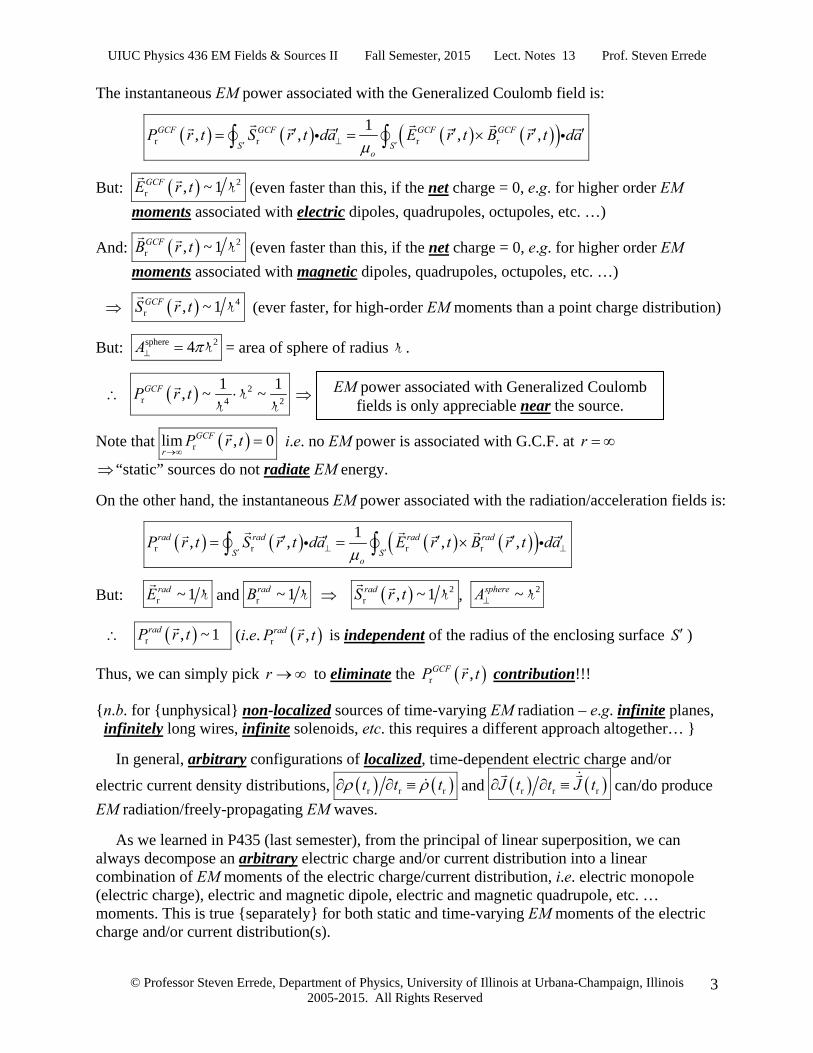
The instantaneous EM power associated with the Generalized Coulomb field is:

r r r r

1, , , ,GCF GCF GCF GCF

S So


But: 2r , ~ 1GCFE r t r (even faster than this, if the net charge = 0, e.g. for higher order EM

moments associated with electric dipoles, quadrupoles, octupoles, etc. …)

And: 2r , ~ 1GCFB r t r (even faster than this, if the net charge = 0, e.g. for higher order EM

moments associated with magnetic dipoles, quadrupoles, octupoles, etc. …)

4r , ~ 1GCFS r t r (ever faster, for high-order EM moments than a point charge distribution)

But: sphere 24A r = area of sphere of radius r .

2r 4 2

1 1, ~ ~GCFP r t rr r

Note that rlim , 0GCF

rP r t

i.e. no EM power is associated with G.C.F. at r

“static” sources do not radiate EM energy.

On the other hand, the instantaneous EM power associated with the radiation/acceleration fields is:

r r r r

1, , , ,rad rad rad rad

S So


But: r ~ 1radE

r and r ~ 1radB r 2r , ~ 1radS r t r , 2~sphereA r

r , ~ 1 radP r t

(i.e. r ,radP r t

is independent of the radius of the enclosing surface S )

Thus, we can simply pick r to eliminate the r ,GCFP r t

contribution!!!

{n.b. for {unphysical} non-localized sources of time-varying EM radiation – e.g. infinite planes, infinitely long wires, infinite solenoids, etc. this requires a different approach altogether… }

In general, arbitrary configurations of localized, time-dependent electric charge and/or

electric current density distributions, r r rt t t and r r rJ t t J t can/do produce

EM radiation/freely-propagating EM waves.

As we learned in P435 (last semester), from the principal of linear superposition, we can always decompose an arbitrary electric charge and/or current distribution into a linear combination of EM moments of the electric charge/current distribution, i.e. electric monopole (electric charge), electric and magnetic dipole, electric and magnetic quadrupole, etc. … moments. This is true {separately} for both static and time-varying EM moments of the electric charge and/or current distribution(s).

EM power associated with Generalized Coulomb fields is only appreciable near the source.



4

For a point electric monopole field {E(0)}, i.e. 3r r,r t q t t c r

r

r(E0)r '

,1,

4 4r

vo o

q t t cr tV r t d

rr r

Where rq t total electric charge of the source at the retarded time rt . But electric charge is

(always) conserved, and furthermore, (by definition) a localized source is one that does not have electric charge q flowing into or away from it. Therefore, the electric monopole moment contribution/portion associated with the (retarded) potential(s) and EM fields is of necessity static – i.e. the electric monopole moment q has no EM radiation associated with it. In other words, there can be no net transversely polarized EM radiation emitted from a spherically-symmetric charge distribution! {See e.g. J. D. Jackson Classical Electrodynamics 3rd ed. p. 410 for additional/further details.} The lowest-order electric multipole moment capable of producing EM radiation is that

associated with a time-varying electric dipole moment r r, ,p r t qd r t

or: r,q r t d

.

Electric dipole (E1) radiation originates from r,r t

The lowest-order magnetic multipole moment capable of producing EM radiation is that

associated with a time-varying magnetic dipole moment r r, ,m r t Ia r t

or: r,I r t a

.

Magnetic dipole (M1) radiation originates from r,J r t

Each time-varying, localized, higher-order EM moment contributes in alternating succession

between r,r t and r,J r t (i.e. electric vs. magnetic) multipole moment terms:

Time-varying localized Time-varying localized electric moments: magnetic moments:

, rr t , rJ r t

0E electric monopole qNO!

0M magnetic monopole g NO!

1E electric dipole p qd

1M magnetic dipole m Ia

2E electric quadrupole 2EQ qdd

2M magnetic quadrupole 2MQ Iaa

3E electric octupole

(3)M magnetic octupole

4E electric sextupole

… etc… 4M magnetic sextupole

no magnetic charges anyways…



5

We will consider/discuss the case of EM radiation from an oscillating E(1) electric dipole and then discuss case of radiation from an arbitrary localized source consisting of an arbitrary linear

combination of time-varying EM moments, 1

n nn

a E n b M n

, where and E n M n are

nth-order time-varying electric and magnetic multipole moments, respectively.

E(1) Electric Dipole Radiation:

Consider an oscillating (i.e. harmonic/sinusoidally time-varying) electric dipole: p t qd t

where the charge separation distance varies in time: ˆ ˆcosd t d t z d t z

, 2 f

Then: ˆ ˆcos cosp t qd t z p t z

, with: p qd .

Equivalently, we can alternatively think of this as: p t q t d

, with: ˆd dz

= constant,

and with time-varying/oscillating electric charge: cosq t q t .

Then: ˆ ˆcos cosp t qd t z p t z

, with: p qd . {n.b. same result!}

Either way one views/thinks about this, the physics associated with a harmonically time-

varying/oscillating electric dipole moment ˆ ˆcos cosp t p t z qd t z

is unchanged.

n.b. an electric current associated with the oscillating electric dipole: ˆ

dq tI t z

dt

, 0 0I t

A picture of this, for a given moment/instant/snapshot in time 0t is shown below:

n.b. exist (as always) some subtleties associated with the calculation of the retarded potentials associated with moving point charges – we will address these subsequently, but not right here /

right now… so, we’ll stick with the oscillating charge cosq t q t version for now…

z

y

x

p qd

q

q

I t r

r

r

Observation / Field Point

P r

2z d

2z d

n.b. The choice of origin is deliberately chosen at the center of the localized charge distribution – at

the center of the oscillating electric dipole.

r r r

r r r



6

Now ˆcosp t p t z

refers to the time-dependence associated with itself. An observer at

field point at P r r

“sees” the effects of the time-varying p t

manifest themselves at a finite

time later, rt t c r or: rt t c r due to the retarded nature of this problem.

Thus, p t

used in the formulae for the retarded scalar and vector potentials must be evaluated

at the retarded time rt , i.e. r r r ˆcosp t p t q t d qd t z

.

r r r r r rE(1)r

charge at charge at charge at charge atˆ ˆ + 2 2 ˆ ˆ + 2 2

cos cos cos cos,

4 4 4 4 4o o o o o

d z d z d z d z

q t q t t t t tq q qV r t

r r r r r

r

rE(1)r ,

4o

I tA r t d

r where: rr rsin

dq tI t q t

dt and: ˆd dzz

Explicitly inserting the retarded time(s): r t t c r :

E(1)r

cos cos,

4 o

t c t cqV r t

r rr r

2E(1)r 2

sinˆ,

4

z do

z d

t cqA r t dz z

rr

Let us first focus our attention on calculating E(1)r ,V r t . From the law of cosines {see P435

Lecture Notes 8 r.e. the derivation of the static multipole moment expansion}:

22 cos 2r rd d r

However, we want to investigate EM radiation in the “far zone” where r d . For this situation we can make the following approximation:

11 cos

4

d dr

r r

r

2

1 cosd

rr

But: 121 1 for 1 .

Thus:

11 cos 1 cos

2 2

d dr r

r r

r for r d .

Similarly/correspondingly:

1 1 11 cos

211 cos

2

d

r rdr

r

r for r d , since:

11

1

for 1 .



7

Likewise, for the cos t c r term, for the “far zone”, when r d we have:

cos cos 1 cos cos cos2 2

cos cos cos sin sin cos2 2

r d r dt c t t

c r c c

r d r dt t

c c c c

r

In order to proceed further, we need to make an additional simplifying assumption, namely that the characteristic spatial dimension a of the source (here, a = d) is wavelength of the emitted radiation, i.e. d { c f }. Thus we have: d c f { 2f }, or:

2d c or: d c .

n.b. This assumption is tantamount/physically equivalent to saying that we will neglect any/all time-retardation effects associated with finite EM propagation delay times over the dimensions characteristic of/associated with the source – i.e. changes in charge/current are essentially coherent/instantaneous over the {small} spatial dimensions of the source, relative to the wavelength of the emitted radiation.

Suppose we have a source (e.g. an atom) with 1 a d nm 10

emitting a 1 f Hz sine-wave. Since EM radiation travels propagates at 1 30 ft cm per nanosecond, a 1 nm dimension source doesn’t run into finite propagation decay time problems until:

c t a d (here) i.e. 1 c t nm 9

178

100.3 10 sec

3 10t

173 10f Hz

Thus, provided that we additionally are in the regime of d , or d c , i.e. 1d

c

.

Noting that if: 1d

c

, then: cos 1 2

d

c

{ 0 }.

Then from the Taylor series expansions of cos 1x and sin x x for very small 1x , we see that:

cos cos cos 0 12

d

c

and: sin cos cos

2 2

d d

c c

Thus: cos cos cos sin2

r d rt c t t

c c c

r

Thus:

E(1)r

1, , 1 cos cos cos sin

4 2 2

1 1 cos cos cos si

2 2

o

q d r d rV r t t t

r r c c c

d r dt

r r c c

n

rt

c



8

Expanding this out:

E(1)r

1, , cos

4 o

q rV r t t

r c

22

cos cos2

cos sin cos sin2 4

d rt

r c

d r d rt t

c c rc c

cosr

tc

2

2

cos cos2

cos sin cos sin2 4

d rt

r c

d r d rt t

c c rc c

Thus:

E(1)r

1, , cos cos cos sin

4

cos 1 cos sin

4

o

o

q d r d rV r t t t

r r c c c

qd r rt t

r r c c c

But: p p qd

. Hence in the “far-zone” d r and d :

E(1)r

cos 1, , sin cos

4 o

p r rV r t t t

r c c r c

In the “far-zone” d r , with the additional restriction that we’ve also imposed on the source EM radiation: d . We now additionally require/impose a third restriction that the “far-zone” also be such that r , thus we have the hierarchical relation: d r for “far-zone” EM

radiation, namely that for r c

r

, then 1

c r

i.e. 1 1

for rr

.

Thus for the far-zone, when d r we can neglect the second term in the above expression for E(1)

r , ,V r t .

Then: E(1)r

cos, , sin

4 o

p rV r t t

c r c

in the far-zone, for d r .

Note that in the static limit, when 0 it is necessary to retain the second term in the above

expression; we obtain in this limit: E(1)r 2

cos,

4 o

pV r

r

{cf w/ P435 Lect. Notes – same!}



9

Now let us focus our attention on calculating E(1)r ,A r t

:

2E(1)r 2

sinˆ,

4

z do

z d

t cqA r t dz z

rr

Because the integration itself introduces a factor of d, then to first order

in 1d r : 2 22 cosr rz z r r with: 2

dz

Thus: 2

2

sin sinz d

z d

t c t r cdz d

r

r

r

Then: E(1)r

1ˆ, sin

4o qd r

A r t t zr c

but: p qd

Thus: E(1)r

1ˆ, sin

4o p r

A r t t zr c

Note that in the static limit, when 0 then E(1)r , 0A r t

as we expect.

Now that we have obtained the (retarded) scalar and vector potentials E(1)r ,V r t and

E(1)r ,A r t

it is a “straight forward’ exercise to compute the associated (retarded) EM fields,

E(1) E(1)r r, and ,E r t B r t

:

E(1)rE(1) E(1)

r r

,, ,

A r tE r t V r t

t

and: E(1) E(1)

r r, ,B r t A r t

In spherical coordinates:

E (1)r ˆn.b. , has no explicit dependence

E(1)r

2

1 1 cosˆ ˆˆ, sinsin 4

1 cos sin cos

4

V r t

o

o

p rV r t r t

r r c r c

p r rt t

c r c rc c

2

1 ˆˆ sin sin

1 ˆˆ ˆcos cos cos sin sin sin4 o

rr t

r c

p r r rt r t r t

cr c c r c c

But for “far-zone” EM radiation, d r we have: 1

c r

~ 1 ~ 1 ~ 1

1cos cos cos sin sin sin

r r rt t t

c c r c c



10

So we can neglect/drop the 1 ˆˆcos sin sin sin

r rt r t

r c c

terms.

2

E(1)r 2

cosˆ, cos

4 o

p rV r t t r

c r c

And: E(1) 2

r , 1ˆ ˆsin cos

4 4o o

A r t p pr rt z t z

t r t c r c

But: ˆˆˆ cos sinz r in spherical coordinates.

E(1) 2

r , ˆˆcos cos sin4o

A r t p rt r

t r c

Then for far-zone EM radiation, with d r : E(1)rE(1) E(1)

r r

,, ,

A r tE r t V r t

t

22

E(1)r 2

ˆˆ ˆ, cos cos cos cos sin4 4

o

o

pp r rE r t t r t r

c r c r c

But: 2 1

o o

c

or: 2

1o oc

2

E(1)r ˆ, cos cos

4o p r

E r t t rr c

2

ˆcos cos4o p r

t rr c

2

ˆ cos sin4o p r

tr c

Or: 2

E(1)r

sin ˆ, cos4

o p rE r t t

r c

Then: E(1) E(1)r r, ,B r t A r t

with: E(1)r

1 1 ˆˆˆ, sin sin cos sin4 4o op pr rA r t t z t rc cr r

Thus:

E(1)r

1, sin

sinB r t A

r

0 A

0

1 1ˆ

sinrA

rr

0

r Ar

0 1ˆ ˆrA

rAr r



11

Thus:

E(1)r

1ˆ,

1 1

4

r

o

AB r t rA

r r

p

r r r

r 1 cosˆsin sin sin

1ˆ cos sin sin sin

4

4

o

o

r rt t

c r c

p r rt t

r c c r c

p

neglect

1ˆcos sin sin

r rt t

r c c r c

Again, 1

c r

here, because r , thus

2

E(1)r

sinˆ, cos

4o p r

B r t tc r c

and:

2E(1)r

sin ˆ, cos4

o p rE r t t

r c

Now since ˆ ˆr , once again we see that: E(1) E(1)r r

1ˆ, ,B r t r E r t

c

, i.e. ˆ and B E B r

Note also that:

a.) E(1) E(1)r r and E B

both vary as ~ 1 r .

b.) E(1) E(1)r r, and ,E r t B r t

are in-phase with each other.

c.) E(1) E(1)r r, and ,E r t B r t

have the same angular dependence ( ~ sin ).

The EM radiation energy density, E(1) ,radu r t

associated with the oscillating E(1) electric dipole

for far-zone EM radiation { d r } is:

E(1) E(1) E(1) E(1)E(1) E(1) E(1) r r r r

2 2 4 222

2 2

1 1, , , , , , ,

2

1 sin cos

2 16

rad Erad Mrado

o

o o o

u r t u r t u r t E r t E r t B r t B r t

p rt

r c

2 4

o

p

22

22 2

2 4 2 42 22 2

2 2 2 2 2 2

sincos

16

1 sin sin cos cos

2 16 16o o

rt

r cc

p pr rt t

c r c c r c

3

Joules

m

n.b. E(1) E(1), ,Erad Mradu r t u r t

using: 2 1 o oc or: 21o oc .

2 4 2

2E(1) 2 2 2

sin, cos

16rad o p r

u r t tc r c

3

Joules

m

for: d r “far zone” limit



12

The EM energy radiated by an oscillating electric dipole, in the “far zone” { d r } limit is given by Poynting’s vector:

E(1) E(1)E(1) r r

1, , ,rad

o

S r t E r t B r t

ˆ ˆˆ

ˆ ˆ ˆ

ˆˆ ˆ

r

r

r

E(1)

1,rad

o

S r t

o

2 22 2

ˆ

ˆ ˆsin cos4 4

o

r

p p rt

r rc c

Or: 2 4 2

2E(1) 2 2

sinˆ, cos

16rad o p r

S r t t rc r c

2

Watts

m

Radial outward flow of EM field energy for: d r “far zone” limit

The EM radiation linear momentum density associated with an oscillating electric dipole, in the far zone { d r } is given by:

E(1) E(1) E(1)2

1, , ,rad rad rad

o or t S r t S r tc

Or: 2 4

2 2E(1) 2 2 3

ˆ, cos sin16

rad o p rr t t r

r c c

2 -sec

kg

m

Radial outward EM field linear momentum for: d r “far zone” limit The EM radiation angular momentum density associated with an oscillating electric dipole, in the far zone { d r } is given by:

E(1) E(1), ,rad radr t r r t

2 4

2 2E(1) 2 2 3

ˆ ˆ, cos sin 016

rad o p rr t t r r

r c c

-sec

kg

m

No EM field angular momentum for: d r “far zone” limit

n.b. The exact E(1) ,rad r t 0 i.e. ignore restrictions on far-zone limit, keep all higher-order

terms . . . we have neglected E(1)r ˆ~E r

term which is non-negligible in the near-zone ~d r

and also in the so-called intermediate, or inductive zone ~ r .



13

Time-Averaged Quantities for E(1) Radiation from an Oscillating Electric Dipole:

Recall the definition of time average: 2

0 0

1 1 1cos

2

t t

o ot tA t A t dt A t dt A

The time-averaged EM radiation energy density associated with an oscillating electric dipole is:

2 4 2

E(1) 2 2 2

sin,

32rad o p

u r tc r

3

Joules

m

for: d r “far-zone” limit

The time-averaged |Poynting’s vector|, which is also the intensity E(1)radI of EM radiation

associated with an oscillating electric dipole is:

2 4 2

2E(1)E(1) E(1) r 2 2

1 sin, ,

2 32rad rad o

o

pI r S r t c E r t

c r

2

Watts

m

for:

We also see that: E(1) E(1) E(1), ,rad rad radI r S r t c u r t

2

Watts

m

.

The time-averaged EM radiated power associated with an oscillating electric dipole is:

2 4

E(1) E(1) 2 2, ,

32rad rad o

S

pP r t S r t da

c r

2r

2 2

0 0cos

2 4

16

sin sin

32

d

o

d d

p

2 2

2c

2 4

2 220 0

sin cos sin cos16

o pd d

c

Let: cosu , cosdu d , 0 1u , 1u , 2 2 2sin 1 cos 1 u

1

1 2 3

11

1 1 1 2 41 1 1 2

3 3 3 3 3u du u u

The time-averaged radiated power associated with an oscillating electric dipole is:

2 4

E(1) ,12

rad o pP r t

c

(Watts) for: d r “far-zone” limit

Note that time-averaged radiated power varies as the 4th power of frequency! The time-averaged EM radiation linear momentum density associated with an oscillating electric dipole is:

2 4 2

E(1) E(1) E(1)2 2 3 2

1 1 sinˆ ˆ, , ,

32rad rad rad o p

r t S r t u r t r rc c c r

2 -

kg

m sec

for:

d r “far-zone” limit

n.b. E(1) ,radP r t

has

no r-dependence!




14

The time-averaged EM radiation angular momentum density associated with an oscillating electric dipole is:

2 4 2

E(1) E(1) 2 3

sinˆ ˆ, , 0

32rad rad o p

r t r r t r rc r

-sec

kg

m

for:

n.b. The exact E(1)rad r 0 i.e. ignore restrictions on far-zone limit, keep all higher-order

terms . . . we have neglected the E(1)r ˆ~E r

term which is non-negligible in the near-zone ~d r

and also in the so-called intermediate, or inductive zone ~ r .

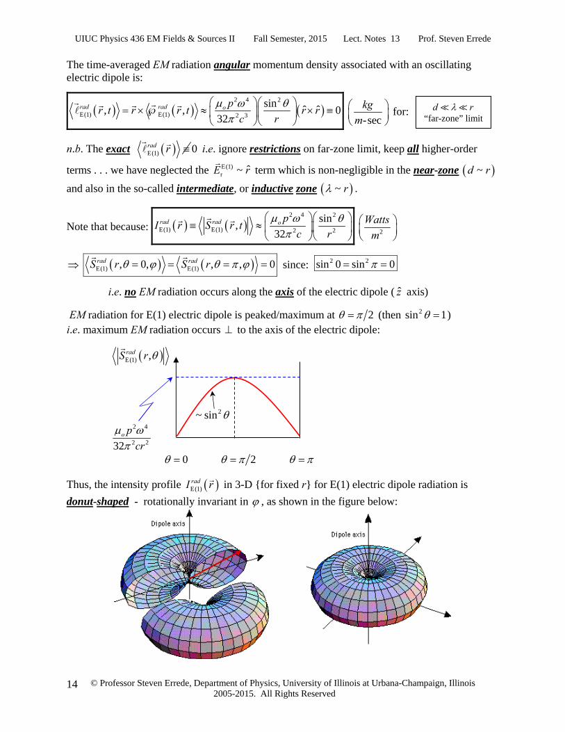
Note that because: 2 4 2

E(1) E(1) 2 2

sin,

32rad rad o p

I r S r tc r

2

Watts

m

E(1) E(1), 0, , , 0rad radS r S r

since: 2 2sin 0 sin 0

i.e. no EM radiation occurs along the axis of the electric dipole ( z axis)

EM radiation for E(1) electric dipole is peaked/maximum at 2 (then 2sin 1 ) i.e. maximum EM radiation occurs to the axis of the electric dipole:

E(1) ,radS r

2~ sin

2 4

2 232o p

cr

0 2

Thus, the intensity profile E(1)radI r

in 3-D {for fixed r} for E(1) electric dipole radiation is

donut-shaped - rotationally invariant in , as shown in the figure below:




15

Griffiths Example 11.1:

The time-averaged power for E(1) electric dipole radiation is 2 4

E(1) 12rad o p

Pc

.

Note that 4E(1) ~radP 4 4(or ~ , or ~ )f

For red light: red 780 nm 8

14red 9

red

3 10 3.85 10

780 10

cf Hz

For violet light: violet 350 nm 8

14violet 9

violet

3 108.57 10

350 10

cf Hz

Hence: 4 4violet 14

4E(1) violet14red

redE(1)

8.57 102.23 24.67

3.85 10

P f

fP

.

4E(1) ~radP explains why the sky is blue! Sunlight {unpolarized light} incident on O2 & N2

molecules in the earth’s atmosphere stimulates the O & N atoms – vibrates the {bound} atomic electrons at {angular} frequency , causing them to oscillate as electric dipoles! Solar EM radiation at a given angular frequency is thus absorbed and re-emitted in this EM radiation + atom scattering process.

The above formula for EM power radiated as E(1) electric dipole radiation by such atoms, by time-reversal invariance of the EM interaction, is also the EM power absorbed by atoms, thus we

see that because of the 4 -dependence of E(1)radP , the higher frequency/shorter wavelength

radiation (i.e. blue/violet light) is preferentially scattered much more so than the lower frequency/longer wavelength radiation (i.e. red light). The Earth’s sky appears blue {e.g. to an observer on the ground, or even e.g. a space shuttle astronaut in orbit around the earth} because the light from the sky is scattered (i.e. re-radiated) light, which is preferentially in the blue/violet portion of the visible light EM spectrum. The scattering of EM radiation off of atoms is known as Rayleigh scattering.

Note that precisely same physics also simultaneously explains why the Sun appears red e.g. to an observer on the ground at sunrise and sunset – because at these times of the day, path that the sunlight takes through the atmosphere is the longest, relative to that associated e.g. with its position at {local} noon. If the higher-frequency blue/violet light is preferentially scattered out of the beam of sunlight, what is left in the beam of sunlight after traversing the entire thickness of the Earth’s atmosphere is the lower-frequency, orange-red light.



16

Note that the Sun is a black-body radiator – its EM spectrum peaks in the infra-red region – thus it is NOT flat by any means {also is affected by frequency-dependent absorption in the atmosphere}:

Note the log scale on the vertical axis! Thus, there is not much violet light in the Sun’s EM spectrum, and hence there is a delicate “balancing” act of flux of EM radiation from the Sun {convoluted} with its black-body spectrum and the scattering of this radiation by atoms in the Earth’s atmosphere – thus we see the sky as blue. Thus, if the black-body temperature of the sun was different, then the color of the Earth’s sky in the visible portion of the EM spectrum would also be different – compare the black-body spectra of our Sun e.g. with that of Spica (260 ly away in the Virgo constellation) and Antares (a red giant 600 ly away in the Scorpio constellation):



17

Light from the Sun is unpolarized (i.e. it consists of all polarizations, randomly oriented over time). However, because EM waves are transversely polarized (defined by the orientation of the E

-field vector) an incident EM plane wave from the Sun with polarization in a given

direction ( to k

-propagation direction) will (transitorily) induce electric dipole moments in

gas atoms in earth’s atmosphere, via mol mol incp E

, where mol is the molecular

polarizability at {angular} frequency {see P435 Lect. Notes 12 and P436 Lect. Notes 7.5}.

The axis of induced electric dipole moments will be || to the plane of polarization of incident wave at that instant, hence the scattered radiation emitted by the atom will be preferentially at

90 2 (i.e. ) to the axis of the (induced) electric dipole of gas atoms in earth’s

atmosphere. There are two specific/limiting cases to consider – (a) when the incident E

-field vector is vertical and (b) when the incident E

-field vector is horizontal. Random polarization is

then an arbitrary linear combination of these two limiting cases:

(a.) incE

vertical:

(b.) incE

horizontal:

Earth

Atom

incB

inck

incE

inducedp

scatE

scatB

scatk

90oscat

= Line of sight

Earth

Atom

incB

inck

incE

inducedp

scatE

scatB

scatk

90oscat

= Line of sight

Same atom and same observer, but observer doesn’t see this scattered radiation – E(1) electric dipoles oscillating along the line-of-sight do not radiate in that direction.

Note: Escat || pinduced || Einc for scat = 90o (max probable direction of emission). E(1) electric dipoles oscillating to line -of-sight preferentially tend to radiate in the line-of-sight direction.



18

Because the blue light an observer sees from a given portion of the sky is due to the preferential scattering of E(1) electric dipole-type Rayleigh scattering of sunlight/solar EM

radiation off of gas atoms in the Earth’s atmosphere, with scatE

to the line-of-sight, this

radiation has a net polarization – i.e. the light from the sky is polarized, especially so away from the sun, i.e. in the northern portions of the sky {in the northern hemisphere} !!! You can very easily observe/explicitly verify this using a pair of polaroid sunglasses – try it some time!!!

It is beneficial to wear polaroid sunglasses e.g. when out boating on a lake – in order to reduce “glare” from {polarized} sunlight reflected off of the surface of the water!!!

As mentioned above, at sunrise or sunset, the sun appears red when an observer is looking directly at the sun, because the blue/violet light is ~ 25 more preferentially scattered out of the beam of light incident from the sun {per unit thickness of atmosphere} than red light. Thus sunlight when the sun is near the horizon consists predominantly of what remains – red light.

Note that this is also true for moonrise and moonset – the moon will {likewise} have a reddish hue at these times, and note that this is also true e.g. for the case of an eclipse of the moon by the Earth.

One can also observe this same phenomenon e.g. using a glass pitcher of milk diluted with water – because milk molecules are efficient Rayleigh scatterers of visible light! Here’s a simple experiment that you can carry out at home, e.g. using a flashlight:



19

The {scalar} EM wave characteristic radiation impedance of an antenna is exactly as we defined the characteristic impedance of a waveguide; noting here that we are dealing with manifestly transverse waves for EM wave radiation from an E(1) electric dipole antenna:

1 1

rad rad rad

antenna radrad rad

o o

E r E r E rZ r

H r B r B r

Let’s check the SI units of this definition:

2-

o

Volts VoltsE Voltsm m Ohms

HenrysB AmpsN NTeslas A m Am

For E(1) electric dipole radiation, the EM wave characteristic radiation impedance in the “far-

zone” limit ( d r ) with 1 o oc is:

2

E(1)r

sin ˆ, cos4

o p rE r t t

r c

and:

2E(1)r

sinˆ, cos

4o p r

B r t tc r c

2

(1)4

oo

antenna

p

Z r

sinr

cosr

tc

2

4o

c

p

sinr

cosr

tc

120 377 oo o

o

c Z

Where: 74 10o Henrys/m = magnetic permeability of free space / vacuum

128.85 10o Farads/m = electric permittivity of free space / vacuum

And: 7

12

4 10 Henrys / m120 377

8.85 10 Farads / mo

oo

Z

Thus we see that E(1) electric dipole antennae (in the “far-zone” limit ( d b r )) are perfectly impedance-matched for propagation of E(1) EM waves into free space / vacuum!

Note also that the “far-zone” ( d r ) EM wave characteristic radiation impedance

(1)antennaZ r

has no spatial and/or frequency dependence.

= {scalar} characteristic impedance of free space/the vacuum.



20

The EM Wave Radiation Resistance of an Antenna:

The {scalar} EM wave radiation resistance of an antenna Rrad is defined in terms of the antenna power Prad and the amplitude of the current I flowing in the antenna:

2antenna antennarad radP I R or:

2antenna antennarad radR P I (Ohms)

For an E(1) electric dipole antenna: I = qω = amplitude of current flowing in the dipole.

In the “far-zone” limit, i.e. d r :

22 4(1)

3 2

12oo

rad

qpR

c I

2 4d

212 c q 2

2 2

12o d

c

In the “far-zone” limit, i.e. d r :

2 2 2 2 2 2 2 2

(1) (1)2 2 2

12 12 12 12o o

rad o rado

d d d dR c Z

c c c c

But: (1)o

o rado

Z Z

In the “far-zone” limit, d r :

22 2(1)

2

1

12 12rad o o

d dR Z Z

c c

However, in the “far-zone” limit, d r we have: 1d

c

Thus, we see that the EM wave radiation resistance (1)radR associated with E(1) electric dipole

antenna in the “far-zone” limit ( d r ) is much less than the EM wave characteristic

radiation impedance (1),M(1) 120 377 rad oZ Z of an electric dipole antenna:

2(1) 1

377 12rad o o

dR Z Z

c

n.b. (1)radR is

frequency-dependent!

p436 lect 13 - university of illinois at...

Documents