package 'aer
TRANSCRIPT
Package ‘AER’January 7, 2017
Version 1.2-5
Date 2017-01-06
Title Applied Econometrics with R
Description Functions, data sets, examples, demos, and vignettes for the bookChristian Kleiber and Achim Zeileis (2008),Applied Econometrics with R, Springer-Verlag, New York.ISBN 978-0-387-77316-2. (See the vignette ``AER'' for a package overview.)
LazyLoad yes
Depends R (>= 2.13.0), car (>= 2.0-19), lmtest, sandwich, survival (>=2.37-5), zoo
Suggests boot, dynlm, effects, fGarch, forecast, foreign, ineq,KernSmooth, lattice, longmemo, MASS, mlogit, nlme, nnet, np,plm, pscl, quantreg, rgl, ROCR, rugarch, sampleSelection,scatterplot3d, strucchange, systemfit, truncreg, tseries, urca,vars
Imports stats, Formula (>= 0.2-0)
License GPL-2 | GPL-3
NeedsCompilation no
Author Christian Kleiber [aut],Achim Zeileis [aut, cre]
Maintainer Achim Zeileis <[email protected]>
Repository CRAN
Date/Publication 2017-01-07 00:11:57
R topics documented:Affairs . . . . . . . . . . . . . . . . . . . . . . . . . . . . . . . . . . . . . . . . . . . . 4ArgentinaCPI . . . . . . . . . . . . . . . . . . . . . . . . . . . . . . . . . . . . . . . . 5Baltagi2002 . . . . . . . . . . . . . . . . . . . . . . . . . . . . . . . . . . . . . . . . . 6BankWages . . . . . . . . . . . . . . . . . . . . . . . . . . . . . . . . . . . . . . . . . 10BenderlyZwick . . . . . . . . . . . . . . . . . . . . . . . . . . . . . . . . . . . . . . . 11
1
2 R topics documented:
BondYield . . . . . . . . . . . . . . . . . . . . . . . . . . . . . . . . . . . . . . . . . . 12CameronTrivedi1998 . . . . . . . . . . . . . . . . . . . . . . . . . . . . . . . . . . . . 13CartelStability . . . . . . . . . . . . . . . . . . . . . . . . . . . . . . . . . . . . . . . . 16CASchools . . . . . . . . . . . . . . . . . . . . . . . . . . . . . . . . . . . . . . . . . 17ChinaIncome . . . . . . . . . . . . . . . . . . . . . . . . . . . . . . . . . . . . . . . . 19CigarettesB . . . . . . . . . . . . . . . . . . . . . . . . . . . . . . . . . . . . . . . . . 20CigarettesSW . . . . . . . . . . . . . . . . . . . . . . . . . . . . . . . . . . . . . . . . 21CollegeDistance . . . . . . . . . . . . . . . . . . . . . . . . . . . . . . . . . . . . . . . 23ConsumerGood . . . . . . . . . . . . . . . . . . . . . . . . . . . . . . . . . . . . . . . 24CPS1985 . . . . . . . . . . . . . . . . . . . . . . . . . . . . . . . . . . . . . . . . . . 25CPS1988 . . . . . . . . . . . . . . . . . . . . . . . . . . . . . . . . . . . . . . . . . . 27CPSSW . . . . . . . . . . . . . . . . . . . . . . . . . . . . . . . . . . . . . . . . . . . 29CreditCard . . . . . . . . . . . . . . . . . . . . . . . . . . . . . . . . . . . . . . . . . . 30dispersiontest . . . . . . . . . . . . . . . . . . . . . . . . . . . . . . . . . . . . . . . . 32DJFranses . . . . . . . . . . . . . . . . . . . . . . . . . . . . . . . . . . . . . . . . . . 34DJIA8012 . . . . . . . . . . . . . . . . . . . . . . . . . . . . . . . . . . . . . . . . . . 35DoctorVisits . . . . . . . . . . . . . . . . . . . . . . . . . . . . . . . . . . . . . . . . . 36DutchAdvert . . . . . . . . . . . . . . . . . . . . . . . . . . . . . . . . . . . . . . . . 37DutchSales . . . . . . . . . . . . . . . . . . . . . . . . . . . . . . . . . . . . . . . . . 38Electricity1955 . . . . . . . . . . . . . . . . . . . . . . . . . . . . . . . . . . . . . . . 39Electricity1970 . . . . . . . . . . . . . . . . . . . . . . . . . . . . . . . . . . . . . . . 41EquationCitations . . . . . . . . . . . . . . . . . . . . . . . . . . . . . . . . . . . . . . 42Equipment . . . . . . . . . . . . . . . . . . . . . . . . . . . . . . . . . . . . . . . . . . 44EuroEnergy . . . . . . . . . . . . . . . . . . . . . . . . . . . . . . . . . . . . . . . . . 46Fatalities . . . . . . . . . . . . . . . . . . . . . . . . . . . . . . . . . . . . . . . . . . . 47Fertility . . . . . . . . . . . . . . . . . . . . . . . . . . . . . . . . . . . . . . . . . . . 50Franses1998 . . . . . . . . . . . . . . . . . . . . . . . . . . . . . . . . . . . . . . . . . 52FrozenJuice . . . . . . . . . . . . . . . . . . . . . . . . . . . . . . . . . . . . . . . . . 54GermanUnemployment . . . . . . . . . . . . . . . . . . . . . . . . . . . . . . . . . . . 55GoldSilver . . . . . . . . . . . . . . . . . . . . . . . . . . . . . . . . . . . . . . . . . . 56Greene2003 . . . . . . . . . . . . . . . . . . . . . . . . . . . . . . . . . . . . . . . . . 58GrowthDJ . . . . . . . . . . . . . . . . . . . . . . . . . . . . . . . . . . . . . . . . . . 77GrowthSW . . . . . . . . . . . . . . . . . . . . . . . . . . . . . . . . . . . . . . . . . 79Grunfeld . . . . . . . . . . . . . . . . . . . . . . . . . . . . . . . . . . . . . . . . . . . 80GSOEP9402 . . . . . . . . . . . . . . . . . . . . . . . . . . . . . . . . . . . . . . . . . 83GSS7402 . . . . . . . . . . . . . . . . . . . . . . . . . . . . . . . . . . . . . . . . . . 85Guns . . . . . . . . . . . . . . . . . . . . . . . . . . . . . . . . . . . . . . . . . . . . . 88HealthInsurance . . . . . . . . . . . . . . . . . . . . . . . . . . . . . . . . . . . . . . . 89HMDA . . . . . . . . . . . . . . . . . . . . . . . . . . . . . . . . . . . . . . . . . . . 91HousePrices . . . . . . . . . . . . . . . . . . . . . . . . . . . . . . . . . . . . . . . . . 92ivreg . . . . . . . . . . . . . . . . . . . . . . . . . . . . . . . . . . . . . . . . . . . . . 93ivreg.fit . . . . . . . . . . . . . . . . . . . . . . . . . . . . . . . . . . . . . . . . . . . 96Journals . . . . . . . . . . . . . . . . . . . . . . . . . . . . . . . . . . . . . . . . . . . 97KleinI . . . . . . . . . . . . . . . . . . . . . . . . . . . . . . . . . . . . . . . . . . . . 99Longley . . . . . . . . . . . . . . . . . . . . . . . . . . . . . . . . . . . . . . . . . . . 100ManufactCosts . . . . . . . . . . . . . . . . . . . . . . . . . . . . . . . . . . . . . . . 101MarkDollar . . . . . . . . . . . . . . . . . . . . . . . . . . . . . . . . . . . . . . . . . 102MarkPound . . . . . . . . . . . . . . . . . . . . . . . . . . . . . . . . . . . . . . . . . 103
R topics documented: 3
MASchools . . . . . . . . . . . . . . . . . . . . . . . . . . . . . . . . . . . . . . . . . 105Medicaid1986 . . . . . . . . . . . . . . . . . . . . . . . . . . . . . . . . . . . . . . . . 106Mortgage . . . . . . . . . . . . . . . . . . . . . . . . . . . . . . . . . . . . . . . . . . 108MotorCycles . . . . . . . . . . . . . . . . . . . . . . . . . . . . . . . . . . . . . . . . 109MotorCycles2 . . . . . . . . . . . . . . . . . . . . . . . . . . . . . . . . . . . . . . . . 110MSCISwitzerland . . . . . . . . . . . . . . . . . . . . . . . . . . . . . . . . . . . . . . 111Municipalities . . . . . . . . . . . . . . . . . . . . . . . . . . . . . . . . . . . . . . . . 113MurderRates . . . . . . . . . . . . . . . . . . . . . . . . . . . . . . . . . . . . . . . . 114NaturalGas . . . . . . . . . . . . . . . . . . . . . . . . . . . . . . . . . . . . . . . . . 115NMES1988 . . . . . . . . . . . . . . . . . . . . . . . . . . . . . . . . . . . . . . . . . 116NYSESW . . . . . . . . . . . . . . . . . . . . . . . . . . . . . . . . . . . . . . . . . . 119OECDGas . . . . . . . . . . . . . . . . . . . . . . . . . . . . . . . . . . . . . . . . . . 120OECDGrowth . . . . . . . . . . . . . . . . . . . . . . . . . . . . . . . . . . . . . . . . 121OlympicTV . . . . . . . . . . . . . . . . . . . . . . . . . . . . . . . . . . . . . . . . . 123OrangeCounty . . . . . . . . . . . . . . . . . . . . . . . . . . . . . . . . . . . . . . . . 124Parade2005 . . . . . . . . . . . . . . . . . . . . . . . . . . . . . . . . . . . . . . . . . 124PepperPrice . . . . . . . . . . . . . . . . . . . . . . . . . . . . . . . . . . . . . . . . . 126PhDPublications . . . . . . . . . . . . . . . . . . . . . . . . . . . . . . . . . . . . . . 127ProgramEffectiveness . . . . . . . . . . . . . . . . . . . . . . . . . . . . . . . . . . . . 128PSID1976 . . . . . . . . . . . . . . . . . . . . . . . . . . . . . . . . . . . . . . . . . . 129PSID1982 . . . . . . . . . . . . . . . . . . . . . . . . . . . . . . . . . . . . . . . . . . 133PSID7682 . . . . . . . . . . . . . . . . . . . . . . . . . . . . . . . . . . . . . . . . . . 134RecreationDemand . . . . . . . . . . . . . . . . . . . . . . . . . . . . . . . . . . . . . 136ResumeNames . . . . . . . . . . . . . . . . . . . . . . . . . . . . . . . . . . . . . . . 138ShipAccidents . . . . . . . . . . . . . . . . . . . . . . . . . . . . . . . . . . . . . . . . 140SIC33 . . . . . . . . . . . . . . . . . . . . . . . . . . . . . . . . . . . . . . . . . . . . 142SmokeBan . . . . . . . . . . . . . . . . . . . . . . . . . . . . . . . . . . . . . . . . . . 143SportsCards . . . . . . . . . . . . . . . . . . . . . . . . . . . . . . . . . . . . . . . . . 144STAR . . . . . . . . . . . . . . . . . . . . . . . . . . . . . . . . . . . . . . . . . . . . 146StockWatson2007 . . . . . . . . . . . . . . . . . . . . . . . . . . . . . . . . . . . . . . 149StrikeDuration . . . . . . . . . . . . . . . . . . . . . . . . . . . . . . . . . . . . . . . . 160summary.ivreg . . . . . . . . . . . . . . . . . . . . . . . . . . . . . . . . . . . . . . . . 162SwissLabor . . . . . . . . . . . . . . . . . . . . . . . . . . . . . . . . . . . . . . . . . 163TeachingRatings . . . . . . . . . . . . . . . . . . . . . . . . . . . . . . . . . . . . . . 164TechChange . . . . . . . . . . . . . . . . . . . . . . . . . . . . . . . . . . . . . . . . . 166tobit . . . . . . . . . . . . . . . . . . . . . . . . . . . . . . . . . . . . . . . . . . . . . 167TradeCredit . . . . . . . . . . . . . . . . . . . . . . . . . . . . . . . . . . . . . . . . . 168TravelMode . . . . . . . . . . . . . . . . . . . . . . . . . . . . . . . . . . . . . . . . . 169UKInflation . . . . . . . . . . . . . . . . . . . . . . . . . . . . . . . . . . . . . . . . . 170UKNonDurables . . . . . . . . . . . . . . . . . . . . . . . . . . . . . . . . . . . . . . 171USAirlines . . . . . . . . . . . . . . . . . . . . . . . . . . . . . . . . . . . . . . . . . 172USConsump1950 . . . . . . . . . . . . . . . . . . . . . . . . . . . . . . . . . . . . . . 174USConsump1979 . . . . . . . . . . . . . . . . . . . . . . . . . . . . . . . . . . . . . . 175USConsump1993 . . . . . . . . . . . . . . . . . . . . . . . . . . . . . . . . . . . . . . 176USCrudes . . . . . . . . . . . . . . . . . . . . . . . . . . . . . . . . . . . . . . . . . . 177USGasB . . . . . . . . . . . . . . . . . . . . . . . . . . . . . . . . . . . . . . . . . . . 178USGasG . . . . . . . . . . . . . . . . . . . . . . . . . . . . . . . . . . . . . . . . . . . 179USInvest . . . . . . . . . . . . . . . . . . . . . . . . . . . . . . . . . . . . . . . . . . . 181
4 Affairs
USMacroB . . . . . . . . . . . . . . . . . . . . . . . . . . . . . . . . . . . . . . . . . 182USMacroG . . . . . . . . . . . . . . . . . . . . . . . . . . . . . . . . . . . . . . . . . 183USMacroSW . . . . . . . . . . . . . . . . . . . . . . . . . . . . . . . . . . . . . . . . 185USMacroSWM . . . . . . . . . . . . . . . . . . . . . . . . . . . . . . . . . . . . . . . 187USMacroSWQ . . . . . . . . . . . . . . . . . . . . . . . . . . . . . . . . . . . . . . . 188USMoney . . . . . . . . . . . . . . . . . . . . . . . . . . . . . . . . . . . . . . . . . . 189USProdIndex . . . . . . . . . . . . . . . . . . . . . . . . . . . . . . . . . . . . . . . . 190USSeatBelts . . . . . . . . . . . . . . . . . . . . . . . . . . . . . . . . . . . . . . . . . 191USStocksSW . . . . . . . . . . . . . . . . . . . . . . . . . . . . . . . . . . . . . . . . 192WeakInstrument . . . . . . . . . . . . . . . . . . . . . . . . . . . . . . . . . . . . . . . 193WinkelmannBoes2009 . . . . . . . . . . . . . . . . . . . . . . . . . . . . . . . . . . . 194
Index 202
Affairs Fair’s Extramarital Affairs Data
Description
Infidelity data, known as Fair’s Affairs. Cross-section data from a survey conducted by PsychologyToday in 1969.
Usage
data("Affairs")
Format
A data frame containing 601 observations on 9 variables.
affairs numeric. How often engaged in extramarital sexual intercourse during the past year?
gender factor indicating gender.
age numeric variable coding age in years: 17.5 = under 20, 22 = 20–24, 27 = 25–29, 32 = 30–34,37 = 35–39, 42 = 40–44, 47 = 45–49, 52 = 50–54, 57 = 55 or over.
yearsmarried numeric variable coding number of years married: 0.125 = 3 months or less, 0.417= 4–6 months, 0.75 = 6 months–1 year, 1.5 = 1–2 years, 4 = 3–5 years, 7 = 6–8 years, 10 =9–11 years, 15 = 12 or more years.
children factor. Are there children in the marriage?
religiousness numeric variable coding religiousness: 1 = anti, 2 = not at all, 3 = slightly, 4 =somewhat, 5 = very.
education numeric variable coding level of education: 9 = grade school, 12 = high school graduate,14 = some college, 16 = college graduate, 17 = some graduate work, 18 = master’s degree, 20= Ph.D., M.D., or other advanced degree.
occupation numeric variable coding occupation according to Hollingshead classification (reversenumbering).
rating numeric variable coding self rating of marriage: 1 = very unhappy, 2 = somewhat unhappy,3 = average, 4 = happier than average, 5 = very happy.
ArgentinaCPI 5
Source
Online complements to Greene (2003). Table F22.2.
http://pages.stern.nyu.edu/~wgreene/Text/tables/tablelist5.htm
References
Greene, W.H. (2003). Econometric Analysis, 5th edition. Upper Saddle River, NJ: Prentice Hall.
Fair, R.C. (1978). A Theory of Extramarital Affairs. Journal of Political Economy, 86, 45–61.
See Also
Greene2003
Examples
data("Affairs")
## Greene (2003)## Tab. 22.3 and 22.4fm_ols <- lm(affairs ~ age + yearsmarried + religiousness + occupation + rating,
data = Affairs)fm_probit <- glm(I(affairs > 0) ~ age + yearsmarried + religiousness + occupation + rating,
data = Affairs, family = binomial(link = "probit"))
fm_tobit <- tobit(affairs ~ age + yearsmarried + religiousness + occupation + rating,data = Affairs)
fm_tobit2 <- tobit(affairs ~ age + yearsmarried + religiousness + occupation + rating,right = 4, data = Affairs)
fm_pois <- glm(affairs ~ age + yearsmarried + religiousness + occupation + rating,data = Affairs, family = poisson)
library("MASS")fm_nb <- glm.nb(affairs ~ age + yearsmarried + religiousness + occupation + rating,
data = Affairs)
## Tab. 22.6library("pscl")fm_zip <- zeroinfl(affairs ~ age + yearsmarried + religiousness + occupation + rating | age +
yearsmarried + religiousness + occupation + rating, data = Affairs)
ArgentinaCPI Consumer Price Index in Argentina
Description
Time series of consumer price index (CPI) in Argentina (index with 1969(4) = 1).
6 Baltagi2002
Usage
data("ArgentinaCPI")
Format
A quarterly univariate time series from 1970(1) to 1989(4).
Source
Online complements to Franses (1998).
References
De Ruyter van Steveninck, M.A. (1996). The Impact of Capital Imports; Argentina 1970–1989.Amsterdam: Thesis Publishers.
Franses, P.H. (1998). Time Series Models for Business and Economic Forecasting. Cambridge, UK:Cambridge University Press.
See Also
Franses1998
Examples
data("ArgentinaCPI")plot(ArgentinaCPI)plot(log(ArgentinaCPI))
library("dynlm")## estimation sample 1970.3-1988.4 meansacpi <- window(ArgentinaCPI, start = c(1970,1), end = c(1988,4))
## eq. (3.90), p.54acpi_ols <- dynlm(d(log(acpi)) ~ L(d(log(acpi))))summary(acpi_ols)
## alternativelyar(diff(log(acpi)), order.max = 1, method = "ols")
Baltagi2002 Data and Examples from Baltagi (2002)
Description
This manual page collects a list of examples from the book. Some solutions might not be exact andthe list is certainly not complete. If you have suggestions for improvement (preferably in the formof code), please contact the package maintainer.
Baltagi2002 7
References
Baltagi, B.H. (2002). Econometrics, 3rd ed., Berlin: Springer-Verlag.
See Also
BenderlyZwick, CigarettesB, EuroEnergy, Grunfeld, Mortgage, NaturalGas, OECDGas, OrangeCounty,PSID1982, TradeCredit, USConsump1993, USCrudes, USGasB, USMacroB
Examples
################################## Cigarette consumption data ##################################
## datadata("CigarettesB", package = "AER")
## Table 3.3cig_lm <- lm(packs ~ price, data = CigarettesB)summary(cig_lm)
## Figure 3.9plot(residuals(cig_lm) ~ price, data = CigarettesB)abline(h = 0, lty = 2)
## Figure 3.10cig_pred <- with(CigarettesB,
data.frame(price = seq(from = min(price), to = max(price), length = 30)))cig_pred <- cbind(cig_pred, predict(cig_lm, newdata = cig_pred, interval = "confidence"))plot(packs ~ price, data = CigarettesB)lines(fit ~ price, data = cig_pred)lines(lwr ~ price, data = cig_pred, lty = 2)lines(upr ~ price, data = cig_pred, lty = 2)
## Chapter 5: diagnostic tests (p. 111-115)cig_lm2 <- lm(packs ~ price + income, data = CigarettesB)summary(cig_lm2)## Glejser tests (p. 112)ares <- abs(residuals(cig_lm2))summary(lm(ares ~ income, data = CigarettesB))summary(lm(ares ~ I(1/income), data = CigarettesB))summary(lm(ares ~ I(1/sqrt(income)), data = CigarettesB))summary(lm(ares ~ sqrt(income), data = CigarettesB))## Goldfeld-Quandt test (p. 112)gqtest(cig_lm2, order.by = ~ income, data = CigarettesB, fraction = 12, alternative = "less")## NOTE: Baltagi computes the test statistic as mss1/mss2,## i.e., tries to find decreasing variances. gqtest() always uses## mss2/mss1 and has an "alternative" argument.
## Spearman rank correlation test (p. 113)cor.test(~ ares + income, data = CigarettesB, method = "spearman")## Breusch-Pagan test (p. 113)

8 Baltagi2002
bptest(cig_lm2, varformula = ~ income, data = CigarettesB, student = FALSE)## White test (Table 5.1, p. 113)bptest(cig_lm2, ~ income * price + I(income^2) + I(price^2), data = CigarettesB)## White HC standard errors (Table 5.2, p. 114)coeftest(cig_lm2, vcov = vcovHC(cig_lm2, type = "HC1"))## Jarque-Bera test (Figure 5.2, p. 115)hist(residuals(cig_lm2), breaks = 16, ylim = c(0, 10), col = "lightgray")library("tseries")jarque.bera.test(residuals(cig_lm2))
## Tables 8.1 and 8.2influence.measures(cig_lm2)
####################################### US consumption data (1950-1993) #######################################
## datadata("USConsump1993", package = "AER")plot(USConsump1993, plot.type = "single", col = 1:2)
## Chapter 5 (p. 122-125)fm <- lm(expenditure ~ income, data = USConsump1993)summary(fm)## Durbin-Watson test (p. 122)dwtest(fm)## Breusch-Godfrey test (Table 5.4, p. 124)bgtest(fm)## Newey-West standard errors (Table 5.5, p. 125)coeftest(fm, vcov = NeweyWest(fm, lag = 3, prewhite = FALSE, adjust = TRUE))
## Chapter 8library("strucchange")## Recursive residualsrr <- recresid(fm)rr## Recursive CUSUM testrcus <- efp(expenditure ~ income, data = USConsump1993)plot(rcus)sctest(rcus)## Harvey-Collier testharvtest(fm)## NOTE" Mistake in Baltagi (2002) who computes## the t-statistic incorrectly as 0.0733 viamean(rr)/sd(rr)/sqrt(length(rr))## whereas it should be (as in harvtest)mean(rr)/sd(rr) * sqrt(length(rr))
## Rainbow testraintest(fm, center = 23)
## J test for non-nested models
Baltagi2002 9
library("dynlm")fm1 <- dynlm(expenditure ~ income + L(income), data = USConsump1993)fm2 <- dynlm(expenditure ~ income + L(expenditure), data = USConsump1993)jtest(fm1, fm2)
## Chapter 11## Table 11.1 Instrumental-variables regressionusc <- as.data.frame(USConsump1993)usc$investment <- usc$income - usc$expenditurefm_ols <- lm(expenditure ~ income, data = usc)fm_iv <- ivreg(expenditure ~ income | investment, data = usc)## Hausman testcf_diff <- coef(fm_iv) - coef(fm_ols)vc_diff <- vcov(fm_iv) - vcov(fm_ols)x2_diff <- as.vector(t(cf_diff) %*% solve(vc_diff) %*% cf_diff)pchisq(x2_diff, df = 2, lower.tail = FALSE)
## Chapter 14## ACF and PACF for expenditures and first differencesexps <- USConsump1993[, "expenditure"](acf(exps))(pacf(exps))(acf(diff(exps)))(pacf(diff(exps)))
## dynamic regressions, eq. (14.8)fm <- dynlm(d(exps) ~ I(time(exps) - 1949) + L(exps))summary(fm)
################################## Grunfeld's investment data ##################################
## select the first three companies (as panel data)data("Grunfeld", package = "AER")pgr <- subset(Grunfeld, firm %in% levels(Grunfeld$firm)[1:3])library("plm")pgr <- plm.data(pgr, c("firm", "year"))
## Ex. 10.9library("systemfit")gr_ols <- systemfit(invest ~ value + capital, method = "OLS", data = pgr)gr_sur <- systemfit(invest ~ value + capital, method = "SUR", data = pgr)
########################################### Panel study on income dynamics 1982 ###########################################
## datadata("PSID1982", package = "AER")
10 BankWages
## Table 4.1earn_lm <- lm(log(wage) ~ . + I(experience^2), data = PSID1982)summary(earn_lm)
## Table 13.1union_lpm <- lm(I(as.numeric(union) - 1) ~ . - wage, data = PSID1982)union_probit <- glm(union ~ . - wage, data = PSID1982, family = binomial(link = "probit"))union_logit <- glm(union ~ . - wage, data = PSID1982, family = binomial)## probit OK, logit and LPM rather different.
BankWages Bank Wages
Description
Wages of employees of a US bank.
Usage
data("BankWages")
Format
A data frame containing 474 observations on 4 variables.
job Ordered factor indicating job category, with levels "custodial", "admin" and "manage".
education Education in years.
gender Factor indicating gender.
minority Factor. Is the employee member of a minority?
Source
Online complements to Heij, de Boer, Franses, Kloek, and van Dijk (2004).
http://www.oup.com/uk/booksites/content/0199268010/datasets/ch6/xr614bwa.asc
References
Heij, C., de Boer, P.M.C., Franses, P.H., Kloek, T. and van Dijk, H.K. (2004). Econometric Methodswith Applications in Business and Economics. Oxford: Oxford University Press.
BenderlyZwick 11
Examples
data("BankWages")
## exploratory analysis of job ~ education## (tables and spine plots, some education levels merged)xtabs(~ education + job, data = BankWages)edcat <- factor(BankWages$education)levels(edcat)[3:10] <- rep(c("14-15", "16-18", "19-21"), c(2, 3, 3))tab <- xtabs(~ edcat + job, data = BankWages)prop.table(tab, 1)spineplot(tab, off = 0)plot(job ~ edcat, data = BankWages, off = 0)
## fit multinomial model for male employeeslibrary("nnet")fm_mnl <- multinom(job ~ education + minority, data = BankWages,
subset = gender == "male", trace = FALSE)summary(fm_mnl)confint(fm_mnl)
## same with mlogit packageif(require("mlogit")) {fm_mlogit <- mlogit(job ~ 1 | education + minority, data = BankWages,
subset = gender == "male", shape = "wide", reflevel = "custodial")summary(fm_mlogit)}
BenderlyZwick Benderly and Zwick Data: Inflation, Growth and Stock Returns
Description
Time series data, 1952–1982.
Usage
data("BenderlyZwick")
Format
An annual multiple time series from 1952 to 1982 with 5 variables.
returns real annual returns on stocks, measured using the Ibbotson-Sinquefeld data base.
growth annual growth rate of output, measured by real GNP (from the given year to the next year).
inflation inflation rate, measured as growth of price rate (from December of the previous year toDecember of the present year).
growth2 annual growth rate of real GNP as given by Baltagi.
inflation2 inflation rate as given by Baltagi
12 BondYield
Source
The first three columns of the data are from Table 1 in Benderly and Zwick (1985). The remainingcolumns are taken from the online complements of Baltagi (2002). The first column is identicalin both sources, the other two variables differ in their numeric values and additionally the growthseries seems to be lagged differently. Baltagi (2002) states Lott and Ray (1992) as the source forhis version of the data set.
References
Baltagi, B.H. (2002). Econometrics, 3rd ed. Berlin, Springer.
Benderly, J., and Zwick, B. (1985). Inflation, Real Balances, Output and Real Stock Returns.American Economic Review, 75, 1115–1123.
Lott, W.F., and Ray, S.C. (1992). Applied Econometrics: Problems with Data Sets. New York: TheDryden Press.
Zaman, A., Rousseeuw, P.J., and Orhan, M. (2001). Econometric Applications of High-BreakdownRobust Regression Techniques. Economics Letters, 71, 1–8.
See Also
Baltagi2002
Examples
data("BenderlyZwick")plot(BenderlyZwick)
## Benderly and Zwick (1985), p. 1116library("dynlm")bz_ols <- dynlm(returns ~ growth + inflation,
data = BenderlyZwick/100, start = 1956, end = 1981)summary(bz_ols)
## Zaman, Rousseeuw and Orhan (2001)## use larger period, without scalingbz_ols2 <- dynlm(returns ~ growth + inflation,
data = BenderlyZwick, start = 1954, end = 1981)summary(bz_ols2)
BondYield Bond Yield Data
Description
Monthly averages of the yield on a Moody’s Aaa rated corporate bond (in percent/year).
Usage
data("BondYield")
CameronTrivedi1998 13
Format
A monthly univariate time series from 1990(1) to 1994(12).
Source
Online complements to Greene (2003), Table F20.1.
http://pages.stern.nyu.edu/~wgreene/Text/tables/tablelist5.htm
References
Greene, W.H. (2003). Econometric Analysis, 5th edition. Upper Saddle River, NJ: Prentice Hall.
See Also
Greene2003
Examples
data("BondYield")plot(BondYield)
CameronTrivedi1998 Data and Examples from Cameron and Trivedi (1998)
Description
This manual page collects a list of examples from the book. Some solutions might not be exact andthe list is certainly not complete. If you have suggestions for improvement (preferably in the formof code), please contact the package maintainer.
References
Cameron, A.C. and Trivedi, P.K. (1998). Regression Analysis of Count Data. Cambridge: Cam-bridge University Press.
See Also
DoctorVisits, NMES1988, RecreationDemand
Examples
library("MASS")library("pscl")
############################################# Australian health service utilization #############################################
14 CameronTrivedi1998
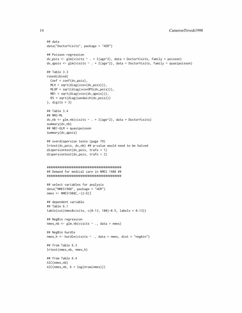
## datadata("DoctorVisits", package = "AER")
## Poisson regressiondv_pois <- glm(visits ~ . + I(age^2), data = DoctorVisits, family = poisson)dv_qpois <- glm(visits ~ . + I(age^2), data = DoctorVisits, family = quasipoisson)
## Table 3.3round(cbind(
Coef = coef(dv_pois),MLH = sqrt(diag(vcov(dv_pois))),MLOP = sqrt(diag(vcovOPG(dv_pois))),NB1 = sqrt(diag(vcov(dv_qpois))),RS = sqrt(diag(sandwich(dv_pois)))
), digits = 3)
## Table 3.4## NM2-MLdv_nb <- glm.nb(visits ~ . + I(age^2), data = DoctorVisits)summary(dv_nb)## NB1-GLM = quasipoissonsummary(dv_qpois)
## overdispersion tests (page 79)lrtest(dv_pois, dv_nb) ## p-value would need to be halveddispersiontest(dv_pois, trafo = 1)dispersiontest(dv_pois, trafo = 2)
############################################ Demand for medical care in NMES 1988 ############################################
## select variables for analysisdata("NMES1988", package = "AER")nmes <- NMES1988[,-(2:6)]
## dependent variable## Table 6.1table(cut(nmes$visits, c(0:13, 100)-0.5, labels = 0:13))
## NegBin regressionnmes_nb <- glm.nb(visits ~ ., data = nmes)
## NegBin hurdlenmes_h <- hurdle(visits ~ ., data = nmes, dist = "negbin")
## from Table 6.3lrtest(nmes_nb, nmes_h)
## from Table 6.4AIC(nmes_nb)AIC(nmes_nb, k = log(nrow(nmes)))
CameronTrivedi1998 15
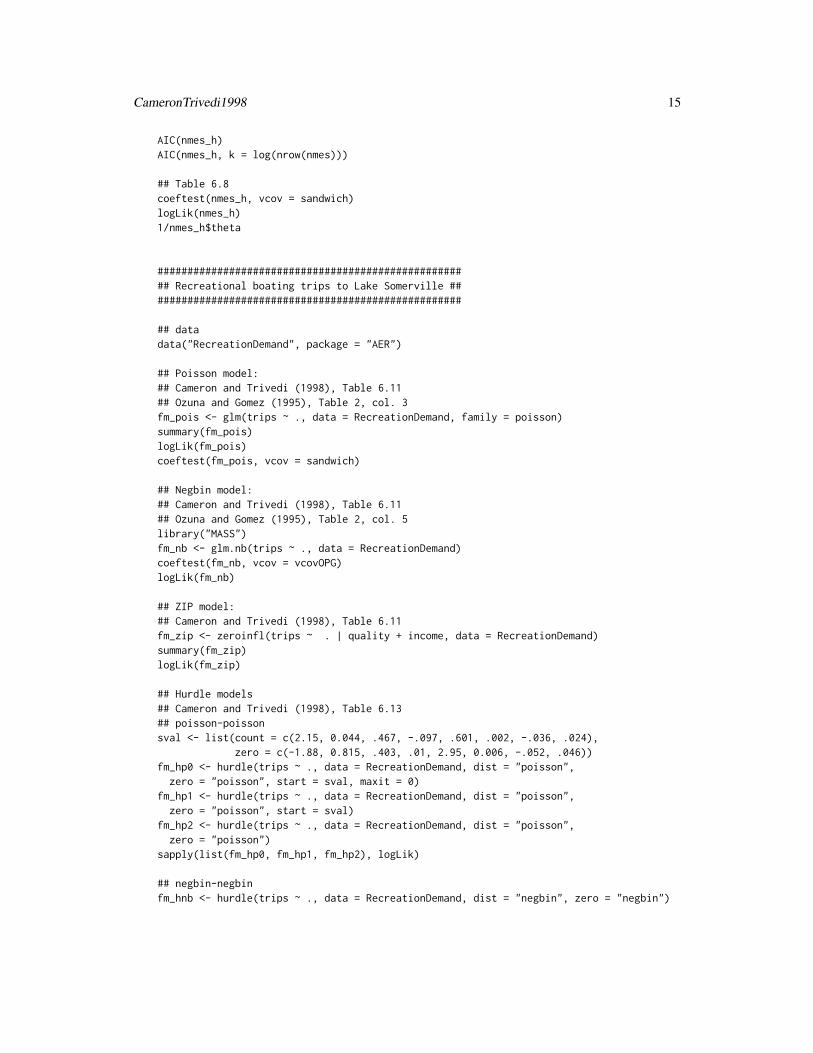
AIC(nmes_h)AIC(nmes_h, k = log(nrow(nmes)))
## Table 6.8coeftest(nmes_h, vcov = sandwich)logLik(nmes_h)1/nmes_h$theta
##################################################### Recreational boating trips to Lake Somerville #####################################################
## datadata("RecreationDemand", package = "AER")
## Poisson model:## Cameron and Trivedi (1998), Table 6.11## Ozuna and Gomez (1995), Table 2, col. 3fm_pois <- glm(trips ~ ., data = RecreationDemand, family = poisson)summary(fm_pois)logLik(fm_pois)coeftest(fm_pois, vcov = sandwich)
## Negbin model:## Cameron and Trivedi (1998), Table 6.11## Ozuna and Gomez (1995), Table 2, col. 5library("MASS")fm_nb <- glm.nb(trips ~ ., data = RecreationDemand)coeftest(fm_nb, vcov = vcovOPG)logLik(fm_nb)
## ZIP model:## Cameron and Trivedi (1998), Table 6.11fm_zip <- zeroinfl(trips ~ . | quality + income, data = RecreationDemand)summary(fm_zip)logLik(fm_zip)
## Hurdle models## Cameron and Trivedi (1998), Table 6.13## poisson-poissonsval <- list(count = c(2.15, 0.044, .467, -.097, .601, .002, -.036, .024),
zero = c(-1.88, 0.815, .403, .01, 2.95, 0.006, -.052, .046))fm_hp0 <- hurdle(trips ~ ., data = RecreationDemand, dist = "poisson",
zero = "poisson", start = sval, maxit = 0)fm_hp1 <- hurdle(trips ~ ., data = RecreationDemand, dist = "poisson",
zero = "poisson", start = sval)fm_hp2 <- hurdle(trips ~ ., data = RecreationDemand, dist = "poisson",
zero = "poisson")sapply(list(fm_hp0, fm_hp1, fm_hp2), logLik)
## negbin-negbinfm_hnb <- hurdle(trips ~ ., data = RecreationDemand, dist = "negbin", zero = "negbin")
16 CartelStability
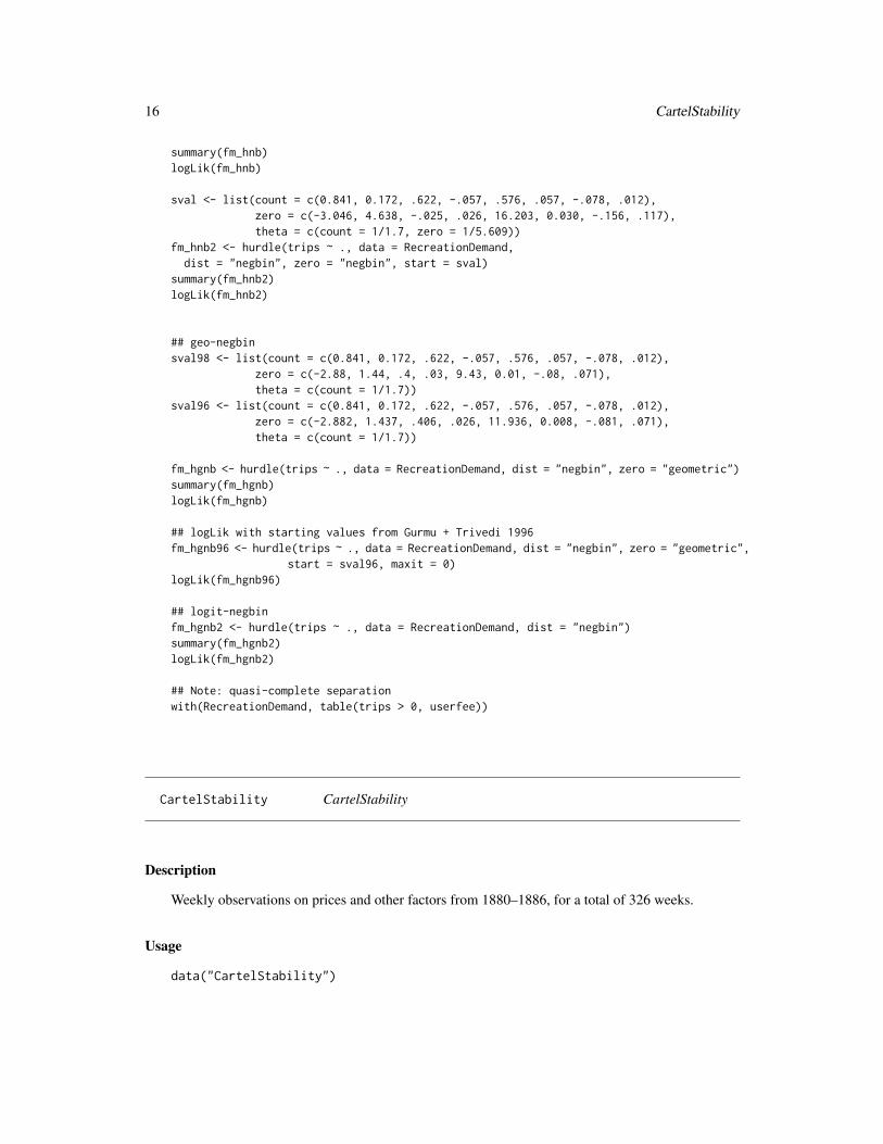
summary(fm_hnb)logLik(fm_hnb)
sval <- list(count = c(0.841, 0.172, .622, -.057, .576, .057, -.078, .012),zero = c(-3.046, 4.638, -.025, .026, 16.203, 0.030, -.156, .117),theta = c(count = 1/1.7, zero = 1/5.609))
fm_hnb2 <- hurdle(trips ~ ., data = RecreationDemand,dist = "negbin", zero = "negbin", start = sval)
summary(fm_hnb2)logLik(fm_hnb2)
## geo-negbinsval98 <- list(count = c(0.841, 0.172, .622, -.057, .576, .057, -.078, .012),
zero = c(-2.88, 1.44, .4, .03, 9.43, 0.01, -.08, .071),theta = c(count = 1/1.7))
sval96 <- list(count = c(0.841, 0.172, .622, -.057, .576, .057, -.078, .012),zero = c(-2.882, 1.437, .406, .026, 11.936, 0.008, -.081, .071),theta = c(count = 1/1.7))
fm_hgnb <- hurdle(trips ~ ., data = RecreationDemand, dist = "negbin", zero = "geometric")summary(fm_hgnb)logLik(fm_hgnb)
## logLik with starting values from Gurmu + Trivedi 1996fm_hgnb96 <- hurdle(trips ~ ., data = RecreationDemand, dist = "negbin", zero = "geometric",
start = sval96, maxit = 0)logLik(fm_hgnb96)
## logit-negbinfm_hgnb2 <- hurdle(trips ~ ., data = RecreationDemand, dist = "negbin")summary(fm_hgnb2)logLik(fm_hgnb2)
## Note: quasi-complete separationwith(RecreationDemand, table(trips > 0, userfee))
CartelStability CartelStability
Description
Weekly observations on prices and other factors from 1880–1886, for a total of 326 weeks.
Usage
data("CartelStability")
CASchools 17
Format
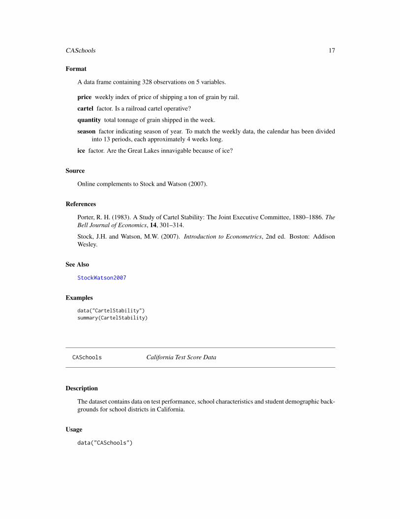
A data frame containing 328 observations on 5 variables.
price weekly index of price of shipping a ton of grain by rail.
cartel factor. Is a railroad cartel operative?
quantity total tonnage of grain shipped in the week.
season factor indicating season of year. To match the weekly data, the calendar has been dividedinto 13 periods, each approximately 4 weeks long.
ice factor. Are the Great Lakes innavigable because of ice?
Source
Online complements to Stock and Watson (2007).
References
Porter, R. H. (1983). A Study of Cartel Stability: The Joint Executive Committee, 1880–1886. TheBell Journal of Economics, 14, 301–314.
Stock, J.H. and Watson, M.W. (2007). Introduction to Econometrics, 2nd ed. Boston: AddisonWesley.
See Also
StockWatson2007
Examples
data("CartelStability")summary(CartelStability)
CASchools California Test Score Data
Description
The dataset contains data on test performance, school characteristics and student demographic back-grounds for school districts in California.
Usage
data("CASchools")
18 CASchools
Format
A data frame containing 420 observations on 14 variables.
district character. District code.
school character. School name.
county factor indicating county.
grades factor indicating grade span of district.
students Total enrollment.
teachers Number of teachers.
calworks Percent qualifying for CalWorks (income assistance).
lunch Percent qualifying for reduced-price lunch.
computer Number of computers.
expenditure Expenditure per student.
income District average income (in USD 1,000).
english Percent of English learners.
read Average reading score.
math Average math score.
Details
The data used here are from all 420 K-6 and K-8 districts in California with data available for 1998and 1999. Test scores are on the Stanford 9 standardized test administered to 5th grade students.School characteristics (averaged across the district) include enrollment, number of teachers (mea-sured as “full-time equivalents”, number of computers per classroom, and expenditures per student.Demographic variables for the students are averaged across the district. The demographic variablesinclude the percentage of students in the public assistance program CalWorks (formerly AFDC),the percentage of students that qualify for a reduced price lunch, and the percentage of students thatare English learners (that is, students for whom English is a second language).
Source
Online complements to Stock and Watson (2007).
References
Stock, J. H. and Watson, M. W. (2007). Introduction to Econometrics, 2nd ed. Boston: AddisonWesley.
See Also
StockWatson2007, MASchools
ChinaIncome 19
Examples
## data and transformationsdata("CASchools")CASchools$stratio <- with(CASchools, students/teachers)CASchools$score <- with(CASchools, (math + read)/2)
## Stock and Watson (2007)## p. 152fm1 <- lm(score ~ stratio, data = CASchools)coeftest(fm1, vcov = sandwich)
## p. 159fm2 <- lm(score ~ I(stratio < 20), data = CASchools)## p. 199fm3 <- lm(score ~ stratio + english, data = CASchools)## p. 224fm4 <- lm(score ~ stratio + expenditure + english, data = CASchools)
## Table 7.1, p. 242 (numbers refer to columns)fmc3 <- lm(score ~ stratio + english + lunch, data = CASchools)fmc4 <- lm(score ~ stratio + english + calworks, data = CASchools)fmc5 <- lm(score ~ stratio + english + lunch + calworks, data = CASchools)
## More examples can be found in:## help("StockWatson2007")
ChinaIncome Chinese Real National Income Data
Description
Time series of real national income in China per section (index with 1952 = 100).
Usage
data("ChinaIncome")
Format
An annual multiple time series from 1952 to 1988 with 5 variables.
agriculture Real national income in agriculture sector.
industry Real national income in industry sector.
construction Real national income in construction sector.
transport Real national income in transport sector.
commerce Real national income in commerce sector.
20 CigarettesB
Source
Online complements to Franses (1998).
References
Chow, G.C. (1993). Capital Formation and Economic Growth in China. Quarterly Journal ofEconomics, 103, 809–842.
Franses, P.H. (1998). Time Series Models for Business and Economic Forecasting. Cambridge, UK:Cambridge University Press.
See Also
Franses1998
Examples
data("ChinaIncome")plot(ChinaIncome)
CigarettesB Cigarette Consumption Data
Description
Cross-section data on cigarette consumption for 46 US States, for the year 1992.
Usage
data("CigarettesB")
Format
A data frame containing 46 observations on 3 variables.
packs Logarithm of cigarette consumption (in packs) per person of smoking age (> 16 years).
price Logarithm of real price of cigarette in each state.
income Logarithm of real disposable income (per capita) in each state.
Source
The data are from Baltagi (2002).
References
Baltagi, B.H. (2002). Econometrics, 3rd ed. Berlin, Springer.
Baltagi, B.H. and Levin, D. (1992). Cigarette Taxation: Raising Revenues and Reducing Consump-tion. Structural Change and Economic Dynamics, 3, 321–335.
CigarettesSW 21
See Also
Baltagi2002, CigarettesSW
Examples
data("CigarettesB")
## Baltagi (2002)## Table 3.3cig_lm <- lm(packs ~ price, data = CigarettesB)summary(cig_lm)
## Chapter 5: diagnostic tests (p. 111-115)cig_lm2 <- lm(packs ~ price + income, data = CigarettesB)summary(cig_lm2)## Glejser tests (p. 112)ares <- abs(residuals(cig_lm2))summary(lm(ares ~ income, data = CigarettesB))summary(lm(ares ~ I(1/income), data = CigarettesB))summary(lm(ares ~ I(1/sqrt(income)), data = CigarettesB))summary(lm(ares ~ sqrt(income), data = CigarettesB))## Goldfeld-Quandt test (p. 112)gqtest(cig_lm2, order.by = ~ income, data = CigarettesB, fraction = 12, alternative = "less")## NOTE: Baltagi computes the test statistic as mss1/mss2,## i.e., tries to find decreasing variances. gqtest() always uses## mss2/mss1 and has an "alternative" argument.
## Spearman rank correlation test (p. 113)cor.test(~ ares + income, data = CigarettesB, method = "spearman")## Breusch-Pagan test (p. 113)bptest(cig_lm2, varformula = ~ income, data = CigarettesB, student = FALSE)## White test (Table 5.1, p. 113)bptest(cig_lm2, ~ income * price + I(income^2) + I(price^2), data = CigarettesB)## White HC standard errors (Table 5.2, p. 114)coeftest(cig_lm2, vcov = vcovHC(cig_lm2, type = "HC1"))## Jarque-Bera test (Figure 5.2, p. 115)hist(residuals(cig_lm2), breaks = 16, ylim = c(0, 10), col = "lightgray")library("tseries")jarque.bera.test(residuals(cig_lm2))
## Tables 8.1 and 8.2influence.measures(cig_lm2)
## More examples can be found in:## help("Baltagi2002")
CigarettesSW Cigarette Consumption Panel Data
22 CigarettesSW
Description
Panel data on cigarette consumption for the 48 continental US States from 1985–1995.
Usage
data("CigarettesSW")
Format
A data frame containing 48 observations on 7 variables for 2 periods.
state Factor indicating state.
year Factor indicating year.
cpi Consumer price index.
population State population.
packs Number of packs per capita.
income State personal income (total, nominal).
tax Average state, federal and average local excise taxes for fiscal year.
price Average price during fiscal year, including sales tax.
taxs Average excise taxes for fiscal year, including sales tax.
Source
Online complements to Stock and Watson (2007).
References
Stock, J.H. and Watson, M.W. (2007). Introduction to Econometrics, 2nd ed. Boston: AddisonWesley.
See Also
StockWatson2007, CigarettesB
Examples
## Stock and Watson (2007)## data and transformationsdata("CigarettesSW")CigarettesSW$rprice <- with(CigarettesSW, price/cpi)CigarettesSW$rincome <- with(CigarettesSW, income/population/cpi)CigarettesSW$tdiff <- with(CigarettesSW, (taxs - tax)/cpi)c1985 <- subset(CigarettesSW, year == "1985")c1995 <- subset(CigarettesSW, year == "1995")
## convenience function: HC1 covarianceshc1 <- function(x) vcovHC(x, type = "HC1")

CollegeDistance 23
## Equations 12.9--12.11fm_s1 <- lm(log(rprice) ~ tdiff, data = c1995)coeftest(fm_s1, vcov = hc1)fm_s2 <- lm(log(packs) ~ fitted(fm_s1), data = c1995)fm_ivreg <- ivreg(log(packs) ~ log(rprice) | tdiff, data = c1995)coeftest(fm_ivreg, vcov = hc1)
## Equation 12.15fm_ivreg2 <- ivreg(log(packs) ~ log(rprice) + log(rincome) | log(rincome) + tdiff, data = c1995)coeftest(fm_ivreg2, vcov = hc1)## Equation 12.16fm_ivreg3 <- ivreg(log(packs) ~ log(rprice) + log(rincome) | log(rincome) + tdiff + I(tax/cpi),
data = c1995)coeftest(fm_ivreg3, vcov = hc1)
## More examples can be found in:## help("StockWatson2007")
CollegeDistance College Distance Data
Description
Cross-section data from the High School and Beyond survey conducted by the Department of Edu-cation in 1980, with a follow-up in 1986. The survey included students from approximately 1,100high schools.
Usage
data("CollegeDistance")
Format
A data frame containing 4,739 observations on 14 variables.
gender factor indicating gender.
ethnicity factor indicating ethnicity (African-American, Hispanic or other).
score base year composite test score. These are achievement tests given to high school seniors inthe sample.
fcollege factor. Is the father a college graduate?
mcollege factor. Is the mother a college graduate?
home factor. Does the family own their home?
urban factor. Is the school in an urban area?
unemp county unemployment rate in 1980.
wage state hourly wage in manufacturing in 1980.
distance distance from 4-year college (in 10 miles).
24 ConsumerGood
tuition average state 4-year college tuition (in 1000 USD).
education number of years of education.
income factor. Is the family income above USD 25,000 per year?
region factor indicating region (West or other).
Details
Rouse (1995) computed years of education by assigning 12 years to all members of the seniorclass. Each additional year of secondary education counted as a one year. Students with vocationaldegrees were assigned 13 years, AA degrees were assigned 14 years, BA degrees were assigned 16years, those with some graduate education were assigned 17 years, and those with a graduate degreewere assigned 18 years.
Stock and Watson (2007) provide separate data files for the students from Western states and theremaining students. CollegeDistance includes both data sets, subsets are easily obtained (see alsoexamples).
Source
Online complements to Stock and Watson (2007).
References
Rouse, C.E. (1995). Democratization or Diversion? The Effect of Community Colleges on Educa-tional Attainment. Journal of Business \& Economic Statistics, 12, 217–224.
Stock, J.H. and Watson, M.W. (2007). Introduction to Econometrics, 2nd ed. Boston: AddisonWesley.
See Also
StockWatson2007
Examples
## exclude students from Western statesdata("CollegeDistance")cd <- subset(CollegeDistance, region != "west")summary(cd)
ConsumerGood Properties of a Fast-Moving Consumer Good
Description
Time series of distribution, market share and price of a fast-moving consumer good.
CPS1985 25
Usage
data("ConsumerGood")
Format
A weekly multiple time series from 1989(11) to 1991(9) with 3 variables.
distribution Distribution.
share Market share.
price Price.
Source
Online complements to Franses (1998).
References
Franses, P.H. (1998). Time Series Models for Business and Economic Forecasting. Cambridge, UK:Cambridge University Press.
See Also
Franses1998
Examples
data("ConsumerGood")plot(ConsumerGood)
CPS1985 Determinants of Wages Data (CPS 1985)
Description
Cross-section data originating from the May 1985 Current Population Survey by the US CensusBureau (random sample drawn for Berndt 1991).
Usage
data("CPS1985")
26 CPS1985
Format
A data frame containing 534 observations on 11 variables.
wage Wage (in dollars per hour).
education Number of years of education.
experience Number of years of potential work experience (age - education - 6).
age Age in years.
ethnicity Factor with levels "cauc", "hispanic", "other".
region Factor. Does the individual live in the South?
gender Factor indicating gender.
occupation Factor with levels "worker" (tradesperson or assembly line worker), "technical"(technical or professional worker), "services" (service worker), "office" (office and cleri-cal worker), "sales" (sales worker), "management" (management and administration).
sector Factor with levels "manufacturing" (manufacturing or mining), "construction", "other".
union Factor. Does the individual work on a union job?
married Factor. Is the individual married?
Source
StatLib.
http://lib.stat.cmu.edu/datasets/CPS_85_Wages
References
Berndt, E.R. (1991). The Practice of Econometrics. New York: Addison-Wesley.
See Also
CPS1988, CPSSW
Examples
data("CPS1985")
## Berndt (1991)## Exercise 2, p. 196cps_2b <- lm(log(wage) ~ union + education, data = CPS1985)cps_2c <- lm(log(wage) ~ -1 + union + education, data = CPS1985)
## Exercise 3, p. 198/199cps_3a <- lm(log(wage) ~ education + experience + I(experience^2),
data = CPS1985)cps_3b <- lm(log(wage) ~ gender + education + experience + I(experience^2),
data = CPS1985)cps_3c <- lm(log(wage) ~ gender + married + education + experience + I(experience^2),
data = CPS1985)cps_3e <- lm(log(wage) ~ gender*married + education + experience + I(experience^2),

CPS1988 27
data = CPS1985)
## Exercise 4, p. 199/200cps_4a <- lm(log(wage) ~ gender + union + ethnicity + education + experience + I(experience^2),
data = CPS1985)cps_4c <- lm(log(wage) ~ gender + union + ethnicity + education * experience + I(experience^2),
data = CPS1985)
## Exercise 6, p. 203cps_6a <- lm(log(wage) ~ gender + union + ethnicity + education + experience + I(experience^2),
data = CPS1985)cps_6a_noeth <- lm(log(wage) ~ gender + union + education + experience + I(experience^2),
data = CPS1985)anova(cps_6a_noeth, cps_6a)
## Exercise 8, p. 208cps_8a <- lm(log(wage) ~ gender + union + ethnicity + education + experience + I(experience^2),
data = CPS1985)summary(cps_8a)coeftest(cps_8a, vcov = vcovHC(cps_8a, type = "HC0"))
CPS1988 Determinants of Wages Data (CPS 1988)
Description
Cross-section data originating from the March 1988 Current Population Survey by the US CensusBureau.
Usage
data("CPS1988")
Format
A data frame containing 28,155 observations on 7 variables.
wage Wage (in dollars per week).
education Number of years of education.
experience Number of years of potential work experience.
ethnicity Factor with levels "cauc" and "afam" (African-American).
smsa Factor. Does the individual reside in a Standard Metropolitan Statistical Area (SMSA)?
region Factor with levels "northeast", "midwest", "south", "west".
parttime Factor. Does the individual work part-time?
28 CPS1988
Details
A sample of men aged 18 to 70 with positive annual income greater than USD 50 in 1992, whoare not self-employed nor working without pay. Wages are deflated by the deflator of PersonalConsumption Expenditure for 1992.
A problem with CPS data is that it does not provide actual work experience. It is therefore cus-tomary to compute experience as age - education - 6 (as was done by Bierens and Ginther,2001), this may be considered potential experience. As a result, some respondents have negativeexperience.
Source
http://www.personal.psu.edu/hxb11/MEDIAN.HTM
References
Bierens, H.J., and Ginther, D. (2001). Integrated Conditional Moment Testing of Quantile Regres-sion Models. Empirical Economics, 26, 307–324.
Buchinsky, M. (1998). Recent Advances in Quantile Regression Models: A Practical Guide forEmpirical Research. Journal of Human Resources, 33, 88–126.
See Also
CPS1985, CPSSW
Examples
## data and packageslibrary("quantreg")data("CPS1988")CPS1988$region <- relevel(CPS1988$region, ref = "south")
## Model equations: Mincer-type, quartic, Buchinsky-typemincer <- log(wage) ~ ethnicity + education + experience + I(experience^2)quart <- log(wage) ~ ethnicity + education + experience + I(experience^2) +
I(experience^3) + I(experience^4)buchinsky <- log(wage) ~ ethnicity * (education + experience + parttime) +
region*smsa + I(experience^2) + I(education^2) + I(education*experience)
## OLS and LAD fits (for LAD see Bierens and Ginter, Tables 1-3.A.)mincer_ols <- lm(mincer, data = CPS1988)mincer_lad <- rq(mincer, data = CPS1988)quart_ols <- lm(quart, data = CPS1988)quart_lad <- rq(quart, data = CPS1988)buchinsky_ols <- lm(buchinsky, data = CPS1988)buchinsky_lad <- rq(buchinsky, data = CPS1988)
CPSSW 29
CPSSW Stock and Watson CPS Data Sets
Description
Stock and Watson (2007) provide several subsets created from March Current Population Surveys(CPS) with data on the relationship of earnings and education over several year.
Usage
data("CPSSW9204")data("CPSSW9298")data("CPSSW04")data("CPSSW3")data("CPSSW8")data("CPSSWEducation")
Format
CPSSW9298: A data frame containing 13,501 observations on 5 variables. CPSSW9204: A dataframe containing 15,588 observations on 5 variables. CPSSW04: A data frame containing 7,986observations on 4 variables. CPSSW3: A data frame containing 20,999 observations on 3 variables.CPSSW8: A data frame containing 61,395 observations on 5 variables. CPSSWEducation: A dataframe containing 2,950 observations on 4 variables.
year factor indicating year.
earnings average hourly earnings (sum of annual pretax wages, salaries, tips, and bonuses, dividedby the number of hours worked annually).
education number of years of education.
degree factor indicating highest educational degree ("bachelor" or"highschool").
gender factor indicating gender.
age age in years.
region factor indicating region of residence ("Northeast", "Midwest", "South", "West").
Details
Each month the Bureau of Labor Statistics in the US Department of Labor conducts the CurrentPopulation Survey (CPS), which provides data on labor force characteristics of the population,including the level of employment, unemployment, and earnings. Approximately 65,000 randomlyselected US households are surveyed each month. The sample is chosen by randomly selectingaddresses from a database. Details can be found in the Handbook of Labor Statistics and is describedon the Bureau of Labor Statistics website (http://www.bls.gov/).
The survey conducted each March is more detailed than in other months and asks questions aboutearnings during the previous year. The data sets contain data for 2004 (from the March 2005 survey),and some also for earlier years (up to 1992).
30 CreditCard
If education is given, it is for full-time workers, defined as workers employed more than 35 hoursper week for at least 48 weeks in the previous year. Data are provided for workers whose highesteducational achievement is a high school diploma and a bachelor’s degree.
Earnings for years earlier than 2004 were adjusted for inflation by putting them in 2004 USD usingthe Consumer Price Index (CPI). From 1992 to 2004, the price of the CPI market basket rose by34.6%. To make earnings in 1992 and 2004 comparable, 1992 earnings are inflated by the amountof overall CPI price inflation, by multiplying 1992 earnings by 1.346 to put them into 2004 dollars.
CPSSW9204 provides the distribution of earnings in the US in 1992 and 2004 for college-educatedfull-time workers aged 25–34. CPSSW04 is a subset of CPSSW9204 and provides the distribution ofearnings in the US in 2004 for college-educated full-time workers aged 25–34. CPSSWEducationis similar (but not a true subset) and contains the distribution of earnings in the US in 2004 forcollege-educated full-time workers aged 29–30. CPSSW8 contains a larger sample with workersaged 21–64, additionally providing information about the region of residence. CPSSW9298 is sim-ilar to CPSSW9204 providing data from 1992 and 1998 (with the 1992 subsets not being exactlyidentical). CPSSW3 provides trends (from 1992 to 2004) in hourly earnings in the US of workingcollege graduates aged 25–34 (in 2004 USD).
Source
Online complements to Stock and Watson (2007).
References
Stock, J.H. and Watson, M.W. (2007). Introduction to Econometrics, 2nd ed. Boston: AddisonWesley.
See Also
StockWatson2007, CPS1985, CPS1988
Examples
data("CPSSW3")with(CPSSW3, interaction.plot(year, gender, earnings))
## Stock and Watson, p. 165data("CPSSWEducation")plot(earnings ~ education, data = CPSSWEducation)fm <- lm(earnings ~ education, data = CPSSWEducation)coeftest(fm, vcov = sandwich)abline(fm)
CreditCard Expenditure and Default Data
Description
Cross-section data on the credit history for a sample of applicants for a type of credit card.
CreditCard 31
Usage
data("CreditCard")
Format
A data frame containing 1,319 observations on 12 variables.
card Factor. Was the application for a credit card accepted?
reports Number of major derogatory reports.
age Age in years plus twelfths of a year.
income Yearly income (in USD 10,000).
share Ratio of monthly credit card expenditure to yearly income.
expenditure Average monthly credit card expenditure.
owner Factor. Does the individual own their home?
selfemp Factor. Is the individual self-employed?
dependents Number of dependents.
months Months living at current address.
majorcards Number of major credit cards held.
active Number of active credit accounts.
Details
According to Greene (2003, p. 952) dependents equals 1 + number of dependents, our calcu-lations suggest that it equals number of dependents.
Greene (2003) provides this data set twice in Table F21.4 and F9.1, respectively. Table F9.1 has justthe observations, rounded to two digits. Here, we give the F21.4 version, see the examples for theF9.1 version. Note that age has some suspiciously low values (below one year) for some applicants.One of these differs between the F9.1 and F21.4 version.
Source
Online complements to Greene (2003). Table F21.4.
http://pages.stern.nyu.edu/~wgreene/Text/tables/tablelist5.htm
References
Greene, W.H. (2003). Econometric Analysis, 5th edition. Upper Saddle River, NJ: Prentice Hall.
See Also
Greene2003
32 dispersiontest
Examples
data("CreditCard")
## Greene (2003)## extract data set F9.1ccard <- CreditCard[1:100,]ccard$income <- round(ccard$income, digits = 2)ccard$expenditure <- round(ccard$expenditure, digits = 2)ccard$age <- round(ccard$age + .01)## suspicious:CreditCard$age[CreditCard$age < 1]## the first of these is also in TableF9.1 with 36 instead of 0.5:ccard$age[79] <- 36
## Example 11.1ccard <- ccard[order(ccard$income),]ccard0 <- subset(ccard, expenditure > 0)cc_ols <- lm(expenditure ~ age + owner + income + I(income^2), data = ccard0)
## Figure 11.1plot(residuals(cc_ols) ~ income, data = ccard0, pch = 19)
## Table 11.1mean(ccard$age)prop.table(table(ccard$owner))mean(ccard$income)
summary(cc_ols)sqrt(diag(vcovHC(cc_ols, type = "HC0")))sqrt(diag(vcovHC(cc_ols, type = "HC2")))sqrt(diag(vcovHC(cc_ols, type = "HC1")))
bptest(cc_ols, ~ (age + income + I(income^2) + owner)^2 + I(age^2) + I(income^4), data = ccard0)gqtest(cc_ols)bptest(cc_ols, ~ income + I(income^2), data = ccard0, studentize = FALSE)bptest(cc_ols, ~ income + I(income^2), data = ccard0)
## More examples can be found in:## help("Greene2003")
dispersiontest Dispersion Test
Description
Tests the null hypothesis of equidispersion in Poisson GLMs against the alternative of overdisper-sion and/or underdispersion.
Usage
dispersiontest(object, trafo = NULL, alternative = c("greater", "two.sided", "less"))
dispersiontest 33
Arguments
object a fitted Poisson GLM of class "glm" as fitted by glm with family poisson.
trafo a specification of the alternative (see also details), can be numeric or a (positive)function or NULL (the default).
alternative a character string specifying the alternative hypothesis: "greater" correspondsto overdispersion, "less" to underdispersion and "two.sided" to either one.
Details
The standard Poisson GLM models the (conditional) mean E[y] = µ which is assumed to be equalto the variance VAR[y] = µ. dispersiontest assesses the hypothesis that this assumption holds(equidispersion) against the alternative that the variance is of the form:
VAR[y] = µ + α · trafo(µ).
Overdispersion corresponds to α > 0 and underdispersion to α < 0. The coefficient α can beestimated by an auxiliary OLS regression and tested with the corresponding t (or z) statistic whichis asymptotically standard normal under the null hypothesis.
Common specifications of the transformation function trafo are trafo(µ) = µ2 or trafo(µ) = µ.The former corresponds to a negative binomial (NB) model with quadratic variance function (calledNB2 by Cameron and Trivedi, 2005), the latter to a NB model with linear variance function (calledNB1 by Cameron and Trivedi, 2005) or quasi-Poisson model with dispersion parameter, i.e.,
VAR[y] = (1 + α) · µ = dispersion · µ.
By default, for trafo = NULL, the latter dispersion formulation is used in dispersiontest. Oth-erwise, if trafo is specified, the test is formulated in terms of the parameter α. The transfor-mation trafo can either be specified as a function or an integer corresponding to the functionfunction(x) x^trafo, such that trafo = 1 and trafo = 2 yield the linear and quadratic formu-lations respectively.
Value
An object of class "htest".
References
Cameron, A.C. and Trivedi, P.K. (1990). Regression-based Tests for Overdispersion in the PoissonModel. Journal of Econometrics, 46, 347–364.
Cameron, A.C. and Trivedi, P.K. (1998). Regression Analysis of Count Data. Cambridge: Cam-bridge University Press.
Cameron, A.C. and Trivedi, P.K. (2005). Microeconometrics: Methods and Applications. Cam-bridge: Cambridge University Press.
See Also
glm, poisson, glm.nb
34 DJFranses
Examples
data("RecreationDemand")rd <- glm(trips ~ ., data = RecreationDemand, family = poisson)
## linear specification (in terms of dispersion)dispersiontest(rd)## linear specification (in terms of alpha)dispersiontest(rd, trafo = 1)## quadratic specification (in terms of alpha)dispersiontest(rd, trafo = 2)dispersiontest(rd, trafo = function(x) x^2)
## further examplesdata("DoctorVisits")dv <- glm(visits ~ . + I(age^2), data = DoctorVisits, family = poisson)dispersiontest(dv)
data("NMES1988")nmes <- glm(visits ~ health + age + gender + married + income + insurance,
data = NMES1988, family = poisson)dispersiontest(nmes)
DJFranses Dow Jones Index Data (Franses)
Description
Dow Jones index time series computed at the end of the week where week is assumed to run fromThursday to Wednesday.
Usage
data("DJFranses")
Format
A weekly univariate time series from 1980(1) to 1994(42).
Source
Online complements to Franses (1998).
References
Franses, P.H. (1998). Time Series Models for Business and Economic Forecasting. Cambridge, UK:Cambridge University Press.
See Also
Franses1998
DJIA8012 35
Examples
data("DJFranses")plot(DJFranses)
DJIA8012 Dow Jones Industrial Average (DJIA) index
Description
Time series of the Dow Jones Industrial Average (DJIA) index.
Usage
data("DJIA8012")
Format
A daily univariate time series from 1980-01-01 to 2012-12-31 (of class "zoo" with "Date" index).
Source
Online complements to Franses, van Dijk and Opschoor (2014).
http://www.cambridge.org/us/academic/subjects/economics/econometrics-statistics-and-mathematical-economics/time-series-models-business-and-economic-forecasting-2nd-edition
References
Franses, P.H., van Dijk, D. and Opschoor, A. (2014). Time Series Models for Business and Eco-nomic Forecasting, 2nd ed. Cambridge, UK: Cambridge University Press.
Examples
data("DJIA8012")plot(DJIA8012)
# p.26, Figure 2.18dldjia <- diff(log(DJIA8012))plot(dldjia)
# p.141, Figure 6.4plot(window(dldjia, start = "1987-09-01", end = "1987-12-31"))
# p.167, Figure 7.1dldjia9005 <- window(dldjia, start = "1990-01-01", end = "2005-12-31")qqnorm(dldjia9005)qqline(dldjia9005, lty = 2)
# p.170, Figure 7.4

36 DoctorVisits
acf(dldjia9005, na.action = na.exclude, lag.max = 250, ylim = c(-0.1, 0.25))acf(dldjia9005^2, na.action = na.exclude, lag.max = 250, ylim = c(-0.1, 0.25))acf(abs(dldjia9005), na.action = na.exclude, lag.max = 250, ylim = c(-0.1, 0.25))
DoctorVisits Australian Health Service Utilization Data
Description
Cross-section data originating from the 1977–1978 Australian Health Survey.
Usage
data("DoctorVisits")
Format
A data frame containing 5,190 observations on 12 variables.
visits Number of doctor visits in past 2 weeks.gender Factor indicating gender.age Age in years divided by 100.income Annual income in tens of thousands of dollars.illness Number of illnesses in past 2 weeks.reduced Number of days of reduced activity in past 2 weeks due to illness or injury.health General health questionnaire score using Goldberg’s method.private Factor. Does the individual have private health insurance?freepoor Factor. Does the individual have free government health insurance due to low income?freerepat Factor. Does the individual have free government health insurance due to old age, dis-
ability or veteran status?nchronic Factor. Is there a chronic condition not limiting activity?lchronic Factor. Is there a chronic condition limiting activity?
Source
Journal of Applied Econometrics Data Archive.
http://qed.econ.queensu.ca/jae/1997-v12.3/mullahy/
References
Cameron, A.C. and Trivedi, P.K. (1986). Econometric Models Based on Count Data: Comparisonsand Applications of Some Estimators and Tests. Journal of Applied Econometrics, 1, 29–53.
Cameron, A.C. and Trivedi, P.K. (1998). Regression Analysis of Count Data. Cambridge: Cam-bridge University Press.
Mullahy, J. (1997). Heterogeneity, Excess Zeros, and the Structure of Count Data Models. Journalof Applied Econometrics, 12, 337–350.
DutchAdvert 37
See Also
CameronTrivedi1998
Examples
data("DoctorVisits", package = "AER")library("MASS")
## Cameron and Trivedi (1986), Table III, col. (1)dv_lm <- lm(visits ~ . + I(age^2), data = DoctorVisits)summary(dv_lm)
## Cameron and Trivedi (1998), Table 3.3dv_pois <- glm(visits ~ . + I(age^2), data = DoctorVisits, family = poisson)summary(dv_pois) ## MLH standard errorscoeftest(dv_pois, vcov = vcovOPG) ## MLOP standard errorslogLik(dv_pois)## standard errors denoted RS ("unspecified omega robust sandwich estimate")coeftest(dv_pois, vcov = sandwich)
## Cameron and Trivedi (1986), Table III, col. (4)dv_nb <- glm.nb(visits ~ . + I(age^2), data = DoctorVisits)summary(dv_nb)logLik(dv_nb)
DutchAdvert TV and Radio Advertising Expenditures Data
Description
Time series of television and radio advertising expenditures (in real terms) in The Netherlands.
Usage
data("DutchAdvert")
Format
A four-weekly multiple time series from 1978(1) to 1994(13) with 2 variables.
tv Television advertising expenditures.
radio Radio advertising expenditures.
Source
Originally available as an online supplement to Franses (1998). Now available via online comple-ments to Franses, van Dijk and Opschoor (2014).
http://www.cambridge.org/us/academic/subjects/economics/econometrics-statistics-and-mathematical-economics/time-series-models-business-and-economic-forecasting-2nd-edition
38 DutchSales
References
Franses, P.H. (1998). Time Series Models for Business and Economic Forecasting. Cambridge, UK:Cambridge University Press.
Franses, P.H., van Dijk, D. and Opschoor, A. (2014). Time Series Models for Business and Eco-nomic Forecasting, 2nd ed. Cambridge, UK: Cambridge University Press.
See Also
Franses1998
Examples
data("DutchAdvert")plot(DutchAdvert)
## EACF tables (Franses 1998, Sec. 5.1, p. 99)ctrafo <- function(x) residuals(lm(x ~ factor(cycle(x))))ddiff <- function(x) diff(diff(x, frequency(x)), 1)eacf <- function(y, lag = 12) {
stopifnot(all(lag > 0))if(length(lag) < 2) lag <- 1:lagrval <- sapply(
list(y = y, dy = diff(y), cdy = ctrafo(diff(y)),Dy = diff(y, frequency(y)), dDy = ddiff(y)),
function(x) acf(x, plot = FALSE, lag.max = max(lag))$acf[lag + 1])rownames(rval) <- lagreturn(rval)
}
## Franses (1998, p. 103), Table 5.4round(eacf(log(DutchAdvert[,"tv"]), lag = c(1:19, 26, 39)), digits = 3)
DutchSales Dutch Retail Sales Index Data
Description
Time series of retail sales index in The Netherlands.
Usage
data("DutchSales")
Format
A monthly univariate time series from 1960(5) to 1995(9).
Electricity1955 39
Source
Online complements to Franses (1998).
References
Franses, P.H. (1998). Time Series Models for Business and Economic Forecasting. Cambridge, UK:Cambridge University Press.
See Also
Franses1998
Examples
data("DutchSales")plot(DutchSales)
## EACF tables (Franses 1998, p. 99)ctrafo <- function(x) residuals(lm(x ~ factor(cycle(x))))ddiff <- function(x) diff(diff(x, frequency(x)), 1)eacf <- function(y, lag = 12) {
stopifnot(all(lag > 0))if(length(lag) < 2) lag <- 1:lagrval <- sapply(list(y = y, dy = diff(y), cdy = ctrafo(diff(y)),
Dy = diff(y, frequency(y)), dDy = ddiff(y)),function(x) acf(x, plot = FALSE, lag.max = max(lag))$acf[lag + 1])
rownames(rval) <- lagreturn(rval)
}
## Franses (1998), Table 5.3round(eacf(log(DutchSales), lag = c(1:18, 24, 36)), digits = 3)
Electricity1955 Cost Function of Electricity Producers (1955, Nerlove Data)
Description
Cost function data for 145 (+14) US electricity producers in 1955.
Usage
data("Electricity1955")

40 Electricity1955
Format
A data frame containing 159 observations on 8 variables.
cost total cost.
output total output.
labor wage rate.
laborshare cost share for labor.
capital capital price index.
capitalshare cost share for capital.
fuel fuel price.
fuelshare cost share for fuel.
Details
The data contains several extra observations that are aggregates of commonly owned firms. Onlythe first 145 observations should be used for analysis.
Source
Online complements to Greene (2003). Table F14.2.
http://pages.stern.nyu.edu/~wgreene/Text/tables/tablelist5.htm
References
Greene, W.H. (2003). Econometric Analysis, 5th edition. Upper Saddle River, NJ: Prentice Hall.
Nerlove, M. (1963) “Returns to Scale in Electricity Supply.” In C. Christ (ed.), Measurement inEconomics: Studies in Mathematical Economics and Econometrics in Memory of Yehuda Grunfeld.Stanford University Press, 1963.
See Also
Greene2003, Electricity1970
Examples
data("Electricity1955")Electricity <- Electricity1955[1:145,]
## Greene (2003)## Example 7.3## Cobb-Douglas cost functionfm_all <- lm(log(cost/fuel) ~ log(output) + log(labor/fuel) + log(capital/fuel),
data = Electricity)summary(fm_all)
## hypothesis of constant returns to scalelinearHypothesis(fm_all, "log(output) = 1")
Electricity1970 41
## Table 7.4## log quadratic cost functionfm_all2 <- lm(log(cost/fuel) ~ log(output) + I(log(output)^2) + log(labor/fuel) + log(capital/fuel),
data = Electricity)summary(fm_all2)
## More examples can be found in:## help("Greene2003")
Electricity1970 Cost Function of Electricity Producers 1970
Description
Cross-section data, at the firm level, on electric power generation.
Usage
data("Electricity1970")
Format
A data frame containing 158 cross-section observations on 9 variables.
cost total cost.
output total output.
labor wage rate.
laborshare cost share for labor.
capital capital price index.
capitalshare cost share for capital.
fuel fuel price.
fuelshare cost share for fuel.
Details
The data are from Christensen and Greene (1976) and pertain to the year 1970. However, the filecontains some extra observations, the holding companies. Only the first 123 observations are neededto replicate Christensen and Greene (1976).
Source
Online complements to Greene (2003), Table F5.2.
http://pages.stern.nyu.edu/~wgreene/Text/tables/tablelist5.htm
42 EquationCitations
References
Christensen, L. and Greene, W.H. (1976). Economies of Scale in U.S. Electric Power Generation.Journal of Political Economy, 84, 655–676.
Greene, W.H. (2003). Econometric Analysis, 5th edition. Upper Saddle River, NJ: Prentice Hall.
See Also
Greene2003, Electricity1955
Examples
data("Electricity1970")
## Greene (2003), Ex. 5.6: a generalized Cobb-Douglas cost functionfm <- lm(log(cost/fuel) ~ log(output) + I(log(output)^2/2) +
log(capital/fuel) + log(labor/fuel), data=Electricity1970[1:123,])
EquationCitations Number of Equations and Citations for Evolutionary Biology Publica-tions
Description
Analysis of citations of evolutionary biology papers published in 1998 in the top three journals (asjudged by their 5-year impact factors in the Thomson Reuters Journal Citation Reports 2010).
Usage
data("EquationCitations")
Format
A data frame containing 649 observations on 13 variables.
journal Factor. Journal in which the paper was published (The American Naturalist, Evolution,Proceedings of the Royal Society of London B: Biological Sciences).
authors Character. Names of authors.
volume Volume in which the paper was published.
startpage Starting page of publication.
pages Number of pages.
equations Number of equations in total.
mainequations Number of equations in main text.
appequations Number of equations in appendix.
cites Number of citations in total.

EquationCitations 43
selfcites Number of citations by the authors themselves.
othercites Number of citations by other authors.
theocites Number of citations by theoretical papers.
nontheocites Number of citations by nontheoretical papers.
Details
Fawcett and Higginson (2012) investigate the relationship between the number of citations evolu-tionary biology papers receive, depending on the number of equations per page in the cited paper.Overall it can be shown that papers with many mathematical equations significantly lower the num-ber of citations they receive, in particular from nontheoretical papers.
Source
Online supplements to Fawcett and Higginson (2012).
http://www.pnas.org/lookup/suppl/doi:10.1073/pnas.1205259109/-/DCSupplemental
References
Fawcett, T.W. and Higginson, A.D. (2012). Heavy Use of Equations Impedes Communicationamong Biologists. PNAS – Proceedings of the National Academy of Sciences of the United Statesof America, 109, 11735–11739. http://dx.doi.org/10.1073/pnas.1205259109
See Also
PhDPublications
Examples
## load data and MASS packagedata("EquationCitations", package = "AER")library("MASS")
## convenience function for summarizing NB modelsnbtable <- function(obj, digits = 3) round(cbind(
"OR" = exp(coef(obj)),"CI" = exp(confint.default(obj)),"Wald z" = coeftest(obj)[,3],"p" = coeftest(obj)[, 4]), digits = digits)
################### Replication ###################
## Table 1m1a <- glm.nb(othercites ~ I(equations/pages) * pages + journal,
data = EquationCitations)m1b <- update(m1a, nontheocites ~ .)m1c <- update(m1a, theocites ~ .)
44 Equipment
nbtable(m1a)nbtable(m1b)nbtable(m1c)
## Table 2m2a <- glm.nb(
othercites ~ (I(mainequations/pages) + I(appequations/pages)) * pages + journal,data = EquationCitations)
m2b <- update(m2a, nontheocites ~ .)m2c <- update(m2a, theocites ~ .)nbtable(m2a)nbtable(m2b)nbtable(m2c)
################# Extension #################
## nonlinear page effect: use log(pages) instead of pages+interactionm3a <- glm.nb(othercites ~ I(equations/pages) + log(pages) + journal,
data = EquationCitations)m3b <- update(m3a, nontheocites ~ .)m3c <- update(m3a, theocites ~ .)
## nested models: allow different equation effects over journalsm4a <- glm.nb(othercites ~ journal / I(equations/pages) + log(pages),
data = EquationCitations)m4b <- update(m4a, nontheocites ~ .)m4c <- update(m4a, theocites ~ .)
## nested model best (wrt AIC) for all responsesAIC(m1a, m2a, m3a, m4a)nbtable(m4a)AIC(m1b, m2b, m3b, m4b)nbtable(m4b)AIC(m1c, m2c, m3c, m4c)nbtable(m4c)## equation effect by journal/response## comb nontheo theo## AmNat =/- - +## Evolution =/+ = +## ProcB - - =/+
Equipment Transportation Equipment Manufacturing Data
Description
Statewide data on transportation equipment manufacturing for 25 US states.
Equipment 45
Usage
data("Equipment")
Format
A data frame containing 25 observations on 4 variables.
valueadded Aggregate output, in millions of 1957 dollars.
capital Capital input, in millions of 1957 dollars.
labor Aggregate labor input, in millions of man hours.
firms Number of firms.
Source
Journal of Applied Econometrics Data Archive.
http://qed.econ.queensu.ca/jae/1998-v13.2/zellner-ryu/
Online complements to Greene (2003), Table F9.2.
http://pages.stern.nyu.edu/~wgreene/Text/tables/tablelist5.htm
References
Greene, W.H. (2003). Econometric Analysis, 5th edition. Upper Saddle River, NJ: Prentice Hall.
Zellner, A. and Revankar, N. (1969). Generalized Production Functions. Review of EconomicStudies, 36, 241–250.
Zellner, A. and Ryu, H. (1998). Alternative Functional Forms for Production, Cost and Returns toScale Functions. Journal of Applied Econometrics, 13, 101–127.
See Also
Greene2003
Examples
## Greene (2003), Example 17.5data("Equipment")
## Cobb-Douglasfm_cd <- lm(log(valueadded/firms) ~ log(capital/firms) + log(labor/firms), data = Equipment)
## generalized Cobb-Douglas with Zellner-Revankar trafoGCobbDouglas <- function(theta)lm(I(log(valueadded/firms) + theta * valueadded/firms) ~ log(capital/firms) + log(labor/firms),
data = Equipment)
## yields classical Cobb-Douglas for theta = 0fm_cd0 <- GCobbDouglas(0)
## ML estimation of generalized model
46 EuroEnergy
## choose starting values from classical modelpar0 <- as.vector(c(coef(fm_cd0), 0, mean(residuals(fm_cd0)^2)))
## set up likelihood functionnlogL <- function(par) {
beta <- par[1:3]theta <- par[4]sigma2 <- par[5]
Y <- with(Equipment, valueadded/firms)K <- with(Equipment, capital/firms)L <- with(Equipment, labor/firms)
rhs <- beta[1] + beta[2] * log(K) + beta[3] * log(L)lhs <- log(Y) + theta * Y
rval <- sum(log(1 + theta * Y) - log(Y) +dnorm(lhs, mean = rhs, sd = sqrt(sigma2), log = TRUE))
return(-rval)}
## optimizationopt <- optim(par0, nlogL, hessian = TRUE)
## Table 17.2opt$parsqrt(diag(solve(opt$hessian)))[1:4]-opt$value
## re-fit ML modelfm_ml <- GCobbDouglas(opt$par[4])deviance(fm_ml)sqrt(diag(vcov(fm_ml)))
## fit NLS modelrss <- function(theta) deviance(GCobbDouglas(theta))optim(0, rss)opt2 <- optimize(rss, c(-1, 1))fm_nls <- GCobbDouglas(opt2$minimum)-nlogL(c(coef(fm_nls), opt2$minimum, mean(residuals(fm_nls)^2)))
EuroEnergy European Energy Consumption Data
Description
Cross-section data on energy consumption for 20 European countries, for the year 1980.
Usage
data("EuroEnergy")
Fatalities 47
Format
A data frame containing 20 observations on 2 variables.
gdp Real gross domestic product for the year 1980 (in million 1975 US dollars).
energy Aggregate energy consumption (in million kilograms coal equivalence).
Source
The data are from Baltagi (2002).
References
Baltagi, B.H. (2002). Econometrics, 3rd ed. Berlin, Springer.
See Also
Baltagi2002
Examples
data("EuroEnergy")energy_lm <- lm(log(energy) ~ log(gdp), data = EuroEnergy)influence.measures(energy_lm)
Fatalities US Traffic Fatalities
Description
US traffic fatalities panel data for the “lower 48” US states (i.e., excluding Alaska and Hawaii),annually for 1982 through 1988.
Usage
data("Fatalities")
Format
A data frame containing 336 observations on 34 variables.
state factor indicating state.
year factor indicating year.
spirits numeric. Spirits consumption.
unemp numeric. Unemployment rate.
income numeric. Per capita personal income in 1987 dollars.
emppop numeric. Employment/population ratio.
48 Fatalities
beertax numeric. Tax on case of beer.
baptist numeric. Percent of southern baptist.
mormon numeric. Percent of mormon.
drinkage numeric. Minimum legal drinking age.
dry numeric. Percent residing in “dry” countries.
youngdrivers numeric. Percent of drivers aged 15–24.
miles numeric. Average miles per driver.
breath factor. Preliminary breath test law?
jail factor. Mandatory jail sentence?
service factor. Mandatory community service?
fatal numeric. Number of vehicle fatalities.
nfatal numeric. Number of night-time vehicle fatalities.
sfatal numeric. Number of single vehicle fatalities.
fatal1517 numeric. Number of vehicle fatalities, 15–17 year olds.
nfatal1517 numeric. Number of night-time vehicle fatalities, 15–17 year olds.
fatal1820 numeric. Number of vehicle fatalities, 18–20 year olds.
nfatal1820 numeric. Number of night-time vehicle fatalities, 18–20 year olds.
fatal2124 numeric. Number of vehicle fatalities, 21–24 year olds.
nfatal2124 numeric. Number of night-time vehicle fatalities, 21–24 year olds.
afatal numeric. Number of alcohol-involved vehicle fatalities.
pop numeric. Population.
pop1517 numeric. Population, 15–17 year olds.
pop1820 numeric. Population, 18–20 year olds.
pop2124 numeric. Population, 21–24 year olds.
milestot numeric. Total vehicle miles (millions).
unempus numeric. US unemployment rate.
emppopus numeric. US employment/population ratio.
gsp numeric. GSP rate of change.
Details
Traffic fatalities are from the US Department of Transportation Fatal Accident Reporting System.The beer tax is the tax on a case of beer, which is an available measure of state alcohol taxes moregenerally. The drinking age variable is a factor indicating whether the legal drinking age is 18, 19,or 20. The two binary punishment variables describe the state’s minimum sentencing requirementsfor an initial drunk driving conviction.
Total vehicle miles traveled annually by state was obtained from the Department of Transportation.Personal income was obtained from the US Bureau of Economic Analysis, and the unemploymentrate was obtained from the US Bureau of Labor Statistics.
Fatalities 49
Source
Online complements to Stock and Watson (2007).
References
Ruhm, C. J. (1996). Alcohol Policies and Highway Vehicle Fatalities. Journal of Health Economics,15, 435–454.
Stock, J. H. and Watson, M. W. (2007). Introduction to Econometrics, 2nd ed. Boston: AddisonWesley.
See Also
StockWatson2007
Examples
## data from Stock and Watson (2007)data("Fatalities", package = "AER")## add fatality rate (number of traffic deaths## per 10,000 people living in that state in that year)Fatalities$frate <- with(Fatalities, fatal/pop * 10000)## add discretized version of minimum legal drinking ageFatalities$drinkagec <- cut(Fatalities$drinkage,
breaks = 18:22, include.lowest = TRUE, right = FALSE)Fatalities$drinkagec <- relevel(Fatalities$drinkagec, ref = 4)## any punishment?Fatalities$punish <- with(Fatalities,
factor(jail == "yes" | service == "yes", labels = c("no", "yes")))## plm packagelibrary("plm")
## for comparability with Stata we use HC1 below## p. 351, Eq. (10.2)f1982 <- subset(Fatalities, year == "1982")fm_1982 <- lm(frate ~ beertax, data = f1982)coeftest(fm_1982, vcov = vcovHC(fm_1982, type = "HC1"))
## p. 353, Eq. (10.3)f1988 <- subset(Fatalities, year == "1988")fm_1988 <- lm(frate ~ beertax, data = f1988)coeftest(fm_1988, vcov = vcovHC(fm_1988, type = "HC1"))
## pp. 355, Eq. (10.8)fm_diff <- lm(I(f1988$frate - f1982$frate) ~ I(f1988$beertax - f1982$beertax))coeftest(fm_diff, vcov = vcovHC(fm_diff, type = "HC1"))
## pp. 360, Eq. (10.15)## (1) via formulafm_sfe <- lm(frate ~ beertax + state - 1, data = Fatalities)## (2) by handfat <- with(Fatalities,
50 Fertility
data.frame(frates = frate - ave(frate, state),beertaxs = beertax - ave(beertax, state)))
fm_sfe2 <- lm(frates ~ beertaxs - 1, data = fat)## (3) via plm()fm_sfe3 <- plm(frate ~ beertax, data = Fatalities,
index = c("state", "year"), model = "within")
coeftest(fm_sfe, vcov = vcovHC(fm_sfe, type = "HC1"))[1,]## uses different df in sd and p-valuecoeftest(fm_sfe2, vcov = vcovHC(fm_sfe2, type = "HC1"))[1,]## uses different df in p-valuecoeftest(fm_sfe3, vcov = vcovHC(fm_sfe3, type = "HC1", method = "white1"))[1,]
## pp. 363, Eq. (10.21)## via lm()fm_stfe <- lm(frate ~ beertax + state + year - 1, data = Fatalities)coeftest(fm_stfe, vcov = vcovHC(fm_stfe, type = "HC1"))[1,]## via plm()fm_stfe2 <- plm(frate ~ beertax, data = Fatalities,
index = c("state", "year"), model = "within", effect = "twoways")coeftest(fm_stfe2, vcov = vcovHC) ## different
## p. 368, Table 10.1, numbers refer to cols.fm1 <- plm(frate ~ beertax, data = Fatalities, index = c("state", "year"), model = "pooling")fm2 <- plm(frate ~ beertax, data = Fatalities, index = c("state", "year"), model = "within")fm3 <- plm(frate ~ beertax, data = Fatalities, index = c("state", "year"), model = "within",
effect = "twoways")fm4 <- plm(frate ~ beertax + drinkagec + jail + service + miles + unemp + log(income),
data = Fatalities, index = c("state", "year"), model = "within", effect = "twoways")fm5 <- plm(frate ~ beertax + drinkagec + jail + service + miles,
data = Fatalities, index = c("state", "year"), model = "within", effect = "twoways")fm6 <- plm(frate ~ beertax + drinkage + punish + miles + unemp + log(income),
data = Fatalities, index = c("state", "year"), model = "within", effect = "twoways")fm7 <- plm(frate ~ beertax + drinkagec + jail + service + miles + unemp + log(income),
data = Fatalities, index = c("state", "year"), model = "within", effect = "twoways")## summaries not too close, s.e.s generally too smallcoeftest(fm1, vcov = vcovHC)coeftest(fm2, vcov = vcovHC)coeftest(fm3, vcov = vcovHC)coeftest(fm4, vcov = vcovHC)coeftest(fm5, vcov = vcovHC)coeftest(fm6, vcov = vcovHC)coeftest(fm7, vcov = vcovHC)
## TODO: Testing exclusion restrictions
Fertility Fertility and Women’s Labor Supply

Fertility 51
Description
Cross-section data from the 1980 US Census on married women aged 21–35 with two or morechildren.
Usage
data("Fertility")data("Fertility2")
Format
A data frame containing 254,654 (and 30,000, respectively) observations on 8 variables.
morekids factor. Does the mother have more than 2 children?
gender1 factor indicating gender of first child.
gender2 factor indicating gender of second child.
age age of mother at census.
afam factor. Is the mother African-American?
hispanic factor. Is the mother Hispanic?
other factor. Is the mother’s ethnicity neither African-American nor Hispanic, nor Caucasian? (seebelow)
work number of weeks in which the mother worked in 1979.
Details
Fertility2 is a random subset of Fertility with 30,000 observations.
There are conflicts in the ethnicity coding (see also examples). Hence, it was not possible to createa single factor and the original three indicator variables have been retained.
Not all variables from Angrist and Evans (1998) have been included.
Source
Online complements to Stock and Watson (2007).
References
Angrist, J.D., and Evans, W.N. (1998). Children and Their Parents’ Labor Supply: Evidence fromExogenous Variation in Family Size American Economic Review, 88, 450–477.
Stock, J.H. and Watson, M.W. (2007). Introduction to Econometrics, 2nd ed. Boston: AddisonWesley.
See Also
StockWatson2007
52 Franses1998
Examples
data("Fertility2")
## conflicts in ethnicity codingftable(xtabs(~ afam + hispanic + other, data = Fertility2))
## create convenience variablesFertility2$mkids <- with(Fertility2, as.numeric(morekids) - 1)Fertility2$samegender <- with(Fertility2, factor(gender1 == gender2))Fertility2$twoboys <- with(Fertility2, factor(gender1 == "male" & gender2 == "male"))Fertility2$twogirls <- with(Fertility2, factor(gender1 == "female" & gender2 == "female"))
## similar to Angrist and Evans, p. 462fm1 <- lm(mkids ~ samegender, data = Fertility2)summary(fm1)
fm2 <- lm(mkids ~ gender1 + gender2 + samegender + age + afam + hispanic + other, data = Fertility2)summary(fm2)
fm3 <- lm(mkids ~ gender1 + twoboys + twogirls + age + afam + hispanic + other, data = Fertility2)summary(fm3)
Franses1998 Data and Examples from Franses (1998)
Description
This manual page collects a list of examples from the book. Some solutions might not be exact andthe list is certainly not complete. If you have suggestions for improvement (preferably in the formof code), please contact the package maintainer.
References
Franses, P.H. (1998). Time Series Models for Business and Economic Forecasting. Cambridge, UK:Cambridge University Press.
See Also
ArgentinaCPI, ChinaIncome, ConsumerGood, DJFranses, DutchAdvert, DutchSales, GermanUnemployment,MotorCycles, OlympicTV, PepperPrice, UKNonDurables, USProdIndex
Examples
############################# Convenience functions #############################
## EACF tables (Franses 1998, p. 99)ctrafo <- function(x) residuals(lm(x ~ factor(cycle(x))))
Franses1998 53
ddiff <- function(x) diff(diff(x, frequency(x)), 1)eacf <- function(y, lag = 12) {
stopifnot(all(lag > 0))if(length(lag) < 2) lag <- 1:lagrval <- sapply(list(y = y, dy = diff(y), cdy = ctrafo(diff(y)),
Dy = diff(y, frequency(y)), dDy = ddiff(y)),function(x) acf(x, plot = FALSE, lag.max = max(lag))$acf[lag + 1])
rownames(rval) <- lagreturn(rval)
}
######################################### Index of US industrial production #########################################
data("USProdIndex", package = "AER")plot(USProdIndex, plot.type = "single", col = 1:2)
## Franses (1998), Table 5.1round(eacf(log(USProdIndex[,1])), digits = 3)
## Franses (1998), Equation 5.6: Unrestricted airline model## (Franses: ma1 = 0.388 (0.063), ma4 = -0.739 (0.060), ma5 = -0.452 (0.069))arima(log(USProdIndex[,1]), c(0, 1, 5), c(0, 1, 0), fixed = c(NA, 0, 0, NA, NA))
############################################# Consumption of non-durables in the UK #############################################
data("UKNonDurables", package = "AER")plot(UKNonDurables)
## Franses (1998), Table 5.2round(eacf(log(UKNonDurables)), digits = 3)
## Franses (1998), Equation 5.51## (Franses: sma1 = -0.632 (0.069))arima(log(UKNonDurables), c(0, 1, 0), c(0, 1, 1))
################################ Dutch retail sales index ################################
data("DutchSales", package = "AER")plot(DutchSales)
## Franses (1998), Table 5.3round(eacf(log(DutchSales), lag = c(1:18, 24, 36)), digits = 3)
############################################# TV and radio advertising expenditures #############################################
54 FrozenJuice
data("DutchAdvert", package = "AER")plot(DutchAdvert)
## Franses (1998), Table 5.4round(eacf(log(DutchAdvert[,"tv"]), lag = c(1:19, 26, 39)), digits = 3)
FrozenJuice Price of Frozen Orange Juice
Description
Monthly data on the price of frozen orange juice concentrate and temperature in the orange-growingregion of Florida.
Usage
data("FrozenJuice")
Format
A monthly multiple time series from 1950(1) to 2000(12) with 3 variables.
price Average producer price for frozen orange juice.ppi Producer price index for finished goods. Used to deflate the overall producer price index for
finished goods to eliminate the effects of overall price inflation.fdd Number of freezing degree days at the Orlando, Florida, airport. Calculated as the sum of
the number of degrees Fahrenheit that the minimum temperature falls below freezing (32degrees Fahrenheit = about 0 degrees Celsius) in a given day over all days in the month: fdd= sum(max(0, 32 - minimum daily temperature)), e.g. for February fdd is the number offreezing degree days from January 11 to February 10.
Details
The orange juice price data are the frozen orange juice component of processed foods and feedsgroup of the Producer Price Index (PPI), collected by the US Bureau of Labor Statistics (BLS serieswpu02420301). The orange juice price series was divided by the overall PPI for finished goodsto adjust for general price inflation. The freezing degree days series was constructed from dailyminimum temperatures recorded at Orlando area airports, obtained from the National Oceanic andAtmospheric Administration (NOAA) of the US Department of Commerce.
Source
Online complements to Stock and Watson (2007).
References
Stock, J.H. and Watson, M.W. (2007). Introduction to Econometrics, 2nd ed. Boston: AddisonWesley.
GermanUnemployment 55
See Also
StockWatson2007
Examples
## load datadata("FrozenJuice")
## Stock and Watson, p. 594library("dynlm")fm_dyn <- dynlm(d(100 * log(price/ppi)) ~ fdd, data = FrozenJuice)coeftest(fm_dyn, vcov = vcovHC(fm_dyn, type = "HC1"))
## equivalently, returns can be computed 'by hand'## (reducing the complexity of the formula notation)fj <- ts.union(fdd = FrozenJuice[, "fdd"],
ret = 100 * diff(log(FrozenJuice[,"price"]/FrozenJuice[,"ppi"])))fm_dyn <- dynlm(ret ~ fdd, data = fj)
## Stock and Watson, p. 595fm_dl <- dynlm(ret ~ L(fdd, 0:6), data = fj)coeftest(fm_dl, vcov = vcovHC(fm_dl, type = "HC1"))
## Stock and Watson, Table 15.1, p. 620, numbers refer to columns## (1) Dynamic Multipliersfm1 <- dynlm(ret ~ L(fdd, 0:18), data = fj)coeftest(fm1, vcov = NeweyWest(fm1, lag = 7, prewhite = FALSE))## (2) Cumulative Multipliersfm2 <- dynlm(ret ~ L(d(fdd), 0:17) + L(fdd, 18), data = fj)coeftest(fm2, vcov = NeweyWest(fm2, lag = 7, prewhite = FALSE))## (3) Cumulative Multipliers, more lags in NWcoeftest(fm2, vcov = NeweyWest(fm2, lag = 14, prewhite = FALSE))## (4) Cumulative Multipliers with monthly indicatorsfm4 <- dynlm(ret ~ L(d(fdd), 0:17) + L(fdd, 18) + season(fdd), data = fj)coeftest(fm4, vcov = NeweyWest(fm4, lag = 7, prewhite = FALSE))## monthly indicators needed?fm4r <- update(fm4, . ~ . - season(fdd))waldtest(fm4, fm4r, vcov= NeweyWest(fm4, lag = 7, prewhite = FALSE)) ## close ...
GermanUnemployment Unemployment in Germany Data
Description
Time series of unemployment rate (in percent) in Germany.
Usage
data("GermanUnemployment")
56 GoldSilver
Format
A quarterly multiple time series from 1962(1) to 1991(4) with 2 variables.
unadjusted Raw unemployment rate,
adjusted Seasonally adjusted rate.
Source
Online complements to Franses (1998).
References
Franses, P.H. (1998). Time Series Models for Business and Economic Forecasting. Cambridge, UK:Cambridge University Press.
See Also
Franses1998
Examples
data("GermanUnemployment")plot(GermanUnemployment, plot.type = "single", col = 1:2)
GoldSilver Gold and Silver Prices
Description
Time series of gold and silver prices.
Usage
data("GoldSilver")
Format
A daily multiple time series from 1977-12-30 to 2012-12-31 (of class "zoo" with "Date" index).
gold spot price for gold,
silver spot price for silver.
Source
Online complements to Franses, van Dijk and Opschoor (2014).
http://www.cambridge.org/us/academic/subjects/economics/econometrics-statistics-and-mathematical-economics/time-series-models-business-and-economic-forecasting-2nd-edition
GoldSilver 57
References
Franses, P.H., van Dijk, D. and Opschoor, A. (2014). Time Series Models for Business and Eco-nomic Forecasting, 2nd ed. Cambridge, UK: Cambridge University Press.
Examples
data("GoldSilver", package = "AER")
## p.31, daily returnslgs <- log(GoldSilver)plot(lgs[, c("silver", "gold")])
dlgs <- 100 * diff(lgs)plot(dlgs[, c("silver", "gold")])
## p.31, monthly log priceslgs7812 <- window(lgs, start = as.Date("1978-01-01"))lgs7812m <- aggregate(lgs7812, as.Date(as.yearmon(time(lgs7812))), mean)plot(lgs7812m, plot.type = "single", lty = 1:2, lwd = 2)
## p.93, empirical ACF of absolute daily gold returns, 1978-01-01 - 2012-12-31absgret <- abs(100 * diff(lgs7812[, "gold"]))sacf <- acf(absgret, lag.max = 200, na.action = na.exclude, plot = FALSE)plot(1:201, sacf$acf, ylim = c(0.04, 0.28), type = "l", xaxs = "i", yaxs = "i", las = 1)
## ARFIMA(0,1,1) model, eq. (4.44)library("longmemo")WhittleEst(absgret, model = "fARIMA", p = 0, q = 1, start = list(H = 0.3, MA = .25))
library("forecast")arfima(as.vector(absgret), max.p = 0, max.q = 1)
## p.254: VAR(2), monthly data for 1986.1 - 2012.12library("vars")
lgs8612 <- window(lgs, start = as.Date("1986-01-01"))dim(lgs8612)
lgs8612m <- aggregate(lgs8612, as.Date(as.yearmon(time(lgs8612))), mean)plot(lgs8612m)dim(lgs8612m)
VARselect(lgs8612m, 5)gs2 <- VAR(lgs8612m, 2)
summary(gs2)summary(gs2)$covres
## ACF of residuals, p.256acf(resid(gs2), 2, plot = FALSE)
58 Greene2003
## Figure 9.1, p.260 (somewhat different)plot(irf(gs2, impulse = "gold", n.ahead = 50), ylim = c(-0.02, 0.1))plot(irf(gs2, impulse = "silver", n.ahead = 50), ylim = c(-0.02, 0.1))
## Table 9.2, p.261fevd(gs2)
## p.266ls <- lgs8612[, "silver"]lg <- lgs8612[, "gold"]
gsreg <- lm(lg ~ ls)summary(gsreg)sgreg <- lm(ls ~ lg)summary(sgreg)
library("tseries")adf.test(resid(gsreg), k = 0)adf.test(resid(sgreg), k = 0)
Greene2003 Data and Examples from Greene (2003)
Description
This manual page collects a list of examples from the book. Some solutions might not be exact andthe list is certainly not complete. If you have suggestions for improvement (preferably in the formof code), please contact the package maintainer.
References
Greene, W.H. (2003). Econometric Analysis, 5th edition. Upper Saddle River, NJ: Prentice Hall.URL http://pages.stern.nyu.edu/~wgreene/Text/tables/tablelist5.htm.
See Also
Affairs, BondYield, CreditCard, Electricity1955, Electricity1970, Equipment, Grunfeld,KleinI, Longley, ManufactCosts, MarkPound, Municipalities, ProgramEffectiveness, PSID1976,SIC33, ShipAccidents, StrikeDuration, TechChange, TravelMode, UKInflation, USConsump1950,USConsump1979, USGasG, USAirlines, USInvest, USMacroG, USMoney
Examples
####################################### US consumption data (1970-1979) #######################################
## Example 1.1
Greene2003 59
data("USConsump1979", package = "AER")plot(expenditure ~ income, data = as.data.frame(USConsump1979), pch = 19)fm <- lm(expenditure ~ income, data = as.data.frame(USConsump1979))summary(fm)abline(fm)
####################################### US consumption data (1940-1950) #######################################
## datadata("USConsump1950", package = "AER")usc <- as.data.frame(USConsump1950)usc$war <- factor(usc$war, labels = c("no", "yes"))
## Example 2.1plot(expenditure ~ income, data = usc, type = "n", xlim = c(225, 375), ylim = c(225, 350))with(usc, text(income, expenditure, time(USConsump1950)))
## single modelfm <- lm(expenditure ~ income, data = usc)summary(fm)
## different intercepts for war yes/nofm2 <- lm(expenditure ~ income + war, data = usc)summary(fm2)
## compareanova(fm, fm2)
## visualizeabline(fm, lty = 3)abline(coef(fm2)[1:2])abline(sum(coef(fm2)[c(1, 3)]), coef(fm2)[2], lty = 2)
## Example 3.2summary(fm)$r.squaredsummary(lm(expenditure ~ income, data = usc, subset = war == "no"))$r.squaredsummary(fm2)$r.squared
########################## US investment data ##########################
data("USInvest", package = "AER")
## Chapter 3 in Greene (2003)## transform (and round) data to match Table 3.1us <- as.data.frame(USInvest)us$invest <- round(0.1 * us$invest/us$price, digits = 3)us$gnp <- round(0.1 * us$gnp/us$price, digits = 3)
60 Greene2003
us$inflation <- c(4.4, round(100 * diff(us$price)/us$price[-15], digits = 2))us$trend <- 1:15us <- us[, c(2, 6, 1, 4, 5)]
## p. 22-24coef(lm(invest ~ trend + gnp, data = us))coef(lm(invest ~ gnp, data = us))
## Example 3.1, Table 3.2cor(us)[1,-1]pcor <- solve(cor(us))dcor <- 1/sqrt(diag(pcor))pcor <- (-pcor * (dcor %o% dcor))[1,-1]
## Table 3.4fm <- lm(invest ~ trend + gnp + interest + inflation, data = us)fm1 <- lm(invest ~ 1, data = us)anova(fm1, fm)
## Example 4.1set.seed(123)w <- rnorm(10000)x <- rnorm(10000)eps <- 0.5 * wy <- 0.5 + 0.5 * x + epsb <- rep(0, 500)for(i in 1:500) {
ix <- sample(1:10000, 100)b[i] <- lm.fit(cbind(1, x[ix]), y[ix])$coef[2]
}hist(b, breaks = 20, col = "lightgray")
################################# Longley's regression data #################################
## package and datadata("Longley", package = "AER")library("dynlm")
## Example 4.6fm1 <- dynlm(employment ~ time(employment) + price + gnp + armedforces,
data = Longley)fm2 <- update(fm1, end = 1961)cbind(coef(fm2), coef(fm1))
## Figure 4.3plot(rstandard(fm2), type = "b", ylim = c(-3, 3))abline(h = c(-2, 2), lty = 2)
#########################################
Greene2003 61
## US gasoline market data (1960-1995) ###########################################
## datadata("USGasG", package = "AER")
## Greene (2003)## Example 2.3fm <- lm(log(gas/population) ~ log(price) + log(income) + log(newcar) + log(usedcar),
data = as.data.frame(USGasG))summary(fm)
## Example 4.4## estimates and standard errors (note different offset for intercept)coef(fm)sqrt(diag(vcov(fm)))## confidence intervalconfint(fm, parm = "log(income)")## test linear hypothesislinearHypothesis(fm, "log(income) = 1")
## Figure 7.5plot(price ~ gas, data = as.data.frame(USGasG), pch = 19,
col = (time(USGasG) > 1973) + 1)legend("topleft", legend = c("after 1973", "up to 1973"), pch = 19, col = 2:1, bty = "n")
## Example 7.6## re-used in Example 8.3## linear time trendltrend <- 1:nrow(USGasG)## shock factorshock <- factor(time(USGasG) > 1973, levels = c(FALSE, TRUE), labels = c("before", "after"))
## 1960-1995fm1 <- lm(log(gas/population) ~ log(income) + log(price) + log(newcar) + log(usedcar) + ltrend,
data = as.data.frame(USGasG))summary(fm1)## pooledfm2 <- lm(log(gas/population) ~ shock + log(income) + log(price) + log(newcar) + log(usedcar) + ltrend,data = as.data.frame(USGasG))
summary(fm2)## segmentedfm3 <- lm(log(gas/population) ~ shock/(log(income) + log(price) + log(newcar) + log(usedcar) + ltrend),data = as.data.frame(USGasG))
summary(fm3)
## Chow testanova(fm3, fm1)library("strucchange")sctest(log(gas/population) ~ log(income) + log(price) + log(newcar) + log(usedcar) + ltrend,
data = USGasG, point = c(1973, 1), type = "Chow")
62 Greene2003
## Recursive CUSUM testrcus <- efp(log(gas/population) ~ log(income) + log(price) + log(newcar) + log(usedcar) + ltrend,
data = USGasG, type = "Rec-CUSUM")plot(rcus)sctest(rcus)## Note: Greene's remark that the break is in 1984 (where the process crosses its boundary)## is wrong. The break appears to be no later than 1976.
## Example 12.2library("dynlm")resplot <- function(obj, bound = TRUE) {
res <- residuals(obj)sigma <- summary(obj)$sigmaplot(res, ylab = "Residuals", xlab = "Year")grid()abline(h = 0)if(bound) abline(h = c(-2, 2) * sigma, col = "red")lines(res)
}resplot(dynlm(log(gas/population) ~ log(price), data = USGasG))resplot(dynlm(log(gas/population) ~ log(price) + log(income), data = USGasG))resplot(dynlm(log(gas/population) ~ log(price) + log(income) + log(newcar) + log(usedcar) +log(transport) + log(nondurable) + log(durable) +log(service) + ltrend, data = USGasG))
## different shock variable than in 7.6shock <- factor(time(USGasG) > 1974, levels = c(FALSE, TRUE), labels = c("before", "after"))resplot(dynlm(log(gas/population) ~ shock/(log(price) + log(income) + log(newcar) + log(usedcar) +log(transport) + log(nondurable) + log(durable) + log(service) + ltrend), data = USGasG))
## NOTE: something seems to be wrong with the sigma estimates in the `full' models
## Table 12.4, OLSfm <- dynlm(log(gas/population) ~ log(price) + log(income) + log(newcar) + log(usedcar),
data = USGasG)summary(fm)resplot(fm, bound = FALSE)dwtest(fm)
## MLg <- as.data.frame(USGasG)y <- log(g$gas/g$population)X <- as.matrix(cbind(log(g$price), log(g$income), log(g$newcar), log(g$usedcar)))arima(y, order = c(1, 0, 0), xreg = X)
######################################### US macroeconomic data (1950-2000) ########################################### data and trenddata("USMacroG", package = "AER")ltrend <- 0:(nrow(USMacroG) - 1)
## Example 5.3## OLS and IV regressionlibrary("dynlm")
Greene2003 63
fm_ols <- dynlm(consumption ~ gdp, data = USMacroG)fm_iv <- dynlm(consumption ~ gdp | L(consumption) + L(gdp), data = USMacroG)
## Hausman statisticlibrary("MASS")b_diff <- coef(fm_iv) - coef(fm_ols)v_diff <- summary(fm_iv)$cov.unscaled - summary(fm_ols)$cov.unscaled(t(b_diff) %*% ginv(v_diff) %*% b_diff) / summary(fm_ols)$sigma^2
## Wu statisticauxreg <- dynlm(gdp ~ L(consumption) + L(gdp), data = USMacroG)coeftest(dynlm(consumption ~ gdp + fitted(auxreg), data = USMacroG))[3,3]## agrees with Greene (but not with errata)
## Example 6.1## Table 6.1fm6.1 <- dynlm(log(invest) ~ tbill + inflation + log(gdp) + ltrend, data = USMacroG)fm6.3 <- dynlm(log(invest) ~ I(tbill - inflation) + log(gdp) + ltrend, data = USMacroG)summary(fm6.1)summary(fm6.3)deviance(fm6.1)deviance(fm6.3)vcov(fm6.1)[2,3]
## F testlinearHypothesis(fm6.1, "tbill + inflation = 0")## alternativelyanova(fm6.1, fm6.3)## t statisticsqrt(anova(fm6.1, fm6.3)[2,5])
## Example 6.3## Distributed lag model:## log(Ct) = b0 + b1 * log(Yt) + b2 * log(C(t-1)) + uus <- log(USMacroG[, c(2, 5)])fm_distlag <- dynlm(log(consumption) ~ log(dpi) + L(log(consumption)),
data = USMacroG)summary(fm_distlag)
## estimate and test long-run MPCcoef(fm_distlag)[2]/(1-coef(fm_distlag)[3])linearHypothesis(fm_distlag, "log(dpi) + L(log(consumption)) = 1")## correct, see errata
## Example 6.4## predict investiment in 2001(1)predict(fm6.1, interval = "prediction",
newdata = data.frame(tbill = 4.48, inflation = 5.262, gdp = 9316.8, ltrend = 204))
## Example 7.7## no GMM available in "strucchange"## using OLS instead yieldsfs <- Fstats(log(m1/cpi) ~ log(gdp) + tbill, data = USMacroG,
64 Greene2003
vcov = NeweyWest, from = c(1957, 3), to = c(1991, 3))plot(fs)## which looks somewhat similar ...
## Example 8.2## Ct = b0 + b1*Yt + b2*Y(t-1) + vfm1 <- dynlm(consumption ~ dpi + L(dpi), data = USMacroG)## Ct = a0 + a1*Yt + a2*C(t-1) + ufm2 <- dynlm(consumption ~ dpi + L(consumption), data = USMacroG)
## Cox test in both directions:coxtest(fm1, fm2)## ... and do the same for jtest() and encomptest().## Notice that in this particular case two of them are coincident.jtest(fm1, fm2)encomptest(fm1, fm2)## encomptest could also be performed `by hand' viafmE <- dynlm(consumption ~ dpi + L(dpi) + L(consumption), data = USMacroG)waldtest(fm1, fmE, fm2)
## Table 9.1fm_ols <- lm(consumption ~ dpi, data = as.data.frame(USMacroG))fm_nls <- nls(consumption ~ alpha + beta * dpi^gamma,
start = list(alpha = coef(fm_ols)[1], beta = coef(fm_ols)[2], gamma = 1),control = nls.control(maxiter = 100), data = as.data.frame(USMacroG))
summary(fm_ols)summary(fm_nls)deviance(fm_ols)deviance(fm_nls)vcov(fm_nls)
## Example 9.7## F testfm_nls2 <- nls(consumption ~ alpha + beta * dpi,
start = list(alpha = coef(fm_ols)[1], beta = coef(fm_ols)[2]),control = nls.control(maxiter = 100), data = as.data.frame(USMacroG))
anova(fm_nls, fm_nls2)## Wald testlinearHypothesis(fm_nls, "gamma = 1")
## Example 9.8, Table 9.2usm <- USMacroG[, c("m1", "tbill", "gdp")]fm_lin <- lm(m1 ~ tbill + gdp, data = usm)fm_log <- lm(m1 ~ tbill + gdp, data = log(usm))## PE auxiliary regressionsaux_lin <- lm(m1 ~ tbill + gdp + I(fitted(fm_log) - log(fitted(fm_lin))), data = usm)aux_log <- lm(m1 ~ tbill + gdp + I(fitted(fm_lin) - exp(fitted(fm_log))), data = log(usm))coeftest(aux_lin)[4,]coeftest(aux_log)[4,]## matches results from errata## With lmtest >= 0.9-24:## petest(fm_lin, fm_log)
Greene2003 65
## Example 12.1fm_m1 <- dynlm(log(m1) ~ log(gdp) + log(cpi), data = USMacroG)summary(fm_m1)
## Figure 12.1par(las = 1)plot(0, 0, type = "n", axes = FALSE,
xlim = c(1950, 2002), ylim = c(-0.3, 0.225),xaxs = "i", yaxs = "i",xlab = "Quarter", ylab = "", main = "Least Squares Residuals")
box()axis(1, at = c(1950, 1963, 1976, 1989, 2002))axis(2, seq(-0.3, 0.225, by = 0.075))grid(4, 7, col = grey(0.6))abline(0, 0)lines(residuals(fm_m1), lwd = 2)
## Example 12.3fm_pc <- dynlm(d(inflation) ~ unemp, data = USMacroG)summary(fm_pc)## Figure 12.3plot(residuals(fm_pc))## natural unemployment ratecoef(fm_pc)[1]/coef(fm_pc)[2]## autocorrelationres <- residuals(fm_pc)summary(dynlm(res ~ L(res)))
## Example 12.4coeftest(fm_m1)coeftest(fm_m1, vcov = NeweyWest(fm_m1, lag = 5))summary(fm_m1)$r.squareddwtest(fm_m1)as.vector(acf(residuals(fm_m1), plot = FALSE)$acf)[2]## matches Tab. 12.1 errata and Greene 6e, apart from Newey-West SE
################################################### Cost function of electricity producers 1870 ###################################################
## Example 5.6: a generalized Cobb-Douglas cost functiondata("Electricity1970", package = "AER")fm <- lm(log(cost/fuel) ~ log(output) + I(log(output)^2/2) +
log(capital/fuel) + log(labor/fuel), data=Electricity1970[1:123,])
###################################################### SIC 33: Production for primary metals industry ######################################################
## datadata("SIC33", package = "AER")
66 Greene2003
## Example 6.2## Translog modelfm_tl <- lm(output ~ labor + capital + I(0.5 * labor^2) + I(0.5 * capital^2) + I(labor * capital),data = log(SIC33))
## Cobb-Douglas modelfm_cb <- lm(output ~ labor + capital, data = log(SIC33))
## Table 6.2 in Greene (2003)deviance(fm_tl)deviance(fm_cb)summary(fm_tl)summary(fm_cb)vcov(fm_tl)vcov(fm_cb)
## Cobb-Douglas vs. Translog modelanova(fm_cb, fm_tl)## hypothesis of constant returnslinearHypothesis(fm_cb, "labor + capital = 1")
################################# Cost data for US airlines #################################
## datadata("USAirlines", package = "AER")
## Example 7.2fm_full <- lm(log(cost) ~ log(output) + I(log(output)^2) + log(price) + load + year + firm,
data = USAirlines)fm_time <- lm(log(cost) ~ log(output) + I(log(output)^2) + log(price) + load + year,
data = USAirlines)fm_firm <- lm(log(cost) ~ log(output) + I(log(output)^2) + log(price) + load + firm,
data = USAirlines)fm_no <- lm(log(cost) ~ log(output) + I(log(output)^2) + log(price) + load, data = USAirlines)
## full fitted modelcoef(fm_full)[1:5]plot(1970:1984, c(coef(fm_full)[6:19], 0), type = "n",
xlab = "Year", ylab = expression(delta(Year)),main = "Estimated Year Specific Effects")
grid()points(1970:1984, c(coef(fm_full)[6:19], 0), pch = 19)
## Table 7.2anova(fm_full, fm_time)anova(fm_full, fm_firm)anova(fm_full, fm_no)
## alternatively, use plm()
Greene2003 67
library("plm")usair <- plm.data(USAirlines, c("firm", "year"))fm_full2 <- plm(log(cost) ~ log(output) + I(log(output)^2) + log(price) + load,
data = usair, model = "within", effect = "twoways")fm_time2 <- plm(log(cost) ~ log(output) + I(log(output)^2) + log(price) + load,
data = usair, model = "within", effect = "time")fm_firm2 <- plm(log(cost) ~ log(output) + I(log(output)^2) + log(price) + load,
data = usair, model = "within", effect = "individual")fm_no2 <- plm(log(cost) ~ log(output) + I(log(output)^2) + log(price) + load,
data = usair, model = "pooling")pFtest(fm_full2, fm_time2)pFtest(fm_full2, fm_firm2)pFtest(fm_full2, fm_no2)
## Example 13.1, Table 13.1fm_no <- plm(log(cost) ~ log(output) + log(price) + load, data = usair, model = "pooling")fm_gm <- plm(log(cost) ~ log(output) + log(price) + load, data = usair, model = "between")fm_firm <- plm(log(cost) ~ log(output) + log(price) + load, data = usair, model = "within")fm_time <- plm(log(cost) ~ log(output) + log(price) + load, data = usair, model = "within",
effect = "time")fm_ft <- plm(log(cost) ~ log(output) + log(price) + load, data = usair, model = "within",
effect = "twoways")
summary(fm_no)summary(fm_gm)summary(fm_firm)fixef(fm_firm)summary(fm_time)fixef(fm_time)summary(fm_ft)fixef(fm_ft, effect = "individual")fixef(fm_ft, effect = "time")
## Table 13.2fm_rfirm <- plm(log(cost) ~ log(output) + log(price) + load, data = usair, model = "random")fm_rft <- plm(log(cost) ~ log(output) + log(price) + load, data = usair, model = "random",
effect = "twoways")summary(fm_rfirm)summary(fm_rft)
################################################### Cost function of electricity producers 1955 ###################################################
## Nerlove datadata("Electricity1955", package = "AER")Electricity <- Electricity1955[1:145,]
## Example 7.3## Cobb-Douglas cost functionfm_all <- lm(log(cost/fuel) ~ log(output) + log(labor/fuel) + log(capital/fuel),
68 Greene2003
data = Electricity)summary(fm_all)
## hypothesis of constant returns to scalelinearHypothesis(fm_all, "log(output) = 1")
## Figure 7.4plot(residuals(fm_all) ~ log(output), data = Electricity)## scaling seems to be different in Greene (2003) with logQ > 10?
## grouped functionsElectricity$group <- with(Electricity, cut(log(output), quantile(log(output), 0:5/5),
include.lowest = TRUE, labels = 1:5))fm_group <- lm(
log(cost/fuel) ~ group/(log(output) + log(labor/fuel) + log(capital/fuel)) - 1,data = Electricity)
## Table 7.3 (close, but not quite)round(rbind(coef(fm_all)[-1], matrix(coef(fm_group), nrow = 5)[,-1]), digits = 3)
## Table 7.4## log quadratic cost functionfm_all2 <- lm(log(cost/fuel) ~ log(output) + I(log(output)^2) + log(labor/fuel) + log(capital/fuel),data = Electricity)
summary(fm_all2)
############################ Technological change ############################
## Exercise 7.1data("TechChange", package = "AER")fm1 <- lm(I(output/technology) ~ log(clr), data = TechChange)fm2 <- lm(I(output/technology) ~ I(1/clr), data = TechChange)fm3 <- lm(log(output/technology) ~ log(clr), data = TechChange)fm4 <- lm(log(output/technology) ~ I(1/clr), data = TechChange)
## Exercise 7.2 (a) and (c)plot(I(output/technology) ~ clr, data = TechChange)sctest(I(output/technology) ~ log(clr), data = TechChange,
type = "Chow", point = c(1942, 1))
#################################### Expenditure and default data ####################################
## full data set (F21.4)data("CreditCard", package = "AER")
## extract data set F9.1
Greene2003 69
ccard <- CreditCard[1:100,]ccard$income <- round(ccard$income, digits = 2)ccard$expenditure <- round(ccard$expenditure, digits = 2)ccard$age <- round(ccard$age + .01)## suspicious:CreditCard$age[CreditCard$age < 1]## the first of these is also in TableF9.1 with 36 instead of 0.5:ccard$age[79] <- 36
## Example 11.1ccard <- ccard[order(ccard$income),]ccard0 <- subset(ccard, expenditure > 0)cc_ols <- lm(expenditure ~ age + owner + income + I(income^2), data = ccard0)
## Figure 11.1plot(residuals(cc_ols) ~ income, data = ccard0, pch = 19)
## Table 11.1mean(ccard$age)prop.table(table(ccard$owner))mean(ccard$income)
summary(cc_ols)sqrt(diag(vcovHC(cc_ols, type = "HC0")))sqrt(diag(vcovHC(cc_ols, type = "HC2")))sqrt(diag(vcovHC(cc_ols, type = "HC1")))
bptest(cc_ols, ~ (age + income + I(income^2) + owner)^2 + I(age^2) + I(income^4),data = ccard0)
gqtest(cc_ols)bptest(cc_ols, ~ income + I(income^2), data = ccard0, studentize = FALSE)bptest(cc_ols, ~ income + I(income^2), data = ccard0)
## Table 11.2, WLS and FGLScc_wls1 <- lm(expenditure ~ age + owner + income + I(income^2), weights = 1/income,
data = ccard0)cc_wls2 <- lm(expenditure ~ age + owner + income + I(income^2), weights = 1/income^2,
data = ccard0)
auxreg1 <- lm(log(residuals(cc_ols)^2) ~ log(income), data = ccard0)cc_fgls1 <- lm(expenditure ~ age + owner + income + I(income^2),
weights = 1/exp(fitted(auxreg1)), data = ccard0)
auxreg2 <- lm(log(residuals(cc_ols)^2) ~ income + I(income^2), data = ccard0)cc_fgls2 <- lm(expenditure ~ age + owner + income + I(income^2),
weights = 1/exp(fitted(auxreg2)), data = ccard0)
alphai <- coef(lm(log(residuals(cc_ols)^2) ~ log(income), data = ccard0))[2]alpha <- 0while(abs((alphai - alpha)/alpha) > 1e-7) {
alpha <- alphaicc_fgls3 <- lm(expenditure ~ age + owner + income + I(income^2), weights = 1/income^alpha,
data = ccard0)
70 Greene2003
alphai <- coef(lm(log(residuals(cc_fgls3)^2) ~ log(income), data = ccard0))[2]}alpha ## 1.7623 for Greenecc_fgls3 <- lm(expenditure ~ age + owner + income + I(income^2), weights = 1/income^alpha,
data = ccard0)
llik <- function(alpha)-logLik(lm(expenditure ~ age + owner + income + I(income^2), weights = 1/income^alpha,
data = ccard0))plot(0:100/20, -sapply(0:100/20, llik), type = "l", xlab = "alpha", ylab = "logLik")alpha <- optimize(llik, interval = c(0, 5))$minimumcc_fgls4 <- lm(expenditure ~ age + owner + income + I(income^2), weights = 1/income^alpha,
data = ccard0)
## Table 11.2cc_fit <- list(cc_ols, cc_wls1, cc_wls2, cc_fgls2, cc_fgls1, cc_fgls3, cc_fgls4)t(sapply(cc_fit, coef))t(sapply(cc_fit, function(obj) sqrt(diag(vcov(obj)))))
## Table 21.21, Poisson and logit modelscc_pois <- glm(reports ~ age + income + expenditure, data = CreditCard, family = poisson)summary(cc_pois)logLik(cc_pois)xhat <- colMeans(CreditCard[, c("age", "income", "expenditure")])xhat <- as.data.frame(t(xhat))lambda <- predict(cc_pois, newdata = xhat, type = "response")ppois(0, lambda) * nrow(CreditCard)
cc_logit <- glm(factor(reports > 0) ~ age + income + owner,data = CreditCard, family = binomial)
summary(cc_logit)logLik(cc_logit)
## Table 21.21, "split population model"library("pscl")cc_zip <- zeroinfl(reports ~ age + income + expenditure | age + income + owner,
data = CreditCard)summary(cc_zip)sum(predict(cc_zip, type = "prob")[,1])
##################################### DEM/GBP exchange rate returns #####################################
## data as given by Greene (2003)data("MarkPound")mp <- round(MarkPound, digits = 6)
## Figure 11.3 in Greene (2003)plot(mp)
## Example 11.8 in Greene (2003), Table 11.5
Greene2003 71
library("tseries")mp_garch <- garch(mp, grad = "numerical")summary(mp_garch)logLik(mp_garch)## Greene (2003) also includes a constant and uses different## standard errors (presumably computed from Hessian), here## OPG standard errors are used. garchFit() in "fGarch"## implements the approach used by Greene (2003).
## compare Errata to Greene (2003)library("dynlm")res <- residuals(dynlm(mp ~ 1))^2mp_ols <- dynlm(res ~ L(res, 1:10))summary(mp_ols)logLik(mp_ols)summary(mp_ols)$r.squared * length(residuals(mp_ols))
################################## Grunfeld's investment data ##################################
## subset of data with mistakesdata("Grunfeld", package = "AER")ggr <- subset(Grunfeld, firm %in% c("General Motors", "US Steel",
"General Electric", "Chrysler", "Westinghouse"))ggr[c(26, 38), 1] <- c(261.6, 645.2)ggr[32, 3] <- 232.6
## Tab. 13.4fm_pool <- lm(invest ~ value + capital, data = ggr)summary(fm_pool)logLik(fm_pool)## White correctionsqrt(diag(vcovHC(fm_pool, type = "HC0")))
## heteroskedastic FGLSauxreg1 <- lm(residuals(fm_pool)^2 ~ firm - 1, data = ggr)fm_pfgls <- lm(invest ~ value + capital, data = ggr, weights = 1/fitted(auxreg1))summary(fm_pfgls)
## ML, computed as iterated FGLSsigmasi <- fitted(lm(residuals(fm_pfgls)^2 ~ firm - 1 , data = ggr))sigmas <- 0while(any(abs((sigmasi - sigmas)/sigmas) > 1e-7)) {
sigmas <- sigmasifm_pfgls_i <- lm(invest ~ value + capital, data = ggr, weights = 1/sigmas)sigmasi <- fitted(lm(residuals(fm_pfgls_i)^2 ~ firm - 1 , data = ggr))}
fm_pmlh <- lm(invest ~ value + capital, data = ggr, weights = 1/sigmas)summary(fm_pmlh)logLik(fm_pmlh)
72 Greene2003
## Tab. 13.5auxreg2 <- lm(residuals(fm_pfgls)^2 ~ firm - 1, data = ggr)auxreg3 <- lm(residuals(fm_pmlh)^2 ~ firm - 1, data = ggr)rbind(
"OLS" = coef(auxreg1),"Het. FGLS" = coef(auxreg2),"Het. ML" = coef(auxreg3))
## Chapter 14: explicitly treat as panel datalibrary("plm")pggr <- plm.data(ggr, c("firm", "year"))
## Tab. 14.1library("systemfit")fm_sur <- systemfit(invest ~ value + capital, data = pggr, method = "SUR",
methodResidCov = "noDfCor")fm_psur <- systemfit(invest ~ value + capital, data = pggr, method = "SUR", pooled = TRUE,
methodResidCov = "noDfCor", residCovWeighted = TRUE)
## Tab 14.2fm_ols <- systemfit(invest ~ value + capital, data = pggr, method = "OLS")fm_pols <- systemfit(invest ~ value + capital, data = pggr, method = "OLS", pooled = TRUE)## or "by hand"fm_gm <- lm(invest ~ value + capital, data = ggr, subset = firm == "General Motors")mean(residuals(fm_gm)^2) ## Greene uses MLE## etc.fm_pool <- lm(invest ~ value + capital, data = ggr)
## Tab. 14.3 (and Tab 13.4, cross-section ML)## (not run due to long computation time)## Not run:fm_ml <- systemfit(invest ~ value + capital, data = pggr, method = "SUR",
methodResidCov = "noDfCor", maxiter = 1000, tol = 1e-10)fm_pml <- systemfit(invest ~ value + capital, data = pggr, method = "SUR", pooled = TRUE,
methodResidCov = "noDfCor", residCovWeighted = TRUE, maxiter = 1000, tol = 1e-10)
## End(Not run)
## Fig. 14.2plot(unlist(residuals(fm_sur)[, c(3, 1, 2, 5, 4)]),
type = "l", ylab = "SUR residuals", ylim = c(-400, 400), xaxs = "i", yaxs = "i")abline(v = c(20,40,60,80), h = 0, lty = 2)
##################### Klein model I #####################
## datadata("KleinI", package = "AER")
## Tab. 15.3, OLS
Greene2003 73
library("dynlm")fm_cons <- dynlm(consumption ~ cprofits + L(cprofits) + I(pwage + gwage), data = KleinI)fm_inv <- dynlm(invest ~ cprofits + L(cprofits) + capital, data = KleinI)fm_pwage <- dynlm(pwage ~ gnp + L(gnp) + I(time(gnp) - 1931), data = KleinI)summary(fm_cons)summary(fm_inv)summary(fm_pwage)## Notes:## - capital refers to previous year's capital stock -> no lag needed!## - trend used by Greene (p. 381, "time trend measured as years from 1931")## Maddala uses years since 1919
## preparation of data frame for systemfitKI <- ts.intersect(KleinI, lag(KleinI, k = -1), dframe = TRUE)names(KI) <- c(colnames(KleinI), paste("L", colnames(KleinI), sep = ""))KI$trend <- (1921:1941) - 1931
library("systemfit")system <- list(
consumption = consumption ~ cprofits + Lcprofits + I(pwage + gwage),invest = invest ~ cprofits + Lcprofits + capital,pwage = pwage ~ gnp + Lgnp + trend)
## Tab. 15.3 OLS againfm_ols <- systemfit(system, method = "OLS", data = KI)summary(fm_ols)
## Tab. 15.3 2SLS, 3SLS, I3SLSinst <- ~ Lcprofits + capital + Lgnp + gexpenditure + taxes + trend + gwagefm_2sls <- systemfit(system, method = "2SLS", inst = inst,
methodResidCov = "noDfCor", data = KI)
fm_3sls <- systemfit(system, method = "3SLS", inst = inst,methodResidCov = "noDfCor", data = KI)
fm_i3sls <- systemfit(system, method = "3SLS", inst = inst,methodResidCov = "noDfCor", maxiter = 100, data = KI)
############################################## Transportation equipment manufacturing ##############################################
## datadata("Equipment", package = "AER")
## Example 17.5## Cobb-Douglasfm_cd <- lm(log(valueadded/firms) ~ log(capital/firms) + log(labor/firms),
data = Equipment)
## generalized Cobb-Douglas with Zellner-Revankar trafoGCobbDouglas <- function(theta)
74 Greene2003
lm(I(log(valueadded/firms) + theta * valueadded/firms) ~ log(capital/firms) + log(labor/firms),data = Equipment)
## yields classical Cobb-Douglas for theta = 0fm_cd0 <- GCobbDouglas(0)
## ML estimation of generalized model## choose starting values from classical modelpar0 <- as.vector(c(coef(fm_cd0), 0, mean(residuals(fm_cd0)^2)))
## set up likelihood functionnlogL <- function(par) {
beta <- par[1:3]theta <- par[4]sigma2 <- par[5]
Y <- with(Equipment, valueadded/firms)K <- with(Equipment, capital/firms)L <- with(Equipment, labor/firms)
rhs <- beta[1] + beta[2] * log(K) + beta[3] * log(L)lhs <- log(Y) + theta * Y
rval <- sum(log(1 + theta * Y) - log(Y) +dnorm(lhs, mean = rhs, sd = sqrt(sigma2), log = TRUE))
return(-rval)}
## optimizationopt <- optim(par0, nlogL, hessian = TRUE)
## Table 17.2opt$parsqrt(diag(solve(opt$hessian)))[1:4]-opt$value
## re-fit ML modelfm_ml <- GCobbDouglas(opt$par[4])deviance(fm_ml)sqrt(diag(vcov(fm_ml)))
## fit NLS modelrss <- function(theta) deviance(GCobbDouglas(theta))optim(0, rss)opt2 <- optimize(rss, c(-1, 1))fm_nls <- GCobbDouglas(opt2$minimum)-nlogL(c(coef(fm_nls), opt2$minimum, mean(residuals(fm_nls)^2)))
############################## Municipal expenditures ##############################

Greene2003 75
## Table 18.2data("Municipalities", package = "AER")summary(Municipalities)
############################# Program effectiveness #############################
## Table 21.1, col. "Probit"data("ProgramEffectiveness", package = "AER")fm_probit <- glm(grade ~ average + testscore + participation,
data = ProgramEffectiveness, family = binomial(link = "probit"))summary(fm_probit)
###################################### Labor force participation data ######################################
## data and transformationsdata("PSID1976", package = "AER")PSID1976$kids <- with(PSID1976, factor((youngkids + oldkids) > 0,
levels = c(FALSE, TRUE), labels = c("no", "yes")))PSID1976$nwincome <- with(PSID1976, (fincome - hours * wage)/1000)
## Example 4.1, Table 4.2## (reproduced in Example 7.1, Table 7.1)gr_lm <- lm(log(hours * wage) ~ age + I(age^2) + education + kids,
data = PSID1976, subset = participation == "yes")summary(gr_lm)vcov(gr_lm)
## Example 4.5summary(gr_lm)## or equivalentlygr_lm1 <- lm(log(hours * wage) ~ 1, data = PSID1976, subset = participation == "yes")anova(gr_lm1, gr_lm)
## Example 21.4, p. 681, and Tab. 21.3, p. 682gr_probit1 <- glm(participation ~ age + I(age^2) + I(fincome/10000) + education + kids,
data = PSID1976, family = binomial(link = "probit") )gr_probit2 <- glm(participation ~ age + I(age^2) + I(fincome/10000) + education,
data = PSID1976, family = binomial(link = "probit"))gr_probit3 <- glm(participation ~ kids/(age + I(age^2) + I(fincome/10000) + education),
data = PSID1976, family = binomial(link = "probit"))## LR test of all coefficientslrtest(gr_probit1)## Chow-type testlrtest(gr_probit2, gr_probit3)## equivalently:anova(gr_probit2, gr_probit3, test = "Chisq")## Table 21.3
76 Greene2003
summary(gr_probit1)
## Example 22.8, Table 22.7, p. 786library("sampleSelection")gr_2step <- selection(participation ~ age + I(age^2) + fincome + education + kids,
wage ~ experience + I(experience^2) + education + city,data = PSID1976, method = "2step")
gr_ml <- selection(participation ~ age + I(age^2) + fincome + education + kids,wage ~ experience + I(experience^2) + education + city,data = PSID1976, method = "ml")
gr_ols <- lm(wage ~ experience + I(experience^2) + education + city,data = PSID1976, subset = participation == "yes")
## NOTE: ML estimates agree with Greene, 5e errata.## Standard errors are based on the Hessian (here), while Greene has BHHH/OPG.
###################### Ship accidents ######################
## subset datadata("ShipAccidents", package = "AER")sa <- subset(ShipAccidents, service > 0)
## Table 21.20sa_full <- glm(incidents ~ type + construction + operation, family = poisson,
data = sa, offset = log(service))summary(sa_full)
sa_notype <- glm(incidents ~ construction + operation, family = poisson,data = sa, offset = log(service))
summary(sa_notype)
sa_noperiod <- glm(incidents ~ type + operation, family = poisson,data = sa, offset = log(service))
summary(sa_noperiod)
## model comparisonanova(sa_full, sa_notype, test = "Chisq")anova(sa_full, sa_noperiod, test = "Chisq")
## test for overdispersiondispersiontest(sa_full)dispersiontest(sa_full, trafo = 2)
######################################## Fair's extramarital affairs data ########################################
## datadata("Affairs", package = "AER")
GrowthDJ 77
## Tab. 22.3 and 22.4fm_ols <- lm(affairs ~ age + yearsmarried + religiousness + occupation + rating,
data = Affairs)fm_probit <- glm(I(affairs > 0) ~ age + yearsmarried + religiousness + occupation + rating,
data = Affairs, family = binomial(link = "probit"))
fm_tobit <- tobit(affairs ~ age + yearsmarried + religiousness + occupation + rating,data = Affairs)
fm_tobit2 <- tobit(affairs ~ age + yearsmarried + religiousness + occupation + rating,right = 4, data = Affairs)
fm_pois <- glm(affairs ~ age + yearsmarried + religiousness + occupation + rating,data = Affairs, family = poisson)
library("MASS")fm_nb <- glm.nb(affairs ~ age + yearsmarried + religiousness + occupation + rating,
data = Affairs)
## Tab. 22.6library("pscl")fm_zip <- zeroinfl(affairs ~ age + yearsmarried + religiousness + occupation + rating | age +
yearsmarried + religiousness + occupation + rating, data = Affairs)
######################## Strike durations ########################
## data and packagedata("StrikeDuration", package = "AER")library("MASS")
## Table 22.10fit_exp <- fitdistr(StrikeDuration$duration, "exponential")fit_wei <- fitdistr(StrikeDuration$duration, "weibull")fit_wei$estimate[2]^(-1)fit_lnorm <- fitdistr(StrikeDuration$duration, "lognormal")1/fit_lnorm$estimate[2]exp(-fit_lnorm$estimate[1])## Weibull and lognormal distribution have## different parameterizations, see Greene p. 794
## Example 22.10library("survival")fm_wei <- survreg(Surv(duration) ~ uoutput, dist = "weibull", data = StrikeDuration)summary(fm_wei)
GrowthDJ Determinants of Economic Growth
78 GrowthDJ
Description
Growth regression data as provided by Durlauf & Johnson (1995).
Usage
data("GrowthDJ")
Format
A data frame containing 121 observations on 10 variables.
oil factor. Is the country an oil-producing country?
inter factor. Does the country have better quality data?
oecd factor. Is the country a member of the OECD?
gdp60 Per capita GDP in 1960.
gdp85 Per capita GDP in 1985.
gdpgrowth Average growth rate of per capita GDP from 1960 to 1985 (in percent).
popgrowth Average growth rate of working-age population 1960 to 1985 (in percent).
invest Average ratio of investment (including Government Investment) to GDP from 1960 to 1985(in percent).
school Average fraction of working-age population enrolled in secondary school from 1960 to 1985(in percent).
literacy60 Fraction of the population over 15 years old that is able to read and write in 1960 (inpercent).
Details
The data are derived from the Penn World Table 4.0 and are given in Mankiw, Romer and Weil(1992), except literacy60 that is from the World Bank’s World Development Report.
Source
Journal of Applied Econometrics Data Archive.
http://qed.econ.queensu.ca/jae/1995-v10.4/durlauf-johnson/
References
Durlauf, S.N., and Johnson, P.A. (1995). Multiple Regimes and Cross-Country Growth Behavior.Journal of Applied Econometrics, 10, 365–384.
Koenker, R., and Zeileis, A. (2009). On Reproducible Econometric Research. Journal of AppliedEconometrics, 24(5), 833–847.
Mankiw, N.G, Romer, D., and Weil, D.N. (1992). A Contribution to the Empirics of EconomicGrowth. Quarterly Journal of Economics, 107, 407–437.
Masanjala, W.H., and Papageorgiou, C. (2004). The Solow Model with CES Technology: Nonlin-earities and Parameter Heterogeneity. Journal of Applied Econometrics, 19, 171–201.
GrowthSW 79
See Also
OECDGrowth, GrowthSW
Examples
## data for non-oil-producing countriesdata("GrowthDJ")dj <- subset(GrowthDJ, oil == "no")## Different scalings have been used by different authors,## different types of standard errors, etc.,## see Koenker & Zeileis (2009) for an overview
## Durlauf & Johnson (1995), Table IImrw_model <- I(log(gdp85) - log(gdp60)) ~ log(gdp60) +
log(invest/100) + log(popgrowth/100 + 0.05) + log(school/100)dj_mrw <- lm(mrw_model, data = dj)coeftest(dj_mrw)
dj_model <- I(log(gdp85) - log(gdp60)) ~ log(gdp60) +log(invest) + log(popgrowth/100 + 0.05) + log(school)
dj_sub1 <- lm(dj_model, data = dj, subset = gdp60 < 1800 & literacy60 < 50)coeftest(dj_sub1, vcov = sandwich)
dj_sub2 <- lm(dj_model, data = dj, subset = gdp60 >= 1800 & literacy60 >= 50)coeftest(dj_sub2, vcov = sandwich)
GrowthSW Determinants of Economic Growth
Description
Data on average growth rates over 1960–1995 for 65 countries, along with variables that are poten-tially related to growth.
Usage
data("GrowthSW")
Format
A data frame containing 65 observations on 6 variables.
growth average annual percentage growth of real GDP from 1960 to 1995.
rgdp60 value of GDP per capita in 1960, converted to 1960 US dollars.
tradeshare average share of trade in the economy from 1960 to 1995, measured as the sum ofexports (X) plus imports (M), divided by GDP; that is, the average value of (X + M)/GDPfrom 1960 to 1995.
education average number of years of schooling of adult residents in that country in 1960.
80 Grunfeld
revolutions average annual number of revolutions, insurrections (successful or not) and coup d’etatsin that country from 1960 to 1995.
assassinations average annual number of political assassinations in that country from 1960 to 1995(in per million population).
Source
Online complements to Stock and Watson (2007).
References
Beck, T., Levine, R., and Loayza, N. (2000). Finance and the Sources of Growth. Journal ofFinancial Economics, 58, 261–300.
Stock, J. H. and Watson, M. W. (2007). Introduction to Econometrics, 2nd ed. Boston: AddisonWesley.
See Also
StockWatson2007, GrowthDJ, OECDGrowth
Examples
data("GrowthSW")summary(GrowthSW)
Grunfeld Grunfeld’s Investment Data
Description
Panel data on 11 large US manufacturing firms over 20 years, for the years 1935–1954.
Usage
data("Grunfeld")
Format
A data frame containing 20 annual observations on 3 variables for 11 firms.
invest Gross investment, defined as additions to plant and equipment plus maintenance and repairsin millions of dollars deflated by the implicit price deflator of producers’ durable equipment(base 1947).
value Market value of the firm, defined as the price of common shares at December 31 (or, forWH, IBM and CH, the average price of December 31 and January 31 of the following year)times the number of common shares outstanding plus price of preferred shares at December31 (or average price of December 31 and January 31 of the following year) times number ofpreferred shares plus total book value of debt at December 31 in millions of dollars deflatedby the implicit GNP price deflator (base 1947).
Grunfeld 81
capital Stock of plant and equipment, defined as the accumulated sum of net additions to plantand equipment deflated by the implicit price deflator for producers’ durable equipment (base1947) minus depreciation allowance deflated by depreciation expense deflator (10 years mov-ing average of wholesale price index of metals and metal products, base 1947).
firm factor with 11 levels: "General Motors", "US Steel", "General Electric", "Chrysler","Atlantic Refining", "IBM", "Union Oil", "Westinghouse", "Goodyear", "Diamond Match","American Steel".
year Year.
Details
This is a popular data set for teaching purposes. Unfortunately, there exist several different versions(see Kleiber and Zeileis, 2010, for a detailed discussion). In particular, the version provided byGreene (2003) has a couple of errors for "US Steel" (firm 2): investment in 1940 is 261.6 (insteadof the correct 361.6), investment in 1952 is 645.2 (instead of the correct 645.5), capital in 1946 is132.6 (instead of the correct 232.6).
Here, we provide the original data from Grunfeld (1958). The data for the first 10 firms are identicalto those of Baltagi (2002) or Baltagi (2005), now also used by Greene (2008).
Source
The data are taken from Grunfeld (1958, Appendix, Tables 2–9 and 11–13).
References
Baltagi, B.H. (2002). Econometrics, 3rd ed., Berlin: Springer-Verlag.
Baltagi, B.H. (2005). Econometric Analysis of Panel Data, 3rd ed. Chichester, UK: John Wiley.
Greene, W.H. (2003). Econometric Analysis, 5th edition. Upper Saddle River, NJ: Prentice Hall.
Greene, W.H. (2008). Econometric Analysis, 6th edition. Upper Saddle River, NJ: Prentice Hall.
Grunfeld, Y. (1958). The Determinants of Corporate Investment. Unpublished Ph.D. Dissertation,University of Chicago.
Kleiber, C., and Zeileis, A. (2010). “The Grunfeld Data at 50.” German Economic Review, 11(4),404–417. http://dx.doi.org/10.1111/j.1468-0475.2010.00513.x
See Also
Baltagi2002, Greene2003
Examples
data("Grunfeld", package = "AER")
## Greene (2003)## subset of data with mistakesggr <- subset(Grunfeld, firm %in% c("General Motors", "US Steel",
"General Electric", "Chrysler", "Westinghouse"))ggr[c(26, 38), 1] <- c(261.6, 645.2)ggr[32, 3] <- 232.6
82 Grunfeld
## Tab. 14.2, col. "GM"fm_gm <- lm(invest ~ value + capital, data = ggr, subset = firm == "General Motors")mean(residuals(fm_gm)^2) ## Greene uses MLE
## Tab. 14.2, col. "Pooled"fm_pool <- lm(invest ~ value + capital, data = ggr)
## equivalentlylibrary("plm")pggr <- plm.data(ggr, c("firm", "year"))library("systemfit")fm_ols <- systemfit(invest ~ value + capital, data = pggr, method = "OLS")fm_pols <- systemfit(invest ~ value + capital, data = pggr, method = "OLS",
pooled = TRUE)
## Tab. 14.1fm_sur <- systemfit(invest ~ value + capital, data = pggr, method = "SUR",
methodResidCov = "noDfCor")fm_psur <- systemfit(invest ~ value + capital, data = pggr, method = "SUR", pooled = TRUE,
methodResidCov = "noDfCor", residCovWeighted = TRUE)
## Further examples:## help("Greene2003")
## Panel modelslibrary("plm")pg <- plm.data(subset(Grunfeld, firm != "American Steel"), c("firm", "year"))
fm_fe <- plm(invest ~ value + capital, model = "within", data = pg)summary(fm_fe)coeftest(fm_fe, vcov = vcovHC)
fm_reswar <- plm(invest ~ value + capital, data = pg,model = "random", random.method = "swar")
summary(fm_reswar)
## testing for random effectsfm_ols <- plm(invest ~ value + capital, data = pg, model = "pooling")plmtest(fm_ols, type = "bp")plmtest(fm_ols, type = "honda")
## Random effects modelsfm_ream <- plm(invest ~ value + capital, data = pg, model = "random",
random.method = "amemiya")fm_rewh <- plm(invest ~ value + capital, data = pg, model = "random",
random.method = "walhus")fm_rener <- plm(invest ~ value + capital, data = pg, model = "random",
random.method = "nerlove")
## Baltagi (2005), Tab. 2.1
GSOEP9402 83
rbind("OLS(pooled)" = coef(fm_ols),"FE" = c(NA, coef(fm_fe)),"RE-SwAr" = coef(fm_reswar),"RE-Amemiya" = coef(fm_ream),"RE-WalHus" = coef(fm_rewh),"RE-Nerlove" = coef(fm_rener))
## Hausman testphtest(fm_fe, fm_reswar)
## Further examples:## help("Baltagi2002")## help("Greene2003")
GSOEP9402 German Socio-Economic Panel 1994–2002
Description
Cross-section data for 675 14-year old children born between 1980 and 1988. The sample is takenfrom the German Socio-Economic Panel (GSOEP) for the years 1994 to 2002 to investigate thedeterminants of secondary school choice.
Usage
data("GSOEP9402")
Format
A data frame containing 675 observations on 12 variables.
school factor. Child’s secondary school level.
birthyear Year of child’s birth.
gender factor indicating child’s gender.
kids Total number of kids living in household.
parity Birth order.
income Household income.
size Household size
state factor indicating German federal state.
marital factor indicating mother’s marital status.
meducation Mother’s educational level in years.
memployment factor indicating mother’s employment level: full-time, part-time, or not working.
year Year of GSOEP wave.
84 GSOEP9402
Details
This sample from the German Socio-Economic Panel (GSOEP) for the years between 1994 and2002 has been selected by Winkelmann and Boes (2009) to investigate the determinants of sec-ondary school choice.
In the German schooling system, students are separated relatively early into different school types,depending on their ability as perceived by the teachers after four years of primary school. Af-ter that, around the age of ten, students are placed into one of three types of secondary school:"Hauptschule" (lower secondary school), "Realschule" (middle secondary school), or "Gymnasium"(upper secondary school). Only a degree from the latter type of school (called Abitur) provides di-rect access to universities.
A frequent criticism of this system is that the tracking takes place too early, and that it cementsinequalities in education across generations. Although the secondary school choice is based on theteachers’ recommendations, it is typically also influenced by the parents; both indirectly throughtheir own educational level and directly through influence on the teachers.
Source
Online complements to Winkelmann and Boes (2009).
http://econsites.uzh.ch/rwinke/microdata.zip
References
Winkelmann, R., and Boes, S. (2009). Analysis of Microdata, 2nd ed. Berlin and Heidelberg:Springer-Verlag.
See Also
WinkelmannBoes2009
Examples
## datadata("GSOEP9402", package = "AER")
## some convenience data transformationsgsoep <- GSOEP9402gsoep$year2 <- factor(gsoep$year)
## visualizationplot(school ~ meducation, data = gsoep, breaks = c(7, 9, 10.5, 11.5, 12.5, 15, 18))
## Chapter 5, Table 5.1library("nnet")gsoep_mnl <- multinom(
school ~ meducation + memployment + log(income) + log(size) + parity + year2,data = gsoep)
coeftest(gsoep_mnl)[c(1:6, 1:6 + 14),]
GSS7402 85
## alternativelyif(require("mlogit")) {gsoep_mnl2 <- mlogit(
school ~ 0 | meducation + memployment + log(income) + log(size) + parity + year2,data = gsoep, shape = "wide", reflevel = "Hauptschule")
coeftest(gsoep_mnl2)[1:12,]}
## Table 5.2library("effects")gsoep_eff <- effect("meducation", gsoep_mnl,
xlevels = list(meducation = sort(unique(gsoep$meducation))))gsoep_eff$probplot(gsoep_eff, confint = FALSE)
## omit yeargsoep_mnl1 <- multinom(
school ~ meducation + memployment + log(income) + log(size) + parity,data = gsoep)
lrtest(gsoep_mnl, gsoep_mnl1)
## Chapter 6## Table 6.1library("MASS")gsoep_pop <- polr(school ~ meducation + I(memployment != "none") + log(income) + log(size) + parity + year2,data = gsoep, method = "probit", Hess = TRUE)
gsoep_pol <- polr(school ~ meducation + I(memployment != "none") + log(income) + log(size) + parity + year2,data = gsoep, Hess = TRUE)
## compare polr and multinom via AICgsoep_pol1 <- polr(
school ~ meducation + memployment + log(income) + log(size) + parity,data = gsoep, Hess = TRUE)
AIC(gsoep_pol1, gsoep_mnl)
## effectseff_pol1 <- allEffects(gsoep_pol1)plot(eff_pol1, ask = FALSE, confint = FALSE)
## More examples can be found in:## help("WinkelmannBoes2009")
GSS7402 US General Social Survey 1974–2002
86 GSS7402
Description
Cross-section data for 9120 women taken from every fourth year of the US General Social Surveybetween 1974 and 2002 to investigate the determinants of fertility.
Usage
data("GSS7402")
Format
A data frame containing 9120 observations on 10 variables.
kids Number of children. This is coded as a numerical variable but note that the value 8 actuallyencompasses 8 or more children.
age Age of respondent.
education Highest year of school completed.
year GSS year for respondent.
siblings Number of brothers and sisters.
agefirstbirth Woman’s age at birth of first child.
ethnicity factor indicating ethnicity. Is the individual Caucasian ("cauc") or not ("other")?
city16 factor. Did the respondent live in a city (with population > 50,000) at age 16?
lowincome16 factor. Was the income below average at age 16?
immigrant factor. Was the respondent (or both parents) born abroad?
Details
This subset of the US General Social Survey (GSS) for every fourth year between 1974 and 2002has been selected by Winkelmann and Boes (2009) to investigate the determinants of fertility. Todo so they typically restrict their empirical analysis to the women for which the completed fertilityis (assumed to be) known, employing the common cutoff of 40 years. Both, the average number ofchildren borne to a woman and the probability of being childless, are of interest.
Source
Online complements to Winkelmann and Boes (2009).
http://econsites.uzh.ch/rwinke/microdata.zip
References
Winkelmann, R., and Boes, S. (2009). Analysis of Microdata, 2nd ed. Berlin and Heidelberg:Springer-Verlag.
See Also
WinkelmannBoes2009
GSS7402 87
Examples
## completed fertility subsetdata("GSS7402", package = "AER")gss40 <- subset(GSS7402, age >= 40)
## Chapter 1## exploratory statisticsgss_kids <- prop.table(table(gss40$kids))names(gss_kids)[9] <- "8+"
gss_zoo <- as.matrix(with(gss40, cbind(tapply(kids, year, mean),tapply(kids, year, function(x) mean(x <= 0)),tapply(education, year, mean))))
colnames(gss_zoo) <- c("Number of children","Proportion childless", "Years of schooling")
gss_zoo <- zoo(gss_zoo, sort(unique(gss40$year)))
## visualizations instead of tablesbarplot(gss_kids,
xlab = "Number of children ever borne to women (age 40+)",ylab = "Relative frequencies")
library("lattice")trellis.par.set(theme = canonical.theme(color = FALSE))print(xyplot(gss_zoo[,3:1], type = "b", xlab = "Year"))
## Chapter 3, Example 3.14## Table 3.1gss40$nokids <- factor(gss40$kids <= 0, levels = c(FALSE, TRUE), labels = c("no", "yes"))gss40$trend <- gss40$year - 1974nokids_p1 <- glm(nokids ~ 1, data = gss40, family = binomial(link = "probit"))nokids_p2 <- glm(nokids ~ trend, data = gss40, family = binomial(link = "probit"))nokids_p3 <- glm(nokids ~ trend + education + ethnicity + siblings,
data = gss40, family = binomial(link = "probit"))lrtest(nokids_p1, nokids_p2, nokids_p3)
## Chapter 4, Figure 4.4library("effects")nokids_p3_ef <- effect("education", nokids_p3, xlevels = list(education = 0:20))plot(nokids_p3_ef, rescale.axis = FALSE, ylim = c(0, 0.3))
## Chapter 8, Example 8.11kids_pois <- glm(kids ~ education + trend + ethnicity + immigrant + lowincome16 + city16,
data = gss40, family = poisson)library("MASS")kids_nb <- glm.nb(kids ~ education + trend + ethnicity + immigrant + lowincome16 + city16,
data = gss40)lrtest(kids_pois, kids_nb)
88 Guns
## More examples can be found in:## help("WinkelmannBoes2009")
Guns More Guns, Less Crime?
Description
Guns is a balanced panel of data on 50 US states, plus the District of Columbia (for a total of 51states), by year for 1977–1999.
Usage
data("Guns")
Format
A data frame containing 1,173 observations on 13 variables.
state factor indicating state.
year factor indicating year.
violent violent crime rate (incidents per 100,000 members of the population).
murder murder rate (incidents per 100,000).
robbery robbery rate (incidents per 100,000).
prisoners incarceration rate in the state in the previous year (sentenced prisoners per 100,000 res-idents; value for the previous year).
afam percent of state population that is African-American, ages 10 to 64.
cauc percent of state population that is Caucasian, ages 10 to 64.
male percent of state population that is male, ages 10 to 29.
population state population, in millions of people.
income real per capita personal income in the state (US dollars).
density population per square mile of land area, divided by 1,000.
law factor. Does the state have a shall carry law in effect in that year?
Details
Each observation is a given state in a given year. There are a total of 51 states times 23 years =1,173 observations.
Source
Online complements to Stock and Watson (2007).
HealthInsurance 89
References
Ayres, I., and Donohue, J.J. (2003). Shooting Down the ‘More Guns Less Crime’ Hypothesis.Stanford Law Review, 55, 1193–1312.
Stock, J.H. and Watson, M.W. (2007). Introduction to Econometrics, 2nd ed. Boston: AddisonWesley.
See Also
StockWatson2007
Examples
## datadata("Guns")
## visualizationlibrary("lattice")xyplot(log(violent) ~ as.numeric(as.character(year)) | state, data = Guns, type = "l")
## Stock & Watson (2007), Empirical Exercise 10.1, pp. 376--377fm1 <- lm(log(violent) ~ law, data = Guns)coeftest(fm1, vcov = sandwich)
fm2 <- lm(log(violent) ~ law + prisoners + density + income +population + afam + cauc + male, data = Guns)
coeftest(fm2, vcov = sandwich)
fm3 <- lm(log(violent) ~ law + prisoners + density + income +population + afam + cauc + male + state, data = Guns)
printCoefmat(coeftest(fm3, vcov = sandwich)[1:9,])
fm4 <- lm(log(violent) ~ law + prisoners + density + income +population + afam + cauc + male + state + year, data = Guns)
printCoefmat(coeftest(fm4, vcov = sandwich)[1:9,])
HealthInsurance Medical Expenditure Panel Survey Data
Description
Cross-section data originating from the Medical Expenditure Panel Survey survey conducted in1996.
Usage
data("HealthInsurance")

90 HealthInsurance
Format
A data frame containing 8,802 observations on 11 variables.
health factor. Is the self-reported health status “healthy”?.
age age in years.
limit factor. Is there any limitation?
gender factor indicating gender.
insurance factor. Does the individual have a health insurance?
married factor. Is the individual married?
selfemp factor. Is the individual self-employed?
family family size.
region factor indicating region.
ethnicity factor indicating ethnicity: African-American, Caucasian, other.
education factor indicating highest degree attained: no degree, GED (high school equivalent), highschool, bachelor, master, PhD, other.
Details
This is a subset of the data used in Perry and Rosen (2004).
Source
Online complements to Stock and Watson (2007).
References
Perry, C. and Rosen, H.S. (2004). “The Self-Employed are Less Likely than Wage-Earners to HaveHealth Insurance. So What?” in Holtz-Eakin, D. and Rosen, H.S. (eds.), Entrepeneurship andPublic Policy, MIT Press.
Stock, J.H. and Watson, M.W. (2007). Introduction to Econometrics, 2nd ed. Boston: AddisonWesley.
See Also
StockWatson2007
Examples
data("HealthInsurance")summary(HealthInsurance)prop.table(xtabs(~ selfemp + insurance, data = HealthInsurance), 1)

HMDA 91
HMDA Home Mortgage Disclosure Act Data
Description
Cross-section data on the Home Mortgage Disclosure Act (HMDA).
Usage
data("HMDA")
Format
A data frame containing 2,380 observations on 14 variables.
deny Factor. Was the mortgage denied?pirat Payments to income ratio.hirat Housing expense to income ratio.lvrat Loan to value ratio.chist Factor. Credit history: consumer payments.mhist Factor. Credit history: mortgage payments.phist Factor. Public bad credit record?unemp 1989 Massachusetts unemployment rate in applicant’s industry.selfemp Factor. Is the individual self-employed?insurance Factor. Was the individual denied mortgage insurance?condomin Factor. Is the unit a condominium?afam Factor. Is the individual African-American?single Factor. Is the individual single?hschool Factor. Does the individual have a high-school diploma?
Details
Only includes variables used by Stock and Watson (2007), some of which had to be generated fromthe raw data.
Source
Online complements to Stock and Watson (2007).
References
Munnell, A. H., Tootell, G. M. B., Browne, L. E. and McEneaney, J. (1996). Mortgage Lending inBoston: Interpreting HMDA Data. American Economic Review, 86, 25–53.
Stock, J. H. and Watson, M. W. (2007). Introduction to Econometrics, 2nd ed. Boston: AddisonWesley.

92 HousePrices
See Also
StockWatson2007
Examples
data("HMDA")
## Stock and Watson (2007)## Equations 11.1, 11.3, 11.7, 11.8 and 11.10, pp. 387--395fm1 <- lm(I(as.numeric(deny) - 1) ~ pirat, data = HMDA)fm2 <- lm(I(as.numeric(deny) - 1) ~ pirat + afam, data = HMDA)fm3 <- glm(deny ~ pirat, family = binomial(link = "probit"), data = HMDA)fm4 <- glm(deny ~ pirat + afam, family = binomial(link = "probit"), data = HMDA)fm5 <- glm(deny ~ pirat + afam, family = binomial(link = "logit"), data = HMDA)
## More examples can be found in:## help("StockWatson2007")
HousePrices House Prices in the City of Windsor, Canada
Description
Sales prices of houses sold in the city of Windsor, Canada, during July, August and September,1987.
Usage
data("HousePrices")
Format
A data frame containing 546 observations on 12 variables.
price Sale price of a house.
lotsize Lot size of a property in square feet.
bedrooms Number of bedrooms.
bathrooms Number of full bathrooms.
stories Number of stories excluding basement.
driveway Factor. Does the house have a driveway?
recreation Factor. Does the house have a recreational room?
fullbase Factor. Does the house have a full finished basement?
gasheat Factor. Does the house use gas for hot water heating?
aircon Factor. Is there central air conditioning?
garage Number of garage places.
prefer Factor. Is the house located in the preferred neighborhood of the city?
ivreg 93
Source
Journal of Applied Econometrics Data Archive.
http://qed.econ.queensu.ca/jae/1996-v11.6/anglin-gencay/
References
Anglin, P., and Gencay, R. (1996). Semiparametric Estimation of a Hedonic Price Function. Journalof Applied Econometrics, 11, 633–648.
Verbeek, M. (2004). A Guide to Modern Econometrics, 2nd ed. Chichester, UK: John Wiley.
Examples
data("HousePrices")
### Anglin + Gencay (1996), Table IIfm_ag <- lm(log(price) ~ driveway + recreation + fullbase + gasheat +
aircon + garage + prefer + log(lotsize) + log(bedrooms) +log(bathrooms) + log(stories), data = HousePrices)
### Anglin + Gencay (1996), Table IIIfm_ag2 <- lm(log(price) ~ driveway + recreation + fullbase + gasheat +
aircon + garage + prefer + log(lotsize) + bedrooms +bathrooms + stories, data = HousePrices)
### Verbeek (2004), Table 3.1fm <- lm(log(price) ~ log(lotsize) + bedrooms + bathrooms + aircon, data = HousePrices)summary(fm)
### Verbeek (2004), Table 3.2fm_ext <- lm(log(price) ~ . - lotsize + log(lotsize), data = HousePrices)summary(fm_ext)
### Verbeek (2004), Table 3.3fm_lin <- lm(price ~ . , data = HousePrices)summary(fm_lin)
ivreg Instrumental-Variable Regression
Description
Fit instrumental-variable regression by two-stage least squares. This is equivalent to direct instrumental-variables estimation when the number of instruments is equal to the number of predictors.
Usage
ivreg(formula, instruments, data, subset, na.action, weights, offset,contrasts = NULL, model = TRUE, y = TRUE, x = FALSE, ...)
94 ivreg
Arguments
formula, instruments
formula specification(s) of the regression relationship and the instruments. Ei-ther instruments is missing and formula has three parts as in y ~ x1 + x2 | z1 + z2 + z3(recommended) or formula is y ~ x1 + x2 and instruments is a one-sidedformula ~ z1 + z2 + z3 (only for backward compatibility).
data an optional data frame containing the variables in the model. By default thevariables are taken from the environment of the formula.
subset an optional vector specifying a subset of observations to be used in fitting themodel.
na.action a function that indicates what should happen when the data contain NAs. Thedefault is set by the na.action option.
weights an optional vector of weights to be used in the fitting process.
offset an optional offset that can be used to specify an a priori known component to beincluded during fitting.
contrasts an optional list. See the contrasts.arg of model.matrix.default.
model, x, y logicals. If TRUE the corresponding components of the fit (the model frame, themodel matrices , the response) are returned.
... further arguments passed to ivreg.fit.
Details
ivreg is the high-level interface to the work-horse function ivreg.fit, a set of standard methods(including print, summary, vcov, anova, hatvalues, predict, terms, model.matrix, bread,estfun) is available and described on summary.ivreg.
Regressors and instruments for ivreg are most easily specified in a formula with two parts on theright-hand side, e.g., y ~ x1 + x2 | z1 + z2 + z3, where x1 and x2 are the regressors and z1,z2, and z3 are the instruments. Note that exogenous regressors have to be included as instrumentsfor themselves. For example, if there is one exogenous regressor ex and one endogenous regressoren with instrument in, the appropriate formula would be y ~ ex + en | ex + in. Equivalently,this can be specified as y ~ ex + en | . - en + in, i.e., by providing an update formula with a .in the second part of the formula. The latter is typically more convenient, if there is a large numberof exogenous regressors.
Value
ivreg returns an object of class "ivreg", with the following components:
coefficients parameter estimates.
residuals a vector of residuals.
fitted.values a vector of predicted means.
weights either the vector of weights used (if any) or NULL (if none).
offset either the offset used (if any) or NULL (if none).
n number of observations.
ivreg 95
nobs number of observations with non-zero weights.
rank the numeric rank of the fitted linear model.
df.residual residual degrees of freedom for fitted model.
cov.unscaled unscaled covariance matrix for the coefficients.
sigma residual standard error.
call the original function call.
formula the model formula.
terms a list with elements "regressors" and "instruments" containing the termsobjects for the respective components.
levels levels of the categorical regressors.
contrasts the contrasts used for categorical regressors.
model the full model frame (if model = TRUE).
y the response vector (if y = TRUE).
x a list with elements "regressors", "instruments", "projected", containingthe model matrices from the respective components (if x = TRUE). "projected"is the matrix of regressors projected on the image of the instruments.
References
Greene, W. H. (1993) Econometric Analysis, 2nd ed., Macmillan.
See Also
ivreg.fit, lm, lm.fit
Examples
## datadata("CigarettesSW", package = "AER")CigarettesSW$rprice <- with(CigarettesSW, price/cpi)CigarettesSW$rincome <- with(CigarettesSW, income/population/cpi)CigarettesSW$tdiff <- with(CigarettesSW, (taxs - tax)/cpi)
## modelfm <- ivreg(log(packs) ~ log(rprice) + log(rincome) | log(rincome) + tdiff + I(tax/cpi),
data = CigarettesSW, subset = year == "1995")summary(fm)summary(fm, vcov = sandwich, df = Inf, diagnostics = TRUE)
## ANOVAfm2 <- ivreg(log(packs) ~ log(rprice) | tdiff, data = CigarettesSW, subset = year == "1995")anova(fm, fm2)
96 ivreg.fit
ivreg.fit Fitting Instrumental-Variable Regressions
Description
Fit instrumental-variable regression by two-stage least squares. This is equivalent to direct instrumental-variables estimation when the number of instruments is equal to the number of predictors.
Usage
ivreg.fit(x, y, z, weights, offset, ...)
Arguments
x regressor matrix.y vector with dependent variable.z instruments matrix.weights an optional vector of weights to be used in the fitting process.offset an optional offset that can be used to specify an a priori known component to be
included during fitting.... further arguments passed to lm.fit or link[stats]{lm.wfit}, respectively.
Details
ivreg is the high-level interface to the work-horse function ivreg.fit, a set of standard methods(including summary, vcov, anova, hatvalues, predict, terms, model.matrix, bread, estfun) isavailable and described on summary.ivreg.ivreg.fit is a convenience interface to lm.fit (or lm.wfit) for first projecting x onto the imageof z and the running a regression of y onto the projected x.
Value
ivreg.fit returns an unclassed list with the following components:
coefficients parameter estimates.residuals a vector of residuals.fitted.values a vector of predicted means.weights either the vector of weights used (if any) or NULL (if none).offset either the offset used (if any) or NULL (if none).estfun a matrix containing the empirical estimating functions.n number of observations.nobs number of observations with non-zero weights.rank the numeric rank of the fitted linear model.df.residual residual degrees of freedom for fitted model.cov.unscaled unscaled covariance matrix for the coefficients.sigma residual standard error.
Journals 97
See Also
ivreg, lm.fit
Examples
## datadata("CigarettesSW")CigarettesSW$rprice <- with(CigarettesSW, price/cpi)CigarettesSW$rincome <- with(CigarettesSW, income/population/cpi)CigarettesSW$tdiff <- with(CigarettesSW, (taxs - tax)/cpi)
## high-level interfacefm <- ivreg(log(packs) ~ log(rprice) + log(rincome) | log(rincome) + tdiff + I(tax/cpi),
data = CigarettesSW, subset = year == "1995")
## low-level interfacey <- fm$yx <- model.matrix(fm, component = "regressors")z <- model.matrix(fm, component = "instruments")ivreg.fit(x, y, z)$coefficients
Journals Economics Journal Subscription Data
Description
Subscriptions to economics journals at US libraries, for the year 2000.
Usage
data("Journals")
Format
A data frame containing 180 observations on 10 variables.
title Journal title.
publisher factor with publisher name.
society factor. Is the journal published by a scholarly society?
price Library subscription price.
pages Number of pages.
charpp Characters per page.
citations Total number of citations.
foundingyear Year journal was founded.
subs Number of library subscriptions.
field factor with field description.
98 Journals
Details
Data on 180 economic journals, collected in particular for analyzing journal pricing. See alsohttp://www.econ.ucsb.edu/~tedb/Journals/jpricing.html for general information on thistopic as well as a more up-to-date version of the data set. This version is taken from Stock andWatson (2007).
The data as obtained from the online complements for Stock and Watson (2007) contained twojournals with title “World Development”. One of these (observation 80) seemed to be an error andwas changed to “The World Economy”.
Source
Online complements to Stock and Watson (2007).
References
Bergstrom, T. (2001). Free Labor for Costly Journals? Journal of Economic Perspectives, 15,183–198.
Stock, J.H. and Watson, M.W. (2007). Introduction to Econometrics, 2nd ed. Boston: AddisonWesley.
See Also
StockWatson2007
Examples
## data and transformed variablesdata("Journals")journals <- Journals[, c("subs", "price")]journals$citeprice <- Journals$price/Journals$citationsjournals$age <- 2000 - Journals$foundingyearjournals$chars <- Journals$charpp*Journals$pages/10^6
## Stock and Watson (2007)## Figure 8.9 (a) and (b)plot(subs ~ citeprice, data = journals, pch = 19)plot(log(subs) ~ log(citeprice), data = journals, pch = 19)fm1 <- lm(log(subs) ~ log(citeprice), data = journals)abline(fm1)
## Table 8.2, use HC1 for comparability with Statafm2 <- lm(subs ~ citeprice + age + chars, data = log(journals))fm3 <- lm(subs ~ citeprice + I(citeprice^2) + I(citeprice^3) +
age + I(age * citeprice) + chars, data = log(journals))fm4 <- lm(subs ~ citeprice + age + I(age * citeprice) + chars, data = log(journals))coeftest(fm1, vcov = vcovHC(fm1, type = "HC1"))coeftest(fm2, vcov = vcovHC(fm2, type = "HC1"))coeftest(fm3, vcov = vcovHC(fm3, type = "HC1"))coeftest(fm4, vcov = vcovHC(fm4, type = "HC1"))waldtest(fm3, fm4, vcov = vcovHC(fm3, type = "HC1"))
KleinI 99
## changes with respect to agelibrary("strucchange")## Nyblom-Hansen testscus <- gefp(subs ~ citeprice, data = log(journals), fit = lm, order.by = ~ age)plot(scus, functional = meanL2BB)## estimate breakpoint(s)journals <- journals[order(journals$age),]bp <- breakpoints(subs ~ citeprice, data = log(journals), h = 20)plot(bp)bp.age <- journals$age[bp$breakpoints]## visualizationplot(subs ~ citeprice, data = log(journals), pch = 19, col = (age > log(bp.age)) + 1)abline(coef(bp)[1,], col = 1)abline(coef(bp)[2,], col = 2)legend("bottomleft", legend = c("age > 18", "age < 18"), lty = 1, col = 2:1, bty = "n")
KleinI Klein Model I
Description
Klein’s Model I for the US economy.
Usage
data("KleinI")
Format
An annual multiple time series from 1920 to 1941 with 9 variables.
consumption Consumption.
cprofits Corporate profits.
pwage Private wage bill.
invest Investment.
capital Previous year’s capital stock.
gnp Gross national product.
gwage Government wage bill.
gexpenditure Government spending.
taxes Taxes.
Source
Online complements to Greene (2003). Table F15.1.
http://pages.stern.nyu.edu/~wgreene/Text/tables/tablelist5.htm
100 Longley
References
Greene, W.H. (2003). Econometric Analysis, 5th edition. Upper Saddle River, NJ: Prentice Hall.
Klein, L. (1950). Economic Fluctuations in the United States, 1921–1941. New York: John Wiley.
Maddala, G.S. (1977). Econometrics. New York: McGraw-Hill.
See Also
Greene2003
Examples
data("KleinI", package = "AER")plot(KleinI)
## Greene (2003), Tab. 15.3, OLSlibrary("dynlm")fm_cons <- dynlm(consumption ~ cprofits + L(cprofits) + I(pwage + gwage), data = KleinI)fm_inv <- dynlm(invest ~ cprofits + L(cprofits) + capital, data = KleinI)fm_pwage <- dynlm(pwage ~ gnp + L(gnp) + I(time(gnp) - 1931), data = KleinI)summary(fm_cons)summary(fm_inv)summary(fm_pwage)
## More examples can be found in:## help("Greene2003")
Longley Longley’s Regression Data
Description
US macroeconomic time series, 1947–1962.
Usage
data("Longley")
Format
An annual multiple time series from 1947 to 1962 with 4 variables.
employment Number of people employed (in 1000s).
price GNP deflator.
gnp Gross national product.
armedforces Number of people in the armed forces.
ManufactCosts 101
Details
An extended version of this data set, formatted as a "data.frame" is available as longley in baseR.
Source
Online complements to Greene (2003). Table F4.2.
http://pages.stern.nyu.edu/~wgreene/Text/tables/tablelist5.htm
References
Greene, W.H. (2003). Econometric Analysis, 5th edition. Upper Saddle River, NJ: Prentice Hall.
Longley, J.W. (1967). An Appraisal of Least-Squares Programs from the Point of View of the User.Journal of the American Statistical Association, 62, 819–841.
See Also
longley, Greene2003
Examples
data("Longley")library("dynlm")
## Example 4.6 in Greene (2003)fm1 <- dynlm(employment ~ time(employment) + price + gnp + armedforces,
data = Longley)fm2 <- update(fm1, end = 1961)cbind(coef(fm2), coef(fm1))
## Figure 4.3 in Greene (2003)plot(rstandard(fm2), type = "b", ylim = c(-3, 3))abline(h = c(-2, 2), lty = 2)
ManufactCosts Manufacturing Costs Data
Description
US time series data on prices and cost shares in manufacturing, 1947–1971.
Usage
data("ManufactCosts")
102 MarkDollar
Format
An annual multiple time series from 1947 to 1971 with 9 variables.
cost Cost index.
capitalcost Capital cost share.
laborcost Labor cost share.
energycost Energy cost share.
materialscost Materials cost share.
capitalprice Capital price.
laborprice Labor price.
energyprice Energy price.
materialsprice Materials price.
Source
Online complements to Greene (2003).
http://pages.stern.nyu.edu/~wgreene/Text/tables/tablelist5.htm
References
Berndt, E. and Wood, D. (1975). Technology, Prices, and the Derived Demand for Energy. Reviewof Economics and Statistics, 57, 376–384.
Greene, W.H. (2003). Econometric Analysis, 5th edition. Upper Saddle River, NJ: Prentice Hall.
See Also
Greene2003
Examples
data("ManufactCosts")plot(ManufactCosts)
MarkDollar DEM/USD Exchange Rate Returns
Description
A time series of intra-day percentage returns of Deutsche mark/US dollar (DEM/USD) exchangerates, consisting of two observations per day from 1992-10-01 through 1993-09-29.
Usage
data("MarkDollar")
MarkPound 103
Format
A univariate time series of 518 returns (exact dates unknown) for the DEM/USD exchange rate.
Source
Journal of Business \& Economic Statistics Data Archive.http://www.amstat.org/publications/jbes/upload/index.cfm?fuseaction=ViewArticles&pub=JBES&issue=96-2-APR
References
Bollerslev, T., and Ghysels, E. (1996). Periodic Autoregressive Conditional Heteroskedasticity.Journal of Business \& Economic Statistics, 14, 139–151.
See Also
MarkPound
Examples
library("tseries")data("MarkDollar")
## GARCH(1,1)fm <- garch(MarkDollar, grad = "numerical")summary(fm)logLik(fm)
MarkPound DEM/GBP Exchange Rate Returns
Description
A daily time series of percentage returns of Deutsche mark/British pound (DEM/GBP) exchangerates from 1984-01-03 through 1991-12-31.
Usage
data("MarkPound")
Format
A univariate time series of 1974 returns (exact dates unknown) for the DEM/GBP exchange rate.
104 MarkPound
Details
Greene (2003, Table F11.1) rounded the series to six digits while eight digits are given in Bollerslevand Ghysels (1996). Here, we provide the original data. Using round a series can be producedthat is virtually identical to that of Greene (2003) (except for eight observations where a slightlydifferent rounding arithmetic was used).
Source
Journal of Business \& Economic Statistics Data Archive.http://www.amstat.org/publications/jbes/upload/index.cfm?fuseaction=ViewArticles&pub=JBES&issue=96-2-APR
References
Bollerslev, T., and Ghysels, E. (1996). Periodic Autoregressive Conditional Heteroskedasticity.Journal of Business \& Economic Statistics, 14, 139–151.
Greene, W.H. (2003). Econometric Analysis, 5th edition. Upper Saddle River, NJ: Prentice Hall.
See Also
Greene2003, MarkDollar
Examples
## data as given by Greene (2003)data("MarkPound")mp <- round(MarkPound, digits = 6)
## Figure 11.3 in Greene (2003)plot(mp)
## Example 11.8 in Greene (2003), Table 11.5library("tseries")mp_garch <- garch(mp, grad = "numerical")summary(mp_garch)logLik(mp_garch)## Greene (2003) also includes a constant and uses different## standard errors (presumably computed from Hessian), here## OPG standard errors are used. garchFit() in "fGarch"## implements the approach used by Greene (2003).
## compare Errata to Greene (2003)library("dynlm")res <- residuals(dynlm(mp ~ 1))^2mp_ols <- dynlm(res ~ L(res, 1:10))summary(mp_ols)logLik(mp_ols)summary(mp_ols)$r.squared * length(residuals(mp_ols))
MASchools 105
MASchools Massachusetts Test Score Data
Description
The dataset contains data on test performance, school characteristics and student demographic back-grounds for school districts in Massachusetts.
Usage
data("MASchools")
Format
A data frame containing 220 observations on 16 variables.
district character. District code.
municipality character. Municipality name.
expreg Expenditures per pupil, regular.
expspecial Expenditures per pupil, special needs.
expbil Expenditures per pupil, bilingual.
expocc Expenditures per pupil, occupational.
exptot Expenditures per pupil, total.
scratio Students per computer.
special Special education students (per cent).
lunch Percent qualifying for reduced-price lunch.
stratio Student-teacher ratio.
income Per capita income.
score4 4th grade score (math + English + science).
score8 8th grade score (math + English + science).
salary Average teacher salary.
english Percent of English learners.
Details
The Massachusetts data are district-wide averages for public elementary school districts in 1998.The test score is taken from the Massachusetts Comprehensive Assessment System (MCAS) test,administered to all fourth graders in Massachusetts public schools in the spring of 1998. The test issponsored by the Massachusetts Department of Education and is mandatory for all public schools.The data analyzed here are the overall total score, which is the sum of the scores on the English,Math, and Science portions of the test. Data on the student-teacher ratio, the percent of students re-ceiving a subsidized lunch and on the percent of students still learning english are averages for eachelementary school district for the 1997–1998 school year and were obtained from the Massachusettsdepartment of education. Data on average district income are from the 1990 US Census.
106 Medicaid1986
Source
Online complements to Stock and Watson (2007).
References
Stock, J. H. and Watson, M. W. (2007). Introduction to Econometrics, 2nd ed. Boston: AddisonWesley.
See Also
StockWatson2007, CASchools
Examples
## Massachusettsdata("MASchools")
## compare with Californiadata("CASchools")CASchools$stratio <- with(CASchools, students/teachers)CASchools$score4 <- with(CASchools, (math + read)/2)
## Stock and Watson, parts of Table 9.1, p. 330vars <- c("score4", "stratio", "english", "lunch", "income")cbind(
CA_mean = sapply(CASchools[, vars], mean),CA_sd = sapply(CASchools[, vars], sd),MA_mean = sapply(MASchools[, vars], mean),MA_sd = sapply(MASchools[, vars], sd))
## Stock and Watson, Table 9.2, p. 332, col. (1)fm1 <- lm(score4 ~ stratio, data = MASchools)coeftest(fm1, vcov = vcovHC(fm1, type = "HC1"))
## More examples, notably the entire Table 9.2, can be found in:## help("StockWatson2007")
Medicaid1986 Medicaid Utilization Data
Description
Cross-section data originating from the 1986 Medicaid Consumer Survey. The data comprise twogroups of Medicaid eligibles at two sites in California (Santa Barbara and Ventura counties): agroup enrolled in a managed care demonstration program and a fee-for-service comparison groupof non-enrollees.
Usage
data("Medicaid1986")

Medicaid1986 107
Format
A data frame containing 996 observations on 14 variables.
visits Number of doctor visits.
exposure Length of observation period for ambulatory care (days).
children Total number of children in the household.
age Age of the respondent.
income Annual household income (average of income range in million USD).
health1 The first principal component (divided by 1000) of three health-status variables: functionallimitations, acute conditions, and chronic conditions.
health2 The second principal component (divided by 1000) of three health-status variables: func-tional limitations, acute conditions, and chronic conditions.
access Availability of health services (0 = low access, 1 = high access).
married Factor. Is the individual married?
gender Factor indicating gender.
ethnicity Factor indicating ethnicity ("cauc" or "other").
school Number of years completed in school.
enroll Factor. Is the individual enrolled in a demonstration program?
program Factor indicating the managed care demonstration program: Aid to Families with De-pendent Children ("afdc") or non-institutionalized Supplementary Security Income ("ssi").
Source
Journal of Applied Econometrics Data Archive.
http://qed.econ.queensu.ca/jae/1997-v12.3/gurmu/
References
Gurmu, S. (1997). Semi-Parametric Estimation of Hurdle Regression Models with an Applicationto Medicaid Utilization. Journal of Applied Econometrics, 12, 225–242.
Examples
## data and packagesdata("Medicaid1986")library("MASS")library("pscl")
## scale regressorsMedicaid1986$age2 <- Medicaid1986$age^2 / 100Medicaid1986$school <- Medicaid1986$school / 10Medicaid1986$income <- Medicaid1986$income / 10
## subsetsafdc <- subset(Medicaid1986, program == "afdc")[, c(1, 3:4, 15, 5:9, 11:13)]ssi <- subset(Medicaid1986, program == "ssi")[, c(1, 3:4, 15, 5:13)]

108 Mortgage
## Gurmu (1997):## Table VI., Poisson and negbin modelsafdc_pois <- glm(visits ~ ., data = afdc, family = poisson)summary(afdc_pois)coeftest(afdc_pois, vcov = sandwich)
afdc_nb <- glm.nb(visits ~ ., data = afdc)ssi_pois <- glm(visits ~ ., data = ssi, family = poisson)ssi_nb <- glm.nb(visits ~ ., data = ssi)
## Table VII., Hurdle models (without semi-parametric effects)afdc_hurdle <- hurdle(visits ~ . | . - access, data = afdc, dist = "negbin")ssi_hurdle <- hurdle(visits ~ . | . - access, data = ssi, dist = "negbin")
## Table VIII., Observed and expected frequenciesround(cbind(
Observed = table(afdc$visits)[1:8],Poisson = sapply(0:7, function(x) sum(dpois(x, fitted(afdc_pois)))),Negbin = sapply(0:7, function(x) sum(dnbinom(x, mu = fitted(afdc_nb), size = afdc_nb$theta))),Hurdle = colSums(predict(afdc_hurdle, type = "prob")[,1:8]))/nrow(afdc), digits = 3) * 100
round(cbind(Observed = table(ssi$visits)[1:8],Poisson = sapply(0:7, function(x) sum(dpois(x, fitted(ssi_pois)))),Negbin = sapply(0:7, function(x) sum(dnbinom(x, mu = fitted(ssi_nb), size = ssi_nb$theta))),Hurdle = colSums(predict(ssi_hurdle, type = "prob")[,1:8]))/nrow(ssi), digits = 3) * 100
Mortgage Fixed versus Adjustable Mortgages
Description
Cross-section data about fixed versus adjustable mortgages for 78 households.
Usage
data("Mortgage")
Format
A data frame containing 78 observations on 16 variables.
rate Factor with levels "fixed" and "adjustable".
age Age of the borrower.
school Years of schooling for the borrower.
networth Net worth of the borrower.
interest Fixed interest rate.
MotorCycles 109
points Ratio of points paid on adjustable to fixed rate mortgages.
maturities Ratio of maturities on adjustable to fixed rate mortgages.
years Years at the present address.
married Factor. Is the borrower married?
first Factor. Is the borrower a first-time home buyer?
selfemp Factor. Is the borrower self-employed?
tdiff The difference between the 10-year treasury rate less the 1-year treasury rate.
margin The margin on the adjustable rate mortgage.
coborrower Factor. Is there a co-borrower?
liability Short-term liabilities.
liquid Liquid assets.
Source
The data is from Baltagi (2002).
References
Baltagi, B.H. (2002). Econometrics, 3rd ed. Berlin, Springer.
Dhillon, U.S., Shilling, J.D. and Sirmans, C.F. (1987). Choosing Between Fixed and AdjustableRate Mortgages. Journal of Money, Credit and Banking, 19, 260–267.
See Also
Baltagi2002
Examples
data("Mortgage")plot(rate ~ interest, data = Mortgage, breaks = fivenum(Mortgage$interest))plot(rate ~ margin, data = Mortgage, breaks = fivenum(Mortgage$margin))plot(rate ~ coborrower, data = Mortgage)
MotorCycles Motor Cycles in The Netherlands
Description
Time series of stock of motor cycles (two wheels) in The Netherlands (in thousands).
Usage
data("MotorCycles")
110 MotorCycles2
Format
An annual univariate time series from 1946 to 1993.
Details
An updated version is available under the name MotorCycles2. However, the values for the years1992 and 1993 differ there.
Source
Online complements to Franses (1998).
References
Franses, P.H. (1998). Time Series Models for Business and Economic Forecasting. Cambridge, UK:Cambridge University Press.
See Also
Franses1998, MotorCycles2
Examples
data("MotorCycles")plot(MotorCycles)
MotorCycles2 Motor Cycles in The Netherlands
Description
Time series of stock of motor cycles (two wheels) in The Netherlands (in thousands).
Usage
data("MotorCycles2")
Format
An annual univariate time series from 1946 to 2012.
Details
This is an update of the series that was available with Franses (1998). However, the values for theyears 1992 and 1993 differ.

MSCISwitzerland 111
Source
Online complements to Franses, van Dijk and Opschoor (2014).
http://www.cambridge.org/us/academic/subjects/economics/econometrics-statistics-and-mathematical-economics/time-series-models-business-and-economic-forecasting-2nd-edition
References
Franses, P.H. (1998). Time Series Models for Business and Economic Forecasting. Cambridge, UK:Cambridge University Press.
Franses, P.H., van Dijk, D. and Opschoor, A. (2014). Time Series Models for Business and Eco-nomic Forecasting, 2nd ed. Cambridge, UK: Cambridge University Press.
See Also
Franses1998, MotorCycles
Examples
data("MotorCycles2")plot(MotorCycles2)
MSCISwitzerland MSCI Switzerland Index
Description
Time series of the MSCI Switzerland index.
Usage
data("MSCISwitzerland")
Format
A daily univariate time series from 1994-12-30 to 2012-12-31 (of class "zoo" with "Date" index).
Source
Online complements to Franses, van Dijk and Opschoor (2014).
http://www.cambridge.org/us/academic/subjects/economics/econometrics-statistics-and-mathematical-economics/time-series-models-business-and-economic-forecasting-2nd-edition
References
Ding, Z., Granger, C. W. J. and Engle, R. F. (1993). A Long Memory Property of Stock MarketReturns and a New Model. Journal of Empirical Finance, 1(1), 83–106.
Franses, P.H., van Dijk, D. and Opschoor, A. (2014). Time Series Models for Business and Eco-nomic Forecasting, 2nd ed. Cambridge, UK: Cambridge University Press.
112 MSCISwitzerland
Examples
data("MSCISwitzerland", package = "AER")
## p.190, Fig. 7.6dlmsci <- 100 * diff(log(MSCISwitzerland))plot(dlmsci)
dlmsci9501 <- window(dlmsci, end = as.Date("2001-12-31"))
## Figure 7.7plot(acf(dlmsci9501^2, lag.max = 200, na.action = na.exclude),
ylim = c(-0.1, 0.3), type = "l")
## GARCH(1,1) model, p.190, eq. (7.60)
## standard errors using first derivatives (as apparently used by Franses et al.)library("tseries")msci9501_g11 <- garch(zooreg(dlmsci9501), trace = FALSE)summary(msci9501_g11)
## standard errors using second derivativeslibrary("fGarch")msci9501_g11a <- garchFit( ~ garch(1,1), include.mean = FALSE,
data = dlmsci9501, trace = FALSE)summary(msci9501_g11a)
round(msci9501_g11a@fit$coef, 3)round(msci9501_g11a@fit$se.coef, 3)
## Fig. 7.8, p.192plot(msci9501_g11a, which = 2)abline(h = sd(dlmsci9501))
## TGARCH model (also known as GJR-GARCH model), p. 191, eq. (7.61)msci9501_tg11 <- garchFit( ~ aparch(1,1), include.mean = FALSE,
include.delta = FALSE, delta = 2, data = dlmsci9501, trace = FALSE)summary(msci9501_tg11)
## GJR form using reparameterization as given by Ding et al. (1993, pp. 100-101)coef(msci9501_tg11)["alpha1"] * (1 - coef(msci9501_tg11)["gamma1"])^2 ## alpha*4 * coef(msci9501_tg11)["alpha1"] * coef(msci9501_tg11)["gamma1"] ## gamma*
## GARCH and GJR-GARCH with rugarchlibrary("rugarch")spec_g11 <- ugarchspec(variance.model = list(model = "sGARCH"),
mean.model = list(armaOrder = c(0,0), include.mean = FALSE))msci9501_g11b <- ugarchfit(spec_g11, data = dlmsci9501)msci9501_g11b
spec_gjrg11 <- ugarchspec(variance.model = list(model = "gjrGARCH", garchOrder = c(1,1)),
Municipalities 113
mean.model = list(armaOrder = c(0, 0), include.mean = FALSE))msci9501_gjrg11 <- ugarchfit(spec_gjrg11, data = dlmsci9501)msci9501_gjrg11
round(coef(msci9501_gjrg11), 3)
Municipalities Municipal Expenditure Data
Description
Panel data set for 265 Swedish municipalities covering 9 years (1979-1987).
Usage
data("Municipalities")
Format
A data frame containing 2,385 observations on 5 variables.
municipality factor with ID number for municipality.
year factor coding year.
expenditures total expenditures.
revenues total own-source revenues.
grants intergovernmental grants received by the municipality.
Details
Total expenditures contains both capital and current expenditures.
Expenditures, revenues, and grants are expressed in million SEK. The series are deflated and in percapita form. The implicit deflator is a municipality-specific price index obtained by dividing totallocal consumption expenditures at current prices by total local consumption expenditures at fixed(1985) prices.
The data are gathered by Statistics Sweden and obtained from Financial Accounts for the Munici-palities (Kommunernas Finanser).
Source
Journal of Applied Econometrics Data Archive.
http://qed.econ.queensu.ca/jae/2000-v15.4/dahlberg-johansson/
References
Dahlberg, M., and Johansson, E. (2000). An Examination of the Dynamic Behavior of Local Gov-ernments Using GMM Bootstrapping Methods. Journal of Applied Econometrics, 15, 401–416.
Greene, W.H. (2003). Econometric Analysis, 5th edition. Upper Saddle River, NJ: Prentice Hall.
114 MurderRates
See Also
Greene2003
Examples
## Greene (2003), Table 18.2data("Municipalities")summary(Municipalities)
MurderRates Determinants of Murder Rates in the United States
Description
Cross-section data on states in 1950.
Usage
data("MurderRates")
Format
A data frame containing 44 observations on 8 variables.
rate Murder rate per 100,000 (FBI estimate, 1950).
convictions Number of convictions divided by number of murders in 1950.
executions Average number of executions during 1946–1950 divided by convictions in 1950.
time Median time served (in months) of convicted murderers released in 1951.
income Median family income in 1949 (in 1,000 USD).
lfp Labor force participation rate in 1950 (in percent).
noncauc Proportion of population that is non-Caucasian in 1950.
southern Factor indicating region.
Source
Maddala (2001), Table 8.4, p. 330
References
Maddala, G.S. (2001). Introduction to Econometrics, 3rd ed. New York: John Wiley.
McManus, W.S. (1985). Estimates of the Deterrent Effect of Capital Punishment: The Importanceof the Researcher’s Prior Beliefs. Journal of Political Economy, 93, 417–425.
Stokes, H. (2004). On the Advantage of Using Two or More Econometric Software Systems toSolve the Same Problem. Journal of Economic and Social Measurement, 29, 307–320.
NaturalGas 115
Examples
data("MurderRates")
## Maddala (2001, pp. 331)fm_lm <- lm(rate ~ . + I(executions > 0), data = MurderRates)summary(fm_lm)
model <- I(executions > 0) ~ time + income + noncauc + lfp + southernfm_lpm <- lm(model, data = MurderRates)summary(fm_lpm)
## Binomial models. Note: southern coefficientfm_logit <- glm(model, data = MurderRates, family = binomial)summary(fm_logit)
fm_logit2 <- glm(model, data = MurderRates, family = binomial,control = list(epsilon = 1e-15, maxit = 50, trace = FALSE))
summary(fm_logit2)
fm_probit <- glm(model, data = MurderRates, family = binomial(link = "probit"))summary(fm_probit)
fm_probit2 <- glm(model, data = MurderRates , family = binomial(link = "probit"),control = list(epsilon = 1e-15, maxit = 50, trace = FALSE))
summary(fm_probit2)
## Explanation: quasi-complete separationwith(MurderRates, table(executions > 0, southern))
NaturalGas Natural Gas Data
Description
Panel data originating from 6 US states over the period 1967–1989.
Usage
data("NaturalGas")
Format
A data frame containing 138 observations on 10 variables.
state factor. State abbreviation.
statecode factor. State Code.
year factor coding year.
consumption Consumption of natural gas by the residential sector.
116 NMES1988
price Price of natural gas
eprice Price of electricity.
oprice Price of distillate fuel oil.
lprice Price of liquefied petroleum gas.
heating Heating degree days.
income Real per-capita personal income.
Source
The data are from Baltagi (2002).
References
Baltagi, B.H. (2002). Econometrics, 3rd ed. Berlin, Springer.
See Also
Baltagi2002
Examples
data("NaturalGas")summary(NaturalGas)
NMES1988 Demand for Medical Care in NMES 1988
Description
Cross-section data originating from the US National Medical Expenditure Survey (NMES) con-ducted in 1987 and 1988. The NMES is based upon a representative, national probability sampleof the civilian non-institutionalized population and individuals admitted to long-term care facilitiesduring 1987. The data are a subsample of individuals ages 66 and over all of whom are covered byMedicare (a public insurance program providing substantial protection against health-care costs).
Usage
data("NMES1988")

NMES1988 117
Format
A data frame containing 4,406 observations on 19 variables.
visits Number of physician office visits.
nvisits Number of non-physician office visits.
ovisits Number of physician hospital outpatient visits.
novisits Number of non-physician hospital outpatient visits.
emergency Emergency room visits.
hospital Number of hospital stays.
health Factor indicating self-perceived health status, levels are "poor", "average" (reference cat-egory), "excellent".
chronic Number of chronic conditions.
adl Factor indicating whether the individual has a condition that limits activities of daily living("limited") or not ("normal").
region Factor indicating region, levels are northeast, midwest, west, other (reference category).
age Age in years (divided by 10).
afam Factor. Is the individual African-American?
gender Factor indicating gender.
married Factor. is the individual married?
school Number of years of education.
income Family income in USD 10,000.
employed Factor. Is the individual employed?
insurance Factor. Is the individual covered by private insurance?
medicaid Factor. Is the individual covered by Medicaid?
Source
Journal of Applied Econometrics Data Archive for Deb and Trivedi (1997).
http://qed.econ.queensu.ca/jae/1997-v12.3/deb-trivedi/
References
Cameron, A.C. and Trivedi, P.K. (1998). Regression Analysis of Count Data. Cambridge: Cam-bridge University Press.
Deb, P., and Trivedi, P.K. (1997). Demand for Medical Care by the Elderly: A Finite MixtureApproach. Journal of Applied Econometrics, 12, 313–336.
Zeileis, A., Kleiber, C., and Jackman, S. (2008). Regression Models for Count Data in R. Journalof Statistical Software, 27(8). URL http://www.jstatsoft.org/v27/i08/.
See Also
CameronTrivedi1998
118 NMES1988
Examples
## packageslibrary("MASS")library("pscl")
## select variables for analysisdata("NMES1988")nmes <- NMES1988[, c(1, 7:8, 13, 15, 18)]
## dependent variablehist(nmes$visits, breaks = 0:(max(nmes$visits)+1) - 0.5)plot(table(nmes$visits))
## convenience transformations for exploratory graphicsclog <- function(x) log(x + 0.5)cfac <- function(x, breaks = NULL) {
if(is.null(breaks)) breaks <- unique(quantile(x, 0:10/10))x <- cut(x, breaks, include.lowest = TRUE, right = FALSE)levels(x) <- paste(breaks[-length(breaks)], ifelse(diff(breaks) > 1,c(paste("-", breaks[-c(1, length(breaks))] - 1, sep = ""), "+"), ""), sep = "")
return(x)}
## bivariate visualizationpar(mfrow = c(3, 2))plot(clog(visits) ~ health, data = nmes, varwidth = TRUE)plot(clog(visits) ~ cfac(chronic), data = nmes)plot(clog(visits) ~ insurance, data = nmes, varwidth = TRUE)plot(clog(visits) ~ gender, data = nmes, varwidth = TRUE)plot(cfac(visits, c(0:2, 4, 6, 10, 100)) ~ school, data = nmes, breaks = 9)par(mfrow = c(1, 1))
## Poisson regressionnmes_pois <- glm(visits ~ ., data = nmes, family = poisson)summary(nmes_pois)
## LM test for overdispersiondispersiontest(nmes_pois)dispersiontest(nmes_pois, trafo = 2)
## sandwich covariance matrixcoeftest(nmes_pois, vcov = sandwich)
## quasipoisson modelnmes_qpois <- glm(visits ~ ., data = nmes, family = quasipoisson)
## NegBin regressionnmes_nb <- glm.nb(visits ~ ., data = nmes)
## hurdle regressionnmes_hurdle <- hurdle(visits ~ . | chronic + insurance + school + gender,
data = nmes, dist = "negbin")
NYSESW 119
## zero-inflated regression modelnmes_zinb <- zeroinfl(visits ~ . | chronic + insurance + school + gender,
data = nmes, dist = "negbin")
## compare estimated coefficientsfm <- list("ML-Pois" = nmes_pois, "Quasi-Pois" = nmes_qpois, "NB" = nmes_nb,
"Hurdle-NB" = nmes_hurdle, "ZINB" = nmes_zinb)round(sapply(fm, function(x) coef(x)[1:7]), digits = 3)
## associated standard errorsround(cbind("ML-Pois" = sqrt(diag(vcov(nmes_pois))),
"Adj-Pois" = sqrt(diag(sandwich(nmes_pois))),sapply(fm[-1], function(x) sqrt(diag(vcov(x)))[1:7])),digits = 3)
## log-likelihoods and number of estimated parametersrbind(logLik = sapply(fm, function(x) round(logLik(x), digits = 0)),
Df = sapply(fm, function(x) attr(logLik(x), "df")))
## predicted number of zerosround(c("Obs" = sum(nmes$visits < 1),
"ML-Pois" = sum(dpois(0, fitted(nmes_pois))),"Adj-Pois" = NA,"Quasi-Pois" = NA,"NB" = sum(dnbinom(0, mu = fitted(nmes_nb), size = nmes_nb$theta)),"NB-Hurdle" = sum(predict(nmes_hurdle, type = "prob")[,1]),"ZINB" = sum(predict(nmes_zinb, type = "prob")[,1])))
## coefficients of zero-augmentation modelst(sapply(fm[4:5], function(x) round(x$coefficients$zero, digits = 3)))
NYSESW Daily NYSE Composite Index
Description
A daily time series from 1990 to 2005 of the New York Stock Exchange composite index.
Usage
data("NYSESW")
Format
A daily univariate time series from 1990-01-02 to 2005-11-11 (of class "zoo" with "Date" index).
Source
Online complements to Stock and Watson (2007).
120 OECDGas
References
Stock, J.H. and Watson, M.W. (2007). Introduction to Econometrics, 2nd ed. Boston: AddisonWesley.
See Also
StockWatson2007
Examples
## returnsdata("NYSESW")ret <- 100 * diff(log(NYSESW))plot(ret)
## Stock and Watson (2007), p. 667, GARCH(1,1) modellibrary("tseries")fm <- garch(coredata(ret))summary(fm)
OECDGas Gasoline Consumption Data
Description
Panel data on gasoline consumption in 18 OECD countries over 19 years, 1960–1978.
Usage
data("OECDGas")
Format
A data frame containing 342 observations on 6 variables.
country Factor indicating country.
year Year.
gas Logarithm of motor gasoline consumption per car.
income Logarithm of real per-capita income.
price Logarithm of real motor gasoline price.
cars Logarithm of the stock of cars per-capita.
Source
The data is from Baltagi (2002).
OECDGrowth 121
References
Baltagi, B.H. (2002). Econometrics, 3rd ed. Berlin, Springer.
Baltagi, B.H. and Griffin, J.M. (1983). Gasoline Demand in the OECD: An Application of Poolingand Testing Procedures. European Economic Review, 22, 117–137.
See Also
Baltagi2002
Examples
data("OECDGas")
library("lattice")xyplot(exp(cars) ~ year | country, data = OECDGas, type = "l")xyplot(exp(gas) ~ year | country, data = OECDGas, type = "l")
OECDGrowth OECD Macroeconomic Data
Description
Cross-section data on OECD countries, used for growth regressions.
Usage
data("OECDGrowth")
Format
A data frame with 22 observations on the following 6 variables.
gdp85 real GDP in 1985 (per person of working age, i.e., age 15 to 65), in 1985 internationalprices.
gdp60 real GDP in 1960 (per person of working age, i.e., age 15 to 65), in 1985 internationalprices.
invest average of annual ratios of real domestic investment to real GDP (1960–1985).
school percentage of the working-age population that is in secondary school.
randd average of annual ratios of gross domestic expenditure on research and development tonominal GDP (of available observations during 1960–1985).
popgrowth annual population growth 1960–1985, computed as log(pop85/pop60)/25.
Source
Appendix 1 Nonneman and Vanhoudt (1996), except for one bad misprint: The value of school forNorway is given as 0.01, the correct value is 0.1 (see Mankiw, Romer and Weil, 1992). OECDGrowthcontains the corrected data.
122 OECDGrowth
References
Mankiw, N.G., Romer, D., and Weil, D.N. (1992). A Contribution to the Empirics of EconomicGrowth. Quarterly Journal of Economics, 107, 407–437.
Nonneman, W., and Vanhoudt, P. (1996). A Further Augmentation of the Solow Model and theEmpirics of Economic Growth. Quarterly Journal of Economics, 111, 943–953.
Zaman, A., Rousseeuw, P.J., and Orhan, M. (2001). Econometric Applications of High-BreakdownRobust Regression Techniques. Economics Letters, 71, 1–8.
See Also
GrowthDJ, GrowthSW
Examples
data("OECDGrowth")
## Nonneman and Vanhoudt (1996), Table IIcor(OECDGrowth[, 3:6])cor(log(OECDGrowth[, 3:6]))
## textbook Solow model## Nonneman and Vanhoudt (1996), Table IV, and## Zaman, Rousseeuw and Orhan (2001), Table 2so_ols <- lm(log(gdp85/gdp60) ~ log(gdp60) + log(invest) + log(popgrowth+.05),
data = OECDGrowth)summary(so_ols)
## augmented and extended Solow growth model## Nonneman and Vanhoudt (1996), Table IVaso_ols <- lm(log(gdp85/gdp60) ~ log(gdp60) + log(invest) +
log(school) + log(popgrowth+.05), data = OECDGrowth)eso_ols <- lm(log(gdp85/gdp60) ~ log(gdp60) + log(invest) +
log(school) + log(randd) + log(popgrowth+.05), data = OECDGrowth)
## determine unusual observations using LTSlibrary("MASS")so_lts <- lqs(log(gdp85/gdp60) ~ log(gdp60) + log(invest) + log(popgrowth+.05),
data = OECDGrowth, psamp = 13, nsamp = "exact")
## large residualsnok1 <- abs(residuals(so_lts))/so_lts$scale[2] > 2.5residuals(so_lts)[nok1]/so_lts$scale[2]
## high leverageX <- model.matrix(so_ols)[,-1]cv <- cov.rob(X, nsamp = "exact")mh <- sqrt(mahalanobis(X, cv$center, cv$cov))nok2 <- mh > 2.5mh[nok2]
## bad leverage
OlympicTV 123
nok <- which(nok1 & nok2)nok
## robust results without bad leverage pointsso_rob <- update(so_ols, subset = -nok)summary(so_rob)## This is similar to Zaman, Rousseeuw and Orhan (2001), Table 2## but uses exact computations (and not sub-optimal results## for the robust functions lqs and cov.rob)
OlympicTV Television Rights for Olympic Games
Description
Television rights for Olympic Games for US networks (in millions USD).
Usage
data("OlympicTV")
Format
A data frame with 10 observations and 2 variables.
rights time series of television rights (in million USD),
network factor coding television network.
Source
Online complements to Franses (1998).
References
Franses, P.H. (1998). Time Series Models for Business and Economic Forecasting. Cambridge, UK:Cambridge University Press.
See Also
Franses1998
Examples
data("OlympicTV")plot(OlympicTV$rights)
124 Parade2005
OrangeCounty Orange County Employment
Description
Quarterly time series data on employment in Orange county, 1965–1983.
Usage
data("OrangeCounty")
Format
A quarterly multiple time series from 1965 to 1983 with 2 variables.
employment Quarterly employment in Orange county.
gnp Quarterly real GNP.
Source
The data is from Baltagi (2002).
References
Baltagi, B.H. (2002). Econometrics, 3rd ed. Berlin, Springer.
See Also
Baltagi2002
Examples
data("OrangeCounty")plot(OrangeCounty)
Parade2005 Parade Magazine 2005 Earnings Data
Description
US earnings data, as provided in an annual survey of Parade (here from 2005), the Sunday news-paper magazine supplementing the Sunday (or Weekend) edition of many daily newspapers in theUSA.
Usage
data("Parade2005")
Parade2005 125
Format
A data frame containing 130 observations on 5 variables.
earnings Annual personal earnings.
age Age in years.
gender Factor indicating gender.
state Factor indicating state.
celebrity Factor. Is the individual a celebrity?
Details
In addition to the four variables provided by Parade (earnings, age, gender, and state), a fifth vari-able was introduced, the “celebrity factor” (here actors, athletes, TV personalities, politicians, andCEOs are considered celebrities). The data are quite far from a simple random sample, there beingsubstantial oversampling of celebrities.
Source
Parade (2005). What People Earn. Issue March 13, 2005.
Examples
## datadata("Parade2005")attach(Parade2005)summary(Parade2005)
## bivariate visualizationsplot(density(log(earnings), bw = "SJ"), type = "l", main = "log(earnings)")rug(log(earnings))plot(log(earnings) ~ gender, main = "log(earnings)")
## celebrity vs. non-celebrity earningsnoncel <- subset(Parade2005, celebrity == "no")cel <- subset(Parade2005, celebrity == "yes")
library("ineq")plot(Lc(noncel$earnings), main = "log(earnings)")lines(Lc(cel$earnings), lty = 2)lines(Lc(earnings), lty = 3)
Gini(noncel$earnings)Gini(cel$earnings)Gini(earnings)
## detach datadetach(Parade2005)
126 PepperPrice
PepperPrice Black and White Pepper Prices
Description
Time series of average monthly European spot prices for black and white pepper (fair averagequality) in US dollars per ton.
Usage
data("PepperPrice")
Format
A monthly multiple time series from 1973(10) to 1996(4) with 2 variables.
black spot price for black pepper,
white spot price for white pepper.
Source
Originally available as an online supplement to Franses (1998). Now available via online comple-ments to Franses, van Dijk and Opschoor (2014).
http://www.cambridge.org/us/academic/subjects/economics/econometrics-statistics-and-mathematical-economics/time-series-models-business-and-economic-forecasting-2nd-edition
References
Franses, P.H. (1998). Time Series Models for Business and Economic Forecasting. Cambridge, UK:Cambridge University Press.
Franses, P.H., van Dijk, D. and Opschoor, A. (2014). Time Series Models for Business and Eco-nomic Forecasting, 2nd ed. Cambridge, UK: Cambridge University Press.
Examples
## datadata("PepperPrice")plot(PepperPrice, plot.type = "single", col = 1:2)
## packagelibrary("tseries")library("urca")
## unit root testsadf.test(log(PepperPrice[, "white"]))adf.test(diff(log(PepperPrice[, "white"])))pp.test(log(PepperPrice[, "white"]), type = "Z(t_alpha)")pepper_ers <- ur.ers(log(PepperPrice[, "white"]),
PhDPublications 127
type = "DF-GLS", model = "const", lag.max = 4)summary(pepper_ers)
## stationarity testskpss.test(log(PepperPrice[, "white"]))
## cointegrationpo.test(log(PepperPrice))pepper_jo <- ca.jo(log(PepperPrice), ecdet = "const", type = "trace")summary(pepper_jo)pepper_jo2 <- ca.jo(log(PepperPrice), ecdet = "const", type = "eigen")summary(pepper_jo2)
PhDPublications Doctoral Publications
Description
Cross-section data on the scientific productivity of PhD students in biochemistry.
Usage
data("PhDPublications")
Format
A data frame containing 915 observations on 6 variables.
articles Number of articles published during last 3 years of PhD.
gender factor indicating gender.
married factor. Is the PhD student married?
kids Number of children less than 6 years old.
prestige Prestige of the graduate program.
mentor Number of articles published by student’s mentor.
Source
Online complements to Long (1997).
http://www.indiana.edu/~jslsoc/research_rm4cldvs.htm
References
Long, J.S. (1990). Regression Models for Categorical and Limited Dependent Variables. ThousandOaks: Sage Publications.
Long, J.S. (1997). The Origin of Sex Differences in Science. Social Forces, 68, 1297–1315.
128 ProgramEffectiveness
Examples
## from Long (1997)data("PhDPublications")
## Table 8.1, p. 227summary(PhDPublications)
## Figure 8.2, p. 220plot(0:10, dpois(0:10, mean(PhDPublications$articles)), type = "b", col = 2,
xlab = "Number of articles", ylab = "Probability")lines(0:10, prop.table(table(PhDPublications$articles))[1:11], type = "b")legend("topright", c("observed", "predicted"), col = 1:2, lty = rep(1, 2), bty = "n")
## Table 8.2, p. 228fm_lrm <- lm(log(articles + 0.5) ~ ., data = PhDPublications)summary(fm_lrm)-2 * logLik(fm_lrm)fm_prm <- glm(articles ~ ., data = PhDPublications, family = poisson)library("MASS")fm_nbrm <- glm.nb(articles ~ ., data = PhDPublications)
## Table 8.3, p. 246library("pscl")fm_zip <- zeroinfl(articles ~ . | ., data = PhDPublications)fm_zinb <- zeroinfl(articles ~ . | ., data = PhDPublications, dist = "negbin")
ProgramEffectiveness Program Effectiveness Data
Description
Data used to study the effectiveness of a program.
Usage
data("ProgramEffectiveness")
Format
A data frame containing 32 cross-section observations on 4 variables.
grade Factor with levels "increase" and "decrease".
average Grade-point average.
testscore Test score on economics test.
participation Factor. Did the individual participate in the program?
PSID1976 129
Details
The data are taken form Spencer and Mazzeo (1980) who examined whether a new method ofteaching economics significantly influenced performance in later economics courses.
Source
Online complements to Greene (2003).
http://pages.stern.nyu.edu/~wgreene/Text/tables/tablelist5.htm
References
Greene, W.H. (2003). Econometric Analysis, 5th edition. Upper Saddle River, NJ: Prentice Hall.
Spector, L. and Mazzeo, M. (1980). Probit Analysis and Economic Education. Journal of EconomicEducation, 11, 37–44.
See Also
Greene2003
Examples
data("ProgramEffectiveness")
## Greene (2003), Table 21.1, col. "Probit"fm_probit <- glm(grade ~ average + testscore + participation,
data = ProgramEffectiveness, family = binomial(link = "probit"))summary(fm_probit)
PSID1976 Labor Force Participation Data
Description
Cross-section data originating from the 1976 Panel Study of Income Dynamics (PSID), based ondata for the previous year, 1975.
Usage
data("PSID1976")
Format
A data frame containing 753 observations on 21 variables.
participation Factor. Did the individual participate in the labor force in 1975? (This is essentiallywage > 0 or hours > 0.)
hours Wife’s hours of work in 1975.
130 PSID1976
youngkids Number of children less than 6 years old in household.
oldkids Number of children between ages 6 and 18 in household.
age Wife’s age in years.
education Wife’s education in years.
wage Wife’s average hourly wage, in 1975 dollars.
repwage Wife’s wage reported at the time of the 1976 interview (not the same as the 1975 esti-mated wage). To use the subsample with this wage, one needs to select 1975 workers withparticipation == "yes", then select only those women with non-zero wage. Only 325women work in 1975 and have a non-zero wage in 1976.
hhours Husband’s hours worked in 1975.
hage Husband’s age in years.
heducation Husband’s education in years.
hwage Husband’s wage, in 1975 dollars.
fincome Family income, in 1975 dollars. (This variable is used to construct the property incomevariable.)
tax Marginal tax rate facing the wife, and is taken from published federal tax tables (state and localincome taxes are excluded). The taxable income on which this tax rate is calculated includesSocial Security, if applicable to wife.
meducation Wife’s mother’s educational attainment, in years.
feducation Wife’s father’s educational attainment, in years.
unemp Unemployment rate in county of residence, in percentage points. (This is taken from brack-eted ranges.)
city Factor. Does the individual live in a large city?
experience Actual years of wife’s previous labor market experience.
college Factor. Did the individual attend college?
hcollege Factor. Did the individual’s husband attend college?
Details
This data set is also known as the Mroz (1987) data.
Warning: Typical applications using these data employ the variable wage (aka earnings in previousversions of the data) as the dependent variable. The variable repwage is the reported wage in a 1976interview, named RPWG by Greene (2003).
Source
Online complements to Greene (2003). Table F4.1.
http://pages.stern.nyu.edu/~wgreene/Text/tables/tablelist5.htm
PSID1976 131
References
Greene, W.H. (2003). Econometric Analysis, 5th edition. Upper Saddle River, NJ: Prentice Hall.
McCullough, B.D. (2004). Some Details of Nonlinear Estimation. In: Altman, M., Gill, J., andMcDonald, M.P.: Numerical Issues in Statistical Computing for the Social Scientist. Hoboken, NJ:John Wiley, Ch. 8, 199–218.
Mroz, T.A. (1987). The Sensitivity of an Empirical Model of Married Women’s Hours of Work toEconomic and Statistical Assumptions. Econometrica, 55, 765–799.
Winkelmann, R., and Boes, S. (2009). Analysis of Microdata, 2nd ed. Berlin and Heidelberg:Springer-Verlag.
Wooldridge, J.M. (2002). Econometric Analysis of Cross-Section and Panel Data. Cambridge, MA:MIT Press.
See Also
Greene2003, WinkelmannBoes2009
Examples
## data and transformationsdata("PSID1976")PSID1976$kids <- with(PSID1976, factor((youngkids + oldkids) > 0,
levels = c(FALSE, TRUE), labels = c("no", "yes")))PSID1976$nwincome <- with(PSID1976, (fincome - hours * wage)/1000)PSID1976$partnum <- as.numeric(PSID1976$participation) - 1
##################### Greene (2003) #####################
## Example 4.1, Table 4.2## (reproduced in Example 7.1, Table 7.1)gr_lm <- lm(log(hours * wage) ~ age + I(age^2) + education + kids,
data = PSID1976, subset = participation == "yes")summary(gr_lm)vcov(gr_lm)
## Example 4.5summary(gr_lm)## or equivalentlygr_lm1 <- lm(log(hours * wage) ~ 1, data = PSID1976, subset = participation == "yes")anova(gr_lm1, gr_lm)
## Example 21.4, p. 681, and Tab. 21.3, p. 682gr_probit1 <- glm(participation ~ age + I(age^2) + I(fincome/10000) + education + kids,
data = PSID1976, family = binomial(link = "probit") )gr_probit2 <- glm(participation ~ age + I(age^2) + I(fincome/10000) + education,
data = PSID1976, family = binomial(link = "probit"))gr_probit3 <- glm(participation ~ kids/(age + I(age^2) + I(fincome/10000) + education),
data = PSID1976, family = binomial(link = "probit"))## LR test of all coefficients
132 PSID1976
lrtest(gr_probit1)## Chow-type testlrtest(gr_probit2, gr_probit3)## equivalently:anova(gr_probit2, gr_probit3, test = "Chisq")## Table 21.3summary(gr_probit1)
## Example 22.8, Table 22.7, p. 786library("sampleSelection")gr_2step <- selection(participation ~ age + I(age^2) + fincome + education + kids,
wage ~ experience + I(experience^2) + education + city,data = PSID1976, method = "2step")
gr_ml <- selection(participation ~ age + I(age^2) + fincome + education + kids,wage ~ experience + I(experience^2) + education + city,data = PSID1976, method = "ml")
gr_ols <- lm(wage ~ experience + I(experience^2) + education + city,data = PSID1976, subset = participation == "yes")
## NOTE: ML estimates agree with Greene, 5e errata.## Standard errors are based on the Hessian (here), while Greene has BHHH/OPG.
######################### Wooldridge (2002) #########################
## Table 15.1, p. 468wl_lpm <- lm(partnum ~ nwincome + education + experience + I(experience^2) +
age + youngkids + oldkids, data = PSID1976)wl_logit <- glm(participation ~ nwincome + education + experience + I(experience^2) +
age + youngkids + oldkids, family = binomial, data = PSID1976)wl_probit <- glm(participation ~ nwincome + education + experience + I(experience^2) +
age + youngkids + oldkids, family = binomial(link = "probit"), data = PSID1976)## (same as Altman et al.)
## convenience functionspseudoR2 <- function(obj) 1 - as.vector(logLik(obj)/logLik(update(obj, . ~ 1)))misclass <- function(obj) 1 - sum(diag(prop.table(table(
model.response(model.frame(obj)), round(fitted(obj))))))
coeftest(wl_logit)logLik(wl_logit)misclass(wl_logit)pseudoR2(wl_logit)
coeftest(wl_probit)logLik(wl_probit)misclass(wl_probit)pseudoR2(wl_probit)
## Table 16.2, p. 528form <- hours ~ nwincome + education + experience + I(experience^2) + age + youngkids + oldkidswl_ols <- lm(form, data = PSID1976)
PSID1982 133
wl_tobit <- tobit(form, data = PSID1976)summary(wl_ols)summary(wl_tobit)
######################### McCullough (2004) #########################
## p. 203mc_probit <- glm(participation ~ nwincome + education + experience + I(experience^2) +
age + youngkids + oldkids, family = binomial(link = "probit"), data = PSID1976)mc_tobit <- tobit(hours ~ nwincome + education + experience + I(experience^2) + age +
youngkids + oldkids, data = PSID1976)coeftest(mc_probit)coeftest(mc_tobit)coeftest(mc_tobit, vcov = vcovOPG)
PSID1982 PSID Earnings Data 1982
Description
Cross-section data originating from the Panel Study on Income Dynamics, 1982.
Usage
data("PSID1982")
Format
A data frame containing 595 observations on 12 variables.
experience Years of full-time work experience.
weeks Weeks worked.
occupation factor. Is the individual a white-collar ("white") or blue-collar ("blue") worker?
industry factor. Does the individual work in a manufacturing industry?
south factor. Does the individual reside in the South?
smsa factor. Does the individual reside in a SMSA (standard metropolitan statistical area)?
married factor. Is the individual married?
gender factor indicating gender.
union factor. Is the individual’s wage set by a union contract?
education Years of education.
ethnicity factor indicating ethnicity. Is the individual African-American ("afam") or not ("other")?
wage Wage.
134 PSID7682
Details
PSID1982 is the cross-section for the year 1982 taken from a larger panel data set PSID7682 for theyears 1976–1982, originating from Cornwell and Rupert (1988). Baltagi (2002) just uses the 1982cross-section; hence PSID1982 is available as a standalone data set because it was included in AERprior to the availability of the full PSID7682 panel version.
Source
The data is from Baltagi (2002).
References
Baltagi, B.H. (2002). Econometrics, 3rd ed. Berlin, Springer.
Cornwell, C., and Rupert, P. (1988). Efficient Estimation with Panel Data: An Empirical Compari-son of Instrumental Variables Estimators. Journal of Applied Econometrics, 3, 149–155.
See Also
PSID7682, Baltagi2002
Examples
data("PSID1982")plot(density(PSID1982$wage, bw = "SJ"))
## Baltagi (2002), Table 4.1earn_lm <- lm(log(wage) ~ . + I(experience^2), data = PSID1982)summary(earn_lm)
## Baltagi (2002), Table 13.1union_lpm <- lm(I(as.numeric(union) - 1) ~ . - wage, data = PSID1982)union_probit <- glm(union ~ . - wage, data = PSID1982, family = binomial(link = "probit"))union_logit <- glm(union ~ . - wage, data = PSID1982, family = binomial)## probit OK, logit and LPM rather different.
PSID7682 PSID Earnings Panel Data (1976–1982)
Description
Panel data on earnings of 595 individuals for the years 1976–1982, originating from the Panel Studyof Income Dynamics.
Usage
data("PSID7682")

PSID7682 135
Format
A data frame containing 7 annual observations on 12 variables for 595 individuals.
experience Years of full-time work experience.
weeks Weeks worked.
occupation factor. Is the individual a white-collar ("white") or blue-collar ("blue") worker?
industry factor. Does the individual work in a manufacturing industry?
south factor. Does the individual reside in the South?
smsa factor. Does the individual reside in a SMSA (standard metropolitan statistical area)?
married factor. Is the individual married?
gender factor indicating gender.
union factor. Is the individual’s wage set by a union contract?
education Years of education.
ethnicity factor indicating ethnicity. Is the individual African-American ("afam") or not ("other")?
wage Wage.
year factor indicating year.
id factor indicating individual subject ID.
Details
The data were originally analyzed by Cornwell and Rupert (1988) and employed for assessingvarious instrumental-variable estimators for panel models (including the Hausman-Taylor model).Baltagi and Khanti-Akom (1990) reanalyzed the data, made corrections to the data and also suggestmodeling with a different set of instruments.
PSID7682 is the version of the data as provided by Baltagi (2005), or Greene (2008).
Baltagi (2002) just uses the cross-section for the year 1982, i.e., subset(PSID7682, year == "1982").This is also available as a standalone data set PSID1982 because it was included in AER prior tothe availability of the full PSID7682 panel version.
Source
Online complements to Baltagi (2005).
http://www.wiley.com/legacy/wileychi/baltagi3e/data_sets.html
Also provided in the online complements to Greene (2008), Table F9.1.
http://pages.stern.nyu.edu/~wgreene/Text/Edition6/tablelist6.htm
References
Baltagi, B.H., and Khanti-Akom, S. (1990). On Efficient Estimation with Panel Data: An EmpiricalComparison of Instrumental Variables Estimators. Journal of Applied Econometrics, 5, 401–406.
Baltagi, B.H. (2001). Econometric Analysis of Panel Data, 2nd ed. Chichester, UK: John Wiley.
Baltagi, B.H. (2002). Econometrics, 3rd ed. Berlin, Springer.
136 RecreationDemand
Baltagi, B.H. (2005). Econometric Analysis of Panel Data, 3rd ed. Chichester, UK: John Wiley.
Cornwell, C., and Rupert, P. (1988). Efficient Estimation with Panel Data: An Empirical Compari-son of Instrumental Variables Estimators. Journal of Applied Econometrics, 3, 149–155.
Greene, W.H. (2008). Econometric Analysis, 6th ed. Upper Saddle River, NJ: Prentice Hall.
See Also
PSID1982, Baltagi2002
Examples
data("PSID7682")
library("plm")psid <- plm.data(PSID7682, c("id", "year"))
## Baltagi & Khanti-Akom, Table I, column "HT"## original Cornwell & Rupert choice of exogenous variablespsid_ht1 <- plm(log(wage) ~ weeks + south + smsa + married +experience + I(experience^2) + occupation + industry + union + gender + ethnicity + education |weeks + south + smsa + married + gender + ethnicity,data = psid, model = "ht")
## Baltagi & Khanti-Akom, Table II, column "HT"## alternative choice of exogenous variablespsid_ht2 <- plm(log(wage) ~ occupation + south + smsa + industry +experience + I(experience^2) + weeks + married + union + gender + ethnicity + education |occupation + south + smsa + industry + gender + ethnicity,data = psid, model = "ht")
## Baltagi & Khanti-Akom, Table III, column "HT"## original choice of exogenous variables + time dummies## (see also Baltagi, 2001, Table 7.1)psid$time <- psid$yearpsid_ht3 <- plm(log(wage) ~ weeks + south + smsa + married + experience + I(experience^2) +
occupation + industry + union + gender + ethnicity + education + time |weeks + south + smsa + married + gender + ethnicity + time,data = psid, model = "ht")
RecreationDemand Recreation Demand Data
Description
Cross-section data on the number of recreational boating trips to Lake Somerville, Texas, in 1980,based on a survey administered to 2,000 registered leisure boat owners in 23 counties in easternTexas.
RecreationDemand 137
Usage
data("RecreationDemand")
Format
A data frame containing 659 observations on 8 variables.
trips Number of recreational boating trips.
quality Facility’s subjective quality ranking on a scale of 1 to 5.
ski factor. Was the individual engaged in water-skiing at the lake?
income Annual household income of the respondent (in 1,000 USD).
userfee factor. Did the individual pay an annual user fee at Lake Somerville?
costC Expenditure when visiting Lake Conroe (in USD).
costS Expenditure when visiting Lake Somerville (in USD).
costH Expenditure when visiting Lake Houston (in USD).
Details
According to the original source (Seller, Stoll and Chavas, 1985, p. 168), the quality rating is on ascale from 1 to 5 and gives 0 for those who had not visited the lake. This explains the remarkablylow mean for this variable, but also suggests that its treatment in various more recent publicationsis far from ideal. For consistency with other sources we handle the variable as a numerical variable,including the zeros.
Source
Journal of Business \& Economic Statistics Data Archive.http://www.amstat.org/publications/jbes/upload/index.cfm?fuseaction=ViewArticles&pub=JBES&issue=96-4-OCT
References
Cameron, A.C. and Trivedi, P.K. (1998). Regression Analysis of Count Data. Cambridge: Cam-bridge University Press.
Gurmu, S. and Trivedi, P.K. (1996). Excess Zeros in Count Models for Recreational Trips. Journalof Business \& Economic Statistics, 14, 469–477.
Ozuna, T. and Gomez, I.A. (1995). Specification and Testing of Count Data Recreation DemandFunctions. Empirical Economics, 20, 543–550.
Seller, C., Stoll, J.R. and Chavas, J.-P. (1985). Validation of Empirical Measures of Welfare Change:A Comparison of Nonmarket Techniques. Land Economics, 61, 156–175.
See Also
CameronTrivedi1998
138 ResumeNames
Examples
data("RecreationDemand")
## Poisson model:## Cameron and Trivedi (1998), Table 6.11## Ozuna and Gomez (1995), Table 2, col. 3fm_pois <- glm(trips ~ ., data = RecreationDemand, family = poisson)summary(fm_pois)logLik(fm_pois)coeftest(fm_pois, vcov = sandwich)
## Negbin model:## Cameron and Trivedi (1998), Table 6.11## Ozuna and Gomez (1995), Table 2, col. 5library("MASS")fm_nb <- glm.nb(trips ~ ., data = RecreationDemand)coeftest(fm_nb, vcov = vcovOPG)
## ZIP model:## Cameron and Trivedi (1998), Table 6.11library("pscl")fm_zip <- zeroinfl(trips ~ . | quality + income, data = RecreationDemand)summary(fm_zip)
## Hurdle models## Cameron and Trivedi (1998), Table 6.13## poisson-poissonfm_hp <- hurdle(trips ~ ., data = RecreationDemand, dist = "poisson", zero = "poisson")## negbin-negbinfm_hnb <- hurdle(trips ~ ., data = RecreationDemand, dist = "negbin", zero = "negbin")## binom-negbin == geo-negbinfm_hgnb <- hurdle(trips ~ ., data = RecreationDemand, dist = "negbin")
## Note: quasi-complete separationwith(RecreationDemand, table(trips > 0, userfee))
ResumeNames Are Emily and Greg More Employable Than Lakisha and Jamal?
Description
Cross-section data about resume, call-back and employer information for 4,870 fictitious resumes.
Usage
data("ResumeNames")
ResumeNames 139
Format
A data frame containing 4,870 observations on 27 variables.
name factor indicating applicant’s first name.gender factor indicating gender.ethnicity factor indicating ethnicity (i.e., Caucasian-sounding vs. African-American sounding first
name).quality factor indicating quality of resume.call factor. Was the applicant called back?city factor indicating city: Boston or Chicago.jobs number of jobs listed on resume.experience number of years of work experience on the resume.honors factor. Did the resume mention some honors?volunteer factor. Did the resume mention some volunteering experience?military factor. Does the applicant have military experience?holes factor. Does the resume have some employment holes?school factor. Does the resume mention some work experience while at school?email factor. Was the e-mail address on the applicant’s resume?computer factor. Does the resume mention some computer skills?special factor. Does the resume mention some special skills?college factor. Does the applicant have a college degree or more?minimum factor indicating minimum experience requirement of the employer.equal factor. Is the employer EOE (equal opportunity employment)?wanted factor indicating type of position wanted by employer.requirements factor. Does the ad mention some requirement for the job?reqexp factor. Does the ad mention some experience requirement?reqcomm factor. Does the ad mention some communication skills requirement?reqeduc factor. Does the ad mention some educational requirement?reqcomp factor. Does the ad mention some computer skills requirement?reqorg factor. Does the ad mention some organizational skills requirement?industry factor indicating type of employer industry.
Details
Cross-section data about resume, call-back and employer information for 4,870 fictitious resumessent in response to employment advertisements in Chicago and Boston in 2001, in a randomizedcontrolled experiment conducted by Bertrand and Mullainathan (2004). The resumes containedinformation concerning the ethnicity of the applicant. Because ethnicity is not typically includedon a resume, resumes were differentiated on the basis of so-called “Caucasian sounding names”(such as Emily Walsh or Gregory Baker) and “African American sounding names” (such as LakishaWashington or Jamal Jones). A large collection of fictitious resumes were created and the pre-supposed ethnicity (based on the sound of the name) was randomly assigned to each resume. Theseresumes were sent to prospective employers to see which resumes generated a phone call from theprospective employer.
140 ShipAccidents
Source
Online complements to Stock and Watson (2007).
References
Bertrand, M. and Mullainathan, S. (2004). Are Emily and Greg More Employable Than Lakishaand Jamal? A Field Experiment on Labor Market Discrimination. American Economic Review, 94,991–1013.
Stock, J.H. and Watson, M.W. (2007). Introduction to Econometrics, 2nd ed. Boston: AddisonWesley.
See Also
StockWatson2007
Examples
data("ResumeNames")summary(ResumeNames)prop.table(xtabs(~ ethnicity + call, data = ResumeNames), 1)
ShipAccidents Ship Accidents
Description
Data on ship accidents.
Usage
data("ShipAccidents")
Format
A data frame containing 40 observations on 5 ship types in 4 vintages and 2 service periods.
type factor with levels "A" to "E" for the different ship types,
construction factor with levels "1960-64", "1965-69", "1970-74", "1975-79" for the periods ofconstruction,
operation factor with levels "1960-74", "1975-79" for the periods of operation,
service aggregate months of service,
incidents number of damage incidents.
ShipAccidents 141
Details
The data are from McCullagh and Nelder (1989, p. 205, Table 6.2) and were also used by Greene(2003, Ch. 21), see below.
There are five ships (observations 7, 15, 23, 31, 39) with an operation period before the constructionperiod, hence the variables service and incidents are necessarily 0. An additional observation(34) has entries representing accidentally empty cells (see McCullagh and Nelder, 1989, p. 205).
It is a bit unclear what exactly the above means. In any case, the models are fit only to thoseobservations with service > 0.
Source
Online complements to Greene (2003).
http://pages.stern.nyu.edu/~wgreene/Text/tables/tablelist5.htm
References
Greene, W.H. (2003). Econometric Analysis, 5th edition. Upper Saddle River, NJ: Prentice Hall.
McCullagh, P. and Nelder, J.A. (1989). Generalized Linear Models, 2nd edition. London: Chapman\& Hall.
See Also
Greene2003
Examples
data("ShipAccidents")sa <- subset(ShipAccidents, service > 0)
## Greene (2003), Table 21.20## (see also McCullagh and Nelder, 1989, Table 6.3)sa_full <- glm(incidents ~ type + construction + operation, family = poisson,
data = sa, offset = log(service))summary(sa_full)
sa_notype <- glm(incidents ~ construction + operation, family = poisson,data = sa, offset = log(service))
summary(sa_notype)
sa_noperiod <- glm(incidents ~ type + operation, family = poisson,data = sa, offset = log(service))
summary(sa_noperiod)
## model comparisonanova(sa_full, sa_notype, test = "Chisq")anova(sa_full, sa_noperiod, test = "Chisq")
## test for overdispersiondispersiontest(sa_full)dispersiontest(sa_full, trafo = 2)
142 SIC33
SIC33 SIC33 Production Data
Description
Statewide production data for primary metals industry (SIC 33).
Usage
data("SIC33")
Format
A data frame containing 27 observations on 3 variables.
output Value added.
labor Labor input.
capital Capital stock.
Source
Online complements to Greene (2003). Table F6.1.
http://pages.stern.nyu.edu/~wgreene/Text/tables/tablelist5.htm
References
Greene, W.H. (2003). Econometric Analysis, 5th edition. Upper Saddle River, NJ: Prentice Hall.
See Also
Greene2003
Examples
data("SIC33")
## Example 6.2 in Greene (2003)## Translog modelfm_tl <- lm(output ~ labor + capital + I(0.5 * labor^2) + I(0.5 * capital^2) + I(labor * capital),
data = log(SIC33))## Cobb-Douglas modelfm_cb <- lm(output ~ labor + capital, data = log(SIC33))
## Table 6.2 in Greene (2003)deviance(fm_tl)deviance(fm_cb)summary(fm_tl)summary(fm_cb)vcov(fm_tl)
SmokeBan 143
vcov(fm_cb)
## Cobb-Douglas vs. Translog modelanova(fm_cb, fm_tl)## hypothesis of constant returnslinearHypothesis(fm_cb, "labor + capital = 1")
## 3D Visualizationif(require("scatterplot3d")) {
s3d <- scatterplot3d(log(SIC33)[,c(2, 3, 1)], pch = 16)s3d$plane3d(fm_cb, lty.box = "solid", col = 4)
}
## Interactive 3D Visualization
if(require("rgl")) {x <- log(SIC33)[,2]y <- log(SIC33)[,3]z <- log(SIC33)[,1]rgl.open()rgl.bbox()rgl.spheres(x, y, z, radius = 0.15)x <- seq(4.5, 7.5, by = 0.5)y <- seq(5.5, 10, by = 0.5)z <- outer(x, y, function(x, y) predict(fm_cb, data.frame(labor = x, capital = y)))rgl.surface(x, y, z, color = "blue", alpha = 0.5, shininess = 128)
}
SmokeBan Do Workplace Smoking Bans Reduce Smoking?
Description
Estimation of the effect of workplace smoking bans on smoking of indoor workers.
Usage
data("SmokeBan")
Format
A data frame containing 10,000 observations on 7 variables.
smoker factor. Is the individual a current smoker?
ban factor. Is there a work area smoking ban?
age age in years.
education factor indicating highest education level attained: high school (hs) drop out, high schoolgraduate, some college, college graduate, master’s degree (or higher).
144 SportsCards
afam factor. Is the individual African-American?
hispanic factor. Is the individual Hispanic?
gender factor indicating gender.
Details
SmokeBank is a cross-sectional data set with observations on 10,000 indoor workers, which is asubset of a 18,090-observation data set collected as part of the National Health Interview Surveyin 1991 and then again (with different respondents) in 1993. The data set contains information onwhether individuals were, or were not, subject to a workplace smoking ban, whether or not theindividuals smoked and other individual characteristics.
Source
Online complements to Stock and Watson (2007).
References
Evans, W. N., Farrelly, M.C., and Montgomery, E. (1999). Do Workplace Smoking Bans ReduceSmoking? American Economic Review, 89, 728–747.
Stock, J.H. and Watson, M.W. (2007). Introduction to Econometrics, 2nd ed. Boston: AddisonWesley.
See Also
StockWatson2007
Examples
data("SmokeBan")
## proportion of non-smokers increases with educationplot(smoker ~ education, data = SmokeBan)
## proportion of non-smokers constant over ageplot(smoker ~ age, data = SmokeBan)
SportsCards Endowment Effect for Sports Cards
Description
Trading sports cards: Does ownership increase the value of goods to consumers?
Usage
data("SportsCards")

SportsCards 145
Format
A data frame containing 148 observations on 9 variables.
good factor. Was the individual given good A or B (see below)?dealer factor. Was the individual a dealer?permonth number of trades per month reported by the individual.years number of years that the individual has been trading.income factor indicating income group (in 1000 USD).gender factor indicating gender.education factor indicating highest level of education (8th grade or less, high school, 2-year col-
lege, other post-high school, 4-year college or graduate school).age age in years.trade factor. Did the individual trade the good he was given for the other good?
Details
SportsCards contains data from 148 randomly selected traders who attended a trading card showin Orlando, Florida, in 1998. Traders were randomly given one of two sports collectables, say goodA or good B, that had approximately equal market value. Those receiving good A were then giventhe option of trading good A for good B with the experimenter; those receiving good B were giventhe option of trading good B for good A with the experimenter. Good A was a ticket stub from thegame that Cal Ripken Jr. set the record for consecutive games played, and Good B was a souvenirfrom the game that Nolan Ryan won his 300th game.
Source
Online complements to Stock and Watson (2007).
References
List, J.A. (2003). Does Market Experience Eliminate Market Anomalies? Quarterly Journal ofEconomcis, 118, 41–71.
Stock, J.H. and Watson, M.W. (2007). Introduction to Econometrics, 2nd ed. Boston: AddisonWesley.
See Also
StockWatson2007
Examples
data("SportsCards")summary(SportsCards)
plot(trade ~ permonth, data = SportsCards,ylevels = 2:1, breaks = c(0, 5, 10, 20, 30, 70))
plot(trade ~ years, data = SportsCards,ylevels = 2:1, breaks = c(0, 5, 10, 20, 60))
146 STAR
STAR Project STAR: Student-Teacher Achievement Ratio
Description
The Project STAR public access data set, assessing the effect of reducing class size on test scoresin the early grades.
Usage
data("STAR")
Format
A data frame containing 11,598 observations on 47 variables.
gender factor indicating student’s gender.
ethnicity factor indicating student’s ethnicity with levels "cauc" (Caucasian), "afam" (African-American), "asian" (Asian), "hispanic" (Hispanic), "amindian" (American-Indian) or "other".
birth student’s birth quarter (of class yearqtr).
stark factor indicating the STAR class type in kindergarten: regular, small, or regular-with-aide.NA indicates that no STAR class was attended.
star1 factor indicating the STAR class type in 1st grade: regular, small, or regular-with-aide. NAindicates that no STAR class was attended.
star2 factor indicating the STAR class type in 2nd grade: regular, small, or regular-with-aide. NAindicates that no STAR class was attended.
star3 factor indicating the STAR class type in 3rd grade: regular, small, or regular-with-aide. NAindicates that no STAR class was attended.
readk total reading scaled score in kindergarten.
read1 total reading scaled score in 1st grade.
read2 total reading scaled score in 2nd grade.
read3 total reading scaled score in 3rd grade.
mathk total math scaled score in kindergarten.
math1 total math scaled score in 1st grade.
math2 total math scaled score in 2nd grade.
math3 total math scaled score in 3rd grade.
lunchk factor indicating whether the student qualified for free lunch in kindergarten.
lunch1 factor indicating whether the student qualified for free lunch in 1st grade.
lunch2 factor indicating whether the student qualified for free lunch in 2nd grade.
lunch3 factor indicating whether the student qualified for free lunch in 3rd grade.
schoolk factor indicating school type in kindergarten: "inner-city", "suburban", "rural" or"urban".
STAR 147
school1 factor indicating school type in 1st grade: "inner-city", "suburban", "rural" or "urban".
school2 factor indicating school type in 2nd grade: "inner-city", "suburban", "rural" or"urban".
school3 factor indicating school type in 3rd grade: "inner-city", "suburban", "rural" or "urban".
degreek factor indicating highest degree of kindergarten teacher: "bachelor", "master", "specialist",or "master+".
degree1 factor indicating highest degree of 1st grade teacher: "bachelor", "master", "specialist",or "phd".
degree2 factor indicating highest degree of 2nd grade teacher: "bachelor", "master", "specialist",or "phd".
degree3 factor indicating highest degree of 3rd grade teacher: "bachelor", "master", "specialist",or "phd".
ladderk factor indicating teacher’s career ladder level in kindergarten: "level1", "level2", "level3","apprentice", "probation" or "pending".
ladder1 factor indicating teacher’s career ladder level in 1st grade: "level1", "level2", "level3","apprentice", "probation" or "noladder".
ladder2 factor indicating teacher’s career ladder level in 2nd grade: "level1", "level2", "level3","apprentice", "probation" or "noladder".
ladder3 factor indicating teacher’s career ladder level in 3rd grade: "level1", "level2", "level3","apprentice", "probation" or "noladder".
experiencek years of teacher’s total teaching experience in kindergarten.
experience1 years of teacher’s total teaching experience in 1st grade.
experience2 years of teacher’s total teaching experience in 2nd grade.
experience3 years of teacher’s total teaching experience in 3rd grade.
tethnicityk factor indicating teacher’s ethnicity in kindergarten with levels "cauc" (Caucasian) or"afam" (African-American).
tethnicity1 factor indicating teacher’s ethnicity in 1st grade with levels "cauc" (Caucasian) or"afam" (African-American).
tethnicity2 factor indicating teacher’s ethnicity in 2nd grade with levels "cauc" (Caucasian) or"afam" (African-American).
tethnicity3 factor indicating teacher’s ethnicity in 3rd grade with levels "cauc" (Caucasian), "afam"(African-American), or "asian" (Asian).
systemk factor indicating school system ID in kindergarten.
system1 factor indicating school system ID in 1st grade.
system2 factor indicating school system ID in 2nd grade.
system3 factor indicating school system ID in 3rd grade.
schoolidk factor indicating school ID in kindergarten.
schoolid1 factor indicating school ID in 1st grade.
schoolid2 factor indicating school ID in 2nd grade.
schoolid3 factor indicating school ID in 3rd grade.
148 STAR
Details
Project STAR (Student/Teacher Achievement Ratio) was a four-year longitudinal class-size studyfunded by the Tennessee General Assembly and conducted in the late 1980s by the State Departmentof Education. Over 7,000 students in 79 schools were randomly assigned into one of three inter-ventions: small class (13 to 17 students per teacher), regular class (22 to 25 students per teacher),and regular-with-aide class (22 to 25 students with a full-time teacher’s aide). Classroom teacherswere also randomly assigned to the classes they would teach. The interventions were initiated asthe students entered school in kindergarten and continued through third grade.
The Project STAR public access data set contains data on test scores, treatment groups, and studentand teacher characteristics for the four years of the experiment, from academic year 1985–1986 toacademic year 1988–1989. The test score data analyzed in this chapter are the sum of the scores onthe math and reading portion of the Stanford Achievement Test.
Stock and Watson (2007) obtained the data set from the Project STAR Web site at http://www.heros-inc.org/star.htm.
The data is provided in wide format. Reshaping it into long format is illustrated below. Note thatthe levels of the degree, ladder and tethnicity variables differ slightly between kindergartenand higher grades.
Source
Online complements to Stock and Watson (2007).
References
Stock, J.H. and Watson, M.W. (2007). Introduction to Econometrics, 2nd ed. Boston: AddisonWesley.
See Also
StockWatson2007
Examples
data("STAR")
## Stock and Watson, p. 488fmk <- lm(I(readk + mathk) ~ stark, data = STAR)fm1 <- lm(I(read1 + math1) ~ star1, data = STAR)fm2 <- lm(I(read2 + math2) ~ star2, data = STAR)fm3 <- lm(I(read3 + math3) ~ star3, data = STAR)
coeftest(fm3, vcov = sandwich)plot(I(read3 + math3) ~ star3, data = STAR)
## Stock and Watson, p. 489fmke <- lm(I(readk + mathk) ~ stark + experiencek, data = STAR)coeftest(fmke, vcov = sandwich)
## reshape data from wide into long format
StockWatson2007 149
## 1. variables and their levelsnam <- c("star", "read", "math", "lunch", "school", "degree", "ladder",
"experience", "tethnicity", "system", "schoolid")lev <- c("k", "1", "2", "3")## 2. reshapingstar <- reshape(STAR, idvar = "id", ids = row.names(STAR),
times = lev, timevar = "grade", direction = "long",varying = lapply(nam, function(x) paste(x, lev, sep = "")))
## 3. improve variable names and typenames(star)[5:15] <- namstar$id <- factor(star$id)star$grade <- factor(star$grade, levels = lev, labels = c("kindergarten", "1st", "2nd", "3rd"))rm(nam, lev)
## fit a single model nested in grade (equivalent to fmk, fm1, fm2, fmk)fm <- lm(I(read + math) ~ 0 + grade/star, data = star)coeftest(fm, vcov = sandwich)
## visualizationlibrary("lattice")bwplot(I(read + math) ~ star | grade, data = star)
StockWatson2007 Data and Examples from Stock and Watson (2007)
Description
This manual page collects a list of examples from the book. Some solutions might not be exact andthe list is certainly not complete. If you have suggestions for improvement (preferably in the formof code), please contact the package maintainer.
References
Stock, J.H. and Watson, M.W. (2007). Introduction to Econometrics, 2nd ed. Boston: AddisonWesley.
See Also
CartelStability, CASchools, CigarettesSW, CollegeDistance, CPSSW04, CPSSW3, CPSSW8,CPSSW9298, CPSSW9204, CPSSWEducation, Fatalities, Fertility, Fertility2, FrozenJuice,GrowthSW, Guns, HealthInsurance, HMDA, Journals, MASchools, NYSESW, ResumeNames, SmokeBan,SportsCards, STAR, TeachingRatings, USMacroSW, USMacroSWM, USMacroSWQ, USSeatBelts, USStocksSW,WeakInstrument
Examples
################################# Current Population Survey #################################
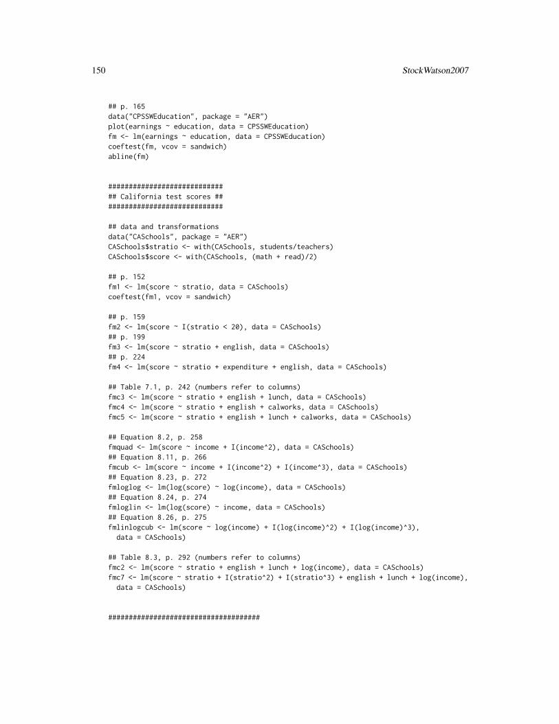
150 StockWatson2007
## p. 165data("CPSSWEducation", package = "AER")plot(earnings ~ education, data = CPSSWEducation)fm <- lm(earnings ~ education, data = CPSSWEducation)coeftest(fm, vcov = sandwich)abline(fm)
############################## California test scores ##############################
## data and transformationsdata("CASchools", package = "AER")CASchools$stratio <- with(CASchools, students/teachers)CASchools$score <- with(CASchools, (math + read)/2)
## p. 152fm1 <- lm(score ~ stratio, data = CASchools)coeftest(fm1, vcov = sandwich)
## p. 159fm2 <- lm(score ~ I(stratio < 20), data = CASchools)## p. 199fm3 <- lm(score ~ stratio + english, data = CASchools)## p. 224fm4 <- lm(score ~ stratio + expenditure + english, data = CASchools)
## Table 7.1, p. 242 (numbers refer to columns)fmc3 <- lm(score ~ stratio + english + lunch, data = CASchools)fmc4 <- lm(score ~ stratio + english + calworks, data = CASchools)fmc5 <- lm(score ~ stratio + english + lunch + calworks, data = CASchools)
## Equation 8.2, p. 258fmquad <- lm(score ~ income + I(income^2), data = CASchools)## Equation 8.11, p. 266fmcub <- lm(score ~ income + I(income^2) + I(income^3), data = CASchools)## Equation 8.23, p. 272fmloglog <- lm(log(score) ~ log(income), data = CASchools)## Equation 8.24, p. 274fmloglin <- lm(log(score) ~ income, data = CASchools)## Equation 8.26, p. 275fmlinlogcub <- lm(score ~ log(income) + I(log(income)^2) + I(log(income)^3),
data = CASchools)
## Table 8.3, p. 292 (numbers refer to columns)fmc2 <- lm(score ~ stratio + english + lunch + log(income), data = CASchools)fmc7 <- lm(score ~ stratio + I(stratio^2) + I(stratio^3) + english + lunch + log(income),
data = CASchools)
#####################################
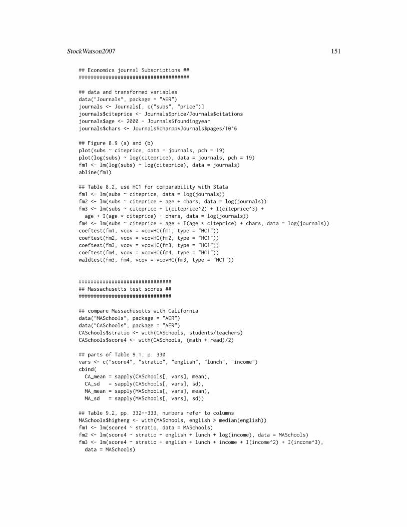
StockWatson2007 151
## Economics journal Subscriptions #######################################
## data and transformed variablesdata("Journals", package = "AER")journals <- Journals[, c("subs", "price")]journals$citeprice <- Journals$price/Journals$citationsjournals$age <- 2000 - Journals$foundingyearjournals$chars <- Journals$charpp*Journals$pages/10^6
## Figure 8.9 (a) and (b)plot(subs ~ citeprice, data = journals, pch = 19)plot(log(subs) ~ log(citeprice), data = journals, pch = 19)fm1 <- lm(log(subs) ~ log(citeprice), data = journals)abline(fm1)
## Table 8.2, use HC1 for comparability with Statafm1 <- lm(subs ~ citeprice, data = log(journals))fm2 <- lm(subs ~ citeprice + age + chars, data = log(journals))fm3 <- lm(subs ~ citeprice + I(citeprice^2) + I(citeprice^3) +
age + I(age * citeprice) + chars, data = log(journals))fm4 <- lm(subs ~ citeprice + age + I(age * citeprice) + chars, data = log(journals))coeftest(fm1, vcov = vcovHC(fm1, type = "HC1"))coeftest(fm2, vcov = vcovHC(fm2, type = "HC1"))coeftest(fm3, vcov = vcovHC(fm3, type = "HC1"))coeftest(fm4, vcov = vcovHC(fm4, type = "HC1"))waldtest(fm3, fm4, vcov = vcovHC(fm3, type = "HC1"))
################################# Massachusetts test scores #################################
## compare Massachusetts with Californiadata("MASchools", package = "AER")data("CASchools", package = "AER")CASchools$stratio <- with(CASchools, students/teachers)CASchools$score4 <- with(CASchools, (math + read)/2)
## parts of Table 9.1, p. 330vars <- c("score4", "stratio", "english", "lunch", "income")cbind(
CA_mean = sapply(CASchools[, vars], mean),CA_sd = sapply(CASchools[, vars], sd),MA_mean = sapply(MASchools[, vars], mean),MA_sd = sapply(MASchools[, vars], sd))
## Table 9.2, pp. 332--333, numbers refer to columnsMASchools$higheng <- with(MASchools, english > median(english))fm1 <- lm(score4 ~ stratio, data = MASchools)fm2 <- lm(score4 ~ stratio + english + lunch + log(income), data = MASchools)fm3 <- lm(score4 ~ stratio + english + lunch + income + I(income^2) + I(income^3),
data = MASchools)
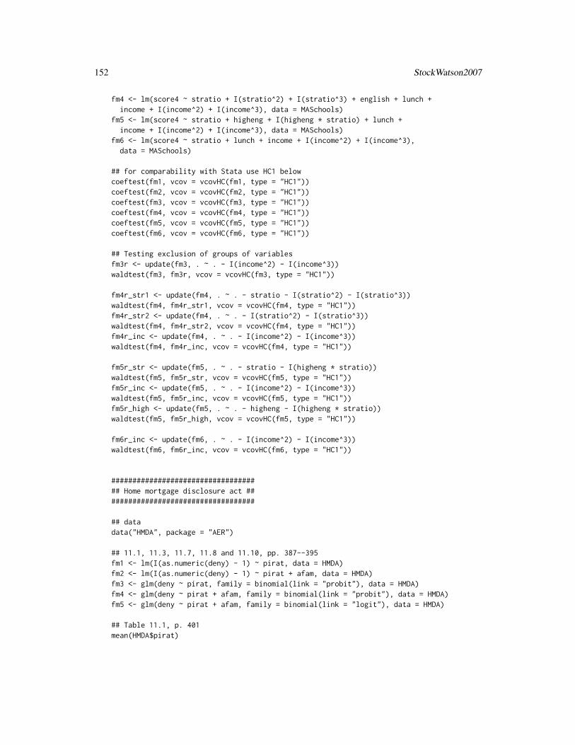
152 StockWatson2007
fm4 <- lm(score4 ~ stratio + I(stratio^2) + I(stratio^3) + english + lunch +income + I(income^2) + I(income^3), data = MASchools)
fm5 <- lm(score4 ~ stratio + higheng + I(higheng * stratio) + lunch +income + I(income^2) + I(income^3), data = MASchools)
fm6 <- lm(score4 ~ stratio + lunch + income + I(income^2) + I(income^3),data = MASchools)
## for comparability with Stata use HC1 belowcoeftest(fm1, vcov = vcovHC(fm1, type = "HC1"))coeftest(fm2, vcov = vcovHC(fm2, type = "HC1"))coeftest(fm3, vcov = vcovHC(fm3, type = "HC1"))coeftest(fm4, vcov = vcovHC(fm4, type = "HC1"))coeftest(fm5, vcov = vcovHC(fm5, type = "HC1"))coeftest(fm6, vcov = vcovHC(fm6, type = "HC1"))
## Testing exclusion of groups of variablesfm3r <- update(fm3, . ~ . - I(income^2) - I(income^3))waldtest(fm3, fm3r, vcov = vcovHC(fm3, type = "HC1"))
fm4r_str1 <- update(fm4, . ~ . - stratio - I(stratio^2) - I(stratio^3))waldtest(fm4, fm4r_str1, vcov = vcovHC(fm4, type = "HC1"))fm4r_str2 <- update(fm4, . ~ . - I(stratio^2) - I(stratio^3))waldtest(fm4, fm4r_str2, vcov = vcovHC(fm4, type = "HC1"))fm4r_inc <- update(fm4, . ~ . - I(income^2) - I(income^3))waldtest(fm4, fm4r_inc, vcov = vcovHC(fm4, type = "HC1"))
fm5r_str <- update(fm5, . ~ . - stratio - I(higheng * stratio))waldtest(fm5, fm5r_str, vcov = vcovHC(fm5, type = "HC1"))fm5r_inc <- update(fm5, . ~ . - I(income^2) - I(income^3))waldtest(fm5, fm5r_inc, vcov = vcovHC(fm5, type = "HC1"))fm5r_high <- update(fm5, . ~ . - higheng - I(higheng * stratio))waldtest(fm5, fm5r_high, vcov = vcovHC(fm5, type = "HC1"))
fm6r_inc <- update(fm6, . ~ . - I(income^2) - I(income^3))waldtest(fm6, fm6r_inc, vcov = vcovHC(fm6, type = "HC1"))
#################################### Home mortgage disclosure act ####################################
## datadata("HMDA", package = "AER")
## 11.1, 11.3, 11.7, 11.8 and 11.10, pp. 387--395fm1 <- lm(I(as.numeric(deny) - 1) ~ pirat, data = HMDA)fm2 <- lm(I(as.numeric(deny) - 1) ~ pirat + afam, data = HMDA)fm3 <- glm(deny ~ pirat, family = binomial(link = "probit"), data = HMDA)fm4 <- glm(deny ~ pirat + afam, family = binomial(link = "probit"), data = HMDA)fm5 <- glm(deny ~ pirat + afam, family = binomial(link = "logit"), data = HMDA)
## Table 11.1, p. 401mean(HMDA$pirat)
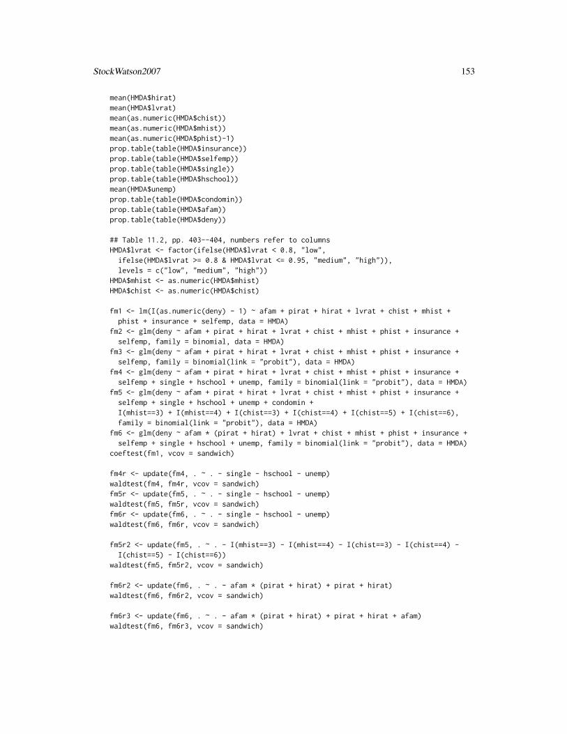
StockWatson2007 153
mean(HMDA$hirat)mean(HMDA$lvrat)mean(as.numeric(HMDA$chist))mean(as.numeric(HMDA$mhist))mean(as.numeric(HMDA$phist)-1)prop.table(table(HMDA$insurance))prop.table(table(HMDA$selfemp))prop.table(table(HMDA$single))prop.table(table(HMDA$hschool))mean(HMDA$unemp)prop.table(table(HMDA$condomin))prop.table(table(HMDA$afam))prop.table(table(HMDA$deny))
## Table 11.2, pp. 403--404, numbers refer to columnsHMDA$lvrat <- factor(ifelse(HMDA$lvrat < 0.8, "low",
ifelse(HMDA$lvrat >= 0.8 & HMDA$lvrat <= 0.95, "medium", "high")),levels = c("low", "medium", "high"))
HMDA$mhist <- as.numeric(HMDA$mhist)HMDA$chist <- as.numeric(HMDA$chist)
fm1 <- lm(I(as.numeric(deny) - 1) ~ afam + pirat + hirat + lvrat + chist + mhist +phist + insurance + selfemp, data = HMDA)
fm2 <- glm(deny ~ afam + pirat + hirat + lvrat + chist + mhist + phist + insurance +selfemp, family = binomial, data = HMDA)
fm3 <- glm(deny ~ afam + pirat + hirat + lvrat + chist + mhist + phist + insurance +selfemp, family = binomial(link = "probit"), data = HMDA)
fm4 <- glm(deny ~ afam + pirat + hirat + lvrat + chist + mhist + phist + insurance +selfemp + single + hschool + unemp, family = binomial(link = "probit"), data = HMDA)
fm5 <- glm(deny ~ afam + pirat + hirat + lvrat + chist + mhist + phist + insurance +selfemp + single + hschool + unemp + condomin +I(mhist==3) + I(mhist==4) + I(chist==3) + I(chist==4) + I(chist==5) + I(chist==6),family = binomial(link = "probit"), data = HMDA)
fm6 <- glm(deny ~ afam * (pirat + hirat) + lvrat + chist + mhist + phist + insurance +selfemp + single + hschool + unemp, family = binomial(link = "probit"), data = HMDA)
coeftest(fm1, vcov = sandwich)
fm4r <- update(fm4, . ~ . - single - hschool - unemp)waldtest(fm4, fm4r, vcov = sandwich)fm5r <- update(fm5, . ~ . - single - hschool - unemp)waldtest(fm5, fm5r, vcov = sandwich)fm6r <- update(fm6, . ~ . - single - hschool - unemp)waldtest(fm6, fm6r, vcov = sandwich)
fm5r2 <- update(fm5, . ~ . - I(mhist==3) - I(mhist==4) - I(chist==3) - I(chist==4) -I(chist==5) - I(chist==6))
waldtest(fm5, fm5r2, vcov = sandwich)
fm6r2 <- update(fm6, . ~ . - afam * (pirat + hirat) + pirat + hirat)waldtest(fm6, fm6r2, vcov = sandwich)
fm6r3 <- update(fm6, . ~ . - afam * (pirat + hirat) + pirat + hirat + afam)waldtest(fm6, fm6r3, vcov = sandwich)
154 StockWatson2007
########################################################### Shooting down the "More Guns Less Crime" hypothesis ###########################################################
## datadata("Guns", package = "AER")
## Empirical Exercise 10.1fm1 <- lm(log(violent) ~ law, data = Guns)fm2 <- lm(log(violent) ~ law + prisoners + density + income +
population + afam + cauc + male, data = Guns)fm3 <- lm(log(violent) ~ law + prisoners + density + income +
population + afam + cauc + male + state, data = Guns)fm4 <- lm(log(violent) ~ law + prisoners + density + income +
population + afam + cauc + male + state + year, data = Guns)coeftest(fm1, vcov = sandwich)coeftest(fm2, vcov = sandwich)printCoefmat(coeftest(fm3, vcov = sandwich)[1:9,])printCoefmat(coeftest(fm4, vcov = sandwich)[1:9,])
############################# US traffic fatalities #############################
## data from Stock and Watson (2007)data("Fatalities")## add fatality rate (number of traffic deaths## per 10,000 people living in that state in that year)Fatalities$frate <- with(Fatalities, fatal/pop * 10000)## add discretized version of minimum legal drinking ageFatalities$drinkagec <- cut(Fatalities$drinkage,
breaks = 18:22, include.lowest = TRUE, right = FALSE)Fatalities$drinkagec <- relevel(Fatalities$drinkagec, ref = 4)## any punishment?Fatalities$punish <- with(Fatalities,
factor(jail == "yes" | service == "yes", labels = c("no", "yes")))## plm packagelibrary("plm")
## for comparability with Stata we use HC1 below## p. 351, Eq. (10.2)f1982 <- subset(Fatalities, year == "1982")fm_1982 <- lm(frate ~ beertax, data = f1982)coeftest(fm_1982, vcov = vcovHC(fm_1982, type = "HC1"))
## p. 353, Eq. (10.3)f1988 <- subset(Fatalities, year == "1988")fm_1988 <- lm(frate ~ beertax, data = f1988)coeftest(fm_1988, vcov = vcovHC(fm_1988, type = "HC1"))
StockWatson2007 155
## pp. 355, Eq. (10.8)fm_diff <- lm(I(f1988$frate - f1982$frate) ~ I(f1988$beertax - f1982$beertax))coeftest(fm_diff, vcov = vcovHC(fm_diff, type = "HC1"))
## pp. 360, Eq. (10.15)## (1) via formulafm_sfe <- lm(frate ~ beertax + state - 1, data = Fatalities)## (2) by handfat <- with(Fatalities,
data.frame(frates = frate - ave(frate, state),beertaxs = beertax - ave(beertax, state)))
fm_sfe2 <- lm(frates ~ beertaxs - 1, data = fat)## (3) via plm()fm_sfe3 <- plm(frate ~ beertax, data = Fatalities,
index = c("state", "year"), model = "within")
coeftest(fm_sfe, vcov = vcovHC(fm_sfe, type = "HC1"))[1,]
## uses different df in sd and p-valuecoeftest(fm_sfe2, vcov = vcovHC(fm_sfe2, type = "HC1"))[1,]
## uses different df in p-valuecoeftest(fm_sfe3, vcov = vcovHC(fm_sfe3, type = "HC1", method = "white1"))[1,]
## pp. 363, Eq. (10.21)## via lm()fm_stfe <- lm(frate ~ beertax + state + year - 1, data = Fatalities)coeftest(fm_stfe, vcov = vcovHC(fm_stfe, type = "HC1"))[1,]## via plm()fm_stfe2 <- plm(frate ~ beertax, data = Fatalities,
index = c("state", "year"), model = "within", effect = "twoways")coeftest(fm_stfe2, vcov = vcovHC) ## different
## p. 368, Table 10.1, numbers refer to cols.fm1 <- plm(frate ~ beertax, data = Fatalities, index = c("state", "year"),
model = "pooling")fm2 <- plm(frate ~ beertax, data = Fatalities, index = c("state", "year"),
model = "within")fm3 <- plm(frate ~ beertax, data = Fatalities, index = c("state", "year"),
model = "within", effect = "twoways")fm4 <- plm(frate ~ beertax + drinkagec + jail + service + miles + unemp + log(income),
data = Fatalities, index = c("state", "year"), model = "within", effect = "twoways")fm5 <- plm(frate ~ beertax + drinkagec + jail + service + miles,
data = Fatalities, index = c("state", "year"), model = "within", effect = "twoways")fm6 <- plm(frate ~ beertax + drinkage + punish + miles + unemp + log(income),
data = Fatalities, index = c("state", "year"), model = "within", effect = "twoways")fm7 <- plm(frate ~ beertax + drinkagec + jail + service + miles + unemp + log(income),
data = Fatalities, index = c("state", "year"), model = "within", effect = "twoways")## summaries not too close, s.e.s generally too smallcoeftest(fm1, vcov = vcovHC)
156 StockWatson2007
coeftest(fm2, vcov = vcovHC)coeftest(fm3, vcov = vcovHC)coeftest(fm4, vcov = vcovHC)coeftest(fm5, vcov = vcovHC)coeftest(fm6, vcov = vcovHC)coeftest(fm7, vcov = vcovHC)
######################################## Cigarette consumption panel data ########################################
## data and transformationsdata("CigarettesSW", package = "AER")CigarettesSW$rprice <- with(CigarettesSW, price/cpi)CigarettesSW$rincome <- with(CigarettesSW, income/population/cpi)CigarettesSW$tdiff <- with(CigarettesSW, (taxs - tax)/cpi)c1985 <- subset(CigarettesSW, year == "1985")c1995 <- subset(CigarettesSW, year == "1995")
## convenience function: HC1 covarianceshc1 <- function(x) vcovHC(x, type = "HC1")
## Equations 12.9--12.11fm_s1 <- lm(log(rprice) ~ tdiff, data = c1995)coeftest(fm_s1, vcov = hc1)fm_s2 <- lm(log(packs) ~ fitted(fm_s1), data = c1995)fm_ivreg <- ivreg(log(packs) ~ log(rprice) | tdiff, data = c1995)coeftest(fm_ivreg, vcov = hc1)
## Equation 12.15fm_ivreg2 <- ivreg(log(packs) ~ log(rprice) + log(rincome) | log(rincome) + tdiff,
data = c1995)coeftest(fm_ivreg2, vcov = hc1)## Equation 12.16fm_ivreg3 <- ivreg(log(packs) ~ log(rprice) + log(rincome) | log(rincome) + tdiff + I(tax/cpi),
data = c1995)coeftest(fm_ivreg3, vcov = hc1)
## Table 12.1, p. 448ydiff <- log(c1995$packs) - log(c1985$packs)pricediff <- log(c1995$price/c1995$cpi) - log(c1985$price/c1985$cpi)incdiff <- log(c1995$income/c1995$population/c1995$cpi) -
log(c1985$income/c1985$population/c1985$cpi)taxsdiff <- (c1995$taxs - c1995$tax)/c1995$cpi - (c1985$taxs - c1985$tax)/c1985$cpitaxdiff <- c1995$tax/c1995$cpi - c1985$tax/c1985$cpi
fm_diff1 <- ivreg(ydiff ~ pricediff + incdiff | incdiff + taxsdiff)fm_diff2 <- ivreg(ydiff ~ pricediff + incdiff | incdiff + taxdiff)fm_diff3 <- ivreg(ydiff ~ pricediff + incdiff | incdiff + taxsdiff + taxdiff)coeftest(fm_diff1, vcov = hc1)coeftest(fm_diff2, vcov = hc1)coeftest(fm_diff3, vcov = hc1)
StockWatson2007 157
## checking instrument relevancefm_rel1 <- lm(pricediff ~ taxsdiff + incdiff)fm_rel2 <- lm(pricediff ~ taxdiff + incdiff)fm_rel3 <- lm(pricediff ~ incdiff + taxsdiff + taxdiff)linearHypothesis(fm_rel1, "taxsdiff = 0", vcov = hc1)linearHypothesis(fm_rel2, "taxdiff = 0", vcov = hc1)linearHypothesis(fm_rel3, c("taxsdiff = 0", "taxdiff = 0"), vcov = hc1)
## testing overidentifying restrictions (J test)fm_or <- lm(residuals(fm_diff3) ~ incdiff + taxsdiff + taxdiff)(fm_or_test <- linearHypothesis(fm_or, c("taxsdiff = 0", "taxdiff = 0"), test = "Chisq"))## warning: df (and hence p-value) invalid above.## correct df: # instruments - # endogenous variablespchisq(fm_or_test[2,5], df.residual(fm_diff3) - df.residual(fm_or), lower.tail = FALSE)
####################################################### Project STAR: Student-teacher achievement ratio #######################################################
## datadata("STAR", package = "AER")
## p. 488fmk <- lm(I(readk + mathk) ~ stark, data = STAR)fm1 <- lm(I(read1 + math1) ~ star1, data = STAR)fm2 <- lm(I(read2 + math2) ~ star2, data = STAR)fm3 <- lm(I(read3 + math3) ~ star3, data = STAR)coeftest(fm3, vcov = sandwich)
## p. 489fmke <- lm(I(readk + mathk) ~ stark + experiencek, data = STAR)coeftest(fmke, vcov = sandwich)
## equivalently:## - reshape data from wide into long format## - fit a single model nested in grade## (a) variables and their levelsnam <- c("star", "read", "math", "lunch", "school", "degree", "ladder",
"experience", "tethnicity", "system", "schoolid")lev <- c("k", "1", "2", "3")## (b) reshapingstar <- reshape(STAR, idvar = "id", ids = row.names(STAR),
times = lev, timevar = "grade", direction = "long",varying = lapply(nam, function(x) paste(x, lev, sep = "")))
## (c) improve variable names and typenames(star)[5:15] <- namstar$id <- factor(star$id)star$grade <- factor(star$grade, levels = lev,
labels = c("kindergarten", "1st", "2nd", "3rd"))rm(nam, lev)## (d) model fitting
158 StockWatson2007
fm <- lm(I(read + math) ~ 0 + grade/star, data = star)
################################################### Quarterly US macroeconomic data (1957-2005) ###################################################
## datadata("USMacroSW", package = "AER")library("dynlm")usm <- ts.intersect(USMacroSW, 4 * 100 * diff(log(USMacroSW[, "cpi"])))colnames(usm) <- c(colnames(USMacroSW), "infl")
## Equation 14.7, p. 536fm_ar1 <- dynlm(d(infl) ~ L(d(infl)),
data = usm, start = c(1962,1), end = c(2004,4))coeftest(fm_ar1, vcov = sandwich)
## Equation 14.13, p. 538fm_ar4 <- dynlm(d(infl) ~ L(d(infl), 1:4),
data = usm, start = c(1962,1), end = c(2004,4))coeftest(fm_ar4, vcov = sandwich)
## Equation 14.16, p. 542fm_adl41 <- dynlm(d(infl) ~ L(d(infl), 1:4) + L(unemp),
data = usm, start = c(1962,1), end = c(2004,4))coeftest(fm_adl41, vcov = sandwich)
## Equation 14.17, p. 542fm_adl44 <- dynlm(d(infl) ~ L(d(infl), 1:4) + L(unemp, 1:4),
data = usm, start = c(1962,1), end = c(2004,4))coeftest(fm_adl44, vcov = sandwich)
## Granger causality test mentioned on p. 547waldtest(fm_ar4, fm_adl44, vcov = sandwich)
## Equation 14.28, p. 559fm_sp1 <- dynlm(infl ~ log(gdpjp), start = c(1965,1), end = c(1981,4), data = usm)coeftest(fm_sp1, vcov = sandwich)
## Equation 14.29, p. 559fm_sp2 <- dynlm(infl ~ log(gdpjp), start = c(1982,1), end = c(2004,4), data = usm)coeftest(fm_sp2, vcov = sandwich)
## Equation 14.34, p. 563: ADF by handfm_adf <- dynlm(d(infl) ~ L(infl) + L(d(infl), 1:4),
data = usm, start = c(1962,1), end = c(2004,4))coeftest(fm_adf)
## Figure 14.5, p. 570## SW perform partial break test of unemp coefs## here full model is usedlibrary("strucchange")
StockWatson2007 159
infl <- usm[, "infl"]unemp <- usm[, "unemp"]usm <- ts.intersect(diff(infl), lag(diff(infl), k = -1), lag(diff(infl), k = -2),
lag(diff(infl), k = -3), lag(diff(infl), k = -4), lag(unemp, k = -1),lag(unemp, k = -2), lag(unemp, k = -3), lag(unemp, k = -4))
colnames(usm) <- c("dinfl", paste("dinfl", 1:4, sep = ""), paste("unemp", 1:4, sep = ""))usm <- window(usm, start = c(1962, 1), end = c(2004, 4))fs <- Fstats(dinfl ~ ., data = usm)sctest(fs, type = "supF")plot(fs)
## alternatively: re-use fm_adl44mf <- model.frame(fm_adl44)mf <- ts(as.matrix(mf), start = c(1962, 1), freq = 4)colnames(mf) <- c("y", paste("x", 1:8, sep = ""))ff <- as.formula(paste("y", "~", paste("x", 1:8, sep = "", collapse = " + ")))fs <- Fstats(ff, data = mf, from = 0.1)plot(fs)lines(boundary(fs, alpha = 0.01), lty = 2, col = 2)lines(boundary(fs, alpha = 0.1), lty = 3, col = 2)
############################################ Monthly US stock returns (1931-2002) ############################################
## package and datalibrary("dynlm")data("USStocksSW", package = "AER")
## Table 14.3, p. 540fm1 <- dynlm(returns ~ L(returns), data = USStocksSW, start = c(1960,1))coeftest(fm1, vcov = sandwich)fm2 <- dynlm(returns ~ L(returns, 1:2), data = USStocksSW, start = c(1960,1))waldtest(fm2, vcov = sandwich)fm3 <- dynlm(returns ~ L(returns, 1:4), data = USStocksSW, start = c(1960,1))waldtest(fm3, vcov = sandwich)
## Table 14.7, p. 574fm4 <- dynlm(returns ~ L(returns) + L(d(dividend)),
data = USStocksSW, start = c(1960, 1))fm5 <- dynlm(returns ~ L(returns, 1:2) + L(d(dividend), 1:2),
data = USStocksSW, start = c(1960, 1))fm6 <- dynlm(returns ~ L(returns) + L(dividend),
data = USStocksSW, start = c(1960, 1))
#################################### Price of frozen orange juice ####################################
## load datadata("FrozenJuice")
160 StrikeDuration
## Stock and Watson, p. 594library("dynlm")fm_dyn <- dynlm(d(100 * log(price/ppi)) ~ fdd, data = FrozenJuice)coeftest(fm_dyn, vcov = vcovHC(fm_dyn, type = "HC1"))
## equivalently, returns can be computed 'by hand'## (reducing the complexity of the formula notation)fj <- ts.union(fdd = FrozenJuice[, "fdd"],
ret = 100 * diff(log(FrozenJuice[,"price"]/FrozenJuice[,"ppi"])))fm_dyn <- dynlm(ret ~ fdd, data = fj)
## Stock and Watson, p. 595fm_dl <- dynlm(ret ~ L(fdd, 0:6), data = fj)coeftest(fm_dl, vcov = vcovHC(fm_dl, type = "HC1"))
## Stock and Watson, Table 15.1, p. 620, numbers refer to columns## (1) Dynamic Multipliersfm1 <- dynlm(ret ~ L(fdd, 0:18), data = fj)coeftest(fm1, vcov = NeweyWest(fm1, lag = 7, prewhite = FALSE))## (2) Cumulative Multipliersfm2 <- dynlm(ret ~ L(d(fdd), 0:17) + L(fdd, 18), data = fj)coeftest(fm2, vcov = NeweyWest(fm2, lag = 7, prewhite = FALSE))## (3) Cumulative Multipliers, more lags in NWcoeftest(fm2, vcov = NeweyWest(fm2, lag = 14, prewhite = FALSE))## (4) Cumulative Multipliers with monthly indicatorsfm4 <- dynlm(ret ~ L(d(fdd), 0:17) + L(fdd, 18) + season(fdd), data = fj)coeftest(fm4, vcov = NeweyWest(fm4, lag = 7, prewhite = FALSE))## monthly indicators needed?fm4r <- update(fm4, . ~ . - season(fdd))waldtest(fm4, fm4r, vcov= NeweyWest(fm4, lag = 7, prewhite = FALSE)) ## close ...
############################################### New York Stock Exchange composite index ###############################################
## returnsdata("NYSESW", package = "AER")ret <- 100 * diff(log(NYSESW))plot(ret)
## fit GARCH(1,1)library("tseries")fm <- garch(coredata(ret))
StrikeDuration Strike Durations
Description
Data on the duration of strikes in US manufacturing industries, 1968–1976.
StrikeDuration 161
Usage
data("StrikeDuration")
Format
A data frame containing 62 observations on 2 variables for the period 1968–1976.
duration strike duration in days.
uoutput unanticipated output (a measure of unanticipated aggregate industrial production net ofseasonal and trend components).
Details
The original data provided by Kennan (1985) are on a monthly basis, for the period 1968(1) through1976(12). Greene (2003) only provides the June data for each year. Also, the duration for observa-tion 36 is given as 3 by Greene while Kennan has 2. Here we use Greene’s version.
uoutput is the residual from a regression of the logarithm of industrial production in manufacturingon time, time squared, and monthly dummy variables.
Source
Online complements to Greene (2003).
http://pages.stern.nyu.edu/~wgreene/Text/tables/tablelist5.htm
References
Greene, W.H. (2003). Econometric Analysis, 5th edition. Upper Saddle River, NJ: Prentice Hall.
Kennan, J. (1985). The Duration of Contract Strikes in US Manufacturing. Journal of Economet-rics, 28, 5–28.
See Also
Greene2003
Examples
data("StrikeDuration")library("MASS")
## Greene (2003), Table 22.10fit_exp <- fitdistr(StrikeDuration$duration, "exponential")fit_wei <- fitdistr(StrikeDuration$duration, "weibull")fit_wei$estimate[2]^(-1)fit_lnorm <- fitdistr(StrikeDuration$duration, "lognormal")1/fit_lnorm$estimate[2]exp(-fit_lnorm$estimate[1])## Weibull and lognormal distribution have## different parameterizations, see Greene p. 794
162 summary.ivreg
## Greene (2003), Example 22.10library("survival")fm_wei <- survreg(Surv(duration) ~ uoutput, dist = "weibull", data = StrikeDuration)summary(fm_wei)
summary.ivreg Methods for Instrumental-Variable Regression
Description
Methods to standard generics for instrumental-variable regressions fitted by ivreg.
Usage
## S3 method for class 'ivreg'summary(object, vcov. = NULL, df = NULL, diagnostics = FALSE, ...)## S3 method for class 'ivreg'anova(object, object2, test = "F", vcov = NULL, ...)
## S3 method for class 'ivreg'terms(x, component = c("regressors", "instruments"), ...)## S3 method for class 'ivreg'model.matrix(object, component = c("projected", "regressors", "instruments"), ...)
Arguments
object, object2, x
an object of class "ivreg" as fitted by ivreg.
vcov., vcov a specification of the covariance matrix of the estimated coefficients. This canbe specified as a matrix or as a function yielding a matrix when applied to thefitted model. If it is a function it is also employed in the two diagnostic F tests(if diagnostics = TRUE in the summary() method).
df the degrees of freedom to be used. By default this is set to residual degrees offreedom for which a t or F test is computed. Alternatively, it can be set to Inf(or equivalently 0) for which a z or Chi-squared test is computed.
diagnostics logical. Should diagnostic tests for the instrumental-variable regression be car-ried out? These encompass an F test of the first stage regression for weak instru-ments, a Wu-Hausman test for endogeneity, and a Sargan test of overidentifyingrestrictions (only if there are more instruments than regressors).
test character specifying whether to compute the large sample Chi-squared statistic(with asymptotic Chi-squared distribution) or the finite sample F statistic (withapproximate F distribution).
component character specifying for which component of the terms or model matrix shouldbe extracted. "projected" gives the matrix of regressors projected on the imageof the instruments.
... currently not used.
SwissLabor 163
Details
ivreg is the high-level interface to the work-horse function ivreg.fit, a set of standard methods(including summary, vcov, anova, hatvalues, predict, terms, model.matrix, bread, estfun) isavailable.
See Also
ivreg, lm.fit
Examples
## datadata("CigarettesSW")CigarettesSW$rprice <- with(CigarettesSW, price/cpi)CigarettesSW$rincome <- with(CigarettesSW, income/population/cpi)CigarettesSW$tdiff <- with(CigarettesSW, (taxs - tax)/cpi)
## modelfm <- ivreg(log(packs) ~ log(rprice) + log(rincome) | log(rincome) + tdiff + I(tax/cpi),
data = CigarettesSW, subset = year == "1995")summary(fm)summary(fm, vcov = sandwich, df = Inf, diagnostics = TRUE)
## ANOVAfm2 <- ivreg(log(packs) ~ log(rprice) | tdiff, data = CigarettesSW, subset = year == "1995")anova(fm, fm2, vcov = sandwich, test = "Chisq")
SwissLabor Swiss Labor Market Participation Data
Description
Cross-section data originating from the health survey SOMIPOPS for Switzerland in 1981.
Usage
data("SwissLabor")
Format
A data frame containing 872 observations on 7 variables.
participation Factor. Did the individual participate in the labor force?income Logarithm of nonlabor income.age Age in decades (years divided by 10).education Years of formal education.youngkids Number of young children (under 7 years of age).oldkids Number of older children (over 7 years of age).foreign Factor. Is the individual a foreigner (i.e., not Swiss)?

164 TeachingRatings
Source
Journal of Applied Econometrics Data Archive.
http://qed.econ.queensu.ca/jae/1996-v11.3/gerfin/
References
Gerfin, M. (1996). Parametric and Semi-Parametric Estimation of the Binary Response Model ofLabour Market Participation. Journal of Applied Econometrics, 11, 321–339.
Examples
data("SwissLabor")
### Gerfin (1996), Table I.fm_probit <- glm(participation ~ . + I(age^2), data = SwissLabor,
family = binomial(link = "probit"))summary(fm_probit)
### alternativelyfm_logit <- glm(participation ~ . + I(age^2), data = SwissLabor,
family = binomial)summary(fm_logit)
TeachingRatings Impact of Beauty on Instructor’s Teaching Ratings
Description
Data on course evaluations, course characteristics, and professor characteristics for 463 courses forthe academic years 2000–2002 at the University of Texas at Austin.
Usage
data("TeachingRatings")
Format
A data frame containing 463 observations on 13 variables.
minority factor. Does the instructor belong to a minority (non-Caucasian)?
age the professor’s age.
gender factor indicating instructor’s gender.
credits factor. Is the course a single-credit elective (e.g., yoga, aerobics, dance)?
beauty rating of the instructor’s physical appearance by a panel of six students, averaged acrossthe six panelists, shifted to have a mean of zero.
eval course overall teaching evaluation score, on a scale of 1 (very unsatisfactory) to 5 (excellent).
TeachingRatings 165
division factor. Is the course an upper or lower division course? (Lower division courses are mainlylarge freshman and sophomore courses)?
native factor. Is the instructor a native English speaker?
tenure factor. Is the instructor on tenure track?
students number of students that participated in the evaluation.
allstudents number of students enrolled in the course.
prof factor indicating instructor identifier.
Details
A sample of student instructional ratings for a group of university teachers along with beauty rating(average from six independent judges) and a number of other characteristics.
Source
The data were provided by Prof. Hamermesh. The first 8 variables are also available in the onlinecomplements to Stock and Watson (2007) at
References
Hamermesh, D.S., and Parker, A. (2005). Beauty in the Classroom: Instructors’ Pulchritude andPutative Pedagogical Productivity. Economics of Education Review, 24, 369–376.
Stock, J.H. and Watson, M.W. (2007). Introduction to Econometrics, 2nd ed. Boston: AddisonWesley.
See Also
StockWatson2007
Examples
data("TeachingRatings")
## evaluation score vs. beautyplot(eval ~ beauty, data = TeachingRatings)fm <- lm(eval ~ beauty, data = TeachingRatings)abline(fm)summary(fm)
## prediction of Stock & Watson's evaluation scoresw <- with(TeachingRatings, mean(beauty) + c(0, 1) * sd(beauty))names(sw) <- c("Watson", "Stock")predict(fm, newdata = data.frame(beauty = sw))
## Hamermesh and Parker, 2005, Table 3fmw <- lm(eval ~ beauty + gender + minority + native + tenure + division + credits,
weights = students, data = TeachingRatings)coeftest(fmw, vcov = sandwich)## (same coefficients but with different covariances)
166 TechChange
TechChange Technological Change Data
Description
US time series data, 1909–1949.
Usage
data("TechChange")
Format
An annual multiple time series from 1909 to 1949 with 3 variables.
output Output.
clr Capital/labor ratio.
technology Index of technology.
Source
Online complements to Greene (2003), Table F7.2.
http://pages.stern.nyu.edu/~wgreene/Text/tables/tablelist5.htm
References
Greene, W.H. (2003). Econometric Analysis, 5th edition. Upper Saddle River, NJ: Prentice Hall.
Solow, R. (1957). Technical Change and the Aggregate Production Function. Review of Economicsand Statistics, 39, 312–320.
See Also
Greene2003
Examples
data("TechChange")
## Greene (2003)## Exercise 7.1fm1 <- lm(I(output/technology) ~ log(clr), data = TechChange)fm2 <- lm(I(output/technology) ~ I(1/clr), data = TechChange)fm3 <- lm(log(output/technology) ~ log(clr), data = TechChange)fm4 <- lm(log(output/technology) ~ I(1/clr), data = TechChange)
## Exercise 7.2 (a) and (c)plot(I(output/technology) ~ clr, data = TechChange)
tobit 167
library("strucchange")sctest(I(output/technology) ~ log(clr), data = TechChange, type = "Chow", point = c(1942, 1))
tobit Tobit Regression
Description
Fitting and testing tobit regression models for censored data.
Usage
tobit(formula, left = 0, right = Inf, dist = "gaussian",subset = NULL, data = list(), ...)
Arguments
formula a symbolic description of a regression model of type y ~ x1 + x2 + ....
left left limit for the censored dependent variable y. If set to -Inf, y is assumed notto be left-censored.
right right limit for the censored dependent variable y. If set to Inf, the default, y isassumed not to be right-censored.
dist assumed distribution for the dependent variable y. This is passed to survreg,see the respective man page for more details.
subset a specification of the rows to be used.
data a data frame containing the variables in the model.
... further arguments passed to survreg.
Details
The function tobit is a convenience interface to survreg (for survival regression, including cen-sored regression) setting different defaults and providing a more convenient interface for specifica-tion of the censoring information.
The default is the classical tobit model (Tobin 1958, Greene 2003) assuming a normal distributionfor the dependent variable with left-censoring at 0.
Technically, the formula of type y ~ x1 + x2 + ... passed to tobit is simply transformedinto a formula suitable for survreg: This means the dependent variable is first censored and thenwrapped into a Surv object containing the censoring information which is subsequently passed tosurvreg, e.g., Surv(ifelse(y <= 0, 0, y), y > 0, type = "left") ~ x1 + x2 + ... forthe default settings.
Value
An object of class "tobit" inheriting from class "survreg".
168 TradeCredit
References
Greene, W.H. (2003). Econometric Analysis, 5th edition. Upper Saddle River, NJ: Prentice Hall.
Tobin, J. (1958). Estimation of Relationships for Limited Dependent Variables. Econometrica, 26,24–36.
Examples
data("Affairs")
## from Table 22.4 in Greene (2003)fm.tobit <- tobit(affairs ~ age + yearsmarried + religiousness + occupation + rating,
data = Affairs)fm.tobit2 <- tobit(affairs ~ age + yearsmarried + religiousness + occupation + rating,
right = 4, data = Affairs)
summary(fm.tobit)summary(fm.tobit2)
TradeCredit Trade Credit and the Money Market
Description
Macroeconomic time series data from 1946 to 1966 on trade credit and the money market.
Usage
data("TradeCredit")
Format
An annual multiple time series from 1946 to 1966 on 7 variables.
trade Nominal total trade money.
reserve Nominal effective reserve money.
gnp GNP in current dollars.
utilization Degree of market utilization.
interest Short-term rate of interest.
size Mean real size of the representative economic unit (1939 = 100).
price GNP price deflator (1958 = 100).
Source
The data are from Baltagi (2002).

TravelMode 169
References
Baltagi, B.H. (2002). Econometrics, 3rd ed. Berlin, Springer.
Laffer, A.B. (1970). Trade Credit and the Money Market. Journal of Political Economy, 78, 239–267.
See Also
Baltagi2002
Examples
data("TradeCredit")plot(TradeCredit)
TravelMode Travel Mode Choice Data
Description
Data on travel mode choice for travel between Sydney and Melbourne, Australia.
Usage
data("TravelMode")
Format
A data frame containing 840 observations on 4 modes for 210 individuals.
individual Factor indicating individual with levels 1 to 200.
mode Factor indicating travel mode with levels "car", "air", "train", or "bus".
choice Factor indicating choice with levels "no" and "yes".
wait Terminal waiting time, 0 for car.
vcost Vehicle cost component.
travel Travel time in the vehicle.
gcost Generalized cost measure.
income Household income.
size Party size.
Source
Online complements to Greene (2003).
http://pages.stern.nyu.edu/~wgreene/Text/tables/tablelist5.htm
170 UKInflation
References
Greene, W.H. (2003). Econometric Analysis, 5th edition. Upper Saddle River, NJ: Prentice Hall.
See Also
Greene2003
Examples
data("TravelMode")
## overall proportions for chosen modewith(TravelMode, prop.table(table(mode[choice == "yes"])))
## travel vs. waiting time for different travel modeslibrary("lattice")xyplot(travel ~ wait | mode, data = TravelMode)
## Greene (2003), Table 21.11, conditional logit modelif(require("mlogit")) {TravelMode$incair <- with(TravelMode, income * (mode == "air"))tm_cl <- mlogit(choice ~ gcost + wait + incair, data = TravelMode,
shape = "long", alt.var = "mode", reflevel = "car")summary(tm_cl)}
UKInflation UK Manufacturing Inflation Data
Description
Time series of observed and expected price changes in British manufacturing.
Usage
data("UKInflation")
Format
A quarterly multiple time series from 1972(1) to 1985(2) with 2 variables.
actual Actual inflation.
expected Expected inflation.
Source
Online complements to Greene (2003), Table F8.1.
http://pages.stern.nyu.edu/~wgreene/Text/tables/tablelist5.htm
UKNonDurables 171
References
Greene, W.H. (2003). Econometric Analysis, 5th edition. Upper Saddle River, NJ: Prentice Hall.
Pesaran, M.H., and Hall, A.D. (1988). Tests of Non-nested Linear Regression Models Subject ToLinear Restrictions. Economics Letters, 27, 341–348.
See Also
Greene2003
Examples
data("UKInflation")plot(UKInflation)
UKNonDurables Consumption of Non-Durables in the UK
Description
Time series of consumption of non-durables in the UK (in 1985 prices).
Usage
data("UKNonDurables")
Format
A quarterly univariate time series from 1955(1) to 1988(4).
Source
Online complements to Franses (1998).
References
Osborn, D.R. (1988). A Survey of Seasonality in UK Macroeconomic Variables. InternationalJournal of Forecasting, 6, 327–336.
Franses, P.H. (1998). Time Series Models for Business and Economic Forecasting. Cambridge, UK:Cambridge University Press.
See Also
Franses1998
172 USAirlines
Examples
data("UKNonDurables")plot(UKNonDurables)
## EACF tables (Franses 1998, p. 99)ctrafo <- function(x) residuals(lm(x ~ factor(cycle(x))))ddiff <- function(x) diff(diff(x, frequency(x)), 1)eacf <- function(y, lag = 12) {
stopifnot(all(lag > 0))if(length(lag) < 2) lag <- 1:lagrval <- sapply(list(y = y, dy = diff(y), cdy = ctrafo(diff(y)),
Dy = diff(y, frequency(y)), dDy = ddiff(y)),function(x) acf(x, plot = FALSE, lag.max = max(lag))$acf[lag + 1])
rownames(rval) <- lagreturn(rval)
}
## Franses (1998), Table 5.2round(eacf(log(UKNonDurables)), digits = 3)
## Franses (1998), Equation 5.51## (Franses: sma1 = -0.632 (0.069))arima(log(UKNonDurables), c(0, 1, 0), c(0, 1, 1))
USAirlines Cost Data for US Airlines
Description
Cost data for six US airlines in 1970–1984.
Usage
data("USAirlines")
Format
A data frame containing 90 observations on 6 variables.
firm factor indicating airline firm.
year factor indicating year.
output output revenue passenger miles index number.
cost total cost (in USD 1000).
price fuel price.
load average capacity utilization of the fleet.
USAirlines 173
Source
Online complements to Greene (2003). Table F7.1.
http://pages.stern.nyu.edu/~wgreene/Text/tables/tablelist5.htm
References
Greene, W.H. (2003). Econometric Analysis, 5th edition. Upper Saddle River, NJ: Prentice Hall.
See Also
Greene2003
Examples
data("USAirlines")
## Example 7.2 in Greene (2003)fm_full <- lm(log(cost) ~ log(output) + I(log(output)^2) + log(price) + load + year + firm,
data = USAirlines)fm_time <- lm(log(cost) ~ log(output) + I(log(output)^2) + log(price) + load + year,
data = USAirlines)fm_firm <- lm(log(cost) ~ log(output) + I(log(output)^2) + log(price) + load + firm,
data = USAirlines)fm_no <- lm(log(cost) ~ log(output) + I(log(output)^2) + log(price) + load, data = USAirlines)
## Table 7.2anova(fm_full, fm_time)anova(fm_full, fm_firm)anova(fm_full, fm_no)
## alternatively, use plm()library("plm")usair <- plm.data(USAirlines, c("firm", "year"))fm_full2 <- plm(log(cost) ~ log(output) + I(log(output)^2) + log(price) + load,
data = usair, model = "within", effect = "twoways")fm_time2 <- plm(log(cost) ~ log(output) + I(log(output)^2) + log(price) + load,
data = usair, model = "within", effect = "time")fm_firm2 <- plm(log(cost) ~ log(output) + I(log(output)^2) + log(price) + load,
data = usair, model = "within", effect = "individual")fm_no2 <- plm(log(cost) ~ log(output) + I(log(output)^2) + log(price) + load,
data = usair, model = "pooling")pFtest(fm_full2, fm_time2)pFtest(fm_full2, fm_firm2)pFtest(fm_full2, fm_no2)
## More examples can be found in:## help("Greene2003")
174 USConsump1950
USConsump1950 US Consumption Data (1940–1950)
Description
Time series data on US income and consumption expenditure, 1940–1950.
Usage
data("USConsump1950")
Format
An annual multiple time series from 1940 to 1950 with 3 variables.
income Disposable income.
expenditure Consumption expenditure.
war Indicator variable: Was the year a year of war?
Source
Online complements to Greene (2003). Table F2.1.
http://pages.stern.nyu.edu/~wgreene/Text/tables/tablelist5.htm
References
Greene, W.H. (2003). Econometric Analysis, 5th edition. Upper Saddle River, NJ: Prentice Hall.
See Also
Greene2003, USConsump1979, USConsump1993
Examples
## Greene (2003)## datadata("USConsump1950")usc <- as.data.frame(USConsump1950)usc$war <- factor(usc$war, labels = c("no", "yes"))
## Example 2.1plot(expenditure ~ income, data = usc, type = "n", xlim = c(225, 375), ylim = c(225, 350))with(usc, text(income, expenditure, time(USConsump1950)))
## single modelfm <- lm(expenditure ~ income, data = usc)summary(fm)
USConsump1979 175
## different intercepts for war yes/nofm2 <- lm(expenditure ~ income + war, data = usc)summary(fm2)
## compareanova(fm, fm2)
## visualizeabline(fm, lty = 3)abline(coef(fm2)[1:2])abline(sum(coef(fm2)[c(1, 3)]), coef(fm2)[2], lty = 2)
## Example 3.2summary(fm)$r.squaredsummary(lm(expenditure ~ income, data = usc, subset = war == "no"))$r.squaredsummary(fm2)$r.squared
USConsump1979 US Consumption Data (1970–1979)
Description
Time series data on US income and consumption expenditure, 1970–1979.
Usage
data("USConsump1979")
Format
An annual multiple time series from 1970 to 1979 with 2 variables.
income Disposable income.
expenditure Consumption expenditure.
Source
Online complements to Greene (2003). Table F1.1.
http://pages.stern.nyu.edu/~wgreene/Text/tables/tablelist5.htm
References
Greene, W.H. (2003). Econometric Analysis, 5th edition. Upper Saddle River, NJ: Prentice Hall.
See Also
Greene2003, USConsump1950, USConsump1993
176 USConsump1993
Examples
data("USConsump1979")plot(USConsump1979)
## Example 1.1 in Greene (2003)plot(expenditure ~ income, data = as.data.frame(USConsump1979), pch = 19)fm <- lm(expenditure ~ income, data = as.data.frame(USConsump1979))summary(fm)abline(fm)
USConsump1993 US Consumption Data (1950–1993)
Description
Time series data on US income and consumption expenditure, 1950–1993.
Usage
data("USConsump1993")
Format
An annual multiple time series from 1950 to 1993 with 2 variables.
income Disposable personal income (in 1987 USD).
expenditure Personal consumption expenditures (in 1987 USD).
Source
The data is from Baltagi (2002).
References
Baltagi, B.H. (2002). Econometrics, 3rd ed. Berlin, Springer.
See Also
Baltagi2002, USConsump1950, USConsump1979
Examples
## data from Baltagi (2002)data("USConsump1993", package = "AER")plot(USConsump1993, plot.type = "single", col = 1:2)
## Chapter 5 (p. 122-125)fm <- lm(expenditure ~ income, data = USConsump1993)summary(fm)
USCrudes 177
## Durbin-Watson test (p. 122)dwtest(fm)## Breusch-Godfrey test (Table 5.4, p. 124)bgtest(fm)## Newey-West standard errors (Table 5.5, p. 125)coeftest(fm, vcov = NeweyWest(fm, lag = 3, prewhite = FALSE, adjust = TRUE))
## Chapter 8library("strucchange")## Recursive residualsrr <- recresid(fm)rr## Recursive CUSUM testrcus <- efp(expenditure ~ income, data = USConsump1993)plot(rcus)sctest(rcus)## Harvey-Collier testharvtest(fm)## NOTE" Mistake in Baltagi (2002) who computes## the t-statistic incorrectly as 0.0733 viamean(rr)/sd(rr)/sqrt(length(rr))## whereas it should be (as in harvtest)mean(rr)/sd(rr) * sqrt(length(rr))
## Rainbow testraintest(fm, center = 23)
## J test for non-nested modelslibrary("dynlm")fm1 <- dynlm(expenditure ~ income + L(income), data = USConsump1993)fm2 <- dynlm(expenditure ~ income + L(expenditure), data = USConsump1993)jtest(fm1, fm2)
## Chapter 14## ACF and PACF for expenditures and first differencesexps <- USConsump1993[, "expenditure"](acf(exps))(pacf(exps))(acf(diff(exps)))(pacf(diff(exps)))
## dynamic regressions, eq. (14.8)fm <- dynlm(d(exps) ~ I(time(exps) - 1949) + L(exps))summary(fm)
USCrudes US Crudes Data
Description
Cross-section data originating from 99 US oil field postings.
178 USGasB
Usage
data("USCrudes")
Format
A data frame containing 99 observations on 3 variables.
price Crude prices (USD/barrel).
gravity Gravity (degree API).
sulphur Sulphur (in %).
Source
The data is from Baltagi (2002).
References
Baltagi, B.H. (2002). Econometrics, 3rd ed. Berlin, Springer.
See Also
Baltagi2002
Examples
data("USCrudes")plot(price ~ gravity, data = USCrudes)plot(price ~ sulphur, data = USCrudes)fm <- lm(price ~ sulphur + gravity, data = USCrudes)
## 3D Visualizationif(require("scatterplot3d")) {
s3d <- scatterplot3d(USCrudes[, 3:1], pch = 16)s3d$plane3d(fm, lty.box = "solid", col = 4)
}
USGasB US Gasoline Market Data (1950–1987, Baltagi)
Description
Time series data on the US gasoline market.
Usage
data("USGasB")
USGasG 179
Format
An annual multiple time series from 1950 to 1987 with 6 variables.
cars Stock of cars.
gas Consumption of motor gasoline (in 1000 gallons).
price Retail price of motor gasoline.
population Population.
gnp Real gross national product (in 1982 dollars).
deflator GNP deflator (1982 = 100).
Source
The data are from Baltagi (2002).
References
Baltagi, B.H. (2002). Econometrics, 3rd ed. Berlin, Springer.
See Also
Baltagi2002, USGasG
Examples
data("USGasB")plot(USGasB)
USGasG US Gasoline Market Data (1960–1995, Greene)
Description
Time series data on the US gasoline market.
Usage
data("USGasG")
Format
An annual multiple time series from 1960 to 1995 with 10 variables.
gas Total US gasoline consumption (computed as total expenditure divided by price index).
price Price index for gasoline.
income Per capita disposable income.
newcar Price index for new cars.
180 USGasG
usedcar Price index for used cars.
transport Price index for public transportation.
durable Aggregate price index for consumer durables.
nondurable Aggregate price index for consumer nondurables.
service Aggregate price index for consumer services.
population US total population in millions.
Source
Online complements to Greene (2003). Table F2.2.
http://pages.stern.nyu.edu/~wgreene/Text/tables/tablelist5.htm
References
Greene, W.H. (2003). Econometric Analysis, 5th edition. Upper Saddle River, NJ: Prentice Hall.
See Also
Greene2003, USGasB
Examples
data("USGasG", package = "AER")plot(USGasG)
## Greene (2003)## Example 2.3fm <- lm(log(gas/population) ~ log(price) + log(income) + log(newcar) + log(usedcar),
data = as.data.frame(USGasG))summary(fm)
## Example 4.4## estimates and standard errors (note different offset for intercept)coef(fm)sqrt(diag(vcov(fm)))## confidence intervalconfint(fm, parm = "log(income)")## test linear hypothesislinearHypothesis(fm, "log(income) = 1")
## Example 7.6## re-used in Example 8.3trend <- 1:nrow(USGasG)shock <- factor(time(USGasG) > 1973, levels = c(FALSE, TRUE),
labels = c("before", "after"))
## 1960-1995fm1 <- lm(log(gas/population) ~ log(income) + log(price) + log(newcar) +
log(usedcar) + trend, data = as.data.frame(USGasG))summary(fm1)
USInvest 181
## pooledfm2 <- lm(log(gas/population) ~ shock + log(income) + log(price) + log(newcar) +
log(usedcar) + trend, data = as.data.frame(USGasG))summary(fm2)## segmentedfm3 <- lm(log(gas/population) ~ shock/(log(income) + log(price) + log(newcar) +
log(usedcar) + trend), data = as.data.frame(USGasG))summary(fm3)
## Chow testanova(fm3, fm1)library("strucchange")sctest(log(gas/population) ~ log(income) + log(price) + log(newcar) +
log(usedcar) + trend, data = USGasG, point = c(1973, 1), type = "Chow")## Recursive CUSUM testrcus <- efp(log(gas/population) ~ log(income) + log(price) + log(newcar) +
log(usedcar) + trend, data = USGasG, type = "Rec-CUSUM")plot(rcus)sctest(rcus)## Note: Greene's remark that the break is in 1984 (where the process crosses its## boundary) is wrong. The break appears to be no later than 1976.
## More examples can be found in:## help("Greene2003")
USInvest US Investment Data
Description
Time series data on investments in the US, 1968–1982.
Usage
data("USInvest")
Format
An annual multiple time series from 1968 to 1982 with 4 variables.
gnp Nominal gross national product,
invest Nominal investment,
price Consumer price index,
interest Interest rate (average yearly discount rate at the New York Federal Reserve Bank).
Source
Online complements to Greene (2003). Table F3.1.
http://pages.stern.nyu.edu/~wgreene/Text/tables/tablelist5.htm
182 USMacroB
References
Greene, W.H. (2003). Econometric Analysis, 5th edition. Upper Saddle River, NJ: Prentice Hall.
See Also
Greene2003
Examples
data("USInvest")
## Chapter 3 in Greene (2003)## transform (and round) data to match Table 3.1us <- as.data.frame(USInvest)us$invest <- round(0.1 * us$invest/us$price, digits = 3)us$gnp <- round(0.1 * us$gnp/us$price, digits = 3)us$inflation <- c(4.4, round(100 * diff(us$price)/us$price[-15], digits = 2))us$trend <- 1:15us <- us[, c(2, 6, 1, 4, 5)]
## p. 22-24coef(lm(invest ~ trend + gnp, data = us))coef(lm(invest ~ gnp, data = us))
## Example 3.1, Table 3.2cor(us)[1,-1]pcor <- solve(cor(us))dcor <- 1/sqrt(diag(pcor))pcor <- (-pcor * (dcor %o% dcor))[1,-1]
## Table 3.4fm <- lm(invest ~ trend + gnp + interest + inflation, data = us)fm1 <- lm(invest ~ 1, data = us)anova(fm1, fm)
## More examples can be found in:## help("Greene2003")
USMacroB US Macroeconomic Data (1959–1995, Baltagi)
Description
Time series data on 3 US macroeconomic variables for 1959–1995, extracted from the Citibankdata base.
Usage
data("USMacroB")
USMacroG 183
Format
A quarterly multiple time series from 1959(1) to 1995(2) with 3 variables.
gnp Gross national product.
mbase Average of the seasonally adjusted monetary base.
tbill Average of 3 month treasury-bill rate (per annum).
Source
The data is from Baltagi (2002).
References
Baltagi, B.H. (2002). Econometrics, 3rd ed. Berlin, Springer.
See Also
Baltagi2002, USMacroSW, USMacroSWQ, USMacroSWM, USMacroG
Examples
data("USMacroB")plot(USMacroB)
USMacroG US Macroeconomic Data (1950–2000, Greene)
Description
Time series data on 12 US macroeconomic variables for 1950–2000.
Usage
data("USMacroG")
Format
A quarterly multiple time series from 1950(1) to 2000(4) with 12 variables.
gdp Real gross domestic product (in billion USD),
consumption Real consumption expenditures,
invest Real investment by private sector,
government Real government expenditures,
dpi Real disposable personal income,
cpi Consumer price index,
m1 Nominal money stock,
184 USMacroG
tbill Quarterly average of month end 90 day treasury bill rate,
unemp Unemployment rate,
population Population (in million), interpolation of year end figures using constant growth rate perquarter,
inflation Inflation rate,
interest Ex post real interest rate (essentially, tbill - inflation).
Source
Online complements to Greene (2003). Table F5.1.
http://pages.stern.nyu.edu/~wgreene/Text/tables/tablelist5.htm
References
Greene, W.H. (2003). Econometric Analysis, 5th edition. Upper Saddle River, NJ: Prentice Hall.
See Also
Greene2003, USMacroSW, USMacroSWQ, USMacroSWM, USMacroB
Examples
## data and trend as used by Greene (2003)data("USMacroG")ltrend <- 1:nrow(USMacroG) - 1
## Example 6.1## Table 6.1library("dynlm")fm6.1 <- dynlm(log(invest) ~ tbill + inflation + log(gdp) + ltrend, data = USMacroG)fm6.3 <- dynlm(log(invest) ~ I(tbill - inflation) + log(gdp) + ltrend, data = USMacroG)summary(fm6.1)summary(fm6.3)deviance(fm6.1)deviance(fm6.3)vcov(fm6.1)[2,3]
## F testlinearHypothesis(fm6.1, "tbill + inflation = 0")## alternativelyanova(fm6.1, fm6.3)## t statisticsqrt(anova(fm6.1, fm6.3)[2,5])
## Example 8.2## Ct = b0 + b1*Yt + b2*Y(t-1) + vfm1 <- dynlm(consumption ~ dpi + L(dpi), data = USMacroG)## Ct = a0 + a1*Yt + a2*C(t-1) + ufm2 <- dynlm(consumption ~ dpi + L(consumption), data = USMacroG)
USMacroSW 185
## Cox test in both directions:coxtest(fm1, fm2)## ...and do the same for jtest() and encomptest().## Notice that in this particular case two of them are coincident.jtest(fm1, fm2)encomptest(fm1, fm2)## encomptest could also be performed `by hand' viafmE <- dynlm(consumption ~ dpi + L(dpi) + L(consumption), data = USMacroG)waldtest(fm1, fmE, fm2)
## More examples can be found in:## help("Greene2003")
USMacroSW US Macroeconomic Data (1957–2005, Stock \& Watson)
Description
Time series data on 7 (mostly) US macroeconomic variables for 1957–2005.
Usage
data("USMacroSW")
Format
A quarterly multiple time series from 1957(1) to 2005(1) with 7 variables.
unemp Unemployment rate.
cpi Consumer price index.
ffrate Federal funds interest rate.
tbill 3-month treasury bill interest rate.
tbond 1-year treasury bond interest rate.
gbpusd GBP/USD exchange rate (US dollar in cents per British pound).
gdpjp GDP for Japan.
Details
The US Consumer Price Index is measured using monthly surveys and is compiled by the Bureauof Labor Statistics (BLS). The unemployment rate is computed from the BLS’s Current Population.The quarterly data used here were computed by averaging the monthly values. The interest data arethe monthly average of daily rates as reported by the Federal Reserve and the dollar-pound exchangerate data are the monthly average of daily rates; both are for the final month in the quarter. Japanesereal GDP data were obtained from the OECD.
Source
Online complements to Stock and Watson (2007).
186 USMacroSW
References
Stock, J.H. and Watson, M.W. (2007). Introduction to Econometrics, 2nd ed. Boston: AddisonWesley.
See Also
StockWatson2007, USMacroSWM, USMacroSWQ, USMacroB, USMacroG
Examples
## Stock and Watson (2007)data("USMacroSW", package = "AER")library("dynlm")library("strucchange")usm <- ts.intersect(USMacroSW, 4 * 100 * diff(log(USMacroSW[, "cpi"])))colnames(usm) <- c(colnames(USMacroSW), "infl")
## Equations 14.7, 14.13, 14.16, 14.17, pp. 536fm_ar1 <- dynlm(d(infl) ~ L(d(infl)),
data = usm, start = c(1962,1), end = c(2004,4))fm_ar4 <- dynlm(d(infl) ~ L(d(infl), 1:4),
data = usm, start = c(1962,1), end = c(2004,4))fm_adl41 <- dynlm(d(infl) ~ L(d(infl), 1:4) + L(unemp),
data = usm, start = c(1962,1), end = c(2004,4))fm_adl44 <- dynlm(d(infl) ~ L(d(infl), 1:4) + L(unemp, 1:4),
data = usm, start = c(1962,1), end = c(2004,4))coeftest(fm_ar1, vcov = sandwich)coeftest(fm_ar4, vcov = sandwich)coeftest(fm_adl41, vcov = sandwich)coeftest(fm_adl44, vcov = sandwich)
## Granger causality test mentioned on p. 547waldtest(fm_ar4, fm_adl44, vcov = sandwich)
## Figure 14.5, p. 570## SW perform partial break test of unemp coefs## here full model is usedmf <- model.frame(fm_adl44) ## re-use fm_adl44mf <- ts(as.matrix(mf), start = c(1962, 1), freq = 4)colnames(mf) <- c("y", paste("x", 1:8, sep = ""))ff <- as.formula(paste("y", "~", paste("x", 1:8, sep = "", collapse = " + ")))fs <- Fstats(ff, data = mf, from = 0.1)plot(fs)lines(boundary(fs, alpha = 0.01), lty = 2, col = 2)lines(boundary(fs, alpha = 0.1), lty = 3, col = 2)
## More examples can be found in:## help("StockWatson2007")
USMacroSWM 187
USMacroSWM Monthly US Macroeconomic Data (1947–2004, Stock \& Watson)
Description
Time series data on 4 US macroeconomic variables for 1947–2004.
Usage
data("USMacroSWM")
Format
A monthly multiple time series from 1947(1) to 2004(4) with 4 variables.
production index of industrial production.
oil oil price shocks, starting 1948(1).
cpi all-items consumer price index.
expenditure personal consumption expenditures price deflator, starting 1959(1).
Source
Online complements to Stock and Watson (2007).
References
Stock, J.H. and Watson, M.W. (2007). Introduction to Econometrics, 2nd ed. Boston: AddisonWesley.
See Also
StockWatson2007, USMacroSW, USMacroSWQ, USMacroB, USMacroG
Examples
data("USMacroSWM")plot(USMacroSWM)
188 USMacroSWQ
USMacroSWQ Quarterly US Macroeconomic Data (1947–2004, Stock \& Watson)
Description
Time series data on 2 US macroeconomic variables for 1947–2004.
Usage
data("USMacroSWQ")
Format
A quarterly multiple time series from 1947(1) to 2004(4) with 2 variables.
gdp real GDP for the United States in billions of chained (2000) dollars seasonally adjusted, annualrate.
tbill 3-month treasury bill rate. Quarterly averages of daily dates in percentage points at an annualrate.
Source
Online complements to Stock and Watson (2007).
References
Stock, J.H. and Watson, M.W. (2007). Introduction to Econometrics, 2nd ed. Boston: AddisonWesley.
See Also
StockWatson2007, USMacroSW, USMacroSWM, USMacroB, USMacroG
Examples
data("USMacroSWQ")plot(USMacroSWQ)
USMoney 189
USMoney USMoney
Description
Money, output and price deflator time series data, 1950–1983.
Usage
data("USMoney")
Format
A quarterly multiple time series from 1950 to 1983 with 3 variables.
gnp nominal GNP.
m1 M1 measure of money stock.
deflator implicit price deflator for GNP.
Source
Online complements to Greene (2003), Table F20.2.
http://pages.stern.nyu.edu/~wgreene/Text/tables/tablelist5.htm
References
Greene, W.H. (2003). Econometric Analysis, 5th edition. Upper Saddle River, NJ: Prentice Hall.
See Also
Greene2003
Examples
data("USMoney")plot(USMoney)
190 USProdIndex
USProdIndex Index of US Industrial Production
Description
Index of US industrial production (1985 = 100).
Usage
data("USProdIndex")
Format
A quarterly multiple time series from 1960(1) to 1981(4) with 2 variables.
unadjusted raw index of industrial production,
adjusted seasonally adjusted index.
Source
Online complements to Franses (1998).
References
Franses, P.H. (1998). Time Series Models for Business and Economic Forecasting. Cambridge, UK:Cambridge University Press.
See Also
Franses1998
Examples
data("USProdIndex")plot(USProdIndex, plot.type = "single", col = 1:2)
## EACF tables (Franses 1998, p. 99)ctrafo <- function(x) residuals(lm(x ~ factor(cycle(x))))ddiff <- function(x) diff(diff(x, frequency(x)), 1)eacf <- function(y, lag = 12) {
stopifnot(all(lag > 0))if(length(lag) < 2) lag <- 1:lagrval <- sapply(list(y = y, dy = diff(y), cdy = ctrafo(diff(y)),
Dy = diff(y, frequency(y)), dDy = ddiff(y)),function(x) acf(x, plot = FALSE, lag.max = max(lag))$acf[lag + 1])
rownames(rval) <- lagreturn(rval)
}
USSeatBelts 191
## Franses (1998), Table 5.1round(eacf(log(USProdIndex[,1])), digits = 3)
## Franses (1998), Equation 5.6: Unrestricted airline model## (Franses: ma1 = 0.388 (0.063), ma4 = -0.739 (0.060), ma5 = -0.452 (0.069))arima(log(USProdIndex[,1]), c(0, 1, 5), c(0, 1, 0), fixed = c(NA, 0, 0, NA, NA))
USSeatBelts Effects of Mandatory Seat Belt Laws in the US
Description
Balanced panel data for the years 1983–1997 from 50 US States, plus the District of Columbia, forassessing traffic fatalities and seat belt usage.
Usage
data("USSeatBelts")
Format
A data frame containing 765 observations on 12 variables.
state factor indicating US state (abbreviation).
year factor indicating year.
miles millions of traffic miles per year.
fatalities number of fatalities per million of traffic miles (absolute frequencies of fatalities = fatalitiestimes miles).
seatbelt seat belt usage rate, as self-reported by state population surveyed.
speed65 factor. Is there a 65 mile per hour speed limit?
speed70 factor. Is there a 70 (or higher) mile per hour speed limit?
drinkage factor. Is there a minimum drinking age of 21 years?
alcohol factor. Is there a maximum of 0.08 blood alcohol content?
income median per capita income (in current US dollar).
age mean age.
enforce factor indicating seat belt law enforcement ("no", "primary", "secondary").
Details
Some data series from Cohen and Einav (2003) have not been included in the data frame.
Source
Online complements to Stock and Watson (2007).
192 USStocksSW
References
Cohen, A., and Einav, L. (2003). The Effects of Mandatory Seat Belt Laws on Driving Behaviorand Traffic Fatalities. The Review of Economics and Statistics, 85, 828–843
Stock, J.H. and Watson, M.W. (2007). Introduction to Econometrics, 2nd ed. Boston: AddisonWesley.
See Also
StockWatson2007
Examples
data("USSeatBelts")summary(USSeatBelts)
library("lattice")xyplot(fatalities ~ as.numeric(as.character(year)) | state, data = USSeatBelts, type = "l")
USStocksSW Monthly US Stock Returns (1931–2002, Stock \& Watson)
Description
Monthly data from 1931–2002 for US stock prices, measured by the broad-based (NYSE andAMEX) value-weighted index of stock prices as constructed by the Center for Research in SecurityPrices (CRSP).
Usage
data("USStocksSW")
Format
A monthly multiple time series from 1931(1) to 2002(12) with 2 variables.
returns monthly excess returns. The monthly return on stocks (in percentage terms) minus thereturn on a safe asset (in this case: US treasury bill). The return on the stocks includes theprice changes plus any dividends you receive during the month.
dividend 100 times log(dividend yield). (Multiplication by 100 means the changes are interpretedas percentage points). It is calculated as the dividends over the past 12 months, divided by theprice in the current month.
Source
Online complements to Stock and Watson (2007).
WeakInstrument 193
References
Campbell, J.Y., and Yogo, M. (2006). Efficient Tests of Stock Return Predictability Journal ofFinancial Economics, 81, 27–60.
Stock, J.H. and Watson, M.W. (2007). Introduction to Econometrics, 2nd ed. Boston: AddisonWesley.
See Also
StockWatson2007
Examples
data("USStocksSW")plot(USStocksSW)
## Stock and Watson, p. 540, Table 14.3library("dynlm")fm1 <- dynlm(returns ~ L(returns), data = USStocksSW, start = c(1960,1))coeftest(fm1, vcov = sandwich)fm2 <- dynlm(returns ~ L(returns, 1:2), data = USStocksSW, start = c(1960,1))waldtest(fm2, vcov = sandwich)fm3 <- dynlm(returns ~ L(returns, 1:4), data = USStocksSW, start = c(1960,1))waldtest(fm3, vcov = sandwich)
## Stock and Watson, p. 574, Table 14.7fm4 <- dynlm(returns ~ L(returns) + L(d(dividend)), data = USStocksSW, start = c(1960, 1))fm5 <- dynlm(returns ~ L(returns, 1:2) + L(d(dividend), 1:2), data = USStocksSW, start = c(1960,1))fm6 <- dynlm(returns ~ L(returns) + L(dividend), data = USStocksSW, start = c(1960,1))
WeakInstrument Artificial Weak Instrument Data
Description
Artificial data set to illustrate the problem of weak instruments.
Usage
data("WeakInstrument")
Format
A data frame containing 200 observations on 3 variables.
y dependent variable.
x regressor variable.
z instrument variable.

194 WinkelmannBoes2009
Source
Online complements to Stock and Watson (2007).
References
Stock, J.H. and Watson, M.W. (2007). Introduction to Econometrics, 2nd ed. Boston: AddisonWesley.
See Also
StockWatson2007
Examples
data("WeakInstrument")fm <- ivreg(y ~ x | z, data = WeakInstrument)summary(fm)
WinkelmannBoes2009 Data and Examples from Winkelmann and Boes (2009)
Description
This manual page collects a list of examples from the book. Some solutions might not be exact andthe list is not complete. If you have suggestions for improvement (preferably in the form of code),please contact the package maintainer.
References
Winkelmann, R., and Boes, S. (2009). Analysis of Microdata, 2nd ed. Berlin and Heidelberg:Springer-Verlag.
See Also
GSS7402, GSOEP9402, PSID1976
Examples
########################################### US General Social Survey 1974--2002 ###########################################
## datadata("GSS7402", package = "AER")
## completed fertility subsetgss40 <- subset(GSS7402, age >= 40)
WinkelmannBoes2009 195
## Chapter 1## Table 1.1gss_kids <- table(gss40$kids)cbind(absolute = gss_kids,
relative = round(prop.table(gss_kids) * 100, digits = 2))
## Table 1.2sd1 <- function(x) sd(x) / sqrt(length(x))with(gss40, round(cbind(
"obs" = tapply(kids, year, length),"av kids" = tapply(kids, year, mean)," " = tapply(kids, year, sd1),"prop childless" = tapply(kids, year, function(x) mean(x <= 0))," " = tapply(kids, year, function(x) sd1(x <= 0)),"av schooling" = tapply(education, year, mean)," " = tapply(education, year, sd1)
), digits = 2))
## Table 1.3gss40$trend <- gss40$year - 1974kids_lm1 <- lm(kids ~ factor(year), data = gss40)kids_lm2 <- lm(kids ~ trend, data = gss40)kids_lm3 <- lm(kids ~ trend + education, data = gss40)
## Chapter 2## Table 2.1kids_tab <- prop.table(xtabs(~ kids + year, data = gss40), 2) * 100round(kids_tab[,c(4, 8)], digits = 2)## Figure 2.1barplot(t(kids_tab[, c(4, 8)]), beside = TRUE, legend = TRUE)
## Chapter 3, Example 3.14## Table 3.1gss40$nokids <- factor(gss40$kids <= 0,
levels = c(FALSE, TRUE), labels = c("no", "yes"))nokids_p1 <- glm(nokids ~ 1, data = gss40, family = binomial(link = "probit"))nokids_p2 <- glm(nokids ~ trend, data = gss40, family = binomial(link = "probit"))nokids_p3 <- glm(nokids ~ trend + education + ethnicity + siblings,
data = gss40, family = binomial(link = "probit"))
## p. 87lrtest(nokids_p1, nokids_p2, nokids_p3)
## Chapter 4, Example 4.1gss40$nokids01 <- as.numeric(gss40$nokids) - 1nokids_lm3 <- lm(nokids01 ~ trend + education + ethnicity + siblings, data = gss40)coeftest(nokids_lm3, vcov = sandwich)
## Example 4.3## Table 4.1nokids_l1 <- glm(nokids ~ 1, data = gss40, family = binomial(link = "logit"))
196 WinkelmannBoes2009
nokids_l3 <- glm(nokids ~ trend + education + ethnicity + siblings,data = gss40, family = binomial(link = "logit"))
lrtest(nokids_p3)lrtest(nokids_l3)
## Table 4.2nokids_xbar <- colMeans(model.matrix(nokids_l3))sum(coef(nokids_p3) * nokids_xbar)sum(coef(nokids_l3) * nokids_xbar)dnorm(sum(coef(nokids_p3) * nokids_xbar))dlogis(sum(coef(nokids_l3) * nokids_xbar))dnorm(sum(coef(nokids_p3) * nokids_xbar)) * coef(nokids_p3)[3]dlogis(sum(coef(nokids_l3) * nokids_xbar)) * coef(nokids_l3)[3]exp(coef(nokids_l3)[3])
## Figure 4.4## everything by hand (for ethnicity = "cauc" group)nokids_xbar <- as.vector(nokids_xbar)nokids_nd <- data.frame(education = seq(0, 20, by = 0.5), trend = nokids_xbar[2],
ethnicity = "cauc", siblings = nokids_xbar[4])nokids_p3_fit <- predict(nokids_p3, newdata = nokids_nd,
type = "response", se.fit = TRUE)plot(nokids_nd$education, nokids_p3_fit$fit, type = "l",
xlab = "education", ylab = "predicted probability", ylim = c(0, 0.3))polygon(c(nokids_nd$education, rev(nokids_nd$education)),
c(nokids_p3_fit$fit + 1.96 * nokids_p3_fit$se.fit,rev(nokids_p3_fit$fit - 1.96 * nokids_p3_fit$se.fit)),col = "lightgray", border = "lightgray")
lines(nokids_nd$education, nokids_p3_fit$fit)
## using "effects" package (for average "ethnicity" variable)library("effects")nokids_p3_ef <- effect("education", nokids_p3, xlevels = list(education = 0:20))plot(nokids_p3_ef, rescale.axis = FALSE, ylim = c(0, 0.3))
## using "effects" plus modification by handnokids_p3_ef1 <- as.data.frame(nokids_p3_ef)plot(pnorm(fit) ~ education, data = nokids_p3_ef1, type = "n", ylim = c(0, 0.3))polygon(c(0:20, 20:0), pnorm(c(nokids_p3_ef1$upper, rev(nokids_p3_ef1$lower))),
col = "lightgray", border = "lightgray")lines(pnorm(fit) ~ education, data = nokids_p3_ef1)
## Table 4.6## McFadden's R^21 - as.numeric( logLik(nokids_p3) / logLik(nokids_p1) )1 - as.numeric( logLik(nokids_l3) / logLik(nokids_l1) )## McKelvey and Zavoina R^2r2mz <- function(obj) {
ystar <- predict(obj)sse <- sum((ystar - mean(ystar))^2)s2 <- switch(obj$family$link, "probit" = 1, "logit" = pi^2/3, NA)n <- length(residuals(obj))sse / (n * s2 + sse)
WinkelmannBoes2009 197
}r2mz(nokids_p3)r2mz(nokids_l3)## AUClibrary("ROCR")nokids_p3_pred <- prediction(fitted(nokids_p3), gss40$nokids)nokids_l3_pred <- prediction(fitted(nokids_l3), gss40$nokids)plot(performance(nokids_p3_pred, "tpr", "fpr"))abline(0, 1, lty = 2)performance(nokids_p3_pred, "auc")plot(performance(nokids_l3_pred, "tpr", "fpr"))abline(0, 1, lty = 2)performance(nokids_l3_pred, "auc")@y.values
## Chapter 7## Table 7.3## subset selectiongss02 <- subset(GSS7402, year == 2002 & (age < 40 | !is.na(agefirstbirth)))#Z# This selection conforms with top of page 229. However, there#Z# are too many observations: 1374. Furthermore, there are six#Z# observations with agefirstbirth <= 14 which will cause problems in#Z# taking logs!
## computing time to first birthgss02$tfb <- with(gss02, ifelse(is.na(agefirstbirth), age - 14, agefirstbirth - 14))#Z# currently this is still needed before taking logsgss02$tfb <- pmax(gss02$tfb, 1)
tfb_tobit <- tobit(log(tfb) ~ education + ethnicity + siblings + city16 + immigrant,data = gss02, left = -Inf, right = log(gss02$age - 14))
tfb_ols <- lm(log(tfb) ~ education + ethnicity + siblings + city16 + immigrant,data = gss02, subset = !is.na(agefirstbirth))
## Chapter 8## Example 8.3gss2002 <- subset(GSS7402, year == 2002 & (agefirstbirth < 40 | age < 40))gss2002$afb <- with(gss2002, Surv(ifelse(kids > 0, agefirstbirth, age), kids > 0))afb_km <- survfit(afb ~ 1, data = gss2002)afb_skm <- summary(afb_km)print(afb_skm)with(afb_skm, plot(n.event/n.risk ~ time, type = "s"))plot(afb_km, xlim = c(10, 40), conf.int = FALSE)
## Example 8.9library("survival")afb_ex <- survreg(
afb ~ education + siblings + ethnicity + immigrant + lowincome16 + city16,data = gss2002, dist = "exponential")
afb_wb <- survreg(afb ~ education + siblings + ethnicity + immigrant + lowincome16 + city16,data = gss2002, dist = "weibull")
afb_ln <- survreg(afb ~ education + siblings + ethnicity + immigrant + lowincome16 + city16,
198 WinkelmannBoes2009
data = gss2002, dist = "lognormal")
## Example 8.11kids_pois <- glm(kids ~ education + trend + ethnicity + immigrant + lowincome16 + city16,
data = gss40, family = poisson)library("MASS")kids_nb <- glm.nb(kids ~ education + trend + ethnicity + immigrant + lowincome16 + city16,
data = gss40)lrtest(kids_pois, kids_nb)
############################################## German Socio-Economic Panel 1994--2002 ##############################################
## datadata("GSOEP9402", package = "AER")
## some convenience data transformationsgsoep <- GSOEP9402gsoep$meducation2 <- cut(gsoep$meducation, breaks = c(6, 10.25, 12.25, 18),
labels = c("7-10", "10.5-12", "12.5-18"))gsoep$year2 <- factor(gsoep$year)
## Chapter 1## Table 1.4 plus visualizationsgsoep_tab <- xtabs(~ meducation2 + school, data = gsoep)round(prop.table(gsoep_tab, 1) * 100, digits = 2)spineplot(gsoep_tab)plot(school ~ meducation, data = gsoep, breaks = c(7, 10.25, 12.25, 18))plot(school ~ meducation, data = gsoep, breaks = c(7, 9, 10.5, 11.5, 12.5, 15, 18))
## Chapter 5## Table 5.1library("nnet")gsoep_mnl <- multinom(
school ~ meducation + memployment + log(income) + log(size) + parity + year2,data = gsoep)
coeftest(gsoep_mnl)[c(1:6, 1:6 + 14),]
## alternativelyif(require("mlogit")) {gsoep_mnl2 <- mlogit(school ~ 0 | meducation + memployment + log(income) +
log(size) + parity + year2, data = gsoep, shape = "wide", reflevel = "Hauptschule")coeftest(gsoep_mnl2)[1:12,]}
## Table 5.2library("effects")gsoep_eff <- effect("meducation", gsoep_mnl,
xlevels = list(meducation = sort(unique(gsoep$meducation))))gsoep_eff$prob
WinkelmannBoes2009 199
plot(gsoep_eff, confint = FALSE)
## Table 5.3, oddsexp(coef(gsoep_mnl)[, "meducation"])
## all effectseff_mnl <- allEffects(gsoep_mnl)plot(eff_mnl, ask = FALSE, confint = FALSE)plot(eff_mnl, ask = FALSE, style = "stacked", colors = gray.colors(3))
## omit yeargsoep_mnl1 <- multinom(
school ~ meducation + memployment + log(income) + log(size) + parity,data = gsoep)
lrtest(gsoep_mnl, gsoep_mnl1)eff_mnl1 <- allEffects(gsoep_mnl1)plot(eff_mnl1, ask = FALSE, confint = FALSE)plot(eff_mnl1, ask = FALSE, style = "stacked", colors = gray.colors(3))
## Chapter 6## Table 6.1library("MASS")gsoep$munemp <- factor(gsoep$memployment != "none",
levels = c(FALSE, TRUE), labels = c("no", "yes"))gsoep_pop <- polr(school ~ meducation + munemp + log(income) + log(size) + parity + year2,
data = gsoep, method = "probit", Hess = TRUE)gsoep_pol <- polr(school ~ meducation + munemp + log(income) + log(size) + parity + year2,
data = gsoep, Hess = TRUE)lrtest(gsoep_pop)lrtest(gsoep_pol)
## Table 6.2## todoeff_pol <- allEffects(gsoep_pol)plot(eff_pol, ask = FALSE, confint = FALSE)plot(eff_pol, ask = FALSE, style = "stacked", colors = gray.colors(3))
###################################### Labor Force Participation Data ######################################
## Mroz datadata("PSID1976", package = "AER")PSID1976$nwincome <- with(PSID1976, (fincome - hours * wage)/1000)
## visualizationsplot(hours ~ nwincome, data = PSID1976,
xlab = "Non-wife income (in USD 1000)",ylab = "Hours of work in 1975")
plot(jitter(hours, 200) ~ jitter(wage, 50), data = PSID1976,
200 WinkelmannBoes2009
xlab = "Wife's average hourly wage (jittered)",ylab = "Hours of work in 1975 (jittered)")
## Chapter 1, p. 18hours_lm <- lm(hours ~ wage + nwincome + youngkids + oldkids, data = PSID1976,
subset = participation == "yes")
## Chapter 7## Example 7.2, Table 7.1hours_tobit <- tobit(hours ~ nwincome + education + experience + I(experience^2) +
age + youngkids + oldkids, data = PSID1976)hours_ols1 <- lm(hours ~ nwincome + education + experience + I(experience^2) +
age + youngkids + oldkids, data = PSID1976)hours_ols2 <- lm(hours ~ nwincome + education + experience + I(experience^2) +
age + youngkids + oldkids, data = PSID1976, subset = participation == "yes")
## Example 7.10, Table 7.4wage_ols <- lm(log(wage) ~ education + experience + I(experience^2),
data = PSID1976, subset = participation == "yes")
library("sampleSelection")wage_ghr <- selection(participation ~ nwincome + age + youngkids + oldkids +
education + experience + I(experience^2),log(wage) ~ education + experience + I(experience^2), data = PSID1976)
## Exercise 7.13hours_cragg1 <- glm(participation ~ nwincome + education +
experience + I(experience^2) + age + youngkids + oldkids,data = PSID1976, family = binomial(link = "probit"))
library("truncreg")hours_cragg2 <- truncreg(hours ~ nwincome + education +
experience + I(experience^2) + age + youngkids + oldkids,data = PSID1976, subset = participation == "yes")
## Exercise 7.15wage_olscoef <- sapply(c(-Inf, 0.5, 1, 1.5, 2), function(censpoint)
coef(lm(log(wage) ~ education + experience + I(experience^2),data = PSID1976[log(PSID1976$wage) > censpoint,])))
wage_mlcoef <- sapply(c(0.5, 1, 1.5, 2), function(censpoint)coef(tobit(log(wage) ~ education + experience + I(experience^2),data = PSID1976, left = censpoint)))
#################################### Choice of Brand for Crackers ####################################
## dataif(require("mlogit")) {data("Cracker", package = "mlogit")head(Cracker, 3)crack <- mlogit.data(Cracker, varying = 2:13, shape = "wide", choice = "choice")head(crack, 12)
WinkelmannBoes2009 201
## Table 5.6 (model 3 probably not fully converged in W&B)crack$price <- crack$price/100crack_mlogit1 <- mlogit(choice ~ price | 0, data = crack, reflevel = "private")crack_mlogit2 <- mlogit(choice ~ price | 1, data = crack, reflevel = "private")crack_mlogit3 <- mlogit(choice ~ price + feat + disp | 1, data = crack,
reflevel = "private")lrtest(crack_mlogit1, crack_mlogit2, crack_mlogit3)
## IIA testcrack_mlogit_all <- update(crack_mlogit2, reflevel = "nabisco")crack_mlogit_res <- update(crack_mlogit_all,
alt.subset = c("keebler", "nabisco", "sunshine"))hmftest(crack_mlogit_all, crack_mlogit_res)}
Index
∗Topic datasetsAffairs, 4ArgentinaCPI, 5Baltagi2002, 6BankWages, 10BenderlyZwick, 11BondYield, 12CameronTrivedi1998, 13CartelStability, 16CASchools, 17ChinaIncome, 19CigarettesB, 20CigarettesSW, 21CollegeDistance, 23ConsumerGood, 24CPS1985, 25CPS1988, 27CPSSW, 29CreditCard, 30DJFranses, 34DJIA8012, 35DoctorVisits, 36DutchAdvert, 37DutchSales, 38Electricity1955, 39Electricity1970, 41EquationCitations, 42Equipment, 44EuroEnergy, 46Fatalities, 47Fertility, 50Franses1998, 52FrozenJuice, 54GermanUnemployment, 55GoldSilver, 56Greene2003, 58GrowthDJ, 77GrowthSW, 79Grunfeld, 80
GSOEP9402, 83GSS7402, 85Guns, 88HealthInsurance, 89HMDA, 91HousePrices, 92Journals, 97KleinI, 99Longley, 100ManufactCosts, 101MarkDollar, 102MarkPound, 103MASchools, 105Medicaid1986, 106Mortgage, 108MotorCycles, 109MotorCycles2, 110MSCISwitzerland, 111Municipalities, 113MurderRates, 114NaturalGas, 115NMES1988, 116NYSESW, 119OECDGas, 120OECDGrowth, 121OlympicTV, 123OrangeCounty, 124Parade2005, 124PepperPrice, 126PhDPublications, 127ProgramEffectiveness, 128PSID1976, 129PSID1982, 133PSID7682, 134RecreationDemand, 136ResumeNames, 138ShipAccidents, 140SIC33, 142SmokeBan, 143
202
INDEX 203
SportsCards, 144STAR, 146StockWatson2007, 149StrikeDuration, 160SwissLabor, 163TeachingRatings, 164TechChange, 166TradeCredit, 168TravelMode, 169UKInflation, 170UKNonDurables, 171USAirlines, 172USConsump1950, 174USConsump1979, 175USConsump1993, 176USCrudes, 177USGasB, 178USGasG, 179USInvest, 181USMacroB, 182USMacroG, 183USMacroSW, 185USMacroSWM, 187USMacroSWQ, 188USMoney, 189USProdIndex, 190USSeatBelts, 191USStocksSW, 192WeakInstrument, 193WinkelmannBoes2009, 194
∗Topic htestdispersiontest, 32
∗Topic regressionivreg, 93ivreg.fit, 96summary.ivreg, 162tobit, 167
Affairs, 4, 58anova.ivreg (summary.ivreg), 162ArgentinaCPI, 5, 52
Baltagi2002, 6, 12, 21, 47, 81, 109, 116, 121,124, 134, 136, 169, 176, 178, 179,183
BankWages, 10BenderlyZwick, 7, 11BondYield, 12, 58bread.ivreg (summary.ivreg), 162
CameronTrivedi1998, 13, 37, 117, 137CartelStability, 16, 149CASchools, 17, 106, 149ChinaIncome, 19, 52CigarettesB, 7, 20, 22CigarettesSW, 21, 21, 149CollegeDistance, 23, 149ConsumerGood, 24, 52CPS1985, 25, 28, 30CPS1988, 26, 27, 30CPSSW, 26, 28, 29CPSSW04, 149CPSSW04 (CPSSW), 29CPSSW3, 149CPSSW3 (CPSSW), 29CPSSW8, 149CPSSW8 (CPSSW), 29CPSSW9204, 149CPSSW9204 (CPSSW), 29CPSSW9298, 149CPSSW9298 (CPSSW), 29CPSSWEducation, 149CPSSWEducation (CPSSW), 29CreditCard, 30, 58
deviance.survreg (tobit), 167dispersiontest, 32DJFranses, 34, 52DJIA8012, 35DoctorVisits, 13, 36DutchAdvert, 37, 52DutchSales, 38, 52
Electricity1955, 39, 42, 58Electricity1970, 40, 41, 58EquationCitations, 42Equipment, 44, 58estfun.ivreg (summary.ivreg), 162EuroEnergy, 7, 46
Fatalities, 47, 149Fertility, 50, 149Fertility2, 149Fertility2 (Fertility), 50fitted.survreg (tobit), 167formula.tobit (tobit), 167Franses1998, 6, 20, 25, 34, 38, 39, 52, 56,
110, 111, 123, 171, 190FrozenJuice, 54, 149
204 INDEX
GermanUnemployment, 52, 55glm, 33glm.nb, 33GoldSilver, 56Greene2003, 5, 13, 31, 40, 42, 45, 58, 81,
100–102, 104, 114, 129, 131, 141,142, 161, 166, 170, 171, 173–175,180, 182, 184, 189
GrowthDJ, 77, 80, 122GrowthSW, 79, 79, 122, 149Grunfeld, 7, 58, 80GSOEP9402, 83, 194GSS7402, 85, 194Guns, 88, 149
hatvalues.ivreg (summary.ivreg), 162HealthInsurance, 89, 149HMDA, 91, 149HousePrices, 92
ivreg, 93, 96, 97, 162, 163ivreg.fit, 94, 95, 96, 163
Journals, 97, 149
KleinI, 58, 99
linearHypothesis.tobit (tobit), 167lm, 95lm.fit, 95–97, 163lm.wfit, 96Longley, 58, 100longley, 101lrtest.tobit (tobit), 167
ManufactCosts, 58, 101MarkDollar, 102, 104MarkPound, 58, 103, 103MASchools, 18, 105, 149Medicaid1986, 106model.frame.tobit (tobit), 167model.matrix.default, 94model.matrix.ivreg (summary.ivreg), 162Mortgage, 7, 108MotorCycles, 52, 109, 111MotorCycles2, 110, 110MSCISwitzerland, 111Municipalities, 58, 113MurderRates, 114
NaturalGas, 7, 115NMES1988, 13, 116nobs.survreg (tobit), 167NYSESW, 119, 149
OECDGas, 7, 120OECDGrowth, 79, 80, 121OlympicTV, 52, 123OrangeCounty, 7, 124
Parade2005, 124PepperPrice, 52, 126PhDPublications, 43, 127poisson, 33predict.ivreg (summary.ivreg), 162print.ivreg (ivreg), 93print.summary.ivreg (summary.ivreg), 162print.summary.tobit (tobit), 167print.tobit (tobit), 167ProgramEffectiveness, 58, 128PSID1976, 58, 129, 194PSID1982, 7, 133, 135, 136PSID7682, 134, 134
RecreationDemand, 13, 136ResumeNames, 138, 149round, 104
ShipAccidents, 58, 140SIC33, 58, 142SmokeBan, 143, 149SportsCards, 144, 149STAR, 146, 149StockWatson2007, 17, 18, 22, 24, 30, 49, 51,
55, 80, 89, 90, 92, 98, 106, 120, 140,144, 145, 148, 149, 165, 186–188,192–194
StrikeDuration, 58, 160summary.ivreg, 94, 96, 162summary.tobit (tobit), 167Surv, 167survreg, 167SwissLabor, 163
TeachingRatings, 149, 164TechChange, 58, 166terms.ivreg (summary.ivreg), 162tobit, 167TradeCredit, 7, 168
INDEX 205
TravelMode, 58, 169
UKInflation, 58, 170UKNonDurables, 52, 171update.tobit (tobit), 167USAirlines, 58, 172USConsump1950, 58, 174, 175, 176USConsump1979, 58, 174, 175, 176USConsump1993, 7, 174, 175, 176USCrudes, 7, 177USGasB, 7, 178, 180USGasG, 58, 179, 179USInvest, 58, 181USMacroB, 7, 182, 184, 186–188USMacroG, 58, 183, 183, 186–188USMacroSW, 149, 183, 184, 185, 187, 188USMacroSWM, 149, 183, 184, 186, 187, 188USMacroSWQ, 149, 183, 184, 186, 187, 188USMoney, 58, 189USProdIndex, 52, 190USSeatBelts, 149, 191USStocksSW, 149, 192
vcov.ivreg (summary.ivreg), 162
waldtest.tobit (tobit), 167WeakInstrument, 149, 193weights.survreg (tobit), 167WinkelmannBoes2009, 84, 86, 131, 194
yearqtr, 146