package ‘psychmeta’ - r · 2019-12-19 · moderator analyses subgroup moderator analyses are...

Package ‘psychmeta’February 20, 2020

Type Package

Title Psychometric Meta-Analysis Toolkit

Version 2.3.6

Date 2020-02-19

BugReports https://github.com/psychmeta/psychmeta/issues

DescriptionTools for computing bare-bones and psychometric meta-analyses and for generating psychomet-ric data for use in meta-analysis simulations. Supports bare-bones, individual-correction, and arti-fact-distribution methods for meta-analyzing correlations and d values. Includes tools for convert-ing effect sizes, computing sporadic artifact corrections, reshaping meta-analytic databases, com-puting multivariate corrections for range variation, and more. Bugs can be re-ported to <https://github.com/psychmeta/psychmeta/issues> or <[email protected]>.

License GPL (>= 3)

Depends R (>= 3.4.0)

Encoding UTF-8

LazyData true

VignetteBuilder knitr

Imports dplyr, stats, methods, MASS, boot, tmvtnorm, tibble, reshape2,ggplot2, metafor, nor1mix, progress, tidyr (>= 1.0.0), stringi,stringr, rlang, curl, purrr, data.table, cli, crayon

Suggests bib2df, rmarkdown, knitr

RoxygenNote 7.0.2

NeedsCompilation no

Author Jeffrey A. Dahlke [aut, cre],Brenton M. Wiernik [aut],Michael T. Brannick [ctb] (Testing),Jack Kostal [ctb] (Code for reshape_mat2dat function),Sean Potter [ctb] (Testing; Code for cumulative and leave1out plots),John Sakaluk [ctb] (Code for funnel and forest plots),Yuejia (Mandy) Teng [ctb] (Testing)

Maintainer Jeffrey A. Dahlke <[email protected]>

1

https://github.com/psychmeta/psychmeta/issues

2 R topics documented:

Repository CRAN

Date/Publication 2020-02-20 09:20:02 UTC

R topics documented:psychmeta-package . . . . . . . . . . . . . . . . . . . . . . . . . . . . . . . . . . . . . 4.ma_r_order2 . . . . . . . . . . . . . . . . . . . . . . . . . . . . . . . . . . . . . . . . 7.tau_squared_m_solver . . . . . . . . . . . . . . . . . . . . . . . . . . . . . . . . . . . 7.tau_squared_r_solver . . . . . . . . . . . . . . . . . . . . . . . . . . . . . . . . . . . . 8adjust_n_d . . . . . . . . . . . . . . . . . . . . . . . . . . . . . . . . . . . . . . . . . . 9adjust_n_r . . . . . . . . . . . . . . . . . . . . . . . . . . . . . . . . . . . . . . . . . . 10anova.ma_psychmeta . . . . . . . . . . . . . . . . . . . . . . . . . . . . . . . . . . . . 11composite_d_matrix . . . . . . . . . . . . . . . . . . . . . . . . . . . . . . . . . . . . 12composite_d_scalar . . . . . . . . . . . . . . . . . . . . . . . . . . . . . . . . . . . . . 13composite_rel_matrix . . . . . . . . . . . . . . . . . . . . . . . . . . . . . . . . . . . . 14composite_rel_scalar . . . . . . . . . . . . . . . . . . . . . . . . . . . . . . . . . . . . 15composite_r_matrix . . . . . . . . . . . . . . . . . . . . . . . . . . . . . . . . . . . . . 16composite_r_scalar . . . . . . . . . . . . . . . . . . . . . . . . . . . . . . . . . . . . . 17composite_u_matrix . . . . . . . . . . . . . . . . . . . . . . . . . . . . . . . . . . . . 19composite_u_scalar . . . . . . . . . . . . . . . . . . . . . . . . . . . . . . . . . . . . . 20compute_alpha . . . . . . . . . . . . . . . . . . . . . . . . . . . . . . . . . . . . . . . 21compute_dmod . . . . . . . . . . . . . . . . . . . . . . . . . . . . . . . . . . . . . . . 21compute_dmod_npar . . . . . . . . . . . . . . . . . . . . . . . . . . . . . . . . . . . . 24compute_dmod_par . . . . . . . . . . . . . . . . . . . . . . . . . . . . . . . . . . . . . 27conf.limits.nc.chisq . . . . . . . . . . . . . . . . . . . . . . . . . . . . . . . . . . . . . 29confidence . . . . . . . . . . . . . . . . . . . . . . . . . . . . . . . . . . . . . . . . . . 31confidence_r . . . . . . . . . . . . . . . . . . . . . . . . . . . . . . . . . . . . . . . . . 32confint . . . . . . . . . . . . . . . . . . . . . . . . . . . . . . . . . . . . . . . . . . . . 32control_intercor . . . . . . . . . . . . . . . . . . . . . . . . . . . . . . . . . . . . . . . 33control_psychmeta . . . . . . . . . . . . . . . . . . . . . . . . . . . . . . . . . . . . . 35convert_es . . . . . . . . . . . . . . . . . . . . . . . . . . . . . . . . . . . . . . . . . . 38convert_ma . . . . . . . . . . . . . . . . . . . . . . . . . . . . . . . . . . . . . . . . . 40correct_d . . . . . . . . . . . . . . . . . . . . . . . . . . . . . . . . . . . . . . . . . . 41correct_d_bias . . . . . . . . . . . . . . . . . . . . . . . . . . . . . . . . . . . . . . . . 44correct_glass_bias . . . . . . . . . . . . . . . . . . . . . . . . . . . . . . . . . . . . . . 45correct_matrix_mvrr . . . . . . . . . . . . . . . . . . . . . . . . . . . . . . . . . . . . 46correct_means_mvrr . . . . . . . . . . . . . . . . . . . . . . . . . . . . . . . . . . . . 47correct_r . . . . . . . . . . . . . . . . . . . . . . . . . . . . . . . . . . . . . . . . . . . 48correct_r_bias . . . . . . . . . . . . . . . . . . . . . . . . . . . . . . . . . . . . . . . . 51correct_r_coarseness . . . . . . . . . . . . . . . . . . . . . . . . . . . . . . . . . . . . 52correct_r_dich . . . . . . . . . . . . . . . . . . . . . . . . . . . . . . . . . . . . . . . . 54correct_r_split . . . . . . . . . . . . . . . . . . . . . . . . . . . . . . . . . . . . . . . . 55create_ad . . . . . . . . . . . . . . . . . . . . . . . . . . . . . . . . . . . . . . . . . . 56create_ad_group . . . . . . . . . . . . . . . . . . . . . . . . . . . . . . . . . . . . . . . 61create_ad_tibble . . . . . . . . . . . . . . . . . . . . . . . . . . . . . . . . . . . . . . . 63credibility . . . . . . . . . . . . . . . . . . . . . . . . . . . . . . . . . . . . . . . . . . 67data_d_bb_multi . . . . . . . . . . . . . . . . . . . . . . . . . . . . . . . . . . . . . . 68

R topics documented: 3

data_d_meas_multi . . . . . . . . . . . . . . . . . . . . . . . . . . . . . . . . . . . . . 69data_r_bvdrr . . . . . . . . . . . . . . . . . . . . . . . . . . . . . . . . . . . . . . . . . 69data_r_bvirr . . . . . . . . . . . . . . . . . . . . . . . . . . . . . . . . . . . . . . . . . 70data_r_gonzalezmule_2014 . . . . . . . . . . . . . . . . . . . . . . . . . . . . . . . . . 70data_r_mcdaniel_1994 . . . . . . . . . . . . . . . . . . . . . . . . . . . . . . . . . . . 71data_r_mcleod_2007 . . . . . . . . . . . . . . . . . . . . . . . . . . . . . . . . . . . . 71data_r_meas . . . . . . . . . . . . . . . . . . . . . . . . . . . . . . . . . . . . . . . . . 72data_r_meas_multi . . . . . . . . . . . . . . . . . . . . . . . . . . . . . . . . . . . . . 72data_r_oh_2009 . . . . . . . . . . . . . . . . . . . . . . . . . . . . . . . . . . . . . . . 73data_r_roth_2015 . . . . . . . . . . . . . . . . . . . . . . . . . . . . . . . . . . . . . . 73data_r_uvdrr . . . . . . . . . . . . . . . . . . . . . . . . . . . . . . . . . . . . . . . . . 74data_r_uvirr . . . . . . . . . . . . . . . . . . . . . . . . . . . . . . . . . . . . . . . . . 74estimate_artifacts . . . . . . . . . . . . . . . . . . . . . . . . . . . . . . . . . . . . . . 75estimate_length_sb . . . . . . . . . . . . . . . . . . . . . . . . . . . . . . . . . . . . . 79estimate_prod . . . . . . . . . . . . . . . . . . . . . . . . . . . . . . . . . . . . . . . . 80estimate_q_dist . . . . . . . . . . . . . . . . . . . . . . . . . . . . . . . . . . . . . . . 82estimate_rel_dist . . . . . . . . . . . . . . . . . . . . . . . . . . . . . . . . . . . . . . 82estimate_rel_sb . . . . . . . . . . . . . . . . . . . . . . . . . . . . . . . . . . . . . . . 83estimate_u . . . . . . . . . . . . . . . . . . . . . . . . . . . . . . . . . . . . . . . . . . 84estimate_var_artifacts . . . . . . . . . . . . . . . . . . . . . . . . . . . . . . . . . . . . 86estimate_var_rho_int . . . . . . . . . . . . . . . . . . . . . . . . . . . . . . . . . . . . 96estimate_var_rho_tsa . . . . . . . . . . . . . . . . . . . . . . . . . . . . . . . . . . . . 98estimate_var_tsa . . . . . . . . . . . . . . . . . . . . . . . . . . . . . . . . . . . . . . . 107filter_ma . . . . . . . . . . . . . . . . . . . . . . . . . . . . . . . . . . . . . . . . . . . 111format_num . . . . . . . . . . . . . . . . . . . . . . . . . . . . . . . . . . . . . . . . . 112generate_bib . . . . . . . . . . . . . . . . . . . . . . . . . . . . . . . . . . . . . . . . . 114generate_directory . . . . . . . . . . . . . . . . . . . . . . . . . . . . . . . . . . . . . 116get_stuff . . . . . . . . . . . . . . . . . . . . . . . . . . . . . . . . . . . . . . . . . . . 116heterogeneity . . . . . . . . . . . . . . . . . . . . . . . . . . . . . . . . . . . . . . . . 122limits_tau . . . . . . . . . . . . . . . . . . . . . . . . . . . . . . . . . . . . . . . . . . 125limits_tau2 . . . . . . . . . . . . . . . . . . . . . . . . . . . . . . . . . . . . . . . . . 126lm_mat . . . . . . . . . . . . . . . . . . . . . . . . . . . . . . . . . . . . . . . . . . . 127ma_d . . . . . . . . . . . . . . . . . . . . . . . . . . . . . . . . . . . . . . . . . . . . 129ma_d_order2 . . . . . . . . . . . . . . . . . . . . . . . . . . . . . . . . . . . . . . . . 142ma_generic . . . . . . . . . . . . . . . . . . . . . . . . . . . . . . . . . . . . . . . . . 144ma_r . . . . . . . . . . . . . . . . . . . . . . . . . . . . . . . . . . . . . . . . . . . . . 145ma_r_order2 . . . . . . . . . . . . . . . . . . . . . . . . . . . . . . . . . . . . . . . . . 163merge_simdat_d . . . . . . . . . . . . . . . . . . . . . . . . . . . . . . . . . . . . . . . 165merge_simdat_r . . . . . . . . . . . . . . . . . . . . . . . . . . . . . . . . . . . . . . . 166metabulate . . . . . . . . . . . . . . . . . . . . . . . . . . . . . . . . . . . . . . . . . . 166metabulate_rmd_helper . . . . . . . . . . . . . . . . . . . . . . . . . . . . . . . . . . . 170metareg . . . . . . . . . . . . . . . . . . . . . . . . . . . . . . . . . . . . . . . . . . . 172mix_dist . . . . . . . . . . . . . . . . . . . . . . . . . . . . . . . . . . . . . . . . . . . 173mix_matrix . . . . . . . . . . . . . . . . . . . . . . . . . . . . . . . . . . . . . . . . . 175mix_r_2group . . . . . . . . . . . . . . . . . . . . . . . . . . . . . . . . . . . . . . . . 176plot_forest . . . . . . . . . . . . . . . . . . . . . . . . . . . . . . . . . . . . . . . . . . 177plot_funnel . . . . . . . . . . . . . . . . . . . . . . . . . . . . . . . . . . . . . . . . . 178predict . . . . . . . . . . . . . . . . . . . . . . . . . . . . . . . . . . . . . . . . . . . . 181

4 psychmeta-package

print . . . . . . . . . . . . . . . . . . . . . . . . . . . . . . . . . . . . . . . . . . . . . 181psychmeta_news . . . . . . . . . . . . . . . . . . . . . . . . . . . . . . . . . . . . . . 182reattribute . . . . . . . . . . . . . . . . . . . . . . . . . . . . . . . . . . . . . . . . . . 182reshape_mat2dat . . . . . . . . . . . . . . . . . . . . . . . . . . . . . . . . . . . . . . 183reshape_vec2mat . . . . . . . . . . . . . . . . . . . . . . . . . . . . . . . . . . . . . . 184reshape_wide2long . . . . . . . . . . . . . . . . . . . . . . . . . . . . . . . . . . . . . 186sensitivity . . . . . . . . . . . . . . . . . . . . . . . . . . . . . . . . . . . . . . . . . . 187simulate_alpha . . . . . . . . . . . . . . . . . . . . . . . . . . . . . . . . . . . . . . . 190simulate_d_database . . . . . . . . . . . . . . . . . . . . . . . . . . . . . . . . . . . . 191simulate_d_sample . . . . . . . . . . . . . . . . . . . . . . . . . . . . . . . . . . . . . 194simulate_matrix . . . . . . . . . . . . . . . . . . . . . . . . . . . . . . . . . . . . . . . 195simulate_psych . . . . . . . . . . . . . . . . . . . . . . . . . . . . . . . . . . . . . . . 196simulate_r_database . . . . . . . . . . . . . . . . . . . . . . . . . . . . . . . . . . . . . 198simulate_r_sample . . . . . . . . . . . . . . . . . . . . . . . . . . . . . . . . . . . . . 201sparsify_simdat_d . . . . . . . . . . . . . . . . . . . . . . . . . . . . . . . . . . . . . . 202sparsify_simdat_r . . . . . . . . . . . . . . . . . . . . . . . . . . . . . . . . . . . . . . 203summary . . . . . . . . . . . . . . . . . . . . . . . . . . . . . . . . . . . . . . . . . . 204truncate_dist . . . . . . . . . . . . . . . . . . . . . . . . . . . . . . . . . . . . . . . . . 204truncate_mean . . . . . . . . . . . . . . . . . . . . . . . . . . . . . . . . . . . . . . . . 205truncate_var . . . . . . . . . . . . . . . . . . . . . . . . . . . . . . . . . . . . . . . . . 206unmix_matrix . . . . . . . . . . . . . . . . . . . . . . . . . . . . . . . . . . . . . . . . 206unmix_r_2group . . . . . . . . . . . . . . . . . . . . . . . . . . . . . . . . . . . . . . 208var_error_A . . . . . . . . . . . . . . . . . . . . . . . . . . . . . . . . . . . . . . . . . 209var_error_alpha . . . . . . . . . . . . . . . . . . . . . . . . . . . . . . . . . . . . . . . 210var_error_d . . . . . . . . . . . . . . . . . . . . . . . . . . . . . . . . . . . . . . . . . 211var_error_delta . . . . . . . . . . . . . . . . . . . . . . . . . . . . . . . . . . . . . . . 212var_error_g . . . . . . . . . . . . . . . . . . . . . . . . . . . . . . . . . . . . . . . . . 213var_error_mult_R . . . . . . . . . . . . . . . . . . . . . . . . . . . . . . . . . . . . . . 214var_error_q . . . . . . . . . . . . . . . . . . . . . . . . . . . . . . . . . . . . . . . . . 215var_error_r . . . . . . . . . . . . . . . . . . . . . . . . . . . . . . . . . . . . . . . . . 216var_error_rel . . . . . . . . . . . . . . . . . . . . . . . . . . . . . . . . . . . . . . . . 217var_error_r_bvirr . . . . . . . . . . . . . . . . . . . . . . . . . . . . . . . . . . . . . . 218var_error_u . . . . . . . . . . . . . . . . . . . . . . . . . . . . . . . . . . . . . . . . . 222wt_cov . . . . . . . . . . . . . . . . . . . . . . . . . . . . . . . . . . . . . . . . . . . . 223wt_dist . . . . . . . . . . . . . . . . . . . . . . . . . . . . . . . . . . . . . . . . . . . . 224

Index 226

psychmeta-package psychmeta: Psychometric meta-analysis toolkit

Description

Overview of the psychmeta package.

psychmeta-package 5

Details

The psychmeta package provides tools for computing bare-bones and psychometric meta-analysesand for generating psychometric data for use in meta-analysis simulations. Currently, psychmetasupports bare-bones, individual-correction, and artifact-distribution methods for meta-analyzingcorrelations and d values. Please refer to the overview tutorial vignette for an introduction to psy-chmeta’s functions and workflows.

Running a meta-analysis

The main functions for conducting meta-analyses in psychmeta are ma_r for correlations and ma_dfor d values. These functions take meta-analytic dataframes including effect sizes and sample sizes(and, optionally, study labels, moderators, construct and measure labels, and psychometric arti-fact information) and return the full results of psychometric meta-analyses for all of the speci-fied variable pairs. Examples of correctly formatted meta-analytic datasets for ma functions aredata_r_roth_2015, data_r_gonzalezmule_2014, and data_r_mcdaniel_1994. Individual partsof the meta-analysis process can also be run separately; these functions are described in detail be-low.

Preparing a database for meta-analysis

The convert_es function can be used to convert a variety of effect sizes to either correlationsor d values. Sporadic psychometric artifacts, such as artificial dichotomization or uneven splitsfor a truly dichotomous variable, can be individually corrected using correct_r and correct_d.These functions can also be used to compute confidence intervals for observed, converted, andcorrected effect sizes. ’Wide’ meta-analytic coding sheets can be reformatted to the ’long’ dataframes used by psychmeta with reshape_wide2long. A correlation matrix and accompanyingvectors of information can be similarly reformatted using reshape_mat2dat.

Meta-analytic models

psychmeta can compute barebones meta-analyses (no corrections for psychometric artifacts), aswell as models correcting for measurement error in one or both variables, univariate direct (CaseII) range restriction, univariate indirect (Case IV) range restriction, bivariate direct range restric-tion, bivariate indirect (Case V) range restriction, and multivariate range restriction. Artifacts canbe corrected individually or using artifact distributions. Artifact distribution corrections can be ap-plied using either Schmidt and Hunter’s (2015) interactive method or Taylor series approximationmodels. Meta-analyses can be computed using various weights, including sample size (default forcorrelations), inverse variance (computed using either sample or mean effect size; error based onmean effect size is the default for d values), and weight methods imported from metafor.

Preparing artifact distributions meta-analyses

For individual-corrections meta-analyses, reliability and range restriction (u) values should be sup-plied in the same data frame as the effect sizes and sample sizes. Missing artifact data can beimputed using either bootstrap or other imputation methods. For artifact distribution meta-analyses,artifact distributions can be created automatically by ma_r or ma_d or manually by the create_adfamily of functions.

6 psychmeta-package

Moderator analyses

Subgroup moderator analyses are run by supplying a moderator matrix to the ma_r or ma_d familiesof functions. Both simple and fully hierarchical moderation can be computed. Subgroup moderatoranalysis results are shown by passing an ma_obj to print(). Meta-regression analyses can be runusing metareg.

Reporting results and supplemental analyses

Meta-analysis results can be viewed by passing an ma object to print(). Bootstrap confidence in-tervals, leave one out analyses, and other sensitivity analyses are available in sensitivity. Supple-mental heterogeneity statistics (e.g., Q, I2) can be computed using heterogeneity. Meta-analyticresults can be converted between the r and d metrics using convert_ma. Each ma_obj contains ametafor escalc object in ma$...$escalc that can be passed to metafor’s functions for plotting,publication/availability bias, and other supplemental analyses. Second-order meta-analyses of cor-relations can be computed using ma_r_order2. Example second-order meta-analysis datasets fromSchmidt and Oh (2013) are available. Tables of meta-analytic results can be written as rich text filesusing the metabulate function, which exports near publication-quality tables that will typicallyrequire only minor customization by the user.

Simulating psychometric meta-analyses

psychmeta can be used to run Monte Carlo simulations for different meta-analytic models. simulate_r_sampleand simulate_d_sample simulate samples of correlations and d values, respectively, with measure-ment error and/or range restriction artifacts. simulate_r_database and simulate_d_databasecan be used to simulate full meta-analytic databases of sample correlations and d values, respecitively,with artifacts. Example datasets fitting different meta-analytic models simulated using these func-tions are available (data_r_meas, data_r_uvdrr, data_r_uvirr, data_r_bvdrr, data_r_bvirr,data_r_meas_multi, and data_d_meas_multi). Additional simulation functions are also avail-able.

Author(s)

Maintainer: Jeffrey A. Dahlke <[email protected]>

Authors:

• Brenton M. Wiernik <[email protected]>

Other contributors:

• Michael T. Brannick (Testing) [contributor]

• Jack Kostal (Code for reshape_mat2dat function) [contributor]

• Sean Potter (Testing; Code for cumulative and leave1out plots) [contributor]

• John Sakaluk (Code for funnel and forest plots) [contributor]

• Yuejia (Mandy) Teng (Testing) [contributor]

.ma_r_order2 7

See Also

Useful links:

• Report bugs at https://github.com/psychmeta/psychmeta/issues

.ma_r_order2 Internal function for computing individual-correction meta-analysesof correlations

Description

Internal function for computing individual-correction meta-analyses of correlations

Usage

.ma_r_order2(data, type = "all", run_lean = FALSE, ma_arg_list)

Arguments

data Data frame of individual-correction information.

type Type of correlation to be meta-analyzed: "ts" for true score, "vgx" for validitygeneralization with "X" as the predictor, "vgy" for for validity generalizationwith "X" as the predictor, and "all" for the complete set of results.

run_lean If TRUE, the meta-analysis will not generate a data object. Meant to speed upbootstrap analyses that do not require supplemental output.

ma_arg_list List of arguments to be used in the meta-analysis function.

Value

A meta-analytic table and a data frame.

.tau_squared_m_solver tau_m_squared Solver

Description

Function to solve for tau_m_squared (outlier-robust estimator of tau_squared based on absolutedeviations from median)

Usage

.tau_squared_m_solver(Q_m, wi, k)

https://github.com/psychmeta/psychmeta/issues

8 .tau_squared_r_solver

Arguments

Q_m The Q_r statistic.

wi Vector of inverse within-study sampling variances.

k The number of effect sizes included in the meta-analysis.

Value

tau_r_squared

Author(s)

Lifeng Lin and Haitao Chu

.tau_squared_r_solver tau_r_squared Solver

Description

Function to solve for tau_r_squared (outlier-robust estimator of tau_squared based on absolute de-viations from mean)

Usage

.tau_squared_r_solver(Q_r, wi)

Arguments

Q_r The Q_r statistic.

wi Vector of inverse within-study sampling variances.

Value

tau_r_squared

Author(s)

Lifeng Lin and Haitao Chu

adjust_n_d 9

adjust_n_d Adjusted sample size for a non-Cohen d value for use in a meta-analysis of Cohen’s d values

Description

This function is used to convert a non-Cohen d value (e.g., Glass’ ∆) to a Cohen’s d value byidentifying the sample size of a Cohen’s d that has the same standard error as the non-Cohen d.This function permits users to account for the influence of sporadic corrections on the samplingvariance of d prior to use in a meta-analysis.

Usage

adjust_n_d(d, var_e, p = NA)

Arguments

d Vector of non-Cohen d standardized mean differences.

var_e Vector of error variances of standardized mean differences.

p Proportion of participants in a study belonging to one of the two groups beingcontrasted.

Details

## The adjusted sample size is computed as:

nadjusted =d2p(1− p) + 2

2p(1− p)vare

Value

A vector of adjusted sample sizes.

References

Schmidt, F. L., & Hunter, J. E. (2015). Methods of meta-analysis: Correcting error and bias inresearch findings (3rd ed.). Thousand Oaks, CA: SAGE. https://doi.org/10/b6mg. Chapter 7(Equations 7.23 and 7.23a).

Examples

adjust_n_d(d = 1, var_e = .03, p = NA)

https://doi.org/10/b6mg

10 adjust_n_r

adjust_n_r Adjusted sample size for a non-Pearson correlation coefficient for usein a meta-analysis of Pearson correlations

Description

This function is used to compute the adjusted sample size of a non-Pearson correlation (e.g., atetrachoric correlation) based on the correlation and its estimated error variance. This functionallows users to adjust the sample size of a correlation corrected for sporadic artifacts (e.g., unequalsplits of dichotomous variables, artificial dichotomization of continuous variables) prior to use in ameta-analysis.

Usage

adjust_n_r(r, var_e)

Arguments

r Vector of correlations.

var_e Vector of error variances.

Details

The adjusted sample size is computed as:

nadjusted =(r2 − 1)2 + vare

vare

Value

A vector of adjusted sample sizes.

References

Schmidt, F. L., & Hunter, J. E. (2015). Methods of meta-analysis: Correcting error and bias inresearch findings (3rd ed.). Thousand Oaks, CA: SAGE. https://doi.org/10/b6mg. Equation3.7.

Examples

adjust_n_r(r = .3, var_e = .01)


anova.ma_psychmeta 11

anova.ma_psychmeta Wald-type tests for moderators in psychmeta meta-analyses

Description

This function computes Wald-type pairwise comparisons for each level of categorical moderatorsfor an ma_psychmeta object, as well as an ombnibus one-way ANOVA test (equal variance notassumed).

Currently, samples across moderator levels are assumed to be indepdent.

Usage

## S3 method for class 'ma_psychmeta'anova(object,...,analyses = "all",moderators = NULL,L = NULL,ma_obj2 = NULL,ma_method = c("bb", "ic", "ad"),correction_type = c("ts", "vgx", "vgy"),conf_level = NULL

)

Arguments

object A psychmeta meta-analysis object.... Additional arguments.analyses Which analyses to to test moderators for? Can be either "all" to test moderators

for all meta-analyses in the object (default) or a list containing one or more ofthe arguments construct, construct_pair, pair_id, k_min, and N_min. Seefilter_ma() for details. Note that analysis_id should not be used. If k_minis not supplied, it is set to 2.

moderators A character vector of moderators to test. If NULL, all categorical moderators aretested.

L A named list with with elements specifying set of linear contrasts for each vari-able in moderators. (Not yet implemented.)

ma_obj2 A second psychmeta meta-analysis object to compare to object (Not yet imple-mented.)

ma_method Meta-analytic methods to be included. Valid options are: "bb", "ic", and "ad"correction_type

Types of meta-analytic corrections to be incldued. Valid options are: "ts", "vgx",and "vgy"

conf_level Confidence level to define the width of confidence intervals (defaults to valueset when object was fit)

12 composite_d_matrix

Value

An object of class anova.ma_psychmeta. A tibble with a row for each construct pair in object anda column for each moderator tested. Cells lists of contrasts tested.

Note

Currently, only simple (single) categorical moderators (one-way ANOVA) are supported.

Examples

ma_obj <- ma_r(rxyi, n, construct_x = x_name, construct_y = y_name,moderators = moderator, data = data_r_meas_multi)

anova(ma_obj)

composite_d_matrix Matrix formula to estimate the standardized mean difference associ-ated with a weighted or unweighted composite variable

Description

This function is a wrapper for composite_r_matrix that converts d values to correlations, com-putes the composite correlation implied by the d values, and transforms the result back to the dmetric.

Usage

composite_d_matrix(d_vec, r_mat, wt_vec, p = 0.5)

Arguments

d_vec Vector of standardized mean differences associated with variables in the com-posite to be formed.

r_mat Correlation matrix from which the composite is to be computed.

wt_vec Weights to be used in forming the composite (by default, all variables receiveequal weight).

p The proportion of cases in one of the two groups used the compute the standard-ized mean differences.

Details

The composite d value is computed by converting the vector of d values to correlations, computingthe composite correlation (see composite_r_matrix), and transforming that composite back intothe d metric. See "Details" of composite_r_matrix for the composite computations.

Value

The estimated standardized mean difference associated with the composite variable.

composite_d_scalar 13

Examples

composite_d_matrix(d_vec = c(1, 1), r_mat = matrix(c(1, .7, .7, 1), 2, 2),wt_vec = c(1, 1), p = .5)

composite_d_scalar Scalar formula to estimate the standardized mean difference associ-ated with a composite variable

Description

This function estimates the d value of a composite of X variables, given the mean d value of theindividual X values and the mean correlation among those variables.

Usage

composite_d_scalar(mean_d,mean_intercor,k_vars,p = 0.5,partial_intercor = FALSE

)

Arguments

mean_d The mean standardized mean differences associated with variables in the com-posite to be formed.

mean_intercor The mean correlation among the variables in the composite.

k_vars The number of variables in the composite.

p The proportion of cases in one of the two groups used the compute the standard-ized mean differences.

partial_intercor

Logical scalar determining whether the intercor represents the partial (i.e.,within-group) correlation among variables (TRUE) or the overall correlation be-tween variables (FALSE).

Details

There are two different methods available for computing such a composite, one that uses the partialintercorrelation among the X variables (i.e., the average within-group correlation) and one that usesthe overall correlation among the X variables (i.e., the total or mixture correlation across groups).

If a partial correlation is provided for the interrelationships among variables, the following formulais used to estimate the composite d value:

dX =dxi

k√ρxixj

k2 +(1− ρxixj

)k

14 composite_rel_matrix

where dX is the composite d value, dxi is the mean d value, ρxixj is the mean intercorrelationamong the variables in the composite, and k is the number of variables in the composite. Otherwise,the composite d value is computed by converting the mean d value to a correlation, computing thecomposite correlation (see composite_r_scalar for formula), and transforming that compositeback into the d metric.

Value

The estimated standardized mean difference associated with the composite variable.

References

Rosenthal, R., & Rubin, D. B. (1986). Meta-analytic procedures for combining studies with multi-ple effect sizes. Psychological Bulletin, 99(3), 400–406.

Examples

composite_d_scalar(mean_d = 1, mean_intercor = .7, k_vars = 2, p = .5)

composite_rel_matrix Matrix formula to estimate the reliability of a weighted or unweightedcomposite variable

Description

This function computes the reliability of a variable that is a weighted or unweighted composite ofother variables.

Usage

composite_rel_matrix(rel_vec, r_mat, sd_vec, wt_vec = rep(1, length(rel_vec)))

Arguments

rel_vec Vector of reliabilities associated with variables in the composite to be formed.

r_mat Correlation matrix from which the composite is to be computed.

sd_vec Vector of standard deviations associated with variables in the composite to beformed.

wt_vec Weights to be used in forming the composite (by default, all variables receiveequal weight).

composite_rel_scalar 15

Details

This function treats measure-specific variance as reliable.

The Mosier composite formula is computed as:

ρXX =wT (r ◦ s) + wTSw −wT s

wTSw

where ρXX is a composite reliability estimate, r is a vector of reliability estimates, w is a vector ofweights, S is a covariance matrix, and s is a vector of variances (i.e., the diagonal elements of S).

Value

The estimated reliability of the composite variable.

References

Mosier, C. I. (1943). On the reliability of a weighted composite. Psychometrika, 8(3), 161–168.https://doi.org/10.1007/BF02288700

Schmidt, F. L., & Hunter, J. E. (2015). Methods of meta-analysis: Correcting error and bias inresearch findings (3rd ed.). Thousand Oaks, CA: Sage. https://doi.org/10/b6mg. pp. 441 -447.

Examples

composite_rel_matrix(rel_vec = c(.8, .8),r_mat = matrix(c(1, .4, .4, 1), 2, 2), sd_vec = c(1, 1))

composite_rel_scalar Scalar formula to estimate the reliability of a composite variable

Description

This function computes the reliability of a variable that is a unit-weighted composite of other vari-ables.

Usage

composite_rel_scalar(mean_rel, mean_intercor, k_vars)

Arguments

mean_rel The mean reliability of variables in the composite.

mean_intercor The mean correlation among the variables in the composite.

k_vars The number of variables in the composite.

https://doi.org/10.1007/BF02288700


16 composite_r_matrix

Details

The Mosier composite formula is computed as:

ρXX =ρxixik + k (k − 1) ρxixj

k + k (k − 1) ρxixj

where ρxixiis the mean reliability of variables in the composite, ρxixj

is the mean intercorrelationamong variables in the composite, and k is the number of variables in the composite.

Value

The estimated reliability of the composite variable.

References

Mosier, C. I. (1943). On the reliability of a weighted composite. Psychometrika, 8(3), 161–168.https://doi.org/10.1007/BF02288700


Examples

composite_rel_scalar(mean_rel = .8, mean_intercor = .4, k_vars = 2)

composite_r_matrix Matrix formula to estimate the correlation between two weighted orunweighted composite variables

Description

This function computes the weighted (or unweighted, by default) composite correlation between aset of X variables and a set of Y variables.

Usage

composite_r_matrix(r_mat,x_col,y_col,wt_vec_x = rep(1, length(x_col)),wt_vec_y = rep(1, length(y_col))

)

https://doi.org/10.1007/BF02288700


composite_r_scalar 17

Arguments

r_mat Correlation matrix from which composite correlations are to be computed.

x_col Column indices of variables from ’r_mat’ in the X composite (specify a singlevariable if Y is an observed variable rather than a composite).

y_col Column indices of variables from ’r_mat’ in the Y composite (specify a singlevariable if Y is an observed variable rather than a composite).

wt_vec_x Weights to be used in forming the X composite (by default, all variables receiveequal weight).

wt_vec_y Weights to be used in forming the Y composite (by default, all variables receiveequal weight).

Details

This is computed as:

ρXYwTXRXYwY√(

wTXRXXwX

) (wTYRY YwY

)where ρXY is the composite correlation, w is a vector of weights, and R is a correlation matrix.The subscripts of w and R indicate the variables indexed within the vector or matrix.

Value

A composite correlation

References

Mulaik, S. A. (2010). Foundations of factor analysis. Boca Raton, FL: CRC Press. pp. 83–84.

Examples

composite_r_scalar(mean_rxy = .3, k_vars_x = 4, mean_intercor_x = .4)R <- reshape_vec2mat(.4, order = 5)R[-1,1] <- R[1,-1] <- .3composite_r_matrix(r_mat = R, x_col = 2:5, y_col = 1)

composite_r_scalar Scalar formula to estimate the correlation between a composite andanother variable or between two composite variables

Description

This function estimates the correlation between a set of X variables and a set of Y variables using ascalar formula.

18 composite_r_scalar

Usage

composite_r_scalar(mean_rxy,k_vars_x = NULL,mean_intercor_x = NULL,k_vars_y = NULL,mean_intercor_y = NULL

)

Arguments

mean_rxy Mean correlation between sets of X and Y variables.

k_vars_x Number of X variables.mean_intercor_x

Mean correlation among X variables.

k_vars_y Number of Y variables.mean_intercor_y

Mean correlation among Y variables.

Details

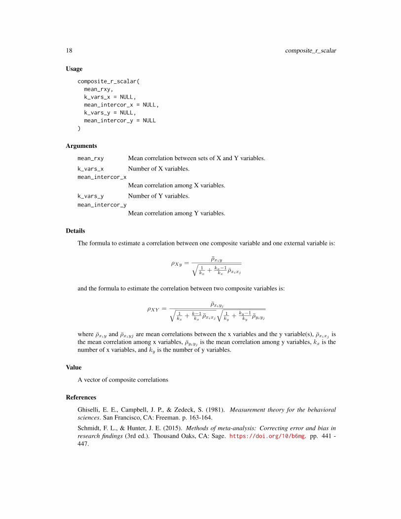
The formula to estimate a correlation between one composite variable and one external variable is:

ρXy =ρxiy√

1kx

+ kx−1kx

ρxixj

and the formula to estimate the correlation between two composite variables is:

ρXY =ρxiyj√

1kx

+ k−1kxρxixj

√1ky

+ky−1ky

ρyiyj

where ρxiy and ρxiyj are mean correlations between the x variables and the y variable(s), ρxixjis

the mean correlation among x variables, ρyiyj is the mean correlation among y variables, kx is thenumber of x variables, and ky is the number of y variables.

Value

A vector of composite correlations

References

Ghiselli, E. E., Campbell, J. P., & Zedeck, S. (1981). Measurement theory for the behavioralsciences. San Francisco, CA: Freeman. p. 163-164.



composite_u_matrix 19

Examples

## Composite correlation between 4 variables and an outside variable with which## the four variables correlate .3 on average:composite_r_scalar(mean_rxy = .3, k_vars_x = 4, mean_intercor_x = .4)

## Correlation between two composites:composite_r_scalar(mean_rxy = .3, k_vars_x = 2, mean_intercor_x = .5,

k_vars_y = 2, mean_intercor_y = .2)

composite_u_matrix Matrix formula to estimate the u ratio of a composite variable

Description

This function estimates the u ratio of a composite variable when at least one matrix of correlations(restricted or unrestricted) among the variables is available.

Usage

composite_u_matrix(ri_mat = NULL,ra_mat = NULL,u_vec,wt_vec = rep(1, length(u_vec)),sign_r_vec = 1

)

Arguments

ri_mat Range-restricted correlation matrix from which the composite is to be computed(if NULL, ri_mat is estimated from ra_mat).

ra_mat Unrestricted correlation matrix from which the composite is to be computed (ifNULL, ra_mat is estimated from ri_mat).

u_vec Vector of u ratios associated with variables in the composite to be formed.wt_vec Weights to be used in forming the composite (by default, all variables receive

equal weight).sign_r_vec The signs of the relationships between the variables in the composite and the

variable by which range restriction was induced.

Details


ucomposite =

√(w ◦ u)

TRi (w ◦ u)

wTRaw

where ucomposite is the composite u ratio, u is a vector of u ratios, Ri is a range-restricted correla-tion matrix, Ra is an unrestricted correlation matrix, and w is a vector of weights.

20 composite_u_scalar

Value

The estimated u ratio of the composite variable.

Examples

composite_u_matrix(ri_mat = matrix(c(1, .3, .3, 1), 2, 2), u_vec = c(.8, .8))

composite_u_scalar Scalar formula to estimate the u ratio of a composite variable

Description

This function provides an approximation of the u ratio of a composite variable based on the u ratiosof the component variables, the mean restricted intercorrelation among those variables, and themean unrestricted correlation among those variables. If only one of the mean intercorrelations isknown, the other will be estimated using the bivariate indirect range-restriction formula. This tendsto compute a conservative estimate of the u ratio associated with a composite.

Usage

composite_u_scalar(mean_ri = NULL, mean_ra = NULL, mean_u, k_vars)

Arguments

mean_ri The mean range-restricted correlation among variables in the composite.mean_ra The mean unrestricted correlation among variables in the composite.mean_u The mean u ratio of variables in the composite.k_vars The number of variables in the composite.

Details


ucomposite =

√ρiu2k(k − 1) + ku2

ρak(k − 1) + k

where ucomposite is the composite u ratio, u is the mean univariate u ratio, ρi is the mean restrictedcorrelation among variables, ρa is the mean unrestricted correlation among variables, and k is thenumber of variables in the composite.

Value

The estimated u ratio of the composite variable.

Examples

composite_u_scalar(mean_ri = .3, mean_ra = .4, mean_u = .8, k_vars = 2)

compute_alpha 21

compute_alpha Compute coefficient alpha

Description

Compute coefficient alpha

Usage

compute_alpha(sigma = NULL, data = NULL, standardized = FALSE, ...)

Arguments

sigma Covariance matrix (must be supplied if data argument is not supplied)

data Data matrix or data frame (must be supplied if sigma argument is not supplied)

standardized Logical scalar determining whether alpha should be computed from an unstan-dardized covariance matrix (TRUE) or a correlation matrix (FALSE).

... Additional arguments to be passed to cov() function.

Value

Coefficient alpha

Examples

compute_alpha(sigma = reshape_vec2mat(cov = .4, order = 10))

compute_dmod Comprehensive d_Mod calculator

Description

This is a general-purpose function to compute dMod effect sizes from raw data and to perform boot-strapping. It subsumes the functionalities of the compute_dmod_par (for parametric computations)and compute_dmod_npar (for non-parametric computations) functions and automates the genera-tion of regression equations and descriptive statistics for computing dMod effect sizes. Please seedocumentation for compute_dmod_par and compute_dmod_npar for details about how the effectsizes are computed.

22 compute_dmod

Usage

compute_dmod(data,group,predictors,criterion,referent_id,focal_id_vec = NULL,conf_level = 0.95,rescale_cdf = TRUE,parametric = TRUE,bootstrap = TRUE,boot_iter = 1000,stratify = FALSE,empirical_ci = FALSE,cross_validate_wts = FALSE

)

Arguments

data Data frame containing the data to be analyzed (if not a data frame, must be anobject convertible to a data frame via the as.data.frame function). The data setmust contain a criterion variable, at least one predictor variable, and a categoricalvariable that identifies the group to which each case (i.e., row) in the data setbelongs.

group Name or column-index number of the variable that identifies group membershipin the data set.

predictors Name(s) or column-index number(s) of the predictor variable(s) in the data set.No predictor can be a factor-type variable. If multiple predictors are specified,they will be combined into a regression-weighted composite that will be carriedforward to compute dMod effect sizes.

• Note: If weights other than regression weights should be used to combinethe predictors into a composite, the user must manually compute such acomposite, include the composite in the dat data set, and identify the com-posite variable in predictors.

criterion Name or column-index number of the criterion variable in the data set. Thecriterion cannot be a factor-type variable.

referent_id Label used to identify the referent group in the group variable.

focal_id_vec Label(s) to identify the focal group(s) in the group variable. If NULL (the de-fault), the specified referent group will be compared to all other groups.

conf_level Confidence level (between 0 and 1) to be used in generating confidence intervals.Default is .95

rescale_cdf Logical argument that indicates whether parametric dMod results should be rescaledto account for using a cumulative density < 1 in the computations (TRUE; default)or not (FALSE).

compute_dmod 23

parametric Logical argument that indicates whether dMod should be computed using anassumed normal distribution (TRUE; default) or observed frequencies (FALSE).

bootstrap Logical argument that indicates whether dMod should be bootstrapped (TRUE;default) or not (FALSE).

boot_iter Number of bootstrap iterations to compute (default = 1000).

stratify Logical argument that indicates whether the random bootstrap sampling shouldbe stratified (TRUE) or unstratified (FALSE; default).

empirical_ci Logical argument that indicates whether the bootstrapped confidence invervalsshould be computed from the observed empirical distributions (TRUE) or com-puted using bootstrapped means and standard errors via the normal-theory ap-proach (FALSE).

cross_validate_wts

Only relevant when multiple predictors are specified and bootstrapping is per-formed. Logical argument that indicates whether regression weights derivedfrom the full sample should be used to combine predictors in the bootstrappedsamples (TRUE) or if a new set of weights should be derived during each iterationof the bootstrapping procedure (FALSE; default).

Value

If bootstrapping is selected, the list will include:

• point_estimate A matrix of effect sizes (dModSigned, dModUnsigned

, dModUnder, dModOver

),proportions of under- and over-predicted criterion scores, minimum and maximum differ-ences, and the scores associated with minimum and maximum differences. All of these valuesare computed using the full data set.

• bootstrap_mean A matrix of the same statistics as the point_estimate matrix, but the valuesin this matrix are the means of the results from bootstrapped samples.

• bootstrap_se A matrix of the same statistics as the point_estimate matrix, but the valuesin this matrix are bootstrapped standard errors (i.e., the standard deviations of the results frombootstrapped samples).

• bootstrap_CI_Lo A matrix of the same statistics as the point_estimate matrix, but thevalues in this matrix are the lower confidence bounds of the results from bootstrapped samples.

• bootstrap_CI_Hi A matrix of the same statistics as the point_estimate matrix, but thevalues in this matrix are the upper confidence bounds of the results from bootstrapped samples.

If no bootstrapping is performed, the output will be limited to the point_estimate matrix.

References

Nye, C. D., & Sackett, P. R. (2016). New effect sizes for tests of categorical moderation and differ-ential prediction. Organizational Research Methods, https://doi.org/10.1177/1094428116644505.

Examples

# Generate some hypothetical data for a referent group and three focal groups:set.seed(10)

24 compute_dmod_npar

refDat <- MASS::mvrnorm(n = 1000, mu = c(.5, .2),Sigma = matrix(c(1, .5, .5, 1), 2, 2), empirical = TRUE)

foc1Dat <- MASS::mvrnorm(n = 1000, mu = c(-.5, -.2),Sigma = matrix(c(1, .5, .5, 1), 2, 2), empirical = TRUE)

foc2Dat <- MASS::mvrnorm(n = 1000, mu = c(0, 0),Sigma = matrix(c(1, .3, .3, 1), 2, 2), empirical = TRUE)

foc3Dat <- MASS::mvrnorm(n = 1000, mu = c(-.5, -.2),Sigma = matrix(c(1, .3, .3, 1), 2, 2), empirical = TRUE)

colnames(refDat) <- colnames(foc1Dat) <- colnames(foc2Dat) <- colnames(foc3Dat) <- c("X", "Y")dat <- rbind(cbind(G = 1, refDat), cbind(G = 2, foc1Dat),

cbind(G = 3, foc2Dat), cbind(G = 4, foc3Dat))

# Compute point estimates of parametric d_mod effect sizes:compute_dmod(data = dat, group = "G", predictors = "X", criterion = "Y",

referent_id = 1, focal_id_vec = 2:4,conf_level = .95, rescale_cdf = TRUE, parametric = TRUE,bootstrap = FALSE)

# Compute point estimates of non-parametric d_mod effect sizes:compute_dmod(data = dat, group = "G", predictors = "X", criterion = "Y",

referent_id = 1, focal_id_vec = 2:4,conf_level = .95, rescale_cdf = TRUE, parametric = FALSE,bootstrap = FALSE)

# Compute unstratified bootstrapped estimates of parametric d_mod effect sizes:compute_dmod(data = dat, group = "G", predictors = "X", criterion = "Y",

referent_id = 1, focal_id_vec = 2:4,conf_level = .95, rescale_cdf = TRUE, parametric = TRUE,boot_iter = 10, bootstrap = TRUE, stratify = FALSE, empirical_ci = FALSE)

# Compute unstratified bootstrapped estimates of non-parametric d_mod effect sizes:compute_dmod(data = dat, group = "G", predictors = "X", criterion = "Y",

referent_id = 1, focal_id_vec = 2:4,conf_level = .95, rescale_cdf = TRUE, parametric = FALSE,boot_iter = 10, bootstrap = TRUE, stratify = FALSE, empirical_ci = FALSE)

compute_dmod_npar Function for computing non-parametric d_Mod effect sizes for a sin-gle focal group

Description

This function computes non-parametric dMod effect sizes from user-defined descriptive statisticsand regression coefficients, using a distribution of observed scores as weights. This non-parametricfunction is best used when the assumption of normally distributed predictor scores is not reasonableand/or the distribution of scores observed in a sample is likely to represent the distribution of scoresin the population of interest. If one has access to the full raw data set, the dMod function may beused as a wrapper to this function so that the regression equations and descriptive statistics can becomputed automatically within the program.

compute_dmod_npar 25

Usage

compute_dmod_npar(referent_int,referent_slope,focal_int,focal_slope,focal_x,referent_sd_y

)

Arguments

referent_int Referent group’s intercept.

referent_slope Referent group’s slope.

focal_int Focal group’s intercept.

focal_slope Focal group’s slope.

focal_x Focal group’s vector of predictor scores.

referent_sd_y Referent group’s criterion standard deviation.

Details

The dModSignedeffect size (i.e., the average of differences in prediction over the range of predictor

scores) is computed as

dModSigned=

∑mi=1 ni [Xi (b11 − b12) + b01 − b02 ]

SDY1

∑mi=1 ni

,

where

• SDY1is the referent group’s criterion standard deviation;

• m is the number of unique scores in the distribution of focal-group predictor scores;

• X is the vector of unique focal-group predictor scores, indexed i = 1 through m;

• Xi is the ith unique score value;

• n is the vector of frequencies associated with the elements of X;

• ni is the number of cases with a score equal to Xi;

• b11 and b12 are the slopes of the regression of Y on X for the referent and focal groups,respectively; and

• b01 and b02 are the intercepts of the regression of Y on X for the referent and focal groups,respectively.

The dModUnderand dModOver

effect sizes are computed using the same equation as dModSigned, but

dModUnderis the weighted average of all scores in the area of underprediction (i.e., the differences

in prediction with negative signs) and dModOveris the weighted average of all scores in the area of

overprediction (i.e., the differences in prediction with negative signs).

26 compute_dmod_npar

The dModUnsignedeffect size (i.e., the average of absolute differences in prediction over the range

of predictor scores) is computed as

dModUnsigned=

∑mi=1 ni |Xi (b11 − b12) + b01 − b02 |

SDY1

∑mi=1 ni

.

The dMin effect size (i.e., the smallest absolute difference in prediction observed over the range ofpredictor scores) is computed as

dMin =1

SDY1

Min [|X (b11 − b12) + b01 − b02 |] .

The dMax effect size (i.e., the largest absolute difference in prediction observed over the range ofpredictor scores)is computed as

dMax =1

SDY1

Max [|X (b11 − b12) + b01 − b02 |] .

Note: When dMin and dMax are computed in this package, the output will display the signs of thedifferences (rather than the absolute values of the differences) to aid in interpretation.

Value

A vector of effect sizes (dModSigned, dModUnsigned


), proportions of under-and over-predicted criterion scores, minimum and maximum differences (i.e., dModUnder

and dModOver),

and the scores associated with minimum and maximum differences.

Examples

# Generate some hypothetical data for a referent group and three focal groups:set.seed(10)refDat <- MASS::mvrnorm(n = 1000, mu = c(.5, .2),

Sigma = matrix(c(1, .5, .5, 1), 2, 2), empirical = TRUE)foc1Dat <- MASS::mvrnorm(n = 1000, mu = c(-.5, -.2),

Sigma = matrix(c(1, .5, .5, 1), 2, 2), empirical = TRUE)foc2Dat <- MASS::mvrnorm(n = 1000, mu = c(0, 0),

Sigma = matrix(c(1, .3, .3, 1), 2, 2), empirical = TRUE)foc3Dat <- MASS::mvrnorm(n = 1000, mu = c(-.5, -.2),

Sigma = matrix(c(1, .3, .3, 1), 2, 2), empirical = TRUE)colnames(refDat) <- colnames(foc1Dat) <- colnames(foc2Dat) <- colnames(foc3Dat) <- c("X", "Y")

# Compute a regression model for each group:refRegMod <- lm(Y ~ X, data.frame(refDat))$coeffoc1RegMod <- lm(Y ~ X, data.frame(foc1Dat))$coeffoc2RegMod <- lm(Y ~ X, data.frame(foc2Dat))$coeffoc3RegMod <- lm(Y ~ X, data.frame(foc3Dat))$coef

# Use the subgroup regression models to compute d_mod for each referent-focal pairing:

# Focal group #1:compute_dmod_npar(referent_int = refRegMod[1], referent_slope = refRegMod[2],

focal_int = foc1RegMod[1], focal_slope = foc1RegMod[2],

compute_dmod_par 27

focal_x = foc1Dat[,"X"], referent_sd_y = 1)


focal_int = foc2RegMod[1], focal_slope = foc1RegMod[2],focal_x = foc2Dat[,"X"], referent_sd_y = 1)


focal_int = foc3RegMod[1], focal_slope = foc3RegMod[2],focal_x = foc3Dat[,"X"], referent_sd_y = 1)

compute_dmod_par Function for computing parametric d_Mod effect sizes for any num-ber of focal groups

Description

This function computes dMod effect sizes from user-defined descriptive statistics and regressioncoefficients. If one has access to a raw data set, the dMod function may be used as a wrapper to thisfunction so that the regression equations and descriptive statistics can be computed automaticallywithin the program.

Usage

compute_dmod_par(referent_int,referent_slope,focal_int,focal_slope,focal_mean_x,focal_sd_x,referent_sd_y,focal_min_x,focal_max_x,focal_names = NULL,rescale_cdf = TRUE

)

Arguments

referent_int Referent group’s intercept.

referent_slope Referent group’s slope.

focal_int Focal groups’ intercepts.

focal_slope Focal groups’ slopes.

focal_mean_x Focal groups’ predictor-score means.

focal_sd_x Focal groups’ predictor-score standard deviations.

28 compute_dmod_par

referent_sd_y Referent group’s criterion standard deviation.

focal_min_x Focal groups’ minimum predictor scores.

focal_max_x Focal groups’ maximum predictor scores.

focal_names Focal-group names. If NULL (the default), the focal groups will be given numericlabels ranging from 1 through the number of groups.

rescale_cdf Logical argument that indicates whether parametric dMod results should be rescaledto account for using a cumulative density < 1 in the computations (TRUE; default)or not (FALSE).

Details

The dModSignedeffect size (i.e., the average of differences in prediction over the range of predictor

scores) is computed as

dModSigned=

1

SDY1

∫f2(X) [X (b11 − b12) + b01 − b02 ] dX,

where

• SDY1 is the referent group’s criterion standard deviation;

• f2(X) is the normal-density function for the distribution of focal-group predictor scores;

• b11 and b10 are the slopes of the regression of Y on X for the referent and focal groups,respectively;

• b01 and b00 are the intercepts of the regression of Y on X for the referent and focal groups,respectively; and

• the integral spans all X scores within the operational range of predictor scores for the focalgroup.

The dModUnderand dModOver

effect sizes are computed using the same equation as dModSigned, but

dModUnderis the weighted average of all scores in the area of underprediction (i.e., the differences

in prediction with negative signs) and dModOveris the weighted average of all scores in the area of

overprediction (i.e., the differences in prediction with negative signs).

The dModUnsignedeffect size (i.e., the average of absolute differences in prediction over the range

of predictor scores) is computed as

dModUnsigned=

1

SDY1

∫f2(X) |X (b11 − b12) + b01 − b02 | dX.

The dMin effect size (i.e., the smallest absolute difference in prediction observed over the range ofpredictor scores) is computed as

dMin =1

SDY1

Min [|X (b11 − b12) + b01 − b02 |] .

The dMax effect size (i.e., the largest absolute difference in prediction observed over the range ofpredictor scores)is computed as

dMax =1

SDY1

Max [|X (b11 − b12) + b01 − b02 |] .

conf.limits.nc.chisq 29

Note: When dMin and dMax are computed in this package, the output will display the signs of thedifferences (rather than the absolute values of the differences) to aid in interpretation.

If dMod effect sizes are to be rescaled to compensate for a cumulative density less than 1 (seethe rescale_cdf argument), the result of each effect size involving integration will be divided bythe ratio of the cumulative density of the observed range of scores (i.e., the range bounded by thefocal_min_x and focal_max_x arguments) to the cumulative density of scores bounded by -Infand Inf.

Value

A matrix of effect sizes (dModSigned, dModUnsigned


), proportions of under-and over-predicted criterion scores, minimum and maximum differences (i.e., dModUnder

and dModOver),

and the scores associated with minimum and maximum differences. Note that if the regression linesare parallel and infinite focal_min_x and focal_max_x values were specified, the extrema will bedefined using the scores 3 focal-group SDs above and below the corresponding focal-group means.

References

Nye, C. D., & Sackett, P. R. (2016). New effect sizes for tests of categorical moderation and differ-ential prediction. Organizational Research Methods, https://doi.org/10.1177/1094428116644505.

Examples

compute_dmod_par(referent_int = -.05, referent_slope = .5,focal_int = c(.05, 0, -.05), focal_slope = c(.5, .3, .3),focal_mean_x = c(-.5, 0, -.5), focal_sd_x = rep(1, 3),referent_sd_y = 1,focal_min_x = rep(-Inf, 3), focal_max_x = rep(Inf, 3),focal_names = NULL, rescale_cdf = TRUE)

conf.limits.nc.chisq Confidence limits for noncentral chi square parameters (functionand documentation from package ’MBESS’ version 4.4.3) Functionto determine the noncentral parameter that leads to the observedChi.Square-value, so that a confidence interval for the populationnoncentral chi-squrae value can be formed.

Description

Confidence limits for noncentral chi square parameters (function and documentation from package’MBESS’ version 4.4.3) Function to determine the noncentral parameter that leads to the observedChi.Square-value, so that a confidence interval for the population noncentral chi-squrae value canbe formed.

30 conf.limits.nc.chisq

Usage

conf.limits.nc.chisq(Chi.Square = NULL,conf.level = 0.95,df = NULL,alpha.lower = NULL,alpha.upper = NULL,tol = 1e-09,Jumping.Prop = 0.1

)

Arguments

Chi.Square the observed chi-square value

conf.level the desired degree of confidence for the interval

df the degrees of freedom

alpha.lower Type I error for the lower confidence limit

alpha.upper Type I error for the upper confidence limit

tol tolerance for iterative convergence

Jumping.Prop Value used in the iterative scheme to determine the noncentral parameters neces-sary for confidence interval construction using noncentral chi square-distributions(0 < Jumping.Prop < 1)

Details

If the function fails (or if a function relying upon this function fails), adjust the Jumping.Prop (toa smaller value).

Value

• Lower.LimitValue of the distribution with Lower.Limit noncentral value that has at its spec-ified quantile Chi.Square

• Prob.Less.LowerProportion of cases falling below Lower.Limit

• Upper.LimitValue of the distribution with Upper.Limit noncentral value that has at its speci-fied quantile Chi.Square

• Prob.Greater.UpperProportion of cases falling above Upper.Limit

Author(s)

Ken Kelley (University of Notre Dame; <[email protected]>), Keke Lai (University of California–Merced)

confidence 31

confidence Construct a confidence interval

Description

Function to construct a confidence interval around an effect size or mean effect size.

Usage

confidence(mean,se = NULL,df = NULL,conf_level = 0.95,conf_method = c("t", "norm"),...

)

Arguments

mean Mean effect size (if used in a meta-analysis) or observed effect size (if used onindividual statistics).

se Standard error of the statistic.

df Degrees of freedom of the statistic (necessary if using the t distribution).

conf_level Confidence level that defines the width of the confidence interval (default = .95).

conf_method Distribution to be used to compute the width of confidence intervals. Availableoptions are "t" for t distribution or "norm" for normal distribution.

... Additional arguments

Details

CI = meanes ± quantile× SEes

Value

A matrix of confidence intervals of the specified width.

Examples

confidence(mean = c(.3, .5), se = c(.15, .2), df = c(100, 200), conf_level = .95, conf_method = "t")confidence(mean = c(.3, .5), se = c(.15, .2), conf_level = .95, conf_method = "norm")

32 confint

confidence_r Construct a confidence interval for correlations using Fisher’s z trans-formation

Description

Construct a confidence interval for correlations using Fisher’s z transformation

Usage

confidence_r(r, n, conf_level = 0.95)

Arguments

r A vector of correlations

n A vector of sample sizes


Value

A confidence interval of the specified width (or matrix of confidence intervals)

Examples

confidence_r(r = .3, n = 200, conf_level = .95)

confint Confidence interval method for objects of classes deriving from"lm_mat"

Description

Confidence interval method for objects of classes deriving from "lm_mat." Returns lower and upperbounds of confidence intervals for regression coefficients.

Arguments

object Matrix regression object.

parm a specification of which parameters are to be given confidence intervals, eithera vector of numbers or a vector of names. If missing, all parameters are consid-ered.

level Confidence level

... further arguments passed to or from other methods.

control_intercor 33

control_intercor Control function to curate intercorrelations to be used in automaticcompositing routine

Description

Control function to curate intercorrelations to be used in automatic compositing routine

Usage

control_intercor(rxyi = NULL,n = NULL,sample_id = NULL,construct_x = NULL,construct_y = NULL,construct_names = NULL,facet_x = NULL,facet_y = NULL,intercor_vec = NULL,intercor_scalar = 0.5,dx = NULL,dy = NULL,p = 0.5,partial_intercor = FALSE,data = NULL,...

)

Arguments

rxyi Vector or column name of observed correlations.

n Vector or column name of sample sizes.

sample_id Vector of identification labels for samples/studies in the meta-analysis.construct_x, construct_y

Vector of construct names for constructs designated as "X" or "Y".construct_names

Vector of all construct names to be included in the meta-analysis.facet_x, facet_y

Vector of facet names for constructs designated as "X" or "Y".

intercor_vec Named vector of pre-specified intercorrelations among measures of constructsin the meta-analysis.

intercor_scalar

Generic scalar intercorrelation that can stand in for unobserved or unspecifiedvalues.

34 control_intercor

dx, dy d values corresponding to construct_x and construct_y. These values onlyneed to be supplied for cases in which rxyi represents a correlation betweentwo measures of the same construct.

p Scalar or vector containing the proportions of group membership correspondingto the d values.

partial_intercor

For meta-analyses of d values only: Logical scalar, vector, or column cor-responding to values in rxyi that determines whether the correlations are tobe treated as within-group correlations (i.e., partial correlation controlling forgroup membership; TRUE) or not (FALSE; default). Note that this only con-verts correlation values from the rxyi argument - any values provided in theintercor_vec or intercor_scalar arguments must be total correlations orconverted to total correlations using the mix_r_2group() function prior to run-ning control_intercor.

data Data frame containing columns whose names may be provided as arguments tovector arguments.

... Further arguments to be passed to functions called within the meta-analysis.

Value

A vector of intercorrelations

Examples

## Create a dataset in which constructs correlate with themselvesrxyi <- seq(.1, .5, length.out = 27)construct_x <- rep(rep(c("X", "Y", "Z"), 3), 3)construct_y <- c(rep("X", 9), rep("Y", 9), rep("Z", 9))dat <- data.frame(rxyi = rxyi,

construct_x = construct_x,construct_y = construct_y,stringsAsFactors = FALSE)

dat <- rbind(cbind(sample_id = "Sample 1", dat),cbind(sample_id = "Sample 2", dat),cbind(sample_id = "Sample 3", dat))

## Identify some constructs for which intercorrelations are not## represented in the data object:construct_names = c("U", "V", "W")

## Specify some externally determined intercorrelations among measures:intercor_vec <- c(W = .4, X = .1)

## Specify a generic scalar intercorrelation that can stand in for missing values:intercor_scalar <- .5

control_intercor(rxyi = rxyi, sample_id = sample_id,construct_x = construct_x, construct_y = construct_y,construct_names = construct_names,

intercor_vec = intercor_vec, intercor_scalar = intercor_scalar, data = dat)

control_psychmeta 35

control_psychmeta Control for psychmeta meta-analyses

Description

Control for psychmeta meta-analyses

Usage

control_psychmeta(error_type = c("mean", "sample"),conf_level = 0.95,cred_level = 0.8,conf_method = c("t", "norm"),cred_method = c("t", "norm"),var_unbiased = TRUE,pairwise_ads = FALSE,moderated_ads = FALSE,residual_ads = TRUE,check_dependence = TRUE,collapse_method = c("composite", "average", "stop"),intercor = control_intercor(),clean_artifacts = TRUE,impute_artifacts = TRUE,impute_method = c("bootstrap_mod", "bootstrap_full", "simulate_mod", "simulate_full","wt_mean_mod", "wt_mean_full", "unwt_mean_mod", "unwt_mean_full", "replace_unity","stop"),

seed = 42,use_all_arts = TRUE,estimate_pa = FALSE,decimals = 2,hs_override = FALSE,...

)

Arguments

error_type Method to be used to estimate error variances: "mean" uses the mean effect sizeto estimate error variances and "sample" uses the sample-specific effect sizes.

conf_level Confidence level to define the width of the confidence interval (default = .95).

cred_level Credibility level to define the width of the credibility interval (default = .80).


cred_method Distribution to be used to compute the width of credibility intervals. Availableoptions are "t" for t distribution or "norm" for normal distribution.

36 control_psychmeta

var_unbiased Logical scalar determining whether variances should be unbiased (TRUE) ormaximum-likelihood (FALSE).

pairwise_ads Logical value that determines whether to compute artifact distributions in aconstruct-pair-wise fashion (TRUE) or separately by construct (FALSE, default).

moderated_ads Logical value that determines whether to compute artifact distributions sep-arately for each moderator combination (TRUE) or for overall analyses only(FALSE, default).

residual_ads Logical argument that determines whether to use residualized variances (TRUE)or observed variances (FALSE) of artifact distributions to estimate sd_rho.

check_dependence

Logical scalar that determines whether database should be checked for viola-tions of independence (TRUE) or not (FALSE).

collapse_method

Character argument that determines how to collapse dependent studies. Optionsare "composite" (default), "average," and "stop."

intercor The intercorrelation(s) among variables to be combined into a composite. Canbe a scalar, a named vector with element named according to the names of con-structs, or output from the control_intercor function. Default scalar value is.5.

clean_artifacts

If TRUE, multiple instances of the same construct (or construct-measure pair, ifmeasure is provided) in the database are compared and reconciled with eachother in the case that any of the matching entries within a study have differentartifact values. When impute_method is anything other than "stop", this methodis always implemented to prevent discrepancies among imputed values.

impute_artifacts

If TRUE, artifact imputation will be performed (see impute_method for impu-tation procedures). Default is FALSE for artifact-distribution meta-analyses andTRUE otherwise. When imputation is performed, clean_artifacts is treated asTRUE so as to resolve all discrepancies among artifact entries before and afterimputation.

impute_method Method to use for imputing artifacts. Choices are:

• bootstrap_modSelect random values from the most specific moderator categories available(default).

• bootstrap_fullSelect random values from the full vector of artifacts.

• simulate_modGenerate random values from the distribution with the mean and varianceof observed artifacts from the most specific moderator categories available.(uses rnorm for u ratios and rbeta for reliability values).

• simulate_fullGenerate random values from the distribution with the mean and varianceof all observed artifacts (uses rnorm for u ratios and rbeta for reliabilityvalues).

control_psychmeta 37

• wt_mean_modReplace missing values with the sample-size weighted mean of the distribu-tion of artifacts from the most specific moderator categories available (notrecommended).

• wt_mean_fullReplace missing values with the sample-size weighted mean of the full dis-tribution of artifacts (not recommended).

• unwt_mean_modReplace missing values with the unweighted mean of the distribution ofartifacts from the most specific moderator categories available (not recom-mended).

• unwt_mean_fullReplace missing values with the unweighted mean of the full distributionof artifacts (not recommended).

• replace_unityReplace missing values with 1 (not recommended).

• stopStop evaluations when missing artifacts are encountered.

If an imputation method ending in "mod" is selected but no moderators are pro-vided, the "mod" suffix will internally be replaced with "full".

seed Seed value to use for imputing artifacts in a reproducible way. Default value is42.

use_all_arts Logical scalar that determines whether artifact values from studies without valideffect sizes should be used in artifact distributions (TRUE; default) or not (FALSE).

estimate_pa Logical scalar that determines whether the unrestricted subgroup proportionsassociated with univariate-range-restricted effect sizes should be estimated byrescaling the range-restricted subgroup proportions as a function of the range-restriction correction (TRUE) or not (FALSE; default).

decimals Number of decimal places to which interactive artifact distributions should berounded (default is 2 decimal places).

hs_override When TRUE, this will override settings for wt_type (will set to "sample_size"),error_type (will set to "mean"), correct_bias (will set to TRUE), conf_method(will set to "norm"), cred_method (will set to "norm"), var_unbiased (will setto FALSE), residual_ads (will be set to FALSE), and use_all_arts (will set toFALSE).


Value

A list of control arguments in the package environment.

Examples

control_psychmeta()

38 convert_es

convert_es Convert effect sizes and compute confidence intervals

Description

This function converts a variety of effect sizes to either correlations or Cohen’s d values. Thefunction also computes and prints confidence intervals for the output effect sizes.

Usage

convert_es(es,input_es = c("r", "d", "delta", "g", "t", "p.t", "F", "p.F", "chisq", "p.chisq", "or",

"lor", "Fisherz", "A", "auc", "cles"),output_es = c("r", "d", "A", "auc", "cles"),n1 = NULL,n2 = NULL,df1 = NULL,df2 = NULL,sd1 = NULL,sd2 = NULL,tails = 2,correct_bias = TRUE,conf_level = 0.95

)

Arguments

es Vector of effect sizes to convert.

input_es Scalar. Metric of input effect sizes. Currently supports correlations, Cohen’s d,independent samples t values (or their p values), two-group one-way ANOVA Fvalues (or their p values), 1df χ2 values (or their p values), odds ratios, log oddsratios, Fisher z, and the common language effect size (CLES, A, AUC).

output_es Scalar. Metric of output effect sizes. Currently supports correlations, Cohen’s dvalues, and common language effect sizes (CLES, A, AUC).

n1 Vector of total sample sizes or sample sizes of group 1 of the two groups beingcontrasted.

n2 Vector of sample sizes of group 2 of the two groups being contrasted.

df1 Vector of input test statistic degrees of freedom (for t and χ2) or between-groupsdegree of freedom (for F).

df2 Vector of input test statistic within-group degrees of freedom (for F).

sd1 Vector of pooled (within-group) standard deviations or standard deviations ofgroup 1 of the two groups being contrasted.

sd2 Vector of standard deviations of group 2 of the two groups being contrasted.

convert_es 39

tails Vector of the tails for p values when input_es = "p.t". Can be ‘2‘ (defualt) or‘1‘.

correct_bias Logical argument that determines whether to correct output effect sizes anderror-variance estimates for small-sample bias (TRUE) or not (FALSE) when com-puting confidence intervals.


Value

A psychmeta effect size es object containing:

meta_input A matrix of converted effect sizes and adjusted sample sizes for use in subse-quent meta-anlayses.

original_es The input data.confidence The output data with computed confidence intervals (for printing).

Notes

To use converted effect sizes in a meta-analysis, add the values from es$meta_input to your meta-analytic input data frame.

References

Chinn, S. (2000). A simple method for converting an odds ratio to effect size for use in meta-analysis. Statistics in Medicine, 19(22), 3127–3131. https://doi.org/10/c757hm

Lipsey, M. W., & Wilson, D. B. (2001). Practical meta-analysis. Thousand Oaks, CA: SAGE.

Ruscio, J. (2008). A probability-based measure of effect size: Robustness to base rates and otherfactors. Psychological Methods, 13(1), 19–30. https://doi.org/10.1037/1082-989X.13.1.19

Schmidt, F. L., & Hunter, J. E. (2015). Methods of meta-analysis: Correcting error and bias inresearch findings (3rd ed.). Thousand Oaks, CA: SAGE. https://doi.org/10/b6mg

Examples

## To convert a statistic to r or d metric:convert_es(es = 1, input_es="d", output_es="r", n1=100)convert_es(es = 1, input_es="d", output_es="r", n1=50, n2 = 50)convert_es(es = .2, input_es="r", output_es="d", n1=100, n2=150)convert_es(es = -1.3, input_es="t", output_es="r", n1 = 100, n2 = 140)convert_es(es = 10.3, input_es="F", output_es="d", n1 = 100, n2 = 150)convert_es(es = 1.3, input_es="chisq", output_es="r", n1 = 100, n2 = 100)convert_es(es = .021, input_es="p.chisq", output_es="d", n1 = 100, n2 = 100)convert_es(es = 4.37, input_es="or", output_es="r", n1=100, n2=100)convert_es(es = 4.37, input_es="or", output_es="d", n1=100, n2=100)convert_es(es = 1.47, input_es="lor", output_es="r", n1=100, n2=100)convert_es(es = 1.47, input_es="lor", output_es="d", n1=100, n2=100)

## To simply compute a confidence interval for r, d, or A:convert_es(es = .3, input_es="r", output_es="r", n1=100)convert_es(es = .8, input_es="d", output_es="d", n1=64, n2=36)convert_es(es = .8, input_es="A", output_es="A", n1=64, n2=36)

https://doi.org/10/c757hm

https://doi.org/10.1037/1082-989X.13.1.19


40 convert_ma

convert_ma Function to convert meta-analysis of correlations to d values or vice-versa

Description

Takes a meta-analysis class object of d values or correlations (classes r_as_r, d_as_d, r_as_d,and d_as_r; second-order meta-analyses are currently not supported) as an input and uses con-version formulas and Taylor series approximations to convert effect sizes and variance estimates,respectively.

Usage

convert_ma(ma_obj, ...)

convert_meta(ma_obj, ...)

Arguments

ma_obj A meta-analysis object of class r_as_r, d_as_d, r_as_d, or d_as_r... Additional arguments.

Details

The formula used to convert correlations to d values is:

d =r√

1p(1−p)

√1− r2

The formula used to convert d values to correlations is:

r =d√

d2 + 1p(1−p)

To approximate the variance of correlations from the variance of d values, the function computes:

varr ≈ a2dvardwhere ad is the first partial derivative of the d-to-r transformation with respect to d:

ad = − 1

[d2p (1− p)− 1]√d2 + 1

p−p2

To approximate the variance of d values from the variance of correlations, the function computes:

vard ≈ a2rvarrwhere ar is the first partial derivative of the r-to-d transformation with respect to r:

ar =

√1

p−p2

(1− r2)1.5

correct_d 41

Value

A meta-analysis converted to the d value metric (if ma_obj was a meta-analysis in the correlationmetric) or converted to the correlation metric (if ma_obj was a meta-analysis in the d value metric).

correct_d Correct d values for measurement error and/or range restriction

Description

This function is a wrapper for the correct_r() function to correct d values for statistical andpsychometric artifacts.

Usage

correct_d(correction = c("meas", "uvdrr_g", "uvdrr_y", "uvirr_g", "uvirr_y", "bvdrr", "bvirr"),d,ryy = 1,uy = 1,rGg = 1,pi = NULL,pa = NULL,uy_observed = TRUE,ryy_restricted = TRUE,ryy_type = "alpha",k_items_y = NA,sign_rgz = 1,sign_ryz = 1,n1 = NULL,n2 = NA,conf_level = 0.95,correct_bias = FALSE

)

Arguments

correction Type of correction to be applied. Options are "meas", "uvdrr_g", "uvdrr_y","uvirr_g", "uvirr_y", "bvdrr", "bvirr"

d Vector of d values.

ryy Vector of reliability coefficients for Y (the continuous variable).

uy Vector of u ratios for Y (the continuous variable).

rGg Vector of reliabilities for the group variable (i.e., the correlations between ob-served group membership and latent group membership).

pi Proportion of cases in one of the groups in the observed data (not necessary ifn1 and n2 reflect this proportionality).

42 correct_d

pa Proportion of cases in one of the groups in the population.

uy_observed Logical vector in which each entry specifies whether the corresponding uy valueis an observed-score u ratio (TRUE) or a true-score u ratio. All entries are TRUEby default.

ryy_restricted Logical vector in which each entry specifies whether the corresponding rxxvalue is an incumbent reliability (TRUE) or an applicant reliability. All entriesare TRUE by default.

ryy_type String vector identifying the types of reliability estimates supplied (e.g., "alpha","retest", "interrater_r", "splithalf"). See the documentation for ma_r for a full listof acceptable reliability types.

k_items_y Numeric vector identifying the number of items in each scale.

sign_rgz Vector of signs of the relationships between grouping variables and the selectionmechanism.

sign_ryz Vector of signs of the relationships between Y variables and the selection mech-anism.

n1 Optional vector of sample sizes associated with group 1 (or the total sample size,if n2 is NULL).

n2 Optional vector of sample sizes associated with group 2.


correct_bias Logical argument that determines whether to correct error-variance estimates forsmall-sample bias in correlations (TRUE) or not (FALSE). For sporadic corrections(e.g., in mixed artifact-distribution meta-analyses), this should be set to FALSE(the default).

Value

Data frame(s) of observed d values (dgyi), operational range-restricted d values corrected for mea-surement error in Y only (dgpi), operational range-restricted d values corrected for measurementerror in the grouping only (dGyi), and range-restricted true-score d values (dGpi), range-correctedobserved-score d values (dgya), operational range-corrected d values corrected for measurementerror in Y only (dgpa), operational range-corrected d values corrected for measurement error in thegrouping only (dGya), and range-corrected true-score d values (dGpa).

References

Alexander, R. A., Carson, K. P., Alliger, G. M., & Carr, L. (1987). Correcting doubly truncated cor-relations: An improved approximation for correcting the bivariate normal correlation when trunca-tion has occurred on both variables. Educational and Psychological Measurement, 47(2), 309–315.https://doi.org/10.1177/0013164487472002

Dahlke, J. A., & Wiernik, B. M. (2018). One of these artifacts is not like the others: Accounting forindirect range restriction in organizational and psychological research. Manuscript submitted forreview.

Hunter, J. E., Schmidt, F. L., & Le, H. (2006). Implications of direct and indirect range restrictionfor meta-analysis methods and findings. Journal of Applied Psychology, 91(3), 594–612. https://doi.org/10.1037/0021-9010.91.3.594

https://doi.org/10.1177/0013164487472002

https://doi.org/10.1037/0021-9010.91.3.594

https://doi.org/10.1037/0021-9010.91.3.594

correct_d 43

Le, H., Oh, I.-S., Schmidt, F. L., & Wooldridge, C. D. (2016). Correction for range restrictionin meta-analysis revisited: Improvements and implications for organizational research. PersonnelPsychology, 69(4), 975–1008. https://doi.org/10.1111/peps.12122

Schmidt, F. L., & Hunter, J. E. (2015). Methods of meta-analysis: Correcting error and bias inresearch findings (3rd ed.). Thousand Oaks, CA: SAGE. https://doi.org/10/b6mg. pp. 43–44,140–141.

Examples

## Correction for measurement error onlycorrect_d(correction = "meas", d = .5, ryy = .8, uy = .7,

rGg = .9, pi = .7, pa = .5)correct_d(correction = "meas", d = .5, ryy = .8, uy = .7,

rGg = .9, pi = NULL, pa = .5, n1 = 100, n2 = 200)

## Correction for direct range restriction in the continuous variablecorrect_d(correction = "uvdrr_y", d = .5, ryy = .8, uy = .7,

rGg = .9, pi = .7, pa = .5)correct_d(correction = "uvdrr_y", d = .5, ryy = .8, uy = .7,

rGg = .9, pi = NULL, pa = .5, n1 = 100, n2 = 200)

## Correction for direct range restriction in the grouping variablecorrect_d(correction = "uvdrr_g", d = .5, ryy = .8, uy = .7,

rGg = .9, pi = .7, pa = .5)correct_d(correction = "uvdrr_g", d = .5, ryy = .8, uy = .7,

rGg = .9, pi = NULL, pa = .5, n1 = 100, n2 = 200)

## Correction for indirect range restriction in the continuous variablecorrect_d(correction = "uvdrr_y", d = .5, ryy = .8, uy = .7,


rGg = .9, pi = NULL, pa = .5, n1 = 100, n2 = 200)

## Correction for indirect range restriction in the grouping variablecorrect_d(correction = "uvirr_g", d = .5, ryy = .8, uy = .7,

rGg = .9, pi = .7, pa = .5)correct_d(correction = "uvirr_g", d = .5, ryy = .8, uy = .7,

rGg = .9, pi = NULL, pa = .5, n1 = 100, n2 = 200)

## Correction for indirect range restriction in the continuous variablecorrect_d(correction = "uvdrr_y", d = .5, ryy = .8, uy = .7,


rGg = .9, pi = NULL, pa = .5, n1 = 100, n2 = 200)

## Correction for direct range restriction in both variablescorrect_d(correction = "bvdrr", d = .5, ryy = .8, uy = .7,

rGg = .9, pi = .7, pa = .5)correct_d(correction = "bvdrr", d = .5, ryy = .8, uy = .7,

rGg = .9, pi = NULL, pa = .5, n1 = 100, n2 = 200)

## Correction for indirect range restriction in both variables

https://doi.org/10.1111/peps.12122


44 correct_d_bias

correct_d(correction = "bvirr", d = .5, ryy = .8, uy = .7,rGg = .9, pi = .7, pa = .5)

correct_d(correction = "bvirr", d = .5, ryy = .8, uy = .7,rGg = .9, pi = NULL, pa = .5, n1 = 100, n2 = 200)

correct_d_bias Correct for small-sample bias in Cohen’s d values

Description

Corrects a vector of Cohen’s d values for small-sample bias, as Cohen’s d has a slight positive bias.The bias-corrected d value is often called Hedges’s g.

Usage

correct_d_bias(d, n)

Arguments

d Vector of Cohen’s d values.n Vector of sample sizes.

Details

The bias correction is:g = dc = dobs × J

where

J =Γ(n−2

2 )√n−22 × Γ(n−3

2 )

and dobs is the observed effect size, g = dc is the corrected (unbiased) estimate, n is the total samplesize, and Γ() is the gamma function.

Historically, using the gamma function was computationally intensive, so an approximation for Jwas used (Borenstein et al., 2009):

J = 1− 3/(4 ∗ (n− 2)− 1)

This approximation is no longer necessary with modern computers.

Value

Vector of g values (d values corrected for small-sample bias).

References

Hedges, L. V., & Olkin, I. (1985). Statistical methods for meta-analysis. Academic Press. p. 104

Borenstein, M., Hedges, L. V., Higgins, J. P. T., & Rothstein, H. R. (2009). Introduction to meta-analysis. Wiley. p. 27.

correct_glass_bias 45

Examples

correct_d_bias(d = .3, n = 30)correct_d_bias(d = .3, n = 300)correct_d_bias(d = .3, n = 3000)

correct_glass_bias Correct for small-sample bias in Glass’ ∆ values

Description

Correct for small-sample bias in Glass’ ∆ values

Usage

correct_glass_bias(delta, nc, ne, use_pooled_sd = rep(FALSE, length(delta)))

Arguments

delta Vector of Glass’ ∆ values.

nc Vector of control-group sample sizes.

ne Vector of experimental-group sample sizes.

use_pooled_sd Logical vector determining whether the pooled standard deviation was used(TRUE) or not (FALSE; default).

Details

The bias correction is estimated as:

∆c = ∆obs

Γ(ncontrol−1

2

)Γ(ncontrol−1

2

)Γ(ncontrol−2

2

)where ∆ is the observed effect size, ∆c is the corrected estimate of ∆, ncontrol is the control-groupsample size, and Γ() is the gamma function.

Value

Vector of d values corrected for small-sample bias.

References

Hedges, L. V. (1981). Distribution theory for Glass’s estimator of effect size and related estimators.Journal of Educational Statistics, 6(2), 107–128. https://doi.org/10.2307/1164588

Examples

correct_glass_bias(delta = .3, nc = 30, ne = 30)

46 correct_matrix_mvrr

correct_matrix_mvrr Multivariate select/correction for covariance matrices

Description

Correct (or select upon) a covariance matrix using the Pearson-Aitken-Lawley multivariate selectiontheorem.

Usage

correct_matrix_mvrr(Sigma_i,Sigma_xx_a,x_col,y_col = NULL,standardize = FALSE,var_names = NULL

)

Arguments

Sigma_i The complete range-restricted (unrestricted) covariance matrix to be corrected(selected upon).

Sigma_xx_a The matrix of unrestricted (range-restricted) covariances among of selectionvariables.

x_col The row/column indices of the variables in Sigma_i that correspond, in order,to the variables in Sigma_xx_a.

y_col Optional: The variables in Sigma_i not listed in x_col that are to be manipuatedby the multivariate range-restriction formula.

standardize Should the function’s output matrix be returned in standardized form (TRUE) orin unstandardized form (FALSE; the default).

var_names Optional vector of names for the variables in Sigma_i, in order of appearancein the matrix.

Value

A matrix that has been manipulated by the multivariate range-restriction formula.

References

Aitken, A. C. (1934). Note on selection from a multivariate normal population. Proceedings of theEdinburgh Mathematical Society (Series 2), 4(2), 106–110.

Lawley, D. N. (1943). A note on Karl Pearson’s selection formulae. Proceedings of the RoyalSociety of Edinburgh. Section A. Mathematical and Physical Sciences, 62(1), 28–30.

correct_means_mvrr 47

Examples

Sigma_i <- reshape_vec2mat(cov = .2, var = .8, order = 4)Sigma_xx_a <- reshape_vec2mat(cov = .5, order = 2)correct_matrix_mvrr(Sigma_i = Sigma_i, Sigma_xx_a = Sigma_xx_a, x_col = 1:2, standardize = TRUE)

correct_means_mvrr Multivariate select/correction for vectors of means

Description

Correct (or select upon) a vector of means using principles from the Pearson-Aitken-Lawley multi-variate selection theorem.

Usage

correct_means_mvrr(Sigma,means_i = rep(0, ncol(Sigma)),means_x_a,x_col,y_col = NULL,var_names = NULL

)

Arguments

Sigma The complete covariance matrix to be used to manipulate means: This ma-trix may be entirely unrestricted or entirely range restricted, as the regressionweights estimated from this matrix are expected to be invariant to the effects ofselection.

means_i The complete range-restricted (unrestricted) vector of means to be corrected(selected upon).

means_x_a The vector of unrestricted (range-restricted) means of selection variables

x_col The row/column indices of the variables in Sigma that correspond, in order, tothe variables in means_x_a

y_col Optional: The variables in Sigma not listed in x_col that are to be manipuatedby the multivariate range-restriction formula.

var_names Optional vector of names for the variables in Sigma, in order of appearance inthe matrix.

Value

A vector of means that has been manipulated by the multivariate range-restriction formula.

48 correct_r

References

Aitken, A. C. (1934). Note on selection from a multivariate normal population. Proceedings of theEdinburgh Mathematical Society (Series 2), 4(2), 106–110.

Lawley, D. N. (1943). A note on Karl Pearson’s selection formulae. Proceedings of the RoyalSociety of Edinburgh. Section A. Mathematical and Physical Sciences, 62(1), 28–30.

Examples

Sigma <- diag(.5, 4)Sigma[lower.tri(Sigma)] <- c(.2, .3, .4, .3, .4, .4)Sigma <- Sigma + t(Sigma)diag(Sigma) <- 1correct_means_mvrr(Sigma = Sigma, means_i = c(.3, .3, .1, .1),means_x_a = c(-.1, -.1), x_col = 1:2)

correct_r Correct correlations for range restriction and/or measurement error

Description

Correct correlations for range restriction and/or measurement error

Usage

correct_r(correction = c("meas", "uvdrr_x", "uvdrr_y", "uvirr_x", "uvirr_y", "bvdrr", "bvirr"),rxyi,ux = 1,uy = 1,rxx = 1,ryy = 1,ux_observed = TRUE,uy_observed = TRUE,rxx_restricted = TRUE,rxx_type = "alpha",k_items_x = NA,ryy_restricted = TRUE,ryy_type = "alpha",k_items_y = NA,sign_rxz = 1,sign_ryz = 1,n = NULL,conf_level = 0.95,correct_bias = FALSE

)

correct_r 49

Arguments

correction Type of correction to be applied. Options are "meas", "uvdrr_x", "uvdrr_y","uvirr_x", "uvirr_y", "bvdrr", "bvirr"

rxyi Vector of observed correlations.

ux Vector of u ratios for X.

uy Vector of u ratios for Y.

rxx Vector of reliability coefficients for X.

ryy Vector of reliability coefficients for Y.

ux_observed Logical vector in which each entry specifies whether the corresponding ux valueis an observed-score u ratio (TRUE) or a true-score u ratio. All entries are TRUEby default.


rxx_restricted Logical vector in which each entry specifies whether the corresponding rxxvalue is an incumbent reliability (TRUE) or an applicant reliability. All entriesare TRUE by default.

rxx_type, ryy_type

String vector identifying the types of reliability estimates supplied (e.g., "alpha","retest", "interrater_r", "splithalf"). See the documentation for ma_r for a full listof acceptable reliability types.

k_items_x, k_items_y

Numeric vector identifying the number of items in each scale.

ryy_restricted Logical vector in which each entry specifies whether the corresponding rxxvalue is an incumbent reliability (TRUE) or an applicant reliability. All entriesare TRUE by default.

sign_rxz Vector of signs of the relationships between X variables and the selection mech-anism.

sign_ryz Vector of signs of the relationships between Y variables and the selection mech-anism.

n Optional vector of sample sizes associated with the rxyi correlations.


correct_bias Logical argument that determines whether to correct error-variance estimates forsmall-sample bias in correlations (TRUE) or not (FALSE). For sporadic corrections(e.g., in mixed artifact-distribution meta-analyses), this should be set to FALSE,the default).

Details

The correction for measurement error is:

ρTP =ρXY√ρXXρY Y

50 correct_r

The correction for univariate direct range restriction is:

ρTPa =

ρXYi

uX√ρY Yi

√(1u2X

− 1)ρ2XYi

ρY Yi+ 1

/√ρXXa

The correction for univariate indirect range restriction is:

ρTPa=

ρXYi

uT√ρXXiρY Yi

√(1u2T

− 1)

ρ2XYi

ρXXiρY Yi

+ 1

The correction for bivariate direct range restriction is:

ρTPa =

ρ2XYi−1

2ρXYiuXuY + sign (ρXYi

)

√(1−ρ2

XYi

)24ρXYi

u2Xu2Y + 1

√ρXXaρY Ya

The correction for bivariate indirect range restriction is:

ρTPa=ρXYiuXuY + λ

√|1− u2X | |1− u2Y |√

ρXXaρY Ya

where the λ value allows uX and uY to fall on either side of unity so as to function as a two-stagecorrection for mixed patterns of range restriction and range enhancement. The λ value is computedas:

λ = sign [ρSTaρSPa

(1− uX) (1− uY )]sign (1− uX) min

(uX ,

1uX

)+ sign (1− uY ) min

(uY ,

1uY

)min

(uX ,

1uX

)min

(uY ,

1uY

)Value

Data frame(s) of observed correlations (rxyi), operational range-restricted correlations correctedfor measurement error in Y only (rxpi), operational range-restricted correlations corrected formeasurement error in X only (rtyi), and range-restricted true-score correlations (rtpi), range-corrected observed-score correlations (rxya), operational range-corrected correlations corrected formeasurement error in Y only (rxpa), operational range-corrected correlations corrected for mea-surement error in X only (rtya), and range-corrected true-score correlations (rtpa).

References

Alexander, R. A., Carson, K. P., Alliger, G. M., & Carr, L. (1987). Correcting doubly truncated cor-relations: An improved approximation for correcting the bivariate normal correlation when trunca-tion has occurred on both variables. Educational and Psychological Measurement, 47(2), 309–315.https://doi.org/10.1177/0013164487472002


https://doi.org/10.1177/0013164487472002

correct_r_bias 51



Schmidt, F. L., & Hunter, J. E. (2015). Methods of meta-analysis: Correcting error and bias inresearch findings (3rd ed.). Thousand Oaks, CA: SAGE. https://doi.org/10/b6mg. pp. 43-44,140–141.

Examples

## Correction for measurement error onlycorrect_r(correction = "bvirr", rxyi = .3, ux = .8, uy = .8, rxx = .8, ryy = .8,

ux_observed = TRUE, uy_observed = TRUE, rxx_restricted = TRUE, ryy_restricted = TRUE)correct_r(correction = "meas", rxyi = .3, ux = .8, uy = .8, rxx = .8, ryy = .8,

ux_observed = TRUE, uy_observed = TRUE, rxx_restricted = TRUE, ryy_restricted = TRUE, n = 100)

## Correction for direct range restriction in Xcorrect_r(correction = "uvdrr_x", rxyi = .3, ux = .8, uy = .8, rxx = .8, ryy = .8,

ux_observed = TRUE, uy_observed = TRUE, rxx_restricted = TRUE, ryy_restricted = TRUE)correct_r(correction = "uvdrr_x", rxyi = .3, ux = .8, uy = .8, rxx = .8, ryy = .8,


## Correction for indirect range restriction in Xcorrect_r(correction = "uvirr_x", rxyi = .3, ux = .8, uy = .8, rxx = .8, ryy = .8,

ux_observed = TRUE, uy_observed = TRUE, rxx_restricted = TRUE, ryy_restricted = TRUE)correct_r(correction = "uvirr_x", rxyi = .3, ux = .8, uy = .8, rxx = .8, ryy = .8,


## Correction for direct range restriction in X and Ycorrect_r(correction = "bvdrr", rxyi = .3, ux = .8, uy = .8, rxx = .8, ryy = .8,

ux_observed = TRUE, uy_observed = TRUE, rxx_restricted = TRUE, ryy_restricted = TRUE)correct_r(correction = "bvdrr", rxyi = .3, ux = .8, uy = .8, rxx = .8, ryy = .8,


## Correction for indirect range restriction in X and Ycorrect_r(correction = "bvirr", rxyi = .3, ux = .8, uy = .8, rxx = .8, ryy = .8,

ux_observed = TRUE, uy_observed = TRUE, rxx_restricted = TRUE, ryy_restricted = TRUE)correct_r(correction = "bvirr", rxyi = .3, ux = .8, uy = .8, rxx = .8, ryy = .8,


correct_r_bias Correct correlations for small-sample bias

Description

Correct correlations for small-sample bias

https://doi.org/10.1037/0021-9010.91.3.594

https://doi.org/10.1037/0021-9010.91.3.594



52 correct_r_coarseness

Usage

correct_r_bias(r, n)

Arguments


n Vector of sample sizes.

Details

rc =robs(2n−22n−1

)Value

Vector of correlations corrected for small-sample bias.

References

Schmidt, F. L., & Hunter, J. E. (2015). Methods of meta-analysis: Correcting error and bias in re-search findings (3rd ed.). Thousand Oaks, CA: SAGE. https://doi.org/10/b6mg. pp. 140–141.

Examples

correct_r_bias(r = .3, n = 30)correct_r_bias(r = .3, n = 300)correct_r_bias(r = .3, n = 3000)

correct_r_coarseness Correct correlations for scale coarseness

Description

Correct correlations for scale coarseness

Usage

correct_r_coarseness(r,kx = NULL,ky = NULL,n = NULL,dist_x = "norm",dist_y = "norm",bin_value_x = c("median", "mean", "index"),bin_value_y = c("median", "mean", "index"),width_x = 3,


correct_r_coarseness 53

width_y = 3,lbound_x = NULL,ubound_x = NULL,lbound_y = NULL,ubound_y = NULL,index_values_x = NULL,index_values_y = NULL

)

Arguments

r Observed correlation.

kx, ky Number of scale points used to measure the x and y variables. Set to NULL totreat as continuously measured.

n Optional sample size.

dist_x, dist_y Assumed latent distribution of the x and y variables.bin_value_x, bin_value_y

Are the scale points used to measure the of the x and y variables assumed torepresent bin medians, means, or index values?

width_x, width_y

For symmetrically distributed variables, how many standard deviations above/belowthe latent mean should be be used for the latent variable range to make the cor-rection? (Note: Setting width > 3 produces erratic results.) The latent variablerange can alternatively be set using lbound and ubound.

lbound_x, lbound_y

What lower bound of the range for the latent x and y variables should be used tomake the correction? (Note: For normally distributed variables, setting lbound< -3 produces erratic results.)

ubound_x, ubound_y

What upper bound of the range for the latent x and y variables should be used tomake the correction? (Note: For normally distributed variables, setting ubound> 3 produces erratic results.)

index_values_x, index_values_y

Optional. If bin_value = "index", the bin index values. If unspecified, values1:k are used.

Value

Vector of correlations corrected for scale coarseness (if n is supplied, corrected error variance andadjusted sample size is also reported).

References

Aguinis, H., Pierce, C. A., & Culpepper, S. A. (2009). Scale coarseness as a methodological artifact:Correcting correlation coefficients attenuated from using coarse scales. Organizational ResearchMethods, 12(4), 623–652. https://doi.org/10.1177/1094428108318065

https://doi.org/10.1177/1094428108318065

54 correct_r_dich

Schmidt, F. L., & Hunter, J. E. (2015). Methods of meta-analysis: Correcting error and bias inresearch findings (3rd ed.). Thousand Oaks, CA: SAGE. https://doi.org/10/b6mg. pp. 287-288.

Peters, C. C., & Van Voorhis, W. R. (1940). Statistical procedures and their mathematical bases.New York, NY: Mcgraw-Hill. https://doi.org/10.1037/13596-000. pp. 393–399.

Examples

correct_r_coarseness(r = .35, kx = 5, ky = 4, n = 100)correct_r_coarseness(r = .35, kx = 5, n = 100)correct_r_coarseness(r = .35, kx = 5, ky = 4, n = 100, dist_x="unif", dist_y="norm")

correct_r_dich Correct correlations for artificial dichotomization of one or both vari-ables

Description

Correct correlations for artificial dichotomization of one or both variables

Usage

correct_r_dich(r, px = NA, py = NA, n = NULL, ...)

Arguments

r Vector of correlations attenuated by artificial dichomization.

px Vector of proportions of the distribution on either side of the split applied to X(set as NA if X is continuous).

py Vector of proportions of the distribution on either side of the split applied to Y(set as NA if Y is continuous).

n Optional vector of sample sizes.

... Additional arguments.

Details

rc =robs[

φ(pX)pX(1−pX)

] [φ(pY )

pY (1−pY )

]Value

Vector of correlations corrected for artificial dichomization (if n is supplied, corrected error varianceand adjusted sample size is also reported).


https://doi.org/10.1037/13596-000

correct_r_split 55

References

Schmidt, F. L., & Hunter, J. E. (2015). Methods of meta-analysis: Correcting error and bias inresearch findings (3rd ed.). Thousand Oaks, CA: SAGE. https://doi.org/10/b6mg. pp. 43–44.

Examples

correct_r_dich(r = 0.32, px = .5, py = .5, n = 100)

correct_r_split Correct correlations for uneven/unrepresentative splits

Description

This correction is mathematically equivalent to correcting the correlation for direct range restrictionin the split variable.

Usage

correct_r_split(r, pi, pa = 0.5, n = NULL)

Arguments

r Vector of correlations affected by an uneven or unrepresentative split of a di-chotomous variable.

pi Vector of proportions of incumbent/sample cases in one of the categories of thedichotomous variable.

pa Vector of proportions of applicant/population cases in one of the categories ofthe dichotomous variable.

n Optional vector of sample sizes.

Details

rc =robs

u√(

1u2 − 1

)r2obs + 1

where u =√

pi(1−pi)pa(1−pa) , the ratio of the dichotomous variance in the sample (pi is the incum-

bent/sample proportion in one of the two groups) to the dichotomous variance in the population (pais the applicant/population proportion in one of the two groups). This correction is identical to thecorrection for univariate direct range restriction, applied to a dichotomous variable.

Value

Vector of correlations corrected for unrepresentative splits (if n is supplied, corrected error varianceand adjusted sample size is also reported).


56 create_ad

References

Schmidt, F. L., & Hunter, J. E. (2015). Methods of meta-analysis: Correcting error and bias inresearch findings (3rd ed.). Thousand Oaks, CA: SAGE. https://doi.org/10/b6mg. pp. 287-288.

Examples

correct_r_split(r = 0.3, pi = .9, pa = .5, n = 100)

create_ad Generate an artifact distribution object for use in artifact-distributionmeta-analysis programs.

Description

This function generates artifact-distribution objects containing either interactive or Taylor seriesartifact distributions. Use this to create objects that can be supplied to the ma_r_ad and ma_r_adfunctions to apply psychometric corrections to barebones meta-analysis objects via artifact distri-bution methods.

Allows consolidation of observed and estimated artifact information by cross-correcting artifactdistributions and forming weighted artifact summaries.

For u ratios, error variances can be computed for independent samples (i.e., settings in which theunrestricted standard deviation comes from an external study) or dependent samples (i.e., settingsin which the range-restricted standard deviation comes from a sample that represents a subset ofthe applicant sample that provided the unrestricted standard deviation). The former circumstance ispresumed to be more common, so error variances are computed for independent samples by default.

Usage

create_ad(ad_type = c("tsa", "int"),rxxi = NULL,n_rxxi = NULL,wt_rxxi = n_rxxi,rxxi_type = rep("alpha", length(rxxi)),k_items_rxxi = rep(NA, length(rxxi)),rxxa = NULL,n_rxxa = NULL,wt_rxxa = n_rxxa,rxxa_type = rep("alpha", length(rxxa)),k_items_rxxa = rep(NA, length(rxxa)),ux = NULL,ni_ux = NULL,na_ux = NULL,wt_ux = ni_ux,dep_sds_ux_obs = rep(FALSE, length(ux)),


create_ad 57

ut = NULL,ni_ut = NULL,na_ut = NULL,wt_ut = ni_ut,dep_sds_ut_obs = rep(FALSE, length(ut)),mean_qxi = NULL,var_qxi = NULL,k_qxi = NULL,mean_n_qxi = NULL,qxi_dist_type = rep("alpha", length(mean_qxi)),mean_k_items_qxi = rep(NA, length(mean_qxi)),mean_rxxi = NULL,var_rxxi = NULL,k_rxxi = NULL,mean_n_rxxi = NULL,rxxi_dist_type = rep("alpha", length(mean_rxxi)),mean_k_items_rxxi = rep(NA, length(mean_rxxi)),mean_qxa = NULL,var_qxa = NULL,k_qxa = NULL,mean_n_qxa = NULL,qxa_dist_type = rep("alpha", length(mean_qxa)),mean_k_items_qxa = rep(NA, length(mean_qxa)),mean_rxxa = NULL,var_rxxa = NULL,k_rxxa = NULL,mean_n_rxxa = NULL,rxxa_dist_type = rep("alpha", length(mean_rxxa)),mean_k_items_rxxa = rep(NA, length(mean_rxxa)),mean_ux = NULL,var_ux = NULL,k_ux = NULL,mean_ni_ux = NULL,mean_na_ux = rep(NA, length(mean_ux)),dep_sds_ux_spec = rep(FALSE, length(mean_ux)),mean_ut = NULL,var_ut = NULL,k_ut = NULL,mean_ni_ut = NULL,mean_na_ut = rep(NA, length(mean_ut)),dep_sds_ut_spec = rep(FALSE, length(mean_ut)),estimate_rxxa = TRUE,estimate_rxxi = TRUE,estimate_ux = TRUE,estimate_ut = TRUE,var_unbiased = TRUE,...

)

58 create_ad

Arguments

ad_type Type of artifact distribution to be computed: Either "tsa" for Taylor series ap-proximation or "int" for interactive.

rxxi Vector of incumbent reliability estimates.

n_rxxi Vector of sample sizes associated with the elements of rxxi.

wt_rxxi Vector of weights associated with the elements of rxxi (by default, sample sizeswill be used as weights).

rxxi_type, rxxa_type, qxi_dist_type, rxxi_dist_type, qxa_dist_type, rxxa_dist_type


k_items_rxxi, mean_k_items_qxi, mean_k_items_rxxi, k_items_rxxa, mean_k_items_qxa, mean_k_items_rxxa

Numeric vector of the number of items in each scale (or mean number of items,for pre-specified distributions).

rxxa Vector of applicant reliability estimates.

n_rxxa Vector of sample sizes associated with the elements of rxxa.

wt_rxxa Vector of weights associated with the elements of rxxa (by default, sample sizeswill be used as weights).

ux Vector of observed-score u ratios.

ni_ux Vector of incumbent sample sizes associated with the elements of ux.

na_ux Vector of applicant sample sizes that can be used in estimating the samplingerror of supplied ux values. NULL by default. Only used when ni_ux is notNULL. If supplied, must be either a scalar or the same length as ni_ux.

wt_ux Vector of weights associated with the elements of ux (by default, sample sizeswill be used as weights).

dep_sds_ux_obs Logical scalar or vector determining whether supplied ux values were computedusing dependent samples (TRUE) or independent samples (FALSE).

ut Vector of true-score u ratios.

ni_ut Vector of incumbent sample sizes associated with the elements of ut.

na_ut Vector of applicant sample sizes that can be used in estimating the samplingerror of supplied ut values. NULL by default. Only used when ni_ut is not NULL.If supplied, must be either a scalar or the same length as ni_ut.

wt_ut Vector of weights associated with the elements of ut (by default, sample sizeswill be used as weights).

dep_sds_ut_obs Logical scalar or vector determining whether supplied ut values were computedusing dependent samples (TRUE) or independent samples (FALSE).

mean_qxi Vector that can be used to supply the means of externally computed distributionsof incumbent square-root reliabilities.

var_qxi Vector that can be used to supply the variances of externally computed distribu-tions of incumbent square-root reliabilities.

k_qxi Vector that can be used to supply the number of studies included in externallycomputed distributions of incumbent square-root reliabilities.

create_ad 59

mean_n_qxi Vector that can be used to supply the mean sample sizes of externally computeddistributions of incumbent square-root reliabilities.

mean_rxxi Vector that can be used to supply the means of externally computed distributionsof incumbent reliabilities.

var_rxxi Vector that can be used to supply the variances of externally computed distribu-tions of incumbent reliabilities.

k_rxxi Vector that can be used to supply the number of studies included in externallycomputed distributions of incumbent reliabilities.

mean_n_rxxi Vector that can be used to supply the mean sample sizes of externally computeddistributions of incumbent reliabilities.

mean_qxa Vector that can be used to supply the means of externally computed distributionsof applicant square-root reliabilities.

var_qxa Vector that can be used to supply the variances of externally computed distribu-tions of applicant square-root reliabilities.

k_qxa Vector that can be used to supply the number of studies included in externallycomputed distributions of applicant square-root reliabilities.

mean_n_qxa Vector that can be used to supply the mean sample sizes of externally computeddistributions of applicant square-root reliabilities.

mean_rxxa Vector that can be used to supply the means of externally computed distributionsof applicant reliabilities.

var_rxxa Vector that can be used to supply the variances of externally computed distribu-tions of applicant reliabilities.

k_rxxa Vector that can be used to supply the number of studies included in externallycomputed distributions of applicant reliabilities.

mean_n_rxxa Vector that can be used to supply the mean sample sizes of externally computeddistributions of applicant reliabilities.

mean_ux Vector that can be used to supply the means of externally computed distributionsof observed-score u ratios.

var_ux Vector that can be used to supply the variances of externally computed distribu-tions of observed-score u ratios.

k_ux Vector that can be used to supply the number of studies included in externallycomputed distributions of observed-score u ratios.

mean_ni_ux Vector that can be used to supply the mean incumbent sample sizes of externallycomputed distributions of observed-score u ratios.

mean_na_ux Vector or scalar that can be used to supply the mean applicant sample size(s) ofexternally computed distributions of observed-score u ratios.

dep_sds_ux_spec

Logical scalar or vector determining whether externally computed ux distribu-tions were computed using dependent samples (TRUE) or independent samples(FALSE).

mean_ut Vector that can be used to supply the means of externally computed distributionsof true-score u ratios.

60 create_ad

var_ut Vector that can be used to supply the variances of externally computed distribu-tions of true-score u ratios.

k_ut Vector that can be used to supply the number of studies included in externallycomputed distributions of true-score u ratios.

mean_ni_ut Vector that can be used to supply the mean sample sizes for of externally com-puted distributions of true-score u ratios.

mean_na_ut Vector or scalar that can be used to supply the mean applicant sample size(s) ofexternally computed distributions of true-score u ratios.

dep_sds_ut_spec

Logical scalar or vector determining whether externally computed ut distribu-tions were computed using dependent samples (TRUE) or independent samples(FALSE).

estimate_rxxa Logical argument to estimate rxxa values from other artifacts (TRUE) or to onlyused supplied rxxa values (FALSE). TRUE by default.

estimate_rxxi Logical argument to estimate rxxi values from other artifacts (TRUE) or to onlyused supplied rxxi values (FALSE). TRUE by default.

estimate_ux Logical argument to estimate ux values from other artifacts (TRUE) or to onlyused supplied ux values (FALSE). TRUE by default.

estimate_ut Logical argument to estimate ut values from other artifacts (TRUE) or to onlyused supplied ut values (FALSE). TRUE by default.

var_unbiased Logical scalar determining whether variance should be unbiased (TRUE) or maximum-likelihood (FALSE).

... Further arguments.

Value

Artifact distribution object (matrix of artifact-distribution means and variances) for use artifact-distribution meta-analyses.

Examples

## Example computed using observed values only:create_ad(ad_type = "tsa", rxxa = c(.9, .8), n_rxxa = c(50, 150),

rxxi = c(.8, .7), n_rxxi = c(50, 150),ux = c(.9, .8), ni_ux = c(50, 150))

create_ad(ad_type = "int", rxxa = c(.9, .8), n_rxxa = c(50, 150),rxxi = c(.8, .7), n_rxxi = c(50, 150),ux = c(.9, .8), ni_ux = c(50, 150))

## Example computed using all possible input arguments (arbitrary values):rxxa <- rxxi <- ux <- ut <- c(.7, .8)n_rxxa <- n_rxxi <- ni_ux <- ni_ut <- c(50, 100)na_ux <- na_ut <- c(200, 200)mean_qxa <- mean_qxi <- mean_ux <- mean_ut <- mean_rxxi <- mean_rxxa <- c(.7, .8)var_qxa <- var_qxi <- var_ux <- var_ut <- var_rxxi <- var_rxxa <- c(.1, .05)k_qxa <- k_qxi <- k_ux <- k_ut <- k_rxxa <- k_rxxi <- 2

create_ad_group 61

mean_n_qxa <- mean_n_qxi <- mean_ni_ux <- mean_ni_ut <- mean_n_rxxa <- mean_n_rxxi <- c(100, 100)dep_sds_ux_obs <- dep_sds_ux_spec <- dep_sds_ut_obs <- dep_sds_ut_spec <- FALSEmean_na_ux <- mean_na_ut <- c(200, 200)

wt_rxxa <- n_rxxawt_rxxi <- n_rxxiwt_ux <- ni_uxwt_ut <- ni_ut

estimate_rxxa <- TRUEestimate_rxxi <- TRUEestimate_ux <- TRUEestimate_ut <- TRUEvar_unbiased <- TRUE

create_ad(rxxa = rxxa, n_rxxa = n_rxxa, wt_rxxa = wt_rxxa,mean_qxa = mean_qxa, var_qxa = var_qxa,k_qxa = k_qxa, mean_n_qxa = mean_n_qxa,mean_rxxa = mean_rxxa, var_rxxa = var_rxxa,k_rxxa = k_rxxa, mean_n_rxxa = mean_n_rxxa,

rxxi = rxxi, n_rxxi = n_rxxi, wt_rxxi = wt_rxxi,mean_qxi = mean_qxi, var_qxi = var_qxi,k_qxi = k_qxi, mean_n_qxi = mean_n_qxi,mean_rxxi = mean_rxxi, var_rxxi = var_rxxi,k_rxxi = k_rxxi, mean_n_rxxi = mean_n_rxxi,

ux = ux, ni_ux = ni_ux, na_ux = na_ux, wt_ux = wt_ux,dep_sds_ux_obs = dep_sds_ux_obs,mean_ux = mean_ux, var_ux = var_ux, k_ux =k_ux, mean_ni_ux = mean_ni_ux,mean_na_ux = mean_na_ux, dep_sds_ux_spec = dep_sds_ux_spec,

ut = ut, ni_ut = ni_ut, na_ut = na_ut, wt_ut = wt_ut,dep_sds_ut_obs = dep_sds_ut_obs,mean_ut = mean_ut, var_ut = var_ut,k_ut = k_ut, mean_ni_ut = mean_ni_ut,mean_na_ut = mean_na_ut, dep_sds_ut_spec = dep_sds_ut_spec,

estimate_rxxa = estimate_rxxa, estimate_rxxi = estimate_rxxi,estimate_ux = estimate_ux, estimate_ut = estimate_ut, var_unbiased = var_unbiased)

create_ad_group Generate an artifact distribution object for a dichotomous groupingvariable.

Description

This function generates artifact-distribution objects containing either interactive or Taylor series ar-tifact distributions for dichotomous group-membership variables. Use this to create objects that can

62 create_ad_group

be supplied to the ma_r_ad and ma_d_ad functions to apply psychometric corrections to barebonesmeta-analysis objects via artifact distribution methods.

Allows consolidation of observed and estimated artifact information by cross-correcting artifactdistributions and forming weighted artifact summaries.

Usage

create_ad_group(ad_type = c("tsa", "int"),rGg = NULL,n_rGg = NULL,wt_rGg = n_rGg,pi = NULL,pa = NULL,n_pi = NULL,n_pa = NULL,wt_p = n_pi,mean_rGg = NULL,var_rGg = NULL,k_rGg = NULL,mean_n_rGg = NULL,var_unbiased = TRUE,...

)

Arguments

ad_type Type of artifact distribution to be computed: Either "tsa" for Taylor series ap-proximation or "int" for interactive.

rGg Vector of incumbent reliability estimates.

n_rGg Vector of sample sizes associated with the elements of rGg.

wt_rGg Vector of weights associated with the elements of rGg (by default, sample sizeswill be used as weights if provided).

pi Vector of incumbent/sample proportions of members in one of the two groupsbeing compared (one or both of pi/pa can be vectors - if both are vectors, theymust be of equal length).

pa Vector of applicant/population proportions of members in one of the two groupsbeing compared (one or both of pi/pa can be vectors - if both are vectors, theymust be of equal length).

n_pi Vector of sample sizes associated with the elements in pi.

n_pa Vector of sample sizes associated with the elements in pa.

wt_p Vector of weights associated with the collective element pairs in pi and pa.

mean_rGg Vector that can be used to supply the means of externally computed distributionsof correlations between observed and latent group membership.

var_rGg Vector that can be used to supply the variances of externally computed distribu-tions of correlations between observed and latent group membership.

create_ad_tibble 63

k_rGg Vector that can be used to supply the number of studies included in externallycomputed distributions of correlations between observed and latent group mem-bership.

mean_n_rGg Vector that can be used to supply the mean sample sizes of externally computeddistributions of correlations between observed and latent group membership.

var_unbiased Logical scalar determining whether variance should be unbiased (TRUE) or maximum-likelihood (FALSE).


Value

Artifact distribution object (matrix of artifact-distribution means and variances) for use in artifact-distribution meta-analyses.

Examples

## Example artifact distribution for a dichotomous grouping variable:create_ad_group(rGg = c(.8, .9, .95), n_rGg = c(100, 200, 250),

mean_rGg = .9, var_rGg = .05,k_rGg = 5, mean_n_rGg = 100,

pi = c(.6, .55, .3), pa = .5, n_pi = c(100, 200, 250), n_pa = c(300, 300, 300),var_unbiased = TRUE)

create_ad_group(ad_type = "int", rGg = c(.8, .9, .95), n_rGg = c(100, 200, 250),mean_rGg = .9, var_rGg = .05,k_rGg = 5, mean_n_rGg = 100,

pi = c(.6, .55, .3), pa = .5, n_pi = c(100, 200, 250), n_pa = c(300, 300, 300),var_unbiased = TRUE)

create_ad_tibble Create a tibble of artifact distributions by construct

Description

Create a tibble of artifact distributions by construct

Usage

create_ad_tibble(ad_type = c("tsa", "int"),n = NULL,sample_id = NULL,construct_x = NULL,facet_x = NULL,measure_x = NULL,construct_y = NULL,facet_y = NULL,

64 create_ad_tibble

measure_y = NULL,rxx = NULL,rxx_restricted = TRUE,rxx_type = "alpha",k_items_x = NA,ryy = NULL,ryy_restricted = TRUE,ryy_type = "alpha",k_items_y = NA,ux = NULL,ux_observed = TRUE,uy = NULL,uy_observed = TRUE,estimate_rxxa = TRUE,estimate_rxxi = TRUE,estimate_ux = TRUE,estimate_ut = TRUE,moderators = NULL,cat_moderators = TRUE,moderator_type = c("simple", "hierarchical", "none"),construct_order = NULL,supplemental_ads = NULL,data = NULL,control = control_psychmeta(),...

)

create_ad_list(ad_type = c("tsa", "int"),n = NULL,sample_id = NULL,construct_x = NULL,facet_x = NULL,measure_x = NULL,construct_y = NULL,facet_y = NULL,measure_y = NULL,rxx = NULL,rxx_restricted = TRUE,rxx_type = "alpha",k_items_x = NA,ryy = NULL,ryy_restricted = TRUE,ryy_type = "alpha",k_items_y = NA,ux = NULL,ux_observed = TRUE,uy = NULL,

create_ad_tibble 65

uy_observed = TRUE,estimate_rxxa = TRUE,estimate_rxxi = TRUE,estimate_ux = TRUE,estimate_ut = TRUE,moderators = NULL,cat_moderators = TRUE,moderator_type = c("simple", "hierarchical", "none"),construct_order = NULL,supplemental_ads = NULL,data = NULL,control = control_psychmeta(),...

)

Arguments

ad_type Type of artifact distributions to be computed: Either "tsa" for Taylor series ap-proximation or "int" for interactive.


sample_id Optional vector of identification labels for samples/studies in the meta-analysis.construct_x, construct_y

Vector of construct names for constructs initially designated as "X" or "Y".facet_x, facet_y

Vector of facet names for constructs initially designated as "X" or "Y". Facetnames "global", "overall", and "total" are reserved to indicate observations thatrepresent effect sizes that have already been composited or that represent construct-level measurements rather than facet-level measurements. To avoid double-compositing, any observation with one of these reserved names will only beeligible for auto-compositing with other such observations and will not be com-bined with narrow facets.

measure_x, measure_y

Vector of names for measures associated with constructs initially designated as"X" or "Y".

rxx Vector or column name of reliability estimates for X.

rxx_restricted Logical vector or column name determining whether each element of rxx is anincumbent reliability (TRUE) or an applicant reliability (FALSE).

rxx_type, ryy_type

String vector identifying the types of reliability estimates supplied. See docu-mentation of ma_r for a full list of acceptable values.



ryy Vector or column name of reliability estimates for Y.

ryy_restricted Logical vector or column name determining whether each element of ryy is anincumbent reliability (TRUE) or an applicant reliability (FALSE).

ux Vector or column name of u ratios for X.

66 create_ad_tibble

ux_observed Logical vector or column name determining whether each element of ux is anobserved-score u ratio (TRUE) or a true-score u ratio (FALSE).

uy Vector or column name of u ratios for Y.

uy_observed Logical vector or column name determining whether each element of uy is anobserved-score u ratio (TRUE) or a true-score u ratio (FALSE).

estimate_rxxa Logical argument to estimate rxxa values from other artifacts (TRUE) or to onlyused supplied rxxa values (FALSE). TRUE by default.

estimate_rxxi Logical argument to estimate rxxi values from other artifacts (TRUE) or to onlyused supplied rxxi values (FALSE). TRUE by default.

estimate_ux Logical argument to estimate ux values from other artifacts (TRUE) or to onlyused supplied ux values (FALSE). TRUE by default.

estimate_ut Logical argument to estimate ut values from other artifacts (TRUE) or to onlyused supplied ut values (FALSE). TRUE by default.

moderators Matrix or column names of moderator variables to be used in the meta-analysis(can be a vector in the case of one moderator).

cat_moderators Logical scalar or vector identifying whether variables in the moderators argu-ment are categorical variables (TRUE) or continuous variables (FALSE).

moderator_type Type of moderator analysis: "none" means that no moderators are to be used,"simple" means that moderators are to be examined one at a time, and "hierar-chical" means that all possible combinations and subsets of moderators are to beexamined.

construct_order

Vector indicating the order in which variables should be arranged, with variableslisted earlier in the vector being preferred for designation as X.

supplemental_ads

Named list (named according to the constructs included in the meta-analysis) ofsupplemental artifact distribution information from studies not included in themeta-analysis. This is a list of lists, where the elements of a list associated witha construct are named like the arguments of the create_ad() function.

data Data frame containing columns whose names may be provided as arguments tovector arguments.

control Output from the control_psychmeta() function or a list of arguments con-trolled by the control_psychmeta() function. Ellipsis arguments will be screenedfor internal inclusion in control.

... Additional arguments

Value

A tibble of artifact distributions

Examples

## Examples to create Taylor series artifact distributions:# Overall artifact distributions (not pairwise, not moderated)create_ad_tibble(ad_type = "tsa",

credibility 67

n = n, rxx = rxxi, ryy = ryyi,construct_x = x_name, construct_y = y_name,sample_id = sample_id, moderators = moderator,data = data_r_meas_multi,control = control_psychmeta(pairwise_ads = FALSE,

moderated_ads = FALSE))

# Overall artifact distributions by moderator combinationcreate_ad_tibble(ad_type = "tsa",

n = n, rxx = rxxi, ryy = ryyi,construct_x = x_name, construct_y = y_name,sample_id = sample_id, moderators = moderator,data = data_r_meas_multi,control = control_psychmeta(pairwise_ads = FALSE,

moderated_ads = TRUE))

# Pairwise artifact distributions (not moderated)create_ad_tibble(ad_type = "tsa",

n = n, rxx = rxxi, ryy = ryyi,construct_x = x_name, construct_y = y_name,sample_id = sample_id, moderators = moderator,data = data_r_meas_multi,control = control_psychmeta(pairwise_ads = TRUE,

moderated_ads = FALSE))

# Pairwise artifact distributions by moderator combinationcreate_ad_tibble(ad_type = "tsa",

n = n, rxx = rxxi, ryy = ryyi,construct_x = x_name, construct_y = y_name,sample_id = sample_id, moderators = moderator,data = data_r_meas_multi,control = control_psychmeta(pairwise_ads = TRUE,

moderated_ads = TRUE))

credibility Construct a credibility interval

Description

Function to construct a credibility interval around a mean effect size.

Usage

credibility(mean, sd, k = NULL, cred_level = 0.8, cred_method = c("t", "norm"))

Arguments

mean Mean effect size.

sd Residual/true standard deviation of effect sizes, after accounting for variancefrom artifacts.

68 data_d_bb_multi

k Number of studies in the meta-analysis.

cred_level Credibility level that defines the width of the credibility interval (default = .80).

cred_method Distribution to be used to compute the width of credibility intervals. Availableoptions are "t" for t distribution or "norm" for normal distribution.

Details

CR = meanes ± quantile× SDes

Value

A matrix of credibility intervals of the specified width.

Examples

credibility(mean = .3, sd = .15, cred_level = .8, cred_method = "norm")credibility(mean = .3, sd = .15, cred_level = .8, k = 10)credibility(mean = c(.3, .5), sd = c(.15, .2), cred_level = .8, k = 10)

data_d_bb_multi Hypothetical d value dataset simulated with sampling error only

Description

Data set for use in example meta-analyses of multiple variables.

Usage

data(data_d_bb_multi)

Format

data.frame

Examples

data(data_d_bb_multi)

data_d_meas_multi 69

data_d_meas_multi Hypothetical d value dataset simulated to satisfy the assumptions ofthe correction for measurement error only in multiple constructs

Description

Data set for use in example meta-analyses correcting for measurement error in multiple variables.

Usage

data(data_d_meas_multi)

Format

data.frame

Examples

data(data_d_meas_multi)

data_r_bvdrr Hypothetical dataset simulated to satisfy the assumptions of the bi-variate correction for direct range restriction

Description

Data set for use in example meta-analyses of bivariate direct range restriction. Note that the BVDRRcorrection is only an approximation of the appropriate range-restriction correction and tends to havea noticeable positive bias when applied in meta-analyses.

Usage

data(data_r_bvdrr)

Format

data.frame

Examples

data(data_r_bvdrr)

70 data_r_gonzalezmule_2014

data_r_bvirr Hypothetical dataset simulated to satisfy the assumptions of the bi-variate correction for indirect range restriction

Description

Data set for use in example meta-analyses of bivariate indirect range restriction.

Usage

data(data_r_bvirr)

Format

data.frame

Examples

data(data_r_bvirr)

data_r_gonzalezmule_2014

Meta-analysis of OCB correlations with other constructs

Description

Data set to demonstrate corrections for univariate range restriction and measurement error usingindividual corrections or artifact distributions. NOTE: This is an updated version of the data setreported in the Gonzalez-Mulé, Mount, an Oh (2014) article that was obtained from the first author.

Usage

data(data_r_gonzalezmule_2014)

Format

data.frame

References

Gonzalez-Mulé, E., Mount, M. K., & Oh, I.-S. (2014). A meta-analysis of the relationship betweengeneral mental ability and nontask performance. Journal of Applied Psychology, 99(6), 1222–1243.https://doi.org/10.1037/a0037547

Examples

data(data_r_gonzalezmule_2014)

https://doi.org/10.1037/a0037547

data_r_mcdaniel_1994 71

data_r_mcdaniel_1994 Artifact-distribution meta-analysis of the validity of interviews

Description

Data set to demonstrate corrections for univariate range restriction and criterion measurement errorusing artifact distributions.

Usage

data(data_r_mcdaniel_1994)

Format

data.frame

References

McDaniel, M. A., Whetzel, D. L., Schmidt, F. L., & Maurer, S. D. (1994). The validity of em-ployment interviews: A comprehensive review and meta-analysis. Journal of Applied Psychology,79(4), 599–616. https://doi.org/10.1037/0021-9010.79.4.599

Examples

data(data_r_mcdaniel_1994)

data_r_mcleod_2007 Bare-bones meta-analysis of parenting and childhood depression

Description

Data set to demonstrate bare-bones meta-analysis.

Usage

data(data_r_mcleod_2007)

Format

data.frame

References

McLeod, B. D., Weisz, J. R., & Wood, J. J., (2007). Examining the association between parentingand childhood depression: A meta-analysis. Clinical Psychology Review, 27(8), 986–1003. https://doi.org/10.1016/j.cpr.2007.03.001

https://doi.org/10.1037/0021-9010.79.4.599

https://doi.org/10.1016/j.cpr.2007.03.001

https://doi.org/10.1016/j.cpr.2007.03.001

72 data_r_meas_multi

Examples

data(data_r_mcleod_2007)

data_r_meas Hypothetical dataset simulated to satisfy the assumptions of the cor-rection for measurement error only

Description

Data set for use in example meta-analyses correcting for measurement error in two variables.

Usage

data(data_r_meas)

Format

data.frame

Examples

data(data_r_meas)

data_r_meas_multi Hypothetical correlation dataset simulated to satisfy the assumptionsof the correction for measurement error only in multiple constructs

Description

Data set for use in example meta-analyses correcting for measurement error in multiple variables.

Usage

data(data_r_meas_multi)

Format

data.frame

Examples

data(data_r_meas_multi)

data_r_oh_2009 73

data_r_oh_2009 Second order meta-analysis of operational validities of big five per-sonality measures across East Asian countries

Description

Example of a second-order meta-analysis of correlations corrected using artifact-distribution meth-ods.

Usage

data(data_r_oh_2009)

Format

data.frame

References

Oh, I. -S. (2009). The Five-Factor Model of personality and job performance in East Asia: A cross-cultural validity generalization study. (Doctoral dissertation) Iowa City, IA: University of Iowa.http://search.proquest.com/dissertations/docview/304903943/

Schmidt, F. L., & Oh, I.-S. (2013). Methods for second order meta-analysis and illustrative ap-plications. Organizational Behavior and Human Decision Processes, 121(2), 204–218. https://doi.org/10.1016/j.obhdp.2013.03.002

Examples

data(data_r_oh_2009)

data_r_roth_2015 Artifact-distribution meta-analysis of the correlation between schoolgrades and cognitive ability

Description

Data set to demonstrate corrections for univariate range restriction and cognitive ability measure-ment error.

Usage

data(data_r_roth_2015)

Format

data.frame

http://search.proquest.com/dissertations/docview/304903943/

https://doi.org/10.1016/j.obhdp.2013.03.002

https://doi.org/10.1016/j.obhdp.2013.03.002

74 data_r_uvirr

References

Roth, B., Becker, N., Romeyke, S., Schäfer, S., Domnick, F., & Spinath, F. M. (2015). Intelligenceand school grades: A meta-analysis. Intelligence, 53, 118–137. https://doi.org/10.1016/j.intell.2015.09.002

Examples

data(data_r_roth_2015)

data_r_uvdrr Hypothetical dataset simulated to satisfy the assumptions of the uni-variate correction for direct range restriction

Description

Data set for use in example meta-analyses correcting for univariate direct range restriction.

Usage

data(data_r_uvdrr)

Format

data.frame

Examples

data(data_r_uvdrr)

data_r_uvirr Hypothetical dataset simulated to satisfy the assumptions of the uni-variate correction for indirect range restriction

Description

Data set for use in example meta-analyses correcting for univariate indirect range restriction.

Usage

data(data_r_uvirr)

Format

data.frame

Examples

data(data_r_uvirr)

https://doi.org/10.1016/j.intell.2015.09.002

https://doi.org/10.1016/j.intell.2015.09.002

estimate_artifacts 75

estimate_artifacts Estimation of applicant and incumbent reliabilities and of true- andobserved-score u ratios

Description

Functions to estimate the values of artifacts from other artifacts. These functions allow for reliabilityestimates to be corrected/attenuated for range restriction and allow u ratios to be converted betweenobserved-score and true-score metrics. Some functions also allow for the extrapolation of an artifactfrom other available information.

Available functions include:

• estimate_rxxaEstimate the applicant reliability of variable X from X’s incumbent reliability value and X’sobserved-score or true-score u ratio.

• estimate_rxxa_uEstimate the applicant reliability of variable X from X’s observed-score and true-score u ratios.

• estimate_rxxiEstimate the incumbent reliability of variable X from X’s applicant reliability value and X’sobserved-score or true-score u ratio.

• estimate_rxxi_uEstimate the incumbent reliability of variable X from X’s observed-score and true-score uratios.

• estimate_uxEstimate the true-score u ratio for variable X from X’s reliability coefficient and X’s observed-score u ratio.

• estimate_uyEstimate the observed-score u ratio for variable X from X’s reliability coefficient and X’strue-score u ratio.

• estimate_ryyaEstimate the applicant reliability of variable Y from Y’s incumbent reliability value, Y’s cor-relation with X, and X’s u ratio.

• estimate_ryyiEstimate the incumbent reliability of variable Y from Y’s applicant reliability value, Y’s cor-relation with X, and X’s u ratio.

• estimate_uyEstimate the observed-score u ratio for variable Y from Y’s applicant and incumbent reliabilitycoefficients.

• estimate_upEstimate the true-score u ratio for variable Y from Y’s applicant and incumbent reliabilitycoefficients.

76 estimate_artifacts

Usage

estimate_rxxa(rxxi,ux,ux_observed = TRUE,indirect_rr = TRUE,rxxi_type = "alpha"

)

estimate_rxxi(rxxa,ux,ux_observed = TRUE,indirect_rr = TRUE,rxxa_type = "alpha"

)

estimate_ut(ux, rxx, rxx_restricted = TRUE)

estimate_ux(ut, rxx, rxx_restricted = TRUE)

estimate_ryya(ryyi, rxyi, ux)

estimate_ryyi(ryya, rxyi, ux)

estimate_uy(ryyi, ryya, indirect_rr = TRUE, ryy_type = "alpha")

estimate_up(ryyi, ryya)

estimate_rxxa_u(ux, ut)

estimate_rxxi_u(ux, ut)

Arguments

rxxi Vector of incumbent reliability estimates for X.

ux Vector of observed-score u ratios for X (if used in the context of estimating areliability value, a true-score u ratio may be supplied by setting ux_observed toFALSE).

ux_observed Logical vector determining whether each element of ux is an observed-score uratio (TRUE) or a true-score u ratio (FALSE).

indirect_rr Logical vector determining whether each reliability value is associated with in-direct range restriction (TRUE) or direct range restriction (FALSE).

rxxi_type, rxxa_type, ryy_type


estimate_artifacts 77

rxxa Vector of applicant reliability estimates for X.

rxx Vector of reliability estimates for X (used in the context of estimating ux and ut -specify that reliability is an incumbent value by setting rxx_restricted to FALSE).

rxx_restricted Logical vector determining whether each element of rxx is an incumbent relia-bility (TRUE) or an applicant reliability (FALSE).

ut Vector of true-score u ratios for X.

ryyi Vector of incumbent reliability estimates for Y.

rxyi Vector of observed-score incumbent correlations between X and Y.

ryya Vector of applicant reliability estimates for Y.

Details

#### Formulas to estimate rxxa ####

Formulas for indirect range restriction:

ρXXa= 1− u2X (1− ρXXi

)

ρXXa=

ρXXi

ρXXi+ u2T − ρXXi

u2T

Formula for direct range restriction:

ρXXa =ρXXi

u2X

[1 + ρXXi

(1u2X

− 1)]

#### Formulas to estimate rxxi ####

Formulas for indirect range restriction:

ρXXi = 1− 1− ρXXa

u2X

ρXXi = 1− 1− ρXXa

ρXXa

[u2T −

(1− 1

ρXXa

)]Formula for direct range restriction:

ρXXi =ρXXi

u2X1 + ρXXi (u2X − 1)

#### Formulas to estimate ut ####

uT =

√ρXXiu

2X

1 + ρXXiu2X − u2X

uT =

√u2X − (1− ρXXa

)

ρXXa

78 estimate_artifacts

#### Formulas to estimate ux ####

uX =

√√√√ u2T

ρXXi

(1 +

u2T

ρXXi− u2T

)

uX =

√ρXXa

[u2T −

(1− 1

ρXXa

)]#### Formula to estimate ryya ####

ρY Ya= 1− 1− ρY Yi

1− ρ2XYi

(1− 1

u2X

)#### Formula to estimate ryyi

ρY Yi = 1− (1− ρY Ya)

[1− ρ2XYi

(1− 1

u2X

)]

#### Formula to estimate uy ####

uY =

√1− ρY Ya

1− ρY Yi

#### Formula to estimate up ####

uP =

√√√√ 1−ρY Ya

1−ρY Yi− (1− ρY Ya)

ρY Ya

Value

A vector of estimated artifact values.

References

Schmidt, F. L., & Hunter, J. E. (2015). Methods of meta-analysis: Correcting error and bias inresearch findings (3rd ed.). Thousand Oaks, CA: Sage. https://doi.org/10/b6mg p. 127.

Le, H., & Schmidt, F. L. (2006). Correcting for indirect range restriction in meta-analysis: Testinga new meta-analytic procedure. Psychological Methods, 11(4), 416–438. https://doi.org/10.1037/1082-989X.11.4.416




https://doi.org/10.1037/1082-989X.11.4.416

https://doi.org/10.1037/1082-989X.11.4.416

https://doi.org/10.1037/0021-9010.91.3.594

https://doi.org/10.1037/0021-9010.91.3.594


estimate_length_sb 79

Examples

estimate_rxxa(rxxi = .8, ux = .8, ux_observed = TRUE)estimate_rxxi(rxxa = .8, ux = .8, ux_observed = TRUE)estimate_ut(ux = .8, rxx = .8, rxx_restricted = TRUE)estimate_ux(ut = .8, rxx = .8, rxx_restricted = TRUE)estimate_ryya(ryyi = .8, rxyi = .3, ux = .8)estimate_ryyi(ryya = .8, rxyi = .3, ux = .8)estimate_uy(ryyi = c(.5, .7), ryya = c(.7, .8))estimate_up(ryyi = c(.5, .7), ryya = c(.7, .8))estimate_rxxa_u(ux = c(.7, .8), ut = c(.65, .75))estimate_rxxi_u(ux = c(.7, .8), ut = c(.65, .75))

estimate_length_sb Inverse Spearman-Brown formula to estimate the amount by which ameasure would have to be lengthened or shorted to achieve a desiredlevel of reliability

Description

This function implements the inverse of the Spearman-Brown prophecy formula and answers thequestion: "How much would I have to increase (do decrease) the length of this measure to obtaina desired reliability level given the current reliability of the measure?" The result of the functionis the multiplier by which the length of the original measure should be adjusted. The formulaimplemented here assumes that all items added to (or subtracted from) the measure will be parallelforms of the original items.

Usage

estimate_length_sb(rel_initial, rel_desired)

Arguments

rel_initial Initial reliability of a measure.

rel_desired Desired reliability of a lengthened or shortened measure.

Details


k∗ =ρ∗XX(ρXX − 1)

(ρ∗XX − 1)ρXX

where ρXX is the inital reliability, ρ∗XX is the predicted reliability of a measure with a differentlength, and k∗ is the number of times the measure would have to be lengthened to obtain a reliabilityequal to ρ∗XX .

80 estimate_prod

Value

The estimated number of times by which the number of items in the initial measure would have tobe multiplied to achieve the desired reliability.

References

Ghiselli, E. E., Campbell, J. P., & Zedeck, S. (1981). Measurement theory for the behavioralsciences. San Francisco, CA: Freeman. p. 236.

Examples

## Estimated k to achieve a reliability of .8 from a measure with an initial reliability of .7estimate_length_sb(rel_initial = .7, rel_desired = .8)

## Estimated k to achieve a reliability of .8 from a measure with an initial reliability of .9estimate_length_sb(rel_initial = .9, rel_desired = .8)

estimate_prod Estimation of statistics computed from products of random, normalvariables

Description

This family of functions computes univariate descriptive statistics for the products of two variablesdenoted as "x" and "y" (e.g., mean(x * y) or var(x * y)) and the covariance between the products of"x" and "y" and of "u" and "v" (e.g., cov(x * y, u * v) or cor(x * y, u * v)). These functions presumeall variables are random normal variables.


• estimate_mean_prodEstimate the mean of the product of two variables: x * y.

• estimate_var_prodEstimate the variance of the product of two variables: x * y.

• estimate_cov_prodsEstimate the covariance between the products of two pairs of variables: x * y and u * v.

• estimate_cor_prodsEstimate the correlation between the products of two pairs of variables: x * y and u * v.

Usage

estimate_mean_prod(mu_x, mu_y, cov_xy)

estimate_var_prod(mu_x, mu_y, var_x, var_y, cov_xy)

estimate_cov_prods(mu_x, mu_y, mu_u, mu_v, cov_xu, cov_xv, cov_yu, cov_yv)

estimate_prod 81

estimate_cor_prods(mu_x,mu_y,mu_u,mu_v,var_x,var_y,var_u,var_v,cov_xu,cov_xv,cov_yu,cov_yv,cov_xy,cov_uv

)

Arguments

mu_x Expected value of variable x.

mu_y Expected value of variable y.

cov_xy Covariance between x and y.

var_x Variance of variable x.

var_y Variance of variable y.

mu_u Expected value of variable u.

mu_v Expected value of variable v.

cov_xu Covariance between x and u.

cov_xv Covariance between x and v.

cov_yu Covariance between y and u.

cov_yv Covariance between y and v.

var_u Variance of variable u.

var_v Variance of variable v.

cov_uv Covariance between u and v.

Value

An estimated statistic computed from the products of random, normal variables.

References

Bohrnstedt, G. W., & Goldberger, A. S. (1969). On the exact covariance of products of randomvariables. Journal of the American Statistical Association, 64(328), 1439. https://doi.org/10.2307/2286081

Goodman, L. A. (1960). On the exact variance of products. Journal of the American StatisticalAssociation, 55(292), 708. https://doi.org/10.2307/2281592

https://doi.org/10.2307/2286081

https://doi.org/10.2307/2286081

https://doi.org/10.2307/2281592

82 estimate_rel_dist

estimate_q_dist Estimate descriptive statistics of square-root reliabilities

Description

Estimate descriptive statistics of square-root reliabilities from descriptive statistics of reliabilitiesvia Taylor series approximation

Usage

estimate_q_dist(mean_rel, var_rel)

Arguments

mean_rel Mean reliability value.

var_rel Variance of reliability values.

Details

varqX =varρXX

4q2X

Value

The estimated mean and variance of a distribution of square-root reliability values.

Examples

estimate_q_dist(mean_rel = .8, var_rel = .15)

estimate_rel_dist Estimate descriptive statistics of reliabilities

Description

Estimate descriptive statistics of reliabilities from descriptive statistics of square-root reliabilitiesvia Taylor series approximation

Usage

estimate_rel_dist(mean_q, var_q)

Arguments

mean_q Mean square-root reliability value.

var_q Variance of square-root reliability values.

estimate_rel_sb 83

Details

varρXX= 4q2XvarρXX

Value

The estimated mean and variance of a distribution of reliability values.

Examples

estimate_rel_dist(mean_q = .9, var_q = .05)

estimate_rel_sb Spearman-Brown prophecy formula to estimate the reliability of alengthened measure

Description

This function implements the Spearman-Brown prophecy formula for estimating the reliability of alengthened (or shortened) measure. The formula implemented here assumes that all items added to(or subtracted from) the measure will be parallel forms of the original items.

Usage

estimate_rel_sb(rel_initial, k)

Arguments

rel_initial Initial reliability of a measure.

k The number of times by which the measure should be lengthened (if k > 1) orshortened (if k < 1), assuming that all new items are parallel forms of initialitems.

Details


ρ∗XX =kρXX

1 + (k − 1)ρXX

where ρXX is the initial reliability, k is the multiplier by which the measure is to be lengthened (orshortened), and ρ∗XX is the predicted reliability of a measure with a different length.

Value

The estimated reliability of the lengthened (or shortened) measure.

84 estimate_u

References

Ghiselli, E. E., Campbell, J. P., & Zedeck, S. (1981). Measurement theory for the behavioralsciences. San Francisco, CA: Freeman. p. 232.

Examples

## Double the length of a measure with an initial reliability of .7estimate_rel_sb(rel_initial = .7, k = 2)

## Halve the length of a measure with an initial reliability of .9estimate_rel_sb(rel_initial = .9, k = .5)

estimate_u Estimate u ratios from available artifact information

Description

Uses information about standard deviations, reliability estimates, and selection ratios to estimateu ratios. Selection ratios are only used to estimate u when no other information is available, butestimates of u computed from SDs and reliabilities will be averaged to reduce error.

Usage

estimate_u(measure_id = NULL,sdi = NULL,sda = NULL,rxxi = NULL,rxxa = NULL,item_ki = NULL,item_ka = NULL,n = NULL,meani = NULL,sr = NULL,rxya_est = NULL,data = NULL

)

Arguments

measure_id Vector of measure identifiers.

sdi Scalar or vector containing restricted standard deviation(s).

sda Scalar or vector containing unrestricted standard deviation(s).

rxxi Scalar or vector containing restricted reliability coefficient(s).

rxxa Scalar or vector containing unrestricted reliability coefficient(s).

estimate_u 85

item_ki Scalar or vector containing the number of items used in measures within sam-ples.

item_ka Scalar or vector indicating the number of items toward which reliability esti-mates should be adjusted using the Spearman-Brown formula.


meani Vector of sample means.

sr Vector of selection ratios (used only when no other useable u-ratio inputs areavailable).

rxya_est Vector of estimated unrestricted correlations between the selection mechanismand the variable of interest (used only when sr is used).

data Optional data frame containing any or all information for use in other arguments.

Value

A vector of estimated u ratios.

Examples

sdi <- c(1.4, 1.2, 1.3, 1.4)sda <- 2rxxi <- c(.6, .7, .75, .8)rxxa <- c(.9, .95, .8, .9)item_ki <- c(12, 12, 12, NA)item_ka <- NULLn <- c(200, 200, 200, 200)meani <- c(2, 1, 2, 3)sr <- c(.5, .6, .7, .4)rxya_est <- .5

## Estimate u from standard deviations only:estimate_u(sdi = sdi, sda = sda)

## Estimate u from incumbent standard deviations and the## mixture standard deviation:estimate_u(sdi = sdi, sda = "mixture", meani = meani, n = n)

## Estimate u from reliability information:estimate_u(rxxi = rxxi, rxxa = rxxa)

## Estimate u from both standard deviations and reliabilities:estimate_u(sdi = sdi, sda = sda, rxxi = rxxi, rxxa = rxxa,

item_ki = item_ki, item_ka = item_ka, n = n,meani = meani, sr = sr, rxya_est = rxya_est)

estimate_u(sdi = sdi, sda = "average", rxxi = rxxi, rxxa = "average",item_ki = item_ki, item_ka = item_ka, n = n, meani = meani)

## Estimate u from selection ratios as direct range restriction:estimate_u(sr = sr)

86 estimate_var_artifacts

## Estimate u from selection ratios as indirect range restriction:estimate_u(sr = sr, rxya_est = rxya_est)

estimate_var_artifacts

Taylor series approximations for the variances of estimates artifactdistributions.

Description

Taylor series approximations to estimate the variances of artifacts that have been estimated fromother artifacts. These functions are implemented internally in the create_ad function and relatedfunctions, but are useful as general tools for manipulating artifact distributions.


• estimate_var_qxiEstimate the variance of a qxi distribution from a qxa distribution and a distribution of u ratios.

• estimate_var_rxxiEstimate the variance of an rxxi distribution from an rxxa distribution and a distribution of uratios.

• estimate_var_qxaEstimate the variance of a qxa distribution from a qxi distribution and a distribution of u ratios.

• estimate_var_rxxaEstimate the variance of an rxxa distribution from an rxxi distribution and a distribution of uratios.

• estimate_var_utEstimate the variance of a true-score u ratio distribution from an observed-score u ratio distri-bution and a reliability distribution.

• estimate_var_uxEstimate the variance of an observed-score u ratio distribution from a true-score u ratio distri-bution and a reliability distribution.

• estimate_var_qyiEstimate the variance of a qyi distribution from the following distributions: qya, rxyi, and ux.

• estimate_var_ryyiEstimate the variance of an ryyi distribution from the following distributions: ryya, rxyi, andux.

• estimate_var_qyaEstimate the variance of a qya distribution from the following distributions: qyi, rxyi, and ux.

• estimate_var_ryyaEstimate the variance of an ryya distribution from the following distributions: ryyi, rxyi, andux.

estimate_var_artifacts 87

Usage

estimate_var_qxi(qxa,var_qxa = 0,ux,var_ux = 0,cor_qxa_ux = 0,ux_observed = TRUE,indirect_rr = TRUE,qxa_type = "alpha"

)

estimate_var_qxa(qxi,var_qxi = 0,ux,var_ux = 0,cor_qxi_ux = 0,ux_observed = TRUE,indirect_rr = TRUE,qxi_type = "alpha"

)

estimate_var_rxxi(rxxa,var_rxxa = 0,ux,var_ux = 0,cor_rxxa_ux = 0,ux_observed = TRUE,indirect_rr = TRUE,rxxa_type = "alpha"

)

estimate_var_rxxa(rxxi,var_rxxi = 0,ux,var_ux = 0,cor_rxxi_ux = 0,ux_observed = TRUE,indirect_rr = TRUE,rxxi_type = "alpha"

)

estimate_var_ut(rxx,var_rxx = 0,


ux,var_ux = 0,cor_rxx_ux = 0,rxx_restricted = TRUE,rxx_as_qx = FALSE

)

estimate_var_ux(rxx,var_rxx = 0,ut,var_ut = 0,cor_rxx_ut = 0,rxx_restricted = TRUE,rxx_as_qx = FALSE

)

estimate_var_ryya(ryyi,var_ryyi = 0,rxyi,var_rxyi = 0,ux,var_ux = 0,cor_ryyi_rxyi = 0,cor_ryyi_ux = 0,cor_rxyi_ux = 0

)

estimate_var_qya(qyi,var_qyi = 0,rxyi,var_rxyi = 0,ux,var_ux = 0,cor_qyi_rxyi = 0,cor_qyi_ux = 0,cor_rxyi_ux = 0

)

estimate_var_qyi(qya,var_qya = 0,rxyi,var_rxyi = 0,ux,var_ux = 0,


cor_qya_rxyi = 0,cor_qya_ux = 0,cor_rxyi_ux = 0

)

estimate_var_ryyi(ryya,var_ryya = 0,rxyi,var_rxyi = 0,ux,var_ux = 0,cor_ryya_rxyi = 0,cor_ryya_ux = 0,cor_rxyi_ux = 0

)

Arguments

qxa Square-root of applicant reliability estimate.

var_qxa Variance of square-root of applicant reliability estimate.

ux Observed-score u ratio.

var_ux Variance of observed-score u ratio.

cor_qxa_ux Correlation between qxa and ux.

ux_observed Logical vector determining whether u ratios are observed-score u ratios (TRUE)or true-score u ratios (FALSE).

indirect_rr Logical vector determining whether reliability values are associated with indi-rect range restriction (TRUE) or direct range restriction (FALSE).

qxi Square-root of incumbent reliability estimate.

var_qxi Variance of square-root of incumbent reliability estimate.

cor_qxi_ux Correlation between qxi and ux.

rxxa Incumbent reliability value.

var_rxxa Variance of incumbent reliability values.

cor_rxxa_ux Correlation between rxxa and ux.

rxxi Incumbent reliability value.

var_rxxi Variance of incumbent reliability values.

cor_rxxi_ux Correlation between rxxi and ux.rxxi_type, rxxa_type, qxi_type, qxa_type


rxx Generic argument for a reliability estimate (whether this is a reliability or thesquare root of a reliability is clarified by the rxx_as_qx argument).


var_rxx Generic argument for the variance of reliability estimates (whether this pertainsto reliabilities or the square roots of reliabilities is clarified by the rxx_as_qxargument).

cor_rxx_ux Correlation between rxx and ux.

rxx_restricted Logical vector determining whether reliability estimates were incumbent relia-bilities (TRUE) or applicant reliabilities (FALSE).

rxx_as_qx Logical vector determining whether the reliability estimates were reliabilities(TRUE) or square-roots of reliabilities (FALSE).

ut True-score u ratio.

var_ut Variance of true-score u ratio.

cor_rxx_ut Correlation between rxx and ut.

ryyi Incumbent reliability value.

var_ryyi Variance of incumbent reliability values.

rxyi Incumbent correlation between X and Y.

var_rxyi Variance of incumbent correlations.

cor_ryyi_rxyi Correlation between ryyi and rxyi.

cor_ryyi_ux Correlation between ryyi and ux.

cor_rxyi_ux Correlation between rxyi and ux.

qyi Square-root of incumbent reliability estimate.

var_qyi Variance of square-root of incumbent reliability estimate.

cor_qyi_rxyi Correlation between qyi and rxyi.

cor_qyi_ux Correlation between qyi and ux.

qya Square-root of applicant reliability estimate.

var_qya Variance of square-root of applicant reliability estimate.

cor_qya_rxyi Correlation between qya and rxyi.

cor_qya_ux Correlation between qya and ux.

ryya Applicant reliability value.

var_ryya Variance of applicant reliability values.

cor_ryya_rxyi Correlation between ryya and rxyi.

cor_ryya_ux Correlation between ryya and ux.

Details

#### Partial derivatives to estimate the variance of qxa using ux ####

Indirect range restriction:

buX=

(q2Xi− 1)uX√

(q2Xi− 1)u2X + 1

bqXi=

q2Xiu2X√

(q2Xi− 1)u2X + 1


Direct range restriction:

buX=

q2Xi(q2Xi

− 1)uX√−

q2Xi

q2Xi

(u2X−1)−u2

X

(q2Xi(u2X − 1)− u2X)2

bqXi=

qXiu2X√

−q2Xi

q2Xi

(u2X−1)−u2

X

(q2Xi(u2X − 1)− u2X)2

#### Partial derivatives to estimate the variance of rxxa using ux ####

Indirect range restriction:buX

= 2 (ρXXi− 1)uX

ρXXi: bρXXi

= u2X


buX=

2(ρXXi− 1)ρXXi

uX(−ρXXi

u2X + ρXXi+ u2X)2

bρXXi=

u2X(−ρXXiu

2X + ρXXi + u2X)2

#### Partial derivatives to estimate the variance of rxxa using ut ####

buT=

2(ρXXi− 1) ∗ ρXXi

uT(−ρXXiu

2T + ρXXi + u2T )2

bρXXi=

u2T(−ρXXi

u2T + ρXXi+ u2T )2

#### Partial derivatives to estimate the variance of qxa using ut ####

buT=

q2Xi(q2Xi

− 1)uT√−q2

Xi

q2Xi

∗(u2T−1)−u2

T

(q2Xi(u2T − 1)− u2T )2

bqXi=

qXiu2T√

q2Xi

u2T−q2

Xi(u2

T−1)

(u2T − q2Xi(u2T − 1))2

#### Partial derivatives to estimate the variance of qxi using ux ####


buX=

1− qxa2

u3X

√q2Xa

+u2X−1

u2X

bqXa=

qXa

u2X

√q2Xa−1

u2X

+ 1



buX= −

q2Xa(q2Xa

− 1)uX√q2Xau2X

q2Xa

(u2X−1)+1

(q2Xa(u2X − 1) + 1)2

bqXa=

qXau2X√

q2Xau2X

q2Xa

(u2X−1)+1

(q2Xa(u2X − 1) + 1)2

#### Partial derivatives to estimate the variance of rxxi using ux ####


buX=

2− 2ρXXa

u3X

bρXXa=

1

u2X


buX= − 2(ρXXa − 1)ρXXauX

(ρXXa(u2X − 1) + 1)2

bρXXa=

u2X(ρXXa

(u2X − 1) + 1)2

#### Partial derivatives to estimate the variance of rxxi using ut ####

uT : buT= − 2(ρXXa − 1)ρXXauT

(ρXXa(u2T − 1) + 1)2

bρXXa=

u2T(ρXXa

(u2T − 1) + 1)2

#### Partial derivatives to estimate the variance of qxi using ut ####

buT= −

(qXa− 1)q2Xa

(qXa+ 1)uT√

q2Xau2T

q2Xau2T−q2

Xa+1

(q2Xau2T − q2Xa

+ 1)2

bqXa=

qXau2T√

q2Xau2T

q2Xau2T−q2

Xa+1

(q2Xau2T − q2Xa

+ 1)2

#### Partial derivatives to estimate the variance of ut using qxi ####

buX=

q2XiuX√

q2Xiu2X

(q2Xi

−1)u2X+1

((q2Xi− 1)u2X + 1)2


bqXi= − u2X(u2X − 1)√

q2Xiu2X

(q2Xi

−1)u2X+1

((q2Xi− 1)u2X + 1)2

#### Partial derivatives to estimate the variance of ut using rxxi ####

buX=

ρXXiuX√

ρXXiu2X

(ρXXi−1)u2

X+1

((ρXXi− 1)u2X + 1)2

bρXXi= − u2X(u2X − 1)

2

√ρXXi

u2X

(ρXXi−1)u2

X+1

((ρXXi− 1)u2X + 1)2

#### Partial derivatives to estimate the variance of ut using qxa ####

buX=

uX

q2Xa

√q2Xa

+u2X−1

q2Xa

bqXa=

1− u2X

q3Xa

√q2Xa

+u2X−1

q2Xa

#### Partial derivatives to estimate the variance of ut using rxxa ####

buX=

uX

ρXXa

√ρXXa+u

2X−1

ρXXa

bρXXa=

1− u2X2ρ2XXa

√ρXXa+u

2X−1

ρXXa

#### Partial derivatives to estimate the variance of ux using qxi ####

buT=

q2XiuT√

u2T

u2T−q2

Xi(u2

T−1)

(u2T − q2Xi(u2T − 1))2

bqXi=

qXi(u2T − 1)

(u2T

u2T−q2

Xi(u2

T−1)

)1.5

u2T

#### Partial derivatives to estimate the variance of ux using rxxi ####

buT=

ρXXiuT√u2T

−ρXXiu2T+ρXXi

+u2T

(−ρXXiu2T + ρXXi

+ u2T )2


bρXXi=

(u2T − 1)(

u2T

−ρXXiu2T+ρXXi

+u2T

)1.52u2T

#### Partial derivatives to estimate the variance of ux using qxa ####

buT=

q2XauT√

q2Xa(u2T − 1) + 1

bqXa=

qXa(uT − 1)√q2Xa

(u2T − 1) + 1

#### Partial derivatives to estimate the variance of ux using rxxa ####

buT=

ρXXauT√ρXXa

(u2T − 1) + 1

bρXXa=

u2T − 1

2√ρXXa

(u2T − 1) + 1

#### Partial derivatives to estimate the variance of ryya ####

bρY Yi=

1

ρ2XYi

(1u2X

− 1)

+ 1

buX=

2(ρY Yi − 1)ρ2XYiuX

(u2X − ρ2XYi(u2X − 1))2

bρXYi=

2(ρY Yi− 1)ρXYi

u2X(u2X − 1)

(u2X − ρ2XYi(u2X − 1))2

#### Partial derivatives to estimate the variance of qya ####

bqYi=

qYi[1− ρ2XYi

(1− 1

u2X

)]√1−

1−q2Yi

1−ρ2XYi

(1− 1

u2X

)buX

= −(1− q2Yi

)ρ2XYi

u3X

[1− ρ2XYi

(1− 1

u2X

)]√1−

1−q2Yi

1−ρ2XYi

(1− 1

u2X

)

bρXYi= −

(1− q2Yi)ρXYi

(1− 1

u2X

)[1− ρ2XYi

(1− 1

u2X

)]√1−

1−q2Yi

1−ρ2XYi

(1− 1

u2X

)#### Partial derivatives to estimate the variance of ryyi ####


ρY Ya : bρY Ya= ρ2XYi

(1

u2X− 1

)+ 1

buX= −

2(ρY Ya − 1)ρ2XYi

u3X

bρXYi= −2(ρY Ya

− 1)ρXYi(u2X − 1)

u2X

#### Partial derivatives to estimate the variance of qyi ####

bqYa=

qYa

[1− ρ2XYi

(1− 1

u2X

)]√

1− (1− qYa)[1− ρ2XYi

(1− 1

u2X

)]

buX=

(1− q2Ya)ρXYi

(1− 1

u2X

)√

1− (1− qYa)[1− ρ2XYi

(1− 1

u2X

)]bρXYi

=(1− q2Ya

)ρ2XYi

u3X

√1− (1− qYa

)[1− ρ2XYi

(1− 1

u2X

)]Examples

estimate_var_qxi(qxa = c(.8, .85, .9, .95), var_qxa = c(.02, .03, .04, .05),ux = .8, var_ux = 0,ux_observed = c(TRUE, TRUE, FALSE, FALSE),indirect_rr = c(TRUE, FALSE, TRUE, FALSE))

estimate_var_qxa(qxi = c(.8, .85, .9, .95), var_qxi = c(.02, .03, .04, .05),ux = .8, var_ux = 0,ux_observed = c(TRUE, TRUE, FALSE, FALSE),indirect_rr = c(TRUE, FALSE, TRUE, FALSE))

estimate_var_rxxi(rxxa = c(.8, .85, .9, .95),var_rxxa = c(.02, .03, .04, .05), ux = .8, var_ux = 0,ux_observed = c(TRUE, TRUE, FALSE, FALSE),indirect_rr = c(TRUE, FALSE, TRUE, FALSE))

estimate_var_rxxa(rxxi = c(.8, .85, .9, .95), var_rxxi = c(.02, .03, .04, .05),ux = .8, var_ux = 0,ux_observed = c(TRUE, TRUE, FALSE, FALSE),indirect_rr = c(TRUE, FALSE, TRUE, FALSE))

estimate_var_ut(rxx = c(.8, .85, .9, .95), var_rxx = 0,ux = c(.8, .8, .9, .9), var_ux = c(.02, .03, .04, .05),rxx_restricted = c(TRUE, TRUE, FALSE, FALSE),

rxx_as_qx = c(TRUE, FALSE, TRUE, FALSE))estimate_var_ux(rxx = c(.8, .85, .9, .95), var_rxx = 0,

ut = c(.8, .8, .9, .9), var_ut = c(.02, .03, .04, .05),rxx_restricted = c(TRUE, TRUE, FALSE, FALSE),

rxx_as_qx = c(TRUE, FALSE, TRUE, FALSE))

96 estimate_var_rho_int

estimate_var_ryya(ryyi = .9, var_ryyi = .04, rxyi = .4, var_rxyi = 0, ux = .8, var_ux = 0)estimate_var_ryya(ryyi = .9, var_ryyi = .04, rxyi = .4, var_rxyi = 0, ux = .8, var_ux = 0)estimate_var_qyi(qya = .9, var_qya = .04, rxyi = .4, var_rxyi = 0, ux = .8, var_ux = 0)estimate_var_ryyi(ryya = .9, var_ryya = .04, rxyi = .4, var_rxyi = 0, ux = .8, var_ux = 0)

estimate_var_rho_int Non-linear estimate of variance of ρ corrected for psychometric arti-facts using numeric integration

Description

Functions to estimate the variance of ρ corrected for psychometric artifacts. These functions in-tegrate over the residual distribution of correlations from an interactive artifact-distribution meta-analysis to non-linearly estimate the variance of ρ.


• estimate_var_rho_int_measVariance of ρ corrected for measurement error only

• estimate_var_rho_int_uvdrrVariance of ρ corrected for univariate direct range restriction (i.e., Case II) and measurementerror

• estimate_var_rho_int_bvdrrVariance of ρ corrected for bivariate direct range restriction and measurement error

• estimate_var_rho_int_uvirrVariance of ρ corrected for univariate indirect range restriction (i.e., Case IV) and measure-ment error

• estimate_var_rho_int_bvirrVariance of ρ corrected for bivariate indirect range restriction (i.e., Case V) and measurementerror

• estimate_var_rho_int_rbVariance of ρ corrected using Raju and Burke’s correction for direct range restriction andmeasurement error

Usage

estimate_var_rho_int_meas(mean_qx, mean_qy, var_res)

estimate_var_rho_int_uvdrr(mean_rxyi,mean_rtpa,mean_qxa,mean_qyi,mean_ux,var_res

)

estimate_var_rho_int 97

estimate_var_rho_int_uvirr(mean_rxyi,mean_rtpa,mean_qxi,mean_qyi,mean_ut,var_res

)

estimate_var_rho_int_bvirr(mean_qxa, mean_qya, mean_ux, mean_uy, var_res)

estimate_var_rho_int_bvdrr(mean_rxyi,mean_rtpa,mean_qxa,mean_qya,mean_ux,mean_uy,var_res

)

estimate_var_rho_int_rb(mean_rxyi,mean_rtpa,mean_qx,mean_qy,mean_ux,var_res

)

Arguments

mean_qx Mean square root of reliability for X.

mean_qy Mean square root of reliability for Y.

var_res Residual variance from an interative artifact distribution (i.e., variance of ob-served correlations minus predicted error variance and predicted artifact vari-ance).

mean_rxyi Mean observed correlation.

mean_rtpa Mean corrected correlation.

mean_qxa Mean square root of unrestricted reliability for X.

mean_qyi Mean square root of restricted reliability for Y.

mean_ux Mean observed-score u ratio for X.

mean_qxi Mean square root of restricted reliability for X.

mean_ut Mean true-score u ratio for X.

mean_qya Mean square root of unrestricted reliability for Y.

mean_uy Mean observed-score u ratio for Y.

98 estimate_var_rho_tsa

Value

A vector of non-linear estimates of the variance of rho.

Notes

estimate_var_rho_int_meas and estimate_var_rho_int_bvirr do not make use of numericintegration because they are linear functions.

References

Law, K. S., Schmidt, F. L., & Hunter, J. E. (1994). Nonlinearity of range corrections in meta-analysis: Test of an improved procedure. Journal of Applied Psychology, 79(3), 425–438. https://doi.org/10.1037/0021-9010.79.3.425

estimate_var_rho_tsa Taylor Series Approximation of variance of ρ corrected for psychome-tric artifacts

Description

Functions to estimate the variance of ρ corrected for psychometric artifacts. These functions useTaylor series approximations (i.e., the delta method) to estimate the variance in observed effect sizespredictable from the variance in artifact distributions based on the partial derivatives.

The available Taylor-series functions include:

• estimate_var_rho_tsa_measVariance of ρ corrected for measurement error only

• estimate_var_rho_tsa_uvdrrVariance of ρ corrected for univariate direct range restriction (i.e., Case II) and measurementerror

• estimate_var_rho_tsa_bvdrrVariance of ρ corrected for bivariate direct range restriction and measurement error

• estimate_var_rho_tsa_uvirrVariance of ρ corrected for univariate indirect range restriction (i.e., Case IV) and measure-ment error

• estimate_var_rho_tsa_bvirrVariance of ρ corrected for bivariate indirect range restriction (i.e., Case V) and measurementerror

• estimate_var_rho_tsa_rb1Variance of ρ corrected using Raju and Burke’s TSA1 correction for direct range restrictionand measurement error

• estimate_var_rho_tsa_rb2Variance of ρ corrected using Raju and Burke’s TSA2 correction for direct range restrictionand measurement error. Note that a typographical error in Raju and Burke’s article has beencorrected in this function so as to compute appropriate partial derivatives.

https://doi.org/10.1037/0021-9010.79.3.425

https://doi.org/10.1037/0021-9010.79.3.425

estimate_var_rho_tsa 99

Usage

estimate_var_rho_tsa_meas(mean_rtp,var_rxy,var_e,mean_qx = 1,var_qx = 0,mean_qy = 1,var_qy = 0,...

)

estimate_var_rho_tsa_uvdrr(mean_rtpa,var_rxyi,var_e,mean_ux = 1,var_ux = 0,mean_qxa = 1,var_qxa = 0,mean_qyi = 1,var_qyi = 0,...

)

estimate_var_rho_tsa_bvdrr(mean_rtpa,var_rxyi,var_e = 0,mean_ux = 1,var_ux = 0,mean_uy = 1,var_uy = 0,mean_qxa = 1,var_qxa = 0,mean_qya = 1,var_qya = 0,...

)

estimate_var_rho_tsa_uvirr(mean_rtpa,var_rxyi,var_e,mean_ut = 1,var_ut = 0,mean_qxa = 1,var_qxa = 0,


mean_qyi = 1,var_qyi = 0,...

)

estimate_var_rho_tsa_bvirr(mean_rtpa,var_rxyi,var_e = 0,mean_ux = 1,var_ux = 0,mean_uy = 1,var_uy = 0,mean_qxa = 1,var_qxa = 0,mean_qya = 1,var_qya = 0,sign_rxz = 1,sign_ryz = 1,...

)

estimate_var_rho_tsa_rb1(mean_rtpa,var_rxyi,var_e,mean_ux = 1,var_ux = 0,mean_rxx = 1,var_rxx = 0,mean_ryy = 1,var_ryy = 0,...

)

estimate_var_rho_tsa_rb2(mean_rtpa,var_rxyi,var_e,mean_ux = 1,var_ux = 0,mean_qx = 1,var_qx = 0,mean_qy = 1,var_qy = 0,...

)


Arguments

mean_rtp Mean corrected correlation.

var_rxy Variance of observed correlations.

var_e Error variance of observed correlations


var_qx Variance of square roots of reliability estimates for X.


var_qy Variance of square roots of reliability estimates for Y.



var_rxyi Variance of observed correlations.


var_ux Variance of observed-score u ratios for X.


var_qxa Variance of square roots of unrestricted reliability estimates for X.


var_qyi Variance of square roots of restricted reliability estimates for Y.


var_uy Variance of observed-score u ratios for Y.


var_qya Variance of square roots of unrestricted reliability estimates for Y.


var_ut Variance of true-score u ratios for X.

sign_rxz Sign of the relationship between X and the selection mechanism.

sign_ryz Sign of the relationship between Y and the selection mechanism.

mean_rxx Mean reliability for X.

var_rxx Variance of reliability estimates for X.

mean_ryy Mean reliability for Y.

var_ryy Variance of reliability estimates for Y.

Details

######## Measurement error only ########

The attenuation formula for measurement error is

ρXY = ρTP qXqY

where ρXY is an observed correlation, ρTP is a true-score correlation, and qX and qY are the squareroots of reliability coefficients for X and Y, respectively.


The Taylor series approximation of the variance of ρTP can be computed using the following linearequation,

varρTP≈[varrXY

− vare −(b21varqX + b22varqY

)]/b23

where b1, b2, and b3 are first-order partial derivatives of the attenuation formula with respect to qX ,qY , and ρTP , respectively. The first-order partial derivatives of the attenuation formula are:

b1 =∂ρXY∂qX

= ρTP qY

b2 =∂ρXY∂qY

= ρTP qX

b3 =∂ρXY∂ρTP

= qXqY

######## Univariate direct range restriction (UVDRR; i.e., Case II) ########

The UVDRR attenuation procedure may be represented as

ρXYi=

ρTPaqYiqXa

uX√ρ2TPa

q2Xa(u2X − 1) + 1

The attenuation formula can also be represented as:

ρXYi= ρTPa

qYiqXa

uXA

where

A =1√

ρ2TPaq2Xa

(u2X − 1) + 1

The Taylor series approximation of the variance of ρTPa can be computed using the following linearequation,

varρTPa≈[varrXYi

− vare −(b21varqXa

+ b22varqYi+ b23varuX

)]/b24

where b1, b2, b3, and b4 are first-order partial derivatives of the attenuation formula with respect toqXa

, qYi, uX , and ρTPa

, respectively. The first-order partial derivatives of the attenuation formulaare:

b1 =∂ρXYi

∂qXa

= ρTPaqYiuXA

3

b2 =∂ρXYi

∂qYi

=ρXYi

qYi

b3 =∂ρXYi

∂uX= −ρTPa

qYiqXa

(ρ2TPa

q2Xa− 1)A3


b4 =∂ρXYi

∂ρTPa

= qYiqXa

uXA3

######## Univariate indirect range restriction (UVIRR; i.e., Case IV) ########

Under univariate indirect range restriction, the attenuation formula yielding ρXYiis:

ρXYi =uT qXa√

u2T q2Xa

+ 1− q2Xa

uT ρTPa√u2T ρ

2TPa

+ 1− ρ2TPa

The attenuation formula can also be represented as:

ρXYi= qXa

qYiρTPa

u2TAB

where

A =1√

u2T q2Xa

+ 1− q2Xa

and

B =1√

u2T ρ2TPa

+ 1− ρ2TPa

The Taylor series approximation of the variance of ρTPacan be computed using the following linear

equation,

varρTPa≈[varrXYi


+ b22varqYi+ b23varuT

)]/b24

where b1, b2, b3, and b4 are first-order partial derivatives of the attenuation formula with respect toqXa , qYi , uT , and ρTPa , respectively. The first-order partial derivatives of the attenuation formulaare:

b1 =∂ρXYi

∂qXa

=ρXYi

qXa

− ρXYiqXaB2(u2T − 1

)b2 =

∂ρXYi

∂qYi

=ρXYi

qYi

b3 =∂ρXYi

∂uT=

2ρXYi

uT− ρXYi

uT q2XaB2 − ρXYi

uT ρ2TPa

A2

b4 =∂ρXYi

∂ρTPa

=ρXYi

ρTPa

− ρXYiρTPa

A2(u2T − 1

)######## Bivariate direct range restriction (BVDRR) ########

Under bivariate direct range restriction, the attenuation formula yielding ρXYiis:


ρXYi =A+ ρ2TPa

qXaqYa − 1qXaqYa

2ρTPauXuY

where

A =

√(1

qXaqYa

− ρ2TPaqXa

qYa

)2

+ 4ρTPau2Xu

2Y


equation,

varρTPa≈[varrXYi



+ b24varuY

)]/b25

where b1, b2, b3, b4, and b5 are first-order partial derivatives of the attenuation formula with respectto qXa , qYa , uX , uY , and ρTPa , respectively. First, we define terms to simplify the computation ofpartial derivatives:

B =(ρ2TPa

q2Xaq2Ya

+ qXaqYa

A− 1)

C = 2ρTPaq2Xa

q2YauXuYA

The first-order partial derivatives of the attenuation formula are:

b1 =∂ρXYi

∂qXa

=

(ρ2TPa

q2Xaq2Ya

+ 1)B

qXaC

b2 =∂ρXYi

∂qYi

=

(ρ2TPa

q2Xaq2Ya

+ 1)B

qYaC

b3 =∂ρXYi

∂uX= − (ρTPa

qXaqYa− 1) (ρTPa

qXaqYa

+ 1)B

uXC

b4 =∂ρXYi

∂uY= − (ρTPa

qXaqYa− 1) (ρTPa

qXaqYa

+ 1)B

uY C

b5 =∂ρXYi

∂ρTPa

=

(ρ2TPa

q2Xaq2Ya

+ 1)B

ρTPaC

######## Bivariate indirect range restriction (BVIRR; i.e., Case V) ########

Under bivariate indirect range restriction, the attenuation formula yielding ρXYiis:

ρXYi =ρTPaqXaqYa − λ

√|1− u2X | |1− u2Y |

uXuY


equation,


varρTPa≈[varrXYi



+ b24varuY

)]/b25

where b1, b2, b3, b4, and b5 are first-order partial derivatives of the attenuation formula with respectto qXa

, qYa, uX , uY , and ρTPa

, respectively. First, we define terms to simplify the computation ofpartial derivatives:

b1 =∂ρXYi

∂qXa

=ρTPa

qYa

uXuY

b2 =∂ρXYi

∂qYi

=ρTPaqXa

uXuY

b3 =∂ρXYi

∂uX=λ(1− u2X

)√|1− u2Y |

uY |1− u2X |1.5 − ρXYi

uX

b4 =∂ρXYi

∂uY=λ(1− u2Y

)√|1− u2X |

uX |1− u2Y |1.5 − ρXYi

uY

b5 =∂ρXYi

∂ρTPa

=qXa

qYa

uXuY

######## Raju and Burke’s TSA1 procedure ########

Raju and Burke’s attenuation formula may be represented as

ρXYi=

ρTPauX√ρXXa

ρY Ya√ρ2TPa

ρXXaρY Ya

u2X − ρ2TPaρXXa

ρY Ya+ 1


equation,

varρTPa≈[varrXYi

− vare −(B2varρY Ya

+ C2varρXXa+D2varuX

)]/A2

where A, B, C, and D are first-order partial derivatives of the attenuation formula with respectto ρTPa , ρXXa , ρY Ya , and uX , respectively. The first-order partial derivatives of the attenuationformula are:

A =∂ρXYi

∂ρTPa

=ρXYi

ρTPa

+ρ3XYi(1−u2

X)

ρTPau2X

B =∂ρXYi

∂ρY Ya

=1

2

ρXYi

ρY Ya

+ρ3XYi(1−u2

X)

ρY Yau2X

C =

∂ρXYi

∂ρXXa

=1

2

ρXYi

ρXXa

+ρ3XYi(1−u2

X)

ρXXau2X


D =∂ρXYi

∂uX=ρXYi − ρ3XYi

uX

######## Raju and Burke’s TSA2 procedure ########

Raju and Burke’s attenuation formula may be represented as

ρXYi=

ρTPaqXa

qYauX√

ρ2TPaq2Xa

q2Yau2X − ρ2TPa

q2Xaq2Ya

+ 1


equation,

varρTPa≈[varrXYi

− vare −(F 2varqYa

+G2varqXa+H2varuX

)]/E2

where E, F, G, and H are first-order partial derivatives of the attenuation formula with respect toρTPa

, qXa, qYa

, and uX , respectively. The first-order partial derivatives of the attenuation formula(with typographic errors in the original article corrected) are:

E =∂ρXYi

∂ρTPa

=ρXYi

ρTPa

+ρ3XYi(1−u2

X)

ρTPau2X

F =∂ρXYi

∂qYa

=ρXYi

qYa

+ρ3XYi(1−u2

X)

qYau2X

G =∂ρXYi

∂qXa

=ρXYi

qXa

+ρ3XYi(1−u2

X)

qXau2X

H =∂ρXYi

∂uX=ρXYi

− ρ3XYi

uX

Value

Vector of meta-analytic variances estimated via Taylor series approximation.

Notes

A typographical error in Raju and Burke’s article has been corrected in estimate_var_rho_tsa_rb2so as to compute appropriate partial derivatives.

References



Raju, N. S., & Burke, M. J. (1983). Two new procedures for studying validity generalization.Journal of Applied Psychology, 68(3), 382–395. https://doi.org/10.1037/0021-9010.68.3.382

https://doi.org/10.1037/0021-9010.91.3.594

https://doi.org/10.1037/0021-9010.91.3.594

https://doi.org/10.1037/0021-9010.68.3.382

https://doi.org/10.1037/0021-9010.68.3.382

estimate_var_tsa 107

Examples

estimate_var_rho_tsa_meas(mean_rtp = .5, var_rxy = .02, var_e = .01,mean_qx = .8, var_qx = .005,mean_qy = .8, var_qy = .005)

estimate_var_rho_tsa_uvdrr(mean_rtpa = .5, var_rxyi = .02, var_e = .01,mean_ux = .8, var_ux = .005,mean_qxa = .8, var_qxa = .005,mean_qyi = .8, var_qyi = .005)

estimate_var_rho_tsa_bvdrr(mean_rtpa = .5, var_rxyi = .02, var_e = .01,mean_ux = .8, var_ux = .005,mean_uy = .8, var_uy = .005,mean_qxa = .8, var_qxa = .005,mean_qya = .8, var_qya = .005)

estimate_var_rho_tsa_uvirr(mean_rtpa = .5, var_rxyi = .02, var_e = .01,mean_ut = .8, var_ut = .005,mean_qxa = .8, var_qxa = .005,mean_qyi = .8, var_qyi = .005)

estimate_var_rho_tsa_bvirr(mean_rtpa = .5, var_rxyi = .02, var_e = .01,mean_ux = .8, var_ux = .005,mean_uy = .8, var_uy = .005,mean_qxa = .8, var_qxa = .005,mean_qya = .8, var_qya = .005,sign_rxz = 1, sign_ryz = 1)

estimate_var_rho_tsa_rb1(mean_rtpa = .5, var_rxyi = .02, var_e = .01,mean_ux = .8, var_ux = .005,mean_rxx = .8, var_rxx = .005,mean_ryy = .8, var_ryy = .005)

estimate_var_rho_tsa_rb2(mean_rtpa = .5, var_rxyi = .02, var_e = .01,mean_ux = .8, var_ux = .005,mean_qx = .8, var_qx = .005,mean_qy = .8, var_qy = .005)

estimate_var_tsa Taylor Series Approximation of effect-size variances corrected for psy-chometric artifacts

Description

Functions to estimate the variances corrected for psychometric artifacts. These functions use Taylorseries approximations (i.e., the delta method) to estimate the corrected variance of an effect-sizedistribution.

The available Taylor-series functions include:

• estimate_var_tsa_measVariance of ρ corrected for measurement error only

• estimate_var_tsa_uvdrrVariance of ρ corrected for univariate direct range restriction (i.e., Case II) and measurementerror

108 estimate_var_tsa

• estimate_var_tsa_bvdrrVariance of ρ corrected for bivariate direct range restriction and measurement error

• estimate_var_tsa_uvirrVariance of ρ corrected for univariate indirect range restriction (i.e., Case IV) and measure-ment error

• estimate_var_tsa_bvirrVariance of ρ corrected for bivariate indirect range restriction (i.e., Case V) and measurementerror

• estimate_var_tsa_rb1Variance of ρ corrected using Raju and Burke’s TSA1 correction for direct range restrictionand measurement error

• estimate_var_tsa_rb2Variance of ρ corrected using Raju and Burke’s TSA2 correction for direct range restrictionand measurement error. Note that a typographical error in Raju and Burke’s article has beencorrected in this function so as to compute appropriate partial derivatives.

Usage

estimate_var_tsa_meas(mean_rtp, var = 0, mean_qx = 1, mean_qy = 1, ...)

estimate_var_tsa_uvdrr(mean_rtpa,var = 0,mean_ux = 1,mean_qxa = 1,mean_qyi = 1,...

)

estimate_var_tsa_bvdrr(mean_rtpa,var = 0,mean_ux = 1,mean_uy = 1,mean_qxa = 1,mean_qya = 1,...

)

estimate_var_tsa_uvirr(mean_rtpa,var = 0,mean_ut = 1,mean_qxa = 1,mean_qyi = 1,...

)

estimate_var_tsa 109

estimate_var_tsa_bvirr(mean_rtpa,var = 0,mean_ux = 1,mean_uy = 1,mean_qxa = 1,mean_qya = 1,sign_rxz = 1,sign_ryz = 1,...

)

estimate_var_tsa_rb1(mean_rtpa,var = 0,mean_ux = 1,mean_rxx = 1,mean_ryy = 1,...

)

estimate_var_tsa_rb2(mean_rtpa,var = 0,mean_ux = 1,mean_qx = 1,mean_qy = 1,...

)

Arguments

mean_rtp Mean corrected correlation.

var Variance to be corrected for artifacts.












110 estimate_var_tsa


mean_rxx Mean reliability for X.

mean_ryy Mean reliability for Y.

Value

Vector of variances corrected for mean artifacts via Taylor series approximation.

Notes

A typographical error in Raju and Burke’s article has been corrected in estimate_var_tsa_rb2 soas to compute appropriate partial derivatives.

References




Examples

estimate_var_tsa_meas(mean_rtp = .5, var = .02,mean_qx = .8,mean_qy = .8)

estimate_var_tsa_uvdrr(mean_rtpa = .5, var = .02,mean_ux = .8,mean_qxa = .8,mean_qyi = .8)

estimate_var_tsa_bvdrr(mean_rtpa = .5, var = .02,mean_ux = .8,mean_uy = .8,mean_qxa = .8,mean_qya = .8)

estimate_var_tsa_uvirr(mean_rtpa = .5, var = .02,mean_ut = .8,mean_qxa = .8,mean_qyi = .8)

estimate_var_tsa_bvirr(mean_rtpa = .5, var = .02,mean_ux = .8,mean_uy = .8,mean_qxa = .8,mean_qya = .8,sign_rxz = 1, sign_ryz = 1)

estimate_var_tsa_rb1(mean_rtpa = .5, var = .02,

https://doi.org/10.1037/0021-9010.91.3.594

https://doi.org/10.1037/0021-9010.91.3.594

https://doi.org/10.1037/0021-9010.68.3.382

https://doi.org/10.1037/0021-9010.68.3.382

filter_ma 111

mean_ux = .8,mean_rxx = .8,mean_ryy = .8)

estimate_var_tsa_rb2(mean_rtpa = .5, var = .02,mean_ux = .8,mean_qx = .8,mean_qy = .8)

filter_ma Filter meta-analyses

Description

Filter psychmeta meta-analysis objects based on specified criteria.

Usage

filter_ma(ma_obj,analyses = "all",match = c("all", "any"),case_sensitive = TRUE,...

)

filter_meta(ma_obj,analyses = "all",match = c("all", "any"),case_sensitive = TRUE,...

)

Arguments

ma_obj A psychmeta meta-analysis object.

analyses Which analyses to extract? Can be either "all" to extract all meta-analyses inthe object (default) or a list containing one or more of the following arguments:

• construct: A list or vector of construct names to search for.• construct_pair: A list of vectors of construct pairs to search for.

(e.g., list(c("X","Y"),c("X","Z")) ).• pair_id: A list or vector of numeric construct pair IDs (unique construct-

pair indices).• analysis_id: A list or vector of numeric analysis IDs (unique analysis in-

dexes).• k_min: A numeric value specifying the minimum k for extracted meta-

analyses.

112 format_num

• N_min: A numeric value specifying the minimum N for extracted meta-analyses.

match Should extracted meta-analyses match all (default) or any of the criteria givenin analyses?

case_sensitive Logical scalar that determines whether character values supplied in analysesshould be treated as case sensitive (TRUE, default) or not (FALSE).


Value

A psychmeta meta-analysis object with analyses matching the specified criteria.

Examples

ma_obj <- ma_r(ma_method = "ic", rxyi = rxyi, n = n, rxx = rxxi, ryy = ryyi,construct_x = x_name, construct_y = y_name, sample_id = sample_id, citekey = NULL,

moderators = moderator, data = data_r_meas_multi,impute_artifacts = FALSE, clean_artifacts = FALSE)

ma_obj <- ma_r_ad(ma_obj, correct_rr_x = FALSE, correct_rr_y = FALSE)

filter_ma(ma_obj, analyses="all")filter_ma(ma_obj, analyses=list(construct="X"), match="all")filter_ma(ma_obj, analyses=list(construct="X", k_min=21), match="any")filter_ma(ma_obj, analyses=list(construct="X", k_min=21), match="all")

format_num Format numbers for presentation

Description

A function to format numbers and logical values as characters for display purposes. Includes controlover formatting of decimal digits, leading zeros, sign characters, and characters to replace logical,NA, NaN, and Inf values. Factors are converted to strings. Strings are returned verbatim.

Usage

format_num(x, digits = 2L, decimal.mark = getOption("OutDec"),leading0 = "conditional", drop0integer = FALSE,neg.sign = "\u2212", pos.sign = "figure",big.mark = "\u202F", big.interval = 3L,small.mark = "\u202F", small.interval = 3L,na.mark = "\u2014", lgl.mark = c("+", "\u2212"),inf.mark = c("+\u221E", "\u2212\u221E") )

format_num 113

Arguments

x A vector, matrix, or data.frame of numbers to format

digits The number of decimal digits desired (used strictly; default: 2)

decimal.mark The character to use for the decimal point (defaults to locale default: getOption("OutDec"))

leading0 How to print leading zeros on decimals. Can be logical to print (TRUE) or sup-press (FALSE) leading zeros or a character string to subsitute for leading zeros.If "conditional" (default), leading zeros are shown if a column contains anyabsolute values greater than 1 and suppressed otherwise. If "figure", lead-ing zeros are replaced with a figure space (U+2007) if a column contains anyabsolute values greater than 1 and suppressed otherwise. If "figure_html",the same as "figure", but using the HTML entity for figure space (useful forWindows users in some locales).

drop0integer Logical. Should trailing decimal zeros be dropped for integers?

neg.sign Character to use as negative sign. Defaults to minus-sign (U+2212).

pos.sign Character to use as positive sign. Set to FALSE to suppress. If "figure" (de-fault), the positive sign is a figure-space (U+2007) if a column contains anynegative numbers and suppressed otherwise. If "figure_html", the same as"figure", but using the HTML entity for figure space (useful for Windowsusers in some locales).

big.mark Character to mark between each big.interval digits before the decimal point.Set to FALSE to suppress. Defaults to the SI/ISO 31-0 standard-recommenedthin-spaces (U+202F).

big.interval See big.mark above; defaults to 3.

small.mark Character to mark between each small.interval digits after the decimal point.Set to FALSE to suppress. Defaults to the SI/ISO 31-0 standard-recommenedthin-spaces (U+202F).

small.interval See small.mark above; defaults to 3.

na.mark Character to replace NA and NaN values. Defaults to em-dash (U+2014))

lgl.mark A length 2 vector containing characters to replace TRUE and FALSE. Defaults toc("+", "U+2212").

inf.mark A length 2 vector containing characters to replace Inf and -Inf. Defaults toc("+U+221e", "U+2212U+221e").

Examples

# format_num() converts numeric values to characters with the specified formatting options.# By default, thousands digit groups are separated by thin spaces, negative signs are replaced# with minus signs, and positive signs and leading zeros are replaced with figure spaces# (which have the same width as numbers and minus signs). These options ensure that all# results will align neatly in columns when tabled.format_num(x = c(10000, 1000, 2.41, -1.20, 0.41, -0.20))

# By default, format_num() uses your computer locale's default decimal mark as# the decimal point. To force the usage of "." instead (e.g., for submission to# a U.S. journal), set decimal.mark = ".":

https://unicode-table.com/en/2007/



https://unicode-table.com/en/202f/

https://unicode-table.com/en/202f/



https://unicode-table.com/en/221e/


https://unicode-table.com/en/221e/

114 generate_bib

format_num(x = .41, decimal.mark = ".")

# By default, format_num() separates groups of large digits using thin spaces.# This is following the international standard for scientific communication (SI/ISO 31-0),# which advises against using "." or "," to seprate digits because doing so can lead# to confusion for human and computer readers because "." and "," are also used# as decimal marks in various countries. If you prefer to use commmas to separate# large digit groups, set big.mark = ",":format_num(x = 10000, big.mark = ",")

generate_bib Generate a list of references included in meta-analyses

Description

This function generates a list of studies contributing to a meta-analysis

Usage

generate_bib(ma_obj = NULL,bib = NULL,title.bib = NULL,style = "apa",additional_citekeys = NULL,file = NULL,output_dir = getwd(),output_format = c("word", "html", "pdf", "text", "odt", "rmd", "biblatex", "citekeys"),analyses = "all",match = c("all", "any"),case_sensitive = TRUE,save_build_files = FALSE,header = list(),...

)

Arguments

ma_obj A psychmeta meta-analysis object with citekeys supplied.

bib A BibTeX file containing the citekeys for the meta-analyses.

title.bib The title to give to the bibliography. If NULL, defaults to "Sources Contributingto Meta-Analyses"

style What style should references be formatted in? Can be a file path or URL for aCSL citation style or the style ID for any style available from the Zotero StyleRepository). Defaults to APA style. (Retrieving a style by ID requires an internetconnection. If unavailable, references will be rendered in Chicago style.).

https://github.com/citation-style-language/styles

https://zotero.org/styles


generate_bib 115

additional_citekeys

Additional citekeys to include in the reference list.

file The filename or filepath for the output file. If NULL, function will output di-rectly to the R console (if output_format is "text", a tibble with basic citationinformation; if "citekeys", the citekeys for included sources; otherwise, code togenerate the bibliography in an RMarkdown document).

output_dir The filepath for the output file. Defaults to the current working directory.

output_format The format of the output reference list. Available options are Word (default),HTML, PDF (requires LaTeX to be installed), ODT, or Rmarkdown, plain text,and BibLaTeX. Returning only the item citekeys is also possible. You can alsospecify the full name of another RMarkdown output_format.

analyses Which analyses to extract references for? See filter_ma for details.

match Match all or any of the filter criteria? See filter_ma for details.


save_build_files

Should the BibTeX and RMarkdown files used to generate the bibliography besaved (default: FALSE; always TRUE if file is NULL)?

header A list of YAML header parameters to pass to link{rmarkdown::render}.

... Additional arguments to pass to render.

Value

A list containing a tibble of bibtex reference data. Additionally, a reference list formatted in therequested style and output_format is exported (or printed if file is "console").

See Also

Other output functions: metabulate_rmd_helper(), metabulate()

Examples

## Not run:## Run a meta-analysis using ma_r() and include a citekey argument to provide## citation information for each source contributing to the meta-analyses.ma_obj <- ma_r(ma_method = "ic", rxyi = rxyi, n = n, rxx = rxxi, ryy = ryyi,

construct_x = x_name, construct_y = y_name, sample_id = sample_id,moderators = moderator, citekey = citekey, data = data_r_meas_multi)

## Next, use generate_bib() to generate the bibliography for the retained studies.## The bib argument is the BibTeX or BibLaTeX .bib file containing the full## reference information for each of the citekeys included in the meta-analysis database.generate_bib(ma_obj, bib = system.file("templates/sample_bibliography.bib", package="psychmeta"),

file = "sample bibliography", output_dir = tempdir(), output_format = "word")

## End(Not run)

116 get_stuff

generate_directory Generate a system of folders from a file path to a new directory

Description

This function is intended to be helpful in simulations when directories need to be created and namedaccording to values that are used or created within the simulation.

Usage

generate_directory(path)

Arguments

path The path to the directory to be created

Value

Creates a system of folders to a new directory.

get_stuff Extract results from a psychmeta meta-analysis object

Description

Functions to extract specific results from a meta-analysis tibble. This family of functions harvestsinformation from meta-analysis objects and returns it as lists or tibbles that are easily navigable.


• get_stuffWrapper function for all other "get_" functions.

• get_metatabRetrieve list of meta-analytic tables.

• get_adRetrieve list of artifact-distribution objects or a summary table of artifact descriptive statistics.

• get_plotsRetrieve list of meta-analytic plots.

• get_escalcRetrieve list of escalc objects (i.e., effect-size data) for use with metafor.

• get_metaforAlias for get_escalc.

• get_followupRetrieve list of follow-up analyses.

get_stuff 117

• get_leave1outRetrieve list of leave-one-out meta-analyses (special case of get_followup).

• get_cumulativeRetrieve list of cumulative meta-analyses (special case of get_followup).

• get_bootstrapRetrieve list of bootstrap meta-analyses (special case of get_followup).

• get_metaregRetrieve list of meta-regression analyses (special case of get_followup).

• get_heterogeneityRetrieve list of heterogeneity analyses (special case of get_followup).

• get_matrixRetrieve a tibble of matrices summarizing the relationships among constructs (only applicableto meta-analyses with multiple constructs).

Usage

get_stuff(ma_obj,what = c("metatab", "escalc", "metafor", "ad", "followup", "heterogeneity","leave1out", "cumulative", "bootstrap", "metareg", "matrix", "plots"),

analyses = "all",match = c("all", "any"),case_sensitive = TRUE,ma_method = c("bb", "ic", "ad"),correction_type = c("ts", "vgx", "vgy"),moderators = FALSE,as_ad_obj = TRUE,inputs_only = FALSE,ad_type = c("tsa", "int"),follow_up = c("heterogeneity", "leave1out", "cumulative", "bootstrap", "metareg"),plot_types = c("funnel", "forest", "leave1out", "cumulative"),...

)

get_escalc(ma_obj,analyses = "all",match = c("all", "any"),case_sensitive = TRUE,moderators = TRUE,...

)

get_metafor(ma_obj,analyses = "all",match = c("all", "any"),

118 get_stuff

case_sensitive = TRUE,moderators = TRUE,...

)

get_metatab(ma_obj,analyses = "all",match = c("all", "any"),case_sensitive = TRUE,ma_method = c("bb", "ic", "ad"),correction_type = c("ts", "vgx", "vgy"),...

)

get_ad(ma_obj,analyses = "all",match = c("all", "any"),case_sensitive = TRUE,ma_method = c("ad", "ic"),ad_type = c("tsa", "int"),as_ad_obj = FALSE,inputs_only = FALSE,...

)

get_followup(ma_obj,analyses = "all",match = c("all", "any"),case_sensitive = TRUE,follow_up = c("heterogeneity", "leave1out", "cumulative", "bootstrap", "metareg"),...

)

get_heterogeneity(ma_obj,analyses = "all",match = c("all", "any"),case_sensitive = TRUE,...

)

get_leave1out(ma_obj,analyses = "all",match = c("all", "any"),

get_stuff 119

case_sensitive = TRUE,...

)

get_cumulative(ma_obj,analyses = "all",match = c("all", "any"),case_sensitive = TRUE,...

)

get_bootstrap(ma_obj,analyses = "all",match = c("all", "any"),case_sensitive = TRUE,...

)

get_metareg(ma_obj,analyses = "all",match = c("all", "any"),case_sensitive = TRUE,...

)

get_matrix(ma_obj,analyses = "all",match = c("all", "any"),case_sensitive = TRUE,...

)

get_plots(ma_obj,analyses = "all",match = c("all", "any"),case_sensitive = TRUE,plot_types = c("funnel", "forest", "leave1out", "cumulative"),...

)

Arguments


120 get_stuff

what For the get_stuff() function only: Character scalar telling get_stuff() whatto get. All suffixes from functions in the "get_" family can be passed as argu-ments to what: "metatab", "escalc", "metafor", "ad", "followup", "heterogene-ity", "leave1out", "cumulative", "bootstrap", "metareg", "matrix", "plots"

analyses Which analyses to extract? Can be either "all" to extract references for allmeta-analyses in the object (default) or a list containing one or more of thefollowing arguments:

• construct: A list or vector of construct names to search for.• construct_pair: A list of vectors of construct pairs to search for.

(e.g., list(c("X","Y"),c("X","Z"))).• pair_id: A list or vector of numeric construct pair IDs (unique construct-

pair indices).• analysis_id: A list or vector of numeric analysis IDs (unique analysis in-

dexes).• k_min: A numeric value specifying the minimum k for extracted meta-

analyses.• N_min: A numeric value specifying the minimum N for extracted meta-

analyses.



ma_method Meta-analytic methods to be included. Valid options are: "bb", "ic", and "ad"correction_type


moderators Logical scalar that determines whether moderator variables should be includedin escalc objects (TRUE; default) or not (FALSE).

as_ad_obj Logical scalar that determines whether artifact information should be returnedas artifact-distribution objects (TRUE) or a summary table of artifact-distributiondescriptive statistics (FALSE; default).

inputs_only Used only if as_ad_obj = TRUE: Logical scalar that determines whether artifactinformation should be returned as summaries of the raw input values (TRUE)or artifact values that may have been cross-corrected for range restriction andmeasurement error (FALSE; default).

ad_type Used only if ma_method = "ic": Character value(s) indicating whether Taylor-series approximation artifact distributions ("tsa") and/or interactive artifact dis-tributions ("int") should be retrieved.

follow_up Vector of follow-up analysis names (options are: "heterogeneity", "leave1out","cumulative", "bootstrap", "metareg").

plot_types Vector of plot types (options are: "funnel", "forest", "leave1out", "cumulative";multiple allowed).


get_stuff 121

Value

Selected set of results.

Examples

## Not run:## Run meta-analysis:ma_obj <- ma_r(ma_method = "ic", rxyi = rxyi, n = n, rxx = rxxi, ryy = ryyi,

construct_x = x_name, construct_y = y_name,sample_id = sample_id, citekey = NULL,moderators = moderator, data = data_r_meas_multi,impute_artifacts = FALSE, clean_artifacts = FALSE)

ma_obj <- ma_r_ad(ma_obj, correct_rr_x = FALSE, correct_rr_y = FALSE)

## Run additional analyses:ma_obj <- heterogeneity(ma_obj)ma_obj <- sensitivity(ma_obj, boot_iter = 10, boot_ci_type = "norm")ma_obj <- metareg(ma_obj)ma_obj <- plot_funnel(ma_obj)ma_obj <- plot_forest(ma_obj)

## View summary:summary(ma_obj)

## Extract selected analyses:get_metatab(ma_obj)get_matrix(ma_obj)get_escalc(ma_obj)get_bootstrap(ma_obj)get_cumulative(ma_obj)get_leave1out(ma_obj)get_heterogeneity(ma_obj)get_metareg(ma_obj)get_plots(ma_obj)get_ad(ma_obj, ma_method = "ic", as_ad_obj = TRUE)get_ad(ma_obj, ma_method = "ic", as_ad_obj = FALSE)

## Same extractions as above, but using get_stuff() and the "what" argument:get_stuff(ma_obj, what = "metatab")get_stuff(ma_obj, what = "matrix")get_stuff(ma_obj, what = "escalc")get_stuff(ma_obj, what = "bootstrap")get_stuff(ma_obj, what = "cumulative")get_stuff(ma_obj, what = "leave1out")get_stuff(ma_obj, what = "heterogeneity")get_stuff(ma_obj, what = "metareg")get_stuff(ma_obj, what = "plots")get_stuff(ma_obj, what = "ad", ma_method = "ic", as_ad_obj = TRUE)get_stuff(ma_obj, what = "ad", ma_method = "ic", as_ad_obj = FALSE)

## End(Not run)

122 heterogeneity

heterogeneity Supplemental heterogeneity statistics for meta-analyses

Description

This function computes a variety of supplemental statistics for meta-analyses. The statistics hereare included for interested users. It is strongly recommended that heterogeneity in meta-analysisbe interpreted using the SDres, SDρ, and SDδ statistics, along with corresponding credibilityintervals, which are reported in the default ma_obj output (Wiernik et al., 2017).

Usage

heterogeneity(ma_obj,es_failsafe = NULL,conf_level = attributes(ma_obj)$inputs$conf_level,var_res_ci_method = c("profile_var_es", "profile_Q", "normal_logQ"),...

)

Arguments

ma_obj Meta-analysis object.

es_failsafe Failsafe effect-size value for file-drawer analyses.

conf_level Confidence level to define the width of confidence intervals (default is conf_levelspecified in ma_obj).

var_res_ci_method

Which method to use to estimate the limits. Options are profile_var_es fora profile-likelihood interval assuming σ2

es χ2(k − 1), profile_Q for a profile-

likelihood interval assumingQχ2(k−1, λ), λ =∑ki=1 wi(θ−θ)2, and normal_logQ

for a delta method assuming log(Q) follows a standard normal distribution.


Value

ma_obj with heterogeneity statistics added. Included statistics include:

es_type The effect size metric used.percent_var_accounted

Percent variance accounted for statistics (by sampling error, by other artifacts,and total). These statistics are widely reported, but not recommended, as theytend to be misinterpreted as suggesting only a small portion of the observedvariance is accounted for by sampling error and other artifacts (Schmidt, 2010;Schmidt & Hunter, 2015, p. 15, 425). The square roots of these values are moreinterpretable and appropriate indices of the relations between observed effectsizes and statistical artifacts (see cor(es,perturbations)).

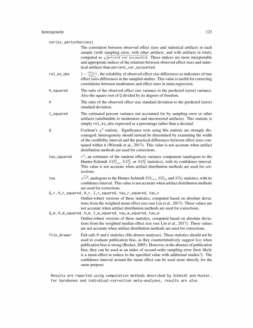
heterogeneity 123

cor(es, perturbations)

The correlation between observed effect sizes and statistical artifacts in eachsample (with sampling error, with other artifacts, and with artifacts in total),computed as

√percent var accounted. These indices are more interpretable

and appropriate indices of the relations between observed effect sizes and statis-tical artifacts than percent_var_accounted.

rel_es_obs 1− varprevares

, the reliability of observed effect size differences as indicators of trueeffect sizes differences in the sampled studies. This value is useful for correctingcorrelations between moderators and effect sizes in meta-regression.

H_squared The ratio of the observed effect size variance to the predicted (error) variance.Also the square root of Q divided by its degrees of freedom.

H The ratio of the observed effect size standard deviation to the predicted (error)standard deviation.

I_squared The estimated percent variance not accounted for by sampling error or otherartifacts (attributable to moderators and uncorrected artifacts). This statistic issimply rel_es_obs expressed as a percentage rather than a decimal.

Q Cochran’s χ2 statistic. Significance tests using this statistic are strongly dis-couraged; heterogeneity should instead be determined by examining the widthof the credibility interval and the practical differences between effect sizes con-tained within it (Wiernik et al., 2017). This value is not accurate when artifactdistribution methods are used for corrections.

tau_squared τ2, an estimator of the random effects variance component (analogous to theHunter-Schmidt SD2

res, SD2ρ, or SD2

δ statistics), with its confidence interval.This value is not accurate when artifact distribution methods are used for cor-rections.

tau√τ2, analogous to the Hunter-Schmidt SDres, SDρ, and SDδ statistics, with its

confidence interval. This value is not accurate when artifact distribution methodsare used for corrections.

Q_r, H_r_squared, H_r, I_r_squared, tau_r_squared, tau_r

Outlier-robust versions of these statistics, computed based on absolute devia-tions from the weighted mean effect size (see Lin et al., 2017). These values arenot accurate when artifact distribution methods are used for corrections.

Q_m, H_m_squared, H_m, I_m_squared, tau_m_squared, tau_m

Outlier-robust versions of these statistics, computed based on absolute devia-tions from the weighted median effect size (see Lin et al., 2017). These valuesare not accurate when artifact distribution methods are used for corrections.

file_drawer Fail-safe N and k statistics (file-drawer analyses). These statistics should not beused to evaluate publication bias, as they counterintuitively suggest less whenpublication bias is strong (Becker, 2005). However, in the absence of publicationbias, they can be used as an index of second-order sampling error (how likelyis a mean effect to reduce to the specified value with additional studies?). Theconfidence interval around the mean effect can be used more directly for thesame purpose.

Results are reported using computation methods described by Schmidt and Hunter.For barebones and indivdiual-correction meta-analyses, results are also

124 heterogeneity

reported using computation methods described by DerSimonian and Laird,outlier-robust computation methods, and, if weights from \pkg{metafor}are used, heterogeneity results from \pkg{metafor}.

References

Becker, B. J. (2005). Failsafe N or file-drawer number. In H. R. Rothstein, A. J. Sutton, & M.Borenstein (Eds.), Publication bias in meta-analysis: Prevention, assessment and adjustments (pp.111–125). Hoboken, NJ: Wiley. https://doi.org/10.1002/0470870168.ch7

Higgins, J. P. T., & Thompson, S. G. (2002). Quantifying heterogeneity in a meta-analysis. Statis-tics in Medicine, 21(11), 1539–1558. https://doi.org/10.1002/sim.1186

Lin, L., Chu, H., & Hodges, J. S. (2017). Alternative measures of between-study heterogeneityin meta-analysis: Reducing the impact of outlying studies. Biometrics, 73(1), 156–166. https://doi.org/10.1111/biom.12543

Schmidt, F. (2010). Detecting and correcting the lies that data tell. Perspectives on PsychologicalScience, 5(3), 233–242. https://doi.org/10.1177/1745691610369339

Schmidt, F. L., & Hunter, J. E. (2015). Methods of meta-analysis: Correcting error and bias inresearch findings (3rd ed.). Thousand Oaks, CA: Sage. https://doi.org/10/b6mg. pp. 15, 414,426, 533–534.

Wiernik, B. M., Kostal, J. W., Wilmot, M. P., Dilchert, S., & Ones, D. S. (2017). Empirical bench-marks for interpreting effect size variability in meta-analysis. Industrial and Organizational Psy-chology, 10(3). https://doi.org/10.1017/iop.2017.44

Examples

## Correlationsma_obj <- ma_r_ic(rxyi = rxyi, n = n, rxx = rxxi, ryy = ryyi, ux = ux,

correct_rr_y = FALSE, data = data_r_uvirr)ma_obj <- ma_r_ad(ma_obj, correct_rr_y = FALSE)ma_obj <- heterogeneity(ma_obj = ma_obj)ma_obj$heterogeneity[[1]]$barebonesma_obj$heterogeneity[[1]]$individual_correction$true_scorema_obj$heterogeneity[[1]]$artifact_distribution$true_score

## d valuesma_obj <- ma_d_ic(d = d, n1 = n1, n2 = n2, ryy = ryyi,

data = data_d_meas_multi)ma_obj <- ma_d_ad(ma_obj)ma_obj <- heterogeneity(ma_obj = ma_obj)ma_obj$heterogeneity[[1]]$barebonesma_obj$heterogeneity[[1]]$individual_correction$latentGroup_latentYma_obj$heterogeneity[[1]]$artifact_distribution$latentGroup_latentY

https://doi.org/10.1002/0470870168.ch7

https://doi.org/10.1002/sim.1186

https://doi.org/10.1111/biom.12543

https://doi.org/10.1111/biom.12543

https://doi.org/10.1177/1745691610369339


https://doi.org/10.1017/iop.2017.44

limits_tau 125

limits_tau Confidence limits of tau

Description

Note that this interval does not incorporate uncertainty in artifact estimates, so the interval will besomewhat conservative when applied to individual-correction or artifact-distribution meta-analyses.

Usage

limits_tau(var_es,var_pre,k,method = c("profile_var_es", "profile_Q", "normal_logQ"),conf_level = 0.95,var_unbiased = TRUE

)

Arguments

var_es The observed variance of effect sizes.

var_pre The predicted variance of effect sizes due to artifacts.

k The number of studies in a meta-analysis.

method Which method to use to estimate the limits. Options are profile_var_es fora profile-likelihood interval assuming σ2




conf_level Confidence level.

var_unbiased Are variances computed using the unbiased (TRUE) or maximum likelihood (FALSE)estimator?

Value

The confidence limits of tau

Examples

limits_tau(var_es = 0.008372902, var_pre = 0.004778935, k = 20)

126 limits_tau2

limits_tau2 Confidence limits of tau-squared

Description

Note that this interval does not incorporate uncertainty in artifact estimates, so the interval will besomewhat conservative when applied to individual-correction or artifact-distribution meta-analyses.

Usage

limits_tau2(var_es,var_pre,k,method = c("profile_var_es", "profile_Q", "normal_logQ"),conf_level = 0.95,var_unbiased = TRUE

)

Arguments

var_es The observed variance of effect sizes.

var_pre The predicted variance of effect sizes due to artifacts.

k The number of studies in a meta-analysis.

method Which method to use to estimate the limits. Options are profile_var_es fora profile-likelihood interval assuming σ2




conf_level Confidence level.

var_unbiased Are variances computed using the unbiased (TRUE) or maximum likelihood (FALSE)estimator?

Value

The confidence limits of tau-squared

Examples

limits_tau2(var_es = 0.008372902, var_pre = 0.004778935, k = 20)

lm_mat 127

lm_mat Compute linear regression models and generate "lm" objects from co-variance matrices.

Description

Compute linear regression models and generate "lm" objects from covariance matrices.

Usage

lm_mat(formula,cov_mat,mean_vec = rep(0, ncol(cov_mat)),n = Inf,se_beta_method = c("lm", "normal"),...

)

matrixreg(formula,cov_mat,mean_vec = rep(0, ncol(cov_mat)),n = Inf,se_beta_method = c("lm", "normal"),...

)

matreg(formula,cov_mat,mean_vec = rep(0, ncol(cov_mat)),n = Inf,se_beta_method = c("lm", "normal"),...

)

lm_matrix(formula,cov_mat,mean_vec = rep(0, ncol(cov_mat)),n = Inf,se_beta_method = c("lm", "normal"),...

)

128 lm_mat

Arguments

formula Regression formula with a single outcome variable on the left-hand side and oneor more predictor variables on the right-hand side (e.g., Y ~ X1 + X2).

cov_mat Covariance matrix containing the variables to be used in the regression.

mean_vec Vector of means corresponding to the variables in cov_mat.

n Sample size to be used in significance testing

se_beta_method Method to use to estimate the standard errors of standardized regression (beta)coefficients. Current options include "lm" (estimate standard errors using con-ventional regression formulas) and "normal" (use the Jones-Waller normal-theoryapproach from the fungible::seBeta() and fungible::seBetaCor() func-tions)


Value

An object with the class "lm_mat" that can be used with summary, print, predict, and anova methods.

Examples

## Generate dataS <- reshape_vec2mat(cov = c(.3 * 2 * 3,

.4 * 2 * 4,

.5 * 3 * 4),var = c(2, 3, 4)^2,var_names = c("X", "Y", "Z"))

mean_vec <- setNames(c(1, 2, 3), colnames(S))dat <- data.frame(MASS::mvrnorm(n = 100, mu = mean_vec,

Sigma = S, empirical = TRUE))

## Compute regression models with lmlm_out1 <- lm(Y ~ X, data = dat)lm_out2 <- lm(Y ~ X + Z, data = dat)

## Compute regression models with lm_matmatreg_out1 <- lm_mat(formula = Y ~ X, cov_mat = S, mean_vec = mean_vec, n = nrow(dat))matreg_out2 <- lm_mat(formula = Y ~ X + Z, cov_mat = S, mean_vec = mean_vec, n = nrow(dat))

## Compare results of lm and lm_mat with one predictorlm_out1matreg_out1

## Compare summaries of lm and lm_mat with one predictorsummary(lm_out1)summary(matreg_out1)

## Compare results of lm and lm_mat with two predictorslm_out2matreg_out2

ma_d 129

## Compare summaries of lm and lm_mat with two predictorssummary(lm_out2)summary(matreg_out2)

## Compare predictions made with lm and lm_matpredict(object = matreg_out1, newdata = data.frame(X = 1:5))predict(object = summary(matreg_out1), newdata = data.frame(X = 1:5))predict(lm_out1, newdata = data.frame(X = 1:5))

## Compare predictions made with lm and lm_mat (with confidence intervals)predict(object = matreg_out1, newdata = data.frame(X = 1:5),

se.fit = TRUE, interval = "confidence")predict(lm_out1, newdata = data.frame(X = 1:5),

se.fit = TRUE, interval = "confidence")

## Compare predictions made with lm and lm_mat (with prediction intervals)predict(object = matreg_out1, newdata = data.frame(X = 1:5),

se.fit = TRUE, interval = "prediction")predict(lm_out1, newdata = data.frame(X = 1:5),

se.fit = TRUE, interval = "prediction")

## Compare model comparisons computed using lm and lm_mat objectsanova(lm_out1, lm_out2)anova(matreg_out1, matreg_out2)

## Model comparisons can be run on lm_mat summaries, too:anova(summary(matreg_out1), summary(matreg_out2))## Or summaries and raw models can be mixed:anova(matreg_out1, summary(matreg_out2))anova(summary(matreg_out1), matreg_out2)

## Compare confidence intervals computed using lm and lm_mat objectsconfint(object = lm_out1)confint(object = matreg_out1)confint(object = summary(matreg_out1))

confint(object = lm_out2)confint(object = matreg_out2)confint(object = summary(matreg_out2))

ma_d Meta-analysis of d values

Description

The ma_r_bb, ma_r_ic, and ma_r_ad functions implement bare-bones, individual-correction, andartifact-distribution correction methods for d values, respectively. The ma_d function is the mas-ter function for meta-analyses of d values - it facilitates the computation of bare-bones, artifact-distribution, and individual-correction meta-analyses of correlations for any number of group-wise

130 ma_d

contrasts and any number of dependent variables. When artifact-distribution meta-analyses are per-formed, ma_d will automatically extract the artifact information from a database and organize it intothe requested type of artifact distribution object (i.e., either Taylor series or interactive artifact dis-tributions). ma_d is also equipped with the capability to clean databases containing inconsistentlyrecorded artifact data, impute missing artifacts (when individual-correction meta-analyses are re-quested), and remove dependency among samples by forming composites or averaging effect sizesand artifacts. The automatic compositing features in ma_d are employed when sample_ids and/orconstruct names are provided.

Usage

ma_d(d,n1,n2 = NULL,n_adj = NULL,sample_id = NULL,citekey = NULL,treat_as_r = FALSE,ma_method = c("bb", "ic", "ad"),ad_type = c("tsa", "int"),correction_method = "auto",group_id = NULL,group1 = NULL,group2 = NULL,group_order = NULL,construct_y = NULL,facet_y = NULL,measure_y = NULL,construct_order = NULL,wt_type = c("n_effective", "sample_size", "inv_var_mean", "inv_var_sample", "DL",

"HE", "HS", "SJ", "ML", "REML", "EB", "PM"),correct_bias = TRUE,correct_rel = NULL,correct_rGg = FALSE,correct_ryy = TRUE,correct_rr = NULL,correct_rr_g = TRUE,correct_rr_y = TRUE,indirect_rr = NULL,indirect_rr_g = TRUE,indirect_rr_y = TRUE,rGg = NULL,pi = NULL,pa = NULL,ryy = NULL,ryy_restricted = TRUE,ryy_type = "alpha",k_items_y = NULL,

ma_d 131

uy = NULL,uy_observed = TRUE,sign_rz = NULL,sign_rgz = 1,sign_ryz = 1,moderators = NULL,cat_moderators = TRUE,moderator_type = c("simple", "hierarchical", "none"),supplemental_ads = NULL,data = NULL,control = control_psychmeta(),...

)

ma_d_ad(ma_obj,ad_obj_g = NULL,ad_obj_y = NULL,correction_method = "auto",use_ic_ads = c("tsa", "int"),correct_rGg = FALSE,correct_ryy = TRUE,correct_rr_g = TRUE,correct_rr_y = TRUE,indirect_rr_g = TRUE,indirect_rr_y = TRUE,sign_rgz = 1,sign_ryz = 1,control = control_psychmeta(),...

)

ma_d_bb(d,n1,n2 = rep(NA, length(d)),n_adj = NULL,sample_id = NULL,citekey = NULL,wt_type = c("n_effective", "sample_size", "inv_var_mean", "inv_var_sample", "DL",

"HE", "HS", "SJ", "ML", "REML", "EB", "PM"),correct_bias = TRUE,moderators = NULL,cat_moderators = TRUE,moderator_type = c("simple", "hierarchical", "none"),data = NULL,control = control_psychmeta(),...

132 ma_d

)

ma_d_ic(d,n1,n2 = NULL,n_adj = NULL,sample_id = NULL,citekey = NULL,treat_as_r = FALSE,wt_type = c("n_effective", "sample_size", "inv_var_mean", "inv_var_sample", "DL",

"HE", "HS", "SJ", "ML", "REML", "EB", "PM"),correct_bias = TRUE,correct_rGg = FALSE,correct_ryy = TRUE,correct_rr_g = FALSE,correct_rr_y = TRUE,indirect_rr_g = TRUE,indirect_rr_y = TRUE,rGg = NULL,pi = NULL,pa = NULL,ryy = NULL,ryy_restricted = TRUE,ryy_type = "alpha",k_items_y = NULL,uy = NULL,uy_observed = TRUE,sign_rgz = 1,sign_ryz = 1,moderators = NULL,cat_moderators = TRUE,moderator_type = c("simple", "hierarchical", "none"),supplemental_ads_y = NULL,data = NULL,control = control_psychmeta(),...

)

Arguments

d Vector or column name of observed d values.

n1 Vector or column name of sample sizes.

n2 Vector or column name of sample sizes.

n_adj Optional: Vector or column name of sample sizes adjusted for sporadic artifactcorrections.

sample_id Optional vector of identification labels for samples/studies in the meta-analysis.

ma_d 133

citekey Optional vector of bibliographic citation keys for samples/studies in the meta-analysis (if multiple citekeys pertain to a given effect size, combine them into asingle string entry with comma delimiters (e.g., "citkey1,citekey2").

treat_as_r Logical scalar determining whether d values are to be meta-analyzed as d values(FALSE; default) or whether they should be meta-analyzed as correlations andhave the final results converted to the d metric (TRUE).

ma_method Method to be used to compute the meta-analysis: "bb" (barebones), "ic" (indi-vidual correction), or "ad" (artifact distribution).

ad_type For when ma_method is "ad", specifies the type of artifact distribution to use:"int" or "tsa".

correction_method

Character scalar or a matrix with group_id levels as row names and construct_ylevels as column names. When ma_method is "ad", select one of the follow-ing methods for correcting artifacts: "auto", "meas", "uvdrr", "uvirr", "bvdrr","bvirr", "rbOrig", "rb1Orig", "rb2Orig", "rbAdj", "rb1Adj", and "rb2Adj". (note:"rb1Orig", "rb2Orig", "rb1Adj", and "rb2Adj" can only be used when Taylor se-ries artifact distributions are provided and "rbOrig" and "rbAdj" can only be usedwhen interactive artifact distributions are provided). See "Details" of ma_d_adfor descriptions of the available methods.

group_id Vector of group comparison IDs (e.g., Treatment1-Control, Treatment2-Control).The group_id argument supersedes the group1 and group2 arguments. If group_idis not NULL, the values supplied to the group_order argument must correspondto group_id values.

group1, group2 Vector of group identification labels (e.g., Treatment1, Treatment2, Control)group_order Optional vector indicating the order in which (1) group1 and group2 values or

(2) group_ids should be arranged. If group_order is NULL, the order of grouppairings will be determined internally using alpha-numeric ordering.

construct_y Vector of construct names for construct designated as "Y".facet_y Vector of facet names for constructs designated as "Y". Facet names "global",

"overall", and "total" are reserved to indicate observations that represent effectsizes that have already been composited or that represent construct-level mea-surements rather than facet-level measurements. To avoid double-compositing,any observation with one of these reserved names will only be eligible for auto-compositing with other such observations and will not be combined with narrowfacets.

measure_y Vector of names for measures associated with constructs designated as "Y".construct_order

Vector indicating the order in which Y variables should be arranged.wt_type Type of weight to use in the meta-analysis: options are "n_effective" (effec-

tive sample size), "sample_size", "inv_var_mean" (inverse variance computedusing mean effect size), and "inv_var_sample" (inverse variance computed us-ing sample-specific effect sizes). Supported options borrowed from metafor are"DL", "HE", "HS", "SJ", "ML", "REML", "EB", and "PM" (see metafor docu-mentation for details about the metafor methods).

correct_bias Logical scalar that determines whether to correct correlations for small-samplebias (TRUE) or not (FALSE).

134 ma_d

correct_rel Optional named vector that supersedes correct_rGg and correct_ryy. Namesshould correspond to construct names in group_id and construct_y to deter-mine which constructs should be corrected for unreliability.

correct_rGg Logical scalar or vector that determines whether to correct the grouping variablevariable for measurement error (TRUE) or not (FALSE).

correct_ryy Logical scalar or vector that determines whether to correct the Y variable formeasurement error (TRUE) or not (FALSE).

correct_rr Optional named vector that supersedes correct_rr_g and correct_rr_y. Namesshould correspond to construct names in group_id and construct_y to deter-mine which constructs should be corrected for range restriction.

correct_rr_g Logical scalar or vector or column name determining whether each d valueshould be corrected for range restriction in the grouping variable (TRUE) or not(FALSE).

correct_rr_y Logical scalar or vector or column name determining whether each d should becorrected for range restriction in Y (TRUE) or not (FALSE).

indirect_rr Optional named vector that supersedes indirect_rr_g and indirect_rr_y.Names should correspond to construct names in group_id and construct_y todetermine which constructs should be corrected for indirect range restriction.

indirect_rr_g Logical vector or column name determining whether each d should be correctedfor indirect range restriction in the grouping variable (TRUE) or not (FALSE).Superseded in evaluation by correct_rr_g (i.e., if correct_rr_g == FALSE,the value supplied for indirect_rr_g is disregarded).

indirect_rr_y Logical vector or column name determining whether each d should be correctedfor indirect range restriction in Y (TRUE) or not (FALSE). Superseded in evalua-tion by correct_rr_y (i.e., if correct_rr_y == FALSE, the value supplied forindirect_rr_y is disregarded).

rGg Vector or column name of reliability estimates for X.

pi Scalar or vector containing the restricted-group proportions of group member-ship. If a vector, it must either (1) have as many elements as there are d valuesor (2) be named so as to match with levels of the group_id argument.

pa Scalar or vector containing the unrestricted-group proportions of group mem-bership (default = .5). If a vector, it must either (1) have as many elements asthere are d values or (2) be named so as to match with levels of the group_idargument.


ryy_restricted Logical vector or column name determining whether each element of ryy is anincumbent reliability (TRUE) or an applicant reliability (FALSE).

ryy_type String vector identifying the types of reliability estimates supplied (e.g., "alpha","retest", "interrater_r", "splithalf"). See the documentation for ma_r for a full listof acceptable reliability types.

k_items_y Numeric vector identifying the number of items in each scale.



ma_d 135

sign_rz Optional named vector that supersedes sign_rgz and sign_ryz. Names shouldcorrespond to construct names in group_id and construct_y to determine thesign of each construct’s relationship with the selection mechanism.

sign_rgz Sign of the relationship between X and the selection mechanism (for use withbvirr corrections only).

sign_ryz Sign of the relationship between Y and the selection mechanism (for use withbvirr corrections only).



moderator_type Type of moderator analysis: "none" means that no moderators are to be used,"simple" means that moderators are to be examined one at a time, "hierarchical"means that all possible combinations and subsets of moderators are to be exam-ined, and "all" means that simple and hierarchical moderator analyses are to beperformed.

supplemental_ads

Named list (named according to the constructs included in the meta-analysis) ofsupplemental artifact distribution information from studies not included in themeta-analysis. This is a list of lists, where the elements of a list associated witha construct are named like the arguments of the create_ad() function.

data Data frame containing columns whose names may be provided as arguments tovector arguments and/or moderators.



ma_obj For ma_d_ad only: Meta-analysis object of correlations or d values (regardlessof input metric, output metric will be d).

ad_obj_g For ma_d_ad only: Artifact-distribution object for the grouping variable (outputof the link{create_ad} or link{create_ad_group} functions). If ma_obj isof the class ma_master (i.e., the output of ma_r or ma_d), the object supplied forad_obj_g must be a named list of artifact distributions with names. correspond-ing to the "X" constructs in the meta-analyses contained within ma_obj.

ad_obj_y For ma_d_ad only: AArtifact-distribution object for the Y variable (output of thecreate_ad function). If ma_obj is of the class ma_master, the object suppliedfor ad_obj_y must be a named list of artifact distributions with names corre-sponding to the "Y" constructs in the meta-analyses contained within ma_obj.

use_ic_ads For ma_d_ad only: Determines whether artifact distributions should be extractedfrom the individual correction results in ma_obj. Only evaluated when ad_obj_gor ad_obj_y is NULL and ma_obj does not contain individual correction results.Use one of the following commands: tsa to use the Taylor series method or intto use the interactive method.

136 ma_d

supplemental_ads_y

For ma_d_ic only: List supplemental artifact distribution information from stud-ies not included in the meta-analysis. The elements of this list are named likethe arguments of the create_ad() function.

Details

The options for correction_method are:

• "auto"Automatic selection of the most appropriate correction procedure, based on the available arti-facts and the logical arguments provided to the function. (default)

• "meas"Correction for measurement error only.

• "uvdrr"Correction for univariate direct range restriction (i.e., Case II). The choice of which variable tocorrect for range restriction is made using the correct_rr_x and correct_rr_y arguments.

• "uvirr"Correction for univariate indirect range restriction (i.e., Case IV). The choice of which vari-able to correct for range restriction is made using the correct_rr_x and correct_rr_y ar-guments.

• "bvdrr"Correction for bivariate direct range restriction. Use with caution: This correction is an ap-proximation only and is known to have a positive bias.

• "bvirr"Correction for bivariate indirect range restriction (i.e., Case V).

• "rbOrig"Not recommended: Raju and Burke’s version of the correction for direct range restriction,applied interactively. We recommend using "uvdrr" instead.

• "rbAdj"Not recommended: Raju and Burke’s version of the correction for direct range restriction, ap-plied interactively. Adjusted to account for range restriction in the reliability of the Y variable.We recommend using "uvdrr" instead.

• "rb1Orig"Not recommended: Raju and Burke’s version of the correction for direct range restriction,applied using their TSA1 method. We recommend using "uvdrr" instead.

• "rb1Adj"Not recommended: Raju and Burke’s version of the correction for direct range restriction,applied using their TSA1 method. Adjusted to account for range restriction in the reliabilityof the Y variable. We recommend using "uvdrr" instead.



ma_d 137

Value

A nested tabular object of the class "ma_psychmeta". Components of output tables for bare-bonesmeta-analyses:

• Pair_IDUnique identification number for each construct-contrast pairing.

• group_contrastName of the variable analyzed as the group-contrast variable.

• construct_yName of the variable analyzed as construct Y.

• analysis_idUnique identification number for each analysis.

• analysis_typeType of moderator analyses: Overall, Simple Moderator, or Hierarchical Moderator.

• kNumber of effect sizes meta-analyzed.

• NTotal sample size of all effect sizes in the meta-analysis.

• mean_dMean observed d value.

• var_dWeighted variance of observed d values.

• var_ePredicted sampling-error variance of observed d values.

• var_resVariance of observed d values after removing predicted sampling-error variance.

• sd_dSquare root of var_r.

• se_dStandard error of mean_d.

• sd_eSquare root of var_e.

• sd_resSquare root of var_res.

• CI_LL_XXLower limit of the confidence interval around mean_d, where "XX" represents the confidencelevel as a percentage.

• CI_UL_XXUpper limit of the confidence interval around mean_d, where "XX" represents the confidencelevel as a percentage.

• CR_LL_XXLower limit of the credibility interval around mean_d, where "XX" represents the credibilitylevel as a percentage.

138 ma_d

• CR_UL_XXUpper limit of the credibility interval around mean_d, where "XX" represents the credibilitylevel as a percentage.

Components of output tables for individual-correction meta-analyses:

• pair_idUnique identification number for each construct-contrast pairing.










• var_resVariance of observed d values after removing predicted sampling-error variance.

• sd_dSquare root of var_r.




• mean_deltaMean artifact-corrected d value.

• var_d_cVariance of artifact-corrected d values.

• var_e_cPredicted sampling-error variance of artifact-corrected d values.

• var_deltaVariance of artifact-corrected d values after removing predicted sampling-error variance.

ma_d 139

• sd_d_cSquare root of var_r_c.

• se_d_cStandard error of mean_delta.

• sd_e_cSquare root of var_e_c.

• sd_deltaSquare root of var_delta.

• CI_LL_XXLower limit of the confidence interval around mean_delta, where "XX" represents the confi-dence level as a percentage.

• CI_UL_XXUpper limit of the confidence interval around mean_delta, where "XX" represents the confi-dence level as a percentage.

• CR_LL_XXLower limit of the credibility interval around mean_delta, where "XX" represents the credi-bility level as a percentage.

• CR_UL_XXUpper limit of the credibility interval around mean_delta, where "XX" represents the credi-bility level as a percentage.

Components of output tables for artifact-distribution meta-analyses:

• pair_idUnique identification number for each construct-contrast pairing.










140 ma_d

• var_artAmount of variance in observed d values that is attributable to measurement-error and range-restriction artifacts.

• var_preTotal predicted artifactual variance (i.e., the sum of var_e and var_art).

• var_resVariance of observed d values after removing predicted sampling-error variance and predictedartifact variance.

• sd_dSquare root of var_d.



• sd_artSquare root of var_art.

• sd_preSquare root of var_pre.


• mean_deltaMean artifact-corrected d value.

• var_dWeighted variance of observed d values corrected to the metric of delta.

• var_ePredicted sampling-error variance of observed d values corrected to the metric of delta.

• var_artAmount of variance in observed d values that is attributable to measurement-error and range-restriction artifacts corrected to the metric of delta.

• var_preTotal predicted artifactual variance (i.e., the sum of var_e and var_art) corrected to themetric of delta.

• var_deltaVariance of artifact-corrected d values after removing predicted sampling-error variance andpredicted artifact variance.

• sd_dSquare root of var_d corrected to the metric of delta.

• se_dStandard error of mean_d corrected to the metric of delta.

• sd_eSquare root of var_e corrected to the metric of delta.

• sd_artSquare root of var_art corrected to the metric of delta.

ma_d 141

• sd_preSquare root of var_pre corrected to the metric of delta.

• sd_deltaSquare root of var_delta.

• CI_LL_XXLower limit of the confidence interval around mean_delta, where "XX" represents the confi-dence level as a percentage.

• CI_UL_XXUpper limit of the confidence interval around mean_delta, where "XX" represents the confi-dence level as a percentage.

• CR_LL_XXLower limit of the credibility interval around mean_delta, where "XX" represents the credi-bility level as a percentage.

• CR_UL_XXUpper limit of the credibility interval around mean_delta, where "XX" represents the credi-bility level as a percentage.

Note

The difference between "rb" methods with the "orig" and "adj" suffixes is that the original does notaccount for the impact of range restriction on criterion reliabilities, whereas the adjusted procedureattempts to estimate the applicant reliability information for the criterion. The "rb" procedures areincluded for posterity: We strongly recommend using the "uvdrr" procedure to appropriately correctfor univariate range restriction.

References

Schmidt, F. L., & Hunter, J. E. (2015). Methods of meta-analysis: Correcting error and bias inresearch findings (3rd ed.). Thousand Oaks, California: SAGE Publications, Inc. Chapter 4.

Law, K. S., Schmidt, F. L., & Hunter, J. E. (1994). Nonlinearity of range corrections in meta-analysis: Test of an improved procedure. Journal of Applied Psychology, 79(3), 425.


Raju, N. S., & Burke, M. J. (1983). Two new procedures for studying validity generalization.Journal of Applied Psychology, 68(3), 382. https://doi.org/10.1037/0021-9010.68.3.382

Examples

### Demonstration of ma_d ##### The 'ma_d' function can compute multi-construct bare-bones meta-analyses:ma_d(d = d, n1 = n1, n2 = n2, construct_y = construct, data = data_d_meas_multi)

## It can also perform multiple individual-correction meta-analyses:ma_d(ma_method = "ic", d = d, n1 = n1, n2 = n2, ryy = ryyi,

construct_y = construct, data = data_d_meas_multi)

142 ma_d_order2

## And 'ma_d' can also curate artifact distributions and compute multiple## artifact-distribution meta-analyses:ma_d(ma_method = "ad", d = d, n1 = n1, n2 = n2,

ryy = ryyi, correct_rr_y = FALSE,construct_y = construct, data = data_d_meas_multi)

### Demonstration of ma_d_bb ##### Example meta-analyses using simulated data:ma_d_bb(d = d, n1 = n1, n2 = n2,

data = data_d_meas_multi[data_d_meas_multi$construct == "Y",])ma_d_bb(d = d, n1 = n1, n2 = n2,

data = data_d_meas_multi[data_d_meas_multi$construct == "Z",])

### Demonstration of ma_d_ic ##### Example meta-analyses using simulated data:ma_d_ic(d = d, n1 = n1, n2 = n2, ryy = ryyi, correct_rr_y = FALSE,

data = data_d_meas_multi[data_d_meas_multi$construct == "Y",])ma_d_ic(d = d, n1 = n1, n2 = n2, ryy = ryyi, correct_rr_y = FALSE,

data = data_d_meas_multi[data_d_meas_multi$construct == "Z",])

ma_d_order2 Second-order meta-analysis function for d values

Description

This function computes second-order meta-analysis function for d values. It supports second-orderanalyses of bare-bones, artifact-distribution, and individual-correction meta-analyses.

Usage

ma_d_order2(k,N = NULL,d = NULL,delta = NULL,var_d = NULL,var_d_c = NULL,ma_type = c("bb", "ic", "ad"),sample_id = NULL,citekey = NULL,moderators = NULL,moderator_type = "simple",construct_x = NULL,construct_y = NULL,construct_order = NULL,data = NULL,control = control_psychmeta(),

ma_d_order2 143

...)

Arguments

k Vector or column name of meta-analyses’ k values.

N Vector or column name of meta-analyses’ total sample sizes (optional).

d Vector or column name of mean observed d values.

delta Vector or column name of mean corrected d values.

var_d Vector or column name of observed variances of observed d values.

var_d_c Vector or column name of observed variances of corrected d values.

ma_type Type of meta-analyses being analyzed: "bb" (barebones), "ic" (individual cor-rection), or "ad" (artifact distribution).

sample_id Vector or column name of study ID labels.



moderator_type Type of moderator analysis ("none", "simple", or "hierarchical").

construct_x Vector or column name of construct names for X.

construct_y Vector or column name of construct names for Y.

construct_order





Value

A nested tabular object of the class "ma_psychmeta".

144 ma_generic

ma_generic Bare-bones meta-analysis of generic effect sizes

Description

This function computes bare-bones meta-analyses of any effect size using user-supplied effect errorvariances.

Usage

ma_generic(es,n,var_e,sample_id = NULL,citekey = NULL,construct_x = NULL,construct_y = NULL,group1 = NULL,group2 = NULL,wt_type = c("sample_size", "inv_var", "DL", "HE", "HS", "SJ", "ML", "REML", "EB",

"PM"),moderators = NULL,cat_moderators = TRUE,moderator_type = c("simple", "hierarchical", "none"),data = NULL,control = control_psychmeta(),weights = NULL,...

)

Arguments

es Vector or column name of observed effect sizes.


var_e Vector or column name of error variances.


citekey Optional vector of bibliographic citation keys for samples/studies in the meta-analysis (if multiple citekeys pertain to a given effect size, combine them intoa single string entry with comma delimiters (e.g., "citkey1,citekey2"). WhenTRUE, program will use sample-size weights, error variances estimated from themean effect size, maximum likelihood variances, and normal-distribution confi-dence and credibility intervals.

construct_x, construct_y

Vector of construct names for constructs designated as "X" and as "Y".

ma_r 145

group1, group2 Vector of groups’ names associated with effect sizes that represent pairwise con-trasts.

wt_type Type of weight to use in the meta-analysis: native options are "sample_size" and"inv_var" (inverse error variance). Supported options borrowed from metaforare "DL", "HE", "HS", "SJ", "ML", "REML", "EB", and "PM" (see metafordocumentation for details about the metafor methods).

moderators Matrix of moderator variables to be used in the meta-analysis (can be a vectorin the case of one moderator).





weights Optional vector of weights to be used. When weights is non-NULL, theseweights override the argument supplied to wt_type.


Value


Examples

es <- c(.3, .5, .8)n <- c(100, 200, 150)var_e <- 1 / nma_obj <- ma_generic(es = es, n = n, var_e = var_e)ma_objsummary(ma_obj)

ma_r Meta-analysis of correlations

Description

The ma_r_bb, ma_r_ic, and ma_r_ad functions implement bare-bones, individual-correction, andartifact-distribution correction methods for correlations, respectively. The ma_r function is the mas-ter function for meta-analyses of correlations - it facilitates the computation of bare-bones, artifact-distribution, and individual-correction meta-analyses of correlations for any number of constructpairs. When artifact-distribution meta-analyses are performed, ma_r will automatically extract theartifact information from a database and organize it into the requested type of artifact distributionobject (i.e., either Taylor series or interactive artifact distributions). ma_r is also equipped with

146 ma_r

the capability to clean databases containing inconsistently recorded artifact data, impute missingartifacts (when individual-correction meta-analyses are requested), and remove dependency amongsamples by forming composites or averaging effect sizes and artifacts. The automatic compositingfeatures in ma_r are employed when sample_ids and/or construct names are provided.

Usage

ma_r(rxyi,n,n_adj = NULL,sample_id = NULL,citekey = NULL,ma_method = c("bb", "ic", "ad"),ad_type = c("tsa", "int"),correction_method = "auto",construct_x = NULL,construct_y = NULL,facet_x = NULL,facet_y = NULL,measure_x = NULL,measure_y = NULL,construct_order = NULL,wt_type = c("sample_size", "inv_var_mean", "inv_var_sample", "DL", "HE", "HS", "SJ",

"ML", "REML", "EB", "PM"),correct_bias = TRUE,correct_rel = NULL,correct_rxx = TRUE,correct_ryy = TRUE,correct_rr = NULL,correct_rr_x = TRUE,correct_rr_y = TRUE,indirect_rr = NULL,indirect_rr_x = TRUE,indirect_rr_y = TRUE,rxx = NULL,rxx_restricted = TRUE,rxx_type = "alpha",k_items_x = NULL,ryy = NULL,ryy_restricted = TRUE,ryy_type = "alpha",k_items_y = NULL,ux = NULL,ux_observed = TRUE,uy = NULL,uy_observed = TRUE,sign_rz = NULL,sign_rxz = 1,

ma_r 147

sign_ryz = 1,moderators = NULL,cat_moderators = TRUE,moderator_type = c("simple", "hierarchical", "none"),supplemental_ads = NULL,data = NULL,control = control_psychmeta(),...

)

ma_r_ad(ma_obj,ad_obj_x = NULL,ad_obj_y = NULL,correction_method = "auto",use_ic_ads = c("tsa", "int"),correct_rxx = TRUE,correct_ryy = TRUE,correct_rr_x = TRUE,correct_rr_y = TRUE,indirect_rr_x = TRUE,indirect_rr_y = TRUE,sign_rxz = 1,sign_ryz = 1,control = control_psychmeta(),...

)

ma_r_bb(r,n,n_adj = NULL,sample_id = NULL,citekey = NULL,wt_type = c("sample_size", "inv_var_mean", "inv_var_sample", "DL", "HE", "HS", "SJ",

"ML", "REML", "EB", "PM"),correct_bias = TRUE,moderators = NULL,cat_moderators = TRUE,moderator_type = c("simple", "hierarchical", "none"),data = NULL,control = control_psychmeta(),...

)

ma_r_ic(rxyi,n,

148 ma_r

n_adj = NULL,sample_id = NULL,citekey = NULL,wt_type = c("sample_size", "inv_var_mean", "inv_var_sample", "DL", "HE", "HS", "SJ",

"ML", "REML", "EB", "PM"),correct_bias = TRUE,correct_rxx = TRUE,correct_ryy = TRUE,correct_rr_x = TRUE,correct_rr_y = TRUE,indirect_rr_x = TRUE,indirect_rr_y = TRUE,rxx = NULL,rxx_restricted = TRUE,rxx_type = "alpha",k_items_x = NULL,ryy = NULL,ryy_restricted = TRUE,ryy_type = "alpha",k_items_y = NULL,ux = NULL,ux_observed = TRUE,uy = NULL,uy_observed = TRUE,sign_rxz = 1,sign_ryz = 1,moderators = NULL,cat_moderators = TRUE,moderator_type = c("simple", "hierarchical", "none"),supplemental_ads_x = NULL,supplemental_ads_y = NULL,data = NULL,control = control_psychmeta(),...

)

Arguments

rxyi, r Vector or column name of observed correlations. The r argument is used withthe ma_r_bb (i.e., the barebones function) function and the rxyi argument isused with ma_r and ma_r_ic (i.e., the function in which corrections are applied).


n_adj Optional: Vector or column name of sample sizes adjusted for sporadic artifactcorrections.



ma_r 149

ma_method Method to be used to compute the meta-analysis: "bb" (barebones), "ic" (indi-vidual correction), or "ad" (artifact distribution).

ad_type For when ma_method is "ad". Dpecifies the type of artifact distribution to use:"int" or "tsa".

correction_method

For when ma_method is "ad". Character scalar or a square matrix with thecollective levels of construct_x and construct_y as row names and columnnames. Select one of the following methods for correcting artifacts: "auto","meas", "uvdrr", "uvirr", "bvdrr", "bvirr", "rbOrig", "rb1Orig", "rb2Orig", "rbAdj","rb1Adj", and "rb2Adj". (note: "rb1Orig", "rb2Orig", "rb1Adj", and "rb2Adj"can only be used when Taylor series artifact distributions are provided and"rbOrig" and "rbAdj" can only be used when interative artifact distributions areprovided). See "Details" of ma_r_ad for descriptions of the available methods.

construct_x, construct_y

Vector of construct names for constructs initially designated as "X" or as "Y".

facet_x, facet_y

Vector of facet names for constructs initially designated as "X" or as "Y". Facetnames "global", "overall", and "total" are reserved to indicate observations thatrepresent effect sizes that have already been composited or that represent construct-level measurements rather than facet-level measurements. To avoid double-compositing, any observation with one of these reserved names will only beeligible for auto-compositing with other such observations and will not be com-bined with narrow facets.

measure_x, measure_y

Vector of names for measures associated with constructs initially designated as"X" or as "Y".

construct_order


wt_type Type of weight to use in the meta-analysis: options are "sample_size", "inv_var_mean"(inverse variance computed using mean effect size), and "inv_var_sample" (in-verse variance computed using sample-specific effect sizes). Supported optionsborrowed from metafor are "DL", "HE", "HS", "SJ", "ML", "REML", "EB", and"PM" (see metafor documentation for details about the metafor methods).

correct_bias Logical scalar that determines whether to correct correlations for small-samplebias (TRUE) or not (FALSE).

correct_rel Optional named vector that supersedes correct_rxx and correct_ryy. Namesshould correspond to construct names in construct_x and construct_y to de-termine which constructs should be corrected for unreliability.

correct_rxx, correct_ryy

Logical scalar or vector that determines whether to correct the X or Y variablefor measurement error (TRUE) or not (FALSE).

correct_rr Optional named vector that supersedes correct_rr_x and correct_rr_y. Namesshould correspond to construct names in construct_x and construct_y to de-termine which constructs should be corrected for range restriction.

150 ma_r

correct_rr_x Logical scalar, logical vector, or column name determining whether each cor-relation in rxyi should be corrected for range restriction in X (TRUE) or not(FALSE). If using artifact distribution methods, this must be a scalar value.

correct_rr_y Logical scalar, logical vector, or column name determining whether each cor-relation in rxyi should be corrected for range restriction in Y (TRUE) or not(FALSE). If using artifact distribution methods, this must be a scalar value.

indirect_rr Optional named vector that supersedes indirect_rr_x and indirect_rr_y.Names should correspond to construct names in construct_x and construct_yto determine which constructs should be corrected for indirect range restriction.

indirect_rr_x Logical vector or column name determining whether each correlation in rxyishould be corrected for indirect range restriction in X (TRUE) or not (FALSE).Superseded in evaluation by correct_rr_x (i.e., if correct_rr_x == FALSE,the value supplied for indirect_rr_x is disregarded).

indirect_rr_y Logical vector or column name determining whether each correlation in rxyishould be corrected for indirect range restriction in Y (TRUE) or not (FALSE).Superseded in evaluation by correct_rr_y (i.e., if correct_rr_y == FALSE,the value supplied for indirect_rr_y is disregarded).

rxx Vector or column name of reliability estimates for X.

rxx_restricted Logical vector or column name determining whether each element of rxx is anincumbent reliability (TRUE) or an applicant reliability (FALSE).

rxx_type, ryy_type

String vector identifying the types of reliability estimates supplied. Acceptablereliability types are:

• internal_consistencyA generic designation for internal-consistency reliability estimates derivedfrom responses to a single test administration.

• multiple_administrationsA generic designation for reliability estimates derived from multiple ad-ministrations of a test.

• alphaCoefficient alpha.

• lambdaGeneric designation for a Guttman’s lambda coefficient.

• lambda1Guttman’s lambda 1 coefficient.






ma_r 151

• omegaOmega coefficient indicating the proportion variance in a variable accountedfor by modeled latent factors.

• iccIntraclass correlation coefficient.

• interrater_rInter-rater correlation coefficient.

• interrater_r_sbInter-rater correlation coefficient, stepped up with the Spearman-Brown for-mula.

• splithalfSplit-half reliability coefficient.

• splithalf_sbSplit-half reliability coefficient, corrected toward the full test length withthe Spearman-Brown formula.

• retestTest-retest reliability coefficient.

• parallelParallel-forms reliability coefficient with tests taken during the same testingsession.

• alternateAlternate-forms reliability coefficient with tests taken during the same test-ing session.

• parallel_delayedParallel-forms reliability coefficient with tests taken during separate testingsessions with a time delay in between.

• alternate_delayedAlternate-forms reliability coefficient with tests taken during separate test-ing sessions with a time delay in between.




ryy_restricted Logical vector or column name determining whether each element of coderyy isan incumbent reliability (TRUE) or an applicant reliability (FALSE).

ux Vector or column name of u ratios for X.

ux_observed Logical vector or column name determining whether each element of ux is anobserved-score u ratio (TRUE) or a true-score u ratio (FALSE).



sign_rz Optional named vector that supersedes sign_rxz and sign_ryz. Names shouldcorrespond to construct names in construct_x and construct_y to determinethe sign of each construct’s relationship with the selection mechanism.

sign_rxz Sign of the relationship between X and the selection mechanism (for use withbvirr corrections only).

152 ma_r

sign_ryz Sign of the relationship between Y and the selection mechanism (for use withbvirr corrections only).

moderators Either (1) a vector of column names in data of moderator variables to be usedin the meta-analysis (names can be quoted or unquoted), or (2) a vector, dataframe, or matrix containing moderator variables.

cat_moderators Either (1) A character vector listing the variable names in moderators that arecategorical, or (2) a logical scalar or vector identifying whether each variable inmoderators is categorical (TRUE) or continuous (FALSE).

moderator_type Type of moderator analysis: "none" means that no moderators are to be used,"simple" means that moderators are to be examined one at a time, and "hierar-chical" means that all possible combinations and subsets of moderators are to beexamined.

supplemental_ads

For ma_r only: Named list (named according to the constructs included in themeta-analysis) of supplemental artifact distribution information from studies notincluded in the meta-analysis. This is a list of lists, where the elements of a listassociated with a construct are named like the arguments of the create_ad()function.




ma_obj For ma_r_ad only: Meta-analysis object of correlations or d values (regardlessof input metric, output metric will be r).

ad_obj_x For ma_r_ad only: Artifact-distribution object for the X variable (output of thecreate_ad function). If ma_obj is of the class ma_master (i.e,. the output ofma_r or ma_d), the object supplied for ad_obj_x must be a named list of arti-fact distributions with names corresponding to the "X" constructs in the meta-analyses contained within ma_obj.

ad_obj_y For ma_r_ad only: Artifact-distribution object for the Y variable (output of thecreate_ad function). If ma_obj is of the class ma_master, the object suppliedfor ad_obj_y must be a named list of artifact distributions with names corre-sponding to the "Y" constructs in the meta-analyses contained within ma_obj.

use_ic_ads For ma_r_ad only: Determines whether artifact distributions should be extractedfrom the individual correction results in ma_obj. Only evaluated when ad_obj_xor ad_obj_y is NULL and ma_obj does not contain individual correction results.Use one of the following commands: tsa to use the Taylor series method or intto use the interactive method.

supplemental_ads_x, supplemental_ads_y

For ma_r_ic only: List supplemental artifact distribution information from stud-ies not included in the meta-analysis. The elements of this list are named likethe arguments of the create_ad() function.

ma_r 153

Details

The options for correction_method are:

• "auto"Automatic selection of the most appropriate correction procedure, based on the available arti-facts and the logical arguments provided to the function. (default)

• "meas"Correction for measurement error only.

• "uvdrr"Correction for univariate direct range restriction (i.e., Case II). The choice of which variable tocorrect for range restriction is made using the correct_rr_x and correct_rr_y arguments.

• "uvirr"Correction for univariate indirect range restriction (i.e., Case IV). The choice of which vari-able to correct for range restriction is made using the correct_rr_x and correct_rr_y ar-guments.

• "bvdrr"Correction for bivariate direct range restriction. Use with caution: This correction is an ap-proximation only and is known to have a positive bias.

• "bvirr"Correction for bivariate indirect range restriction (i.e., Case V).

• "rbOrig"Not recommended: Raju and Burke’s version of the correction for direct range restriction,applied interactively. We recommend using "uvdrr" instead.

• "rbAdj"Not recommended: Raju and Burke’s version of the correction for direct range restriction, ap-plied interactively. Adjusted to account for range restriction in the reliability of the Y variable.We recommend using "uvdrr" instead.





Value

A nested tabular object of the class "ma_psychmeta". Components of output tables for bare-bonesmeta-analyses:

154 ma_r

• pair_idUnique identification number for each construct pairing.

• construct_xName of the variable analyzed as construct X.






• mean_rMean observed correlation.

• var_rWeighted variance of observed correlations.

• var_ePredicted sampling-error variance of observed correlations.

• var_resVariance of observed correlations after removing predicted sampling-error variance.

• sd_rSquare root of var_r.

• se_rStandard error of mean_r.



• CI_LL_XXLower limit of the confidence interval around mean_r, where "XX" represents the confidencelevel as a percentage.

• CI_UL_XXUpper limit of the confidence interval around mean_r, where "XX" represents the confidencelevel as a percentage.

• CR_LL_XXLower limit of the credibility interval around mean_r, where "XX" represents the credibilitylevel as a percentage.

• CR_UL_XXUpper limit of the credibility interval around mean_r, where "XX" represents the credibilitylevel as a percentage.

Components of output tables for individual-correction meta-analyses:

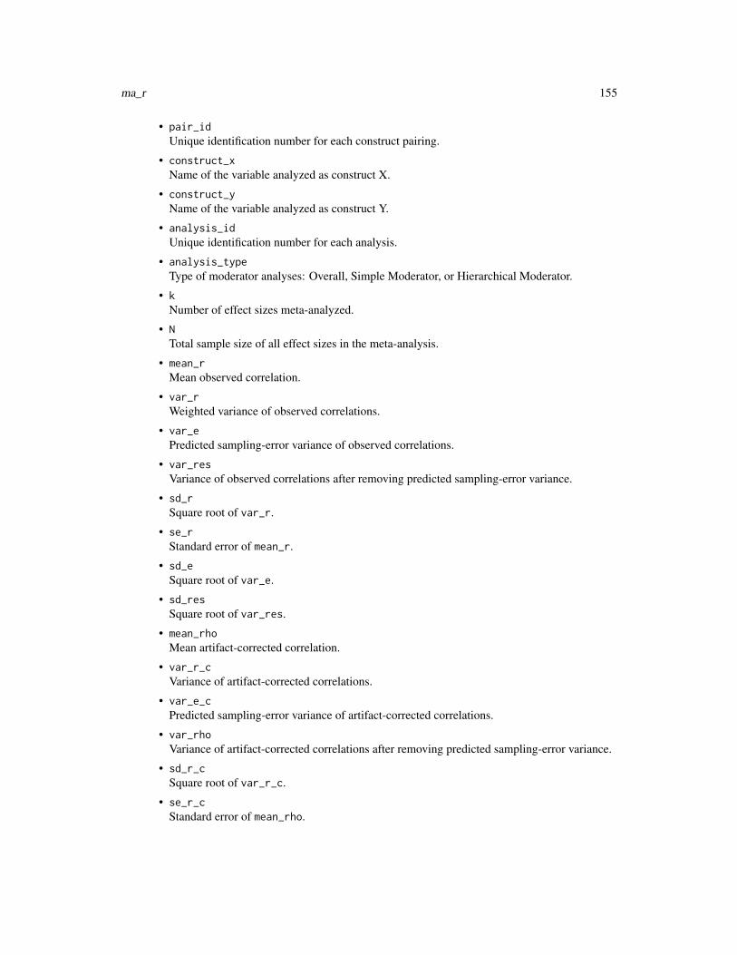
ma_r 155











• var_resVariance of observed correlations after removing predicted sampling-error variance.





• mean_rhoMean artifact-corrected correlation.

• var_r_cVariance of artifact-corrected correlations.

• var_e_cPredicted sampling-error variance of artifact-corrected correlations.

• var_rhoVariance of artifact-corrected correlations after removing predicted sampling-error variance.

• sd_r_cSquare root of var_r_c.

• se_r_cStandard error of mean_rho.

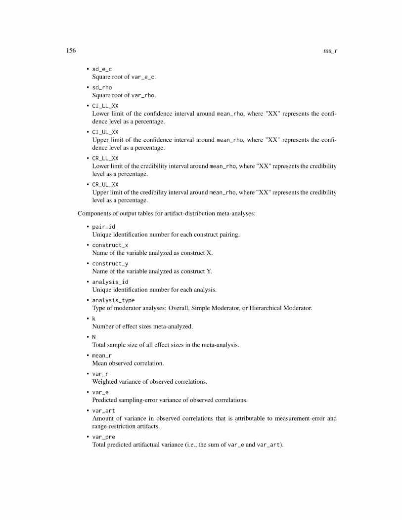
156 ma_r

• sd_e_cSquare root of var_e_c.

• sd_rhoSquare root of var_rho.

• CI_LL_XXLower limit of the confidence interval around mean_rho, where "XX" represents the confi-dence level as a percentage.

• CI_UL_XXUpper limit of the confidence interval around mean_rho, where "XX" represents the confi-dence level as a percentage.

• CR_LL_XXLower limit of the credibility interval around mean_rho, where "XX" represents the credibilitylevel as a percentage.

• CR_UL_XXUpper limit of the credibility interval around mean_rho, where "XX" represents the credibilitylevel as a percentage.

Components of output tables for artifact-distribution meta-analyses:











• var_artAmount of variance in observed correlations that is attributable to measurement-error andrange-restriction artifacts.

• var_preTotal predicted artifactual variance (i.e., the sum of var_e and var_art).

ma_r 157

• var_resVariance of observed correlations after removing predicted sampling-error variance and pre-dicted artifact variance.




• sd_artSquare root of var_art.

• sd_preSquare root of var_pre.


• mean_rhoMean artifact-corrected correlation.

• var_r_cWeighted variance of observed correlations corrected to the metric of rho.

• var_e_cPredicted sampling-error variance of observed correlations corrected to the metric of rho.

• var_art_cAmount of variance in observed correlations that is attributable to measurement-error andrange-restriction artifacts corrected to the metric of rho.

• var_pre_cTotal predicted artifactual variance (i.e., the sum of var_e and var_art) corrected to themetric of rho.

• var_rhoVariance of artifact-corrected correlations after removing predicted sampling-error varianceand predicted artifact variance.

• sd_r_cSquare root of var_r corrected to the metric of rho.

• se_r_cStandard error of mean_r corrected to the metric of rho.

• sd_e_cSquare root of var_e corrected to the metric of rho.

• sd_art_cSquare root of var_art corrected to the metric of rho.

• sd_pre_cSquare root of var_pre corrected to the metric of rho.

• sd_rhoSquare root of var_rho.

158 ma_r

• CI_LL_XXLower limit of the confidence interval around mean_rho, where "XX" represents the confi-dence level as a percentage.

• CI_UL_XXUpper limit of the confidence interval around mean_rho, where "XX" represents the confi-dence level as a percentage.

• CR_LL_XXLower limit of the credibility interval around mean_rho, where "XX" represents the credibilitylevel as a percentage.

• CR_UL_XXUpper limit of the credibility interval around mean_rho, where "XX" represents the credibilitylevel as a percentage.

Note

The difference between "rb" methods with the "orig" and "adj" suffixes is that the original does notaccount for the impact of range restriction on criterion reliabilities, whereas the adjusted procedureattempts to estimate the applicant reliability information for the criterion. The "rb" procedures areincluded for posterity: We strongly recommend using the "uvdrr" procedure to appropriately correctfor univariate range restriction.

References

Schmidt, F. L., & Hunter, J. E. (2015). Methods of meta-analysis: Correcting error and bias inresearch findings (3rd ed.). Thousand Oaks, CA: Sage. https://doi.org/10/b6mg. Chapter 4.

Law, K. S., Schmidt, F. L., & Hunter, J. E. (1994). Nonlinearity of range corrections in meta-analysis: Test of an improved procedure. Journal of Applied Psychology, 79(3), 425–438. https://doi.org/10.1037/0021-9010.79.3.425



Examples

## Not run:## The 'ma_r' function can compute multi-construct bare-bones meta-analyses:ma_obj <- ma_r(rxyi = rxyi, n = n, rxx = rxxi, ryy = ryyi,

construct_x = x_name, construct_y = y_name, sample_id = sample_id,moderators = moderator, data = data_r_meas_multi)

summary(ma_obj)

## It can also perform multiple individual-correction meta-analyses:ma_obj <- ma_r(ma_method = "ic", rxyi = rxyi, n = n, rxx = rxxi, ryy = ryyi,



https://doi.org/10.1037/0021-9010.79.3.425

https://doi.org/10.1037/0021-9010.79.3.425

https://doi.org/10.1037/0021-9010.68.3.382

https://doi.org/10.1037/0021-9010.68.3.382

ma_r 159

summary(ma_obj)ma_obj$meta_tables[[1]]$individual_correction$true_score

## And 'ma_r' can also curate artifact distributions and compute multiple## artifact-distribution meta-analyses:ma_obj <- ma_r(ma_method = "ad", ad_type = "int", rxyi = rxyi, n = n, rxx = rxxi, ryy = ryyi,

correct_rr_x = FALSE, correct_rr_y = FALSE,construct_x = x_name, construct_y = y_name, sample_id = sample_id,clean_artifacts = FALSE, impute_artifacts = FALSE,moderators = moderator, data = data_r_meas_multi)

summary(ma_obj)ma_obj$meta_tables[[1]]$artifact_distribution$true_score

## Even if no studies in the database provide artifact information,## pre-specified artifact distributions from previous meta-analyses## can still be used! (These results should match the previous example.)ma_obj <- ma_r(ma_method = "ad", rxyi = rxyi, n = n,

correct_rr_x = FALSE, correct_rr_y = FALSE,construct_x = x_name, construct_y = y_name, sample_id = sample_id,clean_artifacts = FALSE, impute_artifacts = FALSE,moderators = moderator, data = data_r_meas_multi,supplemental_ads =

list(X = list(mean_qxi = 0.8927818, var_qxi = 0.0008095520, k_qxi = 40,mean_n_qxi = 11927 / 40, qxi_dist_type = "alpha"),

Y = list(mean_qxi = 0.8941266, var_qxi = 0.0009367234, k_qxi = 40,mean_n_qxi = 11927 / 40, qxi_dist_type = "alpha"),

Z = list(mean_qxi = 0.8962108, var_qxi = 0.0007840593, k_qxi = 40,mean_n_qxi = 11927 / 40, qxi_dist_type = "alpha")))


## Artifact information may also be supplied by passing "ad_obj" class objects with the## "supplemental_ads" argument.## Create a list of artifact-distribution objects:ad_list <- create_ad_list(n = n, rxx = rxxi, ryy = ryyi,

construct_x = x_name, construct_y = y_name,sample_id = sample_id,data = data_r_meas_multi)

ad_list <- setNames(ad_list$ad_x, ad_list$construct_x)

## Run the artifact-distribution meta-analysis:ma_obj <- ma_r(ma_method = "ad", rxyi = rxyi, n = n,

correct_rr_x = FALSE, correct_rr_y = FALSE,construct_x = x_name, construct_y = y_name, sample_id = sample_id,clean_artifacts = FALSE, impute_artifacts = FALSE,moderators = moderator, data = data_r_meas_multi,supplemental_ads = ad_list)


## Artifact information from studies not included in the meta-analysis can also be used to make## corrections. Passing artifact information with the 'supplemental_ads' argument allows for

160 ma_r

## additional artifact values and/or means and variances of artifacts to be used.## The 'supplemental_ads' analysis below gives the same results as the prior meta-analysis.x_ids <- c(data_r_meas_multi$x_name, data_r_meas_multi$y_name) == "X"rxxi <- c(data_r_meas_multi$rxxi, data_r_meas_multi$ryyi)[x_ids]n_rxxi = c(data_r_meas_multi$n, data_r_meas_multi$n)[x_ids]

y_ids <- c(data_r_meas_multi$x_name, data_r_meas_multi$y_name) == "Y"ryyi <- c(data_r_meas_multi$rxxi, data_r_meas_multi$ryyi)[y_ids]n_ryyi = c(data_r_meas_multi$n, data_r_meas_multi$n)[y_ids]

z_ids <- c(data_r_meas_multi$x_name, data_r_meas_multi$y_name) == "Z"rzzi <- c(data_r_meas_multi$rxxi, data_r_meas_multi$ryyi)[z_ids]n_rzzi = c(data_r_meas_multi$n, data_r_meas_multi$n)[z_ids]

ma_obj <- ma_r(ma_method = "ad", rxyi = rxyi, n = n,correct_rr_x = FALSE, correct_rr_y = FALSE,construct_x = x_name, construct_y = y_name,moderators = moderator, sample_id = sample_id, data = data_r_meas_multi,

supplemental_ads = list(X = list(rxxi = rxxi, n_rxxi = n_rxxi, wt_rxxi = n_rxxi),Y = list(rxxi = ryyi, n_rxxi = n_ryyi, wt_rxxi = n_ryyi),Z = list(rxxi = rzzi, n_rxxi = n_rzzi, wt_rxxi = n_rzzi)))


## If 'use_all_arts' is set to TRUE, artifacts from studies without valid correlations## will be used to inform artifact distributions. Below, correlations and artifacts## are provided by non-overlapping sets of studies.dat1 <- dat2 <- data_r_meas_multidat1$rxxi <- dat1$ryyi <- NAdat2$rxyi <- NAdat2$sample_id <- dat2$sample_id + 40dat <- rbind(dat1, dat2)ma_obj <- ma_r(ma_method = "ad", rxyi = rxyi, n = n, rxx = rxxi, ryy = ryyi,

correct_rr_x = FALSE, correct_rr_y = FALSE,construct_x = x_name, construct_y = y_name,sample_id = sample_id, moderators = moderator,use_all_arts = TRUE, data = dat)


### Demonstration of ma_r_bb ##### Example analysis using data from Gonzalez-Mule et al. (2014):

## Not correcting for bias and using normal distributions to compute uncertainty intervals## allows for exact replication of the results reported in the text:ma_r_bb(r = rxyi, n = n, correct_bias = FALSE, conf_method = "norm", cred_method = "norm",

data = data_r_gonzalezmule_2014)

## Using hs_override = TRUE allows one to easily implement the traditional Hunter-Schmidt method:ma_r_bb(r = rxyi, n = n, hs_override = TRUE, data = data_r_gonzalezmule_2014)

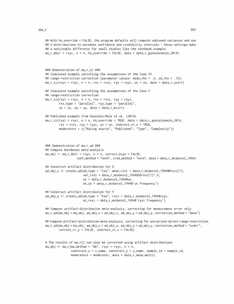
ma_r 161

## With hs_override = FALSE, the program defaults will compute unbiased variances and use## t-distributions to estimate confidence and credibility intervals - these settings make## a noticeable difference for small studies like the textbook example:ma_r_bb(r = rxyi, n = n, hs_override = FALSE, data = data_r_gonzalezmule_2014)

### Demonstration of ma_r_ic ##### Simulated example satisfying the assumptions of the Case IV## range-restriction correction (parameter values: mean_rho = .3, sd_rho = .15):ma_r_ic(rxyi = rxyi, n = n, rxx = rxxi, ryy = ryyi, ux = ux, data = data_r_uvirr)

## Simulated example satisfying the assumptions of the Case V## range-restriction correctionma_r_ic(rxyi = rxyi, n = n, rxx = rxxi, ryy = ryyi,

rxx_type = "parallel", ryy_type = "parallel",ux = ux, uy = uy, data = data_r_bvirr)

## Published example from Gonzalez-Mule et al. (2014)ma_r_ic(rxyi = rxyi, n = n, hs_override = TRUE, data = data_r_gonzalezmule_2014,

rxx = rxxi, ryy = ryyi, ux = ux, indirect_rr_x = TRUE,moderators = c("Rating source", "Published", "Type", "Complexity"))

### Demonstration of ma_r_ad ##### Compute barebones meta-analysisma_obj <- ma_r_bb(r = rxyi, n = n, correct_bias = FALSE,

conf_method = "norm", cred_method = "norm", data = data_r_mcdaniel_1994)

## Construct artifact distribution for Xad_obj_x <- create_ad(ad_type = "tsa", mean_rxxi = data_r_mcdaniel_1994$Mrxxi[1],

var_rxxi = data_r_mcdaniel_1994$SDrxxi[1]^.5,ux = data_r_mcdaniel_1994$ux,wt_ux = data_r_mcdaniel_1994$`ux frequency`)

## Construct artifact distribution for Yad_obj_y <- create_ad(ad_type = "tsa", rxxi = data_r_mcdaniel_1994$ryyi,

wt_rxxi = data_r_mcdaniel_1994$`ryyi frequency`)

## Compute artifact-distribution meta-analysis, correcting for measurement error onlyma_r_ad(ma_obj = ma_obj, ad_obj_x = ad_obj_x, ad_obj_y = ad_obj_y, correction_method = "meas")

## Compute artifact-distribution meta-analysis, correcting for univariate direct range restrictionma_r_ad(ma_obj = ma_obj, ad_obj_x = ad_obj_x, ad_obj_y = ad_obj_y, correction_method = "uvdrr",

correct_rr_y = FALSE, indirect_rr_x = FALSE)

# The results of ma_r() can also be corrected using artifact distributionsma_obj <- ma_r(ma_method = "bb", rxyi = rxyi, n = n,


162 ma_r

# The create_ad_list function can be used to generate batches of artifact-distribution objects.# Here is an example in which one distribution is created per construct.ad_tibble <- create_ad_list(n = n, rxx = rxxi, ryy = ryyi,

construct_x = x_name, construct_y = y_name,sample_id = sample_id,data = data_r_meas_multi)

# Passing that collection of distributions to ma_r_ad() corrects 'ma_obj' for artifacts:ma_obj_tibble <- ma_r_ad(ma_obj = ma_obj,

ad_obj_x = ad_tibble, ad_obj_y = ad_tibble)summary(ma_obj_tibble)ma_obj_tibble$meta_tables[[1]]$artifact_distribution$true_score

# The same outcomes as the previous example can be achieved by passing a named list of# artifact information, with each element bearing the name of a construct:ad_list <- setNames(ad_tibble$ad_x, ad_tibble$construct_x)ma_obj_list <- ma_r_ad(ma_obj = ma_obj,

ad_obj_x = ad_list, ad_obj_y = ad_list)summary(ma_obj_list)ma_obj_list$meta_tables[[1]]$artifact_distribution$true_score

# It is also possible to construct artifact distributions in a pairwise fashion.# For example, if correlations between X and Y and between X and Z are being analyzed,# X will get a different distribution for its relationships with Y than with Z.# These pairwise distributions are based only on artifact data from specific construct pairs.ad_tibble_pair <- create_ad_list(n = n, rxx = rxxi, ryy = ryyi,

construct_x = x_name, construct_y = y_name,sample_id = sample_id,control = control_psychmeta(pairwise_ads = TRUE),data = data_r_meas_multi)

# Passing these pairwise distributions to ma_r_ad() corrects 'ma_obj' for artifacts:ma_obj_pair <- ma_r_ad(ma_obj = ma_obj,

ad_obj_x = ad_tibble_pair, ad_obj_y = ad_tibble_pair)summary(ma_obj_pair)ma_obj_pair$meta_tables[[1]]$artifact_distribution$true_score

# Sometimes moderators have important influcnces on artifact distributions as well as# distributions of effect sizes. When this occurs, moderated artifact distributions# can be created to make more appropriate corrections.ad_tibble_mod <- create_ad_list(n = n, rxx = rxxi, ryy = ryyi,

construct_x = x_name, construct_y = y_name,sample_id = sample_id,control = control_psychmeta(moderated_ads = TRUE),moderators = moderator,data = data_r_meas_multi)

# Passing these moderated distributions to ma_r_ad() corrects 'ma_obj' for artifacts:ma_obj_mod <- ma_r_ad(ma_obj = ma_obj,

ad_obj_x = ad_tibble_mod, ad_obj_y = ad_tibble_mod)summary(ma_obj_mod)ma_obj_mod$meta_tables[[1]]$artifact_distribution$true_score

ma_r_order2 163

# It is also possible to create pairwise moderated artifact distributions.ad_tibble_pairmod <- create_ad_list(n = n, rxx = rxxi, ryy = ryyi,

construct_x = x_name, construct_y = y_name,sample_id = sample_id,control = control_psychmeta(moderated_ads = TRUE,

pairwise_ads = TRUE),moderators = moderator,data = data_r_meas_multi)

# Passing these pairwise moderated distributions to ma_r_ad() corrects 'ma_obj' for artifacts:ma_obj_pairmod <- ma_r_ad(ma_obj = ma_obj,

ad_obj_x = ad_tibble_pairmod, ad_obj_y = ad_tibble_pairmod)summary(ma_obj_pairmod)ma_obj_pairmod$meta_tables[[1]]$artifact_distribution$true_score

# For even more control over which artifact distributions are used in corrections, you can supply# un-named list of distributions in which the order of distributions corresponds to the order of# meta-analyses in ma_obj. It is important for the elements to be un-named, as the absence of names# and the length of the list are the two ways in which ma_r_ad() validates the lists.ad_list_pairmod_x <- ad_tibble_pairmod$ad_xad_list_pairmod_y <- ad_tibble_pairmod$ad_y# Passing these lists of distributions to ma_r_ad() corrects 'ma_obj' for artifacts:ma_obj_pairmodlist <- ma_r_ad(ma_obj = ma_obj,

ad_obj_x = ad_list_pairmod_x, ad_obj_y = ad_list_pairmod_y)summary(ma_obj_pairmodlist)ma_obj_pairmodlist$meta_tables[[1]]$artifact_distribution$true_score

## End(Not run)

ma_r_order2 Second-order meta-analysis function for correlations

Description

This function computes second-order meta-analysis function for correlations. It supports second-order analyses of bare-bones, artifact-distribution, and individual-correction meta-analyses.

Usage

ma_r_order2(k,N = NULL,r = NULL,rho = NULL,var_r = NULL,var_r_c = NULL,ma_type = c("bb", "ic", "ad"),sample_id = NULL,

164 ma_r_order2

citekey = NULL,moderators = NULL,moderator_type = "simple",construct_x = NULL,construct_y = NULL,construct_order = NULL,data = NULL,control = control_psychmeta(),...

)

Arguments

k Vector or column name of meta-analyses’ k values.

N Vector or column name of meta-analyses’ total sample sizes (optional).

r Vector or column name of mean observed correlations.

rho Vector or column name of mean corrected correlations.

var_r Vector or column name of observed variances of observed correlations.

var_r_c Vector or column name of observed variances of corrected correlations.

ma_type Type of meta-analyses being analyzed: "bb" (barebones), "ic" (individual cor-rection), or "ad" (artifact distribution).

sample_id Vector or column name of study ID labels.




construct_x Vector or column name of construct names for X.

construct_y Vector or column name of construct names for Y.construct_order





Value


merge_simdat_d 165

Examples

## Analysis of the validity of conscientiousness as a predictor of job performance in East Asiaout <- ma_r_order2(k = k, r = r_bar_i, rho = rho_bar_i, var_r = var_r,

var_r_c = NULL, ma_type = c("bb", "ad"),sample_id = NULL, moderators = NULL,construct_x = NULL, construct_y = NULL,

data = dplyr::filter(data_r_oh_2009, Predictor == "Conscientiousness"))summary(out)

## Analysis of the validity of the Big Five traits as predictors of job performance in East Asiaout <- ma_r_order2(k = k, r = r_bar_i, rho = rho_bar_i, var_r = var_r,

var_r_c = NULL, ma_type = c("bb", "ad"),sample_id = NULL, moderators = NULL, construct_x = Predictor,data = data_r_oh_2009)

summary(out)

## Analysis of the average validity of the Big Five traits as predictors of## job performance by Eastern Asian countryout <- ma_r_order2(k = k, r = r_bar_i, rho = rho_bar_i, var_r = var_r,

var_r_c = NULL, ma_type = c("bb", "ad"),sample_id = NULL, moderators = "Country", data = data_r_oh_2009)

summary(out)

merge_simdat_d Merge multiple "simdat_d_database" class objects

Description

This function allows for multiple simulated databases from simulate_d_database to be mergedtogether into a single database. Merged databases will be assigned moderator variable codes.

Usage

merge_simdat_d(...)

Arguments

... Collection of objects created by the "simulate_d_database" function. Simply en-ter the database objects as merge_simdat_d(data_obj1, data_obj2, data_obj_3).

Value

A merged database of class simdat_d

166 metabulate

merge_simdat_r Merge multiple "simdat_r_database" class objects

Description

This function allows for multiple simulated databases from simulate_r_database to be mergedtogether into a single database. Merged databases will be assigned moderator variable codes.

Usage

merge_simdat_r(...)

Arguments

... Collection of objects created by the "simulate_r_database" function. Simply en-ter the database objects as merge_simdat_r(data_obj1, data_obj2, data_obj_3).

Value

A merged database of class simdat_r_database

metabulate Write a summary table of meta-analytic results

Description

Write a summary table of meta-analytic results

Usage

metabulate(ma_obj,file = NULL,output_dir = getwd(),output_format = c("word", "html", "pdf", "odt", "text", "rmd"),show_msd = TRUE,show_conf = TRUE,show_cred = TRUE,show_se = FALSE,show_var = FALSE,analyses = "all",match = c("all", "any"),case_sensitive = TRUE,ma_method = "ad",correction_type = "ts",collapse_construct_labels = TRUE,

metabulate 167

bold_headers = TRUE,digits = 2L,decimal.mark = getOption("OutDec"),leading0 = "conditional",drop0integer = FALSE,neg.sign = "−",pos.sign = "figure_html",big.mark = " ",big.interval = 3L,small.mark = " ",small.interval = 3L,na.mark = "—",lgl.mark = c("+", "−"),inf.mark = c("+∞", "−∞"),conf_format = "brackets",cred_format = "brackets",symbol_es = "ES",caption = "Results of meta-analyses",header = NULL,verbose = FALSE,unicode = NULL,bib = NULL,title.bib = NULL,style = "apa",additional_citekeys = NULL,save_build_files = FALSE,...

)

Arguments


file The filename (optionally with a subfolder path) for the output file. If NULL, thefunction will output directly to the R console (also useful if you want to includepsychmeta results in a larger RMarkdown document).

output_dir The filepath for the output directory/folder. Defaults to the current workingdirectory.

output_format The format of the output tables. Available options are Word (default), HTML,PDF (requires LaTeX and the unicode-math LaTeX package to be installed),ODT, rmd (Rmarkdown), and text (plain text). You can also specify the fullname of another RMarkdown output_format.

show_msd Logical. Should means and standard deviations of effect sizes be shown (defaultTRUE)

show_conf Logical. Should confidence intervals be shown (default: TRUE)?

show_cred Logical. Should credibility intervals be shown (default: TRUE)?

show_se Logical Should standard errors be shown (default: FALSE)?

168 metabulate

show_var Logical. Should variances be shown (default: FALSE)?

analyses Which analyses to extract references for? See filter_ma for details.

match Match all or any of the filter criteria? See filter_ma for details.


ma_method Meta-analytic methods to be included. Valid options are: "ad", "ic", and "bb".Multiple methods are permitted. By default, results are given for one methodwith order of priority: 1. "ad", 2. "ic", 3. "bb".

correction_type

Type of meta-analytic corrections to be incldued. Valid options are: "ts" (de-fault), "vgx", and "vgy". Multiple options are permitted.

collapse_construct_labels

Should the construct labels for construct pairs with multiple rows of results besimplified so that only the first occurence of each set of construct names is shown(TRUE; default) or should construct labels be shown for each row of the table(FALSE).

bold_headers Logical. Should column headers be bolded (default: TRUE)?

digits, decimal.mark, leading0, drop0integer, neg.sign, pos.sign, big.mark, big.interval, small.mark, small.interval, na.mark, lgl.mark, inf.mark

Number formatting arguments. See format_num for details.

conf_format How should confidence intervals be formatted? Options are:

• parentheses: Bounds are enclosed in parentheses and separated by a comma:(LO, UP).

• brackets: Bounds are enclosed in square brackets and separated by acomma: [LO, UP].

• columns: Bounds are shown in individual columns.

cred_format How should credility intervals be formatted? Options are the same as for conf_formatabove.

symbol_es For meta-analyses of generic (non-r, non-d) effect sizes, the symbol used for theeffect sizes (default: symbol_es = "ES").

caption Caption to print before tables. Either a character scalar or a named character vec-tor with names corresponding to combinations of ma_method and correction_type(i.e., bb, ic_ts, ad_vgx, etc.).

header A list of YAML header parameters to pass to link[rmarkdown]{render}.

verbose Logical. Should detailed SD and variance components be shown (default: FALSE)?

unicode Logical. If output_format is "text", should UTF-8 characters be used (defaultsto system default).

bib A BibTeX file containing the citekeys for the meta-analyses. If provided and fileis not NULL, a bibliography will be included with the meta-analysis table. Seegenerate_bib for additional arguments controlling the bibliography.

title.bib The title to give to the bibliography (see bib above). If NULL, defaults to "SourcesContributing to Meta-Analyses"

metabulate 169

style What style should the bibliography (see bib above) be formatted in? Can be afile path or URL for a CSL citation style or the style ID for any style availablefrom the Zotero Style Repository). Defaults to APA style. (Retrieving a style byID requires an internet connection. If unavailable, references will be renderedin Chicago style.).

additional_citekeys

Additional citekeys to include in the reference list (see bib above).save_build_files

Should the RMarkdown and BibLaTeX (if any) files used to generate the outputbe saved (default: FALSE)?

... Additional arguments to pass to render.

Value

A list of meta-analysis results tibbles with "caption" and "footnote" attributes.

If file is specified, formatted tables and bibliographies are exported in the requested output_format.

Formatted tables of meta-analytic output.

See Also

Other output functions: generate_bib(), metabulate_rmd_helper()

Examples

## Not run:## Create a results table for meta-analysis of correlations and output to Word:ma_r_obj <- ma_r(ma_method = "ic", rxyi = rxyi, n = n, rxx = rxxi, ryy = ryyi,

construct_x = x_name, construct_y = y_name,moderators = moderator, data = data_r_meas_multi)

metabulate(ma_obj = ma_r_obj, file = "meta tables correlations",output_format = "word", output_dir = tempdir())

## Output to PDF:metabulate(ma_obj = ma_r_obj, file = "meta tables correlations",

output_format = "pdf", output_dir = tempdir())

## Output to ODT (LibreOffice):metabulate(ma_obj = ma_r_obj, file = "meta tables correlations",

output_format = "odt", output_dir = tempdir())

## To produce Markdown tables to include inline in an RMarkdown report,## leave file == NULL and output_format to anything but "text":ma_table <- metabulate(ma_obj = ma_r_obj, file = NULL, output_format = "rmd")

## Use the metabulate_rmd_helper() function to ensure all symbols render properly.Insert the following code as 'as-is' output:metabulate_rmd_helper()

## Then, add the formatted table to your document using your preferred table

https://github.com/citation-style-language/styles


170 metabulate_rmd_helper

## formatting functions:

#### Using just the 'knitr' package, include the following as 'as-is' output:knitr::kable(ma_table[[1]], caption = attr(ma_table[[1]], "caption"))cat("\n", attr(ma_table[[1]], "footnote"))

#### Using 'knitr' plus the 'kableExtra' package:knitr::kable(ma_table[[1]], "latex", booktabs = TRUE,

caption = attr(ma_table[[1]], "caption")) %>%kableExtra::kable_styling(latex_options = c("striped", "hold_position")) %>%kableExtra::footnote(general = attr(ma_table[[1]], "footnote")

# !!! Note: On Windows, R currently can only handle Unicode characters if kables# are printed at top-level (e.g., not in an if() statement, in a for() loop,# or in lapply() or map() ). To correctly print Unicode metabulate tables, call# kable() as a top-level function (as above).

## Create output table for meta-analysis of d values:ma_d_obj <- ma_d(ma_method = "ic", d = d, n1 = n1, n2 = n2, ryy = ryyi,

construct_y = construct, data = data_d_meas_multi)ma_d_obj <- ma_d_ad(ma_obj = ma_d_obj, correct_rr_g = FALSE, correct_rr_y = FALSE)metabulate(ma_obj = ma_d_obj, file = "meta tables d values", output_dir = tempdir())

## Create output table for meta-analysis of generic effect sizes:dat <- data.frame(es = data_r_meas_multi$rxyi,

n = data_r_meas_multi$n,var_e = (1 - data_r_meas_multi$rxyi^2)^2 / (data_r_meas_multi$n - 1))

ma_obj <- ma_generic(es = es, n = n, var_e = var_e, data = dat)metabulate(ma_obj = ma_obj, file = "meta tables generic es", output_dir = tempdir())

## End(Not run)

metabulate_rmd_helper Add metabulate equation commands and LaTeX dependencies

Description

metabulate requires several lines of code to correctly render meta-analysis results table columnheadings and footnotes. If metabulate is used to render files directly, these are added to the internalRMarkdown document. If you use metabulate output in a larger RMarkdown document, use thisfunction to automatically add the necessary lines of code based on your chosen output format.

Usage

metabulate_rmd_helper(latex = TRUE, html = TRUE, word_proc = TRUE)

metabulate_rmd_helper 171

Arguments

latex Should required commands be included when converting to PDF, LaTeX, andrelated formats?

html Should required commands be included when converting to HTML and relatedformats?

word_proc Should required commands be included when converting to Word, ODT, andrelated formats?

Value

Requested commands are printed to the console.

PDF and LaTeX output

If latex is TRUE and you render to PDF, LaTeX, or other output formats requiring LaTeX (e.g.,beamer_presentation, see knitr::is_latex_output), a YAML metadata block with a header-includesargument calling the required unicode-math LaTeX package is printed.

An RMarkdown file can only include one header-includes metadata entry. If your documentalready has one, set latex to FALSE and manually add add the unicode-math package to yourLaTeX header instead.

(Note that header-includes is generally discouraged in favor of adding an include argumentto specific output formats, see http://rmarkdown.rstudio.com/pdf_document_format.html#includes.)

HTML output

If html is TRUE and you render to HTML (or related formats, see knitr::is_html_output, thefollowing LaTeX math commands are defined:

• symit

• symup

• symbfit

• symbfup

If you define your own LaTeX or MathJax macros for these commands, set html to FALSE.

Microsoft Office and LibreOffice output

If word_proc is TRUE and you render to Word or ODT (or related formats such as PowerPoint), thefollowing LaTeX math commands are defined:

• symit

• symup

• symbfit

• symbfup

If you define your own LaTeX, Office, or OpenDocument macros for these commands, set word_procto FALSE.

http://rmarkdown.rstudio.com/pdf_document_format.html#includes

http://rmarkdown.rstudio.com/pdf_document_format.html#includes

172 metareg

See Also

Other output functions: generate_bib(), metabulate()

Examples

## Include this line as 'asis' output in your RMarkdown document:metabulate_rmd_helper()

## If you've already included \usepackage{unicode-math} in your RMarkdown header## for PDF (and related formats) header, set latex to FALSE:metabulate_rmd_helper(latex = FALSE)

metareg Compute meta-regressions

Description

This function is a wrapper for metafor’s rma function that computes meta-regressions for all bare-bones and individual-correction meta-analyses within an object. It makes use of both categoricaland continuous moderator information stored in the meta-analysis object and allows for interactioneffects to be included in the regression model. Output from this function will be added to the meta-analysis object in a list called follow_up_analyses. If using this function with a multi-constructmeta-analysis object from ma_r or ma_d, note that the follow_up_analyses list is appended to themeta-analysis object belonging to a specific construct pair within the construct_pairs list.

Usage

metareg(ma_obj, formula_list = NULL, ...)

Arguments


formula_list Optional list of regression formulas to evaluate. NOTE: If there are spaces inyour moderator names, replace them with underscores (i.e., "_") so that the for-mula(s) will perform properly. The function will remove spaces in the data,you only have to account for this in formula_list when you supply your ownformula(s).


Value

ma_obj with meta-regression results added (see ma_obj$follow_up_analyses$metareg).

mix_dist 173

Examples

## Meta-analyze the data from Gonzalez-Mule et al. (2014)## Note: These are corrected data and we have confirmed with the author that## these results are accurate:ma_obj <- ma_r_ic(rxyi = rxyi, n = n, hs_override = TRUE, data = data_r_gonzalezmule_2014,

rxx = rxxi, ryy = ryyi, ux = ux, indirect_rr_x = TRUE,correct_rr_x = TRUE, moderators = Complexity)

## Pass the meta-analysis object to the meta-regression function:ma_obj <- metareg(ma_obj)

## Examine the meta-regression results for the bare-bones and corrected data:ma_obj$metareg[[1]]$barebones$`Main Effects`ma_obj$metareg[[1]]$individual_correction$true_score$`Main Effects`

## Meta-analyze simulated d-value datadat <- data_d_meas_multi## Simulate a random moderatorset.seed(100)dat$moderator <- sample(1:2, nrow(dat), replace = TRUE)ma_obj <- ma_d(ma_method = "ic", d = d, n1 = n1, n2 = n2, ryy = ryyi,

construct_y = construct, sample_id = sample_id,moderators = moderator, data = dat)

## Pass the meta-analysis object to the meta-regression function:ma_obj <- metareg(ma_obj)

## Examine the meta-regression results for the bare-bones and corrected data:ma_obj$metareg[[1]]$barebones$`Main Effects`ma_obj$metareg[[1]]$individual_correction$latentGroup_latentY$`Main Effects`

mix_dist Descriptive statistics for a mixture distribution

Description

Compute descriptive statistics for a mixture distribution. This function returns the grand mean, thepooled sample variance (mean square within), variance of sample means (mean square between),portions of the total variance that are within and between groups, and mixture (total sample) vari-ance of the mixture sample data.

Usage

mix_dist(mean_vec, var_vec, n_vec, unbiased = TRUE, na.rm = FALSE)

174 mix_dist

Arguments

mean_vec Vector of sample means.

var_vec Vector of sample variances.

n_vec Vector of sample sizes.

unbiased Logical scalar determining whether variance should be unbiased (TRUE; de-fault) or maximum-likelihood (FALSE).

na.rm Logical scalar determining whether to remove missing values prior to computingoutput (TRUE) or not (FALSE; default)

Details

The grand mean of a mixture distribution is computed as:

µ =Σki=1xiniΣki=1ni

where µ is the grand mean, xi represents the sample means, and ni represents the sample sizes.

Maximum-likelihood mixture variances are computed as:

varpooledML= MSWML =

Σki=1 (xi − µ)niΣki=1ni

varmeansML= MSBML =

Σki=1 (xi − µ)nik

varBGML=

Σki=1 (xi − µ)niΣki=1ni

varWGML=

Σki=1viniΣki=1ni

varmixML= varBGML

+ varWGML

where vi represents the sample variances.

Unbiased mixture variances are computed as:

varpooledUnbiased= MSWUnbiased =

Σki=1vi (ni − 1)(Σki=1ni

)− k

varmeansUnbiased= MSBUnbiased =

Σki=1 (xi − µ)nik − 1

varBGUnbiased=

Σki=1 (xi − µ)ni(Σki=1ni

)− 1

varWGUnbiased=

Σki=1vi (ni − 1)(Σki=1ni

)− 1

varmixUnbiased= varBGUnbiased

+ varWGUnbiased

mix_matrix 175

Value

The mean, pooled sample (within-sample) variance, variance of sample means (between-groups),and mixture (total sample) variance of the mixture sample data.

Examples

mix_dist(mean_vec = c(-.5, 0, .5), var_vec = c(.9, 1, 1.1), n_vec = c(100, 100, 100))

mix_matrix Estimate mixture covariance matrix from within-group covariance ma-trices

Description

Estimate mixture covariance matrix from within-group covariance matrices

Usage

mix_matrix(sigma_list,mu_mat,p_vec,N = Inf,group_names = NULL,var_names = NULL

)

Arguments

sigma_list List of covariance matrices.

mu_mat Matrix of mean parameters, with groups on the rows and variables on the columns.

p_vec Vector of proportion of cases in each group.

N Optional total sample size across all groups (used to compute unbiased covari-ance estimates).

group_names Optional vector of group names.

var_names Optional vector of variable names.

Value

List of mixture covariances and means.

176 mix_r_2group

Examples

out <- unmix_matrix(sigma_mat = reshape_vec2mat(.5, order = 2),mu_mat = rbind(c(0, 0), c(.5, 1)),p_vec = c(.3, .7), N = 100)

mix_matrix(sigma_list = out$cov_group_unbiased,mu_mat = out$means_raw[-3,],p_vec = out$p_group, N = out$N)

mix_r_2group Estimate the mixture correlation for two groups

Description

Estimate the mixture correlation for two groups

Usage

mix_r_2group(rxy, dx, dy, p = 0.5)

Arguments

rxy Average within-group correlation

dx Standardized mean difference between groups on X.

dy Standardized mean difference between groups on Y.

p Proportion of cases in one of the two groups.

Details

The average within-group correlation is estimated as:

ρxyWG= ρxyMix

√(d2xp(1− p) + 1)

(d2yp(1− p) + 1

)−√d2xd

2yp

2(1− p)2

where ρxyWGis the average within-group correlation, ρxyMix

is the overall mixture correlation, dxis the standardized mean difference between groups on X, dy is the standardized mean differencebetween groups on Y, and p is the proportion of cases in one of the two groups.

Value

A vector of two-group mixture correlations

Examples

mix_r_2group(rxy = .375, dx = 1, dy = 1, p = .5)

plot_forest 177

plot_forest Create forest plots

Description

Create forest plots

Usage

plot_forest(ma_obj,analyses = "all",match = c("all", "any"),case_sensitive = TRUE,show_filtered = FALSE,ma_facetname = "Summary",facet_levels = NULL,conf_level = 0.95,conf_method = "t",x_limits = NULL,x_breaks = NULL,x_lab = NULL,y_lab = "Reference"

)

Arguments


analyses Which analyses to extract? Can be either "all" to extract references for allmeta-analyses in the object (default) or a list containing arguments for [fil-ter_ma].



show_filtered Logical scalar that determines whether the meta-analysis object given in theoutput should be the modified input object (FALSE, default) or the filtered object(TRUE).

ma_facetname Label to use for meta-analysis results in the facet_grid() function from ggplot2.

facet_levels Order in which moderator levels should be displayed.



x_limits Span of the X values to be plotted.

178 plot_funnel

x_breaks Breaks for the X values to be plotted.

x_lab Label to use for the X axis.

y_lab Label to use for the Y axis.

Value

A list of forest plots.

Author(s)

Based on code by John Sakaluk

Examples

## Not run:ma_obj <- ma_r(ma_method = "ic", rxyi = rxyi, n = n, rxx = rxxi, ryy = ryyi,


plot_forest(ma_obj = ma_obj)plot_forest(ma_obj = ma_obj, analyses = list(pair_id = 2))plot_forest(ma_obj = ma_obj, analyses = list(pair_id = 1), show_filtered = TRUE)

## d valuesma_obj <- ma_d(ma_method = "ic", d = d, n1 = n1, n2 = n2, ryy = ryyi,

construct_y = construct, sample_id = sample_id,data = data_d_meas_multi)

plot_forest(ma_obj = ma_obj)plot_forest(ma_obj = ma_obj, analyses = list(pair_id = 2))plot_forest(ma_obj = ma_obj, analyses = list(pair_id = 1, analysis_id = 1), show_filtered = TRUE)

## End(Not run)

plot_funnel Create funnel plots

Description

This function creates funnel plots for meta-analyses (plots of effect size versus . Both traditionalfunnel plots and

Usage

plot_funnel(ma_obj,se_type = c("auto", "mean", "sample"),label_es = NULL,conf_level = c(0.95, 0.99),conf_linetype = c("dashed", "dotted"),

plot_funnel 179

conf_fill = NA,conf_alpha = 1,null_effect = NA,null_conf_level = c(0.9, 0.95, 0.99),null_conf_linetype = c("solid", "dashed", "dotted"),null_conf_fill = "black",null_conf_alpha = c(0.1, 0.2, 0.4),analyses = "all",match = c("all", "any"),case_sensitive = TRUE,show_filtered = FALSE

)

plot_cefp(ma_obj,se_type = "sample",label_es = NULL,conf_level = NA,conf_linetype = NA,conf_fill = NA,conf_alpha = 1,null_effect = NULL,null_conf_level = c(0.9, 0.95, 0.99),null_conf_linetype = c("solid", "dashed", "dotted"),null_conf_fill = "black",null_conf_alpha = c(0, 0.2, 0.4),analyses = "all",match = c("all", "any"),case_sensitive = TRUE,show_filtered = FALSE

)

Arguments


se_type Method to calculate standard errors (y-axis). Options are "auto" (default) to usethe same method as used to estimate the meta-analysis models, "mean" to cal-culate SEs using the mean effect size and indivdiual sample sizes, or ‘"sample"“to use the SE calculated using the sample effect sizes and sample sizes.

label_es Label for effect size (x-axis). Defaults to "Correlation (r)" for correlation meta-analyses, "Cohen’s d (Hedges’s g)" for d value meta-analyses, and "Effect size"for generic meta-analyses.

conf_level Confidence regions levels to be plotted (default: .95, .99).

conf_linetype Line types for confidence region boundaries. Length should be either 1 or equalto the length of conf_level.

conf_fill Colors for confidence regions. Set to NA for transparent. Length should be either1 or equal to to the length of conf_level.

180 plot_funnel

conf_alpha Transparency level for confidence regions. Length should be either 1 or equal toto the length of conf_level.

null_effect Null effect to be plotted for contour-enhanced funnel plots. If NA, not shown.If NULL, set to the null value for the effect size metric (0 for correlations and dvalues).

null_conf_level

Null-effect confidence regions levels to be plotted (default: .90, .95, .99).null_conf_linetype

Line types for null-effect confidence region boundaries. Length should be either1 or equal to the length of null_conf_level.

null_conf_fill Colors for null-effect confidence regions. Set to NA for transparent. Lengthshould be either 1 or equal to the length of null_conf_level.

null_conf_alpha

Transparency level for null-effect confidence regions. Length should be either 1or equal to the length of null_conf_level.

analyses Which analyses to extract? Can be either "all" to extract references for allmeta-analyses in the object (default) or a list containing arguments for filter_ma.



show_filtered Logical scalar that determines whether the meta-analysis object given in theoutput should be the modified input object (FALSE, default) or the filtered object(TRUE).

Value

A list of funnel plots.

Author(s)

Based on code by John Sakaluk

Examples

## Not run:## Correlationsma_obj <- ma_r(ma_method = "ic", rxyi = rxyi, n = n, rxx = rxxi, ryy = ryyi,


plot_funnel(ma_obj = ma_obj)plot_funnel(ma_obj = ma_obj, analyses = list(pair_id = 2))plot_funnel(ma_obj = ma_obj, analyses = list(pair_id = 1, analysis_id = 1), show_filtered = TRUE)

## d valuesma_obj <- ma_d(ma_method = "ic", d = d, n1 = n1, n2 = n2, ryy = ryyi,

construct_y = construct, sample_id = sample_id,data = data_d_meas_multi)

predict 181

plot_funnel(ma_obj = ma_obj)plot_funnel(ma_obj = ma_obj, analyses = list(pair_id = 2))plot_funnel(ma_obj = ma_obj, analyses = list(pair_id = 1, analysis_id = 1), show_filtered = TRUE)

## End(Not run)

predict Prediction method for objects of classes deriving from "lm_mat"

Description

Prediction method for objects of classes deriving from "lm_mat"

Arguments

object Object of class inheriting from "lm_mat"

newdata An optional data frame in which to look for variables with which to predict. Ifomitted, the fitted values are used.

se.fit A switch indicating if standard errors are required.

df Degrees of freedom for scale.

interval Type of interval calculation. Can be abbreviated.

level Tolerance/confidence level.

... further arguments passed to or from other methods.

Value

An set of predicted values

print Print methods for psychmeta

Description

Print methods for psychmeta output objects with classes exported from psychmeta.

Arguments

x Object to be printed (object is used to select a method).


digits Number of digits to which results should be rounded.]

n Number of rows to print for meta-analysis results tables. Defaults to all rows.See tibble::print.tbl() for details.

182 reattribute

width Width of text output to generate for meta-analysis results tables. See tibble::print.tbl()for details.

n_extra Number of extra columns to print abbreviated information for, if the width is toosmall for the entire tibble. See tibble::print.tbl() for details.

ma_methods Meta-analytic methods to be included. Valid options are: "bb", "ic", and "ad"correction_types


verbose Logical scalar that determines whether printed object should contain verboseinformation (e.g., non-standard columns of meta-analytic output; TRUE) or not(FALSE).

symbolic.cor For lm_mat output: logical. If TRUE, print the correlations in a symbolic form(see symnum) rather than as numbers.

signif.stars For lm_mat output: logical. If TRUE, ‘significance stars’ are printed for eachcoefficient.

psychmeta_news Retrieve the NEWS file for the psychmeta package

Description

This function gives a shortcut to the utils::news(package = "psychmeta") function and displayspsychmeta’s NEWS file, which contains version information, outlines additions and changes to thepackage, and describes other updates.

Usage

psychmeta_news()

Examples

psychmeta_news()

reattribute Copy class and attributes from the original version of an object to amodified version.

Description

Copy class and attributes from the original version of an object to a modified version.

Usage

reattribute(x, result)

reshape_mat2dat 183

Arguments

x The original object, which has a class/attributes to copy

result The modified object, which is / might be missing the class/attributes.

Value

result, now with class/attributes restored.

reshape_mat2dat Extract a long-format correlation database from a correlation matrixand its supporting vectors/matrices of variable information

Description

This function is designed to extract data from a correlation matrix that is in the format commonlypublished in journals, with leading columns of construct names and descriptive statistics being listedalong with correlation data.

Usage

reshape_mat2dat(var_names,cor_data,common_data = NULL,unique_data = NULL,diag_label = NULL,lower_tri = TRUE,data = NULL

)

Arguments

var_names Vector (or scalar column name to match with data) containing variable names.

cor_data Square matrix (or vector of column names to match with data) containing cor-relations among variables.

common_data Vector or matrix (or vector of column names to match with data) of data com-mon to both X and Y variables (e.g., sample size, study-wise moderators).

unique_data Vector or matrix (or vector of column names to match with data) of data uniqueto X and Y variables (e.g., mean, SD, reliability).

diag_label Optional name to attribute to values extracted from the diagonal of the matrix(if NULL, no values are extracted from the diagonal).

lower_tri Logical scalar that identifies whether the correlations are in the lower triangle(TRUE) or in the upper triangle FALSE of the matrix.

data Matrix, dataframe, or tibble containing study data (when present, column namesof data will be matched to column names provided as other arguments).

184 reshape_vec2mat

Value

Long-format dataframe of correlation data, variable names, and supporting information

Author(s)

Jack W. Kostal

Examples

## Create a hypothetical matrix of data from a small study:mat <- data.frame(var_names = c("X", "Y", "Z"),

n = c(100, 100, 100),mean = c(4, 5, 3),sd = c(2.4, 2.6, 2),rel = c(.8, .7, .85),reshape_vec2mat(cov = c(.3, .4, .5)))

## Arguments can be provided as quoted characters or as the unquoted names of data's columns:reshape_mat2dat(var_names = var_names,

cor_data = c("Var1", "Var2", "Var3"),common_data = "n",unique_data = c("mean", "sd", "rel"),data = mat)

## Arguments can also provided as raw vectors, matrices, dataframes, etc. without a data argument:reshape_mat2dat(var_names = mat[,1],

cor_data = mat[,6:8],common_data = mat[,2],unique_data = mat[,3:5])

## If data is not null, arguments can be a mix of matrix/dataframe/vector and column-name argumentsreshape_mat2dat(var_names = mat[,1],

cor_data = mat[,6:8],common_data = "n",unique_data = c("mean", "sd", "rel"),data = mat)

reshape_vec2mat Assemble a variance-covariance matrix

Description

The reshape_vec2mat function facilitates the creation of square correlation/covariance matricesfrom scalars or vectors of variances/covariances. It allows the user to supply a vector of covariancesthat make up the lower triangle of a matrix, determines the order of the matrix necessary to holdthose covariances, and constructs a matrix accordingly.

reshape_vec2mat 185

Usage

reshape_vec2mat(cov = NULL,var = NULL,order = NULL,var_names = NULL,by_row = FALSE,diag = FALSE

)

Arguments

cov Scalar or vector of covariance information to include the lower-triangle positionsof the matrix (default value is zero). If a vector, the elements must be providedin the order associated with concatenated column (by_row = FALSE; default)or row (by_row = TRUE) vectors of the lower triangle of the desired matrix. Ifvariances are included in these values, set the diag argument to TRUE.

var Scalar or vector of variance information to include the diagonal positions of thematrix (default value is 1).

order If cov and var are scalars, this argument determines the number of variables tocreate in the output matrix.


by_row Logical scalar indicating whether cov values should fill the lower triangle byrow (TRUE) or by column (FALSE; default).

diag Logical scalar indicating whether cov values include variances (FALSE by de-fault; if TRUE, the variance values supplied with the cov argument will supersedethe var argument).

Value

A variance-covariance matrix

Examples

## Specify the lower triangle covariances## Can provide names for the variablesreshape_vec2mat(cov = c(.3, .2, .4), var_names = c("x", "y", "z"))

## Specify scalar values to repeat for the covariances and variancesreshape_vec2mat(cov = .3, var = 2, order = 3)

## Give a vector of variances to create a diagonal matrixreshape_vec2mat(var = 1:5)

## Specify order only to create identity matrixreshape_vec2mat(order = 3)

## Specify order and scalar variance to create a scalar matrix

186 reshape_wide2long

reshape_vec2mat(var = 2, order = 3)

## A quick way to make a 2x2 matrix for bivariate correlationsreshape_vec2mat(cov = .2)

reshape_wide2long Reshape database from wide format to long format

Description

This function automates the process of converting a wide-format database (i.e., a database in whichintercorrelations between construct pairs define the columns, such that there are multiple columnsof correlations) to a long-format database (i.e., a database with just one column of correlations).The meta-analysis functions in psychmeta work best with long-format databases, so this functioncan be a helpful addition to one’s workflow when data are organized in a wide format.

Usage

reshape_wide2long(data,common_vars = NULL,es_design = NULL,n_design = NULL,other_design = NULL,es_name = "rxyi",missing_col_action = c("warn", "ignore", "stop")

)

Arguments

data Database of data for use in a meta-analysis in "wide" format.

common_vars String vector of column names relevant to all variables in data.

es_design p x p matrix containing the names of columns of intercorrelations among vari-ables in the lower triangle of the matrix.

n_design Scalar sample-size column name or a p x p matrix containing the names ofcolumns of sample sizes the lower triangle of the matrix.

other_design A matrix with variable names on the rows and names of long-format variables tocreate on the columns. Elements of this matrix must be column names of data.

es_name Name of the effect size represented in data.missing_col_action

Character scalar indicating how missing columns should be handled. Optionsare: "warn", "ignore", and "stop"

Value

A long-format database

sensitivity 187

Examples

n_params = c(mean = 150, sd = 20)rho_params <- list(c(.1, .3, .5),

c(mean = .3, sd = .05),rbind(value = c(.1, .3, .5), weight = c(1, 2, 1)))

rel_params = list(c(.7, .8, .9),c(mean = .8, sd = .05),rbind(value = c(.7, .8, .9), weight = c(1, 2, 1)))

sr_params = c(list(1, 1, c(.5, .7)))sr_composite_params = list(1, c(.5, .6, .7))wt_params = list(list(c(1, 2, 3),

c(mean = 2, sd = .25),rbind(value = c(1, 2, 3), weight = c(1, 2, 1))),

list(c(1, 2, 3),c(mean = 2, sd = .25),rbind(value = c(1, 2, 3), weight = c(1, 2, 1))))

## Simulate with wide formatdata <- simulate_r_database(k = 10, n_params = n_params, rho_params = rho_params,

rel_params = rel_params, sr_params = sr_params,sr_composite_params = sr_composite_params, wt_params = wt_params,

var_names = c("X", "Y", "Z"), format = "wide")$statistics

## Define values to abstract from the data objectcommon_vars <- "sample_id"es_design <- matrix(NA, 3, 3)var_names <- c("X", "Y", "Z")es_design[lower.tri(es_design)] <- c("rxyi_X_Y", "rxyi_X_Z", "rxyi_Y_Z")rownames(es_design) <- colnames(es_design) <- var_namesn_design <- "ni"other_design <- cbind(rxxi = paste0("parallel_rxxi_", var_names),

ux_local = paste0("ux_local_", var_names),ux_external = paste0("ux_external_", var_names))

rownames(other_design) <- var_names

## Reshape the data to "long" formatreshape_wide2long(data = data, common_vars = common_vars, es_design = es_design,

n_design = n_design, other_design = other_design)

sensitivity Sensitivity analyses for meta-analyses

Description

Wrapper function to compute bootstrap analyses, leave-one-out analyses, and cumulative meta-analyses. This function helps researchers to examine the stability/fragility of their meta-analyticresults with bootstrapping and leave-one-out analyses, as well as detect initial evidence of publica-tion bias with cumulative meta-analyses.

188 sensitivity

Usage

sensitivity(ma_obj,leave1out = TRUE,bootstrap = TRUE,cumulative = TRUE,sort_method = c("weight", "n", "inv_var"),boot_iter = 1000,boot_conf_level = 0.95,boot_ci_type = c("bca", "norm", "basic", "stud", "perc"),...

)

sensitivity_bootstrap(ma_obj,boot_iter = 1000,boot_conf_level = 0.95,boot_ci_type = c("bca", "norm", "basic", "stud", "perc"),...

)

sensitivity_cumulative(ma_obj, sort_method = c("weight", "n", "inv_var"), ...)

sensitivity_leave1out(ma_obj, ...)

Arguments


leave1out Logical scalar determining whether to compute leave-one-out analyses (TRUE)or not (FALSE).

bootstrap Logical scalar determining whether bootstrapping is to be performed (TRUE) ornot (FALSE).

cumulative Logical scalar determining whether a cumulative meta-analysis is to be com-puted (TRUE) or not (FALSE).

sort_method Method to sort samples in the cumulative meta-analysis. Options are "weight"to sort by weight (default), "n" to sort by sample size, and "inv_var" to sort byinverse variance.

boot_iter Number of bootstrap iterations to be computed.boot_conf_level

Width of confidence intervals to be constructed for all bootstrapped statistics.

boot_ci_type Type of bootstrapped confidence interval. Options are "bca", "norm", "basic","stud", and "perc" (these are "type" options from the boot::boot.ci function).Default is "bca". Note: If you have too few iterations, the "bca" method willnot work and you will need to either increase the iterations or choose a differentmethod.


sensitivity 189

Value

An updated meta-analysis object with sensitivity analyses added.

• When bootstrapping is performed, the bootstrap section of the follow_up_analyses sec-tion of the updated ma_obj returned by this function will contain both a matrix summarizingthe mean, variance, and confidence intervals of the bootstrapped samples and a table of meta-analytic results from all bootstrapped samples.

• When leave-one-out analyses are performed, the ma_obj will acquire a list of leave-one-outresults in its follow_up_analyses section that contains a table of all leave-one-out meta-analyses along with plots of the mean and residual variance of the effect sizes in the meta-analyses.

• When cumulative meta-analysis is performed, the ma_obj will acquire a list of cumulativemeta-analysis results in its follow_up_analyses section that contains a table of all meta-analyses computed along with plots of the mean and residual variance of the effect sizes in themeta-analyses, sorted by the order in which studies were added to the meta-analysis.

Examples

## Not run:## Run a meta-analysis using simulated correlation data:ma_obj <- ma_r_ic(rxyi = rxyi, n = n, rxx = rxxi, ryy = ryyi, ux = ux,

correct_rr_y = FALSE, data = data_r_uvirr)ma_obj <- ma_r_ad(ma_obj, correct_rr_y = FALSE)

## Pass the meta-analysis object to the sensitivity() function:ma_obj <- sensitivity(ma_obj = ma_obj, boot_iter = 10,

boot_ci_type = "norm", sort_method = "inv_var")

## Examine the tables and plots produced for the IC meta-analysis:ma_obj$bootstrap[[1]]$barebonesma_obj$bootstrap[[1]]$individual_correction$true_scorema_obj$leave1out[[1]]$individual_correction$true_scorema_obj$cumulative[[1]]$individual_correction$true_score

## Examine the tables and plots produced for the AD meta-analysis:ma_obj$bootstrap[[1]]$artifact_distribution$true_scorema_obj$leave1out[[1]]$artifact_distribution$true_scorema_obj$cumulative[[1]]$artifact_distribution$true_score

## Run a meta-analysis using simulated d-value data:ma_obj <- ma_d_ic(d = d, n1 = n1, n2 = n2, ryy = ryyi,

data = filter(data_d_meas_multi, construct == "Y"))ma_obj <- ma_d_ad(ma_obj)

## Pass the meta-analysis object to the sensitivity() function:ma_obj <- sensitivity(ma_obj = ma_obj, boot_iter = 10,

boot_ci_type = "norm", sort_method = "inv_var")

## Examine the tables and plots produced for the IC meta-analysis:ma_obj$bootstrap[[1]]$barebones

190 simulate_alpha

ma_obj$bootstrap[[1]]$individual_correction$latentGroup_latentYma_obj$leave1out[[1]]$individual_correction$latentGroup_latentYma_obj$cumulative[[1]]$individual_correction$latentGroup_latentY

## Examine the tables and plots produced for the AD meta-analysis:ma_obj$bootstrap[[1]]$artifact_distribution$latentGroup_latentYma_obj$leave1out[[1]]$artifact_distribution$latentGroup_latentYma_obj$cumulative[[1]]$artifact_distribution$latentGroup_latentY

## End(Not run)

simulate_alpha Generate a vector of simulated sample alpha coefficients

Description

This function generates inter-item covariance matrices from a population matrix and computes acoefficient alpha reliability estimate for each matrix.

Usage

simulate_alpha(item_mat = NULL,alpha = NULL,k_items = NULL,n_cases,k_samples,standarized = FALSE

)

Arguments

item_mat Item correlation/covariance matrix. If item_mat is not supplied, the user mustsupply both alpha and k_items. If item_mat is NULL, the program will assumethat all item intercorrelations are equal.

alpha Population alpha value. Must be supplied if item_mat is NULL.

k_items Number of items on the test to be simulated. Must be supplied if item_mat isNULL.

n_cases Number of cases to simulate in sampling distribution of alpha.

k_samples Number of samples to simulate.

standarized Should alpha be computed from correlation matrices (TRUE) or unstandardizedcovariance matrices (FALSE)?

Value

A vector of simulated sample alpha coefficients

simulate_d_database 191

Examples

## Define a hypothetical matrix:item_mat <- reshape_vec2mat(cov = .3, order = 12)

## Simulations of unstandardized alphasset.seed(100)simulate_alpha(item_mat = item_mat, n_cases = 50, k_samples = 10, standarized = FALSE)set.seed(100)simulate_alpha(alpha = mean(item_mat[lower.tri(item_mat)]) / mean(item_mat),k_items = ncol(item_mat), n_cases = 50, k_samples = 10, standarized = FALSE)

## Simulations of standardized alphasset.seed(100)simulate_alpha(item_mat = item_mat, n_cases = 50, k_samples = 10, standarized = TRUE)set.seed(100)simulate_alpha(alpha = mean(item_mat[lower.tri(item_mat)]) / mean(item_mat),k_items = ncol(item_mat), n_cases = 50, k_samples = 10, standarized = TRUE)

simulate_d_database Simulate d value databases of primary studies

Description

The simulate_d_database function generates databases of psychometric d value data from sample-size parameters, correlation parameters, mean parameters, standard deviation parameters, reliabilityparameters, and selection-ratio parameters. The output database can be provided in a long format.If composite variables are to be formed, parameters can also be defined for the weights used to formthe composites as well as the selection ratios applied to the composites. This function will returna database of statistics as well as a database of parameters - the parameter database contains theactual study parameters for each simulated sample (without sampleing error) to allow comparisonsbetween meta-analytic results computed from the statistics and the actual means and variances ofparameters. The merge_simdat_d function can be used to merge multiple simulated databases andthe sparsify_simdat_d function can be used to randomly delete artifact information (a procedurecommonly done in simulations of artifact-distribution methods).

Usage

simulate_d_database(k,n_params,rho_params,mu_params = NULL,sigma_params = 1,rel_params = 1,sr_params = 1,k_items_params = 1,wt_params = NULL,allow_neg_wt = FALSE,

192 simulate_d_database

sr_composite_params = NULL,group_names = NULL,var_names = NULL,composite_names = NULL,diffs_as_obs = FALSE,show_applicant = FALSE,keep_vars = NULL,decimals = 2,max_iter = 100,...

)

Arguments

k Number of studies to simulate.

n_params List of parameter distributions (or data-generation function; see details) for sub-group sample sizes.

rho_params List containing a list of parameter distributions (or data-generation functions;see details) for correlations for each simulated group. If simulating data from asingle fixed population matrix in each group, supply a list of those matrices forthis argument (if the diagonals contains non-unity values and ’sigma_params’argument is not specified, those values will be used as variances).

mu_params List containing a list of parameter distributions (or data-generation functions;see details) for means for each simulated group. If NULL, all means will be setto zero.

sigma_params List containing a list of parameter distributions (or data-generation functions;see details) for standard deviations for each simulated group. If NULL, all stan-dard deviations will be set to unity.

rel_params List containing a list of parameter distributions (or data-generation functions;see details) for reliabilities for each simulated group. If NULL, all reliabilitieswill be set to unity.

sr_params List of parameter distributions (or data-generation functions; see details) forselection ratios. If NULL, all selection ratios will be set to unity.

k_items_params List of parameter distributions (or data-generation functions; see details) for thenumber of test items comprising each of the variables to be simulated (all aresingle-item variables by default).

wt_params List of parameter distributions (or data-generation functions; see details) to cre-ate weights for use in forming composites. If multiple composites are formed,the list should be a list of lists, with the general format: list(comp1_params =list(...params...),comp2_params = list(...params...),etc.).

allow_neg_wt Logical scalar that determines whether negative weights should be allowed (TRUE)or not (FALSE).

sr_composite_params

Parameter distributions (or data-generation functions; see details) for compositeselection ratios.


simulate_d_database 193

var_names Optional vector of variable names for all non-composite variables.composite_names

Optional vector of names for composite variables.

diffs_as_obs Logical scalar that determines whether standard deviation parameters representstandard deviations of observed scores (TRUE) or of true scores (FALSE; default).

show_applicant Should applicant data be shown for sample statistics (TRUE) or suppressed (FALSE)?

keep_vars Optional vector of variable names to be extracted from the simulation and re-turned in the output object. All variables are returned by default. Use this argu-ment when only some variables are of interest and others are generated solely toserve as selection variables.

decimals Number of decimals to which statistical results (not parameters) should be rounded.Rounding to 2 decimal places best captures the precision of data available frompublished primary research.

max_iter Maximum number of iterations to allow in the parameter selection process be-fore terminating with convergence failure. Must be finite.


Details

Values supplied as any argument with the suffix "params" can take any of three forms (see Examplesfor a demonstration of usage):

• A vector of values from which study parameters should be sampled.

• A vector containing a mean with a variance or standard deviation. These values must be named"mean," "var," and "sd", respectively, for the program to recognize which value is which.

• A matrix containing a row of values (this row must be named "values") from which studyparameters should be sampled and a row of weights (this row must be labeled ’weights’)associated with the values to be sampled.

• A matrix containing a column of values (this column must be named "values") from whichstudy parameters should be sampled and a column of weights (this column must be labeled’weights’) associated with the values to be sampled.

• A function that is configured to generate data using only one argument that defines the numberof cases to generate, e.g., fun(n = 10).

Value

A database of simulated primary studies’ statistics and analytically determined parameter values.

Examples

## Define sample sizes, means, and other parameters for each of two groups:n_params <- list(c(mean = 200, sd = 20),

c(mean = 100, sd = 20))rho_params <- list(list(c(.3, .4, .5)),

list(c(.3, .4, .5)))mu_params <- list(list(c(mean = .5, sd = .5), c(-.5, 0, .5)),

list(c(mean = 0, sd = .5), c(-.2, 0, .2)))

194 simulate_d_sample

sigma_params <- list(list(1, 1),list(1, 1))

rel_params <- list(list(.8, .8),list(.8, .8))

sr_params <- list(1, .5)

simulate_d_database(k = 5, n_params = n_params, rho_params = rho_params,mu_params = mu_params, sigma_params = sigma_params,rel_params = rel_params, sr_params = sr_params,k_items = c(4, 4),group_names = NULL, var_names = c("y1", "y2"),show_applicant = TRUE, keep_vars = c("y1", "y2"), decimals = 2)

simulate_d_sample Simulate a sample of psychometric d value data with measurementerror, direct range restriction, and/or indirect range restriction

Description

This function generates a simulated psychometric sample consisting of any number of groups andcomputes the d values that result after introducing measurement error and/or range restriction.

Usage

simulate_d_sample(n_vec,rho_mat_list,mu_mat,sigma_mat = 1,rel_mat = 1,sr_vec = 1,k_items_vec = 1,wt_mat = NULL,sr_composites = NULL,group_names = NULL,var_names = NULL,composite_names = NULL,diffs_as_obs = FALSE

)

Arguments

n_vec Vector of sample sizes (or a vector of proportions, if parameters are to be esti-mated).

rho_mat_list List of true-score correlation matrices.


sigma_mat Matrix of standard-deviation parameters, with groups on the rows and variableson the columns.

simulate_matrix 195

rel_mat Matrix of reliability parameters, with groups on the rows and variables on thecolumns.

sr_vec Vector of selection ratios.

k_items_vec Number of test items comprising each of the variables to be simulated (all aresingle-item variables by default).

wt_mat Optional matrix of weights to use in forming a composite of the variables inrho_mat. Matrix should have as many rows (or vector elements) as there arevariables in rho_mat.

sr_composites Optional vector selection ratios for composite variables. If not NULL, sr_compositesmust have as many elements as there are columns in wt_mat.


var_names Optional vector of variable names.composite_names


diffs_as_obs Logical scalar that determines whether standard deviation parameters representstandard deviations of observed scores (TRUE) or of true scores (FALSE; default).

Value

A sample of simulated mean differences.

Examples

## Simulate statistics by providing integers as "n_vec":simulate_d_sample(n_vec = c(200, 100), rho_mat_list = list(reshape_vec2mat(.5),

reshape_vec2mat(.4)),mu_mat = rbind(c(1, .5), c(0, 0)), sigma_mat = rbind(c(1, 1), c(1, 1)),rel_mat = rbind(c(.8, .7), c(.7, .7)), sr_vec = c(1, .5),group_names = c("A", "B"))

## Simulate parameters by providing proportions as "n_vec":simulate_d_sample(n_vec = c(2/3, 1/3), rho_mat_list = list(reshape_vec2mat(.5),

reshape_vec2mat(.4)),mu_mat = rbind(c(1, .5), c(0, 0)), sigma_mat = rbind(c(1, 1), c(1, 1)),rel_mat = rbind(c(.8, .7), c(.7, .7)), sr_vec = c(1, .5),group_names = c("A", "B"))

simulate_matrix Generate a list of simulated sample matrices sampled from the Wishartdistribution

Description

This function generates simulated sample matrices based on a population matrix and a sample size.It uses the Wishart distribution (i.e., the multivariate χ2 distribution) to obtain data, rescales the datainto the input metric, and can be standardized into a correlation matrix by setting as_cor to TRUE.The function can produce a list of matrices for any number of samples.

196 simulate_psych

Usage

simulate_matrix(sigma, n, k = 1, as_cor = FALSE)

Arguments

sigma Population covariance matrix. May be standardized or unstandardized.n Sample size for simulated sample matrices.k Number of sample matrices to generate.as_cor Should the simulated matrices be standardized (TRUE) or unstandardized (FALSE)?

Value

A list of simulated sample matrices.

Examples

## Define a hypothetical matrix:sigma <- reshape_vec2mat(cov = .4, order = 5)

## Simualte a list of unstandardized covariance matrices:simulate_matrix(sigma = sigma, n = 50, k = 10, as_cor = FALSE)

## Simualte a list of correlation matrices:simulate_matrix(sigma = sigma, n = 50, k = 10, as_cor = TRUE)

simulate_psych Simulate Monte Carlo psychometric data (observed, true, and errorscores)

Description

Simulate Monte Carlo psychometric data (observed, true, and error scores)

Usage

simulate_psych(n,rho_mat,mu_vec = rep(0, ncol(rho_mat)),sigma_vec = rep(1, ncol(rho_mat)),rel_vec = rep(1, ncol(rho_mat)),sr_vec = rep(1, ncol(rho_mat)),k_items_vec = rep(1, ncol(rho_mat)),wt_mat = NULL,sr_composites = NULL,var_names = NULL,composite_names = NULL

)

simulate_psych 197

Arguments

n Number of cases to simulate before performing selection.

rho_mat Matrix of true-score correlations.

mu_vec Vector of means.

sigma_vec Vector of observed-score standard deviations.

rel_vec Vector of reliabilities corresponding to the variables in rho_mat.

sr_vec Vector of selection ratios corresponding to the variables in rho_mat. (set selec-tion ratios to 1 for variables that should not be used in selection).




var_names Vector of variable names corresponding to the variables in rho_mat.composite_names


Value

A list of observed-score, true-score, and error-score data frames. If selection is requested, the dataframes will include logical variables indicating whether each case would be selected on the basis ofobserved scores, true scores, or error scores.

Examples

## Generate data for a simple sample with two variables without selection:simulate_psych(n = 1000, rho_mat = matrix(c(1, .5, .5, 1), 2, 2), sigma_vec = c(1, 1),

rel_vec = c(.8, .8), var_names = c("Y", "X"))

## Generate data for a simple sample with two variables with selection:simulate_psych(n = 1000, rho_mat = matrix(c(1, .5, .5, 1), 2, 2), sigma_vec = c(1, 1),

rel_vec = c(.8, .8), sr_vec = c(1, .5), var_names = c("Y", "X"))

## Generate data for samples with five variables, of which subsets are used to form composites:rho_mat <- matrix(.5, 5, 5)diag(rho_mat) <- 1simulate_psych(n = 1000, rho_mat = rho_mat,

rel_vec = rep(.8, 5), sr_vec = c(1, 1, 1, 1, .5),wt_mat = cbind(c(0, 0, 0, .3, 1), c(1, .3, 0, 0, 0)), sr_composites = c(.7, .5))

## Generate data for similar scenario as above, but with scales consisting of 1-5 items:rho_mat <- matrix(.5, 5, 5)diag(rho_mat) <- 1simulate_psych(n = 1000, rho_mat = rho_mat,

rel_vec = rep(.8, 5), sr_vec = c(1, 1, 1, 1, .5),

198 simulate_r_database

k_items_vec = 1:5,wt_mat = cbind(c(0, 0, 0, .3, 1), c(1, .3, 0, 0, 0)), sr_composites = c(.7, .5))

simulate_r_database Simulate correlation databases of primary studies

Description

The simulate_r_database function generates databases of psychometric correlation data fromsample-size parameters, correlation parameters, reliability parameters, and selection-ratio parame-ters. The output database can be provided in either a long format or a wide format. If compositevariables are to be formed, parameters can also be defined for the weights used to form the com-posites as well as the selection ratios applied to the composites. This function will return a databaseof statistics as well as a database of parameters - the parameter database contains the actual studyparameters for each simulated sample (without sampleing error) to allow comparisons betweenmeta-analytic results computed from the statistics and the actual means and variances of param-eters. The merge_simdat_r function can be used to merge multiple simulated databases and thesparsify_simdat_r function can be used to randomly delete artifact information (a procedurecommonly done in simulations of artifact-distribution methods).

Usage

simulate_r_database(k,n_params,rho_params,mu_params = 0,sigma_params = 1,rel_params = 1,sr_params = 1,k_items_params = 1,wt_params = NULL,allow_neg_wt = FALSE,sr_composite_params = NULL,var_names = NULL,composite_names = NULL,n_as_ni = FALSE,show_applicant = FALSE,keep_vars = NULL,decimals = 2,format = "long",max_iter = 100,...

)

simulate_r_database 199

Arguments

k Number of studies to simulate.n_params Parameter distribution (or data-generation function; see details) for sample size.rho_params List of parameter distributions (or data-generation functions; see details) for

correlations. If simulating data from a single fixed population matrix, that matrixcan be supplied for this argument (if the diagonal contains non-unity values and’sigma_params’ is not specified, those values will be used as variances).

mu_params List of parameter distributions (or data-generation functions; see details) formeans.

sigma_params List of parameter distributions (or data-generation functions; see details) forstandard deviations.

rel_params List of parameter distributions (or data-generation functions; see details) forreliabilities.

sr_params List of parameter distributions (or data-generation functions; see details) forselection ratios.

k_items_params List of parameter distributions (or data-generation functions; see details) for thenumber of test items comprising each of the variables to be simulated (all aresingle-item variables by default).

wt_params List of parameter distributions (or data-generation functions; see details) to cre-ate weights for use in forming composites. If multiple composites are formed,the list should be a list of lists, with the general format: list(comp1_params =list(...params...),comp2_params = list(...params...),etc.).

allow_neg_wt Logical scalar that determines whether negative weights should be allowed (TRUE)or not (FALSE).

sr_composite_params

Parameter distributions (or data-generation functions; see details) for compositeselection ratios.

var_names Optional vector of variable names for all non-composite variables.composite_names

Optional vector of names for composite variables.n_as_ni Logical argument determining whether n specifies the incumbent sample size

(TRUE) or the applicant sample size (FALSE; default). This can only be TRUEwhen only one variable is involved in selection.

show_applicant Should applicant data be shown for sample statistics (TRUE) or suppressed (FALSE)?keep_vars Optional vector of variable names to be extracted from the simulation and re-

turned in the output object. All variables are returned by default. Use this argu-ment when only some variables are of interest and others are generated solely toserve as selection variables.

decimals Number of decimals to which statistical results (not parameters) should be rounded.Rounding to 2 decimal places best captures the precision of data available frompublished primary research.

format Database format: "long" or "wide."max_iter Maximum number of iterations to allow in the parameter selection process be-

fore terminating with convergence failure. Must be finite.... Additional arguments.

200 simulate_r_database

Details

Values supplied as any argument with the suffix "params" can take any of three forms (see Examplesfor a demonstration of usage):

• A vector of values from which study parameters should be sampled.• A vector containing a mean with a variance or standard deviation. These values must be named

"mean," "var," and "sd", respectively, for the program to recognize which value is which.• A matrix containing a row of values (this row must be named "values") from which study

parameters should be sampled and a row of weights (this row must be labeled ’weights’)associated with the values to be sampled.

• A matrix containing a column of values (this column must be named "values") from whichstudy parameters should be sampled and a column of weights (this column must be labeled’weights’) associated with the values to be sampled.

• A function that is configured to generate data using only one argument that defines the numberof cases to generate, e.g., fun(n = 10).

Value

A database of simulated primary studies’ statistics and analytically determined parameter values.

Examples

## Note the varying methods for defining parameters:n_params = function(n) rgamma(n, shape = 100)rho_params <- list(c(.1, .3, .5),

c(mean = .3, sd = .05),rbind(value = c(.1, .3, .5), weight = c(1, 2, 1)))

rel_params = list(c(.7, .8, .9),c(mean = .8, sd = .05),rbind(value = c(.7, .8, .9), weight = c(1, 2, 1)))

sr_params = c(list(1, 1, c(.5, .7)))sr_composite_params = list(1, c(.5, .6, .7))wt_params = list(list(c(1, 2, 3),

c(mean = 2, sd = .25),rbind(value = c(1, 2, 3), weight = c(1, 2, 1))),

list(c(1, 2, 3),c(mean = 2, sd = .25),cbind(value = c(1, 2, 3), weight = c(1, 2, 1))))

## Simulate with long formatsimulate_r_database(k = 10, n_params = n_params, rho_params = rho_params,

rel_params = rel_params, sr_params = sr_params,sr_composite_params = sr_composite_params, wt_params = wt_params,var_names = c("X", "Y", "Z"), format = "long")

## Simulate with wide formatsimulate_r_database(k = 10, n_params = n_params, rho_params = rho_params,

rel_params = rel_params, sr_params = sr_params,sr_composite_params = sr_composite_params, wt_params = wt_params,var_names = c("X", "Y", "Z"), format = "wide")

simulate_r_sample 201

simulate_r_sample Simulation of data with measurement error and range-restriction arti-facts

Description

This function simulates a psychometric sample and produces correlation matrices, artifact infor-mation, and other descriptive statistics that have been affected by measurement error and/or rangerestriction. It allows the formation of composite variables within the simulation and allows selec-tion to be performed on any or all variables, including composites. By setting the sample size ton = Inf, users can explore the effects of measurement error and/or range restriction on parameterswithout the influence of sampling error. To generate multiple samples and compile a database ofsimulated statistics, see the simulate_r_database function.

Usage

simulate_r_sample(n,rho_mat,rel_vec = rep(1, ncol(rho_mat)),mu_vec = rep(0, ncol(rho_mat)),sigma_vec = rep(1, ncol(rho_mat)),sr_vec = rep(1, ncol(rho_mat)),k_items_vec = rep(1, ncol(rho_mat)),wt_mat = NULL,sr_composites = NULL,var_names = NULL,composite_names = NULL,n_as_ni = FALSE,...

)

Arguments

n Number of cases to simulate before performing selection. If Inf, function willsimulate parameter values.

rho_mat Matrix of true-score correlations.

rel_vec Vector of reliabilities corresponding to the variables in rho_mat.

mu_vec Vector of means.

sigma_vec Vector of observed-score standard deviations.

sr_vec Vector of selection ratios corresponding to the variables in rho_mat (set selec-tion ratios to 1 for variables that should not be used in selection).


202 sparsify_simdat_d



var_names Vector of variable names corresponding to the variables in rho_mat.composite_names


n_as_ni Logical argument determining whether n specifies the incumbent sample size(TRUE) or the applicant sample size (FALSE; default). This can only be TRUEwhen only one variable is involved in selection.


Value

A list of study information, including correlations, reliabilities, standard deviations, means, and uratios for true scores and for observed scores.

Examples

## Generate data for a simple sample with two variables:simulate_r_sample(n = 1000, rho_mat = matrix(c(1, .5, .5, 1), 2, 2),

rel_vec = c(.8, .8), sr_vec = c(1, .5), var_names = c("Y", "X"))

## Generate data for samples with five variables, of which subsets are used to form composites:rho_mat <- matrix(.5, 5, 5)diag(rho_mat) <- 1

## Simulate parameters by supply n = Infsimulate_r_sample(n = Inf, rho_mat = rho_mat,


## Finite sample sizes allow the generation of sample datasimulate_r_sample(n = 1000, rho_mat = rho_mat,


sparsify_simdat_d Create sparse artifact information in a "simdat_d_database" class ob-ject

Description

This function can be used to randomly delete artifact from databases produced by the simulate_d_databasefunction. Deletion of artifacts can be performed in either a study-wise fashion for complete missing-ness within randomly selected studies or element-wise missingness for completely random deletionof artifacts in the database. Deletion can be applied to reliability estimates and/or u ratios.

sparsify_simdat_r 203

Usage

sparsify_simdat_d(data_obj,prop_missing,sparify_arts = c("rel", "u"),study_wise = TRUE

)

Arguments

data_obj Object created by the "simdat_d_database" function.

prop_missing Proportion of studies in from which artifact information should be deleted.

sparify_arts Vector of codes for the artifacts to be sparsified: "rel" for reliabilities, "u" for uratios, or c("rel", "u") for both.

study_wise Logical scalar argument determining whether artifact deletion should occur forall variables in a study (TRUE) or randomly across variables within studies (FALSE).

Value

A sparsified database

sparsify_simdat_r Create sparse artifact information in a "simdat_r_database" class ob-ject

Description

This function can be used to randomly delete artifact from databases produced by the simulate_r_databasefunction. Deletion of artifacts can be performed in either a study-wise fashion for complete missing-ness within randomly selected studies or element-wise missingness for completely random deletionof artifacts in the database. Deletion can be applied to reliability estimates and/or u ratios.

Usage

sparsify_simdat_r(data_obj,prop_missing,sparify_arts = c("rel", "u"),study_wise = TRUE

)

204 truncate_dist

Arguments

data_obj Object created by the "simdat_r_database" function.

prop_missing Proportion of studies in from which artifact information should be deleted.

sparify_arts Vector of codes for the artifacts to be sparsified: "rel" for reliabilities, "u" for uratios, or c("rel", "u") for both.

study_wise Logical scalar argument determining whether artifact deletion should occur forall variables in a study (TRUE) or randomly across variables within studies (FALSE).

Value

A sparsified database

summary Summary methods for psychmeta

Description

Summary methods for psychmeta output objects with classes exported from psychmeta.

Arguments

object Object to be printed (object is used to select a method).


Value

Summary object.

truncate_dist Truncation function for normal distributions (truncates both mean andvariance)

Description

This function computes the mean and variance of a normal distributions that has been truncated atone or both ends.

Usage

truncate_dist(a = -Inf, b = Inf, mean = 0, sd = 1)

truncate_mean 205

Arguments

a Quantile (i.e., cut score) below which scores should be censored from the distri-bution.

b Quantile (i.e., cut score) above which scores should be censored from the distri-bution.

mean Scalar mean or vector of means.sd Scalar standard deviation or vector of standard deviations.

Value

A matrix of truncated means (column 1) and truncated variances (column 2).

Examples

truncate_dist(a = -1, b = 3, mean = 0, sd = 1)truncate_dist(a = 1, b = Inf, mean = 0, sd = 1)truncate_dist(a = c(-1, 1), b = c(3, Inf), mean = 0, sd = 1)

truncate_mean Truncation function for means

Description

This function computes the mean of a normal distributions that has been truncated at one or bothends.

Usage

truncate_mean(a = -Inf, b = Inf, mean = 0, sd = 1)

Arguments



mean Scalar mean or vector of means.sd Scalar standard deviation or vector of standard deviations.

Value

A vector of truncated means.

Examples

truncate_mean(a = -1, b = 3, mean = 0, sd = 1)truncate_mean(a = 1, b = Inf, mean = 0, sd = 1)truncate_mean(a = c(-1, 1), b = c(3, Inf), mean = 0, sd = 1)

206 unmix_matrix

truncate_var Truncation function for variances

Description

This function computes the variance of a normal distributions that has been truncated at one or bothends.

Usage

truncate_var(a = -Inf, b = Inf, mean = 0, sd = 1)

Arguments



mean Scalar mean or vector of means.

sd Scalar standard deviation or vector of standard deviations.

Value

A vector of truncated variances

Examples

truncate_var(a = -1, b = 3, mean = 0, sd = 1)truncate_var(a = 1, b = Inf, mean = 0, sd = 1)truncate_var(a = c(-1, 1), b = c(3, Inf), mean = 0, sd = 1)

unmix_matrix Estimate average within-group covariance matrices from a mixture co-variance matrix

Description

Estimate average within-group covariance matrices from a mixture covariance matrix

unmix_matrix 207

Usage

unmix_matrix(sigma_mat,mu_mat,p_vec,N = Inf,group_names = NULL,var_names = NULL

)

Arguments

sigma_mat Mixture covariance matrix.


p_vec Vector of proportion of cases in each group.

N Optional total sample size across all groups (used to compute unbiased covari-ance estimates).



Value

List of within-group covariances and means.

Examples

out <- unmix_matrix(sigma_mat = reshape_vec2mat(.5, order = 2),mu_mat = rbind(c(0, 0), c(.5, 1)),p_vec = c(.3, .7), N = 100)

## Result of unmix_matrix:out

## Simulated data reproduce the total parameter matrix:dat <- NULLfor(i in 1:2){

dat <- rbind(dat, cbind(group = i,data.frame(MASS::mvrnorm(n = round(out$p_group[i] * out$N),

mu = out$means_raw[i,],Sigma = out$cov_group_unbiased[[i]],

empirical = TRUE))))}cov(dat[,-1])

208 unmix_r_2group

unmix_r_2group Estimate the average within-group correlation from a mixture corre-lation for two groups

Description

Estimate the average within-group correlation from a mixture correlation for two groups

Usage

unmix_r_2group(rxy, dx, dy, p = 0.5)

Arguments

rxy Overall mixture correlation.

dx Standardized mean difference between groups on X.

dy Standardized mean difference between groups on Y.

p Proportion of cases in one of the two groups.

Details

The mixture correlation for two groups is estimated as:

rxyMix

ρxyWG+√d2xd

2yp

2(1− p)2√(d2xp(1− p) + 1)

(d2yp(1− p) + 1

)where ρxyWG

is the average within-group correlation, ρxyMixis the overall mixture correlation, dx

is the standardized mean difference between groups on X, dy is the standardized mean differencebetween groups on Y, and p is the proportion of cases in one of the two groups.

Value

A vector of average within-group correlations

References

Oswald, F. L., Converse, P. D., & Putka, D. J. (2014). Generating race, gender and other subgroupdata in personnel selection simulations: A pervasive issue with a simple solution. InternationalJournal of Selection and Assessment, 22(3), 310-320.

Examples

unmix_r_2group(rxy = .5, dx = 1, dy = 1, p = .5)

var_error_A 209

var_error_A Estimate the error variance of the probability-based effect size (A,AUC, the common language effect size [CLES])

Description

Estimate the error variance of the probability-based effect size (A, AUC, the common languageeffect size [CLES])

Usage

var_error_A(A, n1, n2 = NA)

var_error_auc(A, n1, n2 = NA)

var_error_cles(A, n1, n2 = NA)

Arguments

A Vector of probability-based effect sizes (common language effect sizes)

n1 Vector of sample sizes from group 1 (or the total sample size with the assumptionthat groups are of equal size, if no group 2 sample size is supplied).

n2 Vector of sample sizes from group 2.

Details

The sampling variance of a A (also called AUC [area under curve] or CLES [common-languageeffect size]) value is: [(

1n1

)+(

1n2

)+(

1n1n2

)]12

When groups 1 and 2 are of equal size, this reduces to

[(1n

)+(

1n2

)]3

Value

A vector of sampling-error variances.

References

Ruscio, J. (2008). A probability-based measure of effect size: Robustness to base rates and otherfactors. Psychological Methods, 13(1), 19–30. https://doi.org/10.1037/1082-989X.13.1.19

https://doi.org/10.1037/1082-989X.13.1.19

210 var_error_alpha

Examples

var_error_A(A = 1, n1 = 30, n2 = 30)var_error_auc(A = 1, n1 = 60, n2 = NA)var_error_cles(A = 1, n1 = 30, n2 = 30)

var_error_alpha Analytic estimate of the sampling variance of alpha

Description

Analytic estimate of the sampling variance of alpha

Usage

var_error_alpha(item_mat = NULL, alpha = NULL, k_items = NULL, n_cases)

Arguments

item_mat Item correlation/covariance matrix. If item_mat is not supplied, the user mustsupply both alpha and k_items. If item_mat is NULL, the program will assumethat all item intercorrelations are equal.

alpha Vector of population alpha values. Must be supplied if item_mat is NULL.

k_items Vector of numbers of items to be simulated. Must be supplied if item_mat isNULL.

n_cases Vector of sample sizes to simulate in sampling distribution of alpha.

Value

Vector of sampling variances of the supplied alpha(s).

References

Duhachek, A., & Iacobucci, D. (2004). Alpha’s standard error (ASE): An accurate and preciseconfidence interval estimate. Journal of Applied Psychology, 89(5), 792–808. https://doi.org/10.1037/0021-9010.89.5.792

Examples

item_mat <- matrix(.3, 5, 5)diag(item_mat) <- 1alpha <- mean(item_mat[lower.tri(item_mat)]) / mean(item_mat)k_items <- nrow(item_mat)

var_error_alpha(item_mat = item_mat, n_cases = 50)var_error_alpha(alpha = alpha, k_items = k_items, n_cases = 50)var_error_alpha(alpha = c(alpha, alpha), k_items = c(k_items, k_items), n_cases = 50)

https://doi.org/10.1037/0021-9010.89.5.792

https://doi.org/10.1037/0021-9010.89.5.792

var_error_d 211

var_error_d Estimate the error variance Cohen’s d values

Description

Allows for error variance to be estimated using total sample size of both groups being compared (inthis case, supply sample sizes using only the n1 argument) or using separate sample sizes for group1 and group 2 (i.e., the groups being compared; in this case, supply sample sizes using both the n1and n2 arguments).

Usage

var_error_d(d, n1, n2 = NA, correct_bias = TRUE)

Arguments

d Vector of Cohen’s d values.



correct_bias Logical argument that determines whether to correct error-variance estimates forsmall-sample bias in d values (TRUE) or not (FALSE).

Details

The sampling variance of a d value is:(n− 1

n− 3

)(n1 + n2n1n2

+d2

2(n1 + n2)

)When groups 1 and 2 are of equal size, this reduces to

vare =

(n− 1

n− 3

)(4

n

)(1 +

d2

8

)This can be corrected for bias by first correcting the d value (see correct_d_bias) prior to esti-mating the error variance.

Value


References

Schmidt, F. L., & Hunter, J. E. (2015). Methods of meta-analysis: Correcting error and bias inresearch findings (3rd ed.). Thousand Oaks, CA: Sage. https://doi.org/10/b6mg. pp. 292–295.


212 var_error_delta

Examples

var_error_d(d = 1, n1 = 30, n2 = 30, correct_bias = TRUE)var_error_d(d = 1, n1 = 60, n2 = NA, correct_bias = TRUE)

var_error_delta Estimate the error variance of Glass’ delta values

Description

Estimate the error variance of Glass’ delta values

Usage

var_error_delta(delta, nc, ne = NA, use_pooled_sd = FALSE, correct_bias = TRUE)

Arguments

delta Vector of Glass’ delta values.

nc Vector of control-group sample sizes (or the total sample size with the assump-tion that groups are of equal size, if no experimental-group sample size is sup-plied).

ne Vector of experimental-group sample sizes.

use_pooled_sd Logical vector determining whether the pooled standard deviation was used(TRUE) or not (FALSE). FALSE by default.

correct_bias Logical argument that determines whether to correct error-variance estimates forsmall-sample bias in d values (TRUE) or not (FALSE).

Value


Examples

var_error_delta(delta = .3, nc = 30, ne = 30)var_error_delta(delta = .3, nc = 60, ne = NA)

var_error_g 213

var_error_g Estimate the error variance Hedges’s g values

Description

Allows for error variance to be estimated using total sample size of both groups being compared (inthis case, supply sample sizes using only the n1 argument) or using separate sample sizes for group1 and group 2 (i.e., the groups being compared; in this case, supply sample sizes using both the n1and n2 arguments).

Usage

var_error_g(g, n1, n2 = NA, a_method = c("gamma", "approx"))

Arguments

g Vector of Hedges’s g values.



a_method Method used to correct the bias in Cohen’s d to convert to Hedges’s g. Op-tions are "gamma" (default) for the exact method based on the gamma function(Hedges & Olkin, 1985) or "approx" for the computationally trivial approxima-tion (Borenstein et al., 2006).

Value


References

Hedges, L. V., & Olkin, I. (1985). Statistical methods for meta-analysis. Academic Press. p. 104

Borenstein, M., Hedges, L. V., Higgins, J. P. T., & Rothstein, H. R. (2009). Introduction to meta-analysis. Wiley. p. 27.

Examples

var_error_g(g = 1, n1 = 30, n2 = 30)var_error_g(g = 1, n1 = 60, n2 = NA)

214 var_error_mult_R

var_error_mult_R Estimate the error variance of multiple correlations and squared mul-tiple correlations for linear regressions

Description

Estimate the error variance of multiple correlations and squared multiple correlations for linearregressions

Usage

var_error_mult_R(R, n, p)

var_error_mult_Rsq(Rsq, n, p)

var_error_R(R, n, p)

var_error_Rsq(Rsq, n, p)

Arguments

R Vector of multiple correlation coefficients.n Vector of sample sizes.p Vector of numbers of predictors in the model.Rsq Vector of squared multiple correlation coefficients.

Details

The sampling variance of a multiple correlation is approximately:

vare =(1−R2)2(n− p− 1)2

(n2 − 1)(n+ 3)

The sampling variance of a squared multiple correlation is approximately:

vare =4R2(1−R2)2(n− p− 1)2

(n2 − 1)(n+ 3)

Value


References

Cohen, J., Cohen, P., West, S. G., & Aiken, L. S. (2003). Applied multiple regression/correlationanalysis for the behavioral sciences (3rd ed.). Mahwah, NJ: Erlbaum. https://doi.org/10/crtf.p. 88.

Olkin, I., & Finn, J. D. (1995). Correlations redux. Psychological Bulletin, 118(1), 155–164.https://doi.org/10/bt48vd

https://doi.org/10/crtf

var_error_q 215

Examples

var_error_mult_R(R = .5, n = 30, p = 4)var_error_mult_R(R = .5, n = 30, p = 4)var_error_mult_Rsq(Rsq = .25, n = 30, p = 4)var_error_mult_Rsq(Rsq = .25, n = 30, p = 4)

var_error_q Estimate the error variance of square roots of reliability estimates

Description

Estimate the error variance of square roots of reliability estimates

Usage

var_error_q(q, n, rel_type = "alpha", k_items = NULL)

Arguments

q Vector of square roots of reliability estimates.


rel_type Character vector indicating the type(s) of reliabilities being analyzed. See doc-umentation for ma_r for a full list of acceptable reliability types. NOTE: Cur-rently, only alpha has its own dedicated error-variance estimate; the error vari-ance of other reliability types is estimated using the generic definition of relia-bility as the squared correlation between observed scores and true scores.

k_items Optional numeric vector indicating the number of items in each scale for whichreliabilities are being analyzed.

Details

The sampling variance of the square root of a reliability coefficient is:

vare =(1− q2X)2

n− 1

For the equation to estimate the variance of coefficient alpha, see Duhachek and Iacobucci (2004).

Value


216 var_error_r

References

Dahlke, J. A., & Wiernik, B. M. (2017). One of these artifacts is not like the others: New methodsto account for the unique implications of indirect range-restriction corrections in organizationalresearch. Unpublished manuscript.


Examples

var_error_q(q = .8, n = 100)var_error_q(q = .8, n = 100, rel_type = "alpha", k_items = 10)

var_error_r Estimate the error variance of correlations

Description

Estimate the error variance of correlations

Usage

var_error_r(r, n, correct_bias = TRUE)

Arguments



correct_bias Logical argument that determines whether to correct error-variance estimates forsmall-sample bias in correlations (TRUE) or not (FALSE).

Details

The sampling variance of a correlation is:

vare =(1− r2)2

n− 1

This can be corrected for bias by first correcting the correlation (see correct_r_bias) prior toestimating the error variance.

Value


https://doi.org/10.1037/0021-9010.89.5.792

https://doi.org/10.1037/0021-9010.89.5.792

var_error_rel 217

References

Schmidt, F. L., & Hunter, J. E. (2015). Methods of meta-analysis: Correcting error and bias inresearch findings (3rd ed.). Thousand Oaks, CA: Sage. https://doi.org/10/b6mg. p. 99.

Examples

var_error_r(r = .3, n = 30, correct_bias = TRUE)var_error_r(r = .3, n = 30, correct_bias = FALSE)

var_error_rel Estimate the error variance of reliability estimates

Description

Estimate the error variance of reliability estimates

Usage

var_error_rel(rel, n, rel_type = "alpha", k_items = NULL)

Arguments

rel Vector of reliability estimates.


rel_type Character vector indicating the type(s) of reliabilities being analyzed. See doc-umentation for ma_r for a full list of acceptable reliability types. NOTE: Cur-rently, only alpha has its own dedicated error-variance estimate; the error vari-ance of other reliability types is estimated using the generic definition of relia-bility as the squared correlation between observed scores and true scores.

k_items Optional numeric vector indicating the number of items in each scale for whichreliabilities are being analyzed.

Details

The sampling variance of a reliability coefficient is:

vare =4rXX(1− rXX)2

n− 1

For the equation to estimate the variance of coefficient alpha, see Duhachek and Iacobucci (2004).

Value



218 var_error_r_bvirr

References

Dahlke, J. A., & Wiernik, B. M. (2017). One of these artifacts is not like the others: New methodsto account for the unique implications of indirect range-restriction corrections in organizationalresearch. Unpublished manuscript.


Examples

var_error_rel(rel = .8, n = 100)var_error_rel(rel = .8, n = 100, rel_type = "alpha", k_items = 10)

var_error_r_bvirr Taylor series approximation of the sampling variance of correlationscorrected using the Case V correction for indirect range restriction

Description

This function propagates error in the bivariate indirect range-restriction correction formula to allowfor the computation of a pseudo compound attenuation factor in individual-correction meta-analysis.Traditional methods for estimating compound attenuation factors (i.e., dividing the observed cor-relation by the corrected correlation) do not work with the BVIRR correction because BVIRR hasan additive term that makes the corrected correlation inappropriate for use in estimating the effectof the correction on the variance of the sampling distribution of correlations. The equation-impliedadjustment for the BVIRR correction (i.e., the first derivative of the correction equation with respectto the observed correlation) underestimates the error of corrected correlations, so this function helpsto account for that additional error.

Usage

var_error_r_bvirr(rxyi,var_e = NULL,ni,na = NA,ux = rep(1, length(rxyi)),ux_observed = rep(TRUE, length(rxyi)),uy = rep(1, length(rxyi)),uy_observed = rep(TRUE, length(rxyi)),qx = rep(1, length(rxyi)),qx_restricted = rep(TRUE, length(rxyi)),qx_type = rep("alpha", length(rxyi)),k_items_x = rep(NA, length(rxyi)),qy = rep(1, length(rxyi)),qy_restricted = rep(TRUE, length(rxyi)),

https://doi.org/10.1037/0021-9010.89.5.792

https://doi.org/10.1037/0021-9010.89.5.792

var_error_r_bvirr 219

qy_type = rep("alpha", length(rxyi)),k_items_y = rep(NA, length(rxyi)),mean_rxyi = NULL,mean_ux = NULL,mean_uy = NULL,mean_qxa = NULL,mean_qya = NULL,var_rxyi = NULL,var_ux = NULL,var_uy = NULL,var_qxa = NULL,var_qya = NULL,cor_rxyi_ux = 0,cor_rxyi_uy = 0,cor_rxyi_qxa = 0,cor_rxyi_qya = 0,cor_ux_uy = 0,cor_ux_qxa = 0,cor_ux_qya = 0,cor_uy_qxa = 0,cor_uy_qya = 0,cor_qxa_qya = 0,sign_rxz = 1,sign_ryz = 1,r_deriv_only = FALSE

)

Arguments

rxyi Vector of observed correlations.

var_e Vector of estimated sampling variances for rxyi values.

ni Vector of incumbent sample sizes (necessary when variances of correlations/artifactsare not supplied).

na Optional vector of applicant sample sizes (for estimating error variance of uratios and applicant reliabilities).

ux Vector of observed-score u ratios for X.

ux_observed Logical vector in which each entry specifies whether the corresponding ux valueis an observed-score u ratio (TRUE) or a true-score u ratio. All entries are TRUEby default.

uy Vector of observed-score u ratios for Y.


qx Vector of square roots of reliability estimates for X.

qx_restricted Logical vector determining whether each element of qx is derived from an in-cumbent reliability (TRUE) or an applicant reliability (FALSE).

220 var_error_r_bvirr

qx_type, qy_type




qy Vector of square roots of reliability estimates for X.

qy_restricted Logical vector determining whether each element of qy is derived from an in-cumbent reliability (TRUE) or an applicant reliability (FALSE).

mean_rxyi Mean observed correlation.

mean_ux Mean observed-score u ratio for X (for use in estimating sampling errors in thecontext of a meta-analysis).

mean_uy Mean observed-score u ratio for Y (for use in estimating sampling errors in thecontext of a meta-analysis).

mean_qxa Mean square-root applicant reliability estimate for X (for use in estimating sam-pling errors in the context of a meta-analysis).

mean_qya Mean square-root applicant reliability estimate for Y (for use in estimating sam-pling errors in the context of a meta-analysis).

var_rxyi Optional pre-specified variance of correlations.

var_ux Optional pre-specified variance of observed-score u ratios for X.

var_uy Optional pre-specified variance of observed-score u ratios for Y.

var_qxa Optional pre-specified variance of square-root applicant reliability estimate forX.

var_qya Optional pre-specified variance of square-root applicant reliability estimate forY.

cor_rxyi_ux Correlation between rxyi and ux (zero by default).

cor_rxyi_uy Correlation between rxyi and uy (zero by default).

cor_rxyi_qxa Correlation between rxyi and qxa (zero by default).

cor_rxyi_qya Correlation between rxyi and qya (zero by default).

cor_ux_uy Correlation between ux and uy (zero by default).

cor_ux_qxa Correlation between ux and qxa (zero by default).

cor_ux_qya Correlation between ux and qya (zero by default).

cor_uy_qxa Correlation between uy and qxa (zero by default).

cor_uy_qya Correlation between uy and qya (zero by default).

cor_qxa_qya Correlation between qxa and qya (zero by default).



r_deriv_only Logical scalar determining whether to use the partial derivative with respectto rxyi only (TRUE) or a full Taylor series approximation of the disattenuationformula (FALSE).

var_error_r_bvirr 221

Details

Per the principles of propagation of uncertainty and assuming that qXa , qYa , uX , uY , and ρXYi , areindependent, we can derive a linear approximation of the sampling error of ρTPa

. We begin withthe bivariate indirect range restriction formula,

ρTPa =ρXYi

uXuY + λ√|1− u2X | |1− u2Y |

qXaqYa

which implies the following linear approximation of the sampling variance of ρTPa:

SE2ρTPa

= b21SE2qXa

+ b22SE2qYa

+ b23SE2uX

+ b24SE2uY

+ b25SE2ρXYi

where b1, b2, b3, b4, and b5 are the first-order partial derivatives of the disattenuation formula withrespect to qXa

, qYa, uX , uY , and ρXYi

, respectively. These partial derivatives are computed asfollows:

b1 =∂ρTPa

∂qXa

= −ρTPa

qXa

b2 =∂ρTPa

∂qYa

= −ρTPa

qYa

b3 =∂ρTPa

∂uX=

[ρXYiuY −

λuX(1− u2X

)√|1− u2Y |

|1− u2X |1.5

]/ (qXaqYa)

b4 =∂ρTPa

∂uY=

[ρXYi

uX −λuY

(1− u2Y

)√|1− u2X |

|1− u2Y |1.5

]/ (qXa

qYa)

b5 =∂ρTPa

∂ρXYi

=uXuYqXa

qYa

Value

A vector of corrected correlations’ sampling-error variances.

References


Examples

var_error_r_bvirr(rxyi = .3, var_e = var_error_r(r = .3, n = 100), ni = 100,ux = .8, uy = .8,qx = .9, qx_restricted = TRUE,qy = .9, qy_restricted = TRUE,sign_rxz = 1, sign_ryz = 1)

222 var_error_u

var_error_u Estimate the error variance of u ratios

Description

Estimate the error variance of u ratios

Usage

var_error_u(u, ni, na = NA, dependent_sds = FALSE)

Arguments

u Vector of u ratios.ni Vector of incumbent-group sample sizes.na Vector of applicant-group sample sizes.dependent_sds Logical vector identifying whether each u ratio is based on standard deviations

from independent samples (FALSE) or based on standard deviations from anapplicant sample and an incumbent sample that is a subset of that applicantsample (TRUE).

Details

The sampling variance of a u ratio is computed differently for independent samples (i.e., settingswhere the referent unrestricted standard deviation comes from an different sample than the range-restricted standard deviation) than for dependent samples (i.e., unrestricted samples from which asubset of individuals are selected to be in the incumbent sample).

The sampling variance for independent samples (the more common case) is:

vare =u2

2

(1

ni − 1+

1

na − 1

)and the sampling variance for dependent samples is:

vare =u2

2

(1

ni − 1− 1

na − 1

)where u is the u ratio, ni is the incumbent sample size, and na is the applicant sample size.

Value


References


wt_cov 223

Examples

var_error_u(u = .8, ni = 100, na = 200)var_error_u(u = .8, ni = 100, na = NA)

wt_cov Compute weighted covariances

Description

Compute the weighted covariance among variables in a matrix or between the variables in twoseparate matrices/vectors.

Usage

wt_cov(x,y = NULL,wt = NULL,as_cor = FALSE,use = c("everything", "listwise", "pairwise"),unbiased = TRUE,df_type = c("count", "sum_wts")

)

wt_cor(x, y = NULL, wt = NULL, use = "everything")

Arguments

x Vector or matrix of x variables.

y Vector or matrix of y variables

wt Vector of weights

as_cor Logical scalar that determines whether the covariances should be standardized(TRUE) or unstandardized (FALSE).

use Method for handling missing values. "everything" uses all values and does notaccount for missingness, "listwise" uses only complete cases, and "pairwise"uses pairwise deletion.

unbiased Logical scalar determining whether variance should be unbiased (TRUE) ormaximum-likelihood (FALSE).

df_type Character scalar determining whether the degrees of freedom for unbiased esti-mates should be based on numbers of cases (n - 1; "count"; default) or squaredsums of weights (1 - sum(w^2); "sum_wts").

Value

Scalar, vector, or matrix of covariances.

224 wt_dist

Examples

wt_cov(x = c(1, 0, 2), y = c(1, 2, 3), wt = c(1, 2, 2), as_cor = FALSE, use = "everything")wt_cov(x = c(1, 0, 2), y = c(1, 2, 3), wt = c(1, 2, 2), as_cor = TRUE, use = "everything")wt_cov(x = cbind(c(1, 0, 2), c(1, 2, 3)), wt = c(1, 2, 2), as_cor = FALSE, use = "everything")wt_cov(x = cbind(c(1, 0, 2), c(1, 2, 3)), wt = c(1, 2, 2), as_cor = TRUE, use = "everything")wt_cov(x = cbind(c(1, 0, 2, NA), c(1, 2, 3, 3)),

wt = c(1, 2, 2, 1), as_cor = FALSE, use = "listwise")wt_cov(x = cbind(c(1, 0, 2, NA), c(1, 2, 3, 3)),

wt = c(1, 2, 2, 1), as_cor = TRUE, use = "listwise")

wt_dist Weighted descriptive statistics for a vector of numbers

Description

Compute the weighted mean and variance of a vector of numeric values. If no weights are supplied,defaults to computing the unweighted mean and the unweighted maximum-likelihood variance.

Usage

wt_dist(x,wt = rep(1, length(x)),unbiased = TRUE,df_type = c("count", "sum_wts")

)

wt_mean(x, wt = rep(1, length(x)))

wt_var(x,wt = rep(1, length(x)),unbiased = TRUE,df_type = c("count", "sum_wts")

)

Arguments

x Vector of values to be analyzed.

wt Weights associated with the values in x.

unbiased Logical scalar determining whether variance should be unbiased (TRUE) ormaximum-likelihood (FALSE).

df_type Character scalar determining whether the degrees of freedom for unbiased esti-mates should be based on numbers of cases ("count"; default) or sums of weights("sum_wts").

wt_dist 225

Details

The weighted mean is computed as

xw =Σki=1xiwiΣki=1wi

where x is a numeric vector and w is a vector of weights.

The weighted variance is computed as

varw(x) =Σki=1 (xi − xw)

2wi

Σki=1wi

and the unbiased weighted variance is estimated by multiplying varw(x) by kk−1 .

Value

A weighted mean and variance if weights are supplied or an unweighted mean and variance ifweights are not supplied.

Examples

wt_dist(x = c(.1, .3, .5), wt = c(100, 200, 300))wt_mean(x = c(.1, .3, .5), wt = c(100, 200, 300))wt_var(x = c(.1, .3, .5), wt = c(100, 200, 300))

Index

∗Topic datagensimulate_d_database, 191simulate_psych, 196simulate_r_database, 198simulate_r_sample, 201

∗Topic datasetsdata_d_bb_multi, 68data_d_meas_multi, 69data_r_bvdrr, 69data_r_bvirr, 70data_r_gonzalezmule_2014, 70data_r_mcdaniel_1994, 71data_r_mcleod_2007, 71data_r_meas, 72data_r_meas_multi, 72data_r_oh_2009, 73data_r_roth_2015, 73data_r_uvdrr, 74data_r_uvirr, 74

∗Topic distributionsimulate_alpha, 190simulate_matrix, 195

∗Topic regressionmetareg, 172

∗Topic univarmix_dist, 173truncate_dist, 204truncate_mean, 205truncate_var, 206wt_dist, 224

∗Topic utilitiesgenerate_directory, 116

.ma_r_order2, 7

.tau_squared_m_solver, 7

.tau_squared_r_solver, 8

adjust_n_d, 9adjust_n_r, 10anova.ma_psychmeta, 11

composite_d_matrix, 12composite_d_scalar, 13composite_r_matrix, 12, 16composite_r_scalar, 14, 17composite_rel_matrix, 14composite_rel_scalar, 15composite_u_matrix, 19composite_u_scalar, 20compute_alpha, 21compute_dmod, 21compute_dmod_npar, 24compute_dmod_par, 27conf.limits.nc.chisq, 29confidence, 31confidence_r, 32confint, 32control_intercor, 33control_psychmeta, 35convert_es, 5, 38convert_ma, 6, 40convert_meta (convert_ma), 40correct_d, 5, 41correct_d_bias, 44, 211correct_glass_bias, 45correct_matrix_mvrr, 46correct_means_mvrr, 47correct_r, 5, 48correct_r(), 41correct_r_bias, 51, 216correct_r_coarseness, 52correct_r_dich, 54correct_r_split, 55create_ad, 5, 56, 86, 152create_ad_group, 61create_ad_list (create_ad_tibble), 63create_ad_tibble, 63credibility, 67

data_d_bb_multi, 68data_d_meas_multi, 6, 69

226

INDEX 227

data_r_bvdrr, 6, 69data_r_bvirr, 6, 70data_r_gonzalezmule_2014, 5, 70data_r_mcdaniel_1994, 5, 71data_r_mcleod_2007, 71data_r_meas, 6, 72data_r_meas_multi, 6, 72data_r_oh_2009, 73data_r_roth_2015, 5, 73data_r_uvdrr, 6, 74data_r_uvirr, 6, 74

estimate_artifacts, 75estimate_cor_prods (estimate_prod), 80estimate_cov_prods (estimate_prod), 80estimate_length_sb, 79estimate_mean_prod (estimate_prod), 80estimate_prod, 80estimate_q_dist, 82estimate_rel_dist, 82estimate_rel_sb, 83estimate_rxxa (estimate_artifacts), 75estimate_rxxa_u (estimate_artifacts), 75estimate_rxxi (estimate_artifacts), 75estimate_rxxi_u (estimate_artifacts), 75estimate_ryya (estimate_artifacts), 75estimate_ryyi (estimate_artifacts), 75estimate_u, 84estimate_up (estimate_artifacts), 75estimate_ut (estimate_artifacts), 75estimate_ux (estimate_artifacts), 75estimate_uy (estimate_artifacts), 75estimate_var_artifacts, 86estimate_var_prod (estimate_prod), 80estimate_var_qxa

(estimate_var_artifacts), 86estimate_var_qxi

(estimate_var_artifacts), 86estimate_var_qya

(estimate_var_artifacts), 86estimate_var_qyi

(estimate_var_artifacts), 86estimate_var_rho_int, 96estimate_var_rho_int_bvdrr

(estimate_var_rho_int), 96estimate_var_rho_int_bvirr

(estimate_var_rho_int), 96estimate_var_rho_int_meas

(estimate_var_rho_int), 96

estimate_var_rho_int_rb(estimate_var_rho_int), 96

estimate_var_rho_int_uvdrr(estimate_var_rho_int), 96

estimate_var_rho_int_uvirr(estimate_var_rho_int), 96

estimate_var_rho_tsa, 98estimate_var_rho_tsa_bvdrr

(estimate_var_rho_tsa), 98estimate_var_rho_tsa_bvirr

(estimate_var_rho_tsa), 98estimate_var_rho_tsa_meas

(estimate_var_rho_tsa), 98estimate_var_rho_tsa_rb1

(estimate_var_rho_tsa), 98estimate_var_rho_tsa_rb2

(estimate_var_rho_tsa), 98estimate_var_rho_tsa_uvdrr

(estimate_var_rho_tsa), 98estimate_var_rho_tsa_uvirr

(estimate_var_rho_tsa), 98estimate_var_rxxa

(estimate_var_artifacts), 86estimate_var_rxxi

(estimate_var_artifacts), 86estimate_var_ryya

(estimate_var_artifacts), 86estimate_var_ryyi

(estimate_var_artifacts), 86estimate_var_tsa, 107estimate_var_tsa_bvdrr

(estimate_var_tsa), 107estimate_var_tsa_bvirr

(estimate_var_tsa), 107estimate_var_tsa_meas

(estimate_var_tsa), 107estimate_var_tsa_rb1

(estimate_var_tsa), 107estimate_var_tsa_rb2

(estimate_var_tsa), 107estimate_var_tsa_uvdrr

(estimate_var_tsa), 107estimate_var_tsa_uvirr

(estimate_var_tsa), 107estimate_var_ut

(estimate_var_artifacts), 86estimate_var_ux

(estimate_var_artifacts), 86

228 INDEX

filter_ma, 111, 115, 168, 180filter_ma(), 11filter_meta (filter_ma), 111format_num, 112, 168

gamma function, 44, 45generate_bib, 114, 168, 169, 172generate_directory, 116get_ad (get_stuff), 116get_bootstrap (get_stuff), 116get_cumulative (get_stuff), 116get_escalc (get_stuff), 116get_followup (get_stuff), 116get_heterogeneity (get_stuff), 116get_leave1out (get_stuff), 116get_matrix (get_stuff), 116get_metafor (get_stuff), 116get_metareg (get_stuff), 116get_metatab (get_stuff), 116get_plots (get_stuff), 116get_stuff, 116

heterogeneity, 6, 122

knitr::is_html_output, 171knitr::is_latex_output, 171

limits_tau, 125limits_tau2, 126lm_mat, 127lm_matrix (lm_mat), 127

ma_d, 5, 6, 129, 135, 152, 172ma_d_ad, 133ma_d_ad (ma_d), 129ma_d_barebones (ma_d), 129ma_d_bb (ma_d), 129ma_d_ic (ma_d), 129ma_d_order2, 142ma_generic, 144ma_r, 5, 6, 42, 49, 58, 65, 76, 89, 134, 135,

145, 152, 172, 220ma_r_ad, 56, 149ma_r_ad (ma_r), 145ma_r_barebones (ma_r), 145ma_r_bb (ma_r), 145ma_r_ic (ma_r), 145ma_r_order2, 6, 163matreg (lm_mat), 127

matrixreg (lm_mat), 127merge_simdat_d, 165, 191merge_simdat_r, 166, 198metabulate, 6, 115, 166, 170, 172metabulate_rmd_helper, 115, 169, 170metareg, 6, 172mix_dist, 173mix_matrix, 175mix_r_2group, 176

output_format, 115, 167

plot_cefp (plot_funnel), 178plot_forest, 177plot_funnel, 178predict, 181print, 181psychmeta (psychmeta-package), 4psychmeta-package, 4psychmeta_news, 182

reattribute, 182render, 115, 169reshape_mat2dat, 5, 183reshape_vec2mat, 184reshape_wide2long, 5, 186

sensitivity, 6, 187sensitivity_bootstrap (sensitivity), 187sensitivity_cumulative (sensitivity),

187sensitivity_leave1out (sensitivity), 187simulate_alpha, 190simulate_d_database, 6, 165, 191, 202simulate_d_sample, 6, 194simulate_matrix, 195simulate_psych, 196simulate_r_database, 6, 166, 198, 201, 203simulate_r_sample, 6, 201sparsify_simdat_d, 191, 202sparsify_simdat_r, 198, 203summary, 204

tibble, 169tibble::print.tbl(), 181, 182truncate_dist, 204truncate_mean, 205truncate_var, 206

unmix_matrix, 206

INDEX 229

unmix_r_2group, 208

var_error_A, 209var_error_alpha, 210var_error_auc (var_error_A), 209var_error_cles (var_error_A), 209var_error_d, 211var_error_delta, 212var_error_g, 213var_error_mult_R, 214var_error_mult_Rsq (var_error_mult_R),

214var_error_q, 215var_error_R (var_error_mult_R), 214var_error_r, 216var_error_r_bvirr, 218var_error_rel, 217var_error_Rsq (var_error_mult_R), 214var_error_u, 222

wt_cor (wt_cov), 223wt_cov, 223wt_dist, 224wt_mean (wt_dist), 224wt_var (wt_dist), 224

package ‘psychmeta’ - r · 2019-12-19 · moderator analyses subgroup moderator analyses are...

Documents