package ‘capm’

Package ‘capm’October 24, 2019

Type Package

Title Companion Animal Population Management

Depends R (>= 3.4)

Imports deSolve, FME, survey, ggplot2, dplyr, tidyr, magrittr, grid,stats, circlize, utils, sf

Description Quantitative analysis to support companion animal populationmanagement. Some functions assist survey sampling tasks (calculate samplesize for simple and complex designs, select sampling units and estimatepopulation parameters) while others assist the modelling of populationdynamics. For demographic characterizations and population managementevaluations see: ``Baquero, et al.'' (2018),<doi:10.1016/j.prevetmed.2018.07.006>. For modelling ofpopulation dynamics see: ``Baquero et al.'' (2016),<doi:10.1016/j.prevetmed.2015.11.009>. For sampling methodssee: ``Levy PS & Lemeshow S'' (2013), ``ISBN-10: 0470040076'';``Lumley'' (2010), ``ISBN: 978-0-470-28430-8''.

License GPL (>= 2)

LazyData true

URL http://oswaldosantos.github.io/capm

Version 0.14.0

Date 2019-10-24

RoxygenNote 6.1.1

NeedsCompilation no

Author Oswaldo Santos Baquero [aut, cre],Marcos Amaku [ctb],Fernando Ferreira [ctb]

Maintainer Oswaldo Santos Baquero <[email protected]>

Repository CRAN

Date/Publication 2019-10-24 16:50:05 UTC

1

http://oswaldosantos.github.io/capm

2 capm-package

R topics documented:capm-package . . . . . . . . . . . . . . . . . . . . . . . . . . . . . . . . . . . . . . . . 2Calculate2StageSampleSize . . . . . . . . . . . . . . . . . . . . . . . . . . . . . . . . 3CalculateGlobalSens . . . . . . . . . . . . . . . . . . . . . . . . . . . . . . . . . . . . 4CalculateLocalSens . . . . . . . . . . . . . . . . . . . . . . . . . . . . . . . . . . . . . 6CalculatePopChange . . . . . . . . . . . . . . . . . . . . . . . . . . . . . . . . . . . . 7CalculateSimpleSampleSize . . . . . . . . . . . . . . . . . . . . . . . . . . . . . . . . 8CalculateStratifiedSampleSize . . . . . . . . . . . . . . . . . . . . . . . . . . . . . . . 9cats . . . . . . . . . . . . . . . . . . . . . . . . . . . . . . . . . . . . . . . . . . . . . 11cluster_sample . . . . . . . . . . . . . . . . . . . . . . . . . . . . . . . . . . . . . . . 12DesignSurvey . . . . . . . . . . . . . . . . . . . . . . . . . . . . . . . . . . . . . . . . 13dogs . . . . . . . . . . . . . . . . . . . . . . . . . . . . . . . . . . . . . . . . . . . . . 15FreqTab . . . . . . . . . . . . . . . . . . . . . . . . . . . . . . . . . . . . . . . . . . . 16GetDataIASA . . . . . . . . . . . . . . . . . . . . . . . . . . . . . . . . . . . . . . . . 17MapkmlPSU . . . . . . . . . . . . . . . . . . . . . . . . . . . . . . . . . . . . . . . . 19PlotGlobalSens . . . . . . . . . . . . . . . . . . . . . . . . . . . . . . . . . . . . . . . 20PlotHHxSpecies . . . . . . . . . . . . . . . . . . . . . . . . . . . . . . . . . . . . . . . 22PlotImmigrationFlow . . . . . . . . . . . . . . . . . . . . . . . . . . . . . . . . . . . . 23PlotLocalSens . . . . . . . . . . . . . . . . . . . . . . . . . . . . . . . . . . . . . . . . 24PlotModels . . . . . . . . . . . . . . . . . . . . . . . . . . . . . . . . . . . . . . . . . 26PlotPopPyramid . . . . . . . . . . . . . . . . . . . . . . . . . . . . . . . . . . . . . . . 28psu_ssu . . . . . . . . . . . . . . . . . . . . . . . . . . . . . . . . . . . . . . . . . . . 30SamplePPS . . . . . . . . . . . . . . . . . . . . . . . . . . . . . . . . . . . . . . . . . 31SampleSystematic . . . . . . . . . . . . . . . . . . . . . . . . . . . . . . . . . . . . . . 32SetRanges . . . . . . . . . . . . . . . . . . . . . . . . . . . . . . . . . . . . . . . . . . 33SolveIASA . . . . . . . . . . . . . . . . . . . . . . . . . . . . . . . . . . . . . . . . . 34SolveSI . . . . . . . . . . . . . . . . . . . . . . . . . . . . . . . . . . . . . . . . . . . 37SolveTC . . . . . . . . . . . . . . . . . . . . . . . . . . . . . . . . . . . . . . . . . . . 39SummarySurvey . . . . . . . . . . . . . . . . . . . . . . . . . . . . . . . . . . . . . . . 40

Index 42

capm-package The capm Package

Description

Companion Animal Population Management. Provides functions for quantitative Companion Ani-mal Population Management. Further information can be found in the URL given below.

Details

Package: capmType: PackageVersion: 0.14.0Date: 2019-10-24Depends: R (>= 3.4)

Calculate2StageSampleSize 3

Imports: deSolve, FME, survey, dplyr, tidyr, magrittr, ggplot2, grid, stats, utils, sfLicense: GPL (>= 2)LazyLoad: yesURL: http://oswaldosantos.github.io/capmAuthor: Oswaldo Santos Baquero <[email protected]>Maintainer: Oswaldo Santos Baquero <[email protected]>Contributors: Marcos Amaku <[email protected]>, Fernando Ferreira <[email protected]>

Calculate2StageSampleSize

Two-stage cluster sampling size and composition (Deprecated)

Description

Calculates sample size and composition to estimate a total from a two-stage cluster sampling design.This function is deprecated, see details.

Usage

Calculate2StageSampleSize(psu.ssu = NULL, psu.x = NULL,conf.level = 0.95, error = 0.1, cost = 4, minimum.ssu = 15)

Arguments

psu.ssu data.frame with all primary sampling units (PSU). First column contains PSUunique identifiers. Second column contains numeric PSU sizes.

psu.x data.frame. Each row corresponds to a secondary sampling unit (SSU) in-cluded in a pilot study. First column contains the PSU identifiers to which thessu belongs to. Second column contains the totals observed in the ssu and mustbe numeric.

conf.level the confidence level required. It must be numeric between 0 and 1 inclusive.

error the maximum relative difference between the estimate and the unknown popu-lation value. It must be numeric between 0 and 1 inclusive.

cost the ratio of the cost of sampling a PSU to the cost of sampling a SSU.

minimum.ssu integer to define the minimum number of SSU to be selected per PSU. If the cal-culated number of SSU to be selected is lesser than minimum.ssu, it is redefinedas minimum.ssu. To avoid any lower threshold, define minimum.ssu as equal to0.


4 CalculateGlobalSens

Details

It is assumed that PSU from the pilot are selected with probability proportional to size (PPS) andwith replacement. SSU are assumed to be selected via simple (systematic) random sampling.

PSU must have the same identifiers in psu.ssu and in psu.x. This function is deprecated becausea study (Baquero et. al, 2018a) showed that the calculated sample size are too large for practicalpurposes. The same study found predefined sample compositions that result in estimates with pre-cision equivalent to that achieved with the algorithm implemented in this function. The predefinedsample compositions are (PSU * SSU): 65 \* 15, 50 \* 20, and 30 \* 30. If possible, take largersamples.

Value

Matrix with the sample size and composition and with variability estimates.

References

Baquero, O. S., Marconcin, S., Rocha, A., & Garcia, R. D. C. M. (2018). Companion animaldemography and population management in Pinhais, Brazil. Preventive Veterinary Medicine.


Levy P and Lemeshow S (2008). Sampling of populations: methods and applications, Fourth edi-tion. John Wiley and Sons, Inc.


CalculateGlobalSens Global sensitivity analysis

Description

Wraper for sensRange function, which calculates sensitivities of population sizes to parametersused in one of the following functions: SolveIASA, SolveSI or SolveTC.

Usage

CalculateGlobalSens(model.out = NULL, ranges = NULL, sensv = NULL,all = FALSE)

Arguments

model.out output from one of the previous function or a list with equivalent structure.

ranges output from the SetRanges function applied to the pars argument used in thefunction specified in model.out.

sensv string with the name of the output variables for which the sensitivity are to beestimated.

all logical. If FALSE, sensitivity ranges are calculated for each parameter. If TRUE,sensitivity ranges are calculated for the combination of all aparameters.


CalculateGlobalSens 5

Details

When all is equal to TRUE, dist argument in sensRange is defined as "latin" and when equal toFALSE, as "grid". The num argument in sensRange is defined as 100.

Value

A data.frame (extended by summary.sensRange when all == TRUE) containing the parameter setand the corresponding values of the sensitivity output variables.

References

Soetaert K and Petzoldt T (2010). Inverse modelling, sensitivity and monte carlo analysis in R usingpackage FME. Journal of Statistical Software, 33(3), pp. 1-28.

Reichert P and Kfinsch HR (2001). Practical identifiability analysis of large environmental simula-tion models. Water Resources Research, 37(4), pp.1015-1030.



See Also

sensRange.

Examples

## IASA model

## Parameters and intial conditions.data(dogs)dogs_iasa <- GetDataIASA(dogs,

destination.label = "Pinhais",total.estimate = 50444)

# Solve for point estimates.solve_iasa_pt <- SolveIASA(pars = dogs_iasa$pars,

init = dogs_iasa$init,time = 0:15,alpha.owned = TRUE,method = 'rk4')

## Set ranges 10 % greater and lesser than the## point estimates.rg_solve_iasa <- SetRanges(pars = dogs_iasa$pars)

## Calculate golobal sensitivity of combined parameters.## To calculate global sensitivity to each parameter, set## all as FALSE.glob_all_solve_iasa <- CalculateGlobalSens(

model.out = solve_iasa_pt,ranges = rg_solve_iasa,


6 CalculateLocalSens

sensv = "n2", all = TRUE)

CalculateLocalSens Local sensitivity analysis

Description

Wraper for sensFun function, which estimates local effect of all model parameters on populationsize, applying the so-called sensitivity functions. The set of parameters used in any of the followingfunctions can be assessed: SolveIASA, SolveSI or SolveTC.

Usage

CalculateLocalSens(model.out = NULL, sensv = "n")

Arguments

model.out output from one of the previous functions or a list with equivalent structure.

sensv string with the name of the output variables for which sensitivity are to be esti-mated.

Details

For further arguments of sensFun, defaults are used. See the help page of this function for details.Methods for class "sensFun" can be used.

Value

a data.frame of class sensFun containing the sensitivity functions. There is one row for eachsensitivity variable at each independent time. The first column x, contains the time value; thesecond column var, the name of the observed variable; and remaining columns have the sensitivityparameters.

References


Reichert P and Kfinsch HR (2001). Practical identifiability analysis of large environmental simula-tion models. Water Resources Research, 37(4), pp.1015-1030.



See Also

sensRange.


CalculatePopChange 7

Examples

## IASA model





## Calculate local sensitivities to all parameters.local_solve_iasa2 <- CalculateLocalSens(

model.out = solve_iasa_pt, sensv = "n2")local_solve_iasa1 <- CalculateLocalSens(

model.out = solve_iasa_pt, sensv = "n1")

CalculatePopChange Population change.

Description

Calculate the change in population size between two times. When only one time is specified, thepopulation size at that time is returned.

Usage

CalculatePopChange(model.out = NULL, variable = NULL, t1 = NULL,t2 = NULL, ratio = TRUE)

Arguments

model.out output from one of the following functions or a list with equivalent structure:SolveIASA, SolveSI, SolveTC or CalculateGlobalSens. When the last func-tion is used, its all argument must be TRUE.

variable string with the name of the the output variable for which the change are to becalculated (see the variable argument for PlotModels.

t1 value specifying the first time.

t2 value specifying the second time.

ratio logical. When TRUE, the calculated change is based on poulation size at t2 di-vided by population size at t1. When FALSE, the calculated change is based onpoulation size at t2 minus population size at t1.

8 CalculateSimpleSampleSize

Value

Value representing the ratio (if ratio is TRUE) or the difference (if ratio is FALSE) between pop-ulation size at time t2 and t1. If only one time is specified, the value is the population size at thattime.

References



Examples

## IASA model





# Calculate the population change (ratio) between times 0 and 15.CalculatePopChange(solve_iasa_pt, variable = 'N1', t2 = 15, t1 = 0)

# Calculate the population change (difference) between times 0 and 15.CalculatePopChange(solve_iasa_pt, variable = 'N1', t2 = 15,

t1 = 0, ratio = FALSE)

# Calculate the population zises at time 15.CalculatePopChange(solve_iasa_pt, variable = 'N1', t2 = 15)

CalculateSimpleSampleSize

Simple random sample size

Description

Calculates sample size to estimate a total from a simple sampling design.


CalculateStratifiedSampleSize 9

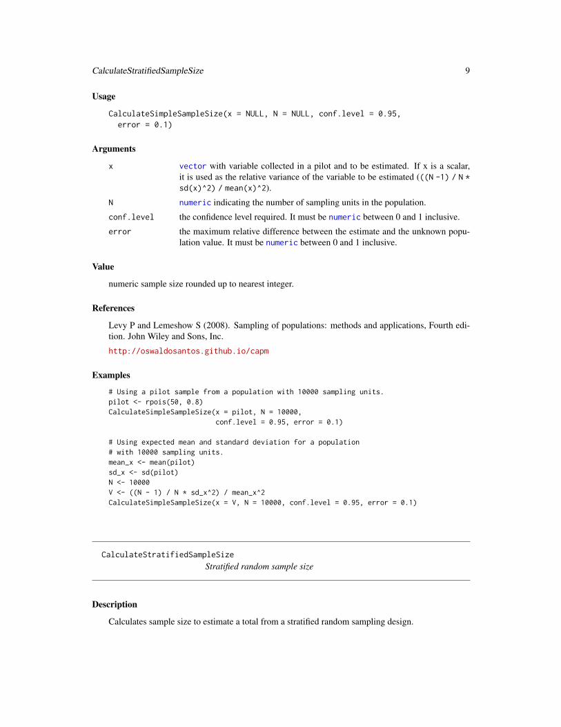
Usage

CalculateSimpleSampleSize(x = NULL, N = NULL, conf.level = 0.95,error = 0.1)

Arguments

x vector with variable collected in a pilot and to be estimated. If x is a scalar,it is used as the relative variance of the variable to be estimated (((N -1) / N *sd(x)^2) / mean(x)^2).

N numeric indicating the number of sampling units in the population.



Value

numeric sample size rounded up to nearest integer.

References



Examples

# Using a pilot sample from a population with 10000 sampling units.pilot <- rpois(50, 0.8)CalculateSimpleSampleSize(x = pilot, N = 10000,

conf.level = 0.95, error = 0.1)

# Using expected mean and standard deviation for a population# with 10000 sampling units.mean_x <- mean(pilot)sd_x <- sd(pilot)N <- 10000V <- ((N - 1) / N * sd_x^2) / mean_x^2CalculateSimpleSampleSize(x = V, N = 10000, conf.level = 0.95, error = 0.1)

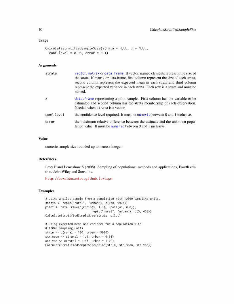
CalculateStratifiedSampleSize

Stratified random sample size

Description

Calculates sample size to estimate a total from a stratified random sampling design.


10 CalculateStratifiedSampleSize

Usage

CalculateStratifiedSampleSize(strata = NULL, x = NULL,conf.level = 0.95, error = 0.1)

Arguments

strata vector, matrix or data.frame. If vector, named elements represent the size ofthe strata. If matrix or data.frame, first column represent the size of each strata,second column represent the expected mean in each strata and third columnrepresent the expected variance in each strata. Each row is a strata and must benamed.

x data.frame representing a pilot sample. First column has the variable to beestimated and second column has the strata membership of each observation.Needed when strata is a vector.



Value

numeric sample size rounded up to nearest integer.

References



Examples

# Using a pilot sample from a population with 10000 sampling units.strata <- rep(c("rural", "urban"), c(100, 9900))pilot <- data.frame(c(rpois(5, 1.3), rpois(45, 0.8)),

rep(c("rural", "urban"), c(5, 45)))CalculateStratifiedSampleSize(strata, pilot)

# Using expected mean and variance for a population with# 10000 sampling units.str_n <- c(rural = 100, urban = 9900)str_mean <- c(rural = 1.4, urban = 0.98)str_var <- c(rural = 1.48, urban = 1.02)CalculateStratifiedSampleSize(cbind(str_n, str_mean, str_var))


cats 11

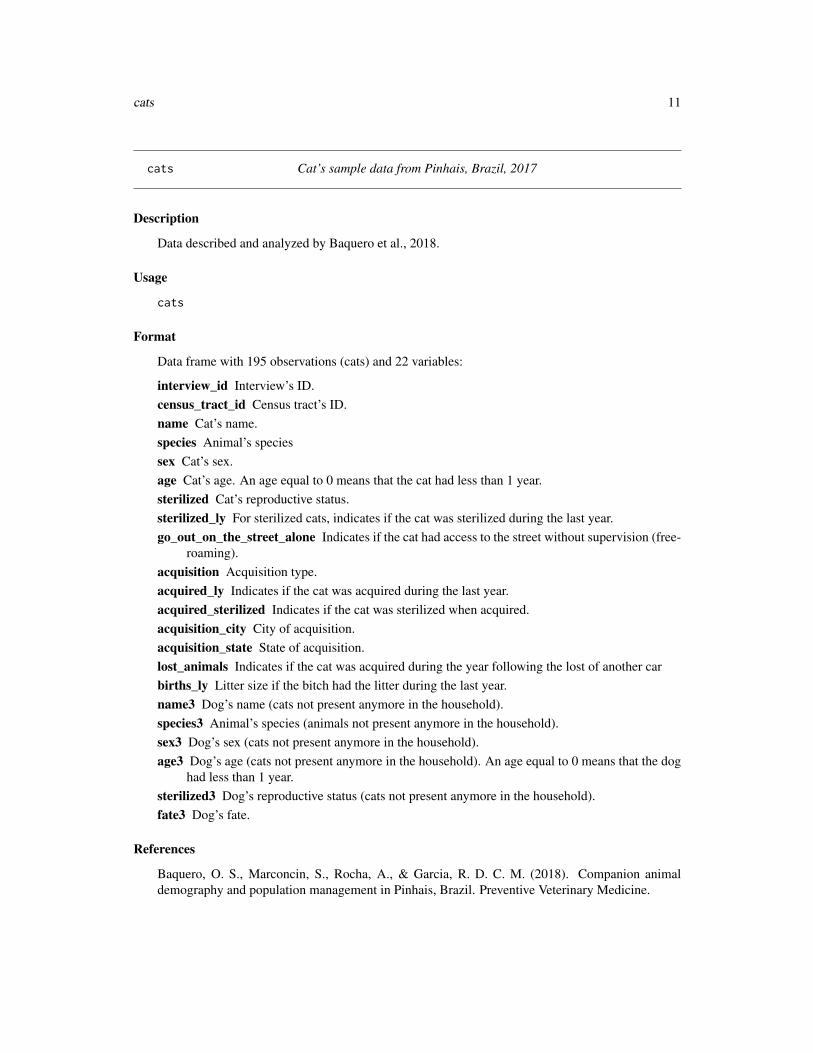
cats Cat’s sample data from Pinhais, Brazil, 2017

Description

Data described and analyzed by Baquero et al., 2018.

Usage

cats

Format

Data frame with 195 observations (cats) and 22 variables:

interview_id Interview’s ID.census_tract_id Census tract’s ID.name Cat’s name.species Animal’s speciessex Cat’s sex.age Cat’s age. An age equal to 0 means that the cat had less than 1 year.sterilized Cat’s reproductive status.sterilized_ly For sterilized cats, indicates if the cat was sterilized during the last year.go_out_on_the_street_alone Indicates if the cat had access to the street without supervision (free-

roaming).acquisition Acquisition type.acquired_ly Indicates if the cat was acquired during the last year.acquired_sterilized Indicates if the cat was sterilized when acquired.acquisition_city City of acquisition.acquisition_state State of acquisition.lost_animals Indicates if the cat was acquired during the year following the lost of another carbirths_ly Litter size if the bitch had the litter during the last year.name3 Dog’s name (cats not present anymore in the household).species3 Animal’s species (animals not present anymore in the household).sex3 Dog’s sex (cats not present anymore in the household).age3 Dog’s age (cats not present anymore in the household). An age equal to 0 means that the dog

had less than 1 year.sterilized3 Dog’s reproductive status (cats not present anymore in the household).fate3 Dog’s fate.

References


12 cluster_sample

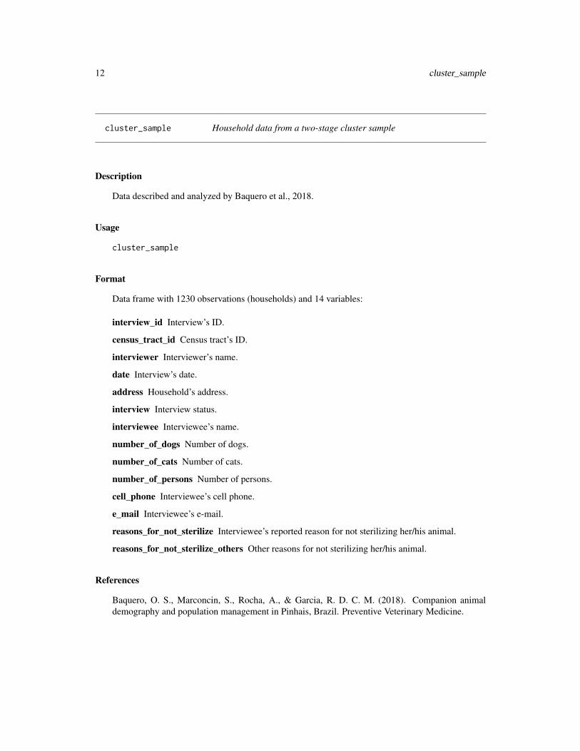
cluster_sample Household data from a two-stage cluster sample

Description


Usage

cluster_sample

Format

Data frame with 1230 observations (households) and 14 variables:

interview_id Interview’s ID.

census_tract_id Census tract’s ID.

interviewer Interviewer’s name.

date Interview’s date.

address Household’s address.

interview Interview status.

interviewee Interviewee’s name.

number_of_dogs Number of dogs.

number_of_cats Number of cats.

number_of_persons Number of persons.

cell_phone Interviewee’s cell phone.

e_mail Interviewee’s e-mail.

reasons_for_not_sterilize Interviewee’s reported reason for not sterilizing her/his animal.

reasons_for_not_sterilize_others Other reasons for not sterilizing her/his animal.

References


DesignSurvey 13

DesignSurvey Survey design

Description

A wraper for svydesign function from the survey package, to define one of the following surveydesigns: two-stage cluster, simple (systematic) or stratified. In the first case, weights are calculatedconsidering a sample with probability proportional to size and with replacement for the first stageand a simple random sampling for the second stage. Finite population correction is specified as thepopulation size for each level of sampling.

Usage

DesignSurvey(sample = NULL, psu.ssu = NULL, psu.col = NULL,ssu.col = NULL, cal.col = NULL, N = NULL, strata = NULL,cal.N = NULL, ...)

Arguments

sample data.frame with sample observations. for two-stage cluster designs, one ofthe columns must contain unique identifiers for PSU and another column mustcontain unique identifiers for Secondary Sampling Units (SSU).

psu.ssu data.frame with all Primary Sampling Units (PSU). First column contains PSUunique identifiers. Second column contains numeric PSU sizes. It is used onlyfor two-stage cluster designs.

psu.col the column of sample containing the psu identifiers (for two-stage cluster de-signs). It is used only for two-stage cluster designs.

ssu.col the column of sample containing the ssu identifiers (for two-stage cluster de-signs). It is used only for two-stage cluster designs.

cal.col the column of sample with the variable to calibrate estimates. It must be usedtogether with cal.N.

N for simple designs, a numeric value representing the total of sampling units inthe population. for a stratified design, it is a column of sample indicating, foreach observation, the total of sampling units in its respective strata. N is ignoredin two-stage cluster designs.

strata for stratified designs, a column of sample indicating the strata memebership ofeach observation.

cal.N population total for the variable to calibrate the estimates. It must be usedtogheter with cal.col.

... further arguments passed to svydesign function.

14 DesignSurvey

Details

For two-stage cluster designs, a PSU appearing in both psu.ssu and in sample must have the sameidentifier. SSU identifiers must be unique but can appear more than once if there is more than oneobservation per SSU. sample argument must have just the varibles to be estimated plus the variablesrequired to define the design (two-stage cluster or stratified). cal.col and cal.N are needed onlyif estimates will be calibrated. The calibration is based on a population total.

Value

An object of class survey.design.

References

Lumley, T. (2011). Complex surveys: A guide to analysis using R (Vol. 565). Wiley.



Examples

data("cluster_sample")data("psu_ssu")

## Calibrated two-stage cluster designdesign <- DesignSurvey(na.omit(cluster_sample),

psu.ssu = psu_ssu,psu.col = "census_tract_id",ssu.col = "interview_id",cal.col = "number_of_persons",cal.N = 129445)

## Simple design# If data in cluster_sample were from a simple design:design <- DesignSurvey(na.omit(cluster_sample),

N = sum(psu_ssu$hh),cal.N = 129445)

## Stratified design# Simulate strata and assume that the data in cluster_design came# from a stratified designcluster_sample$strat <- sample(c("urban", "rural"),

nrow(cluster_sample),prob = c(.95, .05),replace = TRUE)

cluster_sample$strat_size <- round(sum(psu_ssu$hh) * .95)cluster_sample$strat_size[cluster_sample$strat == "rural"] <-

round(sum(psu_ssu$hh) * .05)design <- DesignSurvey(cluster_sample,

N = "strat_size",strata = "strat",


dogs 15

cal.N = 129445)

dogs Dog’s sample data from Pinhais, Brazil, 2017

Description


Usage

dogs

Format

Data frame with 1252 observations (dogs) and 22 variables:

interview_id Interview’s ID.

census_tract_id Census tract’s ID.

name Dog’s name.

species Animal’s species

sex Dog’s sex.

age Dog’s age. An age equal to 0 means that the dog had less than 1 year.

sterilized Dog’s reproductive status.

sterilized_ly For sterilized dogs, indicates if the dog was sterilized during the last year.

go_out_on_the_street_alone Indicates if the dog had access to the street without supervision (free-roaming).

acquisition Acquisition type.

acquired_ly Indicates if the dog was acquired during the last year.

acquired_sterilized Indicates if the dog was sterilized when acquired.

acquisition_city City of acquisition.

acquisition_state State of acquisition.

lost_animals Indicates if the dog was acquired during the year following the lost of another dog

births_ly Litter size if the bitch had the litter during the last year.

name3 Dog’s name (dogs not present anymore in the household).

species3 Animal’s species (animals not present anymore in the household).

sex3 Dog’s sex (dogs not present anymore in the household).

age3 Dog’s age (dogs not present anymore in the household). An age equal to 0 means that the doghad less than 1 year.

sterilized3 Dog’s reproductive status (dogs not present anymore in the household).

fate3 Dog’s fate.

16 FreqTab

References


FreqTab Frequency table of categorical variables

Description

Calculates and sort the count and relative frequency of categories.

Usage

FreqTab(data = NULL, variables = NULL, rnd = 3, decreasing = TRUE,use.na = FALSE)

Arguments

data data.frame with categorical variables.variables name or position of categorical variables. If more than one variable is provided,

contingency frequencies are calculated.rnd the number of decimal places (round) or significant digits (signif) to be used.decreasing logical. If TRUE, frequencies will be sorted in decreasing order, if FALSE, they

will be sorted in increasing order.use.na logical. If FALSE (default), missing values are omitted.

Value

data.frame.

References

Baquero, O. S., Marconcin, S., Rocha, A., & Garcia, R. D. C. M. (2018). Companion animaldemography and population management in Pinhais, Brazil. Preventive Veterinary Medicine. http://oswaldosantos.github.io/capm

See Also

table and sort.

Examples

data(cluster_sample)FreqTab(cluster_sample$number_of_dogs)

data(dogs)FreqTab(dogs, c("species", "sex"))



GetDataIASA 17

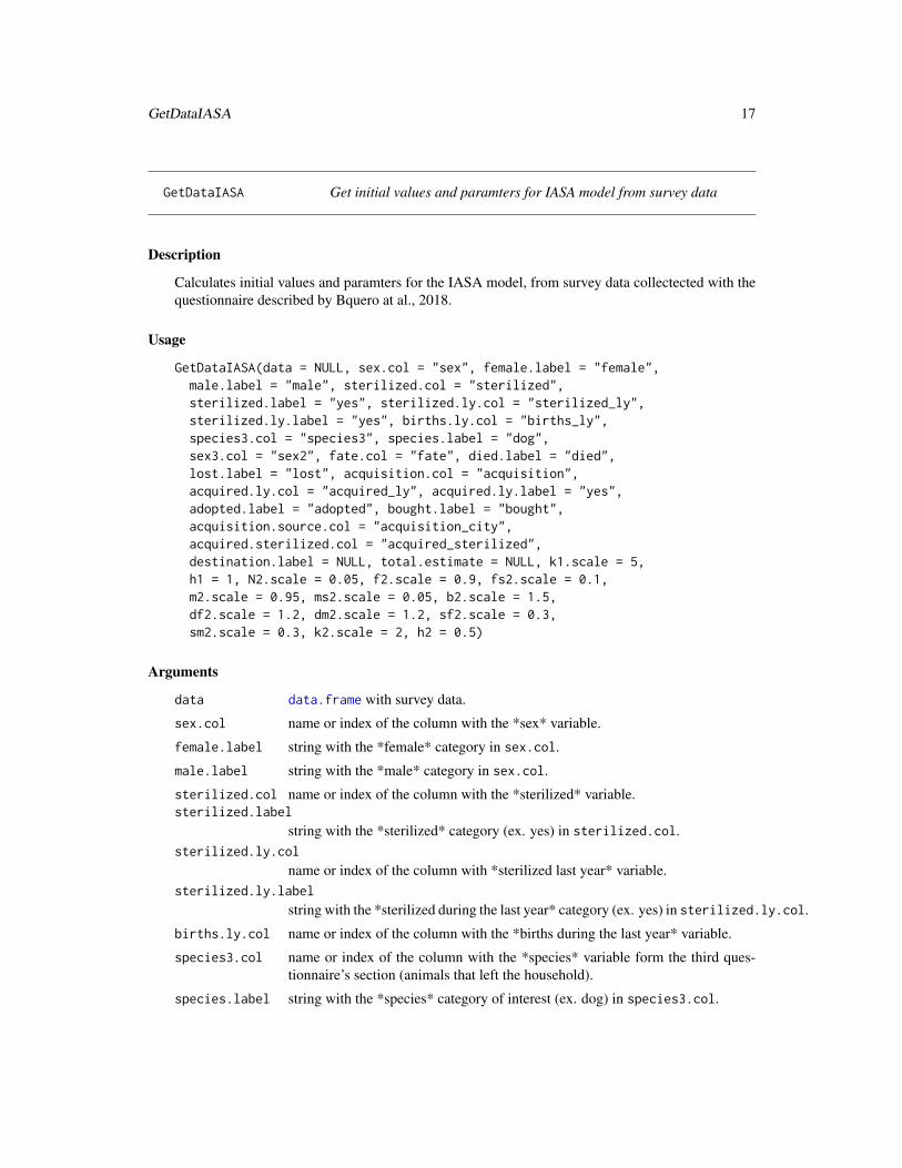
GetDataIASA Get initial values and paramters for IASA model from survey data

Description

Calculates initial values and paramters for the IASA model, from survey data collectected with thequestionnaire described by Bquero at al., 2018.

Usage

GetDataIASA(data = NULL, sex.col = "sex", female.label = "female",male.label = "male", sterilized.col = "sterilized",sterilized.label = "yes", sterilized.ly.col = "sterilized_ly",sterilized.ly.label = "yes", births.ly.col = "births_ly",species3.col = "species3", species.label = "dog",sex3.col = "sex2", fate.col = "fate", died.label = "died",lost.label = "lost", acquisition.col = "acquisition",acquired.ly.col = "acquired_ly", acquired.ly.label = "yes",adopted.label = "adopted", bought.label = "bought",acquisition.source.col = "acquisition_city",acquired.sterilized.col = "acquired_sterilized",destination.label = NULL, total.estimate = NULL, k1.scale = 5,h1 = 1, N2.scale = 0.05, f2.scale = 0.9, fs2.scale = 0.1,m2.scale = 0.95, ms2.scale = 0.05, b2.scale = 1.5,df2.scale = 1.2, dm2.scale = 1.2, sf2.scale = 0.3,sm2.scale = 0.3, k2.scale = 2, h2 = 0.5)

Arguments

data data.frame with survey data.

sex.col name or index of the column with the *sex* variable.

female.label string with the *female* category in sex.col.

male.label string with the *male* category in sex.col.

sterilized.col name or index of the column with the *sterilized* variable.sterilized.label

string with the *sterilized* category (ex. yes) in sterilized.col.sterilized.ly.col

name or index of the column with *sterilized last year* variable.sterilized.ly.label

string with the *sterilized during the last year* category (ex. yes) in sterilized.ly.col.

births.ly.col name or index of the column with the *births during the last year* variable.

species3.col name or index of the column with the *species* variable form the third ques-tionnaire’s section (animals that left the household).

species.label string with the *species* category of interest (ex. dog) in species3.col.

18 GetDataIASA

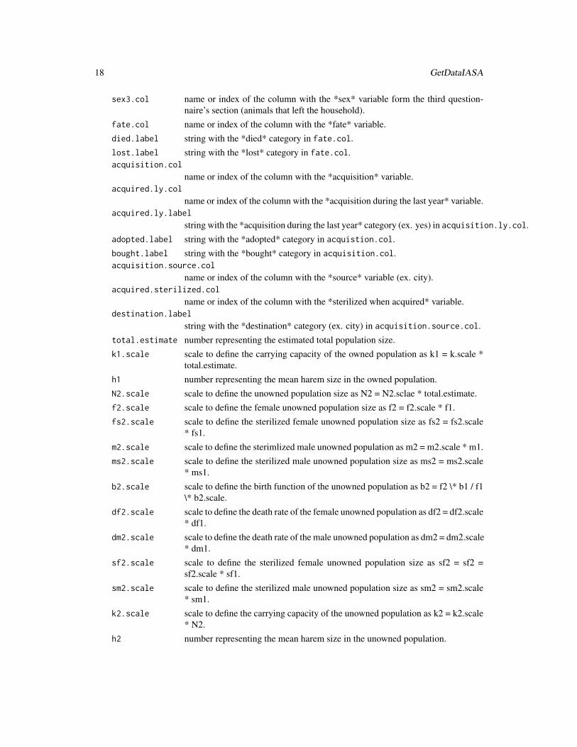
sex3.col name or index of the column with the *sex* variable form the third question-naire’s section (animals that left the household).

fate.col name or index of the column with the *fate* variable.died.label string with the *died* category in fate.col.lost.label string with the *lost* category in fate.col.acquisition.col

name or index of the column with the *acquisition* variable.acquired.ly.col

name or index of the column with the *acquisition during the last year* variable.acquired.ly.label

string with the *acquisition during the last year* category (ex. yes) in acquisition.ly.col.adopted.label string with the *adopted* category in acquistion.col.bought.label string with the *bought* category in acquisition.col.acquisition.source.col

name or index of the column with the *source* variable (ex. city).acquired.sterilized.col

name or index of the column with the *sterilized when acquired* variable.destination.label

string with the *destination* category (ex. city) in acquisition.source.col.total.estimate number representing the estimated total population size.k1.scale scale to define the carrying capacity of the owned population as k1 = k.scale *

total.estimate.h1 number representing the mean harem size in the owned population.N2.scale scale to define the unowned population size as N2 = N2.sclae * total.estimate.f2.scale scale to define the female unowned population size as f2 = f2.scale * f1.fs2.scale scale to define the sterilized female unowned population size as fs2 = fs2.scale

* fs1.m2.scale scale to define the sterimlized male unowned population as m2 = m2.scale * m1.ms2.scale scale to define the sterilized male unowned population size as ms2 = ms2.scale

* ms1.b2.scale scale to define the birth function of the unowned population as b2 = f2 \* b1 / f1

\* b2.scale.df2.scale scale to define the death rate of the female unowned population as df2 = df2.scale

* df1.dm2.scale scale to define the death rate of the male unowned population as dm2 = dm2.scale

* dm1.sf2.scale scale to define the sterilized female unowned population size as sf2 = sf2 =

sf2.scale * sf1.sm2.scale scale to define the sterilized male unowned population size as sm2 = sm2.scale

* sm1.k2.scale scale to define the carrying capacity of the unowned population as k2 = k2.scale

* N2.h2 number representing the mean harem size in the unowned population.

MapkmlPSU 19

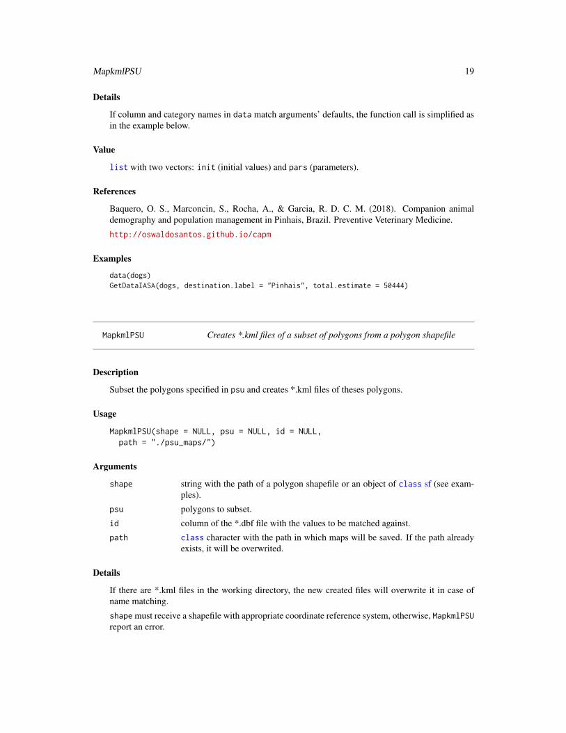
Details

If column and category names in data match arguments’ defaults, the function call is simplified asin the example below.

Value

list with two vectors: init (initial values) and pars (parameters).

References



Examples

data(dogs)GetDataIASA(dogs, destination.label = "Pinhais", total.estimate = 50444)

MapkmlPSU Creates *.kml files of a subset of polygons from a polygon shapefile

Description

Subset the polygons specified in psu and creates *.kml files of theses polygons.

Usage

MapkmlPSU(shape = NULL, psu = NULL, id = NULL,path = "./psu_maps/")

Arguments

shape string with the path of a polygon shapefile or an object of class sf (see exam-ples).

psu polygons to subset.

id column of the *.dbf file with the values to be matched against.

path class character with the path in which maps will be saved. If the path alreadyexists, it will be overwrited.

Details

If there are *.kml files in the working directory, the new created files will overwrite it in case ofname matching.

shape must receive a shapefile with appropriate coordinate reference system, otherwise, MapkmlPSUreport an error.


20 PlotGlobalSens

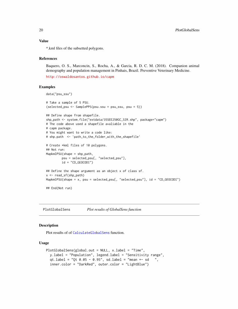
Value

*.kml files of the subsetted polygons.

References



Examples

data("psu_ssu")

# Take a sample of 5 PSU.(selected_psu <- SamplePPS(psu.ssu = psu_ssu, psu = 5))

## Define shape from shapefile.shp_path <- system.file("extdata/35SEE250GC_SIR.shp", package="capm")# The code above used a shapefile avaliable in the# capm package.# You might want to write a code like:# shp.path <- 'path_to_the_folder_with_the_shapefile'

# Create *kml files of 10 polygons.## Not run:MapkmlPSU(shape = shp_path,

psu = selected_psu[, "selected_psu"],id = "CD_GEOCODI")

## Define the shape argument as an object x of class sf.x <- read_sf(shp_path)MapkmlPSU(shape = x, psu = selected_psu[, "selected_psu"], id = "CD_GEOCODI")

## End(Not run)

PlotGlobalSens Plot results of GlobalSens function

Description

Plot results of of CalculateGlobalSens function.

Usage

PlotGlobalSens(global.out = NULL, x.label = "Time",y.label = "Population", legend.label = "Sensitivity range",qt.label = "Qt 0.05 - 0.95", sd.label = "mean +- sd ",inner.color = "DarkRed", outer.color = "LightBlue")


PlotGlobalSens 21

Arguments

global.out output from CalculateGlobalSens function.

x.label string with the name for the x axis.

y.label string with the name for the y axis.

legend.label string with the name for the legend.

qt.label string with the name for the envelope calculated using the quantiles 0.05 and0.95.

sd.label string with the name for the envelope calculated using the mean +- standarddeviation ranges.

inner.color any valid specification of a color for the inner envelope.

outer.color any valid specification of a color for the outer envelope.

Details

Font size of saved plots is usually different to the font size seen in graphic browsers. Before chang-ing font sizes, see the final result in saved (or preview) plots.

Other details of the plot can be modifyed using appropriate functions from ggplot2 package.

References



See Also

plot.deSolve.

Examples

## IASA model





## Set ranges 10 % greater and lesser than the## point estimates.


22 PlotHHxSpecies

rg_solve_iasa <- SetRanges(pars = dogs_iasa$pars)

## Calculate golobal sensitivity of combined parameters.## To calculate global sensitivity to each parameter, set## all as FALSE.glob_all_solve_iasa <- CalculateGlobalSens(

model.out = solve_iasa_pt,ranges = rg_solve_iasa,sensv = "n2", all = TRUE)

PlotGlobalSens(glob_all_solve_iasa)

PlotHHxSpecies Distribution of households according to the number of inhabitants oneor more species

Description

Dodged bar plot of the distribution of households according to the number of inhabitants of one ormore species.

Usage

PlotHHxSpecies(dat = NULL, species = NULL, proportion = TRUE,x.label = "Individuals per household",y.label = "Proportion of households", legend = TRUE)

Arguments

dat data.frame with households as observation unit and columns with the numberof individuals of the species of interest.

species names or positions of columns with species data.

proportion logical. If TRUE (default), the y axis will represent proportions, if FALSE, itwould represent raw counts.

x.label title for x axis.

y.label title for y axis.

legend logical. If TRUE (default), the legend will be showed, if FALSE, it will beremoved.

References


See Also

geom_bar.

PlotImmigrationFlow 23

Examples

data(cluster_sample)PlotHHxSpecies(cluster_sample, c("number_of_persons",

"number_of_dogs","number_of_cats"))

PlotImmigrationFlow Plot immigration flows

Description

Plot rimmigration flows from many sources to one destination.

Usage

PlotImmigrationFlow(data = NULL, source = NULL, destination = NULL,n.sources = 5, agg.sources.prefix = "Other ",agg.sources.suffix = " sources", cls = NULL, start.degree = 0,sources.label.dist = 0.15, sources.label.size = 0.75,ticks.label.size = 0.7)

Arguments

data data.frame with sources and destination.

source data’s column name or index with places’ names. Sources’ names and destina-tion’s name must be in this column.

destination destination’s name.

n.sources number of sources to plot. If smaller than the total number of sources source,the less frequent sources are aggregated.

agg.sources.prefix

string. If n.sources is smaller than the total number of sources, agg.sources.prefixis used to label the aggregated sources.

agg.sources.suffix

character. If n.sources is smaller than the total number of sources, agg.sources.prefixis used to label the aggregated sources.

cls Optional character vector with n.sources + 1 colors.

start.degree The starting degree from which the circle begins to draw. It is passed to thestart.degree argumento of circlize::circos.par function.

sources.label.dist

Data point on y-axis to separate the sources’ labels from the circle. It is passedto the y argument of circlize::circos.text function.

sources.label.size

Font size for sources’ labels. It is passed to the cex argument of circlize::circos.textfunction.

24 PlotLocalSens

ticks.label.size

Font size for sources’ labels. It is passed to the labels.cex argument of circlize::circos.axisfunction.

Details

The numbers arround the circle indicate the number of animals.

References

Gu, Z. (2014) circlize implements and enhances circular visualization in R. Bioinformatics. DOI:10.1093/bioinformatics/btu393



Examples

data(dogs)cls <- c("blue3", "orange", "skyblue", "darkgreen", "yellow3", "black")PlotImmigrationFlow(dogs, "acquisition_city", "Pinhais",

cls = cls, agg.sources.suffix = " cities")

PlotLocalSens Plot results of CalculateLocalSens function

Description

Plot results of the CalculateLocalSens function.

Usage

PlotLocalSens(local.out = NULL, x.sens = "Time",y.sens = "Sensitivity", y.ind = c("L1", "L2", "Mean", "Min", "Max"),bar.colors = "DarkRed", label.size = 10, x.axis.angle = 90,type = 1)

Arguments

local.out output from CalculateLocalSens function.

x.sens string with the name for the x axis.

y.sens string with the name for the y axis of the sensitivity functions (when type = 6).

y.ind string with the name for the y axis of the parameter importance indices.

bar.colors any valid specification of a color.

label.size a number to specify the size of axes labels and text.


PlotLocalSens 25

x.axis.angle a number with angle of rotation for x axis text. Passed to angle argument ofelement_text.

type a number to define the type of graphical output. 1: importance index L1; 2: im-portance index L2; 3: mean of sensitivity functions; 5: minimum of sensitivityfunctions; and 5: maximum of sensitivity functions; 6: sensitivity functions andall importance indices are ploted.

Details


References

Chang W (2012). R Graphics Cookbook. O’Reilly Media, Inc.

Soetaert K, Cash J and Mazzia F (2012). Solving differential equations in R. Springer.



See Also

plot.sensFun.

Examples

## IASA model#'## Parameters and intial conditions.data(dogs)dogs_iasa <- GetDataIASA(dogs,




## Calculate local sensitivities to all parameters.local_solve_iasa2 <- CalculateLocalSens(model.out = solve_iasa_pt, sensv = "n2")

## Plot local sensitivitiesPlotLocalSens(local_solve_iasa2)


26 PlotModels

PlotModels Plot results of capm model functions

Description

Plot results of one of the following functions: SolveIASA, SolveSI or SolveTC.

Usage

PlotModels(model.out = NULL, variable = NULL, col = "red",col1 = c("cadetblue1", "yellow", "red"), col2 = c("blue","darkgreen", "darkred"), x.label = "Years", y.label = NULL,legend.label = NULL, pop = NULL)

Arguments

model.out output of one of the function previously mentioned.

variable string to specify the variable to be ploted.For SolveSI function:"n" (population size)."q" (proportion of sterilized animals).For SolveIASA function using only point estimates:"f1" (owned intact females)."fs1" (owned sterilized females)."m1" (owned intact males)."ms1" (owned sterilized males)."f2" (unowned intact females)."fs2" (unowned sterilized females)."m2" (unowned intact males)."ms2" (unowned sterilized males)."n1" (owned intact animals)."ns1" (owned sterilized animals)."n2" (unowned intact animals)."ns2" (unowned sterilized animals)."N1" (owned animals)."N2" (unowned animals)."N" (total population).For SolveIASA function using *.range arguments:"f" (intact females)."fs" (sterilized females)."m" (intact males)."ms" (sterilized males)."n" (intact animals).

PlotModels 27

"ns" (sterilized animals)."N" (Total population stratified by reproductive status).For SolveTC function:"n" (fertile animals)."g" (sterilized animals)."u" (cumulative of sterilized animals)

col string indicating the color of ploted line, when s.range is NULL.

col1 character vector indicating the color of lowest (highest) population sizes(proportion of sterilized animals), when s.range is not NULL.

col2 character vector indicating the color of highest (lowest) population sizes(proportion of sterilized animals), when s.range is not NULL.

x.label string with the name for x axis.

y.label string with the name for y axis.

legend.label string with the name of the legend, for plots of SolveIASA output.

pop value indicating the output of SolveIASA to be ploted. When NULL (default),plots for owned and unowned populations under scenarios created by immi-gartion rate are created. If 1, the plots of owned population for the minimumimmigartion rate are ploted. When 2, the plots of unowned population for theminimum immigartion rate are ploted. If 3, the plots of owned population for themaximum immigartion rate are ploted. When 4, the plots of owned populationfor the maximum immigartion rate are ploted.

Details


Other details of the plot can be modifyed using appropriate functions from ggplot2 package.

References

Chang W (2012). R Graphics Cookbook. O’Reilly Media, Inc.


See Also

plot.deSolve.

Examples

## IASA model




28 PlotPopPyramid



solve_iasa_rg <- SolveIASA(pars = dogs_iasa$pars,init = dogs_iasa$init,time = 0:10,alpha.owned = TRUE,s.range = seq(0, .4, l = 15),a.range = c(0, .2),alpha.range = c(0, .05),v.range = c(0, .1),method = 'rk4')

## Plot unowned population sizes using point estimates## Not run:PlotModels(solve_iasa_pt, variable = "ns2")

## Plot all scenarios and change the label for the scenarios.## Not runPlotModels(solve_iasa_rg, variable = "ns")

## End(Not run)

PlotPopPyramid Population PlotPopPyramid

Description

Displays two opposed horizontal barplots (pyramid).

Usage

PlotPopPyramid(dat = NULL, age.col = NULL, sex.col = NULL,str.col = NULL, str.tip = NULL, x.label = "Count",stage.label = "Years", legend.label = "Sterilized",inner.color = "LightBlue", outer.color = "DarkRed",label.size = 13)

Arguments

dat data.frame.

age.col dat column that has a numeric vector representing ages or stage categories.

sex.col dat column that has two unique values representing the sex of individuals (seeDetails).

PlotPopPyramid 29

str.col dat column that has two unique values representing the reproductive status ofindividuals (see Details).

str.tip string with the category of str.col to place at tip of the bars.

x.label string to be used as a label for the x axis. If undefined, x.label is equal to"Total" (see Details).

stage.label a string to be used as a label for the ages or stage categories. If undefined,stage.label is equal to "Years" (see Details).

legend.label a string to be used as a label for the legend. If undefined, legend.label is equalto "Sterilized".

inner.color any valid specification of a color. When str.col is not NULL, inner.color isthe color of inner bars.

outer.color any valid way specification of a color. When str.col is NULL, outer.color isthe default color. When str.col is not NULL, outer.color is the outer color ofbars.

label.size string to define the font size for labels.

Details

PlotPopPyramid is mainly intended for companion animals population pyramids, although it candisplay other types of opposed bar charts.

The bars to the left of the x axis correspond to sort(unique(dat[,sex.col]))[1]. If str.col isnot NULL, bars will be stacked, with sort(unique(dat[,str.col]))[1] as their base.

On the top of the plot, it is displayed the total number of observations of each dat[,sex.col]unique value. This unique values are used as labels.

The legend labels are equal to the dat[,str.col] unique values.


Other details of the plot can be modifyed using appropriate functions from ggplot2 package (seeexamples).

Value

Two opposed horizontal barplots.

Note

In companion animals population surveys, some age categories might be empty. One differencebetween PlotPopPyramid and pryramid.plot is that the first does not drop empty age categories.

References




30 psu_ssu

Examples

data(dogs)

PlotPopPyramid(dogs,age.col = "age",sex.col = "sex",str.col = "sterilized")

PlotPopPyramid(dogs,age.col = "age",sex.col = "sex")

## Merge age categoriespp_age <- cut(c(dogs$age, dogs$age3),

breaks = c(0, 1, 3, 5, 7, 9, 11, 13, 15,max(c(dogs$age, dogs$age3), na.rm = TRUE)),

labels = c("<1", "1-3", "3-5", "5-7", "7-9","9-11", "11-13", "13-15", ">15"),

include.lowest = TRUE)pp_sex <- c(dogs$sex, dogs$sex3)pp_ster <- c(dogs$sterilized, dogs$sterilized3)pp <- data.frame(age = pp_age, sex = pp_sex, sterilized = pp_ster)

PlotPopPyramid(pp,age.col = "age",sex.col = "sex",str.col = "sterilized")

PlotPopPyramid(pp,age.col = "age",sex.col = "sex")

psu_ssu Census tracts of Pinhais, Brazil.

Description

Census tracts of Pinhais, Brazil, according to the census of 2010. Data described and analyzed byBaquero et al., 2018.

Usage

psu_ssu

Format

A data frame with 655 observations and 5 variables:

census_tract_id Census track’s ID.hh Number of households.

SamplePPS 31

Source

http://www.ibge.gov.br/

References


SamplePPS Sampling with probability proportional to size and with replacement

Description

Select Primary Sampling Units (PSU) with probability proportional to size and with replacement.

Usage

SamplePPS(psu.ssu = NULL, psu = NULL, write = FALSE, ...)

Arguments

psu.ssu data.frame with all PSU. First column contains PSU unique identifiers. Secondcolumn contains numeric PSU sizes.

psu the number of PSU to be selected.

write logical. If TRUE, a *.csv file containing the PSU and their Secondary SamplingUnits (SSU) is writed in the current working directory.

... further arguments passed to write.table function.

Value

data.frame. First column contains the selected PSU identifiers, coerced by as.character, toavoid scientific notation in case the identifiers be large numbers of class numeric. Second columncontain PSU sizes, a variable needed for second stage sampling with SampleSystematic.

References




See Also

SampleSystematic.

http://www.ibge.gov.br/


32 SampleSystematic

Examples

data(psu_ssu)

# Take a sample of 10 PSU.SamplePPS(psu.ssu = psu_ssu, psu = 10, write = FALSE)

SampleSystematic Simple and stratified systematic sampling

Description

Select sampling units using simple or stratified systematic samplin. In the context of two-stagecluster sampling, select Secondary Sampling Units (SSU) in one or more Primary Sampling Units(PSU), using systematic sampling.

Usage

SampleSystematic(psu.ssu = NULL, su = NULL, N = NULL,write = FALSE, ...)

Arguments

psu.ssu data.frame with all PSU. First column contains PSU unique identifiers. Secondcolumn contains numeric PSU sizes. It is used only for the second stage of atwo-stage cluster design (see details).

su numeric indicating the number of sampling units to be selected. If su has morethan one element, stratified sampling is applied and psu.ssu is ignored (seedetails).

N numeric indicating the number of sampling units in the population. It is in-tended for simple or stratified sampling designs and when used, psu.ssu isignored (see details).

write logical. If TRUE, a *.csv file containing the PSU and their SSU is writed in thecurrent working directory.

... further arguments passed to write.table function.

Details

When N is defined, psu.ssu is ignored. If N has one element, su must too and the result is a simplesystematic selection. If N has more than one element, su must have the same number of elementsand each oredered pair represent an strata. Thus, when N has more than one element, the result is astratified sampling with systematic selection within each strata (see examples).

SetRanges 33

Value

A matrix. For the second stage in a two-stage cluster sampling, the names of columns are the iden-tifiers of selected psu, coerced by as.character to avoid scientific notation in case the identifiersbe of class numeric. The rows correspond to the selected SSU within each PSU. For simple sys-tematic sampling, the rows correspond to the selected sampling units. For stratified sampling, eachcolumn represent an strata and the rows correspond to the selected sampling units in each strata.

References




See Also

SamplePPS.

Examples

data(psu_ssu)

## Two-stage cluster samplingselected_psu <- SamplePPS(psu.ssu = psu_ssu, psu = 10)

# Take a systematic sampling of 5 SSU within each selected PSU.SampleSystematic(selected_psu, 5, write = FALSE)

## Simple systematic samplingSampleSystematic(su = 5, N = 100)

## Stratified systematic samplingSampleSystematic(su = c("urban" = 50, "rural" = 10),

N = c("urban" = 4000, "rural" = 150))

SetRanges Parameter ranges for global sensitivity analysis

Description

Define the minimum and maximum values for parameters whose global sensitivities are to be as-sessed with CalculateGlobalSens or sensRange functions.

Usage

SetRanges(pars = NULL, range = 0.1)


34 SolveIASA

Arguments

pars the same pars vector used in one of the following functions: SolveSI or SolveIASA.

range scale factor to define the minimum and maximum for each parameter. The de-fault is 0.1, which set the minimum and maximum as 10 percent lesser andgreater than the pars values.

Value

data.frame with the complete set of parameter ranges.

References


Reichert P and Kfinsch HR (2001). Practical identifiability analysis of large environmental simula-tion models. Water Resources Research, 37(4), pp. 1015-1030.



See Also

sensRange and SolveSI.

Examples

## IASA model



## Set ranges 10 % greater and lesser than the## point estimates.rg_solve_iasa <- SetRanges(pars = dogs_iasa$pars)

SolveIASA Modelling of immigration, abandonment, sterilization and adoption ofcompanion animals

Description

System of ordinary differential equations to simulate the effect of immigration of owned dogs,abandonment, sterilization of owned and unowned dogs and adoption, on population dynamics.


SolveIASA 35

Usage

SolveIASA(pars = NULL, init = NULL, time = NULL,alpha.owned = TRUE, immigration.reference = "N1", s.range = NULL,a.range = NULL, alpha.range = NULL, v.range = NULL, s.fm = TRUE,...)

Arguments

pars a named vector of length 21, with point estimates of model parameters (seedetails).

init a named vector of length 8, with point estimates of model parameters (seedetails).

time time sequence for which output is wanted; the first value of times must be theinitial time.

alpha.owned logical. If TRUE (default), adoption rate is relative to the owned population(proportion of the owned population). If FALSE, it is relative to the unownedpopulation.

immigration.reference

character indicating the value of reference to calculate the immigration rate.If "N1" (default), the total of immigrants is the product of the owned populationsize times the immigration rate (N1 \* v). If k1, it is the product of the ownedcarrying capacity times the immigration rate (k1 \* v).

s.range optional sequence (between 0 and 1) of the sterilization rates to be simulated.

a.range optional vector of length 2, with range (ie, confidence interval) of abandonmentrates to be assessed. If given, the rates evaluated are those specified by theargument plus the point estimate given in pars.

alpha.range optional vector of length 2, with range (ie, confidence interval) of adoptionrates to be assessed. If given, the rates evaluated are those specified by theargument plus the point estimate given in pars.

v.range optional vector of length 2, with range of values of immigration rates to beassessed.

s.fm logical. If TRUE, s.range is used for females and males and if FALSE, it is usedfor only females (for males, the point estimate given in pars is used.)

... further arguments passed to ode function.

Details

The implemented model is described by Baquero, et. al., 2016 and the function is a wrapper aroundthe defaults of ode function, whose help page must be consulted for details.

The pars argument must contain named values, using the following conventions: 1: owned animals;2: unowned animals; f: females; m: males. Then:

b1 and b2: number of births.

df1, dm1, df2 and dm2: death rate.

sf1, sm1, sf2 and sm2: sterilization rate.

36 SolveIASA

k1 and k2: carrying capacity.

h1 and h2: mean harem size.

a: abandonment rate.

alpha: adoption rate.

v: immigration rate.

z: proportion of sterilized immigrants.

The init argument must contain named values for the inital number of animals, using the followingconventions: 1: owned animals; 2: unowned animals; f: females; m: males; and s: sterilized. Then,the names are:

f1, fs1, m1, ms1, f2, fs2, m2 and ms2.

If any range is specified (e.g s.range), the remaining ranges must be specified too (a.range,alpha.range and v.range). The function is a wrapper around the defaults of ode function, whosehelp page must be consulted for details. An exception is the method argument, which here has "rk4"as a default.

Value

list. The first element, name, is a string with the name of the function, the second element, model,is the model function. The third, fourth and fifth elements are vectors (pars, init, time, respec-tively) containing the pars, init and time arguments of the function. The sixth element results isa data.frame with up to as many rows as elements in time. The first column contain the time andsubsequent columns contain the size of specific subpopulations, named according to conventionsabove. The group column differentiate between owned and unowned. When *.range arguments aregiven, the last fourth columsn specify their instances.

Note

Logistic growth models are not intended for scenarios in which population size is greater thancarrying capacity and growth rate is negative.

References

Baquero, O. S., Marconcin, S., Rocha, A., & Garcia, R. D. C. M. (2018). Companion animaldemography and population management in Pinhais, Brazil. Preventive Veterinary Medicine. Ba-quero, O. S., Akamine, L. A., Amaku, M., & Ferreira, F. (2016). Defining priorities for dog popu-lation management through mathematical modeling. Preventive veterinary medicine, 123, 121-127.


See Also

ode.


SolveSI 37

Examples





solve_iasa_rg <- SolveIASA(pars = dogs_iasa$pars,init = dogs_iasa$init,time = 0:10,alpha.owned = TRUE,s.range = seq(0, .4, l = 15),a.range = c(0, .2),alpha.range = c(0, .05),v.range = c(0, .1),method = 'rk4')

SolveSI Modelling of sterilization and immigration of comapnion animals.

Description

System of ordinary differential equations to simulate the effect of sterilization and immigration onpopulation dynamics.

Usage

SolveSI(pars = NULL, init = NULL, time = NULL, dd = "b", im = 0,s.range = NULL, ...)

Arguments

pars vector of length 4. The values are point estimates of birth rate, death rate,carrying capacity and sterilization rate. The names of this values must be "b","d", "k" and "s", respectively.

init vector of length 2. The values are initial population size and initial proportionof sterilized animals. The names of this values must be "n" and "q", respectively.


dd string equal to b, d or bd to define if density-dependece act on birth rate, deathrarte or both, respectively.

38 SolveSI

im a number representing the total of immigrants per time unit.

s.range optional sequence (between 0 and 1) of the sterilization rates to be simulated.


Details

The implemented model is described by Amaku, et. al., 2009 and the function is a wrapper aroundthe defaults of ode function, whose help page must be consulted for details.

Value

list. The first element, name, is a string with the name of the function, the second element, model,is the model function. The third, fourth and fifth elements are vectors (pars, init, time, respec-tively) containing the pars, init and time arguments of the function. The sisxth element resultsis a data.frame with up to as many rows as elements in time. First column contains the time, sec-ond column the population size and third column the proportion of sterilized animals. If s.rangeis specified, fourth column contains its specific instances.

Note

Logistic growth models are not intended for scenarios in which population size is greater thancarrying capacity and growth rate is negative.

References

Amaku M, Dias R and Ferreira F (2009). Dinamica populacional canina: potenciais efeitos decampanhas de esterilizacao. Revista Panamericana de Salud Publica, 25(4), pp. 300-304.

Soetaert K, Cash J and Mazzia F (2012). Solving differential equations in R. Springer.


See Also

ode.

Examples

# Parameters and initial conditions.pars_solve_si = c(b = 0.245, d = 0.101,

k = 98050, s = 0.048)init_solve_si = c(n = 89137, q = 0.198)

# Solve for a specific sterilization rate.solve_si_pt = SolveSI(pars = pars_solve_si,

init = init_solve_si,time = 0:15, dd = "b",im = 100, method = "rk4")

# Solve for a range of sterilization rates.solve_si_rg = SolveSI(pars = pars_solve_si,

init = init_solve_si,


SolveTC 39

time = 0:15, dd = "b", im = 100,s.range = seq(0, .4, l = 50),method = "rk4")

SolveTC Modelling of reversible contraception for companion animals

Description

System of ordinary differential equations to simulate the effect of reversible contraception in apopulation at equilibrium, where deaths are compensated by births and net immigration.

Usage

SolveTC(pars = NULL, init = NULL, time = NULL, f.range = NULL,s.range = NULL, z.range = NULL, ...)

Arguments

pars a named vector of length 5. The values are point estimates of the death rate (d),the fertility recovery rate (f), the sterilization rate (s), the proportion of infertileimmigrants (z) and the proportion of the death rate compensated by immigration(r). Abreviations in parentheses indicate the names that must be given to thevalues.

init a named vector of length 2, with the total number of fertile (n) and infertile (g)animals.


f.range optional sequence (between 0 and 1) with the fertility recovery rates to be sim-ulated.

s.range optional vector of length 2, with a range of sterilization rates to be assessed.If given, the rates evaluated are those specified by the argument plus the pointestimate given in pars.

z.range optional vector of length 2, with a range of the proportion of infertile immi-grants. If given, the rates evaluated are those specified by the argument plus thepoint estimate given in pars.


Value

list. The first element, name, is a string with the name of the function, the second element, model,is the model function. The third, fourth and fifth elements are vectors (pars, init, time, re-spectively) containing the pars, init and time arguments of the function. The sisxthth elementresults is a data.frame with up to as many rows as elements in time. The first fourth columnscontain the time and the variables: n, g and u. When *.range arguments are given, additionalcolumns contain the variables f, s and z.

40 SummarySurvey

References


Baquero, O. S., Brandao, A. P. D., Amaku, M., & Ferreira, F. (2016). Effectiveness of reversiblecontraception in dog population management. Acta Scientiae Veterinariae, 44, 01-06.

See Also

ode.

Examples

# Parameters and initial conditions.pars_solvetc <- c(d = 1 / 6, f = 0.5, s = 0.2,

z = 0.2, r = 0.8)

init_solvetc <- c(n = 950, g = 50)

# Solve for point estimates.solve_tc_pt <- SolveTC(pars = pars_solvetc,

init = init_solvetc,time = 0:10, method = "rk4")

# Solve for parameter ranges.solve_tc_rg <- SolveTC(pars = pars_solvetc,

init = init_solvetc,time = 0:15,f.range = seq(0, 1, 0.1),s.range = c(0.05, 0.4),z.range = c(0.05, 0.4),method = "rk4")

SummarySurvey Summary statistics for sample surveys

Description

Wraps functions for summary statistics from survey package.

Usage

SummarySurvey(design = NULL, variables = NULL, conf.level = 0.95,rnd = 3)


SummarySurvey 41

Arguments

design an output form DesignSurvey function.

variables character vector with the type of estimate for each variable contained indesign. Possible types: total, mean, and prop (see details).

conf.level the confidence level required.

rnd the number of decimal places (round) or significant digits (signif) to be used. IfNA, scientific notation is used.

Details

The length of variables must be equal to the length of names(design$variables) (see exam-ples).

Value

Matrix with survey summaries. The error (column "Error (

References

Lumley, T. (2011). Complex surveys: A guide to analysis using R (Vol. 565). Wiley.



Examples

data("cluster_sample")data("psu_ssu")

## Calibrated two-stage cluster designcs <- cluster_sample[ , c("interview_id",

"census_tract_id","number_of_persons","number_of_dogs","number_of_cats")]

design <- DesignSurvey(na.omit(cs),psu.ssu = psu_ssu,psu.col = "census_tract_id",ssu.col = "interview_id",cal.col = "number_of_persons",cal.N = 129445)

SummarySurvey(design, c("total", "total", "total"))


Index

∗Topic datasetscats, 11cluster_sample, 12dogs, 15psu_ssu, 30

∗Topic packagecapm-package, 2

as.character, 31, 33

Calculate2StageSampleSize, 3CalculateGlobalSens, 4, 7, 20, 21, 33CalculateLocalSens, 6, 24CalculatePopChange, 7CalculateSimpleSampleSize, 8CalculateStratifiedSampleSize, 9capm-package, 2cats, 11character, 23, 27, 35, 41class, 19, 31, 33cluster_sample, 12

data.frame, 3, 6, 10, 13, 16, 17, 22, 23, 28,31, 32, 34, 36, 38, 39

DesignSurvey, 13, 41dogs, 15

element_text, 25

FALSE, 4, 5FreqTab, 16

geom_bar, 22GetDataIASA, 17

labels, 29list, 4, 6, 7, 19, 36, 38, 39logical, 16, 22, 35

MapkmlPSU, 19matrix, 10

numeric, 3, 9, 10, 13, 28, 31–33

ode, 35, 36, 38–40

plot.deSolve, 21, 27plot.sensFun, 25PlotGlobalSens, 20PlotHHxSpecies, 22PlotImmigrationFlow, 23PlotLocalSens, 24PlotModels, 7, 26PlotPopPyramid, 28psu_ssu, 30

SamplePPS, 31, 33SampleSystematic, 31, 32sensFun, 6sensRange, 4–6, 33, 34SetRanges, 4, 33sf, 19SolveIASA, 4, 6, 7, 26, 27, 34, 34SolveSI, 4, 6, 7, 26, 34, 37SolveTC, 4, 6, 7, 26, 27, 39sort, 16SummarySurvey, 40svydesign, 13

table, 16

vector, 9, 10, 23, 27, 28, 35, 37, 39, 41

write.table, 31, 32

42

package ‘capm’

Documents