package ‘epi’ - uaem.mx · package ‘epi’ february 15, 2013 version 1.1.44 date 2013-02-06...
TRANSCRIPT
Package ‘Epi’February 15, 2013
Version 1.1.44
Date 2013-02-06
Title A package for statistical analysis in epidemiology.
Maintainer Bendix Carstensen <[email protected]>
Depends R (>= 2.14.0), utils
Suggests splines, nlme, survival, mstate, etm, MASS
Description Functions for demographic and epidemiological analysis inthe Lexis diagram, i.e. register and cohort follow-up data,including interval censored data and representation ofmultistate data. Also some useful functions for tabulation andplotting. Contains some epidemiological datasets.
License GPL-2
URL http://BendixCarstensen.com/Epi/
Author Bendix Carstensen [aut, cre], Martyn Plummer [aut], Michael Hills [aut], Esa Laara [ctb]
Repository CRAN
Date/Publication 2013-02-07 12:36:25
NeedsCompilation yes
R topics documented:apc.fit . . . . . . . . . . . . . . . . . . . . . . . . . . . . . . . . . . . . . . . . . . . . 3apc.frame . . . . . . . . . . . . . . . . . . . . . . . . . . . . . . . . . . . . . . . . . . 7apc.lines . . . . . . . . . . . . . . . . . . . . . . . . . . . . . . . . . . . . . . . . . . . 9apc.plot . . . . . . . . . . . . . . . . . . . . . . . . . . . . . . . . . . . . . . . . . . . 11B.dk . . . . . . . . . . . . . . . . . . . . . . . . . . . . . . . . . . . . . . . . . . . . . 12bdendo . . . . . . . . . . . . . . . . . . . . . . . . . . . . . . . . . . . . . . . . . . . . 13bdendo11 . . . . . . . . . . . . . . . . . . . . . . . . . . . . . . . . . . . . . . . . . . 14
1
2 R topics documented:
births . . . . . . . . . . . . . . . . . . . . . . . . . . . . . . . . . . . . . . . . . . . . 14blcaIT . . . . . . . . . . . . . . . . . . . . . . . . . . . . . . . . . . . . . . . . . . . . 15boxes.MS . . . . . . . . . . . . . . . . . . . . . . . . . . . . . . . . . . . . . . . . . . 15brv . . . . . . . . . . . . . . . . . . . . . . . . . . . . . . . . . . . . . . . . . . . . . . 21cal.yr . . . . . . . . . . . . . . . . . . . . . . . . . . . . . . . . . . . . . . . . . . . . 22ccwc . . . . . . . . . . . . . . . . . . . . . . . . . . . . . . . . . . . . . . . . . . . . . 24ci.cum . . . . . . . . . . . . . . . . . . . . . . . . . . . . . . . . . . . . . . . . . . . . 25ci.lin . . . . . . . . . . . . . . . . . . . . . . . . . . . . . . . . . . . . . . . . . . . . . 27ci.pd . . . . . . . . . . . . . . . . . . . . . . . . . . . . . . . . . . . . . . . . . . . . . 29clogistic . . . . . . . . . . . . . . . . . . . . . . . . . . . . . . . . . . . . . . . . . . . 31contr.cum . . . . . . . . . . . . . . . . . . . . . . . . . . . . . . . . . . . . . . . . . . 32cutLexis . . . . . . . . . . . . . . . . . . . . . . . . . . . . . . . . . . . . . . . . . . . 33detrend . . . . . . . . . . . . . . . . . . . . . . . . . . . . . . . . . . . . . . . . . . . 36diet . . . . . . . . . . . . . . . . . . . . . . . . . . . . . . . . . . . . . . . . . . . . . 37DMconv . . . . . . . . . . . . . . . . . . . . . . . . . . . . . . . . . . . . . . . . . . . 38DMlate . . . . . . . . . . . . . . . . . . . . . . . . . . . . . . . . . . . . . . . . . . . 39effx . . . . . . . . . . . . . . . . . . . . . . . . . . . . . . . . . . . . . . . . . . . . . 40effx.match . . . . . . . . . . . . . . . . . . . . . . . . . . . . . . . . . . . . . . . . . . 42ewrates . . . . . . . . . . . . . . . . . . . . . . . . . . . . . . . . . . . . . . . . . . . 44expand.data . . . . . . . . . . . . . . . . . . . . . . . . . . . . . . . . . . . . . . . . . 44fit.add . . . . . . . . . . . . . . . . . . . . . . . . . . . . . . . . . . . . . . . . . . . . 45fit.baseline . . . . . . . . . . . . . . . . . . . . . . . . . . . . . . . . . . . . . . . . . . 46fit.mult . . . . . . . . . . . . . . . . . . . . . . . . . . . . . . . . . . . . . . . . . . . . 47float . . . . . . . . . . . . . . . . . . . . . . . . . . . . . . . . . . . . . . . . . . . . . 48foreign.Lexis . . . . . . . . . . . . . . . . . . . . . . . . . . . . . . . . . . . . . . . . 50ftrend . . . . . . . . . . . . . . . . . . . . . . . . . . . . . . . . . . . . . . . . . . . . 51gen.exp . . . . . . . . . . . . . . . . . . . . . . . . . . . . . . . . . . . . . . . . . . . 53gmortDK . . . . . . . . . . . . . . . . . . . . . . . . . . . . . . . . . . . . . . . . . . 55hivDK . . . . . . . . . . . . . . . . . . . . . . . . . . . . . . . . . . . . . . . . . . . . 57Icens . . . . . . . . . . . . . . . . . . . . . . . . . . . . . . . . . . . . . . . . . . . . . 58lep . . . . . . . . . . . . . . . . . . . . . . . . . . . . . . . . . . . . . . . . . . . . . . 60Lexis . . . . . . . . . . . . . . . . . . . . . . . . . . . . . . . . . . . . . . . . . . . . 60Lexis.diagram . . . . . . . . . . . . . . . . . . . . . . . . . . . . . . . . . . . . . . . . 63Lexis.lines . . . . . . . . . . . . . . . . . . . . . . . . . . . . . . . . . . . . . . . . . . 66Life.lines . . . . . . . . . . . . . . . . . . . . . . . . . . . . . . . . . . . . . . . . . . 67lls . . . . . . . . . . . . . . . . . . . . . . . . . . . . . . . . . . . . . . . . . . . . . . 68lungDK . . . . . . . . . . . . . . . . . . . . . . . . . . . . . . . . . . . . . . . . . . . 69M.dk . . . . . . . . . . . . . . . . . . . . . . . . . . . . . . . . . . . . . . . . . . . . . 70merge.data.frame . . . . . . . . . . . . . . . . . . . . . . . . . . . . . . . . . . . . . . 72merge.Lexis . . . . . . . . . . . . . . . . . . . . . . . . . . . . . . . . . . . . . . . . . 72mh . . . . . . . . . . . . . . . . . . . . . . . . . . . . . . . . . . . . . . . . . . . . . . 73mortDK . . . . . . . . . . . . . . . . . . . . . . . . . . . . . . . . . . . . . . . . . . . 75N.dk . . . . . . . . . . . . . . . . . . . . . . . . . . . . . . . . . . . . . . . . . . . . . 76N2Y . . . . . . . . . . . . . . . . . . . . . . . . . . . . . . . . . . . . . . . . . . . . . 77ncut . . . . . . . . . . . . . . . . . . . . . . . . . . . . . . . . . . . . . . . . . . . . . 78nice . . . . . . . . . . . . . . . . . . . . . . . . . . . . . . . . . . . . . . . . . . . . . 79nickel . . . . . . . . . . . . . . . . . . . . . . . . . . . . . . . . . . . . . . . . . . . . 80occup . . . . . . . . . . . . . . . . . . . . . . . . . . . . . . . . . . . . . . . . . . . . 81
apc.fit 3
pctab . . . . . . . . . . . . . . . . . . . . . . . . . . . . . . . . . . . . . . . . . . . . . 82plot.Lexis . . . . . . . . . . . . . . . . . . . . . . . . . . . . . . . . . . . . . . . . . . 83plotEst . . . . . . . . . . . . . . . . . . . . . . . . . . . . . . . . . . . . . . . . . . . . 85plotevent . . . . . . . . . . . . . . . . . . . . . . . . . . . . . . . . . . . . . . . . . . . 88projection.ip . . . . . . . . . . . . . . . . . . . . . . . . . . . . . . . . . . . . . . . . . 89rateplot . . . . . . . . . . . . . . . . . . . . . . . . . . . . . . . . . . . . . . . . . . . 89Relevel . . . . . . . . . . . . . . . . . . . . . . . . . . . . . . . . . . . . . . . . . . . 93ROC . . . . . . . . . . . . . . . . . . . . . . . . . . . . . . . . . . . . . . . . . . . . . 94S.typh . . . . . . . . . . . . . . . . . . . . . . . . . . . . . . . . . . . . . . . . . . . . 96splitLexis . . . . . . . . . . . . . . . . . . . . . . . . . . . . . . . . . . . . . . . . . . 97stack.Lexis . . . . . . . . . . . . . . . . . . . . . . . . . . . . . . . . . . . . . . . . . 99start.Lexis . . . . . . . . . . . . . . . . . . . . . . . . . . . . . . . . . . . . . . . . . . 100stat.table . . . . . . . . . . . . . . . . . . . . . . . . . . . . . . . . . . . . . . . . . . . 101stattable.funs . . . . . . . . . . . . . . . . . . . . . . . . . . . . . . . . . . . . . . . . 103subset.Lexis . . . . . . . . . . . . . . . . . . . . . . . . . . . . . . . . . . . . . . . . . 104summary.Lexis . . . . . . . . . . . . . . . . . . . . . . . . . . . . . . . . . . . . . . . 105thoro . . . . . . . . . . . . . . . . . . . . . . . . . . . . . . . . . . . . . . . . . . . . . 106timeBand . . . . . . . . . . . . . . . . . . . . . . . . . . . . . . . . . . . . . . . . . . 107timeScales . . . . . . . . . . . . . . . . . . . . . . . . . . . . . . . . . . . . . . . . . . 109transform.Lexis . . . . . . . . . . . . . . . . . . . . . . . . . . . . . . . . . . . . . . . 109twoby2 . . . . . . . . . . . . . . . . . . . . . . . . . . . . . . . . . . . . . . . . . . . 111Y.dk . . . . . . . . . . . . . . . . . . . . . . . . . . . . . . . . . . . . . . . . . . . . . 112
Index 114
apc.fit Fit an Age-Period-Cohort model to tabular data.
Description
Fits the classical five models to tabulated rate data (cases, person-years) classified by two of age,period, cohort: Age, Age-drift, Age-Period, Age-Cohort and Age-period. There are no assumptionsabout the age, period or cohort classes being of the same length, or that tabulation should be onlyby two of the variables. Only requires that mean age and period for each tabulation unit is given.
Usage
apc.fit( data,A,P,D,Y,
ref.c,ref.p,dist = c("poisson","binomial"),
model = c("ns","bs","ls","factor"),dr.extr = c("weighted","Holford"),
parm = c("ACP","APC","AdCP","AdPC","Ad-P-C","Ad-C-P","AC-P","AP-C"),
4 apc.fit
npar = c( A=5, P=5, C=5 ),scale = 1,alpha = 0.05,
print.AOV = TRUE )
Arguments
data Data frame with (at least) variables, A (age), P (period), D (cases, deaths) and Y(person-years). Cohort (date of birth) is computed as P-A. If thsi argument isgiven the arguments A, P, D and Y are ignored.
A Age; numerical vector with mean age at diagnosis for each unit.
P Period; numerical vector with mean date of diagnosis for each unit.
D Cases, deaths; numerical vector.
Y Person-years; numerical vector. Also used as denominator for binomial data,see the dist argument.
ref.c Reference cohort, numerical. Defaults to median date of birth among cases. Ifused with parm="AdCP" or parm="AdPC", the resdiual cohort effects will be 1 atref.c
ref.p Reference period, numerical. Defaults to median date of diagnosis among cases.
dist Distribution (or more precisely: Likelihood) used for modelling. if a binomialmodel us ised, Y is assuemd to be the denominator; "binomial" gives a binomialmodel with logit link.
model Type of model fitted:
• ns fits a model with natural splines for each of the terms, with npar param-eters for the terms.
• bs fits a model with B-splines for each of the terms, with npar parametersfor the terms.
• ls fits a model with linear splines.• factor fits a factor model with one parameter per value of A, P and C. npar
is ignored in this case.
dr.extr Character. How the drift parameter should be extracted from the age-period-cohort model. "weighted" (default) lets the weighted average (by marginal no.cases, D) of the estimated period and cohort effects have 0 slope. "Holford"uses the naive average over all values for the estimated effects, disregarding theno. cases.
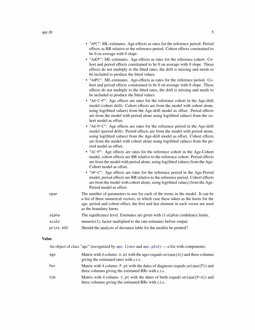
parm Character. Indicates the parametrization of the effects. The first four refer to theML-fit of the Age-Period-Cohort model, the last four give Age-effects from asmaller model and residuals relative to this. If one of the latter is chosen, theargument dr.extr is ignored. Possible values for parm are:
• "ACP": ML-estimates. Age-effects as rates for the reference cohort. Cohorteffects as RR relative to the reference cohort. Period effects constrained tobe 0 on average with 0 slope.
apc.fit 5
• "APC": ML-estimates. Age-effects as rates for the reference period. Periodeffects as RR relative to the reference period. Cohort effects constrained tobe 0 on average with 0 slope.
• "AdCP": ML-estimates. Age-effects as rates for the reference cohort. Co-hort and period effects constrained to be 0 on average with 0 slope. Theseeffects do not multiply to the fitted rates, the drift is missing and needs tobe included to produce the fitted values.
• "AdPC": ML-estimates. Age-effects as rates for the reference period. Co-hort and period effects constrained to be 0 on average with 0 slope. Theseeffects do not multiply to the fitted rates, the drift is missing and needs tobe included to produce the fitted values.
• "Ad-C-P": Age effects are rates for the reference cohort in the Age-driftmodel (cohort drift). Cohort effects are from the model with cohort alone,using log(fitted values) from the Age-drift model as offset. Period effectsare from the model with period alone using log(fitted values) from the co-hort model as offset.
• "Ad-P-C": Age effects are rates for the reference period in the Age-driftmodel (period drift). Period effects are from the model with period alone,using log(fitted values) from the Age-drift model as offset. Cohort effectsare from the model with cohort alone using log(fitted values) from the pe-riod model as offset.
• "AC-P": Age effects are rates for the reference cohort in the Age-Cohortmodel, cohort effects are RR relative to the reference cohort. Period effectsare from the model with period alone, using log(fitted values) from the Age-Cohort model as offset.
• "AP-C": Age effects are rates for the reference period in the Age-Periodmodel, period effects are RR relative to the reference period. Cohort effectsare from the model with cohort alone, using log(fitted values) from the Age-Period model as offset.
npar The number of parameters to use for each of the terms in the model. It can bea list of three numerical vectors, in which case these taken as the knots for theage, period and cohort effect, the first and last element in each vector are usedas the boundary knots.
alpha The significance level. Estimates are given with (1-alpha) confidence limits.
scale numeric(1), factor multiplied to the rate estimates before output.
print.AOV Should the analysis of deviance table for the models be printed?
Value
An object of class "apc" (recognized by apc.lines and apc.plot) — a list with components:
Age Matrix with 4 colums: A.pt with the ages (equals unique(A)) and three columnsgiving the estimated rates with c.i.s.
Per Matrix with 4 colums: P.pt with the dates of diagnosis (equals unique(P)) andthree columns giving the estimated RRs with c.i.s.
Coh Matrix with 4 colums: C.pt with the dates of birth (equals unique(P-A)) andthree columns giving the estimated RRs with c.i.s.

6 apc.fit
Drift A 3 column matrix with drift-estimates and c.i.s: The first row is the ML-estimate of the drift (as defined by drift), the second row is the estimate fromthe Age-drift model. For the sequential parametrizations, only the latter is given.
Ref Numerical vector of length 2 with reference period and cohort. If ref.p or ref.cwas not supplied the corresponding element is NA.
AOV Analysis of deviance table comparing the five classical models.Type Character string explaining the model and the parametrization.Knots If model is one of "ns" or "bs", a list with three components: Age, Per, Coh,
each one a vector of knots. The max and the min are the boundary knots.
Author(s)
Bendix Carstensen, http://BendixCarstensen.com
References
The considerations behind the parametrizations used in this function are given in details in a preprintfrom Department of Biostatistics in Copenhagen: "Demography and epidemiology: Age-Period-Cohort models in the computer age", http://biostat.ku.dk/reports/2006/ResearchReport06-1.pdf/, later published as: B. Carstensen: Age-period-cohort models for the Lexis diagram. Statisticsin Medicine, 10; 26(15):3018-45, 2007.
See Also
apc.frame, apc.lines, apc.plot.
Examples
library( Epi )data(lungDK)
# Taylor a dataframe that meets the requirementsexd <- lungDK[,c("Ax","Px","D","Y")]names(exd)[1:2] <- c("A","P")
# Two different ways of parametrizing the APC-model, MLex.H <- apc.fit( exd, npar=7, model="ns", dr.extr="Holford", parm="ACP", scale=10^5 )ex.W <- apc.fit( exd, npar=7, model="ns", dr.extr="weighted", parm="ACP", scale=10^5 )
# Sequential fit, first AC, then P given AC.ex.S <- apc.fit( exd, npar=7, model="ns", parm="AC-P", scale=10^5 )
# Show the estimated driftsex.H[["Drift"]]ex.W[["Drift"]]ex.S[["Drift"]]
# Plot the effectsfp <- apc.plot( ex.H )apc.lines( ex.W, frame.par=fp, col="red" )apc.lines( ex.S, frame.par=fp, col="blue" )

apc.frame 7
apc.frame Produce an empty frame for display of parameter-estimates from Age-Period-Cohort-models.
Description
A plot is generated where both the age-scale and the cohort/period scale is on the x-axis. The leftvertical axis will be a logarithmic rate scale referring to age-effects and the right a logarithmicrate-ratio scale of the same relative extent as the left referring to the cohort and period effects (rateratios).
Only an empty plot frame is generated. Curves or points must be added with points, lines or thespecial utility function apc.lines.
Usage
apc.frame( a.lab,cp.lab,r.lab,
rr.lab = r.lab / rr.ref,rr.ref = r.lab[length(r.lab)/2],a.tic = a.lab,
cp.tic = cp.lab,r.tic = r.lab,
rr.tic = r.tic / rr.ref,tic.fac = 1.3,a.txt = "Age",
cp.txt = "Calendar time",r.txt = "Rate per 100,000 person-years",
rr.txt = "Rate ratio",ref.line = TRUE,
gap = diff(range(c(a.lab, a.tic)))/3,col.grid = gray(0.85),
sides = c(1,2,4) )
Arguments
a.lab Numerical vector of labels for the age-axis.
cp.lab Numerical vector of labels for the cohort-period axis.
r.lab Numerical vector of labels for the rate-axis (left vertical)
rr.lab Numerical vector of labels for the RR-axis (right vertical)
rr.ref At what level of the rate scale is the RR=1 to be.
a.tic Location of additional tick marks on the age-scale
cp.tic Location of additional tick marks on the cohort-period-scale
r.tic Location of additional tick marks on the rate-scale

8 apc.frame
rr.tic Location of additional tick marks on the RR-axis.
tic.fac Factor with which to diminish intermediate tick marks
a.txt Text for the age-axis (left part of horizontal axis).
cp.txt Text for the cohort/period axis (right part of horizontal axis).
r.txt Text for the rate axis (left vertical axis).
rr.txt Text for the rate-ratio axis (right vertical axis)
ref.line Logical. Should a reference line at RR=1 be drawn at the calendar time part ofthe plot?
gap Gap between the age-scale and the cohort-period scale
col.grid Colour of the grid put in the plot.
sides Numerical vector indicating on which sides axes should be drawn and annotated.This option is aimed for multi-panel displays where axes only are put on theouter plots.
Details
The function produces an empty plot frame for display of results from an age-period-cohort model,with age-specific rates in the left side of the frame and cohort and period rate-ratio parameters in theright side of the frame. There is a gap of gap between the age-axis and the calendar time axis, ver-tical grid lines at c(a.lab,a.tic,cp.lab,cp.tic), and horizontal grid lines at c(r.lab,r.tic).
The function returns a numerical vector of length 2, with names c("cp.offset","RR.fac"). They-axis for the plot will be a rate scale for the age-effects, and the x-axis will be the age-scale. Thecohort and period effects are plotted by subtracting the first element (named "cp.offset") of thereturned result form the cohort/period, and multiplying the rate-ratios by the second element of thereturned result (named "RR.fac").
Value
A numerical vector of length two, with names c("cp.offset","RR.fac"). The first is the offsetfor the cohort period-axis, the second the multiplication factor for the rate-ratio scale.
Side-effect: A plot with axes and grid lines but no points or curves. Moreover, the option apc.frame.paris given the value c("cp.offset","RR.fac"), which is recognized by apc.plot and apc.lines.
Author(s)
Bendix Carstensen, Steno Diabetes Center, http://BendixCarstensen.com
References
B. Carstensen: Age-Period-Cohort models for the Lexis diagram. Statistics in Medicine, 26: 3018-3045, 2007.
See Also
apc.lines,apc.fit

apc.lines 9
Examples
par( mar=c(4,4,1,4) )res <-apc.frame( a.lab=seq(30,90,20), cp.lab=seq(1880,2000,30), r.lab=c(1,2,5,10,20,50),
a.tic=seq(30,90,10), cp.tic=seq(1880,2000,10), r.tic=c(1:10,1:5*10),gap=27 )
res# What are the axes actually?par(c("usr","xlog","ylog"))# How to plot in the age-part: a point at (50,10)points( 50, 10, pch=16, cex=2, col="blue" )# How to plot in the cohort-period-part: a point at (1960,0.3)points( 1960-res[1], 0.3*res[2], pch=16, cex=2, col="red" )
apc.lines Plot APC-estimates (and other things) in an APC-frame.
Description
When an APC-frame has been produced by apc.frame, this function draws a set of estimates froman APC-fit in the frame. An optional drift parameter can be added to the period parameters andsubtracted from the cohort and age parameters.
Usage
apc.lines( A, P, C,scale = c("log","ln","rates","inc","RR"),
frame.par = options()[["apc.frame.par"]],drift = 0,
c0 = median( C[,1] ),a0 = median( A[,1] ),p0 = c0 + a0,ci = rep( FALSE, 3 ),lwd = c(3,1,1),lty = 1,col = "black",
type = "l",knots = FALSE,... )
pc.points( x, y, ... )pc.lines( x, y, ... )pc.matpoints( x, y, ... )pc.matlines( x, y, ... )cp.points( x, y, ... )cp.lines( x, y, ... )cp.matpoints( x, y, ... )cp.matlines( x, y, ... )

10 apc.lines
Arguments
A Age effects. A 4-column matrix with columns age, age-specific rates, lower andupper c.i. If A is of class apc (see apc.fit, P, C, c0, a0 and p0 are ignored, andthe estimates from there plotted.
P Period effects. Rate-ratios. Same form as for the age-effects.
C Cohort effects. Rate-ratios. Same form as for the age-effects.
scale Are effects given on a log-scale? Character variable, one of "log", "ln","rates", "inc", "RR". If "log" or "ln" it is assumed that effects are log(rates)and log(RRs) otherwise the actual effects are assumed given in A, P and C. If Ais of class apc, it is assumed to be "rates".
frame.par 2-element vector with the cohort-period offset and RR multiplicator. This willtypically be the result from the call of apc.frame. See this for details.
drift The drift parameter to be added to the period effect. If scale="log" this isassumed to be on the log-scale, otherwise it is assumed to be a multiplicativefactor per unit of the first columns of A, P and C
c0 The cohort where the drift is assumed to be 0; the subtracted drift effect isdrift*(C[,1]-c0).
a0 The age where the drift is assumed to be 0.
p0 The period where the drift is assumed to be 0.
ci Should confidence interval be drawn. Logical or character. If character, anyoccurrence of "a" or "A" produces confidence intervals for the age-effect. Sim-ilarly for period and cohort.
lwd Line widths for estimates, lower and upper confidence limits.
lty Linetypes for the three effects.
col Colours for the three effects.
type What type of lines / points should be used.
knots Should knots from the model be shown?
... Further parameters to be transmitted to points lines, matpoints or matlinesused for plotting the three sets of curves.
x vector of x-coordinates.
y vector of y-coordinates.
Details
The drawing of three effects in an APC-frame is a rather trivial task, and the main purpose of theutility is to provide a function that easily adds the functionality of adding a drift so that several setsof lines can be easily produced in the same frame.
Since the Age-part of the frame is referred to by its real coordinates plotting in the calendar timepart requires translation and scaling to put things correctly there, that is done by the functionspc.points etc. The functions cp.points etc. are just synonyms for these, in recognition of thefact that you can never remember whether it is "pc" pr "cp".
apc.plot 11
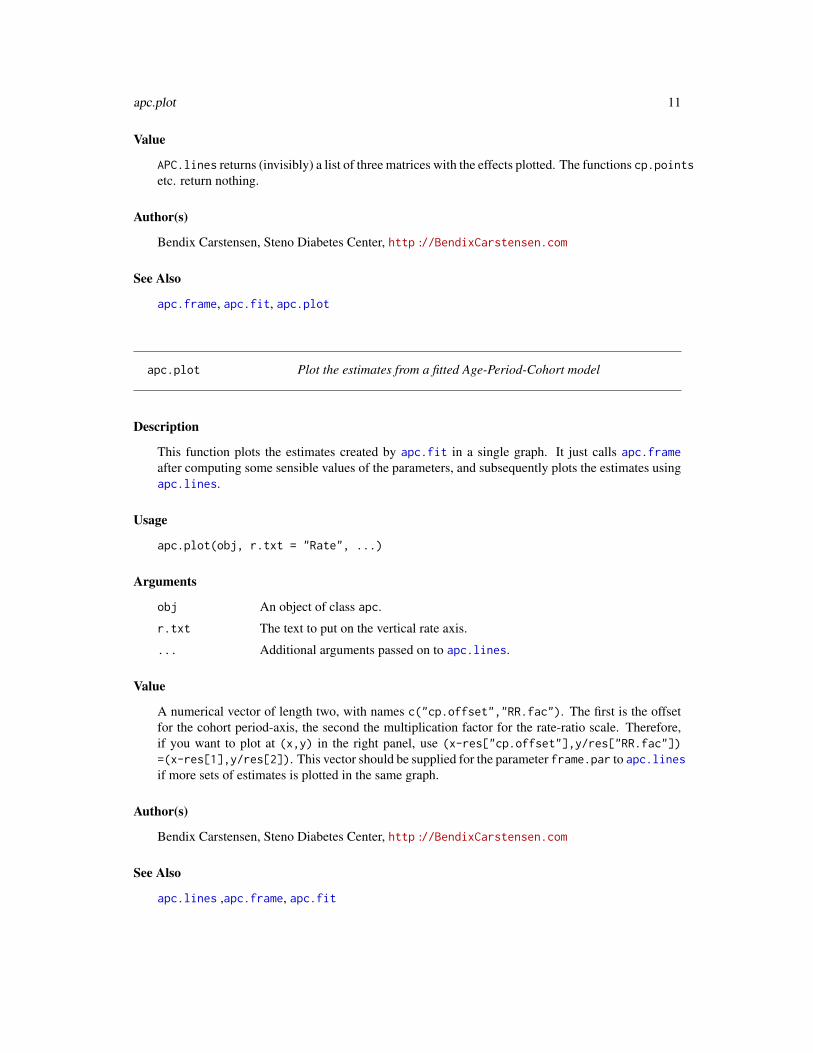
Value
APC.lines returns (invisibly) a list of three matrices with the effects plotted. The functions cp.pointsetc. return nothing.
Author(s)
Bendix Carstensen, Steno Diabetes Center, http://BendixCarstensen.com
See Also
apc.frame, apc.fit, apc.plot
apc.plot Plot the estimates from a fitted Age-Period-Cohort model
Description
This function plots the estimates created by apc.fit in a single graph. It just calls apc.frameafter computing some sensible values of the parameters, and subsequently plots the estimates usingapc.lines.
Usage
apc.plot(obj, r.txt = "Rate", ...)
Arguments
obj An object of class apc.
r.txt The text to put on the vertical rate axis.
... Additional arguments passed on to apc.lines.
Value
A numerical vector of length two, with names c("cp.offset","RR.fac"). The first is the offsetfor the cohort period-axis, the second the multiplication factor for the rate-ratio scale. Therefore,if you want to plot at (x,y) in the right panel, use (x-res["cp.offset"],y/res["RR.fac"])=(x-res[1],y/res[2]). This vector should be supplied for the parameter frame.par to apc.linesif more sets of estimates is plotted in the same graph.
Author(s)
Bendix Carstensen, Steno Diabetes Center, http://BendixCarstensen.com
See Also
apc.lines ,apc.frame, apc.fit
12 B.dk
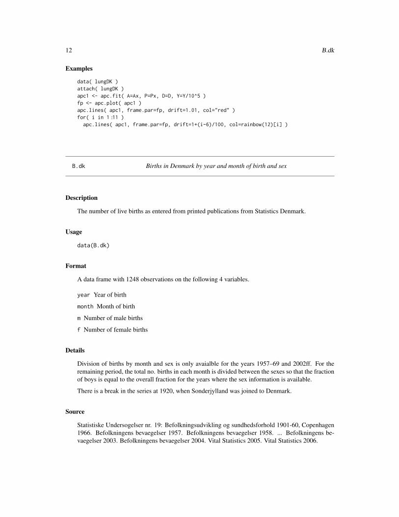
Examples
data( lungDK )attach( lungDK )apc1 <- apc.fit( A=Ax, P=Px, D=D, Y=Y/10^5 )fp <- apc.plot( apc1 )apc.lines( apc1, frame.par=fp, drift=1.01, col="red" )for( i in 1:11 )
apc.lines( apc1, frame.par=fp, drift=1+(i-6)/100, col=rainbow(12)[i] )
B.dk Births in Denmark by year and month of birth and sex
Description
The number of live births as entered from printed publications from Statistics Denmark.
Usage
data(B.dk)
Format
A data frame with 1248 observations on the following 4 variables.
year Year of birth
month Month of birth
m Number of male births
f Number of female births
Details
Division of births by month and sex is only avaialble for the years 1957–69 and 2002ff. For theremaining period, the total no. births in each month is divided between the sexes so that the fractionof boys is equal to the overall fraction for the years where the sex information is available.
There is a break in the series at 1920, when Sonderjylland was joined to Denmark.
Source
Statistiske Undersogelser nr. 19: Befolkningsudvikling og sundhedsforhold 1901-60, Copenhagen1966. Befolkningens bevaegelser 1957. Befolkningens bevaegelser 1958. ... Befolkningens be-vaegelser 2003. Befolkningens bevaegelser 2004. Vital Statistics 2005. Vital Statistics 2006.
bdendo 13
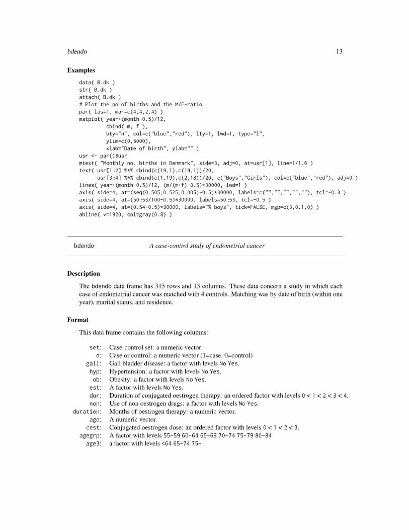
Examples
data( B.dk )str( B.dk )attach( B.dk )# Plot the no of births and the M/F-ratiopar( las=1, mar=c(4,4,2,4) )matplot( year+(month-0.5)/12,
cbind( m, f ),bty="n", col=c("blue","red"), lty=1, lwd=1, type="l",ylim=c(0,5000),xlab="Date of birth", ylab="" )
usr <- par()$usrmtext( "Monthly no. births in Denmark", side=3, adj=0, at=usr[1], line=1/1.6 )text( usr[1:2] %*% cbind(c(19,1),c(19,1))/20,
usr[3:4] %*% cbind(c(1,19),c(2,18))/20, c("Boys","Girls"), col=c("blue","red"), adj=0 )lines( year+(month-0.5)/12, (m/(m+f)-0.5)*30000, lwd=1 )axis( side=4, at=(seq(0.505,0.525,0.005)-0.5)*30000, labels=c("","","","",""), tcl=-0.3 )axis( side=4, at=(50:53/100-0.5)*30000, labels=50:53, tcl=-0.5 )axis( side=4, at=(0.54-0.5)*30000, labels="% boys", tick=FALSE, mgp=c(3,0.1,0) )abline( v=1920, col=gray(0.8) )
bdendo A case-control study of endometrial cancer
Description
The bdendo data frame has 315 rows and 13 columns. These data concern a study in which eachcase of endometrial cancer was matched with 4 controls. Matching was by date of birth (within oneyear), marital status, and residence.
Format
This data frame contains the following columns:
set: Case-control set: a numeric vectord: Case or control: a numeric vector (1=case, 0=control)
gall: Gall bladder disease: a factor with levels No Yes.hyp: Hypertension: a factor with levels No Yes.ob: Obesity: a factor with levels No Yes.
est: A factor with levels No Yes.dur: Duration of conjugated oestrogen therapy: an ordered factor with levels 0 < 1 < 2 < 3 < 4.non: Use of non oestrogen drugs: a factor with levels No Yes.
duration: Months of oestrogen therapy: a numeric vector.age: A numeric vector.cest: Conjugated oestrogen dose: an ordered factor with levels 0 < 1 < 2 < 3.
agegrp: A factor with levels 55-59 60-64 65-69 70-74 75-79 80-84age3: a factor with levels <64 65-74 75+
14 births
Source
Breslow NE, and Day N, Statistical Methods in Cancer Research. Volume I: The Analysis of Case-Control Studies. IARC Scientific Publications, IARC:Lyon, 1980.
Examples
data(bdendo)
bdendo11 A 1:1 subset of the endometrial cancer case-control study
Description
The bdendo11 data frame has 126 rows and 13 columns. This is a subset of the dataset bdendo inwhich each case was matched with a single control.
Source
Breslow NE, and Day N, Statistical Methods in Cancer Research. Volume I: The Analysis of Case-Control Studies. IARC Scientific Publications, IARC:Lyon, 1980.
Examples
data(bdendo11)
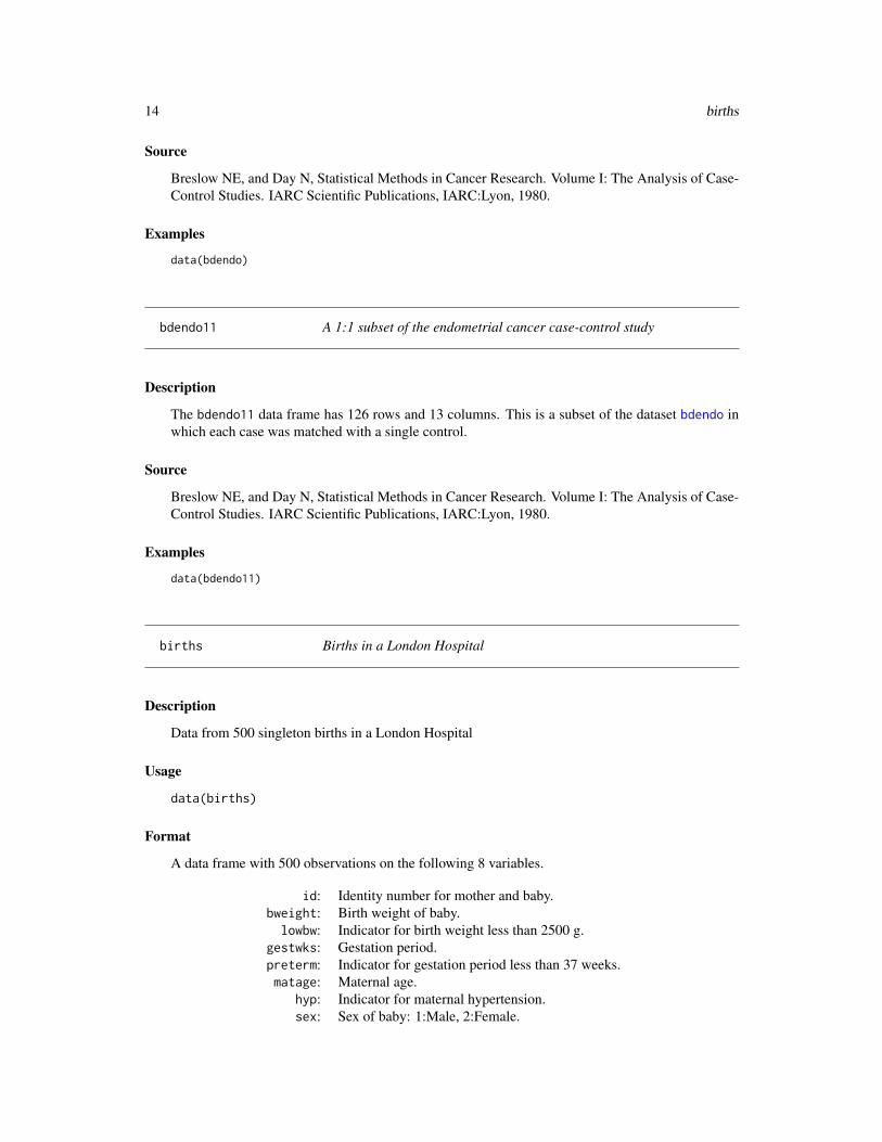
births Births in a London Hospital
Description
Data from 500 singleton births in a London Hospital
Usage
data(births)
Format
A data frame with 500 observations on the following 8 variables.
id: Identity number for mother and baby.bweight: Birth weight of baby.lowbw: Indicator for birth weight less than 2500 g.
gestwks: Gestation period.preterm: Indicator for gestation period less than 37 weeks.matage: Maternal age.
hyp: Indicator for maternal hypertension.sex: Sex of baby: 1:Male, 2:Female.

boxes.MS 15
Source
Anonymous
References
Michael Hills and Bianca De Stavola (2002). A Short Introduction to Stata 8 for Biostatistics,Timberlake Consultants Ltd http://www.timberlake.co.uk
Examples
data(births)
blcaIT Bladder cancer mortality in Italian males
Description
Number of deaths from bladder cancer and person-years in the Italian male population 1955–1979,in ages 25–79.
Format
A data frame with 55 observations on the following 4 variables:
age: Age at death. Left endpoint of age classperiod: Period of death. Left endpoint of period
D: Number of deathsY: Number of person-years.
Examples
data(blcaIT)
boxes.MS Draw boxes and arrows for illustration of multistate models.
Description
Boxes can be drawn with text (tbox) or a cross (dbox), and arrows pointing between the boxes(boxarr) can be drawn automatically not overlapping the boxes. The boxes method for Lexisobjects generates displays of states with person-years and transitions with events or rates.
16 boxes.MS
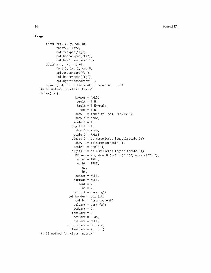
Usage
tbox( txt, x, y, wd, ht,font=2, lwd=2,col.txt=par("fg"),col.border=par("fg"),col.bg="transparent" )
dbox( x, y, wd, ht=wd,font=2, lwd=2, cwd=5,col.cross=par("fg"),col.border=par("fg"),col.bg="transparent" )
boxarr( b1, b2, offset=FALSE, pos=0.45, ... )## S3 method for class ’Lexis’boxes( obj,
boxpos = FALSE,wmult = 1.5,hmult = 1.5*wmult,cex = 1.5,
show = inherits( obj, "Lexis" ),show.Y = show,
scale.Y = 1,digits.Y = 1,show.D = show,
scale.D = FALSE,digits.D = as.numeric(as.logical(scale.D)),show.R = is.numeric(scale.R),
scale.R = scale.D,digits.R = as.numeric(as.logical(scale.R)),DR.sep = if( show.D ) c("\n(",")") else c("",""),eq.wd = TRUE,eq.ht = TRUE,
wd,ht,
subset = NULL,exclude = NULL,
font = 2,lwd = 2,
col.txt = par("fg"),col.border = col.txt,
col.bg = "transparent",col.arr = par("fg"),lwd.arr = 2,font.arr = 2,pos.arr = 0.45,txt.arr = NULL,
col.txt.arr = col.arr,offset.arr = 2, ... )
## S3 method for class ’matrix’
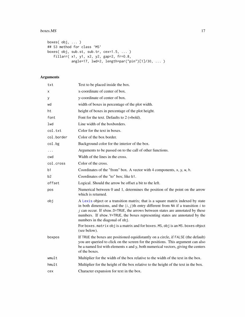
boxes.MS 17
boxes( obj, ... )## S3 method for class ’MS’boxes( obj, sub.st, sub.tr, cex=1.5, ... )
fillarr( x1, y1, x2, y2, gap=2, fr=0.8,angle=17, lwd=2, length=par("pin")[1]/30, ... )
Arguments
txt Text to be placed inside the box.
x x-coordinate of center of box.
y y-coordinate of center of box.
wd width of boxes in percentage of the plot width.
ht height of boxes in percentage of the plot height.
font Font for the text. Defaults to 2 (=bold).
lwd Line width of the boxborders.
col.txt Color for the text in boxes.
col.border Color of the box border.
col.bg Background color for the interior of the box.
... Arguments to be passed on to the call of other functions.
cwd Width of the lines in the cross.
col.cross Color of the cross.
b1 Coordinates of the "from" box. A vector with 4 components, x, y, w, h.
b2 Coordinates of the "to" box; like b1.
offset Logical. Should the arrow be offset a bit to the left.
pos Numerical between 0 and 1, determines the position of the point on the arrowwhich is returned.
obj A Lexis object or a transition matrix; that is a square matrix indexed by statein both dimensions, and the (i, j)th entry different from NA if a transition i toj can occur. If show.D=TRUE, the arrows between states are annotated by thesenumbers. If show.Y=TRUE, the boxes representing states are annotated by thenumbers in the diagonal of obj.For boxes.matrix obj is a matrix and for boxes.MS, obj is an MS.boxes object(see below).
boxpos If TRUE the boxes are positioned equidistantly on a circle, if FALSE (the default)you are queried to click on the screen for the positions. This argument can alsobe a named list with elements x and y, both numerical vectors, giving the centersof the boxes.
wmult Multiplier for the width of the box relative to the width of the text in the box.
hmult Multiplier for the height of the box relative to the height of the text in the box.
cex Character expansion for text in the box.
18 boxes.MS
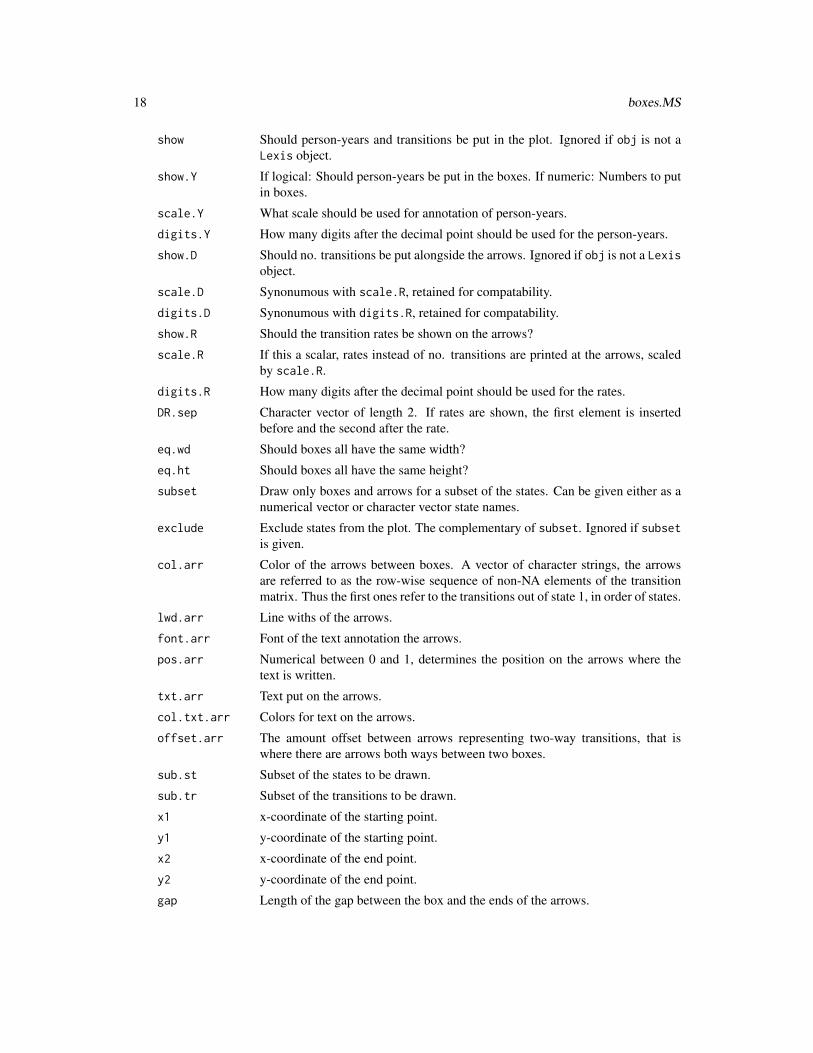
show Should person-years and transitions be put in the plot. Ignored if obj is not aLexis object.
show.Y If logical: Should person-years be put in the boxes. If numeric: Numbers to putin boxes.
scale.Y What scale should be used for annotation of person-years.
digits.Y How many digits after the decimal point should be used for the person-years.
show.D Should no. transitions be put alongside the arrows. Ignored if obj is not a Lexisobject.
scale.D Synonumous with scale.R, retained for compatability.
digits.D Synonumous with digits.R, retained for compatability.
show.R Should the transition rates be shown on the arrows?
scale.R If this a scalar, rates instead of no. transitions are printed at the arrows, scaledby scale.R.
digits.R How many digits after the decimal point should be used for the rates.
DR.sep Character vector of length 2. If rates are shown, the first element is insertedbefore and the second after the rate.
eq.wd Should boxes all have the same width?
eq.ht Should boxes all have the same height?
subset Draw only boxes and arrows for a subset of the states. Can be given either as anumerical vector or character vector state names.
exclude Exclude states from the plot. The complementary of subset. Ignored if subsetis given.
col.arr Color of the arrows between boxes. A vector of character strings, the arrowsare referred to as the row-wise sequence of non-NA elements of the transitionmatrix. Thus the first ones refer to the transitions out of state 1, in order of states.
lwd.arr Line withs of the arrows.
font.arr Font of the text annotation the arrows.
pos.arr Numerical between 0 and 1, determines the position on the arrows where thetext is written.
txt.arr Text put on the arrows.
col.txt.arr Colors for text on the arrows.
offset.arr The amount offset between arrows representing two-way transitions, that iswhere there are arrows both ways between two boxes.
sub.st Subset of the states to be drawn.
sub.tr Subset of the transitions to be drawn.
x1 x-coordinate of the starting point.
y1 y-coordinate of the starting point.
x2 x-coordinate of the end point.
y2 y-coordinate of the end point.
gap Length of the gap between the box and the ends of the arrows.

boxes.MS 19
fr Length of the arrow as the fraction of the distance between the boxes. Ignoredunless given explicitly, in which case any value given for gap is ignored.
angle What angle should the arrow-head have?
length Length of the arrow head in inches. Defaults to 1/30 of the physical width of theplot.
Details
These functions are designed to facilitate the drawing of multistate models, mainly by automaticcalculation of the arrows between boxes.
tbox draws a box with centered text, and returns a vector of location, height and width of the box.This is used when drawing arrows between boxes. dbox draws a box with a cross, symbolizing adeath state. boxarr draws an arrow between two boxes, making sure it does not intersect the boxes.Only straight lines are drawn.
boxes.Lexis takes as input a Lexis object sets up an empty plot area (with axes 0 to 100 in bothdirections) and if boxpos=FALSE (the default) prompts you to click on the locations for the stateboxes, and then draws arrows implied by the actual transitions in the Lexis object. The default isto annotate the transitions with the number of transitions.
A transition matrix can also be supplied, in which case the row/column names are used as statenames, diagnonal elements taken as person-years, and off-diagnonal elements as number of transi-tions. This also works for boxes.matrix.
Optionally returns the R-code reproducing the plot in a file, which can be useful if you want toproduce exactly the same plot with differing arrow colors etc.
boxarr draws an arrow between two boxes, on the line connecting the two box centers. The offsetargument is used to offset the arrow a bit to the left (as seen in the direction of the arrow) on order toaccommodate arrows both ways between boxes. boxarr returns a named list with elements x, y andd, where the two former give the location of a point on the arrow used for printing (see argumentpos) and the latter is a unit vector in the direction of the arrow, which is used by boxes.Lexis toposition the annotation of arrows with the number of transitions.
boxes.MS re-draws what boxes.Lexis has done based on the object of class MS produced byboxes.Lexis. The point being that the MS object is easily modifiable, and thus it is a machinery tomake variations of the plot with different color annotations etc.
fill.arr is just a utility drawing nicer arrows than the default arrows command, basically byusing filled arrow-heads; called by boxarr.
Value
The functions tbox and dbox return the location and dimension of the boxes, c(x,y,w,h), whichare designed to be used as input to the boxarr function.
The boxarr function returns the coordinates (as a named list with names x and y) of a point on thearrow, designated to be used for annotation of the arrow.
The function boxes.Lexis returns an MS object, a list with five elements: 1) Boxes - a dataframewith one row per box and columns xx, yy, wd, ht, font, lwd, col.txt, col.border and col.bg,2) an object State.names with names of states (possibly an expression, hence not possible toinclude as a column in Boxes), 3) a matrix Tmat, the transition matrix, 4) a data frame, Arrows with

20 boxes.MS
one row per transition and columns: lwd.arr, col.arr, pos.arr, col.txt.arr, font.arr andoffset.arr and 5) an object Arrowtext with names of states (possibly an expression, hence notpossible to include as a column in Arrows)
An MS object is used as input to boxes.MS, the primary use is to modify selected entries in the MSobject first, e.g. colors, or supply subsetting arguments in order to produce displays that have thesame structure, but with different colors etc.
Author(s)
Bendix Carstensen
See Also
tmat.Lexis
Examples
par( mar=c(0,0,0,0), cex=1.5 )plot( NA,
bty="n",xlim=0:1*100, ylim=0:1*100, xaxt="n", yaxt="n", xlab="", ylab="" )
bw <- tbox( "Well" , 10, 60, 22, 10, col.txt="blue" )bo <- tbox( "other Ca", 45, 80, 22, 10, col.txt="gray" )bc <- tbox( "Ca" , 45, 60, 22, 10, col.txt="red" )bd <- tbox( "DM" , 45, 40, 22, 10, col.txt="blue" )bcd <- tbox( "Ca + DM" , 80, 60, 22, 10, col.txt="gray" )bdc <- tbox( "DM + Ca" , 80, 40, 22, 10, col.txt="red" )
boxarr( bw, bo , col=gray(0.7), lwd=3 )# Note the argument adj= can takes values outside (0,1)text( boxarr( bw, bc , col="blue", lwd=3 ),
expression( lambda[Well] ), col="blue", adj=c(1,-0.2), cex=0.8 )boxarr( bw, bd , col=gray(0.7) , lwd=3 )boxarr( bc, bcd, col=gray(0.7) , lwd=3 )
text( boxarr( bd, bdc, col="blue", lwd=3 ),expression( lambda[DM] ), col="blue", adj=c(1.1,-0.2), cex=0.8 )
# Set up a transition matrix allowing recoverytm <- rbind( c(NA,1,1), c(1,NA,1), c(NA,NA,NA) )rownames(tm) <- colnames(tm) <- c("Cancer","Recurrence","Dead")tmboxes.matrix( tm, boxpos=TRUE )
# Illustrate texting of arrowsboxes.Lexis( tm, boxpos=TRUE, txt.arr=c("en","to","tre","fire") )zz <- boxes( tm, boxpos=TRUE, txt.arr=c(expression(lambda[C]),
expression(mu[C]),"recovery",expression(mu[R]) ) )
# Change color of a boxzz$Boxes[3,c("col.bg","col.border")] <- "green"boxes( zz )

brv 21
# Set up a Lexis objectdata(DMlate)str(DMlate)dml <- Lexis( entry=list(Per=dodm, Age=dodm-dobth, DMdur=0 ),
exit=list(Per=dox),exit.status=factor(!is.na(dodth),labels=c("DM","Dead")),
data=DMlate[1:1000,] )
# Split follow-up at Insulindmi <- cutLexis( dml, cut=dml$doins, new.state="Ins", pre="DM" )summary( dmi )boxes( dmi, boxpos=TRUE )
# Set up a bogus recovery date jut to illustrate two-way transitionsdmi$dorec <- dmi$doins + runif(nrow(dmi),0.5,10)dmi$dorec[dmi$dorec>dmi$dox] <- NAdmR <- cutLexis( dmi, cut=dmi$dorec, new.state="DM", pre="Ins" )summary( dmR )boxes( dmR, boxpos=TRUE )boxes( dmR, boxpos=TRUE, show.D=FALSE )boxes( dmR, boxpos=TRUE, show.D=FALSE, show.Y=FALSE )boxes( dmR, boxpos=TRUE, scale.R=1000 )MSobj <- boxes( dmR, boxpos=TRUE, scale.R=1000, show.D=FALSE )MSobj <- boxes( dmR, boxpos=TRUE, scale.R=1000, DR.sep=c(" (",")") )class( MSobj )boxes( MSobj )MSobj$Boxes[1,c("col.txt","col.border")] <- "red"MSobj$Arrows[1:2,"col.arr"] <- "red"boxes( MSobj )
brv Bereavement in an elderly cohort
Description
The brv data frame has 399 rows and 11 columns. The data concern the possible effect of maritalbereavement on subsequent mortality. They arose from a survey of the physical and mental healthof a cohort of 75-year-olds in one large general practice. These data concern mortality up to 1January, 1990 (although further follow-up has now taken place).
Subjects included all lived with a living spouse when they entered the study. There are three distinctgroups of such subjects: (1) those in which both members of the couple were over 75 and thereforeincluded in the cohort, (2) those whose spouse was below 75 (and was not, therefore, part of themain cohort study), and (3) those living in larger households (that is, not just with their spouse).
Format
This data frame contains the following columns:
22 cal.yr
id subject identifier, a numeric vector
couple couple identifier, a numeric vector
dob date of birth, a date
doe date of entry into follow-up study, a date
dox date of exit from follow-up study, a date
dosp date of death of spouse, a date (if the spouse was still alive at the end of follow-up,this wascoded to January 1, 2000)
fail status at end of follow-up, a numeric vector (0=alive,1=dead)
group see Description, a numeric vector
disab disability score, a numeric vector
health perceived health status score, a numeric vector
sex a factor with levels Male and Female
Source
Jagger C, and Sutton CJ, Death after Marital Bereavement. Statistics in Medicine, 10:395-404,1991. (Data supplied by Carol Jagger).
Examples
data(brv)
cal.yr Functions to convert character, factor and various date objects into anumber, and vice versa.
Description
Dates are converted to a numerical value, giving the calendar year as a fractional number. 1 January1970 is converted to 1970.0, and other dates are converted by assuming that years are all 365.25days long, so inaccuracies may arise, for example, 1 Jan 2000 is converted to 1999.999. Differencesbetween converted values will be 1/365.25 of the difference between corresponding Date objects.
Usage
cal.yr( x, format="%Y-%m-%d", wh=NULL )## S3 method for class ’cal.yr’
as.Date( x, ... )
cal.yr 23
Arguments
x A factor or character vector, representing a date in format format, or an objectof class Date, POSIXlt, POSIXct, date, dates or chron (the latter two requiresthe chron package). If x is a data frame, all variables in the data-frame whichare of one the classes mentioned are converted to class cal.yr. See arguemt wh,though.
format Format of the date values if x is factor or character. If this argument is sup-plied and x is a datafame, all character variables are converted to class cal.yr.Factors in the dataframe will be ignored.
wh Indices of the variables to convert if x is a data frame. Can be either a numericalor character vector.
... Arguments passed on from other methods.
Value
cal.yr returns a numerical vector of the same length as x, of class c("cal.yr","numeric"). If xis a data frame a dataframe with some of the columns converted to class "cal.yr" is returned.
as.Date.cal.yr returns a Date object.
Author(s)
Bendix Carstensen, Steno Diabetes Center \& Dept. of Biostatistics, University of Copenhagen,<[email protected]>, http://BendixCarstensen.com
See Also
DateTimeClasses, Date
Examples
# Character vector of dates:birth <- c("14/07/1852","01/04/1954","10/06/1987","16/05/1990",
"12/11/1980","01/01/1997","01/01/1998","01/01/1999")# Proper conversion to class "Date":birth.dat <- as.Date( birth, format="%d/%m/%Y" )# Converson of character to class "cal.yr"bt.yr <- cal.yr( birth, format="%d/%m/%Y" )# Back to class "Date":bt.dat <- as.Date( bt.yr )# Numerical calculation of days since 1.1.1970:days <- Days <- (bt.yr-1970)*365.25# Blunt assignment of class:class( Days ) <- "Date"# Then data.frame() to get readable output of results:data.frame( birth, birth.dat, bt.yr, bt.dat, days, Days, round(Days) )
24 ccwc
ccwc Generate a nested case-control study
Description
Given the basic outcome variables for a cohort study: the time of entry to the cohort, the time of exitand the reason for exit ("failure" or "censoring"), this function computes risk sets and generates amatched case-control study in which each case is compared with a set of controls randomly sampledfrom the appropriate risk set. Other variables may be matched when selecting controls.
Usage
ccwc( entry=0, exit, fail, origin=0, controls=1, match=list(),include=list(), data=NULL, silent=FALSE )
Arguments
entry Time of entry to follow-up
exit Time of exit from follow-up
fail Status on exit (1=Fail, 0=Censored)
origin Origin of analysis time scale
controls The number of controls to be selected for each case
match List of categorical variables on which to match cases and controls
include List of other variables to be carried across into the case-control study
data Data frame in which to look for input variables
silent If FALSE, echos a . to the screen for each case-control set created; otherwiseproduces no output.
Value
The case-control study, as a dataframe containing:
Set case-control set number
Map row number of record in input dataframe
Time failure time of the case in this set
Fail failure status (1=case, 0=control)
These are followed by the matching variables, and finally by the variables in the include list
Author(s)
David Clayton

ci.cum 25
References
Clayton and Hills, Statistical Models in Epidemiology, Oxford University Press, Oxford:1993.
See Also
Lexis
Examples
## For the diet and heart dataset, create a nested case-control study# using the age scale and matching on job#data(diet)dietcc <- ccwc( doe, dox, chd, origin=dob, controls=2, data=diet,
include=energy, match=job)
ci.cum Compute cumulative sum of estimates.
Description
Computes the cumulative sum of parameter functions and the standard error of it. Optionally theexponential is applied to the parameter functions before it is cumulated.
Usage
ci.cum( obj,ctr.mat = NULL,subset = NULL,intl = 1,
alpha = 0.05,Exp = TRUE,
sample = FALSE )
Arguments
obj A model object (of class lm, glm, coxph, survreg, lme,mer,nls,gnlm, MIresultor polr).
ctr.mat Contrast matrix defining the parameter functions from the parameters of themodel.
subset Subset of the parameters of the model to which ctr.mat should be applied.intl Interval length for the cumulation. Either a constant or a numerical vector of
length nrow(ctr.mat).alpha Significance level used when computing confidence limits.Exp Should the parameter function be exponentiated before it is cumulated?sample Should a sample of the original parameters be used to compute a cumulative
rate?

26 ci.cum
Details
The purpose of this function is to compute cumulative rate based on a model for the rates. If themodel is a multiplicative model for the rates, the purpose of ctr.mat is to return a vector of ratesor log-rates when applied to the coefficients of the model. If log-rates are returned from the model,the they should be exponentiated before cumulated, and the variances computed accordingly. Sincelog-linear models are the most common the Exp parameter defaults to TRUE.
Value
A matrix with 4 columns: Estimate, lower and upper c.i. and standard error. If sample is TRUE,a sampled vector is reurned, if sample is numeric a matrix with sample columns is returned, eachcolumn a cumulative rate based on a random sample from the distribution of the parameter esti-mates.
Author(s)
Bendix Carstensen, http://BendixCarstensen.com
See Also
See also ci.lin
Examples
# Packages required for this examplelibrary( splines )library( survival )data( lung )par( mfrow=c(1,2) )
# Plot the Kaplan-meier-estimatorplot( survfit( Surv( time, status==2 ) ~ 1, data=lung ) )
# Declare data as LexislungL <- Lexis( exit=list("tfd"=time),
exit.status=(status==2)*1, data=lung )summary( lungL )
# Cut the follow-up every 10 dayssL <- splitLexis( lungL, "tfd", breaks=seq(0,1100,10) )str( sL )summary( sL )
# Fit a Poisson model with a natural spline for the effect of time.# Extract the variables neededD <- status(sL, "exit")Y <- dur(sL)tB <- timeBand( sL, "tfd", "left" )MM <- ns( tB, knots=c(50,100,200,400,700), intercept=TRUE )mp <- glm( D ~ MM - 1 + offset(log(Y)),
family=poisson, eps=10^-8, maxit=25 )
ci.lin 27
# Contrast matrix to extract effects, i.e. matrix to multiply with the# coefficients to produce the log-rates: unique rows of MM, in time order.T.pt <- sort( unique( tB ) )T.wh <- match( T.pt, tB )Lambda <- ci.cum( mp, ctr.mat=MM[T.wh,], intl=diff(c(0,T.pt)) )
# Put the estimated survival function on top of the KM-estimatormatlines( c(0,T.pt[-1]), exp(-Lambda[,1:3]), lwd=c(3,1,1), lty=1, col="Red" )
# Extract and plot the fitted intensity functionlambda <- ci.lin( mp, ctr.mat=MM[T.wh,], Exp=TRUE )matplot( T.pt, lambda[,5:7]*10^3, type="l", lwd=c(3,1,1), col="black", lty=1,
log="y", ylim=c(0.2,20) )
ci.lin Compute linear functions of parameters with s.e.
Description
For a given model object the function computes a linear function of the parameters and the corre-sponding standard errors, p-values and confidence intervals.
Usage
ci.lin( obj,ctr.mat = NULL,subset = NULL,subint = NULL,diffs = FALSE,fnam = !diffs,vcov = FALSE,
alpha = 0.05,df = Inf,Exp = FALSE,
sample = FALSE )ci.exp( ..., Exp = TRUE )Wald( obj, H0=0, ... )ci.mat( alpha = 0.05, df=Inf )
Arguments
obj A model object (of class lm, glm, coxph, survreg, lme, mer, nls, gnlm, MIresultor polr).
ctr.mat Contrast matrix to be multiplied to the parameter vector, i.e. the desired linearfunction of the parameters.
28 ci.lin
subset The subset of the parameters to be used. If given as a character vector, theelements are in turn matched against the parameter names (using grep) to findthe subset. Repeat parameters may result from using a character vector. This isconsidered a facility.
subint SUBset selection like for subset, except that elements of a character vectorgiven as argument will be used to select a number of subsets of parameters andonly the INTersection of these is returned.
diffs If TRUE, all differences between parameters in the subset are computed. ctr.matis ignored. If obj inherits from lm, and subset is given as a string subset isused to search among the factors in the model and differences of all factor levelsfor the first match are shown. If subset does not match any of the factors in themodel, all pairwise differences between parameters matching are returned.
fnam Should the common part of the parameter names be included with the annotationof contrasts? Ignored if diffs==T. If a sting is supplied this will be prefixed tothe labels.
vcov Should the covariance matrix of the set of parameters be returned? If this is set,Exp is ignored. See details.
alpha Significance level for the confidence intervals.
df Integer. Number of degrees of freedom in the t-distribution used to compute thequantiles used to construct the confidence intervals.
Exp If TRUE columns 5:6 are replaced with exp( columns 1,5,6 ).
sample Logical or numerical. If TRUE or numerical a sample of size as.numeric(sample)of the linear parameter function as defined by subset and ctr.mat is returned.
H0 The null values for the selected/transformed parameters to be tested by a Waldtest. Must have the same length as the selected parameter vector.
... Parameters passed on to ci.lin.
Value
ci.lin returns a matrix with number of rows and rownames as ctr.mat. The columns are Es-timate, Std.Err, z, P, 2.5% and 97.5%. If vcov=TRUE a list with components est, the desiredfunctional of the parameters and vcov, the variance covariance matrix of this, is returned but notprinted. If Exp==TRUE the confidence intervals for the parameters are replaced with three columns:exp(estimate,c.i.).
ci.exp returns only the exponentiated parameter estimates with confidence intervals. It is merely awrapper for ci.lin, fishing out the last 3 columns from ci.lin(...,Exp=TRUE).
Wald computes a Wald test for a subset of (possibly linearly transformed) parameters. The selectionof the subset of parameters is the same as for ci.lin. Using the ctr.mat argument makes itpossible to do a Wald test for equality of parameters. Wald returns a named numerical vector oflength 3, with names Chisq, d.f. and P.
ci.mat returns a 2 by 3 matrix with rows c(1,0,0) and c(0,-1,1)*1.96, devised to post-multiplyto a p by 2 matrix with columns of estimates and standard errors, so as to produce a p by 3 matrix ofestimates and confidence limits. Used internally in ci.lin and ci.cum. The 1.96 is replaced by theappropriate quantile from the normal or t-distribution when arguments alpha and/or df are given.
ci.pd 29
Author(s)
Bendix Carstensen, BendixCarstensen.com & Michael Hills http://www.mhills.pwp.blueyonder.co.uk/
See Also
See also ci.cum
Examples
# Bogus data:f <- factor( sample( letters[1:5], 200, replace=TRUE ) )g <- factor( sample( letters[1:3], 200, replace=TRUE ) )x <- rnorm( 200 )y <- 7 + as.integer( f ) * 3 + 2 * x + 1.7 * rnorm( 200 )
# Fit a simple model:mm <- lm( y ~ x + f + g )ci.lin( mm )ci.lin( mm, subset=3:6, diff=TRUE, fnam=FALSE )ci.lin( mm, subset=3:6, diff=TRUE, fnam=TRUE )ci.lin( mm, subset="f", diff=TRUE, fnam="f levels:" )print( ci.lin( mm, subset="g", diff=TRUE, fnam="gee!:", vcov=TRUE ) )
# Use character defined subset to get ALL contrasts:ci.lin( mm, subset="f", diff=TRUE )
# A Wald test of wheter the g-parameters are 0Wald( mm, subset="g" )# Wald test of whether the three first f-parameters are equal:( CM <- rbind( c(1,-1,0,0), c(1,0,-1,0)) )Wald( mm, subset="f", ctr.mat=CM )# or alternatively( CM <- rbind( c(1,-1,0,0), c(0,1,-1,0)) )Wald( mm, subset="f", ctr.mat=CM )
ci.pd Compute confidence limits for a difference of two independent propor-tions.
Description
The usual formula for the c.i. of at difference of proportions is inaccurate. Newcombe has compared11 methods and method 10 in his paper looks like a winner. It is implemented here.
30 ci.pd
Usage
ci.pd(aa, bb=NULL, cc=NULL, dd=NULL,method = "Nc",alpha = 0.05, conf.level=0.95,digits = 3,print = TRUE,
detail.labs = FALSE )
Arguments
aa Numeric vector of successes in sample 1. Can also be a matrix or array (seedetails).
bb Successes in sample 2.
cc Failures in sample 1.
dd Failures in sample 2.
method Method to use for calculation of confidence interval, see "Details".
alpha Significance level
conf.level Confidence level
print Should an account of the two by two table be printed.
digits How many digits should the result be rounded to if printed.
detail.labs Should the computing of probability differences be reported in the labels.
Details
Implements method 10 from Newcombe(1998) (method="Nc") or from Agresti & Caffo(2000)(method="AC").
aa, bb, cc and dd can be vectors. If aa is a matrix, the elements [1:2,1:2] are used, with successesaa[,1:2]. If aa is a three-way table or array, the elements aa[1:2,1:2,] are used.
Value
A matrix with three columns: probability difference, lower and upper limit. The number of rowsequals the length of the vectors aa, bb, cc and dd or, if aa is a 3-way matrix, dim(aa)[3].
Author(s)
Bendix Carstensen, Esa Laara. http://BendixCarstensen.com
References
RG Newcombe: Interval estimation for the difference between independent proportions. Compari-son of eleven methods. Statistics in Medicine, 17, pp. 873-890, 1998.
A Agresti & B Caffo: Simple and effective confidence intervals for proportions and differences ofproportions result from adding two successes and two failures. The American Statistician, 54(4),pp. 280-288, 2000.

clogistic 31
See Also
twoby2, binom.test
Examples
( a <- matrix( sample( 10:40, 4 ), 2, 2 ) )ci.pd( a )twoby2( t(a) )prop.test( t(a) )( A <- array( sample( 10:40, 20 ), dim=c(2,2,5) ) )ci.pd( A )ci.pd( A, detail.labs=TRUE, digits=3 )
clogistic Conditional logistic regression
Description
Estimates a logistic regression model by maximizing the conditional likelihood. The conditionallikelihood calculations are exact, and scale efficiently to strata with large numbers of cases.
Usage
clogistic(formula, strata, data, subset, na.action, init,model = TRUE, x = FALSE, y = TRUE, contrasts = NULL,iter.max=20, eps=1e-6, toler.chol = sqrt(.Machine$double.eps))
Arguments
formula Model formulastrata Factor describing membership of strata for conditioningdata data frame containing the variables in the formula and strata argumentssubset subset of records to usena.action missing value handlinginit initial valuesmodel a logical value indicating whether model frame should be included as a compo-
nent of the returned valuex,y logical values indicating whether the response vector and model matrix used in
the fitting process should be returned as components of the returned value.contrasts an optional list. See the contrasts.arg of model.matrix.defaultiter.max maximum number of iterationseps Convergence tolerence. Iteration continues until the relative change in the con-
ditional log likelihood is less than eps. Must be positive.toler.chol Tolerance used for detection of a singularity during a Cholesky decomposition
of the variance martrix. This is used to detect redundant predictor variables.Must be less than eps.
32 contr.cum
Value
An object of class "clogistic". This is a list containing the following components:
coefficients the estimates of the log-odds ratio parameters. If the model is over-determinedthere will be missing values in the vector corresponding to the redundant columnsin the model matrix.
var the variance matrix of the coefficients. Rows and columns corresponding to anymissing coefficients are set to zero.
loglik a vector of length 2 containing the log-likelihood with the initial values and withthe final values of the coefficients.
iter number of iterations used.n number of observations used. Observations may be dropped either because they
are missing, or because they belong to a homogenous stratum. For more detailson which observations were used, see informative below.
informative if model=TRUE, a logical vector of length equal to the number of rows in themodel frame. This indicates whether an observation is informative, in the sensethat it makes a non-zero contribution to the log-likelihood. If model=FALSE, thisis NULL.
The output will also contain the following, for documentation see the glm object: terms, formula,call, contrasts, xlevels, and, optionally, x, y, and/or frame.
Author(s)
Martyn Plummer
See Also
glm
Examples
data(bdendo)clogistic(d ~ cest + dur, strata=set, data=bdendo)
contr.cum Contrast matrices
Description
Return a matrix of contrasts for factor coding.
Usage
contr.cum(n)contr.diff(n)contr.2nd(n)contr.orth(n)

cutLexis 33
Arguments
n A vector of levels for a factor, or the number of levels.
Details
These functions are used for creating contrast matrices for use in fitting regression models. Thecolumns of the resulting matrices contain contrasts which can be used for coding a factor with nlevels.
contr.cum gives a coding corresponding to successive differences between factor levels.
contr.diff gives a coding that correspond to the cumulative sum of the value for each level. Thisis not meaningful in a model where the intercept is included, therefore n columns ia always returned.
contr.2nd gives contrasts corresponding to 2nd order differences between factor levels. Returns amatrix with n-2 columns.
contr.orth gives a matrix with n-2 columns, which are mutually orthogonal and orthogonal to thematrix cbind(1,1:n)
Value
A matrix with n rows and k columns, with k=n for contr.diff k=n-1 for contr.cum k=n-2 forcontr.2nd and contr.orth.
Author(s)
Bendix Carstensen
See Also
contr.treatment
Examples
contr.cum(6)contr.2nd(6)contr.diff(6)contr.orth(6)
cutLexis Cut follow-up at a specified date for each person.
Description
Follow-up intervals in a Lexis object are divided into two sub-intervals: one before and one after anintermediate event. The intermediate event may denote a change of state, in which case the entryand exit status variables in the split Lexis object are modified.

34 cutLexis
Usage
cutLexis( data, cut, timescale = 1,new.state = nlevels(data$lex.Cst)+1,new.scale = FALSE,split.states = FALSE,progressive = FALSE,precursor.states = NULL,count = FALSE)
countLexis( data, cut, timescale = 1 )
Arguments
data A Lexis object.
cut A numeric vector with the times of the intermediate event. If a time is missing(NA) then the event is assumed to occur at time Inf. cut can also be a dataframe,see details.
timescale The timescale that cut refers to. Numeric or character.
new.state The state to which a transition occur at time cut. It may be a single value, whichis then applied to all rows of data, or a vector with a separate value for each row
new.scale Name of the timescale defined as "time since entry to new.state". If TRUE a namefor the new scale is constructed. See details.
split.states Should states that are not precursor states be split according to whether the in-termediate event has occurred.
progressive a logical flag that determines the changes to exit status. See details.precursor.states
an optional vector of states to be considered as "less severe" than new.state.See Details below
count logical indicating whether the countLexis options should be used. Specify-ing count=TRUE amounts to calling countLexis, in which case the argumentsnew.state, progressive and precursor.states will be ignored.
Details
The cutLexis function allows a number of different ways of specifying the cutpoints and of modi-fying the status variable.
If the cut argument is a dataframe it must have columns lex.id, cut and new.state. The valuesof lex.id must be unique. In this case it is assumed that each row represents a cutpoint (on thetimescale indicated in the argument timescale). This cutpoint will be applied to all records in datawith the corresponding lex.id. This makes it possible to apply cutLexis to a split Lexis object.
If a new.state argument is supplied, the status variable is only modified at the time of the cut point.However, it is often useful to modify the status variable after the cutpoint when an important eventoccurs. There are three distinct ways of doing this.
If the progressive=TRUE argument is given, then a "progressive" model is assumed, in which thestatus can either remain the same or increase during follow-up, but never decrease. This assumesthat the state variables lex.Cst and lex.Xst are either numeric or ordered factors. In this case,
cutLexis 35
if new.state=X, then any exit status with a value less than X is replaced with X. The Lexis objectmust already be progressive, so that there are no rows for which the exit status is less than the entrystatus. If lex.Cst and lex.Xst are factors they must be ordered factors if progressive=TRUE isgiven.
As an alternative to the progressive argument, an explicit vector of precursor states, that are con-sidered less severe than the new state, may be given. If new.state=X and precursor.states=c(Y,Z)then any exit status of Y or Z in the second interval is replaced with X and all other values for theexit status are retained.
The countLexis function is a variant of cutLexis when the cutpoint marks a recurrent event, andthe status variable is used to count the number of events that have occurred. Times given in cutrepresent times of new events. Splitting with countLexis increases the status variable by 1. If thecurrent status is X and the exit status is Y before cutting, then after cutting the entry status is X, X+1for the first and second intervals, respectively, and the exit status is X+1, Y+1 respectively. Moreoverthe values of the status is increased by 1 for all intervals for all intervals after the cut for the personin question. Hence, a call to countLexis is needed for as many times as the person with mostevents. But also it is immaterial in what order the cutpoints are entered.
Value
A Lexis object, for which each follow-up interval containing the cutpoint is split in two: one beforeand one after the cutpoint. An extra time-scale is added; the time since the event at cut. This is NAfor any follow-up prior to the intermediate event.
Note
The cutLexis function superficially resembles the splitLexis function. However, the splitLexisfunction splits on a vector of common cut-points for all rows of the Lexis object, whereas thecutLexis function splits on a single time point, which may be distinct for each row, modifies thestatus variables, and adds a new timescale.
Author(s)
Bendix Carstensen, Steno Diabetes Center, <[email protected]>,
Martyn Plummer, IARC, <[email protected]>
See Also
splitLexis, Lexis, summary.Lexis, boxes.Lexis
Examples
# A small artificial examplexx <- Lexis( entry=list(age=c(17,24,33,29),per=c(1920,1933,1930,1929)),
duration=c(23,57,12,15), exit.status=c(1,2,1,2) )xxcut <- c(33,47,29,50)cutLexis(xx, cut, new.state=3, precursor=1)cutLexis(xx, cut, new.state=3, precursor=2)cutLexis(xx, cut, new.state=3, precursor=1:2)
36 detrend
# The same as the last examplecutLexis(xx, cut, new.state=3)
# The same example with a factor status variableyy <- Lexis(entry = list(age=c(17,24,33,29),per=c(1920,1933,1930,1929)),
duration = c(23,57,12,15),entry.status = factor(rep("alpha",4),levels=c("alpha","beta","gamma")),exit.status = factor(c("alpha","beta","alpha","beta"),levels=c("alpha","beta","gamma")))
cutLexis(yy,c(33,47,29,50),precursor="alpha",new.state="gamma")cutLexis(yy,c(33,47,29,50),precursor=c("alpha","beta"),new.state="aleph")
## Using a dataframe as cut argumentrl <- data.frame( lex.id=1:3, cut=c(19,53,26), timescale="age", new.state=3 )rlcutLexis( xx, rl )cutLexis( xx, rl, precursor=1 )cutLexis( xx, rl, precursor=0:2 )
## It is immaterial in what order splitting and cutting is donexs <- splitLexis( xx, breaks=seq(0,100,10), time.scale="age" )xsxsC <- cutLexis(xs, rl, precursor=0 )
xC <- cutLexis( xx, rl, pre=0 )xCxCs <- splitLexis( xC, breaks=seq(0,100,10), time.scale="age" )xCs
detrend Projection of a model matrix on to the orthogonal complement of atrend.
Description
The columns of the model matrix M is projected on the orthogonal complement to the matrix (1,t).Orthogonality is defined w.r.t. an inner product defined by the weights weight.
Usage
detrend( M, t, weight = rep(1, nrow(M)) )
Arguments
M A model matrix.t The trend defining a subspace. A numerical vector of length nrow(M)
weight Weights defining the inner product of vectors x and y as sum(x*w*y). A numer-ical vector of length nrow(M), defaults to a vector of 1s.

diet 37
Details
The functions is intended to be used in parametrization of age-period-cohort models.
Value
A full-rank matrix with columns orthogonal to (1,t).
Author(s)
Bendix Carstensen, Steno Diabetes Center, http://BendixCarstensen.com, with help from PeterDalgaard.
See Also
projection.ip
diet Diet and heart data
Description
The diet data frame has 337 rows and 14 columns. The data concern a subsample of subjectsdrawn from larger cohort studies of the incidence of coronary heart disease (CHD). These subjectshad all completed a 7-day weighed dietary survey while taking part in validation studies of dietaryquestionnaire methods. Upon the closure of the MRC Social Medicine Unit, from where thesestudies were directed, it was found that 46 CHD events had occurred in this group, thus allowing aserendipitous study of the relationship between diet and the incidence of CHD.
Format
This data frame contains the following columns:
id: subject identifier, a numeric vector.doe: date of entry into follow-up study, a Date variable.dox: date of exit from the follow-up study, a Date variable.dob: date of birth, a Date variable.
y: - number of years at risk, a numeric vector.fail: status on exit, a numeric vector (codes 1, 3, 11, and 13 represent CHD events)job: occupation, a factor with levels Driver Conductor Bank worker
month: month of dietary survey, a numeric vectorenergy: total energy intake (KCal per day/100), a numeric vectorheight: (cm), a numeric vectorweight: (kg), a numeric vector
fat: fat intake (g/day), a numeric vectorfibre: dietary fibre intake (g/day), a numeric vector
energy.grp: high daily energy intake, a factor with levels <=2750 KCal >2750 KCalchd: CHD event, a numeric vector (1=CHD event, 0=no event)
38 DMconv
Source
The data are described and used extensively by Clayton and Hills, Statistical Models in Epidemiol-ogy, Oxford University Press, Oxford:1993. They were rescued from destruction by David Claytonand reentered from paper printouts.
Examples
data(diet)# Illustrate the follow-up in a Lexis diagramLexis.diagram( age=c(30,75), date=c(1965,1990),
entry.date=cal.yr(doe), exit.date=cal.yr(dox), birth.date=cal.yr(dob),fail=(fail>0), pch.fail=c(NA,16), col.fail=c(NA,"red"), cex.fail=1.0,data=diet )
DMconv Conversion to diabetes
Description
Data from a randomized intervention study ("Addition") where persons with prediabetic conditionsare followed up for conversion to diabetes (DM). Conversion dates are interval censored. Originaldata are not published yet, so id-numbers have been changed and all dates have been randomlyperturbed.
Usage
data(DMconv)
Format
A data frame with 1519 observations on the following 6 variables.
id Person identifier
doe Date of entry, i.e. first visit.
dlw Date last seen well, i.e. last visit without DM.
dfi Date first seen ill, i.e. first visit with DM.
gtol Glucose tolerance. Factor with levels: 1="IFG" (impaired fasting glucose), 2="IGT" (im-paired glucose tolerance).
grp Randomization. Factor with levels: 1="Intervention", 2="Control".
Source
Signe Saetre Rasmussen, Steno Diabetes Center. The Addition Study.
DMlate 39
Examples
data(DMconv)str(DMconv)head(DMconv)
DMlate The Danish National Diabetes Register.
Description
These two datasets each contain a random sample of 10,000 persons from the Danish NationalDiabetes Register. DMrand is a random sample from the register, whereas DMlate is a randomsample among those with date of diagnosis after 1.1.1995.
Usage
data(DMrand)data(DMlate)
Format
A data frame with 10000 observations on the following 7 variables.
sex Sex, a factor with levels M F
dobth Date of birth
dodm Date of inclusion in the register
dodth Date of death
dooad Date of 2nd prescription of OAD
doins Date of 2nd insulin prescription
dox Date of exit from follow-up.
Details
All dates are given in fractions of years, so 1997.00 corresponds to 1 January 1997 and 1997.997 to31 December 1997.
Source
Danish National Board of Health.
References
B Carstensen, JK Kristensen, P Ottosen and K Borch-Johnsen: The Danish National Diabetes Reg-ister: Trends in incidence, prevalence and mortality, Diabetologia, 51, pp 2187–2196, 2008.
In partucular see the appendix at the end of the paper.
40 effx
Examples
data(DMlate)str(DMlate)dml <- Lexis( entry=list(Per=dodm, Age=dodm-dobth, DMdur=0 ),
exit=list(Per=dox),exit.status=factor(!is.na(dodth),labels=c("DM","Dead")),
data=DMlate )# Split follow-up at insulin, introduce a new timescale,# and split non-precursor statessystem.time(dmi <- cutLexis( dml, cut = dml$doins,
pre = "DM",new.state = "Ins",new.scale = "t.Ins",
split.states = TRUE ) )summary( dmi )
effx Function to calculate effects
Description
The function calculates the effects of an exposure on a response, possibly stratified by a stratifyingvariable, and/or controlled for one or more confounding variables.
Usage
effx( response, type = "metric",fup = NULL,
exposure,strata = NULL,control = NULL,
weights = NULL,eff = NULL,
alpha = 0.05,base = 1,
digits = 3,data = NULL )
Arguments
response The response variable - must be numeric or logical. If logical, TRUE is consid-ered the outcome.
type The type of responsetype - must be one of "metric", "binary", "failure", or"count"
fup The fup variable contains the follow-up time for a failure response. This mustbe numeric.
effx 41
exposure The exposure variable can be numeric or a factor
strata The strata stratifying variable - must be a factor
control The control variable(s) (confounders) - these are passed as a list if there aremore than one.
weights Frequency weights for binary response only
eff How should effects be measured. If response is binomial, the default is "OR"(odds-ratio) with "RR" (relative risk) as an option. If response is failure, thedefault is "RR" (rate-ratio) with "RD" (rate difference) as an option.
base Baseline for the effects of a categorical exposure, either a number or a name ofthe level. Defaults to 1
digits Number of significant digits for the effects, default 3
alpha 1 - confidence level
data data refers to the data used to evaluate the function
Details
The function is a wrapper for glm. Effects are calculated as differences in means for a metricresponse, odds ratios/relatiev risks for a binary response, and rate ratios/rate differences for a failureor count response.
The k-1 effects for a categorical exposure with k levels are relative to a baseline which, by default,is the first level. The effect of a metric (quantitative) exposure is calculated per unit of exposure.
The exposure variable can be numeric or a factor, but if it is an ordered factor the order will beignored.
Value
comp1 Effects of exposure
comp2 Tests of significance
Author(s)
Michael Hills
References
www.mhills.pwp.blueyonder.co.uk
Examples
library(Epi)data(births)births$hyp <- factor(births$hyp,labels=c("normal","hyper"))births$sex <- factor(births$sex,labels=c("M","F"))
# bweight is the birth weight of the baby in gms, and is a metric# response (the default)
42 effx.match
# effect of hypertension on birth weighteffx(bweight,exposure=hyp,data=births)# effect of hypertension on birth weight stratified by sexeffx(bweight,exposure=hyp,strata=sex,data=births)# effect of hypertension on birth weight controlled for sexeffx(bweight,exposure=hyp,control=sex,data=births)# effect of gestation time on birth weighteffx(bweight,exposure=gestwks,data=births)# effect of gestation time on birth weight stratified by sexeffx(bweight,exposure=gestwks,strata=sex,data=births)# effect of gestation time on birth weight controlled for sexeffx(bweight,exposure=gestwks,control=sex,data=births)
# lowbw is a binary response coded 1 for low birth weight and 0 otherwise# effect of hypertension on low birth weighteffx(lowbw,type="binary",exposure=hyp,data=births)effx(lowbw,type="binary",exposure=hyp,eff="RR",data=births)
effx.match Function to calculate effects for individually matched case-controlstudies
Description
The function calculates the effects of an exposure on a response, possibly stratified by a stratifyingvariable, and/or controlled for one or more confounding variables.
Usage
effx.match(response,exposure,match,strata=NULL,control=NULL,base=1,digits=3,alpha=0.05,data=NULL)
Arguments
response The response variable - must be numeric
exposure The exposure variable can be numeric or a factor
match The variable which identifies the matched sets
strata The strata stratifying variable - must be a factor
control The control variable(s). These are passed as a list if there are more than one ofthem.
effx.match 43
base Baseline for the effects of a categorical exposure, default 1
digits Number of significant digits for the effects, default 3
alpha 1 - confidence level
data data refers to the data used to evaluate the function
Details
Effects are calculated odds ratios. The function is a wrapper for clogit, from the survival package.The k-1 effects for a categorical exposure with k levels are relative to a baseline which, by default,is the first level. The effect of a metric (quantitative) exposure is calculated per unit of exposure.The exposure variable can be numeric or a factor, but if it is an ordered factor the order will beignored.
Value
comp1 Effects of exposure
comp2 Tests of significance
Author(s)
Michael Hills
References
www.mhills.pwp.blueyonder.co.uk
Examples
library(Epi)library(survival)data(bdendo)
# d is the case-control variable, set is the matching variable.# The variable est is a factor and refers to estrogen use (no,yes)# The variable hyp is a factor with 2 levels and refers to hypertension (no, yes)# effect of est on the odds of being a caseeffx.match(d,exposure=est,match=set,data=bdendo)# effect of est on the odds of being a case, stratified by hypeffx.match(d,exposure=est,match=set,strata=hyp,data=bdendo)# effect of est on the odds of being a case, controlled for hypeffx.match(d,exposure=est,match=set,control=hyp,data=bdendo)

44 expand.data
ewrates Rates of lung and nasal cancer mortality, and total mortality.
Description
England and Wales mortality rates from lung cancer, nasal cancer, and all causes 1936 - 1980. The1936 rates are repeated as 1931 rates in order to accomodate follow up for the nickel study.
Usage
data(ewrates)
Format
A data frame with 150 observations on the following 5 variables:
id: Subject identifier (numeric)year Calendar period, 1931: 1931–35, 1936: 1936–40, . . .age Age class: 10: 10–14, 15:15–19, . . .lung Lung cancer mortality rate per 1,000,000 py.
nasal Nasal cancer mortality rate per 1,000,000 py.other All cause mortality rate per 1,000,000 py.
Source
From Breslow and Day, Vol II, Appendix IX.
Examples
data(ewrates)str(ewrates)
expand.data Function to expand data for regression analysis of interval censoreddata.
Description
This is a utility function.
The original records with first.well, last.well and first.ill are expanded to multiple records;several for each interval where the person is known to be well and one where the person is known tofail. At the same time columns for the covariates needed to estimate rates and the response variableare generated.
fit.add 45
Usage
expand.data(fu, formula, breaks, data)
Arguments
fu A 3-column matrix with first.well, last.well and first.ill in each row.
formula Model fromula, used to derive the model matrix.
breaks Defines the intervals in which the baseline rate is assumed constant. All follow-up before the first and after the last break is discarded.
data Datafrem in which fu and formula is interpreted.
Value
Returns a list with three components
rates.frame Dataframe of covariates for estimation of the baseline rates — one per intervaldefined by breaks.
cov.frame Dataframe for estimation of the covariate effects. A data-framed version of thedesignmatrix from formula.
y Response vector.
Author(s)
Martyn Plummer, <[email protected]>
References
B Carstensen: Regression models for interval censored survival data: application to HIV infectionin Danish homosexual men. Statistics in Medicine, 15(20):2177-2189, 1996.
See Also
Icens fit.mult fit.add
fit.add Fit an addive excess risk model to interval censored data.
Description
Utility function.
The model fitted assumes a piecewise constant intensity for the baseline, and that the covariates actadditively on the rate scale.
Usage
fit.add( y, rates.frame, cov.frame, start )
46 fit.baseline
Arguments
y Binary vector of outcomes
rates.frame Dataframe expanded from the original data by expand.data, cooresponding tocovariates for the rate parameters.
cov.frame do., but covariates corresponding to the formula argument of Icens
start Starting values for the rate parameters. If not supplied, then starting values aregenerated.
Value
A list with one component:
rates A glm object from a binomial model with log-link function.
Author(s)
Martyn Plummer, <[email protected]>
References
B Carstensen: Regression models for interval censored survival data: application to HIV infectionin Danish homosexual men. Statistics in Medicine, 15(20):2177-2189, 1996.
CP Farrington: Interval censored survival data: a generalized linear modelling approach. Statisticsin Medicine, 15(3):283-292, 1996.
See Also
Icens fit.mult
Examples
data( HIV.dk )
fit.baseline Fit a piecewise contsnt intesity model for interval censored data.
Description
Utility function
Fits a binomial model with logaritmic link, with y as outcome and covariates in rates.frame toestimate rates in the inttervals between breaks.
Usage
fit.baseline( y, rates.frame, start )
fit.mult 47
Arguments
y Binary vector of outcomes
rates.frame Dataframe expanded from the original data by expand.data
start Starting values for the rate parameters. If not supplied, then starting values aregenerated.
Value
A glm object, with binomial error and logaritmic link.
Author(s)
Martyn Plummer, <[email protected]>
See Also
fit.add fit.mult
fit.mult Fits a multiplicative relative risk model to interval censored data.
Description
Utility function.
The model fitted assumes a piecewise constant baseline rate in intervals specified by the argumentbreaks, and a multiplicative relative risk function.
Usage
fit.mult( y, rates.frame, cov.frame, start )
Arguments
y Binary vector of outcomes
rates.frame Dataframe expanded from the original data by expand.data, cooresponding tocovariates for the rate parameters.
cov.frame do., but covariates corresponding to the formula argument of Icens
start Starting values for the rate parameters. If not supplied, then starting values aregenerated.
Details
The model is fitted by alternating between two generalized linear models where one estimates theunderlying rates in the intervals, and the other estimates the log-relative risks.
48 float
Value
A list with three components:
rates A glm object from a binomial model with log-link, estimating the baseline rates.
cov A glm object from a binomial model with complementary log-log link, estimat-ing the log-rate-ratios
niter Nuber of iterations, a scalar
Author(s)
Martyn Plummer, <[email protected]>, Bendix Carstensen, <[email protected]>
References
B Carstensen: Regression models for interval censored survival data: application to HIV infectionin Danish homosexual men. Statistics in Medicine, 15(20):2177-2189, 1996.
CP Farrington: Interval censored survival data: a generalized linear modelling approach. Statisticsin Medicine, 15(3):283-292, 1996.
See Also
Icens fit.add
Examples
data( HIV.dk )
float Calculate floated variances
Description
Given a fitted model object, the float() function calculates floating variances (a.k.a. quasi-variances) for a given factor in the model.
Usage
float(object, factor, iter.max=50)
Arguments
object a fitted model object
factor character string giving the name of the factor of interest. If this is not given, thefirst factor in the model is used.
iter.max Maximum number of iterations for EM algorithm
float 49
Details
The float() function implements the "floating absolute risk" proposal of Easton, Peto and Babiker(1992). This is an alternative way of presenting parameter estimates for factors in regression mod-els, which avoids some of the difficulties of treatment contrasts. It was originally designed forepidemiological studies of relative risk, but the idea is widely applicable.
Treatment contrasts are not orthogonal. Consequently, the variances of treatment contrast estimatesmay be inflated by a poor choice of reference level, and the correlations between them may alsobe high. The float() function associates each level of the factor with a "floating" variance (orquasi-variance), including the reference level. Floating variances are not real variances, but theycan be used to calculate the variance error of contrast by treating each level as independent.
Plummer (2003) showed that floating variances can be derived from a covariance structure modelapplied to the variance-covariance matrix of the contrast estimates. This model can be fitted by min-imizing the Kullback-Leibler information divergence between the true distribution of the parameterestimates and the simplified distribution given by the covariance structure model. Fitting is doneusing the EM algorithm.
In order to check the goodness-of-fit of the floating variance model, the float() function comparesthe standard errors predicted by the model with the standard errors derived from the true variance-covariance matrix of the parameter contrasts. The maximum and minimum ratios between true andmodel-based standard errors are calculated over all possible contrasts. These should be within 5percent, or the use of the floating variances may lead to invalid confidence intervals.
Value
An object of class floated. This is a list with the following components
coef A vector of coefficients. These are the same as the treatment contrasts but thereference level is present with coefficient 0.
var A vector of floating (or quasi-) variances
limits The bounds on the accuracy of standard errors over all possible contrasts
Note
Menezes(1999) and Firth and Menezes (2004) take a slightly different approach to this problem,using a pseudo-likelihood approach to fit the quasi-variance model. Their work is implemented inthe package qvcalc.
Author(s)
Martyn Plummer
References
Easton DF, Peto J and Babiker GAG (1991) Floating absolute risk: An alternative to relative risk insurvival and case control analysis avoiding an arbitrary reference group. Statistics in Medicine, 10,1025-1035.
Firth D and Mezezes RX (2004) Quasi-variances. Biometrika 91, 65-80.

50 foreign.Lexis
Menezes RX(1999) More useful standard errors for group and factor effects in generalized linearmodels. D.Phil. Thesis, Department of Statistics, University of Oxford.
Plummer M (2003) Improved estimates of floating absolute risk, Statistics in Medicine, 23, 93-104.
See Also
ftrend, qvcalc
foreign.Lexis Create a data structures suitable for use with packages mstate, etm.
Description
The mstate package requires input in the form of a stacked dataset with specific variable names.This is provided by msdata.Lexis. The resulting dataframe contains the same information as theresult of a call to stack.Lexis.
The etm package requires input (almost) in the form of a Lexis object, but with specific columnnames etc. This is provided by etm.Lexis.
Usage
msdata(obj, ...)## S3 method for class ’Lexis’msdata(obj,
time.scale = timeScales(obj)[1],... )
## S3 method for class ’Lexis’etm( obj,
time.scale = timeScales(obj)[1],cens.name = "cens",
s = 0,t = "last",
covariance = TRUE,delta.na = TRUE,
... )
Arguments
obj A Lexis object.time.scale Name or number of timescale in the Lexis object.cens.name Name of the code for censoring used by etm. It is only necessary to change this
if one of the states in the Lexis object has name "cens".s Passed on to etm.t Passed on to etm.covariance Passed on to etm.delta.na Passed on to etm.... Further arguments.
ftrend 51
Value
msdata.Lexis returns a dataframe with the Lexis specific variables stripped, and with the follow-ing added: id, Tstart, Tstop, from, to, trans, status, which are used in the mstate package.
etm.Lexis transforms the Lexis object into a dataframe suitable for analysis by the function etmfrom the etm package, and actually calls this function, so returns an object of class etm.
Author(s)
Bendix Carstensen, <[email protected]>, http://BendixCarstensen.com
See Also
stack.Lexis, msdata, etm
Examples
data(DMlate)str(DMlate)dml <- Lexis( entry=list(Per=dodm,Age=dodm-dobth,DMdur=0),
exit=list(Per=dox),exit.status=factor(!is.na(dodth),labels=c("DM","Dead")),
data=DMlate[1:1000,] )dmi <- cutLexis( dml, cut=dml$doins, new.state="Ins", pre="DM" )summary( dmi )
# Use the interface to the mstate packageif( require(mstate) ){ms.dmi <- msdata.Lexis( dmi )# Check that all the transitions and person-years got across.with( ms.dmi, rbind( table(status,trans),
tapply(Tstop-Tstart,trans,sum) ) )}
# Use the etm package directly with a Lexis objectif( require(etm) ){dmi <- subset(dmi,lex.id<1000)etm.D <- etm.Lexis( dmi, time.scale=3 )plot( etm.D, col=rainbow(5), lwd=2, lty=1, xlab="DM duration" )}
ftrend Fit a floating trend to a factor in generalized linear model
Description
Fits a "floating trend" model to the given factor in a glm in a generalized linear model by centeringcovariates.
52 ftrend
Usage
ftrend(object, ...)
Arguments
object fitted lm or glm object. The model must not have an intercept term
... arguments to the nlm function
Details
ftrend() calculates "floating trend" estimates for factors in generalized linear models. This is analternative to treatment contrasts suggested by Greenland et al. (1999). If a regression model isfitted with no intercept term, then contrasts are not used for the first factor in the model. Instead,there is one parameter for each level of this factor. However, the interpretation of these parameters,and their variance-covariance matrix, depends on the numerical coding used for the covariates. Ifan arbitrary constant is added to the covariate values, then the variance matrix is changed.
The ftrend() function takes the fitted model and works out an optimal constant to add to the co-variate values so that the covariance matrix is approximately diagonal. The parameter estimates canthen be treated as approximately independent, thus simplifying their presentation. This is particu-larly useful for graphical display of dose-response relationships (hence the name).
Greenland et al. (1999) originally suggested centring the covariates so that their weighted mean,using the fitted weights from the model, is zero. This heuristic criterion is improved upon byftrend() which uses the same minimum information divergence criterion as used by Plummer(2003) for floating variance calculations. ftrend() calls nlm() to do the minimization and willpass optional arguments to control it.
Value
A list with the following components
coef coefficients for model with adjusted covariates.
vcov Variance-covariance matrix of adjusted coefficients.
Note
The "floating trend" method is an alternative to the "floating absolute risk" method, which is imple-mented in the function float().
Author(s)
Martyn Plummer
References
Greenland S, Michels KB, Robins JM, Poole C and Willet WC (1999) Presenting statistical uncer-tainty in trends and dose-response relations, American Journal of Epidemiology, 149, 1077-1086.
gen.exp 53
See Also
float
gen.exp Generate covariates for drug-exposure follow-up from drug purchaserecords.
Description
From records of drug purchase and possibly known treatment intensity, the time since first drug useand cumulative dose at prespecified times is computed. Optionally, lagged exposures are computedtoo, i.e. cumulative exposure a prespecified time ago.
Usage
gen.exp(purchase, id = "id", dop = "dop", amt = "amt", dpt = "dpt",fu, doe = "doe", dox = "dox",
breaks,use.dpt = ( dpt %in% names(purchase) ),
lags = NULL,push.max = Inf,pred.win = Inf,lag.dec = 1 )
Arguments
purchase Data frame with columns id-person id, dop-date of purchase, amt-amount pur-chased, and optionally dpt-defined daily dose, that is how much is assumed tobe ingested per unit time. The time unit used here is assumed to be the same asthat used in dop, so despite the name it is not necessarily measured per day.
id Name of the id variable in the data frame.
dop Name of the date of purchase variable in the data frame.
amt Name of the amount purchased variable in the data frame.
dpt Name of the dose-per-time variable in the data frame.
fu Data frame with follow-up period for each person, the person id variable musthave the same name as in the purchase data frame.
doe Name of the date of entry variable.
dox Name of the date of exit variable.
use.dpt Logical, should we use information on dose per time.
breaks Numerical vector of time points where the time since exposure and the cumula-tive dose are computed.
lags Numerical vector of lag-times used in computing lagged cumulative doses.
push.max How much can purchases maximally be pushed forward in time. See details.

54 gen.exp
pred.win The length of the window used for constructing the average dose per time usedto compute the duration of the last purchase
lag.dec How many decimals to use in the construction of names for the lagged exposurevariables
Details
Each purchase record is converted into a time-interval of exposure.
If use.dpt is TRUE then the dose per time information is used to compute the exposure intervalassociated with each purchase. Exposure intervals are stacked, that is each interval is put after anyprevious. This means that the start of exposure to a given purchase can be pushed into the future.The parameter push.max indicates the maximally tolerated push. If this is reached by a person, theassumption is that some of the purchased drug is not counted in the exposure calculations.
The dpt can either be a constant, basically translating the purchased amount into exposure time thesame way for all persons, or it can be a vector with different treatment intensities for each purchase.In any case the cumulative dose is computed taking this into account.
If use.dpt is FALSE then the exposure from one purchase is assumed to stretch over the time tothe next purchase, so we are effectively assuming different rates of dose per time between any twoadjacent purchases. Moreover, with this approach, periods of non-exposure does not exist.
The intention of this function is to generate covariates for a particular drug for the entire follow-upof each person. The reason that the follow-up prior to drug purchase and post-exposure is includedis that the covariates must be defined for these periods too, in order to be useful for analysis ofdisease outcomes.
Value
A data frame with one record per follow-up interval between breaks, with columns:
id person id.
dof date of follow up, i.e. start of interval. Apart from possibly the first interval for each person,this will assume values in the set of the values in breaks.
Y the length of interval.
tfi time from first initiation of drug.
tfc time from latest cessation of drug.
cdur cumulative time on the drug.
cdos cumulative dose.
ldos suffixed with one value per element in lags, the latter giving the cumulative doses lagsbefore dof.
Author(s)
Bendix Carstensen, <[email protected]>
See Also
Lexis, splitLexis
gmortDK 55
Examples
# Construct a simple data frame of purchases for 3 persons# The purchase units (in variable dose) correspond ton <- c( 10, 17, 8 )dop <- c( 1995.2+cumsum(sample(1:4/10,n[1],replace=TRUE)),
1997.3+cumsum(sample(1:4/10,n[2],replace=TRUE)),1997.3+cumsum(sample(1:4/10,n[3],replace=TRUE)) )
amt <- sample( 1:3/15, sum(n), replace=TRUE )dpt <- sample( 15:20/25, sum(n), replace=TRUE )dfr <- data.frame( id = rep(1:3,n),
dop,amt = amt,dpt = dpt )
round( dfr, 3 )# Construct a simple dataframe for follow-up periods for these 3 personsfu <- data.frame( id = 1:3,
doe = c(1995,1997,1996)+1:3/4,dox = c(2001,2003,2002)+1:3/5 )
round( fu, 3 )dpos <- gen.exp( dfr,
fu = fu,breaks = seq(1990,2015,0.5),
lags = 2:3/5 )xpos <- gen.exp( dfr,
fu = fu,use.dpt = FALSE,breaks = seq(1990,2015,0.5),
lags = 2:3/5 )cbind( xpos, dpos )
# How many relevant columnsnvar <- ncol(xpos)-3clrs <- rainbow(nvar)
# Show how the variables relate to the follow-up timepar( mfrow=c(3,1), mar=c(3,3,1,1), mgp=c(3,1,0)/1.6, bty="n" )for( i in unique(xpos$id) )matplot( xpos[xpos$id==i,"dof"],
xpos[xpos$id==i,-(1:3)],xlim=range(xpos$dof), ylim=range(xpos[,-(1:3)]),type="l", lwd=2, lty=1, col=clrs,ylab="", xlab="Date of follow-up" )
ytxt <- par("usr")[3:4]ytxt <- ytxt[1] + (nvar:1)*diff(ytxt)/(nvar+2)xtxt <- rep( sum(par("usr")[1:2]*c(0.98,0.02)), nvar )text( xtxt, ytxt, colnames(xpos)[-(1:3)], font=2,
col=clrs, cex=1.5, adj=0 )
gmortDK Population mortality rates for Denmark in 5-years age groups.
56 gmortDK
Description
The gmortDK data frame has 418 rows and 21 columns.
Format
This data frame contains the following columns:
agr: Age group, 0:0–4, 5:5–9,..., 90:90+.per: Calendar period, 38: 1938–42, 43: 1943–47, ..., 88:1988-92.sex: Sex, 1: male, 2: female.risk: Number of person-years in the Danish population.dt: Number of deaths.rt: Overall mortality rate in cases per 1000 person-years, i.e. rt=1000*dt/risk
Cause-specific mortality rates in cases per 1000 person-years:r1: Infectionsr2: Cancer.r3: Tumors, benign, unspecific nature.r4: Endocrine, metabolic.r5: Blood.r6: Nervous system, psychiatric.r7: Cerebrovascular.r8: Cardiac.r9: Respiratory diseases, excl. cancer.
r10: Liver, excl. cancer.r11: Digestive, other.r12: Genitourinary.r13: Ill-defined symptoms.r14: All other, natural.r15: Violent.
Source
Statistics Denmark, National board of health provided original data. Michael Andersson groupedthe causes of death.
See Also
thoro, mortDK
Examples
data(gmortDK)
hivDK 57
hivDK hivDK: seroconversion in a cohort of Danish men
Description
Data from a survey of HIV-positivity of a cohort of Danish men followed by regular tests from 1983to 1989.
Usage
data(hivDK)
Format
A data frame with 297 observations on the following 7 variables.
id ID of the person
entry Date of entry to the study. Date variable.
well Date last seen seronegative. Date variable.
ill Date first seen seroconverted. Date variable.
bth Year of birth minus 1950.
pyr Annual number of sexual partners.
us Indicator of wheter the person has visited the USA.
Source
Mads Melbye, Statens Seruminstitut.
References
Becker N.G. and Melbye M.: Use of a log-linear model to compute the empirical survival curvefrom interval-censored data, with application to data on tests for HIV-positivity, Australian Journalof Statistics, 33, 125–133, 1990.
Melbye M., Biggar R.J., Ebbesen P., Sarngadharan M.G., Weiss S.H., Gallo R.C. and Blattner W.A.:Seroepidemiology of HTLV-III antibody in Danish homosexual men: prevalence, transmission anddisease outcome. British Medical Journal, 289, 573–575, 1984.
Examples
data(hivDK)str(hivDK)
58 Icens
Icens Fits a regression model to interval censored data.
Description
The models fitted assumes a piecewise constant baseline rate in intervals specified by the argumentbreaks, and for the covariates either a multiplicative relative risk function (default) or an additiveexcess risk function.
Usage
Icens( first.well, last.well, first.ill,formula, model.type=c("MRR","AER"), breaks,boot=FALSE, alpha=0.05, keep.sample=FALSE,data )
Arguments
first.well Time of entry to the study, i.e. the time first seen without event. Numericalvector.
last.well Time last seen without event. Numerical vector.
first.ill Time first seen with event. Numerical vector.
formula Model formula for the log relative risk.
model.type Which model should be fitted.
breaks Breakpoints between intervals in which the underlying timescale is assumedconstant. Any observation outside the range of breaks is discarded.
boot Should bootstrap be performed to produce confidence intervals for parameters.If a number is given this will be the number of bootsrap samples. The default is1000.
alpha 1 minus the confidence level.
keep.sample Should the bootstrap sample of the parameter values be returned?
data Data frame in which the times and formula are interpreted.
Details
The model is fitted by calling either fit.mult or fit.add.
Value
An object of class "Icens": a list with three components:
rates A glm object from a binomial model with log-link, estimating the baseline rates,and the excess risk if "AER" is specfied.
Icens 59
cov A glm object from a binomial model with complementary log-log link, estimat-ing the log-rate-ratios. Only if "MRR" is specfied.
niter Nuber of iterations, a scalar
boot.ci If boot=TRUE, a 3-column matrix with estimates and 1-alpha confidence inter-vals for the parameters in the model.
sample A matrix of the parameterestimates from the bootstrapping. Rows refer to pa-rameters, columns to bootstrap samples.
Author(s)
Martyn Plummer, <[email protected]>, Bendix Carstensen, <[email protected]>
References
B Carstensen: Regression models for interval censored survival data: application to HIV infectionin Danish homosexual men. Statistics in Medicine, 15(20):2177-2189, 1996.
CP Farrington: Interval censored survival data: a generalized linear modelling approach. Statisticsin Medicine, 15(3):283-292, 1996.
See Also
fit.add fit.mult
Examples
data( hivDK )# Convert the dates to fractional years so that rates are# expressed in cases per yearfor( i in 2:4 ) hivDK[,i] <- cal.yr( hivDK[,i] )
m.RR <- Icens( entry, well, ill,model="MRR", formula=~pyr+us, breaks=seq(1980,1990,5),data=hivDK)
# Currently the MRR model returns a list with 2 glm objects.round( ci.lin( m.RR$rates ), 4 )round( ci.lin( m.RR$cov, Exp=TRUE ), 4 )# There is actually a print method:print( m.RR )
m.ER <- Icens( entry, well, ill,model="AER", formula=~pyr+us, breaks=seq(1980,1990,5),data=hivDK)
# There is actually a print method:print( m.ER )
60 Lexis
lep An unmatched case-control study of leprosy incidence
Description
The lep data frame has 1370 rows and 7 columns. This was an unmatched case-control study inwhich incident cases of leprosy in a region of N. Malawi were compared with population controls.
Format
This data frame contains the following columns:
id: subject identifier: a numeric vectord: case/control status: a numeric vector (1=case, 0=control)
age: a factor with levels 5-9 10-14 15-19 20-24 25-29 30-44 45+sex: a factor with levels male, femalebcg: presence of vaccine scar, a factor with levels no yes
school: schooling, a factor with levels none 1-5yrs 6-8yrs sec/terthouse: housing, a factor with levels brick sunbrick wattle temp
Source
The study is described in more detail in Clayton and Hills, Statistical Models in Epidemiology,Oxford University Press, Oxford:1993.
Examples
data(lep)
Lexis Create a Lexis object
Description
Create an object of class Lexis to represent follow-up in multiple states on multiple time scales.
Usage
Lexis(entry, exit, duration, entry.status = 0, exit.status = 0, id, data,merge=TRUE, states, tol=.Machine$double.eps^0.5 )

Lexis 61
Arguments
entry a named list of entry times. Each element of the list is a numeric variable rep-resenting the entry time on the named time scale. All time scales must have thesame units (e.g. years). The names of the timescales must be different from anycolumn name in data.
exit a named list of exit times.
duration a numeric vector giving the duration of follow-up.
entry.status a vector or a factor giving the status at entry
exit.status a vector or factor giving status at exit. Any change in status during follow-up isassumed to take place exactly at the exit time.
id a vector giving a unique identity value for each row of the Lexis object.
data an optional data frame, list, or environment containing the variables. If notfound in data, the variables are taken from the environment from which Lexiswas called.
merge a logical flag. If TRUE then the data argument will be coerced to a data frameand then merged with the resulting Lexis object.
states A vector of labels for the states. If given, the state variables lex.Cst andlex.Xst are returned as factors with identical levels attributes.
tol Numerical tolerance for follow-up time. Rows with duration less than this valueare automatically dropped.
Details
The analysis of long-term population-based follow-up studies typically requires multiple time scalesto be taken into account, such as age, calender time, or time since an event. A Lexis object is adata frame with additional attributes that allows these multiple time dimensions of follow-up to bemanaged.
Separate variables for current end exit state allows representation of multistate data.
Lexis objects are named after the German demographer Wilhelm Lexis (1837-1914), who is creditedwith the invention of the "Lexis diagram" for representing population dynamics simultaneously byseveral timescales.
The Lexis function creates a minimal Lexis object with only those variables required to define thefollow-up history in each row. Additional variables can be merged into the Lexis object using themerge method for Lexis objects. This is the default.
There are also merge, subset and transform methods for Lexis objects. They work as the corre-sponding methods for data-frames but ensures that the result is a Lexis object.
Value
An object of class Lexis. This is represented as a data frame with a column for each time scale,and additional columns with the following names:
lex.id Identification of the inidvidual (record in data, that is).
lex.dur Duration of follow-up.

62 Lexis
lex.Cst Entry status (Current state), i.e. the state in which the follow up takes place.
lex.Xst Exit status (eXit state), i.e. that state taken up after dur in lex.Cst.
If merge=TRUE (the default) then the Lexis object will also contain all variables from the dataargument.
Note
Only two of the three arguments entry, exit and duration need to be given. If the third parameteris missing, it is imputed.
entry, exit must be numeric, using Date variables will cause some of the utilites to crash. Trans-formation by cal.yr is recommended.
If only either exit or duration are supplied it is assumed that entry is 0. This is only meaningful(and therefore checked) if there is only one timescale.
If any of entry.status or exit.status are of mode character, they will both be converted tofactors.
If entry.status is not given, then its class is automatically set to that of exit.status. If exit.statusis factor, the value of entry.status is set to the first level. This may be highly undesirable, andtherefore noted. For example, if exit.status is character the first level will be the first in the al-phabetical ordering; slightly unfortunate if values are c("Well","Diseased"). If exit.statusis logical, the value of entry.status set to FALSE. If exit.status is numeric, the value ofentry.status set to 0.
If entry.status or exit.status are factors or character, the corresponding state variables in thereturned Lexis object, lex.Cst and lex.Xst will be (unordered) factors with identical set of levels,namely the union of the levels of entry.status and exit.status.
Author(s)
Martyn Plummer
See Also
plot.Lexis, splitLexis, cutLexis, merge.Lexis, subset.Lexis, transform.Lexis, summary.Lexis,timeScales, timeBand, entry, exit, dur
Examples
# A small bogus cohortxcoh <- structure( list( id = c("A", "B", "C"),
birth = c("14/07/1952", "01/04/1954", "10/06/1987"),entry = c("04/08/1965", "08/09/1972", "23/12/1991"),exit = c("27/06/1997", "23/05/1995", "24/07/1998"),fail = c(1, 0, 1) ),
.Names = c("id", "birth", "entry", "exit", "fail"),row.names = c("1", "2", "3"),
class = "data.frame" )
# Convert the character dates into numerical variables (fractional years)xcoh <- cal.yr( xcoh, format="%d/%m/%Y", wh=2:4 )

Lexis.diagram 63
# See how it looksxcoh
# Define as Lexis object with timescales calendar time and ageLcoh <- Lexis( entry = list( per=entry ),
exit = list( per=exit, age=exit-birth ),exit.status = fail,
data = xcoh )Lcoh
# Using character states may have undesired effects:xcoh$Fail <- c("Dead","Well","Dead")Lexis( entry = list( per=entry ),
exit = list( per=exit, age=exit-birth ),exit.status = Fail,
data = xcoh )
# unless you order the levels correctly( xcoh$Fail <- factor( xcoh$Fail, levels=c("Well","Dead") ) )Lexis( entry = list( per=entry ),
exit = list( per=exit, age=exit-birth ),exit.status = Fail,
data = xcoh )
Lexis.diagram Plot a Lexis diagram
Description
Draws a Lexis diagram, optionally with life lines from a cohort, and with lifelines of a cohort ifsupplied. Intended for presentation purposes.
Usage
Lexis.diagram( age = c( 0, 60),alab = "Age",date = c( 1940, 2000 ),dlab = "Calendar time",int = 5,
lab.int = 2*int,col.life = "black",lwd.life = 2,age.grid = TRUE,
date.grid = TRUE,coh.grid = FALSE,col.grid = gray(0.7),lwd.grid = 1,
las = 1,entry.date = NA,
64 Lexis.diagram
entry.age = NA,exit.date = NA,exit.age = NA,
risk.time = NA,birth.date = NA,
fail = NA,cex.fail = 1.1,pch.fail = c(NA,16),col.fail = rep( col.life, 2 ),
data = NULL, ... )
Arguments
age Numerical vector of length 2, giving the age-range for the diagram
alab Label on the age-axis.
date Numerical vector of length 2, giving the calendar time-range for the diagram
dlab label on the calendar time axis.
int The interval between grid lines in the diagram. If a vector of length two is given,the first value will be used for spacing of age-grid and the second for spacing ofthe date grid.
lab.int The interval between labelling of the grids.
col.life Colour of the life lines.
lwd.life Width of the life lines.
age.grid Should grid lines be drawn for age?
date.grid Should grid lines be drawn for date?
coh.grid Should grid lines be drawn for birth cohorts (diagonals)?
col.grid Colour of the grid lines.
lwd.grid Width of the grid lines.
las How are the axis labels plotted?entry.date, entry.age, exit.date, exit.age, risk.time, birth.date
Numerical vectors defining lifelines to be plotted in the diagram. At least threemust be given to produce lines. Not all subsets of three will suffice, the givensubset has to define life lines. If insufficient data is given, no life lines areproduced.
fail Logical of event status at exit for the persons whose life lines are plotted.
pch.fail Symbols at the end of the life lines for censorings (fail==0) and failures (fail != 0).
cex.fail Expansion of the status marks at the end of life lines.
col.fail Character vector of length 2 giving the colour of the failure marks for censoringsand failures respectively.
data Dataframe in which to interpret the arguments.
... Arguments to be passed on to the initial call to plot.
Lexis.diagram 65
Details
The default unit for supplied variables are (calendar) years. If any of the variables entry.date,exit.date or birth.date are of class "Date" or if any of the variables entry.age, exit.age orrisk.time are of class "difftime", they will be converted to calendar years, and plotted correctlyin the diagram. The returned dataframe will then have colums of classes "Date" and "difftime".
Value
If sufficient information on lifelines is given, a data frame with one row per person and columnswith entry ages and dates, birth date, risk time and status filled in.
Side effect: a plot of a Lexis diagram is produced with the life lines in it is produced. This will bethe main reason for using the function. If the primary aim is to illustrate follow-up of a cohort, thenit is better to represent the follow-up in a Lexis object, and use the generic plot.Lexis function.
Author(s)
Bendix Carstensen, http://BendixCarstensen.com
See Also
Life.lines, Lexis.lines
Examples
Lexis.diagram( entry.age = c(3,30,45),risk.time = c(25,5,14),birth.date = c(1970,1931,1925.7),
fail = c(TRUE,TRUE,FALSE) )LL <- Lexis.diagram( entry.age = sample( 0:50, 17, replace=TRUE ),
risk.time = sample( 5:40, 17, r=TRUE),birth.date = sample( 1910:1980, 17, r=TRUE ),
fail = sample( 0:1, 17, r=TRUE ),cex.fail = 1.1,lwd.life = 2 )
# Identify the persons’ entry and exitstext( LL$exit.date, LL$exit.age, paste(1:nrow(LL)), col="red", font=2, adj=c(0,1) )text( LL$entry.date, LL$entry.age, paste(1:nrow(LL)), col="blue", font=2, adj=c(1,0) )data( nickel )attach( nickel )LL <- Lexis.diagram( age=c(10,100), date=c(1900,1990),
entry.age=age1st, exit.age=ageout, birth.date=dob,fail=(icd %in% c(162,163)), lwd.life=1,cex.fail=0.8, col.fail=c("green","red") )
abline( v=1934, col="blue" )nickel[1:10,]LL[1:10,]
66 Lexis.lines
Lexis.lines Draw life lines in a Lexis diagram.
Description
Add life lines to a Lexis diagram.
Usage
Lexis.lines( entry.date = NA,exit.date = NA,birth.date = NA,entry.age = NA,exit.age = NA,risk.time = NA,col.life = "black",lwd.life = 2,
fail = NA,cex.fail = 1,pch.fail = c(NA, 16),col.fail = col.life,
data = NULL )
Arguments
entry.date, entry.age, exit.date, exit.age, risk.time, birth.date
Numerical vectors defining lifelines to be plotted in the diagram. At least threemust be given to produce lines. Not all subsets of three will suffice, the givensubset has to define life lines. If insufficient data is given, no life lines areproduced.
col.life Colour of the life lines.
lwd.life Width of the life lines.
fail Logical of event status at exit for the persons whose life lines are plotted.
cex.fail The size of the status marks at the end of life lines.
pch.fail The status marks at the end of the life lines.
col.fail Colour of the marks for censorings and failures respectively.
data Data frame in which to interpret values.
Value
If sufficient information on lifelines is given, a data frame with one row per person and columnswith entry ages and dates, birth date, risk time and status filled in.
Side effect: Life lines are added to an existing Lexis diagram. Lexis.lines adds life lines to anexisting plot.
Life.lines 67
Author(s)
Bendix Carstensen, Steno Diabetes Center, http://BendixCarstensen.com
See Also
Lexis.diagram, Life.lines
Examples
Lexis.diagram( entry.age = c(3,30,45),risk.time = c(25,5,14),birth.date = c(1970,1931,1925.7),
fail = c(TRUE,TRUE,FALSE) )Lexis.lines( entry.age = sample( 0:50, 100, replace=TRUE ),
risk.time = sample( 5:40, 100, r=TRUE),birth.date = sample( 1910:1980, 100, r=TRUE ),
fail = sample(0:1,100,r=TRUE),cex.fail = 0.5,lwd.life = 1 )
Life.lines Compute dates/ages for life lines in a Lexis diagram
Description
Fills out the missing information for follow up of persons in a Lexis diagram if sufficient informa-tion is given.
Usage
Life.lines( entry.date = NA,exit.date = NA,
birth.date = NA,entry.age = NA,exit.age = NA,risk.time = NA )
Arguments
entry.date, exit.date,birth.date, entry.age, exit.age, risk.time
Vectors defining lifelines to be plotted in the diagram. At least three must begiven to produce a result. Not all subsets of three will suffice, the given subsethas to define life lines. If insufficient data is given, nothing is returned and awarning is given.

68 lls
Value
Data frame with variables entry.date, entry.age, exit.date, exit.age, risk.time, birth.date,with all entries computed for each person. If any of entry.date, exit.date or birth.date are ofclass Date or if any of entry.age, exit.age or risk.time are of class difftime the date variableswill be of class Date and the other three of class difftime.
See Also
Lexis.diagram, Lexis.lines
Examples
( Life.lines( entry.age = c(3,30,45),risk.time = c(25,5,14),birth.date = c(1970,1931,1925.7) ) )
# Draw a Lexis diagramLexis.diagram()
# Compute entry and exit age and date.( LL <- Life.lines( entry.age = c(3,30,45),
risk.time = c(25,5,14),birth.date = c(1970,1931,1925.7) ) )
segments( LL[,1], LL[,2], LL[,3], LL[,4] ) # Plot the life lines.
# Compute entry and exit age and date, supplying a date variablebd <- ( c(1970,1931,1925.7) - 1970 ) * 365.25class( bd ) <- "Date"( Life.lines( entry.age = c(3,30,45),
risk.time = c(25,5,14),birth.date = bd ) )
lls Functions to manage and explore the workspace
Description
These functions help you to find out what has gone wrong and to start afresh if needed.
Usage
lls(pos = 1, pat = "", all=FALSE, print=TRUE )clear()
lungDK 69
Arguments
pos Numeric. What position in the search path do you want listed.
pat Character. List only objects that have this string in their name.
all Logical. Should invisible objects be printed too - see ls to which this argumentis passed.
print Logical. Should the result be printed?
Details
lls is designed to give a quick overview of the name, mode, class and dimension of the object inyour workspace. They may not always be what you think they are.
clear clears all your objects from workspace, and all attached objects too — it only leaves theloaded packages in the search path; thus allowing a fresh start without closing and restarting R.
Value
lls returns a data frame with four character variables: codename, codemode, codeclass and code-size and one row per object in the workspace (if pos=1). size is either the length or the dimensionof the object. The data frame is by default printed with left-justified columns.
Author(s)
lls: Unknown. Modified by Bendix Carstensen from a long forgotten snatch.
clear: Michael Hills / David Clayton.
Examples
x <- 1:10y <- rbinom(10, 1, 0.5)m1 <- glm( y ~ x, family=binomial )M <- matrix( 1:20, 4, 5 ).M <- Mlls()clear()lls()
lungDK Male lung cancer incidence in Denmark
Description
Male lung cancer cases and population riks time in Denmark, for the period 1943–1992 in ages40–89.
Usage
data(lungDK)
70 M.dk
Format
A data frame with 220 observations on the following 9 variables.
A5: Left end point of the age interval, a numeric vector.P5: Left enpoint of the period interval, a numeric vector.C5: Left enpoint of the birth cohort interval, a numeric vector.up: Indicator of upper trianges of each age by period rectangle in the Lexis diagram. (up=(P5-A5-C5)/5).Ax: The mean age of diagnois (at risk) in the triangle.Px: The mean date of diagnosis (at risk) in the triangle.Cx: The mean date of birth in the triangle, a numeric vector.D: Number of diagnosed cases of male lung cancer.Y: Risk time in the male population, person-years.
Details
Cases and person-years are tabulated by age and date of diagnosis (period) as well as date of birth(cohort) in 5-year classes. Each observation in the dataframe correponds to a triangle in a Lexisdiagram. Triangles are classified by age and date of diagnosis, period of diagnosis and date of birth,all in 5-year groupings.
Source
The Danish Cancer Registry and Statistics Denmark.
References
For a more thorough exposition of statistical inference in the Lexis diagram, see: B. Carstensen:Age-Period-Cohort models for the Lexis diagram. Statistics in Medicine, 26: 3018-3045, 2007.
Examples
data( lungDK )# Draw a Lexis diagram and show the number of cases in it.attach( lungDK )Lexis.diagram( age=c(40,90), date=c(1943,1993), coh.grid=TRUE )text( Px, Ax, paste( D ), cex=0.7 )
M.dk Mortality in Denmark 1974 ff.
Description
Mortality in one-year classes of age (0-98,99+) and period (1974 ff.) in Denmark.
Usage
data(M.dk)
M.dk 71
Format
A data frame with 6400 observations on the following 6 variables.
A Age-class, 0-98, 99:99+
sex Sex. 1:males, 2:females
P Period (year) of death
D Number of deaths
Y Number of person-years
rate Mortality rate per 1000 person-years
Details
Deaths in ages over 100 are in the class labelled 99. Risk time is computed by tabulation of the risktime in Y.dk, except for the class 99+ where the average of the population size in ages 99+ at thefirst and last date of the year is used.
Source
http://www.statistikbanken.dk/statbank5a/SelectTable/omrade0.asp?SubjectCode=02&PLanguage=1&ShowNews=OFF
Examples
data(M.dk)str(M.dk)
zz <- xtabs( rate ~ sex+A+P, data=M.dk )zz[zz==0] <- NA # 0s makes log-scale plots crashpar(mfrow=c(1,2), mar=c(0,0,0,0), oma=c(3,3,1,1), mgp=c(3,1,0)/1.6 )for( i in 1:2 ){matplot( dimnames(zz)[[2]], zz[i,,],
lty=1, lwd=1, col=rev(heat.colors(37)),log="y", type="l", ylim=range(zz,na.rm=TRUE),ylab="", xlab="", yaxt="n" )
text( 0, max(zz,na.rm=TRUE), c("M","F")[i], font=2, adj=0:1, cex=2, col="gray" )if( i==1 ) axis( side=2, las=1 )}mtext( side=1, "Age", line=2, outer=TRUE )mtext( side=2, "Mortality rate", line=2, outer=TRUE )

72 merge.Lexis
merge.data.frame Merge data frame with a Lexis object
Description
Merge two data frames, or a data frame with a Lexis object.
Usage
## S3 method for class ’data.frame’merge(x, y, ...)
Arguments
x, y data frames, or objects to be coerced into one
... optional arguments for the merge method
Details
This version of merge.default masks the one in the base. It ensures that, if either x or y is a Lexisobject, then merge.Lexis is called.
Value
A merged Lexis object or data frame.
Author(s)
Martyn Plummer
See Also
Lexis
merge.Lexis Merge a Lexis object with a data frame
Description
Merge additional variables from a data frame into a Lexis object.
Usage
## S3 method for class ’Lexis’merge(x, y, id, by, ...)
mh 73
Arguments
x an object of class Lexis
y a data frame
id the name of the variable in y to use for matching against the variable lex.id inx.
by if matching is not done by id, a vector of variable names common to both x andy
... optional arguments to be passed to merge.data.frame
Details
A Lexis object can be considered as an augmented data frame in which some variables are time-dependent variables representing follow-up. The Lexis function produces a minimal object con-taining only these time-dependent variables. Additional variables may be added to a Lexis objectusing the merge method.
Value
A Lexis object with additional columns taken from the merged data frame.
Note
The variable given as the by.y argument must not contain any duplicate values in the data frame y.
Author(s)
Martyn Plummer
See Also
merge.data.frame, subset.Lexis
mh Mantel-Haenszel analyses of cohort and case-control studies
Description
This function carries out Mantel-Haenszel comparisons in tabulated data derived from both cohortand case-control studies.
Usage
mh(cases, denom, compare=1, levels=c(1, 2), by=NULL,cohort=!is.integer(denom), confidence=0.9)
74 mh
Arguments
cases the table of case frequencies (a multiway array).
denom the denominator table. For cohort studies this should be a table of person-yearsobservation, while for case-control studies it should be a table of control fre-quencies.
compare the dimension of the table which defines the comparison groups (can be referredto either by number or by name). The default is the first dimension of the table.
levels a vector identifying (either by number or by name) the two groups to be com-pared. The default is the first two levels of the selected dimension.
by the dimensions not to be collapsed in the Mantel-Haenszel computations. Thus,this argument defines the structure of the resulting tables of estimates and tests.
cohort an indicator whether the data derive from a cohort or a case-control study. If thedenominator table is stored as an integer, a case-control study is assumed.
confidence the approximate coverage probability for the confidence intervals to be com-puted.
Details
Multiway tables of data are accepted and any two levels of any dimension can be chosen as definingthe comparison groups. The rate (odds) ratio estimates and the associated significance tests may becollapsed over all the remaining dimensions of the table, or over selected dimensions only, so thattables of estimates and tests are computed.
Value
A list giving tables of rate (odds) ratio estimates, their standard errors (on a log scale), lower andupper confidence limits, chi-squared tests (1 degree of freedom) and the corresponding p-values.The result list also includes numerator and denominator of the Mantel-Haenszel estimates (q, r),and score test statistics and score variance (u, v).
Side Effects
None
References
Clayton, D. and Hills, M. : Statistical Models in Epidemiology, Oxford University Press (1993).
See Also
Lexis
Examples
# If d and y are 3-way tables of cases and person-years# observation formed by tabulation by two confounders# (named "C1" and "C2") an exposure of interest ("E"),# the following command will calculate an overall

mortDK 75
# Mantel-Haenszel comparison of the first two exposure# groups.## Generate some bogus datadnam <- list( E=c("low","medium","high"), C1=letters[1:2], C2=LETTERS[1:4] )d <- array( sample( 2:80, 24),
dimnames=dnam, dim=sapply( dnam, length ) )y <- array( abs( rnorm( 24, 227, 50 ) ),
dimnames=dnam, dim=sapply( dnam, length ) )mh(d, y, compare="E")## Or, if exposure levels named "low" and "high" are to be# compared and these are not the first two levels of E :#mh(d, y, compare="E", levels=c("low", "high"))## If we wish to carry out an analysis which controls for C1,# but examines the results at each level of C2:#mh(d, y, compare="E", by="C2")## It is also possible to look at rate ratios for every# combination of C1 and C2 :#mh(d, y, compare="E", by=c("C1", "C2"))## If dimensions and levels of the table are unnamed, they must# be referred to by number.#
mortDK Population mortality rates for Denmark in 1-year age-classes.
Description
The mortDK data frame has 1820 rows and 21 columns.
Format
This data frame contains the following columns:
age: Age class, 0–89, 90:90+.per: Calendar period, 38: 1938–42, 43: 1943–47, ..., 88:1988-92.sex: Sex, 1: male, 2: female.risk: Number of person-years in the Danish population.dt: Number of deaths.rt: Overall mortality rate in cases per 1000 person-years, i.e. rt=1000*dt/risk
Cause-specific mortality rates in cases per 1000 person-years:r1: Infections
76 N.dk
r2: Cancer.r3: Tumors, benign, unspecific nature.r4: Endocrine, metabolic.r5: Blood.r6: Nervous system, psychiatric.r7: Cerebrovascular.r8: Cardiac.r9: Respiratory diseases, excl. cancer.
r10: Liver, excl. cancer.r11: Digestive, other.r12: Genitourinary.r13: Ill-defined symptoms.r14: All other, natural.r15: Violent.
Source
Statistics Denmark, National board of health provided original data. Michael Andersson groupedthe causes of death.
See Also
thoro, gmortDK
Examples
data(mortDK)
N.dk Population size in Denmark
Description
The population size at 1st January in ages 0-99.
Usage
data(N.dk)
Format
A data frame with 7200 observations on the following 4 variables.
sex Sex, 1:males, 2:females
A Age. 0:0, 1:1, ..., 98:98, 99:99+
P Year
N Number of persons alive at 1st January year P
N2Y 77
Source
http://www.statistikbanken.dk/statbank5a/SelectTable/omrade0.asp?SubjectCode=02&PLanguage=1&ShowNews=OFF
Examples
data(N.dk)str(N.dk)with(N.dk,addmargins(tapply(N,list(P,sex),sum),2))with(subset(N.dk,P==max(P)),addmargins(tapply(N,list(A,sex),sum)))
N2Y Create risk time (Person-Years) in Lexis triangles from populationdata.
Description
Data on population size at equidistant dates and age-classes are used to estimate person-time at riskin Lexis-triangles, i.e. classes classified by age, period AND cohort.
Usage
N2Y( A, P, N,data = NULL,return.dfr = TRUE)
Arguments
A Name of the age-variable, which should be numeric, corresponding to the leftendpoints of the age intervals.
P Name of the period-variable, which should be numeric, corresponding to thedate of population count.
N The population size at date P in age class A.
data A data frame in which arguments are interpreted.
return.dfr Logical. Should the results be returned as a data frame (default TRUE) or as atable.
Details
The calculation of the risk time from the population figures is done as described in: B. Carstensen:Age-Period-Cohort models for the Lexis diagram. Statistics in Medicine, 26: 3018-3045, 2007.

78 ncut
Value
A data frame with variables A, P and Y, representing the mean age and period in the Lexis trianglesand the person-time in them.
If res.dfr=FALSE a three-way table classified by the left end point of the age-classes and theperiods and a factor wh taking the values up and lo corresponding to upper (early cohort) and lower(late cohort) Lexis triangles.
Author(s)
Bendix Carstensen, BendixCarstensen.com
References
B. Carstensen: Age-Period-Cohort models for the Lexis diagram. Statistics in Medicine, 26: 3018-3045, 2007.
See Also
splitLexis, apc.fit
Examples
# Danish population at 1 Jan each year by sex and agedata( N.dk )# An illustrative subset( Nx <- subset( N.dk, sex==1 & A<5 & P<1975 ) )# Show the data in tabular formxtabs( N ~ A + P, data=Nx )# Lexis triangles as data frameNt <- N2Y( data=Nx, return.dfr=TRUE )xtabs( Y ~ round(A,2) + round(P,2), data=Nt )# Lexis triangles as a 3-dim arrayftable( N2Y( data=Nx, return.dfr=FALSE ) )
ncut Function to group a variable in intervals.
Description
Cuts a continuous variable in intervals. As opposed to cut which returns a factor, ncut returns anumeric variable.
Usage
ncut(x, breaks, type="left" )
nice 79
Arguments
x A numerical vector.
breaks Vector of breakpoints. NA will results for values below min(breaks) if type="left",for values above max(breaks) if type="right" and for values outside range(breaks)if type="mid"
type Character: one of c("left","right","mid"), indicating whether the left, rightor midpoint of the intervals defined in breaks is returned.
Details
The function uses the base function findInterval.
Value
A numerical vector of the same length as x.
Author(s)
Bendix Carstensen, Steno Diabetes Center, <[email protected]>, http://BendixCarstensen.com,with essential input from Martyn Plummer, IARC.
See Also
cut, findInterval
Examples
br <- c(-2,0,1,2.5)x <- c( rnorm( 10 ), br, -3, 3 )cbind( x, l=ncut( x, breaks=br, type="l" ),
m=ncut( x, breaks=br, type="m" ),r=ncut( x, breaks=br, type="r" ) )[order(x),]
x <- rnorm( 200 )plot( x, ncut( x, breaks=br, type="l" ), pch=16, col="blue", ylim=range(x) )abline( 0, 1 )abline( v=br )points( x, ncut( x, breaks=br, type="r" ), pch=16, col="red" )points( x, ncut( x, breaks=br, type="m" ), pch=16, col="green" )
nice Nice breakpoints
Description
The function calls pretty for linear scale. For a log-scale nice are computed using a set of specifiednumber in a decade.

80 nickel
Usage
nice(x, log = F, lpos = c(1, 2, 5), ...)
Arguments
x Numerical vector to
log Logical. Is the scale logartimic?
lpos Numeric. Numbers between 1 and 10 giving the desired breakpoints in thisinterval.
... Arguments passed on to pretty if log=FALSE
Value
A vector of breakpoints.
Author(s)
Bendix Carstensen, <[email protected]>, http://BendixCarstensen.com
See Also
pretty
Examples
nice( exp( rnorm( 100 ) ), log=TRUE )
nickel A Cohort of Nickel Smelters in South Wales
Description
The nickel data frame has 679 rows and 7 columns. The data concern a cohort of nickel smeltingworkers in South Wales and are taken from Breslow and Day, Volume 2. For comparison purposes,England and Wales mortality rates (per 1,000,000 per annum) from lung cancer (ICDs 162 and163), nasal cancer (ICD 160), and all causes, by age group and calendar period, are supplied in thedataset ewrates.
Format
This data frame contains the following columns:
id: Subject identifier (numeric)icd: ICD cause of death if dead, 0 otherwise (numeric)
exposure: Exposure index for workplace (numeric)dob: Date of birth (numeric)
age1st: Age at first exposure (numeric)
occup 81
agein: Age at start of follow-up (numeric)ageout: Age at end of follow-up (numeric)
Source
Breslow NE, and Day N, Statistical Methods in Cancer Research. Volume II: The Design andAnalysis of Cohort Studies. IARC Scientific Publications, IARC:Lyon, 1987.
Examples
data(nickel)str(nickel)
occup A small occupational cohort
Description
This is the data that is behind the illustrative Lexis diagram in Breslow & Day’s book on case-controlstudies.
Usage
data(occup)
Format
A data frame with 13 observations on the following 4 variables.
AoE a numeric vector, Age at Entry
DoE a numeric vector, Date of entry
DoX a numeric vector, Date of eXit
Xst eXit status D-event, W-withdrawal, X-censoring
References
Breslow & Day: Statistical Methods in Cancer Research, vol 1: The analysis of case-control studies,figure 2.2, p. 48.
82 pctab
Examples
data(occup)lx <- Lexis( entry = list( per=DoE, age=AoE ),
exit = list( per=DoX ),entry.status = "W",exit.status = Xst,
data = occup )plot( lx )# Split follow-up in 5-year classessx <- splitLexis( lx, seq(1940,1960,5), "per" )sx <- splitLexis( sx, seq( 40, 60,5), "age" )plot( sx )
# Plot with a bit more paraphernalia and a device to get# the years on the same physical scale on both axesypi <- 2.5 # Years per inchx11( height=15/ypi+1, width=20/ypi+1 ) # add an inch in each direction forpar( mai=c(3,3,1,1)/4, mgp=c(3,1,0)/1.6 ) # the margins set in inches by mai=plot(sx,las=1,col="black",lty.grid=1,lwd=2,type="l",
xlim=c(1940,1960),ylim=c(40,55),xaxs="i",yaxs="i",yaxt="n",xlab="Calendar year", ylab="Age (years)")
axis( side=2, at=seq(40,55,5), las=1 )points(sx,pch=c(NA,16)[(sx$lex.Xst=="D")+1] )box()# Annotation with the person-yearsPY.ann.Lexis( sx, cex=0.8 )
pctab Create percentages in a table
Description
Computes percentages and a margin of totals along a given margin of a table.
Usage
pctab(TT, margin = length(dim(TT)), dec=1)
Arguments
TT A table or array object
margin Which margin should be the the total?
dec How many decimals should be printed? If 0 or FALSE nothing is printed
Value
A table of percentages, where all dimensions except the one specified margin has two extra levelsnamed "All" (where all entries are 100) and "N". The function prints the table with dec decimals.
plot.Lexis 83
Author(s)
Bendix Carstensen, Steno Diabetes Center, http://BendixCarstensen.com.
See Also
addmargins
Examples
Aye <- sample( c("Yes","Si","Oui"), 177, replace=TRUE )Bee <- sample( c("Hum","Buzz"), 177, replace=TRUE )Sea <- sample( c("White","Black","Red","Dead"), 177, replace=TRUE )A <- table( Aye, Bee, Sea )Aftable( pctab( A ) )ftable( pctab( addmargins( A, 1 ), 3 ) )round( ftable( pctab( addmargins( A, 1 ), 3 ), row.vars=3 ), 1)
plot.Lexis Lexis diagrams
Description
The follow-up histories represented by a Lexis object can be plotted using one or two dimensions.The two dimensional plot is a Lexis diagram showing follow-up time simultaneously on two timescales.
Usage
## S3 method for class ’Lexis’plot(x=Lexis( entry=list(Date=1900,Age=0), exit=list(Age=0) ),
time.scale = NULL, type="l", breaks="lightgray", ...)## S3 method for class ’Lexis’points(x, time.scale = options()[["Lexis.time.scale"]] , ...)## S3 method for class ’Lexis’lines(x, time.scale = options()[["Lexis.time.scale"]], ...)## S3 method for class ’Lexis’PY.ann(x, time.scale = options()[["Lexis.time.scale"]], digits=1, ...)
Arguments
x An object of class Lexis. The default is a bogus Lexis object, so that plot.Lexiscan be called without the first argument and still produce a(n empty) Lexis di-agram. Unless arguments xlim and ylim are given in this case the diagram islooking pretty daft.
time.scale A vector of length 1 or 2 giving the time scales to be plotted either by name ornumerical order
84 plot.Lexis
type Character indication what to draw: "n" nothing (just set up the diagram), "l" -liefelines, "p" - endpoints of follow-up, "b" - both lifelines and endpoints.
breaks a string giving the colour of grid lines to be drawn when plotting a split Lexisobject. Grid lines can be suppressed by supplying the value NULL to the breaksargument
digits Numerical. How many digits after the demimal points should be when plottingthe person-years.
... Further graphical parameters to be passed to the plotting methods.Grids can be drawn (behind the life lines) using the following parameters inplot:
• grid If logical, a background grid is set up using the axis ticks. If a list,the first component is used as positions for the vertical lines and the last aspositions for the horizontal. If a nunerical vector, grids on both axes are setup using the distance between the numbers.
• col.grid="lightgray" Color of the background grid.• lty.grid=2 Line type for the grid.• coh.grid=FALSE Should a 45 degree grid be plotted?
Details
The plot method for Lexis objects traces “life lines” from the start to the end of follow-up. Thepoints method plots points at the end of the life lines.
If time.scale is of length 1, the life lines are drawn horizontally, with the time scale on the X axisand the id value on the Y axis. If time.scale is of length 2, a Lexis diagram is produced, withdiagonal life lines plotted against both time scales simultaneously.
If lex has been split along one of the time axes by a call to splitLexis, then vertical or horizontalgrid lines are plotted (on top of the life lines) at the break points.
PY.ann writes the length of each (segment of) life line at the middle of the line. Not advisable touse with large cohorts. Another example is in the example file for occup.
Author(s)
Martyn Plummer
See Also
Lexis, splitLexis
Examples
# A small bogus cohortxcoh <- structure( list( id = c("A", "B", "C"),
birth = c("14/07/1952", "01/04/1957", "10/06/1987"),entry = c("04/08/1965", "08/09/1972", "23/12/1991"),exit = c("27/06/1997", "23/05/1995", "24/07/1998"),fail = c(1, 0, 1) ),
.Names = c("id", "birth", "entry", "exit", "fail"),

plotEst 85
row.names = c("1", "2", "3"),class = "data.frame" )
# Convert the character dates into numerical variables (fractional years)xcoh$bt <- cal.yr( xcoh$birth, format="%d/%m/%Y" )xcoh$en <- cal.yr( xcoh$entry, format="%d/%m/%Y" )xcoh$ex <- cal.yr( xcoh$exit , format="%d/%m/%Y" )
# See how it looksxcoh
# Define as Lexis object with timescales calendar time and ageLcoh <- Lexis( entry = list( per=en ),
exit = list( per=ex, age=ex-bt ),exit.status = fail,
data = xcoh )
# Default plot of follow-upplot( Lcoh )# Show follow-up timePY.ann( Lcoh )
# Show exit statusplot( Lcoh, type="b" )# Same but failures onlyplot( Lcoh, type="b", pch=c(NA,16)[Lcoh$fail+1] )
# With a grid and deaths as endpointsplot( Lcoh, grid=0:10*10, col="black" )points( Lcoh, pch=c(NA,16)[Lcoh$lex.Xst+1] )# With a lot of bells and whistles:plot( Lcoh, grid=0:20*5, col="black", xaxs="i", yaxs="i",
xlim=c(1960,2010), ylim=c(0,50), lwd=3, las=1 )points( Lcoh, pch=c(NA,16)[Lcoh$lex.Xst+1], col="red", cex=1.5 )
plotEst Plot estimates with confidence limits (forest plot)
Description
Plots parameter estimates with confidence intervals, annotated with parameter names. A dot is plot-ted at the estimate and a horizontal line extending from the lower to the upper limit is superimposed.
Usage
plotEst( ests,y = dim(ests)[1]:1,
txt = rownames(ests),txtpos = y,ylim = range(y)-c(0.5,0),
86 plotEst
xlab = "",xtic = nice(ests[!is.na(ests)], log = xlog),xlim = range( xtic ),xlog = FALSE,pch = 16,cex = 1,lwd = 2,col = "black",
col.txt = "black",font.txt = 1,col.lines = col,
col.points = col,vref = NULL,grid = FALSE,
col.grid = gray(0.9),restore.par = TRUE,
... )
linesEst( ests, y = dim(ests)[1]:1, pch = 16, cex = 1, lwd = 2,col="black", col.lines=col, col.points=col, ... )
pointsEst( ests, y = dim(ests)[1]:1, pch = 16, cex = 1, lwd = 2,col="black", col.lines=col, col.points=col, ... )
Arguments
ests Matrix with three columns: Estimate, lower limit, upper limit. If a model objectis supplied, ci.lin is invoked for this object first.
y Vertical position of the lines.
txt Annotation of the estimates.
txtpos Vertical position of the text. Defaults to y.
ylim Extent of the vertical axis.
xlab Annotation of the horizontal axis.
xtic Location of tickmarks on the x-axis.
xlim Extent of the x-axis.
xlog Should the x-axis be logarithmic?
pch What symbol should be used?
cex Expansion of the symbol.
col Colour of the points and lines.
col.txt Colour of the text annotating the estimates.
font.txt Font for the text annotating the estimates.
col.lines Colour of the lines.
col.points Colour of the symbol.
lwd Thickness of the lines.
plotEst 87
vref Where should vertical reference line(s) be drawn?grid If TRUE, vertical gridlines are drawn at the tickmarks. If a numerical vector is
given vertical lines are drawn at grid.col.grid Colour of the vertical gridlinesrestore.par Should the graphics parameters be restored? If set to FALSE the coordinate sys-
tem will still be available for additional plotting, and par("mai") will still havethe very large value set in order to make room for the labelling of the estimates.
... Arguments passed on to ci.lin when a model object is supplied as ests.
Details
plotEst makes a news plot, whereas linesEst and pointsEst (identical functions) adds to anexisting plot.
If a model object of class "glm", "coxph", "clogistic" or "gnlm" is supplied the argument xlogdefaults to TRUE, and exponentiated estimates are extracted by default.
Value
NULL
Author(s)
Bendix Carstensen, <[email protected]>, http://BendixCarstensen.com
See Also
ci.lin
Examples
# Bogus data and a linear modelf <- factor( sample( letters[1:5], 100, replace=TRUE ) )x <- rnorm( 100 )y <- 5 + 2 * as.integer( f ) + 0.8 * x + rnorm(100) * 2m1 <- lm( y ~ f )
# Produce some confidence intervals for contrast to first level( cf <- ci.lin( m1, subset=-1 )[,-(2:4)] )
# Plots with increasing amounts of bells and whistlespar( mfcol=c(3,2), mar=c(3,3,2,1) )plotEst( cf )plotEst( cf, grid=TRUE )plotEst( cf, grid=TRUE, cex=2, lwd=3 )plotEst( cf, grid=TRUE, cex=2, col.points="red", col.lines="green" )plotEst( cf, grid=TRUE, cex=2, col.points="red", col.lines="green",
xlog=TRUE, xtic=c(1:8), xlim=c(0.8,6) )rownames( cf )[1] <- "Contrast to fa:\n\n fb"plotEst( cf, grid=TRUE, cex=2, col.points=rainbow(4), col.lines=rainbow(4), vref=1 )
88 plotevent
plotevent Plot Equivalence Classes
Description
For interval censored data, segments of times between last.well and first.ill are plotted for eachconversion in the data. It also plots the equivalence classes.
Usage
plotevent(last.well, first.ill, data)
Arguments
last.well Time at which the individuals are last seen negative for the event
first.ill Time at which the individuals are first seen positive for the event
data Data with a transversal shape
Details
last.well and first.ill should be written as character in the function.
Value
Graph
Author(s)
Delphine Maucort-Boulch, Bendix Carstensen, Martyn Plummer
References
Carstensen B. Regression models for interval censored survival data: application to HIV infectionin Danish homosexual men.Stat Med. 1996 Oct 30;15(20):2177-89.
Lindsey JC, Ryan LM. Tutorial in biostatistics methods for interval-censored data.Stat Med. 1998Jan 30;17(2):219-38.
See Also
Icens
projection.ip 89
projection.ip Projection of columns of a matrix.
Description
Projects the columns of the matrix M on the space spanned by the columns of the matrix X, withrespect to the inner product defined by weight: <x|y>=sum(x*w*y).
Usage
projection.ip(X, M, orth = FALSE, weight = rep(1, nrow(X)))
Arguments
X Matrix defining the space to project onto.
M Matrix of columns to be projected. Must have the same number of rows as X.
orth Should the projection be on the orthogonal complement to span(X)?
weight Weights defining the inner product. Numerical vector of length nrow(X).
Value
A matrix of full rank with columns in span(X).
Author(s)
Bendix Carstensen, Steno Diabetes Center, http://BendixCarstensen.com, with help from PeterDalgaard.
See Also
detrend
rateplot Functions to plot rates from a table classified by age and calendartime (period)
Description
Produces plots of rates versus age, connected within period or cohort (Aplot), rates versus pe-riod connected within age-groups (Pplot) and rates and rates versus date of birth cohort (Cplot).rateplot is a wrapper for these, allowing to produce the four classical displays with a single call.

90 rateplot
Usage
rateplot( rates,which = c("ap","ac","pa","ca"),age = as.numeric( dimnames( rates )[[1]] ),per = as.numeric( dimnames( rates )[[2]] ),grid = FALSE,
a.grid = grid,p.grid = grid,c.grid = grid,ygrid = grid,
col.grid = gray( 0.9 ),a.lim = range( age, na.rm=TRUE ) + c(0,diff( range( age ) )/30),p.lim = range( per, na.rm=TRUE ) + c(0,diff( range( age ) )/30),c.lim = NULL,ylim = range( rates[rates>0], na.rm=TRUE ),at = NULL,
labels = paste( at ),a.lab = "Age at diagnosis",p.lab = "Date of diagnosis",c.lab = "Date of birth",ylab = "Rates",type = "l",lwd = 2,lty = 1,
log.ax = "y",las = 1,ann = FALSE,
a.ann = ann,p.ann = ann,c.ann = ann,xannx = 1/20,
cex.ann = 0.8,a.thin = seq( 1, length( age ), 2 ),p.thin = seq( 1, length( per ), 2 ),c.thin = seq( 2, length( age ) + length( per ) - 1, 2 ),
col = par( "fg" ),a.col = col,p.col = col,c.col = col,... )
Aplot( rates, age = as.numeric( dimnames( rates )[[1]] ),per = as.numeric( dimnames( rates )[[2]] ), grid = FALSE,a.grid = grid, ygrid = grid, col.grid = gray( 0.9 ),a.lim = range( age, na.rm=TRUE ), ylim = range( rates[rates>0], na.rm=TRUE ),at = NULL, labels = paste( at ), a.lab = names( dimnames( rates ) )[1],ylab = deparse( substitute( rates ) ), type = "l", lwd = 2, lty = 1,col = par( "fg" ), log.ax = "y", las = 1, c.col = col, p.col = col,
rateplot 91
c.ann = FALSE, p.ann = FALSE, xannx = 1/20, cex.ann = 0.8,c.thin = seq( 2, length( age ) + length( per ) - 1, 2 ),p.thin = seq( 1, length( per ), 2 ), p.lines = TRUE,c.lines = !p.lines, ... )
Pplot( rates, age = as.numeric( dimnames( rates )[[1]] ),per = as.numeric( dimnames( rates )[[2]] ), grid = FALSE,p.grid = grid, ygrid = grid, col.grid = gray( 0.9 ),p.lim = range( per, na.rm=TRUE ) + c(0,diff(range(per))/30),ylim = range( rates[rates>0], na.rm=TRUE ), p.lab = names( dimnames( rates ) )[2],ylab = deparse( substitute( rates ) ), at = NULL, labels = paste( at ),type = "l", lwd = 2, lty = 1, col = par( "fg" ), log.ax = "y",las = 1, ann = FALSE, cex.ann = 0.8, xannx = 1/20,a.thin = seq( 1, length( age ), 2 ), ... )
Cplot( rates, age = as.numeric( rownames( rates ) ),per = as.numeric( colnames( rates ) ), grid = FALSE,c.grid = grid, ygrid = grid, col.grid = gray( 0.9 ),c.lim = NULL, ylim = range( rates[rates>0], na.rm=TRUE ),at = NULL, labels = paste( at ), c.lab = names( dimnames( rates ) )[2],ylab = deparse( substitute( rates ) ), type = "l", lwd = 2, lty = 1,col = par( "fg" ), log.ax = "y", las = 1, xannx = 1/20, ann = FALSE,cex.ann = 0.8, a.thin = seq( 1, length( age ), 2 ), ... )
Arguments
rates A two-dimensional table (or array) with rates to be plotted. It is assumed thatthe first dimension is age and the second is period.
which A character vector with elements from c("ap","ac","apc","pa","ca"), indi-cation which plots should be produced. One plot per element is produced. Thefirst letter indicates the x-axis of the plot, the remaining which groups should beconnected, i.e. "pa" will plot rates versus period and connect age-classes, and"apc" will plot rates versus age, and connect both periods and cohorts.
age Numerical vector giving the means of the age-classes. Defaults to the rownamesof rates as numeric.
per Numerical vector giving the means of the periods. Defaults to the columnnamesof rates as numeric.
grid Logical indicating whether a background grid should be drawn.
a.grid Logical indicating whether a background grid on the age-axis should be drawn.If numerical it indicates the age-coordinates of the grid.
p.grid do. for the period.
c.grid do. for the cohort.
ygrid do. for the rate-dimension.
col.grid The colour of the grid.
a.lim Range for the age-axis.

92 rateplot
p.lim Range for the period-axis.
c.lim Range for the cohort-axis.
ylim Range for the y-axis (rates).
at Position of labels on the y-axis (rates).
labels Labels to put on the y-axis (rates).
a.lab Text on the age-axis. Defaults to "Age".
p.lab Text on the period-axis. Defaults to "Date of diagnosis".
c.lab Text on the cohort-axis. Defaults to "Date of birth".
ylab Text on the rate-axis. Defaults to the name of the rate-table.
type How should the curves be plotted. Defaults to "l".
lwd Width of the lines. Defaults to 2.
lty Which type of lines should be used. Defaults to 1, a solid line.
log.ax Character with letters from "apcyr", indicating which axes should be logarith-mic. "y" and "r" both refer to the rate scale. Defaults to "y".
las see par.
ann Should the curves be annotated?
a.ann Logical indicating whether age-curves should be annotated.
p.ann do. for period-curves.
c.ann do. for cohort-curves.
xannx The fraction that the x-axis is expanded when curves are annotated.
cex.ann Expansion factor for characters annotating curves.
a.thin Vector of integers indicating which of the age-classes should be labelled.
p.thin do. for the periods.
c.thin do. for the cohorts.
col Colours for the curves.
a.col Colours for the age-curves.
p.col do. for the period-curves.
c.col do. for the cohort-curves.
p.lines Should rates from the same period be connected?
c.lines Should rates from the same cohort be connected?
... Additional arguments pssed on to matlines when plotting the curves.
Details
Zero values of the rates are ignored. They are neiter in the plot nor in the calculation of the axisranges.
Value
NULL. The function is used for its side-effect, the plot.

Relevel 93
Author(s)
Bendix Carstensen, Steno Diabetes Center, http://BendixCarstensen.com
See Also
apc.frame
Examples
data( blcaIT )attach(blcaIT)
# Table of rates:bl.rate <- tapply( D, list(age,period), sum ) /
tapply( Y, list(age,period), sum )bl.rate
# The four classical plots:par( mfrow=c(2,2) )rateplot( bl.rate*10^6 )
# The labels on the vertical axis could be nicer:rateplot( bl.rate*10^6, at=10^(-1:3), labels=c(0.1,1,10,100,1000) )
# More bells an whistlespar( mfrow=c(1,3), mar=c(3,3,1,1), oma=c(0,3,0,0), mgp=c(3,1,0)/1.6 )rateplot( bl.rate*10^6, ylab="", ann=TRUE, which=c("AC","PA","CA"),
at=10^(-1:3), labels=c(0.1,1,10,100,1000),col=topo.colors(11), cex.ann=1.2 )
Relevel Reorder and combine levels of a factor
Description
The levels of a factor are re-ordered so that the levels specified by ref is first and the others aremoved down. This is useful for contr.treatment contrasts which take the first level as the refer-ence. Levels may also be combined.
Usage
## S3 method for class ’factor’Relevel( x, ref, first = TRUE, collapse="+", ... )

94 ROC
Arguments
x An unordered factor
ref The names or numbers of levels to be the first. If ref is a list, factor levelsmentioned in each list element are combined. If the list is named the names areused as new factor levels.
first Should the levels mentioned in ref come before those not?
collapse String used when collapsing factor levels.
... Arguments passed on to other methods.
Value
An unordered factor, where levels of x have been reordered and/or collapsed.
See Also
Relevel.Lexis
Examples
ff <- factor( sample( letters[1:5], 100, replace=TRUE ) )table( ff, Relevel( ff, list( AB=1:2, "Dee"=4, c(3,5) ) ) )table( ff, rr=Relevel( ff, list( 5:4, Z=c("c","a") ), coll="-und-", first=FALSE ) )
ROC Function to compute and draw ROC-curves.
Description
Computes sensitivity, specificity and positive and negative predictive values for a test based ondichotomizing along the variable test, for prediction of stat. Plots curves of these and a ROC-curve.
Usage
ROC( test = NULL,stat = NULL,form = NULL,plot = c("sp", "ROC"),PS = is.null(test),PV = TRUE,MX = TRUE,MI = TRUE,
AUC = TRUE,grid = seq(0,100,10),
col.grid = gray( 0.9 ),cuts = NULL,

ROC 95
lwd = 2,data = parent.frame(),... )
Arguments
test Numerical variable used for prediction.
stat Logical variable of true status.
form Formula used in a logistic regression. If this is given, test and stat are ignored.If not given then both test and stat must be supplied.
plot Character variable. If "sp", the a plot of sensitivity, specificity and predictivevalues against test is produced, if "ROC" a ROC-curve is plotted. Both may begiven.
PS logical, if TRUE the x-axis in the plot "ps"-plot is the the predicted probabilityfor stat==TRUE, otherwise it is the scale of test if this is given otherwise thescale of the linear predictor from the logistic regression.
PV Should sensitivity, specificity and predictive values at the optimal cutpoint begiven on the ROC plot?
MX Should the “optimal cutpoint” (i.e. where sens+spec is maximal) be indicatedon the ROC curve?
MI Should model summary from the logistic regression model be printed in theplot?
AUC Should the area under the curve (AUC) be printed in the ROC plot?
grid Numeric or logical. If FALSE no background grid is drawn. Otherwise a grid isdrawn on both axes at grid percent.
col.grid Colour of the grid lines drawn.
cuts Points on the test-scale to be annotated on the ROC-curve.
lwd Thickness of the curves
data Data frame in which to interpret the variables.
... Additional arguments for the plotting of the ROC-curve. Passed on to plot
Details
As an alternative to a test and a status variable, a model formula may given, in which case thethe linear predictor is the test variable and the response is taken as the true status variable. The testused to derive sensitivity, specificity, PV+ and PV- as a function of x is test≥ x as a predictor ofstat=TRUE.
Value
A list with two components:
res dataframe with variables sens, spec, pvp, pvn and name of the test variable.The latter is the unique values of test or linear predictor from the logistic re-gression in ascending order with -Inf prepended. Since the sensitivity is defined
96 S.typh
as P (test > x)|status = TRUE, the first row has sens equal to 1 and specequal to 0, corresponding to drawing the ROC curve from the upper right to thelower left corner.
lr glm object with the logistic regression result used for construction of the ROCcurve
0, 1 or 2 plots are produced according to the setting of plot.
Author(s)
Bendix Carstensen, Steno Diabetes Center \& University of Copenhagen, http://BendixCarstensen.com
Examples
x <- rnorm( 100 )z <- rnorm( 100 )w <- rnorm( 100 )tigol <- function( x ) 1 - ( 1 + exp( x ) )^(-1)y <- rbinom( 100, 1, tigol( 0.3 + 3*x + 5*z + 7*w ) )ROC( form = y ~ x + z, plot="ROC" )
S.typh Salmonella Typhimurium outbreak 1996 in Denmark.
Description
Matched case-control study of food poisoning.
Format
A data frame with 136 observations on the following 15 variables:
id: Person identificationset: Matched set indicatorcase: Case-control status (1:case, 0:controlage: Age of individualsex: Sex of individual (1:male, 2:female)
abroad: Within the last two weeks visited abroad (1:yes, 0:no)beef: Within the last two weeks eaten beefpork: Within the last two weeks eaten porkveal: Within the last two weeks eaten veal
poultry: Within the last two weeks eaten poultryliverp: Within the last two weeks eaten liverpaste
veg: Within the last two weeks eaten vegetablesfruit: Within the last two weeks eaten fruitegg: Within the last two weeks eaten eggs
plant7: Within the last two weeks eaten meat from plant no. 7
splitLexis 97
Details
In the fall of 1996 an unusually large number of Salmonella Typhimurium cases were recorded inFyn county in Denmark. The Danish Zoonosis Centre set up a matched case-control study to findthe sources. Cases and two age-, sex- and residency-matched controls were telephone interviewedabout their food intake during the last two weeks.
The participants were asked at which retailer(s) they had purchased meat. Retailers were indepen-dently of this linked to meat processing plants, and thus participants were linked to meat processingplants. This way persons could be linked to (amongst other) plant no 7.
Source
Tine Hald.
References
Molbak K and Hald T: Salmonella Typhimurium outbreak in late summer 1996. A Case-controlstudy. (In Danish: Salmonella typhimurium udbrud paa Fyn sensommeren 1996. En case-kontrolundersogelse.) Ugeskrift for Laeger., 159(36):5372-7, 1997.
Examples
data(S.typh)
splitLexis Split follow-up time in a Lexis object
Description
The splitLexis function divides each row of a Lexis object into disjoint follow-up intervals ac-cording to the supplied break points.
Usage
splitLexis(lex, breaks, time.scale, tol=.Machine$double.eps^0.5)
Arguments
lex an object of class Lexis
breaks a vector of break points
time.scale the name or number of the time scale to be split
tol numeric value >= 0. Intervals shorter than this value are dropped
98 splitLexis
Value
An object of class Lexis with multiple rows for each row of the argument lex. Each row of thenew Lexis object contains the part of the follow-up interval that falls inside one of the time bandsdefined by the break points.
The variables representing the various time scales, are appropriately updated in the new Lexisobject. The entry and exit status variables are also updated according to the rule that the entry statusis retained until the end of follow-up. All other variables are considered to represent variables thatare constant in time, and so are replicated across all rows having the same id value.
Note
The splitLexis() function divides follow-up time into intervals using breakpoints that are com-mon to all rows of the Lexis object. To split a Lexis object by break points that are unique to eachrow, use the cut.Lexis function.
Author(s)
Martyn Plummer
See Also
timeBand, cutLexis, summary.Lexis
Examples
# A small bogus cohortxcoh <- structure( list( id = c("A", "B", "C"),
birth = c("14/07/1952", "01/04/1954", "10/06/1987"),entry = c("04/08/1965", "08/09/1972", "23/12/1991"),exit = c("27/06/1997", "23/05/1995", "24/07/1998"),fail = c(1, 0, 1) ),
.Names = c("id", "birth", "entry", "exit", "fail"),row.names = c("1", "2", "3"),
class = "data.frame" )
# Convert the character dates into numerical variables (fractional years)xcoh$bt <- cal.yr( xcoh$birth, format="%d/%m/%Y" )xcoh$en <- cal.yr( xcoh$entry, format="%d/%m/%Y" )xcoh$ex <- cal.yr( xcoh$exit , format="%d/%m/%Y" )
# See how it looksxcoh
# Define as Lexis object with timescales calendar time and ageLcoh <- Lexis( entry = list( per=en ),
exit = list( per=ex, age=ex-bt ),exit.status = fail,
data = xcoh )
# Default plot of follow-upplot( Lcoh )
stack.Lexis 99
# With a grid and deaths as endpointsplot( Lcoh, grid=0:10*10, col="black" )points( Lcoh, pch=c(NA,16)[Lcoh$lex.Xst+1] )# With a lot of bells and whistles:plot( Lcoh, grid=0:20*5, col="black", xaxs="i", yaxs="i",
xlim=c(1960,2010), ylim=c(0,50), lwd=3, las=1 )points( Lcoh, pch=c(NA,16)[Lcoh$lex.Xst+1], col="red", cex=1.5 )
# Split time along two time-axes( x2 <- splitLexis( Lcoh, breaks = seq(1900,2000,5), time.scale="per") )( x2 <- splitLexis( x2, breaks = seq(0,80,5), time.scale="age" ) )str( x2 )
# Tabulate the cases and the person-yearssummary( x2 )tapply( status(x2,"exit")==1, list( timeBand(x2,"age","left"),
timeBand(x2,"per","left") ), sum )tapply( dur(x2), list( timeBand(x2,"age","left"),
timeBand(x2,"per","left") ), sum )
stack.Lexis Functions to facilitate analysis of multistate models.
Description
stack.Lexis produces a stacked object suited for analysis of several transition intensities simulta-neously.
Usage
## S3 method for class ’Lexis’stack(x, ...)tmat( x, ... )## S3 method for class ’Lexis’tmat(x, Y=FALSE, mode = "numeric", ...)
Arguments
x A Lexis object.
Y Logical. Should the risk time be put in the diagonal? This is a facility which isused by boxes.Lexis.
mode Should the matrix be returned as a numeric matrix with NAs at unused places or(mode="logical") as a logical matrix with FALSE on the diagonal.
... Not used.
100 start.Lexis
Value
tmat.Lexis returns a square transition matrix, classified by the levels of lex.Cst and lex.Xst, forevery transition occurring the entry is the number of transitions occurring and NA in all oter entries.If Y=TRUE, the diagonal will contain the risk time in each of the states.
stack.Lexis returns a dataframe to be used for analysis of multistate data when all transitionsare modelled together, for example if some parameters are required to be the same for differenttransitions. The dataframe has class stacked.Lexis, and inherits the attributes time.scales andbreaks from the Lexis object, and so function timeBand applies to a stacked.Lexis object too.
The dataframe has same variables as the original Lexis object, but with each record duplicated asmany times as there are possible exits from the current state, lex.Cst. Two variables are added:lex.Fail, an indicator of wheter an event for the transition named in the factor lex.Tr has occurredor not. lex.Tr is a factor with levels made up of combinations of the levels of lex.Cst and lex.Xstthat do occur together in x, joined by a "->".
Author(s)
Bendix Carstensen, <[email protected]>, http://BendixCarstensen.com
See Also
splitLexis cutLexis Lexis
Examples
data(DMlate)str(DMlate)dml <- Lexis( entry=list(Per=dodm, Age=dodm-dobth, DMdur=0 ),
exit=list(Per=dox),exit.status=factor(!is.na(dodth),labels=c("DM","Dead")),
data=DMlate )dmi <- cutLexis( dml, cut=dml$doins, new.state="Ins", pre="DM" )summary( dmi )ls.dmi <- stack( dmi )str( ls.dmi )# Check that all the transitions and person-years got across.with( ls.dmi, rbind( table(lex.Fail,lex.Tr),
tapply(lex.dur,lex.Tr,sum) ) )
start.Lexis Time series methods for Lexis objects
Description
Extract the entry time, exit time, status or duration of follow-up from a Lexis object.
stat.table 101
Usage
entry(x, time.scale = NULL, by.id=FALSE)exit(x, time.scale = NULL, by.id=FALSE)
status(x, at="exit" , by.id=FALSE)dur(x, by.id=FALSE)
Arguments
x an object of class Lexis.
time.scale a string or integer indicating the time scale. If omitted, all times scales are used.
by.id Logical, if TRUE, only one record per unique value of lex.id is returned; eitherthe first, the last or for dur, the sum of lex.dur. If TRUE, the returned objecthave the lex.id as (row)nmes attribute.
at string indicating the time point(s) at which status is to be measured.
Value
The entry and exit functions return a vector of entry times and exit times, respectively, on therequested time scale. If multiple time scales are requested, then a matrix is returned.
The status function returns a vector giving the status at entry or exit and dur returns a vector withthe lengths of the follow-up intervals.
Author(s)
Martyn Plummer
See Also
Lexis
stat.table Tables of summary statistics
Description
stat.table creates tabular summaries of the data, using a limited set of functions. A list of indexvariables is used to cross-classify summary statistics. It does NOT work inside with()!
Usage
stat.table(index, contents = count(), data, margins = FALSE)## S3 method for class ’stat.table’print(x, width=7, digits,...)
102 stat.table
Arguments
index A factor, or list of factors, used for cross-classification. If the list is named, thenthe names will be used when printing the table. This feature can be used to giveinformative labels to the variables.
contents A function call, or list of function calls. Only a limited set of functions maybe called (See Details below). If the list is named, then the names will be usedwhen printing the table.
data an optional data frame containing the variables to be tabulated. If this is omitted,the variables will be searched for in the calling environment.
margins a logical scalar or vector indicating which marginal tables are to be calculated.If a vector, it should be the same length as the index argument: values corre-sponding to TRUE will be retained in marginal tables.
x an object of class stat.table.
width a scalar giving the minimum column width when printing.
digits a scalar, or named vector, giving the number of digits to print after the decimalpoint. If a named vector is used, the names should correspond to one of the per-mitted functions (See Details below) and all results obtained with that functionwill be printed with the same precision.
... further arguments passed to other print methods.
Details
This function is similar to tapply, with some enhancements: multiple summaries of multiple vari-ables may be mixed in the same table; marginal tables may be calculated; columns and rows maybe given informative labels; pretty printing may be controlled by the associated print method.
This function is not a replacement for tapply as it also has some limitations. The only functionsthat may be used in the contents argument are: count, mean, weighted.mean, sum, quantile,median, IQR, max, min, ratio, percent, and sd.
The count() function, which is the default, simply creates a contingency table of counts. The otherfunctions are applied to each cell created by combinations of the index variables.
Value
An object of class stat.table, which is a multi-dimensional array. A print method is available tocreate formatted one-way and two-way tables.
Note
The permitted functions in the contents list are defined inside stat.table. They have the sameinterface as the functions callable from the command line, except for two differences. If there isan argument na.rm then its default value is always TRUE. A second difference is that the quantilefunction can only produce a single quantile in each call.
Author(s)
Martyn Plummer
stattable.funs 103
See Also
table, tapply, mean, weighted.mean, sum, quantile, median, IQR, max, min, ratio, percent,count, sd.
Examples
data(warpbreaks)# A one-way tablestat.table(tension,list(count(),mean(breaks)),data=warpbreaks)# The same table with informative labelsstat.table(index=list("Tension level"=tension),list(N=count(),
"mean number of breaks"=mean(breaks)),data=warpbreaks)
# A two-way tablestat.table(index=list(tension,wool),mean(breaks),data=warpbreaks)# The same table with margins over tension, but not woolstat.table(index=list(tension,wool),mean(breaks),data=warpbreaks,
margins=c(TRUE, FALSE))
# A table of column percentagesstat.table(list(tension,wool), percent(tension), data=warpbreaks)# Cell percentages, with marginsstat.table(list(tension,wool),percent(tension,wool), margin=TRUE,
data=warpbreaks)
# A table with multiple statistics# Note how each statistic has its own default precisiona <- stat.table(index=list(wool,tension),
contents=list(count(),mean(breaks),percent (wool)),data=warpbreaks)
print(a)# Print the percentages rounded to the nearest integerprint(a, digits=c(percent=0))
stattable.funs Special functions for use in stat.table
Description
These functions may be used as contents arguments to the function stat.table. They are definedinternally in stat.table and have no independent existence.
Usage
count(id)ratio(d,y,scale=1, na.rm=TRUE)percent(...)
104 subset.Lexis
Arguments
id numeric vector in which identical values identify the same individual.d, y numeric vectors of equal length (d for Deaths, y for person-Years)scale a scalar giving a value by which the ratio should be multipliedna.rm a logical value indicating whether NA values should be stripped before computa-
tion proceeds.... a list of variables taken from the index argument to stat.table
Value
When used as a contents argument to stat.table, these functions create the following tables:
count If given without argument (count()) it returns a contingency table of counts. Ifgiven an id argument it returns a table of the number of different values of id ineach cell, i.e. how many persons contribute in each cell.
ratio returns a table of values scale * sum(d)/sum(y)
percent returns a table of percentages of the classifying variables. Variables that are inthe index argument to stat.table but not in the call to percent are used todefine strata, within which the percentages add up to 100.
Author(s)
Martyn Plummer
See Also
stat.table
subset.Lexis Subsetting Lexis (and stacked.Lexis) objects
Description
Return subsets of Lexis objects which meet conditions
Usage
## S3 method for class ’Lexis’subset(x, ...)## S3 method for class ’stacked.Lexis’subset(x, ...)
Arguments
x an object of class Lexis... additional arguments to be passed to subset.data.frame. This will normally
be some logical expression selecting a subset of the rows. For details see subset.data.frame.
summary.Lexis 105
Details
The subset method for Lexis objects works exactly as the method for data frames.
The method for stacked.Lexis objects also shrinks the set of levels for lex.Cst and lex.Xst tothose actually occurring in the data frame.
Value
A Lexis object with selected rows and columns.
Author(s)
Martyn Plummer
See Also
Lexis, merge.Lexis
summary.Lexis Summarize transitions and risk time from a Lexis object
Description
A two-way table of records and transitions classified by states (lex.Cst and lex.Xst), as well therisk time in each state.
Usage
## S3 method for class ’Lexis’summary( object, simplify=TRUE, scale=1, by=NULL, Rates=FALSE, ... )## S3 method for class ’summary.Lexis’
print( x, ..., digits=2 )
Arguments
object A Lexis object.simplify Should rows with 0 follow-up time be dropped?scale Scaling factor for the rates. The calculated rates are multiplied by this number.by Character vector of name(s) of variable(s) in object. Used to give a separate
summaries for subsets of object. If longer than than 1, the interaction betweenthat variables is used to stratify the summary. It is also possible to supply avector of length nrow(object), and the distinct values of this will be used tostratify the summary.
Rates Should a component with transition rates be returned (and printed) too?x A summary.Lexis object.digits How many digits should be used for printing?... Other parameters - ignored

106 thoro
Value
An object of class summary.Lexis, a list with two components, Transitions and Rates, each onea matrix with rows classified by states where persons spent time, and columns classified by statesto which persons transit. The Transitions contains number of transitions and has 4 extra columnswith number of records, total number of events, total risk time and number of person contributingattached. The Rates contains the transitions rates.
If the argument Rates is FALSE (the default), then only the first component of the list is returned.
Author(s)
Bendix Carstensen, <[email protected]>
Examples
data( nickel )# Lung cancer deaths and other deaths are coded 1 and 2nic <- Lexis( data=nickel,
entry=list(age=agein),exit=list(age=ageout,cal=ageout+dob,tfh=ageout-age1st),
exit.status=factor( (icd > 0) + (icd %in% c(162,163)),labels=c("Alive","Other","Lung") ) )
str( nic )head( nic )summary( nic )# More detailed summary, by exposure levelsummary( nic, by=nic$exposure>5, Rates=TRUE, scale=100 )
thoro Thorotrast Study
Description
The thoro data frame has 2470 rows and 14 columns. Each row represents one patient that havehad cerebral angiography (X-ray of the brain) with an injected contrast medium, either Thorotrastor another one (the controls).
Format
This data frame contains the following columns:
id Identification of person.
sex Sex, 1: male / 2: female.
birthdat Date of birth, Date variable.
contrast Group, 1: Thorotrast / 2: Control.
injecdat Date of contrast injection, Date variable.
volume Injected volume of Thorotrast in ml. Control patients have a 0 in this variable.

timeBand 107
exitdat Date of exit from the study, Date variable.
exitstat Status at exit, 1: dead / 2: alive, censored at closing of study, 20 February 1992 / 3:censored alive at some earlier date.
cause Cause of death. See causes in the helpfile for gmortDK.
liverdat Date of liver cancer diagnosis, Date variable.
liver Indicator of liver cancer diagnosis. Not all livercancers are histologically verified, henceliver >= hepcc + chola + hmang
hepcc Hepatocellular carcinoma at liverdat.
chola Cholangiocellular carcinoma at liverdat.
hmang Haemangisarcoma carcinoma at liverdat.
Source
M Andersson, M Vyberg, J Visfeldt, B Carstensen & HH Storm: Primary liver tumours amongDanish patients exposed to Thorotrast. Radiation Research, 137, pp. 262–273, 1994.
M Andersson, B Carstensen HH Storm: Mortality and cancer incidence after cerebral angiography.Radiation Research, 142, pp. 305–320, 1995.
See Also
mortDK, gmortDK
Examples
data(thoro)str(thoro)
timeBand Extract time band data from a split Lexis object
Description
The break points of a Lexis object (created by a call to splitLexis) divide the follow-up intervalsinto time bands along a given time scale. The breaks function returns the break points, for a giventime scale, and the timeBand classifies each row (=follow-up interval) into one of the time bands.
Usage
timeBand(lex, time.scale, type="integer")breaks(lex, time.scale)
Arguments
lex an object of class Lexis
time.scale a character or integer vector of length 1 identifying the time scale of interest
type a string that determines how the time bands are labelled. See Details below

108 timeBand
Details
Time bands may be labelled in various ways according to the type argument. The permitted valuesof the type argument, and the corresponding return values are:
"integer" a numeric vector with integer codes starting from 0.
"factor" a factor (unordered) with labels "(left,right]"
"left" the left-hand limit of the time band
"middle" the midpoint of the time band
"right" the right-hand limit of the time band
Value
The breaks function returns a vector of break points for the Lexis object, or NULL if no breakpoints have been defined by a call to splitLexis. The timeBand function returns a numeric vectoror factor, depending on the value of the type argument.
Note
A newly created Lexis object has no break points defined. In this case, breaks will return NULL,and timeBand will a vector of zeros.
Author(s)
Martyn Plummer
See Also
Lexis
Examples
data(diet)diet <- cal.yr(diet)diet.lex <- Lexis(entry=list(period=doe),
exit=list(period=dox, age=dox-dob),exit.status=chd,
data=diet)diet.split <- splitLexis(diet.lex, breaks=seq(40,70,5), "age" )age.left <- timeBand(diet.split, "age", "left")table(age.left)age.fact <- timeBand(diet.split, "age", "factor")table(age.fact)age.mid <- timeBand(diet.split, "age", "mid")table(age.mid)
timeScales 109
timeScales The time scales of a Lexis object
Description
Function to get the names of the time scales of a Lexis object.
Usage
timeScales(x)
Arguments
x an object of class Lexis.
Value
A character vector containing the names of the variables in x that represent the time scales. Ex-tracted from the time.scales attribute of the object.
Author(s)
Martyn Plummer
See Also
Lexis, splitLexis
transform.Lexis Transform a Lexis (or stacked.Lexis) objects
Description
Modify a Lexis object.
Usage
## S3 method for class ’Lexis’transform( ‘_data‘, ...)## S3 method for class ’Lexis’Relevel( x, states, print = TRUE, ... )## S3 method for class ’Lexis’factorize( x, states, print = TRUE, ... )## S3 method for class ’stacked.Lexis’transform( ‘_data‘, ...)

110 transform.Lexis
Arguments
_data an object of class Lexis.
x an object of class Lexis.
states Names of the factor levels (states) for lex.Cst and lex.Xst. Can be a list, inwhich case some levels are collapsed, see the documentation for Relevel. Nosanity check for the latter operation is undertaken.
print Should a conversion between old and new levels be printed?
... Additional arguments to be passed to transform.data.frame or Relevel.
Details
The transform method for Lexis objects works exactly as the method for data frames. factorizetransforms the variables lex.Cst and lex.Xst to factors with identical set of levels, optionally withnames given in states, and optionally collapsing states. Relevel is merely an alias for factorize,since the function does the same as Relevel, but for both the factors lex.Cst and lex.Xst. Adefault sideeffect is to produce a table of old states versus new states if states is a list.
If states is NULL, as when for example the argument is not passed to the function, the returnedobject have levels of lex.Cst, lex.Xst (and for stacked.Lexis objects lex.Tr) shaved down tothe actually occurring values.
Value
A transformed Lexis object.
Author(s)
Martyn Plummer, Bendix Carstensen
See Also
Lexis, merge.Lexis, subset.Lexis, subset.stacked.Lexis, Relevel
Examples
data( nickel )nic <- Lexis( data = nickel,
id = id,entry = list(age=agein),exit = list(age=ageout,cal=ageout+dob,tfh=ageout-age1st),
## Lung cancer deaths are coded 2 and other deaths are coded 1exit.status = ( (icd > 0) + (icd %in% c(162,163)) ) )
str( nic )nit <- transform( nic, cumex = exposure*(agein-age1st) )str( nit )## It is still a Lexis object!summary( nic )nix <- factorize.Lexis( nic, c("Alive","Lung","Dead"))niw <- factorize.Lexis( nix, c("Alive","Pulm","Mort"))niz <- factorize.Lexis( niw, states=list("Alive",c("Pulm","Mort")), coll=" \n& ")
twoby2 111
boxes( niw, boxpos=TRUE )par( new=TRUE )boxes( niz, boxpos=TRUE )siw <- stack( niw )str( siw )
twoby2 Analysis of a two by two table
Description
Computes the usual measures of association in a 2 by 2 table with confidence intervals. Alsoproduces asymtotic and exact tests. Assumes that comparison of probability of the first columnlevel between levels of the row variable is of interest. Output requires that the input matrix hasmeaningful row and column labels.
Usage
twoby2(exposure, outcome,alpha = 0.05, print = TRUE, dec = 4,conf.level = 1-alpha, F.lim = 10000)
Arguments
exposure If a table the analysis is based on the first two rows and first two columns of this.If a variable, this variable is tabulated against
outcome as the second variable
alpha Significance level
print Should the results be printed?
dec Number of decimals in the printout.
conf.level 1-alpha
F.lim If the table total exceeds F.lim, Fisher’s exact test is not computed
Value
A list with elements:
table The analysed 2 x 2 table augmented with probabilities and confidence intervals.The confidence intervals for the probabilities are computed using the normalapproximation to the log-odds. Confidence intervals for the difference of pro-portions are computed using method 10 from Newcombe, Stat.Med. 1998, 17,pp.873 ff.
measures A table of Odds-ratios and relative risk with confidence intervals.
p.value Exact p-value for the null hypothesis of OR=1
112 Y.dk
Author(s)
Mark Myatt. Modified by Bendix Carstensen.
Examples
Treat <- sample(c("A","B"), 50, rep=TRUE )Resp <- c("Yes","No")[1+rbinom(50,1,0.3+0.2*(Treat=="A"))]twoby2( Treat, Resp )twoby2( table( Treat, Resp )[,2:1] ) # Comparison the other way round
Y.dk Population risk time in Denmark
Description
Risk time (person-years) in the Danish population, classified by sex, age, period and date of birthin 1-year classes. This corresponds to triangles in a Lexis diagram.
Usage
data(Y.dk)
Format
A data frame with 13860 observations on the following 6 variables.
sex Sex. 1:males, 2:females
A One-year age class
P Period
C Birth cohort
Y Person-years
upper Indicator of upper triangle in the Lexis diagram
Details
The risk time is computed from the population size figures in N.dk, using the formulae devised inB. Carstensen: "Demography and epidemiology: Age-Period-Cohort models in the computer age",http://biostat.ku.dk/reports/2006/ResearchReport06-1.pdf/, later published as: B. Carstensen:Age-period-cohort models for the Lexis diagram. Statistics in Medicine, 10; 26(15):3018-45, 2007.
Source
http://www.statistikbanken.dk/statbank5a/SelectTable/omrade0.asp?SubjectCode=02&PLanguage=1&ShowNews=OFF

Y.dk 113
Examples
data(Y.dk)str(Y.dk)# Compute mean age, period for the trianglesattach( Y.dk )age <- A + (1+upper)/3per <- P + (2-upper)/3# Plot a Lexis diagramlibrary( Epi )Lexis.diagram( age=c(0,10), date=c(1990,2000), coh.grid=TRUE, int=1 )box()# Print the person-years for males theretext( per[sex==1], age[sex==1],
formatC( Y[sex==1]/1000, format="f", digits=1 ) )
Index
∗Topic DataN2Y, 77
∗Topic aplotplot.Lexis, 83
∗Topic arraydetrend, 36merge.Lexis, 72pctab, 82projection.ip, 89
∗Topic attributeslls, 68
∗Topic attributetimeBand, 107timeScales, 109
∗Topic categorystat.table, 101stattable.funs, 103
∗Topic chroncal.yr, 22
∗Topic data manipulationgen.exp, 53
∗Topic datagenccwc, 24
∗Topic datasetsB.dk, 12bdendo, 13bdendo11, 14births, 14blcaIT, 15brv, 21diet, 37DMconv, 38DMlate, 39ewrates, 44gmortDK, 55hivDK, 57lep, 60lungDK, 69M.dk, 70
mortDK, 75N.dk, 76nickel, 80occup, 81S.typh, 96thoro, 106Y.dk, 112
∗Topic designcontr.cum, 32
∗Topic distributionci.pd, 29
∗Topic dplotLexis.diagram, 63Lexis.lines, 66Life.lines, 67
∗Topic hplotapc.frame, 7apc.lines, 9apc.plot, 11boxes.MS, 15Lexis.diagram, 63Lexis.lines, 66plot.Lexis, 83plotEst, 85rateplot, 89
∗Topic htestci.pd, 29mh, 73ROC, 94twoby2, 111
∗Topic iplotboxes.MS, 15
∗Topic iterationstat.table, 101stattable.funs, 103
∗Topic manipcal.yr, 22Life.lines, 67merge.Lexis, 72
114
INDEX 115
ncut, 78nice, 79pctab, 82Relevel, 93ROC, 94splitLexis, 97subset.Lexis, 104transform.Lexis, 109
∗Topic methodspctab, 82
∗Topic modelsapc.fit, 3ci.cum, 25ci.lin, 27clogistic, 31contr.cum, 32effx, 40effx.match, 42expand.data, 44fit.add, 45fit.baseline, 46fit.mult, 47Icens, 58plotEst, 85plotevent, 88
∗Topic regressionapc.fit, 3ci.cum, 25ci.lin, 27effx, 40effx.match, 42expand.data, 44fit.add, 45fit.baseline, 46fit.mult, 47float, 48ftrend, 51Icens, 58plotevent, 88
∗Topic survivalboxes.MS, 15cutLexis, 33expand.data, 44fit.add, 45fit.baseline, 46fit.mult, 47foreign.Lexis, 50Icens, 58
Lexis, 60plotevent, 88stack.Lexis, 99start.Lexis, 100summary.Lexis, 105
∗Topic tsmerge.data.frame, 72start.Lexis, 100
∗Topic univartwoby2, 111
hivDK (hivDK), 57
addmargins, 83apc.fit, 3, 8, 10, 11, 78apc.frame, 6, 7, 9–11, 93apc.lines, 5–8, 9, 11apc.plot, 5, 6, 8, 11, 11Aplot (rateplot), 89arrows, 19as.Date.cal.yr (cal.yr), 22
B.dk, 12bdendo, 13, 14bdendo11, 14binom.test, 31births, 14blcaIT, 15boxarr (boxes.MS), 15boxes (boxes.MS), 15boxes.Lexis, 35, 99boxes.MS, 15breaks (timeBand), 107brv, 21
cal.yr, 22, 62ccwc, 24ci.cum, 25, 29ci.exp (ci.lin), 27ci.lin, 26, 27, 86ci.mat (ci.lin), 27ci.pd, 29clear (lls), 68clogistic, 31contr.2nd (contr.cum), 32contr.cum, 32contr.diff (contr.cum), 32contr.orth (contr.cum), 32contr.treatment, 33

116 INDEX
count, 102, 103count (stattable.funs), 103countLexis (cutLexis), 33cp.lines (apc.lines), 9cp.matlines (apc.lines), 9cp.matpoints (apc.lines), 9cp.points (apc.lines), 9Cplot (rateplot), 89cut, 79cutLexis, 33, 62, 98, 100
Date, 22, 23, 37, 62date, 23DateTimeClasses, 23dbox (boxes.MS), 15detrend, 36, 89diet, 37DMconv, 38DMlate, 39DMrand (DMlate), 39dur, 62dur (start.Lexis), 100
effx, 40effx.match, 42entry, 62entry (start.Lexis), 100etm, 51etm (foreign.Lexis), 50ewrates, 44, 80exit, 62exit (start.Lexis), 100expand.data, 44, 46, 47
factorize (transform.Lexis), 109fillarr (boxes.MS), 15findInterval, 79fit.add, 45, 45, 47, 48, 58, 59fit.baseline, 46fit.mult, 45–47, 47, 58, 59float, 48, 53foreign.Lexis, 50ftrend, 50, 51
gen.exp, 53glm, 32, 47gmortDK, 55, 76, 107
hivDK, 57
Icens, 45–48, 58, 88IQR, 102, 103
lep, 60Lexis, 15, 17, 25, 35, 50, 54, 60, 65, 72, 74,
84, 99–101, 105, 108–110Lexis.diagram, 63, 67, 68Lexis.lines, 65, 66, 68Life.lines, 65, 67, 67lines.Lexis (plot.Lexis), 83linesEst (plotEst), 85lls, 68ls, 69lungDK, 69
M.dk, 70max, 102, 103mean, 102, 103median, 102, 103merge.data.frame, 72, 73merge.Lexis, 62, 72, 105, 110mh, 73min, 102, 103mortDK, 56, 75, 107msdata, 51msdata (foreign.Lexis), 50
N.dk, 76, 112N2Y, 77ncut, 78nice, 79nickel, 44, 80
occup, 81, 84
pc.lines (apc.lines), 9pc.matlines (apc.lines), 9pc.matpoints (apc.lines), 9pc.points (apc.lines), 9pctab, 82percent, 102, 103percent (stattable.funs), 103plot.Lexis, 62, 65, 83plotEst, 85plotevent, 88points.Lexis (plot.Lexis), 83pointsEst (plotEst), 85POSIXct, 23POSIXlt, 23

INDEX 117
Pplot (rateplot), 89pretty, 79print.floated (float), 48print.Icens (Icens), 58print.stat.table (stat.table), 101print.summary.Lexis (summary.Lexis), 105projection.ip, 37, 89PY.ann (plot.Lexis), 83
quantile, 102, 103
rateplot, 89ratio, 102, 103ratio (stattable.funs), 103Relevel, 93, 110Relevel.Lexis, 94Relevel.Lexis (transform.Lexis), 109ROC, 94
S.typh, 96sd, 102, 103splitLexis, 35, 54, 62, 78, 84, 97, 100, 109stack.Lexis, 50, 51, 99start.Lexis, 100stat.table, 101, 104stattable.funs, 103status (start.Lexis), 100subset.data.frame, 104subset.Lexis, 62, 73, 104, 110subset.stacked.Lexis, 110subset.stacked.Lexis (subset.Lexis), 104sum, 102, 103summary.Lexis, 35, 62, 98, 105
table, 103tapply, 103tbox (boxes.MS), 15thoro, 56, 76, 106timeBand, 62, 98, 100, 107timeScales, 62, 109tmat (stack.Lexis), 99tmat.Lexis, 20transform.data.frame, 110transform.Lexis, 62, 109transform.stacked.Lexis
(transform.Lexis), 109twoby2, 31, 111
Wald (ci.lin), 27
weighted.mean, 102, 103
Y.dk, 71, 112