package ‘rstanarm’ - the comprehensive r archive network · package ‘rstanarm’ november 10,...

Package ‘rstanarm’November 10, 2018

Type Package

Title Bayesian Applied Regression Modeling via Stan

Version 2.18.2

Date 2018-11-08

Description Estimates previously compiled regression models using the 'rstan'package, which provides the R interface to the Stan C++ library for Bayesianestimation. Users specify models via the customary R syntax with a formula anddata.frame plus some additional arguments for priors.

License GPL (>= 3)

Depends R (>= 3.4.0), Rcpp (>= 0.12.0), methods

Imports bayesplot (>= 1.5.0), ggplot2 (>= 2.2.1), lme4 (>= 1.1-8), loo(>= 2.0.0), Matrix (>= 1.2-13), nlme (>= 3.1-124), rstan (>=2.18.1), rstantools (>= 1.4.0), shinystan (>= 2.3.0), stats,survival (>= 2.40.1), utils

Suggests betareg, data.table (>= 1.10.0), digest, gridExtra, HSAUR3,knitr (>= 1.15.1), MASS, mgcv (>= 1.8-13), rmarkdown, roxygen2,testthat (>= 1.0.2)

LinkingTo StanHeaders (>= 2.18.0), rstan (>= 2.18.1), BH (>= 1.66.0),Rcpp (>= 0.12.0), RcppEigen (>= 0.3.3.3.0)

SystemRequirements GNU make, pandoc (>= 1.12.3), pandoc-citeproc

VignetteBuilder knitr

LazyData true

NeedsCompilation yes

URL http://discourse.mc-stan.org, http://mc-stan.org/,

http://mc-stan.org/rstanarm/

BugReports https://github.com/stan-dev/rstanarm/issues

RoxygenNote 6.1.0

Author Jonah Gabry [aut],Imad Ali [ctb],Sam Brilleman [ctb],

1

http://discourse.mc-stan.org

http://mc-stan.org/


https://github.com/stan-dev/rstanarm/issues

2 R topics documented:

Jacqueline Buros Novik [ctb] (R/stan_jm.R),AstraZeneca [ctb] (R/stan_jm.R),Trustees of Columbia University [cph],Simon Wood [cph] (R/stan_gamm4.R),R Core Deveopment Team [cph] (R/stan_aov.R),Douglas Bates [cph] (R/pp_data.R),Martin Maechler [cph] (R/pp_data.R),Ben Bolker [cph] (R/pp_data.R),Steve Walker [cph] (R/pp_data.R),Brian Ripley [cph] (R/stan_aov.R, R/stan_polr.R),William Venables [cph] (R/stan_polr.R),Paul-Christian Burkner [cph] (R/misc.R),Ben Goodrich [cre, aut]

Maintainer Ben Goodrich <[email protected]>

Repository CRAN

Date/Publication 2018-11-10 16:30:02 UTC

R topics documented:rstanarm-package . . . . . . . . . . . . . . . . . . . . . . . . . . . . . . . . . . . . . . 3adapt_delta . . . . . . . . . . . . . . . . . . . . . . . . . . . . . . . . . . . . . . . . . 6as.matrix.stanreg . . . . . . . . . . . . . . . . . . . . . . . . . . . . . . . . . . . . . . 7available-algorithms . . . . . . . . . . . . . . . . . . . . . . . . . . . . . . . . . . . . . 8available-models . . . . . . . . . . . . . . . . . . . . . . . . . . . . . . . . . . . . . . 9bayes_R2.stanreg . . . . . . . . . . . . . . . . . . . . . . . . . . . . . . . . . . . . . . 11example_jm . . . . . . . . . . . . . . . . . . . . . . . . . . . . . . . . . . . . . . . . . 12example_model . . . . . . . . . . . . . . . . . . . . . . . . . . . . . . . . . . . . . . . 12launch_shinystan.stanreg . . . . . . . . . . . . . . . . . . . . . . . . . . . . . . . . . . 13log_lik.stanreg . . . . . . . . . . . . . . . . . . . . . . . . . . . . . . . . . . . . . . . 15loo.stanreg . . . . . . . . . . . . . . . . . . . . . . . . . . . . . . . . . . . . . . . . . . 17loo_predict.stanreg . . . . . . . . . . . . . . . . . . . . . . . . . . . . . . . . . . . . . 21neg_binomial_2 . . . . . . . . . . . . . . . . . . . . . . . . . . . . . . . . . . . . . . . 23pairs.stanreg . . . . . . . . . . . . . . . . . . . . . . . . . . . . . . . . . . . . . . . . . 24plot.predict.stanjm . . . . . . . . . . . . . . . . . . . . . . . . . . . . . . . . . . . . . 26plot.stanreg . . . . . . . . . . . . . . . . . . . . . . . . . . . . . . . . . . . . . . . . . 28plot.survfit.stanjm . . . . . . . . . . . . . . . . . . . . . . . . . . . . . . . . . . . . . . 31posterior_interval.stanreg . . . . . . . . . . . . . . . . . . . . . . . . . . . . . . . . . . 33posterior_linpred.stanreg . . . . . . . . . . . . . . . . . . . . . . . . . . . . . . . . . . 35posterior_predict.stanreg . . . . . . . . . . . . . . . . . . . . . . . . . . . . . . . . . . 36posterior_survfit . . . . . . . . . . . . . . . . . . . . . . . . . . . . . . . . . . . . . . . 39posterior_traj . . . . . . . . . . . . . . . . . . . . . . . . . . . . . . . . . . . . . . . . 43posterior_vs_prior . . . . . . . . . . . . . . . . . . . . . . . . . . . . . . . . . . . . . . 49pp_check.stanreg . . . . . . . . . . . . . . . . . . . . . . . . . . . . . . . . . . . . . . 51pp_validate . . . . . . . . . . . . . . . . . . . . . . . . . . . . . . . . . . . . . . . . . 54predict.stanreg . . . . . . . . . . . . . . . . . . . . . . . . . . . . . . . . . . . . . . . . 55predictive_error.stanreg . . . . . . . . . . . . . . . . . . . . . . . . . . . . . . . . . . . 56predictive_interval.stanreg . . . . . . . . . . . . . . . . . . . . . . . . . . . . . . . . . 58

rstanarm-package 3

print.stanreg . . . . . . . . . . . . . . . . . . . . . . . . . . . . . . . . . . . . . . . . . 59priors . . . . . . . . . . . . . . . . . . . . . . . . . . . . . . . . . . . . . . . . . . . . 60prior_summary.stanreg . . . . . . . . . . . . . . . . . . . . . . . . . . . . . . . . . . . 68ps_check . . . . . . . . . . . . . . . . . . . . . . . . . . . . . . . . . . . . . . . . . . 70QR-argument . . . . . . . . . . . . . . . . . . . . . . . . . . . . . . . . . . . . . . . . 71rstanarm-datasets . . . . . . . . . . . . . . . . . . . . . . . . . . . . . . . . . . . . . . 72rstanarm-deprecated . . . . . . . . . . . . . . . . . . . . . . . . . . . . . . . . . . . . . 75stanmvreg-methods . . . . . . . . . . . . . . . . . . . . . . . . . . . . . . . . . . . . . 75stanreg-methods . . . . . . . . . . . . . . . . . . . . . . . . . . . . . . . . . . . . . . . 78stanreg-objects . . . . . . . . . . . . . . . . . . . . . . . . . . . . . . . . . . . . . . . 80stanreg_list . . . . . . . . . . . . . . . . . . . . . . . . . . . . . . . . . . . . . . . . . 82stan_aov . . . . . . . . . . . . . . . . . . . . . . . . . . . . . . . . . . . . . . . . . . . 83stan_betareg . . . . . . . . . . . . . . . . . . . . . . . . . . . . . . . . . . . . . . . . . 86stan_biglm . . . . . . . . . . . . . . . . . . . . . . . . . . . . . . . . . . . . . . . . . . 89stan_clogit . . . . . . . . . . . . . . . . . . . . . . . . . . . . . . . . . . . . . . . . . . 91stan_gamm4 . . . . . . . . . . . . . . . . . . . . . . . . . . . . . . . . . . . . . . . . . 94stan_glm . . . . . . . . . . . . . . . . . . . . . . . . . . . . . . . . . . . . . . . . . . . 98stan_glmer . . . . . . . . . . . . . . . . . . . . . . . . . . . . . . . . . . . . . . . . . . 104stan_jm . . . . . . . . . . . . . . . . . . . . . . . . . . . . . . . . . . . . . . . . . . . 107stan_mvmer . . . . . . . . . . . . . . . . . . . . . . . . . . . . . . . . . . . . . . . . . 116stan_nlmer . . . . . . . . . . . . . . . . . . . . . . . . . . . . . . . . . . . . . . . . . . 119stan_polr . . . . . . . . . . . . . . . . . . . . . . . . . . . . . . . . . . . . . . . . . . 122summary.stanreg . . . . . . . . . . . . . . . . . . . . . . . . . . . . . . . . . . . . . . 125

Index 128

rstanarm-package Applied Regression Modeling via RStan

Description

The rstanarm package is an appendage to the rstan package that enables many of the most commonapplied regression models to be estimated using Markov Chain Monte Carlo, variational approxi-mations to the posterior distribution, or optimization. The rstanarm package allows these modelsto be specified using the customary R modeling syntax (e.g., like that of glm with a formula and adata.frame).

The sections below provide an overview of the modeling functions and estimation algorithms usedby rstanarm.

Details

The set of models supported by rstanarm is large (and will continue to grow), but also limitedenough so that it is possible to integrate them tightly with the pp_check function for graphicalposterior predictive checks with bayesplot and the posterior_predict function to easily estimatethe effect of specific manipulations of predictor variables or to predict the outcome in a training set.

The objects returned by the rstanarm modeling functions are called stanreg objects. In additionto all of the typical methods defined for fitted model objects, stanreg objects can be passed to the

4 rstanarm-package

loo function in the loo package for model comparison or to the launch_shinystan function inthe shinystan package in order to visualize the posterior distribution using the ShinyStan graphicaluser interface. See the rstanarm vignettes for more details about the entire process.

Prior distributions

See priors help page and the vignette Prior Distributions for rstanarm Models for an overview of thevarious choices the user can make for prior distributions. The package vignettes for the modelingfunctions also provide examples of using many of the available priors as well as more detaileddescriptions of some of the novel priors used by rstanarm.

Modeling functions

The model estimating functions are described in greater detail in their individual help pages andvignettes. Here we provide a very brief overview:

stan_lm, stan_aov, stan_biglm Similar to lm or aov but with novel regularizing priors on themodel parameters that are driven by prior beliefs about R2, the proportion of variance in theoutcome attributable to the predictors in a linear model.

stan_glm, stan_glm.nb Similar to glm but with various possible prior distributions for the coef-ficients and, if applicable, a prior distribution for any auxiliary parameter in a GeneralizedLinear Model (GLM) that is characterized by a family object (e.g. the shape parameter inGamma models). It is also possible to estimate a negative binomial model in a similar way tothe glm.nb function in the MASS package.

stan_glmer, stan_glmer.nb, stan_lmer Similar to the glmer, glmer.nb and lmer functions inthe lme4 package in that GLMs are augmented to have group-specific terms that deviate fromthe common coefficients according to a mean-zero multivariate normal distribution with ahighly-structured but unknown covariance matrix (for which rstanarm introduces an innova-tive prior distribution). MCMC provides more appropriate estimates of uncertainty for modelsthat consist of a mix of common and group-specific parameters.

stan_nlmer Similar to nlmer in the lme4 package for nonlinear "mixed-effects" models, but thegroup-specific coefficients have flexible priors on their unknown covariance matrices.

stan_gamm4 Similar to gamm4 in the gamm4 package, which augments a GLM (possibly withgroup-specific terms) with nonlinear smooth functions of the predictors to form a GeneralizedAdditive Mixed Model (GAMM). Rather than calling glmer like gamm4 does, stan_gamm4essentially calls stan_glmer, which avoids the optimization issues that often crop up withGAMMs and provides better estimates for the uncertainty of the parameter estimates.

stan_polr Similar to polr in the MASS package in that it models an ordinal response, but theBayesian model also implies a prior distribution on the unknown cutpoints. Can also be usedto model binary outcomes, possibly while estimating an unknown exponent governing theprobability of success.

stan_betareg Similar to betareg in that it models an outcome that is a rate (proportion) but,rather than performing maximum likelihood estimation, full Bayesian estimation is performedby default, with customizable prior distributions for all parameters.

stan_clogit Similar to clogit in that it models an binary outcome where the number of suc-cesses and failures is fixed within each stratum by the research design. There are some minorsyntactical differences relative to clogit that allow stan_clogit to accept group-specificterms as in stan_glmer.

http://mc-stan.org/rstanarm/articles/priors.html

rstanarm-package 5

stan_mvmer A multivariate form of stan_glmer, whereby the user can specify one or more sub-models each consisting of a GLM with group-specific terms. If more than one submodel isspecified (i.e. there is more than one outcome variable) then a dependence is induced by as-suming that the group-specific terms for each grouping factor are correlated across submodels.

stan_jm Estimates shared parameter joint models for longitudinal and time-to-event (i.e. survival)data. The joint model can be univariate (i.e. one longitudinal outcome) or multivariate (i.e.more than one longitudinal outcome). A variety of parameterisations are available for linkingthe longitudinal and event processes (i.e. a variety of association structures).

Estimation algorithms

The modeling functions in the rstanarm package take an algorithm argument that can be one ofthe following:

Sampling (algorithm="sampling") Uses Markov Chain Monte Carlo (MCMC) — in particular,Hamiltonian Monte Carlo (HMC) with a tuned but diagonal mass matrix — to draw fromthe posterior distribution of the parameters. See sampling (rstan) for more details. This isthe slowest but most reliable of the available estimation algorithms and it is the default andrecommended algorithm for statistical inference.

Mean-field (algorithm="meanfield") Uses mean-field variational inference to draw from an ap-proximation to the posterior distribution. In particular, this algorithm finds the set of inde-pendent normal distributions in the unconstrained space that — when transformed into theconstrained space — most closely approximate the posterior distribution. Then it draws re-peatedly from these independent normal distributions and transforms them into the constrainedspace. The entire process is much faster than HMC and yields independent draws but is notrecommended for final statistical inference. It can be useful to narrow the set of candidatemodels in large problems, particularly when specifying QR=TRUE in stan_glm, stan_glmer,and stan_gamm4, but is only an approximation to the posterior distribution.

Full-rank (algorithm="fullrank") Uses full-rank variational inference to draw from an approx-imation to the posterior distribution by finding the multivariate normal distribution in the un-constrained space that — when transformed into the constrained space — most closely ap-proximates the posterior distribution. Then it draws repeatedly from this multivariate normaldistribution and transforms the draws into the constrained space. This process is slower thanmeanfield variational inference but is faster than HMC. Although still an approximation to theposterior distribution and thus not recommended for final statistical inference, the approx-imation is more realistic than that of mean-field variational inference because the parametersare not assumed to be independent in the unconstrained space. Nevertheless, fullrank varia-tional inference is a more difficult optimization problem and the algorithm is more prone tonon-convergence or convergence to a local optimum.

Optimizing (algorithm="optimizing") Finds the posterior mode using a C++ implementationof the LBGFS algorithm. See optimizing for more details. If there is no prior information,then this is equivalent to maximum likelihood, in which case there is no great reason to use thefunctions in the rstanarm package over the emulated functions in other packages. However,if priors are specified, then the estimates are penalized maximum likelihood estimates, whichmay have some redeeming value. Currently, optimization is only supported for stan_glm.

6 adapt_delta

References

Bates, D., Maechler, M., Bolker, B., and Walker, S. (2015). Fitting linear mixed-Effects modelsusing lme4. Journal of Statistical Software. 67(1), 1–48.

Gelman, A., Carlin, J. B., Stern, H. S., Dunson, D. B., Vehtari, A., and Rubin, D. B. (2013).Bayesian Data Analysis. Chapman & Hall/CRC Press, London, third edition. http://stat.columbia.edu/~gelman/book/

Gelman, A. and Hill, J. (2007). Data Analysis Using Regression and Multilevel/Hierarchical Mod-els. Cambridge University Press, Cambridge, UK. http://stat.columbia.edu/~gelman/arm/

Stan Development Team. (2017). Stan Modeling Language Users Guide and Reference Manual.http://mc-stan.org/documentation/

Vehtari, A., Gelman, A., and Gabry, J. (2017). Practical Bayesian model evaluation using leave-one-out cross-validation and WAIC. Statistics and Computing. 27(5), 1413–1432. doi:10.1007/s11222-016-9696-4. arXiv preprint: http://arxiv.org/abs/1507.04544/

Yao, Y., Vehtari, A., Simpson, D., and Gelman, A. (2018) Using stacking to average Bayesianpredictive distributions. Bayesian Analysis, advance publication, doi:10.1214/17-BA1091. (online).

Gabry, J., Simpson, D., Vehtari, A., Betancourt, M., and Gelman, A. (2018). Visualization inBayesian workflow. Journal of the Royal Statistical Society Series A, accepted for publication.arXiv preprint: http://arxiv.org/abs/1709.01449.

Muth, C., Oravecz, Z., and Gabry, J. (2018) User-friendly Bayesian regression modeling: A tutorialwith rstanarm and shinystan. The Quantitative Methods for Psychology. 14(2), 99–119. https://www.tqmp.org/RegularArticles/vol14-2/p099/p099.pdf

See Also

• http://mc-stan.org/ for more information on the Stan C++ package used by rstanarm formodel fitting.

• https://github.com/stan-dev/rstanarm/issues/ to submit a bug report or feature re-quest.

• http://discourse.mc-stan.org to ask a question about rstanarm on the Stan-users forum.

adapt_delta Target average acceptance probability

Description

Details about the adapt_delta argument to rstanarm’s modeling functions.

Details

For the No-U-Turn Sampler (NUTS), the variant of Hamiltonian Monte Carlo used used by rstan-arm, adapt_delta is the target average proposal acceptance probability for adaptation. adapt_deltais ignored if algorithm is not "sampling".

The default value of adapt_delta is 0.95, except when the prior for the regression coefficients isR2, hs, or hs_plus, in which case the default is 0.99.

http://stat.columbia.edu/~gelman/book/


http://stat.columbia.edu/~gelman/arm/

http://mc-stan.org/documentation/

http://arxiv.org/abs/1507.04544/

https://projecteuclid.org/euclid.ba/1516093227

http://arxiv.org/abs/1709.01449

https://www.tqmp.org/RegularArticles/vol14-2/p099/p099.pdf


http://mc-stan.org/

https://github.com/stan-dev/rstanarm/issues/

http://discourse.mc-stan.org

as.matrix.stanreg 7

In general you should not need to change adapt_delta unless you see a warning message aboutdivergent transitions, in which case you can increase adapt_delta from the default to a valuecloser to 1 (e.g. from 0.95 to 0.99, or from 0.99 to 0.999, etc). The step size used by the numericalintegrator is a function of adapt_delta in that increasing adapt_delta will result in a smaller stepsize and fewer divergences. Increasing adapt_delta will typically result in a slower sampler, butit will always lead to a more robust sampler.

References


as.matrix.stanreg Extract the posterior sample

Description

For models fit using MCMC (algorithm="sampling"), the posterior sample —the post-warmupdraws from the posterior distribution— can be extracted from a fitted model object as a matrix, dataframe, or array. The as.matrix and as.data.frame methods merge all chains together, whereasthe as.array method keeps the chains separate. For models fit using optimization ("optimizing")or variational inference ("meanfield" or "fullrank"), there is no posterior sample but rather amatrix (or data frame) of 1000 draws from either the asymptotic multivariate Gaussian samplingdistribution of the parameters or the variational approximation to the posterior distribution.

Usage

## S3 method for class 'stanreg'as.matrix(x, ..., pars = NULL, regex_pars = NULL)

## S3 method for class 'stanreg'as.array(x, ..., pars = NULL, regex_pars = NULL)

## S3 method for class 'stanreg'as.data.frame(x, ..., pars = NULL, regex_pars = NULL)

Arguments

x A fitted model object returned by one of the rstanarm modeling functions. Seestanreg-objects.

... Ignored.

pars An optional character vector of parameter names.

regex_pars An optional character vector of regular expressions to use for parameter selec-tion. regex_pars can be used in place of pars or in addition to pars. Currently,all functions that accept a regex_pars argument ignore it for models fit usingoptimization.


8 available-algorithms

Value

A matrix, data.frame, or array, the dimensions of which depend on pars and regex_pars, as wellas the model and estimation algorithm (see the Description section above).

See Also

stanreg-methods

Examples

if (!exists("example_model")) example(example_model)# Extract posterior sample after MCMCdraws <- as.matrix(example_model)print(dim(draws))

# For example, we can see that the median of the draws for the intercept# is the same as the point estimate rstanarm usesprint(median(draws[, "(Intercept)"]))print(example_model$coefficients[["(Intercept)"]])

# The as.array method keeps the chains separatedraws_array <- as.array(example_model)print(dim(draws_array)) # iterations x chains x parameters

# Extract draws from asymptotic Gaussian sampling distribution# after optimizationfit <- stan_glm(mpg ~ wt, data = mtcars, algorithm = "optimizing")draws <- as.data.frame(fit)print(colnames(draws))print(nrow(draws)) # 1000 draws are taken

# Extract draws from variational approximation to the posterior distributionfit2 <- update(fit, algorithm = "meanfield")draws <- as.data.frame(fit2, pars = "wt")print(colnames(draws))print(nrow(draws)) # 1000 draws are taken

available-algorithms Estimation algorithms available for rstanarm models

Description

Estimation algorithms available for rstanarm models

available-models 9

Estimation algorithms

The modeling functions in the rstanarm package take an algorithm argument that can be one ofthe following:

Sampling (algorithm="sampling") Uses Markov Chain Monte Carlo (MCMC) — in particular,Hamiltonian Monte Carlo (HMC) with a tuned but diagonal mass matrix — to draw fromthe posterior distribution of the parameters. See sampling (rstan) for more details. This isthe slowest but most reliable of the available estimation algorithms and it is the default andrecommended algorithm for statistical inference.

Mean-field (algorithm="meanfield") Uses mean-field variational inference to draw from an ap-proximation to the posterior distribution. In particular, this algorithm finds the set of inde-pendent normal distributions in the unconstrained space that — when transformed into theconstrained space — most closely approximate the posterior distribution. Then it draws re-peatedly from these independent normal distributions and transforms them into the constrainedspace. The entire process is much faster than HMC and yields independent draws but is notrecommended for final statistical inference. It can be useful to narrow the set of candidatemodels in large problems, particularly when specifying QR=TRUE in stan_glm, stan_glmer,and stan_gamm4, but is only an approximation to the posterior distribution.

Full-rank (algorithm="fullrank") Uses full-rank variational inference to draw from an approx-imation to the posterior distribution by finding the multivariate normal distribution in the un-constrained space that — when transformed into the constrained space — most closely ap-proximates the posterior distribution. Then it draws repeatedly from this multivariate normaldistribution and transforms the draws into the constrained space. This process is slower thanmeanfield variational inference but is faster than HMC. Although still an approximation to theposterior distribution and thus not recommended for final statistical inference, the approx-imation is more realistic than that of mean-field variational inference because the parametersare not assumed to be independent in the unconstrained space. Nevertheless, fullrank varia-tional inference is a more difficult optimization problem and the algorithm is more prone tonon-convergence or convergence to a local optimum.

Optimizing (algorithm="optimizing") Finds the posterior mode using a C++ implementationof the LBGFS algorithm. See optimizing for more details. If there is no prior information,then this is equivalent to maximum likelihood, in which case there is no great reason to use thefunctions in the rstanarm package over the emulated functions in other packages. However,if priors are specified, then the estimates are penalized maximum likelihood estimates, whichmay have some redeeming value. Currently, optimization is only supported for stan_glm.

See Also


available-models Modeling functions available in rstanarm

Description

Modeling functions available in rstanarm


10 available-models

Modeling functions

The model estimating functions are described in greater detail in their individual help pages andvignettes. Here we provide a very brief overview:

stan_lm, stan_aov, stan_biglm Similar to lm or aov but with novel regularizing priors on themodel parameters that are driven by prior beliefs about R2, the proportion of variance in theoutcome attributable to the predictors in a linear model.

stan_glm, stan_glm.nb Similar to glm but with various possible prior distributions for the coef-ficients and, if applicable, a prior distribution for any auxiliary parameter in a GeneralizedLinear Model (GLM) that is characterized by a family object (e.g. the shape parameter inGamma models). It is also possible to estimate a negative binomial model in a similar way tothe glm.nb function in the MASS package.

stan_glmer, stan_glmer.nb, stan_lmer Similar to the glmer, glmer.nb and lmer functions inthe lme4 package in that GLMs are augmented to have group-specific terms that deviate fromthe common coefficients according to a mean-zero multivariate normal distribution with ahighly-structured but unknown covariance matrix (for which rstanarm introduces an innova-tive prior distribution). MCMC provides more appropriate estimates of uncertainty for modelsthat consist of a mix of common and group-specific parameters.

stan_nlmer Similar to nlmer in the lme4 package for nonlinear "mixed-effects" models, but thegroup-specific coefficients have flexible priors on their unknown covariance matrices.

stan_gamm4 Similar to gamm4 in the gamm4 package, which augments a GLM (possibly withgroup-specific terms) with nonlinear smooth functions of the predictors to form a GeneralizedAdditive Mixed Model (GAMM). Rather than calling glmer like gamm4 does, stan_gamm4essentially calls stan_glmer, which avoids the optimization issues that often crop up withGAMMs and provides better estimates for the uncertainty of the parameter estimates.

stan_polr Similar to polr in the MASS package in that it models an ordinal response, but theBayesian model also implies a prior distribution on the unknown cutpoints. Can also be usedto model binary outcomes, possibly while estimating an unknown exponent governing theprobability of success.

stan_betareg Similar to betareg in that it models an outcome that is a rate (proportion) but,rather than performing maximum likelihood estimation, full Bayesian estimation is performedby default, with customizable prior distributions for all parameters.

stan_clogit Similar to clogit in that it models an binary outcome where the number of suc-cesses and failures is fixed within each stratum by the research design. There are some minorsyntactical differences relative to clogit that allow stan_clogit to accept group-specificterms as in stan_glmer.

stan_mvmer A multivariate form of stan_glmer, whereby the user can specify one or more sub-models each consisting of a GLM with group-specific terms. If more than one submodel isspecified (i.e. there is more than one outcome variable) then a dependence is induced by as-suming that the group-specific terms for each grouping factor are correlated across submodels.

stan_jm Estimates shared parameter joint models for longitudinal and time-to-event (i.e. survival)data. The joint model can be univariate (i.e. one longitudinal outcome) or multivariate (i.e.more than one longitudinal outcome). A variety of parameterisations are available for linkingthe longitudinal and event processes (i.e. a variety of association structures).

bayes_R2.stanreg 11

See Also


bayes_R2.stanreg Compute a Bayesian version of R-squared for regression models

Description

Compute a Bayesian version of R-squared for regression models

Usage

## S3 method for class 'stanreg'bayes_R2(object, newdata = NULL, re.form = NULL,offset = NULL, ...)

Arguments

object A fitted model object returned by one of the rstanarm modeling functions. Seestanreg-objects.

newdata Similar to the newdata argument to posterior_linpred and posterior_predictexcept, in addition to new observations of the predictors, new observations of theoutcome must be also included. See the Examples section below.

re.form, offset

For models with group-level terms, these arguments are passed to posterior_linpredif the newdata argument is specified.

... Currently ignored.

Value

A vector of Bayesian R-squared values with length equal to the posterior sample size.

See Also

https://github.com/jgabry/bayes_R2

Examples

fit <- stan_glm(mpg ~ wt + cyl, data = mtcars, QR = TRUE, chains = 2)rsq <- bayes_R2(fit)print(median(rsq))

# specifying newdata (including outcome variable 'mpg')nd <- data.frame(mpg = c(10, 20, 30), wt = c(4, 3, 2), cyl = c(8, 6, 4))rsq_new <- bayes_R2(fit, newdata = nd)print(median(rsq_new))


https://github.com/jgabry/bayes_R2

12 example_model

# multilevel binomial modelif (!exists("example_model")) example(example_model)print(example_model)median(bayes_R2(example_model))median(bayes_R2(example_model, re.form = NA)) # exclude group-level

example_jm Example joint longitudinal and time-to-event model

Description

A model for use in the rstanarm examples related to stan_jm.

Format

Calling example("example_jm") will run the model in the Examples section, below, and the re-sulting stanmvreg object will then be available in the global environment. The chains and iterarguments are specified to make this example be small in size. In practice, we recommend that theybe left unspecified in order to use the default values or increased if there are convergence problems.The cores argument is optional and on a multicore system, the user may well want to set that equalto the number of chains being executed.

Examples

set.seed(123)example_jm <-

stan_jm(formulaLong = logBili ~ year + (1 | id),dataLong = pbcLong[1:101,],formulaEvent = survival::Surv(futimeYears, death) ~ sex + trt,dataEvent = pbcSurv[1:15,],time_var = "year",# this next line is only to keep the example small in size!chains = 1, seed = 12345, iter = 200, refresh = 0)

example_model Example model

Description

A model for use in rstanarm examples.

launch_shinystan.stanreg 13

Format

Calling example("example_model") will run the model in the Examples section, below, and theresulting stanreg object will then be available in the global environment. The chains and iterarguments are specified to make this example be small in size. In practice, we recommend that theybe left unspecified in order to use the default values (4 and 2000 respectively) or increased if thereare convergence problems. The cores argument is optional and on a multicore system, the usermay well want to set that equal to the number of chains being executed.

See Also

cbpp for a description of the data.

Examples

example_model <-stan_glmer(cbind(incidence, size - incidence) ~ size + period + (1|herd),

data = lme4::cbpp, family = binomial, QR = TRUE,# this next line is only to keep the example small in size!chains = 2, cores = 1, seed = 12345, iter = 500, refresh = 0)

example_model

launch_shinystan.stanreg

Using the ShinyStan GUI with rstanarm models

Description

The ShinyStan interface provides visual and numerical summaries of model parameters and con-vergence diagnostics.

Usage

## S3 method for class 'stanreg'launch_shinystan(object, ppd = TRUE, seed = 1234,model_name = NULL, note = NULL,rstudio = getOption("shinystan.rstudio"), ...)

Arguments


ppd Should rstanarm draw from the posterior predictive distribution before launch-ing ShinyStan? The default is TRUE, although for very large objects it can beconvenient to set it to FALSE as drawing from the posterior predictive distribu-tion can be time consuming. If ppd is TRUE then graphical posterior predictivechecks are available when ShinyStan is launched.

seed Passed to pp_check (rstanarm) if ppd is TRUE.

14 launch_shinystan.stanreg

model_name, note

Optional arguments passed to as.shinystan.

rstudio Only relevant for ’RStudio’ users. The default (FALSE) is to launch the appin the user’s default web browser rather than the pop-up Viewer provided by’RStudio’. Users can change the default to TRUE by setting the global optionoptions(shinystan.rstudio = TRUE).

... Optional arguments passed to runApp.

Details

The launch_shinystan function will accept a stanreg object as input. Currently, almost anymodel fit using one of rstanarm’s model-fitting functions can be used with ShinyStan. The only ex-ception is that ShinyStan does not currently support rstanarm models fit using algorithm='optimizing'.See the shinystan package documentation for more information.

Faster launch times

For some rstanarm models ShinyStan may take a very long time to launch. If this is the case withone of your models you may be able to speed up launch_shinystan in one of several ways:

Prevent ShinyStan from preparing graphical posterior predictive checks: When used with a stanregobject (rstanarm model object) ShinyStan will draw from the posterior predictive distributionand prepare graphical posterior predictive checks before launching. That way when you go tothe PPcheck page the plots are immediately available. This can be time consuming for mod-els fit to very large datasets and you can prevent this behavior by creating a shinystan objectbefore calling launch_shinystan. To do this use as.shinystan with optional argument ppdset to FALSE (see the Examples section below). When you then launch ShinyStan and go to thePPcheck page the plots will no longer be automatically generated and you will be presentedwith the standard interface requiring you to first specify the appropriate y and yrep, whichcan be done for many but not all rstanarm models.

Use a shinystan object: Even if you don’t want to prevent ShinyStan from preparing graphicalposterior predictive checks, first creating a shinystan object using as.shinystan can reducefuture launch times. That is, launch_shinystan(sso) will be faster than launch_shinystan(fit),where sso is a shinystan object and fit is a stanreg object. It still may take some time foras.shinystan to create sso initially, but each time you subsequently call launch_shinystan(sso)it will reuse sso instead of internally creating a shinystan object every time. See the Examplessection below.

References






log_lik.stanreg 15

Examples

## Not run:if (!exists("example_model")) example(example_model)

# Launch the ShinyStan app without saving the resulting shinystan objectif (interactive()) launch_shinystan(example_model)

# Launch the ShinyStan app (saving resulting shinystan object as sso)if (interactive()) sso <- launch_shinystan(example_model)

# First create shinystan object then call launch_shinystansso <- shinystan::as.shinystan(example_model)if (interactive()) launch_shinystan(sso)

# Prevent ShinyStan from preparing graphical posterior predictive checks that# can be time consuming. example_model is small enough that it won't matter# much here but in general this can help speed up launch_shinystansso <- shinystan::as.shinystan(example_model, ppd = FALSE)if (interactive()) launch_shinystan(sso)

## End(Not run)

log_lik.stanreg Pointwise log-likelihood matrix

Description

For models fit using MCMC only, the log_lik method returns the S byN pointwise log-likelihoodmatrix, where S is the size of the posterior sample and N is the number of data points, or in thecase of the stanmvreg method (when called on stan_jm model objects) an S byNpatmatrix whereNpat is the number of individuals.

Usage

## S3 method for class 'stanreg'log_lik(object, newdata = NULL, offset = NULL, ...)

## S3 method for class 'stanmvreg'log_lik(object, m = 1, newdata = NULL, ...)

## S3 method for class 'stanjm'log_lik(object, newdataLong = NULL,newdataEvent = NULL, ...)

16 log_lik.stanreg

Arguments


newdata An optional data frame of new data (e.g. holdout data) to use when evaluatingthe log-likelihood. See the description of newdata for posterior_predict.

offset A vector of offsets. Only required if newdata is specified and an offset wasspecified when fitting the model.


m Integer specifying the number or name of the submodelnewdataLong, newdataEvent

Optional data frames containing new data (e.g. holdout data) to use when evalu-ating the log-likelihood for a model estimated using stan_jm. If the fitted modelwas a multivariate joint model (i.e. more than one longitudinal outcome), thennewdataLong is allowed to be a list of data frames. If supplying new data, thennewdataEvent should also include variables corresponding to the event timeand event indicator as these are required for evaluating the log likelihood forthe event submodel. For more details, see the description of newdataLong andnewdataEvent for posterior_survfit.

Value

For the stanreg and stanmvreg methods an S by N matrix, where S is the size of the posteriorsample and N is the number of data points. For the stanjm method an S by Npat matrix whereNpat is the number of individuals.

Examples

roaches$roach100 <- roaches$roach1 / 100fit <- stan_glm(

y ~ roach100 + treatment + senior,offset = log(exposure2),data = roaches,family = poisson(link = "log"),prior = normal(0, 2.5),prior_intercept = normal(0, 10),iter = 500 # to speed up example

)ll <- log_lik(fit)dim(ll)all.equal(ncol(ll), nobs(fit))

# using newdata argumentnd <- roaches[1:2, ]nd$treatment[1:2] <- c(0, 1)ll2 <- log_lik(fit, newdata = nd, offset = c(0, 0))head(ll2)dim(ll2)all.equal(ncol(ll2), nrow(nd))

loo.stanreg 17

loo.stanreg Information criteria and cross-validation

Description

For models fit using MCMC, compute approximate leave-one-out cross-validation (LOO, LOOIC)or, less preferably, the Widely Applicable Information Criterion (WAIC) using the loo package.Functions for K-fold cross-validation, model comparison, and model weighting/averaging are alsoprovided. Note: these functions are not guaranteed to work properly unless the data argument wasspecified when the model was fit. Also, as of loo version 2.0.0 the default number of cores is nowonly 1, but we recommend using as many (or close to as many) cores as possible by setting thecores argument or using options(mc.cores = VALUE) to set it for an entire session.

Usage

## S3 method for class 'stanreg'loo(x, ..., cores = getOption("mc.cores", 1),save_psis = FALSE, k_threshold = NULL)

## S3 method for class 'stanreg'waic(x, ...)

kfold(x, K = 10, save_fits = FALSE, folds = NULL)

compare_models(..., loos = list(), detail = FALSE)

## S3 method for class 'stanreg_list'loo_model_weights(x, ...,cores = getOption("mc.cores", 1), k_threshold = NULL)

Arguments

x For loo, waic, and kfold methods, a fitted model object returned by one of therstanarm modeling functions. See stanreg-objects.For loo_model_weights, x should be a "stanreg_list" object, which is a list offitted model objects created by stanreg_list.

... For compare_models, ... should contain two or more objects returned by theloo, kfold, or waic method (see the Examples section, below).For loo_model_weights, ... should contain arguments (e.g. method) to passto the default loo_model_weights method from the loo package.

cores, save_psis

Passed to loo.

18 loo.stanreg

k_threshold Threshold for flagging estimates of the Pareto shape parameters k estimatedby loo. See the How to proceed when loo gives warnings section, below, fordetails.

K For kfold, the number of subsets (folds) into which the data will be partitionedfor performing K-fold cross-validation. The model is refit K times, each timeleaving out one of the K folds. If K is equal to the total number of observations inthe data then K-fold cross-validation is equivalent to exact leave-one-out cross-validation.

save_fits For kfold, if TRUE, a component 'fits' is added to the returned object to storethe cross-validated stanreg objects and the indices of the omitted observationsfor each fold. Defaults to FALSE.

folds For kfold, an optional integer vector with one element per observation in thedata used to fit the model. Each element of the vector is an integer in 1:Kindicating to which of the K folds the corresponding observation belongs. Thereare some convenience functions available in the loo package that create integervectors to use for this purpose (see the Examples section below and also thekfold-helpers page).If folds is not specified then the default is to call loo::kfold_split_randomto randomly partition the data into K subsets of equal (or as close to equal aspossible) size.

loos For compare_models, a list of two or more objects returned by the loo, kfold,or waic method. This argument can be used as an alternative to passing theseobjects via ....

detail For compare_models, if TRUE then extra information about each model (cur-rently just the model formulas) will be printed with the output.

Value

The structure of the objects returned by loo and waic methods are documented in detail in theValue section in loo and waic (from the loo package).

kfold returns an object with classes ’kfold’ and ’loo’ that has a similar structure as the objectsreturned by the loo and waic methods.

compare_models returns a vector or matrix with class ’compare.loo’. See the Comparing modelssection below for more details.

Approximate LOO CV

The loo method for stanreg objects provides an interface to the loo package for approximate leave-one-out cross-validation (LOO). The LOO Information Criterion (LOOIC) has the same purpose asthe Akaike Information Criterion (AIC) that is used by frequentists. Both are intended to estimatethe expected log predictive density (ELPD) for a new dataset. However, the AIC ignores priors andassumes that the posterior distribution is multivariate normal, whereas the functions from the loopackage do not make this distributional assumption and integrate over uncertainty in the parameters.This only assumes that any one observation can be omitted without having a major effect on theposterior distribution, which can be judged using the diagnostic plot provided by the plot.loomethod and the warnings provided by the print.loo method (see the How to Use the rstanarmPackage vignette for an example of this process).

loo.stanreg 19

How to proceed when loo gives warnings (k_threshold): The k_threshold argument to theloo method for rstanarm models is provided as a possible remedy when the diagnostics revealproblems stemming from the posterior’s sensitivity to particular observations. Warnings aboutPareto k estimates indicate observations for which the approximation to LOO is problematic (thisis described in detail in Vehtari, Gelman, and Gabry (2017) and the loo package documentation).The k_threshold argument can be used to set the k value above which an observation is flagged.If k_threshold is not NULL and there are J observations with k estimates above k_thresholdthen when loo is called it will refit the original model J times, each time leaving out one of theJ problematic observations. The pointwise contributions of these observations to the total ELPDare then computed directly and substituted for the previous estimates from these J observationsthat are stored in the object created by loo.Note: in the warning messages issued by loo about large Pareto k estimates we recommendsetting k_threshold to at least 0.7. There is a theoretical reason, explained in Vehtari, Gelman,and Gabry (2017), for setting the threshold to the stricter value of 0.5, but in practice they findthat errors in the LOO approximation start to increase non-negligibly when k > 0.7.

K-fold CV

The kfold function performs exact K-fold cross-validation. First the data are randomly partitionedinto K subsets of equal (or as close to equal as possible) size (unless the folds are specified man-ually). Then the model is refit K times, each time leaving out one of the K subsets. If K is equalto the total number of observations in the data then K-fold cross-validation is equivalent to exactleave-one-out cross-validation (to which loo is an efficient approximation). The compare_modelsfunction is also compatible with the objects returned by kfold.

Comparing models

compare_models is a method for the compare function in the loo package that performs some extrachecks to make sure the rstanarm models are suitable for comparison. These extra checks includeverifying that all models to be compared were fit using the same outcome variable and likelihoodfamily.

If exactly two models are being compared then compare_models returns a vector containing thedifference in expected log predictive density (ELPD) between the models and the standard errorof that difference (the documentation for compare in the loo package has additional details aboutthe calculation of the standard error of the difference). The difference in ELPD will be negative ifthe expected out-of-sample predictive accuracy of the first model is higher. If the difference is bepositive then the second model is preferred.

If more than two models are being compared then compare_models returns a matrix with one rowper model. This matrix summarizes the objects and arranges them in descending order accordingto expected out-of-sample predictive accuracy. That is, the first row of the matrix will be for themodel with the largest ELPD (smallest LOOIC). The columns containing the ELPD difference andthe standard error of the difference contain values relative to the model with the best ELPD. See theDetails section at the compare page in the loo package for more information.

Model weights

The loo_model_weights method can be used to compute model weights for a "stanreg_list"object, which is a list of fitted model objects made with stanreg_list. The end of the Examples

20 loo.stanreg

section has a demonstration. For details see the loo_model_weights documentation in the loopackage.

References




See Also

• The new loo package vignettes and various rstanarm vignettes for more examples using looand related functions with rstanarm models.

• pareto-k-diagnostic in the loo package for more on Pareto k diagnostics.

• log_lik.stanreg to directly access the pointwise log-likelihood matrix.

Examples

fit1 <- stan_glm(mpg ~ wt, data = mtcars)fit2 <- stan_glm(mpg ~ wt + cyl, data = mtcars)

# compare on LOOIC# (for bigger models use as many cores as possible)loo1 <- loo(fit1, cores = 2)print(loo1)loo2 <- loo(fit2, cores = 2)print(loo2)

# when comparing exactly two models, the reported 'elpd_diff'# will be positive if the expected predictive accuracy for the# second model is higher. the approximate standard error of the# difference is also reported.compare_models(loo1, loo2)compare_models(loos = list(loo1, loo2)) # can also provide list

# when comparing three or more models they are ordered by# expected predictive accuracy. elpd_diff and se_diff are relative# to the model with best elpd_loo (first row)fit3 <- stan_glm(mpg ~ disp * as.factor(cyl), data = mtcars)loo3 <- loo(fit3, cores = 2, k_threshold = 0.7)compare_models(loo1, loo2, loo3)

# setting detail=TRUE will also print model formulascompare_models(loo1, loo2, loo3, detail=TRUE)




http://mc-stan.org/loo/articles/

http://mc-stan.org/rstanarm/articles/

loo_predict.stanreg 21

# Computing model weightsmodel_list <- stanreg_list(fit1, fit2, fit3)loo_model_weights(model_list, cores = 2) # can specify k_threshold=0.7 if necessary

# if you have already computed loo then it's more efficient to pass a list# of precomputed loo objects than a "stanreg_list", avoiding the need# for loo_models weights to call loo() internallyloo_list <- list(fit1 = loo1, fit2 = loo2, fit3 = loo3) # names optional (affects printing)loo_model_weights(loo_list)

# 10-fold cross-validation(kfold1 <- kfold(fit1, K = 10))kfold2 <- kfold(fit2, K = 10)compare_models(kfold1, kfold2, detail=TRUE)

# Cross-validation stratifying by a grouping variable# (note: might get some divergences warnings with this model but# this is just intended as a quick example of how to code this)library(loo)fit4 <- stan_lmer(mpg ~ disp + (1|cyl), data = mtcars)table(mtcars$cyl)folds_cyl <- kfold_split_stratified(K = 3, x = mtcars$cyl)table(cyl = mtcars$cyl, fold = folds_cyl)kfold4 <- kfold(fit4, K = 3, folds = folds_cyl)

loo_predict.stanreg Compute weighted expectations using LOO

Description

These functions are wrappers around the E_loo function (loo package) that provide compatibilityfor rstanarm models.

Usage

## S3 method for class 'stanreg'loo_predict(object, type = c("mean", "var","quantile"), probs = 0.5, ..., psis_object = NULL)

## S3 method for class 'stanreg'loo_linpred(object, type = c("mean", "var","quantile"), probs = 0.5, transform = FALSE, ...,psis_object = NULL)

## S3 method for class 'stanreg'loo_predictive_interval(object, prob = 0.9, ...,psis_object = NULL)

22 loo_predict.stanreg

Arguments


type The type of expectation to compute. The options are "mean", "variance", and"quantile".

probs For computing quantiles, a vector of probabilities.

... Currently unused.

psis_object An object returned by psis. If missing then psis will be run internally, whichmay be time consuming for models fit to very large datasets.

transform Passed to posterior_linpred.

prob For loo_predictive_interval, a scalar in (0, 1) indicating the desired proba-bility mass to include in the intervals. The default is prob=0.9 (90% intervals).

Value

A list with elements value and pareto_k.

For loo_predict and loo_linpred the value component is a vector with one element per obser-vation.

For loo_predictive_interval the value component is a matrix with one row per observationand two columns (like predictive_interval). loo_predictive_interval(..., prob = p)is equivalent to loo_predict(..., type = "quantile", probs = c(a, 1-a)) witha = (1 - p)/2, except it transposes the result and adds informative column names.

See E_loo and pareto-k-diagnostic for details on the pareto_k diagnostic.

References




Examples

## Not run:if (!exists("example_model")) example(example_model)

# optionally, log-weights can be pre-computed and reusedpsis_result <- loo::psis(log_ratios = -log_lik(example_model))

loo_probs <- loo_linpred(example_model, type = "mean", transform = TRUE, psis_object = psis_result)str(loo_probs)




neg_binomial_2 23

loo_pred_var <- loo_predict(example_model, type = "var", psis_object = psis_result)str(loo_pred_var)

loo_pred_ints <- loo_predictive_interval(example_model, prob = 0.8, psis_object = psis_result)str(loo_pred_ints)

## End(Not run)

neg_binomial_2 Family function for negative binomial GLMs

Description

Specifies the information required to fit a Negative Binomial GLM in a similar way to negative.binomial.However, here the overdispersion parameter theta is not specified by the user and always esti-mated (really the reciprocal of the dispersion parameter is estimated). A call to this function canbe passed to the family argument of stan_glm or stan_glmer to estimate a Negative Binomialmodel. Alternatively, the stan_glm.nb and stan_glmer.nb wrapper functions may be used, whichcall neg_binomial_2 internally.

Usage

neg_binomial_2(link = "log")

Arguments

link The same as for poisson, typically a character vector of length one among"log", "identity", and "sqrt".

Value

An object of class family very similar to that of poisson but with a different family name.

Examples

if (!grepl("^sparc", R.version$platform))stan_glm(Days ~ Sex/(Age + Eth*Lrn), data = MASS::quine, seed = 123,

family = neg_binomial_2, QR = TRUE, algorithm = "optimizing")

# or, equivalently, call stan_glm.nb() without specifying the family

24 pairs.stanreg

pairs.stanreg Pairs method for stanreg objects

Description

Interface to bayesplot’s mcmc_pairs function for use with rstanarm models. Be careful not tospecify too many parameters to include or the plot will be both hard to read and slow to render.

Usage

## S3 method for class 'stanreg'pairs(x, pars = NULL, regex_pars = NULL,condition = pairs_condition(nuts = "accept_stat__"), ...)

Arguments


pars An optional character vetor of parameter names. All parameters are included bydefault, but for models with more than just a few parameters it may be far toomany to visualize on a small computer screen and also may require substantialcomputing time.


condition Same as the condition argument to mcmc_pairs except the default is differentfor rstanarm models. By default, the mcmc_pairs function in the bayesplotpackage plots some of the Markov chains (half, in the case of an even number ofchains) in the panels above the diagonal and the other half in the panels belowthe diagonal. However since we know that rstanarm models were fit usingStan (which bayesplot doesn’t assume) we can make the default more useful bysplitting the draws according to the accept_stat__ diagnostic. The plots belowthe diagonal will contain realizations that are below the median accept_stat__and the plots above the diagonal will contain realizations that are above themedian accept_stat__. To change this behavior see the documentation of thecondition argument at mcmc_pairs.

... Optional arguments passed to mcmc_pairs. The np, lp, and max_treedeptharguments to mcmc_pairs are handled automatically by rstanarm and do notneed to be specified by the user in .... The arguments that can be speci-fied in ... include transformations, diag_fun, off_diag_fun, diag_args,off_diag_args, and np_style. These arguments are documented thoroughlyon the help page for mcmc_pairs.

pairs.stanreg 25

Examples

if (!exists("example_model")) example(example_model)

bayesplot::color_scheme_set("purple")

# see 'condition' argument above for details on the plots below and# above the diagonal. default is to split by accept_stat__.pairs(example_model, pars = c("(Intercept)", "log-posterior"))

pairs(example_model,regex_pars = "herd:[2,7,9]",diag_fun = "dens",off_diag_fun = "hex"

)

# for demonstration purposes, intentionally fit a model that# will (almost certainly) have some divergencesfit <- stan_glm(

mpg ~ ., data = mtcars,iter = 1000,# this combo of prior and adapt_delta should lead to some divergencesprior = hs(),adapt_delta = 0.9

)

pairs(fit, pars = c("wt", "sigma", "log-posterior"))

pairs(fit,pars = c("wt", "sigma", "log-posterior"),transformations = list(sigma = "log"), # show log(sigma) instead of sigmaoff_diag_fun = "hex" # use hexagonal heatmaps instead of scatterplots

)

bayesplot::color_scheme_set("brightblue")pairs(

fit,pars = c("(Intercept)", "wt", "sigma", "log-posterior"),transformations = list(sigma = "log"),off_diag_args = list(size = 3/4, alpha = 1/3), # size and transparency of scatterplot pointsnp_style = pairs_style_np(div_color = "black", div_shape = 2) # color and shape of the divergences

)

# Using the condition argument to show divergences above the diagonalpairs(

fit,pars = c("(Intercept)", "wt", "log-posterior"),

26 plot.predict.stanjm

condition = pairs_condition(nuts = "divergent__"))

plot.predict.stanjm Plot the estimated subject-specific or marginal longitudinal trajectory

Description

This generic plot method for predict.stanjm objects will plot the estimated subject-specific ormarginal longitudinal trajectory using the data frame returned by a call to posterior_traj. Toensure that enough data points are available to plot the longitudinal trajectory, it is assumed thatthe call to posterior_traj would have used the default interpolate = TRUE, and perhaps alsoextrapolate = TRUE (the latter being optional, depending on whether or not the user wants to seeextrapolation of the longitudinal trajectory beyond the last observation time).

Usage

## S3 method for class 'predict.stanjm'plot(x, ids = NULL, limits = c("ci", "pi","none"), xlab = NULL, ylab = NULL, vline = FALSE,plot_observed = FALSE, facet_scales = "free_x",ci_geom_args = NULL, grp_overlay = FALSE, ...)

Arguments

x A data frame and object of class predict.stanjm returned by a call to thefunction posterior_traj. The object contains point estimates and uncertaintyinterval limits for the fitted values of the longitudinal response.

ids An optional vector providing a subset of subject IDs for whom the predictedcurves should be plotted.

limits A quoted character string specifying the type of limits to include in the plot. Canbe one of: "ci" for the Bayesian posterior uncertainty interval for the estimatedmean longitudinal response (often known as a credible interval); "pi" for theprediction interval for the estimated (raw) longitudinal response; or "none" forno interval limits.

xlab, ylab An optional axis label passed to labs.

vline A logical. If TRUE then a vertical dashed line is added to the plot indicating theevent or censoring time for the individual. Can only be used if each plot withinthe figure is for a single individual.

plot_observed A logical. If TRUE then the observed longitudinal measurements are overlaid onthe plot.

facet_scales A character string passed to the scales argument of facet_wrap when plottingthe longitudinal trajectory for more than one individual.

plot.predict.stanjm 27

ci_geom_args Optional arguments passed to geom_ribbon and used to control features of theplotted interval limits. They should be supplied as a named list.

grp_overlay Only relevant if the model had lower level units clustered within an individual.If TRUE, then the fitted trajectories for the lower level units will be overlaid inthe same plot region (that is, all lower level units for a single individual will beshown within a single facet). If FALSE, then the fitted trajectories for each lowerlevel unit will be shown in a separate facet.

... Optional arguments passed to geom_smooth and used to control features of theplotted longitudinal trajectory.

Value

A ggplot object, also of class plot.predict.stanjm. This object can be further customised usingthe ggplot2 package. It can also be passed to the function plot_stack_jm.

See Also

posterior_traj, plot_stack_jm, posterior_survfit, plot.survfit.stanjm

Examples

# Run example model if not already loadedif (!exists("example_jm")) example(example_jm)

# For a subset of individuals in the estimation dataset we will# obtain subject-specific predictions for the longitudinal submodel# at evenly spaced times between 0 and their event or censoring time.pt1 <- posterior_traj(example_jm, ids = c(7,13,15), interpolate = TRUE)plot(pt1) # credible interval for mean responseplot(pt1, limits = "pi") # prediction interval for raw responseplot(pt1, limits = "none") # no uncertainty interval

# We can also extrapolate the longitudinal trajectories.pt2 <- posterior_traj(example_jm, ids = c(7,13,15), interpolate = TRUE,

extrapolate = TRUE)plot(pt2)plot(pt2, vline = TRUE) # add line indicating event or censoring timeplot(pt2, vline = TRUE, plot_observed = TRUE) # overlay observed longitudinal data

# We can change or add attributes to the plotplot1 <- plot(pt2, ids = c(7,13,15), xlab = "Follow up time",

vline = TRUE, plot_observed = TRUE,facet_scales = "fixed", color = "blue", linetype = 2,ci_geom_args = list(fill = "red"))

plot1

# Since the returned plot is also a ggplot object, we can# modify some of its attributes after it has been returnedplot1 +ggplot2::theme(strip.background = ggplot2::element_blank()) +

28 plot.stanreg

ggplot2::labs(title = "Some plotted longitudinal trajectories")

plot.stanreg Plot method for stanreg objects

Description

The plot method for stanreg-objects provides a convenient interface to the MCMC module in thebayesplot package for plotting MCMC draws and diagnostics. It is also straightforward to use thefunctions from the bayesplot package directly rather than via the plot method. Examples of bothmethods of plotting are given below.

Usage

## S3 method for class 'stanreg'plot(x, plotfun = "intervals", pars = NULL,regex_pars = NULL, ...)

Arguments


plotfun A character string naming the bayesplot MCMC function to use. The defaultis to call mcmc_intervals. plotfun can be specified either as the full name ofa bayesplot plotting function (e.g. "mcmc_hist") or can be abbreviated to thepart of the name following the "mcmc_" prefix (e.g. "hist"). To get the namesof all available MCMC functions see available_mcmc.

pars An optional character vector of parameter names.regex_pars An optional character vector of regular expressions to use for parameter selec-

tion. regex_pars can be used in place of pars or in addition to pars. Currently,all functions that accept a regex_pars argument ignore it for models fit usingoptimization.

... Additional arguments to pass to plotfun for customizing the plot. These aredescribed on the help pages for the individual plotting functions. For example,the arguments accepted for the default plotfun="intervals" can be found atmcmc_intervals.

Value

Either a ggplot object that can be further customized using the ggplot2 package, or an object createdfrom multiple ggplot objects (e.g. a gtable object created by arrangeGrob).

References



plot.stanreg 29

See Also

• The vignettes in the bayesplot package for many examples.

• MCMC-overview (bayesplot) for links to the documentation for all the available plotting func-tions.

• color_scheme_set (bayesplot) to change the color scheme used for plotting.

• pp_check for graphical posterior predictive checks.

• plot_nonlinear for models with nonlinear smooth functions fit using stan_gamm4.

Examples

# Use rstanarm example modelif (!exists("example_model")) example(example_model)fit <- example_model

######################################## Intervals and point estimates ########################################plot(fit) # same as plot(fit, "intervals"), plot(fit, "mcmc_intervals")

p <- plot(fit, pars = "size", regex_pars = "period",prob = 0.5, prob_outer = 0.9)

p + ggplot2::ggtitle("Posterior medians \n with 50% and 90% intervals")

# Shaded areas under densitiesbayesplot::color_scheme_set("brightblue")plot(fit, "areas", regex_pars = "period",

prob = 0.5, prob_outer = 0.9)

# Make the same plot by extracting posterior draws and calling# bayesplot::mcmc_areas directlyx <- as.array(fit, regex_pars = "period")bayesplot::mcmc_areas(x, prob = 0.5, prob_outer = 0.9)

##################################### Histograms & density plots #####################################plot_title <- ggplot2::ggtitle("Posterior Distributions")plot(fit, "hist", regex_pars = "period") + plot_titleplot(fit, "dens_overlay", pars = "(Intercept)",

regex_pars = "period") + plot_title

####################### Scatterplots #######################bayesplot::color_scheme_set("teal")plot(fit, "scatter", pars = paste0("period", 2:3))plot(fit, "scatter", pars = c("(Intercept)", "size"),

size = 3, alpha = 0.5) +

30 plot.stanreg

ggplot2::stat_ellipse(level = 0.9)

####################################################### Rhat, effective sample size, autocorrelation #######################################################bayesplot::color_scheme_set("red")

# rhatplot(fit, "rhat")plot(fit, "rhat_hist")

# ratio of effective sample size to total posterior sample sizeplot(fit, "neff")plot(fit, "neff_hist")

# autocorrelation by chainplot(fit, "acf", pars = "(Intercept)", regex_pars = "period")plot(fit, "acf_bar", pars = "(Intercept)", regex_pars = "period")

##################### Traceplots ###################### NOTE: rstanarm doesn't store the warmup draws (to save space because they# are not so essential for diagnosing the particular models implemented in# rstanarm) so the iterations in the traceplot are post-warmup iterations

bayesplot::color_scheme_set("pink")(trace <- plot(fit, "trace", pars = "(Intercept)"))

# change traceplot colors to ggplot defaults or custom valuestrace + ggplot2::scale_color_discrete()trace + ggplot2::scale_color_manual(values = c("maroon", "skyblue2"))

# changing facet layoutplot(fit, "trace", pars = c("(Intercept)", "period2"),

facet_args = list(nrow = 2))# same plot by calling bayesplot::mcmc_trace directlyx <- as.array(fit, pars = c("(Intercept)", "period2"))bayesplot::mcmc_trace(x, facet_args = list(nrow = 2))

############### More ###############

# regex_pars examplesplot(fit, regex_pars = "herd:1\\]")plot(fit, regex_pars = "herd:[279]")plot(fit, regex_pars = "herd:[279]|period2")plot(fit, regex_pars = c("herd:[279]", "period2"))

plot.survfit.stanjm 31

# For graphical posterior predictive checks see# help("pp_check.stanreg")

plot.survfit.stanjm Plot the estimated subject-specific or marginal survival function

Description

This generic plot method for survfit.stanjm objects will plot the estimated subject-specific ormarginal survival function using the data frame returned by a call to posterior_survfit. The callto posterior_survfit should ideally have included an "extrapolation" of the survival function,obtained by setting the extrapolate argument to TRUE.

The plot_stack_jm function takes arguments containing the plots of the estimated subject-specificlongitudinal trajectory (or trajectories if a multivariate joint model was estimated) and the plot ofthe estimated subject-specific survival function and combines them into a single figure. This is mosteasily understood by running the Examples below.

Usage

## S3 method for class 'survfit.stanjm'plot(x, ids = NULL, limits = c("ci", "none"),xlab = NULL, ylab = NULL, facet_scales = "free",ci_geom_args = NULL, ...)

plot_stack_jm(yplot, survplot)

Arguments

x A data frame and object of class survfit.stanjm returned by a call to the func-tion posterior_survfit. The object contains point estimates and uncertaintyinterval limits for estimated values of the survival function.

ids An optional vector providing a subset of subject IDs for whom the predictedcurves should be plotted.

limits A quoted character string specifying the type of limits to include in the plot.Can be one of: "ci" for the Bayesian posterior uncertainty interval for the es-timated survival probability (often known as a credible interval); or "none" forno interval limits.


facet_scales A character string passed to the scales argument of facet_wrap when plottingthe longitudinal trajectory for more than one individual.


... Optional arguments passed to geom_line and used to control features of theplotted survival function.

32 plot.survfit.stanjm

yplot An object of class plot.predict.stanjm, returned by a call to the genericplot method for objects of class predict.stanjm. If there is more than onelongitudinal outcome, then a list of such objects can be provided.

survplot An object of class plot.survfit.stanjm, returned by a call to the generic plotmethod for objects of class survfit.stanjm.

Value

The plot method returns a ggplot object, also of class plot.survfit.stanjm. This object can befurther customised using the ggplot2 package. It can also be passed to the function plot_stack_jm.

plot_stack_jm returns an object of class bayesplot_grid that includes plots of the estimatedsubject-specific longitudinal trajectories stacked on top of the associated subject-specific survivalcurve.

See Also

posterior_survfit, plot_stack_jm, posterior_traj, plot.predict.stanjm

plot.predict.stanjm, plot.survfit.stanjm, posterior_predict, posterior_survfit

Examples


# Obtain subject-specific conditional survival probabilities# for all individuals in the estimation dataset.ps1 <- posterior_survfit(example_jm, extrapolate = TRUE)

# We then plot the conditional survival probabilities for# a subset of individualsplot(ps1, ids = c(7,13,15))# We can change or add attributes to the plotplot(ps1, ids = c(7,13,15), limits = "none")plot(ps1, ids = c(7,13,15), xlab = "Follow up time")plot(ps1, ids = c(7,13,15), ci_geom_args = list(fill = "red"),

color = "blue", linetype = 2)plot(ps1, ids = c(7,13,15), facet_scales = "fixed")

# Since the returned plot is also a ggplot object, we can# modify some of its attributes after it has been returnedplot1 <- plot(ps1, ids = c(7,13,15))plot1 +

ggplot2::theme(strip.background = ggplot2::element_blank()) +ggplot2::coord_cartesian(xlim = c(0, 15)) +ggplot2::labs(title = "Some plotted survival functions")

# We can also combine the plot(s) of the estimated# subject-specific survival functions, with plot(s)# of the estimated longitudinal trajectories for the# same individuals

posterior_interval.stanreg 33

ps1 <- posterior_survfit(example_jm, ids = c(7,13,15))pt1 <- posterior_traj(example_jm, , ids = c(7,13,15))plot_surv <- plot(ps1)plot_traj <- plot(pt1, vline = TRUE, plot_observed = TRUE)plot_stack_jm(plot_traj, plot_surv)

# Lastly, let us plot the standardised survival function# based on all individuals in our estimation datasetps2 <- posterior_survfit(example_jm, standardise = TRUE, times = 0,

control = list(epoints = 20))plot(ps2)

if (!exists("example_jm")) example(example_jm)ps1 <- posterior_survfit(example_jm, ids = c(7,13,15))pt1 <- posterior_traj(example_jm, ids = c(7,13,15), extrapolate = TRUE)plot_surv <- plot(ps1)plot_traj <- plot(pt1, vline = TRUE, plot_observed = TRUE)plot_stack_jm(plot_traj, plot_surv)

posterior_interval.stanreg

Posterior uncertainty intervals

Description

For models fit using MCMC (algorithm="sampling") or one of the variational approximations("meanfield" or "fullrank"), the posterior_interval function computes Bayesian posterioruncertainty intervals. These intervals are often referred to as credible intervals, but we use the termuncertainty intervals to highlight the fact that wider intervals correspond to greater uncertainty.

Usage

## S3 method for class 'stanreg'posterior_interval(object, prob = 0.9,type = "central", pars = NULL, regex_pars = NULL, ...)

Arguments


prob A number p ∈ (0, 1) indicating the desired probability mass to include in theintervals. The default is to report 90% intervals (prob=0.9) rather than the tra-ditionally used 95% (see Details).

34 posterior_interval.stanreg

type The type of interval to compute. Currently the only option is "central" (seeDetails). A central 100p% interval is defined by the α/2 and 1− α/2 quantiles,where α = 1− p.

pars An optional character vector of parameter names.



Details

Interpretation: Unlike for a frenquentist confidence interval, it is valid to say that, conditionalon the data and model, we believe that with probability p the value of a parameter is in its 100p%posterior interval. This intuitive interpretation of Bayesian intervals is often erroneously appliedto frequentist confidence intervals. See Morey et al. (2015) for more details on this issue and theadvantages of using Bayesian posterior uncertainty intervals (also known as credible intervals).

Default 90% intervals: We default to reporting 90% intervals rather than 95% intervals forseveral reasons:

• Computational stability: 90% intervals are more stable than 95% intervals (for which eachend relies on only 2.5% of the posterior draws).

• Relation to Type-S errors (Gelman and Carlin, 2014): 95% of the mass in a 90% centralinterval is above the lower value (and 95% is below the upper value). For a parameter θ, itis therefore easy to see if the posterior probability that θ > 0 (or θ < 0) is larger or smallerthan 95%.

Of course, if 95% intervals are desired they can be computed by specifying prob=0.95.

Types of intervals: Currently posterior_interval only computes central intervals becauseother types of intervals are rarely useful for the models that rstanarm can estimate. Additionalpossibilities may be provided in future releases as more models become available.

Value

A matrix with two columns and as many rows as model parameters (or the subset of parametersspecified by pars and/or regex_pars). For a given value of prob, p, the columns correspond to thelower and upper 100p% interval limits and have the names 100α/2% and 100(1 − α/2)%, whereα = 1− p. For example, if prob=0.9 is specified (a 90% interval), then the column names will be"5%" and "95%", respectively.

References

Gelman, A. and Carlin, J. (2014). Beyond power calculations: assessing Type S (sign) and Type M(magnitude) errors. Perspectives on Psychological Science. 9(6), 641–51.

Morey, R. D., Hoekstra, R., Rouder, J., Lee, M. D., and Wagenmakers, E. (2016). The fallacy ofplacing confidence in confidence intervals. Psychonomic Bulletin & Review. 23(1), 103–123.

posterior_linpred.stanreg 35

See Also

confint.stanreg, which, for models fit using optimization, can be used to compute traditionalconfidence intervals.

predictive_interval for predictive intervals.

Examples

if (!exists("example_model")) example(example_model)posterior_interval(example_model)posterior_interval(example_model, regex_pars = "herd")posterior_interval(example_model, pars = "period2", prob = 0.5)

posterior_linpred.stanreg

Posterior distribution of the linear predictor

Description

Extract the posterior draws of the linear predictor, possibly transformed by the inverse-link func-tion. This function is occasionally useful, but it should be used sparingly. Inference and modelchecking should generally be carried out using the posterior predictive distribution (i.e., usingposterior_predict).

Usage

## S3 method for class 'stanreg'posterior_linpred(object, transform = FALSE,newdata = NULL, draws = NULL, re.form = NULL, offset = NULL,XZ = FALSE, ...)

Arguments


transform Should the linear predictor be transformed using the inverse-link function? Thedefault is FALSE, in which case the untransformed linear predictor is returned.

newdata, draws, re.form, offset

Same as for posterior_predict.

XZ If TRUE then instead of computing the linear predictor the design matrix X (orcbind(X,Z) for models with group-specific terms) constructed from newdatais returned. The default is FALSE.


36 posterior_predict.stanreg

Value

The default is to return a draws by nrow(newdata) matrix of simulations from the posterior distri-bution of the (possibly transformed) linear predictor. The exception is if the argument XZ is set toTRUE (see the XZ argument description above).

Note

For models estimated with stan_clogit, the number of successes per stratum is ostensibly fixedby the research design. Thus, when calling posterior_linpred with new data and transform =TRUE, the data.frame passed to the newdata argument must contain an outcome variable and astratifying factor, both with the same name as in the original data.frame. Then, the probabilitieswill condition on this outcome in the new data.

See Also

posterior_predict to draw from the posterior predictive distribution of the outcome, which istypically preferable.

Examples

if (!exists("example_model")) example(example_model)print(family(example_model))

# linear predictor on log-odds scalelinpred <- posterior_linpred(example_model)colMeans(linpred)

# probabilitiesprobs <- posterior_linpred(example_model, transform = TRUE)colMeans(probs)

# not conditioning on any group-level parametersprobs2 <- posterior_linpred(example_model, transform = TRUE, re.form = NA)apply(probs2, 2, median)

posterior_predict.stanreg

Draw from posterior predictive distribution

Description

The posterior predictive distribution is the distribution of the outcome implied by the model afterusing the observed data to update our beliefs about the unknown parameters in the model. Sim-ulating data from the posterior predictive distribution using the observed predictors is useful forchecking the fit of the model. Drawing from the posterior predictive distribution at interesting val-ues of the predictors also lets us visualize how a manipulation of a predictor affects (a function of)the outcome(s). With new observations of predictor variables we can use the posterior predictivedistribution to generate predicted outcomes.

posterior_predict.stanreg 37

Usage

## S3 method for class 'stanreg'posterior_predict(object, newdata = NULL,draws = NULL, re.form = NULL, fun = NULL, seed = NULL,offset = NULL, ...)

## S3 method for class 'stanmvreg'posterior_predict(object, m = 1, newdata = NULL,draws = NULL, re.form = NULL, fun = NULL, seed = NULL, ...)

Arguments


newdata Optionally, a data frame in which to look for variables with which to predict.If omitted, the model matrix is used. If newdata is provided and any variableswere transformed (e.g. rescaled) in the data used to fit the model, then these vari-ables must also be transformed in newdata. This only applies if variables weretransformed before passing the data to one of the modeling functions and notif transformations were specified inside the model formula. Also see the Notesection below for a note about using the newdata argument with with binomialmodels.

draws An integer indicating the number of draws to return. The default and maximumnumber of draws is the size of the posterior sample.

re.form If object contains group-level parameters, a formula indicating which group-level parameters to condition on when making predictions. re.form is specifiedin the same form as for predict.merMod. The default, NULL, indicates that allestimated group-level parameters are conditioned on. To refrain from condition-ing on any group-level parameters, specify NA or ~0. The newdata argumentmay include new levels of the grouping factors that were specified when themodel was estimated, in which case the resulting posterior predictions marginal-ize over the relevant variables.

fun An optional function to apply to the results. fun is found by a call to match.funand so can be specified as a function object, a string naming a function, etc.

seed An optional seed to use.offset A vector of offsets. Only required if newdata is specified and an offset argu-

ment was specified when fitting the model.... For stanmvreg objects, argument m can be specified indicating the submodel for

which you wish to obtain predictions.m Integer specifying the number or name of the submodel

Value

A draws by nrow(newdata) matrix of simulations from the posterior predictive distribution. Eachrow of the matrix is a vector of predictions generated using a single draw of the model parametersfrom the posterior distribution. The returned matrix will also have class "ppd" to indicate it containsdraws from the posterior predictive distribution.

38 posterior_predict.stanreg

Note

For binomial models with a number of trials greater than one (i.e., not Bernoulli models), if newdatais specified then it must include all variables needed for computing the number of binomial trials touse for the predictions. For example if the left-hand side of the model formula is cbind(successes, failures)then both successes and failures must be in newdata. The particular values of successes andfailures in newdata do not matter so long as their sum is the desired number of trials. If theleft-hand side of the model formula were cbind(successes, trials - successes) then bothtrials and successes would need to be in newdata, probably with successes set to 0 and trialsspecifying the number of trials. See the Examples section below and the How to Use the rstanarmPackage for examples.

For models estimated with stan_clogit, the number of successes per stratum is ostensibly fixed bythe research design. Thus, when doing posterior prediction with new data, the data.frame passedto the newdata argument must contain an outcome variable and a stratifying factor, both with thesame name as in the original data.frame. Then, the posterior predictions will condition on thisoutcome in the new data.

See Also

pp_check for graphical posterior predictive checks. Examples of posterior predictive checking canalso be found in the rstanarm vignettes and demos.

predictive_error and predictive_interval.

Examples

if (!exists("example_model")) example(example_model)yrep <- posterior_predict(example_model)table(yrep)

# Using newdatacounts <- c(18,17,15,20,10,20,25,13,12)outcome <- gl(3,1,9)treatment <- gl(3,3)fit3 <- stan_glm(counts ~ outcome + treatment, family = poisson(link="log"),

prior = normal(0, 1), prior_intercept = normal(0, 5))nd <- data.frame(treatment = factor(rep(1,3)), outcome = factor(1:3))ytilde <- posterior_predict(fit3, nd, draws = 500)print(dim(ytilde)) # 500 by 3 matrix (draws by nrow(nd))ytilde <- data.frame(count = c(ytilde),

outcome = rep(nd$outcome, each = 500))ggplot2::ggplot(ytilde, ggplot2::aes(x=outcome, y=count)) +

ggplot2::geom_boxplot() +ggplot2::ylab("predicted count")

# Using newdata with a binomial model.# example_model is binomial so we need to set# the number of trials to use for prediction.# This could be a different number for each# row of newdata or the same for all rows.

posterior_survfit 39

# Here we'll use the same value for all.nd <- lme4::cbppprint(formula(example_model)) # cbind(incidence, size - incidence) ~ ...nd$size <- max(nd$size) + 1L # number of trialsnd$incidence <- 0 # set to 0 so size - incidence = number of trialsytilde <- posterior_predict(example_model, newdata = nd)

# Using fun argument to transform predictionsmtcars2 <- mtcarsmtcars2$log_mpg <- log(mtcars2$mpg)fit <- stan_glm(log_mpg ~ wt, data = mtcars2)ytilde <- posterior_predict(fit, fun = exp)

posterior_survfit Estimate subject-specific or standardised survival probabilities

Description

This function allows us to generate estimated survival probabilities based on draws from the poste-rior predictive distribution. By default the survival probabilities are conditional on an individual’sgroup-specific coefficients (i.e. their individual-level random effects). If prediction data is providedvia the newdataLong and newdataEvent arguments, then the default behaviour is to sample newgroup-specific coefficients for the individuals in the new data using a Monte Carlo scheme thatconditions on their longitudinal outcome data provided in newdataLong (sometimes referred to as"dynamic predictions", see Rizopoulos (2011)). This default behaviour can be stopped by speci-fying dynamic = FALSE, in which case the predicted survival probabilities will be marginalisedover the distribution of the group-specific coefficients. This has the benefit that the user does notneed to provide longitudinal outcome measurements for the new individuals, however, it does meanthat the predictions will incorporate all the uncertainty associated with between-individual varia-tion, since the predictions aren’t conditional on any observed data for the individual. In addition,by default, the predicted subject-specific survival probabilities are conditional on observed valuesof the fixed effect covariates (ie, the predictions will be obtained using either the design matricesused in the original stan_jm model call, or using the covariate values provided in the newdataLongand newdataEvent arguments). However, if you wish to average over the observed distributionof the fixed effect covariates then this is possible – such predictions are sometimes referred to asstandardised survival probabilties – see the standardise argument below.

Usage

posterior_survfit(object, newdataLong = NULL, newdataEvent = NULL,extrapolate = TRUE, control = list(), condition = NULL,last_time = NULL, prob = 0.95, ids, times = NULL,standardise = FALSE, dynamic = TRUE, scale = 1.5, draws = NULL,seed = NULL, ...)

40 posterior_survfit

Arguments

object A fitted model object returned by the stan_jm modelling function. See stanreg-objects.newdataLong, newdataEvent

Optionally, a data frame (or in the case of newdataLong this can be a list ofdata frames) in which to look for variables with which to predict. If omitted,the model matrices are used. If new data is provided, then it should also con-tain the longitudinal outcome data on which to condition when drawing the newgroup-specific coefficients for individuals in the new data. Note that there is onlyallowed to be one row of data for each individual in newdataEvent, that is, time-varying covariates are not allowed in the prediction data for the event submodel.Also, newdataEvent can optionally include a variable with information aboutthe last known survival time for the new individuals – see the description for thelast_time argument below – however also note that when generating the sur-vival probabilities it is of course assumed that all individuals in newdataEventhave not yet experienced the event (that is, any variable in newdataEvent thatcorresponds to the event indicator will be ignored).

extrapolate A logical specifying whether to extrapolate the estimated survival probabilitiesbeyond the times specified in the times argument. If TRUE then the extrapolationcan be further controlled using the control argument.

control A named list with parameters controlling extrapolation of the estimated survivalfunction when extrapolate = TRUE. The list can contain one or more of thefollowing named elements:

epoints a positive integer specifying the number of discrete time points atwhich to calculate the forecasted survival probabilities. The default is 10.

edist a positive scalar specifying the amount of time across which to forecastthe estimated survival function, represented in units of the time variabletime_var (from fitting the model). The default is to extrapolate betweenthe times specified in the times argument and the maximum event or cen-soring time in the original data. If edist leads to times that are beyond themaximum event or censoring time in the original data then the estimatedsurvival probabilities will be truncated at that point, since the estimate forthe baseline hazard is not available beyond that time.

condition A logical specifying whether the estimated subject-specific survival probabili-ties at time t should be conditioned on survival up to a fixed time point u. Thedefault is for condition to be set to TRUE, unless standardised survival probabil-ities have been requested (by specifying standardise = TRUE), in which casecondition must (and will) be set to FALSE. When conditional survival proba-bilities are requested, the fixed time point u will be either: (i) the value specifiedvia the last_time argument; or if the last_time argument is NULL then thelatest observation time for each individual (taken to be the value in the timesargument if newdataEvent is specified, or the observed event or censoring timeif newdataEvent is NULL.

last_time A scalar, character string, or NULL. This argument specifies the last known sur-vival time for each individual when conditional predictions are being obtained.If newdataEvent is provided and conditional survival predictions are being ob-tained, then the last_time argument can be one of the following: (i) a scalar,

posterior_survfit 41

this will use the same last time for each individual in newdataEvent; (ii) a char-acter string, naming a column in newdataEvent in which to look for the last timefor each individual; (iii) NULL, in which case the default is to use the time of thelatest longitudinal observation in newdataLong. If newdataEvent is NULL thenthe last_time argument cannot be specified directly; instead it will be set equalto the event or censoring time for each individual in the dataset that was usedto estimate the model. If standardised survival probabilities are requested (i.e.standardise = TRUE) then conditional survival probabilities are not allowedand therefore the last_time argument is ignored.

prob A scalar between 0 and 1 specifying the width to use for the uncertainty in-terval (sometimes called credible interval) for the predictions. For exampleprob = 0.95 (the default) means that the 2.5th and 97.5th percentiles willbe provided.

ids An optional vector specifying a subset of IDs for whom the predictions shouldbe obtained. The default is to predict for all individuals who were used in esti-mating the model or, if newdataLong and newdataEvent are specified, then allindividuals contained in the new data.

times A scalar, a character string, or NULL. Specifies the times at which the estimatedsurvival probabilities should be calculated. It can be either: (i) NULL, in whichcase it will default to the last known survival time for each individual, as deter-mined by the last_time argument; (ii) a scalar, specifying a time to estimatethe survival probability for each of the individuals; or (iii) if newdataEvent isprovided, it can be the name of a variable in newdataEvent that indicates thetime at which the survival probabilities should be calculated for each individual.

standardise A logical specifying whether the estimated subject-specific survival probabil-ities should be averaged across all individuals for whom the subject-specificpredictions are being obtained. This can be used to average over the covariateand random effects distributions of the individuals used in estimating the model,or the individuals included in the newdata arguments. This approach of aver-aging across the observed distribution of the covariates is sometimes referred toas a "standardised" survival curve. If standardise = TRUE, then the timesargument must be specified and it must be constant across individuals, that is,the survival probabilities must be calculated at the same time for all individuals.

dynamic A logical that is only relevant if new data is provided via the newdataLong andnewdataEvent arguments. If dynamic = TRUE, then new group-specific param-eters are drawn for the individuals in the new data, conditional on their longitu-dinal biomarker data contained in newdataLong. These group-specific parame-ters are then used to generate individual-specific survival probabilities for theseindividuals. These are often referred to as "dynamic predictions" in the jointmodelling context, because the predictions can be updated each time additionallongitudinal biomarker data is collected on the individual. On the other hand,if dynamic = FALSE then the survival probabilities will just be marginalisedover the distribution of the group-specific coefficients; this will mean that thepredictions will incorporate all uncertainty due to between-individual variationso there will likely be very wide credible intervals on the predicted survivalprobabilities.

scale A scalar, specifying how much to multiply the asymptotic variance-covariance

42 posterior_survfit

matrix for the random effects by, which is then used as the "width" (ie. variance-covariance matrix) of the multivariate Student-t proposal distribution in the Metropolis-Hastings algorithm. This is only relevant when newdataEvent is supplied anddynamic = TRUE, in which case new random effects are simulated for the indi-viduals in the new data using the Metropolis-Hastings algorithm.

draws An integer indicating the number of MCMC draws to return. The default is toset the number of draws equal to 200, or equal to the size of the posterior sampleif that is less than 200.

seed An optional seed to use.

... Currently unused.

Value

A data frame of class survfit.stanjm. The data frame includes columns for each of the follow-ing: (i) the median of the posterior predictions of the estimated survival probabilities (survpred);(ii) each of the lower and upper limits of the corresponding uncertainty interval for the estimatedsurvival probabilities (ci_lb and ci_ub); (iii) a subject identifier (id_var), unless standardised sur-vival probabilities were estimated; (iv) the time that the estimated survival probability is calculatedfor (time_var). The returned object also includes a number of additional attributes.

Note

Note that if any variables were transformed (e.g. rescaled) in the data used to fit the model, thenthese variables must also be transformed in newdataLong and newdataEvent. This only appliesif variables were transformed before passing the data to one of the modeling functions and not iftransformations were specified inside the model formula.

References

Rizopoulos, D. (2011). Dynamic predictions and prospective accuracy in joint models for longitu-dinal and time-to-event data. Biometrics 67, 819.

See Also

plot.survfit.stanjm for plotting the estimated survival probabilities, ps_check for for graphicalchecks of the estimated survival function, and posterior_traj for estimating the marginal orsubject-specific longitudinal trajectories, and plot_stack_jm for combining plots of the estimatedsubject-specific longitudinal trajectory and survival function.

Examples


# Obtain subject-specific survival probabilities for a few# selected individuals in the estimation dataset who were# known to survive up until their censoring time. By default# the posterior_survfit function will estimate the conditional

posterior_traj 43

# survival probabilities, that is, conditional on having survived# until the event or censoring time, and then by default will# extrapolate the survival predictions forward from there.ps1 <- posterior_survfit(example_jm, ids = c(7,13,15))# We can plot the estimated survival probabilities using the# associated plot functionplot(ps1)

# If we wanted to estimate the survival probabilities for the# same three individuals as the previous example, but this time# we won't condition on them having survived up until their# censoring time. Instead, we will estimate their probability# of having survived between 0 and 5 years given their covariates# and their estimated random effects.# The easiest way to achieve the time scale we want (ie, 0 to 5 years)# is to specify that we want the survival time estimated at time 0# and then extrapolated forward 5 years. We also specify that we# do not want to condition on their last known survival time.ps2 <- posterior_survfit(example_jm, ids = c(7,13,15), times = 0,extrapolate = TRUE, condition = FALSE, control = list(edist = 5))

# Instead we may want to estimate subject-specific survival probabilities# for a set of new individuals. To demonstrate this, we will simply take# the first two individuals in the estimation dataset, but pass their data# via the newdata arguments so that posterior_survfit will assume we are# predicting survival for new individuals and draw new random effects# under a Monte Carlo scheme (see Rizopoulos (2011)).ndL <- pbcLong[pbcLong$id %in% c(1,2),]ndE <- pbcSurv[pbcSurv$id %in% c(1,2),]ps3 <- posterior_survfit(example_jm,

newdataLong = ndL, newdataEvent = ndE,last_time = "futimeYears", seed = 12345)

head(ps3)# We can then compare the estimated random effects for these# individuals based on the fitted model and the Monte Carlo schemeranef(example_jm)$Long1$id[1:2,,drop=FALSE] # from fitted modelcolMeans(attr(ps3, "b_new")) # from Monte Carlo scheme

# Lastly, if we wanted to obtain "standardised" survival probabilities,# (by averaging over the observed distribution of the fixed effect# covariates, as well as averaging over the estimated random effects# for individuals in our estimation sample or new data) then we can# specify 'standardise = TRUE'. We can then plot the resulting# standardised survival curve.ps4 <- posterior_survfit(example_jm, standardise = TRUE,

times = 0, extrapolate = TRUE)plot(ps4)

posterior_traj Estimate the subject-specific or marginal longitudinal trajectory

44 posterior_traj

Description

This function allows us to generate an estimated longitudinal trajectory (either subject-specific, orby marginalising over the distribution of the group-specific parameters) based on draws from theposterior predictive distribution.

Usage

posterior_traj(object, m = 1, newdata = NULL, newdataLong = NULL,newdataEvent = NULL, interpolate = TRUE, extrapolate = FALSE,control = list(), last_time = NULL, prob = 0.95, ids,dynamic = TRUE, scale = 1.5, draws = NULL, seed = NULL,return_matrix = FALSE, ...)

Arguments

object A fitted model object returned by the stan_jm modelling function. See stanreg-objects.

m Integer specifying the number or name of the submodel

newdata Deprecated: please use newdataLong instead. Optionally, a data frame in whichto look for variables with which to predict. If omitted, the model matrix is used.If newdata is provided and any variables were transformed (e.g. rescaled) inthe data used to fit the model, then these variables must also be transformed innewdata. This only applies if variables were transformed before passing thedata to one of the modeling functions and not if transformations were specifiedinside the model formula.

newdataLong, newdataEvent

Optionally, a data frame (or in the case of newdataLong this can be a list ofdata frames) in which to look for variables with which to predict. If omitted, themodel matrices are used. If new data is provided, then two options are available.Either one can provide observed covariate and outcome data, collected up tosome time t, and use this data to draw new individual-specific coefficients (i.e.individual-level random effects). This is the default behaviour when new datais provided, determined by the argument dynamic = TRUE, and requiring bothnewdataLong and newdataEvent to be specified. Alternatively, one can specifydynamic = FALSE, and then predict using just covariate data, by marginalis-ing over the distribution of the group-specific coefficients; in this case, onlynewdataLong needs to be specified and it only needs to be a single data framewith the covariate data for the predictions for the one longitudinal submodel.

interpolate A logical specifying whether to interpolate the estimated longitudinal trajectoryin between the observation times. This can be used to achieve a smooth estimateof the longitudinal trajectory across the entire follow up time. If TRUE then theinterpolation can be further controlled using the control argument.

extrapolate A logical specifying whether to extrapolate the estimated longitudinal trajectorybeyond the time of the last known observation time. If TRUE then the extrapola-tion can be further controlled using the control argument.

control A named list with parameters controlling the interpolation or extrapolation ofthe estimated longitudinal trajectory when either interpolate = TRUE orextrapolate = TRUE. The list can contain one or more of the following named

posterior_traj 45

elements:

ipoints a positive integer specifying the number of discrete time points atwhich to calculate the estimated longitudinal response for interpolate = TRUE.These time points are evenly spaced starting at 0 and ending at the lastknown observation time for each individual. The last observation time foreach individual is taken to be either: the event or censoring time if no newdata is provided; the time specified in the "last_time" column if provided inthe new data (see Details section below); or the time of the last longitudinalmeasurement if new data is provided but no "last_time" column is included.The default is 15.

epoints a positive integer specifying the number of discrete time points atwhich to calculate the estimated longitudinal response for extrapolate = TRUE.These time points are evenly spaced between the last known observationtime for each individual and the extrapolation distance specifed using ei-ther edist or eprop. The default is 15.

eprop a positive scalar between 0 and 1 specifying the amount of time acrosswhich to extrapolate the longitudinal trajectory, represented as a proportionof the total observed follow up time for each individual. For example spec-ifying eprop = 0.2 means that for an individual for whom the latest oftheir measurement, event or censoring times was 10 years, their estimatedlongitudinal trajectory will be extrapolated out to 12 years (i.e. 10 + (0.2 *10)). The default value is 0.2.

edist a positive scalar specifying the amount of time across which to extrap-olate the longitudinal trajectory for each individual, represented in units ofthe time variable time_var (from fitting the model). This cannot be speci-fied if eprop is specified.

last_time A scalar, character string, or NULL. This argument specifies the last known sur-vival time for each individual when conditional predictions are being obtained.If newdataEvent is provided and conditional survival predictions are being ob-tained, then the last_time argument can be one of the following: (i) a scalar,this will use the same last time for each individual in newdataEvent; (ii) a char-acter string, naming a column in newdataEvent in which to look for the last timefor each individual; (iii) NULL, in which case the default is to use the time of thelatest longitudinal observation in newdataLong. If newdataEvent is NULL thenthe last_time argument cannot be specified directly; instead it will be set equalto the event or censoring time for each individual in the dataset that was usedto estimate the model. If standardised survival probabilities are requested (i.e.standardise = TRUE) then conditional survival probabilities are not allowedand therefore the last_time argument is ignored.

prob A scalar between 0 and 1 specifying the width to use for the uncertainty interval(sometimes called credible interval) for the predicted mean response and theprediction interval for the predicted (raw) response. For example prob = 0.95(the default) means that the 2.5th and 97.5th percentiles will be provided. Onlyrelevant when return_matrix is FALSE.

ids An optional vector specifying a subset of subject IDs for whom the predictionsshould be obtained. The default is to predict for all individuals who were used in

46 posterior_traj

estimating the model or, if newdata is specified, then all individuals containedin newdata.

dynamic A logical that is only relevant if new data is provided via the newdata argu-ment. If dynamic = TRUE, then new group-specific parameters are drawn forthe individuals in the new data, conditional on their longitudinal biomarker datacontained in newdata. These group-specific parameters are then used to gener-ate individual-specific survival probabilities for these individuals. These are of-ten referred to as "dynamic predictions" in the joint modelling context, becausethe predictions can be updated each time additional longitudinal biomarker datais collected on the individual. On the other hand, if dynamic = FALSE thenthe survival probabilities will just be marginalised over the distribution of thegroup-specific coefficients; this will mean that the predictions will incorporateall uncertainty due to between-individual variation so there will likely be verywide credible intervals on the predicted survival probabilities.

scale A scalar, specifying how much to multiply the asymptotic variance-covariancematrix for the random effects by, which is then used as the "width" (ie. variance-covariance matrix) of the multivariate Student-t proposal distribution in the Metropolis-Hastings algorithm. This is only relevant when newdataEvent is supplied anddynamic = TRUE, in which case new random effects are simulated for the indi-viduals in the new data using the Metropolis-Hastings algorithm.

draws An integer indicating the number of MCMC draws to return. The default is toset the number of draws equal to 200, or equal to the size of the posterior sampleif that is less than 200.


return_matrix A logical. If TRUE then a draws by nrow(newdata) matrix is returned whichcontains all the actual simulations or draws from the posterior predictive distri-bution. Otherwise if return_matrix is set to FALSE (the default) then a dataframe is returned, as described in the Value section below.

... Other arguments passed to posterior_predict, for example draws, re.form,seed, etc.

Details

The posterior_traj function acts as a wrapper to the posterior_predict function, but allowspredictions to be easily generated at time points that are interpolated and/or extrapolated betweentime zero (baseline) and the last known survival time for the individual, thereby providing predic-tions that correspond to a smooth estimate of the longitudinal trajectory (useful for the plottingvia the associated plot.predict.stanjm method). In addition it returns a data frame by default,whereas the posterior_predict function returns a matrix; see the Value section below for details.Also, posterior_traj allows predictions to only be generated for a subset of individuals, via theids argument.

Value

When return_matrix = FALSE, a data frame of class predict.stanjm. The data frame includesa column for the median of the posterior predictions of the mean longitudinal response (yfit),a column for each of the lower and upper limits of the uncertainty interval corresponding to the

posterior_traj 47

posterior predictions of the mean longitudinal response (ci_lb and ci_ub), and a column for eachof the lower and upper limits of the prediction interval corresponding to the posterior predictions ofthe (raw) longitudinal response. The data frame also includes columns for the subject ID variable,and each of the predictor variables. The returned object also includes a number of attributes.

When return_matrix = TRUE, the returned object is the same as that described for posterior_predict.

See Also

plot.predict.stanjm, posterior_predict, posterior_survfit

Examples


# Obtain subject-specific predictions for all individuals# in the estimation datasetpt1 <- posterior_traj(example_jm, interpolate = FALSE, extrapolate = FALSE)head(pt1)

# Obtain subject-specific predictions only for a few selected individualspt2 <- posterior_traj(example_jm, ids = c(1,3,8))

# If we wanted to obtain subject-specific predictions in order to plot the# longitudinal trajectories, then we might want to ensure a full trajectory# is obtained by interpolating and extrapolating time. We can then use the# generic plot function to plot the subject-specific predicted trajectories# for the first three individuals. Interpolation and extrapolation is# carried out by default.pt3 <- posterior_traj(example_jm)head(pt3) # predictions at additional time points compared with pt1plot(pt3, ids = 1:3)

# If we wanted to extrapolate further in time, but decrease the number of# discrete time points at which we obtain predictions for each individual,# then we could specify a named list in the 'control' argumentpt4 <- posterior_traj(example_jm, control = list(ipoints = 10, epoints = 10, eprop = 0.5))

# If we have prediction data for a new individual, and we want to# estimate the longitudinal trajectory for that individual conditional# on this new data (perhaps extrapolating forward from our last# longitudinal measurement) then we can do that. It requires drawing# new individual-specific parameters, based on the full likelihood,# so we must supply new data for both the longitudinal and event# submodels. These are sometimes known as dynamic predictions.ndL <- pbcLong[pbcLong$id == 8, , drop = FALSE]ndE <- pbcSurv[pbcSurv$id == 8, , drop = FALSE]ndL$id <- "new_subject" # new id can't match one used in training datandE$id <- "new_subject"pt5 <- posterior_traj(example_jm,

newdataLong = ndL,

48 posterior_traj

newdataEvent = ndE)

# By default it is assumed that the last known survival time for# the individual is the time of their last biomarker measurement,# but if we know they survived to some later time then we can# condition on that information using the last_time argumentpt6 <- posterior_traj(example_jm,

newdataLong = ndL,newdataEvent = ndE,last_time = "futimeYears")

# Alternatively we may want to estimate the marginal longitudinal# trajectory for a given set of covariates. To do this, we can pass# the desired covariate values in a new data frame (however the only# covariate in our fitted model was the time variable, year). To make sure# that we marginalise over the random effects, we need to specify an ID value# which does not correspond to any of the individuals who were used in the# model estimation and specify the argument dynamic=FALSE.# The marginal prediction is obtained by generating subject-specific# predictions using a series of random draws from the random# effects distribution, and then integrating (ie, averaging) over these.# Our marginal prediction will therefore capture the between-individual# variation associated with the random effects.nd <- data.frame(id = rep("new1", 11), year = (0:10 / 2))pt7 <- posterior_traj(example_jm, newdataLong = nd, dynamic = FALSE)head(pt7) # note the greater width of the uncertainty interval compared

# with the subject-specific predictions in pt1, pt2, etc

# Alternatively, we could have estimated the "marginal" trajectory by# ignoring the random effects (ie, assuming the random effects were set# to zero). This will generate a predicted longitudinal trajectory only# based on the fixed effect component of the model. In essence, for a# linear mixed effects model (ie, a model that uses an identity link# function), we should obtain a similar point estimate ("yfit") to the# estimates obtained in pt5 (since the mean of the estimated random effects# distribution will be approximately 0). However, it is important to note that# the uncertainty interval will be much more narrow, since it completely# ignores the between-individual variability captured by the random effects.# Further, if the model uses a non-identity link function, then the point# estimate ("yfit") obtained only using the fixed effect component of the# model will actually provide a biased estimate of the marginal prediction.# Nonetheless, to demonstrate how we can obtain the predictions only using# the fixed effect component of the model, we simply specify 're.form = NA'.# (We will use the same covariate values as used in the prediction for# example for pt5).pt8 <- posterior_traj(example_jm, newdataLong = nd, dynamic = FALSE,

re.form = NA)head(pt8) # note the much narrower ci, compared with pt5

posterior_vs_prior 49

posterior_vs_prior Juxtapose prior and posterior

Description

Plot medians and central intervals comparing parameter draws from the prior and posterior dis-tributions. If the plotted priors look different than the priors you think you specified it is likelyeither because of internal rescaling or the use of the QR argument (see the documentation for theprior_summary method for details on these special cases).

Usage

posterior_vs_prior(object, ...)

## S3 method for class 'stanreg'posterior_vs_prior(object, pars = NULL,regex_pars = NULL, prob = 0.9, color_by = c("parameter", "vs","none"), group_by_parameter = FALSE, facet_args = list(), ...)

Arguments


... The S3 generic uses ... to pass arguments to any defined methods. For themethod for stanreg objects, ... is for arguments (other than color) passed togeom_pointrange to control the appearance of the plotted intervals.

pars An optional character vector specifying a subset of parameters to display. Pa-rameters can be specified by name or several shortcuts can be used. Usingpars="beta" will restrict the displayed parameters to only the regression co-efficients (without the intercept). "alpha" can also be used as a shortcut for"(Intercept)". If the model has varying intercepts and/or slopes they can beselected using pars = "varying".In addition, for stanmvreg objects there are some additional shortcuts avail-able. Using pars = "long" will display the parameter estimates for the longi-tudinal submodels only (excluding group-specific pparameters, but includingauxiliary parameters). Using pars = "event" will display the parameterestimates for the event submodel only, including any association parameters.Using pars = "assoc" will display only the association parameters. Usingpars = "fixef" will display all fixed effects, but not the random effects or theauxiliary parameters. pars and regex_pars are set to NULL then all fixed effectregression coefficients are selected, as well as any auxiliary parameters and thelog posterior.If pars is NULL all parameters are selected for a stanreg object, while for astanmvreg object all fixed effect regression coefficients are selected as well asany auxiliary parameters and the log posterior. See Examples.

50 posterior_vs_prior


prob A number p ∈ (0, 1) indicating the desired posterior probability mass to includein the (central posterior) interval estimates displayed in the plot. The default is0.9.

color_by How should the estimates be colored? Use "parameter" to color by param-eter name, "vs" to color the prior one color and the posterior another, and"none" to use no color. Except when color_by="none", a variable is mappedto the color aesthetic and it is therefore also possible to change the defaultcolors by adding one of the various discrete color scales available in ggplot2(scale_color_manual, scale_color_brewer, etc.). See Examples.

group_by_parameter

Should estimates be grouped together by parameter (TRUE) or by posterior andprior (FALSE, the default)?

facet_args A named list of arguments passed to facet_wrap (other than the facets argu-ment), e.g., nrow or ncol to change the layout, scales to allow axis scales tovary across facets, etc. See Examples.

Value

A ggplot object that can be further customized using the ggplot2 package.

References


Examples

## Not run:if (!exists("example_model")) example(example_model)# display non-varying (i.e. not group-level) coefficientsposterior_vs_prior(example_model, pars = "beta")

# show group-level (varying) parameters and group by parameterposterior_vs_prior(example_model, pars = "varying",

group_by_parameter = TRUE, color_by = "vs")

# group by parameter and allow axis scales to vary across facetsposterior_vs_prior(example_model, regex_pars = "period",

group_by_parameter = TRUE, color_by = "none",facet_args = list(scales = "free"))

# assign to object and customize with functions from ggplot2(gg <- posterior_vs_prior(example_model, pars = c("beta", "varying"), prob = 0.8))


pp_check.stanreg 51

gg +ggplot2::geom_hline(yintercept = 0, size = 0.3, linetype = 3) +ggplot2::coord_flip() +ggplot2::ggtitle("Comparing the prior and posterior")

# compare very wide and very narrow priors using roaches example# (see help(roaches, "rstanarm") for info on the dataset)roaches$roach100 <- roaches$roach1 / 100wide_prior <- normal(0, 10)narrow_prior <- normal(0, 0.1)fit_pois_wide_prior <- stan_glm(y ~ treatment + roach100 + senior,

offset = log(exposure2),family = "poisson", data = roaches,prior = wide_prior)

posterior_vs_prior(fit_pois_wide_prior, pars = "beta", prob = 0.5,group_by_parameter = TRUE, color_by = "vs",facet_args = list(scales = "free"))

fit_pois_narrow_prior <- update(fit_pois_wide_prior, prior = narrow_prior)posterior_vs_prior(fit_pois_narrow_prior, pars = "beta", prob = 0.5,

group_by_parameter = TRUE, color_by = "vs",facet_args = list(scales = "free"))

# look at cutpoints for ordinal modelfit_polr <- stan_polr(tobgp ~ agegp, data = esoph, method = "probit",

prior = R2(0.2, "mean"), init_r = 0.1)(gg_polr <- posterior_vs_prior(fit_polr, regex_pars = "\\|", color_by = "vs",

group_by_parameter = TRUE))# flip the x and y axesgg_polr + ggplot2::coord_flip()

## End(Not run)

pp_check.stanreg Graphical posterior predictive checks

Description

Interface to the PPC (posterior predictive checking) module in the bayesplot package, provid-ing various plots comparing the observed outcome variable y to simulated datasets yrep fromthe posterior predictive distribution. The pp_check method for stanreg-objects prepares the ar-guments required for the specified bayesplot PPC plotting function and then calls that function. Itis also straightforward to use the functions from the bayesplot package directly rather than via thepp_check method. Examples of both are given below.

Usage

## S3 method for class 'stanreg'

52 pp_check.stanreg

pp_check(object, plotfun = "dens_overlay",nreps = NULL, seed = NULL, ...)

Arguments


plotfun A character string naming the bayesplot PPC function to use. The default is tocall ppc_dens_overlay. plotfun can be specified either as the full name of abayesplot plotting function (e.g. "ppc_hist") or can be abbreviated to the partof the name following the "ppc_" prefix (e.g. "hist"). To get the names of allavailable PPC functions see available_ppc.

nreps The number of yrep datasets to generate from the posterior predictive distribu-tion and show in the plots. The default depends on plotfun. For functions thatplot each yrep dataset separately (e.g. ppc_hist), nreps defaults to a smallvalue to make the plots readable. For functions that overlay many yrep datasets(e.g., ppc_dens_overlay) a larger number is used by default, and for other func-tions (e.g. ppc_stat) the default is to set nreps equal to the posterior samplesize.

seed An optional seed to pass to posterior_predict.

... Additonal arguments passed to the bayesplot function called. For many plottingfunctions ... is optional, however for functions that require a group or x argu-ment, these arguments should be specified in .... If specifying group and/or x,they can be provided as either strings naming variables (in which case they aresearched for in the model frame) or as vectors containing the actual values ofthe variables. See the Examples section, below.

Value

pp_check returns a ggplot object that can be further customized using the ggplot2 package.

Note

For binomial data, plots of y and yrep show the proportion of ’successes’ rather than the raw count.Also for binomial models see ppc_error_binned for binned residual plots.

References

Gelman, A., Carlin, J. B., Stern, H. S., Dunson, D. B., Vehtari, A., and Rubin, D. B. (2013).Bayesian Data Analysis. Chapman & Hall/CRC Press, London, third edition. (Ch. 6)


See Also

• The vignettes in the bayesplot package for many examples. Examples of posterior predictivechecks can also be found in the rstanarm vignettes and demos.


pp_check.stanreg 53

• PPC-overview (bayesplot) for links to the documentation for all the available plotting func-tions.

• posterior_predict for drawing from the posterior predictive distribution.

• color_scheme_set to change the color scheme of the plots.

Examples

fit <- stan_glmer(mpg ~ wt + am + (1|cyl), data = mtcars,iter = 400, chains = 2) # just to keep example quick

# Compare distribution of y to distributions of multiple yrep datasetspp_check(fit)pp_check(fit, plotfun = "boxplot", nreps = 10, notch = FALSE)pp_check(fit, plotfun = "hist", nreps = 3)

# Same plot (up to RNG noise) using bayesplot package directlybayesplot::ppc_hist(y = mtcars$mpg, yrep = posterior_predict(fit, draws = 3))

# Check histograms of test statistics by level of grouping variable 'cyl'pp_check(fit, plotfun = "stat_grouped", stat = "median", group = "cyl")

# Defining a custom test statisticq25 <- function(y) quantile(y, probs = 0.25)pp_check(fit, plotfun = "stat_grouped", stat = "q25", group = "cyl")

# Scatterplot of two test statisticspp_check(fit, plotfun = "stat_2d", stat = c("mean", "sd"))

# Scatterplot of y vs. average yreppp_check(fit, plotfun = "scatter_avg") # y vs. average yrep# Same plot (up to RNG noise) using bayesplot package directlybayesplot::ppc_scatter_avg(y = mtcars$mpg, yrep = posterior_predict(fit))

# Scatterplots of y vs. several individual yrep datasetspp_check(fit, plotfun = "scatter", nreps = 3)

# Same plot (up to RNG noise) using bayesplot package directlybayesplot::ppc_scatter(y = mtcars$mpg, yrep = posterior_predict(fit, draws = 3))

# yrep intervals with y points overlaid# by default 1:length(y) used on x-axis but can also specify an x variablepp_check(fit, plotfun = "intervals")pp_check(fit, plotfun = "intervals", x = "wt") + ggplot2::xlab("wt")

# Same plot (up to RNG noise) using bayesplot package directlybayesplot::ppc_intervals(y = mtcars$mpg, yrep = posterior_predict(fit),

x = mtcars$wt) + ggplot2::xlab("wt")

# predictive errorspp_check(fit, plotfun = "error_hist", nreps = 6)pp_check(fit, plotfun = "error_scatter_avg_vs_x", x = "wt") +

54 pp_validate

ggplot2::xlab("wt")

# Example of a PPC for ordinal models (stan_polr)fit2 <- stan_polr(tobgp ~ agegp, data = esoph, method = "probit",

prior = R2(0.2, "mean"), init_r = 0.1)pp_check(fit2, plotfun = "bars", nreps = 500, prob = 0.5)pp_check(fit2, plotfun = "bars_grouped", group = esoph$agegp,

nreps = 500, prob = 0.5)

pp_validate Model validation via simulation

Description

The pp_validate function is based on the methods described in Cook, Gelman, and Rubin (2006)for validating software developed to fit particular Bayesian models. Here we take the perspectivethat models themselves are software and thus it is useful to apply this validation approach to indi-vidual models.

Usage

pp_validate(object, nreps = 20, seed = 12345, ...)

Arguments


nreps The number of replications to be performed. nreps must be sufficiently large sothat the statistics described below in Details are meaningful. Depending on themodel and the size of the data, running pp_validate may be slow. See also theNote section below for advice on avoiding numerical issues.

seed A seed passed to Stan to use when refitting the model.


Details

We repeat nreps times the process of simulating parameters and data from the model and refittingthe model to this simulated data. For each of the nreps replications we do the following:

1. Refit the model but without conditioning on the data (setting prior_PD=TRUE), obtainingdraws θtrue from the prior distribution of the model parameters.

2. Given θtrue, simulate data y∗ from the prior predictive distribution (calling posterior_predicton the fitted model object obtained in step 1).

3. Fit the model to the simulated outcome y∗, obtaining parameters θpost.

predict.stanreg 55

For any individual parameter, the quantile of the "true" parameter value with respect to its posteriordistribution should be uniformly distributed. The validation procedure entails looking for deviationsfrom uniformity by computing statistics for a test that the quantiles are uniformly distributed. Theabsolute values of the computed test statistics are plotted for batches of parameters (e.g., non-varying coefficients are grouped into a batch called "beta", parameters that vary by group level arein batches named for the grouping variable, etc.). See Cook, Gelman, and Rubin (2006) for moredetails on the validation procedure.

Value


Note

In order to make it through nreps replications without running into numerical difficulties you mayhave to restrict the range for randomly generating initial values for parameters when you fit theoriginal model. With any of rstanarm’s modeling functions this can be done by specifying theoptional argument init_r as some number less than the default of 2.

References

Cook, S., Gelman, A., and Rubin, D. (2006). Validation of software for Bayesian models usingposterior quantiles. Journal of Computational and Graphical Statistics. 15(3), 675–692.

See Also

pp_check for graphical posterior predictive checks and posterior_predict to draw from the pos-terior predictive distribution.

color_scheme_set to change the color scheme of the plot.

Examples

## Not run:if (!exists("example_model")) example(example_model)try(pp_validate(example_model)) # fails with default seed / priors

## End(Not run)

predict.stanreg Predict method for stanreg objects

Description

This method is primarily intended to be used only for models fit using optimization. For models fitusing MCMC or one of the variational approximations, see posterior_predict.

56 predictive_error.stanreg

Usage

## S3 method for class 'stanreg'predict(object, ..., newdata = NULL, type = c("link","response"), se.fit = FALSE)

Arguments


... Ignored.

newdata Optionally, a data frame in which to look for variables with which to predict. Ifomitted, the model matrix is used.

type The type of prediction. The default 'link' is on the scale of the linear predic-tors; the alternative 'response' is on the scale of the response variable.

se.fit A logical scalar indicating if standard errors should be returned. The default isFALSE.

Value

A vector if se.fit is FALSE and a list if se.fit is TRUE.

See Also

posterior_predict

predictive_error.stanreg

In-sample or out-of-sample predictive errors

Description

This is a convenience function for computing y − yrep (in-sample, for observed y) or y − y (out-of-sample, for new or held-out y). The method for stanreg objects calls posterior_predict inter-nally, whereas the method for objects with class "ppd" accepts the matrix returned by posterior_predictas input and can be used to avoid multiple calls to posterior_predict.

Usage

## S3 method for class 'stanreg'predictive_error(object, newdata = NULL,draws = NULL, re.form = NULL, seed = NULL, offset = NULL, ...)

## S3 method for class 'ppd'predictive_error(object, y, ...)

predictive_error.stanreg 57

Arguments

object Either a fitted model object returned by one of the rstanarm modeling functions(a stanreg object) or, for the "ppd" method, a matrix of draws from the posteriorpredictive distribution returned by posterior_predict.

newdata, draws, seed, offset, re.form

Optional arguments passed to posterior_predict. For binomial models, pleasesee the Note section below if newdata will be specified.


y For the "ppd" method only, a vector of y values the same length as the numberof columns in the matrix used as object. The method for stanreg objects takesy directly from the fitted model object.

Value

A draws by nrow(newdata) matrix. If newdata is not specified then it will be draws by nobs(object).

Note

The Note section in posterior_predict about newdata for binomial models also applies forpredictive_error, with one important difference. For posterior_predict if the left-hand sideof the model formula is cbind(successes, failures) then the particular values of successesand failures in newdata don’t matter, only that they add to the desired number of trials. This isnot the case for predictive_error. For predictive_error the particular value of successesmatters because it is used as y when computing the error.

See Also

posterior_predict to draw from the posterior predictive distribution without computing predic-tive errors.

Examples

if (!exists("example_model")) example(example_model)err1 <- predictive_error(example_model, draws = 50)hist(err1)

# Using newdata with a binomial modelformula(example_model)nd <- data.frame(size = c(10, 20),incidence = c(5, 10),period = factor(c(1,2)),herd = c(1, 15))err2 <- predictive_error(example_model, newdata = nd, draws = 10, seed = 1234)

# stanreg vs ppd methodsfit <- stan_glm(mpg ~ wt, data = mtcars, iter = 300)preds <- posterior_predict(fit, seed = 123)

58 predictive_interval.stanreg

all.equal(predictive_error(fit, seed = 123),predictive_error(preds, y = fit$y)

)

predictive_interval.stanreg

Predictive intervals

Description

For models fit using MCMC (algorithm="sampling") or one of the variational approximations("meanfield" or "fullrank"), the predictive_interval function computes Bayesian predictiveintervals. The method for stanreg objects calls posterior_predict internally, whereas the methodfor objects of class "ppd" accepts the matrix returned by posterior_predict as input and can beused to avoid multiple calls to posterior_predict.

Usage

## S3 method for class 'stanreg'predictive_interval(object, prob = 0.9,newdata = NULL, draws = NULL, re.form = NULL, fun = NULL,seed = NULL, offset = NULL, ...)

## S3 method for class 'ppd'predictive_interval(object, prob = 0.9, ...)

Arguments

object Either a fitted model object returned by one of the rstanarm modeling functions(a stanreg object) or, for the "ppd" method, a matrix of draws from the posteriorpredictive distribution returned by posterior_predict.

prob A number p ∈ (0, 1) indicating the desired probability mass to include in theintervals. The default is to report 90% intervals (prob=0.9) rather than the tra-ditionally used 95% (see Details).

newdata, draws, fun, offset, re.form, seed

Passed to posterior_predict.


Value

A matrix with two columns and as many rows as are in newdata. If newdata is not provided thenthe matrix will have as many rows as the data used to fit the model. For a given value of prob, p,the columns correspond to the lower and upper 100p% central interval limits and have the names100α/2% and 100(1 − α/2)%, where α = 1 − p. For example, if prob=0.9 is specified (a 90%interval), then the column names will be "5%" and "95%", respectively.

print.stanreg 59

See Also

predictive_error, posterior_predict, posterior_interval

Examples

fit <- stan_glm(mpg ~ wt, data = mtcars, iter = 300)predictive_interval(fit)predictive_interval(fit, newdata = data.frame(wt = range(mtcars$wt)),

prob = 0.5)

# stanreg vs ppd methodspreds <- posterior_predict(fit, seed = 123)all.equal(

predictive_interval(fit, seed = 123),predictive_interval(preds)

)

print.stanreg Print method for stanreg objects

Description

The print method for stanreg objects displays a compact summary of the fitted model. See the De-tails section below for descriptions of the different components of the printed output. For additionalsummary statistics and diagnostics use the summary method.

Usage

## S3 method for class 'stanreg'print(x, digits = 1, ...)

## S3 method for class 'stanmvreg'print(x, digits = 3, ...)

Arguments


digits Number of digits to use for formatting numbers.

... Ignored.

60 priors

Details

Point estimates: Regardless of the estimation algorithm, point estimates are medians com-puted from simulations. For models fit using MCMC ("sampling") the posterior sample is used.For optimization ("optimizing"), the simulations are generated from the asymptotic Gaussiansampling distribution of the parameters. For the "meanfield" and "fullrank" variational ap-proximations, draws from the variational approximation to the posterior are used. In all cases, thepoint estimates reported are the same as the values returned by coef.

Uncertainty estimates (MAD_SD): The standard deviations reported (labeled MAD_SD in theprint output) are computed from the same set of draws described above and are proportional tothe median absolute deviation (mad) from the median. Compared to the raw posterior standarddeviation, the MAD_SD will be more robust for long-tailed distributions. These are the same asthe values returned by se.

Additional output:

• The median and MAD_SD are also reported for mean_PPD, the sample average posteriorpredictive distribution of the outcome. This is useful as a quick diagnostic. A useful heuristicis to check if mean_PPD is plausible when compared to mean(y). If it is plausible then thisdoes not mean that the model is good in general (only that it can reproduce the sample mean),however if mean_PPD is implausible then it is a sign that something is wrong (severe modelmisspecification, problems with the data, computational issues, etc.).

• For GLMs with group-specific terms (see stan_glmer) the printed output also shows pointestimates of the standard deviations of the group effects (and correlations if there are bothintercept and slopes that vary by group).

• For analysis of variance models (see stan_aov) models, an ANOVA-like table is also dis-played.

• For joint longitudinal and time-to-event (see stan_jm) models the estimates are presentedseparately for each of the distinct submodels.

Value

Returns x, invisibly.

See Also

summary.stanreg, stanreg-methods

priors Prior distributions and options

Description

The functions described on this page are used to specify the prior-related arguments of the variousmodeling functions in the rstanarm package (to view the priors used for an existing model seeprior_summary).

priors 61

The default priors used in the various rstanarm modeling functions are intended to be weakly in-formative in that they provide moderate regularlization and help stabilize computation. For manyapplications the defaults will perform well, but prudent use of more informative priors is encour-aged. Uniform prior distributions are possible (e.g. by setting stan_glm’s prior argument to NULL)but, unless the data is very strong, they are not recommended and are not non-informative, givingthe same probability mass to implausible values as plausible ones.

More information on priors is available in the vignette Prior Distributions for rstanarm Models aswell as the vignettes for the various modeling functions. In particular, for details on the priors usedfor multilevel models see the vignette Estimating Generalized (Non-)Linear Models with Group-Specific Terms with rstanarm.

Usage

normal(location = 0, scale = NULL, autoscale = TRUE)

student_t(df = 1, location = 0, scale = NULL, autoscale = TRUE)

cauchy(location = 0, scale = NULL, autoscale = TRUE)

hs(df = 1, global_df = 1, global_scale = 0.01, slab_df = 4,slab_scale = 2.5)

hs_plus(df1 = 1, df2 = 1, global_df = 1, global_scale = 0.01,slab_df = 4, slab_scale = 2.5)

laplace(location = 0, scale = NULL, autoscale = TRUE)

lasso(df = 1, location = 0, scale = NULL, autoscale = TRUE)

product_normal(df = 2, location = 0, scale = 1)

exponential(rate = 1, autoscale = TRUE)

decov(regularization = 1, concentration = 1, shape = 1, scale = 1)

lkj(regularization = 1, scale = 10, df = 1, autoscale = TRUE)

dirichlet(concentration = 1)

R2(location = NULL, what = c("mode", "mean", "median", "log"))

Arguments

location Prior location. In most cases, this is the prior mean, but for cauchy (which isequivalent to student_t with df=1), the mean does not exist and location isthe prior median. The default value is 0, except for R2 which has no default valuefor location. For R2, location pertains to the prior location of the R2 under aBeta distribution, but the interpretation of the location parameter depends onthe specified value of the what argument (see the R2 family section in Details).

http://mc-stan.org/rstanarm/articles/priors.html

http://mc-stan.org/rstanarm/articles/glmer.html


62 priors

scale Prior scale. The default depends on the family (see Details).

autoscale A logical scalar, defaulting to TRUE. If TRUE then the scales of the priors onthe intercept and regression coefficients may be additionally modified internallyby rstanarm in the following cases. First, for Gaussian models only, the priorscales for the intercept, coefficients, and the auxiliary parameter sigma (errorstandard deviation) are multiplied by sd(y). Additionally — not only for Gaus-sian models — if the QR argument to the model fitting function (e.g. stan_glm)is FALSE then: for a predictor with only one value nothing is changed; for a pre-dictor x with exactly two unique values, we take the user-specified (or default)scale(s) for the selected priors and divide by the range of x; for a predictor xwith more than two unique values, we divide the prior scale(s) by sd(x).

df, df1, df2 Prior degrees of freedom. The default is 1 for student_t, in which case it isequivalent to cauchy. For the hierarchical shrinkage priors (hs and hs_plus) thedegrees of freedom parameter(s) default to 3. For the product_normal prior, thedegrees of freedom parameter must be an integer (vector) that is at least 2 (thedefault).

global_df, global_scale, slab_df, slab_scale

Optional arguments for the hierarchical shrinkage priors. See the Hierarchicalshrinkage family section below.

rate Prior rate for the exponential distribution. Defaults to 1. For the exponentialdistribution, the rate parameter is the reciprocal of the mean.

regularization Exponent for an LKJ prior on the correlation matrix in the decov or lkj prior.The default is 1, implying a joint uniform prior.

concentration Concentration parameter for a symmetric Dirichlet distribution. The default is1, implying a joint uniform prior.

shape Shape parameter for a gamma prior on the scale parameter in the decov prior. Ifshape and scale are both 1 (the default) then the gamma prior simplifies to theunit-exponential distribution.

what A character string among 'mode' (the default), 'mean', 'median', or 'log'indicating how the location parameter is interpreted in the LKJ case. If 'log',then location is interpreted as the expected logarithm of the R2 under a Betadistribution. Otherwise, location is interpreted as the what of the R2 under aBeta distribution. If the number of predictors is less than or equal to two, themode of this Beta distribution does not exist and an error will prompt the user tospecify another choice for what.

Details

The details depend on the family of the prior being used:

Student t family: Family members:

• normal(location, scale)

• student_t(df, location, scale)

• cauchy(location, scale)

Each of these functions also takes an argument autoscale.

priors 63

For the prior distribution for the intercept, location, scale, and df should be scalars. For theprior for the other coefficients they can either be vectors of length equal to the number of coef-ficients (not including the intercept), or they can be scalars, in which case they will be recycledto the appropriate length. As the degrees of freedom approaches infinity, the Student t distribu-tion approaches the normal distribution and if the degrees of freedom are one, then the Student tdistribution is the Cauchy distribution.If scale is not specified it will default to 10 for the intercept and 2.5 for the other coefficients,unless the probit link function is used, in which case these defaults are scaled by a factor ofdnorm(0)/dlogis(0), which is roughly 1.6.If the autoscale argument is TRUE (the default), then the scales will be further adjusted as de-scribed above in the documentation of the autoscale argument in the Arguments section.

Hierarchical shrinkage family: Family members:

• hs(df, global_df, global_scale, slab_df, slab_scale)

• hs_plus(df1, df2, global_df, global_scale, slab_df, slab_scale)

The hierarchical shrinkage priors are normal with a mean of zero and a standard deviation thatis also a random variable. The traditional hierarchical shrinkage prior utilizes a standard devia-tion that is distributed half Cauchy with a median of zero and a scale parameter that is also halfCauchy. This is called the "horseshoe prior". The hierarchical shrinkage (hs) prior in the rstan-arm package instead utilizes a regularized horseshoe prior, as described by Piironen and Vehtari(2017), which recommends setting the global_scale argument equal to the ratio of the expectednumber of non-zero coefficients to the expected number of zero coefficients, divided by the squareroot of the number of observations.The hierarhical shrinkpage plus (hs_plus) prior is similar except that the standard deviation thatis distributed as the product of two independent half Cauchy parameters that are each scaled in asimilar way to the hs prior.The hierarchical shrinkage priors have very tall modes and very fat tails. Consequently, theytend to produce posterior distributions that are very concentrated near zero, unless the predictorhas a strong influence on the outcome, in which case the prior has little influence. Hierarchicalshrinkage priors often require you to increase the adapt_delta tuning parameter in order todiminish the number of divergent transitions. For more details on tuning parameters and divergenttransitions see the Troubleshooting section of the How to Use the rstanarm Package vignette.

Laplace family: Family members:

• laplace(location, scale)

• lasso(df, location, scale)

Each of these functions also takes an argument autoscale.The Laplace distribution is also known as the double-exponential distribution. It is a symmetricdistribution with a sharp peak at its mean / median / mode and fairly long tails. This distributioncan be motivated as a scale mixture of normal distributions and the remarks above about thenormal distribution apply here as well.The lasso approach to supervised learning can be expressed as finding the posterior mode when thelikelihood is Gaussian and the priors on the coefficients have independent Laplace distributions.It is commonplace in supervised learning to choose the tuning parameter by cross-validation,whereas a more Bayesian approach would be to place a prior on “it”, or rather its reciprocal inour case (i.e. smaller values correspond to more shrinkage toward the prior location vector). We

64 priors

use a chi-square prior with degrees of freedom equal to that specified in the call to lasso or, bydefault, 1. The expectation of a chi-square random variable is equal to this degrees of freedomand the mode is equal to the degrees of freedom minus 2, if this difference is positive.It is also common in supervised learning to standardize the predictors before training the model.We do not recommend doing so. Instead, it is better to specify autoscale = TRUE (the defaultvalue), which will adjust the scales of the priors according to the dispersion in the variables. Seethe documentation of the autoscale argument above and also the prior_summary page for moreinformation.

Product-normal family: Family members:

• product_normal(df, location, scale)

The product-normal distribution is the product of at least two independent normal variates eachwith mean zero, shifted by the location parameter. It can be shown that the density of a product-normal variate is symmetric and infinite at location, so this prior resembles a “spike-and-slab”prior for sufficiently large values of the scale parameter. For better or for worse, this prior maybe appropriate when it is strongly believed (by someone) that a regression coefficient “is” equalto the location, parameter even though no true Bayesian would specify such a prior.Each element of df must be an integer of at least 2 because these “degrees of freedom” areinterpreted as the number of normal variates being multiplied and then shifted by location toyield the regression coefficient. Higher degrees of freedom produce a sharper spike at location.Each element of scale must be a non-negative real number that is interpreted as the standard devi-ation of the normal variates being multiplied and then shifted by location to yield the regressioncoefficient. In other words, the elements of scale may differ, but the k-th standard deviation ispresumed to hold for all the normal deviates that are multiplied together and shifted by the k-thelement of location to yield the k-th regression coefficient. The elements of scale are not theprior standard deviations of the regression coefficients. The prior variance of the regression coef-ficients is equal to the scale raised to the power of 2 times the corresponding element of df. Thus,larger values of scale put more prior volume on values of the regression coefficient that are farfrom zero.

Dirichlet family: Family members:

• dirichlet(concentration)

The Dirichlet distribution is a multivariate generalization of the beta distribution. It is perhapsthe easiest prior distribution to specify because the concentration parameters can be interpreted asprior counts (although they need not be integers) of a multinomial random variable.The Dirichlet distribution is used in stan_polr for an implicit prior on the cutpoints in an ordinalregression model. More specifically, the Dirichlet prior pertains to the prior probability of observ-ing each category of the ordinal outcome when the predictors are at their sample means. Giventhese prior probabilities, it is straightforward to add them to form cumulative probabilities andthen use an inverse CDF transformation of the cumulative probabilities to define the cutpoints.If a scalar is passed to the concentration argument of the dirichlet function, then it is repli-cated to the appropriate length and the Dirichlet distribution is symmetric. If concentration is avector and all elements are 1, then the Dirichlet distribution is jointly uniform. If all concentrationparameters are equal but greater than 1 then the prior mode is that the categories are equiprobable,and the larger the value of the identical concentration parameters, the more sharply peaked thedistribution is at the mode. The elements in concentration can also be given different values torepresent that not all outcome categories are a priori equiprobable.

priors 65

Covariance matrices: Family members:

• decov(regularization, concentration, shape, scale)

• lkj(regularization, scale, df)

(Also see vignette for stan_glmer, Estimating Generalized (Non-)Linear Models with Group-Specific Terms with rstanarm)Covariance matrices are decomposed into correlation matrices and variances. The variances arein turn decomposed into the product of a simplex vector and the trace of the matrix. Finally, thetrace is the product of the order of the matrix and the square of a scale parameter. This prior on acovariance matrix is represented by the decov function.The prior for a correlation matrix is called LKJ whose density is proportional to the determinantof the correlation matrix raised to the power of a positive regularization parameter minus one. Ifregularization = 1 (the default), then this prior is jointly uniform over all correlation matricesof that size. If regularization > 1, then the identity matrix is the mode and in the unlikely casethat regularization < 1, the identity matrix is the trough.The trace of a covariance matrix is equal to the sum of the variances. We set the trace equal to theproduct of the order of the covariance matrix and the square of a positive scale parameter. Theparticular variances are set equal to the product of a simplex vector — which is non-negative andsums to 1 — and the scalar trace. In other words, each element of the simplex vector representsthe proportion of the trace attributable to the corresponding variable.A symmetric Dirichlet prior is used for the simplex vector, which has a single (positive) concentrationparameter, which defaults to 1 and implies that the prior is jointly uniform over the space of sim-plex vectors of that size. If concentration > 1, then the prior mode corresponds to all variableshaving the same (proportion of total) variance, which can be used to ensure the the posterior vari-ances are not zero. As the concentration parameter approaches infinity, this mode becomesmore pronounced. In the unlikely case that concentration < 1, the variances are more polar-ized.If all the variables were multiplied by a number, the trace of their covariance matrix would increaseby that number squared. Thus, it is reasonable to use a scale-invariant prior distribution for thepositive scale parameter, and in this case we utilize a Gamma distribution, whose shape and scaleare both 1 by default, implying a unit-exponential distribution. Set the shape hyperparameter tosome value greater than 1 to ensure that the posterior trace is not zero.If regularization, concentration, shape and / or scale are positive scalars, then they are re-cycled to the appropriate length. Otherwise, each can be a positive vector of the appropriate length,but the appropriate length depends on the number of covariance matrices in the model and theirsizes. A one-by-one covariance matrix is just a variance and thus does not have regularizationor concentration parameters, but does have shape and scale parameters for the prior standarddeviation of that variable.Note that for stan_mvmer and stan_jm models an additional prior distribution is provided throughthe lkj function. This prior is in fact currently used as the default for those modelling func-tions (although decov is still available as an option if the user wishes to specify it through theprior_covariance argument). The lkj prior uses the same decomposition of the covariancematrices into correlation matrices and variances, however, the variances are not further decom-posed into a simplex vector and the trace; instead the standard deviations (square root of thevariances) for each of the group specific parameters are given a half Student t distribution withthe scale and df parameters specified through the scale and df arguments to the lkj function.The scale parameter default is 10 which is then autoscaled, whilst the df parameter default is 1(therefore equivalent to a half Cauchy prior distribution for the standard deviation of each group



66 priors

specific parameter). This prior generally leads to similar results as the decov prior, but it is alsolikely to be **less** diffuse compared with the decov prior; therefore it sometimes seems to leadto faster estimation times, hence why it has been chosen as the default prior for stan_mvmer andstan_jm where estimation times can be long.

R2 family: Family members:

• R2(location, what)

The stan_lm, stan_aov, and stan_polr functions allow the user to utilize a function called R2to convey prior information about all the parameters. This prior hinges on prior beliefs about thelocation ofR2, the proportion of variance in the outcome attributable to the predictors, which has aBeta prior with first shape hyperparameter equal to half the number of predictors and second shapehyperparameter free. By specifying what to be the prior mode (the default), mean, median, orexpected log of R2, the second shape parameter for this Beta distribution is determined internally.If what = 'log', location should be a negative scalar; otherwise it should be a scalar on the (0, 1)interval.For example, if R2 = 0.5, then the mode, mean, and median of the Beta distribution are all thesame and thus the second shape parameter is also equal to half the number of predictors. Thesecond shape parameter of the Beta distribution is actually the same as the shape parameter inthe LKJ prior for a correlation matrix described in the previous subsection. Thus, the smaller isR2, the larger is the shape parameter, the smaller are the prior correlations among the outcomeand predictor variables, and the more concentrated near zero is the prior density for the regressioncoefficients. Hence, the prior on the coefficients is regularizing and should yield a posterior distri-bution with good out-of-sample predictions if the prior location of R2 is specified in a reasonablefashion.

Value

A named list to be used internally by the rstanarm model fitting functions.

References

Gelman, A., Carlin, J. B., Stern, H. S., Dunson, D. B., Vehtari, A., and Rubin, D. B. (2013).Bayesian Data Analysis. Chapman & Hall/CRC Press, London, third edition. http://stat.columbia.edu/~gelman/book/

Gelman, A., Jakulin, A., Pittau, M. G., and Su, Y. (2008). A weakly informative default priordistribution for logistic and other regression models. Annals of Applied Statistics. 2(4), 1360–1383.

Piironen, J., and Vehtari, A. (2017). Sparsity information and regularization in the horseshoe andother shrinkage priors. https://arxiv.org/abs/1707.01694


See Also

The various vignettes for the rstanarm package also discuss and demonstrate the use of some ofthe supported prior distributions.



https://arxiv.org/abs/1707.01694


priors 67

Examples

fmla <- mpg ~ wt + qsec + drat + am

# Draw from prior predictive distribution (by setting prior_PD = TRUE)prior_pred_fit <- stan_glm(fmla, data = mtcars, prior_PD = TRUE,

chains = 1, seed = 12345, iter = 250, # for speed onlyprior = student_t(df = 4, 0, 2.5),prior_intercept = cauchy(0,10),prior_aux = exponential(1/2))

plot(prior_pred_fit, "hist")

# Can assign priors to namesN05 <- normal(0, 5)fit <- stan_glm(fmla, data = mtcars, prior = N05, prior_intercept = N05)

# Visually compare normal, student_t, cauchy, laplace, and product_normalcompare_priors <- function(scale = 1, df_t = 2, xlim = c(-10, 10)) {

dt_loc_scale <- function(x, df, location, scale) {1/scale * dt((x - location)/scale, df)

}dlaplace <- function(x, location, scale) {

0.5 / scale * exp(-abs(x - location) / scale)}dproduct_normal <- function(x, scale) {

besselK(abs(x) / scale ^ 2, nu = 0) / (scale ^ 2 * pi)}stat_dist <- function(dist, ...) {

ggplot2::stat_function(ggplot2::aes_(color = dist), ...)}ggplot2::ggplot(data.frame(x = xlim), ggplot2::aes(x)) +

stat_dist("normal", size = .75, fun = dnorm,args = list(mean = 0, sd = scale)) +

stat_dist("student_t", size = .75, fun = dt_loc_scale,args = list(df = df_t, location = 0, scale = scale)) +

stat_dist("cauchy", size = .75, linetype = 2, fun = dcauchy,args = list(location = 0, scale = scale)) +

stat_dist("laplace", size = .75, linetype = 2, fun = dlaplace,args = list(location = 0, scale = scale)) +

stat_dist("product_normal", size = .75, linetype = 2, fun = dproduct_normal,args = list(scale = 1))

}# Cauchy has fattest tails, followed by student_t, laplace, and normalcompare_priors()

# The student_t with df = 1 is the same as the cauchycompare_priors(df_t = 1)

# Even a scale of 5 is somewhat large. It gives plausibility to rather# extreme valuescompare_priors(scale = 5, xlim = c(-20,20))

68 prior_summary.stanreg

# If you use a prior like normal(0, 1000) to be "non-informative" you are# actually saying that a coefficient value of e.g. -500 is quite plausiblecompare_priors(scale = 1000, xlim = c(-1000,1000))

prior_summary.stanreg Summarize the priors used for an rstanarm model

Description

The prior_summary method provides a summary of the prior distributions used for the parametersin a given model. In some cases the user-specified prior does not correspond exactly to the priorused internally by rstanarm (see the sections below). Especially in these cases, but also in general,it can be much more useful to visualize the priors. Visualizing the priors can be done using theposterior_vs_prior function, or alternatively by fitting the model with the prior_PD argumentset to TRUE (to draw from the prior predictive distribution instead of conditioning on the outcome)and then plotting the parameters.

Usage

## S3 method for class 'stanreg'prior_summary(object, digits = 2, ...)

Arguments


digits Number of digits to use for rounding.

... Currently ignored by the method for stanreg objects.

Value

A list of class "prior_summary.stanreg", which has its own print method.

Intercept (after predictors centered)

For rstanarm modeling functions that accept a prior_intercept argument, the specified prior forthe intercept term applies to the intercept after rstanarm internally centers the predictors so theyeach have mean zero. The estimate of the intercept returned to the user correspond to the interceptwith the predictors as specified by the user (unmodified by rstanarm), but when specifying the priorthe intercept can be thought of as the expected outcome when the predictors are set to their means.The only exception to this is for models fit with the sparse argument set to TRUE (which is onlypossible with a subset of the modeling functions and never the default).

prior_summary.stanreg 69

Adjusted scales

For some models you may see "adjusted scale" in the printed output and adjusted scales in-cluded in the object returned by prior_summary. These adjusted scale values are the prior scalesactually used by rstanarm and are computed by adjusting the prior scales specified by the userto account for the scales of the predictors (as described in the documentation for the autoscaleargument). To disable internal prior scale adjustments set the autoscale argument to FALSE whensetting a prior using one of the distributions that accepts an autoscale argument. For example,normal(0, 5, autoscale=FALSE) instead of just normal(0, 5).

Coefficients in Q-space

For the models fit with an rstanarm modeling function that supports the QR argument (see e.g,stan_glm), if QR is set to TRUE then the prior distributions for the regression coefficients specifiedusing the prior argument are not relative to the original predictor variables X but rather to thevariables in the matrix Q obtained from the QR decomposition of X .

In particular, if prior = normal(location,scale), then this prior on the coefficients in Q-spacecan be easily translated into a joint multivariate normal (MVN) prior on the coefficients on theoriginal predictors in X . Letting θ denote the coefficients on Q and β the coefficients on X then ifθ ∼ N(µ, σ) the corresponding prior on β is β ∼ MVN(Rµ,R′Rσ2), where µ and σ are vectorsof the appropriate length. Technically, rstanarm uses a scaled QR decomposition to ensure thatthe columns of the predictor matrix used to fit the model all have unit scale, when the autoscaleargument to the function passed to the prior argument is TRUE (the default), in which case thematrices actually used are Q∗ = Q

√n− 1 and R∗ = 1√

n−1R. If autoscale = FALSE we insteadscale such that the lower-right element of R∗ is 1, which is useful if you want to specify a prior onthe coefficient of the last predictor in its original units (see the documentation for the QR argument).

If you are interested in the prior on β implied by the prior on θ, we strongly recommend visualizingit as described above in the Description section, which is simpler than working it out analytically.

See Also

The priors help page and the Prior Distributions vignette.

Examples

if (!exists("example_model")) example(example_model)prior_summary(example_model)

priors <- prior_summary(example_model)names(priors)priors$prior$scalepriors$prior$adjusted_scale

# for a glm with adjusted scales (see Details, above), compare# the default (rstanarm adjusting the scales) to setting# autoscale=FALSE for prior on coefficientsfit <- stan_glm(mpg ~ wt + am, data = mtcars,

prior = normal(0, c(2.5, 4)),prior_intercept = normal(0, 5),iter = 10, chains = 1) # only for demonstration

70 ps_check

prior_summary(fit)

fit2 <- update(fit, prior = normal(0, c(2.5, 4), autoscale=FALSE),prior_intercept = normal(0, 5, autoscale=FALSE))

prior_summary(fit2)

ps_check Graphical checks of the estimated survival function

Description

This function plots the estimated marginal survival function based on draws from the posteriorpredictive distribution of the fitted joint model, and then overlays the Kaplan-Meier curve based onthe observed data.

Usage

ps_check(object, check = "survival", limits = c("ci", "none"),draws = NULL, seed = NULL, xlab = NULL, ylab = NULL,ci_geom_args = NULL, ...)

Arguments

object A fitted model object returned by the stan_jm modelling function. See stanreg-objects.

check The type of plot to show. Currently only "survival" is allowed, which comparesthe estimated marginal survival function under the joint model to the estimatedKaplan-Meier curve based on the observed data.

limits A quoted character string specifying the type of limits to include in the plot. Canbe one of: "ci" for the Bayesian posterior uncertainty interval (often known asa credible interval); or "none" for no interval limits.

draws An integer indicating the number of MCMC draws to use to to estimate thesurvival function. The default and maximum number of draws is the size of theposterior sample.




... Optional arguments passed to geom_line and used to control features of theplotted trajectory.

Value


QR-argument 71

See Also

posterior_survfit for the estimated marginal or subject-specific survival function based on drawsof the model parameters from the posterior distribution, posterior_predict for drawing from theposterior predictive distribution for the longitudinal submodel, and pp_check for graphical checksof the longitudinal submodel.

Examples

if (!exists("example_jm")) example(example_jm)# Compare estimated survival function to Kaplan-Meier curveps <- ps_check(example_jm)ps +ggplot2::scale_color_manual(values = c("red", "black")) + # change colorsggplot2::scale_size_manual(values = c(0.5, 3)) + # change line sizesggplot2::scale_fill_manual(values = c(NA, NA)) # remove fill

QR-argument The QR argument

Description

Details about the QR argument to rstanarm’s modeling functions.

Details

The QR argument is a logical scalar defaulting to FALSE, but if TRUE applies a scaled qr decom-position to the design matrix, X = Q∗R∗. If autoscale = TRUE (the default) in the call tothe function passed to the prior argument, then Q∗ = Q

√n− 1 and R∗ = 1√

n−1R. Whenautoscale = FALSE, R is scaled such that the lower-right element of R∗ is 1.

The coefficients relative to Q∗ are obtained and then premultiplied by the inverse of R∗ to obtaincoefficients relative to the original predictors, X . Thus, when autoscale = FALSE, the coefficienton the last column of X is the same as the coefficient on the last column of Q∗.

These transformations do not change the likelihood of the data but are recommended for computa-tional reasons when there are multiple predictors. Importantly, while the columns of X are almostgenerally correlated, the columns of Q∗ are uncorrelated by design, which often makes samplingfrom the posterior easier. However, because when QR is TRUE the prior argument applies to the co-efficients relative toQ∗ (and those are not very interpretable), setting QR=TRUE is only recommendedif you do not have an informative prior for the regression coefficients or if the only informative prioris on the last regression coefficient (in which case you should set autoscale = FALSE when speci-fying such priors).

For more details see the Stan case study The QR Decomposition For Regression Models at http://mc-stan.org/users/documentation/case-studies/qr_regression.html.

http://mc-stan.org/users/documentation/case-studies/qr_regression.html

http://mc-stan.org/users/documentation/case-studies/qr_regression.html

72 rstanarm-datasets

References


rstanarm-datasets Datasets for rstanarm examples

Description

Small datasets for use in rstanarm examples and vignettes.

Format

bball1970 Data on hits and at-bats from the 1970 Major League Baseball season for 18 players.Source: Efron and Morris (1975).18 obs. of 5 variables

• Player Player’s last name• Hits Number of hits in the first 45 at-bats of the season• AB Number of at-bats (45 for all players)• RemainingAB Number of remaining at-bats (different for most players)• RemainingHits Number of remaining hits

bball2006 Hits and at-bats for the entire 2006 American League season of Major League Baseball.Source: Carpenter (2009)302 obs. of 2 variables

• y Number of hits• K Number of at-bats

kidiq Data from a survey of adult American women and their children (a subsample from theNational Longitudinal Survey of Youth).Source: Gelman and Hill (2007)434 obs. of 4 variables

• kid_score Child’s IQ score• mom_hs Indicator for whether the mother has a high school degree• mom_iq Mother’s IQ score• mom_age Mother’s age

mortality Surgical mortality rates in 12 hospitals performing cardiac surgery in babies.Source: Spiegelhalter et al. (1996).12 obs. of 2 variables

• y Number of deaths• K Number of surgeries


rstanarm-datasets 73

pbcLong,pbcSurv Longitudinal biomarker and time-to-event survival data for 40 patients withprimary biliary cirrhosis who participated in a randomised placebo controlled trial of D-penicillamine conducted at the Mayo Clinic between 1974 and 1984.Source: Therneau and Grambsch (2000)304 obs. of 8 variables (pbcLong) and 40 obs. of 7 variables (pbcSurv)

• age in years• albumin serum albumin (g/dl)• logBili logarithm of serum bilirubin• death indicator of death at endpoint• futimeYears time (in years) between baseline and the earliest of death, transplantion or

censoring• id numeric ID unique to each individual• platelet platelet count• sex gender (m = male, f = female)• status status at endpoint (0 = censored, 1 = transplant, 2 = dead)• trt binary treatment code (0 = placebo, 1 = D-penicillamine)• year time (in years) of the longitudinal measurements, taken as time since baseline)

radon Data on radon levels in houses in the state of Minnesota.Source: Gelman and Hill (2007)919 obs. of 4 variables

• log_radon Radon measurement from the house (log scale)• log_uranium Uranium level in the county (log scale)• floor Indicator for radon measurement made on the first floor of the house (0 = basement,

1 = first floor)• county County name (factor)

roaches Data on the efficacy of a pest management system at reducing the number of roaches inurban apartments.Source: Gelman and Hill (2007)262 obs. of 6 variables

• y Number of roaches caught• roach1 Pretreatment number of roaches• treatment Treatment indicator• senior Indicator for only eldery residents in building• exposure2 Number of days for which the roach traps were used

tumors Tarone (1982) provides a data set of tumor incidence in historical control groups of rats;specifically endometrial stromal polyps in female lab rats of type F344.Source: Gelman and Hill (2007)71 obs. of 2 variables

• y Number of rats with tumors• K Number of rats

74 rstanarm-datasets

wells A survey of 3200 residents in a small area of Bangladesh suffering from arsenic contamina-tion of groundwater. Respondents with elevated arsenic levels in their wells had been encour-aged to switch their water source to a safe public or private well in the nearby area and thesurvey was conducted several years later to learn which of the affected residents had switchedwells.Souce: Gelman and Hill (2007)3020 obs. of 5 variables

• switch Indicator for well-switching• arsenic Arsenic level in respondent’s well• dist Distance (meters) from the respondent’s house to the nearest well with safe drinking

water.• association Indicator for member(s) of household participate in community organiza-

tions• educ Years of education (head of household)

References

Carpenter, B. (2009) Bayesian estimators for the beta-binomial model of batting ability. http://lingpipe-blog.com/2009/09/23/

Efron, B. and Morris, C. (1975) Data analysis using Stein’s estimator and its generalizations. Jour-nal of the American Statistical Association 70(350), 311–319.

Gelman, A. and Hill, J. (2007). Data Analysis Using Regression and Multilevel/Hierarchical Mod-els. Cambridge University Press, Cambridge, UK. http://stat.columbia.edu/~gelman/arm/

Spiegelhalter, D., Thomas, A., Best, N., & Gilks, W. (1996) BUGS 0.5 Examples. MRC Biostatis-tics Unit, Institute of Public health, Cambridge, UK.

Tarone, R. E. (1982) The use of historical control information in testing for a trend in proportions.Biometrics 38(1):215–220.

Therneau, T. and Grambsch, P. (2000) Modeling Survival Data: Extending the Cox Model. Springer-Verlag, New York, US.

Examples

# Using 'kidiq' datasetfit <- stan_lm(kid_score ~ mom_hs * mom_iq, data = kidiq,

prior = R2(location = 0.30, what = "mean"),# the next line is only to make the example go fast enoughchains = 1, iter = 500, seed = 12345)

pp_check(fit, nreps = 20)

bayesplot::color_scheme_set("brightblue")pp_check(fit, plotfun = "stat_grouped", stat = "median",

group = factor(kidiq$mom_hs, labels = c("No HS", "HS")))

http://lingpipe-blog.com/2009/09/23/

http://lingpipe-blog.com/2009/09/23/

http://stat.columbia.edu/~gelman/arm/

rstanarm-deprecated 75

rstanarm-deprecated Deprecated functions

Description

These functions are deprecated and will be removed in a future release. The Arguments section be-low provides details on how the functionality obtained via each of the arguments has been replaced.

Usage

prior_options(prior_scale_for_dispersion = 5, min_prior_scale = 1e-12,scaled = TRUE)

Arguments

prior_scale_for_dispersion, min_prior_scale, scaled

Arguments to deprecated prior_options function. The functionality providedby the now deprecated prior_options function has been replaced as follows:

prior_scale_for_dispersion Instead of using the prior_scale_for_dispersionargument to prior_options, priors for these parameters can now be spec-ified directly when calling stan_glm (or stan_glmer, etc.) using the newprior_aux argument.

scaled Instead of setting prior_options(scaled=FALSE), internal rescalingis now toggled using the new autoscale arguments to normal, student_t,and cauchy (the other prior distributions do not support ’autoscale’).

min_prior_scale No replacement. min_prior_scale (the minimum possiblescale parameter value that be used for priors) is now fixed to 1e-12.

stanmvreg-methods Methods for stanmvreg objects

Description

S3 methods for stanmvreg objects. There are also several methods (listed in See Also, below)with their own individual help pages. The main difference between these methods and the stanregmethods is that the methods described here generally include an additional argument m which allowsthe user to specify which submodel they wish to return the result for. If the argument m is set toNULL then the result will generally be a named list with each element of the list containing the resultfor one of the submodels.

76 stanmvreg-methods

Usage

## S3 method for class 'stanmvreg'coef(object, m = NULL, ...)

## S3 method for class 'stanmvreg'fitted(object, m = NULL, ...)

## S3 method for class 'stanmvreg'residuals(object, m = NULL, ...)

## S3 method for class 'stanmvreg'se(object, m = NULL, ...)

## S3 method for class 'stanmvreg'formula(x, fixed.only = FALSE, random.only = FALSE,m = NULL, ...)

## S3 method for class 'stanmvreg'update(object, formula., ..., evaluate = TRUE)

## S3 method for class 'stanjm'update(object, formulaLong., formulaEvent., ...,evaluate = TRUE)

## S3 method for class 'stanmvreg'fixef(object, m = NULL, remove_stub = TRUE, ...)

## S3 method for class 'stanmvreg'ngrps(object, ...)

## S3 method for class 'stanmvreg'ranef(object, m = NULL, ...)

## S3 method for class 'stanmvreg'sigma(object, m = NULL, ...)

Arguments

object, x A fitted model object returned by one of the multivariate rstanarm modellingfunctions. See stanreg-objects.

m Integer specifying the number or name of the submodel

... Ignored, except by the update method. See update.

fixed.only A logical specifying whether to only retain the fixed effect part of the longitudi-nal submodel formulas

random.only A logical specifying whether to only retain the random effect part of the longi-tudinal submodel formulas

stanmvreg-methods 77

formula. An updated formula for the model. For a multivariate model formula. shouldbe a list of formulas, as described for the formula argument in stan_mvmer.

evaluate See update.formulaLong., formulaEvent.

An updated formula for the longitudinal or event submodel, when object wasestimated using stan_jm. For a multivariate joint model formulaLong. shouldbe a list of formulas, as described for the formulaLong argument in stan_jm.

remove_stub Logical specifying whether to remove the string identifying the submodel (e.g.y1|, y2|, Long1|, Long2|, Event|) from each of the parameter names.

Details

Most of these methods are similar to the methods defined for objects of class ’lm’, ’glm’, ’glmer’,etc. However there are a few exceptions:

coef Medians are used for point estimates. See the Point estimates section in print.stanmvregfor more details. coef returns a list equal to the length of the number of submodels. The firstelements of the list are the coefficients from each of the fitted longitudinal submodels and arethe same layout as those returned by coef method of the lme4 package, that is, the sum ofthe random and fixed effects coefficients for each explanatory variable for each level of eachgrouping factor. The final element of the returned list is a vector of fixed effect coefficientsfrom the event submodel.

se The se function returns standard errors based on mad. See the Uncertainty estimates section inprint.stanmvreg for more details.

confint Not supplied, since the posterior_interval function should be used instead to computeBayesian uncertainty intervals.

residuals Residuals are always of type "response" (not "deviance" residuals or any other type).

See Also

• The print, summary, and prior_summary methods for stanmvreg objects for information onthe fitted model.

• The plot method to plot estimates and diagnostics.

• The pp_check method for graphical posterior predictive checking of the longitudinal or glmersubmodels.

• The ps_check method for graphical posterior predictive checking of the event submodel.

• The posterior_traj for predictions for the longitudinal submodel (for models estimatedusing stan_jm), as well as it’s associated plot method.

• The posterior_survfit for predictions for the event submodel, including so-called "dy-namic" predictions (for models estimated using stan_jm), as well as it’s associated plotmethod.

• The posterior_predict for predictions for the glmer submodel (for models estimated usingstan_mvmer).

• The posterior_interval for uncertainty intervals for model parameters.

78 stanreg-methods

• The loo, and log_lik methods for leave-one-out model comparison, and computing the log-likelihood of (possibly new) data.

• The as.matrix, as.data.frame, and as.array methods to access posterior draws.

Other S3 methods for stanmvreg objects, which have separate documentation, including print.stanmvreg,and summary.stanmvreg.

Also posterior_interval for an alternative to confint, and posterior_predict, posterior_trajand posterior_survfit for predictions based on the fitted joint model.

stanreg-methods Methods for stanreg objects

Description

The methods documented on this page are actually some of the least important methods defined forstanreg objects. The most important methods are documented separately, each with its own page.Links to those pages are provided in the See Also section, below.

Usage

## S3 method for class 'stanreg'coef(object, ...)

## S3 method for class 'stanreg'confint(object, parm, level = 0.95, ...)

## S3 method for class 'stanreg'fitted(object, ...)

## S3 method for class 'stanreg'nobs(object, ...)

## S3 method for class 'stanreg'residuals(object, ...)

## S3 method for class 'stanreg'se(object, ...)

## S3 method for class 'stanreg'update(object, formula., ..., evaluate = TRUE)

## S3 method for class 'stanreg'vcov(object, correlation = FALSE, ...)

## S3 method for class 'stanreg'fixef(object, ...)

stanreg-methods 79

## S3 method for class 'stanreg'ngrps(object, ...)

## S3 method for class 'stanreg'ranef(object, ...)

## S3 method for class 'stanreg'sigma(object, ...)

## S3 method for class 'stanreg'VarCorr(x, sigma = 1, ...)

Arguments

object, x A fitted model object returned by one of the rstanarm modeling functions. Seestanreg-objects.

... Ignored, except by the update method. See update.

parm For confint, an optional character vector of parameter names.

level For confint, a scalar between 0 and 1 indicating the confidence level to use.formula., evaluate

See update.

correlation For vcov, if FALSE (the default) the covariance matrix is returned. If TRUE, thecorrelation matrix is returned instead.

sigma Ignored (included for compatibility with VarCorr).

Details

The methods documented on this page are similar to the methods defined for objects of class ’lm’,’glm’, ’glmer’, etc. However there are a few key differences:

residuals Residuals are always of type "response" (not "deviance" residuals or any other type).However, in the case of stan_polr with more than two response categories, the residuals arethe difference between the latent utility and its linear predictor.

coef Medians are used for point estimates. See the Point estimates section in print.stanreg formore details.

se The se function returns standard errors based on mad. See the Uncertainty estimates section inprint.stanreg for more details.

confint For models fit using optimization, confidence intervals are returned via a call to confint.default.If algorithm is "sampling", "meanfield", or "fullrank", the confint will throw an errorbecause the posterior_interval function should be used to compute Bayesian uncertaintyintervals.

See Also

• The print, summary, and prior_summary methods for stanreg objects for information on thefitted model.

80 stanreg-objects

• launch_shinystan to use the ShinyStan GUI to explore a fitted rstanarm model.

• The plot method to plot estimates and diagnostics.

• The pp_check method for graphical posterior predictive checking.

• The posterior_predict and predictive_error methods for predictions and predictive er-rors.

• The posterior_interval and predictive_interval methods for uncertainty intervals formodel parameters and predictions.

• The loo, kfold, and log_lik methods for leave-one-out or K-fold cross-validation, modelcomparison, and computing the log-likelihood of (possibly new) data.

• The as.matrix, as.data.frame, and as.array methods to access posterior draws.

stanreg-objects Fitted model objects

Description

The rstanarm model-fitting functions return an object of class 'stanreg', which is a list contain-ing at a minimum the components listed below. Each stanreg object will also have additionalclasses (e.g. ’aov’, ’betareg’, ’glm’, ’polr’, etc.) and several additional components depending onthe model and estimation algorithm.

Some additional details apply to models estimated using the stan_mvmer or stan_jm modellingfunctions. The stan_mvmer modelling function returns an object of class 'stanmvreg', which in-herits the 'stanreg' class, but has a number of additional elements described in the subsectionbelow. The stan_jm modelling function returns an object of class 'stanjm', which inherits boththe 'stanmvreg' and 'stanreg' classes, but has a number of additional elements described in thesubsection below. Both the 'stanjm' and 'stanmvreg' classes have several of their own methodsfor situations in which the default 'stanreg' methods are not suitable; see the See Also sectionbelow.

Elements for stanreg objects

coefficients Point estimates, as described in print.stanreg.

ses Standard errors based on mad, as described in print.stanreg.

residuals Residuals of type 'response'.

fitted.values Fitted mean values. For GLMs the linear predictors are transformed by the inverselink function.

linear.predictors Linear fit on the link scale. For linear models this is the same as fitted.values.

covmat Variance-covariance matrix for the coefficients based on draws from the posterior distribu-tion, the variational approximation, or the asymptotic sampling distribution, depending on theestimation algorithm.

model,x,y If requested, the the model frame, model matrix and response variable used, respec-tively.

stanreg-objects 81

family The family object used.

call The matched call.

formula The model formula.

data,offset,weights The data, offset, and weights arguments.

algorithm The estimation method used.

prior.info A list with information about the prior distributions used.

stanfit,stan_summary The object of stanfit-class returned by RStan and a matrix of varioussummary statistics from the stanfit object.

rstan_version The version of the rstan package that was used to fit the model.

Elements for stanmvreg objects

The stanmvreg objects contain the majority of the elements described above for stanregobjects, but in most cases these will be a list with each elements of the list correponding toone of the submodels (for example, the family element of a stanmvreg object will be a listwith each element of the list containing the family object for one submodel). In addition,stanmvreg objects contain the following additional elements:

The names of the grouping factors and group specific parameters, collapsed across the longi-tudinal or glmer submodels.

cnmsflevels The unique factor levels for each grouping factor, collapsed across the longitudinal orglmer submodels.

n_markers The number of longitudinal or glmer submodels.

n_yobs The number of observations for each longitudinal or glmer submodel.

n_grps The number of levels for each grouping factor (for models estimated using stan_jm, thiswill be equal to n_subjects if the individual is the only grouping factor).

runtime The time taken to fit the model (in minutes).

Additional elements for stanjm objects

The stanjm objects contain the elements described above for stanmvreg objects, but alsocontain the following additional elements:

The names of the variables distinguishing between individuals, and representing time in thelongitudinal submodel.

id_var,time_varn_subjects The number of individuals.

n_events The number of non-censored events.

eventtime,status The event (or censoring) time and status indicator for each individual.

basehaz A list containing information about the baseline hazard.

assoc An array containing information about the association structure.

epsilon The width of the one-sided difference used to numerically evaluate the slope of the lon-gitudinal trajectory; only relevant if a slope-based association structure was specified (e.g.etaslope, muslope, etc).

qnodes The number of Gauss-Kronrod quadrature nodes used to evaluate the cumulative hazard inthe joint likelihood function.

82 stanreg_list

Note

The stan_biglm function is an exception. It returns a stanfit object rather than a stanreg object.

See Also

stanreg-methods, stanmvreg-methods

stanreg_list Create a list of fitted model objects

Description

Create a list of fitted model objects

Usage

stanreg_list(...)

stanmvreg_list(...)

stanjm_list(...)

Arguments

... One or more fitted model objects.

Value

A list of class "stanreg_list", "stanmvreg_list", or "stanjm_list", containing the fittedmodel objects and some metadata stored as attributes.

See Also

loo_model_weights for usage of stanreg_list.

stan_aov 83

stan_aov Bayesian regularized linear models via Stan

Description

Bayesian inference for linear modeling with regularizing priors on the model parameters that aredriven by prior beliefs about R2, the proportion of variance in the outcome attributable to the pre-dictors. See priors for an explanation of this critical point. stan_glm with family="gaussian"also estimates a linear model with normally-distributed errors and allows for various other priors onthe coefficients.

Usage

stan_aov(formula, data, projections = FALSE, contrasts = NULL, ...,prior = R2(stop("'location' must be specified")), prior_PD = FALSE,algorithm = c("sampling", "meanfield", "fullrank"),adapt_delta = NULL)

stan_lm(formula, data, subset, weights, na.action, model = TRUE,x = FALSE, y = FALSE, singular.ok = TRUE, contrasts = NULL,offset, ..., prior = R2(stop("'location' must be specified")),prior_intercept = NULL, prior_PD = FALSE, algorithm = c("sampling","meanfield", "fullrank"), adapt_delta = NULL)

stan_lm.wfit(x, y, w, offset = NULL, singular.ok = TRUE, ...,prior = R2(stop("'location' must be specified")),prior_intercept = NULL, prior_PD = FALSE, algorithm = c("sampling","meanfield", "fullrank"), adapt_delta = NULL)

stan_lm.fit(x, y, offset = NULL, singular.ok = TRUE, ...,prior = R2(stop("'location' must be specified")),prior_intercept = NULL, prior_PD = FALSE, algorithm = c("sampling","meanfield", "fullrank"), adapt_delta = NULL)

Arguments

formula, data, subset

Same as lm, but we strongly advise against omitting the data argument. Unlessdata is specified (and is a data frame) many post-estimation functions (includingupdate, loo, kfold) are not guaranteed to work properly.

projections For stan_aov, a logical scalar (defaulting to FALSE) indicating whether projshould be called on the fit.

... Further arguments passed to the function in the rstan package (sampling, vb,or optimizing), corresponding to the estimation method named by algorithm.For example, if algorithm is "sampling" it is possibly to specify iter, chains,cores, refresh, etc.

84 stan_aov

prior Must be a call to R2 with its location argument specified or NULL, which wouldindicate a standard uniform prior for the R2.

prior_PD A logical scalar (defaulting to FALSE) indicating whether to draw from the priorpredictive distribution instead of conditioning on the outcome.

algorithm A string (possibly abbreviated) indicating the estimation approach to use. Canbe "sampling" for MCMC (the default), "optimizing" for optimization, "meanfield"for variational inference with independent normal distributions, or "fullrank"for variational inference with a multivariate normal distribution. See rstanarm-packagefor more details on the estimation algorithms. NOTE: not all fitting functionssupport all four algorithms.

adapt_delta Only relevant if algorithm="sampling". See the adapt_delta help page fordetails.

na.action, singular.ok, contrasts

Same as lm, but rarely specified.model, offset, weights

Same as lm, but rarely specified.

x, y In stan_lm, stan_aov, logical scalars indicating whether to return the designmatrix and response vector. In stan_lm.fit or stan_lm.wfit, a design ma-trix and response vector.

prior_intercept

Either NULL (the default) or a call to normal. If a normal prior is specifiedwithout a scale, then the standard deviation is taken to be the marginal standarddeviation of the outcome divided by the square root of the sample size, which islegitimate because the marginal standard deviation of the outcome is a primitiveparameter being estimated.Note: If using a dense representation of the design matrix —i.e., if the sparseargument is left at its default value of FALSE— then the prior distribution forthe intercept is set so it applies to the value when all predictors are centered. Ifyou prefer to specify a prior on the intercept without the predictors being auto-centered, then you have to omit the intercept from the formula and include acolumn of ones as a predictor, in which case some element of prior specifies theprior on it, rather than prior_intercept. Regardless of how prior_interceptis specified, the reported estimates of the intercept always correspond to a pa-rameterization without centered predictors (i.e., same as in glm).

w Same as in lm.wfit but rarely specified.

Details

The stan_lm function is similar in syntax to the lm function but rather than choosing the param-eters to minimize the sum of squared residuals, samples from the posterior distribution are drawnusing MCMC (if algorithm is "sampling"). The stan_lm function has a formula-based interfaceand would usually be called by users but the stan_lm.fit and stan_lm.wfit functions might becalled by other functions that parse the data themselves and are analogous to lm.fit and lm.wfitrespectively.

In addition to estimating sigma — the standard deviation of the normally-distributed errors —this model estimates a positive parameter called log-fit_ratio. If it is positive, the marginal

stan_aov 85

posterior variance of the outcome will exceed the sample variance of the outcome by a multiplicativefactor equal to the square of fit_ratio. Conversely if log-fit_ratio is negative, then the modelunderfits. Given the regularizing nature of the priors, a slight underfit is good.

Finally, the posterior predictive distribution is generated with the predictors fixed at their samplemeans. This quantity is useful for checking convergence because it is reasonably normally dis-tributed and a function of all the parameters in the model.

The stan_aov function is similar to aov, but does a Bayesian analysis of variance that is basicallyequivalent to stan_lm with dummy variables. stan_aov has a somewhat customized print methodthat prints an ANOVA-like table in addition to the output printed for stan_lm models.

Value

A stanreg object is returned for stan_lm, stan_aov.

A stanfit object (or a slightly modified stanfit object) is returned if stan_lm.fit or stan_lm.wfitis called directly.

References

Lewandowski, D., Kurowicka D., and Joe, H. (2009). Generating random correlation matricesbased on vines and extended onion method. Journal of Multivariate Analysis. 100(9), 1989–2001.

See Also

The vignettes for stan_lm and stan_aov, which have more thorough descriptions and examples.http://mc-stan.org/rstanarm/articles/

Also see stan_glm, which — if family = gaussian(link="identity") — also estimates alinear model with normally-distributed errors but specifies different priors.

Examples

op <- options(contrasts = c("contr.helmert", "contr.poly"))fit_aov <- stan_aov(yield ~ block + N*P*K, data = npk,

prior = R2(0.5), seed = 12345)options(op)print(fit_aov)

(fit <- stan_lm(mpg ~ wt + qsec + am, data = mtcars, prior = R2(0.75),# the next line is only to make the example go fast enoughchains = 1, iter = 500, seed = 12345))

plot(fit, prob = 0.8)plot(fit, "hist", pars = c("wt", "am", "qsec", "sigma"),

transformations = list(sigma = "log"))


86 stan_betareg

stan_betareg Bayesian beta regression models via Stan

Description

Beta regression modeling with optional prior distributions for the coefficients, intercept, and auxil-iary parameter phi (if applicable).

Usage

stan_betareg(formula, data, subset, na.action, weights, offset,link = c("logit", "probit", "cloglog", "cauchit", "log", "loglog"),link.phi = NULL, model = TRUE, y = TRUE, x = FALSE, ...,prior = normal(), prior_intercept = normal(), prior_z = normal(),prior_intercept_z = normal(), prior_phi = exponential(),prior_PD = FALSE, algorithm = c("sampling", "optimizing","meanfield", "fullrank"), adapt_delta = NULL, QR = FALSE)

stan_betareg.fit(x, y, z = NULL, weights = rep(1, NROW(x)),offset = rep(0, NROW(x)), link = c("logit", "probit", "cloglog","cauchit", "log", "loglog"), link.phi = NULL, ..., prior = normal(),prior_intercept = normal(), prior_z = normal(),prior_intercept_z = normal(), prior_phi = exponential(),prior_PD = FALSE, algorithm = c("sampling", "optimizing","meanfield", "fullrank"), adapt_delta = NULL, QR = FALSE)

Arguments


Same as betareg, but we strongly advise against omitting the data argument.Unless data is specified (and is a data frame) many post-estimation functions(including update, loo, kfold) are not guaranteed to work properly.

na.action Same as betareg, but rarely specified.

link Character specification of the link function used in the model for mu (specifiedthrough x). Currently, "logit", "probit", "cloglog", "cauchit", "log", and "loglog"are supported.

link.phi If applicable, character specification of the link function used in the model forphi (specified through z). Currently, "identity", "log" (default), and "sqrt" aresupported. Since the "sqrt" link function is known to be unstable, it is advis-able to specify a different link function (or to model phi as a scalar parameterinstead of via a linear predictor by excluding z from the formula and excludinglink.phi).

model, offset, weights

Same as betareg.

stan_betareg 87

x, y In stan_betareg, logical scalars indicating whether to return the design ma-trix and response vector. In stan_betareg.fit, a design matrix and responsevector.


prior The prior distribution for the regression coefficients. prior should be a call toone of the various functions provided by rstanarm for specifying priors. Thesubset of these functions that can be used for the prior on the coefficients can begrouped into several "families":

Family FunctionsStudent t family normal, student_t, cauchyHierarchical shrinkage family hs, hs_plusLaplace family laplace, lassoProduct normal family product_normal

See the priors help page for details on the families and how to specify the argu-ments for all of the functions in the table above. To omit a prior —i.e., to use aflat (improper) uniform prior— prior can be set to NULL, although this is rarelya good idea.

Note: Unless QR=TRUE, if prior is from the Student t family or Laplace family,and if the autoscale argument to the function used to specify the prior (e.g.normal) is left at its default and recommended value of TRUE, then the defaultor user-specified prior scale(s) may be adjusted internally based on the scales ofthe predictors. See the priors help page and the Prior Distributions vignette fordetails on the rescaling and the prior_summary function for a summary of thepriors used for a particular model.

prior_intercept

The prior distribution for the intercept. prior_intercept can be a call tonormal, student_t or cauchy. See the priors help page for details on thesefunctions. To omit a prior on the intercept —i.e., to use a flat (improper) uni-form prior— prior_intercept can be set to NULL.

Note: If using a dense representation of the design matrix —i.e., if the sparseargument is left at its default value of FALSE— then the prior distribution forthe intercept is set so it applies to the value when all predictors are centered. Ifyou prefer to specify a prior on the intercept without the predictors being auto-centered, then you have to omit the intercept from the formula and include acolumn of ones as a predictor, in which case some element of prior specifies theprior on it, rather than prior_intercept. Regardless of how prior_interceptis specified, the reported estimates of the intercept always correspond to a pa-rameterization without centered predictors (i.e., same as in glm).

prior_z Prior distribution for the coefficients in the model for phi (if applicable). Sameoptions as for prior.

88 stan_betareg

prior_intercept_z

Prior distribution for the intercept in the model for phi (if applicable). Sameoptions as for prior_intercept.

prior_phi The prior distribution for phi if it is not modeled as a function of predictors. Ifz variables are specified then prior_phi is ignored and prior_intercept_zand prior_z are used to specify the priors on the intercept and coefficients inthe model for phi. When applicable, prior_phi can be a call to exponentialto use an exponential distribution, or one of normal, student_t or cauchy touse half-normal, half-t, or half-Cauchy prior. See priors for details on thesefunctions. To omit a prior —i.e., to use a flat (improper) uniform prior— setprior_phi to NULL.




QR A logical scalar defaulting to FALSE, but if TRUE applies a scaled qr decomposi-tion to the design matrix. The transformation does not change the likelihood ofthe data but is recommended for computational reasons when there are multiplepredictors. See the QR-argument documentation page for details on how rstan-arm does the transformation and important information about how to interpretthe prior distributions of the model parameters when using QR=TRUE.

z For stan_betareg.fit, a regressor matrix for phi. Defaults to an interceptonly.

Details

The stan_betareg function is similar in syntax to betareg but rather than performing maximumlikelihood estimation, full Bayesian estimation is performed (if algorithm is "sampling") viaMCMC. The Bayesian model adds priors (independent by default) on the coefficients of the betaregression model. The stan_betareg function calls the workhorse stan_betareg.fit function,but it is also possible to call the latter directly.

Value

A stanreg object is returned for stan_betareg.

A stanfit object (or a slightly modified stanfit object) is returned if stan_betareg.fit is calleddirectly.

References

Ferrari, SLP and Cribari-Neto, F (2004). Beta regression for modeling rates and proportions. Jour-nal of Applied Statistics. 31(7), 799–815.

stan_biglm 89

See Also

stanreg-methods and betareg.

The vignette for stan_betareg. http://mc-stan.org/rstanarm/articles/

Examples

### Simulated dataN <- 200x <- rnorm(N, 2, 1)z <- rnorm(N, 2, 1)mu <- binomial(link = "logit")$linkinv(1 + 0.2*x)phi <- exp(1.5 + 0.4*z)y <- rbeta(N, mu * phi, (1 - mu) * phi)hist(y, col = "dark grey", border = FALSE, xlim = c(0,1))fake_dat <- data.frame(y, x, z)

fit <- stan_betareg(y ~ x | z, data = fake_dat,link = "logit",link.phi = "log",algorithm = "optimizing" # just for speed of example)

print(fit, digits = 2)

stan_biglm Bayesian regularized linear but big models via Stan

Description

This is the same model as with stan_lm but it utilizes the output from biglm in the biglm packagein order to proceed when the data is too large to fit in memory.

Usage

stan_biglm(biglm, xbar, ybar, s_y, ...,prior = R2(stop("'location' must be specified")),prior_intercept = NULL, prior_PD = FALSE, algorithm = c("sampling","meanfield", "fullrank"), adapt_delta = NULL)

stan_biglm.fit(b, R, SSR, N, xbar, ybar, s_y, has_intercept = TRUE, ...,prior = R2(stop("'location' must be specified")),prior_intercept = NULL, prior_PD = FALSE, algorithm = c("sampling","meanfield", "fullrank"), adapt_delta = NULL)


90 stan_biglm

Arguments

biglm The list output by biglm in the biglm package.

xbar A numeric vector of column means in the implicit design matrix excluding theintercept for the observations included in the model.

ybar A numeric scalar indicating the mean of the outcome for the observations in-cluded in the model.

s_y A numeric scalar indicating the unbiased sample standard deviation of the out-come for the observations included in the model.


prior Must be a call to R2 with its location argument specified or NULL, which wouldindicate a standard uniform prior for the R2.

prior_intercept

Either NULL (the default) or a call to normal. If a normal prior is specifiedwithout a scale, then the standard deviation is taken to be the marginal standarddeviation of the outcome divided by the square root of the sample size, which islegitimate because the marginal standard deviation of the outcome is a primitiveparameter being estimated.Note: If using a dense representation of the design matrix —i.e., if the sparseargument is left at its default value of FALSE— then the prior distribution forthe intercept is set so it applies to the value when all predictors are centered. Ifyou prefer to specify a prior on the intercept without the predictors being auto-centered, then you have to omit the intercept from the formula and include acolumn of ones as a predictor, in which case some element of prior specifies theprior on it, rather than prior_intercept. Regardless of how prior_interceptis specified, the reported estimates of the intercept always correspond to a pa-rameterization without centered predictors (i.e., same as in glm).




b A numeric vector of OLS coefficients, excluding the intercept

R A square upper-triangular matrix from the QR decomposition of the design ma-trix, excluding the intercept

SSR A numeric scalar indicating the sum-of-squared residuals for OLS

N A integer scalar indicating the number of included observations

stan_clogit 91

has_intercept A logical scalar indicating whether to add an intercept to the model when esti-mating it.

Details

The stan_biglm function is intended to be used in the same circumstances as the biglm functionin the biglm package but with an informative prior on the R2 of the regression. Like biglm, thememory required to estimate the model depends largely on the number of predictors rather thanthe number of observations. However, stan_biglm and stan_biglm.fit have additional requiredarguments that are not necessary in biglm, namely xbar, ybar, and s_y. If any observations haveany missing values on any of the predictors or the outcome, such observations do not contribute tothese statistics.

Value

The output of both stan_biglm and stan_biglm.fit is an object of stanfit-class rather thanstanreg-objects, which is more limited and less convenient but necessitated by the fact thatstan_biglm does not bring the full design matrix into memory. Without the full design matrix,someof the elements of a stanreg-objects object cannot be calculated, such as residuals. Thus, thefunctions in the rstanarm package that input stanreg-objects, such as posterior_predict can-not be used.

Examples

# create inputsols <- lm(mpg ~ wt + qsec + am, data = mtcars, # all row are complete so ...

na.action = na.exclude) # not necessary in this caseb <- coef(ols)[-1]R <- qr.R(ols$qr)[-1,-1]SSR <- crossprod(ols$residuals)[1]not_NA <- !is.na(fitted(ols))N <- sum(not_NA)xbar <- colMeans(mtcars[not_NA,c("wt", "qsec", "am")])y <- mtcars$mpg[not_NA]ybar <- mean(y)s_y <- sd(y)post <- stan_biglm.fit(b, R, SSR, N, xbar, ybar, s_y, prior = R2(.75),

# the next line is only to make the example go fastchains = 1, iter = 500, seed = 12345)

cbind(lm = b, stan_lm = rstan::get_posterior_mean(post)[13:15,]) # shrunk

stan_clogit Conditional logistic (clogit) regression models via Stan

Description

A model for case-control studies with optional prior distributions for the coefficients, intercept, andauxiliary parameters.

92 stan_clogit

Usage

stan_clogit(formula, data, subset, na.action = NULL, ..., strata,prior = normal(), prior_covariance = decov(), prior_PD = FALSE,algorithm = c("sampling", "optimizing", "meanfield", "fullrank"),adapt_delta = NULL, QR = FALSE, sparse = FALSE)

Arguments

formula, data, subset, na.action

Same as for glmer, except that any global intercept included in the formula willbe dropped. We strongly advise against omitting the data argument. Unlessdata is specified (and is a data frame) many post-estimation functions (includingupdate, loo, kfold) are not guaranteed to work properly.


strata A factor indicating the groups in the data where the number of successes (pos-sibly one) is fixed by the research design. It may be useful to use interactionor strata to create this factor. However, the strata argument must not rely onany object besides the data data.frame.



See the priors help page for details on the families and how to specify the argu-ments for all of the functions in the table above. To omit a prior —i.e., to use aflat (improper) uniform prior— prior can be set to NULL, although this is rarelya good idea.Note: Unless QR=TRUE, if prior is from the Student t family or Laplace family,and if the autoscale argument to the function used to specify the prior (e.g.normal) is left at its default and recommended value of TRUE, then the defaultor user-specified prior scale(s) may be adjusted internally based on the scales ofthe predictors. See the priors help page and the Prior Distributions vignette fordetails on the rescaling and the prior_summary function for a summary of thepriors used for a particular model.

prior_covariance

Cannot be NULL when lme4-style group-specific terms are included in the formula.See decov for more information about the default arguments. Ignored when

stan_clogit 93

there are no group-specific terms.





sparse A logical scalar (defaulting to FALSE) indicating whether to use a sparse repre-sentation of the design (X) matrix. If TRUE, the the design matrix is not centered(since that would destroy the sparsity) and likewise it is not possible to specifyboth QR = TRUE and sparse = TRUE. Depending on how many zeros there arein the design matrix, setting sparse = TRUE may make the code run faster andcan consume much less RAM.

Details

The stan_clogit function is mostly similar in syntax to clogit but rather than performing maxi-mum likelihood estimation of generalized linear models, full Bayesian estimation is performed (ifalgorithm is "sampling") via MCMC. The Bayesian model adds priors (independent by default)on the coefficients of the GLM.

The data.frame passed to the data argument must be sorted by the variable passed to the strataargument.

The formula may have group-specific terms like in stan_glmer but should not allow the interceptto vary by the stratifying variable, since there is no information in the data with which to estimatesuch deviations in the intercept.

Value

A stanreg object is returned for stan_clogit.

See Also

stanreg-methods and clogit.

The vignette for Bernoulli and binomial models, which has more details on using stan_clogit.http://mc-stan.org/rstanarm/articles/


94 stan_gamm4

Examples

dat <- infert[order(infert$stratum), ] # order by stratapost <- stan_clogit(case ~ spontaneous + induced + (1 | education),

strata = stratum,data = dat,subset = parity <= 2,QR = TRUE,chains = 2, iter = 500) # for speed only

nd <- dat[dat$parity > 2, c("case", "spontaneous", "induced", "education", "stratum")]# next line would fail without case and stratum variablespr <- posterior_linpred(post, newdata = nd, transform = TRUE) # transform=TRUE gives probabilities

# not a random variable b/c probabilities add to 1 within strataall.equal(rep(sum(nd$case), nrow(pr)), rowSums(pr))

stan_gamm4 Bayesian generalized linear additive models with optional group-specific terms via Stan

Description

Bayesian inference for GAMMs with flexible priors.

Usage

stan_gamm4(formula, random = NULL, family = gaussian(), data,weights = NULL, subset = NULL, na.action, knots = NULL,drop.unused.levels = TRUE, ..., prior = normal(),prior_intercept = normal(), prior_smooth = exponential(autoscale =FALSE), prior_aux = exponential(), prior_covariance = decov(),prior_PD = FALSE, algorithm = c("sampling", "meanfield", "fullrank"),adapt_delta = NULL, QR = FALSE, sparse = FALSE)

plot_nonlinear(x, smooths, ..., prob = 0.9, facet_args = list(),alpha = 1, size = 0.75)

Arguments

formula, random, family, data, knots, drop.unused.levels

Same as for gamm4. We strongly advise against omitting the data argument.Unless data is specified (and is a data frame) many post-estimation functions(including update, loo, kfold) are not guaranteed to work properly.

subset, weights, na.action

Same as glm, but rarely specified.

... Further arguments passed to sampling (e.g. iter, chains, cores, etc.) or to vb(if algorithm is "meanfield" or "fullrank").

stan_gamm4 95




prior_intercept

The prior distribution for the intercept. prior_intercept can be a call tonormal, student_t or cauchy. See the priors help page for details on thesefunctions. To omit a prior on the intercept —i.e., to use a flat (improper) uni-form prior— prior_intercept can be set to NULL.Note: If using a dense representation of the design matrix —i.e., if the sparseargument is left at its default value of FALSE— then the prior distribution forthe intercept is set so it applies to the value when all predictors are centered. Ifyou prefer to specify a prior on the intercept without the predictors being auto-centered, then you have to omit the intercept from the formula and include acolumn of ones as a predictor, in which case some element of prior specifies theprior on it, rather than prior_intercept. Regardless of how prior_interceptis specified, the reported estimates of the intercept always correspond to a pa-rameterization without centered predictors (i.e., same as in glm).

prior_smooth The prior distribution for the hyperparameters in GAMs, with lower valuesyielding less flexible smooth functions.prior_smooth can be a call to exponential to use an exponential distribution,or normal, student_t or cauchy, which results in a half-normal, half-t, or half-Cauchy prior. See priors for details on these functions. To omit a prior —i.e.,to use a flat (improper) uniform prior— set prior_smooth to NULL. The numberof hyperparameters depends on the model specification but a scalar prior will berecylced as necessary to the appropriate length.

prior_aux The prior distribution for the "auxiliary" parameter (if applicable). The "auxil-iary" parameter refers to a different parameter depending on the family. For

96 stan_gamm4

Gaussian models prior_aux controls "sigma", the error standard deviation.For negative binomial models prior_aux controls "reciprocal_dispersion",which is similar to the "size" parameter of rnbinom: smaller values of "reciprocal_dispersion"correspond to greater dispersion. For gamma models prior_aux sets the prioron to the "shape" parameter (see e.g., rgamma), and for inverse-Gaussian mod-els it is the so-called "lambda" parameter (which is essentially the reciprocal ofa scale parameter). Binomial and Poisson models do not have auxiliary param-eters.prior_aux can be a call to exponential to use an exponential distribution, ornormal, student_t or cauchy, which results in a half-normal, half-t, or half-Cauchy prior. See priors for details on these functions. To omit a prior —i.e.,to use a flat (improper) uniform prior— set prior_aux to NULL.

prior_covariance

Cannot be NULL; see decov for more information about the default arguments.






x An object produced by stan_gamm4.

smooths An optional character vector specifying a subset of the smooth functions speci-fied in the call to stan_gamm4. The default is include all smooth terms.

prob For univarite smooths, a scalar between 0 and 1 governing the width of theuncertainty interval.

facet_args An optional named list of arguments passed to facet_wrap (other than thefacets argument).

alpha, size For univariate smooths, passed to geom_ribbon. For bivariate smooths, size/2is passed to geom_contour.

stan_gamm4 97

Details

The stan_gamm4 function is similar in syntax to gamm4 in the gamm4 package. But rather thanperforming (restricted) maximum likelihood estimation with the lme4 package, the stan_gamm4function utilizes MCMC to perform Bayesian estimation. The Bayesian model adds priors on thecommon regression coefficients (in the same way as stan_glm), priors on the standard deviations ofthe smooth terms, and a prior on the decomposition of the covariance matrices of any group-specificparameters (as in stan_glmer). Estimating these models via MCMC avoids the optimization issuesthat often crop up with GAMMs and provides better estimates for the uncertainty in the parameterestimates.

See gamm4 for more information about the model specicification and priors for more informationabout the priors on the main coefficients. The formula should include at least one smooth term,which can be specified in any way that is supported by the jagam function in the mgcv package.The prior_smooth argument should be used to specify a prior on the unknown standard deviationsthat govern how smooth the smooth function is. The prior_covariance argument can be used tospecify the prior on the components of the covariance matrix for any (optional) group-specific terms.The gamm4 function in the gamm4 package uses group-specific terms to implement the departurefrom linearity in the smooth terms, but that is not the case for stan_gamm4 where the group-specificterms are exactly the same as in stan_glmer.

The plot_nonlinear function creates a ggplot object with one facet for each smooth functionspecified in the call to stan_gamm4 in the case where all smooths are univariate. A subset of thesmooth functions can be specified using the smooths argument, which is necessary to plot a bivari-ate smooth or to exclude the bivariate smooth and plot the univariate ones. In the bivariate case,a plot is produced using geom_contour. In the univariate case, the resulting plot is conceptuallysimilar to plot.gam except the outer lines here demark the edges of posterior uncertainty intervals(credible intervals) rather than confidence intervals and the inner line is the posterior median of thefunction rather than the function implied by a point estimate. To change the colors used in the plotsee color_scheme_set.

Value

A stanreg object is returned for stan_gamm4.

plot_nonlinear returns a ggplot object.

References

Crainiceanu, C., Ruppert D., and Wand, M. (2005). Bayesian analysis for penalized spline regres-sion using WinBUGS. Journal of Statistical Software. 14(14), 1–22. https://www.jstatsoft.org/article/view/v014i14

See Also

stanreg-methods and gamm4.

The vignette for stan_glmer, which also discusses stan_gamm4. http://mc-stan.org/rstanarm/articles/

https://www.jstatsoft.org/article/view/v014i14

https://www.jstatsoft.org/article/view/v014i14



98 stan_glm

Examples

# from example(gamm4, package = "gamm4"), prefixing gamm4() call with stan_

dat <- mgcv::gamSim(1, n = 400, scale = 2) ## simulate 4 term additive truth## Now add 20 level random effect `fac'...dat$fac <- fac <- as.factor(sample(1:20, 400, replace = TRUE))dat$y <- dat$y + model.matrix(~ fac - 1) %*% rnorm(20) * .5

br <- stan_gamm4(y ~ s(x0) + x1 + s(x2), data = dat, random = ~ (1 | fac),chains = 1, iter = 200) # for example speed

print(br)plot_nonlinear(br)plot_nonlinear(br, smooths = "s(x0)", alpha = 2/3)

stan_glm Bayesian generalized linear models via Stan

Description

Generalized linear modeling with optional prior distributions for the coefficients, intercept, andauxiliary parameters.

Usage

stan_glm(formula, family = gaussian(), data, weights, subset,na.action = NULL, offset = NULL, model = TRUE, x = FALSE,y = TRUE, contrasts = NULL, ..., prior = normal(),prior_intercept = normal(), prior_aux = exponential(),prior_PD = FALSE, algorithm = c("sampling", "optimizing","meanfield", "fullrank"), mean_PPD = algorithm != "optimizing",adapt_delta = NULL, QR = FALSE, sparse = FALSE)

stan_glm.nb(formula, data, weights, subset, na.action = NULL,offset = NULL, model = TRUE, x = FALSE, y = TRUE,contrasts = NULL, link = "log", ..., prior = normal(),prior_intercept = normal(), prior_aux = exponential(),prior_PD = FALSE, algorithm = c("sampling", "optimizing","meanfield", "fullrank"), mean_PPD = algorithm != "optimizing",adapt_delta = NULL, QR = FALSE)

stan_glm.fit(x, y, weights = rep(1, NROW(y)), offset = rep(0, NROW(y)),family = gaussian(), ..., prior = normal(),prior_intercept = normal(), prior_aux = exponential(),prior_smooth = exponential(autoscale = FALSE), prior_ops = NULL,group = list(), prior_PD = FALSE, algorithm = c("sampling","optimizing", "meanfield", "fullrank"), mean_PPD = algorithm !="optimizing", adapt_delta = NULL, QR = FALSE, sparse = FALSE)

stan_glm 99

Arguments


Same as glm, but we strongly advise against omitting the data argument. Unlessdata is specified (and is a data frame) many post-estimation functions (includingupdate, loo, kfold) are not guaranteed to work properly.

family Same as glm, except negative binomial GLMs are also possible using the neg_binomial_2family object.

na.action, contrasts

Same as glm, but rarely specified.model, offset, weights

Same as glm.

x In stan_glm, logical scalar indicating whether to return the design matrix. Instan_glm.fit, usually a design matrix but can also be a list of design matriceswith the same number of rows, in which case the first element of the list is inter-preted as the primary design matrix and the remaining list elements collectivelyconstitute a basis for a smooth nonlinear function of the predictors indicated bythe formula argument to stan_gamm4.

y In stan_glm, logical scalar indicating whether to return the response vector. Instan_glm.fit, a response vector.





100 stan_glm

prior_intercept


prior_aux The prior distribution for the "auxiliary" parameter (if applicable). The "auxil-iary" parameter refers to a different parameter depending on the family. ForGaussian models prior_aux controls "sigma", the error standard deviation.For negative binomial models prior_aux controls "reciprocal_dispersion",which is similar to the "size" parameter of rnbinom: smaller values of "reciprocal_dispersion"correspond to greater dispersion. For gamma models prior_aux sets the prioron to the "shape" parameter (see e.g., rgamma), and for inverse-Gaussian mod-els it is the so-called "lambda" parameter (which is essentially the reciprocal ofa scale parameter). Binomial and Poisson models do not have auxiliary param-eters.prior_aux can be a call to exponential to use an exponential distribution, ornormal, student_t or cauchy, which results in a half-normal, half-t, or half-Cauchy prior. See priors for details on these functions. To omit a prior —i.e.,to use a flat (improper) uniform prior— set prior_aux to NULL.



mean_PPD A logical value indicating whether the sample mean of the posterior predictivedistribution of the outcome should be calculated in the generated quantitiesblock. If TRUE then mean_PPD is computed and displayed as a diagnostic in theprinted output. The default is TRUE except if algorithm=="optimizing". Auseful heuristic is to check if mean_PPD is plausible when compared to mean(y).If it is plausible then this does not mean that the model is good in general (onlythat it can reproduce the sample mean), but if mean_PPD is implausible thenthere may be something wrong, e.g., severe model misspecification, problemswith the data and/or priors, computational issues, etc.


stan_glm 101



link For stan_glm.nb only, the link function to use. See neg_binomial_2.

prior_smooth The prior distribution for the hyperparameters in GAMs, with lower valuesyielding less flexible smooth functions.prior_smooth can be a call to exponential to use an exponential distribution,or normal, student_t or cauchy, which results in a half-normal, half-t, or half-Cauchy prior. See priors for details on these functions. To omit a prior —i.e.,to use a flat (improper) uniform prior— set prior_smooth to NULL. The numberof hyperparameters depends on the model specification but a scalar prior will berecylced as necessary to the appropriate length.

prior_ops Deprecated. See rstanarm-deprecated for details.

group A list, possibly of length zero (the default), but otherwise having the structure ofthat produced by mkReTrms to indicate the group-specific part of the model. Inaddition, this list must have elements for the regularization, concentrationshape, and scale components of a decov prior for the covariance matricesamong the group-specific coefficients.

Details

The stan_glm function is similar in syntax to glm but rather than performing maximum likelihoodestimation of generalized linear models, full Bayesian estimation is performed (if algorithm is"sampling") via MCMC. The Bayesian model adds priors (independent by default) on the coeffi-cients of the GLM. The stan_glm function calls the workhorse stan_glm.fit function, but it isalso possible to call the latter directly.

The stan_glm.nb function, which takes the extra argument link, is a wrapper for stan_glm withfamily = neg_binomial_2(link).

Value

A stanreg object is returned for stan_glm, stan_glm.nb.

A stanfit object (or a slightly modified stanfit object) is returned if stan_glm.fit is called directly.

References

Gelman, A. and Hill, J. (2007). Data Analysis Using Regression and Multilevel/Hierarchical Mod-els. Cambridge University Press, Cambridge, UK. (Ch. 3-6)

102 stan_glm


See Also

stanreg-methods and glm.

The various vignettes for stan_glm at http://mc-stan.org/rstanarm/articles/.

Examples

if (!grepl("^sparc", R.version$platform)) {### Linear regressionmtcars$mpg10 <- mtcars$mpg / 10fit <- stan_glm(

mpg10 ~ wt + cyl + am,data = mtcars,QR = TRUE,# for speed of example only (default is "sampling")algorithm = "fullrank")

plot(fit, prob = 0.5)plot(fit, prob = 0.5, pars = "beta")plot(fit, "hist", pars = "sigma")}

### Logistic regressionhead(wells)wells$dist100 <- wells$dist / 100fit2 <- stan_glm(

switch ~ dist100 + arsenic,data = wells,family = binomial(link = "logit"),prior_intercept = normal(0, 10),QR = TRUE,# for speed of example onlychains = 2, iter = 200

)print(fit2)prior_summary(fit2)

# ?bayesplot::mcmc_areasplot(fit2, plotfun = "areas", prob = 0.9,

pars = c("(Intercept)", "arsenic"))

# ?bayesplot::ppc_error_binnedpp_check(fit2, plotfun = "error_binned")

### Poisson regression (example from help("glm"))count_data <- data.frame(




stan_glm 103

counts = c(18,17,15,20,10,20,25,13,12),outcome = gl(3,1,9),treatment = gl(3,3)

)fit3 <- stan_glm(

counts ~ outcome + treatment,data = count_data,family = poisson(link="log"),prior = normal(0, 2, autoscale = FALSE),# for speed of example onlychains = 2, iter = 250

)print(fit3)

bayesplot::color_scheme_set("viridis")plot(fit3)plot(fit3, regex_pars = c("outcome", "treatment"))plot(fit3, plotfun = "combo", regex_pars = "treatment") # ?bayesplot::mcmc_comboposterior_vs_prior(fit3, regex_pars = c("outcome", "treatment"))

### Gamma regression (example from help("glm"))clotting <- data.frame(log_u = log(c(5,10,15,20,30,40,60,80,100)),

lot1 = c(118,58,42,35,27,25,21,19,18),lot2 = c(69,35,26,21,18,16,13,12,12))

fit4 <- stan_glm(lot1 ~ log_u,data = clotting,family = Gamma(link="log"),iter = 500 # for speed of example only)

print(fit4, digits = 2)

fit5 <- update(fit4, formula = lot2 ~ log_u)

# ?bayesplot::ppc_dens_overlaybayesplot::bayesplot_grid(

pp_check(fit4, seed = 123),pp_check(fit5, seed = 123),titles = c("lot1", "lot2")

)

### Negative binomial regressionfit6 <- stan_glm.nb(Days ~ Sex/(Age + Eth*Lrn), data = MASS::quine,

link = "log", prior_aux = exponential(1.5),chains = 2, iter = 200) # for speed of example only

prior_summary(fit6)bayesplot::color_scheme_set("brightblue")plot(fit6)pp_check(fit6, plotfun = "hist", nreps = 5) # ?bayesplot::ppc_hist

# 80% interval of estimated reciprocal_dispersion parameter

104 stan_glmer

posterior_interval(fit6, pars = "reciprocal_dispersion", prob = 0.8)plot(fit6, "areas", pars = "reciprocal_dispersion", prob = 0.8)

stan_glmer Bayesian generalized linear models with group-specific terms via Stan

Description

Bayesian inference for GLMs with group-specific coefficients that have unknown covariance matri-ces with flexible priors.

Usage

stan_glmer(formula, data = NULL, family = gaussian, subset, weights,na.action = getOption("na.action", "na.omit"), offset,contrasts = NULL, ..., prior = normal(),prior_intercept = normal(), prior_aux = exponential(),prior_covariance = decov(), prior_PD = FALSE,algorithm = c("sampling", "meanfield", "fullrank"),adapt_delta = NULL, QR = FALSE, sparse = FALSE)

stan_lmer(formula, data = NULL, subset, weights,na.action = getOption("na.action", "na.omit"), offset,contrasts = NULL, ..., prior = normal(),prior_intercept = normal(), prior_aux = exponential(),prior_covariance = decov(), prior_PD = FALSE,algorithm = c("sampling", "meanfield", "fullrank"),adapt_delta = NULL, QR = FALSE)

stan_glmer.nb(formula, data = NULL, subset, weights,na.action = getOption("na.action", "na.omit"), offset,contrasts = NULL, link = "log", ..., prior = normal(),prior_intercept = normal(), prior_aux = exponential(),prior_covariance = decov(), prior_PD = FALSE,algorithm = c("sampling", "meanfield", "fullrank"),adapt_delta = NULL, QR = FALSE)

Arguments

formula, data Same as for glmer. We strongly advise against omitting the data argument.Unless data is specified (and is a data frame) many post-estimation functions(including update, loo, kfold) are not guaranteed to work properly.

family Same as for glmer except it is also possible to use family=mgcv::betar toestimate a Beta regression with stan_glmer.

stan_glmer 105

subset, weights, offset

Same as glm.na.action, contrasts


... For stan_glmer, further arguments passed to sampling (e.g. iter, chains,cores, etc.) or to vb (if algorithm is "meanfield" or "fullrank"). Forstan_lmer and stan_glmer.nb, ... should also contain all relevant argumentsto pass to stan_glmer (except family).




prior_intercept


prior_aux The prior distribution for the "auxiliary" parameter (if applicable). The "auxil-iary" parameter refers to a different parameter depending on the family. For

106 stan_glmer

Gaussian models prior_aux controls "sigma", the error standard deviation.For negative binomial models prior_aux controls "reciprocal_dispersion",which is similar to the "size" parameter of rnbinom: smaller values of "reciprocal_dispersion"correspond to greater dispersion. For gamma models prior_aux sets the prioron to the "shape" parameter (see e.g., rgamma), and for inverse-Gaussian mod-els it is the so-called "lambda" parameter (which is essentially the reciprocal ofa scale parameter). Binomial and Poisson models do not have auxiliary param-eters.prior_aux can be a call to exponential to use an exponential distribution, ornormal, student_t or cauchy, which results in a half-normal, half-t, or half-Cauchy prior. See priors for details on these functions. To omit a prior —i.e.,to use a flat (improper) uniform prior— set prior_aux to NULL.

prior_covariance

Cannot be NULL; see decov for more information about the default arguments.






link For stan_glmer.nb only, the link function to use. See neg_binomial_2.

Details

The stan_glmer function is similar in syntax to glmer but rather than performing (restricted)maximum likelihood estimation of generalized linear models, Bayesian estimation is performedvia MCMC. The Bayesian model adds priors on the regression coefficients (in the same way asstan_glm) and priors on the terms of a decomposition of the covariance matrices of the group-specific parameters. See priors for more information about the priors.

The stan_lmer function is equivalent to stan_glmer with family = gaussian(link = "identity").

stan_jm 107

The stan_glmer.nb function, which takes the extra argument link, is a wrapper for stan_glmerwith family = neg_binomial_2(link).

Value

A stanreg object is returned for stan_glmer, stan_lmer, stan_glmer.nb.

References

Gelman, A. and Hill, J. (2007). Data Analysis Using Regression and Multilevel/Hierarchical Mod-els. Cambridge University Press, Cambridge, UK. (Ch. 11-15)


See Also

stanreg-methods and glmer.

The vignette for stan_glmer and the Hierarchical Partial Pooling vignette. http://mc-stan.org/rstanarm/articles/

Examples

# see help(example_model) for details on the model belowif (!exists("example_model")) example(example_model)print(example_model, digits = 1)

stan_jm Bayesian joint longitudinal and time-to-event models via Stan

Description

Fits a shared parameter joint model for longitudinal and time-to-event (e.g. survival) data under aBayesian framework using Stan.

Usage

stan_jm(formulaLong, dataLong, formulaEvent, dataEvent, time_var, id_var,family = gaussian, assoc = "etavalue", lag_assoc = 0, grp_assoc,epsilon = 1e-05, basehaz = c("bs", "weibull", "piecewise"),basehaz_ops, qnodes = 15, init = "prefit", weights,priorLong = normal(), priorLong_intercept = normal(),priorLong_aux = cauchy(0, 5), priorEvent = normal(),priorEvent_intercept = normal(), priorEvent_aux = cauchy(),priorEvent_assoc = normal(), prior_covariance = lkj(),prior_PD = FALSE, algorithm = c("sampling", "meanfield", "fullrank"),adapt_delta = NULL, max_treedepth = 10L, QR = FALSE,sparse = FALSE, ...)





108 stan_jm

Arguments

formulaLong A two-sided linear formula object describing both the fixed-effects and random-effects parts of the longitudinal submodel, similar in vein to formula specifi-cation in the lme4 package (see glmer or the lme4 vignette for details). Notehowever that the double bar (||) notation is not allowed when specifying therandom-effects parts of the formula, and neither are nested grouping factors(e.g. (1 | g1/g2)) or (1 | g1:g2), where g1, g2 are grouping factors. For amultivariate joint model (i.e. more than one longitudinal marker) this should bea list of such formula objects, with each element of the list providing the formulafor one of the longitudinal submodels.

dataLong A data frame containing the variables specified in formulaLong. If fitting a mul-tivariate joint model, then this can be either a single data frame which containsthe data for all longitudinal submodels, or it can be a list of data frames whereeach element of the list provides the data for one of the longitudinal submodels.

formulaEvent A two-sided formula object describing the event submodel. The left hand sideof the formula should be a Surv() object. See Surv.

dataEvent A data frame containing the variables specified in formulaEvent.

time_var A character string specifying the name of the variable in dataLong which rep-resents time.

id_var A character string specifying the name of the variable in dataLong which dis-tinguishes between individuals. This can be left unspecified if there is only onegrouping factor (which is assumed to be the individual). If there is more thanone grouping factor (i.e. clustering beyond the level of the individual) then theid_var argument must be specified.

family The family (and possibly also the link function) for the longitudinal submodel(s).See glmer for details. If fitting a multivariate joint model, then this can option-ally be a list of families, in which case each element of the list specifies thefamily for one of the longitudinal submodels.

assoc A character string or character vector specifying the joint model associationstructure. Possible association structures that can be used include: "etavalue"(the default); "etaslope"; "etaauc"; "muvalue"; "muslope"; "muauc"; "shared_b";"shared_coef"; or "null". These are described in the Details section below. For amultivariate joint model, different association structures can optionally be usedfor each longitudinal submodel by specifying a list of character vectors, witheach element of the list specifying the desired association structure for one of thelongitudinal submodels. Specifying assoc = NULL will fit a joint model withno association structure (equivalent to fitting separate longitudinal and time-to-event models). It is also possible to include interaction terms between theassociation term ("etavalue", "etaslope", "muvalue", "muslope") and observeddata/covariates. It is also possible, when fitting a multivariate joint model, to in-clude interaction terms between the association terms ("etavalue" or "muvalue")corresponding to the different longitudinal outcomes. See the Details section aswell as the Examples below.

lag_assoc A non-negative scalar specifying the time lag that should be used for the asso-ciation structure. That is, the hazard of the event at time t will be assumed tobe associated with the value/slope/auc of the longitudinal marker at time t-u,

stan_jm 109

where u is the time lag. If fitting a multivariate joint model, then a differenttime lag can be used for each longitudinal marker by providing a numeric vec-tor of lags, otherwise if a scalar is provided then the specified time lag will beused for all longitudinal markers. Note however that only one time lag can bespecified for linking each longitudinal marker to the event, and that that time lagwill be used for all association structure types (e.g. "etavalue", "etaslope","etaauc", "muvalue", etc) that are specified for that longitudinal marker in theassoc argument.

grp_assoc Character string specifying the method for combining information across lowerlevel units clustered within an individual when forming the association struc-ture. This is only relevant when a grouping factor is specified in formulaLongthat corresponds to clustering within individuals. This can be specified as either"sum", mean, "min" or "max". For example, specifying grp_assoc = "sum" in-dicates that the association structure should be based on a summation across thelower level units clustered within an individual, or specifying grp_assoc = "mean"indicates that the association structure should be based on the mean (i.e. aver-age) taken across the lower level units clustered within an individual. So, forexample, specifying assoc = "muvalue" and grp_assoc = "sum" wouldmean that the log hazard at time t for individual i would be linearly related tothe sum of the expected values at time t for each of the lower level units (whichmay be for example tumor lesions) clustered within that individual.

epsilon The half-width of the central difference used to numerically calculate the derivatewhen the "etaslope" association structure is used.

basehaz A character string indicating which baseline hazard to use for the event sub-model. Options are a B-splines approximation estimated for the log baselinehazard ("bs", the default), a Weibull baseline hazard ("weibull", the default),or a piecewise constant baseline hazard ("piecewise"). (Note however thatthere is currently limited post-estimation functionality available for models es-timated using a piecewise constant baseline hazard).

basehaz_ops A named list specifying options related to the baseline hazard. Currently thiscan include:

df A positive integer specifying the degrees of freedom for the B-splines ifbasehaz = "bs", or the number of intervals used for the piecewise constantbaseline hazard if basehaz = "piecewise". The default is 6.

knots An optional numeric vector specifying the internal knot locations for theB-splines if basehaz = "bs", or the internal cut-points for defining inter-vals of the piecewise constant baseline hazard if basehaz = "piecewise".Knots cannot be specified if df is specified. If not specified, then the de-fault is to use df - 4 knots if basehaz = "bs", or df - 1 knots ifbasehaz = "piecewise", which are placed at equally spaced percentilesof the distribution of observed event times.

qnodes The number of nodes to use for the Gauss-Kronrod quadrature that is used toevaluate the cumulative hazard in the likelihood function. Options are 15 (thedefault), 11 or 7.

init The method for generating the initial values for the MCMC. The default is"prefit", which uses those obtained from fitting separate longitudinal and

110 stan_jm

time-to-event models prior to fitting the joint model. The separate longitudi-nal model is a (possibly multivariate) generalised linear mixed model estimatedusing variational bayes. This is achieved via the stan_mvmer function withalgorithm = "meanfield". The separate Cox model is estimated using coxph.This is achieved using the and time-to-event models prior to fitting the jointmodel. The separate models are estimated using the glmer and coxph functions.This should provide reasonable initial values which should aid the MCMC sam-pler. Parameters that cannot be obtained from fitting separate longitudinal andtime-to-event models are initialised using the "random" method for stan. How-ever it is recommended that any final analysis should ideally be performed withseveral MCMC chains each initiated from a different set of initial values; thiscan be obtained by setting init = "random". In addition, other possibilities forspecifying init are the same as those described for stan.

weights Experimental and should be used with caution. The user can optionally sup-ply a 2-column data frame containing a set of ’prior weights’ to be used in theestimation process. The data frame should contain two columns: the first con-taining the IDs for each individual, and the second containing the correspondingweights. The data frame should only have one row for each individual; that is,weights should be constant within individuals.

priorLong, priorEvent, priorEvent_assoc

The prior distributions for the regression coefficients in the longitudinal sub-model(s), event submodel, and the association parameter(s). Can be a call toone of the various functions provided by rstanarm for specifying priors. Thesubset of these functions that can be used for the prior on the coefficients can begrouped into several "families":

Family FunctionsStudent t family normal, student_t, cauchyHierarchical shrinkage family hs, hs_plusLaplace family laplace, lasso

See the priors help page for details on the families and how to specify the argu-ments for all of the functions in the table above. To omit a prior —i.e., to use aflat (improper) uniform prior— prior can be set to NULL, although this is rarelya good idea.Note: Unless QR=TRUE, if prior is from the Student t family or Laplace fam-ily, and if the autoscale argument to the function used to specify the prior(e.g. normal) is left at its default and recommended value of TRUE, then thedefault or user-specified prior scale(s) may be adjusted internally based on thescales of the predictors. See the priors help page for details on the rescaling andthe prior_summary function for a summary of the priors used for a particularmodel.

priorLong_intercept, priorEvent_intercept

The prior distributions for the intercepts in the longitudinal submodel(s) andevent submodel. Can be a call to normal, student_t or cauchy. See the priorshelp page for details on these functions. To omit a prior on the intercept —i.e.,to use a flat (improper) uniform prior— prior_intercept can be set to NULL.

stan_jm 111

Note: The prior distribution for the intercept is set so it applies to the valuewhen all predictors are centered. Moreover, note that a prior is only placed onthe intercept for the event submodel when a Weibull baseline hazard has beenspecified. For the B-splines and piecewise constant baseline hazards there isnot intercept parameter that is given a prior distribution; an intercept parameterwill be shown in the output for the fitted model, but this just corresponds to thenecessary post-estimation adjustment in the linear predictor due to the centeringof the predictiors in the event submodel.

priorLong_aux The prior distribution for the "auxiliary" parameters in the longitudinal sub-models (if applicable). The "auxiliary" parameter refers to a different param-eter depending on the family. For Gaussian models priorLong_aux controls"sigma", the error standard deviation. For negative binomial models priorLong_auxcontrols "reciprocal_dispersion", which is similar to the "size" parame-ter of rnbinom: smaller values of "reciprocal_dispersion" correspond togreater dispersion. For gamma models priorLong_aux sets the prior on to the"shape" parameter (see e.g., rgamma), and for inverse-Gaussian models it isthe so-called "lambda" parameter (which is essentially the reciprocal of a scaleparameter). Binomial and Poisson models do not have auxiliary parameters.priorLong_aux can be a call to exponential to use an exponential distribution,or normal, student_t or cauchy, which results in a half-normal, half-t, or half-Cauchy prior. See priors for details on these functions. To omit a prior —i.e.,to use a flat (improper) uniform prior— set priorLong_aux to NULL.If fitting a multivariate joint model, you have the option to specify a list of priordistributions, however the elements of the list that correspond to any longitudinalsubmodel which does not have an auxiliary parameter will be ignored.

priorEvent_aux The prior distribution for the "auxiliary" parameters in the event submodel. The"auxiliary" parameters refers to different parameters depending on the baselinehazard. For basehaz = "weibull" the auxiliary parameter is the Weibull shapeparameter. For basehaz = "bs" the auxiliary parameters are the coefficients forthe B-spline approximation to the log baseline hazard. For basehaz = "piecewise"the auxiliary parameters are the piecewise estimates of the log baseline hazard.

prior_covariance

Cannot be NULL; see priors for more information about the prior distributionson covariance matrices. Note however that the default prior for covariance ma-trices in stan_jm is slightly different to that in stan_glmer (the details of whichare described on the priors page).




112 stan_jm

max_treedepth A positive integer specifying the maximum treedepth for the non-U-turn sam-pler. See the control argument in stan.




Details

The stan_jm function can be used to fit a joint model (also known as a shared parameter model)for longitudinal and time-to-event data under a Bayesian framework. The underlying estimation iscarried out using the Bayesian C++ package Stan (http://mc-stan.org/).

The joint model may be univariate (with only one longitudinal submodel) or multivariate (withmore than one longitudinal submodel). For the longitudinal submodel a (possibly multivariate)generalised linear mixed model is assumed with any of the family choices allowed by glmer.If a multivariate joint model is specified (by providing a list of formulas in the formulaLong ar-gument), then the multivariate longitudinal submodel consists of a multivariate generalized linearmodel (GLM) with group-specific terms that are assumed to be correlated across the different GLMsubmodels. That is, within a grouping factor (for example, patient ID) the group-specific terms areassumed to be correlated across the different GLM submodels. It is possible to specify a differentoutcome type (for example a different family and/or link function) for each of the GLM submod-els, by providing a list of family objects in the family argument. Multi-level clustered data areallowed, and that additional clustering can occur at a level higher than the individual-level (e.g.patients clustered within clinics), or at a level lower than the individual-level (e.g. tumor lesionsclustered within patients). If the clustering occurs at a level lower than the individual, then theuser needs to indicate how the lower level clusters should be handled when forming the associationstructure between the longitudinal and event submodels (see the grp_assoc argument describedabove).

For the event submodel a parametric proportional hazards model is assumed. The baseline haz-ard can be estimated using either a cubic B-splines approximation (basehaz = "bs", the de-fault), a Weibull distribution (basehaz = "weibull"), or a piecewise constant baseline hazard(basehaz = "piecewise"). If the B-spline or piecewise constant baseline hazards are used, thenthe degrees of freedom or the internal knot locations can be (optionally) specified. If the degrees offreedom are specified (through the df argument) then the knot locations are automatically generated

http://mc-stan.org/

stan_jm 113

based on the distribution of the observed event times (not including censoring times). Otherwiseinternal knot locations can be specified directly through the knots argument. If neither df or knotsis specified, then the default is to set df equal to 6. It is not possible to specify both df and knots.

Time-varying covariates are allowed in both the longitudinal and event submodels. These should bespecified in the data in the same way as they normally would when fitting a separate longitudinalmodel using lmer or a separate time-to-event model using coxph. These time-varying covariatesshould be exogenous in nature, otherwise they would perhaps be better specified as an additionaloutcome (i.e. by including them as an additional longitudinal outcome in the joint model).

Bayesian estimation of the joint model is performed via MCMC. The Bayesian model includes inde-pendent priors on the regression coefficients for both the longitudinal and event submodels, includ-ing the association parameter(s) (in much the same way as the regression parameters in stan_glm)and priors on the terms of a decomposition of the covariance matrices of the group-specific param-eters. See priors for more information about the priors distributions that are available.

Gauss-Kronrod quadrature is used to numerically evaluate the integral over the cumulative haz-ard in the likelihood function for the event submodel. The accuracy of the numerical approximationcan be controlled using the number of quadrature nodes, specified through the qnodes argument.Using a higher number of quadrature nodes will result in a more accurate approximation.

Association structures: The association structure for the joint model can be based on any of thefollowing parameterisations:

• current value of the linear predictor in the longitudinal submodel ("etavalue")• first derivative (slope) of the linear predictor in the longitudinal submodel ("etaslope")• the area under the curve of the linear predictor in the longitudinal submodel ("etaauc")• current expected value of the longitudinal submodel ("muvalue")• the area under the curve of the expected value from the longitudinal submodel ("muauc")• shared individual-level random effects ("shared_b")• shared individual-level random effects which also incorporate the corresponding fixed effect

as well as any corresponding random effects for clustering levels higher than the individual)("shared_coef")

• interactions between association terms and observed data/covariates ("etavalue_data", "etaslope_data","muvalue_data", "muslope_data"). These are described further below.

• interactions between association terms corresponding to different longitudinal outcomes in amultivariate joint model ("etavalue_etavalue(#)", "etavalue_muvalue(#)", "muvalue_etavalue(#)","muvalue_muvalue(#)"). These are described further below.

• no association structure (equivalent to fitting separate longitudinal and event models) ("null"or NULL)

More than one association structure can be specified, however, not all possible combinations areallowed. Note that for the lagged association structures baseline values (time = 0) are used forthe instances where the time lag results in a time prior to baseline. When using the "etaauc"or "muauc" association structures, the area under the curve is evaluated using Gauss-Kronrodquadrature with 15 quadrature nodes. By default, "shared_b" and "shared_coef" contributeall random effects to the association structure; however, a subset of the random effects can bechosen by specifying their indices between parentheses as a suffix, for example, "shared_b(1)"or "shared_b(1:3)" or "shared_b(1,2,4)", and so on.

114 stan_jm

In addition, several association terms ("etavalue", "etaslope", "muvalue", "muslope") canbe interacted with observed data/covariates. To do this, use the association term’s main handleplus a suffix of "_data" then followed by the model matrix formula in parentheses. For exampleif we had a variable in our dataset for gender named sex then we might want to obtain differentestimates for the association between the current slope of the marker and the risk of the event foreach gender. To do this we would specify assoc = c("etaslope", "etaslope_data(~ sex)").

It is also possible, when fitting a multivariate joint model, to include interaction terms between theassociation terms themselves (this only applies for interacting "etavalue" or "muvalue"). Forexample, if we had a joint model with two longitudinal markers, we could specify assoc = list(c("etavalue", "etavalue_etavalue(2)"), "etavalue").The first element of list says we want to use the value of the linear predictor for the first marker,as well as it’s interaction with the value of the linear predictor for the second marker. The secondelement of the list says we want to also include the expected value of the second marker (i.e. asa "main effect"). Therefore, the linear predictor for the event submodel would include the "maineffects" for each marker as well as their interaction.

There are additional examples in the Examples section below.

Value

A stanjm object is returned.

See Also

stanreg-objects, stanmvreg-methods, print.stanmvreg, summary.stanmvreg, posterior_traj,posterior_survfit, posterior_predict, posterior_interval, pp_check, ps_check, stan_mvmer.

Examples

###### Univariate joint model, with association structure based on the# current value of the linear predictorf1 <- stan_jm(formulaLong = logBili ~ year + (1 | id),

dataLong = pbcLong,formulaEvent = Surv(futimeYears, death) ~ sex + trt,dataEvent = pbcSurv,time_var = "year",# this next line is only to keep the example small in size!chains = 1, cores = 1, seed = 12345, iter = 1000)

print(f1)summary(f1)

###### Univariate joint model, with association structure based on the# current value and slope of the linear predictorf2 <- stan_jm(formulaLong = logBili ~ year + (year | id),

dataLong = pbcLong,formulaEvent = Surv(futimeYears, death) ~ sex + trt,dataEvent = pbcSurv,

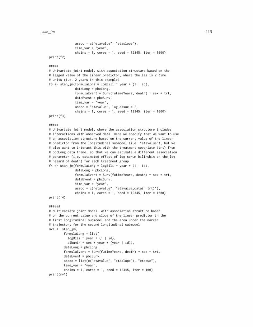
stan_jm 115

assoc = c("etavalue", "etaslope"),time_var = "year",chains = 1, cores = 1, seed = 12345, iter = 1000)

print(f2)

###### Univariate joint model, with association structure based on the# lagged value of the linear predictor, where the lag is 2 time# units (i.e. 2 years in this example)f3 <- stan_jm(formulaLong = logBili ~ year + (1 | id),

dataLong = pbcLong,formulaEvent = Surv(futimeYears, death) ~ sex + trt,dataEvent = pbcSurv,time_var = "year",assoc = "etavalue", lag_assoc = 2,chains = 1, cores = 1, seed = 12345, iter = 1000)

print(f3)

###### Univariate joint model, where the association structure includes# interactions with observed data. Here we specify that we want to use# an association structure based on the current value of the linear# predictor from the longitudinal submodel (i.e. "etavalue"), but we# also want to interact this with the treatment covariate (trt) from# pbcLong data frame, so that we can estimate a different association# parameter (i.e. estimated effect of log serum bilirubin on the log# hazard of death) for each treatment groupf4 <- stan_jm(formulaLong = logBili ~ year + (1 | id),

dataLong = pbcLong,formulaEvent = Surv(futimeYears, death) ~ sex + trt,dataEvent = pbcSurv,time_var = "year",assoc = c("etavalue", "etavalue_data(~ trt)"),chains = 1, cores = 1, seed = 12345, iter = 1000)

print(f4)

####### Multivariate joint model, with association structure based# on the current value and slope of the linear predictor in the# first longitudinal submodel and the area under the marker# trajectory for the second longitudinal submodelmv1 <- stan_jm(

formulaLong = list(logBili ~ year + (1 | id),albumin ~ sex + year + (year | id)),

dataLong = pbcLong,formulaEvent = Surv(futimeYears, death) ~ sex + trt,dataEvent = pbcSurv,assoc = list(c("etavalue", "etaslope"), "etaauc"),time_var = "year",chains = 1, cores = 1, seed = 12345, iter = 100)

print(mv1)

116 stan_mvmer

###### Multivariate joint model, where the association structure is formed by# including the expected value of each longitudinal marker (logBili and# albumin) in the linear predictor of the event submodel, as well as their# interaction effect (i.e. the interaction between the two "etavalue" terms).# Note that whether such an association structure based on a marker by# marker interaction term makes sense will depend on the context of your# application -- here we just show it for demostration purposes).mv2 <- stan_jm(

formulaLong = list(logBili ~ year + (1 | id),albumin ~ sex + year + (year | id)),

dataLong = pbcLong,formulaEvent = Surv(futimeYears, death) ~ sex + trt,dataEvent = pbcSurv,assoc = list(c("etavalue", "etavalue_etavalue(2)"), "etavalue"),time_var = "year",chains = 1, cores = 1, seed = 12345, iter = 100)

###### Multivariate joint model, with one bernoulli marker and one# Gaussian marker. We will artificially create the bernoulli# marker by dichotomising log serum bilirubinpbcLong$ybern <- as.integer(pbcLong$logBili >= mean(pbcLong$logBili))mv3 <- stan_jm(

formulaLong = list(ybern ~ year + (1 | id),albumin ~ sex + year + (year | id)),

dataLong = pbcLong,formulaEvent = Surv(futimeYears, death) ~ sex + trt,dataEvent = pbcSurv,family = list(binomial, gaussian),time_var = "year",chains = 1, cores = 1, seed = 12345, iter = 1000)

stan_mvmer Bayesian multivariate generalized linear models with correlatedgroup-specific terms via Stan

Description

Bayesian inference for multivariate GLMs with group-specific coefficients that are assumed to becorrelated across the GLM submodels.

Usage

stan_mvmer(formula, data, family = gaussian, weights, prior = normal(),prior_intercept = normal(), prior_aux = cauchy(0, 5),

stan_mvmer 117

prior_covariance = lkj(), prior_PD = FALSE,algorithm = c("sampling", "meanfield", "fullrank"),adapt_delta = NULL, max_treedepth = 10L, init = "random",QR = FALSE, sparse = FALSE, ...)

Arguments

formula A two-sided linear formula object describing both the fixed-effects and random-effects parts of the longitudinal submodel similar in vein to formula specifica-tion in the lme4 package (see glmer or the lme4 vignette for details). Notehowever that the double bar (||) notation is not allowed when specifying therandom-effects parts of the formula, and neither are nested grouping factors (e.g.(1 | g1/g2)) or (1 | g1:g2), where g1, g2 are grouping factors. For a multi-variate GLM this should be a list of such formula objects, with each element ofthe list providing the formula for one of the GLM submodels.

data A data frame containing the variables specified in formula. For a multivariateGLM, this can be either a single data frame which contains the data for all GLMsubmodels, or it can be a list of data frames where each element of the listprovides the data for one of the GLM submodels.

family The family (and possibly also the link function) for the GLM submodel(s). Seeglmer for details. If fitting a multivariate GLM, then this can optionally be a listof families, in which case each element of the list specifies the family for oneof the GLM submodels. In other words, a different family can be specified foreach GLM submodel.

weights Same as in glm, except that when fitting a multivariate GLM and a list of dataframes is provided in data then a corresponding list of weights must be pro-vided. If weights are provided for one of the GLM submodels, then they mustbe provided for all GLM submodels.

prior, prior_intercept, prior_aux

Same as in stan_glmer except that for a multivariate GLM a list of priors can beprovided for any of prior, prior_intercept or prior_aux arguments. That is,different priors can optionally be specified for each of the GLM submodels. If alist is not provided, then the same prior distributions are used for each GLM sub-model. Note that the "product_normal" prior is not allowed for stan_mvmer.

prior_covariance

Cannot be NULL; see priors for more information about the prior distributionson covariance matrices. Note however that the default prior for covariance ma-trices in stan_mvmer is slightly different to that in stan_glmer (the details ofwhich are described on the priors page).



118 stan_mvmer


max_treedepth A positive integer specifying the maximum treedepth for the non-U-turn sam-pler. See the control argument in stan.

init The method for generating initial values. See stan.




Details

The stan_mvmer function can be used to fit a multivariate generalized linear model (GLM) withgroup-specific terms. The model consists of distinct GLM submodels, each which contains group-specific terms; within a grouping factor (for example, patient ID) the grouping-specific terms areassumed to be correlated across the different GLM submodels. It is possible to specify a differentoutcome type (for example a different family and/or link function) for each of the GLM submodels.

Bayesian estimation of the model is performed via MCMC, in the same way as for stan_glmer.Also, similar to stan_glmer, an unstructured covariance matrix is used for the group-specific termswithin a given grouping factor, with priors on the terms of a decomposition of the covariance ma-trix.See priors for more information about the priors distributions that are available for the covari-ance matrices, the regression coefficients and the intercept and auxiliary parameters.

Value

A stanmvreg object is returned.

See Also

stan_glmer, stan_jm, stanreg-objects, stanmvreg-methods, print.stanmvreg, summary.stanmvreg,posterior_predict, posterior_interval.

stan_nlmer 119

Examples

###### A multivariate GLM with two submodels. For the grouping factor 'id', the# group-specific intercept from the first submodel (logBili) is assumed to# be correlated with the group-specific intercept and linear slope in the# second submodel (albumin)f1 <- stan_mvmer(

formula = list(logBili ~ year + (1 | id),albumin ~ sex + year + (year | id)),

data = pbcLong,# this next line is only to keep the example small in size!chains = 1, cores = 1, seed = 12345, iter = 1000)

summary(f1)

###### A multivariate GLM with one bernoulli outcome and one# gaussian outcome. We will artificially create the bernoulli# outcome by dichotomising log serum bilirubinpbcLong$ybern <- as.integer(pbcLong$logBili >= mean(pbcLong$logBili))f2 <- stan_mvmer(

formula = list(ybern ~ year + (1 | id),albumin ~ sex + year + (year | id)),

data = pbcLong,family = list(binomial, gaussian),chains = 1, cores = 1, seed = 12345, iter = 1000)

stan_nlmer Bayesian nonlinear models with group-specific terms via Stan

Description

Bayesian inference for NLMMs with group-specific coefficients that have unknown covariance ma-trices with flexible priors.

Usage

stan_nlmer(formula, data = NULL, subset, weights, na.action, offset,contrasts = NULL, ..., prior = normal(), prior_aux = exponential(),prior_covariance = decov(), prior_PD = FALSE,algorithm = c("sampling", "meanfield", "fullrank"),adapt_delta = NULL, QR = FALSE, sparse = FALSE)

120 stan_nlmer

Arguments

formula, data Same as for nlmer. We strongly advise against omitting the data argument.Unless data is specified (and is a data frame) many post-estimation functions(including update, loo, kfold) are not guaranteed to work properly.

subset, weights, offset

Same as glm.na.action, contrasts






prior_aux The prior distribution for the "auxiliary" parameter (if applicable). The "auxil-iary" parameter refers to a different parameter depending on the family. ForGaussian models prior_aux controls "sigma", the error standard deviation.For negative binomial models prior_aux controls "reciprocal_dispersion",which is similar to the "size" parameter of rnbinom: smaller values of "reciprocal_dispersion"correspond to greater dispersion. For gamma models prior_aux sets the prioron to the "shape" parameter (see e.g., rgamma), and for inverse-Gaussian mod-els it is the so-called "lambda" parameter (which is essentially the reciprocal ofa scale parameter). Binomial and Poisson models do not have auxiliary param-eters.prior_aux can be a call to exponential to use an exponential distribution, or

stan_nlmer 121

normal, student_t or cauchy, which results in a half-normal, half-t, or half-Cauchy prior. See priors for details on these functions. To omit a prior —i.e.,to use a flat (improper) uniform prior— set prior_aux to NULL.

prior_covariance

Cannot be NULL; see decov for more information about the default arguments.prior_PD A logical scalar (defaulting to FALSE) indicating whether to draw from the prior

predictive distribution instead of conditioning on the outcome.algorithm A string (possibly abbreviated) indicating the estimation approach to use. Can

be "sampling" for MCMC (the default), "optimizing" for optimization, "meanfield"for variational inference with independent normal distributions, or "fullrank"for variational inference with a multivariate normal distribution. See rstanarm-packagefor more details on the estimation algorithms. NOTE: not all fitting functionssupport all four algorithms.




Details

The stan_nlmer function is similar in syntax to nlmer but rather than performing (approximate)maximum marginal likelihood estimation, Bayesian estimation is by default performed via MCMC.The Bayesian model adds independent priors on the "coefficients" — which are really intercepts— in the same way as stan_nlmer and priors on the terms of a decomposition of the covariancematrices of the group-specific parameters. See priors for more information about the priors.

The supported transformation functions are limited to the named "self-starting" functions in thestats library: SSasymp, SSasympOff, SSasympOrig, SSbiexp, SSfol, SSfpl, SSgompertz, SSlogis,SSmicmen, and SSweibull.

Value

A stanreg object is returned for stan_nlmer.

See Also

stanreg-methods and nlmer.

The vignette for stan_glmer, which also discusses stan_nlmer models. http://mc-stan.org/rstanarm/articles/



122 stan_polr

Examples

data("Orange", package = "datasets")Orange$circumference <- Orange$circumference / 100Orange$age <- Orange$age / 100fit <- stan_nlmer(

circumference ~ SSlogis(age, Asym, xmid, scal) ~ Asym|Tree,data = Orange,# for speed onlychains = 1,iter = 1000)

print(fit)posterior_interval(fit)plot(fit, regex_pars = "b\\[")

stan_polr Bayesian ordinal regression models via Stan

Description

Bayesian inference for ordinal (or binary) regression models under a proportional odds assumption.

Usage

stan_polr(formula, data, weights, ..., subset,na.action = getOption("na.action", "na.omit"), contrasts = NULL,model = TRUE, method = c("logistic", "probit", "loglog", "cloglog","cauchit"), prior = R2(stop("'location' must be specified")),prior_counts = dirichlet(1), shape = NULL, rate = NULL,prior_PD = FALSE, algorithm = c("sampling", "meanfield", "fullrank"),adapt_delta = NULL, do_residuals = NULL)

stan_polr.fit(x, y, wt = NULL, offset = NULL, method = c("logistic","probit", "loglog", "cloglog", "cauchit"), ...,prior = R2(stop("'location' must be specified")),prior_counts = dirichlet(1), shape = NULL, rate = NULL,prior_PD = FALSE, algorithm = c("sampling", "meanfield", "fullrank"),adapt_delta = NULL, do_residuals = algorithm == "sampling")

Arguments


Same as polr, but we strongly advise against omitting the data argument. Un-less data is specified (and is a data frame) many post-estimation functions (in-cluding update, loo, kfold) are not guaranteed to work properly.

stan_polr 123

weights, na.action, contrasts, model

Same as polr, but rarely specified.


method One of ’logistic’, ’probit’, ’loglog’, ’cloglog’ or ’cauchit’, but can be abbrevi-ated. See polr for more details.

prior Prior for coefficients. Should be a call to R2 to specify the prior location of theR2 but can be NULL to indicate a standard uniform prior. See priors.

prior_counts A call to dirichlet to specify the prior counts of the outcome when the predic-tors are at their sample means.

shape Either NULL or a positive scalar that is interpreted as the shape parameter for aGammaDistribution on the exponent applied to the probability of success whenthere are only two outcome categories. If NULL, which is the default, then theexponent is taken to be fixed at 1.

rate Either NULL or a positive scalar that is interpreted as the rate parameter for aGammaDistribution on the exponent applied to the probability of success whenthere are only two outcome categories. If NULL, which is the default, then theexponent is taken to be fixed at 1.




do_residuals A logical scalar indicating whether or not to automatically calculate fit residualsafter sampling completes. Defaults to TRUE if and only if algorithm="sampling".Setting do_residuals=FALSE is only useful in the somewhat rare case thatstan_polr appears to finish sampling but hangs instead of returning the fittedmodel object.

x A design matrix.

y A response variable, which must be a (preferably ordered) factor.

wt A numeric vector (possibly NULL) of observation weights.

offset A numeric vector (possibly NULL) of offsets.

Details

The stan_polr function is similar in syntax to polr but rather than performing maximum likeli-hood estimation of a proportional odds model, Bayesian estimation is performed (if algorithm = "sampling")

124 stan_polr

via MCMC. The stan_polr function calls the workhorse stan_polr.fit function, but it is possi-ble to call the latter directly.

As for stan_lm, it is necessary to specify the prior location of R2. In this case, the R2 pertains tothe proportion of variance in the latent variable (which is discretized by the cutpoints) attributableto the predictors in the model.

Prior beliefs about the cutpoints are governed by prior beliefs about the outcome when the predictorsare at their sample means. Both of these are explained in the help page on priors and in therstanarm vignettes.

Unlike polr, stan_polr also allows the "ordinal" outcome to contain only two levels, in whichcase the likelihood is the same by default as for stan_glm with family = binomial but the prioron the coefficients is different. However, stan_polr allows the user to specify the shape and ratehyperparameters, in which case the probability of success is defined as the logistic CDF of the linearpredictor, raised to the power of alpha where alpha has a gamma prior with the specified shapeand rate. This likelihood is called “scobit” by Nagler (1994) because if alpha is not equal to 1,then the relationship between the linear predictor and the probability of success is skewed. If shapeor rate is NULL, then alpha is assumed to be fixed to 1.

Otherwise, it is usually advisible to set shape and rate to the same number so that the expectedvalue of alpha is 1 while leaving open the possibility that alpha may depart from 1 a little bit.It is often necessary to have a lot of data in order to estimate alpha with much precision andalways necessary to inspect the Pareto shape parameters calculated by loo to see if the results areparticularly sensitive to individual observations.

Users should think carefully about how the outcome is coded when using a scobit-type model.When alpha is not 1, the asymmetry implies that the probability of success is most sensitive to thepredictors when the probability of success is less than 0.63. Reversing the coding of the successesand failures allows the predictors to have the greatest impact when the probability of failure is lessthan 0.63. Also, the gamma prior on alpha is positively skewed, but you can reverse the coding ofthe successes and failures to circumvent this property.

Value

A stanreg object is returned for stan_polr.

A stanfit object (or a slightly modified stanfit object) is returned if stan_polr.fit is called directly.

References

Nagler, J., (1994). Scobit: An Alternative Estimator to Logit and Probit. American Journal ofPolitical Science. 230 – 255.

See Also

stanreg-methods and polr.

The vignette for stan_polr. http://mc-stan.org/rstanarm/articles/

Examples

if (!grepl("^sparc", R.version$platform)) {fit <- stan_polr(tobgp ~ agegp, data = esoph, method = "probit",


summary.stanreg 125

prior = R2(0.2, "mean"), init_r = 0.1, seed = 12345,algorithm = "fullrank") # for speed only

print(fit)plot(fit)

}

summary.stanreg Summary method for stanreg objects

Description

Summaries of parameter estimates and MCMC convergence diagnostics (Monte Carlo error, effec-tive sample size, Rhat).

Usage

## S3 method for class 'stanreg'summary(object, pars = NULL, regex_pars = NULL,probs = NULL, ..., digits = 1)

## S3 method for class 'summary.stanreg'print(x, digits = max(1, attr(x,"print.digits")), ...)

## S3 method for class 'summary.stanreg'as.data.frame(x, ...)

## S3 method for class 'stanmvreg'summary(object, pars = NULL, regex_pars = NULL,probs = NULL, ..., digits = 3)

## S3 method for class 'summary.stanmvreg'print(x, digits = max(1, attr(x,"print.digits")), ...)

Arguments


pars An optional character vector specifying a subset of parameters to display. Pa-rameters can be specified by name or several shortcuts can be used. Usingpars="beta" will restrict the displayed parameters to only the regression co-efficients (without the intercept). "alpha" can also be used as a shortcut for"(Intercept)". If the model has varying intercepts and/or slopes they can beselected using pars = "varying".

126 summary.stanreg

In addition, for stanmvreg objects there are some additional shortcuts avail-able. Using pars = "long" will display the parameter estimates for the longi-tudinal submodels only (excluding group-specific pparameters, but includingauxiliary parameters). Using pars = "event" will display the parameterestimates for the event submodel only, including any association parameters.Using pars = "assoc" will display only the association parameters. Usingpars = "fixef" will display all fixed effects, but not the random effects or theauxiliary parameters. pars and regex_pars are set to NULL then all fixed effectregression coefficients are selected, as well as any auxiliary parameters and thelog posterior.If pars is NULL all parameters are selected for a stanreg object, while for astanmvreg object all fixed effect regression coefficients are selected as well asany auxiliary parameters and the log posterior. See Examples.


probs For models fit using MCMC or one of the variational algorithms, an optionalnumeric vector of probabilities passed to quantile.


digits Number of digits to use for formatting numbers when printing. When callingsummary, the value of digits is stored as the "print.digits" attribute of thereturned object.

x An object of class "summary.stanreg".

Value

The summary method returns an object of class "summary.stanreg" (or "summary.stanmvreg",inheriting "summary.stanreg"), which is a matrix of summary statistics and diagnostics, with at-tributes storing information for use by the print method. The print method for summary.stanregor summary.stanmvreg objects is called for its side effect and just returns its input. The as.data.framemethod for summary.stanreg objects converts the matrix to a data.frame, preserving row and col-umn names but dropping the print-related attributes.

See Also

prior_summary to extract or print a summary of the priors used for a particular model.

Examples

if (!exists("example_model")) example(example_model)summary(example_model, probs = c(0.1, 0.9))

# These produce the same output for this example,# but the second method can be used for any modelsummary(example_model, pars = c("(Intercept)", "size",

paste0("period", 2:4)))summary(example_model, pars = c("alpha", "beta"))

summary.stanreg 127

# Only show parameters varying by groupsummary(example_model, pars = "varying")as.data.frame(summary(example_model, pars = "varying"))

Index

adapt_delta, 6, 63, 84, 88, 90, 93, 96, 100,106, 111, 118, 121, 123

aes, 50aov, 4, 10, 85arrangeGrob, 28as.array.stanreg (as.matrix.stanreg), 7as.data.frame.stanreg

(as.matrix.stanreg), 7as.data.frame.summary.stanreg

(summary.stanreg), 125as.matrix, 78, 80as.matrix.stanreg, 7as.shinystan, 14autoscale, 69available-algorithms, 8available-models, 9available_mcmc, 28available_ppc, 52

bayes_R2 (bayes_R2.stanreg), 11bayes_R2.stanreg, 11bayesplot, 3, 28, 51, 52bayesplot_grid, 32bball1970 (rstanarm-datasets), 72bball2006 (rstanarm-datasets), 72Beta, 66betareg, 4, 10, 86, 88, 89biglm, 89–91

cauchy, 75cauchy (priors), 60cbpp, 13clogit, 4, 10, 93coef, 60coef.stanmvreg (stanmvreg-methods), 75coef.stanreg (stanreg-methods), 78color_scheme_set, 29, 53, 55, 97compare, 19compare_models (loo.stanreg), 17confint.default, 79

confint.stanreg, 35confint.stanreg (stanreg-methods), 78coxph, 110, 113

data.frame, 92decov, 92, 96, 101, 106, 121decov (priors), 60dirichlet, 123dirichlet (priors), 60

E_loo, 21, 22example_jm, 12example_model, 12exponential (priors), 60

facet_wrap, 26, 31, 50, 96factor, 73family, 4, 10, 23, 81, 112fitted.stanmvreg (stanmvreg-methods), 75fitted.stanreg (stanreg-methods), 78fixef (stanreg-methods), 78fixef.stanmvreg (stanmvreg-methods), 75formula, 81, 84, 87, 90, 95, 100, 105formula.stanmvreg (stanmvreg-methods),

75

gamm4, 4, 10, 94, 97GammaDist, 123geom_contour, 96, 97geom_line, 31, 70geom_pointrange, 49geom_ribbon, 27, 31, 70, 96geom_smooth, 27glm, 3, 4, 10, 94, 99, 101, 102, 105, 117, 120glm.nb, 4, 10glmer, 4, 10, 92, 104, 106–108, 110, 112, 117glmer.nb, 4, 10

hs, 6hs (priors), 60hs_plus, 6

128

INDEX 129

hs_plus (priors), 60

interaction, 92

jagam, 97

kfold, 80kfold (loo.stanreg), 17kfold-helpers, 18kfold_split_random, 18kidiq (rstanarm-datasets), 72

labs, 26, 31, 70laplace (priors), 60lasso (priors), 60launch_shinystan, 4, 14, 80launch_shinystan

(launch_shinystan.stanreg), 13launch_shinystan.stanreg, 13lkj (priors), 60lm, 4, 10, 83, 84lm.fit, 84lm.wfit, 84lmer, 4, 10, 113log_lik, 78, 80log_lik (log_lik.stanreg), 15log_lik.stanreg, 15, 20loo, 4, 17–19, 78, 80, 124loo (loo.stanreg), 17loo.stanreg, 17loo_linpred (loo_predict.stanreg), 21loo_model_weights, 17, 20, 82loo_model_weights (loo.stanreg), 17loo_predict (loo_predict.stanreg), 21loo_predict.stanreg, 21loo_predictive_interval

(loo_predict.stanreg), 21

mad, 60, 77, 79, 80match.fun, 37MCMC, 28mcmc_intervals, 28mcmc_pairs, 24methods, 3mkReTrms, 101mortality (rstanarm-datasets), 72

neg_binomial_2, 23, 99, 101, 106, 107negative.binomial, 23ngrps (stanreg-methods), 78

ngrps.stanmvreg (stanmvreg-methods), 75nlmer, 4, 10, 120, 121nobs.stanreg (stanreg-methods), 78normal, 75, 84, 87, 90, 92, 95, 99, 105, 110,

120normal (priors), 60

optimizing, 5, 9, 83, 87, 90, 92, 99, 112, 118,120, 123

pairs.stanreg, 24pairs_condition (pairs.stanreg), 24pairs_style_np (pairs.stanreg), 24pbcLong (rstanarm-datasets), 72pbcSurv (rstanarm-datasets), 72plot, 32, 77, 80plot.gam, 97plot.loo, 18plot.predict.stanjm, 26, 32, 46, 47plot.stanreg, 28plot.survfit.stanjm, 27, 31, 32, 42plot_nonlinear, 29plot_nonlinear (stan_gamm4), 94plot_stack_jm, 27, 32, 42plot_stack_jm (plot.survfit.stanjm), 31poisson, 23polr, 4, 10, 122–124posterior predictive distribution, 52posterior_interval, 59, 77–80, 114, 118posterior_interval

(posterior_interval.stanreg),33

posterior_interval.stanreg, 33posterior_linpred, 11, 22posterior_linpred

(posterior_linpred.stanreg), 35posterior_linpred.stanreg, 35posterior_predict, 3, 11, 16, 32, 35, 36, 46,

47, 52–59, 71, 77, 80, 91, 114, 118posterior_predict

(posterior_predict.stanreg), 36posterior_predict.stanreg, 36posterior_survfit, 16, 27, 31, 32, 39, 47,

71, 77, 114posterior_traj, 26, 27, 32, 42, 43, 77, 114posterior_vs_prior, 49, 68pp_check, 3, 13, 29, 38, 55, 71, 77, 80, 114pp_check (pp_check.stanreg), 51pp_check.stanreg, 51

130 INDEX

pp_validate, 54PPC, 51, 52ppc_dens_overlay, 52ppc_error_binned, 52predict.merMod, 37predict.stanreg, 55predictive_error, 38, 59, 80predictive_error

(predictive_error.stanreg), 56predictive_error.stanreg, 56predictive_interval, 22, 35, 38, 80predictive_interval

(predictive_interval.stanreg),58

predictive_interval.stanreg, 58print, 77, 79, 85print.loo, 18print.stanmvreg, 77, 78, 114, 118print.stanmvreg (print.stanreg), 59print.stanreg, 59, 79, 80print.summary.stanmvreg

(summary.stanreg), 125print.summary.stanreg

(summary.stanreg), 125printed output, 100prior_options (rstanarm-deprecated), 75prior_summary, 49, 60, 64, 77, 79, 87, 92, 95,

99, 105, 110, 120, 126prior_summary (prior_summary.stanreg),

68prior_summary.stanreg, 68priors, 60, 83, 88, 95–97, 100, 101, 106, 111,

113, 117, 118, 121, 123, 124priors help page, 4, 69, 87, 92, 95, 99, 100,

105, 110, 120product_normal (priors), 60proj, 83ps_check, 42, 70, 77, 114psis, 22

QR, 69qr, 71, 88, 93, 96, 101, 106, 112, 118, 121QR-argument, 71, 88, 93, 96, 101, 106, 112,

118, 121quantile, 126

R2, 6, 84, 90, 123R2 (priors), 60radon (rstanarm-datasets), 72

ranef (stanreg-methods), 78ranef.stanmvreg (stanmvreg-methods), 75regular expressions, 7, 24, 28, 34, 50, 126residuals.stanmvreg

(stanmvreg-methods), 75residuals.stanreg (stanreg-methods), 78rgamma, 96, 100, 106, 111, 120rnbinom, 96, 100, 106, 111, 120roaches (rstanarm-datasets), 72rstanarm (rstanarm-package), 3rstanarm-datasets, 72rstanarm-deprecated, 75, 101rstanarm-package, 3runApp, 14

sampling, 5, 9, 83, 87, 90, 92, 94, 99, 105,112, 118, 120, 123

scale_color_brewer, 50scale_color_manual, 50se, 60se.stanmvreg (stanmvreg-methods), 75se.stanreg (stanreg-methods), 78seed, 37, 42, 46, 52, 70shinystan, 14sigma (stanreg-methods), 78sigma.stanmvreg (stanmvreg-methods), 75SSasymp, 121SSasympOff, 121SSasympOrig, 121SSbiexp, 121SSfol, 121SSfpl, 121SSgompertz, 121SSlogis, 121SSmicmen, 121SSweibull, 121stan, 110, 112, 118stan_aov, 60, 66, 83stan_betareg, 4, 10, 86stan_biglm, 82, 89stan_clogit, 4, 10, 36, 38, 91stan_gamm4, 4, 5, 9, 10, 29, 94, 99stan_glm, 4, 5, 9, 10, 23, 61, 69, 75, 83, 85,

97, 98, 106, 113, 124stan_glm.nb, 23stan_glmer, 4, 5, 9, 10, 23, 60, 75, 93, 97,

104, 111, 117, 118stan_glmer.nb, 23

INDEX 131

stan_jm, 5, 10, 12, 15, 16, 39, 40, 44, 60, 65,66, 70, 77, 80, 81, 107, 118

stan_lm, 4, 10, 66, 89, 124stan_lm (stan_aov), 83stan_lmer (stan_glmer), 104stan_mvmer, 5, 10, 65, 66, 77, 80, 110, 114,

116stan_nlmer, 4, 10, 119, 121stan_polr, 4, 10, 64, 66, 79, 122stanfit, 82, 85, 88, 101, 124stanjm, 114stanjm_list (stanreg_list), 82stanmvreg, 75, 118stanmvreg-methods, 75stanmvreg_list (stanreg_list), 82stanreg, 3, 14, 18, 75, 78, 85, 88, 93, 97, 101,

107, 121, 124stanreg object, 57, 58stanreg-methods, 78stanreg-objects, 17, 28, 51, 80stanreg_list, 17, 19, 82strata, 92student_t, 75student_t (priors), 60summary, 59, 77, 79summary.stanmvreg, 78, 114, 118summary.stanmvreg (summary.stanreg), 125summary.stanreg, 60, 125Surv, 108

tumors (rstanarm-datasets), 72

update, 76, 77, 79update.stanjm (stanmvreg-methods), 75update.stanmvreg (stanmvreg-methods), 75update.stanreg (stanreg-methods), 78

VarCorr, 79VarCorr (stanreg-methods), 78vb, 83, 87, 90, 92, 94, 99, 105, 112, 118, 120,

123vcov.stanreg (stanreg-methods), 78

waic, 18waic (loo.stanreg), 17wells (rstanarm-datasets), 72

package ‘rstanarm’ - the comprehensive r archive network · package ‘rstanarm’ november 10,...

Documents