package ‘statmeasures’ - the comprehensive r …€¦ · package ‘statmeasures ... 3 auc ......

Package ‘StatMeasures’March 27, 2015

Type Package

Title Easy Data Manipulation, Data Quality and Statistical Checks

Version 1.0

Date 2015-03-24

Author Akash Jain

Maintainer Akash Jain <[email protected]>

Description Offers useful functions to perform day-to-day data manipulationoperations, data quality checks and post modelling statistical checks.One can effortlessly change class of a number of variables to factor,remove duplicate observations from the data, create deciles of avariable, perform data quality checks for continuous (integer or numeric),categorical (factor) and date variables, and compute goodness of fitmeasures such as auc for statistical models. The functions are consistentfor objects of class 'data.frame' and 'data.table', which is an enhanced'data.frame' implemented in the package 'data.table'.

Depends R (>= 3.1.3)

Imports data.table (>= 1.9.4)

License GPL-2

NeedsCompilation no

Repository CRAN

Date/Publication 2015-03-27 23:46:22

R topics documented:accuracy . . . . . . . . . . . . . . . . . . . . . . . . . . . . . . . . . . . . . . . . . . . 2actvspred . . . . . . . . . . . . . . . . . . . . . . . . . . . . . . . . . . . . . . . . . . 3auc . . . . . . . . . . . . . . . . . . . . . . . . . . . . . . . . . . . . . . . . . . . . . . 4contents . . . . . . . . . . . . . . . . . . . . . . . . . . . . . . . . . . . . . . . . . . . 5decile . . . . . . . . . . . . . . . . . . . . . . . . . . . . . . . . . . . . . . . . . . . . 6dqcategorical . . . . . . . . . . . . . . . . . . . . . . . . . . . . . . . . . . . . . . . . 7dqcontinuous . . . . . . . . . . . . . . . . . . . . . . . . . . . . . . . . . . . . . . . . 8dqdate . . . . . . . . . . . . . . . . . . . . . . . . . . . . . . . . . . . . . . . . . . . . 9

1

2 accuracy

factorise . . . . . . . . . . . . . . . . . . . . . . . . . . . . . . . . . . . . . . . . . . . 10gini . . . . . . . . . . . . . . . . . . . . . . . . . . . . . . . . . . . . . . . . . . . . . 11imputemiss . . . . . . . . . . . . . . . . . . . . . . . . . . . . . . . . . . . . . . . . . 12iv . . . . . . . . . . . . . . . . . . . . . . . . . . . . . . . . . . . . . . . . . . . . . . 13ks . . . . . . . . . . . . . . . . . . . . . . . . . . . . . . . . . . . . . . . . . . . . . . 14mape . . . . . . . . . . . . . . . . . . . . . . . . . . . . . . . . . . . . . . . . . . . . . 15outliers . . . . . . . . . . . . . . . . . . . . . . . . . . . . . . . . . . . . . . . . . . . 16pentile . . . . . . . . . . . . . . . . . . . . . . . . . . . . . . . . . . . . . . . . . . . . 17randomise . . . . . . . . . . . . . . . . . . . . . . . . . . . . . . . . . . . . . . . . . . 18rmdupkey . . . . . . . . . . . . . . . . . . . . . . . . . . . . . . . . . . . . . . . . . . 19rmdupobs . . . . . . . . . . . . . . . . . . . . . . . . . . . . . . . . . . . . . . . . . . 20splitdata . . . . . . . . . . . . . . . . . . . . . . . . . . . . . . . . . . . . . . . . . . . 21

Index 22

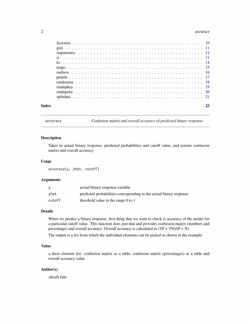
accuracy Confusion matrix and overall accuracy of predicted binary response

Description

Takes in actual binary response, predicted probabilities and cutoff value, and returns confusionmatrix and overall accuracy

Usage

accuracy(y, yhat, cutoff)

Arguments

y actual binary response variable

yhat predicted probabilities corresponding to the actual binary response

cutoff threshold value in the range 0 to 1

Details

When we predict a binary response, first thing that we want to check is accuracy of the model fora particular cutoff value. This function does just that and provides confusion matrix (numbers andpercentage) and overall accuracy. Overall accuracy is calculated as (TP + TN)/(P + N).

The output is a list from which the individual elements can be picked as shown in the example.

Value

a three element list: confusion matrix as a table, confusion matrix (percentages) as a table andoverall accuracy value

Author(s)

Akash Jain

actvspred 3

See Also

ks, auc, iv, splitdata

Examples

# A 'data.frame' with y and yhatdf <- data.frame(y = c(1, 0, 1, 1, 0),

yhat = c(0.86, 0.23, 0.65, 0.92, 0.37))

# Accuracy tables and overall accuracy figuresltAccuracy <- accuracy(y = df[, 'y'], yhat = df[, 'yhat'], cutoff = 0.7)accuracyNumber <- ltAccuracy$accuracyNumaccuracyPercentage <- ltAccuracy$accuracyPeroverallAccuracy <- ltAccuracy$overallAcc

actvspred Comparison of actual and predicted linear response

Description

Takes in actual, predicted linear response and quantile value, and returns average actual and pre-dicted response in each quantile

Usage

actvspred(y, yhat, n)

Arguments

y actual linear response

yhat predicted linear response

n quantiles to be created for comparison

Details

actvspred function divides the data into n (given as input by the user) quantiles and computesmean of y and yhat for each quantile. All NA’s in n, y and yhat are removed for calculation.

The function also plots a line chart of average actual response and average predicted response overn quantiles. This plot can be used to visualize how close both the lines are.

Value

a data.frame with average actual and predicted response in each quantile

Author(s)

Akash Jain

4 auc

See Also

mape, splitdata

Examples

# A 'data.frame' with y and yhatdf <- data.frame(y = c(1, 2, 3, 6, 8, 10, 15),

yhat = c(1.2, 2.5, 3.3, 6.9, 9.3, 6.5, 12.3))

# Get actual vs predicted tableACTVSPRED <- actvspred(y = df[, 'y'], yhat = df[, 'yhat'], n = 5)

auc Area under curve of predicted binary response

Description

Takes in actual binary response and predicted probabilities, and returns auc value

Usage

auc(y, yhat)

Arguments

y actual binary response


Details

Area under the receiver operating characteristic (ROC) curve is the most sought after criteria forjudging how good model predictions are.

auc function calculates the true positive rates (TPR) and false positive rates (FPR) for each cutofffrom 0.01 to 1 and calculates the area using trapezoidal approximation. A ROC curve is alsogenerated.

Value

area under the ROC curve

Author(s)

Akash Jain

See Also

accuracy, ks, iv, gini, splitdata

contents 5

Examples

# A 'data.frame' with y and yhatdf <- data.frame(y = c(1, 0, 1, 1, 0, 0, 1, 0, 1, 0),

yhat = c(0.86, 0.23, 0.65, 0.92, 0.37, 0.45, 0.72, 0.19, 0.92, 0.50))

# AUC figureAUC <- auc(y = df[, 'y'], yhat = df[, 'yhat'])

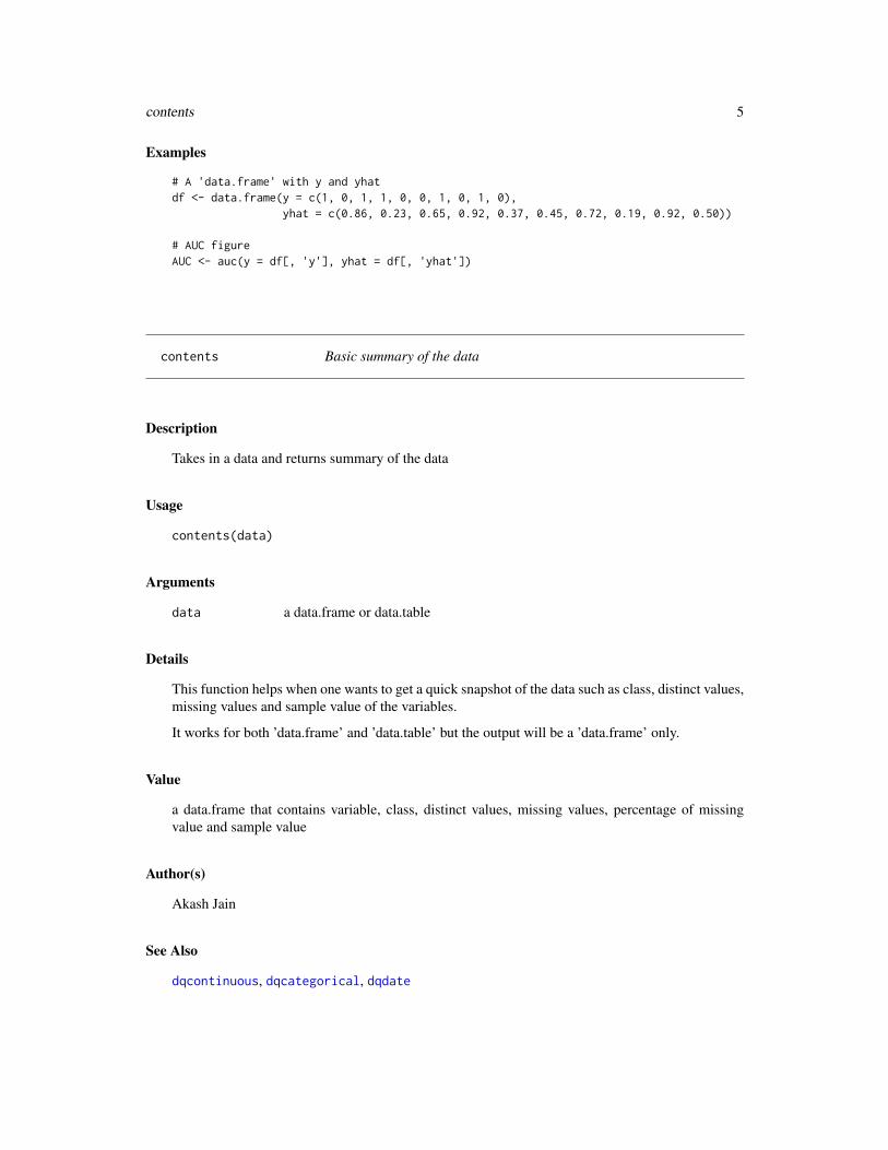
contents Basic summary of the data

Description

Takes in a data and returns summary of the data

Usage

contents(data)

Arguments

data a data.frame or data.table

Details

This function helps when one wants to get a quick snapshot of the data such as class, distinct values,missing values and sample value of the variables.

It works for both ’data.frame’ and ’data.table’ but the output will be a ’data.frame’ only.

Value

a data.frame that contains variable, class, distinct values, missing values, percentage of missingvalue and sample value

Author(s)

Akash Jain

See Also

dqcontinuous, dqcategorical, dqdate

6 decile

Examples

# A data framedf <- data.frame(x = c(1, 2, 3, 4, NA),

y = c('a', 'b', 'c', 'd', 'e'),z = c(1, 1, 0, 0, 1))

# Summary of the datadfContents <- contents(data = df)

decile Create deciles of a variable

Description

Takes in a vector, and returns the deciles

Usage

decile(vector, decreasing = FALSE)

Arguments

vector an integer or numeric vector

decreasing a logical input, which if set to FALSE puts smallest values in decile 1 and if setto TRUE puts smallest values in decile 10; FALSE is default

Details

decile is a convinient function to get integer deciles of an integer or numeric vector. By default,the smallest values are placed in the smallest decile.

Sometimes one may want to put smallest values in the biggest decile, and for that the user can setthe decreasing argument to TRUE; by default it is FALSE.

Value

an integer vector of decile values

Author(s)

Akash Jain

See Also

pentile, outliers, imputemiss

dqcategorical 7

Examples

# Scores vectorscores <- c(1, 4, 7, 10, 15, 21, 25, 27, 32, 35,

49, 60, 75, 23, 45, 86, 26, 38, 34, 67)

# Create deciles based on the values of the vectordecileScores <- decile(vector = scores)decileScores <- decile(vector = scores, decreasing = TRUE)

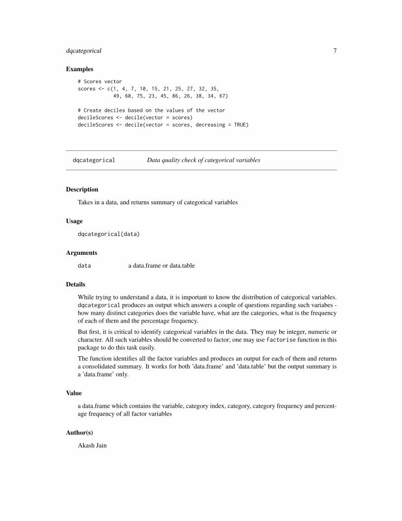
dqcategorical Data quality check of categorical variables

Description

Takes in a data, and returns summary of categorical variables

Usage

dqcategorical(data)

Arguments


Details

While trying to understand a data, it is important to know the distribution of categorical variables.dqcategorical produces an output which answers a couple of questions regarding such variabes -how many distinct categories does the variable have, what are the categories, what is the frequencyof each of them and the percentage frequency.

But first, it is critical to identify categorical variables in the data. They may be integer, numeric orcharacter. All such variables should be converted to factor; one may use factorise function in thispackage to do this task easily.

The function identifies all the factor variables and produces an output for each of them and returnsa consolidated summary. It works for both ’data.frame’ and ’data.table’ but the output summary isa ’data.frame’ only.

Value

a data.frame which contains the variable, category index, category, category frequency and percent-age frequency of all factor variables

Author(s)

Akash Jain

8 dqcontinuous

See Also

dqcontinuous, dqdate, contents

Examples

# A 'data.frame'df <- data.frame(phone = c('IP', 'SN', 'HO', 'IP', 'SN', 'IP', 'HO', 'SN', 'IP', 'SN'),

colour = c('black', 'blue', 'green', 'blue', 'black', 'silver', 'black','white', 'black', 'green'))

# Factorise categorical variablesdf <- factorise(data = df, colNames = c('phone', 'colour'))

# Generate a data quality report of continuous variablessummaryCategorical <- dqcategorical(data = df)

dqcontinuous Data quality check of continuous variables

Description

Takes in a data, and returns summary of continuous variables

Usage

dqcontinuous(data)

Arguments


Details

It is of utmost importance to know the distribution of continuous variables in the data. dqcontinuousproduces an output which tells - continuous variable, non-missing values, missing values, percent-age missing, minumum, average, maximum, standard deviation, variance, common percentiles from1 to 99, and number of outliers for each continuous variable.

The function tags all integer and numeric variables as continuous, and produces output for them; ifyou think there are some variables which are integer or numeric in the data but they don’t representa continuous variable, change their type to an appropriate class.

dqcontinuous uses the same criteria to identify outliers as the one used for box plots. All valuesthat are greater than 75th percentile value + 1.5 times the inter quartile range or lesser than 25thpercentile value - 1.5 times the inter quartile range, are tagged as outliers.

This function works for both ’data.frame and ’data.table’ but returns a ’data.frame’ only.

dqdate 9

Value

a data.frame which contains the non-missing values, missing values, percentage of missing values,mimimum, mean, maximum, standard deviation, variance, percentiles and count of outliers of allinteger and numeric variables

Author(s)

Akash Jain

See Also

dqcategorical, dqdate, contents

Examples

# A 'data.frame'df <- data.frame(x = c(1, 2, 3, 4, 5, 6, 7, 8, 9, 10),

y = c(22, NA, 66, 12, 78, 34, 590, 97, 56, 37))

# Generate a data quality report of continuous variablessummaryContinuous <- dqcontinuous(data = df)

dqdate Data quality check of date variables

Description

Takes in a data, and returns summary of date variables

Usage

dqdate(data)

Arguments


Details

dqdate produces summary of all date variables in the data. The function identifies all variables asdate if they are of class ’Date’ or ’IDate’.

Generally the dates are imported in R as character. They must be converted to an appropriate dateformat and then the function should be used.

The summary includes variable, non-missing values, missing values, minimum and maximum ofthe date variabes. Input data can be a ’data.frame’ or ’data.table’ but the output summary will be a’data.frame’ only.

10 factorise

Value

a data.frame which contains the variable, non-missing values, missing values, minimum and maxi-mum of all date variables

Author(s)

Akash Jain

See Also

dqcontinuous, dqcategorical, contents

Examples

# A 'data.frame'df <- data.frame(date = c('2012-11-21', '2015-1-4', '1996-4-30', '1979-9-23', '2005-5-13'),

temperature = c(26, 32, 35, 7, 14))

# Convert character date to date formatdf[, 'date'] <- as.Date(df[, 'date'])

# Generate a data quality report of date variablessummaryDate <- dqdate(data = df)

factorise Change the class of variables to factor

Description

Takes in data and colNames, and returns the data with all variables mentioned in colNames con-verted to factor

Usage

factorise(data, colNames)

Arguments


colNames a character vector of variable names to be converted to factor

Details

We often face the task of converting a bunch of variables to factor. This function is particularlyuseful in such a situation. Just specify the data and variable names and all of them will be convertedto factor.

It works for both ’data.frame’ and ’data.table’, and the output is data of the same class as that ofinput.

gini 11

Value

data of same class as input with specified variables converted to factor

Author(s)

Akash Jain

See Also

randomise, rmdupkey, rmdupobs

Examples

# A 'data.frame'df <- data.frame(x = c(1, 2, 3, 4, 5),

y = c('a', 'b', 'c', 'd', 'e'),z = c(1, 1, 0, 0, 1))

# Change the class of variables y and z to factorsdfFac <- factorise(data = df, colNames = c('y', 'z'))

gini Gini coefficient of a distribution

Description

Takes in a distribution and returns gini coefficient

Usage

gini(y)

Arguments

y an integer or numeric distribution

Details

To compute the gini coefficient of a distribution, gini is the right function. It uses trapezoidalapproximation to calculate the area of the curve.

Lorenz curve is also plotted as output.

Value

gini coefficient of the distribution

Author(s)

Akash Jain

12 imputemiss

See Also

auc

Examples

# Distributiondist <- c(1, 4, 7, 15, 10)

# Gini coefficientGINI <- gini(y = dist)

imputemiss Impute missing values in a variable

Description

Takes in a vector and a value, and returns the vector with missing values imputed with that value

Usage

imputemiss(vector, value)

Arguments

vector a vector with missing values

value the value to be used for imputation

Details

imputemiss imputes the missing (NA) values in the vector with a specified value. The functionsimplifies the code for imputation.

Value

vector of the same class as input vector with imputed missing values

Author(s)

Akash Jain

See Also

decile, pentile, outliers

iv 13

Examples

# Scores vectorscores <- c(1, 2, 3, NA, 4, NA)

# Imputd scores vectorscoresImp <- imputemiss(vector = scores, value = 5)

iv Information value of an independent variable in predicting a binaryresponse

Description

Takes in independent and dependent variable and returns IV value

Usage

iv(x, y)

Arguments

x an independent variable

y a binary response variable

Details

Information value of a variable is a significant indicator of its relevance in the prediction of a binaryresponse variable. iv computes that value using the formula, IV = summation[(Responders - Non-responders)*ln(Responders / Non-responders) for each bin].

Ten bins are created for continous variables while categories itself are used as bins for categoricalindependent variables.

Value

information value of x

Author(s)

Akash Jain

See Also

accuracy, auc, ks, splitdata

14 ks

Examples

# A 'data.frame'df <- data.frame(x = c('a', 'a', 'a', 'b', 'b', 'b'),

y = c(0, 1, 0, 1, 0, 1))

# Information valueIV <- iv(x = df[, 'x'], y = df[, 'y'])

ks Kolmogorov-Smirnov statistic for predicted binary response

Description

Takes in actual binary response and predicted probabilities, and returns table used for KS computa-tion and KS value

Usage

ks(y, yhat)

Arguments

y actual binary response


Details

Kolmogorov-Smirnov statistic can be easily computed using ks function. It not only computesthe statistic but also returns the table used for ks computation. A chart is also plotted for quickvisualization of split between percentage of responders and non-responders. Deciles are used forcomputation.

Appropriate elements of the 2 element list (ie. ksTable or ks) can be picked using the code given inthe example.

Value

a two element list: table for KS computation and KS value itself

Author(s)

Akash Jain

See Also

accuracy, auc, iv, splitdata

mape 15

Examples

# A 'data.frame' with y and yhatdf <- data.frame(y = c(1, 0, 1, 1, 0),

yhat = c(0.86, 0.23, 0.65, 0.92, 0.37))

# KS table and valueltKs <- ks(y = df[, 'y'], yhat = df[, 'yhat'])ksTable <- ltKs$ksTableKS <- ltKs$ks

mape Compute mean absolute percentage error

Description

Takes in actual and predicted linear response, and returns MAPE value

Usage

mape(y, yhat)

Arguments

y actual linear responseyhat predicted linear response

Details

mape calculates the mean absolute percentage error in a predicted linear response.

Value

mean absolute percentage error

Author(s)

Akash Jain

See Also

actvspred, splitdata

Examples

# A 'data.frame' with y and yhatdf <- data.frame(y = c(1.5, 2, 3.2),

yhat = c(3.4, 2.2, 2.7))

# Compute mapeMAPE <- mape(y = df[, 'y'], yhat = df[, 'yhat'])

16 outliers

outliers Identify outliers in a variable

Description

Takes in a vector, and returns count and index of outliers

Usage

outliers(vector)

Arguments


Details

The function uses the same criteria to identify outliers as the one used for box plots. All valuesthat are greater than 75th percentile value + 1.5 times the inter quartile range or lesser than 25thpercentile value - 1.5 times the inter quartile range, are tagged as outliers.

The individual elements (number of outliers and index of outliers) of the two element output listcan be picked using the code given in example. The index of outliers can be used to get a vector ofall outliers.

Value

a list with two elements: count and index of outliers

Author(s)

Akash Jain

See Also

decile, pentile, imputemiss

Examples


49, 60, 75, 23, 45, 86, 26, 38, 34, 223, -3)

# Identify the count of outliers and their indexltOutliers <- outliers(vector = scores)numOutliers <- ltOutliers$numOutliersidxOutliers <- ltOutliers$idxOutliersvalOutliers <- scores[idxOutliers]

pentile 17

pentile Create pentiles of a variable

Description

Takes in a vector, and returns a vector of pentiles

Usage

pentile(vector, decreasing = FALSE)

Arguments


decreasing a logical input, which if set to FALSE puts smallest values in pentile 1 and if setto TRUE puts smallest values in pentile 5; FALSE is default

Details

pentile is a convinient function to get integer pentiles of an integer or numeric vector. By default,the smallest values are placed in the smallest pentile.

Sometimes one may want to put smallest values in the biggest pentile, and for that the user can setthe decreasing argument to TRUE; by default it is FALSE.

Value

an integer vector of pentile values

Author(s)

Akash Jain

See Also

decile, outliers, imputemiss

Examples


49, 60, 75, 23, 45, 86, 26, 38, 34, 67)

# Create pentiles based on the values of the vectorpentileScores <- pentile(vector = scores)pentileScores <- pentile(vector = scores, decreasing = TRUE)

18 randomise

randomise Order the rows of a data randomly

Description

Takes in data and seed, and returns the data with randomly ordered observations

Usage

randomise(data, seed = NULL)

Arguments

data a matrix, data.frame or data.table

seed an integer value

Details

Some of the modeling algorithms pick top p percent of the observations for training the model,which could lead to skewed predictions. This function solves that problem by randomly orderingthe observations so that the response variable has more or less the same distribution even if thealgorithms don’t pick training observations randomly.

Value

data of same class as input with randomly ordered observations

Author(s)

Akash Jain

See Also

factorise, rmdupkey, rmdupobs

Examples

# A 'data.frame'df <- data.frame(x = c(1, 2, 3, 4, 5), y = c('a', 'b', 'c', 'd', 'e'))

# Change the order of the observations randomlydfRan <- randomise(data = df)dfRan <- randomise(data = df, seed = 150)

rmdupkey 19

rmdupkey Remove observations with duplicate keys from data

Description

Takes in a data and key, and returns data with duplicate observations by key removed

Usage

rmdupkey(data, by)

Arguments


by a character vector of keys to be used

Details

Remove duplicate observations by key(s) is what this function does. How it is different from otherfunctions that remove duplicates is that rmdupkey works for both ’data.frame’ and ’data.table’, andit also returns the duplicated observations.

Many a times we want to go back to the duplicated observations and see why that duplicationoccured. One can pick the duplicated observations using the code given in example.

Value

a two element list: unique data and duplicate data

Author(s)

Akash Jain

See Also

randomise, factorise, rmdupobs

Examples

# A 'data.frame'df <- data.frame(x = c(1, 2, 1, 1), y = c(3, 3, 1, 3))

# Remove duplicate observations by key from dataltDf <- rmdupkey(data = df, by = c('x'))unqDf <- ltDf$unqDatadupDf <- ltDf$dupData

20 rmdupobs

rmdupobs Remove duplicate observations from data

Description

Takes in a data, and returns it with duplicate observations removed

Usage

rmdupobs(data)

Arguments


Details

Duplicate observations are redundant and they need to be removed from the data. rmdupobs doesjust that; it removes the duplicated observations (the ones in which value of every variable is dupli-cated) and returns the data with only unique observations.

It works for both ’data.frame’ and ’data.table’ and returns the data with same class as that of input.

Value

a data of same class as input with only unique observations

Author(s)

Akash Jain

See Also

randomise, rmdupkey, factorise

Examples

# A 'data.frame'df <- data.frame(x = c(1, 2, 5, 1), y = c(3, 3, 1, 3))

# Remove duplicate observations from datadfUnq <- rmdupobs(data = df)

splitdata 21

splitdata Split modeling data into test and train set

Description

Takes in data, fraction (for train set) and seed, and returns train and test set

Usage

splitdata(data, fraction, seed = NULL)

Arguments

data a matrix, data.frame or data.tablefraction proportion of observations that should go in the train setseed an integer value

Details

An essential task before doing modeling is to split the modeling data into train and test sets.splitdata is built for this task and returns a list with train and test sets, which can be pickedusing the code given in example.

fraction corresponds to the train dataset, while the rest of the observations go to the test dataset.If the user wants to generate the same test and train dataset everytime, he should specify a seedvalue.

Value

a list with two elements: train and test set

Author(s)

Akash Jain

See Also

actvspred, mape, accuracy, auc, iv, ks

Examples

# A 'data.frame'df <- data.frame(x = c(1, 2, 3, 4, 5, 6, 7, 8, 9, 10),

y = c('a', 'b', 'c', 'd', 'e', 'f', 'g', 'h', 'i', 'j'),z = c(1, 1, 0, 0, 1, 0, 0, 1, 1, 0))

# Split data into train (70%) and test (30%)ltData <- splitdata(data = df, fraction = 0.7, seed = 123)trainData <- ltData$traintestData <- ltData$test

Index

accuracy, 2, 4, 13, 14, 21actvspred, 3, 15, 21auc, 3, 4, 12–14, 21

contents, 5, 8–10

decile, 6, 12, 16, 17dqcategorical, 5, 7, 9, 10dqcontinuous, 5, 8, 8, 10dqdate, 5, 8, 9, 9

factorise, 10, 18–20

gini, 4, 11

imputemiss, 6, 12, 16, 17iv, 3, 4, 13, 14, 21

ks, 3, 4, 13, 14, 21

mape, 4, 15, 21

outliers, 6, 12, 16, 17

pentile, 6, 12, 16, 17

randomise, 11, 18, 19, 20rmdupkey, 11, 18, 19, 20rmdupobs, 11, 18, 19, 20

splitdata, 3, 4, 13–15, 21

22

package ‘statmeasures’ - the comprehensive r …€¦ · package ‘statmeasures ... 3 auc ......

Documents