packard snowﬂakes on the von neumann neighborhood · packard snowﬂakes on the von neumann...

“JCA” — “JCA0051” — 2008/2/5 — 11:53 — page 57 — #1

Journal of Cellular Automata, Vol. 3, pp. 57–79 ©2008 Old City Publishing, Inc.Reprints available directly from the publisher Published by license under the OCP Science imprint,Photocopying permitted by license only a member of the Old City Publishing Group

Packard Snowflakes on the von NeumannNeighborhood

Charles D. Brummitt1,∗, Hannah Delventhal2

and Michael Retzlaff3

15000 N. Woodruff Ave, Milwaukee, WI 5321722804 N Calvert St. Apt. 1R, Baltimore, MD 21218

E-mail: [email protected] S. Fremont Ave., Baltimore, MD 21230

E-mail: [email protected]

Received: July 16, 2007. Accepted: July 23, 2007.

In 1984, Packard [1] introduced simple planar cellular automata to emulatethe growth of snow crystals. These Packard Snowflakes have since beenpopularized by S. Wolfram and others, most recently in [2]. The presentpaper provides a rigorous analysis of the simplest examples: those withnearest neighbor interaction on the two-dimensional integers. In each casewe determine the asymptotic density with which the spreading crystal fillsthe plane. For the basicExactly 1 rule started from a singleton, we establishalternate representations of the final state as a uniform tag system and as asubstitution system.

Keywords: cellular automata, crystal growth, asymptotic density, solidification,uniform tag system, substitution system.

1 PRELIMINARIES

IntroductionSnow crystals have inspired mathematical modeling for more than a century,dating back at least as far as the early fractal known as the Koch Snowflake [3].The details of real snowflake growth, wherebywater vapor gradually freezes toform the growing crystal, are still poorly understood.An extremely simple pro-totype for planar growth was proposed by Packard [1]. In his cellular automa-ton (CA) model, each cell (or site) of a planar lattice changes from empty to

∗E-mail: [email protected]

57

“JCA” — “JCA0051” — 2008/2/5 — 11:53 — page 58 — #2

58 Charles D. Brummitt et al.

occupied as that location turns to ice and remains occupied thereafter. A cell“freezes”when it has one frozen neighbor, orwhen the number of frozen neigh-bors equals some prescribed higher count. Cells of the original 1984model hadsix nearest neighbors, reflecting the hexagonal molecular structure of ice andobserved symmetry of actual snow crystals. Subsequenct studies [2,4] includesimulations on the two-dimensional intergers Z2 with 4 and 8 nearest neigh-bors, the so-called von Neumann and Moore neighborhoods, respectively.As they grow, hexagonal Packard Snowflakes develop intricate patterns

reminscient of real snowflakes (cf. Fig. 8 of [5]). Indeed, Wolfram and othershave argued (e.g., in [6,7], and [2]) that the similarity demonstrates the abilityof simple local interactions to capture essential features of complex naturalprocesses. Recent advances in our understanding of real snow crystal growth,however, make it clear that the Packard rules evolve in a very different mannerthan do the sectored plates they ressemble at certain stages of development.More realistic lattice algorithms, based on physical principles, are currentlybeing developed by Gravner and Griffeath [5, 8]; see those articles for anextensive bibliography of the modeling literature.Despite their limited realism, the Packard rules are basic cellular automata

with fascinating properties. Wolfram has described the patterns they gener-ate as “intricate, if very regular” [2, p. 171]. Gravner and Griffeath [9] firstprovided a precise analysis of a Packard Snowflake on the Moore neighbor-hood and proved that it fills the plane with asymptotic density 4

9 . Their morerecent paper [10] gives quite a complete rigorous treatment of all the original,hexagonal Packard rules.Our objective here is to present a corresponding mathematical description

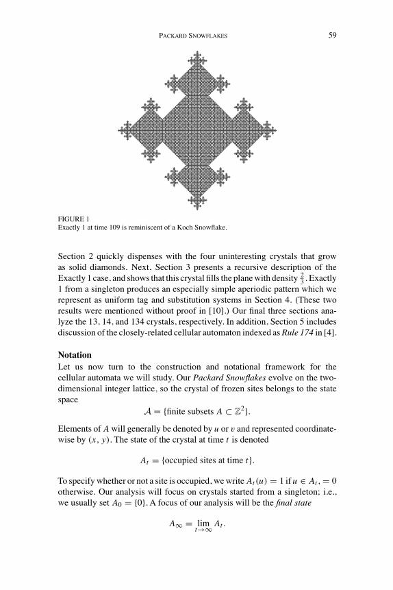
for all Packard automata with the most elementary neighborhood structure:the von Neumann case. We will focus on the evolution of crystals started froma singleton, derivation of exact formulas for their cell counts at dyadic times,and calculation of asymptotic densities with which they fill the plane. Figure 1shows a still frame of the Exactly 1 Packard Snowflake that will be the fea-tured example of our study.Amore general analysis of asymptotic density fromarbitrary finite initial seeds can be carried out using the methods of [10]. Tech-niques from that paper also apply to the description of macroscopic dynamics.While mathematically rigorous, our results have been obtained after exten-

sive experimentation. This project would not have been possible without theaid of an interactive CA simulator for visualization and data analysis. We aregrateful toMirekWojtowicz for creating theMCell software [11] used through-out our research and for all the figures included here. Likewise, the readershould consider MCell (or some such simulator) indispensible for carefulstudy of our work.The paper is organized as follows. In the remainder of this Introduction, we

formalize the cellular automata we will study, describe a simple transforma-tion T that plays a key role in our analysis, and then review the familiarSierpinski lattice embedded within the evolution of Packard Snowflakes.

“JCA” — “JCA0051” — 2008/2/5 — 11:53 — page 59 — #3

Packard Snowflakes 59

FIGURE 1Exactly 1 at time 109 is reminiscent of a Koch Snowflake.

Section 2 quickly dispenses with the four uninteresting crystals that growas solid diamonds. Next, Section 3 presents a recursive description of theExactly 1 case, and shows that this crystal fills the planewith density 23 . Exactly1 from a singleton produces an especially simple aperiodic pattern which werepresent as uniform tag and substitution systems in Section 4. (These tworesults were mentioned without proof in [10].) Our final three sections ana-lyze the 13, 14, and 134 crystals, respectively. In addition, Section 5 includesdiscussion of the closely-related cellular automaton indexed asRule 174 in [4].

NotationLet us now turn to the construction and notational framework for thecellular automata we will study. Our Packard Snowflakes evolve on the two-dimensional integer lattice, so the crystal of frozen sites belongs to the statespace

A = {finite subsets A ⊂ Z2}.Elements ofAwill generally be denoted by u or v and represented coordinate-wise by (x, y). The state of the crystal at time t is denoted

At = {occupied sites at time t}.

To specifywhether or not a site is occupied, wewriteAt(u) = 1 if u ∈ At, = 0otherwise. Our analysis will focus on crystals started from a singleton; i.e.,we usually set A0 = {0}. A focus of our analysis will be the final state

A∞ = limt→∞ At .

“JCA” — “JCA0051” — 2008/2/5 — 11:53 — page 60 — #4


Sitewise convergence here is automatic since Packard Snowflakes solidify,meaning that once a cell freezes it belongs to the crystal forever.To prescribe the dynamics of At , let us begin with the neighborhood of

interaction. We denote the familiar nearest neighbor norms as

∥(x, y)∥1 = |x| + |y|,

and∥(x, y)∥∞ = max{|x|, |y|}.

This paper studies Packard Snowflakes with the von Neumann neighborhoodof a cell u given by

∂1u = {v : ∥v − u∥1 = 1}It will also be convenient to introduce the Moore neighborhood of u

∂∞u = {v : ||v − u||∞ = 1},

although systematic analysis of Packard Snowflakes on this latter neighbor-hood is deferred to a future project. When the norm and neighborhood areclear from context, we write them simply as ||u|| and ∂u. We also define theneighborhood of a set of cells A ∈ A,

∂A = {u ∈ Ac : u ∈ ∂v for some v ∈ A}.

Packard Snowflakes specify whether a site joins the crystal based on howmany occupied neighbors the site “sees.” Thus we introduce the set of sites in∂A that see k neighbors in A as

Sk = Sk(A) = {u ∈ ∂A : #(∂u ∩ A) = k}, k = 1, . . . , 4. (1)

The solidification rules we study are transformations τI : A → A given by

τI (A) = A ∪!

i∈I

Si,

where the rule index I ⊂ {1, 2, 3, 4} and 1 ∈ I. In words, a site u joins thecrystalA if the number of occupied sites u sees belongs to I . For convenience,we abbreviate τ{1,3} = τ13, etc. The basic case τ1 is often called the Exactly 1rule. We also abbreviate τ t

I (A0) = AIt for t ≤ ∞.

It will be useful to distinguish regions of Z2, specifically the diamond

Dt = {x : ∥x∥1 ≤ t},

and the boxBt = {x : ∥x∥∞ ≤ t}.

Started from A0 = {0}, the crystals AIt exhibit a diamond-shaped outline

at the end of each dyadic time interval (cf. Fig. 2). Thus it is particularly

“JCA” — “JCA0051” — 2008/2/5 — 11:53 — page 61 — #5


FIGURE 2Exactly 1 from a singleton at times 3, 7, and 15.

convenient to analyze the evolution along the subsequence of times N =Nn = 2n − 1, comparing the population and pattern of frozen cells to those ofthe full diamond DN .Appealing to symmetry, we will inspect the portion of crystals in the first

quadrant. Hence we write, for A ∈ A,

Q(A) = {u = (x, y) : u ∈ A, x ≥ 0, y ≥ 0}.

For brevity, setQt = Q(At).A principal goal of this paper is to compute the asymptotic density ρ for

each τI . To this end, let us denote the population counts at dyadic times as

an = #AN, qn = #QN,

and define

ρI = limN→∞

an

#DN,

where I specifies the rule index of τI . We will see that the limit exists inevery case. Methods from [10] can be applied in our setting to show that ρsatisfies the general definition of asymptotic density given in that paper and isindependent of the initial finite seed A0.

The rotation T

Packard Snowflakes on the von Neumann neighborhood display diamond-shaped features, reflecting the geometry of ∂1. Rotated by 45◦ the crystalboundaries align horizontally and vertically, making their patterns easier todetect(see, e.g., Fig. 3). Originally motivated by computer visualization, wewill see in Section 3 that this rotation T reveals especially beautiful structureof the Exactly 1 rule.

“JCA” — “JCA0051” — 2008/2/5 — 11:53 — page 62 — #6


FIGURE 3The Exactly 1 crystal (left) and rotated by T (right).

Formally, let us introduce

T ="1 1

−1 1

#,

which maps Z2 to the even checkerboard Ce = {(x, y) : x + y is even}. Inparticular, note that TDN = BN ∩ Ce.Write τ ∗

I = T τI T−1 for the rotated versions of the τI . Note that each τ ∗

I isan update rule on subsets of Ce with neighborhoods ∂∗u = ∂∞u \ ∂1u. Also,putA∗

t = τ ∗nAt , and so on. In this manner, the rotated rules τ ∗I and their occu-

pied sets A∗t can be viewed as new cellular automata. Since T is one-to-one,

#(A∗N) = an, so applying T does not affect population counts. We abbreviate

the portion of the rotated crystal in the first quadrant asQ∗N = Q(A∗

N).Iterates of the odd checkerboard Co = {(x, y) : x +y is odd} under T will

play a central role in our analysis of Exactly 1, so we will make repeated useof the following elementary facts.

Proposition 1. Let (x, y) ∈ Z2. Then

TCo = D := {(x, y) : x odd, y odd}, (2)

TD = 2Co. (3)

Proof. To check (2), let (x, y) ∈ Co with x + y = 2n + 1 for some integer n.Then

T

"x

y

#=

"2n + 1

−2x + (2n + 1)

#,

the coordinates of which are both odd. Moreover,

T

"m − n

m + n + 1

#=

"2m + 12n + 1

#,

so any site with both coordinates odd is obtained from a suitable choice ofx and y.

“JCA” — “JCA0051” — 2008/2/5 — 11:53 — page 63 — #7


To check (3), let (x, y) ∈ D with x = 2m + 1 and y = 2n + 1. Then

T

"x

y

#= 2

"m + n + 1

n − m

#∈ 2Co.

Conversely,

T

"2a − 2k − 12k + 1

#=

"2a

2(2k + 1− a)

#

exhibits any site in 2C as the image of a site in D. ✷

In combination, (2) and (3) imply that T 2Co = 2Co, T 3Co = 2D, T 4Co =4Co, . . .. Thus for all k ≥ 0,

T 2kCo = 2kCo (4)

T 2k+1Co = 2kD. (5)

Sierpinski embeddingThe familiar Sierpinski lattice (or sieve, or triangle) [12] is embedded in A∞for all the rules τI we are considering (cf. Fig. 4). This structure is generatedas the space-time trace of the one-dimensional XOR CA with two nearestneighbors and starting from a singleton. Vacant sites at the boundary of the“light cone” in our Packard Snowflakes (e.g., cells within the first quadrantalong the line x + y = t at time t) see exactly two neighbors that could beoccupied. If exactly one of those neighbors is occupied, then the site solidifiessince 1 ∈ I for all of our rules. In particular, the crystal advances along the

FIGURE 4Exactly 1 with embedded Sierpinski lattices in a darker shade.

“JCA” — “JCA0051” — 2008/2/5 — 11:53 — page 64 — #8


axes every update. If 2 ∈ I , then τI fills the plane, as we will show below. Ifk ∈ I with k ≥ 3, a site on the edge of the light cone cannot solidify by thek rule since at most two neighbors can be occupied. Hence, in all cases with2 /∈ I , the cells of each quadrant that solidify at light speed form a copy of theSierpinski lattice.In subsequent sections we will make use of the following well-known

properties of the Sierpinski lattice in its XOR representation with neighbor set{−1, 1}:

• At time N all odd sites in [−N, N] are occupied.• At time N + 1 all sites are empty except ±(N + 1).

• Sites on the edge of the light cone solidify; i.e., ±t are occupied attime t .

2 THE RULES τI , 2 ∈ I

We begin our study of von Neumann neighborhood Packard Snowflakes withthe four trivial cases such that 2 ∈ I ; namely, τ12, τ123, τ124, andτ1234.Starting from a singleton these rules cover Dt at time t .

Proposition 2. Suppose 2 ∈ I and A0 = {0}. Then AI∞ = Z2 and ρI = 1.

Proof. We show that for any t ≥ 0,

At = Dt . (6)

At time t = 1 the cells of A1 = {(0, 0), (0, 1), (1, 0), (0, −1), (−1, 0)} = D1are frozen. Assuming (6), at time t + 1 any cell (x, y) of Q(∂Dt) satisfiesx + y = t + 1. If x = 0 or y = 0, then (x, y) has one occupied neighborin At at (x − 1, 0) or (y − 1, 0), respectively. If x, y ̸= 0, then (x, y) has 2occupied neighbors at (x, y −1) and (x −1, y). In either case (x, y) solidifies.(Note that since all cells within the light cone Dt solidify due to the 1 or 2condition, the 3 and 4 conditions are superfulous.) ThusQ(Dt+1) = Q(At+1)By symmetry, (6) holds for all t . In particular, A∞ = Z2 and ρI = 1. ✷

3 THE EXACTLY 1 RULE

Wenowderive an exact population formula for the simplest non-trivial nearest-neighbor Packard Snowflake started from a singleton, showing that it fills theplane with density 2

3 .

Proposition 3. For τ1, if A0 = {0} the number of occupied cells at timeN = 2n − 1 is an = 4n+1−1

3 . Hence ρ1 = 23 .

“JCA” — “JCA0051” — 2008/2/5 — 11:53 — page 65 — #9


Let us begin by proving the population formula for the rotated Exactly 1rule τ ∗

1 , since this is easier to visualize, and then transform back to τ1. Recallthat an denotes the population of the entire crystal at time N = 2n − 1. LetQn = Q(A∗

Nn) be the portion of the rotated crystal in the first quadrant, qn =

#Qn its population. By direct enumeration, a1 = 5, a2 = 21, a3 = 85, . . .;q1 = 2, q2 = 6, q3 = 22, . . .. In fact, #Q(A∗

t ∩ DN) does not change aftertime t = Nn; i.e., the final configuration on DN is attained at time N , but wedefer the verification of this until the proposition is proved.First, we claim thatQn+1 consists of four rigid transformations ofQn (see

Fig. 5).Assuming the claim for themoment, the three new clones ofQn branchfrom the seed at (2n, 2n) in the NW, NE and SE directions. Since qn+1 countsthis seed only once,

qn+1 = 4qn − 2. (7)

The whole crystal An consists of 4 copies of Qn, but the origin is countedthree too many times in an. Hence

an = 4qn − 3. (8)

Using the initial data to solve (7) and (8), we have

qn = 4n + 23

, an = 4n+1 − 13

, (9)

as desired. Since the box Bn = [−N, N]2 has order 4n+1 sites, it follows thatthe asymptotic density ρ∗

1 of the rotated crystal equals13 . Applying T −1 to

recover the original orientation conserves the crystal cell count but halves the

FIGURE 5The first quadrant of the rotated Exactly 1 crystal at time 15. The lighter cells, i.e., the new growthfrom time N3 to N4, are rigid transformations of the darker cells grown by time N3.

“JCA” — “JCA0051” — 2008/2/5 — 11:53 — page 66 — #10


area. (T dilates the original pattern by a factor of 2 by inserting a permantentlyempty cell between each pair of cells.) Hence ρ1 = 2

3 .Next we prove the claimed cloning structure of Qn+1 in terms of Qn by

induction. Since A∗t is symmetric started from a singleton, the same analysis

applies to the other three quadrants. Let us begin with the boundaries ofQn.

Lemma 1. A∗∞ contains no cells on the x- or y-axes except the origin.

Proof. Because the dynamics within the four quadrants of the plane are sym-metric, sites on the axes have either 0, 2, or 4 occupied neighbors at all times,so they never join the crystal. ✷

Lemma 2. A∗∞ contains no cells in the rows and columns {N + 1} × [1, N ]

and [1, N ] × {N + 1}.

Proof. Since halves of two Sierpinski lattices are embedded inQ(A∗∞), cells

of {N} × [1, N ] and [1, N ] × {N} are alternately occupied and empty. Cellsin the next row and column (i.e., in [1, N ]× {N + 1} and in {N + 1}× [1, N ],respectively) look to their corner neighbors and see either 0 or 2 occupiedcells. According to τ ∗

1 , these cells never join the crystal. ✷

Lemmas 1 and 2 determine the boundaries for the evolution of Qn, whilethe following property gives rise to recursive structure. See Fig. 6.

Lemma 3. Under τ ∗1 , a ray of occupied cells travels from (0, 0) at speed 1 in

the NE direction. That is, (t, t) joins the rotated crystal at time t .

FIGURE 6Depiction of the three lemmas used to analyze growth of τ∗

1 . The empty cells guaranteed byLemmas 1 and 2 are light gray, while the darkest cells are occupied by Lemma 3. Together thesedetermine the boundaries of dyadic regions.

“JCA” — “JCA0051” — 2008/2/5 — 11:53 — page 67 — #11


Proof. Observe that (1, 1) joins the crystal at times 1. Assume (t, t) joins attime t . At this time, the light cone, i.e., the set of sites that can be affected bythe initial seed, is Ct := Bt ∩Ce. Site (t + 1, t + 1), which is outside the lightcone, has only one neighbor that could be occupied: namely, (t, t). Hence, if(t, t) is occupied at time t , then (t + 1, t + 1) joins at time t + 1 accordingto τ ∗

1 . The lemma follows by induction. ✷

Returning to the proof of the claimed cloning process, we iterate τ ∗1 to time

Nn. By Lemma 3, there is a new “seed,” or occupied cell, at (Nn +1, Nn +1).By Lemma 1, there is a boundary of empty cells to the left and below thisseed (namely, in {Nn + 1} × [1, Nn] and in [1, Nn] × {Nn + 1}). Therefore,evolution from this seed is analogous to that from the origin. More precisely,because there are exactly the same boundary conditions as at time 0 (the rowand column of empty cells on the axes as established by Lemma 1), the crystalwill grow exactly as before within the boundaries. Because the boundaryconditions NE, NW, and SE of the seed are identical to those at the origin, theconfiguration Qn will be exactly copied NE, NW, and SE of the new seed.The new squares are:

[Nn + 1, Nn + 1] × [Nn+1, Nn+1] for the NE copy,

[1, Nn + 1] × [Nn + 1, Nn+1] for the NW copy,

[Nn + 1, 1] × [Nn+1, Nn + 1] for the SE copy.

Thus, the rotated Exactly 1 rule evolves recursively as described above.Finally, we return to the claim that under τ ∗

1 , the final configuration onBN is attained at time N (i.e., A∗

N = A∗∞ ∩ BN ). By symmetry, it suffices

to consider the first quadrant; empty cells guaranteed by Lemma 1 precludeinteraction across the axes.Iterate τ ∗

1 to time N2 = 3. At the next iteration, a new seed forms at (4, 4).By Lemma 1, sites in the row and column to the left and below this seed (i.e.,in [0, 3] × {4} and in {4} × [0, 3]) never join A∞. Because the boundaries ofQ(B3) never join A∞, sites inQ(B3) are not affected by sites outsideQ(B3)after time 3. Evidently, sites in Q(B3) are not affected by sites inside Q(B3)after time 3 since one can observe that the configuration on Q(B3) at timeN2 = 3 equals the configuration on Q(B3) at time N3 = 7. This shows thatthe final configuration on B3 is attained at time N = 3.Next, assume the claim holds on BNn at time Nn. Again appealing to

symmetry, we consider only the first quadrant. According to the recursion ofτ ∗1 proved above, the configuration onQ(BNn+1) consists ofQ(BNn) and threerigid transformations of Q(BNn). The original Q(BNn) satisfies the claim bythe induction hypothesis. Each of the three new copies ofQ(BNn) begins fromthe seed (2n, 2n) at time Nn + 1 and grows exactly asQn did from the originbecause they have the same boundaries. Hence the three copies attain their

“JCA” — “JCA0051” — 2008/2/5 — 11:53 — page 68 — #12


final configuration at timeNn+1 in the sameway thatQn did at timeNn, whichcompletes the proof.Since the rotation T is an isomorphism of dynamics on the ∂1 and ∂∗

neighborhoods, the analogous result (9) for the Exactly 1 rule τ1 is immediate.

4 OTHER CHARACTERIZATIONS OFA∗∞ AND A∞ FOR τ1

Started from a singleton, the final states of all Packard Snowflakes onthe von Neumann neighborhood are exactly solvable in the sense of [10].Exactly 1, structurally the simplest (non-trivial) case, admits three alternaterepresentations to the recursion of the last section.

The binary ruleFirst, there is a simple description of sites (x, y) belonging to the final statein terms of the binary representations of x and y.

Proposition 4. A∗∞ satisfies the binary rule:

(x, y) is occupied iff

$x = y = 0, or x, y ̸= 0 and the greatestpowers of 2 dividing x and y are the same.

(10)

Proof. By symmetry, it suffices to check (10) in the first quadrant. Lemma 1establishes the binary rule on {x = 0 or y = 0}. It can also easily be checkedthat the occupied set of the binary rule on Q(B3) agrees with Q3. Now weassume the binary rule agrees withQn onQ(Bn) and show that it also agreeswith Qn+1 on Q(Bn+1). The square [0, 0] × [Nn, Nn] is cloned into threesquares NE, NW, and SE of the new seed by translating and rotating by 0◦,+90◦, and−90◦, respectively, as described in Section 3. Since τ ∗

1 is symmetricacross the x = 0, y = 0 and y = ±x axes, the configuration in the NWsquare is Qn reflected across the line x = Nn. Likewise, the SE square isQn reflected across the line y = Nn. Thus we can choose the cloning to map(x, y) in [0, 0]× [Nn, Nn] to (x, y)+ (ϵ12n, ϵ22n), where ϵ1 = ϵ2 = 1 for theNE square, ϵ1 = 0, ϵ2 = 1 for the NW square, and ϵ1 = 1, ϵ2 = 0 for the SEsquare.Take any (x, y) ∈ [1, 1]×[Nn, Nn]. Clearly, the greatest dyadic divisors of

both x and y are between 1 and 2n−1. Thus, adding 2n to x or y merely puts a1 on the left end of its binary representation. If the greatest powers of two thatdividex andy are the same (different), then after adding 2n to either or both ofxand y, their greatest power of two divisors are still the same (different). Hencethe binary rule holds on the set [1, 1] × [Nn+1, Nn+1] \ {x = 2n or y = 2n}.In the remaining cases, the greatest dyadic divisor of one of x and y is 2n

and the other is at most 2n. If they both are 2n, which corresponds to the site(2n, 2n), then x and y share the same greatest dyadic divisor, so the site is

“JCA” — “JCA0051” — 2008/2/5 — 11:53 — page 69 — #13


occupied. (This is the “seed” mentioned in the cloning proccess earlier.) If, onthe other hand, the greatest dyadic divisor of one of x and y is less than 2n,then they have different greatest dyadic divisors, so the cell is empty. (Thiscorresponds to the boundaries of empty cells established in Lemmas 1 and 2.)Hence the binary rule holds on all of [0, 0] × [Nn+1, Nn+1]. By induction therotated Exactly 1 crystal A∗

n satisfies the binary rule. ✷

A∗∞ in terms of dilated odd checkerboards

Next, it turns out that the union of all odd iterates of the odd checkerboard Co

under T yields the rotated Exactly 1 pattern.

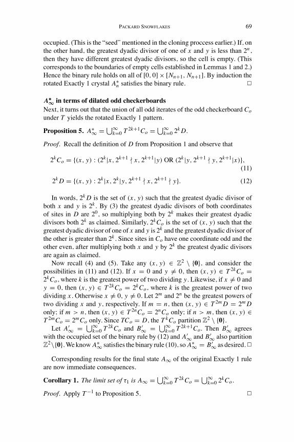
Proposition 5. A∗∞ = %∞

k=0 T 2k+1Co = %∞k=0 2kD.

Proof. Recall the definition of D from Proposition 1 and observe that

2kCo = {(x, y) : (2k|x, 2k+1 ! x, 2k+1|y) OR (2k|y, 2k+1 ! y, 2k+1|x)},(11)

2kD = {(x, y) : 2k|x, 2k|y, 2k+1 ! x, 2k+1 ! y}. (12)

In words, 2kD is the set of (x, y) such that the greatest dyadic divisor ofboth x and y is 2k . By (3) the greatest dyadic divisors of both coordinatesof sites in D are 20, so multiplying both by 2k makes their greatest dyadicdivisors both 2k as claimed. Similarly, 2kCo is the set of (x, y) such that thegreatest dyadic divisor of one of x and y is 2k and the greatest dyadic divisor ofthe other is greater than 2k . Since sites in Co have one coordinate odd and theother even, after multiplying both x and y by 2k the greatest dyadic divisorsare again as claimed.Now recall (4) and (5). Take any (x, y) ∈ Z2 \ {0}, and consider the

possibilities in (11) and (12). If x = 0 and y ̸= 0, then (x, y) ∈ T 2kCo =2kCo, where k is the greatest power of two dividing y. Likewise, if x ̸= 0 andy = 0, then (x, y) ∈ T 2kCo = 2kCo, where k is the greatest power of twodividing x. Otherwise x ̸= 0, y ̸= 0. Let 2m and 2n be the greatest powers oftwo dividing x and y, respectively. If m = n, then (x, y) ∈ T 2mD = 2mD

only; if m > n, then (x, y) ∈ T 2nCo = 2nCo only; if n > m, then (x, y) ∈T 2mCo = 2mCo only. Since TCo = D, the T kCo partition Z2 \ {0}.Let A′

∞ = %∞k=0 T 2kCo and B ′

∞ = %∞k=0 T 2k+1Co. Then B ′

∞ agreeswith the occupied set of the binary rule by (12) andA′

∞ and B ′∞ also partition

Z2\{0}.We knowA∗∞ satisfies the binary rule (10), soA∗

∞ = B ′∞ as desired.✷

Corresponding results for the final state A∞ of the original Exactly 1 ruleare now immediate consequences.

Corollary 1. The limit set of τ1 is A∞ = %∞k=0 T 2kCo = %∞

k=0 2kCo.

Proof. Apply T −1 to Proposition 5. ✷

“JCA” — “JCA0051” — 2008/2/5 — 11:53 — page 70 — #14


FIGURE 7A∞ (left) and T A∞ (right) are complementary off 0.

Corollary 2. A∞ satisfies the complementary binary rule:

(x, y) is occupied iff

$x = 0 or y = 0, or x, y ̸= 0 and thegreatest powers of 2 dividing x and y differ.

(13)

Proof. Abbreviate A† for the occupied set of the complementary binary rule.We showed above that if u ∈ T 2kCo for some k then u ∈ A†, and ifu ∈ T 2kD for some k then u /∈ A†. Since the T 2kCo and T 2kD partitionZ2 \ 0,%∞

k=0 T 2kCo = A†. By Corollary 1, A∞ = A†. ✷

Combining the structural properties now established, we arrive at a remark-able inversion property for A∞ under 45◦ rotation, as illustrated in Fig. 7.

Corollary 3. The limit sets A∞ and A∗∞ of τ1 and τ ∗

1 , respectively, arecomplementary away from the origin.

Proof. This is immediate from the observation above that A′∞ and B ′

∞partition Z2 \ 0. ✷

We remark that Corollary 1 provides an alternate proof that ρ1 = 23 .

Namely, since A∞ = %∞k=0 T 2kCo, since applying T 2 moves cells 4 times

further apart, and since the checkerboard Co has density 12 , the asymptotic

density of A∞ is ρ1 = 12 + 1

2 · 14 + 12 · 1

42+... =23 . Corollary 3 then implies

that the asymptotic density ρ∗1 of the rotated crystal equals

13 .

A substitution systemIn addition, the final state of Exactly 1 is generated by an extremely simplesubstitution system (or L-system). The scheme for τ1 in the first quadrant isshown in Fig. 8.By Corollary 3, reversing black and white yields the system for τ ∗

1 , asin Fig. 9.

“JCA” — “JCA0051” — 2008/2/5 — 11:53 — page 71 — #15


FIGURE 8Substitution system for τ1.

FIGURE 9Substitution system for τ∗

1 .

FIGURE 10Evolution of the substitution system for τ1 in the first quadrant.

FIGURE 11Evolution of the substitution system for τ∗

1 in the first quadrant.

The first four iterates of the two substitution systems are shown in Figs. 10and 11.To show that the scheme of Fig. 8, started from a single black cell, gener-

ates Q(A∞), we prove agreement with the complementary binary rule (13)by induction. It is easy to check that the pattern generated by two iterations ofthe substitution scheme equals Q(B3) ∩ A∞, as shown in the middle frameof Fig. 10. Assume next that the pattern after n iterations agrees with (13) onQ(BNn). Take any (x, y) in the pattern generated by n iterations of the substi-tution system. This schememaps (x, y) to (2x, 2y), (2x+1, 2y), (2x, 2y+1),and (2x + 1, 2y + 1). If (x, y) is occupied, i.e., the greatest powers of twodividing x and y differ, then the greatest powers of two dividing 2x and 2y stilldiffer, so (2x, 2y) is occupied. The sites (2x +1, 2y) and (2x, 2y +1) consistof an odd and an even, so their greatest dyadic divisors differ, and hence thesesites are also occupied. The site (2x + 1, 2y + 1) consists of two odds, whichshare the same greatest dyadic divisor of 1, so this site is empty. Alternatively,if (x, y) is empty, i.e., the greatest powers of two dividing x and y are thesame, then the greatest powers of two dividing 2x and 2y are still the same,

“JCA” — “JCA0051” — 2008/2/5 — 11:53 — page 72 — #16


so (2x, 2y) is empty. The sites (2x +1, 2y) and (2x, 2y +1) consist of an oddand an even, so their greatest dyadic divisors differ, and hence these sites areoccupied. Finally, the site (2x + 1, 2y + 1) consists of two odds, which sharethe same greatest dyadic divisor of 1, so this site is empty. Agreement for alln follows.

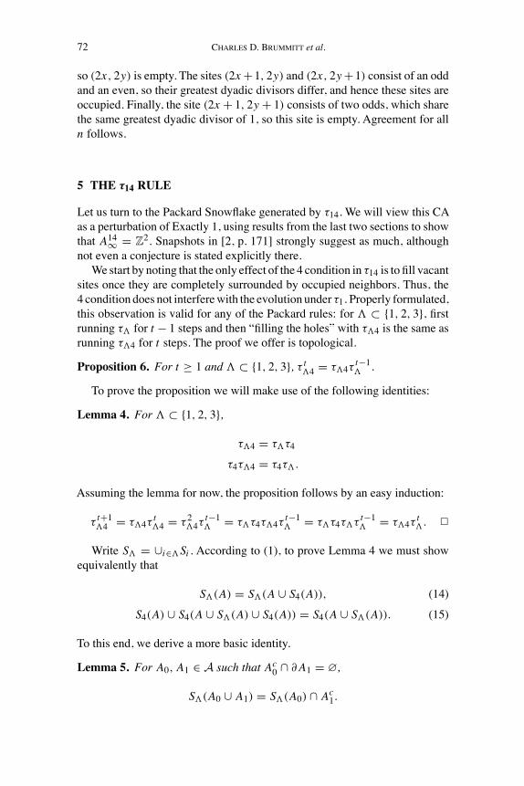
5 THE τ14 RULE

Let us turn to the Packard Snowflake generated by τ14. We will view this CAas a perturbation of Exactly 1, using results from the last two sections to showthat A14∞ = Z2. Snapshots in [2, p. 171] strongly suggest as much, althoughnot even a conjecture is stated explicitly there.We start by noting that the only effect of the 4 condition in τ14 is to fill vacant

sites once they are completely surrounded by occupied neighbors. Thus, the4 condition does not interferewith the evolution under τ1. Properly formulated,this observation is valid for any of the Packard rules: for % ⊂ {1, 2, 3}, firstrunning τ% for t − 1 steps and then “filling the holes” with τ%4 is the same asrunning τ%4 for t steps. The proof we offer is topological.

Proposition 6. For t ≥ 1 and % ⊂ {1, 2, 3}, τ t%4 = τ%4τ

t−1% .

To prove the proposition we will make use of the following identities:

Lemma 4. For % ⊂ {1, 2, 3},

τ%4 = τ%τ4

τ4τ%4 = τ4τ%.

Assuming the lemma for now, the proposition follows by an easy induction:

τ t+1%4 = τ%4τ

t%4 = τ 2%4τ

t−1% = τ%τ4τ%4τ

t−1% = τ%τ4τ%τ t−1

% = τ%4τt%. ✷

Write S% = ∪i∈%Si . According to (1), to prove Lemma 4 we must showequivalently that

S%(A) = S%(A ∪ S4(A)), (14)

S4(A) ∪ S4(A ∪ S%(A) ∪ S4(A)) = S4(A ∪ S%(A)). (15)

To this end, we derive a more basic identity.

Lemma 5. For A0, A1 ∈ A such that Ac0 ∩ ∂A1 = ∅,

S%(A0 ∪ A1) = S%(A0) ∩ Ac1.

“JCA” — “JCA0051” — 2008/2/5 — 11:53 — page 73 — #17


Proof. ∂(A0∪A1) = (∂A0∩Ac1)∪(∂A1∩Ac

0). By hypothesis, and elementaryproperties of S%,

S%(A0 ∪ A1) = {x ∈ ∂A0 ∩ Ac1 : #{∂x ∪ (A0 ∩ A1)} ∈ %}

= {x ∈ ∂A0 ∩ Ac1 : #{y ∈ (A0 ∩ A1) : x ∈ ∂y} ∈ %}

= {x ∈ ∂A0 ∩ Ac1 : #{y ∈ A0 : x ∈ ∂y} ∈ %}

= {x ∈ ∂A0 ∩ Ac1 : #{∂x ∩ A0} ∈ %}

= S%(A0) ∩ Ac1.

Note that the third equality holds since x ∈ ∂A0 implies x ∈ Ac0, whereas

y ∈ A1 and x ∈ ∂y imply x ∈ ∂A1, contradicting the hypothesis. ✷

Now to show (14), set A0 = A and A1 = S4(A) in Lemma 5. Since∂S4(A) ⊂ A the assumption of the lemma is satisfied. Thus,

S%(A ∪ S4(A)) = S%(A) ∩ S4(A)c = S%(A) ∩ Ac = S%(A)

as desired. For (15), setA0 = A∪S%(A) andA1 = S4(A) in Lemma 5.Againthe hypothesis holds, so

S4(A ∪ S%(A) ∪ S4(A)) = S4(A ∪ S%(A)) ∩ S4(A)c = S4(A ∪ S%(A)),

this last since S4(A ∪ S%(A)) ⊂ S4(A)c. It remains to check that S4(A) ⊂S4(A ∪ S%(A)). Suppose x ∈ S4(A). If x /∈ S4(A ∪ S%(A)), then S4(A) andS%(A)) are not disjoint, a contradiction. ✷

Proposition 6 lets us analyze the solidification ofA14t by determining whichcells are added to A1t . We can extend this analysis to the correspnding finalstates by applying a simple continuity result.

Lemma 6. If At → A∞, then τ%(At ) → τ%(A∞).

Proof. Fix u ∈ Z2 and write ∂̄u = u ∪ ∂u. The convergence At → A∞implies that

At ∩ ∂̄u = A∞ ∩ ∂̄u eventually in t . (16)

For t such that (16) holds,

(τ%(At ))(u) = (τ%(A∞))(u).

Therefore, τ%(At ) → τ%(A∞). ✷

In our analysis of the Exactly 1 rule we showed that cell (x, y) is not amember of A1∞ if and only if x and y share the same greatest power of 2

“JCA” — “JCA0051” — 2008/2/5 — 11:53 — page 74 — #18


divisor. We also saw that the same condition characterizes membership inAN ∩ DN . Let

x =∞&

i=02ixi , y =

∞&

j=02j yj

with xi, yj ∈ {0, 1}. Suppose (x, y) /∈ A1∞. Then there exists k ≥ 0 suchthat xk = yk = 1 and xi = yi = 0, for i < k. In particular, the odd-evenparities of x and y agree. Hence the four neighbors of (x, y) have coordinateswith different parity. Thus S4(A1∞) = (A1∞)c. Combining Proposition 6 withLemma 6,

A14∞ = limt→∞ τ t

14(A0) = limt→∞ τ14(τ

t−11 (A0)) = τ14(A

1∞) = Z2. (17)

In particular, ρ14 = 1.In similar fashion, one can show that

A14N+1 = DN ∪ {(±(N + 1), 0), (0, ±(N + 1))}.

Another variant of Exactly 1Packard and Wolfram [4, Section 2] discussed a CA related to Exactly 1 thatthey incorrectly identified as a solidification rule. Namely, Rule 174 (accord-ing to their numbering scheme) is the modification of τ1 in which a vacantcell becomes occupied if exactly one of its four neighbors is occupied whilean occupied cell becomes empty if all four neighbors are occupied. Let usdenote this CA map as τPW and its final state from a singleton as APW

∞ . Inmuch the same way as for Packard Snowflakes, one can verify the analog ofProposition 6,

τnPW = τPW τn−1

1 . (18)We omit the proof. Proceeding as in (17), we conclude from (18) thatAPW

∞ = A1∞ \ A◦∞, where A◦

∞ consists of all sites in A1∞ with four neigh-bors in A1∞. Recall the decomposition of Corollary 1 and the complementarybinary rule of Corollary 2. Note that Co /∈ A◦

∞ since two neighbors of any sitein the odd checkerboard have both coordinates odd. Moreover, for any k ≥ 1,2kCo ∈ A◦

∞ since the coordinates of all four neighbors of any site in thedilated odd checkerboard have opposite parity. We conclude that Rule 174 hasasymptotic density 1

2 and Co as its final state. One can also show that

APWN+1 = (Co ∩ DN) ∪ {(±(N + 1), 0), (0, ±(N + 1))}.

6 THE τ13 RULE

Intriguingly, although the patterns generated by τ13 differ considerably fromthose of τ1 (cf. Fig. 12), the populations at dyadic times, and hence theasymptotic densities, are identical.

“JCA” — “JCA0051” — 2008/2/5 — 11:53 — page 75 — #19


FIGURE 12Comparison of τ1 and τ13. Cell counts are both 341 after 15 iterations from a singleton.

Proposition 7. For τ13, if A0 = {0} the number of occupied cells at timeN = 2n − 1 is an = 4n+1−1

3 , and so ρ13 = 23 .

As we did for Exactly 1, let us begin by deriving the population formula forthe rotated rule τ ∗

13 and then transform back to τ13. Again let an = a∗n = #A∗

Nbe the population of the entire rotated crystal at time N , qn the population ofthe portion of the rotated crystal in the first quadrant. Directly enumerating thefirst few cell counts shows that they are the same as for τ ∗

1 : a1 = 5, a2 = 21,a3 = 85, . . .; q1 = 2, q2 = 6, q3 = 22, . . . .Oncemore, our strategy is to analyze the cloning of dyadic blocks.Whereas

τ1 reproduces square regions simply, the more intricate evolution of τ13 repro-duces triangular regions. Thus we divide Q(BNn+1) into six lattice trianglesand one square, as shown in Fig. 13:

(I) y > 0, x < Nn, y < x;(II) y < Nn, x > 0, y > x;(III) y ≥ Nn + 1, x > 0, y < −x + Nn+1 + 1;(IV) y < Nn+1 + 1, x < Nn + 1, y > −x + Nn+1 + 1;(V) x ≥ Nn + 1, y > 0, y < −x + Nn+1 + 1;(VI) x < Nn+1 + 1, y < Nn + 1, y > −x + Nn+1 + 1;(VII) [Nn + 1, Nn+1] × [Nn + 1, Nn+1]

Againwe abbreviateQn = Q(A∗Nn

). Whereas for τ1 we used the configura-tion on a square,Qn, as the fundamental cloning object, for τ13 we instead usethe configuration in triangular region I. We claim that Qn+1 consists of eightrigid transformations of the configuration in I and four rigid transformationsof the diagonal y = x (0 ≤ x ≤ Nn), with some overlap (cf. Fig. 13).Denote the population in each of the seven regions as pI = #(A∗

∞ ∩ I ),etc., and let d = N +1 be the population of the diagonal y = x (0 ≤ x ≤ Nn).By symmetry, pI = pII , so qn = 2pI + d.Due to the embedded Sierpinski Lattice, the lines [0, N ] × {N} and

{N} × [0, N ] consist of alternating occupied and empty cells. Under τ ∗13,

“JCA” — “JCA0051” — 2008/2/5 — 11:53 — page 76 — #20


FIGURE 13Seven regions for the analysis of τ13.

these boundaries bahave equivalently to empty rows. At time N + 1 a seedforms at (N + 1, N + 1), which belongs to region VII only. By reasoningsimilar to that for Lemma 1, Qn (i.e., the configuration on the union ofregions I, II, and the diagonal adjoining them) copies exactly into region VII.Since after time N + 1 the N × N squares NW and SE of the seed evolvefor time N with boundary conditions equivalent to those at the origin attime 0, a solid diagonal advances at lightspeed in both directions along theline y = −x + Nn+1 + 1. Since the seed (N + 1, N + 1) belongs to VII,the population of the two diagonals separating III from IV and V from VI is2d − 2. Hence qn+1 = 4pI + 2d + pIII + pIV + pV + pVI + 2d − 2.Since the segments [0, N ]× {N} and {N}× [0, N ] behave like boundaries

of empty cells under the 1 or 3 rule, the boundary conditions for growth intoregions III and V starting at the seed (N + 1, N + 1) are identical to theconditions for growth into I and II starting from (1, 1) at time 1. However, theboundary conditions for growth into IV and VI starting from (N + 1, N + 1)are identical to the conditions starting from (0, 0) at time 0 growing intoregions I and II. Because of this, the configurations on triangles III and Vare shifted by (+1, −1) and (−1, +1), respectively. In other words, one canimagine that the growth into region I from the seed (0, 0) is identical to thegrowth into III from a seed at (Nn +2, Nn) rather than from (Nn +1, Nn +1).Likewise, the growth into region I from (0, 0) is identical to the growth intoV from (Nn, Nn + 2). These shifts do not affect the population of the rigidtransformations of the configuration in region I. Hence pI = pIII = pIV =pV = pVI .

“JCA” — “JCA0051” — 2008/2/5 — 11:53 — page 77 — #21


Putting all this together, we obtain

qn+1 = 8pI + 4d − 2 = 4(2pI + d) − 2

= 4qn − 2.

This difference equation and initial data are the same as for Exactly 1, so again(8) and (9) hold in the new setting and the asymptotic densities of the rotatedrule τ ∗

13 and original rule τ13 are 13 and23 , respectively.

The proof by induction of the recursive evolution for τ ∗13 is analogous to the

proof for τ ∗1 , so we will skip the details. The boundary conditions described

above determine the growth within triangles III through VI.

7 THE τ134 RULE

To conclude the paper we turn to the final Packard Snowflake on the vonNeumannneighborhood, generated by τ134.Weview this case as a perturbationof τ13, just as we considered τ14 a perturbation of τ1. By Proposition 6,

τ t134 = τ134τ

t−113 .

Thus we can determine A134∞ by filling in the holes in A13∞. Moreover, theboundary conditions for evolution of τ13 in regions I–VII and the cloningstructure within those regions can be verified for τ134 in the same way. How-ever, the population of τ134 has extra contributions from the 4 condition along“seams” between regions I and V, between regions II and III, and at fouradditional sites (cf. Fig. 14).Let qn be the quadrant population count of τ134, pI the count in region

I, and d = N + 1 the diagonal population as in the previous section. Nowqn = 2pI + d + 2, since additional cells are added at (2, 0) and (0, 2) by the4 condition. The modified recursion is

qn+1 = 8pI + (4d − 2) + (sn + 4), (19)

where sn+4 represents the contribution from sites along the above-mentionedseams and four additional sites. Simplifying, we get qn+1 = 4qn + sn − 6.A final lemma now evaluates the seam correction.

Lemma 7. There are 2n−1 occupied sites forming a period 2 sequence alongthe boundary ofQn that are candidates to fill in by the 4 condition, but 2n−1of these are already filled in by τ13. Thus sn = 2n − 2n.

Proof. The seams y = Nn + 1, 0 ≤ x ≤ Nn + 1; and x = Nn + 1, 0 ≤ y ≤Nn +1 have a total of 2n+1−1 cells. Due to the shifted recursion for τ13, thereare cells alternating between occupied and empty on both sides of the seams.However, the 2n−1 cells at (Nn +2−2i , Nn +1) and (Nn +1, Nn +2−2i ),

“JCA” — “JCA0051” — 2008/2/5 — 11:53 — page 78 — #22


FIGURE 14Cells added by the 4 condition of τ134 are darker. These boundary cells are added on every dyadicscale, then reproduced by the cloning process.

where 0 ≤ i < n, are already filled in by τ13, due to the embedding of theSierpinski lattice. This leaves (2n −1)− (2n−1) previously empty cells withfour occupied neighbors that fill by the 4 condition, as claimed. ✷

Thereforeqn+1 = 4qn + 2n − 2n − 6,

which has solution

qn = 29724n − 2n−1 + 2

3n + 20

9.

The crystal size is an = 4qn − 7 because the 4 added cells on the axes aredouble counted and the origin is counted 3 times too many. It follows that

an = 29184n − 2n+1 + 8

3n + 17

9,

and the asymptotic density of the rotated rule τ ∗134 and original rule τ134 are

ρ∗134 = 29

72 and ρ134 = 2936 , respectively.

In closing, we note that ρ134 = 2936 is lower than ρ14 = 1 even though

cells join the crystal with the former density in an additional case. The lackof monotonicity in nontrivial Packard Snowflakes that produces their exoticstructure also accounts for surprises such as this.

“JCA” — “JCA0051” — 2008/2/5 — 11:53 — page 79 — #23


8 ACKNOWLEDGMENTS

This research was conducted by a Collaborative Undergraduate Research Lab(CURL), under the supervision of Professor David Griffeath, at the Univer-sity of Wisconsin – Madison during the 2006–7 academic year. The CURLwas sponsored by a National Science Foundation VIGRE award to the UW-MadisonMathematic Department. The named authors took the lead preparingthis paper for publication.

REFERENCES

[1] Packard N. Lattice models for solidification and aggregation. Institute for Advanced StudyPreprint. Reprinted (1986). Theory andApplication of Cellular Automata, Wolfram S. (ed.).World Scientific, 305–310, 1984.

[2] Wolfram S. A New Kind of Science. Champaign: Wolfram Media. 2002.[3] von KochH. Sur une courbe continue sans tangente, obtenue par une construction géométri-

que élémentaire. Arkiv för Mathematik, Astronomi och Fysik 1 (1904), 681–702.[4] Packard N. and Wolfram S. Two dimensional cellular automata. Journal of Statistical

Physics 38 (1985), 901–946.[5] Gravner J. and Griffeath D. Modeling Snow Crystal Growth II. To appear, 2007.[6] Wolfram S. Computer software in science andmathematics. ScientificAmerican 251 (1984),

188–203.[7] Levy S. Artificial Life: The Quest for a New Creation. New York City: Pantheon Books,

1992.[8] Gravner J. and Griffeath D. Modeling Snow Crystal Growth III. In preparation, 2007.[9] Gravner J. and Griffeath D. Cellular automaton growth on Z2: theorems, examples and

problems. Advances in Applied Mathematics 21 (1998), 241–304.[10] Gravner J. and Griffeath D. Modeling snow crystal growth I. Experimental Mathematics 15

(2006), 421–444.[11] Wojtowicz M.Mirek’s Cellebration: a 1D and 2D Cellular Automata explorer http://www.

mirwoj.opus.chelm.pl/ca/.[12] Sierpinski W. Sur une courbe dont tout point est un point de ramification. C. R. A. S. 160

(1915), 302–305.

“JCA” — “JCA0051” — 2008/2/5 — 11:53 — page 80 — #24

packard snowﬂakes on the von neumann neighborhood · packard snowﬂakes on the von neumann...

Documents