padis.uniroma1.itpadis.uniroma1.it/bitstream/10805/1164/1/phd_orlandini.pdfpadis.uniroma1.it
TRANSCRIPT

Universita di Roma ”Sapienza“Dottorato in Scienza Chimiche
XXIII ciclo
Formation and transformation of
complex Silicon structures
Sergio Orlandini
University of Rome ”Sapienza“
Chemistry Department
and
C.A.S.P.U.R.
Consorzio interuniversitario per le Applicazioni di Supercalcolo
Per Univerita e Ricerca
Tutors:
Prof. F.A. Gianturco
PhD. S. Meloni
A thesis submitted for the degree of
PhilosophiæDoctor (PhD)
2010 October


Contents
1 Introduction 3
2 Potential 8
1 Modified Tersoff Potential . . . . . . . . . . . . . . . . . . . . . . 9
3 Phase Diagram of Silicon Dioxide 14
1 Theoretical Background . . . . . . . . . . . . . . . . . . . . . . . 14
2 Calculation of the Gibbs Free Energy of the Various Phases . . . . 16
2.1 Liquid phase . . . . . . . . . . . . . . . . . . . . . . . . . . 17
2.2 Crystal phases . . . . . . . . . . . . . . . . . . . . . . . . . 19
3 Results . . . . . . . . . . . . . . . . . . . . . . . . . . . . . . . . . 22
4 Self Diffusion in Amorphous Silicon Dioxide 25
1 Theoretical Background . . . . . . . . . . . . . . . . . . . . . . . 26
2 Sample Preparation and Computational Setup . . . . . . . . . . . 32
3 Results and Discussion . . . . . . . . . . . . . . . . . . . . . . . . 34
3.1 Migration Energy . . . . . . . . . . . . . . . . . . . . . . 34
3.2 Mechanisms . . . . . . . . . . . . . . . . . . . . . . . . . . 37
5 Amorphous-Crystal Phase Transition 45
1 Sample Preparation. . . . . . . . . . . . . . . . . . . . . . . . . . 47
2 Free Energy Calculations . . . . . . . . . . . . . . . . . . . . . . . 50
3 Collective Variables . . . . . . . . . . . . . . . . . . . . . . . . . . 54
3.1 Size of the Nano-particles . . . . . . . . . . . . . . . . . . 54
1

CONTENTS
3.2 Bond Order Parameter . . . . . . . . . . . . . . . . . . . . 57
4 Improving the Sampling of the Configurational Space . . . . . . . 65
4.1 Parallel Tempering (aka Replica Exchange Method) . . . . 67
5 Simulation Protocol . . . . . . . . . . . . . . . . . . . . . . . . . . 72
6 Results . . . . . . . . . . . . . . . . . . . . . . . . . . . . . . . . . 73
6.1 Order-Disorder Phase Change . . . . . . . . . . . . . . . . 73
6.2 Structural Trends . . . . . . . . . . . . . . . . . . . . . . . 76
6 Committor Analysis 81
1 Theoretical Background . . . . . . . . . . . . . . . . . . . . . . . 83
2 Committor Analysis . . . . . . . . . . . . . . . . . . . . . . . . . 90
3 Results . . . . . . . . . . . . . . . . . . . . . . . . . . . . . . . . . 92
7 Hydrodynamic Evolution of an Interface 102
1 Theoretical Background . . . . . . . . . . . . . . . . . . . . . . . 103
2 Non Equilibrium Molecular Dynamic . . . . . . . . . . . . . . . . 106
3 Hydrodynamic Evolution of an Interface . . . . . . . . . . . . . . 107
4 Computational Setup . . . . . . . . . . . . . . . . . . . . . . . . . 110
5 Results . . . . . . . . . . . . . . . . . . . . . . . . . . . . . . . . . 113
8 Conclusion 118
A Derivatives of the Tersoff potential 121
0.1 Potential . . . . . . . . . . . . . . . . . . . . . . . . . . . . 121
0.2 First Derivatives . . . . . . . . . . . . . . . . . . . . . . . 123
0.3 Second Derivatives . . . . . . . . . . . . . . . . . . . . . . 125
Bibliography 130
2

Chapter 1
Introduction
The present information and communication technology industry is based on the
Silicon technology. The success of this technology is due to the significant increase
of performance and reduction of costs achieved over years. The Moore’s law [1],
that predict a dubling of the number of transistors on a chip every two years,
has been obeys till nowadays. However, micro-electronic is going towards the
problem of ”electronic bottleneck“. Indeed, as the number of transistors inside a
chip increases more interconnecting wires must be included in the chip to link the
transistors. For instance current chips contain one kilometer of wires per cm2.
Sending informations along these wires introduce delays in signal transmission
and an increase in power dissipation. The scaling process exacerbates both of
these problems and the overall performance may be compromised. Until these
days, the problem of the ”electronic bottleneck“ was postponed by the use of
appropriate materials, such as Aluminum or Copper, for the interconnections
between transistors. However a new approach to information transfers become
necessary if Silicon devices will continue to shrink in the future.
A very promising approach is to use optical inter-connections between the
transistors. No more electrons but photons will transport information under the
form of an optical signal. By adopting this solution there will be the elimina-
tion of both problems: the delay in the transport of information and of power
dissipation in signal propagation. The main goal of the micro-photonics is the
development of a device that can emits/receives light signals and that can be
efficiently integrated in Silicon based chips. A very appealing idea would be to
make also this component by Silicon. Unfortunately bulk Silicon is a poor ma-
3

1. INTRODUCTION
terial for light emitting devices, because it has an indirect electronic band gap.
This means that the emission or absorption of a photon requires a simultaneous
absorption or emission of a phonon in order to conserve the crystal momentum.
Therefore the emission/absorption of a photon is a three particles process with
a very low rate. Due to this reason, for long time Silicon has been considered
not suitable for optical applications. However, Silicon nano-structures have been
identified as a promising material for photonics. Indeed, once a semiconductor
is reduced to the nano-scale the probability associated to an optical transition
increases. This is due to the confinement which increases the energy gap between
the valence and conduction band and introduces uncertainty on the momentum.
The last effect relaxes the momentum conservation rule and allows a greater por-
tion of the phonon density of states to assist the indirect band-to-band transition
[2]. Moreover, the shrinking of the dimension of the system confines spatially the
wave-functions of both the electron and the hole which are responsible for the
transition. Thus, the rate of the optical transition is higher because, according
to the Fermi’s golden rule, it is proportional to the overlap integral that connects
the wave-functions of the electron and the hole with the dipole operator [3].
The interest around nano-structured Silicon material as useful optical device
began in the early nineties with the first experimental evidence of photolumi-
nescence from porous Silicon by Canham [4]. After this first evidence, a great
interest was focused on the Silicon nano-structure materials. The porous Silicon
resulted to be not suitable for industrial applications due to its great chemical
reactivity and very fragile mechanical nature. In order to solve these drawbacks
Silicon nano-structures are embedded in a matrix. A lot of experimental works
has been conducted with the aim of finding the best material for opto-electronic
applications. At the moment the most promising candidate are the Silicon nano-
particles embedded in an amorphous matrix of SiO2 [5].
The optical efficiency of this system strongly depends on the structural proper-
ties, as the dimension, shape and phase (amorphous or crystalline), of the Silicon
nano-particles. For instance, the optical emission can be tuned by simply vary-
ing the dimension of the nano-structures of Silicon [4, 6, 7]. These structural
properties depend on the method and on the conditions under which the Silicon
nano-particles are formed. Typically, Si nano-particles embedded in amorphous
SiO2 (a-SiO2) are produced by starting from Silicon-rich a-SiO2 samples. These
4

samples can be obtained by implanting Si atoms in stoichiometric a-SiO2 or by
interleaving a-SiO2 to Si layers. In all cases, Si nano-particles are obtained af-
ter a proper thermal treatment. While the procedure for obtaining a generic
Si/a-SiO2 system is ”as simple as just described“, obtaining a system with well
defined properties (size, nature of the nano-particle - if ordered or disordered)
is much more complex. With the objective of optimizing this process, a signifi-
cant effort was made to identify the formation mechanism of the nano-particles.
However, the interplay between many parameters (temperature, size of the nano-
particle, stoichiometry of the sample, etc.) prevented its clear identification via
experiments.
Computer simulations can be a useful tool to get microscopic understanding of
the physical process. Indeed, atomistic simulations, and in particular molecular
dynamics (MD), might be helpful to achieve this objective but, unfortunately, of-
ten the characteristic time of these processes largely exceeds the timescale reach-
able by MD. In fact, often two meta-stable state, i.e. local minimum of the
free energy, are separated by free energy barriers exceeding the thermal energy
(∆F kBT with F the free energy, kB the Boltzmann constant and T the
temperature). In these cases, the system spends a long time in a meta-stable
state and rarely jumps to another state. Thus, a brute force simulation becomes
prohibitively time consuming. As a consequence the evaluation of the free en-
ergy in the transition region is poor. In fact, the free energy is defined as the
logarithm of the probability of observing the system in a given state, therefore
its calculation requires an accurate estimate of this probability. A brute force
molecular dynamics simulation will spend most of the time by sampling a region
of the space that is irrelevant to the transition event. Instead let us image to
force a MD trajectory to focus the sampling on transition region without wasting
of time on the portion of the phase space where the rare events did not occur.
In this way the statistical sampling of rare events will be accurate enough to get
quantitative informations on the process.
In recent years, progresses on simulations of rare events provided techniques
for overcoming the timescale problem. A variety of methods for computing the
free energy have been developed, such as Umbrella Sampling [8, 9, 10], Meta-
Dynamics [11], Temperature Accelerated Molecular Dynamics [12], etc.. A com-
mon approach shared by these methods is to describe the process in terms of a
5

1. INTRODUCTION
set of collective variables rather than the actual configuration of the system. The
collective coordinates are variables that depend on the configurations of all the
atoms in a system and they are able to characterize the states of this system. For
instance, let suppose to describe the isomerization of the cyclohexane. A useful
choice of collective variables should be its torsional angles θ, φ. These collective
variables depend on the position of all the six Carbon atoms. A certain realization
of these collective variables identified a possible configuration of the cyclohexane.
The discrimination between the boat and the chair conformation is due to the
torsional angle θ, indeed, the chair is given by θ = 0, 180, while θ = 90 cor-
responds to a boat. The probability to observe the system at a given value of
θ is Pθ(θ∗) = 1/Z
∫dx ρ(x) δ(θ(x) − θ∗), where ρ(x) is the probability density
function (e.g. e−βV (x) for the canonical ensemble), Z is the relative partition func-
tion, δ(· · · ) is the Dirac’s delta function and θ∗ is a realization of the collective
variable θ(x). As explained before the free energy of the system is related to the
logarithm of this probability. The torsional angle θ is a good collective variable
for the isomerization of the cyclohexane because the value of the angle describes
the progress of the reaction of the molecule passing from a state to another. It is
worth to mention that this collective coordinates would simplify the description
of the process especially if the reactive is carried on in solution, where the actual
position of the solvent molecules, especially those far apart from the cyclohexane,
play no role in the isomerization. This latter argument is valid in general in most
of the process occurring in condensed phase, where the actual configuration of
the atoms belonging to the environment is irrelevant to the process. We applied
collective variable based methods for reconstructing the free energy to the study
of order-disorder phase transition in Si nano-particles embedded in a-SiO2.
The collective variables can also be a useful tool to simply monitor the occur-
rence of a particular process. In Sec.(4) an accurate study of the self-diffusion
in a-SiO2 will be exposed. A particular set of collective variables is developed in
order to monitor the occurrence of certain mechanisms of diffusion. The diffusion
of Si (and O) in a-SiO2 is very important for the formation of Si nano-particles as
it is thought that the Ostwald ripening mechanism is the limiting step in this pro-
cess. The principle of Ostwald ripening is that the growth of larger nano-particles
is due to the diffusion of atoms from smaller ones. This is due to the fact that
larger nano-particles are thermodynamically more favorable than smaller ones for
6

lower surface/volume ratio. Therefore the knowledge of the activation energy of
Si self-diffusion in a-SiO2 could give us indications on the mechanism of formation
of Silicon nano-particles.
This thesis is organized as follows. In Sec.(2) is described the force field used
for simulations of the Silicon-Silica system. This potential is relatively new (pub-
lished in 2006) and little is known on the corresponding phase diagram. There-
fore, with the aim of further validating the potential and correctly positioning our
simulations on the diffusion in a-SiO2 and phase change in Si nano-particles, the
theoretical phase diagram of SiO2 is computed. We studied the phase diagram of
this material rather than that of Si for several reasons. First, the phase diagram
is very rich, with several crystalline structures and it is therefore more challenging
to reproduce. Second, since this potential does not include explicit electrostatic
terms, the reproduction of the phase diagram of SiO2 is once again expected to
be more challenging. The results of this study are presented in Sec.(3). In Sec.(4)
the self diffusion in a-SiO2 is analyzed. While in Secs.(5, 6) is analyzed the prob-
lem of the phase transition of a Si nano-particle embedded in a a-SiO2 matrix
from the crystalline to the amorphous phase.
Finally the last chapter is the result of a period of study spends at the Uni-
versity College of Dublin in the group of Prof. G.Ciccotti funded by a grant
of the SimBioMa scientific network. This chapter deals with the hydrodynamic
evolution of an interface between two immiscible liquids. This problem is an
example of an application of a method for non-equilibrium simulations that has
been developed in collaboration with Prof. Ciccotti during this scientific visit. In
the chapter will be presented a rigorous method to evaluate ensemble average in
a non-equilibrium system subject to macroscopic initial conditions.
7

Chapter 2
Potential
Classical interatomic potential are less accurate than ab-initio methods, but such
potentials are invaluable for treatment of complex and large systems of thousands
of atoms or for extended in time calculations. Indeed molecular dynamic simula-
tions using empirical potentials are a powerful tool for studying systems with a
great number of atoms (104 or more).
For Silicon and Silica, several empirical potentials have been used. The most
successful are the Stillinger-Weber potential [14], the van Beest, Kramer and van
Santen (BKS) potential [15], Tersoff potential [16, 17, 18] and its modified version
[19, 20].
The Stilling-Weber potential is widely used in molecular dynamic simulation
of pure Si and Silica, since the melting point and other properties are well repro-
duced. The BKS potential is also a frequently used potential for Silicon based
systems. However, the BKS does not contain any three body term. Many body
effects is of crucial importance in reproducing the energetics and structures of
amorphous silica. In particular in the case in which the silica is subject to hetero-
geneous environment like at the liquid-crystal interface or in the case of surfaces.
A useful characteristic of this potential is the presence of environment-dependent
terms which allows to properly treat various kinds of defects on distortions of the
original geometry. A drawback of the BKS potential is that it includes a explicit
electrostatic term, which makes it computationally expensive and therefore inad-
equate for large scale simulations. On the contrary, such a term is not present
in Tersoff-like potential and this fact, together with their reliability makes them
perhaps the most used class of force field for Si-based material simulations.
8

1 Modified Tersoff Potential
The environment-dependency in the original Tersoff potential was introduced
by making the two and three body term depending on the coordination of the
atoms [16]. The Tersoff potential is well known to reproduce reasonably well
several properties of liquid and amorphous Si. However, in disagreement with
experimental results, it favors the four-fold coordination in liquid Silicon and the
simulated melting temperature is much higher than the experimental value. These
drawbacks are partially solved in a Tersoff-like potential proposed by Billeter et
al. [19, 20]. In the next section I will present this modified Tersoff potential used
in the simulations.
1 Modified Tersoff Potential
The modified version of the Tersoff potential is a short-range potential for covalent
systems where the environment-dependence is introduced via an effective coordi-
nation number that affect the strength of the bonds (two body term). Moreover,
a penalty term is added to reduce the tendency of the original Tersoff potential
to produce highly undercoordinated samples.
The functional form of the Billeter et al. potential is
E =1
2
∑i6=j
Vij +∑
I
NIE0I +
∑i
Eci (2.1)
where Vij is a generalized Morse potential, NI is the number of atoms of the
I-th element, E0I is the core energy, and Ec
i is the penalty for under and over
coordination.
The generalized Morse potential Vij is an explicit function of the distance rij
between the atoms i and j,
Vij = f IJij
[AIJ e
−λIJ rij − bIJij BIJ e
−µIJ rij]
(2.2)
where I, J are indices for the species of the atoms i and j, f IJij is a cutoff function,
bIJij is the damping factor, λIJ and µIJ are the inverse decay lengths, AIJ and BIJ
are coefficients.
The environment-dependence is included in the bIJij term. All the deviations
from a simple pair potential are due to the dependence of the bIJij term upon
9

2. POTENTIAL
the chemical environment. In practice, bIJij represents the strength of the bond
between the atoms i and j.
The cutoff function is used to restrict the range of the potential to the first
coordination shell and it is defined as
f IJij =
1 if rij ≤ RIJ
12
[1 + cos
(π
rij−RIJ
SIJ−RIJ
)]if RIJ < rij ≤ SIJ
0 if rij > SIJ
(2.3)
where RIJ and SIJ are the inner and outer cutoff radii between elements of the
species I and J .
The inverse decay lengths λIJ and µIJ , the cutoff distances RIJ and SIJ , and
the coefficients AIJ and BIJ depend only on the type of the two interacting atoms.
For multicomponent systems the coefficients are defined through the following
combination rules:
AIJ = (AIAJ)1/2, BIJ = (BIBJ)1/2 (2.4)
RIJ = (RIRJ)1/2, SIJ = (SISJ)1/2 (2.5)
and
λIJ =λI + λJ
2, µIJ =
µI + µJ
2(2.6)
see Tab.2.1 for the values of these coefficients.
The three-body term, which takes into account the local symmetry, is intro-
duced into the damping factors bIJij of the two-body attractive interaction through
the effective coordination number βI ζIJij :
bIJij = χIJ
[1 +
(βI ζ
IJij
)nI]− 1
2nI (2.7)
where χIJ , βI and nI are parameters (see Tab.2.1), and ζIJij is defined by
ζIJij =
∑k 6=i,j
f IKik eIJK
ijk tIijk (2.8)
where the sum runs over all the neighbours of the i-th atom apart the atom j.
Here the terms eIJKijk and tIijk represents, the radial and the angular influence of a
third atom on the bond between atoms i and j, respectively.
10

1 Modified Tersoff Potential
Parameter Silicon Oxygen
AI 1830.80 3331.06
BI 471.175 260.477
λI 2.45918 3.75383
µI 1.76191 3.35421
RI 2.44810 2.26069
SI 3.08355 3.31294
βI 1.0999 × 10⁻⁶ 0.28010
nI 0.78665 0.75469
mI 3 1
cI 1.0039 × 10⁵ 0
dI 16.21697 1
hI -0.59912 0.96783
Table 2.1: Parameters of the modified Tersoff potential of Ref.[19]. Values are in
eV, A, and A−1.
The term eIJKijk is introduced in order to take into account the fact that the
radial influence of a third atom k on the bond between the atom i and j decreases
when the distance rik becomes larger than the distance rij between i and j. The
term eIJKijk takes the form
eIJKijk = e(µIJ rij−µIK rik)mI . (2.9)
The term tIijk incorporates the effect of the angle ˆijk (θijk)
tIijk = 1 +c2Id2
I
− c2Id2
I + (hI − cos(θijk))2(2.10)
The pairwise interaction term is augmented by the core energies E0I , the second
term (Eq.2.1). This term allows to make simulations at varying composition
(e.g. gran-canonical MC). Moreover, another term is added, namely∑
iEic ,
that allows to properly treat coordination defective samples This further term is
fundamental in the case of systems with an interface, such as those treated in
this thesis. It is worth to mention that the occurrence of over coordination or
under coordination is also included in the damping term (Eq.2.7). However, the
11

2. POTENTIAL
Parameter Si-O
AIJ/(AIAJ)1/2 1.04753
BIJ/(BIBJ)1/2 1.00000
λIJ − (λI + λJ)/2 0.67692
µIJ − (µI + µJ)/2 -0.43480
Table 2.2: Coefficients of mixed terms for Si-O species of the modified Tersoff
potential of Ref.[19]
dependence on the coordination of this term only would not be sufficient. I shall
illustrate this problem with an example. Consider the case in which the atom i is
over/undercoordinated while the coordination of the atom j is the regular one. In
this case only the term Vij is damped, while the corresponding term Vji remains
unaffected. This drawback favors the formation of defects at Si/SiO2 interfaces.
In order to avoid this inconvenience the following miscoordination penalty term
is added
Eci = cI,1 ∆zi + cI,2 ∆z2
i (2.11)
where ∆zi is the deviation from the expected coordination number and is given
by
∆zi =zi − z0
I
|zi − z0I |fs(|zi − z0
I |) (2.12)
here z0I is the ideal coordination numbers while zi, the actual coordination, is
given by
zi =∑j 6=i
f IJij bIJ
ij (2.13)
and fs(z) is a switching function that avoid discontinuity along the dynamic in
case of bond breaking and formation. The functional form of fs(z) is
|fs(z)|= int(|z|) +
0 if |z|≤ zT − zB,
12
[1 + sin
(π |z|−zT
2zB
)]if zT − zB < |z|≤ zT + zB,
1 if zT + zB < |z|
(2.14)
where zT = 0.49751 and zB = 0.200039 are equal for all the elements.
12

1 Modified Tersoff Potential
Parameter Silicon Oxygen
E0I -103.733 -432.158
z0I 3.70 2.80
cI,1 -0.1238 -0.0038
cI,2 0.2852 0.1393
Table 2.3: Parameters of the terms in Eqs.(2.11,2.12,2.13,2.14). The values of E0I
are in eV.
Previous works have shown that this potential is able to correctly reproduce
several properties of SiO2 and Si/SiO2 systems [19, 21, 22]. In Particular, we
tested the ability of the Billeter et al. potential to reproduce the energetics and the
path for the Oxygen vacancy-mediated diffusion in crystalline SiO2. We started
from the NEB trajectory obtained by Laino et al. [23] based on an ab initio force
model. We performed a NEB simulation using the Billeter et al. potential finding
a migration energy which is the 80 % of that found by Laino et al. The agreement
between classical and ab initio configurations along the NEB trajectory is even
better, being the maximum difference in the bond lengths lower than 3 %.
13

Chapter 3
Phase Diagram of Silicon Dioxide
A key element in the description of a material is its phase diagram. The phase
diagram is the stability fields of the liquid, gas and various crystal phases as func-
tion of thermodynamical variables. In a phase diagram is reported the domains
of stability of the various phases of a given system with respect to the thermo-
dynamic variables (V , T , P , xii=1,N i in the case of multicomponent systems,
etc.). The knowledge of the stability domains of the various phases is crucial
in simulation to define the external conditions (P , T , etc.) at which to run the
calculation as, usually, neither classical nor ab-initio force field reproduce well
the experimental phase diagram. As a result, by picking the value of, say, P and
T , in the stability domain of a given phase of the experimental phase diagram
might introduce severe artifacts in the simulation results.
The aim of this section is to test the reliability of the modified Tersoff potential
described in Sec.(2), which is used as potential in the calculations of Secs.(4, 5,
6). In the present section a procedure for evaluating the stability domains in
the P -T diagram is presented and the results obtained for the liquid and various
crystal phases of the SiO2 are presented.
1 Theoretical Background
The phase diagram of a specie is constructed by identifying the equilibrium curves
in, say, the P -T diagram. These curves represent the locus of points in which
two phases are in equilibrium between them. When considering pressure and
temperature as thermodynamical variables, the corresponding thermodynamic
14
1 Theoretical Background
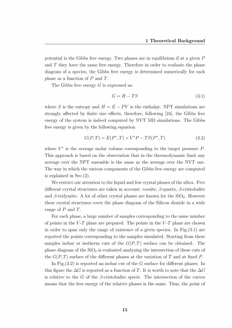
potential is the Gibbs free energy. Two phases are in equilibrium if at a given P
and T they have the same free energy. Therefore in order to evaluate the phase
diagram of a species, the Gibbs free energy is determined numerically for each
phase as a function of P and T .
The Gibbs free energy G is expressed as:
G = H − TS (3.1)
where S is the entropy and H = E − PV is the enthalpy. NPT simulations are
strongly affected by finite size effects, therefore, following [24], the Gibbs free
energy of the system is indeed computed by NVT MD simulations. The Gibbs
free energy is given by the following equation
G(P, T ) = E(P ∗, T ) + V ∗P − TS(P ∗, T ) (3.2)
where V ∗ is the average molar volume corresponding to the target pressure P .
This approach is based on the observation that in the thermodynamic limit any
average over the NPT ensemble is the same as the average over the NVT one.
The way in which the various components of the Gibbs free energy are computed
is explained in Sec.(2).
We restrict our attention to the liquid and few crystal phases of the silica. Five
different crystal structures are taken in account: coesite, β-quartz, β-cristobalite
and β-tridymite. A lot of other crystal phases are known for the SiO2. However
these crystal structures cover the phase diagram of the Silicon dioxide in a wide
range of P and T .
For each phase, a large number of samples corresponding to the same number
of points in the V -T plane are prepared. The points in the V -T plane are chosen
in order to span only the range of existence of a given species. In Fig.(3.1) are
reported the points corresponding to the samples simulated. Starting from these
samples isobar or isotherm cuts of the G(P, T ) surface can be obtained. The
phase diagram of the SiO2 is evaluated analyzing the intersection of these cuts of
the G(P, T ) surface of the different phases at the variation of T and at fixed P .
In Fig.(3.2) is reported an isobar cut of the G surface for different phases. In
this figure the ∆G is reported as a function of T . It is worth to note that the ∆G
is relative to the G of the β-cristobalite specie. The intersection of the curves
means that the free energy of the relative phases is the same. Thus, the point of
15

3. PHASE DIAGRAM OF SILICON DIOXIDE
0
1000
2000
3000
4000
5000
6000
5 6 7 8 9 10 11
Tem
pera
ture
[K
]
Volume [cm3 mol-1]
Figure 3.1: Position in the V -T plane of the state points simulated. For the
liquid phase are used red pluses, for coesite green squares, for β-cristobalite black
circles, for β-tridymite violet triangles, and finally for β-quartz blue crosses.
intersection of the two curves corresponds to a point in the phase diagram at the
T of intersection and at the P of the isobar cut.
2 Calculation of the Gibbs Free Energy of the
Various Phases
In order to calculate G(P, T ) from Eq.(3.2) we have to evaluate the E(V ∗, T ),
P (V ∗, T ), S(V ∗, T ) terms as functions of V ∗ and T . The computational procedure
differs from the liquid to the crystalline phases. The different procedures are
described separately in the following sections.
16

2 Calculation of the Gibbs Free Energy of the Various Phases
-1
0
1
2
3
4
1500 2000 2500 3000 3500 4000
∆G /
eV m
ol-1
Temperature / K
LIQUIDCRIST
TRIDM
Figure 3.2: ∆G as a function of T at fixed P (P = 0). In the figure the ∆G is
evaluated as the difference between the Gibbs free energy of a specie with respect
to a reference specie. In the present case the reference specie is the β-cristobalite.
2.1 Liquid phase
The liquid phase is modeled by a sample containing 1536 atoms. The liquid
samples consists of eight isochores from volumes of 4.83 cm3 mol−1 to 10.59 cm3
mol−1. For each isochor the sample are equilibrated in a range of temperatures
from 2500 K to 6000 K at intervals of 500 K (see Fig.(3.1)). In the present
simulations the temperature is controlled via the Nose-Hoover chain method [25]
with a time step of 0.05 fs. In order to identify equilibrium curves in an accurate
way we need to obtain an analytical approximation to G(P, T ). However, we
compute the various terms of Eq.(3.2) only on a discrete grid. One pass from this
discrete to a continuous representation by interpolating the data by third order,
for the energy, and fourth order, for the pressure, polynomials.
In practice we first fit E(V, T ) along isochores
E(V , T ) =3∑
n=0
αn(V )T n (3.3)
17

3. PHASE DIAGRAM OF SILICON DIOXIDE
Figure 3.3: Example of the fitted procedure for E in the liquid phase. Left) E as
a function of T at fixed volume V = 6.9 cm3 mol−1. Right) E as a function of P
at fixed temperature T = 4500 K.
and then along isothermals
E(V, T ) =3∑
n=0
3∑m=0
βn,m VmT n (3.4)
P (V, T ) is obtained in a similar way. In Fig.(3.3) and Fig.(3.4) the fitted
curves of E(V, T ) and P (V, T ) are shown along an isochor and isothermal.
The value of the entropy S at a given point in V -T is calculated by thermo-
dynamic integration using the following relation
S(V, T ) = SR(VR, TR) +
∫ T
TR
1
T
(∂E(VR, T )
∂T
)VR
dT +1
T
∫ V
VR
P (V , T ) dV (3.5)
where SR is the entropy for a reference state at reference values of volume and
temperature (VR, TR). Eq.(3.5) is indeed the variation of entropy from a reference
state computed along a path composed of an isochor, bringing the system from
(VR, TR) to (VR, T ), and then along an isothermal, bringing the system from
(VR, T ) to (V, T ). The second term of the Eq.(3.5) is evaluated analytically from
the fitting for E(V, T ) as a function of T described above, see Eq.(3.3). While the
integral over the volume is obtained numerically using the Simpson’s rule from
the fitting of the P (V, T ) as a function of V .
18

2 Calculation of the Gibbs Free Energy of the Various Phases
Figure 3.4: Example of the fitted procedure for P in the liquid phase. Left) P as
a function of T at fixed volume V = 6.9 cm3 mol−1. Right) P as a function of P
at fixed temperature T = 4500 K.
For the entropy at the reference point is used the expression of the entropy of
an ideal gas composed of two species
SR(VR, TR) = NSi kB
ln
[VR
NSi
(2πmSi kB TR
~2
)3/2]
+NO kB
ln
[VR
NO
(2πmO kB TR
~2
)3/2]
− kB ln(2π√NSiNO)
(3.6)
here NSi, NO and mSi, mO are the number of atoms and the masses for Silicon
and Oxygen, ~ the Planck constant and kB the Boltzmann constant.
With the above procedure the value of E, P , and S for an arbitrary point
V0, T0 can be obtained form molecular dynamic simulations at fixed V and T .
Finally using Eq.(3.2) the value of G at the given point is evaluated for the liquid
phase.
2.2 Crystal phases
As explained before, we focused on five different crystal structures. The crystal
phase analyzed are: coesite, β-cristobalite, β-quartz and β-tridymite. In Tab.3.1
the crystal symmetries and lattice parameters of the crystal phases analyzed are
19

3. PHASE DIAGRAM OF SILICON DIOXIDE
β-crist. [26] β-quartz [27] β-trid. [28] coesite [29]
symmetry cubic hexagonal hexagonal monocliniclattice 7.16 4.91 5.40 7.17 12.38 7.13 12.37 7.17angles 90 90 120 90 120 90 120.34 90
Pearson sym. Fd3m P6222 P63/mmc C2/cgroup N 227 180 194 15
Table 3.1: crystallographic data for β-cristobalite, β-quartz, β-tridymite and
coesite
reported. It is worth to note that the simulated crystal phases correspond to the
main structures of the silica crystals.
In principle, the E(V, T ), P (V, T ) and S(V, T ) terms of Eq.(3.2) can be com-
puted according to the procedure explained above for the liquid phase. However,
at a variance with the liquid phase, the crystal one might be anisotropic. As a
consequence, the ratio among the lattice parameter can change with T and V .
So, the procedure for computing G(P, T ) must be adopted. The samples are first
prepared according to experimental crystallographic data (see Tab.(3.1)). The
structures at different volumes are obtained by scaling up and down the origi-
nal structures. This step is followed by a geometry optimization. A 40 ps NPT
simulation for relaxing the lattice structure follows. The pressure is fixed at the
average value corresponding to the present volume, the latter is therefore almost
preserved.
Finally a NVT simulation of 30 ps is performed, so that the average values of
E and P are computed. At the end of this procedure the value of E and P at
the grid points are computed. Using the same fitting procedure explained above,
an approximation of the E(V, T ) and P (V, T ) surface over the entire V -T space
of the given crystal are computed.
In order to estimate the entropy for an arbitrary point of the V -T plane the
Eq.(3.5) can be used as in the liquid phase. However the reference state is different
from the liquid phase. For a crystal phase the entropy at the reference state SR
can be approximated by
SR = Sharm + Sanh (3.7)
where the Sharm is the harmonic contribution and the Sanh is the anharmonic
20
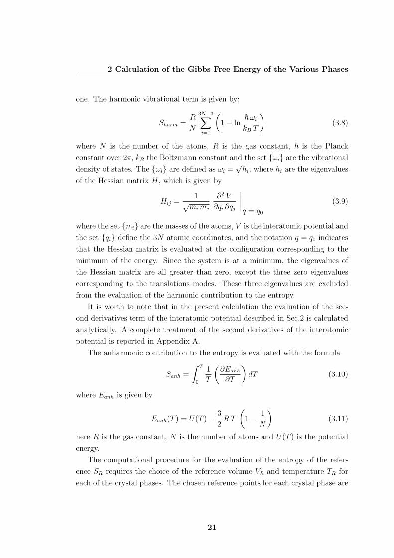
2 Calculation of the Gibbs Free Energy of the Various Phases
one. The harmonic vibrational term is given by:
Sharm =R
N
3N−3∑i=1
(1− ln
~ωi
kB T
)(3.8)
where N is the number of the atoms, R is the gas constant, ~ is the Planck
constant over 2π, kB the Boltzmann constant and the set ωi are the vibrational
density of states. The ωi are defined as ωi =√hi, where hi are the eigenvalues
of the Hessian matrix H, which is given by
Hij =1
√mimj
∂2 V
∂qi ∂qj
∣∣∣∣q = q0
(3.9)
where the set mi are the masses of the atoms, V is the interatomic potential and
the set qi define the 3N atomic coordinates, and the notation q = q0 indicates
that the Hessian matrix is evaluated at the configuration corresponding to the
minimum of the energy. Since the system is at a minimum, the eigenvalues of
the Hessian matrix are all greater than zero, except the three zero eigenvalues
corresponding to the translations modes. These three eigenvalues are excluded
from the evaluation of the harmonic contribution to the entropy.
It is worth to note that in the present calculation the evaluation of the sec-
ond derivatives term of the interatomic potential described in Sec.2 is calculated
analytically. A complete treatment of the second derivatives of the interatomic
potential is reported in Appendix A.
The anharmonic contribution to the entropy is evaluated with the formula
Sanh =
∫ T
0
1
T
(∂Eanh
∂T
)dT (3.10)
where Eanh is given by
Eanh(T ) = U(T )− 3
2RT
(1− 1
N
)(3.11)
here R is the gas constant, N is the number of atoms and U(T ) is the potential
energy.
The computational procedure for the evaluation of the entropy of the refer-
ence SR requires the choice of the reference volume VR and temperature TR for
each of the crystal phases. The chosen reference points for each crystal phase are
21

3. PHASE DIAGRAM OF SILICON DIOXIDE
reported in Fig.(3.1). Then starting from the final configuration of the previous
procedure for evaluating the E and P surface the atomic position of this configu-
ration are optimized so that the minimum energy configuration is reached. Then
the eigenfrequency spectrum of the Hessian matrix (see Eq.3.9) is evaluated from
these minimum energy configurations, one for each crystal phase. The eigenfre-
quency spectrum is evaluated diagonalizing the Hessian matrix in order to found
the Hessian eigenvalues. Using Eq.(3.8) the harmonic contribution to the SR is
obtained.
To calculate Sanh we use the energy optimized configuration used for the
evaluation of the Hessian matrix as starting point for a set of simulation at
constant T and V from 100 K to 1500 K equally spaced of 100 K. First the
temperature is raised from 0 K to the desired T until 1500 K. Then the systems
are equilibrated at the desired T for 50 ps with a NVT simulation at constant
T . From these simulations the value of Eanh is evaluated, see Eq.(3.11), using a
polynomial fit
Eanh = c0 +nmax∑n=2
cnTn (3.12)
From the evaluation of Eanh using the Eq.(3.10) the value of the anharmonic
contribution of SR is obtained for each crystal phase. Finally the value of the en-
tropy of the reference points is obtained as a sum of the harmonic and anharmonic
contributions (see Eq.3.7).
With the previous procedure the E, P and S surfaces of a crystal phase are
obtained for every arbitrary point (V, T ). From these surface the value of the
Gibbs free energy can be evaluated, as in the liquid phase.
3 Results
In Fig.(3.5) is reported the diagram of the SiO2 in the P -T plane as obtained by
the method above. The phase diagram must be compared with the experimental
one reported in Fig.(3.6). It is quite evident that the agreement between theo-
retical and experimental diagram is only qualitative. Indeed the simulated phase
diagram shows clear quantitative deficiencies. The phase boundaries between the
species are not at the same condition of neither T nor P .
22
3 Results
-2
0
2
4
6
8
10
0 1000 2000 3000 4000 5000 6000
Pres
sure
/ G
Pa
Temperature / K
Coesite
QLiquid
T C
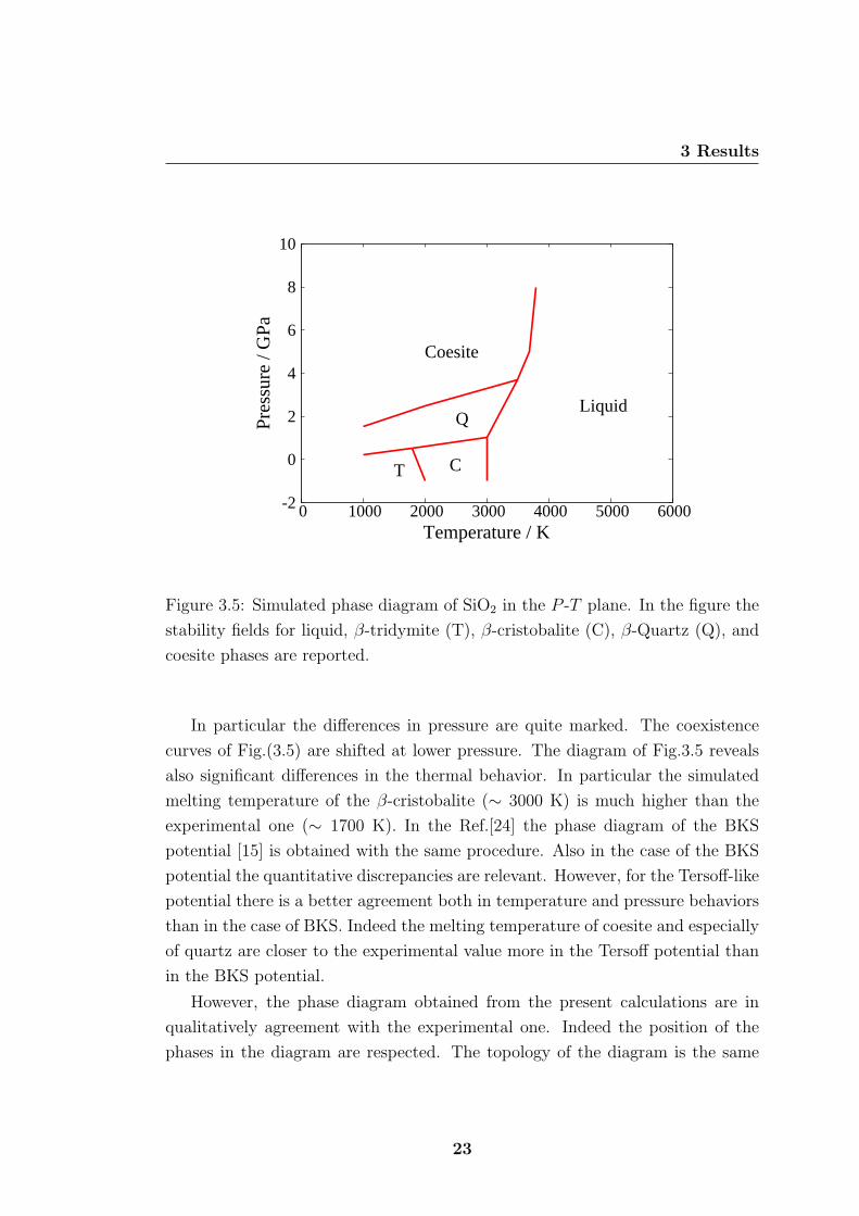
Figure 3.5: Simulated phase diagram of SiO2 in the P -T plane. In the figure the
stability fields for liquid, β-tridymite (T), β-cristobalite (C), β-Quartz (Q), and
coesite phases are reported.
In particular the differences in pressure are quite marked. The coexistence
curves of Fig.(3.5) are shifted at lower pressure. The diagram of Fig.3.5 reveals
also significant differences in the thermal behavior. In particular the simulated
melting temperature of the β-cristobalite (∼ 3000 K) is much higher than the
experimental one (∼ 1700 K). In the Ref.[24] the phase diagram of the BKS
potential [15] is obtained with the same procedure. Also in the case of the BKS
potential the quantitative discrepancies are relevant. However, for the Tersoff-like
potential there is a better agreement both in temperature and pressure behaviors
than in the case of BKS. Indeed the melting temperature of coesite and especially
of quartz are closer to the experimental value more in the Tersoff potential than
in the BKS potential.
However, the phase diagram obtained from the present calculations are in
qualitatively agreement with the experimental one. Indeed the position of the
phases in the diagram are respected. The topology of the diagram is the same
23

3. PHASE DIAGRAM OF SILICON DIOXIDE
at T=0 in Fig. 4(b) and extract the coexistence pressuresfrom the slope of “common tangent constructions” bridging
coexisting phases. The T=0 coexistence pressures are plotted
in Fig. 5(b) and serve to check that the method used to de-termine coexistence boundaries at finite T is consistent with
the (more straightforward) T=0 evaluation. Note that we donot locate the !-quartz/stishovite coexistence condition atT=0 due to the fact that !-quartz transforms to "-quartzbefore T=0 is reached at the relevant volume for the com-
mon tangent construction.
Throughout the evaluation scheme described above, the
largest single source of statistical error is the uncertainty
cited in Ref. [15] for SR, the entropy of the liquid at thereference state point. We therefore create confidence limits
for our melting lines, shown in Fig. 5, by allowing the value
of SR to vary by ±0.18 J mol!1 K!1.
III. RESULTS AND DISCUSSION
Figure 5(b) plots P-T coexistence conditions, both stableand metastable, occurring among the liquid phase !L" and thecrystalline phases !-quartz !Q", coesite !C", and stishovite!S". Figure 6 is the projection of the same boundaries ontothe plane of V and T. This plot exposes the volume differ-
ences of coexisting phases along phase boundaries. This type
of plot is rarely constructed for real materials, due to the
challenge of determining the densities of coexisting phases,
especially at high pressure. However, it is readily constructed
from simulation data.
Comparison of the BKS and experimental phase bound-
aries [3] in Fig. 5 exposes the quantitative deficiencies of themodel. Apparent in particular is the difference between the
pressures at which corresponding features occur. For ex-
ample, the S-L-C triple point occurs at 13.4 GPa in real
silica, but at only 5.8 GPa in the model. Overall, the P range
of the crystal stability fields is substantially lower in the
model. The pressure difference between the model and real-
ity is more of a shift than a rescaling. For example, the
coesite stability field has approximately the same extent in P
(about 5 GPa) at low T in both BKS and real silica. However,
the S-C coexistence boundary is shifted downward in P in
the model by more than 7 GPa compared to real silica. The
result is that coesite, rather than quartz, is the equilibrium
phase of BKS silica at ambient P for most of the temperature
range. Indeed, at the very lowest T, the stishovite stability
field just reaches ambient P, making stishovite the T=0
ground state of BKS silica at P=0 (filled square in Fig. 5(b)].The correspondence of the thermal behavior is better than
that of the mechanical behavior, but significant differences
still occur. The T of the S-L-C and C-L-Q triple points are
respectively 15% and 32% higher than their experimental
values. Also, the maximum T reached by the coesite, and
especially the !-quartz stability fields, are too high comparedto reality. However, the curvature of the crystal-liquid coex-
istence boundaries are comparable to experiment.
FIG. 5. (a) Experimentally determined coexistence lines of silicain the P-T plane. Stability fields for the stishovite !S", coesite!C" , !-quartz !Q", and liquid !L" phases are shown. Both stable(solid) and metastable (dashed) coexistence lines are shown. Theinset shows the stability fields of cristobalite and tridymite, not
considered in this work. Adapted from Ref. [3]. (b) Phase diagramof BKS silica in the P-T plane. Solid lines are stable coexistence
lines. Dotted lines show error estimates for the crystal-liquid coex-
istence lines, as described in the text. Metastable coexistence lines
(dashed) are also shown that meet at the metastable S-L-Q triple
point. The locations of the S-C (filled square) and C-Q (filled circle)coexistence boundaries at T=0, determined from Fig. 4(b), are alsoshown.
FIG. 6. Phase diagram of BKS silica in the V-T plane. The
notation and symbols used have the same meaning as in Fig. 5.
Note that in this projection, both one-phase stability fields as well as
two-phase coexistence regions are located. The projections of the
metastable coexistence lines (dashed) shown in Fig. 5 are alsopresented.
PHASE DIAGRAM OF SILICA FROM COMPUTER SIMULATION PHYSICAL REVIEW E 70, 061507 (2004)
061507-5
Figure 3.6: Experimental phase diagram of SiO2 in the P -T plane. In the figure
the stability fields for liquid (L), β-Quartz (Q), coesite (C), stishovite (S) phases
are reported. In the inset is reported the stability fields of β-cristobalite ad
β-tridymite. Figure taken from Ref.[24].
in both cases. It is worth to note that the equilibrium phases at ambient P ,
i.e. P = 0 GPa, of modified Tersoff potential are the same like the experimental
diagram. Indeed at ambient temperature the stable phase is the quartz, for higher
temperature first the tridymite and then the cristobalite become the stable phase.
On the contrary for the BKS potential the stable phase is the coesite for all the
temperature range [24]. For the modified Tersoff potential in exam, the only
drawback at ambient P is that the coexistence lines between the phases are shifted
at higher temperature. This means that, taking in account the deficiencies, the
modified version of the Tersoff potential [19] is suitable for molecular dynamics
simulations at ambient pressure.
24

Chapter 4
Self Diffusion in Amorphous
Silicon Dioxide
Several authors suggest that the formation of nano-particles is governed by the
Ostwald ripening mechanism [30] and, in particular, by the diffusivity of Si atoms
from smaller to larger nano-particles. It was also found a strong dependency of
the crystal growth from Si supersaturation, which seems to be in conflict with
the Ostwald mechanism (see Ref.[31] and reference therein). However, also in
this case, this was considered an indication that the Si diffusion is the limiting
step of the overall process. It would be therefore of particular interest to study
the diffusivity of Si and its mechanism in stoichiometric and non-stoichiometric
conditions. Unfortunately, to the best of my knowledge, no experimental studies
on diffusion of Si in amorphous SiO2 in absence of a Si/SiO2 extended interfaces
(i.e. in real conditions for the formation of nano-particles) are available, especially
concerning the identification of the mechanism of the diffusion. This is likely due
to the fact that it is hard to generate a controlled concentration profile of isotopic
Si into a bulk-like sample (with no interface), so as to measure its variation upon
thermal annealing. However, in a recent paper, Yu et al. [31] have addressed the
identification of the atomistic mechanisms of diffusion of one excess Si atom in
a-SiO2 by performing ab-initio calculations. In this paper, the authors identified
possible equilibrium sites and calculated the corresponding energy barrier for the
diffusion of the excess Si atom by means of the Nudged Elastic Band (NEB)
method [32, 33]. However, this investigation did not take into account neither
the different concentrations of excess Si atoms nor the possible fluctuation of Si
25

4. SELF DIFFUSION IN AMORPHOUS SILICON DIOXIDE
density within the samples. Finally, because of the use of NEB, the effect of
temperature is not taken into account.
In this section I will present the results on the study of the diffusion mecha-
nisms of Si and O in a-SiO2 at different temperatures and for different Si-atoms
concentrations by means of classical molecular dynamics (MD) simulations. We
do not assume any a priori hypothesis on the mechanisms. Rather, by analyzing
the MD trajectories we identify the set of most relevant mechanisms occurring
at various thermodynamical and chemical conditions. Finally, we calculate the
contribution of each individual mechanism to diffusion and analyze the role of
thermodynamical and chemical conditions.
The section is organized as follows: in Sec.(1) the theoretical background
of calculation of diffusivity within MD framework is shortly revised. Moreover
a novel method for calculating the contribution of different mechanisms to the
diffusivity is presented. In Sec.(2) the preparation of the sample is presented.
In Sec.(3.1) the results on the diffusivity are presented and they are compared
with experimental and computational results available in literature. Finally, in
Sec.(3.2) the contribution of a set of possible mechanisms to the diffusivity of
silicon are analyzed.
1 Theoretical Background
Solid-state self-diffusion is commonly due to several possible concurrent mecha-
nisms, typically related to the presence and the dynamics of defects of different
kind. For example, in crystals these defects typically are vacancy, self-interstitial,
etc. Even though in amorphous materials the origin of self-diffusivity is less well
understood, also in this case it is thought that it is induced by several concurrent
mechanisms. Typically, however, the experimental interpretation of diffusivity-
vs-temperature measurements is based on the phenomenological Arrhenius law
D(T ) = D∞ exp
(− E
kB
)(4.1)
where D∞ is the diffusivity at high temperature and E is the (average) migration
energy, representing the (average) energy barrier to be overcome during diffusion.
In Eq.(4.1) T and kB represent the temperature and the Boltzmann constant,
26

1 Theoretical Background
respectively. The theoretical atomic scale investigation on self-diffusion is rather
based on the calculation of the mean square displacement (MSD), according to
the Einstein random-walk equation
D(T ) = limt→∞
1
6
d〈∆r2(t)〉dt
(4.2)
where the t → ∞ limit stands for simulations performed for long enough times.
Eq.(4.2) is straightforwardly implemented in molecular dynamics (MD) since the
MSD is defined as
〈∆r2(t)〉 = 〈N∑
i=1
[~ri(t)− ~ri(0)]〉 (4.3)
where ~ri(t) and ~ri(0) are the positions of the i-th atom at time t and time t = 0,
respectively, and it is therefore directly computed from the computer-generated
atomic trajectories. Indeed, 〈· · · 〉 is the ensemble average over all possible initial
configurations and velocities. The ensemble average is extended over the config-
urational space available to the system. Since we perform MD simulations, the
integral implied by Eq.(4.3) is calculates by means of a time average over the
trajectory of the atoms. This means that we assume that the ergodic hypothesis
holds true for these systems in the given thermodynamical conditions.
In addition, by means of Eq.(4.2) it is relatively easy to calculate the contri-
bution to self-diffusion by each given mechanisms, provided that they are clearly
identified. Once again, this information can be extracted by animation and in-
spection of atomic trajectories.
However, determining the contribution of each individual mechanism to the
diffusivity is not trivial. In the following we shall demonstrate that under proper
conditions the MSD is additive and therefore D(T ) is additive as well. We can
therefore resort to Eq.(4.2) for calculating the D(T ) of each mechanism.
We assume that the diffusion occurs through a sequence of stepwise events.
This assumption is justified by the empirical observation that indeed Si and O
atoms diffuse through a stepwise mechanism in this material (see Fig.(4.1)). We
can therefore rewrite Eq.(4.3) as follows
27

4. SELF DIFFUSION IN AMORPHOUS SILICON DIOXIDE
0 10 20 30 40 50
Ato
mic
Dis
plac
emen
t (° A
2 )
Time (ps)
50 °A2
Figure 4.1: MSD displacement of few Si atoms selected randomly in the sample.
The figure clearly shows that the diffusion occurs via stepwise events.
〈∆r2(t)〉 = 〈 1
N
N∑i=1
[L∑
α=1
∆~ri(tα)
]2
〉 (4.4)
where L is the number of diffusive steps and ∆~ri(tα) is the (vector) displacement
of i-th atom occurring at the time tα. If the diffusive steps belong to different
mechanisms, then Eq.(4.4) can be rewritten as follows:
〈∆r2(t)〉 = 〈 1
N
N∑i=1
[ ∑α∈M1
∆~ri(tα) +∑
β∈M2
∆~ri(tβ) + · · ·
]2
〉 (4.5)
where ∆~ri(tα) is the displacement of i-th atom due to an event of type M1. An
analogous definition is valid for ∆~ri(tβ). The indexes α and β run over the set of
events belonging to mechanism M1 and M2, respectively.
Eq.(4.5) can be further manipulated
28

1 Theoretical Background
〈∆r2(t)〉 = 〈∆~r2M1
(t)〉+ 〈∆~r2M2
(t)〉+ · · ·+ 2〈∆~rM1(t) ·∆~rM2(t)〉+ · · · (4.6)
where
〈∆r2M1
(t)〉 = 〈 1
N
N∑i=1
[∑α∈M1
∆~ri(tα)
]2
〉 (4.7)
and
〈∆~rM1(t) ·∆~rM2(t)〉 = 〈 1
N
N∑i=1
∑α∈M1
∑β∈M2
∆~ri(tα) ·∆~ri(tβ)〉 (4.8)
Similar definitions are assumed for other mechanisms.
If the sample is monophasic and there are no external fields acting on it, the
product ∆~rM1(tα) ·∆~rM2(tβ) can assume with the same probability positive and
negative values. Therefore, the term 〈∆~rM1(t)·∆~rM2(t)〉 becomes zero. This is the
case in the performed simulations. In fact, the term 〈∆~rM1(t) ·∆~rM2(t)〉 is about
three order of magnitude smaller than the smallest 〈∆r2Mα
(t)〉 term. Therefore,
Eq.(4.6) reduces to
〈∆r2(t)〉 ∼= 〈∆r2M1
(t)〉+ 〈∆r2M2
(t)〉+ · · · (4.9)
Eq.(4.9) states that, under the above hypothesis, the total MSD is the sum of
MSDs relative to each mechanism. Under the same hypothesis, using once again
the fact that two discrete diffusive steps (even if belonging to the same mecha-
nism) are independent, Eq.(4.7) can be further simplified into:
〈∆r2M1
(t)〉 ∼=1
N〈
N∑i=1
∑α∈M1
∆r2i (tα)〉 (4.10)
Also in this case the cross term 〈∑
i
∑α,α′
∆~ri(tα)·∆~ri(tα′)〉 is negligible with respect
to 〈∑
i
∑α
∆r2i (tα)〉 (about three order of magnitude smaller).
Unfortunately, ∆r2i (t) is noisy (see top panel of Fig.(4.2)). This is due to
the interplay of two phenomena: diffusive steps and atomic vibrations about
equilibrium positions. The problem of the noise can be reduced by averaging the
29

4. SELF DIFFUSION IN AMORPHOUS SILICON DIOXIDE
atomic positions on a time window τ centered on the time t. The window τ needs
to be larger than the period of a vibration, but not too large otherwise distinct
diffusive steps can be confused. A τ of 100 fs is used in the simulations. The
∆r2i (t) computed on average positions is much more regular (compare Fig.(4.2/a)
and Fig.(4.2/b)) and shows a clear stepwise behavior. The ∆r2i (tα) to be used in
Eq.(4.10) is computed by the difference of average atomic positions before and
after the time tα.
A key issue is still open, namely how to identify the times tα, tβ, . . . . at which
the events of type M1, M2, . . . . occur. For each mechanism, order parameters
θl(~r1(t), · · · , ~rN(t)) that monitor the occurrence of a diffusive step can be identi-
fied. For example, assuming that one diffusive mechanism implies the change of
coordination number of a Si atom. By monitoring changes of the coordination
number of each silicon the total displacement of the mechanism can be evaluated,
as indicated in Eq.(4.10) (see Fig.(4.2)).
The complete description of the collective coordinates used for monitoring
the mechanisms identified in this paper is given in Sec.(3.2). Anticipating the
results, it is worth remarking that using this technique a set of three mechanisms
accounting for more than the 90 % of the diffusivity is identified.
On the basis of the so computed MSD, we can calculate the diffusivity of each
self-diffusion mechanism and, from this, the corresponding migration energy EMα
and the pre-exponential factor DMα∞ . Of course, as for the overall E and D∞,
these are phenomenological parameters.
A somewhat related approach for the calculation of parameters governing the
mass transport in crystals has been devised and applied by Da Fano and Jacucci
[34]. In this approach, the frequency of events of a given type occurring in a MD
run is counted and analyzed according to the following Arrhenius-type formula
ΓMα(T ) = DMα∞ exp
(−EMα
kBT
)= νMα exp (SMα/kB) exp
(−EMα
kBT
)(4.11)
where ΓMα(T ) is the number of events of a give type, νMα is the corresponding
attempt frequency, EMα is the migration energy and SMα is the migration entropy.
In this case, Eq.(4.11), and therefore the parameters contained into it, is no longer
30

1 Theoretical Background
02468
101214
−150 −100 −50 0 50 100 1501
2
3
4
5
DISPLACEMENT
02468
101214
−150 −100 −50 0 50 100 1501
2
3
4
5
Time (fs)
Ato
mic
Dis
plac
emen
t (° A2 )
Coo
rd. n
umbe
r
a)
b)
COORDINATION
DISPLACEMENT
Figure 4.2: Panel a) ∆r2i (t) for a Si atom (dotted line) and the corresponding
variation of the coordination number (continuous line). Panel b) same data after
time average over a time window τ . Values are reported with respect to average
values in the period plotted. The time origin in the graph is taken at the instant
at which the average coordination number changes its value, i.e. the instant at
which an event of this mechanism occurs.
phenomenological. Rather, it is derived from Transition State Theory in harmonic
approximation.
It is worth mentioning that while the Da Fano and Jacucci method is perfectly
justified in the case of crystals, where all the events of the same kind give the same
contribution to the mass transport, in the case of amorphous materials the validity
of this method is more questionable. In fact, depending on the environment of
the atoms undergoing to a diffusive event, the corresponding displacement can
vary significantly. This means that in the case of amorphous materials we must
understand a diffusive mechanism in a more loose sense. However, in the following
we have performed both kind of analysis and, anticipating our results, they both
bring to the same qualitative conclusions.
31

4. SELF DIFFUSION IN AMORPHOUS SILICON DIOXIDE
2 Sample Preparation and Computational Setup
The stoichiometric a-SiO2 sample was obtained by quenching from the melt.
Within this approach disordered structures are generated by quenching from an
equilibrated silica melt to room temperature. The procedure starts from a well
equilibrated sample of fluid SiO2 at 8500 K. The silica melt is obtained by molec-
ular dynamic simulations at constant volume and the temperature is controlled
using the Nose-Hoover chain method [25] using a time step of 0.5 fs. The liq-
uid sample is obtained by melting a beta-cristobalite sample. The density of the
sample was kept fixed at the experimental density of a-SiO2 (2.17 g/cm3). After
25 ps at 8500 K, the high temperature liquid is cooled down to 4000 K with
a rate of 4 · 1013 K/s. The sample is equilibrated at 4000 K for 50 ps. Then
the sample is cooled slowly down to room temperature as follows. First a run
of 50 ps is performed to obtain a sample at 2000 K which is equilibrated for 25
ps. Then the sample at 2000 K is cooled again to 300 K in 100 ps and finally
it is equilibrated at room temperature. In Fig.(4.3) the complete amorphization
procedure is shown.
a-SiO2 was modeled by samples of size ranging from 5184 to 24000 atoms.
Three samples of different size are prepared in order to compare the results. In
all cases a cubic cell of β-cristobalite are prepared. The smallest sample consists
of 5184 atoms, that correspond to 1728 units of SiO2. The cell dimension for
this sample is 42.996 x 42.996 x 42.996 A. Another sample of 12288 atoms (4096
SiO2 units) is prepared from a cubic cell with L=57.328 A. For the last sample,
a cubic cell of 71.660 A containing as many as 24000 atoms (8000 SiO2 units) is
used. It is worth to note that the results for the three samples are essentially the
same. This means that the size of the smallest sample obtained is big enough
to correctly reproduce the self diffusion of a-SiO2. The atomic interactions are
treated by means of the modified Tersoff potential developed by Billeter et al. [19]
and described in Sec.(2).
It is important to stress that, since the cooling rate is several order of mag-
nitude higher than the experimental one, the consistency of this computational
model with the experimental samples must be carefully checked. The g(r) (see
Fig.(4.4)) obtained with the above procedure is compared with previous experi-
mental [35, 36] and ab initio [37] data, obtaining a very good quantitative agree-
32

2 Sample Preparation and Computational Setup
0
1000
2000
3000
4000
5000
6000
7000
8000
9000
0 50 100 150 200 250 300
Tem
pera
ture
(K
)
Time (ps)
Figure 4.3: Quenching thermal cycles used for the amorphization of SiO2.
ment.
a-SiO2 samples at various stoichiometries (from 33 % to 45 % of Si) are ob-
tained from the stoichiometric SiO2 by random substitution of Oxygen atoms
with Silicon atoms. After the substitution, the system was relaxed for 50 ps,
with a time step of 0.5 fs, by mean of constant temperature MD using the Nose-
Hoover chain method [25]. Since the experimental density is not available, the
density of these systems is fixed at the density of stoichiometric a-SiO2. However,
we verified that with this setup the internal pressure of such samples is negligible.
The self diffusion in stoichiometric and sub-stoichiometric samples of SiO2 is
investigated in a range of temperature from 1500 K to about 3000 K, depending
on the concentration of Si. Total and mechanism specific MSD of Eqs.(4.3-4.6)
are computed by means of MD at constant number of particles, volume and
energy (NVE). Simulations at different temperatures is performed changing the
total energy of the system. At each concentration and temperature, 200 ps MD
simulations are run. We verified that such long simulations are adequate for
reaching the linear regime of the MSD required by Eq.(4.2).
33

4. SELF DIFFUSION IN AMORPHOUS SILICON DIOXIDE
0
2
4
6
g(r)
Si-Si
Si-O
O-O
Present Results
Ref. [9]Ref. [8]Ref. [7]
0
10
20
30
g(r)
0 2 4 6 8
0 1 2 3 4 5 6
g(r)
r (°A)
Figure 4.4: Pair correlation function of stoichiometric a-SiO2 as obtained from
the quenching from the melt procedure described in the text. Positions and, when
available, magnitudes of peaks as obtained in previous experimental (Johnson et
al.[35] and Susman et al.[36]) and ab initio MD (Sarnthein et al.[37]) works are
reported for comparison.
3 Results and Discussion
3.1 Migration Energy
Fig.(4.5) shows the diffusivity of Si atoms at various temperatures and concen-
trations as obtained from MSD (see section 1). Corresponding data for O were
computed as well but not shown in figure as there are no corresponding ex-
perimental data to compare with. It is worth noticing that we performed MD
simulations in a temperature range higher than the experimental one. This is a
standard method for accelerating MD simulations to study diffusivity. In partic-
ular, under the only hypothesis of an Arrhenius dependence upon temperature (a
very widely and common-sense assumption, indeed) high-temperature data can
safely be extrapolated down to room temperature. Of course the reliability of
34

3 Results and Discussion
10-35
10-30
10-25
10-20
10-15
10-10
3.0 3.5 4.0 4.5 5.0 5.5 6.0 6.5 7.0 7.5 8.0
3000 K 2500 K 2000 K 1500 KD
iffu
sivi
ty (
cm2 s-1
)
104/T (K-1)
33% Si35% Si37% Si41% Si45% Si
Figure 4.5: Diffusivity of Si atoms as a function of the inverse of temperature
for SiO2−x samples at various Si concentrations. The cyan frame in the graph
represents the range of observed experimental values.
the results must be checked a posteriori. In the present case, we have performed
two tests: (i) assessing whether the system was still in amorphous phase at the
higher temperatures; (ii) assessing whether the diffusion data extracted from such
a sample can be extrapolated at lower temperatures. As for (i), by analyzing the
g(r) we verified that the system persisted in the amorphous phase also at the
higher temperatures. This is not surprising as in simulations, especially constant
volume simulations of (relatively) small samples, large fluctuations of the density
are forbidden and the system can stay in a metastable state despite the fact that
exists another phase at lower free energy. As for (ii), we verified that the log of
diffusivity is inversely proportional to the temperature over the whole range of
temperature simulated, as requested from the Arrhenius law. For sake of com-
parison, we also report the D(T ) vs T range of experimental data[38, 39, 40, 41]
(the cyan box in Fig.(4.5)). It can be seen that extrapolated computational data
are well within the experimental range, confirming the overall agreement of the
present results with experimental data.
35

4. SELF DIFFUSION IN AMORPHOUS SILICON DIOXIDE
From Fig.(4.5) and the corresponding data for the diffusion of O, we calculated
migration energies as a function of the Si concentration (see Fig.(4.6), top). For
the migration energy of Si at the stoichiometric composition we found a value
that is the 65-75 % of the experimental values [38, 39, 40, 41], depending on the
considered experiment. These results are in line with the predictive capability
of the Billeter et al. potential, as evaluated by the test of diffusion in α-Quartz,
which is in the range of 80 % (see section 2), and the typical accuracy of diffusivity
calculated by means of classical MD.
A relevant difference exists between the present simulations and the experi-
mental setup. The experimental diffusivity is calculated by fitting the concen-
tration distribution of radioactive Si atoms in a sample of SiO2. The radioactive
Si is provided by a sample of crystalline Si through a Si/a-SiO2 interface. The
diffusivity is therefore due to a possible two-step mechanism: i) crossing of the
Si/a-SiO2 interface, ii) diffusion in a-SiO2. Moreover, these experiments are per-
formed in non-equilibrium conditions. So, the experimental conditions, which
are meant to study the diffusivity occurring in different kind of systems, are not
directly mimicked by our simulations.
Finally, the results are in qualitative agreement with previous DFT calcula-
tions [31], which report an energy barrier of 4.5-5 eV. However, also in this case
it is worth noticing some difference in the setup. In fact, the DFT calculations
were carried out by guessing a diffusion path composed of several steps. The
atomistic model for simulating each of these steps was indeed a cluster model,
therefore elastic forces due to the condensed phase environment were neglected.
Moreover, even though the authors mention that the diffusion energy changes
from one initial/final site to another of the same type, results are reported only
for one of them. In addition, the small size of the sample (just 24 SiO2 units)
does not allow neither the fluctuation of the (local) density nor of the (local)
chemical composition of the sample. Since migration energy is affected by the
concentration (see below), results might change in function of these fluctuations.
Furthermore, since just one path has been tested, results of Yu et al. [31] might
be strongly biased by the only mechanism actually considered.
As for the stoichiometry of the sample, Fig.(4.5) shows an increase of diffusion
of Si with its concentration. This is reflected by a decrease of the migration energy
E (see Fig.(4.6), top) and by an increase of the pre-exponential coefficient D∞
36

3 Results and Discussion
1.0
1.5
2.0
2.5
3.0
3.5
33 35 37 39 41 43 45
Ene
rgy
(eV
) SiO
1.0
2.0
3.0
4.0
5.0
6.0
33 35 37 39 41 43 45
D∞
(cm
2 /s)
Percentage of Silicon (%)
SiO
Figure 4.6: Si and O migration energy (top panel) and pre-exponential factor D∞
(bottom panel) as a function of the Si concentration.
(see Fig.(4.6), bottom). This trend is in agreement with experimental findings
[41]. It is interesting noticing that a similar trend is observed for the diffusion of
O as well. This seems to suggest that the diffusion of O and Si atoms is indeed
correlated.
3.2 Mechanisms
In this paragraph the diffusion mechanisms of silicon and their dependence on
the stoichiometry of the sample are analyzed.
By visual inspection of the trajectories three types of stepwise mechanisms
(see Sec.(1)) are identified. These types of mechanisms can be described in terms
of change of coordination for Si and O atoms or swapping of a Si-Si bond for a Si-
O bond (or viceversa). Please notice that, at a variance from previous papers[31],
the model under consideration does not take into account the actual value of the
coordination number, rather its variation. The rationale for this choice is that
in amorphous samples there might exist many atoms with different coordination,
37

4. SELF DIFFUSION IN AMORPHOUS SILICON DIOXIDE
all undergoing to one of the mechanisms introduced above.
More in detail, the first mechanism consists in the change of coordination
of Oxygen atoms. An example of such an event is presented in the top panel of
Fig.(4.7). In this diffusive event an O atom which is initially one-fold coordinated
(the blue atom labeled “O1” in the panel) recovers its complete coordination by
forming a bond with a Si atom (the violet atom labeled “Si” in the panel). In
order to do so, the Si atom breaks a bond with another O (the green atom labeled
“O2” in the same panel) which therefore becomes one-fold coordinated. Hereafter
this mechanism is called O-driven. Of course, events with O and Si atoms with
different initial and final coordination, all belonging to the O-driven mechanism,
occur in the simulations.
The second kind of mechanism is analogous to the first one but for that in
this case Si atoms change their coordination. An example of such an event is
shown in the central panel of Fig.(4.7). Here, two Si atoms are initially 3-fold
coordinated (blue and green atoms labeled “Si1” and “Si2”, respectively, in the
panel). By forming a bond among them they change their coordination from 3
to 4, so restoring their perfect coordination. Hereafter this mechanism is called
Si-driven. As above, events with O and Si atoms with different initial and final
coordination, all belonging to the Si-driven mechanism, occur in the simulation.
Finally, in the third kind of mechanism a Si-Si bond is swapped for a Si-O
bond (or viceversa). An example of this mechanism is presented in the bottom
panel of Fig.(4.7). In this event, the green Si (labeled “Si2’ and the violet O
(labeled “O”) are initially bonded. After the swapping the green Si atom is
bonded to the blue Si (labeled “Si1”). This mechanism shall be called bond-
swapping. A possible explanation of the behavior described above is the attempt
of miscoordinated Si and O atoms to restore the optimal coordination (O-driven
and Si-driven mechanisms) or to establish a network of chemical bonds that
minimize the stress in a region of the sample (bond-swapping).
In order to implement the method described in Sec.(1) a set of collective
variables able to monitor the occurrence of events of the above types is needed.
For this purpose we use total and partial coordination numbers. The former
counts the total number of neighbors of a given atom, while the latter takes
into account also their chemical nature. Mathematically, the partial coordination
number is defined as:
38

3 Results and Discussion
Figure 4.7: Snapshots of events belonging to the O-driven mechanism (top),
Si-driven mechanism (center), and bond-swapping mechanism (bottom). The
mechanisms are described in detail in the text. Atoms involved in the processes
are highlighted in green, blue and violet.
θBi =
∑j∈B
Θ(rij − rcut) (4.12)
where θBi is the coordination number of the i−th atom with respect to atoms
of the species B, Θ(r − rcut) is the Heaviside step function, rij is the distance
between atom i and atom j, rcut is the cutoff distance beyond which two atoms
are no longer considered bonded. The sum in Eq.(4.12) runs over atoms of the
chemical species B. The total coordination number can be obtained from partial
coordination number according to the following formula:
39

4. SELF DIFFUSION IN AMORPHOUS SILICON DIOXIDE
θi =
Nsp∑B=1
θBi (4.13)
where the sum runs over the Nsp chemical species in the sample (two in the
present case).
The O-driven mechanism can be monitored following the variation of the
total coordination number of the O atoms (hereafter referenced by the symbol
θO). It is worth mentioning that analyzing the partial coordination numbers we
discovered that θOO (number of O atoms bonded to O atoms) is always zero. This
means that under the condition of the present simulations O2 molecules are never
formed. Similarly, events belonging to the Si-driven mechanism are identified
by monitoring changes in the value of the total coordination of Si atoms (θSi).
Finally, the partial coordination θOSi and θSi
Si are used to identify events in which a
Si-O bond is swapped for a Si-Si bond (or viceversa), under the constrain that the
total coordination number of the atom considered is unchanged (∆θOSi+∆θSi
Si = 0).
Using these collective variables, the time at which events of a given mechanism
occurs can be identified. The change of collective variables θBi and θi also indicates
that the atom i (and possibly the atoms bonded to it) is involved in the diffusive
step. Then, applying Eq.(4.10) on these atoms, distinguishing between Si and
O, we compute the MSD displacement relative to a given mechanism and the
corresponding diffusivity. The three mechanisms introduced above account for
more than the 90% of the total MSD at all temperatures and Si concentrations.
From the so computed MSD the DMα(T ) of each individual mechanism and,
from this, the corresponding EMα and DMα∞ can be calculated. In Fig.(4.8) are
reported EMα and DMα∞ at various stoichiometries. For comparison, in Fig.(4.9)
are reported the corresponding data obtained through the Da Fano and Jacucci
method [34]. Our calculations (Fig.(4.8), top) show that at lower Si-concentration
the mechanism with the lowest migration energy is the O-driven mechanism.
When the Si-concentration is increased, the activation energy of the Si-driven
and bond-swapping mechanisms is reduced below that of the O-driven mechanism
which, for a Si-concentration above 37%, rises. Concerning the pre-exponential
factor, for Si-concentration below 39% the DMα∞ of Si-driven and O-driven mech-
anism is about the same (see Fig.(4.8/B)). However, above this value, the DMα∞
of the O-driven mechanism is largely reduced.
40

3 Results and Discussion
0.5
1.5
2.5
3.5
4.5
5.5
33 35 37 39 41 43 45
Ene
rgy
(eV
)
0.0
1.5
3.0
4.5
6.0
7.5
33 35 37 39 41 43 45
D∞
(cm
2 /s)
Percentage of Silicon (%)
Figure 4.8: Relative contribution to the total diffusivity due to O-driven (red
squares), Si-driven (blue dots), and bond-swapping (green triangles) mechanisms.
An equivalent analysis performed on the basis of Eq.(4.11) taken from Da Fano
and Jacucci [34] produced results in qualitative agreement with those obtained
from the MSD of each individual mechanism (see above). EMα and DMα∞ obtained
from Eq.(4.11) are reported in Fig.(4.9). It can be seen that, as in the case of
Fig.(4.8), the migration energy of the O-driven mechanism rises for higher Si-
concentration. At the same time, the migration energy of the Si-driven and
bond-swapping mechanisms both decrease.
It is also interesting to determine the relevance of each mechanism with re-
spect to the total diffusivity at the given temperature and Si concentration. In
Fig.(4.10) we report the relative occurrence of the D(T ) due to each of the three
mechanisms (hereafter referred to as %D(T )) as a function of the stoichiometry of
the samples at few selected temperatures. A similar trend is observed in the whole
range of temperature considered in this paper (1500− 3000 K). For temperature
41

4. SELF DIFFUSION IN AMORPHOUS SILICON DIOXIDE
0.5
1.5
2.5
3.5
4.5
33 35 37 39 41 43 45
Ene
rgy
(eV
)
6.09.0
12.015.018.021.024.027.0
33 35 37 39 41 43 45
D∞
(cm
2 /s)
Percentage of Silicon (%)
Figure 4.9: O-driven (red squares), Si-driven (blue dots), and bond-swapping
(green triangles) migration energies EMα and pre-exponential factor DMα∞ com-
puted according to Ref.[34].
below 1500 K, we calculated the %D(T ) on the basis of data extrapolated from
the EMα and DMα∞ of each mechanism, both using our method and the method
of Da Fano and Jacucci. These results are shown in Fig.(4.11).
Fig.(4.10) shows that in stoichiometric conditions the O-driven mechanism is
the dominating one. However, as the Si concentration increases, the Si-driven
mechanism becomes the most relevant. At low temperatures (T ≤ 2300K), al-
ready an increase of Si concentration as low as 2 % has a dramatic effect on
the fraction of diffusivity due to Si and O under-coordination. At higher tem-
peratures (T ≥ 2600) this effect is less evident. For example, at 3000 K and a
%Si = 35 %, the contribution of Si-driven and O-driven mechanisms is about the
same. Concerning the bond-swapping mechanism, its contribution to the diffu-
sivity is negligible for Si concentration < 37− 41 %. At higher Si concentrations
42

3 Results and Discussion
0
20
40
60
80
100
% D
(T)
T = 2300 K
0
20
40
60
80
100
% D
(T)
T = 2600 K
0
20
40
60
80
100
32 34 36 38 40 42 44 46
% D
(T)
% Si
T = 3000 K
Figure 4.10: Relative contribution to the total diffusivity due to O-driven (red
squares), Si-driven (blue dots), and bond-swapping (green triangles) mechanisms.
(≥ 41 %) it becomes active, reaching a level of contribution to the diffusivity as
high as 15− 20 %.
Overall the above results substantiate a robust model for diffusion in stoichio-
metric and non-stoichiometric a-SiO2. In systems close to stoichiometric SiO2
(%Si ≤ 35 %) there is a natural abundance of Si and O coordination defects.
However, while 3-fold coordinated Si atoms are rather stable one-fold coordi-
nated O are not. Therefore, an higher number of defective O will undergoes to
stepwise diffusive events aimed at restoring their perfect coordination and this
causes the stepwise diffusive events observed in our simulations. Concerning the
bond-swapping mechanism, it is not effective in causing the diffusivity as very
few and stable Si-Si bonds are either present or can be formed at a low Si con-
centration.
At variance, for higher Si concentrations the overall amount of defects present
in the samples, both of coordination or “local” stoichiometry nature, is higher
and this increases the Si diffusivity. However, due to the overabundance of Si,
43

4. SELF DIFFUSION IN AMORPHOUS SILICON DIOXIDE
0
20
40
60
80
100
32 34 36 38 40 42 44 46
% D
(T)
% Si
0
20
40
60
80
100
32 34 36 38 40 42 44 46
% D
(T)
% Si
Figure 4.11: Relative contribution to the total diffusivity due to O-driven (red
squares), Si-driven (blue dots), and bond-swapping (green triangles) mechanisms.
the amount of defective O atoms is reduced. This fact reduces the contribution of
the corresponding mechanism to the diffusivity. On the contrary, the amount of
defective Si is increased and therefore the Si-driven mechanism is more effective
at these concentrations. At the same time, the concentration of Si-Si bonds is also
increased which induce an increase of the diffusivity due to the bond-swapping
mechanism.
Finally, as for the thermodynamical conditions, the effect of the temperature
is to level the contributions of the various mechanisms to the diffusivity. This is
consistent with our model as, at higher temperatures, energetically less favored
defects become more abundant and therefore the corresponding mechanisms be-
come more frequent.
44

Chapter 5
Amorphous-Crystal Phase
Transition in Silicon
Nano-particles Embedded in
Amorphous SiO2 Matrices
Nano-scale systems behave differently than ordinary bulk materials since, among
other reasons, their physico-chemical properties do depend upon their size and
shape. Considerable effort is ongoing to understand, design, fabricate, and ma-
nipulate materials at such a small length scale, so as to get tailored properties.
In particular, the identification of how the structural features depend upon the
actual thermodynamic conditions is attracting an increasing interest as it paves
the way toward explaining the structure-property relationship, an issue of large
technological impact. Among the nano-sized systems of technological interest,
semiconductor nano-particles embedded in amorphous matrices are especially
important for their possible application as photo-emitting materials for opto-
electronics as well as materials for the light harvesting component of solar cells.
A feature strongly affecting the properties of nano-sized semiconductor parti-
cles is whether they are crystalline or amorphous. In particular, it has been ex-
perimentally observed that the photoluminescence intensity of Si nano-particles
embedded in silica strongly depends (both in wavelength and intensity) on their
crystallinity. Their structural evolution has been accordingly characterized: Si
nano-particles are initially formed amorphous and then transformed into crys-
45

5. AMORPHOUS-CRYSTAL PHASE TRANSITION
talline upon thermal annealing at high temperatures (typically at 1100C or
above) [30, 42, 43, 44, 45]. During annealing, another phenomenon has been
nevertheless observed (namely the growth of nano-particles) which makes it dif-
ficult to unambiguously identify the actual atomistic mechanisms driving the
observed evolution. Two models have been proposed to explain the experimental
results: i) the system is always at the thermodynamic equilibrium state, but such
a state could correspond to either a disordered or to an ordered atomic architec-
ture, depending on the size of the nano-particles; ii) alternatively, the system is
initially formed in the metastable disordered state, then evolving into the more
stable crystalline one. In this latter case it is also assumed that the ordered phase
is the most stable one for any nano-particle size (a typical bulk-like behavior), al-
though the nano-particle is assumed to initially form in the amorphous state since
this configuration is kinetically favored. Evolution towards the crystalline state
is eventually observed provided that the temperature is high enough to overtake
the free energy barrier separating the disordered from the ordered phase.
A fully atomistic theoretical explanation of the observed micro structure evo-
lution of an embedded Si nano-particle is elaborated, by performing computer
experiments aimed at measuring its free energy in different states of aggregation.
The main output of the present investigation is that the most stable phase is
identified as a function of the particle size and the thermal conditions. This re-
sult is unprecedented and valuable on its own since it was unclear whether at the
nano-scale the relative stability of the ordered and disordered phase is the same
as in bulk samples. We show that this result is able to explain the experimental
findings on the mechanism of formation of crystalline nano-particles [46]. In ad-
dition, a fully characterization of the atomic architecture of the nano-particle is
given by calculating its pair correlation function g(r) and by analyzing the Stein-
hardt et al. Q6 bond-orientational order parameter [47]. We shall demonstrate
that standard theories of nucleation, such as the classical nucleation theory, are
not able to model the formation mechanism of Si nano-particles in silica as the
basic assumptions of these theories are violated.
46

1 Sample Preparation.
1 Sample Preparation.
The sample consists of a nano-particle of pure Silicon embedded in a matrix of
amorphous SiO2. The computational samples are prepared by thermally anneal-
ing a periodically-repeated amorphous silica system, embedding Si nano-grains
(extracted from a well equilibrates either amorphous or crystalline bulk).
Three systems are prepared which correspond to a nano-particle of Silicon with
a radius varying in the range 1-2 nm. The computational procedure to obtain the
sample is the following. First a matrix of amorphous SiO2 of the dimension of
the total system is prepared and amorphized with the quenching from the melt
procedure described in the Sec.(2) Two samples of pure Silicon are also prepared
for generating the nano-particles, one for the crystalline nano-particle and the
other for the amorphous one. The crystalline Si sample is generated from a β-
cristobalite crystal structure equilibrated at room temperature. From this sample
an amorphous one is generated with the procedure described in Sec.(2). From
the systems of pure Silicon a sphere with the radius of the nano-particle is taken.
In the system of SiO2 a spherical hole of the same dimension is cut out and the
nano-particle of pure Si is inserted into it. Three systems with nano-particles
of radius 1.0, 1.5 and 2.0 are prepared. Then, the obtained samples are first
thermalized at 300 K in order to release possible stress at the Si/silica interface.
Typically, during such a thermalization step, the nano-particles slightly shrinks.
After this initial step, the restraint on the size of the nano-particles is imposed (see
Sec.(3.1)) and the samples are thermalized at the various target temperatures.
Because of the restraint on their size, at this stage neither a further shrinking nor
a growing of the nano-particles are observed. After this treatment the samples
are ready for the biased simulations described below. In order to verify possible
artifacts due to finite-size effects, the calculation of the mean force are repeated
at few selected value of Q∗6 (see below) on samples of different size of the silica
matrix. No significant difference in the mean force is observed (the differences
were within the statistical error). This demonstrates that there are no finite-size
effects on our free energy calculations.
At the end of computational procedure the three systems have the following
characteristic. The smallest nano-particle has a radius of 0.8 nm. It is embedded
in an a-SiO2 cubic matrix of about 43 A of cell dimension. The total system
47

5. AMORPHOUS-CRYSTAL PHASE TRANSITION
Figure 5.1: Section of the system of Si nano-particle, with radius of 1.3 nm,
embedded in a matrix of SiO2. In the left panel is reported the section of a
crystal nano-particle, while on the right is shown the same section in the case of
an amorphous nano-particle.
contains as many as 5109 particles. The other two nano-particles are inserted into
a a-SiO2 sample of ∼ 57 A in size. At the end of the computational procedure
the Si nano-particles have a radius of 1.3 nm and 1.8 nm. The total number of
atoms is 12080 for the former system and 11788 for the latter.
In Fig.(5.1) a section of the total system is reported both for the crystal (left
panel) and for the amorphous nano-particle (right panel) in the case of the nano-
particle of radius 1.3 nm. It is quite clear the presence of order in the case of the
crystal nano-particle in contrast with the random disposition of the atoms in the
case of amorphous nano-particle.
In Fig.(5.2) are reported the pair correlation function (top panel) and the
angular distribution (bottom panel) only of the atoms belonging to the nano-
particle. The data are relative to the nano-particle with a radius of 1.3 nm after
the thermalization at 300 K. The position of the first peak in the g(r) is the same
for the two phases. On the other hand the intensities are different. Moreover,
the g(r) of the crystalline phase shows a long range order which is absent in
the amorphous one. Indeed, the amorphous sample has only one broad peak at
48

1 Sample Preparation.
0
2
4
6
8
10
12
14
16
0 1 2 3 4 5 6
g(r)
Distance (Å)
AMORPHOUS
CRYSTAL
0
2
4
6
8
10
12
14
16
18
20
0 20 40 60 80 100 120 140 160 180
g(θ)
Angle (deg)
AMORPHOUS
CRYSTAL
Figure 5.2: Pair radial distribution functions (top) and angle distributions (bot-
tom) for the two nano-particles obtained with the computational procedure de-
scribed in Sec.(1).
49

5. AMORPHOUS-CRYSTAL PHASE TRANSITION
about 4 A while the crystal sample shows several peaks between 3 and 6 A. The
differences in the g(θ) are more evident. The crystal structure has a narrow peak
around 110 degrees relative to the tetrahedral disposition of the atoms in the
β-cristobalite structure geometry. While the amorphous shows a more broad and
less intensive peak in the same position and a new peak around 40 degrees.
2 Free Energy Calculations
For measuring the degree of order of the Si nano-particle I use the Steinhardt
et al. [47] bond orientational order parameter Q6. The Q6 is described in detail
in Sec.(3.2). Anticipating the conclusion of Sec.(3.2), for a disordered Si nano-
particle Q6 is small (still not exactly zero due to finite size effects). On the
contrary, in a crystalline object Q6 is much larger, and its actual value depends
on the size. The free energy of nano-particles at different level of order are
calculated according to this parameter.
The free energy of the system in the space of the collective variables Q6 is
given by
F(Q∗6) = − kB T ln
∫dx e−β V (x) δ(Q6(x)−Q∗
6)∫dx e−β V (x)
(5.1)
here V (x) is the physical potential (see Sec.(2)) Q6(x) is the collective variable
which depends only on the position of the atoms and not on their momenta, Q∗6
is a particular value of the collective variable, T is the temperature and kB is the
Boltzmann constant.
The Eq.(5.1) is the free energy of a system in the state in which Q6(x) = Q∗6.
Indeed, the ratio in Eq.(5.1) ”counts“ the number of configurations of the system
associated to a given value Q∗6 of the collective variable. This means that the
probability P (Q∗6) of the macro-state Q6(x) = Q∗
6 is given by
P (Q∗6) = e−βF(Q∗
6). (5.2)
In principle, the probability density function of Eq.(5.2) can be computed
running a molecular dynamic simulation and counting the number of times that
50

2 Free Energy Calculations
the system is found with a value of Q6(x) = Q∗6. The only requirement is that the
simulation samples a canonical ensemble. Then monitoring the value of Q6(x(t))
the probability density can be obtained building a histogram of the value of Q6(x)
along the simulated trajectory. With the Eq.(5.2) one can estimate the value of
the free energy as a function of Q6 from the probability density function.
Unfortunately, if the free energy barrier that separates the meta-stable states
is higher than the thermal energy of the system, the accurate estimate of the
histogram of the probability density become impossible in practice. In fact, the
characteristic time for jumping between two meta-stable states separated by a
barrier ∆F is proportional to eβ∆F and when ∆F β this time largely ex-
ceed the maximum duration of MD simulations, or the equivalent number of
steps of Montecarlo simulations. Thus, the system can be trapped in one of this
metastable state for all the duration of the simulation. As a consequence, the MD
trajectory is not ergodic and the construction of the histogram of the probability
density is impossible. This kind of situation is called a rare events; in the sense
that this events are observed with a low frequency.
Unfortunately this is the case of the process under investigation. Indeed,
starting from each of the two states obtained with the procedure described in the
Sec.(1) the system remains for all the duration of the simulation in the initial
state. The transition from one state to another is never observed in an unbiased
simulation governed only by the physical potential developed by Billeter et al. [19]
and described in Sec.(2).
A possibility to solve this problem is to perform a biasing simulation in or-
der to drive the molecular dynamic. In this case, the method derived from the
temperature accelerated MD of Maragliano and Vanden-Eijnden [12] is used. We
introduce a biasing potential of the form
Uk(x) =1
2k (Q6(x)−Q∗
6)2 (5.3)
where the parameter k determines the degree of biasing of the simulation (for
k = 0 the MD simulation is unbiased) and Q∗6 is a given value of the collec-
tive variable Q6(x). In the present investigation, the biased MD is governed
by the superposition of the physical potential (namely the Billeter et al. [19, 20]
environment-dependent force field described in Sec.(2)) and the biasing potential.
As a consequence of the introduction of the biasing potential, a new dynamics is
51

5. AMORPHOUS-CRYSTAL PHASE TRANSITION
defined, where the force is given not only by the gradient of the physical potential
but also by the derivatives of the collective variable. This leads to the following
expression for the time evolution of the i-th atom
pi = −∂V (x)
∂xi
+ k (Q∗6 −Q6(x))
∂Q6(x)
∂xi
(5.4)
The new expression for the free energy with the biasing potential is given by
Fk(Q∗6) = − kB T ln
∫dx e−β (V (x) + Uk(x))∫
dx e−β V (x)(5.5)
In the limit of large k e−βUk(x) goes into δ(Q6(x)−Q∗6) and the Fk(Q∗
6) is the free
energy of the system at the temperature T . Unfortunately, due to the presence of
meta-stabilities the denominator in the logarithm of Eq.(5.5), and therefore the
entire formulas cannot be computed directly from MD. However, Maragliano and
Vanden-Eijnden in Ref.[12] demonstrate that the derivative of the free energy can
be obtained from a MD simulation. Indeed, an approximation to the derivative
of the free energy with respect the Q6(x) (hereafter referred to as “mean force”)
is given by
∂Fk(Q∗6)
∂Q∗6
β k→∞−−−−→
∫dx e−β (V (x) + Uk(x)) k(Q6(x)−Q∗
6)∫dx e−β (V (x) + Uk(x))
(5.6)
And in the limit of βk →∞ (in practice large k)
limβ k→∞
∂Fk(Q∗6)
∂Q∗6
=∂F(Q∗
6)
∂Q∗6
(5.7)
where F(Q∗6) is the free energy of the system in the state Q6(x) = Q∗
6. As a
consequence, one can use MD to estimate the integral in Eq.(5.6). This integral
gives, in the proper regime, the derivative of F(Q∗6) as a function of Q6(x) (see
Eq.(5.7)) from which the free energy of the system can be obtained by integration
over Q∗6 (thermodynamic integration). of the free energy with respect the Q6(x)
is performed. Assuming ergodicity apart for Q6(x), the mean force is computed
according to the expression
52

2 Free Energy Calculations
∂Fk(Q∗6)
∂Q∗6
=1
τ
∫ τ
0
dt k(Q6(x(t))−Q∗6) (5.8)
where x(t) is the all-atom configuration at the time t along a biased molecular
dynamics trajectory generated at temperature T , and τ is the duration of the MD
simulation. Please note that the k in this expression is the same as in Eq.(5.4).
The above computational device holds valid for a bulk system. However, the
aim of the present study is to investigate possible order-disorder transitions at
a given (i.e. fixed) nano-particle dimension. Therefore, the above procedure
is modified by introducing the notion of size through the collective coordinate
R(x), defined as the distance between the center rc of the nano-particle (a point
kept fixed during the simulations) and the closest oxygen atom, i.e. R(x) =
min |rc − rOi |, where rO
i is the coordinate of the i-th oxygen atom. The biased
MD described above is therefore further extended by introducing a second biasing
potential given by
U ′k′(x) =
1
2k′ (R(x)−R∗)2 (5.9)
here k′ is a parameter that control the biasing only on the size of the nano-particle.
The k′ parameter could be different from the k parameter of the biasing potential
of the Q6(x) of the Eq.(5.3). The integral given in Eq.(5.8) is therefore calculated
along a biased MD in which Q6(x) and R(x) are both restrained. Moreover
an advantage can be taken of this second collective coordinate to identify the
Si atoms belonging to the nano-particle to be used in the calculation of the
Q6(x) collective coordinate (see Sec.(3.2)). These atoms satisfy the condition
|rc − rSii | < R∗ − l, where l is a parameter introduced to exclude the atoms at
the frontier with the silica matrix (l = 2.3 A in the present calculations). By MD
simulations biased both on Q6(x) and R(x), ∂F(Q6(x);R∗)/∂Q6(x) has been
computed at several values of R∗, keeping R∗ fixed. By numerically integrating
the ∂F(Q6(x);R∗)/∂Q6(x) over Q∗6 the free energy at given size of the nano-
particle R∗ can be obtained.
53

5. AMORPHOUS-CRYSTAL PHASE TRANSITION
3 Collective Variables
3.1 Size of the Nano-particles
The second biasing potential of Eq.(5.9) gives rise to additional contributions to
the interatomic forces which, unfortunately, cannot be straightforwardly evalu-
ated since R(x) = min |rc − rOi | is a non-analytical function of x (and, therefore,
there is no way to proceed through the direct calculation of ∇R(x)). However, we
were able to approximate R(x) by a smooth analytical function and to perform
biased MD runs according to this representation of R(x).
The smooth analytical approximation to the R(x) is obtained in two steps: i)
first obtaining an analytic and explicit expression of min |rc − rOi | as a function
of the positions rOi of an Oxygen atom, where rc is the vector of the center of the
nano-particle, ii) then introducing a smooth approximation to this expression.
The first step consists in recognizing the following identity:
mini|rc − rO
i | ≡Ni∑i=1
|rc − rOi |
Ni∏j 6=i
H(|rc − rOj | − |rc − rO
i |) (5.10)
where Ni is the number of Oxygen atoms and H(x) is the Heaviside step function,
that is a function such that
H(x) =
0 if x < 0
1 if x ≥ 0.(5.11)
If k is the Oxygen atom closest to the center of the nano-particle, then
Ni∏j 6=i
H(|rc − rOj | − |rc − rO
i |) = δik (5.12)
where δik is the Kronecker symbol. Thus, the product is 1 if and only if the
atom i is the closet Oxygen atom k to the center of the nano-particle and it is 0
otherwise. In Fig.5.3 has been reported the Heaviside step function of a generic
element of the product in Eq.5.10. It is evident that if the i-th atom is not the
closet atom to the center of the nano-particle there will be at least one Oxygen
atom j for which ric > rjc therefore the product of Eq.5.10 will be zero. The only
term different from zero in the sum is the one relative to the Oxygen atom closest
54

3 Collective Variables
0
1
r
HeavisideSmooth
ric > rjc ric = rjc ric < rjc
Figure 5.3: Heaviside step function and the corresponding smoothed function.
Generic contribution of a term in the product of Eq.(5.10). If the i-th atom is
the closest Oxygen atom to the center of the nano-particle for all the other atoms
ric < rjc and the corresponding Heaviside function is unitary. While if the atom i
is not the closest there is almost one j atom for which ric > rjc and the Heaviside
step function is zero. The smoothed version of the Heaviside step function is
reported with the dashed line.
to rc, for which every Oxygen atom j will satisfy ric < rjc. In this case the product
will be unitary (see Fig.5.3) and the only distance |rc− rOi | that ”survives“ is the
one of the closet Oxygen atom. Eq.(5.10) is therefore the definition of the particle
size.
The analytical expression for the collective variable of Eq.5.10 is not useful
in a molecular dynamic simulation because it leads to an impulsive dynamic. In
order to avoid this drawback a smooth approximation to R(x) has to be used. It
can be obtained by replacing the Heaviside step function by a sigmoid function
(see Fig.5.3). In this case, the sigmoid function is expressed in term of the Fermi
function:
55

5. AMORPHOUS-CRYSTAL PHASE TRANSITION
S(x;x0, λ) = 1− 1
1 + expλ(x− x0)(5.13)
where λ is the parameter controlling the smoothness of the Fermi function and x0
is the center of the function. In the present case x0 = R∗ In the simulations λ has
been chosen such that the sigmoid function goes from 0.95 to 0.05 in one atomic
layer (≈ 2 A). In Fig.5.4 is reported a schematic representation of the nano-
particle. In the figure rc is the center of the particle and ri and rj are two generic
Oxygen atoms, where the atom i is the closest to the center. The continuous
line passing through ri represents the value of the radius of the nano-particle
obtained from Eq.5.10 with the use of the Heaviside step function. The use of
the Heaviside function implies that every Oxygen atom that is distant more than
the atom i has a zero contribute to the radius. While using a smoothed version
of the Heaviside function every atom inside a shell around the atom i contributes
to the radius of the nano-particle. The contribution of these atoms is weighted
by the value of the sigmoid function at the point corresponding to their position.
A consequence of this is that the size of the nano-particle is now defined as a
weighted average of the distance of one atomic layer of oxygen atoms from the
center of the nano-particle (see Fig.5.4).
The collective variable R(x) has to be modified in order to take in account
the fact that more than one Oxygen atom can be found in the spherical region
around the radius of the nano-particle. The new and final functional form of the
collective variable is given by:
R(x) =
Ni∑i=1
|rc − rOi |
Ni∏j 6=i
S(|rc − rOj | − |rc − rO
i |)
Ni∑i=1
Ni∏j 6=i
S(|rc − rOj | − |rc − rO
i |)
(5.14)
where S(x) is the smoothed function of the Heaviside step function. It is worth
to note that the smoothed version of Eq.5.10 is normalized for the number of
Oxygen atoms found in the spherical shell around the radius of the particle, in
order to include in the correct way the situation of multi-contribution of the
Oxygen atoms.
56

3 Collective Variables
rc
ri
rj
Figure 5.4: Schematic representation of the nano-particle. rc is the center of the
nano-particle, ri is the closet Oxygen atom to rc and rj is another Oxygen atom.
Using the analytical functional form of R(x) of Eq.(5.10) the radius of the nano-
particle is the continuous line passing for ri. The contribution relative to rj in
the Eq.(5.10) is zero. While using the Eq.(5.14) all the atoms inside the dashed
line, i.e. rj in the figure, contribute to the R(x).
3.2 Bond Order Parameter
As explained in Sec.(2), in order to compute the free energy an order parameter
that is sensitive to the overall degree of crystallinity of the system is needed. The
crucial point of the procedure explained in Sec.(2) is the choice of the collective
variables.
A good order parameter should satisfy certain requirements. The principal
characteristics are the following. i) It must not only distinguish between a crystal
phase and a disordered phase but it must also quantitatively measure the degree
of order of the system; ii) It does not favour one crystal structure over all the
others; iii) The value of the order parameter should be rotational invariant, so it
should be independent on the orientation of the crystal on the space; iv) Moreover
the order parameter should be suitable for constrained molecular dynamics; v)
Finally a good parameter should be easy to calculate.
The distinction between a crystal and a liquid, or more in general a disordered
57

5. AMORPHOUS-CRYSTAL PHASE TRANSITION
phase, is that the former has two distinct types of order that do not exist in the
latter. Indeed, in the crystal phase there are both translational and rotational
symmetries. Instead, in a liquid or amorphous phase, the particle are disposed in
a random arrangement which does not exhibit neither translational nor rotational
symmetry.
Different methods have been proposed in order to quantify the degree of order
in a system. The principal characteristic of a solid is that the positions of the
particles are repeated periodically in the three dimensions of the space. A typical
measure of this order is the structure factor S(k). This corresponds in real space
to the pair distribution function (g(r)) and the angle distribution function (g(θ)).
In the top panel of Fig.(5.2) are reported the g(r) of the amorphous and crystal
phase of the Silicon nano-particle. The shape of the curves is very different for the
two phases. A clear evidence of the presence of order can obtained comparing the
pair correlation function of the two phases. Another order parameter could be
obtained analyzing the Voronoi tessellation of the space [48, 49, 50, 51]. In order
to analyze the structure of the system a Voronoi signature is obtained from the
Voronoi tessellation of the space. In a Voronoi tessellation the Voronoi polyhedra
are used. A Voronoi polyhedron associated with a given atom is defined as the
part of space containing the set of points that are closer to the given atom than
any other atom in the system. The Voronoi signature consists in a string of
numbers that shows the number of triangular, square, pentagonal, etc. faces of
the Voronoi polyhedra. For example the Voronoi signature of a body center cubic
cell is (0608), because the Voronoi polyhedra consist of 0 triangular, 6 squared, 0
pentagonal and 8 hexagonal faces. There are also oder parameter that quantify
the order analyzing the translational or rotational properties of the system. A
typical example of these parameters is the one developed by Torquato et al. [52]
which is a translational order parameter. In order to quantify the affinity to a
tetrahedral structure a parameter is obtained from the distribution of cosines
[53, 54]. The functional form of this parameter is (cos(θ) + 1/3), where θ is the
bond angle[54].
Although the order parameters listed above are able to discriminate between
an ordered and a disordered phases, i.e. the first requirement, they do not satisfy
all the other requirements. The structure factor is not a ”good“ order parameter
because it is dependent on the type of the crystal. Indeed the structure factor is a
58

3 Collective Variables
function of the wave vector k which is a basis vector in the reciprocal lattice that is
relate to the crystal lattice under consideration. In this sense the structure factor
does not satisfy the second requirement. The Voronoi signatures are very sensitive
to the thermal fluctuations. Indeed a thermal vibration of the particles around
their lattice positions can significantly modify the Voronoi signature of a crystal
structure. This drawback leads to a distribution of Voronoi signature for a given
structure rather than a single signature. Moreover different crystal structures
have very different Voronoi signature. While is useful an order parameter which
has a similar value for every crystal structure and a very different value for the
disordered phase. In the best condition the value for the crystals should be large
and the parameter should be vanishing for the disordered phase. Therefore a
quantitative measure of the order of the system is not simple to achieve with
the Voronoi signature. The g(r) and g(θ) are not good order parameters because
they are vectorial variables and therefore not suitable for driving a molecular
dynamics. The translational order parameters are not rotationally invariant and
so they does not satisfy the third requirement of a ”good“ parameters. Finally the
tetrahedral order parameters favour only one crystal structure, the tetrahedral
precisely, over all the others.
A good starting point to develop an order parameter that satisfy all the char-
acteristic described above is to focus the attention on the orientation of the bonds
of the system. A key feature of a crystal is the positional ordering of the atoms,
in the sense that any particle is surrounded by other ones in a certain preferred
direction. A good measure of the crystallinity should be the bond order of the
system. A bond order parameter is a quantitative measure of this preferred ori-
entation. As a consequence it should assume a certain value for a crystal phase
and on the contrary it should be zero for a disordered phase where there is the
lack of the preferred orientation.
A good choice is to use of the bond order parameter developed by Steinhardt et
al. [47] used by other authors with good results especially in the field of nucleation
of Lennard-Jones liquids [55, 56, 57, 58].
The procedure for obtaining the bond order parameter is the following. First
the neighbours of an atom are identified by introducing a distance cutoff. The
value of the cutoff radius is set to the distance of the first minimum of the radial
partial distribution functions. In this way only the first coordination shell is taken
59

5. AMORPHOUS-CRYSTAL PHASE TRANSITION
Figure 5.5: Spherical coordinates (r, θ, φ) in a Cartesian reference frame. The
orientation of a vector ~r is defined by the polar angle θ and the azimuthal angle
φ.
in account (i.e. chemical bonded atoms). In the present case, for the Silicon atom
a cutoff radius of 2.8 A is set in the case of the Si-Si distance and otherwise a value
of 1.5 A is set in the case of the Si-O pair. Once identified the neighbours, a bond
is defined as the vector ~r connecting two atom. The unit vector r specifies the
orientation of this bond. In a given arbitrary frame (see Fig.(5.5)) the orientation
of the unit vector r is uniquely specified by the couple of angles θ and φ that
correspond to the polar and the azimuthal angles, respectively. We want to define
a measure of the coherence of the orientation of the bonds formed by the atoms
belonging to the sample. In a crystal this coherence is high, in a liquid is low. In
order to achieve this objective for each bond rij formed by the atom i the value of
the spherical harmonic Y`m(θ(r), φ(r)) of degree ` and component m is computed
From them, a local order parameter q(i)`m(rij), associated to a given atom i, can be
defined summing over all contributions of the values of the spherical harmonics
of the neighbours and normalizing for the number of neighbours. This leads to
the following relation
60

3 Collective Variables
q(i)`m(rij) =
1
Mi
Mi∑j=1
Y`m(rij) (5.15)
where the sum runs over the number of neighbours Mi of the atom i. This order
parameter is able to characterize a local structure around a given particle. It is
worth to note that this parameter depends only on the orientation of the bonds
around a certain atom and not on the distance of the bond.
Then a global order parameter Q`m(rij) can be defined summing the q(i)`m(rij)
of every atom, this leads to
Q`m(rij) =
N∑i=1
Mi q(i)`m(rij)
N∑i=1
Mi
. (5.16)
However the global order parameter Q`m(rij) depends on the reference frame. In-
deed the spherical harmonics Y`m(θ, φ) form a (2`+1)-dimensional representation
of the rotational group SO(3). As a consequence a rotation of the frame shuf-
fle the spherical harmonics. In order to eliminate this drawback, an associated
rotationally invariant property can be defined as follows
Q` =
(4π
2 `+ 1
∑m=−`
|Q`m(rij)|2) 1
2
. (5.17)
The Q` is able to quantify the order in a system. Indeed, when the system
is crystalline and the temperature is 0 K the environment of all the atoms is
the same and therefore Q` are maxima as there is not interference among the
q(i)`m(rij). In other words, every atom has the neighbours in the same orientation
and all the contribution of the spherical harmonics is in phase. On the contrary,
in a perfectly disordered system the orientation of bonds is random and therefore
there is complete destructive interference among the q(i)`m(rij), and Q` is zero.
Indeed in a disordered phase there is only a local orientational order which decay
rapidly, so the global bond order parameter is small.
Only the spherical harmonics of a certain ` are suitable as order parameters. In
particular, only the spherical harmonics with even ` order are used. As spherical
61

5. AMORPHOUS-CRYSTAL PHASE TRANSITION
Figure 5.6: Histograms of Ql with even ` for simple crystal structures. Figure is
taken from Ref.[47].
harmonics with odd ` are anti-symmetric by inversion and so the corresponding
q(i)`m(rij) is zero by construction. Moreover, The spherical harmonics Y00 is not
suitable because its value is always constant (Y00 = 1/√
4π), so the corresponding
order parameter Q00 depends only on the number of neighbours and not on their
orientation. This means that ordered and disordered phases may have the same
Q`. In Fig.(5.6) the value of Q` with even ` (` = 2, 4, 6, 8, 10) are reported
for few simple crystalline structures. It is worth to note that for the icosahedral
geometry only the Q` with ` = 6, 10 are different from zero. From Fig.(5.6) it
is clear that the only Q` that has a high value for every crystal geometry is the
Q` of 6-th order. Tab.5.1 shows value of Q6 for different geometries. It is worth
to note that the value of Q6 is included in the range from 0.35 to 0.66 and for
62

3 Collective Variables
fcc hpc bcc sc ico liquid
Q4 0.191 0.097 0.036 0.764 0 0
Q6 0.575 0.485 0.511 0.354 0.663 0
Table 5.1: Bond order parameter Q4 and Q6 for a set of simple geometries. fcc:
face centered cubic structure; hpc: hexagonal closepacked structure; bcc: body
centered cubic structure; sc: single cubic structure; ico: icosahedral structure;
tetra: tetrahedral structure.
every crystal phase is significantly different from zero. In such way the order
parameter Q6 is able to measure the crystallinity of a system, that is the first
requirement for a order parameter. Moreover the Q6 parameter is very useful
for a restrained MD, in the sense that none of the crystal phase is favourite with
respect to another. Indeed, a MD can be driven from a liquid to an ordered phase
simple forcing the system to increase its value of Q6. Any of the crystal structure
can be formed because all the crystal phases have a value of Q6 well above zero
and their values are very similar to each other.
It is worth to note that the values of Q6 in Tab.5.1 are relative to an ideal
case where the system has zero temperature and infinite size. For real systems at
finite temperature the value of Q` oscillates around the value reported in Tab.5.1.
Moreover for finite systems the value of Q6 for a liquid is not zero, but it is usually
very small. This value decreases with N , number of atoms, with the usual 1/√N
law. It is also worth to mention that the value of Q6 of amorphous sample is very
near to zero, like in liquids.
The Q` order parameter as defined in Eqs.(5.17, 5.16, 5.15) is not suitable
for restrained molecular dynamics because of the presence of a cutoff radius used
to identify nearest neighbor atoms. This means that Q` is not a continuous
differentiable function. This drawback can lead to an impulsive dynamics. In
order to avoid this problem, a smooth approximation of Eq.(5.16) is defined. In
this approximation, each q(i)`m(rij) term is weighted by a function of the rij distance.
This function goes smoothly from 1 (when rij < Rc) to 0 (when rij > Rc) where
Rc is the cutoff radius used to find the nearest neighbours. The new functional
form of the q(i)`m(rij) is given by
63

5. AMORPHOUS-CRYSTAL PHASE TRANSITION
q(i)`m(rij) =
1
Mi
Mi∑j=1
Y`m(rij) S(|ri − rj|;Rc) (5.18)
where S(|ri−rj|;Rc) is the smooth function mentioned above. Different analytical
forms of the smooth function can be used. The one used in this work is based on
the Fermi function
F(rij −Rc;λ) =1
eλ(rc −Rc) + 1(5.19)
λ is a parameter controlling the smoothness of the function. The Fermi function
does not definitively goes to zero in a certain range.
In conclusion, the bond orientational order parameter of Steinhardt et al. sat-
isfies all the requirements of a ”good“ order parameter. As a matter of fact it is
sensitive to the degree of crystallinity in the system but insensitive to the specific
nature of the system (see Tab.5.1). Moreover the Q` is insensitive to the orienta-
tion of the crystal in the space. This requirement is satisfied by the rotationally
invariant combination of Eq.(5.17). The Q` is relative easy to calculate because
the only requirement is to know the nearest neighbours of the atoms. Finally,
using the q(i)`m(rij) of Eq.(5.18), the Q` order parameters is also suitable for a
restrained molecular dynamics.
The bond order parameter of Steinhardt et al. [47] is developed for bulk sys-
tems. On the contrary, we want to monitor/accelerate the crystallization in a
confined system Thus, the original definition of Q`m(rij) is modified by limiting
the sum to just the atoms belonging to the nano-particle. The functional form of
Q`m(rij) in the case of confined systems is given by
Q`m(rij) =
N∑i=1
Mi q(i)`m(rij)
(1−H(|rSi
i − rc| − R∗))
N∑i=1
Mi
(5.20)
where H(x) is the Heaviside step function (see Eq.5.11) and R∗ is the size of
the given nano-particle (see Sec.(3.1)). The last term in Eq.5.20 damps down
abruptly the q(i)`m(rij) contributions of the Silicon atoms beyond the radius of the
nano-particle.
64

4 Improving the Sampling of the Configurational Space
The biasing potential related to Q6(x) gives rise to additional contributions
to the interatomic forces that include the term ∇Q`. There is therefore the
problem of computing the derivative of an Heaviside step function, which would
produce an impulsive force. This problem is solved by replacing the Heaviside
step function H(x) with a sigmoid function S(x), which makes the force no longer
impulsive. In conclusion, the functional form of the Q`m(rij) implemented in the
restrained molecular dynamic is
Q`m(rij) =
N∑i=1
Mi q(i)`m(rij) S(|rSi
i − rc| − R∗)
N∑i=1
Mi
(5.21)
Also in this case the sigmoid function is defined in terms of a Fermi function
(see Eq.(5.19)). In this case the parameter λ, controlling the smoothness of the
sigmoid, is chosen such that the sigmoid goes from 0.95 to 0.05 in one atomic
layer (≈ 2 A). In this way only the atoms belong to the nano-particle according
to the definition |rSii − rc| ≤ R∗ are biased.
4 Improving the Sampling of the Configurational
Space
Despite the use of biased MD, the calculation of ∂F(Q∗6;R∗)/∂Q∗
6 through Eq.(5.8)
resulted to converge very slowly for some values of Q∗6. This is because there can
exist more than one metastable state in the domain of unbiased degrees of freedom
corresponding to the same Q∗6 value. If these metastable states are separated by
a free energy barrier larger than the thermal energy, then the ergodic hypothesis
on the unbiased degrees of freedom at the basis of Eq.(5.8) is violated: there-
fore mean force cannot be accurately estimated via the biased MD described
above. An example is offered by the two quasi-crystalline configurations shown
in Fig.(5.7), corresponding to the same value of the Q6 parameter, but embed-
ding different defected structures. The configuration shown in the top panel is
characterized by an extended disordered region in the bottom-right part of the
nano-particle. At a variance, two smaller disordered regions characterize the sec-
65

5. AMORPHOUS-CRYSTAL PHASE TRANSITION
Figure 5.7: Two different configurations of an embedded silicon nano-particle
with radius as large as 0.18 nm. They both correspond to Q∗6 = 0.19. Oxygen
atoms are displayed in red and Silicon atoms in yellow. In order to improve the
readability, only the atoms laying within a 15 A-thick slice are drawn.
66

4 Improving the Sampling of the Configurational Space
ond configuration shown in bottom panel, respectively in the bottom-right and
top-left part of the nano-particle. Both configurations should be considered for
the correct evaluation of the integral appearing in Eq.(5.8) corresponding to the
same value of Q∗6. While these additional “slow” but unbiased degrees of free-
dom most likely affect the mechanism of nucleation of an ordered phase within
the disordered nano-particle (and vice versa), our description of the temperature-
induced disorder-to-order transition depends only on the relative stability of the
initial and final metastable states (which are adequately described by the Q∗6 and
R∗ collective coordinates). The difference of free energy between the two states
can be computed by integrating the mean force along whatever path connecting
them. Therefore the original plan can still followed, namely computing and inte-
grating the mean force on Q∗6 at fixed values of R∗, provided that the derivative
of the free energy can accurately computed.
4.1 Parallel Tempering (aka Replica Exchange Method)
The problem of poor sampling is solved by combining biased MD with the parallel
tempering (also known as replica exchange method) [59].
The basic idea of the parallel tempering is to simulate a number of replicas
of the original system each in a canonical ensemble and at different temperatures
[59, 60, 61]. Each replica of the system, at its own temperature, is simulated in
parallel with the others. From time to time two replica are allowed to exchange
their configurations according to a given probability. This procedure guarantees
an ergodic sampling of the system. As replica at high T can overcome free energy
barriers and visit unsampled meta-stable states. Then, their swapping at low
temperature allows to perform a proper sampling of the unsampled region at the
relevant physical T . In conclusion, the key feature of this method is that the
sampling of the system phase space obtained by the piece-like replica exchange
trajectories is consistent with the canonical probability density function at each
target temperature. However, since the individual pieces of the replica exchange
trajectories are obtained by swapping from higher temperatures, they more likely
overcome possible free energy barriers. In short: the replica exchange trajectories
are ergodic.
In practice, in this work a version of replica exchange method for molecular
67

5. AMORPHOUS-CRYSTAL PHASE TRANSITION
dynamics developed by Sugita and Okamoto [61] is used. In the following a
description of the principles of this method will be described. Let us consider a
general system of N atoms. The Hamiltonian of this system is given by the sum
of the kinetic energy K(~p ) and the potential energy V (~r ), where the coordinates
of all the atoms are denoted with the set ~r ≡ ~r 1, . . . , ~r N and the momenta
with the set ~p ≡ ~p 1, . . . , ~p N.
H(~r , ~p ) = K(~p ) + V (~r ) (5.22)
where
K(~p ) =N∑
i=1
~p 2i
2mi
(5.23)
here mi is the mass of the i-th atom. In the present case V (~r ) is the biased
potential of Eq.5.3. Each replica of the system can be identified by the set of
coordinates and momenta and by the temperature. Thus, for the i-th replica at
the temperature Tm we can define the replica xiTm
as
xiTm≡ (~r i, ~p i)Tm (5.24)
here the index i identify the replica and the subscript is related to the temperature
of the replica. If we consider a generalized ensemble formed by all the M replica
of the system, we can define a state X of this generalized ensemble as the set of
all the M replica of the system
X ≡ (xiTm, . . . , xM
TM). (5.25)
In the canonical ensemble at the temperature T each state is weighted by the
Boltzmann factor exp(−βH(~r , ~p )) with β = 1/kBT . As a consequence of the
fact that the replica are non interacting, the Boltzmann factor W of the state X
of the generalized ensemble is given by the product of the Boltzmann factor of
each replica. Thus, the partition function of the extended system is given by
68

4 Improving the Sampling of the Configurational Space
W (X) =M∏i=1
Wi
= exp
(−
M∑i=1
βi H(~r i, ~p i)
) (5.26)
where βm = 1/kBTm and Wi = exp(−βiH) is the canonical partition function for
a single replica i at temperature Ti.
When a swapping between a pair of replicas is attempted, the coordinates of
the replica are exchanged while the momenta are rescaled to the target T . Let
us suppose that the i-th replica at temperature Tm is swapped with the replica
j-th at temperature Tn. The exchange of replica can be written asxi
Tm≡ (~r i, ~p i)Tm −→ xj′
Tm≡ (~r j, ~p j′)Tm
xjTn≡ (~r j, ~p j)Tn −→ xi′
Tn≡ (~r i, ~p i′)Tn
(5.27)
where the ~r i are simply exchanged with the ~r j while the momenta are rescaled
following the given criterion ~p i′ =
√Tn
Tm
~p i
~p j′ =
√Tm
Tn
~p j
(5.28)
This uniform rescaling of the momenta by the square root of the ratio of the two
temperatures ensures that the average kinetic energy remains equal to 3/2NkBT
〈K(p)〉 = 〈N∑
k=1
~p 2k
2mk
〉 =3
2NkBT. (5.29)
When a swapping move is performed the corresponding state of the generalized
ensemble is modified as follow
X ≡ (. . . , xiTm, . . . , xj
Tn, . . . ) → X ′ ≡ (. . . , xj′
Tm, . . . , xi′
Tn, . . . ). (5.30)
Imposing the detailed balance condition on the transition probability w(X →X ′) we obtain
69

5. AMORPHOUS-CRYSTAL PHASE TRANSITION
W (X) w(X → X ′) = W (X ′) w(X ′ → X) (5.31)
From Eqs.(5.22,5.23,5.26,5.31) we obtain
w(X → X ′)
w(X ′ → X)= exp
(−βmH(~r j, ~r j′)− βnH(~r i, ~r i′) + βmH(~r i, ~r i) + βnH(~r j, ~r j)
)= exp
(− (βn − βm) (V (~r i)− V (~r j))
)(5.32)
The move can be accepted/rejected according to the Metropolis criterion
w(X → X ′) =
1 for ∆ ≤ 0
exp(−∆) for ∆ > 0(5.33)
where ∆ ≡ (βn−βm) (V (~r i)−V (~r j)). If the swapping is rejected, the microstates
are further aged at their own temperature.
Summarizing, a parallel tempering procedure consists in two steps:
i) A certain number of replicas of the system is simulated at different temper-
ature simultaneously and independently for a fixed number of steps;
ii) A pair of replica are exchanged according to the probability given by Eq.(5.33).
Typically only the swapping between adjacent temperatures is allowed. In
Fig.5.8 a schematic picture of the swapping process is shown.
Unfortunately, there are no simple tests to be performed to check the ade-
quacy of the maximum T . One can just compare the results obtained with and
without parallel tempering. Anticipating the results, with the use of the con-
strained molecular dynamics plus parallel tempering two meta-stable states are
found. One is relative to the crystalline nano-particle and the other corresponds
to the amorphous particle. It is worth to note that the same results are obtained
starting the dynamics from the disordered phase and going to the ordered one
and viceversa (no hysteresis). On the contrary without parallel tempering only
one meta-stable state is found. Moreover, the nature meta-stable of this state
depends on the direction of the path followed by the restrained molecular dynam-
ics. Indeed, starting from a disordered phase and going toward the crystalline,
70

4 Improving the Sampling of the Configurational Space
Figure 5.8: Schematic swapping between the replicas in a parallel tempering
simulation. Figure takes from Ref.[60].
only the meta-stable state corresponding to the amorphous phase is found. While
moving in the opposite direction only the crystalline meta-stable state is found.
This hysteresis is a consequence of a poor sampling of the phase space which pro-
duce an unreliable mean force. The behavior described above is well represented
by the free energy vs. Q6 curves reported in Fig.(5.10). These curves have been
obtained with restrained MD without parallel tempering and have been computed
following the two opposite path described above.
It is evident that two different metastable states are obtained. The results
shown in Fig.(5.9) should be compared with the one obtained with the parallel
tempering reported in the middle panel of Fig.((5.10)). We can see that using
parallel tempering two meta-stable states are found. It is worth noticing that in
the latter case the same results are obtained through both paths. This clearly
illustrates that parallel tempering allows to get out meta-stable states in the
remaining possible ”slow“ degrees of freedom not accelerated by the bias on Q6
(see Fig.(5.7)).
71

5. AMORPHOUS-CRYSTAL PHASE TRANSITION
0.010 0.025 0.040 0.055 0.070 0.085 0.100 0.115Q6
0
5
10
15
20
Free
Ene
rgy
/ eV
AMOR -> CRYSCRYS -> AMOR
Figure 5.9: Free energy profiles as a function of the bond order parameter Q6
for the system n-Si/SiO2 containing a Si nano-particle with a radius of 1.3 nm
at the temperature of 750 K. The free energy profile reported in black/circle
line is relative to the path from amorphous to crystalline phase. While the free
energy profile relative to the path from crystal to amorphous is reported with the
red/square line.
5 Simulation Protocol
The simulations proceed as follows. Eight biased MD simulations are run in
parallel at different temperatures (ranging from 500 K and 2000 K) but at the
same target value of Q∗6 and R∗. After a relaxation time, in which the swapped
trajectories reach the thermal equilibrium at the new temperature, we use these
trajectories to compute the integral of Eq.(5.8). In principle, the replica exchange
method implies the extra cost of running several MD simulations at different tem-
peratures. However, since we are interested in computing the free energy at all
these temperatures we rather took advantage by following this procedure. The
parallel tempering technique can make efficient use of large CPU clusters where
72

6 Results
the replicas can be run in parallel. In practice, we implemented the replica ex-
change/biased MD scheme in our CMPTool code [62, 63] by adopting a two-fold
parallel scheme. Since the replica exchange protocol involves a minimal level of
synchronization and interaction among the independent biased MD runs, paral-
lelism is here implemented at a level of scripting language. However, as men-
tioned above, each individual MD simulation is computationally intensive as the
samples contains up to ∼ 12000 atoms. Therefore, each MD simulation is a par-
allel run implemented by the Message Passing Interface (MPI) API [64]. Each
MPI simulation was ran on eight cores and, therefore, the complete replica ex-
change/biased MD simulation was globally executed on 64 cores. One advantage
of this approach is that it works well also on non-tightly connected cluster of
multicore/multisocket machines. For example, part of the simulations were ran
on a cluster of quad-core/dual-socket compute nodes interconnected via gigabit
Ethernet.
6 Results
6.1 Order-Disorder Phase Change
Before presenting the results, the experimental findings, which are interpreted
atomistically, are summarized. By comparing Energy Filtered Transmission Elec-
tron Microscopy (EFTEM) and Dark-Field Transmission Electron Microscopy
(DFTEM) images in Si-rich SiOx samples it was shown that Si nano-particles
start to form at 1000C [46]. At this temperature they all are amorphous, while
at 1100C about one third become crystalline. By further increasing the annealing
temperature by 50C, the fraction of crystalline nano-particles rises up to 60%,
while the average size of the nano-particles and the distribution of their size re-
mains almost unchanged. Finally, at the annealing temperature of 1250C, 100%
of nano-particles are crystalline. At this temperature the average size is slightly
increased, but the particle size distribution is still largely superimposed to the
distributions observed at 1100C and 1150C. It was also found that the system
has reached the thermodynamic equilibrium with respect to the amorphous vs.
crystalline population. Similar investigations have been performed on Si/SiO2
multilayers [46] where the growth of the crystalline fraction with the annealing
73

5. AMORPHOUS-CRYSTAL PHASE TRANSITION
temperature is even more sudden: the degree of crystallinity increases from about
15% to 90% when the annealing temperature is increased from 1100C to 1200C.
Also in this case it was demonstrated that the samples are at the equilibrium.
Turning to the results of the present simulations. In Fig.(5.10) are shown the
free energy curves of Si nano-particles of size R∗ = 0.8 nm, R∗ = 1.3 nm, and
R∗ = 1.8 nm at various temperatures in the range 227C - 1477C (please note
that calculation were performed in Kelvin while the results are presented in Cel-
sius for homogeneity with available experimental data). It is worth mentioning
that this curves are computed both starting from the crystalline region (high Q6)
and going toward the amorphous region (lowQ6) and vice versa without observing
any significant difference. In other words, the results are not affected by hystere-
sis. The present simulations provide a qualitative but sharp picture, namely: for
small nano-particles (R∗ = 0.8 − 1.3 nm) at low temperature (T < 727C) the
most stable configuration corresponds to a disordered phase, while the crystalline
state is found to be more stable at higher temperatures. On the contrary, for
larger particles (R∗ ≥ 1.8 nm) this behavior is inverted resulting similar to bulk-
like conditions: at low temperatures (T < 977 C) the crystalline phase is the
most stable one, while the disordered phase is preferred at higher temperatures.
Interestingly enough, for small nano-particles the equilibrium temperature (i.e.
the temperature at which the free energy of the disordered and ordered phase
are the same) decreases with the increase of the size of the nano-particle. This
is indeed an effect of the steady increase of stability of the crystalline phase with
respect the disordered one with the size of the nano-particles.
The simulations further provide the following all-atom picture, consistent with
the experimental results. At low annealing temperature the nano-particles are
small and amorphous as, due to the inversion of stability with respect to bulk-
like systems, this is thermodynamically the most stable phase. At moderately
higher temperatures the size and the size distribution of the nano-particles is
unchanged and the largest particles in the sample transform from amorphous to
crystalline, the most stable phase at this temperature. By further increasing the
temperature the average size of the nano-particles increases and the larger nano-
particles tend toward the crystalline state (i.e. they follow the change in stability
from disorder to order, as induced by their growing size). On the other hand,
the smaller particles undergo a disorder-to-order transition due to the increase of
74

6 Results
0.04 0.075 0.11 0.145 0.18 0.215 0.25 0.285
Amorphous Q6 Crystalline
0
5
10
15
20
25
30
35
40
Free
Ene
rgy
[eV
]
477 °C 727 °C 977 °C1227 °C
R*= 0.8 nm
0.07 0.15 0.23 0.31
Amorphous Q6 Crystalline
0
5
10
15
20
25
30
35
40
45
50
55
60
Free
Ene
rgy
[eV
]
227 °C477 °C727 °C977 °C
R* = 1.3 nm
0.03 0.08 0.13 0.18 0.23 0.28 0.33 0.38
Amorphous Q6 Crystalline
20
30
40
50
60
70
80
90
100
110
120
130
140
Free
Ene
rgy
[eV
]
477 °C 977 °C1227 °C1477 °C
R* = 1.8 nm
Figure 5.10: Free energy vs Q6 curves for nano-particles with radius 0.8 nm
(top), 1.3 nm (middle) and 1.8 nm (bottom). The curves are shifted to improve
readability.
75

5. AMORPHOUS-CRYSTAL PHASE TRANSITION
the temperature and the inversion of the stability with respect to the bulk-like
system. Even in this case they eventually crystallize.
6.2 Structural Trends
Fig.(5.10) contains also information on the structural differences among nano-
particles with unsimilar size. These information are provided by the values of Q∗6
corresponding to the local minima of the free energy. Let us indicate such values
asQd6(R∗, T ) andQc
6(R∗, T ), for the disordered and crystalline phase respectively.
We remark that the Qd6(R∗, T ) turns out to be essentially independent from both
the size and the temperature. This indicates that there is essentially no effect
on the ordering by these parameters in the disordered phase. This is because
in disordered (amorphous) Si there is only short range order which is hardly
affected by the size of the nano-particle and by the temperature. On the contrary,
Qc6(R∗, T ) is affected by both the temperature and the size. In the following
we shall compare the Qc6(R∗, T ) corresponding to temperatures well within the
domain of stability of the crystal line phase, namely 1227 C, 977 C and 477 C
corresponding to the 0.8 nm, 1.3 nm and 1.8 nm nano-particles, respectively.
The values of Qc6(R∗, T ) are 0.18, 0.27 and 0.33 for the 0.8 nm, 1.3 nm and
1.8 nm nano-particles, respectively, clearly indicating that the order increases for
larger dots tending to the bulk value (Q6 ≈ 0.63 at T = 0 K and Q6 ≈ 0.57 at
T = 1000 K).
The Q6 difference between bulk Si and crystalline nano-particles possibly
stems from two effects. On the one hand, this difference might be due to the
presence of the interface: atoms at the interface have a different environment
from atoms in the core and this reduces the total Q6. On the other hand, the
difference could be due to a distortion of the core of the nano-particle or to the
presence of a significant number of localized as well as extended defects in the
internal region.
In the text above the fact that the meta-stable state at higher Q6 correspond
to a crystalline one has been assumed. However, this is not at all self-evident
and a more specific analysis need to be carried out in order to prove it. This is
especially needed as we can see that the higher Q6 meta-stable state of the 0.8
nm nano-particle is in the same Q6 range of the low Q6 meta-stable state of the
76

6 Results
0.4 0.6 0.8 1 1.2 1.4 1.6R [nm]
0.20.25
0.30.350.4
0.450.5
Q6c (R
;R*)
R* = 0.8 nmR* = 1.3 nmR* = 1.8 nm
0 0.2 0.4 0.6 0.8 1R* - R [nm]
0.20.25
0.30.350.4
0.450.5
Q
6c (R; R
*)
Figure 5.11: (top) Qc6 as a function of the distance R from the center of the
nano-particles. (bottom) Qc6 as a function of the distance from the interface.
1.3 nm one, which seems to indicate a significant difference in the structure as a
function of the size.
Indeed after having confirmed that the meta-stable states at high Q6 are
crystalline, remains to demonstrate the origin of the different level of order in
the crystalline phase of nano-particles of different size. In particular, we want to
address the question whether in smaller nano-particle the larger level of disorder
is homogeneously distributed or localized in a specific region.
Experimental results on Si nano-particles and, more in general, on confined
systems, indicate that the degree of order decreases in going from the center to
the surface of the cluster [65, 66]. In order to clarify this issue we computed the
Q6 by including only atoms falling within a given distance R from the center of
the nano-particle (Qc6(R;R∗)). The top panel of Fig.(5.11) demonstrates that the
degree of order as measured by the Qc6(R;R∗) decreases in going from the center
77

5. AMORPHOUS-CRYSTAL PHASE TRANSITION
to the periphery of the nano-particles. Once again, this result is consistent with
the experimental picture of Ref.[65, 66].
Present results suggest that well established theories for modeling the nu-
cleation of new phases, such as the classical theory of nucleation (see [67]), are
inadequate in the case of formation of Si nano-particles in amorphous silica. In
fact, several results contrast with the basic assumption of these theories. Perhaps
the most relevant one is that Si nano-particles are initially formed amorphous and
then transformed into crystalline, as shown by experiments and by now under-
stood by our simulations. As a consequence, the chemical potential is not constant
during the nucleation and growth of the nano-particle, as assumed in the classical
nucleation theory. In addition, the results shown in Fig.(5.11) also suggest that:
i) when the nano-particle is in the crystalline phase the structure as described
by the Qc6 parameter is different from the bulk one and therefore the chemical
potential should differ from the bulk value as well; ii) the Qc6 changes in going
from the center to the periphery of the nano-particle and therefore the chemical
potential will not be constant within the nano-particle; and iii) Qc6 depends on
the size of the nano-particle and therefore the chemical potential and the surface
free energy change during the nucleation process.
Another interesting conclusion can be achieved by reporting the Qc6(R;R∗)
versus R∗−R (i.e. the distance from the interface), as shown in the bottom panel
of Fig.(5.11). From this plot we conclude that far enough from the interface the
degree of order is independent of the nano-particle size. On the other hand,
dQc6(R;R∗)/dR strongly depends on the size of the nano-particle close to the
interface. A possible qualitative interpretation relies on the assumption that the
matrix is a source of stress on the nano-particle. Such a stress field generates a
distortion (with respect to the bulk configuration) which is randomly distributed
on the interface atoms. This prevents the reconstruction that normally occurs
at surfaces. Furthermore, since the number of interface atoms among which the
stress is distributed changes as a function of the size of the nano-particle (in
particular is proportional to (R∗)2), the degree of distortion at the interface is a
function of the nano-particle size. The stress induced by the matrix is balanced
by the opposite action of the crystalline core of the nano-particle. Let us call this
effect “inertia” of the nano-particle against the distortion. This phenomenon is
as well function of the area of the layer which is subject of this inertia which, for a
78

6 Results
0 1 2 3 4 5 6R [Å]
0
5
10
15
20
25
30g(
R)
Bulk crystalline
R = 1.8 nm
R = 1.3 nm
R = 0.8 nm
Bulk Amorphous
Figure 5.12: Pair distribution function of nano-particles of different size. For
comparison, the g(r) of bulk silicon is also reported.
given distance from an interface, is stronger for smaller nano-particles. The overall
effect of the two contrasting phenomena is inducing a disorder distributed over
few layers beyond which the original order is recovered. For the reasons described
above, the (negative) slope of Qc6(R;R∗) is higher for smaller nano-particles. Of
course there can be cases in which the level of order in the nano-particle cannot
recover the bulk value. For example, in the present simulations only the largest
particle recover the finite temperature bulk value in the core region.
The structural differences among the crystalline phase of the three nano-
particles is also illustrated by the g(r) calculated on the biased MD trajecto-
ries (see Fig.(5.12)). Indeed, the main difference between bulk crystalline Si and
the largest nano-particle is, essentially the intensity of the peaks, which however
remain all well separated. In particular, the intensity of the first peak is signif-
icantly decreased but its integral is preserved. This means that the number of
nearest neighbors is preserved. Indeed, the change of intensity is due to a broader
distribution of the Si-Si bond length rather than an increase of the Debye-Waller
79

5. AMORPHOUS-CRYSTAL PHASE TRANSITION
factor, which is essentially unchanged between the bulk and nano-sized Si. With
the shrinking of the nano-particle the second set of peaks becomes broader and
less intense. However, also in the case of the 0.8 nm nano-particle, the two peaks
of the second set are still visible. As for the first peak, its intensity is not signif-
icantly affected by the size of the nano-particle. These results indicate that also
in small nano-particle there is still a short and medium range order. Concluding,
the ordered states of the three nano-particle are identified to be crystalline.
80

Chapter 6
Committor Analysis
For many physical problems the energy landscape is characterized by some meta-
stable states separated by energy barriers. The configuration corresponding to
this energy barrier is often call transition state. The study of the transition
processes, i.e. the path by which the system goes from one meta-stable to another,
has been a topic of great interest in the recent years. In the reconstruction of
the transition pathways the low temperature limit approximation is often made.
This allows to focus on the most likely path rather than computing the ensemble
of transition paths. In cartesian coordinates, this path is represented by the
minimum energy path (MEP). The MEP allows us to identify the relevant saddle
points which are the bottlenecks of a reaction process.
Several methods have been proposed in order to identify and analyze the MEP
of a transition. The most successful are the nudged elastic band (NEB) [68, 69],
the zero-temperature-string method (ZTS) [70, 71], the transition path sampling
(TPS) [72, 73, 74].
Unfortunately, the methods mentioned above are not well suited for complex
system with many degrees of freedom and only few of them participating into
the process (e.g. chemical reaction in solution). For these systems the standard
technique is to coarse grain the system using a set of collective coordinates. A
collective variable is a property of the system, that alone or in conjunction with
others, is able to properly describe the process. Examples of collective variables
are bond length, bond and dihedral angles but more complex, and more collective,
variables might also be needed for describing the process. The Q6 collective
variable introduced in Sec.(3.2) is an example of this second class of collective
81

6. COMMITTOR ANALYSIS
variables.
The success of this approach depends strongly on the choice of the collec-
tive coordinates. Indeed if little is known about the mechanism of a reaction a
poor choice of the collective coordinates may lead to a wrong description of the
transition mechanism. Due to the fact that the system may sample the wrong
part of the phase space. It is worth noticing that a coordinate that is able to
distinguish between two meta-stable states may be not sufficient to characterize
also the dynamical process between them. In other words, the projection of the
free energy landscape onto a lower dimensional space, the space of the collective
coordinates, may be too restrictive for the representation of the process.
In general, the term order parameter is used for variables which are able only
to distinguish between meta-stable states, while the term collective coordinate
(variable) is used for coordinates which are also able to describe the mechanism
of the transition. This distinction may be illustrated by an example, assume an
energy landscape with two meta-stable states, A and B, as reported in Fig.(6.1).
In the figure, two illustrative examples of two-dimensional energy landscapes
are reported. In the top panels are shown the energy landscapes in the two-
dimensional space (function of q and q′). The free energy in the two-dimensional
space is given by F (q, q′) = −1/β ln ρ(q, q′) where ρ(q, q′) is the probability
density function. In order to express the free energy as a function of only one
coordinate we have to consider the marginal probability of ρ(q, q′) which for q is
obtained integrating ρ(q, q′) over q′: ρ(q) =∫dq′ ρ(q, q′) =
∫dq′ exp(−βF (q, q′)).
From the marginal probability one can obtain the free energy associated to ρ(q),
function of only q, which is given by F (q) = −1/β ρ(q). In the bottom panels are
reported the energy profile projected in the space of only the coordinate q. For
both cases the coordinate q is a good order parameter. In the sense that if the
free energy profile is reported as a function of q the two basins of attraction of the
energy are well reproduced. In other words, the q coordinate is able to reproduce
the bi-stable profile of the energy landscape. In such way the q coordinate is
a good coordinate for obtain thermodynamic information in both cases. The
same is not true if we want to know dynamical informations. In the left scenario
the coordinate q can also used as collective coordinate because the maximum
at q = q∗ is a good approximation of a transition state which divide the two
basins of the energy. Instead, in the right scenario the q can not be used as
82

1 Theoretical Background
collective coordinate because the crossing events of the barrier occur also in the
space of q′ coordinate. This means that in the latter case the configurations of
the phase space relative to the maximum at q = q∗ are pour approximations of
the transition state. As a consequence in the right case the use of q as a collective
coordinate can lead to misleading conclusions. This situation is common in real
physical scenarios where complex systems are described with using few collective
variables.
In the previous section, two meta-stable states have been found in the free
energy landscape in the system of Si nano-particle embedded in a-SiO2. It has
been shown that the Q6 order parameters is able to reproduce the bi-stable na-
ture of the systems. This means that the Q6 is a good order parameter. The
aim of this section is to investigate the reliability of the Q6 parameter also as
collective coordinate. If the Q6 parameter is also a good collective coordinate,
informations about the mechanism of the nucleation of the Si nano-particle can
also be obtained. Moreover the values of the free barrier energies can be taken in
account for kinetic considerations.
1 Theoretical Background
Typically, a trajectory in a system with meta-stabilities spends most of the time in
the meta-stable states. Sometimes, the trajectory goes (quickly) from one meta-
stable state to another. This portion of the trajectory corresponds to the activated
event. The dynamical informations on the transition can be obtained from the
analysis of the reactive part of the trajectory. In this section a method to define
the probability density of a reactive process is reported. This method implies
the use of the committor function. The committor functions is the probability
that a system at a given point in the phase space reaches the products before the
reactants. It will be shown how to obtain dynamical informations, as transition
rate and probability current, from the committor function.
Let consider a system of N atoms in which the dynamics is ergodic. This
means that for a generic observable O(x), with x ≡ (r3N , p3N) a point in phase
space, the time average is equivalent to the ensemble average in the limit of an
83

6. COMMITTOR ANALYSIS
Figure 6.1: Two illustrative examples of bi-stable free energy landscapes. Top
panels) Free energy landscapes as functions of two collective coordinates q and
q′. Bottom panels) Free energy curves as functions of only the coordinate q. In
both cases the bi-stable form of the energy landscape is well reproduced. In the
left scenario q is a reasonable collective variable because the transition surface
coincides with the maximum of the free energy in the bottom panel (q = q∗).
In the example the coordinate q′ is also important in the reaction mechanism.
The maximum at q = q∗ does not coincide with the transition surface. Indeed
trajectories started from a configuration with q = q∗ all end in the state B. In
this case coordinate q alone is not a good collective coordinate. Figure taken
from Ref.[74].
84

1 Theoretical Background
infinitely long trajectory
limT→∞
1
T
∫ T
0
O(x(t))dt =
∫Ω
O(x)ρ(x)dx (6.1)
where x(t) is a trajectory in the phase space Ω, ρ(x) is the probability density
and T is the duration of the trajectory.
Suppose to consider a bi-stable system with two meta-stable states A and B.
Typically the system is confined in the two energetic attractive basins. Thus, a
trajectory spends almost all the time in the region of the phase space given by
the union of the two stable states A∪B. A reactive trajectory x(t) is a trajectory
such that the system comes to A and goes into B. The set of reactive trajectories
can be defined as x(t) : x ∈ R where t ∈ R if x(t) /∈ A ∪ B, and x(t+AB) ∈ B,
x(t−AB) ∈ A in which t+AB is the smallest time (Γ, t)t in which the trajectory is
either in A or B and t−AB is the largest time ≤ t such that the trajectory is either
in A or B.
In a bimodal system, the probability density ρ(x) is mostly localized in the
portion of phase space A ∪ B, and therefore is not an accurate indicator of the
properties of the reactive trajectory. We therefore introduce the probability den-
sity function of reactive trajectories ρR(x). ρR(x) is the probability density of be
in x conditional to the trajectory to be reactive. We now derive the form of this
function. Let us introduce the indicator function χS
χS
=
1 if x ∈ S
0 Otherwise(6.2)
where S is a set in Ω (S ∈ Ω). Assuming ergodicity, we can define ρR(x) through
the following relation
limT→∞
1
2T
∫ T
−T
O(x(t)) χA∪B
(x(t)) χA(x(t+AB)) χ
B(x(t−AB)) dt =
∫A∪B
O(x) ρR dx
(6.3)
This integral represents the average value of the observable O(x) compute along
reactive trajectories as the integrant is non zero only when the condition to be
reactive (see above) is met. The results of this is that the probability density of
reactive trajectory is the probability to be in x times the probability to be reactive
(PR(x)): ρR(x) = ρ(x) · PR(x) and the latter is the probability to comes from A
85

6. COMMITTOR ANALYSIS
rather than B and to go to B rather than A. Therefore ρR(x) = ρ(x) q+(x) q−(x),
where q+ and q− are committor functions, forward and backward, respectively.
The committor functions q+ gives the probability that the trajectory reaches B
rather than A, given that x(t) = x. While the backward committor function q− is
the probability that the trajectory came last from A rather than B, always given
that x(t) = x. However, this equation is not normalized and therefore it need to
be changed into
ρR(x) = ρ(x) q+(x) q−(x) /ZAB (6.4)
where ZAB is the normalizing factor and it is given by
ZAB =
∫A∪B
ρ(x) q+(x) q−(x)dx
= limT→∞
1
T
∫ T
0
χA∪B
(x(t)) χB(x(t+AB)) χ
A(x(t−AB)) dt
(6.5)
Let us consider a time reversible dynamics, the probability that a system is
in x at time t and in y at time t + s, with s > 0, is the same as the probability
that the system is in y at time t and in x at the time t + s. For this dynamic
the forward and backward committors are related by q−(x) = 1 − q+(x), so the
product of the committors in Eq.(6.4) leads to: q+(x) q−(x) = q(x) (1 − q(x)),
where q(x) takes the place of q+(x).
The explanation above demonstrates that the committor function is the key
ingredient to compute the statistical information on reactive trajectories. Indeed,
it can be shown that the committor function allows also to compute the reaction
rate and other quantities.
Moreover, It is the statistical indicator of the progress of the transition from
the state A to the state B. In such way the committor function is a key quantity
to describe the statistical quantity of the reactive trajectory. It is therefore ”the“
collective coordinate of a process. In the sense that if q(x) is known than whatever
can be computed about a process. Unfortunately, it is a complex function of
the positions and the momenta of all the atom in the system. In general, the
committor function satisfies the backward Kolmogorov equation0 =
N∑i,j=1
∂
∂xi
(aij(x)ρ(x)
∂q(x)
∂xj
)q(x)
∣∣∣x∈∂A
= 0 ; q(x)∣∣∣x∈∂B
= 1
(6.6)
86

1 Theoretical Background
The equation above is impossible to solve except for trivial cases. In fact, in
general, it is a differential equation of 6N variables, with N the number of atoms.
However an approximation to the committor function can be obtained with the
use of a set of collective variables.
Let us assume that the committor is function only of the atomic positions and
only through a set of n collective coordinates θ(r) = (θ1(r), . . . , θn(r)) such that
q(x) ≡ q(r, p) ≈ f(θ1(r), . . . , θn(r)) (6.7)
where f(θ1(r), . . . , θn(r)) is an unknown function. The best approximation of the
function f can be obtained by minimizing the following functional
I[f ] =
∫RNXRN
dr dp e−βH(r,v)|Lf(θ(r))|2 (6.8)
where H is the Hamiltonian of the system and L is the differential operator of
the Kolmogorov equation (Eq.(6.6)). Since I ≥ 0 by definition, and I = 0 only if
f(θ(r) = q(x), then the best approximation to q(x) is the function f(θ(r)) that
minimize the functional of Eq.(6.8). By some algebra Eq.(6.8) can be transformed
into
I[f ] =
∫Rn
dz eβF (z)
n∑i,j=1
∂f(z)
∂zi
Mij(z)∂f(z)
∂zj
(6.9)
where z are the dynamical variable associated to the collective variables θ(r), i.e.
a realization of θ(r). Eq.(6.9) has the following boundary conditions f |z∈a = 0
and f |z∈b = 0 where a and b are the representation of the set A and B in the
space of the collective variables and
Mij(z) = eβF (z)
∫dr e−βV (r) ∇θi ∇θj δ(θ(r)− z) (6.10)
is the metric tensor associated with the change from the space of the coordinates
into the space of the collective variables.
The Euler-Lagrange associated with the minimization of Eq.(6.9) is0 =
n∑i,j=1
∂
∂zi
(Mij(z)e
−βF (z) ∂f
∂zj
)f∣∣∣z∈a
= 0 ; f∣∣∣z∈b
= 1
(6.11)
87

6. COMMITTOR ANALYSIS
It is worth noticing that the equation above is n-dimensional, with n the number
of the collective variables used. This is a gain with respect the 6N dimensions of
Eq.(6.6), but to solve numerically Eq.(6.11) might result still impossible. More-
over, Eq.(6.11) contains terms, like Mij(z) and F (z), which are not readily avail-
able. By resorting to stochastic calculus, we recognize that there is a dynamics
equation associated to Eq.(6.11) (see Ref[71]) which is
zi(τ) = −n∑
J=1
(Mij(z(τ))
∂F (z(τ))
∂zj
− β−1∂Mij(z(τ))
∂zj
)+√
2β−1
N∑j=1
M1/2ij (z(τ))ηj(τ)
(6.12)
where ηj(τ) is a white noise such that 〈ηj(τ)ηj(τ′)〉 = δijδ(τ − τ
′) and τ is an
artificial time. The introduction of an artificial time derives from the fact that the
collective variables do not depend on the momenta. This means that Eq.(6.12)
is the dynamical equation (in collective variable space) generating reactive tra-
jectories with an associated committor f(z) that satisfy Eq.(6.11). If the set of
collective coordinates θ(r) is a good set of variables to describe the mechanism
of the reaction, then this mechanism should be analyzed by the reaction given in
the system defined by Eq.(6.12). As shown in the Ref.[71] in the limit of β →∞the Eq.(6.12) can be written as
zi(τ) = −n∑
j=1
Mij(z(τ))∂F (z(τ))
∂zj
(6.13)
The solution of the equation above connects a saddle point of F (z) to the two
minima of F (z).
In order to better understand the solution of the Eq.(6.11) is useful to recall
the minimum energy path.The MEP in an energy landscape V (x) in terms of
Cartesian coordinates x is a path which connects two minima of V (x) via a
saddle point. This MEP corresponds to the steepest descent path on V (x) from
the saddle point. For our purpose it is better to parameterize the MEP by the
curve x(α), where α ∈ [0, 1] is the parameter that parameterize the curve. By
definition the force −∇V (x) is everywhere tangent to the MEP, this leads to
dxk(α)
dα|| ∂V (x(α))
∂xk
(6.14)
with the boundary condition x(0) = xa and x(1) = xb where xa and xb are
88

1 Theoretical Background
the corresponding values of the coordinate x at the minimum of V (x). In the
space of the collective variables z = θ(x), supposing that passing from x to
z = θ(x) is like a change of coordinate, from Eq.(6.14), let that z(α) = θ(x(α))
and V (x) = U(θ(x)), can be obtained
dzi(α)
dα=
N∑k=1
∂θi(x(α))
∂xk
dxk(α)
dα||
N∑k=1
∂θi(x(α))
∂xk
∂V (x(α))
∂xk
=N∑
j,k=1
∂θi
∂xk
∂θj
∂xk
U(z(α))
∂zj
(6.15)
The same consideration about the MEP is valid for the free energy. In the same
way one can obtain the minimum free energy path (MFEP). Replacing U(z)
with F (z) and the tensor∑
k(∂θi/∂xk)(∂θj/∂xk) with the average Mij given by
Eq.(6.10), the Eq.(6.15) leads to
dzi(α)
dα||
n∑j=1
Mij(z(α))∂F (z(α))
∂zj
(6.16)
The solution z(α) of Eq.(6.16) gives the minimum free energy path. The
MFEP is a very important path in a dynamical process because it is the most
likelihood path of the transition between the states A and B. It is worth to note
that the condition of the MFEP (Eq.(6.16)) corresponds to the Eq.(6.13) relative
to the Euler-Lagrange equation.
Summarizing the solution of the Eq.(6.16) z(α) is the MFEP on F (z). Along
this special path of the free energy surface an approximation of the committor
function can be obtained from Eq.(6.11). In Ref.[71] is given a procedure to
evaluate the approximation of the committor function f(z) around the MFEP.
This approximation is obtained using the capability of foliation of the committor
function. Indeed, the phase space can be divided in iso-surface with constant
value of the committor function. The main property of these iso-surfaces is that
they are not crossing each other. This means that the MFEP can be divided in iso-
surface along which the value of the committor is the same for every point. Thus,
the MFEP can be parameterized with a parameter α ∈ [0, 1]. The conclusion is
that along the MFEP the value of the approximation of the committor function
f(z(α)), as expressed in terms of collective variables, is such that
89

6. COMMITTOR ANALYSIS
f(z(α)) ≈
0 if α < αs
1/2 if α = αs
1 if α > αs
(6.17)
where αs is the value of the parameter at the saddle point. The Eq.(6.17) gives a
posteriori criterion to evaluate the reliability of the approximation to express the
committor function as a function of a set of collective variables. If the committor
on the surface relative to the saddle point is equal to 1/2 then the choice of the
collective variables is adequate to sample the dynamics of a reactive trajectory.
The physical meaning of Eq.(6.17) is that the stable states are equally accessible
from the transition state.
In Fig.(6.2) is reported the committor function along the MFEP and the
corresponding pictorial view of the system. In the figure is reported a reactive
trajectory that goes from the state A to the state B. With the dashed line is
reported the iso-surface relative to the transition state. If a trajectory starts from
the configuration relative to the transition state, it has the same probability to
reach the state A rather than the B. This means that the committor has the
value 0.5 for the transition state. While a trajectory that starts from a point after
the saddle point, it reaches the state B. Thus, the value of the committor is 1.
This is the third case of Eq.(6.17). Otherwise taking as starting configuration a
point before the transition state, the trajectory reaches A and the corresponding
value of the committor is zero.
2 Committor Analysis
As explained in the previous section the calculation of the committor on the
iso-surface at the saddle point is an indicator of the goodness of the collective
variables. It is worth to note that the transition state is identified as the saddle
point of the free energy expressed in terms of collective variables. This means
that the given transition state is a function of the collective variables, while the
committor is a function of the coordinates and momenta of the atoms. As a
consequence a transition state is represented with a set of atomic configurations
that satisfy the conditions on the collective coordinates to be at the saddle point
90

2 Committor Analysis
Figure 6.2: The committor as a function of time along a reactive trajectory. The
portion of the phase space relative to the transition state is represented with a
dashed line. The corresponding committor value is 1/2. While for points of the
reactive trajectory before of the transition state the committor is zero, and for
points after the transition state the committor has a unitary value. Figure taken
from Ref.[74].
of the free energy. In other words there is not a bijection between the transition
state identified with the collective variables and the relative atomic configurations
which satisfy these collective variables. Thus, using molecular dynamic simula-
tions we can not obtain the value of the committor function but we can evaluate
the distribution of the committor.
The calculation of the committor distribution is a two steps process. The
first step consists in the generation of a set of configurations for which is satisfied
the restrain consistent with the saddle point. Then for each of these restrained
configurations a set of unbiased simulations is performed with initial velocities
91

6. COMMITTOR ANALYSIS
obtained from a Boltzmann distribution. The contribution to the distribution
of the committor of a single restrained configuration is obtained counting the
number of unbiased trajectories that reach B rather than A.
The distribution of the committor is a powerful analysis for discriminating
coordinates that are able to drive a transition with those that are only corre-
lated with it. The committor distribution relative to collective variables that are
important from a dynamical point of view will be narrowly distributed around
1/2.
As an example, in Fig.(6.3) are shown three possible free energy landscapes.
In this figure the energy landscapes are reported as a function of two collective
variables. On the right panel are also reported the committor distributions for the
maximum of the free energy as a function of only one of the coordinates. Suppose
one wants to known if the coordinate q is a good collective coordinate for the three
cases in exam. If the free energy in the space of the q coordinate has a maximum
for q = q∗, one has to evaluate the corresponding committor distribution. In
the case (a) the reaction is correctly described by the collective variable q, as a
consequence the committor distribution is peaked at 1/2. Instead in the case (b)
the coordinate q is not the only relevant coordinate in the dynamical process, but
also q′ plays a significant role. Indeed, in this case, the committor distribution
is not peaked at 0.5 but it has a bi-modal shape. Finally, also in the case (c) q′
plays a significant role in the reaction and q is not a good reaction coordinate.
The corresponding committor distribution is flat and with the same value.
In the next section will be reported the results obtained for the committor
distribution in the case of the Q6 collective variable.
3 Results
As explained in the Sec.(5), in the present calculations two meta-stable states, one
crystalline and the other amorphous, are found for Si nano-particles embedded in
a-SiO2. In order to understand if the Q6 bond order parameter is a good reaction
coordinate the committor distributions are analyzed. In the present case only
one collective coordinate is used. Thus, the free energy profile is obtained as a
function of only one coordinate. The ensemble of the transition state is given
by the atomic configurations that satisfy the constrain on the Q6 relative to the
92

3 Results
Figure 6.3: Three examples of free energy landscape of bi-stable systems. On
the left is reported the energy landscape as a function of two collective variables.
The collective coordinate q is able to reproduce the two basins of the free energy
landscape for each of the three cases. The maximum of the free energy is obtained
for the value q = q∗. On the right is reproduced the distribution of the committor
for the maximum of the free energy as a function of only the coordinate q. Figure
taken from Ref.[74].
93

6. COMMITTOR ANALYSIS
0.00
0.05
0.10
0.15
0.20
0 0.1 0.2 0.3 0.4 0.5 0.6 0.7 0.8 0.9 1
Arb
itra
ry u
nit
s
Probability
Figure 6.4: Committor distribution of the nano-particle of radius 1.3 nm evalu-
ated at 1250 K. The distribution is relative to the transition ensemble given by
Q6 = 0.187.
point of maximum of the free energy reported as a function of Q6.
The first step in the calculation of the committor distribution is the generation
of a set of configurations relative to the iso-committor surface of the saddle point
of the energy landscape. In the present case the transition state is represented
by the maximum point in the free energy profiles of Fig.(5.10). This means that
the distribution of the committor should be evaluated for the configurations that
satisfy the requirement Q6 = Qmax6 where Qmax
6 is the value of Q6 for which there
is a maximum of free energy.
It is worth to note that the points in the Fig.(5.10) represent the value ofQ6 for
which the free energy is calculated through the combination of restrained MD and
parallel tempering method, as explained in Sec.(2). Thus, the configurations in
the trajectories used for the calculation of the integral in Eq.(5.8) compose a good
transition ensemble from which the committor distributions can be evaluated.
Due to the interval between the points in the curves of Fig.(5.10) it is possible
94

3 Results
that the maximum in the free energy does not correspond to a value of Q∗6 used in
the calculation of the free energy (i.e. the values of Q6 reported in the figure). In
other words, the chosen values of Q6 used to restrain the MD for the evaluation
of the free energy may be not corresponding to a maximum in the free energy.
In order to remedy to this drawback the value of Qmax6 is estimated through
a fitting procedure. The free energy profiles as functions of Q6 are fitted with
a cubic spline. The point of maximum in the free energy is obtained by this
extrapolation. Then a set of configurations relative to the extrapolated value of
Qmax6 are simulated imposing the restrain Q6 = Qmax
6 . These new configurations
are our best approximation to the transition ensemble.
Due to the very high computational effort needed by the evaluation of the
committor distribution, it is evaluated only for a single temperature for each
dimension of the Silicon nano-particle. The distributions are evaluated at a tem-
perature high enough to eliminate possible biases due to poor sampling.
In the case of the nano-particle of radius 1.3 nm. The temperature of the
analysis is 1250 K. The maximum of the free energy, as obtained with the extrap-
olation procedure, is located at Q6 = 0.187. A set of configurations that satisfy
this restrain is obtained starting from the trajectories used to evaluate the free
energy profile with the Q∗6 closer to 0.187 and imposing the new restrain. These
configurations can be used as starting points of the committor analysis. Thirty
different configurations are extracted from the transition ensemble. Their com-
mittor value is computed from 100 trajectories generated from each configuration
by assigning initial random momenta distributed as a Boltzmann distribution.
The committor distribution is evaluated counting the number of trajectories, for
every starting configuration, that reaches the crystalline state rather than the
amorphous.
In Fig.(6.4) is reported the resulting distribution. Useful informations can be
extracted both from the shape of the curve and from the location of the peak.
The shape of the distribution is good because it is single peaked. This is an
indicator of the fact that in this case the Q6 is able also to give information on
the dynamic of the transition. Moreover the peak is centered around 0.55. This
means that the hyper-surface chosen as transition state is a good approximation
of the iso-committor 1/2 surface.
It is worth noticing that the distribution of the committor for the transition
95

6. COMMITTOR ANALYSIS
0.00
0.05
0.10
0.15
0.20
0.25
0 0.1 0.2 0.3 0.4 0.5 0.6 0.7 0.8 0.9 1
Arb
itra
ry u
nit
s
Probability
Figure 6.5: Same as Fig.(6.4) except that the transition ensemble s given by
Q6 = 0.19.
ensemble obtained without the extrapolation procedure of the maximum of the
free energy leads to worse results. Indeed, the distribution of the transition en-
semble given by Qmax6 = 0.19, which is the closest Q∗
6 used in the calculation of
the free energy profile, is reported in Fig.(6.5). While the distribution exhibits
a single peak as before, in this case the distribution is centered at higher values.
Indeed the peak is further from 1/2. This means that this transition ensemble is
a worse approximation than the one obtained with the procedure of the extrap-
olation of the maximum. However, from the distribution of Fig.(6.5) a further
confirm of the reliability of the Q6 as collective variable can be achieve. Indeed,
the committor distribution of Fig.(6.5) is obtained from an approximation of the
transition state that is closer to the crystal state than in the previous case. As
explained before the value of the committor gives the probability to reach the
crystalline state rather than the amorphous, it is a quantitatively indicator of the
progress of a reaction. This means that the probability to reach the crystal state
should be higher for state close to the crystal state. In fact, in Fig.(6.5) the distri-
96

3 Results
bution of the committor is peaked at higher value than the curve of Fig.(6.4). In
other words, the committor, hence the probability to reach the product, is higher
for the state closer to the product. This is what one expects from a reaction
coordinate.
0.00
0.05
0.10
0.15
0.20
0.25
0.30
0 0.1 0.2 0.3 0.4 0.5 0.6 0.7 0.8 0.9 1
Arb
itra
ry u
nit
s
Probability
Figure 6.6: Committor distribution for transition state given by Q6 = 0.11 for
the nano-particle of radius 0.8 nm at 1500 K.
The same conclusion on the reliability of the Q6 as collective variable holds
true in the case of the nano-particle of smaller size (radius of 0.8 nm). In this
case the committor is analyzed at 1500 K, which is relative to the free energy
profile reported with a line and triangles in Fig.(5.10). The maximum of the free
energy is obtained for Q6 = 0.11 and its distribution of the committor is reported
in Fig.(6.6). In the present case the distribution is even better peaked. Indeed
the maximum of the curve is closer to the 0.5 than the previous case.
For the larger nano-particle, the distribution of the committor is reported in
Fig.(6.7). In this case the distribution is not so good than for the smaller nano-
particles. Indeed, the distribution is double peaked. Moreover there is any peak
around 1/2. This means that in the case of large nano-particles the Q6 does not
97

6. COMMITTOR ANALYSIS
0.00
0.05
0.10
0.15
0.20
0.25
0.30
0 0.1 0.2 0.3 0.4 0.5 0.6 0.7 0.8 0.9 1
Arb
itra
ry u
nit
s
Probability
Figure 6.7: Committor distribution for transition ensemble given by Q6 = 0.155
for the nano-particle of radius 1.8 nm at 1500 K.
describe the dynamical process completely. In this case there is another slow
coordinate that is relevant in the dynamical process and the Q6 parameter is not
enough to obtain dynamical information on the process.
The analysis of the committor distributions can lead to useful informations on
the mechanism of the nucleation of the Silicon nano-particles. This suggests that
the mechanism process of the nucleation depends on the size of the nano-particle.
It is important to stress that the Q6 bond order parameter is a global order
parameter. In the sense that it depends on the overall order of the system. In
the case of confined systems (the small nano-particles) the Q6 is a good collective
coordinate. This suggests that the nucleation takes place as a homogeneous
process. In other words all the regions of the nano-particle become crystalline at
the same time without any point of aggregation.
Instead for bulk systems, the large nano-particle, has been revealed that the
only Q6 is not sufficient to describe the process of nucleation completely. This
leads to the conclusion that the nucleation mechanism for bulk system is different
98

3 Results
and that it is not a homogeneous process. In fact the Q6 is not able to identify
possible nucleation sites. As a consequence of the global nature of the bond
order parameters, Q6 is not able to discern a large crystal cluster from two little
ones inside the nano-particle. For example, a nano-particle with a large portion
of crystalline core and another with two little crystalline regions could have the
same value of Q6. Thus, the Q6 parameter is not a good collective coordinate for
heterogeneous nucleation.
This is an important difference which is useful to better understand the nu-
cleation process. Indeed the above-quoted Q` bond order parameters are often
used to study the mechanism of nucleation in bulk system, like in Refs.[55, 56],
where Frenkel and collaborators studied the nucleation of a Lennard-Jones sys-
tem driving the MD with Q` bond order parameters. In the case of bulk system
one has to take in account that the Q` are not good collective coordinates and
the dynamical informations may be misleading.
Once demonstrated the reliability of the Q6 used as collective variable, the
free energy barriers of the phase transition from crystalline to amorphous nano-
particles can be evaluated from Fig.(5.10). The energetic barriers for Si nano-
particles of different size are reported in Fig.(6.8) as functions of the temperature.
The barriers are defined by the difference between the free energies of the transi-
tion state (TS) and of the most stable state. As clearly shown in the figure the
energetic barrier depends on the temperature. The energetic barrier decreases
with the temperature for each of the three sizes of the nano-particle.
Moreover in the figure are reported the free energy difference between the tran-
sition state and a single meta-stable state. The barriers relative to the amorphous
state are reported with a dashed line, while with the dotted line are reported the
energetic differences of the crystal phase and the transition state. The temper-
ature of inversion of stability between the amorphous and the crystal phase can
be estimated from the intersection of the two curves. As shown in the figure, for
small nano-particles, the temperature of inversion raises with the size of the nano-
particle. Indeed, in both cases of small nano-particles (Radius = 0.8, 1.3 nm)
the inversion of stability takes place between the last two temperatures reported
in the figure. For the smallest the T of inversion is very near to 1500 K, while
for the particle with a radius of 1.3 nm is about 1100 K. Finally for the largest
nano-particle the temperature of inversion of the phase is about 1400 K. However,
99

6. COMMITTOR ANALYSIS
0
2
4
6
8
10
12
14
750 1000 1250 1500
∆F /
eV
Temperature / K
Radius = 0.8 nmAMOR - TS
CRYS - TS
0 2 4 6 8
10 12 14 16 18 20
300 500 700 900 1100 1300
∆F /
eV
Temperature / K
Radius = 1.3 nmAMOR - TS
CRYS - TS
0
5
10
15
20
25
30
35
40
550 800 1050 1300 1550 1800
∆F /
eV
Temperature / K
Radius = 1.8 nmAMOR - TS
CRYS - TS
Figure 6.8: Free energy barriers of the transition from crystalline to amorphous
phase of Si nano-particle embedded in a-SiO2 for different size of the nano-particle
(Radius = 0.8, 1.3, 1.8 nm). The barriers are relative to the difference between
the free energy of the transition state and the most stable state of the profiles
reported in Fig.(5.10). Moreover, with a dashed line is reported the free energy
difference between the transition state and the amorphous phase. While the
dotted lines shows the free energy differences between the crystalline and the
transition state.
100

3 Results
it is worth to stress that the free energy barriers for large nano-particles have to
be take in account with the adequate precaution because we know that the Q6 is
not the only relevant collective coordinate in the present physical process.
101

Chapter 7
Hydrodynamic Evolution of an
Interface from Statistical
Mechanics
In order to model phenomena in the hydrodynamic limit, i.e. when the scale
length and time are much longer than the characteristic atomistic value, contin-
uum theory have been developed. The continuum equations are derived from
conservation laws such that mass, momentum and energy conservation, in combi-
nation with phenomenological laws of transport. The equations of transport are
characterized by the transport coefficients, like diffusion coefficient in the case of
mass transport or viscosity and thermal conductivity in the case of momentum
and heat transport. The transport coefficients are phenomenological quantities
depending on the nature and the conditions of the system. The validity of the
continuum theory of the hydrodynamic is limited by the knowledge of these trans-
port coefficients.
A fundamental question which is still open is the validity of the hydrodynamic
description at the nanometric scale. An atomistic model of the hydrodynamic
should be overcome the limitations of the continuum theory. In the 1950 Irving
and Kirkwood [75] derived the atomistic theory of the hydrodynamic by means
of the classical statistical mechanics.
An atomistic model of hydrodynamic deal with non equilibrium statistical
mechanics. Since molecular dynamic provide a powerful tool to sample ensemble
average from a system at equilibrium. This is ensured by the ergodic theorem
102

1 Theoretical Background
that justified the use of time average in place of ensemble average. In the case of
non-equilibrium dynamics the situation is much complex. In the non-equilibrium
processes the use of time average is not justified except in the case of a linear
response [76] to an external field or for stationary non-equilibrium process [77].
The case of the evolution of an interface between two immiscible liquids is an
example of non-equilibrium process that is not included nor in the case of the lin-
ear response neither in the case of stationary non-equilibrium. The hydrodynamic
evolution of an interface is a genuine non-equilibrium process.
In this chapter will be presented a method for studying the evolution of an
interface between two immiscible liquids. The chapter is organized as follows. In
Sec.(1) an atomistic definition of the hydrodynamic variables is given. Then in
Sec.(2) a method for evaluating non-equilibrium ensemble average will be exposed.
In the following section the application of the method in the case of the evolution
of an interface will be presented. The final section is reserved to the results.
1 Theoretical Background
Let consider a system composed by N particles. Let ~r i and ~p i be the position and
the momenta, respectively, of the i-th particle and Γ=~r i, ~p i be a point in the
phase space. In statistical mechanical theory the expectation value of any macro-
scopic dynamical variable O(Γ, t) is given by an ensemble average over the phase
space of the corresponding microscopic observable O((Γ, t)) =N∑
i=1
Oi(Γ)δ(~r i−~r )
that is given by
O(Γ, t) =
∫R6N
dΓ O(~r ,Γ) w(Γ, t) ≡ 〈O(~r ,Γ), w(Γ, t)〉 (7.1)
where w(Γ, t) is the normalized probability density. Hereafter 〈O, w〉 denotes the
expectation value of a given observable O of a distribution w. It is simply the
inner product of O and w over phase space.
Irving and Kirkwood express the dynamical variables concerned in the equa-
tions of hydrodynamics as expectation values over an ensemble having w as dis-
tribution function [75]. First they defined the density field starting from the
consideration that the probability per unit of volume that the i-th molecule is at
103

7. HYDRODYNAMIC EVOLUTION OF AN INTERFACE
~r i is ∫. . .
∫d~r 1 · · · d~r i−1 d~r i+1 · · · d~r N d~p 1 · · · d~p N w(Γ; t) (7.2)
where the integrals are over all the position vectors except ~r i and over all mo-
menta. Note that the integral above is 6N − 3 dimensional. Introducing the
Dirac’s delta function, the probability per unit volume that the i-th molecule is
at ~r at time t is
〈δ(~r i − ~r ), w(t)〉 =
∫R6N
dΓ δ(~r i − ~r ) w(Γ; t) (7.3)
Thus, the total mass density at ~r and at time t is given by
ρ(~r ; t) =N∑
i=1
mi〈δ(~r i − ~r ), w(t)〉 (7.4)
The equation above defines the macroscopic density field.
The mean momentum of the i-th particle, providing that it is in ~r while the
positions of the others particle remain undefined, is given by∫R6N
dΓ ~p i δ(~r i − ~r ) w(Γ, t)∫R6N
dΓ δ(~r i − ~r ) w(Γ, t)=〈~p i δ(~r i − ~r ), w(~r ; t)〉〈δ(~r i − ~r ), w(~r ; t)〉
(7.5)
This means that the factor 〈~p i δ(~r i − ~r ), w(~r ; t)〉 is the product of the mean
momentum by the probability per unit of volume that the particle i is at ~r . In
other words it is the contribution of the particle i to the total momentum. The
total momentum density at ~r is obtained simply summing the contribution of all
particles, which leads to
~v (~r ; t) =
N∑i=1
〈~p i δ(~r i − ~r ), w(t)〉
ρ(~r ; t)(7.6)
where ~v (~r ; t) is the velocity field at ~r .
Once defined the density and the velocity field, the temperature field can be
defined as
T (~r ; t) =1
2mkB
N∑i=1
〈[~p i −m~v (~r ; t)
]2δ(~r i − ~r ), w(t)〉
ρ(~r ; t)(7.7)
104

1 Theoretical Background
where kB is the Boltzmann constant. Note that in the equation above the ~p i
is the momentum of the particle i, while ~v (~r ; t) is the velocity field as given
by Eq.(7.6). Thus the temperature field is given by the square of the difference
between the momentum of a given particle minus the global momentum of all the
particles given by the velocity field.
Moreover the energetic fields can be defined. The kinetic energy of the i-
th particle is given by ~p 2i /2mi. While the contribution to the kinetic density
given that the particle is at ~r is given by the term 〈(~p 2i /2mi)δ(~r i − ~r ), w(t)〉.
The total kinetic energy density is obtained by the sum of the contribution of all
the particles, this leads to the following expression
EK(~r ; t) =N∑
i=1
〈 ~p2i
2mi
δ(~r i − ~r ), w(t)〉. (7.8)
As regards to the potential energy, suppose that there is no external force
on the system, consequently the potential energy of the system is given only
by the mutual interaction energy between the particles. Under this condition the
potential energy of the system can be express like a sum of two body contributions
1/2N∑
i=1
N∑j 6=i
Vij. The total interaction potential energy density at ~r is given by
EV (~r ; t) =1
2
N∑i=1
N∑j 6=i
〈Vij δ(~r i − ~r ), w(t)〉. (7.9)
The expression of the total energy density at ~r can be obtained simply sum-
ming the contribution of the kinetic and the potential energy density. That leads
to
ET (~r ; t) = EV (~r ; t) + EK(~r ; t). (7.10)
In such way a exhaustive definition of the dynamical fields concerning the hy-
drodynamics are introduced on the base of the statistical mechanic theory. These
quantities are key observables to compute during a hydrodynamic simulation. In
the next section a method to compute this quantity in the case of non equilibrium
dynamic is exposed.
105

7. HYDRODYNAMIC EVOLUTION OF AN INTERFACE
2 Non Equilibrium Molecular Dynamic
The statistical properties of a non-stationary system out of equilibrium can be
obtained with the dynamical approach to non-equilibrium molecular dynamic
(NEMD) [78, 79, 80]. Within this method rigorous ensemble average of a micro-
scopic observable can be obtained by taking an average over the initial ensemble
of the observable evolved in time under a perturbed dynamic. The basic theory
of the method is the following.
Supposing to compute the response for a given property of a system to a
Hamiltonian perturbation. The total Hamiltonian H of the system can be defined
as a sum of the standard equilibrium Hamiltonian H0 = K+V plus a perturbing
term HP
H = H0 +HP (7.11)
where the perturbing term is given by
HP = −A(Γ) ψ(Γ, t) (7.12)
where A is a suitable local property coupling the system with an external local
field ψ(Γ, t).
The dynamic corresponding to the total Hamiltonian is given by~r = ∂H0
∂~p+ ∂HP
∂~p= ~p
m− ∂A
∂~pψ(t)
~p = −∂H0
∂~r− ∂HP
∂~r= F + ∂A
∂~rψ(t)
(7.13)
The probability density associated to the dynamic of Eq.(7.13) is the solution
of the Liouville equation
∂w
∂t= iL(t)w = (iL0 + iLP )w = H,w (7.14)
where H, · · · are the Poisson bracket and iL(t) ≡ · · · , H(~r , ~p ) is the Liou-
ville operator.
A formal solution of the Eq.(7.14) is given by
w(Γ, t) = S† w(Γ, 0) (7.15)
where S† is the adjoint of the time evolution operator of the dynamic of Eq.(7.13).
This means that an observable of the system evolves with O(t) ≡ O(~r (t), ~p (t)) =
S(t)O(Γ, 0)
106

3 Hydrodynamic Evolution of an Interface
The operator S† satisfies the Dyson equation
S†(t) = S†0 +
∫ t
0
dτ S†(t− τ) iLP (τ)S†(τ) (7.16)
This can be simply verified substituting Eq.(7.15) into Eq.(7.14).
Assuming that at the initial instant t = 0 the system is at equilibrium with
w(Γ, t = 0) = weq(Γ), the time dependent non-equilibrium average of any observ-
able that evolves like O(t) = S(t)O can be obtained as follows
O(t) = 〈O〉NE =
∫dΓ O(Γ) w(Γ, t) ≡
(O,S†(t)w0
)=
=(S(t)O, weq
)≡ 〈S(t)O〉eq
(7.17)
where (· · · , · · · ) denotes the ensemble average of the scalar product and the
property of the scalar product (Oψ, φ) = (ψ, O†φ) is used. The Eq.(7.17) is the
Onsager-Kubo equation. It is of fundamental importance to understand a non-
equilibrium dynamic. The meaning of Eq.(7.17) is that for system initially at
equilibrium the non equilibrium properties can be obtained as an average over
the equilibrium ensemble of the observable evoluted with the full dynamic. In
other words the non-equilibrium properties can be computed using equilibrium
average according to evolve the system with the full dynamic.
The computational procedure is to chose some independent configurations of
the system in a steady state then a non-equilibrium dynamic is started from each
of these configurations. Along the perturbed trajectories the microscopic observ-
ables is evaluated. A macroscopic field is an ensemble average of a microscopic
observable over all the perturbed trajectories. In the Fig.(7.1) a pictorial view
of the method is reported. In the figure is shown the stationary MD trajectory
from which a set of configurations, i.e. the point along the trajectory, is chosen
as starting points for non-equilibrium dynamics.
3 Hydrodynamic Evolution of an Interface
In the present case the relaxation of an interface between two immiscible liquids
is analyzed. In order to define an interface between the liquids a discrete decom-
position of the sample is done. Suppose to divide the sample in M cells. In such
107

7. HYDRODYNAMIC EVOLUTION OF AN INTERFACE
Figure 7.1: Pictorial example of a NEMD simulation. The stationary MD trajec-
tory is reported with a black line. The point along the trajectory are the starting
points for a set of non-equilibrium dynamics which are represented with the blue
lines. The expectation value of an observable is evaluated as an average over the
non-equilibrium trajectories.
a way the simulation box is composed by a grid of M points. Each of these points
represents a cell.
Let ~xα define a grid point of the simulation box, in the discretized represen-
tation the microscopic observable O in the cell α is given by
O(~xα;~r , ~p ) =1
Ωα
∫Ωα
d~xN∑
i=1
δ(~x− ~r i) Oi(~r , ~p ) (7.18)
where Ωα is the volume of the cell α. Note that in the equation above the sum
runs over all the atoms and the delta function selects only the atoms which reside
inside the cell α.
As explained in the previous section the time evolution of an observable is
evaluated from an ensemble average on an initial condition of the system (see
Eq.(7.17)). The present initial condition is such that a non flat interface is de-
fined between the two liquids. In order to define the interface in the discretized
representation of the system, the difference of the density of the species inside
the cell is analyzed.
The ∆ρ of a cell α is simply given by the difference of the density of the specie
A and the density of the specie B inside the cell ∆ρ(~xα) = ρA(~xα)−ρB(~xα), where
108

3 Hydrodynamic Evolution of an Interface
the densities are defined, according to the Eq.(7.18), as
ρ(~xα;~r , ~p ) =1
Ωα
∫Ωα
d~x
N∑i=1
δ(~x− ~r i) (7.19)
An interface between the two specie can be defined as the surface S on which
∆ρ = 0. Thus the initial condition is given by
∆ρ(~xα; t = 0) = ρA(~xα; t = 0)− ρB(~xα; t = 0) = 0 (7.20)
for each cell α which belongs to the surface S (i.e. ~xα ∈ S).
In order to sample the initial condition a restrained MD is used. In such way
a biased term is added to the Hamiltonian. The total Hamiltonian is given by
the sum of the original one plus the biased term, this leads to
H(~r , ~p ) = H0(~r , ~p ) +k
2
∑~xα∈S
∆ρ(~xα;~r )2 (7.21)
The sum of the perturbated Hamiltonian runs only on the cells which belong to
the interface. There is no bias on the other cells of the system.
A macroscopic field O at time t can be evaluated with the Onsager-Kubo
equation (Eq.(7.17)). In the present case the Onsager-Kubo equation for a field
O in the cell β given the initial macroscopic condition of Eq.(7.20) is
O(~xβ, t|∆ρ0 = 0, ~xα ∈ S) =⟨S(t)O
⟩w0
≡⟨O(~xβ;~r (t), ~p (r))
⟩w0
(7.22)
where the notation O(~xβ, t|∆ρ0 = 0, ~xα ∈ S) is used to stress the fact that the
observable depends parametrically on the initial condition ∆ρ0 = 0 on the cells
at the interface. The average on the equation above is explicitly given by⟨O(~xβ;~r (t), ~p (r))
⟩w0
=
=
∫d~r 0d~p 0 O(~xβ;~r (r), ~p (t)) w0(~r
0, ~p 0|∆ρ0 = 0, ~xα ∈ S) (7.23)
where the integral is over the coordinations ~r 0 and the momenta ~p 0 of the
initial configurations and w0 is the probability density distribution of the initial
109

7. HYDRODYNAMIC EVOLUTION OF AN INTERFACE
conditions of the system given that at the initial the system is in a canonical
ensemble. The w0 can be expressed as
w0(~r0, ~p 0|∆ρ0 = 0, ~xα ∈ S) =
exp(−β(~r 0, ~p 0))∏
~xα∈S
δ(∆ρ(~xα;~r 0))
ZP [∆ρ(~xα;~r 0) = 0, ~xα ∈ S](7.24)
where exp(−β(~r 0, ~p 0) is the probability density of the initial canonical ensemble,
Z is the relative partition function and P [∆ρ(~xα;~r 0) = 0, ~xα ∈ S] is the proba-
bility that the system is in the given initial condition. The delta function means
that contribute only the microscopic states for which ∆ρ(~xα;~r 0) = 0.
Summarizing, the simulation of the evolution of the surface is performed av-
eraging the surface computed on a given number of unbiased MD simulations
started from point in the phase space extracted along a biased MD governed by
the Hamiltonian of Eq.(7.21).
It is worth to note that the biased dynamic describe above may lead to an
impulsive dynamic in the case of atoms which resides in the boundary of the cells.
Suppose the case in which a atom i enters and exits from a cell during the biased
dynamic. There is an impulsive force acting on it due to the derivative ∂∆ρ/∂~r i.
This drawback is solved by approximating the Dirac’s delta function δ(~x − ~r i)
with a Gaussian function.
g(~x− ~r i) =1
(2πσ2)3/2exp
(−(~x− ~r i)
2
2σ2
)σ→0−−→ δ(~x− ~r i) (7.25)
4 Computational Setup
In the present calculations the evolution of an interface between two immiscible
Lennard-Jones liquids are evaluated.
The computational procedure can be summarized as follows. First a sample
of a single specie of the chosen density is thermalized at a given temperature.
Then the particles of the sample is differentiated in order to create an interface
of a given shape between the two species. At this time the attractive part of
the inter-specie interaction is suppressed and the restrained MD is performed in
order to keep fix the interface between the liquids. Then unbiased simulation
110

4 Computational Setup
are performed starting from initial configurations extracted by the biased trajec-
tory. The macroscopic fields can be evaluated as an average over the unbiased
trajectories.
In the present calculations the interaction is modeled by a Lennard-Jones
potential. The interaction between particles of the same specie is described by a
6-12 Lennard-Jones potential with both the attractive and the repulsive part
V AA(r) = V BB(r) =
4ε[(
σr
)12 − (σr
)6]if r < rcut
0 if r > rcut
(7.26)
where a cutoff radius rcut is introduced in order to cut long range contribution.
The cutoff radius is fixed at 3σ. While for the interaction between different species
the attractive part is suppressed in order to take in account the immiscible nature
of the liquids
V AB = 4ε(σr
)12
. (7.27)
The parameter of the potential is ε = 0.01032 eV and σ = 3.405 A. The masses
are all unitary.
The first step of the procedure is the preparation of a well equilibrated sample
at given density and temperature. The sample is composed of 171500 particles in
a simulation box of ∼ 45 x 45 x 90 in units of σ. This correspond to a density of
1.024 particles·σ3. It is equilibrated at the temperature of 1.5 ε/kB for 50 ps with
a time step of 4.53·10−3 τ in reduced units with τ ≡ σ(ε/m)1/2. The condition
of the simulation is chosen in accord to the phase diagram of the Lennard-Jones
system [81], in order to ensure that in the given condition a LJ system is in the
liquid phase. After the equilibration the pair correlation function of the sample is
analyzed in order to check the phase of the system. The g(r) calculated correctly
reproduces a pair distribution function of a Lennard-Jones liquid.
Then an interface is introduced in the sample by differentiating the specie
of the particles. The particles of the two species are not different apart from
their label. The interface is chosen such that divides the sample in two regions
along the long direction of the sample, i.e. along the direction z. The shape of
the interface is given by a sinusoid along one of the short direction, i.e. along
x. In this kind of system the rule is to call perpendicular the long direction,
i.e. z coordinate. While the directions parallel to the interface, i.e. x and
111

7. HYDRODYNAMIC EVOLUTION OF AN INTERFACE
v(!x!,max) ! 80 m/s
!!("x!; t) = 0
Figure 7.2: Initial restrained configuration at time t = 0. In the figure the total
simulation box is reported. In the bottom of the box is shown the projection of
the difference of the density fields of the two species. The red region corresponds
to the region with ∆ρ > 0. In other words the region with the specie A. While for
the blue region ∆ρ < 0, that corresponds to the region occupied by the particles
of the specie B. The surface shown is the isosurface of ∆ρ = 0 which corresponds
to the interface between the liquids.
y in this case, are called the lateral coordinates. The shape and the position
along the perpendicular direction of the interface is controlled with the function
Θ(A(z −Mz/2) − sin(kπx/Mx)) where Θ is the Heaviside step function, z and
x are the coordinates of a particle, Mz and Mx are the corresponding lengths of
the simulation box, A is a parameter that controls the curvature of the interface
and k gives the number of the nodes of the interface. The specie of the particle
are chosen by the value of the Θ function, if Θ = 0 the specie of the particle is A
otherwise the specie is B. In the present calculation the parameter A is fixed at
∼ 17.6 σ that correspond to a 1/5 of the perpendicular direction. While k = 1
corresponding to a single phase of the sinusoid. Finally an interface is created
in the middle of the long direction. The final sample consists of 88889 particles
of specie A and 82611 particles of specie B. The sample obtained is shown in
Fig.(7.2).
112

5 Results
At this point the sample is discretized into cells. The cell length is chosen
such that at least thirty atoms are inside each cell. The resulting cell is a cubic
box of length 3.22 σ. The grid consists of 14 x 14 x 28 points for a total of 5488
cells.
Now the biased MD is performed imposing the restrain that ∆ρ(~x) = 0 for
~x ∈ S(~x) : A(~xz − L/2) + sin(π~xx/L) = 0 where L is the cell length and ~x`
is the coordinate ` of the grid point ~x. The restrained simulation needed a time
step of an order of magnitude lower than the usual time step of a LJ system, so
the time step is fixed at 4.53·10−4 in reduced units. From the biased trajectory
the starting configurations for the unbiased dynamics are extracted.
In order to take un-correlated starting configurations the auto-correlation
function of the velocities for the restrained MD are evaluated. The auto-correlation
function of the restrained MD goes to zero in about 50000 steps. Thus every 75000
steps of the restrained trajectory an unbiased MD simulation is started from the
restrained configuration. The macroscopic fields are evaluated as average over
forty unbiased configurations.
5 Results
The evolution of the interface is evaluated calculating the time evolution of the
difference of the macroscopic density fields of the two species ∆ρ(~xα) = ρA(~xα)−ρB(~xα). The density fields are evaluated according to the Eq.(7.4). In Fig.(7.3) is
reported the evolution of the interface at different time. As expected the interface
become flat. The interface at the equilibrium is located on the plane that lie in the
middle of the starting interface. Indeed the smoothness direction of the interface
is opposite in the middle of the interface end at the periphery of the box, as
clearly shown in Fig.(7.3). The time required for the smoothing of the interface
is of about 35 ps. This means that the average velocity of the process is ∼ 80
m/s.
The analysis of the perpendicular component of the velocities of all the atoms,
given by
vzA/B =
1
NA/B
NA/B∑i=1
vzi (7.28)
reveals that the interface relax at the equilibrium via a damped oscillation which
113

7. HYDRODYNAMIC EVOLUTION OF AN INTERFACE
t
t
v(!x!,max) ! 80 m/s
!!("x!; t) = 0
Figure 7.3: Time evolution of the interface between the immiscible liquids. At
different times the interface is reported with different colors.
could be related to a pressure wave. In Fig.(7.4) is reported the component z of
the velocities of all the atoms of the specie A and of the specie B. As shown in the
figure the particles of the two species follow a synchronous damped oscillation.
The analysis of the macroscopic field of the velocity (see Eq.(7.6)) can give
information about the mechanism of the smoothness of the interface. In Fig.(7.5)
(top panel) is reported the projection of the velocity field in the plane perpen-
dicular the interface, i.e. the x-z plane. The interface relaxes to the equilibrium
through a convective flow from the center to the periphery of the interface. For
clarity sake is reported only one slab of the velocity field and only the field relative
to one specie. Note that the overall flow is symmetric with respect to the sym-
metry plane which divide transversely the plane of the figure. This means that
the field of the present simulation respects the natural symmetry of the problem.
In the Fig.(7.5) (bottom panel) is reported the velocity field of a single un-
biased trajectory. In other word the vector field not averaged over the unbiased
trajectories, but the vector field given by
114

5 Results
Figure 7.4: Time evolution of the component z (i.e. long direction) of the ve-
locities for the particles of the specie A (continuous line) and for the particles of
specie B (dashed line). The component z of the velocities are evaluated according
to Eq.(7.28).
~v (~x; t) =~p (~x; t)
ρ(~x; t). (7.29)
The velocity field of this single trajectory is quite different from the velocity
field averaged over the unbiased trajectories. Indeed in this case the interface
relaxes to the equilibrium through a flow that circles in anti-clockwise. It starts
in the middle of the interface and ends in the top of the plane. It is important to
stress that the single realization may not respect the symmetry of the problem.
This means that the analysis of a single MD of a non-equilibrium process, even
if locally mediated on time, may lead to misleading conclusions. It is important
to stress this point because it is a common practice to study process of non-
equilibrium averaging the observable on time [82, 83]. This technique should
be used with caution because the present case is a typical example in which the
115

7. HYDRODYNAMIC EVOLUTION OF AN INTERFACE
Figure 7.5: top panel) Projection along the x-z plane of the macroscopic velocity
field for only the particles of specie A. Each vector is relative to a cell of the
system. The velocity field are evaluated according to Eq.(7.6). The symmetry
plane is also reported in the figure with a bold dashed line. bottom panel) Same as
top panel except the fact that the velocity field is not averaged over the unbiased
trajectories but it is relative to a single trajectory. In this case the velocity field
is evaluated according to Eq.(7.29). In this case the natural symmetry of the
system is not respected by the velocity field.
116

5 Results
average on time may be not sufficient to describe the problem or in the worst case
may lead to wrong results. Instead the D-NEMD approach described in Sec.(2)
gives rigorous ensemble average that avoids this drawback.
117

Chapter 8
Conclusion
Nano-sized systems are attracting much interest as in many cases their properties
are different, and improved, with respect to the bulk counterpart. However, in
preparing such system it must be taken in account that also the phase diagram
might strongly differ from the bulk case. This is the case of Si nano-particles
embedded in amorphous silica. In fact at a variance from the Si bulk, the range
of temperature in which the crystalline or the amorphous phase is the most stable
depends on the size of the nano-particle. This fact is of paramount importance
for developing new approach for the preparation of systems of well defined struc-
tural properties. Another relevant aspect to be considered in developing nano-
sized systems is that their structural properties, and therefore possible also other
properties (like photoluminescence, etc.), are not homogeneous within the par-
ticle. However, the origin of this inhomogeneity is not the presence of localized
defect, rather the structure of the system changes continuously in going from the
center to the periphery of the nano-particle. This is the result of the stress field
induced by the presence of the amorphous embedding matrix. This suggest that
on the one hand one have to take into account this inhomogeneity when designing
a new system with tailored properties; on the other hand, it could be possible
to introduce dopants to increase the ”inertia“ of the interface to the distortion
induced by the matrix, so as to keep the structure homogeneous all over the
nano-particle.
In Sec.(5) the phase diagram of Silicon nano-particles embedded in silica as a
function of the size of the nano-particle and the temperature is reported. In small
nano-particles the relative stability of disordered and ordered phase is inverted
118

with respect to the bulk. Indeed at lower temperature the most stable phase
is the amorphous, while at high temperature the crystalline become the most
stable. The phase diagram gives us informations about the mechanism of the
formation of the nano-particles. Indeed the nano-particles are initially formed
in the amorphous state not because this configuration is kinetically favored and
the evolution to the crystalline state is observed at a temperature high enough
to overcome the free energy barrier but because the amorphous state is the most
stable. In this case the system is always in the thermodynamic equilibrium state.
On the basis of the results of Sec.5 a mechanism for interpreting the exper-
imental results can be proposed. i) At lower annealing temperature the nano-
particles are small (this is an experimental evidence) and amorphous as it is
thermodynamically the most stable phase. ii) At higher temperatures there are
two effects: on the one hand the temperature increases the size of the nano-
particle and at this size (and temperature) the crystal phase is the most stable.
However, in real sample the nano-particles do not have all the same size and some
remain small. But, due to the inversion of stability in the small nano-particle,
at the higher temperature the most stable phase is the crystal one. The mecha-
nism is able to explain the experimental results that the fraction of amorphous
nano-particles decrease with the temperature.
Moreover, the structural data of the Si nano-particles have been reported,
demonstrating that the crystalline phase of small nano-particles is less ordered
than the corresponding phase of larger nano-particles and that the degree of order
decreases in going from the center to the surface of the nano-particle.
The bond orientational order parameter developed by Steinhardt et al. [47]
has been used to obtain a free energy profile of the Si nano-particles as a function
of the size of the nano-particle and the temperature. The Q6 has been revealed
a good order parameter because it is able to discern the amorphous from the
crystalline phase. In Sec.(6) the ability of Q6 also as collective variable has been
checked. The committor analysis reported in the section is essential in order to
study also the mechanism of the process.
On the basis of the results of Sec.(6), a possible mechanism of the nucleation
of the Silicon nano-particle embedded in a-SiO2 can be given. Since the Q6 is an
adequate collective coordinate only for the small nano-particles and not for large
ones, the mechanism of nucleation is sensitive to the size of the nano-particle.
119

8. CONCLUSION
Since the Q6 is able to detect only the overall degree of order, in the case of small
nano-particles the nucleation is an overall and homogeneous process. While for
large nano-particles (i.e. in bulk phase) the nucleation process is a heterogeneous
process that involve nucleation sites.
In Sec.(4) the Silicon diffusion process is investigated. A set of mechanisms
of diffusion have been identified. In particular, the three most important mecha-
nisms governing the diffusion are: i) the tendency of undercoordinated O atoms
to restore the complete coordination, ii) the tendency of undercoordinated Si
atom to restore the complete coordination, and iii) the swapping of Si-O bonds
for Si-Si bonds (and vice versa). This behavior has been interpreted in terms of
the abundance of defects compatible with the identified mechanisms. In order to
measure the contribution of each of them to the diffusivity, a method to compute
the diffusivity associated to each mechanism has been developed. At low Silicon
concentration the O-driven mechanism is responsible for the diffusion of Si while
at higher concentration the diffusion is due to the Si-driven and bond-swapping
mechanisms. These results, and, in particular, the dependency of the relevance of
the various mechanisms on the Si concentration and the thermodynamical con-
ditions, suggest two main conclusions: i) a single diffusion path is not adequate
for describing this phenomenon as it might depend on the local Si concentration
(fluctuations of stoichiometry might occur in real samples) and iii) temperature
deeply affects the diffusion mechanism.
120

Appendix A
Derivatives of the Tersoff
potential
0.1 Potential
In the Tersoff like potential described in Ref.[19], as reported in the Sec.(2) the
general equation for the energy is
E =1
2
∑i6=j
Vij +NI
∑I
E0I +
∑i
Eci (A.1)
where Vij is given by
Vij = f IJij
(AIJ e
−λIJ rij − bIJij BIJ e
−µIJ rij)
(A.2)
the Vij explicit depends on
Vij = Vij(rij, bij) (A.3)
The cutoff function is defined as
f IJij =
1 if rij ≤ RIJ
12
[1 + cos
(π
rij−RIJ
SIJ−RIJ
)]if RIJ < rij ≤ SIJ
0 if rij > SIJ
(A.4)
The damping factor as
bIJij = χIJ
[1 +
(βI ζ
IJij
)nI]− 1
2nI (A.5)
121

A. DERIVATIVES OF THE TERSOFF POTENTIAL
and it depends on
bij = bij(ζij) (A.6)
The ζij function is defined by
ζIJij =
∑k 6=i,j
f IKik eIJK
ijk tIijk (A.7)
and it depends on the distance rij and rik and on the angle θijk between these
two distances
ζij = ζij(rij, rik, θijk) (A.8)
The radial contribution is given by
eIJKijk = e(µIJ rij−µIK rik)mI . (A.9)
while the angular by
tIijk = 1 +c2Id2
I
− c2Id2
I + (hI − cos(θijk))2(A.10)
The augmented part of the Billeter et al. potential is defined as
Eci = cI,1 ∆zi + cI,2 ∆z2
i (A.11)
where the term ∆zi is given by
∆zi =zi − z0
I
|zi − z0I |fs(|zi − z0
I |) (A.12)
with
zi =∑j 6=i
f IJij bIJ
ij (A.13)
and
|fs(z)|= int(|z|) +
0 if |z|≤ zT − zB,
12
[1 + sin
(π |z|−zT
2zB
)]if zT − zB < |z|≤ zT + zB,
1 if zT + zB < |z|
(A.14)
122

0.2 First Derivatives
The term Vij of Eq.A.2 depends on rij and bij, see Eq.A.3. Its derivatives is given
by:∂Vij
∂qαl
=∂Vij
∂rij
∂rij
∂qαl
(1− δlk) +∂Vij
∂bij
∂bij∂qα
l
(A.15)
where δlk is the Kronecker delta. The first term in the Eq.A.15 contains the
derivatives of the distance rij with respect of the generic component of the i-th
atom, which is given by
∂rij
∂qαi
= −∂rij
∂qαj
=qαi − qα
i
rij
=qαij
rij
. (A.16)
The first term of Eq.A.15 contains also the explicit derivative of Vij from the
distance rij, which is given by
∂Vij
∂rij
=1
2
∂fij
∂rij
(AIJ e
−λIJ rij − bij BIJ e−µIJ rij
)+
1
2fij
(−λIJAIJ e
−λIJ rij + µIJ bij BIJ e−µIJ rij
) (A.17)
where the derivative of the cutoff function from a generic distance ril takes the
form
∂fix
∂ril
=
0 se ril ≤ RIL
−12π δlx
SIL−RILsin(π ril−RIL
SIL−RIL
)se RIL < ril ≤ SIL
0 se ril > SIL
(A.18)
The second term of the Eq.A.17 is more complex and it is composed by two
derivatives. The first is the derivative of Vij with respect the bij and it is given
by∂Vij
∂bij= − 1
2fij BIJe
−µIJ rij . (A.19)
The second is the derivative of bij with respect of the generic component qαl . The
term bij depends only by ζij (see Eqs.A.5,A.6) and its derivative takes the form
∂bij∂qα
l
=∂bij∂ζij
;∂ζij∂qα
l
(A.20)
where the first term is given by
∂bij∂ζij
= −1
2χIJ β
2I (βIζij)
nI−1 [1 + (βζij)nI ]
− 12nI
−1(A.21)
123

A. DERIVATIVES OF THE TERSOFF POTENTIAL
and the second, depending on the distances rij, rik and on the angle θijk between
these two bonds (see Eqs.A.7,A.8), by
∂ζij∂qα
l
=∂ζij∂rij
∂rij
∂qαl
(1− δlk) +∑
k
[∂ζij∂rik
∂rik
∂qαl
(1− δlj)
]+∑
k
[∂ζij
∂ cos(θijk)
∂ cos(θijk)
∂qαl
] (A.22)
where the derivatives of the distances rij and rik with respect of the generic
component qαl are expressed with the Eq.A.16. While the derivatives of the cosine
of the angle θijk with respect of the generic component is given by
∂ cos(θijk)
∂qαl
= − 1
ril
[qαim
rim
− qαil
ril
cos(θijk)
](A.23)
and they obey to this relation
∂ cos(θijk)
∂qαi
= −∂ cos(θijk)
∂qαj
− ∂ cos(θijk)
∂qαk
. (A.24)
In the Eq.A.22 there are the radial and angular derivatives of the ζij that
take, respectively, the form
∂ζij∂ril
=∑
k
[fik
∂eijk
∂ril
tijk +∂fik
∂ril
eijk tijk (1− δlj)
](A.25)
and
∂ζij∂ cos(θijk)
= fik eijk∂tijk
∂ cos(θijk)(A.26)
where the radial derivatives of the cutoff function of the second term in the
Eq.A.25 is given by the Eq.A.18, while the radial derivatives of the eijk function
is given by
∂eijk
∂ril
=[mI e
(µIJ rij−µIK rik)mI (µIJ rij − µIK rik)mI −1
](µIJ δlj − µIK δlk) (A.27)
and the angular derivatives of the function tijk by
∂tijk∂ cos(θijk)
=−2 c2I (hI − cos(θijk))
[d2I + (hI − cos(θijk))2]
2 . (A.28)
124

Finally the first derivatives of the term bij with respect to a generic component
α of the coordinates of the l-th atom, qαl , is given by
∂bij∂qα
l
=∂bij∂ζij
fik
∂eijk
∂ril
tijk
[∂rij
∂qαl
(1− δlk) +∑
k
∂rik
∂qαl
(1− δlj)
]
+∑
k
[fik eijk
∂tijk∂ cos(θijk)
∂ cos(θijk)
∂qαl
]+∂fik
∂ril
eijk tijk∂ril
∂qαl
(1− δlj)
(A.29)
0.3 Second Derivatives
The second derivative of the pair potential term Vij with respect to two generic
component, α and β, of two generic atoms l and m is given by
∂
∂qβm
(∂Vij
∂qαl
)=∂rij
∂qαl
∂
∂qβm
(∂Vij
∂rij
)+∂bij∂qα
l
∂
∂qβm
(∂Vij
∂bij
)+∂Vij
∂rij
∂
∂qβm
(∂rij
∂qαl
)+∂Vij
∂bij
∂
∂qβm
(∂bij∂qα
l
) (A.30)
This derivative is composed by four terms. The first two terms are composed
by a first derivative with respect the generic component of, respectively, rij and
bij. The derivatives of these two terms are analyzed in the previous section and
they are given by Eq.A.16 and Eq.A.20, respectively. The other two components
are the derivatives of the two first derivatives given in the previous sections (see
Eq.A.17 and Eq.A.19). The derivative of Vij with respect to the distance rij
depends explicitly on rij and bij (see Eq.A.17)
∂Vij
∂rij
=∂Vij
∂rij
(rij, bij) (A.31)
thus its derivative is
∂
∂qαl
(∂Vij
∂rij
)=
∂
∂rij
(∂Vij
∂rij
)∂rij
∂qαl
+∂
∂bij
(∂Vij
∂rij
)∂bij∂qα
l
(A.32)
where the last derivatives of the two terms are given by Eq.A.16 and Eq.A.20,
respectively. While the second derivative with respect of the rij distance of the
pair interaction is given by
125

A. DERIVATIVES OF THE TERSOFF POTENTIAL
∂
∂rij
(∂Vij
∂rij
)=
1
2
∂2fij
∂r2ij
[AIJ e
−λIJ rij − bij BIJ e−µIJ rij
]+∂fij
∂rij
[−λIJ AIJ e
−λIJ rij + µIJ bij BIJ e−µIJ rij
]+
1
2fij
[λ2
IJ AIJ e−λIJ rij − µ2
IJ bij BIJ e−µIJ rij
](A.33)
where the second derivative with respect of two generic distances of the cutoff
function is given by
∂
∂rim
∂fix
∂ril
=
0 se ril < RIL
−12π2 δlx δmx
(SIL−RIL)2· cos
(π ril−RIL
SIL−RIL
)se RIL < ril ≤ SIL
0 se ril > SIL
(A.34)
while the first derivative of the second term in Eq.A.32 is given by
∂
∂bij
(∂Vij
∂rij
)=
∂
∂rij
(∂Vij
∂bij
)= −1
2BIJ e
−µIJ rij∂fij
∂rij
+1
2µIJ BIJe
−µIJ rij fij
(A.35)
Finally the last derivative of the second term in the Eq.A.30 is given by
∂
∂qαl
(∂Vij
∂bij
)=
∂
∂rij
(∂Vij
∂bij
)∂rij
∂qαl
(A.36)
here the first term is equal to the previous equation (Eq.A.35) and the last deriva-
tive is given in the previous section (see Eq.A.16).
The second two terms of Eq.A.30 consist of a product of a first derivative,
∂Vij/∂rij for the former (see Eq.A.17) and ∂Vij/∂bij for the latter (see Eq.A.19),
for a second derivatives with respect of two generic component of two atoms. The
second derivatives of the distance rij can be obtained by the following generic
equation
∂
∂qβm
(∂rix
∂qαl
)=
(δli − δlx) (δmx − δmi)
rix
[δαβ −
(qαix
rix
qβix
rix
)]. (A.37)
The second order derivative of the last term in the Eq.A.30 is given by
∂
∂qβm
(∂bij∂qα
l
)=∂ζij∂qα
l
∂
∂qβm
(∂bij∂ζij
)+∂bij∂ζij
∂
∂qβm
(∂ζij∂qα
l
)(A.38)
126

where the first derivative of the first term is analyzed in the Eq.A.22 and the the
second derivative of the first term is given by
∂
∂qβm
(∂bij∂ζij
)=
∂
∂ζij
(∂bij∂ζij
)∂ζij
∂qβm
(A.39)
where ∂ζij/∂qβm is given in Eq.A.22 and the other term is given by
∂
∂ζij
(∂bij∂ζij
)= −1
2χIJβ
2I
[(nI − 1) (βIζij)
nI−2 [1 + (βζij)nI ]
− 12nI
−1
(nI +1
2) (βIζij)
2(nI−1) [1 + (βζij)nI ]
− 12nI
−2
].
(A.40)
The last term in the Eq.A.38 is given by
∂
∂qβm
(∂bij∂qα
l
)=
∂
∂qβm
(∂ζij∂rij
)∂rij
∂qαl
(1− δlk) +∂ζij∂rij
∂
∂qβm
(∂rij
∂qαl
)(1− δlk)
+∑
k
[∂
∂qβm
(∂ζij∂rik
)∂rik
∂qαl
(1− δlj)
]+∑
k
[∂ζij∂rik
∂
∂qβm
(∂rik
∂qαl
)(1− δlj)
]+∑
k
[∂
∂qβm
(∂ζij
∂ cos(θijk)
)∂ cos(θijk)
∂qαl
]+∑
k
[∂ζij
∂ cos(θijk)
∂
∂qβm
(∂ cos(θijk)
∂qαl
)](A.41)
where the first three terms contain a new term that can be obtained from this
general formula
∂
∂qβm
(∂ζij∂ril
)=
∂
∂rij
(∂ζij∂ril
)∂rij
∂qβm
(1− δmk) +∂
∂rik
(∂ζij∂ril
)∂rik
∂qβm
(1− δmj)
+∂
∂ cos(θijk)
(∂ζij∂ril
)∂ cos(θijk)
∂qβm
(A.42)
127

A. DERIVATIVES OF THE TERSOFF POTENTIAL
with the double radial derivatives of ζij that is
∂
∂rim
(∂ζij∂ril
)=∑
k
[fik
∂2eijk
∂rim∂ril
tijk
]+
∂fik
∂rim
∂eijk
∂ril
tijk (1− δlj)(1− δmj)
+∂fik
∂ril
∂eijk
∂rim
tijk δlkδmk +∂2fik
∂rim∂ril
eijk tijk δlkδmk
(A.43)
in which the only new term is the second derivative of the function eijk with
respect to the generic distances ril and rim that is given by
∂
∂rim
(∂eijk
∂ril
)=mI e
(µIJ rij−µIK rik)mI
[(mI − 1) (µIJ rij − µIK rik)
mI−2 + mI (µIJ rij − µIK rik)2(mI−1)
](µIJ δlj − µIK δlk) (µIJ δmj − µIK δmk)
(A.44)
and the angular derivative of the radial derivative of ζij given by
∂
∂ cos(θijk)
(∂ζij∂ril
)=∑
k
[fik
∂eijk
∂ril
∂tijk∂ cos(θijk)
]+∂fik
∂ril
eijk∂tijk
∂ cos(θijk)(1− δlj).
(A.45)
The fifth term in the Eq.A.41 contains a new term that is given by
∂
∂qβm
(∂ζij
∂ cos(θijk)
)=
∂
∂rij
(∂ζij
∂ cos(θijk)
)∂rij
∂qβm
(1− δmk)
+∂
∂rik
(∂ζij
∂ cos(θijk)
)∂rik
∂qβm
(1− δmj)
+∂
∂ cos(θijk)
(∂ζij
∂ cos(θijk)
)∂ cos(θijk)
∂qβm
(A.46)
where
∂
∂ cos(θijk)
(∂ζij
∂ cos(θijk)
)= fik eijk
∂
∂ cos(θijk)
(∂tijk
∂ cos(θijk)
)(A.47)
with
∂
∂ cos(θijk)
(∂tijk
∂ cos(θijk)
)=
2 c2I
[d2I + (hI − cos(θijk))2]
2 +8 c2I (hI − cos(θijk))
2
[d2I + (hI − cos(θijk))2]
3
(A.48)
128

The last term in Eq.A.41 contains the second derivative of the cosine of the
angle θijk with respect to two generic components of two atoms. This derivative
can be obtained by the following generic formula
∂
∂qβm
(∂ cos(θijk)
∂qαl
)=−(1− δlm)
rijrik
[− δαβ +
qαij
rij
qβij
rij
+qαik
rik
qβik
rik
−
(qαij
rij
qβik
rik
· δlj +qβij
rij
qαik
rik
δlk
)cos(θijk)
]
+−δlmr2il
[qαij
rij
qβik
rik
+qβij
rij
qαik
rik
+
(δαβ − 3
qαil
ril
qβil
ril
)cos(θijk)
](A.49)
These second order derivatives respect the following relation
∂
∂qβi
(∂ cos(θijk)
∂qαl
)=
∂
∂qαl
(∂ cos(θijk)
∂qβi
)=
− ∂
∂qβj
(∂ cos(θijk)
∂qαl
)− ∂
∂qβk
(∂ cos(θijk)
∂qαl
) (A.50)
129

Bibliography
[1] G. Moore, Electronics 38, 1 (1965).
[2] D. Kovalev, H. Heckler, M. Ben-Chorin, G. Polisski, M. Schwartzkopff, and
F. Koch, Phys. Rev. Lett. 81, 2803 (1998).
[3] B. Delley and E. F. Steigmeier, Phys. Rev. B 47, 1397 (1993).
[4] L. T. Canham, Appl. Phys. Lett. 57, 1046 (1990).
[5] B. Gelloz, T. Nakagawa, and N. Koshida, Appl. Phys. Lett. 73, 2021 (1998).
[6] H. Mizuno, H. Koyama, and N. Koshida, Appl. Phys. Lett. 69, 3779 (1996).
[7] O. Akcakir, J. Therrien, G. Belomoin, N. Barry, J. D. Muller, E. Gratton,
and M. Nayfeh, Appl. Phys. Lett. 76, 1857 (2000).
[8] G. M. Torrie and J. P. Valleau, J. Comp. Phys. 23, 187 (1977).
[9] J. P. Valleau, J. Comp. Phys. 96, 193 (1991).
[10] J. P. Valleau, J. Chem. Phys. 99, 4718 (1993).
[11] A. Laio and M. Parrinello, Proc. Nat. Acad. Sci. USA 99, 12562 (2002).
[12] L. Maragliano and E. Vanden-Eijnden, Chem. Phys. Lett. 426, 168 (2006).
[13] H. Eyring, J. Chem. Phys. 3, 107 (1935).
[14] F. H. Stillinger and T. A. Weber, Phys. Rev. B 31, 5262 (1985).
130

BIBLIOGRAPHY
[15] B. W. H. van Beest, G. J. Kramer, and R. A. van Santen, Phys. Rev. Lett.
64, 1955 (1990).
[16] J. Tersoff, Phys. Rev. Lett. 56, 632 (1986).
[17] J. Tersoff, Phys. Rev. B 37, 6991 (1988).
[18] J. Tersoff, Phys. Rev. B 39, 5566 (1989).
[19] S. R. Billeter, A. Curioni, D. Fischer, and W. Andreoni, Phys. Rev. B 73,
155329 (2006).
[20] S. R. Billeter, A. Curioni, D. Fischer, and W. Andreoni, Phys. Rev. B 79,
169904 (2009).
[21] D. Fischer, A. Curioni, S. Billeter, and W. Andreoni, Appl. Phys. Lett. 88,
012101 (2006).
[22] M. Ippolito, S. Meloni, and L. Colombo, Appl. Phys. Lett. 93, 153109 (2008).
[23] T. Laino, D. Donadio, and I. W. Kuo, Phys. Rev. B 76, 195210 (2007).
[24] I. Saika-Voivod, F. Sciortino, T. Grande, and P. H. Poole, Phys. Rev. E 70,
061507 (2004).
[25] G. J. Martyna, M. L. Klein, and M. Tuckerman, J. Chem. Phys. 97, 2635
(1992).
[26] R. W. G. Wyckoff, Crystal Structures (Comparative Studies in Behavioral
Science: A Wiley Series) (John Wiley & Sons, 1969), 2nd ed.
[27] K. Kihara, Eur J Mineral 2, 63 (1990).
[28] W. A. Dollase and W. H. Baur, American Mineralogist 61, 971 (1976).
[29] L. Levien and C. T. Prewitt, American Mineralogist 66, 324 (1981).
[30] X. X. Wang, J. G. Zhang, L. Ding, B. W. Cheng, W. K. Ge, J. Z. Yu, and
Q. M. Wang, Phys. Rev. B 72, 195313 (2005).
131

BIBLIOGRAPHY
[31] D. Yu, G. S. Hwang, T. A. Kirichenko, and S. K. Banerjee, Phys. Rev. B
72, 205204 (2005).
[32] G. Henkelman and H. Jnsson, J. Chem. Phys. 113, 9978 (2000).
[33] G. Henkelman, B. P. Uberuaga, and H. Jnsson, J. Chem. Phys. 113, 9901
(2000).
[34] A. D. Fano and G. Jacucci, Phys. Rev. Lett. 39, 950 (1977).
[35] P. A. V. Johnson, A. C. Wright, and R. N. Sinclair, J. Non-Cryst. Sol. 58,
109 (1983).
[36] S. Susman, K. J. Volin, D. L. Price, M. Grimsditch, J. P. Rino, R. K. Kalia,
P. Vashishta, G. Gwanmesia, Y. Wang, and R. C. Liebermann, Phys. Rev.
B 43, 1194 (1991).
[37] J. Sarnthein, A. Pasquarello, and R. Car, Phys. Rev. B 52, 12690 (1995).
[38] M. Uematsu, H. Kageshima, Y. Takahashi, S. Fukatsu, K. M. Itoh, K. Shi-
raishi, and U. Gosele, Appl. Phys. Lett. 84, 876 (2004).
[39] T. Takahashi, S. Fukatsu, K. M. Itoh, M. Uematsu, A. Fujiwara,
H. Kageshima, Y. Takahashi, and K. Shiraishi, J. Appl. Phys. 93, 3674
(2003).
[40] D. Tsoukalas, C. Tsamis, and P. Normand, J. Appl. Phys. 89, 7809 (2001).
[41] D. Mathiot, J. P. Schunck, M. Perego, M. Fanciulli, P. Normand, C. Tsamis,
and D. Tsoukalas, J. Appl. Phys. 94, 2136 (2003).
[42] F. Iacona, J. Appl. Phys. 95, 3723 (2004).
[43] I. Stenger, B. Gallas, L. Siozade, C. Kao, S. Chenot, S. Fisson, G. Vuye, and
J. Rivory, J. Appl. Phys. 103, 114303 (2008).
[44] Y. Wakayama, T. Inokuma, and S. Hasegawa, J. Cryst. Growth 183, 124
(1998).
[45] T. Inokuma, Y. Wakayama, T. Muramoto, R. Aoki, Y. Kurata, and
S. Hasegawa, J. Appl. Phys. 83, 2228 (1998).
132

BIBLIOGRAPHY
[46] S. Boninelli, F. Iacona, G. Franz, C. Bongiorno, C. Spinella, and F. Priolo,
J. Phys.: Cond. Mat. 19, 225003 (2007).
[47] P. J. Steinhardt, D. R. Nelson, and M. Ronchetti, Phys. Rev. B 28, 784
(1983).
[48] M. Tanemura, Y. Hiwatari, H. Matsuda, T. Ogawa, N. Ogita, and A. Ueda,
Prog. Theor. Phys. 58, 1079 (1977).
[49] J. N. Cape, J. Chem. Phys. 75, 2366 (1981).
[50] S. Nose and F. Yonezawa, J. Chem. Phys. 84, 1803 (1986).
[51] W. C. Swope and H. C. Andersen, Phys. Rev. B 41, 7042 (1990).
[52] S. Torquato, T. M. Truskett, and P. G. Debenedetti, Phys. Rev. Lett. 84,
2064 (2000).
[53] N. Quirke and P. Sheng, Chem. Phys. Lett. 110, 63 (1984).
[54] M. J. Uttormark, M. O. Thompson, and P. Clancy, Phys. Rev. B 47, 15717
(1993).
[55] J. S. van Duijneveldt and D. Frenkel, J. Chem. Phys. 96, 4655 (1992).
[56] P. R. ten Wolde, M. J. Ruiz-Montero, and D. Frenkel, J. Chem. Phys. 104,
9932 (1996).
[57] A. Cacciuto and D. Frenkel, Phys. Rev. E 72, 041604 (2005).
[58] F. Trudu, D. Donadio, and M. Parrinello, Phys. Rev. Lett. 97, 105701 (2006).
[59] D. J. Earl and M. W. Deem, Phys. Chem. Chem. Phys. 7, 3910 (2005).
[60] M. Falcioni and M. W. Deem, J. Chem. Phys. 110, 1754 (1999).
[61] Y. Sugita and Y. Okamoto, Chem. Phys. Lett. 314, 141 (1999), ISSN 0009-
2614.
[62] S. Meloni, M. Rosati, A. Federico, L. Ferraro, A. Mattoni, and L. Colombo,
Comp. Phys. Comm. 169, 462 (2005).
133

BIBLIOGRAPHY
[63] URL https://cmsportal.caspur.it/index.php/CMPTool.
[64] URL http://www.mcs.anl.gov/research/projects/mpi.
[65] N. Daldosso, M. Luppi, S. Ossicini, E. Degoli, R. Magri, G. Dalba, P. For-
nasini, R. Grisenti, F. Rocca, L. Pavesi, et al., Phys. Rev. B 68, 085327
(2003).
[66] U. Gasser, E. R. Weeks, A. Schofield, P. N. Pusey, and D. A. Weitz, Science
292, 258 (2001).
[67] K. Kelton and A. Greer, Nucleation in Condensed Matter (Elsevier, Ams-
terdam, 2010).
[68] G. Henkelman, B. P. Uberuaga, and H. Jnsson, J. Chem. Phys. 113, 9901
(2000).
[69] G. Henkelman and H. Jnsson, J. Chem. Phys. 113, 9978 (2000).
[70] W. E, W. Ren, and E. Vanden-Eijnden, Phys. Rev. B 66, 58 (2002).
[71] L. Maragliano, A. Fischer, E. Vanden-Eijnden, and G. Ciccotti, J. Chem.
Phys. 125, 024106 (2006).
[72] C. Dellago, P. G. Bolhuis, F. S. Csajka, and D. Chandler, J. Chem. Phys.
108, 1964 (1998).
[73] P. G. Bolhuis, D. Chandler, C. Dellago, and P. L. Geissler, Ann. Rev. Phys.
Chem. 53, 291 (2002).
[74] C. Dellago, P. G. Bolhuis, and P. L. Geissler, Transition Path Sampling
(John Wiley & Sons, Inc., 2003).
[75] J. H. Irving and J. G. Kirkwood, J. Chem. Phys. 18, 817 (1950).
[76] B. J. Alder and T. E. Wainwright, Phys. Rev. A 1, 18 (1970).
[77] D. J. Evans and G. P. Morriss, Statistical mechanics of nonequilibrium liquids
(Cambridge University Press, 2008).
[78] G. Ciccotti and G. Jacucci, Phys. Rev. Lett. 35, 789 (1975).
134

BIBLIOGRAPHY
[79] G. Ciccotti, G. Jacucci, and I. R. McDonald, J. Stat. Phys. 21, 1 (1979).
[80] G. Ciccotti, C. Pierleoni, and J. P. Ryckaert, in Microscopic simulations of
complex hydrodynamic phenomena (Plenum Press, 1992), pp. 25–45.
[81] J. Hansen and L. Verlet, Phys. Rev. 184, 151 (1969).
[82] A. Milchev and K. Binder, J. Chem. Phys. 114, 8610 (2001).
[83] R. L. C. Vink, J. Horbach, and K. Binder, J. Chem. Phys. 122, 134905
(2005).
135