chapter8.fm page 315 monday, may 19, 2008 6:37...

315

Chapter 8 Pulse Compression

Range resolution for a given radar can be significantly improved by usingvery short pulses. Unfortunately, utilizing short pulses decreases the averagetransmitted power, hence reducing the SNR. Since the average transmittedpower is directly linked to the receiver SNR, it is often desirable to increasethe pulse width (i.e., the average transmitted power) while simultaneouslymaintaining adequate range resolution. This can be made possible by usingpulse compression techniques and the matched filter receiver. Pulse compres-sion allows us to achieve the average transmitted power of a relatively longpulse, while obtaining the range resolution corresponding to a short pulse. Inthis chapter, two pulse compression techniques are discussed. The first tech-nique is known as correlation processing which is predominantly used for nar-row band and some medium band radar operations. The second technique iscalled stretch processing and is normally used for extremely wide band radaroperations.

8.1. Time-Bandwidth ProductConsider a radar system that employs a matched filter receiver. Let the

matched filter receiver bandwidth be denoted as . Then the noise poweravailable within the matched filter bandwidth is given by

(8.1)

where the factor of two is used to account for both negative and positive fre-quency bands, as illustrated in Fig. 8.1. The average input signal power over apulse duration is

(8.2)

B

Ni 2 0

2----- B=

0

SiEx

0-----=

chapter8.fm Page 315 Monday, May 19, 2008 6:37 PM

© 2009 by Taylor & Francis Group, LLC

316 Radar Signal Analysis and Processing Using MATLAB

is the signal energy. Consequently, the matched filter input SNR is given by

(8.3)

The output peak instantaneous SNR to the input SNR ratio is

(8.4)

The quantity is referred to as the time-bandwidth product for a givenwaveform or its corresponding matched filter. The factor by which theoutput SNR is increased over that at the input is called the matched filter gain,or simply the compression gain.

In general, the time-bandwidth product of an unmodulated pulse approachesunity. The time-bandwidth product of a pulse can be made much greater thanunity by using frequency or phase modulation. If the radar receiver transferfunction is perfectly matched to that of the input waveform, then the compres-sion gain is equal to . Clearly, the compression gain becomes smaller than

as the spectrum of the matched filter deviates from that of the input sig-nal.

8.2. Radar Equation with Pulse CompressionThe radar equation for a pulsed radar can be written as

(8.5)

where is peak power, is pulse width, is antenna gain, is targetRCS, is range, is Boltzmann’s constant, is 290 degrees Kelvin, isnoise figure, and is total radar losses.

B B

0 2

0

noise PSD

frequency

Figure 8.1. Input noise power.

Ex

SNR iSi

Ni----- E

0B 0---------------= =

SNR t0

SNR i-------------------- 2B 0=

B 0B 0

B 0B 0

SNRPt 0G2 2

4 3R4kT0FL------------------------------------=

Pt 0 GR k T0 F

L



Basic Principal of Pulse Compression 317

Pulse compression radars transmit relatively long pulses (with modulation)and process the radar echo into very short pulses (compressed). One can viewthe transmitted pulse as being composed of a series of very short subpulses(duty is 100%), where the width of each subpulse is equal to the desired com-pressed pulse width. Denote the compressed pulse width as . Thus, for anindividual subpulse, Eq. (8.5) can be written as

(8.6)

The SNR for the uncompressed pulse is then derived from Eq. (8.6) as

(8.7)

where is the number of subpulses. Equation (8.7) is denoted as the radarequation with pulse compression.

Observation of Eq. (8.5) and Eq.(8.7) indicates the following (note that bothequations have the same form): For a given set of radar parameters, and as longas the transmitted pulse remains unchanged, the SNR is also unchangedregardless of the signal bandwidth. More precisely, when pulse compression isused, the detection range is maintained while the range resolution is drasticallyimproved by keeping the pulse width unchanged and by increasing the band-width. Remember that range resolution is proportional to the inverse of the sig-nal bandwidth:

(8.8)

8.3. Basic Principal of Pulse Compression For this purpose, consider a long pulse with LFM modulation and assume a

matched filter receiver. The output of the matched filter (along the delay axis,i.e., range) is an order of magnitude narrower than that at its input. More pre-cisely, the matched filter output is compressed by a factor , where is the pulse width and is the bandwidth. Thus, by using long pulses andwideband LFM modulation, large compression ratios can be achieved.

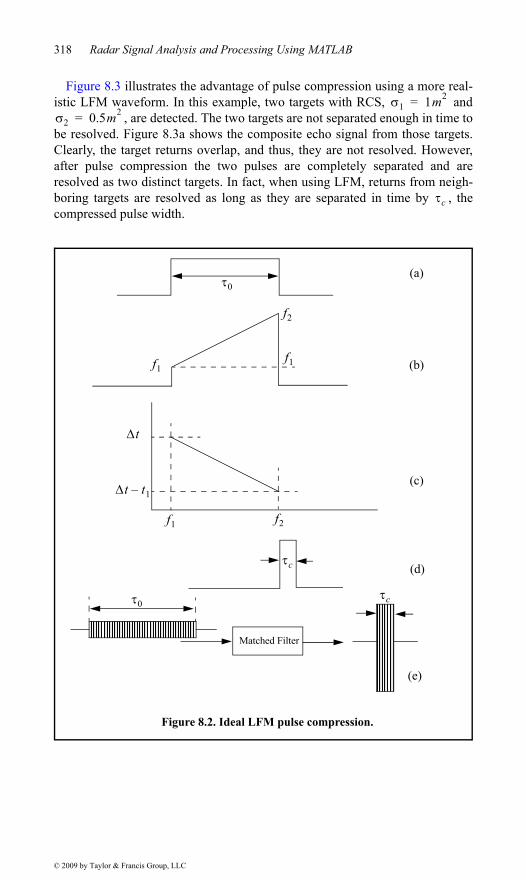
Figure 8.2 shows an ideal LFM pulse compression process. Part (a) showsthe envelope of a pulse, part (b) shows the frequency modulation (in this case itis an upchirp LFM) with bandwidth . Part (c) shows the matchedfilter time-delay characteristic while part (d) shows the compressed pulseenvelope. Finally part (e) shows the matched filter input/output waveforms.

c

SNRc

Pt cG2 2

4 3R4kT0FL------------------------------------=

SNRPt 0 nP c= G2 2

4 3R4kT0FL--------------------------------------------------=

nP

R c2B-------=

B 0= 0B

B f2 f1–=

chapter8.fm 17 Monday, May 19, 2008 6:37 PM



Figure 8.3 illustrates the advantage of pulse compression using a more real-istic LFM waveform. In this example, two targets with RCS, and

, are detected. The two targets are not separated enough in time tobe resolved. Figure 8.3a shows the composite echo signal from those targets.Clearly, the target returns overlap, and thus, they are not resolved. However,after pulse compression the two pulses are completely separated and areresolved as two distinct targets. In fact, when using LFM, returns from neigh-boring targets are resolved as long as they are separated in time by , thecompressed pulse width.

1 1m2=2 0.5m2=

c

(a)

(b)

(c)

(d)

(e)

Matched Filter

0

f2

f1

t

t t1–

f1 f2

c

0 c

Figure 8.2. Ideal LFM pulse compression.

f1



Basic Principal of Pulse Compression 319

Figure 8.3a. Composite echo signal for two unresolved targets.

Figure 8.3b. Composite echo signal corresponding to Fig. 8.3a after pulse compression.




8.4. Correlation ProcessorRadar operations (search, track, etc.) are usually carried out over a specified

range window, referred to as the receive window and defined by the differencebetween the radar maximum and minimum range. Returns from all targetswithin the receive window are collected and passed through matched filter cir-cuitry to perform pulse compression. One implementation of such analog pro-cessors is the Surface Acoustic Wave (SAW) devices. Because of the recentadvances in digital computer development, the correlation processor is oftenperformed digitally using the FFT. This digital implementation is called FastConvolution Processing (FCP) and can be implemented at base band. The fastconvolution process is illustrated in Fig. 8.4.

Since the matched filter is a linear time invariant system, its output can bedescribed mathematically by the convolution between its input and its impulseresponse,

(8.9)

where is the input signal, is the matched filter impulse response(replica), and the ( ) operator symbolically represents convolution. From theFourier transform properties,

(8.10)

and when both signals are sampled properly, the compressed signal canbe computed from

(8.11)

where is the inverse FFT. When using pulse compression, it is desir-able to use modulation schemes that can accomplish a maximum pulse com-pression ratio and can significantly reduce the sidelobe levels of thecompressed waveform. For the LFM case the first sidelobe is approximately

FFT multiplier

FFT of

Inv. FFTinputsignal

matched filter output

Figure 8.4. Computing the matched filter output using an FFT.

storedreplica

y t s t h t=

s t h t

FFT s t h t S f H f=

y t

y FFT 1– S H=

FFT 1–



Correlation Processor 321

below the main peak, and for most radar applications this may not besufficient. In practice, high sidelobe levels are not preferable because noiseand/or jammers located at the sidelobes may interfere with target returns in themain lobe.

Weighting functions (windows) can be used on the compressed pulse spec-trum in order to reduce the sidelobe levels. The cost associated with such anapproach is a loss in the main lobe resolution, and a reduction in the peak value(i.e., loss in the SNR). Weighting the time domain transmitted or received sig-nal instead of the compressed pulse spectrum will theoretically achieve thesame goal. However, this approach is rarely used, since amplitude modulatingthe transmitted waveform introduces extra burdens on the transmitter.

Consider a radar system that utilizes a correlation processor receiver (i.e.,matched filter). The receive window in meters is defined by

(8.12)

where and , respectively, define the maximum and minimum rangeover which the radar performs detection. Typically is limited to the extentof the target complex. The normalized complex transmitted signal has the form

(8.13)

is the pulse width, , and is the bandwidth.

The radar echo signal is similar to the transmitted one with the exception of atime delay and an amplitude change that correspond to the target RCS. Con-sider a target at range . The echo received by the radar from this target is

(8.14)

where is proportional to target RCS, antenna gain, and range attenuation.The time delay is given by

(8.15)

The first step of the processing consists of removing the frequency . Thisis accomplished by mixing with a reference signal whose phase is .The phase of the resultant signal, after lowpass filtering, is then given by

(8.16)

and the instantaneous frequency is

13.4dB

Rrec Rmax Rmin–=

Rmax RminRrec

s t j2 f0t 2---t2+exp= 0 t 0

0 B 0= B

R1

sr t a1 j2 f0 t t1– 2--- t t1– 2+exp=

a1t1

t1 2R1 c=

f0sr t 2 f0t

t 2 f– 0t1 2--- t t1– 2+=




(8.17)

The quadrature components are

(8.18)

Sampling the quadrature components is performed next. The number of sam-ples, , must be chosen so that foldover (ambiguity) in the spectrum isavoided. For this purpose, the sampling frequency, (based on the Nyquistsampling rate), must be

(8.19)

and the sampling interval is

(8.20)

Using Eq. (8.17) it can be shown that (the proof is left as an exercise) the fre-quency resolution of the FFT is

(8.21)

The minimum required number of samples is

(8.22)

Equating Eqs. (8.20) and (8.22) yields

(8.23)

Consequently, a total of real samples, or complex samples, is suf-ficient to completely describe an LFM waveform of duration and band-width . For example, an LFM signal of duration and bandwidth

requires 200 real samples to determine the input signal (100samples for the I-channel and 100 samples for the Q-channel).

For better implementation of the FFT is extended to the next power oftwo, by zero padding. Thus, the total number of samples, for some positiveinteger , is

(8.24)

The final steps of the FCP processing include (1) taking the FFT of the sam-pled sequence, (2) multiplying the frequency domain sequence of the signal

fi t 12------

tdd t t t1– B

0---- t

2R1

c---------–= = =

xI t

xQ ttcostsin

=

Nfs

fs 2B

t 1 2B

f 1 0=

N 1f t

----------- 0

t-----= =

N 2B 0

2B 0 B 0

0B 0 20= s

B 5 MHz=

N

m

NFFT 2m N=




with the FFT of the matched filter impulse response, and (3) performing theinverse FFT of the composite frequency domain sequence in order to generatethe time domain compressed pulse. Of course, weighting, antenna gain, andrange attenuation compensation must also be performed.

Assume that targets at ranges , , and so forth are within the receivewindow. From superposition, the phase of the down-converted signal is

(8.25)

The times represent the two-way time delays,where coincides with the start of the receive window. As an example, con-sider the case where

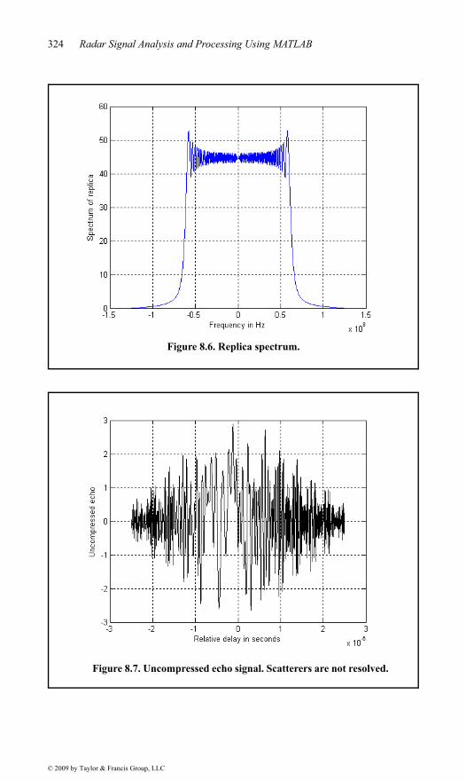
Note that the compressed pulsed range resolution is . Figure 8.5and Fig. 8.6 shows the real part and the amplitude spectrum of the replica usedfor this example. Figure 8.7 shows the uncompressed echo, while Fig. 8.8shows the compressed MF output. Note that the scatterer amplitude attenuationis a function of the inverse of the scatterer’s range within the receive window.Figure 8.9 is similar to Fig. 8.8, except in this case the first and second scatter-ers are less than 1.5 meter apart (they are at 70 and 71 meters).

# targets Rrec pulse width

Band-width

targets range Target RCS

Window type

3 200m 0.005ms 100e6 Hz [10 75 120] m [1 2 1]m2 Ham-ming

I R1 R2

t 2 f– 0ti 2--- t ti– 2+

i 1=

I

=

ti 2Ri c i; 1 2 I= =t1

R 1.5m=

Figure 8.5. Real part of replica.




Figure 8.6. Replica spectrum.

Figure 8.7. Uncompressed echo signal. Scatterers are not resolved.




Figure 8.8. Compressed echo signal corresponding to Fig. 8.7. Scatterers are completely resolved.

Figure 8.8. Compressed echo signal corresponding to Fig. 5.7. Scatterers are completely resolved.

Figure 8.9. Compressed echo signal of three scatterers, two of which are not resolved.




8.5. Stretch ProcessorStretch processing, also known as active correlation, is normally used to

process extremely high-bandwidth LFM waveforms. This processing tech-nique consists of the following steps: First, the radar returns are mixed with areplica (reference signal) of the transmitted waveform. This is followed byLow Pass Filtering (LPF) and coherent detection. Next, Analog-to-Digital (A/D) conversion is performed; and finally, a bank of Narrow-Band Filters(NBFs) is used in order to extract the tones that are proportional to targetrange, since stretch processing effectively converts time delay into frequency.All returns from the same range bin produce the same constant frequency.

8.5.1. Single LFM Pulse

Figure 8.10 shows a block diagram for a stretch processing receiver. The ref-erence signal is an LFM waveform that has the same LFM slope as the trans-mitted LFM signal. It exists over the duration of the radar “receive-window,”which is computed from the difference between the radar maximum and mini-mum range. Denote the start frequency of the reference chirp as . Considerthe case when the radar receives returns from a few close (in time or range) tar-gets, as illustrated in Fig. 8.10. Mixing with the reference signal and perform-ing lowpass filtering are effectively equivalent to subtracting the returnfrequency chirp from the reference signal. Thus, the LPF output consists ofconstant tones corresponding to the targets’ positions. The normalized trans-mitted signal can be expressed by

(8.26)

where is the LFM coefficient and is the chirp start frequency.Assume a point scatterer at range . The signal received by the radar is

(8.27)

where is proportional to target RCS, antenna gain, and range attenuation.The time delay is

(8.28)

The reference signal is

(8.29)

The receive window in seconds is

fr

s1 t 2 f0t 2---t2+cos= 0 t 0

B 0= f0R

sr t a 2 f0 t t0– 2--- t t0– 2+cos=

at0

t0 2R c=

sref t 2 2 frt 2---t2+cos= 0 t Trec



Stretch Processor327

return

1ret

urn 2

return

3

time

frequency

f0

time

frequency

fr

return 1return 2

return 3

time

frequency

f1

f3f2

refere

nce ch

irp

frequency

1 2 3

ampl

itude

0

mixer sidelobeLPF FFTcoherentdetection& A/D weighting

LO

Figure 8.10. Stretch processing block diagram.

t

Trec

Trec

f1 fr f0–=

f2 fr f0– t+=

f3 fr f0– 2 t+=

Trec receive window=

chapter8.fm Page 327 M

onday, May 19, 2008 6:37 PM



(8.30)

It is customary to let . The output of the mixer is the product of thereceived and reference signals. After lowpass filtering the signal is

(8.31)

Substituting Eq. (8.28) into Eq. (8.31) and collecting terms yield

(8.32)

and since , Eq. (8.32) is approximated by

(8.33)

The instantaneous frequency is

(8.34)

which clearly indicates that target range is proportional to the instantaneousfrequency. Therefore, proper sampling of the LPF output and taking the FFT ofthe sampled sequence lead to the following conclusion: a peak at some fre-quency indicates presence of a target at range

(8.35)

Assume close targets at ranges , , and so forth ( ).From superposition, the total signal is

(8.36)

where are proportional to the targets’ cross sections,antenna gain, and range. The times representthe two-way time delays, where coincides with the start of the receive win-dow. Using Eq. (8.32) the overall signal at the output of the LPF can then bedescribed by

(8.37)

Trec2 Rmax Rmin–

c------------------------------------

2Rrec

c-------------= =

fr f0=

s0 t a 2 f0t0 2 t0t t02–+cos=

s0 t a 4 BRc 0

-------------- t 2Rc

------- 2 f02 BR

c 0--------------–+cos=

0 2R c»

s0 t a 4 BRc 0

-------------- t 4 Rc

----------f0+cos

finst1

2------

tdd 4 BR

c 0--------------t 4 R

c----------f0+( ) 2BR

c 0-----------= =

f1

R1 f1c 0 2B=

I R1 R2 R1 R2 RI

sr t ai t 2 f0 t ti– 2--- t ti– 2+cos

i 1=

I

=

ai t i; 1 2 I=ti 2Ri c i; 1 2 I= =

t1

so t ai4 BRi

c 0---------------- t

2Ric

-------- 2 f02 BRi

c 0----------------–+cos

i 1=

I

=



Stretch Processor 329

Hence, target returns appear as constant frequency tones that can be resolvedusing the FFT. Consequently, determining the proper sampling rate and FFTsize is very critical. The rest of this section presents a methodology for com-puting the proper FFT parameters required for stretch processing.

Assume a radar system using a stretch processor receiver. The pulse width is and the chirp bandwidth is . Since stretch processing is normally used in

extreme bandwidth cases (i.e., very large ), the receive window over whichradar returns will be processed is typically limited to from a few meters to pos-sibly less than 100 meters. The compressed pulse range resolution is computedfrom Eq. (8.8). Declare the FFT size to be and its frequency resolution to be

. The frequency resolution can be computed using the following procedure:Consider two adjacent point scatterers at ranges and . The minimum fre-quency separation, , between those scatterers so that they are resolved canbe computed from Eq. (8.34). More precisely,

(8.38)

Substituting Eq. (8.8) into Eq. (8.38) yields

(8.39)

The maximum frequency resolvable by the FFT is limited to the region. Thus, the maximum resolvable frequency is

(8.40)

Using Eqs. (8.30) and (8.39) into Eq. (8.40) and collecting terms yield

(8.41)

For better implementation of the FFT, choose an FFT of size

(8.42)

where is a nonzero positive integer. The sampling interval is then given by

(8.43)

As an example, consider the case where

0 BB

Nf

R1 R2f

f f2 f1– 2Bc 0------- R2 R1– 2B

c 0------- R= = =

f 2Bc 0------- c

2B------- 1

0----= =

N f 2

N f2

----------2B Rmax Rmin–

c 0---------------------------------------- 2BRrec

c 0-----------------=

N 2BTrec

NFFT N 2m=

m

f 1TsNFFT-----------------= Ts

1fNFFT

------------------=




Note that the compressed pulse range resolution, without using a window, is. Figure 8.11 and Fig. 8.12, respectively, show the uncompressed

and compressed echo signals corresponding to this example. Figures 8.13 aand b are similar to Fig. 8.11 and Fig. 8.12 except in this case two of the scat-terers are less than 15 cm apart (i.e., unresolved targets at

).

# targets 3

pulsewidth 10 ms

center frequency 5.6 GHz

bandwidth 1 GHz

receive window 30 m

relative target’s range [2 5 10] m

target’s RCS [1, 1, 2] m2

window 2 (Kaiser)

R 0.15m=

Rrelative 3 3.1 m=

Figure 8.11. Uncompressed echo signal. Three targets are unresolved.




Figure 8.12. Compressed echo signal. Three targets are resolved.

Figure 8.13a. Uncompressed echo signal. Three targets.




8.5.2. Stepped Frequency Waveforms

Stepped Frequency Waveforms (SFW) are used in extremely wide bandradar applications where very large time bandwidth product is required. Gener-ation of SFW was discussed in Chapter 5. For this purpose, consider an LFMsignal whose bandwidth is and whose pulsewidth is and refer to it as theprimary LFM. Divide this long pulse into subpulses each of width togenerate a sequence of pulses whose PRI is denoted by . It follows that

. Define the beginning frequency for each subpulse as that valuemeasured from the primary LFM at the leading edge of each subpulse, as illus-trated in Fig. 8.14. That is

(8.44)

where is the frequency step from one subpulse to another. The set of sub-pulses is often referred to as a burst. Each subpulse can have its own LFMmodulation. To this end, assume that each subpluse is of width and band-width , then the LFM slope of each pulse is

(8.45)

Figure 8.13b. Compressed echo signal. Three targets, two are not resolved.

Bi TiN 0

TTi n 1– T=

fi f0 i f+= i 0 N 1–=;

f n

0B

B0

----=




The SFW operation and processing involve the following steps:

1. A series of narrow-band LFM pulses is transmitted. The chirp beginningfrequency from pulse to pulse is stepped by a fixed frequency step , asdefined in Eq. (8.44). Each group of pulses is referred to as a burst.

2. The LFM slope (quadratic phase term) is first removed from the receivedsignal, as described in Fig. 8.10. The reference slope must be equal to thecombined primary LFM and single subpulse slopes. Thus, the received sig-nal is reduced to a series of subpulses.

3. These subpulses are then sampled at a rate that coincides with the center ofeach pulse, sampling rate equivalent to ( ).

4. The quadrature components for each burst are collected and stored.5. Spectral weighting (to reduce the range sidelobe levels) is applied to the

quadrature components. Corrections for target velocity, phase, and ampli-tude variations are applied.

6. The IDFT of the weighted quadrature components of each burst is calcu-lated to synthesize a range profile for that burst. The process is repeated for

bursts to obtain consecutive high resolution range profiles.

Within a burst, the transmitted waveform for the step can be described as

(3.46)

f0

f1

f2

f3

f4

f

0T

time

Figure 8.14. Example of stepped frequency waveform burst; .N 5=

Ti

f

f

f

primaryLFM slope

Bi

Nf

N

1 T

M

ith

xi t Ci1

0

---------Rect t0

---- ej2 fit 2

--- t2+

0

=iT t iT 0+

elsewhere;




where are constants. The received signal from a target located at range is then given by

(8.47)

where are constant and the round trip delay is given by

(8.48)

where is the speed of light and is the target radial velocity.

In order to remove the quadratic phase term, mixing is first performed withthe reference signal given by

(8.49)

Next lowpass filtering is performed to extract the quadrature components.More precisely, the quadrature components are given by

(8.50)

where are constants, and

(8.51)

where now . For each pulse, the quadrature components are then sam-pled at

(8.52)

is the time delay associated with the range that corresponds to the start ofthe range profile.

The quadrature components can then be expressed in complex form as

(8.53)

Equation (8.53) represents samples of the target reflectivity, due to a singleburst, in the frequency domain. This information can then be transformed intoa series of range delay reflectivity (i.e., range profile) values by using theIDFT. It follows that

Ci R0

xri t Ci ej2 fi t t– 2

--- t t– 2–iT t+ t iT 0 t+ +,=

Ci t

tR0 vt–

c 2----------------=

c v

yi t ej2 fit 2

--- t2+= iT t iT 0+;

xI t

xQ t

Ai i tcos

Ai i tsin=

Ai

i t 2 fi2R0

c--------- 2vt

c--------––=

fi f=

ti iT r

2----

2R0

c---------+ +=

r

Xi Aiej i=




(8.54)

Substituting Eq. (8.51) and Eq. (8.53) into (8.54) and collecting terms yield

(8.55)

By normalizing with respect to and by assuming that and that thetarget is stationary (i.e., ), then Eq. (8.55) can be written as

(8.56)

Using inside Eq. (8.56) yields

(8.57)

which can be simplified to

(8.58)

where

(8.59)

Finally, the synthesized range profile is

(8.60)

Range Resolution and Range Ambiguity in SFW

As usual, range resolution is determined from the overall system bandwidth.Assuming an SFW with steps and step size , then the correspondingrange resolution is equal to

Hl1N---- Xi j2 li

N----------exp

i 0=

N 1–

= 0 l N 1–;

Hl1N---- Ai j 2 li

N---------- 2 fi

2R0

c---------

2vtic

---------––exp

i 0=

N 1–

=

N Ai 1=v 0=

Hl j 2 liN

---------- 2 fi2R0

c---------–exp

i 0=

N 1–

=

fi i f=

Hl j2 iN

-------- 2NR0 fc

------------------- l+–exp

i 0=

N 1–

=

Hlsin

N------sin

-------------- jN 1–2

------------- 2N

---------exp=

2NR0 f–c

----------------------- l+=

Hlsin

N------sin

--------------=

N f




(8.61)

Range ambiguity associated with an SFW can be determined by examiningthe phase term that corresponds to a point scatterer located at range . Moreprecisely,

(8.62)

It follows that

(8.63)

or equivalently,

(8.64)

It is clear from Eq. (8.64) that range ambiguity exists for .Therefore,

(8.65)

and the unambiguous range window is

(8.66)

A range profile synthesized using a particular SFW represents the relativerange reflectivity for all scatterers within the unambiguous range window, withrespect to the absolute range that corresponds to the burst time delay. Addition-ally, if a specific target extent is larger than , then all scatterers falling out-side the unambiguous range window will fold over and appear in thesynthesized profile. This fold-over problem is identical to the spectral fold-over that occurs when using a Fast Fourier Transform (FFT) to resolve certainsignal frequency contents. For example, consider an FFT with frequency reso-lution and size . In this case, this FFT can resolvefrequency tones between and . When this FFT is used toresolve the frequency content of a sine-wave tone equal to , fold-overoccurs and a spectral line at the fourth FFT bin (i.e., ) appears. There-fore, in order to avoid fold-over in the synthesized range profile, the frequencystep must be

(8.67)

R c2N f-------------=

R0

i t 2 fi2R0

c---------=

f-------

4 fi 1+ fi–fi 1+ fi–

------------------------------R0

c----- 4 R0

c-------------= =

R0 f------- c

4------=

2N+=

R02N+f

------------------------ c4------ R0 N c

2 f---------+= =

Ruc

2 f---------=

Ru

f 50Hz= NFFT 64=1600Hz– 1600Hz

1800Hz200Hz

f

f c 2E




where is the target extent in meters.

Additionally, the pulsewidth must also be large enough to contain the wholetarget extent. Thus,

(8.68)

and in practice,

(8.69)

This is necessary in order to reduce the amount of contamination of the synthe-sized range profile caused by the clutter surrounding the target under consider-ation.

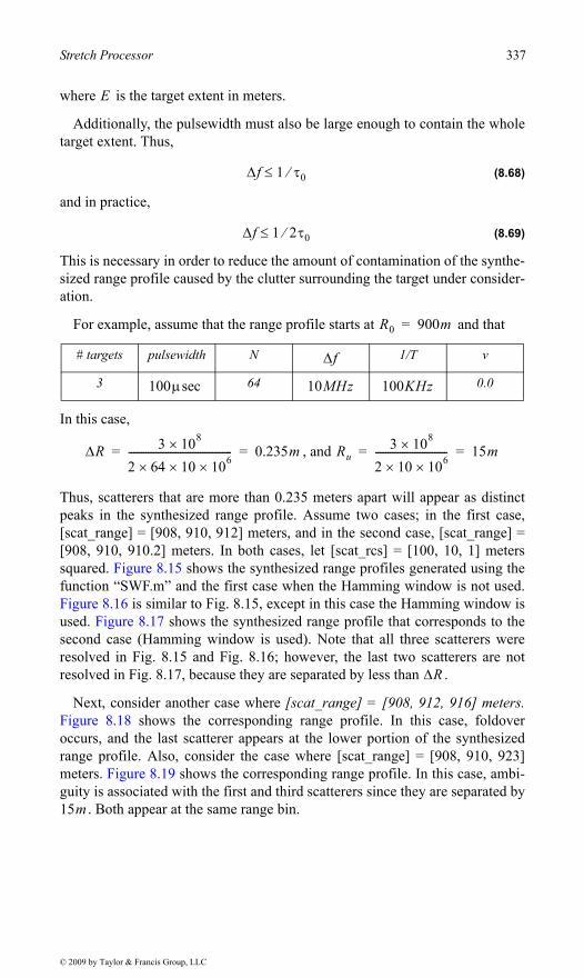
For example, assume that the range profile starts at and that

In this case,

, and

Thus, scatterers that are more than 0.235 meters apart will appear as distinctpeaks in the synthesized range profile. Assume two cases; in the first case,[scat_range] = [908, 910, 912] meters, and in the second case, [scat_range] =[908, 910, 910.2] meters. In both cases, let [scat_rcs] = [100, 10, 1] meterssquared. Figure 8.15 shows the synthesized range profiles generated using thefunction “SWF.m” and the first case when the Hamming window is not used.Figure 8.16 is similar to Fig. 8.15, except in this case the Hamming window isused. Figure 8.17 shows the synthesized range profile that corresponds to thesecond case (Hamming window is used). Note that all three scatterers wereresolved in Fig. 8.15 and Fig. 8.16; however, the last two scatterers are notresolved in Fig. 8.17, because they are separated by less than .

Next, consider another case where [scat_range] = [908, 912, 916] meters.Figure 8.18 shows the corresponding range profile. In this case, foldoveroccurs, and the last scatterer appears at the lower portion of the synthesizedrange profile. Also, consider the case where [scat_range] = [908, 910, 923]meters. Figure 8.19 shows the corresponding range profile. In this case, ambi-guity is associated with the first and third scatterers since they are separated by

. Both appear at the same range bin.

# targets pulsewidth N 1/T v

3 64 0.0

E

f 1 0

f 1 2 0

R0 900m=

f

100 sec 10MHz 100KHz

R 3 108

2 64 10 106------------------------------------------ 0.235m= = Ru

3 108

2 10 106----------------------------- 15m= =

R

15m




Figure 8.15. Synthetic range profile for three resolved scatterers. No window.

Figure 8.16. Synthetic range profile for three scatterers. Hamming window.




Figure 8.17. Synthetic range profile for three scatterers. Two are unresolved.

Figure 8.18. Synthetic range profile for three scatterers. Third scatterer folds over.




8.5.2.1. Effect of Target Velocity

The range profile defined in Eq. (8.60) is obtained by assuming that the tar-get under examination is stationary. The effect of target velocity on the synthe-sized range profile can be determined by starting with Eq. (8.55) and assumingthat . Performing similar analysis as that of the stationary target caseyields a range profile given by

(8.70)

The additional phase term present in Eq. (8.70) distorts the synthesized rangeprofile. In order to illustrate this distortion, consider the SFW described in theprevious section, and assume the three scatterers of the first case. Also, assumethat . Figure 8.20 shows the synthesized range profile for thiscase. Comparisons of Figs. 8.16 and 8.20 clearly show the distortion effectscaused by the uncompensated target velocity. Figure 8.21 is similar to Fig. 8.20except in this case, . Note in either case, the targets have movedfrom their expected positions (to the left or right) by (1.28 m).

Figure 8.19. Synthetic range profile for three scatterers. The first and third scatterers appear in the same FFT bin.

v 0

Hl Ai j2 liN

---------- j2 fi2Rc

------- 2vc

------ iT r

2---- 2R

c-------+ +––exp

i 0=

N 1–

=

v 200m s=

v 200– m s=Disp 2 n v PRF=




This distortion can be eliminated by multiplying the complex received dataat each pulse by the phase term

(3.71)

and are, respectively, estimates of the target velocity and range. This pro-cess of modifying the phase of the quadrature components is often referred toas “phase rotation.” In practice, when good estimates of and are not avail-able, then the effects of target velocity are reduced by using frequency hoppingbetween the consecutive pulses within the SFW. In this case, the frequency ofeach individual pulse is chosen according to a predetermined code. Waveformsof this type are often called Frequency Coded Waveforms (FCW). Costaswaveforms or signals are a good example of this type of waveform.

Figure 8.22 shows a synthesized range profile for a moving target whose RCSis and . The initial target range is at . Allother parameters are as before. This figure can be reproduced using the follow-ing MATLAB code.clear all;close all;nscat = 1;scat_range = 912;scat_rcs = 10;n =64;deltaf = 10e6;prf = 10e3;v = 10;rnote = 900,winid = 1;count = 0;for time = 0:.05:3 count = count +1; hl = SFW (nscat, scat_range, scat_rcs, n, deltaf, prf, v, rnote, winid); array(count,:) = transpose(hl); hl(1:end) = 0; scat_range = scat_range - 2 * n * v / prf;endfigure (1) numb = 2*256;% this number matches that used in hrr_profile. delx_meter = 15 / numb; xmeter = 0:delx_meter:15-delx_meter; imagesc(xmeter, 0:0.05:4,array) colormap(gray)ylabel ('Time in seconds')xlabel('Relative distance in meters')

j– 2 fi2v̂c

------ iT r2---- 2R̂

c-------+ +exp=

v̂ R

v̂ R̂

10m2= v 10m s= R 912m=




Figure 8.20. Illustration of range profile distortion due to target velocity.

Figure 8.21. Illustration of range profile distortion due to target velocity.



MATLAB Program Listings 343

8.6. MATLAB Program ListingsThis section presents listings for all the MATLAB programs used to produce

all of the MATLAB-generated figures in this chapter.

8.6.1. MATLAB Function “matched_filter.m”

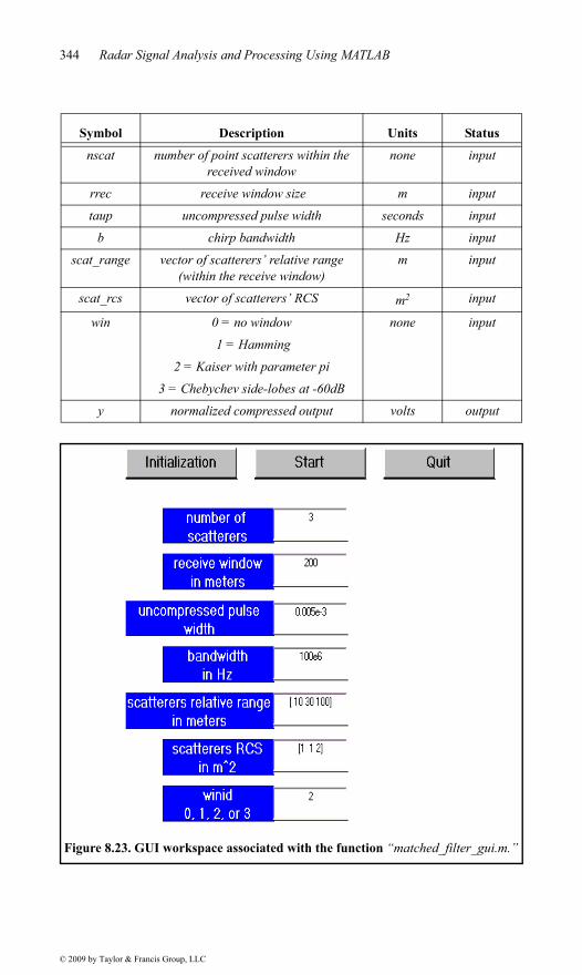
The function “matched_filter.m” performs fast convolution processing. Theuser can access this function either by a MATLAB function call or by execut-ing the MATLAB program “matched_filter_gui.m,” which utilizes a MAT-LAB-based GUI. The work space associated with this program is shown inFig. 8.23. The outputs for this function include plots of the compressed anduncompressed signals as well as the replica used in the pulse compression pro-cess. This function utilizes the function “power_integer_2.m.”

The function “matched_filter.m” syntax is as follows:

[y] = matched_filter(nscat, rrec, taup, b, scat_range, scat_rcs, win)

where

Figure 8.22. Synthesized range profile for a moving target (4 seconds long).




Symbol Description Units Status

nscat number of point scatterers within the received window

none input

rrec receive window size m input

taup uncompressed pulse width seconds input

b chirp bandwidth Hz input

scat_range vector of scatterers’ relative range (within the receive window)

m input

scat_rcs vector of scatterers’ RCS m2 input

win 0 = no window

1 = Hamming

2 = Kaiser with parameter pi

3 = Chebychev side-lobes at -60dB

none input

y normalized compressed output volts output

Figure 8.23. GUI workspace associated with the function “matched_filter_gui.m.”




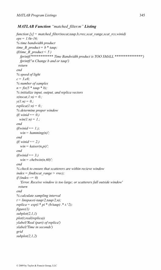
MATLAB Function “matched_filter.m” Listing

function [y] = matched_filter(nscat,taup,b,rrec,scat_range,scat_rcs,winid)eps = 1.0e-16;% time bandwidth producttime_B_product = b * taup;if(time_B_product < 5 ) fprintf('************ Time Bandwidth product is TOO SMALL ***************') fprintf('\n Change b and or taup') returnend% speed of lightc = 3.e8; % number of samplesn = fix(5 * taup * b);% initialize input, output, and replica vectorsx(nscat,1:n) = 0.;y(1:n) = 0.;replica(1:n) = 0.;% determine proper windowif( winid == 0.) win(1:n) = 1.;endif(winid == 1.); win = hamming(n)';endif( winid == 2.) win = kaiser(n,pi)';endif(winid == 3.) win = chebwin(n,60)';end% check to ensure that scatterers are within recieve windowindex = find(scat_range > rrec);if (index ~= 0) 'Error. Receive window is too large; or scatterers fall outside window' returnend% calculate sampling intervalt = linspace(-taup/2,taup/2,n);replica = exp(i * pi * (b/taup) .* t.^2);figure(1)subplot(2,1,1)plot(t,real(replica))ylabel('Real (part) of replica')xlabel('Time in seconds')gridsubplot(2,1,2)




sampling_interval = taup / n;freqlimit = 0.5/ sampling_interval;freq = linspace(-freqlimit,freqlimit,n);plot(freq,fftshift(abs(fft(replica))));ylabel('Spectrum of replica')xlabel('Frequency in Hz')grid for j = 1:1:nscat range = scat_range(j) ; x(j,:) = scat_rcs(j) .* exp(i * pi * (b/taup) .* (t +(2*range/c)).^2) ; y = x(j,:) + y;endfigure(2) y = y .* win;plot(t,real(y),'k')xlabel ('Relative delay in seconds')ylabel ('Uncompressed echo')gridout =xcorr(replica, y);out = out ./ n;s = taup * c /2;Npoints = ceil(rrec * n /s);dist =linspace(0, rrec, Npoints);delr = c/2/b;figure(3)plot(dist,abs(out(n:n+Npoints-1)),'k')xlabel ('Target relative position in meters')ylabel ('Compressed echo')gridreturn

MATLAB Function “power_integer_2.m” Listing

function n = power_integer_2 (x)m = 0.;for j = 1:30 m = m + 1.; delta = x - 2.^m; if(delta < 0.) n = m; return else endendreturn




8.6.2. MATLAB Function “stretch.m”

The function “stretch.m” presents a digital implementation of stretch pro-cessing. The syntax is as follows:

[y] = stretch (nscat, taup, f0, b, scat_range, rrec, scat_rcs, win)

where

The user can access this function either by a MATLAB function call or by exe-cuting the MATLAB program “stretch_gui.m,” which utilizes MATLAB-based GUI and is shown in Fig. 8.24. The outputs of this function are the com-plex array and plots of the uncompressed and compressed echo signal versustime.

MATLAB Function “stretch.m” Listing

function [y] = stretch(nscat, taup, f0, b, scat_range, rrec, scat_rcs, winid)eps = 1.0e-16;htau = taup / 2.;c = 3.e8;trec = 2. * rrec / c;n = fix(2. * trec * b);m = power_integer_2(n);nfft = 2.^m;x(nscat,1:n) = 0.;y(1:n) = 0.;if( winid == 0.) win(1:n) = 1.;


nscat number of point scatterers within the receive window

none input

taup uncompressed pulse width seconds input

f0 chirp start frequency Hz input

b chirp bandwidth Hz input

scat_range vector of scatterers’ range m input

rrec range receive window m input

scat_rcs vector of scatterers’ RCS m2 input

win 0 = no window

1 = Hamming

2 = Kaiser with parameter pi

3 = Chebychev side-lobes at -60dB

none input

y compressed output volts output

y




win =win';else if(winid == 1.) win = hamming(n); else if( winid == 2.) win = kaiser(n,pi); else if(winid == 3.) win = chebwin(n,60); end end endenddeltar = c / 2. / b;max_rrec = deltar * nfft / 2.;maxr = max(scat_range);if(rrec > max_rrec | maxr >= rrec ) 'Error. Receive window is too large; or scatterers fall outside window' returnend

Figure 8.24. GUI workspace associated with the function “stretch_gui.m.”

chapter8.fm 8 Monday, May 19, 2008 6:37 PM



t = linspace(0,taup,n);for j = 1:1:nscat range = scat_range(j);% + rmin; psi1 = 4. * pi * range * f0 / c - ... 4. * pi * b * range * range / c / c/ taup; psi2 = (2*4. * pi * b * range / c / taup) .* t; x(j,:) = scat_rcs(j) .* exp(i * psi1 + i .* psi2); y = y + x(j,:);endfigure(1)plot(t,real(y),'k')xlabel ('Relative delay in seconds')ylabel ('Uncompressed echo')gridywin = y .* win';yfft = fft(y,n) ./ n;out= fftshift(abs(yfft));figure(2)delinc = rrec/ n;%dist = linspace(-delinc-rrec/2,rrec/2,n);dist = linspace((-rrec/2), rrec/2,n);plot(dist,out,'k')xlabel ('Relative range in meters')ylabel ('Compressed echo')axis autogrid

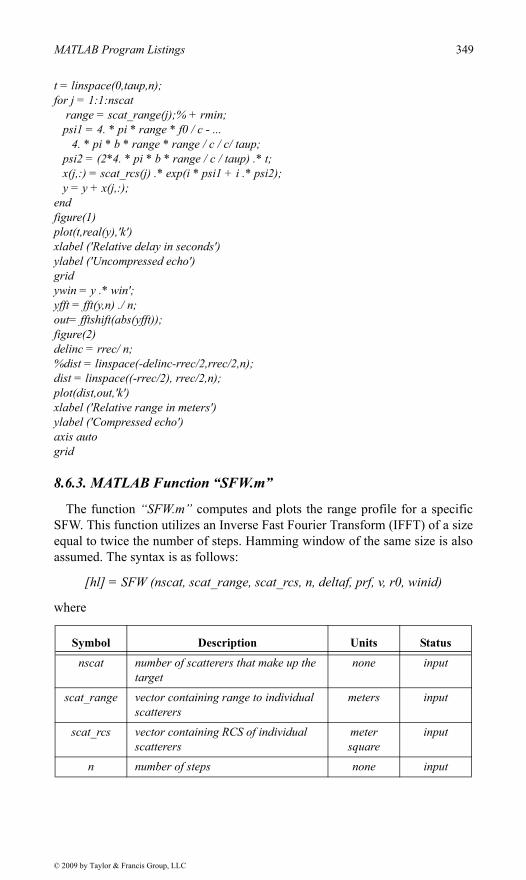
8.6.3. MATLAB Function “SFW.m”

The function “SFW.m” computes and plots the range profile for a specificSFW. This function utilizes an Inverse Fast Fourier Transform (IFFT) of a sizeequal to twice the number of steps. Hamming window of the same size is alsoassumed. The syntax is as follows:

[hl] = SFW (nscat, scat_range, scat_rcs, n, deltaf, prf, v, r0, winid)

where


nscat number of scatterers that make up the target

none input

scat_range vector containing range to individual scatterers

meters input

scat_rcs vector containing RCS of individual scatterers

meter square

input

n number of steps none input




MATLAB Function “SFW.m” Listing

function [hl] = SFW (nscat, scat_range, scat_rcs, n, deltaf, prf, v, rnote,winid)% Range or Time domain Profile% Range_Profile returns the Range or Time domain plot of a simulated % HRR SFWF returning from a predetermined number of targets with a predetermined% RCS for each target.c=3.0e8; % speed of light (m/s)num_pulses = n;SNR_dB = 40;nfft = 256;% carrier_freq = 9.5e9; %Hz (10GHz)freq_step = deltaf; %Hz (10MHz)V = v; % radial velocity (m/s) -- (+)=towards radar (-)=awayPRI = 1. / prf; % (s)if (nfft > 2*num_pulses) num_pulses = nfft/2;elseendInphase = zeros((2*num_pulses),1);Quadrature = zeros((2*num_pulses),1);Inphase_tgt = zeros(num_pulses,1);Quadrature_tgt = zeros(num_pulses,1);IQ_freq_domain = zeros((2*num_pulses),1);Weighted_I_freq_domain = zeros((num_pulses),1);Weighted_Q_freq_domain = zeros((num_pulses),1);Weighted_IQ_time_domain = zeros((2*num_pulses),1);Weighted_IQ_freq_domain = zeros((2*num_pulses),1);abs_Weighted_IQ_time_domain = zeros((2*num_pulses),1);dB_abs_Weighted_IQ_time_domain = zeros((2*num_pulses),1);taur = 2. * rnote / c;for jscat = 1:nscat ii = 0; for i = 1:num_pulses ii = ii+1;

deltaf frequency step Hz input

prf PRF of SFW Hz input

v target velocity meter/sec-ond

input

r0 profile starting range meters input

winid number>0 for Hamming window

number < 0 for no window

none input

hl range profile dB output





rec_freq = ((i-1)*freq_step); Inphase_tgt(ii) = Inphase_tgt(ii) + sqrt(scat_rcs(jscat)) * cos(-2*pi*rec_freq*... (2.*scat_range(jscat)/c - 2*(V/c)*((i-1)*PRI + taur/2 + 2*scat_range(jscat)/c))); Quadrature_tgt(ii) = Quadrature_tgt(ii) + sqrt(scat_rcs(jscat))*sin(-2*pi*rec_freq*... (2*scat_range(jscat)/c - 2*(V/c)*((i-1)*PRI + taur/2 + 2*scat_range(jscat)/c))); endendif(winid >= 0) window(1:num_pulses) = hamming(num_pulses);else window(1:num_pulses) = 1;endInphase = Inphase_tgt;Quadrature = Quadrature_tgt;Weighted_I_freq_domain(1:num_pulses) = Inphase(1:num_pulses).* window';Weighted_Q_freq_domain(1:num_pulses) = Quadrature(1:num_pulses).* window';Weighted_IQ_freq_domain(1:num_pulses)= Weighted_I_freq_domain + ... Weighted_Q_freq_domain*j;Weighted_IQ_freq_domain(num_pulses:2*num_pulses)=0.+0.i;Weighted_IQ_time_domain = (ifft(Weighted_IQ_freq_domain));abs_Weighted_IQ_time_domain = (abs(Weighted_IQ_time_domain));dB_abs_Weighted_IQ_time_domain =20.0*log10(abs_Weighted_IQ_time_domain)+SNR_dB;% calculate the unambiguous range window sizeRu = c /2/deltaf;hl = dB_abs_Weighted_IQ_time_domain; numb = 2*num_pulses;delx_meter = Ru / numb;xmeter = 0:delx_meter:Ru-delx_meter;plot(xmeter, dB_abs_Weighted_IQ_time_domain,'k')xlabel ('Relative distance in meters')ylabel ('Range profile in dB')grid



chapter8.fm page 315 monday, may 19, 2008 6:37...

Documents