1

INTRODUCTIONThe earliest foresters were fully aware of the enormous range of properties of

Australian timbers (Baker, 1919: Swain, 1928), and the urgent need to establish the bestutilisation procedures and applications for each species. Historically, there was a need forearly research, as large areas were explored and opened up by timber-getters, who werefollowed generally by agricultural, dairy, or grazing, industries.

The most desirable species were either naturally scarce, or, like red cedar, to which amemorial is preserved at Lismore, N. S. W., had been exploited relentlessly, and attentionwas directed to the use of what, at the time, were less favoured species. This attentionbrought with it the recognition that some timbers were not durable in service, and,consequently, careful selection of uses or preservative treatment would be required in orderto utilise the technical and physical qualities of some of these timbers.

This thesis reports the developments of some of this work in Queensland, where amuch greater range and number of timber species were present than in the southern states.It chronicles some of the problems faced by the timber industry, social and politicalconstraints determining the direction of work, nature of both basic and applied research thatwas required and the solutions which were offered to industry. The thesis is not, therefore,a circumscribed analysis of a single problem, but a record of identification of numerouscomplex problems, and, for most of them, the first sensible and practical steps towards theirsolution.

One of the first of the problems preventing the extension of the list of desirable timberspecies was a need to preserve sapwoods which were susceptible to attack by the powderpost beetle, Lyctus brunneusProducts, CSIRO (Cummins and Wilson, 1936), a veneer treatment plant was establishedat Austral Plywood Ltd., Brisbane in 1938. However advice by health authorities was thatsodium silicofluoride, as the original preservative, was excessively hazardous (Q.F.S.,file.1938).

It was rapidly replaced (Cummins, 1939) by boric acid. The total of such plants, usingthe “Hot Immersion” process, remained static at 14, until conversion of the veneer andplywood industry to use of a “Momentary Dip” process when the total rose to about 30 by1965.

Sawn timber treatment began in June 1946 at the Brisbane firm of T. W. Brandon andSons, subsequently extending to a multimillion dollar business in Queensland. From thoseearly beginnings, illustrated by a total of 18 plants at commencement of 1949, with a further74 plants under construction in that year, for the year 1978, there was a total of 124 plantsusing varied processes, and a range of preservatives. Total capacity rose to in excess of200,000 m3, in sawn timber, veneer, plywoods, poles and piles, representing more than 50% of timber output demands.

In excess of 200 plant operators, with an additional number of supplementary staff,were directly employed. A total of more than 350 local species was handled, which, addedto a range of imported timbers, meant local industry was handling in excess of 600 species.

The timber preservation industry developed as a direct consequence of governmentinitiatives, catalysed by the establishment, in 1928, of the then Division of Forest Products(D.F.P.) within the Council for Scientific and Industrial Research, later to become theCommonwealth Scientific and Industrial Research Organisation (CSIRO). This supple-

2

mented units in State Forest organisations, particularly the Division of Wood Technology,New South Wales Forestry Commission, the Investigations Branch of the QueenslandForest Service, and, subsequently, the Forest Research Institute of the New ZealandMinistry of Forests. Following the 1939-45 war, an active forests products group wasestablished in Papua New Guinea, which had particular relevance to timber preservationwork in Queensland due to similarities between the ranges of species and the environmentalconditions.

Trees and timber propertiesAs indicated briefly above, one of the considerations in timber utilisation in Queens-

land was the very large number of commercial timber species available.

These were from tropical and subtropical rain forests as well as from open forests ofthe coastal and inland regions. Over 350 species were available in commercial quantities.Timber properties were known for less than 100 species, and these species showed a verylarge range of properties. Thus, timber utilisation cannot be considered without referenceto the recognition of timbers and species.

Pioneering work on the description, properties and on the utilisation of tropical andsubtropical Australian timber species was carried out by Maiden (1904-1925), Jolly (1917,1917), Baker (1919), Swain (1927,1928a), Dadswell and co-workers (1932, 1934, 1935),and Francis (1929, 1951). Swain was ably assisted by Watson (1947, 1951, 1964), whosework in many areas of Queensland timber identification and utilisation is still definitive.White (1925), Everist (1981) and L.Smith (u.p) developed the botanical understanding offorest species throughout Queensland. Assisted by Tracey, Webb (1950) was responsiblefor the definitive survey of phytochemicals particularly in tropical species. Webb (1956)has written a major study on rain forests, their relationships to such as soil and growthconditions. Hyland (1971) and Volk (u.p) have made major contributions to tropical forestbotany. Tracey (1982) has researched rehabilitation of the forest communities in NorthQueensland. Swain’s (1928) collation of available data was, and remains, a major referencein tropical forest products literature. His numeric classification (1927) of species on thewood structure was unique and forms a basis for the writer’s research reported here leadingto the classification of particularly local, but inclusive of imported timbers, on the basis ofpreservative treatment characteristics.

Queensland experiences a wide range of climatic and soil conditions, with a corre-sponding range of tree species and likelihood of biodeterioration (hazard). This range ofconditions led to the study of timber deterioration and preservation at an early stage in thedevelopment of the Queensland Forest Service. For example, Watson et al. (1936)examined the nature and distribution of problems caused by marine organisms attackingtimber. He developed a species rating scheme (Watson, 1964) for the purpose of promotingeffective utilisation of timbers.

For some decades, however, there were no investigations into the relationshipsbetween climate, geomorphology, biodeterioration hazard and the performance of a timberspecies in service in Queensland. Two exceptions were a series of specialised studies intothe distribution and effects of insects (Brimblecombe, 1956), and a Climate Hazard Indexdeveloped by Cokley and Ryley (1968). This latter work demonstrated the difficulties ofdrafting uniform legislation over a wide range of environmental and service conditions.

However some regulation of timber usage was required and legislation [The Timber

3

Marketing Act (1946), short title TMA, in New South Wales], [The Timber UsersProtection Act (1949), short title T.U.P.A., in Queensland] was soon enacted. Codes ofrecommended usage (Watson 1951, 1964), and Australian Standards (A S 1604 -1980)were initiated for the usage of timber in buildings.

Development of Forest Products Research.

Following World War II, Australian forest products research was co-ordinatedbetween State Forest authorities and the Division of Forest Products (CSIRO) through theestablishment in 1946 of a Forest Products Research Conference (short title -The ForestProducts Conference). The Conference awarded priorities to programs for all facets oftimber research, including work on the control of the powder post beetle, Lyctus brunneusSteph., one of the most urgent problems at the time. The Conference considered reports onprograms, and then made decisions on research directions and priorities. For many years,submissions to the conference were regarded by Forest authorities as formal scientificpublications, and much of the work reported in this thesis was first presented as conferencereports. These reports had restricted distribution, as they formed the basis of governmentspolicy and in the drafting of legislation. In 1969, industry representatives were admitted toconference, which changed its format to that of a workshop, but the proceedings of thesemeetings continued to have only a limited distribution.

A Preservation Committee was established in 1963 by the Forest Products Conference,with representatives from the State forest authorities with preservation groups.

This was chaired by the Officer in Charge of the Preservation Section, CSIRO Divisionof Forest Products. This committee advised States on the relevant legislation, plannedresearch, co-ordinated special investigations, and acted in liason with other bodies. Itplayed a major role in establishment of relevant Australian Standards. Discussions andminutes, as well as other proceedings of this Committee, which was concerned with a greatdeal of the work described in this thesis, were confidential. New Zealand and Papua NewGuinea representatives became members. At a later stage, a separate joint committee wasestablished between the Preservation Committee and a restricted number of invited industryrepresentatives.

A Fire Retardent Committee was also set up under the aegis of the Forest ProductsConference, comprising the two States with relevant legislation, New South Wales(represented by the Wood Technology Division, Sydney) and Queensland (which wasrepresented by the renamed Forest Products Research, and later titled Timber Utilisation,Branch, Brisbane) jointly with the Division of Forest Products and the Building ResearchStation, Ryde, New South Wales. Industry was not represented due to strict confidentialityprovisions in the charter of the Building Research Station, and the involvement of thisCommittee with State Acts, or with national and international fire control authorities.

The author was a continuing delegate to the Forest Products Conference and Queens-land representative on the Preservation and Fire Retardent Committees, as well as Staterepresentative on relevant Standards Association Committees. The Queensland ForestService laboratory acted as a test laboratory, using its legislative powers for temporaryapprovals of processes, preservatives and installations.

The Conference and Committees had a profound influence on Forest Products

4

research, development, legislation and on industrial applications that was to be felt for manyyears. When the CSIRO Division of Forest Products was divided between the Divisions ofBuilding Research and Chemical Technology, the responsibilities for the Forest ProductsConference and Committees were transferred to the Division of Building Research.

The involvement of the author with these continued until his retirement in 1981, atwhich date his direct association with timber preservation ended.

As is described below, wood is a physico-chemical complex and, as effective,accurate, reproducible analytical data was needed, there was, in consequence, continuingneed for research into methods of extraction and estimation of wood constituents andpreservative impregnants. Changes in techniques were necessary, with increased need asinstrumental systems became available. Co-operative studies frequently involved otherState laboratories in such developments.

Timber preservation as a scientific activity

Three important principles are involved in the study and in the utilisation of forestproducts. They are;

1. Timber is a complex physical and chemical matrix (Cokley, 1978), properties ofwhich vary between species of a single genus, and even between trees of the same speciesgrown, or used, under different environmental conditions.

2. The complexity of constitution, properties and usage of timber are such that anyinvestigation of timber requires application of more than one, and usually many, scientificdisciplines. These disciplines range from physical and biological sciences, through statis-tics and engineering to social, health, educational and even industrial relations considera-tions.

3. Timber is of organic origin, and is subject to physical deterioration by elements ofweather, and to degradation by insects and decay organisms. Fire and mechanical stress also

Timber preservation is the amalgam of sciences formed to prevent, or at least delay,the deterioration of timber in service. This thesis presents research and technologicalstudies from which timber preservation in Queensland progressed to the stage where a widerange of species could be utilised effectively and economically. This work had twounderlying objectives, to make the best use of the resources available and to therebyfacilitate the conservation of the whole forest resource.

5

CHAPTER 1

ADMINISTRATIVE AND SOCIAL IMPERATIVES TO ESTABLISHPRESERVATION. RESEARCH PHILOSOPHY AND PUBLICATIONS.

In the establishment of the preservation industry in Queensland, two major distinct,interrelated, imperatives were influential: namely the administrative and social needs of theState and its people.

1. Administrative Imperatives.

For an understanding of the emphasis in Queensland on research to improve theutilisable volume and range for local timber species, it is pertinent to briefly discuss rolesof the Forest Service. Its charter is to administer the existing, or establish new, timberresources such that no significant, lasting effect of timber removal on conservation, nor onnatural species distribution, will occur.

Forest services, however, control only the resources or areas approved by thegovernment, as proclaimed under enabling Acts of Parliament. They do not controlresources on private land, nor those which have been alienated by government for otherpurposes. Subject to the government policies, the charter means it may market thoseresources, or exclude from marketing, if justified by valid scientific reasons, or socialinterests. If forest lands are excluded from commercial use, suitable and adequate areas areproclaimed under an Act of Parliament. In Queensland, these were classified as NationalParks, Water Catchment Reserves, or similar.

Where these special areas do not exist, it is implicit the Forest Service effectivelymarkets the timber for a maximum utilisation obtainable. Such must be economic and thelocal population needs adequately met before external markets are supplied. It must satisfythe need of conservation. Employment is a vital factor.

In Queensland, an extensive range of species, each with distinct characteristics, led togreat demands for both silvicultural, and utilisation, research and relevant technologies ofapplication.

The Investigations Branch was established to serve those latter needs.

The effects of the war on timber supplies made wide scale preservation essential sothat the forest service could maintain the objectives of resource conservation. A criticaloutcome of the concern by the Department was its involvement with the Forest ProductsConference. It explains certain fundamental policy differences between the administrationof legislation in Queensland and New South Wales.

Following acceptance of the need for a timber preservation industry, the QueenslandForest Service (QFS) made three important policy decisions. Alternatives defined to, andaccepted by Government, were;

(a) Preservation must be developed by the Queensland Forest Service. It should notbecome an industry dependent only on private initiative. Preservation would be a necessaryfunction of the Investigations Branch.

6

(b) Though preservatives could fall under legislation operated by the then Departmentof Agriculture and Stock, it was preferable a new Act be promulgated. The Timber UsersProtection Act became law in 1949.

(c) The most pressing decision was the procedure to initiate the timber preservationindustry. Over 350 species were involved over wide ranges of geographical and climaticvariations. It was necessary to study these and carry out research into suitable techniques.That involved fundamental aspects of treatment processes and preservatives proposed foruse. Commercial application was essential.

That meant developing laboratory analytical procedures, and field techniques forquality control, to meet legally acceptable standards. Thus, responsibilities to developcontrol procedures suitable for treatment plant situations, and user applications, were alsodelegated to the Investigations Branch.

Preservation strategies should relate not only to the sawmill.

They should also include the forest, especially in areas subject to delay in logextraction such as those caused by monsoonal weather. They should be applicable to mill,to transport or to storage, and extend to both secondary manufacturers, such as joineryworks, and end-users such as dwellings, rail systems or port authorities.

The multiple objectives explain certain restrictions which were imposed on somepreservative chemical formulations which certain suppliers applied to market in Queens-land. They also lead to an understanding of the plurality of roles which this writer wasrequired to assume. This multiplicity of role responsibilities did not exist in any otherAustralian Forest Products group in these fields.

Such a combination of roles was due to the relatively small number of staff in theBranch, the financial limits placed on the then sub-department, and the resulting problemsof recruitment.

These roles included not only that of a research worker in Forest Products fields, butalso acting as development advisor, an educator/consultant to the industry, and a technicalservice facility for user groups. It did necessitate acting as the “translator” of researchresults from organisations, such as CSIRO and the Conference, to industry. Conversely,industry needs were translated to the research and regulatory bodies.

The writer’s position combined apparently contradictory roles of referee, and of legalauthority under State legislation (T.U.P.A., 1949), delegate on certain national and statecommittees, a member of a number of Australian Standards Committees. It included actingas assessor for preservative approvals, for plants, training and/or certification of plantoperators.

There were interactions with other responsibilities, such as Wood Chemistry,Plywood and Veneer production, whilst Seasoning data clarified requirements in preser-vation. One special role related to detection of shrapnel in logs from Pacific Rim countriespreviously affected by the war. In 1958, by invitation, the author was seconded forextended studies and higher training in these fields to the Division of Forest Products,Melbourne.

7

Over the same period, Branch staffing was increased, but it still used expertise of theGovernment Botanist and staff. Modern laboratory equipment became available, with alicence to use radio isotope techniques being granted to the writer.

This advisory, educative role extended to overseas countries by involvement intraining schemes, such as The Colombo Plan. It included mainly Pacific Rim, and otherSouth East Asia countries, but did extend to other areas.

Additional to such schemes, assistance was sought by countries with climate, speciesand hazards similar to those of tropical North Queensland. Problems, which some overseasexporters had in meeting, or in interpreting, Australian Standards, or satisfying statelegislative needs, required continuing advice.

Certain pre-war factors influenced the development of timber preservation inAustralia. These were;

(1) The establishment of the Forestry and Timber Bureau. It was influential in policieswhich led to establishment of softwood plantations, especially fast-growing, exoticspecies. Those plantations became of great importance, especially for southern states.

(2) By agreement, a Forestry School, based at Canberra, was established. It laterbecame a School of the Australian National University, operating with State Universities.

(3) In 1939, widespread bushfires destroyed large areas of Victorian forest resources.That resulted in a much greater dependence on softwoods or smaller logs of native species.Growing stresses caused problems in usage of the latter. Though chronologically later(1960s), the root rot fungus Phytophora cinnamomi caused widespread deaths over wideareas of hardwood forests. Initially found in West Australia, it was confirmed in the easternstates, in both eucalypt and rain forests. That placed further strain on the national resourcesof native timber species. These highlighted the much increased importance of plantations,and effective preservation of non-durable species. Following the New Zealand precedent,Australia began to adopt multi-purpose waterborne preservatives in the industry.

(4) In Queensland, areas of plantations were less than in the southern states, especiallyin the fast growing exotic coniferous species.

For other than cabinet woods and decorative plywoods, the rain forest timbers had notbeen widely used. Except for very few species, their durability was not high and sapwoodvolumes were significant. Most were susceptible to the powder post beetle. All of theseimperatives led to urgent, but controlled, study and initiation of the preservation industryin Queensland.

Initially, it had been evisaged that, after about ten years, the industry should be self-supporting for technical service, and the departmental involvement should change to amonitoring role, with emphasis on the user as was prescribed by the Act. The ingress ofproprietary preservative suppliers, who also contracted to supply a plant and train theoperator, should have meant the above policy was possible. In practice it was not totallyachieved.

However, the industry, operating in three major processes or fields of application,described in later text, was based on priorities, and became established progressively as;

8

a. Veneer treatment, later incorporating plywood by other processes, initially used the“Hot Diffusion” or the “Hot Immersion” process, but converted to the “Momentary Dip”.

b. Sawn timbers treated by open tank processes, using waterborne salts, but extendingto large structural uses, such as rail sleepers and girders, using oil based preservatives. Thelatter will not be further discussed in this thesis. Most production was for uses in buildingsituations.

c. Vacuum-pressure systems using multiple waterborne salts, but including lightorganic solvent treatments. Products included sawn timbers, poles and piling treated bymultisalt, general purpose preservatives.

As indicated in the Introduction, growth of the industry was rapid, and, operationally,the writer considers it to have been substantially completed in establishment by about 1970,with final consolidation over the next decade. In this latter era, service results on majorapplications became clarified.

The effects on utilisation and conservation of resources are cited in the Introduction,and in separate Chapters in this thesis.

2. Sociopolitical Imperatives and Advantages.

Timber preservation is very definitely a technical activity designed to provide aclearly defined social benefit - an improvement in the service life and properties of timber.Consequently, social and political contexts in which timber is used have a vital influenceon the desire for, need for, and development of preservation techniques, as well as upon theunderlying research that forms this thesis. The 1939-45 war made massive demands ontimber supplies. They were co-ordinated through both Commonwealth and State TimberControllers. For that period, the State Sawmill Licencing Act was abrogated under specialCommonwealth wartime powers.

Demand for building materials escalated after the war. Many families lived in formerarmy camps. With local supplies being inadequate, urgent social requirements were suchthat the State Government suspended some provisions of the Sawmill Licensing Act,allowing over- cutting of timber resources, particularly on private land. The over-cuttingwas commonly associated with inferior timber, and timber products from these causedproblems in service. Throughout Australia, materials previously considered to beunsuitable (small girth trees having low durability, species with a high percentage ofsapwood, or species susceptible to sapstain fungi) were pressed into use.

Representations by the Queensland Forest Service were eventually successful inhaving the provisions of the Act restored.

Due to the massive demand and low volumes of suitable local timber for homes, largenumbers of prefabricated houses were imported from Europe. Some of these structurescontained infestations of Hylotrupes bajulus L. and many thousands of houses in Brisbane,and other centres, had to be fumigated in order to effect control. This experience persuadedthe government of the need for an effective preservation industry, which could give a full,and permanent, protection to timber products. Low durability, or susceptibility of thesapwood of numerous species to pests such as the powder post beetle, Lyctus brunneus

9

Steph. restricted their use, and there was an urgent desire to extend the list of useful timbersby suitable, especially preservative, treatments.

To be adopted, the preservative treatments had to be technically feasible and, withcessation of hostilities, economically viable as well. Once timber preservatives began tobe used, there was also constant attention to their effects, not only on insects or decayorganisms, but also on human health, on soils, and on crop plants. Public works, includingroad and rail usages, also demanded large quantities of structural timbers, generallyspecified to be in large sizes of the strongest and most durable species.

Underground mining development also required large volumes of hardwood poles ofsmall girths, for which use spotted gum (Eucalytus maculata Hook.) was preferred. Forreasons of safety and economy, it was essential that these pit props be treated withpreservative.

Except for supplies to cities or for special purposes such as plywood manufacture, theQueensland timber industry was very localised, often associated with dairying. Typically,sawmills provided local requirements for building and packing cases only. Most sawmillmachinery was usually in need of repairs and improvisation the norm. Many mill operatorswere highly skilled in assessing qualities of logs they received and converting them to thebest, most appropriate, products. However, in that period, an influx of unskilled millers ledto production of much sawn timber of poor quality. As a consequence, samples of timberto be used in Queensland Housing Commission buildings had to be submitted to theForestry Department for approval.

Additionally, material was required to conform with specifications set out inQueensland Forestry advisory bulletins, which described timber in terms of local (Queens-land) sources and utility classes. These technical policies had major commercial andpolitical consequences. In particular, they resulted in timber suppliers from northern NewSouth Wales being effectively excluded from the Queensland market.

Farther afield, there was conflict from the suppliers of softwoods from New Zealand,operating under a free trade agreement with Australia, from Victoria and from SouthAustralia. Verbal representations included a possibility of invoking the Constitutionalprovision for free trade between states (Section 92). In addition, many secondarymanufacturers of timber products, such as doors and timber mouldings, used speciesimported from Pacific islands, and plymills operated on imported logs.

Commercially, these problems worked themselves out, but, politically and techni-cally, decisions were required that only recognized a preservative treatment plant operatingoutside Queensland jurisdiction if it operated to standards as agreed between state, or othergovernment, authorities.

Another important aspect of the application of preservative treatment was training ofplant operators, usually in their own installation. This was repaid through cooperation fromthe sawmillers, who greatly aided many research projects, and through more conscientiousoperation of preservative processes. The variety of locations at which training wasprovided, from the New South Wales border to Bamaga on Cape York, gave the author aninsight into the local conditions affecting plant performance, enabled rapid evaluation ofoperational problems as well as the peculiarities associated with some timbers.Concurrently,it assisted the writer to assess variations of service life and relationships of hazard with

10

climate.

Finally, there were two important political controls on the timber preservationindustry which were legacies of the war. Firstly, price controls applied to timber,determining the income to a miller, and consequently the capital resources available forplant improvement. Secondly, the Lend Lease debt to the USA limited purchases from thatcountry, which was the major source of preservative (boric acid and borax) chemicals. Thishad resulted in detailed quarterly estimates of preservative requirements for each plantbeing prepared and justified by the author.

Progressively, the Queensland Housing Commission and local authorities introducedbuilding codes, followed by the establishment of Australian Standards, and other zoninglaws, all of which influenced types of material that could be used in buildings, and thepreservative treatments that may be permitted or required. The burden of regulation wasaddressed at a “Timber in Housing” conference in 1971 (Cokley 1971b). Attention wasdrawn to costs that this imposed on home buyers. Since that time, uniform buildingregulations have been introduced.

A substantial, economic, preservation industry, and related legislation, have beenestablished ensuring timber has a reasonable service life and should not fail prematurely(cf. Chapter 15) due to normal hazards of use. It is based on what is defined as “durability”,and separately referred (Chapter 3) to as “service life”.

3. Research Philosophy.

i. Need for expanded research initiatives. (Author’s note; References to specifictopics, or to previous research data, are cited, but details of those are dealt with in therelevant Chapter of this thesis). The earlier described imperatives for establishment of apreservation industry were based on studies by Cummins and Wilson (1936), Cummins(1939), and Gregory (1942).

Locally, the fledging industry was given an impetus by Brimblecombe (1944 to 1946),and by Brimblecombe and Cook (a series of studies, 1945). The process studied was basedon the “Hot Maintenance “ (Appendix 14) for sawn timbers and was similar in principle(see Introduction) to that used for veneers. Studies demonstrated it was inadequate forwidespread industry use. Young (1946 c, d) initiated open tank treatments (T.W.Brandonand Sons) by the “Hot and Cold” Process, and a Steam/ Cold Quench plant in NorthQueensland.

Expansion was slow, due, inter alia, to problems (Cokley, 1948d) in plant construc-tion and treatments, caused by the use of boric acid (Chapters 8, 10) as preservative. In1947, the then Conservator of Forests, responsible to the Minister for Lands, did notconsider the Timber Users Protection Bill (which later became the Act) then in preparation,should be implemented until evidence of an adequate scale of a preservation industry, andtreated timber, was shown. This was demonstrated by the writer in 1949.

This author was given responsibility for preservation (and other roles) in 1947. Hesought, and obtained departmental approval for coordinated and comprehensive researchprograms, and concurrent prioritisation of objectives. He submitted them as necessary forthe effective establishment of, and extension of, a widely dispersed industry. The work waswithin the co-ordinated general programs established (see introduction) by the Forest

11

Products Conference. Approval was given to this writer to initiate and develop theseproposals.

ii. General Philosophy. Establishment of an effective timber preservation industrycould be considered as a multivariant research program with each variant having multiplestrands. Though it would be extensive, with many facets developed over some decades,it was essential for problems to be treated as separate research projects, objectives stated,establishing roles of related variables, and priorities, and also quantifying separateparameters for elucidation.

iii. The objectives and priorities are described below. These involved, as a coherentpart, the commercially successful application by industry of fundamental researchundertaken. Separate policy decisions were involved, dependent on the scope of research(eg. Chapters 3, 4, 6, 10, 12, 14) possible in some phases. (See Flowchart 1.)

iii.i. Objectives were;

b. attainment of resource conservation of the many timber species which occur in thisState.

c. achievement of satisfactory economic and social outcomes by an effective timberresource utilisation, including preservation.

d. accommodation of the changing conditions taking place in the timber industry.

The magnitude of these objectives is illustrated in Table 9 (Chapter 8) (QueenslandForestry Department, 1972), based on data from forestry records and research.

iii.ii. Priorities, and Quantification, of the Program.

iii.ii.i. The introduction of legislation (Chapter 2) placed prevention of Lyctus attackas initial priority. In consequence, the detection of starch became the only legal way toquantify the extent of species affected. That, in turn, led to extensive research (discussedin Chapters 4-7), needed to validate the test methods. Associated aspects involvingsusceptibility of timber species to Lyctus (Chapter 9), and the preservative aspects are dealtwith in subsequent chapters (eg. Chapter 10, 11, 12).

iii.ii.ii. Quantification and classification of material under the general title of“Sapwood” and its relation to Lyctusof “sapwood” and its identification, its interrelation to durability and variability in species,and economic consequences. Starch positive sapwood, defined as “Lyctus susceptibletimber”, meant the latter became an “indicator” (Chapter 8) for the nondurable portions ofa tree stem. There were deficiencies in the currently available methods for the non-destructive, field identification of “sapwood”, which had important consequences for laterresearch (Chapter 8). Prior to this work, research on “sapwood” was primarily carried outby wood chemists, plant pathologists, or wood technologists, and generally based onlaboratory conditions. There was a need to apply that existing knowledge to industry, toquantify requirements in terms of species and of total timber volumes affected, and toascertain possible regional effects and demands. Data, particularly for tropical/sub-tropicaltimbers, were not then generally available. These two priorities formed the central axeson which all of the other planned developments were dependent. Unless they wereclarified, and quantified,

12

primary objectives, as stated above, were not achievable.

iii.iii. The achievement of these goals was heavily influenced by the methods both ofutilising “sapwood”, with adequate detection by industry of that zone, and, concurrently,protecting, by preservation, timbers of low natural resistance to hazards, including fire.

iii.iv. The objectives implied a viable, noncentralised, economic, and effective,preservation industry (for processes, see Appendix 14), resulting in reduced demands onforest resources in particular. (See Flowchart 2.) This led to;

a. development of processes, plants, preservatives, on-site control systems suitable forlarge or small scale timber production, and removal of “waste” problems of non-utilisation.

b. close involvement with, and by, industry in the development of preservativetreatments.

c. general grouping of timber species in sapwood classes (defined by the starch test)for both volume required to be treated and treatability groups.

iii.v. This activity, over such a wide area as Queensland, required the definition of thevariation of possible distribution of hazards (Chapter 3). It also required research on, andquantification of any possible regional (source) effects on the treatability of species. If aneffect on treatability was present, statistically sound methods needed to be researched toincorporate these effects in treatment practices and control by industry.

iii.vi. Later developments placed emphasis on “Durability”, and the application ofgeneral purpose preservatives.

Mandates of such magnitude, particularly under legislative jurisdiction, had notoccurred in any other country, except for Papua New Guinea and New Zealand.

Adherance to the above priorities, enabled the writer to examine each phase and toensure those objectives were met. The consequences were a large expansion in the numbersof treatment plants, including veneers (see Introduction).

The marked increase in production of treated timber, with the effective plant,and laboratory, control, resulted in corresponding volume recovery from a log,effective species utilisation, and conservation of forest resources (Chapter 2). Changeof preservative from boric acid (Chapters 8, 10) to borax was a major influence.

Publication Policies on Research Findings.

The publication policies of the Department of Forestry, and the bodies to whichresearch results were reported, did not include routine submission of Journal articles.Departmental reports were submitted as Forest Products Conference papers, which werepeer reviewed prior to the acceptance of their results, and implementation of recommen-dations. Numerous issues covered by these reports were subject to confidentialityprovisions, which prevented open peer review of results, but which were confidentiallyreviewed by Committees (cf. Introduction). In this way, research was assessed, but not inthe manner now accepted as conventional. Dissemination of information to industry wasbased primarily on direct communication by correspondence, or in person during a plantvisit. That was often the best way to ensure an operator did understand, and apply, resultseg. from CSIRO, and the Forest Products Conferences.

13

CHAPTER 2

INFLUENCE OF LEGISLATION ON RESEARCH, ON RESOURCECONSERVATION, AND THE TIMBER PRESERVATION INDUSTRY.

In Australia, two States, New South Wales and Queensland introduced specificlegislation for the control of timber preservation. New Zealand subsequently followed suit.The principal examination here is of the Queensland Act (The Timber Users Protection Actof 1949, short title T.U.P.A., 1949), although both it, and the corresponding New SouthWales Act (The Timber Marketing Act of 1946, short title, TMA, 1946), influencedAustralian Standards (AS 1604-1980).

In addition to citing some major differences between the two Acts, this review isrestricted to three topics. Each of these topics gave impetus to, and justified, the existingresearch priorites (cf. Section 3, Chapter 1), the programs, and their conclusions, describedin this thesis.

They were the nexus between basic research and technology with an effectivepreservation industry, jointly enabling Forestry to succeed in its primary aims of conserva-tion of timber resources. These topics are;

(a) The definition of “Lyctus susceptible sapwood”. In Queensland, the term waschanged to “Lyctus susceptible timber”. Author’s note; under legal convention, in bothTMA (1946) and T.U.P.A. (1949), the lower case form of “lyctus” was used. To avoid

Lyctus” in this thesis.

(b) Quantitative measurements of the legally defined term “approved preservativetreatment”, relative to legal requirements.

(c) Susceptibility of timber to Lyctus spp. was defined not only by the presence ofstarch, but also as species named in a “Schedule to the Act”. This schedule defined bothstandard trade names and the botanical name. To place these topics in context, it is desirableto briefly review relevant portions of the two State Acts.

1. The Timber Marketing Act of New South Wales. In 1946, the New South WalesGovernment proclaimed the initial Timber Marketing Act of 1945 (short title, TMA, 1946)to “provide for the control of the sale and use of certain timbers”. That Act was amendedin 1952, and titled “The Timber Marketing Act 1945 -1952”. It was administered by theNew South Wales Forestry Commission, and placed full onus on the industry for operationand control. Author’s note; under the Queensland legislation (T.U.P.A., 1949), qualitycontrol at a treatment plant (see text) was mandatory and supervised by the QueenslandForest Service. Special aspects of the TMA (1946) were;

1.i. Preservative treatment plants were required to register. Plant quality control wasnot prescribed. Preservatives and brands (identifying marks applied to treated products)were allowed for multiple purposes.

1.ii. Certain timbers were required to be sold only in terms of a specified nomenclature.Material could be sold “as mixed or unclassified” under which the buyer was not protected.

1.iii. Restrictions were placed on the sale, or use, of “Lyctus susceptible sapwood”.Technically, and legally, “sapwood” was defined in terms of an Australian Standard eg. AS01-1964.

1.iv. “Lyctus” was defined as “a beetle of the genus”. The TMA (1946) [refer previous

14

note] defined “Lyctus susceptible sapwood” as that -”containing sufficient starch to renderit liable to attack by Lyctus”. Existing Lyctus attack was “ex-officio” evidence. That Actprescribed neither legal quantitative starch levels, nor methods of detection, nor analyticaldetermination of the starch.

2. The Queensland Timber Users’ Protection Act of 1949. (amended in 1965 and in1972 {see text}) A formal decision was made to initiate the State Act. For this legislation(short title, T.U.P.A., 1949), the then sub-department did adopt major parts of the TimberMarketing Act, but made certain changes, not only in definitions, but in the philosophy ofthe Act. Strong emphasis was placed on the role of preservation in promoting resourceconservation, which led to the decision to regulate the existing preservation industry. Theinfluence of post-war social conditions (Chapter 1) on the government’s view has beencited. Those mandates caused the administration to;

2.i. Decide the proposed Timber Users Protection Act (1949) would be a ConsumerProtection one.

2.ii. Significantly increase relevant requirements of the Timber Marketing Actproposed for the Queensland Act, to ensure that rights of users were protected. Theseapplied to supply of timber, use of any timber susceptible to attack by the Powder Postbeetle, and the control of moisture content for specified uses.

2.iii. Give strong powers in terms of inspection access. Certain sections did nominate“ex- officio” proof of defined offences. In such as Section 14,. the Act initially limited “anapproved preservative treatment”, defined by the term, a “preservative treatment”, as beingapplicable only to Lyctus, spp. This (Section 14) provided the basis for the Regulations.

In its application, the T.U.P.A. and Regulations differed substantially to the “TimberMarketing Act” of New South Wales. The Act was amended in 1965 to make itsrequirements general and applicable to any hazard. It was metricated in 1972 and became“The Timber Users` Protection Act 1949-1972”. An Appeal Court decision, viz. “Lovedayvs Ayre, 1955”, was based on definition of an “approved preservative treatment”. Thatappeal showed the Act fell not, as envisaged, under the Civil Law Code of jurisprudence,but under the Criminal Law Code, and caused changes to approval procedures. For Lyctuscontrol, a preservative was approved by gazettal. The author had defined such preservativesas “Lyctuscides”. Each plant for treatment, required to use an approved preservative,applied for approval, which included methods of plant quality control.

A nominated brand format (applied to treated products), concurrently applied for, wasapproved for treatments against Lyctus. The general purposes preservatives were givenseparate approvals, based on hazard. They included lyctuscides and general purposemultisalt use. The preservative was stipulated by a firm making application for approvalof a treatment plant. After amendment to T.U.P.A. (1949), multiple brands were approved.Certain approvals were later modified due (Chapter 15) to service results. The Actspermitted temporary approvals to be granted. That provision was important for enablingplant trials when a preservative supplier wished to introduce a new or modified formulation.Suppliers availed themselves of the facility. Trials of a new preservative, or process, couldbe required on a plant operational basis prior to formal approval. When a multisalt was undertest, approvals were given for a lower level of hazard for the test period, usually for threemonths.

(a) Definition of LyctusForestry legislative planning group adopted the definition of “Lyctus”, as in the TimberMarketing Act, major changes in the legal definition of “Lyctus susceptible timber” weremade. Counsel opinion stated that the definition of “Lyctus susceptible sapwood” as givenin the New South Wales Act was indeterminate and would be difficult to prove in any courtproceedings. No entomological authority would give a positive definition. Hence the

15

administrative group made the decision to set a zero starch level. The definition for “Lyctussusceptible timber” was; “timber of any of the species specified in the Schedule to this Actand containing starch other than any such timber which has been treated by an approvedpreservative treatment”. The author protested against the absolute prohibition of any starchlevel. There was provision in definition of “building”, and in other sections, for use ofLyctus susceptible timber, provided it was shown “to be not detrimental to the use or servicereasonably expected”. The administration accepted a compromise in the grading for starchconcentration. A level of “trace” (Chapter 4) was accepted as “not detrimental” in thedefinition of “building” and the other relevant sections. These levels were based on jointresearch work (Cokley and Rees, 1964 u.p), and studies by the writer (Chapters 4, 9).Entomological opinions did agree with that data. The correctness of that decision wasconfirmed by in-service results.

a.i. The definition of “sapwood” as given in Australian Standards presented similarlegal difficulties. The term, (cf. Chapter 8) was not used in Queensland legislation, althoughit was generally recognised in the field, and by industry.

(b) Quantitative Measurement of “Approved Preservative Treatment”.Lyctus susceptible timber”

and its relation to starch content. This led to evaluation of an “approved preservativetreatment” in timber. As the term “sapwood” did not appear in the Act, a treatment tocontrol Lyctus, in a species designated in the Schedule, required a minimum retention at anypoint where the specimen showed a positive starch test. For other hazards, the preservativewas to be present in a nominated zone, defined as “the treated zone”. Legally such a testwas often required to be performed on only a single specimen. A similar condition appliedunder the TMA (1946). Species identification was certified by a wood anatomist. TheSchedule did not apply to general hazards. “Durability” did not occur as a definition in theActs. Thus, there was an absolute zero of permissable samples in a batch, or “parcel”, oftreated timber, which could fall below a “prescribed minimum concentration” of thepreservative in the required zone. “Safety margins” were developed by the writer intreatment schedules. Overseas specifications cited preservative retention as salt concen-tration, expressed as kg/m3

Queensland plant control procedure was based on that principle. There was a need to legallyconfirm for existing preservatives, or to determine (Chapters 10, 11) for any newformulations, whether valid statistical relationships were established between the bulk(charge) retention figure, the preservative distribution patterns, and concentrations, atincreasing depths from the surface of the treated pieces. The measured concentrations were

Lyctus approvals. Thusspecimen density (Chapters 3, 12, Appendix 27) became a legal criterion.

b.ii. A chemical determination of an element, or salt, should include a standarddeviation so that timber preservative analyses should have a legally permissable tolerance.The same position arose as for starch, and the writer obtained formal approval to classifylevels below legal minima in terms of “detrimental” or “not detrimental”, based on theanalytical and statistical tolerances.

Analytical control became more important when multisalt formulations were ap-proved for general use. Commercially they were registered under legislatively approvedTrade Names which specified both a salt combination, and composition tolerances. Undercommercial law, if a registered Trade Name is used, components should be present in asolution or a treated product in that ratio, or within the specified tolerance. In practice(Chapter 10), the composition of treating solutions (dependent on climatic and waterquality factors) required control, and the salt component distribution varied within timberspecies being treated.

16

Several conditions modified the way in which multisalts could be used. Firstly, theinfluences of any changes in preservative content of timber on its durability in the field werefactors to be considered in the approval of timber for use under conditions of hazards suchas decay. Secondly, certain species, that did not absorb, nor retain, one or more of themultisalt components, required investigation. Thirdly, there was also a need to determinewhether one component of a nominated formula gave a valid and adequate correlation forchemical assessment, or use in plant quality control.

(c) Susceptibility to Lyctusimportant as the Lyctus susceptible timbers were specified by both botanical and nominatedTrade Name. Certain identification of timber could, especially for legal purposes, be madeonly by an experienced Wood Technologist, with access to reference collections ofauthenticated specimens. It was argued administratively that a worker in the industryshould reasonably be in a position to formally identify a specimen. Experience with industrysatisfied the author such was not the position. Therefore, the writer recommended theSchedule should be amended so as to list only species classified as “Immune”, reducing thetotal of species numbered in the schedule from over two hundred to about thirty. Most“immune” species were readily identified by industry. However that approach was notaccepted, as legal opinion did not favour the use of a “negative” definition.

The consequence was that plant operators treated all “visual” or “apparent sapwood”in timber species cut from open forest sources. With few exceptions, and with approvalfrom the Department, total sawn output (Chapter 8) of rain forest timbers was treated withpreservative.

Relationship of Queensland Preservation Legislation to Australian Standards.

Reference is made in this thesis to a number of Australian Standards publications,which include AS 060-1956, AS 1604 -1980 (revised 1980), AS 1605-1974, AS 0117-1970,all of which refer to aspects of timber preservation. Similarly, AS 1376-1973 deals withconversion factors to metric units. The State Acts, in both Queensland and New SouthWales, overrode these Standards. Thus, T.U.P.A. (1949-1972) was metricated by a generalAct of State Parliament - “The Metric Conversion Act of 1972” (not referenced). For otherthan moisture content [T.U.P.A., 1949, Section 6 (5), Section 7 (3), Section 17), the Actdoes not mention the Australian Standards as most were introduced seven years, or more,after the proclamation of the Act (1949). An important further difference between them, andreason for the Act overriding Standards, rested in requirements (Section 15) of thelegislation which endorses application of legal proof (eg. inadequate levels of preservativein a starch positive board) to a “single piece or specimen” as being “conclusive evidence”of an offence. Provision, under the Standard documents, for “culling” and for a variable“pass rate” specification, precluded their adoption.

Legislative “Life” and “Sunset Clauses”.

A disadvantage, common to Acts and Standards, is they tend to be neither easily, norfrequently, amended. Social justification for many laws changes.

This writer considered that all legislation, standards, and other statutory specifica-tions, relating especially to timber preservation, should have a “sunset clause”, after whicha mandatory review is necessary.

17

The writer believed that need for change applied to these Acts in the late 1970 era.This proposition was accepted, and a review was commenced of the relevant Queenslandlegislation. A new Act was later promulgated.

The Timber Utilisation and Marketing Act of 1987 (TUMA).

The earlier legislation was repealed on 1 July 1987, and replaced by a new Act(TUMA, 1987). General earlier provisions were maintained.

However two changes, which this writer had strongly advocated, were made.

They are; (a) Listing in the Schedule of only species declared to be not susceptibleto Lyctus, though earlier legal opinion had not favoured a “negative” definition. (b) Ofimportance to this writer was final adoption of his recommendations for “Hazard Branding”(Cokley, 1981) to be incorporated with a plant identification brand. In the original Act(T.U.P.A., 1949), the hazard level to which the product was treated was stated by certificate.By incorporation of these with the brand, and increasing from grades H1, H3, H5 to H6with increased levels of treatment against hazards, the product service condition suitabilitiesare unequivocally given to a buyer.

Overall Consequences of Legislation (T.U.P.A., 1949)

This author considers the Acts promoted the timber conservation aims of the ForestService.

High standards of industry performance were concurrently achieved, and the essentialcooperation by that industry freely given. Application of the new legislation (T.U.P.A.,1949) did increase the availability of timber, without increase in total log volume cut fromforests. It reduced pollution associated with waste timber disposal. Preservation increasedtimber recovery by up to 30% in the open forest hardwood species, and by up to 100% formany rain forest timbers.

Timber preservation assisted in maintaining a more “normal” mixture of species in theforest by less selective logging. Prior to preservation, only the “prime species” wereharvested in many forest areas. The economic life of sawmills was increased, resulting ina reduced dependence on imported timbers, and creating increased employment in thesawmilling and building industries. A “domino effect” occurred in manufacture of whitegoods, and additional household requirements.

The most important direct result of timber preservation was in giving the Departmenttime to increase areas of plantations, and enable the existing ones to reach maturity. It alsoenabled extended time for research on regeneration of naturally durable open forest species.Establishment of the preservation industry ensured that low durability, fast growing, exoticplantation softwood output can be treated to match the utility of present durable species formany applications. Preservation enabled our valuable native softwoods, which could begrown in plantations, to be used for plywood, cabinet, or furniture manufacture. Thesesoftwoods, hoop pine, Araucaria cunninghamii, in South Queensland, and Queenslandkauri pine, Agathis robustaspecies.

18

Chapter 3

GEOCLIMATE, ITS INFLUENCE ON TIMBER HAZARD AND SERVICELIFE IN QUEENSLAND, ON WOOD STRUCTURE, PROPERTIES, ANDPRESERVATION.

3. Continued emphasis is placed in this thesis on the roles of the Forest Service inconservation of timber resources, with a consequent stressing of the importance ofutilisation, and preservation, practices in those roles. It is also true, though not widelyrecognised that climatic, and soil, factors exert important influences on timber propertiesand usage. This Chapter will examine some of the geoclimatic effects on properties oftimber and its service in Queensland.

3.a. Economic use of timber depends on three criteria:i. mechanical properties of the timber, such as strength, fissility, paint holding

ii. the nominal durability under standard test conditions;iii. Service conditions, defined as “Service Hazards”, which affect timber perform-

ance, include exposure to probable or possible hazards, such as fungi (eg. brown rots),insects (eg. Lyctus spp.), marine organisms, fire, fluctuations in moisture content,

These conditions combine to determine the service life, which is defined here (seefurther definitions below) as “years of service under a given exposure to hazards”.

It is obvious that service life of a species will vary greatly. In this Chapter, emphasisis placed on four aspects;

(a) definitions of service life, of durability and a delineation of hazard distribution inQueensland;

(b) elucidation of geoclimatic interactions with distribution of the hazards to whichtimbers are exposed in service;

(c) correlation with geoclimatic regions of properties influencing the “permeability”or “penetrability” of timbers (Chapters 8, 12) especially to preservatives.

(d) clarification of these possible geoclimatic influences with earlier research onforest distribution.

3.i. Definitions of the Service Life and Durability of Timbers. Delineation of theDistribution of Hazards in Queensland.

There were seven powerful economic, and conservation, reasons for clarification anddefinitions of terms associated with the durability of timber in service.

(a). For all local species, only the “sapwood” (for detailed definition, see Chapter 8)can be treated with preservatives. clarified, there will be severe restrictions on the use of millable species. This is determinedonly in terms only of nominal durability.

(b). If scientific application of preservative practices was to be an effective, andeconomic, tool in resource utilisation, an important criterion must be comparison toheartwood of an untreated species giving adequate service under equivalent hazardconditions.

(c). The preservative applied, and the level to which the product is treated, should givelong term control against nominated insect, or fungal, hazards of service. At the point oftreatment, the location of end-use is not generally known. A need to establish the range ofpossible service hazards in any region, and thus anticipated for a consignment of timber,

19

was integral to economic preservative treament.(d). Unless likely service hazard is established, the lack of information of hazard

would lead to demand for, legislative restrictions of chemical treatments to, or excessiveusage of, only general purpose preservatives. When this work was started about 1947, thegeneral purpose preservative industry (refer Chapter 10) was not established in Australia,and commercial treatments were against Lyctus only.

(e). It was considered that practices in South Africa (Tooke, 1949), involving regionalquarantine measures, could not be justified in Queensland because of the distribution ofsupply and demand centres.

(f). In terms of recommendations on timber utilisation, it was desirable scientificspecialists in the Forestry Department should be able to advise objectively on exposurehazards in different areas of the state, for example in the developing coal mining towns inCentral Queensland during the 1970s.

(g). In the assessment (Chapter 2) of a preservative level of treatment, relative to theprescribed legal standard of an “approved preservative treatment”, (T.U.P.A., 1949), thedecision by the testing officer for issuance of a test rating as “not detrimental” could besupported by an awareness of potential hazards of the usage site. As most testing underT.U.P.A. related to buildings, areas of service were then known.

3.i.i. Definitions of Durability (refer Chapter 8) and Service Life. Durability isdefined for the purposes of this thesis as- “the period of time for which timber can be exposedto a defined physical and/or biological environment without a significant loss of thestructural and mechanical properties of the timber”. It is not defined in StandardsAssociation document, AS 01-1964.

the number of years betweeninstallation of a given species and provenance, and its removal because of failure, orimpending failure, in a defined class of service”. A given preservative treatment is aimedat the extension of that service life.

The classification of timber durability in Australia was based initially on subjectiveevaluation of existing structures. This was followed by controlled tests against specificfungi or insects.

Durability ratings were then extrapolated to other timbers known to have similarservice lives. Preservative treated timbers were tested similarly, and the preservativeefficacy then predicted for the tested, and other, species.

When CCA multisalt preservatives were first introduced in Australia, long-term datawere not available for local species and preservative efficacy was extrapolated fromoverseas data. The author found major discrepancies between nominal durability ratingswith results under Queensland conditions.

This difficulty of extrapolating from overseas, and southern, data to Queenslandconditions suggested strongly that local, or regional, service conditions were crucial todevelopment of a reliable classification for timber durability.

It has been suggested in Chapter 1 that initial forest conditions, utilisation and storageconditions, as well as usage, were regarded as being pertinent to timber preservation inQueensland. It also emphasised that training treatment plant operators “on site” providedan opportunity to also utilise their local expertice for valuable assessment of local serviceconditions, and, in preservative treatment, to evaluate the effects of origin on variation intreatability and other aspects, such as timber seasoning characteristics (Chapter 1) whichwere part of the writer’s then responsibilities.

These, together with both research, and field staff, of the Department of Forestry, andother organisations, provided an important information resource to the writer.

20

Substantial anecdotal evidence accumulated suggesting that a timber source influ-enced durability of a species in service (see Section 5.i), but the writer also accumulatedevidence that the location of use influenced the service life when timber of the same specieswas used under apparently common hazard conditions.

These anomalies between durability under standard test conditions, timber source, andlocation of use led the author to examine the interrelations of these factors (includingservice hazards, as defined in Section 3.i.i).

This decision to carry out research into these factors was supported by data fromCummins and Dadswell (1935), who, in discussing both durability, and service life, asapplicable to pole timbers, describe the evidence (survey of the pole authorities) on whichthey made their classification of species. For the former (their report, p. 16) they indicatepossible general relations between growth rate (eg “fast grown” material is less durable),and density.

They also discuss (p. 24) the effects of location of end use, including soil types, (cf.“site indices”, Chapter 15) as factors. They referred to advantages in treatment of “fastgrown” pole material.

3.i.ii. The Discrepancy between Durability Ratings and Service Life. It becameapparent that confusion existed between the two terms. The former had become restrictive,and, in fact, was generally applied to “in-ground” service.

The latter, viz. service life, as had been expressed by Watson (1964), in his classifi-cation of species usages, was a criterion of utilisation for timber in most situations. For that,Watson had nominated a broad definition of the hazards to which his ratings applied.

The discrepancy is illustrated by two examples, where, for species cited, the nominaldurability is Class 4, and hence the timber is not suitable for exposed situations. They are;

a. Use of native hoop and bunya pines, Araucaria spp., for external sheeting inQueensland. Both species are giving service performance in excess of 50 years. Isolatedfailures are known, but have been shown to be principally caused by faulty buildingpractices, or maintenance.

Similarly hoop pine is subject to attack by the Queensland Hoop Pine beetle(Appendix 1). As roofing timbers, under galvanised roofs, it was used successfully with noattack. However, when used under tiled roofs, or as internal floors, as furniture, and linings,severe infestation is found. These apparently contradictory results can be explained byconsideration of temperature and relative humidity (RH%) regimes, and by the fact thatinsect survival and attack may be possible only within certain ranges of the temperature andrelative humidity. These ranges are not yet known with certainty.

b. Some imported timbers, marketed as “Borneo cedars” (Shorea spp.), classified asnon-durable (class 4), were used successfully in plywood sheeting on external doors, andas external framing timbers for “window walls”. In both purposes, preservative treatmentwas confined to treatment by Lyctuscides. Except for isolated cases, where the materialswere affected by excessive moisture as a consequence of design, or construction, faults,service lives of those timbers were adequate. To the author, these examples illustrated thepossibility that the susceptibility to a hazard, and service life ratings (and requiredpreservative treatment of timbers), may be influenced by what he subsequently describesas “microclimates”.

They indicated the need for recognition of requirements for improved classificationsof both the preservative treatment, and the service characteristics, of timbers used inQueensland.

There were two components of this work, namely research and data collation.

21

The framework of the research program established by the writer is described inAppendix 2. It sought to correlate wood structural characteristics with properties affectingthe preservative treatment, and also with service life of timbers.

The results of the correlation with treatability are examined in especially chapters 8,10, and 12. In the latter, they were incorporated with treatment, and pilot, plant data leadingto classification systems of timbers for treatment.

The second aspect of the work was to collate information on the influence of the sourceof timber on its service life, using field records of the writer and observations reported bystaff of the Department of Forestry and by users, particularly the Queensland HousingCommission, which maintained accurate service data on the service characteristics oftreated timbers for their extensive constructions throughout Queensland.

This information was additional to the data provided by preservative treatment studies,and to reports by plant operators, and by users. The data eventually led to a workableclassification of the durability, and service life, of timbers, although the incorporation ofgeoclimatic influences into timber preservation and utilisation practices were not fullyaccepted by some workers not directly involved in these fields.

It became apparent that many of those workers had assumed the variations present intimbers, including wood properties, preservative treatability, and service characteristics,to be primarily caused by random distribution factors, which fell into acceptible ranges.

Analogies of these relationships, discussed by the writer, occur in agriculture. Theyexplain selection criteria of plantation sites for hoop pine. The terms - “slow grown”, “fastgrown”, “thin walled”, or “thick walled” -apply (see further in this Chapter) to these effects.They are further exemplified by the ranges, and large Coefficients of Variation (referAppendix 27, Chapter 12) of wood density. Table 55, Appendix 23 (citing variations inspecies data for numeric listings in Swain’s Index), confirms these differences. The effectsoccur in physical properties (Bolza and Kloot, 1963), and seasoning characteristics.

Conversely, encouragement was given by other specialists in timber. They includedDr. M. Chattaway (D.F.P., CSIRO), whose work was extensively applied (Chapter 8) bythe writer. It will be shown that, in preservative treatability, (Chapters 8, 12, 14) theserelationships had significant effects on timbers. The research described in Chapters 10, 12,14, was due to these differences being proven to be real, and statistically significant.Evidence of effects in wood properties from these causes will be cited in this text.

The developments (Chapters 9, 12) by the writer of the concepts of the “SpecificVessel Void Volume, and Vessel Void Concentration” were used (Section 5.ii.i.i.b.) asindices of quantitative changes in structure (porosity [count and diameter]), density, andabsorption characteristics, of timbers as a function of species, and source, effects.

3.ii. Geoclimate and Service Hazards.Geoclimate is defined as the combination of macroclimate and geomorphology

resulting in distinctive conditions that influence tree growth and timber properties. Withinthe macroclimatic zones, microclimatic variation occurs in nature, affecting timber use and

22

service life. Major geoclimatic units were described by Cokley and Ryley (1968), andmodified by the writer (Map 1). host timbers and climatic conditions was derived from Brimblecombe (1956). Comparabledata on wood destroying fungi, or sap staining organisms, were not available from theliterature, and field observations collated by the writer, and his colleagues, were theprincipal source of this information. Field data was confirmed by mycological examinationby specialists from the Department of Primary Industries, and from CSIRO. A generalclassification of service hazards associated with the major geoclimatic zones is given inAppendix 1.

4. Major Geoclimatic Regions.The large areas, and extensive coastline of Queensland, result in a great range of

climates and service hazards to timber. The climatic zones are commonly associated withgeomorphological features that result in distinctive vegetation types. These will bedescribed briefly with indications of the principal service hazards.

4.i. The Inland Plains. These cover most of the State west of the Great Dividing Range,with altitudes varying from sea level near the Gulf of Carpentaria in the north to between200m and 600m above sea level in most of the region.

Relief is generally low, but there are scattered low ranges of hills. The climate ismarked by low and erratic rainfall, generally increasing from west to east, high diurnaltemperatures, generally low humidities, but again increasing from west to east.

The vegetation is mostly savannah woodland to grassland, and with desert in thewestern extremity. Grass fires are common in the dry season. There are two sub-regions.

4.i.i. In the western part, atmospheric humidities are very low, and the timberEquilibrium Moisture Contents (EMC) are commonly 5 to 10%. Timber supplied from thecoast should be stored prior to use. Decay and Lyctus attack are limited, but termites presenta serious hazard, particularly in the northern areas, or near rivers. Floods may persist forseveral weeks.

4.i.ii. Towards the east of the region, rainfall and the atmospheric humidities arehigher. Dry sclerophyll forests occur in the central portion, and cypress pine forests in theeast. Pinhole borer attack of freshly felled hardwood logs, and Lyctus infestations ofuntreated, susceptible, sapwood are significant. Bush fires are a problem, especially incypress pine stands, where volatile foliage constituents increase fire risk. Large volumesof timber are required in the underground coal mines of Central Queensland, and theproblems of use and storage for these applications are discussed under microclimaticinfluences.

4.ii. The Fertile Plateaux. Two elevated areas which occur on the western side of theDividing Range are marked by very fertile soils. They are important centres of agriculturalactivity, but they also have implications for timber usage. They are;

4.ii.i. The Atherton Tableland. This area in North Queensland, is largely of volcanicorigin, up to 250 km wide and an altitude varying between 500 and 1000m. In the higherrainfall eastern part, the Tableland was a source of rainforest timbers. Decay and sapstainare significant utilisation problems. Lyctus and various stem borers occur throughout theregion, and shothole borer (Appendix 1) infestation of fallen rainforest logs is severe. Openforest occurs on the drier western margins of the Tableland, and is the source of durablehardwood timbers.

4.ii.ii. The Darling Downs. This area, in southern Queensland, slopes generallywestward from the Dividing Range to the Inland Plains. Altitudes in the east from 500-700m fall to about 200m in the western districts. Acidic rocks underlie the southern portion,and sediments underlie the more grassy central and northern portions. Rainfall is moderate

23

and the diurnal temperature range is substantial. The soils are very deep, black, crackingclays. When wet, they form unstable foundations for construction, and when dry they allowdeep air (Chapter 15) penetration. Buildings are subjected to considerable flexing betweenwet and dry seasons. Power poles (Chapter 15) may sink into the ground, or lean, after ashort time. Moderate decay and insect hazards are noted, including Lyctus, especially ineastern areas.

4.iii. The Cape York Peninsula. The southern boundary stretches from Cooktown inthe east to Normanton on the Gulf of Carpentaria. Most of the forests are open hardwood,with small areas of rainforest near Bamaga, and scattered wetlands on both the Gulf ofCarpentaria and, particularly the eastern, coasts. Termites present a general hazard, butinsufficient data is available to describe other hazards except for specific details at Bamaga,where Lyctus

4.iv. The Coastal Zone. This region extends from Cape York to the New South Walesborder, between the Pacific Coast and the Dividing Range, and on the Gulf of Carpentariacoast, where it may extend for (mainly in the Cape York region) up to 50-100km from thecoastline. There are three major regions of higher rainfall, separated by what have beentermed “Hot Dry Inclusions” (Cokley and Ryley, 1968). Rainfall varies from 500mm toover 2500mm per year, with a pronounced summer wet season in the north, and a moreuniform distribution in the south. Along the Pacific Coast, daily and seasonal temperaturefluctations are moderate. Relative Humidities commonly average 60 to 70%, rising to 90%in the wet season. Condensation of water on interior walls of buildings may occur duringhumid weather in the northern regions. The natural forests of this zone range from opensclerophyll through wet sclerophyll to rainforest. Much of the coastal forests have beencleared for agriculture. Most of the coniferous plantations of Queensland are in this region.

In the north, both decay and general insect hazards, especially log borers, are severein the wet season. A powder post beetle, Lyctus decidens (Brimblecombe, 1956) is (Chapter9) widespread. Most species used for sawn timber require preservation. Seasoning (gener-ally with use of prophylactic sapstain control preservatives) is necessary to control sapstain.There is a progressive decrease in hazard, particularly of decay, towards the south of theregion. Timbers are affected by termites, log borers, and Lyctus sp. (Appendix 1).Preservation of sapwood is essential.

4.iv.i. Hot Dry inclusions. The geomorphology and climate of these areas are similarto those of the Inland Plain, with lower relief, rainfall and humidities than the adjacenthigher rainfall coastal zones.

4.iv.i.i. The Inland Gulf Inclusion. This is a large area to the south of the Gulf ofCarpentaria, bordering the Inland Plain and Cape York zones. It is not particularlyimportant from a timber utilisation point of view due to the sparse population.

4.iv.i.ii. The Townsville-Bowen Inclusion. This area includes the western falls of theCardwell and Harvey Ranges, and on the coastal strip extends with a sharp delineation inclimate, species, and hazards, from the town of Rollingstone, about 50km north ofTownsville, south to between Bowen and Proserpine (again with a sharp separation). Itextends west to the Inland Plain and north west to the Inland Gulf Inclusion. In the south,the area adjoins the Rockhampton Dry Inclusion about 120 km west of Mackay.

The forests of this area are typically open dry sclerophyll, containing many highdensity and durable timber species. The principal environmental hazards are similar to the

24

Inland Plains, although temperature variation is slightly less, and relative humidities arehigher. North of the Tropic of Capricorn, above a line from Ayr, curving south and west toWinton, severe timber degrade occurs due to the termite, Mastotermes darwiniensis.

4.iv.i.iii. The Rockhampton Inclusion. This area extends from south of Mackay (asharp change between Carmilla and St. Lawrence) to south of Gladstone. It extendswestward to the Inland Plains. Forests are typically open dry sclerophyll, with numeroushigh density and durable timber species. Timber hazards include low humidities, high daily,and seasonal, temperature fluctations, with log borers, Lyctus sp., and termites beingimportant. The incidence of decay is variable.

4.iv.ii. High Rainfall Zones. These zones are coincident with the higher elevationportions of the Great Dividing Range, but including the coastal strips, with three areas inthe northern, central and southern parts of Queensland.

Annual rainfall may exceed 2000mm, mainly in summer, and accompanied bycyclonic conditions. Humidities are often high, even during the dry season. Dailytemperatures are moderate, and with less fluctuations, than in the drier regions.

The forests of the northern and central zones are typically rainforests, and wetsclerophyll forests admixed with rainforests in the south.

Altogether they contain a very large number of both commercial, and potentiallycommercial, timber species. Most of the northern zone has now been included in a WorldHeritage Area, from which timber removal has been expressly forbidden.

4.ii.i. Northern High Rainfall Zone. This is a discontinuous zone generally less than100 km wide, stretching from south of Cooktown, across the Bloomfield and DaintreeRiver catchments, the eastern slopes and crests of the Atherton Tableland. It includes thedistricts of Yungaburra, Millaa Millaa and Ravenshoe, and joins to the Cardwell Range andHarvey Range. The coastal strip is included. This zone ceases abruptly at Rollingstonebetween Ingham and Townsville. The hazards include most log borers, both Lyctus spp.(Appendix 1), severe decay and sapstains.

4.ii.ii. The Mackay-Proserpine High Rainfall Zone. This area is confined to easternslopes and crests of the Clarke, Eungella, and northern part of Connors, Ranges, includingthe Conway Range. Based on earlier Forestry recommendations, much of the timberresource, especially in the Conway and Eungella Ranges (about 50% for the latter) havebeen alienated (Chapter 1) as National Parks. There is a sharp transition to dry inland zoneson the western slopes. Hazards are less severe than in the northern zone. Lyctus sp. as wellas decay organisms, including sapstains, are present, but rapidity of attack is lower.

4.ii.iii. Southern High Rainfall Zone. This zone is discontinuous, the main areaincluding the Mary River catchment south from Gympie, Blackbutt, D’Aigular andMcPherson Ranges, and the Dividing Range between Mt. Mistake and the New SouthWales Border. Outliers occur at Blackdown Tableland, Goodnight Scrub, Many Peaks andBunya Mountains.

The rainfall in these areas is generally lower than occurs in similar forest formationsin the north. Wet sclerophyll and araucarian forests are very prominent. Species compo-sition of the rainforests change substantially from north to south in this region. Substantialplantations of exotic species have been developed in addition to those of hoop pine.

Secondary industries, such as manufacture of particle boards, operate on resourcesfrom this zone. Timber hazards are generally moderate, or severe for specific insects or sub-zones, and are associated with starch feeding insects, pinhole and shothole borers, andtermites. The hoop pine shothole borer (Appendix 1) is a severe problem. Decay hazardsvary from moderate to severe. of rainforest, and exotic coniferous, timber after felling is essential.

25

4.v. Microclimates. Microoclimates influence considerably the service life of timber,as shown by studies into soft rots (Cokley, 1971d,e, 1972a-d, 1973) and marine organisms(Cokley, 1969a,b,c). environments, or may be created by conditions of timber use. Five examples of differentmicroclimatic conditions serve to illustrate these conditions.

4.v.i. Mount Isa City and Mines. Situated 850 km west of Townsville, Mt Isa is in avery dry region, with a very severe Mastotermes darwiniensis hazard in the surroundingdistrict, although not in the city. A mining company developed a good water supply for thecity, and evaporative coolers are used to moderate temperatures in many buildings. Thishas increased humidities and equilibrium moisture contents of timber. Lyctus is a moderatehazard, and some decay develops in ground fixtures. The mines, especially in deepworkings, have been conditioned to ensure worker comfort, resulting in both increasedhumidities and reduced temperatures. These conditions are ideal for Lyctus attack, and allpit props, and structural timber, must be treated with preservative (Lyctuscides). Decay isnot a problem for underground tramway sleepers, and many of these are of low durability,or contain sapwood, which has not been treated with preservative other than as above. Long

4.v.ii. Underground Coal Mines. In most underground coal mines there are contrastsbetween a fresh-air intake area of the workings, controlled to provide comfortable workingconditions, and the return air systems, where humidity frequently approaches dew point.Condensation on timber structures is common, and decay is a major cause of failure. Forexample, young durable hardwood species such as grey ironbark, Eucalyptus paniculata,failed after three to five years, and severe pinhole borer attack caused failure of pit propsin two to three years. These timber pieces were of small dimension, and with a high sapwoodcontent. Initially these timbers were untreated, and consequently became a source of largepopulations of insects and decay organisms. Mines at Moura and Blackwater (in the dryinland zone) and at Ipswich (in the coastal zone) suffered from these problems. Studies ledto partial remedial utilisation of preservation to overcome these, but the economics of coalmining resulted in incomplete adoption by managements.

4.v.iii. Urban Residential Practices. Traditional Queensland houses were constructedon high stumps, which provided very good ventilation beneath the floor. Metal “stumpcaps” provided effective termite protection. Changes to low-set, and concrete slab,construction led to very greatly reduced ventilation below floors and to decay failure, evenwhen the site was a low decay region. Grey ironbark (E. paniculata), durability 1, floorbearers were recorded as failing in under 10 years. Similar failures occurred where gardendevelopments blocked adequate ventilation, increased soil wetness and atmospherichumidity, or provided termite access across built barriers. Soil termiticide chemicalbarriers caused additional problems, including pollution. Forest clearing for urbandevelopment has often increased termite hazards, due to the replacement of natural foodsources by building materials.

4.v.iv. Floods. Floods produce decay problems in areas normally of low hazard. Aftersuch events, the author’s observations of buildings in service have shown that surfacedeposits of silt from flood waters accentuated decay by retarding drying rates.

4.v.v. Natural Topography. Many examples have been observed by the author wheresmall valleys are isolated by high ridges, so that they have distinctly different climates from

26

the surrounding region. These peculiarities may lead to the occurrence of rainforest, or wetsclerophyll, species in regions with a generally open dry sclerophyll vegetation. Theservice hazards of timber in such valleys are those of the geoclimatic zones they resemble,rather than the broad zone in which they may be included. Many areas around Brisbaneare affected by these topographic conditions, and particular care must be taken in selectingthe appropriate timbers, or preservative treatments.

5. Research on Associations between Timber Properties and Geoclimatic sources.These are examined from two aspects, namely;

5.i. Interactions with suitability for utilisation and effects on service life of timbers.5.ii. Relations, and quantifications of effects, with the preservative treatment of

timbers from multiple sources.

5.i. Interaction of geoclimatic source with suitability for utilisation and effects onservice life of timbers.

Major sources of data on these relationships were;

(a) firstly the writer’s observations and assessments of timber performances in service,correlated with evidence of source.

Railway sleepers provide an illustration. The maintenance records, sleeper cutters,Forestry Department records, eg. licences for supplies, enabled adequate confirmation ofsource/ service site/ service life to be made.

They were supplemented by joint Forestry/ CSIRO and Railway, extended servicetrials through the State. Rail sleepers provided an opportunity to isolate local soil fromdirect effects by the practice of use of ballast. It did not separate climatic, or hazard, effectson service.

A unique example is in the light rail line from Almaden (western fall of the AthertonTableland) to Forsyth near the Gulf of Carpentaria. Here Cooktown ironwood, Eucalyptuschlorostachys, pieces, including “rounds”, have given continuing service in excess of 50years in a very severe termite area. Some are laid directly on the rail bed.

An opportunity to evaluate sleeper source, and quality, arose with construction(1960s) of the railway lines (under Acts of Parliament) for the Central Queensland coalmines. Due to timber volumes, and time spans which prevailed, sleepers were cut, andsupplied, by sawmillers using sawmill quality logs. As the lines were for high speed, hightonnage, coal trains, track maintenance, and replacements, were high. Transmission poles(Chapter 15) enabled similar analyses.

(b) specific investigation by the writer, such as change in seasoning properties of brushbox, Tristania conferta, dependent on origin.

(c) Repeated assertations by sawmillers, and timber workers, on timber performancesand properties.

(d) observations of trained field workers.

(e) Forestry records held within the Branch.

27

Many claims were received, but unless confirmed, they were not given any credenceby the writer. However, consistent assertations, by a number of observers, were treatedseriously. Consequent research demonstrated clear associations between the geoclimaticsource of timber and its properties, including mechanical, and service life. For example,timber grown on ridges tended to be harder, denser, and long-lasting, even withoutpreservative treatment. Sapwood bands were narrow.

The grain was often interlocked, or wavy, so the timber was hard to split. In contrast,timber grown in a moist and fertile river valley tended to be light, with a wide sapwood, andwas relatively non-durable. It was also commonly straight grained and fissile.

These observations were used to good effect by timber workers in the past, many ofwhom cut, and shaped, large building timbers by hand, or made tools handles, from thesetimbers. It is extremely difficult to quantify in a rigorous scientific manner all of thecharacteristics considered by these workers.

The “timber maturity” was a factor in use. However characteristics such as density,mechanical properties, structure, and growth, could be correlated. For example, the terms“fast, or slow, grown” could be related, as could “wall thickness”. The “Standing TreeMoisture Content”, and “Saturation Moisture Content” (Chapter 12) showed changes.

5.ii. Relations, and quantifications of effects, with the preservative treatment oftimbers from multiple sources. Emerging from both controlled pilot plant, and the initialcommercial operations, the author found evidence that timber variability was influenced byits source. Results from pilot plant trials showed a much lower standard deviation about themean than material from the initial Hot and Cold (Appendix 14) commercial plant operated(Chapter 1) by T. W. Brandon and Sons, with supplies from over about 300-400 km range.

The writer did establish that, for a high volume species, namely, brown tulip oak,A.trifoliolatum, but applicable over a range of timbers, these large variations were relatedto random sources, and it appeared timber structural associations could be possible. Overthat time the writer was researching a method of species classification (Chapter 12) for

porosity (defined as size andfrequency), and ray count. Consequently, these properties were examined from theseaspects of source.

As the industry expanded (Chapter 1), the practice of training plant operators “on site”,under their own conditions, had increased over wide geographical, and climatic, ranges soenabling the writer to test, and verify, these variations existed. The subsequent informationfrom this “source network”, including experienced field workers, such as timber cutters,confirmed the probable influences of source conditions on treatability.

As the writer found similar differences in seasoning of timbers from varying sources,and as they were for both treatment and for seasoning, he concluded they could relate totinber characteristics which had influences on moisture, and/or preservative, movement.

The differences included the maturity of the tree, which influenced wood structure,importantly in terms of, not only its serviceability, but also in terms of its response topreservation processes. Timber constituents, “Reactivity” (Chapter 8), “Wettability”(Appendix 15) and the physicochemical properties of wood, had effects on treatability,

28

which required measurement. The terms “permeability” and “penetrability”, required(Chapter 8) further definitions.

Hence, if the classification system being developed by the writer (Chapter 12) was tobe effective, the research on the influence on timber properties in terms of treatmentrequired clarification in these areas. Frequent, significant, differences were found in;

a. wood density (cf. Chapter 12, Appendix 27).b. porosity variation in terms of count and mean vessel diameter (Chapter 9, Appendix

16, Chapter 12).c. wettability.d. moisture content, for which “Standing Tree” and “Stable Green” (see text) values

varied with species and source.e. permeability, and penetrability (Chapter 8), affected by items a to d.f. starch levels were frequently (Chapters 4-7) found to vary with source.Factors (a) and (d) influenced thermodynamics as examined in Chapter 13.

5.ii.i Confirmation of Variability effects of Source.The writer used identification of “treatable zones” in timbers (Chapters 4, 8) with

techniques and control systems, which had been developed (Chapters 10, 11), for treatmentoperations (which included treatment solutions) to quantify these possible variations withespecially structural groups for treatment (Chapter 12). Results enabled adequate flexibiltyin the recommended treatment schedules advised to the industry.

5.ii.i.i. Two procedures, and criteria, were developed;

5.ii.i.i.a. Tests, using statistical controls outlined (Chapters 10, 11), and based oncomparison with material of the same species from a known source, and treatability, wereconducted on the species, and source, under investigation. For each of the reference, andtest, materials, six specimens were treated, per charge, for each of three charges. For somespecies in plants, the result was significantly outside those from the reference, or standard,material, and was confirmed by tests (Section 5.ii.i.i.b) on structural differences, andcompared in full commercial charges in similar plants. Subsequent testing under strictlycontrolled pilot plant condition showed the variance was real, and did point to involvementof (at least one) factors additional to the treatment process. Further research on these“anomalies” over a wide range of plants, of species, and sources, confirmed thesedifferences were real, and a positive correlation with the geoclimatic influences waspresent.

Two general examples illustrate differences found.i. Young, fast grown, thin-walled material had a marked negative deviation about the

species mean density, had greater depths of sapwood, but a very positive effect ontreatability. It is frequently low in extractives such as polyphenols. For this type of material,caution is needed in acceptance of treatability results, of service data and leachabilityevidence, the latter being a consequence of low extractives, and of structure.

ii. Conversely slow grown logs, from the Inland Plains and Dry Inclusions, showedreverse values in these properties, and treatability. Possible hybridisation was noted insome eucalypt species. Variations extended to rainforest species, where sub-species, orvarieties, did exist. Wettability was a problem, being present in both open forest andrainforest species.

Detailed discussion of these are given in Chapter 8.5.ii.i.i.b. Quantitative indices of the structural and treatability differences due to

29

source.As elaborated in Chapter 12, the writer established an effective species treatability

classification which he had related to Swain’s (1927) Universal Index. Density, porosity(size and count), and ray structure were significant. Though Swain’s separate indices foreach property (Chapter 12) were amenable to statistical analysis, the composite Index wasnot suitable.

Two concepts developed by the writer for the purpose of measuring differences inpreservative retention in hardwoods as compared to those in softwoods, met this need, andenabled correlations of geoclimatic and/or source differences. The concepts (Chapter 12)are;

a. The “Specific Vessel Void Volume” (SVV), which is the measurement, by meanvessel diameter, pore count (sq.mm), per unit crosssection and volume, and the wooddensity, of the actual volume of vessels / unit density. When actual sample measured dataare included, local variations are shown by this value.

b. The “Specific Vessel Concentration” (Sc), derived from the value of “SVV”, is aquantitative measure of the preservative uptake. Their uses are described in Chapter 12.Typical values of “SVV” are shown in Table 68 (Appendix 32), and application of “Sc” inAppendix 33. They were also utilised (Chapter 9, Appendix 16) to clarify susceptibilityof a timber species to Lyctus attack.

They were correlated with tests (Section 5.ii.i.i.a) and variations due to sourcedifferences were confirmed. These relationships are fully explored in Chapter 8, butspecific examples are cited.

They were;a. brown tulip oak from areas near the Bunya Mountains, and Kyogle (N.S.W) was

much denser, more refractory and less “wettable” than from other areas.b. spotted gum from coastal zones, eg. Brisbane, Grafton (N.S.W.) was lower in

density, had higher “SVV”, and “Sc” values than material from north west of Gatton, andthe Burnett catchment forests.

6. Departmental policy on expanded geoclimatic research. In this area of research, theDepartmental (Chapter 1) policy permitted the writer to elucidate the geoclimaticinfluences as discussed in Sections 3, 4, 5, and enabled industry to compensate in treatmentpractices, where these variations occurred. However, the Department considered growthconditions could be better studied by the Silvicultural Branch.

7. Relationship of Geoclimatic Influences on Hazards, and Timber Treatability withearlier research on Forest Distribution. The writer postulated a more fundamental relation-ship could exist to explain results described above. That was confirmed by the researchpublications of Swain (1928b), and of Webb (1956). Map 2 is reproduced from Swain, butappears in both studies. Both workers use a numerical classification of zones, which vary,but zonal classifications by this writer agree with theirs for other than the case noted below.

The difference is in the classification between those workers for the Mackay-Proserpine High Rainfall Zone [Section 4.ii.ii.], for which the writer agrees with Webb’sdistribution of rainforest zones. Swain, however, includes it in a general 1250 mm rainfallarea, but does not differentiate it from, what this writer terms, the “Hot Dry Inclusions”.However, though Swain does not differentiate these Inclusions, he does, in this writer’sview, describe a probable cause for them by relating their general location to earlygeological conditions, and influences of dry winds from the west.

30

8. Analogy of General Relationships. The writer suggests that, to describe timberutilisation (all aspects), an analogy is given by representing each component part as aseparate spoke of a wheel, each emanating from a central hub. These include moisture,structure, and other properties, such as hardness, growing stresses and density. Each mustbe integrated with other components for the total wheel assembly.

That hub, which is the basic axis, appears to be made up of variations of effects of allthe growth conditions on that species.

It conjointly includes effects of the soil, the climate, the topography, or biologicalinfluences, on a tree, and thus on the timber cut from that stem. To complete the analogy,utilisation represents choice of the correct wheel for the required purpose.

The service life, or performance, of the timber is represented by the wheel’s rim.Preservation at the prophylactic, or maintenance, level is equivalent to lubrication of thehub on the axle. For the long term preservation, this is equivalent to fitting of a metal, orrubber, tyre to the rim, thus extending the life of the total wheel against hazards.

31

CHAPTER 4

VISUAL ESTIMATION OF WOOD STARCH: ITS SIGNIFICANCE ANDVALIDATION.

Because of his wide powers and influences in both political and church affairs, ThomasMore is described, in a play by Robert Bolt, as “A Man for All Seasons”. A like descriptioncould be applied to starch in contexts of forestry and forest products, as it influences thebiochemistry, physiology, and growth of trees, as well as all aspects of timber utilisation.This non-structural carbohydrate is a very important metabolic storage product, accumu-lating in the living vascular and axial parenchyma cells (Zimmerman and Brown, 1971).The amount of starch present in wood is seasonally influenced in species such as E.maculata (Brimblecombe, 1940a), and by environmental conditions. The seasonal varia-tions in starch have significant economic consequences for timber usage. Other storageproducts, particularly fats, also occur in varying amounts in timber, but their influence ontimber usage is generally less critical than the role of starch.

An important commercial effect is that infestation by several insects (Brimblecombe,1956) is related to starch content of timbers. Severity of attack is closely dependent uponstarch concentration in susceptible timber (Brimblecombe, 1947). More than 50% ofcommercial Queensland timber species (Queensland Forest Service, 1972) are susceptibleto attack by Lyctus brunneusare shown to be only Durability Class C, for which the heartwood is suitable only for aprotected low hazard service condition, unless treated with a general purpose preservative.High sapwood volumes are present in many species, of which a large number aresusceptible to attack by Lyctustimbers. For resource conservation and for an effective utilisation, these sapwood volumesrequire a preservative treatment to prevent any insect attack in sapwood. Achievement ofthose objectives of effective timber utilisation and conservation in Queensland neededreliable tests for timbers which may be susceptible to insect attack. Starch was, for mostspecies, the only method of such testing. Where timber susceptibility varied during the year,a quantitative description of the starch content became critical.

As stated in introducing this topic, wood starch, its fractions, and degradationproducts, such as sugars, are highly significant in effective timber utilisation. To adequatelyuse this powerful tool, the writer (Sections A and B) undertook research into a number ofinter-related aspects of starch occurrence in wood, and its estimation, with aims whichincluded the ability to scientifically apply it in the total usage of timbers.

This aspect of his research played a major, and continuing, part in the author’s role (andmandate) of establishing an effective preservation industry. As this was a major program,in addition to aspects described in subsequent chapters 6, 7, 8, and 9, discussion of theapplicable research (later also utilising data cited in Chapter 5), on which work reported inthose chapters was predicated, is made in a number of inter-related sections. They are;

A. Scientific, Legal, Historical, and Economic factors influencing research into starchassessment in wood.

B. Optical and Visual Gradings.

These included preliminary quantitative assessment and study of factors which

32

influenced starch determinations, which led to procedures developed by the writer toexclude variables in assessment. These were validated by use of an independent analyticalprocedure. This latter confirmed the relationships between visual assessment and starchconcentrations in timbers were logarithmic, were species and operator dependent. Tech-niques developed by the author suitable for both field, and for laboratory, application,removed these dependencies on the substrate, and operator.

C. Recommended Visual Classifications of wood starch.

D. Constraints on the assumptions of total starch estimation based only on the amylosefraction. The author confirms the developments, and gradings as recommended from thiswork, meet both research and the industry requirements.

A. Scientific, Legal, Historical, and Economic factors influencing research into starchassessment in wood.

At the commencement of these studies, it was clear that little research had been doneon the problem of starch assessment in timber. There was an opportunity, and a pressingneed, for evaluation of methods for quantitative description of significant factors associatedwith variation of starch in wood, analytical determination and for field estimation. Unlessthat need for reliable estimation of starch was satisfactorily met, subsequent developmentsin effective preservation, and resultant resource conservation, would not have beenfeasible.

When the work to be described was begun, existing starch tests had an assumedvalidity that was not always justified when viewed in terms of legal, or scientific,requirements. Before the introduction (Chapter 2) of detailed legislation in 1946 (NewSouth Wales) and 1949 (Queensland), for most applications, common practice wassatisfied if the test demonstrated whether starch was present, or absent. Intermediatejudgements between a negative and a high starch presence were very subjective. For greateraccuracy, wood samples required laboratory analysis (cf. Chapter 6) where the consistencyof the results depended on the analytical method used.

This section of the Thesis describes ensuing research by the author, particularly inareas related to assessment of starch in timbers. Several factors influenced the course of thisresearch, and they are most readily described in the following sequence:

A.i. Deficiencies of existing starch tests and varied requirements which were neces-sary to meet.

A.ii. Assumptions made on the nature of starch, and on test methods.

A.iv. Legal constraints to timber certification and use.

A.v. Historical developments of starch tests on wood and wood products are summa-rised in Appendix 3.

Two substantial and critical research projects undertaken by the author are outlined inAppendices 2 and 13.

A.i. Deficiencies of, and Requirements for, Starch Tests. Prior to the research

33

described starch testing practices were subjective, varied between operators so they wereunable to satisfy the following conditions.

A number of anomalies (Irvine, 1948, Gay, 1950) were noted, where timbers with a“negative” starch rating exhibited Lyctus attack.

A.i.i. A need to carry out large scale starch testing over more than 350 timber species,

A.i.ii. Correlation under legislation and Standards (Chapter 2) of starch absence, or itspresence and concentration, with the results of preservative treatments.

A.i.iii. Be applicable by personnel (for example, by building inspectors or preservativetreatment operators) with a wide range of expertise, who may be required to test materialrelative to suitability for its usage in terms of legislative requirements, or for classificationas to requiring preservative treatment.

A.i.iv. Be objective and usable in research studies.A.i.v. Meet legal requirements in a court of law. Because of importance of starch to

use, and treatment, of timber it was necessary to develop a method of testing for, and

A.ii. Classical Definition of Starch. Starch was recognised in biological usage in the1940s, as having a granular structure, possessing birefringence under polarised light. It issoluble in boiling water, and is precipitated by ethanol from an aqueous solution. It givesa “blue” colouration with an aqueous solution of iodine and potassium iodide (I/KI).

This definition relies on optical microscopy, on a single, but non-specific, chemicalreaction, and is, effectively, only qualitative, and subjective.

A.ii.i. Assumptions made on Starch tests. Many workers assumed (and some still do)that starch is a single chemical compound. In fact, starch is a variable mixture of twocarbohydrates, each a polymer of glucose, but each with different structure, and differencesin chemical reactions. The most important of these differences (refer Chapter 5), in thepresent context, rests in their reactions with the iodine-potassium iodide (I/KI) reagent.

One of the starch polymers, amylose, does react with I/KI to produce a blue colourationwith a narrow maximum absorption wave band. The other polymer, amylopectin, typicallyabout 75% of starch, does not form the classical blue colour with I/KI. A colour reactiondoes occur, which will be discussed in detail (refer Chapter 5, “Blue Value”). Degradationproducts of starch (Chapter 5) may not give this reaction.

Agricultural starches vary greatly in composition and such is dependent on (seeChapter 5) their source. This is usually included as part of a full description (BDH, 1949)of such starches. For cereal starches, the type of extractant, temperature, and pH ofextraction, affected their reactions, and hence chemical (AOAC) estimation of starchconcentration.

There had been little analysis of wood starches in relation to information available onagricultural starches. For wood starches from different species, equivalent data was notavailable, nor were the consequences of any variation in starch composition on Lyctusnutrition realised. This is examined in Chapter 9.

It was originally assumed that the chemical constitutions of wood starches, theirchemical reactions, and the patterns of nutrition of feeding insects such as Lyctus larvaewere constant. There was every reason to conclude that the same qualifications applied to

34

wood starch determinations. This topic is discussed in detail in Chapters 5, 6, 7 and 9.

A.ii.ii. Relations to Agricultural Starch Standards and Methods.In this research on starch, which included wood starch, including quantitative analysis,

(Chapter 6) the writer used purified potato starch as a standard (BDH, 1949) in order tomaintain continuity with earlier research by overseas workers such as Campbell (1935).The author used purified potato amylose as the reference to standardise varying suppliesof the potato, and of other, starches. Laboratory grade potato starch nominally contains 27%of amylose (BDH, 1949) but it may vary with grade between 25 and 27%.

Laboratory analytical methods use purified agricultural source starches (AOAC) asthe reference, hence other starches were studied, and compared to potato starch. Evidenceaccumulated by the writer indicated a starch source is significant when comparing resultsby different analyses. A standard laboratory starch derived from arrowroot with an amylosecontent of 21% gave different results to the potato starch, typically 25-27% amylosecontent. This was independently confirmed. Later tests of potato and maize starches(Kennedy, 1971) for iodine-iodate procedures, showed a significant difference was presentbetween the two starch sources. Separate studies, which did include potato amylose ascontrol, were made of quantitative evaluation of degrade in starch extracts. The potatoamylose was also used as standard for specific research projects where possible variationscaused by amylopectin, illustrated by studies in Chapters 6 and 7, in starch were excluded.

That evidence also showed the essentiality of comparison of extraction and analyticaltechniques to rigidly controlled standardised reference procedures. A minimum degrada-tion of starch fractions (Chapters 5 and 6), use of a known, or a constant, proportion ofamylose to amylopectin in reference starches, are requisites to effective standardisationmethods.

A.iii. Initial Data. From 1946-47, and subsequent to training under Dr. A.R.Brimblecombe (cf. Section A.v.), the author compiled extensive data on starch occurrenceand assessment. This was from research projects and routine service responsibilities. It isimportant that, in that era, no access to computer storage facilities was available and thesedata were recorded, and retrieved, by hand. Initially at least 3000 records were added eachyear, increasing to over 5000 as research and industry activity and demands increased. Aspart of standard laboratory quality controls, the records from sample registers werecorrelated. Results, most directly on this topic, were analysed for source, preservative, ormanufacturing, process, including seasoning effects (Chapter 7). Data were examined, anytrends determined, and, where applicable, included statistical study.

Information, using this data bank, led to the writer undertaking research into factors,such as the influences of service and preservative, processing, or seasoning treatments onthe stability of starch in timber, its possible degradation, and effects on its assessment.These are further examined in Chapters 5 and 7.

A.iv. Statutory framework, and legal constraints, for starch assessment. Differencesbetween the Queensland and New South Wales legislation concerning susceptibility toLyctus spp., were important to research on starch assessment. Acts in both States nominatedspecific timbers as “susceptible” but the Timber Marketing Act of New South Wales (TMA,1946) specified “LyctusQueensland (T.U.P.A. 1949) (Chapter 2) specified only “Lyctus susceptible timber” as thegeneral term. Both Acts related susceptibilities of timbers to the visual presence, andqualitative estimate, of starch in each timber. A starch test became the only legal means ofdelineating the timber zones or conditions defined under the Acts. Neither Act prescribedspecific procedures in testing. The legal emphasis on starch required positive, and/ or,

35

negative findings on its presence in timber.A.iv.i The two defined terms of “sapwood” and “timber”, though apparently inter-

changeable, and the applications of the starch test, had very different consequences ontimber utilisation.

These were:A.iv.i.i. In Queensland, a distinction between “Lyctus susceptible sapwood”, or non-

susceptible heartwood was simple in the open forest species (eg. eucalypts), but wasdifficult, or impracticable, in many rain forest species. Research (Chapter 8) by the author,and others, showed that adoption by Queensland of “Lyctus susceptible timber” was verysound due to the situation that total log volume of many rain forest species, and not simplythe sapwood, could be Lyctus susceptible.

A.iv.ii. For timber to be defined as “not susceptible” under the Act (T.U.P.A. 1949),there had to be a complete absence of starch in timber. Zero grade (Table 1) becamemandatory in classification systems under the Queensland legislation, and a necessary partof research on the quantification of methods of starch assessment involved separation ofthis from positive grades. The New South Wales Act implied the minimum zero rating wasnot required, or was flexible.

A.iv.iii. As the Act did not specify a procedure to test for starch, for prosecutions tosucceed under the Act, some senior legal opinions held that a test for “Lyctus susceptibletimber” must be universally applicable, including field usage by operators of non-specifiedqualifications. Subsequently tests for legal actions were accepted only if they were carriedout only by trained personnel empowered (or gazetted) under the Acts.

A.iv.iv. Though the Acts did not specify a starch test, it became an essential part ofthe Act, and Regulations. Consequently the starch test had to be acceptible in legalproceedings under the Act (criminal law [Chapter 2]) and civil law actions.

A.iv.v. Legal restrictions on timber usage had been made on the basis of a “blue” colourreaction of starch with an aqueous “iodine solution”. For conditions (Chapter 2) where a“non-zero” starch test result was permitted, the intensity of colour had to be quantified(Chapters 5, 6). These consequences formed the bases of much of the work described in thisThesis.

A.v. Historical Development of Visual Starch Grading Classifications.

A visual grading system for starch in Australian timbers was originally based ondevelopments by the Forest Products Laboratory, Princess Risborough (Fisher, 1928,Henderson, 1935, Parkin, 1934,1936). They were adapted by Cummins and Wilson (1936),and Brimblecombe (1940a), whose scale is cited in Table 1. Initial systems contained four,or five, grades, describing the distribution of starch grains in specimens, as identified by I/KI staining. The system was adopted for usage in Queensland without independentverification study being carried out other than by a subjective visual rating. The adopted(and amended) procedures are outlined, with sampling methods (and special precautionsdescribed for veneers) in Appendix 3. Appendix 10 describes the procedures whichdeveloped from this research. The relationship between the starch and possible Lyctusattack is examined in Chapter 9.

Brimblecombe (1940), used five numeric categories for starch (interpreted by someworkers as being linear scale increments of concentration) and concluded (Brimblecombe,1947a) that timbers which had a numerical rating in excess of 1, that is starch distributionwhich was at least “sparse but regular” (Table 1), were susceptible to Lyctus attack.

A.v.i. Subsequently, a scale compiled by Brimblecombe (1947b) for commerciallygrading species susceptibility to Lyctus spp., used only a single rating, which combinednumeric grades 0 and 1, as “Immune” (Table 1). Grade 2 became “Rarely Susceptible”

36

The term “Immune” was not defined in either of the State Acts. It thus became an “exofficio” equivalent of the 4 classifications scales of Parkin (1934), Henderson (1935, 1943),and other workers. Differences between the States authorities, and CSIRO, in interpretatingcommercial ratings “Immune”, and “Rarely Susceptible” for classifications of somespecies, were resolved by entomological concordance.

That apparent disparity between Brimblecombe’s 1940 and 1947 classifications isexplained by the fact that the 1940 scale was for evaluation of seasonal starch variations inE. maculata, but the 1947 scale was designed for a commercial susceptibility rating forLyctus brunneus Steph.

TABLE 1 Comparative ratings and classification of visual starch grading systems.

Title Description Numeric rating Gradeviewed by 10x (Note 1) (b)lens six five(a)

____________________________________________________

Nil No Starch present 0 0 Imm.____________________________________________________

Trace Isolated, very 1 1 Imm.(Note 1) scattered___________________________________

Slight Few, but scattered 2 1

Light Sparse but regular 3 2 R.S.

Medium Numerous, uniform Mod.generally separate 4 3 Sus.and distinguishable

____________________________________________________

Heavy Heavy concentration High.and distribution; 5 4 Sus.grains difficult to differentiate.

____________________________________________________

(a) (Brimblecombe, 1940)Note 1. For Trace, and subsequent grades, starch present. Trace used in five numeric rating title forgrade 1 (after Brimblecombe, 1940). Six numeric scale used in research program by the author.(b) grades used by Brimblecombe (1947b) for commercialclassification of susceptibility.“Imm” = Immume. “R.S.” = Rarely susceptible. Sus” = susceptible““Mod. Sus.” = moderately susceptible.“High Sus.” = very susceptible.

37

B. Quantitative Assessment of Starch in Timbers.

A quantitative starch grading system for field use, as well as in the laboratory, had tobe cheap, simple, and reliable. Chemical analyses (Chapter 6) were impractical as a routinefor all samples, and the development of optical/visual tests was needed. These had to beverified by more precise microscopic and/or chemical analyses. These processes aredescribed in the following sections.

B.i. Optical and Visual Gradings.B.i.i. Preliminary Quantitative assessments.B.ii.i. Significant Factors, other than operators, on the assessment of starch in timbers.B.ii.ii. Influence of operators on assessment.B.iii. Validation of grading systems.B.iii.i. Factors influencing validation.B.iii.ii. General program.B.iii.iii. Extraction and Quantitative Evaluations.B.iii.iii.i. Effects of Extraction on assessment, and the development of this technique

as a suitable assessment system.B.iii.iii.ii. Independent calibration of grading systems, including effects of species

and operators, by an independent analytical procedure.

B.i. Preliminary investigations and starch assessment standards.

This work had two objectives;(a) to describe precisely the extent of variation in the testing for starch in timbers, and;(b) to develop a grading system suitable for both field and laboratory use.

B.i.i. Quantitative assessment in timbers.

Starch content of timber specimens was estimated by several visual techniques todetermine the reliability of current methods, based on the reaction with I/KI reagent. Initialdata (Section A.iii) used a single sample per test (multiple species and origins), but, asevidence of variability accumulated, the writer increased his studies to replicates.

This was subsequently expanded to a research project to initially confirm, andsubsequently to clarify, the variabilities, and factors influencing such variation. For eachmethod of assessment, at least six estimates (single operator [later extended to threeoperators]) of the number of stained starch grains were made on each of three samples, foreach level of starch over initially a wide range of species (Section A.iii), but, subsequently,a total of five species (representative of the timbers in Appendix 2) were used as standards.Specimen examination included multiple tests at different depths in the wood, andprogressive longitudinal sections. They were selected to ensure a wide range of colour, raystructure, starch and density, and were;

(a). initial species were Brachychiton sp., a kurrajong, A. trifoliolatum, brown tulipoak, E. maculata, spotted gum, with starch grades from zero to heavy (Table 1).

Beilschmiedia bancroftii,yellow walnut (golden yellow in colour) and Cardwellia sublimis, N. silky oak (dark brown

38

with prominent ray structure).These species were also used for operator assessment, but for that particular phase, a

standard (Section B.i.ii.) of three replicates for each starch grade, per species, per operator,were used.

The studies were supplemented by routine samples. Radial surfaces were used asstandard. Methods employed were;

B.i.i.a. A stereoscopic microscope, operating at 10x (see below) magnification, withvernier and scale facilities. Samples were measured in the reflectance mode.

B.i.i.b. A 10x magnification hand lens, selecting fields of view at random.B.i.i.c. Estimation by the naked eye.

The estimates made with the 10X stereoscopic microscope were taken as the standard,as they could be determined with the greatest precision. Estimates by the unaided eye werenot satisfactory, especially when the number of grains was small, but there was nodifference between the results obtained from the microscope and hand lens.

B.i.i.d. Stereoscopic microscope as in Section B.i.i.a., but with 20x magnification.B.i.i.e. Stereoscopic microscope as in Section B.i.i.a., but with 40x magnification.B.i.i.f. Compound microscopic examination of very thin sections of timbers.

Surface examination at 20x or 40x did not result in an increased precision of estimatesof the number of starch grains over those made at 10x, but the higher magnification didindicate the effects of pretreatments of timbers on the characteristics of starch grains. Thinsectioning, and compound microscope examination, of timber specimens was not suitablefor application to routine starch estimation. Softening of the timber by boiling prior tosectioning altered the size, and sometimes (cf. “coalescence”, Section B.ii.vi) the numberand colour of starch grains. This technique presented only a very small sample area forstarch assessment.

For other than a relatively low count of starch grains, the author concluded that, forother than specific cases, typified by these studies, where an authentic standard wasrequired, the count procedure was not practicable as a routine. The most practicable methodwas to assess the relative size, and frequency of starch grains, using the scale developed byBrimblecombe (1940), supported by the photographic index developed by the author.

B.i.ii. Operator interactions with species and starch grades in assessment.

Three trained estimators were used to grade the starch content in five species (cf.Section B.i.i.) covering a range of timber colour, ray structure, and density, and with eachspecies having a wide range of starch contents. Each specimen for estimation was assessedmicroscopically for each grade, by an independent assessor, from nil to heavy according toTable 1. Three specimens were tested for each species and starch level, and three estimateswere randomly made on each specimen. The results of visual assessment (unaided eye or10x hand lens) were significantly associated with operator and species. There was goodagreement at the “heavy” grades, but variations (+/- 1 grade) occurred for the other levels.This was noted for estimations between zero and grade 1 (Table 1).

Operators also followed the previous practice of tests on multiple depths in a sample.This variation confirmed a need to develop an independent technique for starch testing.

39

B.i.iii. Development of a photographic index.

The studies described above demonstrated the need to standardise the assessmentsmade by different skilled operators and to take account of factors such as timber colour andstructure. Because microscopic examination was impracticable in the field, a photographicindex was developed by the author. The three operators and five timber species were usedin this development.

This modification was tested, and used, for the multiple assessments required inrelation to the major project in Appendix 2.

B.ii.i. Significant factors in starch assessment, other than operators.

B.ii.i.i. Wood structure was important, particularly the relative size, and spacing, ofthe vascular and axial parenchyma tissue, and the proportion and pattern of distribution ofeach. These tissues were the sites of starch accumulation. Wide, prominent, radial tissuesuch as in the silky oaks, Cardwelliadid not give that prominence.

It was important that, in assessment, an observer focussed on the starch in a ray zone,but evaluated it as a function of the total surface. Starch density varies between rays andalong the length of a board.

B.ii.i.ii. Orientation of wood surface tested had an important effect on the starchgrading (Section B.ii.i.i, above re structure). Grading is an estimation of the concentrationof starch per unit area of wood. The starch is located in parenchyma cells, and proportionsof these cells in a section vary considerably with orientation. In particular, the radialsections will expose greater proportions of parenchymateous tissue than will a transverseor tangential section, due to disposition of vascular and axial parenchyma.

Allowance for variable ratios (Tables 2 and 3) of ray tissues to total surface andimplications for volume is important.For identification, and classification, of timberspecies, counting of the rays (Swain, 1927) is based on the numbers in a 5mm. diametercircle. As the ray size decreased, count increased, and the numerical rating is an inversemeasure of size as visible to the eye, or low (10x) magnification. This enabled proximateevaluation of the influence of ray structure on assessment.

B.ii.i.iii. Starch grain size varies (Bamber 1964) considerably with species. Manyoperators made visual assessments only on the “total colour” estimate, a function ofapparent grain size, and surface appearance, rather than actual count, or estimate, of size,and number, of starch grains.

This was the principal difference between a correct usage of Brimblecombe‘s (1940)classifications and common practices. That author stressed the relationship between starchgrains frequency and distribution with numerical ratings. A visual appearance is affectedby pre-treatment given to a specimen prior to examination, as described in Section B.ii.i.iv.below.

B.ii.i.iv. Wood colour affected the ease with which “blue” stained starch grains couldbe seen. Pale cream colours (kurrajong), or yellow-gold (yellow walnut) accentuate the“blue” starch; brown timbers (brown tulip oak) tend to mask the colour. An overall resultis that an operator will overestimate the former, but generally underestimates the latter.Sensitivity of operators to blue wavelengths, referred to in later discussions, is affected by

40

the wood colour.The author established that prior application of 10% chloral hydrate to a wood surface

reduced the intensity of colour. It did not interfere with the starch estimation, but when aconcentration in excess of 10% is used, some swelling of the starch grains is caused.

B.ii.i.v. Wettability of a timber increased the ease with which the aqueous I/KI solutionpenetrated the wood parenchyma.

This was also a function of moisture content of the specimen. Very low moisturecontents affected wettability and starch assessments. They are discussed (Chapter 7) asdehydration effects. For veneers, and plywood, that was important.

B.ii.i.vi. Processing treatments sometimes influenced the appearance of both woodand starch. Logs were commonly boiled in water prior to peeling, or in slicing, for veneermanufacture (see Appendix 3), and this material commonly indicated low starch contents.

Microscope examination of many samples by the author confirmed there is reductionin starch ratings in the scale following (refer Appendix 3, Chapters 7 and 8) a lengthy, hotwater immersion. This change was also noted from extended high humidity heat treatment(cf. Chapter 7). In the context of testing timber, this is related (Chapter 5) to degradation(Greenwood, 1967), or to hydrolysis, of starch.

Solution (see Chapters 6 and 7) of starch frequently occurs under these conditions.Dextrins may be formed, and starch may be degraded below the “Limit Dextrins” (cited inChapter 5). Further examination showed that immersion of wood sections in water, oraqueous salt solutions, at, or above, 70o C. for extended periods caused some loss of grainstructure, which resulted in some gelatinisation and/or solution of starch. A like effect wasnoted from prolonged immersion at lower temperatures. In addition, hot water treatmentaltered the colour produced by I/KI from “greenish-blue” to “deep blue” or “blue-black”.

“Coalescence” of Starch Grains. Examination of large numbers of samples from manyspecies in routine work led the author to recognise that, as the number of starch grains inan axial ray increased, a heat treatment in water, or high humidity, resulted in “coalescence”(and often loss of structure), of grains. The consequence of this was that the position of asample in the grading system (Table 1) could increase to the highest of the starch ratingsas the result of treatment.

B.ii.i.vii. Effects of Preservatives and Adhesives.

Wood preservatives, and some glues that contained starch or cereal flour, interferedwith the starch test. Samples were frequently required to be examined after such treatments.Research on a total of 22 preservatives (Appendix 4) showed interference to starch tests wassignificant in many cases.

Four oil-based preservatives, including creosote formulations, light organic solventsand heavy oils (eg. distillate) caused substantial interference in the starch test. All of thisclass of preservatives required to be removed by Soxhlet extraction before the starchdeterminations could be made.

Water-borne preservatives showed variable effects. Tests on five single salts andsimple mixtures (boron and fluorine compounds and mixtures) did not interfere in the starchtest. Seven other simple formulations, including some chlorinated hydrocarbon emulsions,gave no interference, or only very limited effects, on starch tests. Methyl bromide gas, usedin the quarantine fumigation of imported logs or timbers, had no effect on determination.Five multisalt (eg. copper/chrome/arsenate) formulations all showed major interference

41

with the starch test, shown to be related to the copper, and/ or chromium (reduced)component giving a “black”, apparent granular, effect in (particularly the vertical)parenchymateous tissue. This was interpreted as an apparent high starch rating. Thisinterference can be reduced by pretreating samples with 1% HCl without causing measur-able effects on the starch content. The “false” rating does not then occur.

B.ii.i.viii. Some observers tended to extrapolate surface concentration as applicable toa volume of wood, or alternatively estimate several readings at different depths as a meanvalue for the volume. It was confirmed that this assumption was invalid.

A volume measurement must be made on extracts of ground samples. This is examinedin further developments here (Section B.iii.iii.i), and in Chapter 9.

Examination of thin (approximately 1 mm thick) sequential radial sections resulted instarch gradings which commonly vary from the preceding, or subsequent, sections by morethan one grade. This effect was first noted in thin sliced veneers, and is frequently found insequence sections of timber.

The variabilities found, including operator effects, led to further studies (SectionsB.iii, and B.iii.iii,i) for more uniform, consistent, and effective means of estimating, andconfirming of, starch in timber.

B.ii.ii. Variation between operators in starch testing.

The studies (Section B.i.ii) showed a critical feature of visual grading systems wassubjectivity of assessment by the operator, even where skilled personnel were used. Resultswere most significant for lower starch levels, and tended to reach agreement, and combine,on higher levels. Variation between operators in excess of +/- 1 was present, heavilydependent on species, but with indications that a sub-division (see Table 1, six numericrating) in the lower grades 1 and 2 may be present.

This was in agreement with the earlier microscope examinations. Photographicstandards (Section B.i.iii) proved satisfactory in reducing the inter-operator variablity.Repetitive training of the assessment team resulted in their individual attainment ofreproducible measurement standards. When species effects were present, they were notreduced to below +/- 1 , except for a zero, or the highest rating of 4 using the five numericscale (Table 1).

B.ii.ii.i Operator Sensitivity to Wavelength. A physical factor present was thepersonal sensitivity of an operator to these (blue) wavelengths. This was affected by thecolour and texture of the wood. Colour sensitivity, particularly in small changes in shades,or hues of a colour, occurs in laboratory procedures. This is illustrated by indicators, fieldcomparison of the colour for reactions such as pH., or for phosphate determinations. Itseems more prevalent in the blue end of the spectrum.Direct results were amendmentsdescribed (see Chapter 11) for the solution control of boron compounds, by a change fromuse of bromthymol blue and methyl orange indicators, for titration in solution, or wood,analyses.

B.iii. Validation Research Studies on Grading Systems.B.iii.i. Factors for assessment in research on the validation of starch gradings.

42

Resulting from factors discussed above, the writer decided to conduct a series ofstudies to validate visual grading systems for starch in wood of species classified as likelyto be affected by Lyctus. Such must meet the requirements discussed earlier in this Chapter.For these stages of the program, the author postulated;-

B.iii.i.i. the preliminary evidence clearly showed wood influences such as structure,

B.iii.i.ii. Additional to colour sensitivity, operator reliability is heavily influenced byfactors in i., but there was need to separate out these variables to confirm if an operatorvariation was independently present.

B.iii.i.iii. However in most situations, the operator assessment would be on the wood,and an independent calibration of operators to an external analytical procedure is essential.If that could not be done, extractions, dependent on results under discussion, and/orquantitative analysis would be the only meaningful options available.

B.iii.i.iv. Starch is, by definition, an extractive. The author had found that problemsin estimation of tannins (Cokley, 1946b,c) were reduced by extraction from groundmaterial. It seemed problems found in starch detection could be removed, or be reduced, byan extraction prior to assessment, subject to need for such technique to be usable under fieldconditions.

B.iii.i.v. As an extractive, starch solubility from wood tissue may be affected byextractant, or technique, used. The extraction techniques or reagents can also degrade thestructure of the starch fractions. If so, and structure of starch fractions is modified duringextraction, it needs to be shown that results are repeatable, that is, any changes areconsistent.

B.iii.i.vi. Final visual assessment on extract should be capable of independentverification. For the visual grading, provided operator assessments on extracts are repro-ducible, shown by an independent study, that would be adequate.

B.iii.i.vii. The current procedure did not truly reflect the variation of starch with depth.Accordingly it did not give an accurate assessment of starch concentration per unit volumeof wood. It will be shown the Lyctus larva consumes a volume of wood in its digestion,which (Chapter 9) includes non-parenchymateous tissues i.e. additional to radial (mainstarch site) tissues. A preservative retention is measured as a percentage of mass, whichrelates to wood volume by density. It had currently involved, as stressed above, the relatingof that retention to a surface starch estimate.

B.iii.i.viii. Legal implications to the quantification of visual starch estimates bychemical procedures.

Implications of variations in a starch constitution, stated (Section A.ii.) underdefinition of starch, apply to studies on extraction assessments, but they are moreapplicable, and significant, where chemical quantitative calibration is involved. Thoughthey affect absolute values determined, they do not nullify use of the potato starch as areference (discussed hereunder) and which is also considered in examination of results.

a. Under legislation (T.U.P.A., 1949) only “starch” was named in relation to thedefinition of susceptibility to Lyctus spp. The TMA (1946), as indicated in Chapter 2,implied there was a quantitative measurement of starch in terms of susceptibility of timbersto Lyctus spp.

b. Neither of the two Acts gave formal procedures for starch detection or estimation.

c. Legally, and though chemically a mixture, “starch” is a single term, where both

43

components are assumed present in “normal” proportions. The Acts give starch a legal“entity”.

d. Starch ratings of a specimen were (refer discussion Section C, and Chapters 5, 6, 7and 9) nominated, as earlier discussed, based on the scale (Table 1) as “starch” using a“blue” reaction with I/KI. Accordingly, quantitative correlations of the “wood starch” werenecessarily on an equivalent reaction, viz. the “Blue Iodine” colour. Significance of this isexamined in Section D in discussion of results and, especially, in Chapter 9, dealing withLyctus.

e. In earlier discussion (Section A.ii) the writer stated that starch is composed of twofractions, and that only amylose gives a blue reaction with the iodine reagent. Moreover,he stressed that ratios of these fractions for timber species were not clarified, but inagricultural starches the ratio (variable with source) was of a general ratio order of 1 partof amylose to 3 parts of amylopectin.

Thus it is appropriate to presently state that “wood starch” measurement resultsobtained are more correctly described as “wood amylose” expressed against potato starchstandard. On this basis, unless the presence of amylopectin is shown, such measured valuesmay be (see discussion, Sections D.i, D.ii) magnified by the potato starch/amylose ratio,which in this discussion is a factor of about 4:1.

B.iii.ii. General Program.For meaningful interpretations of any assessment studies, it was necessary to confirm,

or exclude, these postulates. If they were correct, then the removal of variables, and theconcurrent operator measurement correlated to an independent analytical method, wouldremove, or reduce, the subjectivity of, and validate, the visual starch test. Study wouldinclude a statistical analysis of correlations. Part of general research programs into starchdeterminations involved (Chapter 6) separate studies on methods and suitable extractantsfor semi-quantitative and analytical purposes.

A great diversity of techniques was tested, some of which are discussed in Chapter 6,which covers analytical studies. Results discussed here formed part of on-going study inthese fields. The program under discussion would, in turn, independently indicate if theplanned co-ordinated analytcal procedures based on ground material (chapter 6) werejustified. If not, then new alternative preparatory techniques could be needed for quantita-tive analytical methods.

These studies concentrated on the removal of influences of the wood substrate byextraction of starch from wood samples, followed by semi-quantitative, and, subsequent,quantitative separate correlation of operator visual determination. They were carried out intwo related stages.

They were;1. assessment of extraction on visual starch estimation.2. An independent calibration of visual estimation by the operators and the starch

rating scale using an iodiometric spectrophotometric technique.

B.iii.iii. Extraction and Quantitative Evaluation.

B.iii.iii.i. Influence of Extraction upon Reproducibility of Visual Estimation byoperators.

44

B.iii.iii.i.i. Experimental procedure used is described in Appendix 5, with applicableannotation.

B.iii.iii.i.ii. Species.Based on timbers selected for the research project (Appendix 2), the writer selected 3

species (Table 2) to compare reproducibility of extraction techniques, which were from thesame species (enabling direct comparison) used in preliminary studies (Sections B.i.i,B.i.i.ii).

They were;(a) kurrajong, Brachychiton sp., prob.acerifolius. (b) yellow walnut, Beilschmiedia

bancroftii. (c) Northern silky oak, Cardwellia sublimis.Operator effectiveness was tested under these conditions. Due to staff changes, two of

the original three assessors as used in the preliminary phases were replaced. To ensurecontinuity of the program, both new appointees were given the same training as the previouspersonnel. To ensure lack of operator bias, for tests cited in Table 2, the choice, by a referee,of starch grades for each species, was on a random basis.

B.iii.iii.i.iii. Results of Extraction on the Visual Estimation by Operators.a. Results, using separate, triplicate specimens, for the three operators, for each

species, are shown in Table 2.b. Reproducability within, and between, species for operators is satisfactory for

equivalent grades.c. Structural, and colour effects of species are absent.Results confirmed the author‘s hypotheses that species physical characteristics have

a major influence in assessment. The method was confirmed by extensive tests as suitablefor field use, and is comparable to similar tests, such as soil pH values.

The procedure, developed (circa 1950) by the writer, has now been tested on wideranges of species, samples and operators. It was adopted for standard training of new, andfield, staff. Apparent disparity of times for the visual extract, compared to analytical data(Chapter 6), is caused by relative differences in extractant volume for the wood. For thevisual test, volume proportion of extractant is 2.5 times that in the analytical procedure.

It should be noted extraction using only water as extractant is referred to in both ofAppendices 4, 5. That was studied, but was used only as noted in Appendix 5, as some colourwas extracted, which was not the case with the calcium chloride.

Table 2.Effects of starch extraction from timber samples on

operator visual assessment.Ray Operator

No. Species / grades (1)(5mm)2 A B C

1 water/extractant control 0 0 02 Beilschmiedia bancroftii 16-25 0 0 03 Beilschmiedia bancroftii 3 3 34 Beilschmiedia bancroftii 4 4 45 Brachychiton sp. 0-15 0 0 06 Brachychiton sp. 0 0 07 Brachychiton sp. 2 2 28 Cardwellia sublimis 0-15 0 0 09 Cardwellia sublimis (16-35)* 1 1 110 Cardwellia sublimis 1 1 1

45

Note; (1) starch grades randomly independently chosen within species. Triplicate measurements made.* other source material variable. Ray data after Swain (1927) - class index used in testing.

B.iii.iii.ii. Independent Calibration of Visual Grading systems, including the effects ofspecies, and operator, variables by an independent analytical procedure.

Further projects to test these postulates, involved the study and use of independentreference methods, utilising starch analytical spectrophotometric methods based (Humphreys,and Kelly, 1950) on iodiometric techniques. Aims were;

a. To examine operator inter-calibration over a range of species.b. Using one operator as constant, to confirm variability did exist in visual starch

gradings between species.c. To further examine reproducability of grade 1 rating in the 5 numeric scale

(Brimblecombe, 1940), to clarify if the preliminary indications could be confirmed.For this, it was sub-divided (Table 1) into two grades, forming a six numeric scale.

However separate comparisons were made using Brimblecombe‘s standard scale (1940) forthe first section.

B.iii.iii.ii.i. Species. Timber samples from the general study (Appendix 2) were usedto establish quantitative data in these investigations. They included the three species usedin extraction tests (Table 2) involving separate samples. Studies in this section on specieseffects used additional samples for the three species included in Table 2. The total of sevenspecies chosen (Table 3) included open forest and rainforest species, and covered a widerange of characteristics, in wood densities, of colouration and ray size. Measured densitiesare shown.

Evidence, including starch results relating to studies (Appendices 2 and 13), and alsoillustrated in Table 10, Chapter 8, demonstrated that not all specimens included the fullranges of starch listed in Table 1. Particularly for open forest species of higher densities,normal maxima are of the order of grades 2—3. A maximum grade of 3 only was present(six rating scale) in spotted gum, brown tulip oak, yellow carabeen and for whitecheesewood. Starch concentration grades vary within a board (along a length and withdepth). Sampling was over a wide range of boards to ensure data was representative.Specimens were selected by independent referee sampling.

B.iii.iii.ii.ii. Experimental Procedure.

B.iii.iii.ii.ii.i Selection and Visual Assessment of test specimens for starch grades.a. Due to incomplete ranges of all starch grades in all of the species chosen, to ensure

maximum variation in the wood characteristics, statistical design in this phase involved;ai. For the effect of operator variation, starch grading was used as the variable.

Triplicate measurements were made for each grade present in each species by each operator.Each of three trained operators independently assessed each specimen in random sequence.

aii. A separate comparison was made by the operators for all specimens, using thestandard 5 numeric scale.

aiii. For an evaluation of species effects, six replicates for each grade, per species, wereused. Kurrajong and yellow walnut material included all grades, but Northern Silky oakspecimens contained up to, and including grade 4. Operator 2 separately randomly assessedeach specimen.

B.iii.iii.ii.ii.ii. Specimen Thickness and Preparation for Analysis by an IndependentProcedure.

To minimise volume differences on reduction, each specimen was surface planed andabout 3mm in thickness. After visual assessments, specimens were reduced (Chapter 6) to

46

40-60 mesh for chemical analysis. Quantitative analytical results obtained by an iodiometricprocedure (Humphreys, and Kelly, 1950) were independent references.

B.iii.iii. ii.iii. Experimental Findings. The data were statistically analysed with respectto:- (i) Operator correlation over all species, i.e. inter-operator variation relative to chemicalanalysis. (ii) Using operator 2 as constant, correlation between visual gradings for three ofthe species and chemical analysis.

B.iii.iii.ii.iv. Results of Study.

a. In all results, “y” is the dependent variable “estimate” and “x” the analytical result.Statistically, a general linear transformation was determined to apply. Values of constantsdiffered for each operator and species. They are summarised in Table 4. The general formof the equation was;

y = +/- a + b ( 1 + log x)Results, using the chemical analytical data, are depicted as linear transformations in

(Graph 1, 1a) lines 1, 2, 3 for individual operators, and line 4 for all operators. Statistically,no line passes through the origin.

TABLE 3.

Species (a) Ray (m) Density (d)

Flame kurrajong (b) 0-15 472Spotted gum (c) 51-75 903Yellow carabeen (c) 51-75(r) 624Red tulip oak (c) 16-35(t) 615White cheesewood (c) 16-35 357Yellow walnut (b) 16-35 640Northern silky oak (b) 0-15* 656

(1) Starch grades covered full range 0-5 in six numeric classification. see note (c). (a) Standard TradeNames; As 2543—1983. (b) species in test of species effect with operator constant used 6 additionalreplicates of specimens for all starch grades per species. (c) species did not exceed grade 3.(d) measured a.d. density (kg/ m3). * variable, also 16-35 (r),(t) - variable counts.(m) Ray count / (5mm)2

(Swain, 1927), class index used. Also Dadswell et al. (1934, 1935).

b. Graph 2 (results of all operators) shows the direct relation (linear transformationform of equation cited for line 4a). It emphasises the non-linearity of visual estimates. Line4b, Graph 2, using the five numeric scale as comparison, shows clearly the effects ofdifferent ratings. They are emphasised above critical values under evaluation. Theserelationships are further discussed in Chapter 9, and will be cited later in this discussion.

c. Graph 3, with operator 2 as constant, also shows the direct relationships (lineartransformation equations shown) which exist between species. These are later examined.

The broad relationship (previously commented on in the preliminary tests) was notedof differences found between species and the ray structure, in terms of the visible relativearea of surface examined by a 10x lens.

47

TABLE 4Coefficients of equations in correlation of visual ratings by chemical analysis.

General equation y= +/- a + b (1 + log x) (see text)

equation values of constants/ coefficientsdetail a b r(c) sig.

(a) (b) value (1)

operator 1 + 1.0677 1.2859 0.3113 N.S.(note 2) 2 + 0.9620 1.7998 0.6495 ***

3 - 0.0813 2.2903 0.6290 ***all operators + 0.6495 1.7920 0.4675 **

species (note 1)(notes 3,4) a b r sig

kurrajong (472) + 1.968 1.1098 0.5281 N.S.yellow Walnut(640) - 1.3027 3.5512 0.8195 **northern silkyoak (656) - 0.0595 2.3740 0.8221 **

(1) Confidence Limit.note 1. Standard Trade names —AS 2543—1983.note 2. Individual, and combined, operators for all species.note 3. operator 2 constant for each species.note 4. Measured density (kg./ m3) shown in brackets.(a) Regression Constant. (b) Regression Coefficient.(c) correlation coefficient.

B.iii.iii.ii.v. Discussion of Results.

1. Evaluation of Six Numeric Scale and Visual Ratings led to the following conclu-sions relative to visual gradings;-

1a. Relationships between the visual grades of starch and the quantitative chemicalanalysis confirm that variation in the former are dependent on operator as well as species.

1b. For the six numeric code, statistical differences between visual grades 1, 2, occurbut, at the 95% confidence limit, they are not significant, due to inter-operator differences.Thus there is no value in the sub-division of the original level of grade 1 in the five numericscale Table 1. However, based on overall relationships (all operators/all species) shown inGraph 2, lines 4a, 4b, statistical differences become valid in comparison of different scales.

1c. At the 95% confidence level, significant differences exist between grades 2 and 3,as well as between grades 3 and 4. As such, each of these classifications is meaningful.

1d. Consideration of grades 4 and 5 shows, for these, in the six grade scale (grade 5extrapolated), the curve approaches typical logarithmic “parallelism” to the concentrationaxis. The shallow slope show the curve is not fully parallel and statistically there aredifferences occurring between the two grades, which are very species dependent.

Graph 3 emphasises this to a greater degree than does Graph 2, especially for grade 4.In the former, differing values for grade 4 for two species, fall to almost half that given byspecies 3, so representing the wide variations due to species, compared to the results for allspecies/all operators shown by lines 4a, 4b in Graph 2. Thus, no justification exists for

48

separation of visual grades 4-5. This non-correlation is due to the major influences of whatthis writer defines as a “packing fraction” of starch grains, particularly in ray tissue. At thehigh starch levels, the grains “coalesce” and appear continuous to an observer.

1e. Grade 4 appears the maximum acceptable level of a visual assessment of starch intimber species. This agreed with visual results in preliminary investigations.

1f. Results confirm that the five numeric rating scale, given by Brimblecombe (1940),is valid for the visual assessment of starch concentration in the significant regions.

1g. Species have significant influence (Graph 3) on a visual estimate.1h. The most important conclusion is a confirmation by these results of the writer‘s

perception that neither of the visual scales has a linear base of equal increments. Each isrelated logarithmically to starch concentration. See also the earlier comments on legalrestraints on results (Section B.iii.i.viii.), and the restrictions examined later in Section D.

1i. Comparison of Scales (Table 1). Though specific relationships between the visualgrades and starch concentration for both scales are later discussed in this Chapter, and inChapter 9, the lines 4a, 4b, in each of the grades, as combined relationships (for operatorsand species) show that operators did;

a. equate grades 1 for each scale, and thus indicated some evidence justifying earlierpossible sub-division or, more aptly, a refinement in Brimblecombe‘s grade 1.

b. equate grade 2 (six numeric) to grade 2 of the five rating scale (refer Table 1). It is,in fact, equivalent to grade 1 of that latter scale. Thus a transposition difference is shownbetween the two scales in ratings.

c. Above that grade 2, the lines show increasing divergences but with the same general“up-placement” of ratings relative to the standard scale. In terms of concentration,compared to general results (line 4b, five rating scale), the “drift” between ratings for thetwo scales is much less pronounced in the six numeric one. This applies for species 1, 2,Graph 3, both being light coloured timbers, where the preliminary research showed visualgradings are emphasised. However, in species 3 (N. silky oak), differences are greater.

Comparison of ray structures by Swain‘s Index (Swain, 1927) shows both kurrajong(species 1) and N. silky oak (species 3 [grade 5 extrapolated]) have equivalent (Table 3)relative ray structure. Large changes in relationships of visual gradings to chemicalconcentrations for the latter is attributed to the difference in colour, with a possible effectof density. Yellow walnut, has a less prominent ray structure, is intermediate in colour, andin density, relative to species 1, 3. Its results are intermediate to the other two species.

Possible relation to density (Table 3), and correlation of the starch concentrations (andfractions) in terms of nutrition of Lyctus spp. will be discussed in Chapter 9.

1j. When quantitative comparisons are made, as in this study, the importance is thatabove a certain rating level, the two visual scales are not mutually reconcilable to each other,

The divergences are accentuated (see below) by operators. For the latter, opticalsensitivity becomes a factor, as is expanded below, and hence, in turn, influencingsubjectivity present in assessments. Divergence is present in a number of other visualtechniques where an operator assesses non-linearly increasing population variables, or incolour grades.

1k. The second most significant conclusion is a consequence of these divergencesabove, principally, the rating grade 3. Results confirm the preliminary findings of subjec-tivity in non-calibrated visual starch gradings, wherein all operators tended to showagreement at “zero” or “heavy” concentrations only, with variations {Brimblecombe`sscale (0-4)} of +/-1, for intermediate grades and where species variation occurs. Theauthor’s overall conclusion has been that use of neither a five nor a six numeric scale is

49

appropriate for a wide range of species, especially if comparison may be required between,and by, different workers.

Based on this research, he recommends using only a four scale assessment (see SectionC) as the more representative of operator results and species effects.

1l.It justifies the emphasis placed by the writer on the use of extraction techniques asa support method for visual test.

B.iii.iii.ii.v.i. Operator Variation.

Results confirm that an operator variation exists for visual tests on wood surfaces,when compared to independent checks by instrumental reference methods (see conclusions1a, 1b above). That variation is not present on extraction of specimens. They confirm needfor controlled inter-operator comparison to be a standard procedure in a laboratory. Theevidence (Graphs 1, 1a, 2) confirms that operator inter-calibration is valid. The authorsuggests that operator differences are due to;

(i). wood characteristics as the dominant influence. Results on extracted specimensshow good agreement between operators (Table 2) over a differing range of speciesproperties.

(ii). differences between operator responses in the blue wavelengths, measured againstchanges in wood background colour. Reflectance angles, due to wood texture or surfaceroughness, would emphasise this effect.

(iii). As the relationships are logarithmic, actual values of concentration between eachof the lower grades are at least threefold to the previous grade, and (Chapter 6) havemeasurably different colour depths which are functions of concentration. As such, whenoptical sensitivity is a factor, the variations cited in 1k. are explicable.

(iv). problems of evaluating starch occurrence in part of the total surface and relatingthat to the full section. Again it appears related to structure of the wood. As demonstrated(Section B.iii.iii.i) by these studies, the operator related factors are eliminated, for otherthan the colour sensitivity, which is significantly reduced, by using extraction, whichexcludes wood substrate effects.

That procedure achieves overall positive results in obtaining operator uniformity.This allows referee testing suitable for field conditions to be made for staff of variableexpertise. As continuing research projects, the writer confirmed these results andpostulates over a wide range of species, grades, and of operators.

C. Recommendations on Starch Grades.

Note: These recommendations are based on the five numeric scale (Table 1), asvalidated in this program.

Based on all evidence, the writer considers that grading be on a four level scale,including zero. This is suitable for all purposes and is as below.

0— zero starch. No “blue colouration”, and starch grains absent.

1— Trace starch, corresponding to the original “1” as defined in Brimblecombe`s(1940) five numeric rating scale. This is both operationally and legally important for a termapproved as “not detrimental” (Chapter 2) under legislation. An important implication ofBrimblecombe`s commercial usage (Section A.v.i.) of the rating of “1” for inclusion in

50

“Immune” is the apparent acceptance by him that low values of starch concentration didmake a specimen equivalent to what this author had sought, and obtained, (Chapter 2), inacceptance of the definition, which is, under T.U.P.A. (1949), termed “not detrimental”.

2— Light starch, is equivalent to Brimblecombe‘s rating of “2”. This grade(Brimblecombe, 1940) represents the starch value at which positive susceptibility to Lyctusspp. occurs.

3— Heavy starch, combining the grades “3” and “4” as defined by Brimblecombe(1940).

However, this writer does not recommend general usage of the terms “Immune” or“Rarely Susceptible” in any starch rating system.

Susceptibility to Lyctusconcentrations, but is related to taxonomy and vessel diameter. “Immunity” may be presentdue to structure, even though high concentrations of starch are present. This relation to otherfactors justifies exclusion of that term “Immune”. when used for starch assessment. Anumber of workers in this field tended to disregard that relationship to structure. It is in thatdistinction of starch concentration, where the TMA (Chapter 2) has an apparent advantageover T.U.P.A.(1949).

The following stipulations are made;-

(a) For all low values, extraction referee tests should be carried out as confirmation.This practice was followed by the writer‘s laboratory, when, particularly, legal opinionswere needed. For tests involving legal actions, such as prosecution, a quantitative analysisshould be made. The legislation did not allow this (see Chapter 2, administrative acceptanceof the rating of “not detrimental”). For further, see Section D.i. below.

D. Constitution of Wood Starches and Research Constraints.

Earlier in this chapter, effects of legal constraints (Section B.iii.i.viii.) and implica-tions on research and quantification in these areas were stressed.

Due to their importance they are re-stated as applicable to the conclusions drawn, andactions taken, by this writer.

D.i. Acceptance of this evidence was indicated, for a rating of “Not Detrimental”under the legislation. Relevance is discussed in Chapter 2.

D.ii. It is emphasised the studies are quantified using the iodiometric standards and donot confirm starch fraction ratios of amylose to amylopectin are constant in wood.

The qualification is applicable within, or between, various species, stressing use ofpotato starch as a reference.

The steep slope of the curves for the original grades 1-3, and applicable for both scales,confirms need for a standardisation of methods of verification, including the referencechemicals. That applies particularly in quantitative studies on calibrations of an operator.

51

D.iii. They do not independently confirm analytical techniques give complete starchextraction. Measurements of repetitive extracts do confirm a constant quantity, or per cent,of wood starch is extracted, which may reach equilibrium. They imply no random changedoes occur in extracted polymer length (D.P.), discussed in Chapter 5. Extract replicationsdid give constant iodiometric spectroscopy characteristics. Studies, and evaluation ofspectrophotometric (Chapter 6) standards, show the colour measurement based on mass ofstarch used as reference is a multiple of the mass of amylose producing an equivalent colourdensity.

D.iv. Limitations on expanded research (cf. Chapter 6).

Limitations due to policies, and the reasons, set out by the Department, and discussedin Chapter 6, precluded the extension of this research as separate projects into ratios intimbers, totalling over 350 species, of the two fractions of starch, and the differences

i. The legal and industry applications and their relationship to the “blue starchcomplex”, stated as “Legal Constraints “ in early discussions, emphasise a need for a simpletest adaptable for field use. That need was met by this research, especially by the simpleextraction technique. Further direct research on starch component variations within, orbetween, species would have resulted in extensive time delays in establishment of thepreservation industry. The primary policy of resource conservation would have beenexcessively delayed.

ii. It would have meant loss of continuity with the earlier research on species andsusceptibility to Lyctus.

iii. Chemically, provided the analytical reference method is standardised, and starchreference source defined, results could be correlated with other data.

Put alternatively, starch is a “storage carbohydrate” and other sugar compounds, suchas glucophosphates, occur in plant tissue during growth. If alternative evaluation is by non-iodiometric methods, such as total sugars (Chapter 6, Appendix 9), some of which givecolorimetric tests, separation of these extraneous sugars would be necessary.

Special approval allowed the author to undertake research, examined in Chapters 5 to9, on a number of analytical aspects, of applicable fundamental starch technology, whichincluded aspects of process influences. Potato amylose played a role. Research intoalternative analytical methods was approved.

Investigation of fractionation techniques and the separation of amylose and amylopectin(joint Lyctus nutrition study with CSIRO., Chapter 9) were two additional important results.

D.v. The writer stresses this anomaly is not unique to starch determinations asdiscussed. There are similar assumptions in areas where an extractive, or degradation,product is being quantified in terms of a reference and specific procedure.

D.vi. These, and similar research data collated in a number of studies lead the authorto postulate that a range in ratios of the amylose/ amylopectin fractions does occur intimbers. He suggests they may be generally equated in this property to agricultural starches,and differing with source. Sites of starch distribution in wood support these views.

52

D.vii. Modification to Visual Test Procedures.

Starch reaction with (I/KI), and subsequent assessment, are functions of time andpenetration of the wood tissue. Initial practices (Appendix 3) made no allowance for this.Subsequent to these studies, and the results cited in Chapter 6, standard visual techniqueson wood were modified (Appendix 10) in terms of reagent contact time with wood.

D.viii. Are the Objectives of Visual Estimation achieved by this research ?

The original requirements which the author stated for starch testing may be summa-rised as four purposes.

These are;-

1. A primary purpose of visual estimation is to establish whether a timber specimenmay contain starch. If it does not, subject to other criteria, the material is suitable forutilisation.

2. When, or if, starch is found, is it at, or above, a level where attack by starch-feedinginsects, such as Lyctus spp. may occur? Here, it is essentally a test for distinguishing anegative from susceptible levels of starch occurrence in wood. For both legislative andutilisation applications, the starch level above those needs is not relevant to administrators,to a legal prosecution (or defence), nor to industry.

3. There are differences in the starch test classifications for the purposes just stated anda research application, as the latter needs statistically reliable grade classifications. This isexemplified by geoclimatic effects of growth on the starch level in trees, or timbers felledfor marketing. Plant physiology uses starch as a measure of growth. Effects of processingon starch degrade (Chapter 7) used such a scale. Studies of treatment results to starchoccurrence (Table 10, Chapter 8) also required a scale.

4. Most importantly, especially due to remoteness of many areas from laboratoryfacilities, tests must be applicable and reproducible to a legal level under field conditions.

The test succeeds if it registers a repeatable result at those four levels. It must beuniversal in application.

Results outlined, and procedures as modified by work described in this Chapter, meetobjective requirements outlined by the author earlier in this Chapter, within the limitationsimposed by definitions and legislation.

53

Chapter 5

AGRICULTURAL STARCH TECHNOLOGY RELEVANT FOR RESEARCHMODELS ON WOOD STARCHES.

The major roles played by wood starch in an effective understanding of woodutilisation have been indicated, but, with only few exceptions, very little applicableinformation was available. Webb (1950) found a similar lack of fundamental data in hisextensive research on, and his correlation of, the phytochemical constituents of Australianplants.

For many situations in the parallel fields of Wood Chemistry and Preservation,primary research objectives are not aimed at elucidating a definitive structural, chemicalformulation. A prime requirement is to enable a research worker to determine theoperational parameters within which to work.

Thus, for starch, and its fractions, there was a main aim of development of consistent,scientifically based means of evaluation and quantitative analysis. There was a need fordevelopment of sound, logical premises on which they were based, and concurrently foradequate reasoning to explain, and extend, the data obtained in current research studies.

Until legislation placed emphasis on detection and analysis of starch, the then currentvisual techniques could be said to have been adequate. When this emphasis was given,research showed need for re-evaluation, and for the further development of programs forthat purpose. Similarly, classical analytical iodiometric methods showed variability inresults which appeared to be possible functions of methods of extraction from the substrate,and of purification, as well as stability of the “starch-iodine” complex with time. Concur-rently, this writer established processing conditions affect starch, with evidence indicatinginfluences of both temperature and humidity when each related to wood moisture contents.Information was required by the author on which to develop models, whereby programscould be initiated to evaluate these problems, so deriving adequate explanations andsolutions.

That was potentially available by study of agricultural starches. Their relevance wasexamined, and, as found necessary, tests made to clarify applicability of their use. As aconsequence, the sources, references, and applications, of that data covered more than onephase of the subjects of this thesis.

It is desirable to assemble in one Chapter, only those references which are mostrelevant, and classify them in terms of topic. Hence some may appear more than once. Also,note, or comment, is made on aspects which were of major assistance, or if tests werecarried out. There are two exclusions, as next below.

1. Enzymolysis was used in the research but, for other than in relation to otherreferences, that procedure is not specifically discussed.

2. As alternative analytical procedures are referred to in Appendix 9, it would besuperfluous for them to be named here.

54

A reader will note that this research covers almost three decades, showing not only theon-going nature of the research, but the time span had been related to a number ofdevelopments. They are discussed as two topics;-

i. Over that period, the research program was effective in clarifying causes of initialproblems in detection and estimation of wood starch.

ia. It succeeded in making visual estimation of starch both legally and scientificallyvalid. It quantified the relation of results from that test to the independent analyticaltechniques. This is described in Chapter 4.

ib. It enabled clarification of variables in the current methods which had affectedreproducability of results, and development of a reliable analytical method based oniodiometry. This then enabled continued inter-relation to the visual test. Results onapplications in this area are set out in Chapter 6.

ic. Confirmation was obtained of the influences of humidity and temperature (Chapter7, Appendix 11), both separately and conjointly, on the reactions of, and on detection, andmeasurement, of the wood starch. There was, and is, continuing need for those tests anddata, to ensure that timber is effectively utilised, a need which is increased with highproduction techniques, and more rapid throughput in processing of that material.

ii. There was a general change of laboratory techniques and methods to instrumental,or hydrolysis based on enzymolysis or acids, and estimation as simple sugars. Thoseprocedural changes explain the concluding part of Chapter 6, and the format of Appendices9 and 10.

Principal Topics of Application of Source Information.

These are;-

A. Structure of Starch and Fractions.B. Purification and Separation of Starch Fractions.C. The Significance of the “Blue Value” postulate.D. Degradation and Dehydration in Starches.E. Reactions of Starch, its fractions and Iodine.F. Boron Spiranes.

A. Structure of Starch and Fractions.

In discussing assumptions on visual starch testing, emphasis has been placed (Chapter4), on the importance of there being two fractions in typical starch. The author stressed theuse of agricultural starches, and a lack of available data on presence, or distribution, ofwood starch fractions.

No definitive structural data has yet been developed for starch nor its fractions. Inintroducing this Chapter, the author pointed out this was not unique in these fields. Forextractives, one cause is the method of extraction will frequently fragment the “in situ”structure. Applicable evidence is cited as next below.

The general equation for Starch is cited as (C6H10O5)n.

55

Structurally both starch fractions are polymers of glucose. However most reactionsof glucose, including any polymerisations, are due to its cyclic structure. Two steric ringstructures are important. They are the pyranose, or six membered, ring and the furanose,

It has been generally acceptedthat amylose is a straight chain of 1—>4 glucose linkages. Amylopectin is regarded as abranched structure of 1—>4 and 1—>6 linkages. They can form a steric helix configura-tion.

The fractions are variable in proportions, typically occurring in an approximate ratioof one amylose to three amylopectins but this may vary over a range dependent on source.Certain cereals, such as waxy maize starch (Bourne et al., 1949), have very small amountsof amylose.

The amylose fraction gives a typical “blue” iodine-complex and the amylopectin givesa colour variously described as “pink” to “purple”.

The peak absorbance of the”amylose blue” complex is at 625nm. At this frequency,absorbance of the amylopectin complex is very small and, after careful purification, thelatter gives absorbance values significantly less than that by the amylose. The importanceof these is described in topics C, D and E. Campbell (1935) referred to a residual extractgiving a “royal purple” with iodine.

B. Purification and Separation of Starch Fractions.

Many workers have detailed procedures for fractionation of the two natural polymers,amylose and amylopectin. These references may be summarised as showing the necessityto specify fractionation procedures used, as they significantly affect the fractions. Anumber of authors show that the “Degree of Polymerisation (D.P.)” is influenced byextraction and fractionation techniques. Bourne et al.(1948,1949) carried out research onsome aspects, examined in other sections.

Schoch (1945) stated no satifactory method has been found to remove the residual 3-4% of amylose in the amylopectin. His work was a part cause for this writer’s adoption ofpre-extraction methods, as stated in Chapter 6. That was emphasised when the need aroseto remove oil borne preservatives, and solvents, for these studies. In work discussed (TopicC), this author found the statement was valid, only being able to reduce the figure to lowervalues by multiple repurification, with loss in recovery.

Muetgeert (1961) reviewed techniques and problems in starch fractionation. Heshowed that sub-fractionation of amylose, into different molecular weight products,occurred readily in some salt solutions (refer “hydrolysis”, Section D) and suggested useof magnesium sulphate. He discussed the length of the amylose chain (see Section E), andits affinity for iodine.

Greenwood (1956) defined three main forms of amylose which are dependent onpreparation:

(a) When starch is “retrograded”, that is aggregated andprecipitated, then:-

(i) above 50o C. it forms an “A” type.

56

(ii) below 50o C. it forms a “B” type.

(b) In complexes with iodine, alcohols or fatty acids, he postulated a “V” type isnecessary.

Sullivan (1935) examined extraction of starch, inclusive of from woody tissue. Caesar(1932) reported on both concentration and temperature effects on consistency changes instarch pastes. He reported positive effects, which were influenced by starch source, andsuggested starch is a mixture of “Alpha and Beta amyloses”.

C. The Significance of the “Blue Value” postulate.

As part of studies into developing fractionation methods, as discussed in a laterparagraph below, Bourne and co-workers (1948, 1949) quantified a scale termed the “BlueValue” (B.V.), based on the “Absorbance Value” (A.V.) of the starch complex with iodine,measured at 625nm. This accepted that the blue colour measures purity of the amylose, and

It should be noted those authors did not use this to test completeness of starchextraction and stressed that its application was measurement of efficacy of fractionation. Itwas applied (Chapter 9) by the writer in testing the purity of amylopectin fractions. On thisscale, the corresponding “B.V.” of amylopectin (Bourne et al., 1949,1949) is very lowcompared to the amylose. If complete fractionation occurred, amylopectin readings shouldnot significantly exceed a control “blank”. Those workers reported that some residual“Absorbance Value” occurred for that fraction. This was in agreement with findings bySchoch (1945), and by this writer.

In this writer's own work, he subsequently found it was more suitable for direct useof instrument scale readings as being equivalent to the “Blue Value”, (B.V.) described bythose workers. By using this, the maximum value of 1.0 applied. As, locally, this scale didbecome an important quantitative method in the assessment of purity of the amylopectinfraction, explanation is given of iodiometric determination by then used procedures.Absorbance of a coloured liquid is measured against a control by variation of the incident(filtered) light using an absorptiometer. Based on a popular instrument (Perkin Elmer), thiswas by adjustment of an aperture by a drum (logarithmic drive), such that a “null” readingis given on a galvanometer. The drum scale is converted to linear. Reading times are short.

When the “Blue Value” was used as the criterion, conventional thymol/cyclo-hexanol(Bourne et al., 1948) technique, use of aluminium hydroxide (Bourne and co-workers,1949), did not reduce the “Blue Value” of the amylopectin to zero. Column separation(Lederer and Lederer, 1957) or leaching by 30% ethanol gave no additional purity ofamylopectin. Their findings agreed with residual amylose impurities as reported by Schoch(1945).

In fractionating these carbohydrates for studies on Lyctus spp., the writer, as statedabove, using “B.V.” as criterion, did confirm that residual amylose was present. Presenceof small concentrations of amylose in the purified amylopectin had resulted in difficultiesfor the writer in his assessment of relative extractabilities of amylose and amylopectin fromwood.

Though (Chapter 4), policy restrictions precluded long term research over multiplespecies, approval was given for expanded research in connection with basic studies(Chapter 6) on the analytical methods, and on (Chapter 7) possible effects of processing on

57

starch.Further approval was given for the author to undertake research on fractionation of

starch and to be involved in joint (CSIRO) nutrient studies (Chapter 9) with Lyctus spp.,and use of the starch fractions for that purpose.

D. “Degradation” and “Dehydration” in Starches.

Relationships between “Degradation” and “Dehydration” of starch are considered bythe writer to be some of the most significant in timber use. For this research, starch fromagricultural sources provided valuable models on which to proceed. Results of the use ofthose models are described in Chapter 7, Appendix 12.

Before proceeding to examination of such sources, the writer considers specificdefinitions, as below, are advisable to clarify their relationhips to, but not exclusively,timber conditions. Additional extensions of those have been made, and are included indiscussions.

D.1. Definitions of “Degradation” and “Dehydration”.

These two phenomena (author‘s emphasis) are defined as:-

“DEGRADATION” is a reduction in the molecular chain length, termed the “Degreeof Polymerisation (D.P.)”, by thermal, or by other causes, such by enzymes, of the starchfractions in solution, or at high humidities. Further discussion by the writer introduces asub-division (see below), and which he defines, for effects in solution, as “Hydrolysis”.

“DEHYDRATION” is defined as the irreversible removal of one, or more, watermolecule(s) from the polymer. It is accompanied by physical and chemical changes.

Significant aspects of “Degradation”.

Greenwood (1967) emphasised different degradation and dehydration effects. Theformer can be achieved by enzymolysis, by solubilising treatments (Hanes, 1936), or acidhydrolysis. Myrback (1948) discussed end products of enzymolysis. When multiple chainsof shorter length are produced, which are longer than the A.G.U.(see topic E) of 6-8 glucoseunits, or small multiples of it, the end product dextrins continue to react with iodine.

When these “limit dextrins” have been reached, the type of alpha amylase attackchanges.

“Hydrolysis”.

In view of the importance in differentiation between degrade effects in solution andin high humidities, if “Degradation” takes place in solution, the writer suggests it be definedas “Hydrolysis”. That term, hydrolysis, includes when degradation proceeds to the pointwhere the mono- or di-saccharides are formed as end products of the reaction. The authorconsiders this extension as important, not only in a context of timber.

“Degradation” emphasises roles of high moisture contents, or of the reactions beingin solution, in the process of dextrinisation.

“Dehydration”.

“Dehydration” differs from the former condition, in that it is critically dependent ona reduction of humidity and increase of temperature. It can vary in degree. A final stage

58

of “Dehydration” occurs when the remaining available water molecules are completelyremoved from a carbohydrate molecule or fraction. In timber, the loss corresponds to themoisture content condition (Chapter 7) termed “oven dry” or “anhydrous”. Before thisstage, the writer suggests, the term “Partial Dehydration” applies.

Solubility, sensitivity to enzymes, reactivity with iodine reagents, are all influencedby the degree of dehydration. Willits (1951), in discussing moisture content determinationand effects of temperature / humidity, referred to sharp increases in weight loss in ovendry determination of starch. This change occurred at just below 150o C.

When the carbohydrate molecule is severely dehydrated, the writer prefers theconditions should be described as “Charring”, and finally as “Carbonisation”.

D.2. Effects of Drying Temperatures on Amylose and Starch.

Increased temperatures have effects on starch, but they are more significant when lowhumidities are present.

Greenwood (1967) discussed thermal degradation of starch. Bramhall, cited byGreenwood (1967) showed degradation effects by an increase in reducing power, adecrease in Beta-amylolysis limit, a sharp increase in solubility, but a marked decrease inlinear material. Treatment for 1 hour at 75oC. was significant. Thermal stability foramylose, and amylopectin, decreased by 46% over the range of 219-251oC. Starchdecreased by only 37.6%. The effect was influenced by inorganic salts. Sodium borate, apreservative chemical, was significant and this was irrespective of temperature. Thisevidence is supported by the data cited in Chapter 7. Kiln drying (Appendix 11), techniquesof “reconditioning”, which use “wet steam”, satisfy those conditions.

Holdaway (1964) examined electronic methods to evaluate heat damage in artificiallydried corn. Farrand (1964) reported damage to alpha amylose and starch in flour.

D.3. Starch “Resorption” in Timber.

This is a special case of “degradation”, having a very real effect on timber utilisation.In this context, it may be defined (for further, see Chapter 7) as a change in wood starchto below the “limit dextrins” or to the sugars. It may be caused by continued respiration infreshly fallen logs, or freshly sawn product stored under warm temperatures, with generallyhigh humidities, so that significant drying does not occur. Other causes are continuedenzymic activity, or invasion by bacteria or other microorganisms.

A. peralatum, whentransported to Melbourne from North Queensland, with the starch loss up to 25 mm fromthe outer zones.

Early work by Henderson (1943) examined starch depletion as a function of tempera-ture in low temperature kiln drying. He concluded there was maximum resorption over arange of 31-36oC., and correlated this with continued cell viability and oxygen demand. Itis of interest that he considered the possible roles of enzymes. Higher temperature (52oC)had resulted in a decrease.

A major study (Appendix 2), showed this phenomenon to be very significant. Starchresorption (negative reactions to [I/KI] reagent), to depths of 2-3 mm, prevented attack byLyctus brunneus Steph., but removal of that depth, and later exposure, resulted in attack bythat insect.

59

E. Reactions of Starch, and it‘s Fractions, with Iodine (I/KI, or similar iodine reagents).

Many investigators studied the classical methods of measurement of starch based onformation of a blue complex with iodine / potassium iodide. Their findings may besummarised as:—

1. The reaction forming the blue complex was considered to be specific for theamylose fraction (Bourne et al., 1948, 1949, 1949) with a peak absorbance at 625nm. Thecomplex is given by degradation dextrins (Section E.1) until a point of hydrolysis termedthe “Achroic Point” (Greenwood et al., 1968) is reached. Below this point, the reaction withiodine does not occur, and there are changes in the method of enzyme attack.

Cramer (1955) classified the starch /iodine complex as being representative of a largegroup which he termed “Inclusion Compounds”. In a private communication (1956) to thisauthor he considered the reaction to be adequately specific for wood starch provided certainprecautions were taken. It appears confirmed the complex is formed by absorption of theiodine in a helical starch formation. One sub-unit, or fragment, of this helix (see below) maybe of the order of 6 - 8 glucose units, or a small multiple of that.

A number of workers examined quantified relationships of the “bound” iodine. Larsenand co-workers (1953) cited a figure of 18 gms of “bound” iodine for each 100 gms ofamylose, but this writer found that consumption of iodine (Chapter 6) was a function ofthe degree of “hydrolysis” of the amylose.

On theoretical grounds, Eliassef and Lewin (1964) challenged Larsen‘s data, and,postulating one “Aldo-Glucose Unit” or “A.G.U.” reacts with one molecule of the iodine,derive a glucose value for one “A.G.U.” is 6.8 (+/- tolerances [different]) for amylose andamylopectin. This relation to a “unit” agrees with the author’s experience (cf. Section E.1)on variable usage, but, in such work, this writer was unable to confirm the iodine usagefigures quoted by them. To have done so, would exceed research policy constraints citedin Chapter 6.

Greenwood (1956, 1967) and jointly with Milne (1968), dealt with the physicalchemistry and degradation of starch and its components. He also defined the equivalent ofthe “A.G.U”. with similar values to those of Eliassef and Lewin (1964). Lambert (1951)criticised some aspects in use of classical starch-iodine complexes and studied interfer-ences. Schoch (1945) stressed a need to “defat” the starch before fundamental studies,postulated instability of starch sols is due to a linear “A” fraction, and favoured use ofalcoholic systems for fractionation. This author found starch sols influenced (Chapter 6)the quantitative analysis. Nussenbaum (1951) proposed chromatographic techniques indifferentiation of amylopectins, of amylodextrins, and of amlyose-fatty acid complexes,where he used iodine reagents. Dependent on source, he defined colour reactions over arange of 8 amylopectins. Babbitt (1956) used periodate oxidation as a method of structuralelucidation. Karlson (1965) discussed the effects of the 1—> 4, and 1—> 6 linkages ondextrinisation; there is an implication from his work the iodine complex may be associatedwith 1—> 4 linkages only. It is suggested this could be due to the fact that the 1—> 6 cross-linkage may not permit a stable helix, and thus prevents the inclusion of the iodine.

E.1. The hypothesised usage of Iodine as a Function of “Degradation” of Starch.

60

As referred to above, in work by the writer, usage of iodine was found to increase withdegree of carbohydrate “Degradation” (Topic D), and a term “Hydrolysis” has beensuggested by him to differentiate such effects in solution. This increase in iodine usage withrate of hydrolysis can be explained in terms of dextrinisation. If, originally, amylose is inheliical form of “n” turns, then, for hydrolysis to be within limit dextrin conditions, that is,for reaction above the “Achroic Point”, each degradation product must retain the helicalstructure for formation (Cramer, 1955) of the blue “Inclusion Compound”. For example ina helical form of (n-y) turns, where the value of (n-y) decreases with each stage ofdegradation, then the final value of (n-y) turns must be equal to, or exceed, an “A.G.U.”unit value.

Accepting data of Greenwood, and of Eliassef and Lewin, as described above, of theminimum “A.G.U.” consisting of 6-8 glucose units, a minimum limit dextrin must consistof a helix of one, or a small multiple of this number, of the “A.G.U.s”, with correspondingglucose fragments. If individual helices absorb iodine dependent on the number of“A.G.U.s” present, and as the writer found that iodine consumption changes with the timeof degradation of amylose at temperature, conclusions drawn by this writer are that either;

(i) in the original amylose helix, the “packing-fraction” of the bound iodine is less than1.0, that is the helix is unsaturated. For each dextrin formed, increased site accessibilityfor iodine reaction becomes available. The equivalent “packing fraction” in each isincreased.

or;-(ii) the rate of iodine penetration into the helix is a time dependent function. This

second alternative is not considered probable in that, if it were so, the rate of complexformation is inadequate to explain data reported (Tables 6, 7, Chapter 6), where precipita-tion rate of the “starch-iodine” complex is rapid, and is complete in just in excess of 1minute. For visual tests on timber, time prior to assessment was increased to two minutes.This period was related to time necessary for reagent to penetrate the wood tissue, and toreact with the starch grains. Final time of reaction under those conditions, nor assessment,are not affected by the above precipitation time.

If these postulates are valid, then, for hydrolysis below the “Achroic Point”, fragmentsformed are insufficient to form a helix, resulting in a straight chain of which the maximumlength would be less than one “A.G.U.” of 6-8 glucose units. This explains relationship ofthe “Achroic Point” and the importance of type of change in methods of enzymolysis belowit. This does not disagree with findings by Meutgeert (1961), who discussed amylose lengthand its reaction with iodine. Bemeller (1967) examined hydrolysis of starches by such asthe mineral acids, with production of hydrolysates. These interpretations agreed with data(Greenwood, 1968) on both significance of enzymolysis and the products formed.

E.2. “Inversion”.

Bourne and Peat (1949) discounted any possible inversion, but Myrback (1948)supported enzymic change and also developed the equation:-

km = 1 ln 1 - a1——— ———t2 - t1 1-a 2

where a (alpha in original reference text) is the degree of hydrolysis based on thenumber of reducing groups set free.

He cited an alpha maximum of 0.8, and relates “km” to the Fruedenberg hypothesis

61

which postulates a reaction velocity (hydrolysis) depends, not only on the nature of thelinkage, but also on its position in the chain. He related the occurrence of 1—>6 glucosidiclinkages to the hydrolysis.

F. Boron Spiranes.

The non-interference of boron salts in the formation of the “starch-iodine” complexis considered important. Interaction of boric acid and carbohydrates, which have suitableadjacent hydroxyl groups, is well known and is a basis for analysis of boron compounds(Cokley 1949a,b).

Deuel et al.(1948) studied formation of “boron spiranes” with polysaccharides.Boeseken (1949) discussed possible mechanisms of their formation. He pointed outhydrogen ion concentration may be a criterion for favourable positions of the hydroxylgroups to form the “spirane”. When these aspects are considered in relationship to the non-interference of boron salts on the formation of the starch-iodine complex, they lead toconclusions which are as follows:-

(i) If, as hypothesised earlier, the “starch-iodine” complex formation is related to thehelical structure of, in particular, the amylose, or of amylo-dextrins, a rigid structure of the“boron-spirane” would prevent formation of iodine “Inclusion Compounds”. As the latterare formed, “boron spiranes” must either not be present, or, if present, must be ofinsufficient frequency as not to be a significant steric hinderance.

(ii) Studies of the penetration by preservatives in angiosperms show it is by radial andvascular pathways, and preferentially through vessel lumen. Penetration, including mobilesalts, especially boron, occurs in wood ray tissues. However, where the rays are filled withextractives, and where the “intra-radial cell access” is impeded, or where the ray contentsare reactive in terms of the penetrant, illustrated by multisalts, there is a low concentrationof preservative, including boron.

Insitu sensitive “spot test” techniques confirm that the preservative concentrationvaries in the rays, and with similar variations occurring (Chapters 8, 12) in vessels. Tyloses,and extractives, may occur also in vessels, and could cause an obstruction. Waterpenetrates all tissues, including fibres. Access of water and boron salts, especially in hotand cold processes, is shown by starch “extracted” during a treatment schedule, or a “pre-peeling” treatment by boiling (Appendix 3), prior to veneer manufacture.

(iii) Under conditions where penetration of boron occurs, as the “blue-iodine”complex is formed, degradation of the amylose fraction of wood starch generally does notexceed the limit dextrins.

The available evidence suggests that “boron spiranes” are not formed to a degreewhich is sufficient to inhibit formation of an “iodine complex”. Some “spiranes” may bepresent in small, but, in this context, non-significant quantities, a view held by the writer.

If this theory is correct, a helical structure of amylose and the amylodextrins may besuch that the frequency of occurrence of any structure in the polymer with suitably oriented

If so, this may be associated with the (Boesekin, 1949) theory that mutually repulsiveforces exist between hydroxyl groups. Amylose might thus be in a state of strain. This wouldpartially explain the tendency for it to form a helix.

62

Due to the aspects of boron toxicity against Lyctus spp., the possible relation of“borane spiranes” relative to enzyme activity was studied. However, to isolate interactions(next paragraph) re enzyme inhibition by other “boron complexes”, the iodine reactionwas used for this specific research. Similar to the earlier data (Brimhall) cited for amylose,some boron may be reacting (hydrolysing), with both amylose and amylopectin, or may becomplexing with lower dextrins, or glucose. and in later discussions (Chapter 9) onnutrition of Lyctus spp. reference is made in terms of interference from these on possibleenzyme activity.

F.1.Tests of “Boron Spirane” Interference in Enzymolysis.

Knowledge of the spirane interference is important, not only in terms of basic reactionsof “starch-iodine” complex formation, but with possible effects upon enzymic breakdownto the limit dextrins, and/or simple sugars, relative to mechanisms by which boroncompounds are effective as a Lyctuscide.

A sensitive test of significance in terms of possible boron interference is enzymolysisof potato amylose using alpha amylase, where the rate of enzymolysis is measured in timeto give a negative iodine reaction. Results showed samples, which contained boric acid, didnot differ significantly from controls.

63

Chapter 6

QUANTITATIVE DETERMINATION OF STARCH IN WOOD. INFLUENCEOF POLICIES ON SCOPE OF RESEARCH.

Studies on visual estimation of starch, described in Chapter 4, emphasised need for anaccurate, reproducible, method for quantitative, analytical determination of wood starch.

6.i. Prelude to Analytical Research on Wood Starch.

Several important topics in this thesis were influenced not only by their own intrinsicroles in the primary charter of the Branch in terms of utilisation and consequently inDepartmental policies aimed at resource conservation. There were other influences whichplayed a part in orienting directions of research investigations and limitations. They arestated to enable a reader to put these aspects into correct perspectives. Starch, with its widerinvolvement as described in other chapters, was a topic which was an enduring one of majorinterest, and importance, to both the author, and to the Department. In terms of projectsrelating to starch and its uses, its detection, estimation and analysis, perusal of referencesand discussions in Chapters 4 to 9, shows the writer’s research spanned about three decades.It is appropriate to indicate relevant influences on direction of the study of, and constraintson, analytical starch research. These influences involve related aspects of the writer’s rolesin both Wood Chemistry and Preservation, and also include certain justified policy tenets.These are classified under two headings and are;

6.i.(a). Associated investigations.

6.i.(b). Policy Limitations.

6.i.(a). Investigations associated with the Analytical Research on Starch.

6.i.(a).i. In the field of wood chemistry, the writer’s first special areas of interest hadbeen centred on wood, bark and foliage, extractives, with emphasis (Cokley, 1946a,b,c,d)on tannins and essential oils.

That extended to the wood constituents, as well as to extractives influencing thecorrosion and wettability of wood by liquids, such as adhesives, paints and finishes. Itincluded their role in fire susceptibility of species. A sequential progression on extractiveswas to the enigma of starch extraction and analysis, particularly in the reproducibility of itsestimation. There is a striking analogy between tannins and starch. Both are of similarsensitivity to extractant, pH and temperature.

6.i.(a).ii. A joint successful study (Chapter 9) with a researcher from the Division ofEntomology, CSIRO, involved separation of the two starch fractions, amylose andamylopectin, for study as to which, or both, or simple sugars, was the significant nutrientfor Lyctus. That need, required quantitative verification of separation efficacy and level ofpurity of each fraction.

6.i.(b). Policy Restrictions on the Scope of Research on Starch.

It became apparent that an extensive research study into starch would need major staffresources, and necessarily extend to fields outside the charters of the Branch set out inChapter 1. Reference is also made (Chapter 1) to the Research Philosophy and prioritisation

64

of objectives and scope in aspects of proposed programs. Application of this was stated inChapter 4, and is discussed in this phase.

The policy logically considered fundamental extensions beyond starch detection, oranalytical aspects, should, with certain exceptions such as research into alternativemethods, or the joint study with CSIRO, be by a laboratory group with less directinvolvement in timber utilisation, and with a much greater range of facilities and staff. Thisresulted in an apparent restriction of the scope of investigation of starch analysis. Howeverthe policy, as enunciated above, did fit in with the Research Philosophy for which the authorsought, and had obtained, approval (Chapter 1), and did not restrict flexibility in researchobjectives, as stated below. It is appropriate to indicate that policy was influenced byconditions of the immediate postwar two decades, when the Government priorities were for

Forestry, with Main Road and Railway Departments, was one of the three majoremployers of a general labour force. Reasons, as above, required the writer to submit datafor Branch estimates and, thus, for approval of expenditure as part of allocation for totaldepartmental funds by the Parliament. The writer had, as part of this approval (Chapter 1)of a Research Policy, re-activated a Forestry laboratory. He had continued access to theGovernment Chemical Laboratory (where he had been previously seconded for this work)and liason with the Agricultural Chemical Laboratory, as Forestry laboratory facilities andavailability of specialised equipment were restricted in that era by fundings, but this laterimproved.

6.ii. Objectives of this aspect of Starch Research.

They were to clarify, to evaluate, and to quantify, suitable extraction and estimationtechniques for starch. The primary purposes were identification of specific conditionswhich may affect either extraction of wood starch or stability of measurement byiodiometry and to define parameters enabling that stability to be achieved. This led toresearch on, and development of, methods in extraction techniques which were adequatelyconsistent for analytical evaluation. It will be indicated that the early methods of extractiongave variable results in iodiometry, suggesting (Chapter 5) possible degradation (termed“hydrolysis”, by the writer) was occurring. That, then, required further techniques toquantify if changes did occur in such extraction, or subsequent measurement.

Particular stress is placed on measurement of starch by iodiometry, but use ofalternative procedures (Appendix 9) is introduced.

However, as the writer’s studies had progressed over some decades, discussion islimited to highlighting important results and conclusions.

6.iii. Significant Aspects of the Chemistry of Starch, and its Fractions, influencingAnalysis.

The chemistry, postulated structures of the starch fractions, the significant literaturestudies found important, and which led to many conclusions in this, and other relatedchapters, have been discussed in Chapter 5. Hence, only minimal, necessary, references tospecific aspects of literature then examined, and correlated, are restated so as to elaborateon reasons for the author’s investigational procedures, and his conclusions.

65

6.iii.i. Problems of Starch Estimation.

As occur in many natural products, there were a number of problems, most of whichcentred on suitable techniques of preliminary extraction of the wood starch, or itssubsequent stability. For many local timber species, “wettability” (Appendix 15) was aproblem and this explains this writer’s advocacy of addition of non-ionic (non-foaming)wetting agents for use in routine starch extraction. The principal problem was one ofextraction in a consistent and reproducible chemical (Chapter 5) form. Typically extractiondoes not yield total recovery, except in special conditions, but results only in an equilibrium,but necessarily reproducible, condition.

Starch is not (cf. discussion, Section 6.ix.i) soluble in cold water, but forms a “sol”, andthis is unstable in aqueous dispersion under a number of conditions.

6.iii.ii. Principles of Iodiometric Estimation of Starch Fractions.

Many hypotheses have been put forward on the formation of a “blue iodine complex”(Chapter 5). It is desirable to summarise only those which provided the most valid, logicalanswers to explain the experimental results. The hypotheses suggest relationships of starchfractions as due to being helical in structure, discuss the “Degree of Polymerisation”, or“D.P.”, and the “Achroic Point”, nominate aldo-glucose units, (or A.G.U.s), in theformation of the iodine “Blue Complex”. They define a “Blue Value”, and illustrate itsapplication to the two fractions of starch. Beyond a certain reduction in length of thestructural chain, defined as the “Limit Dextrin”, the complex is not formed, and subsequentenzymolysis is random. Other principal items interrelate to structure, with degradation ofthe helical status, and use of iodine. Those references did enable the author to predict, andto test, some concepts based on theoretical (or derived experimental) models based on datain Chapter 5 and which could explain anomalies which then existed.

These concepts, and models, did assist the author in production of consistent andlogical results in his research. Those results enabled development by the writer of suitableprocedures, which, in turn (cf. Appendix 7) enabled any extraction conditions to bemonitored for degradation of the starch fractions, especially amylose. If iodimetry, basedon the “Blue Colour” is used for quantitative starch estimation, the significance of evidence(Chapter 5) rests in the need that extraction methods must not cause degradation beyond thecritical limits.

6.iii.iii. Use of Agricultural Starches as Models to test Analytical Conditions.

The chemistry and technology of agricultural starches and data on their extractionshowed that those starches were sensitive to procedures (Chapter 5) used for extraction.This study examined, classified, variables by the use of agricultural starches, so enablingthe writer to develop meanngful, reproducible, extraction and final analytical proceduresto be used in examining wood starches. For example, when extraction technique criteriaof time and temperature were being developed, the agricultural starches were tested fordegrade, with the type and level of degrade measured. Extracts of wood starches were thensimilarly tested to correlate if their reactions were equivalent. That was confirmed over arange of timber species.

6.iv. Choice of Reference Analytical Method for Starch.

Subsequent to preliminary trials of iodiometric methods, the procedure described by

66

Humphreys and Kelly (1950) was selected as the reference method. In that method, a finewood “flour” (of less than 200 mesh, prepared by a power sander) was extracted byperchloric acid. Subsequently the extracted starch was determined using a mixed reagentof potassium iodide and potassium iodate. Studies by those authors into effects of variationsof concentration of perchloric acid, and reaction time, found these factors significant.Graphs 4 and 5, based on that reference, show these effects. A final concentration of 7.2%of perchloric acid, a dispersion time of 10 minutes, and a sample mass of 0.4 grams, werechosen as optimum by those workers.

6.v. Development of a Modified Analytical Procedure for Starch Estimation.

For operational purposes, the writer found it desirable to amend several parts of theselected reference method. Research, to modify these, led to amendments in three areas,which were;

6.v.a. the dispersing agent.6.v b. the reagent for the iodiometry.6.v.c. a readily obtained, representative, mesh size of the material for extraction was

of importance. A unit sample mass was also chosen to meet requirements of the locallaboratory production systems.

6.v.a. Choice of Dispersing Agent.

Use of perchloric acid, particularly in its sensitivity to concentration and reaction time,presented a problem. Hence research was begun into use of water, or of salt solutions, asthe extractant. Based on that work, calcium chloride solution was the optimum choice. Thisincluded development of techniques to determine the degree of hydrolysis (Chapter 5) ofthe starch fractions. Results are outlined in sections 6.vi., 6.vii., 6.vii.i., and in 6.vii.ii.

6.v. b. Iodiometric Reagent.

For similar reasons, a standard N/20 iodine/potassium iodide (I/KI) reagent (used inmany techniques [cf. Chapters 4 and 5]) was adopted. That led to further investigation onstability of the starch “complex” for quantitative iodiometric methods. Lambert (1951)examined (cf. Chapter 5) a number of starch-iodine reagents and discussed some interfer-ences. Differences were examined in optical characteristics between (I/KI), and iodatereagents, using spectrography, including fluorescence, but the differences present were notsignificant over the wavelengths used during analysis. An additional reason rested in theuse of the first reagent in normal legal tests. It enabled correlation with visual (Chapter 4)methods and factors (Chapters 7, 8) affecting starch detection, analysis, or its use insapwood estimation.

6.v.c. Wood Sample Size (mesh) and its Preparation.

When multiple sample analyses were planned, problems arose in production of a finewood flour as used in the control method. Studies were made to evaluate coarser material,of 40 to 60 mesh, as used in other laboratory procedures. These were successful, and thatmesh size was standardised, but major change was required in the sample extraction times,which were increased. Details of timber sample preparation, and pre-extraction techniques,are described (Appendices 6 and 10). They include precautions when preservatives may bepresent.

67

6.vi. Measurement of Degree of Degradation (Hydrolysis).

In view of the importance of extraction methods on later estimation, a quantificationof any hydrolytic effects was developed. As the physicochemical principles and evidenceare reviewed in Chapter 5, only the pertinent theoretical bases are stated below.

Many workers concluded (Chapter 5) the iodine is bound in a complex dependent onhelical spatial configurations of starch (cf. Chapter 5 re the relation of the “Blue Value” asa function of purity of the amylose fraction, and qualifications discussed in the visualestimation [Section D, Chapter 4]). As the helix is “unwound”, more sites becomeaccessible and available for the iodine. When the “Limit Dextrins” (and “Achroic Point”)are reached, further “iodine-complex” formation cannot occur. Eliassef and Lewin (1964)quantify an iodine usage to the Aldo-Glucose Units (“A.G.U.”s), formed (Chapter 5) as aresult of the starch amylose degradation .

Early work by the author showed when the “starch-iodine complex” is formed andmeasured spectrophotometrically, there were differences in “iodine blue” colour, whichappeared to be a function of the extraction times and conditions.

The results obtained led the writer to deduce the resultant usage of iodine, on a massbasis, in formation of the complex, is quantitatively increased as access to reactive sitesincreases. That premise led to the tentative conclusion that, provided excess iodine reagentwas added, usage in terms of formation of the “complex” is also a function of accessiblesites. That may be equated to increase of the actual number of “complexes” formed per unitmass of original starch amylose.

The author hypothesised that the validity of this premise may be initially tested by anincrease in the value of the relative absorbance of the complex due to an increased numberof sites involved. Results could be quantified by spectrophotometry.

If matching samples of amylose, which was used instead of starch to excludeamylopectin influence, were dispersed at different temperatures for a sufficient time tocause “Degradation” (Chapter 5) as defined by Greenwood (1967), which, in this context,is the making accessible of more reaction sites to iodine, then any increased “complexes”would be measurable by the proposed method. In addition, it could confirm other researchdata on possible critical time / temperature effects.

To test his hypothesis, the writer dispersed potato amylose (500mg) in a litre of water,for 6 hours at 3 temperatures from ambient (Table 5) to near boiling. The dispersion wasstored for two days under refrigeration, equilibrated, with shaking, at 27 degrees and thecomplex formed. Readings were made (625nm) within one minute. Triplicate measure-ments were made with results as in Table 5.

The hypothesis was confirmed. Potato starch, and wood starch extracts, gave corre-sponding results.

This result led the author to develop the theory that the measurement of “unbound”,or excess, added iodine could quantitatively indicate any influence of extraction conditionson the degree of “hydrolysis” of especially the amylose fraction. He terms “opening” of thehelical structure as “Hydrolysis” (Chapter 5), and refers to it as causing an increasedaccessibility for iodine to the dextrin (or “A.G.U.”), sites. This further postulate was testedand confirmed. The author found the “complex” could be aggregated and separated fromthe liquid phase (refer Tables 6 and 7). Excess iodine was extractable by carbon tetrachlo-ride. Back titration gave the usage of iodine. Details of recommended procedures andalternative test for preliminary assessment are given in Appendix 7.

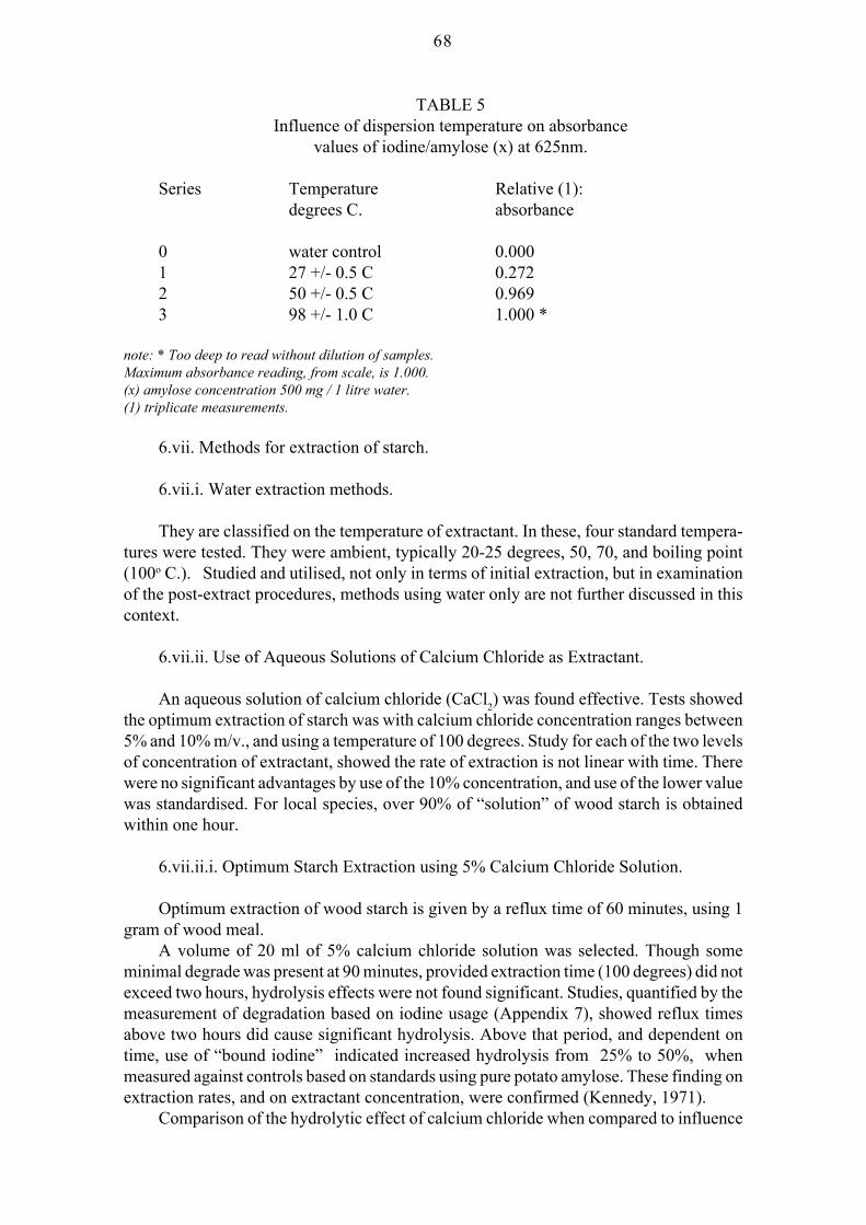
68

TABLE 5Influence of dispersion temperature on absorbance

values of iodine/amylose (x) at 625nm.

Series Temperature Relative (1):degrees C. absorbance

0 water control 0.0001 27 +/- 0.5 C 0.2722 50 +/- 0.5 C 0.9693 98 +/- 1.0 C 1.000 *

note: * Too deep to read without dilution of samples.Maximum absorbance reading, from scale, is 1.000.(x) amylose concentration 500 mg / 1 litre water.(1) triplicate measurements.

6.vii. Methods for extraction of starch.

6.vii.i. Water extraction methods.

They are classified on the temperature of extractant. In these, four standard tempera-tures were tested. They were ambient, typically 20-25 degrees, 50, 70, and boiling point(100o C.). Studied and utilised, not only in terms of initial extraction, but in examinationof the post-extract procedures, methods using water only are not further discussed in thiscontext.

6.vii.ii. Use of Aqueous Solutions of Calcium Chloride as Extractant.

An aqueous solution of calcium chloride (CaCl2) was found effective. Tests showedthe optimum extraction of starch was with calcium chloride concentration ranges between5% and 10% m/v., and using a temperature of 100 degrees. Study for each of the two levelsof concentration of extractant, showed the rate of extraction is not linear with time. Therewere no significant advantages by use of the 10% concentration, and use of the lower valuewas standardised. For local species, over 90% of “solution” of wood starch is obtainedwithin one hour.

6.vii.ii.i. Optimum Starch Extraction using 5% Calcium Chloride Solution.

Optimum extraction of wood starch is given by a reflux time of 60 minutes, using 1gram of wood meal.

A volume of 20 ml of 5% calcium chloride solution was selected. Though someminimal degrade was present at 90 minutes, provided extraction time (100 degrees) did notexceed two hours, hydrolysis effects were not found significant. Studies, quantified by themeasurement of degradation based on iodine usage (Appendix 7), showed reflux timesabove two hours did cause significant hydrolysis. Above that period, and dependent ontime, use of “bound iodine” indicated increased hydrolysis from 25% to 50%, whenmeasured against controls based on standards using pure potato amylose. These finding onextraction rates, and on extractant concentration, were confirmed (Kennedy, 1971).

Comparison of the hydrolytic effect of calcium chloride when compared to influence

69

of temperature, showed the latter was more significant, and, at the nominated saltconcentrations, calcium chloride solution is classified as only a mild degrading extractantof starch, including wood starch.

Multiple studies confirmed extraction was complete when tests on aliquots of theextract gave a negative blue colour with N/20 iodine/ potassium iodide (I/KI).

In initial research on extractions of timber, or on use of different extractants, orchanges in technique, the writer found it is preferable to confirm completeness of extractionby tests based on group carbohydrate reactions such as those by orcinol (Appendix 9), orby tests using Benedict’s solution. The orcinol test is not applicable directly on wood, butis effective, with a detection level of 5 to 8 micrograms, in tests on starch extracts, fromwhich calcium should be separated (Appendix 9).

6.viii. Starch Separation, and Purification, subsequent to Extraction.

After extraction, the hot mixture (extract and wood meal) is filtered and washed withhot water. It is then cooled to room temperature. Complete quantitative precipitation of thecarbohydrate is obtained by addition of ethanol (in excess of four volumes to one volumeof extract). The precipitate is centrifuged, washed with ethanol and air dried, prior to finaldispersion in boiling water. The aqueous dispersion is cooled and made to volume. Calciumchloride is soluble in ethanol, (Sidgwick, 1962), (Handbook of Chemistry, 1967-68), andit is adequately removed during precipitation and washing with ethanol as described.

Dependent on end requirements, purification is repeated, the precipitate is washedwith a water/ethanol mixture, and re-dried at ambient, or low temperatures (Chapter 7). Itis re-dispersed at 100 degrees in water, cooled (see “sol” below) and made to volume. Atypical final volume of 500 mls is used. To ensure uniform dispersion, this is shaken beforean aliquot is taken.

6.ix. Formation of the “Starch-Iodine-Complex” and Reporting of Results.

To meet requirements both of excess iodine reagent, and the readibility range ofspectrophotometry, a volume of 1.0 ml of N/20 iodine/potassium iodide reagent on the basisof a 10 ml aliquot taken from 500 mls of starch dispersion, was found suitable. Though thisreaction is based on amylose (or amlyodextrins), when potato starch is used as standard, andwith a typical amylose content of 25%, all results are reported as “equivalent starch”. Ifdifferent total volumes of wood extract are used, eg. 50 mls, an adjustment of the additionof iodine reagent is made. In his research, when specific investigations were carried outusing amylose, the writer generally reported results as that fraction of starch. Reading ismade (Section 6.ix.ii.) within one minute. If a starch (or amylose) concentration higher thanthis level is present, depth of colour may be above readability and diluted aliquots areneeded.

6.ix.i. Characteristics of Starch in Aqueous Medium, and Starch “sols”.

In this writer’s experience, the single most important factor in starch analysis is that,though described as a “solution”, starch dispersion is, in fact, a “sol” and, thus, particlescan aggregate, and precipitation occur. It is not colloidal and, thus, more correctly, it shouldbe described as a “dispersion”.

Aggregation problems are not as significant at elevated temperatures, and led the

70

author to standardise on use of elevated temperatures for aqueous washings. However,when making starch (amylose) extracts to volume, ambient temperatures are required. Thestarch, and amylose, dispersions should be shaken prior to sampling. This fact is well knownin analytical laboratories, and some suppliers manufacture a specific “soluble starch”.Schoch (1945) suggests the instability of starch “sols” is due to the presence of the linear“A” fraction and favours alcoholic systems of fractionation. This phenomenon has mostsignificance in iodiometric methods, and this instability due to “dispersion” causesdifficulties in any method requiring measurement of clear liquids. That problem applieswhere spectrophotometry is used. Any formation and settlement of a precipitate giveunstable readings of absorbance due to light scatter. Neither Beer’s nor Lambert’s law canapply. To confirm, and to quantify, the effect, the writer, using special optical cells, testedsignificance of aggregation on iodiometric colour measurement, as a function of reactiontime (Section 6.ix.ii.) after complex formation. A technique (Section 6.ix.ii.ii.) wasdeveloped to reduce the effect.

Estimation as simple sugars involve a “solubilising” step by hydrolysing with diluteacid, or, alternatively, enzymolysis. Thus, for such procedures, once hydrolysis hasprogressed, there is a minimal effect of the “sol” on uniformity of starch distribution in anaqueous medium. Other references to pre-treatment for solubility, are given (cf. Appendix10 and Chapter 5).

6.ix.ii. Effect of Reaction time on Iodiometric Stability of the “Starch-Iodine Com-plex”.

When iodine reagent is added to a “dispersion” of starch, many methods specified“immediate” reading, but limiting time conditions were not defined. In earlier work theauthor had noted (Chapter 4) a variable rate in settling of precipitate after formation of the“iodine-complex” in assessment of starch, and particularly, wood starch. To confirm thiseffect was present and was significant in quantitative spectrographic studies, three speci-mens of each of three species, with variations in their starch levels (Table 6), were thenextracted, and purified, as described above.

Iodine reagent was added, and separate triplicates for each specimen, measured at 0.5,and 15 minutes, showed precipitation did occur. Differences to the values at 0.5 minuteswere found. It was noted (Table 6) a relatively high residual absorbance was present in somesamples after 15 minutes. Results confirmed evidence accumulated by the writer inextractions over a wide range of species that precipitates were formed, and were confirmedas typical “starch-iodine” complex. This was one reason why the author specified centrifu-gation in measurement by iodine (Appendix 7) of the degree of starch degradation.

This time difference in absorbance was not found (Section 6.ix.ii.i., below) in similarstudies using amlyose and with centrifugation. It was considered to be a function of the“settling rate” of the complex, suggesting the effect is a function of wood starch concen-tration, and starch characteristics from different species (Chapter 4). As measurementswere at a narrow waveband (625nm), the residual colour is not attributed to possible iodinereaction (cf. Chapter 5) with amylopectin extracted from the wood meal.

6.ix.ii.i. Aggregation Stability in Spectrophotometric Measurement of the Amylose-Iodine Complex.

71

TABLE 6Decrease of absorbance of wood starch/iodine

(not centrifuged) complex at 625nm.

species sample relative(note 1) number absorbance(2)(4)

(3)0.5mins. 15mins.

water control 0 0.000 0.000

yellow walnut 1 0.225 0.022“ “ 2 0.565 0.320“ “ 3 0.002 0.000

n. silky oak 1 0.004 0.000“ “ 2 0.039 0.000“ “ 3 0.682 0.444

kurrajong 1 0.486 0.161“ 2 0.476 0.254“ 3 0.214 0.196

note 1. species were;yellow walnut, Beilschmiedia bancroftii..northern silky oak, Cardwelliasublimis. kurrajong, Brachychiton spp. prob.acerifolius.note 2. relative absorbance.note 3. separate wood specimens used for each species.note 4. data shows variation between species in termsof decrease in rate of aggregation as apercentage of initial readings.

To evaluate, and clarify, the variability in stability of the complex and its effects onmeasurement, as well as to confirm it was a function of the reaction, and not a characteristicof wood starch only, further research was conducted using purified laboratory gradeamylose.

The author used a 0.01% m/v solution of amylose in 5% calcium chloride (Section 6.viii.). After precipitation and re-dispersion of the amylose in water, iodine reagent (I/KI)was added to aliquots, and the resultant blue colour read spectrophotometrically at times asin Table 7. Separate triplicate samplings, and measurements, were made.

A matching sample was rapidly centrifuged after standing for an equal time, and thenmeasured. In view of the predicted short stability times, a spectrophotometer was usedwhich enabled the initial complex formation to be formed (with shaking prior to reading)in optical cells. A matching complex was formed in a small centrifuge tube, with separatereplicates for each test, and in which it was held for the required time and then centrifuged(cf. Section 6.ix.ii). The centrifuged samples were then decanted into a cell for measure-ment. Results (Table 7) confirmed a significant time effect on the optical stability. The datato one minute were not statistically different, but longer times (for direct measurement)above one minute were significantly different. Non-significant differences, found after thecentrifugation, in spectrophotometer readings of the “reacted” samples, but which were notpresent in the control (reagent) water blank, demonstrate an “optical stability” which theauthor attributes to a “soluble effective” component of the “amylose-iodine” complex.

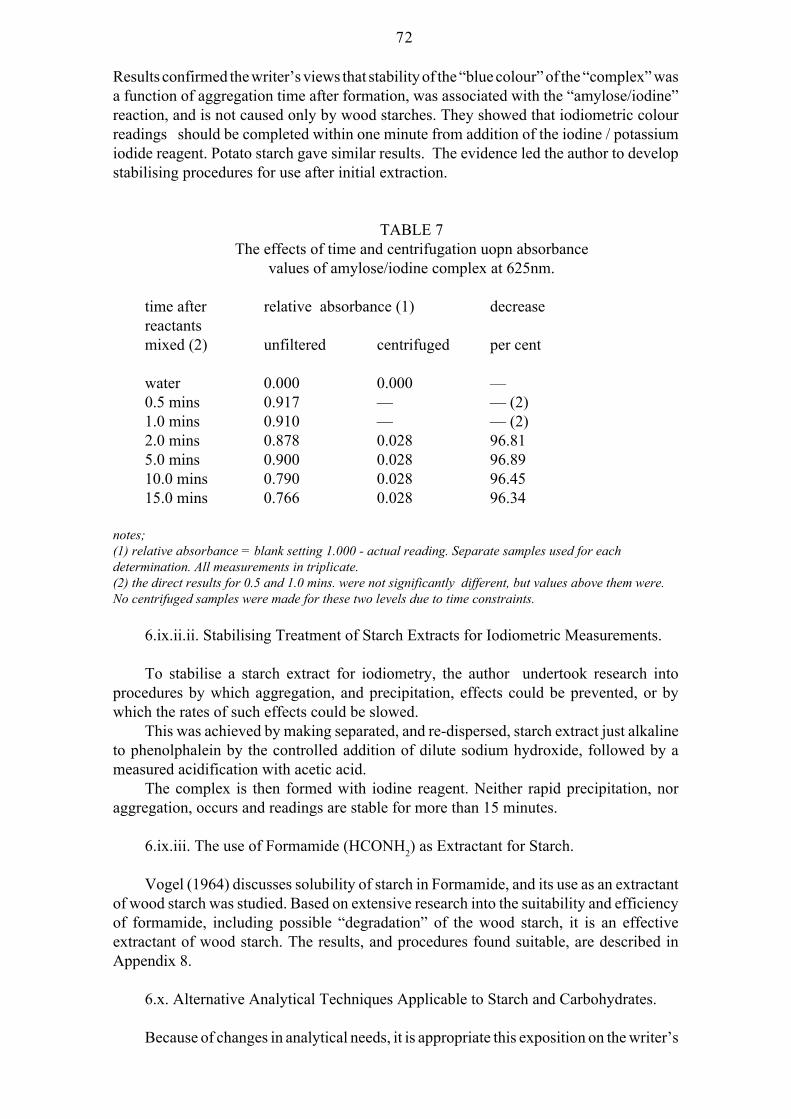
72

Results confirmed the writer’s views that stability of the “blue colour” of the “complex” wasa function of aggregation time after formation, was associated with the “amylose/iodine”reaction, and is not caused only by wood starches. They showed that iodiometric colourreadings should be completed within one minute from addition of the iodine / potassiumiodide reagent. Potato starch gave similar results. The evidence led the author to developstabilising procedures for use after initial extraction.

TABLE 7The effects of time and centrifugation uopn absorbance

values of amylose/iodine complex at 625nm.

time after relative absorbance (1) decreasereactantsmixed (2) unfiltered centrifuged per cent

water 0.000 0.000 —0.5 mins 0.917 — — (2)1.0 mins 0.910 — — (2)2.0 mins 0.878 0.028 96.815.0 mins 0.900 0.028 96.8910.0 mins 0.790 0.028 96.4515.0 mins 0.766 0.028 96.34

notes;(1) relative absorbance = blank setting 1.000 - actual reading. Separate samples used for eachdetermination. All measurements in triplicate.(2) the direct results for 0.5 and 1.0 mins. were not significantly different, but values above them were.No centrifuged samples were made for these two levels due to time constraints.

6.ix.ii.ii. Stabilising Treatment of Starch Extracts for Iodiometric Measurements.

To stabilise a starch extract for iodiometry, the author undertook research intoprocedures by which aggregation, and precipitation, effects could be prevented, or bywhich the rates of such effects could be slowed.

This was achieved by making separated, and re-dispersed, starch extract just alkalineto phenolphalein by the controlled addition of dilute sodium hydroxide, followed by ameasured acidification with acetic acid.

The complex is then formed with iodine reagent. Neither rapid precipitation, noraggregation, occurs and readings are stable for more than 15 minutes.

6.ix.iii. The use of Formamide (HCONH2) as Extractant for Starch.

Vogel (1964) discusses solubility of starch in Formamide, and its use as an extractantof wood starch was studied. Based on extensive research into the suitability and efficiencyof formamide, including possible “degradation” of the wood starch, it is an effectiveextractant of wood starch. The results, and procedures found suitable, are described inAppendix 8.

6.x. Alternative Analytical Techniques Applicable to Starch and Carbohydrates.

Because of changes in analytical needs, it is appropriate this exposition on the writer’s

73

research on estimation of starch, should conclude by a brief review of alternative methodsfor carbohydrates. The review includes wood starch analysis, and the examination of somefundamental aspects in methods of estimation, including methods (Appendix 9) where theprimary method is not specifically to measure starch, or its fractions, but where thatmeasurement is as carbohydrate. Of those described, use was made of a number which wereof application in the author’s research. Fractionation using alumina, tests of paper, and ofcolumn, chromatography, applying reagents described by Feigl (1966), and severaltechniques developed for sugar analyses using reagents such as orcinol, illustrate theappropriate utilisation by the author. That use did extend to fields of research not directlydealt within, or by, this Chapter.

74

Chapter 7

PROCESSING CONDITIONS AFFECT STARCH IN TIMBER, MOISTUREAND TEMPERATURE ARE SIGNIFICANT.

7.1. Many of the early workers (Campbell,1935) who studied starch in wood, usedmaterial not subject to processing conditions which were critical to starch. These circum-stances were at variance with those applying to Forest Products Laboratories operating in,especially, New South Wales and Queensland. Both were charged with advising localtimber producing, and using, industries in effective utilisation of resources and, at the sametime, with the administration of legislation heavily involved in detection and estimation ofstarch. That injunction resulted in need to examine stability of starch under a number ofconditions. General implications (Chapter 2) of legislation were reviewed.

Two relevant major results of these roles were a requirement of knowledge ofinteractions with processing procedures, and concurrently the estimation of starch in woodproducts which had been subjected to a range of processing conditions, with manyinvolving a thermal, and or moisture content, change, or which included a chemicalcomponent in such operation.

7.1.i. Operational evidence which had shown a number of anomalous results, butwhich were not explained by causes such as differences in growth conditions of trees, ledthe writer to consider if anomalies may be functions of certain processing factors and, inmany cases, might result in changes in starch, or its detection, from a fallen tree to thefinished product. Anomalies included;-

7.1.i.i. non-significant Lyctus attack in untreated plywood, manufactured by hotpressing of starch positive (after peeling) veneer subsequent to seasoning of the veneer bymachine drying (Cokley, 1956) at temperatures equal to, or above, 100-120oC.

7.1.i.ii. A non-significant level of Lyctus attack in starch positive timber, which hadbeen inadequately preservative treated by processes operating at elevated temperatures.The incidence of attacked samples was low, and was less than fifty cases in 20 years.

Attack was found in timber specimens with corresponding low preservative retentionlevels which had been treated by processes operating at ambient temperatures. Air dried,untreated timber was attacked. The incidence of positive attack included veneer (Chapter9) which had been dried at ambient temperatures, or below 70 degrees, and with largequantities attacked.

7.1.i.iii. In all but one anomaly, that is, where no Lyctus attack was found ininadequately treated, or untreated product, the corresponding processing during manufac-ture involved marked increases in temperatures, and times, to which the timber wasexposed, often resulting in large reductions in moisture content of the product. Additionalinstances involved the presence of chemicals in adhesives or the use of preservative, otherthan conventional total impregnation, such as quarantine fumigation of timber, or log,imports by methyl bromide. Two special, commercially inportant, circumstances placedgreater emphasis on a possible inter-connection between these two external influences oftemperature and moisture with starch. They are:-

7.1.i.iii.a. Prior to “peeling” on a rotary lathe, or “slicing”, into veneers, thepreparation of logs, and flitches, involves “thermal softening” (Appendix 3) in water, which

75

required “pre-boiling” of logs or flitches for some days in concrete vats. Generally, starchfrom such sources was “swollen”, readily extracted, “soluble”, and measurable. However,consequent on research programs (Appendix 13) on starch distribution, cases were notedwhere starch results were at variance to measurements on the fresh logs.

7.1.i.iii.b. Production of bent, turned, timber products such as tool handles was fromyoung, small girth, logs and with a preference for spotted gum (E. maculata). Material,“dressed” in a “semi-green” state, was steamed for up to several days using low temperature“wet” steam, with progressive bending in clamps. It was air-dried, machined, and severalvarnish coats applied. Though the manufacturer had subsequently installed preservativeprocesses (hot and cold and later vacuum/pressure), with kiln seasoning, incidence ofLyctus attack on untreated, starch positive (when sawn) product was extremely low. Of thefew, one was a shovel handle owned by this author.

7.1.ii. The exception in those anomalies differed in that there were no increases intemperature, nor changes in moisture content. That refers to “Starch Resorption” and isexamined in Chapter 5, and in review of susceptilibity of timber species to possible Lyctusattack (Chapter 9).

7.2. Possible effects of Processing Conditions on Starch.

After reviewing the evidence, the writer considered that wood starch may be degradedby certain processing conditions or treatments. There was minimal literature on this topicas relating to wood starch. Confirmation of the author’s theory of processing factors ascausing possible degradation, required research into effects of such conditions on starch.Initially there was a need to quantify influences on starch of factors common in thesemanufacturing procedures, such as high temperatures, and, if they were present, todetermine critical parameters.

7.2.i. Use of Agricultural Starch Information.

The writer accordingly followed practices similar to those used in studies on starchevaluation and reactions (Chapters 4, 5, 6), and utilised agricultural starches as the modelsfor comparison. A large body of literature was available for those types of starch onsusceptibilities to processing conditions.

A reader is justified in asking why the author did not follow practices of impregnationof starch, or of its fractions, into small blocks and subsequent testing of possible causes onthat basis. One reason is demonstrated in Chapters 9 and 12, where he shows sites ofdeposition by impregnation, including starch (or its fractions), and especially for angiosperms,will differ from natural sites of starch occurrence in the wood. Procedures in impregnationof small blocks were used routinely for tests for pathways of the penetration of preservativesinto timber. Performance of such sizes, under processing, is significantly different to macrospecimens, with particular reference to time/temperature and the moisture content relation-ships. Further, there arose problems in quantitative extraction of impregnated starch, whichmust necessarily include the degraded forms after any studies. Substantially, problems ofsuch extraction were reasons for this study to proceed.

If wood starches are susceptible, particularly to effects of thermal degradation, andmoisture content changes, as noted for the agricultural starches (Chapter 5), then, to confirmthe hypothesis, it is necessary to confirm the degradation products. This requires experi-mental evidence that any susceptibilities of wood starch to degradation are equivalent tothose of agricultural starches induced by the same conditions. The relationships are further

76

examined in this Chapter, where evidence collated in Chapter 5 was combined with serviceresults, and with laboratory testing, as guides to any physical and/or chemical, processingfactors which may affect starch or its fractions.

7.3. Factors Significant in Wood Starch Reactions.

It is not considered surprising that much indicative data suggested moisture and/ortemperature conditions, and their interactions, may possibly be significant in any changescaused in starch, as these two factors exert major influences in all facets of woodperformance, and the effects include wood components and extractives. However, theauthor considers a discussion of these interactions with starch and its stability (includingits detection and assessment), is the most appropriate place to introduce topics, and terms,relating to temperature, and moisture, and their involvement with the processing of timberproducts.

For this reason, an apparent digression is made to identify, and to define, these topics,and so indicate their relevance to wood. This digression will enable a reader, beforeevaluation of the possible effects of such conditions on wood starch, to clarify theirimportance, to put them into a correct perspective, and thus, to consider the roles played by,what the writer terms, basic common factors in wood production (and usage). Details onsome of the processes are given in Appendix 11. In almost all processes, two, or more, ofthe factors (and their interactions) occur. Though definitions for some of the factors arecontained in Australian Standards (short title SAA AS 01-1964), in this context, the authorplaces change of emphasis on some of those terms (discussed after definitions) to moreclearly show their interactions with wood processing as well as with starch chemistry andtechnology. The factors are;

7.3.(a).Thermal Gradient.Timber is primarily an insulator and, in a later context in preservation (Chapter 13),

the term “diffusivity” is introduced. For the topic under discussion, it suffices to state theability of timber to disseminate heat is a function of its moisture content and of wooddensity. The specimen cross-section is important. Thus, when wood is exposed to increasesin temperature, there is a steep and measurable thermal gradient from the surface exposedto the heat source to the centre of the timber section. As time of exposure increases,temperature increases with depth, but the rate of increase is non-linear. The higher thetemperature of the external source, the associated moisture (see next below) contents vary,and the steeper the gradient. Conversely, exposure to a lower temperature results in, whatis termed here, a negative gradient, and usually an increased moisture content in the outerzone.

7.3.(b). Moisture Gradient.Similar to a thermal gradient, if timber is exposed to lower humidities, drying

commences from outer surfaces, but the rate of drying (termed seasoning) and, thus, lossof moisture, decreases with depth. This variation of moisture with depth, or length, is termeda “Moisture Gradient” and is influenced by temperature and time. Physical properties(Chapters 12 and 13) have effects as for temperature, and the moisture content gradientsare similarly non-linear. Angle of cut (AS 01-1964) plays a role. If moisture (and generallythermal) differentials are extreme, especially for the outer layers, “surface inactivation”(Appendix 15) occurs, and moisture contents are low. Wise (1946) attributes the cause ofthis condition, which he refers to as “case hardening”, to a chemical cross-linkage of anyavailable hydroxyl and carboxyl sites in constituents. For this condition, a timber surfacebecomes difficult to wet with any aqueous additives and stresses are set up in the section.To relieve or remove the “inactivation” and stress effect, external conditions are reversed

77

by using heat with high humidities, a process termed “Reconditioning”. Under theseconditions, such as when the external humidity is high, as given by “wet” steam, or byimmersion in water, especially if above ambient temperatures, a reverse moisture gradientresults.

7.3.(c). Critical Moisture Contents.There are six primary separate critical moisture contents in relation to timber, each of

which were found to have a significant role in starch stability. It is in definition of, andextension for, some of these terms (cf. Moisture Content Concepts, Chapter 12) where thewriter wishes to expand limitations of, and emphasis given in, Australian Standard AS 01-1964. Four terms (and abbreviations) are;

7.3.(c).i. Green (G.O.S.).7.3.(c).ii. Fibre Saturation Point (FSP).7.3.(c).iii. Equilibrium Moisture Content (EMC).7.3.(c).iv. Oven Dry (o.d.).

The state of “oven dry” in a specimen plays an important role in many measurementsin timber research, illustrated by topics in Chapters 12, 13, 14, such as “Void Volume”calculations, or “Basic Density”. As defined in AS 01-1964, the term “Oven Dry” relatesto the condition where a specimen “will not lose moisture in a ventilated oven —— between100o and 105 oC.” There are some species, including softwoods, which contain volatiles, or,alternatively, extractives which are thermally degraded at the nominated temperature rangeto measure the “oven dry” state. Cypress and slash pines, as well as many eucalypt foliages(essential oils) fall into that category. This was a problem in moisture tests underT.U.P.A.(1949), and Australian Standards. More correctly, the “Oven Dry” term should bedefined as “the state (at a nominated temperature range) of no further loss of, or equilibriumin, sample mass, and which loss is assumed as due to loss of water”.

Two additional terms not defined above, but consequential on them, are significant forfields of Wood Chemistry, of Preservation, and of Timber Physics. Of these, the formerterm is an extension of a listed term, “green”, and the latter of the term, “oven dry”. Theyare referred to as:-

7.3.(c).v. “Saturation Moisture Content”, is defined as the point where the moisturecontent in a specimen is at a maximum, and differs from the term defined as “green”, andwhich is, by definition (AS 01-1964), indeterminate as a specific value, as well as two termsintroduced by the author (Chapter 12). They are the two concepts of a “Standing Tree”, anda “Stable Green”, moisture content.

“Saturation Moisture Content” is experimentally attained by repetitive impregnation(to constant mass) of a sample by water. It may be obtained by the continued boiling of aspecimen in water, but, in many studies, effects of boiling on a sample are undesirable, andthe writer found repeated evacuation and absorption to be generally applicable. For bothprocedures, soluble extractives may be removed. In later discussions it will be shown the“Saturation Moisture Content” is used (Chapters 12 and 14, Appendices 37 and 38) as aguide to “Void Volume”, and the possible maximum preservative impregnation in aspecimen, but problems may arise in its use (Chapter 12), without qualification, for thepreservative uptake in angiosperms.

7.3.(c).vi. “Anhydrous” is an extension of the definition of “oven dry”, with which itis partly synonomous. It refers to situations, which are not restricted by definition to an oventemperature (100 oC.). The term includes conditions where all of the moisture has been

78

removed from a specimen. Hence, it includes removal of the moisture by chemicalprocedures, or by influences of manufacturing processes. Examples of these conditions arechemical techniques, such as moisture estimation by the Dean and Stark procedure, orsolvent extraction followed by vacuum drying, used as reference methods for moisturecontent determinations. “Chemical Seasoning” of timber products has been advocated ona commercial scale.

The necessary extension to the definition of “oven dry” explains the writer’s usage ofthe term “anhydrous”. That condition of complete loss of moisture may be described(Chapter 5) as “Dehydration”. If these processing conditions become more severe, there ispossible water loss from wood constituents, other than that defined (AS 01-1964) as the“combined”, or more commonly, the “bound” water. Final states of wood degradation areconsidered as being equivalent (Section D, Chapter 5) to the conditions of “Charring”, and,finally, to “Carbonisation” at which the chemical structures are broken down (cf. Section7.4.b.). This progression in degrade occurs where high temperature processing, includingRF gluing under certain conditions, or exposure to fire, is present.

7.4. Correspondence of Processing Factors with Research on Starch Stability.

To support the writer’s hypothesis of the above factors having effects on starch, itwas necessary to measure processing conditions to which wood starch is exposed, enablingdetermination of their similarity (cf. Section 7.2.i.) to those reported to affect agriculturalstarch. Comparison was made of both starch types (or fractions) for any chemical, orphysical, degrade when exposed to equivalent process conditions indicated by measure-ments.

Greenwood (1967) discusses both the “degradation” of, and “dehydration” of, starch.To stress a special case of “degradation”, the author defined (Chapter 5) a term “hydroly-sis”, indicating possible cleavage of the helical structure of starch (or fractions). Otherreferences (Chapter 5) indicate a number of effects of chemicals on starch. To co-ordinateall aspects, the writer suggests processing conditions of timber products may be equated tothose defined by workers such as Greenwood. Thus;-

7.4.a. For conditions above “Fibre Saturation Point” (FSP) and increasing to thelimiting one of “Saturation Moisture” content, and where free moisture is present, thermaland moisture effects on starch can be equated to possible “hydrolysis”. That effect issynonomous with the term “degradation”, and precedes “dehydration”.

7.4.b. As the Moisture Content decreases below FSP, then, by definition, free moisturehas been removed, and “hydrolysis” ceases. As drying progresses from FSP to EMC (cf.“contained” and “bound” water concepts, Section 14.4.3.i.i, Chapter 14), some of the“contained” water is removed. From EMC to the oven dry state (where residual “contained”and “bound” water is removed), some critical moisture changes occur in wood starch(Appendix 12), which is equivalent to its “dehydration” as defined (Chapter 5) byGreenwood (1967). If drying conditions continue past the nominal oven dry, eg. by increasein temperature, then from that point, water removed may be associated with its loss fromwood components and/or extractives. Under these final conditions, the specimen is initially“charred” and finally the component chemical structures are broken down with “carboni-sation” occurring and includes the starch present in the specimen.

7.5. Selection of Experimental Conditions based on Data from Agricultural StarchSources.

79

Examined in Chapter 5, specific evidence is cited for the laboratory comparison ofagricultural starches with wood starches after extraction. If the comparisons show woodstarch is susceptible to these test conditions, further examination of possible effects onwood starch “in situ” would be justified. Examples of critical parameters for comparisonare summarised as:

7.5.a. Early work by Henderson (1943) examined starch depletion as a function ofconditions attained during low temperature kiln drying. He concluded the maximumresorption was over a temperature range of 31-36o C., but higher temperatures (52o C.)resulted in a decrease. He correlated this with continued cell viability and oxygen demand.It is of interest that Henderson considered the possible roles of enzymes on starch stability.

7.5.b. Willits (1951) discusses temperature factors in determination of moisturecontent in agricultural starch, as functions of temperature / humidity. He refers to the sharpincrease in loss of weight when using oven dry procedures for the determination of moisturecontent in starch. This change occurred at just below 150o C.

7.5.c. Holdaway (1964) correlates degrade by drying at elevated temperatures as afunction of glutamic acid decarboxylase activity. He concluded that 85o C. is critical, butthe activity at 115o C. is only 50% of that at ambient temperature. He states that starchdegrade is influenced by the source of the starch and its moisture content.

7.5.d. Sullivan and Johnson (1964) examined the effect of time, and temperature, onstarch birefringence and Beta- amylolysis. They defined the critical temperature range asthe point of reduction to 50% for birefringence or for production of maltose. Dependent onthe starch source, critical temperature ranges of 55-74o C. were obtained, but sourcedifferences tended to disappear at 85 - 90o C. They report waxy starches did not exhibitsignificant effects at 70o C. They found degree of gelatinisation was mainly in the first hour,reaching equilibrium in 4-5 hours, but was dependent on starch source.

7.5.e. Greenwood(1967) discusses (Chapter 5) the thermal degradation of starch.Brimhall is cited by Greenwood (1967) as showing effects of degradation by an increasein reducing power, decrease in the Beta-amylolysis limit, with a sharp increase in solubility,but with marked decrease in linear material. Treatment for 1 hour at 175o C. was significant.The thermal stability of amylose and of amylopectin decreased by 46% over a range of 219- 251o C., but starch itself decreased by only 37.6%. The effect was influenced by inorganicsalts; sodium borate, a major preservative chemical, had a very significant effect irrespec-tive of temperature.

7.6. The Sensitivity of Wood Starch to Temperature and Humidity.

The evidence suggested effects of especially temperature as low as 50o C., rising tolevels described (Appendix 11) for wood processing conditions. All data suggested

o C. It also related changes inmoisture content of timber to the stability of starch.

7.6.i. Studies were made, using potato amylose as the control, including, and in excessof, these ranges. Amylose was selected as control (Chapter 5) to remove any influence ofamylopectin, and emphasised the definitive test for reaction was the positive formation ofan amylose “blue complex” with (I/KI) reagent. Wood starch was then extracted, andpurified, under mild conditions, from a range of species and exposed to similar conditionsas potato amylose. Results and exposure conditions are listed in Table 8. Solubility resultscited relate to product dispersion (Chapter 6) in water. Iodine (I/KI) tests were made on thedispersed material, but, in some cases, tests were repeated on moistened solid product.Complementary studies made, confirmed the reactions (Table 8) were equivalent for potato

80

amylose, potato starch, and wood starches. The author concluded that his hypotheses wereconfirmed and;

7.6.i.i. Normal operations, including extended treatments for preservation or kilndrying, at continued temperature > 70-100 o C, can degrade, or hydrolyse, wood starch.

Table 8.Influence of drying conditions on starch extracted from timber species, and using

potato amylose(x) as control.

series test result (see text)no. condition

app. sol. iodine(3)(temp. degs C.) (1) (2) complex

1 air dry control pale v.g. pos.(ambient temp.) buff

2 vacuum dry(ambient temp.) “ “ “

3 vacuum dry (a) buff satis. “(135mm, 70deg)from ethanol pptn.

4 as for 3, but fromaqueous solution “ “ “

5 as for 3 at temp. pale v.g. “of 40 degrees. buff

6 oven dry at pale poor sl.70 degrees. (b) reddish

brown7 oven dry at red poor sl.

100 degrees. brown8 microwave (2470Mhz.) pale satis. pos.

3 mins./100 degrees, brownhumidity control.(c)

9 microwave as for 8 deep insol. neg.at 120 degrees, no redhumidity control. brown

notes;(1) appearance. (2) solubility in water (100 degrees) v.g.= very good. (3) standard reagent. sl.=tracecolour only.(a) over 12 hours, degrade increased. Solubility and reactivity decreased. (b) degrade increased to total,as a function of moisture loss and time. (c) water cell for equivalent 5% mc. (x) complimentary testsusing potato starch gave equivalent results.

7.6.i.ii. For the same temperature / humidity conditions, the effect is pronounced onsolubility of wood starch and its reaction with (I/KI) reagent when compared to potatoamylose and potato starch.

7.6.ii. As the extracted wood starch was influenced by, and susceptible to, theconditions similar to those used in process operations, general conclusions are:-

81

(a) There are both solubilising effects and partial degradation in aqueous preservativetreatments and normal kiln drying to Equilibrium Moisture Content.

(b) Timber preservative treatment by the vacuum pressure processes where oilsolutions and temperatures in excess of 80o C., are used, can cause severe degradation andpossible dehydration of wood starch.

(c) Where manufacturing processes are above 100o C. and may result in very lowrelative humidities for extended periods (of the order of 12 hours), near dehydration of sawntimber surfaces (and section depth) can occur, with a consequent effect on the wood starch.

(d) Where processing temperatures, greater than 120o C., and low moisture contents(< 3-5% m/c) are involved, a dehydration of starch fractions occurs. The time effect ofexposure depends on section thickness and rate of heat transfer and is dependent on species.For thin sections such as veneer, which have high surface/thickness ratios, the effects (c),(d) will occur in less than 20 minutes.

7.7. Service Confirmations.

Starch reactions from a large range of open forest, rain forest, and plantation softwood,species were examined after the exposure of products to processing conditions. Results areshown in Appendix 12.

7.8. Legal Approvals Based on these Studies.

As a consequence of this aspect of the author’s research, an exemption, under T.U.P.A.(1949), was given from need for conventional preservation treatments (against Lyctus spp.)for machine dried (using high temperatures and low humidities), hot pressed, veneer madeinto plywood.

82

Chapter 8

ECONOMIC AND SCIENTIFIC IMPORTANCE OF SAPWOOD AND ITSIDENTIFICATION. THE INFLUENCES OF SOURCE, AND FACTORS INTREATMENT BY, AND REACTIVITY WITH, AQUEOUS SOLUTIONS.

8.1. Previous text (Chapters 1, 2, 3), stressed the roles of sapwood in effectiveutilisation of timber resources. For a number of reasons, conventional tenets were thissignificant volume of a tree was nonutilisable except for very limited, and generallytemporary, applications. Legislation enabling its use (Chapter 2), establishment (cf.Introduction) of Forest Products Conferences, were for the primary aims of changing thatimage, so ensuring sapwood utilisation. This was expanded to, particularly in tropical/ sub-tropical rainforest species, a total usage of previously not used timbers, but necessary aseffective utilisation of sapwood was a central focus of conservation. Unless that was done,none of the general aims of conserving resources could be met. The magnitude of thatrequirement is shown in Table 9. (Queensland Forest Service, 1972.)

TABLE 9

Relation of total number of Queensland species to Lyctus susceptilibity and rateddurability. (x)

item data

number of utilisable species 351

percentage (number) susceptible 49.5to Lyctus spp. note (a) (174)

________________________________________________

percent (number) class A durability 9.2note (a), note (b) (32)

class B durability 27.9(98)

class C durability 63.0(221)

________________________________________________

notes(a) Total of species in classes shown in brackets.(b) for durability ratings, refer Watson (1964). (x). QFS, 1972

Author’s notes; in this thesis, in use of the two terms, “gymnosperm” and “angiosperm”,the writer will follow a general practice of use of italics (irrespective of upper or lower case).AS 01-1964 uses the upper case, but the principal reason for this choice is emphasis in thetext. A similar practice is followed for the term “porosity”, when (Chapters 12, 14), thoughnormally interchangeable with “vessel” (eg. Chapter 9), the “pore” is primarily differen-tiated in physical contexts of a “duct” (eg. for liquid flow), and is defined jointly in termsof pore size (diameter) and count (or frequency), per unit area.

83

The administrative importance placed on this charter of Forest Services (Chapter 1)for conservation, especially of sapwood, is shown by an approval to the author of a ResearchPhilosophy (Chapter 1) with an emphasis on establishing scientifically based preservationpractices by the industry to make its use viable, and in forms whereby the user public wouldhave confidence its long term service is adequate for their needs. The same aims appliedto species which were rated as having a nominally (Chapter 3) low “durability”. Researchinto, and roles of, starch in sapwood utilisation, and in legislation, were also principal axesin achieving that goal.

Watson (1964) specifies restriction on usage of sapwood in building timbers unlesspreservative treated.

8.1.i. It was stated (Chapters 2-4) that, for the greater number of Queensland species,visual identification of the sapwood was impracticable, and starch assessment neededvalidation. Effects of manufacturing processes on assessments of starch (Chapter 7) weresimultaneously involved. Relationships are reviewed (Chapter 9) with the most economi-cally important hazard for sapwood, namely attack by Lyctus spp.

In this Chapter, defined identifications, involvements, questions of economics, ofsapwood, treatability and species variability, are addressed. Differences between classicalterminology for forest classes, in industry use based on properties, and this author’sencouragement of classifications described in this text were important in having uniformityin all areas of timber preservation. It illustrates (Chapter 1) the author’s role of being a“translator” between industry and research groups.

8.1.ii. The discussion on sapwood indicates reasons for format used by the author inthis thesis in describing the research and technology applied in establishment of thepreservation industry in this state. He elaborates on that format in discussion of seveninterrelated items, and, of which, several expand on source variability as cited in Chapter3. They are ;-

(a). Terminology of Classification of Forest Types.

(b). Significance (Section 8.7) of “Outer Heartwood” and “Transition Wood” inangiosperms.

(c). Variability within species and groups.

(d). Factors in Penetration of timbers by Water-Borne Preservatives.

(e). The postulate, relative to penetration by aqueous salt solutions, of timber beingtermed “Reactive” (Section 8.xii). Wood is not an inert physical system. In many situations,timber may behave as a chromatographic medium.

(f). Lyctus susceptible timber” as an indicator for the non-durable zones of a species.

(g) Particularly topics 8.1.ii (a)-(e) demonstrate some common factors whichinfluence the responses of a timber to preservation, dependence on properties which affectwood “permeability”, “penetrability”, and its resultant “treatability”. As these terms areintrinsic to many phases, they are defined, and discussed in topics (b) to (d).

Initially, reference is made to problems directly due to non-utilisation of this large part

84

of our resource, and deficiencies in non-destructive, especially definitive, field identifica-tion of an important zone of a tree.

As stated (Section 8.2.A) the definitions are developed for generally SAA documents.A weakness of this rests in the system of Committees, which comprise specialists in specificfields. Though draft documents are circulated for review, in practice that draft review iscarried out by similar specialists rather than by a wider group.

8.2. Formal Definitions.

8.2.A. Sapwood.i. Australian Standard AS 01-1964 defines sapwood as;- “The living outer layers of

the wood of a tree, in which its food materials are conveyed and stored.” The writer (Chapter2) points out legal opinion stated the above definition was inadequate, and the term was notincluded in the Acts (T.U.P.A., 1949). It was also inadequate as a research definition, andthough the term “sapwood” was used, the formal Standards definition was not employed bygeneral industry.

ii. Chattaway (1952) defines sapwood physiologically as “the zone containing livingcells, food reserves, where heartwood formation, inclusive of polyphenols, has not begun”.Under both of these definitions, sapwood is limited by the term “living” (refer laterdiscussion).

In general, sapwood does not contain complex cell inclusions such as tyloses. Certainspecies may exhibit immature tyloses, but sapwood does not contain heavy incrustations oninterior lumen walls, is theoretically conductive to fluid flow, and is considered permeableto permanent gases or vapour phases. Of importance is Chattaway’s inclusion, in herdefinition of “sapwood”, of the presence of reserve food materials.Kozlowski (1971,volume 1) gives a comprehensive review of the relations of sapwood and heartwood.Kremer (1963) discusses the chemistry of developing wood.

8.2.B. Heartwood.The AS01-1964 definition of heartwood may be termed as opposite to that of

“sapwood”, but classifies the term “truewood”, which is used by industry, as synonomouswith heartwood. That standard also defines a number of terms (generally associated withdefects) as “heart” with differentiation according to cause, and, to users, this associationof the term “heart” suggested defective wood. It was for similar reasons (Wilson, 1936) thatindustry had standardised on the use of the term “truewood” as denoting the high quality,and durability, parts of a log, and, in most cases, continued to do so.

8.2.i. Problems in Application of Definitions.

Difficulties occur in assessing sapwood by physiological definitions. Clarity ofdefinition is necessary for exact scientific assessments of the relations of particularly“sapwood” and “heartwood”. A principal problem rests in inclusion in SAA documents(AS 01-1964), of a requirement of “living outer layers”, and “living cells” in that ofChattaway’s definition. No method to determine this criterion is practicable in industry asit depends on specific laboratory techniques. The only effective, practicable, utilisationmethod (especially in the field) for sapwood delineation is identification of reservenutrients and the choice, imposed by legislation, but justified by results, of detection bystarch. Sugars, as the alternative means of detection, are suitable only in a laboratory, orby skilled staff using sophisticated chemical procedures.

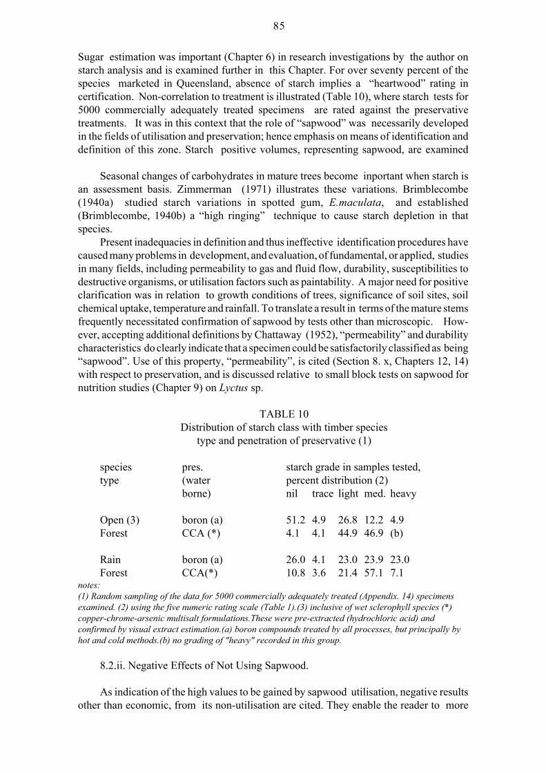
85

Sugar estimation was important (Chapter 6) in research investigations by the author onstarch analysis and is examined further in this Chapter. For over seventy percent of thespecies marketed in Queensland, absence of starch implies a “heartwood” rating incertification. Non-correlation to treatment is illustrated (Table 10), where starch tests for5000 commercially adequately treated specimens are rated against the preservativetreatments. It was in this context that the role of “sapwood” was necessarily developedin the fields of utilisation and preservation; hence emphasis on means of identification anddefinition of this zone. Starch positive volumes, representing sapwood, are examined

Seasonal changes of carbohydrates in mature trees become inportant when starch isan assessment basis. Zimmerman (1971) illustrates these variations. Brimblecombe(1940a) studied starch variations in spotted gum, E.maculata, and established(Brimblecombe, 1940b) a “high ringing” technique to cause starch depletion in thatspecies.

Present inadequacies in definition and thus ineffective identification procedures havecaused many problems in development, and evaluation, of fundamental, or applied, studiesin many fields, including permeability to gas and fluid flow, durability, susceptibilities todestructive organisms, or utilisation factors such as paintability. A major need for positiveclarification was in relation to growth conditions of trees, significance of soil sites, soilchemical uptake, temperature and rainfall. To translate a result in terms of the mature stemsfrequently necessitated confirmation of sapwood by tests other than microscopic. How-ever, accepting additional definitions by Chattaway (1952), “permeability” and durabilitycharacteristics do clearly indicate that a specimen could be satisfactorily classified as being“sapwood”. Use of this property, “permeability”, is cited (Section 8. x, Chapters 12, 14)with respect to preservation, and is discussed relative to small block tests on sapwood fornutrition studies (Chapter 9) on Lyctus sp.

TABLE 10Distribution of starch class with timber species

type and penetration of preservative (1)

species pres. starch grade in samples tested,type (water percent distribution (2)

borne) nil trace light med. heavy

Open (3) boron (a) 51.2 4.9 26.8 12.2 4.9Forest CCA (*) 4.1 4.1 44.9 46.9 (b)

Rain boron (a) 26.0 4.1 23.0 23.9 23.0Forest CCA(*) 10.8 3.6 21.4 57.1 7.1

notes:(1) Random sampling of the data for 5000 commercially adequately treated (Appendix. 14) specimensexamined. (2) using the five numeric rating scale (Table 1).(3) inclusive of wet sclerophyll species (*)copper-chrome-arsenic multisalt formulations.These were pre-extracted (hydrochloric acid) andconfirmed by visual extract estimation.(a) boron compounds treated by all processes, but principally byhot and cold methods.(b) no grading of "heavy" recorded in this group.

8.2.ii. Negative Effects of Not Using Sapwood.

As indication of the high values to be gained by sapwood utilisation, negative resultsother than economic, from its non-utilisation are cited. They enable the reader to more

86

readily understand steps taken to make it usable. They include relevant changes in theindustry practices, relate those to non-utilised volume due to tree form. These changes sawloss of expertise in the adze, of the broadaxe. The latter were important in preparation ofpoles, piling, bridge timbers by removal of “sapwood”. Sleeper cutting methods, andsources, changed.

8.2.ii.i Role of “Taper” in Non-utilisation of Sapwood.

Conventionally, sapwood occurs in outer layers of a tree and it possesses differentproperties to heartwood. When estimating the resultant availability of sapwood in a log,or for a “round” section in timber, many workers made insufficient allowance for log“Taper”, defined as a decrease in diameter of a log from “Butt” (ground end) to the “top”or “Head”. It results in higher percentages of a top cross-section being present as sapwood.Kozlowski (1971, pp. 12-14) discusses the typical distribution, and shows normal taper ofa stem. The depth of sapwood may be a function of species and growth. Typical patternsexists in open forest species, but are less uniform in rainforest timbers. Modern high speedsawing practice, operating by cutting parallel to a line perpendicular to ends of a log, isaffected by taper to give variable sapwood distribution in boards. In many open forestspecies, such as eucalypts, the sapwood percentage decreases with tree age and girth. Thatdoes not apply to the same degree in rainforest species.

Variations are excellently shown by comparison of timber from three blackbutt, E.pilularis, stands.

a. Virgin stands, averaging about 5m centre girth from the Blackall Range, atMapleton, about 150 km north of Brisbane.

b. High quality plantation material, about 3m in centre girth from Casino, N.S.W.c. Small girth, (about 1m centre girth), regeneration stands at Belthorpe, about 60 km

north of Brisbane.This last material had over 15mm of sapwood, was of good form, was readily treated,

but contained tension wood resulting in severe splitting (Plate 11, Chapter 15).

8.2.ii.ii. Pollution Aspects.

Table 9 shows the high volumes of log and sawn timber affected by sapwood. Non-utilisation of the sapwood, of itself, accentuates problems of pollution. Where logs werebrought to sawmills, sapwood rejection meant lower recoveries of sawn timber, resultingin larger volumes of “off-cuts”, sawdust, and “shorts”. These were burnt in incinerators,or “ground-pits”, with an alternative use in filling low lying sites. For the latter, leachingand decomposition resulted in the transfer of extractives and decomposition products tolocal streams; spontaneous combustion presented fire risks in sawdust heaps. Where woodwaste is burned, heavy smoke pollution and unburnt carbonised particles are present inlocal atmospheres.

8.3. Timber “Lore”.

Industry changes (Chapters 1 and 2) were described, which included the importanceof “on- site” liason. A major consequence of that practice (Chapter 3) was an opportunityto evaluate the wealth of unwritten “timber lore”, as developed through several generationsof experience, with some applicable to topics of this Chapter. As stressed in Chapter 3,

87

much unverified material was discarded, but other data provided important information forthe writer’s work.

8.4. Measurement of Wood pH values.

A pH value is common in discussion of wood properties, especially in areas such ascorrosion and preservation. However, the author found a position similar to soils, eg. pH,or phosphate, was applicable for pH measurements on wood. Briefly, measurement of thisvalue on extracts, by a pH meter, gives results heavily influenced by water solubleextractives. They relate to whether these are extracted by “cold” or “hot” water techniquesand, unless standardised, do not show good repeatability between specimens (or sources)for an accurate measurement. Conversely, direct pH measurements on wood by indicatorsolutions are dependent on the indicator solvent.

Where a wood specimen is difficult to wet (cf. Appendix 15), an indicator in alcoholicsolvent is more effective than tests using an aqueous solution. The writer found mostconsistent results were given by initial “insitu” tests with “Universal Indicator”. If closervalues were needed, an indicator suitable for ranges as predicted by universal indicator wasused.

8.5. Terminology of Classification of Forest Types.

Earlier, the writer indicated terminology illustrated his role (Chapter 1) as a“translator” for industry. In Chapter 12, the author describes a system developed forclassification of species in terms of principally physical, structural (particularly “macrostructural”) properties into groups, each increasing from previous ones in terms of the levelof treatability by initially an open tank process, but extended to other preservation systems.Preservation processes, the associated terms, and operational practices, are summarised inAppendix 14.

Subsequent research, based on his own findings for an initial classification (Cokley,1951a), led the author to application of, particularly, Swain’s Index (1927) to confirm hisown groupings. Swain (1928) issued the “Timbers and Forest Products of Queensland”.Dadswell et al (1932, 1934, 1935) described numbers of species in terms of properties andsemi-microscopic structure, with systems of identification. These works were applied bythe writer, but at levels other than the plant operator.

In Chapter 2, the writer indicated assumptions on the ability of operators at thetreatment plant, or other industry environments, to competently, and legally, identifytimbers, in terms of the listing in the Acts (T.U.P.A., 1949), with a full schedule ofsusceptible species. He pointed out that position did not apply.

It was, however, necessary for the author to ensure that a scientifically acceptablespecies classification was used, one which was understandable to, or could be used by,industry, and was acceptable to the Department. The classification could be usedadministratively, but must be in a format suitable for translating of the species treatabilityclassifications to plant operators.

8.5.i. Nomenclature.

8.5.i.i. The classical nomenclature, eg. wet, or dry, sclerophyll, or rainforest, wascomprehensively reviewed by Webb (1956) particularly in rainforest species. Swain(1928) similarly examined and described the forest groups, but industry did not useclassical botanical grouping, and had adopted a classification based on timber properties.

88

That was;-

8.5.i.i.(a). “Hardwoods”, represented by Eucalyptus spp. and brush box, Tristaniaconferta. However this includes such as tulip oaks, Argyrodendron spp. All species aredifficult to “work”, with good physical properties, are used for structural purposes, are ofmedium to high density. They included all botanical angiosperm groups.

8.5.i.i.(b). “Softwoods”, represented species of low to medium density, were readily“worked”, and used for such as cabinet timbers. They included cross-sections of all of thebotanical classes, and species correctly classed as softwoods, namely the gymnosperms.

8.5.i.ii. It was a major, and unsuccessful, exercise to induce industry to adopt botanicalclassifications. There were corresponding good reasons, in terms of species, not tocompound the confusion, by an acceptance of the industry practice. Due to reasons, citedin introducing this topic, and which were important in classification of sapwood fortreatment, the writer adopted what may be termed a “compromise”, which the industry hadgenerally accepted, and was as stated below. That was;-

A. Open Forest Species.

For industry and classification (see Table 10) purposes, it was adequate to combineboth “Dry” and “Wet” Forest (author’s terms, next below) under a term, “Open Forest”.This combined;

i. Dry Forest, equivalent to dry sclerophyll.

ii. Wet Forest, equivalent to Eucalyptus spp., but including timber species (such asbrush box, Tristania conferta), classified as wet sclerophylls.

B. Rain Forest.

C. Softwoods (or Pines), representing gymnosperms.

Technical criticisms may be advanced on the writer’s sub-groupings, but his aim wasachieved of removing a major confusion in the industry with which he was associated. Itbroadly agreed with a general classification used for sawmill licence returns by the ForestryDepartment, and these groups are used in this context in the thesis.

8.5.ii.i. Open Forest Groups. (cf. Section 8.7 - “Outer Heartwood”).

There are significant difference between Open Forest and Rain Forest species. ForOpen Forest groups, significant physio-chemical differences occur in the properties fromsapwood to heartwood. Sharp colour changes occur between sapwood and heartwood.Species of these groups, other than eucalypts, have been noted to have very similarsapwood separations. Differences for Open Forest groups include extractive content,wettability (Appendix 15) and pH. In these species, eucalypt heartwood has a low pH (2.0-4.0), but wet sclerophylls generally have heartwood pH values at the higher end of thisrange. The sapwood is about 2 pH units higher (pH 4.5-6.5). The pH (sapwood) changesare important in applications of multi-purpose preservatives (typified by CCA salts).

This change also enables pH indicators, such as dimethyl yellow (Bamber, 1964), to

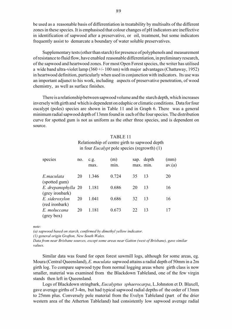
89

be used as a reasonable basis of differentiation in treatability by multisalts of the differentzones in these species. It is emphasised that colour changes of pH indicators are ineffectivein identification of sapwood after a preservative, or oil, treatment, but some indicatorsfrequently assist to demarcate a boundary of water soluble preservatives.

Supplementary tests (other than starch) for presence of polyphenols and measurementof resistance to fluid flow, have enabled reasonable differentiation, in preliminary research,of the sapwood and heartwood zones. For most Open Forest species, the writer has utiliseda wide band ultra-violet lamp (360 +/- 100 nm) with major advantages (Chattaway, 1952)in heartwood definition, particularly when used in conjunction with indicators. Its use wasan important adjunct to his work, including aspects of preservative penetration, of woodchemistry, as well as surface finishes.

There is a relationship between sapwood volume and the starch depth, which increasesinversely with girth and which is dependent on edaphic or climatic conditions. Data for foureucalypt (poles) species are shown in Table 11 and in Graph 6. There was a generalminimum radial sapwood depth of 13mm found in each of the four species. The distributioncurve for spotted gum is not as uniform as the other three species, and is dependent onsource.

TABLE 11Relationship of centre girth to sapwood depthin four Eucalypt pole species (regrowth) (1)

species no. c.g. (m) sap. depth (mm)max. min. max. min. av.(a)

E.maculata 20 1.346 0.724 35 13 20(spotted gum)E. drepanophylla 20 1.181 0.686 20 13 16(grey ironbark)E. sideroxylon 20 1.041 0.686 32 13 16(red ironbark)E. moluccana 20 1.181 0.673 22 13 17(grey box)

note:(a) sapwood based on starch, confirmed by dimethyl yellow indicator.(1) general origin Grafton, New South Wales.Data from near Brisbane sources, except some areas near Gatton (west of Brisbane), gave similarvalues.

Similar data was found for open forest sawmill logs, although for some areas, eg.Moura (Central Queensland), E. maculata sapwood attains a radial depth of 50mm in a 2mgirth log. To compare sapwood type from normal logging areas where girth class is nowsmaller, material was examined from the Blackdown Tableland, one of the few virginstands then left in Queensland.

Logs of Blackdown stringbark, Eucalyptus sphaerocarpa, L.Johnston et D. Blaxell,gave average girths of 3-4m, but had typical sapwood radial depths of the order of 13mmto 25mm plus. Conversely pole material from the Evelyn Tableland (part of the drierwestern area of the Atherton Tableland) had consistently low sapwood average radial

90

depths of 5-6mm.

8.5.ii.ii. Rain Forest Species. (cf. “Intermediate or Transition Wood”, Section 8.7.).

In Rain Forest timbers, except for a limited number of species such as black bean,Castanospermum australe, northern silky oak, Cardwellia sublimis, the colour differen-tiation between the heartwood and sapwood zones is unreliable. The normal species tendto change over a band, or region, rather than by sharp delineation. A gradual transitionoccurs from the sapwood through a zone termed “Intermediate or Transition Wood” toheartwood.

Changes in pH are insignificant. They are in a general range of pH 4.5 - 6.5. Thisrenders the use of indicators inapplicable. Maximum utilisation is made of ultravioletfluorescence, generally under laboratory conditions only. Site/species relationships(edaphic) may alter this. Northern silky oak, Cardwellia sublimis, ex the Cardwell Range(North Queensland), has a heartwood pH range often less than pH 3.0, but this is atypicalfor the species. Frequently non-concentric zones of included heartwood can (Chattaway,1952) occur in the sapwood areas. Converse occurrence (Kozlowski, 1971) of pockets ofincluded sapwood is found in the heartwood zones. Both inclusion types occur in yellowwalnut, Beilschmiedia bancroftiiincluded, pockets which present component distribution problems (Plate 6, Chapter 15)for multisalt (CCA) use.

Complete sapwood species such as white cheesewood, Alstonia scholaris, occur.

Examples of sapwood dimensions and variations, based on positive starch tests, areshown (Graph 7), illustrating an imported, a North Queensland, and a South Queenslandspecies. Yellow carabeen shows source effects. Logs of this species from Mt. Mistake,(south west of Brisbane), differ from material from Richmond River (N.S.W.) areas.Further quantitative studies (cf. Section 8.6), which includes the evidence on which Graph7 is based, are detailed in a discussion of sapwood radial measurements (by starch) for arange of species.

Based on Chattaway’s earlier definition, practicable differentiation in rainforestgroups is made on the presence, or the absence, of “carbohydrate” extractives. De losSantos (1963) cites tests on tropical species with comparative data, inclusive of Fehling’stest and Benedict’s solution, but commented variable results had occurred betweenspecies. Air dried material reacted differently to “green”. This author used Benedict`ssolution in his laboratory studies on starch and sugars (Chapter 6), but tests for the latterwere impracticable for a general industry application.

Starch is used as a general test (Chapters 2 and 4), but, other than as tests (T.U.P.A.,1949) against Lyctus, presence of any water soluble “carbohydrate” extractive (Chapter 6)may be assumed as indicating sapwood. In such tests, a structural, or by-product, carbohy-drate must be differentiated from true extractives (Buchanan, 1963), or extractives eg.nutrients, such as starch, or simple sugars. This last type of test (based on sugars) is usuallycarried out only under laboratory conditions.

8.5.ii.iii. Softwoods.

In indigenous gymnospermsgrowth and girth. Compression wood, eccentric “hearts”, soil conditions, may influence

91

assessment, such as in hoop pine, Araucaria cunninghamii, material from the Pinnacle areanear Mackay. Growing on very steep southern slopes of the Clarke Range (700-1000melevation), this material is difficult to assess and process. Hardness is about twice that ofnormal hoop pine, and, for most use properties, it is different in performance. Howevervirgin hoop pine from the Goodnight Scrub area, near Bundaberg, does not exhibit suchproperties, but is harder than the plantation hoop pine from eg. Many Peaks (north east ofMonto, Coastal Central Queensland). A contrast is shown to indigenous material by hooppine from plantations at Many Peaks, Yarraman (Brisbane Valley), Imbil in the MaryValley. All exhibit excellant uniformity in both treatment and utilisation. A pathologicalcondition causes some virgin hoop pine, termed “sinker pine” by the industry, to have a veryhigh density value (often over 1000 kg/ m3).

Major differences were present in large girth, mature logs of kauri pine, Agathisrobusta, studied at Mareeba, North Queensland. Measuring about 7m in centre girth, theywere still available in the immediate post-war eras, and were used for particularly veneerproduction. Much of that material was harder than subsequent log production fromplantations at Gadgarra (Atherton Tableland).

Some exotic plantation species such as P. radiata, have reliable colour differentiationof the heartwood from the sapwood, associated with chemical changes (Hemingway andHillis, 1971). Variation of preservative properties in slash pine, P. elliottii var. elliottii,depends on age and site. A broad correlation exists with taper and growth rings. Plantationmaterial from just north of Brisbane differs from the same species from the Gympie-Maryborough areas and from Byfield near Rockhampton as well as material south ofBrisbane; the last sources (private) are younger than Forestry plantations.

Locally, Jermyn et al. (1961), as part of their research studies on P.elliottii Engelm.var.elliottii, examined moisture content distribution through a series of stems. Their workwas of major importance in utilisation of that and of similar softwoods. Though those datawere based on relatively young stems, with small heartwood percentages, clear patternsof an overlapping “conical” distribution of moisture emerged. Sapwood is similar.

Kurth et al. (1931, 1932) examined ether extractives, indicating variable results withheight, age and stem spacing. Kurth (1933) reported studies in Longleaf and Shortleaf Pine.Stalker (1971) reviewed appropriate tests to distinguish heartwood in pine. The above tests

gymnosperms. It is appropriateto indicate this writer’s interest in the work by those authors lay in heavy exudation of oleo-resins from locally grown slash pine, which caused severe problems in sapstain control,seasoning, gluing, and in treatments by water-borne multisalts.

Site variation effects on tests were significant, and it is suggested conditions,Araucaria spp., may be

involved for softwood plantations north of Brisbane.

8.6. Quantification of Sapwood Volume in Log Utilisation.

The possible utilisation of sapwood was economically necessary in the sawmillingand plywood industries. This is illustrated by data in Table 9. It was first necessary,particularly for the rainforest timbers, to assess and quantify sapwood occurrence andvolumes as a means of measurement of the required treatment capacity, and determination

92

of the most effective, and economic, commercial segregation practices which could beused. With industry co-operation, the author began research studies on the sapwood(measured by presence of starch) volume. A program was carried out in plymills (Table 12),covered a range of species, sources and girth classes (Cokley, 1951d, 1952a), withobjectives of assessing if;

(1) sapwood volumes could be related to species.

(2) whether species were economically classifiable into classes based on the consist-ency of their sapwood depth.

If those aims were practicable and could be achieved, the plant operator couldconsequently reasonably estimate the economic feasibility of “sapwood” separation fortreatment based on identification of species and source. That would not (Chapter 2) requireformal identification of the species by operators, but depended on a local, known(taxonomically reconciled) nomenclature practice. Studies were made at plymills for anumber of reasons. They include avoidance of log “taper” as a significant factor, accessto round log sections, ability to measure pre-treatment effects (Appendix 3), accuracy ofstarch measurement both in the log form, and with later access to 1.5mm (and thicker)veneer. It enabled a subsequent evaluation of post-peeling processes, or practices, such asseasoning, on starch. As industry manufacturing production practices changed, exempli-fied by high speed, high temperature driers, synthetic resin adhesives, and hot presstechniques, further research evaluated their effects (Chapter 7). Much of the data cited inChapter 7, and Appendix 3, were determined in similar fashion.

The (as later expanded) studies involved North and South Queensland mills, andincluded a total of 545 logs of 29 indigenous and imported species (Table 12). Subsequentstudies were made in sawmill environments to test general applicability of results, andconfirmed data derived from the research. Also planned was examination of possiblerelations with South Latitude for the values of, or characteristic penetration of, wood starch.

Detailed results and starch classification of the study are given (Appendix 13). Threerepresentative species are shown in Graph 7.

Accepted procedure for starch testing of logs was to cut “V” incisions by axe on logends at three points around the girth to expose a radial section. Iodine/potassium iodide (I/KI) solution (N/20) was then applied and the radial depth of starch assessed and averaged.

To support, and verify, the procedure, a short disc (full diameter), cut as full lengthlogs were sectioned to the peeler lengths (1.82m [6ft.]), was selected for confirmationstudies. Wheels were taken at each end of each peeler block, so that replicate discs wereavailable for each log processed. These were tested on split radial sections and the discsamples were returned to the laboratory for other tests. After peeling on the lathe,continuous tests were made on veneer of (mostly) 1.5 mm in thickness. Subsequent testing

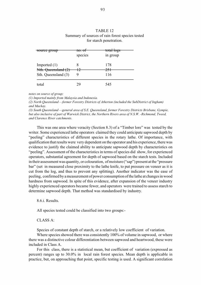
93

TABLE 12Summary of sources of rain forest species tested

for starch penetration.

source group no. of total logsspecies in group

Imported (1) 8 178Nth. Queensland (2) 12 251Sth. Queensland (3) 9 116

total 29 545

notes on source of group;(1) Imported mainly from Malaysia and Indonesia.(2) North Queensland —former Forestry Districts of Atherton (included the SubDistrict of Ingham)and Mackay.(3) South Queensland —general area of S.E. Queensland, former Forestry Districts Brisbane, Gympie,but also inclusive of part of Warwick District, the Northern Rivers area of N.S.W. -Richmond, Tweed,and Clarence River catchments.

This was one area where veracity (Section 8.3) of a “Timber lore” was tested by thewriter. Some experienced lathe operators claimed they could anticipate sapwood depth by“peeling” characteristics of different species in the rotary lathe. Of importance, withqualification that results were very dependent on the operator and his experience, there wasevidence to justify the claimed ability to anticipate sapwood depth by characteristics on“peeling”. Assessment of the characteristics in terms of species did show, for experiencedoperators, substantial agreement for depth of sapwood based on the starch tests. Includedin their assessment was quantity, or colouration, of moisture (“sap”) present at the “pressurebar” (set in measured close proximity to the lathe knife, to put pressure on veneer as it iscut from the log, and thus to prevent any splitting). Another indicator was the ease ofpeeling, confirmed by a measurement of power consumption of the lathe at changes in woodhardness from sapwood. In spite of this evidence, after expansion of the veneer industryhighly experienced operators became fewer, and operators were trained to assess starch todetermine sapwood depth. That method was standardised by industry.

8.6.i. Results.

All species tested could be classified into two groups:-

CLASS A:

Species of constant depth of starch, or a relatively low coefficient of variation.Where species showed there was consistently 100% of volume in sapwood, or where

there was a distinctive colour differentiation between sapwood and heartwood, these wereincluded in Class A.

For this class, there is a statistical mean, but coefficient of variation (expressed aspercent) ranges up to 30.0% in local rain forest species. Mean depth is applicable inpractice, but, on approaching that point, specific testing is used. A significant correlation

94

was determined between sapwood volume, the mean radial depth of starch and log girth.This was:-

S% = (3948 x/G) . (0.318 - x/G) (8.1)

where S% = per cent starch positive volume of total log volume.x = mean radial starch depth. G = centre girth.

note; original equation was developed in imperial units, viz. inches and superficial feethoppus (log volume).

Conversion Factors: 1 super foot hoppus = 0.003 m3; 1 inch = 25.4 mm.

CLASS B:

Where there was non-uniformity in starch depth, or marked variation in the sapwoodrange, and also non-significant colour differentiation, species were graded Class B. Inthese, entire production is treated.

Examination of Graph 7 shows, for certain species, there are non-symmetricaldistribution curves of starch depth. which did not occur with imported species. For northernsilky oak, Cardwellia sublimisthis may be related to site, or origin. Similarly yellow carabeen, Sloanea woollsii, shows atypical peak at 167mm, but with a second peak (of total sapwood) at 320mm.

Results show no significant correlation between families or species and SouthLatitude. Imported species generally have lower starch depths and higher girth classes.North Queensland species do not vary significantly from South Queensland material exceptin that the percentage of total starch positive sapwood depth is higher (but not significantlyso) in the former. The writer concluded that soil, climate eg. rainfall, or ecological factors,override any latitude effect.

These relationships, and class groupings, were applied over a large range of bothplymills and sawmills and were found satisfactory. They enabled accurate estimation ofpreservative treatment plant capacity required.

8.7. Significance of “Outer Heartwood” and “Transition Wood” in angiosperms.

Author’s notes:

a. references to “transition” and “intermediate” woods are made relative to rainforestspecies. Though included with “outer heartwood”, the writer found in his extended researchinto these phenomena, the first two are, in fact, synonomous to both of what Rudman [1959]terms “inner sapwood” and “outer heartwood”.

b. Subsequent to introduction of “Immunisation” (anti-Lyctus treatments), sapwoodwas utilised. No problems for these inner zones were found when using simple boron salts,especially with heat systems. Sodium fluoride (Chapter 10) was not used for sawn timbertreatments and hence its penetration into this “outer heartwood” zone (see below) was notknown on a commercial scale.

In 1957, the first commercial vacuum pressure cylinder, for pole treatments, wasestablished at Grafton N.S.W. Creosote oil was the preservative to treat principallyeucalypts, such as spotted gum, Sapwood was visually assessed to recorded measurements

95

not exceeding accuracy of 2-3mm. The position developed where a narrow pale band ofirregular contour, averaging 4-6mm in radial depth, and externally adjacent to the visualheartwood, was not penetrated by the creosote. As all pale areas in “outer” zones of poleswere visually classified as “Sapwood”, and as no separate confirmatory tests, such as starch,were used for purposes of pre-treatment assessment by the treater, or an inspector, of

Plant investigations, and increased treatment schedules, were ineffective. Viability, interms of economics and hardwood pole utilisation, was under threat, and the problem wasreferred to the Division of Forest Products, CSIRO, for investigation and recommendations.

Rudman (1959) determined three specific zones viz:-(1) Outer Sapwood (2) Inner Sapwood(3) Outer Heartwood

Of these three, zones (1) and (2) were penetrable and also typically starch positive. Thethird zone classified as “Outer Heartwood” was physiologically assessed as being charac-teristically heartwood, but where the normal dark colouration had not occurred. It wasfound to be more durable (Rudman, 1959) than normal sapwood and sufficiently close tonormal heartwood to be classified as that zone. Further studies showed “outer heartwood”to be detectable by use of dimethyl yellow pH indicator (Bamber, 1964). If, as wassubsequently adopted, the wood pole was tested prior to treatment, the indicator changedat the “outer heartwood” boundary to an orange-red colouration as compared to the“sapwood” zones which turned yellow.

Subsequent to Rudman’s findings, the author studied the distribution and identifica-tion of “Outer Heartwood” in a range of eucalypts and other timbers. Study was extendedto include a large number of rainforest species, and the writer established:-

(1) It occurs in all eucalypts from Queensland and from Northern New South Walesareas, including large, mature logs, and with an average radial depth of 5-10mm.

(2) It is distinguishable by use of a portable U.V.lamp (peak 360nm) and, as dimethylyellow indicator increases fluorescence, a line of demarcation is definite, but is irregular.

(3) It occurs in wet sclerophylls and some rain forest species. In some species, typifiedby rose mahogany, Dysoxylum fraseranum, its radial depth may increase to 10-15mm.

(4) In rainforest timbers (cf. author’s note above), a zone described by the industryas a “Transition, or Intermediate Wood”, was proven equivalent to what Rudman differen-tiated into the two zones below, and separate to, the “Outer Sapwood”. Importantly,“Transition Wood” in rainforest species, is NOT detectable by pH indicators, andultraviolet effectiveness is variable with species and sample. In most rainforest species,trace starch concentrations have been found in these inner zones.

8.7.i. Penetration of “Outer Heartwood” and “Transition Wood” by Preservatives andLiquids.

In all species, the author has found these zones to be penetrated by simple salt typeformulation such as boron salts using open tank processes, especially by the hot and coldprocess, but were usually penetrated only by the arsenic component of copper-chrome-arsenic (CCA) salts. Specifically, the copper component appeared to be precipitated in thevessels at an “inner sapwood” boundary with the “outer heartwood”, effects similar to those

96

given by resin acids in heartwood, or wound (and pruning) tissues of softwoods such as

The “Outer Heartwood, or Transition” zones are readily penetrated by polar solventssuch as water and ethanol, by benzol, mineral turpentine, white spirits. Indicator, or dye,solutions in ethanol are readily impregnated into these zones. Pentachlorophenol in lightorganic solvents, such as solvent naphtha, will penetrate, but if in heavy solvents such asdistillate, no penetration is obtained. Evidence indicated chlorinated hydrocarbon emul-sions do partially penetrate the “outer heartwood”.

The general evidence over a wide range of studies and species, and which had includedlaboratory research and commercial applications, led the writer to conclude “penetrability”of these zones was a function of solvent, and characteristics associated with chemical“reactivity” (Section 8.xii) of either the solute, or component of such as creosote mixtures.For liquids, the viscosity and the ease of wetting were factors.

8.8. Variability of liquid and preservative penetration within species and groups.

Variability is a consistent problem encountered in all of the applications of timber. Ifit occurs in research on physical properties, adequate sampling will enable a valid mean ofthe property to be determined. However in industrial application of preservation, it cannotbe dealt with on a similar basis to the physical properties. When variability was found, afterstatistical sampling of a minimum of three charges (Chapters 3, 10), the writer amendedschedule grouping of material from the source. In consequence, many plants in reasonablegeographic proximity, frequently treated the same species by schedules differing from eachother.

8.8.i. Source effects.

In Chapter 3, the writer indicated variability of species occurred as a function ofsource. He cited examples, described the research into quantification of these differences,and stated extended discussions would take place in this Chapter on sapwood. Thesedifferences from source effects caused major changes (Chapter 3) in preservative practices.If undetected, they resulted in large variations of uptake (for both water and salt) within atreatment charge. However, when the original planning was proceeding for establishmentof preservation as an industry, studies of these variations were not considered by someresearch groups to be warranted.

8.8.ii. Physical and Chemical properties of timbers.

In later parts of this Chapter, the writer discusses the importance of factors he foundaffecting the penetration of waterborne preservatives, and they include physical as well aschemical properties of timbers. In so doing, he introduces some reasons for consideringresearch into physical properties, such as density, as significant. He relates this (Chapters12, 13, 14) to the paradigm of interlocked parameters of air content, moisture content, anddensity, which were related to structural properties for treatment classifications, and a needto allow for, and to train a plant operator in, variations caused by those changes in timberproperties.

Detailed study, including microscopic, showed while the anatomical arrangements(and thus species identification) remained similar, differences in vessel mean diameters,

97

and frequency (typically count/ 20 mm2), and jointly defined by the writer as “Porosity”(Chapter 12), values of distribution of maximum, and minimum values about a mean weresignificantly different. Anatomical variations in vessel, tracheid, and fibre, diameters aredocumented in literature on wood structure and terms, such as “thick walled”, areillustrative of this.

Differences in physicochemical data were also factors. The research led the writer todefine a term “Reactivity” (Section 8.xii). He also describes evidence suggesting that the“Reactivity” of a timber is significant in preservative penetration and “fixation”, the latterbeing examined in Chapter 12 in terms of wood structure and leachability of water-bornemultisalt preservatives.

8.8.ii.i. In discussion of softwoods examples of (Section 8.5.ii.iii) the variation werecited relative to physical properties, and their reactions to preservative treatment were alongsimilar lines. However, for the important influence of this factor on treatment of hardwoods,the writer feels it is advantageous to quote several specific examples of variability.

8.8.ii.i.i. The tulip oaks, Argyrodendron spp. (refer Reactivity [Section 8.xii],Wettability [Appendix 15]).

a. only red tulip oak, Argyrodendron peralatum, has a very distinctive colour

b. The other three species, including Mackay tulip oak, Argyrodendron actinophylliumsubsp. diversifolium, are extremely variable, and have no reliable differentiation in colourfor sapwood, are variable to treatment by CCA components (cf. Table 89, Chapter 15). Theycontain up to 100% of log volume in starch positive timber. A zone (see Section 8.7“transition wood”), typically 100-150mm in radial depth, is present between the micro-scopically classified heartwood, and the outer 50mm of “normal sapwood”, and is termed“Intermediate Wood” by industry. It contains starch and is treatable by boron salts. It wasdesirable to discourage use by industry of the term, “Intermediate Wood”, due to possibleconfusion with both the “Inner Sapwood” and the “Outer Heartwood” zones, but large partsof industry continued to do so.

Mackay tulip oak is distinctly different in properties, and seasoning characteristics,from the other tulip oaks, and is intermediate between the red tulip oak and blush tulip oak.It is denser, is significantly more refractory to treatment, approaching Group 3 (Chapter 12)in its treatability classification, and differs in stability characteristics, to blush tulip oak andred tulip oak. Site variations are important.

Material from the Eungella Range exhibits characteristics of the Mackay tulip oak. Alater botanical study had confirmed it as a separate sub-species. However material onforward slopes of the Clarke Range, near Proserpine, is similar to normal blush tulip oak.Separation of the latter type from Mackay tulip oak appears as broadly on a lineperpendicular to the axis of the range, running near Cathu to the coast, and about midwaybetween Mackay and Proserpine.

Brown tulip oak, Argyrodendron trifiolatum, exhibits large site differences. Materialfrom Wengenville, near Yarraman, just north east of the Bunya Mountains, has densitydifferences of up to 25% over other sources of the species, except for two sites located inthe Kyogle and Alstonville areas, Northern Rivers, N.S.W. Material from sources closer toBrisbane does not exhibit extreme broad ranges described. All of the tulip oaks exhibit

98

variable degrees of problems in wettability with aqueous solutions, but minimally by

8.8.ii.i.ii. Spotted gum, E. maculata, and E. citriodora.

Similar variabilitites may be described for spotted gum, E.maculata, and E. citriodora,but over a wider range due to the distribution in terms of climate and sites. A possiblehybridisation (E. maculata with E.citriodora), appeared to occur in forests located in theDawson and Burnett river system basins. One large variation is in the Gatton area, closelyfollowed by timber from the general area centred on Allies Creek, near Mundubbera, to aline approximately to Theodore. It applies to the general central western areas to Emerald.Very high quality stands are found at Arcadia, north west of Injune, near Roma, and overto Wandoan. Vessel diameters and wettability vary in wide ranges.

As E. maculata moves to coastal areas, it shows a large increase in wettability and easein treatability. In most coastal sites, physical properties such as hardness and densitychange, typically as a reduction, but there are marked increases in sapwood depth. It wasthe writer’s experience the changes, and ease of treatment, were more significant for coastalsources in the Northern Rivers areas in New South Wales, and in Southern Queensland.

8.ix. Basic Factors in Application of Waterborne Salt Preservatives for, and theirPenetration into, Timber.

As the writer classified his extensive research data and co-ordinated significant factorsin preservation, he found treatment processes, collectively and separately, showeddependence on timber properties. Provided certain minimum requirements of a process,such as temperature, were present, or while there may be some differences in a sequentialrating for importance of factors (dependent on process), more significant changes intreatment results were caused by timber properties than were caused by the process. Thisis demonstrated in further discussion and illustrates the importance of adequate identifica-tion of sapwood in preservation and in timber utilisation.

Thus, though certain topics are expanded in later chapters, for example, wood densityand moisture contents suitable for treatments are examined in Chapters 12, 13 and 14, it isappropriate the format, the philosophies and principles (Flow Chart 1, Chapter 12) by whichresearch, eg. Section 8.ix.b., was co-ordinated, are discussed, and interrelated, as indicatedin this Chapter.

In Chapter 1, the writer has indicated a need for wider expansion of the preservationindustry and pointed out initial existing practices were not fully effective (Flow Chart 2,Chapter 12) in establishment of preservation on a more flexible, and widely dispersed,scale. For all open tank processes (Appendix 14), the basic assumption was that the timberundergoing treatment must be “green”, and thus above fibre saturation point (FSP) inmoisture content, That requirement for treatment of “green” timber played a large role innon-expansion of the preservation industry. To maintain timber in a “green” state presenteddegrade, and climatic, problems. Only primary processors, that is relatively large sawmillersand plymillers, could operate under that requirement. A steam boiler with reserve capacitywas considered necessary. Generally, secondary processors could not do so. All processeswere considered primarily dependent on “diffusion”. Cummins (1939), Gregory (1942),and later Brimblecombe and Cook (1945) recognised the possible need to vary schedulesin terms of species, or thickness, but all of those workers advocated high moisture contentsabove FSP as being necessary. assumed FSP of 25% m.c.).

99

“general schedule” (25mm thickness) was developed, using brown tulip oak, A. trifoliolatum,as test species and was also based on “green” timber (viz. above an

Bryan, (1946) and (Young, 1946c) each reported a “partial vacuum” may occur(Chapter 12) during cooling cycles of hot and cold treatments. However both writersstressed a need for timber moisture contents to be in the “green” state when water-bornepreservatives were used. This writer found a conflict between the requirements for “green”timber and those workers not recognising that a partial vacuum is based on de-aeration andshould be related (Chapter 12) to the “Void Volume”. Thus, for the “partial vacuum” tooccur, the “green” state must differ from the “saturation moisture content” (Chapter 7), andhence a certain minimum of air content is present, which implies reduced moisture contentshould increase “vacuum effects”. The discrepancy was one reason why this authorextensively researched (Chapters 12, 13, 14), the air content, moisture content, wooddensity in timbers, and, importantly, the distribution of the air and moisture as functions ofstructure between softwoods and hardwoods, and conditions for effective preservation.

Preservation processes are summarised in Appendix 14.

To accelerate preservation on effective principles, three urgent priorities (Chapter 1)may be restated as;

8.ix.a. research into timbers with the aim of determining significant propertiesenabling the effective (including methods suitable for field applications) identification ofsapwoods, their “permeability”, their “penetrability”, and the criteria, including density, airand moisture contents, affecting preservative treatments.

The need was, having examined and validated (Chapter 4) starch presence as aprincipal index to sapwood, having examined species variability, including (Chapter 3)distribution, to extend areas of research into priority 8.ix. b.(below), i.e. to the preservationprocesses, and to ascertain separate investigational priorities in that phase. To nominate the

8.ix.b. identification of significant factors in, and the fundamental principles applyingto, preservation.

Due to social conditions and economics, emphasis was initially on thermal processes(Appendix 14), but there was a priority to examine (Cokley, 1948a,b, 1950a, 1965b) rangesin moisture contents suitable for treatment by all processes, including those at ambienttemperatures, a relationship inextricably related to topic 8.ix.a. With adoption of vacuum/pressure systems, similar needs arose. Research on one aspect applied to the other.

8.ix.c. carry out research into alternative preservatives and so eliminate restrictions(Chapter 10) posed by boric acid and sodium fluoride on plant construction and in the useof fungicides. These restrictions are not further examined here, other than in discussions on“reactivity”.

Author’s note; The factor of “wettability” (Appendix 15) is shown as being importantin all treatments. One very prominent reason for research into, and adoption of, the sodiumborate family, and study of their effectiveness in treatments as a function of solution pH,related to this phenomenon. Borax, using especially thermal processes, markedly reducedthat problem.

8.x. Significant Factors in Preservation Practices.

Success here was directly dependent on establishment of a series of separate, but inter-

100

related, priorities. As evidence (Table 10) demonstrated that presence of starch was not theonly factor in penetration of water-borne salts, successful extension and operation of timberpreservation required a further test for sapwood which necessarily must be supplementaryto a starch test. Progress was subject to development of at least one test, based on physicalmeans, to prove a timber sample under study was sapwood. The author, by usingChattaway’s definition (other than that of “living cells”) of sapwood, nominating“permeability” (Section 8.2.A.ii.) as a property, made judgements on both grounds, namelystarch, and “permeability” of a sample to principally liquids (solvents), but also on“penetrability” (Section 8.x.i.) for solutions. Small block tests, effectively eliminatingother treatment factors, were used when other test evidence was inconclusive. Studies on“included heartwood” in yellow walnut, Beilschmiedia bancroftii, used small blocks inresearch.

Experimental evidence confirmed that if a timber zone was not penetrable by a hot andcold treatment using borax, supplementary laboratory small block studies confirmed it asbeing effectively “nonpenetrable” by aqueous solutions and solutes.

Variations, using water and salt solutions, were found for water, and salt, absorptionsbetween heartwood and sapwood. They showed need for clarity in differentiation oftechniques to measure variable distribution of, and in the terminology [Sections 8.1.ii (g),8.2.i, and Chapter 12] relating to, gases, liquids and solutes, particularly in use of the terms“permeability” and “penetratibility”.

8.x.i. The terms “permeability” and “penetrability”, both of which separately refer tomovement of a gas, a liquid, a solution and solute, applied to preservation processes forhardwoods, required more specific definitions than given in literature [cf. Sections 8.1.ii(g), 8.2.A.ii.]. They are suitably defined, and differentiated, as below;

“Permeability” is the “movement of a gas, or a liquid, through wood such that accessis to all tissues, and this access is not restricted to specific sites or pathways”. Movementmay be inclusive of through what is defined by the writer (Chapter 12) as, “EffectiveOrifices”, which, in this context may be described as “microducts”.

“Penetrability” is “access, generally by liquids, such as solutions, which is byrestricted movement “routes”, and which is dependent on possible reactions with woodconstituents, or on physical factors, eg. semi-permeable membranes”. The “routes” (cf.“pathways”, next below) may be described as “macroducts” compared to the “effectiveorifices”, or “microducts”.

The writer utilised a further term “pathway” to indicate that “routes” for the movement(Section 12.4, Chapter 12) by “permeation” of gases, or solvents, (cf. general use of term“pathway”, Chapter 14) may differ from those for “penetration” by solutions and solutes.This variation in “pathways” may be associated with (mainly) structural differencesbetween softwoods and hardwoods.

By this definition, solutes in a solution, or liquids of high viscosities, depend on“penetration pathways” (which include access by solutions, through normal pits, intosoftwood tracheids) into specimens, and may also be restricted (Chapter 12) to specific“sites of deposition” in the timber. The sites may also vary between softwoods andhardwoods.

101

Extensive literature (Preston, 1959), on penetration of preservatives in, especially,softwoods, and (Skene, 1965) later data for hardwoods (cf. Chapter 12) confirmed (forsapwood) that;

a. for gymnosperms, penetration, dependent on the pit openings, occurs in all tracheidsand rays.

b. for angiosperms, water penetration (from the solution) is possible into all tissues.

These support the conclusions (Chapter 12) that access of the solute is essentially (cf.“pathways”) restricted to vessel lumina, and ray tissue. This implies (Chapter 12) that thereis solvent access into fibres (and cell walls) by diffusion (“permeation”), and solutionlongitudinal movement from one vessel is dependent on the perforation plates for progressto a second vessel, and on pits for access to the rays. Typical published general dimensionsfor wood tissues are given in Table 13. In the hardwoods, capillary flow of liquid throughvessels, and rays, is subsequently described (Chapter 12) as a factor in an initial waterabsorption when the timber is treated below fibre saturation point at ambient conditions.Water then permeates through all tissues. Salt diffusion can take place (Section 8.x.iii.)through vessel and ray cavities when the state of “free moisture” is attained.

8.x.i.i. Many studies in timber, eg. the “void volume”, equivalent “moisture content”at measured “void volume”, or change from “saturation moisture content”, appeared toplace more emphasis on flow mechanisms of gases and liquids (cited in this work asparticularly solvents, eg. water) under a pressure differential, and base the flow calculationson such as Poiseuille’s equation (Chapters 12, 14). Those conditions apply principally toa “duct”, and for this purpose, to the cell cavity, or pit orifice.

The writer associates the term -”Permeability”- with the movement of gases andliquids (solvents) into all tissues, including cell walls. For liquids, it depends on propertiessuch as “ease of wetting”, polarity, and viscosity. As examined (Section 14.4.3.i.ii.a.ii, andsub-sections, Chapter 14), the writer defines total air as “Contained Air”, with three sub-divisions including the “embedded air” and “dissolved air”.

The significance of these premises lies in the means by which the air moves into, orout of, the cell walls, or is displaced by water. As water displaces the air, swelling of aspecimen takes place from below, up to, but not above, FSP. The writer suggests the term“embedded” may be also applied to the possible distribution of water within cell walls, suchthat not all of that water exists as “combined or bound”, and some may only be physically“embedded” within interstices of the wall matrix. Deduced relative levels of significanceof structural elements (Stamm, 1964) in diffusion, and possible paths for drying at varyingswollen specific gravities, are given (Table 14). Seasoning is a movement of both liquid,and vapour, phases of water from wood, but similar ratios may occur for penetration(“permeation”) of water from a solution into tissues.

As stated below, water permeates heartwood in both liquid and vapour phases, but atmuch slower rates relative to sapwood. Some mobile salts (eg. sodium chloride) can alsopenetrate parts of that zone (cf. sites of distribution, Chapter 12) at very slow rates, at lowconcentrations, and must not be “reactive” (Section 8.xii) with wood contents. Resistanceto, or the absence of, solution (or solute) “penetration” through a specimen is a guide todifferences between sapwood to heartwood.

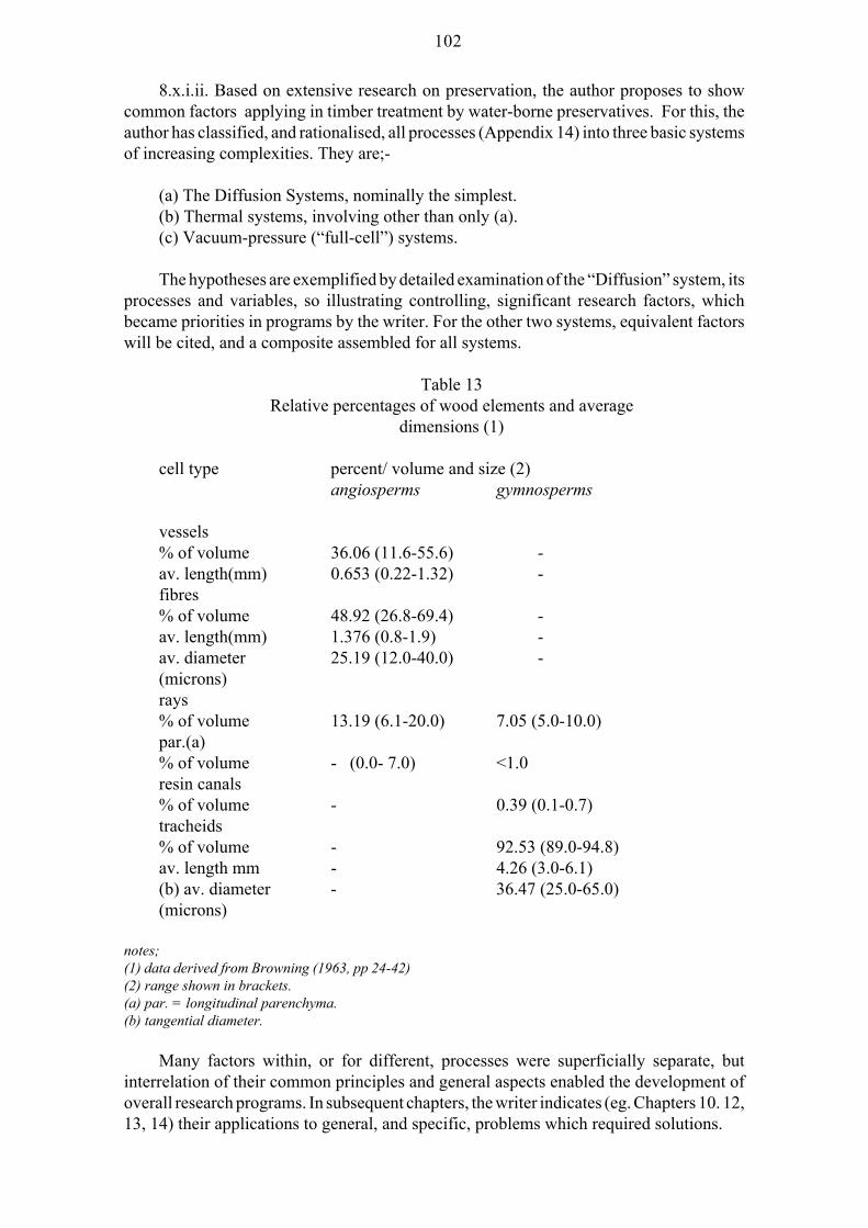
102

8.x.i.ii. Based on extensive research on preservation, the author proposes to showcommon factors applying in timber treatment by water-borne preservatives. For this, theauthor has classified, and rationalised, all processes (Appendix 14) into three basic systemsof increasing complexities. They are;-

(a) The Diffusion Systems, nominally the simplest.(b) Thermal systems, involving other than only (a).(c) Vacuum-pressure (“full-cell”) systems.

The hypotheses are exemplified by detailed examination of the “Diffusion” system, itsprocesses and variables, so illustrating controlling, significant research factors, whichbecame priorities in programs by the writer. For the other two systems, equivalent factorswill be cited, and a composite assembled for all systems.

Table 13Relative percentages of wood elements and average

dimensions (1)

cell type percent/ volume and size (2)angiosperms gymnosperms

vessels% of volume 36.06 (11.6-55.6) -av. length(mm) 0.653 (0.22-1.32) -fibres% of volume 48.92 (26.8-69.4) -av. length(mm) 1.376 (0.8-1.9) -av. diameter 25.19 (12.0-40.0) -(microns)rays% of volume 13.19 (6.1-20.0) 7.05 (5.0-10.0)par.(a)% of volume - (0.0- 7.0) <1.0resin canals% of volume - 0.39 (0.1-0.7)tracheids% of volume - 92.53 (89.0-94.8)av. length mm - 4.26 (3.0-6.1)(b) av. diameter - 36.47 (25.0-65.0)(microns)

notes;(1) data derived from Browning (1963, pp 24-42) (2) range shown in brackets.(a) par. = longitudinal parenchyma.(b) tangential diameter.

Many factors within, or for different, processes were superficially separate, butinterrelation of their common principles and general aspects enabled the development ofoverall research programs. In subsequent chapters, the writer indicates (eg. Chapters 10. 12,13, 14) their applications to general, and specific, problems which required solutions.

103

8.x.a. Diffusion. “Diffusion” is seemingly the most basic process system, butexamination shows presence of factors, additional to the system, and it is used as thedetailed example in this analysis.

8.x.a.i. While theories on diffusion are well documented, it is preferable to restatesome aspects most applicable to the preservation of timber. Theoretically, diffusion ismovement of a soluble ion, or solute, from a zone of high concentration to one of lowerconcentration. For these discussions, a “solute” refers to dissociated ions as well asdissolved salts, and that concentration is dependent not only on degree of dissociation insolvent (water), but also (cf. “Reactivity”, Section 8.xii) on its state in the wood matrix.Common in diffusion processes, for salt mixtures, and for differing ionic mobilities, as wellas being dependent on the degree of dissociation, the term “solute” applies to each ioniccomponent. Similarly though the water phase (termed “sap”) in especially sapwood doescontain dissolved compounds, including nutrients, in these discussions it is assumed to be“water”.

Author’s note; Due to problems in treatment of some products, or species, (hazardsadditional to Lyctus with emphasis on termites were present, or when leaching was a factor),the author initiated studies into emulsion-based preservatives, but found only two (aldrinand dieldrin) emulsions were sufficiently stable. Particle size uniformity and the lack ofsignificant interparticle charge were such that aggregation, and/or precipitation, did notoccur. Other emulsions tested were unstable and ineffective. For this topic, significance liesin the writer’s findings that, due to their stability, both products performed similarly to asolute in a solution, and were used in research and industry applications.

8.x.a.ii. Rate of diffusion is dependent on concentration and mobility of a solute, usingthe latter in the general context as defined above. At any point, a concentration gradientexists. Put alternatively, for effective solute diffusion, a “concentration differential” exists,which is redefined as a “(solute) diffusion differential”. That redefinition stresses it is notonly a function of solute concentration differences to a treating solution, but depends ongradient levels of solutes between surface (or external solution) concentration and depth inwood.

Table 14Relative percentage of diffusion through each of threepossible paths in drying of wood at varying swollen

volume specific gravity at 50 o C. (1)

swollen per cent diffusion occurring through;volume fibre cavity fibre cavity cellspecific /cell wall / pit (b) wallgravity. (a) combination (c)

0.2 95 4.2 0.80.4 86 10.1 3.90.8 55 22.2 22.8

(a),(b),(c) termed respectively Type I, Type 2, Type 3.(1) Initial reference (Stamm, 1964, pp.438-439) also applies to later discussion.

104

When the “diffusion differential”, and solute mobility, are high, the correspondingdiffusion rates increase. Thus, in diffusion, the aim was a high concentration of one, or more,highly mobile solutes. That was achieved by either an increase of temperature, or the useof a high concentration “mixed formulation” of mobile salts for treatment.

8.x.a.iii. Solute movement through a membrane to a volume of the same solvent (lowerin solute concentration), is dependent on whether the membrane is “permeable”, or is “semi-permeable”. Wood tissue walls are considered to be “semi-permeable” membranes only.

For the angiosperms, water migrates (“permeates”) through all tissues, including bythe “microducts”, but solutes have access (Chapter 12) only through “macroduct” systems,specifically only by vessel lumina and radial tissues. Diffusion proceeds by solute movingthrough a free liquid phase in these tissues, which, especially for vessels, means, as theprogressive solute concentration gradients (and diffusion differentials) fall, rates of solutediffusion decrease. Due to the change in free moisture caused by gradients (Chapter 7), thisresults in the decrease of effective preservative concentration levels with increase in depthin a section.

Continuous free water is necessary for diffusion. If the pathway, eg. vessel lumen, isnot in a moisture content state of containing free water, the author found an initial liquiduptake occurred and this was shown to be (Chapter 12) due to a capillary flow. Threeimportant aspects related to moisture content and diffusion arose from his findings, namely;

8.x.a.iii.a. For free moisture to be present in a vessel lumen, material must, bydefinition (cf. Chapter 7), be above fibre saturation point, FSP. In this condition, freemoisture must be present in the fibres. Thus, above FSP, but below “Saturation Moisture”values (Chapters 7, 12), water flow, and diffusion (“permeation”), must take place fromfibres to vessels (and rays). Conversely, for lower wood moisture contents at, or below,FSP, when the vessels contain penetrated liquid (water or solution) by capillary flow (forother processes, impregnation under either thermal, or applied, pressures) an increase in the“cross-sectional moisture content”, which was found, and demonstrated, must be associ-ated with water movement from vessels (and rays) through walls, and flow through pits tofibres, including the interfibre walls. It is in this area, the writer considers data in Table 14applicable. It was concluded progressive changes in preservative concentrations with depthof section, may be functions of the rates of water flow through pits and of diffusion(“permeation”) rates of water through cell walls.

8.x.a.iii.b. As the sapwood vessel lumina are relatively unobstructed, and do not havesignificant incrustations on the walls, this flow rate (Section 8.x.a.iii.a.) is one importantdifference to heartwood. The vessel lumen, or ray, may be artificially obstructed by theprecipitation of a solute, or if the solute is complexed on a vessel (or ray) wall.

8.x.a.iii.c. For most research projects, and industrial applications, cross-sectional,moisture content values of a specimen are used. This masks effects of the moisture gradient(Chapter 7), where, for a cross-sectional value at, or below, FSP, outer, and end, zones aregenerally lower in moisture content, and can fall significantly below FSP, at which pointdiffusion should not occur, but capillary flow mechanisms are involved in liquid uptake.At greater depths in a section, exemplified by a 25mm thickness board, internal moisturesare higher and can approach, or exceed, FSP. For these higher zones, rate of water uptakedoes decrease, but the effective solute concentrations correspondingly, and, progressively,

105

also decrease. Equivalent diffusion rates fall with thickness, so causing high salt gradientsfrom the outer layers to the inner.

8.x.a.iv. A Diffusion differential is significantly increased by not only soluteconcentration, but by temperature increase, and these function in two ways. The first allowsincrease in diffusion, but the second (temperature) influences rates of diffusion throughwood, so increasing effective gradients and decreasing process time. These applications of“diffusion differential” and “thermal diffusion” are in agreement with thermodynamicprinciples discussed by De Groot (1963). Gregory (1942), Brimblecombe and Cook (1945)emphasised these factors in sawn timbers, recognising effects on species. Elevatedtemperatures are used in some “Dip Diffusions”, with especially a “Hot Maintenance” or“Hot Immersion” system. The former applies to sawn timber. The latter refers to veneertreatment, and was supplanted by the “Momentary Dip” (Plates 1, 2). Additional factors areinvolved in the diffusion of wood preservatives into timber, namely;

i. ease of wetting by the solution (Appendix 15).

iii. permeability, and penetrability, of the timber.iv. reactions between preservative and wood elements, and are examined (Section

8.xii.) under “Reactivity”.

8.x.a.v. Commercially two forms of diffusion apply to timber treatment. Processdetails are nominated by the form in which diffusion takes place, and are;

8.x.a.v.a. Total immersion in treatment solution.

8.x.a.v.a.i. treatment at ambient temperature, termed the “Cold Soak” (Cokley, 1949).

It had been thought necessary for timber to be at high moisture contents (over FSP),Studies (Cokley, 1948a) confirmed that requirement was not critical. Subject to ease ofwetting by the solution, the author (cf. Section 8.x.a.iii., and Chapter 12) determinedmechanisms were;

i. for timbers significantly above FSP, with adequate free water liquid phase in thevessel, normal diffusion takes place.

ii. for material at, or below, fibre saturation point, an initial “capillary flow” of liquidoccurs, such that free water is then present. Subsequently the solute(s) does diffuse.Adequate sapwood preservative retentions were obtained for especially simple, mobilesalts, a result confirmed over a wide range of species, thicknesses, and treatment operationson a commercial basis.

8.x.a.v.a.ii. Total immersion in heated solution, usually at, or near, boiling point. Thissystem is termed “Hot Immersion” or “Hot Maintenance” treatment.

For types (a.i, a.ii), penetration is complete at the end of an immersion cycle. In these,group schedules based on (Chapter 12) the macro structural properties of species, anddimensions, are used.

8.x.a.v.b. “Dip Diffusion” treatment at, or near, ambient temperature, is exemplifiedby “Momentary Dip” or “Spray” for veneers.

Tables 15, 16, show typical local results for “Momentary Dip” for veneer operations.

106

In Papua New Guinea (Levy et al, 1972), dip diffusion of sawn timbers operates atambient temperatures and uses patented formulations (Johanson, 1974).

8.x.a.v.b.i “Dip Diffusion” at elevated temperatures, using a high level of solutionconcentration is widely used, and employs mixed boron salts (“Timbor”, Tables 17, 18)for timber treatments in New Zealand.

Differences in treatment practices between Papua New Guinea and New Zealand are;i. Papua New Guinea treats using a patented multisalt preservative, with a “general

schedule” for all timbers, with no segregation of, particularly rainforest, species in termsof the sapwood, but specifications, (Levy et al., 1972) require a nominated preservativepenetration in both the sapwood and heartwood zones. Results cited by those authors showchanges in formulation components, and variable preservative concentrations, occur withdepth in timber section.

Table 15Variation of salt usage (kg/ 100 m2) of treated

veneer at two veneer mills, and mean plant usage (1)

mill usage standard coefficientkg/100 m2 deviation of variation(1)(2) (3) (3)

1 0.707 0.166 23.42 (x) 1.741 0.380 21.8

mean 1.219(all plants)-

notes;(1) based on actual usage of borax decahydrate.(2) equivalent 1.5mm (1/16 ins.) veneer thickness.(standard production statistical measurement).(x) differences in species density and thickness with a different solution concentration (refer Table 16).Converted to 1.5mm standard as in (2)(3) variation in usage based on the species and thickness, similar in all Queensland veneer plants.

ii. For New Zealand, treating basically one species, namely radiata pine, P.radiata,the requirements are similar to States legislation. Results are consistent. In both types,(8.x.a.v.b and b.i) wood is momentarily immersed in solution, or is sprayed by thepreservative solution, and nominally with surface coverage by solution at the nominatedconcentration to ensure a steep chemical gradient, or “diffusion differential”, exists, andwith sufficient solute to theoretically ensure an adequate preservative penetration ateffective toxic levels. All timber is treated at high moisture contents and diffusion takesplace away from the plant.

The strong interest in the process (or modifications) is shown by the number ofreferences on various aspects of its use. Based on studies with boric acid and sodiumfluoride and using diffusion cells, Christensen (1947) derived a formula applicable totimbers. Harrow (1951, 1952), Tamblyn (1956, 1958), Levy et al. (1972), reported onvarying topics.

107

Table 16Typical industry results in the Momentary Dip treatment of Queensland veneers.

species solution analysis (1)conc. (1) core(*)

1.5mm 3mm(2)

Beilschmiedia 2.25 0.45 0.19bancroftiiyellow walnut

mixed species 2.25 0.44 0.17mixed species 3.00 1.18 0.55

notes;(*) Core taken as inner 50% of thickness after surface planing (SAA AS 060-1956). (1) Analyses andsolution concentrations as boric acid equivalent.(2) veneer thickness.

Johanson (1958, 1963, 1974) developed formulae of high (ambient) concentrationmultisalts. The Wood Technology Division of N.S.W. (1956), tested high concentrationsof boron salts by the incorporation of “binding” agents. McQuire and Gaudie (1972) carriedout research on ways of ensuring accelerated solute penetration.

Local studies included Rees (1950), Bardsley (1962), Cokley (1951b, 1957, 1960).Additional research and pilot studies were carried out over a range of preservatives,climates, species, and section thicknesses in sapwood. A commercial treatment plant (sawntimbers) was approved (at Cooroy, north of Brisbane) for mixed species but, for starchpositive sapwood (Chapter 2), variations in the preservative concentrations both forspecies and thickness, required a constant supervision by the author, and laboratory staff.

8.x.a.vi. For the general Diffusion systems, the author concludes basic factorsinvolved are;

a. wettability of the wood by the solution.b. penetrability of the wood substrate, defined as ease of penetration of the solute in

adequate concentrations to give protection against nominated hazards.c. diffusion rate, and diffusion differential, of solute through the timbers pathways, as

well as in solutions.d. solute reactivity and stability (refer Section 8.xii, and Chapter 10).e. wood structure.f. moisture contents at which diffusion takes place.g. thermal effects on diffusion, and which are separately influenced by wood density

and moisture contents (cf. Chapter 13).h. solution concentration, its viscosity and mobility.

8.xi. Application of Factors to other Systems.

For these systems, grouped as below, similar analyses show relevant factors to be;

108

8.xi.i.Thermal Systems (for other than direct diffusion).

For these processes, original requirements for “green” timber, based on “Diffusion”(cf. Section 8.ix) theories, were shown not to be necessary (Chapter 12).

The principal mechanism involved creation of a “partial thermal vacuum” (induced byincrease and decrease in the temperature of the treating system, Chapters 12, 13, 14).Absorption of solution, and the solute, depended on;

a. wettability of the wood.b. thermal “diffusivity” into the timber (Chapter 13), resulting in expansion (Chapter

12) of contained air, and, in a later part of a cycle, with the timber fully immersed undersolution, reversal of the temperature gradient for cooling, and so resulting in the formationof a partial vacuum. In this context, temperature changes produce thermal differentials,

c. de-aeration (Chapters 12, 14) of angiosperms applies not only to vessels and rays,but also requires air removal from fibre lumina and walls. That need applies to heartwoodsections (Section 8.xiii.) present in timber specimens, which occurs at slower rates than insapwood.

d. wood density (Appendix 27) and moisture content, which jointly influence thermalproperties, including thermal “diffusivity” (Chapter 13), and thermal differentials. They,with structure, influence (Chapter 12) absorption into the timber, especially by water andsolutes, and, consequently, the absorption rate.

All other factors, as determined for Diffusion, including “Reactivity”, “penetrationpathways” and the “deposition sites” of a preservative apply equally to these systems.

8.xi.ii. Vacuum Pressure (“full-cell”) systems. Analysis of these show primarydifferentials are the rate and effectiveness of initial de-aeration of the timber (Chapter 14),and, as for thermal processes, they require the de-aeration of all tissues, includingheartwood.

For vacuum/pressure systems (and thermal vacuum systems), resistance to penetra-tion of a preservative solution is caused by compression (Harrow, 1947) of any residual airwhich had not been evacuated. Thus the controlling factor is residual air in the vessels,fibres, and other wood elements. Volume” at moisture content of treatment, is a function of aerodynamics (Chapter 14) oftimber species, and of plants in which treatment takes place. For this system, timber istreated (Appendix 14) as a “bundle” in a “block stack” condition. Uniform de-aeration, andthe complete access by solution, are factors. Block stacking can have a negative effect onwettability.

A theoretical reverse requirement, to that for the Diffusion processes, was emphasisfor the vacuum pressure treatments to be applied to timber (cf. Section 8.xi.i., thermalsystems) with a moisture content below FSP. For local timbers, and climatic conditions(Chapter 14), that need introduced problems requiring further research by the writer.Arising from pre-treatment shrinkage at the lower (< FSP) moisture contents, an initialwater uptake expanded the wood restrained in bundles, and there was compression (bystrappings) of the timber, resulting in increase in resistance to penetration of solution. Thewriter established (Chapters 12, 14) requirements for lower moisture contents (below FSP)

109

was only partially correct for all timbers, and especially for angiosperms.For this system, under Queensland climate, increase in wood surface temperatures (70o

+ C.) above ambient had significant negative effects on “reactivity” (Section 8.xii) ofspecies and mulitsalts, on solution stability and penetration of multisalts. That was onereason for approval of boron salts as preservatives for alternative end-uses when treatmentwas by this process.

Other factors were similar to thermal processes, but with a lower emphasis on wooddensity in terms of commercial treatment schedules (Chapter 14, Appendix 43), but withgreater emphasis on wood structure, particularly porosity measurements of species, andrelated moisture contents.

8.xi.iii. General Factors and Conclusions- all Systems.

Using the above, and related data, the author coordinated factors for all systems. Whenthat was done, specific common major research topics were shown as;

8.xi.iii.i. “Wettability” (Appendix 15), “permeability”, “penetrability” of, and “path-ways” through, wood.

Though of prime importance, “wettability” is a function of species and is laterexamined under “reactivity” (Section 8.xii).

8.xi.iii.ii. Thermodynamics of timbers, processes and plants. Priority was due to

8.xi.iii.iii. wood density, which is discussed with items 8.xi.iii. ii, iv, v, vi.

8.xi.iii.iv. Wood moisture relationships, for a process, applicable to ranges of localconditions and species. They are involved with density in study of “Void Volume” andthermodynamics.

8.xi.iii.v. Wood structure, variabilities present, and classifications into scientificallybased ratings, or formulae (Chapters 12, 13, 14), and which were necessary for effectivetreatment operations.

8.xi.iii.vi. Aerodynamics of timbers and plants.

8.xi.iii.vii. Optimum preservatives for local needs.

Supplementary, essential, needs for research, included effects of variations ofphysicochemical factors within species caused by such as geoclimatic influences, anddevelopment of plant, as well as laboratory, controls for treatment operations (process andsolution) and products. The final priority of factors is related to the process chosen.

In Queensland, these total needs were required to satisfy not only scientific standards,but, additionally, to meet economic, conservation, and legal, requirements. While the workis described by the writer under these separate topics, they were interrelated as researchprograms.

For example, research on a substitution of boric acid by the borax family of salts was

110

integral to geographic expansion of the industry, flexibility in plant designs and treatmenteconomics. Particularly sapstain control, which was essential for utilisation of tropicalspecies, either as a separate operation, or integrated with the preservation treatments, wasdetermined by that change.

8.xii. Timber as a “Reactive” Medium.

As stated (cf. Introduction) timber is a physicochemical matrix, and, with respect tointeraction with chemicals (which applies to gases, liquids, solutions or solutes), should notbe considered as “inert” or “non-reactive”. If that (incorrect) assumption is made, most ofthe principles, and mechanisms, eg. in timber physics, in wood chemistry, or plantphysiology would be ignored. The special case of interactions by water with timbers is anexample. In terms of its preservation by impregnation with solutions, or salts, the writersuggests timber behaves as a “reactive” medium and not simply as an “inert micro/macroduct” system.

“Reactivity” is defined, in this context, as “a chemical, or physicochemical, cause fora timber to reject, to delay movement of, to react with, or to cause separation (cf.“Chromatography”) of, the components of impregnating solutions into the solvent, hereemphasised as water, and a solutemixed, or multisalt, formulation.

Similar to “factors” in penetration, the “reactivity” is heavily influenced by whethera specimen is sapwood or heartwood. Though the latter is more reactive due to contentstypified by the poylphenols, the former has “reactive sites” more readily accessible andavailable on the vessel (or ray) internal wall. As for other parts of this research, sapwoodidentification is important. It is in this definition of “reactivity” that this writer separatesits importance from the terms (Sections 8.x.i, 8.x.i.i.) “permeability” or “penetratibility”,which are frequently interchanged in literature. Evidence (Section 8.xii.iv.) indicates that,in addition, timber may be equated to a “chromatographic column”. This emerges in thisthesis in relation to distribution of preservatives, but inclusion here is justified as it goes along way in explaining why certain preservative formulations do not effectively giveprotection against especially fungal hazards. This topic is divided into three divisions,which are;

8.xii.i. Wettability (cf. Appendix 15).8.xii.ii. and iii. Chemical reactivity.8.xii.iv. Chromatography.For the last two, several examples will be cited in support of the writer’s hypotheses.

8.xii.i. “Wettability”. (cf. Appendix 15).

“Wettability” is both physical and chemical in origin, but, operationally, may bedefined as difficulty by aqueous solutions to “wet”, and to “penetrate”, timber, and is thusclassified as a special form of “reactivity”. The importance of this property rests in the fact,that, irespective of the process used, unless a solution “wets” the wood, no penetration,including solutes, occurs.

This problem was attacked in two ways, and the first, on which further research intothe phenomenon depended, was utilisation (Appendix 15) of a test method to indicate itspresence, with modifications and expansions of the test to enable assessment of the severity

111

of the problem as well as clarifying possible causes. It will be noted (Appendix 15) theexpanded tests include measurement, especially ambient, of temperatures to which a timberis exposed, especially prior to treatment. The second way was by research into conditionswhich could alleviate, or eliminate, the problem, with emphasis on any physical andchemical techniques applicable by industry.

These resulted in;-

8.xii.i.a. The problem was noted in ambient temperature treatments, and, for somespecies, was aggravated by extended block stacking after sawing. Examples includedbrown tulip oak, A. trifoliolatum, spotted gum, E. maculata, slash pine, P. elliottii. Veneerscut from many rainforest species were affected after peeling and then being block stacked.

8.xii.i.b. low surface moisture contents, including the condition (Chapter 7) of“surface inactivation”, or “case hardening”, resulted in poor wettability. The author haddetermined establishment of reverse moisture gradients (Chapter 7) by “reconditioning”would help to alleviate the condition. A presteaming with “wet” steam (with post-steamingstorage to allow for total cooling and increase in surface moisture) was used to obtain asatisfactory multisalt penetration in plywood and sawn slash pine, the latter being from theMaryborough area.

8.xii.i.b.i. Based on the “reconditioning” results, it was possible that a similar, orimproved, effect would be given by a hot and cold treatment. The combination of a heatingcycle, while timber is immersed in a treatment solution, should, with time, increase thewettability of timbers. When this was tested, the improved wettability, and improvedpenetration, confirmed the theory. Solutions of boric acid, and of sodium fluoride, wereused in early studies.

8.xii.i.c. Based on previous extensive study on effects of pH in application of adhesives(when the plywood industry changed to synthetic resins) the author extended “wettability”research into effects on the condition from change in the solution pH and/or use ofsurfactants. The results confirmed that, as for adhesives, acid solutions such as boric acid,sodium fluoride, or CCA multisalts, were less effective in ameliorating “wetting” problems.As the CCA multisalt solutions were more acid (values of about pH 2.0), their effect wasleast.

Tests on solutions, approximately neutral in pH, such as mixtures of boric acid andborax, were more effective than boric acid, and reduced the problem. This effect was onereason for research (which led to use of borax) by the author into characteristics of thesodium borate family of salts, of boric oxide and boric acid, and mixtures. The full familyof boron compounds used in timber preservation, and pH values of their solutions, areshown (Table 17), with the relative effectiveness of penetration (compared to boric acid)of two of the more commonly used ones shown in Table 18. “Timbor”, which was acommercial mixture used in New Zealand, is included for comparison.

When these findings, especially use of alkaline boron salts, were combined with useof surfactants, they reduced problems of “wettability” to nonsignificant proportions for alltreatments at ambient temperatures (Appendix 14), which included vacuum pressureprocesses. As indicated, thermal processes with alkaline boron salts removed any problemsin treatment. Preservatives, such as the CCA multisalts, were supplemented in processes atambient conditions, by the addition of low concentrations of non-ionic, non-foaming,

112

surfactants. Satisfactory results were obtained.

8.xii.ii. Chemical Reactivity.

This is illustrated by two examples. Others will emerge in the thesis.

8.xii.ii.i. Performance of Boron Compounds.

The author has indicated a number of reasons for change to borax (Cokley, 1948d).Evidence in justification of that change is discussed in Chapters 10, 12. Consequent to thatdevelopment, it was suggested by some workers that borax, being alkaline, would causean excessive solution of wood extractives resulting in a possible need for early, andfrequent, replacement of treating solution, due to its excessive discolouration.

For all processes, the author proved that concentrations of the extractives reachedequilibrium in the solution, and corresponding discolouration did not exceed values at thatequilibrium point. Importantly the discolouration (multiple species) remained as surfaceonly, except for very thin (< 1 mm) veneers, and over a range of timbers did not exceed about2mm depth.

A sharp change occurred in the pH of samples treated with borax such that there wasa decrease from highly alkaline surface values (> pH 9.0) to one of normal sapwood values(pH 4-6) below the surface. The change occurred over less than the 3mm based on gradientsection (Table 20) thickness, and was typically to 1mm in depth.

Additional confirmatory tests were made, for which the application of solution wasby momentary dip, followed by “block stacking” for periods up to 24 hours. Thicknessesof material from 1mm to 10mm were evaluated.

Penetration was from both faces (tested 25mm from edges to exclude edge effects).Examination showed the affected depth (change in pH) to be a function of the solutionstrength, block stack time, the surface to thickness ratio for thin sections which wereincluded, but depth of discolouration did not typically exceed 0.5 to 1mm. Other aspects areexamined in later topics (Chapters 10, 12), and only the data to illustrate possible

8.xii.ii.i.i. The writer’s early research (Cokley, 1948d) including pilot plant, andcommercial, studies, examined relevant “penetrability” for solutions of borax to boric acid.Representative results (Table 19) are shown.

In these early studies, though subsequently (Chapter 10) all boron compounds wereestimated, and standardised, as the equivalent boric acid, equal concentrations of eachcompound, namely boric acid and borax (Table 19), were used. Change to standardconcentrations (Chapters 10, 12) was made after assessing data from preliminary industryadoption of the research.

If wood was not reactive, and as, in terms of equivalent boric acid, the borax solutionwas only about 60% of the boric acid (theoretical ratio of 1.54, Table 17) then similar lowratios should be found (as equivalent boric acid) in the treated timber, nor should sharpchanges in pH occur, as this implies reaction of timber components with sodium or borate

113

ions.TABLE 17

Compounds of boron used in timber preservation.

Trade or (a) stoichometric eq. mass soln.Common % nomenclature to (1) pHName boric (b) boric

oxide acid.

Boric oxide 100 Boron trioxide 0.563 4-5Boric Acid 56.3 ortho-boric acid 1.000 4-5Borax 36.52 sodium 1:2 borate 1.542 9.2

decahydrateBorax 46.0 sodium 1:2 borate 1.178 9.2pentahydrate pentahydrateBorax 69.2 sodium 1:2 borate 0.814 9.2anhydrous“Polybor” 66.2 sodium 1:4 borate 0.850 8.4(2) (3) tetrahydrate“Timbor” - sodium 1:4 borate 0.599 7.5(2) (3)Sodium (2) 58.98 sodium 1:5 borate 0.955 8.4pentaborate decahydratesodium (4) NaBO3, 4H2O -used as oxidiser.perborate (no equivalent formulation)———————————————————————————

notes;-(1) weight in kg. to give equivalent boric oxide as given by 1 kg. of ortho-boric acid. (2) Trade name.(3) Nominal formulation. Proprietary blend. Timbor used in N.Z. for Dip Diffusion. (a) Nominaltheoretical percentage based on salt manufacturer’s specification. (b) Based on Kemp’s (1956)classification. showing ratio of sodium oxide to boric oxide.(4) oxidising properties used for solutionclarification and special purposes (bleaching) in veneer treatments.

If wood was reactive, changes in ionic concentrations and ratios, as well as theincreased rate of “penetrability” of borax, which may occur, should mean a decrease in thatratio of 1.54:1, when compared to boric acid treaments. Results (Table 19) showedsignificant increase by borax in the equivalent “core” concentration (as boric acid), a resultconfirmed by many years of industry use for all processes, and monitored under the Acts(Chapter 2). The theoretical ratio did not apply, and borax (Table 17) usage ratio to boricacid was shown not to be 1.54, but to be equal to 1.1, and, concurrently, there was a verysignificant increase in relative penetration rate (Table 19) of the borax.

This difference in “core” retention would be explained if, when borax was used aspreservative, the borate ion (expressed as boric oxide) ratio to sodium ion, increased withinthe timber. Based on these theories, the writer, using hot and cold treatments, furtherexamined the separate sodium, and borate, ion penetrations with depth into timbers. Theseinvestigations confirmed earlier data (within constraints of then available techniques, andinstrumentation, for “semimicro” and “micro” analysis) on the significant changes in ionicconcentrations, and showed an increase of boric oxide to sodium ratios. They alsoconfirmed pH changes previously measured, and which occurred at very shallow depthsinto timber. To prove the sharp changes in component ionic ratios and pH were not onlyof thicknesses,

114

function of thermal treatment processes, the initial studies were extended over wide rangessolution concentrations, processes (which included “cold soak” [Appendix 14]), andspecies.

Differences in results to boric acid were in agreement with the writer’s theories andwere attributed to higher degree of dissociation of borax (and homologues), its alkaline pH,increased ionic mobilities, and reactivity with timber.

Similar results were obtained for all members (when in solution, and so independentof water of crystallisation) of the sodium borate series (Tables 17, 18).

TABLE 18Effective order of penetration rate of boron

compounds (1) in Queensland species (2) as afunction of solution pH.

relat. compound solution operatingorder (1) pH (3) pH (4)

1 borax and homologues 9.2 8.5 +sodium 1:2 borate, nH20(n = O, 5, 10) (b)

2 “Polybor” (5) 8.4 7.5-8sodium 1:4 borate, 4H20

3 “Timbor” 7.5 7-7.3sodium 1:4 borate.

4(a) boric acid 4-5 (a) 4-5

notes;-(1) For details of compounds, see Table 17.(2) Similar for imported and interstate species.(3) distilled water solutions.(4) operating values, including wood extractives.(5) used principally in vacuum/ pressure systems.Small significant difference relative to borax.(a) When made alkaline to pH 9.0, using sodium hydroxide or sodium carbonate/ hydroxide mixture,penetration rate is almost equivalent to borax.(b) for n = 0 (anhydrous borax), solubility problems were present, and, except for special studies (as inthis research), it was not widely used in Queensland.

8.xii.ii.i.i. Commercial Application of Borax.

Subsequent (Chapter 10) to initial successful research (Cokley, 1948d), the industrywas advised to adopt use of borax, a recommendation rapidly followed by treaters, or firmsplanning for installation of plants. This enabled significant modifications to the treatmentof timbers.

8.xii.ii.i.ii. Verification of previous research on the distribution of impregnatedsodium and boron in treated timber.

115

TABLE 19Relative penetration (core % on o.d. m/m. basis) in 25mmthick boards treated by equal mass/volume solutions ofboric acid and borax decahydrate. (Note; results citedrepresent extensive studies in research and industry).

Equivalent mass/volume concentrations used in test. (a) 2.0% m./v. boric acid, H3BO3. (b) 2.0% m./v. borax decahydrate, Na2B4O7,10 H2O. (b1) solution (b) is equivalent to 1.29% boric acid. (c) the theoretical ratio, 1 part of boric acid is equal in boric oxide content to 1.54 parts of borax.

sample core concentration (1)no. (as % m/m. boric acid) using;

2% borax.(b) 2% boric acid.(a)

1 0.81 0.212 0.56 0.403 0.63 0.264 0.59 0.10 (d)5 0.38 0.566 0.37 0.16 (d)

mean 0.56 0.36

notes;-(1) all reported as % m/m. equivalent boric acid on oven dry condition.(a) (b) see top of table for explanation.(d) Starch free in analytical section. Disregarded in mean to ensure that no wood structural bias waspresent in result.

In approximately 1970, suitable microanalytical methods, and instruments, becameavailable to confirm the earlier findings. An imported rainforest species, jelutong, Dyerasp. was treated in 25mm thick boards by a hot and cold process with a borax pentahydratesolution (2% boric acid equivalent), using five boards in each treatment, and with matched,untreated, controls taken from the same boards. Microanalyses (triplicate) of water soluble,and total, sodium, and boron (reported as boric oxide), at standard gradients (Diagram 1,Chapter 10) were made. Analyses of boron (as boric oxide) included both soluble and totalto allow for formation of insoluble salts (cf. Table 22). Precautions were taken duringpreparation to exclude possible cross-contamination of each gradient section.

Author’s note; jelutong, Dyera sp., was selected in this study as it was a “totalsapwood” species, was of low density, had poor wettability but high permeability, and lowconcentration of coloured organic extractives. It was used in similar studies for calcium andmagnesium.

Results, summarised in Table 20 (soluble sodium) and Table 21 (total, and soluble,sodium to boric oxide ratios) were;

116

a. soluble sodium concentrations did change significantly (Table 20), relative tocontrols, and gradient depth of penetration.

b. soluble and total sodium to boric oxide ratios changed significantly (Table 21) withdepth (position 3 much higher than mean) into the timber.

c. for both “soluble” and “total” ratios, compared to “nominal” ratio, significantdifferences for gradient (other than in position 4), and mean, values were found.

When treatment is by borax, the sharp change of sodium to borate ionic ratios withdepth, and correlation to “sites of deposition” (cf. Chapter 12), and to “penetrationpathways” (Section 8.x.i) led to the conclusion that reaction occurs only in “sites” whereaccess of the preservative takes place. data suggest these “reaction sites” are associated with, particularly, the internal vessellumen walls.

TABLE 20Distribution of water soluble sodium in jelutong, Dyerasp. treated in sodium 1:2 borate pentahydrate solution,(2.0% m/v equivalent boric acid)- hot and cold process.

board series sodium concentration/gradient position(1)

no st. tr. microgms/gm of wood.(c)(a) (b) 1 2 3 4 5

1 + c. 1604.55 668.56 668.56 802.28 1203.41+ t. 4278.8 935.99 802.28 1203.41 4011.38

2 N c. 1363.87 240.68 80.28 240.68 1123.19+ t. 3690.47 1123.19 320.91 1363.87 3610.24

3 N c. 561.59 80.23 N.D. 80.23 722.05+ t. 3610.24 1123.19 641.82 722.05 2406.83

4 + c. 882.50 320.91 240.68 80.23 481.37+ t. 2807.96 1363.87 1203.41 1765.01 2888.19

5 + c. 882.50 320.91 320.91 160.46 1129.19N t. 5776.38 1604.55 802.28 641.82 2807.96

mean c. 1059.00 326.26 327.61* 272.78 931.84t. 4032.77 1230.16 754.14 1139.23 3144.92

notes;(a) st. = starch, N= Negative, + = starch present.(b) tr. = treatment, c. =control, t. = treated.(c) typical variable distribution in untreated boards which appeared to be caused by seasoning. Analysesoffull cross-sections do not exhibit this variation to a similar degree.(1) gradient depth position, approx 3mm thick, taken for full thickness. Position 1 is opposite face topos. 5. (12mm side rejection to avoid edge effects).N.D. not determined.* = mean of 4 samples; others, mean of 5 samples.

117

As gradient change (Table 20) for sodium is very sharp with depth, the implication isany “highly dissociated”, or, in this context, “very reactive” ion, such as sodium, willcombine with those sites very quickly after entry in the timber. This theory does partlyexplain reactions of multisalt components, and is in agreement with findings by the writer(Chapter 12, Tables 66, 67, Appendix 30) on relation of wood structure to uptake andfixation, and with data reviewed (Belford et al., 1959) in Appendix 44.

TABLE 21Relative ratio of sodium oxide to boric oxide, in termsof depth of penetration, for 5 specimens of jelutong,

Dyera sp., after the treatment by a solution of sodium1:2 borate pentahydrate, using a hot and cold process.

ratio mean (x) gradient section totalof (1) value of “n” at gradient samples1 Na20 1 2 3 4 5 mean:”n” B2O3 (n)

soluble 2.99 2.67 3.84 2.01 3.05 2.912total 3.64 3.26 3.85 2.16 3.77 3.337nominal 2.00 2.00 2.00 2.00 2.00 2.00

diff. (a) 0.99 0.67 1.84 0.01 1.05 0.912(b) 1.64 1.26 1.85 0.16 1.77 1.337

notes;-(1) ratio of sodium (Na2 O) to boron (B2 O3 ).nominal = theoretical formulation ratio.(a) soluble minus nominal.(b) total minus nominal.(x) mean value of 5 boards for each gradient position.

8.xii.iii. The hypothesis of wood being reactive with preservatives, or treatmentsolutions, would be strongly supported if, additional to the changes of sodium, and its ratiosto boric oxide, research could demonstrate changes of inorganic ions present in wood tissue(or cell contents). The theory of “reactivity” should apply if, when boards are treated by ahot and cold process, there is change in both “total” and “water soluble” concentrations, anddistribution, of the ions compared to untreated controls.

The writer selected two important elements in wood, namely calcium and magnesium(cf. Chapters 5 and 15 for suggested roles in wood and its service performance) to test thehypothesis.As neither of these two elements is generally considered to be part of the“mainstream” preservation subjects discussed in this thesis, it is appropriate and opportuneto indicate reasons why the author investigated calcium and magnesium, and why theyform part of research in this study of wood “reactivity”.

i. Both elements are important in biological activities. This applied not only in treegrowth, but for roles in possible (Section 15. 4.ii, Chapter 15) marine borer attack, and theirpostulated associated relationships to salinity in marine, and estuarine, waters.

ii. Reaction to produce insoluble products could proceed between these elements

118

(Table 22) and some preservative anions.TABLE 22

Solubility (1) of calcium and magnesium salts ofreactive preservatives used in timber treatments.

reactive solubility mg./100 mls.preservative calcium magnesiumanion. salt salt

fluoride 1.6 7.6borates 250 insoluble(metaborate)orthoarsenate (2) 13 insoluble

Notes ;-(1) Handbook of Chemistry and Physics, 1967-68.(2) as Ca(AsO4)2.

Using similar procedures in treatments, and analyses, as for the sodium and borateions, data indicated a change in “total”, and “water soluble”, concentrations of the calcium,and magnesium, in treated wood. As with studies on the sodium to borate ion distribution,the writer confirmed the earlier evidence when modern techniques in analysis (circa 1970)were available.

Using jelutong, Dyera sp., for the reasons stated, and similar treatment regimes as usedfor the research on “reactivity” of borax, the results (Table 23), based on analyses(including microanalyses) for “total” and “water soluble” elemental concentrations, were;

8.xii.iii.a. Magnesium.

i. “water soluble” magnesium.Eighty-eight percent (based on the gradient mean) change occurred in concentrations

when compared to untreated controls for the same gradient sections, and significantdifferences were found with gradient position in the timber. This is attributed to the processtemperatures and times of the maintenance cycle (refer below re possible reaction) intreatment. There is an implication that significant concentrations of “water soluble”magnesium may be present in “sites” which are readily accessible in treatments.

ii. “total” magnesium.Based on mean concentration / gradient position, overall there was about 51.5%

change after treatment for “total” magnesium concentration. Other than for position 3 (the“core”), statistically significant differences in change (depletion) were found to haveoccurred for the “total” magnesium relative to gradient position in boards.

8.xii.iii.b. Calcium.

Results were broadly similar to magnesium, namely;

i. “water soluble” calcium.Based on the mean of all gradient positions, there was a difference (depletion) of

57.6% to untreated controls.Significant differences were found (for other than the gradientpositions 3, 4) in terms of gradient position with depth.

119

ii. “total” calcium.Comparison to untreated controls, showed outer gradient positions had nominal

decreases of about 14-18%. There was an increase in the “core”, but a mean change (allpositions) of only 6.5%. With a standard deviation of 150 micrograms/gm wood (totalcalcium only), position 1 differs significantly (with a slightly lower change found forposition 5).

It was of interest to note that, for both calcium and magnesium, and based on untreatedcontrol specimens, the percentage of “water soluble” to “total” suggests major concentra-tions of the elements (calcium at 19.9% is lower than magnesium at 43.3%) may be initiallyin a “combined” form in wood, and with corresponding different effects to treatment. Forboth elements, the author concluded high percentages of the accessible (untreated) “watersoluble” component of calcium and, particularly, magnesium, ions may have reacted toform insoluble compounds, possibly as borate salts.

8.xii.iv. Chromatographic Properties of Timber.

These are readily demonstrated in the laboratory by standing a partly dried section ofwood (but not fully immersed) in an aqueous solution of mixed dyes. After standing,differences are noted in vertical penetration of water with time, and concurrently,separation of the dyes. The wettability method (Appendix 15) is based on that principle.However, this does not apply equally to non-polar solvent solutions, where the movementinto wood is more uniform. Two examples applicable especially to CCA multisalts (otherthan by treatments using vacuum-pressure systems), are cited, each showing similarseparation of multisalt components dependent on ionic mobility and reactivity. They are;

(i) Extensive studies (Wood Technology Division, 1956) were made on treatment ofsapling (cf. Chapter 3) size timbers.

Based on a method proposed for farmers to treat fencing timbers, it involved standingfreshly cut “green” posts (not completely immersed) in a 200 litre drum of CCA multisaltpreservative solution (at ambient temperature). Theoretically, CCA salts “diffused” up inthe posts, with the vertical distance being a function of time. A “steeping” time of 7 daysfor posts of approximately 1.5m in length was advised.

A vertical separation of salt components occurred in the saplings.

(ii) A system of treating “green” round pine timbers was developed by a New Zealandresearcher (G. Mason, u.s.), based on treatment by a metal, sealed “cap” (tested to aprescribed hydraulic pressure, typically 1400 kPa).

It was satisfactorily tested on hardwoods. The cap was externally connected throughvalves to a CCA preservative solution stored in a drum, and then fitted (by ring clampgaskets) to the butt end of a pole, or log. Application of pressure (a function of pole lengthand species) to the cap forced CCA solution through the full length of sapwood. For thissystem (relative to initial component ratios), analysis of emergent solution (which had beencollected to ensure pollution of the site did not occur) showed component separation hadoccurred, but to lesser degrees than “steeping” as in (i).

120

TABLE 23Change in calcium and magnesium (water soluble and

total) concentrations in 5 specimens of jelutong,Dyera sp., treated (1) in a borax solution.

element estimation (4)(C) water soluble. (D) total.

mean (5) gradient concentration1 2 3 4 5 mean (3)

calcium(C) UT(a)(x) 224 182 161 139 75 156.2

T(b) <32 <32 128 107 <32 66.2diff. (5) 192 150 33 32 43 90.0diff. % 85.7 82.4 20.5 23.0 57.3 57.6(3)

(D) UT(a)(x) 1059 663 621 696 877 783T(b) 867 631 717 696 749 732

diff. 192 32 -96 0.00 128 51diff. % 18.1 4.8 15.5 0.00 14.6 6.5

magnesium.(C) UT(a)(x) 248 274 182 270 156 226.0

T(b) < 6 <19 51 45 < 6 25.4diff. 242 255 131 225 150 200.6diff % 97.6 93.1 72.0 83.3 96.2 88.8(4)

(D) UT(a)(x) 627 509 396 561 516 522T(b) 295 192 274 250 268 256

diff. 332 317 122 311 248 269diff. % 52.9562.3 30.8 55.4 48.1 51.5

notes;-(x) variation typical in board thickness in seasoning. (a) UT = untreated control. (b) T = treated.diff.=difference. (1) treatment-hot and cold process.(2) mean based on all data. Where a result is shownas < , mean and diff. were based on the figure shown.(3) lower limit difference based on reproducibilityfor each element, inclusive of reagent “blanks”.(4) microgram/gram wood on oven dry, elemental basis.(5) based on means of individual boards.

Treatment by the “pressure cap” method was complete in 3 hours for spotted gum polesup to 12m in length. Physical transverse tangential cuts (deliberately made during tests) intothe sapwood caused solution to continue to flow around that obstacle, but it exuded fromthe cut vessels (or branch stubs), confirming that flow was longitudinally through vessels.

8.xiii. Influence of board sapwood profile on treatment.In this Chapter, emphasis has been placed (eg. Sections 8.2.i, 8.6.) on identification

of, and treatment problems for, sapwood, but, in research programs, or pilot plant studies,as well as commercial operation, the additional zones defined by Rudman (1959), andexpanded by this writer (Sections 8.7, 8.7.i) became significant. For pilot plant studies,specimens were generally selected (on a positive test for starch) to consist fully of sapwood.

Consequent on establishing significance of post-cutting (and sawing) storage condi-

121

tions on “starch resorption” (Section D.3, Chapter 5, Section 7.1.ii, Chapter 7), alternativetests were necessary to confirm penetrated zones were sapwood. Table 10 shows presenceof starch does not unilaterally indicate that a specimen may be treatable. That required(Sections 8.8, 8.8.ii) extensive research into physical, and chemical, properties of sapwood,other than presence of starch, which influence “penetration” (Sections 8.x.i, 8.x.i.ii) ofsolutions and solutes. For these, heartwood penetration is minimal.

In commercial sawn timber treatment operations it is not generally practicable, oreconomic, to segregate “charges or bundles” (Appendix 14) only on the basis of heartwood.Where a board consists of mixed sapwood and heartwood, the writer terms this a “boardprofile” for sapwood content. There are varying relative ratios of sapwood to heartwood,whether in volume or surface area, and these different profiles affect heating and de-aeration rates, as well as rates of penetration of water, solution, and solutes. When aheartwood/ sapwood profile is present, additional cycle times in treatment are required (cf.Chapters 10, 12, 13, 14). This, in turn, led the writer to correlate “macro- structural”properties (Chapter 12) of timbers for sapwood compared to heartwood, and to introduceadequate flexibility (Section 12.3.iii.i) in the treatment schedules.

As wood density (Section 12.3.iv) was important for, especially, schedules based onthe thermal processes, detailed research on density of local species (Appendix 27), enabledthe writer to correlate relevant timber properties, and to standardise the treatment schedules,on published heartwood densities (Table 53, Chapter 12), with appropriate allowances (afactor of 0.8 of heartwood density [Section 12.3.iv]) for both the sapwood and fast-grownmaterial.

8.xiv. “Lyctus susceptible timber” as an indicator for the non-durable zones of aspecies.

In Chapter 3, timber hazards and their distribution are described. Also, in that Chapter,the author discussed definitions of timber service life and durability not stated in Standardsdocuments.

In contexts of sapwood, an assumption of non-durability was accepted unless thetimber was preservative treated. Watson (1964) had advised certain limitations on its use.Accordingly, though timber is anatomically sapwood, if it gives a positive starch test, andis treated only against Lyctus, it is permitted for situations either protected from the weather,or (Watson, 1964) of low hazard. The economic, and utilisation, results of this dependenceon starch tests rest in the fact that over 60% of treated timber is utilised under theseconditions.

For the bulk of Queensland species, the writer stresses a starch test is necessary todifferentiate the sapwood zone. Commercially, if a wood specimen did not give a starchpositive test, it was recorded (Chapter 2) as not susceptible to Lyctus attack, was classedas commercial “heartwood” and utilised. The criteria of use, other than classification as“sapwood”, are taxonomic species identification, and utilisation classifications advised byWatson (1964). For other than in species, such as eucalypts, where visual heartwood isapparent, the implication was that a starch test, legally used only to delineate zones assusceptible to Lyctus (cf. “porosityin utilisation ratings and, thus, of nominal durability of timber species recommended for lowhazard conditions.

122

8.xv. Operationally, the Queensland Forest Service had installed service trials basedon full structures, such as houses, office blocks, a bridge, using low durability timbers, withhigh utilisation of plantation softwoods. Some of these timbers were substantiallyuntreated, or alternatively were heartwood and/or treated by boron salts (the boron saltswere leached in external use), or by low level CCA multisalts. Except for only a few minorcases, all service results were satisfactory after 25 years. Those long term service resultsindicated durability grouping (Chapter 3 and AS 1604 - 1980) should be reviewed.

8.xvi. Overall conclusions drawn were that research and utilisation practices forsapwood, as described above, and which had resulted in very significant increases in logvolume utilised, thus aiding resource conservation, justified priorities placed by theDepartment on research into starch and (Chapters 2, 9) on Lyctus control.

123

CHAPTER 9

SEARCH FOR CAUSES OF TIMBER SUSCEPTIBILITY TO LYCTUSSPECIES, RESEARCH INTO EFFECTIVE TIMBER PRESERVATIVES.

9.1. Lyctus spp. could be considered (cf. Introduction) as being the prime causes forestablishment of the preservation industry, and thus effective utilisation of local species. Inspite of that prominence, and although it was known that Lyctus was a carbohydrate feeder,and attack was on angiospermsdeficiencies were present in factual evidence as to the specific causes of timber suscepti-bility. In many drier geographic regions, Lyctus attack did not (Chapter 3) occur even inuntreated starch positive timbers. In this Chapter, the writer evaluates, and summarises, thethen available evidence relevant to what causes a timber to be susceptible to Lyctus attack,and examines recommended preservatives.

In turn, there were a number of possible scientific and, subsequent to introduction ofthe Acts (T.U.P.A., 1949), legal ambiguities relative to the distinctions between “sapwoodzone” (Chapter 8) to “starch positive timber” (Chapters 4, 6), “porosity” (in terms of critical

Lyctus susceptible timber”.Effective sapwood (Chapter 8) preservation, and resource utilisation, rested on clarificationof these questions. The example of brush box, Tristania conferta, will be used to illustratethe ambiguities. Scientifically, and legally, this species was classified as being notsusceptible to Lyctus, its mean pore diameter was classified as “small (100-200 microns),but distinct”, with vessels also above that range, and hence theoretically liable to attack.Samples, tested by (I/KI) reagent, contained adequate levels of starch for infestation.However, only one confirmed case of Lyctus attack (25 m3 [10,000 su.ft]- unpublished data,Wood Technology Division, circa 1946) had been recorded for that species.

9.1.i. From about 1920 onwards, with overseas major studies mainly over the period1925-1935, and Australian research from about 1934, programmes were organised toclarify these aspects. These followed two parallel lines:

9.1.i.(a). Co-ordination with biologists, entomologists, and wood anatomists, tocorrelate physical data of insect ovipositor and egg dimensions with timber characteristicssuch as pore size.

9.1.i.(b). Investigations into nutrient requirements:

Clarification was sought as to whether wood cellulose was the principal carbohydrateused by Lyctus, or whether the extractives, and cell contents, such as starch were required;finally, to determine whether enzymes, and or micro-organisms such as Protozoa, wereinvolved. This phase involved examination of specific characteristics of timbers attacked,and relationship of “sapwood” and “heartwood” to attack. In tropical rainforest species,there evolved the acceptance of “total sapwood” trees.

It is appropriate to indicate that policy directive restrictions discussed in Chapters 2,4, 6, limited this writer’s studies particularly into digestive mechanisms of the Lyctus larvae,illustrated by later discussion on the possible roles of enzymes, and on causes of starchresorption. It was justifiably considered that scope was the role of specialist researchworkers, such as F. Gay (Division of Entomology CSIRO, Canberra), and would involveworkers in the biochemical fields. Flexibility was given in this policy for programs such asresearch into the fractions of starch. An example of this is given (Chapter 5) for possible

124

influences of boron compounds in enzymolysis.

9.2. Dimensions of the Lyctusand possible infestation.

note; terms “vessel” and “pore” are used interchangeably.

9.2.i. Studies by Clarke (1928) showed a relationship between pore size and Lyctusattack. Fischer (1928, 1929), followed by Parkin (1934), at Princess Risborough, England,had studied principally Lyctus brunneus, but included Lyctus planicollis and Lyctuslinearis. Results showed that, after initial “suitability testing” of the host timbers by thefemale beetle, eggs were inserted into accessible pores by the ovipositor.

Two important findings were made; the first was that eggs were elastic and so adjustin dimensions dependent on vessel diameter. The second was a recognition by theseoverseas workers of the importance of ovipositor diameters, rather than egg diameters, inrelation to the “pore” size. Typical data (in microns) for the ovipositor diameters of the threetest insect species are given in Table 24, and with mean dimensions (Parkin, 1934), andranges, for normal eggs of Lyctus brunneus shown in Table 25. Mean numbers of eggsdeposited in each pore were determined. These varied between 1 and 8 per pore, dependenton Lyctus

TABLE 24.Variation of ovipositor diameter (microns) in

three Lyctus species [after Parkin (1934)].

species of Lyctus av. min. no.

Lyctus brunneus 78 56 34Lyctus linearis 83 73 10Lyctus planicollis 76 56 19

TABLE 25Average egg dimensions* (with range) of Lyctus

brunneus Steph. (after Parkin [1934]

item av. max. min.

length of egg body 1164 1360 800diameter of egg body 142 180 125length of strand 418 785 215diameter of strand 14 26 9

* All dimensions in microns.

Clarke (1928) indicated a vessel diameter of 137 microns was significant. Working onsimilar lines to those developed above, Chowdhury (1933) examined susceptibility ofIndian timbers. Cummins and Wilson (1934) disagreed with Clarke’s figure, and withChowdhury (1933) who suggested Lyctus attack depended on the percentage of vesselsabove 130 microns in diameter.

9.2.ii. In Australia, using Lyctus brunneus Steph. (cf. Section 9.2.iii.- L. decidens),

125

Cummins and Wilson (1934) examined the local position . Results by these workers, (basedon measurements of 75 eggs) were:-

maximum egg diameter - 163 microns.average egg diameter - 136 microns. (x)minimum egg diameter - 110 microns. (*)

Standard deviation = +/- 10.8 microns.(*) not significantly smaller in diameter than data determined by Parkins. (x) cf.

Clarke’s data of 137 microns.

Lyctus brunneus Steph.gave slightly lower results viz:-

maximum egg diameter - 142 microns.mean egg diameter —— 124 microns.minimum egg diameter - 108 microns.

9.2.ii.i. Cummins and Wilson (1934) examined vessel diameters of a total of 94 (stockspecimens) timber species, each showing Lyctus attack, by measuring a minimum of 100pore counts per species. Of these, based on minimum sapwood dimensions in 52 species,the pore diameter gave a range of 69-385 microns. Using the total group, i.e. maximumradial pore diameters measured in the heartwood, the 94 species showed the same generaldimensions. They subsequently examined 9 species with pore ranges of 40-46 microns(minimum) to 90-119 microns (maximum). As a result of their studies, Cummins andWilson (1934) concluded that a minimum pore diameter of 90 microns in the timber wasnecessary for Lyctus attack. Those authors had assumed that the sapwood, and adjoiningheartwood, pore diameters would be similar. As most wood structure data was based onheartwood, and (Chapters 8, 12, 14) this relation was very important in this writer’sresearch, that assumption (Section 9.4.i.) was tested, and confirmed, by the author.

The importance of fine checks, or cracks, in the timber as a site for egg oviposition wasstudied. Parkin (1934) concluded this was not significant. Both Brimblecombe (1947a) andTooke (1949) agreed with this conclusion; the latter also pointed out that if a pore was filledwith extractives, or was physically blocked (Tooke, 1949), oviposition was prevented.Tooke (1949) showed Lyctusrecorded Lyctus

9.2.iii. The influence, and commercial importance, of Lyctus decidens Blkb. onrelationships of egg dimensions to vessel diameter and susceptibility of timbers.

Brimblecombe (1947a, 1956) had pointed out that this species was smaller than Lyctusbrunneus. As such, the nominated critical pore diameters in terms of timbers may not beapplicable to many North Queensland areas where L. decidens was prevalent. A furtherproblem arose relative to the toxicity of, especially, sodium fluoride (cf. Section 9.x, Table27, and Chapter 10) against that species. As part (Cokley, 1965a) of a review (inclusive ofpreservative toxicities) into the egg dimensions, extended to include a range of Lyctus spp.,Rosel (1969) examined egg diameters (20 per species) of the five main species of Lyctus.The studies gave a mean diameter of 124 microns with a range of +16 and -9, which is inreasonable agreement with his earlier data.

126

9.2.iv. Correlation of relationships between the egg and ovipositor diameters withnominated minimum vessel size for Lyctus attack in Australian timbers.

There is a range (Table 25, Cummins and Wilson [1934], and Rosel [1953, 1969])about the mean diameter of the egg. However, using that data from those workers, neitherthe mean egg diameter, nor the minimum, approaches (falls as low as) the critical porediameter of 90 microns (Cummins and Wilson, 1934) nominated for timbers. The anoma-lies of data discussed, can be reconciled only on;

(i) Original contentions of Fisher (1928, 1929), Clarke (1928) and Parkin (1933, 1934)that, for susceptibility of a timber species to Lyctus, ovipositor diameter is the criticaldimension, are valid.

(ii) All of the evidence shows that the egg diameter is significantly greater than timberpore diameters which are accepted by Australian workers to be the minimum for Lyctusattack. If the eggs are of “normal” size, then, if laid in a pore of 90 microns diameter, theconclusion must be reached that they would be compressed. Hence, the normal eggs, shownto be elastic (Fisher, 1928, 1929), Parkin (1934), would be elongated by approximately25%. This writer considers Parkin’s hypothesis relative to an ovipositor diameter, i.e. (theminimum of) 56 microns, to be a more reliable guide in practice as whether a species may

Lyctus. Subsequent evidence(Sections 9.5, 9.6) is examined to show wood structure is not the only factor.

9.3. Influence of Wood Structure, with special reference to vessel (pore) diameter, andits variability, on attack by Lyctus.

9.3.i. In terms of susceptibility of timbers to Lyctus, initial classifications of the greatrange of commercial species in Australia were based on the vessel diameters. Subsequentevaluation (cf. Chapter 4, and Section 9.6) was in terms of starch concentration in aspecimen based on a visual rating using iodine/potassium iodide reagent.

9.3.i.i. One factor, not clarified, was the relationship between the porosity (Chapters8, 12), defined jointly as “vessel sizes (diameters), and pore counts per unit area of cross-section (usually a 20mm2 unit)”, with incidence and severity of Lyctus attack. Tooke (1949)made general reference to this factor. The significance of this rests in the source variabilitiespresent (Chapters 3, 12) in a species, and which (Section 9.4.ii) will be measurable by rangesin vessel size and frequency for that species.

9.3.i.ii. Bamber and Erskine (1965) examined a range of 127 New South Walesspecies; microscopic dimensions of pore diameters were given (with standard deviations).They concluded that, in terms of the classification of “Resistant”, when correlated to thevalue of 90 microns, 55% had a mean vessel diameter in excess of that value. (author’saddendum; in terms of attack by Lyctus spp., “Resistant” is equivalent to Brimblecombe’scommercial classification of “Immune” [refer Table 1, Chapter 4]).

They concluded that resistance to attack is not primarily dependent on structuralfeatures. This writer considers it significant that, in terms of maximum vessel diameter,64% of their sample data were equal to, or less, than 90 microns, and showed manyspecimens examined had minimum diameters of about 20-30 microns. Those authors alsoshowed there was a general linear relationship between the value of the standard deviation

127

and mean pore diameter.

9.4. Correlation of porositymm2).

9.4.i. In view of importance of utilisation of existing data, this author examined thepossible relation between pore count per unit area of cross-section (20mm2) and vesseldiameter, using data from Cummins and Wilson (1934), and from Dadswell and his co-workers (1932, 1934, 1935). As indicated above, the first source used a total count of 100pores per species examined. The author considered a primary requirement was to confirm;

9.4.i.a. Cummins and Wilson (1934) made the assumption that there were nosignificant differences between “sapwood” and “heartwood” in terms of vessel diameters.This was shown to be valid. Evidence indicated changes occur in the wall thickness,incrustations and tyloses may be present in heartwood, but the data did indicate that vessellumen diameters remain adequately constant between the two zones.

9.4.i.b. There were no significant differences within the species range selected bythose authors, and, as such, random choice by the author of a number of species from theirdata was statistically satisfactory.

The data were related with evidence from other sources and the two assumptionsconfirmed.

Author’s note; confirmation of the above assumptions also justifies utilisation of datafrom Bamber and Erskine (1965), as well as from sources such as Swain (1927). Thecorrelations were expanded (Chapters 12, 14) and used in research on species treatabilityclassifications and on “Specific Vessel Void Volume, SVV “ concepts.

9.4.ii. Twenty-seven species (Appendix 16), representing approximately even popu-lation numbers of both eucalypts and non-eucalypts, and over the full spectrum of porecount and diameter, were selected at random from their [Cummins and Wilsons (1934)]population of 94 species. Other than this approximately equal sample representation withinthe two groups, selection was random.

The writer found three statistically significant linear relationships (cf. Section 12.5.4,Chapter 12) namely:-

(a) Maximum Vessel Diameter “dmax” and Minimum Pore Count “Nmin”.

(dmax)1/2 = 17.9931 - 0.0182 (Nmin) eq. (9.1)

r = 0.7992 ***

(b) Minimum Vessel Diameter “dmin” and Maximum Pore Count “Nmax”.

(dmin)1/2 = 15.2613 - 0.0085 (Nmax) eq. (9.2)

r = 0.6948 ***

(c) Average Vessel Diameter “dav” and Average Pore Count “Nav”.

(dav)1/2 = 16.7221 - 0.0126 (Nav) eq.(9.3)

128

r = 0.7686 ***

Note; for many applications, enlarged forms of equations (9.1), (9.2), (9.3) were usedby this writer (cf. Chapters 3, 8, 12) for research, and industry, purposes.

9.4.ii.i. Based on these relationships, for the critical nonsusceptible pore diameter of90 microns, as nominated by Cummins and Wilson (1934), and this would necessarily bethe maximum pore diameter present, a high frequency count is required for equivalent smallpore diameters.

The nominated critical diameter of 90 microns, would, if used, per se, as a measure forsusceptibility of a timber to Lyctus600 pores / 20 mm2. A tolerance is needed (Section 9.4.ii.iii), as evidence shows (Chapters3, 8, 12) it is invalid to assume pore diameters are constant for a species in terms of rangesof sources and growth. The example of brush box, earlier described, illustrates the difficultyof assuming timber susceptibility relative to pore size.

This view is supported by variations discussed by Bamber and Erskine (1965) and byresearch separately discussed by this author relative to growth conditions (Chapter 3), andon treatment variations (Chapter 12) which led to the “Specific Vessel Void Volume andConcentration” concepts.

9.4.ii.ii. When allowance is made for standard deviations (Bamber and Erskine, 1965)in measured pore diameter, the nominated value of 90 microns falls to about 80 microns,and, hence, dependent on species group, there would be involved, based on the abovestatistical relationships, a minimum pore count of the order of in excess of 700 to 800 /20mm2.

The writer stresses this lower value of pore diameter, namely 80 microns, which he hasderived, is of the same order as the ovipositor data (Parkin, 1934, Table 24) for Lyctusbrunneus, and for which an average diameter of 76 microns, and a minimum of 56 microns,are stated. Using similar arguments as for reduction of the value of pore dianeter of 90microns, the writer further suggests acceptance [cf. Section 9.2.iv (ii)] of measuredminimum ovipositor diameter, namely 56 microns for L.brunneus, as being the moresignificant and, for determination of the non-susceptibility of a timber, that figure shouldbe used to establish the maximum critical value of a vessel (pore) diameter in timbers.

9.4.ii.iii. Pore counts, of the above magnitude, show critical diameters would fall intothe classification of “minute” under Swain’s (1927) Indices ratings, as well as theclassifications by Dadswell et al.(1934, 1935).

On that basis, assuming a maximum pore diameter of 50 microns (that is below aminimum ovipositor diameter of 56 microns), the equivalent frequency value falls withinthe region of 800-900 /20 sq.mm, which, allowing a 10% variation in count, is of the sameorder as species such as sassafras, Daphnandra micrantha, with a pore count of 1000, andof confirmed nonsusceptibility. Thus, unless a species has a consistently high pore count(eg. > 900 per 20mm2), its nonsusceptibility should not be assumed.

This conclusion clarifies the position of species such as brush box. It also correlatesknown variability of infestation by Lyctus of heavier timber species from the drier (Section9.5) climatic regions, and is additional to (Chapters 3, 4, 8) but is interrelated with required

129

concentrations of starch discussed later in this Chapter.

9.5. Relationship of timber moisture content to Lyctus.

As timber moisture content is dependent on environmental conditions, it may changewith service site, and hence is separately discussed to topics in Section 9.6. A number ofworkers, eg. Tooke (1949), Gay (1953), reported on the relation of moisture content oftimber with Lyctus attack. In general a range of 8-30% mc has been quoted as suitable.Below the lower point (8% mc), percentage of cell deaths is significant, and extractives (orsoluble nutrients) contained in the sapwood vessels, or the ray voids, are either crystallisedor in the solid state. As the figures cited are below fibre saturation moisture content (FSP)values, the overall implication is that larvae may use the (bound) moisture in the timber, Atthe lower moisture contents of 8% (Chapter 3- Inland Plains), water/cellulose relationshipsapproach the point where there is chemical cross-linkage (Wise, 1946). The lower moisturecontent range may be due to inability for enzymatic hydrolysis to occur of the starch, andof other carbohydrates, where cross-linkage occurs.

o C. and 50% RH, theconditions were unsuitable for development of Minthea rugicollis. This is equivalent tomoisture contents of 16% mc for typical Australian timber species (Cokley et al., 1953),and suggests that different optimum moisture contents may apply for each Lyctus species.

The operational and commercial significances of moisture content and RelativeHumidity values, which are described in Chapter 3 (also refer to microclimates) andChapter 7, (Appendices 11, 12), illustrate that, for a large area of Queensland, Lyctuspresents a lower service hazard due to low equilibrium moisture contents present in timber.This relationship between moisture content and attack is an important difference betweenLyctids and Bostrychids. The latter require higher moisture contents, and active infestationis found at 60-70% mc in Eucalyptus spp, but Lyctus are restricted to moisture contentsbelow FSP.

9.6. The Roles of factors other than wood structure.

It was early recognised that anatomical features were not the principal criteria ofsusceptibility; these (Sections 9.2, 9.3) caused a number of anomalies. It was accepted thatnutritional constituents present in the wood were, at least, equally significant for Lyctusattack. Modern nutrition investigations can be described as beginning with Campbell(1929) and Wilson (1933), who discussed the possible relationships of wood constituents.Campbell had shown that the principal carbohydrate in wood - cellulose - was not a nutrientfor Lyctus.

9.6.i. Mansour, and Mansour-Bek (1934, 1934) studied the roles of enzymes andmicro-organisms. They emphasised the possible utilisation of sugars and nitrogenoussubstances as well as the influence of protozoa.

They classified wood-eating insects into:1. True Wood-Eating Insects. These were not dependent on micro-organisms.(a) Those without cellulose-degrading enzymes and which derive nutrients from

soluble sugars and starches in the wood.(b) Those with cellulosic-degrading enzymes which utilise the cellulose of the wood.

130

Lyctus fall into Class 1(a).

2. Wood-Eating Insects with intestinal micro-organisms.

They suggested this group utilises the microorganisms as nutrient rather than derivingany digestive assistance from them. Their theory is somewhat in doubt when effects ofprotozoa in various termite species are examined, and when the toxicity of preservativesis investigated.

Detailed studies by Fisher (1928, 1928) and Parkin (1936) examined the digestivesystems of Lyctus spp. Parkin (1936) reported that enzymes included amylase, invertase,maltase, and a “lipase-type” enzyme. Parkin found no clear evidence of proteinases, butshowed that Lyctus could digest proteins. An important finding was the presence of a watersoluble compound extractable at 60o C.

9.6.ii. Research into Starch as a Principal Nutrient for Lyctus.

Relationships of methods for visual assessment of starch, and minimum effectiveconcentrations for Lyctus attack have been examined (Chapter 4).

9.6.ii.i. Parkin determined:-

(a) when impregnated into timber, soluble starch (cf. Section 9.8) was less effectivethan natural starch as the nutrient for Lyctus,.

(b) solvent extraction of specimens by ether and alcohol did not affect nutrition (cf.Section 9.6.i. where that worker considered presence of a compound extracted by water at60o to be significant).

Gay (1952) found a reverse effect with alcohol/benzene extraction.

9.6.ii.i.i. An important result of Parkin’s studies was development of artificial diettechniques, and similar procedures were used by Gay (1950, 1952), who also tested starchimpregnated timber (see later discussion on nutrient impregnation). Henderson (1943)studied the effect of starch concentration, and its depletion, on attack by Lyctus spp. Usinga visual grading system (Chapter 4), Brimblecombe (1940a, 1947a) examined starchrelationships in trees, and to possible Lyctus attack in Queensland timbers. He also (1940b)investigated “high ringing” techniques for starch depletion. Brimblecombe (1947b) alsointroduced the principle (based on veneer) of a section thickness (eg. less than 1mmthickness), and infestation by Lyctus.

9.6.ii.ii. In other studies, Cummins and Wilson (1935, 1936) examined starchconcentration in timber in terms of a relationship with Lyctus attack and subsequently testedthe toxicities of 8 inorganic, and 13 organic, compounds as possible preservatives.

They concluded;

9.6.ii.ii.i. there were differences in results dependent on whether larvae or adult beetleswere used, especially in toxicity research, and that beetle tests were more satisfactory. Thiswriter questions that conclusion as initial oviposition is by adult beetles, but preservative

131

effectiveness is primarily to prevent larval development.9.6.ii.ii.ii. based on four grades of starch, their level of “slight” was moderately

attacked by both larvae and adult insects. There are no indications of the levels of theirclassifications (cf. Chapters 4, 6) in terms of starch assessment or concentration.Brimblecombe (1947b) suggested (cf. Section A.v.i and Table 1, Chapter 4) his grade 1(Trace) was not susceptible (“Immune”). New South Wales workers prefered a term“Resistant”. Irvine (1948) and Gay (1950) separately expressed doubts on validity of the(I/KI) visual test as the sole criterion of possible attack by Lyctus (other than minimumvessel diameters).

9.7. Quantification of Starch Concentrations for possible Lyctus attack.

9.7.i. Correlation of overseas extraction techniques for starch estimation (Henderson,1943) and local visual assessment classification (Brimblecombe, 1947a).

The writer compared overseas results to those using local visual grades (Table 1,Chapter 4) and calibration methods (Chapter 4). Results, using extraction techniques(Henderson, 1943) to measure quantitative starch values, were compared to results usingBrimblecombe’s (1940a, 1947a) 0-4 ratings. There were no significant differences betweenresults using Henderson’s techniques with those shown in graph 2, line 4b (Chapter 4).

9.7.ii. Relation of local controlled service exposures to attack by Lyctus.

The large scale exposure research (Cokley and Rees, 1964), which included Lyctusspp. is cited in Appendix 2. Annual assessment by inspectors using procedures advised, andinitially supervised, by Dr. A.R. Brimblecombe, was based on a physical count ofemergence holes per board, and each hole was marked for subsequent identification. Inconsequence, both the annual incidence and rate of emergence was measured. Quantitativecounts of Lyctus emergence on boards, standardised in dimensions, of determined “starchpositive timber” section, were made over a number of years. Three major factors emerged,which were;

(a) Initially, the mean starch grade (based on three positions [Appendices 2, 3]) foreach board was used for assessment, but serious anomalies in results led to further research,and after being correlated with other supporting evidence as discussed in Chapter 4, led tosubsequent assessment being based on the minimum starch.

(b) This change was also supported by evidence (Section 9.9) on effects of surfacestarch resorption on attack.

(c).i. These studies confirmed validity of acceptance, using the 0-4 scale, of a visualrating of “light” (Table 1, Chapter 4) as the critical level for attack.

There was indicative evidence that, for the same order of starch rating, severity ofattack was associated with the timber species.

(c). ii. Some very low counts of Lyctus attack were noted in some specimens at a gradeof “Trace”, but the order of count at higher levels was at least two to three decades greater.In terms of T.U.P.A. (1949), that low level attack would be classified (Chapter 2) as being“not detrimental”, and justified Brimblecombe’s classification of that grade in terms ofsusceptibilty.

(c).iii. In the context under discussion, a negative starch test, as defined above, did notshow Lyctus attack; however a positive starch test did not, per se, result in infestation.

132

9.7.iii. Comparison of Quantitative, Significant Starch Concentrations in terms ofattack by Lyctus.

9.7.iii.i. Based on analysis of wood sugars, Henderson (1943) made a recommendationthat starch concentrations greater than 1.5% are necessary for Lyctus attack. He found norelationship with susceptibility in terms of nitrogenous compounds.

9.7.iii.ii. By comparison, the author’s results (Graph 2, lines 4a, 4b, Chapter 4) on allspecies, gave respective values of 0.5% for minimum susceptibility, and 1.5% for suscep-tible grades. The latter is of the same order as that determined by Henderson (1943) onEnglish species.

Author’s note; reasons for the development of, and discussion of the six numeric scaleas compared to the five numeric scale (Table 1), including analytical comparisons, havebeen described (Sections B.ii.ii and B.iii.iii.ii.v , Chapter 4).

9.7.iii.iii. At the critical rating levels (graphs 3, Chapter 4), correlations showed that,at levels where the concentration levels of starch became significant in terms of Lyctusattack (Grade 2, six numeric scale, Table 1), species effects were present [Section9.7.ii.(c).i]. Concentration levels of “Slight”, (Chapter 4, graph 3) range from 0.4%. m/m.for the low specific gravity kurrajong, Brachychiton sp., to 1.0% m/m. for yellow walnut,Beilschmiedia bancroftii, and 0.8% m/m. for the Northern silky oak, Cardwellia sublimis.For these three species, a mean starch concentration of 0.70% m/m was determined, andfor all species (Table 3, Chapter 4), the mean was 0.56% of starch. For the three species,and the accepted level (Grade 3, six numeric scale, Table 1) of susceptibility to Lyctus,corresponding concentrations of starch (percent m/m), in order of those species are 0.6%,1.7% and 1.9%, with a mean of 1.4% m/m.

9.7.v. Commercial Range of Starch found in local timbers.

Using the techniques described in Chapter 6, extensive chemical analyses by thewriter’s laboratory, over wide ranges, including sources, of local species, gave typical(exclusive of those which gave zero results) starch concentrations from 0.30% m/m to5.10% m/m. Starch concentrations (Chapters 3, 8), appeared to be functions of tree growth(and sampling time after felling) as well as climatic conditions.

9.8. Digestion of Starch and use of Starch Fractions, or Simple Sugars, by Lyctus spp.

Other than Campbell and Parkin, little research has been carried out into specificenzymes in the larval gut.

In 1948-1949, this author had hypothesised that, as the starch / iodine test was specificfor amylose fractions, and anomalies had been reported by workers (Irvine, 1948 and Gay,1950) in terms of that test, these latter could be explained if the digestive breakdown ofstarch by Lyctus larvae was by enzymolysis, which may possibly be, but not exclusively(Parkin, 1936), by such as the amylases. If so, then either starch fraction could be effectiveas a nutrient. If the starch hydrolysis was to the simple sugars, then their use as nutrientswould also be effective. To confirm that hypothesis, soluble potato starch was fractionatedby the methods of Bourne and co-workers (1948, 1949). These fractions of amylose andamylopectin (Chapter 5) were subjected to Lyctus larva nutritional testing (Gay, 1950)using artificial diet techniques, by courtesy of F. Gay of The Division of Entomology,

133

CSIRO, Canberra, who found :-

Lyctus larvae.

(b) amylopectin was the more nutritive fraction in that the larval life cycle wascompleted in 2.5 months.

(c) by comparison, for amylose, the complete larval development took 8-9 months.This cycle was the normal developmental period in service, thus suggesting amylose is themore important starch fraction.

As a consequence of those results, independent studies by Gay (1950) showed xylose,lactose, dextrose, raffinose, maltose and mannose were effective, but galactose did notsupport the larvae. The only polyhydric alcohol tested - mannitol - was equally effective.

Campbell (1935) postulated a difference in enzymolysis between potato starch andoak starch.

9.9. Surface Resorption of Starch, or other Nutrient.

Resorption (Chapter 5) may be defined as loss of starch as measured by the iodine/potassium iodide (I/KI) test. If the starch fraction, amylose, is degraded to lower carbohy-drates or dextrinised (Chapter 5), Greenwood and Milne (1968) point out that at a certainlimit, defined as the “Achroic Point”, the iodine reaction is negative.

Earlier workers (Section 9.2.i) had indicated that, prior to egg laying, the female Lyctuscarried out “suitability testing”. If neither starch (based on the I/KI test), nor any othersuitable nutrient, was detected, egg-laying by the female would not proceed. Gay (1953)had carried out extensive studies and reported oviposition to a depth of 7mm from the end-grain, and an average depth of 3mm from other faces. The relationship of these depths toaverage ovipositor length has not been clarified.

Studies (Appendix 2) on incidence of Lyctus attack, confirmed that starch “resorption”to a depth of 2mm from the surface was effective in preventing infestation. Removal of the“resorbed” surface section by machining, and thus exposure of a starch positive surface,resulted in subsequent Lyctus attack. Chemical examination had confirmed the starchresorption was generally limited to that depth in boards. This evidence confirmedcommercial experience that starch resorption did occur when boards, initially starchpositive, (refer Chapters 5, 7) from freshly fallen logs, were block-stacked, and stored, suchthat drying was delayed before seasoning and exposure, Lyctus attack did not occur, but,in rainforest timbers, severe sapstain often resulted. The writer had confirmed that, whenmatching material (treated with a surface sapstain control), separated by strips and“stacked”, was seasoned to EMC (12-15% mc), then machined to remove the sapstaincontrol, and exposed, attack by Lyctus took place. Wilson (1935) demonstrated thatsignificant starch concentrations present in the vertical parenchyma tissue in logs of redtulip oak, A. peralatumMelbourne.

It was suggested (Chapter 5), that enzymic (or bacterial) action in the wood, similarto that by the larva during digestion, may be responsible for some, or all, of the resorptionof starch to below the “Achroic Point”, or its hydrolysis to simple sugars. No correlationappears to have been made between the presence of suitable enzymes in wood and starch

134

resorption. Possible roles of bacterial invasion, under suitable storage conditions wherestarch resorption is found, have not been studied. That aspect (cf. Chapter 5) is one as yetunclarified. No detailed studies on suitable enzymes, nor on their occurrence in plants, suchas woody tissues, were made. Amylases are (Greenwood et al.,1968) a generic name.

If the hypothesis of enzyme involvement is correct, this writer suggests that it may beimportant that amylases are calcium or magnesium metallo-enzymes, they are pH andtemperature sensitive, activated by ions such as chloride and are inhibited by heavy metals.Effectiveness of wood preservatives has not been examined in terms of this (enzymic)aspect of Lyctus control. Alpha-amylases, in general, produce glucose residues, whereasBeta-amylases produce maltose residues. Studies of other enzymes, such as emulsin, aspossibly occurring in wood tissues, do not appear to have been made in this area. Evidencehas accumulated that enzymes from animals, higher plants and lower plant organisms, eg.(Siegel, 1962) soft rot fungi, are variable with source.

Because of the multiple roles of phosphate, occurrence of glucophosphates as apathway in metabolic functions of carbohydrates, this author suggests that phosphatasesmay be present in the digestive system of Lyctus larva. In the field of sapstain incidence inplantation softwoods, particularly exotic species, this writer did establish (u.p.) a relation-ship between phosphate nutrient needs and susceptibility to sapstain organisms.

However, the possible cause (s) of starch resorption does not explain why, if the iodine(I/KI) test is negative, service data, other than the anomalies cited, show that, under thoseconditions, Lyctus attack does not occur unless, and until, a section is exposed which isstarch positive by the iodine/potassium iodide (I/KI) test.

The writer has concluded these apparent contradictions can be reconciled only if, priorto oviposition of eggs, the adult beetle must “test” (Section 9.2.i) in terms of specificallyamylose, or a dextrin above the limiting value, or “Achroic Point”. This apparent paradoxis one reason for this author’s emphasis (Chapters 4, 6, 8) on the important respective rolesof amylose and amylopectin in assessment and analysis of starch. This conclusion is notcontradictory to, nor invalidated by, either Parkin’s (1936) or Gay’s (1950, 1952) tests. Thelatter were nutrient studies using larvae, whereas the adult female beetle is responsible foroviposition. This conclusion is also in agreement with differences in test results describedby Cummins and Wilson (1936), especially in toxicity studies of preservatives againstLyctus. The significance rests in the need to nominate whether the larva or beetle has beenused for toxicity research.

9.x. Effectiveness of Preservatives against Lyctus.The most comprehensive studies were by Cummins and Wilson (1936) who tested 8

inorganic, and 13 organic, compounds. These included sodium silicofluoride, sodiumfluoride and sodium borate (borax). Their results show only small differences betweenthese three. Originally the use of sodium silicofluoride was advised, but (cf. Introduction)serious objections arose on health grounds (Chapter 10). Cummins (1939) tested both boraxand boric acid, and two mixtures of these compounds, using larvae. Results are shown inTable 26. Cummins concluded that, from a practical point of view, there was very littledifference between those compounds based on elemental boron. This toxicity was a pointof debate from some workers, when the writer’s research (Chapters 8, 10) led to adoptionof sodium borates as the preservative.

In 1946, acting on those results (Cummins and Wilson, 1936, Cummins, 1939), theForest Products Conference (1946) reached joint agreement to set commercial levels, for

135

all the starch positive zones in timber, of sodium fluoride, and boric acid, at concentrationsof 0.10% m/m. and 0.20% m/m, respectively, by including safety factors above the levelstested. They were adopted under States legislation (TMA, 1946, T.U.P.A.,1949) andAustralian Standard AS 060-1956.

In New Zealand, Spiller (1949) demonstrated boric acid, at equivalent retentions tothose nominated for Lyctus, was an effective preservative against the insect Anobiumpunctatum. De Beer, thus making that preservative (boric acid) available for softwoodtreatment in that country. This finding became economically important with respect toutilisation of plantation softwood species. General usage of boron compounds became

9.x.i. In 1963, large scale active infestation by Lyctus spp., including L. decidens, wasfound (in excess of 4000 separate sheets) present in veneers covering a wide range ofrainforest species which had been treated with sodium fluoride (Chapter 7) at El Arish inNorth Queensland.

Significantly (Chapter 7) all of the veneers had been machine dried at mild temperature(70o C.), and humidity, conditions, such that they were at equilibrium moisture contents of10-15% mc, and after open-sided crating, were stored on site awaiting delivery to southernmarkets.

Chemical analyses showed that “core” concentrations of preservative were presentequal to, and significantly above, the prescribed (AS 060-1956, TMA, 1946, T.U.P.A.,1949) minimum figure of 0.10% m/m. (o.d. basis in starch positive zones). The writerobtained independent referee analyses of material.

TABLE 26Relative toxicity of boron compounds against attackby larvae of Lyctus brunneus Steph., in specimens ofyellow carabeen, Sloanea woollsii. (Cummins, 1939).

compound or lowest concentration (1)formulation. at which no larval(2) development occurred.

t.s.(3)equiv. boron (a)

boric acid 0.14 0.024boric acid / borax 0.28 0.0371:1 mixture.

boric acid / borax 0.12 0.0181:2 mixture.

borax 0.26 0.028

mean (boron) (b) 0.027

notes;-(1) % m/m. based on air dry wood.(2) borax— borax decahydrate.(3) total salts, m/m. expressed as total salt mixture.(a) equivalent elemental boron.(b) Author‘s note; data showed approx. +/- (1/3) variation around the mean.

As a consequence, Rosel (1969) re-examined earlier data (Cummins and Wilson,

136

1936) and retested the toxicity of sodium fluoride against three species of Lyctus., usingthree timber species. Results are given in Table 27. Rosel’s data confirmed toxicitydifferences between insect species, and wood species, were very significant, and differedto original data. Subsequent to the retest, Conference agreed to amend sodium fluorideconcentration to be equal to boric acid. A concentration of 0.20% m/m. of sodium fluoridewas set for both State Acts and Standard AS 1604-1980.

TABLE 27Toxicity of sodium fluoride to Lyctidae (after Rosel, 1969)

insect and highest concentrationtimber spp. of sodium fluoride

(% o.d.wood) showing ;emergence sl. act.(1)

lyctus brunneusflame tree 0.026 0.095spotted gum 0.029 0.057white birch 0.099 0.l44lyctus decidensflame tree 0.056 0.095 (a)spotted gum 0.057 0.095 (a)white birch 0.060 0.l44minthea rugicollisflame tree 0.056 0.095spotted gum 0.057 0.096white birch 0.060 0.146

notes;-(1) sl.act.== slight larval activity. Larval channels noted greater than lcm in length. (a) larval activityless than 0.5cm.

Author’s note; Reference is made (Chapter 8, Appendix 14) to the Momentary DipTreatment of Veneers, citing usage (Table 15) of preservative per unit surface area. Tables15 and 16 (Chapter 8) illustrate the plant usage for quality control and the analysis of the“core” or central veneer zones (AS 060-1956) to ensure that a preservative penetration wasadequate.

Sodium fluoride is slower in diffusion than boron salts and is more sensitive to waterhardness. Over the same period, a survey (including analytical sampling) of 10 veneer millsin North Queensland showed, though the salt usage / unit area of veneer was at, or abovethe assessed level, 40% of the veneers to 3mm thickness, sampled prior to machine (hightemperature) seasoning (Sections 7.6, 7.8, Chapter 7), were under-treated in the “core”,with typical values of 0.05% (m/m, starch positive, o.d. basis), or less, of sodium fluoride.Subsequent research by the author confirmed low “core” values were primarily related tothe solubility problems associated with sodium fluoride in hard waters resulting inprecipitation, with a lower level of soluble salt in solution, and caused a high surfacedeposition of insoluble fluoride salts (mainly calcium) on veneers. However, (cf. Chapter7) all mills tested in the survey operated machine driers at high temperatures such thatnegative starch tests were found after drying and veneer final moisture contents were about3% mc or less.

As the result of the seasoning conditions, no Lyctus infestation occurred. Solubility

137

problems, water quality in relation to preservatives additional to sodium fluoride, and plantquality control, are discussed in Chapter 10.

As a consequence of these problems (cf. Chapter 10), the veneer industry, particularlyin North Queensland, made a change to aldrin and/or dieldrin emulsions (cf. author’s note,Section 8.x.a.i, Chapter 8) for product treatments.

9.x.ii. Toxicity of wood preservatives, other than boron compounds and sodiumfluoride, to Lyctus spp.

Additional to the standard boron and fluoride compounds, other preservatives becameavailable and, independent of (cf. Introduction) protection against other hazards, each wasrequired to preserve susceptible timber against Lyctus attack. These (Chapter 10) includedmultisalt, general purpose, waterborne mixtures, a number of dip diffusion salts, and twochlorinated hydrocarbons, with others nominated in AS 1604-1980. Assessments (cf.Introduction) by the Preservation and Fire Retardent Committees were made to Stateauthorities and SAA Committees.

9.xi. Relationship of sites of starch in wood, and its availability to Lyctus.

The author has emphasised preservative deposition sites (Chapters 8, 12) are restrictedto vessels, to radial and vertical parenchyma tissues, but the natural starch distribution (andconcentration) is restricted only to parenchyma (mainly radial) tissue. Examination ofLyctus larval borings show they are approximately parallel with the longitudinal axes ofvessels.

In view of the limited sites of starch distribution when compared to larval digestion oftotal wood tissues, the author examined a large range of infested specimens to confirm thesedeductions. There is an “enlargement” of the “diameter” of the vessel (which may bedescribed as “empty” and “not containing starch”) by digestion of wood fibres, assumed tobe for larval growth and access (for nutrient) to rays and to vertical parenchyma, throughthe development of these borings. Tunnels are of the order of 2-3mm diameter and up to50mm length. They are variable with species of timber (Table 27), and concentrations ofstarch in the wood. A typical larval boring may include a number of vessels, but this ratio

porosity. It is significant thatborings are perpendicular to the radial tissue and, in consequence, only a small fraction ofthe total starch in any ray is consumed by a single larva during boring. In addition, relativeconcentrations of nutrients (and preservative) are functions of the wood mass digested.When multiple larval infestations occur, there is almost complete destruction of the section,but the above conclusions are still considered applicable. It appeared the quantity of wooddigested is a function, not only of the nutrient (eg. starch), but also of wood density, and isillustrated by the following calculation;

The mean sapwood density (Appendix 27) of Queensland species is 700 kg./m.3 (i.e.0.700 mg./mm.3). Based on the writer’s studies, an average larval boring will be 3mmdiameter x 50 mm length, and the typical larva will consume an amount (o.d.) of wood ofthe order of 250 mg.

Variable distributions of natural and impregnated starch sites in different woodtissues and density effects become important when nutrients are impregnated (cf. “sites ofdeposition”, Chapter 12) into timbers for evaluation.

138

9.xi.i. Research, into particularly the nutrients, should evaluate their distribution inwood, and the density, as major factors in performance. This is illustrated by nutritionimpregnation studies by Gay (1950). That worker impregnated starch into acid hydrolysed,small specimens of white cheesewood, Alstonia scholaris, and mountain ash, Eucalyptusregnans. After nutritional exposure, Gay reported a starch concentration requirement of4.0% for white cheesewood, but a starch value of only 2.0% for mountain ash. This majordifference between the two species for effective nutrient starch concentrations, conflictedwith evidence on starch determinations quoted (Sections 9.7.iii-iv, 9.8, and Chapters 4, 6,8) by this writer, though species differences do occur.

Some effects may be due to preliminary acid hydrolysis, but, particularly for whitecheesewood (and similarly for mountain ash), this writer suggests the apparent anomaly instarch concentrations found effective may be related to sites of starch deposition whenimpregnated into the timber specimens. Impregnation deposits the starch mainly into vessellumina, with lower concentrations in radial tissues. Thus, this writer suggested that, in thoseinvestigations, starch concentrations present in each of the two species were functions ofthe diameters of their vessel lumen, and hence not principally the ray cells. In addition, aswood mass digested depends on the density, and on which both total starch concentration,and mass of starch consumed, are determined, there should be a relationship between theseparate porosity values of the two species, and their densities, with the nominated starchconcentrations required for the larval nutrition.

This hypothesis could be tested by use of the Specific Vessel Void Volume, “SVV.”,and the Specific Vessel Void Concentration, “Sc”,Concepts (Chapter 12), of which one use(Chapters 3, 8) has been described. If the writer’s proposition was valid, then the twodisparate starch concentrations for the white cheesewood and mountain ash could bereconciled.

As the material under report by Gay was treated in small sections, resistance to fluidflow (Chapters 12, 14) was negligible. Effective retentions of equivalent dry starch for boththe white cheesewood and mountain ash were at a maximum.

If the hypothesis is correct, concentrations of starch should be reconcilable with therespective calculated values of “Sc” for the two species. This premise was tested withassumptions, and results, as below;

a. as comparison is based on a ratio, the conceptual value of “P”, which is the pore countper mm2 2.

b. normal published mean vessel diameters, and densities, are used in this example.

c. If the Specific Vessel Void Concentration, “Sc”, (when expressed in the percentagemode) of the starch for each species is represented as “STx”, where the subscript “x” denotesthe species (also for the other parameters), respectively “m” for mountain ash, and “w” forwhite cheesewood, then;-

STm% = { (Pm x Am) / (Pw x Aw) } x (Dw / Dm) x ( STw %)

where ST = Starch concentration as percentage.

139

P = Pore count / 20 mm2.A = estimated lumen volume (mm3) basedon equivalent circular lumen diameter “d”.D = Density (at 12% M.C.).

Substituting published values:-STm% = {(110 x 32.697)/ (70 x 69.307)} x (480 / 678.4) x 4.0= 2.089% (for mountain ash)This calculated result is in good agreement with Gay’s finding of 2.0% for mountain

ash material. As such it is considered Gay’s sites of starch deposition by impregnation were“atypical” compared to natural sites, and the writer’s hypothesis in terms of differences forimpregnation sites of starch is confirmed.

9.xii. General conclusions.

Although there are a number of aspects which are unclarified, this writer considersthat, with certain qualifications, the initial Australian conclusions were valid and ofadequate scientific basis to classify timber susceptibility. Three points appear to bejustifiably criticised. These are:-

(a) excessive reliance was placed on mean vessel diameter as the major structuralcriterion for susceptibility to Lyctusby the North Queensland experience, an insufficient recognition of Lyctus decidens, thoughBrimblecombe (1956) had specificially discussed its occurrence. There were discrepancies(Cummins and Wilson, 1934) when “stock” specimens (with positive Lyctus attack) wereused to assess, and to nominate, the critical “pore diameter” dimensions relative to eitherinsect ovipositor, or egg diameter. As suggested in the text, the conflict on pore size canbe resolved in terms of its relationship to the ovipositor diameter, with the minimum (56microns) being used as the criterion in terms of wood porosity.

(b) inadequate studies were made of the starch, and its fractions, as well as othercarbohydrates (other than cellulose) present in wood. There was excessive critical reliance,as the procedure had been initially practiced (Chapter 4), on an iodine/potassium iodide (I/KI) test for the qualitative determination of presence of, and the quantitative grading ofconcentrations for, wood starch. This over reliance applied to especially the requirements(Chapters 2, 4) of “zero”, or “trace”, starch grades.

(c) Assumptions were made that preservatives acted as a toxicant to larval develop-ment without examination of fundamental causes; no studies were made to ascertain ifpreservative effectiveness was due to mechanical blockage inhibiting oviposition (Tooke,1949),or to “poisoning” of any enzymes present in the larvae, or, alternatively, a reactionwith the carbohydrates to prevent enzymolysis.

However operationally, and legally, these factors did not invalidate either thedevelopment of the industry, nor inhibit the effective utilisation of species which had notbeen previously marketed due to hazards from Lyctus.

140

CHAPTER 10

ASPECTS OF UTILISATION OF PRESERVATIVES UNDER QUEENSLANDCONDITIONS. DEVELOPMENT OF EFFECTIVE PLANT CONTROL.

10.1. In commercial application of, especially, timber preservatives, six major criteriamust be considered and, where necessary, appropriate research conducted to clarifywhether those criteria can be adequately met, and if so, under what conditions, and withwhat amendments. It was this writer’s experience, in preservation and fields such as woodchemistry or plywood and veneer manufacture, that for products found promising underlaboratory study, a ratio of about 1:3 satisfied some of these criteria, but only about 30%of these latter were acceptable under service conditions.

10.1.i. These criteria were;

a. toxicity of the preservative against the anticipated hazard(s) of service. In practice,the evidence was evaluated (Chapter 9) by specialist entomologists or pathologists. UnderAustralian conditions, results were reported to, discussed, and accepted, by the Conference(cf. Introduction) or its appropriate Committees and were promulgated for the Stateslegislation and/or SAA documents.

b. industrial aspects, including health and pollution, but also involving end-usage oftreated products, and their suitability for subsequent utilisation with effects on factorsinvolved such as paintability and gluability.

c. compatibility wih materials of plant construction such that maximum flexibility wasavailable. Corrosion of service metal fittings (eg. crossarm bolts) was involved.

d. flexibility under local conditions of treatment, such as water qualities, ambienttemperatures; alternatively, to be capable of suitable technological amendment to meetthese criteria.

e. for Queensland climatic conditions, susceptibilities of particularly rainforestspecies to sapstain organisms, required preservative compatibility with one, or more,commercially available fungicide of known efficacy.

f. suitable control for the laboratory, for under field and plant operator status, such thatlegal penetration requirements and economic production can be met.

Especially criteria a, b, f, must be to a level (Chapter 2) provable under legalexaminations, and for industrial health they must additionally meet requirements of otherappropriate regulatory departments. As toxicity relative to, particularly, Lyctus has beenexplored in Chapter 9, with relation to fluorine and boron compounds and the positionnominated relative to other preservatives under discussion, that aspect will not be extended,except for specific reference where such is necessary to clarify utilisation of that product.

Additional to these six are the common factors, present in all commercially involved,and for market oriented, industries, of economics of the total operation, and, importantly,acceptance of the product by both producers and users. Other than several specificreferences, this aspect will not be elaborated on further in this context. For research into

141

development of conditions satisfying requirement (f), the detailed discussion will becentred in this chapter on the boron salts by open tank systems. Applications of thoseprocedures and control parameters, as developed, to others, especially the multisalts, willbe demonstrated. As general principles of diffusion, and other treatment systems werediscussed in Chapter 8, they will not be further examined in this chapter.

10.1.i.i. Prior to a discussion (Parts 10. 3, et seq.) of the individual preservatives, theirgeneral properties in relation to nominated criteria are shown in Table 28, appendix 17. Thefollowing comments and classification of aspects of the nominated criteria apply underQueensland conditions.

10.1.i.i.i. materials of plant construction.a. ferrous metals.b. brazing materials - zinc depletion, copper sheeting.c. concrete.d. timber.

Note; For boric acid, Cunmmins (1939), Gregory (1942), pointed out completerestrictions on ferrous materials, with severe reservations on use of unprotected concrete.

Young (1946c) described the initial plant (T.W. Brandon and Sons), which wasconstructed of reinforced concrete with copper lining and timber load bearers. Boric acidwas found to deplete high zinc concentrations in brazing alloys used for protective copper“linings” over the reinforced concrete. The writer (Cokley, 1948c), based on recommenda-tions made by Young, demonstrated good quality reinforced concrete, with adequatecoverage of the reinforcing steel rods, was suitable for boric acid, and the borax family,without a protective lining. Durable species were extensively used to construct treatmentplants (Appendix 14) in timber with joints between planks similar to those used forcooperage or boat building.

10.1.i.i.ii. fungicides.

None of the conventional fungicides was compatible with acid (eg. boric acid)solutions.These included phenyl mercuric acetate (P.M.A.), originally used for sapstaincontrol (but rapidly deleted due to significant health hazards for operators and restrictionsin end uses), salicylanilide (also the sodium compound, Shirlan W.S.), the chlorinatedphenols, namely trichlorophenol (T.C.P.) or pentachlorophenol (P.C.P.), in the form oftheir sodium salts.

Boric acid itself was not effective in sapstain control (Cokley and Young, 1948). Useof, especially, rainforest species depended on an effective control. Young (1946d) reportedhigh levels of T.C.P. volatiles (also confirmed for P.C.P.), during operation of, particularly,plants using boric acid with steam/ cold quench, or hot and cold based treatments (Appendix14). No effective sapstain control was given by chlorinated phenol fungicides (as thesodium salt) when used with boric acid treatments. Extreme problems arose in NorthQueensland plants, and the timber preservation industry and effective resource usage intropical areas were at risk unless an early and satisfactory answer to the problem wasdeveloped.

Research by the writer, established (Cokley, 1947c) the critical pH of precipitation of

142

T.C.P. (from the sodium salt solution) was pH 6.82 (multiple determinations), below whichsolubility fell (cf. table 17, Chapter 8) to ppm values. Results for P.C.P. were of the sameorder. Vapour pressures of free T.C.P. and P.C.P. were high (see above) and significantconcentrations were measurable at 600 C.

With conversion to borax (Cokley, 1948d) as preservative, these problems wereovercome. The chlorinated phenols, as sodium salts, were restricted in concentration suchthat, for direct sapstain control a maximum of 0.5% m/v (and in alkaline solution), but, whenused in conjunction with borax treatments for immunisation, general concentrations of0.2% m/v were suitable. Based on the hazard risk, an effective level of sodium P.C.P. inthese solutions could be reduced to 0.01-0.02% m/v of active fungicide.

Author’s note; originally the chlorinated phenols were regarded as being primarilydermatitic hazards. However, when used as weedicides at high concentrations (5% m/v),it was confirmed (not referenced) by Professor D. Gordon, then the Queensland StateIndustrial Medical Officer, that several cases of lethal toxic poisoning which occurred nearTully, North Queensland, were due to high concentrations of P.C.P. The writer co-operatedwith him in a severe medical (P.C.P.) effects case affecting a plant/kiln operator in NorthQueensland, who was poisoned by repeated exposure (operator incorrectly entered a hotkiln to remove moisture content samples) to free P.C.P. concentrations (cumulative in thebody) which volatilised during kiln seasoning of “green-out-of-vat” preservative stock (cf.P.C.P. glueline studies [Appendix 14]).

Similarly taint in fruit containers was a problem unless the solution was kept alkaline(advised by the writer to be based on tests of the solution using phenolphthalein indicator)and post-treatment seasoning was given.

10.2. Water quality in Queensland.

Water hardness quality (Simmonds, 1962) varies over a wide range, from 28 ppm(Ravenshoe, North Queensland) to nominally 288 at Eidsvold (but it often exceeded 400ppm, dependent on weather), and in many towns rising to 1000 ppm (some plants operatedon underground, or bore, water supplies, where dissolved salts/ hardness was high). Floodsin water catchments affected water quality in many town supplies. All preservatives weresensitive to water hardness, and their reactions required constant study.

Processes using solution heating were less sensitive due to general removal of“temporary hardness”. Water quality became very important in the mixing of, and the

10.3. Principal preservatives used in Queensland.

They were;

a. fluorine compounds - sodium fluoride, though some further discussion ofsilicofluorides is pertinant. The use of, and treatment policies for, BFCA (boron/fluorine)formulations in Papua New Guinea are examined.

b. boric acid, sodium borates and mixtures. As these were described, and thecompounds cited in Tables 17, 18, with penetration performances compared in Table 19

143

(Chapter 8), only their relativity to listed criteria is stated.

d. waterborne emulsions of two chlorinated hydrocarbons, specifically aldrin anddieldrin (later chlordane).

e. special cases used copper (or zinc) naphthenate in a light organic solvent (LOSP)and usually in association with a chlorinated hydrocarbon as an insecticide.

f. pentachlorophenol in heavy oil (and with insecticide) was used in special semi-research/commercial applications under the direct control of the author’s laboratory fortreatment of experimental engineering timbers, such as girders, transmission power poles,and rail sleepers. Pentachlorophenol (5% m/v in distillate) was one chemical used forground-line maintenance of transmission poles against soft rots (Chapter 15), until anindustrial court ruling (Rockhampton, not referenced), circa 1979, decided its use shouldbe discontinued for health reasons. The sodium salts of pentachlorophenol and trichlorophenolwere both initially used as fungicides, but the latter was rapidly phased out as arecommended sapstain control.

10.4. The following specific comments apply to the five major salts, or mixtures, used.

10.4.i. Fluorine compounds.

These compounds are the bases of a large number of overseas formulations. This isevidenced by the extensive literature and commercial patents. Van Groenou et al. (1951)gave an excellent review to about 1950.

10.4.i.i. Sodium silicofluoride.

Though initially proposed, but not used due to its unacceptible health risks, this saltdid play a role in organisation of timber preservation, and an understanding of the sequencesof preservatives is influenced by that salt. Studies had shown that zinc chloride did not stopattack at the larval stage of Lyctus and hence further chemicals were tested (Cummins andWilson, 1936). Due to associated health problems of the sodium fluosilicate, Cummins(1939) advised the alternative of sodium fluoride (NaF), but adopted boric acid.

In later years, Johnstone (1974a, 1974b) and Tamblyn (1974a, 1974c) again proposedrespectively the use of the sodium silicofluoride and the use of the zinc salt. The former wasbased on a higher fluorine content, and the latter on better solubility. Sodium silicofluoridehas an effective solubility of less than 0.5% m/v (Handbook of Chemistry and Physics,1967-68) in water and is also critically affected by water hardness (calcium and magne-sium). As penetration is a function of salt (ionic) concentration, higher fluorine concentra-tion is not gained in practice.

10.4.i.ii. Sodium fluoride.

In 1949, the author examined (Cokley, 1949f) aspects of use of sodium fluoride as atreatment for sawn timber. Using medium hardness water (Brisbane, 100 ppm), problemsin dissolving this salt were due to formation of a “gel” coated with insoluble calcium andmagnesium salts; this was related to the small (< 5%) percentage of sodium silicofluoridegenerally present in the commercial high purity grades of this material. The problems of

144

effective solubility (Section 10.4.i.iv) of the sodium fluoride for use with borax andprevention of corrosion of ferrous and brass fittingswere overcome by its pre-solution withsodium polyphosphate compounds, which were used as alkaline buffers against waterhardness. Subsequent to 1955, the veneer industry adopted sodium fluoride for productsglued with phenolic adhesives, but changed (Chapter 9) to chlorinated hydrocarbons.

Nominal solubility of sodium fluoride (at normal ambient temperatures) is 4% m/v, butin practice only a maximum concentration between 2.5% and 3.0% m/v (very dependenton the water quality) was attainable. Problems of Lyctus infestation (Chapter 9) arose.

10.4.i.ii.i. pH of sodium fluoride treatment solutions and their use with ferrousmaterials and fungicides.

a. Particularly when wood extractives were present, the pH of the sodium fluoridesolution fell to around pH 5-6 and reaction between soluble (from corrosion) iron salts withextractive polyphenols produced a black precipitate which absorbed fluoride and stainedthe treated products.

b. due to solution pH conditions (<pH 6), fungicides, eg. sodium pentachlorophenate,are unstable when used with sodium fluoride solutions. Borax, or a similar alkaline buffer,is necessary.

The writer found, similar to boric acid, that under acid pH conditions of sodiumfluoride, including when BFCA formulations were tested, the fungicide was only slightlysoluble and is, in practice, deposited as a suspension on the board surface rather than as asolution. For timber treated by Dip Diffusion (Chapter 8, Appendix 14) with these typesof formulations, and stored “green-out-of- dip” under “block stack” (Appendix 14)conditions in a humidity chamber, or in seasoning kilns, the relatively high vapour pressureof free pentachlorophenol retards “sap stains” as a fumigant. Until clarified chemically, andmedically, this vapour effect caused assumptions to be made on its efficacy in thesesolutions

10.4.i.ii.ii. Change, or volatility, of sodium fluoride.

Richardson (1972) makes reference to hydrolysis of fluorides in wood at low moisturecontents - below fibre saturation (FSP) - even when bifluorides are not included informulations. That worker attributes some penetration to the gaseous phase.

For local species, within standard deviations of the then analytical limits available,namely +/- 0.03% o.d. m/m in wood, the writer was unable to confirm that claim, even whencomparing (before and after drying) veneers, treated with fluoride, which (after a“blockstacking” period [Appendix 14]) were subjected to high temperature drying sched-ules.

10.4.i.iii. Developments in usage of sodium fluoride.

a. Fluoride offered no technical advantage over the boron salts as a simple preservativefor use against Lyctus. It was approximately 50% dearer / 25kg of salt.

b. Schedules, and hence operating costs, are more severe; plant control, outside of achemical laboratory facility, is difficult. The solution stability is not good, and is markedly

145

dependent on temperature and water quality.c. The potential usage of fluoride, was considered by some workers to be primarily

as a component in multisalt compound (eg. BFCA) formulations. Johanson (1958, 1963,1974) examined the chemistry of copper, fluorine, boron and arsenic formulations asmultisalt mixtures. BFCA is used for treatment in Papua New Guinea (Levy et al. 1972,Pilotti, 1991).

10.4.i.iv. Use of sodium fluoride as a mixed preservative with borax.

In early 1974, due to a world-wide shortage of boron salts, a number of treatment plantsin both Queensland and Northern New South Wales were unable to continue commercialpreservation. Supplies of sodium fluoride were available. The writer successfully substi-tuted a mixed formulation with borax (3:1 in terms of sodium fluoride) in both vacuumpressure cylinders and open tank treatment by the hot and cold process, such substitutionbeing made only where alternative facilities, such as copper-chrome-arsenic (CCA)multisalts were not available, or where utilisation needs precluded their use. Resultsillustrate chemical reactivity (Section 8.xii, Chapter 8).

a. Based on previous experience, a procedure (Queensland Forest Service, 1974) wasevolved of pre-dissolving the sodium fluoride separately (Section 10.4.i.ii), in water witha surfactant and a “polyphosphate water softening” formulation (marketed for boiler watertreatments). This fluoride solution was blended into existing borax solutions.

b. Equivalent vacuum/pressure schedules and temperature maintenance times basedon borax, were increased by 25%. The presence of fluorides caused interference in boronestimations. As reliability of spot tests for fluoride in wood are variable, matching untreatedspecimens from the same boards in the charge were also tested. Confirmatory tests weremade after alkaline ashing and distillation, followed by spot-testing and analysis.

c. Presence of fluoride in the above ratio, over a large range of plants and species, didsignificantly increase (cf. Table 21, Chapter 8) rates of penetration of the borate, but not thefluoride, ion. Evidence indicated a species effect was present, especially in low densityrainforest timbers. In a typical 25mm thick board of white cheesewood, Alstonia scholaris,the required minimum of 0.20% o.d. m/m (equivalent boric acid) was attained at an effectivesolution concentration of 0.6-0.8% m/v (as boric acid).

This did not occur in heavy species (group 2B) to the same degree. It is suggested thistotal effect, i.e. poor penetration rate of fluoride, and increase in that of the borate, is due(Chapter 8) to formation of calcium and magnesium fluorides in treated timber. Levy et al.

10.5. Preservative treatments in Papua New Guinea.

The various treatment processes have been examined in Appendix 14, and theoreticalbases of diffusion, thermal, and vacuum pressure systems, discussed in Chapter 8. In thisevaluation of preservatives it is appropriate to compare the special case of BFCA usage inPapua New Guinea. There has been an almost total dependence by the timber preservationindustry in that country on Dip Diffusion and on the use of multiple salt component BFCAformulations (Levy et al. 1972, Pilottii, 1991).

An initial (circa 1957) specification for klinkii pine (Ar. hunsteinii), with a 5component salt formulation, required total penetration for 25mm thickness, and it was to

146

be substantially complete for 50mm. For timber which was thicker than 50mm, penetration of preservative should be at

least 12mm. There was the additional requirement that any untreated wood exposed insubsequent cutting or machining should be coated with a preservative in a light organic oilsolvent (Levy et. al. 1972, p. 14).

It is further desirable to briefly indicate the apparent reasons for variation inrequirements (Papua New Guinea) to those which were effectively operating on similarspecies, for equivalent hazards and climatic, or terrain, problems in this State and NewSouth Wales and reasons to differ from earlier conclusions of the Forest ProductsConferences on which that country was represented (and later was also a member of thePreservation Committee). The differences are important in that the industry in Papua NewGuinea sought to market in Australia, where (Chapter 2) States legislation, and AustralianStandards, applied.

This dependence was due to the assumption (Levy et al. [1972]) made when Tamblynet al. (1968, n.r.) indicated that “ 70% of timbers likely to be treated could not be penetratedsatisfactorily in the heartwood by pressure treatment methods using either fixed or unfixedpreservatives”. This statement was interpreted to imply both that an effective heartwoodpenetration could be achieved, and on the ability of Dip Diffusion (and salts) to do so.

To this were added policy (Levy et. al. 1972) decisions, which, in summary, resultedin;

i. an assumption that due to species ranges, terrain, variable competence of plant staff,a single treatment regimen should apply irrespective of sapwood/ heartwood.

ii. aim of ensuring “treated (including heartwood) timber must have a durabilityapproaching, or equal to, the most durable species available in protected situations.”

iii. a “core” loading requirement was thought unnecessary as adequate protectionwould be given by a “continuous envelope” of preservative (nominated as 12mm) and a“core” of 0.2% boric acid would be almost be impossible to achieve. The costs would farexceed any benefits which could be achieved.

iv. it was also assumed that “timbers where diffusion was likely to be limited weregenerally fairly durable”.

“Sapwood of all species could be considered of extremely low durability but would be

As termite and decay control were considered necessary, the consequent choice wasa six component (initially five) formulation, incorporating boric acid, boric oxide, anhy-drous borax, sodium fluoride, anhydrous arsenic pentoxide, and sodium dichromate. Thisproduct was commercially manufactured in Australia under a CSIRO licence and was usedat a total concentration of 40% m/v, equal to 25% boric acid equivalent, and withmeasurement by hydrometer. Treatment was made mandatory by regulation in specifica-tions and later “P.N.G. Building Ordinance, 1971” was introduced (Levy et al., 1972).

Proponents of multicomponent formulations such as BFCA, did not appear torecognise effects where the separate components were widely variable in both diffusioncharacteristics and in reactivity with timbers. This was accentuated by wide complexitiesof, and large numbers of, timber species involved. Research and commercial data ontreatments (Levy et. al., 1972) confirmed these problems, and have not justified original

147

assumptions. These differences apply in terms of both penetration and of concentration of

components. For components other for boron, effective penetration depths of only 2-3mmare cited, and for that component, extremely variable depths of effective retentions. Fordepths of that order, subsequent checks, surface machining, or deep machining for a productprofile, would exceed treated areas.

Later research, including omission of the dichromate, gave varying results dependenton species. The process is influenced by surface moisture contents (Pilottii, 1991).

10.6. Boric Acid and Sodium Borates.

The relativity of these boron compounds and their properties in terms of penetrationinto timbers have been examined in Tables 17, 18, 19 (Chapter 8). It was shown that alkalineboron compounds are very mobile penetrants.

10.6.i. The low pH values of boric acid restricted (Chapter 1, Appendix 14) expansionof the preservation industry. That restriction was due to limitations on the use of a widerange of plant constructional materials, and a lack of compatibility with effectivefungicides.

10.6.i.i Volatility of Boric acid.

This preservative is steam volatile, nominally at boiling point, but it was determinedthat critical temperatures for loss were below 100o C., and were functions of the vapourpressures, the solution concentrations and pH. At 85-90o C., as was initially used for sawntimber (Young, 1946b,c), or 100o

losses were significant. Brimblecombe and Cook (1945) reported there were progressivechanges [cf. Section 10.7 (b)] in sawn timber treatments by the Hot Immersion processes.Loss caused from volatility was confirmed by this writer, who found salt loss occurred whencontrol measurements were made on heated treatment plant solutions not containing timber.Volatility does not occur when, as for borax homologues, the solution pH is kept alkaline.This writer suggests variability of toxicities between boric acid and borax mixtures (Table26, Chapter 9), reported by Cummins (1939), may be influenced by this factor. Thisvolatility of boric acid was one reason for research by the author on;

(a) effective temperatures of treatment by the thermal processes and reduction to 70oC.(b) residual preservative values, and redistribution, after subsequent processing,

including kiln drying (sawn timber, veneers and plywood).

Author’s note; particularly in North Queensland, kiln drying of “green-off-saw, or ex-vat” sawn timber was practiced in the “wet season”. Severe corrosion of ferrous fittings inkilns was noted from volatilisation of boric acid. For kiln drying, the problem was mitigatedto non-significant levels by adoption of initial lower temperature seasoning schedules untilthe original high moisture contents were substantially reduced. It is to be noted that,subsequent to impregnation (Chapter 8), borax and its homologues behaved similarly toboric acid in sawn timbers for other than surface (and outer layer) pH values.

(c) when that research was combined with other evidence, as discussed in Chapter 7(effects on starch), it led to conclusions stated in that chapter re non-susceptibility to Lyctus

148

after high temperature machine drying, and hot press operations, in veneer and plywoodmanufacture.

With adoption of borax (Cokley, 1948d) and homologues, with the exception ofvolatility from products of high moisture content (“green-ex-vat”) when subjected to kilndrying (see above), limitations were no longer applicable (cf. Introduction, Chapter 1) andthe industry expanded rapidly. The first steel commercial plants were a fuel fired oneoperated by a furniture manufacturer in Brisbane, a steel steam/cold quench at Tully, NorthQueensland, and three steel hot and cold ones based at Toowoomba, South Queensland. Atthe same time a steel vat using borax was installed at Wiangaree, Northern New SouthWales. The industry expanded (Map 3) from these.

10.6.i.i.i. Solubility Problems.

a. Initial solubility problems and requirements of boric acid were masked by its earlyuse for veneer in small quantities and volumes, or for sawn timber (pilot scale only), bytreatments using “Hot Maintenance”, or high temperature hot and cold processes. Majordifficulties related to effects of the temperature of solutions and of physical mesh size of theproduct. As a result, for ambient temperature processes, or for colder climates, a minimumoperating temperature restriction was imposed.

b. The principal difficulties for all boron compounds was related to the degree ofhydration ranging from boric oxide (Table 17) to anhydrous borax, and they were present,including when heat was used to dissolve salts. Research showed the solubility difficulties,especially for anhydrous, or low water of hydration, formulations were caused by waterquality, wettability problems, by a fine mesh size of the product, and effects of “particleaggregation”. When encountered, those types of anhydrous (or low degree of hydration)products required a “beating action” in a pre-dissolving mixer to achieve maximumsolubility. Bulk storage of salts under warm, dry conditions may cause “lumping” andreversal of hydration of borax decahydate to mixed pentahydrate and dihydrate. The latterproduct was often very difficult to dissolve.

10.6.ii. Problems with waste.

10.6.ii.i. Use of treated waste as fuel.

Particularly at the high solution concentrations (3-4% m/v) used in early treatments forboth veneers and sawn timbers, high surface concentrations of boric acid were present. Theywere removed (cf. Section 10.6.iii.- use with adhesives) in later processing.

Three results emerged, namely;

a. as boron salts are very effective as “fire retardent treatments” at higher levels ofconcentration, combustion as fuel was affected.

b. when “sander dust” from plywood, using veneers treated by boric acid, was burnedin special incinerators, termed “Beehive”, or “McCashney”, corrosion of the firebricks wasprevalent.

c. used as boiler fuel, at the higher temperature, where nominally the fire retardenteffect was reduced, the result was a low temperature fusible “clinker ash” (Cokley, 1946).That “clinker” fused across the firebox bars preventing air access and igniton. Addition of

149

slaked lime (160 kg /tonne of waste) (Young, 1946), use of low temperature, steam injected,firebars alleviated this.The general cause was similar to phosphate in bagasse(sugar mill

fuel) and silica in species such as brush box, Tristania conferta and satinay, Syncarpiahillii from Fraser Island and milled in Maryborough.

10.6.ii.ii. A common practice was for gardeners to use untreated boiler ash as fertiliserfor crops or gardens. Use of treated boiler ash, with high levels of boron, as fertiliser,presented contamination problems in soils and in market gardens. When mills installedtreatments, such uses resulted in severe damage to gardens, to plants (including a “prizepawpaw” owned by a work associate of the writer) and commercial crops.

10.6.iii. Use of adhesives with boron compounds.

In early use with alkaline adhesives, problems of salt concentration or wettability ofveneers, were minimal. In co-operation with plymillers, the author confirmed a phenolicresin based film, “Tego”, reacted adversely. That was particularly associated with the highsurface concentrations of boric acid (Hot Immersion process), such that veneers treatedwith boron salts were not used commercially for that operation.

Subsequently (1947-1949) adhesives used in the plywood industry changed progres-sively to urea formaldehyde resins (catalysed by strong acids, such as hydrochloric, andwith excess formaldehyde), to melamine resins (liquid and film), resorcinol-formaldehyde,phenol-formaldehyde resins (this latter in both liquid and film).

Difficulties, not present with casein, in wettability by the adhesives (Appendix 15)arose. Over the same period treatment changed to use of the Momentary Dip (Chapter 8,Appendix 14), and where this author modified the initial process (Tamblyn, 1949), not onlyto increase production, but principally to remove excess surface concentrations.

10.6.iii.i. Certain theoretical questions were raised by southern research workers.These related to process gluing applications with some urea, melamine and phenolicadhesives, and discolouration of solutions (thus veneers). The queries arose (Gordon, 1949,Huddleston, 1952, Division of Wood Technology, 1954, 1956, Hirst and Johanson, 1958)with respect to usage of veneers treated with borax with phenolic resin adhesives (see abovere “Tego” film). It eventuated that the major problem was with a film type phenolic adhesiveand one liquid phenolic resin glue. Work by the Division of Forest Products showed (cf.process change to Momentary Dip) a maximum surface retention of boron salt of 0.5% m/m (boric acid), was significant. No gluing problems existed with other commercial resins.Wettability of veneer was improved by borax. One plywood manufacturer, RalphSymonds, in Sydney - with a strong research team - manufactured his own phenolic film,

These queries were clarified by a co-operative large scale research and industry study(The Queensland Forest Service, 1951, Cokley and Rees, 1953, 1958). Parties includedadhesive manufacturers, with independent assessment of the plywood by the PlywoodAssociation. The results did not support contentions on gluing problems. Borax, and itshomologues, were fully compatible.

10.6.iii.ii. Adoption of alternative preservatives and practices for veneers to be usedwith phenolic adhesives.

150

As the principal market for North Queensland veneers was in the southern states, thiswriter (Cokley, 1955) recommended approval of sodium fluoride for veneer mills, but alsoadvocated neither preservative was advisable for phenolic glued products. The writerpointed out such products were for external purposes and (Downes, 1955) the preservatives(boron salts and sodium fluoride) used would be susceptible to leaching. This was approvedby the Department. Due to problems associated with sodium fluoride (refer Chapter 9), theindustry, which also required termite control treatments, changed to emulsions (Chapter 8)of dieldrin and aldrin.

10.6.iv. Discolouration of treatment solutions.This was (Section 8.xii.ii.i, Chapter 8) quantitatively investigated by the author using

a Lovibond Tintometer. The research showed that, irrespective of whether boric acid, orborax, was used, an equilibrium condition was reached such that borax solutions were notsignificantly different in colour to boric acid solutions.

10.6.iv.i. Pollution (including odour) problems.

Particularly for hot immersion treatment of veneers, but extended to sawn timber,when using boric acid, extracts from veneers, and fine particulate matter (sawdust) in asolution resulted in a sludge or “nutrient broth” at the bottom of the vat (Plate 1) andbacterial decomposition resulted in an unpleasant “odour” when these solutions were leftfor a short period. For veneers, as small volumes (600 - 800 litres) were involved, solutionswere consequently changed frequently and this, rather than discolouration, was a principalcause for rapid solution turnover. This condition related to the high surface (2m x 1m) tothickness (1.5mm to 3mm) ratio exposed to boric acid (pH 5-6) extraction at 100 oC. for20-40 mins, and could be readily reproduced under laboratory conditions.

As the modified “momentary dip” (Plate 2) used a freshly prepared solution of borax,the problem did not arise. For sawn timber, prior to adoption of the borax family whichenabled incorporation of sodium pentachlorophenate in solutions and which inhibitedbacterial decomposition, the “odour” problem, using boric acid and with processes otherthan the “hot immersion”, was much less significant (change in relative surface/thicknessratios and times of exposure to elevated temperatures [Chapters 8, 12, 13]). Adoption oflower temperatures (70 oC) in treatment reduced levels of extractives. However the largevolumes of solution (5,000-20,000+ litres) resulted in the writer undertaking research intoremedial measures. A change to borax and fungicide (sodium P.C.P.), removed theproblem.

10.6.iv.i.i. Clarification and bleaching of solutions.a. Excessive sludge retarded preservative penetration and “de-sludging” was a

standard practice. For certain species, eg. white cheesewood, the “white appearance” wasa market advantage for uses such as “pattern making” or furniture and, where the treatmentof mixed species was necessary by a plant, to ensure a “clear solution” for these specialproducts, the writer studied clarification, bleaching and “de-sludging” of solutions as acommercial operation (cf. b. below). Optimum procedure was addition of a “slaked lime”slurry to the solution, which was allowed to settle. Some loss of boric acid due toprecipitation as the calcium salt was found, but, in practice, “sludge” and discolourationwere preferentially removed. After a “settlement” period, clear supernatant solution wasfiltered through cotton and linen screens in a wooden frame, connected to a low pressurepump. The precipitated material was dried and disposed of under local authority require-

151

ments.b. subsequent to conversion to borax homologues, the writer used sodium perborate

(Table 17, Chapter 8) as an effective bleach and clarifier. For special veneer products, thiscompound was used in the “momentary dip” to reduce natural colour of the veneers.

10.7. Plant control, “Diffusion loss” from solutions and reconciliation of salt usage forboron compounds.

(a) The aspects of laboratory and plant analytical control are separately examined(Chapter 11). However, in this context, the method of “reconciling” estimated salt usagefrom a treatment solution is significant. The principles and practices developed as a resultof the writer’s research, effectively established the industry and enabled him to overcomemajor control and economic problems, including when CCA salts were introduced. Thelatter is described in Section 10.xiv.

(b) Using the hot immersion process (100o C.) in pilot plant studies on sawn whitecheesewood, Brimblecombe and Cook (1945) had found progressive increases in solutionconcentrations. Using three concentrations of boric acid (1.25%, 2.5% and 5.0%) and threesuccessive charges for each of three periods (4, 6, 8 hrs) of maintenance at the elevatedtemperature, increases were;

conc. as % total (3 charges) increase at;% boric 4hrs 6hrs 8hrsacid (as boric acid m/v)

1.25 0.15 0.23 0.332.50 0.18 0.24 0.455.00 0.29 0.36 0.45

The writer confirmed this apparent increase, but when the treatment solutions werereturned to constant volume and temperature, a decrease in concentration was found.

(c) Early workers assumed that diffusion was the primary factor of significance intreatment by water-borne preservatives and, as such, only “green” material was treatable.In addition, assumptions were made relative to the non-uptake of solution by heartwood.No research was conducted by other workers to determine if any possible concentrationchanges (increase or decrease) were present and could be related to treatment, volatilisation,or due to water movement as a function of the “green” moisture content difference to thesaturation moisture content (Chapter 12) when compared to actual salt uptake by theproduct. No commercial timber operations had commenced.

It is felt lack of further investigation into this aspect was due to;

(i) the limited time of use, and total replacement, for solutions used for hot immersionveneer treatments.

(ii) absence of monitoring analyses before, and after, each veneer treatment, especiallyat plant levels.

(iii) original assumptions (Chapter 8) that sapwood was only that section of a logdetermined positive by the iodine test (Chapters 4-7), and thus all starch negative(particularly rainforest, not visual open forest sapwood) material was considered to be

152

heartwood. This led to the further assumption that only the starch positive sapwood wouldbe treatable. When random sampling was adopted for the assessment of commercialtreatments, evidence (Table 10, Chapter 8) had shown that material, which had givennegative starch tests, did treat to required levels. Confirmatory studies confirmed suchmaterial was not heartwood (Chap. 8).

(iv) based on the principle that diffusion (Chapter 8) was the significant mechanism,only “green” timber (cf. Chapter 12) could be treated and thus moisture content changeswould be minimal.

(d) Subsequent research by the writer (Chapter 8) showed these assumptions wereinvalid, and his further studies in terms of moisture contents (Chapter 12) suitable fortreatment, and of sapwood/heartwood, did confirm that;

i. moisture contents for treatment (cf. Section 10.xiv on CCA) could, for open tankprocesses, include material of lower moisture at, and below, fibre saturation point (FSP),but for the full cell vacuum pressure processes (including modifications, Appendix 14)moisture contents over FSP could be treated. Through treatment (Chapter 12), butdependent on initial moisture content and process, final wood moisture content reached alimiting value, which was also a function of species and density.

ii. There was some absorption of the water phase by heartwood (confirmed structurallyand chemically), but it was not accompanied by preservative. In trial treatments of softwoodpoles by CCA salts, some infrequent (Section 12.4.2.i, Chapter 12), low values of CCApenetration did occur in visual heartwood of P. taeda. From these, and on similar (cf.Chapters 3, 8) results, the writer deduced possible occurrence of what he terms “immatureheartwood” in small girth, or “fast grown”, material. It was noted in exotic plantationsoftwoods, some rainforest species and low girth open forest timbers. He was unable tofully confirm that anatomically or pathologically.

(e). A significant factor found was the change (decrease) in solution concentration(Chapter 8) when final values, taken at constant volume and temperature, were comparedto those at the commencement of treatment.

The loss in solution concentration was found to occur in all processes, including thoseat ambient temperatures.

This “diffusion loss” was of the order of 0.02% to 0.05% m/v (equivalent boric acid),was a function of initial solution concentration and was one reason, other than initialmoisture content [see (d).i. above], why the salt usage for a single charge was notstatistically related to the water usage.

In terms of this chapter, the result was development (Cokley, 1949 b, c) of a techniquewhere the salt change was tested by solution titration before, and subsequent to, a treatmentoperation at a measured solution volume and temperature. Concurrently water usage wasmeasured.

10.7.i.i. reporting of boron compounds.

By agreement of the Forest Products Conference, all boron compounds were esti-mated, and reported as the “equivalent boric acid”. That was followed, with minorexceptions, by all organisations.

153

10.7.i.ii. Development of an effective, statistically reliable sampling system of treatedwood products.

This had two additional objectives which were;

(a) as demonstrated (Chapters 3, 8, 12), the writer had a need for a sound samplingsystem to differentiate, and to quantify, results by treatment plants and processes.

(b) to confirm species differences caused by variables in site and growth, as well asdifferences between species and by different schedules (Chapters 12, 14) in open tankprocesses.

These objectives involved a need for research into early assumptions and into basicparameters and principles. That research involved laboratory studies, pilot plant trials, andcommercial operations. To this was added need to ensure all sampling, testing and recordswere in accordance with legal enactments. This applied in terms of evidential material aswell as, for example, to plant tests on which approvals under the Act (T.U.P.A., 1949) weregranted.

10.7.i.iii. the accurate correlation of plant to timber volumes and solution measure-ments. Other control was dependent on those figures being reliable.

10.7.i.iv. the solution volume, and preservative, usage examined for a statisticallysound basis to timber volume treated.

10.7.i.v. correlation of analytical concentrations within treated timber, relationship ofthe average “core” (six specimens), or central starch positive zone, to minimum “core” andequivalent ratios of these to the average “cross-sections”.

In this early developmental work, the writer used starch positive material. As such, hewas able, especially for rainforest timbers, to exclude “apparent heartwood” in fieldsampling, but to correlate his results with data based on Young (1946a), Brimblecombe andCook (1945), and other workers.

In his continuing research, and commercial studies, the writer extended his studies toinclude “Transition wood” (refer Chapter 8) and starch negative timber, exemplified by thevisually positive, separately confirmed (Chapter 8) “sapwood” zones of Class A rainforestspecies (Chapter 12, Appendix 13) or open forest species. For the latter, subsequent todevelopment of the dimethyl yellow test for sapwood (Bamber, 1964), confirmation was bythis means. That continued research confirmed (Table 10, Chapter 8) that starch negativematerial, but not the identifiable heartwood (Chapter 8), was treatable (cf. Chapters 8, 12,re sites of deposition in hardwoods) by preservatives.

10.7.i.vi. correlation of treated timber volume and salt usage on an annual basis. Dataof this nature (Chapter 1) were required by Customs and Treasury authorities.

10.8. Plant control interactions with process and with fundamental factors andparameters affecting penetration.

It is anachronistic to dissociate research into plant control and its applications, from

154

fundamental research into the basic principles and parameters affecting preservativepenetration in timber, and which are intrinsically (Chapters 8, 12, 13, 14) related to thetreatment process, to thermodynamics, aerodynamics and timber structural characteristics.They include density, sapwood, moisture content, permeability, penetrability and accessi-ble free paths (Chapter 12). An important aspect of applications of those basic principleslay in recognition of their effects on all plant research and control of the type of, and valuesof, the preservative penetration into timbers. Those applications, in a plant environment,were, in turn, functions of process, of wood structure, treatment variables such as density,moisture content and wettability, affecting relative importance, and interdependence, ofpreservative uptake with timbers. Clarification and quantificaton of fundamental factorsand their roles in timber preservation were consequently dependent on statistically valid,and operative, control measurements of salts, solutions and treated timbers.

10.8.i. The following specific interaction examples are given which influencedtreatment and control;

a. Angle of Cut.

(AS 01 - 1964) defines the two extreme values of this as “backcut” and “quartercut”,but places emphasis in those definitions on relative angular inclination of the “growth rings”to the wide face. This emphasis is, in the writer’s opinion, influenced by the gymnosperms,where the rings are generally prominent but in many angiosperms that distinction does notapply. Angle of cut is significant in seasoning. The writer prefers to place emphasis on therelation of radial tissue rather than ‘growth rings”, in that the rays form (cf. Section 12.4,Chapter 12) a significant penetration pathway for fluids and air (gases), into, and fromtimbers. Graph 8, based on data by Young (1946c), illustrates this effect and that wassubsequently confirmed in other studies by the author. That work reinforced the writer’sresearch on penetration pathways. sample selection was on a basis of “random angle of cut”.

(b) For early commercial applications (Young, 1946b, 1946c), prior pilot plantresearch enabled examination of treatment factors, such as time at temperature, with theexclusion of variables present in commercial situations.

Subsequent to initial (Young, 1946c) hot and cold process charges based on pilot plantstudes as in (b) and which used brown tulip oak, Argyrodendron trifoliolatium, as the testspecies, or the steam/cold quench trials in North Queensland (Young, 1946d), using whitecheesewood, Alstonia scholarisstandard schedule (Chapter 12) based on process, followed by immediate post-treatmentintensive sampling and analysis, including solutions, followed by post-seasoning sampling.As field analytical procedures were then unavailable, they were returned, (except for a plantat Ravenshoe, North Queensland, which had a laboratory and trained chemist [B.Sc.] onstaff) to a central Brisbane laboratory for processing, including starch (Chapter 4), moistureand density tests. All species were treated by these common schedules, using a “safetyfactor”. It was necessary for the writer to make allowance for these “factors” in assessmentsof results (Section 12.3, Chapter 12) for development of possible treatability classificationsand schedules for local species. This led to further research on effects of variables (Table52, Chapter 12).

155

Consequent on the industry expansion, problems of central laboratory analysis led thewriter to undertake research into suitable procedures amenable for solution analysis,assessment of levels of treatment and analyses of timber under field, plant and laboratoryconditions. The need included reliable “spot tests” for evaluations and for starch (Chapters2, 4). Success (Chapter 11) in the aims enabled effective plant controls to be initiated,enabled extension in the study of effects by treatment variables on results over a wide rangeof plants and development of effective and practical sampling practices. Typical evidenceis shown in Tables 29 to 32, Appendix 17.

Large, significant divergences were found in analytical data between, and within,species and are illustrated in Tables 31, 32.

(d) Research into causes of variablity in treatment.

Variability (coefficient of variation) was present and more pronounced with lowdensity timbers. It was found to be dependent on the range between, or within, species,based on properties such as source (and density) present in a single charge. The results, asillustrated, were major reasons for this writer’s research into fundamental bases on whichspecies of equivalent permeability or penetrability or structure (cf. Chapters 8, 12) and ofsimilar thermodynamic properties (Chapter 13). could be classified into treatment groups(Cokley, 1951), (cf. Section 12.3, Chapter 12). Extensive plant data (Cokley, 1948, 1949,1950) were incorporated.

10.9. Effective sampling of treated wood products.

Unless this was developed and effectively incorporated into a practical plant controlprocedure, research into other factors, parameters and fundamental influences such asthermodynamic factors, influences of structure and moisture contents could not beconsidered valid for other that an experimental and pilot plant basis. Plant control requiredextension to commercial operations and included legal standards. To determine this data,the studies included;

10.9.i. An important figure on which other determinations rested was the accuracy ofdetermination of the volume of timber in a charge. Studies by the writer (Cokley, 1949c,1950a) showed solid wood volumes ranged from 40% to over 60% of the nominal stackvolume (outline dimensions), and were dependent on the “strip” (Appendix 14) to boardratio in thickness, the uniformity of board lengths and efficiency of erecting the stack orcharge (Appendix 14). The writer developed equations, based on varying strip thicknesses,for average “stripping” efficiency and 25mm thick boards, relating the annual theoreticaland annual actual treatment capacity to daily production. They were based on stackclearances (cf. Chapter 13, thermodynamic effects) to total vat volumes. The relation based

For these, accurate data on solid stack volumes included in those correlations werebased on their measurement by solution displacement in the vat (Appendix 14).

10.9.i.i. As indicated [Section 10.7 (e)] relative to boric acid usage and “diffusion loss”during treatment, solution volume was prescribed by the writer to be calibrated and to bemeasured [cf. Section 10.7.(d)] before and after each treatment charge. Solution analysesof samples, taken after mixing and at a measured solution volume and temperature, gave an

156

accurate determination of the salt usage for each charge. Adkins (1953) issued a nomogramfor that purpose.

10.9.ii. Minimum length and width of specimen to be used, or selected, as a truerepresentative sample.

10.9.ii.i. The Forest Products Conference (1946) selected a maximum sample widthof two fifths of the total board width [t = 0.4 W]. That allowed a sample for analysis to beof indeterminate width. Young (1946a) had demonstrated “side or edge effects” onretentions were significant to 12mm. As such, the theoretical minimum width of a boardwhich could (in starch positive zones) validly represent the retention was in excess of24mm. AS060 - 1956 set an edge effect minimum of 12mm, with a variable sample numberdependent on size of, and range of species, in a charge.

After rejection of 12mm from each edge, this writer set a maximum analytical samplewidth of 25mm (starch positive timber). Gradient sections are shown in diagram 1.

10.9.ii.ii. Seasoning research had demonstrated presence of “an end penetration”effect, such that short length sample boards were “end-sealed”, a practice adopted forpreservative pilot plant and commercial studies. This writer investigated the “end grain “effect both in terms of “thermal effects” during heating and cooling and subsequently(Chapters 12, 14) in terms of evacuation. The “end grain penetrations” resulting from these,were studied and found to be species dependent. They ranged from 5 to 25mm in highdensity (group 2B, 3, 4) timbers to 200mm (highly significant up to 100mm) from unsealedends in low density (group 1) species (Graph 10) such as white cheesewood, Alstoniascholaris.

10.9.ii.ii.i. On that evidence, for general sampling and irrespective of species, adesirable minimum board length for research, or evaluation of charge data, was 300mm,plus analytical section length (minimum 100mm), moisture content, spot test and starch testsections (a total 325 mm), and which total aggregate was approximated to 750mm. Forstudies on, and below, that length, the specimens required effective end-sealing if includedin a charge or research project pilot study. However, for research at plants and for planttesting, the writer did not routinely utilise timber specimens below 1500mm in length. Inaddition, for routine sampling of long products, eg. boards, a minimum length of 450mmwas rejected from the exposed end prior to sampling.

10.9.iii. An important requirement was the sampling number in terms of effectiverepresentation of charge, and source, variables, or in experimental studies. Using data, suchas cited in Tables 29-32, Adkins (1951a) developed a sampling prescription suitable formixed species charges. That specified;

(a) for mixed charges of very disparate species, “a minimum sample number of fourboards, plus 1% of the total number in the charge to a maximum nunber of 12”. To that headded the proviso that a minimum of four samples be selected from the most refractoryspecies.

(b) Subsequently, for generally uniform treatment groups (Cokley, 1951) in a charge,Adkins, and later Mannion (u.d), examined the reliability of results based on a standardsample of six specimens. They concluded results would be satisfactory. That later samplingwas combined with Adkin’s proviso in terms of refractory species. AS 1605 - 1980,provides for a sample of six specimens, but permits “culling” (cf. legal restrictions, Chapter2).

157

10.9.iv. Sampling position in a charge or parcel.For early research and commercial studies, intensive sampling applied until the

variables were ascertained. To this was added the need for representative samplingpositions. They were found similar to those effective in seasoning control.

Standard selection procedure was on opposite diagonal positions along the length,such that two opposite top, two bottom, and two opposite central positions were sampled.In addition, samples were selected at least two vertical columns, or rows, from the sides ortop, of a stack or charge.

10.x. Plant control data parameters.

These are complementary and may be considered conjointly. Criteria (T.U.P.A., 1949)were;

i. all starch positive timber in a charge must be adequately (Chapter 2) treated.ii. A minimum concentration, based on oven dry mass/mass of timber, of 0.20% as

boric acid must be obtained in such zones.

In consequence, early control by the writer required to establish plant controlconditions which enabled those objectives to be economically obtained. Hence, until thespecies and treatments were rationalised (Section 12.3, Table 52, Chapter 12), large safetyfactors and gradients (Graph 11) applied.

10.x.i. Correlation of preservative concentrations in treated timber, gradient ratios tosalt usage (kg/m3).

10.x.i.i. gradients of preservative penetration.

There are differences between the total cross-sectional retention (salt loading), andthat present at a nominated depth, conventionally termed a “core”, or central zone. PlantControl may be summarised as ensuring that an effective, economic treatment is achievedwith a minimum gradient of salt from external face sections to the “core”. That led to studies(Chapter 3, 8, 12, 13, 14) on separate, but interactive, cumulative, influences of thermo-dynamics, aerodynamics, preservative mobility and penetrability, timber wettability,permeability and wood reactivity.

a. Gradient is expressed as the ratio of preservative through the total board thickness,or “crosssection”, and the “core” defined as the innermost, or central, treated zone,conventionally compared on 25mm thick boards.

The gradient is a function of process and importantly a function of species character-istics, thermodynamics and penetrability by preservative and is influenced by the wettability(Appendix 15). This is shown in Graph 11, based on Young’s data (1946c) on the initialcommercial treatment operations, where the effect of post-treatment seasoning is demon-strated. Comparison of results in that Graph to results in Graph 8, indicate the effects ofprocess on the gradient and effective salt retentions.

b. Salt usage is the total quantity of preservative injected into the timber per charge,expressed as kg/m3 of treated wood, each measured as indicated.

158

c. To quantify these measurements and so establish a “base-line” for other controlstatistics and, also, necessarily inter-related to development of the species groups (Cokley,1949, 1951) and appropriate schedules, the author first examined long term treatment data.

For this study, four plants were selected for the hot and cold process, and four for thesteam/cold quench process. These plants were treating a range of species coveringtreatability groups 1, 2A, 2B (Chapter 12) and results for these are tabulated in Table 33,Appendix 17.

Using the same procedures, work was extended to a large number of plants, includingcold soak systems, which use a solution concentration of 3.0%, equivalent boric acid,compared to an average of 2.0% for the other processes.

Data were separately examined for eucalypts of groups 3, 4, where the (visual)sapwood content, confirmed by starch tests, was approximately 30% lower per charge thanfor the other groups. The sapwood (including starch-negative) was also confirmed bydimethyl yellow (Bamber, 1964) and use of an ultraviolet lamp (Chapter 8).

Results are included in Table 33 (Appendix 17), such that for all open tank processes,an overall average usage as boric acid of 7.54 kg/m3 was determined.

Subsequent to adoption of boron compounds in full cell vacuum pressure systems, amean solution concentration of 3.0%, as boric acid, showed an average usage of the sameorder as the cold soak systems.

The results were applied in assessment of the annual salt usage (and requirement) foreach treatment plant. As stated in Chapter 1, the writer was required to supply these statisticsto the Customs and Import control authorities. The relationship is shown in Graph 12.

10.x.i.ii. minimum “core” values.

Of importance were the findings from this research, that to ensure an oven dryminimum of 0.20% (as equivalent boric acid) in all treated timber, on a 25mm thick basis,required a mean average core of 0.39% (as equivalent boric acid), based on a timber meanair dry density of 700 kg / m3

treatment classifications and schedules (Chapter 12) and plant control developed by thewriter, a mean value of 0.52% (o.d. m/m) was achieved by industry.

10.xi Correlation of plant statistics in quality control.

Prior to the effective establishment and promulgation of treatment groups andschedules (Chapter 12), to maintain adequate treatment standards levels when using generalschedules, with an initial non-availability of effective field testing and plant analyticalprocedures, meant that quality control of plants was excessively dependent on extensivefield inspections and with reliance on direct supervisory analytical control by the writer’scentral laboratory. Large coefficients of variations in treatment were present. These werereasons for research into field analytical methods, “spot tests”, into quality control and plantvariables, so enabling the writer to establish effective “in-situ” operating procedures andsupervisory control (Chapter 11), including analytical, for plant and species variables. Thisshould confirm the “treatability classification-schedule regimes”, which were established

159

(Chapter 12), to be consolidated and concurrently result in procedures adequate for on-going rapid confirmation of standards of treatment by the industry, that is to introduceeffective plant quality control mechanisms.

Based on sampling procedures (Sections 10.8, 10.9) and integrating the existinganalytical controls with those developed by the writer (Chapter 11), research was begun intointeractions of laboratory control statistics with plant treatment data. Studies were madeover (Table 34, Appendix 17) a range of plant systems, species and processes. Measuredusage of water and salt based on a solution analysis before, and after, each treatment, withdetermination of charge volume, were correlated against preservative retention andgradient data described above.

In this phase of his work, the writer was able to relate the problem to statisticalanalogies as below;

(a) the total industry was an “infinite” population of species, whose characteristicswere functions of density, porositythermal properties and similar.

(b) For each treatment plant, there was represented a separate “sub-population” ofspecies, each having a range of the above properties affecting their treatability.

(c) Between these “sub-populations”, i.e. each treatment plant environs, differencesmay exist. As such, a plant could be considered as a “cell” for statistical analysis.

Each charge (Appendix 14) being treated was considered to represent samples of thesub-population at a plant. Thus, intercorrelation between cells, was dependent on the authoradequately evaluating differences within, and between, the “cells” (including species) anddeveloping reliable identification of variables in plant control.

(d) For each treatment of a charge and dependent on the treatment group and scheduleand on the distribution of properties, such as density and moisture, variations in treatablevolume (Chapter 8) [sapwood/heartwood ratio] in a charge, would exist about a plant, or“cell”, mean.

(e) On that basis, control measurements illustrated by water, or salt usage, and definedfor this purpose as the variable components, would not be consistent and would vary withinlimits, but when divided into “classes” segregated on the basis of usage measurement, then;

(e).i. if a frequency distribution is determined over a series of charges, a distributionabout a maximum value should be found for the variable components in terms of water andsalt usage, based on total wood volume treated.

(e).ii. Though the data in individual classes, based on different charges, may not showa correlation, when the separate “classes” are evaluated, correlations and trends should befound in terms of these plant variables.

Representative data, based on 134 charges, from a treatment plant are shown in Table35, Appendix 17. The development of evaluations, as described for charge frequencies andclasses, are illustrated in Graphs 13, 14, 15. Trends and ratios for class means are shown inGraphs 16, 17. Those results led to the annual usage data (Graph 12) and were related tosalt penetration, gradients and minimum “core” discussed in Section 10.x.i.

(e).iii. These correlations could be applied within each sub-population in terms ofproperties such as density and moisture content. A change in the relationships indicates achange in “cell” characteristics, that may be species oriented, plant characteristics (eg.thermal properties, Chapter 13) or operator control. For each, further investigation was

160

necessary and undertaken. Thus decrease in salt use or gradient characteristics could showsource variability, thermal or wettability problems. The latter was also associated with lowwater usage.

(e).iv. This research confirmed the requirement developed by the writer (separatelystated, eg. Chapters 3, 12, 14) of a minimum of six specimens for each of three charges inthe evaluation of change of characteristics, including treatment schedules.

Using individual plant data, correlations between the different sub-populationswere made possible for the total industry. In consequence, the departmental policyaims (Chapter 2) were achieved and a timber preservation industry (with plantcontrol) was effectively introduced.

10.xi.i. Seasoning of treated timbers.

Graph 11 also illustrates changes of salt distribution given by seasoning. Samplingcontrol of treatment must take cognisance of this effect. Graph 18 shows the relativeseasoning rates (after Macksey, 1952) of rainforest timbers after treatment by the hot andcold process. It was found the seasoning effects of treatment were functions of the processand preservative, with the processes at ambient temperatures (including the vacuum/pressure) being less effective that thermal systems. The results with borax homologueswere more effective than boric acid, which was, in turn, more effective than CCA salts.

10.xi.ii. the “Plant Efficiency Index”.

Arising from studies as described above, the writer found a method of classifying plantperformance was by what he defines as “The Plant Efficiency Index”. This was thevariability in routine plant operation measured as the “Coefficient of Variation, (C.V.)”based on chemical analyses. In practice, the author used an inverse rating to the C.V. Thusa low “Plant Index” reflected large variabilities, usually in species (eg. multiple species ofdifferent treatment groups and treated by a schedule based on the denser species) anddemonstrated a need for continued closer control supervision. Change in the plant operatorwas indicated and further training given if necessary. A high Index showed consistency inoperations.

As a routine, the control (Index) was supplemented by a (monthly) statisticalmeasurement of salt usage (kg/m3), expressed on the total treated wood volume.

10.xii. Copper/Chrome/Arsenic (CCA) formulations.

In this context, the discussion of these formulations is restricted to;

10.xii.i. General formulations were based on “ASCU” (Narayanamurti andPuroshotham, 1936). That was developed by Indian researchers and later evaluated underthe name of “Greensalt” by McMahon, Hill and Koch (1942), who discussed the classicaldistribution (Graph 19) and component variations in penetration in softwoods. Results bythose authors were confirmed (Graph 20) by other workers (Wilson, 1962) and are in goodagreement with this writer’s general experimental and commercial results on bothgymnosperms and angiosperms.

10.xii.i.i. Two general formulae were utilised for local application.

161

To demonstrate their relativity, this writer classifies them as Types 1, 2. Each consistedof cupric sulphate (variable water of hydration based on formula), arsenic pentoxide[variable water of hydration, typically the dihydrate] (often admixed with sodium, orpotassium, arsenate) and a dichromate salt based either on sodium or potassium. Formula-tions were registered by “Trade names”.

Types 1 and 2 consisted (formulae cited in AS 1604-1980) of constituents as follows;

Type 1.copper sulphate (generally pentahydrate) 30-32%potassium dichromate, typically 45%arsenic pentoxide (as above) 22-26%

Tolerances were nominated (cf. Chapter 2, legal aspects). Other dichromate andarsenic salts may be used. For Type 2, the above constituents, except that, for this, the copperand arsenic concentrations are reversed.

Note; to preserve proprietary brand anonymity, arsenic components are referred to interms of the pentoxide (cf. Section 10.x.iii and Chapter 15) and not specific salts.

10.xii.ii. The political, utilisation, species and geoclimatic aspects of CCA introduc-tion into Queensland. Policy decisions made on research into problems.

Prior to discussion on these CCA salts, clarification is desirable of reasons and thesignificant policy decisions for major research approved, and undertaken, on their use underlocal conditions to ensure an effective, economic utilisation and plant control. Three factorsare highly significant. They are;

10.xii.ii.i. political and utilisation aspects.

To meet the sociological needs (Chapter 1), governmental instrumentalities requiredextensive supplies of timbers, generally in large sizes, with high strength and quality. Theseare illustrated by the needs of Electrical power authorities for transmission poles and theconstruction of cooling towers for large scale power generation being developed. TheHarbours and Marine Department and Harbour Boards were separately undergoing largescale port and wharfage expansions. For these, extensive supplies of adequately durabletimbers would be required. For poles, former practices of “de-sapping” in class 1 durabilityspecies, and, for the latter, restriction to species known, eg. turpentine, Syncarpia glomulifera,to have long-term resistance to marine organisms, would result in major depletion of forestresources to meet the anticipated needs, and then only in larger, mature stems. Negativeeffects of non-utilisation of sapwood have been indicated (Chapter 8).

These needs could both be met by treating the sapwoods of Class 1 durable andrestricted species from Class 2 durable timbers (AS 1117-1970, AS 1604-1980) (The StateElectricity of Queensland, 1974). Very importantly, such utilisation could include maxi-mum sapwood depths and be based on “pole size” natural regeneration sources (refercomments on blackbutt, Chapter 8) and may increase the permissable ranges of speciesacceptable for these uses. Based primarily on overseas softwood service data, it wasanticipated by the Harbour and Marine Department and by Port Authority organisationsthat effective protection against marine organisms would be given by CCA treatment of

162

local hardwoods. To these needs were added increasing demands for structural timberswhich had high strength and durability properties.

It was to satisfy these market needs that a commercial vacuum pressure system,utilising creosote and CCA salts, was installed at Grafton, New South Wales, and anindustry decision made to install plants in this state. A similar decision was made by the New

Author’s note; as their major markets were in Queensland, by agreement by the Stateauthorities (Chapter 1), plants in the Northern Rivers areas (using water-borne salts)operated under equivalent standards and the plant control (open tank and vacuum pressuresystems) as practiced in Queensland. Discussion and developments in use of CCA salts,

10.xii.ii.ii industry changes in production practices and the management of a preserva-tive industry.

Since inception of preservation in 1946, and expansion as described, three changesoccurred in the industry. They were;

a. Amalgamations of mills (and managements), cited in Chapter 1, led to organisa-tional changes, including the establishment of centres for processing and production otherthan for only sawmilling.

b. Due to the above change in organisation, the demand for increased daily productionwas proposed by industry to be met by installation of (full cell) vacuum pressure systems,often at the central processing sites.

c. many of the early open tank systems were approaching the point where substantialmaintenance and updating were required. The frequent consequence, shown up by changein “Plant Index”, was a need for plant tests as described. Due to departmental and plantmanagement co-operation, the writer was empowered to ensure adequate, effective levelsof plant mantenance were carried out to ensure treatment standards were maintained.

Author’s note; a weakness under T.U.P.A. (1949) was lack of provision for either aperiodic re-registration, or closure (or suspension) for other than a proven offence underthe Acts. The writer had sought that provision without success.

10.xii.ii.iii. species and geoclimatic aspects.

10.xii.ii.iii.i. species.

From a species aspect, preferred sources were the Central Queensland, and mid-western districts, or the “Dry Inclusions” (cf. Chapter 3), where strong, high density,durable class 1 and 2 species principally originated. The rich resources of the Burnett,Dawson, and Fitzroy Rivers catchments and the western Darling Downs, were favoured.Regeneration supplies included coastal zones (Chapter 3) and the Northern Rivers areas ofNew South Wales, particularly the Grafton - Casino districts, but also general north-easternareas of the Dorrigo, Armidale and Tenterfield districts.

Author’s note; in Victoria and Tasmania, principal timbers available (cf. Chapter 1 reeffects of the 1939 bush fires on Victorian timber resources) were of lower durability

163

species such as mountain ash, and thus earlier utilisation was made of exotic softwoods.

In North Queensland, timbers of the Evelyn Tableland, as part of the AthertonTablelands, were available. On the coastal sites, as indicated above, the more permeableopen forest species (Chapter 8), in small diameters and wide sapwood, were utilisable.

After feasibility studies, Eidsvold Sawmills (1961) installed a full cell vacuumpressure system using CCA. Markets included power poles, building timbers, and the newlyinitiated open cut, and underground, coal mines (including townships and infrastructure)particularly at the adjacent Moura mines in Central Queensland.

Author’s note; for later installations, in view of their separate influences, the generalwater quality, climate and species are rated relative to Eidsvold. Climatic and waterconditions and species properties are each shown (in that order) in brackets as “cool, softer,less refractory, or similar” thus indicating a relative nature of problems. The significanceof these ratings will become evident in subsequent discussions on problems of saltcomponent chemistry and plant control.

Within a few years (Map 3), plants were installed in Gatton and Toowoomba (cooler,softer, similar), Brisbane, Ipswich, Beaudesert (cooler, softer, less refractory), andBundaberg (cooler, softer, less refractory). A large number of CCA plants, using suppliesfrom the Burnett, Dawson, Fitzroy River catchments (extending to Clermont) includedRockhampton, Gayndah, Mundubbera, Monto, Wowan, Chinchilla, Theodore, Moura,Maryborough, Jandowae. These conditions were generally equal to those at Eidsvold.

Other plants were established in Northern areas, such as at Ravenshoe and Kairi on theAtherton Tablelands, Mackay and Proserpine. They were installed along the coastal zones,including Ingham, Tully, Gordonvale and Cairns. Except for sites such as Townsville, theseoperated under milder conditions, but rainforest species (cf. Chapter 8) required research.Plants at Tolga (Atherton Tableland), Many Peaks, Imbil, and Southport (private stands)were established specifically for plantation softwoods.

10.xii. iii.ii. geoclimatic aspects.

These have been described (Chapter 3) in terms of hazards and species effects. AtEidsvold, and at similar plants, water qualities were, in most cases, chemically very hard,humidities were low, and ambient temperatures high. The refractoriness of timbers, eg.ironbarks and spotted gum, from those areas has been indicated (Chapters 3, 8).

10.xii.iii.iii. policy decisions on the departmental involvement in research andLyctus, these decisions

included service to users of CCA treated products.

a. As indicated in later discussions on aspects of use of CCA salts, problems wereencountered to a degree that not only was the plant control seriously in error, but totaleconomics of the operation were in doubt. They, in turn, would have adverse effects onforest utilisation aims. A policy decision, equivalent to that outlined for industry expansionusing open tank systems (Chapters 1, 2) in terms of departmental involvement, led to anapproval for the writer’s research into and developments of CCA salt utilisation. They areelaborated in subsequent sections. The co-operation of both salt suppliers and the industry

164

was sought and given.b. As described (Appendix 14), major difficulties, low efficiency of treatment, need

for research on species, particularly rainforest timbers, led to investigations on processvariables. These are discussed in Chapters 12, 14 on aerodynamics, and development of theVacuum Pressure Diffusion Process. Expansions cited above were dependent on, andattributable, to that work. In addition (Appendix 14) after tripartite discussions, saltmanufacturers agreed for plants to use boron salts in the systems. Many end-product useswere affected by typical CCA colouration. As a result, a large percentage ot total volumeprocessed through vacuum pressure systems, for other than uses such as poles, particularlyin rainforest and building timber production, was so treated. The trend was followed by NewSouth Wales firms in the Northern Rivers areas.

10.xiii. Application of CCA salts under local conditions.

(a) Solubility of Preservatives.

Reference has been made (Chapter 2) to approval under T.U.P.A. (1949) for plant trialsof new, or amended, salt formulations. Though introduced for boron and fluoride research,the need for plant trials was accentuated for CCA formulations. For transport economics,manufacturers (initially based overseas) utilised the arsenic component as the nominaldihydrate (cf. Section 10.xii.i.i.). Salts were “drum packaged” as a “dry mix”. Thus totaldrum contents (250 kg) needed to be mixed at one time and could not be sub-divided.

To put CCA usage (Section 10.xii.and sub-sections) into perspective under Queens-land climatic conditions, water quality and species, the previous Australian and NewZealand applications were under relatively mild ambient temperatures and soft waterconditions. They, additional to operation on a limited range of relatively very easily treatedtimbers, were in contrast to climate, water and species (cf. Sections 10.2, 10.xii.ii.iii.i. andSection 10.xii.iii.ii) applicable for the proposed local plants.

Previous hardwood CCA plant operations were restricted to cooler climates (eg.Grafton, New South Wales) under conditions in southern states. Using those precedents,based on theoretical “void volume” calculations (Tamblyn and Bowers, 1961), to achieveadequate retentions in spotted gum, E. maculata, at Eidsvold, the salt supplier advised useof much higher solution concentrations for both “mix tank concentrate” (10% m/v) andimpregnating solution. This was of the order of 2 to 3 times above that used for the overseasor southern softwood operations, and this ratio extended to “working solution” concentra-tions of between 5-8% m/v, dependent on salt retention required. Similar levels wereadvised by both major suppliers to appropriate plants in other areas. When the plantationsoftwoods, or when group 1 (Chapter 12) permeable, low density, hardwood species, weretreated as sawn products, the “working solution” could be reduced to 1.5-2% m/v. As it wascommon practice for some plants to mix species groups (eg. 2A, 2B) in these systems, thewriter advised (Appendix 43) concentrations of 3.5% for such treatments.

The higher levels in concentration of mix tank solutions (concentrate) meant asignificant difference in specific gravity to those which were applicable for overseastreatments of softwoods, and problem arose in uniformity of solution distribution whenconcentrate volumes were transferred to “work solutions” of a lower specific gravity. Aftertreatment of a charge (Appendix 14) was completed, a standard procedure in sometreatment plant systems involved reversal of the vacuum pump (Chapter 14) to an air

165

compressor mode for transfer of solution from a cylinder to the storage tank by compressedair.

Theoretically, the compressed air agitation and final “air bubble” would result inuniform mixing in the storage tank. Other plant systems used a circulating pump for transfer.In all cases, a single point sampling was followed by plants. In practice, uniformity took anumber of charges to be achieved and this variation was one cause for early large fluctationsin salt reconciliation. This problem was rectified by re-circulation and/or pumps untiluniform, multipoint, test results were obtained.

10.xiii.i. mixing conditions and problems in use of CCA salts when supplied in powderform.

Using southern experience (see above) typical mixing of CCA salt (in powder form)concentrate was in a steel tank of 4,500 litres capacity, variable with plant size and up to10,000 litres, to make a nominal 10% m/v solution. Mix tanks were fitted with a uni-directional, propeller type stirrer, with small diametrical blades, about 0.3m above thebottom. Cavitation was common. The “dry salt” was gradually added, with a stirring timeof 1 hour. Some plants had “mixing baskets” to hold the powder while it was beingdissolved, but in others the drum was slowly emptied directly into the tank. Generally plantswere advised to agitate the mix tank solutions before transfer to “working solution” storagefor use in treatment. Under these original recommendations by salt suppliers, solubilityproblems arose, accentuated by local water hardness and high ambient temperature,causing serious component imbalance. Extended drum storage of the CCA powder as aresult of surface shipping times caused “compaction” of the salt mixture. After initialmixing, aggregation of undissolved salts presented problems and, in spite of re-agitation,were transferred as particulate suspensions to the “working solutions”. Analysis ofundissolved matter showed up to 50% arsenic content as the pentoxide (Cokley and Smith,Rep. No. 4, 1965).

Author’s note; as research, and industry, investigations were carried out as require-ments for approvals of CCA treatments under the Acts (Chapter 2), it was necessary toensure studies were of a legally and scientifically acceptable standard.

Solubility studies involved separation of suspended salts from the solution as afunction of time.

Results based on filtration by a fine filter paper (Whatman 542) were confirmed by in-plant centrifugation (4000 rpm) and total CCA concentration, as determined hydrometrically,was tested by chemical analyses of separate components. A field laboratory was used by thewriter; the “at-plant” results were supported by further analytical confirmation in thewriter’s laboratory.

Surface deposits, of primarily undissolved arsenic compounds, especially on treatedsawn building products, including from interstate sources, caused negative buyer reactionsand user fears of health problems (circa 1965). Studies were made by this writer’s laboratoryunder jurisdiction of, and in association with, the Queensland Department of Health(Industrial Medicine) and Government Chemical Laboratories. Results showed that thesoluble arsenic pentoxide per unit surface area was within then legal (safety) toxic limitsfor use. The precaution of “hosing down” surface deposits resulted from that study. In 1980,an occurrence of similar deposits on power poles caused significant industrial action (cf.Chapter 15) and in which the writer was involved as arbitrator.

166

10.xiii.i.i. Extensive research by the writer showed;

a. The solubility of CCA salts is variable for components and is very dependent on lowpH values, such that an optimum value is below pH 2.0. Working solutions with extractivesrose to values of pH 2.5 plus, with some consequent component precipitation. That lowvalue of pH 2.0 is critically related to the dichromate component (Kaufmann et al., 1940)in the formulation.

b. the recommended mixing regimen was inadequate under local conditions. It wasfound (confirmed analytically) that the initial CCA “mix solution” concentrates reached anequilibrium value (tested over a range of plants and up to 7 days), but with some residualsalts undissolved.

c. Studies indicated that the nominally dihydrate arsenic pentoxide (cf. Section10.xiii.i.i) salt may include some anhydrous material which, jointly, were extremelydifficult to dissolve. Trials of one product formulation at a plant near Brisbane (softerwater) showed 90% of its arsenic component had remained undissolved after extendedmixing and overnight standing.

10.xiii.i.ii. amendments to mixing practices for CCA powder salt forms.

a. Subsequent to research by the writer, confirmation of results (Cokley and Smith,Rep. no. 4, 1965) from both field and laboratory determinations had shown the arseniccomponent was a major problem. As difficultly soluble low hydrated (and possiblyanhydrous) arsenic pentoxide was present and the pentoxide particle was “coated” bycalcium arsenate, a “beating type mixing” system, similar to ones used for the solution ofcasein for adhesives, appeared to be desirable. This was tested by the periodic reversal ofthe propellor, installation of timber baffle plates and use of non-foaming, non-ionic, wettingagents. The changes were found to significantly improve solution and were recommended.Extended trials confirmed there was marked improvement and the changes were adopted.

b. Mix tank modifications tested, and found efficaceous, included reversible mixerdrives, baffle plates, use of a nonionic, non-foaming, wetting agent. Local representativesof CCA salt manufacturers and the treaters made major modifications, as advised, to plantmixing equipment. Concentration was then constant, with in excess of 90% of thecomponents in solution in approximately 8 to 24 hours (a function of water quality and tanksize). Testing for the stability of a solution was changed by making two successivehydrometric measurements on filtered, mixed, samples (confirmed by routine analyses ofsolution). Multi-height sampling was introduced for both mix and “working” tanks. Theseled to a (continuing) requirement in the approvals under T.U.P.A. (1949) that plants submitsamples of CCA solutions to the Forestry laboratory for assessments. That requirement didnot apply to the simple boron salts. Also copies of charge sheets and salt usage reconcili-ation (cf. Section 10.xiv) were supplied.

c. As the primary factor was water quality, installation of water softening facilities forwater used in mixing was necessary in some plants. Under those conditions, compared within excess of 10 hours with unsoftened water at one plant to reach equilibrium, but not withtotal solution (a mix tank of 10,000 litres and modifications described in a. and b. above),full solution in softened water of all components was substantially completed under 4hours.

10.xiii. i.iii. Modifications to CCA salt formulation and change in degree of hydrationof the arsenic component.

167

Subsequent to transfer of responsibility for CCA salt manufacture, and formulation,to Australian representatives of suppliers, the writer advised manufacturers to;

a. amend the arsenic salt component.

Manufacture of the arsenic pentoxide was by oxidation of “raw source” arsenictrioxide (imported) by nitric acid. Subsequent neutralisation of the excess acid by sodiumhydroxide was followed by a drying and dehydration step to produce the nominal dihydrate.The writer’s research demonstrated the arsenic pentoxide salt was principally the dihydrateand the level of hydration had effects on solubility. This research confirmed earlier studiesand further demonstrated the existing solubility problems may be reduced, or removed, bynot dehydrating the arsenic salt to very low hydration values. Use of the arsenic salt as ahigher hydrate, or a soluble salt, or solution, was a recommended option. Through the co-operation of a local chemical firm, trials of process modifications undertaken weresatisfactory and the changes made. By concentration only of “oxidised arsenic solution”,the CCA solubility difficulties were significantly reduced.

A significant increase in rate of solution and lessening of health hazards resulted. Thechange was made by both major manufacturers with anticipated results, and markedreduction in costs.

b. use a “Liquid CCA Concentrate” for plant applications.

The writer suggested logical extension of those results, with consequent reduction inhealth problems, was supply of the CCA formulation as “a water-based concentrate, orpaste”. The recommendation was accepted. Certain problems in bulk CCA mixing duringmanufacture, were determined (u.p. confidential data supplied to the writer by E.Long,production chemist, Hicksons P/L. Sydney) as due to iron impurities in original baseimported arsenic salts. That was rectified in salt manufacturers’ specifications.

Plant trials (Chapter 2, Section 10.xiii.ii [below]) were carried out satisfactorily for allamendments.

10.xiii.ii. Plant trial requirements.

Because of problems exemplified by the above cases, plant trials (Queensland ForestService, 1965) were introduced (cf. Chapter 2) for new or modified formulations.

In all cases, the salt supplier was required to initiate plant operations and controlprocedures (Celcure, 1973) under restricted approvals. On completion of the trials, bothsupplier (Anon. 1968, Day, 1973, 1974, Rose, 1973) and treatment plant management wererequired to submit appraisal reports using the existing salt practices and usage standardsin plants as minimum criteria. These appraisals included mix and plant control, analysesof solutions, of treated timber and gave data on leaching studies for the mixtures under trial.

10.xiii.iii. Alternative chemical source for copper and arsenic components for CCAmanufacture and use.

A major economic problem in Australia rests in the non-availability and the high costof a base chromium salt, and limited sources of arsenic salts of adequate quality.

168

The author was involved in joint research with a large electrolytic copper refiner andproducer in Townsville. This related to investigation into the electrolytic high levelpurification of copper, wherein an arsenic impurity was a problem.

Arising from those co-operative studies, it was found that a by-product, in largetonnages, from the operation, was a high purity, soluble “tetra-cupric-arsenate” or “TCA”.The writer was able to demonstrate this “TCA” had the elemental copper and arseniccomponent concentrations equivalent to those commonly present in CCA formulations.Further research showed the product could be substituted in CCA manufacture byadditional reaction stages in formulating, and was economic. This reduced dependence onimported arsenical chemicals. Plant trials on use of the formulations based on theapplication of “TCA” were satisfactory and their use was adopted. An important side effectwas economic utilisation by the refiner of what would have been a non-productive by-product, storage of which would require expensive environmental controls.

10.xiii.iv. Problems in utilisation of products treated by CCA salts.

a. paintability.

Evidence showed significant effects on linseed oil based paints due to oxidation ofdouble bonds in the vehicle. Tests related this to the presence of surface dichromate on theproduct. In addition, surfaces required cleansing. Species effects were present, but minimalproblems were found with most water-based formulations such as acrylics. Post-treatmentseasoning was a factor.

b. corrosion.

“Fixation” (Section 12.4.4.i.vii, Appendices 44, 45) is defined for this chapter as beinga “minimum component leachability”. The writer established optimum “fixation” requiredseasoning of treated CCA products to below FSP. Under average Queensland climates andfor local species, a minimum period of six weeks was required and this was a function ofreduction of moisture content. Below that time, soluble components caused corrosion ofmetal fittings, dependent on the position of the metal in the electrochemical series. Forexample, both zinc and iron fittings (including zinc plating and “zinc anneal”) were badlycorroded, but chromium was relatively non-corroded. Aluminium sheetings, in caravans,buildings and bulk cold storage, were corroded in contact with treated timber.

b.i. Corrosion in treatment cylinders was associated with “sludge” build up, where“sludge” is defined as wood particles, extractives and precipitated salt components.Generally the “sludge” resulted in an inert coating effect which required cleaning. Due toan incident occurring at a Central Queensland plant, when an operator collapsed afterentering a cylinder to carry out cleaning maintenance, protective clothing and an independ-ent air supply were stipulated by medical authorities, the latter need being due to enclosedcylinder space and air exhaustion under typical ambient conditions. For these, and forproduction reasons, some plants were fitted with sealable, pressure doors at each end of thecylinder.

As sludge resulted in surface deposits on treated timber and affected penetration, de-sludging of solutions was a standard practice. Similar sludge (to a less degree) was noted

169

in Victorian and New Zealand plants operating on softwoods and using lower solutionconcentrations.

c. gluing.In general some problems were present and research showed they were related to

preservative concentration, fixation as above and to surface deposits on veneers. If at lowretentions, cleaned and seasoned, CCA material could be effectively glued for other thanradio frequency (RF) procedures (these were used mainly for sawn products).

Because of these problems, plywoods were generally treated by CCA salts in thefinished form for general purpose hazards or for combined multipurpose and high level fireretardent treatments.

10.xiv. Plant control and reconciliation of salt usage in CCA treatments.

a. Significant factors in full cell vacuum pressure systems using CCA multisalts,including theoretically assumed moisture content limitations for treatment, have been listed(cf. Chapters 8, 12, 14) but, in terms of control, general assumptions were similar to thosewhich had been initially made for open tank treatments, except that, until researched by theauthor (Chapter 12), all timber was preseasoned to below fibre saturation point.

b. It had been assumed that CCA solution absorption was restricted only to sapwood(cf. the “outer heartwood”, Chapter 8). As heartwood, including the fibres, is permeable towater, but at a slower rate than for sapwood (Chapters 8, 12), it appeared the aboveassumption was made relative to time of exposure to solution during treatment, with nocognisance of vacuum or applied pressure effects on penetration by water. It was alsoassumed such absorption would approach the saturation moisture values and an absorptionefficiency relative to the theoretical value based on “Void Volume Calculations” (Tamblynand Bowers, 1961) would be high. Commercial and research operations showed (Cokleyand Smith, Rep. No.4, 1965) these assumptions were invalid and, in consequence, plantcontrol, calculated salt retentions, economics and usage “reconciliations”, were seriouslyin error.

By controlled treatments of full heartwood charges, the writer demonstrated waterabsorption did occur into the heartwood, but, other than surface, corresponding amounts ofsalt were not absorbed and no penetration occurred.

c. Typical control variations were shown in analysis of 17 consecutive charges at aRockhampton plant. Results were such that, for a mean charge total (mixed sapwood/heartwood) treated volume of 4.75 m3, salt usage, when calculated on changes in solutionconcentration measured before, and subsequent, to treatment, was 50% higher (13.26 kg)than on calculated uptake (8.96 kg) using only the initial concentration (mean 4.58% m/v) and solution usage (mean 190.95 litres).

These conclusions were consistent with evaluation of data (Wilson, 1962) based onchemical analyses and of charge sheets from the Eidsvold plant. They showed (Tables 36,37, Appendix 18) a significant increase in the calculated salt retentions and variations incomponent penetration.

Author’s note; statistical conclusions and correlations of Wilson’s results were made

170

by the writer to compare local evidence.

d. “diffusion loss” in treatment.

A study using hydrometric plant determinations based on filtered samples (confirmedby analyses) of the solutions for 17 consecutive charges (as above) showed progressivedrops from 4.98% m/v at the commencement of the study to 4.30% m/v at the conclusion,and there was a small, but real, change from the start to the finish of treatment in each charge.Results at the end of each treatment of charges showed a corresponding fall from 4.95% m/v for the first charge to 4.26% m/v at the conclusion of the final charge in the study. Aconsistent “diffusion” loss (see below) of 0.03-0.05% m/v for each charge was present.Evidence was confirmed by laboratory analyses of solutions and of treated timber products.The “diffusion loss” is similar to, and is of the same order (up to 0.05% m/v), as that foundfor open tank systems [Section 10.7(e)], and was confirmed for other plants. The value ofsuch “diffusion” loss was dependent on the initial solution concentration, but was of

e. The economic and control consequences of these differences (cited in a. to d. above),employing original control practices, are shown in the data from one plant (Table 38[Appendix 18]) demonstrating average errors in excess of 20% based on the differencesbetween calculated salt usage from the treatments and salt usage from stock. Using theextensive research (Sections 10.8 - 10.xi) on boron salts, and on which an effective plantcontrol procedure was established, the author investigated, and applied, similar require-ments for the vacuum pressure systems. This was extended to the situation when otherpreservatives as well as CCA salts were employed in these systems. They were mademandatory under plant approvals (T.U.P.A., 1949) and adopted by suppliers for general use.The improvement in plant control is shown in Table 39, Appendix 18. Plant reconciliationis within a range of +/- 5%, which was the maximum error deemed adequate for plantcontrol limits, but most plants were then able to operate within +/- 2.0% error. Operatingcosts were then able to be determined and were reduced to economic levels. Table 39Ashows uniformity of salt retention in 12 hardwood poles after changes in plant controlmethods.

10.xv. The analytical correlation of CCA components in commercial treatmentsolutions.

CCA formulations (Chapter 2) had nominated tolerances, but, based onvariabilities present for local conditions and species, the writer’s practical andadministrative aims were to ensure known, stable, measurable, component balances,treatments and reconciliations were attained.

(a) In terms of the routine plant estimation, standard determination of concentrationwas densimetric, using a calibrated hydrometer (Chapter 11). It was necessary to confirmthat densimetric results were reconcilable to chemical analyses (Chapter 11). Extendedcomparisons showed a linear relationship between the two methods of determination, withdifferences between the coefficients dependent on salt types and plants. That need extendedto all components and led to research on that aspect of control, namely change in componentbalance in solutions. As earlier discussed, due to the possible presence of undissolved saltsand precipitates in the CCA “working solutions”, a pre-clarification (cf. Section 10.xv.i)step was essential for accurate estimations.

171

(b) Research did confirm that, dependent on plant, salt type and component balance,three relationships were present and are illustrated by results for one plant by;

y = 0.0805 + 1.3671 x1 eq. (10.1)r = 0.9695 ***

y = 0.3061 + 0.9782 x2 eq. (10.2)r = 0.9885 ***

y = 0.2892 + 1.1422x3 eq.(10.3)r= 0.9647 ***

where y = solution concentration by specific gravity.

x1 = concentration as equivalent total salt based on hexavalent chromium, expressedas potassium dichromate.x2 = concentration as for x1, based on anhydrous copper sulphate.x3 = as above, based on anhydrous arsenic pentoxide.

10.xv.i. Routine analytical control and “Plant Correction Factors” for CCA treatmentsolutions.

As the hexavalent chromium salt was the most sensitive component to change ofconditions and was amenable to field determination, it was selected as routine controlanalytical basis for plant assessment. Periodic analyses for all components were made oftreatment solutions. A “Plant Correction Factor” was determined for each plant. In thiscontext, a “Plant Correction Factor” is defined as the difference in (% total m/v)concentration between densimetric measurement on a filtered solution sample and chemi-cal analysis on dissolvedplant investigation by the writer’s laboratory and the salt supplier. Periodic correlations ofequations [cf. Section 10. xv. (b] relating components (and total salt) based on chemicalanalysis to densimetric measurements established whether, or not, the component balancesfor each (plant) CCA salt formulation had changed significantly and is illustrated in Graph24 and Table 40 (Appendix 19). Graphs 21 and 22 demonstrate the effects of plant, climate,water and species on plant control over a 2 year period.

The “Plant Correction Factors” applicable for a number of plants over an approxi-mately 10 + year period are shown in Graph 23. The variation in CCA component balanceover 4 years for one plant treating eucalypts in a hot climate and with hard water is givenin Graph 24. As illustrated in Graph 24, a change from Type 1 formulation to Type 2occurred after 1965, with “paste mixtures” in later years (1968). Table 40 (Appendix 18)cites component stability for some commercial plants using CCA salts and subsequent tomodifications described (Sections 10.xiii, 10.xiv).

10.xvi. The hexavalent chromium anomaly in CCA treated products.

(a) Current theories of CCA fixation include reduction of hexavalent chromium byreducing compounds in the timber and hence the residual values of this component (in thehexavalent form) should decrease rapidly. Studies on leaching show the typical yellowcolouration of “Crvi” compounds is still present and to a high percentage (but variable) of

172

total chromium salt. Standard “spot tests” for CCA in treated products include adiphenylcarbazide reagent (see below for the specificity of this reagent). Hagar (1969)commented on this phenomenon. If fixation is complete, or at a maximum, there should beonly a minimal occurrence of “Crvi” compounds in the wood.

(b) For general determination, due to standard methods of extraction, the totalchromium salt concentration in wood was based on oxidation to the hexavalent state. Whenthe writer examined normal (blue/green) commercial “sludge”, including washed materialas “control”, from treatment plants, which contained about 7% of elemental chromium, orsynthetic laboratory “sludge” produced by reductants such as mono-, or di-saccharides,normal spot tests (diphenylcarbazide), which are based on the hexavalent state, werenegative. For a positive diphenylcarbazide test on the above washed, dried complex,

However, when timber has been treated, and stored to exclude leaching, a positivediphenylcarbazide dichromate spot test is given by the CCAs. This has been irrespective oftime (to at least 10 years). The hexavalent chromium, determined by analysis of waterextracts, represents a high proportion of total element present in salt form. The anomalyrests in the fact that the diphenylcarbazide reagent used (Feigl, 1958) is specific only forchromium in the hexavalent state. When the chromium is in lower states, such as thetrivalent state, initial oxidation is necessary.

(c) When this anomaly is tested against service data and leaching trials (Section12.4.4.i.vii, Chapter 12), the yellow colouration and positive spot test are found.

The results lead to a conclusion that the major chromium (salt) fraction which isleached, is where the chromium is in the hexavalent state. Hence there is support for thewriter’s hypothesis that, for the sapwood of many angiosperms species, there are inad-equate, or variable, concentrations of reductant present in accessible wood tissue (Liese,1958, concurred with this) sites, where CCA, particularly the hexavalent chromium saltcomponent, is deposited, to cause effective optimum reduction.

This is more so in hardwood timbers due to the sites of deposition [vessels, vertical andradial parenchyma] (Chapter 12) and which were confirmed by Greaves (1972). Anunexplained (and assumed to have an equivalent cause) phenomenon lies in its similar, butto a generally lower degree, occurrence in softwoods, but, for these latter, CCA distributionis in all penetrable tracheids and rays. It would appear the principal concentrations ofchromium salts in treated hardwood timbers would be in the form of what the writer definesas being a “crystallised” or “deposited” complex (Section 12.4.4.i.vii, Chapter 12) andhence they occur primarily only in rays and vessel lumina or walls. It was the writer’s viewthat occurrence of residual, hexavalent, chromium salts in treated timber was a cause ofcertain corrosion, electrical conductivity and health problems which were encountered inservice.

10.xvii. The anticipated future application of CCA formulations under Queenslandconditions.

Subsequent to effective plant control being established, these multisalts were consid-ered by the author to be the best, most economic, general purpose class of water bornepreservative available to industry. However, it became apparent certain timber, and user,

173

industries (also some research groups) were excessively reliant on their use. This over-reliance has increased in recent years by the extensive, excessive, use of CCA treatedplantation softwoods and of non durable (refractory to treatment) imports for external,hazard, situations. This is due to governmental policies for restrictions on use of timberresources of the more durable species. Future pollution, and service, problems may arisefrom these policies.

It is pertinent to indicate that over 60 per cent of treated products are used under serviceconditions where protection is needed only against insects such as Lyctus, or against termitehazards. For these applications, CCA salts offer no advantage over effective simpler salts.

Some decay and termite hazards exist by use of untreated, non durable, species in the“slab-on-ground” construction methods. The hazard uses include the framing and roofingtimbers. Current environmentally based restrictions on use of the former “long life”hydrocarbon termiticides and substitution of “short life” compounds, with requirements for“flood lines” to be permanentally installed to enable subsequent treatments, not onlyreinforces this view but supports the writer’s advocacy for use of “above-ground”construction, including the incorporation of mechanical termite barriers, as well as effectiveventilation within structures, especially for roof and wall cavities.

McCarthy (1971), Cokley and Heather (1971), Da Costa (u.d, 1969, 1971) reviewedaspects of CCA use. Their usage (Cokley, 1971) was reviewed for plywood and veneer.There are a number of unsatisfactory side effects eg. “after-glow” after combustion,electrical conductivity, health and pollution aspects. Many of these are related to degree offixation and the restricted sites of CCA deposition in hardwoods. Certain problems in theirusage (hardwoods) for “in-ground” and marine applications are (Chapter 15) reviewed.Protection against weathering is not given by this class of salt. After an extensive range ofservice experiences in applications under a range of local conditions, there were a numberof aspects in the usage of these salts which led the writer to recommend (Cokley, 1969)research into suitable alternatives.

It was formally accepted (Tamblyn, 1973) by the Forest Products Research Confer-ence that alternatives should be urgently investigated.

10.xviii. The development, capacity and efficiency of the timber preservation indus-try, but inclusive of veneers, in Queensland.

The author has stressed the importance of preservation on the departmental policiesof conservation and utilisation of timber species (Chapter 1, 2, 4-7, 8) and percentagevolumes of these local species which required treatment against, especially, Lyctus spp. Inthose chapters, he indicated initial developments and subsequent expansion of the industryto meet those aims. In this chapter, the writer points out two influences for installation ofvacuum pressure systems were increasing age of open tank units and a concurrentdevelopment of industry practices to amalgamate and centralise production.

The subsequent large increase in numbers of (full cell) vacuum pressure plants was(Appendix 14, Chapter 14) related to modifications in processes, to an increase ofefficiency, development of the Vacuum Pressure Diffusion Process (Chapters 12, 14) andby research (Chapter 12) enabling flexibility of moisture contents suitable for treatmentwith overall increases in treatment economics.

Quantitative increases of sawn (and round) timber and veneer plants, with compara-

174

tive production, are shown in Graphs 25, 26. The years are selected to show the change fromthe open tank systems, then at a zenith and stable in total production capacity, to theinfluence of vacuum pressure plants on their joint total treatment capacity and on theirpercentage of timber production.

It will be noted that, in terms of percentage of total sawn timber production, as listedin Table 41, Appendix 20, the industry total has remained reasonably steady subsequent toapproximately 1967-68, but it is emphasised that round timbers, such as poles, are notincluded in that Table.

The relative capacity increase of the veneer treatment industry (1950/51 to 1972/73)and stability of total veneer production since 1959/60 to 1972/73 are shown in Graph 27.To a large degree, treatment capacity increase was due to use of the “Momentary Dip”process (Appendix 14) and the stability of veneer production was due to rationalisation ofthe industry, partly because of species availability and, in part, loss of market share tocompetitive sheeting materials. became significant in utilisation for veneers and plywood about the early 1970 period.

Author’s note; data, on which these Graphs and Table 41 have been based, werecompiled from plant treatment, and sawmill, returns supplied to the department.

10.xviii.i. Effectiveness of plant control on the quality of treated timber products.

Routine sampling of treated sawn and manufactured product (Chapters 1, 2, 4, 8, 10,12) was carried out at plants, externally by inspectors from such as the Queensland HousingCommission, or financial institutions and by random sampling by Forestry staff. Similarround timber sampling included that by pole inspectors for Electrical authorities. In thisassessment, discussion is limited to sawn timbers, as exemplified by housing timbers andmachined products such as flooring or external sheeting. The effectiveness of plant controlby the industry is shown by results of sampling of a total of 4310 samples over a period of18 months (1973/74), and analysed monthly. Separate results are given for North and SouthQueensland, namely a mean respective sample failure rate of 2.79% and 2.34% for the twozones. That period was selected to indicate need for cognisance of preservative properties,such as leachability, when treated products may be subsequently exposed to extremeconditions of rainfall and, in certain areas, to severe flooding. This relationship is typifiedby findings that, related to abnormal weather conditions, for each of two monthly samplingin that abnormal period, a failure rate of up to 12% in North Queensland areas was detectedfor the random post-treatment sampling. The increase was shown to relate to rainfall andflood leaching effects.

If a failure was detected (Chapter 2), reasons for this were determined and problemsrectified by plant visits, full sampling of treated charges and assessment of operatorefficiency by the writer or a member of the staff (subsequently in North Queensland andlater in Central Queensland by trained extension officers) to ensure the problems wererectified. When CCA salts were marketed, salt suppliers were also involved and theirtechnical support staff liaised with Forestry to rectify the problem and causes.

10.xix. Pollution and occupational health aspects.

Arising from increased concerns (circa 1973-9) over aspects of particularly, but notrestricted to, CCA usage, with emphasis on sludge removal and safe disposal, possible

175

soluble salt escape into waterways, all then regulatory bodies and suppliers investigatedsolutions. Plant health aspects had been reviewed by the Industrial Health bodies. Thiswriter was (u.p) involved with both State and Commonwealth Health and RegulatoryDepartments. A very effective research project (u.p), attributed to D. Price of Koppers Ltd.,used a procedure of cement sealing of sludge similar, but on a simpler scale, to solutionsproposed for disposal of nuclear waste.

These concerns for the pollution and possible health and environmental hazards ofpreservatives have resulted in very strict control (AS 2843.1, 2843.2, 1985) over plantdesigns and operations. The controls include protective clothing, restricted areas, bunds andholding areas for treated stock. In Queensland, a total of 8 regulatory and supervisorybodies, which include the now Forest Service, Primary Industries Department, empoweredby 6 major Acts and by supplementary Regulations, are involved. For the plant operation,all of the above bodies are again involved. Constructional requirements are such that onlya large organisation could undertake preservation under those standards.

10.xx. Chlorinated hydrocarbon emulsions.

The writer indicated (Chapters 8, 9, Section 10.6.iii.ii) use of insecticides for water-proof adhesive bonded plywood showed the need for a non-leachable preservative. and thisneed extended to many timber products. Market requirements were for a termiticide, orgeneral purpose, insect control preservative with effectiveness over a wider range thanboron salts, but without the adverse colouration effects of CCA salts. Two stable emulsifiedformulations, aldrin and dieldrin (later chlordane) were approved for applications such asveneers, or a special case for sawn timbers (a trained chemist was employed) in one vacuumpressure plant. Special control procedures, including health and pollution control, weremandatory and operative in all installations. Control, health and safety requirements weremonitored.

10.xxi. Copper and Zinc Naphthenates.

Particularly the copper naphthenate, admixed with an insecticide, and in light organicsolvent, was used. The copper salt was used for plywood treatments and in two vacuum-atmospheric plants [one marketed commercially with technical service facilities] whichincluded large scale treatments of plywood and plantation timbers.

10.xxii. The cost effectiveness of research into possible alternative preservatives.

A recurring problem in establishment of a research application project on newpreservatives relates to feasability evaluations. The usage in terms of a modern chemicalplant is low, less than 2-3000 tonnes/year. Due to the distances involved, transport, storageand service costs are high. In addition, the timber industry is a low recovery type operation.Typically, and that figure is heavily dependent on preservation as indicated in this thesis,only about 60% of the total log input is utilisable as sawn timber, the industry is highlylabour intensive but generally made up of small individual production units. The imperativefor the justification of preservation (cf. Introduction, Chapter 1) was not only to increaseutilisation and recovery, including range of species, but additionally, a national, as well asstate, financial requirement was to reduce the dependence on imported species, many ofwhich had properties greatly inferior to the wide range available from local timbers. Anannual national expenditure of the order of 3 billion dollars is incurred on such timber

176

imports. There is a constant need by all parts of the timber industry, aided by governmentbodies, to maintain minimum chemical costs, commensurate with effective treatmentstandards with adequate health and safety in plants and for users, to ensure treated productsare economically competitive with alternative materials.

If these are not achieved, the industry would become unprofitable and hencenonviable.

If that situation is reached, the overall utilisation policies of a Forest Service are underthreat. That is one major reason why the Queensland Forest Service had maintained itsextensive services to both the producing and using industries. The Acts (T.U.P.A., 1949)ensured consumer needs were adequately met by timber treatments.

177

CHAPTER 11

QUANTITATIVE DETERMINATION OF PRESERVATIVE COMPOUNDSUSED IN QUEENSLAND. RESEARCH INTO SEMI-QUANTITATIVEDETECTION OF BORON COMPOUNDS IN TIMBERS BY A SPECIFIC“SPOT TEST”.

11.i. In several parts of this thesis (eg. Chapters 10, 12, 14) the writer has emphasisedthe essential need for accurate control of the many aspects of the preservation industry. Hehas made reference to approval (Chapter 1) of a co-ordinated policy for effective establish-ment of that industry which (Chapters 2, 10) required a provision of treated productsguaranteed as suitable (including in health and safety) for their intended use at an economiclevel of cost, an aim with which it is intrinsic that chemical control is effective.

11.1.i. The exigencies of legal requirements (Chapter 2), distances involved andpossible variations (Chapter 3) in service life of treated products, meant chemical controlmust be applicable both in a central laboratory situation and, at the same time, be capableof field application. Additionally, need existed for effective, specific, “spot test” proceduresfor rapid detection and desirably semi-quantitative measurement of treatment levels. Indiscussion of chemical control, with emphasis on boron compounds, the writer firstexamines aspects of necessary analytical research, its applicability to both treated timbersand solutions with its extension to field and treatment plant environs. That was successfuland so enabled extensive research into effective “spot tests”, again with emphasis ondetection of boron compounds and which is then described. Standards (Section 10.x.viii,Chapter 10) of treatment achieved by the industry were directly dependent on successfulresults of research and applications of analytical and “spot tests” techniques.

11.1.i.i. From 1946 until late 1947, when the Branch chemical laboratory was re-initiated by him after its closure (1942) during war years, the writer was seconded to theGovernment Chemical Laboratory for this work and concurrent development of experiencein other analytical fields, also including a close liason with the Government AgriculturalChemical Laboratory (located in an adjacent building [direct joint access]).

Both senior laboratories operated at a high efficiency, but, more importantly in thiscontext, were required also to meet legal standards under a number of both State andCommonwealth Acts. An important aspect was both senior laboratories groups extendedinto field situations. Experience gained from those groups included analytical procedures(with legal standards when applicable) which emphasised the importance of testing allreagents used, for both macro and micro analyses, to ensure an allowance was made for any“reagent blanks” in the determinations, especially those based on an instrumental proce-dure. Experience was gained in areas of plant, eg. timber and crop, analyses, extractive(essential oils and tannins) chemistry, soil and water analyses, health and pollution, paintand corrosion technology.

11.1.i.ii. As illustration of some advantages of that association were certain of thewriter’s research projects, using their special measurement facilities and equipment (but notavailable in the Branch laboratory), such as the initial development by a LovibondTintometer of effective “spot test” techniques for boron compounds in treated timber(Section 11.x), the chemistry and extraction of tannins, development (using the Tintometer)of the clarification techniques for laboratory, field and plant analysis of boric acid solutions

178

(Section 11.4), and studies (Cokley, 1946) on problems when (cf. Section 10.6.ii.i.c) borontreated waste was burned as a fuel or was used (Section 10.6.ii.ii) as a fertiliser.

11.1.ii. Also developing from that association and in addition to the standard analyticalliterature, texts and techniques (eg. Moore and Johnson, 1967), or appropriate Australianand overseas Standards, the writer accepted three major sources as basic references for theForestry laboratory applications (including physical studies - especially for plywood andveneers). As these references were heavily utilised by the writer and laboratory staff indeveloping suitable analytical methods, they are not separately referred to in this thesis forother than specific studies. They were;

1. The A.S.T.M. series of Standards (including physical).2. The A.O.A.C. Methods.3. Soil and Plant Analysis by Piper (1944).

Due to its principal applications, this chapter discusses analytical and field controlmainly for boron compounds, but with subsequent references to other preservatives,including sodium fluoride and CCA multisalt formulations.

11.2. Laboratory Determinations of Boron Compounds.

11.2.i. Historical development in the timber industry.When (1939) the commercial treatment of veneers by Hot Immersion began using

boric acid, no active plant control procedure was prescribed, other than solution make upon a volume usage and its periodic replacement. A sample of boric acid solution wasforwarded to a central chemical laboratory for analysis; the analysis of veneer wasinfrequent. Under circumstances then prevailing, further refinements were impracticable.Qualified staff were few, trained personnel were not employed by industry except in veryisolated cases, nor were suitable academic training courses available to the industry. Onset

11.2.i.i. The method of analysis of solutions recommended by Cummins (1939) wasbased on making an aliquot alkaline with sodium hydroxide, then evaporating cautiouslyin a platinum crucible, ignition to remove organics, solution and final titration. Gregory(1942) developed a plant method of solution analysis, termed the “Crystallisation Method”.Its importance rested in acceptance by industry (and administrators) of possible need forplant control.

In his original proposals for preservative treatments of sawn timber, Gregory (1942)based treatments on boric acid solution concentrations up to 16% m/v. The method wasbased on the solubility of boric acid as a function of temperature. In the “Crystallisation”procedure, for the lower concentrations, a quantitatively weighed mass of boric acid wasadded to an aliquot of the solution, which was heated and allowed to cool. The temperatureat which formation of the first crystals occurred was noted and compared to a table of boricacid concentration with temperature.

Variability of the technique was discussed by Young, Welch and Christensen (1946).

The boric acid concentration / temperature relations were inapplicable when borax, ora homologue, was used, or if admixed with boric acid.

179

TABLE 42Comparison of “Crystallisation” method for estimation

of boric acid concentrations in treatment solutions.inter-laboratory (1) and alternative Methods (2).

method resultsof analysis. Q‘ld. N.S.W. DFP

(a) (b) (c)

crystallisation.operator A 1.70 1.7 1.0-1.5

B 1.65 1.7 -C - 1.9 -D - 1.75 -

standard titration.operator A 1.55 1.77 1.64 +/- 0.2

B 1.57 1.77 -C - 1.74 -

titration (D.W.T.) (3)operator A 1.65 - -

B 1.5 - -B 1.6 - -

clarification (4)operator A 1.73 - -

B 1.65 - -

notes;-(1) Q‘ld= Q‘ld Forest Service. N.S.W.= Division of Wood Technology. DFP = Division of ForestProducts. Reported by;- (a) W. Young. (b) M.B. Welch.(c) Dr.G.N. Christensen.(2) principal objective -evaluation of crystallisation method, originally developed by DFP for veneermills. Reference method was alkaline evaporation/ ashing, and re-solution prior to titration.(3) alternative developed by D.W.T.(4) procedure developed by this author (see text).

11.2.ii. Principles of boron analyses.

11.2.ii.i. Separation of boron compounds from substrate, or mixtures, may be dividedinto procedures based on the initial method (cf. Section 11.1.i.i re “reagent blanks”) usedfor their extraction.

They are;

11.2.ii.i.i. a method based on formation of ethyl borate, separated by distillation intosodium hydroxide solution followed by estimation. This was used only as a referencemethod.

11.2.ii.i.ii. as boric acid is volatile, degradation of the substrate, e.g. timber, by ashing,was necessarily under alkaline conditions. Gregory (1942) introduced the most widely usedmixture for that purpose in wood analysis. That was Lime-Escka (L.E.), a freshly prepareddry mixture of calcium hydroxide and sodium carbonate. With certain modifications, theL.E. method remained the standard production technique. Care was necessary that thecalcium salt did not convert to the carbonate. Problems arose in original use of a “dry mix”in giving a fully effective (L.E.) alkali coating unless reduced wood was of uniform texture,

180

generally obtained by sieving (cf. Chapter 6 - use of a fibrator). If the material was notuniform, for example prepared by a rasp during field analyses, the writer found admixingreduced wood material with a measured slurry of the lime-escka was suitable. A preliminarypre-drying over a low flame was desirable. Subsequently, the ash was cooled, dissolved ina minimum volume of concentrated hydrochloric acid, neutralised to phenolphthalein bysodium hydroxide, made to volume, filtered to remove the precipitated calcium which alsoincluded “co-precipitated boron” (Section 11.2.ii.ii) and an aliquot was titrated by the“Double Indicator” method using methyl orange as an initial neutralising indicator (cf.Section 11.3 re amendments), followed by addition of 1.5gms of mannitol to form a boric-polyol complex for (Magnamini, u.d.) a final titration, using N/20 sodium hydroxide, to aphenolphthalein endpoint.

11.2.ii.i.iii. For high accuracy, variations of alkaline ashing methods were used toremove interferences such as by silica and phosphates (Piper, 1944).

A method, Dodds (Piper, 1944), using these modifications was utilised by the writeras standard reference against which other methods were calibrated.

11.2.ii.i.iv. Acid, or water, extraction under reflux condensers to avoid loss of boricacid.

Sterling (1946), Sterling and McKenzie (1946) showed use of the lime-escka proce-dure caused a loss by precipation during subsequent steps in the analysis. To allow for theloss, which was a function of boric acid concentration in the sample, “PrecipitationCorrection Factors” or “Co-precipitation Factors” were introduced by those workers. Forboric acid concentrations (in wood), these were;

from 0.00 % to 0.05 % - a factor of 1.00from 0.05 % to 1.00 % - a factor of 1.08above 1.00 % - a factor of 1.13

11.2.ii.ii.i. To remove co-precipitation effects, they introduced an alternative proce-dure termed the “Single Indicator” or “Bromthymol Blue” method. However this wasrestricted in the range of boric acid in the aliquot and involved (Section 11.3.ii) a microtitration procedure. It was principally used for analyses of treated timbers rather than fortreatment solutions.

11.2.ii.ii.ii. In research programs on clarification, the writer made supplementaryanalyses of the discoloured solutions by absorption of an aliquot (cf. Section 11.4) in lime-escka, drying before ignition, solution, followed by neutralisation and subsequent titration.

11.3. Research into aspects of titrational estimations of boric acid (and oxide), borax(or its homologues).

As boric acid behaves (Kemp, 1956) as a very weak, poorly dissociated acid, alltitrational procedures were based on a neutral boric acid (Section 11.3.i.i.a) at about pH 4-5. This was reacted (Magnamini, u.d.) with a polyol, such as mannitol, or glycerol, to forma stronger acid complex which could be effectively titrated by alkalis. These reactions

181

required initial conversion of all boron salts to the acid state, which required preliminaryneutralisation of the strong acid (eg. hydrochloric acid) prior to the formation of thecomplex.

That led to two methods of estimation which were;

a. The Double Indicator method.b. the Single Indicator method (Section 11.2.ii.ii.i.)For effective uniformity of results, both methods were inter-calibrated using standard

samples, but the original Double Indicator procedure was first tested, and amended, torectify anomalies found in early research.

11.3.i. Suitability of, and correlation of, the Double and Single Indicator methods fortitrational analyses of boron salts in treatment solutions and treated timber.

11.3.i.i. The Double Indicator method.

There were several disquieting variables in the original method. They included aspectsas follows and with research to rectify the problems being concurrently described;

a. Repeatability of, and reliability in detection by, the use of methyl orange indicator(pH 3.1 to 4.4) in the preliminary neutralisation step. Using potentiometric titrationtechniques, the writer found the neutral point from a methyl orange end-point, which wasdescribed as a “salmon colour”, was of the order of pH 5.0, but varied. The visual end-pointof methyl orange indicator depended on operator colour sensitivity (cf. Chapter 4 re visualstarch tests) and differences in determination were given by several operators. A change tomethyl yellow, in the presence of other non-interfering ionic species (Kemp, p.15, 1956),gave no improvement.

a.i. To clarify the specific end-point values, the author carried (Cokley, 1949e) out aseries of determinations of boric acid conductivity and of the neutral end-point bypotentiometric titration. He found end-point values were functions of concentration of boricacid (Table 43) and were independent of whether tests were on solutions of treated woodash or on treatment plant solutions.

Those studies confirmed the methyl orange end-point was applicable only for veryhigh concentrations of boric acid in an aliquot from either a solution or wood.

a.ii. Influence of molar concentration of boric acid.Boric acid is a weak acid having a dissociation constant of 6 x 10 -10 at concentrations

up to 0.1 molarity and this decreases with temperature (Kemp, pp. 14-15, 1956). De WittStetten (1951) had examined the acid reactions of boric acid and his results confirmed thepH changes above 0.1M concentration. Calculation showed that, for analysis of treatedtimber, within a maximum boron concentration range (as boric acid) being obtained, theuse of 5gms of wood sample, an aliquot of 25ml from a volume of 100mls, resulted in finaltitration molarity not exceeding 0.1M. Values below those quantities were satisfactory.

182

TABLE 43Relation of pH values of boric acid solutions

(in distilled water) to salt concentration.

concentration pH% m/v (1) molar (2)

4.04 0.654 3.973.53 0.571 4.172.97 0.481 4.302.19 0.354 4.482.00 0.324 4.581.51 0.244 4.700.62 0.100 5.70

notes ;-(1) determined gravimetrically and analytically.(2) replicate measurements.

This research led the writer to maintain concentrations being analysed to below thatvalue and modify the method by use of methyl red (pH 4.2 to 6.3) as first indicator.Fortreatment solutions, particularly of concentrations of the order of 3-4%, or higher, unlessthe aliquots were within the above limits, molar concentrations would vary; dilution wouldbe needed to keep values below 0.1M.

a.iii. legal implications.

As stated (Chapter 2), a certain minimum concentration was prescribed, which, forboron salts, was 0.20% m/m as boric acid (o.d. wood mass). For legal determinations, theexisting methods gave a S.D. of 0.03-0.04% m/m, with a standard production reliability of0.05% m/m. Until approvals (Chapter 2) were given in terms of declaration of either starchgrading or an analytical result as “not detrimental”, the writer necessarily made legalanalyses using Dodds method as discussed below.

11.3.ii. Calibration of modified Double Indicator method using Dodds method (Piper,1944) as reference procedure (Section 11.2.ii.i.iii) and inter-laboratory comparisons to theSingle Indicator procedure.

A series of calibration and inter-laboratory comparisons, were made (Cokley, 1949,1950, McMullen, 1950, Adkins, 1951b). They included comparisons between the Divisionof Wood Technology and the writer’s laboratory. For all studies a minimum of sixreplications were examined. They included;

11.3.ii.i. calibration of the amended Double Indicator Method against Dodds methodwas in two stages;

a. comparison of Dodds method against a gravimetric procedure. Results showed therewas a standard deviation for Dodds method (Graph 28) of +/- 0.008% boric acid equivalentin wood when compared to gravimetric results.

b. subsequently (Graph 29), a calibration of the double indicator was made usingDodds method. A linear relation (p = 0.001) was given with the equation of;

183

Y = 0.005 + 1.0475 X (11.1)whereY = % boric acid (m/m, o.d. mass) in wood by amended Double Indicator Method.X = % boric acid (as above) by Dodds Method.

11.3.ii.ii. McMullen (1950) indicated the “Bromthymol Blue” or “Single Indicator”Method became unreliable for boric acid concentrations in samples above 0.45% m/m.Accordingly inter-laboratory correlations were made. Adkins (1951b), as the supervisingstatistical analyst, selected potentiometric titrations as the independent procedure. TheBromothymol Blue method was compared to the calibrated amended Double Indicatormethod. Results (graph 30) were;

y = 0.0807 + 0.6713 x (11.2)r = 0.9942***

wherey = % boric acid (as above) by Double Indicator.x = % boric acid (as above) by Bromthymol Blue.

11.3.iii. Selection of a standard laboratory analytical procedure for boron treated woodspecimens.

Dodds method gave a routine daily production rate, per analyst, of six samples, but theDouble Indicator rate was 12 per day and the latter was adopted as routine.

11.3.iv. The “Char Method”.

There was a need (Chapter 10) for a simple field method of analysis for boric acid inwood and Richardson (1954) developed a suitable technique. The ground (or rasped) woodsample was made alkaline by dilute sodium hydroxide, slowly dried over a Meker burnerand then charred over a portable crucible furnace over the burner. The method wascalibrated against Dodds Method, using the techniques as above. Results (graph 31) were(p = 0.01);

D = 0.9557 C + 0.0763 (11.3)

where D = result by Dodds method.C = result by Char method.

The high value of the intercept (0.0763) was related to carboniferous material admixedwith calcium precipitate after acid “solution” of the “char ash” and which was then madealkaline to phenolphthalein. This was made to volume and filtered. An aliquot was titrated.The cause of the intercept was confirmed by preliminary filtration and washing, prior tomaking the solution alkaline.

11.3.iv. The writer submitted (Cokley, 1949a, 1949b, 1949d) research results onanalytical methods for boron to the Forest Products Conference and recommended that,because accepted methods had standard deviations of the order of +/- 0.03% as boric acid,a tolerance should be adopted for the minimum approved concentration of 0.20% m/m. Itwas considered by the Conference that, as that figure (Chapter 9) had a safety margin overthe value of 0.12-0.14% (Cummins, 1939) no tolerance was necessary. It is pointed outmargins discussed (Chapter 10), relative to a mean industry “mean core” concentration of

184

0.52%, reflect analytical tolerances of standard methods.

11.4. Development of an effective procedure for the field and laboratory analysis oftreatment plant (boron salts) solutions, including by plant operators.

The author indicated (Section 11.2.ii.ii.ii) application of the alkaline evaporation(Cummins, 1939) method for solution analysis (silica or porcelain crucibles were suitable).In developing the modification, variability of the “Crystallisation Method” (Table 42) wasconfirmed.

There was urgent need for a rapid, acceptably accurate, analytical method to testoperating treatment solutions and this was required to be suitable for a laboratory, field andplant, status which satisfied legal requirement (Chapter 2). Discolouration and extractiveswhich caused severe buffer effects would require prior removal for such a method. Thatneed increased with sawn timbers, as original veneer solutions treating by the “HotImmersion” were typically discarded after several weeks use. That practice changed forsawn timbers or the “Momentary Dip” method.

11.4.i. The “Clarification Method” of solution analysis for boron compounds.

11.4.i.i. Using techniques applied particularly in sugar laboratories, Young (n.p.) hadattempted to clarify the discoloured treatment solutions by the addition of lead acetate or,

a. severe buffering occurred and methyl orange end-points were visually indetermi-nate.

b. significant percentages of boron were co-precipitated.

11.4.i.ii. Following from the above, and from earlier work on tannins (Cokley, 1946),the author evaluated a number of clarifying agents and/or techniques (Table 44). Using theLovibond Tintometer (cf. Sections 11.1.i.ii, 11.x.ii.i.ii), he determined wood extractives insolution were measurable as red, blue and yellow units and those in “red” or “blue” groupsaffected readability of the indicators and caused severe buffering. Those measuring as“yellow” units only were found neither to interfere in indicator end-points nor causebuffering effects. Thus “clarifier” reagents were tested in terms of;

(a) removal of the “red” and “blue” extractives.

(b) any significant loss of boron during clarification.

(c) Clarifiers were tested for possible buffer effects by comparison of Double Indicatorresults to potentiometric titration procedures.

Comparison analytically was against the “Evaporation Method” (Cummins, 1939)using Double Indicator titration. The writer developed a modification (Section 11.2.i.v.ii)of the “Evaporation Method”. This was used as a routine, supplementary, analytical controlprocedure in this work. It was subsequently used as a confirmatory field analysis whensolutions were severely coloured by extractives.

11.4.i.iii. For most clarifiers, other than hide powder and gelatine, both of whichrequired extensive washing to ensure no residual solution was retained, particularly for lead

185

(eg. the nitrate) or calcium salts, it was found that, if added under alkaline, or at solution (pH4.5-6) conditions, some boron precipitation did result.

This problem did not occur if, under a lower acid pH, a salt was used, or was formedby “in-situ” reaction with the active clarifier agent, and for which the solubility product (eg.sulphate or oxalate) was lower than that for the corresponding borate salt. The authorstandardised on the latter procedure and good results were given for a number ofclarification reagents.

Results for a range of clarifiers are given in Table 44.

11.4.ii. Final clarification procedure selected by the writer was based on a pre-acidification of an aliquot by 15% m/v sulphuric acid, using methyl red as an internalindicator, and an addition of excess acid to precipitate lead sulphate “in-situ” from lateraddition of a 10% m/v lead nitrate solution. The acid and lead nitrate were added by separatesmall measuring cylinders. The aliquot was “shaken”, made to volume and filtered, priorto an aliquot being taken for titration. Neither buffer effects nor boron precipitationoccurred. Procedures for field analyses of treatment solutions and standardised for use byplant operators are described in Appendix 21 (cf. amendments, Section 11.5).

Use by interstate (New South Wales) plants.

At the invitation of, and with the co-operation of staff from, the Division of WoodTechnology, plant personnel in the general Northern Rivers districts of New South Wales,including to Coffs Harbour, were trained in plant control techniques (Chapter 10), theClarification method of solution analysis and treatment schedule applications as detailed inChapters 12 and 14.

11.5. Amendments in analytical methods for boron salts.

11.5.i. Ratio of mannitol to boric acid in aliquot.

The original procedure nominated a quantitative addition of 1.5gm of mannitol to thealiquot being titrated, after the initial neutralisation, which had (see above) been amendedto use methyl red indicator. This formed a boric acid/polyol complex suitable for titrationby alkali. A number of workers (Magnamini [u.d], Srinivasan and Sreenivasaya [1934],Boesekin [1915] had independently investigated formation of this complex. Kemp (1956)cites a change in the value of the dissociation constant from 6 x 10-10 for boric acid, to a valueof 7 x 10-6 for the complex. That writer also cites authorities who state that, above 0.1M, the

11.5.i.i. Evidence suggested the standard addition weight (1.5gm) of mannitol wouldbe adequate for normal boron (as boric acid) concentrations in wood, but that it may beinsufficient for levels found in treatment solutions.

They were then currently (Young, 1946c) of the order of 3-4% m/v of boric acid.

186

TABLE 44

acid solutions used in the treatment of veneer and sawntimber (Cokley, 1947). (3)

clarifying result (*) remarkscompound cl. bu.

(a) (b)

n. lead acetate + s. boron lossbasic lead acetate + “ “ “lead chloride -lead iodide + +lead nitrate + + ppt.in alkaline pHlead oxalate (1) + +lead oxide -lead sulphate + +“ “ column + +lead sulphate solution initially madeformed “in-situ” + + just acid by sulphuric.gelatine (2) + + requires washinghide powder (2) + + “ “barium salts + +calcium salts (c) + + pptd. in alkaline pHanimal charcoal - absorbs boric acidFuller’s earth -kieselguhr -

notes;-(*) cl. - clarification, bu. - buffer effect(a) + = satisfactory - poor in clarification(b) + = satisfactory, s = severe buffer, - buffer. (c) dependent on calcium compound used. The nitratemay be substituted for the lead nitrate procedure.(1) used for initial plant quality control butreplaced by lead nitrate /sulphuric acid procedure.(2) based on earlier studies on tanning compounds.(3) additional ones used in laboratory as needed.

11.5.i.ii. Alternatively the significant quantity and the relationship to form a complexwith all of the boric acid present may be based on the ratio of mannitol to boric acid. Thealiquot used in the reference evaporation method, using dilution, was low in terms of theactual mass of boric acid present and required titration using a micro-burette with 0.05Msodium hydroxide solution.

To clarify these queries, research was carried out with pure solutions of boric acid,where quantitative ratio of mannitol to boric acid was measured against change in pHvalues. That study and analyses, confirmed the ratio of the complexing reactants was thesignificant variable.

Fall in pH was significant when the ratio dropped below 1.5 mannitol to 1 part of boricacid (graph 32). For values where the mannitol ratio was three, or more, parts to one of boricacid, the pH change was not significant. That ratio was chosen, and, by calculation, an

187

aliquot of solution should not exceed 0.5gm of boric acid for the addition of 1.5 gm ofmannitol to be adequate in forming the complex. For operational concentrations then used(3-4% m/v boric acid), that corresponded to approximately a 10 ml aliquot from the originalsolution. The writer, for this and for reasons associated with the clarification technique andvolume usage (hence life) of 0.1N sodium hydroxide, selected a maximum aliquot of 25mlswhich was then diluted to 100mls. From that, a final aliquot, not exceeding 25mls, wassampled for titration. As treatment solution concentrations were progressively reduced(Chapter 12) to an overall average of 2% m/v (as boric acid equivalent), with lower saltretentions in timbers, the volumetric sampling ratio was maintained.

11.5.ii. Substitution of glycerol for mannitol as the complexing polyol.

Studies showed mannitol was not suitable for plant use, especially under tropicalconditions. If solutions were used instead of gravimetric addition, they required to befreshly made up. Research, following similar lines to that used to determine the mannitolratio, confirmed that 40ml of glycerol, added by measuring cylinder, was equal to 1.5gmof mannitol. This substitution was suitable for field, for laboratory and plant use. Themethod issued to plant operators is given in Appendix 21.

11.5.iii. Comparisons of amended methods to the standard procedures for analysis ofsolutions of boron compounds.

Referee testing was made, some results of which are cited in Table 42, of researchresults as detailed in Table 45, Independent referee analyses are shown in Table 46. Thesemethods were adopted by the industry and were prescribed under T.U.P.A. (1949) for plantcontrol. Clarification procedures were subsequently independently tested by the Divisionof Wood Technology and approved as satisfactory for use by plants under their Act (TMA,1946).

TABLE 45Comparison of results of boric acid (percent m/v)

solution analysis with clarification techniques(1) against the standard laboratory procedures.

clarifying results % m/v. boric acid by;compound standard clarification no.

method (mean / range)

lead oxalate (2) 1.88 1.84 21(1.80 1.92)

“ 0.92 0.92 17(0.88 0.95)

lead sulphate 1.20 1.22 1(3) 2.03 2.04 1

1.87 1.84 11.90 1.88 11.95 1.93 12.31 2.23 12.17 2.20 1

notes ;-(1) part of on-going research (Cokley, 1947).(2) replicate determinations for lead oxalate tests.(3) single determinations {see (1)} to illustrate variance of estimation.

188

11.6. Training of plant operators in solution analysis, in chemical hygiene and in themaintenance of standards of reagent accuracy.

An important part of the author’s role was in training of operators. On-site training(Chapter 2) was used with the operator being trained not only in analysis, but also inchemical hygiene with reagents and preservatives. Where possible, a second person wastrained as support to the operator. An essential factor was maintenance of reagent accuracyin standards. That related particularly to the 0.1M sodium hydroxide (see below), butincluded glycerol. It was pointed out in selection of aliquots, that volume usage was a factor,and, concurrently, the writer found micro, or low volume, burettes were unsuitable.

TABLE 46Referee (1) analyses of boric acid solutions (2) usingclarification and Lime-Escka absorption (3) methods.

sample results ( % m/v boric acid) by(2) std. clar. L.E. ab. (4)

A 1.51 1.50 1.46B 1.49 1.50 1.40C 1.46 1.47 1.41D 1.50 1.51 1.46E 1.25 1.20 1.23(vat 1)F 1.40 1.30 1.38(vat 2)

notes ;-(1) made by Dr. G.N. Christensen, Division of Forest Products, CSIRO, see text.(2) commercial treatment solutions, separate samples.Samples A—D taken from one solution, E and Ffrom other solutions.(3) modification of Lime-Escka method used for wood analysis developed by author for solutions (seetext).(4) std. = standard method; clar. = clarification. L.E. ab. = Lime Escka absorption as in (3).

11.6.i. It was desirable to ensure the sodium hydroxide used by plant operators in

To achieve this, the writer, initially during training of plant operators, or when makingplant inspections, had included small concentrations of barium hydroxide to act as a“marker” for presence of carbonate in the standard. That was shown by a fine precipitatewhich made the solution “cloudy” (due to the solubility product of barium carbonatecompared to sodium carbonate). By an arrangement with chemical suppliers, this additionwas later made before supply of the hydroxide to the plant.

Subsequently chemical suppliers provided a concentrated (25, 50 or 100 ml) sodiumhydroxide in a sealed pipette, which was broken and made up to 1 litre as required. Thevolume useage, based on daily analysis, was calculated to exhaust the litre of standard inapproximately 1 month. A supplementary periodic visit by the writer, or staff, includedchecking of analytical procedures and reagents.

11.6.ii. An effective “support network” was organised by the author with localpharmacists or, especially in North Queensland, by co-operation of local sugar millchemists.

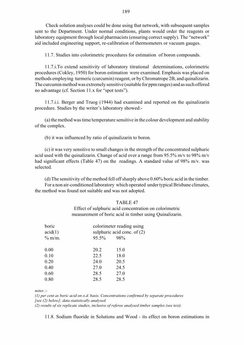
189

Check solution analyses could be done using that network, with subsequent samplessent to the Department. Under normal conditions, plants would order the reagents orlaboratory equipment through local pharmacists (ensuring correct supply). The “network”aid included engineering support, re-calibration of thermometers or vacuum gauges.

11.7. Studies into colorimetric procedures for estimation of boron compounds.

11.7.i.To extend sensitivity of laboratory titrational determinations, colorimetricprocedures (Cokley, 1950) for boron estimation were examined. Emphasis was placed onmethods employing turmeric (curcumin) reagent, or by Chromatrope 2B, and quinalizarin.The curcumin method was extremely sensitive (suitable for ppm ranges) and as such offeredno advantage (cf. Section 11.x for “spot tests”).

11.7.i.i. Berger and Truog (1944) had examined and reported on the quinalizarinprocedure. Studies by the writer’s laboratory showed:-

(a) the method was time/temperature sensitive in the colour development and stabilityof the complex.

(b) it was influenced by ratio of quinalizarin to boron.

(c) it was very sensitive to small changes in the strength of the concentrated sulphuricacid used with the quinalizarin. Change of acid over a range from 95.5% m/v to 98% m/vhad significant effects (Table 47) on the readings. A standard value of 98% m/v. wasselected.

(d) The sensitivity of the method fell off sharply above 0.60% boric acid in the timber.For a non air-conditioned laboratory which operated under typical Brisbane climates,

the method was found not suitable and was not adopted.

TABLE 47Effect of sulphuric acid concentration on colorimetric

measurement of boric acid in timber using Quinalizarin.

boric colorimeter reading usingacid(1) sulphuric acid conc. of (2)% m/m. 95.5% 98%

0.00 20.2 15.00.10 22.5 18.00.20 24.0 20.50.40 27.0 24.50.60 28.5 27.00.80 28.5 28.5

notes ;-(1) per cent as boric acid on o.d. basis. Concentrations confirmed by separate procedures[see (2) below]; data statistically analysed.(2) results of six replicate studies, inclusive of referee analysed timber samples (see text).

11.8. Sodium fluoride in Solutions and Wood - its effect on boron estimations in

190

treatment solutions and chemical determination of fluoride.This is examined from two aspects, namely;

11.8.1.Influence of sodium fluoride on titration of boric acid.

As indicated in Chapter 10, in 1974, due to shortages of boron salts, sodium fluoridewas incorporated with borax.

In development and use of diffusion type preservatives formulations, based primarilyon boron compounds and sodium fluoride, supplier recommended plant control was basedon densimetric techniques, using a hydrometer which was calibrated against solutionconcentration. It was necessary to carry out periodic analysis to confirm the componentbalance. Previous investigations of mixed formulations by the author indicated sodiumfluoride may interfere in conventional double indicator titrations for boric acid. The effectwas associated with the methyl red neutral point. Studies were made to confirm whether thiswas;

(a) a function of concentration of boric acid, or(b) a function of ratio of sodium fluoride to the boron compound.

As borax decahydrate was commonly used as a source of boron compound in dipdiffusion salt mixtures, an initial comparison was made over a concentration range (as boricacid) of borax. The ratio of sodium fluoride solution was varied. Typical data are shown(Table 48). These studies were subsequently extended to cover boric acid and boraxhomologues. Results confirmed interference occurred and it was a function of fluoride ratioto boron (as boric acid) concentrations.

11.8.i.i. When clarification procedures (Appendix 21) are used in solution analysis,

11.8.ii. Chemical determination of sodium fluoride in the solutions or treated productwill be restricted to the examination of, and problems found in, wood analysis, todescription of alternatives adopted (eg. field solutions) and to discussion of other applicablemethods.

11.8.ii.i. Classical methods were based on;

(a) gravimetric(b) distillation as silicofluoride.(c) distillation as fluoride.

For (b) and (c) final estimation was either by volumetric procedures orspectrophotometrically.

11.8.ii.ii. The Australian Standard 060 -1956 prescribed initial alkaline ashingfollowed by steam distillation, using phosphoric acid, into an alkaline absorbent. This wascarried out at 200o +/- 5o C. and at a distillation rate of 400 ml/hr. The high temperaturesprescribed were difficult to maintain. Results were satisfactory when determinations weremade on pure standard solutions.

When wood ash was distilled, particularly if the ash contained some phosphate andcarbonaceous material, severe interference was obtained. Reference sample analyses made

191

(A.O.A.C.) by standard procedures by the Agricultural Chemical Laboratory (cf. Section11.1.i.i), of which the Director was an eminent authority on fluoride analyses, confirmedinterferences.

TABLE 48Effects of ratio of sodium fluoride on determination of boron compounds (1) in

mixed preservative solutions.

series control. boric acid(3); sodium fluoride con. of;(2) 0.00%(a) 0.5% (a) 1.0% (a) 2.0% (a)

1 0.00 0.00 0.00 0.002 0.30 0.31 0.34 0.463 0.60 0.61 0.66 0.764 1.19 1.26 1.45 1.51

notes ;-(a) 1Oml. aliquot of sodium fluoride solution, of the concentration shown, added to 1Oml aliquot of theboron salt of boric acid (equivalent) solution. For control,equivalent 10ml. of distilled water added.(1) studies included borax homologues and boric acid,subsequently extended to commercial plantcontrol.(2) triplicate measurements.(3) measured as equivalent boric acid, % m/v.

Under the high temperatures of distillation and with the reasonably high viscosity dueto the phosphoric acid, it eventuated phosphate entrainment in the distillate, even at the slowrate of distillation, was responsible for the interference.

New Zealand Standard Code of Practice (1953) used a permanganate/sulphuric acidmedia for the distillation, followed by titration using thorium nitrate. No problems werefound using this latter procedure for wood ash and it was adopted as the reference analyticalprocedure. A problem in reproducibility of the titrational end-point was overcome byinvestigation of the volume of indicator added; increase of this from 0.5ml to 2.0ml did notcause interference and improved detectability.

11.8.ii.iii. Estimation of fluoride is difficult and the reference literature on this topicis numerous. Williams (1969) developed microtechniques by alizarin complexes. Garbuttand Levy (1972) published procedures. Australian Standard AS 1605-1974, adopted NewZealand Code of Practice (1953) as the reference standard method.

11.8.ii.iv. high frequency titration of fluoride.

Vogel (1964) discusses use of a high frequency titration for determinations of fluoride.The writer examined these techniques, but found the method desirably still requiresseparation of interfering agents by distillation. Thorium nitrate gave a very satisfactorytitrational curve at a frequency range of 1.5-2.5 Mhz. and with detection by null pointmeasurement. Most high frequency procedures use “zero-beat” techniques against astandard oscillator, with measurement by audio signal. Some error is given by dependenceon the audio null-point which is dependent on signal amplitude. Investigations by the writerfound it was more effective to measure the null on a centre reading d.c. output meter afterrectification, but an alternative, more rapid and accurate, method of end-point measurement

192

was to connect the output to an oscilloscope and visually measure a “zero-beat” condition.

11.8.ii.v. The fluoride specific ion electrode.Forstmanis and Lynch (1968) reviewed application of the fluoride specific ion

electrode. They developed the use of citrate as an inhibitor of phosphate/aluminiuminterference. Silica is also a major interference. Johnstone (1969) reported research into theuse of specific ion techniques with timber. In that period, interference was preferablyremoved in wood analysis by the distillation technique. Kennedy (1974) reviewed currenttechniques applicable in specific ion procedures. He studied use of ammoniumsulphosalicylate-E.D.T.A., a buffer recommended by Palmer (his reference [13]) reportingsatisfactory elimination of interference, particularly of aluminium. He reports detectabilityto 2.0 ppm in the final solution, corresponding to 0.02% m/m of sodium fluoride in thewood.

The specific ion electrode and high frequency titrimeter (or measurement techniquesdescribed above) are valuable alternatives to titrational methods by use of indicators.

11.8.ii.vi. field analysis of sodium fluoride in timber treatment solutions.

For veneer plants, using the “Momentary Dip” (Appendix 14) the non-availability ofplant analysis of fluoride solutions was not a serious problem. When (Chapter 10) it wasincorporated in sawn timber treatment, need arose for such analysis and a suitable controltitrational method (Queensland Forest Service, 1974), based on thorium nitrate wasdeveloped. This was selected over alternative colorimetric methods (Snell and Snell, 1949).The method was modified to a suitable field technique. Selection of titrational methods forplant control was retained due to similarity in colour changes in the end-points to thosepertaining to procedures normally used for boron salts. Interferences were removed by useof an ion-exchange resin, Amberlite IR-45 (OH). In the treatment solutions, the fluorine/boron salts ratio was maintained at 3:1, expressed as sodium fluoride (NaF) to the boron salt,with the latter expressed as boric acid equivalent.

11.9. Solution and wood analyses of CCA preservatives.

Small modifications for solution analyses were required to overseas procedures whichwere adopted. These included a limitation of 3 weeks, prior to analysis, on “workingsolutions” due to wood extractives. Above that time, the reduction of dichromate (Chapter10) was significant. To this was added need for centrifugation, or filtration, to removeinsoluble particles.

For wood, adoption of overseas methods involved changes in extraction techniques;final procedures followed were principally the New Zealand standards and are describedin AS 1605-1974. Later techniques, for especially the copper component, used atomicabsorption.

11.9.i. plant analyses for multisalts.

The writer has (Chapter 10) indicated plant determination of multisalts by operatorswas by hydrometric methods. He discusses the use of and reasons for measurement of thehexavalent chromium salt for routine and field analyses. The applications of a “CorrectionFactor” were discussed.

193

11.9.i.i. During research on which relationships (Chapter 10) were based, it was foundthat, in addition to effects of particulate undissolved salt components and dissolvedextractives on plant hydrometry measuremnts, unexplained variabilities were found. Theywere noted especially in high concentration solutions.

11.9.i.i.i. As a result, during their investigations, the writer and co-worker (Cokley andSmith, Rep. No. 4, 1965) tested hydrometer/solution concentration calibrations, usingfiltered, and/or centrifuged, solution samples, by;

i. direct density by mass/ volume measurement of the centrifuged samples.ii. density by Westphal balance on samples as for i.iii. Certified hydrometers.iv. Measurements as in i. to iii. after clarification using a filter candle.v. Comparisons, using these techniques, were made on measured dilutions of samples

to test calibration tables.

It was found problems described arose from calibration charts supplied to plants andfor which density curves in higher solution concentrations were by extrapolations ofdensity/ hydrometer calibrations from ranges studied [Chapter 10] for the significantlylower solutions used overseas. A second hydrometer, based on the extrapolated curve andchart, was issued by salt suppliers for use for stronger solution concentrations.

Study showed the original concentration/ hydrometer line used had been extrapolatedas linear, but was in fact a shallow curve and the nominal “best fit” linear relations were twolines (tangents to the true curve) intersecting at a common point of 6% m/v. Following onthe studies, in which salt suppliers co-operated, local manufacture, and supply to plants, ofre-calibrated hydrometers and charts relating density to concentration rectified the prob-lems.

11.9.i.ii. Concurrently, Dr. W. Chamberlain, acting as consultant for Hicksons (laterKoppers) Ltd., with assistance from Mr. G. Volk (Queensland manager for Hicksons),developed a suitable clarification technique using kieselguhr, followed by suction filtrationof solutions using a “take-off” line from the plant vacuum pump. The procedure (Cokleyand Smith, Rep. No. 4, 1965) was given formal approval under the Acts, so enabling plant

11.x. Research into, development of, a semi-quantitative spot test for timber treatedwith boron compounds.

Prologue.

“Spot Tests” in research on the presence or distribution of preservatives in timbersubstrates, qualitative/semi-quantitative assessment of a preservative concentration orreactive states, and inclusive of possible effects of environmental conditions on stabilityof preservatives which have been inpregnated into timber.

Spot tests have an extensive association in the classical analytical chemistry fields(Feigl, 1958, 1966) and form part of the preliminary “Group tests” in an analysis ofmixtures. They had an integral role in microchemistry and techniques such as the “boraxbead test” for colour given in “flame tests” on a platinum wire illustrate that role. In mostcases, they had a qualitative role supported by quantitative instrumental methods, eg. flame

194

photometry, which may be described as fore-runners to modern micro techniques such asby atomic absorptiometry or gas chromatography. Modern “breathalyser alcohol” testingis an example; a portable unit gives a semi-quantitative reading which is confirmed by a laterblood sampling for quantitative values.

Spot tests became important tools in preliminary field assessment and classification(Webb, 1956) of, especially rainforest, species in phytochemical studies, separation bypaper, or column, chromatographic techniques which played a part in studies on plantmaterials by university research groups by which chemical constituents, which may havemedicinal value, were extracted and identified.

In timber preservation, spot test roles may be summarised by the aims of their use andare classified by the author in terms of the method of application to timber, namely;

a. Macro application of a reagent, illustrated by starch tests (Chapter 4) or turmeric/boron tests under review. Here an excess of reagent is applied to a surface and presence ofthe impregnand is shown by a colour change. This is important when the impregnand is notan “auto-indicator” such as creosote oil. For this test, the preservative must be soluble, orbe reactive, or be in a form, eg. valency (cf. Chapter 10, hexavalent chromium anomaly)suitable for reaction with the reagent. In these conditions, particularly if the preservative ismobile or soluble in the solvent carrying the reagent, “bleeding” (cf. Chapter 12) across atest surface can lead to errors in assessing preservative distribution sites in timbers. Thatpossible erroneous interpretation on distribution is more likely in hardwoods than insoftwoods.

An illustration is the cutting by saw (eg. T.S. section) of a freshly impregnated sampletreated by a soluble and mobile preservative, such as boric acid, to which the acidifiedalcoholic (95% ethanol) solution of turmeric is applied. Boric acid is soluble in the acidifiedethanol, which is highly mobile in timber; the reacted turmeric is soluble and “colourbleeding” occurs across the adjacent tissues. Transfers across the surface by the sawing alsoaffect assessment. Visual indications, by that procedure, of boron distribution are gravelyin error (cf. Sections 12.3, 12.4, 12.5, Chapter 12). This error from “bleeding” may bereadily confirmed by techniques as in b (below) and is applicable over a wide range ofpreservatives.

a.i. for this area of application, micro, or trace, level of detection is generallyinapplicable. For preservatives to be effective, they are typically present in treated timberin semi-macro, or macro, concentrations.

Higher levels of preservative (over trace concentration) needed a wider range in testassessments. Accordingly, it was often necessary, eg. in the boron/turmeric (curcumin)reaction, to extend ranges past conventional measurement levels. Some situations (cf. typeb, below) arise where trace levels are needed, but these are generally better examined byextraction procedures as developed (Chapter 4) for visual starch values. A micro leveldetection test applies if a preservative movement occurs due to leaching or to volatility(Chapter 10), or where contamination of soils, crops, or water supply pollution, isinvestigated. Micro analyses support the tests.

a.ii. Though not generally classified as “spot tests” in the classical sense, studies, suchas a pH measurement by indicators (Chapter 8), are also considered by the writer asextensions of this area of research.

b. micro spot tests are generally used to examine sites of preservative distribution, but

195

the writer classifies a wettability (Appendix 15) test in this group. Here, the term refers tothe method of application of test reagent, typically by micro-pipette, and a microscopicassessment (x40) to trace (ppm) levels [later supported by U.V.]. In the eras (1947-1965)when much of this micro research was carried out, alternative sub-microscopic techniqueswere unavailable. A large amount of the writer’s research on preservatives and liquids(Chapters 8, 12) involved the clarification of, and differences in, preservative sites ofdeposition between softwoods and hardwoods. These were important applications of spottest techniques.

For both classes of test, each preservative “spot test” required research in its own rightto confirm conclusions drawn on preservative concentrations and distributions. Subject tothat confirmation and supported by analyses, “spot tests” were used to study effects of thetreatment processes on penetration and to study effects of service conditions on thepreservative stability and permanence. Research using “spot tests”, supported by otherstudies, led to principles of penetrability, porosity, reactivity of timbers (Chapter 8),effective species classification (Section 12.3, Chapter 12) for treatment, the accessible freepaths, effective orifice diameters, influence of wood structure on CCA “fixation” and“Specific Vessel Void Volume” concepts (Sections 12.4, 12.5, Chapter 12).

11.x.i. In addition to the joint research on quantitative determinations by analysis forthe presence, or absence, of a preservative, the Forest Products Conference (1946) hadallocated responsibility to the Queensland Department to develop a reliable “spot test” forboric acid. It was anticipated by the Conference that a test similar to the (I/KI) test (Chapter4) for starch may be developed.

11.x.i.i. The preferred method (Feigl, 1958) was based on the reaction of boric acidwith “tincture” of curcumin (turmeric) which depends on presence of boron compounds, inacid conditions, to change from the yellow (untreated) turmeric through orange to a redcolouration dependent on the boric acid concentration. Ferric salts cause slight interference,as does aluminium. Both of these can occur in timber. As a “go/no go” test, using a positive“red” colour for boron as compared to “yellow” for a negative result, development appearedto present no difficulties, but, when preliminary tests were made, the “red” colour was givenonly at boric acid levels which were much higher than the approved concentration of 0.20%.

11.x.i.i.i. Further studies showed;

a. gradients of colour reactions in timber, as compared to surface tests, presentedanomalies in interpretation.

b. Boric acid levels around the critical concentrations for preservation (0.12-0.14%boric acid) gave colours in the “orange” wavelengths, but a nominal negative “yellow”colour was given by the reagent even at low preservative concentrations (0.02-0.03% boricacid).

11.x.ii. Thus, initial quantitative evaluations would be necessary to confirm whetherthe reaction was suitable as a “spot test” on which to assess the boron treatment of timberproducts. Initial research was begun into possible development of a rating system of thecolour developed, which would be similar to that adopted for a qualitative assessment(Table 1, Chapter 4) of starch. Subsequently, based on initial studies, it was proposed, andapproved (Chapter 1), research be extended to develop it (as for starch) to the status of areliable semi-quantitative procedure suitable for not only field and laboratory confirmation

196

of the presence of boric acid, but, within reasonable limits, to indicate level of treatmentjudged against the minimum approved concentration of 0.20%.

By so doing, tests by inspectorial staff may enable a rapid assessment of the treatment.Samples indicating low levels of boric acid could be returned to the laboratory for fullchemical analysis.

11.x.ii.i. The curcumin/ boron reaction is a basis of many colorimetric quantitativeprocedures and extensive published references discuss postulated chemical forms of thereaction and products.

Conventionally, the curcumin reaction had been used only for low (ppm) concentra-tions of boron in colorimetric methods and where the boron present was typically below 10micrograms. Consequently, colorimetric methods were limited to the “yellow to orange”wavelengths and the conventional limits were significantly below the 0.20% as boric acidstipulated under legislation. As a “spot test” technique on wood, dilution was not an option.

11.x.ii.i.i. As a first step, a method of measurement of possible colour reactions (insolution) was necessary as they exceeded ranges used in standard colorimetry. From that,an extension to the measurement of colour on opaque samples would be required.

The colour range includes “red” colours additional to the conventional “yellow toorange” under normal colorimetric methods. As a result, difficulties arose in measurementby colorimetry of relations for boron (as boric acid) concentration to colour values over“yellow to orange to red” spectra produced by the reaction and the range, due to problemsin the spectral sensitivity and resolution of single filters; in conventional colorimeters,samples in “red ranges” would exceed the light levels transmitted through cells and filterscalibrated for “yellow-orange” ranges. These measurement difficulties were overcome bya Lovibond Tintometer.

11.x.ii.i.ii. The Lovibond Tintometer.

The Tintometer is a dual viewing system, similar to a stereoscope, to measurefundamental colours of solutions or opaque objects, using optically calibrated transparentglass slides. These slides were supplied in progressive increments of intensity, for the threebasic colours of Red, Yellow, and Blue. For each colour, a term “Unit” referred tosequentially calibrated numbered slides and additive values of slides were linear incre-ments. In measurement against a standard background for one of the dual eyepieces, theprimary, or strongest, colour in a solution or on an opaque material being studied was termed“the Dominant Colour”. Important differences and advantages of the Tintometer, comparedto a transmission colorimeter, or comparator, are;-

a. it may be used to measure opaque colours, eg. paints, in a reflectance mode.b. For use with liquids, it is not restricted for use only for specific liquid cell sizes. It

is applicable to thin films, eg. blood specimens, prepared on microscopic slides.c. Of direct importance was its ability to measure colour ranges which, by conventional

transmission methods, would be too deep to measure without significant dilution.

These advantages gave the ability to accurately measure beyond normal publishedcolour ranges of the turmeric (curcumin)/ boric acid colorimetric techniques and theseextended ranges were statistically evaluated. It allowed colour tests on solid samples (filterpaper and tinber).

197

11.x.ii.ii. There was a lack of knowledge of the chemical form in which the boron waspresent in the treated wood, and which was assumed to remain as “available boric acid” inthe tissues. There was a similar lack (Chapters 8, 9 and 12) of knowledge on the sites ofdistribution of the impregnand in the wood and, thus, its possible reactivity with thecurcumin when applied to a specimen. There was an “implied assumption” (1946-7) thatdistribution would follow the softwood pattern and would be uniform in all tissues. That wasincorrect, but its clarification was one reason for the writer’s continued research on sites ofpreservative distribution, the role of porosity (size and frequency) in development of timberclassifications (Chapters 8, 12) and his subsequent research (Chapter 8) on permeabilityand penetrability in hardwoods.

11.x.iii. In view of it's importance, the writer studied postulated chemistry of, andvariables for, the reaction. Significant findings are summarised below.

a. curcumin is the active component of turmeric.Feigel (1958) suggests there is a change from a yellow curcumin (diferuloylmethane)

structure to an isometric red-brown rosocyanin. A loose addition product of boric acid andcurcumin is formed as an intermediate. Feigl describes the test using hydrochloric acid.Rosocyanin is turned “green” to “green-black” by alkali, eg. ammonia vapour will convertit to a “bluish- green”, and this is specific for boron. Ferric salts do not give a positivereaction to this latter test.

b. The actual colour reaction was influenced by presence of organic acids and salicylicacid, in the presence of hydrochloric acid, gave a “brown-red” colour rather than an“orange-red”. Oxalic acid gave a typical “yellow-red” reaction. The differences wereconfirmed by spectrometer and by the Tintometer. The Division of Wood Technologyadopted a test method based on salicylic acid. The writer adopted use of concentratedhydrochloric acid (only) as the preferred standard acid.

c. Dyrssen et al. (1972) examined reaction of boric acid and of curcumin under varyingconditions, including in a strong sulphuric acid-acetic acid medium. That extended to astudy of reaction equilibria in aqueous-ethanolic media. Results were;

(c.i) They suggested a 1:2 boric acid - curcumin compound.(c.ii) They cite an acid dissociation constant of 10-7.9 for curcumin in water-ethanol

mixtures. For rosocyanin, the acid dissociation constant was found to be 10 -5.7 in the samemedium.

(c.iii) In their discussion of analytical procedures, they emphasise a need for excesscurcumin and for removal of water.

11.x.iv. Study of boron/ curcumin ratio for reaction.

Author’s note; in discussion of this aspect of research, though the general term“boron” is used, the ratios, or concentrations, are quoted as equivalent boric acid.

11.x.iv.i. In treated timber, for a concentration of 0.2% m/m and wood density of 640mg/mm3 (initial species range used for research in this phase), there was an equivalentdistribution of 3.12 mg/mm3 of boric acid in a sample.

This was an increase by the order of some decades in the range described above ie. the

198

normal 10 “ppm” maximum, measured by the reaction. Hence, an increase in detectionrange of (curcumin/turmeric) reacted colours in terms of boric acid level was requiredwithout, at the same time, decrease in sensitivity of the lower colour ranges from a yellow(negative), through orange to red.

11.x.iv.ii. The writer considered this may be a function of relative proportions of boronto that of the curcumin, as well as the acid type, selected as hydrochloric. To evaluate thishypothesis, became a major, but successful, research project. To test the hypothesis therewere also required quantitative measurements of colour changes at depths of colourproduced by these changes in ratios and high concentrations of boron reacting withcurcumin/ ethanolic/ hydrochloric acid reactants and which were too intense for measure-ment by transmission instrumental procedures. This measurement was made by theLovibond Tintometer. Based on the colour standard techniques used for solutions and forsuch as paints and film coatings, measurements of colour range relationships, developed bya series of boric acid / acidified curcumin (95% ethanol) solutions, were quantified. Thesewere then extended to tests of opaque impregnated filter paper and timbers.

11.x.iv.iii. Use of turmeric and curcumin.

As a separate part of the research, the writer examined the use of and need forpurification of chemical grades of turmeric as a substitute for spectrographic grades ofcurcumin used in early studies. Subject to purification procedures (Appendix 22), its usewas satisfactory, and, for subsequent studies, curcumin from turmeric was used.

Author’s note; For further discussion, with emphasis on the active component, theterm, turmeric, is inter-used with curcumin.

11.x.iv.iv. Specific items studied included;

a. Initially, to exclude interferences, the writer tested the ratios and their effects byaqueous solutions (known concentrations) of boric acid, reacted, with the re-purified, acidsolutions of curcumin in 95% ethanol.

Re-purification of curcumin was necessary (Appendix 22) to remove any insolublematerial in the reagent and need to ensure absence of boron contamination which is notexcluded in suppliers‘ specifications. In the boric acid and curcumin reaction, thesignificant Dominant Colour was “Red”, with reproducible, statistically significant, linearincrements in terms of boric acid ranges.

b. Effective ranges of measurable colour and preservative levels were confirmed to befunctions of the ratio, (relative concentration of boric acid to curcumin), with a maximumratio of the order of 1 part of boric acid : 3 parts of curcumin being desirable. For the reactionto proceed to completion, excess of curcumin was necessary.

c. to determine the optimum curcumin concentration, as the critical range of measure-ment of boric acid was the minimum approved level of 0.20% m/m, solutions over thisequivalent range were studied, with an emphasis on a spread of +/- 50% about this level.

On this basis, and as this order of reagent concentration is used in many colorimetricprocedures, a minimum of 1% turmeric (purified), dissolved in 95% ethanol was used. For

199

this, ratios of boron to turmeric were kept below the 1:3 level by dilution prior to reaction.

Typical calibration data (Cokley, 1947) is shown in Table 49, and Graph 33, for 1%solution of extracted, purified, dried, re-dissolved turmeric. Ethanol (95%) was used as thesolvent. A significant statistical linear relation was found between the Lovibond Red Units(R.U.) and boric acid concentration. That was:-

% Boric acid = 1.3928 R.U. - 0.0424 (11.4)

r = 0.9950 ***

11.x.iv.v. Studies on optimum concentrations of curcumin and ethanol.

a. The writer established a need to remove excess water. That was confirmed byDryssen et al.(1972). After exhaustive tests, he established that 95% ethanol was thesatisfactory concentration for this work. Further studies confirmed that was suitable forapplication to timber.

b. Use of a 1% m/v ethanolic solution (95% EtOH) of turmeric presented certainproblems, associated with high humidity, with variation of the actual boron compoundconcentration and of temperature.

c. As it had been shown excess turmeric is required, restriction to use of 1% turmericalso limited the range of tests in timber where gradients were such that values of up to, and

These problems were eliminated by a saturated solution of turmeric, shaken andfiltered prior to being used, acidification as above, and reaction with boron. Neitheracidification procedures nor the stability, subsequently described (Appendix 22), wereaffected by these changes. Ancillary research on aspects in development of the spot testreagent, alternative solvent media, acidification procedures, preparation of wood surfacesand permissible moisture contents are described in Appendix 22.

TABLE 49

for estimation of boric acid by Lovibond red units (2).

Lovibond boric Lovibond boricred units acid (3) red units acid (3)

0.05 0.06 0.58 0.670.07 0.09 0.5l 0.720.10 0.10 0.72 0.960.11 0.16 0.84 1.100.16 0.18 0.88 1.270.20 0.20 1.00 1.400.29 0.28 1.20 1.620.33 0.32 1.33 1.85

notes ;-(1) acidified using conc. hydrochloric acid. Turmeric dissolved in 95% ethanol (see text).(2) Lovibond Tintometer — optical, calibrated colour slides. (3) independently calibrated.

200

11.x.v. Relation between a turmeric spot test result and boron content in treatedtimbers.

Relationships of the turmeric spot test in treated timber were quantitatively evaluated.

11.x.v.i. Prior to this, and as part of investigation in development of the finalprocedures, measurements were made, using the Tintometer, on filter paper media afterquantitative impregnation by boric acid solutions. The earlier correlations, using solutions,were confirmed.

11.x.v.i.i. This was followed by the (Chapter 12) impregnation of small thin timbersections over a range of species to ascertain if wood colouration, or structure, affecteddetection of ranges in colour, or concentration correlations when measured againstmatching, untreated, controls. Results were satisfactory. A final analysis of the impregnandin the samples confirmed original linear relationships cited above.

11.x.vi. Two methods were evaluated for application of the reagent to treated timberand measurement of colour.

11.x.vi.i. Sections of planed (see discussion [Appendix 22] on surface texture), treatedtimber (known analysis) were cut parallel to the face, i.e. to provide individual gradients(Diagram 1) in thin sections. By the use of gradients, a range of concentrations in matchedsection, structure and colour were obtained. They were treated by an excess of saturated,acidified, turmeric solution. For the initial research studies, a final smooth surface wasobtained by use of a “spoke shave”, as used by cabinet makers. Repeat studies using a fineplane gave no significant difference in texture results. The individual gradient sectionstested, though matching analyses had been carried out on controls, were then separatelyanalysed. No significant difference in boron analyses was found. The colour was developedfor times up to, and then standardised on, 50 minutes and measured by Tintometer in theReflectance mode. Subsequent to this research data, times were reduced to 25-30 minutesin development. There was a highly significant linear relationship between the Red Unitsand the boric acid concentration in the sample. To remove any effects of species colourvariability, all measurement was done against unstained matching sections.

Typical results are shown in Table 50, Graph 34, and equation (11.5).

R.U. = 0.0612 + 8.4796 (% Boric acid, o.d.) (11.5)r = 0.9980 ***

or, alternatively,% Boric acid = 0.1179 R.U. - 0.0072 (11.5a)where:% Boric acid (m/m) = percentage m/m in treated wood.R.U. = Lovibond Red Units.

11.x.vi.ii. During routine examination of treated timber, the sample board was initiallysplit, starch tested and the matching split section, surfaced, as described, when necessary,treated with acidified saturated turmeric in 95% ethanol. The sample reaction was allowedto develop a colour for 20-25 minutes, and then visually assessed for treatment level on thecolour based on the “Red Units”. These were statistically correlated by measurements usingthe Tintometer against chemical analysis.

201

TABLE 50Correlation of colour reaction of turmeric solution to

red unit measurement (Cokley, 1947).

boric acid Lovibond (1)% in wood red units

0.05 0.500.07 0.640.08 0.750.11 0.950.40 3.600.72 6.201.12 9.001.33 11.75

note ;- (1) triplicate measurements. Part of extensive series.

11.x.vii. Standard test procedure adopted in assessments for boron compounds, basedon the turmeric reaction.

After extensive evaluation, illustrated by data as above, formal procedure adopted, interms of colour assessment (cf. Table 10, Chapter 8, for penetration in starch negativezones), was;-

(a) Red colouration. A concentration in excess of 0.20% o.d. m/m, boric acidequivalent, in the tested zone.

(b) orange colouration. A concentration in excess of 0.15% m/m (boric acid), butbelow the minimum of 0.20%. in the zone tested.

Operationally, and legally, this was an important level. Initial CSIRO tests (Cummins,1939) showed a boric acid concentration of 0.12-0.14% was toxic to Lyctus brunneus,Steph. In practice, spot tests with this assessment, if adequate starch was present (Chapter4), were classified as “not detrimental” (Chapter 2) under T.U.P.A. (1949).

(c) yellow-orange colouration. A concentration less than 0.10%-0.15% m/m of boricacid equivalent, but above 0.05% m/m, in the tested zone.

(d) yellow colouration (negative). A concentration from zero to 0.05% m/m, as above,in the tested zone.

Based on a visual assessment, the writer found +/- 0.05 m/m (boric acid equivalent)to be the normal reliability of estimation by operators, including laboratory staff, due to :

(a) slight interaction of wood colouration.

(b) variable response of operators to visual differences in the wavelengths (cf. Chapter4). This applied to the intermediate colours.

202

11.x.viii. Supplementary Use of Ultraviolet light.

These problems were overcome by a further procedure based on the use of a portableultra-violet lamp (Chapter 8). This added procedure increased the reliability of inter-operator assessment to +/- 0.02% m/m. The author demonstrated that, when excited bybroad band ultra-violet waves (Chapter 8), turmeric solutions would fluoresce vividly,particularly in an acidified ethanolic media, as a “pure” yellow colour, and that, whenapplied to untreated timber, the yellow fluorescence was clearly differentiated from boththe natural wood colouration or fluorescence of wood components. In the presence of boricacid, or other boron compounds (converted by the acid in turmeric reagent), fluorescencecovered the distinctive colour ranges of yellow, orange to red. Sharp demarcation betweenthe treated and untreated zones were present and delineable. The sharp definition of thepresence of boron compounds was of assistance in study of distribution of these preserva-tives in wood tissue. It was of aid to operators who had low colour sensitivities in yellow-orange wavelengths. Subsequent to the writer’s laboratory obtaining ultra-violetspectrofluorimeter facilities, the quantitative relationships (turmeric) between exciting andfluorescence wavelengths to the boron concentrations were confirmed. The use of ultra-violet procedures also enabled examination at higher moisture contents [30-40%] (cf.Section 12.5, Chapter 12, “Stable Green” moisture).

11.x.ix. Progressive evaluations of operator assessments.

note; Owing to uses (Section 11.1.i.ii) such as for crop treatment, or tests as a sourceof contamination, sawdust frequently required spot testing (analysis as necessary) to ensurethat boron (also P.C.P.) was not present.

1. Periodic analyses, particularly when training new operators, were carried out onspot test samples to determine operator sensitivity and reproducibility of assessment.Typical random correlations of analysis and spot test are shown in Table 51.

2. All samples which had been operator assessed as failed (< 0.20% m/m), were re-assessed by an independent referee operator, including under ultra-violet light and the zoneof treated timber, which had been failed, rated as above. It was cut from the sample, groundand analysed.

Where assessment is done by a sawmill plant operator, the results are rated only at twolevels:-

(a) Pass: Where the treated zone gives a colour in excess of “definite orange-red”.(b) Fail: Where the colour is below distinctive orange, i.e. yellow.

11.x.x. Status of, and reliability of, assessment levels.

Since the introduction of treatment with boron compounds and development of theturmeric spot test procedure, annual average in excess of 3000 specimens were measured.That covered all species and types of boron compounds. and they were also routinelycorrelated against chemical analysis. Typical random results of such comparisons are citedin Table 51. Possibly conservatively, the author continued the practice of training staff,initially on specimens ranging from planed surface split sections, to typical surfaces asobtained by splitting. In training, an independent assessor gave a separate evaluation,subsequently confirmed by analysis, until the trainee was adequately competent in the spot

203

test. Consequent on large scale research programs, industry control, random sampling, anduser submitted samples extending over many years, a comprehensive range of species, ofoperators, including both plant staff and laboratory personnel, and also consequent ondiscussions with legal advisors, the writer concluded;

1. The principal aim of the assessment was to evaluate, under legal and scientificacceptible standards, whether a specimen did contain a level of boron compounds equal to,or below, 0.20% (as equivalent boric acid) prescribed under both the State Acts,T.U.P.A.(1949), TMA (1946), or Australian Standards and user specifications (The StateHousing Commission and local financial institutions). That objective had been achievedand this acceptance extended to overseas sources of imported timbers.

2. over the significant range, up to, and exceeding, the 0.20% m/m of equivalent boricacid, assessment by the operators was very reliable in terms of the turmeric reaction asdescribed.

3.Results were in excess of the 95% reliability level, which was statistically desirablefor acceptance under both legal and Standards requirements.

4.The technique was acceptible to, and applicable by, the plant operators. This washighly important in terms of policies of quality control as mandated under government andForestry instructions for establishment and operation of the industry.

Results based on over 30 years of tests, its acceptance as scientific evidence insuccessful court proceedings under the Acts, its inclusion in Australian Standards andacceptance by Australian and overseas test authorities justified the extensive research todevelop a proven and reliable procedure as part of an overall quality control.

TABLE 51Correlation of visual ratings (by a turmeric spot test)to the chemical analyses of timbers treated by boron

compounds (based on comparison of commercial treatmenttests against quality control assessments and analyses).

species pass range species fail range(1) (1)

spotted gum 0.23-0.33 spotted gum 0.00-0.00tulip oaks * 0.11-1.25 tulip oak 0.10rose mahogany 0.24-0.51 rose mahogany 0.06-0.13sthn.silky oak 0.85 Crow’s ash 0.06rose maple 0.32-1.01 white cheesewood 0.00-0.12red mahogany 0.59yellow satinash 1.29tulip oak (a) 0.11tallowwood (a) 0.07-0.08

notes;-(1) Results shown were part of laboratory quality control procedures, to evaluate reproducibility ofoperators’ assessments, and to train staff. Results as boric acid (o.d.basis) equivalent. Analyses byrandom tests of sample “cores” passed or failed by staff using turmeric spot test.* tulip oaksrepresenting more than one species; one sample only below 0.20% m/m.(a) rated “just passed” whereassessor was undecided, hence subject to examination by ultraviolet light and chemical analysis. Bothspecies were “brown” in colour, even in the “sapwood”, and showed wettability problems (Appendix15). Samples are included to indicate effect of operator sensitivity to wood colour (Chapter 4) andadvantage of independent assessment and use of U.V.

204

11.xi. Spot tests for fluoride salts.

No satisfactory direct field spot tests were able to be developed.

11.xii. Spot tests for CCA multisalts.

a. Copper.

A suitable (AS 1605-1974) test was use of rubeanic acid, which turns a “blue” to “blue-black” in the presence of copper salts.

b. Hexavalent Chromium.

Diphenylcarbazide (Feigl, 1958) gives an orange to red colouration, dependent on theconcentration (cf. Chromium anomaly, Chapter 10).

c. Arsenic Salts.

An ammonium molybdate reaction is used but interference is found due to phosphatesnaturally in wood and a direct test is unreliable. For the arsenic component, compounds,such as phosphates, give similar reactions to the arsenic “spot test” and it is essential to carryout comparative tests on untreated matching samples. Unless (see below) this is done, testsfor the presence or distribution of this component may be anomalous.

To ensure the validity of an arsenic result, additional to full chemical analysis, theauthor made use of a modified (Feigl, 1958) test for arsenic, reacted to form “arsine”. Inthat modification, sensitive to below the microgram level, silver nitrate crystals are placedover a filter paper seal over a test tube wherin a micro specimen is reacted with acid. Ifarsenic is present, the silver nitrate crystal changes colour, but if phosphate is present asimilar reaction occurs. To prevent this interference, a small cotton wool plug, impregnatedwith lead acetate, is placed in the top of the test tube under the filter paper. Phosphine istrapped by the lead salt and the arsenic test is valid. If control phosphine tests, without a leadacetate trap, show negative results for phosphorus, the wood section may be directly testedby the molybdenum “blue” reaction.

205

CHAPTER 12

DEVELOPMENT OF SPECIES TREATABILITY GROUPS AND EFFECTIVETREATMENT SCHEDULES FOR OPEN TANK SYSTEMS. STRUCTURALFACTORS, INCLUDING DENSITY, INFLUENCING THE TREATMENT OFTIMBERS. VOID VOLUME APPLICATIONS. CONCEPTS ON MOISTURECONTENTS AND OF THE “SPECIFIC VESSEL VOID VOLUME ANDCONCENTRATION”.

12.1. Introduction.

For establishment of a timber preservative industry, two alternative philosophiesneeded to be addressed. They are delineated in Flowchart 2A, and may be described as;

a. The accepted overseas practice (then centred on vacuum pressure systems) wassupply of product to, and treatment by, centralised, high capital cost, treating units (type 1,Flowchart 2A). That implied standardised operations with centralised control. The firstplants were type 1, with total laboratory control by the Forestry Department. A localindustry model of this type was the processing of raw sugar cane supplied from farms to acentral mill.

b. Geographic and economic evidence (Chapter 3, Maps 1, 2) showed wide speciesdistributions and an industry predominantly operated by what the writer (Flow chart 2A)classifies as type 2 units, which were generally regionally de-centralised, including localmarkets.

In especially Chapters 1, 8, the author emphasised the original developments in, andthe consequent mandate for, and approval of, multistranded research into critical factorsin the timber preservation industry. The mandate approved flexibility of operations andsystems. De-centralised, supported, quality control (Chapters 10 and 11), with trained plantoperators would be necessary. This implied development of procedures suitable for localconditions, including for the wide range of species to be treated.

An outline of the relationships between different aspects of this work is given inFlowcharts 1 and 2. The critical factors were;

(i). An operational method was required for classifying the extensive range ofQueensland species into relative treatability groups by utilising their “macro structuralproperties”. No comparable system had been developed elsewhere for these purposes.Based on procedures for, and results of, testing of 13 species by Brimblecombe and Cook(1945), evidence indicated that the practice of evaluating individual species would involvea minimum of 5 years before a comprehensive industry was established. Use of speciespredictions based on known preservative retention results (% boric acid on an oven dry,mass/mass [o.d. m./m.] basis, Chapter 10) when timber was treated by the standardised(Queensland) single schedule (Young, 1946b,c), followed by testing programs over anextended range of species, should confirm its probability and suitability.

ii. based on (i), possible flexibile treatment regimens for species, defined as “sched-ules” (Appendix 14), were to be developed.

iii. These two objectives, required the author to address the apparently conflicting

206

moisture content requirements of open tank, and vacuum pressure (full cell), systems. Withthe open tank method, specifications for “green” timber needed to encompass moisturecontents below FSP. Vacuum pressure treatments which required timber with a lower,defined (below FSP), range of moisture contents, needed a flexible increase in that range.That need for open tank treatments was highlighted in both 1948, and 1949, when majorindustrial disputes caused serious delays in processing, so that material, awaiting treatment,dried to very low moisture contents, and frequently was at the air dried (Chapter 7)condition, or lower moisture contents to EMC (10-12% mc). The author was able toreconcile the two separate needs by the paradigm that “moisture content, air content, anddensity, were interrelated variables in timbers”.

This Chapter is divided into three sections;

a. evolution of the industry.b. process co-ordination and;-c. Especially for angiosperms

density, and interactions with timber preservation.

These led to the development of new concepts in timber moisture content, and inpreservation.

12.2. The Evolution of Timber Preservation Science in Queensland.

As indicated in Chapter 8, research by the writer into basic principles, applicableparticularly to hardwood timbers, confirmed the utility of the air, moisture, and densityparadigm. One result of the research was the development of a new process, namely the“Vacuum Pressure Diffusion Process” (Appendix 14), details of which are examined inChapter 14.

12.2.i. The reduction in treatment moisture content for open tank systems.

At the commencement of the studies, diffusion of aqueous preservatives into timberwas considered as the important factor in preservation by open tank methods, and moisturecontents at, or above, FSP (considered as 25% mc), were accepted as necessary fortreatment. This view persisted even after Young (1946c) and Bryan (1946) suggested thata partial vacuum effect may be more effective. Thus, the interactions of moisture contentswith the preservative uptake in these processes were not investigated by Young.

That writer’s pilot plant, and commercial, studies were conducted on freshly sawn,“green”, material. This writer felt (Chapter 1) flexibility in treatment did require researchinto effective ranges of moisture content for each process. Other factors, such as woodstructure, and properties such as the “permeability”, “penetrability”, “reactivity”,“wettability” (Chapter 8), thermodynamics (Chapter 13), capillary flow, the significance offlow equations such as Poisseuille’s (cf. Section 12.4, this Chapter, and Chapter 14), orsolution absorption, could be important. Thus, studies into moisture contents applicable forthe treatment processes were undertaken.

12.2.i.i. The Cold Soak process.

Research on treatment moisture contents below FSP showed (Cokley, 1948a) the

207

mechanism was initially water, and solution, uptake by capillarity, and followed by saltdiffusion.

The final moisture content, after preservative treatment, varied with species, but didnot attain saturation moisture content under normal treatment conditions (Appendix 26).The rates of salt penetration and the steepness of salt concentration gradients were functionsof salt type (Chapter 8), of the solution concentration, and of temperature.

For all studies, a minimum sampling (Chapter 10) of six starch positive specimenswere used for each moisture content range, timber dimension, and species, for each of threecharges, both in pilot plant studies, and at each preservation plant. Studies were extendedthroughout the State, thus ensuring a wide range of species provenances and climates weretested, and highlighted (Chapter 8) a need for research into “wettability” (Appendix 15)aspects.

Relationships between ambient temperatures and solution concentration, to ensurethere were effective “diffusion differentials” in this process, led to an imposition ofrestrictions on the minimum temperatures of operation of this process, and to developmentof the “warm soak” modification (Appendix 14).

12.2.i.ii. The Hot and Cold process (or modifications).

Young’s (1946c), and Bryan’s (1946) hypotheses that a partial vacuum may becreated by heating (Chapters 8 and 13), and then cooling, under solution, were confirmedby the writer. This was done by sealing thermocouples (Appendix 15 [Section 3], Chapter13) and manometer tubes (Section 2.ii.iii, Chapter 14) into the centre of endsealed boards.Typical time/ vacuum curves were similar to graphs 52a, 52b (Chapter 14), which weretested for similar vacuum ranges as in thermal processes. The same basic principles(Chapter 8) applied to steam / cold quench processes. The principles (Chapter 8) areexamined in appendix 34, Chapter 13, appendix 38, Chapter 14, and are summarised indiscussions on development of treatment classifications based on density and porosity(Sections 12.3.i.ii, 12.3.i.iii).

12.2.i.iii. Examinations of relationships between moisture content, density, andeffective treatability, including void volumes, were made:

12.2.i.iii.i. Re-evaluation of Young’s (1946c) initial data, including pilot, and com-mercial, results.

Young assumed that FSP was 25% mc, and did not examine moisture content as avariable (+/-) about this point. The writer classed Young's data in 5% mc groups and foundthat, as the moisture content in a class decreased, timber moisture absorption increased, butit was a function of treatment cycle (times at maximum temperature and cooling).Progressive samples during the heating phases showed low preservative uptake, and agreater mean increase in moisture content below, than above, 40% mc (Graph 35).However, during the cooling stage, uptake was high. Moisture contents tended to reach alimiting value approaching “saturation moisture content” conditions of about 55-60% mc(Graph 35). For that final stage, there was a strong trend, that, as initial class moisturecontent decreased, salt uptake increased (Graph 36).

For this study, a total of 6 endsealed, starch positive, specimens were selected for eachmoisture content class, with respective classes of 6, 7, 6, for the separate three scheduleconditions (Graph 36). Saturation values for treatment group 3 (after the 22o drop) are the

208

total final moisture content.

In Young’s (1946c) study (in which this writer was involved), subsequent to removalat each treatment stage, specimens were tested for moisture change by weight, and ovendrying. Sections were prepared (diagram 1, Chapter 10) for analysis. After culling for starchpositive subsections (Chapters 4, 7), 29 “cores” were analysed for each stage, with sixspecimens for full crosssection, and 56 analysed after the complete cooling (22o) cycle, andsubsequent seasoning, with six boards for total cross-sectional analyses (Graph 11, Chapter10). After cooling, there was a mean progressive increase in “core” concentration from0.6% m/m to 1.16% m/m as the moisture content decreased from 50 to 30%.

The above conclusions were given support at an early part of this study, when thewriter confirmed that, when treated, unless freshly cut from logs, many commercial stacks,nominally above FSP (accepted initially as 25% mc), could contain material with a rangeof +/- 25% of the mean moisture content of the stack. Extension to reduced moisturecontents, and influenced by industrial delays (Chapter 2), initially under pilot plant status,and then commercial scale, using standard (Chapter 10) sampling numbers and procedures,confirmed those deductions, and supported the possible application of “void volume”principles. Results were progressively statistically analysed for these studies of themoisture content, and retention, relationships.

Over this same period, as part of the extensive research described in Chapter 10, andas summarised in graphs 13-17 (Chapter 10), reduction in solution concentrations werefrom 4% mass/volume (m/v) to 3% m/v, to a final standard of 2% m/v. Changes (Chapters8, 10) were made to use of borax. Results for 25mm brown tulip oak (12% mc) gave “core”concentrations of 0.6% - 0.8% m/m., that is in excess of the theoretical average “core” value(Table 33, appendix 17, Chapter 10) of 0.52 % m/m, but within standard deviation levelsconsidered desirable.

12.2.i.iii.ii. The Steam/ Cold Quench Process.

For this process (Appendix 14), the original application (Young, 1946d) was for lowdensity species of Group 1 (Table 53), but industry sought to extend application to a widerrange of timbers of higher density. Due to thermodynamic properties (Chapter 13) oftimbers of higher densities, the heat requirements resulted in substantial moisture contentincrease in surface, and the outer, layers from water condensation due to the steam heatingcycle. To minimise this effect, for species with wood densities of groups 2B to 4 (Table 53)preseasoning for this process was required. Also an extended time of “soak” in the coldsolution at atmospheric pressure, following the “quenching”, was necessary. These needswere tested in pilot plant studies carried out using specimens from the large scale projectdescribed in Appendix 2, with treatments under close control. The study results weresubsequently confirmed over a range of treatment plants and timber origins. Standardsampling procedures were used in these studies, viz. six starch positive specimens(endsealed), each 25mm thick, for each species, selected for uniform moisture content,were treated by a standard steaming cycle, rapidly “quenched”, and given increasing timesof absorption. The treatments were repeated for a series of three charges. Graph 37 showsthe progressive increase in preservative concentration in mean sample “cores” for 25mmthickness for three representative species, air dried red tulip oak, “green-off-saw” yellowcarabeen, and “green-off-saw” white cheesewood.

209

Graph 37a correlates linear transformations of the data from Graph 37 (“1/concentra-tion” vs “1/time of quench in hours”), showing fitted lines, and where the inverse of theregression coefficient for each species represents a rate of preservative uptake, or the uptakecoefficient. These tranformations were;

for Red Tulip Oak,1/c = 1.2813 + 23.2205 (1/t) (12.1.a)

r = 0.9895***for Yellow Carabeen,1/c = 1.0777 + 13.6786 (1/t) (12.1.b)

r = 0.9882 ***for White Cheesewood,1/c = 0.5782 + 9.9822 (1/t) (12.1.c)

r = 0.9972***

where “c” is mean core concentration (% boric acid on oven dry,mass/mass [o.d. m/m.] basis, and “t” is time in hours of specimen immersion after “Quenching” by boric acidsolution.

Author’s note; the high values of “r” were due to use of specimens (pilot plant) fromresearch material discussed in Appendix 2 with close control on treatments.

Graph 37b shows the relation between the inverse of the coefficient “b” (of the inverseof quench time “t”) with air dried density (Cause et al., 1974). The inverse of the interceptsgave theoretical maximum “core” uptake/ species by this process, and preservativeconcentration. However, Graph 37c shows the value of “1/c” for “t” (as theoreticallyinfinite), bears a linear relationship with the “Specific Vessel Void Volume, SVV”, (cf.Section 12.5.4), and “1/c” may be re-defined as- “being equal to 100% of the “SpecificVessel Void Concentration, Sc,”. The writer (cf. Sections 12.4, 12.5) suggests thisrelationship is associated with sites of deposition of preservatives in hardwoods.

Comparison of the above Steam/Cold Quench data with evidence from the “Hot andCold Quench” process (Appendix 14) showed a similar relation of uptake to absorptiontime, but for the latter, as some salt uptake occurred in the heating/maintenance cycle, theinitial value at the start of quench was not zero as above.

Source effects were prominent in yellow carabeen, Sloanea woollsii, illustrated bymaterial from the Killarney district in south east Queensland. From that general source,material with nominal group 2A structural properties (cf. Section 12.5.4, “Specific VesselVoid Volume” concepts, and Graph 37c) did require, similar to the group 2B species,predrying for these processes.

12.2.i.iii.ii.i. Differences in the Solution Absorption Times, Change in MoistureContent, and Salt Retention, as functions of “cycle”, between both the Steam/Cold Quenchand Conventional Vacuum Pressure Processes with standard Hot and Cold, and Hot andCold Quench, Process results.

For the Steam/ Cold Quench, and the conventional Vacuum / Pressure systems (wherea “dry” vacuum is used [Appendix 14]), no preservative solution is present in either thesteaming phase, nor in evacuation for the latter process, and thus, for other than condensate

210

(S/C.Quench) no solution, and consequently neither moisture increase, nor salt, uptakeoccurs during that initial period. Thus, all salt uptake, and significant moisture contentincrease, occurs subsequent to final “Quench” or “flood/pressure” conditions for these twotreatment systems.

For the standard Hot and Cold, and Hot and Cold Quench, processes, moistureincrease and salt uptake take place during the “heating, maintenance, and cooling cycles”,with principal uptake occurring in equilibrium with the “cooling cycles” from themaximum temperature.

The flexibility found in effective moisture contents for open tank processes (cf.Section 12.4, relationships of FSP in hardwoods) led to subsequent research (Section 12.5)on the significance of moisture contents at, or above, the conventionally “indeterminate”zone of “green moisture content”. That flexibility was successfully later applied (Chapter14) to vacuum/pressure (full cell) processes.

12.2.i.iv. Moisture content effects in vacuum / pressure (full cell) systems.

This is examined in Chapter 14, but has been included in this discussion to demonstrateoverall relativity of process relationships with moisture contents suitable for treatment oflocal species, especially hardwoods. Subsequent to the commercial introduction ofconventional vacuum/pressure treatments, the writer demonstrated that moisture contentconditions similar to thermal processes applied for these systems. Higher moisturecontents, at, or above, FSP, could be used, dependent on species and preservative. Howeverfor optimum applications, process efficiencies (Chapter 14) needed to be increased.

12.3. Classification of species treatability in Open Tank processes.

As indicated in the start of this Chapter, research on all individual species wasimpracticable. However the writer considered that suitable classifications could be basedon generalised primarily physical structure of species. Thus, as a first step, the data obtainedfrom pilot plant and commercial studies under standardised schedule condition, were testedto determine any possible correlations. An examination of data for 50 species reinforced thenotion there appeared a relation between a.d. density and treatability, so a research program(Table 52) was initiated to study the effects of species variables and interactions withprocess conditions. In addition, a similar study was conducted on “cold soak” processes(Appendix 14). The physicochemical properties affecting treatment, such as “sapwood”,starch detection, wettability, and the wood reactivity have been described in Chapters 4 and8. Control procedures have been examined in Chapters 10, 11. Studies cited in Appendix2, enabling tests on a range of species of known properties, and under controlled pilot planttreatments, formed an important part of the total program.

The author hypothesised that timber species may be classifiable on one, or more,structural property into treatability groups, and that schedules for each process (Appendix14) could be developed for each group.

The following sections show how this hypothesis was tested, and confirmed, in a rangeof preservative treatment techniques.

Criteria, utilising standard sampling (Chapter 10), were based (illustrated by data inAppendix 17) around;

211

i. attainment of the minimum “core” concentration of 0.2 percent of boric acid(Chapters 2, 10) in treated timber. When a “core” concentration was below 0.2%, its value,and the depth at which the required 0.2 % was present, were measured.

ii. relation of the “core” concentration to the gradient of salt concentration through thethickness of the board.

iii. Ratio (Chapter 10) of the “Cross-Section to “Core” concentrations, shown toaverage (Table 33, Appendix 17) a value of 2:1. This included the standard deviations (andcoefficients of variation) between, and within, treatments and species. This demonstratedthe effects of source on treatability. Subsequent to the development (Chapter 11) ofsensitive, effective “spot tests”, which allowed an assessment of salt distribution in “sitesof preservative deposition”, and which was supported by chemical analyses, the writer wasable to determine significance of those “sites” to wood properties and “porosity”, as statednext below. The relationships led the writer (Section 12.4) to examine interactions of sitesof preservative deposition, wood density, air, moisture content, and wood structure.

12.3.i. Quantitative classifications of timber species for open tank treatments.

Treatability classifications, were extended to a total of 200 species, and the writerfound density was not a completely adequate index for treatability. Using criteriadescribed, the writer found repetitions in preliminary classifications based only on density.When the analytical evidence was integrated with “in-situ” spot tests as described above,and to “sites of salt deposition” (Sections 12.4, 12.5), these repetitions were found to relateto wood porosity (defined here as vessel size and frequency), and to the proportion of raytissue.

This section examines the interactions with those “macro properties” using selectedspecies as representatives of the structural groups. An important qualification was thesatisfactory relationship between results obtained in the laboratory to pilot plant, andcommercial, operations.

12.3.i.i. Correlation of the laboratory and commercial studies.

Many of the studies indicated in Table 52 and graphs 37, 37a, 37b, 37c, were first madeunder pilot plant status. They were then tested in trials in commercial plants. However dueto the remote locations of some timber sources (Chapter 10), it was frequently necessary forthe research to be undertaken at an operating plant. Several factors had to be taken intoaccount when relating laboratory data to the results found in commercial operations.Compared to matched, uniform, experimental specimens in the laboratory, components ofa commercial “charge” of timber represented a “variable population” (Chapter 10) in termsof trees, source, and physical properties. This variability in commercially available materialcannot be examined thoroughly in this discussion, but attention will be directed tounderlying structural and physical properties of timbers, viz. wood density, porosity, andray structure.

12.3.i.ii Wood density.Cokley (1951) established workable correlations between preservative uptake and air

dry wood densities at 12% mc. The latter were initially derived from Swain (1928),Greenhill and Dadswell (1940), Watson (1947, 1951, 1954), and field determinations madeby the writer (Chapters 3 and 8). The nature of the association varied between treatmentprocesses, but it was possible to construct a general classification shown in Table 53.

The roles of density, and moisture contents, are examined (eg. Appendices 33, 35,

212

Chapter 13) and in Section 12.4 (this Chapter). The influence, as described (cf. Chapter 8)for open tank systems, is illustrated for the thermal processes. There was a need todifferentiate between thermal vacuums attained at the centre of boards, and the rate ofcooling from the maximum temperature.

For the former, and in accordance with the gas laws, the penetration of elevatedtemperatures, and time to reach an internal temperature equilibrium (Chapter 13), result inexpansion of the air within the timber at a rate which is a function of the thermal and airpermeabilities of the wood. In this, air permeability is in terms of flow from the woodtissues. The evidence suggested that the pathways for, and the rates of, movement maydiffer between air and liquids, leading to identification of the “Effective Orifice Diameters”examined later in this Chapter. During the “cooling” or “quenching” cycle of the process,the volume of the air expanded by heating (occupying the same volume in the timber), withan effective lower maximum of 70o

inversely proportional to density. The contraction reduces pressure within the wood(thermal vacuum [Chapter 8]) and a preservative solution is absorbed at a rate determinedprincipally by wood penetrability (Chapter 8) and permeability. Moisture content influ-ences wettability of wood by particularly aqueous preservative solutions (cf. Chapter 8,Appendix 15), and, with wood density, influences (Chapter 13, Appendix 34) heating andcooling rates.

For the Steam/Cold Quench, Graphs 37, 37a, 37b, indicated that a hyperbolicrelationship was present between the preservative uptake and uptake time, and that theuptake rate varied with density. As the “Quench” solution was rapidly admitted atatmospheric temperature, for higher density species, this variation was linked to the coolingrates of the sample “core” (cf. Chapter 13) so that both cooling rates, and uptake, decreasedwith increasing density.

For the standard Hot and Cold processes, it was found necessary (Appendix 14) themaximum temperature to which the solution, and charge, were heated, did not fall below70o C. Provided the time of maintenance at that maximum was sufficient for the “core” toreach that temperature, a temperature drop of “to” C. from that maximum, was foundnecessary to ensure attainment of the required vacuum “pressure differential” for adequatepreservative uptake. Heating, and cooling, effects at the “core” decreased with increasingdensity.

Thus, as density increased, there was need to increase the temperature drop, “to” C.,and the rate at which the “core” temperature reached equilibrium with the solutiondecreased. These perceptions were confirmed by multiple thermocouple (Appendix 15)measurements under laboratory, pilot plant, and commercial conditions, supplemented byvacuum tests by manometers inserted into specimens. That data resulted in a choice of 1200kg/m3 as the highest mean limiting density (several species were 1440 kg/m3), and led toextensive research (Appendix 27) on density variations in local species and sources. Thelimiting maximum densities described in Table 53 were based on analysis of the treatabilitycriteria.

As the number of tested species, and sources, increased, including higher densities,results were obtained for large population “clusters” for species of varying densities, andsources, and the writer confirmed those limiting density values. This illustrates applicationof the writer’s research (Chapter 10) on plant statistics correlation with plant control, andwhere each plant represented a “cell” with “sub-populations”, and from which the data inGraphs 12 to 17 were derived.

213

Graph 38, shows the relationship between air dry density at 12% mc and thetemperature drop required to obtain an adequate preservative uptake by 25mm thick boardsin the Hot and Cold process. The temperature drop “to” C. and density relationship wastransformed (Graph 38a) to a linear regression of the form;

log10 (“t”) = 0.712 + 0.000735 a.d. D (12.2)r = 0.9919 ***

where a.d. D = air dried Density, expressed as kg/m3

This logarithmic relationship confirms the interaction between the volume of air spaceand the nature of cell wall structures (refer Section 12.4) as they affect the de-aeration andpossible preservative uptake.

In derivation of the relationships, though the original records are no longer available,the laboratory was evaluating a minimum of about 3000 specimens per year (cf. Initial DataBank, Section A.iii, Chapter 4), which increased to of the order of 5000/year.

(Author’s note; though experimental files are no longer available, numerical rangescited were prepared for Forestry Department Annual Reports [not referenced]. They werealso recorded for purposes of annual expenditure, projections for cost estimates, and staffrequirements).

TABLE 52Variables studied in development of hot and coldand steam /cold quench processes for treatments

of timbers (1) using boron compounds.

schedule variable (a) process (2)(3) H & C(b) S/C.Q.(c)

solution concentration (d) + +type of boron compound. + +range of maximum temperatures + +time of maintenance at maximum + +temperature.range and rate of temperature + -drop.flood rate of cold solution (e). + +rate of preservative absorption. + +(core and gradient concentrations)effect on degrade and seasoning. + +range of effective moisture + +contents.species, a.d. density (4) + +

notes ;-(1) for discussion of processes, see Appendix 14.(2) Momentary Dip, diffusion and vacuum/ pressure(full-cell) processes separately discussed.(3) interactions, eg. maintenance/temperature drop,were alsostudied.(4)included structure, mc, as functions in schedules.Source factors were studied.(a) studied bothin research and commercial operations.(b) H.and C.—hot and cold process.(c) S./C.Q. —steam/ coldquench process. (d) all boron compounds expressed as % boric acid m/v.(e) A special process, “hot andcold quench”, see text.

214

12.3.i.iii. Vessel (Pore) structure.

Within wood density classes, there was some variation between species, which theauthor found could be grouped into sub-classifications, within density classes, based onporosity (ie. size/frequency) and ray structure.

That conclusion was supported by evidence of capillary flow in cold soak processesand, importantly, by the distribution (Section 12.4) of preservative in wood tissues.Examination of timber specimens showed that preservative penetration was axially throughvessels, and radially through the vascular rays, but there was negligible penetration of woodfibres (Appendix 2, Sections 12.4, 12.5, and Chapter 8). The role of vessels as a primarypathway of penetration is supported by theoretical considerations based on Poisseuille’slaw.

From the preliminary correlations described above, and field experience, vessel sizewas aggregated into three classes, viz., coarse, medium, and fine, but a need arose for these(cf. Chapter 3) to be expressed quantitatively. This was achieved by comparison (Table 57,Appendix 24) with vessel diameter data based on Dadswell et al. (1932, 1934, 1935). Inlisting porosity of species (defined by this writer as vessel size [diameter] and count), thoseauthors frequently referred to larger vessels diameters counted. To confirm the reliabilityof these maximum, minimum, and mean, diameters (and frequency), for the proposedresearch on species treatability properties, and possible classifications into groups basedon structural properties, supplementary measurements of vessel sizes, and frequency, weremade on reference authenticated specimens (Queensland Forestry herbarium collection),as well as specimens collected in research and service work. Later, other data (eg. Bamberand Erskine, 1965) became available.

Many species, particularly rainforest timbers, were not tabulated by Dadswell et al(1932, 1934, 1935). The writer (Chapter 3) had found considerable provenance variations,and in consequence he increasingly measured diameters directly, deriving vessel maxi-mum, minimum, average, values and frequencies. For selected Australian species, theranges of vessel diameters and frequency are illustrated in Appendix 16.

These porosity groupings proved to be effective in clarifying the preservativetreatment requirements of species, and provenances within species, that showed substantialvariation in wood properties. Later research on preservation problems in Zambian timbers(Cokley, 1970) showed low porosity in Brachystegia spp. from that country was, similarto a number of local species, a principal cause of these problems.

12.3.i.iv. Ray structure.

Graph 8 (Chapter 10) shows that, by using quartersawn and backsawn boards (AS 01-1964), vascular rays could affect preservative penetration. Christensen (1947), using adiffusion cell, had derived a pervious fraction (k) as a function of type of wood surfaceexposed to diffusion in the cell. Close relationships on a quantitative basis were notattainable, and the present writer adopted a ray classification of “broad (coarse)”, “me-dium”, and “fine (minute)”. This resulted in a visual grading similar to that developed forstarch (cf. Chapter 4).

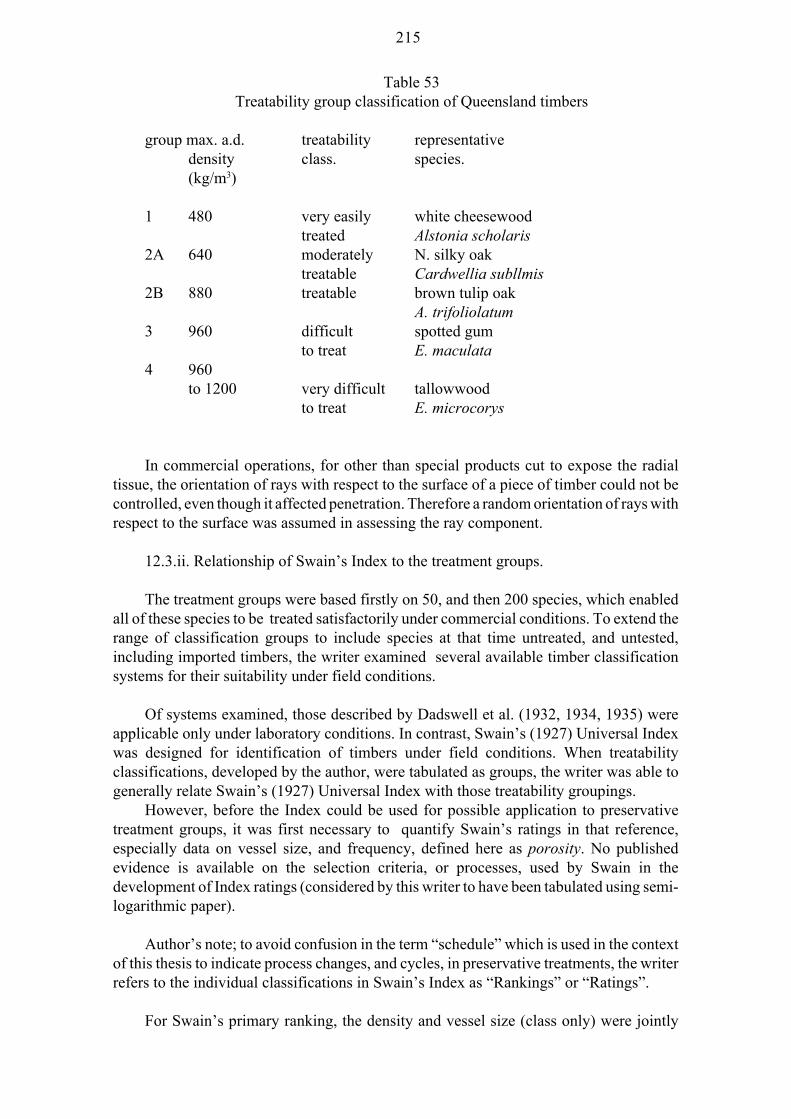
215

Table 53Treatability group classification of Queensland timbers

group max. a.d. treatability representativedensity class. species.(kg/m3)

1 480 very easily white cheesewoodtreated Alstonia scholaris

2A 640 moderately N. silky oaktreatable Cardwellia subllmis

2B 880 treatable brown tulip oakA. trifoliolatum

3 960 difficult spotted gumto treat E. maculata

4 960to 1200 very difficult tallowwood

to treat E. microcorys

In commercial operations, for other than special products cut to expose the radialtissue, the orientation of rays with respect to the surface of a piece of timber could not becontrolled, even though it affected penetration. Therefore a random orientation of rays withrespect to the surface was assumed in assessing the ray component.

12.3.ii. Relationship of Swain’s Index to the treatment groups.

The treatment groups were based firstly on 50, and then 200 species, which enabledall of these species to be treated satisfactorily under commercial conditions. To extend therange of classification groups to include species at that time untreated, and untested,including imported timbers, the writer examined several available timber classificationsystems for their suitability under field conditions.

Of systems examined, those described by Dadswell et al. (1932, 1934, 1935) wereapplicable only under laboratory conditions. In contrast, Swain’s (1927) Universal Indexwas designed for identification of timbers under field conditions. When treatabilityclassifications, developed by the author, were tabulated as groups, the writer was able togenerally relate Swain’s (1927) Universal Index with those treatability groupings.

However, before the Index could be used for possible application to preservativetreatment groups, it was first necessary to quantify Swain’s ratings in that reference,especially data on vessel size, and frequency, defined here as porosity. No publishedevidence is available on the selection criteria, or processes, used by Swain in thedevelopment of Index ratings (considered by this writer to have been tabulated using semi-logarithmic paper).

Author’s note; to avoid confusion in the term “schedule” which is used in the contextof this thesis to indicate process changes, and cycles, in preservative treatments, the writerrefers to the individual classifications in Swain’s Index as “Rankings” or “Ratings”.

For Swain’s primary ranking, the density and vessel size (class only) were jointly

216

grouped from 1 to 20.

For the densest timbers, Swain only cited a specific gravity above “1.0”. Based onmean timber densities, the author has determined this as 1200 kg/m3, deriving the valuefrom the mean highest probable (1184 kg/m3 + S.D) density of local timbers for use. TheIndex supplementary rankings, expressed as a decimal value, only used pore counts(expressed as a range) and vessel size groups. Of these features, vessel size categories of“coarse”, “fine”, and “minute”, were related to density in the primary Ranking 1, and tofrequency in Ranking 3 (Table 54). Thus, for both rankings, it was necessary to quantifythose size ratings. This was done by;

a. for Ranking 1, the air dry density and vessel size ratings were correlated as shownin Table 56, Appendix 24. Three parallel curvilinear (Graph 39), and three similarlogarithmic linear (Graph 39a), relationships were obtained, based on vessel size, namely“coarse”, “fine” and “minute”.

b. for Ranking 3, Swain’s vessel count, and size, ratings were compared (Graph 40).Confirmatory observations were made of the vessel size (Table 57, Appendix 24) andfrequency over a wide range of species with data from Dadswell et al. (1932, 1934, 1935).

Rankings from Swain’s Universal Index that were useful in this writer’s work areshown in Table 54.

12.3.ii.i. Applicability of Swain’s Index to preservative treatment.

The total numeric “derivative” of the separate rankings was not amenable to statisticalapplications. However the writer established that individual relative Rankings (Table 54)were suitable and closely correlated with anatomical properties of wood species, but, ingeneral, were not linear increments of properties.

The utility of this approach was confirmed by the successful prediction of, andexperimental confirmation of, the treatability characteristics of species not then previouslyclassified, or tested. The initial species classification groupings described above wereupdated progressively (Cokley, 1949c, rev. 1965, 1951) and a typical listing (Appendix 25)is shown. It is of interest that;

(a) Density/ ratings curves (Graphs 39, 39a) for each porosity class are approximatelyparallel. When the temperature drop required to produce satisfactory uptake of preservativein the Hot and Cold process was plotted against the maximum density value of each porosityclass (Graph 38), there was a near linear relationship. Graph 38a shows the lineartransformation of Graph 38. However, above about 880 kg/m3 density, the apparent

porosity increased. That changeappeared associated with, but not exclusively, Eucalypt species, which predominate in thisdensity range.

(b) In Ranking 3 (Graph 40), eg. for the finely porous sub-group, when compared toother porosity classes, there is a divergence in slope between lines.

217

Table 54

to classification of species into treatability groups.

ranking numerical descriptionrating

1 1—20 density and vessel size2 0.0— 0.9 ray count/5 mm dia. circle3 0.00—0.09 vessel count (5mm dia. circle)4 0.000—0.009 vessel structure (one group

specifically ring-porous)5 0.0000—0.0009 presence and arrangement

of parenchyma tissue.

12.3.iii. Development of species treatment conditions (or “schedules”) in terms ofgroups.

12.3.iii.i. Treatment schedules.

Coincident with species classifications and as summarised in Table 52, the authordeveloped effective schedules (Cokley, 1949c [rev. 1965], 1951).

The schedules coordinated results with species groups, and moisture content influ-ences, and included special schedules for thicker sizes, or for species, subject to thermaldegrade. As treatment systems (Appendix 14) and species utilisation in terms of hazards(Appendix 1) increased, the author (Cokley, 1965) advocated continued research by ForestProducts groups into timber treatability characteristics.

Recommended schedules, eg. showing times at temperature and cooling ranges, as afunction of treatment groups, and solution concentrations as a function of process, are givenin Tables 58, 59, 60, 61 (Appendix 26).

12.3.iii.ii. Provision for flexibility in schedules.

In establishing treatment schedules for species, the writer ascertained (Chapters 3, 8,13) effects of variation of density, structure, and moisture content. Though based on meandata, or determined specific values [exemplified by Mackay tulip oak (Chapter 8)],schedules were necessarily flexible for changes (Chapter 3) particularly in density (Appen-dix 27), and were typically based on +/- ( 10 %) variation of the mean value. This latter isexamined in Section 12.3.iv. A similar situation was developed for porosity. Where valueswere encountered outside those values;

i. if consistent variation was present (Chapters 3, 8), or was noted in a number of plants,species were upgraded to a higher treatability group.

ii. if of local occurrence, schedules were modified for that plant situation. Whereporosity values were low, schedule change often included local increase of solutionconcentration (especially in vacuum/pressure systems).

12.3.iv. Density and its influence on preservation.

218

Density is one of the most useful indicators of several very important structural andmechanical properties of timber (Kollmann and Cote, 1968) and is incorporated in mostdescriptions (Bolza and Kloot, 1963) of wood properties. Density is also the simplestindicator for the wide range of properties that influence preservation (Chapters 3 and 8) oftimber species being treated by plants which operated over extensive zones (Map 3).

In consequence, it was important to the present work to describe the range of wooddensities between species and the variation in these densities due to environmentalconditions. Extensive field and laboratory research by the author (Appendix 27) issummarised in Tables 62, 63, Appendix 27. If the variation in wood density is distributednormally about the mean, it may be summarised as normal variations at the 68% probabilitylimits are +/- 10%, and the 95 % probability limits are +/- 20 % (of mean, and published,values). A mean wood density for all Queensland species (Appendix 27) was determinedto be 789 kg/m3 (air dry at 12% mc), which is equivalent to a basic density (as specificgravity) of 0.631. This figure was used in appropriate calculations. Wood densities ofsapwood and of fast grown material were generally at the lower end of the 95% probabilityrange, so that a 20% reduction, or a factor of 0.8, of the species density could be applied.Conversely, slow-grown material had wood densities that were at the upper end of the 95%probability range for the species density, and these characteristics had to be taken intoaccount during the planning of preservation treatment schedules.

12.4. Principles of Wood, Air, Water, Interactions, and their Relationships to Pre-servative Treatments.

Practical development of treatment schedules was based initially on findings in boththe laboratory and field. However, the successful results obtained, which included predic-tions in treatment classifications of originally untested species, were predominantly basedon wood “macro structural” properties. They emphasised significances of de-aeration, ofdensity, and of moisture content. It became clear that relationships between wood structure,density, moisture content, de-aeration, separate methods of solvent (discussed here princi-pally as water), and of the preservative solution, penetration into wood, and the resultantpreservative uptake, needed to be examined. The underlying principles of interactionsbetween wood, pathways for gas, liquid and solutions (Chapter 8) movement, as well as“sites of deposition of solutes” had to be clarified. In particular, these were examinedthrough studies of the distribution,interconnection and size of air spaces (void volumes) intimber. One of the most important factors was soon found to be the manner of interconnec-tion of air spaces.

Evidence (Chapter 8) including seasoning research, led to conclusions that, forangiosperms, sites and “flow paths” for air and water, differed to those for preservativesolutions and solutes. Wood tissue is a “semi-permeable” membrane. The interchangeabil-

Importantly, air flow characteristics differed between hardwoods and softwoods, andwere used in terms of pattern, and the rate of flow, as indicators of a timber’s treatability,and thermal uniformity of plants.

gymnosperms, do notapply to angiosperms because of limited access for aqueous solutions, and similarly for“deposition sites” of solutes, which are caused by the “reactivity” and “penetrability”(Chapter 8) of timber.

There were shown to be “macropathways” for solutions, and “deposition sites” of

219

solute were restricted only to these “macro structural” features. However evidence, firstnoted as “expulsion of contained air” (Section 12.4.i) in thermal processes, and of moisture/air changes in seasoning operations, suggested presence of “permeable micropaths”, basedon the wood “microstructure”, may separately control air, and water, movement (cf. use ofmicropore filtered water in studies by Kininmonth, 1971) in timbers.

Density was a common factor, and “air/moisture content” relationships with densitywere defined as a “paradigm”.

12.4.a. Definitions of the terms, “accessible free paths” “orifices” and “effectiveorifice diameter”.

12.4.a.i. “Accessible Free Paths”.

For both sub-phyla, the total “void volume” consists of the separate voids in vessel,ray, fibre (and tracheid) lumina, but also includes the wall cavities.

There arose, in this context, need for a general term to explain, to include, and to enabledifferentiation of (Chapter 8), selective penetration in hardwoods. It should be usable forboth softwoods and hardwoods in these discussions.

The proposed general term would principally apply to the “micro structural move-ments”, but it should also be utilisable for the “macrostructural levels of restrictedmovements” within wood.

This term was titled the “Accessible Free Paths”, and the qualifying keyword,“Accessible”, was further associated with the quantifying adjective “Effective”. Thekeyword identified whether access was unimpeded, or if it was impeded. The adjective“effective” related to equivalent duct lengths, numbers, and diameters (or radii).

If access was restricted to limited “routes”, and was affected by “reactivity” (Chapter8), the definition applied for “penetration” of either certain liquids or of solutions (thus sitesfor solutes) and was applicable to the “macro pathways”, which include vessels and rays.

If access was unimpeded, the term “permeable” (Chapter 8) applied, and was shownby air/water penetration of wood, and “accessible free paths” then significantly related to“pit microducts”, and to “wall apertures or openings”. These were described under thegeneral term of “orifices” (Section 12.4.a.ii.) and of which (Section 12.4.1) the number,“n”, of the “effective orifices” (cf. definition below) could increase, so markedly causinga drop in “effective diameters”. These latter may be dimensionally different to, but couldapproach, the “mean molecular free paths”. Mechanisms for flow could differ for the lattercase.

12.4.a.ii. Orifices and Effective Orifice Diameter.

In early deductions based on treatment and air flow, the writer considered “microducts”were probably different in dimensions to the accepted definition of “pit diameter”. Thislatter was later clarified as being the “pit chamber diameter”, and used in some flowequations. Literature subsequently indicated “microducts” would be of neither uniformsize nor structure. The terms “Orifice”, and the “Orifice Diameter (or Radius)”, were theoptimum expressions to denote “micropaths or microducts” in terms of mechanisms offlow. The former is also described in this work as the “Effective Orifice”, or the smallest

220

pore through which gases or liquids may pass under defined physical conditions.Originally, classical structures, and dimensions, of pits had been considered and used,

but data from Cronshaw (1960) showed they were much more complex. Based on that data,pit membranes are considered equivalent to a “generally impermeable membrane withvariable size micropores”, and the orifices effective for air, and water, movement are theindividual “micropores”.

Their sizes, and equivalent duct lengths, were extremely non-homogeneous (Comstock,1967). That explains use in this text of the “effective orifice diameter”, which, in fact, maynot be the simple additive values (in terms of flow) of each “micropore” available for air,or water, flow (this term also applies to the fine openings in cell walls). When “n” was high,the effective orifice diameter was small, and resultant dimensions became the point at whichthey may approach “mean molecular free paths”, and was one reason for use of Graham’slaw in Chapter 14. However, both of the terms, “microduct” and “diameter”, continue to be

12.4.a.ii.i. This accumulated evidence of low values in the “effective orifice diameter”introduced possible effects of “slip flow” as compared to “viscous flow”. The significanceof this is illustrated by Forest Products Research Laboratory (1964, 1965) studies whichshowed viscous/slip flow effects due to small wall openings were present in softwoodstested, but not present in the three permeable hardwoods examined. Comstock (1967)summarised the respective importance of “slip” and “viscous” flow for two gases and twoliquids. He showed, dependent on swelling properties of a liquid, “permeability” was afunction of wood rather than either the gas, or liquid, used for “porosity” measurement. Healso demonstrated;

a. gas flow measurements under a pressure differential were satisfactory as atechnique in this area. This was in line with principles employed in Chapter 14. In thatChapter, as flow data was measured externally, the effect of “slip flow” is not mathemati-cally separated.

b. mathematical “models” of flow in wood are necessarily simplifications, and inwood, the “pore/duct flow path” (this writer’s term is “complex”) is multiple (suggestingflow is probably not uniform in each separate “path”).

Comstock’s data implied a “probable mean value” would be the best available, andrepresented a wide distribution range. This was in accord with the “effective orifice” theoryas developed by this writer.

12.4.a.iii. The original “microduct” theory, and terms, could not be confirmed untilvacuum studies in 1961-63, which importantly (Section 12.4.1) showed the “effectiveorifice diameter” was a function of the number “n” of “orifices”, and, hence, could be of verysmall sizes. Relationship of size (diameter or radius) became clearly associated withnumbers present (which could be variable) in pit membranes, or in microfibrils (principally)as an “annulus” in softwoods with tori, or in cell walls. Incrustation of walls and membranesmay be a factor.

12.4.1. Effective “orifices” for gas and liquid flow in timbers.

Preliminary studies indicated differences between gymnosperms (softwoods) anddicotyledinous angiosperms

221

specimens under solution as they were heated during preservative treatment. The pattern ofsubsequent uptake of preservative solution indicated strongly that movement of air wasdependent on orifices that were different in size from the lumina of vessels, tracheids orfibres. In particular, degassing at elevated temperature was a direct function of temperature,duration of exposure at that temperature (Chapter 13), timber species, density and cross-sectional dimensions. For both softwoods and hardwoods, and under any treatmentcondition, degassing would cease after a certain time.

A wide range of hardwood and softwood (indigenous and exotic) species were treatedby the open tank thermal processes, and manometers inserted to the cores of specimensindicated that, during the initial (Section 12.3.i.ii) heating cycles, the gas pressure withinthe wood increased, and decreased again during cooling. The initial increase in pressurewould create a gradient in pressure from the centre to the edge of the timber specimen, thusinvoking gas flow and degassing. The same phenomenon (a thermal vacuum) wasconfirmed by mechanical pump evacuation in closed treatment vessels, especially (Chapter14) when the timber was immersed in a solution.

In gymnosperms, bubbles were released in continuous and relatively uniform streams,the rate varying between slow-grown material from native forests and fast-grown plantationmaterial. A difference was noted between earlywood and latewood in exotic plantationspecies.

In contrast, the appearance of bubbles from angiosperm timbers was cyclic, with aseries of generally relatively large bubbles alternating with periods of quiescence. Consid-erable differences were observed in the rates and patterns of degassing that correspondedgenerally with the differences in wood structure.

This cyclic degassing in angiosperms suggested that there was a periodic release of gasfrom vessels, causing the large bubbles, and a more continuous release from other tissues,particularly fibres. It was concluded that the limiting apertures were not the vessel lumina,but were the pit openings, or the perforation plates, and the interfibrillar spaces within cellwalls.

It is pertinent to note that this work was carried out between 1947 and 1960, whenultrastructural descriptions of wood were unavailable, except through the CSIRO Divisionof Forest Products, when theories of gas and liquid movement in wood were much lesselaborate than at present and when laboratory facilities were much less sophisticated thanthose available today.

Subsequently (1961-63), the hypotheses established in this early work were testedunder vacuum treatment conditions.

12.4.1.i. Determination of effective orifice diameters.

To quantify and demonstrate the processes of gas and liquid transport under vacuum,special laboratory facilities were constructed (Diagrams 3a, 3b, 3c, Plate 4, Chapter 14)which permitted studies on specimens up to 1.8m long. The conditions that could be testedwere dry, or wet, vacuum, with, or without, timber specimens. An important practicalfeature of this apparatus (Cokley and Smith, 1965 a,b) was that all units were constructedfrom Quickfit industrial or laboratory glass assemblies, so specimen degassing and liquid

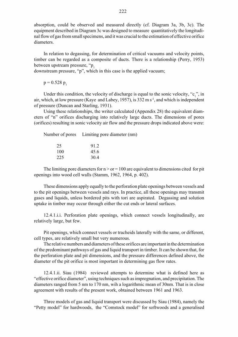
222

absorption, could be observed and measured directly (cf. Diagram 3a, 3b, 3c). Theequipment described in Diagram 3c was designed to measure quantitatively the longitudi-nal flow of gas from small specimens, and it was crucial to the estimation of effective orificediameters.

In relation to degassing, for determination of critical vacuums and velocity points,timber can be regarded as a composite of ducts. There is a relationship (Perry, 1953)between upstream pressure, “p1downstream pressure, “p”, which in this case is the applied vacuum;

p = 0.528 p1

Under this condition, the velocity of discharge is equal to the sonic velocity, “c1”, inair, which, at low pressure (Kaye and Labey, 1957), is 332 m s-1, and which is independentof pressure (Duncan and Starling, 1931).

Using these relationships, the writer calculated (Appendix 28) the equivalent diam-eters of “n” orifices discharging into relatively large ducts. The dimensions of pores(orifices) resulting in sonic velocity air flow and the pressure drops indicated above were:

Number of pores Limiting pore diameter (nm)

25 91.2100 45.6225 30.4

The limiting pore diameters for n > or = 100 are equivalent to dimensions cited for pitopenings into wood cell walls (Stamm, 1962, 1964, p. 402).

These dimensions apply equally to the perforation plate openings between vessels andto the pit openings between vessels and rays. In practice, all these openings may transmitgases and liquids, unless bordered pits with tori are aspirated. Degassing and solutionuptake in timber may occur through either the cut ends or lateral surfaces.

12.4.1.i.i. Perforation plate openings, which connect vessels longitudinally, arerelatively large, but few.

Pit openings, which connect vessels or tracheids laterally with the same, or different,cell types, are relatively small but very numerous.

The relative numbers and diameters of these orifices are important in the determinationof the predominant pathways of gas and liquid transport in timber. It can be shown that, forthe perforation plate and pit dimensions, and the pressure differences defined above, thediameter of the pit orifice is most important in determining gas flow rates.

12.4.1.ii. Siau (1984) reviewed attempts to determine what is defined here as“effective orifice diameter”, using techniques such as impregnation, and precipitation. Thediameters ranged from 5 nm to 170 nm, wih a logarithmic mean of 30nm. That is in closeagreement with results of the present work, obtained between 1961 and 1963.

Three models of gas and liquid transport were discussed by Siau (1984), namely the“Petty model” for hardwoods, the “Comstock model” for softwoods and a generalised

223

model for hardwoods. In the latter model, the predominant role of vessels in transport isemphasised.

angiosperms can bedescribed as follows. In vessels, longitudinal flow is unimpeded until the gas reaches aperforation plate. The pressure difference required to induce sonic velocity flow isdetermined by the size and number of perforations in the plate. For sclariform perforationplates, the effective pore diameter is related more closely to the minor than to the major axisdimension of each perforation. The author found it useful to distinguish between “simple”orifices, in which the perforations were approximately circular in section, and “compound”,in which they were markedly asymmetric.

12.4.1.iv. Concurrently with degassing of vessels, but at different rates, there is acomplex pattern of air flow between fibres, from fibres to vessels and rays, and from vesselsto rays, principally through pit openings. These openings are commonly smaller and morenumerous than those between vessels.

There is also some gas flow between cell wall interstices (Table 14), but theirdimensions are very small compared with vessel pit openings, and the fluid transport ratesmay be low.

In this work, it is concluded that effective pit opening diameters between vessels andrays, and the equivalent dimensions of perforation plates between vessels, are the primaryorifices determining the rates of degassing and of liquid penetration (Chapter 8). Whetherradial, or longitudinal, flow predominates depends on relationships between the samplelength and the dimensions of vessels.

However, for liquid penetration in hardwoods, a long period of observation led thewriter to the conclusion that there were three categories of effective orifices: vessel lumina,perforation plates, and vessel-ray pit apertures. It should be noted that checks in timber alsofunction as effective orifices, and must be avoided when gas and liquid movements arebeing examined in small specimens.

The importance of the role of effective orifices through which exchange occurs isdemonstrated by detailed reviews by Comstock (1967), Kollmann and Cote (1968),Kinninmonth (1971), Siau and Petty (1972) and (Siau, 1984).

12.4.1.v. However, Siau (1984, p. 103) cites data from Comstock (1970) for variationsof about 160-fold between tangential and longitudinal permeabilities, and about 350-foldbetween radial and longitudinal permeabilities, adding that greater variability in the radialdirection could be related to large differences in the permeability of ray tissues.

Chapter 10 (Graph 8) describes marked differences in the preservative concentrations,concentration gradients, and depths of penetration, between backsawn and quartersawn(AS 01 - 1964) material, This applies for all treatment processes and solvents. In seasoningpractices, similar differences between backsawn and quartersawn timbers were reportedby Kollmann and Cote (1968). For other than special species and products, segregation ofsawn timber based on angle of cut was not commercially practicable and distribution(Chapter 10) was random in any charge. However, evidence derived from research, andindustry, studies led the writer to the conclusion that, for local species, a radial movementof preservative in timber is significant.

224

12.4.1.vi. Importantly, for orifices in perforation plates, two differences exist relativeto pit openings in fibres. They are that perforation plates are much larger, and they do notact as “selective” or “semi-permeable barriers” to preservative movement.

12.4.1.vii. Differences in the Pit Structures between gymnosperms and angiosperms.

One reason (Sections 12.4.a.ii, 12.4.1) for adoption by the author of the term “orifice”rests in the structural differences between pits in these two sub-phyla. As a consequenceof these structural differences, the effective “accessible free path” (Section 12.4.a.i) forpreservative solutions, and deposition of solutes, and possible mechanisms of fluidmovement could differ. Use, by the author, of the general term “orifice” though recognisingthe possible differences on flow and “effective radius” (Section 12.4.a.ii), enabled them tobe jointly discussed under that term for this context.

12.4.1.vii.i. It was important to develop this aspect of the writer’s work because ofpractical implications of the anistropy of solvent, and solute, movements in timber withvariation shown between species. Differences between a solution flow and solvent flow,though accepted by industry, was not accepted by some research workers at that time.Though workers such as Rudman (1965, 1966) reported on their examination of experimen-tal material, this writer (Section 12.4.2.ii.iii) found that, in over 300 hardwood species, pitswere consistently impervious to solutions. Only surface fibres showed preservativepenetration. These conclusions were based on sensitive “spot tests” with (Chapter 11) adetection limit below 5 micrograms.

Water, gases, and some solvents, were fully accessible to all tissues, but not all resultedin swelling. The hypothesis (Chapter 8) that the wood tissues were acting as “semiper-meable barriers” appeared to offer an adequate explanation for this evidence.

12.4.1.vii.i.i In gymnosperms, fluid and gas flow ocurs largely through tracheidsconnected by bordered pits, some of which may have tori. Passage of air/liquid interfacesdepends on the relationship between the dimensions of orifices in pit membranes and thepressure differential between adjacent tracheids.

Gymnosperm timber placed under liquid at reduced pressure will emit gas as the resultof its flow between many tracheids. The process will occur more or less uniformly fromall tracheids, except for the smallest and thickest-walled latewood elements. This phenom-enon was seen in preservative treatment studies as uniform escape of many small bubblesfrom the cut surface, and ends, of a piece of timber.

In angiosperms, the volume of a vessel may be about 1000 times greater than thevolume of an adjacent fibre. During evacuation experiments, air expulsion was cyclic, wasprincipally of relatively large bubbles (and thus assumed by the writer as exiting frommainly the vessels) and some smaller ones. These were followed by a period of quiescenceand the cycle was repeated. This cyclic flow was explained as due to slow degassing of thefibres with the relatively large bubbles being emitted from vessels, and the very smallbubbles being emitted more slowly as the fibres are evacuated. By contrast, gymnospermtracheid diameters are relatively constant, and the uniformly small constant air flow fromspecimens may be stated as being consistent with gas flow laws.

The pattern of movement of air during the evacuation phase of preservative treatment

225

can be taken as an indication of the pattern of liquid entry into the timber when the pressurein the system is increased. These hypotheses, which evolved during the development ofpreservative treatment schedules, are consistent with the date and conclusions of otherworkers. These include Ellwood (1958), Preston (1959), Cronshaw (1960), Wardrop andDavies (1961), Rudman (1963), Skene (1965), Stayton and Hart (1965). Liquid penetratoninto the timber is likely to be incomplete, depending on the extent and duration of thereduced pressure phase. Siau (1972) calculated that the fraction of the void volume oftimber filled was related to the square root of the applied pressure.

12.4.2. Anomalies in the applications of theoretical void volume formulae to preser-vation of timbers.

Sections 12.1, 12.2 and 12.3, described development of effective timber classifica-tions and treatment schedules. These were based on “macro structural properties” andmoisture contents. As part of this work, the writer had compared treatment group data,schedules and uptakes, against estimates of void volume (Chapter 14, Appendix 38;Maclean, 1935, 1952; Stamm, 1938, 1964, 1972). This section examines some aspects ofvoid volume of sapwood as it applies to timber preservation. The concept of void volumehas been developed for a variety of purposes by Kollmann and Cote (1968, pp 232-234) andSiau (1984, pp 25-30), who equated it to porosity as calculated from oven dry specificgravity.

Void volume as described by other workers relates to the theortical space available inthe timber for liquids or gases, and it assumes perfect penetration.

Many workers transpose the void volume relationship from being one of “air / moisturecontent / density” to being equivalent to “air / treatment solution / density”.

However (Section 12.4.a), differences were found which demonstrated, though thisassumption was adequately true for gymnosperms, it does not apply for angiosperms. Forthe latter, important physicochemical effects, including “wettability” (Appendix 15), andwood chemical reactivity with preservatives (Chapter 8) affect the void volume availablefor preservative uptake. Siau (1984) made reference to certain of these aspects, but theyhave not been considered in detail elsewhere. Observations and experiments are describedbelow in gymnosperm and angiosperm species, using both sawn timber and poles.

12.4.2.i Gymnosperm species.

At the time this work was initiated, gymnosperm timbers were required to be at, orbelow, fibre saturation point before preservative treatment by vacuum/pressure methods,irrespective of the required level of treatment, or the preservative type (AS 1604-1980) orits characteristics.

This requirement for low moisture contents caused increasing commercial difficulty,and it was necessary to establish the relationship between void volume, moisture contentand preservative retention in order to obtain effective and economic treatment. Theeffectiveness of a preservative treatment depends on specific gravity of the timberspecimen, which varies significantly with tree age, within a given piece, and within growthrings. The variation is particularly pronounced in plantation-grown Pinus species, whereearlywood and latewood bands have very different specific gravities, structure, andpreservative uptake rates, but not very different natural timber durabilities.

226

Substantial variation was observed in the effectiveness of (full cell) commercialtreatment of gymnospermconcentration of preservative across the diameter of two Pinus taeda poles treated (withmean sapwood retention of 24.29kg/m3) in a commercial cylinder as part of a charge ofsimilar poles, and at a nominal CCA solution concentration of 3.0% m/v. Both poles containvisible heartwood. The mean basic density was 0.462, as compared with the published valueof 0.595 (Cause et al., 1974).

The variation in preservative concentration with distance from the surface wascompared at 2.7m and 5.0m from the butt of two P. taeda poles, 9m long, containing novisual heartwood, and with a mean specific gravity of 0.420. To confirm influences ofsolution concentration, the poles were treated in a commercial CCA solution of 10% m/v.Mean diametric gradient results, sampled at 6mm intervals, are presented as Graph 42.Though individual gradient results show assymetry, mean (84.34 kg/m3) CCA concentra-tion was slightly, but not significantly, greater at 2.7m than at 5.0m (78.20kg/m3) from thebutt, indicating penetration over 5m was effective in this species. Decrease in CCAconcentration with increasing distance from the surface suggests that, either there is someradial transport of preservative, or axial transport through the inner sapwood is slower thanthrough the outer sapwood. To test the possible effects of circumferential position in a pole,for these poles, a separate sample 0.3m long was taken above, and adjacent to, the twodiametric sampling positions (2.7m and 5m).

Three radial sub-samples distributed at 120o around the stem, and circumferentiallyaligned with those in the other sample section, were analysed, details of which shown inTable 64, Appendix 29. Results show that, for the bulk samples, neither circumferential norvertical differences were significant. Differences in salt uptake between earlywood andlatewood from the same growth ring in three poles of P. elliottii var elliottii are shown inTable 65, Appendix 29. It will be noted that retentions are in agreement with changes inspecific gravity and differences in structure of these bands. When results are related to datacited in Graphs 41, 42, and to other similar studies made, the conclusion is drawn that radialpenetration is significant. On this basis (and this was found in sawn timbers with early orlatewood face sections), the assymetric results found in those poles may relate to theproportional influence of these bands (Eccles, 1974) present in exotic species.

12.4.2.ii. Angiosperm species.

In addition to the more complex anatomical structure, angiosperm timbers differ fromgymnosperms in the greater range of specific gravities (0.300 to 1.100) (Kollmann and Cote,1968), and locally extending to 1.200. Many open forest species have specific gravities inexcess of 0.800, which [Equation (12.3)] (Section 12.4.3), suggests their void volume isabout half of that of a gymnosperm44).

Work described earlier (Chapters 8, 10, Section 12.4.a) established that preservativesdid not penetrate the heartwood (or fibres), of hardwoods, although water and light polarsolvents (eg. ethanol) did , as reported by Kininmonth (1971). Below fibre saturation point(FSP), penetration of these small polar molecules was shown to be a function of the moisturecontent. Viscosity (a function of temperature), and polarity were observed to control thepenetration of oils, as confirmed by Siau (1972). In mixed solutions, a chromatographiceffect occurred, as described by Huber (1935, n.r.) and in Chapter 8. This phenomenonaffects not only preservative penetration, but also “wettability” (Appendix 15), the

227

measurement of pH (Chapter 8), the distribution and colour of stains, the adhesion of paintsand finishes. Several consequences of differential penetration include:

(a). Gluing, especially of solid timbers using radio frequency heating. The difficultyof gluing generally increased with density, so that increasing the contact surface area bygrooving was practised. This phenomenon was important in finger-jointed flooring,mouldings and structural timbers.

(b). “Incising” by narrow knife cuts parallel to the grain on the lateral surfaces oftimber was used to increase the extent and uniformity of penetration of creosote/oil

(c). The rate of spread of flame on hardwoods was commonly greater than that ofsoftwoods treated with a given concentration of fire retardant chemical. Similar differenceswere also observed between latewood and earlywood of exotic plantation conifer species.

(d). The performance of water repellant treatments was relatively poor in hardwoods,and similar differences existed between latewood and earlywood bands in exotic plantationconifer species.

(e). “Oxy-charring” of transmission poles (Chapter 15) was very effective inpromoting penetration of creosote because it greatly increased the porosity of timbersthrough carbonisation of the outer layer of wood.

(f). Service problems with hardwood species in marine environments (Chapter 15) andsusceptibility of hardwood poles to soft rot in terrestrial service (Chapter 15) wereassociated with the failure of penetration of preservative into fibre tissues below thesurfaces.

12.4.2.ii.i. End- and cross-grain penetration.

Work described in several sections of this thesis (particularly Chapters 10 and 14)bears on the problem of penetration of preservatives along the grain and across the grain.For the majority of Queensland timbers tested by the writer, there was no detectabledeposition of preservative in the fibres beyond the surface 0.5 to 1mm.

12.4.2.ii.i.i. Studies showed that when long boards of white cheesewood (cf. Graph10), with one end sealed to prevent penetration from other than faces and sides, were treatedin 25mm and 50mm thickness, and sampled in 50mm intervals from unsealed ends, an “end-grain” penetration of boron salts (as boric acid) was highly significant to 100mm, andsignificant to 200mm, from the unsealed ends. Tests were made to ascertain if the higher“end-grain” retention could represent possible penetration of fibres.

If fibre penetration had occurred, then the percentage of void volume required tocontain the measured salt concentration would be in excess of vessel cavities (parenchymawas not included in calculations).

This can be determined (Section 12.5.4) by “Specific Void Volume, SVV”, and“Specific Void Concentration, Scis compared to the void volume, it is also calculated on basic density, though for normalcomparisons (refer note below) the air dry density is used. Final “Sc” values are then

228

converted to an equivalent concentration expressed as mass/mass, oven dry basis, for thewhite cheesewood. For the 0-50mm distance, the concentration is 2.1% (o.d.m/m), fallingto 1.23% at 50-100mm. Comparative data were;

Void volume (white cheesewood) = 0.664

For white cheesewood (Graph 10), a mean vessel diameter of 260 microns, a count (20mm2) of 70, i.e 3.5 / mm2, a wood B.D. of 400 kg/m3 are used. The “SVV”, and “Sc”, show(assuming a 2.0% m/v boric solution with a specific gravity equal to 1.000) the salt uptake

“SVV” = (0.2602 x 11/14 x 3.5) / 0.400= 0.4647“Sc” = 0.4647and the retention = 464.7 kg/m3

Thus, as oven dry mass of the wood is 429 kg/m3, the dry salt concentration is;% boric acid = (464.7 / 50) /429= 2.16% o.d., m/m.

and percentage (“SVV” / void volume) = 69.98%As the concentration of 2.16% is of the same order as the measured (0-50mm) value

of 2.1%, it was concluded there had been no significant end-grain penetration of fibres.

The significant end-gradient preservative concentration may be explained as the endzone is subject to the maximum pressure differential, including thermal, and as flowprogresses, the differential is reduced, eg. by the resistance to flow.

Author’s note; when comparison is made between possible treatment of timbers fromdifferent sources, or of different species, the published (or measured) air dry density at 12%mc is used for calculation. When this is used in calculation, a value of 1.8% boric acid (o.d.m/m basis) is given. Comparison of “1/c” [equation (12.1.c)] for Graph 37a, where “1/c”is “nominal uptake at infinite time” is 1.73% boric acid, on an o.d., mass/mass basis.

Analyses away from the end show the “actual to possible” values of “Sc” are less thansaturated, being only of the order of 60%. This can be reconciled with capillary flow, anddecrease of effective pressure with length of duct. The uniformity (non-significantdeviations about the mean) along the length, the differences in gradients in Graph 11, andinfluence (Graph 8) of angle of cut lead to the conclusion that predominantly flow is by thevessel systems, but away from the ends, the effects of a radial penetration becomesignificant. This research explains differences in preservation concentration gradients withspecimen thickness in treatments, reasons to eliminate “end-grain effects” in sampling, anduse of a nominated minimum specimen length for research, or testing, in all processes.

Using similar studies on denser timbers, the “end-grain” salt concentration effect wasshown to be limited to within the 0-25mm zone.

12.4.2.ii.ii. End effects of air flow.

Air movement could be demonstrated up to 200mm from the cut ends of spotted gumsamples (Graphs 52a, 52b, Chapter 14). which is of the same order for thermal vacuums(defined Section 8.xi.i, Chapter 8), but this did not represent the extent of preservative

229

movement. Therefore, unless chemically verified, penetration tests carried out with highlypermeable materials do not reflect the patterns of movement of preservatives, many ofwhich are composed of molecules much larger than stains.

Effective research into preservative penetration required sampling to exclude the end-grain effect, or the use of end sealants. Analysing the different data, it is suggested that thelarge differences of “end-effect” between air (Graphs 52 a, b) and end-grain preservativeconcentration, are related to the density and viscosity differences of air to liquids, and thatincludes aqueous solutions and oils. Similarly, Siau (1972) demonstrated end-grainpenetration as a function of time, liquid viscosity and specimen length.

Rudman (1965) examined penetration of four eucalypt timbers by a range of fluids,preservatives, and wax, and drew conclusions on the penetrability of preservatives. Datacited in that paper show less uptake of creosote than obtained in commercial treatments,especially for spotted gum and mountain ash which meet retentions as specified in both AS0117-1970 and AS 1604-1980. For the former species, this writer carried out refereeanalyses, as well as tests under T.U.P.A. (1949), in which pole sapwood retentions (as inthe above standards) were obtained. Cummins and Dadswell (1935) reported high retentionsin mountain ash poles, and that was confirmed by commercial pole treatments in Victoria.

In an attempt to reconcile the apparent discrepancies, Rudman’s data were reviewedby this writer, and it seemed that many of the conclusions had been influenced by;

a. the possible extent of end-grain penetration in small specimens.b. apparent use of “mature stem” material, as indicated by basic density values quoted

(cf. Appendix 27).c. low values of vessel cavity areas (possibly related to the method used for their

measurement).d. the use of total void volume as the measure (fig. 12 of that paper) of creosote uptake

in spotted gum.

General application of total void volume for preservative retention is indicated in theformula used. This last is anomalous, as one apparent objective of that study was to ascertainif any preservative distribution extended to zones other than vessel cavities.

Using data from that paper, and a procedure similar to the method for analysis of the“end-grain” penetration in white cheesewood (Section 12.4.2.ii.i.i), Rudman’s results weretested against the “Specific Vessel Void Volume, SVV” and the “Specific Void Concen-tration, Sc”. These led to conclusions that wax penetration is restricted only to vessels, butfor water, and possibly chloroform (one species), penetration is in excess of vessel cavitiesas a percentage of total void volume. These opinions were based on the detailed analysisdescribed in Appendix 30A.

Author’s note; it is appropriate to indicate that creosote is not a single compound.Dependent on type, creosote may contain of the order of 180 compounds. About that era,the creosote used in Australia changed from the K55 type (obtained from household gasretorts), which contained higher concentrations of both tar acids and lower boiling pointfractions. A formulated “High Temperature Creosote” was adopted in which, particularly,the tar acid content was reduced.

230

12.4.2.ii.iii. Experimental study of deposition sites of preservatives in hardwoods

Because creosote and oil-borne preservatives may “bleed” from timber (confirmed byGilfedder, 1972) or be smeared across cut surfaces (confirmed by Rudman, 1965), theirpenetration distribution was investigated on split, seasoned surfaces. For aqueous solu-tions, transverse cuts presented similar problems to those described above, and softening,by preboiling, for microscopic studies was found (as for starch granules, Chapter 4) to affectsalt distribution and concentrations in the timber. Presence of “free liquid” prior toseasoning and redistribution (Graph 11) of solutes caused by seasoning, affected thevalidity of assessment. Consequently, studies were made subsequent to a seasoning period,and were standardised on split surfaces (dressed smooth as required), cut away from theends.

Microchemical tests [Feigl, 1958, 1966; Snell and Snell, 1949] (cf. class b - spot tests,Section 11.x, Chapter 11) typically sensitive to less than 5ppm, were employed to establishdeposition sites and, in addition, where applicable, ultraviolet fluorescence techniques(Chapter 8) were used, particularly for oil type preservatives. As studies were on splitsurfaces, stereoscopic microscope (to 40x) examinations were made during tests to confirmdeposition sites.

In the present work, conclusions on deposition sites were established experimentally,and confirmed in commercial operation by impregnating wood at various moisture contentswith mobile and slowly penetrating liquids, salts, multiple preservatives, in aqueous media,a range of solvents, and creosote either alone or admixed with oils (eg. Cokley and Rees1964, Cokley and Smith 1965; Appendix 2). This phase included a ring porous species, redcedar, Toona australis, in the studies. Research extended to include dyes. The cooperationin this work of commercial processors in Queensland and northern New South Wales, theCSIRO Division of Forest Products, and the Division of Wood Technology, New SouthWales Forestry Commission, was vital.

All the evidence indicated that, irrespective of species, preservative, process, ormoisture content at treatment, no effective concentrations of preservatives occurred inangiosperm heartwood fibre lumina other than adjacent to a surface, or in very short end-grain penetration, area. Some penetration occurred in sapwood fibre lumina, but it variedwith chemical species (eg. sodium hydroxide). For other than in the surface, or for short (andvariable) end-grain, fibres, the tests, as described, demonstrated negative (or minimal, eg.at, or below, ppm levels) preservative retentions in adjacent, or multiple, fibres.

Treatment of thin veneers (very high surface / thickness ratios and a high number ofcut, exposed, fibres) using borax, by the “Momentary Dip” process (Chapter 8), where theaqueous preservative film was applied by “pressure roller” during submersion, followed byblockstacking, did, for some species, result in penetration of cut fibres from the surface, orthrough the “peeler checks”, but was only to about 1mm depth from the veneer surfaces, orin fibres adjacent only to the “peeler checks”.

These findings on the absence of effective preservative levels in wood fibres wereverified by field service observations (cf. Chapter 15).

12.4.3. Differences between angiosperms and gymnosperms in relation to loss of freemoisture and distribution of air space in wood cells.

231

As stated in introducing Section 12.4, the writer examined applications of theoreticalformulae to clarify anomalies and differences found by him in relation to the sites and flowpaths between air, water and solutions. Initially, this required quantifications of the volumesof, and dimensions of, the respective wood elements, namely tracheids, fibres and vessels.Subsequently (refer Section 12.5.4), study extended to measurement of levels of preserva-tive deposition.

The relative proportion of wood elements present in hardwoods and softwoods isvariable between species and families. In his early work, the writer found difficulty inobtaining data from independent references on the relative percentages, especially forfibres. In contrast, there were, due to interests in possible wood utilisation as a pulp source,and including the writer’s own analytical data, considerable quantified references oncellulose and lignin concentrations in timbers.

To determine an acceptable value, and as part of his research into “Specific VesselVoid Volume” concepts (refer Section 12.5.4), the writer assessed residual fibre volume.For this, he determined (cf. Appendix 16 and Section 12.5.4) the mean total vessel volume,per mm3, for 45 random species, which ranged from a minimum of 30% to a maximum of37% (mean 35% [compare Table 13]). When allowance was made for such as the radialtissue volume, the value of 50-55% was accepted as a “working” fibre volume, with thecaution that fibre lumen diameters may be a function of wood density. As illustration of therange of variation, assessment of species listed in Appendix 16 show a mean vessel volumeof about 25%. This value was obtained from a sample of 27 species, as compared with the45 species discussed above. value of vessel volume. As such, based on Appendix 16, equivalent fibre volume valueswould increase. Later evidence (eg. Kozlowski, 1971) cited fibre volumes from 50% to70%.

12.4.3.i.a. Use of Published Data.

Browning (1963) lists typical values and also includes ranges, which are summarisedin Table 13 (Chapter 8). This was the first independent reference available to the writer,where wood tissues, for both hardwoods, and softwoods, were listed in both averagedimensions, and as a percentage of the total, and is used, where applicable, in discussion.It will be noted (Table 13) that tracheids occupy the major bulk of softwood volume; theirmean diameter is about 1.5 times that of hardwood fibres and the length about three timesgreater. Vessels (Table 13) occupy about 36% of the total volume and vessel elements areabout one half of the length of the fibres. However liquid flow may be assumed ascontinuous in the axial direction of the stem as vessels are interconnected by simple orcompound perforations plates. A sequence of connected vessel elements may be consideredas a continuous duct, of generally uniform crosssection, but characterised by repetitiousconstricted orifices or orifice plates. Vessels may be interconnected to ray cells, and fibres,by pit “orifices”. A typical vessel (Table 13) diameter (cf. Section 12.5.4) is about 3 x 103

the diameter of an average pit opening and varies between 4 and 20 times the diameter ofa normal fibre.

In view of their relatively small low volume, radial and vasicentric parenchyma ofangiosperms will be excluded in the subsequent discussions on this topic, even thoughthose tissues are generally penetrated by preservatives.

232

12.4.3.ii. Void Volumes, Density and Wood Structure.

12.4.3.ii.i. Determination of Air Space (void volume) in timber.

Considerable research has been conducted into this topic. A number of formulae(Maclean, 1935, 1952, Stamm, 1938, Harrow, 1947, Tamblyn and Bowers, 1961), Teseroet al. (1966) were developed. 1952) and Stamm’s (1938) formulae. Other authors, eg. Siau (1984, pp 25-30), Kollmannand Cote (1968 pp. 232-234) each discuss varying applications. Siau, using the oven dryspecific gravity, equates “void volume” with the term “porosity”. Kollmann and Cote usethe derivative to determine double cell wall thickness.

A formulation proposed by MacLean (1935, 1952) has been principally used fordiscussion by this writer. This is;

Mf = 100 { [1 / spg] - [1 / 1.53]} (12.3)

where Mf = Saturation Moisture Content.spg = specific gravity of specimen on oven dry weight and swollen volume basis.1.53 = specific gravity of wood substance in water.

f” is an inverse linearfunction of the swollen volume Specific Gravity, “spg”. The relationships of swollen woodmoisture content, basic density, percent air space and moisture content, based on MacLean(1935), are shown in Graphs 43, 44. There is a small, but significant, nonlinearity atmoisture contents below FSP. It was found due to;

(a). the use in MacLean’s data of the value of 1.53 for the specific gravity of woodsubstance. This is the value when wood substance is measured in water. When the value of1.46 is substituted at low moisture contents (below FSP), the nonlinearity becomesnonsignificant. Stamm (1938) discusses varying effects on void volume calculations by theseparate allowance for shrinkage and use of the two values of wood specific gravity. Otherauthors (Kollman and Cote, 1968, Siau, 1984) use a value other than 1.53, typically 1.5.

(b). Smith (1975) discusses the inclusion, below FSP, of the wood shrinkage factorof 0.28 x Basic Density (Greenhill and Dadswell, 1940). Smith (1975) also notes Nearn’swork (1953, not referenced in this text) relating variable FSP values to solvent extractionprior to measurement. That work thus suggests possible differences in cell wall structurewith species.

12.4.3.ii.ii. Influences of Density and “Saturation Moisture Content” on void volumecalculations.

The criterion employed is basic density (or the specific gravity), which is determinedon a maximum “saturation moisture” volume (Chapter 7), when it is assumed that all airspaces have been completely filled with water. In practice, “saturation moisture content”may be more accurately defined as that point in the water uptake at which a negligibleincrease in the mass is given, and consequently the “saturated wood volume” is eitherconstant, in equilibrium, or at a maximum. Care is necessary to ensure the oven dry mass,and specific gravity, are accurate, and adequately represent the gross timber sections beingtreated. That need is illustrated by studies on slash pine and loblolly pine [Section 12.4.2].

233

12.4.3.ii.ii.i. The “Degree of Unsaturation” in moisture content examinations oftimbers.

The writer (Cokley, 1979) developed a term, the “Degree of Unsaturation”, or “DUS”,to represent the difference betweem “Mf” (equation 12.3) and actual moisture content “Ma”.Expressed as a percentage, it is;

DUS% = 100 [ (Mf -Ma) / Mf] (12.4)

In terms of hardwood absorption, this represents the probable maximum water uptake(Graph 35) obtainable, but not salt uptake, a difference illustrated in Chapter 10. Forsoftwoods, the difference is that, in preservation, it indicates maximum solution absorption.

12.4.3.iii. Significance of void volume calculations in preservation (cf. Sections 12.1,12.2, 12.3, Section 12.5.4, and Chapters 8, 13, 14, Appendix 38).

It had been generally accepted (Maclean, 1935, 1952), that, “assuming structuraldimensional uniformity in timbers”, such as in softwoods, these calculations were aquantitative measure of water uptake. It should be noted that “structural dimensionaluniformity” is an addendum by this writer. By extension, this was applied to uptake of,especially aqueous, preservative solutions, and of dissolved salts.

For gymnosperms, this assumption is adequately correct for uptake of both water andsolutions (hence solutes).

Siau (1984, p. 30) nominates a formula for calculation of the maximum quantity of aliquid preservative which may be injected into a wood specimen of known specific gravityand moisture content. Using (see addendum above) a similar qualification of uniformity, hedetermines (cf. Section 12.4.4.i.iii) the lumen and wall dimensions. A detailed ( Siau, 1984pp. 80-104) theoretical evaluation of especially permeability was given using the “Petty”and “Comstock” models . Further (1984 pp. 79-82) using a “parallel-uniform-circular-capillary” model in the longitudinal direction, Siau derives an equation, based on volumet-ric flow rate as a function of radii, for the cross-sectional area occupied by vessels, and thus,nominally, the volume fraction of vessels. These are discussed in this thesis (Section12.5.4) as two concepts, namely, “The Specific Vessel Void Volume, SVV”, and the“Specific Vessel Void Concentration, Sc”, which were developed to quantify (cf. Chapter3) variations in treatability of hardwoods timbers.

The patterns of (Section 12.4.2.ii.iii) preservative (solution and solute), air and water,led the author to conclude that, for angiosperms, while it is correct to apply the “voidvolume” concept to water, and gas (air), uptake, it does not represent the situation for uptakeof aqueous salt solutions (or of preservative oils, eg. creosote). In consequence, the authorexamined relationships of void volume with timber (hardwood and softwood) structuralcharacteristics to ascertain if the theoretical premises could support those hypotheses.Discussion for this topic assumes aqueous preservatives as being used.

12.4.4. Relationships between water, and gas flows, and “duct/ orifice” diameters.

If the writer’s theories were applicable, the logical implication is, for preservatives,though total tracheid void (air, or water) volumes apply for softwoods, for hardwood

234

species, the void (air or water) spaces of vessels, rather than total void (air or water) volumeof the full section, were the significant factors. He hypothesised this may be a function ofvessel size and diameters relative to fibres. The “effective orifices” (Section 12.4.1), and“accessible free paths” (Section 12.4.a.i) were considered to have important roles. To thisend, the author generally examined relations between void space, “orifices”, and woodstructure, as a function of moisture content, of gaseous, and fluid, flow based on severalformulations. The air space determined for reducing moisture contents was then evaluatedin terms of the volume of tissue sites (cf. Chapter 14) available.

12.4.4.i. Evaluation assumptions (also refer author’s addendum, Section 12.4.3.iii)

To examine the theoretical significances of structure it is assumed, for all timbers, thatspecimens are initially at complete saturation moisture content, and thus no void space isthen present. Additional assumptions are that specimens are of an effective length, or areend-sealed, such that direct “end-grain” longitudinal drying from cut cells, particularlyother than vessels, is not significant. In addition, it is assumed each specimen thickness (anddrying conditions) are such that the moisture gradient from the surface to the centre is notsignificant.

As the specimen commences to lose free water, and to approach FSP, the watercontent changes from a full volume (no void space) through a liquid having a meniscus, toa bubble. It then changes to a film on the cell walls (which are saturated with water). Bydefinition, to fall below FSP, the wall film and bound moisture have begun to be lost. Thespecimen then loses further moisture to attain EMC, and finally the anhydrous state(Chapter 7). Stamm (1964, p 438) discusses types of moisture movement, and differentiatesthree types, for which (Table 14) he indicates the relative value of percent diffusion.

12.4.4.i.i. Derivation of fluid flow characteristics.

A number of formulae, particularly related to flow and dependent on “orifice” (cf.Section 12.4.1, for differences in pit structures, or “orifices”), and duct diameters suggestedmajor differences exist between gymnosperm and angiosperm woods. Equations ofsignificance are;

(a) Stamm’s Equations.(b) Poiseuille’s Equation(c) Hart’s Equations.(d) The Darcy (and Darcy - Weisbacht) Equation.

The last equation has been extensively discussed (eg. by Bramhall, 1971), and, as itis utilised by this writer in Chapter 14 (aerodynamics), it will not be elaborated on here.

In summary, the author found that Stamm’s equations had most relevance to “orifice”effects, but also related to softwood tracheids and hardwood fibres. Poiseuille’s equationwas very relevant to “duct” flow, and highlighted differences, due to radii, between vesselscompared to fibres, tracheids and pit dimensions. It was applied theoretically to determinethe necessary pressure (Kollmann and Cote, 1968) for a liquid to pass through a pit poreopening and expand the equation in terms of the preservative treatment of wood. Hart’sequations enabled the writer to examine application of his theories to the cavity dimensioneffects and enabled proximate assessment of fibre diameter (lumen and wall) dimensions.

(a) Stamm (1964, pp. 144 and 442) cites two equations;

235

(a) r = 2 . (st. Mw) / [sg. R.T. log (po/p)] (12.5)

(b) P = (RT/ Mw.vo ) log (po /p) (12.6)

where r = pit membrane pore opening radiusR = gas constant (8.316 x 107)sg = density of liquid (asssumed 1 for water)T = absolute temperatureMw = molecular weight of liquid (water)st = surface tension of the liquid(po / p) = the relative vapour pressure ratio.P = liquid tension in the cell cavity.vo = specific volume (assumed constant)

That writer uses an application of equation (12.5) to examine water movement anduptake through cell walls of softwoods.

Stamm (1964, p. 301), citing a critical value of 42 millimicrons, shows that the radiusof the pit membrane pore has a large effect on the liquid tension in the cavity. In equation(12.5), the value of cos (theta) in the general Kelvin equation is assumed to be unity andhence “(theta)” is zero. This assumes complete wetting (refer Appendix 15).

The two equations (12.5), (12.6) were combined by the writer to give a simple, butvaluable, relationship;

P = 2. (st / r) (12.7)

Siau (1984, pp 105-111) independently derives the same equation from surface tensionprinciples.

As the value of “(theta)” is zero, the surface tension “st” of the cell liquid (discussedas water), is assumed to be sufficiently constant under the assumed conditions. Hence, if

f” and “dv” and corresponding“r” values, the pressure associated with a given flow is inversely related to effective radii(equation 12.8). Then;

[ Pv / Pf ] = (rf / rv) = (df /dv) (12.8)

For water to be present in the liquid phase, the Relative Humidity (RH%) must be at,or above, “Dew Point”. Below that, the wood moisture content and capillary pressure is afunction of the relative humidity (Cokley et al., 1953). The author suggests Graham’s law(Findlay, 1944) then becomes significant in flow through the “orifices”. For thermalprocesses in preservation (and kiln seasoning), constant temperature, and uniform surfacetensions, do not initially apply. Under those initial conditions, the writer considers thesystem to be in an unsteady state in terms of equations (12.5) to (12.8), and to remain in thatstate until the total system (Chapter 13) is in, or attains, equilibrium.

(b) Poiseuille’s Equation (Stamm, 1964, p.391).

236

This equation is;

V = (pi. r4. P) / 8 [vis]. L (12.9)

whereV = velocity of flow, cc/sec.pi = 3.1416r = radius of capillary ductP = applied pressure[vis] = liquid viscosityL = duct length

As examined in Chapters 13, 14, Poiseuille’s equation applies to both thermal andvacuum/pressure conditions. Derivations of Poiseuille’s equation are used in calculation(Kollmann and Cote, 1968, pp. 237-238) of pit membrane pore diameter. Similarly Siau(1984, pp. 81, 89) derives a formula for calculation of radius of tracheids, or vessel lumina,and (p. 93) the number of conducting tracheids, but the assumption of uniformity of radiiis important.

(c). Hart’s Equations.

Hart (1964) derives fractional cross-sectional cavity area by an equation [compareequation (12.3) and Tesoro et al (1966)], which states;

Af = 1 - ( sg / sgw) (12.10)

where Af = fractional cross-sectional cavity area.sg = specific gravity at oven dry mc and existing volume basis of specimen.sgw = cell wall substance specific gravity measured in helium (equal to 1.46).

Hart (1964) suggests that moisture flow above fibre saturation point is principallydependent on permeability but below FSP is strongly dependent on density.

He differentiates between Fickian diffusion in the steady state, and in the unsteadystate.

That worker also discusses a proximate relationship between the Diffusion Constant1” and “D2” are related to

their specific gravities, “sg1” and “sg2” by :

(D1 / D2) = (sg1 / sg2)2 (12.11)

Importantly, for this writer’s theories, these equations, (12.10) and (12.11), unitespecific gravities and cell cavities, such that the ratio of the Diffusion Coefficients is afunction of the square of that combination for each characteristic.

Equations (12.10), (12.11) can be combined to express the ratio of the DiffusionCoefficients, “D1”, “D2”, and related specific gravities, “sg1” and “sg2”, in terms of therespective cross-sectional cavity.

237

Thus, as from eqn (12.10);

(sg1 / sg2) = {(1 - Af1) / (1 - Af2) } (12.12a)

then;

(D1 / D2) = {(1 - Af1) / (1 - Af2)}2 (12.12)

12.4.4.i.ii. Applications of formulae to Gymnosperms.

Tracheids (Table 13) are of the same order in dimensions and specific gravity.Consequently, assuming equivalent pit opening diameters and aspiration state (relative topermeability), equations (12.5)-(12.8) show there is no significant difference in liquidtension. Drying from tracheids [equations (12.9), (12.10)] is at a reasonably uniform rateand is adequately simultaneous. Diffusion Constants [equations (12.11), (12.12)] are alsoadequately uniform for equivalent specific gravities and cavity diameters. Thus, theoreti-cally, at any moisture content from Saturation Moisture Content to FSP, all tracheids shouldhave an approximately equal air space. Depth from atmosphere ensures there is a gradient,but the above is still applicable. There is an additional difference due to changes of celldiameters and specific gravity between the earlywood and latewood.

In practice three effects are present:

(i) there is a measurable moisture gradient from the external faces to the centre of aboard. This is present unless the drying differential to atmospheric conditions at the surfaceof the specimen is very small, or the surface/thickness ratio is high, eg. 1.5 mm veneer.

(ii) There is a corresponding decrease in air space within each tracheid relative to depthfrom the surface.

(iii) When the incompressible free moisture in the cell cavity is subjected to an externalhydraulic pressure, there is, with depth, a resultant decrease in effective net pressure whencompared to that given by Poiseuille’s Equation.

Equation (12.10), and its derivative equations, may be used to determine thetheoretical tracheid dimensions (cf. Section 12.4.4.i.iii.i.a., re angiosperms)

12.4.4.i.ii.i. Experimental verificaton of deductions.

This theory was amenable to experimental verification. If valid, then, using anaqueous preservative solution, results should be ;

(i) there is a significant correlation between initial cross-sectional moisture content(air space) and:

(a) increase in cross-sectional moisture content.(b) nett dry salt retention on a cross-sectional basis.

(ii) there is a decrease in the dry salt retention at the “core” relative to the cross-sectional retention.

238

(iii) when the cross-sectional moisture content gradient present is such that, due to thatgradient, there is a significant decrease in internal air space, a resultant increased resistanceto hydraulic pressure will occur. The ratio of “core” to “crosssection” preservativeconcentration will show a marked decrease. However, when a preservative is present as anaqueous solution, a small theoretical dilution of concentration may occur. If, in aqueousmedia (Chapter 8), the preservative is a small, fast, diffusible ionic species, increasedpenetration of the tracheid (and ray) volumes can result.

12.4.4.i.ii.i(a). Typical studies (Cokley and Smith, Rep. No.6, 1965b) are shown inGraph 45(a), (b), (c). Boards (25mm thick) of slash pine (six in each group), of a meanspecific gravity of 0.50 (published density value 625 kg/m3 [Cause et al., 1974]), were testedover a range of initial moisture contents.

Treatment was by the Vacuum Pressure Diffusion Process (cf. Chapter 14), previouslyshown to effectively treat timbers above FSP. All boards were endsealed prior to treatment.Air space and “void volume” data, including the saturation moisture contents, werecalculated from Maclean’s formulae. Measured values of saturation were experimentallydetermined. Examination of Graphs 45 a, b, shows the cross-sectional moisture uptake, andanalysis, relationships to the initial air spaces and moisture contents are nonlinear.

In each moisture content range, small variations were found about mean density valuesof the 6 specimens, caused by some variation in respective densities (with respect to meanvalues) and in ratios of earlywood and latewood. As the effect of nonlinearity was morepronounced at lower moisture content ranges, the sample permeabilities and penetrabilities(and wettabilities) may have been reduced by drying (and shrinkage) before subsequentlybeing stabilised under appropriate humidity conditions to test levels. The writer experi-enced this phenonemon in commercial treatments of dry plywood (very low mc) and kilndried sawn slash pine (this latter ex Maryborough). Both products required reconditioningby “wet steam” (followed by cooling) for effective treatment by vacuum pressure systems.The conclusion is supported by the finding that the zero value of “nett dry salt retention”intercepted the Initial Moisture Content axis at about 135% mc, which is in satisfactoryagreement with a calculated “Saturated Moisture Content” value of 134%.

12.4.4.i.ii.i(b). Results also confirm that the effective (Cokley and Smith, Rep. no. 6,1965b) moisture content of treatment for softwoods by a process, eg. the “full cell” vacuumpressure system, using an aqueous solution, is a function of the required preservativeretention and salt. There were significant linear relationships between the cross-sectionalmoisture content increase, with the cross-sectional and “core” nett dry salt retentions.

These are shown by:

(a) for Cross-section;% M1 = 1.2608 + 56.7683x (12.13)

r = 0.9949 ***(b) for “core”;% M1 = 17.1318 + 64.5986C (12.14)

r = 0.9976 ***where;% M1 = Moisture Content Increase (cross-sectional)x = cross-sectional Nett Dry Salt Retention (p.c.f.)

239

C = “Core” Nett Dry Salt Retention (p.c.f.)Note; original data and equations in imperial units.Factor 1 p.c.f. = 16.018 kg / m3

At oven-dry conditions, for a test solution concentration of 3.89 % m/v CCA, there isa theoretical maximum “core” retention of 1.81 p.c.f. (29 kg / m3), and a cross-sectionalvalue of 2.34 p.c.f. (37.44 kg / m3).

The results indicate that, based on a constant ratio of core/cross-sectional moisture3, a maximum moisture content

at treatment (Graph 45c) of 60% for that species, and density, is satisfactory. For moisturecontents above that value, treatment is dependent on salt retention (AS 1604-1980) requiredfor effective service. It depends on type of preservative. Retention may be varied, eg. bysolution concentration (refer Graph 42), or schedule conditions. These conclusions weretested over a large range of commercial treatments, and experimental studies (Waldron,1965, and Kennedy, 1972). Treatment by hot and cold processes (Kennedy, 1972) iseffective at high moisture contents using boron compounds.

12.4.4.i.iii. Applications of formulae to Angiosperms.

12.4.4.i.iii.i. Applying similar principles to this sub-phyllum, Hart’s data indicatecavity diameters are functions of density. This author argued that, if these equations,particularly equations (12.11, 12.12a, 12.12), were applicable for his projected hypotheses,their use should enable a theoretical determination not only of the tracheids in softwoods,but also of the fibre (but not vessel) cavity diameters, and of fibre wall thickness, inhardwoods. They should demonstrate if the fibre lumen, and wall, dimensions may be afunction of wood specific gravity. If confirmed, that would imply, or indicate, relationshipsof lower moisture contents, especially FSP, to wood specific gravity, are related primarilyto fibre wall thickness and composition.

12.4.4.i.iii.i.a. Theoretical diameters of fibre cavities and walls as functions of woodspecific gravity. The above hypothesis was tested for two values of specific gravities of 0.44and 0.50 (typifying species groups 1, 2A, Table 53). Fibres (Table 13), with a mean diameterof 25.19 microns, occupy 48.9%, rays are 13%, and vessels 36%, of the total volume.

The mass of the specimen is primarily concentrated in the volume (and mass) of thefibres. Excluding extractives, then as a first order approximation, (compare formulae bySiau, 1984 [square model adopted], Kollmann and Cotes, 1968), the volume “v” occupiedby wood substance in the fibre volume may be calculated as;

v = specimen specific gravity / 1.53 (12.15)

The value of 1.53 was used as the specific gravity was based on swollen volume.Hence, for the two specific gravities of 0.44 and 0.50 respectively;

V0.44 = 28.8% of total volumev0.50 = 32.7% of total volume

The corresponding air spaces (lumen volumes) are:

240

a10.44 = 20.1%

a10.50 = 16.2%

When equation (12.10) is applied, and a specific gravity of 1.46 (determined withhelium) for wood substance is used, “Af” includes both the vessel and ray cavities. Then bydifference:

a10.44 = 21%

a10.50 = 17%

i.e. there is good agreement between both calculations.

For these two specific gravities, the ratio of fibre lumen diameter to total diameter isapproximately equal to the square root of the lumen volume ratio to total fibre volume(compare Siau [1984, p.30] and Kollmann and Cote [1968, p. 233]).

Hence, using mean fibre diameter of 25.19 microns (Table 13), a value of 17 micronsis given for the lower density fibre lumen cavity, and 14 microns for the higher densitylumen cavity, with double wall thicknesses of 16 and 20 respectively, that is double wallthickness increases with density, but lumen diameter decreases. The mean lumen diameterof 15 microns is the same order as that cited by Hillis (1972), whose published data indicateseucalypt fibres have a diameter of only about 16 microns and a total wall/lumen ratio ofabout 1.0. This relationship confirms the correctness of the earlier assumptions (Section12.4.3.i) relating the fibre lumen diameter to density.

To confirm the validity of these conclusions, softwood data was tested using apercentage tracheid volume of 92.5% (Table 13), and a mean tracheid diameter of 36.47microns. For a sg. value of 0.44, the calculated values were a tracheid lumen diameter of31.7 microns, and mean double tracheid wall thickness of 9.54 microns. The results are inreasonable agreement with Stamm’s (1964, p. 388) results. That author, based on micro-scopic counts of tracheids, derives values (for a sg. of 0.4) of 33 microns, and 7.1, micronsrespectively. Further, Stamm suggests his formula (1964, pp. 237-238) and method are notapplicable to hardwoods. The writer agrees with Stamm’s reservations, due to the relativelylarge ratio of vessel lumen to wall thickness, and as the mass is concentrated in the fibrelumen wall. Siau (1984, p.30), describes relationships to determine “porosity”, and cell wallthickness of a softwood. For a polar liquid, if;

“V” = volume of wood.FVL = fraction filled with liquid.va = porosity of the wood (Siau, eqn [1.22].sgL = specific gravity of liquid.wL = mass of liquid uptake.a, b = respective diameters of lumina and cells.va = [a2] / [b2]0.667 = specific volume of wood substance (sg. = 1.5)

Then, if vL a”, the formula(Siau, eqn [1.23]) may be expressed as;

FVL / vL = b2 / V. a2 (12.16a)

241

If FVL = 1, then;-

V/vL = (b/a)2 (12.16b)

authors note; compare derivations 12.4.4.i.iii.i.a above.

12.4.4.i.iii.i.a.i. In developing concepts discussed in Sections 12.5.1-4, and based ontreatability groups (Section 12.3), the writer considered that if the number, and the meanvessel lumen diameters, are determined, the corresponding “total vessel volume” (or“vessel lumen voids”) may be calculated as a percentage of total void volume. Variationsdue to species, or growth, or source effects (Chapter 3) should appear in that measurement.The writer subdivided total void volume, “V.V.”, as;

V.V. = C.V. + W.V. (12.17a)where C.V. = cell lumen voids.W.V. = cell wall voids.

author’s note; this separation is supported by discussion (Siau, 1984, p.29) on“microvoids” in cell walls.

For softwoods;C.V. = total (mainly tracheil) lumen volumes. (12.17b)

For hardwoods, as distinct to softwoods, these become;C.V. = VLV + FLV (12.17c)

where VLV = Vessel lumen Voids.FLV = Fibre lumen Voids.

As “V.V.”, “W.V”, and “FLV”, are functions of density, then “Vessel Volume” isassociated with density.

12.4.4.i.iii.i.b. As determined above, fibres are about 60% of the diameter of tracheids(compare Table 13), and though controlling “orifices” are pit (or wall) openings, dryingrates of fibres [equations (12.8), (12.12)], would appear to be about 3% - 4% of that for thetracheids, and [equation (12.9)] would require a much higher pressure for equal flow.

12.4.4.i.iii.i.c. Mean diameter of vessels is about 110 microns (Table 13) and a ratio

Hence, for similar pressures, by equations (12.9), (12.12), the drying rate from vesselsis at least 30 to 40 decades faster than that of fibres. This is accentuated by the multiple flowpaths available for moisture to access, or to exit from, vessels as compared to fibres.Hydrostatic pressure is a factor in flow through the vessel cavities. This result (cf. Section12.5.1) is in agreement with the evidence (Zimmerman and Brown, 1971) discussing flowthrough vessels in trees.

12.4.4.i.iii.i.d. The significance of Poisseuille’s law (equation 12.9) in flow throughvessels, perforation plates, fibres and pits. The “Minimum Resistance” theory for flowbetween two ducts, dependent on their respective radii.

242

In comparing flow, Poisseuille’s law relates liquid viscosity, volume rate of flow “(Q/t)” of a liquid, and importantly the ratio of the duct length to the radius of the duct, or“orifice”. For this discussion, the term “duct” has the general definition of an internal flowdiameter, thus including vessels, fibres, and pits. It is permeable to the fluid (refer specificdefinitions of the “permeability” and “penetrability” [Chapter 8]). Thus, a duct, or anorifice, may be permeable to a solvent, but it may be impenetrable by the dissolved solute,and the situation can exist where separation of solvent and solute may occur.

That equation also states that, where a liquid, under an applied pressure “P”, may flowthrough two ducts of different radii and length, the flow is through the duct of minimumresistance. In explanation, this writer uses an electrical analogue, namely that, in a series/parallel circuit, the current flows along the lowest resistance.

When examined in terms of the relative dimensions of a vessel (and perforation plate“orifice”) relative to those of a “fibre lumen”, or pit opening, the flow will be selectivelythrough the vessel system. Particularly is this so, when a possible air bubble/ liquid interfaceforms in the other tissue orifices. Poiseuille’s equation suggests, for typical vessel / pitdiameters (Table 13), and effective orifices (Siau, 1984) of 30nm, the flow ratio will be ofthe order of [x 103]. A like ratio is given by respective (r4/l) data.

12.4.4.i.iii.i.e. Anomaly of Effective Pressure in terms of penetration for impregnationof timbers.

Siau (1972) examines relations of sample penetration and permeability (compareGraph 10, Chapter 10, discussion Chapter 14), and cites a relation with penetration in termsof fractional void space filled as a square root of applied pressure, time, and viscosity. Hecites Hawley (1931 s.n.a) in support of this relationship.

However, Kollmann and Cote (1968), in discussing that earlier work (Hawley), showclearly that the time to reach equilibrium for each duct does not contain a “pressure” term(cf. Chapter 13, re equilibrium times). The latter authors had (p. 239) introduced a pressureterm. This, based on Poisseuille’s equation, derived relations of;

a = function of (P), and;y = function of (P1/2).

where “a” = the time to fill the first cell.“y” = depth of penetration.

That reference (p. 239) discusses results by Maclean relating the depth “y” as afunction of fluid viscosity, but it excludes application to water borne preservatives.

12.4.4.i.iv. Influence of the sample dimensions on timber permeability, and penetra-bility, in relation especially to preservation.

Short, or thin, sections are used for impregnation for entomological, pathological, orchemical research. Unless specified (see below), this difference of gradient, dependent ondimensions, frequently causes anomalies in correlation of research, experimental pilotplant, and commercial plant data. For many research projects, there is a requirement toisolate the specimen from the maximum number of variables. In many instances, this leads

243

i. Studies (Ellwood, 1958) on water flow through a single vessel in eucalypts tocorrelate structure (vessel diameter) with flow rates, under pressures approaching atmos-pheric, as predicted by Poisseuille’s equation.

ii. Penetration rates (Siau, 1972) were tested for a number of species, using differentshort lengths, with experimentally determined air permeabilities, and with oils withdiffering viscosities. The criterion was the percentage of void volume filled.

iii. In an allied field, moisture content determinations are made using short specimens(about 12mm long). It is also common practice to determine the saturation moisture content,void volumes, and basic density, on small specimens.

In preservation, the needs are to determine the effective pathways for penetration onmacrosize material. For this purpose, translation of results on short sample material (unlessend-sealed) does not represent that macrosize situation. Over a very large range of studies,and species, the author has demonstrated that, where very short, un-sealed, specimens, eg.3-5cm in length, have been experimentally treated, gradient effects on the distribution areminimal. Penetration is principally longitudinal, or “end-grain”, and there is a negligibleresistance to flow. Particularly for hardwoods, there is a penetration of cut surface fibres andthis affects the nominal preservative uptake. This “masking” of gradient, and “end-grain”,effects was noted in specimen lengths up to, and in excess of, 20cm, and was speciesdependent.

Similarly, disparate results emerge when the surface to thickness ratio (eg. thinveneers) is very high, and in which penetration through exposed surface fibres can be a largecomponent of total retention. However, this writer has utilised these apparent adverseconditions for specific purposes, including industrial applications. Examples are;

i. Short length samples, however, are used to examine resistance to flow due to vesselblockage, and (Cokley, 1970) the writer recommended a vacuum suction/cell for study ofZambian species. They were used to test whether specimens were sapwood or heartwood(Chapter 8), or if there was a low porosity present.

ii. In Momentary Dip treatment of veneers (Appendix 14, Chapter 8), where there isa high surface to thickness ratio of veneer accessible to the treatment solution, the writersignificantly increased preservative penetration.

iii. For research into development (Chapter 11) of a turmeric reagent for quantitativeassessment of boron salts in treated timber, having developed the initial relation byimpregnated filter paper, the author required small, short, uniformly treated wood speci-mens, inter alia, to test the influence of wood colour and texture. For this, as softwoods didnot give an adequate range of colour or texture, it was necessary to extend to use ofhardwoods and reduce the difference in uptake between the tissues. This was done byimpregnation of short, thin, sections approximately 5cm long, 25mm wide, under 3mmthick. The “end-grain”, and “surface fibre “, penetration effects ensured uniform concen-trations within the limits imposed by standard analytical methods. After treatment,specimens were air dried, and dressed only on the surface prior to their reaction withturmeric reagent. Chemical analyses were made of all test specimens.

12.4.4.i.v. Calculation of moisture content at which air space is equal to, or exceeds,average vessel volume.

Data (Appendix 16) (for calculation, cf. Section 12.5.4) was determined for “averagevessel volume” for a range of Australian species. A mean vessel percentage volume was

244

determined as 24% for a mean density of 729 kg/m3, giving a basic specific gravity of 0.602(compare mean value (a.d.) of 789 kg/ m3, and basic density (as specific gravity) of 0.631,cited in Section 12.3.i.ii). Sapwood values are lower, and of the order of 0.8 of heartwooddensities. Calculations, using equation (12.3), based on mean data, showed an air spaceequal to, or above, mean vessel volume, occurs at about 40% mc. At a specific gravity of0.44 (group 1 species), this moisture increases to about 60% mc, which is in agreement withresults found by the writer. These values are above FSP, and agree (cf. “Stable Green” and“Commercial Maximum Moisture” concepts) with values quoted in Appendix 31.

12.4.4.i.vi. Overall Conclusions.

i. under the assumed conditions of negligible moisture gradient, or of “end-effects” onthe specimen, when angiosperms commence to dry from the Saturation Moisture Content,final progressive free moisture loss from the fibres may not effectively occur until the

ii. Thus, the writer suggests hardwood vessel cavities are preferentially empty atmoisture content levels substantially different to softwoods. Those levels may exceed thegenerally assumed values of FSP.

iii. Very importantly, the author suggests the values of FSP are a function of woodspecific gravity. As shown, total fibre volumes (Section 12.4.4.i.iii.i.a) increase withspecific gravity, but the fibre lumen diameter decreases. Consequently the mass of fibrewall increases. As fibre walls are saturated at FSP, this suggests the mass of water to saturatethe fibre walls (FSP) would also be a function of specific gravity. The wall structure anddegree of lignification may be factors for especially heartwood zones.

12.4.4.i.vii. Influence of wood structure on distribution and possible fixation of CCApreservatives.

Whilst the topics of fixation and service are examined in Chapter 15, there arecorrelations between structure and the “fixation” of especially multisalt CCA preserva-tives. The term “fixation” is defined in this context as resistance, measured by the residualvalue, of a salt, ionic species, or element, to leaching under nominated extraction condi-tions.

Hence, in Chapter 15, that definition is further examined in terms of service conditionsof exposure.

Intrinsic in fixation is seasoning time after treatment. For local species and conditions,the writer established an average minimum “seasoning” time of 6 weeks under a typicalambient climatic temperature/humidity schedule. Increase of temperature above ambient,eg. kiln drying, decreased that period. The time was related to a moisture reduction in thetreated tissues. Research, and service data, examined in Chapter 15, did emphasise adifference between fixation in softwoods relative to hardwoods. Considered from the effectof distribution, variability and component ratio on availability, the significance of dataoutlined rests in the deductions (using data based on Table 13, Chapter 8, Graph 44) that;

(i) for both softwoods and hardwoods the impregnated solution occupies the pen-etrated cell cavities.

(ii) for CCAs, there is reaction in the solution phase with reducing compounds presentin the cell cavity or associated with, or on, the cell walls to produce “fixed” or “insoluble”

245

products. When incrustations are present, reaction with cell wall constituents is retarded,and it appears that, for other than cell wall constituents, these reducing compounds must besoluble. It is important to include cell inorganic contents, such as calcium and magnesiumsalts (cf. Sections 8.xii.iiia, b, Tables 21, 22, Chapter 8) which can react to form insolublecompounds with the CCA components.

Extractants, or reductants, must necessarily be available only under conditionsequivalent to the sites of impregnation. Liese (1958), as a visiting scientist to CSIRO,agreed with the writer’s theory that the variable concentration, and distribution, of reducingcompounds in timber species could result in variable fixation especially in hardwoodtimbers. These should be water soluble or accessible. Physical and chemical properties ofextracted material are dependent on solvent, or technique, for removal of the reductant/extractive from wood tissue for laboratory research on reduction, with significant effectson results in this field.

(iii) The pH of sapwood in hardwood is generally about pH 4-6+, at which level CCAcomponents are precipitated. The writer found no evidence to suggest pH of vessel luminavaried significantly from the above values. The evidence strongly suggests the pH effect inwood is associated primarily with extractives, and the cell walls.

However, especially during initial penetration of the CCA solution, and post-treat-ment seasoning, the effect is minimal. If it were of major effect, as indicated when studiesare made using wood flour as the test medium, rapid precipitation of the CCA salts wouldoccur and cause “blockage”. Insolubilisation of components would be significantly higherthan found. This low influence is caused by the relatively high aqueous concentration ofCCA salts, the acidity of the solution (Kaufmann et al., 1940) and hence the very smallchange in effective pH of the CCA solution during impregnation. This has been tested bymeasurement of changes in pH of solutions which contain extractives.

(iv) there is reaction with, and penetration to, active sites on, or in, the cell wallmatrices. This varies with components and is generally not applicable with nonpolar oils.It is important when aqueous solutions of sodium salts of weak acids such as sodiumpentachlorophenate are used (cf. “Reactivity”, Section 8.xii, Chapter 8).

(v) as the timber dries after treatment, there is continued concentration of theimpregnated CCA solution until the solubility products of the component solutes areexceeded. Complex “crystallisation”, or “deposition” occurs. Concentration of the solutionis also influenced by diffusion of the water phase through the cell walls. The author’sevidence is that, for maximum fixation, reduction in moisture content, preferably to belowFSP in the treated zone, is necessary and, for average local conditions, about 6 weeks isnecessary. Softwoods reach maximum fixation at a slightly faster rate. There is anassociation of section thickness to surface area in this drying rate.

The limiting position may be described as reacted products in, or on, the cell walls(variable with component), and a solid deposit, or “plug”, in the cell cavity. This depositis a complex mixture of reactant products, i.e. “bound” or “fixed” compounds, as well asof products resulting from reduction, or precipitation, and of “crystallised or deposited”products from the solution. At theoretical saturation, the “deposited, or crystallised, plugs”may follow contours, and dimensions, of cell cavities , but, below that, is equivalent to aheavy coating on the lumen wall surface.

246

The author suggests the relative ratio of these groups is, in fact, the “degree offixation”. Plates 3a, 3b, 3c illustrate the loss of the “plug” from the vessel lumen duringservice leaching and relativity of salts to radial pits, but show no evidence of fibrepenetration based on residual salts.

It is in these types of, the characteristics of, and the concentrations of, the penetrants/reactants/sites in cell cavities that the major differences occur between gymnosperms andangiosperms relative especially to CCA distribution and fixation.

A.Gymnosperms.

Penetration occurs in all accessible tracheids. Pit aspiration is a dominant factor.Tracheids represent about 95% of the total volume of the wood matrix and hence bothreductants and active sites are applicable for about 95% of the total volume. Compared tohardwood vessel dimensions, the tracheid diameters are small, the diameter to length ratiomuch lower. Though relative to hardwood vessels, the ratio of tracheid wall thickness tolumen diameter is higher, there also appeared to be more direct accessibility (and reaction)by penetrating fluids with the cellulose in tracheid cell walls.

B. Angiosperms.

There was no significant penetration of preservatives detected in hardwood fibrelumina. If, as a first order approximation, the relatively low percentage of solution volumewhich is impregnated into ray cells and vertical parenchyma is neglected, all preservativesolution is deposited in the vessel lumina and on vessel walls. These latter may bearincrustations. There is no penetration of the active constituents past several layers of thevessel wall although the water, or solvent, phase may penetrate. Thus only about 36% ofthe total wood (Table 13) volume is occupied and there is, hence, a large reduction in activecell wall sites available. These, and reductants (generally organic), as well as inorganicprecipitants, are limited to those associated with, or available (eg. by diffusion) to, the vesselcavities and walls. Using structural data as above, and (sapwood) retentions for softwoods(24.29kg/m3, Section 12.4.2.i) and hardwoods (16.19kg/m3, Table 39a, Appendix 18) theauthor has calculated (Table 66, Appendix 30B) relative distribution of and concentrationof salt per unit of cell occupied for both gymnosperms and angiosperms.

In normal seasoning treatment (Chapter 7) to below FSP, especially for angiospermspecies, the writer has shown the free water in the liquid phase in the penetrated cell cavitybecomes either absent, or at a minimum. Hence any soluble reductants, or precipitantextractives, are primarily deposited on, or in, the cell walls. Thus, for other than ray cells,effective extractant deposition in hardwoods is principally associated with vessel walls.Some extractives may be present in treatment solutions.

Consequently the critical influences of precipitation, reduction, or reaction, areassociated with the relative ratio of cell wall/salt and salt/unit volume of cell. Whilst thepreservative is in the aqueous phase, precipitation, through the body of the solution in thecell cavity, is a function of the radius of the cell and the mobility with which the extractivescan migrate, or diffuse, through the solution. There is a decrease in their concentrationthrough any cell voids for optimum reaction, and this decrease is a function of the cell radiusand rate of reaction. These ratios of salt/unit volume are quantified by values (lines 10, 11)cited in Table 66. On a macroscale they are quantified by the “Specific Vessel Void Volume,

247

SVV” and “Specific Vessel Void Concentration, “Sc” (Section 12.5.4).

The differences between gymnosperms and angiosperms also quantified by data inTable 66 are;

(a) radius of penetrated cell cavity in the former is only about 20% of the latter, but celllength is about sevenfold. Hence there is faster movement of solutes through the solutionto cell walls.

(b) there is (line 12), for approximately 50% higher preservative retention (line 1),about 13% more cell wall area / unit of salt weight for softwoods and hence the ratio ofactive sites per unit of CCA salt is correspondingly greater than for hardwoods.

(c) as the ratio of salt / unit cell volume in the former is only (line 13) about 40% ofthat in hardwoods, then, typically, it appears that fixation in hardwoods may fall to about60% of that in softwoods due to the much larger ratio of “crystallised” salts deposited ondrying. This value will vary between species and is also dependent on reductant concentra-tion.

This hypothesis was tested by the writer and, for similar conditions, residual valuesfor softwoods are of the order of 90% plus, but fixation in hardwoods is about the predictedvalue. Typical data for hardwoods are subsequently discussed (Chapter 15).

For E. maculata, there is a leaching ratio which ranges from 40% to 60% residual salt(or component) and is dependent on source (Anon, 1968), (Rose, 1973). There aredifferences in leaching ratios of individual components of CCA salts.

The research conducted, and reasons by the author (Chapter 15, Appendices 44, 45)for nomination of a leach method, standardised in this research, is typified by the evaluationof residual CCA salts based on specimens taken from eucalypt poles (Table 67, Appendix30B) after field service for about 6 years. During service, there were three years of aboveaverage rainfall including severe flood conditions. Plugs from these poles, were ground (40-60 mesh), mixed and quartered. Ground samples were then separately Soxhlet extracted upto 75 hours at 60 +/- 5o C (measured in the Soxhlet unit, as compared to boiling point in theextracting water flask). After the extraction, the triplicate, separate, samples were washedfree of residual extractant liquid, air dried, and analysed (triplicate), for each component,with matching control samples similarly analysed for each component.

12.5. Concepts, including moisture contents (Cokley and Ryley, 1968), and quantita-tive assessments (Cokley, 1979) for vessel void volumes, and preservative concentrationdistributions in timber, with emphasis on angiosperms.

12.5.1. The Standing Tree Moisture Content.

This state of timber moisture has not been previously discussed by workers as beingapplicable in the fields of forest products and has been typically included in the indetermi-nate “green zone” (Chapter 7), nor has it been examined in seasoning or preservationapplications. It has been investigated by a number of workers in plant physiology(Kozlowski, 1971) and plant growth. There was evidence (Zimmerman and Brown, 1971)that water flow in the standing tree follows similar laws, and pathways, which are foundimportant in timber product seasoning and preservation practices. In terms of utilisation and

248

preservation of timbers, the significance of the “Standing Tree Moisture Content” rests in;

a. Values (Chapter 3) are a function of growth, climate, and species; sapwood istypically higher than heartwood.

b. For any species, or stem, the values may not be (and are generally lower than)equivalent to the conventional “Saturation Moisture” (Chapter 7 and Section 12.4.3.ii)content values as determined on representative specimens.

c. Most importantly, the value immediately after felling is that maximum moisturecontent from which drying, either in log, or product (eg. sawn boards), commences. For thispurpose, it is shown (Appendix 31) as “Initial” moisture content. This value, approximatelyequivalent to the “Standing Tree Moisture Content” at felling, was variable with species andsource, particularly for low density rainforest timbers and corresponding changes occurredin drying rates, which were dependent on species and “transition wood” (Chapter 8).Reynolds (1966), in discussing internal water balance in trees, analyses earlier data (Craib,s.n.a.) on moisture distribution. He also stresses the values are dependent on seasonalchanges and soil/moisture. That author associates what this writer terms the “Standing TreeMoisture” with possible economics in timber transport and utilisation.

12.5.2. The Concept of “Stable Green” Moisture Content.

After a tree is fallen, there is physical drainage of water in the liquid phase, particularlyfrom the ends of hardwood vessels. Reynolds (1966) describes this occurs in discussion (seeabove) of Craib’s data. This drainage is accompanied by a gravitational loss, including fromthe ray cells. For average climates, the drying rate is very high for 1 to 2 weeks, remainsrelatively rapid for 4 to 5 weeks, and then the slope of the curve, which is approximatelyhyperbolic, decreases. Sapwood (and heartwood) drying, dependent on climatic condi-tions, is then very slow for up to 4-5 months until it approaches FSP, and finally EMC(Chapter 7). Sawing of the log accelerates the drying rate.

The “Stable Green Moisture Content” has been defined by the writer (Cokley andSmith, 1965b, Cokley and Ryley, 1968) as;

“when moisture content is plotted as the vertical axis, and time as the horizontal axis,it is that point in the moisture content/time period curve at which the slope flattens outrelative to the time axis”.

The author suggests that, similar to a standing tree (Kozlowski, 1971, Zimmerman andBrown, 1971), and thus, from “Standing Tree Moisture Content” to the “Stable GreenMoisture Content”, hydrostatic pressure forces free water preferentially through, and from,the vessels. Those latter workers quote studies relating water flow through vessels asobeying Poisseuille’s equation. They compare the relatively unimpeded flow through vinesto flow for such as Quercus spp.

It is suggested “Stable Green Moisture Content” is that point at which hydrostaticpressure comes to equilibrium with atmospheric pressure within, particularly, the vesselcavities. At this point, free moisture may be still present in vessels, but is at a minimum, isshown (Chapter 8) to permit diffusion and capillary flow, and is in equilibrium with the air/water vapour atmosphere. Free moisture is considered to be present in the fibres. The valueof this point is given (approximately) by the intersection of the two tangents to the dryingcurve described above.

249

This concept is in agreement with theoretical deductions (Sections 12.4.4.i.iii.i.a-d,12.4.4.i.v, 12.4.4.i.vi) in analysis of flow and moisture content as functions of the orificediameters, and density, in hardwood timbers. From a commercial and technical aspect, the“Stable Green Moisture Content” value is highly significant in that:

(ii) shrinkage of the specimen has not commenced.(iii) the number of blocked pits is at a minimum.(iv) the wettability of the section and wood elements by aqueous solutions is at an

optimum condition.(v) the treatment receptivity in terms of void volume in the vessels approaches a

maximum.(vi) the Specific Heat of the board is high, and the Heat Conductivity Coefficient is also

high.

The writer found that the Stable Green Moisture Content appeared (Appendix 31) tofall within reasonably close limits for a species. The actual values are related to origin(source, climate, and growth conditions), depth of sapwood, permeability, and density (orspecific gravity).

12.5.3. The “Commercial Maximum Green” Moisture Content.

Based on extensive research and commercial studies, this is the maximum moisturecontent present in the sapwood (Appendix 31) at which preservation is effective. Thus it isdependent on preservative type, the retention required and hence product suitability forservice hazard. It is applicable after normal falling, storage and sawing, or fabrication forpoles, operations.

In practice, relationships between the “Stable Green”, “Commercial Green” moisturecontents, and treatability, were examined relative to preservative type, and requiredretention of dry active salt, for each area, species, and treatment plant.

12.5.3.i Application to Softwoods.

A similar position applies to softwoods. With particular emphasis on plantationmaterial, there is a variable distribution along, and across, the stem. Generally (Chapter 8),it follows (Jerym et al., 1961) a typical conical distribution, broadly correlated with height,age and radial distance from the vertical central axis of the stem. There are correspondingvariabilities in seasoning and preservative treatment.

12.5.4. The Concepts of “Specific Vessel Void Volume” and “Specific Vessel VoidConcentration” in angiosperms.

12.5.4.i. The distributions of wood density, vessel size and frequency, (Chapters 3, 8,Section 12.3) collectively described by the writer as “macro-structural” properties, arevariable within, and between, species. In development of treatment classifications, thewriter (Sections 12.2, 12.3) found statistically reliable relations between vessel size,frequency (jointly defined as porosity) and density, which influenced treatability (Graphs38, 39, 40). As a component (Section 12.4.4.i.iii.i.a.i) of total void volume, “vessel voidvolume” is shown to be associated with density. In that research, it was also confirmed thepreservatives were limited to vessel lumina, to radial and vertical parenchyma tissues and

250

vessel (Appendix 30B) dimensions were factors in the fixation and leaching (Section12.4.4.i.vii) of a CCA preservative.

Density variations are examined (Appendix 27), and needs for flexibility in treatmentare described (Section 12.3.iii.ii). When using published mean pore diameter values,typical standard deviations of 15% were found. In some species, standard deviations rangedup to 30% (supported by Bamber and Erskine, 1965), and these ranges in the standarddeviation appeared to be associated with changes in the pore frequency.

12.5.4.ii. Further research was undertaken to measure, and to express, those changes,and resultant effects on a preservative retention. As (Sections 12.2, 12.3) porosity isinteractive with density, the proposed concepts should be associated in these values withdensity. In turn, any correlation of variation should include that property, and excludeanomalies caused by inclusion, for hardwood timbers, of fibre volume components inpublished formulae which relate to total void volume.

For this research to be valid, it was first necessary to demonstrate statisticallyacceptable relationships were present between the change in vessel [pore] diameters andfrequency per unit area of wood section (T.S.), jointly defined as porosity. For this, thewriter tested the relationships, expressed by minimum, maximum, and mean values, of bothsize (diameter) and count for vessels.

12.5.4.ii.i. Confirmation of relationships between pore diameter, and frequency / unitarea.

To confirm the relationships were not fortuitous, and after discussion with BranchWood Structure specialists, the author (with actual measurements as required) examinedexternal published data (Dadswell et al, 1932, 1934, 1935) (Swain, 1927), and comparedlocal reference material. Relations cited (Sections 12.2, 12.3) in Graphs 39, 40, and Table55, indicate the comparisons of that data. Density data were based on references, eg. Watson(1947, 1951), Dadswell et al (1934, 1935), Greenhill and Dadswell (1940), Cause et al.(1974), Bolza and Kloot (1963). Appendix 16 shows an early selection of data.

Though evidence was available (Sections 12.1 - 12.3) of relationships betweenvariations in the vessel size, and count, the relationships have not been evaluated by otherworkers for these purposes.

Similarly, interrelationships of porosity with density (or specific volume), as enun-ciated in concepts described below, have not been previously reported in literature.

12.5.4.ii.ii. Statistical Correlations.

Due to the wide distribution of species and sources, the writer examined vessel, andfrequency, data for 27 randomly selected eucalypt spp., and for 18 random non- eucalyptspp., and total relationships for both groups. For each group, and for the combined totalof 45 species, statistical correlations were made. Direct correlations (refer Graphs 46, 47)were nonlinear.

For each group, and the total (Graphs 48, 49, 50), there were linear transformationsbetween the square root of the maximum, minimum, and average, pore diameter to

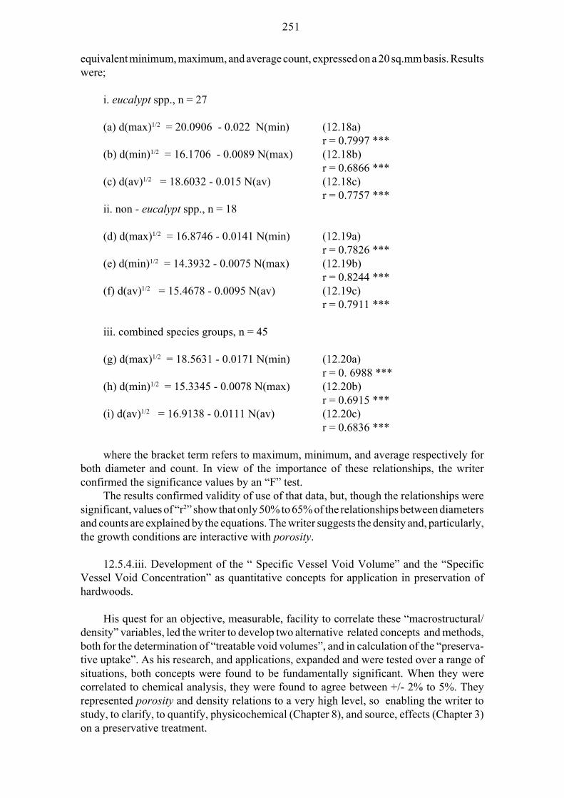
251

equivalent minimum, maximum, and average count, expressed on a 20 sq.mm basis. Resultswere;

i. eucalypt spp., n = 27

(a) d(max)1/2 = 20.0906 - 0.022 N(min) (12.18a)r = 0.7997 ***

(b) d(min)1/2 = 16.1706 - 0.0089 N(max) (12.18b)r = 0.6866 ***

(c) d(av)1/2 = 18.6032 - 0.015 N(av) (12.18c)r = 0.7757 ***

ii. non - eucalypt spp., n = 18

(d) d(max)1/2 = 16.8746 - 0.0141 N(min) (12.19a)r = 0.7826 ***

(e) d(min)1/2 = 14.3932 - 0.0075 N(max) (12.19b)r = 0.8244 ***

(f) d(av)1/2 = 15.4678 - 0.0095 N(av) (12.19c)r = 0.7911 ***

iii. combined species groups, n = 45

(g) d(max)1/2 = 18.5631 - 0.0171 N(min) (12.20a)r = 0. 6988 ***

(h) d(min)1/2 = 15.3345 - 0.0078 N(max) (12.20b)r = 0.6915 ***

(i) d(av)1/2 = 16.9138 - 0.0111 N(av) (12.20c)r = 0.6836 ***

where the bracket term refers to maximum, minimum, and average respectively forboth diameter and count. In view of the importance of these relationships, the writerconfirmed the significance values by an “F” test.

The results confirmed validity of use of that data, but, though the relationships weresignificant, values of “r2” show that only 50% to 65% of the relationships between diametersand counts are explained by the equations. The writer suggests the density and, particularly,the growth conditions are interactive with porosity.

12.5.4.iii. Development of the “ Specific Vessel Void Volume” and the “SpecificVessel Void Concentration” as quantitative concepts for application in preservation ofhardwoods.

His quest for an objective, measurable, facility to correlate these “macrostructural/density” variables, led the writer to develop two alternative related concepts and methods,both for the determination of “treatable void volumes”, and in calculation of the “preserva-tive uptake”. As his research, and applications, expanded and were tested over a range ofsituations, both concepts were found to be fundamentally significant. When they werecorrelated to chemical analysis, they were found to agree between +/- 2% to 5%. Theyrepresented porosity and density relations to a very high level, so enabling the writer tostudy, to clarify, to quantify, physicochemical (Chapter 8), and source, effects (Chapter 3)on a preservative treatment.

252

12.5.4.iii.i Prior to the definitions of these concepts, three aspects are discussed toenable the reader to understand reasons for use, and significance, of the term “Specific” inthose definitions. They are;

12.5.4.iii.i.i. The “Specific Volume” of a substance is the inverse of density, or (cgsunits) specific gravity, and is equal to “ 1/D” or “1/sg.”. In view of wide ranges of densitiesin hardwood timbers, the “specific volume” term became a useful tool.

Thus, void volume, [equation (12.3)] may be written as;

Mf = V.V. = 100 [ 1/sgsp - 1/1.53] (12.21)orV.V. = 100 (S.V.sp - s.v.ws] (12.21a)

and V.V. = 100 x S.V.sp - constant (12.21b)

where sgsp = specimen specific gravity (or density).S.V.sp = specific volume of specimen.s.v.ws = specific volume of wood substance.constant = 100 x s.v.ws.

12.5.4.iii.i.ii. The primary purpose of preservation is to inhibit a degradation (Chapters2, 9, 15) of wood by insects, animals, fire, or microorganisms. Principally for the last,preservative distribution mainly only in hardwood vessels means that a significantpercentage of “total treated volume” is unprotected (Rudman [1965] recognised therelationship), and the degree of this non-protection is a function of the “macro-structure”of a species. As vessel volume in the different species is, in turn, a function of density, thedegree of non-protection can be related to the two vessel void concepts under discussion.In commercial treatments, solution (or oil) absorption is calculated on uptake of a measuredvolume per unit volume (sapwood), hence mass, of timber treated.

12.5.4.iii.i.iii. The data cited (Sections 12.2, 12.3), showed for each species group,treatment conditions prescibed in “schedules”, and for aqueous solutions, the results werestatistically predictable and effective. Each treatment plant was a separate statistical “cell”for quality control (Graphs 13-17, Chapter 10).

12.5.4.iv.a. The “Specific Vessel Void Volume”.

This is denoted by a term “ SVV”, and, with a short title of “Vessel Void Volume”, isdefined as;

“Total vessel cavity volume per unit of 1 mm of length, per unit of cross-section (mm2),per unit of species (specimen) density (expressed in cgs units, and thus equal to specificgravity). The function “(1/D)” is the “Specific Volume” of the species (specimen) for adensity, “D”, at a nominated moisture content (air dry, 12% mc, unless otherwisestipulated)”. The value is;

SVV = ( [P . A] / D ) (12.22)where A = mean cross-sectional vessel area (mm2) based on the equivalent mean

circular vessel diameter, “d”.

253

d = mean circular diameter (mm), based on an average of the major and minor axesof the vessel cross-section.P = mean vessel (pore) count per mm2 of a specimen cross-section.D = wood density expressed as (mg/mm3).

Equation (12.22) may be quantified as;

SVV = { (pi) . P. d2 } / 4D (12.22a)where pi = 3.1416

To facilitate direct use of published data, the above is expressed as;

SVV = [(Pc x dc2) x 0.039] / D (12.22b)

where;Pc = pore count /20 mm2

dc = mean published (or measured) diam.D = density (mg/mm3)

The term “SVV” may be expressed in decimal form (used for calculation of “Sc”[below]), or as a percentage of wood volume.

It is considered as a measurement of change in physical “macro” characteristics oftimber, and is (Chapters 3, 8) normally associated with change of source, or growthconditions, of species. It can be approximately estimated in the field, which was importantin the writer’s work.

12.5.4.iv.b. The “Specific Vessel Void Concentration”.

This is a derivative term developed by the writer, is based on the “SVV”, is cited as“Sc”, and has the short title of “Specific Vessel (or Void) Concentration”. Its value may bedescribed as a quantified measurement of an uptake relative to calculated values based on“SVV”.

It is defined as “absorption in mass, or volume (of known specific gravity), ofimpregnated preservative liquid per unit of the Specific Vessel Void Volume”.

It is expressed as a decimal value, a ratio, or as a percentage of the saturation value.As for “SVV”, it could be approximately determined in the field.

For total saturation, the value of “Sc” is equal to “SVV” multiplied by the specificgravity, “sg.l”, of the liquid absorbed. “Sc” is also used to calculate a nett dry salt retentionfrom the uptake of preservative solutions. The equivalent dry salt from a treatment is mostreadily calculated from a measured solution concentration.

The “Specific Vessel Void Concentration” is;

Sc = (absorbed mass) / (SVV x sg.l) (12.23)

where (absorbed mass) = absorbed volume x specific gravity of impregnated liquid.

254

As sg.l = specific gravity of absorbed liquid.

Sc % = ([absorbed volume / SVV] x 100) (12.23a)

where the absorbed mass (typically applied to, but not restricted to, preservativesolutions, or liquids) is cited (cgs units) as milligrams per cubic millimetre.

When used as a measure of fluid weight absorption, water at a specific gravity valueof 1.000 is assumed. For other solvents, or liquids (oils), the relevant specific gravity, “sg.l”,is used in calculation as appropriate. When “Sc” is expressed in decimal form, then, foraqueous solutions for which specific gravities approach that of water (1.000), its valueshould not exceed unity. If a value in excess of unity is obtained, fibre penetration wouldoccur.

“Sc” is thus an expression of;

i. efficiency of a process or preservative in treatment.ii. measurement of variability of a treatment due to source, or physiochemical, factors.iii. definition of differences between general void volume formulae results for

angiosperms, and volumes relative to preservative and water uptake in timbers.The parameter “Sc

Penetrability, Index” for treatability.

12.5.4.iv.c. Determination of “SVV”.

The “SVV” volume measurement includes;

(i) vessel porosity, based on the measured (or published) values of size and count.(ii) due to difficulty in their quantitative assessment, the parenchymateous (particu-

larly radial) tissues were excluded. Correlation of the quantitative effects of exclusion ofthese tissues, using preservative uptake based on “Sc” determination, and comparison tochemical analyses of total specimens, was shown by the author not to differ by more than+/- 5% of analytical values. That implied concentrations in those parenchymateous tissueswere relatively much lower than in vessels, and “in-situ” spot tests (Chapter 11) agreed withthat conclusion.

(iii) For normal use, air dry wood density values (12% mc) were used, but, for someapplications, basic density (or specific gravity) was utilised, eg. comparisons to estimatedtotal void volume. It was desirable to nominate if basic density was used.

The following comments apply;(a) For reference purposes, published data formed the initial basis for calculation of

“SVV” and “Sc”.(b) When used (Chapters 3, 8) to quantify source effects on treatment and uptake, a

range of measured values applying to local specimens was determined for their calculation.(c) Specific counting should include an adequate range and number of pores to derive

a statistical mean value / unit area. Where the vessels are septate, each septa is individuallycounted.

(d) The actual cross-section of a vessel, or septa, was found to vary in generalgeometric shape. Studies showed that use of the equivalent circular diameter, “d”, as theaverage of the major and minor axes did not introduce an error exceeding +/- 5%. Theauthor’s laboratory, with the co-operation of the wood structure group, determined pore

255

diameters by projection microscope, with micro-photographic reproductions (final 100x)and a standard graticule for frequency measurement.

Appendix 32 (Table 68) lists calculated “SVV” values for a number of species of bothgroups tested.

12.5.4.v.i. Especially for field situations, a smoothly dressed, air dried specimen (L.S.)was found effective in a comparative evaluation of a species pore class size, withconfirmatory laboratory (T.S.) checks.

This method, other than a T.S. count, was used to train plant personnel (Chapter 1) totest for variables (Chapters 3, 8). For operators, the writer, placed emphasis on density, anda visual (L.S.) assessment of pore size / frequency in three classes as compared to samplesof that, or a known, species. From an overall control indication, wood density variationswere the predominant indicators of change, and, thus, any need to examine these values.

Author’s note: proximate (Section 12.5.4.v.ii, below) field measurements of “SVV”,and “Sc” may be determined on relationships of the pore size, and frequency (Graphs 48,49, 50, Table 57), and a mean pore count (T.S.) enables estimation of an “average diameter”for the specimens. When combined with a field measurement of specimen densities,possible average values of “SVV” and “Sc” may be calculated. Comparison of the measureduptake against calculated “Scsolely) to structure.

12.5.4.v.ii. As a routine;

(a) the average relations, based on published data, were initially used for calculationand comparison.

(b) If treatment results showed significant differences (three charges) to other sourcematerial of the same species, measurements included;-

(i) the air dry density was determined.(ii) mean pore count was determined. From the diameter to count relationships, a

comparison was made with vessel dimensions given by (iii).(iii) the vessel class size was initially determined and was compared to data described

in Table 57 (Appendix 24).(iv) the values of “SVV” and “Sc” were calculated and compared to results based on

published, or other source, evidence.(v) dependent on treatment results (six samples for each of three charges), representa-

tive laboratory measurements of pore size, frequency, and density, were made.

These enabled “SVV” and “Scand analytical results of samples.

This is illustrated by, and concurrently exhibits effects of source on, results for E.maculata. Material from Dalby gave a value of 0.1537, but specimens from the SouthBurnett district recorded 0.1137. Pore diameter values were low, and density was high.Spotted gum from areas north west of Gatton (south east Queensland) gave low values. Thevalues of “Sc.” were correspondingly low. Published data for spotted gum, which was ingeneral agreement with coastal sources (Chapter 3), gave a “SVV” up to 0.3230. Specimenstested from Grafton, and (small girth) from Queanbeyan (New South Wales), were

256

generally in agreement with published values, with “Sc” results correspondingly high.

For treatments of material with low values of “SVV” and “Sc”, especially for vacuum/pressure systems when using CCA salts, the solution concentrations were frequentlyincreased (Chapter 10).

12.5.4.vi. Applications of “SVV” and “Sc” concepts.

The author has described applications of these concepts in Chapter 3 (Section 5.ii) andChapter 9 (Sections 9.4.ii and 9.xi.i). Other examples are cited in Appendix 33.

257

Chapter 13

THERMODYNAMIC ASPECTS OF OPEN TANK SYSTEMS USINGELEVATED HEAT PROCESSES AND IMPORTANCE OF DIFFUSIVITY INTHERMALLY BASED PRESERVATIVE TREATMENTS. DEFECTCLASSIFICATION.

13.1. In Chapter 12, the writer refers to the paradigm relating air, moisture and density,which assisted him to effectively develop classifications for treatment of the wide range ofspecies and with appropriate variations in schedules. In those developments, multipleinfluences of, the relationships to, thermodynamics, which are examined in this Chapter,were some of the links between the basic elements (Chapters 8, 12) of structure and theresults of heat in treatments. They were also very important factors as causes of, andsolutions to, problems of treatments or defects in open tank plants (Appendix 14) whichused heat processes. Similarly, thermodynamics and aerodynamics are interactive; bothplay an important role in many aspects of timber utilisation and processing methods,including seasoning, especially kiln processes. Studies of timber service performances asan insulating, flexible material exemplify areas where the timber thermal characteristicsbecome significant. In research (cf. Introduction, Fire Retardent Committee) on combus-tion and “spread of flame index” properties of wood relative to other materials, this interestby the writer included the fire properties of timbers, extending to protective measures such

In discussing the multiple roles thermodynamics played in establishment of preserva-tion as being scientifically based (Chapter 12), the writer first describes aspects indevelopment of hypotheses, based on early experimental data, so as to emphasise therequirement to establish relationships to physical principles and units and test the hypoth-eses against those principles. If confirmed, they would enable the co-ordination of furtherresearch. The basic units, their applications and relevant formulae are described in Section13.7 and Appendix 34. However a derived unit, “Diffusivity” is expanded in Section 13.9.

Author’s note; For continuity of the text, equations and formulae discussed will, unlessstated, refer to relevant numbering [eg. (34.1)] as shown in Appendix 34.

13.1.i. In preservation, three highly important aspects led to the writer undertakingresearch into the relevance of thermodynamics principles to effective, soundly basedpreservation practices. These were;

13.1.i.i. The writer was responsible for assistance to industry in plant design data forpreservation plants, for the hot press systems for plywood and for seasoning kilns (this lastresponsibility was later transferred). That assistance was based on initial “in-house”training courses, aided by design engineers from the State Works Department and laterhigher training at the Division of Forest Products, CSIRO. In deriving data for designs, amean value of timber densities (Cokley, 1949c) and a high presumed moisture content wereused in calculations for heat requirements.

13.1.i.ii. Prior to availability of suitable formulae for these applications (eg. Pound,1951), general formulae such as equations (34.1), (34.10) were utilised, based on separatecalculation of data for water (using an average moisture content) and dry timbers at varyingdensities (cf. Appendix 34, re “specific gravity” and “density”). When the processeschanged, and heating systems began to be other than only steam generators, it eventuated

258

closer data on the thermodynamic influences were needed. It was clear that research intothe differences of thermodynamic properties, as functions of timbers, for preservationpractices was also necessary. Evidence indicated that was as equally important as was plantdesign.

That need was reinforced as ranges of available species, properties, variations in themoisture contents (and Void Volumes), timber sources and densities, increased. Mixedsapwood/heartwood content in boards (Diagram 2a) and more than one species in a chargewere prevalent. The early clarification of these factors was necessary for development ofeffective timber treatment classifications (Chapter 12) and schedules.

13.1.i.iii. Research confirmed thermodynamic properties of timbers were signifi-cantly influenced by, and changes in, “macro properties” of structure, moisture content anddensity (Chapters 3, 8, 12). They were applicable to all processes treating timbers,especially relative to timber de-aeration and the absorption of preservative. For example,temperature of timber surfaces affected CCA treatments.

The extensive literature , eg. Hunt and Garrett (1938), Popham (1931), Young (1946)and Bryant (1946), confirmed wide application of the thermal processes. Gregory (1942)examined the time/ temperature/ thickness relationships for “Hot Diffusion”. Popham,Young and Bryant discussed advantages of both maintenance and cooling cycles in theprocess and empirically recognised positive “partial vacuum” effects of the “cooling cycle”on final results. They had not deduced any thermal/de-aeration/absorption interactions ona quantitative, or selective, basis for species, properties and moisture contents for treat-ments. These interactions were necessary (Chapter. 12) for the development of treatmentschedules and which could then be varied as functions of species characteristics.

If the partial vacuum theory was accepted and confirmed, then the author consideredunderlying principles of these processes may be similar (Chapters 12, 14) to those on whichfull-cell vacuum/pressure systems were based. This implies;

a. a thermally induced vacuum (which, by the gas laws, is dependent on maximumtemperature, the time of maintenance and temperature change), when created within timberwhich is heated [and cooled under solution], causes a negative pressure differential withrespect to atmosphere and this differential is also a function of the temperature changes.

b. it appeared joint relationships of the partial vacuum (which reduces resistance of theresidual “contained” air to inward liquid flow [Chapter 14, Harrow, 1947]) and the negativepressure differential (which induces liquid flow and flow rate [Poiseuille’s law]), result inpreservative solution [and water] uptake (Chapter 8). The uptake was considered topossibly be quantitative functions of both the level of an induced vacuum and the negativepressure differential. Uptake was shown to be dependent (Sections 12.1-12.5, Chapter 12)on timber properties. The pressure differential, “dp” may be defined as :-

dp = (- p1) + p2 + p3 (13.a)

where ;-

p1 = vacuum pressure (negative relative to atmospheric), due to initial air expansionand cooling under solution.

p2 = atmospheric pressure (mm [torr] mercury).

259

p3 = hydraulic pressure due to depth of liquid coverage on a board (equivalent mmHg).

The importance of this definition was that “p1” may be tested and quantified asdescribed below. The levels of heating efficiency and vacuum attained were considered bythe writer to be functions (Chapter 12) of wood density and moisture content. If both vesseland fibre lumina and walls were completely filled with water, the sample is at maximum(saturation) moisture content and, by definition (Chapter 7), there is a minimum (or zero)air volume for thermal expansion. For these conditions, “p1” would also be at a minimum,but by seasoning to, or below, FSP, then to an oven dry state (when “p1” may reach thetheoretical maximum), changes in values [Section 12.4, Chapter (12)] will occur betweenthese limits.

It appeared the effect of “p3” was negligible relative to other factors, as indicated bythe finding (Young, 1946c) there were no significant differences in preservative retentionbetween the top and bottom layers of a treated stack. Young’s findings were confirmed bythe writer over a range of plants and processes. This negligible effect appears due to the factthat effective vertical downwards pressure on any board is not equal to the total height ofthe column of solution. Typical theoretical pressure distribution is shown in Diagram 2b.

13.2. Verification of, and quantification of, de-aeration and partial vacuum effects asfunctions of the thermal changes.

These are described in terms of the hot and cold process, using 25mm thickness boardsas example, but separate studies in other processes, such as the steam/cold quench, showedsimilar relationships for other than rates to achieve the final states and equilibrium. Generalsampling lengths were 0.3-0.5m and 0.8m for laboratory and pilot plant studies respec-tively and with 0.8m (both ends sealed) to 1.8m (one end sealed) boards used for thecommercial tests.

When “end” effects were studied (eg. de-aeration), the shorter samples were sealedonly on one end, but in the general research they were sealed at both ends (see below) withtwo coats of a bitumastic mastic previously found suitable as a sealant at the elevatedtemperatures. When suitable epoxy mastics (polymerised at ambient temperatures) becameavailable, they were used in vacuum studies (Chapter 14). Initial samples were (starchpositive) sapwood, but later included boards of known sapwood/heartwood profiles(Chapter 8).

Thermocouples and 5mm glass tubes were sealed into the ends of laboratory speci-mens and the glass tube connected to a manometer for vacuum studies. This seal wasseparate to the end-sealing described above. For pilot plant and commercial studies, onlythermocouples were used. For other studies, thermocouples were also inserted (and sealed)from an edge, at varying lengths from the end to board centres. When de-aeration (Section12.4.i, Chapter 12) was predominantly from the end-grain, the rates were higher (compareGraphs 52a, 52b, Chapter 14).

Solution temperature was increased to different maxima, and maintained for timesindicated by the thermocouples. Non-linear rates of heat penetration, about 6-12mm/hourfrom the face of an end-sealed 25mm board, were found. As cooling progressed, thetemperatures and vacuum pressures were measured.

Rate of attainment of solution, timber, temperatures and cooling were functions of

260

volume (and mass), of plant design, and efficiency of the heat generator and transfer system.Species density, properties and board moisture content were significant.

When mixed sapwood/heartwood profiles (Chapter 8) were tested, time required forheat penetration increased, but de-aeration rate decreased and these were both related to theheartwood section present. Sample density (Section 12.3, Chapter 12) was a dominantfactor.

The studies confirmed the conclusions [(Section 13.6 and stated in equation (13.b)]that optimum de-aeration was a function of temperature, total times at maintenance, ofspecies and “effective orifices” cited in Section 12.4 (Chapter 12).

The evidence, using 0.8m boards (both ends sealed) under the pilot plant conditionsand confirmed over a range of commercial operations, formed the basis (with treatmentretention results) of schedule temperatures (Chapter 12) and maintenance times nominatedin Appendix 26.

13.2.ii. The practices of using manometer inserts and end-sealing were adopted for theresearch into full-cell vacuum pressure systems (Section 14.2, Chapter 14 and described inAppendix 37). By use of Quickfit one-way valves, the writer utilised manometer tubes forall board lengths (cf. Diagrams 3a, 3b, Chapter 14).

Author’s note; as the tube was 5mm diameter, measurement covered all tissues;temperature and vacuum changes were deduced to occur (Chapter 12) also in fibres.

13.3. Objectives (other than for direct diffusion) in use of preservation, which arebased on thermal processes.

The research on thermal processes, indicated above, led to treatment (Chapter 8)objectives as;

13.3.i. Use of an enclosing medium, that is, with timber fully immersed in andaccessible by solution (or a steam environment) as the heat source and which, theoretically,had an infinite heat capacity relative to demands.

(a) to transfer heat from that source through the full sections of timber at a controlled,adequately uniform, rate (graph 38). Thus central zones of the timber attain an elevated(with respect to ambient) temperature which is such that an effective air expansion (Section13.3.ii) occurs. It is a function of wood properties.

(b) for this purpose, a “charge” was maintained immersed (equations 13.a, 34.5) at amaximum temperature condition and for a time to ensure objective (a) was achieved.

For commercial, and research, operations, to attain and maintain the maximumtemperature, the heat source was externally heated and measured (including input). Thus,thermodynamically, it was shown both treatment solution, or steaming chamber, and chargewere in an unsteady state and where the solution (or steaming chamber) first attainedequilibrium. In practice, a measured, external heat supply to the solution was necessary tocompensate for loss to timber, or environment.

For the steam/cold quench, equilibrium was more rapidly attained. However, in that

261

process, transfer of heat from steam to the “charge” caused some condensation to occur andresulted in changes in surface moisture contents of timber and a need for external,measured, added heat.

13.3.ii. By this procedure, air, and water, contained within the timber cells wereheated. Considered in terms of the air content, results were that;

13.3.ii.a. at the elevated temperature, following the gas laws, there occurs an expan-sion of a mass of the original contained air (Chapter 14), such that nominal air volume (atthe pressure) remained constant. The mass difference was expelled from the timber.

13.3.ii.b. The progressive rate of loss was;

i. a function of heat transfer through a timber section.

ii. an equilibrium condition with the loss (and rate) of dissolved air from the solution.

The writer determined that, as the solution temperature increased, equilibrium masssolubility of air decreased in the aqueous medium. Loss of air mass from the board was alsodependent on rate of air loss from the solution. During heating and maintenance cycles inthe hot and cold processes, there were (cf. Graphs 35, 36, Chapter 12) absorptions(different) of water and preservative into timber. For this and mechanism of air loss throughthe solution, different procedures operated in the steam/cold quench system using steam,but the final principles were the same, namely thermal loss of a mass of contained air.

Data (Section 13.4, Chapters 12, 14) confirmed an air loss occurred from fibre tissue,but at a slower rate.

13.3.iii. Subsequent to, and as a consequence of heating of the solution and timberdescribed in Section 13.3.ii., the following applied;

13.3.iii.a. for the steam/cold quench, the “charge” was rapidly “quenched” such thatno pre-emptive cooling (cf. Section 13.8.iii, re design modifications) could occur and,during the “quench” period, continued steaming was necessary to maintain the expandedair condition of all boards up to and until they were submerged under solution. A partialvacuum (Chapters 8, 12) occurred in the “quench/cooling” cycle. The charge of timberabsorbed solution (graph 37) over a time, which was a function of cooling rate of boardinteriors and timber properties.

13.3.iii.b. for the hot and cold process, a “charge” was cooled off under solution.

b.i. The solution progressively cooled through nominated temperature ranges (Chap-ter 12).

b.ii. Progressive cooling occurred through the thickness of the timber section. This wasa function of cooling of the solution and what the author describes as “negative” heattransfer rates of cooling through the section, relative to change in solution temperature andrate of cooling.

b.iii. The solubility of air in solution increased with drop in temperature but this mass/volume of air was very small compared to atmosphere.

262

When the cooling occurred, the low residual air in the solution ensured air volumewhich was contained within the timber and which had been expanded at the maximumtemperature was reduced as a function of progressive drop in temperature through the boardthickness. It resulted in creation of a partial internal vacuum (confirmed by embeddedmanometer tubes). Though de-aeration occurred, vacuum did not occur during the heatingcycle, but was a function of cooling only.

b.iv. Consequently, there was an absorption (penetration) of solution (Section 12.4,Chapter 12); the water phase also permeated through the pit and wall orifices to fibrelumina. Absorption was significantly greater (including its rate) than would occur ifdiffusion was the principal mechanism for penetration. That total absorption of waterconfirmed deductions concerning a need for the total board section, including heartwoodpresent, to be heated and evacuated. If both the vacuum and negative pressure differentialeffects were inoperative, water movement into fibres would be slower than foundexperimentally.

13.4. Requirements for attainment of thermal and vacuum equilibrium conditions intimbers.

For most of the treatment operations, the writer found unsteady thermal and vacuum(hence the negative pressure differentials) conditions prevailed and steady states wereobtained only as a function of time at each cycle. As the research proceeded, it became clearthat a partial vacuum effect was only one (major) factor in timber treatment by a thermalprocess. If de-aeration was the sole (but dominant) cause of absorption, examples cited nextbelow would not show significant effects of time on results, but those effects were present.Examples are;

13.4.i. For similar dimensions, the treatment schedules covering ranges of speciesrequired, as major components, inclusion of times (equation 13.b) to attain equilibrium foreach cycle of the process. This time at each process condition was dependent on wooddensity and structure, on the heartwood/sapwood profile and is explained by thermodynam-ics.

13.4.ii. Density ranges involve change for each treatment group (Section 12.2, 12.3,Chapter 12) in the maintenance times at temperatures, resulting in differences for therecommended periods which vary by factors of 2-4. Density interacts with moisture content(eg. in equations 34.15, 34.16) in effects on thermal properties.

13.4.iii. Results (Chapter 12), dealing with developments for treatment process(graphs 35, 36), did show separate increases in moisture content and preservative retentionsas a function of time immersed (Appendix 14) at maximum temperature. There was anincrease in uptake caused by cooling cycles from maximum temperatures. Similar effects

13.4.iv. The conclusion reached by the writer was that for each cycle in treatment, itwas necessary to allow an adequate time for attainment of equilibrium conditions toinduce, or approach, the steady state condition for both timber and solution. This need isdemonstrated in processes in which the rapid temperature drops required further immersiontime for the centre of boards to cool and to reach thermal equilibrium (Graphs 37-37c).

A similar effect is present (Chapter 14) in full-cell vacuum pressure systems.

263

13.5. Moisture content states in treatment.

In the heating and maintenance phases of a treatment, applicable particularly toprocesses using immersion in solution, changes in moisture contents, caused by liquidabsorption, occurred from the initial nominal “green” or “air dry” moisture content but didnot approach (Chapter 12) the saturation moistures. They were associated with thermalchanges (Appendix 34) and resulted in increased rates of heat absorption.

Thus for moisture contents, there is an unsteady state condition which does not becomea steady state until the board reaches saturation, or equilibrium, values.

In research into development of treatment practices involving flexibility in permissi-ble moisture content for (Section 12.2.i, Chapter 12) processes, the author found that, in thehot and cold process, moisture contents below FSP had lower effects on times required forheating and maintenance than appeared necessary if thermodynamic effects of the lowersurface moisture contents applied.

The evidence (eg. Graph 35) indicated that progressive moisture content increases,described above, principally occurred in the heating cycle, and were aided by increase inpenetration (and wetting) when borax or its homologues (Chapter 8) were used. Inconsequence, the heat transfer conditions during maintenance cycles were increased andthe final situation was thermally equivalent to boards of higher initial moisture content,especially in the “case” values.

Author’s note; in Appendix 34, the writer derives relationships of change in values ofboth specific heat “c” and thermal conductivity “k” (and thus in the other units involvingthem) in terms of the moisture content differences, density and Void Volumes, within aboard.

However, conclusions drawn are also applicable (Section 2a, Appendix 34) to separateboards, for which the mean cross-sectional data are used.

13.6. Maintenance times at elevated temperature.

13.6.i. The maintenance time (Chapter 12) of a system at maximum temperature isdependent on rate of de-aeration, which is a function of limiting temperature at the centreof the board, thermodynamic properties of the species and thermal penetration rates. In theresearch into reduction of moisture contents (Chapter 12), the writer necessarily investi-gated increases (Appendix 34) in cycle times. The studies included treatment of timbers at,or below, FSP, as compared to “green” timbers.

Schedules were developed with a “safety margin” in the heating and maintenancetimes, but differences (cf. Section 13.5) due to these moisture content changes were lesssignificant than the effects of species density and section size.

13.6.ii. Let “h1” be the total time (hours) required for optimum de-aeration(dependent on timber properties) of a board heated (or steamed) at maximum temperature.

If “h2” is the time (hours) for the centre of a board to reach equilibrium with thetemperature of the medium and which depends on the wood properties and moisture content(Appendices 34, 35), then a total maintenance time of “H” (hours) required at the maximumtemperature is given by;

H = (hl + h2) hours. (13.b)

264

Initially, the writer determined values experimentally, until adequate data had beenconfirmed to establish thermodynamic relationships as a function of species. Density andranges of moisture contents (Chapter 12) were involved (Appendix 34) in such studies.

13.7. Thermodynamic principles found to be significant in timber preservation.

Fluid flow dynamics are more appropriate in terms of vacuum/pressure processes, butthere are interactions with roles of thermodynamics. Little fundamental, or applied,research information was available on the local species for influences of, or roles played by,thermal principles.

That lack extended to the open tank treatment processes based on heat and toprocedures in the development of and in possible flexibility of those processes.

There was a large volume of literature dealing with heat in engineering practice andfor many applications to wood eg. drying coefficients, These included Kollman (who isgenerally examined through his joint publication with Cote (Kollman and Cote, 1968) andMacLean (1941) who had published a series of articles in A.W.P.A. publications over theperiod 1930-1936 (not separately referenced) and whose works are discussed in definitiveanalyses by Stamm (1964), by Kollman and Cote (1968) and by Siau (1984).

Many investigations were under steady state conditions, but in preservation, it wasoften necessary to examine relationships under variable and/or unsteady conditions. Thenumber of variables increased when the research was extended to the commercial opera-tions. As evidence was accumulated and analysed, it was recognised five aspects wererelevant and, in some respects, summarised the data. They were;-

1. Total heat - “Q”2. Specific Heat Capacity - “c”.3. Thermal Conductivity - “k”4. Thermal Capacity - “C”5. Diffusivity - “a”.

Unless stated, their conventional definitions apply and are assumed in discussion. Aseach includes extensive formulae, they are examined, including derivations of the formulae,in Appendix 34.

Only significant, applicable derivations, and discussion using those formulae, arequoted in this text. For each, there are important relationships with moisture in a board, withchanges due to differences in density and real difference in physical heat properties or fluidflow. Change (Diagram 2a) in properties between sapwood [density factor of 0.8, Chapter12] and heartwood zones becomes (Chapter 8) significant.

These properties and changes are involved in total heat demands of the preservationsystem, the times for heat to penetrate timbers of different density, rates of heat transfer fromthe heating medium to a solution and thence through variable thicknesses of boards. Onthese is dependent the treatment efficacy and which, in turn, influences the economics ofoperation.

13.7.i. The Specific Heat Capacity “c”.

Employing both formulae (34.3) and (34.4), variations in specific heat capacity over

265

temperature ranges used in timber preservation are shown in Table 69, Appendix 35.It should be noted that, for species of a low density, moisture contents (Chapter 12) of

a “green” timber, or saturation values, may exceed 100 - 150% when based on an o.d. massof timber. That data is applicable in seasoning and plywood (veneer) applications.

13.7.i.i. As a board dries, differences increase, with depth, between moisture contentsfrom the outer surfaces of the board to that at the centre. The differences are present betweensapwood to heartwood and with thickness. There is a related change of specific heatcapacity with depth (effect of the moisture gradient) in a board (cf. Section 13.8 re jointrelationships of “c” with thermal conductivity). Usual industry standard for measuringmoisture content of the stack is by mean cross-sectional moisture content of sample boards.Data on moisture gradients enabled a working safety factor (Chapter 12) to be establishedand differences in treatment quantified. Commercial applications in the use of values of “c”,were based on the (tested) assumption that, at a plant, cross-sectional moisture contentgradients (cf. effects of change of gradients, equations 34.14, 34.15, 34.16) wereadequately consistent for a particular species and a thickness. The author considered eachtreatment plant (Chapter 10) as a “statistical cell”.

Consequently, it was necessary to correlate the thermal results so obtained againstcalculated results typified by those derived (Table 69, Appendix 35) for gradient sectionsin a board. That agreement was confirmed, but (cf. Section 13.7.ii) emphasised roles ofthermodynamic parameters.

Research on the variations in wood treatability involved calculation of values of totalheat, “Q”. As indicated in Chapter 10, accurate estimates of solution and charge volumes(with density, moisture content ranges for the latter) were necessary. Based on specific heatcapacities and other units below, the distributions of heat, of temperatures and of de-aeration, with depth in timber sections, were calculated and compared to results.

13.7.ii. Thermal Conductivity “k”.

Value of “k” is influenced by moisture content gradients and change of specificgravity. Insulating properties of a timber specimen, varying with moisture content, dependon this characteristic. Unless section thickness is small compared to surface area, acondition applicable to thin veneers, the mean cross-sectional moisture contents giveproximate values only, but are suitable for general applications. Thermal conductivity ishighly significant when thick sections of timbers, such as rail sleepers, are treated bythermal processes, which include a special treatment termed “Boultonising” (boiling for anextended time, in oil solutions, under applied vacuums).

When timber is being heated, equations (34.10), (34.11) are applicable due to gradientsof moisture content and specific gravity. They apply to use of different heating media suchas steam, and differences for aqueous, or oil borne, solutions. However, for all cases, thelimiting conditions are at the surface and centre of the board. Penetration is from all surfacesand, if this is not satisfied (Diagram 2a), values of “Q” at separate points in the same axialplanes will vary. Stamm (1964), Siau (1984), MacLean (1941) point out the longitudinalto the transverse ratio of “k” is 2.25-2.75. Variation between the radial and tangentialdirections were practically negligible. Results obtained in development of treatmentschedules by, for example, the hot and cold processes showed no significant differences incycle times between bachsawn and quartersawn boards. Differences in board total dimen-sions, including length and hence in total heat demand as well as heating or cooling rates,

266

between the pilot plant studies and commercial operations, were important criteria in thedetermination of process cycle times and equilibrium conditions.

13.8. Correlation of both the Specific Heat Capacity and Thermal Conductivity withwood preservation.

13.8.i. Six variable conditions can apply:(a) when the board width is significantly greater than its thickness, edge penetration

can be neglected relative to that from the faces.(b) when the board width is not significantly greater than the thickness, edge

penetration cannot be neglected, but is generally at a much lower rate, relative to the boardcentre, than face penetration. This latter does not apply to square profiles in boards.

(c) where the gradient of moisture content is zero, or is uniform from the surface to thecentre, that is the moisture content gradient from the faces and edges is symmetrical aboutthe central axis. This is the condition assumed (dependent on sapwood/ heartwood profiles)when board mean values are used.

(d) where the moisture gradient is nonsymmetrical about the central axis.(e) where the board is of uniform density (at a standard moisture content) across the

section.(f) where the board is of non-uniform density across the section eg. a sapwood/

heartwood cross-section board.

Equations 34.15 - 34.17a (cf. Section 5, Appendix 34) examine these conditions.

13.8.i.i. the results are:(a) where the moisture gradient is zero and the board is of uniform density, both the

specific heat capacity and thermal conductivity are constant, or uniform, with depth. “Rateof temperature change” calculations are dependent only on section density and moisture.

(b) where there is change of moisture content gradient, or a change of density, thevalues of “c” and “k” will vary. As the lowest moisture content is normally in the outerlayers, values of “k” and “c” will theoretically increase with depth. If this were so, then ata point “x1”cm from the surface, as specific heat capacity increases, total heat required,“Q1”, to raise that unit cross-section temperature also increases.

As the value of “k” is dependent on moisture content, a lower moisture content in theexternal “case” of a board reduces rate of heat transfer. Under these conditions, total heat“Q” is not immediately available to inner sections and the time rate, “tx1”, of heat transferis lower. Similarly a change from depth “x1”cm to “x2”cm results in a comparable differencein rates.

To achieve operating temperature conditions at the board centre theoretically (cf.Sections 13.5, 13.6) requires increase in time, or the final temperatures attained will belower than required for the process.

The values of “k” and”c” (cf. equations 34.3, 34.4, 34.7, 34.8, Appendix 34, Appendix35), vary with change in the moisture content, and both “Q2” and “tx2” change. Anequilibrium condition, which is especially relative to temperature, will result unless theexternal heat is of sufficient quantity and accessability to supply demands. This conditionpertains to the board centre. Dependent on conditions (a), (b), change in “kxn” and “txn” maycause variable penetration from each surface or edge.

267

These conclusions agree with deductions based on Fouriers equations (34.10), (34.11)which cite formulae for heat transfer (Appendix 34) through a non-uniform section.

This situation can arise where boards have swollen and hence edge gaps betweenboards are insufficient to allow adequate quantity of hot solution to circulate freely. Forthese conditions, “tx” from these edges is measurably less than from the other surfaces.Hence de-aeration is reduced as well as subsequent equivalent temperature drop and thisdecreases the negative pressure differental and results in reduced fluid flow. The nett overallresult is inadequate or variable retention in affected zones. An adequate spacing based onswollen volume of the wood was emphasised to industry.

13.8.ii. The importance of Void volume, “V”, in thermal calculations.

The calculations, which include all tissues, are examined in Appendix 34. Resultsconfirm the significance (Chapter 12) of void volumes in determining effective treatments.

The limiting values of density and moisture content are at the surface and center of atimber section and these were significantly influenced by both growth and climaticconditions and by sapwood/heartwood profile.

At saturation, vessel and fibre lumina are theoretically filled, but, on drying, voidvolume in lumina increases until attainment of fibre saturation point (cf. Chapter 12 reinfluence of density on FSP), at which only air is contained in those cavities. Data developed(Chapter 12) by this author showed that moisture change in vessel lumina is very significantand preservative retention is restricted to that zone (Section 12.5, Chapter 12), but moisturecontent of all tissues increases by treatment.

The conclusions drawn from the analyses (Appendix 34) were that any variationwithin, or between, boards, of moisture content, or specific gravity, causes measurabledifferences in the specific heat capacities (Table 69) and thermal conductivities, and theseresult in changes in rate of heat penetration, vacuum levels, moisture and preservativeuptake.

These (Chapter. 10) deviations in preservative retention can occur by mixing air-driedand green-off-saw material. They also explain a need for close control on mixtures ofspecies, eg. treatment groups 1, 3 (Sections 12.2, 12.3, Chapter 12) in the one charge andby which densities and moisture contents may vary twofold.

An exception to this general condition (where outer layer moisture content is lowerthan with depth) lies in the direct heating of wood by steam, especially when using a lowpressure “wet” steam, typified by “reconditioning” (Chapter 7), or, topically, for the steam/

a. the rate of heating by steam is higher than that given by aqueous solutions.b. As the heat content of the steam is used, condensation occurs which causes sharp

increases for the outer layers, termed the “case”, in terms of heat demand, moisture contentsand swelling of those layers. In consequence, a reverse moisture gradient may be caused,resulting in temporary values of “k” being higher than further in the board depth.

A maximum moisture content was (Chapter 12) prescribed for species above treatmentgroup 2A (Sections 12.2, 12.3, Chapter 12). The sapwood/heartwood profile (Section 8.xiii,Chapter 8) of a board affects both the ranges in moisture content and heat characteristics.

268

13.8.iii. Modification which were necessary to be made in initial plant designs forsteam/cold quench systems.

Conventional systems were adapted from a “reconditioning chamber” used in kilnseasoning. For that, the perforated steam coils were mounted only on the roof of thechamber. In this process, at the end of the steaming cycle, rapid entry of the solution causedcooling.

This related not only to the boards being submerged but also to the air space above thesolution, thus resulting in a cooling of the air and of outer layers of boards not yetsubmerged. The result was a variable distribution of poorly treated boards; the writerestablished a pattern relating to “pre-cooling” described above. Plant design neededamendment to ensure that, subsequent to steaming cycle times, flooding of cold solutiondid not cause premature cooling before the charge board layers were progressivelysubmerged. If that occurred, air absorption and low solution uptake resulted.

Multiple steam lines were vertically placed on the walls of the steaming chamber,including above charge height, so that progressive steaming continued during “flooding”(Appendix 14) of solution. Uniformity and consistency of treatment were improved.

13.9. The significance of “Diffusivity”.

“Diffusivity” (Appendix 34) is defined as the term “(k/C)”, denoted by the term “a”,used for British units, MacLean (1930, s.n.r.), McGlashan (1971). Kollmann and Cote(1968) define it by the same symbol. Siau (1984) uses the symbol, “Dh”. Stamm (1964, pp.283-293) denotes it by a symbol “h2

of thermal conditions in a system prior to establishment of equilibrium, i.e. before a linearor steady state is established. MacLean (1952) suggested experimental treatment anddescribes graphical charts of time / temperature / depth.

13.9.i. From the definition of Thermal Capacity “C”, this writer confirmed [based onequations (34.1, 34.12a), Appendix 34] it was equal to the product of the specific gravity“sg” and the specific heat capacity “c”. From its definition as the ratio of the thermalconductivity “k” to the thermal capacity “C”, “Diffusivity” became;

a = (k) / [(sg)(c)] (34.13)

Kollman and Cote (1968), Siau (1984) have independently derived the aboverelationship. Equation 34.13 may be expressed (Appendix 34) as;

a = (k). (S.V.sp) / c (34.13a)

where “(S.Vsp)” is the Specific Volume of a specimen (cf. Section 12.5.4, Chapter 12).Kollman and Cote (1968) cite Maclean (1930) as showing that “h2” (= “a”) has an

average value of 0.000629 m2

reasonably small. However, as both “(sg)” and “(c)” are dependent functions of wooddensity and moisture content, the data (Kollman and Cote, 1968), though numerically small,show density changes from 0.20 to 0.80 (constant moisture content) result in about 25% fallin value of “a”. From the lower density range (0.20) to the value of 0.80, moisture contentchanges from 10% mc to 50% mc have corresponding falls from about 20% to 12% of thatat 10% mc. For local species, specific gravities (Section 12.3, Chapter 12, Appendix 27) will

269

reach values of 1.200 and moisture contents in the lower density species may exceed 100%.Thus the change in “a” becomes significant. Maclean stated the “diffusivity factor dependson the direction of the grain” and he calculated the steaming times for different sections oftimbers using this unit. There were parallels in that work and the objectives by this writer.

13.9.i.i. This form (equation 34.13) of the relationship was most useful as it combinedmajor thermodynamic units in one term with the two major variables in wood, namelymoisture contents and specific gravities. Values of “k”, and “c” are functions of thesevariables. Illustrated by equations (34.3), (34.7), (34.8), (34.14 to 34.16), any changes ina moisture content, or specific gravity, value cause changes in the values of “a”.

Prime importance of “Diffusivity” was as the quantitative measure of rates of diffusionof temperature especially in timbers. De-aeration, which is a critical requirement foreffective treatment by other than direct diffusion, is temperature dependent. Diffusion isalso temperature dependent and Graham’s Law of Diffusion (Findlay, 1944) applies. Intimber preservation, it was often necessary to determine relationships prior to attaining asteady state condition. This applied in assessment of defects in heating systems and their

Owing to the variability of material on a commercial scale, the writer initiallyinvestigated problems by an experimental approach, until, by using thermocouples andthermotubes (and including treatment results), adequate evidence was obtained to justifythe application of formulae. Use under plant conditions confirmed those findings. Graphs35, 37a-c, 38-38a, illustrate their use.

13.9.ii. Limiting values of the product “(sg)(c)”.

Using cgs units, for local species, the author found the position to be such that theproduct “(sg)(c)” did not exceed unity and in practice, except for isolated cases, it wassignificantly less than unity, particularly so in moisture content effects on the product ofthese terms. This is illustrated by a species having a sg = 0.800, and moisture content of 50%.Data from Table 69 shows “c” has a value of approximately 0.54 over normal temperatureranges and this gives a “(sg)(c)” product value of 0.432, which is less than unity.

Author’s note; From a practical usage application, values of “(sg)(c)” may fall to verylow values, but unless “sg” or “c” become zero, the product would only approach, but willnot attain, zero value. It would be an interesting, theoretical, philosophical project toestablish physical conditions at which that may occur. As “sg” is a function of mass, it wouldrequire a condition of “weightlessness” and similarly, for “c” to become zero, an absenceof heat is required, a condition attainable only at absolute zero temperature.

The evidence led the writer to conclude an upper value of the product “(sg)(c)” wasunity.

On this basis, although there is an increase in the value of “k” with increase in the woodmoisture content and in specific gravity, the position applies where the value of “a” changesat a faster rate. Hence the lower limiting value of “a” would equal “k” and calculations asa measure of the temperature diffusion could be based for lower limit conditions directlyon the “k” values.

13.9.ii.i. A typical condition for this to be applicable, was for a mixed sapwood/heartwood crosssection in a board and, though only sapwood required preservation,schedules at elevated temperatures were required to both heat and to de-aerate the

270

heartwood zone, otherwise the latter acted as a “heat sink” and as a source of air in coolingcycles. Designs of heat requirements were desirably based on an “average maximum woodweight condition” and hence the writer used published heartwood data in calculations.Similarly, moisture contents were low in very dry boards (less than 15%), in plywood andin machine dried veneer (both less than 5 to 7%). These low values had increased difficultiesin wetting by the aqueous solution (Appendix 15), a problem not as marked (Chapter 8) forthermally based processes. Non-polar preservative solvents did not present problems to thesame degree. Heat demand was increased by “heat of wetting” and total time for heating wasincreased (cf. Sections 13.5, 13.6). Similar thermal effects were noted in kiln seasoning,in oven drying to measure a moisture content and in the hot press gluing of plywood.

13.9.iii. Applications of Diffusivity in the preservative treatment of timbers sensitiveto thermal changes.

13.9.iii.i. When hot timber was exposed to sharp thermal changes, exemplified by itsremoval from a treatment at temperatures above ambient, sharp thermal gradients werepresent from the surfaces and caused certain species, or thick sections, to experience severe

(a) Reduction of the maximum temperature from 95-98 degrees to 70 degrees, with 68degrees C. as the critical minimum value. Hence (Chapter. 12), after the temperature dropin solution, typically 22 degrees, differences on removal were reduced from a maximum ofabout 40o to 25o, relative to atmospheric temperatures.

Both the degrade and excess drying rates were reduced significantly. The writer foundthese could be quantified and expressed as mathematical functions, assuming a constantexternal humidity. If;-

t1= maximum temperature at the centre of a board,t2 = ambient temperature (at the board surface),

diff,

where tdiff = (t1 - t2).

Similarly the rates of cooling of the board, sequentially from surface to centre, arerepresented (tdiff/time) by;-

r1= rate of cooling of board surface to atmosphere,r2= rate of cooling of board centre to the surface,and dr = f(r1-r2),where “dr” is the differential cooling rate and, as it is related to “tdiff” and “t1”, may be

expressed as;-

dr= F(tdiff, t1)

The relationship was approximately logarithmic, dependent on the species heattransfer characteristics which are functions of its moisture content and specific gravity.Relationships were confirmed by thermocouples in sample boards and by moisture tests.They were similar to normal kiln seasoning, but differed in that the initial moisture gradientswere reversed after treatment.

271

(ii) Where operational requirements were such as to favour retention of the highermaintenance temperatures of 95-98o and cooling of 22o, then after the preservativetreatment, a charge was first cooled in the warm, empty vat, which was a high humidity,warm environment (where air was close to saturation) and was thus protected from lowerambient temperatures. As the air cooled inside the vat, condensation occurred on boardsurfaces (equivalent to a mild “reconditioning” treatment) and moisture gradient stresseswere reduced to non-significant levels and with consequent reduction in checking anddegrade.

As vat temperatures dropped towards ambient, the charge was removed.

Two temperature differentials and two rates of cooling and drying were achievednamely;

diffta = (t1 - tc),and difftb = (tb - t2).

where ;-tc = temperature of warm, humid air in vat.tb = temperature at centre of board after cooling in the vat.

diffta = initial thermal differential between board temperature and tc.difftb = thermal difference after cooling in vat.

Similar relationships applied for both “dr” and for the differential rates of cooling.

13.x. Application of thermodynamics in development of, or control of, or rectificationof defects in, the heating of treatment solutions used in thermally based processes.

Similar thermodynamic considerations applied to solution conditions. Several exam-ples are cited:

13.x.i. Thermosyphon systems.

Heat input was based on an external heat exchanger such as a non-pressure verticalboiler. The rate of solution flow through the vat and charge was regulated by rate of heattransfer in the exchanger, by pump capacity and pipe size. This was the reverse to steam coilheating, but the same principle applied, i.e. conduction through a thin walled cylinder toheat a fluid (Joel, 1969). Equation (34.10) applied. The rate of flow was dependent on:

(a) the coefficients of conductivity of the heating tube walls internal in the heatexchanger (heat input) and separately for the heating pipes (heat output) as well as “outlet”return pipes from the solution to the exchanger.

(b) the temperature differential between heated wall and the heat transfer wall of thetubes as in (a).

These were different as both the inlet heating pipes and outlet pipes (to return solutionto the heat exchanger) below solution height (without a charge) in the vat were perforatedand there were temperature differences to the solution in which they were immersed.Prevention of heat losses over the full length of heating pipes, from heat exchanger to the

272

vat, was a consideration in design.

(c) the rate of equilibrium of the heat, of temperature “diffusion” and uniformity,through the equivalent “total volume” of solution. Diffusivity was a controlling factor in therate of heating, and temperature rise of solution but with convection effective indistribution. Excessive flow rates of heated solution through the pipes, both in the heatexchanger and in transfer to the vat volume, resulted in poor rates of heat exchange and invariable increase in solution temperature. Too slow a flow rate meant wastage of generatedheat, without a corresponding heating of solution and charge. To ensure a uniform heatdistribution, there was an “perforated inlet spreader” (end-capped) and an “outlet intake”similar to the inlet.

The latter had returned solution from the vat through a separate pipe line to the heatexchanger. For initial tests in a plant, the “inlet spreader” and “outlet intake” were initiallytemporarily positioned at opposite ends of the vat (above the floor) The final locations andheights were established after studies (see below) of temperature distribution (and rates) forboth a vat with solution only and then with a charge in place. In other systems, bothperforated inlet and outlet pipes were longitudinally sited along the walls at a height belowthe level of solution without an immersed stack. For the latter, twin (branched) lines werealso used for some plants.

Temperature distribution studies, which included location of the inlet and outlet pipes,were conducted (Cokley, 1949c, 1950a, 1953) similar to plants heated by steam orelectricity. Multiple recorder measurements were made and thermocouples were insertedinto sample boards.

13.x.i.i. Clearance of stack from the top of solution and from walls of a treatment vat.

Thermodynamically, the heating medium (solution or steam) was an infinite source ofconstant heat capacity.

In practice, heat input was provided by steam heating, by electricity or by thermosyphonand, for the first two sources, accurate measurement of heat demands, including losses,could be made. Where heating of a thermosyphon plants was by oil heating, measurementof consumption and combustion properties of the fuel gave an input value. For the open tanksystems, solution heating was assumed to be isobaric.

This discussion will examine treatment solutions in the hot and cold process as theexample.

From the solution surface, heat was lost by evaporation and radiation. Adjacent to thevat walls, heat loss was by heat transfer to the wall which loses it by radiation.

In consequence a layer (either horizontal or vertical, dependent on whether it was thetop surface, or a side wall) had a lower heat capacity to ensure maximum heat transfer tothe boards in that region. The relative order of loss was a function of temperaturedifferentials between the external atmosphere, solution surface and the board, or, respec-tively, temperature of the external wall and its thermal conductivity (dependent oninsulation) and temperatures of both solution in contact and board. As the board temperatureincreased, the differential, or thermal gradient, between it and the solution decreased.

Hence effective rate of heat transfer decreased. If the vat was not insulated, or was notcovered during the heat cycles (removed during the cooling phase), the solution surface, or

273

the hot wall, lost heat to the atmosphere and a measurable thermal gradient existed. Theresult of that gradient was a reduction in the solution capability to supply a uniform andconstant source of heat to the charge. The overall effect of this was that an adequate volumeof heat source, i.e. solution or steam, must be present in the space between board and wallor surface to ensure cooling does not occur. In practice, a minimum side clearance of 150mmwas effective. This was based on the worst position, viz. an unlagged steel vat erected aboveground and exposed to westerly winds. A good wall insulation was necessary.

A minimum solution coverage of 150mm (total advised 300mm over timber) was alsodetermined. This advised depth was necessary to ensure complete coverage during thecooling cycle and for the resultant solution absorption. An adequate clearance between thesurface of the solution and top of the vat was also advised. Similar calculations were made,and tested, for recommended clearances to be appled for inter-board edge spacing (gap wastypically 12mm, but was based on board widths) and for an adequate solution flow betweenboard edges.

Where heating of the solution was by such as steam coils, they were placed above thefloor and were fitted with steam traps to prevent problems with condensate. Thermal flowpatterns from those tubes established the need for a minimum clearance of 0.3m to 0.5mbelow the bottom layers of a “charge”.

13.x.i.iii. The classification of defects in treatment plants, their causes and rectifica-tion.

The writer established criteria for plant efficiency and developed a classification(Cokley, 1949c, rev. 1965) of causes of and correction of thermal defects in treatmentsystems. These were classified on;

i. type of heating system used to heat solution (hot and cold processes) or a charge(steam/cold quench). They were steam, electrical and thermosyphon, but did include theambient processes where a “warm soak” (Appendix 14) condition applied.

ii. type of solution circulation, eg. convection or use of a circulation pump.iii. type of cooling system, eg. cold quench for either a steam/cold quench process or

hot and cold quench process. This related to the uniformity of cooling (cf. Section 13.8.iii)through boards within a charge and to ensure an equilibrium condition existed.

Similar classifications, using process parameters, were introduced by the writer forfull-cell vacuum/pressure treatment systems.

274

CHAPTER 14

RESEARCH INTO AERODYNAMICS OF FULL-CELL VACUUM PRESSURETREATMENT PROCESSES AND VACUUM PUMP CAPACITY.DEVELOPMENT OF THE VACUUM-PRESSURE DIFFUSION PROCESS, ITSCOMMERCIAL APPLICATIONS, TREATMENT SCHEDULES ANDMOISTURE CONTENTS FOR QUEENSLAND SPECIES IN THOSEPROCESSES.

14.1. Introduction.

In earlier chapters (1, 8, 10, 12) the author has made references to the structuraldifferences and sites of deposition of preservatives in local hardwood species as comparedto, particularly, low density exotic softwoods. He has also emphasised the very significantrole played by timber preservation (Chapters 1, 8, 10, 12) in both a maximum forestresource conservation and an effective, scientifically based, utilisation of the State‘s timberresources. Policies of the Forestry Department, allied with bodies such as CSIRO, werestrongly supportive of those objectives and thus (Chapter 1) involvement of the author andhis group in expansion of that role.

In the early 1950 era, following the postwar trend in New Zealand, it was apparent(Chapters 10, 11) that both multipurpose oil-borne and water-borne preservatives, eg. CCAmultisalts, had complementary roles to the generally and successfully currently usedinsecticides (Chapter 9) for anti-Lyctus control.

14.1.i. Alternative Processes involved.

Though thermally based systems were usable for some of the oil-based preservatives,that group of processes was unsuitable for especially CCA salts. Use of the cold soak(Appendix 14) was practicable and was used by the writer at a commercial installation(Moura, Central Queensland) to study the movement of CCA components into timbers. Itwas not a commercially viable economic alternative.

Technically, that need implied introduction of either;

a. the “Empty Cell” process, where the preservative, generally oil-based, was re-stricted to putting a coating on the cell wall but no deposition in the cell cavity.

or;

b. the “full-cell” process, which operated at ambient temperatures for principally waterbased preservatives and by which the aim was to fill a maximum volume of cell lumina.

The significant difference between the processes rested in the air content of the timbercells being treated. For the former, a preservative, which is generally oil-based, isimpregnated against an induced air resistance (caused by preliminary air injection),resulting in an expulsion of excess preservative after the release of an applied pressure, thusleaving a coating of preservative only on the cell lumen wall. For the latter, theoreticallya preservative absorption was subsequent to the maximum preliminary evacuation of air inthe wood cells. This was the process supplied by and recommended by preservativemanufacturers for local conditions.

Particularly for the former, multiple research into and results of treatment, including

275

the preservative depth and its distribution in the timber, appeared in A.W.P.A. Proceedings,especially from about 1955 -1970.

Author’s note; As such references are very extensive, they are neither separatelydiscussed, nor cited, in this thesis. Over that era, only Australia (Queensland and New SouthWales) with New Zealand had legal (Chapter 2) requirements for a minimum retention ofpreservative at a nominated depth in treated timber.

14.1.i.i. The differences caused by local variations in species or climate; preliminaryresearch by the writer.

Subsequent to commercial adoption (1961) in Queensland, problems of CCA pre-servative usage and control procedures were described (Chapters 10, 11). However, due toa need for research into and evaluation of industry applications for the alternative (full-cell)process based on vacuum pressure systems (Chapter 8, Appendix 14) and prior to localinstallation (1961) the writer was given access by preservative (and plant) suppliers to thecommercial units established in Melbourne and Grafton. Problems of “sapwood” treatment(refer “outer heartwood”, Chapter 8) arose with the Grafton plant.

It became apparent that, especially, but not exclusively, if using CCA salts, problemscould occur when the process (Chapters 8, 10, 12) was applied to local angiosperms. Thoseproblems were relatively insignificant in treating gymnosperms, especially young, lowdensity, plantation, primarily exotic, species then extensively treated in New Zealand andproposed particularly in southern Australia.

These differences included;

a. effective sites (Chapters 8, 12) of deposition.

b. the wide ranges of climates, water qualities, density, wettability (Appendix 15),species and industry problems (including economic) associated with the requirement fortreatment at, or below, FSP.

Commencing especially during secondment (1958) to the then Division of ForestProducts, CSIRO, the writer initiated research into applicability of the “full - cell process”for these different conditions. That was intensified after the installation (1961) ofcommercial treatment plants in this State which led the writer to conclude there were needsfor not only investigations into chemical and operating procedures (Chapters 10, 11), butinto variables of the process.

14.1.i.ii. Preliminary background and conclusions.

14.1.i.ii.a. The adverse effects resulting from use of general Void Volume formulaein calculation of an aqueous preservative solution (and dry salt) uptake in hardwoods by thefull-cell process.

In Section 12.4.2 (Chapter 12), the writer discussed the incorrectness of utilising theVoid Volume formulae as a direct calculation of possible preservative absorption inhardwood timbers. In view of its importance in full-cell treatment and the major researchrequired to ensure industry was established on a scientific and economic basis, that earlierstatement is repeated as below;

276

“Void volume as described by other workers relates to the theoretical space availablein the timber for liquids or gases and it assumes perfect penetration.

Many workers transpose the void volume relationship from being one of “air / moisturecontent / density” to being equivalent to “air / treatment solution / density”.

However (Section 12.4.a), differences were found which demonstrated, though thisassumption was adequately true for gymnosperms, it does not apply for angiosperms. Forthe latter, important physicochemical effects, including “wettability” (Appendix 15), andwood chemical reactivity with preservatives (Chapter 8) affect the void volume availablefor preservative uptake “ (end of quote).

It has been this writer’s view that there was inadequate appreciation of studies such asthose by Cronshaw (1960), which placed emphasis on penetration problems through pitmembranes and with similar studies in relation to cell walls. That work demonstrateddifficulty of movement for preservatives from the vessels (and rays) into other wood tissuesand, for hardwoods, supported the restriction of general void volume formulae in applica-tions to other than for water and gases. Later research (Rudman, 1966, Greaves, 1972, 1974)confirmed problems in conventional preservative penetration through cell walls into fibres.

The general, direct inapplicability of these formulae for calculation of uptake, otherthan water or gases (air)processes (cf. Sections 8.x, 8.xii, Chapter 8, Sections 12.4.2 - 12.4.4, 12.5.4, Chapter 12).

The differences to softwoods are quantified by the equations 12.17a-12.17c, 12.22,12.22a-12.22c, 12.23-12.23a (Chapter 12) and the “Specific Vessel Void Volume andConcentration” concepts (Section 12.5.4, Chapter 12) provide an effective method forcalculations of uptake.

Differences to softwoods, in this context, are summarised by physicochemical terms(which also relate to structure [cf. Chapters 8, 12]) involved - permeability, effectiveorifices, accessible free paths, penetrability, porosity and sites of deposition.

The differences in applicability, as defined, are used in Appendix 38, wherein air andmoisture content values used in this research (eg. Section 14.4) are determined.

In commercial calculation of possible preservative uptake in hardwoods, therecontinued to be a non-recognition of these differences (eg, Tamblyn and Bowers, 1961).Rudman (1965) uses similar formulae (Kingston and Risdon, 1961, s.n.r.) to calculate (hisfig. 12) the possible creosote absorption in spotted gum (cf. Chapter 12, Appendix 30A).

In fact, only a maximum percentage (varying with species) wood volume of about 15%to significantly less than 50%, (Appendix 32) was available for the solution penetration.Open forest species were at the lower end of this range.

A major consequence of this broader application of the Void Volume formulae was theassumption by some research workers (and industry advisers) that for local hardwoods,such as “Inland” open forest species (Chapters 3, 8), no fundamental changes would benecessary in the principles, mechanical units or procedures used in current full-celltreatment of softwoods or easily treated hardwoods, other than adjustment (increase) tosolution concentrations.

In consequence, additional to economic and utilisation requirements, major research,

277

described in this Chapter, was required into the fundamental principles involved in de-aeration and absorption mechanisms (and efficiencies) which controlled full-cell vacuum/pressure treatment of hardwood species. Approval (Chapters 1, 10) was given for thisresearch and its industry applications.

14.1.i.ii.a.i. Accruing evidence supported the author’s theories and, in particular, tothose relating to de-aeration practices (Chapters 8, 12, 13) and in general that evidenceindicated that, as practiced, the operating process was, in terms of results, intermediatebetween the two nominal vacuum pressure systems. The conclusions led (see below) to thewriter concentrating initially on the aspects of cycles in evacuation for the full-cell process.

14.1.i.ii.b. Comparison with thermal processes (Chapters 8, 12).

To test whether (Chapters 3, 8) the problems related to the timbers or process, thewriter compared results from thermal processes with conventional full-cell treatments.

These confirmed significant differences existed due to process. They pointed stronglyto inadequate de-aeration and insufficient time at each cycle (Chapters 12, 13) for timberto attain equilibrium conditions during treatment.

14.1.i.ii.c. Due to structure (Chapter 12) and comparison with earlier research onthermal processes, the writer concluded the regimen of advised treatment schedules,especially evacuation times and levels of applied vacuum, could require modification underQueensland conditions.

14.1.i.iii Ambiguities in commercial evacuation cycles.

There were apparent ambiguities within procedures which were advised and whichwere adequate for the low density softwoods, but which introduced significant problems forhardwoods, especially for the denser species. They were;

a. general procedure.

The general practice is described in Appendix 14 and was based on short evacationtimes at about 100-125mm, then a rapid “flooding” of solution into the cylinder and quickpressure impregnation (at 1400 kPa) to “refusal”. Times of cycles were independent ofspecies or sizes. When the pressure was released, high “kickbacks” (as a percentage of totalvolume injected) were common (Harrow, 1947) and the solution was “blown back” (cf.Chapter 10, Appendix 14) by compressed air, Frequently a short final low vacuum wasapplied to “dry” the charge.

Author’s note; subsequent to demonstration to industry of research and commercialapplications described in this chapter, the practice of solution “blow back” was amendedin a number of plants and the solution was pumped out.

This standard procedure appeared based particularly on findings by Maclean (1935).They implied that, provided applied vacuum (sea level) was of the order of 25 inches (125mm) to 26 inches (100 mm), then consequently;

(i). no significant effects would result with increase of the vacuum level.

278

(ii) continuation of vacuum, to prevent a residual air pressure in the charge, after“flooding” was unnecessary.

That was qualified if (see values above) a “low initial vacuum was applied”.(iii) Low moisture contents in timber can cause increased resistance to penetration.

Maclean also suggested that, whilst the optimum relationship between moisture content andtreatment result was not known, the former should not be much lower than FSP.

The above conclusions were not supported by the writer’s preliminary research,conflicted with his theories of a parallel (Chapters 8, 12) to thermal processes. They wereat variance with subsequent results from other workers.

This writer’s conclusions were in agreement with other workers (Kollman and Cote,[1968, p. 145], Siau [1984] with the latter citing Comstock’s recommendations. Bothsources discuss problems of air bubble/liquid interfaces at pore openings. Harrow (1947)recognised both cause and effects of “kick-back” and this writer used his findings as ameasure of de-aeration.

Graham (1964) recognised the effectiveness of time of evacuation under a standardapplied vacuum as a basis for testing treatability of Douglas Fir. Garlick (1948) indevelopment of a simple vacuum treatment recognised there was a major significance in thelevel of applied vacuum, quoting vacuums between 125 and 50mm and emphasised theeffect of a high efficiency vacuum pump.

Author’s note; this apparent anomaly between workers may be explained if, as itappeared from his paper, MacLean (1935) had used spruce, Picea spp., as test species. Thiswriter (cf. Table 82, Section 14.4.5.i) found spruce was insensitive [similar to Group 1species {Chapter 12}] to vacuum levels, a result confirmed for the writer by Dr. D. Belford(1964) of Hicksons U.K.

14.1.ii. Initial research priorities.

The accumulating evidence led the writer to conclude, similar to open tank thermalsystems (Chapters 8, 12, 13), preliminary research, particularly under controlled laboratoryconditions, should examine vacuum conditions. For this to be effective, the results shouldbe at both a laboratory (with small and large sizes and lengths) and a commercial scale.

For the laboratory, a visual assessment (cf. Section 14.1.iii.iii) of sequences andresults in tests on vacuum and absorption should be included. That was considered animportant criterion for the study.

Conventional practices in other laboratories were based on standard short times,vacuums as used in industry and any studies on larger sizes (eg. 0.3m +) were carried outin metal pressurised units and, consequently, neither the de-aeration nor absorption effectscould be observed.

Pressure cycles (up to 1400 kPa) would be more effectively studied on commercialsystems.

As such, the study was proposed to ascertain;14.1.ii a. A minimum level and time of maintenance of the applied vacuum may be

279

necessary, such that equilibrium conditions may be required to be established. That wouldconsequently involve methods of and rates of solution flooding relative to maintenance ofthe vacuum. Thus, in the first place and concurrent with development of valid models in thelaboratory, the writer examined the comparison of proposed research practices withcommercial operations (cf. Section 14.1.iii).

14.1.ii b. Dependent on results from 14.1.ii a, adequate design parameters, as found forthermal systems, could be needed for these types of treatment plants in terms of vacuumpump dimensions and system geometry. A necessary adjunct would be the study of andallowance for local climatic effects on the water-cooled pumps which were generallysupplied to local plants.

14.1.ii c. Research into moisture content relationships for these preservatives (CCA)and process.

14.1.iii. Correlation of significant aspects developed for laboratory models withcommercial operations.

14.1.iii.i Comparison of the treatment results using only vacuum / atmosphericpressure absorptions with those by vacuum / high applied pressure (to 1400kPa).

It was desirable to confirm proposed laboratory research (vacuum / atmospheric)would be meaningful.

The author carried out a range of complementary studies at commercial units, rangingin size from 10m x 1m, to 20m x 1m, 20m x 2m and 27m x 1.8m. These plants had a rangeof design differences, eg. in vacuum pump sizes, pipe line diameters, in their solutiontransfer systems and ambient temperatures.

A complimentary project (next below) was the significance of applied pressure(Harrow, 1947) on absorption rates of solution. The standard applied pressure was 1400kPa, but for these studies, management approval was given to study effects (commercialplants) of not only atmospheric absorption after vacuum, but relatively low pressures of 280kPa and 540 kPa in addition to the standard value.

Author’s note; these and related studies jointly became part of research into develop-ment of the Vacuum-Pressure Diffusion Process (cf. Section 14.6) and establishment ofadequate treatment schedules for local timbers by this (and associated) process.

Varying levels, and times, of vacuum were applied, rates of “flooding” relative tomaintenance of vacuum levels, and with, or without, external applied pressures. Results (cf.Section 14.1.iii.ii) were based on “nett absorption after kick-back (for applied pressures)”.They showed;

(a) other than the time of absorption, no significant differences were found betweenatmospheric and applied pressures in terms of absorption or gradients.

(b) as indicated separately, short (or low) vacuum conditions increased the gradientslope when, especially, elevated pressure was used. In general, results followed a similarpattern to thermal processes.

(c) rates of “flooding” and effects on vacuum levels did have effects on “kick-back”

280

(cf. Section 14.1.iii.ii).

Importantly, all studies confirmed the validity of the proposed laboratory program.

(d) optimum absorption times at atmospheric pressures were a function of cylinder(and charge) volume, but were typically complete in approximately 6 hours.

In the later commercial applications, overnight [12 hrs] or “weekend” absorption (forbuilding timbers) was used to increase economic utilisation of the (high capital cost)treatment plants. Routinely this was followed by a short period under pressure. Subse-quently several plants were designed to operate at low pressures.

(e) the lower pressure levels of 540 kPa (Harrow, 1947) were adequately applicableto local species.

14.1.iii.ii. Study of results of increased vacuum cycle times on reduction of “kick-back” (Harrow, 1947).

Concurrent with an extensive program, described later in (Sections 14.2, 14.3) thischapter, the writer undertook studies on commercial units to determine whether currentvacuum conditions were adequate. If they showed there was significant residual air presentafter evacuation then, additional to chemical and plant control (Chapters 10, 11), this wouldbe demonstrated by significant increase in “kick-back”, subsequent to the release ofpressure, with the “kick-back” being used as a quantitative measure (Harrow, 1947).Comparisons were made using extended vacuum times. Table 70 illustrates the differencesusing conventional practices and extended times, the latter being part of research on the“Vacuum-Pressure Diffusion Process” (refer Sections 14.6, 14.7, and Plate 5).

These results confirmed the need for evaluation of vacuum pump capacity onefficiencies and on rates of evacuation of timbers and systems.

14.1.iii.iii. Additional studies were made into;

14.1.iii.iii a. effects of rapid flooding of solution into a cylinder in terms of mainte-nance of vacuum within the timber. Under conventional operations, a typical loss of 25mm+ in the vacuum resulted. This was partly due (see text) to dissolved air in the solution,accentuated by the “blow back”, but was also due to air entrainment. The problem wassolved by continuation of applied vacuum during solution “flooding” with the latter atcontrolled rates (cf. Section 14.6) so no loss of vacuum did occur. This aspect was one causefor the author’s study into vacuum pump capacities. Preliminary laboratory research(Appendices 36, 37) was made in system 3a (Diagram 3a).

Table 70

281

Effects of times of maintenance of vacuum, at 100-75mm,upon “kick-back” in commercial treatments (note 1).

charge data (note 1).process vol. vacuum pressure kick-back

m3 mtce.(a) mtce.(a) litres

conventional 6.31 15 60 91full-cell std. std.

vacuum press. 6.60 90 61 49diffusion

percent reduction 46.2%

note 1. Mean of ten (10) charges. All other conditions maintained constant.(a) time in minutes; std =standard for all charges.

14.1.iii.iii.b. Studies on vacuum cycle factors in the full-cell process, including bylaboratory systems.

The commercial assumption of adequacy of a short time of application of the vacuumwas tested, initially under laboratory conditions using system 3a, but studies weresubsequently extended to system 3b (Diagram 3b, Plate 4) and on a commercial scale.Embedded manometer lines were inserted into central axes of boards. Similar studies intoevacuation rates of both the system and timber, including rates of vacuum penetration intotimber, were then examined. This phase also included studies of pump capacities in termsof the final vacuum levels attained in timbers. They confirmed (cf. Section 14.2) both thehypotheses and process similarity to thermal systems. Table 71 illustrates need for extendedtimes.

14.2. Research Programs.

Studies were initiated on laboratory (Section 14.2.i) and commercial levels (Diagram4) and using laboratory sample lengths to 1.8-2m (Plate 4), to examine and quantify thewriter’s theories. Results confirmed their validity.

Experimental procedures and systems used were developed in four stages (Appendi-ces 36, 37). The importance of and significance in the author’s use of glass QuickFit, “QF”,modules (suitable to 500 kPa pressure) is shown, so enabling direct visual assessment ofeffects (a situation not met by conventional metal cylinder construction).

14.2.i. Evaluations of significant aspects of treatment cycles included;

14.2.1.i. the vacuum cycle (cf. Section 12.4, Chapter 12 re “effective orifices”) interms of time of attainment, levels of applied vacuum achieved, and final efficiency ofextraction of air from both the empty system and one containing timber.

14.2.i.ii. levels of, interactions of, the time factors involved with vacuum cycles andeffects on absorptions.

Table 71

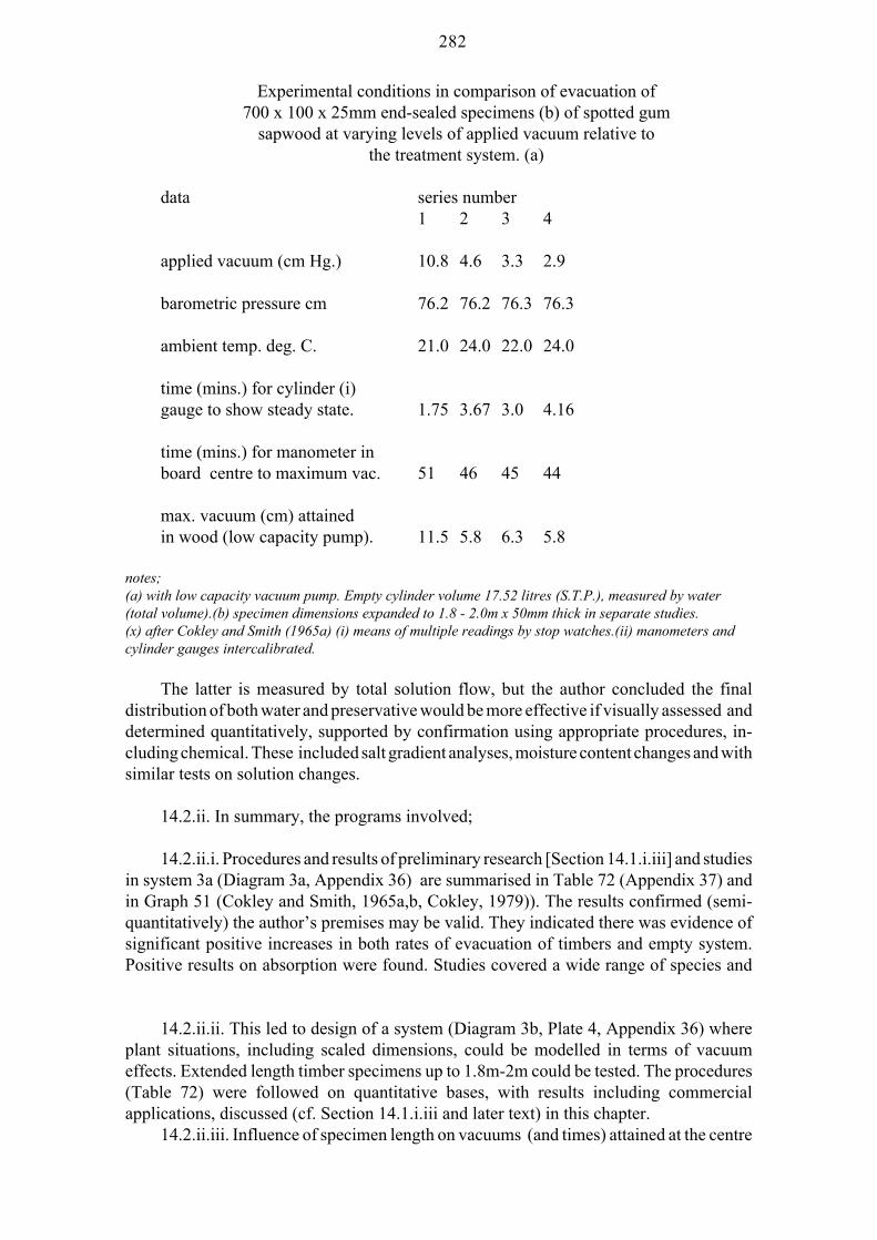
282

Experimental conditions in comparison of evacuation of700 x 100 x 25mm end-sealed specimens (b) of spotted gum

sapwood at varying levels of applied vacuum relative tothe treatment system. (a)

data series number1 2 3 4

applied vacuum (cm Hg.) 10.8 4.6 3.3 2.9

barometric pressure cm 76.2 76.2 76.3 76.3

ambient temp. deg. C. 21.0 24.0 22.0 24.0

time (mins.) for cylinder (i)gauge to show steady state. 1.75 3.67 3.0 4.16

time (mins.) for manometer inboard centre to maximum vac. 51 46 45 44

max. vacuum (cm) attainedin wood (low capacity pump). 11.5 5.8 6.3 5.8

notes;(a) with low capacity vacuum pump. Empty cylinder volume 17.52 litres (S.T.P.), measured by water(total volume).(b) specimen dimensions expanded to 1.8 - 2.0m x 50mm thick in separate studies.(x) after Cokley and Smith (1965a) (i) means of multiple readings by stop watches.(ii) manometers andcylinder gauges intercalibrated.

The latter is measured by total solution flow, but the author concluded the finaldistribution of both water and preservative would be more effective if visually assessed anddetermined quantitatively, supported by confirmation using appropriate procedures, in-cluding chemical. These included salt gradient analyses, moisture content changes and withsimilar tests on solution changes.

14.2.ii. In summary, the programs involved;

14.2.ii.i. Procedures and results of preliminary research [Section 14.1.i.iii] and studiesin system 3a (Diagram 3a, Appendix 36) are summarised in Table 72 (Appendix 37) andin Graph 51 (Cokley and Smith, 1965a,b, Cokley, 1979)). The results confirmed (semi-quantitatively) the author’s premises may be valid. They indicated there was evidence ofsignificant positive increases in both rates of evacuation of timbers and empty system.Positive results on absorption were found. Studies covered a wide range of species and

14.2.ii.ii. This led to design of a system (Diagram 3b, Plate 4, Appendix 36) whereplant situations, including scaled dimensions, could be modelled in terms of vacuumeffects. Extended length timber specimens up to 1.8m-2m could be tested. The procedures(Table 72) were followed on quantitative bases, with results including commercialapplications, discussed (cf. Section 14.1.i.iii and later text) in this chapter.

14.2.ii.iii. Influence of specimen length on vacuums (and times) attained at the centre

283

of spotted gum boards (25mm thickness).Author’s note; studies included multiple thicknesses, but results using 25mm have

been standardised in discussion, giving comparison with thermal data in Chapters 12, 13.

An integral part of the studies, similar to the open tank systems, related to influencesof specimen dimensions on de-aeration results. An effective protocol of end-sealing wasnecessarily developed due to high applied vacuums. By contrast, there was a need forspecimens utilised in vacuum research carried out in the system 3c (Diagram 3c) to beprincipally, and significantly, only under an “end-grain”, or “longitudinal”, influence inevacuation. The study included preliminary experiments to be carried out in laboratorysystem 3b (Diagram 3b) to test end-sealing requirements (cf. Chapters 12, 13) with themanometer tube inserted to a distance of 25mm from the sealed end.

Typical results (low vacuums of the same order as found in the thermal processes) areshown in Graphs 52a, 52b as functions of both pressure differentials “pd” and time inminutes for equilibrium at the board centre relative to length. The effects found were highlysignificant up to 100mm and significant to 200mm from unsealed board ends. Multiple testsconfirmed the efficacy of the end-sealant (an epoxy-asbestos mastic applied as several coatsand polymerised at ambient temperatures [some pre-treatment directly on ends of certainspecies was required]). Study extended to very high vacuums with similar results and tothicker specimens (discussion is limited to only 25mm thickness [refer Author’s note])

14.2.ii.iv. A separate unit (not shown) was designed to study the hydrostatic effect ofsolution pressure on vacuums in development of the Vacuum-Pressure Diffusion Process(Section 14.6). Results from this did confirm evidence based on similar studies with theglass cylinder and experimental data obtained from commercial cylinders (managementapprovals and administrative arrangements were required as plants were legally certifiedpressure vessels). As such, that unit is not further discussed in this text.

14.2.ii.v. Consequently, a special system (Appendix 36, Diagram 3c) was designedby the author to enable a quantitative evaluation of aerodynamic parameters, which aresubsequently described.

The significant theoretical relationships necessary for derivation and evaluation of thedata are nominated in Appendix 38. The studies (including 14.2.ii.iv) jointly formed bases(Cokley, 1976) on which amendments to plant operating practices, designs and resultantefficiencies, were developed for subsequent commercial scale trials.

14.2.iii. Research results obtained are discussed and summarised under six interrelatedtopics, namely;

14.3. Aerodynamics of evacuation of a system.

14.4. Fundamental relationships in de-aeration of timber specimens under appliedvacuums.

14.5. Factors affecting the design of vacuum pumps and de-aeration of commercialcylinder systems. Influence of vacuum pump capacities upon vacuums attained in timbersamples.

14.6. The Vacuum-Pressure Diffusion Process.

284

14.7. Application of research data to commercial plant design and operations.

14.8. The moisture contents and treatment schedules appropriate to the “full-cell” (and

14.3. Fundamental aerodynamic parameters in evacuation of a system. Influence oflevel of an applied vacuum and the establishment of a Critical Velocity Point “Spc”.

The aerodynamic symbols, units employed and their further derivatives are defined inTable 74, Appendix 39. This research was based on results with system 3c (Diagram 3c) andexperimental procedures (Appendices 36, 37).

Results (and the derivations) are detailed in Table 75 (Appendix 39). All measure-ments were converted to S.T.P. under dry air conditions. In view of the legal (Chapter 2)importance and originality of the research conducted, independent confirmatory statisticalanalyses (Cokley and Smith, 1965a), including ANOVA tests, were made and are illus-trated by Table 79 - 81 (Appendix 41).

14.3.a Gas expansion laws applicable for the research conditions.

To validate measurements and derive effective statistical data, it was necessary toexamine whether air expansion (as finally collected), under the applied vacuums and for thetotal system, was either adiabatic or isothermal. The requirement is examined in Appendix38 [Sections 3 and in particularly 3(b)]

Results of experimental measurements when applied to the requirements set out inAppendix 38 [Section 3(b)] proved that the expansion and collection were isothermal. Thusthe gas law (Appendix 38) utilised by the writer was;

p.v = constant

14.3.i. Occurrence of a “Critical Velocity Point”, “Spc” in evacuation of a system.

The results showed there was a significant influence of applied vacuum upon the rate,effectiveness and absolute values of air extracted from the system. This was shown to occurat a nominal value of 4.5cm of applied vacuum. It was independent of whether the systemcontained a wood specimen or was empty.

When analysed for the volume rate of evacuation from the system, an analysis ofvariance (Table 79, Appendix 41) confirmed the differences for this and higher values ofvacuum were highly significant (p = 0.001 level) from the lower levels of vacuum tested.

p” and Relative Velocity of “Rpto R13.5” illustrate the significance of that change at values of applied vacuum p = or <4.5cm.

14.3.i.i. It eventuated that a “Critical Velocity Point” did exist at which extractionconditions were optimum. Though the author had not symbolised this term in earlier reports,it is nominated in this thesis as “Spc” and similarly the “Critical Vacuum Point” (Section14.4) is termed “Vpc”. The two points had values, dependent on statistical analyses, whichranged from 4.3 to 4.7cm and from 2.35 to 2.7cm respectively, with mean nominal values

285

of “4.5cm” and “2.5cm” in terms of applied vacuum.

Author’s note; all vacuum pressure data were recorded in mm of mercury, but, for easeof calulation, are generally cited as cm of mercury.

This optimum point, “Spc”, was shown to be a function of:

(a) effect of vessel design with respect to its diameter and length, as well as therelationship of outlet duct diameter and its length on the attainment of vacuum conditionsin the system.

(b) efficiency of vacuum pump system in extraction and in overcoming of resistanceto flow.

14.3.ii. Physical and statistical examination of data relative to occurrence of the“Critical Velocity Point, Spc”.

As indicated (Section 14.3.1, Table 79, Appendix 41), experimental results gaveevidence of occurrence of this point at a nominal value of applied vacuum “p” of 4.5cm. Toconfirm that conclusion and to examine the physical significance of that critical point,statistical analyses were made, of which representative and significant ones are described.In such, the analyses are cited in terms of parameters important in air movement in, or from,a system.

They emphasise;

a. Kinetic Energy relationships.

b. air velocities, mass rate of flow, momentum and influence of resistance coefficients.These are related to air density at each level of applied vacuum.

c. system geometry, reflected in the Euler and Reynolds Numbers (Appendix 39).

d. Correlation of the Darcy-Weisbach coefficient, “jp”, (equation 14.1) with the above(and related factors) (Appendix 39).

As all measurements were converted to S.T.P.;

pd = (760 - p)

Selected air flow equations from those used in the analysis include:

(i) General Equation of Flow (Rouse, 1949)

P1 - P2 = j . (L/d) . (sg V2) /2 (14.1)

(ii) The Hagan-Poiseuille Equation for Laminar Flow in a pipe of circular cross-section (Binder, 1971) where “pd” is the pressure drop;

pd = 32 u . (L/d2). V (14.2)

286

14.3.ii.i. Use of the term “Relative”.

Dependent on pressure, air is compressible or expandible. Thus, in defining certainparameters and in discussion, the writer has introduced a term “Relative” to indicate:

“The air movement is an evacuation due to a negative pressure differential whenconsidered in terms of vector properties. It is not an effect of an applied positive pressuredifferential. It is efflux from a region of low pressure through the vacuum pump toatmospheric conditions”. As the total air movement is (Appendix 36) an evacuation froma closed system to atmosphere, there are negative and positive vectors involved.

14.3.ii.ii. there was a correlation (Graph 54) between Experimental Linear EffluxVelocity “Vp p” (Table 74).

14.3.ii.iii. there were significant changes in results and flow characteristics, based on“Vp /(p x 10-1)”, for values of “pd” > or = 71.5cm (Graph 55), where “pd” is defined as in Table74.

14.3.ii.iv. Interactions of the Kinetic Energy, “K.E.” and related units with the“Critical Velocity Point”.

14.3.ii.iv.a. For values of “pdnon-linearly (Graph 56) with decrease in “pd”.

Above that value (pd = or > 71.5 cm), there is a highly significant linear correlation.That linear relation was of the form;

pd = 75.9487 - 2.8426 K.E. (14.3)r = O. 9882 ***

Hence,

sgp . (Vp)2 = 53.4361 - 0.7036 pd (14.4)

14.3.ii.iv.b. Mass flow rate, “[m]p”.

As “[m]p” is mass flow rate (mgm/sec) of efflux (Tables 74, 75), for values (Table 75)at applied vacuum pressure “p”cm and as;

[m]p = sgp .vp

the correlation between “[m]p” and “pd” was examined.

For values of “pd” = or > than 71.5 cm, a linear relation (Graph 57) exists of the form;

pd = 76.1183 - 1.5598 [m]p (14.5)r = 0.9985 ***

Below that point, relationships decreased non-linearly.14.3.ii.iv.c. Relation of the Momentum “Ms” (subscript indicating the system) to the

287

Critical Velocity Point.

As Kinetic Energy, “K.E.”, mass flow “[m]p” and volume of efflux “vp”, were allshown to be significantly affected by “Spc”, the Momentum “Ms” was also tested against thisvalue. It was found to vary similarly to the other units, with a change at “p4.5” cm. A linearrelationship (Graph 58) was present at the higher vacuums (p = or < 4.5 cm).

p”, the Kinetic Energyof Efflux “K.E.”, and Pressure Differential “pd”.

From definitions (Table 74),

[(ENp)2 . pd] / K.E. = 1 (14.6)

From the experimental data (Table 75) the value was determined as a constant valueof 1.0056 +/- 0.0097.

p” and the KineticEnergy, “K.E.”, is an inverse value of the pressure differential, “pd”.

14.3.ii.v.i. The relationship between Relative Reynolds Number “Rp” and RelativeEuler Number “ENp” (Table 74).

These two units express air flow conditions in a system.When “Rp” is expressed as the Relative Unit Reynolds Number “R1p”, it has a

relationship to “ENp” of;

ENp /R1p = [Vp /(2pd /sgp)1/2] / [(sgp. Vp) / u] (14.7)

If “u” is shown to be constant and by definition;

sgp = (sgo . p) /76.0

then (ENp /R1p) = constant / (p.pd)1/2 (14.8)

where the constant = u. {(38/sgo)1/2}

= 0.0293This is in agreement with the results (0.0293) calculated on the experimental data

(Table 75).

Hence, for the total system, “u” is constant and thus, as “u”, “sgo”, “L”, are constantfor the system, then:

ENp . [(ppd)1/2 ] / Rp = 0.0293 L-1 (14.9)

The relationship in equation (14.9) may be stated as:

“When a system is evacuated through a duct of length “l” to atmosphere, such that thereis a pressure differential “pdatmosphere, then the ratio of the Euler Number “ENp” to the Reynolds Number “Rp” is aninverse function of the square root of the Pressure Product “ppd”.

288

For any system of a fixed length of duct and geometry of outlet, this ratio is a constantirrespective of the level of applied vacuum. This relationship shows the major significanceof duct length on the aerodynamic efficiency of a system under evacuation conditions. Theauthor has termed it:

“The Equivalence Equation of Evacuation of a System by Discharge through a Ductto Atmosphere”.

The importance of this (and relations of “jp” [Section 14.3.ii.vii.]) is to confirm thatvacuum-pressure systems follow standard aerodynamic formulae and (Diagram 4), treat-ment plants should be designed using those precepts.

14.3.ii.vi. Significance of the Hagan-Poiseiulle Equation in evacuation of a system.

14.3.ii.vi.i. Relation between “Vp” and “pd” at and above the “Critical Velocity Point”.

Equation (14.2) gives this relationship under conditions of laminar flow. Over therange of vacuum pressure studied, value of “u” (for isothermal expansion, Section14.3.ii.v.i) is shown to be constant.

Hence, for laminar flow in any system of fixed geometry;

pd = k . Vp (14.10)

This was tested for values of “pd” above and below values of “Spc” (4.5cm, i.e. where“pd” = 71.5cm).

14.3.ii.vi.ia. For “pd0.3560 +/- 0.0058.

14.3.ii.iv.ib. For “pd” values less than 71.5cm, values of “k” increased inversely with“pd” over a range from 0.4461 (pd = 70.8cm) to 0.7977 (“pd” = 62.5cm). The conclusion hasbeen reached that, for values of “pd” equal to, or greater than, 71.5cm, (vacuums from 4.5cm to 0.4 cm), the air flow satisfies equation (14.2) and is considered to be laminar.

14.3.ii.vi.ii. It is concluded that, below the value of “Spc”, some applied pressuredifferential is dissipated in overcoming resistance to air flow and two synonomous termswere defined to express this. They are;

The “Effective Pressure Differential” or the “Effective Level of Applied Vacuum”.

Each is the resultant between the Applied Pressure (or Applied Vacuum) Differentialand that dissipated in overcoming resistance to flow. The data show “Effective PressureDifferential” has a maximum efficiency at, or above, the Critical Velocity Point.

14.3.ii.vi.iii. Similarly, for internal conditions in the vessel, by definition (Table 74)

k = (D/d). (pd / Vp) (14.11)

289

where D, d are the respective diameters.

Hence the internal velocity flow is a function of the relative diameters of the orificeduct and the system (cylinder).

14.3.ii.vii. Significance of Darcy-Weisbach Resistance Coefficient “jp” in the generalequation (14.1).

By definition (Table 74)

jp = d / { L.(ENp)2} (14.12)

1 / (ENp)2 = 2pd / {(Vp)

2 . sgp} (14.13)

As the system is of fixed dimensions,

d /L =1/670

and thus;

jp = (2/670) . (pd /Vp) . { 1/ [(Vp). sgp] (14.14)

and 335 . jp . [(Vp)2. sgp] = pd (14.15)

When the values of “jpinclusive of values of “Vp” and “sgpwere constant for all “pd” values. Then;

335. [jp {(Vp)2 . sgp}] /pd = 0.9952 +/- 0.0104 (14.16)

14.3.ii.vii.i. There are, however, significant changes in the separate relationships of“jp” to “pd”, “sgp”, “Vp”, such that they are increasing, a minimum, or linear.

When values of”jp” (Table 75) are tested against “pd”, they reached a minimum at“pd71.5” but increased above and (linearly) below that value.

There were corresponding relationships for “Vp” and “sgp”, such that there is aminimum at 71.5 cm, an increase above, and a linear value below that figure for thoseparameters. For all three of these relationships, increase at the higher vacuums levels isapproximately exponential.

Graphs 59, 60, 61 show, for values of “pd” less than 71.5cm, “jp” has, in terms of thoseunits, an inverse relationship to “pd” and to “Vp”, but an increasing one to “sgp”, which latterare statistically linear.

14.3.ii.vii.ii. As the value of “k” (equation 14.10) is constant for values of “pd” at, orabove, the value of pd = or > 71.5 cm, then;

pd = 0.3560 .Vp

290

and, as the value of “Vp” does not vary significantly above “Spc”, then equation (14.16)may, as a first order approximation, be expressed as being equal to ;-

jp = function of (sgp) (14.17)

Thus, above “Spc”, air density appears the principal influence on “jp”. Below “Spc”, thevalue “jp” varies linearly. Over this range;

jp = (lf) of {sgp, (Vp)(-1), (pd)

(-1)} (14.18)

where (lf) = linear function.and the term (-1) indicates a reverse relationship.

Equation (14.18) may be stated as;

“Below the Critical Velocity Point “Spc”, there is a change in relations of “jp” withvalues for the Effective Pressure Differentials”. Below “Spc”, equation (14.18) may bedefined as the quantitative measure of a change in “Applied Pressure Differential” or the“Applied Level of Vacuum” with respect to the system and “jp”.

14.3.ii.vii.iii. Relation of mass rate of flow “[m]p” and the Darcy-Weisbach ResistanceCoefficient, “jp”.

The significance of the relation expressed in equation (14.5) is in terms of the Darcy-Weisbach Resistance Coefficient “jp”. As Mass Flow Rate of Efflux, “[m]p”, is a functionof “sgp” and “vp”, (Tables 74, 75), its relationship to “jp” was examined. The author founda relationship for “[m]p” similar to relations of “jp” with “sgp”.

This, as for the relations of “sgp” with “jp”, leads to the conclusions ;-

(a) there is a change in physicochemical relationships of the air and the system at thisvalue of p = 4.5cm. This is the value of the “Critical Velocity Point”, “Spc”.

(b) due to the above, from “Spcexpanded air molecules from the system for discharge through the orifice and duct. Hence,at this point, there is an equivalent decrease in the “Effective Applied Pressure Differential”relative to levels of the applied vacuum pressure. In consequence, in addition to overcomingline resistances, vacuum pumps must have adequate capacity for this decrease. Vacuumpumps are generally classified in terms of their air volume capacity rate which decreaseswith increase in level of applied vacuum.

14.3.ii.vii.iv. The overall conclusion reached is that the Darcy-Weisbach ResistanceCoefficient “jp”, when applied to evacuation of a system, represents not only conditionsrelative to the resistance of air flow through a duct, but, in addition, it also expressesresistance due to the expanded state of air molecules, or change in physicochemicalrelationships.

14.3.iii. Characteristics and definition of the “Critical Velocity Point”, “Spc” may besummarised in the following terms.

291

“The level of vacuum applied to a system by a vacuum pump through a generally

(a) Gas flow is laminar, satisfying the Hagan-Poiseuille Equation.

(b) Volume rate of Efflux, Relative Velocity Rate of de-aeration, mass rate of flow andMomentum of the system are at a maximum. Change (increase) in their value may beconsidered as primarily caused by a decrease in the air density, or by change inphysicochemical relationships of the evacuated air.

(c) The Linear jet velocity of efflux “Tvp”, the Linear jet velocity “Vp”, and the KineticEnergy of Efflux, “K.E.”, are either a constant value, or a linear function relationship, ofApplied Pressure Differentials, “pd” cm, in the system.

(d) The absolute value of “Spc” is, for any system geometry, dependent on attainmentof the “Effective Pressure Differential”. This is a function of “Effective Capacity” of thevacuum pump and hence (Section 14.5) the capacity of the pump at a required level ofevacuation.

(e) When separately tested against “Vp”, “pd” and “sgp”, resistance to air flow, asmeasured by the Darcy-Weisbach Resistance Coefficient, “jp”, is at a minimum value.

(f) Above “Spc”, the values of “jpgravity of the air, or change in its physicochemical relationship in the system.

(g) Below “Spc”, relationships of “jp” to air density, velocity, to mass flow rate andpressure differential are linear.

These differences are attributed to a decrease in the “Effective Level of Evacuation”caused by loss in vacuum pump capacity. This latter is considered as being due todissipation of capacity in overcoming resistance to flow and to increase in mass per unitvolume of air efflux.

(h) The “Critical Velocity Point” occurs (S.T.P.) at a nominal vacuum of 4.5cm andis shown to be a controlling parameter in de-aeration of a vacuum treatment plant. Belowthe value of “Spc”, evacuation efficiency (see text) decreases rapidly.

Neither the existence of, nor significance of, a Critical Velocity Point in these systems(for vacuum/pressure treatments of timber products), has been reported by other workers.A similar claim is made with respect to the Critical Vacuum Point “Vpc” (Section 14.4).

Section 14. 4. Fundamental relations in the de-aeration of timber specimens under anapplied vacuum.

14.4.a Studies cited (Cokley and Smith, 1965 a,b) showed there also existed a “CriticalVacuum Point, Vpc”, with respect to de-aeration of timber specimens in the system. ThisCritical Vacuum Point “Vpcproperties.

Numerous studies have been made using gas and fluid flow through wood (Stayton andHart, 1965, Wardrop and Davies, 1961, Tesoro et al, 1966, Choong et al, 1972, Wilfong,

292

1966) and, in certain cases, utilised a term, “The Darcy Permeability Coefficient” (Nicholas,1972), in their theoretical calculations. However very little research had been carried outon the influence of applied vacuums on wood de-aeration.

14.4.b. The Paradox of wood density in air flow formulae and in relevant calculations.

There is an apparent paradox in that, whilst the wood density, or specific gravity, is afactor in almost all determinations relative to properties and functions such as moisturecontent and void volume, that term does not appear in the general equations of flow (Section14.3.2), including Poiseuilles equation. Consequently, it does not appear in the derivationsof evacuation characteristics discussed in Sections 14.3 and 14.4.

That paradox was emphasised in development of effective treatment schedules and inthe research into moisture contents at, or above FSP (Chapter 12), for this “full-cell”process, where treatment groups (Chapter 12) found for open tank, especially thermal, wereapplicable. That also applied to the Vacuum-Pressure Diffusion Process (Section 14.6),developed concurrently with modifications in commercial plant design (Section 14.7)which resulted from this research.

The writer examines this anomaly (Section 14.4.5) and he establishes that, inpreservation, the “Void Volume” for calculation of “contained air” is related to density andin de-aeration of wood, “permeability” (Chapter 8) is the controlling factor. In contrast,“porosity” (Chapters 8, 12) and “accessible free paths” (Chapter 12) are the significantcriteria for uptake of preservative solution.

In illustration of the absence of a term for density in the equations of flow, the writercites Siau (1984), who describes (pp. 175 et seq.) mathematical treatments for unsteadygaseous flow where, in contrast to discussions on heat or moisture, density does not appearas a term. That writer (p. 181) cites work by Park (1970, s.n.r.) on unsteady gas flow whichled to the possible conclusion that wood is not a uniformly permeable medium andillustrates that by reference to treatment of the red oaks. He quotes (pp.181-182) studies bySebastian (1973).

Author’s note; it is appropriate to indicate that though, when this research was carriedout, the subsequent extensive references data, described above, were not then available, thatevidence has been used in evaluation of research results in this thesis.

14.4.c. In this section, the bases on which this point, the Critical Vacuum Point, “Vpc”,and its properties, are described and the aerodynamic significances examined. Theexperimental system 3c was used (Diagram 3c) with specimens as described and for whichthe physical properties such as density, moisture content, saturation moisture content, airvoid volumes, were determined as in Appendix 38, with derivations of relevant formulaeand relationships in Appendix 38. An experimental mean saturated moisture content of46.4% was determined, as compared to mean theoretical value of 47.5%. but certain

pc”, were (Section 14.4.5.1)additionally examined by using system 3b. The relevant symbols and units are describedin Table 76 (Appendix 40) with experimental and derived results in Tables 77, 78 of thatAppendix.

Author’s note; To determine the Critical Vacuum Point, of the total eleven sets of data(“p”cm), four would be statistically important in testing, particularly those over the region

293

“p2.5” to “p4.5” of applied vacuums.The primary need was to statistically evaluate that relations between those four values

in terms of data compared to data below them, eg. higher, or lower, “pd” were validlydeduced. Hence, for confirmation, extra statistics and evaluation (see text) of someadditional significant aerodynamic criteria were employed.

14.4.1. Derivation of relationships for characteristics of the Critical Vacuum Point,“Vpc”.

The writer determined relationships as follows;

14.4.1.i. Relation between applied vacuum and Efficiency of Extraction, “E”, and“EA%” (Table 76, Appendix 40) of air from specimens.

Author’s note; though multiple specimens were used in the research program, the textwill refer to “specimen” in the discussions.

14.4.1.i.a. air in the specimen gave a higher resistance to flow under applied vacuumthan the air in the vessel.

Typical results are shown in Graph 62, which also illustrates the difference inextraction rates and absolute volumes of air extracted from the empty system relative to onecontaining a specimen. As rates of extraction above “p2.5” were such as to enable only thetotal times, volumes and rates to be recorded, data are shown for “p5.2” cm and “p8.2” cm.It will be noted the slope of the curve is reduced as levels of evacuation increase.

14.4.1.i.b. there was a highly significant relationship (0.001 level) between “E”,“EA%”, and “p” cm, and the effect was most significant for values of “p” > 2.5 cm, i.e. forlower levels of applied vacuums (3.0 - 13.5 cm). Typical ANOVA values are cited inAppendix 41.

14.4.1.ii. The Effect of Applied Vacuum on “EA%”.

Results are shown in Graphs 63, 64. Statistical analysis showed that;-

14.4.1.ii.a. for values of “p” < or = 2.5cm there were no significant differences betweenvalues.

14.4.1.ii.b. A significant difference (at 0.01 level) was present (Table 80, Appendix41) between “p2.5” and “p3.0” and also “p4.5”. This difference increased (0.001 level) forlower vacuums.

14.4.1.iii. Determination of Critical Vacuum Polnt “Vpc”.

The hyperbolic relationship (Graph 64) between “EA%” and “p” was transformed intoa linear equation of the form;

p /EA% = ap + b (14.19)This was tested for values of “p” above, equal to, and below, an applied vacuum of

2.5cm. Two linear equations were developed, where “p” was expressed in millimetres.

294

These were;

for “p” < or = 25mm;

p /EA% = 0.0lO5p - 0.0024 (14.20)r = 0.9978 ***

and for “p” = 30 mm to 135mm;

p /EA% = 0.0268p - 0.4175 (14.21)r = 0.9938 ***

These linear transformations are shown in Graph 65. The vacuum level for the pointof intersection (equation [14.23]) was defined as the Critical Vacuum Point, “Vpc”, forwhich co-ordinates were determined and;

p / EA% = 0.2650 (14.22)hence Vpc = 25.4663mm (14.23)

14.4.1.iv. Influence of applied vacuum “p”cm on Volume Rate of Extraction, “Q” cc/sec from the specimen.

14.4.1.iv.i. Data (Table 78) were analysed and a general relationship (Graph 66)[compare Graphs 53a, 53b] was transformed (equation [14.24]) to;

p = function (p. Q1/2) (14.24)

for “p” < or = 2.5cm,

p = 0.8468 (p . Q1/2) - 0.0116 (14.25)r = 0.9998***

for “p” > or = to 2.5cm,

p = 2.9419 (p . Q1/2) - 6.3742 (14.26)r = 0.9638 ***

The lines intersected at a point whose co-ordinates were:

p = 2.5601cmand p . Q1/2 = 3.0369

and hence the values of the point of intersection are;

p = 2.5601cm (25.601mm)Q = 1.40 cc/sec

This value of “p” is, of the same order as the nominal value of the Critical VacuumPoint.

295

14.4.1.iv.ia. The relation was also examined in terms of pressure differential, “pd”, andthe product “p.Q”. This showed (Graph 68) a significant difference occurred at a “pd” value= or > 73.5 cm, which corresponds to “Vpc”. For “pd” values below that, there was only a

14.4.1.v. Relation of Kinetic Energy of Efflux from the specimen.

A relationship (Graph 69) was found similar to the one determined for the CriticalVelocity Point “Spc” (Graph 56), except that for Graph 69, the linear relationship occurredonly over values of “p” = or < than 2.5cm.

14.4.1.vi. The Significance of the Critical Vacuum Point on de-aeration. Relation ofevacuation characteristics of the system and Volume Rate of Evacuation of the specimen.

The writer found (Section 14. 3) the Critical Velocity Point “Spc” bore a highlysignificant relation to the volume rate of efflux and the momentum of the system.

The Critical Vacuum Point “Vpca significant relation to the Volume Rate of Extraction, “Q”. “Spc” has a nominal value of45mm, but “Vpc” has been shown to have a value of about 25mm.

The effect on “Q” was studied for:

14.4.1.vi.a. Relation with the Momentum of Efflux of the System “Ms” and “Q”.

14.4.1.vi.b. The Relative Rate of Evacuation “Vp” compared to “V13.5”, for whichcomparative values are shown in Table 78.

Results for both are shown in Graph 70. A significant effect of both parameters wasfound with respect to “Q”. The evidence showed:

14.4.1.vi.b.i. Evacuation effectiveness, and rate, of the air in the specimen was afunction of the conditions of evacuation of the system. Hence any decrease in the efficiencyof the latter is reflected in de-aeration of the specimen. This applies in particular to thevacuum pump capacity and “Effective Pressure Differential”.

14.4.1.vi.b.ii. aerodynamically, the movement of air in the specimen may be princi-pally considered as through a series of small ducts, where the length / diameter ratio isindividually very high and there is a nominal total length of about 63mm as the specimensare primarily under “end-grain”, or “longitudinal”, evacuation at “p” mm external to thesmall ducts. There is also a component of flow perpendicular to the axis through ray cells.It is important to note de-aeration of wood fibre lumina will occur and, similarly, the de-aeration progressively takes place from cell walls for each tissue type and, for that reason,total void volumes (Appendix 38) were measured.

14.4.1.vi.b.iii. If the geometry of the system, the duct outlet dimensions (l/d), vacuumpump capacity, or the time at vacuum, are inadequate to attain “Vpc”, then efficiency of de-aeration is reduced. The value of “EAinitial process conditions were only of the order of 50% efficient.

296

The evidence confirmed the writer’s original theories on the cause of variability in full-cell results, as being, in part, due to insufficient de-aeration of the timber. It also confirmedthe hypothesis that, similar to open tank systems using thermodynamic principles forthermal evacuation of timbers, there exists a “minimum Critical Vacuum” level which isapplicable for local species and conditions. If so, (Chapter 12) that level of applied vacuummay be described (Chapter 13) as equivalent to an “effective minimum” in temperaturerequired for treatment in thermal processes.

It supported the writer’s belief that a mimimum time of vacuum maintenance isnecessary (Sections 14.1, 14.2) for optimum de-aeration of timber, which may be a function(cf. Sections 12.2, 12.3, Chapter 12 re species treatment groups and Graphs 37, 38) of woodstructure. Provided that an adequate level of “Effective Applied Vacuum” was attained inthe “(l/d)” of a treatment plant, laboratory, and plant, studies (Cokley and Smith, 1965a)confirmed the Critical Vacuum Point was independent of plant design characteristics. It wasdependent on species characteristics.

For spotted gum, E. maculata, and for similar species, it was (Section 14.4.5)determined over the range of 25-26mm (related to S.T.P.) with results obtained over a rangeof systems. They were, in all cases, subject to attainment of an “Effective Applied VacuumLevel”.

14.4.1.vii. Relation between Mass Flow, Applied Vacuum Pressure “p” cm andPressure Differential “pd”.

It was shown (Section 14.3) that “Spc” characteristics had significant relationships tomass rate of air flow from the system. As there is a physical inter-dependence between “Vpc”and “Spc”, the possible interrelation of “Spc” was examined in terms of the mass flow,“sgp.Q” (mgm/sec) from the specimen.

Results showed the significant parameter was “Vpc”.

Similar to Graph 57, a linear relation existed between “p” and “p.Q”. For values of “p”> 2.5cm. a random relation existed (Graph 68).

14.4.1.viii. Correlation of the Darcy-Weisbach Resistance Coefficient “jp” with theCritical Vacuum Point “Vpc”.

The author has shown (Section 14.3) that, with respect to evacuation of the system,“jp” approached its minimum value at the Critical Velocity Point “Spc”.

As a relation has been shown between “Spc” and “Vpc”, the writer examined a possiblerelation between “jp” and “Vpccorrelation, this was examined with respect to the function “Q”.

In addition, it was (Section 14.4.2.i.i.) demonstrated that, under typical vacuum pumpefficiencies, an applied vacuum of “p” = 2.5 cm, within the system, results in an upstreamvalue, internal to the specimen, which is equal to “Spc”. As “Spc” was determined to occurat the nominal value, “p” = 4.5cm, it was felt desirable to test whether “jpw” (the subscript“w” indicates the relation to efflux from the specimen) was significantly related to “Vpc” orto “Spc”.

297

The general equation is;

pd = jp . (Le / de) . { sgp. Vp2 } / 2 (14.27)

where, for the specimen,

Le = effective length of microduct (assumed longitudinal flow).de = effective (mean) diameter of orifice.Vp = measured linear velocity.

As Le, and de are constant, and

Vp = 4 Q / [ pi . (de)2 ]

then

pd = [8. Le / (pi)2. de 5]. { jpw. sgp. Q

2 } (14.28)

and

pd = c. ( jpw . sgp . Q2 ) (14.29)

where c = 0.8099 Le / (de)5, and thus

pd / ( sgp . Q2 ) = c . jpw (14.30)

Equations (14.27, 14.28, 14.29) show the major influence of the dimensions of,particularly, “Le” and “de” (the “Effective Orifice Diameter”, Chapter 12) for microductsin the wood matrix. However (Sections 14.4.b, 14.4.5.), these equations do not include thewood density.

The experimental data and derived functions were tested in these equations and theauthor found:-

14.4.1.viii.i. the term, [pd / (sgp . Q2)] had a minimum value of 8.7822 x 10-5 at p =2.

5 cm.

For values < or > than p =2.5 cm, the value rose to limits (of experimental data) of;

for pO.4 cm = 48.7585 x 10-5

P13.5 cm = 43.3636 x 10-5

p with “Spc”, the authorconcluded that;

14.4.1.viii.ii.i. Darcy-Weisbach Resistance Coefficient “jpw” is applicable to air flowconditions in evacuation of wood. The evidence showed the critical influence on “jpw” was

pc”, at 2.5 cm of appliedvacuum pressure.

298

14.4.1.viii.ii.ii. at the value of “Vpc”, the coefficient “jpw” was at a minimum.

14.4.1.viii.ii.iii. as it was increasing from “p2.5” to “p0.4” (expressed in cm), there wasincreased resistance in removal of the residual air.

The writer attributes this (Section 14.4.3.i) to change of site (and mass relative tovolume) of air evacuated from, not only the cell cavity, but also from cell walls and changefrom a multilayer to a monolayer condition.

14.4.2. The interrelationship between the Critical Velocity Point of a system and theCritical Vacuum Point in de-aeration of a timber specimen.

Under the experimental conditions, for the test species, spotted gum, E. maculata, theauthor found both “Vpc” and “Spcbut were dependent on availability of effective vacuum pressure capacity. They occur(relative to S.T.P.) at nominal values of 2.5cm and 4.5 cm respectively.

14.4.2.i. Aerodynamically, the de-aeration of a specimen within the system may bedescribed as a discharge of air from a microduct under an applied vacuum pressure of “Vpc”.This, which is equal to “p2.5”, is external to the microduct, but within the system.

The de-aeration of the specimen within the system is equal to the discharge of air froman internal pressure, within the duct, of “pin” to an “atmosphere” of “psys”cm.

In that context, the value inside the system is “psys”, and is equal to “Vpc”. The resultantair discharge is hence equivalent to that through a small orifice under conditions of laminarflow and maximum velocity.

At the lower moisture contents (Chapter 13), 19% mc, of the study, timber is aninsulating medium, and, in addition to temperature effects, the writer considered othercriteria should desirably be examined to determine if the expansion from the timber orificeswas, in fact, adiabatic. That (adiabatic expansion) was a condition necessary for theapplication (Chapter 12, Appendix 28) in determination of the “effective orifice diameter”in timber. Those criteria were;

14.4.2.i.i. when the duct diameter is small (< 0.4 x l) to the length, “upstream pressure”should bear a relation to the “downstream pressure”. Hence if “rc” is the ratio of theupstream pressure “pin” to the downstream pressure “psys” (Perry, 1953) then;-

rc = (pin) / (psys)

and rc = { 2 /[Y +1] } [Y /(Y -1)] (14.31)

where Y = 1.401 (Table 76)

and hence rc = 0.528 (14.31a)

A mean value of 25mm has been determined for the “downstream” value, namely“Vpc”, and as an “upstream” pressure (Sections 14.4.2.i.ii, iii and iv) is shown to be equal

299

to “Spc” (nominally 45mm) with a measured value of 47 mm, then the ratio (Levitt, 1958)of “downstream” to “upstream” pressures is given by;

pin = (psys / 0.528) (14.31b)

= 25 / 0.528= 47.34 mm

The result of 47.34 mm is of the same order as the data determined experimentally.

14.4.2.i.ii. If the expansion was adiabatic, it was concluded that, under these condi-tions of a “Critical Vacuum Point”, for “Vsys”, applied to the exterior of the specimen, thereis a limiting value of negative pressure within the specimen duct which is equal to the“Critical Velocity Point”, “Spc”, as determined above.

If that conclusion was correct, increase of “p” to values < 2.5cm should not signifi-cantly change the effective internal vacuum in the specimen. This was tested using systems3b, 3c, with the former also used for examination of longer specimens. Results confirmedthat for applied vacuums of “p” to below 1.0 mm (effective maximum vacuum readable withthe single stage oil immersion laboratory vacuum pump), the limiting value (27o C.,corrected) was 47 mm within the specimen, when spotted gum, and similar species, werestudied. This aspect is subsequently examined in terms of a range of species (Section14.4.5).

14.4.2.i.iii. If the “upstream” vacuum has a limiting value of “Spc”, determined at avalue of 4.7cm, the writer concluded that the residual air, “a” cc. remaining in the specimenmay bear a relation to “Spc” rather than to “Vpc”. Possible interactions were examined of;

a. relation of “a” cc. to applied vacuum, “p”.

a.i. It was found (Graph 71) that there were significant differences in values of “a” for“p” = or < than 2.5 cm relative to lower vacuums, viz. “p” > 2.5 cm.

In vacuum ranges from 2.5cm and higher (“p” = or < 2.5cm) a linear relation existed.

a.ii. for values of “p” = or > 5.2 cm, a statistically linear relation existed.

a.iii. There were significant differences for “p3.0” and “p4.5” cms compared to the valuesof “p2.5” and “p5.2” For values between “p2.5” and “p5.2”, there was a sharp increase (acurvilinear relation), such that the “tangent” point was at a “p” values slightly greater than4.5 cm and with an “a” value of about 24 cc.

This corresponds (cf. section, 14.4.2.i.iv) to a vacuum of the order of “Spc”, rather that“Vpc”.

14.4.2.i.iv. Relation between Applied Vacuum ,”p”, and Mass Flow per sec per unitwood volume (mg./sec/cc), “x1” (Table 76).

author’s note; A general term, used in the Langmuir and in similar equations, is “x/m” (Table 76).

300

The wood mass, “m”, is the product of specific gravity, in this instance 1.53, and woodvolume. Thus the term “x1” is a constant function (x 1.53) of “x/m”, where “x” is equal tothe product, “sgp.Q”. For consistency in text calculations, the writer has used the term “x1”rather than “x/m” and as the factor of “1.53” is constant for all values, for the simplificationof calculations, it is implied in all derivations and discussions using this parameter. Aprecedent in this use of adsorption per unit volume of the adsorbent is cited in discussion(Findlay, 1944, p.281) of the adsorption of gases by charcoal. This was tested with resultsas follows;

a. values > or = to p52 mm, bore a linear relationship of the form ;

(p / x1)10-4 = 2.8156 p + 79.8428 (14.32)r = 0.9124 **

b. for vacuums = or < p25

(p / x1)10-4 = 75.476 + 0.1472 p (14.33)This was approximately parallel to the “p” axis.

Between the values of 25 mm and 52 mm, there occurred a curvilinear relation such,that over the approximate range from “p30” to “p52” (decreasing above “p45” to “p52” tobecome collinear at about 63mm with the line expressed by equation [14.32]), a sharpincrease was found for values of (p/x1)10-4.

Results are shown in Graph 72, and are of a similar form to relations of “a” with “p”(Graph 71).

14.4.2.i.v. Correlation of Residual Air “a” cc and “x1”, the mass discharge (mgm /sec/cc) per unit of wood volume (Table 76), in terms of applied vacuum level.

In view of the finding that, under an applied vacuum, “Vpc” (2.5 cm), within the system,a limiting “upstream” vacuum within the specimen was equal to the nominal value of “Spc”(4.5 cm), it was desirable to test whether the residual air “a” cc was related to “x1” and, ifso, was this a function of either “Vpc” or “Spc”.

The tentative finding, based on Graph 71, was subsequently tested by examining therelation to the function “p / x1” (refer Section 14.4.2.i.iv), where “x1” has values as definedin Table 76 (Appendix 40). The relationship, using the product “(p / x1)” [see author’s note,Section 14.4.2.i.iv], was examined (Graph 73) and it was found there were two linearrelationships. These two linear regressions were;

(a). for “p” from 0.4 to 4.5 cm,

a = 0.4063 [(p/x1) 10-4] - 30.1877 (14.34)r = 0.9862 **

(b). for “p” from 5.2 to 13.5 cm,

a = 0.0131 [(p/x1)10-4] + 21.8773 (14.35)r = 0.8773 **

The lines intersected at a “(p/x1)” value equivalent to an applied vacuum of 4.7 cm,and “a” value of 23.5789cc. This vacuum was of the same order as “Spc”, and confirmed the

301

tentative findings based on Graph 71.

14.4.2.i.vi. The author concluded that his hypothesis was correct and that a limiting“upstream” (internal) vacuum was present in the specimen when an external vacuum equalto “Vpc” was applied in the system.

However equation (14.31) applies when maximum velocity is equal to sonic velocityand hence:

The Critical Vacuum Point, “Vpcface of the wood capillary or microduct system (contained within a vessel) whichestablishes an internal upstream pressure of discharge within the duct equal to the “CriticalVelocity Point”, “Spc” of 4.5cm (nominal). Thus, under these conditions, discharge, whichis adiabatic, through the microduct is at sonic velocity.

14.4.3. The Langmuir Function, “x/m”, applied to wood. Moisture content analogiesand significance of dissolved air in preservation.

14.4.3.i. The original Langmuir isotherm equation and a function, “x/m”, weredescribed (Findlay, 1944, pp. 280-284) as an “equilibrium condition between adsorption onthe surface and evaporation, or escape, from the surface of a solid”, as a function of pressure,and assumed “to be of unimolecular depth”. This formula could be developed without“postulating any particular mechanism of condensation and evaporation”. In addition, itwas cited to apply to surface adsorption where the mass is used as a measure of the surface.It was extended to solutions. As it was an equilibrium condition, forces of attraction mustbe balanced by forces repelling the adsorbent.

The function “x/m” was further extended to timber. Stamm (1964, pp. 138 - 141)quotes the Langmuir equation as applicable only to monomolecular adsorption conditionsof type 1 (that writer classifies, pp. 134-136, adsorption phenomena into 5 classes),implying a physicochemical relation between the air and the adsorbent. He describes the“B.E.T.” equation for polymolecular adsorption.

However, it appears wood mass was used in substitution for surface area and,importantly, the function appeared to be used in the same context as concentration of asolute in a solvent, with the latter expressed as mass, and not volume. In measuringadsorption, Stamm (1964) advises “to use a method involving a closed system that can beinitially evacuated to a high degree to remove adsorbed air”. There was a dearth of literatureon measurement of and sites of the “residual air” volumes in wood. The writer believes therecould be a role for the use of radioisotope techniques.

14.4.3.i.i For wood, the writer considered two unanswered questions (or factors)existed in a classification as to whether the air contained within the cell wall matrix wasadsorbed in terms of Stamm’s (1964) definition, or whether it was only absorbed. Thesewere;

(a) difficulty in establishing the difference between adsorption and absorption, bothof which are based on an equilibrium state.

(b) due to its capilllarity and matrix structure, total cell wall surface, including internal,is indeterminate in wood, where “void space” causing internal surfaces is a function of what,by analogy, may be termed the “solid wall packing fraction”. In terms of de-aeration, thesignificance rests in that, as is shown by especially the penetration by water with the

302

consequent swelling (from below and up to FSP), the cell walls are pervious and can becorrectly termed a “matrix” of space and solid wood tissue. Air has been generally assumednot to cause swelling.

The implication drawn by this author is that, for timber, the function “x/m” may notadequately represent the internal “void surfaces” in this general equation. It is consideredto be a valid application of the relation of air to total wood mass.

In subsequent discussions, the Langmuir type equations are used to imply, or toindicate, a change of state of air relationships to wood and similarly for discussion (Section14.4.3.ii) on “Activated Flow”. If conditions are stable, a relation, generally linear, exists,but, if they are unstable, a random relation is present.

An analogy may be drawn with residual moisture content in the wood (Section 12.4,Chapter 12). For moisture, there is an initial removal, either in the liquid, or gaseous, phaseand (cf. Section 7.4.b, Chapter 7) “dehydration” is finally reached. External conditions,such as elevated temperatures and/ or a reduced humidity approaching zero, influence thefinal equilibrium condition. Isotopes could be applicable in studies of those changes. Careis needed in this work to differentiate water present as part of a compound. At the critical(variable with species [Chapter 12]) point of FSP, only the “free” moisture from the celllumina and from wall surfaces, has been removed. Below FSP, the condition of “EMC”applies. FSP may thus be equated to a “saturation value of the cell wall voids” by water,which is in not only the “bound stateterm extends to water “contained” within the wall matrix. EMC (Chapter 7) is anequilibrium function between that moisture content and Relative Humidity (RH%) of asurrounding atmosphere.

For this context of its relativity to the surounding air, the author suggests that “EMC”may be equated to an equilibrium of the separate concentrations between two solvent phases(wood matrix and atmosphere), a phenomenon common in analytical methods for extrac-tion of dissolved substances. For the air contained (Section 14.4.3.i.ii.a) in a woodspecimen, this may be equated to an equilibrium with the atmospheric pressure (and RH%)and/or a change in that pressure (Henrys Law [Findlay, 1944, p. 513]). For this, theLangmuir equations are considered to apply.

14.4.3.i.i.i. Moisture gradients occur in a specimen unless it is saturated, is in an ovendry state or equilibrated under constant RH% conditions. Gradients do not apply if thesurface/thickness ratio is high, or if the specimen is under a direct “end-grain” influence.

The practical implication of EMC is that, being a state of equilibrium with thesurrounding atmosphere, there is what the author describes as “ moisture diffusivity” fromthe “core” to the surface. That means, unless the above conditions for an absence of amoisture gradient are met or the analysis of “Contained Air” is based on the cross-sectional(mean) moisture content values, there exists an air gradient within a specimen. For thisdiscussion, the cross-sectional (mean) values are implied.

14.4.3.i.ii Alternative Concepts, and definitions, in the air content of timber.

To allow for these apparent paradoxes stated in Section 14.4.3.i.i, the author hasdeveloped a wider concept and sub-concepts (Section 14.4.3.i.ii.a.ii), and nominates a term

303

- the “Contained Air” - to describe the air content of timbers in especially de-aeration byany method.

Author’s note; in this, and associated discussions, the term “air” is interpreted toinclude its constituents and their separate physicochemical reactions, especially for“embedded” and “dissolved” fractions of “Contained Air”.

14.4.3.1.ii.a. Analysis of distribution of the “Contained Air” in a timber specimen.

14.4.3.i.ii.a.i. Significance of “Dissolved Air” in wood preservation. Relationship ofVoid Volume formulae.

Void volumes (Maclean, 1935, Stamm, 1938) are based on residual “free space”, otherthan space containing water. That includes moisture contents below FSP. However, withinnormal accuracy required, when these formulae are used they assume zero air content whenthe specimen is at “saturation moisture content” values and a maximum of air at zeromoisture content (anhydrous).

The first assumption (at saturation moisture) ignores the air content of the watercontained within lumina as well as both on the surface of and within cell walls when woodis in equilibrium with the surrounding atmosphere, except when the water has been de-aerated by a vacuum pump, or other (eg. by thermal) process. For normal void volumecalculations, the resultant error is equal to saturation concentration of air, namely about 2%,in water at S.T.P. The writer has quantified this dissolved air by the term “xds”. In theevacuation of a specimen, especially below FSP, the order of “xds” is small, but for hydraulicpressure applications, as used in full-cell treatments [at 1400 kPa ( or about 14 atmos-pheres)], the effect (Section 14.4.3.iii.ii) is, by Henrys law, very significant. The relationof solubility is significant in mechanisms of operation, especially at high vacuums, of water-sealed vacuum pumps and is important in the Vacuum-Pressure Diffusion Process (Sec-tions 14.6 and 14.7).

14.4.3.i.ii.a.ii. Sub-divisions of “Contained Air”.

Between those two limits, namely zero and maximum air content, the writer hasdefined the “Contained Air” as the total (Table 76) of these air components (based on theirdistribution) within the timber and in the water present in the timber, which may beremoved, especially by evacuation (also applicable to thermal effects).

It is sub-divided into;

(i). “xv”, the free air contained in cell lumina.

(ii). “xem”, or the “embedded air”, is that air in wall surface layers, or contained withinthe cell wall matrix.

This may be either absorbed or adsorbed, is in either a “monolayer”, or a “multilayer”,condition (Field, 1963) relative to the wood matrix and does not assume “embedded air”occupies only the sites otherwise occupied by water within the wall matrix.

The writer shows (Section 12.4.4, Chapter 12) that as wood specific gravity increases,the fibre lumen diameter and, consequently, its volume decreases, but fibre wall thicknessincreases (with similar relations for softwood tracheids). As a result, “xv” decreases with

304

an increase of density, but “xem” increases (dependent on relative “packing fraction”,Section 14.4.3.i.i).

(iii). “xds” is total air dissolved (at S.T.P.) in the “free moisture” within cell lumina,or that within the cell wall matrix and including that defined as the “bound moisture”. Asthe solubility of air in water is, by Henrys Law (Findlay, 1944), a function of pressure, then,under evacuation, there is removal of some, or most, of that dissolved air. This is quantifiedby the difference in saturation concentrations (cc of air / cc of water) at S.T.P., and theapplied increased, or decreased, vacuum pressure “p”.

Thus total “Contained Air” = xv + xem + xds

The author suggests ratio of the right hand side to total contained air is an alternativedescription of evacuation efficiency (cf. Section 14.4.3.iii.i) from the specimen.

The accurate determinations of respective values of sub-divisions of the “contained”air may be calculated using void volume equations (Maclean, 1935, Stamm, 1938) when,particularly, values are measured at saturation, FSP and oven dry moisture contents.

The writer has developed an approximate method, which is not directly dependent onwood specific gravity (1.46 or 1.53 [for which Kolmann and Cote, 1968, use a mean valueof 1.50]). However, in development of data (Appendix 38) the writer utilised the conven-tional formulae. To indicate these values, as a first order approximation (5%), they arecalculated (S.T.P.) as;

(a) “xv” is equal to the volume of water contained in a saturated specimen (based onmoisture content) minus that present at FSP (assumed as 30% mc) and with an assumedwater density of 1.00.

(b) “xem” is assumed equal to the water volume at FSP minus water volume at the testmoisture content. As the “contained water” density below FSP (Stamm, 1938) is a functionof mc, this latter volume may be more accurately determined as (the water mass based onmoisture content / density of “contained moisture”). It has a maximum value when thespecimen is anhydrous. Shrinkage during drying is a factor in calculation.

(c) At and below FSP, there is an additional volume allowance made for “xds”, whichis equal to 2% of the equivalent water volume contained within the wall matrix at the testmoisture content.

For these calculations, density of the water is assumed as 1.00 (cf Stamm, 1938) at, andabove, FSP. The orders of these values are illustrated for the test specimens. For these, meanoven dry mass was 221 gms, swollen volume saturation moisture content was 46%, and testmoisture content was 19%.

Hence, at a nominal FSP of 30% mc, a “contained moisture” density of 1.14 (Stamm,1938) an assumed shrinkage of 5% from FSP to 19% mc, then respective air volumes of“xv”, “xem”, and “xds” (for containedcc (“xem” volume uncorrected for “contained water” density is 23 cc), giving a volume of55.8 cc. Using void volume formulae (Appendix 38), a mean air volume of 53.9 cc(converted to 50.4 cc of dry air at S.T.P.) was determined, which is in reasonable agreementwith the alternatively derived figure of 55.8 cc of air.

305

Dissolved air “xds” (0.8 cc) in the “contained moisture” is the same order as residualair, “a” cc, found at the higher vacuums used in the study. This value, namely 0.8 cc at thetest moisture content, is further examined in Section 14.4.3.i.iii and it can be concluded(Section 14.4.3.i.iii.i) an additional force may be required to remove “xds” from thephysicochemically “bound moisture”, as compared to air removal from the generaldefinition of “contained moisture” within the cell wall matrix. This supports the view(Stamm [1964], Siau [1984]) that all of the “contained moisture” is “bound” below FSP.

14.4.3.i.ii.iii. In addition (Section 4.2.i.iv) a term “x1” (Table 76) has been defined bythe author as “mass of air desorbed / sec / cc of wood specimen”. Here the term “desorbed”is used relative to the total air volume removed and is independent as to whether air isabsorbed or adsorbed in the specimen. Again (Chapters 12, 13) similar effects are given bythermal processes.

The Langmuir isotherm is based on an equilibrium state, where the “negative sorption”is equal to the “positive sorption”. Thus, “x1” is described as an expression of thatequilibrium condition at each applied vacuum and so bears a relation to “x” in the term “x/m”.

Using the term “x/m” as a reference to unit total wood mass, it is suggested that, at andfor higher vacuums than “Vpcmonolayer (monomolecular) and multilayer form within cell walls matrices. That shouldinclude residual values of “xdsthere is a limiting air value of 4.4 cc which may be adsorbed as a monolayer in the specimen.

14.4.3.i.iii. Postulated Langmuir relationships which apply to separate components ofthe “Contained Air”.

Equations (14.32), (14.33) are forms (Adamson, 1973, Stamm, 1964) of Langmuirabsorption/desorption isotherm equations (cf. Section 14.4.3.i).

A graph of “p” relative to “(p / x1)10-4” should give the relationships for which theLangmuir type equations (and states) apply. Findlay (1944, pp. 282-283) cites Taylor,relating the adsorbing surface to variation of the amount adsorbed and, specifically, if theadsorbant material has a crystalline structure. To explain the evacuation process in termsof the residual air relationships, using the Langmuir concepts, the writer suggests that themechanism may be;

(i) As equation (14.32) is linear (Adamson, 1973), the Langmuir equation applies. Asthe Langmuir equation is satisfied for “p” > or = 52mm, this is related to evacuation of theair “xv” contained in the lumen, and on the lumen wall. The ratio of actual air evacuated tototal air is a function of applied vacuum “p” and of the pump efficiency.

(ii) From “p52 to “p25”, the relation is typically non-linear and, over this “boundaryregion”, the evacuation is removing air from the wall surface and more than 95% of“embedded air”, “xem” from the matrix.

(iii) For “p4 to p25” [equation (14.33)], the value (0.1472) of the slope coefficientindicates, over this range, the vacuum pressure “p” has only a small effect. Over that range,“(p/x1)10-4” has a mean of “0.00759 +/- 0.00013” with respect to “p”, and that value appearsto be a constant. It may be concluded that at, or below, the value “p25” (i.e. at highervacuums), the air/wood condition, in terms of evacuation, is considered to be at an optimumvalue and the Langmuir equation indicates an equilibrium state for vacuums below the point

306

“p25” relative to the term “p/x1”. Further, if the assumption is made that the wood matrixis not a “smooth surface”, then the air flow may be “activated”, shown by a change in theReflection Coefficient, “fo”, over the range from “p25” to “p4”. This is confirmed in Section14.4.3.ii. As there is a residual value of “a” cc over that region, this suggests that, in fact,the residual air is not only physically contained within the voids (including the “containedmoisture”) in the matrix. To remove this air requires a sharp increase in the work done onthe system.

14.4.3.1.iii.i The residual air over “p25” to “p4”, may relate to non-removal of the air(0.8 cc) from the “contained moisture” (Section 4.3.i.ii.a.ii) in the test specimen. Thissuggests that, at moisture contents below FSP, the total quantity of “xds” is not removed atthese vacuum levels (cf. Section 14.4.3.i.i - the physicochemically “bound water” asseparate to “contained” water).

These hypotheses may be demonstrated mathematically by the slopes of the logarith-mic relations between the Efficiency of Extraction, “E” (Table 76), and residual air, “a” cc(Graph 74).

In that graph, line 1 depicts the total curvilinear changes over all applied vacuums. Line2 represents only the values from “p25” to “p4”, and line 3 indicates the sharp change of slopefor values intermediate between “p45” and “p52” to levels up to “p135”. Values, between “p25”to the intersection with line 3 (namely between “p45” and “p52”), fall on a shallow curve(compare Graphs 71, 72, 73).

If the hypothesis that all, or part, of “xds” is more difficult to remove is correct, thenthis should be shown by the differences in relations of “a” with the functions “(p / EA%)”and “EA%”, where the latter is not interacted with “p”. These are demonstrated in Graph 75,where;

Line 1 shows a sharp change at vacuums higher than “p25”, i.e. to “p4”, such that, forthose values,the residual air is of the same order as that (0.8cc) calculated for “xds” (in“contained water”) under the test conditions. This change is not present in line 2. Both linesshow a change of slope, similar to Graph 74, for the vacuum relationships lower than “p52”(to “p135”).

Author’s note; To confirm this hypothesis of residual effects of “xds” would requirefurther experimental studies, including decrease of moisture content of the specimens to theanhydrous condition. That would have extended beyond the manifests approved to theauthor. A similar position applied to undertaking any research to confirm the generalisedpostulate that, for “xem”, sites for the “embedded” air need not be coincident with thoseoccupied by the “contained or bound moisture” within, or on, the wall matrix. However, thewriter considers that relation of “a” to “xds” applies at the higher vacuums.

That leads to the important conclusions of;

i. At the value of “Vpc“contained air” in terms of the air (14.4.3.i.ii.a.ii) in the lumen voids, “xv” and that containedon, and within, the wall matrix, “xem pc”bears a relation to “Spc” and there has been demonstrated (14.4.2.i.v.) a relation between “a”cc and “Spc”.

307

ii. For the test conditions, the dissolved air, “xds”, in the “contained moisture” withinthe wall matrix is still substantially present.

14.4.3.ii. Relationship of “activated” gas flow in very fine pores.

If, as suggested, the air flow is activated, there should be a change in the ReflectionCoefficient, “fo”, in the Knudson Equation of Flow. Where it was examined (Field et al,1963) in the relationship for activated gas flow in very fine pores of molecular diameteroperating in normal Knudson flow in larger pores, those workers suggested that suchconditions could give rise to an observed flow pattern operating in parallel with gas phaseflow. Those workers point out in the general form of the equation, the reflection coefficient“fo” indicates conditions of reflection of the gas at the capillary walls. In that relation, “Vt”is the thermal velocity.

This general equation is;

U1. ( p/ pd) = (de . Vt / 3L) . ([2 - fo] /fo) (14.36)

When “fo” = 1, the gas is diffusely reflected at the capillary walls, but if it is equal tozero a total specular reflection occurs. Any great change of “fo” from unity, results in anenhanced gas flow rate. Normally, the coefficient is assumed to be equal to unity. Fromequation (14.36), where (Table 76);

U1 = Q

t” is constant, then ;-

Q. (p / pd) = function of ( [ 2 - fo] / fo) (14.37)

where the value of “{(de . Vt(14.37) is expressed as “phi”, then it is equivalent to;-

p. Q = (phi) pd (14.38)

Equation (14.38) is a linear function of “pd” with respect to “(p.Q)”. Any change in thatrelationship does imply a change in the value of “[(2 - fo) /fo]”, and so indicating a changein the value of “fo”. This was tested on the experimentally derived data. Results were:

(i) for “p” < or = 2.5 cm there was a linear relationship of the form;-

pd = 76.0179 - 0.7171 (p.Q) (14.39)r = 0.9964

(ii) for values of “p” above “p2.5to “pd” (Graph 68). Hence the value of “fo” changed above pd = 73.5 cm. To accentuate thelinear relationship relative to, especally “p3.0” and “p4.5” (neither applicable), the “pd” scaleis plotted as “[(P - p) - 60]” cm.

14.4.3.iii. The significance of residual adsorbed air and its removal.

The relationship of residual air to possible preservative retention has been described(Section 14.1.iii.ii, Table 70). It will be further examined in Section 14.5 (in terms of the

308

relation to vacuum pump and system design) and also in Section 14.6 in analysis of effectscompared to both atmospheric (vacuum) and thermal processes. For the latter processes(refer Graphs 52a, 52b), the residual air does not, per se, play as significant a role in netpreservative solution (and salt) uptake as it does in full-cell treatments.

Similar to removal of residual “contained” moisture at values approaching theanhydrous state, where elevated temperatures and, theoretically, a completely moisture-free (dry) atmosphere, are required, if the writer’s theory of a change in physicochemicalstate in relation to the air / moisture/ wood system is correct, an extra force is needed toextract further air from the matrix.

That can be achieved, as earlier stated, by a multistage vacuum pump over extendedtimes, or alternatively by a significantly greater capacity of vacuum pump, where an“Effective Pump Capacity” is exceeded. For this, the author equates the additional capacityto the conditions for moisture and is discussing it in terms of a “force”. To achieve thatfurther additional de-aeration, work is necessary, shown by a rise in temperature of the oilin the pump (or the water in a water-sealed pump).

However, the writer also considered that, under such conditions, total evacuationwould not be completed under experimental conditions and, hence, a final residual airvolume, demonstrated by a measurable vacuum, would remain. The writer hypothesisedthat, if the original experimental data relevant to “pin” was meaningful, when the higheffective capacity was reduced (by extended vacuum lines, reduced diameters, calibrateduse of pump “bleeder valves”) to the same order as the existing pump, results would becomeequated to the original conditions. The former (multi-stage) facilities were not available,but approval was obtained for purchase of a single stage oil immersion pump, with a relativecapacity 2.6 times that of the unit (cf. Section 14.5) used in these studies (and which wasequal to an efficient high pump capacity as used in industry). Tests, which included usingsystem 3b and longer specimens, were conducted to compare pump capacity with theefficiency of evacuation and confirmed (Cokley and Smith, 1965b) the premises werecorrect and;

i. A linear relation, at a much increased rate, existed between the applied vacuum “p1”cm and the vacuum “p” cm attained within the central axis of the specimens. Thisrelationship satisfied the equation;

p = 0.9231 p1 + 0.9382 (14.40)r = 0.9989 ***

ii. A residual vacuum of 10 mm (1.0 cm) existed within the specimen for an appliedvacuum of 1 mm in the system.

iii. As hypothesised, when reduction was made of the high equivalent capacity to thesame order as the standard pump, the value of “pin” was of equivalent values to thoseoriginally measured.

14.4.3.iii.i. Use of Residual Air “a’” cc as an Index of Evacuation of timber.Siau (1984, p. 111) stresses the presence of air within a liquid or within the lumen or

the cell walls. That author, in referring to air bubbles, states “these must ultimately be forcedthrough minute pit openings”.

309

The residual air, “a” cc, may be equated as a measure of the final lumen condition “xv”,and of the embedded air “xem” with respect to air in the voids, other than air “xds” dissolvedin “contained water”.

The writer suggests residual air “a” cc may be described as an “Index of the ease ofEvacuation” of, not only the initially evacuated cell voids, but also, including ease, of cellwall structures. The Darcy-Weisbach Coefficient “jpw” (equations [14.27 - 14.29]) showsthere should be a relation between “Vpc” and wood properties, such as its permeability andporosity. If an effective de-aeration takes place below a “Vpc” value of 25mm, then de-aeration is facile. Table 82 illustrates readily treatable and permeable species, typified bywhite cheesewood and plantation softwoods, including exotic species, show that relation-ship.

14.4.3.iii.ii. Residual air and absorption of liquid.

In hardwoods (Chapter 12), salt uptake is restricted to predominantly vessel and raycells. Moisture uptake is in all accessible tissues, including fibres. The residual air issignificant in net absorption after “kick-back” of aqueous solutions by the full-cell process.Residual air, “xv”, in the lumina is related to air bubble/liquid interfaces discussed byComstock (Siau, 1984) in terms of permeability. Additional to compression effects underpressure, if residual lumen air has been significantly reduced by an initial vacuum,interfaces will have a much lower effect on “kick-back”. If evacuation (Section 14.1) isinadequate, or if, after the initial vacuum period, residual air has been increased by decreasein internal vacuum caused by either an excessive rate of “flooding” or due to inadequatepump capacity (Sections 14.5, 14.6), then the “kick-back” will be high, with effects asshown in Tables 70, 71. If evacuation efficiencies are high (Graphs 63-75), “kick-back” isreduced significantly.

Similarly, residual air present in all tissue walls is considered to be under (cf. Section14.4.3.i.ii.a.ii) conditions where it may be compressed by a liquid uptake. The liquidpenetration into cell walls, including fibres, is [Chapter 12] assumed to be water. On thatbasis, relativity of both “xem” and “xds” to moisture uptake in the cell walls should, bydefinition of FSP, show some interaction with swelling of cell walls.

An alternative conjecture is that, during the pressure cycle, as solubility of air in waterincreases with pressure (Henrys law), residual air in cell lumina and walls will beprogressively dissolved in water permeating the tissues. On release of the system toatmospheric pressure, the excess air (above the solubility level) is released, forms a bubbleand expels some liquid. This is analogous to “bubble” effects in deep water diving, whereembolisms may form.

Where the residual air, “a” cc, is high (Table 70), the net uptake is reduced. Kelso etal. (1963) found there was a significant effect of dissolved, or entrained, air on liquidmovement. They discuss influence of air present in the wood at the start of flow.

14.4.4. Definition and Characteristics of the “Critical Vacuum Point, Vpc”.

This may be fully defined as the level of applied vacuum in de-aeration of wood in anenclosed system, such that:

(a) Efficiency of Air Extraction, Volume Rate and Mass Flow Rate from the specimenare at a maximum.

310

(b) Air flow characteristics through the wood capillaries are such:

(b.i) at “Vpc”, voids are evacuated to a maximum value.(b.ii) the Reflection Coefficient, “fo,” in the Knudson equation of flow changes and

linear relationship between “pd” and “(p.Q)” ceases below a “pd” value of “pd73.5”.(b.iii) there is a significant change in the Darcy-Weisbach Resistance Coefficient “jp”

such that its value is at a minimum at this point.(b.iv) flow becomes laminar.

(c) The most significant property is that when “Vpc” is applied to the enclosing system.As this is the state of the exterior of the specimen, the “upstream” pressure is equal to thevalue of the Critical Velocity Point, “Spc”. Increase of the Applied Vacuum above “Vpc”does not, for the test species, using standard effective vacuum pump efficiencies, increasethe “upstream” vacuum pressure above “Spc”. Under these conditions, sonic velocity isattained from the specimen.

(d) Volume rate, “Q” cc/sec, is influenced by the ratio of velocities and momentum forthe system.

(e) however, although discussed in section 14.4.5.i, and included herein for complete-ness of definition, it is influenced by both the Effective Orifice Diameter, “de”, and EffectiveCapillary Length, “Le”, (Equations [14.27, 14.28, 14.29], Section 14.4.1.viii). As such theabsolute value of the Critical Vacuum Point is species dependent.

Similarly, as the parameters involve the term “Le”, i.e. the effective length of capillary,the length (and thickness) of the specimen and also the “(Le/de)” ratios, will influence ratesof attainment of optimum conditions in wood.

Section 14.4.5. Interaction of applied Critical Vacuum Point, “Vpc”, with de-aerationof species. The apparent anomalies between “kick-back”, preservative penetration, Effi-ciency of Extraction, “EA%” and Residual Air.

In contrast to the calculations for a preservative uptake (Chapter 12), it is importantto note (Section 14.4.b) wood density does not appear in general equations of flow nor inthe analyses of de-aeration.

14.4.5.i. Earlier evidence implied (Section 14.4.1.viii) there was a possible variationin values of “Vpc” with species.

In Chapter 12, the writer describes development of a treatment classification basedprincipally on “porosity” (Chapter 8) with density of species and discussed thermal de-aeration. This research led to quantification of and evaluation of the roles of the “effectiveorifices and diameters”.

They relate to both “permeability” and “accessible free paths” and, with “penetrabil-ity” and “porosity”, they are significant in both de-aeration and preservative uptakerespectively.

Relationships of “Le” and “de” (equations [14.27-14.29]) are shown to influence the

311

response of a species to an applied vacuum, “Vpc”. If the author’s theories (Chapters 8, 12),based on thermal processes, were valid, there should be differences in de-aeration betweenspecies due to changes in “Le” and “de” values, which would relate to “permeability” ratherthan “porosity”. If differences are present for “Le” and/or “de” and they are not related to“porosity” or density, as measured by treatment group classifications, those differencesshould be shown by differences in ease of de-aeration, as measured by “Vpc”. Those withrelatively large (Chapter 12) “effective orifices” should be more easily permeable to airflow and thus should respond (an optimum de-aeration) to a lower value of “pd”, that is toa reduced vacuum, than species with a smaller “de”, or a lower “permeability”. That wassupported by commercial results. In this discussion, the relatively unimpeded flow fromthe vessels (Poiseuilles Equation, Chapter 12) is assumed and is attributed to the “porosity”of the species. Tests were made (Table 82) over a range of species in terms of their responseto the “Critical Vacuum”.

The selected range represented all schedule treatment groups (Chapter 12) with anemphasis on groups 2B, 3 and 4, but was inclusive of the readily treatable groups 1, 2A, andsoftwoods.

Other than spruce, the species selected were of known preservative distribution, which(Chapters 8, 12) was restricted to vessels, vertical and radial parenchyma, but, other thanfor surface, with no fibre penetration. An evaluation of hoop pine heartwood is includedfor comparison.

A special multiple test was conducted (Author’s note, Section 14.1.i.iii) on a singlesample of authenticated spruce, Picea sp, which confirmed the assumptions made that thisspecies would not be significantly influenced by higher vacuums.

14.4.5.i.i Heartwood reactions relative to the Critical Vacuum Point.Though not extended to a separate specific program, this study did examine the

differences between sapwood and the heartwood in de-aeration. Results, illustrated bythose given by heartwood of hoop pine compared to sapwood (Table 82), did confirm thefindings (Chapters 12, 13) de-aeration occurred, but at a slower rate in heartwood than insapwood.

This supported evidence established by the writer that an adequate (and effectivetemperature or vacuum level) time must be given to de-aerate the heartwood, eitherthermally, or by mechanical use of vacuum pumps. If those conditions are not met, thenleakage of non-evacuated air from heartwood into sapwood zones may occur.

14.4.5.ii. Results (Table 82) confirmed the theory that in the denser, more refractory(Groups 2B, 3, 4), species there were no differences in “Vpc”. These led to the conclusionthat neither “Le” nor “de” values changed significantly for these groups. The author’s studiesgave no evidence to suggest that perforation plates (Chapter 12), though reduced in theirequivalent orifice diameter (relative to vessels), are difficult orifices for air movement.

For Group 1 species, typified by white cheesewood, there were significant differencesin “Vpc” results. For these species, the writer concludes “Le” and/or “de” values differ fromdenser, more refractory, timbers.

Accepting that “Vpc” may be considered as equivalent to (cf.Poiseuilles Equation and

312

Darcy-Weisbach Coefficient) a measure of the force applied to microducts to de-aerate aspecimen, it is further concluded that, for these species, the required “force” is significantlylower that for species in the higher Groups. The Group 1 species are also softer and havelower physical strength than the denser species.

The writer (Chapter 12), using data based on Hart (1964), has shown that fibre lumendiameter decreases, but wall thickness increases, with an increase in density and “xv”decreases, but “xem” may increase (cf. Graph 72).

The implication of results cited in Table 82 is that, as wood density and wall thicknessincrease, the “effective orifice diameters” may decrease and/or “accessible free paths” maybe affected.

As differences are found to apply in liquid uptake in these species, as measured bymoisture content change (and, hence, inclusive of the water absorbed into fibres and walls),the results lead the author to suggest pit membrane and cell wall structures (and thislogically includes their chemical constituents as well as possible cell wall incrustions) maybe variable with wood density in terms of air (and water) movement.

If so, it would be possible to deduce basic research on accepted data (eg. Cronshaw,1960) in terms of both pit membrane structure and cell walls should be extended toespecially lower density, softer, rainforest species.

14.4.5.ii.i. Inter-relation of de-aeration with moisture movement in timber.

In evacuation of timber cells (Section 14.4.3.i.iii and Graph 72), initial de-aeration isof cell voids, followed by surface layers on cell walls, and finally by the air contained in cellwalls. Values of “xv” and “xemhardwoods, “xv” is sub-divided (Sections 12.4.4, 12.5.4 and Equations [12.17a-17c]) intovessel and fibre voids. Diffusion of air into specimens is at a slower rate than de-aerationunder an applied vacuum. This is shown by the time required to equilibrate, afterevacuation, when measured by an internal manometer tube.

Injection of air under pressure is faster than diffusion. However, the writer found noreason to assume either the “permeability” or “accessible free paths” in evacuation of airwere different to those for diffusion.

The above conditions and pathways also apply to moisture movement in timber (cf.discussion on FSP and “Stable Green Moisture Content”, Chapter 12) and are confirmedby the Saturation Moisture Content in void volume formulae. To remove moisture, otherthan by equilibration to EMC, requires application of a differential (eg. thermal) “force”and, by which, the rate of removal is increased.

Table 82Effect of applied vacuum upon air extraction from thesapwood of timbers and their Critical Vacuum Points.

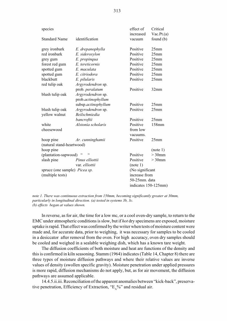
313

species effect of Criticalincreased Vac.Pt.(a)

Standard Name identification vacuum found (b)

grey ironbark E. drepanophylla Positive 25mmred ironbark E. sideroxylon Positive 25mmgrey gum E. propinqua Positive 25mmforest red gum E. tereticornis Positive 25mmspotted gum E. maculata Positive 25mmspotted gum E. citriodora Positive 25mmblackbutt E. pilularis Positive 25mmred tulip oak Argyrodendron sp.

prob. peralatum Positive 32mmblush tulip oak Argyrodendron sp.

prob.actinophyllumsubsp.actinophyllum Positive 25mm

blush tulip oak Argyrodendron sp. Positive 25mmyellow walnut Beilschmiedia

bancroftii Positive 25mmwhite Alstonia scholaris Positive 158mmcheesewood from low

vacuums.hoop pine Ar. cunninghamii Positive 25mm(natural stand-heartwood)hoop pine (note 1)(plantation-sapwood) “ “ Positive > 30mmslash pine Pinus elliottii Positive > 30mm

var. elliottii (note 1)spruce (one sample) Picea sp. (No significant(multiple tests) increase from

50-25mm. dataindicates 150-125mm)

note 1. There was continuous extraction from 150mm, becoming significantly greater at 30mm,particularly in longitudinal direction. (a) tested in systems 3b, 3c.(b) effects began at values shown.

In reverse, as for air, the time for a low mc, or a cool oven-dry sample, to return to theEMC under atmospheric conditions is slow, but if hot dry specimens are exposed, moistureuptake is rapid. That effect was confirmed by the writer when tests of moisture content weremade and, for accurate data, prior to weighing, it was necessary for samples to be cooledin a desiccator after removal from the oven. For high accuracy, oven dry samples shouldbe cooled and weighed in a sealable weighing dish, which has a known tare weight.

The diffusion coefficients of both moisture and heat are functions of the density andthis is confirmed in kiln seasoning. Stamm (1964) indicates (Table 14, Chapter 8) there arethree types of moisture diffusion pathways and where their relative values are inversevalues of density (swollen specific gravity). Moisture penetration under applied pressuresis more rapid, diffusion mechanisms do not apply, but, as for air movement, the diffusionpathways are assumed applicable.

14.4.5.ii.iii. Reconciliation of the apparent anomalies between “kick-back”, preserva-tive penetration, Efficiency of Extraction, “EA%” and residual air.

314

a. Harrow (1947) had shown a relation between inadequate evacuation and “kick-back”. For its application to local species, preliminary studies were necessary to confirma similar relationship. These are illustrated in Table 70, where inadequate de-aerationinfluences on “kick-back” in full-cell treatment are cited. The writer had adopted it (Section14.1) as one criterion of evacuation. The data in Table 71 shows effects of higher vacuumat extended times (cf. Sections 14.5, 14.6. 14.7) on de-aeration.

b. The sites of preservative solution (and salt) uptake in hardwood timbers (Sections12.4.4, 12.5.4, Chapter 12) are limited to vessels, vertical parenchyma and radial tissues.

c. The residual air, “a”cc, is a function of the time of evacuation (Table 71), Efficiencyof Extraction, “EA%” (Section 14.4.i) and capacity of the vacuum pump (Section 14.5). Thetotal residual air is that fraction of initial “Contained Air” (Section 14.4.3.i.ii.a.ii) remainingin the specimen.

The residual distribution of air is described in Section 14.4.3.i.iii and Graph 72.Importantly, this is distributed in tissues which are not restricted to sites of deposition of apreservative solution. Dependent on the efficiency of de-aeration, residual air, as was thecase in earlier treatment practices, included some “xv” and “xem”, in timber.

d. there was an apparent anomaly between the hypothesis that, on release of appliedpressure, residual air would be effective as the cause of “kick-back” of some of the solutionimpregnated into restricted sites of deposition.

e. This apparent anomaly could be reconciled by;

e.i. When the “kick-back” is discussed in preservation, it is generally described interms of “solution volume”. It was found (Appendix 14) to be lower in concentration thanthe impregnating solution (a condition separate to “Diffusion Loss” [Chapter 10]) and thus,in hardwoods, assumption of “kick-back” as equivalent to “impregnating solution” isinvalid.

e.ii. This difference may be explained if the “kick-back” volume includes the waterabsorbed (Chapter 12) in fibre lumina and cell walls (where treatment solution, or salt, isnot present) and which is expelled by the residual air when elevated hydraulic pressure isreleased.

e.iii. When measurements were made of water (as compared to salt) uptake, based onmoisture content data before and after treatment (Schmidt [1962], Chapter 12), it is shownthat the water is distributed in all tissues, including fibres.

Accordingly, there is no anomaly and “kick-back” is valid as an index of residual air,“a” cc, after de-aeration in treatment of local hardwood timbers.

14.5. Relation of vacuum pump capacity and “Effective Pump Capacity”.

It has been pointed out that attainments of the Critical Velocity Point and the CriticalVacuum Point (Sections 14.3, 14.4) are functions of the vacuum pump capacity.

14.5.i. Where used to evacuate a system through a duct, the effective pressuredifferential and the consequent maximum applied level of vacuum “pmax” are functions ofsystem geometry, “g”, and vacuum pump capacity “Cnom”, that is;

315

pmax = function (g. Cnom) (14.41a)

As is common in the local plants, the vacuum pump used is water-sealed then ;-

pmax = Function { g. [t]. CR} (14.41)

whereg = system duct (l/d) ratio

[t] = temperature of vacuum pump seal water.

CR = “Effective Operating Capacity” of vacuum pump.

14.5.i.i. If “Ccal” is the nominal calibrated (m3 / min.) capacity of a water-sealedvacuum pump, studies showed the operational loss of efficiency as being due to ;

(a) high (l/d) ratios and duct frictional losses.

(b) high temperature of seal water and variable rate of water flow through the pump(which was a function of the vacuum level, but which was often overlooked in plants).

(c) relative humidity of the air being evacuated.

(e) vapour pressure of water at operating temperatures.

(f) solubility of air in water at operating temperature and vacuum pressure.

o C. An increase of theseal-water temperature to 32°C (frequently found) decreases pump capacity by about 60%.Introduction of pump water cooling units was necessary in some plants.

Author’s note; dependence of water-sealed vacuum pumps on temperature and flowrate of the water was confirmed. A local plant installed an oil-sealed unit for which theseproblems did not arise. However special precautions were necessary and were installed to

If “Ccapa”, “Ccapb”, to “Ccapf”, are the losses due to the above, and “Ccapn” the loss dueto friction and power factor and leakages, then ;-

total loss “Closs” = sum of Ccapa + —+ Ccapf + Ccapn

14.5.ii. The Residual or Effective Pump Capacity, “CR”, at the cylinder orifice outletis given by;

CR = Cnom - Closs (14.42)The writer has found values for “CR” as low as 50% to 60% (0.5-0.6) of the “Cnom” .The value of “CR” may be increased by;

316

i. change in the (l/d) ratio.ii. decrease in seal water temperature.iii. by substitution of the air space in the cylinder by a treatment solution during

evacuation cycles (Sections 14.6, 14,7 - the Vacuum-Pressure Diffusion Process).

These conclusions were tested experimentally (system 3b) and also on commercialplants. Results based on the change of “CR” are typified by data in Section 14.7.

14.5.iii. Influence of level of applied vacuum on pump capacity.

As the level of applied vacuum increases (from 75mm), the capacity of a single stage,water-cooled, pump decreases significantly. To increase the effective level, fitting a secondstage (termed a “venturi” by industry) enabled increased air flow velocity and vacuumcapacity to be obtained. For this range, a pump capacity was reduced. As the nominal valuesof “Spc” (45 mm) and “Vpccapacity was desirable. The increase in efficiency of evacuation at those Critical levels wassignificant.

14.5.iv. Effect of timber volume on the de-aeration of a vacuum-pressure cylinder.

The Critical Velocity Point “Spc” was independent of the presence of timber specimensin the cylinder.

The actual volume rate of efflux (Section 14.3 and Graph 62) is influenced by thepresence of timber. It was found the method of stacking and relative dimensions of thetimber bundle, i.e. not separated by “strips” (Appendix 14), appeared to influence the rateof de-aeration of the timber. This was particularly so if the system operated below theCritical Vacuum Point, “Vpc”. This effect was confirmed in the laboratory unit (system 3b)and in commercial practice. It was found to be due to:

(a) for practical purposes, the bundle of timber acted as a solid body and hencelongitudinal air flow along the cylinder length to the outlet orifice was impeded. The effectwas equivalent to “fluid drag” around a submerged body.

(b) the air path changed from a typical duct of “(L1/D)” ratio to an annular duct witha nominally equivalent cross-sectional area, “Wf” and which is given by-

Wf = (pi/4). (D2 - Ds2) (14.43)

whereD = diameter of cylinderDs = nominal equivalent diameter of charge of timberpi = 3.1416

In practice “Ds” ranges from 0.75 to 0.90 of the value of D (cylinder diameter).

Hence, if “A” is total cross-sectional area of the empty cylinder, then for;

Ds = 0.75D, Wf1 = 0.44A

317

and for

Ds = 0.90D, Wf2 = 0.19A

As a consequence, air from the timber in the charge is removed by what may be termeda “Venturi Pumping Effect”. This is required to remove the air from all of the cells (rays,fibres and vessels) of a board by a variable path i.e. between boards, and approximatelyperpendicular to the board longitudinal axis.

The nominal maximum air flow path through the bundle to the annulus is theoreticallyequal to 0.5 Ds.

The ideal air flow path is affected when “Ds” is a significant fraction of “D”, or wherea bundle of timber is tightly packed and the air flow between boards is retarded. “Auto-adhesion” between boards, which can be due to extractives, exemplified by resinousexudates in slash pine, or to timbers of high density, is a common cause. In extreme cases,typified by bundles of very dry plywood, both de-aeration and subsequent solution accessunder hydraulic pressure were severely impeded. Under these circumstances, a bundlebehaves as a solid body and the nominal vertical component of air flow (y axis) to the outletorifice tends to be semi-circular or spiral. However measurements of the vacuum level athorizontal positions along the cylinder length show the equivalent levels of applied vacuumare attained in the annulus. To confirm the laboratory experimental results, access to a rangeof positions in a commercial cylinder enabled (by use of one-way valves with pressurestopcocks) the author to measure internal vacuums for different timber volume conditions.For round timber, the actual flow path is more effective than for sawn timber because of the“packing fraction” conditions, caused by irregularities of shape, less “auto-adhesion” andbetter resultant relationships of “sub-ducts” to the annular space.

This led the writer to examine the postulate that, as for the open tank processes, foroptimum efficiency of treatment, free flow of both the air and the solution is desirable forthis process and hence material should preferably be treated in open stack, i.e. in strip. Thiswas tested and confirmed. However economics of operation of this type of plant precludedcommercial adoption of this alternative except in special circumstances. Treatment ofplywood is one case where “pre-stripping” was desirable.

14.6. Development and commercial application of a VacuumPressure DiffusionProcess.

Results in earlier research (Sections 14.1-14.4) had led the writer to examinedevelopment of a process based on the principles (Chapters 8, 12, 13) by which the thermalprocesses operated. The potential related principles and advantages are examined inSection 14.6.i.

14.6.i. Correlation of open tank process applications to conventional full-cell treat-ments for the development of modifications in practices used with the latter process.

In this research, the similarities of current “full-cell” processes to the thermal “Steam/Cold Quench” process (cf. Chapters 12, 13, Appendix 14) were noted. The former was alsocompared to the “Hot and Cold” processes (cf. Chapters 8, 12, 13, Appendix 14)) and fromwhich it was concluded that:

318

(a) The hot and cold process was very flexible with respect to a very wide ranges ofspecies and of moisture contents.

(b) Absorption in the hot and cold process also occurred during “de-aeration” at the

(c) Most importantly, as cooling proceeds and hence an increase occurs in the thermalvacuum, due to the vacuum and negative pressure differential effects (Chapter 13), thereis both preservative solution penetration and water movement into the board. If directinfluences of elevated temperature on diffusion, plasticity and wettability, are excluded, thehot and cold process could be equated to a “thermal vacuum-atmospheric pressure” process,where the de-aeration is carried out for an extended period whilst the timber is submergedin the solution.

During such time solution should penetrate into timber rays and vessels, water shouldpermeate available “voids” and, additionally, salts may diffuse from solution into the“residual” free moisture in the vessels and rays. To this were added the positive effects ofan increased solution contact time (influenced by preservative) upon a more effectivewetting of timbers.

As local climatic conditions were variable, the writer considered one significantpossible effect of extended times of immersion, as proposed, would be a significantdecrease in both the cylinder and charge temperatures, thus resulting in cooler operationsof the vacuum pump and seal water (Section 14.5).

In the conventional full-cell system, after “breaking” of the vacuum to atmosphere, thefraction of solution uptake to a total solution uptake was small. Using the thermal principleof immersion of the charge, during and after evacuation, change of the system from avacuum cycle to atmospheric pressure is equivalent to the major cooling phase in the opentank processes. The absorption (termed “Initial Absorption”) should be significant andrapid. Effects of “kick-back” (Section 14.1) should be reduced. If the system is allowed toreach equilibrium under atmospheric pressure, absorption should be approximately hyper-bolic with respect to time (cf. Graphs 37 to 37c). When the system is subjected to hydraulicpressures above atmospheric, it should result in a rapid absorption/time curve at a ratesignificantly in excess of that given by the conventional de-aeration followed by flooding.The “Initial Absorption” should be a significant fraction of the “Total Absorption”. Thesetheories were amenable to an experimental verification.

(a) in the first instance, increase of the level and time of evacuation should increase theabsorption. They should decrease the time under pressure (time to refusal) as well as totaltime of charge. Solution concentrations should be reduced.

(b) when there is comparable treatment, except that the evacuation is with the chargesubmerged in solution, then an increase in retention, decrease in time to refusal, or in totalcharge time, or in concentration of solution, should occur.

(c) in addition to (a) and (b), reduced resistance to penetration will be reflected in areduction [Table 70 (Section 14.1)] in “kick-back” (Harrow, 1947).

14.6.ii. Laboratory and commercial verification of the Vacuum-Pressure Diffusionprinciples.

319

The theories were confirmed (Cokley and Smith, 1965 a,b), initially in the laboratory.Tests were made on vacuums and times, during immersion (Diagram 3b) under

solution, from about 50 to 100 mm (the latter of the same order {Graphs 52a, 52b} as givenby the hot and cold process). That vacuum was released to atmospheric pressure and withabsorption to equilibrium. Subsequently research was extended to higher vacuums of thelevels of the “Critical Velocity Point” (Section 14.3) and the “Critical Vacuum Point”(Section 14.4).

Extensive studies, including a range of commercial plant applications (Section 14.7),confirmed the earlier data. Positive effects on moisture content ranges, salt usage, scheduleconditions and times, are shown (Sections 14.7, 14.8). They are typified by extended largescale studies on sawn timber and poles (both types of product were over a wide range ofhardwood and softwood species) at a large commercial cylinder operating in Brisbane.

14.6.iii. Influence of Vacuum-Pressure Diffusion Process on “Effective Capacity” ofthe vacuum pump.

Substitution in the cylinder of the preservative solution during the vacuum cycleresulted in;

14.6.iii.i. As solubility of air at S.T.P. is only about 2%, (Chapter 13, Section14.4.3.i.ii.a), evacuation of a cylinder full of solution is equivalent (Cokley and Smith,1965a) to decreasing the cylinder air volume by 98%. At operating vacuums, the air contentin a solution is reduced [Henrys law] to of the order of 0.01 to 0.05%, and this, in turn,increases the “Effective Capacity” of the vacuum pump and increases efficiency of de-aeration.

The mechanism may be described as maintenance over time of a differential indissolved air caused by evacuation at the fluid surface. This differential is transmittedthrough the solution and de-aeration of the board occurs.

This is a similar effect to that (Chapter 13) obtained in the hot and cold process. Theeffect was experimentally verified by measurement of vacuums at the centre of specimenswhen de-aerated under solution. Tests were made (Section 14.7), in a number of plants, bysubstitution of solution during the evacuation cycle, to assess whether that change, as foundunder the laboratory conditions, resulted in increase of “Effective Capacity” of, andreduction of pump temperatures of, the vacuum pump.

Results over a series of plants confirmed the hypothesis.

14.6.iv. Sequences in operation of the Vacuum-Pressure Diffusion Process.These are briefly described as follows;

(a) subsequent to insertion of the charge, for an initial time (generally 10-15 mins.),the vacuum pump was used to establish (Diagram 4) cylinder seals etc. were effective.During that interval, the operator completed initial charge sheet details, took and tested asolution sample (Chapter 11). Solution was then admitted at a controlled rate so as to ensureno loss of vacuum and so that there was complete coverage of the charge. Advantagesincluded removal of “entrained air”, which was a negative feature of the original practiceof rapid “flooding” (Section 14.1) of solution. Over that period, the vacuum was raised tothe operating level which was based on pump characteristics and capacity.

320

(b) the vacuum was continued for a period determined on level of applied vacuum, onspecies (and on thicknesses, [Section 14.8]), ranging up to a maximum of 90 minutes.Standard sampling (Chapter 10) practices were followed.

(c) the solution level (Diagram 4) was maintained by the sight gauge (on the vacuumchest or “pot”) to ensure adequate coverage of the charge, including the “Initial Absorp-tion”. In some plants, a full depth (suitable for pressure) gauge glass was installed. Forcertain plants, similar to the defects described (Chapter 13) in thermal systems, there wereoriginally inadequate side and top clearances for the charges to be completely covered bysolution during absorption. These defects were rectified in plant trials (Chapters 2, 10).Adequate flow volumes (Section 14.5) for seal water in the vacuum pump were tested andadjusted (Nash, u.d., 1994) when required.

(d) After the vacuum cycle, the system was “broken to atmosphere”, at which point,as a result of the vacuum, dissolved air in the solution was very low (Henrys law), withprecaution to maintain solution coverage, resulting in an "Initial Absorption", undersolution, which was up to 75% of the total uptake. Most of that took place within 15 to 30minutes but could extend to about 90 minutes.

(e) For other than plants specifically designed for only low pressures, or “week-end”schedules (Section 14.8), the cylinder solution volume was restored at a controlled rate andpressure applied until “refusal” (Appendix 14). A final vacuum was applied in most plants.

(f) the solution was returned to storage, re-sampled and after its testing, charge sheetdata was completed.

14.6.v. Independent assessment of the process.

As this process was an original development, it was felt desirable to obtain independ-ent assessments of its use and efficacy. These included;

14.6.v.i. Approvals under States legislation (TMA, 1946, T.U.P.A., 1949).

14.6.v.ii. Many commercial plants were operated under a “lease/ buy” arrangementwith preservative suppliers. One effect (Chapter 10) was need for tripartite discussions toenable preservatives (such as boron salts), other than the supplier’s product, to be used. Forthese plants it was ethically, and legally, necessary for both plant management and supplierto grant approval to the writer in terms of any plant modifications and trials, includingchanges such as fitting of second stage pump units and cooling systems for pump watersupplies and, as a result (Section 14.7), a number of plant managements made major re-design modifications. In all cases, these changes were effective and economic. The overallresult was acceptance of the process by interstate and overseas authorities, by suppliers andadoption for their own installations.

14. 6.vi. Commercial adoption (Queensland) status of the Vacuum-Pressure DiffusionProcess. The number, and type, of plants relative to vacuum levels (Sections 14.3, 14.4) areshown (1965) in Table 83 (Cokley and Smith, 1965 b). The number increased until about1975 (when industry became reasonably steady). Products treated were in multiple speciesand sizes. They included veneers, plywoods, sawn timbers (all purposes and hazards),

321

power and telecommunication poles, marine piling, cooling tower timbers, oyster stakes,fencing.

About one-third of plants, which used the Vacuum-Pressure Dffusion process,operated at vacuums below the critical level. Reasons included;

i. small production requirements.ii. species for treatment, such as Group 1, 2A (Chapter 12), did not require Critical

Vacuum levels of 25mm, or products were to be used (Chapter 3, Appendix 1) for lowhazard (eg. Lyctuscide treatments) conditions.

Most of these plants fell into classification i, above, and economics of plant modifi-cations did not justify the amendments. Schedules and cycle times (Section 14.8) weremodified to suit their conditions. Additionally, about 10 other plants operated interstate andoverseas using the process, many of which used the higher vacuum systems.

14.6.vii. Application for and grant of Australian patent for the Vacuum-PressureDiffusion Process.

Consequent upon confirmation of the satisfactory evidence of both economic, andtechnical, results, an application was granted (Patent No. 275,808 of 31 October, 1963,sealed on 28 November, 1967) for a patent (Plate 5), with rights assigned by the official co-inventors (Cokley and Smith) to the Conservator of Forests. Reasons for the patentapplication were;

a. By so doing, the advantages would be available to the total industry. No royalty wascharged, as this research and industry applications were considered (Chapter 1) as functionsof departmental policy on industry assistance.

b. Importantly, they enabled the Department (Chapters 1, 10) to achieve optimumcontrolled utilisation of timber resources, thus ensuring maximum forest conservation.

c. For plants operating under T.U.P.A. (1949), approval was given administratively,but for the plants operating externally to that Act, formal approval was given. Plantsoperating in New South Wales, under the TMA (1946), were approved (Chapter 2) byreciprocal agreements between both States. Preservative suppliers were given approval forits use under their supervision. The patent enabled control over especially the external (toQueensland) plants to ensure effective treatments. As the economic advantages were high,plants managements and suppliers were reluctant to lose that approval.

14.6.vii.i. Policy on application of suitability of the Vacuum-Pressure DiffusionProcess to conditions other than those operative in Queensland.

In areas, external to Queensland, where it was desired to be adopted, it had been thewriter’s recommendation that pilot plant studies (Cokley, 1970) be made to confirm itsapplicability. This was especially so in terms of “Stable Green Moisture Content”, Effectsof “Critical Vacuum and Velocity Points” and relation of species characteristics. Results,similar to those found under local conditions, were obtained in all instances.

The extended range of data, other than in Queensland, confirmed that general andfundamental relationships in timber preservation were involved.

Table 83

322

Commercial plant usage of high vacuum and/or theVacuum Pressure Diffusion Process (1965) [a].

item plants [b] using ;high vacuum and Vacuum PressureVacuum Pressure Diffusion belowDiffusion high vacuum levels

number 16 9size 9x1m -27x 1.8m 9x1m - 21x 1.37mproducts sawn, poles, sawn, poles,[c] piling, plywood piling, plywood

notes; [a] (Cokley and Smith, 1965b). [b] total plant installations did increase, but stabilised about1975. [c] interstate and overseas usage not listed.

14.7. Commercial Applications of High Vacuum and Vacuum-Pressure DiffusionProcess.

14.7.i In applications of the research (Sections 14.3, 14.4, 14.5, 14.6) modificationsto commercial plants included the installation at a Brisbane plant (27 x 1.8m) of a secondstage “venturi” to the Nash H6 water-sealed vacuum pump (about 7m3/min. in capacity).Results (including schedule data, see below) are shown in Table 84.

Original changes to that plant were based on application of Critical Velocity Point,“Spc” of 45mm and Critical Vacuum Point, “Vpc” of 25mm, followed by the subsequentchange to a Vacuum-Pressure Diffusion Process. Economies are shown in Table 84.

Author’s note; This plant, located in Brisbane (sea level), was installed for treatmentof the firm’s own product, but carried out “customer treatment”. As it was a major supplierof CCA treated sawn timber, poles and pilings, as well as cooling tower timbers, it treateda wide range of species and products.

Consequent on further research by the writer and the firm, the pressure cycle wasreduced from a conventional 1400kPa. to 1100kPa. No significant change from this wasnoted in the salt usage, based on decrease from solution before and after treatment, orretention in products.

14.7.i.i Correlation with statutory requirements and the standards issued by Statestatutory bodies, such as the State Electricity Commission and Harbour Boards.

It is important to emphasise that, for all vacuum-pressure plants, specific continuingsupervisory control (Chapters 2, 10, 11, 15) was maintained. Especially for early years ofavailability of CCA treated products in Queensland, the writer’s laboratory was frequentlyasked to test products under statutory specifications. As a result of its heavy commitmentsto these areas of market utilisation, the Brisbane test plant was consequently subject to

Table 84Comparison of treatment results and times between the conventional “full-cell” to

Vacuum-Pressure Diffusion processes obtained in a commercial 27m x 1.82m Plant.Study included effects of higher vacuums for each of the two processes (Cokley and

323

Smith, 1965b).

process mc results obtained (x)(1) ra. sawn timber poles

(2) N.D. tot ref sol N.D. tot ref sol.(3) % S.R. hrs min % S.R. hrs min %

(a) (n) (b) (e) (n) (b)

full-cellat 75mm.N=540 <30% 1.47 4.06 50.66 6.0 22.66 4.16 67.7 6.02

full-cellat 25mmN=800 to

45% 1.83 2.88 16.0 3.82 24.9 3.57 30.25 6.97rel. ratio (123) (71) (29) (63) (110) (86) (44) (116)

Vacuum toPressure 60% (m)Diffusion (mean 40-50%)at 25mm.N= 2000 2.45 2.64 10.56 3.46 28.18 3.55 24.25 6.89rel. ratio (166) (62) (21) (58) (124) (85) (36) (114)

notes; (x) Charges operated on commercial basis. In addition to standard charge analytical sampling, atotal of 20 charges for each variable / group studied was used for statistical analysis for differences.(m) includes low density species and products, eg. posts.(1) Number of charges in each total operation, shown as N = ( )(2) moisture content ranges studied. Measurement by ovendrying of representative specimens.(3) Relative production ratio to conventional process shown as a percentage value in brackets.(a) Salt uptake (N.D.S.R.) [kg/m3] for sawn timber ontotal charge volume. (n) Refusal point (Appendix14).(e) N.D.S.R. [kg/m3] for round timbers, eg. poles, on the sapwood volume of pole charge determined bymeasurement.For both sawn and round, results confirmed by chemical examination of treated product and solutions.(b) Solution concentration at commencement of charge. Todetermine salt usage, concentration was alsomeasured atend of charge (Cokley and Smith, 1965) (plant tests byhydrometer, confirmed by laboratorychemical analysis).

That extended to all plants involved in those markets. As a result of service problems(Chapter 15), this aspect of supervised sampling continued.

14.7.ii. Modification of plant design, and/or vacuum pump capacity (Cokley andSmith, 1965b).

14.7.ii.a. Two plants are illustrated in Table 85.14.7.ii.a.i Based at Toowoomba (700m elevation), the first unit was initially a 15 x

1.1m unit with a Nash AL 673, (capacity of 1 m3/ min to about 100mm of vacuum). Usinga second stage, evacuation rates dropped to 0.3m3 at 25mm (sea level) [note; pumpcapacities are variable with speed (r.p.ms). The plant management, inclusive for economic

324

reasons, decided to amend the plant size and increase productivity. Accordingly, based onthe writer’s data and initial evidence including as cited in Table 84, their engineeringconsultants modified the existing plant design in two stages, namely;

(a) replacement of the AL 673 pump (with a duct diameter of 38 mm) to a Nash H5(operating with a duct diameter of 75mm), coupled with a shortened length to the cylinder.The H5 pump had capacities of about 7m3 and 2m3/ min. at the same vacuum levels as citedabove.

To transfer solution both into, and from, the cylinder, a by-pass centrifugal pump(Diagram 4) was incorporated.

(b) to accommodate special long sizes of power poles with the existing modifications,the cylinder was extended to 27m in length.

14.7.ii.a.ii. The second plant (sited at Bundaberg, sea level) operated a 21 x 1.1m plant,treating sawn (which included native hoop pine from Goodnight Scrub) timbers and roundhardwoods for poles and marine piling, was equipped with a Nash H3, similar to an AL673.The pump was changed to a H4, a capacity intermediate to the H5.

A centrifugal pump was used for solution transfer.

For both plants, (Table 85) the productivity increased, operating costs decreased andtreatment effectiveness improved.

14.7.iii. Economic advantages of process.

Table 86 (Appendix 42) shows the economic and technical advantages, based on saltusage / salt retention, for three plants treating spotted gum, E. maculata.

14.8. Effects of process changes on moisture contents of treatment. General recom-mended treatment schedules.

Aspects of effective moisture contents (Chapter 12) for treatment and initial limita-tions placed on conventional “full -cell” treatments have been examined. One advantagewhich became possible with these amended processes, especially the Vacuum-PressureDiffusion Process, was the greater flexibility in levels of moisture contents which weresuitable for treatment.

As anticipated (Chapter 12), the writer found this was related to;

i. The treatment level required for effective protection against the nominated hazard(Chapters 2, 3).

Table 85Relative effects (1) of variation of plant design andof change of vacuum pump capacity on production.

325

item plant size and pump outlet diameter

plant A plant A plant B(poles, (enlarged) (poles,sawn) sawn)

Condition (x) init mod mod init mod.cyl. size (m) 15 x 1.1 27 x 1.1 21 x 1.1vacuum pump (n) AL673 H5 H5 H3 H4outlet line-mm. 38 75 75 38 38

Ratio of cylinderdimensions 1.00 1.00 1.60 1.00 1.00Ratio of chargeobtained (m3) 1.00 1.26 2.08 1.00 0.94Increase in vac. (n/a) 42 38 (n/a) (n/a)efficiency-mm.Ratio of time toevacuate cylinder 1.00 0.50 0.60 1.00 0.44Ratio of time torefusal 1.00 0.59 0.58 1.00 0.88Ratio of treatmenttime (2). 1.00 0.92 1.21 1.00 0.75Actual time (3)for charge, mins. 123 113 149 226 169Production cap.(4)m3 / min. 1.1251.5341.938 1.16 1.47Relative chargedaily production 1.00 1.36 1.72 1.00 1.27

notes;(after Cokley and Smith, Rep. no. 6, 1965b)1. Effect compared to original plant condition.2. During alteration, plant A amended solution transfer system to use of pump. Time data in plant Ataken to end of pressure cycle.3. Actual time in plant A includes increase of 15 mins. of time of maintenance at vacuum.4. Production capacity (see notes 2, 3) - total charge time.(x) condition, init = as originally installed.mod. = as redesigned and/or pump size changed.enlarged = plant A extended plant size principally for special length poles. (n/a) - not applicable.(n) manufacturer’s data (Nash, u.d., 1994) for watercooled vacuum pumps. Second stage above 75mmvacuum.

ii. the preservative used. Thus, for a mobile salt such as borax (Chapters 8, 10), timberwill treat at higher moisture contents than for complex formulations, such as CCA mixtures.This difference was utilised by the writer in schedules for specific plants operating on boronsalts. However issuance of general schedules was based on the CCA multisalts.

iii. species treatability groups (Chapter 12) were fully applicable for these processes(cf. Section 14.8.2).

14.8.i Moisture content studies for effective treatments and results.

The author did find greater flexibility, which was, in most species, associated with the“Stable Green” and the “Commercial Maximum Green” moisture contents (Section 12.5,

326

Chapter 12). Table 84 lists ranges of moisture contents studied in extended research at oneplant over a range of species, sources and products.

Table 86 (Appendix 42) describes moisture content results on spotted gum at threeplants using Vacuum-Pressure Diffusion. It will be noted that a range up to 45% mc waseffective for those conditions.

Table 87 (Appendix 42) lists values over a range of plants, of species, and products asa function of end-use retentions. In all cases, determinations were by oven dry methods andsample boards followed by chemical analysis. Sampling followed the standard procedure(Chapter 10) of 6 specimens per condition for each of three charges.

14.8.2 Recommended General Treatment Schedules for use in the full-cell andmodified processes.

These are listed in Appendix 43. It will be noted that;

i. No species groupings (as in Appendix 26) are listed.ii. qualifications are made in a number of schedules as being “subject to test”.iii. Limitations are placed on moisture contents in terms of species and products.

The restrictions (including non-classifications based on treatment groups [Chapter12]) were both legally and technically necessary due to the practices by a number of plants,especially when “customer treating” was carried out. For these, the products would bedelivered in bundle form and could be placed with other products (and species) to “makeup a full charge volume”. Restrictions (and approvals under the Acts [T.U.P.A, 1949])issued for the general schedules, placed an onus on the treater and plant operator to ensurethe product for treatment met the specifications as nominated, or was tested beforeutilisation, or sale, as having been treated (Chapter 2) by an “approved treatment”.

It will be noted that, due to high capital cost of this type of plant, use of “bundles” intreatment, practices of “customer treatment”, the general schedules are based on standardsfor “refractory timbers”.

Author’s note; the need for these restrictions in “custom treatment” is illustrated bytwo examples. They were;

a. a large number of “pre-packed bundles” of small sizes of sawn plantation softwoodswere supplied to a plant for CCA treatment to a high hazard retention, but tests by the plantoperator demonstrated that moisture contents were above the range advised for thenominated treatment level. The bundles were “broken down and self-stripped” until testsshowed moisture contents were satisfactory for the required treatment retentions.

b. similar problems were encountered for small diameter plantation softwood “rounds”,or fence paling timbers. Care was taken to ensure moisture contents were reduced to suitablelevels for treatment.

Where “customer treatment” was not practiced, or where a plant was operating onstandard conditions, including the species range (eg. Group 1, 2A, Chapter 12), the writerissued a modified schedule in those situations. That also applied to use of boron salts.

327

328

Chapter 15

EFFECTS OF WOOD STRUCTURE AND PRESERVATIVE DISTRIBUTIONON SERVICE OF TREATED TIMBER (PARTICULARLY HARDWOODS) INTROPICAL AND SUB-TROPICAL ENVIRONMENTS, INCLUDING MARINE.ROLES OF CALCIUM AND MAGNESIUM IN MARINE BORER ATTACK.

15.1. General Service Results.

An over-riding Departmental mandate (Chapter 1) and which justified the extensive(in time and costs) research and industry application in timber preservation was for theeconomic conservation of the State’s natural resources, while, at the same time, enablingdecentralised, varied types of manufacture, of employment and independence from externalsupplies of these products. Necessary legal (Chapter 2) requirements were established. Thelarge numbers and diversities in (particularly the hardwoods) species and in their physicaland chemical properties (including durability, treatability), led to the research described inearlier chapters.

The writer’s research programs in establishment of the industry are summarised inFlow chart 1 and they show the multi-faceted needs for research into many fundamentalquestions of preservative penetration into angiosperms and similar need for research intoprocess principles and applicabilities to local conditions and timbers rather than depend-ence on data developed overseas primarily for gymnosperms. Development includedrequirements to extend the research to industry and service applications. Here, as intreatability, differences between species became important factors in service.

15.1.i. Service effectiveness of treated products.

In this chapter, the writer analyses the effectiveness in service of treated products overthe ranges of applications wherein they were used. Unless that service was adequate,economic and satisfactory for the intended uses, there were no advantages in preservation,nor would the resource conservation aims be achievable.

15.1.i.a. A vital component part of the questions which required answers had includedthe service performance of hardwood sapwoods after preservative treatment.

That applied in the wider context (Chapter 8) of sapwood (as compared to softwoods)and, in particular, after its impregnation by general purpose, water-borne multisalts. In theformer group of species, an average of only about 36% of the wood is penetrable bypreservatives, but for the latter about 95% is treated. The larger volume, ie. fibres, in theangiosperms is not protected. There is a difference between moisture penetration, for bothliquid and vapour phases, compared to preservative penetration with this latter being a jointfunction of the mobility, reactivity and type of preservative. It was suggested if wood wasimpermeable to water in the aqueous phase under pressure, it was unlikely to decay (whenused above ground) if it was subject to intermittent wetting. The writer (Cokley, 1965 c)considered this was invalid and water penetration in the vapour phase was significant, anapproach which was shown correct for local conditions.

15.1.i.i. Where insects were the principal hazards, the macro-structures involved,relative to insect dimensions such as Lyctus larvae, resulted in a masking of problems dueto differences caused by preservative distribution in hardwoods. When hazards were micro,

329

eg. certain fungi, variation in the site of preservative protection in these timbers becamesignificant and is shown in this Chapter.

15.1.i.ii. When exposure was to decay organisms, evidence accumulated by alllaboratories showed that the timber substrate (Da Costa, 1969) was critical in serviceperformance of a preservative. McQuire (1974) reviewed use of boron compounds forbuilding timbers. In all such studies, natural durabilities (Chapter 3) are significant whenheartwoods are tested, but the sapwood durability is rated as being very low and needingpreservation.

15.1.ii. Preservative treated products included;

(a) Building timbers in all species used by the industry. These were for “under-cover”conditions to give insect control, including termites and low, to moderate, decay control,for external, above-ground applications.

(b) Hazard conditions (eg. for “in-ground” fence post applications) for which theeconomic replacement costs, risk to person, or service, were minimal. Exceptions, such asstock fencing, were economically significant.

(c) Cooling tower products, almost totally plantation softwood timbers, for largetower “fill”. They did include hardwoods for smaller industrial air conditioning systems.

(d) Marine piling and other marine uses, such as oyster stakes.

(e) Transmission poles for telecommunications and power purposes.

(f) Special products. These applications very frequently included “fire-retardent”properties as being necessary specific requirements in the preservative.

f.i. Marine, or external, plywood for boat construction, for railway coach sides (to 17mx 4-5m in size) and for bus floors.

f.ii. Purposes associated with high safety and security control of buildings. Twospecial applications were in;

(a) Timber, or plywood, as decorative surfaces for “new age” metals, or plastics (fireand impact resistant), for doorways and wall panelling.

(b) Large surface area, distortion free, lightweight, security doors for specific publicbuildings.

(g) Roofing timbers in large sizes for covered high volume storage reservoirs in urbanwater reticulation systems. This use required special control, often with an additionalprotective sealant, to ensure that no chemical contamination was possible.

Due to possible health risks, there were (Chapter 10) restrictions on preservation ofspecial products. These included children’s playpens, meat skewers, chopsticks, ice creamsticks or disposable medical tongue depressors (made in pine).

15.1.ii.i. Co-ordination of applications of preservation with recommendations onutilisation of local timbers for building and general (eg. poles) applications.

330

By co-ordinating preservation requirements with general utilisation groups (Watson,1964), the writer established relationships between timber species, end products andpreservatives, especially CCA components.

15.1.ii.i.i. Adequacy of the preservative penetration in terms of active components andservice hazard.

Author’s note. As emphasised in Appendix 44 and Chapters 10, 11, 12, the salt formis very important in treatment and service performance. Unless otherwise stated, forpreservatives, especially CCA formulations, references to a component in terms of its metalion implies reference to the salt form and not the element only.

Many machined profiles, such as flooring, mouldings, or external products, such as“chamferboards” (AS 01-1964), were manufactured from initially larger sections whentreated. This had exposed lower levels of treatment to the service hazard. Care was requiredto ensure (Chapter 2, AS 1604-1980) that the “core retentions” were at the minimumconcentrations of active preservative prescribed for such hazard.

15.1.ii.i.ii. “Reactivity” (Chapter 8) and “Wettability” (Appendix 15) of timberspecies were both factors. The Argyrodendron species (Chapter 8, Appendix 15) areexamples of major “wettability” problems, with red tulip oak being less hydrophobic thanthe other three species.

In certain rainforest species, especially the tulip oaks, Argyrodendron spp. and verymarkedly (Chapter 8) for yellow walnut, Beilschmiedia bancroftii, there occur zones ofvariable CCA component distribution and/or selective component absorption (Plate 6) inthe latter species.

Specifically for Mackay tulip oak, Argyrodendron actinophyllum subsp. diversifolium,compared to the red tulip oak, Argrodendron peralatum, (where the copper concentrationis within normal variation [Chapter 11]), penetrability (Table 89) of the copper componentis at very low levels, with normal penetration of the arsenic and variable, but adequate,chromium, components.

For the other tulip oaks (brown and blush) species, copper component penetration isvariable with source, but “rejection” (Chapter 8), or very low levels, of copper salt anddecreasing towards the “core”, is reasonably consistent. However, for these latter twospecies, the arsenic component increases approximately inversely to the copper compo-nent.

15.1.iii. Service Results.

These are described in detail in Appendix 44, but are summarised here as below. Ofthese, separate discussion is made of end use products for marine and transmission poleapplications. Conclusions are based on about 40+ years service for Lyctuscides, such asboron products, and about 20 years for the general purpose CCA salts.

331

Table 89The Influence of differential absorption on retentionof CCA salts and component ratios, by red tulip oak

and Mackay tulip oak, Argyrodendron spp.

species component (1)(2) totaland data Cr Cu As salt

X(a) C X C X C X C

red tulip oak.% m/m 0.70 0.36 0.38 0.21 0.51 0.23 1.59 0.80ratio 44.3 45.0 24.1 26.3 32.3 28.8

Mackay tulip oak.% m/m 0.33 0.09 0.11 0.03 0.26 0.11 0.70 0.23ratio 47.1 37.5 15.7 12.5 37.1 50.0

nominal ratio39.0 (3) 22 33-34

notes;(a) X = total cross-section (25mm boards)-starch positive.C = core section (25mm boards)-starch positive.(1) mean of charge samples (6). Tests repeated over a series of charges.(2) Cr— potassium dichromate anhydrous.Cu— cupric sulphate anhydrous.As— arsenic pentoxide anhydrous.(3) Nominal formulation Brand A, Type 2 (AS 1604-1980).Similar results found with all CCA salt types.

During the periods under discussion, service climates (Chapter 3) for exposed timbersincluded major floods, cyclones and excessive wet seasons which were, in many years,preceded by droughts.

15.1.iii.i. Products cited as class (a) for internal, or protected, situations.

Based on more than 40 years for boron salts and 20 years for CCA respectively, servicedata showed only very low percentages in this group were subject to ground contact, or high,decay hazards. That was except for (Chapter 3) applications such as for “slab-on-ground”construction, house stumps, or “pole houses”, for minimal ventilation in roof, or enclosedwall, cavities (Chapter 3). General insect control, eg. against Lyctus spp., was good.

Considered from the service aspects, it may be stated that CCAs have given goodprotection against all insects, inclusive of the termite species such as Mastotermesdarwiniensis (cf. Section 15.5.iii.xiv) and against the higher wood destroying fungi, eg. theBasidiomycetes. Creosote has shown some weaknesses against termites.

15.1.iii.i.i. For the high hazard applications, problems arose especially for “in-ground”transmission poles and for marine uses, typified by marine piling and by oyster stakes.

Due to these experiences, the author (Cokley, 1969) had recommended to the Forest

332

Products Conference that, though CCA salts were considered the then best economic,water-borne, preservatives commercially available, urgent research should be undertakeninto possible alternatives.

That (Chapter 10) recommendation was adopted.

These two service developments and problems, with actions taken, are examined insubsequent sections.

15.1.iii.ii. Relativity of service performance to the CCA formulations.

The writer (Appendix 44) demonstrates, citing evidence on which his conclusionswere based, there were no direct correlations of product service performance to nominalCCA formulations.

All data pointed to an equilibrium CCA component balance in the treated products.

15.2. Adoption of treated timbers for power poles and for use in marine situations,especially piling timbers.

15.2.i. Subsequent to Australian establishment (1957-58) of vacuum-pressure plantsfor creosote application, a Symposium (Post Master General Department, (Aust.), [shorttitle P.M.G.], 1963) was held on possible use of pole species with lower heartwooddurability where the sapwood had been treated with preservatives, including by creosoteand the then available CCA formulations. A symposium recommending use of CCAs forutility poles (separately organised from the one by P.M.G.) was held in Brisbane, cira 1962/3. The latter, for especially the Electrical Board managers and distribution engineers andat which the writer was a guest, was by a representative of an overseas preservative group.In a number of aspects (based on the then information), Australian Electrical and HarbourAuthorities were (cf. Section 15.5.ii, on electrical “leakage” or conductivity) under thebeliefs that;

(a) fixation was very rapid for these salts.

(b) consequently, CCA (and creosote) treated poles and piles could be used reasonablysoon after treatment.

(c) standard inspections, which involved excavation of “butt” and “below-groundline” zones, were not required for a period (which was not formally nominated) and poleswere to remain “intact”.

15.2.ii. Boyd and De Campos (not referenced in text) had independently determinedthat the primary strength source of a round pole was in the outer intact annulus of 12mmradius of wood. Consequently, Queensland authorities and Australian Standards (AS 0117-1970) based specifications and the design criteria for treated poles on those works.Australian Standard AS-0117 (1970) did not limit species after treatment, but Queenslandpower authorities (State Electricity Commission of Queensland, 1974 [revised from earlierissues]) limited species primarily to Durability class 1, 2, although E. maculata, and E.citriodora

Poles from the Evelyn Tableland area (N. Queensland) did require special approvalsas the typical sapwood depth (Chapters 3, 8) was only about 5 to 10mm.

Conversely, as design life for dwellings was of the order of greater than 50 years, it was

333

considered by the Queensland Housing Commission that, if the treated sapwood did fail inservice, the durable heartwood of the approved species should provide adequate cross-sectional bearing surfaces. Thus, the Queensland Housing Commission prescribed onlydurability 1, 2, species for load-bearing house stumps. Approval was given for use of E.maculata, under certain conditions, from several sources (Chapter 3). This restriction wasimposed as the bearing surface was significant in design and where, dependent on soilconditions, if significant heartwood decay resulted in a residual annulus only, the load maycause “sinkage” of the structure. This effect of “sinkage”, for loads built on supports, eg.piping, had been noted in the blacksoil areas of the Darling Downs.

15.2.ii.i. Reasons for extended research, for industry surveys, training of inspectionstaff of principally, but not solely, the electrical authorities and research into establishmentof preventative “in-situ” treatments.

The legal and the industrial implications, especially for power transmission poles, arediscussed in Appendix 46. As described in Sections 15.5.i.- 15.5.iii, the resources of theForestry Department and industry were extensively involved for a number of years on thisproblem, leading (Appendix 46) to submission, by the writer, of a research program intofundamental aspects.

15.2.iii. Quantity usage of treated transmission poles.

The usage of treated poles (Mason, 1973) in Queensland rose from an initial quantityof 5000 poles in 1962 to an annual average of about 45,000, such that by 1971, a total (allauthorities) of 461,000 had been installed, inclusive of 46,000 for P.M.G. and QueenslandRailway usage. In 1974, there were about 500,000 such power poles in service inQueensland. There was a further projected requirement of 330,000 (S.E.C. Wood PoleCommittee, 1973, 1974) over the decade 1974-1984.

In Victoria and Tasmania, the “regrowth” eucalypts of durability classes 3, 4, (eg.mountain ash) formed the major bulk of supplies. “Heart Rots” became a possible seriousproblem for the latter class of species.

15.2.iv. Initial use of softwoods in transmission poles.

Telecom (then P.M.G. Department) did use large quantities of softwoods in southernStates and, in 1963-64, in co-operation with that Department, a commercially sized(Waldron, 1965), statistically controlled (in terms of seasoning and treatment levels)project was initiated. The project involved 400 mainly slash pine (plantation) poles, P.elliottii var.elliottii. They were treated with multiple retention ranges of CCA salts,installed by the P.M.G. and were kept under inspection. A number were still (1994) inservice in Brisbane areas. No significant “soft rot” problems occurred, but “shelling” ofouter wood layers were noted in some poles. A large number of P.M.G. “marker posts” intreated softwoods had also been put into service with satisfactory results.

15.2.v. Marine products.

Over the same period there was a heavy demand for piling and similar, for harbour andjetty works including new ports, boat harbours, tourist resorts. No independent quantities,as for poles, were correlated. Separate evidence indicated in excess of 3000 had been

334

installed for these latter applications. In New South Wales, an additional large volumemarket was for oyster stakes from treated hardwoods in very small diameters.

15.3. Aspects in service performance of the CCA multisalt formulations.

15.3.i. The fixation of CCA salts and its significance in service life of treated products.

These are examined in Appendices 44 and 45. Considered in terms of service life andleaching, the writer suggests the “crystallised plug” (Chapter 12, Appendices 44, 45], ispreferentially removed. It should be noted that Plates 3a, 3b, taken of piles after marineservice, demonstrate removal of the “crystallised plug”.

Thus, in consequence, the final situation was equivalent (Chapter 14, Section 14.1) toinitial treatment of the timber by the “Empty Cell” process and, hence, at much lower saltconcentrations. In contrast, data typified by Table 67 (Appendix 30, Chapter 12) based onsoxhlet extraction (Appendix 45) from power poles (above ground) after six years ofservice, including floods, demonstrate a much greater level of residual salt.

15.3.ii. Fixation research, including leaching and the residual salt effectiveness as apreservative treatment.

Appendices 44, 45, discuss the range of relevant research on this topic and reasons forit being carried out. The standard procedure developed by the writer is described inAppendix 45. In-service performances of residual salts in terms of “fixation” weresignificant in studies of CCA resistance to hazards. Consideration of “fixation” and“residual soluble salts” extended to service environments and included soil type, soilmoisture content, aeration, soil pH and presence of extraneous chemicals. They includedmarine and climatic exposures.

15.3.iii. Service problems in marine piles, in oyster stakes and transmission poles.

Major problems were encountered in speciality engineering and associated fields ofmarine timbers and power poles. These are discussed to correlate the relationship of CCApreservatives and species to the hazards. These include aspects such as industrial, or safety,requirements. It is pertinent to note that, for all topics, the initial discovery of problemsarose from “unplanned checks” by field staff (poles), or early failure of marine products.

15.3.iv. Legal, industrial influences on usage and on the research aspects of serviceproblems in round timbers used by Government Departments and Statutory Authorities.

Relevant aspects are described (Appendix 46 and Sections 15.2.ii, 15.2.ii.i), includingresultant administrative organisations, especially in the Electrical Industry. For poles, itbecame necessary to follow procedures other than ones directly applicable only to theinvestigations into, clarification of, examination of problems and led to research intoremedial, or rectification, practices.

15.3.v. Deterioration in marine piling and transmission poles; related discussion of

These will be examined in terms of:

335

15.4. marine environmental hazards.15.4.i. Service results and failures of CCA treated hardwood piling timbers under

marine exposures. Joint taxonomic surveys for especially tropical waters.

15.4.ii. The suggested roles of calcium and magnesium in the attack of treated pilingby marine animals.

15.4.iii. The correlation of especially calcium (Ca++) and magnesium (Mg++) ions withsalinity determinations, which have been classically based on an analysis of total solublechloride (Cl-

15.4.iv. Hypothesised reasons for the failure of hardwood marine timbers (treated withCCA salts) against attack by marine animals in saline water conditions.

15.5. transmission poles.

15.5.i, Industrial service problems of (particularly CCA) treated hardwood transmis-sion poles.

15.5.ii. electrical “leakage” (or conductivity) in power transmission poles; associatedindustrial problems.

15.5.iii. “Soft Rot” attack in poles.

15.4. Service Performance of CCA Treated Timber in Marine Environments.

15.4.i. Initial service studies.

15.4.i.i. Initial Queensland tests (Queensland Forest Service, file 143/1A, u.d., circa1963) of CCA to marine borers were exposed, in the Brisbane River, at a site of high severityfrom Nausitoria spp. Watson (Q.F.S. file 143/1A) reported failure of CCA treated Eucalyptsapwood.

A section of double treated (creosote and CCA) pine frame had been included. To then,this was the only study of double treatment. Watson (1957) had previously examinedsalinity relationships to marine organism attack.

15.4.i.ii. Howick (1965) reviewed then Australian test results. Treated Eucalypt spp.were severely attacked at Port Hedland (West Australia) and Tamblyn had (1966)consequently advised against treated (CCA) hardwood piles north of Sydney and Perth. Thelocal decision (Q.F.S. file 143/1A u.d., circa 1966), at a senior Departmental level, resultedin continuation of approvals (T.U.P.A., 1949) for use. A similar decision was made by theNew South Wales authorities and by the relevant Harbours and Marine Departments inthese states.

15.4.i.iii. Failure of CCA treated marine piles in North Queensland.

In January 1969, after a service life of only 2.6 years, massive marine borer infestation(Perman, 1969) was found at Bowen Boat Harbour (Plate 7), such that 47 of a total of 56CCA treated (Brand A, Type 2) piles were condemned.

336

The species included spotted gum, E. maculata, ironbark, prob. E. paniculata andturpentine, Syncarpia glomulifera. Marine organisms (Perman, 1969) included Dicyathercaroli, Bankia sp., Teredo tristii and Martesia striata. Neither Limnoria spp. nor Sphaeromaspp. were detected in any of the piles. Preservative treatment had been carried out on airseasoned material (17-30% moisture content). The piles had initial CCA nominal retentionsof 32 kg/m3 obtained in the sapwood. Treatment records and solution analysis data (cf.Chapter 10) held by the writer’s laboratory and the treatment plant confirmed the originalCCA treatment (Appendix 44) was satisfactory. Analyses of specimens from 44 piles, ata point 1.2m from the head, ie. above tidal range, showed residual values in sapwood of 27-30 kg/m3. The average (analytical) CCA values, residual distributions within piles abovetidal zone and for submerged depths (also refer below), are cited in Tables 90, 91 (Appendix47).

15.4.i.iii.i. Specific Results.On-site investigations and chemical analyses showed;

(a) Degrade (Plates 8, 9a, 9b) was very severe in all sections, inclusive of the treatedsapwood and was most severe at mudline.

“Mudline” is defined as that section immediately above the point at which the pile isembedded in the “bottom”. For Bowen, the mudline was at 9m, with a tidal range of 2.5 to4m. Residual water depth, at low tide datum, was about 4m. Berthing pile distances rangedup to (Plate 7, Map 4) about 20m. The “head” is a common term for the top of a pile.

(b) Detailed studies, including chemical analyses, were made of 44 failed piles. Theseincluded the distribution of CCA components at varying depths from the head to mudline.The writer found (Cokley, 1969) there were large variations of total salt retention,component balance and distribution and results had a significant relation to depth in water.Summarised results of chemical analyses (all 44 piles) with variations in sapwood zones anddepth of immersion are shown in Tables 90, 91, (Appendix 47) and Graphs 76a, 76b, 77a,77b, 78a, 78b, 78c.

(c) There was a marked “migration” of the copper component from the inner zones oftreated sapwood towards the outer 1.5mm surface layer of the pile. This (Cokley, 1969) wassubsequently confirmed in other areas (refer results from Mud Island and Darra [Sections15.4.i.vi.i and 15.4.i.vi.ii below). McQuire (1971) reported movement of the copper salt

(d) results also showed a highly significant effect of both gradient position and depthof immersion on the distribution and concentration of the arsenic component.

(e) there were least changes for the chromium component, for values of which the totalsalt generally followed (Chapter 10) similar curve distribution relationships.

15.4.i.iii.ii. Detailed studies of the Bowen piles showed three important reasonablyconstant relationships. These were;

(a) all piles below tidal range showed surface softening, and erosion.This was particularly so at, and near, the mudline (9m), with evidence of “mud

impregnation” at and below that depth. Although no positive cause thereof could be thendetermined, subsequent research and association with pole problems, strongly suggestedeither “soft rot”, or bacterial, invasion as a possible cause. Such bacteria could include

337

copper solubilising bacteria.

(b) Detailed study, including microscopic, indicated the initial entry of larvae wasfrequently associated with areas of fibre cells. Subsequent enlargement of the animal wassuch that borings were many times greater than any respective wood cell. The fibres are notprotected by preservative (Chapter 12) except by a preservative film from treatment on thepile surface.

(c) microscopic (Plates 3a, 3b, Chapter 12) as well as chemical examination andcomparison with zones above tidal range showed clearly that salt loss was invariablyassociated with depletion of the deposited “plug” in the vessel lumina. Residual copper wasdetected in the vessel wall area. The writer considers it significant that he found the samecharacteristics, viz. loss of the “plug”, in both laboratory studies (Appendices 44, 45) andin certain terrestrial service exposures.

15.4.i.iv. Failure of treated piles at Mooloolaba (S. Queensland, approximately 150km. north of Brisbane).

The Bowen (CCA treated piling) results were confirmed by a further (1972) largescale failure of treated mooring piles at Mooloolaba. Both spotted gum, E. maculata, andironbark, prob. E. paniculata32 kg/m3, failed in approximately 4 years.

15.4.i.iv.i. Based on diver inspection and on underwater photography (Plates 10a, 10b)of “shaved” piles (para. [e]), results were;

(a) of a total (Perman, 1972) 46 inspected, 22 were severely attacked, 8 had slight tolight infestation and the remainder were apparently sound.

(b) Marshall (1973) determined the attack was due to principally one species, Bankiaaustralis.

(c) Chemical and allied studies showed results, other than the marine borer species,similar to those at Bowen. For this reason, the results are not tabulated in this discussion.When compared to the “above tidal” zone data, significant preservative losses had occurredfor the “below tidal” zones.

(d) There were similarities in the types of “bottom” at “mudline”. For the Bowen site,the boat harbour was on a “mangrove island” with a corresponding typical “mud” bottom.For the Mooloolabah site, a similar “mud” bottom (but not directly associated withmangroves) was present.

(e) It will be noted that each of Plates 10a, 10b, demonstrate the incidence of severesurface fouling organisms. In addition, they show the difficulty of assessment of degradein a pile, even after removal of the fouling. From the surface, entry holes are difficult todetect, with no external signs of the sub-surface severity of attack and where the borings aremuch greater in diameter than the small entry holes.

15.4.i.v. Surveys of service data of CCA treated piles.

By courtesy of the Queensland Department of Harbour and Marine and HarbourBoards, (Appendix 46) in view of the technical, economic, the legal and public risk, aspects,urgent inspections, inclusive of diver examination, were made of all installations throughQueensland. Results were;

338

(a) Sites ranged from rivers with high tidal variations, such as the Fish Board Wharf(Pioneer River) at Mackay, to Cairns and Lucinda Point (near Ingham, N. Queensland).Sites included coral areas such as Brampton Island, 40km N.N.E. of Mackay. In all areas,marine borer attack was found but in many cases severity of attack was low. Very severe

teredine attack confirmed atall sites.

(b) A unique example of attack related to the piling supporting a railway bridge nearIngham (N. Queensland), which passed over saline areas.

(c) Bottoms ranged from mud to sand and coral. Stream flows were from very fast toslow and tidal. Water depths were from > 20m but included sites where the material waspartly exposed at low tide. (including rivers, eg. the Pioneer R. at Mackay), tidal rise was in excess of 3m.

Author’s note; salinities in these areas were separately known to conform with seawater, or were sufficiently saline (Watson et al., 1936) to support a range of marine borerspecies.

It was decided that concurrent specific sampling for salinity levels would not be made,including for Bowen and Mooloolaba. That decision by the controlling group (Appendix46) was confirmed by the marine borer species attacking material examined. The writer had(Sections 15.4.ii, 15.4.iii) separately undertaken analytical study on possible relations ofsoluble calcium and magnesium ions with salinity in sea, estuarine and river waters.

15.4.i.v.i. The conclusions reached were;

(a) there was no apparent definitive correlation between site conditions and severityof attack. However (Section 15.4.ii), based on inspections, rather than a specific statisticalstudy of the relationships, this writer considered that “mud”, or “mangrove” sites, weremore severely attacked, than sandy, or coral, bottoms.

The author considered there appeared to be a possible association of severity of attack,which was found in the presence of “mangrove mud” bottoms, with his earlier research(Cokley, 1946) into causes of the red colour in mangrove tannins, rendering them unsuitableas sources of chemicals for those uses by industry. He had demonstrated the prime causeof the colour was associated with high levels of magnesium accumulation (including in thebark) by red mangrove, Rhizophora mucronata, during growth.

In addition (refer the survey by Turner, Marshall and Beesley (discussed, andreferenced, Section 15.4.i.vii), this association of mangroves as preferred breeding sites forteredo spp., was used during that taxonomic survey.

This relation with type of “bottom” in which piles were placed appeared to apply (referSection 15.4.i.iii) to residual concentrations of CCA salts in the piles tested chemically.

However, to confirm that view would have required very major, statistically based,projects not justified under policy (Chapter 1) directives for this writer.

(b) particularly for teredinetimber species or salt retention (as approved) for this purpose.

In many cases where major attack occurred, residual CCA retentions of > 32 kg/m3

were found.

339

However (Table 92, Appendix 47), lower density, coastal, South Queensland andNorthern Rivers (N.S.W.) sourced (Chapter 3) spotted gum, E. maculata, did appear to bemore affected than other species. This may be attributed to high percentages of spotted gumfrom these sources which were in service.

The total evidence showed that CCA salts impregnated into hardwood sapwood weregenerally ineffective, particularly against the teredines, at service lives of about 4 to 6 years.This conclusion was confirmed by massive failure of treated oyster stakes (confidentialinformation to the writer, not referenced) in the Hawkesbury River (N.S.W.), in about 3 to4 years of service life.

15.4.i.vi. The comparative service performance of and residual salt distributions inCCA treated piling in two specific alternative sites in S. Queensland.

An investigation was made of two other service sites, where CCA piling had beeninstalled in S. Queensland.

Author’s note; though definitive site relationships were not studied (Section 15.4.i.v.ia)as specific research projects, in view of the previous failures, piles from these twoalternative sites were made available by the management (Q.C.L). This enabled partialcorrelation with earlier studies reported by Watson et al. (1936), Watson (1957), in respectto marine borer distributions and of salinities (refer Sections 15.4.iii, 15.4.iv).

The sites were marine (Moreton Bay) with high salinity and relatively low salinitywater (Brisbane river-tidal) environments. Of importance, the “bottom” for each site variedfrom that present, particularly, at Bowen. Results of examination of the piles included;

15.4.i.vi.i. Mooring piles from Mud Island (Moreton Bay).

In 1964, treated (Brand B, Type 1) piles were installed at Mud Island in Moreton Bayfor dredging facilities. After 6 years, no serious deterioration had occurred, except whereabrasion was caused by mooring ropes. Here, the bottom was primarily sandy. Due to thefailures at Bowen and by courtesy of the proprietors, the piles were withdrawn forexamination and sampling.

Some teredine attack was noted, ranging from trace to moderate. Chemical analysiswas made of the sapwood zones (inner core, outer 1.5 mm, and cross-section) relative todistance from the head. A total of four ironbark, prob. E. paniculata, and four spotted gum,E. maculata, piles were analysed. Summarised results are shown in Table 92 (Appendix 47).They confirmed;

(a) CCA component migration, principally only of the copper salt, occurred betweensapwood zones for “below water level” results. Depletion was from the “inner core” to theouter 1.5mm. Thus, on a sapwood cross-sectional basis, the salt components remainedreasonably constant and adequate.

(b) no significant arsenic component migration, nor loss, occurred.(c) Though no significant change was noted for the chromium component in the

ironbark piles, there were significant changes (including component ratios) for the spottedgum zones from the “inner core” to the outer 1.5mm, also due possibly to migration of thecopper component.

340

(d) for total salts, there were corresponding changes.

15.4.i.vi.ii. Darra Piles - Brisbane River (upstream).

Hardwood piles installed in a jetty (tidal) at Darra, upstream in the Brisbane River,with approximately six years service, were withdrawn for investigation and chemicalanalyses. These are later discussed re the possible influences of calcium and magnesium andthe possible role of arsenic salts as the trivalent (refer Section 15.4.iv.ii.ii), rather than thepentavalent salt.

Treated by CCA salts (Brand A, type 1), piles had been installed about 1964. Theyshowed significant but random attack in about the same service life of 6 years as the pilesat Mud Island.

15.4.i.vi.ii.i. Complete analyses were made of a treated spotted gum, E. maculata, pile,which was severely attacked by Nausitoria spp. Results, cited in Table 93 (Appendix 47)and Graphs 79a -79d, are means of analyses of the four (diameters at 90o) sapwood gradientsand cross-sections at (nominal) 1.5m increments. They show about 30% variation aroundthe mean of each of the four diametrical positions analysed at each vertical diameter. Thedata also showed the necessity to examine the gradient distribution rather than the totalcross-section in service investigations of this nature.

15.4.i.vi.ii.ii. The Darra site, though many kilometers upstream, (refer Section 15.4.iire roles of calcium and magnesium) is of low, but adequate, salinity and is tidal, such thatsevere attack by Nausitoria spp. occurs (Watson et al., 1936, Watson, 1957). However, thissite has a high calcium availability on the bottom due to its use as an unloading facility fordredged, dead, coral beds to be converted to cement at a local factory.

15.4.i.vi.ii.iii.a. Ranges of preservative distribution of CCA in service are illustratedby the data. They show variability of distribution and component ratio changes discussedin Chapters 10, 12 (and in Appendices 44, 45), relative to service (cf. Section 15.5.iii -poles).

15.4.i.vi.ii.iii.b. Compared to the results from Bowen and Mooloolaba, there weresignificant differences for residual and distribution results for both the Mud island andDarra sites.

These differences were also reasons for the writer to examine possible additionalcauses for severe depletions of CCA salts (Bowen and Mooloolaba) when compared to theabove zones. This is examined in Section 15.4.iv.

In the present context, material from neither the Mud Island, nor the Darra, siteexhibited the severe erosion of the piles, particularly at “mudline”, found at Bowen.

15.4.i.vii. General status of research (and dissemination of data) on CCA treated pilingtimbers.

Chorley (1969, 1971) reviewed the current position with respect to usage. Large scaletests, assisted by the Forestry Department, were installed by the Department of Harboursand Marine, inclusive of “double-treated” hoop pine. Sites were as far north as PortDouglas.

341

Hughes (1971) subsequently examined the relationship of marine wood inhibitingfungi and molluscs of the Teredine family. Turner, Beesley, and Marshall (see below)carried out a comprehensive taxonomic survey, inclusive of some Queensland coastalislands and of Papua New Guinea. For Queensland, the writer and Mr. W. Kynaston (anofficer specialising in seasoning, utilisation and marine borers) had both participated in theMackay survey by Turner and Marshall. The survey results were published (Turner, 1971,University of New South Wales, Division of Forest Products, 1970-1972, [joint publica-tions], Tamblyn, 1971, Beesley, 1971). A total of 43 species were classified. The writer(Cokley, 1969, 1969) described results of studies into the pile failures to the Forest ProductsConference and the Preservation Committee. Evidence (not referenced) from overseasworkers such as McCloy-Hill, Richards of the Batelle Memorial Institute and the Office ofU.S. Naval Research, confirmed the problem was common to other countries.

15.4.i.viii. Change of utilisation practices in piling by the Queensland Department ofHarbours and Marine and the Harbour Boards.

As CCA treated timbers could not be considered to give an adequate, long termprotection for marine piling uses, it was decided reinforced concrete piling would be used.For most operational uses involving piling, the type of “bottom” in which they were placedwas not a controllable factor. Use of treated softwoods would require metal head bands,with increases in dimensions due to the lower strength properties when compared to thehardwood species. The increased initial costs involved in use of reinforced concrete was anacceptable factor. That action and decision to utilise alternative piling materials wasendorsed by Forestry representatives on the supervising group (Appendix 46) and by theDepartment.

The decision meant that reserves of the high strength, high natural durability species,which, of themselves, with the exception of a very limited number of species, were notresistant to marine borers (Watson et. al., 1936), should not, under normal circumstances,be used for this application.

15.4.i.ix. Legal modifications to approvals under the Acts (T.U.P.A., 1949).As a result of their proven poor performances against marine borers in treated

hardwoods, general CCA approvals were withdrawn (Q.F.S., 1973) for treatments for thesepurposes and special, separate approvals were required for each supply. Applications forindividual approvals were required to bear a certificate of acceptance by the specifying andconstruction authority. Approvals were not given for load-bearing structures.

15.4.ii. Postulated significance of calcium and magnesium with respect to marine

15.4.ii.a. Classical relationships of water salinity to marine borer species.

Marine organism occurrence and attack have been (Watson et al., 1936, Watson,1957) classically correlated with salinity. Becker (1959) demonstrates effects of change insalinity concentrations on Limnoria tripunctata. However data used by the former workers(and presumably the last reference) were conventionally based on the general assumptionthat salinity was determined, typically by silver nitrate titration methods, as total solublechloride (Cl-). expressed as equivalent sodium chloride (NaCl), usually as parts perthousand (ppt). The writer had, as part of his duties in supervision and operation of thebranch chemical laboratory, carried out the bulk (after circa 1953), of these analyses for

342

Watson’s (1957) paper on this topic.

15.4.ii.i. Based on his extended analyses (Sections 15.4.ii.ii, 15.4.ii.iii), the author(Cokley, 1975) put forward the theory that, if only salinity was essential, there should beevidence to support either developmental, or metabolic, needs by marine borers for sodiumchloride, or its ions.

Though water salinity had been shown as significant, no evidence was found by thewriter that the biology, the nutrition, or development, of these animals was dependent onlyon sodium chloride from sea water for development. Thus there could be other elements,present as soluble ions in the sea water, which may be important in the biologicaldevelopment of these animals as either larvae or as adults. His research led the writer toconclude soluble calcium (Ca++) and magnesium (Mg++) ions in sea water may be thesesignificant factors.

15.4.ii.i.i. Key components of the theory were;

(a) the elements calcium and magnesium played significant roles in biologicaldevelopment of, especially molluscs, the genus Teredo and its degradation of timber. Asstated, no similar evidence was found in terms of the sodium chloride present in sea watersbeing a biological factor in development, though a minimum level was assumed to be neededfor their occurrence.

(b) If these elements (Section 15.4.ii.ii), calcium and magnesium from any source,namely the host timber, or sea water, are key factors in development of these animals, thenthey may also be significant in performance of CCA salts impregnated into, particularly,angiosperm species.

(c) the assumption of salinity, cited as equivalent total sodium chloride, based onlyon the chloride (Cl-) ion concentration, is not necessarily valid for this purpose.

The author determined (Section 15.4.iii.iii.) analytical and statistical relationshipsbetween the salinity, expressed as above, with both soluble calcium (Ca++) and magnesium(Mg ++) ions (and their ratios).

Author’s note; In a thesis on preservation, the writer deems it to be inappropriate toenumerate, or discuss, the extensive literature details of especially the biology, thehistology of, Teredo spp., or the extensive evidence which show (Ray, 1959, Greenfield,1959) utilisation of cellulose, either directly or from associated bacteria. As such, fromthese aspects, though additional literature has been consulted, principal reference is madeto a symposium edited by Ray (1959). Authors such as Turner (1959), Lane (1959), discussthe overall biological and other aspects of these animals.

15.4.ii.ii. In developing this theory, the author based his evidence on three factors,which are described in Appendix 48. They are summarised as showing evidence of asignificant anomaly which exists between the “saline” theory and the known occurrencesof calcium and magnesium in skeletal organs of the adult teredines, their absence in thelarval form and for the high concentrations of calcium which is the principal inorganicconstituent in the “tubes” constructed by these animals.

These studies also demonstrated that there was not an adequate supply of theseelements from the host timber and relate them to metabolic, as well as protective, roles forthese animals. This latter refers especially to possible excess carbon dioxide which has anegative effect on the growth of these animals.

343

The writer cites evidence (Lane, 1959, cf. Appendix 48) to show that an adequatesupply of sea water is available (4.1 litres per hour per gram weight of the animal) and isused by these marine borers.

15.4.iii. Possible source of calcium and magnesium from sea water.

The data led the writer to the conclusion that the only available source of such excessmagnesium and of the calcium for metabolic and for protective (calcium) uses, eg. “tubes”,must be from the sea water environment.

15.4.iii.i. The additional conclusions reached by this writer are;

(a) the primary role of the calcium, additional to nutrition and formation of inorganicorgans, such as the pallets, is a “protective” one. It is suggested this element may be usedto protect the animal against excess carbon dioxide (Appendix 48) from metabolism butwhich is present in, especially, the sea water flowing through it due to the incurrent siphon.

(b) However, it is suggested the magnesium is primarily utilised in nutrition andformation of skeletal organs. This may be due to the magnesium acting as a co-factor in any

(c) The author considers (Section 15.4.iii.iii, Graphs 80a, 80b) that the ratio of solublecalcium to soluble magnesium appears to be also a significant criterion and additional tofactors related to their absolute values.

This view by the writer, of the separate roles of and the ratio of these (soluble)elements, is supported by the sharp fall in, especially, the ratio below the salinity value of10 ppt, at which Nausitoria spp. are the only teredine species [Watson et al. (1936), Watson(1957)] recorded. Above that figure, both the calcium and magnesium concentrations, aswell as their ratio, do show a correspondence with marine borer species requirements ofsalinity (Watson et al., 1936) and Watson’s (1957) data (especially figure 3 of the laterreport).

15.4.iii.ii. Correlation of elemental concentrations of soluble calcium (Ca++) andmagnesium (Mg++), expressed as ppm, with the “salinity”, expressed as equivalent sodiumchloride (ppt), when measured in local sea waters as well as in estuarine and tidal waters.

If the theory and conclusions were to be valid, presence of a statistically significantcorrelation between these two elements and salinity would need to be demonstrated. Inaddition, there should be a possible change in their respective relationships both to salinitylevels and to each other for each water type and marine animal.

15.4.iii.iii. Over a number of years, the author surveyed local Queensland waters (withemphasis on areas which had been previously surveyed by Watson [1957]) in terms of thesoluble calcium and magnesium ions and the total chloride concentrations (by chemicalanalyses on filtered samples). Analytical results showed high statistically significantcorrelations between salinity as parts per thousand (ppt), determined as total chloride,expressed on the basis of sodium chloride NaCl, with the soluble calcium, and magnesium,respectively, when expressed as parts per million (ppm). These relationships were:

344

Ca++ = 16.0453x - 84.0828 (15.1)r =0.9478 ***

Mg++ = 39.6266x + 90.3385 (15.2)r = 0.9875 ***

where

x = Total Salinity (ppt) as sodium chloride, NaCl

Ca++ = concentration of soluble calcium - ppmMg++ = concentratiom of soluble magnesium - ppm

Author’s note; For reasons similar to those stated in Chapter 8, the writer found therewas a need for improved analytical instrumental methods as illustrated by atomic absorp-tion spectrography. Using those later procedures, earlier analytical data and relationshipswere confirmed in terms of micro and trace determinations.

15.4.iii.iv. Correlation of marine borers distributions based on calcium and magne-sium concentrations, including their ratios, in sea, in estuarine and tidal waters.

Evidence indicated the actual calcium/magnesium ratio to salinity (NaCl) is variablewith site and was possibly indicative of a local high concentration of one of the twoelements. Further research, including isotopes, was proposed but policy limitations applied.

15.4.iii.iv.i. Using the above relationships, comparisons (Graphs 80a, 80b) were madeof both (soluble) calcium and magnesium (ppm) concentrations and their ratios, againstWatson’s (1957) data on salinity (ppt) and on severity of attack on samples of turpentine,Syncarpia glomulifera.

This species [Watson et al., 1936) has a high reputation of resistance against marineborers, attributed (Watson et al. 1936) to a high silica content, a relation queried by Da Silvaet al. (1975). Those latter authors, after examination (using SEM and E.D.A.X.), of silicain turpentine, where it occurs as globules in parenchyma, concluded silica was not thesignificant factor.

Service data showed brush box, Tristania conferta, which has a very high silicacontent, is not resistant.

15.4.iii.iv.ii. It is of interest to note this anomaly may be reconciled by examination,for each species, of respective concentrations of calcium and magnesium.

For the turpentine, calcium (as CaO) is less than 2% of the ash (viz. 1% of the wood)and the magnesium (as MgO) is approximately 1% of the wood ash, but this figure issignificantly lower than mean values (Swain, 1928) over a range of species, namely 35%for calcium (CaO) and 14% for magnesium (MgO) for a mean wood ash of 0.5%. For brushbox, Tristania conferta, comparative figures are 25% and 10% for an ash value of 0.88%.Long term general analytical data for other purposes, carried out by the writer, confirmedthese orders of values. That elemental relationship may explain why plantation grownturpentine from Hawaii was not resistant to marine borer attack.

345

15.4.iii.v. Correlation of results determined using the formulae with artificial seawater.

The survey included estuarine and tidal waters as well as sea water samples. Therewere statistical relationships between the elemental values and, in this context, their ratios,with salinity. For authentically sourced sea and lower estuarine waters, the salinity variedfrom about 25 ppt upwards to 40 ppt. Though analytical measurements were made tosalinities (upstream) of 5 ppt, for upper estuarine to tidal, low salinity waters, ratio valuesare shown (Graph 80b) only down to 10 ppt.

Results were compared to published data on artificial sea water (Handbook ofChemistry and Physics, 1967-68) used normally for corrosion studies. Importantly, thewriter found reference (Becker, 1959) to a successful use of artificial sea water in marineborer research.

The theoretical sea water ratios (of soluble calcium to magnesium) were found not tobe applicable to the tidal ratios, which were lower. For the artificial sea water standard, thenominal ratio was;

(Ca++) to (Mg++) = 0.315 (15.3a)

Based on equations (15.1) and (15.2), ranges in their ratios and mean values were;

(a) For sea and lower estuarine waters, for a salinity from 25 to 40 ppt, the range was0.293 to 0.333, with a mean value of 0.315.

(b) For upper estuarine and upstream tidal waters, over salinity ranges from 10 ppt to20 ppt, the ratio varied from 0.156 to 0.268.

(c) The overall mean ratio of these elements found (all sea and estuarine sources) was;

Ca ++ / Mg ++ = 0. 276 +/- 0.041 (15.3b)(range 0.2126-0.3174).

15.4.iii.vi. Possible experimental verification of these theories on the significance ofcalcium and magnesium in the biology of marine borers and the possible source of these(soluble) elements from sea waters.

Becker (1959) had shown that marine borers could be studied using artificial sea water.The author considers his theories could be evaluated by utilising similar techniques.

The hypotheses could be tested by examination of the survival and development oflarvae and adult animals transferred to an equivalent solution of sodium chloride only, ascompared to artificial sea water containing other cations and anions. The developmentcould be traced through the biological cycles by use of radioisotope “tagged” salts.Subsequent survival studies in infested timbers exposed under similar conditions wouldconfirm if the (soluble calcium/magnesium) theory was correct but departmental policyprecluded that extended research by the writer. This technique would concurrently enablecontrolled study (cf. Section 15.4.iv.i) of toxicity of preservatives against larvae (in terms

346

15.4.iv. The writer sought an explanation for the proven ineffectiveness of hardwoodstreated with CCA salts to give adequate protection against most of these organisms. Thesestudies and the conclusions drawn are described in Appendix 49 and may be summarisedas;

a. a possible symbiotic relationship between bacteria and the larva, as well as in theadult borers.

b. suggested relationships to soft rots, but the writer does not suggest a completesimilarity to the terrestrial occurrences of these fungi.

c. as depth of immersion and type of “bottom”, wherein the piles are embedded, werefound to have roles, the suggestion is made that aerobic and anaerobic organisms may bothbe involved. A possible relationship to either solubilisation, or detoxification, of the CCAcomponents (see below) is also hypothesised. The writer places emphasis on the possibilitythat bacteria, both within the animal and, for example, in the “bottom” environment, areinvolved in the ineffectiveness of the preservatives.

15.4.iv.i. Tentative theory for ineffectiveness of CCA type preservatives againstmarine borers, especially in treated sapwood of hardwood timbers.

The writer considers the evidence points strongly to the needs, emphasised by thepreservative distribution in hardwoods (as compared to softwoods), to differentiatebetween the preservative system, its toxicity against and requirements - including form inwhich it is applied - to prevent larval attachment and developments when compared topreservative systems aimed at protection against the adult animals.

In support of this theory, he submits;

a. Multiple evidence (Watson et al., 1936, Ray, 1959), additional to salinity, is statedin literature to show variation of attack (and its severity) and larval entry, as functions ofthe water height, temperature, turbidity, light and pH. Aerobic/anaerobic microflora andbacteria are discussed (Ray, 1859). The author prefers to define (Chapter 3) such influencesas “aquatic environments”.

b. In examination (Chapter 9) of modes of attack, insects were classified by Mansourand Bek (1934) on their digestive mechanisms and on principal wood constituents for theirnutrition. Concurrently, Cummins and Wilson (1936), after tests made on the larvae andadult Lyctus beetles, had concluded (Chapter 9) that preservatives for that insect should betested using larvae.

15.4.iv.ii. The writer suggests the ineffectiveness of treated pilings is due to theinadequate appreciation of the significance of either the aquatic environment, or ofsequences of infestation in terms of the preservative.

This applies to the separate roles played by larvae (attachment and initial boringpenetration) when compared with those for the adult boring within the host timber. It isconsidered that, accepting the primary larval settlement, this must be considered inconjunction both with the variable CCA distribution in hardwoods and of a possiblesignificance of bacteria in larval requirements for softening of the surface. When comparedto softwoods, where there is substantially a uniform salt distribution, access to untreatedzones is much greater for hardwood timbers.

347

Author’s note; it was significant, especially in terms of larval settlement, that thougha large volume of logs, imported from tropical countries for local veneer and plywoodproduction, had, prior to shipping, been “ponded” or “rafted” in tropical saline waters, noapparent evidence of larval / adult marine borer infestation had been noted. Exposure tosalinity was shown by positive tests for sodium chloride in outer zones of logs.

15.4.iv.ii.i. If the role of, particularly, bacteria is a cause there arises the possibledetoxification by such bacteria (also pertaining to those present in the larval digestivesystem) of the CCA components.

15.4.iv.ii.i.i. Protection against larval settlement on, and its subsequent penetrationinto, the host timber.

The applications of external barriers (Watson et al., 1936) such as Muntz metal, orcopper, sheaths, the use of “concrete collars”, particularly for an inter-tidal zone, demon-strate this protection system. The principle of application of a repellant, protectivepreservative was successfully embodied in the “floating collar” developed by Johnson(Watson et al. 1936). This “collar” also physically removed any larvae which had attachedto the pile surface. It was very effective against crustacean borers. It used K55 creosote (alow temperature creosote with a higher percentage of tar acids than the high temperaturecreosote). This was constantly replenished from a reservoir. These, principally the me-chanical barriers, increased both initial capital and maintenance costs, factors whichinfluenced (Section 15.4.i.viii.) adoption of concrete for piling.

Deterioration problems exist for concrete piling, and a protective treatment industryhas developed for these.

15.4.iv.ii.ii. Preservative effectiveness against adult marine borers.

Using premises similar to those propounded by the author, Trussel (1959) testeddifferences in preservative needs against adults. Under both laboratory controlled andservice trials he tested preservative effectiveness against an adult Teredo sp.

In Canadian tests, using Bankia setacea as the test animal, he found sodium arsenitewas very effective. In those tests, neither sodium arsenate nor copper sulphate wassatisfactory and did not give protection against the adult. These latter salts are majorcomponents in the commercial CCA formulations. Results cited in New Zealand trials(Appendix 49) do not support Trussel’s findings that these are completely ineffective andsuggest the effectiveness of these two CCA components may vary with animals and withboth aquatic environments or assessment criteria.

15.4.iv.ii.iii. When compared to Trussel's (1959) results with the arsenite this writersuggests poor performance of CCA salts, additional to distribution variation within treatedsapwood of hardwoods, may be partly attributed to and associated with the relativesolubility of the metal arsenites (calcium and magnesium), whereas the arsenates areinsoluble and hence could pass through the animal gut system in a detoxified form and, thus,may be expelled through the efferent siphon.

15.4.iv.ii.iii.i. The evidence (Section 15.4.1.iii.ii.b) pointed to a possible preferentiallarval penetration through fibre cell areas, where, other than for surface deposits from

348

treatment, no preservative is present.

This is in agreement with the results noted (refer Section 15.5.iii.ii) for soft rot invasionof poles and the writer considers a selective invasion may also occur in piling timbers. Thiswould explain published (and this writer’s) observations of probable selective sites forlarval attachments to the host timber.

15.4.iv.ii.iii.ii. As chemical analyses of the “tubes” of Teredine spp. showed they were(> 99%) composed only of calcium carbonate, deposition of calcium arsenate does notoccur in their formation. Under these conditions, the writer was also unable to detect coppersalts, calcium chromate, nor dichromate, in the tubes.

Due to absence of all CCA metals in “tubes”, the writer suggests all the CCAcomponents (co-digested with timber) passed through the gut system in a detoxified stateand thus were expelled through the efferent siphon. To this is added the non-uniformdistribution of these salts in the angiosperms in contrast to that in gymnosperms.

15.5. The service performance of treated hardwood poles in Queensland with empha-sis on CCA salts.

The initial principles, design and service inspection assumptions, together with theapproximate total number of treated (mainly by CCA salts) power poles have beenenumerated (Sections 15.2.i to 15.2.iv).

15.5.i. Development of service problems, other than from electrical, or soft rot,conditions.

Subsequent to service installations, a number of problems arose, which included:

(a) Physical degrade, eg. splits, barrel checks and heartwood collapse. Blackbutt, E.pilularis, poles from Belthorpe, 60 km north of Brisbane, (cf. Chapters 3, 8) were veryprone to these defects (Plate 11) and were withdrawn from supply.

(b) Fire Risk (Chapter 10, “afterglow” characteristics of CCA treated timbers),especially “lightning strike”.

Author’s note; “afterglow” is a phenomenon associated with burning properties ofCCA treated timber (especially softwoods). In it, though general combustion appears tohave ceased, the treated fuel continues to “glow” and is reduced to ash. Howevercombustion may recommence from the “afterglow”.

Poles were replaced in some areas from these causes.

Due to “afterglow”, until a study had confirmed means of control of this aspect, thewriter had been hesitant to employ “oxy-char” techniques (Appendix 51, and which wereused as standard [and effective] remedial treatment for decay control in the “dressed” poles)as a prophylactic measure against soft rot organisms in below-ground zones of the CCAtreated poles, though that method concurrently overcame the untreated (Chapter 12) fibreproblem, heat sterilised decay present and provided a large reservoir of oil-based preserva-tive in the resultant carboniferous outer layers of the below-ground zone in poles.

349

(c) Termites, especially Mastotermes darwiniensis. It was found this termite alsopenetrated untreated heartwood from under the “butt”, rather than only radially. Speciallocal techniques were necessary to control this type of hazard.

(d) Handling problems (cf. Chapter 10) affecting health.

These were principally in early years (1962-1965) of use, when poles were supplied“green- ex-treatment” and either erected or stored in holding “dumps”. Problems includeddermatitic effects. There were concerns stated on the “white surface salt” (Chapter 10) withpossible relation to a “surface arsenic” deposit. Protective gloves did present problemsunder a high humidity environment.

Health problems were reduced to practically negligible levels by treatment plantspresenting a “clean” pole and with the later (Section 15.5.ii) restrictions due to electricalconductivity. The occurrence of an industrial health incident (circa 1980), with a require-ment for involvement and arbitration by the writer, demonstrated a need for continuedvigilance by both treaters and pole authorities.

15.5.ii. Problems of electrical conductivity, also termed “leakage”.

In 1963-64, as a result of several serious accidents, investigation showed that treatedpoles, with CCA in particular, were very electrically conductive for up to at least 6 weeksafter treatment. Serious industrial action arose which was not restricted to the Queenslandelectrical industry.

The writer personally confirmed this phenomenon in Townsville, where a service poleshowed a low voltage (240v) leakage at a point midway up the pole. The nominated sixweeks period was based on studies by the Electrical bodies and was in agreement with thewriter’s findings (Chapters 10, 12) relative to maximum (optimum) fixation. It was afunction of seasoning (moisture loss) to below FSP.

Reliance on the insulating value of timber rested on the relationship that high woodelectrical resistance was a function of moisture content. The resistance fell sharply fromhigh (megohm) values to low kilohms with increase in moisture content and it wasinfluenced by any conducting ions (eg. boron preservative) present. This was vividlydemonstrated after the 1974 floods. After “clean-up work” on a house, mains power was tobe reconnected through the circuits. Following safety procedures, the electrician (a licencedvolunteer aware of the relationship) tested the wet timber (cf. Chapter 3, effects of floods)switchboard and which was shown to be fully “live”. The power was not re-connected untila dry board was available.

Author’s note; this period of six weeks post-treatment seasoning was also involved inand made mandatory for industrial health of the workers.

For deeper depths of sapwood (Chapter 8), the seasoning period should have beenincreased but, as conductivity and handling were particularly surface phenonema, the timeof six weeks was adequate as an industry standard.

Standard test safety procedures were instituted by industry. The “leakage” problemwas found in all states. Experimental studies (Robertson, 1968, Clarke and Donaldson,1969, The Electrical Authority of New South Wales, 1967) confirmed the phenonemon.

350

Major research projects by Darveniza and Logothetis (Darveniza and Logothetis,1969, Darveniza 1980), included full length poles and long term conductivity measure-ments on preservative treated poles. They included CCA, creosote, treatments, anduntreated controls. In the case of poles treated by creosote/oil mixtures, the oil appeared toretard drying.

15.5.iii. Incidence of “soft rot” attack in treated hardwood poles (termed “VictaDisease” by the writer).

Historically, this began with samples from three poles submitted (1965/1966) forexamination from the SEQEB (a regional electrical authority) areas. The samples showed“brittleness”, were hard, but no pathological degrade was detected by the departmentalspecialist. Subsequently (cf. Section 15.5.iii.vii. on Characteristics of soft rot), these wereshown to be symptoms of early soft rot attack.

Author’s note; the Electrical industry was divided into Boards, each responsible forseparate areas in this State, but they were subsequently re-organised (circa 1977/78) intoseparate Authorities. For the purpose of denoting both geographical and administrativecontrol distribution, the writer describes them principally in terms of the Board (orAuthority).

In 1968/69, BCC (Brisbane) inspectors accidentally tested a treated pole by excava-tion, resulting in what they had described as “ brown rot” in the treated sapwood. This ledto further excavation with confirmation of the decay. Until 1971, no positive identificationof the causative organism(s) was made by a pathologist. Industry reaction, both adminis-tratively and industrially, was (Appendix 46) immediate. As the technical member (fortimber) of the Wood Pole Committee, the writer was commissioned, with Forestryagreement, to carry out urgent investigations, to co-ordinate field staff inspections and torecommend subsequent actions to the Committee. These are described in later sections ofthis Chapter (and Appendix 46). The progressive research and industry actions, involve-ment of other groups, is summarised in Diagram 5 (Cokley, 1975), initially prepared by thewriter in consultation with the former chairman of the Wood Pole Committee, other thana subsequent specific study (Garland, 1975) into the cost effectiveness of alternativematerials.

15.5.iii.i. Factors influencing soft rot incidence and its importance to the Electricalindustry.

As cited below, there were a number of factors which had influenced the research bythe writer and the practices recommended to and taken by the industry.

Consideration of these is necessary in understanding the reactions of the industry and,separately, the apparent heterogenity found in surveys. They are summarised as;

a. the then general use of higher fungi, with different modes of attack, as standards totest preservatives.

b. demographic (Chapter 1) influences on major localised and geographic concentra-tion of pole populations. This had important effects on rates of soft rot attack and severalexamples are described in terms of site indices and micro-climates.

351

c. pole quality. Graph 6 (Chapter 8) indicates relevance of sapwood depths to CCAgradient concentrations (see para. “f” below) and soft rot attack, and especially in spottedgum, they are significantly over a nominal 12mm.

d. durability rating of heartwoods of species.

e. Site indices and micro-climates.

f. preservative gradients and the significance of the salt distribution, whereby thefibres are unpenetrated (for other than the surface [Chapter 12]). The importance of the“outer 1.5mm” in the treated sapwood is shown.

Of these, items a - d are further examined in Appendix 50.

e. Site Indices (soil and ground cover) and micro-climates in relation to soft rot and itsincidence.

The influence of micro-climates (Chapter 3) has been described for the general effectsof and causes of hazards to timber. For soft rot incidence and severity, these weresignificant, but were superimposed on what the writer had described as “ site indices”.These latter were tested by controlled research studies (Section 15.5.iii.xi.). Five specialcases, additional to the data subsequently detailed, were;

e.i. Mt.Isa (N.W. Queensland), which was described in Chapter 3.e.ii. the mining town of Moranbah, about 200 km west of Mackay, established in the

late 1960s. The town was supplied with adequate water and thus parks, lawns and gardenswere established. It is located on the edge of blacksoil (CSIRO, 1968), but is “red earth” witha high sand component and clay subsoil. By 1973, the town soils were very fertile. It formeda test site (cf. Section 15.5.iii.xi.) for controlled studies. In about 1974/5, most of the general(additional to test) power poles in the town showed significant soft rot attack. Districtsinland from Mackay were part of what was termed “the Brigalow country”.

e.iii. The Darling Downs “Black Soils”, or “Black Earths” (CSIRO, 1968), where softrot was in excess of 30% of poles inspected. Using both the pole “stability” and its “verticalinclination” as indices, the writer determined Darling Downs types of black soil variedsignificantly from other soils, also designated as “black soils”. The writer designated theformer as “unstable black soil” and the latter, shown by areas at Nebo, about 100 km westof Mackay, or by other areas in both Brisbane and Ipswich districts, as a “stable black soil”.A similar “unstable” black soil occurs near Monto (Central Queensland). Importantly,incidence of soft rot in the “stable black soils” was not as severe and was more related to“surface cover”. This difference was confirmed in controlled studies in the Mackay region.The “stable black” soils (as well as the alluvial soils) present in the Lockyer Valley nearGatton illustrate the difference to the Dalby soils. In the Lockyer Valley, though soft rot wasfound in cultivation paddocks (similar to Darling Downs soils), the severity and incidenceof soft rot(s) were much lower than in the “unstable black soil”. The high incidence inIpswich district areas was related to especially lawns (cf. e.v below) as well as sandy loamsoils.

e.iv. Clay soils were generally very severe, demonstrated by Roma and Dirranbandidistricts in S. Queensland and a site at Flying Fish Point (a suburb of Innisfail) in N.

352

Queensland.

e.v. An outstanding effect was in surface cover (see the later controlled studies[Section 15.5.iii.xi]), with particular reference to lawns. This was to such a degree that thewriter named the soft rot problem as “The Victa Disease”, after a popular powered homelawn mower.

A major unexplained exception was a “red volcanic soil” type. Low incidence wasnoted in most areas of this type. That was exemplified by the “red volcanic soil” whichcovered wide areas of the Atherton Tableland. Negligible soft rot occurrence was noted inthat region.

e.v.i. Soft rot occurred in wheat cultivated paddocks on the Darling Downs. However,in sugar cane farms in North Queensland, negligible incidence was observed. The lattercrop is generally grown on sandy type soils. However, large nutrient (nitrogen andphosphate) fertilisation is practiced as well as protective sprays. The writer also attemptedto assess relationships with aerial spraying, eg. superphosphate, in sheep grazing districts,but was unable to determine a clear association.

e.vi. Two examples of site effects associated with demographic causes (Appendix 50)are quoted. They are;

e.vi.i. In southern and western areas of Brisbane and in adjacent districts, former crop(vegetable or fruit), or dairy, farms had been re-zoned for residential purposes (similarly,for other cities and towns, eg. Toowoomba and Cairns, additional to industrial zoning,extensive urban re-development included former farming districts). These soils were allusually highly fertile sandy loams with high nutrient levels, soil depths in excess of 30cm,were very well aerated with a high moisture holding capacity. Gardens and lawns (includingfootpaths) were cultivated.

e.vi.ii. In contrast, were large “canal estates” (Gold Coast), inclusive of housingdevelopments at Broadbeach and Palm Beach at Gold Coast City (approximately 100kmsouth of Brisbane). For these, the building sites and footpaths were primarily “built up/(pumped)” sand soils with only a minimum of cultivation. Nutrients, including organic,were absent. When the writer first (1969-70) assessed poles in these areas, no soft rot decayproblems were noted in any CCA treated poles with service lives of 3-4 years. About fouryears later, a number of decayed (soft rot) poles, reasonably recently installed as powerservices had been expanded, were found. Over that period, lawns and gardens flourished,generally with assistance of added multi-nutrient fertilisers and “organic mulches” to thebasically sandy soils and with “top soil dressing” for some sites being used.

e.vii. Specific examples of site indices (soil, ground cover and aeration).

In addition to controlled studies (Section 15.5.iii.xi), which confirmed the siteinfluences found in the surveys, three extra examples are cited. These are;

a. For the “unstable black soils”, soil depth is great, they are subject to “cracking” anddeep aeration, even for relatively moderate ambient humidities.

The writer has demonstrated this effect by placing a 2m crowbar to its full length insuch cracks. When the soil moisture content is increased by rain, the soil becomes “viscous”

353

with a “top layer”. Importantly, due to sinkage and “leaning” away from a verticalalignment in service, poles in this soil may not have a constant “groundline”.

b. When the writer (with CREB inspector) examined the Cairns to Cooktown powerline, the sequence was significant soft rot to the edge of Cairns city, decrease until Mossman(moderate), but once the Daintree River was crossed, for over 100 km, only a few poles withmoderate soft rot attack, were found. Soil types covered all classifications, but ground coverwas natural vegation and rainforest, until beyond Bloomfield, where coastal (with mainlysandy soils) vegetation began. At Cooktown, soft rot was again found (urban lawn cover).

c. An apparent anomaly was the extensive occurrence of soft rot decayed poles in whatwas “Brisbane Schist”, for which the natural soil cover and fertility were minimal. Studiesfound the sites had been “built up” by top soils for lawns and gardens and this had led to the

15.5.iii.ii. Significance of the preservative gradients and salt distribution in treatedhardwood poles.

This aspect of preservative distribution was essential in assessment of potentialhazards from soft rot organisms. The significance of cross-sectional (or of total sapwoodthickness) concentrations lies in the salt gradients and component distribution found inpreservative treatment, differences to softwoods (Chapter 12) and the variations in naturaldurabilities (Chapter 3) of the heartwoods.

Microscopic evidence from pole samples showed the severe, rapid deterioration inhardwoods was associated with the preferential invasion by soft rot of the fibres, whichhave been shown (Chapter 12) not to be penetrated by CCA and creosote preservatives.

Hyphal penetration of vessel walls and the consequent decrease in structural carbohy-drates, eg. cellulose, may result in leaching (or de-activation) of some, or all, of thepreservative contained in the vessel lumina.

Soft rots are tolerant of normal levels of CCA salts. (Da Costa, 1963) and Tamblyn(1972) stated that no currently available preservative will effectively protect treatedhardwood from these fungi in tropical or warm wet sites.

15.5.iii.ii.i. Preservative gradients decrease with depth (Chapters 10, 11, 12) such that;

15.5.iii.ii.i.a. For a cross-sectional retention of the preservative, eg. 16 kg/m3 andapplicable to all types of preservatives, but very important for CCA salts, the outer 1.5mmof treated sapwood is of the order of 125 -150% of the total cross-sectional loading.

That salt value decreases at the 6mm and 12mm depths. The “core” at a depth of 12mmfalls to 60% of the cross-section, a value which decreases with depth, eg. at 25mm depthof sapwood. For CCA salts, the individual component gradients differ, illustrated by Graphs19, 20 (Chapter 10), 41, 42 (softwoods, Chapter 12), and Graphs 76, 77 (Chapter 15, forpiles above tidal range). These latter were equivalent to service poles which had beensubject to severe leaching. Table 84 (Chapter 14) shows CCA retention values of 22 kg/m3,rising to 28 kg/m3 by adoption of improved treatment techniques described in that chapter.

As later stated (Section 15.5.iii.ii.ii.d), the minimum CCA retention (Q.F.S., 1973)

354

was increased to 24 kg/m3

acceptance of the copper component being the effective fungicide (compare Duncan, 1960)is taken, the nominal gradient for this salt shows its effective concentration is about 25%of total salt, falling to 20% at the “core” and is concentrated within the vessels andparenchyma. These gradients and preservative distribution factors show significance(Chapter 10) of the writer’s work on stability of and measurement of CCA solutions inplants and, thus, of treated products supplied to users.

15.5.iii.ii.i.b. The general CCA salt distribution is (Chapter 12) described by the writeras a “crystallised” or a “deposited” plug in mainly the vascular tissues. Fixation (Chapter12) was a function of seasoning to below FSP. This became significant (Section 15.5.ii) inelectrical conductivity problems in poles.

Subsequent (at Cairns, 1971) to formal discovery of soft rot in poles, it was significantin both analytical and microscopic examination of residual CCA preservatives. Pre-serviceleaching of freshly treated poles exposed to extended rain in storage prior to erection forservice led to massive salt losses in some poles. Based (Cokley, 1972) on joint confidentialchemical research with the BCC and independent confidential data ex CREB (associatedwith studies on electrical properties), it appeared the critical rainfall level was at, or above,50mm falling on a horizontal pole within 1 month of its treatment. For freshly treatedvertical poles, leaching, though present, was found to be significantly lower.

Author’s note; included in the studies of poles attacked by soft rot were analyses ofpoles and the surrounding soils (with a control soil sample taken in excess of 1m from thepole site). The technique was first developed in relation to possible contamination of watertables, wells (potable water) and creeks.

Da Costa (1969) confirmed differences in preservative performance as a function oftimber substrate. The variability of species performance in cooling towers was discussedby Walters (1972). The evidence accumulated by the writer (eg. Cokley, multiple papers1969, 1972, 1973, 1975) demonstrated that (as indicated for marine borer larvae, Section15.4.iv) a lack of uniform distribution of preservative through hardwood tissues wassignificant in terrestrial soft rot attack and confirmed the primary site of attack was via theuntreated fibre tissues. This difference in distribution effect has been recognised by otherworkers (Greaves, 1977 [who quotes this writer as “private communication”], S.E.C,1982).

15.5.iii.ii.ii. Importance of the outer 1.5mm of treated sapwood in terms of preserva-tive retentions and soft rot attack in poles.

The effect of this outer 1.5mm (and its degrade) became important in this writer’sratings of soft rot attack. This emphasis was not, as assumed by some workers, as ameasurement, per se, of loss of pole section. Rather, it related to;

a. This outer zone was significantly higher in the CCA (or creosote) preservativeretention (Chapter 10). Attack of and degradation of that zone implied, as for marine borerattack (Section 15.4.iv), an organism(s) which was significantly tolerant of levels of the

b. As postulated by the writer and based on microscopic studies, penetration ofunprotected fibres indicated an organism(s) with sub-microscopic selective points of entry,

355

again similar to the writer’s research into marine borer larval access to piling timbers. Thisselectivity had not been demonstrated by either insects or by any higher fungi (whichattacked chemical constituents).

c. Operationally, if this outer higher concentration of the preservative was “breached”,the residual lower salt levels may not present an adequate barrier to, not only soft rot attack,but to that of especially the higher fungi which could also attack heartwoods. As pointedout (Appendix 49), the writer found only minimal, and at a very slow rate, soft rot attackin the heartwoods of poles.

This “breaching of the outer and treated protective barrier” is described in terms ofrates of soft rot penetration of poles in service.

d. As a consequence of the above research, the Department (Q.F.S, 1973) accepted thewriter’s recommendation (T.U.P.A., 1949) to increase the minimum CCA retention for thisuse to 24 kg/m3. By this means, the normal variation (Chapter 10) of salts about the chargemean of +/-30% resulted in a higher minimum range in treatments and gradients. Thishigher minimum, including gradients, exposed to the soft rot organism(s), was aimed atslowing down the incidence and rate of soft rot attack. Service evidence indicated effectswere positive, but the increase did not totally prevent attack. The outer 1.5mm CCAretention increased to greater than 30 - 35 kg/m3.

15.5.iii.iii. Standard pole inspection techniques used by the electrical industry.

It was necessary and desirable for the writer to adapt the inspection standardsdeveloped for “de-sapped” poles to treated poles. The practices were based (Appendix 46)on industrial safety agreements with line personnel and are described in Appendix 51.

15.5.iii.iii.i. Modifications to the inspection and decay removal procedures.

a. Though discussed in Appendix 46 and elaborated on in Appendix 51, developmentby the writer of an inspection and maintenance regimen was an integral part in theacceptance, including industrial, by pole inspectors and by particularly line crew (and field

This need was one very essential role in the writer’s extended field surveys, enablingdirect discussion with field crews. Importantly the surveys and subsequent tests in thelaboratory provided a “data base” on which he could scientifically develop and promulgatethe reliable identification characteristics of, to then, unrecognised (in terms of beinganticipated or of causal fungi) major field problems in wooden poles, which the userindustries had accepted as being adequately protected against decay. This necessarilyculminated in the joint “Pole Inspectors School”.

b. for “dressed” poles, one standard (Appendix 51) practice was to “sound” the poleby hitting it with a tool (such as the back of an axe). Sound wood gave a “resonance” effect,but decayed wood (or the presence of internal “pipes”) gave a “dull” sound. For soft-rottedpoles, where the decay was on the external sections, this practice was inapplicable.

c. Under pole inspection and maintenance requirements, all decayed wood (Appendix51) had to be removed.

356

That requirement was confirmed by the proven ability of soft rot to survive and tocontinue degradation of wood tissue below creosote prophylactic treatments (other thanwith “oxy-char” techniques).

d. Based on comparison of visual estimate and microscopic assessment of soft rotpenetration, the writer found that “incipient” soft rot penetration was in excess of visualdetermination by an average depth of 1.5mm. To meet the above requirements of removalof all of the “decayed wood”, the writer consequently advised removal of 1.5mm of“apparently sound” timber below the visually degraded wood, thus ensuring (with areasonable probability) that the incipient soft rot zone was also removed.

15.5.iii.iv. Results of preliminary survey.

In 1969 (Queensland Wood Pole Committee, 1969) the author described results of hisearly in-situ assessments, which confirmed the original line inspection conclusions. Theyincluded (with later pathological assessment) the examination of a total of 20 treated polesat Brisbane, Nambour and Southport. No positive causal organism of the decay was thenidentified by the departmental (or other) pathologist, other than for three poles discussedbelow. The then average life was 3-4 years for most of the CCA treated poles examined.Of four Southport poles affected by what was subsequently (Section 15.5.iii.v) confirmedas “soft rot”, two poles required an immediate replacement. One pole contained about 48kg/m3 of CCA preservative in the decayed zone, but the density of that zone was reducedand subsequent retentions were reported based on “sound above-ground wood” densityvalues. Later evidence confirmed this density loss was due (cf. Section 15.5.iii.vii) to apreferential attack by soft rot of the wood cellulose. During the Southport inspections, inaddition to what were then “unidentified decay degraded” poles, three poles were noted as“being severely decayed” in the treated sapwood for up to 5.7m above ground and, of which,two were decayed to the full length of 17m, with only a residual outer circle of less than12mm of sound wood at the head and where the total pole diameter was less that 30cms. Itis not a pleasant experience to feel a pole “sway”, when inspecting it from the top of a laddersupported by that “degraded” pole.

The causative organism, locally termed “White Death”, was identified by a depart-mental pathologist as Trametes velutina. The writer recorded loss of “desapped” ironbarkpoles from this organism in 10 years.

In the subsequent years, further deterioration of an increasing number of treated poleswere evaluated by the writer for above ground levels, as well as below ground. Density testswere also made on soft rotted sections and compared to results on sound timber. In somepoles, there was a loss of preservative in the affected zone (“core” and “cross-section”)when correlated against analyses for sound wood sampled above ground and correctionsmade for loss of density in the affected zone.

Unless otherwise stated, analytical results are based on the “core” retentions and“sound wood” density. For both the 1969 and 1971 surveys and later ones, the evidenceshowed possible leaching (Section 15.5.iii.ii.i.b) of the CCA salts was an important aspectof the research.

15.5.iii.v. Confirmation of causative fungal organisms and the lack of correlation withCCA salt types.

357

In September 1971, of a total of 300 poles inspected in the Cairns Regional ElectricityBoard, 31 showed severe “below-ground (or bgl)” deterioration of sapwood and, of thisnumber, 11 required urgent, or early, replacement. In these poles, CCA treated sapwoodwas heavily decayed below the ground line. This assessment was confirmed by a specialistforester (J.Bardsley). Poles (Cokley, 1972) included spotted gum, ironbarks, whitemahogany and had been in service for 3 to 7 years with a mean of 5 years.

Causative organisms were determined (September 1971) by a Departmental Patholo-gist, Dr. L. Bolland and this was later confirmed by CSIRO, as “Soft Rot”. All poles werechemically sampled both in the decay zones and in sound wood (at 0.5m above-ground line[agl]). Soil samples, including controls (and > 1.0m remote from the pole), were examinedbut no significant differences were found. Sound wood gave mean preservative retentionsof 25.8kg/m3 with an inner sapwood value of 15.36kg/m3.

Inspections and analyses extended to other areas. Results of chemical retentionsurveys are shown in Table 94. This data includes a wide distribution of both sites and poles.Chemical analyses of a large number of poles in succeeding years confirmed these results.

Table 94Frequency distribution of preservative retention (CCAmultisalts) in decayed zones [“cores”] (1971/1972) ofservice power poles affected by soft rot organisms in

Queensland Electricity Distribution areas.

retention pole retention pole retention polekg/m3 nos. kg/m3 nos. kg/m3 nos.(a)(1) (b) (a)(1) (b) (a)(1) (b)

0.0-1.6 1 11.3-12.8 3 22.5-24.0 91.7-3.2 2 12.9-14.4 14 24.1-25.6 43.3-4.8 0 14.5-16.0 12 25.7-27.2 44.9-6.4 1 16.1-17.6 14 27.3-28.8 56.5-8.0 1 17.7-19.2 15 28.9-30.4 78.1-9.6 0 19.3-20.8 16 30.5-32.0 19.7-11.2 8 20.9-22.4 11 32 + 3total number of poles 131

notes; (a) density determined on individual specimens using displacement methods. Analyses of below-ground zones affected by soft rot organisms. These were converted to results based on above-grounddensity values for a valid comparison. Corresponding analyses made for the above-ground zones.(b) number of poles in each analytical group.(1) some poles with low retentions were noted to have lowabove-ground retentions. Separate evidence (refer text) confirmed pre-installisation leaching bysevererain early after treatment.

15.5.iii.v.i. For these early poles, treatment evidence was related to only one specificpreservative type (cf. Chapter 10). This distribution appeared to be related to commercialmarketing by treatment plant firms to Boards.

To determine if this relationship was co-incidental, the writer arranged (includingJ.Bardsley) for inspection of poles in Mackay Board districts, which had climatic/soil

358

similarities to Cairns areas and where the alternative type CCA had been supplied in largepole volumes over a similar time span. This confirmed soft rot incidence was not restrictedto one CCA brand type or formulation.

Subsequently, the writer conducted a comparison of the two CCA salt types (andcommercial brands) over a range of Boards which confirmed the above conclusions.

15.5.iii.vi. Administrative actions and extended surveys.

As the treated sapwood was included in design criteria, reaction of power authoritiesand industrial unions was immediate. The writer was given approval (Appendix 46) toinvolve the Conference and the Preservation Committee. That approval was based on therestricted nature of both the Conference (cf. Introduction) and the Committee, such that, atthat date, information was supplied on behalf of the Wood Pole Committee as “subject toconfidentiality”. By an agreement with the Pole Committee, the writer had advised localtreatment firms of results on a “restricted confidential” basis and their co-operation wassought.

Decisions made (Diagram 5, Cokley, 1975) included;

i. Dependent on results of field surveys and associated laboratory tests, which includedappropriate chemical and pathological studies, there would be a “Pole Inspector TrainingSchool” (SEAQ, 1973) carried out for all Boards at the SEQEB Line Training school (refer“Work Procedure and Safety Committee”, Appendix 51) at Rocklea, Brisbane. A workinggroup (Garland, 1973) was convened under the chairmanship of a senior SEQEB engineerto coordinate the school.

ii. the writer was requested to make urgent inspections, extended to most Board areasand, initially, up to 800 km inland. For this preliminary survey, during which appropriatespecimens were returned for both laboratory chemical analyses and pathological studies(carried out by Dr. L. Bolland), the writer visited most Board areas in Queensland to;

a. assess the occurrence of soft rot and to quantify the degree of its attack in treatedpoles (CCA and creosote). This also involved seeking, and obtaining, co-operation of line(pole) inspection staff as well as line crews.

b. in co-operation with local personnel, to determine if possible factors such as soil,ground cover, drainage, were (Chapter 3) significant. These were confirmed.

c. to ascertain differences in inspection procedures and their result on inspections andconcurrently, based on cumulative data, to devise a uniform inspection method andreporting system.

d. to develop (with the above working group) adequate training regimens for a poleinspector training school.

iii. A series of confidential (refer later discussions) progress reports and recommen-dations were made over the subsequent years to the Wood Pole Committee (Cokley, 1971,1971, 1972, 1972, 1974,) which were consolidated in a summarised report (Cokley, 1975).These led, inter alia, to an approval of controlled studies in the Mackay region (Section15.5.iii.xi). Smaller similar controlled studies were initiated by other Boards in their areas.

359

In addition (State Electricity Commission, 1973, 1973, 1974), the pole authoritiesintroduced the requirement that any new proposed preservative should undergo servicetrials before acceptance under their specifications. Trials for these were subsequently setup at Condamine (Dalby, “unstable black soil”), and Flying Fish Point (Innisfail, wet claysoil, with lawn coverage). They confirmed the inability of CCA and creosote to inhibit orprevent soft rot attack in treated hardwood sapwood.

15.5.iii.vi.i. Surveys by P.M.G. (later Telecom) staff.

Gilfedder (1972) examined about 100 P.M.G. (now Telecom) poles in the Brisbanearea, inclusive of 25 creosoted hardwoods. 0f these, 55% of poles treated by CCA salts and100% of poles treated with creosote were affected. Preservative “leakage or drainage” losswas noted in the creosoted poles. His data confirmed the writer’s survey observations oncreosoted material.

However, as telecommunication poles were for a less critical use, Telecom did notfollow the same inspection regimens as for power transmission poles. Practices used byTelecom were evaluated by the writer and utilised by him in forming certain recommen-dations in 1979. These may be summarised as limitations in approved species (Section15.5.iii.xvi) and in sapwood thickness of treated poles.

15.5.iii.vii. Characteristics of soft rot attack in the treated sapwood of hardwood poles- the “Victa disease”.

The most significant characteristics of soft rot attack, namely preferential sites of entryand tolerance to high levels of particularly CCA salts and creosote, have been examined(Section 15.5.iii.ii). Thus, the characteristics now described are based principally on thetechniques available in a field situation.

Prior to effectively carrying out meaningful surveys, a prime requirement was for thewriter to develop a close understanding of the characteristics of the attack on treatedsapwood by what was, originally in this context, by an “unidentified fungal organism(s)”.

Based on his initial (and continued) field studies, the writer had found strikinginfluences of soil type and of, especially, the surface cover, with most effect in urban lawncover (Section 15.5.iii.i.e), Later discussion led to establishment of field trials in theMackay District, (Section 15.5.iii.xi) on incidence of soft rot relative to these factors. Inconsequence, for emphasis to field inspectors, he colloqually described the phenomenon as“The Victa Disease”, which was the brand name of a power mower, and hence focussed theattention of staff involved in inspections on the high incidence of attack relative to lawnsand gardens, especially in urban sites.

Very little information has been found in literature on field identification of and rangeof characteristics of “soft rot” organisms in treated hardwood pole timbers. In manyinstances, line inspectors had initially classified attack as “brown rots”. This illustrated thewriter’s role (Chapter 1) in translation of a laboratory research into a form suitable for fieldstaff use. Described below are characteristics of soft rot attack found important by the writerfor field assessments by inspectors.As such, they are based on macro to semi-micro (10xto 100x) aspects or factors suitable in field identification techniques. Typical soft rot attack

360

characteristics, as described below, are shown in Plates 12-15 (note; several Plates werecopied by other writers).

Author’s notes; The writer confirmed the characteristics described were similar in allhardwood pole species and interstate personnel visited Queensland for further data.Inspections (Melbourne areas) with scientific staff from S.E.C. Victoria, confirmed (cf.Section 15.5.iii.ix) the distribution, characteristics and severity of soft rot.

(i) Colour.

With incipient attack, termed “Surface Softening”, wood surface changes (from a“CCA green”) in colour to usually a “charcoal-grey” on the soil contact surface to about 15-30cm above the ground line (agl). This developed internally (below-ground [bgl]) into a“russet brown” and, at an advanced stage whilst wet, became a “chocolate brown” (Plate12). This colour change was confirmed as being associated with progressive decrease inwood structural carbohydrates, especially cellulose (Graph 81), and increase in lignin ratio.These colour changes explained original staff identification as “brown rots”. The externalsurface frequently remained “charcoal grey” in colour, but the external effect was relatedto soil type. As the specimen dried below fibre saturation point, colour (especially above-ground zones) generally faded to a “driftwood” appearance. Discolouration was found tobe an important criterion in a preliminary identification of soft rot incidence.

(ii) Especially when wet, and viewed (10x) from the transverse radial section, thevisual intensification of vessel walls and lumina was a distinctive feature.

(iii) Hardness.

a. When saturated with water, or in wet poles, such as when inspected in (or after) rain,or during the “wet season”, as the depth and severity of soft rot attack increased, there wasa corresponding decrease in the wood hardness. Resistance to penetration by a probebecame negligible in the decayed zones.

b. When dried to below fibre saturation point, hardness increased and appearedequivalent to sound wood. This was a problem for field inspections and is one reason whythere was an apparent correlation of increase in numbers reported with “Wet Season”inspections. In fact, this was due to relative hardness and colouration effects related to thepole moisture content (discussed above). A rise in assessments, after a major (and state-wide) flood (1974) during which 17m poles were fully submerged in some districts inBrisbane, is shown in Line 3, Graph 84a.

c. Care was required in comparative assessment relative to “sound wood” at, or above,the “ground line” level. For the latter, eg. 0.5m above, sapwood was generally at lowermoisture contents and was exposed to the ambient temperatures (up to 60o), with the resultthat the timber was under compression and was frequently very hard. Below ground,moisture and proximity of soil meant a change in these conditions. There were differencesfor poles with “concrete collars”. To compensate for this possibility, inspectors did, asrequired, make additional hardness tests closer to ground-line (eg. 10cms) and around thepole periphery. In addition, allowance was necessary for the reduced hardness for younger(in terms of growth and source) poles compared to “mature, dressed” ones.

(iv) Brittleness, shear, and compressive strength.

361

In early stages (Plates 13, 14a), fine transverse fracture is noted. This increased withseverity of attack to the degree where a total (360o) fracture may be found (see v. below).When probed with a sharp tool, eg. a 10mm wood chisel, which was embedded perpendicu-lar to the vessel longitudinal axis, soft rot affected timber broke with a very characteristictransverse brittle fracture.

Decayed sections (a function of degree of attack) had low shear strength, a negligiblecompressive strength and a low abrasion resistance. These effects were also inversefunctions of moisture content.

The writer developed a simple field test which consists of rubbing of a small wettedspecimen between the palms of the hands. “Soft Rot” material readily disintegrated into aloose powder. In contrast, material attacked by normal “White Rots” or by “Brown Rots”generally disintegrated into fibrous material. Sound wood will not disintegrate but it doesfrequently “splinter”.

(v) Occurrence of tangential and circumferential checks and cracking.

A large percentage of soft rot attacked poles was noted to have fine irregular tangentialchecks, not dissimilar to the general appearance of “brown cubical rot”. In addition therewere frequent occurrences, to about ground line, of definite circumferential checks whichdeveloped into major circumferential cracking (Plate 14) limited to sapwood depth only.These may extend for the full 360o circumference of the pole.

Plate 15 shows a pole from which visual soft rot has been removed (plus 1.5mm) anda prophylactic treatment applied using creosote oil.

(vi) Density.

a. There was a non-linear relationship (Graph 81, earlier discussion on properties andanalytical results) between increased severity of soft rot attack and decrease in densitycompared to that of sound wood of the same pole. This data was determined in conjunctionwith analytical tests. A 12mm (diameter) plug was taken and the density measured (withrepresentative standard cellulose analyses). Thus, the loss of density was a quantitativemeasurement of the soft rot progression in the pole section. The wide spread of data at eachdensity level appeared associated with site conditions. Based on this and similar evidencethe author tentatively suggested;

b. the trend of decrease in density with depth of penetration indicated the invasion isnot only continuous but also that further attack continued in the outer zones until all of thecellulose was utilised by the fungi.

(c) the large variations in decrease in density suggested this could be related todifferent soft rot organisms. Field evidence strongly indicated that change in density wasalso associated with speed of penetration.

(vii) Rate of soft rot penetration and detection levels by field staff.

Based on field (Sections 15.5.iii.ii - v, viii) results, supported by laboratory evaluationsover about 12+ years and inclusive of all sites with the order of 6000 poles personally

362

evaluated, the writer concluded:

(a) Whilst overall there is a mean penetration rate of about 2-3mm/year radially, thisis non-linear due to the decrease in CCA salt concentration associated with the preservativegradients and with any leaching present. The penetration was a function of site indices. Thepresence of “outer heartwood” (Chapter 8, Rudman, 1959) led to the indication that the“inner sapwood” (Chapter 8) zone was less susceptible to soft rot, but the survey data didnot enable any specific conclusions to be drawn.

(b) there is a very significant effect of site.(c) Incipient attack is reliably detectable at about 0.5mm (Graph 84b) penetration.

With a competent inspector who has been trained and is experienced in detection of “slimefungi” (which is found in hardwood timbers in cooling towers) comparison to sound woodshowed soft rot detection (in the form of a “liquid surface sheen” noted on some poles) ispossible below that figure (confirmed by departmental pathologist). Sensitivity andreliability of detection (0.5mm) level by inspectors was an integral part of the proposed“Training School”.

15.5.iii.viii. Survey Results.

Though surveys were conducted over a number of years, the data is described as asummary of all evidence. However, subsequent to 1973, more emphasis was placed onBoards. This change, for other than special purposes, eg. pole research in Mackay, wasbased on the Training school held in 1973. During that school, senior Board inspectorialstaff were trained (and separately “calibrated”) in pole assessment. After completion of theschool, participants were required to train personnel in their particular Board area. Thewriter continued to liaise with local distribution staff to ensure standards were consistent.

Survey results were;The initial survey (Cokley, 1972) covered a total of 4496 poles of which 386 were

severely affected. Creosote treated poles were also comparably affected, with laterevidence indicating more serious attack in poles treated with that preservative. That survey(Cokley, 1972, 1972) showed soft rot attack was then significant in all areas except Balonneand St. George (S. Queensland, near the N.S.W. border) to Mitchell areas and where sandysoils predominated. It ranged from 5.3% (subsequently 12%) in the Brisbane City Councilregions, to 87.5% of the sample in a Central Queensland Authority area. The poles affectedhad a mean service life of 6 years and the incidence of soft rot was endemic in all regions(Map 5). Surveys continued and, although confirmed as “Soft Rot”, no specific organismswere then isolated as the prime causative fungi. Leightley is quoted (S.E.C., 1982) as citingthe frequent presence of Phialophora. The position in 1975, based on Forestry andAuthority inspections, is cited in Table 95. For later correlations, the electrical authoritieswere made responsibile.

5.iii.viii.i. As the moisture content of poles, wetness of site and soil, especially clays,or inspection in the “wet season” influenced pole assessment (Graph 84a), the writerexamined relationships between severity of soft rot attack and rainfall (Graphs 82b, 82c),or number of wet days/month. Analysis of data against the “Antecedant PrecipitationIndex” (used as a measure of the soil saturation by moisture), demonstrated a trendcorrelation only, not statistically significant. The field data did suggest a relation to floodsand, as exact statistics on flood distribution were unavailable, a similar study using streamheights as an indicator of local flooding, also gave only a general correlation.

363

5.iii.viii.ii. Co-ordination of Data.

By request from and in co-operation with, the Wood Pole Committee and Boards, theauthor developed a standard survey format (Diagram 6). All survey data, inclusive of thesoil type, ground cover, drainage, age (installation date), species, the plant data andpreservative type were supplied to the author. These were correlated with detailed chemicaland pathological data. For subsequent surveys, a simplified computer format was designed.

TABLE 95Status of soft rot attack in service hardwood poles (1)

in Queensland (May, 1975)

Board/ % affected Board/ % affectedCouncil Council

Brisbane(m) 11.97 Dalby (4) 37.4Roma (5) 52.17 Cairns 8.8Townsville 8.75 Thallon 11.8Mackay 12.34 Dirranbandi(5) 74.0Capricornia.(2) 1.82 Balonne (5)(x) 2.8Wide Bay.(3) (*) St. George (5) 9.2

overall mean 14.86

notes;(1) Based on total of 27,286 poles. Figures include all soil types and ground covers in areas. Means fortotal areas are cited, but in local districts, data showed variations in percentages affected. Abbreviationsare cited for each Board (refer text) which were used as a data (and geographical) classification basis;eg. BCC. was Brisbane City Council, CREB. was Cairns Regional Electricity Board.(2) Based on approx.13,000 poles - variable in Board districts. Rockhampton city data was much higher. (3) (*) onlydeteriorated poles reported. Advice and on-site inspections indicate a low total percentage - variablewith authority sub-district. (4) Black Soil - flood plain in large part of area.(5) small sample.(x) very sandy soil.(m) S. E. Queensland separately recorded. Percentagevaried with district, eg. Ipswich was > 30 %.

A number of the individual Electrical Boards (eg. Capricornia REB, SEQEB) didassist by computerising data.

15.5.iii.viii.iii. Quantitative data on penetration of soft rot into treated sapwood (basedon field surveys).

Results are shown in Graphs 82, 83, 84 and sub-graphs.

It was originally implied that the problem was unique to, especially, tropical areas.Graph 82a shows results tested against South Latitude and confirms there is no significantrelationship. Similarly Graphs 82b, 82c, show relationships of soft rot attack as a functionof annual rainfall for the same areas. Graph 83 shows a similarity between percentage of softrot attack as a function of treatment source. Of these, one source operated in N. Queensland(local species) and the other was located in Brisbane. These results are over the general timerange from 1962/3 to 1973/75.

It will be noted that;

364

a. percentages of poles attacked increases significantly after about 3-5 years. For theearly years (to about 1964/65) poles were often supplied soon after treatment (cf. Section15.5.ii). The effect continued subsequent to those years, showing that early use was not asubstantive cause. Though not able to prove his theory, the writer felt this time delay wasnot associated with surface salt (Chapter 12) which was abraded during handling and poleerection, but may be associated with soil disturbance in erection of poles. Poles, dependenton size, may require hole depths of up to 1m, by which the natural top and lower soilhorizons were removed and with a random soil replacement after the pole was erected.Frequently, use of “concrete collar” stabilisation was necessary. The author suggested thisprocedure disturbed the normal soil microflora population by changing the possibleaeration and soil moisture content conditions. If the hole was not as deep, or a soil depth (andtype) was constant (eg. “ex farm” sandy loams, or clays) this time was reduced to the lower

b. Graphs 84a, b, c, demonstrate the heterogenity of soft rot data when assessment offrequency of soft rot attack and the depths (or rates) of penetration do not take account ofimportant effects (Section 15.5.iii.i.e.i-vi) of “site indices”. They demonstrate the highimportance (Section 15.5.iii.ii.ii) of the outer 1.5mm of treated sapwood. They emphasisedreasons (Chapter 3) for concern on heartwood durability.

Author’s note; over the full spectrum of sites, the writer found only minimal evidenceof heartwood attack by these organisms. He concluded the risk factor (soft rot attack) forthis zone to be very low. However heart rots (Section 15.5.i) were noted in some poles.

15.5.iii.ix. Occurrence of soft rot in southern States.

The author found (1972/74) occurrence of soft rot attack in all eastern mainland States.In New South Wales, sites were detected 400 km west of Sydney and in metropolitan areas.For Northern Rivers (eg. Grafton and Tweed Valley) districts, severe attack was noted.These were confirmed by separate studies. Dale (1963) reported “soft rot” in a creosotedpole in Victoria, with others showing “surface softening” and which he attributed to soilalkalinity. Greaves (CSIRO, u.d.) had reported invasion by multiple organisms in test stakesat Innisfail.

B. Murray (Scientific Officer, S.E.C. Victoria) carried out a comprehensive survey(not referenced) of soft rot in that State which was made available on a confidential basisto both the writer and the Preservation Committee. D. Shaw (Tasmanian ElectricityAuthority) conducted a similar study in that State and developed a suitable and effectivesonic test unit for field assessment of poles. The Wood Technology Division, N.S.W.Forestry Commission, initiated (1975) a joint soft rot study and survey with the Electricalauthorities in that State.

All results confirmed the widespread distribution and the severity of soft rot attack intreated hardwood timbers in all States and this was independent of geographical location.

15.5.iii.x. Overseas Experience.

Levy (personal communication, 1973) confirmed occurrence in Papua New Guineaand pointed out the problems with concrete collars used for site stability. McQuire (s.n.a)reported soft rot attack in certain indigenous New Zealand hardwoods.

365

Evidence, including a survey (1974) by the scientific officer attached to the Queens-land Agent General office in London, confirmed that soft rot problems (Levy, 1965, Oliver,1959, Unligil and Chafe, 1974) were existent in European countries. Duncan (1960)discusses a wide range of soft rot fungi recorded as attacking timber.

15.5.iii.x.i The significance and importance of access to specialist library facilities andpublications is shown by the soft rot experience. This applied particularly for a smallresearch group. Until the specific identification as “soft rot”, literature searches made bythe author and which were based on the characteristics of the decay found generally resultedin references to such as “brown rot” organisms. Thus papers, such as that by Da Costa(1963) or overseas authors cited, were not available until the above specific identificationof “soft rot” was made. Once the “key word” association of “soft rot” to “poles” or “in-ground uses” and including rail sleepers, rather than to (softwood) “cooling towers” wasmade, reference sources, such as “Forestry Abstracts”, were invaluable.

15.5.iii.xi. The development and initiation of service trials on the effectiveness of arange of supplementary “in-situ” pole treatments. The inclusion of controlled studies on sitefactors of soil, of ground cover and soil moisture content.

As creosote, which had previously been used as an in-situ treatment in pole mainte-nance, was found ineffective, studies were approved by the pole committee to testeffectiveness of alternative prophylactic treatments. It was proposed to commence the trialssubsequent to the “Pole Inspectors School”, using Mackay Board regions. As a conse-quence of initial surveys, authorities accepted the writer’s recommendations to include astudy covering a range of soil types and ground covers with the tests proposed onprophylactic preservatives. A supplementary study, as in other Boards (BCC, Cairns), wasmade of then commercially available bandages. Results of the bandages in those trials werenot promising.

These studies included;

a. A range of 6 prophylactic treatments. They included a number of oil formulationsbased around pentachlorophenol (P.C.P.). Field evidence had shown creosote was noteffective, but a P.C.P. fortified creosote oil mixture was included.

Two proprietary products were included, viz. a viscous cream incorporating P.C.P.,and a proprietary general purpose carbamate fungicide emulsion, applied at a 0.5% m/vconcentration. All the P.C.P. formulations, including a bitumen emulsion were applied at5% m/v, and with the incorporation of a chlorinated hydrocarbon (heptachlor) as atermiticide. The selection of P.C.P. was based on Committee discussion and was inclusiveof the aim that, as it was an effective fungicide which had a measurable vapour pressure,some penetration and protection of the fibres could occur. Representative untreated control(relative to prophylactic chemicals) CCA service poles were included.

b. the soil types, surface covers and sites are shown in Table 96 (Appendix 48).Variables included soil moisture content, “stable black soil”, clay and sandy soils, with theground covers ranging from lawn to natural vegetation cover. Three sites are shown in Plate16, representing;

i. sandy “new development” areas, with minimal ground, or fertilised, cover.ii. an established “urban lawn” site.iii. A “stable black soil” site with natural vegetation.

366

In conducting the study, the writer, assisting Board staff, carried out a preliminarystatistical calibration of inspectorial staff. In that calibration, poles were separately andindividually assessed by the inspectors, including degrees of soft rot attack. He found therewas agreement between inspectors at a 95% level and this was attributed to the “Trainingschool”, held prior to this program. For the study (commenced 1973/74, the time spanrelated to a “wet season”), all poles were assessed, soft rot depth and the circumferentialfraction determined. Subsequently, for each pole, two 12mm diameter plugs had beensampled for both the above-ground and below-ground conditions. All poles were “dressed”to remove soft rot, treatments applied and the soil was then “back-filled”.

Successive inspection practices, including plug samples, continued until 1978/79. Atthat date, an industrial court decision (due to a dispute in the Capricornia REB Authority)was made to cease use of P.C.P. throughout the entire industry. However the trial results tothat date showed that;

i. all of the P.C.P. prophylactic treatments performed adequately, but did not com-pletely prevent attack.

ii. the proprietary P.C.P. cream gave reasonable control. For this, as poles were (safetyreasons) “back-filled” before the cream developed surface hardening, some “creep” (orupward migration) occurred to above-ground zones and, for the same reason, some“puddling” of the soil (ie. preservative admixed with the soil) occurred.

iii. The carbamate emulsion was not satisfactory.

iv. importantly, the study confirmed the significance of soil type and surface cover.Tables 96 - 99 (Appendix 48) show the early results. They were analysed (five year period)by the departmental statistician (ANOVA) showing soil type and site (including the ground

15.5.iii.xii. Establishments of a research fellowship and joint Soft Rot ResearchCommittee.

a. Diagram 5 shows the long range research and the industry applications proposed bythe author. This included the establishment and the funding of a research fellowship(Cokley, 1975), by means of which an appointee could be engaged in fundamental researchon the soft rot problem. The writer considered that the research required a specialistmicrobiologist, or mycologist. This fellowship at a post-doctoral level was formallyestablished at the University of Queensland, with occupancy from 1977.

b. a joint research group (CSIRO, Forestry Department, Division of Wood Technol-ogy and, later, the appointed research fellow, as principal members) was established (over1975-1977) as the “Soft Rot Research Committee” and (nominally) direct emphasis onresearch in this topic had moved from the Preservation Committee.

15.5.iii.xiii. Other studies by the Wood Pole Committee on prophylactic treamentsbased on alternative materials, but including research on possible use of pine poles.

i. A series of XLPE “heatshrink” sleeves were applied to a small number (S.E.C, 1978,1982) of poles in Brisbane.

367

ii. A large study on poles was established at a site near Gatton, using CSIRO developedbandages (S.E.C., 1978).

iii. Following on physical tests by Forestry Department, design data were establishedand some treated plantation pine stubs and poles installed (S.E.C., 1978, 1982).

15.5.iii.xiv. Recommendations on restriction of sapwood and of species.

Based on unsuccessful performances of the then available preservative treatments(refer Tamblyn, 1972) against attack by soft rot organisms, the on-going high costs of polemaintenance procedures and on long term comparison of Telecom pole practices, the writerhad concluded;

i. Though impregnated by an “approved preservative”, the treated hardwood sapwood,irrespective of then available preservatives and processes, was effectively susceptible toattack by soft rot organisms (Section 15.5.iii.ii). To ensure adequate pole service, limitingpoint for the pole residual “load-bearing cross-section” was the heartwood zone and, ofwhich, the service life was dependent on its (Chapter 3) “in-ground” durability. The CCApreservatives generally gave protection against termite (refer later note) attack in treatedsapwood.

ii. Though alternative materials, such as concrete stubs, or poles in metal, or concrete,appeared to be the long term solution, economics and other factors suggested a wooden polewas the preferred option by electrical users.

iii. Evidence indicated that the demand for wooden poles was decreasing. For urbanexpansion, use of “underground” services increased. These were both environtmentally andaesthetically more acceptable, though it was argued cost of installation was increased.

That trend included use of light metal poles, which the writer describes as being more“user friendly”, eg. by lower accident hazards, as vehicle collisions with poles form highaccident risks (particularly when decayed poles are involved) and a big economic costfactor. A local publication, “The Road Ahead” [R.A.C.Q, June (1994) not referenced],quotes “impact with power poles” as a total of 1641 claims and also lists this as No. 7 (ofthe 10 highest) cause for automobile insurance claims.

Based on these conclusions, he formally recommended to the Department, whichapproved the submission, that the Pole committee (S.E.C., 1982) be advised to;

a. consider use of alternative materials such as concrete poles or stubs. The “Stobie”poles (South Australia), or designed “spun concrete” poles are examples.

b. restrict species to durability 1, such that, for below ground application, sapwood beremoved, for other than termite hazards, where a maximum sapwood limit should be set.With mechanical digging equipment (of fixed diameter drill sizes), variable pole “ butt”diameters presented some problems. When the decayed below-ground sections hadjustified replacement, trials were made of removal of the “butt” for attachment (above-ground line) to “in-ground” concrete stubs. The poles were “dressed to a diameter”(sapwood is removed) for attachment by a metal sleeve.

Author’s note; it was, and is, the writer’s view that the problem of Mastotermes attackhad not been effectively solved and hence the use of wooden poles in such areas should be

368

discouraged. For these termite risk areas, when climatic hazards (Chapter 3) are added,policies followed by Queensland Rail of railway line conversion to metal and concretesleepers is realistic.

c. sapwood treatment to continue for above-ground sapwood situations to ensureadequate diameter for fittings etc.

These practices would also conserve timber resources and were formally advised tothe Pole committee in February, 1979. As many pole supplies came from private propertysources, Forestry had only a limited control on these materials.

The writer’s active involvement with the Pole committee ceased with his hospitalisa-tion several weeks later and absence from official duties for 6 months. However (circa 1980)the electrical authorities made a request for his personal involvement and his arbitration inan industrial safety dispute involving treated poles. In retrospect, the author considered hisdirect and Forestry involvement with the Pole Committee and soft rot remedial research,should have ceased subsequent to his position paper (Cokley, 1975) and, at the latest, in1977. Over that period, the electrical industry was being reorganised.

369

CHAPTER 16

SUMMARY OF AND CONCLUSIONS IN MAJOR THESIS TOPICS.PROBLEMS ENCOUNTERED AND SOLUTIONS DEVELOPED.

This thesis describes extensive data on multifaceted research and industry technologywhich were necessary for timber preservation to be effectively established as a scientificallybased industry. To clarify their relevance and interrelationships (including historical) in thethesis it is desirable that, additional to the normal Abstract, important salient topics,associated problems which emerged and for which solutions were developed by the authorshould be summarised. As topics are expanded in the thesis, discussion in this summary isrestricted only to significant problems and to the solutions which emerged. Some topics (eg.[7-15], [5,16]) are jointly examined. The summary includes;

1. Sociopolitical influences and legislation.2. Nomenclature and classes of timber species.3. Wood Starch.4. Sapwood.5. Susceptibility to Lyctus spp.6. Geoclimatic (and source) effects.7. Physicochemical properties of timber.8. Development of in-situ spot tests on both macro and micro scales of assessment,

study of deposition sites.9. Distribution of preservatives in hardwood tissues: difference to distribution in

softwoods.10. Classification of species for treatment by open tank processes (also full cell

vacuum pressure processes) and relationship to moisture content in hardwoods.11. Chemical Control for laboratory and field status.12. Development of plant control systems and operator training.13. Need for alternative preservatives to boric acid and sodium fluoride: borax and its

homologues, CCA.14. Applications of full cell vacuum pressure systems to local climatic conditions and

species.15. Development, with enphasis on preservation, of valid theoretical principles

affecting air/water movements, differences for movement of preservative solutions as wellas sites of preservative salts in wood tissues. The principles should explain accrued researchdata from pilot plant and industry and, by prediction for later applications, enableverification. Studies involved thermodynamics, aerodynamics and fluid flow. They ledto establishment of occurrences of critical levels of temperatures, times and vacuums(functions of the process, plant design and species respectively).

16. Service problems.

1. Sociopolitical aspects.Establishment of this industry should be viewed against the background of social and

political conditions which were present. They may be summarised as, due to a 10 yeardepression followed by a major war, availability of many facilities or materials was low andeducational standards were variable. They ranged from professional scientists in largeresearch groups supported by technical staff to plant managements and operators inindustry. The Queensland Branch was small in numbers and multiple roles were performed.

370

Legislation was introduced in two States. The translation of technical information wasnecessary for operators and conversely a need arose for two levels of communication.Preservative imports were regulated; timber (and other) prices were controlled.

2. Nomenclature and classes of timber species.

This was a continuing problem in that industry did not use either formal speciesnomenclature or classifications eg. rainforest or wet sclerophyll or the sub-phyla. Theyoperated on properties, generally density and handling as well as local common names fora species identification, but this was not in a formal taxonomic sense. To resolve confusionthe author nominated three classes as principal divisions and industry adopted their use inpreservation.

To ensure consistency in research, Forest Products groups and (nominally) industry,adopted Standard Trade Names which were botanically identified (including author) andwhich were tabulated in Australian Standards. They were used in official publications(botanical nomenclature was included), legislation or Standards (SAA) publications whichused principally Standard Trade Names only.

In conformity with that, all nomenclature in this thesis are in conformity with AS 2543- 1983, and authors are implied in conformity with that publication.

3. Wood Starch;

Concurrent with development of the industry, there arose needs to examine conven-tional tests for starch or factors which had influences on visual estimations and analyticaldeterminations, including the effects of processing and of treatment. Legislation acceler-ated those needs. Work on this topic was continuous, but clarification of many of theunanswered questions may be stated as commencing over the period 1947 to 1952. Thatwas continuous for three decades but substantial evidence was accumulated in the sameeras as extended research on and development of preservation. With starch was theassociated long term clarification of sapwood, its definition and detection, its properties interms of particularly preservation. It became apparent, other than open forest timbers(visual separation often used for sapwood relative to heartwood), only minimal research,eg. on limited rainforest timbers, had been carried out in both fields.

This topic had wide ranging applications beyond aspects of its relation to attack ofangiosperms by the Powder Post Borer, was inter-related to sapwood, identification oftreatable or (legally) zones which required to be treated by a lyctuscide. Starch was anindicator of those [based on a “blue reaction” with iodine/potassium iodide (I/KI) reagent]by a visual semi-quantitative in-situ test or by analysis on a quantitative basis of extractedstarch. For both, there were anomalies present which had not been addressed beforewidespread adoption in research studies, legal or industry applications. Anomalies oruntested assumptions are described. For example;

a. Verified examples occurred where wood samples, though tested as negative tostarch, were attacked by Lyctusin log or sawn form and required for use in preservation studies gave positive starch testssoon after felling and/or sawing, were stored under high humidity conditions to maintaina “green” state, but later showed negative starch (“starch resorption”) and were not used intests.

b. The most significant anomaly was in non-recognition of starch being composed oftwo fractions namely amylose and amylopectin which may vary in their relative proportionsin starch.

371

Importantly, only one fraction - amylose - reacted with (I/KI) reagent to give thetypical blue colour. No research had been conducted on the distribution of these fractionsin wood, or in extracts for analysis. Policy decisions precluded further research by the writeron the variations between fractions in species. No correlations had been made withextensive literature for agricultural starches which showed starch and its fractions (in thiscontext, particularly amylose) could be degraded by either hydrolysis or dehydration tolower compounds which may not give the (I/KI) reaction.

a. visual assessment.

a.i. unverified assumptions were that the starch test was independent of the woodspecies, procedure, operator, of preservative or starch concentrations in radial tissues. Itwas also assumed that any log or timber pre-storage, manufacturing or treatment processes,did not affect the applicability of the test.

a.i.i. no correlations had been made of accepted visual assessments against a referencequantitative analytical procedure for starch, particularly in terms of the assumptions statedin a.i.

b. in conventional analytical procedures, unexplained anomalies were present suchthat repeatability of results was variable. Unless the causes of this variability weredetermined and rectified, analytical data could not be used as a reference or a statisticalcomparison.

Research into rectification of problems included;

a. Over a series of studies, the in-situ test was shown to be dependent on species,procedure and operator. It was dependent on starch concentration in a sample and thatconcentration was variable at different points along a length or for different depths in asection.

Studies led to development of a standardised procedure and the use of a photographic“starch rating” reference index. This had reduced operator variability but did not excludespecies or concentration effects.

That led to a simple extraction procedure based on 5% m/v calcium chloride solutionwhich elimated all of these variables.

The variation between visual results caused by factors of species, starch concentrationor operators was confirmed by a reference analytical procedure which had been tested andfound reproducible. That was subsequently modified to enable its use as a routine method.

From this work (including analytical data), quantitative concentrations of starch interms of susceptibility were determined as well as ranges present in local timbers. Asignificant result was acceptance of the authors data by administrators in relation to the“zero level of starch” required under the Queensland legislation by use of a tolerance level

b. Agricultural starch models were extensively used in the research and applied phasesof these investigations to assess chemical and physical properties of starches and applica-bility to wood starches, including effects of pre-treatment, preservative treatment ormanufacturing processes. Agricultural starches, eg. potato starch (or amylose), were used

372

as controls for studies on wood starches from a range of species with emphasis on factorsinfluencing analysis or detection by visual tests. Their use confirmed the significance of thestarch fractions or their degradation products on its estimation by analysis or by visualassessment.

c. The analytical methods were shown to be dependent on extraction times, tempera-tures and extractant. Hydrolysis of starch (or its fractions) could occur. This aspect wasstandardised using 5% m/v. calcium chloride solution with 40-60 mesh size reduced sampleand extraction at boiling point for 1 hour, at which starch removal was optimum. That wasconfirmed by (I/KI) reagent on residual extracted wood meal and supported by tests forsugars.

A method was developed to measure possible starch degradation to reactive dextrinsby extraction and their effects on the reaction.

The major difficulty resided in that starch was not a solution but was present as a “sol”and aggregation could occur on standing.

Spectrophotometric measurement after addition of (I/KI) was nominated as “immedi-ate” but had not been clarified. Studies showed that a maximum reaction time of 1 minutewas required for reproducibility. In excess of that time, a precipitate was formed.

An alternative extractant, formamide, was found suitable for studies on starch in woodsamples.

d. Research was conducted at laboratory and at industry levels to test possible effectsof storage, processing or treatment on starch contents of timber, including logs. The studiesdid confirm effects were significant on both visual detection and analytical estimation. Theeffects may be summarised as being due to temperature, humidity or solution causes whichresulted in either hydrolysis or dehydration of starch fractions below the levels of“solubility” or reaction with (I/KI).

e. the relation of timber to possible susceptibility to attack by Lyctus as a function ofeach fraction of starch was examined by their separation and followed by studies by aCSIRO worker who showed each fraction could support larval development and led to thatworker demonstrating similar effective larval development using simple sugars or polyhydricalcohols. This could explain the anomalous in-situ tests as previously reported.

f. Accumulated results, including controlled tests, had confirmed that starch negativematerial could be treated but, in all such cases, supplementary tests showed it was sapwood.

4. Sapwood Problems and Solutions studied.

Problems in this topic ranged over many facets and were present for all the totalresearch and applied technology programs in many apparently diverse and separate fields.The inter-relationship of many facets to starch explains their joint importance and the on-going nature of the investigations over about three decades. Sapwood problems occurredin;

A. General properties.B. Definition of sapwood and methods of identification.C. Relation to processes used in preservation.

373

D. Assumptions on physicochemical properties of sapwood. Items C and D are alsodiscussed in other topics.

A. General properties.

i. “Sapwood” was formerly mainly studied in terms of tree growth, including as a siteof nutrients such as starch or sugars. Its differences to heartwood were recognised; itsdurability was lower, for hardwood it was susceptible to attack by insects such as Lyctus.For most rainforest species and some exotic plantation softwoods, it was very susceptibleto decay and/or sapstain fungi.

General differences in physical properties such as lower stiffness and colour wereknown. Minimal authenticated information was held of variations due to geoclimaticfactors (separately discussed). For local species with an emphasis on open forest timbers,in contrast to known “heartwood”, it could be impregnated with chemicals (emphasis in thiscontext on preservatives), though some workers considered heartwoods were treatable bydiffusion processes and, based on that assumption, Dip Diffusion was introduced into thePapua New Guinea timber industry.

ii. In early laboratory, pilot plant or commercial test material for studies, all mixedheartwood/sapwood profile sections were excluded. Hence no data were available on therespective ratios of preservative solution or salt to water in each zone. That difference couldbe tested on separate samples of each zone and was confirmed by the writer. This showedthat only water or air permeated the heartwood, with solutions or salts restricted to sapwoodother than for heartwood surfaces only.

Mixed profiles did apply to commercial studies and the differences on solution uptake,separate salt and water usage were major sources of control errors which requiredrectification.

These effects were not appreciated until demonstrated by the author who developedsuitable plant control to remove them. They applied to all processes and salts.

iii. Its differences to the heartwood in structure eg. absence of tyloses, in absence ofextractives such as polyphenols, greater permeability to gas/water flow, faster rates in itsseasoning (including between species) were known.

However, the principle of correlation with differences in species as used in seasoning(density, thermodynamic and permeability were the only properties applicable) was notthen extended to preservation practices. Characteristics between timber species were notexamined, especially in significant properties of “reactivity” or “permeability”. Though thelatter was a principal mechanism for air/water movement, it was not differentiated from

This lack of differentiation led to implied assumptions that all the sapwood tissues (viz.vesels, rays, vertical parenchyma and fibres) could be fully penetrated (as were softwoodtracheids) by waterborne preservative solutions, eg. those of boric acid or sodium fluoride(later CCAs).

iv. That assumption was associated with an apparent lack of appreciation that(particularly) hardwood timbers were not inert matrices of what the author defines as macroand micro ducts and cell walls. Extended research by the author was undertaken to confirm

374

wood was a “reactive” medium and matrix (see later Topics eg. 7, 15).

B. Sapwood definition and identification.

i. Difficulties (field and laboratory) were found with the formal standard definitionrequiring “living outer layers” in the positive identification of sapwood and speciallaboratory techniques were necessary. As these requirements of “living outer layers” in theformal definitions could not be met, the criterion of a reserve food material - starch - becamethe “ex-officio” method for both detection and definition of sapwood which was extendedto an assumption that only starch positive material was “treatable sapwood”.

That view was reinforced by the original priority of treatment of susceptible timberagainst attack by Lyctustreatable.

ii. Though commercial treatment of veneers began in 1939, there were a number ofdeficiencies in data on sapwood. This was particularly so for rainforest timbers and for mostwet sclerophyll (included as open forest) species. Together, they formed over 60% of totaltimber volumes, utilisation of which was essential for optimum resource conservation.

iii. Differences existed between the open forest timbers (including most wet sclerophylls)which were later shown (1959) to have “Outer, Inner Sapwood and Outer Heartwood” andrainforest species in demonstrated occurrence of more than one zone in sapwood or othernon-heartwood zones and on which minimal research had been carried out. They weretermed “Transition or Intermediate Zones” (also “Inner Sapwood”) and the significance ofstarch (or sugars, pH changes or physicochemical properties, when starch was absent) wasfor effective identification of these latter zones in terms of possible penetration in apreservative treatment by oils or waterborne salts. Included sapwood (and/or heartwood)bands were found in some species.

4.i. Solutions developed included;

i.i. Quantitative measurement of starch positive volumes (and effects of processing ondetection) were made for a large number of logs and species in rainforest timbers by studiesat several veneer mills where accuracy (2mm) of depth of starch penetration in peeler blocksshowed that South Latitude was not a significant factor and enabled a classification ofspecies into “sapwood classes”. Studies were later extended to sawmills and included openforest timbers, which emphasised geoclimatic effects on species, sapwood depth, itsproperties and treatability. That data enabled accurate estimates of preservative capacity(and preservative salt) required for plants.

i.i.i A large scale multi-objective study was approved to assess properties such asrelationships of starch to the apparent sapwood, physical properties such as density andtreatability by a range of preservatives.

A total of 10 logs for each of 13 species was studied and included a wide range ofspecies. Study involved use of waterborne salts, light organic solvent preservatives(LOSPs) and a CCA salt.

That comprehensive study enabled measurement (1949-52+), in this context, of starchgrades and distributions in logs and sawn boards, related sapwood/heartwood densitydifferences and properties. After subsequent processing and open tank treatment (includingheartwoods), specimens and controls were tested for preservative retention and distribution

375

as well as for starch, thus showing any changes for the latter to the original conditions.

i.ii. Though extensive research and industry (pilot plant and commercial scales)studies were made using starch positive test material, subsequent accumulated dataconfirmed starch negative products may be treatable. That was additional to when storageor pretreatment had caused “starch resorption or degradation”. To confirm the treatablematerial was not heartwood, research was conducted into use of sugars, absence ofpolyphenolic type extractives, pH changes (and later by ultraviolet fluorescence) andsupported by differences in physical properties such as density. Studies on permeability andpenetrability by air and liquids (which included solvents and solutions) confirmed theywere not heartwood and could be classified as “Transition Zones”. Their presence andtreatability were studied for CCA salts and oils.

i.iii. Extensive research by the author demonstrated that the assumptions of uniformpreservative penetration in all sapwood tissues of hardwoods were invalid and led to himundertaking a wide range of studies to confirm his findings, which showed water and aircould permeate all tissues, but not preservative solutions or salts.

They included study of physicochemical properties, of the differences betweenpermeability and penetrability in wood, pH changes, reactivity and wettability properties.Influence of the preservative on these characteristics and the difference between boroncompounds as a function of reactivity was related to the pH of the compound and thisdifference did become important to the industry. These aspects are described in othertopics.

Topic 6. Geoclimatic factors.Major species distributions, eg. rainforest timbers, were known to be related to

geoclimatic factors. Similarly the changes in Equilibrium Moisture Content (EMC) and infire hazards were functions of reduced service humidities and climatic distribution.Entomologists did relate climatic conditions to insect populations and pathologists hadrelated decay hazards with temperatures/humidities but no research had been conducted toquantitatively correlate changes in service performance of timbers due to either macro ormicroclimates. Formal CSIRO “durability ratings” were based on a nominated and defined“average of Australian capital cities”. No recognition was given to a climatic effect on treegrowths causing changes in properties of wood such as its density, wettability and vesselsizes/frequency and the relationships of these to preservation by chemical solutions.

The high significance of these factors became apparent when treatment plants andtreated products extended over wide areas of the State and the writer found unexplainedvariations in treatment characteristics of timbers and in their service performance, includ-ing untreated material of nominally low durabilities. These differences required extendedon-site research and quantitative evaluations of any treatment and hazard differencescompared to other regions. This is expanded in other topics. In explaining the effects ofsource, the author suggests the taxonomic arrangement of structural elements may beconsidered as being an “inherited characteristic”. For the changes in properties such asdensity, they would be considered as due to “environmental factors”. Of interest was theacceptance by plant operators and “bush workers” of the phenomenon based on their ownexperiences.

Joint discussion of Problems on and of Research into;

Need for alternative preservatives to boric acid and sodium fluoride (13),Physicochemical properties (7) and In-situ spot tests (8), Preservative distribution in

376

hardwoods (9), Classification system of hardwood species for treatment and the relation tomoisture content (10), Chemical control (11), Plant control (12), Development of validfundamental principles (15).

Neither large scale research nor commercial treatment for the wide range of predomi-nantly hardwood species had been carried out under Australian conditions. The industrybegan (1939) with veneer treatment, using a hot immersion (diffusion) process withstandard schedules based on the veneer thickness. Thus preservation practices on overseasspecies (mainly softwoods) and theoretical principles (including formulae) were assumedapplicable except for a very important local requirement (1946) that a nominated minimumof preservative (boric acid or sodium fluoride) was to be impregnated into all starch positivetimber.

This adoption of overseas data led to implied untested assumptions that distributionin hardwood tissues would be uniform (as for softwoods). They were supported by methodsused for measurement of preservative uptake and perceptions by some workers that woodin terms of fluid mechanics may behave as an inert matrix of variable size ducts. Studieson flow were simulated on inert bodies such as sintered glass or ceramic filters to give someequivalent physical data on microduct dimensions in wood. This writer used similartechniques to support his theoretical studies on hardwood species in the specific contextof a comparison for physicochemical properties affecting liquid flow, including preserva-tive solutions (and resultant salt movement) compared to distribution of water in tissues.As was confirmed in the distribution studies some elements, eg. pit structures, behaved asa semi-permeable membrane and timbers were reactive.

13. Alternatives to boric acid and sodium fluoride.

Commercial treatment of sawn timbers began in 1946 with a hot and cold plant(Brisbane) and a steam/cold quench plant (El Arish, North Queensland) followed by asecond hot and cold plant at Ravenshoe, North Queensland. There were further plantsinstalled.

Boric acid was the preservative and treatment was based on a “standard schedule”,experimentally derived by using a “representative species”. This required timber to be ina “green” state, i.e. above Fibre Saturation Point (FSP). Problems arose in restrictions ofmaterials for plant construction and for which only non-ferrous materials were suitable.Sodium fluoride was not commercially used (later adopted for veneers) but had similarproblems. In 1974 due to shortages of all boron salts sodium fluoride was pre-dissolved byan alkaline phosphate water softener and admixed into the borax solutions.

Neither boric acid nor sodium fluoride was compatible with fungicides which may beeffective and treatment in tropical/sub-tropical conditions was at risk. Other problemswhich restricted the development of an industry based on these compounds were related totheir solubility which, for boric acid, was dependent on temperature and a limit on lowerambient temperatures was prescribed for some plant operations. Both were highly sensitiveto water quality: water hardness caused solubility and precipitation problems.

Due to problems associated with infestation in treated veneers sodium fluoride wasreplaced by aldrin/dieldrin emulsions in that industry. In 1961 due to requirements forgeneral purpose treatments CCA salts became prominent for mainly the open forest timbersand softwoods by use of a full cell vacuum pressure process but for most rainforest speciesa borax homologue was ultimately used.

377

Historically (1942-45), research on preservation in terms of an industry was byextensions of existing principles and practices. They were based on hot immersion (boilingpoint) in a solution of boric acid assuming diffusion in green timber but commercially it wasby a conventional hot and cold process. Evidence accumulated in all areas that there werea large number of problems and an insufficient flexibility under those practices which werepreventing a wide expansion of the industry. To achieve the aims of optimum utilisation itappeared current principles may require some modifications for local conditions andspecies and this included effects of their distribution. Formal Departmental approval wasgiven for initiation of research, including wide reviews of the existing practices, applicablefundamental principles and assumptions as well as for starch and sapwood. That wasnecessarily extended to applied research in industry. The reviews of existing practices ledto change in some very significant areas, which included;

a. Studies to resolve the limitations of boric acid began in 1947, when treatments inNorth Queensland districts were at risk due to development of severe sapstains in treatedcharges.

Similarly problems arose for separate sapstain treatments, putting at risk the caseindustry and which included plantation softwoods. Corrosion became a factor for “green-ex-vat” kiln drying of treated timber in tropical wet seasons. The problems were shown dueto the acid pH of boric acid solutions and volatility of the preservative at the elevatedtemperature used. Due to the low solution pH, the sodium salt of the fungicides wasconverted to a free acid form which was soluble only at ppm levels below pH 6.82 andimportantly it became very volatile at elevated temperatures of treatment and kilns.

b. Adoption of alkaline borax (1947-48) removed these pH difficulties, ferrous metalswere suitable for plants and capital, treatment and chemical costs were reduced. Wettabilityproblems found in some species under the low pH conditions of boric acid were reduced bythe alkaline solution.

c. To confirm this apparently simple change from the use of boric acid to borax andits homologues led the author into a study of the chemistry of boron compounds, reasonsfor greatly increased penetration (and rates) of borax in timbers (significantly above atheoretical ratio of boric oxide in boric acid compared to the sodium salt) and why boraxhomologues performed similarly. They led to further investigations of mechanisms ofpreservative penetration, effects of ionic dissociations and mobilities with wood reactivity(also roles of inorganic elements in tissues).

Consequent upon the adoption of borax salts, numbers of plants under constructionrapidly increased, process flexibility was possible and volumes of treated product, espe-cially in rainforest timbers, rose. Processes in open tank systems were quantified and weremodified. Early priorities were given to flexibility in suitable moisture contents as afunction of timber species and of process. Investigations were successful. For thermalsystems, a “thermal vacuum” (initially hypothesised by several early workers) was shownto be significant.

Research began into the significance of this vacuum and factors influencing itseffectiveness. Extended studies showed it was related to species, to maintenance times atand levels of temperature, as well as on range and rates of drop of temperature in cooling.

Equilibrium at each of the process cycle phases was important. Capillary flow was afactor in the solution penetration.

d. In 1961, commercial use began in Queensland of the CCA multisalts by full cell

378

vacuum pressure systems. Research by the writer which had been initiated in the early 1950sera, was expanded during his secondment to CSIRO in 1958. It became clear that local usageof these multisalts by that process was at economic and operational risk unless the methodsof pre-solution and treatment practices could be modified for water qualities, local speciesand climatic range of temperature. Studies were made on the process, on the chemistry andapplications of the multisalts and required lengthy research to ensure their suitability.

They were sensitive to species properties (including chemical), extractives, to ambienttemperatures and water quality. As they were multi-component, studies were moreextensive and included mechanisms of penetration into the multiple species.

Particularly in conventional full cell vacuum pressure processes major modificationswere needed. For these, extended studies in the laboratory and industry showed low levelsof efficiency in then current practices were mainly due to poor evacuation of local species.

Principles and significant factors which emerged for the thermal vacuum applicationswere shown to be applicable except that a mechanical vacuum pump replaced temperatureand cooling to attain vacuums (at higher levels) in wood.

This led to determination of occurrences of a critical level of vacuum applicable toplant design with need for adequate vacuum pump capacity and also an inter-related criticallevel for timber species. Moisture contents, initially required below FSP for this process,were shown to be flexible, were dependent on species, preservative and retention. Amodified process was patented.

Changes made were adopted by industry and an effective, economic industry was theresult. Important increased utilisation of round timbers from regeneration sources led toextensive markets in poles, in mining timbers and marine piling.

8. Development of in-situ spot tests on both macro and micro scales of assessment andstudy of deposition sites.

It was envisaged that a spot test for presence of boric acid in treated products could bedeveloped similar to a starch test and responsibility for it was given by the 1946 ForestProducts Conference to the Queensland group. The classical boric acid/turmeric reactionwas chosen. Thin sections, to exclude gradient concentrations present in thicker sectionssuch as boards, were used in research programs examining procedures, solvents, acid/reagent ratios, species, wood surface, angle of cut and moisture contents affecting the test.Correlation by a Tintometer at boric acid levels above normal ranges of application andmeasurement resulted in an effective multi-range test enabling the laboratory/field semi-quantitative (legally accepted) assessment of levels of treatment.

It was substantially completed in 1947 as a macro test, but extension to a micro test (fordistribution studies on preservative) was on-going (as were later applications of spot testsfor CCA salts), especially in the period from 1947 to 1960 (and later) during developmentof theoretical and physicochemical principles on reactivity, penetrability compared topermeability and physics of flow, from which hardwood preservation was established as ascience. In that era, ultramicroscopic techniques were not available for this type of research.

No satisfactory simple spot test method was found for sodium fluoride. For CCA salts,spot test techniques used overseas were adopted for local uses, but anomalies were foundin the tests for arsenic salts and the dichromate.

379

9. Distribution of preservatives in hardwood tissues; difference in distribution to thatin softwoods.

During research into treatment mechanisms, penetration in timbers, plant control andthe possible organisation of species into treatment groups, evidence was accumulated thatthe assumption of uniform distribution of boric acid in hardwood tissues may be erroneous.Proof of this could not be obtained by conventional analysis of wood sections as all tissueswere represented, nor could mass changes nor moisture content changes show possibledifferences. These latter showed discrepancies to analytical results.

The author investigated use of the spot test on a micro scale to clarify if boric aciddistribution was limited to specific tissues. That micro procedure confirmed the preserva-tive distribution and solution penetrability were restricted to vessels, rays and verticalparenchyma only. Fibres were not penetrated but water and air permeated through alltissues. This applied irrespective of boron compound used in treatment. Some woodelements behaved as semi-permeable membranes. A gradient existed through a boardsection thickness. Void Volume formulae applied to air and water uptake for hardwoodsbut not to uptake of preservative solution. Studies on softwoods showed, in typical tissue,the preservative distribution was uniform in all tracheids. When small unsealed, shortlength wood specimens were treated, longitudinal solution penetration masked this differ-ence of distribution; that masking was confirmed by comparison of end-sealed specimens.

Similarly (especially by T.S. examination on freshly sawn sections), liquid “bleeding”or physical transfer across fibres (particularly when tested shortly after treatment) couldcause erroneous conclusions to be drawn. Study was extended to creosote (auto-indicator)and some oilborne preservatives with similar conclusions. In the research on CCA salts,separate micro spot tests showed similar distribution patterns but salt component presentvaried with species. Selective absorption was found. Consequent research including byCSIRO confirmed these findings. The difference in sites of CCA deposition led the writerto establish and confirm a correlation between the hardwood and softwood sites as anexplanation of differences in fixation of these salts.

11, 12. (combined topics) Chemical Control for laboratory and field status. Develop-ment of plant control systems and operator training.

If the aims of making the industry flexible, including a species classification andprocess schedules, were to be achieved, laboratory and industry control were essential. Toachieve these aims and ensure control at both levels was statistically reliable, five relatedprograms were initiated including operator training. They were;

a. Current laboratory analytical methods for wood and for solutions varied between theresearch groups.

It was necessary to evaluate local procedures against a highly accurate, reproduciblereference method and then inter-calibrate them to those used by other groups. That studywas successful. Research included pH indicators for accurate measurement of both neutraland final titration points, effects of the molarity of boric acid in sample titration, reactantsincluding relative mass (volume) of boric acid and polyhydric alcohols in a formation of thecomplex for final titration and led to development of a suitable method for field analysis.A later review of procedures for sodium fluoride resulted in major changes but CCAtechniques were satisfactory.

b. Original commercial determination of the preservative uptake by charges was basedon a solution volume change calculated on estimated timber volume assuming a constant

380

boric acid concentration of solution which was determined at the central Forestry labora-tory. The writer showed there were changes in the solution concentration measured beforeand after a treatment. For effective plant control, there was need for these determinationsto be made at plant level for each charge to measure salt usage and when this was combinedwith supplementary analyses of samples of the treated timbers very accurate control wasdeveloped. It was used for veneer treatment including non-static Momentary Dip. When saltusage based on solution analysis was related to water usage there were differences (otherthan for non-static Momentary Dip which was based on a solution “pick-up” per unit areaof veneer) and large fluctuations were found if conclusions were based only on a singlecharge. Plant control was aggregated over a series eg, monthly. Three successive chargeswere statistically considered as the desirable minimum number including tests on timbersand treatments.

c. To develop a method suitable for use by the operators, two problems were in thediscolouration of the solution and possible buffer effects of dissolved extractives. Theremoval of both of these by clarification techniques was successful and with small changesto the complexing polyol a highly reliable accurate method was developed, refereecalibrated and adopted through the industry.

d. For general practices, initial charge volume was based on the nominal timber andstack dimensions. Errors were found.

In normal commercial practice a board length was often estimated to +/-150 mm, withwidth and thickness at nominal sizes. In erection of stacks, gaps between boards and shortlengths meant that nominal/true volume varied by up to 30+ %. To accurately measure thesolid timber volume of a charge, displacement of solution was adopted as used in vacuumpressure systems. Veneer volumes were measured based on area of each thickness treated.

e. To ensure accurate salt and water usage, concentration change was tested at standardtemperatures, total volumes of solution measured before and after treatment and then madeto a standard volume with water and salt addition to ensure solution concentrationprescribed for the process. Adequate mixing ensured the solution uniformity. After CCAtreatments were initiated, significant errors present in control were corrected by adoptionof this procedure. Though a suitable densimetric method was developed for use in theplants, as there were three components in CCA salt solutions each having differentsolubilities and reactions with wood, confirmation by an independent solution analysis wasmandatory.

10. Classification of species for treatment by open tank (and full cell vacuum pressure)processes and relation of moisture content in hardwoods.

The first treatments were based on a standard schedule applied in all situations,including for mixed species. As the range of species increased (particularly at the hot andcold plant in Brisbane which drew supplies from over 300-400km), results about chargemeans showed high but variable coefficients of variation. They were also influenced bymixed species in a charge and this mixture showed significant differences to pilot plant testson single species. When species which were significantly heavier than the standard“representative species” were treated, individual and mean results were lower. As plantdistribution expanded, the species ranges increased and source effects were confirmed.

It was apparent different species properties had effects on the treatment. To elucidatethis the writer related patterns of air movements from timbers with times at and levels of

381

temperature during heating cycles and uptake in terms of cooling range and rate with speciesand density.

In all cases, an optimum equilibrium condition for each cycle in treatment related tospecies characteristics. It was found there was a consistent pattern of air movement fromhardwoods (rate of flow was a function of species). The pattern was cyclic with large andsmall bubble sizes with periods of quiescence but in softwoods the flow pattern wasconstant with a uniform bubble size at a faster rate. The author considered the differencein air flow from the hardwoods suggested there were at least two different duct, or “effectiveorifice”, diameters operative for air flow, one micro and the other macro in relative size; forsoftwoods the conclusion was that “effective orifices” were relatively uniform in size.When salt distribution in hardwoods was correlated with this evidence, the writer concludedvessels and rays could be termed “macro ducts” but ducts for air flow included “microorifices”.

Water movement (similar to the air flow) was found to “permeate” through the “microorifices” into all tissues. That led to the conclusion some wood tissues behaved as a “semi-permeable membrane” and these conclusions explained experimental anomalies betweenmoisture uptake over the full section to solution “pathways”, to sites of salt deposition andoverall retention in treatments.

The evidence was examined against analytical data and it suggested a classificationbased on physical properties was practicable. When the results over a total of 50 specieswere analysed it appeared wood density was the controlling factor but as the data bank wasexpanded unexplained repetitions in classification of some species indicated some otherfactor(s) may be present.

Additional to density a factor may be wood structure and correlation with depositionsites as demonstrated by the turmeric spot test should confirm the premise of vessels andrays, i.e. the macro structure, being the significant factor(s). This was verified anddifferences found in classifications for treatment were demonstrated as due to solutionuptake and penetration being affected by macro structure, namely porosity, defined as thediameter and frequency (measured on a nominated T.S. area) and rays. That was confirmedas data expanded to 200 species. The original density based classification was modified toinclude porosity and rays.

In terms of thermally based open tank systems, due to a relation with thermodynamics,wood density (except at higher ranges above 880 kg/m3 where porosity became important)was the dominant factor and porosity/rays secondary but in ambient temperaturetreatments both factors were equally important. Wood reactivity was a factor in treatments.

Further study confirmed de-aeration and solution flow to be involved with density andrespectively with both micro and macro structures in treatments of wood but, based onobserved air flow patterns and rates of achievement of the thermal vacuum as a functionof species, the author considered the numbers of micro ducts may also be variable withspecies and consequently their “Effective Diameters” could be a function of their frequencyin the timber. That proposition was later confirmed (1961-1963) by dedicated research onwood/air/vacuum/moisture/species physical interactions and treatments.

To make the classification generally applicable, it was necessary to quantify density,porosity and ray values. That was done by initial use of published data and measurementas required. The writer established there was a similarity of the classification with Swain’sUniversal Index, but Index data needed statistical verification in applicable rankings anduse of the Index was confirmed.

382

Concurrently quantified and validated variable treatment schedules for species groupsbased on this classification were developed for each process and with a flexibility inmoisture content as a function of species, preservative, process and required salt retention.The paradigm of air, water and density was confirmed. That classification and scheduleswere tested in pilot plant and industry trials and confirmed by predictions of treatment forother species. They were shown to be valid and applicable for the full range of 350 localspecies and imported timbers, totalling about 600 species. They were first formally issuedin 1951 and progressively upgraded.

An important aspect of this research was to ensure that plant construction, chargeerection, operator efficiency, thermal conditions, air and solution flow and absorptionwithin plants were consistent and uniform so that significant variations in treated woodwere not present. For vacuum pressure systems similar needs arose. Together they involvedstudy of critical factors such as diffusivity in thermal plants and for both systems the planteffects on air flow and solution uptake. For early operations, data was collected and collatedin terms of fundamental principles which enabled subsequent plants to be to acceptibledesign criteria. A confidential “Plant Efficiency Index” was developed which enabled plantand operator status to be evaluated.

7. 15. Physicochemical properties of timber and extended research on Developmentof theoretical principles.

Concurrently and consequent on findings in development of treatment the authorbegan to relate research findings and industry data with possible theoretical principles.

It was confirmed there were consistencies of correlations in especially reactivity oftimber, solution penetration and selective sites of salt (and ions) deposition.

As these differed from the permeation of air and water through all wood tissues, the

These principles were first developed and confirmed over time (1948 to 1961-63) forphysicochemical properties, thermodynamics, aerodynamics, for thermal vacuums asfunctions of species response to temperature cycles and a need for equilibrium conditionsto be established in each process cycle. They extended to liquid/gas/solution movementinto timber by what were termed “Accessible Free Paths” and “Orifices”, to “EffectiveOrifice Diameter”, difference between “permeability” and “penetrability”, reactivity intimber in terms of access by air/water or preservative solutions respectively. Evaluationswere made of flow in tissues, of the wood/moisture/density relationships and on limitedapplicabiity of Void Volume formulae to hardwoods. Moisture distributions (and rates) inseasoning of hardwood tissues were shown to differ to softwoods and led to a postulate ofFSP being a function of wood density which was supported by a possible relationshipbetween specific gravity (density) with a fibre lumen diameter and wall thickness but notfor those of vessels. That postulate was confirmed (and included a similar relationship forsoftwood tracheids) in 1964-65.

This research developed two further concepts in accepted indeterminate “green”ranges in moisture content, which the author termed “Stable Green” and “CommercialGreen” moisture content conditions. They were shown to be very important in utilisationand treatment of timbers. They were associated with a concept (new to timber utilisation andpreservation applications) termed the “Standing Tree Moisture Content” shown to differfrom the classical “Saturation Moisture Content” as used for wood/liquid relations. These

383

new concepts were functions of timber species and of source climate conditions.

The research confirmed the theoretical and practical limitations in applications of thegeneral Void Volume formulae to a preservative solution uptake in hardwoods. Resultsconfirmed flow mechanic principles apply (with modifications for hardwoods) forpreservation processes and practices. Direct involvement in application of these principlescontinued over the succeeding years until about 1970-73 (when the author consideredindustry was established on sound theoretical principles and research emphasis wasdirected to the service problems of treated wood). Later literature supported the conclusionsdrawn.

Two quantifiable new concepts relating the preservative uptake as solution or salt asfunctions of density and porosity (diameter and frequency) were developed and were shownto apply to hardwoods. They were defined as the “Specific Vessel Void Volume” and“Specific Vessel Void Concentration”. They enabled the writer to predict and accuratelymeasure differences in a preservative uptake between species and source effects.

In their development, it was necessary to show;

i. Classical void volumes could be shown to be divided into cell voids and wall voids.If, in this discussion, rays (to which similar relations apply) are excluded due to theirrelatively low uptake, then, for the softwoods, tracheid lumina occupy total cell voids andin hardwoods, cell voids include fibre lumina and the vessel voids. As fibre (also tracheid)lumen diameters and walls (hence voids) were shown to be functions of the wood density(specific gravity), vessel voids are functions of density (specific gravity).

ii. a basic relationship may exist in a species between the values of pore diameters andfrequency. Significant separate statistical correlations were confirmed for each of themaximum, minimum, average pore diameters with the respective minimum, maximum,average count per unit area.

The relationships were very relevant in;i. determination whether a species may be classified as susceptible to Lyctus in terms

of suitability of the pore diameter for oviposition of eggs by the adult.ii. in the field assessment (confirmed in the laboratory) of possible or demonstrated

differences in treatability. The principal indicators were density which was a familarproperty for operators in mills or factories and changes in porosity which were readilyaccepted as differences termed “coarse, open or fine grains” (assessed on a L.S.) were ofpractical significance in wood finishing.

iii. Comparison of values calculated from these concepts could be made with thetheoretical maximum concentration in a treated specimen at “infinite time of treatment”. Incommercial operations, away from direct influences of end or surface penetrations,theoretical values were not met.

iv. The concepts were a measure of possible movement of a liquid, solvents such aswater or preservative solutions into fibre tissues.

A novel concept was developed of the air relationships in wood in terms of de-aeration.In that concept, the total “Contained Air” was made up of “free air” in cell lumina,“embedded air” in cell walls and what is described as the “dissolved air” in solution.Solution was in both “free” and “combined or bound” water present above and below FSPrespectively. The theoretical and practical significance of these sub-divisions of air presentin wood rests in the relationships of their removal at different levels in evacuation of timber

384

and applicability of Langmuir type equations in this area of research. Parallels were drawnwith “Contained Moisture” in wood tissues and work done to remove each phase of it indrying of timber samples.

It was necessary to prove from accepted theoretical principles that aerodynamic andvacuum research resulting in the critical values of vacuum or temperature for plant andspecies which were found were significant and real.

The experimental evidence which included applied industry technology was con-firmed by statistical correlations with a wide range of mathematical-physical thermody-namic and aerodynamic parameters.

5,16. Susceptibility to Lyctus spp. and service problems of treated timbers.

In addition to service aspects, both topics are jointly discussed as they illustrate theimportant role of Forest Products Research Conferences and appointed Committees(Preservation and Fire Retardent) in co-ordination by the State and Commonwealth bodiesin developing priorities in research programs or in resolution of problems arising fromapplications of the results. Many research programs required specialist facilities such asstudy on decay organisms or by entomologists in Lyctus studies or in the organisation of anational survey by a world authority on marine borers. For the latter, additional involve-ment was by University of New South Wales personnel. These objectives were accom-plished through the Conference and its Preservation Committee and, for such as the specialsurvey on marine borers, local involvement and sharing of fundings.

Both topics relate to applications of research where the original premises on whichthey were based were shown in some respects to be anomalous but these anomalies did notbecome fully apparent until large scale uses demonstrated aspects of the original premisesrequired further review.

In research on establishment of an industry to enable utilisation of the many speciesof which the sapwood was assessed as being susceptible to attack by Lyctus spp., twoimportant precedents (and a paradox) were developed in the local studies or adopted fromoverseas work. They were;

i. In 1936, Australian workers demonstrated different results in toxicity studiesdependent on whether the test was on Lyctus adults or larvae and subsequent work was onthe larvae.

ii. Studies on nutrition were conducted using artificial diets by which larvae weretested.

The writer considered adequate overseas and early local data on marine borers existedand were then confirmed in his studies to justify similar Australian research in those twoprocedures on mechanisms for their attack and on methods of protection.

iii. there was a fascinating unanswered paradox in the selection by the adult beetle ofa suitable host timber for oviposition of eggs in vessels. That was assumed as due to“suitability” testing of the timber by the female. The paradox lies in the sites where starch(or products) occurs in timber tissues and if the theory of pre-testing is valid the adult mustbe able to selectively test the radial or vertical parenchyma tissues and assess if a restrictedrange of carbohydrates (or simple sugars) is present in adequate concentrations fordevelopment of the larvae. That suggests a role for the ovipositor and for possible use ofenzymes in that test. The paradox is not expanded in the thesis but was one motive for

385

separation of starch fractions for larval tests by a CSIRO worker.

For engineering timbers such as transmission poles and in marine piling, the anomaliesfound in service related to apparent general assumptions of preservative distribution beinguniform in all treated hardwood (sapwood) tissues, but gradients of concentration withdepth may be present.

As a result, its performance would be adequate to give long term protection againstnormal biological hazards and give it similar performance to treated softwoods or to durableheartwoods. There were the added advantages of high strength species in service. Addedassumptions were that a chemically impregnated peripheral minimum envelope of 12 mmdepth in treated sapwood (determined on strength testing as an annulus in poles) surround-ing the heartwood would adequately protect that zone and thus the heartwood durability wasnot significant for many applications, but it was restricted by some user organisations.

In service, apparent abnormally high rates of attack and failures were encountered forthe complete section of treated hardwood marine piling and marine products such as treatedoyster stakes (NSW) and in the treated sapwood of hardwood transmission poles which ledto the review of assumed long term suitability of CCA salts or creosote-treated hardwoodsfor certain applications.

For the latter, there were found problems of electrical conductivity though a woodenpole was utilised not only for strength but as it was an electrical insulator.

For both of these uses, implications additional to their scientific aspects applied. Forthe piling, national and international safety agreements applied and for power poles,industrial agreements, health and public safety. The banning of line work on power poleswas a possibility but was removed by joint work by electrical authorities, line crews andForestry. Certain aspects on conductivity led to major electrical research being conductedby the University of Queensland. In both cases, control was by a committee, but theelectrical committee adopted a strict confidentiality requirement. Forestry was involvedboth as a consultant member and a result of its administration of legislation and approvalsin preservation. The author acted as specialist adviser and co-ordinated research and (forpoles) assessor of the distribution of the problem, in development of inspection techniquesand possible in-situ remedial actions. Unless they were successful, industrial confidence bythe line crews responsible for maintenance of power supply distribution was at risk.

For both investigations, extensive chemical analyses were required as well as fieldinspections co-ordinated with local personnel and the subsequent correlation of data.

The magnitude of the necessary studies in both topics involved a number of Branchstaff and field officers. For a training school for inspectors which was co-ordinated by theindustry, Forestry specialists in wood utilisation and identification and pathology were alsoinvolved.

The Conference and Preservation Committee were involved closely in these develop-ments. The preservation industry was involved, fully for piling research, but restraints wereimposed on pole studies data by electrical industry confidentiality requirements.

In 1975, recommendations by the author were adopted by the electrical industry foran appointment (with support from preservative suppliers) of a research fellow forfundamental study on soft rot. That fellowship was filled in 1977. A separate “Soft Rot”group was formed.

The review may be summarised as demonstrating effects of selective sites of the

386

preservation distribution in these species as compared to softwood and need for extensionin toxicity testing to include a full range of the possible hazards as well as mechanismsinvolved in attack.

5. Susceptibility to Lyctus spp.Problems are described principally as discrepancies in the results. Aspects of research

by the writer in their clarification are jointly discussed and are typified by;

a. For Australian timbers, susceptibility was nominated on a minimum pore diameterof 90 microns and on visual starch tests above a minimum rating. Susceptible species werebotanically identified. The discussion in Topic 3 examines starch tests and the relatedaspects. Problems, later supported by NSW data, arose on this pore diameter classificationas the only structural criterion. Indian work linked attack also to pore frequency. Earlyoverseas studies related pore diameter to that of the ovipositor. The writer examined thewood porosity (diameters and frequency) in terms of oviposition and concluded that wasthe correct criterion. Results are described.

b. No recognition was given in the above testing for Lyctus decidens until an extensiveinfestation (1964) in North Queensland of a wide range of veneer species (which weretreated by sodium fluoride) showed its importance.A similar doubt arose on preservativetoxicity; a review in 1969 by CSIRO resolved them.

Some experimental data had related conditions of the temperature and humidity(moisture content) to attack by certain Lyctid species but neither States legislation nor SAAStandards made any allowances. Studies of climatic factors are separately described whichinclude these aspects.

c. Lyctus spp. differ from many other hazards in that an egg is oviposited within a vesseland developing larvae are directly exposed to preservative during digestion of wood tissues.There were anomalies relating egg diameters to pore diameter and in use of nutrientsimpregnated into a wood specimen to determine their minimum levels for larval develop-ment as impregnation resulted in selective distribution in wood samples which did notcorrespond with natural sites.

Anomalous results on impregnation of starch in two species were clarified by thewriter by a comparison with “Specific Vessel Void Concentrations”.

15. General Service problems and their solutions.

Service problems may be summarised in that for boron salt treated products nosignificant problems arose except for external use and gluing of veneers which wereovercome.

For the CCA general purpose preservatives, above ground service and use wereadequately satisfactory but problems for marine piling and transmission poles in treated

i. For marine piling, rates and severities of service failure (first found in 1969) weresuch that legislative approvals for this use were restricted and the Queensland portauthorities adopted alternative materials. Surface softening, leaching and migration of saltcomponents were significant below tidal range and possible associations of bacteria (andsoft rot organisms) were postulated as a result of the investigations.

There had been no local preliminary research programs for treated hardwoods in termsof any sequence of, or in the mechanisms of, attack by the larvae as compared to adult

387

animals. No research was done on possible symbiotic or synergistic roles of any bacterialassociations with larvae nor on possible detoxification of the CCA salts.

His research led the author to suggest the principles of effective protection and suitablechemicals against the larval attack could differ from those suitable for pile preservation byimpregnation against adult animals and thus preventative measures such as had beenformerly used may be more applicable. They included protection by metal sheaths or by a“floating collar” technique. Evidence was accumulated relating type of environment wherepiles were embedded to possible severity and incidence of attack.

Long term studies led the writer to establish a relation for marine borer skeletaldevelopment (with differences between larvae and adult) and including the distinctive,protective “tubes” with calcium and magnesium ions.

This was supported by literature and with analytical data and led to possible reasonsfor detoxification of the CCA constituents. In marine and tidal waters, the analytical datafor these ions showed highly significant statistical correlations with water salinities whichhad been used as criteria for marine borer distribution. Those studies, which arose fromrecreational activities, coalesced about 1953 when the writer made long term extensivesalinity analyses for a study by a co-worker who was a specialist on marine borers and whoinvestigated their distribution in marine and tidal waters. Though the study establishedsignificant distribution relationships with salinity, the writer was subsequently unable todetermine or correlate either developmental or biochemical relationships with salinity andhad felt other factors may be present.

ii. Transmission poles.

Toxicity tests on preservatives were normally performed only by such as the “brownrots” or “white rots” though occurrences of “soft rots” as service hazards for poles (andpiles) in European countries were later established as well known to pathologists andmicrobiologists. Poles with treated sapwood were first installed in Queensland in 1963. Inconsequence, the writers research on soft rot problems in poles and its control, or inprevention of attack, was (from 1968/69) carried out in a context of “unidentified decayorganisms” until identification was made in 1971.

Soft rot was first identified (1968/69) by inspectors as “brown rot” during unplannedinspections of poles.

Power authorities originally adopted possible “safe (?) non-inspection periods” for upto 10 years. That practice was immediately abolished. Inspections made urgently over anumber of areas confirmed results from that first unplanned inspection.

The writer established certain similarities to brown rots on inspection but that currentattack appeared to be by different organisms and the (subsequently confirmed) soft rotorganisms similarly utilised the cellulose content of the treated sapwood with relatedreduction in density and strength properties. Extensive chemical analyses of the CCAresidual salts and their distribution were made.

The research confirmed that these organisms were tolerant to very high preservativelevels but more importantly it was shown they could penetrate untreated fibre tissue by sub-microscopic points of entry. Due to the proven high preservative tolerance by soft rotorganisms emphasis was placed on the outer 1.5 mm zone of treated sapwood where

388

preservative concentration was significantly higher than the average through the treatedsapwood.

The most pressing requirements were to develop expertise by field pole inspectors inidentifying characteristics of soft rot attack, establish the distribution of the problem,quantify the rate of loss of treated sapwood and assess the possible loss of heartwood.Unless these aims were achieved, the acceptance of poles by industry was at risk. Themeasures taken by this writer jointly with all groups in the electrical industry are described.They were successful. However it became clear that the initial impregnation preservativedistribution in hardwoods meant that a satisfactory long term service protection of poleswas very dependent on prophylactic treatments.

Though implied by some workers that the problem related only to tropical service, thewriter proved distribution was widespread through all Eastern States and extended to thedrier interior climates. Research confirmed that data and also the variable rates ofdeterioration of sapwood which were shown (including large controlled research) to berelated functions of the soil type and surface cover. A difference was demonstrated in typesof black soils in terms of the incidence of soft rots.