palmdale south tangent slab built-in curling and cracking ... curl and crack.pdf · palmdale south...

Palmdale South Tangent Slab Built-In Curling and Cracking:

Preliminary Analysis Report

Draft Report Prepared for the California Department of Transportation

by:

Shreenath Rao and Jeff Roesler

University of Illinois Urbana, IL 61801

Pavement Research Center Institute of Transportation Studies University of California Berkeley

University of California Davis

May 2004

TABLE OF CONTENTS

Table of Contents........................................................................................................................... iii

List of Figures ............................................................................................................................... vii

List of Tables ............................................................................................................................... xiii

1.0 Introduction......................................................................................................................... 1

1.1 Background..................................................................................................................... 2

1.2 Section Layout and Details ............................................................................................. 3

2.0 Testing, Data Collection, Loading, and Instrumentation Plans .......................................... 5

2.1 HVS Loading Plan .......................................................................................................... 5

2.2 HVS Instrumentation Plan .............................................................................................. 5

3.0 First Level Data Analysis.................................................................................................... 9

3.1 Slab Dimensions ............................................................................................................. 9

3.2 FSHCC Flexural Strength ............................................................................................. 10

3.3 FSHCC Elastic Modulus............................................................................................... 13

3.4 FSHCC Coefficient of Thermal Expansion .................................................................. 14

3.5 Crack Pattern and Visual Observation Comparisons.................................................... 14

3.5.1 100-mm nominal thickness sections ......................................................................... 14

3.5.2 Section 519FD .......................................................................................................... 15

3.5.3 Section 520FD .......................................................................................................... 16

3.5.4 Section 521FD .......................................................................................................... 18

3.5.5 100-mm nominal thickness section cracking summary ............................................ 20

3.6 150-mm nominal thickness sections ............................................................................. 21

3.6.1 Section 523FD .......................................................................................................... 21

3.6.2 Section 524FD .......................................................................................................... 24

iii

3.6.3 Section 525FD .......................................................................................................... 24

3.6.4 Section 526FD .......................................................................................................... 28

3.6.5 Section 527FD .......................................................................................................... 30


3.7 200-mm nominal thickness sections ............................................................................. 32

3.7.1 Section 528FD .......................................................................................................... 32

3.7.2 Section 529FD .......................................................................................................... 34

3.7.3 Section 530FD .......................................................................................................... 36

3.7.4 Section 531FD .......................................................................................................... 38


4.0 Temperature Curling and Moisture Warping Analysis..................................................... 41

4.1 Thermal Gradients in Concrete Pavements................................................................... 41

4.2 Construction Curling and Moisture Warping ............................................................... 41

4.3 ISLAB2000 Requirements............................................................................................ 44

4.4 Estimation of Effective Linear Built-In Gradients based on Measured Corner

Deflections ................................................................................................................................ 44

4.5 Curling of Unloaded Slab Due to Ambient Temperature ............................................. 47

4.6 Effect of HVS Shading on Thermocouple Data ........................................................... 50

5.0 Cracking Analysis............................................................................................................. 53

5.1 Fatigue Cracking........................................................................................................... 53

5.2 Critical Stresses in Concrete Slabs ............................................................................... 54

5.2.1 Mechanism of Bottom-Up Transverse Cracking ...................................................... 54

5.2.2 Mechanism of Top-Down Transverse Cracking....................................................... 55

iv

5.2.3 Longitudinal Cracks and Corner Breaks................................................................... 56

5.3 Responses at Critical Locations .................................................................................... 56

5.4 Early-Age Cracking ...................................................................................................... 58

5.5 Influence of Moving HVS Load ................................................................................... 62

5.6 Fatigue Characterization of Concrete Pavements ......................................................... 65

5.6.1 Miner’s Hypothesis and Damage Accumulation ...................................................... 65

5.6.2 Relationship between Stress-Strength Ratio and Load Repetitions.......................... 77

5.6.3 Fatigue Models.......................................................................................................... 77

5.7 Cumulative Damage for Sections ................................................................................. 79

5.7.1 Concrete Fatigue Models .......................................................................................... 82

5.7.2 Miner’s Hypothesis Limiting Assumptions .............................................................. 83

5.8 Critical Stress Location................................................................................................. 83

6.0 Conclusions....................................................................................................................... 87

7.0 Future Work: North Tangent Data Analysis..................................................................... 89

8.0 References......................................................................................................................... 91

v

LIST OF FIGURES

Figure 1. HVS with temperature control chamber at the Palmdale test sections........................... 2

Figure 2. South Tangent pavement structure diagram. .................................................................. 4

Figure 3. Illustration of the placement of the JDMDs and EDMD................................................ 7

Figure 4. Average flexural strength gain curve for South Tangent test sections......................... 12

Figure 5a. 519FD: Schematic of crack development.(4) ............................................................. 15

Figure 5b. 519FD: Overhead photograph of tested section, 60,163 repetitions. ......................... 16

Figure 6a. 520FD: Schematic of crack development.(4). ............................................................ 17


Figure 7. 520FD: Final crack pattern after 74,000 repetitions (35 kN and 100 kN). .................. 18

Figure 8a. 521FD: Schematic of crack development.(4) ............................................................. 19

Figure 8b. 521FD: Overhead photograph of tested section, 168,319 repetitions. ....................... 19

Figure 9. 521FD: Final Crack pattern after 168,319 repetitions (20 kN and 80 kN)................... 20

Figure 10. 523FD: Crack at transverse joint at start of test. ........................................................ 22

Figure 11. 523FD: Crack pattern after 89,963 repetitions of 45 kN............................................ 22

Figure 12a. 523FD: Schematic of crack development.(4) ........................................................... 23

Figure 12b. 523FD: Overhead photograph of tested section, 151,151 repetitions. ..................... 23



Figure 14. 524FD: Final crack pattern after 119,784 repetitions of 45 kN. ................................ 26

Figure 15. 525FD: Corner crack after 1,000 repetitions of 45 kN............................................... 26



Figure 17. 526FD: Corner cracks after 100 repetitions of 85 kN. ............................................... 28

vii

Figure 18. 526FD: Crack pattern after 500 repetitions of 85 kN................................................. 29




Figure 20b. 527FD: Overhead photograph of tested section, 1,233,969 repetitions. .................. 31





Figure 23. 529FD: Final crack pattern after 352,324 repetitions of 40 kN and 60 kN................ 35

Figure 24. 530FD: Final crack pattern after 846,844 repetitions of 40 kN, 60 kN, and 90 kN. .. 36


Figure 25b. 530FD: Overhead photograph of tested section. 846,844 repetitions. ..................... 37



Figure 27. 531FD: Final crack pattern after 65,315 repetitions of 40 kN and 70 kN.................. 39

Figure 28. Downward curling of concrete slab due to daytime positive thermal gradient. ......... 42

Figure 29. Concave curling of concrete slab due to nighttime negative thermal gradient. ......... 42

Figure 30. Predicted corner deflections as a function of slab temperature difference for Section

524FD. .................................................................................................................................. 46

Figure 31. Measured corner deflections for Section 524FD........................................................ 46

Figure 32. Estimated effective linear built-in temperature difference for South Tangent sections.

............................................................................................................................................... 47

viii

Figure 33. Cycling of slab temperature difference and corner deflections under ambient

conditions.............................................................................................................................. 48

Figure 34. Predicted unloaded slab corner deflections assuming zero built-in temperature

difference versus measured deflections under ambient conditions....................................... 49

Figure 35. Effect of built-in gradient and slab surface nonlinearity ratio on predicted slab

deflections. ............................................................................................................................ 51

Figure 36. Predicted unloaded slab corner deflections assuming zero built-in temperature

difference versus measured deflections under ambient conditions....................................... 51

Figure 37. Critical load and structural response location for JPCP bottom-up transverse

cracking................................................................................................................................. 55

Figure 38. Critical load and structural response location for JPCP top-down transverse cracking.

............................................................................................................................................... 56

Figure 39. Critical load and structural response location for JPCP longitudinal cracking. ......... 57

Figure 40. Critical load and structural response location for JPCP corner breaks. ..................... 57

Figure 41. Transverse stress (psi) distribution at top of slab (25-kN [5,600-lb.] load) – Section

520FD. .................................................................................................................................. 59

Figure 42. Transverse stress (psi) distribution at top of slab (no load) – Section 520FD. .......... 59

Figure 43. Longitudinal stress distribution (psi) at top of slab (25-kN [5,600-lb.] load) – Section

520FD. .................................................................................................................................. 60

Figure 44. Longitudinal stress distribution at top of slab (no load) – Section 520FD................. 60

Figure 45. Slab deflection (in.) (25-kN [5,600-lb.] load) – Section 520FD. ............................... 61

Figure 46. Slab deflection (in.) (no load) – Section 520FD......................................................... 61

ix

Figure 47. Influence diagram showing effect of 35-kN moving load on stresses at critical

locations on the concrete slab (Section 520FD – 100 mm slab)........................................... 63

Figure 48. Influence diagram showing effect of 35-kN moving load on transverse stresses at the

transverse joint (Section 520FD – 100 mm slab).................................................................. 66

Figure 49. Influence diagram showing effect of 35-kN moving load on longitudinal stresses at

the lane-shoulder joint (Section 520FD – 100 mm slab). ..................................................... 66

















x

















Figure 66. Number of allowable load applications to damage of 1.0 for various fatigue models.

............................................................................................................................................... 79

Figure 67. Cumulative fatigue damage calculated at transverse joint critical stress location for

Section 523FD (45-kN load)................................................................................................. 80

Figure 68. Plot of calculated critical stress location versus actual crack location measured from

slab corner for South Tangent test sections. ......................................................................... 85

xi

LIST OF TABLES

Table 1 Loading Plan for HVS Tests 519FD to 521FD (100 mm Nominal Thickness).......... 6



Table 4 Joint Spacing and Slab Thickness Summary for

South Tangent Pavement Sections........................................................................................ 10

Table 5 Average Flexural Strengths for South Tangent Sections.......................................... 11

Table 6 Estimated Expected Average Flexural Strength for South Tangent Sections........... 13

Table 7 Summary of Longitudinal Cracks for 100-mm

Nominal Thickness Test Sections......................................................................................... 20

Table 8 Summary of First Crack Occurrence for 150-mm


Table 9 Summary of First Crack Occurrence for 200-mm


Table 10 Influence Chart Analysis Summary for Slab Edge, Sections

520FD, 524FD, and 530FD .................................................................................................. 75

Table 11 Influence Chart Analysis Summary for Transverse Joint at Sections

520FD, 524FD, and 530FD .................................................................................................. 76

Table 12 Fatigue Damage to Failure Calculated using

“Calibrated Mechanistic Design” Model .............................................................................. 80

Table 13 Fatigue Damage to Failure Calculated using “Zero-Maintenance” Model .............. 81

Table 14 Fatigue Damage to Failure Calculated using “ERES/COE” Model ......................... 81

Table 15 Critical Stress Location and Actual Crack Location for

South Tangent Test Sections................................................................................................. 84

xiii

1.0 INTRODUCTION

This report presents a preliminary analysis of slab cracking at the South Tangent sections

tested at Palmdale, California using the Heavy Vehicle Simulator (HVS). The data collected on

the South Tangent include corner and edge deflections, thermocouple data representing

temperature distribution through the slabs, visual and photographic crack surveys, crack activity

measurement data, multi-depth deflection data representing deflections at various depths beneath

the pavement surface, slab strains measured at critical locations using strain gages, and falling

weight deflectometer (FWD) data.

The primary focus of this report is the preliminary cracking analysis of the South Tangent

slabs. The chief tool used in this analysis is the finite element program, ISLAB2000, which is

used to estimate pavement responses for a given geometry under the influence of wheel loadings

and layer temperature profiles. The key data used in the analysis include measured corner

deflections, thermocouple data, and visual crack survey information along with geometry (slab

dimensions) and layer information including FWD backcalculated elastic moduli and modulus of

subgrade reaction, coring data, and laboratory measured flexural strength and thermal expansion

data. The analysis focuses on the following objectives:

• Estimate an effective linear built-in temperature difference (EBITD) in the slab to

simulate the effects of moisture shrinkage and construction temperature gradients.

• Calculate responses including deflections and stresses at critical locations at the top

and bottom of the slab. The responses of the slab are significantly affected by

moisture shrinkage and construction temperature gradients.

• Evaluate slab cracking by attempting to understand the stress state of the slab.

1

Note that the analyses of other collected data (such as crack activity measurements,

multi-depth deflection data, and edge deflection data) are not included in this report. These data

will be used in the development of the final comprehensive cracking and joint deterioration

model following the analysis of the North Tangent sections.

1.1 Background

As part of the California Department of Transportation (Caltrans) Long Life Pavement

Rehabilitation Strategies (LLPRS), a high early strength hydraulic cement was field tested using

an HVS, shown in Figure 1. This fast-setting hydraulic cement concrete (FSHCC) is designed to

gain enough strength to allow it to be opened to traffic within 4 hours of placement. The

objective of the HVS tests was to evaluate the performance of this concrete under the influence

of full-scale loads. The results of the field tests are expected to be utilized both in the assessment

of the use of FSHCC and in the development of a mechanistic-empirical design procedure for

Figure 1. HVS with temperature control chamber at the Palmdale test sections.

2

California pavements. The details of the proposed evaluation plan were outlined in the Test Plan

for CAL/APT Goal LLPRS - Rigid Phase III (1).

Two full-scale test pavements were constructed on State Route 14 approximately 5 miles

south of Palmdale, California. One test pavement was located on the shoulder of northbound

SR14 (North Tangent) and another on the shoulder of southbound SR14 (South Tangent), each

approximately 210 m in length. The materials used consisted of an 80/20 blend of Ultimax® and

Type II PCC. Various test sections, consisting of combinations of concrete slab thickness (100,

150, and 200 mm), tied concrete shoulders, doweled transverse joints, and widened lanes, were

constructed and evaluated using the HVS over a 2-year period.

The main objective South Tangent tests was the evaluation of the fatigue behavior of

100-, 150-, and 200-mm thick FSHCC on an aggregate base under the influence of bi-directional

wheel loads, dry conditions, and a temperature control box around the tested area (not used on all

sections). This report is a preliminary analysis of the South Tangent test sections. A subsequent

report includes in-depth analysis of fatigue for both the North and South Tangent sections, and

incorporates the analysis presented herein as well as the analysis presented in Reference (2).

1.2 Section Layout and Details

The South Tangent includes three test sections of 100-, 150-, and 200-mm nominal

thickness concrete. None of the pavement structures on the South Tangent had dowel bars, tie

bars, or widened lanes. The slab widths were 3.7 m with joint spacing varying between 3.7 m

and 5.8 m. All the test sections in the South Tangent had 150-mm thick Class 2 aggregate base

resting on a compacted granular subgrade and perpendicular transverse joints. Figure 2 shows

the pavement structure diagram for the South Tangent sections. Details of the layout and

material descriptions of the Palmdale test sections are included in Reference (3).

3

South Tangent (pavement structure)

100 mm Fast Setting HydraulicCement Concrete



150 mm Aggregate Base

Subgrade Subgrade Subgrade

150 mm Aggregate Base 150 mm Aggregate Base

South Tangent (overhead)

70 m 70 m 70 m

3.7 m Section 1no tie bars, no dowels

Section 3no tie bars, no dowels

Section 5no tie bars, no dowels

Section 1Section 3

Section 5

Figure 2. South Tangent pavement structure diagram.

4

2.0 TESTING, DATA COLLECTION, LOADING, AND INSTRUMENTATION PLANS

All dynamic data were collected while running the HVS wheel at creep speed (2 km per

hour) in both directions along the test carriage. For fatigue analysis purposes, the appearance of

a crack on the middle slab signified fatigue failure. Cracking on either of the two adjacent slabs

was not considered failure due to the HVS wheeling changing direction on those sections, and it

is established practice to ignore pavement behavior in the HVS “turnaround zones.”

The HVS tests were run beyond the development of a crack in the middle slab in order to

observe the performance of the slabs after the initial crack. The details of the testing, data

collection, loading, and instrumentation plan, as well as post-testing forensic evaluation,

materials testing, and first level analysis are included in Reference (4).

2.1 HVS Loading Plan

The thickness of the slab varied over the lengths of the various sections [see Reference

(4) for details]. Due to these variations, some changes in the loading pattern were made from

test to test. The actual loading pattern is shown in Tables 1, 2, and 3. Trafficking was done in

the “channelized” bi-directional traffic mode in which the HVS outer wheel ran along the edge

of the concrete slabs with the full load on the slabs and without side-to-side wheel wander.

Wander was not introduced since it would have prolonged the time required to achieve fatigue

cracking on each test section.

2.2 HVS Instrumentation Plan

In order to monitor the functional and structural behavior of the pavement under

accelerated loading, various instruments were used. The instrumentation plan is summarized

5

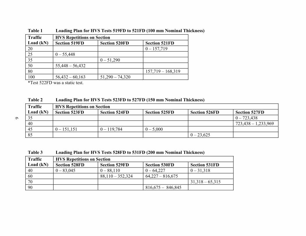
Table 1 Loading Plan for HVS Tests 519FDHVS Repetitions on Section Traffic

Load (kN) Section 519FD Section 520F20 25 0 – 55,448 35 0 – 51,290 50 55,448 – 56,432 80 100 56,432 – 60,163 51,290 – 74,3*Test 522FD was a static test.


Load (kN) Section 523FD Section 524F35 40 45 0 – 151,151 0 – 119,784 85

6


Load (kN) Section 528FD Section 529F40 0 – 83,045 0 – 88,110 60 88,110 – 352,70 90

to 521FD (100 mm Nominal Thickness)

D Section 521FD0 – 157,719 157,719 – 168,319

20


D Section 525FD Section 526FD Section 527FD 0 – 723,438

723,438 – 1,233,9690 – 5,000 0 – 23,625


D Section 530FD Section 531FD 0 – 64,227 0 – 31,318

324 64,227 – 816,675 31,318 – 65,315 816,675 – 846,845

below for the instruments used in this analysis. Complete details of the various instruments,

their recording mechanisms and outputs, are included in References (3, 4).

On each test section, two Joint Deflection Measuring Devices (JDMD) and one Edge

Deflection Measuring Device (EDMD) were installed to record the surface deflections at the

corners of adjacent slabs and at the middle edge of the test slab. A typical installation is shown

in Figure 3. Surface deflections were also captured with the Road Surface Deflectometer (RSD)

on certain sections. These results were used only for calibration purposes between the RSD,

JDMDs and EDMDs.

Figure 3. Illustration of the placement of the JDMDs and EDMD.

7

Test sections were also instrumented with thermocouples, which recorded the surface (0

mm) as well as the temperatures at 50-mm intervals at depth to the bottom of the slab:

Slab thickness: Thermocouples Located at: 100 mm Surface (0 mm), 50 mm, 100 mm 150 mm Surface (0 mm), 50 mm, 100 mm, 150 mm 200 mm Surface (0 mm), 50 mm, 100 mm, 150 mm, 200 mm

Other environmental data, such as rainfall, wind direction, and wind speed were

continuously recorded using a Davis automatic weather station. Environmental data for all test

sections on the South Tangent are included in Reference (4).

8

3.0 FIRST LEVEL DATA ANALYSIS

The performances of the different sections have to be evaluated in the context of their

relative properties such as slab dimensions (joint spacing and thicknesses) and material

properties (layer moduli, FSHCC strength, modulus of subgrade reaction). In addition, the

loading conditions varied from one section to another. Details of section performances,

deflection data, forensic evaluation, and first level data analysis are included in Reference (4).

For the first level analysis of data, the sections are placed into three groups – 100-mm nominal

slab thickness sections, 150-mm nominal slab thickness sections, and 200-mm nominal slab

thickness sections.

3.1 Slab Dimensions

Joint spacing and slab thicknesses for the South Tangent pavement test sections are

summarized in Table 4. For analysis purposes and for a full understanding of section

performance, dimensions of the adjacent slabs are also required and are included in the table. All

of the slabs tested on the South Tangent were 3.66 m wide.

Four cores from each of the three slab thickness groups were taken to verify the

thicknesses. The core was taken about 1 m from the non-loaded slab edge. Details of the coring

are included in References (3, 4). The measured core thicknesses varied greatly from the target

thicknesses. The average core thicknesses were between 7.3 and 13.0 percent greater than the

design thicknesses. The coefficients of variation (COV) ranged from 6.5 percent to 17.2 percent,

with higher COVs for the 100-mm and 150-mm nominal thickness sections. It should be noted

that cores were not taken on all of the loaded test slabs and significant slab thickness variability

can exist between slabs and even within the same slab. The cores were also used to measure the

average slab density.

9

Table 4 Joint Spacing and Slab Thickness Summary for South Tangent Pavement Sections

HVS Test Section

Center Test Slab Number

Thickness Information

(mm)

Joint Spacing

(m)

Adjacent Slabs Joint Spacings (m)

519FD 4 5.80 5.41 3.96

520FD 8 5.77 5.46 4.02

521FD 12 5.76 5.50 3.78

522FD 14

Nominal: 100.0 Mean: 107.3

Std. Dev.: 18.4 COV: 17.2%

3.69 3.99 5.50

523FD 17 5.47 3.62 5.81

524FD 20 5.77 5.55 3.97

525FD 23 3.91 5.77 3.58

526FD 27 4.00 5.79 3.54

527FD 22


Std. Dev.: 27.6 COV: 17.0%

3.58 3.91 5.55

528FD 35 4.03 5.70 3.59

529FD 31 3.94 5.84 3.65

530FD 39 3.95 5.77 3.66

531FD 42


Std. Dev.: 13.8 COV: 6.5%

3.70 3.92 5.39

3.2 FSHCC Flexural Strength

The FSHCC used for the Palmdale test site construction was an 80/20 blend of Ultimax®

and Type II PCC. The consistency of the concrete mix varied considerably from one truck to

another. Many of the mixes arriving at the site were fairly inconsistent and often required the

addition of water. Each of the three nominal thickness groups required approximately 10

truckloads of concrete. Two of these trucks were selected at random to cast beams for 8-hour, 7-

day, and 90-day flexural strength tests. Two beams were tested at each of these ages for each of

the two randomly selected truckloads. The details of the early flexural strengths for all of the

10

sections are included in Reference (3). The long term flexural strength data is included in

Reference (4).

The average flexural strength increased over 90 percent from the 8-hour to the 7-day test.

From day 7 to day 90, average flexural strength gain was 30 percent. The variability in the 90-

day flexural strength for the South Tangent sections ranged from 11 to 22 percent. However,

much of the variation in test sections was due to the variation in strengths between beams taken

from two separate trucks.(3) Since several different truckloads were used for each of the three

nominal thickness groups, and only two trucks were tested for flexural strength, it is not possible

to ascertain the flexural strength characteristics for each section on an individual basis. Because

the variation in strength between trucks is higher than (or of the order of) the variation in

strength between sections of different nominal thicknesses, the average flexural strength value

representative of all South Tangent test sections is used in the analysis. The average flexural

strength of the beam specimens tested is summarized in Table 5.

The strength gain curve based on the average for all South Tangent sections is shown in

Figure 4. This strength gain curve is used to estimate the expected average strength for the South

Tangent sections at the time of HVS testing based on age during testing.

A strength gain model developed using the average laboratory flexural strength data is

shown in Equation 1.

(1) 8582.24812.12562.0075.0)( 23 ++−= AAAMPaStrengthFlexuralFSHCC

where A = Log(Age since construction, days)

Based on the strength gain model, the estimated expected flexural strength for each of the

South Tangent test sections is shown in Table 6. For simplicity of analysis, because of the high

variability in FSHCC strength between different truckloads relative to the effect of average

11

Table 5 Average Flexural Strengths for South Tangent Sections 8 hours Nominal

Thickness (mm)

Mean (MPa)

Std. Dev. (MPa) COV (%)

100 1.87 0.14 7 150 1.92 0.60 31 200 2.45 0.16 7 All Sections 2.08 0.39 19 7 Days 100 3.48 3.48 3.48 150 3.86 3.86 3.86 200 4.48 4.48 4.48 All Sections 3.94 3.94 3.94 90 days 100 4.34 0.50 11 150 4.92 1.10 22 200 5.31 0.97 18 All Sections 4.85 0.90 19 575 days (North Tangent) All Sections (200 mm) 5.18 0.25 5

0.0

1.0

2.0

3.0

4.0

5.0

6.0

0 120 240 360 480 600

Age (days)

Flex

ural

Str

engt

h (M

Pa)

0

100

200

300

400

500

600

700

800

Figure 4. Average flexural strength gain curve for South Tangent test sections.

12

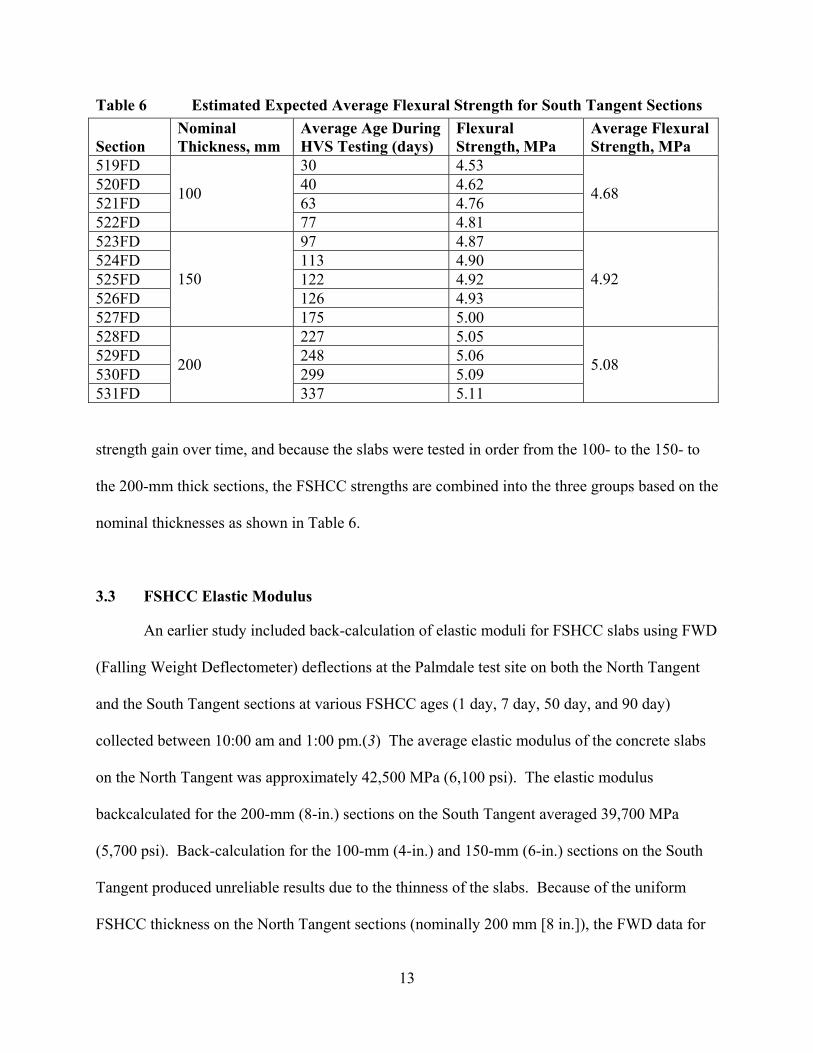
Table 6 Estimated Expected Average Flexural Strength for South Tangent Sections

Section Nominal Thickness, mm

Average Age During HVS Testing (days)

Flexural Strength, MPa

Average Flexural Strength, MPa

519FD 30 4.53 520FD 40 4.62 521FD 63 4.76 522FD

100

77 4.81

4.68

523FD 97 4.87 524FD 113 4.90 525FD 122 4.92 526FD 126 4.93 527FD

150

175 5.00

4.92

528FD 227 5.05 529FD 248 5.06 530FD 299 5.09 531FD

200

337 5.11

5.08

strength gain over time, and because the slabs were tested in order from the 100- to the 150- to

the 200-mm thick sections, the FSHCC strengths are combined into the three groups based on the

nominal thicknesses as shown in Table 6.

3.3 FSHCC Elastic Modulus

An earlier study included back-calculation of elastic moduli for FSHCC slabs using FWD

(Falling Weight Deflectometer) deflections at the Palmdale test site on both the North Tangent

and the South Tangent sections at various FSHCC ages (1 day, 7 day, 50 day, and 90 day)

collected between 10:00 am and 1:00 pm.(3) The average elastic modulus of the concrete slabs

on the North Tangent was approximately 42,500 MPa (6,100 psi). The elastic modulus

backcalculated for the 200-mm (8-in.) sections on the South Tangent averaged 39,700 MPa

(5,700 psi). Back-calculation for the 100-mm (4-in.) and 150-mm (6-in.) sections on the South

Tangent produced unreliable results due to the thinness of the slabs. Because of the uniform

FSHCC thickness on the North Tangent sections (nominally 200 mm [8 in.]), the FWD data for

13

the North Tangent were more consistent than those for the South Tangent. The back-calculation

was performed using the Dynatest ELCON program (5) and the results were reasonably

consistent with other methods of back-calculation such as AREA7 (6). An elastic modulus of

42,500 MPa (6,100 psi) was used in the analysis because of the consistency of the North Tangent

data. Longer term FWD data and the day versus night variation are included in Reference (4).

3.4 FSHCC Coefficient of Thermal Expansion

The average value for the coefficient of thermal expansion of the FSHCC was 8.14 × 10-6

mm/mm/ºC (4.52 in./in./ºF) as determined experimentally by Heath and Roesler (7). This value

was used in the South Tangent analysis.

3.5 Crack Pattern and Visual Observation Comparisons

The following summary is based on detailed observations in Reference (4).

3.5.1 100-mm nominal thickness sections

The visual observations and crack patterns for the 100-mm nominal thickness sections are

summarized below. Since there was no dynamic loading on Section 522FD, the corresponding

visual observations are not included here.

14

3.5.2 Section 519FD

Load Timeline Observation Prior to Loading

Medium size corner break on the left adjacent slab

At 2,105 repetitions of 25-kN load

Longitudinal crack throughout the length of the test slab, about 1.1 to 1.4 m respectively from the left and right slab corners, as shown in Figure 5


Large corner breaks, one on each of the left and right adjacent slabs

From 25,186–37,819 repetitions of 25-kN load

Slab deterioration and more cracking of the test slab (transverse cracks and corner breaks) as testing progressed


After occurrence of the longitudinal crack, the slab edge sunk into the base layer and a total drop-off between the slab edge and the asphalt shoulder of around 20 mm was recorded

Note: Loading Sequence25 kN 10 - 55448 Reps

50 kN 55448 - 56432 Reps100 kN 56432 - 60163 Reps

2105 Reps 25 186 Reps 37 819 Reps 55 446 Reps

60 163 Reps Final

Crack at0 Reps

Joint 4 Joint 5950

490

1165

> 1200

280810

885

550

610

840

1800 750665

Slab 5 Slab 4 Slab 3Slab 5 Slab 4 Slab 3

Figure 5a. 519FD: Schematic of crack development.(4)

15

Note: asphalt was placed in cracked area after test completion. Figure 5b. 519FD: Overhead photograph of tested section, 60,163 repetitions.

3.5.3 Section 520FD


Medium size corner break on the left adjacent slab; Large corner break on the right adjacent slab


Longitudinal crack throughout the length of the test slab, about 1.1 m, from the left slab corner, as shown in Figure 6.

From 1,000 repetitions to end of test

Several transverse cracks and corner breaks occurred as testing progressed. Final crack pattern is shown in Figure 7.

16

0 Reps 1000 Reps

34 320 Reps 51 290 Reps 60 100 Reps 74 320 Reps

1100

920 1590

21302500

1320 80 40

1060

Note: Loading Sequence35 kN: 10 - 0 - 51 240 Reps100 kN 51 290 -74 320 Reps

Joint 8 Joint 7

Crack at0 Reps

12001130


Figure 6a. 520FD: Schematic of crack development.(4).

Figure 6b. 520FD: Overhead photograph of tested section, 74,320 repetitions.

17

Figure 7. 520FD: Final crack pattern after 74,000 repetitions (35 kN and 100 kN).

3.5.4 Section 521FD


Very small corner crack on the left adjacent slab

At 500 repetitions of 20-kN load

Short longitudinal crack, about 1.4 m from the left slab corner, as shown in Figure 8..

At about 1,000 repetitions of 20-kN load

Corner break formed by progression of the short longitudinal crack towards the shoulder


Longitudinal crack between the corner break and the right joint, about 1.2 m from the right corner.

142,072 repetitions through end of test.

Several transverse cracks and corner breaks occurred as testing progressed. The final crack pattern is shown in Figure 9.

18

Joint 12 Joint 11

1640

0 Reps500

100014 2072157 719

2170

460

1200

600

740

940

590

1950

610

Crack at 0 Reps

Note: Loading Sequence20 kN: 0 - 157 719 Reps

80 kN 157 719 - 168 319 Reps




19

Figure 9. 521FD: Final Crack pattern after 168,319 repetitions (20 kN and 80 kN).

3.5.5 100-mm nominal thickness section cracking summary

All three sections had corner breaks or cracks on adjacent slabs prior to HVS loading. In

addition, Section 520FD had a corner crack on the leave end of the test slab prior to loading.

However, the first crack to occur on all of the 100-mm test slabs after HVS loading was a

longitudinal crack at a distance of between 1.1 and 1.4 m from the slab corners. The associated

load and number of repetitions for these longitudinal cracks is summarized in Table 7.

Table 7 Summary of Longitudinal Cracks for 100-mm Nominal Thickness Test Sections

Section Load, kN Repetitions Distance from Corner 1, m

Distance from Corner 2, m

519FD 25 2,105 1.10 1.42

520FD 35 1,000 1.10 1.10

521FD 20 500 1.35 -

20

3.6 150-mm nominal thickness sections


summarized below.

3.6.1 Section 523FD


Several cracks on left adjacent slab.

Prior to Loading

Full length transverse crack on test slab approximately 300 mm from the left corner, as shown in Figure 10. The effect length of this slab is therefore approximately 5.10 m.

At 89,963 repetitions of 45-kN load.

The first crack after the HVS loading. This was a longitudinal crack that turned into a corner break on the test slab and remained a longitudinal crack on the adjacent slab, as shown in Figure 11. The distance of the longitudinal crack was 1.58 m from the right slab corner. The corner break intersected the slab-shoulder joint at a distance of 2.0 m from the right slab corner. The schematic of crack development is shown in Figure 12.

21

Figure 10. 523FD: Crack at transverse joint at start of test.

Figure 11. 523FD: Crack pattern after 89,963 repetitions of 45 kN.

22

Joint 17 Joint 16

610

Slab width = 3 660

Note: Loading Sequence

45 kN: 0 - 151 151 Reps

0 Reps50089 963

2 000

1 580

Slab 18 Slab 17 Slab 16



23

3.6.2 Section 524FD

Load Timeline Observation At 30,000 repetitions of 45-kN load

Corner break on right adjacent slab after 30,000 repetitions of 45 kN


Short longitudinal crack on right joint of test slab at a distance of 1.6 m from right slab corner, as shown in Figure 13.


The longitudinal crack progressed into a corner break, as shown in Figure 14.

3.6.3 Section 525FD


Corner break on test slab at a transverse distance of 1.66 m from the right slab corner, as shown in Figure 15. The longitudinal distance of this corner break was 1.7 m from the right slab corner as measured along the length of the slab. The schematic of crack development is shown in Figure 16.

24

Joint 20 Joint 19

610

Slab width = 3 660


45 kN: 0 - 119 784 Reps

30 000 Reps64 000102 935

Slab 21 Slab 20 Slab 19



25

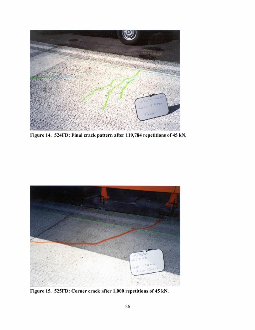
Figure 14. 524FD: Final crack pattern after 119,784 repetitions of 45 kN.

Figure 15. 525FD: Corner crack after 1,000 repetitions of 45 kN.

26

Joint 23 Joint 22

610

Slab width = 3 660


45 kN: 0 - 5 000 Reps

0 Reps

1 000

1 700

1 660



Note: Asphalt was filled into cracked area at completion of testing. Figure 16b. 525FD: Overhead photograph of tested section, 5,000 repetitions.

27

3.6.4 Section 526FD

Load Timeline Observation Prior to loading.

Transverse crack on left adjacent slab

At 100 repetitions of 85-kN load.

Corner breaks on test slab and right adjacent slab, as shown in Figure 17. The transverse distance of the corner break was approximately 1.5 m and the longitudinal distance as measured along the length of the slab was approximately 1.6 m.

At 500 repetitions of 85-kN load

Longitudinal crack on test slab from left joint after. This crack intersects the existing corner break on the test slab as shown in Figures 18 and 19. Transverse cracks on both the test slab and right adjacent slab. Corner break on the left adjacent slab.

Figure 17. 526FD: Corner cracks after 100 repetitions of 85 kN.

28

Figure 18. 526FD: Crack pattern after 500 repetitions of 85 kN.

Joint 27 Joint 26

610

Slab width = 3 660


85 kN: 0 - 23 625 Reps

0 Reps100500



29


3.6.5 Section 527FD

Load Timeline Observation Prior to loading

Large corner break on left adjacent slab


Partial longitudinal crack at a transverse distance of 1.5 m from the left slab corner, as shown in Figure 20.


Short longitudinal crack at a transverse distance of 1.5 m from the right slab corner. This crack progressed into a full length crack on the right adjacent slab.

30

Joint 22 Joint 21

610

Slab width = 3 660


35 kN: 0 - 1 233 969 Reps

0 Reps129 805890 0001 133 694


1 700 1 500

1 000


Note: Asphalt was placed in the cracked area at the completion of testing. Figure 20b. 527FD: Overhead photograph of tested section, 1,233,969 repetitions.

31


Some of the test sections had corner breaks or cracks on adjacent slabs prior to HVS

loading. However, the first crack to occur on all the 150-mm test slabs after HVS loading was a

longitudinal crack or a corner break at a transverse distance of between 1.5 and 1.7 m from the

slab corners. The associated load and number of repetitions for cracks is summarized in Table 8.

Table 8 Summary of First Crack Occurrence for 150-mm Nominal Thickness Test Sections.

Section Crack Type Load,

kN Repetitions

Transverse Distance from

Corner, m

Longitudinal Distance from

Corner, m 523FD corner break 45 89,963 1.6 2.0

524FD Longitudinal crack* 45 64,000 1.6 2.1

525FD Corner break 45 1,000 1.7 1.7

526FD Corner break 85 100 1.5 1.6

527FD Longitudinal Crack 35 129,805 1.5 - *Progressed after additional loading to corner break.

3.7 200-mm nominal thickness sections


summarized below.

3.7.1 Section 528FD


Midslab transverse crack, as shown in Figure 21.

56,912 repetitions of 40-kN load to end of test.

The midslab transverse crack extended with additional load applications but did not extend to the full length of the slab or did not become a corner break.

32

Joint 35 Joint 34

610

Slab width = 3 660


40 kN: 0 - 83 045 Reps

56 912 Reps

83 045




33

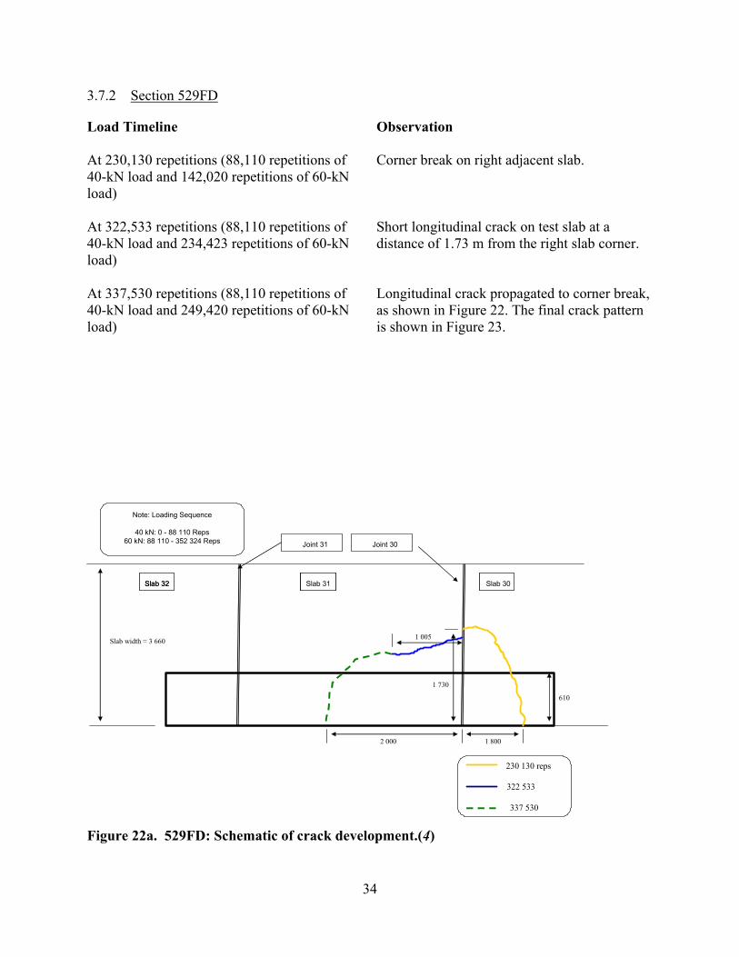
3.7.2 Section 529FD

Load Timeline Observation At 230,130 repetitions (88,110 repetitions of 40-kN load and 142,020 repetitions of 60-kN load)

Corner break on right adjacent slab.

At 322,533 repetitions (88,110 repetitions of 40-kN load and 234,423 repetitions of 60-kN load)

Short longitudinal crack on test slab at a distance of 1.73 m from the right slab corner.

At 337,530 repetitions (88,110 repetitions of 40-kN load and 249,420 repetitions of 60-kN load)

Longitudinal crack propagated to corner break, as shown in Figure 22. The final crack pattern is shown in Figure 23.

Joint 31 Joint 30

610

Slab width = 3 660


40 kN: 0 - 88 110 Reps60 kN: 88 110 - 352 324 Reps

230 130 reps

322 533

337 530

2 000

1 730

1 800

1 005

Slab 32 Slab 31 Slab 30Slab 32 Slab 31 Slab 30Slab 32 Slab 31 Slab 30


34

Note: asphalt was filled into cracked area at completion of testing. Figure 22b. 529FD: Overhead photograph of tested section, 352,324 repetitions.

Figure 23. 529FD: Final crack pattern after 352,324 repetitions of 40 kN and 60 kN.

35

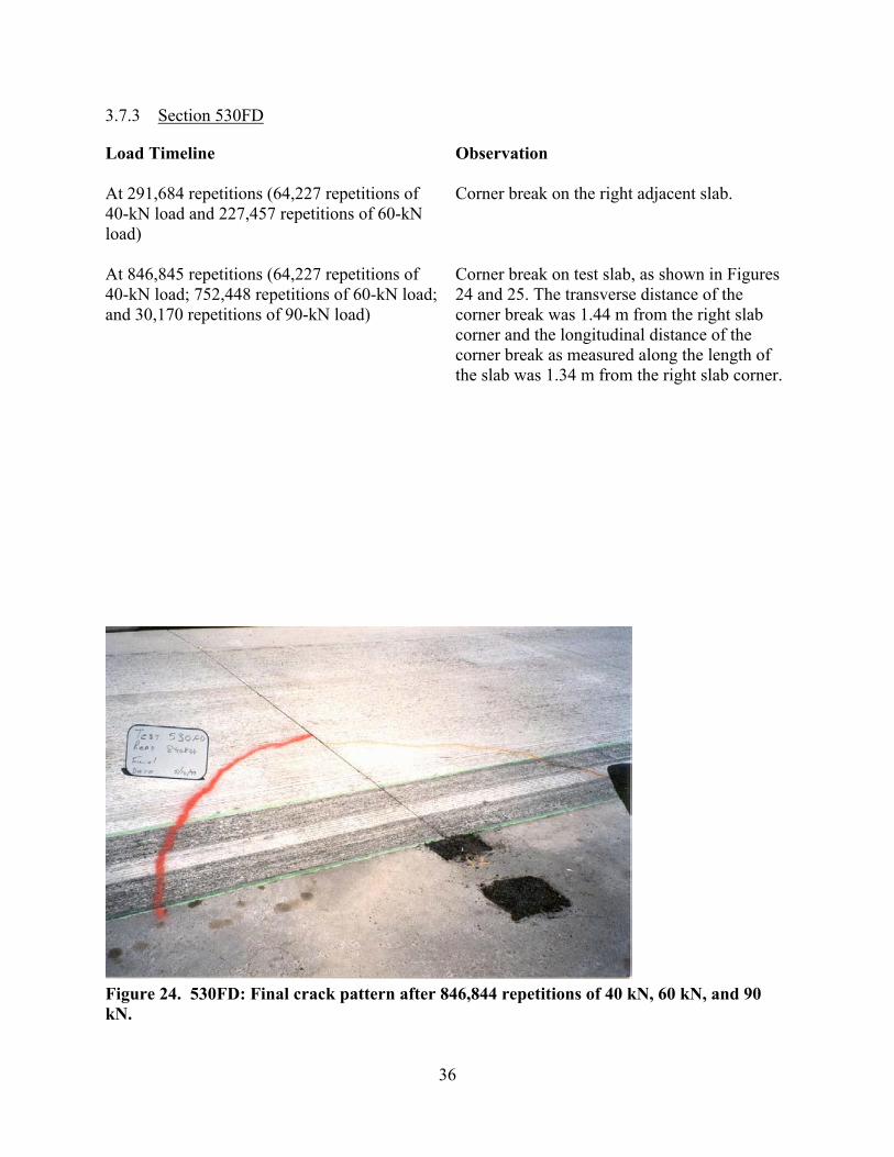
3.7.3 Section 530FD


Corner break on the right adjacent slab.

At 846,845 repetitions (64,227 repetitions of 40-kN load; 752,448 repetitions of 60-kN load; and 30,170 repetitions of 90-kN load)

Corner break on test slab, as shown in Figures 24 and 25. The transverse distance of the corner break was 1.44 m from the right slab corner and the longitudinal distance of the corner break as measured along the length of the slab was 1.34 m from the right slab corner.

Figure 24. 530FD: Final crack pattern after 846,844 repetitions of 40 kN, 60 kN, and 90 kN.

36

Joint 39 Joint 38

610

Slab width = 3 660


40 kN: 0 - 64 227 Reps60 kN: 64 227 - 816 674 Reps

90 kN: 816 674 - 846 844 Reps

291 684 Reps

830 463

1 340

1 440

1400

1 290



Figure 25b. 530FD: Overhead photograph of tested section. 846,844 repetitions.

37

3.7.4 Section 531FD


Longitudinal crack on left adjacent slab. Corner break on test slab, as shown in Figures 26 and 27. This corner break measures 1.7 m from the left slab corner in the transverse direction and 1.5 m from the left slab corner in the longitudinal direction as measured along the length of the slab.

Joint 42 Joint 41

610

Slab width = 3 660


40 kN: 0 - 31 318 Reps60 kN: 31 318 - 65 315 Reps

31 495 Reps

1 500

1 7002 100



38


Figure 27. 531FD: Final crack pattern after 65,315 repetitions of 40 kN and 70 kN.

39


None of the test sections or the adjacent slabs had any cracks prior to HVS loading.

However, the first crack to occur on three of the 200-mm test slabs after HVS loading was a

longitudinal crack (or a corner break) at a transverse distance of between 1.4 and 1.7 m from the

slab corners. Section 528FD never developed a corner break or a longitudinal crack through the

course of the HVS loading. The only crack on this section was a short transverse crack. The

associated load and number of repetitions for first cracks on the test slab is summarized in Table

9.

Table 9 Summary of First Crack Occurrence for 200-mm Nominal Thickness Test Sections

Section Crack Type Load, kN Repetitions

Transverse Distance from

Corner, m

Longitudinal Distance from

Corner, m 528FD Transverse crack 40 56,912 - 2.0

529FD Longitudinal crack* 40 60

88,110 234,423 1.7 -

530FD Corner break 40 60 90

64,227 752,448 30,170

1.4 1.3

531FD Corner break 40 70

31,318 31,495 1.7 1.5

*Progressed after additional loading to corner break.

40

4.0 TEMPERATURE CURLING AND MOISTURE WARPING ANALYSIS

The objective of the analysis is to estimate an effective linear built-in temperature

difference (EBITD) in the slab to simulate the effects of moisture shrinkage and construction

temperature gradients. This section includes:

• Discussion of thermal gradients in concrete pavements and construction curling and

moisture warping resulting in an effective built-in temperature difference.

• Procedure for estimating effective linear built-in temperature difference using rolling

wheel deflections and finite element analysis.

• Discussion of why unloaded slab deflections measured under ambient conditions

cannot be used to estimate effective linear built-in temperature difference for slabs

with high negative curl.

4.1 Thermal Gradients in Concrete Pavements

During daytime, the top of the concrete slab is warmer than the bottom, resulting in a

positive thermal gradient through the slab. The result is an elongation of the top of the slab

relative to the bottom of the slab and a convex curvature, as shown in Figure 28. This is

effectively equivalent to a void beneath the middle of the slab. During nighttime, the top of the

concrete slab is cooler than the bottom, resulting in a negative thermal gradient through the slab.

This difference results in a concave curvature of the slab, as shown in Figure 29, that is

effectively equivalent to voids beneath the edges and corners of the slab.

4.2 Construction Curling and Moisture Warping

Concrete paving is typically performed during the daytime in warmer months of the year.

During daytime paving with rapid setting materials, the top of the slab is warmer than the bottom

41

Figure 28. Downward (convex) curling of concrete slab due to daytime positive thermal gradient.

Figure 29. Upward (concave) curling of concrete slab due to nighttime negative thermal gradient.

42

at set time in many cases. Because the concrete slab sets under this condition, the flat slab

condition is no longer associated with a zero temperature gradient. When the temperature

gradient in the slab is zero, the slab curls upward at the corners toward a concave profile rather

than remains flat. Thus, an effective negative temperature gradient is “built into” the slab, and is

referred to as the built-in construction curling gradient.

After placement, water evaporates from the top of the slab and also to a lesser extent,

from the bottom of the slab. Over time, the top of the slab shrinks more relative to the bottom of

the slab. This results in a concave warping of the slab. As in the case of construction curling, an

effect negative temperature is “built into” the slab, and this is called the built-in moisture

warping gradient.

The combination of the construction curling and moisture warping effectively results in a

void beneath the slab corners and to a lesser extent, beneath the slab edges. The net result of

these effective voids beneath the slab is higher deflections in the slab under the influence of

applied loads at the slab edge and corners. For the purposes of deflections, the combination of

the construction curling and moisture warping can be modeled as an effective negative linear

temperature difference between the top and the bottom of the slab.

Using Finite Element Analysis (FEM) software such as ISLAB2000, this effective linear

built-in temperature difference in the slab can be estimated using the measured corner

deflections. Note that the actual effective built-in temperature distribution in the concrete can be

highly nonlinear. However, the equivalent linear difference that results in the same deflection as

the actual nonlinear distribution can be estimated. The equivalent linear differences are easier to

quantify, analyze, communicate, and compare as opposed to nonlinear temperature distributions,

however the non-linear gradients produce higher stresses than the equivalent linear differences.

43

4.3 ISLAB2000 Requirements

The inputs required to run ISLAB2000 are listed below:

• Geometry – slab lengths and widths

• Mesh – finite element meshed required for the analysis

• Load – magnitudes, positions, and tire imprint dimensions assuming rectangular loads

• Subgrade – modulus of subgrade reaction (k-value)

• Temperature – type of temperature distribution through slab (linear, quadratic, and

nonlinear) and corresponding temperatures

• Load Transfer Efficiency (LTE) – ratio of unloaded slab deflection to loaded slab

deflection across a joint

• Slab thickness and base thickness

• Slab properties – elastic modulus, Poisson’s ratio, unit weight, coefficient of thermal

expansion

• Base properties – elastic modulus, Poisson’s ratio, unit weight, coefficient of thermal

expansion, bond type with slab

4.4 Estimation of Effective Linear Built-In Gradients based on Measured Corner Deflections

Using known values for the ISLAB2000 inputs (Section 4.3) for the South Tangent test

sections, slab corner deflections are calculated as a function of vertical temperature difference in

the slab. After taking into consideration the actual temperature difference in the slab during test

conditions, the resulting temperature difference corresponding to the measured corner deflection

is the effective linear built-in temperature difference.

The corner deflection data point was selected such that it satisfied the following criteria:

44

• Number of repetitions should not exceed load repetitions when first crack observed.

The ISLAB2000 modeling used assumes that the slab is intact. Therefore, a cracked

slab would negate the results.

• The first few data points typically had very high corner and edge deflections. These

deflections settled down after 500 – 1000 load repetitions. The high deflections could

have been due to the settling of slab in position resulting from base/subgrade

irregularities that occurred during construction and during slab thermal movement

prior to loading. Because the deflections were not representative, the first few data

points were not used.

• The slab deflections were also affected by permanent deformation of the underlying

base and subgrade layers which occurs over time. Therefore, the earliest stable

corner deflection values were used.

For example, for Section 524FD, using known design inputs and ISLAB2000, corner

deflections are calculated as a function of temperature differential in the slab, as shown in Figure

30. The HVS corner deflections for the section, measured at various load repetitions, are shown

in Figure 31. The point on the graph, denoted by the darker black circle, was used as the data

point for estimating effective linear built-in temperature difference. The measured corner

deflection at this point is 3400 m × 10-6, which corresponds to a temperature differential of -

30.2ºC, as shown in Figure 30. After accounting for the measured temperature differential in the

slab, the effective linear built-in temperature difference for Section 524FD is estimated as -

28.5ºC.

Using the above analysis technique, the effective linear built-in temperature difference

for the South Tangent sections was calculated. The results are shown in Figure 32. Note that the

45

0

500

1,000

1,500

2,000

2,500

3,000

3,500

4,000

4,500

5,000

-50 -45 -40 -35 -30 -25 -20 -15 -10

Temperature Differential, ºC

Cor

ner

Def

lect

ions

, m ×

10-6

0

0.02

0.04

0.06

0.08

0.1

0.12

0.14

Cor

ner

Def

lect

ions

, in.

Figure 30. Predicted corner deflections as a function of slab temperature difference for Section 524FD.

0

1,000

2,000

3,000

4,000

5,000

0 20,000 40,000 60,000 80,000 100,000 120,000

Load Repetitions

Cor

ner

Def

lect

ions

, m ×

10-6

0

0.04

0.08

0.12

0.16

Def

lect

ions

, in.

Used forFEM Analysis

Corner breakright adjacent slab

Short Longitudinal crack on test slab

Figure 31. Measured corner deflections for Section 524FD.

46

-35

-30

-25

-20

-15

-10

-5

0519 520 521 522 523 524 525 526 527 528 529 530 531

Section Number

Eff

ectiv

e L

inea

r T

empe

ratu

reD

iffer

ence

, ºC

-63

-54

-45

-36

-27

-18

-9

0

Eff

ectiv

e L

inea

r T

empe

ratu

reD

iffer

ence

, ºF

Section 521: Unusually high deflections Section 522: Static edge loading (no corner loading) Figure 32. Estimated effective linear built-in temperature difference for South Tangent sections.

FEM analysis assumes static loading whereas the South Tangent slabs were tested at creep

speeds.

4.5 Curling of Unloaded Slab Due to Ambient Temperature

The 24-hour corner deflection of Slab 39 (Section 530FD) was measured using JDMDs

over a period of several days under environmental loading conditions only. Thermocouples

installed in the slab were used to measure the temperature distribution through the slab. Figure

33 shows the variation in slab temperature difference and corner deflections due to the daily

fluctuation in ambient air temperature.

47

-2.0

-1.5

-1.0

-0.5

0.0

0.5

1.0

1.5

2.0

10/24/98 0:00 10/24/9812:00

10/25/98 0:00 10/25/9812:00

10/26/98 0:00 10/26/9812:00

10/27/98 0:00

Time, hours

Def

lect

ion,

mm

-10

-8

-6

-4

-2

0

2

4

6

8

10

∆T, º

C

Corner Deflections

Slab Temperature Difference (Top - Bottom)

Figure 33. Cycling of slab temperature difference and corner deflections under ambient conditions.

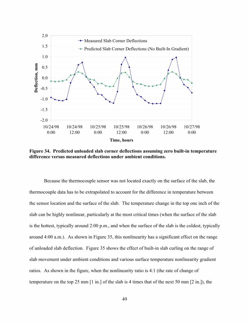
Using a finite element analysis (FEM) program (ISLAB2000), the slab corner deflections

due to temperature distribution only in the slab can be calculated. Figure 34 shows the results of

this analysis assuming zero effective built-in temperature difference in the slab. Because the

measured deflections do not have a reference value, it is important to compare the range of the

measured deflections to the range of the prediction deflections rather than the actual values. As

can be seen from the figure, the range of the measured deflections is significantly higher than

that of the predicted deflections. The predicted deflections of the slab are low when a zero

effective built-in gradient is assumed since the corners are initially supported. To match the

range of the measured deflections, the FEM calculations should be performed with a negative

effective built-in temperature difference, which is equivalent to a void beneath the slab corner

resulting in higher deflections.

48

-2.0

-1.5

-1.0

-0.5

0.0

0.5

1.0

1.5

2.0

10/24/980:00

10/24/9812:00

10/25/980:00

10/25/9812:00

10/26/980:00

10/26/9812:00

10/27/980:00

Time, hours

Def

lect

ion,

mm

Measured Slab Corner Deflections

Predicted Slab Corner Deflections (No Built-In Gradient)

Figure 34. Predicted unloaded slab corner deflections assuming zero built-in temperature difference versus measured deflections under ambient conditions.

Because the thermocouple sensor was not located exactly on the surface of the slab, the

thermocouple data has to be extrapolated to account for the difference in temperature between

the sensor location and the surface of the slab. The temperature change in the top one inch of the

slab can be highly nonlinear, particularly at the most critical times (when the surface of the slab

is the hottest, typically around 2:00 p.m., and when the surface of the slab is the coldest, typically

around 4:00 a.m.). As shown in Figure 35, this nonlinearity has a significant effect on the range

of unloaded slab deflection. Figure 35 shows the effect of built-in slab curling on the range of

slab movement under ambient conditions and various surface temperature nonlinearity gradient

ratios. As shown in the figure, when the nonlinearity ratio is 4:1 (the rate of change of

temperature on the top 25 mm [1 in.] of the slab is 4 times that of the next 50 mm [2 in.]), the

49

range of the calculated deflections is equal to that of the measured JDMD deflections for

effective built-in temperature differences less than –17ºC (–30ºF).

Note that the deflection range shown in Figure 35 is approximately the same for all built-

in effective temperature differences less than –17ºC (–30ºF). This implies that for an unloaded

slab under the influence of daily temperature cycling (as shown in Figure 33), it is not possible to

determine effective linear built-in gradients of less than –17ºC (–30ºF) using deflection range

only and without using a reference point relative to flat slab condition. This is because for built-

in effective temperature differences more negative than–17 ºC (-30 ºF), the slab corners never

come in contact with the base/subbase, even at the warmest temperatures (most positive thermal

gradients) thus resulting in similar deflection ranges. This analysis suggests that the effective

linear built-in gradient due to the combination of construction curling and moisture warping is

more negative than –17ºC (–30ºF), but the precise value cannot be determined using unloaded

slab deflection values.

Figure 36 shows the comparison of predicted unloaded slab corner deflections assuming

–17ºC (–30ºF) built-in effective temperature difference versus measured deflections. Note that

this figure is similar to those assuming –22ºC (–40ºF), –27ºC (–50ºF), or –33ºC (–60ºF) because

of the similar deflection ranges for all built-in effective temperature differences more negative

than –17ºC (–30ºF).

4.6 Effect of HVS Shading on Thermocouple Data

The measured slab temperature data used in the analysis is from the thermocouples that

are installed in the test slab. The portion of the slab tested was enclosed in a temperature control

box (excluding sections 522FD, 525FD, and 527FD). As a result, the slab temperatures

measured using the thermocouples did not vary significantly from the top of the slab to the

50

0.0

0.4

0.8

1.2

1.6

2.0

2.4

2.8

3.2

-39 -34 -29 -24 -19 -14 -9 -4

Effective Linear Built-In Gradient, ∆T, ºC

Cal

cula

ted

Def

lect

ion

Ran

ge, m

m

Linear (1:1) Nonlinear (2:1)

Nonlinear (3:1) Nonlinear (4:1)

Measured Deflection Range Small Change in Deflection Range

-17ºC

Figure 35. Effect of built-in gradient and slab surface nonlinearity ratio on predicted slab deflections.

-2.0

-1.5

-1.0

-0.5

0.0

0.5

1.0

1.5

2.0

10/24/98 0:00 10/24/98 12:00 10/25/98 0:00 10/25/98 12:00 10/26/98 0:00 10/26/98 12:00 10/27/98 0:00

Time, hours

Def

lect

ion,

mm

Measured Slab Corner Deflections

Predicted Slab Corner Deflections -17ºC effectivebuilt-in temperature difference

Figure 36. Predicted unloaded slab corner deflections assuming zero built-in temperature difference versus measured deflections under ambient conditions.

51

bottom of the slab. However, analyses of the North Tangent test sections show that the

temperatures (air temperature, slab temperature, shade, etc.) that are outside the temperature

control box affect slab responses measured inside the temperature control box. This is because a

portion of the slab is exposed to ambient conditions outside the HVS and is subject to changes in

weather, sunlight, HVS shadows, etc. These effects need to be accounted for in the analyses of

the South Tangent test sections. This will be done after an extensive analysis of the North

Tangent test sections, where more detailed and comprehensive information was collected.

52

5.0 CRACKING ANALYSIS

The objective of the cracking analysis is to evaluate slab cracking by attempting to

understand the stress state of the slab. This section includes:

• Discussion of the mechanism of fatigue cracking and responses at critical locations.

• Influence diagrams for South Tangent sections representing the stresses at the top of

the concrete slab simulating the effect of a load moving in a given direction (left to

right) on a fixed point.

• Discussion of fatigue characterization of concrete pavements and various fatigue

models.

• Calculation of fatigue damage to failure using various models for South Tangent

sections.

• Comparison of predicted versus actual locations of critical damage for South Tangent

sections.

5.1 Fatigue Cracking

Cracking in concrete pavements occurs as a result of either early-age environmental

stresses with or without load stresses that exceed the concrete strength of the slabs or fatigue

failure. The environmental stresses are caused by the combined effects of the restraint forces

(the restraint against the contraction of concrete in response to either shrinkage or temperature

change), thermal curling, and moisture warping. Most of the cracking from these mechanisms

occurs soon after construction. Several slabs at the Palmdale test site cracked due to high

stresses which occurred at early age and before the concrete had not gained adequate strength.

Details of this type of early-age cracking at Palmdale are discussed in Reference (7).

53

Fatigue cracking is a key measure of concrete pavement performance and is caused by

the repeated application of traffic and environmental loading at stress levels less than the

cracking strength of the concrete. As the loadings are repeated over time, cracking can occur in

the slab. Analysis of fatigue cracking includes determination of critical stresses in the slab (both

traffic and environmentally induced) and the locations of these stresses. These stresses are used

in a fatigue cracking model that relates stresses and number of load applications to damage at the

location of critical stress.

5.2 Critical Stresses in Concrete Slabs

Each application of traffic and environmental load on a pavement results in stresses that

occur in the concrete slab. The consequence of these stresses is an accumulation of damage in

that portion of the concrete slab. After sufficient damage has accumulated in a region of the

concrete slab, cracking will be visible on the surface of the slab. Fatigue cracking in jointed

plain concrete pavement (JPCP) can be divided into four major categories depending on the

location of the accumulated damage and can be further reviewed in References (8, 9):

• Bottom-up transverse cracks.

• Top-down transverse cracks.

• Longitudinal cracks.

• Corner breaks.

5.2.1 Mechanism of Bottom-Up Transverse Cracking

When loads are near the longitudinal edge of the slab, midway between the transverse

joints, a critical tensile bending stress occurs at the bottom of the slab, as shown in Figure 37.

54

This stress increases greatly when there is a high positive thermal gradient through the slab (top

of the slab is warmer than bottom of the slab). Repeated heavy loadings result in fatigue damage

along the edge of the slab, which results in microcracks that propagate to the slab surface from

the bottom and transversely across the slab.

5.2.2 Mechanism of Top-Down Transverse Cracking

When the load is near the transverse joints at the corner of the slab, a high tensile stress

occurs at the top of the slab between the axles, some distance from the joint, as shown in Figure

38. This stress increases greatly when there is a negative thermal gradient through the slab, a

built-in negative gradient from construction, and/or a significant drying shrinkage at the top of

the slab. Repetitive loading results in fatigue damage at the top of the slab, which eventually

results in micro-cracks that propagate downward through the slab and transversely or diagonally

across the slab. As in the case of bottom-up cracking, these micro-cracks join and result in a

transverse crack that is visible on the surface of the slab.

Critical Stress

Midpoint

Critical location

Outside Lane

Shoulder

Figure 37. Critical load and structural response location for JPCP bottom-up transverse cracking.

55

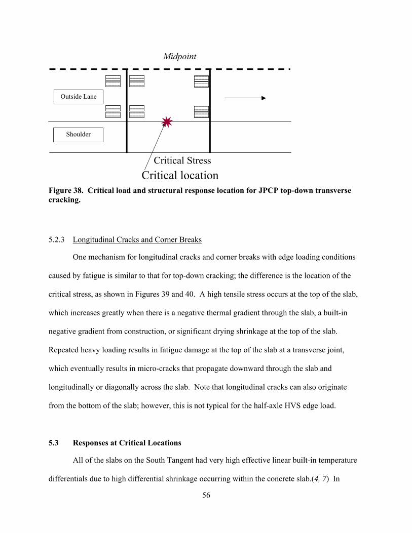
Critical Stress

Midpoint

Critical location

Outside Lane

Shoulder

Figure 38. Critical load and structural response location for JPCP top-down transverse cracking.

5.2.3 Longitudinal Cracks and Corner Breaks

One mechanism for longitudinal cracks and corner breaks with edge loading conditions

caused by fatigue is similar to that for top-down cracking; the difference is the location of the

critical stress, as shown in Figures 39 and 40. A high tensile stress occurs at the top of the slab,

which increases greatly when there is a negative thermal gradient through the slab, a built-in

negative gradient from construction, or significant drying shrinkage at the top of the slab.

Repeated heavy loading results in fatigue damage at the top of the slab at a transverse joint,

which eventually results in micro-cracks that propagate downward through the slab and

longitudinally or diagonally across the slab. Note that longitudinal cracks can also originate

from the bottom of the slab; however, this is not typical for the half-axle HVS edge load.

5.3 Responses at Critical Locations

All of the slabs on the South Tangent had very high effective linear built-in temperature

differentials due to high differential shrinkage occurring within the concrete slab.(4, 7) In

56

Critical Stress

Midpoint

Critical location

Outside Lane

Shoulder

Figure 39. Critical load and structural response location for JPCP longitudinal cracking.

Critical Stress

Midpoint

Critical location

Outside Lane

Shoulder

Figure 40. Critical load and structural response location for JPCP corner breaks.

57

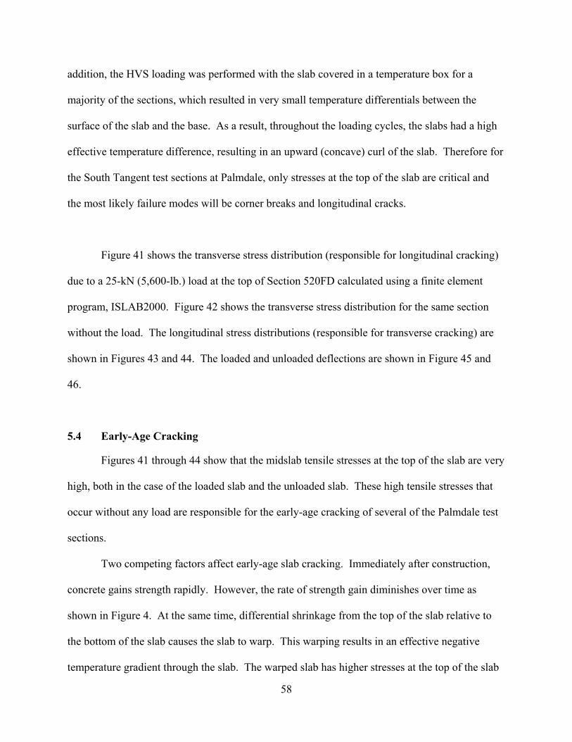
addition, the HVS loading was performed with the slab covered in a temperature box for a

majority of the sections, which resulted in very small temperature differentials between the

surface of the slab and the base. As a result, throughout the loading cycles, the slabs had a high

effective temperature difference, resulting in an upward (concave) curl of the slab. Therefore for

the South Tangent test sections at Palmdale, only stresses at the top of the slab are critical and

the most likely failure modes will be corner breaks and longitudinal cracks.

Figure 41 shows the transverse stress distribution (responsible for longitudinal cracking)

due to a 25-kN (5,600-lb.) load at the top of Section 520FD calculated using a finite element

program, ISLAB2000. Figure 42 shows the transverse stress distribution for the same section

without the load. The longitudinal stress distributions (responsible for transverse cracking) are

shown in Figures 43 and 44. The loaded and unloaded deflections are shown in Figure 45 and

46.

5.4 Early-Age Cracking

Figures 41 through 44 show that the midslab tensile stresses at the top of the slab are very

high, both in the case of the loaded slab and the unloaded slab. These high tensile stresses that

occur without any load are responsible for the early-age cracking of several of the Palmdale test

sections.

Two competing factors affect early-age slab cracking. Immediately after construction,

concrete gains strength rapidly. However, the rate of strength gain diminishes over time as

shown in Figure 4. At the same time, differential shrinkage from the top of the slab relative to

the bottom of the slab causes the slab to warp. This warping results in an effective negative

temperature gradient through the slab. The warped slab has higher stresses at the top of the slab

58

Stresses in X-direction

563525467409351293235177119613

-55-113-171-190

X

Y

X

Y

X

Y

Location of maximum stress

Load location


563525467409351293235177119613

-55-113-171-190

X

Y

X

Y

X

Y


563525467409351293235177119613

-55-113-171-190

X

Y

X

Y

X

Y


Load location


Load location

Figure 41. Transverse stress (psi) distribution at top of slab (25-kN [5,600-lb.] load) – Section 520FD.


53951247143038934930826722618514410463228


X

Y

X

Y

X

YStresses in X-direction

53951247143038934930826722618514410463228



53951247143038934930826722618514410463228

Location of maximum stressLocation of maximum stress

X

Y

X

Y

X

Y

Figure 42. Transverse stress (psi) distribution at top of slab (no load) – Section 520FD.

59

Stresses in Y-direction

578534469403337272206140749

-57-123-188-254-276

X

Y

X

Y

X

Y

Locations of maximum stress

Load location


578534469403337272206140749

-57-123-188-254-276

X

Y

X

Y

X

Y


Load location


Load location

Figure 43. Longitudinal stress distribution (psi) at top of slab (25-kN [5,600-lb.] load) – Section 520FD.


58655651246742337833429024520115611267238

X

Y

X

Y

X

Y



58655651246742337833429024520115611267238

X

Y

X

Y

X

Y


Figure 44. Longitudinal stress distribution at top of slab (no load) – Section 520FD.

60

Deflections

0.01300.00780.0001

-0.0077-0.0154-0.0232-0.0309-0.0387-0.0465-0.0542-0.0620-0.0697-0.0775-0.0852-0.0878

Figure 45. Slab deflection (in.) (25-kN [5,600-lb.] load) – Section 520FD.

Deflections

0.00650.0018

-0.0053-0.0124-0.0195-0.0265-0.0336-0.0407-0.0478-0.0549-0.0620-0.0691-0.0762-0.0832-0.0856

Figure 46. Slab deflection (in.) (no load) – Section 520FD.

61

caused by the weight of the lifted slab corners (and edges). This is shown in Figures 42 and 44,

where high stresses at the midslab location exist without any applied load. If during the early-

age development of the concrete, these warping stresses exceed the strength of the concrete, the

slab cracks even before any load is applied.

5.5 Influence of Moving HVS Load

Under the application of the HVS load, the midslab stresses do not change significantly

and therefore do not affect the fatigue behavior of the slab. This is illustrated in Figure 47,

which shows the influence chart for a moving HVS load applied at the edge of the slab for the

100-mm nominal thickness section, 520FD. An influence chart is a graphic representation of a

response (stress) at a fixed point due to placement of a load at several different points thus

simulating the effect of a load moving in a given direction (left to right) on that fixed point.

Figure 47 shows 4 influence lines denoting stresses at the top of the slab as predicted at 4

locations on the slab including:

• Transverse stress (at critical location on transverse joint) responsible for longitudinal

fatigue cracking and corner breaks originating from the transverse joint (A).

• Longitudinal stress (at critical location on slab edge) responsible for transverse

fatigue cracking and corner breaks originating from the lane-shoulder joint (B).

• Transverse stress (at midslab location) responsible for early-age cracking (C).

• Longitudinal stress (at midslab location) responsible for early-age cracking (D).

Note that the midslab stresses are not significantly affected by the movement of the load

(or by the presense/absence of the load). However, the transverse stresses measured at the

transverse joint and the longitudinal stresses measured at the slab edge can vary considerably

62

-8

-4

0

4

8

-6 -4 -2 0 2 4 6 8

Distance from left corner, m

Stre

ss, M

Pa

-1200

-600

0

600

1200

Stre

ss, p

si

A, Trans. Jt. Stress (Trans. Dir.)B, Sh. Edge Stress (Long. Dir.)C, Midslab Stress (Trans. Dir.)D, Midslab Stress (Long. Dir.)

Test Slab

Test Slab Legend

B

C

AD

Top of Slab StressesTension - Positive

Approach Slab

Figure 47. Influence diagram showing effect of 35-kN moving load on stresses at critical locations on the concrete slab (Section 520FD – 100 mm slab).

relative to the unloaded slab as shown in Figure 47. It is assumed that stress changes cause

fatigue as opposed to peak tensile stress.

Figures 48 through 65 show the influence lines denoting the following stresses at the top

of the slab with positive values representing tensile stresses and negative values representing

compressive stresses:

• Transverse stress (at critical location on transverse joint) responsible for longitudinal

fatigue cracking and corner breaks originating from the transverse joint (A) for three

values of effective linear temperature difference in the slab.

• Longitudinal stress (at critical location on slab edge) responsible for transverse

fatigue cracking and corner breaks originating from the lane-shoulder joint (B) for

63

three values of effective linear temperature difference in the slab. Note that each

influence line corresponding to each of the three effective linear temperature

difference taken at different points on the slab. This is because the critical point

(point with the greatest tensile stress) changes depending on the magnitude of the

effective linear temperature difference.

The influence lines are shown for Sections 520FD (100-mm nominal thickness), 524FD

(150-mm nominal thickness), and 530FD (200-mm nominal thickness), for three different load

levels, 35 kN (7,875 lbs.), 20 kN (4,500 lbs.), and 60kN (13,500 lbs.), and three effective

temperature differences, 100 percent of estimated built-in curl, 50 percent of estimated built-in

curl, and zero (no slab temperature difference). The following conclusions can be drawn from

these influence lines:

• The effective temperature difference in the slab has a significant effect on the peak

stress for both the critical transverse joint location (A) and the critical slab edge

location (B). However, the exact location of the peak stress depends on the

magnitude of the temperature difference (Figures 48 and 49). The larger the

temperature difference, the greater the uplift at the slab corners, and farther away

from the corner and closer to the midslab edge is the location of the peak stress.

• Depending on the magnitude of the temperature difference, the location of the peak

stress can vary up to 2 m relative to the peak stress location during flat slab (zero

temperature difference) condition (Figures 49, 51, and 53). This variation is smaller

along the transverse joint (A) and larger along the slab edge (B).

64

• The critical location on the slab edge (B) typically experiences a stress reversal, i.e.

the stress changes from tension to compression and back to tension under the

influence of a moving load (Figures 49, 51, and 53).

• The magnitude of the stress reversal depends on the slab thickness and the magnitude

of the applied load. In cases when the load is small or the slab thickness is large,

there is no stress reversal (Figure 57).

• Both the magnitude of the applied load and the thickness of the slab significantly

affect stresses in the slab, but not the shape of the stress influence line.

The results of the influence chart analysis for the three sections are summarized in Tables

10 and 11.

5.6 Fatigue Characterization of Concrete Pavements

5.6.1 Miner’s Hypothesis and Damage Accumulation

Miner’s fatigue damage accumulation hypothesis is empirically based and is given as

follows (10):

∑=i

i

Nn

DamageFatigue (2)

where ni = Number of actual load applications of under conditions represented by i. Ni = Number of allowable load applications until failure under conditions

represented by i.

65

-8

-4

0

4

8

-6 -4 -2 0 2 4 6 8


Stre

ss, M

Pa

-1200

-600

0

600

1200

Stre

ss, p

si

Temp. Difference = -12ºC


Temp. Difference = 0ºC

Test Slab35-kN Load

Test Slab Legend

A


Figure 48. Influence diagram showing effect of 35-kN moving load on transverse stresses at the transverse joint (Section 520FD – 100 mm slab).

-8

-4

0

4

8

-6 -4 -2 0 2 4 6 8


Stre

ss, M

Pa

-1200

-600

0

600

1200

Stre

ss, p

si




Test Slab35-kN Load

Test Slab Legend

B


Figure 49. Influence diagram showing effect of 35-kN moving load on longitudinal stresses at the lane-shoulder joint (Section 520FD – 100 mm slab).

66

-8

-4

0

4

8

-6 -4 -2 0 2 4 6 8


Stre

ss, M

Pa

-1200

-600

0

600

1200

Stre

ss, p

si




Test Slab20-kN Load

Test Slab Legend

A



-8

-4

0

4

8

-6 -4 -2 0 2 4 6 8


Stre

ss, M

Pa

-1200

-600

0

600

1200

Stre

ss, p

si




Test Slab20-kN Load

Test Slab Legend

B



67

-8

-4

0

4

8

-6 -4 -2 0 2 4 6 8


Stre

ss, M

Pa

-1200

-600

0

600

1200

Stre

ss, p

si




60-kN Load

Test Slab Legend

A


Test Slab


-8

-4

0

4

8

-6 -4 -2 0 2 4 6 8


Stre

ss, M

Pa

-1200

-600

0

600

1200

Stre

ss, p

si




Test Slab60-kN Load

Test Slab Legend

B



68

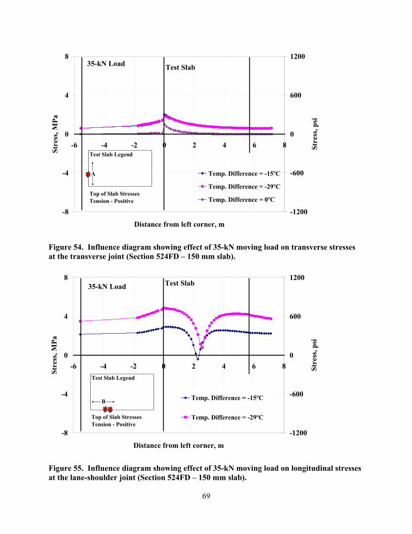
-8

-4

0

4

8

-6 -4 -2 0 2 4 6 8


Stre

ss, M

Pa

-1200

-600

0

600

1200

Stre

ss, p

si




Test Slab35-kN Load

Test Slab Legend

A



-8

-4

0

4

8

-6 -4 -2 0 2 4 6 8


Stre

ss, M

Pa

-1200

-600

0

600

1200

Stre

ss, p

si



Test Slab35-kN Load

Test Slab Legend

B



69

-8

-4

0

4

8

-6 -4 -2 0 2 4 6 8


Stre

ss, M

Pa

-1200

-600

0

600

1200

Stre

ss, p

si




Test Slab20-kN Load

Test Slab Legend

A



-8

-4

0

4

8

-6 -4 -2 0 2 4 6 8


Stre

ss, M

Pa

-1200

-600

0

600

1200

Stre

ss, p

si



Test Slab20-kN Load

Test Slab Legend

B



70

-8

-4

0

4

8

-6 -4 -2 0 2 4 6 8


Stre

ss, M

Pa

-1200

-600

0

600

1200

Stre

ss, p

si




Test Slab60-kN Load

Test Slab Legend

A



-8

-4

0

4

8

-6 -4 -2 0 2 4 6 8


Stre

ss, M

Pa

-1200

-600

0

600

1200

Stre

ss, p

si



Test Slab60-kN Load

Test Slab Legend

B



71

-8

-4

0

4

8

-6 -4 -2 0 2 4 6 8


Stre

ss, M

Pa

-1200

-600

0

600

1200

Stre

ss, p

si




Test Slab35-kN Load

Test Slab Legend

A



-8

-4

0

4

8

-6 -4 -2 0 2 4 6 8


Stre

ss, M

Pa

-1200

-600

0

600

1200

Stre

ss, p

si




Test Slab35-kN Load

Test Slab Legend

B



72

-8

-4

0

4

8

-6 -4 -2 0 2 4 6 8


Stre

ss, M

Pa

-1200

-600

0

600

1200

Stre

ss, p

si




Test Slab20-kN Load

Test Slab Legend

A



-8

-4

0

4

8

-6 -4 -2 0 2 4 6 8


Stre

ss, M

Pa

-1200

-600

0

600

1200

Stre

ss, p

si




Test Slab20-kN Load

Test Slab Legend

B



73

-8

-4

0

4

8

-6 -4 -2 0 2 4 6 8


Stre

ss, M

Pa

-1200

-600

0

600

1200

Stre

ss, p

si




Test Slab60-kN Load

Test Slab Legend

A



-8

-4

0

4

8

-6 -4 -2 0 2 4 6 8


Stre

ss, M

Pa

-1200

-600

0

600

1200

Stre

ss, p

si




Test Slab60-kN Load

Test Slab Legend

B



74

Table 10 Influence Chart Analysis Summary for Slab Edge, Sections 520FD, 524FD, and 530FD

Slab Edge (B)

Peak Tensile Stress, MPa

Minimum Stress, MPa

Unloaded Slab Stress, MPa

Max. Stress Change, MPa

Stress Change Relative to Unloaded Slab, MPa

Section Load, kN

Temp. Grad., ºC P M U P-M P-U -23 4.66 -1.89 3.03 6.56 1.63 -12 2.80 -3.44 0.82 6.24 1.98 35 0 1.93 -4.06 0.00 5.99 1.93 -23 4.40 -0.57 3.03 4.96 1.36 -12 2.23 -1.43 0.82 3.66 1.41 20 0 1.23 -2.25 0.00 3.48 1.23 -23 5.00 -4.39 3.03 9.39 1.97 -12 3.69 -6.16 0.82 9.85 2.87

520FD

60 0 2.63 -7.16 0.00 9.79 2.63 -29 4.84 0.79 3.48 4.04 1.36 -15 2.90 -0.42 2.14 3.32 0.76 35 0 0.98 -2.34 0.00 3.32 0.98 -29 4.35 1.74 3.48 2.61 0.88 -15 2.69 0.45 2.14 2.24 0.55 20 0 0.62 -1.37 0.00 1.99 0.62 -29 5.32 -0.71 3.48 6.03 1.84 -15 3.11 -1.46 2.14 4.58 0.97

524FD

60 0 1.47 -3.71 0.00 5.18 1.47 -29 1.67 -1.16 0.63 2.84 1.04 -15 1.69 -0.87 0.74 2.56 0.96 35 0 0.69 -1.47 0.00 2.16 0.69 -29 1.24 -0.40 0.63 1.64 0.61 -15 1.32 -0.29 0.74 1.61 0.59 20 0 0.42 -0.78 0.00 1.20 0.42 -29 2.30 -2.07 0.63 4.37 1.67 -15 2.08 -1.52 0.74 3.60 1.35

530FD

60 0 1.04 -2.41 0.00 3.44 1.04

75

Table 11 Influence Chart Analysis Summary for Transverse Joint at Sections 520FD, 524FD, and 530FD

Transverse Joint (A)

Peak Tensile Stress, MPa

Minimum Stress, MPa

Unloaded Slab Stress, MPa

Max. Stress Change, MPa

Stress Change Relative to Unloaded Slab, MPa

Section Load, kN

Temp. Grad., ºC P M U P-M P-U -23 4.04 1.30 1.30 2.74 2.74 -12 3.02 0.80 0.80 2.22 2.22 35 0 1.73 0.00 0.00 1.73 1.73 -23 3.31 1.30 1.30 2.02 2.02 -12 2.31 0.80 0.80 1.52 1.52 20 0 1.04 0.00 0.00 1.04 1.04 -23 4.72 1.30 1.30 3.43 3.43 -12 4.01 0.80 0.80 3.21 3.21

520FD

60 0 2.70 0.00 0.00 2.70 2.70 -29 1.87 0.57 0.58 1.30 1.29 -15 2.04 0.60 0.60 1.43 1.43 35 0 0.97 0.00 0.00 0.97 0.97 -29 1.32 0.57 0.58 0.75 0.74 -15 1.49 0.60 0.60 0.89 0.89 20 0 0.58 0.00 0.00 0.58 0.58 -29 2.69 0.56 0.58 2.12 2.11 -15 2.53 0.60 0.60 1.93 1.93

524FD

60 0 1.56 0.00 0.00 1.56 1.56 -29 1.43 0.50 0.50 0.93 0.93 -15 1.46 0.49 0.49 0.97 0.97 35 0 0.70 0.00 0.00 0.70 0.70 -29 1.04 0.50 0.50 0.54 0.54 -15 1.06 0.49 0.49 0.57 0.57 20 0 0.41 0.00 0.00 0.41 0.41 -29 2.04 0.50 0.50 1.53 1.53 -15 1.92 0.49 0.49 1.43 1.43

530FD

60 0 1.15 0.00 0.00 1.15 1.15

76

The Miner’s hypothesis allows the summation of fatigue damage from loads of various

magnitudes under various conditions. According to Miner’s hypothesis, materials should

fracture when the fatigue damage equals 1.0. However, observation shows that variability in

material properties, environmental conditions, and load sequencing can result in fractures

occurring at fatigue damage values at significantly less than or greater than 1.0.

5.6.2 Relationship between Stress-Strength Ratio and Load Repetitions

The stress ratio experienced by a concrete pavement has traditionally been assumed to be

linearly related to the log of the number of load applications required to produce fatigue-related

failure, where the stress ratio is the ratio of the combined tensile stress experienced by a loaded

concrete pavement to the concrete modulus of rupture:

MR

SR σ= (3)

where SR = Stress ratio σ = Total tensile stress due to traffic and curling at slab edge MR = Modulus of rupture

5.6.3 Fatigue Models

Several fatigue curves for concrete beams have been developed using field and lab data

that relate the stress ratio to the number of loads to failure. These include:

77

• Zero-Maintenance Design Fatigue Model (11-13)

SRN ⋅−= 61.1761.17log (4)

where N = Number of stress applications to failure for the given stress ratio

SR

• Calibrated Mechanistic Design Fatigue Model (14)

( ) 2276.0367.5

0032.01loglog

−−=

− PSRN (5)

where P = Cracking probability

• ERES/COE Fatigue Model (15)

log (6) 2.113.2 −⋅= SRN

• PCA Fatigue Model (16)

log 55.0077.12737.11 ≥⋅−= SRforSRN (7a)

55.045.04325.0

2577.4 268.3

<<

−= SRfor

SRN (7b)

N = unlimited for SR ≤ 0.45 (7c)

The log of number of allowable load applications for various fatigue models

corresponding to damage of 1.0 as a function of stress ratio is shown in Figure 66.

78

0

2

4

6

8

10

12

0.4 0.5 0.6 0.7 0.8 0.9 1.0

Stress Ratio, SR

log

N

Zero Maintenance Design

PCA

ERES/COE

Calibrated Mechanistic Design

Figure 66. Number of allowable load applications to damage of 1.0 for various fatigue models.

5.7 Cumulative Damage for Sections

ISLAB2000 was used to calculate critical stresses at several locations on the South

Tangent test slabs. The calculations were performed for each of the two-hour increments that

thermocouple data was collected while loaded with the HVS. The ratio of the calculated stress to

the slab strength is the stress ratio corresponding to each time increment. This stress ratio is used

to calculate the allowable number of load applications to failure for that time increment using the

fatigue models. The ratio of the actual number of HVS applications within the time increment to

the calculated allowable number of load applications is the damage for that time increment. The

damage for all time increments to failure (appearance of first crack) is summed at each of the

stress locations. Cumulative fatigue damage as a function of number of applied loads for Section

523FD using the ERES/COE model is shown in Figure 67. Tables 12 through 14 show the

79

0

1

2

3

4

5

6

7

8

0 10,000 20,000 30,000 40,000 50,000 60,000 70,000 80,000 90,000 100,000

Number of Load Repetitions

Cum

ulat

ive

Fatig

ue D

amag

e

Figure 67. Cumulative fatigue damage calculated at transverse joint critical stress location for Section 523FD (45-kN load).

Table 12 Fatigue Damage to Failure Calculated using “Calibrated Mechanistic

Design” Model Section Left Shoulder

Joint Left Transverse Joint

Right Shoulder Joint

Right Transverse Joint

520FD 0.384 0.316 0.380 0.323 523FD 18.592 0.324 19.642 0.117 524FD 23.038 0.080 22.263 0.179 525FD 0.008 0.003 0.006 0.006 527FD 0.007 0.033 0.016 0.010 528FD 0.003 0.001 0.004 0.002 529FD 0.062 0.010 0.021 0.038 530FD 0.023 0.001 0.010 0.007 531FD 0.000 0.007 0.002 0.003

80

Table 13 Fatigue Damage to Failure Calculated using “Zero-Maintenance” Model Section Left Shoulder




520FD 2.77E+00 1.30E+00 2.67E+00 1.40E+00 523FD 4.74E+01 4.80E-03 5.77E+01 1.11E-03 524FD 1.92E+02 6.24E-04 1.68E+02 1.98E-03 525FD 2.37E-04 4.23E-05 1.29E-04 1.50E-04 527FD 4.17E-05 2.04E-04 9.49E-05 5.64E-05 528FD 1.59E-05 4.80E-06 2.07E-05 1.05E-05 529FD 3.49E-04 5.82E-05 1.17E-04 2.08E-04 530FD 1.40E-04 1.74E-05 6.92E-05 5.42E-05 531FD 2.75E-06 4.04E-05 8.81E-06 1.38E-05

Table 14 Fatigue Damage to Failure Calculated using “ERES/COE” Model Section Left Shoulder




520FD 2.630 2.278 2.605 2.313 523FD 148.441 7.335 154.596 3.427 524FD 159.514 2.435 155.528 4.420 525FD 0.130 0.067 0.105 0.111 527FD 0.459 1.403 0.839 0.574 528FD 0.146 0.057 0.179 0.108 529FD 2.935 0.766 1.339 2.040 530FD 1.925 0.253 1.030 0.817 531FD 0.041 0.354 0.113 0.162

calculated fatigue damage at four critical locations on the slab using different fatigue models.

For these computations, the peak stresses, P, were used.

A cumulative fatigue damage of 1.0 to failure is not expected for these sections for

several reasons including:

• Fatigue model limitations and variability among models.

• Different testing conditions and method for calculating stresses compared to those

used to develop the fatigue models.

• Miner’s hypothesis assumptions: linear damage accumulation, homogenous material,

limited testing.

81

• Fatigue models developed for 1.0 to correspond to 50 percent of slabs cracking (given

a large section with number of slabs). In the above analysis we are calculating fatigue

damage for a single slab.

5.7.1 Concrete Fatigue Models

The differences in the allowable number of load repetitions among the presented fatigue

models resulted in significant differences in the calculated cumulative damage. Fatigue models

have been developed and calibrated based on several data sources, failure definitions, stress

computations, and stress components. The “Calibrated Mechanistic Design” model was

developed using Army Corp of Engineers (COE) field aircraft data and American Association of

State Highway Officials (AASHO) Road Test data, with failure defined as 50 percent slab

cracking. Load and temperature curling stresses were calculated at the slab edge using the finite

element program, ILLI-SLAB. The “ERES/COE” model was developed using Corp of Engineers

(COE) field aircraft data, with failure defined as 50 percent slab cracking. Load stresses

calculated at the slab edge using the influence chart software, H-51, and reduced by a factor of

0.75 to account for load transfer and support conditions. The “Zero-Maintenance” model was

develop using concrete beams, with failure defined as complete beam fracture. Load stresses

were calculated at the bottom of the beam using the bending beam equation.

Application of a fatigue model without proper calibration can lead to an erroneous

conclusion. Further complicating matters are the concrete material size and geometry, which are

not considered directly in any of the existing fatigue models but have shown to be factors in the

fatigue resistance of concrete.

82

5.7.2 Miner’s Hypothesis Limiting Assumptions

Miner’s hypothesis has been used extensively in concrete and asphalt fatigue analysis to

account for variable stress states over time. Its ease of application in pavement design has

prolonged its life. The main limitation of log N versus SR curves coupled with Miner’s

hypothesis lies in a phenomenological explanation of fatigue failure of concrete through the

stress ratio. The stress ratio approach assumes the stress state in the concrete is constant over the

entire concrete fatigue life, which disregards incremental damage or more accurately, crack

propagation. This is not a valid assumption, since the previous load cycles damage the concrete,

which in turn increases the subsequent stress states in the concrete material. This is why Miner’s

hypothesis is not sustainable and should not be expected to provide an intrinsic explanation for

concrete fatigue failure. Furthermore, factors such as material homogeneity, endurance limit,

variable load amplitude, loading rates and rest periods, stress history, and stress reversal are

known to affect the fatigue life of concrete and yet cannot be accurately accounted for in a stress

ratio / Miner’s hypothesis approach.

Another deficiency of using Miner’s hypothesis with fatigue damage models is that for

new pavements, an initial damage of zero is assumed. Weak zones in the concrete resulting from

factors such as drying shrinkage, poor mix characteristics, etc., are not considered. Although the

test slabs did not have visual cracks prior to fatigue testing, several of the longer slabs on the test

strip cracked prior to any load application.

5.8 Critical Stress Location

Table 15 shows the location of the critical peak stresses and the locations of the field

observed cracks on the South Tangent sections. In the tables, longitudinal crack distances are

measured in the transverse direction from the slab corner, transverse crack distances are

83

Table 15 Critical Stress Location and Actual Crack Location for South Tangent Test Sections

Section Critical Stress Distance (m) Observed Crack

Observed Crack Distance

520FD 1.0 Longitudinal 1.1 523FD 1.3, 2.0 Corner 1.6, 2.0 524FD 1.2, 2.2 Corner 1.6, 2.1 525FD 1.3, 1.4 Corner 1.7, 1.7 527FD 1.4 Longitudinal 1.5 528FD 1.5 Transverse 2.0 529FD 1.3, 1.5 Corner 1.7, 2.0 530FD 1.3, 1.4 Corner 1.4, 1.3 531FD 1.4, 1.4 Corner 1.7, 1.5

measured in the longitudinal direction from the nearest slab corner. Both longitudinal and

transverse distances from the nearest slab corner are measured for corner breaks. As can be seen

from the tables, the locations of the critical peak stresses calculated using ISLAB2000

correspond very well with the locations of the observed cracks. Note that the locations of the

critical peak stresses are also typically the locations of the critical stress difference (peak loaded

slab – unloaded slab). A plot of the calculated critical distance (location of peak stress) versus

the actual crack location (on lane-shoulder joint and transverse joint) is shown in Figure 68. The

plot suggests that although Miner’s approach and cumulative damage using existing fatigue

models cannot be used to predict the timing or number of load repetitions corresponding to slab

cracking, it is possible to predict the location of the crack based on rolling wheel analysis and

slab stresses.

84

0.0

0.5

1.0

1.5

2.0

2.5

0.0 0.5 1.0 1.5 2.0 2

Actual crack distance, m

Cal

cula

ted

criti

cal s

tres

s dis

tanc

e, m

.5

Figure 68. Plot of calculated critical stress location versus actual crack location measured from slab corner for South Tangent test sections.

85

6.0 CONCLUSIONS

The results of a preliminary analysis of effective built-in temperature difference and slab

cracking at the South Tangent sections tested at Palmdale, California using the HVS is included

in this report. A detailed analysis of the South Tangent sections will be performed again

following the analysis of the North Tangent sections. Because the North Tangent has

significantly more information and also includes sections with different designs (i.e., dowels,

widened lane, tied shoulders), a better understanding of the cracking behavior of concrete

pavements, particularly FSHCC slabs under the influence of an HVS load is expected after the

North Tangent analysis.

As part of the South Tangent analysis, a preliminary investigation of the effective linear

built-in temperature distribution due to a combination of construction curling and moisture

warping was performed. The analysis showed that the effective linear built-in temperature

differences of the FSHCC slabs are very high (particularly due to the large amount of surface

moisture-related shrinkage) and can be of the order of 25-40ºC (45-70ºF). A detailed analysis of

the North Tangent sections is required to confirm this result. This effective built-in temperature

distribution can be highly nonlinear and can be approximated by a bilinear distribution. The

bilinearity of the temperature distribution does not affect the slab deflections but significantly

affects slab stresses.

A rolling wheel analysis in which the stress state of the slab under the influence of a

moving wheel load was performed using a finite element program. The results of the rolling

wheel analysis were inconclusive with regards to the stresses to be used (peak loaded slab stress,

maximum loaded slab stress change, difference of peak loaded slab stress and unloaded slab

stress). A primary reason for this is the fact that the built-in temperature distribution can be

highly nonlinear and can considerably affect slab stresses. Following the analysis of the North

87

Tangent sections, the South Tangent sections will be reanalyzed using various bilinear

temperature distributions. It is expected that most of the shrinkage in the slab occurs in the top

100-mm of the slab. This results in an approximately linear temperature distribution for the 100-

mm nominal thickness slabs and a bilinear distribution for the thicker 150-mm and 200-mm

nominal thickness slabs. Using such a distribution, the stress states are expected to be

significantly different from those presented in this report. Such an analysis is expected to

provide greater insight with regards to the stresses to be used in damage computations.

The results of the damage accumulation analysis shows that although it is possible to

predict the location of the crack based on rolling wheel analysis and slab stresses, Miner’s

approach using current fatigue transfer functions cannot be used to predict the timing or number

of load repetitions corresponding to slab cracking. The fatigue transfer functions need to be

modified in order to be used in the analysis of the Palmdale slabs. This procedure will be

developed for the North Tangent sections and will be calibrated and validated using the South

Tangent data.

In addition, it is unclear as to what value of stress (peak loaded slab stress, maximum

loaded slab stress change, difference of peak loaded slab stress and unloaded slab stress) and

even what value of strength (full strength, reduced strength, increased strength) should be used in

the analysis. One reason for this is that although cracks/microcracks in a slab originate at

individual points, in order for the crack to be visible during a visual survey, it has to propagate

along the length and the width of the slab. Thus the location of critical stress is constantly

changing and moving as the crack propagates through the slab.

88

7.0 FUTURE WORK: NORTH TANGENT DATA ANALYSIS

Based on the South Tangent data analysis the following tasks will be performed on the

North Tangent sections:

1. Develop a procedure to estimate built-in curl in concrete slabs.

2. Examine the influence of concrete pavement design features (dowel bars, widen

lanes, concrete shoulders, slab thickness) on built-in curl.

3. Assess current procedures for calculating damage and predicting slab cracking.

4. Factor in the effects of nonlinearity of temperature and moisture gradients in the slab

on damage and slab cracking.

5. Identify stress components affecting slab failure.

6. Account for shrinkage cracking and non-zero initial damage to the test slabs due to

early age stresses and develop correction factors to modify stresses using fracture

mechanics principles to model slab cracking.

Following the development of the procedure using the North Tangent data, the South

Tangent sections will be reanalyzed and incorporated into a complete cracking model for the

Palmdale slabs.

89

8.0 REFERENCES

1. CAL/APT Contract Team. Test Plan for CAL/APT Goal LLPRS – Rigid Phase III. California Department of Transportation. 1998.

2. Rao, S. and J. Roesler. Analysis and Estimation of Effective Built-In Temperature Difference for North Tangent Slabs: Data analysis from the Palmdale, California Rigid Pavement Test Site. Draft report prepared for the California Department of Transportation. Pavement Research Center, Institute of Transportation Studies, University of California Berkeley and University of California Davis. 2004.

3. Darter, M. I. Design of Zero-Maintenance Plain Jointed Concrete Pavement, Volume I: Development of Design Procedure. FHWA-RD-77-111. Federal Highway Administration. Washington, DC. 1977.

4. Darter, M. I. 1988. A Comparison between Corps of Engineers and ERES Consultants, Inc. Rigid Pavement Design Procedures. Technical Report Prepared for the United States Air Force SAC Command. Savoy, IL.

5. Darter, M. I., and E. J. Barenberg. Zero-Maintenance Pavements: Results of Field Studies on the Performance Requirements and Capabilities of Conventional Pavement Systems. Federal Highway Administration. FHWA-RD-76-105. Washington, DC. 1976.

6. Darter, M. I., and E. J. Barenberg. Design of Zero-Maintenance Plain Jointed Concrete Pavement, Volume 1—Development of Design Procedures. FHWA-RD-77-111. Washington, DC. 1977.

7. du Plessis, L., Bush, D., Jooste, F., Hung, D., Scheffy, C., Roesler, J., Popescu, L., and Harvey, J. HVS Test Results on Fast-Setting Hydraulic Cement Concrete, Palmdale, California Test Sections, South Tangent. Report Prepared for California Department of Transportation. Pavement Research Center, Institute of Transportation Studies, University of California Berkeley. 2002.

8. Hall, K.T., Darter, M. I., Hoerner, T. E., and Khazanovich, L. LTPP Data Analysis—Phase I: Validation of Guidelines for k-Value Selection and Concrete Pavement Performance Prediction. Technical Report FHWA-RD-96-198. 1997.

9. Heath, A. C., and Roesler, J. R. Shrinkage and Thermal Cracking of Fast-Setting Hydraulic Cement Concrete Pavements in Palmdale, California. Report Prepared for California Department of Transportation. Pavement Research Center, Institute of Transportation Studies, University of California Berkeley. 1999.

10. Heath, A.C., Roesler, J.R., and Harvey, J.T. “Quantifying Longitudinal, Corner and Transverse Cracking in Jointed Concrete Pavements.” Paper pre-print 00775, Journal of the Transportation Research Board, Washington, D.C., 25 pp. 2002.

91

92

11. Hiller, J. E. and Roesler, J. R. “Transverse Joint Analysis for use in Mechanistic-Empirical Design of Rigid Pavements.” Paper pre-print 02-2426, Journal of the Transportation Research Board, Washington, D.C., 29 pp. 2002.

12. Miner, M. A. “Cumulative Damage in Fatigue.” Transactions, American Society of Mechanical Engineers. Volume 67. A159-A164. 1945.

13. Packard, R. G. and S. D. Tayabji. “Mechanistic Design of Concrete Pavements to Control Joint Faulting and Subbase Erosion.” Paper Presented at the International Seminar on Drainage and Erodability at the Concrete Slab-Subbase-Shoulder Interfaces. Paris, France. 1983.

14. Roesler, J. R., Scheffy, C. W., Ali, A., and Bush, D. Construction, Instrumentation, and Testing of Fast-Setting Hydraulic Cement Concrete in Palmdale, California. Report Prepared for California Department of Transportation. Pavement Research Center, Institute of Transportation Studies, University of California Berkeley. 1998.

15. Salsilli, R. A., E. J. Barenberg, and M. I. Darter. “Calibrated Mechanistic Design Procedure to Prevent Transverse Cracking of Jointed Plain Concrete Pavements.” Proceedings of the 5th International Conference on Concrete Pavement Design and Rehabilitation. Purdue University. West LaFayette, IN. 1993.

16. Ullidtz, P. ELCON: Evaluation of Layer Moduli and Overlay Design (ELMOD for Concrete). Dynatest Engineering A/S, Denmark. 1987.

palmdale south tangent slab built-in curling and cracking ... curl and crack.pdf · palmdale south...

Documents