Pampered Bureaucracy, Political Stability,and Trade Integration1

Caleb Stroup

Ben Zissimos2

Vanderbilt University

First draft: April 29th 2010

This draft: June 4th 2011

Abstract: This paper shows how, under threat of revolution, a nation�selite are able to maintain political stability and hence ownership of their wealthby creating or expanding a �pampered bureaucracy.�The elite thus divert partof an otherwise entrepreneurial middle class frommore productive manufactur-ing activities, reducing economic e¢ ciency. If the country has a comparativeadvantage in primary products, trade integration is potentially destabilizingsince it raises the payo¤ to the lower classes of mounting a revolution andchallenging the elite for their wealth. In that case trade integration mandatesexpansion of the pampered bureaucracy. Therefore, trade integration may ac-tually reduce economic e¢ ciency. The econometric results provide supportiveevidence for our model.

Keywords. E¢ ciency, ine¢ cient institutions, property rights, social con-�ict, trade integration.JEL Classification Numbers: D30, D74, F10, O12, P14.

1Previously circulated under the title �Pampered Bureaucracy and Trade Liberalization.�For usefulcomments and/or conversations about earlier versions of the paper we thank Daron Acemoglu, Constan-tine Angyridis, Klenio Barbosa, Tibor Besedes, Rick Bond, Maggie Chen, Bill Collins, Kerem Cosar,Arnaud Costinot, Mario Crucini, Amrita Dhillon, Bob Driskill, Chris Ellis, James Foster, BernardoGuimaraes, Oleg Itskhoki, Rod Ludema, Anna Maria Mayda, Ajit Mishra, Dilip Mookherjee, Michael O.Moore, German Pupato, Joel Rodrigue, Rubens Segura-Cayuela, Vladimir Teles, Ping Wang, Quan Wen,Isleide Zissimos, and seminar participants at Essex, FGV (Rio de Janeiro and Sao Paulo), George Wash-ington, Georgetown, Georgia Tech, Ryerson, University of Cyprus, Vanderbilt, the Fourth SoutheasternInternational Development Conference, Atlanta, the Midwest Meetings, Wisconsin, and the SouthernEconomic Association Meetings, Atlanta. For excellent research assistance, thanks are due to SarahBrand and Mike Slade. Financial support by the Center for the Americas at Vanderbilt University is alsogratefully acknowledged.

2Corresponding author: Department of Economics, Vanderbilt University, Nashville, TN 37235.Tel: ++1 615 322 3339.E-mail: ben.zissimos@vanderbilt.edu

1. Introduction

A salient feature of many developing countries, notably those in Africa, Latin America

and the Middle East, is the existence in those countries of an apparently wasteful gov-

ernment bureaucracy. More striking still is that this bureaucracy often has demanding

entry criteria, admitting capable applicants predominantly from the middle classes, but

then o¤ers its employees highly protected lifetime employment with limited productivity

incentives. We will refer to this institution as a �pampered bureaucracy�. Varma (1998)

documents the division within the middle classes created by the states� actions to set

up such an institution and its equivalent created by the middle classes�own e¤orts in

the private sector. Thus Varma (1998) makes a useful distinction, which we will exploit,

between the conventional role of the entrepreneurial middle classes as key drivers of eco-

nomic growth and the less familiar role of the middle classes employed in the pampered

bureaucracy as a brake on economic development.

The purpose of this paper is to explore the relationship between potential social

con�ict, trade integration and economic e¢ ciency. Much of the literature in economics,

especially in international trade, takes factor ownership as �xed. Yet recent research has

established the prevalence in countries with highly skewed income distributions and poor

property rights enforcement of land expropriation and politically motivated violence in

response to real income shocks. For example, Hidalgo, Naidu, Nichter and Richardson

(2010) study a database of over �ve thousand occurrences of land invasion in Brazil, show-

ing how this type of political violence is provoked by real income shocks associated with

rainfall. Their study helps establish the empirical relevance of the type of redistributive

con�ict on which we will focus. (See also Do and Iyer 2006, Dube and Vargas 2006 and

Angrist and Kugler 2008.) A central focus of the present paper is on the implications

for economic e¢ ciency of the real income shocks provoked by trade integration when

land may be expropriated in the process of a revolution and when the elite can maintain

political stability by manipulating the size of the pampered bureaucracy.3

Our paper�s �rst main contribution is to show how, in the face of the threat of

3As standard in the economics literature, revolution has two components: One is economic, wherebythe rest of society expropriate the elites�wealth. The second is political, whereby the elite are stripped oftheir political power and in�uence which are directed in our setting at employment in the bureaucracy.

1

revolution, a nation�s elite can in�uence the size of the pampered bureaucracy to maintain

the status quo and in doing so limit the emergence of an entrepreneurial middle class.

Since employment in manufacturing is more productive than in the pampered bureaucracy,

increasing the size of the pampered bureaucracy reduces economic e¢ ciency and in this

sense it may be regarded as an ine¢ cient economic institution. Thus we present a new way

of understanding how a dictatorship is able to prevent a political transition, or prolong the

transition to democracy, bene�tting themselves at the expense of national welfare. Since

expansion of the pampered bureaucracy implies a contraction of the manufacturing sector,

we also present a new way of understanding the natural-resource curse documented by

Sachs and Warner (2001) among others, whereby natural-resource-rich countries exhibit

relatively slow growth of gross domestic product (GDP) attributed to slow growth in

manufacturing.

The prior literature has built on the basic idea that powerful groups within a society

manipulate institutions to maintain their power and wealth in the face of challenges from

other groups (North 1981). One branch of the literature has focused on the conditions

under which civil con�ict breaks out between competing groups (Collier and Hoe­ er

1998, Blattman and Miguel 2011). Another looks at when an elite is forced to give up its

power and extend the franchise in order to prevent a revolution (Acemoglu and Robinson

2000, 2001). The previous literature has largely overlooked the question of how the elite

manipulate ine¢ cient institutions in order to stay in power. In shedding light on this

issue, our paper helps to explain the existence throughout the developing world of high

levels of inequality without the consolidation of democracy or the outbreak of politically

motivated violence.4

The paper�s second main contribution is to show that if the country has a compar-

ative advantage (c.a.) in primary products then trade integration tends to increase the

elites�wealth and this increases the incentive for the lower classes to mount a revolution,

mandating an increase in the size of the pampered bureaucracy. Therefore, by taking

explicit account of the potential for social con�ict, this paper presents a new explanation

based on the role of institutions for how trade integration may provoke a reduction in

4Since our focus is on how the elite manipulate government employment in their own interests, weabstract from the issue of voting. Robinson, Torvik and Verdier (2006) study the incentives of governmentsto increase government employment using the proceeds of a natural resource boom in order to win o¢ ce.

2

economic e¢ ciency.5

Scant attention has been paid in the prior literature to how the potential for social

con�ict triggered by trade integration can undermine economic performance through the

manipulation of an ine¢ cient institution. Rodrik (1999) comes close by studying the

potential for social con�ict that is generated by trade integration and how this con�ict

would be defused by the introduction of e¢ cient institutions such as the rule of law,

competitiveness of political participation, and public spending on social insurance. He

shows that if these institutions could be introduced where they are absent, or made

to function better, then growth would be supported. Since by contrast our pampered

bureaucracy is an ine¢ cient institution, its manipulation to maintain the status quo has

the unintended consequence of undermining economic e¢ ciency by hampering growth of

the manufacturing sector.

These contributions are obtained by constructing a new model that combines a stan-

dard model of international trade with a model where one group�s endowment may be

expropriated by others. There are three goods: commodities, food and manufactures;

commodities and food will be referred to collectively as primary products. There are

three socio-economic groups within society: the elite, the middle classes and workers.

The middle classes and the workers will be referred to collectively as the lower classes.

And there are three factors: land, labor and human capital. Land is split into two further

subcategories. The elites�wealth (i.e. their endowment) is held in their �latifundia�; large

estates of highly productive land that has been selected for its suitability to grow (or

mine) a commodity. There is also an excess supply of low-grade land in the hinterlands

which may be settled for free. This land is not suitable for producing the commodity but

labor can be employed on this land to produce food. The elite and the workers share an

endowment in common; each has a unit of labor which they can use to work in the lati-

fundia or on low-grade land. The middle classes are endowed with human capital which

5The term �trade integration�goes at least as far back as Heckscher (1935). In general, trade inte-gration may be driven endogenously by tari¤ liberalization or exogenously by a fall in transport costs.In our model, trade integration is exogenously determined in order to focus attention on the endogenousdetermination of the pampered bureaucracy. As we will discuss below, the same basic results would beachieved in the more complex environment of endogenous tari¤ liberalization. Treating trade integrationas exogenous in our theory dovetails with our econometric testing of the model which uses an exoge-nous gravity-based measure of trade integration to avoid endogeneity-problems that would arise underalternative measures.

3

they can allocate to a �rm that produces a manufactured good. Or, if it exists, the middle

classes may alternatively choose employment in the pampered bureaucracy. This may be

regarded as a short-run model in the sense that factors cannot move between sectors of

production.6

A key feature of the model is that the characterization of economic equilibrium,

whether under international trade or autarky, is independent of who owns which factors.

This feature makes it possible to analyze the lower classes�surplus obtained from revolu-

tion, taking the economic equilibrium as given, as the outcome of a Nash bargain. If the

lower classes decide to mount a revolution then ownership of the latifundia is transferred

to them (at a cost), and the elite are left only with the fruits of their labor. The elite

attempt to manipulate the size of the pampered bureaucracy in order to reduce to zero

the surplus that the lower classes obtain from revolution and hence avert its occurrence.

The signi�cance of the pampered bureaucracy as an institution is that it enables the

elite to make publicly observable (with noise) credible commitments to transfers from

itself to the rest of society through the employment contracts entailed. With speci�c

reference to Ghana, Pellow and Chazan (1986) state that the ruling elite �had reduced

the role of the state to that of a dispenser of patronage ... [and] ... established a new

social stratum directly dependent on the state.�The new social stratum that they refer to

corresponds to what we call the pampered bureaucracy.7 In our framework the pampered

bureaucracy is set up speci�cally for the purpose of making publicly observable transfers

and in the interest of clarity plays no other role in our model. (In related contexts, more

active roles are given to bureaucrats by Bhagwati 1982, Acemoglu 2005, and Acemoglu,

Ticchi and Vindigni (2011) among others.)

6This framework approximates a more general framework in which both the elite and the middleclasses are active in the manufacturing sector but where the middle classes are more productive. Wecould generalize our model in that direction and then characterize an equilibrium wherein the elite arenot su¢ ciently productive to compete with the middle classes in manufacturing. We could endow themiddle classes with labor as well, but that would complicate the model without changing the resultsin a meaningful way. There is no explicit role for capital in our model. Consistent with the short-runinterpretation, a certain allocation of capital could be �xed in each sector without qualitatively changingour results. Reversing the endowment structure by giving human capital to the elite and land to the lowerclasses can make the lower classes vulnerable to expropriation by the elite as a result of trade integration.

7More broadly, such in�uence by the elite over public sector employment decisions is documented forAfrica by Acemoglu, Johnson and Robinson (2001); for Latin America by Sokolo¤ and Engerman (2000);for Saudi Arabia, see State Department (1996).

4

Our model re�ects most closely the arrangements in Saudi Arabia where the royal

family, which controls government, channels oil revenues directly into spending on the

bureaucracy (as well as other areas of government employment) and where income taxa-

tion and capital taxation are almost non-existent. However, we take the simple structure

of our model to proxy more complex arrangements in other countries. In Latin America,

for example, taxation was often treated as a quid pro quo for extension of the franchise

when this was restricted to the elite. Even where the extension of the franchise is now

almost universal, Acemoglu and Robinson (2008) argue that the elite have often retained

until today the de facto power sanctioned by these earlier arrangements. Of course, in

practice there are other country-speci�c mechanisms through which the elite can make

such credible commitments to transfers but the pampered bureaucracy appears to be one

that exists across a broad range of countries.8

The main economic margin in the model is the allocation of the middle classes between

entrepreneurship and the pampered bureaucracy; it is by the appropriate choice of this

margin that revolution can be averted. The elite draw members of the middle classes into

the pampered bureaucracy by o¤ering them terms that are at least as good as they could

obtain from entrepreneurship. The forces motivating the outcome are slightly di¤erent

under autarky and free trade but the basic outcome is the same. Under autarky, there

are two e¤ects. First, elite income is used to fund the pampered bureaucracy directly

so the surplus from revolution is reduced when the pampered bureaucracy is increased

in size. Second, by making entrepreneurs more scarce, this raises the return both to

entrepreneurship and also to a career in the pampered bureaucracy since the returns to

either career path must be ex ante identical. This in turn reduces the incentive to mount

a revolution. Under free trade only the �rst e¤ect operates since the world price pins

down the returns to entrepreneurship. But the qualitative e¤ect of increasing the size of

the pampered bureaucracy on the occurrence of revolution is the same under autarky and

free trade.8It is tempting to think that the elite could always suppress any uprising using the military instead of

the pampered bureaucracy. However, the elite may fear building a bigger military lest it be coopted by thelower classes and used against them (Acemoglu, Ticchi and Vindigni 2009). This e¤ective upper boundon the size of the military necessitates the use of other institutions such as the pampered bureaucracy tomaintain political stability. We also assume that more e¢ cient means of (lump-sum) redistribution suchas land reforms are not available. One reason could be that there is an (unmodeled) scale advantage tomaintaining the latifundia above a certain size.

5

In keeping with standard predictions from trade theory, if a country in our model has

relatively large endowments of land and labor, then it will tend to have a c.a. in primary

products. If the country has a relatively large endowment of human capital then it will

tend to have a c.a. in the production of manufactures. If a country has a c.a. in primary

products then, by increasing the income of the elite, trade integration tends to mandate

an increase in the size of the pampered bureaucracy in order to prevent a revolution. The

reduction of e¢ ciency entailed by an increase in the size of the pampered bureaucracy

works against the standard gains from trade and, if su¢ ciently large (as determined by

the primitives of the model), implies that trade integration may induce a reduction of

economic e¢ ciency. If a country has a c.a. in manufactures then trade integration tends

to reduce the income of the elite, which in turn facilitates a reduction in the size of the

pampered bureaucracy. In that case the e¢ ciency gains that work through the reduction

in the size of the pampered bureaucracy create a channel additional to the usual gains

from trade through which trade integration increases economic e¢ ciency.

From the theoretical results of our model, we develop a testable prediction which we

take to the data. The key issue we face in deriving a testable prediction of our model is

that the size of the pampered bureaucracy is not directly observed.9 The closest available

measure of this across a reasonable range of countries and years (1972-2008 for 100 coun-

tries) is total central government spending on wages and salaries. This measure includes

not only spending on the bureaucracy but also employment to carry out the legitimate

functions of government which we refer to as �structural government employment�. The

way we address this issue is to introduce the identifying restriction that, while the ef-

fect of trade integration on the size of the pampered bureaucracy is determined by a

country�s c.a., the e¤ect of trade integration on structural government employment is un-

correlated with a country�s c.a. One motivation for this assumption is based on the �social

insurance framework�developed by Rodrik (1998, 2000). He argues that an increase in

trade integration requires an increase in government spending and employment because

9There does appear to be widespread evidence to suggest that, in an attempt to quell social unrest,the elite make transfers to the rest of society through an increase of government spending. For example,The Economist (2011) documents several instances where dictators made transfers to the rest of societythrough government spending in response to the �Arab Spring�; the recent wave of uprisings in the MiddleEast. The di¢ culty, which we will address through our identi�cation strategy, is that such transfers cannotbe distinguished in a direct manner from transfers made for the legitimate functions of government.

6

the government is called upon to play a greater insurance role in response to the greater

volatility of a more open economy. Note that while we assume structural government

employment is una¤ected by c.a., in our robustness checks we do allow for the possibility

to the contrary.

The testable prediction of our model is that an increase in trade integration leads to

an increase in the size of the pampered bureaucracy in countries with a c.a. in primary

products relative to those with a c.a. in manufactures. Our paper�s third main contri-

bution is to present econometric results that support this prediction across a variety of

speci�cations. We �rst present evidence that the prediction holds in a regression that

pools all countries in our sample. We then allow for heterogeneity by level of develop-

ment. As one might expect, we �nd stronger support for our theory among developing

countries. This is possibly because the institutional structure of developed countries is

strong enough to prevent their elites from in�uencing government employment decisions

and possibly because property rights can be more e¤ectively enforced in countries that

are more highly developed.10

The paper closest to ours is by Gar�nkel, Skaperdas and Syropoulos (2008). In a

di¤erent model to ours where competition for a natural resource takes place between two

symmetrical groups, they also study potential social con�ict under international trade.

But they focus instead on how terms-of-trade movements can be welfare reducing in an

economy that is already open. They do not show how trade integration can reduce welfare

in the presence of potential social con�ict as we do here. Other papers in the literature

focus on the relationship between international trade and institutions but without incor-

porating the feature of social con�ict. For example, Levchenko (2007) and Nunn (2007)

model institutional di¤erences as a source of c.a. within frameworks of incomplete con-

10The usual assumption in the literature is that the threat of revolution is more applicable to developingcountries/dictatorships. Moreover, our model�s feature that factor ownership is not transferrable throughthe market may be taken to better re�ect the situation in a typical developing country. Conversely, indeveloped countries, markets tend to be better developed so that the lower classes are able to acquire assetsbacked by factors in other sectors such as the latifundia, and consequently do not support expropriation.This may help to explain why our econometric results hold better for developing rather than developedcountries. However, we think a case can be made for the broader applicability of our framework todeveloped countries/democracies as well. It may be argued that revolution is the �nal backstop thatunderpins all political-economic systems including those in democracies. Under this interpretation, thereason we tend to observe fewer occurrences of political violence in developed countries is because theinstitutional structure is more supportive of the status quo.

7

tracts and show empirically that these are an important determinant of trade �ows. Do

and Levchenko (2009) model institutions as �xed costs of entry in a framework where

preferences over entry costs depend on �rm size and are endogenously determined in a

political equilibrium. In this environment, trade integration can lead to higher entry

costs when it tilts political power towards a small group of large exporters who prefer to

install high entry barriers. Costinot (2009) shows how the technological disparities that

can underpin gains from trade are determined in part by variations in institutional qual-

ity that a¤ect contract enforcement. Stefanides (2010) shows that in an economy with

poor institutions, trade integration leads to institutional degradation. Segura-Cayuela

(2006) shows how trade integration frees the elite from adverse general equilibrium price

e¤ects when they attempt to tax and expropriate resources from the rest of society, giving

them freer rein to enact extractive policies that reduce e¢ ciency. Liu and Ornelas (2009)

examine the role of trade agreements in the consolidation of democracy.

The paper is in eight sections. Section 2 sets out the basic model, determines the

sequence of events and provides a de�nition of economic e¢ ciency. Section 3 determines

economic equilibrium under autarky and free trade respectively. The political equilibrium

is determined in Section 4. It is here that the main theoretical results are presented. The

paper then moves on to the empirical analysis. Section 5 presents a description of the

data and some summary statistics. Section 6 develops the framework for estimation. The

main econometric results are presented in Section 7. Conclusions are drawn in Section 8.

2. The Basic Model

We extend a standard model of international trade to allow, in a novel way, for the

possibility of revolution wherein an endowment is reallocated from one group of citizens

to another. Each citizen is placed in one of three socioeconomic groups: the rich elite, r,

the middle classes, m, or the workers, w. The mass of the total population is normalized

to one, and the share of each group in the population is �xed exogenously at �r, �m > 0,

and �w = 1� �r � �m respectively.

Endowments are as follows: Each member of the elite has an endowment (assumed to

be positive), L, of latifundia (so that the total land in the latifundia is measured by �rL)

8

and a unit endowment of labor; each member of the middle classes has an endowment

(again positive), H, of human capital; each worker has a unit endowment of labor only.

There is an unlimited amount of �low-grade land�which is free and may be settled by

anyone. If there is a revolution then the elites� latifundia are redistributed among the

other groups, leaving the elite with labor only.

There are three homogeneous goods: A commodity, c (think of this as being any-

thing from co¤ee to gold); food, f ; and a manufactured good, g. The commodity is the

numeraire in the model. The price of food is denoted by q and the price of manufactures

is denoted by p.11

2.1. Production and Income

Production of manufactures occurs as follows. Each member of the middle classes can

become an entrepreneur, allocating her human capital to the set-up of a �rm. A �rm built

with human capital H produces output using a linear production technology, g = H.12

Thus, for each member of the middle classes, setting up a �rm yields an income from

entrepreneurship, ye, of

ye (p) = pH: (2.1)

The share of entrepreneurs in the middle classes is �e 2 [0; 1].13

Members of the middle classes can be attracted to the bureaucracy by an income,

yb, that gives them a level of welfare that is at least as high as they would achieve from

entrepreneurship; vb � ve, where vi is the welfare of a member of group i as measured

by their indirect utility function vi (p; yi) (to be speci�ed explicitly below).14 Denote the

share of bureaucrats in the middle classes by �b. Since the middle classes can either be

bureaucrats or entrepreneurs, �b = 1� �e.

The middle classes take �b as given, �lling all available vacancies providing vb � ve.11Both of these prices are measured relative to the numeraire from the outset.12The assumption of linear production technology in manufacturing is made for simplicity and could

be generalized so that output is concave in H without qualitatively a¤ecting the results.13Thus the share of entrepreneurs in the total population is given by �e�m. Note that parameters

will be suppressed from functional notation throughout the exposition. Therefore, for example, the fullfunctional form ye (p;H) = pH is suppressed to ye (p) = pH.14Throughout the set-up and analysis of the model, for brevity we will drop the adjective �pampered�

and simply use the term �bureaucracy�.

9

Then �e = 1��b is determined residually. At this stage we take the size of the bureaucracy,�b, as given and use the model to examine the e¤ects of an exogenous change in �b. In

general, �b can take any value on the unit interval [0; 1]. However, for convenience we will

adopt a baseline assumption that �b 2 (0; 1), which implies that we can di¤erentiate anyfunction that has �b as an argument in order to evaluate the implications of a change in

the size of the bureaucracy. The elite choose yb to satisfy vb = ve.15 Thus

yb (p) = pH: (2.2)

Although bureaucrats receive an income, they are assumed not to produce anything. This

is a stylized characterization of a situation where the middle classes are more productive

in manufacturing than in the bureaucracy.

Production of the commodity takes place on the latifundia and requires labor. Lat-

ifundia are not used for the production of any other good in the model.16 The amount

of labor employed on the latifundia is �c 2 [0; �r + �w]. The (aggregate) production

technology of the commodity takes the Leontief form c = min f�rL; �cg :17

The remaining labor, �r+�w��c, is employed on the low-grade land where it producesfood. There, a unit of labor produces a �xed quantity of output, y, using low-grade land

15We assume that yb is chosen to yield vb = ve for expositional purposes only, so that when it comesto the bargaining stage we can consider the middle classes as a single homogeneous group. Because weassume that each group is able to resolve its collective action problem, we are able to model the incentivesof the workers and the middle classes to mount a revolution by a two-player Nash bargain. In general,the elite also consider choosing yb to yield vb > ve, so that a given amount of revenue results in a smallerbut �more pampered�bureaucracy. As will become clear, allowing bureaucrats and entrepreneurs to actas two separate groups within the middle classes would yield exactly the same results via a three-playerNash bargain (where again we assume that each of the - now three - groups is able to resolve its collectiveaction problem). Note that if employment in the bureaucracy implied being coopted into the elite thenexpansion of the pampered bureaucracy would not serve the role of a transfer between the elite and thelower classes and so would not avert revolution. This condition would place an upper bound on yb whenconsidering vb > ve. Our model could be extended to allow a subset of the bureaucrats to be cooptedinto the elite while the rest remained in the middle classes without changing the results qualitatively. Fora model where the elite and the bureaucrats form a coalition, see Acemoglu, Ticchi and Vindigni (2011).16This is a strong simplifying assumption that could be relaxed. All that we require is that the elite

would rather produce the commodity than food, which requires in turn that the price of the commodityis su¢ ciently high in equilibrium. We will see that this is ensured by making the intercept of the demandcurve for the commodity su¢ ciently large.17The assumption of Leontief production technology is a tractable version of a more general constant-

elasticity-of-substitution technology wherein the elasticity of substitution between inputs is assumed to berelatively low. This assumption is an integral part of the feature of our model that economic equilibriumis determined independently of political equilibrium. This in turn will make it possible to evaluate thepayo¤ to the lower classes of revolution in a tractable way. With a high elasticity of substitution betweeninputs the same qualitative results can be obtained but the analysis is signi�cantly more complicated.

10

(which is free because it is in excess supply) and earns a return qy. Parameters are �xed

such that �r + �w > �rL and y is su¢ ciently low that there is excess supply of labor to

the commodity sector. The market clearing price level q will be determined below as part

of labor- and product-market equilibrium.18 The role of the food sector in the model is

to pin down the return to labor at qy. This in turn puts an upper bound on payments to

labor, which ensures that elite income is positive in equilibrium.19

Under the assumption that each member of the elite contributes equally towards the

costs of the bureaucracy and employs his labor in his own commodity production, elite

per-capita income is given by

yr�q; yb; �b

�= L�

�(�c � �r) qy + �b�myb

�=�r: (2.3)

The �rst term in brackets is the share of income that a member of the elite must pay to

the workers that he hires and the second term in brackets is the per-elite-capita cost of

the bureaucracy (when divided by �r).20

In the event of a revolution, each member of the elite retains his labor income, qy;

the lower classes incur a cost of mounting a revolution, d, and as a result of revolution

the latifundia are transferred to them.21 The conditions under which a revolution may

occur or be prevented will be determined in Section 4.

18In general the output of a worker on ordinary land should be determined as the outcome of anoptimization decision. Here we are e¤ectively assuming that there exists an exogenously imposed upperbound on each individual�s output that is below their unconstrained optimum output level. One externalconstraint that could justify such an upper bound would be the ability of an individual to maintain thesecurity of their own land. In due course we will determine an exact upper bound on y.19Doing without the food sector would raise two issues. If there is more labor than can be employed

on the latifundia then its return falls to zero. In that case the solution to the consumer problem is notinterior for labor, introducing distracting complexities to the equilibrium solution. This also potentiallyimplies di¤erent autarky prices under revolution and no revolution which, while possibly interesting, isnot what we want to focus on. If there is less labor than can be employed on the latifundia then thispotentially puts power into the hands of labor which, again, is not a feature of the situation that we wantto consider here. Note that the same issues would arise if we were to merge the middle classes and theworkers into a single homogenous group.20Note that payment to a member of the elite for his own labor services has been netted out of this

expression.21Throughout our analysis, for simplicity we will treat d as exogenous. An extension to endogenize d

would not change the results qualitatively. After the statement of Proposition 1, we will brie�y explainthe e¤ects of endogenizing d.

11

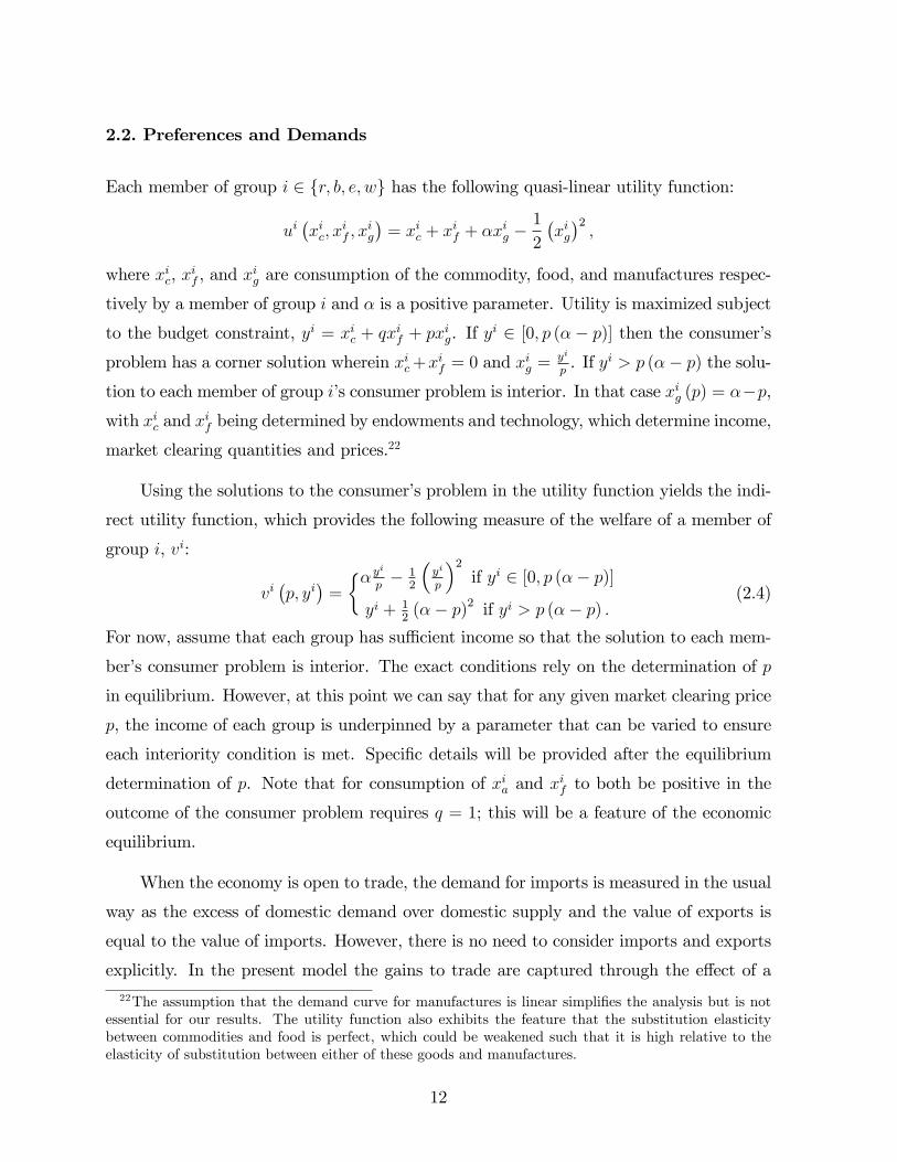
2.2. Preferences and Demands

Each member of group i 2 fr; b; e; wg has the following quasi-linear utility function:

ui�xic; x

if ; x

ig

�= xic + x

if + �x

ig �

1

2

�xig�2;

where xic, xif , and x

ig are consumption of the commodity, food, and manufactures respec-

tively by a member of group i and � is a positive parameter. Utility is maximized subject

to the budget constraint, yi = xic + qxif + px

ig. If y

i 2 [0; p (�� p)] then the consumer�sproblem has a corner solution wherein xic+x

if = 0 and x

ig =

yi

p. If yi > p (�� p) the solu-

tion to each member of group i�s consumer problem is interior. In that case xig (p) = ��p,with xic and x

if being determined by endowments and technology, which determine income,

market clearing quantities and prices.22

Using the solutions to the consumer�s problem in the utility function yields the indi-

rect utility function, which provides the following measure of the welfare of a member of

group i, vi:

vi�p; yi

�=

�� yip� 1

2

�yi

p

�2if yi 2 [0; p (�� p)]

yi + 12(�� p)2 if yi > p (�� p) :

(2.4)

For now, assume that each group has su¢ cient income so that the solution to each mem-

ber�s consumer problem is interior. The exact conditions rely on the determination of p

in equilibrium. However, at this point we can say that for any given market clearing price

p, the income of each group is underpinned by a parameter that can be varied to ensure

each interiority condition is met. Speci�c details will be provided after the equilibrium

determination of p. Note that for consumption of xia and xif to both be positive in the

outcome of the consumer problem requires q = 1; this will be a feature of the economic

equilibrium.

When the economy is open to trade, the demand for imports is measured in the usual

way as the excess of domestic demand over domestic supply and the value of exports is

equal to the value of imports. However, there is no need to consider imports and exports

explicitly. In the present model the gains to trade are captured through the e¤ect of a

22The assumption that the demand curve for manufactures is linear simpli�es the analysis but is notessential for our results. The utility function also exhibits the feature that the substitution elasticitybetween commodities and food is perfect, which could be weakened such that it is high relative to theelasticity of substitution between either of these goods and manufactures.

12

change in the terms of trade, p, on vi. We will think of trade integration as exogenous.

As mentioned in the Introduction, this is to focus attention on the determination of the

size of the bureaucracy. After the discussion of Proposition 2, we will consider how the

model could be extended to make trade integration endogenous.

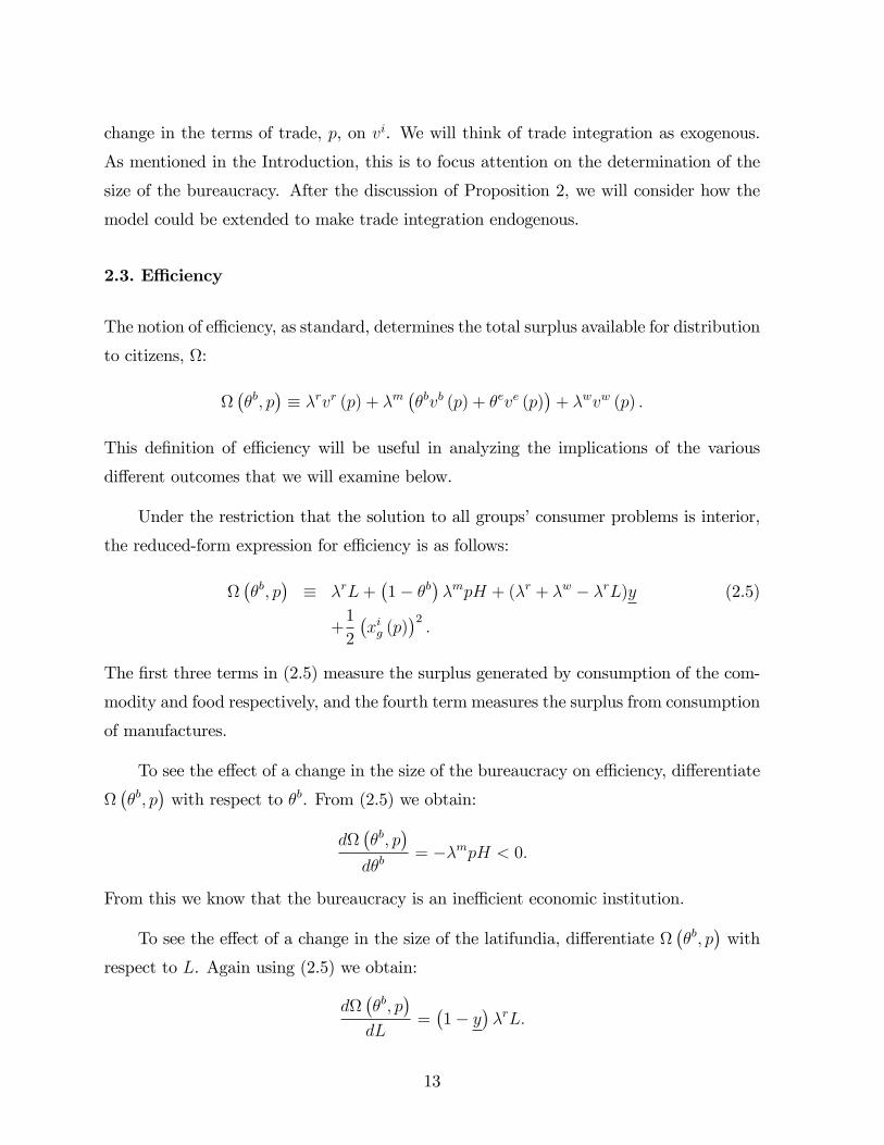
2.3. E¢ ciency

The notion of e¢ ciency, as standard, determines the total surplus available for distribution

to citizens, :

��b; p

�� �rvr (p) + �m

��bvb (p) + �eve (p)

�+ �wvw (p) :

This de�nition of e¢ ciency will be useful in analyzing the implications of the various

di¤erent outcomes that we will examine below.

Under the restriction that the solution to all groups�consumer problems is interior,

the reduced-form expression for e¢ ciency is as follows:

��b; p

�� �rL+

�1� �b

��mpH + (�r + �w � �rL)y (2.5)

+1

2

�xig (p)

�2:

The �rst three terms in (2.5) measure the surplus generated by consumption of the com-

modity and food respectively, and the fourth term measures the surplus from consumption

of manufactures.

To see the e¤ect of a change in the size of the bureaucracy on e¢ ciency, di¤erentiate

��b; p

�with respect to �b. From (2.5) we obtain:

d��b; p

�d�b

= ��mpH < 0:

From this we know that the bureaucracy is an ine¢ cient economic institution.

To see the e¤ect of a change in the size of the latifundia, di¤erentiate ��b; p

�with

respect to L. Again using (2.5) we obtain:

d��b; p

�dL

=�1� y

��rL:

13

For an increase of L to increase e¢ ciency requires the condition 0 < y < 1. This condition

imposes an upper bound on the productivity of low-grade land so that, as the size of the

latifundia are increased and labor is drawn to work on them, this raises overall surplus.

Without this condition, labor could be so productive on low-grade land that the planner

would shut down the latifundia and have all labor, including that of the elite, work on

low-grade land. The condition 0 < y < 1 will be assumed to hold throughout.

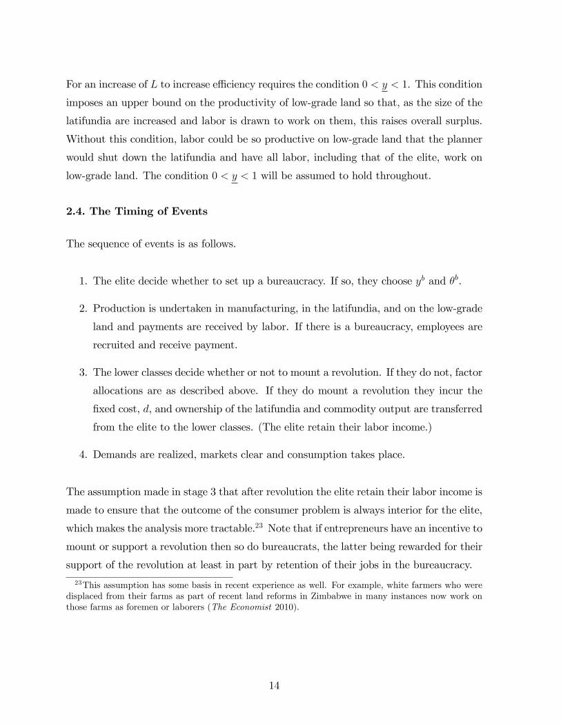
2.4. The Timing of Events

The sequence of events is as follows.

1. The elite decide whether to set up a bureaucracy. If so, they choose yb and �b.

2. Production is undertaken in manufacturing, in the latifundia, and on the low-grade

land and payments are received by labor. If there is a bureaucracy, employees are

recruited and receive payment.

3. The lower classes decide whether or not to mount a revolution. If they do not, factor

allocations are as described above. If they do mount a revolution they incur the

�xed cost, d, and ownership of the latifundia and commodity output are transferred

from the elite to the lower classes. (The elite retain their labor income.)

4. Demands are realized, markets clear and consumption takes place.

The assumption made in stage 3 that after revolution the elite retain their labor income is

made to ensure that the outcome of the consumer problem is always interior for the elite,

which makes the analysis more tractable.23 Note that if entrepreneurs have an incentive to

mount or support a revolution then so do bureaucrats, the latter being rewarded for their

support of the revolution at least in part by retention of their jobs in the bureaucracy.

23This assumption has some basis in recent experience as well. For example, white farmers who weredisplaced from their farms as part of recent land reforms in Zimbabwe in many instances now work onthose farms as foremen or laborers (The Economist 2010).

14

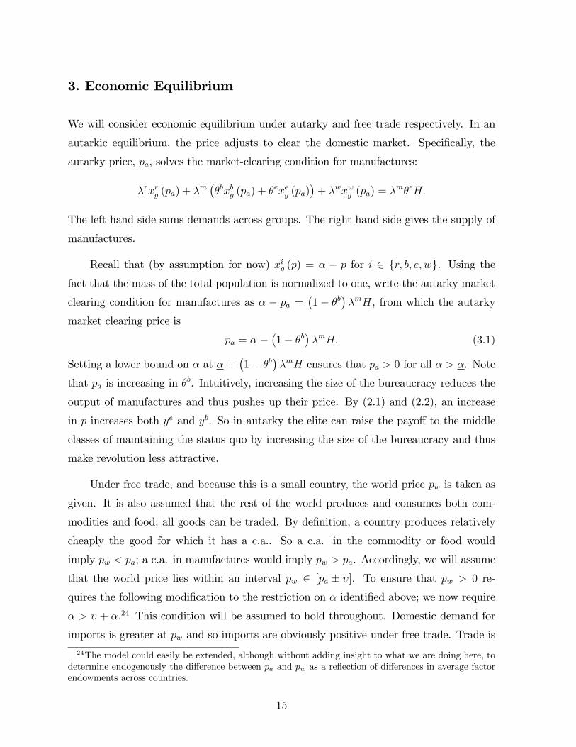
3. Economic Equilibrium

We will consider economic equilibrium under autarky and free trade respectively. In an

autarkic equilibrium, the price adjusts to clear the domestic market. Speci�cally, the

autarky price, pa, solves the market-clearing condition for manufactures:

�rxrg (pa) + �m��bxbg (pa) + �

exeg (pa)�+ �wxwg (pa) = �

m�eH:

The left hand side sums demands across groups. The right hand side gives the supply of

manufactures.

Recall that (by assumption for now) xig (p) = � � p for i 2 fr; b; e; wg. Using thefact that the mass of the total population is normalized to one, write the autarky market

clearing condition for manufactures as � � pa =�1� �b

��mH, from which the autarky

market clearing price is

pa = ���1� �b

��mH: (3.1)

Setting a lower bound on � at � ��1� �b

��mH ensures that pa > 0 for all � > �. Note

that pa is increasing in �b. Intuitively, increasing the size of the bureaucracy reduces the

output of manufactures and thus pushes up their price. By (2.1) and (2.2), an increase

in p increases both ye and yb. So in autarky the elite can raise the payo¤ to the middle

classes of maintaining the status quo by increasing the size of the bureaucracy and thus

make revolution less attractive.

Under free trade, and because this is a small country, the world price pw is taken as

given. It is also assumed that the rest of the world produces and consumes both com-

modities and food; all goods can be traded. By de�nition, a country produces relatively

cheaply the good for which it has a c.a.. So a c.a. in the commodity or food would

imply pw < pa; a c.a. in manufactures would imply pw > pa. Accordingly, we will assume

that the world price lies within an interval pw 2 [pa � �]. To ensure that pw > 0 re-

quires the following modi�cation to the restriction on � identi�ed above; we now require

� > � + �.24 This condition will be assumed to hold throughout. Domestic demand for

imports is greater at pw and so imports are obviously positive under free trade. Trade is

24The model could easily be extended, although without adding insight to what we are doing here, todetermine endogenously the di¤erence between pa and pw as a re�ection of di¤erences in average factorendowments across countries.

15

balanced in free trade equilibrium so there is an equal value of exports to clear the trade

account.

We can now characterize economic equilibrium as follows.

Lemma 1 (Characterization of Economic Equilibrium). There exist ranges of � and �m

su¢ ciently small and ranges of H and L su¢ ciently large that in economic equilibrium,

whether under autarky or free trade, the solution to the consumer problem for each group

i 2 fr; b; e; wg is interior and q = 1.

The proof of Lemma 1 is in two parts. The �rst part establishes the conditions for which

yi > p (�� p) for any p 2 [pa � �] and for each i 2 fr; b; e; wg. We take yb and ye �rstsince the argument is easiest to establish for these two. Since the incomes of entrepreneurs

and bureaucrats are underpinned by their endowments of human capital, the condition is

satis�ed for H su¢ ciently large. To ensure that the condition is met for yw we impose a

condition on �m that limits the size of p (�� p).25 Finally, by (2.3), yr depends positivelyon L which is otherwise unrestricted and can simply be increased without bound to ensure

that the condition yr > p (�� p) is met. Henceforth it will be assumed that � and �m

are su¢ ciently small and H and L su¢ ciently large to ensure that the consumer problem

for each group is indeed interior in economic equilibrium.

The second part of the proof establishes that the markets for all three goods clear

in autarky at p = pa and q = 1. It establishes that any perturbation of equilibrium

results in a restoration of equilibrium at q = 1 both through the labor market and the

goods market. Then given q = 1, by Walras�law, p = pa ensures that all markets clear.

Providing p 2 [pa � �], the same holds under trade integration.

The e¢ ciency implications of trade integration can be evaluated in a straightforward

way using (2.5) to obtain a reduced-form expression for in autarky, and then di¤eren-

tiating this with respect to p in order to evaluate the gains from trade. Use in (2.5) the

25Since in general yw = qy, and there is an upper bound of unity on y, for any given q we need tolimit the size of p (�� p) in order to ensure that yw > p (�� p). This is achieved by imposing an upperbound on �m. To see this �rst note that p (�� p) = pxg, where the right hand side is decreasing in �mfor �m su¢ ciently small since a smaller �m makes xg more scarce, hence increasing p towards � frombelow. There will thus exist a size of �m su¢ ciently small that yw > pxg, so that xc, xf > 0 and thesolution to w�s problem is interior.

16

fact that xig (pa) = �� pa for i 2 fr; b; e; wg to obtain

��b; p

�� �rL+

�1� �b

��mpH + (�r + �w � �rL)y (3.2)

+1

2(�� p)2 :

Di¤erentiating this expression with respect to p,

d��b; p

�dp

=�1� �b

��mH � (�� p) : (3.3)

From this expression we �nd that, whether the country has a c.a. in manufactures or

primary products, trade integration always raises e¢ ciency. To see this use (3.1) to

substitute the reduced form of pa for p, and note that d��b; p

�=dp��p=pa

= 0, while

@2��b; p

�=@p2 = 1. Thus, e¢ ciency obtains a minimum in autarky. Given this structure

observe how the condition above that ensures pa > 0 also ensures that e¢ ciency increases

whether the country has a c.a. in primary products (in which case trade integration

implies p > pa) or a c.a. in manufactures (in which case trade integration implies p <

pa). Trade integration, either as an incremental step away from autarky or a move right

from autarky to free trade, thus implies an increase in e¢ ciency whether the country has

a c.a. in primary products or manufactures. This result will serve as a useful benchmark

against which to compare the e¢ ciency implications of trade integration when the size of

the bureaucracy is endogenous.

We can also evaluate the e¤ects of trade integration on individual factor rewards and

see that the Stolper-Samuelson theorem holds in our model (although not strictly for w):

dye=dp = H while dyr=dp = ��b�mH=�r and dyw=dp = 0. That is, an increase in the

(relative) price of manufactures, p, leads to an increase in the (nominal and real) income

of entrepreneurs, and the condition vb = ve implies that the income of bureaucrats must

increase as well. This also implies a fall in the income of the elite, and no change in

the income of workers. The converse holds for a fall in p. The welfare implications are

less immediate but are consistent with the Stolper-Samuelson. First, dvb=dp = dve=dp =

H � (�� p). The proof of Lemma 1 (in Appendix A.1) establishes that the conditionon H is precisely H > (�� p) ; and it follows that an increase in p makes entrepreneursand bureaucrats better o¤. On the other hand, dvr=dp = � (�� p) � �b�mH=�r whiledvw=dp = � (�� p) which are both negative (given � > �+�) again as we should expect,

17

so that a rise in the price of the commodity or food, captured by a fall in p, would make

the elite and workers better o¤. (See part (ii) of the proof of Lemma 1 for further details

of how q adjusts to clear the market for food.)

4. Political Equilibrium

Assume that each group within the lower classes, the middle classes and the workers

respectively, is able to resolve the collective action problem inherent in the decision over

whether or not to revolt. The objective of the elite will be to reduce the surplus from

revolution to zero through its manipulation of the size of the bureaucracy, thus removing

the incentive to revolt.

The aim is now to establish that there exists a value of �b that would reduce the

surplus from revolution to zero, where the surplus is given by the total value of elite net

income (less their return to labor) after production has taken place minus the cost of

mounting a revolution. We will say that such a value of �b satis�es the no-revolution-

constraint (NRC ), and refer to this value as ~�b, whereNRC is written formally as follows:26

NRC : h�~�b; p�= �ryr

�~�b; p�� d (4.1)

= �r�L� (L� 1) y

�� ~�b�mpH � d = 0:

We will use (4.1) to study ~�bin the next subsection.

4.1. The Equilibrium Size of the Pampered Bureaucracy

It is instructive to solve for ~�b�rst under free trade and then under autarky. Under free

trade, take p as given and obtain ~�bby rearranging (4.1):

e�b (p) = �r�L� (L� 1) y

�� d

�mpH: (4.2)

For ~�bto satisfy NRC, it must lie in the interval (0; 1]. If the solution lies at or below zero

then this implies that d is too large relative to �ryr��b; p

�for a revolution to be worth

26Since our focus is on the existence of a value of �b that brings the surplus from revolution to zero,we do not need to worry about how the surplus would be divided between i 2 fm;wg if it were positive.It would re�ect the relative incomes received by the respective groups in the status quo if the revolutionfailed. See Appendix A.2 for a full derivation of the NRC.

18

while. From (4.2), an increase in d makes this more likely. If the solution is greater than

one then the NRC cannot be satis�ed for any value of ~�band there is nothing that the

elite can do (within the context of the present model) to prevent revolution. For y 2 [0; 1),an increase in L makes this more likely. An increase in the cost of revolution tightens the

NRC while an increase in the value of the latifundia increases the payo¤ to revolution

and hence relaxes the NRC.

Let us now establish the conditions for which there exists a solution e�b 2 (0; 1] underautarky. Substituting (3.1) into (4.1),

h��b; pa

�= �ryr

��b; pa

�� d (4.3)

= �r�L� (L� 1) y

�� �b�mH

���

�1� �b

��mH

�� d:

Conditions under which there exists a solution e�b 2 (0; 1] can be obtained by the interme-diate value theorem. Using values �b = 0 and �b = 1, by inspection of (4.3), the following

endpoints of h��b; p

�are determined:

h (0; pa) = �r�L� (L� 1) y

�� d;

h (1; pa) = �r�L� (L� 1) y

�� d� ��mH:

Thus, given �r, if L is su¢ ciently large relative to d then h (0; pa) > 0. MakeH su¢ ciently

large as to ensure that h (1; pa) < 0. Since h��b; p

�is a continuous function of �b, there

must exist a value ~�bthat satis�es h

��b; pa

�= 0. Therefore we can characterize political

equilibrium in autarky:

Proposition 1 (Characterization of Political Equilibrium in Autarky). There exist ranges

of d su¢ ciently small and H su¢ ciently large that in the autarky equilibrium the equi-

librium size of the pampered bureaucracy, i.e. the (unique) value e�b 2 (0; 1] satisfying theNRC, prevents a revolution.

The restrictions on d and H are imposed to ensure that h (0; pa) > 0 and h (1; pa) < 0.

The proof of this result shows that the �rst derivative of h��b; p

�is negative with respect

to �b, thus establishing that e�b is unique (see Appendix A.1). This result shows that,providing the cost of mounting a revolution is not too large, and that there is su¢ cient

human capital, it is always both possible and in their interests for the elite to expand the

19

size of the pampered bureaucracy to the point where a revolution is not worth while for

the lower classes. If d is too large relative to L then the relatively high cost of mounting

a revolution, or equivalently the damage done by it, means that it is not worth while and

there is no need even to set up a pampered bureaucracy. If H is too small relative to

d then the income paid to each bureaucrat multiplied by the share of the population in

the middle classes is not large enough to reduce elite income to the point where the NRC

binds. In what follows we will assume that the values of d and H lie in their respective

ranges for which e�b 2 (0; 1). The reason for not including the end-point e�b = 1 is becausewe will want the function characterizing e�b to be di¤erentiable.274.2. The E¤ects of Trade Integration on the Pampered Bureaucracy

Having now determined the size of a bureaucracy that prevents a revolution in autarky, if

a pampered bureaucracy exists we can examine the e¤ects on its size of trade integration.

We will focus on the case where the country has a c.a. in primary products. The logic

works in reverse if the country has a c.a. in manufactures. The �rst step will be to show

that, given e�b 2 (0; 1), trade integration as captured by a reduction of p from pa creates

an incentive to mount a revolution. The second step will be to examine how ~�bmust be

changed in order to prevent revolution under trade integration.

Di¤erentiating the NRC, (4.1), with respect to p,

dh��b; p

�dp

= ��b�mH:

The reduction of p entailed by trade integration increases h��b; p

�, establishing that trade

integration generates an incentive to mount a revolution (for any given �b and p and hence~�band pa).

To calculate the change in the size of the bureaucracy mandated by trade integration,

di¤erentiate the reduced form expression for ~�b, (4.2), with respect to p:

d~�b(p)

dp= �

�rL� �r (L� 1) y � d�mp2H

: (4.4)

27If d were subject to random shocks, the choice of e�b would not necessarily satisfy the NRC ex post.Yet even in such a stochastic environment the logic of our deterministic model would apply in that higherincome among the elite would still tend to mandate a larger transfer from the elite to the lower classesthrough the pampered bureaucracy.

20

Given the structure imposed on the model, d~�b=dp < 0. If the country has a c.a. in

primary products then trade integration mandates an increase in the size of the pampered

bureaucracy in order to prevent a revolution. Intuitively, the fall in p increases yr, thus

raising the surplus to the lower classes from revolution. However, from (2.3), increasing

the size of the bureaucracy, �b, serves to lower yr and with it the payo¤ to revolution.

Providing they are not constrained by the upper bound, �b = 1, the elite are able to

increase the size of the bureaucracy to prevent revolution in the face of trade integration.

If the country has a c.a. in manufactures then, by applying the above reasoning with

the signs reversed, trade integration mandates a reduction in the size of the pampered

bureaucracy.

We can now examine the e¢ ciency implications of trade integration when the size

of the bureaucracy is endogenous. Recall from (4.2) that ~�bis a function of p. For

convenience, express equation (4.2) as ~�b(p). Using ~�

b(p) in (3.2),

d�~�b(p) ; p

�dp

=�1� ~�b (p)

��mH � (�� p) (4.5)

�p�mHd~�b(p)

dp:

where now, since �b is endogenous, is a function only of p. The �rst line captures

the standard gains from trade and is the same as in (3.3) which was calculated for �b

exogenous; recall that this is equal to zero at p = pa and is una¤ected by the fact that

now �b is chosen endogenously as a function of p. The second line captures the e¤ect

on e¢ ciency of an endogenous change in the size of �b; this is positive since d~�b=dp < 0.

Therefore trade integration for a country with a c.a. in primary products that entails

a small reduction in p from the autarky price, pa, necessarily implies a reduction of

economic e¢ ciency. However, for larger reductions in p the �rst line will be positive

and may dominate the second line, so that trade integration will be e¢ ciency increasing;

observe that @2�~�b(p) ; p

�=@p2 = 1, just as with �b exogenous. The logic is that while

the standard gains from trade are relatively small in the neighborhood of autarky, they

increase and ultimately overwhelm the e¢ ciency reducing e¤ects of changes in the size of

the pampered bureaucracy. Thus we have our second main result:

21

Proposition 2 (E¤ects of Trade Integration on Political Equilibrium). Start from an

autarky equilibrium with the size of the pampered bureaucracy endogenously determined

at e�b 2 (0; 1). If the country has a comparative advantage in primary products then inthe region of autarky trade integration increases e�b and hence is e¢ ciency-reducing. Ifthe country has a comparative advantage in manufactures then trade integration reducese�b and hence is always e¢ ciency-increasing.A formal proof is in Appendix A.1.28

It is worth re�ecting on what trade integration implies for the income and welfare of

the elite with �b endogenous. Using (2.2) and (2.3),

dyr

dp= �

~�b(p)�m

�rH � d

~�b=dp

�r��m(pH) + �r (L� 1) y

�: (4.6)

Assume the country has a c.a. in primary products. The �rst term of (4.6) shows that

when �b is held constant a reduction of p due to trade integration increases yr. The

second term tells us that the resulting increase of ~�b(p) works in the opposite direction;

intuitively, the increase in elite incomes is eroded by the fact that they must pay for a

larger bureaucracy to prevent revolution. Turning to the NRC, given that (4.1) holds

before revolution, the elite must increase �b by just enough to ensure that it continues to

hold after any given reduction in p. Therefore, given ~�b(p) 2 [0; 1] both before and after

trade integration, there is no change in elite income, yr. However, by (2.4), the elite still

have an interest in trade integration since they enjoy a consumption gain from the fact

that p falls. If the country has a c.a. in manufactures then the opposite is true; with the

size of the pampered bureaucracy endogenously determined and yr thus held constant,

the elite lose from trade integration through a consumption loss as p rises. Based on this

property of the model it might appear that if we initially allowed the elite to control trade

policy, then when the country has a c.a. in manufactures the elite would resist trade

28Proposition 2 would not necessarily change qualitatively if d were endogenous. The standard as-sumption is that d is a decreasing function of lower class income yb, ye and yw based on the idea that thelower classes become better able to coordinate as their incomes rise. If the country had a c.a. in primaryproducts then trade integration implies a reduction of p, which lowers yb and ye. This would increased, reducing the extent to which the elite have to increase �b in order to restore the NRC and leavingthe elite with higher income than if d were exogenous. If the country had a c.a. in manufactures thenthe e¤ects work in reverse. The e¤ective upper bound placed in the size of the military discussed in theintroduction, which would be imposed by the elite�s fear that a large military could be used against them,would be captured formally by an upper bound on d below the level required to suppress a revolution.

22

integration. However, since revolution would also transfer control of trade policy to the

lower classes, elite resistance to trade integration could generate an alternative incentive

to mount a revolution.

5. From Theory to Estimation

We now develop an empirical analogue of (4.4), which gives the relationship between

the size of the bureaucracy and trade integration. First, let O denote the level of trade

integration and let C 2 f0; 1g be an indicator which takes a value of 0 if the country�s c.a.is in manufactures and 1 if its c.a. is in primary products. Standard trade theory predicts

a monotonic relationship between trade integration and the relative price of manufactures,

p, which may be expressed as a function, p (O). As noted above, if the country has a c.a.

in manufactures (C = 0) then an increase in trade integration brings about an increase in

p, while if the country has a c.a. in primary products (C = 1) then an increase in trade

integration brings about a decrease in p. Summarizing this formally:

If C = 0 then @p=@O > 0; (5.1)

if C = 1 then @p=@O < 0:

Denote by A and B the level of structural government employment and employment

in the (pampered) bureaucracy respectively. Then D � A + B, where D denotes total

central government spending on employment (henceforth �total government employment�).

For the purposes of exposition, for now suppose A and B are functions only of p, assuming

that all other in�uences on government employment are subsumed in a residual term, "a:

A = A (p) + "a and B = B (p).

Our identifying restriction is as follows. The e¤ect of trade integration on structural

government employment is independent of c.a.; @A@p

@p@O

���C=1

= @A@p

@p@O

���C=0. With some abuse

of notation, write this more compactly as follows:

@A�

@O=@A�

@O; (5.2)

where the superscript � denotes a country with a c.a. in primary products and the

superscript � denotes the same thing for manufactures. Notice that this formulation

23

conditions on other determinants of A that may be correlated with trade integration,

i.e. "a. In principle, the causal e¤ect of trade integration on structural government

employment may be positive or negative.29

We will now show how (5.2) is helpful in deriving a testable prediction of our model.

Equations (4.4) and (5.1) imply that c.a. determines the direction of the e¤ect of a

change in trade integration on the size of the pampered bureaucracy. In particular,@B@p

@p@O

���C=1

> 0 > @B@p

@p@O

���C=0. Since this result is derived from a static model, we extrapo-

late its implication to a dynamic setting as being that, over time, @B@p

@p@O

���C=1

> @B@p

@p@O

���C=0.

We will refer to this as our main prediction. Again, with some abuse of notation, write

this more compactly as:@B�

@O>@B�

@O: (5.3)

We now show how the identifying restriction can be used to empirically test (5.3). First

note that countries can be partitioned by c.a. and that the response of D� and D� to a

change in O can be measured. By the foregoing we have:

@D�

@O� @D

�

@O=@A�

@O� @A

�

@O+@B�

@O� @B

�

@O: (5.4)

Now observe that, using (5.2), a �nding of @D�

@O� @D�

@O> 0 implies that @B

�

@O> @B�

@O, which

would be evidence of our main prediction.

We di¤erence the data to remove country-speci�c �xed e¤ects. To distinguish between

the e¤ect of trade integration on the size of the bureaucracy across the two types of c.a.,

we interact trade integration with a dummy variable Ci which takes a value of Ci = 0 if

the country has a c.a. in manufactures and Ci = 1 if a country has a c.a. in primary

products. This gives us the following estimating equation:30

29For example, according to Rodrik�s (1998, 2000) social insurance framework, an increase in tradeintegration requires governments to play a greater insurance role in the face of increased terms of tradevolatility due to world market price �uctuations; @A

�

@O = @A�

@O > 0. In the face of greater volatility, citizensmight have a higher probability of displacement from employment. Particularly in developing countrieswhere dedicated social security frameworks may be less well developed, this may mandate the governmentto play a greater role in providing social insurance in the form of government employment. However,his theory does not condition on comparative advantage. Under a competing hypothesis governmentemployment may be called upon to play a lesser role in social insurance when increased trade integrationstabilizes domestic price �uctuations through access to world markets, i.e. @A�

@O = @A�

@O < 0, where againthis argument does not depend on comparative advantage. Although it goes beyond the scope of ourtheoretical model, as a robustness check we will control for the possibility that the relationship betweenA and O is correlated with comparative advantage.30See Appendix A.3 for a full derivation of the estimating equation.

24

�Di;t = �0 +

TX�=1

���Di;t�� + �1�Oit + �2�Oit � Ci + �Zit +�"it; (5.5)

To understand how the estimating equation can be used to test our main prediction, focus

on coe¢ cients �1 and �2. Consider what �1 would measure if there were no interaction

term (�Oit � Ci). In that case, �1 would capture the average partial e¤ect of a changein trade integration on total government employment both through changes in structural

government employment and through changes in the size of the pampered bureaucracy.

Inclusion of the interaction term allows us to test the predication of our model by esti-

mating di¤erent partial e¤ects of trade integration by c.a.. In our speci�cation, �1 is the

average partial e¤ect of trade integration on total government employment for countries

with a c.a. in manufactures, and �1 + �2 is the average partial e¤ect of trade integration

on total government employment for countries with a c.a. in primary products. This is

appealing because �2 alone captures the di¤erence in the average partial e¤ect by c.a.

which, according to our main prediction (5.3), is expected to be positive. Note that our

framework does not make any prediction about the sign of �1 since it is partly determined

by the e¤ect of trade integration on structural government employment for which existing

theories o¤er contrasting predictions.

Our linear dynamic panel-data (DPD) formulation is attractive because it allows

for persistence in the bureaucracy as well as unobserved time-invariant country-speci�c

characteristics. Yet it is well-known that DPDmodels may contain unobserved e¤ects that

are correlated with the lagged dependent variable, potentially leading to inconsistency of

the parameter estimates. Consistent estimates may be obtained with the Generalized

Method of Moments (GMM) estimator originally proposed by Arellano and Bond (1991,

henceforth referred to as A/B). This method uses the moment conditions E(Dis�"it) = 0

for time periods s � t � T , where T is the terminal time period, so that �Di;t�1 may

be instrumented with the lagged levels Di;t�T ; Di;t�T�1; ::: . However, lagged levels are

often poor instruments for lagged di¤erences (Arellano and Bover, 1995). Blundell and

Bond (1998, henceforth B/B) show that imposing the moment conditions E(�Dit"it) = 0

and E(�Zit"it) = 0 allows one to instrument the lagged dependent variable with the

lagged di¤erences �Di;t�T ; �Di;t�T�1; ::: . This procedure, by imposing stronger moment

assumptions, can lead to better instrument performance. Our main analysis uses the less

25

restrictive moment conditions of the A/B estimator, but we will check our main results

using the B/B moment conditions as well.

This section concludes with a brief discussion of the estimation strategy. First, we

estimate the model according to the A/B and B/B speci�cations using the two-step GMM

estimator which is asymptotically e¢ cient and robust to arbitrary heteroskedasticity. Sec-

ond, both the A/B and B/B estimators are inconsistent in the presence of serial correla-

tion, so for each estimated equation we report p-values for the test of serial correlation in

the �rst-di¤erenced residuals. Finally, since the estimating equation is overidenti�ed, we

will test whether the instruments are independent of the error process using the standard

Hansen-Sargan approach to test the null hypothesis that the GMM criterion function is

su¢ ciently close to zero. This latter test is commonly referred to as a test of �instrument

validity.�

6. Data and Summary Statistics

We measure total government employment across countries and time, Dit, with annual

data for central government spending on wages and salaries (1972-2008 in millions of

real US dollars) from the International Monetary Fund�s (IMF�s) Government Finance

Statistics database.31 A full list of countries is given in Table A1; see Appendix B.

We employ the measure of revealed c.a. (RCA) due to Balassa (1965), and construct

it from World Bank trade �ows.32 Let Xikt be country i�s exports of product category k

to the rest of the world in period t, and let Xi!t be total exports from country i to the rest

of the world within a set of product categories !. Xnkt is the sum of all other countries�

(i.e. j 6= i) exports in product category k, and Xn!t are total world exports in the set

of product categories. Then RCAikt = (Xikt=Xi!t)=(Xnkt=Xn!t): Following the standard

31Since our estimation procedure identi�es parameters using only within-variation, we need a samplewhose variables exhibit signi�cant variation across time. Fortunately, both trade integration and centralgovernment employment varied signi�cantly during our sample period for many countries. An alternativewould have been to employ data from the International Labor Organization. Unfortunately, for ourpurposes, these data are not nearly as comprehensive in their coverage across countries as the IMF series,especially prior to 1995.32An alternative approach would be to assume a factor-endowments model of c.a. and proxy it with

factor endowment ratios as in Nunn (2007). Yet, unlike Nunn, whose goal is to explain the determinantsof c.a., we take c.a. as given and examine the implications it has for our model�s prediction.

26

approach, country i has a revealed c.a. in product k if and only if RCAikt > 1. In our

sample, RCA is stable over time, allowing use of the mode across years as our measure

of a country�s c.a..

Our primary measure of trade integration is the gravity-based measure used by Rose

(2004), and Gorg, Hijzen, and Munchin (2008) among others, which is the distance-

weighted average of all trading partners�GDPs. First de�ne Yit as country i�s GDP in

year t expressed in millions of constant dollars and let �ij be the distance between countries

i and j. This measure of trade integration is ~Oit =P

j 6=i Yjt=�ij: Unlike other measures

of trade integration such as tari¤s and the terms of trade, which are clearly endogenous,

a country�s government has limited if any in�uence over the distance-weighted average

of its trading partners�GDPs. Therefore, variation in ~Oit plausibly extracts identifying

variation in relative prices.

For robustness we employ a common alternative measure of trade integration, which

is constructed in each year for a particular country by summing its exports and imports

across all trading partners and dividing by GDP.33 Although this latter measure is widely

used, it is probably determined endogenously in equilibrium along with central government

spending on employment. Nevertheless, it provides a useful check to our main results.

Crucial to our empirical implementation is the assumption that heterogeneity in the

relationship between trade integration and total government employment across countries

with a c.a. in primary products and those with a c.a. in manufactures is not confounded by

other observable determinants of total government employment. To control for this possi-

bility, �rst we di¤erence the data to remove time-invariant country-speci�c confounders.

This allows for factors that may simultaneously a¤ect trade integration and total gov-

ernment employment. This approach is appealing because it allows for country-speci�c

in�uences on total government employment (speci�cally, demographic composition, frac-

tionalization of society along ethnic, linguistic and religious lines, levels of inequality, and

the system of government) without requiring explicit measurement of these factors. This

33To construct this measure, �rst de�ne xijt as exports from country i to country j in year t andmijt as imports from country j to country t in year t: Total exports from and imports to country iin year t are given by Xi =

Pj 6=i xij and Mi =

Pj 6=imij . Then trade integration is given as Oit =

(Xit +Mit)=Yit; which we obtained from the Penn World Tables mark 6.3. These data are available athttp://pwt.econ.upenn.edu/php_site/pwt_index.php.

27

also accounts for institutional characteristics (e.g. the protection of property rights), to

the extent that these remain constant throughout our sample period. Second, an advan-

tage of our dynamic panel data approach is that we are able to control for time-variation

in individual country variation in total government employment by including lags of the

dependent variable. In doing so we take as given the component of bureaucracy size that

can be explained by its size in previous periods, thus indirectly capturing country-speci�c

trends in institutions, economic development and other time-varying variables that deter-

mine changes in total government employment.

Finally, we explicitly control for observable determinants of total government em-

ployment that may be correlated with both trade integration and comparative advantage.

For example, larger countries may tend to have both a c.a. in manufacturing and to expe-

rience larger responses of total government employment to changes in trade integration.

To capture these country-size e¤ects, we include total GDP expressed in millions of US

dollars (Yit) and population in thousands of people (Nit). Similarly, countries with higher

incomes may tend to have higher wage rates and thus higher central government spending

on wages and salaries. This may vary systematically by c.a. to the extent that countries

with a c.a. in manufacturing have higher average wage rates than countries with a c.a. in

primary products. An ideal measure would be middle class wage rates or the minimum

wage. Since no such data exist at the annual level for a wide variety of developing coun-

tries, we use per-capita income in thousands of dollars (yit). These three series came from

the Penn World Tables. Additionally, since political or credit constraints may in�uence

total government employment, especially in developing countries, we control for central

government revenues (Rit), which are published in the IMF�s Government Finance Sta-

tistics. In the robustness checks presented below, we will also construct controls related

to three alternative hypotheses.

The �nal sample includes 100 countries and 1605 country years, so that over the 36

year period, there are an average of 16.05 observations per country. The �rst column of

Table 1 presents summary statistics. In columns (2) and (3) we split the sample into

low and high trade integration observations where high trade integration is de�ned as

the logarithm of ~Oit above the mean (0.42). More open economies tend to be richer but

smaller and have higher total government employment relative to less open economies.

28

7. Econometric Results

Table 2 presents estimates of equation (5.5) in logs using the moment conditions suggested

by Arellano and Bond. For brevity, we suppress the constant terms in the reported output.

The �rst column presents results from an estimate that incorporates, on the right hand

side, ~Oi and its interaction with c.a. in primary products and two lags of the dependent

variable. In all speci�cations, two lags of the dependent variable are su¢ cient to eliminate

serial correlation in the di¤erenced residuals.

The estimated coe¢ cients on the dependent variable lags indicate that changes in

total government employment are persistent. Looking across the table from the second to

the �fth columns, we can see evidence that higher population, GDP, and (average) per-

capita income tend to translate into greater total government employment, but an increase

in government revenue is associated with a decrease in total government employment,

perhaps re�ecting possible e¢ ciency increases as government expands.

The covariate of interest, �2; is presented in the �rst row. In all speci�cations the esti-

mate for �2, the coe¢ cient on trade integration interacted with c.a. in primary products,

is positive as predicted by our model and signi�cant at conventional levels. This �nding

is evidence of our main prediction. The estimated magnitude in column (1) implies that

the response in the size of the bureaucracy to changes in trade integration is 18.2 percent

greater in the countries with a c.a. in primary products than for countries with a c.a. in

manufactures. The second row presents estimates of �1 across the various speci�cations.

We see that the estimated sign is sensitive to model speci�cation, but is not a concern

because, as discussed above, our model does not make predictions about �1.

Turning to the bottom of the table, the Sargan overidentifying restrictions test does

not reject the null of instrument validity. Finally, tests of serial correlation at the bottom

of the table indicate strong persistence in the levels residuals, providing support for the

di¤erenced speci�cation, and the null of serial correlation is not rejected at the second

order, indicating that the estimated model is free of serial correlation in the di¤erenced

residuals.

In Table 3, we allow for heterogeneity in the estimated e¤ect between developed and

29

developing countries as de�ned by the International Monetary Fund (IMF).34 The �rst row

of the table shows that the estimated parameter values for �2 are positive and signi�cant

for developing countries in all speci�cations. The second row shows that the estimates of

�2 for developed countries are smaller and in columns (3), (4) and (5) are not statistically

signi�cant suggesting that, as discussed in the Introduction, our main prediction may

not hold as strongly for developed countries. Results from the speci�cation tests are

qualitatively similar to those presented in Table 2.

In Table 4, we explicitly account for three alternative explanations that might con-

found our results. (We have already addressed a number of alternative hypotheses about

what might explain variation in total government employment by accounting for time-

invariant country level e¤ects, country-speci�c trends in the size of the bureaucracy, and

by including likely time-varying confounders.) The �rst alternative explanation is that a

planned economy, in its transition to a market-based economy, may simultaneously un-

dergo trade integration and vary total government employment. If in addition planned

economies tend to disproportionately have a c.a. in manufacturing we might observe,

even after accounting for country-speci�c �xed e¤ects, that planned economies have (on

average) a lower response of total government employment to changes in trade integration

than do countries with a c.a. in primary products. To ensure that our results are not

driven by this potential confounding channel, we constructed for each country a variable

that takes a value of one in all years after a country made a transition to a market-based

economy (post_Sit).

A second confounding channel would arise if spending on the bureaucracy was dispro-

portionately in�uenced by balance-of-payments crises occurring in countries with similar

comparative advantage patterns.35 We addressed this possibility by obtaining, from the

IMF, data on all outstanding loans with conditionalities, for each year and for every coun-

34The aim of including the level of development in the regressions is to capture variation in underlyinginstitutional quality. It could be argued that a preferable approach would be to use a direct measureof institutional quality like POLITY IV or the International Country Risk Guide. The reason we didnot adopt this approach is because Glaeser, la Porta, Lopez-de-Silanes and Shleifer (2004) have shownthat such direct measures of institutions might not in fact capture the institutional quality of a countrybut might instead re�ect short-run choices made by politicians, either as dictators or as democraticallyelected representatives of government. On the other hand, there seems to be a consensus that the levelof development does go some way to capturing institutional quality broadly de�ned.35These crises were often addressed by obtaining IMF loans issued subject to conditionalities that

typically mandated both trade liberalization and reduced government expenditures.

30

try in our sample, and constructing a variable that takes a value of one for a particular

country in those years in which it had an outstanding IMF loan to which were attached

conditionalities during the previous year (imfit).

A �nal possibility can be derived under the null of Rodrik�s social insurance frame-

work (1998, 2000). This possibility may arise if countries with a c.a. in primary products

experience greater terms-of-trade volatility as a result of trade integration, since pro-

duction tends to be more specialized in countries with a c.a. in primary products than

countries with a c.a. in manufactures. To the extent that the di¤erence in terms-of-trade

volatility by c.a. is persistent over time, we have already accounted for it with country

�xed e¤ects, but this does not rule out the possibility that the e¤ect varies over time. As

an additional test, we exploit the fact that production and export concentration tend to

be correlated and constructed the Her�ndahl export diversi�cation index for each country

at the annual level.36

Although the COMTRADE database, used to construct this measure, is the most

comprehensive category-level trade data source available, its annual coverage is limited

relative to our other data series, especially for developing countries. Nevertheless, we

proceed with this limited sample. To capture the possibility that export concentration

risk interacts with trade integration in a meaningful way, we also interacted the Her�ndahl

index with trade integration in addition to including it alone.

Table 4 reports results from the main equation re-estimated with these robustness

controls included. Henceforth, we suppress lags of the dependent variable to save space.

This table retains the distinction between developed and developing countries and in

addition to previous controls introduces the e¤ect of IMF conditionalities, transition from

a planned to a market-based economy, the Her�ndahl index and its interaction with trade

integration.

From Table 4, we can see that the model�s prediction is robust to the introduction

36The Her�ndahl index is given by Hi =nPk=1

hxktxi

i2where n is the number of di¤erent products

exported, xkt is total exports of product k in period t; and xi is total exports from country i in period t.The Her�ndahl index lies in the interval (0; 1), with larger values corresponding to more concentration(less diversi�cation) of total exports. This index was constructed using SITC 4 digit product-level tradedata obtained from the United Nations COMTRADE Database.

31

of controls for these three additional hypotheses; the estimate of �2 remains positive and

signi�cant for developing countries. The estimated e¤ect is larger when these controls

are included, yet this is probably due to sample attrition associated with the Her�ndahl

index. As before, evidence in support of the model�s prediction is weaker for developed

countries. The sign on the Her�ndahl index is positive and signi�cant, suggesting that the

government may indeed play a greater insurance role when the economy is highly concen-

trated. However, the coe¢ cient on the Her�ndahl index interacted with trade integration

is not signi�cant, indicating that if the government plays an additional insurance role

in responses to trade integration, its main policy instrument may not be central govern-

ment employment. Perhaps surprisingly, the transition from a Soviet to a market-based

economy does not appear to have had a signi�cant e¤ect on total (central) government

employment. As predicted, the presence of an outstanding IMF loan with conditionalities

tends to have a negative impact on total government employment.

Appendix B presents a number of additional robustness checks. First, in Table A2,

we re-estimate equation (5.5) using the stronger B/B moment conditions. As before, the

estimated coe¢ cients on �2 are signi�cant with the predicted sign. The B/B estimator

produces estimates of �1 that are less stable across various speci�cations relative to the

A/B estimator. Speci�cation test results at the bottom of the table are qualitatively

similar to those before.

In Table A3, we re-estimate (5.5) with separate average partial e¤ects for developed

and developing countries using the B/B estimator. As before, we �nd stronger support for

the model�s main prediction for developing countries than for developed countries. In this

speci�cation, the e¤ect of government revenue is positive while the e¤ect of population

growth is netagive and, as in the previous table, the estimated coe¢ cients on �1 are

sensitive to model speci�cation.

In Table A4, we re-estimate (5.5) using the conventional trade integration measure

Oit instead of ~Oit; even though we believe this measure is likely to be a¤ected by domestic

policy choices. The results for �2 are still positive and signi�cant across all speci�cations.

From the estimates of �1 presented in the second row we see that, interestingly, there seems

to be clearer evidence of a negative relationship between total government employment

and trade integration for countries with a c.a. in manufactures. Since the trade integration

32

measure is endogenous, the negative relationship might be evidence of policy initiatives to

�liberalize, privatize and stabilize�among developed countries (who overwhelmingly have

a c.a. in manufactures) in the 1980s and 1990s.

In Table A5 we re-estimate the main equation with separate average partial e¤ects

for developed and developing countries using the conventional trade integration measure.

The estimates for �2 are still positive and signi�cant across all speci�cations. With this

measure, prima facie there appears to be stronger support for the model in developed

countries, but as noted before this result could be spurious since trade integration may

be determined simultaneously along with total government employment.

8. Conclusions

In this paper, we have shown how a country�s elite may be able to create a pampered

bureaucracy and manipulate its size in order to maintain political stability. One e¤ect

of increasing the size of the pampered bureaucracy is to reduce the amount of surplus

available for expropriation, thus making revolution less attractive. Under autarky, another

e¤ect is to make entrepreneurs more scarce and thus raise the income of the middle

classes and hence their interest in maintaining the status quo. In a situation where the

country has a c.a. in primary products, trade integration increases the income of the elite

relative to the lower classes and thus mandates an increase in the size of the pampered

bureaucracy relative to countries that have a c.a. in manufactures in order to maintain

political stability. We were able to �nd support for this prediction in the data.

We think that the main idea of the present paper could usefully be developed in

a number of directions. One would be to think about how the model could be used to

motivate the social con�ict that has arisen as a result of the prescriptions of condition-

ality imposed by the International Monetary Fund and World Bank. Such conditionality

required that recipients of loans should �liberalize, privatize and stabilize.� Elaborating

on the �rst and second requirements, (the third is concerned with the macroeconomic

environment and is beyond the scope of the present paper) these were for a country to

reduce the size of government while liberalizing trade. The present paper suggests a new

way in which an externally imposed reduction in the size of government in conjunction

33

with trade liberalization may trigger social unrest in countries that have a c.a. in primary

products. It would be interesting to explore this idea in greater detail.

The model of the present paper focused on one particular ine¢ cient economic insti-

tution, the pampered bureaucracy, while regarding all other institutions as exogenous. It

would be worth thinking about the interaction of the pampered bureaucracy with other

institutions. Our focus on the size of the pampered bureaucracy seems reasonable, hold-

ing other institutions constant, since the elite is likely to have direct control over it and

can adjust its size relatively quickly. But it would be interesting to try to capture the

interactions between the pampered bureaucracy and other institutions that adjust more

slowly.

References

[1] Acemoglu, D., (2005); �Politics and Economics in Weak and Strong States.�Journal

of Monetary Economics, 52: 1199-1226.

[2] Acemoglu, D., S. Johnson and J.A. Robinson, (2003); �An African Success Story:

Botswana.�Published in Dani Rodrik ed. In Search of Prosperity: Analytic Narra-

tives on Economic Growth, Princeton; Princeton University Press.

[3] Acemoglu, D. and J.A. Robinson, (2000); �Why Did the West Extend the Franchise?

Democracy, Inequality and Growth in Historical Perspective.�Quarterly Journal of

Economics, 115: 1167-1199.

[4] Acemoglu, D. and J.A. Robinson, (2001); �A Theory of Political Transitions.�Amer-

ican Economic Review, 91(4): 938-963.

[5] Acemoglu, D. and J.A. Robinson, (2008); �Persistence of Powers, Elites and Institu-

tions.�American Economic Review, 98: 267-293.

[6] Acemoglu, D., D. Ticchi and A. Vindigni, (2009); �Persistence of Civil Wars.�Type-

script.

[7] Acemoglu, D., D. Ticchi and A. Vindigni, (2011); �Emergence and Persistence of

Ine¢ cient States.�To appear in Journal of the European Economic Association.

34

[8] Angrist, J. and A. Kugler, (2008); �Rural Windfall or New Resource Curse.�Review

of Economics and Statistics, 90: 191-215.

[9] Arellano, M. and S. Bond, (1991); �Some Tests of Speci�cation for Panel Data:

Monte Carlo Evidence and an Application to Employment Equations.�Review of

Economic Studies, 58(2): 277-97.

[10] Arellano, M. and O. Bover, (1995); �Another look at the instrumental variable esti-

mation of error-components models.�Journal of Econometrics 68: 29-51.

[11] Bhagwati, J.N., (1982); �Directly Unproductive, Pro�t-seeking (DUP) Activities.�

Journal of Political Economy 90(5): 988-1002.

[12] Blattman, C., and E. Miguel, (2011); �Civil War�Journal of Economic Literature

48(1): 3-57.

[13] Blundell, R. and S. Bond, (1998); �Initial conditions and moment restrictions in

dynamic panel data models.�Journal of Econometrics 87: 115-143.

[14] Collier, P., and A. Hoe­ er (1998); �On Economic Causes of Civil War.�Oxford

Economic Papers, 50(4): 563-73.

[15] Costinot, A., (2009); �On the Origins of Comparative Advantage.�Journal of Inter-

national Economics, 77: 255-264.

[16] Do, Q.-T. and L. Iyer, (2006); �An Empirical Analysis of Civil Con�ict in Nepal.�

Center on Institutions and Governance Working Paper No. 12, U.C. Berkeley.

[17] Do, Q.-T. and A. Levchenko, (2009); �Trade, Inequality, and the Political Economy

of Institutions.�Journal of Economic Theory, 144(4): 1489-1520.

[18] Dube, O. and J.F. Vargas, (2006); �The Co¤ee Crisis and Armed Con�ict in

Columbia.�Harvard University typescript.

[19] The Economist (2010); �Brie�ng on Zimbabwe: Can Robert Mugabe Ever Be Per-

suaded to Give Up?�October 9th 2010: 35-38.

[20] The Economist (2011); �Throwing Money at the Street.�March 12th 2011: 32.

35

[21] Gar�nkel, M., S. Skaperdas and C. Syropoulos, (2008); �Globalization and Domestic

Con�ict.�Journal of International Economics.

[22] Glaeser, E.L., R. la Porta, F. Lopez de Silanes and A. Shleifer, (2005); �Do Institu-

tions Cause Growth?�Journal of Economic Growth, 9: 271-303.

[23] Heckscher, E., (1931); Mercantilism. London. Allen & Unwin Ltd.

[24] Hidalgo, D.N., S. Naidu, S. Nichter and N. Richardson, (2010); �Economic Determi-

nants of Land Invasions.�Review of Economics and Statistics, 92(3): 505-523.

[25] Gorg, H., A. Hijzen, and M. Manchin, (2008); �Cross-Border Mergers and Acquisi-

tions and the Role of Trade Costs.�European Economic Review 52: 849�866.

[26] Levchenko, A., (2007); �Institutional Quality and International Trade.�Review of

Economic Studies, 74:3 (July 2007), 791-819.

[27] Liu, X. and E. Ornelas, (2009); �Free Trade Agreements and the Consolidation of

Democracy.�Typescript.

[28] North, D., (1981); Structure and Change in Economic History. W.W. Norton & Co.,

New York.

[29] Nunn, N., (2007); �Relationship-Speci�city, Incomplete Contracts, and the Pattern

of Trade,�Quarterly Journal of Economics, 122(2): 569-600.

[30] Pellow, D. and N. Chazan, (1986); Ghana: Coping with Uncertainty, Westview Press,

Boulder, CO.

[31] Robinson, J., R. Torvik and T. Verdier, (2006); �Political Foundations of the Re-

source Curse.�Journal of Development Economics, 79(2): 447-468.

[32] Rodrik, D., (1998); �Why Do More Open Economies Have Bigger Governments?�

Journal of Political Economy, 106(5), 997-1032.

[33] Rodrik, D., (1999); �Where Did All the Growth Go? External Shocks, Social Con�ict

and Growth Collapses.�Journal of Economic Growth, 4: 385�412.

36

[34] Rodrik, D., (2000); �What Drives Public Employment in Developing Countries?�

Review of Development Economics, 4(3): 229-243.

[35] Rose, A., (2004); �Do WTO Members Have More Liberal Trade Policy?�Journal of

International Economics, 63: 209-235.

[36] Sachs, J.D. and A.M. Warner, (2001); �The Curse of Natural Resources.�European

Economic Review, 45: 827-838.

[37] Segura-Cayuela, R. (2006); �Ine¢ cient Policies, Ine¢ cient Institutions and Trade.�

Bank of Spain Working Paper no. 0633

[38] Sokolo¤, K.L. and S.L. Engerman, (2000); �History Lessons: Institutions, Factor

Endowments, and Paths of Development in the New World.�Journal of Economic

Perspectives, 14(3): 217-232.

[39] Stefanides, C. (2010); �Appropriation, Property Rights Institutions, and Interna-

tional Trade.�American Economic Journal: Economic Policy, 2(4): 148�72.

[40] Varma, P., (1998); The Great Indian Middle Class. Viking/Penguin Press.

37

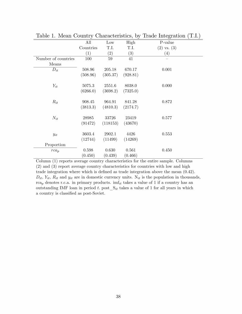
Table 1. Mean Country Characteristics, by Trade Integration (T.I.)All Low High P-value

Countries T.I. T.I. (2) vs. (3)(1) (2) (3) (4)

Number of countries 100 59 41 �MeansDit 508.96 205.18 670.17 0.001

(508.96) (305.37) (928.81)

Yit 5075.3 2551.6 8038.0 0.000(6266.0) (3698.2) (7325.0)

Rit 908.45 964.91 841.28 0.872(3813.3) (4810.3) (2174.7)

Nit 28985 33726 23419 0.577(91472) (118153) (43670)

yit 3603.4 2902.1 4426 0.553(12744) (11499) (14269)

Proportionrcap 0.598 0.630 0.561 0.450

(0.450) (0.439) (0.466)Column (1) reports average country characteristics for the entire sample. Columns(2) and (3) report average country characteristics for countries with low and hightrade integration where which is de�ned as trade integration above the mean (0.42):Dit, Yit, Rit and yit are in domestic currency units. Nit is the population in thousands,rcap denotes r.c.a. in primary products. imfit takes a value of 1 if a country has anoutstanding IMF loan in period t. post_Sit takes a value of 1 for all years in whicha country is classi�ed as post-Soviet.

38

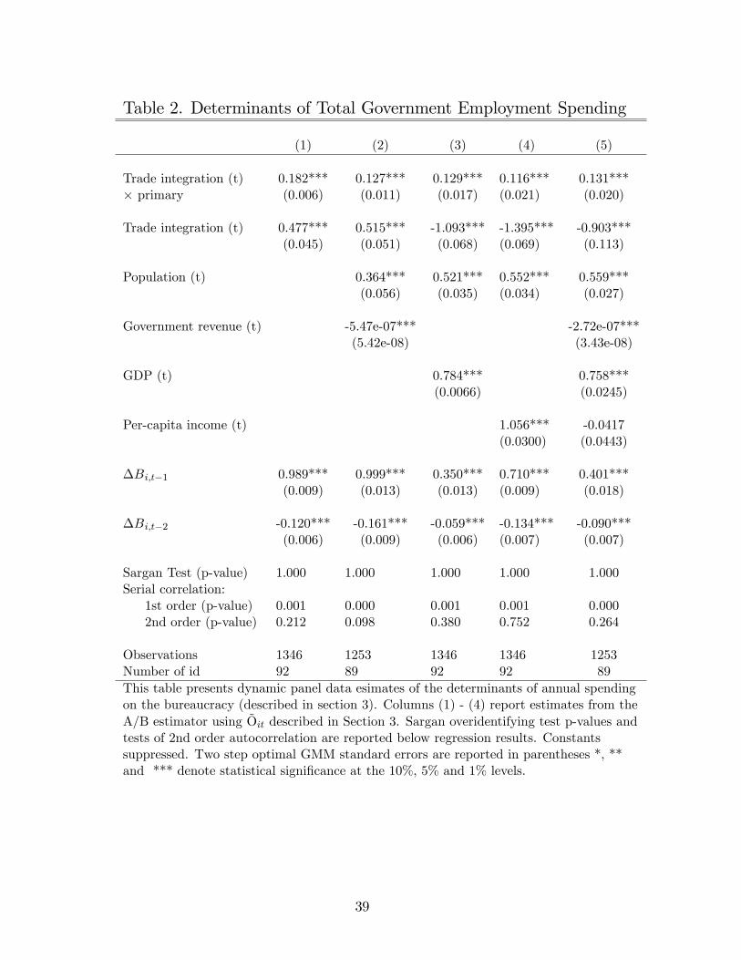
Table 2. Determinants of Total Government Employment Spending

(1) (2) (3) (4) (5)

Trade integration (t) 0.182*** 0.127*** 0.129*** 0.116*** 0.131***� primary (0.006) (0.011) (0.017) (0.021) (0.020)

Trade integration (t) 0.477*** 0.515*** -1.093*** -1.395*** -0.903***(0.045) (0.051) (0.068) (0.069) (0.113)

Population (t) 0.364*** 0.521*** 0.552*** 0.559***(0.056) (0.035) (0.034) (0.027)

Government revenue (t) -5.47e-07*** -2.72e-07***(5.42e-08) (3.43e-08)

GDP (t) 0.784*** 0.758***(0.0066) (0.0245)

Per-capita income (t) 1.056*** -0.0417(0.0300) (0.0443)

�Bi;t�1 0.989*** 0.999*** 0.350*** 0.710*** 0.401***(0.009) (0.013) (0.013) (0.009) (0.018)

�Bi;t�2 -0.120*** -0.161*** -0.059*** -0.134*** -0.090***(0.006) (0.009) (0.006) (0.007) (0.007)

Sargan Test (p-value) 1.000 1.000 1.000 1.000 1.000Serial correlation:

1st order (p-value) 0.001 0.000 0.001 0.001 0.0002nd order (p-value) 0.212 0.098 0.380 0.752 0.264

Observations 1346 1253 1346 1346 1253Number of id 92 89 92 92 89This table presents dynamic panel data esimates of the determinants of annual spendingon the bureaucracy (described in section 3). Columns (1) - (4) report estimates from theA/B estimator using Õit described in Section 3. Sargan overidentifying test p-values andtests of 2nd order autocorrelation are reported below regression results. Constantssuppressed. Two step optimal GMM standard errors are reported in parentheses *, **and *** denote statistical signi�cance at the 10%, 5% and 1% levels.

39

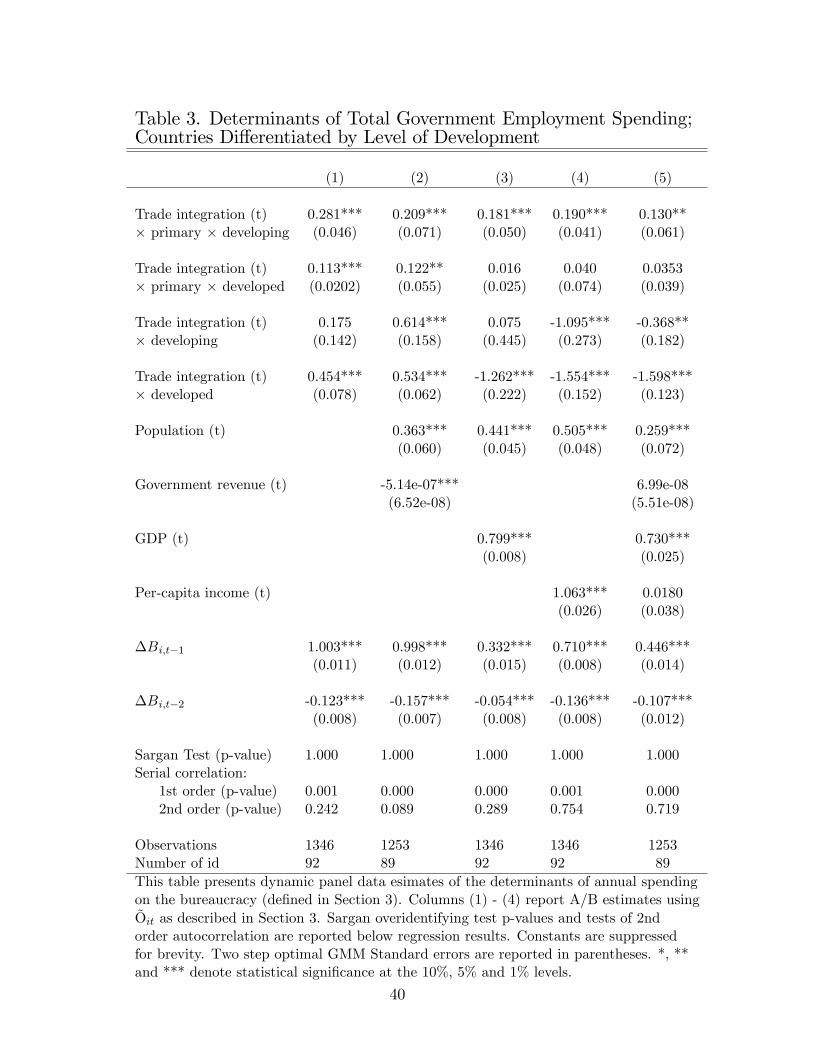
Table 3. Determinants of Total Government Employment Spending;Countries Di¤erentiated by Level of Development

(1) (2) (3) (4) (5)

Trade integration (t) 0.281*** 0.209*** 0.181*** 0.190*** 0.130**� primary � developing (0.046) (0.071) (0.050) (0.041) (0.061)

Trade integration (t) 0.113*** 0.122** 0.016 0.040 0.0353� primary � developed (0.0202) (0.055) (0.025) (0.074) (0.039)

Trade integration (t) 0.175 0.614*** 0.075 -1.095*** -0.368**� developing (0.142) (0.158) (0.445) (0.273) (0.182)

Trade integration (t) 0.454*** 0.534*** -1.262*** -1.554*** -1.598***� developed (0.078) (0.062) (0.222) (0.152) (0.123)

Population (t) 0.363*** 0.441*** 0.505*** 0.259***(0.060) (0.045) (0.048) (0.072)

Government revenue (t) -5.14e-07*** 6.99e-08(6.52e-08) (5.51e-08)

GDP (t) 0.799*** 0.730***(0.008) (0.025)

Per-capita income (t) 1.063*** 0.0180(0.026) (0.038)

�Bi;t�1 1.003*** 0.998*** 0.332*** 0.710*** 0.446***(0.011) (0.012) (0.015) (0.008) (0.014)

�Bi;t�2 -0.123*** -0.157*** -0.054*** -0.136*** -0.107***(0.008) (0.007) (0.008) (0.008) (0.012)

Sargan Test (p-value) 1.000 1.000 1.000 1.000 1.000Serial correlation:

1st order (p-value) 0.001 0.000 0.000 0.001 0.0002nd order (p-value) 0.242 0.089 0.289 0.754 0.719

Observations 1346 1253 1346 1346 1253Number of id 92 89 92 92 89This table presents dynamic panel data esimates of the determinants of annual spendingon the bureaucracy (de�ned in Section 3). Columns (1) - (4) report A/B estimates usingÕit as described in Section 3. Sargan overidentifying test p-values and tests of 2ndorder autocorrelation are reported below regression results. Constants are suppressedfor brevity. Two step optimal GMM Standard errors are reported in parentheses. *, **and *** denote statistical signi�cance at the 10%, 5% and 1% levels.

40

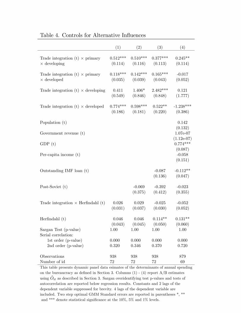
Table 4. Controls for Alternative In�uences

(1) (2) (3) (4)

Trade integration (t) � primary 0.512*** 0.510*** 0.377*** 0.245**� developing (0.114) (0.116) (0.113) (0.114)

Trade integration (t) � primary 0.118*** 0.142*** 0.165*** -0.017� developed (0.035) (0.039) (0.043) (0.052)

Trade integration (t) � developing 0.411 1.406* 2.482*** 0.121(0.549) (0.846) (0.848) (1.777)

Trade integration (t) � developed 0.774*** 0.598*** 0.522** -1.238***(0.186) (0.181) (0.220) (0.386)

Population (t) 0.142(0.132)

Government revenue (t) 1.07e-07(1.12e-07)

GDP (t) 0.774***(0.087)

Per-capita income (t) -0.058(0.151)

Outstanding IMF loan (t) -0.087 -0.112**(0.136) (0.047)

Post-Soviet (t) -0.069 -0.392 -0.023(0.375) (0.412) (0.355)

Trade integration � Her�ndahl (t) 0.026 0.029 -0.025 -0.052(0.031) (0.037) (0.030) (0.052)

Her�ndahl (t) 0.046 0.046 0.114** 0.131**(0.043) (0.045) (0.050) (0.060)

Sargan Test (p-value) 1.00 1.00 1.00 1.00Serial correlation:

1st order (p-value) 0.000 0.000 0.000 0.0002nd order (p-value) 0.320 0.346 0.370 0.720

Observations 938 938 938 879Number of id 72 72 72 69This table presents dynamic panel data esimates of the determinants of annual spendingon the bureaucracy as de�ned in Section 3. Columns (1) - (4) report A/B estimatesusing ~Oit as described in Section 3. Sargan overidentifying test p-values and tests ofautocorrelation are reported below regression results. Constants and 2 lags of thedependent variable suppressed for brevity. 4 lags of the dependent variable areincluded. Two step optimal GMM Standard errors are reported in parentheses *, **and *** denote statistical signi�cance at the 10%, 5% and 1% levels.

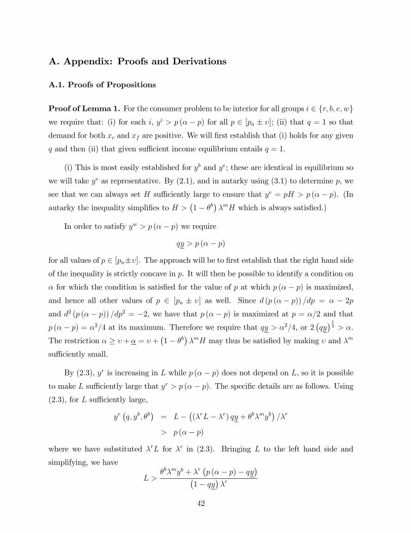
A. Appendix: Proofs and Derivations

A.1. Proofs of Propositions

Proof of Lemma 1. For the consumer problem to be interior for all groups i 2 fr; b; e; wgwe require that: (i) for each i, yi > p (�� p) for all p 2 [pa � �]; (ii) that q = 1 so thatdemand for both xc and xf are positive. We will �rst establish that (i) holds for any given

q and then (ii) that given su¢ cient income equilibrium entails q = 1.

(i) This is most easily established for yb and ye; these are identical in equilibrium so

we will take ye as representative. By (2.1), and in autarky using (3.1) to determine p, we

see that we can always set H su¢ ciently large to ensure that ye = pH > p (�� p). (Inautarky the inequality simpli�es to H >

�1� �b

��mH which is always satis�ed.)

In order to satisfy yw > p (�� p) we require

qy > p (�� p)

for all values of p 2 [pa��]. The approach will be to �rst establish that the right hand sideof the inequality is strictly concave in p. It will then be possible to identify a condition on

� for which the condition is satis�ed for the value of p at which p (�� p) is maximized,and hence all other values of p 2 [pa � �] as well. Since d (p (�� p)) =dp = � � 2pand d2 (p (�� p)) =dp2 = �2, we have that p (�� p) is maximized at p = �=2 and thatp (�� p) = �2=4 at its maximum. Therefore we require that qy > �2=4, or 2

�qy� 12 > �.

The restriction � � �+� = �+�1� �b

��mH may thus be satis�ed by making � and �m

su¢ ciently small.

By (2.3), yr is increasing in L while p (�� p) does not depend on L, so it is possibleto make L su¢ ciently large that yr > p (�� p). The speci�c details are as follows. Using(2.3), for L su¢ ciently large,

yr�q; yb; �b

�= L�

�(�rL� �r) qy + �b�myb

�=�r

> p (�� p)

where we have substituted �rL for �c in (2.3). Bringing L to the left hand side and

simplifying, we have

L >�b�myb + �r

�p (�� p)� qy

��1� qy

��r

42

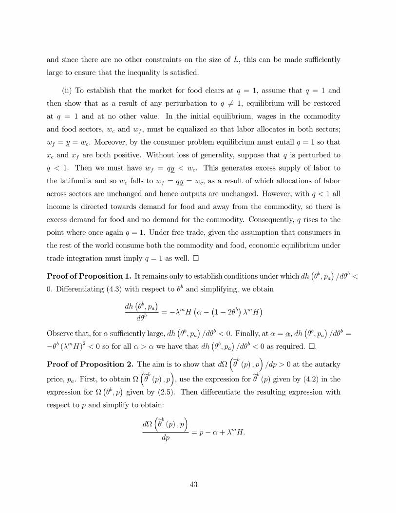
and since there are no other constraints on the size of L, this can be made su¢ ciently

large to ensure that the inequality is satis�ed.

(ii) To establish that the market for food clears at q = 1, assume that q = 1 and

then show that as a result of any perturbation to q 6= 1, equilibrium will be restored

at q = 1 and at no other value. In the initial equilibrium, wages in the commodity

and food sectors, wc and wf , must be equalized so that labor allocates in both sectors;

wf = y = wc. Moreover, by the consumer problem equilibrium must entail q = 1 so that

xc and xf are both positive. Without loss of generality, suppose that q is perturbed to

q < 1. Then we must have wf = qy < wc. This generates excess supply of labor to

the latifundia and so wc falls to wf = qy = wc, as a result of which allocations of labor

across sectors are unchanged and hence outputs are unchanged. However, with q < 1 all

income is directed towards demand for food and away from the commodity, so there is

excess demand for food and no demand for the commodity. Consequently, q rises to the

point where once again q = 1. Under free trade, given the assumption that consumers in

the rest of the world consume both the commodity and food, economic equilibrium under

trade integration must imply q = 1 as well. �

Proof of Proposition 1. It remains only to establish conditions under which dh��b; pa

�=d�b <

0. Di¤erentiating (4.3) with respect to �b and simplifying, we obtain

dh��b; pa

�d�b

= ��mH���

�1� 2�b

��mH

�Observe that, for � su¢ ciently large, dh

��b; pa

�=d�b < 0. Finally, at � = �, dh

��b; pa

�=d�b =

��b (�mH)2 < 0 so for all � > � we have that dh��b; pa

�=d�b < 0 as required. �:

Proof of Proposition 2. The aim is to show that d�e�b (p) ; p� =dp > 0 at the autarky

price, pa. First, to obtain �e�b (p) ; p�, use the expression for e�b (p) given by (4.2) in the

expression for ��b; p

�given by (2.5). Then di¤erentiate the resulting expression with

respect to p and simplify to obtain:

d�e�b (p) ; p�dp

= p� �+ �mH:

43

Now use (3.1) and (4.2) to obtain an expression for pa as a function of e�b (p):pa =

1

2

0@�� �mH +q���mH � (�mH)2

�+ 4 (�mH)2

��rL� �r (L� 1) y � d

��mH

1AUsing this to substitute for p in the above, observe that d

�e�b (p) ; p� =dp > 0 providingthat �rL� �r (L� 1) y � d > 0, which is satis�ed given e�b (p) 2 (0; 1); see (4.2). �A.2. Derivation of the Surplus from Revolution

The economic surplus generated by a revolution is determined using a Nash Bargaining

Solution (NBS), where the bargain is between the middle classes and the workers. This

surplus is determined in the usual way as the di¤erence between the payo¤ to the lower

classes from revolution and the payo¤ to them from maintaining the status quo. W is the

total surplus generated by the lower classes:

W��b; yr; yb; ye; yw; p

�� �m

��bvb

�yb; p

�+�1� �b

�ve (ye; p)

�+ �wvw (yw; p) .

where the �rst term on the right hand side measures surplus generated by the middle

classes and the second term measures the same for the workers. From this de�nition, and

using (2.1)-(2.2), we can determine a reduced form for the total payo¤ to the lower classes

from maintaining the status quo, Wsq:

Wsq (p) = �m

�pH +

1

2(�� p)2

�+ �w

�y +

1

2(�� p)2

�;

where the �rst term measures the welfare of the middle classes and the second term

measures that of workers. The total payo¤to the lower classes frommounting a revolution,

Wrev, is determined as follows:

Wrev

��b; p

�� �ryr

��b; p

�� d+ �m

�pH +

1

2(�� p)2

�+ �w

�y +

1

2(�� p)2

�.

Here, the �rst term measures the gain to the lower classes from revolution in terms of the

increase in their income and hence welfare derived through possession of the latifundia

net of the cost of revolution. Then the total net surplus for the lower classes generated

by revolution is h��b; p

�� Wrev

��b; p

��Wsq (p) = �

ryr��b; p

�� d. Thus we have (4.1).

The total surplus received by group i 2 fm;wg, as calculated by the NBS, is then givenby si = �ivi (p; yi) + 1

2

��ryr

��b; p

�� d

�:

44

A.3. Derivation of Estimating Equation

To develop the empirical model, we introduce additional �exibility by allowing for observed

persistence in the dependent variable and the possibility of other confounders, which we

will denote by Z. We now introduce the following general functions for Ait and Bit, which

represent A and B in country i and period t respectively:37

Ait = Ait(

�Xt=0

Di;t�1; p(Oit);Zit);

Bit = Bit(p(Oit);Zit):

where Zit is a vector of time-varying country-speci�c confounders. These functions replace

the functions A (p) and B (p) introduced earlier, allowing us to condition on unobservable

covariates and persistence in the dependent variable. We may then write

Dit(�Xt=0

Di;t�1; p(Oit);Zit) = Ait(�Xt=0

Di;t�1; p(Oit);Zit) +Bit(p(Oit);Zit): (A.1)

To obtain an estimating equation, we linearly approximateDit(�Pt=0

Di;t�1; p(Oit);Zit) under

monotonicity of p(�) and additive separability of A(�) and B(�):

Ait =�Xt=0

atDi;t�1 + bOit + cZit + "ait;

Bit = dOi;t + eZit + "dit

where at; b; d are scalar parameters, c and e are parameter vectors and "ait, "dit are idio-

syncratic errors. Using equation (A.1) and collecting terms we can then write

Dit =�Xt=0

atDi;t�1 + (b+ d)Oit + (c+ e)Zit + "it

where "it = "ait + "dit. This expression is then di¤erenced and the interactive dummy Ci is

introduced to obtain (5.5).

37Allowing Bit to depend on previous values of total government employment,�Pt=0Di;t�1, would compli-

cate the interpretation of coe¢ cients by introducing incomplete adjustment of the pampered bureaucracywithin a period to changes in trade integration.

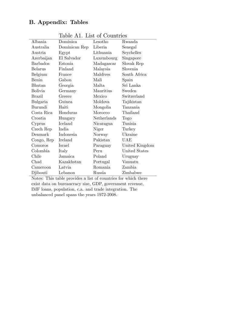
B. Appendix: Tables

Table A1. List of CountriesAlbania Dominica Lesotho RwandaAustralia Dominican Rep Liberia SenegalAustria Egypt Lithuania SeychellesAzerbaijan El Salvador Luxembourg SingaporeBarbados Estonia Madagascar Slovak RepBelarus Finland Malaysia SloveniaBelgium France Maldives South AfricaBenin Gabon Mali SpainBhutan Georgia Malta Sri LankaBolivia Germany Mauritius SwedenBrazil Greece Mexico SwitzerlandBulgaria Guinea Moldova TajikistanBurundi Haiti Mongolia TanzaniaCosta Rica Honduras Morocco ThailandCroatia Hungary Netherlands TogoCyprus Iceland Nicaragua TunisiaCzech Rep India Niger TurkeyDenmark Indonesia Norway UkraineCongo, Rep Ireland Pakistan UAEComoros Israel Paraguay United KingdomColombia Italy Peru United StatesChile Jamaica Poland UruguayChad Kazakhstan Portugal VanuatuCameroon Latvia Romania ZambiaDjibouti Lebanon Russia ZimbabweNotes: This table provides a list of countries for which thereexist data on bureaucracy size, GDP, government revenue,IMF loans, population, c.a. and trade integration. Theunbalanced panel spans the years 1972-2008.

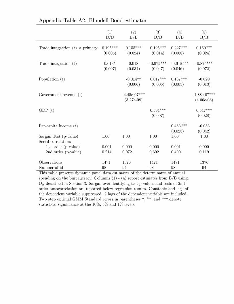
Appendix Table A2. Blundell-Bond estimator

(1) (2) (3) (4) (5)B/B B/B B/B B/B B/B

Trade integration (t) � primary 0.195*** 0.155*** 0.195*** 0.227*** 0.160***(0.005) (0.024) (0.014) (0.008) (0.024)

Trade integration (t) 0.013* 0.018 -0.975*** -0.618*** -0.875***(0.007) (0.034) (0.047) (0.046) (0.072)

Population (t) -0.014** 0.017*** 0.137*** -0.020(0.006) (0.005) (0.005) (0.013)

Government revenue (t) -4.45e-07*** -1.88e-07***(3.27e-08) (4.00e-08)

GDP (t) 0.594*** 0.547***(0.007) (0.028)

Per-capita income (t) 0.483*** -0.053(0.025) (0.042)

Sargan Test (p-value) 1.00 1.00 1.00 1.00 1.00Serial correlation:

1st order (p-value) 0.001 0.000 0.000 0.001 0.0002nd order (p-value) 0.214 0.072 0.392 0.400 0.119

Observations 1471 1376 1471 1471 1376Number of id 98 94 98 98 94This table presents dynamic panel data estimates of the determinants of annualspending on the bureaucracy. Columns (1) - (4) report estimates from B/B using:~Oit described in Section 3. Sargan overidentifying test p-values and tests of 2ndorder autocorrelation are reported below regression results. Constants and lags ofthe dependent variable suppressed. 2 lags of the dependent variable are included.Two step optimal GMM Standard errors in parentheses *, ** and *** denotestatistical signi�cance at the 10%, 5% and 1% levels.

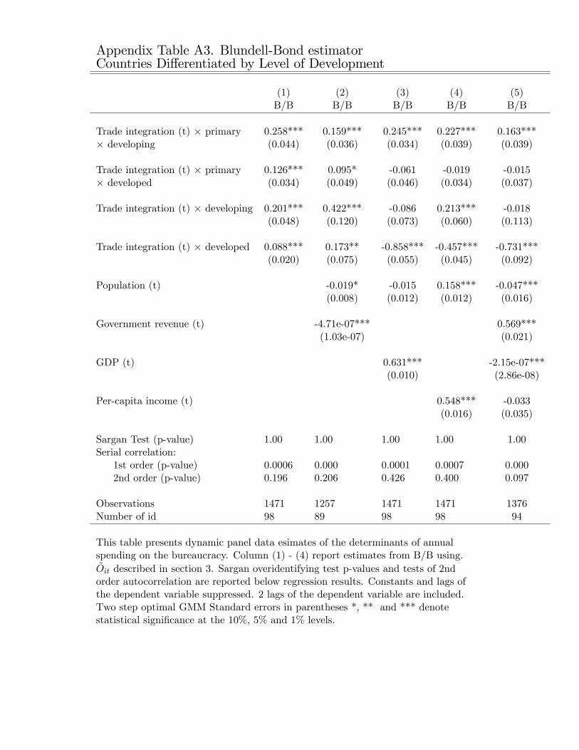
Appendix Table A3. Blundell-Bond estimatorCountries Di¤erentiated by Level of Development

(1) (2) (3) (4) (5)B/B B/B B/B B/B B/B

Trade integration (t) � primary 0.258*** 0.159*** 0.245*** 0.227*** 0.163***� developing (0.044) (0.036) (0.034) (0.039) (0.039)

Trade integration (t) � primary 0.126*** 0.095* -0.061 -0.019 -0.015� developed (0.034) (0.049) (0.046) (0.034) (0.037)

Trade integration (t) � developing 0.201*** 0.422*** -0.086 0.213*** -0.018(0.048) (0.120) (0.073) (0.060) (0.113)

Trade integration (t) � developed 0.088*** 0.173** -0.858*** -0.457*** -0.731***(0.020) (0.075) (0.055) (0.045) (0.092)

Population (t) -0.019* -0.015 0.158*** -0.047***(0.008) (0.012) (0.012) (0.016)

Government revenue (t) -4.71e-07*** 0.569***(1.03e-07) (0.021)

GDP (t) 0.631*** -2.15e-07***(0.010) (2.86e-08)

Per-capita income (t) 0.548*** -0.033(0.016) (0.035)

Sargan Test (p-value) 1.00 1.00 1.00 1.00 1.00Serial correlation:

1st order (p-value) 0.0006 0.000 0.0001 0.0007 0.0002nd order (p-value) 0.196 0.206 0.426 0.400 0.097

Observations 1471 1257 1471 1471 1376Number of id 98 89 98 98 94

This table presents dynamic panel data esimates of the determinants of annualspending on the bureaucracy. Column (1) - (4) report estimates from B/B using:~Oit described in section 3. Sargan overidentifying test p-values and tests of 2ndorder autocorrelation are reported below regression results. Constants and lags ofthe dependent variable suppressed. 2 lags of the dependent variable are included.Two step optimal GMM Standard errors in parentheses *, ** and *** denotestatistical signi�cance at the 10%, 5% and 1% levels.

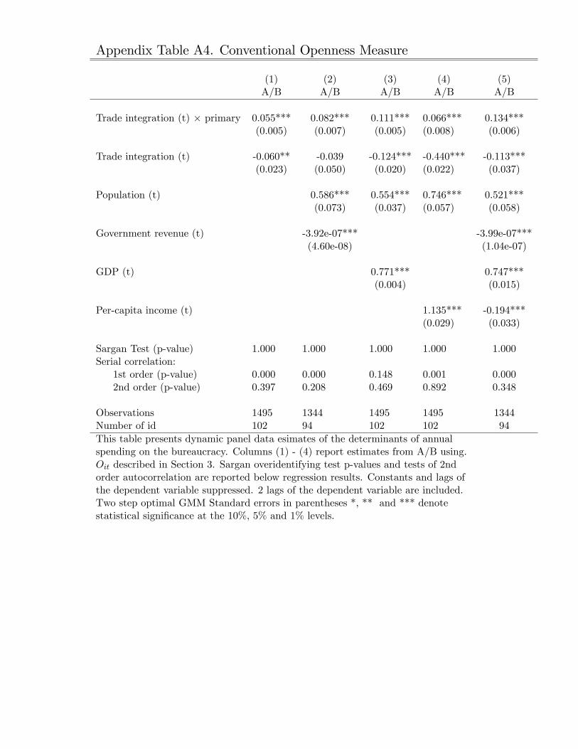
Appendix Table A4. Conventional Openness Measure

(1) (2) (3) (4) (5)A/B A/B A/B A/B A/B

Trade integration (t) � primary 0.055*** 0.082*** 0.111*** 0.066*** 0.134***(0.005) (0.007) (0.005) (0.008) (0.006)

Trade integration (t) -0.060** -0.039 -0.124*** -0.440*** -0.113***(0.023) (0.050) (0.020) (0.022) (0.037)

Population (t) 0.586*** 0.554*** 0.746*** 0.521***(0.073) (0.037) (0.057) (0.058)

Government revenue (t) -3.92e-07*** -3.99e-07***(4.60e-08) (1.04e-07)

GDP (t) 0.771*** 0.747***(0.004) (0.015)

Per-capita income (t) 1.135*** -0.194***(0.029) (0.033)

Sargan Test (p-value) 1.000 1.000 1.000 1.000 1.000Serial correlation:

1st order (p-value) 0.000 0.000 0.148 0.001 0.0002nd order (p-value) 0.397 0.208 0.469 0.892 0.348

Observations 1495 1344 1495 1495 1344Number of id 102 94 102 102 94This table presents dynamic panel data esimates of the determinants of annualspending on the bureaucracy. Columns (1) - (4) report estimates from A/B using:Oit described in Section 3. Sargan overidentifying test p-values and tests of 2ndorder autocorrelation are reported below regression results. Constants and lags ofthe dependent variable suppressed. 2 lags of the dependent variable are included.Two step optimal GMM Standard errors in parentheses *, ** and *** denotestatistical signi�cance at the 10%, 5% and 1% levels.

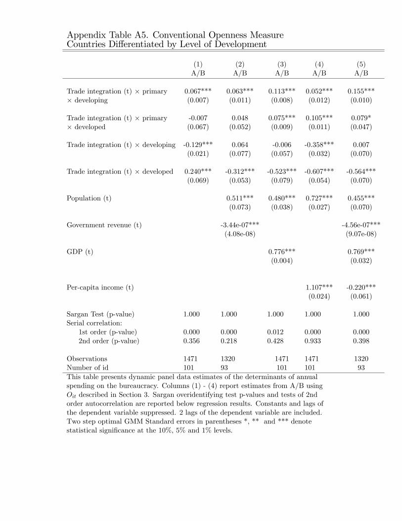
Appendix Table A5. Conventional Openness MeasureCountries Di¤erentiated by Level of Development

(1) (2) (3) (4) (5)A/B A/B A/B A/B A/B

Trade integration (t) � primary 0.067*** 0.063*** 0.113*** 0.052*** 0.155***� developing (0.007) (0.011) (0.008) (0.012) (0.010)

Trade integration (t) � primary -0.007 0.048 0.075*** 0.105*** 0.079*� developed (0.067) (0.052) (0.009) (0.011) (0.047)

Trade integration (t) � developing -0.129*** 0.064 -0.006 -0.358*** 0.007(0.021) (0.077) (0.057) (0.032) (0.070)

Trade integration (t) � developed 0.240*** -0.312*** -0.523*** -0.607*** -0.564***(0.069) (0.053) (0.079) (0.054) (0.070)

Population (t) 0.511*** 0.480*** 0.727*** 0.455***(0.073) (0.038) (0.027) (0.070)

Government revenue (t) -3.44e-07*** -4.56e-07***(4.08e-08) (9.07e-08)

GDP (t) 0.776*** 0.769***(0.004) (0.032)

Per-capita income (t) 1.107*** -0.220***(0.024) (0.061)

Sargan Test (p-value) 1.000 1.000 1.000 1.000 1.000Serial correlation:

1st order (p-value) 0.000 0.000 0.012 0.000 0.0002nd order (p-value) 0.356 0.218 0.428 0.933 0.398

Observations 1471 1320 1471 1471 1320Number of id 101 93 101 101 93This table presents dynamic panel data estimates of the determinants of annualspending on the bureaucracy. Columns (1) - (4) report estimates from A/B usingOit described in Section 3. Sargan overidentifying test p-values and tests of 2ndorder autocorrelation are reported below regression results. Constants and lags ofthe dependent variable suppressed. 2 lags of the dependent variable are included.Two step optimal GMM Standard errors in parentheses *, ** and *** denotestatistical signi�cance at the 10%, 5% and 1% levels.