METHOD Open Access

Pandora: nucleotide-resolution bacterialpan-genomics with reference graphsRachel M. Colquhoun1,2,3, Michael B. Hall1, Leandro Lima1, Leah W. Roberts1, Kerri M. Malone1, Martin Hunt1,4,Brice Letcher1, Jane Hawkey5, Sophie George4, Louise Pankhurst4,6 and Zamin Iqbal1*

* Correspondence: zi@ebi.ac.uk1European Bioinformatics Institute,Hinxton, Cambridge CB10 1SD, UKFull list of author information isavailable at the end of the article

Abstract

We present pandora, a novel pan-genome graph structure and algorithms foridentifying variants across the full bacterial pan-genome. As much bacterialadaptability hinges on the accessory genome, methods which analyze SNPs in justthe core genome have unsatisfactory limitations. Pandora approximates a sequencedgenome as a recombinant of references, detects novel variation and pan-genotypesmultiple samples. Using a reference graph of 578 Escherichia coli genomes, wecompare 20 diverse isolates. Pandora recovers more rare SNPs than single-reference-based tools, is significantly better than picking the closest RefSeq reference, andprovides a stable framework for analyzing diverse samples without reference bias.

Keywords: Pan-genome, Genome graph, Accessory genome, Nanopore

BackgroundBacterial genomes evolve by multiple mechanisms including mutation during replica-

tion, allelic and non-allelic homologous recombination. These processes result in a

population of genomes that are mosaics of each other. Given multiple contemporary

genomes, the segregating variation between them allows inferences to be made about

their evolutionary history. These analyses are central to the study of bacterial genomics

and evolution [1–4] with different questions requiring focus on separate aspects of the

mosaic: fine-scale (mutations) or coarse (gene presence, synteny). In this paper, we

provide a new and accessible conceptual model that combines both fine and coarse

bacterial variation. Using this new understanding to better represent variation, we can

access previously hidden single-nucleotide polymorphisms (SNPs), insertions and dele-

tions (indels). This can be used to add resolution to phylogenetic analyses of diverse

cohorts, to investigate selection and adaptation in the accessory genome, and to aid

bacterial genome-wide association studies (GWAS).

In the standard approach to analyzing genetic variation, a single genome is treated as

a reference and all other genomes are interpreted as differences from it. This approach

is problematic in bacteria, because while genes cover 85–90% of bacterial genomes [5],

the full set of genes present in a bacterial species—the pan-genome—is in general

© The Author(s). 2021 Open Access This article is licensed under a Creative Commons Attribution 4.0 International License, whichpermits use, sharing, adaptation, distribution and reproduction in any medium or format, as long as you give appropriate credit tothe original author(s) and the source, provide a link to the Creative Commons licence, and indicate if changes were made. Theimages or other third party material in this article are included in the article's Creative Commons licence, unless indicated otherwisein a credit line to the material. If material is not included in the article's Creative Commons licence and your intended use is notpermitted by statutory regulation or exceeds the permitted use, you will need to obtain permission directly from the copyrightholder. To view a copy of this licence, visit http://creativecommons.org/licenses/by/4.0/. The Creative Commons Public DomainDedication waiver (http://creativecommons.org/publicdomain/zero/1.0/) applies to the data made available in this article, unlessotherwise stated in a credit line to the data.

Colquhoun et al. Genome Biology (2021) 22:267 https://doi.org/10.1186/s13059-021-02473-1

much larger than the number found in any single genome. Further, the frequency dis-

tribution of genes has a characteristic asymmetric U-shaped curve [6–10], as shown in

Fig. 1A. As a result, a single-reference genome will inevitably lack many of the genes in

the pan-genome and completely miss genetic variation therein (Fig. 1B). We call this

hard reference bias, to distinguish from the more common concern, that increased di-

vergence of a reference from the genome under study leads to read-mapping problems,

which we term soft reference bias. The standard workaround for these issues in bacter-

ial genomics is to restrict analysis either to very similar genomes using a closely related

reference (e.g., in an outbreak) or to analyze SNPs only in the core genome (present in

most samples) and outside the core to simply study presence/absence of genes [11].

In this study, we address the variation deficit caused by a single-reference approach.

Given Illumina or Nanopore sequence data from potentially divergent isolates of a bac-

terial species, we attempt to detect all of the variants between them. Our approach is to

decompose the pan-genome into atomic units (loci) which tend to be preserved over

evolutionary timescales. Our loci are genes and intergenic regions in this study, but the

method is agnostic to such classifications, and one could add any other grouping

wanted (e.g., operons or mobile genetic elements). Instead of using a single genome as

a reference, we collect a panel of representative reference genomes and use them to

construct a set of reference graphs, one for each locus. Reads are mapped to this set of

graphs and from this we are able to discover and genotype variation. By letting go of

prior information on locus ordering in the reference panel, we are able to recognize

and genotype variation in a locus regardless of its wider context. Since Nanopore reads

are typically long enough to encompass multiple loci, it is possible to subsequently infer

the order of loci—although that is outside the scope of this study.

The use of graphs as a generalization of a linear reference is an active and maturing

field [12–19]. Much recent graph genome work has gone into showing that genome

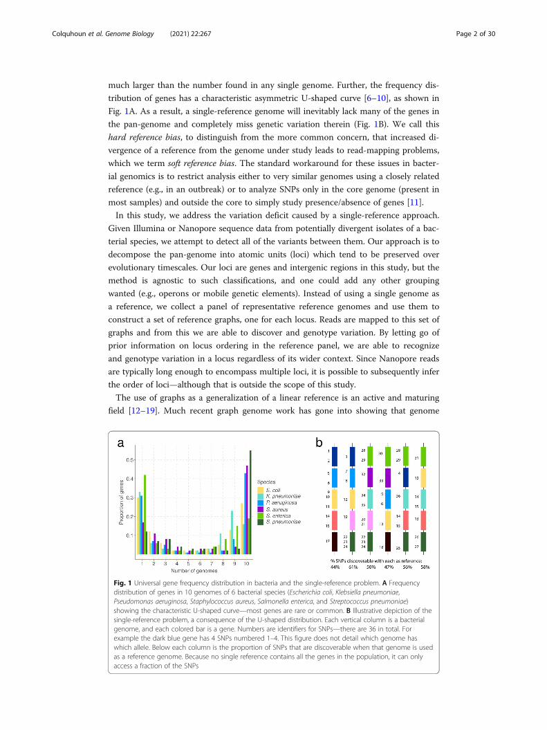
Fig. 1 Universal gene frequency distribution in bacteria and the single-reference problem. A Frequencydistribution of genes in 10 genomes of 6 bacterial species (Escherichia coli, Klebsiella pneumoniae,Pseudomonas aeruginosa, Staphylococcus aureus, Salmonella enterica, and Streptococcus pneumoniae)showing the characteristic U-shaped curve—most genes are rare or common. B Illustrative depiction of thesingle-reference problem, a consequence of the U-shaped distribution. Each vertical column is a bacterialgenome, and each colored bar is a gene. Numbers are identifiers for SNPs—there are 36 in total. Forexample the dark blue gene has 4 SNPs numbered 1–4. This figure does not detail which genome haswhich allele. Below each column is the proportion of SNPs that are discoverable when that genome is usedas a reference genome. Because no single reference contains all the genes in the population, it can onlyaccess a fraction of the SNPs

Colquhoun et al. Genome Biology (2021) 22:267 Page 2 of 30

graphs reduce the impact of soft reference bias on mapping [12, 14, 15], and on gener-

alizing alignment to graphs [16, 20]. These methods have almost universally been de-

signed for the human pan-genome, where hard reference bias is a comparatively minor

issue compared with bacteria (two human genomes are over 99% alignable, whereas

two bacteria of the same species might be 50% alignable). In particular, all current

graph methods (e.g., vg [12], Giraffe [21], GraphTyper [14, 15], paragraph [22], Bayes-

Typer [23]) require a reference genome to be provided in advance to output genetic

variants in the standard Variant Call Format (VCF) [24]—thus immediately inheriting a

hard bias when applied to bacteria (see Fig. 1B). Thus, there has not yet been any study

(to our knowledge) addressing SNP analysis across a diverse cohort, including more

variants that can fit on any single reference.

We have made a number of technical innovations. First, we use a recursive clustering

algorithm that converts a multiple sequence alignment (MSA) of a locus into a graph.

This avoids the complexity “blowups” that plague graph genome construction from

unphased VCF files [14,15]. Second, we introduce a graph representation of genetic

variation based on (w,k)-minimizers [25]. Third, using this representation, we avoid un-

necessary full alignment to the graph and instead use quasi-mapping to genotype on

the graph. Fourth, we use local assembly to discover variation missing from the refer-

ence graph. Fifth, we infer a canonical dataset-dependent reference genome designed to

maximize clarity of description of variants (the value of this will be made clear in the

main text).

We describe these below and evaluate our implementation, pandora, on a diverse set

of E. coli genomes with both Illumina and Nanopore data. We show that, compared

with reference-based approaches, pandora recovers a significant proportion of the

missing variation in rare loci, performs much more stably across a diverse dataset, suc-

cessfully infers a better reference genome for VCF output, and outperforms current

tools for Nanopore data.

ResultsPan-genome graph representation

We set out to define a generalized reference structure which allows detection of SNPs

and other variants across the whole pan-genome, without attempting to record long-

range structure or coordinates. We define a Pan-genome Reference Graph (PanRG) as an

unordered collection of sequence graphs, termed local graphs, each of which represents a

locus, such as a gene or intergenic region. Each local graph is constructed from a MSA of

known alleles of this locus, using a recursive cluster-and-collapse (RCC) algorithm (Add-

itional file 1: Supplementary Animation 1: recursive clustering construction). The output

is guaranteed to be a directed acyclic sequence graph allowing hierarchical nesting of gen-

etic variation while meeting a “balanced parentheses” criterion (see Fig. 2B and

“Methods”). Each path through the graph from source to sink represents a possible re-

combinant sequence for the locus. The disjoint nature of this pan-genome reference al-

lows loci such as genes to be compared regardless of their wider genomic context. We

implement this construction algorithm in the make_prg tool which outputs the graph as a

file (see Fig. 2A–C, “Methods”). We also implement a PanRG update algorithm in make_

prg which allows rapid augmentation of a pre-built PanRG with new alleles (see Fig. 2D,

Colquhoun et al. Genome Biology (2021) 22:267 Page 3 of 30

“Methods”). Subsequent operations, based on this PanRG, are implemented in the soft-

ware package pandora. The overall workflow is shown in Fig. 2.

To index a PanRG, we generalize a type of sparse marker k-mer ((w,k)-minimizer, also

referred to as a minimizing k-mer), previously defined for strings, to directed acyclic

graphs (see “Methods”). Informally, each minimizer is the smallest k-mer in a window of

w consecutive k-mers. This has become a popular method for rapidly indexing and com-

paring genomes and long reads (e.g., MASH [26], minimap [27, 28]). It has the advantage

that the number of indexing k-mers scales with the length of the sequence so that differ-

ent length local graphs are each well represented in the index. In addition, it enables

shorter indexing k-mers to be used, which improves mapping with noisy reads.

Each local graph is sketched with minimizing k-mers, and these are then used to con-

struct a new graph (the k-mer graph) for each local graph from the PanRG. Each min-

imizing k-mer is a node, and edges are added between two nodes if they are adjacent

minimizers on a path through the original local graph. This k-mer graph is isomorphic

to the original if w ≤ k (and outside the first and last w + k − 1 bases); all subsequent

operations are performed on this graph, which, to avoid unnecessary new terminology,

we also call the local graph.

Fig. 2 The pandora workflow. A Reference panel of genomes; color signifies locus (gene or intergenicregion) identifier, and blobs are SNPs. B The multiple sequence alignment (MSA) for each locus is convertedinto a directed acyclic graph (termed local graph). C Local graphs constructed from the loci in thereference panel. D Workflow: the collection of local graphs, termed the PanRG, is indexed. Reads from eachsample under study are independently quasi-mapped to the graph, and a determination is made as towhich loci are present in each sample. In this process, for each locus, a mosaic approximation of thesequence for that sample is inferred, and variants are genotyped. E Regions of low coverage are detected,and local de novo assembly is used to generate candidate novel alleles missing from the graph. Returningto D, the dotted line shows all the candidate alleles from all samples are then gathered and added to thePanRG. Then, reads are quasi-mapped one more time, to the augmented PanRG, generating new mosaicapproximations for all samples and storing coverages across the graphs; no de novo assembly is done thistime. A pan-genome matrix showing which input loci are present in each sample is created. Finally, allsamples are compared, and a VCF file is produced, with a per-locus reference that is inferred by pandora

Colquhoun et al. Genome Biology (2021) 22:267 Page 4 of 30

A global index maps each minimizing k-mer to a list of all local graphs containing

that k-mer and the positions therein. Long or short reads are approximately mapped

(quasi-mapped) to the PanRG by determining the minimizing k-mers in each read. Any

of these read quasi-mappings found in a local graph are called hits, and any local graph

with sufficient clustered hits on a read is considered present in the sample.

Initial sequence approximation as a mosaic of references

For each locus identified as present in a sample, we initially approximate the sample’s

sequence as a path through the local graph. The result is a mosaic of sequences from

the reference panel. This path is chosen to have maximal support by reads, using a dy-

namic programming algorithm on the graph induced by its (w,k)-minimizers (details in

“Methods”). The result of this process serves as our initial approximation to the

genome under analysis.

Improved sequence approximation: modify mosaic by local assembly

At this point, we have quasi-mapped reads, and approximated the genome by finding

the closest mosaic in the graph; however, we expect the genome under study to contain

variants that are not present in the PanRG. Therefore, to allow discovery of novel SNPs

and small indels that are not in the graph, for each sample and locus, we identify re-

gions of the inferred mosaic sequence where there is a drop in read coverage (as shown

in Fig. 2E). Slices of overlapping reads are extracted, and a form of de novo assembly is

performed using a de Bruijn graph. Instead of trying to find a single correct path, the

de Bruijn graph is traversed (see “Methods” for details) to obtain all feasible candidate

novel alleles for the sample. These alleles are then added to the local graph. If compar-

ing multiple samples, the graphs are augmented with all new alleles from all samples at

the same time.

Optimal VCF reference construction for multi-genome comparison

In the compare step of pandora (see Fig. 2D), we enable continuity of downstream ana-

lysis by outputting genotype information in the conventional VCF [24]. In this format,

each row (record) describes possible alternative allele sequence(s) at a position in a

(single) reference genome and information about the type of sequence variant. A col-

umn for each sample details the allele seen in that sample, often along with details

about the support from the data for each allele.

To output graph variation, we first select a path through the graph to be the refer-

ence sequence and describe any variation within the graph with respect to this path as

shown in Fig. 3. We use the chromosome field to detail the local graph within the

PanRG in which a variant lies, and the position field to give the position in the chosen

reference path sequence for that graph. In addition, we output the reference path se-

quences used as a separate file.

For a collection of samples, we want small differences between samples to be re-

corded as short alleles in the VCF file rather than longer alleles with shared flanking se-

quence as shown in Fig. 3B. We therefore choose the reference path for each local

graph to be maximally close to the sample mosaic paths. To do this, we make a copy of

the k-mer graph and increment the coverage along each sample mosaic path, producing

Colquhoun et al. Genome Biology (2021) 22:267 Page 5 of 30

a graph with higher weights on paths shared by more samples. We reuse the mosaic

path-finding algorithm (see “Methods”) with a modified probability function defined

such that the probability of a node is proportional to the number of samples covering

it. This produces a dataset-dependent VCF reference able to succinctly describe segre-

gating variation in the cohort of genomes under analysis.

Constructing a PanRG of E. coli

We chose to evaluate pandora on the recombining bacterial species, E. coli, whose pan-

genome has been heavily studied [7, 29–32]. MSAs for gene clusters curated with panX

[33] from 350 RefSeq assemblies were downloaded from http://pangenome.de on 3

May 2018. MSAs for intergenic region clusters based on 228 E. coli ST131 genome se-

quences were previously generated with Piggy [34] for their publication. While this

panel of intergenic sequences does not reflect the full diversity within E. coli, we in-

cluded them as an initial starting point. This resulted in an E. coli PanRG containing

local graphs for 23,051 genes and 14,374 intergenic regions. Pandora took 15m in

CPU time (11 m in runtime with 16 threads) and 12.9 GB of RAM to index the PanRG.

As one would expect from the U-shaped gene frequency distribution, many of the

genes were rare in the 578 (=350 + 228) input genomes, and so 59%/44% of the genic/

intergenic graphs were linear, with just a single allele.

Constructing an evaluation set of diverse genomes

We first demonstrate that using a PanRG reduces hard bias when comparing a diverse

set of 20 E. coli samples by comparison with standard single-reference variant callers.

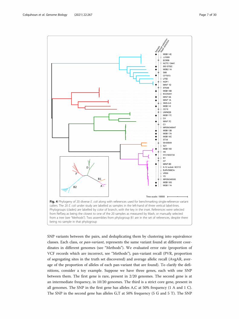
We selected samples from across the phylogeny (including phylogroups A, B2, D and F

[35]) where we were able to obtain both long- and short-read sequence data from the

same isolate.

We used Illumina-polished long-read assemblies as truth data, masking positions

where the Illumina data did not support the assembly (see “Methods”). As comparators,

we used SAMtools [36] (the “classical” variant caller based on pileups) and Freebayes

[37] (a haplotype-based caller which reduces soft reference bias, wrapped by snippy

[38]) for Illumina data, and medaka [39] and nanopolish [40] for Nanopore data. In all

cases, we ran the reference-based callers with 24 carefully selected reference genomes

(see “Methods” and Fig. 4). We defined a “truth set” of 618,305 segregating variants by

performing all pairwise whole genome alignments of the 20 truth assemblies, collecting

Fig. 3 The representation problem. A A local graph with sequence explicitly shown. B, C The same graphwith black reference path and alternate alleles in different colors, and the corresponding VCF records. In B,the black reference path is distinct from both alleles. The blue/red SNP then requires flanking sequence inorder to allow it to have a coordinate. The SNP is thus represented as two ALT alleles, each 3 bases long,and the user is forced to notice they only differ in one base. C The reference follows the blue path, thusenabling a more succinct and natural representation of the SNP

Colquhoun et al. Genome Biology (2021) 22:267 Page 6 of 30

SNP variants between the pairs, and deduplicating them by clustering into equivalence

classes. Each class, or pan-variant, represents the same variant found at different coor-

dinates in different genomes (see “Methods”). We evaluated error rate (proportion of

VCF records which are incorrect, see “Methods”), pan-variant recall (PVR, proportion

of segregating sites in the truth set discovered) and average allelic recall (AvgAR, aver-

age of the proportion of alleles of each pan-variant that are found). To clarify the defi-

nitions, consider a toy example. Suppose we have three genes, each with one SNP

between them. The first gene is rare, present in 2/20 genomes. The second gene is at

an intermediate frequency, in 10/20 genomes. The third is a strict core gene, present in

all genomes. The SNP in the first gene has alleles A,C at 50% frequency (1 A and 1 C).

The SNP in the second gene has alleles G,T at 50% frequency (5 G and 5 T). The SNP

Fig. 4 Phylogeny of 20 diverse E. coli along with references used for benchmarking single-reference variantcallers. The 20 E. coli under study are labelled as samples in the left-hand of three vertical label-lines.Phylogroups (clades) are labelled by color of branch, with the key in the inset. References were selectedfrom RefSeq as being the closest to one of the 20 samples as measured by Mash, or manually selectedfrom a tree (see “Methods”). Two assemblies from phylogroup B1 are in the set of references, despite therebeing no sample in that phylogroup

Colquhoun et al. Genome Biology (2021) 22:267 Page 7 of 30

in the third gene has alleles A,T with 15 A and 5 T. Suppose a variant caller found the

SNP in the first gene, detecting the two correct alleles. For the second gene’s SNP, it

detected only one G and one T, failing to detect either allele in the other 8 genomes.

For the third gene’s SNP, it detected all the 5 T’s, but no A. Here, the pan-variant recall

would be: (1 + 1 + 0) / 3 = 0.66—i.e., score a 1 if both alleles are found, irrespective of

how often- and the average allelic recall would be (2/2 + 2/10 + 5/20)/3 = 0.48. Thus

PVR and AvgAR are pan-genome equivalents of standard site discovery power and

genotyping accuracy.

Pandora detects rare variation inaccessible to single-reference methods

First, we evaluate the primary aim of pandora—the ability to access genetic variation

within the accessory genome. Figure 5 shows the PVR of SNPs in the truth set broken

down by the number of samples the SNP (either allele) is present in. Results are shown

for pandora, medaka, and nanopolish using Nanopore sequence data, and Additional

file 1: Supplementary Figure 1 shows an almost identical result for pandora, snippy,

and SAMtools using Illumina sequence data.

If we restrict our attention to rare variants (present only in 2–5 genomes), we find

pandora recovers at least 17.5/24.5/11.6/20.8 k more SNPs than SAMtools/snippy/me-

daka/nanopolish respectively. As a proportion of rare SNPs in the truth set, this is a lift

in PVR of 10.9/15.3/7.2/13.0% respectively. If, instead of pan-variant recall, we look at

the variation of AvgAR across the locus frequency spectrum (see Additional file 1: Sup-

plementary Figure 2), the gap between pandora and the other tools on rare loci is even

larger. These observations confirm and quantify the extent to which we are able to re-

cover accessory genetic variation that is inaccessible to single-reference-based methods.

Benchmarking recall, error rate, and dependence on reference

We show in Fig. 6A,B the Illumina and Nanopore AvgAR/error rate plots for pandora

and four single-reference tools with no filters applied. For all of these, we modify only

the minimum genotype confidence to move up and down the curves (see “Methods”).

We highlight three observations. Firstly, pandora achieves essentially the same recall

and error rate for the Illumina and Nanopore data (85% AvgAR and 0.2–0.3% error rate

Fig. 5 Pan-variant recall across the locus frequency spectrum. Every SNP occurs in a locus, which is presentin some subset of the full set of 20 genomes. SNPs in the golden truth set are broken down by thenumber of samples the locus is present in. In panel A, we show the absolute count of pan-variants foundand in panel B we show the proportion of pan-variants found (PVR) for pandora (dotted line), nanopolish,and medaka with Nanopore data

Colquhoun et al. Genome Biology (2021) 22:267 Page 8 of 30

at the top-right of the curve, completely unfiltered). Second, choice of reference has a

significant effect on both AvgAR and error rate for the single-reference callers; the ref-

erence which enables the highest recall does not lead to the best error rate. Third, pan-

dora achieves better AvgAR (85%) than all other tools (all between 73 and 84%, see

Additional file 1: Supplementary Table 1), and a better error rate (0.2–0.3%) than SAM-

tools (1.0%), nanopolish (2.4%), and medaka (14.8%). However, snippy achieves a signifi-

cantly better error rate than all other tools (0.01%). We confirmed that adding further

filters slightly improved error rates, but did not change the overall picture (Additional

file 1: Supplementary Figure 3, “Methods”, Additional file 1: Supplementary Table 1).

The results are also in broad agreement if the PVR is plotted instead of AvgAR (Add-

itional file 1: Supplementary Figure 4). However, these AvgAR and PVR figures are

hard to interpret because pandora and the reference-based tools have recall that varies

differently across the locus frequency spectrum, as described above. We explore this

further below.

We ascribe the similarity between the Nanopore and Illumina performance of pan-

dora to three reasons. First, the PanRG is a strong prior—our first approximation does

not contain any Nanopore sequence, but simply uses quasi-mapped reads to find the

nearest mosaic in the graph. Second, mapping long Nanopore reads which completely

cover entire genes is easier than mapping Illumina data and allows us to filter out errone-

ous k-mers within reads after deciding when a gene is present. Third, this performance is

Fig. 6 Benchmarks of recall/error rate and dependence of precision on reference genome, for pandora andother tools on 20-way dataset. A The average allelic recall and error rate curve for pandora, SAMtools, andsnippy on 100× of Illumina data. Snippy/SAMtools both run 24 times with the different reference genomesshown in Fig. 4, resulting in multiple lines for each tool (one for each reference). B The average allelic recalland error rate curve for pandora, medaka, and nanopolish on 100× of Nanopore data; multiple lines formedaka/nanopolish, one for each reference genome. Note panels A and B have the same y-axis scale andlimits, but different x axes. C The precision of pandora, SAMtools, and snippy on 100× of Illumina data. Theboxplots show the distribution of SAMtools’ and snippy’s precision depending on which of the 24 referenceswas used, and the blue line connects pandora’s results. D The precision of pandora (line plot), medaka, andnanopolish (both boxplots) on 100× of Nanopore data. Note different y-axis scale/limits in panels C and D

Colquhoun et al. Genome Biology (2021) 22:267 Page 9 of 30

only achieved when we use methylation-aware basecalling of Nanopore reads, presumably

removing most systematic bias (see Additional file 1: Supplementary Figure 5).

In Fig. 6C,D, we show for Illumina and Nanopore data, the impact of reference choice on

the precision of calls on each of the 20 samples. While precision is consistent across all sam-

ples for pandora, we see a dramatic effect of reference choice on precision of SAMtools, me-

daka, and nanopolish. The effect is also detectable for snippy, but to a much lesser extent.

Finally, we measured the performance of locus presence detection, restricting to

genes/intergenic regions in the PanRG, so that in principle perfect recall would be pos-

sible (see “Methods”). In Additional file 1: Supplementary Figure 6, we show the distri-

bution of locus presence calls by pandora, split by length of locus for Illumina and

Nanopore data. Overall, 93.7%/94.3% of loci were correctly classified as present or ab-

sent for Illumina/Nanopore respectively. Misclassifications were concentrated on small

loci (below 500 bp). While 59.5%/57.4% of all loci in the PanRG are small, 75.5%/75.7%

of false positive calls and 99.1%/98.5% of false negative calls are small loci (see Add-

itional file 1: Supplementary Figure 6).

Pandora has consistent results across E. coli phylogroups

We measure the impact of reference bias (and population structure) by quantifying

how recall varies in phylogroups A, B2, D, and F depending on whether the reference

genome comes from the same phylogroup.

We plot the results for snippy with 5 exemplar references in Fig. 7A (results for all

tools and for all references are in Additional file 1: Supplementary Figures 7-10), show-

ing that single references give 5–10% higher recall for samples in their own phylogroup

than other phylogroups. By comparison, pandora’s recall is much more consistent, stay-

ing stable at ~ 90% for all samples regardless of phylogroup. References in phylogroups

A and B2 achieve higher recall in their own phylogroup, but consistently worse than

pandora for samples in the other phylogroups (in which the reference does not lie).

Fig. 7 Single-reference callers achieve higher recall for samples in the same phylogroup as the referencegenome, but not for rare loci. A Pandora recall (black line) and snippy recall (colored bars) of pan-variants ineach of the 20 samples; each histogram corresponds to the use of one of 5 exemplar references, one fromeach phylogroup. The background color denotes the reference’s phylogroup (see Fig. 4 inset); note thatphylogroup B1 (yellow background) is an outgroup, containing no samples in this dataset. B Same as A butrestricted to SNPs present in precisely two samples (i.e., where 18 samples have neither allele because theentire locus is missing). Note the differing y-axis limits in the two panels

Colquhoun et al. Genome Biology (2021) 22:267 Page 10 of 30

References in the external phylogroup B1, for which we had no samples in our dataset,

achieve higher recall for samples in the nearby phylogroup A (see inset, Fig. 4), but

lower than pandora for all others. We also see that choosing a reference genome from

phylogroup F, which sits intermediate to the other phylogroups, provides the most uni-

form recall across other groups—2–5% higher than pandora.

These results will, however, be dominated by the shared, core genome. If we replot Fig. 7A,

restricting to variants in loci present in precisely 2 genomes (abbreviated to 2-variants; Fig.

7B), we find that pandora achieves 49–86% recall for each sample (complete data in Add-

itional file 1: Supplementary Figure 11). By contrast, for any choice of reference genome, the

results for single-reference callers vary dramatically per sample, ranging from 4 to 83% for

snippy for example. Most sample-reference pairs (388/480) have recall under 49% (the lower

bound for pandora recall), and there is no pattern of improved recall for samples in the same

phylogroup as the reference. Following up that last observation, if we look at which pairs of

genomes share 2-variants (Fig. 8), we find there is no enrichment within phylogroups at all.

This simply confirms in our data that presence of rare loci is not correlated with the overall

phylogeny. For completeness, Additional file 1: Supplementary Animation 2 shows the pan-

dora and snippy recall for all 24 references, split by variant frequency.

Pandora VCF reference is closer to samples than any single reference

The relationship between phylogenetic distance and gene repertoire similarity is not

linear. In fact, 2 genomes in different phylogroups may have more similar accessory

genes than 2 in the same phylogroup—as illustrated in the previous section (also see

Fig. 3 in Rocha [3]). As a result, it is unclear a priori how to choose a good reference

Fig. 8 Sharing of variants present in precisely 2 genomes, showing which pairs of genomes they lie in andwhich phylogroups; darker colors signify higher counts (log scale). Axes are labelled with genomeidentifiers, colored by their phylogroup (see Fig. 4 inset)

Colquhoun et al. Genome Biology (2021) 22:267 Page 11 of 30

genome for comparison of accessory loci between samples. Pandora specifically aims to

construct an appropriate reference for maximum clarity in VCF representation. We

evaluate how well pandora is able to find a VCF reference close to the samples under

study as follows. We first identified the location of all loci in all the 20 sample assem-

blies and the 24 references (see “Methods”).

We then measured the edit distance between each locus in each of the references and

the corresponding version in the 20 samples. We found that the pandora’s VCF refer-

ence lies within 1% edit distance (scaled by locus length) of the sample far more than

any of the references for loci present in ≤ 9 samples (Fig. 9; note the log scale). Add-

itional file 1: Supplementary Figure 12 shows a similar result for 0% edit distance (exact

match). In both cases, the improvement is much reduced in the core genome; essen-

tially, in the core, a phylogenetically close reference provides a good approximation,

but it is hard to choose a single reference that provides a close approximation to all

rare loci. By contrast, pandora is able to leverage its reference panel, and the dataset

under study, to find a good approximation.

Computational performance

We report here the CPU time and maximum RAM consumed by the evaluated tools.

All of the single-reference tools analyzed isolates independently, whereas pandora has a

subsequent joint analysis step to compare them all; we therefore compare the end-to-

end performance of pandora analyzing all 20 samples against the mean performance of

each single-reference tool (summing all 20 samples, and then averaging over the differ-

ent reference genomes). In short, pandora took 9.2 CPU hours to analyze the 20

Fig. 9 How often do references closely approximate a sample? Pandora aims to infer a reference for use inits VCF, which is as close as possible to all samples. We evaluate the success of this here. The x-axis showsthe number of genomes in which a locus occurs. The y-axis shows the (log-scaled) count of loci in the 20samples that are within 1% edit distance (scaled by locus length) of each reference—box plots for thereference genomes, and line plot for the VCF reference inferred by pandora

Colquhoun et al. Genome Biology (2021) 22:267 Page 12 of 30

isolates with Illumina data while snippy and SAMtools both took 0.4 CPU hours. With

Nanopore data, pandora took 16.4 CPU hours, which is slower than medaka (0.7 CPU

hours), but faster than nanopolish (84 CPU hours). In terms of memory usage, for the

Illumina data, pandora used a maximum of 13.4 GB of RAM, compared with snippy

(3.2 GB), and SAMtools (1.0 GB), whereas for the Nanopore data, pandora used a max-

imum of 15.7 GB of RAM, compared with medaka (5.9 GB) and nanopolish (10.4 GB).

DiscussionBacteria are the most diverse and abundant cellular life form [41]. Some species are ex-

quisitely tuned to a particular niche (e.g., obligate pathogens of a single host) while

others are able to live in a wide range of environments (e.g., E. coli can live on plants,

in the earth, or commensally in the gut of various hosts). Broadly speaking, a wider

range of environments correlates with a larger pan-genome, and some parts of the gene

repertoire are associated with specific niches [42]. Our perception of a pan-genome

therefore depends on our sampling of the unknown underlying population structure,

and similarly the effectiveness of a PanRG will depend on the choice of reference panel

from which it is built.

Many examples from different species have shown that bacteria are able to leverage

this genomic flexibility, adapting to circumstance sometimes by using or losing novel

genes acquired horizontally, and at other times by mutation. There are many situations

where precise nucleotide-level variants matter in interpreting pan-genomes. Some ex-

amples include compensatory mutations in the chromosome reducing the fitness bur-

den of new plasmids [43–45]; lineage-specific accessory genes with SNP mutations

which distinguish carriage from infection [46]; SNPs within accessory drug resistance

genes leading to significant differences in antibiograms [47]; and changes in CRISPR

spacer arrays showing immediate response to infection [48, 49]. However, up until

now, there has been no automated way of studying non-core gene SNPs at all; still less

a way of integrating them with gene presence/absence information. Pandora solves

these problems, allowing detection and genotyping of core and accessory variants. It

also addresses the problem of what reference to use as a coordinate system, inferring a

mosaic “VCF reference” which is as close as possible to all samples under study. We

find this gives more consistent SNP calling than any single reference in our diverse

dataset. We focussed primarily on Nanopore data when designing pandora and show it

is possible to achieve higher quality SNP calling with this data than with current Nano-

pore tools. The impact of this approach does depend on the dataset under study. We

find that, if analyzing closely related samples, then single-reference methods provide

improved recall compared with pandora. However, if analyzing more diverse datasets,

hard reference bias is a bigger issue for single-reference tools, and pandora offers im-

proved recall.

Prior graph genome work, focussing on soft reference bias (in humans), has evaluated

different approaches for selecting alleles for addition to a population graph, based on

frequency, avoiding creating new repeats, and avoiding exponential blow-up of haplo-

types in clusters of variants [50]. This approach makes sense when you have unphased

diploid VCF files and are considering all recombinants of clustered SNPs as possible.

However, this is effectively saying we consider the recombination rate to be high

enough that all recombinants are possible. Our approach, building from local MSAs

Colquhoun et al. Genome Biology (2021) 22:267 Page 13 of 30

and only collapsing haplotypes when they agree for a fixed number of bases, preserves

more haplotype structure and avoids combinatorial explosion. Another alternative ap-

proach was recently taken by Norri et al. [51], inferring a set of pseudo founder ge-

nomes from which to build the graph.

With pandora, we break the genome into atomic units which may reorder freely be-

tween samples, but within which the degree of variation is more constrained. This ap-

proach is directly motivated by our knowledge of the mechanisms underlying genomic

flexibility in bacteria. The breadth of diversity we see in these bacteria arises primarily

as a result of horizontally acquired DNA which is incorporated into the genome by dif-

ferent forms of recombination. Homologous recombination between closely related se-

quences may result in allele conversion and in some species contributes as many

nucleotide changes as point mutation [52]. As a result, locally we expect sequences to

look like mosaics of each other, possibly with additional novel mutations. Genes are ac-

quired (and lost) as a result of homologous or site-specific recombination and at hot-

spots [53, 54]. The dynamics of this are organized [30], and result in global genome

mosaicism. The choice of atomic unit used to build each local graph should again be

motivated by this underlying biology. A locus should be large enough for its presence

and sequence to be useful independently of other graphs, but small enough as to be

typically inherited as an entire unit. Biologically speaking, genes fulfil this requirement

and there already exist a plethora of tools designed to extract and align genes (and

intergenic regions) in a set of bacterial genomes (prokka [55], panaroo [56], roary [57],

panX [33], piggy [34]). Operons or groups of genes which co-occur contiguously might

also make a good choice, although isolating a set of reference sequences for these re-

gions would be more of a challenge.

Another issue is how to select the reference panel of genomes in order to minimize

hard reference bias. One cannot escape the U-shaped frequency distribution; whatever

reference panel is chosen, future genomes under study will contain rare genes not

present in the PanRG. Given the known strong population structure in bacteria, and

the association of accessory repertoires with lifestyle and environment, we would advo-

cate sampling by phylogeny, geography, host species (if appropriate), lifestyle (e.g.,

pathogenic versus commensal), and/or environment. In this study, we built our PanRG

from a biased dataset (RefSeq) which does not attempt to achieve balance across phyl-

ogeny or ecology, limiting our pan-variant recall to 49% for rare variants (see Fig. 5B,

Additional file 1: Supplementary Figure 1C). A larger, carefully curated input panel,

such as that from Horesh et al. [58], would provide a better foundation and potentially

improve results.

A natural question is then to ask if the PanRG should continually grow, absorbing all

variants ever encountered. From our perspective, the answer is no—a PanRG with vari-

ants at all non-lethal positions would be potentially intractable. The goal is not to have

every possible allele in the PanRG—no more than a dictionary is required to contain

absolutely every word that has ever been said in a language. As with dictionaries, there

is a trade-off between completeness and utility, and in the case of bacteria, the language

is far richer than English. The perfect PanRG contains the vast majority of the genes

and intergenic regions you are likely to meet, and just enough breadth of allelic diver-

sity to ensure reads map without too many mismatches. Missing alleles should be dis-

coverable by local assembly and added to the graph, allowing multi-sample comparison

Colquhoun et al. Genome Biology (2021) 22:267 Page 14 of 30

of the cohort under study. This allows one to keep the main PanRG lightweight enough

for rapid and easy use.

For bacterial genomes, genotype calls are often used to perform phylogenetic ana-

lyses. By detecting accessory variation, three things become possible. First, pragmatic-

ally, one can choose clusters of similar genomes based on the cohort-wide core

genome, and then by restricting the pandora VCF to genes present in each cluster, re-

analyze based on the cluster-specific core genome. Normally this would require choos-

ing a cluster-specific reference, remapping reads and re-running a variant caller, but

with pandora all of the necessary data is provided in one step. Secondly, the accessory

SNPs provide an extra level of resolution when comparing samples which are very close

on a core genome tree, which may be useful. Finally, one cannot represent all pan-

genome variation in a phylogeny as the evolutionary history is fundamentally not com-

patible with a simple vertical-inheritance model. However, the pandora output would

make ideal material on which to build and test population genetic models.

We finish with potential applications of pandora. First, the PanRG should provide a

more interpretable substrate for pan-genome-wide genome-wide association studies, as

current methods are forced to either ignore the accessory genome or reduce it to k-mers

or unitigs [59–61] abstracted from their wider context. Second, it would allow investiga-

tion of selection and adaptation of accessory SNPs. Third, if performing prospective sur-

veillance of microbial isolates taken in a hospital, the PanRG provides a consistent and

unchanging reference, which will cope with the diversity of strains seen without requiring

the user to keep switching reference genome. Finally, if studying a fixed dataset very care-

fully, then one may not want to use a population PanRG, as it necessarily will miss some

rare accessory genes in the dataset. In these circumstances, one could construct a refer-

ence graph purely of the genes/intergenic regions present in this dataset.

There are a number of limitations to this study. Firstly, although pandora achieves a

gain of recall in rare variation compared with single-reference tools (at least 12–25 k

more SNPs in loci present in 2–5 genomes out of 20 depending on choice of tool and

reference—a lift of at least 7–15% in recall), this is offset by 11% loss of recall at core

SNPs. However, the gain in recall of rare variants will increase both with dataset size

(due to the U-shaped gene frequency curve) and with a PanRG constructed from either

a better-sampled input reference panel, or the dataset itself. By contrast, there is no a

priori reason why pandora should miss core SNPs, and this issue will need to be ad-

dressed in future work. Finally, by working in terms of atomic loci instead of a mono-

lithic genome-wide graph, pandora opens up graph-based approaches to structurally

diverse species (and eases parallelisation) but at the cost of losing genome-wide order-

ing. At present, ordering can be resolved by (manually) mapping pandora-discovered

genes onto whole genome assemblies. However the design of pandora also allows for

gene-ordering inference: when Nanopore reads cover multiple genes, the linkage be-

tween them is stored in a secondary de Bruijn graph where the alphabet consists of

gene identifiers. This results in a huge alphabet, but the k-mers are almost always

unique, dramatically simplifying “assembly” compared with normal DNA de Bruijn

graphs. This work is still in progress and the subject of a future study. In the meantime,

pandora provides new ways to access previously hidden variation.

Colquhoun et al. Genome Biology (2021) 22:267 Page 15 of 30

ConclusionsThe algorithms implemented in pandora provide a solution to the problem of analyzing core

and accessory genetic variation across a set of bacterial genomes. This study demonstrates as

good SNP genotype error rates with Nanopore as with Illumina data and improved recall of

accessory variants. It also shows the benefit of an inferred VCF reference genome over simply

picking from RefSeq. The main limitations were the use of a biased reference panel (RefSeq)

for building the PanRG, and a slightly lower recall for core SNPs than single-reference tools—

both of which are addressable, not fundamental limitations. This work opens the door to im-

proved analyses of many existing and future bacterial genomic datasets.

MethodsLocal graph construction

We construct each local graph in the PanRG from an MSA using an iterative partitioning

process. The resulting sequence graph contains nested bubbles representing alternative alleles.

Let A be an MSA of length n. For each row of the MSA a = {a0,…, an−1} ∈A let ai, j =

{ai,…, aj−1} be the subsequence of a in interval [i, j). Let s(a) be the DNA sequence ob-

tained by removing all non-AGCT symbols. We can partition alignment A either verti-

cally by partitioning the interval [0, n) or horizontally by partitioning the set of rows of

A. In both cases, the partition induces a number of sub-alignments.

For vertical partitions, we define sliceA(i, j) = {ai,j : a ∈A}. We say that interval [i, j) is a

match interval if j − i ≥m, where m = 7 is the default minimum match length, and there

is a single non-trivial sequence in the slice, i.e.,

jfsðaÞ : a ∈ sliceAði; jÞ and sðaÞ≠””gj ¼ 1:

Otherwise, we call it a non-match interval.

For horizontal partitions, we use a reference-based approach combined with K-means

clustering [62] to divide sequences into increasing numbers of clusters K = 2, 3, … until

each cluster meets a “one-reference-like” criterion or until K = 10. More formally, let U

be the set of all m-mers (substrings of length m, the minimum match length) in {s(a) :

a ∈A}. For a ∈A, we transform sequence s(a) into a count vector �xa ¼ fxa1;…; xajU jgwhere xa

i is the count of unique m-mer i ∈ U. The K-means algorithm partitions {s(a) :

a ∈A} into K clusters �C ¼ fC1;…;CKg by minimizing the inertia, defined as

arg minCXK

j¼1

X

�xa∈C j

�xa−μ j

������2

where μ j ¼ 1jC jj

P�xa∈C j

�xa is the mean of cluster j.

Given a (sub-)alignment A, we define the reference of A, ref(A), to be the concaten-

ation of the most frequent nucleotide at each position of A. We say that a K-partition

is one-reference-like if for the corresponding sub-alignments A1, …, AK the hamming

distance between each sequence and its sub-alignment reference

jsðaÞ−re f ðAiÞj < d�lenðAÞ ∀a ∈ Ai

where | | denotes the Hamming distance, and d denotes a maximum hamming distance

threshold, set at 0.2 by default. In this case, we accept the partition; otherwise, we look

for a K + 1-partition.

Colquhoun et al. Genome Biology (2021) 22:267 Page 16 of 30

The recursive algorithm first partitions an MSA vertically into match and non-match

intervals. Match intervals are collapsed down to the single sequence they represent. In-

dependently for each non-match interval, the alignment slice is partitioned horizontally

into clusters. The same process is then applied to each induced sub-alignment until a

maximum number of recursion levels, r = 5, has been reached. For any remaining align-

ments, a node is added to the local graph for each unique sequence. See Additional file

1: Supplementary Animation 1 to see an example of this algorithm. We name this algo-

rithm Recursive Cluster and Collapse (RCC). When building the local graph from a

MSA, we record and serialize the recursion tree of the RCC algorithm, as well as mem-

oizing all the data in each recursion node. We shall call this algorithm memoized RCC

(MRCC). Once the MRCC recursion tree is generated, we can obtain the local graph

through a pre-order traversal of the tree (which is equivalent to the call order of the re-

cursive functions in an execution of the RCC algorithm). To update the local graph

with new alleles using the MRCC algorithm, we can deserialize the recursion tree from

disk, infer in which leaves of the recursion tree the new alleles should be added, add

the new alleles in bulk, and then update each modified leaf. This leaf update operation

consists of updating just the subaligment of the leaf (which is generally a small fraction

of the whole MSA) with the new alleles using MAFFT [63] and recomputing the recur-

sion at the leaf node. All of this is implemented in the make_prg repository (see “Code

availability”).

(w,k)-minimizers of graphs

We define (w,k)-minimizers of strings as in Li [27]. Let φ : Σk→R be a k-mer hash

function and let π : Σ∗ × {0, 1}→ Σ∗ be defined such that π(s, 0) = s and πðs; 1Þ ¼ �s, where

�s is the reverse complement of s. Consider any integers k ≥w > 0. For window start pos-

ition 0 ≤ j ≤ |s| −w − k + 1, let

T j ¼ π sp;pþk ; r� �

: j≤p < jþ w; r∈ 0; 1f g� �

be the set of forward and reverse-complement k-mers of s in this window. We define a

(w,k)-minimizer to be any triple (h, p, r) such that

h ¼ φ π sp;pþk ; r� �� � ¼ min φ tð Þ : t ∈T j

� �:

The set W(s) of (w,k)-minimizers for s, is the union of minimizers over such

windows:

W ðsÞ ¼ ⋃0≤ j≤ jsj−w−kþ1

fðh; p; rÞ : h ¼ minfφðtÞ : t ∈T jgg:

We extend this definition intuitively to an acyclic sequence graph G = (V,E). Define

|v| to be the length of the sequence associated with node v ∈V and let i = (v, a, b), 0 ≤

a ≤ b ≤ |v| represent the sequence interval [a, b) on v. We define a path in G by

�p ¼ i1;…; imð Þ : v j; v jþ1� �

∈E and bj ≡ jv jj for 1≤ j < m� �

:

This matches the intuitive definition for a path in a sequence graph except that we

allow the path to overlap only part of the sequence associated with the first and last

nodes. We will use s�p to refer to the sequence along the path �p in the graph.

Colquhoun et al. Genome Biology (2021) 22:267 Page 17 of 30

Let �q be a path of length w + k − 1 in G. The string s�q contains w consecutive k-mers

for which we can find the (w,k)-minimizer(s) as before. We therefore define the (w,k)-

minimizer(s) of the graph G to be the union of minimizers over all paths of length w +

k − 1 in G:

W ðGÞ ¼ ⋃�q∈G :∣�q ∣¼wþk−1

fðh; �p; rÞ : h ¼ minfφðtÞ : t∈T �qgg:

Local graph indexing with (w,k)-minimizers

To find minimizers for a graph, we use a streaming algorithm as described in Add-

itional file 1: Supplementary Algorithm 1. For each minimizer found, it simply finds the

next minimizer(s) until the end of the graph has been reached.

Let walk(v, i,w, k) be a function which returns all vectors of w consecutive k-mers in

G starting at position i on node v. Suppose we have a vector of k-mers x. Let shift(x) be

the function which returns all possible vectors of k-mers which extend x by one k-mer.

It does this by considering possible ways to walk one letter in G from the end of the

final k-mer of x. For a vector of k-mers of length w, the function minimize(x) returns

the minimizing k-mers of x.

We define K to be a k-mer graph with nodes corresponding to minimizers ðh; �p; rÞ .We add edge (u,v) to K if there exists a path in G for which u and v are both mini-

mizers and v is the first minimizer after u along the path. Let K← add(s, t) denote the

addition of nodes s and t to K and the directed edge (s,t). Let K← add(s, T) denote the

addition of nodes s and t ∈ T to K as well as directed edges (s,t) for t ∈ T, and define

K← add(S, t) similarly.

The resulting PanRG index stores a map from each minimizing k-mer hash value to

the positions in all local graphs where that (w,k)-minimizer occurred. In addition, we

store the induced k-mer graph for each local graph.

Quasi-mapping reads

We infer the presence of PanRG loci in reads by quasi-mapping. For each read, a sketch

of (w,k)-minimizers is made, and these are queried in the index. For every (w,k)-

minimizer shared between the read and a local graph in the PanRG index, we define a

hit to be the coordinates of the minimizer in the read and local graph and whether it

was found in the same or reverse orientation. We define clusters of hits from the same

read, local graph, and orientation if consecutive read coordinates are within a certain

distance. If this cluster is of sufficient size, the locus is deemed to be present and we

keep the hits for further analysis. Otherwise, they are discarded as noise. The default

for this “sufficient size” is at least 10 hits and at least 1/5th the length of the shortest

path through the k-mer graph (Nanopore) or the number of k-mers in a read sketch

(Illumina). Note that there is no requirement for all these hits to lie on a single path

through the local graph. A further filtering step is therefore applied after the sequence

at a locus is inferred to remove false positive loci, as indicated by low mean or median

coverage along the inferred sequence by comparison with the global average coverage.

This quasi-mapping procedure is described in pseudocode in Additional file 1: Supple-

mentary Algorithm 2.

Colquhoun et al. Genome Biology (2021) 22:267 Page 18 of 30

Initial sequence approximation as a mosaic of references

For each locus identified as present in the set of reads, quasi-mapping provides (fil-

tered) coverage information for nodes of the directed acyclic k-mer graph. We use

these to approximate the sequence as a mosaic of references as follows. We model k-

mer coverage with a negative binomial distribution and use the simplifying assumption

that k-mers are read independently. Let Θ be the set of possible paths through the k-

mer graph, which could correspond to the true genomic sequence from which reads

were generated. Let r + s be the number of times the underlying DNA was read by the

machine, generating a k-mer coverage of s, and r instances where the k-mer was se-

quenced with errors. Let 1 − p be the probability that a given k-mer was sequenced cor-

rectly. For any path θ ∈Θ, let {X1,…, XM} be independent and identically distributed

random variables with probability distribution f ðxi; r; pÞ ¼ ΓðrþsÞΓðrÞs! p

rð1−pÞs , representingthe k-mer coverages along this path. Since the mean and variance are ð1−pÞr

p and ð1−pÞrp2 ,

we solve for r and p using the observed k-mer coverage mean and variance across all k-

mers in all graphs for the sample. Let D be the k-mer coverage data seen in the read

dataset. We maximize the score θ̂ ¼ farg max lðθjDÞgθ∈Θ where lðθjDÞ ¼ 1M

PMi¼1

log f ðsi; r; pÞ , where si is the observed coverage of the i-th k-mer in θ. This score is an

approximation to a log likelihood, but averages over (up to) a fixed number of k-mers in

order to retain sensitivity over longer paths in our C++ implementation. By construction,

the k-mer graph is directed and acyclic so this maximization problem can be solved

with a dynamic programming algorithm (for pseudocode, see Additional file 1: Supple-

mentary Algorithm 3).

For choices of w ≤ k there is a unique sequence along the discovered path through

the k-mer graph (except in rare cases within the first or last w − 1 bases). We use this

closest mosaic of reference sequences as an initial approximation of the sample

sequence.

De novo variant discovery

The first step in our implementation of local de novo variant discovery in genome

graphs is finding the candidate regions of the graph that show evidence of dissimilarity

from the sample’s reads.

Finding candidate regions

The input required for finding candidate regions is a local graph, n, within the PanRG,

the maximum likelihood path of both sequence and k-mers in n, lmpn and kmpn re-

spectively, and a padding size w for the number of positions surrounding the candidate

region to retrieve.

We define a candidate region, r, as an interval within n where coverage on lmpn is

less than a given threshold, c, for more than l and less than m consecutive positions. m

acts to restrict the size of variants we are able to detect. If set too large, the following

steps become much slower due to the combinatorial expansion of possible paths. For a

given read, s, that has a mapping to r we define sr to be the subsequence of s that maps

to r, including an extra w positions either side of the mapping. We define the pileup Pras the set of all sr ∈ r.

Colquhoun et al. Genome Biology (2021) 22:267 Page 19 of 30

Enumerating paths through candidate regions

For r ∈ R, where R is the set of all candidate regions, we construct a de Bruijn graph Gr

from the pileup Pr using the GATB library [64]. AL and AR are defined as sets of k-mers

to the left and right of r in the local graph. They are anchors to allow re-insertion of

new sequences found by de novo discovery into the local graph. If we cannot find an

anchor on both sides, then we abandon de novo discovery for r. We use sets of k-mers

for AL and AR, rather than a single anchor k-mer, to provide redundancy in the case

where sequencing errors cause the absence of some k-mers in Gr. Once Gr is built, we

define the start anchor k-mer, aL, as the first k-mer in AL that is also in Gr. Likewise,

we define the end anchor k-mer, aR, as the first k-mer in AR that is also in Gr.

Tr is the spanning tree obtained by performing depth-first search (DFS) on Gr, beginning from

node aL. We define pr as a path, from the root node aL of Tr and ending at node aR, which fulfils

the two conditions: (1) pr is shorter than the maximum allowed path length; (2) no more than k

nodes along pr have coverage < f er, where er is the expected k-mer coverage for r and f is nr ∗ s ,

where nr is the number of iterations of path enumeration for r and s is a step size (0.1 by default).

Vr is the set of all pr. If |Vr| is greater than a predefined threshold, then we have too

many candidate paths, and we decide to filter more aggressively: f is incremented by s—

effectively requiring more coverage for each pr—and Vr is repopulated. If f > 1.0, then

de novo discovery is abandoned for r.

Pruning the path-space in a candidate region

As we operate on both accurate and error-prone sequencing reads, the number of valid

paths in Gr can be very large. Primarily, this is due to cycles that can occur in Gr and

exploring paths that will never reach our required end anchor aR. In order to reduce

the path-space within Gr, we prune paths based on multiple criteria. Critically, this

pruning happens at each step of the graph walk (path-building).

We used a distance-based optimisation based on Rizzi et al. [65]. In addition to Tr,

obtained by performing DFS on Gr, we produce a distance map Dr that results from

running reversed breadth-first search (BFS) on Gr, beginning from node aR. We say re-

versed BFS as we explore the predecessors of each node, rather than the successors. Dr

is implemented as a binary search tree where each node in the tree represents a k-mer

in Gr that is reachable from aR via reversed BFS. Each node additionally has an integer

attached to it that describes the distance from that node to aR.

We can use Dr to prune the path-space by (1) for each node n ∈ pr, we require n ∈Dr

and (2) requiring aR be reached from n in, at most, i nodes, where i is defined as the

maximum allowed path length minus the number of nodes walked to reach n.

If one of these conditions is not met, we abandon pr. The advantage of this pruning

process is that we never explore paths that will not reach our required endpoint within

the maximum allowed path length and when caught in a cycle, we abandon the path

once we have made too many iterations around the cycle.

Graph-based genotyping and optimal reference construction for multi-genome

comparison

We use graph-based genotyping to output a comparison of samples in a VCF. A path

through the graph is selected to be the reference sequence, and graph variation is

Colquhoun et al. Genome Biology (2021) 22:267 Page 20 of 30

described with respect to this reference. The chromosome field then details the local

graph and the position field gives the position within the chosen reference sequence for

possible variant alleles. The reference path for each local graph is chosen to be max-

imally close to the set of sample mosaic paths. This is achieved by reusing the mosaic

path-finding algorithm detailed in Additional file 1: Supplementary Algorithm 3 on a

copy of the k-mer graph with coverages incremented along each sample mosaic path,

and a modified probability function defined such that the probability of a node is pro-

portional to the number of samples covering it. This results in an optimal path, which

is used as the VCF reference for the multi-sample VCF file.

For each sample and site in the VCF file, the mean forward and reverse coverage on

k-mers tiling alleles is calculated. A likelihood is then independently calculated for each

allele based on a Poisson model. An allele A in a site is called if: (1) A is on the sample

mosaic path (i.e., it is on the maximum likelihood path for that sample); (2) A is the

most likely allele to be called based on the previous Poisson model. Every allele not in

the sample mosaic path will not satisfy (1) and will thus not be called. In the uncom-

mon event where an allele satisfies (1), but not (2), we have an incompatibility between

the global and the local choices, and then the site is genotyped as null.

Comparison of variant callers on a diverse set of E. coli

Sample selection

We used a set of 20 diverse E. coli samples for which matched Nanopore and Illumina

data and a high-quality assembly were available. These are distributed across 4 major

phylogroups of E. coli as shown in Fig. 4. Of these, 16 were isolated from clinical infec-

tions and rectal screening swabs in ICU patients in an Australian hospital [66]. One is

the reference strain CFT073 that was resequenced and assembled by the REHAB con-

sortium [67]. One is from an ST216 cardiac ward outbreak (identifier: H131800734);

the Illumina data was previously obtained [68], and we did the Nanopore sequencing

(see below). The two final samples were obtained from Public Health England: one is a

Shiga toxin encoding E. coli (we used the identifier O63) [69], and the other an enter-

oaggregative E. coli (we used the identifier ST38) [70]. Coverage data for these samples

can be found in Additional file 1: Supplementary Table 2.

PanRG construction

MSAs for gene clusters curated with panX [33] from 350 RefSeq assemblies were

downloaded from http://pangenome.de on 3 May 2018. MSAs for intergenic region

clusters based on 228 E. coli ST131 genome sequences were previously generated with

Piggy [34] for their publication. The PanRG was built using make_prg. Three loci

(GC00000027_2, GC00004221 and GC00000895_r1_r1_1) out of 37,428 were excluded

because pandora did not complete in reasonable time (~ 24 h) once de novo variants

were added.

Nanopore sequencing of sample H131800734

DNA was extracted using a Blood & Cell Culture DNA Midi Kit (Qiagen, Germany)

and prepared for Nanopore sequencing using kits EXP-NBD103 and SQK-LSK108.

Colquhoun et al. Genome Biology (2021) 22:267 Page 21 of 30

Sequencing was performed on a MinION Mk1 Shield device using a FLO-MIN106

R9.4 Spoton flowcell and MinKNOW version 1.7.3, for 48 h.

Nanopore basecalling

Recent improvements to the accuracy of Nanopore reads have been largely driven by

improvements in basecalling algorithms [71]. For comparison, 4 samples were base-

called with the default (methylation unaware) model and with the methylation-aware,

high-accuracy model provided with the proprietary guppy basecaller (version 3.4.5).

Additional file 1: Supplementary Figure 5 shows the effect of methylation-aware Nano-

pore basecalling on the AvgAR/error rate curve for pandora with/without novel variant

discovery via local assembly for those 4 samples. With normal basecalling, local de

novo assembly increases the error rate substantially from 0.22 to 0.60%, with a negli-

gible increase in recall, from 89.1 to 90.1%, whereas with methylation-aware basecalling

it increases the recall from 89.5 to 90.6% and just slightly increases the error rate from

0.18 to 0.22%. On the basis of this, demultiplexing of the subsequent basecalled data

was performed using the same methylation-aware version of the guppy software suite

with barcode kits EXP-NBD104 and EXP-NBD114 and an option to trim the barcodes

from the output.

Phylogenetic tree construction

Chromosomes were aligned using MAFFT [63] v7.467 as implemented in Parsnp [72]

v1.5.3. Gubbins v2.4.1 was used to filter for recombination (default settings), and phylo-

genetic construction was carried out using RAxML [73] v8.2.12 (GTR + GAMMA sub-

stitution model, as implemented in Gubbins [74]).

Reference selection for mapping-based callers

A set of references was chosen for testing single-reference variant callers using two

standard approaches, as follows. First, a phylogeny was built containing our 20 samples

and 243 reference genomes from RefSeq. Then, for each of our 20 samples, the nearest

RefSeq E. coli reference was found using Mash [26]. Second, for each of the 20 samples,

the nearest RefSeq reference in the phylogeny was manually selected; sometimes one

RefSeq assembly was the closest to more than one of the 20. At an earlier stage of the

project, there had been another sample (making a total of 21) in phylogroup B1; this

was discarded when it failed quality filters (data not shown). Despite this, the Mash/

manual selected reference genomes were left in the set of mapping references, to evalu-

ate the impact of mapping to a reference in a different phylogroup to all 20 of our

samples.

Construction of truth assemblies

16/20 samples were obtained with matched Illumina and Nanopore data and a hybrid

assembly. Sample H131800734 was assembled using the hybrid assembler Unicycler

[75] with PacBio and Illumina reads followed by polishing with the PacBio reads using

Racon [76], and finally with Illumina reads using Pilon [77]. A small 1 kb artefactual

contig was removed from the H131800734 assembly due to low quality and coverage.

Colquhoun et al. Genome Biology (2021) 22:267 Page 22 of 30

In all cases, we mapped the Illumina data to the assembly and masked all positions

where the pileup of Illumina reads did not support the assembly.

Construction of a comprehensive and filtered truth set of pairwise SNPs

All pairwise comparisons of the 20 truth assemblies were performed with varifier

(https://github.com/iqbal-lab-org/varifier), using subcommand make_truth_vcf. In sum-

mary, varifier compares two given genomes (referenced as G1 and G2) twice—first

using dnadiff [78] and then using minimap2/paftools [28]. The two output sets of pair-

wise SNPs are then joined and filtered. We create one sequence probe for each allele (a

sequence composed of the allele and 50 bases of flank on either side taken from G1)

and then map both to G2 using minimap2. We then evaluate these mappings to verify

if the variant found is indeed correct (TP) or not (FP) as follows. If the mapping quality

is zero, the variant is discarded to avoid paralogs/duplicates/repeats that are inherently

hard to assess. We then check for mismatches in the allele after mapping and confirm

that the called allele is the better match.

Constructing a set of ground truth pan-genome variants

When seeking to construct a truth set of all variants within a set of bacterial genomes,

there is no universal coordinate system. We start by taking all pairs of genomes and

finding the variants between them, and then need to deduplicate them—e.g., when a

variant between genomes 1 and 2 is the same as a variant between genomes 3 and 4,

they should be identified; we define “the same” in terms of genome, coordinate and al-

lele. An allele A in a position PA of a chromosome CA in a genome GA is defined as a

triple A = (GA,CA, PA). A pairwise variant PwV = {A1,A2} is defined as a pair of alleles

that describes a variant between two genomes, and a pan-genome variant PgV = {A1,

A2,…, An} is defined as a set of two or more alleles that describes the same variant be-

tween two or more genomes. A pan-genome variant PgV can also be defined as a set of

pairwise variants PgV = {PwV1, PwV2,…, PwVn}, as we can infer the set of alleles of PgV

from the pairs of alleles in all these pairwise variants. Note that pan-genome variants

are thus able to represent rare and core variants. Given a set of pairwise variants, we

seek a set of pan-genome variants satisfying the following properties:

1. [Surjection]:

a. Each pairwise variant is in exactly one pan-genome variant;

b. A pan-genome variant contains at least one pairwise variant;

2. [Transitivity]: if two pairwise variants PwV1 and PwV2 share an allele, then PwV1

and PwV2 are in the same pan-genome variant PgV.

We model the above problem as a graph problem. We represent each pairwise vari-

ant as a node in an undirected graph G. There is an edge between two nodes n1 and n2if n1 and n2 share an allele. Each component (maximal connected subgraph) of G then

defines a pan-genome variant, built from the set of pairwise variants in the component,

satisfying all the properties previously described. Therefore, the set of components of G

defines the set of pan-genome variants P. However, a pan-genome variant in P could (i)

have more than one allele stemming from a single genome, due to a duplication/repeat;

Colquhoun et al. Genome Biology (2021) 22:267 Page 23 of 30

(ii) represent biallelic, triallelic, or tetrallelic SNPs/indels. For this evaluation, we chose

to have a smaller, but more reliable set of pan-genome variants, and thus we filtered P

by restricting it to the set of pan-genome variants P′ defined by the variants PgV ∈ P

such that (i) PgV has at most one allele stemming from each genome; (ii) PgV is a bial-

lelic SNP. P′ is the set of 618,305 ground truth filtered pan-genome variants that we

extracted by comparing and deduplicating the pairwise variants present in our 20 sam-

ples and that we use to evaluate the recall of all the tools in this paper. Additional file

1: Supplementary Figure 13 shows an example summarizing the described process of

building pan-genome variants from a set of pairwise variants.

Subsampling read data and running all tools

All read data was randomly subsampled to 100× coverage using rasusa—the pipeline is

available at https://github.com/iqbal-lab-org/subsampler. A snakemake [79] pipeline to

run the pandora workflow with and without de novo discovery (see Fig. 2D) is available

at https://github.com/iqbal-lab-org/pandora_workflow. A snakemake pipeline to run

snippy, SAMtools, nanopolish, and medaka on all pairwise combinations of 20 samples

and 24 references is available at https://github.com/iqbal-lab-org/variant_callers_

pipeline.

Evaluating VCF files

Calculating precision Given a variant/VCF call made by any of the evaluated tools,

where the input were reads from a sample (or several samples, in the case of pandora)

and a reference sequence (or a PanRG, in the case of pandora), we perform the follow-

ing steps to assess how correct a call is:

1. Construct a probe for the called allele, consisting of the sequence of the allele

flanked by 150 bp on both sides from the reference sequence. This reference

sequence is one of the 24 chosen references for snippy, SAMtools, nanopolish, and

medaka; or the multi-sample inferred VCF reference for pandora;

2. Map the probe to the sample sequence using BWA-MEM [80];

3. Remove multi-mappings by looking at the Mapping Quality (MAPQ) measure [36]

of the SAM records. If the probe is mapped uniquely, then its mapping passes the

filter. If there are multiple mappings for the probe, we select the mapping m1 with

the highest MAPQ if the difference between its MAPQ and the second highest

MAPQ exceeds 10. If m1 does not exist, then there are at least two good enough

mappings, and it is ambiguous to choose which one to evaluate. In this case, we

prefer to be conservative and filter this call (and all its related mappings) out of the

evaluation;

4. We further remove calls mapping to masked regions of the sample sequence, in

order to not evaluate calls lying on potentially misassembled regions;

5. Now we evaluate the mapping, giving the call a continuous precision score

between 0 and 1. We look only at the alignment of the called allele (i.e., we ignore

the flanking sequences alignment) and give a score as follows: number of matches /

alignment length.

Colquhoun et al. Genome Biology (2021) 22:267 Page 24 of 30

Finally, we compute the precision for the tool by summing the score of all evaluated

calls and dividing by the number of evaluated calls. Note that here we evaluate all types

of variants, including SNPs and indels.

Calculating recall We perform the following steps to calculate the recall of a tool:

1. Apply the VCF calls to the associated reference using the VCF consensus builder

(https://github.com/leoisl/vcf_consensus_builder), creating a mutated reference

with the variants identified by the tool;

2. Build probes for each allele of each pan-genome variant previously computed (see

section “Constructing a set of ground truth pan-genome variants”);

3. Map all pan-genome variants’ probes to the mutated reference using BWA-MEM;

4. Evaluate each probe mapping, which is classified as a TP only if all bases of the allele

were correctly mapped to the mutated reference. In the uncommon case where a

probe multimaps, it is enough that one of the mappings are classified as TP;

5. Finally, as we now know for each pan-genome variant which of its alleles were

found, we calculate both the pan-variant recall and the average allelic recall as per

section “Pandora detects rare variation inaccessible to single-reference methods.”

Filters Given a VCF file with likelihoods for each genotype, the genotype confidence is

defined as the log likelihood of the maximum likelihood genotype minus the log likeli-

hood of the next best genotype. Thus a confidence of zero means the two most likely

alleles are equally likely, and high-quality calls have higher confidences. In the recall/

error rate plots of Fig. 6A,B, each point corresponds to the error rate and recall com-

puted as previously described, on a genotype confidence (gt-conf) filtered VCF file with

a specific threshold for minimum confidence.

We also show the same plot with further filters applied in Additional file 1: Supple-

mentary Figure 3. The filters were as follows. For Illumina data: for pandora, a mini-

mum coverage filter of 5×, a strand bias filter of 0.05 (minimum 5% of reads on each

strand), and a gaps filter of 0.8 were applied. The gaps filter means at least 20% of the

minimizer k-mers on the called allele must have coverage above 10% of the expected

depth. As snippy has its own internal filtering, no filters were applied. For SAMtools, a

minimum coverage filter of 5× was used. For Nanopore data, for pandora, a minimum

coverage filter of 10×, a strand bias filter of 0.05, and a gaps filter of 0.6 were used. For

nanopolish, we applied a coverage filter of 10×. We were unable to apply a minimum

coverage filter for medaka due to a software bug that prevents annotating the VCF file

with coverage information.

Locus presence and distance evaluation

For all loci detected as present in at least one sample by pandora, we mapped the

multi-sample inferred reference to all 20 sample assemblies and 24 reference sequences,

to identify their true locations. To be confident of these locations, we employed a strict

mapping using bowtie2 [81] and requiring end-to-end alignments. From the mapping

of all loci to all samples, we computed a truth locus presence-absence matrix and com-

pared it with pandora’s locus presence-absence matrix, classifying each pandora locus

Colquhoun et al. Genome Biology (2021) 22:267 Page 25 of 30

call as true/false positive/negative. Additional file 1: Supplementary Figure 6 shows

these classifications split by locus length. Having the location of all loci in all the 20

sample assemblies and the 24 references, we then computed the edit distance between

them.

Supplementary InformationThe online version contains supplementary material available at https://doi.org/10.1186/s13059-021-02473-1.

Additional file 1: A: Supplementary figures 1-13. B: Supplementary tables 1-2. C: Supplementary algorithms 1-3.D: Detailed data availability. E: Supplementary animations 1-2.

Additional file 2: Review history.

AcknowledgementsWe are grateful to the REHAB consortium (https://modmedmicro.nsms.ox.ac.uk/rehab/) and the Transmission ofCarbapenemase-producing Enterobacteriaceae (TRACE) study investigators for sharing sequencing data (for CFT073and H131800734) in support of this work. We would like to thank Sion Bayliss and Ed Thorpe for discussions and helpwith Piggy. We are grateful to Kelly Wyres for sharing sequence data for the Australian samples, and to Tim Dallmanand David Greig for sharing their data from Public Health England. We would like to thank the following for helpfulconversations during the prolonged genesis of this project: Gil McVean, Derrick Crook, Eduardo Rocha, Bill Hanage, EdFeil, Sion Bayliss, Ed Thorpe, Richard Neher, Camille Marchet, Rayan Chikhi, Kat Holt, Claire Gorrie, Rob Patro, FatemehAlmodaresi, Nicole Stoesser, Liam Shaw, Phelim Bradley, and Sorina Maciuca. We would also like to thank the re-viewers, with whose help the study was significantly improved.

Review historyThe review history is available as additional file 2.

Peer review informationAndrew Cosgrove was the primary editor of this article and managed its editorial process and peer review incollaboration with the rest of the editorial team.

Authors’ contributionsRMC designed and implemented the fundamental data structures, and RCC, map and compare algorithms. MBHdesigned and implemented the de novo variant discovery component. LL designed and implemented the updatealgorithm for RCC. LL optimized the codebase. RMC, MBH, and LL designed and implemented (several iterations of)the evaluation pipeline, one component of which was written by MH. BL reimplemented and improved the RCCcodebase. JH, SG, and LP sequenced 18/20 of the samples. LWR, MBH, LL, KM, and ZI analyzed and visualized the 20-way data. ZI designed the study. ZI and RMC wrote the bulk of the paper, LL and MBH wrote sections, and all authorsread and improved drafts. The author(s) read and approved the final manuscript.

FundingRMC was funded by a Wellcome Trust PhD studentship (105279/Z/14/Z), and ZI was partially funded by a WellcomeTrust/Royal Society Sir Henry Dale Fellowship (102541/Z/13/Z). Open Access funding enabled and organized by ProjektDEAL.

Availability of data and materialsReproducibilityAll input data for our analyses, including panX’s and Piggy’s MSAs, PanRG, reference sequences, and sample data arepublicly available (see “Data availability” below). The pandora code, as well as all code needed to reproduce theseanalyses are also publicly available (see “Code availability” below). Software environment reproducibility is achievedusing Python virtual environments if all dependencies and source code are in Python, and otherwise using Docker [82]containers run with Singularity [83]. We ran pandora version 0.9.1 and make_prg version 0.2.0 in this study. The exactcommit of all repositories used to obtain the results in this paper can be retrieved with the git branch or tagpandora_paper_update_31_03_2021.Data availabilityGene MSAs from panX, and intergenic MSAs from Piggy: [84]E. coli PanRG: [85]Accession identifiers or Figshare links for the sample and reference assemblies, and Illumina and Nanopore reads arelisted in Section D of Additional file 1.Input packages containing all data to reproduce all analyses described in “Results” are also available in Section D ofAdditional file 1.Code availabilityAll code is open source and available under an MIT license:make_prg (RCC graph construction and update algorithm): https://github.com/leoisl/make_prgpandora: https://github.com/rmcolq/pandoravarifier: https://github.com/iqbal-lab-org/varifierPan-genome variations pipeline taking a set of assemblies and returning a set of filtered pan-genome variants:https://github.com/iqbal-lab-org/pangenome_variations

Colquhoun et al. Genome Biology (2021) 22:267 Page 26 of 30

pandora workflow: https://github.com/iqbal-lab-org/pandora_workflowRun snippy, SAMtools, nanopolish and medaka pipeline: https://github.com/iqbal-lab-org/variant_callers_pipelineEvaluation pipeline (recall/error rate curves, etc.): https://github.com/iqbal-lab-org/pandora_paper_rocLocus presence and distance from reference pipeline: https://github.com/iqbal-lab-org/pandora_gene_distanceA master repository to reproduce everything in this paper, marshalling all of the above: https://github.com/iqbal-lab-org/paper_pandora2020_analysesAlthough all containers are hosted on https://hub.docker.com/ (for details, see https://github.com/iqbal-lab-org/paper_pandora2020_analyses/blob/master/scripts/pull_containers/pull_containers.sh), and are downloaded automaticallyduring the pipelines’ execution, we also provide Singularity [83] containers (converted from Docker containers) athttps://doi.org/10.6084/m9.figshare.14779257.v1.Frozen packages with all the code repositories for pandora and the analysis framework can be found at [86].

Declarations

Ethics approval and consent to participateNot applicable

Consent for publicationNot applicable

Competing interestsThe authors declare that they have no competing interests

Author details1European Bioinformatics Institute, Hinxton, Cambridge CB10 1SD, UK. 2Wellcome Trust Centre for Human Genetics,University of Oxford, Roosevelt Drive, Oxford, UK. 3Institute of Evolutionary Biology, Ashworth Laboratories, Universityof Edinburgh, Edinburgh, UK. 4Nuffield Department of Medicine, University of Oxford, Oxford, UK. 5Department ofInfectious Diseases, Central Clinical School, Monash University, Melbourne, Victoria 3004, Australia. 6Department ofZoology, University of Oxford, Mansfield Road, Oxford, UK.

Received: 26 November 2020 Accepted: 19 August 2021

References1. Lynch M, Ackerman MS, Gout J-F, Long H, Sung W, Thomas WK, et al. Genetic drift, selection and the evolution of the

mutation rate. Nat Rev Genet. Nature Publishing Group. 2016;17(11):704–14. https://doi.org/10.1038/nrg.2016.104.2. Didelot X, Maiden MCJ. Impact of recombination on bacterial evolution. Trends Microbiol. 2010;18(7):315–22. https://doi.

org/10.1016/j.tim.2010.04.002.3. Rocha EPC. Neutral Theory, Microbial practice: challenges in bacterial population genetics. Mol Biol Evol. Oxford

Academic. 2018;35(6):1338–47. https://doi.org/10.1093/molbev/msy078.4. Fraser C, Alm EJ, Polz MF, Spratt BG, Hanage WP. The bacterial species challenge: making sense of genetic and

ecological diversity. Science. American Association for the Advancement of Science. 2009;323(5915):741–6. https://doi.org/10.1126/science.1159388.

5. Mira A, Ochman H, Moran NA. Deletional bias and the evolution of bacterial genomes. Trends Genet. Elsevier. 2001;17(10):589–96. https://doi.org/10.1016/S0168-9525(01)02447-7.

6. Domingo-Sananes MR, McInerney JO. Selection-based model of prokaryote pangenomes. bioRxiv. Cold Spring HarborLaboratory; 2019;782573.

7. Gordienko EN, Kazanov MD, Gelfand MS. Evolution of pan-genomes of Escherichia coli, Shigella spp., and Salmonellaenterica. J Bacteriol. American Society for Microbiology Journals. 2013;195:2786–92.

8. Lobkovsky AE, Wolf YI, Koonin EV. Gene frequency distributions reject a neutral model of genome evolution. GenomeBiol Evol. 2013;5(1):233–42. https://doi.org/10.1093/gbe/evt002.

9. Bolotin E, Hershberg R. Gene loss dominates as a source of genetic variation within clonal pathogenic bacterial species.Genome Biol Evol. Oxford Academic. 2015;7(8):2173–87. https://doi.org/10.1093/gbe/evv135.

10. Haegeman B, Weitz JS. A neutral theory of genome evolution and the frequency distribution of genes. BMC Genomics.2012;13(1):196. https://doi.org/10.1186/1471-2164-13-196.

11. Hadfield J, Croucher NJ, Goater RJ, Abudahab K, Aanensen DM, Harris SR. Phandango: an interactive viewer for bacterialpopulation genomics. Bioinformatics. Oxford Academic. 2018;34(2):292–3. https://doi.org/10.1093/bioinformatics/btx610.

12. Garrison E, Sirén J, Novak AM, Hickey G, Eizenga JM, Dawson ET, et al. Variation graph toolkit improves read mapping byrepresenting genetic variation in the reference. Nat Biotechnol. Nature Publishing Group. 2018;36(9):875–9. https://doi.org/10.1038/nbt.4227.

13. Maciuca S, Elias C Del O, Mcvean G, Iqbal Z. A natural encoding of genetic variation in a Burrows-Wheeler transform toenable mapping and genome inference. algorithms in bioinformatics [Internet]. Springer, Cham; 2016 [cited 2020 Dec9]. p. 222–33. Available from: https://doi.org/10.1007/978-3-319-43681-4_18

14. Eggertsson HP, Jonsson H, Kristmundsdottir S, Hjartarson E, Kehr B, Masson G, et al. Graphtyper enables population-scalegenotyping using pangenome graphs. Nat Genet. Nature Publishing Group. 2017;49(11):1654–60. https://doi.org/10.1038/ng.3964.

15. Eggertsson HP, Kristmundsdottir S, Beyter D, Jonsson H, Skuladottir A, Hardarson MT, et al. GraphTyper2 enablespopulation-scale genotyping of structural variation using pangenome graphs. Nature Communications. NaturePublishing Group; 2019;10:5402.

16. Rautiainen M, Marschall T. GraphAligner: rapid and versatile sequence-to-graph alignment. bioRxiv. Cold Spring HarborLaboratory; 2019;810812.

Colquhoun et al. Genome Biology (2021) 22:267 Page 27 of 30

17. Schneeberger K, Hagmann J, Ossowski S, Warthmann N, Gesing S, Kohlbacher O, et al. Simultaneous alignment of shortreads against multiple genomes. Genome Biology. 2009;10(9):R98. https://doi.org/10.1186/gb-2009-10-9-r98.

18. Rabbani L, Müller J, Weigel D. An algorithm to build a multi-genome reference. bioRxiv. Cold Spring Harbor Laboratory.2020;2020(04):11.036871.

19. The Computational Pan-Genomics Consortium. Computational pan-genomics: status, promises and challenges. BriefingsBioinformatics. 2018;19:118–35.

20. Rautiainen M, Marschall T. Aligning sequences to general graphs in O(V + mE) time. bioRxiv. Cold Spring HarborLaboratory; 2017;216127.

21. Sirén J, Monlong J, Chang X, Novak AM, Eizenga JM, Markello C, et al. Genotyping common, large structural variations in5,202 genomes using pangenomes, the Giraffe mapper, and the vg toolkit. bioRxiv. Cold Spring Harbor Laboratory.2021;2020(12):04.412486.

22. Chen S, Krusche P, Dolzhenko E, Sherman RM, Petrovski R, Schlesinger F, et al. Paragraph: a graph-based structuralvariant genotyper for short-read sequence data. Genome Biology. 2019;20(1):291. https://doi.org/10.1186/s13059-019-1909-7.

23. Sibbesen JA, Maretty L, Krogh A. Accurate genotyping across variant classes and lengths using variant graphs. NatGenet. 2018;50(7):1054–9. https://doi.org/10.1038/s41588-018-0145-5.

24. Danecek P, Auton A, Abecasis G, Albers CA, Banks E, DePristo MA, et al. The variant call format and VCFtools.Bioinformatics. Oxford Academic. 2011;27(15):2156–8. https://doi.org/10.1093/bioinformatics/btr330.

25. Roberts M, Hayes W, Hunt BR, Mount SM, Yorke JA. Reducing storage requirements for biological sequence comparison.Bioinformatics. Oxford Academic. 2004;20(18):3363–9. https://doi.org/10.1093/bioinformatics/bth408.

26. Ondov BD, Treangen TJ, Melsted P, Mallonee AB, Bergman NH, Koren S, et al. Mash: fast genome and metagenomedistance estimation using MinHash. Genome Biology. 2016;17(1):132. https://doi.org/10.1186/s13059-016-0997-x.

27. Li H. Minimap and miniasm: fast mapping and de novo assembly for noisy long sequences. Bioinformatics. OxfordAcademic. 2016;32(14):2103–10. https://doi.org/10.1093/bioinformatics/btw152.

28. Li H. Minimap2: pairwise alignment for nucleotide sequences. Bioinformatics. 2018;34(18):3094–100. https://doi.org/10.1093/bioinformatics/bty191.

29. Touchon M, Perrin A, De SJAM, Vangchhia B, Burn S, O’Brien CL, et al. Phylogenetic background and habitat drive thegenetic diversification of Escherichia coli. PLOS Genetics. Public Library of Science. 2020;16:e1008866.

30. Touchon M, Hoede C, Tenaillon O, Barbe V, Baeriswyl S, Bidet P, et al. Organised genome dynamics in the Escherichiacoli species results in highly diverse adaptive paths. PLOS Genetics. Public Library of Science. 2009;5:e1000344.

31. Decano AG, Downing T. An Escherichia coli ST131 pangenome atlas reveals population structure and evolution across4,071 isolates. Sci Rep. Nature Publishing Group. 2019;9:17394.

32. Rasko DA, Rosovitz MJ, Myers GSA, Mongodin EF, Fricke WF, Gajer P, et al. The pangenome structure of Escherichia coli:comparative genomic analysis of E. coli commensal and pathogenic isolates. J Bacteriol. American Society forMicrobiology Journals. 2008;190:6881–93.

33. Ding W, Baumdicker F, Neher RA. panX: pan-genome analysis and exploration. Nucleic Acids Res. Oxford Academic.2018;46:e5–5.

34. Thorpe HA, Bayliss SC, Sheppard SK, Feil EJ. Piggy: a rapid, large-scale pan-genome analysis tool for intergenic regions inbacteria. Gigascience [Internet]. Oxford Academic; 2018 [cited 2020 Jul 3];7. Available from: https://academic.oup.com/gigascience/article/7/4/giy015/4919733

35. Clermont O, Christenson JK, Denamur E, Gordon DM. The Clermont Escherichia coli phylo-typing method revisited:improvement of specificity and detection of new phylo-groups. Environ Microbiol Rep. 2013;5(1):58–65. https://doi.org/10.1111/1758-2229.12019.

36. Li H, Handsaker B, Wysoker A, Fennell T, Ruan J, Homer N, et al. The Sequence Alignment/Map format and SAMtools.Bioinformatics. Oxford Academic. 2009;25(16):2078–9. https://doi.org/10.1093/bioinformatics/btp352.

37. Garrison E, Marth G. Haplotype-based variant detection from short-read sequencing. arXiv:12073907 [q-bio] [Internet].2012 [cited 2020 Jul 3]; Available from: http://arxiv.org/abs/1207.3907

38. Snippy [Internet]. Available from: https://github.com/tseemann/snippy39. Medaka [Internet]. Available from: https://github.com/Nanoporetech/medaka40. Loman NJ, Quick J, Simpson JT. A complete bacterial genome assembled de novo using only nanopore sequencing

data. Nat Methods. Nature Publishing Group. 2015;12(8):733–5. https://doi.org/10.1038/nmeth.3444.41. Louca S, Mazel F, Doebeli M, Parfrey LW. A census-based estimate of Earth’s bacterial and archaeal diversity. PLOS

Biology. Public Library of Science. 2019;17:e3000106.42. Brockhurst MA, Harrison E, Hall JPJ, Richards T, McNally A, MacLean C. The ecology and evolution of pangenomes. Curr

Biol. 2019;29(20):R1094–103. https://doi.org/10.1016/j.cub.2019.08.012.43. Harrison E, Brockhurst MA. Plasmid-mediated horizontal gene transfer is a coevolutionary process. Trends Microbiol.

Elsevier. 2012;20(6):262–7. https://doi.org/10.1016/j.tim.2012.04.003.44. Harrison E, Dytham C, Hall JPJ, Guymer D, Spiers AJ, Paterson S, et al. Rapid compensatory evolution promotes the survival of

conjugative plasmids. Mobile Genet Elements. 2016;6(3):e1179074. https://doi.org/10.1080/2159256X.2016.1179074.45. Loftie-Eaton W, Bashford K, Quinn H, Dong K, Millstein J, Hunter S, et al. Compensatory mutations improve general

permissiveness to antibiotic resistance plasmids. Nat Ecol Evol. 2017;1(9):1354–63. https://doi.org/10.1038/s41559-017-0243-2.46. Gori A, Harrison OB, Mlia E, Nishihara Y, Chan JM, Msefula J, et al. Pan-GWAS of Streptococcus agalactiae highlights

lineage-specific genes associated with virulence and niche adaptation. mBio [Internet]. American Society forMicrobiology; 2020 [cited 2020 Jul 16];11. Available from: https://mbio.asm.org/content/11/3/e00728-20

47. Bonnet R. Growing group of extended-spectrum β-lactamases: the CTX-M enzymes. Antimicrob Agents Chemother.2004;48(1):1–14. https://doi.org/10.1128/AAC.48.1.1-14.2004.

48. Louwen R, Staals RHJ, Endtz HP, van Baarlen P, van der Oost J. The role of CRISPR-Cas systems in virulence ofpathogenic bacteria. Microbiol Mol Biol Rev. American Society for Microbiology. 2014;78(1):74–88. https://doi.org/10.1128/MMBR.00039-13.

49. Horvath P, Romero DA, Coûté-Monvoisin A-C, Richards M, Deveau H, Moineau S, et al. Diversity, activity, and evolutionof CRISPR loci in Streptococcus thermophilus. J Bacteriol. American Society for Microbiology Journals. 2008;190:1401–12.

Colquhoun et al. Genome Biology (2021) 22:267 Page 28 of 30

50. Pritt J, Chen N-C, Langmead B. FORGe: prioritizing variants for graph genomes. Genome Biology. 2018;19(1):220. https://doi.org/10.1186/s13059-018-1595-x.

51. Norri T, Cazaux B, Kosolobov D, Mäkinen V. Linear time minimum segmentation enables scalable founderreconstruction. Algorithms for Molecular Biology. 2019;14(1):12. https://doi.org/10.1186/s13015-019-0147-6.

52. Vos M, Didelot X. A comparison of homologous recombination rates in bacteria and archaea. ISME J. 2009;3(2):199–208.https://doi.org/10.1038/ismej.2008.93.

53. Oliveira PH, Touchon M, Cury J, Rocha EPC. The chromosomal organization of horizontal gene transfer in bacteria. NatCommun. 2017;8(1):841. https://doi.org/10.1038/s41467-017-00808-w.

54. Didelot X, Méric G, Falush D, Darling AE. Impact of homologous and non-homologous recombination in the genomicevolution of Escherichia coli. BMC Genomics. 2012;13(1):256. https://doi.org/10.1186/1471-2164-13-256.

55. Seemann T. Prokka: rapid prokaryotic genome annotation. Bioinformatics. 2014;30(14):2068–9. https://doi.org/10.1093/bioinformatics/btu153.

56. Tonkin-Hill G, MacAlasdair N, Ruis C, Weimann A, Horesh G, Lees JA, et al. Producing polished prokaryotic pangenomeswith the Panaroo pipeline. Genome Biology. 2020;21(1):180. https://doi.org/10.1186/s13059-020-02090-4.

57. Page AJ, Cummins CA, Hunt M, Wong VK, Reuter S, Holden MTG, et al. Roary: rapid large-scale prokaryote pan genomeanalysis. Bioinformatics. 2015;31(22):3691–3. https://doi.org/10.1093/bioinformatics/btv421.

58. Horesh G, Blackwell G, Tonkin-Hill G, Corander J, Heinz E, Thomson NR. A comprehensive and high-quality collection ofE. coli genomes and their genes. bioRxiv. Cold Spring Harbor Laboratory. 2020;2020(09):21.293175.

59. Lees JA, Vehkala M, Välimäki N, Harris SR, Chewapreecha C, Croucher NJ, et al. Sequence element enrichment analysis todetermine the genetic basis of bacterial phenotypes. Nat Commun. Nature Publishing Group. 2016;7:1–8.

60. Earle SG, Wu C-H, Charlesworth J, Stoesser N, Gordon NC, Walker TM, et al. Identifying lineage effects when controlling forpopulation structure improves power in bacterial association studies. Nat Microbiol. Nature Publishing Group. 2016;1:1–8.

61. Jaillard M, Lima L, Tournoud M, Mahé P, Van BA, Lacroix V, et al. A fast and agnostic method for bacterial genome-wideassociation studies: bridging the gap between k-mers and genetic events. PLOS Genetics. Public Library of Science.2018;14:e1007758.

62. MacQueen J. Some methods for classification and analysis of multivariate observations. The Regents of the University ofCalifornia; 1967 [cited 2020 Jul 6]. Available from: https://projecteuclid.org/euclid.bsmsp/1200512992

63. Katoh K, Misawa K, Kuma K, Miyata T. MAFFT: a novel method for rapid multiple sequence alignment based on fastFourier transform. Nucleic Acids Res. 2002;30(14):3059–66. https://doi.org/10.1093/nar/gkf436.

64. Drezen E, Rizk G, Chikhi R, Deltel C, Lemaitre C, Peterlongo P, et al. GATB: Genome Assembly & Analysis Tool Box.Bioinformatics. Oxford Academic. 2014;30(20):2959–61. https://doi.org/10.1093/bioinformatics/btu406.

65. Rizzi R, Sacomoto G, Sagot M-F. Efficiently listing bounded length st-paths. In: Jan K, Miller M, Froncek D, editors.Combinatorial Algorithms. Cham: Springer International Publishing; 2015. p. 318–29. https://doi.org/10.1007/978-3-319-19315-1_28.

66. Wyres KL, Nguyen TNT, Lam MMC, Judd LM, van Vinh CN, Dance DAB, et al. Genomic surveillance for hypervirulenceand multi-drug resistance in invasive Klebsiella pneumoniae from South and Southeast Asia. Genome Medicine. 2020;12(1):11. https://doi.org/10.1186/s13073-019-0706-y.

67. De Maio N, Shaw LP, Hubbard A, George S, Sanderson ND, Swann J, et al. Comparison of long-read sequencingtechnologies in the hybrid assembly of complex bacterial genomes. Microb Genom. 2019;5.

68. Decraene V, Phan HTT, George R, Wyllie DH, Akinremi O, Aiken Z, et al. A large, refractory nosocomial outbreak ofKlebsiella pneumoniae carbapenemase-producing Escherichia coli demonstrates carbapenemase gene outbreaksinvolving sink sites require novel approaches to infection control. Antimicrob Agents Chemother. 2018;62(12). https://doi.org/10.1128/AAC.01689-18.

69. Greig D, Dallman T, Jenkins C. Oxford Nanopore sequencing elucidates a novel stx2f carrying prophage in a Shiga toxinproducing Escherichia coli(STEC) O63:H6 associated with a case of haemolytic uremic syndrome (HUS). AccessMicrobiology. Microbiology Society; 2019;1:782.

70. Greig DR, Dallman TJ, Hopkins KL, Jenkins C. MinION nanopore sequencing identifies the position and structure ofbacterial antibiotic resistance determinants in a multidrug-resistant strain of enteroaggregative Escherichia coli.Microbial Genomics. Microbiology Society; 2018;4:e000213.

71. Rang FJ, Kloosterman WP, de Ridder J. From squiggle to basepair: computational approaches for improving nanoporesequencing read accuracy. Genome Biology. 2018;19(1):90. https://doi.org/10.1186/s13059-018-1462-9.

72. Treangen TJ, Ondov BD, Koren S, Phillippy AM. The Harvest suite for rapid core-genome alignment and visualization ofthousands of intraspecific microbial genomes. Genome Biology. 2014;15(11):524. https://doi.org/10.1186/s13059-014-0524-x.

73. Stamatakis A. RAxML version 8: a tool for phylogenetic analysis and post-analysis of large phylogenies. Bioinformatics.2014;30(9):1312–3. https://doi.org/10.1093/bioinformatics/btu033.

74. Croucher NJ, Page AJ, Connor TR, Delaney AJ, Keane JA, Bentley SD, et al. Rapid phylogenetic analysis of large samplesof recombinant bacterial whole genome sequences using Gubbins. Nucleic Acids Res. 2015;43(3):e15. https://doi.org/10.1093/nar/gku1196.

75. Wick RR, Judd LM, Gorrie CL, Holt KE. Unicycler: Resolving bacterial genome assemblies from short and long sequencingreads. PLOS Computational Biology. Public Library of Science; 2017;13:e1005595.

76. Vaser R, Sović I, Nagarajan N, Šikić M. Fast and accurate de novo genome assembly from long uncorrected reads.Genome Res. 2017;27(5):737–46. https://doi.org/10.1101/gr.214270.116.

77. Walker BJ, Abeel T, Shea T, Priest M, Abouelliel A, Sakthikumar S, et al. Pilon: an integrated tool for comprehensivemicrobial variant detection and genome assembly improvement. PLOS ONE. Public Library of Science. 2014;9:e112963.

78. Kurtz S, Phillippy A, Delcher AL, Smoot M, Shumway M, Antonescu C, et al. Versatile and open software for comparinglarge genomes. Genome Biol. 2004;5(2):R12. https://doi.org/10.1186/gb-2004-5-2-r12.

79. Köster J, Rahmann S. Snakemake-a scalable bioinformatics workflow engine. Bioinformatics. 2018;34(20):3600. https://doi.org/10.1093/bioinformatics/bty350.

80. Li H. Aligning sequence reads, clone sequences and assembly contigs with BWA-MEM. arXiv:13033997 [q-bio] [Internet].2013 [cited 2020 Nov 2]; Available from: http://arxiv.org/abs/1303.3997

Colquhoun et al. Genome Biology (2021) 22:267 Page 29 of 30

81. Langmead B, Salzberg SL. Fast gapped-read alignment with Bowtie 2. Nat Methods. 2012;9(4):357–9. https://doi.org/10.1038/nmeth.1923.

82. Merkel D. Docker: lightweight Linux containers for consistent development and deployment. Linux J. 2014;2014:2:2.83. Kurtzer GM, Sochat V, Bauer MW. Singularity: scientific containers for mobility of compute. PLOS ONE. Public Library of

Science; 2017;12:e0177459.84. Colquhoun R, Hall M, Lima L, Roberts L, Malone K, Hunt M, et al. Pandora: nucleotide-resolution bacterial pan-genomics

with reference graphs. Datasets. Gene MSAs. Available from: https://doi.org/10.6084/m9.figshare.14781732.v185. Colquhoun R, Hall M, Lima L, Roberts L, Malone K, Hunt M, et al. Pandora: nucleotide-resolution bacterial pan-genomics

with reference graphs. Datasets. E coli PanRG. Available from: https://doi.org/10.6084/m9.figshare.14781756.v186. Colquhoun R, Hall M, Lima L, Roberts L, Malone K, Hunt M, et al. Pandora: nucleotide-resolution bacterial pan-genomics

with reference graphs. Software. Code repositories for pandora and the paper analysis framework. Available from:https://doi.org/10.6084/m9.figshare.14815899.v2

Publisher’s NoteSpringer Nature remains neutral with regard to jurisdictional claims in published maps and institutional affiliations.

Colquhoun et al. Genome Biology (2021) 22:267 Page 30 of 30