panel probit with flexible correlated …harding1/resources/harding_panelprobit.pdfpanel probit with...

PANEL PROBIT WITH FLEXIBLE CORRELATED EFFECTS:QUANTIFYING TECHNOLOGY SPILLOVERS IN THE PRESENCE

OF LATENT HETEROGENEITY

MARTIN BURDAa,b AND MATTHEW HARDINGc*a Department of Economics, University of Toronto, Ontario, Canada

b IES, Charles University, Prague, Czech Republicc Department of Economics, Stanford University, CA, USA

SUMMARYIn this paper, we introduce a Bayesian panel probit model with two flexible latent effects: first, unobserved individualheterogeneity that is allowed to vary in the population according to a nonparametric distribution; and second, a latentserially correlated common error component. In doing so, we extend the approach developed in Albert and Chib(Journal of the American Statistical Association 1993; 88: 669–679; in Bayesian Biostatistics, Berry DA, StanglDK (eds), Marcel Dekker: New York, 1996), and in Chib and Carlin (Statistics and Computing 1999; 9: 17–26) byreleasing restrictive parametric assumptions on the latent individual effect and eliminating potential spurious statedependence with latent time effects. The model is found to outperform more traditional approaches in an extensiveseries ofMonte Carlo simulations. We then apply the model to the estimation of a patent equation using firm-level dataon research and development (R&D). We find a strong effect of technology spillovers on R&D but little evidence ofproduct market spillovers, consistent with economic theory. The distribution of latent firm effects is found to have amultimodal structure featuring within-industry firm clustering. Copyright © 2012 John Wiley & Sons, Ltd.

Received 11 May 2010; Revised 5 March 2012

Supporting information can be found in the online version of this article.

1. INTRODUCTION

There is broad agreement that individual heterogeneity plays a crucial role in many economic models.In linear models, panel data can be used to identify the effects of interest while at the same timecontrolling for unobserved individual heterogeneity (Hausman and Taylor, 1981). Nonlinear modelswith unobserved heterogeneity pose substantial theoretical and computational challenges (Arellanoand Hahn, 2006). In particular, in the case of nonlinear panel data models it is in general not possibleto remove the unobserved effects by differencing as is commonly done in linear models. Convenientsolutions can be obtained in some cases when a specific parametric form is assumed for the distributionof heterogeneity, such as in the negative binomial regression. Nonetheless, relaxing parametricassumptions on the distribution of unobserved heterogeneity in nonlinear models is important, as oftensuch restrictions cannot be justified by economic theory.One possibility is to treat the unobserved effects as nuisance parameters to be estimated along with the

parameters of interest. This approach requires large amounts of data though, as consistency is guaranteedonly in the large N and large T limit. In most microeconomic applications, the econometrician only has asmall number of repeated cross-sections to work with and the estimation of the individual fixed effects asincidental parameters induces bias. In the logit case Abrevaya (1999) shows that the model with fixedeffects and only two time periods leads to severe bias and the estimated coefficients can reach twice theirtrue value. In the parametric setting it is possible in some cases to circumnavigate this problem by

* Correspondence to: Matthew Harding, Department of Economics, Stanford University, 579 Serra Mall, Stanford, CA 94305,USA. E-mail: [email protected]

Copyright © 2012 John Wiley & Sons, Ltd.

JOURNAL OF APPLIED ECONOMETRICSJ. Appl. Econ. (2012)Published online in Wiley Online Library(wileyonlinelibrary.com) DOI: 10.1002/jae.2285

redefining the quantity of interest. Fernandez-Val (2007) shows that under certain assumptions theinclusion of fixed effects does not affect the consistency of the marginal effects. More recently, Arellanoand Bonhomme (2009) show that well-chosen weights in average or integrated likelihood settings canproduce estimators that are first-order unbiased.

Removing the parametric assumptions on the distribution of unobserved heterogeneity is alsobeneficial since economic models are usually silent on how to formally describe individual heteroge-neity. At the same time, recent attempts at estimating nonlinear models nonparametrically are oftenrather difficult to implement (Berry and Haile, 2009).

Fueled by advances in computation, as well as their flexibility and conceptual simplicity, Bayesianmethods provide a powerful alternative to the more traditional approaches to solving these problems. Inparticular, Bayesian hierarchical models can be readily extended to incorporate inference on latentclasses of similar individuals or mixtures of distributions for various objects of interest. This makesBayesian modeling an extremely flexible tool and a promising avenue to explore relaxing theassumptions discussed.

In some special cases such as the probit model, Bayesian data augmentation completely avoids theneed to specify the likelihood in the form of a multivariate integral. This feature was introduced for theprobit model in a seminal paper by Albert and Chib (1993). Instead of formulating the likelihood byintegrating out the latent utility, the estimation problem is recast in the form of an iterative schemeof linear regressions where the latent utility is explicitly sampled along with other model parameters.Thus the estimation is free from the curse of dimensionality that plagues inference with integral-basedlikelihoods. The approach was further developed for limited dependent variable (LDV) models toinclude parametric random latent effects in Albert and Chib (1996), Chib and Carlin (1999), and Guet al. (2009).

In this paper, we further extend this line of research by introducing a model with two latent variables:first, we introduce unobserved individual heterogeneity that is allowed to vary in the population accordingto a nonparametric distribution; and second, a latent error component that is serially correlated over time.The unobserved individual effects are allowed to be correlated with the observed regressors, in the spirit ofChamberlain (1982, 1984). Our model thus extends beyond the class of traditional random effects models(for a discussion on this issue see, for example, Wooldridge, 2001). We model the distribution of theunobserved heterogeneity component with a nonparametric Dirichlet Process (DP) mixture model. Theprior for the latent time component is specified as a parametric autoregressive process but its influencedecreases linearly with the amount of data available. Due to its structure we label the proposed modelas the ‘flexible latent effects probit’ (FLEP). We note that individual building blocks of our model havebeen used in separate settings, such as modeling autoregressiveprocesses in discrete-choice models(Allenby and Lenk, 1994) and implementing the DP prior for studying heterogeneity in choice models(Li and Zheng, 2008; Rossi, 2010). However, the combined model with panel latent effects consideredhere has not yet been applied in the literature. Our aim in this paper is to show how to account for bothflexible forms of unobserved heterogeneity and common latent time effects within the same framework.

We conduct an extensive empirical analysis of the decision to innovate where we suspect that unob-served heterogeneity plays an important role at the firm level. At the same time, patenting activity mayalso be driven by a common time trend reflecting the macroeconomic environment or the overall stockof scientific knowledge. Without properly accounting for these latent effects it is not possible tocorrectly identify effects of interest or test hypotheses based on economic theory. We use data froma recent study of firm-level research and development (R&D) by Bloom et al. (2010) (henceforthBSV) to estimate a patent equation and test theoretical predictions on R&D spillovers. The datasetcaptures the majority of the patents granted between 1980 and 2001 in the USA.

We explore the possibility that R&D leads to two major externalities. On the one hand, R&D mayincrease the productivity of firms using similar technology whereby a firm can benefit from the R&Dconducted by another firm in the same technology area. On the other hand, R&D can have a product

M. BURDA AND M. HARDING

Copyright © 2012 John Wiley & Sons, Ltd. J. Appl. Econ. (2012)DOI: 10.1002/jae

market rivalry effect, with a number of firms striving to develop essentially the same product, which isdetrimental to social welfare. Economic theory predicts that the marginal effect of technology spilloverson patenting activity is positive, while the marginal effect of product market spillovers on patenting activ-ity is zero. Our econometric approach allows us to additionally account for the two important types oflatent effects in the analysis of R&D spillovers mentioned above: firm-level heterogeneity and commontime factors. We document the presence of both statistically significant technology spillover effects andfirm-level heterogeneity. The estimated distribution of firm-level heterogeneity shows many interestingfeatures and its multimodality suggests the clustering of heterogeneity across different firms. One impor-tant advantage of our approach is that it estimates firm-level clustering without having to rely on a prioriguesses of the form of heterogeneity. As we shall see, industry classifications, a common proxy for hetero-geneity, does a poor job at capturing the measured variation in latent firm-level heterogeneity.Our paper also introduces a series of computational innovations for the Bayesian estimation of this class

of models. A core component in our implementation strategy is the efficient computation of the posteriorsusing a recent Sequentially Allocated Merge–Split (SAMS) algorithm (Dahl, 2005) that is substantiallymore efficient than samplers used previously in similar contexts. The SAMS sampler can update inone move large blocks of elements involved in implementation of the DP sampling scheme. It thus avoidsa shortcoming of sequential samplers, such as the Polya urn scheme, that can get stuck in particularclustering configurations due to the one-at-a-time nature of their updates. Moreover, the SAMS algorithmis applicable to both conjugate and non-conjugate DP mixture models.Our approach builds on the stream of literature aiming to relax restrictive assumptions of existing

limited dependent variable models. A recent state-of-the-art Bayesian nonparametric analysis wasintroduced in Chib and Jeliazkov (2006), who study a binary dependent variable model with AR(p) errorsand normally distributed unobserved individual heterogeneity. These authors focus on a nonparametricestimation of an unknown function of the model covariates, while we model nonparametrically thedistribution of the unobserved individual heterogeneity. Burda et al. (2008) analyze a flexible model formultinomial discrete choice with a flexible distribution of several parameters on the observable regressors.Their unobserved error component was fully parametric with an extreme-value type 1 distribution. As aresult, their model was based on the logit closed-form solution facilitated by such assumption. Moreover,their model did not incorporate any dynamic element. In contrast, the error component in our modelcontains both flexible unobserved individual heterogeneity and common latent time effects, which makesour estimation method suitable for panel data with a dynamic latent factor structure. The Normal distribu-tion of the transitory idiosyncratic component stipulates a probit structure here, precluding the closed-formlogit likelihood derivation utilized in Burda et al. (2008). Instead, here we rely on data augmentation dueto Albert and Chib (1993) using an iterative scheme of linear regressions in sampling the latent utilityalong with other model parameters.Random error components that induce correlation over alternatives and time can also be accommodated

by frequentist procedures. Such an approach would assume a model for the distribution of the latentcomponents and then specify the model likelihood in the form of an integral whose dimensions are formedby the individual unobserved components. Typically, such an integral is analytically intractable and henceis estimated by numerical simulation methods, such as the GHK simulator developed by Geweke (1991),Hajivassiliou (1990), and Keane (1990). The resulting simulated likelihood (SML) is thenmaximizedwithrespect to the model parameters. The GHK procedure thus numerically approximates the likelihoodintegral until convergence at every iteration of the model parameters within the optimization procedure.In contrast, Bayesian Gibbs sampling factorizes the high-dimensional multivariate integral into a sequenceof low-dimensional conditional density kernels, drawing one dimension at a time until a single conver-gence state of the resulting Markov chain is attained. In many cases, this implies that Bayesian parameterestimation is substantially faster than SML. For example, in an empirical comparison study for a paramet-ric multinomial probit model Bolduc et al. (1997) found the Bayesian approach about twice as fast andmuch simpler to implement, both conceptually and computationally, than the GHK method.

FLEXIBLE PANEL PROBIT


Moreover, the Bayesian Markov chain of parameter draws can be directly used for inference inanalogy to a bootstrap sample. In contrast, frequentist SML procedures including GHK requireadditional estimation of the shape of the simulated likelihood around the argmax parameter value; thisprocess is fraught with peril as integral likelihoods often suffer from multiple local modes or saddles(Knittel and Metaxoglou, 2008). Dealing with such features is avoided using the Bayesian approach.In a comparison study between a Bayesian approach and the frequentist SML approach for a classof parametric mixed logit models, Train (2001) finds the Bayesian approach to possess theoreticaladvantages from both a classical and Bayesian perspective. Additional benefits of Bayesian inferencein latent variable models are discussed, for example, in Paap (2002).

The advantages of Bayesian methods become even more pronounced with increased dimensionality ofthe underlying problem. A nonparametric model for the distribution of unobserved heterogeneity, asconsidered in this paper, if estimated using the GHK approach, would necessitate maximization of aflexible functional form such as a series or kernel estimator involving a large number of parameteriterations. The high-dimensional likelihood integral would need to be numerically approximated to asufficient degree of precision at each of these iterations, which may become computationally prohibitivefor larger sample sizes. In contrast, the Bayesian conditional Gibbs sampling can be performed veryaccurately along each latent dimension whereby higher dimensionality of the problem does not diminishthe precision of inference.

The remainder of the paper is organized as follows. Section 2 introduces our model and discusses theassumptions and sampling procedures. Section 3 presents an application of the method to the estimationof the effect of technological spillovers and product market competition on innovation. Section 4concludes. A series of Monte Carlo studies comparing the performance of our method with other existingapproaches is presented in an online supplement to this article as supporting information.

2. MODEL

Consider a sample of binary responses yit, for N individuals indexed by i, and T time periods indexedby t. We assume that the data are drawn from the following error-components model:

~yit ¼ xitbþ uit (1)

uit ¼ ti þ lt þ eit

yit ¼ 1 ~yit≥0ð Þ (2)

where xit is a (1�K ) vector of explanatory variables, ti represents unobserved individual heterogeneity,lt captures latent time effects, and 1 Cð Þ denotes the indicator function, which takes the value one if thecondition C is satisfied and zero otherwise. The term ~yit can be thought of as a latent utility of individuali at time t. In this error-components model the unobserved error uit is decomposed into three parts: anindividual specific error ti, a time-specific component lt and an idiosyncratic and transitory shock eit. Thisstructure of uit allows for both the presence of individual heterogeneity and serial correlation in the residualwhile these components can still be separately identified. In this model we observe the covariates xit, butnot ti, lt or eit . The model is specified in terms of the latent variable ~yit , not observed by the econometri-cian, who only observes the binary outcome variable yit.

Let ~yi ¼ ~yi1; . . . ;~yiTð Þ′; ~y ¼ ~y′1; . . . ;~y′N

� �′; Xi ¼ x′i1; . . . ; x′iT

� �′, and X ¼ X′

1; . . . ;X′N

� �′;l ¼

l1; . . . ; lTð Þ′;t ¼ t1i′; . . . ; tNi′� �′

; ei ¼ ei1; . . . ; eiTð Þ′; e ¼ e′1; . . . ; e′T� �′

and let i denote a (T� 1)vector of ones. Model (1) can thus be rewritten more compactly as~yi ¼ Xibþ tiiþ lþ ei for i= 1, . . . ,N or simply ~y ¼ Xbþ tþ lþ e. Following the notation in Geweke (2005), let the set-valued function



Cit ¼ cit ~yitð Þ with Cit= (�1, 0] if yit= 0 and Cit= (0,1) if yit= 1. Denote the collectionC= {Cit : i= 1, . . . ,N; t= 1, . . . ,T}.The hierarchical structure of our model allows us to distinguish four different layers of parameters.

The first layer corresponds to the structure of the error components ti, lt and eit. Its properties are givenby the following Assumption.

Assumption 1. The error components ti, lt, and eti, for i= 1, . . . ,N and t = 1, . . . ,T, are mutuallyindependent conditionally on the X.

The second parameter layer characterizes the distributional properties of the first-layer parameters inAssumptions 2–4.

Assumption 2. The variables t1, . . . , tN are independent, identically distributed:

ti � F0t

where F0t is a continuous unknown distribution, conditionally on Xi and the other model parameters of

primary economic interest.

Instead of imposing a parametric family model, F0t will be estimated as an infinite mixture of

distributions using a Bayesian Dirichlet Process Mixture (DPM) model which we shall introduce below.Moreover, our sampling mechanism allows for joint posterior correlation of ti with other regressors. Wedo not impose any prior assumptions on this feature explicitly due to the absence of any initial informationon this property. Since ti is sampled conditional on Xi, such potential relationship is entirely data-driven.The next assumption specifies the prior distribution for the latent time effects.

Assumption 3. lt is assumed to follow a stationary Gaussian autoregressive process:

lt ¼ r1lt�1 þ . . .þ rslt�s þ �t

with �t � N 0; s2��

. Furthermore, �t is independent of eti for each t= 1, . . . , T.

Failure to account for serial correlation of the error term has potential negative consequences. In theBayesian framework, the posterior distribution is a weighted average of the prior distribution and theparameter update learned from the data via the likelihood function. The latter is implied by the probitmodel specification (1). In our sampling scheme detailed below, the prior has weight 1/(T+1) while thelikelihood information has weight T/(T+1). In samples with very small T this autoregressive specificationfor the prior impacts inference but the prior influence declines linearly with T. The autoregressive priorspecification also facilitates learning about the posterior distribution of the latent time processhyperparameters r and s� that provide information about the nature of the persistence and volatility inthe latent time error component.The parametric nature of Assumption 3 renders the dynamic model specification potentially quite

restrictive, especially in cases where the data-generating process follows some other form of dynamics.Nonetheless, panels of data in micro-econometric applications are typically characterized by large Nand small T dimensions and hence a parametric model appears as a suitable way to capture therelatively limited amount of information conveyed by the time dimension. Conversely, the relativelyrich informational content of the cross-sectional dimension lends itself to non-parametric modeling,which we undertake in this paper.Assumption 3 is stated conditional on a given lag order s. Model selection criteria can be further

employed to determine the optimal lag order for a given dataset. A method of lag selection for theautoregressive model is discussed in Troughton and Godsill (1997).



The following assumption defines the probit structure of the model.

Assumption 4. eit�N(0, 1) is a stochastic error component uncorrelated with any other regressor.

Our proposed model builds on the traditional error-components framework due to its popularity inapplied work. The random error to an observation, uit= ti+ lt+ eit, is given by the sum of an individualeffect ti, a time effect lt and an idiosyncratic shock eit. Variations on this framework can be readilyincorporated into our model.

The third parameter layer in our model is formed by parameters of primary economic interestcaptured in the vector θ = (b′,s�, r′)′. The assumptions on the prior distributions for this layer arespecified as follows.

Assumption 5.

b � Nð�b;

X� b

Þ (3)

s2� � IG v0; s0ð Þ (4)

r � Uniform Ωð Þ (5)

where Ω⊆Rs is the stationarity region of the autoregressive process.The fourth parameter layer is comprised of the remaining hyperparameters introduced in

Assumptions 2–5. In order to fully characterize this layer, we will elaborate on the model specifiedfor the distribution of the unobserved heterogeneity component. implies the following model basedon Neal (2000):

ti ci � Ft cið Þj (6)

ci G � Gj (7)

G � DP a;G0ð Þ (8)

Thus Ft is specified as an infinite mixture of distributions Ft(c), with the mixing distribution overc being G. Here, ci are hyperparameters of the distribution Ft(ci) of ti drawn from a random probabilitymeasure G, which itself is distributed according to a DP prior. The DP prior for G is indexed by twohyperparameters: a distributionG0 that defines the ‘location’ of the DP prior and a positive scalar precisionparameter a. The distribution G0 may be viewed as a baseline prior that would be used in a typicalparametric analysis. The flexibility of the DP prior model environment stems from allowing G to stochas-tically deviate from G0. The precision parameter a determines the concentration of the prior for G aroundthe DP prior location G0 and thus measures the strength of belief in G0. For large values of a, a sampledG is very likely to be close toG0, and vice versa. Early important applications of the DP prior to economicswere made in Chib and Hamilton (2002) and Hirano (2002).

By Assumption 2 the distribution Ft is sampled conditional on the primary parameters of economicinterest θ and on the regressors X. This sampling framework gives us the flexibility to treat ti asnuisance parameters while at the same time allowing for the possibility of the individual effects beingcorrelated with other right-hand-side variables. Following Arellano and Bonhomme (2009) we implicitlyassume that the support of Ft contains an open neighborhood of the true parameters θ.



The fourth parameter layer is thus formed by the hyperparameters cif gNi¼1;G; a;G0;�b;P�b

; v0, and

s0. In our implementation, G0;�b;P�b; v0, and s0 are fixed, cif gNi¼1, and a are sampled, while bypassing

explicit sampling of G.Let t ¼ tif gNi¼1; mit ¼ xitbþ ti þ lt, and denote by Φ(mit) and f(mit) the cdf and pdf of the Normal

random variable with unity variance, respectively. Denote generically by p(�) a probability density ormass function and by k(�) a prior density function. The posterior of our model can then be expressed as

pð~y; t; b; l; s2�; rjyÞ / pðyj~y; t; b; l; s2�; r;c; aÞpð~yjt; b; l; s2�;c; aÞ

�k cjað Þk að Þk bð Þk lð Þkðs2�Þk rð Þ(9)

with k(r), k(b), and k s2��

given in Assumption 5, k(l) in Section 5.5 in the Appendix, k(a) specified asin Escobar and West (1995), and k(c|a) given by (7–8). The remainder of the model is formulated

similarly to Albert and Chib (1993) with the single index given by mit. Specifically,p ~yð jt; b; l; s2�; r;c; aÞ ¼

Qi

Qtf mitð Þ and p yj~y; t; b; l; s2�; r;c; a

� �assigns probability mass one to

yit= 1 if ~yit > 0 and to yit= 0 if ~yit≤0 .Thus yit are independent Bernoulli random variables withpit=Φ(mit).

2.1. Average Partial Effects

In nonlinear models the estimated coefficients are only of limited interest by themselves. Instead, theaverage partial effects (APEs) are particularly useful for computing economic counterfactuals andare widely used in applied work. In this section we describe how they are computed within the setupof our model. We utilize the classical concept of the APEs augmented with the latent variables. Let

mitk ¼ @E yit½ jxitb; ti; lt�@xitk

¼ f xitbþ ti þ ltð Þbk

denote the marginal effect of a change in xk, where f(�) denotes the standard normal density function.Define

~g ¼ 1NT

XNi¼1

XTt¼1

f xitbþ ti þ ltð Þ (10)

The APE of xk on y is then given by

1NT

XNi¼1

XTt¼1

mitk ¼ ~gbk (11)

We sample explicitly ti and lt throughout the MC iterations and hence can compute the APEsdirectly from the definition of ~g, as



g ¼ 1NTS

XNi¼1

XTt¼1

XSs¼1

f xitbs þ tis þ ltsð Þ (12)

where s is the index over MC steps.In both the application and the simulation study (included in supporting information), we report the

mean bias and means squared error of the estimated ‘APE scale’ coefficient g defined in (12). To obtainthe APEs, g is simply multiplied by each respective bk.

3. INNOVATION AND R&D SPILLOVERS

3.1. The Role of Latent Effects in R&D Analysis

An ongoing puzzle in the economic literature on R&D concerns the relationship between innovation asmeasured by the patenting activity of firms and the spillover effects resulting from the strategic interactionsbetween firms. Firms often interact in geographically delimited markets, which leads to a localization ofthe spillover effects in terms of geographic distance (Griffith et al., 2011). At the same time firms interactin more abstract spaces, such as the technology space defined by the extent to which two firms are close toeach other in terms of the underlying technology, and the product market space defined by the extent towhich two firms compete for the same product market (Bloom et al., 2010). Such spillover effects oftenhave contradictory impacts on firm performance. While technological spillover effects may benefit a firmby enhancing the overall stock of knowledge to the firm, product market spillovers can lead to businessstealing due to overlapping product offerings to consumers. These issues have been explored in thetheoretical literature but have been very difficult to estimate empirically due to the presence ofconfounding latent effects which are particularly problematic in this setting.

On the one hand, innovation and the patenting activity of firms are likely to be influenced byunobserved firm-level heterogeneity. Firm-specific differences in corporate culture, investment strategies,know-how, or brand name will arguably shape the different degrees of intensity of the innovation activityin firms. Griffith et al. (2011) show that ignoring unobserved heterogeneity can have a large quantitativeimpact on our understanding of innovative activity. On the other hand, the econometric analysis ofspillover effects is confounded by the presence of systematic common time effects reflecting themacroeconomic environment, technological trends, or global political events that also affect the resourceallocation in firms’ R&D funding. When such common time effects dominate it is easy to falsely attributethe observed correlation in innovative activity to spillover effects.

The econometric analysis of innovation thus presents the econometrician with an important challenge interms of consistently estimating the effect of spillover effects between firms while accounting for thepresence of unobserved individual and time effects. The Bayesian model introduced in this paper presentsa useful approach to the consistent estimation of spillover effects while accounting for the presence oflatent individual and time effects. As we will show, our proposed model is not only computationallyfeasible to implement on large datasets but it is also superior to more traditional frequentist approachesin terms of its ability to correctly predict the incidence of innovative activity in firms.

In particular, we apply the method developed in this paper to the estimation of a patent equation onfirm-level data and test theoretical predictions on R&D spillovers. Since no economic theory isavailable that would recommend a particular distributional form for the unobserved heterogeneitywe can take advantage of an important feature of our model, namely the ability to specify the distribu-tion of the unobserved individual heterogeneity component nonparametrically. As we will show, thisexpands the applicability of the analysis substantially since it allows us to investigate the presenceof clustering in the unobserved effects and derive new economic insights into the innovative activitiesof firms in different industries. At the same time, our model is flexible enough to account for the



presence of potentially confounding time factors which, if not properly accounted, will induce spuriouscorrelations in innovative activity not attributable to the spillover effects under consideration.

3.2. Data

We employ data from a recent study of firm-level R&D by Bloom et al. (2010) (denoted by BSV forthe rest of this section). BSV collected firm-level accounting data, such as sales, from the USCompustat database. These data were then matched to the NBER US Patent and Trademark Office datacontaining detailed information on granted US patents, yielding an unbalanced panel of 729 firms withobservations recorded between 1980 and 2001.BSV investigate two major spillover effects of R&D: technological and product market spillovers.

One the one hand, R&D may increase the productivity of firms using similar technology. A firm canbenefit from the R&D conducted by another firm in the same technology area. On the other hand, itcan have a product market rivalry effect, which is detrimental to social welfare. Using the firm-levelinformation available, BSV attempt to map the location of each firm in both the technology andproduct space, by comparing information on patents and information on sales across firms.Following BSV we measure the technological closeness between firms using information on patents

for each firm. All available patents are allocated to k= 1, . . . , 425 different technological classes. If wethen let Ti = (Tik) denote a vector where each element represents the average share of patents of firm i intechnological class k over the period 1980–2001, we can define technological closeness (Tech)between two firms i and j by the uncentered correlation between the allocations for the two firms:

Techi; j ¼ TiT ′j

TiT ′ið Þ1=2 TjT ′

j

� �1=2 (13)

The degree of technology spillover SpillTech is then measured as the technology distance weightedaverage of the R&D stock of all other firms at each point in time:

SpillTechi;t ¼Xj;i6¼j

Techi;jRj;t (14)

where Rj, t is the stock of R&D of firm j at time t computed from the expenditure on R&D data availablein the accounting statements recorded by US Compustat.Similarly, the distance between firms in the product market can be computed by decomposing each

firm’s sales by the respective four-digit industry code. Most firms are multi-product firms with reportedsales in an average of 5.2 different industry codes. The sample of firms spans a total of 762 differentindustries. The distance between firms in the product market is then measured as the uncentered correla-tion between the allocation of sales activity of firms into industries. The degree of product marketspillovers (SpillSIC) is computed as the product market distance weighted average of the R&D stock ofall other firms.The above definition of technology and product market spillovers are based on the Jaffe (1986)

distance measure. BSV note as its drawback the implicit assumption of technology spillovers onlyoccurring within the same product technology class. Patent class categorizations, however, areextremely narrow. As BSV illustrate, the Patent Office distinguishes between ‘arithmetic processingand calculating’ and ‘processing architectures and instruction processing’ when they both may referto very similar computer technology. Moreover, categorization into patent classes may well be subjectto measurement error. As such, it is worthwhile to investigate additional distance measures which takeinto account the fact that technological spillovers may occur across patent classes. One such option is



the Mahalanobis distance, which allows spillovers to occur across multiple patent classes but weighstheir importance by the extent to which a firm is active across different patent classes. A Mahalanobismeasure of the product market spillovers is constructed similarly. We enrich our analysis by adding aMahalanobis version of the SpillTech and SpillTech variables, which will serve as a subsequentrobustness check on our baseline specifications and guard against measurement errors resulting fromthe more narrow Jaffe variable construction.

The dataset contains two additional variables of interest. The first is the R&D stock, which hasalready been mentioned above. The second is a firm-specific measure of industry sales (Sales). Thisvariable uses the same SIC weighting technique as SpillSIC but applied to rival firm sales.

The dependent variable of interest Patenting is a binary variable denoting whether or not firm i filedat least one patent in year t. The data summary statistics are given in Table 1. All independent variablesare expressed in logarithms and have been lagged by one period to remove simultaneity concerns.

3.3. Econometric Implementation

We implement the model developed in Section 2 to the estimation of R&D spillover effects onpatenting activity using the data described above. We use a Bayesian Gibbs sampling scheme(the precise implementation details of drawing from individual Gibbs blocks are given in theAppendix). Under the Model (1) and Assumptions 1-5, the joint posterior density can be decomposedinto the following Gibbs blocks:

1. b t; l;c; θ=b;~y; y;X:��

2. ~y t; l;c; θ; y;X:j

3. Update the assignments of ti to latent classes by alternating between the SAMS (Dahl, 2005) andAlgorithm 7 (Neal, 2000), which includes sampling cif gNi¼1.

4. ti c; θ; l;~y; y;X for each i:j

5. l t;c; θ;~y; y;X:j

6. s2� t; l;c; θ=s2� ; y~; y;X:

��7. r t; l;c; θ=r;~y; y;X:

��

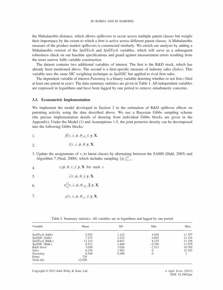
Table I. Summary statistics. All variables are in logarithms and lagged by one period

Variable Mean SD Min. Max.

SpillTech (Jaffe) 9.554 1.142 4.838 11.707SpillSIC (Jaffe) 7.272 2.323 �4.602 11.154SpillTech (Mah.) 11.314 0.847 8.235 13.156SpillSIC (Mah.) 8.513 1.660 �0.356 11.559R&D Stock 3.030 3.026 �2.513 10.765Sales 6.230 1.962 0 12.103Patenting 0.540 0.498 0 1Firms 729Total obs. 12,928



The Bayesian model described above contains a non-parametric specification of the individual effectsand we will denote it as FLEP (flexible latent effects probit). It is possible to estimate a restrictedparametric version of the same model by imposing the condition that in the unobserved individual effectsare Normally distributed. We shall label this version of the model as PLEP (parametric latent effectsprobit). By comparing the results of different specifications of the unrestricted nonparametric version withthe restricted parametric version of the samemodel we can gain additional insights into the importance andadvantages of using a flexible nonparametric specification over more traditional parametric approaches.Posterior means are reported for these two techniques, obtained from chains of total length of 10,000MC steps with a 5000 burn-in section.Additionally we implement two frequentist approaches to the estimation of spillover effects. First, we

implement the fixed-effects probit model with time dummies (denoted by FE). As we shall see, thisapproach suffers from serious computational limitations in large data. Second, we implement therandom-effects probit model with time dummies and the Chamberlain (1982) device (which wedenote by RE).Each estimation technique was applied to the two different specifications of the econometric model:

one using the Jaffe distance measure and one using the Mahalanobis distance measure. Below we shalldiscuss the empirical results in detail and perform additional econometric robustness checks.

3.4. Empirical Results

In a simple model of R&D BSV show that it is possible to derive a number of theoretical implicationsof these two spillover effects. If we assume that the production of knowledge is exogenous then wewould not expect to find an effect of market rivalry on patent counts. Empirically, this means thatthe coefficient on SpillSIC should be close to zero. The presence of positive market spillover effectsmay, however, indicate endogenous patenting activity. Thus we can investigate the extent to whichstrategic patenting activity is consistent with the evidence in the data.At the same time we expect the marginal effect of technology spillovers on patent counts to be

positive. The production of knowledge benefits from the innovation activity in a firm conditional onits own R&D stock. Empirically this implies that we should expect the coefficient on SpillTech to bepositive and significant.We will test these predictions using our model and several alternative benchmark models that are

commonly applied in the empirical literature. Recall that we define the dependent variable to be oneif the given firm registered a patent during the particular year or not. We can think of this case as anindicator of innovation for a given firm–year dyad. We then regress this indicator on the measuresof technological and product market spillovers discussed above: SpillTech and SpillSIC. In order tocontrol for observed firm-level heterogeneity, we include two additional variables. One correspondsto firm sales Ln(Sales), while the other corresponds to the pre-existing stock of R&D available withinthe firm Ln(R&D stock). Furthermore, we lag all right-hand-side variables by one period so as toremove the possibility of contemporaneous effects.

3.4.1. Partial EffectsEstimation results on the partial effects and the latent common time component are reported in Table 2.In the absence of endogenous patenting activity we should see the marginal effect of technologyspillovers SpillTech on patenting activity to be positive and the marginal effect of product marketspillovers SpillSIC to be zero.Across the various model specifications we find the effect of market rivalry to be small and statistically

insignificant, with the exception of PLEP for the Mahalanobis distance. Moreover, the effect changes signdepending on which distance measure is used. The evidence presented therefore does not reject the



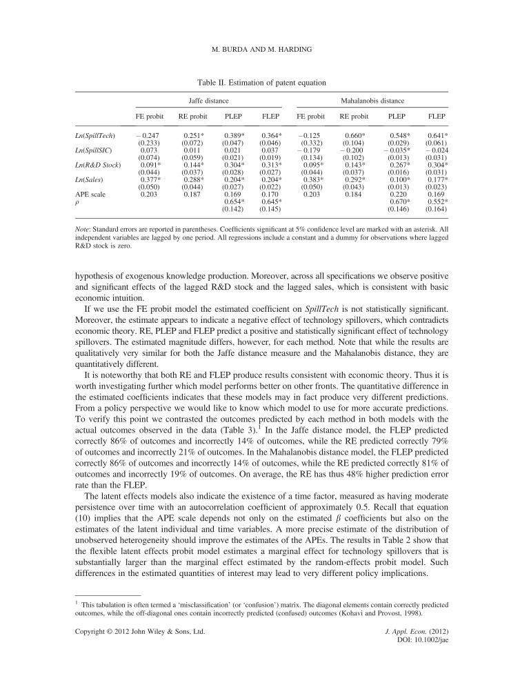
hypothesis of exogenous knowledge production. Moreover, across all specifications we observe positiveand significant effects of the lagged R&D stock and the lagged sales, which is consistent with basiceconomic intuition.

If we use the FE probit model the estimated coefficient on SpillTech is not statistically significant.Moreover, the estimate appears to indicate a negative effect of technology spillovers, which contradictseconomic theory. RE, PLEP and FLEP predict a positive and statistically significant effect of technologyspillovers. The estimated magnitude differs, however, for each method. Note that while the results arequalitatively very similar for both the Jaffe distance measure and the Mahalanobis distance, they arequantitatively different.

It is noteworthy that both RE and FLEP produce results consistent with economic theory. Thus it isworth investigating further which model performs better on other fronts. The quantitative difference inthe estimated coefficients indicates that these models may in fact produce very different predictions.From a policy perspective we would like to know which model to use for more accurate predictions.To verify this point we contrasted the outcomes predicted by each method in both models with theactual outcomes observed in the data (Table 3).1 In the Jaffe distance model, the FLEP predictedcorrectly 86% of outcomes and incorrectly 14% of outcomes, while the RE predicted correctly 79%of outcomes and incorrectly 21% of outcomes. In the Mahalanobis distance model, the FLEP predictedcorrectly 86% of outcomes and incorrectly 14% of outcomes, while the RE predicted correctly 81% ofoutcomes and incorrectly 19% of outcomes. On average, the RE has thus 48% higher prediction errorrate than the FLEP.

The latent effects models also indicate the existence of a time factor, measured as having moderatepersistence over time with an autocorrelation coefficient of approximately 0.5. Recall that equation(10) implies that the APE scale depends not only on the estimated b coefficients but also on theestimates of the latent individual and time variables. A more precise estimate of the distribution ofunobserved heterogeneity should improve the estimates of the APEs. The results in Table 2 show thatthe flexible latent effects probit model estimates a marginal effect for technology spillovers that issubstantially larger than the marginal effect estimated by the random-effects probit model. Suchdifferences in the estimated quantities of interest may lead to very different policy implications.

1 This tabulation is often termed a ‘misclassification’ (or ‘confusion’) matrix. The diagonal elements contain correctly predictedoutcomes, while the off-diagonal ones contain incorrectly predicted (confused) outcomes (Kohavi and Provost, 1998).

Table II. Estimation of patent equation

Jaffe distance Mahalanobis distance

FE probit RE probit PLEP FLEP FE probit RE probit PLEP FLEP

Ln(SpillTech) � 0.247 0.251* 0.389* 0.364* �0.125 0.660* 0.548* 0.641*(0.233) (0.072) (0.047) (0.046) (0.332) (0.104) (0.029) (0.061)

Ln(SpillSIC) 0.073 0.011 0.021 0.037 � 0.179 � 0.200 � 0.035* � 0.024(0.074) (0.059) (0.021) (0.019) (0.134) (0.102) (0.013) (0.031)

Ln(R&D Stock) 0.091* 0.144* 0.304* 0.313* 0.095* 0.143* 0.267* 0.304*(0.044) (0.037) (0.028) (0.027) (0.044) (0.037) (0.016) (0.031)

Ln(Sales) 0.377* 0.288* 0.204* 0.204* 0.383* 0.292* 0.100* 0.177*(0.050) (0.044) (0.027) (0.022) (0.050) (0.043) (0.013) (0.023)

APE scale 0.203 0.187 0.169 0.170 0.203 0.184 0.220 0.169r 0.654* 0.645* 0.670* 0.552*

(0.142) (0.145) (0.146) (0.164)

Note: Standard errors are reported in parentheses. Coefficients significant at 5% confidence level are marked with an asterisk. Allindependent variables are lagged by one period. All regressions include a constant and a dummy for observations where laggedR&D stock is zero.



3.4.2. Unobserved Firm HeterogeneityWe have noted above that both FLEP and PLEP produce quantitatively similar results for both distancemeasures.2 A key advantage of FLEP is that it does not impose the normality constraint on the unobservedheterogeneity. Furthermore, FLEP is the only model that allows us to uncover a nonparametric estimate ofthe distribution of firm heterogeneity.There is no sound economic reason to assume that this distribution isnormal and in fact we would expect that different types of production processes have very different formsof unobserved heterogeneity which impact patenting activity. In our application, the distribution ofheterogeneity is shown to have a multimodal clustering structure, as plotted in Figure 1. These clustersmay reflect the presence of missing variables important for characterizing innovation, such as firm cultureor investment strategy. In Figure 1 we can easily discern several major clustering structures in eachdistance model, labeled by numbers in square boxes, corresponding to the major modes of the distribution.In the Appendix we show that this clustering is robust to the choice of the DPM prior hyperparameter.In the FLEP output in Figure 1, each clustering structure is composed of draws of the firm-specific

unobserved heterogeneity component ti, which we can use to further analyze the composition of eachcluster. Table 4 lists the SIC code names for 20 firms whose ti was most frequently drawn within eachgiven clustering structure. Thus, for the Jaffe distance model, the lowest unobserved heterogeneitycomponent group (Clustering 1) is composed, for example, of ‘meat packing plants’, ‘blowers andfans’, or ‘department stores’; the medium unobserved heterogeneity component group (Clustering 2)includes ‘food and kindred products’, ‘footwear’, and ‘electrical industrial apparatus’; while the highunobserved heterogeneity component group (Clustering 3) features ‘semiconductors and relateddevices’, ‘electronic components’, or ‘commercial physical research’. The cluster composition is verysimilar in the Mahalanobis distance model and hence not reported here. Uncovering such clusterstructures of firms that behave similarly in terms of their unobserved characteristics can provide impor-tant insights for industry analysts and policy makers analyzing firms’ R&D behavior. Below we furtherinvestigate the extent to which our theoretical predictions are satisfied for each cluster.Using the FLEP output we can also explore the evolution of the draws of the unobserved heterogeneity

parameters ti for specific individual companies in order to investigate whether the draws are concentratedor show large variances as the Markov chain progresses. Overall, we have found the draws to be remark-ably stable, indicating a clear tendency of the model to associate each firmwith a narrow range of draws ofti. If a draw of ti jumps to a different cluster, it does not stay there long and returns shortly back to itslong-term average. This is an important indicator that the clustering of ti values observed in the estimateddistribution of unobserved heterogeneity may contain relevant information since it establishes a fairly tight

2 Nonetheless, PLEP estimated statistically significant product market spillovers, which was not confirmed by any othermodel specification.

Table III. Actual vs. predicted outcomes for RE and FLEP in the Jaffe distance model and Mahalanobis distancemodel

Predicted

RE FLEP

0 1 0 1

Actual

Jaffe 0 4473 1470 5026 917distance 1 1190 5795 911 6074

Mahalanobis 0 4591 1352 5020 923distance 1 1148 5837 911 6074



link between firms and different modes of the distribution of heterogeneity. To exemplify, we plot thedraws of ti for the first five firms for the model of positive patents model in Figure 2.

The estimated distribution of the unobserved heterogeneity provides valuable economic informationwhich can be used to analyze the data further and test additional economic hypotheses of interest. One

Table IV. Most frequent members of clustering structures for the Jaffe distance model

Clustering 1 Clustering 2 Clustering 3

4923 Gas Transmission andDistribution

3841 Surgical and MedicalInstruments

2835 Diagnostic Substances

2851 Paints and Allied Products 3661 Telephone and TelegraphApparatus

2840 Cosmetics

3060 Fabricated Rubber Products 3825 Instruments To MeasureElectricity

3714 Motor Vehicle Parts andAccessories

3440 Fabricated Structural Metal 3577 Computer PeripheralEquipment

2761 Manifold Business Forms

2011 Meat Packing Plants 4011 Railroads, Line-haulOperating

2390 Misc. Fabricated Textile

2731 Book Publishing 3590 Misc. industrial machinery 3823 Process Control Instruments3561 Pumps and Pumping Equipment 3537 Industrial Trucks and Tractors 3572 Computer Storage Devices3640 Electric Lighting and Wiring

Equipment6324 Hospital and Medical Service

Plans3674 Semiconductors and Related

Devices2030 Canned, Frozen, and Preserved

Fruit2000 Food and Kindred Products 3679 Electronic Components

3533 Oil and Gas Field Machinery 3669 Communications Equipment 3420 Handtools3663 Radio and TV Communications

Eqpt3310 Steel Works, Blast Furnaces 2842 Sanitation Goods

3944 Games, Toys, and Children’sVehicles

3140 Footwear, Except Rubber 3990 Misc. Manufacturing Industries

3621 Motors and Generators 3620 Electrical IndustrialApparatus

8731 Commercial Physical Research

2253 Knit Outerwear Mills 2834 Pharmaceutical Preparations 3613 Switchgear and SwitchboardApparatus

3579 Office Machines 3711 Motor Vehicles and CarBodies

3670 Electronic Components andAccessories

3743 Railroad Equipment 4931 Electric and Other ServicesCombined

3530 Material Handling Equipment

3490 Miscellaneous Fabricated MetalProducts

3021 Rubber and Plastics Footwear 3829 Measuring and ControllingDevices

3564 Blowers and Fans 2911 Petroleum Refining 8731 Commercial Physical Research2522 Office Furniture, Except Wood 3569 General Industrial Machinery 2821 Plastics Materials and Resins5311 Department Stores 3690 Misc. Electrical Machinery 3861 Photographic Equipment and

Supplies

1 2 3

0.2

.4.6

.8D

ensi

ty

−5 0 5

tau

1 2 3

0.2

.4.6

.8D

ensi

ty

−5 0 5

tau

Figure 1. Flexible latent effects probit (FLEP) distribution of unobserved heterogeneity for the Jaffe distancemodel (left) and Mahalanobis distance model (right)



such hypothesis is that there are unobserved industry-level factors driving innovation. In order toinvestigate this hypothesis, we plot the average sampled value of the unobserved heterogeneitycomponent ti by each SIC code for the two estimated models of innovation in Figure 3. The absence ofany discernible pattern in the graphs suggests that the unobserved heterogeneity component is not drivenby industry factors but is rather firm-specific at the individual level. Indeed, further examination ofindividual ti revealed large differences in company types even within SIC categories. It appears thatassociating the unobserved heterogeneity with industry categories and attempting to capture it, forexample by industry indicator variables, may obscure important differences among firms regarding theirinnovation activity. When we re-estimated the models using industry dummies in addition to the variablesintroduced above, the resulting changes were negligible. The nonparametric density estimates of theunobserved heterogeneity were almost identical to the ones previously discussed. This further highlightsthe benefit of the FLEP model in tracking unobserved heterogeneity at the individual level.

3.4.3. Cluster-Based Partial EffectsGiven that we have established the presence of three major clusters in the distribution of firm heterogeneity,we can revisit our original model and re-estimate it separately for each cluster. This allows us to investigatethe extent to which the strength of the spillover effects varies across groups of firms. As BSV emphasize,an important robustness check for the economic model is to verify the extent to which the results holdacross groups of firms. If they do not, this may indicate that the estimated spillover effects are spuriouslygenerated by pooling across different types of firms. The summary statistics for the firms in each clusterare given in Table 5. It is interesting to note that the extent of patenting activity varies substantially across

−2

−1

01

23

Indi

vidu

al h

eter

ogen

eity

dra

ws

0 2000 4000 6000 8000 10000

MC step

−2

−1

01

23

Indi

vidu

al h

eter

ogen

eity

dra

ws

5000 6000 7000 8000 9000 10000

MC step

Figure 2. Draws of ti for the first five companies. Jaffe distance model (left) and Mahalanobis distance model (right)

−4

−3

−2

−1

01

23

4

avgt

au

0 2000 4000 6000 8000 10000sic

−4

−3

−2

−1

01

23

4

avgt

au

0 2000 4000 6000 8000 10000sic

Figure 3. Average ti of companies for each SIC. Jaffe distance model (left) and Mahalanobis distance model (right)



clusters. The first cluster corresponding to negative values for the firm-level heterogeneity has a lowdegree of patenting activity, while the third cluster corresponding to positive values of the firm-levelheterogeneity has a high degree of patenting activity. The summary statistics for the observable variablesare, however, fairly similar across clusters, which indicates that the unobserved heterogeneity has animportant role to play. The results of the patent equation estimation with FLEP are given in Table 6 foreach cluster, respectively. The presence of technology spillover effects is confirmed for each clusterindividually. The effect of product market rivalry continues to be statistically negligible for each cluster.These results show that the economic model is thus robust to unobserved heterogeneity.

Table V. Summary statistics for individual clusters. All variables are in logarithms and lagged by one period

Variable


Mean SD Min. Max. Mean SD Min. Max.

Cluster 1SpillTech 9.516 1.029 4.838 11.707 11.252 0.801 8.519 13.156SpillSIC 7.157 2.420 �4.602 11.154 8.417 1.685 1.220 11.559R&D Stock 4.112 1.996 �0.888 10.231 2.378 2.909 �1.482 10.231Sales 6.143 1.922 1.098 11.760 6.144 1.946 1.098 11.760Patenting 0.262 0.440 0 1 0.291 0.454 0 1Firms 219 260Total obs. 3916 4593Cluster 2SpillTech 9.621 1.181 4.935 11.531 11.377 0.868 8.252 13.110SpillSIC 7.388 2.283 �4.321 11.053 8.585 1.656 �0.356 11.355R&D Stock 4.694 2.219 �2.513 10.765 3.511 3.082 �2.513 10.765Sales 6.286 2.023 0.693 12.103 6.320 2.000 0 12.103Patenting 0.622 0.484 0 1 0.649 0.477 0 1Firms 415 402Total obs. 7361 7155Cluster 3SpillTech 9.346 1.195 5.017 11.411 11.172 0.860 8.235 12.840SpillSIC 7.032 2.233 �2.700 10.981 8.4523 1.565 2.631 11.268R&D Stock 4.318 1.698 0.085 8.306 4.0012 1.530 0.085 8.161Sales 6.187 1.764 0 10.430 6.0130 1.752 1.386 10.430Patenting 0.832 0.373 0 1 0.8457 0.361 0 1Firms 95 67Total obs. 1651 1180

Table VI. Estimation of patent equation by cluster with FLEP


Cluster 1 Cluster 2 Cluster 3 Cluster 1 Cluster 2 Cluster 3

Ln(SpillTech) 0.681* 0.529* 0.720* 0.852* 0.610* 0.897*(0.077) (0.043) (0.097) (0.069) (0.040) (0.124)

Ln(SpillSIC) 0.026 0.035 0.016 �0.031 �0.008 �0.066(0.026) (0.019) (0.054) (0.027) (0.017) (0.069)

Ln(R&D Stock) 0.219* 0.345* 0.290* 0.198* 0.332* 0.385*(0.035) (0.022) (0.088) (0.033) (0.024) (0.117)

Ln(Sales) 0.157* 0.182* 0.347* 0.169* 0.177* 0.205*(0.028) (0.019) (0.068) (0.024) (0.017) (0.086)

APE scale 0.192 0.170 0.067 0.191 0.167 0.054r 0.671* 0.620* 0.274* 0.468* 0.689* 0.514*

(0.147) (0.150) (0.214) (0.197) (0.130) (0.196)

Note: Standard errors are reported in parentheses. Coefficients significant at 5% confidence level are marked with an asterisk. Allindependent variables are lagged by one period. All regressions include a constant and a dummy for observations where laggedR&D stock is zero.



We can also perform one additional robustness check. If the FLEP model has correctly identifiedeach cluster we should be able to estimate the model reasonably well using RE by sub-setting the datafor each cluster. If heterogeneity is driving the resultsof the model once we condition on a cluster REshould perform similar to FLEP.3 The robustness check results are reported in Table 7, using subsets ofdata corresponding to each cluster. RE and FLEP perform similarly in terms of predictions. It isimportant to remember, however, that this exercise can only be performed in post estimation,conditional on the given cluster. A priori, we can never be sure about the structure of the distributionof the unobserved heterogeneity, which emphasizes the importance of using a flexible model whenaddressing unobserved heterogeneity.

4. CONCLUSION

This paper introduced a new Bayesian semi-parametric approach to the estimation of the probit model inpanel data with unobserved heterogeneity. The proposed model substantially improved on currentbenchmark methods by relaxing three assumptions that are often either ignored or treated in an ad hocfashion in empirical work. First, we modeled unobserved individual effects using a flexible nonparametricform with desirable local adaptability properties. Second, we allowed for the unobserved heterogeneity tobe correlated with the observables. Finally, our model incorporated common latent time effects.We employed a combination of recent powerful sampling algorithms in order to draw from a DP

Mixture model specified for the unobserved heterogeneity component. We evaluated the proposedmodel in a number of Monte Carlo simulations along with existing fixed and random effects modelalternatives. The underlying parameters are shown to be estimated with high precision in the proposedmodel, unlike for the benchmark cases. The simulations presented in the online supporting informationhighlight the benefit of using the flexible proposed model when the underlying heterogeneity is notwell approximated by a parametric distributional form.We applied the proposed method to the estimation of a patent equation in the presence of both

technological and product market spillover effects. We showed that technological innovation is subject

3 Note that FLEP also controls for the presence of time factors which are ignored by the RE model. If, however, firm-specificheterogeneity dominates in the data, then we would expect both models to have similar performance.

Table VII. Actual vs. predicted outcomes for RE and FLEP in the Jaffe distance model and Mahalanobis distancemodel for each cluster

Predicted

RE FLEP

0 1 0 1

Actual

Cluster 1 0 2668 219 2674 2131 412 617 426 603

Cluster 2 0 2212 567 2195 5841 480 4102 497 4085

Cluster 3 0 213 64 214 631 26 1348 26 1348

Cluster 1 0 2987 269 2987 2701 481 856 471 866

Cluster 2 0 1959 546 1922 5831 463 4187 443 4206

Cluster 3 0 145 37 147 351 20 978 19 979



to substantial firm-level heterogeneity which persists within individual industries. We have shown thatinnovation depends in an important way on technology spillovers but that there is little evidence in favorof product market spillover effects. On the basis of the estimated firm-level heterogeneity we also showedthat unobserved heterogeneity is heavily clustered and that the clustering matters when making in-samplepredictions of patenting activity.

ACKNOWLEDGEMENTS

We are grateful to Nick Bloom for sharing the data for the empirical application with us. We also thankSiddhartha Chib, David Dahl, Christian Gourieroux, Jerry Hausman, Ivan Jeliazkov, Andriy Norets,seminar participants at UC Berkeley and UC Irvine, and conference audiences at the North AmericanSummer Meetings of the Econometric Society in Boston 2009, and the Canadian Econometrics StudyGroup 2009 Ottawa meetings for useful comments. This work was made possible by the facilities ofthe Shared Hierarchical Academic Research Computing Network (SHARCNET: www.sharcnet.ca).

REFERENCES

Abrevaya J. 1999. Leapfrog estimation of a fixed-effects model with unknown transformation of the dependentvariable. Journal of Econometrics 93(2): 203–228.

Albert J, Chib S. 1993. Bayesian analysis of binary and polychotomous response data. Journal of the AmericanStatistical Association 88(422): 669–679.

Albert J, Chib S. 1996. Bayesian modeling of binary repeated measures data with application to crossover trials. InBayesian Biostatistics Berry DA, Stangl DK (eds). Marcel Dekker: New York; 577–600.

Allenby G, Lenk P. 1994. Modeling household purchase behavior with logistic normal regression. Journal of theAmerican Statistical Association 89: 1218–1231.

Arellano M, Bonhomme S. 2009. Robust priors in nonlinear panel data models. Econometrica 77(2): 489–536.Arellano M, Hahn J. 2006. A likelihood-based approximate solution to the incidental parameter problem in

dynamic nonlinear models with multiple effects. Working paper, CEMFI.Berry ST, Haile PA>2009. Nonparametric identification of multinomial choice demand models with heterogeneous

consumers. Cowles Foundation Discussion Papers 1718, Cowles Foundation, Yale University.Bloom N, Schankerman M, Van Reenen J. 2010. Identifying technology spillovers and product market rivalry.

NBER Working Paper 13060.Bolduc D, Fortin B, Gordon S. 1997. Multinomial probit estimation of spatially interdependent choices: an empirical

comparison of two new techniques. International Regional Science Review 20(1–2): 77101.Burda M, Harding MC, Hausman JA. 2008. A Bayesian mixed logit–probit model for multinomial choice. Journal

of Econometrics 147(2): 232–246.BurdaM, Liesenfeld R, Richard J-F. 2011. Bayesian analysis of a probit panel data model with unobserved individual

heterogeneity and autocorrelated errors. International Journal of Statistics and Management Systems 6(1–2): 1–21.Chamberlain G. 1982. Multivariate regression models for panel data. Journal of Econometrics 18: 5–46.Chamberlain G. 1984. Panel data. In Handbook of Econometrics, Vol. 2, Griliches Z, Intriligator M (eds).

North-Holland: Amsterdam; 1247–1318.Chib S. 1993. Bayes estimation of regressions with autoregressive errors: a Gibbs sampling approach. Journal of

Econometrics 58: 275–294.Chib S, Carlin B. 1999. On MCMC sampling in hierarchical longitudinal models. Statistics and Computing 9: 17–26.Chib S, Hamilton B. 2002. Semiparametric Bayes analysis of longitudinal data treatment models. Journal of

Econometrics 110: 67–89.Chib S, Jeliazkov I. 2006. Inference in semiparametric dynamic models for binary longitudinal data. Journal of the

American Statistical Association 101(474): 685–700.Dahl DB. 2005. Sequentially-allocated merge–split sampler for conjugate and nonconjugate Dirichlet process

mixture models. Technical report, Texas A&M University.Escobar MD, West M. 1995. Bayesian density estimation and inference using mixtures. Journal of the American

Statistical Association 90: 577–588.Fernandez-Val I. 2007. Fixed effects estimation of structural parameters and marginal effects in panel probit

models. Working paper, Boston University.



http://www.sharcnet.ca

Geweke J. 1991. Efficient simulation from the multivariate normal and Student-t distributions subject to linearconstraints. In Computing Science and Statistics: Proceedings of the Twenty-Third Symposium on the Interface,Keramidas EM (ed.). Interface Foundation of North America: Fairfax, VA.

Geweke J. 2005. Contemporary Bayesian Econometrics and Statistics. Wiley: Chichester.Griffith R, Lee S, Van Reenen J. 2011. Is distance dying at last? Falling home bias in fixed effects models of patent

citations. Quantitative Economics 2(2): 211–250.Gu Y, Fiebig DG, Cripps E, Kohn R. 2009. Bayesian estimation of a random effects heteroscedastic probit model.

Econometrics Journal 12(2): 324–339.Hajivassiliou V. 1990. Smooth estimation simulation of panel data LDV models. Working paper, Yale University.Hausman JA, Taylor WE. 1981. Panel data and unobservable individual effects. Econometrica 49(6): 1377–1398.Hirano K. 2002. Semiparametric Bayesian inference in autoregressive panel data models. Econometrica 70: 781–799.Jaffe AB. 1986. Technological opportunity and spillovers of R&D: evidence from firms’ patents, profits, and

market value. American Economic Review 76(5): 984–1001.Keane M. 1990. A computationally efficient practical simulation estimator for panel data, with applications to

estimating temporal dependence in employment and wages. Working paper, University of Minnesota.Knittel CR, Metaxoglou K. 2008. Estimation of random coefficient demand models: challenges, difficulties and

warnings. Working paper, NBER.Kohavi R, Provost F. 1998. Glossary of terms. Editorial for the special issue on application of machine learning

and the knowledge of discovery process. Machine Learning 30: 271–274.Lancaster T. 2004. An Introduction to Modern Bayesian Econometrics. Blackwell: Malden, MA.Li T, Zheng X. 2008. Semiparametric Bayesian inference for dynamic Tobit panel data models with unobserved

heterogeneity. Journal of Applied Econometrics 23: 699–728.Neal R. 2000. Markov chain sampling methods for Dirichlet process mixture models. Journal of Computational

and Graphical Statistics 9(2): 249–265.Paap R. 2002. What are the advantages of MCMC based inference in latent variable models? Statistica

Neerlandica 56(1): 2–22.Rossi P. 2010. Bayesm: Bayesian inference for marketing/micro-econometrics. R package version 2.2-3.Train K. 2001. A comparison of hierarchical Bayes and maximum simulated likelihood for mixed logit. Working

paper, Department of Economics, University of California, Berkeley.Train K. 2003. Discrete Choice Methods with Simulation. Cambridge University Press: Cambridge, UK.Troughton P, Godsill S. 1997. Bayesian model selection for time series using Markov chain Monte Carlo. In IEEE

International Conference on Acoustics, Speech, and Signal Processing, 1997 (ICASSP-97), Vol. 5; 3733–3736.Wooldridge JM. 2001. Econometric Analysis of Cross Section and Panel Data. MIT Press: Cambridge, MA.



APPENDIX A

Sampling b

In this block we apply the method of Albert and Chib (1993) to the recentered latent variable~y�it ¼ ~yit � ti � lt. The joint conditional density of b; y~�Þð is given by

p�b; y~�jt; l;c; θ=b; y~; y;X

�/ exp

h� 12

b��b

� �′�Σ�1b b�

�b

� �iexph� 12

y~� � Xbð Þ′ y~� � Xbð Þi

yielding a closed form of the conditional posterior for b which facilitates direct sampling fromb � � N �b;Σ�

� �� where

�b ¼ Σ� Σ�1� �

bþ X′y~��

Σ� ¼ Σ��1 þ X′X

� �� 1

In the application, we specify the hyperparameter values�b ¼ 0 and Σ�b

¼ 10I, where I is the identity

matrix. This specification is aimed at rendering the prior for b sufficiently diffuse.

Sampling ~yit

Here we benefit from the second step of the Albert and Chib (1993) procedure, augmented by ti and lt.Thus we sample directly

~yiyj� � N vit; 1ð Þ

vit ¼ xitbþ ti þ lt

truncated by 0 from the left if yit= 1 and from the right if yit= 0.

Updating Latent Class Assignments

For this block we utilize a hybrid sampler that alternates between the non-conjugate version of theSAMS sampler of Dahl (2005) and Algorithm 7 of Neal (2000). This approach is suggested by Dahl(2005) as optimally combining the virtues of each method: the ability to move large blocks of elementsamong latent classes in one step for the former, and one-at-a-time allocations of individual elementsamong latent classes for the latter.

The SAMS sampler is based on an alternative expression of the model (6)–(8) in terms of a set partition

p= {S1, . . . , Sq} for S0 = {1, . . . , n} in addition to the latent class parameters f ¼ fS1 ; . . . ;fSq

n o, where

fS is associated with component S. The set partition p for S0 is a set of subsets S1, . . . , Sq such that

(1) ∪ S2 pS = S0, (2) Si∩ Sj =∅ for all Si 6¼ Sj, and (3) S 6¼∅ for all S2 p. Using this notation, the model

(6)–(8) can be recast as (Dahl, 2005)



ti p;f � Ft fiS

� �� (15)

cjp �YS2p

G0 fSð Þ (16)

p � bYS2p

�0Γ Sj jð Þ (17)

where |S| is the number of elements of the component S. The sampling scheme works as follows. Ineach MC iteration, uniformly select a pair of distinct indices i and j. If i and j belong to the samecomponent in p, say S, propose p* by splitting S. Otherwise, i and j belong to different componentsin p, say Si and Sj. Propose p* by merging Si and Sj. In each case, compute the Metropolis–Hastings(MH) ratio a(p*,f*|p,f) and accept the new latent class configuration p* with probability given by thisratio. We derive the MH ratio for our model in the following section.Algorithm 7 of Neal (2000), which we utilize in every alternateMC step, is based on limiting probabilities

of a latent class finite mixture model, with the number of classes tending to infinity. The sampling procedureitself is built around drawing with a stochastic number of mixture components or classes whose number andsize varies at each MC iteration. Denote by c a label of a generic latent class with membership count Nc.Given the current state of the system, ti are first reassigned to latent classes with labels ci, whereby new clas-ses can be created and old ones may vanish. The probabilities of class assignment for the ti are proportionalto the likelihood of ti conditional on the current draw of the class parameters cc. Second, the classparameterscc are updated in a standard way for each class separately. If we specify Ft as an infinite mixtureof Normals, then cc ¼ mtc; s

2tc

� �are the moments of the Normal density.

For updatingc in the Algorithm 7 scan, we specify Ft as a mixture of Normals withc ¼ mt; s2t

� �. Since

for all ti that fall into one latent class it holds that ti � N mtc; s2tc

� �we can apply result B (p. 300) of Train

(2003) to each latent class separately: for an IG(s0, v0) prior, the posterior of s2tc is given by IG(s1, v1) withv1 = v0 +Nc and s1 ¼ v0s0 þ Nc�scið Þ= v0 þ Ncð Þ where �sc ¼ N�1

c

PNci¼1 t2i .We utilize a diffuse IG prior.

Analogously, to samplemtcwe use result A of Train (2003) applied to each latent class. The hyperparameterof the DP prior a is sampled according to the scheme of Escobar and West (1995).The iteration between the samplers of Dahl (2005) and Neal (2000) alleviates the influence of particular

starting values. The SAMS sampler is capable of reallocating large blocks of data to one of the latentclasses, while the Neal algorithm addresses the individual by individual allocation to latent classes. Thisallows us to initialize the procedure with a unique parametric component. This is then rapidly split intoclasses by the SAMS sampler before the Neal procedure continues to fine-tune the posterior draws.

Sampling ti

Let y~��i ¼ y~i � Xib� l. Then

y~��i ¼ tiiþ ei

Consider for the moment the case ti � N�t; s2t� �

; it will be used as a building block in the DP prior

sampling. In this case, for every i we have one latent regression with one parameter ti and a (T� 1)vector of ones as explanatory variables in place of a hypothetical Xi. Using standard latent regressionresults (see, for example, Lancaster, 2004)



p tið j�Þ ¼ f �ti; �s2ti� �

(18)

�ti ¼ �s2ti s�2t �tþ

XTi¼1

y~��i

!

�s2ti ¼ s�2t þ T

� ��1

Since ti � N mtc; s2tc

� �given a previous assignment to the latent class c, let

�t ¼ mtc; s2t ¼ s2tc and

sample ti directly from (18).

Sampling l

Let

y~il ¼ y~i � Xib� tii

Then the joint density implied for y~l ¼ y~1l ; . . . ; y~NlÞ�by the recentered probit model conditional on

l is

f ~ylð jl; �Þ ¼ 2pð Þ�NT=2det ITð Þ�N=2exp

n� 12

XNi¼1

y~il′I�1T y~il � 2l′I�1

T y~li þ l′I�1T l�

while the prior density specified by Assumption 3 takes the form

f lð Þ ¼ 2pð Þ�T=2det ITð Þ�1=2exp � 12l′Ω�1

l l� 2l′Ω�1l Λrþ r′Λ′Ω�1

l Λr�

where Λt ¼ lt�1; . . . ; lt�sð Þ;Λ ¼ Λ′1; . . . ;Λ′

T

� �′;r ¼ r1; . . . ; rsð Þ and Ωl is the covariance matrix

associated with the autoregressive process. Hence we can sample l directly from N �l;Σ�

l

� �where

�l ¼ Σ�

lΩ�1

l �lþ

XNi¼1

y~li

!

�Σl ¼ Ω�1l þ N � IT

� ��1

For ease of implementation we restrict ourselves to the AR(1) specification with a singleautoregressive parameter r in the application. In this case



Ωl ¼ g0

r0 r1 r2 ⋯ rT�1

r1 r0 r1 ⋯ rT�2

r2 r1 r0 rT�3

⋮ ⋮ ⋱ ⋮rT�1 rT�2 rT�3 ⋯ r0

266664

377775

g0 ¼s2�

1� r2

Sampling r

Note that for the AR(1) process

pðlt lt�1; �j Þ /exp � 1� r2ð Þ

2s2�l21

!; t ¼ 1

exp � 12s2�

lt � rlt�1ð Þ2 !

; t ¼ 2; . . . ; T

8>>>><>>>>:

and hence

pðr lj Þ ¼ exp � 12s2�

1� r2� �

l21 þXTt¼2

lt � rlt�1ð Þ2" # !

¼ exp12s2�

r2XTt¼2

l2t�1 � l21

!� 2r

XTt¼2

ltlt�1 þXTt¼1

l2t

" ! #ÞMatching this expression with a Gaussian kernel exp � 1

2s2 r2 � 2rmþ m2½ �� yields

�s2r ¼ s2�XT�1

t¼2

l2t

!�1

�mr ¼ �s2rs2�

XTt¼2

ltlt�1

¼XT�1

t¼2

l2t

!�1XTt¼2

ltlt�1

We can therefore sample r directly from N �mr; �s2r

� �truncated at �1 and 1 to preserve stationarity.

Extension to AR(p) will amend the likelihood function p(lt|lt� 1,�) but the derivation would be similar.The approach for sampling the AR(p) parameters conditional on the initial observations is presented inChib (1993).



Sampling s2�

For this block we use the result derived in Burda et al. (2011), which adapts the standard result onsampling univariate variances (given, for example, by result B, p. 300 of Train, 2003) to the likelihoodof the variance of the AR process. Conditional on l and r, the likelihood function of s2� takes the form

Lðs2� l; θ=s2�

�� /

ffiffiffiffiffiffiffiffiffiffiffiffiffi1� r2

ps�

ffiffiffiffiffiffi2p

p exp � 1� r2

2s2�l21

" #YTt¼2

1

s�ffiffiffiffiffiffi2p

p exp � 12s2�

lt � rlt�1ð Þ2" #

An IG(v0, s0) prior has density

k s2��

¼ 1

m0sv0þ1ð Þ=2�

exp � v0s02s�

where m0 is a normalizing constant. We can then sample directly from the posterior

Lðs2� l; θ=s2�

�� / Lðs2� l; θ=s2�

�� k s2��

/ 1

s Tþv0þ1ð Þ=2�

exp � 1� r2ð Þl21 þPT

t¼2 lt � rlt�1ð Þ2 þ v0s02s2�

" #

¼ IG v1; s1ð Þ

where

v1 ¼ v0 þ T

s1 ¼ v0s0 þ 1� r2ð Þl21 þPT

t¼2 lt � rlt�1ð Þ2v0 þ T

In the application, the prior for s2� will be specified as diffuse with s0! 0 and v0¼ 0.

The SAMS Sampler

In this section, we explicitly derive the form of the MH ratio for our case. For a general description, seeDahl (2005). Let k be the successive values in random permutations of the indices in S. In our model,the MH ratio is given by

a p�;f�ð jp;fÞ ¼ minh1;p p�;f�ð jyÞp p;fð jyÞ

q p;fð jp�;f�Þq p�;f�ð jp;fÞ

i

If the proposal involves a split, q(p*,f*|p,f) is the split probability and q(p,f|p*,f*)¼ 1 is themerge probability. If the proposal involves a merge, the roles of q(p*,f*|p,f) and q(p,f|p*,f*) arereversed. Consider, for example, proposal for a split:



qðp�;f� p;fj Þ ¼YNk¼1

Pðk 2 Si Si; Sj;f; y��

PðfSiÞ

The first term is given in equation (13) in Dahl (2005). The second term P fSið Þ is the proposaldensity of the new fSi .The merge probability is

q p;f p�;f�j Þ ¼ 1ð

By Bayes’ theorem

p p;f yj Þ / p y p;fj Þp p;fð Þðð (19)

where p(y|p,f) is the likelihood

pðy p;fj Þ ¼Yni¼1

pðyi fSiÞ��

and p(p,f) is the prior

p p;fð Þ ¼ p f pj Þp pð Þð (20)

where

p fð jpÞ ¼QS2p F0 fSð Þp pð Þ ¼ b

QS2p �0Γ Sj jð Þ

b�1 ¼Yni¼1

Γ �0 þ i� 1ð Þ

Note that for a split of a class Ss into Si and Sj

p yjp�;f�ð Þpðy p;fj Þ ¼

Q Sij jt¼1 pðyt fSij ÞQ Sjj j

t¼1 pðyt fSjj ÞQ Ssj jt¼1 p ytjfSsð Þ

(21)

where the index t in p yt fSij Þð refers to elements of the class Si.Similarly, for a merge of classes Si and Sj

into Ss

pðy p�;f�j Þpðy p;fj Þ ¼

Q Ssj jt¼1 pðyt fSsj ÞQ Sij j

t¼1 p yt fSij ÞQ Sjj jt¼1 p yt fSjj Þð

�

i.e. the inverse of the ratio of split probabilities. Note that for a split we can use the stored values of thelikelihood evaluations from the allocation of k into Si and Sj. Hence only two additional likelihoodevaluations p yi fSij Þð and p yj fSjj Þ�

that initiated the split need to be performed for obtaining the ratiop yjp;fð Þp yjp�;f�ð Þ. For a merge, only 2|Si| + |Sj| likelihood evaluations need to be performed, which for small clas-ses can be substantially less than the sample size n. In the same spirit, for computing prior componentsfor a split



ptðf� p�j Þptðf pj Þ ¼ F0 fSið ÞF0 fSjð Þ

F0 fSsð Þand

p p�ð Þp pð Þ ¼ Γ Sij jð ÞΓ Sjj jð Þ

Γ Ssj jð Þwhile for a merge

ptðf� p�j Þptðf pj Þ ¼ F0 fSsð Þ

F0 fSið ÞF0 fSjð Þand

p p�ð Þp pð Þ ¼ Γ Ssj jð Þ

Γ Sij jð ÞΓ Sjj jð Þ

Thus, using (19), the ratio of the p-terms for a split becomes

ptðp�;f� yj Þptðp;f yj Þ ¼

Q Sij jt¼1 ptðyt fSij ÞQ Sjj j

t¼1 ptðyt fSjj ÞQ Ssj jt¼1 ptðyt fSsj Þ

F0 fSið ÞF0 fSjð ÞF0 fSsð Þ

Γ Sij jð ÞΓ Sjj jð ÞΓ Ssj jð Þ (22)

while for a merge this ratio is given by the inverse of the expression in (22).

DPM Prior Hyperparameter

In order to explore the distribution of unobserved heterogeneity, ti, in our patent models we need tomake sure that its behavior is not implicitly restricted by the estimation procedure or some other deepmodel parameters. One parameter that is of concern to us is the smoothing parameter a that controls theextent to which the DP draws mixture distributions that are more or less ‘similar’ to the Normalbaseline parametric distribution G0. In the limiting case of a!1 the mixture distribution becomesequivalent to G0, while in the other extreme a! 0 the mixture distribution limits to a convolution ofdensity kernels centered at each data point without any influence of the DP prior. The posteriordistribution estimate for both models is plotted in Figure 4. The distributions are concentrated arounda mode of 2, indicating a strong influence of data relative to the baseline prior distribution.

0.1

.2.3

.4

Den

sity

0 2 4 6 8

alpha

0.1

.2.3

.4D

ensi

ty

0 2 4 6 8

alpha

Figure 4. Density of draws of a, Jaffe distance model (left) and Mahalanobis distance model (right)



panel probit with flexible correlated …harding1/resources/harding_panelprobit.pdfpanel probit with...

Documents