paper on mode 4 - center for global development docs/10.23.03 gdn conf... · email:...
TRANSCRIPT

THE IMPACT OF THE MODE 4 LIBERALIZATION OF SERVICES ON ECONOMIC GROWTH, AND POLICY OPTIONS
Hennadige. N. Thenuwara*
Additional Director Economic Research Department
Central Bank of Sri Lanka 30, Janadhipathi Mawatha
Colombo 01-Sri Lanka
Tel: 94 –1- 2477168 Fax: 94-1-2477712
Email: [email protected]
Abstract
This paper develops a model based on realistic assumptions of international movement of natural persons such as the heterogeneity of and private information on agent types, and outlines the scope for national policy and the role of private agents. The paper argues that it is always beneficial for a country to have a liberal policy on the acceptance of natural persons, and admit high quality human capital. However, due to private information on the quality of human capital, professional organizations and private agents may maintain certain standards of observable attributes of would-be migrants. Those standards are costly to adhere to, thus serve as a screening device for choosing high quality human capital.
The model demonstrates that high quality human capital in a poor country tends to migrate under Mode 4 liberalization to rich countries. However, if the poor country is above a threshold poverty level, actual migration may or may not take place, i. e. there could be multiple equilibria. The source of multiple equilibria is the strategic complementarity and failure in coordinating actions of a large number of agents. Therefore, a poor country, while having a liberal policy on movement of natural persons, could strengthen economic and social infrastructure to avoid herd behavior and mass migration of high quality human capital.
Liberal policies on movement of natural persons could reduce welfare of a host country if not accompanied by costly screening mechanisms. With such costly screening, movement of natural persons always increases welfare of the all agents in host countries, as well as welfare of migrants, but reduces the welfare of agents with low quality human capital in source countries.
JEL Classification Numbers: F22, O15, O40
* The author is Additional Director of Economic Research attached to the Central Bank of Sri Lanka. The views expressed in this papers are his own and do not represent those of the Central Bank of Sri Lanka. The author wishes to thank Steve Williamson, Thomas Pogue, Robert Tamura, Gene Savin and Forrest Nelson and Yi Wen for comments. He also wishes to thank participants of the Conference on Immigration held at the University of Nebraska, Lincoln, Participants of the Macro Seminars at the University of Iowa and Participants of Central Bank of Sri Lanka Seminar Series. All errors are his own.
1
1 Introduction
Services play a dominant role in economic growth and development of a country.
Quah (1997) shows that most of the economic growth in many developed and developing
countries arises from growth in the services sector. In view of the benefits of larger
markets, the World Trade Organization (WTO) encourages countries to grant foreign
service suppliers greater access to their markets. The fundamental economic reasoning is
similar to the reasons discussed in Smith (1776), and reasons behind the benefits of trade
in goods. However, services can be supplied by more ways, or modes, than goods, which
are supplied only through cross-border mode (Mode 1). The other modes of supplying
services are through consumption abroad (Mode 2), commercial presence (Mode 3) and
movement of natural persons (Mode 4). To allow services flow through all four modes,
countries have to undertake complicated liberalization measures in several markets such
as financial market, labor market, and in immigration procedures.
Services sector spans across a wide spectrum (WTO Secretariat 1991). WTO
Secretariat (1991) has listed twelve categories of services. Production of many of those
services requires high quality human capital. Thus, Mode 4 liberalization would amount
to significant extent of high quality human capital moving across countries. The duration
of stay by a service provider in a foreign country is temporary as explained by the WTO
Secretariat (2002). However, WTO Secretariat (2002, pp 2) further explains that ‘there is
no specified time frame in the GATS of what constitutes ‘temporary’ movement; this is
defined negatively, through the explicit exclusion of permanent presence’. Thus, the

2
duration of stay of a service provider could be a longer period, as long as the stay is not
extended to arouse political economy issues of migration as discussed in Winters (2002).
Thus, I use the term ‘migration’ in this paper to indicate movement of natural persons for
considerably longer periods of time. This consideration is realistic since natural persons
providing services tends to stay longer periods in host countries once they establish
service centers, or join service centers domiciled in host countries. Any short-term
movement is more akin to Mode 1 supply of goods, and does not enable an interesting
analysis on the impact of Mode 4 liberalization.
As WTO Secretariat (2002) indicates, Mode 4 is the least liberalized mode, which
indicates that there is a reluctance to admit natural persons liberally. However, there
exists a general bias in favor of admitting high quality human capital such as executives,
managers and specialists. This is achieved by establishing screening devices to separate
high quality human capital from low quality human capital.
The objectives of this paper are to construct a model of migration of high quality
human capital, to use the model to evaluate the welfare and growth implications of
migration in economies, and to focus on appropriate economic policies for countries. I
explain the motivation to migrate to supply services and motivation to invite such
migrants using the model. The model portrays stylized facts of migration such as a host
country’s reluctance to grant free entry, but preference for screening of natural persons to
choose high quality human capital. The model enables us to examine long run dynamic
impact of migration, which is different from other models such as Winters (2002) which
takes into account only the static impact.

3
The principal factor driving economic growth in the model is the accumulation of
human capital. Accumulation of human capital is a principal source of economic growth
according to a class of growth models made popular by Lucas (1988). Theories of
migration have not established a link between migration and economic growth.1
However, we notice that economists have already indicated that migration of high quality
human capital causes an adverse impact on source countries and a positive impact on host
countries. During the seventies, Bhagwati (1976) and Bhagwati and Partington (1976)
highlighted the possibility of an adverse economic impact of the migration on poor
countries. They went to the extent of suggesting a compensation scheme for poor
countries as the loss of human capital causes a loss of welfare. Borjas (1994) suggested
that “immigrants with a high level of productivity and who adapt rapidly to conditions in
the host countries’ labor market can make a significant contribution to the economic
growth”.
The model presented in the paper assumes heterogeneity of and private
information on agent types in countries. Agents evaluate the costs and benefits of
migration before making a decision on whether to leave the ‘source’ country or to accept
a migrant in the ‘host’ country. Although there could be various types of costs, the cost
of migration considered in this paper arises due to existence of private information on
agent types. Different agents in a country are initially endowed with different levels of
unobservable human capital and the same level of observable human capital. Agents are
of different types based on the endowment of the level of unobservable human capital.
1 A model of international migration was presented in Braun (1993). He imposes a limitation of migration

4
The agent type is known only to the agent. Hence, if an agent wishes to migrate, she
should issue a costly signal indicating her type as in the Spence (1973, 1974) models of
“job market signaling”. The signal is the level of observable human capital, which has an
opportunity cost of acquiring.
As in Lucas’s (1988) and Tamura’s (1991, 1994) models of endogenous growth,
each country has a positive production externality in human capital accumulation
associated with its average level of human capital.2 Therefore, a country with a higher
average level of human capital gives greater benefits to its inhabitants. All agents in any
country prefer either to increase the average level of human capital in their own country,
or to migrate to a country with a higher average level of human capital, depending on
which will increase their welfare. By definition a ‘poor’ country has a lower level of
average human capital than a ‘rich’ country. Hence it follows that, when the cost of
migration is lower than benefits, all agents with higher levels of human capital in the
poor country will tend to migrate to rich countries. Rich countries will only allow the
migration of agents with high levels of human capital.
The existence of a positive production externality generates a “strategic
complementarity” in human capital.3 Strategic complementarity is the phenomenon where
any one agent’s actions affect other agents’ actions. The impact of this on equilibria is as
follows. If some agents with high quality human capital migrate to a richer country from
through a congestion of a natural resource. This congestion eliminates long run growth. 2 Similar externalities were used in intra-country urban-rural migration models of Todaro (1969) and Glomm (1992). Harris and Todaro (1970) use a politically motivated minimum wage in the urban sector. 3 See Cooper and John (1988).
5
a poor country, it will decrease the average level of human capital in the poor country.
This further encourages other agents with high quality human capital to migrate.
Similarly, if agents with higher levels of human capital do not migrate, it will diminish
any other agent’s desire to migrate.
An interesting result arising from the strategic complementarity is the existence of
multiple equilibria in poor countries, when agents’ actions are nor coordinated, or when
there is a coordination failure. For example, if a country is not so poor, costs of
migration will outweigh the benefits of migration if all agents with high quality human
capital decide not to migrate. This will lead to a no-migration equilibrium. However, if
all but one agent decides to migrate, the benefits will outweigh the costs for the particular
agent due to the strategic complementarity, leading to a symmetric Nash equilibrium
where all agents migrate.
The model further reveals that if a country is poorer than a “threshold poverty
level”, the strategic complementarity and coordination failure may not be strong enough
to generate a no-migration equilibrium. At those poverty levels, the benefits of migration
will outweigh the costs irrespective of whether other agents with high quality human
capital migrate or not. Hence, the only resulting equilibrium is a migration equilibrium.
The model has following growth features. In a closed economy high type agents’
income grows at a lower rate while low type agents’ income grows at a higher rate until
both agent types converge to a common long run growth rate. The rich country will have
a higher growth rate than the poor country during the transition. In a perfect information
environment, high quality agents tend to migrate to a richer country. Migration greatly

6
reduces both per capita income and low type agents’ income in the poor country. It
increases migrants’ income and growth rate. However, after migration the growth rate of
per capita income in a poor country is higher than the growth rate without migration.
This is due to the slower growth of agents with higher levels of human capital in a closed
economy which in turn slows down per capita income growth. Once migration takes
place, there is only one type of agents in the poor country, and their human capital grows
at the long run growth rate. Migration increases the per capita income and income of all
agents in the rich country.
A comparison of welfare in different equilibria reveals that the rich country
always gains from migration. Agents with lower levels of human capital in the poor
country always lose welfare in a migration equilibrium. However, the effect on the
welfare of agents with a high level of human capital in the poor country depends on the
relative poverty of their country. If a poor country’s proportion of low-type agents is less
than a critical value (i. e. if the poor country is not so poor), the welfare of agents with
higher levels of human capital in a migration equilibrium is lower than the welfare in the
no-migration equilibrium. 4 But, if the proportion is larger than the critical value, those
agents’ welfare is greater in a migration equilibrium than in a no-migration equilibrium.
The model further reveals that policy option of complete liberalization could
possibly reduce the welfare of the rich or host country, due to the possible migration of
low level human capital. Thus, the host country, or professional groups in the host
country could set up costly screening systems to choose only the high level human

7
capital. The policy of the poor country could be a political outcome as there are
different types of agents who also differ in terms of welfare gains as a result of any
economic policy. To avoid mass migration due to strategic complementarity, a poor or
source country could improve economic and social environment to provide additional
incentives for the high quality human capital to remain in their country.
The rest of the paper is structured as follows. Part 2 describes the model
environment. The costs and benefits of migration and agent behavior are discussed in part
3. In part 4, migration under the assumption of full information on agent types is
considered. Migration under private information and under the two policy alternatives of
complete liberalization and liberalization with costly screening are considered in part 5.
Part 6 investigates the strategic complementarity and its role on generating multiple
equilibria and threshold poverty level. In part 7, welfare, growth and policy options are
discussed. Part 8 concludes the study.
2 Environment of the Migration Model
The model is adopted from Thenuwara (1997). The model considers two
countries with a population of agents in each country normalized to 1. Time is discrete
and indexed by t=0,1,2,.... In both countries, agents are of two types and are indexed by i
(i=1,2). The lower type (i=1) has a lower initial level of human capital and the higher
type (i=2) has a higher initial level of human capital. The fraction of type 1 agents
(agents with lower level of human capital) in the two countries are denoted as θ1 and θ
4 The critical value is a proportion of agents above the threshold poverty level determined by model

8
1*
respectively, and θ 1 > θ 1*. The two countries are labeled ‘rich’ and ‘poor’ based on
the average level of human capital prevailing in a country at the beginning of time 0.
At the beginning of time 0, agent type i in any country is endowed with si0 level
of observable human capital and hui0 level of unobservable human capital. The total
human capital of an agent is hi0 (=si0+huio) Both agent types have the same level of
observable human capital, but different levels of unobservable human capital. The level
of unobservable human capital is considered private information. All agents are also
endowed with one unit of labor hours in each period of time.
In the period 0, agents invest their time in upgrading human capital. They begin
producing and consuming goods starting from period 1. In the period 0, they privately
produce human capital and may decide on migrating and acquire observable human
capital to use as a signal.
Production technologies in period 0 are as follows.
h a x hiu
i i1 0= . (2.1)
( )s b x hi i i= −. 1 0 (2.2)
where a>b >1, h s hi i iu
0 0 0= + , and fraction of labor hours invested in the unobservable
human capital by an agent type i is xi .
At the beginning of period 1, if they have already decided, they issue signals and
migrate. Starting from period 1, they enter into the production of consumption goods and
human capital. They will then be subject to the production externality. Agent type i
parameters.

9
devotes uit fraction of labor hours to the production of the consumption good, and
production takes the following form.
y u hit it it= , where h h sit itu
it= + . (2.3)
The production of observable and unobservable human capital after period 0 is
given by (2.4a) and (2.4b).
( )( )h a x u h Hitu
it it it t+−= −1
11.α α (2.4a)
( )( )( )s b x u h Hit it it it t+−= − −1
11 1.α α (2.4b)
where 0<α<1 and Ht is the average level of human capital in a country, which is an
externality as in Lucas (1988).
The two equations (2.4a) and (2.4b) could be combined to obtain the aggregate
human capital accumulation given in (2.5).
( )( ) αα −+ −= 1
1 1. tititit HhuAh (2.5)
where ( )A a b= +− − −1 1 1 1 1/ /α α α>1.
Agents derive utility from consuming goods over the life time starting from
period 1. The utility is given by the following.
U ctit
t= −
=
∞
∑β 1
1ln , where 0 <β <1 is the rate of time preference and cit is the
consumption by the agent i at time t.
1.3 The Migration Model

10
3.1 Cost of Migration
The cost of migration arises from having asymmetric information on agent types.
An agent is able to migrate if he can convince the rich country that he is the high type.
This is done by issuing a signal. The signal is the level of observable human capital. At
the beginning of time 0, all agents look alike as they are endowed with the same amount
of observable human capital. Hence, if the high type wishes to issue a signal they have to
acquire more observable human capital during the period 0. There is an opportunity cost
of acquiring observable human capital.5 In order to obtain a formula for the cost of
signaling in terms of foregone human capital, consider an agent i investing time xi in
producing the observable human capital. The signal (si) defined as the observable human
capital is given in (2.2).
The signal si lies in the interval [ ]0, si , where the upper bound of the signal is
given by s bhi i= 0 . The cost of signaling defined as f(si) arises due to the lower efficiency
in producing observable human capital.
( ) ( ){ }f s h a x h b x hi i i i i i( ) ,max= − + −1 01 (3.1)
( )f s s
a bbi i( ) =−
(3.2)
where h ahi i1 0,max =
5 In real life agents in poor countries spend time on preparing for various screening tests, acquiring knowledge in foreign languages, and acquiring other educational qualifications which do not directly enhance their level of human capital.

11
Since a>b, it follows that f(0)=0, ′ >f 0 , and ′′=f 0.
After issuing a signal of strength si, the human capital an agent could acquire is given by
(3.3).
h h f si i i1 1= −,max ( ) (3.3)
3.2 Benefits of Migration
Benefits of migration arise from being able to live in an environment with a
higher level of human capital externality. Both agent types in the poor country prefer to
migrate to the rich country where the level of average human capital is higher. All agents
in the rich country prefer to have only the high type agents from the poor country migrate
to the rich country. We assume that migration takes place at the beginning of the time
period 1.6 In order to compute the benefits of migration, we consider indirect utility
of an agent living in a country with average human capital { }Ht t=
∞
1. The indirect utility is
given by the solution to the problem (CP) defined below.
( ) ( )[ ]V h Max c V hi it c h it i itit it
= ++
+,ln
11β
subject to (CP)
c u hit it it=
( )h A u h Hit it it t+−= −1
11α α α
h h f si i i1 1= −,max ( ) is given.
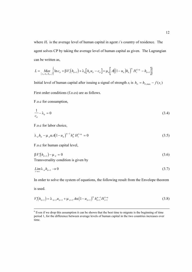
12
where Ht is the average level of human capital in agent i’s country of residence. The
agent solves CP by taking the average level of human capital as given. The Lagrangian
can be written as,
{ }( ) [ ] ( )( )[ ]{ }L Max c V h h u c A u h H h
c u h it i it it it it it it it it t itit it it
= + + − + − −+
+−
+, ,ln
11
111β λ µ
α α
Initial level of human capital after issuing a signal of strength si is h h f si i i1 1= −,max ( ) First order conditions (f.o.cs) are as follows.
F.o.c for consumption,
10
citit− =λ (3.4)
F.o.c for labor choice,
( )λ µ α α α αit it it it it th A u h H− − =− −1 01 1 (3.5)
F.o.c for human capital level,
( )β µ′ − =+V hi it it1 0 (3.6) Transversality condition is given by Lim ht it it→∞ + →λ 1 0 (3.7)
In order to solve the system of equations, the following result from the Envelope theorem
is used.
( ) ( )′ = + −+ + + + + +−
+−V h u A u h Hi it it it it it it t1 1 1 1 1 1
11
11λ µ α α α α (3.8)
6 Even if we drop this assumption it can be shown that the best time to migrate is the beginning of time period 1, for the difference between average levels of human capital in the two countries increases over time.

13
The solution implied by the first order conditions is given in (3.9) - (3.11). Appendix A
gives the solution procedure.
uit = −1 αβ , t=1,2,... (3.9)
( )h A h Hit it t+−=1
1αβ α α α t=1,2,.. (3.10)
( )c hit it= −1 αβ t=1,2,.. (3.11)
As shown in Appendix A, (3.7) and (3.8) can be solved to produce
( )h A h hs
itt t
i j jj
tt s
=
=∑∏
−−
αβ θα α α
α
1 1
11
0 t=1,2,... (3.12)
( ) ( )c A h hs
itt t
i j jj
tt s
= −
=∑∏
−−
10
1 1
11
αβ αβ θα α α
α
t=1,2,... (3.13)
The value function of the agent type i in poor country (Vi) is given in (3.14).
( ) ( )( )V A h hit
t
t
i j jjs
tt s
= β αβ αβ θα α α
α
=
∞ −
=
−
∑ ∑∏−
01 1
1
0
1
1ln
which is simplified in Appendix A to produce
( ) ( )( )V k h f s Hi i i= +
−− +
−−
ln( )
ln ( ) ln .,max1
1111 1αβα ββ
(3.14)
where ( ) ( )lnln( )
( ) ( )lnk A= − +
−−
+−
111 1 2α
αββ
ββ
αβ α
It is noted that the value function depends positively on the initial level of human capital
and the level of externality in the agent’s country of residence, and negatively on the cost
of signaling.
14
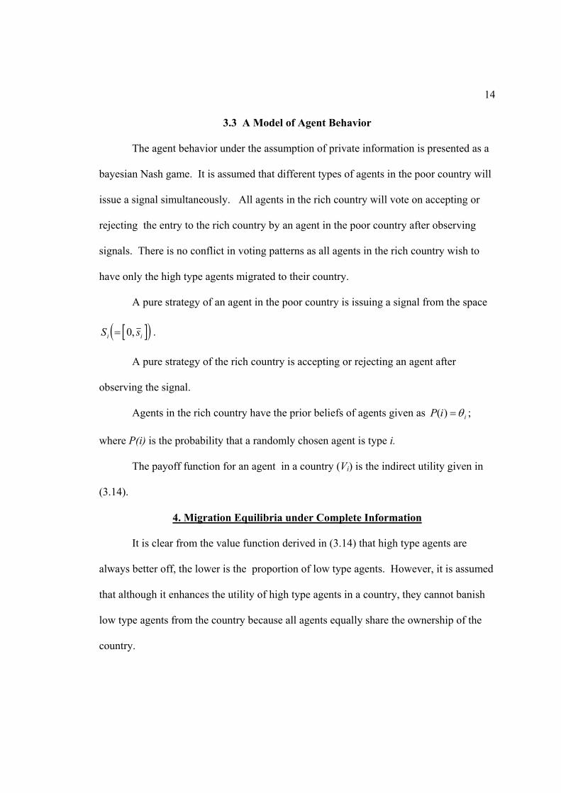
3.3 A Model of Agent Behavior
The agent behavior under the assumption of private information is presented as a
bayesian Nash game. It is assumed that different types of agents in the poor country will
issue a signal simultaneously. All agents in the rich country will vote on accepting or
rejecting the entry to the rich country by an agent in the poor country after observing
signals. There is no conflict in voting patterns as all agents in the rich country wish to
have only the high type agents migrated to their country.
A pure strategy of an agent in the poor country is issuing a signal from the space
[ ]( )S si i= 0, .
A pure strategy of the rich country is accepting or rejecting an agent after
observing the signal.
Agents in the rich country have the prior beliefs of agents given as P i i( ) =θ ;
where P(i) is the probability that a randomly chosen agent is type i.
The payoff function for an agent in a country (Vi) is the indirect utility given in
(3.14).
4. Migration Equilibria under Complete Information
It is clear from the value function derived in (3.14) that high type agents are
always better off, the lower is the proportion of low type agents. However, it is assumed
that although it enhances the utility of high type agents in a country, they cannot banish
low type agents from the country because all agents equally share the ownership of the
country.
15
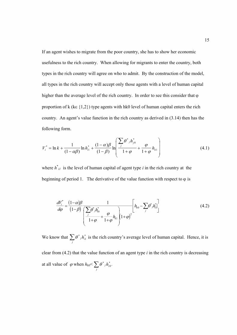
If an agent wishes to migrate from the poor country, she has to show her economic
usefulness to the rich country. When allowing for migrants to enter the country, both
types in the rich country will agree on who to admit. By the construction of the model,
all types in the rich country will accept only those agents with a level of human capital
higher than the average level of the rich country. In order to see this consider that ϕ
proportion of k (k∈{1,2}) type agents with hk0 level of human capital enters the rich
country. An agent’s value function in the rich country as derived in (3.14) then has the
following form.
V k hh
hi i
j jj
k* *
* *
ln( )
ln( )( )
ln= +−
+−− +
++
∑1
111 1 11
0
1αβα ββ
θ
ϕϕϕ
(4.1)
where h*i1 is the level of human capital of agent type i in the rich country at the
beginning of period 1. The derivative of the value function with respect to ϕ is
( )( )
( )
dVd h
h
h hi
jj
i
k
k jj
i
*
* ** *
ϕα ββ θ
ϕϕϕ
ϕ
θ=−−
++
+
+
−
∑ ∑1
11
1 11
0
12
0 1 (4.2)
We know that θ * *j
jih∑ 1 is the rich country’s average level of human capital. Hence, it is
clear from (4.2) that the value function of an agent type i in the rich country is decreasing
at all value of ϕ when hk0< θ * *j
jih∑ 0 .

16
Hence in an equilibrium all high type agents in the poor country will migrate to
the rich country. Welfare and growth implications of migration with full information are
discussed in part 7.
5 Migration Equilibria under Incomplete Information and Coordination
5.1 Migration Equilibria under Incomplete Information and Full Liberalization
The agent types are considered private information in this part. In this
environment the host country will liberally admit any agent from a source country. There
are no costly screening requirements. Thus, the low type agents in a poor country will
have a greater advantage in migrating to a richer country. This will increase welfare of
migrants, and high type agents in the poor country, while reducing the welfare of all
agents in the host country. Hence, it is natural that all countries will adopt a policy of
costly screening when agent type is uncertain, and only private information.
5.2 Migration Equilibria under Incomplete Information, Coordination and Partial Liberalization with Costly Screening
It is clear that agents in the rich country are not willing to migrate to the poor
country. Furthermore, as explained in the previous part, agents will be able to migrate
17
only if they have at least the average human capital level of the rich country. It is also
clear that the rich country will not admit agents from the poor country randomly (without
any screening) as the expected human capital possessed by an agent is less than the
average human capital in the rich country.
In this part we restrict our attention to the equilibria when all high type agents in
the poor country could coordinate their actions. As explained in the next part, there
could be multiple equilibria when the coordination fails.
In the following discussion, we show that under the rational beliefs of the rich
country on the agent types of the poor country, two types of pure strategy equilibria could
exist. In one equilibrium, all high type agents of the poor country will migrate to the rich
country. This equilibrium is called the ‘migration equilibrium’7. The other type of
equilibrium is called the ‘no-migration equilibrium’8 where no agent from the poor
country will migrate. The existence of any type of equilibrium depends on the relative
level of poverty of the poor country indicated by the proportion of low type agents (θ1).
5.1 Defining Equilibria
When defining equilibria we take into account the rational beliefs of the rich
country, costs and benefits of adapting a particular strategy by an agent in the poor
7 This is called ‘separating equilibrium’ in Signaling Literature. 8 This is called ‘pooling equilibrium’.

18
country, the rationality of such a strategy given beliefs of the rich country, the strategy of
the rich country and the rationality of the strategy of the rich country.
When an agent issues a signal, he incurs a cost in terms of human capital
accumulation within the period 0 and as a result utility is reduced. Hence, his action is
rationalized only if he could receive a compensating benefit. The benefit of the action is
that the agent could be transferred to an environment with a greater externality. For
example, if a high type agent in the poor country issues a signal, he will do so if he could
migrate to the rich country where the human capital externality is greater. A low type
agent will signal either if he could migrate or if he could deter high type agents from
migrating. In both cases he will enjoy a higher level of human capital externality.
An equilibrium is defined by adapting the signaling equilibrium defined in
Osborn and Rubinstein (1995).
Definition 5.1- A Perfect Bayesian Signaling Equilibrium is the set of strategies by the agents in
the poor country, set of posterior beliefs by agents in the rich country on agent types of
the poor country after observing the signals, strategy of agents in the rich country, and
resulting externalities in the two countries { }H Ht t t, *
=
∞
1, such that the following
conditions are satisfied.
R1. Sequential Rationality, - given rich country’s beliefs, the strategy set of agents in
both countries is at least as good as any other action. This implies that
a. each agent in the poor country maximizes his utility given his strategy,

19
strategies of other agent types in the poor country and beliefs and strategies of the
agents in the rich country;
b. Agents in the rich country maximizes their utility given their beliefs and
strategies, and strategies of the agents in the poor country.
R2. Consistency - { }H Ht t t, *
=
∞
1 are consistent with agents’ strategies, and beliefs.
R3. Bayesian Updating - after observing and considering the rationality of action taken
by agents in the poor country, agents in the rich country updates their beliefs on the type
of the agent who took the action, according to Bayes Rule.
A migration equilibrium is a perfect bayesian equilibrium where two types of
agents in the poor country choose to issue different signals. The rich country could
correctly identify the high type agents, who will be able to migrate. In a no-migration
equilibrium both types issue the same signal and the rich country will not allow migration
of any agent. This is because the expected level of human capital of a migrant with prior
probabilities is less than the average level of human capital in the rich country.
5.3 Rational Beliefs of the Rich Country and Screening We argue in this section that the rich country could impose a minimum signal
required for migration that separates the low type from the high type. At this minimum
signal, the low type will always find it too costly to migrate. The high type may or may
not migrate depending on the benefits of migration. For example, if a country is
relatively poor, the benefits of migration are larger, thus providing an incentive for

20
signaling and migrating. However, if the gap between the two countries is not too large,
the benefits of migration may not outweigh the costs, thus providing no incentive for
migration.
Potential benefits of issuing a signal by the low type are twofold. One benefit is
that they may be able to migrate. The other benefit is that they could deter migration of
the high type by issuing the same signal as the high type. The minimum signal imposed
by the rich country should be large enough that the low type will not be able to migrate.
The rich country’s beliefs are rational if they assume that only high type will issue a
signal larger than the minimum signal. As a first step of characterizing the minimum
signal (smin) we consider the signal that will deter any low type agent migrating to the rich
country.
Suppose that a low type agent issue a signal s1 and migrate to the rich country.
The cost of the signal is f(s1) and the benefit arises from being able to enjoy the relatively
higher externality in the rich country .
Their utility after migration, V1(s1,H*1), is given in (5.1 ).
( ) ( ) ( )( )V s H k h f s H1 1 1 11 1 1
11
11
, ln( )
ln ( ) ln .*,max
*= +−
− +−−αβα ββ
(5.1)
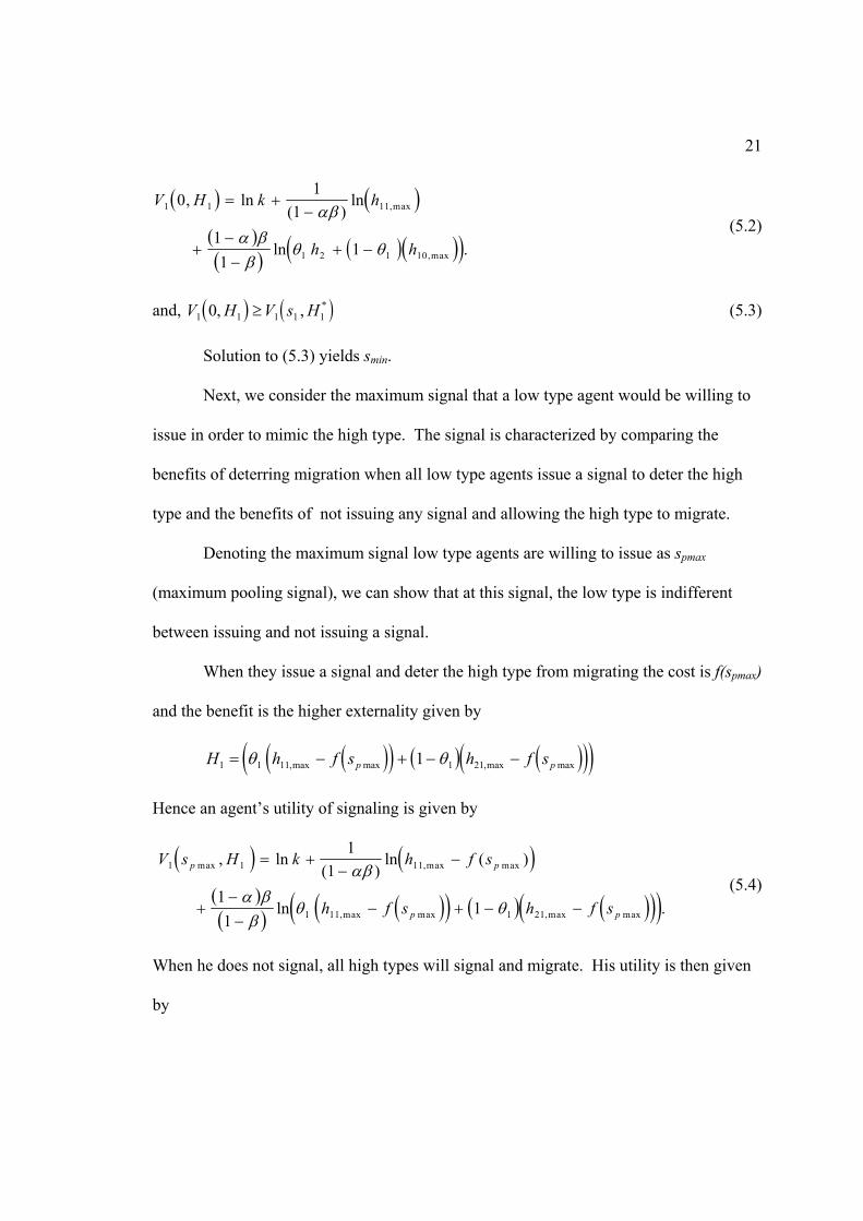
In order for the agent to stay in the poor country, the minimum signal must be
made large enough so that the utility from not issuing a signal and not migrating
(V1(0,H1)) given in (5.2) should be at least as large as the utility given in (5.1).
21
( ) ( )( )( ) ( )( )( )
V H k h
h h
1 1 11
1 2 1 10
01
111
1
, ln( )
ln
ln .
,max
,max
= +−
+−−
+ −
αβα ββ
θ θ (5.2)
and, ( ) ( )V H V s H1 1 1 1 10, , *≥ (5.3)
Solution to (5.3) yields smin.
Next, we consider the maximum signal that a low type agent would be willing to
issue in order to mimic the high type. The signal is characterized by comparing the
benefits of deterring migration when all low type agents issue a signal to deter the high
type and the benefits of not issuing any signal and allowing the high type to migrate.
Denoting the maximum signal low type agents are willing to issue as spmax
(maximum pooling signal), we can show that at this signal, the low type is indifferent
between issuing and not issuing a signal.
When they issue a signal and deter the high type from migrating the cost is f(spmax)
and the benefit is the higher externality given by
( )( ) ( ) ( )( )( )H h f s h f sp p1 1 11 1 211= − + − −θ θ,max max ,max max
Hence an agent’s utility of signaling is given by
( ) ( )
( )( ) ( )( ) ( ) ( )( )( )
V s H k h f s
h f s h f s
p p
p p
1 1 11
1 11 1 21
11
11
1
max ,max max
,max max ,max max
, ln( )
ln ( )
ln .
= +−
−
+−−
− + − −
αβα ββ
θ θ (5.4)
When he does not signal, all high types will signal and migrate. His utility is then given
by

22
( ) ( )( )V H k h h1 1 11 110
11
11
, ln( )
ln ln .,max ,max= +−
−−αβα ββ
+ (5.5)
The maximum signal a low type is willing to issue is now given by
( ) ( )V H V s Hp1 1 1 10, ,max≥ . (5.6)
Hence the signal used in screening is the maximum of smin and the spmax. We can show
that when two initial levels of human capital of the two agent types are sufficiently
different, smin < spmax. hence we will consider spmax as the screening signal.
5.4 Characterizing Equilibria In this section, conditions under which different equilibria exist are outlined. We
can characterize two types of equilibria, one where all high types migrate (migration
equilibrium) and another where no one migrates (no-migration equilibrium). The type of
equilibrium depends on whether the cost of signaling for the high type outweighs the
benefits.
5.4.1 Migration Equilibrium
In order to show the existence of a migration equilibrium, consider that all high
type agents issue a signal ss larger than spmax. According to the ‘intuitive criterion’
discussed by Cho and Kreps (1988), the high type will issue a signal just above spmax in a
separating equilibrium.
In order to ensure the sequential rationality of the strategy, requirements R1 - R3
given in definition 5.1 should hold.
23
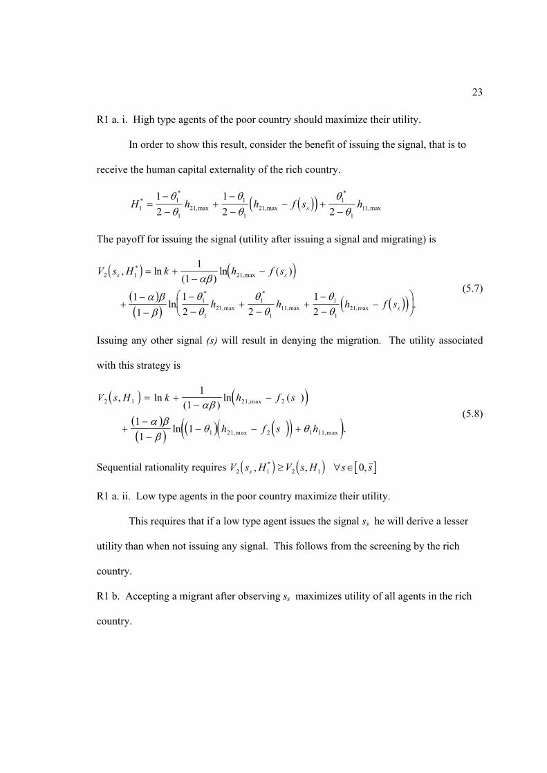
R1 a. i. High type agents of the poor country should maximize their utility.
In order to show this result, consider the benefit of issuing the signal, that is to
receive the human capital externality of the rich country.
( )( )H h h f s hs11
121
1
121
1
111
12
12 2
**
,max ,max
*
,max=−−
+−−
− +−
θθ
θθ
θθ
The payoff for issuing the signal (utility after issuing a signal and migrating) is
( ) ( )( )( ) ( )( )
V s H k h f s
h h h f s
s s
s
2 1 21
1
121
1
111
1
121
11
11
12 2
12
, ln( )
ln ( )
ln .
*,max
*
,max
*
,max ,max
= +−
−
+−−
−−
+−
+−−
−
αβ
α ββ
θθ
θθ
θθ
(5.7)
Issuing any other signal (s) will result in denying the migration. The utility associated
with this strategy is
( ) ( )( )( ) ( ) ( )( )( )
V s H k h f s
h f s h
2 1 21 2
1 21 2 1 11
11
11
1
, ln( )
ln ( )
ln .
,max
,max ,max
= +−
−
+−−
− − +
αβα ββ
θ θ (5.8)
Sequential rationality requires ( ) ( ) [ ]V s H V s H s ss2 1 2 1 0, , ,* ≥ ∀ ∈
R1 a. ii. Low type agents in the poor country maximize their utility.
This requires that if a low type agent issues the signal ss he will derive a lesser
utility than when not issuing any signal. This follows from the screening by the rich
country.
R1 b. Accepting a migrant after observing ss maximizes utility of all agents in the rich
country.

24
This happens when the high type has at least the average human capital of the rich
country after issuing the signal.
Requirements 2 and 3 of the perfect bayesian equilibrium are already incorporated
in the requirements 1 i and 1 ii which were verified above.
5.4.2 No-migration Equilibrium
We can show that in a no-migration equilibrium, the cost of issuing a signal by
high type agents is greater than the potential benefits.
High type agents’ utility after issuing a signal ss and after migrating is given in
(5.7). Since low type agents do not issue a signal, the utility of not issuing a signal is
( ) ( )( ) ( )( )V H k h h h2 1 21 1 11 1 210
11
11
1, ln( )
ln ln .,max ,max ,max= +−
−−
+ −αβ
α ββ
θ θ+ (5.9)
Hence ( ) ( )V H V s Hs2 1 2 10, , *≥ (5.10)
The rich country does not admit any agents as no one issues a signal.
5.5 Existence of Equilibria
We can also show that if the proportion of the low type in the poor country is
below a certain critical value, we can support a no-migration equilibrium. If the
proportion is above this value, a migration equilibrium could exist. The proof of the
existence is carried out in several steps.
First we show that, at higher levels of θ1, a migration equilibrium exits and at
lower levels of θ1 a zero-migration equilibrium exists. In order to show this, we
25
consider the maximum signal a high type agent is willing to issue so that she could
separate herself from the low type (ss,max) and the maximum signal a low type agent is
willing to issue in order to mimic the high type (sp,max). If ss,max is lower than sp,max,
then a zero-migration equilibrium exits. On the other hand, if sp,max is greater than ss,max, a
migration equilibrium exists. Next we show that ss,max is an increasing function of θ1 and
sp,max is a decreasing function of θ1. Finally, we show that when θ1 approaches 1, i. e. a
country become very poor, ss,max > sp,max and when θ1 approaches θ1*, i. e. country is
almost as rich as the rich country, ss,max < sp,max Then it is shown that there exists a
particular value of θ1, at which ss,max = sp,max, which is the critical level of poverty.
Lemma 5.1 -
The maximum signal used in separation, ss,max is an increasing function of θ1.
Proof -
In order to prove the lemma, first we characterize ss,max, which is the maximum
signal a high type agent is willing to issue in order to separate her from the low type. At
this level of signal, the utility of migrating should at least be equal to the utility of not
issuing any signal and not migrating. Using (5.10), this can be written as
( ) ( )V s H V Hs2 1 2 10,max*, ,=
The above condition implies that

26
( ) ( )( ) ( )( )
( )( ) ( )( )
11
11
12 2
12
11
11
1
21
1
121
1
111
1
121
21 1 21 1 11
( )ln ( ) ln .
( )ln ln .
,max ,max
*
,max
*
,max
,max ,max
,max ,max ,max
−− +
−−
−−
+−
+−−
−
=−
+−−
− +
αβα ββ
θθ
θθ
θθ
αβα ββ
θ θ
h f sh h
h f s
h h h
s
s (5.11)
The lemma is then proven using the implicit function theorem. The proof is given in
Appendix B.
Lemma 5.2 -
The maximum signal a low type agent is willing to issue, sp,max. is a decreasing
function of θ1 .
Proof -
The sp,max. is the maximum signal a low type agent is willing to issue in order to
mimic the high type. This could be characterized by using condition (5.6). At the
maximum signal,
( ) ( )V H V s Hp1 1 1 10, ,max= .
This implies
( )( )
( ) ( )( )
( )( )( ) ( )( )
=−
−
−=
−− +
−−
−
+ − −
11
11
11
11 1
11 11
11
1 11
1 21
( )ln ln
( )ln ( ) ln .
,max ,max
,max ,max
,max ,max
,max ,max
αβα ββ
αβα ββ
θ
θ
h h
h f sh f s
h f sp
p
p
+
(5.12)
Using implicit function theorem, the lemma is proven. The proof is given in Appendix
B.
27
Lemma 5.3 -
When θ1 → 1, then sp,max < ss,max and when θ1 → θ*1, then sp,max > ss,max.
Proof -
Proof is given in Appendix B.
Proposition 5.1 -
If the proportion of low type agents in a poor country is above a critical value of
~θ , endogenously derived using other parameters of the model, a migration equilibrium
can be supported. If the proportion is above the critical value, a no-migration equilibrium
can be supported.
Proof -
Proof follows from Lemma 5.1 - Lemma 5.3.
Lemma 5.3 shows that when θ1 approaches the value θ1* , sp,max> ss,max and when
θ1 approaches the value 1, sp,max< ss,max. Furthermore, according to Lemmas 5.2 and 5.3
sp,max is a decreasing function of θ1 and ss,max is an increasing function of θ1. Hence it
follows that there exists a particular value of θ1 ( )[ ]~ ,*θε θ 1 1 , at which sp,max = ss,max . QED.
Welfare and growth implications of equilibria with private information are
discussed in part 7.
6 Coordination Failure, Multiple Equilibria
28
and Threshold Poverty
In this part we use the strategic complementarity and coordination failure in
order to establish the existence of multiple equilibria at a given level of poverty and the
existence of threshold poverty level.
The “strategic complementarity” is the positive influence on any one agent’s
utility by other agents’ actions as discussed in Cooper and John (1988). It is clear that
any high type agent migrating will cause an impact on the utilities of other high type
agents in the poor country. Hence there is a tendency for all high type agents to take
similar actions. As already shown, in a no-migration equilibrium none of the high type
agents issues a signal and migrates. This is an equilibrium because issuing no signal and
not migrating is the best action when other high type do not migrate. However, we can
further show that when this equilibrium occurs, it is likely that a migration equilibrium
could also occur. This latter equilibrium occurs because if other high type agents issue
signals and migrate, the best response by any single high type agent is also to issue a
signal and migrate. This is stated in proposition 6.1.
When there is a migration equilibrium, a no-migration equilibrium could also be
supported if a country is above the ‘threshold poverty level’ as stated in proposition 6.2.
The threshold poverty level is defined as the boundary of poverty levels at which the
migration equilibrium is the only equilibrium that could exist even with coordination
failure.
6.1 Existence of Multiple Equilibria and Poverty Threshold
29
Assuming that one high type agent will issue a signal si and other high type
agents will issue s-i, the value function of being in an environment with externality H is
written as V(si, s-i, H). For example, following this notation, the value function of a high
type agent not issuing any signal and not migrating while others issue signals and
migrating could be written as V(0, s-i, H). We use this notation when proving the
following proposition.
Proposition 6.1 -
If the proportion of low type agents in a country is below the critical ratio, it
could have at least two equilibria, migration and no-migration.
Proof -
Existence of a no-migration equilibrium if the low type agents in a country is less
than the critical ratio is already established in the proposition 5.1.
When all but one high type agent migrate, the situation is similar to a country
with a very high proportion of low type agents. Hence the optimal action by any high
type agent is to signal and migrate.
QED. Proposition 6.2 -
When the proportion of low type agents in a country is higher than the critical
ratio, two equilibria could exist if the country is not too poor.
Proof -
We have already shown that when a country’s proportion of low type agents is
higher than the critical ratio, a migration equilibrium exists. In order to prove that an
30
agent’s action of not issuing a signal in response to other agents not issuing a signal and
not migrating is optimal for a certain range of θ1, consider the utility of an agent issuing a
signal and migrating when others do not issue signals and do not migrate. The agent will
issue the minimum signal required for migration, which is spmax and the utility is V(spmax,
0, H1*), where
( ) ( )( )( )( ) ( )( )
V s H k h f s
h h
p pmax*
,max max
*,max
*,max
, , ln( )
ln
ln .
01
111
1
1 21
1 11 1 21
= +−
−
−−
+ −
αβα ββ
θ θ +
The externality is the rich country’s average level of human capital since
migration of one agent does not change the average human capital level of the rich
country significantly.
The utility of not issuing a signal when others do not issue a signal is V(0,0,H) as
given in (5.9). For the existence of a no-migration equilibrium, it should be true that
( ) ( )V s H V Hp max*, , , ,0 0 01 1< . (6.1)
In order to show this result, consider an implication of lemma 5.3 which suggests
that at the critical ratio of low type agents the following holds.
( ) ( )V s s H V Hp pmax max*, , , ,1 10 0= (6.2)
Assuming that when high type from the poor country migrates the externality of the rich
country is greater, we can show that
( ) ( )V s s H V s Hp p pmax max*
max*, , , ,1 10> (6.3)
Hence (6.1) holds as a strict inequality at the critical ratio of poverty.
31
According to lemma 5.2, spmax is a decreasing and continuos function of θ1,.
Hence V(spmax, 0, H1*) is an increasing and continuos function of θ1. It can be shown that
V(0,0,H1) is a decreasing and continuos function of θ1. Hence, there exits a non empty
sub set of ( ~θ 1 , 1] in which (6.1) holds as a weak inequality.
6.2 Defining and Characterizing Threshold Poverty
We define the threshold poverty as the lower bound of θ1, (~~θ 1) at which the
inequality given in (6.1) does not hold. Hence, if a country has a proportion of low type
agents higher than the threshold poverty level, strategic complementarity is not strong
enough to support a no-migration equilibrium. The only equilibrium that can be
supported is a migration equilibrium.
The threshold poverty can be characterized using (6.1) as an equality. Hence at
the threshold poverty level,
( ) ( )V s H V Hp max*, , , ,0 0 01 1=
This implies
( )( ) ( )( ) ( )( )
( )( ) ( )
ln( )
ln ln
ln( )
ln ln ~~ ~~
,max max*
,max*
,max
,max ,max ,max
k h f s h h
k h h h
p+−
−−−
+ −
= +−
−−
+ −
11
11
1
11
11
1
21 1 11 1 21
21 1 11 1 21
αβα ββ
θ θ
αβα ββ
θ θ
+
+ (6.4)
The equation (6.4) suggests that the threshold poverty is an increasing function of
the ratio of low type agents (θ 1* ) in the rich country. At very low levels of θ 1
* , the
threshold poverty may not exist since the rich country is too rich for an agent to be able

32
to migrate. When θ 1* is too high, migration may not overweigh the costs thus increasing
the threshold poverty to a very high level. Figure 1 illustrates the boundary of threshold
poverty.
6.3 Summary of Results
In this section we summarize the results obtained so far. The figure 2 shows the
threshold poverty level and critical poverty level. The horizontal line in the figure
depicts different poverty levels (ratio of the low type agents) of the poor country.
Comparison of value functions in each region depicted in figure 2 is as follows.
1. In region 1, i. e. [0, ~θ )
Value of signaling and migrating when other high type agents migrate, V(spmax,
spmax, H1* ), is smaller than the value of not signaling and not migrating when others do
not signal and do not migrate, V(0, 0, H1), but it is larger than the value of not signaling
and not migrating when others signal and migrate, V(0, spmax, H1* ), and the value of
signaling and migrating when others do not signal and migrate, V(0, spmax, H1 ).
i. e. ( ) ( ) ( ) ( )11maxmax*1max1max ,0,0,,,0,,,0 HVHssVHsVHsV pppp <<<
In this case most likely equilibrium is the no-migration equilibrium.
2. In region 2, i. e. [~θ ,
~~θ )
Value of not signaling and not migrating when other high type agents do not
signal and do not migrate, ( )1,0,0 HV , is smaller than the value of signaling and

33
migrating when others signal and migrate, ( )*1maxmax ,, HssV pp , but it is larger than the
value of signaling and migrating when others do not signal and do not migrate,
( )*1max ,0, HsV p .
i. e. ( ) ( ) ( )*
1max1*1maxmax ,0,,0,0,, HsVHVHssV ppp >>
In this case multiple equilibria could take place.
2. In region 3, i. e. [~~θ ,1)
Value of signaling and migrating is larger than value of not signaling and not
migrating no matter what other agents do. i. e. ( ) ( )V H V s s Hp p0 0 1 1, , , ,*max max
*< and
( ) ( )V H V s Hp0 0 0 1, , , ,* max*< . In this case only possibility is the migration equilibrium.
~~θ 1 Boundary of Threshold Poverty θ1
* Figure 1 - Threshold Level of Poverty as a Function of the proportion of low type agents in the Rich country

34
Poverty Level (ratio of low type agents) →
0 no migration ~θ multiple eq.
~~θ migration 1
Figure 2 - Comparison of Critical Poverty Level and the Threshold Poverty Level
_____________________________________________________________
Note: Critical Poverty Level -~θ , Threshold Poverty Level -
~~θ
35
7 Welfare, Growth and Economic Policy
7.1 Welfare and Growth in a Closed Economy
Solutions given in (3.10) and (3.11) can be used to discuss the welfare and growth
in a closed economy. A closed economy is considered as an environment where
migration is not allowed. Hence agents do not signal, and the initial human capital level
of an agent i and the externality of the country are given by h hi i1 1= ,max , and
H hj jj
1 1= ∑θ ,max respectively. Using those solutions an agent i’s growth rates of
human capital (ghit), consumption (gcit), and income (gyit) at time t can be derived.
( ) ( )g g g Ah
hhit cit yit
j jj
i
t
t= = =
∑
−
−αβ
θα
α
α
α α
1
1
11
,max
,max
(7.1)
The per capita income of the country is the weighted average of all agents’ income. The
growth rate of per capita income is given in (7.2).
g
yj
yj
u hj
u hj
yt
j jt
j jt
j jt jt
j jt jt
= =+ + +∑
∑
∑
∑
θ
θ
θ
θ
1 1 1
( )= A
hj
hj
j j
j j
t
t
αβ
θ
θ
α
α
α
α
1
1
1
,max
,max
+∑
∑
(7.2)
Since h20,max > h10,max and α<1, the following can be established.
i.) During the transition, the growth of low human capital agents is greater than
that of high human capital agents in a given country. Furthermore, the low type will
36
grow faster than the long run growth rate, whereas the high type will grow slower than
the long run growth rate.
ii.) The growth rate per capita income of the country is slower than the long run
growth during the transition period. This is because during the transition the high type
grows slower than the long run growth of the country.
iii). Human capital, consumption and income of any agent i will eventually
converge to the long run growth rate. i.e. ( )limt hit cit ytg g g A→∞
= = → αβ α .
iv). Human capital levels of all agents will converge to a common level, i.e.
L imhh
i jt
jt
it→ ∞
→ ∀1; ,
v). During the transition, the rich country will grow faster than the poor country.
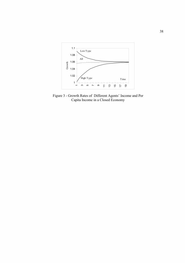
Figure 3 describes the growth in the closed economy. The growth rate of low
type agents’ income is greater than the long run steady growth during the transition as
they are benefited by the higher average human capital in the country. The growth of the
high type is lower due to the human capital externality.
7.2 Welfare and Growth in an Open Economy
with Full Information
We have shown that in an open economy with full information all high type
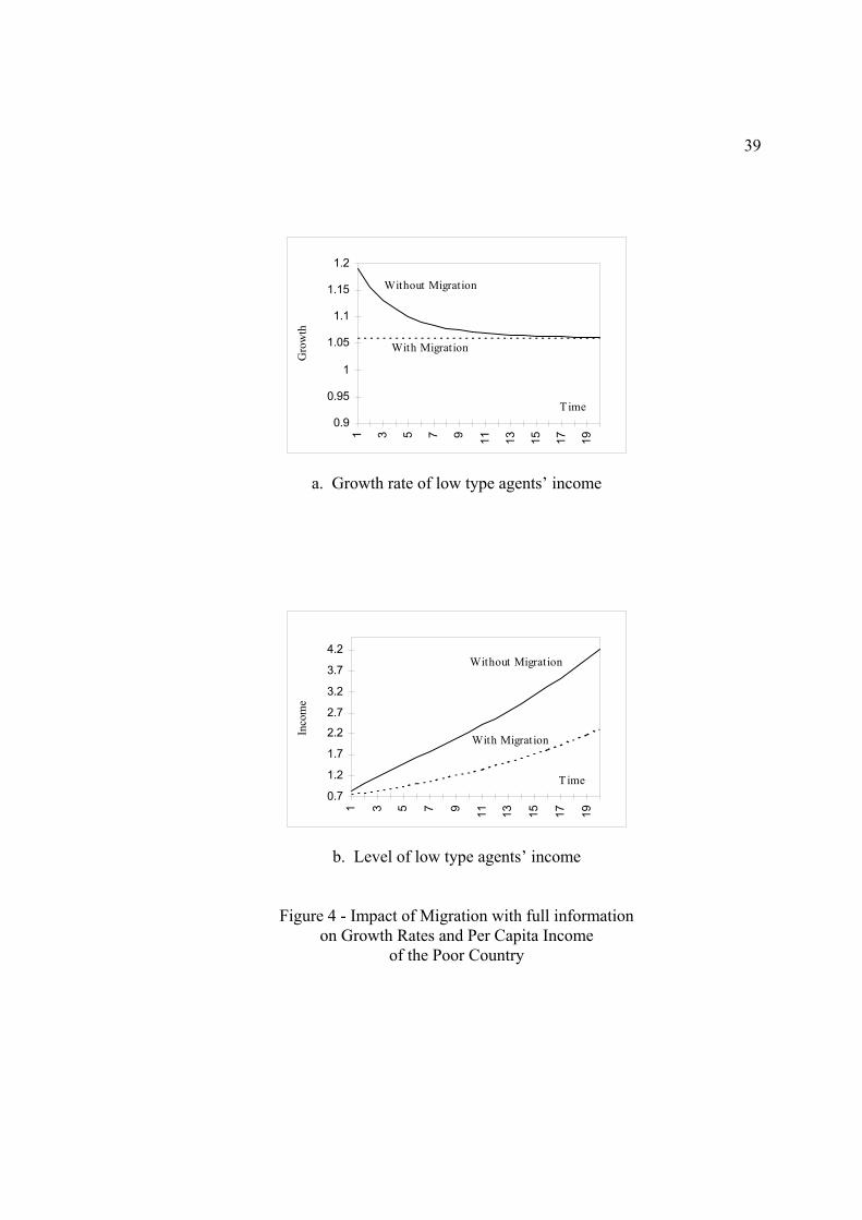
agents will migrate to the rich country. The impact of migration is shown in Figure 4.
As seen in Figures 4a and 4b, the migration lowers the growth rate of low type agents in
the poor country. Their income levels will fall leading to a loss of welfare (utility).

37
As discussed earlier, the per capita income of the country is the weighted average
of agents’ income. As seen in Figure 4c, the growth of per capita income is slower than
the long run growth during the period of transition. However after all high type agents
migrate to the rich country, the growth rate of per capita income will converge to the long
run rate leading to an increase in growth. The per capita income will drop sharply as
shown in Figure 4d, but will grow faster afterwards.9 All agents in the rich country and
its per capita income will grow faster as a result of migration. The welfare of migrants
and both agent types in the rich country increases while the welfare of the low type
agents in the poor country decreases.
7.3 Welfare and Growth in an Open Economy with Private Information
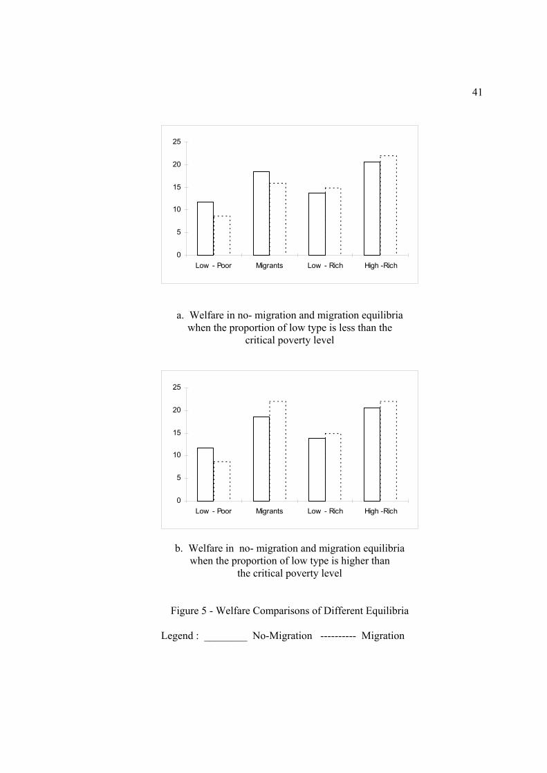
We have shown that if a country is above the threshold poverty level, multiple
migration equilibria could exist. As seen in Figure 5, all agents in the rich country are
benefited in a migration equilibrium. The low type agents in the poor country are hurt.
Welfare of migrants is different depending on whether the country is below or above the
critical poverty level. When the country is above the critical poverty level, (i. e. when it
is not too poor) migrants’ welfare is lower in a migration equilibrium. Their welfare is
greater if the country is below the critical poverty level.
9 A similar phenomenon occurs in the neo-classical growth model. Assuming the steady state of the model, consider loss of a part of physical capital. This will lower the income level of agents, but the economy will grow faster during the transition to the steady state.
38
1
1.02
1.04
1.06
1.08
1.1
1 3 5 7 9 11 13 15 17 19
Time
Gro
wth
Low Type
High Type
All
Figure 3 - Growth Rates of Different Agents’ Income and Per Capita Income in a Closed Economy
39
0.9
0.95
1
1.05
1.1
1.15
1.2
1 3 5 7 9 11 13 15 17 19
Time
Gro
wth
Without Migration
With Migration
a. Growth rate of low type agents’ income
0.7
1.2
1.7
2.2
2.7
3.2
3.7
4.2
1 3 5 7 9 11 13 15 17 19
Time
Inco
me
Without Migration
With Migration
b. Level of low type agents’ income
Figure 4 - Impact of Migration with full information on Growth Rates and Per Capita Income
of the Poor Country

40
1
1.01
1.02
1.031.04
1.05
1.06
1.07
1.08
1 3 5 7 9 11 13 15 17 19
Time
Gro
wth
With Migration
Without Migration
c. Growth rates of per capita income
0.7
1.7
2.7
3.7
4.7
5.7
6.7
7.7
1 3 5 7 9 11 13 15 17 19
Time
Per C
apita
Inco
me Without Migration
With Migration
d. Level of per capita income
Figure 4 contd.
41
0
5
10
15
20
25
Low - Poor Migrants Low - Rich High -Rich
a. Welfare in no- migration and migration equilibria
when the proportion of low type is less than the critical poverty level
0
5
10
15
20
25
Low - Poor Migrants Low - Rich High -Rich
b. Welfare in no- migration and migration equilibria when the proportion of low type is higher than
the critical poverty level
Figure 5 - Welfare Comparisons of Different Equilibria
Legend : ________ No-Migration ---------- Migration

42
7. 4 Policy Options
The policy for any country should be designed to enhance the benefits of its
people. The policy options available for the rich country are straight forward. Their
policy should be to impose the minimum required screening signal and allow the
migration of high type agents. As explained in part 5, the rich country should not follow
a policy of open liberalization, or should not randomly choose agents from poor
countries, for it will reduce the average level of human capital in the rich country. There
has to be a screening mechanism to allow self selection of high quality human capital to
migrate. Policy options available to the poor country depends on how poor they are. If
the poor country is above the critical poverty level, (i. e. if it is not too poor) policies on
controlling migration will enhance the welfare of both agent types. However, if the
country is below the critical poverty level or the threshold poverty level, controlling
migration will hurt would-be migrants, but will help the low type. Hence the policy
could be addressed in a political economy framework. The poor country could avoid
herd behavior or mass migration arising from strategic complementarity by improving the
economic and social infrastructure in the country.
8 Conclusion
Under the Mode 4 liberalization of services, natural persons can move freely
between countries. As WTO explains the temporary nature of the movement of natural
persons is defined negatively, to exclude permanent presence. The presence of natural
43
persons in a host country has to be for a significantly longer period, since they have to
establish service centers or join service centers domiciled in host countries.
WTO has noted that the Mode 4 liberalization has not taken place significantly,
restricting the movement of natural persons. The model of migration with private
information on agent types presented in this paper confirms this phenomenon of
reluctance to freely liberalize the movement of natural persons. In this model, migration,
or movement of natural persons for considerably longer periods, takes place from poor to
rich countries, provided the host country adopts a liberal policy coupled with a costly
screening system. The cost encourages self selection, where only those with
considerably high human capital could migrate.
In this environment, there are no incentives to migrate if the source country is
sufficiently rich. The incentive for migration increases as the degree of poverty in the
source country increases. After a critical poverty level, multiple equilibria could
emerge. But, if the poor country is below a “threshold poverty level” there can only be a
migration equilibrium.
The different equilibria are the outcomes of costly signaling and strategic
complementarity. A rich country can screen the high type by using an appropriately
chosen level of observable human capital. If the poor country is considerably poor, the
benefits of migration outweigh the costs leading to a migration equilibrium. However,
for any high-type agent, the gap between costs and benefits depends on whether other
high-type agents choose to issue a signal or not. This strategic complementarity of high
type agents’ actions leads to two equilibria unless the poverty level of the country falls
44
below the threshold poverty level. However, any high type agent living in a significantly
poor country (falling below the threshold poverty level) will choose to migrate
irrespective of the actions of other high type agents.
Migration reduces the income of low type agents and the per capita income of the
poor country. However, after the migration takes place the per capita income of the poor
country grows faster during the transition to the long run growth rate. This increase in
per capita income growth is a result of the absence of high types in the country after
migration whose growth in a closed economy is slower than the long run growth. After
migration takes place only low types remain, and since they are homogenous, the country
grows at the long run rate which is higher than the growth rate in a closed economy
during the transition.
Migration always increases welfare in the rich country and reduces the welfare of
low type agents in the poor country. The change in welfare of migrants depends on
whether the poor country is above or below a “critical poverty level”. If the country is
above the critical poverty level, i. e. not so poor, would-be migrants (i. e. high type
agents in the poor country) will have a higher level of welfare in the no-migration
equilibrium than in the migration equilibrium. Hence a no-migration equilibrium is
preferred by both agent types. However, if the poor country is below the critical poverty
ratio, the migration equilibrium increases the welfare of migrants. A poor country lying
above the critical poverty level could draw appropriate economic policies to avoid the
migration equilibrium, which will benefit all agents in the country. However, if a
45
country is below the critical poverty level, there is no economic policy which will benefit
all agent types. Hence policy could be a political outcome.
The policy for any country should be designed to enhance the benefits of its
people. The policy options available for the rich country are straight forward. Their
policy should be to impose the minimum required screening signal and allow the
migration of high type agents. The rich country should not follow a policy of open
liberalization, or should not randomly choose agents from poor countries as this will
reduce the average level of human capital in the rich country.
Policy options available to the poor country depends on how poor they are. If the
poor country is above the critical poverty level, (i. e. if it is not too poor) policies on
controlling migration will enhance the welfare of both agent types. However, if the
country is below the critical poverty level or the threshold poverty level, controlling
migration will hurt would-be migrants, but will help the low type. Hence the policy
could be addressed in a political economy framework. The poor country could avoid
herd behavior or mass migration arising from strategic complementarity by improving the
economic and social infrastructure in the country.
The paper considered only a one-time migration. Continuing migration could be
addressed when population growth is introduced to the model. This is left as a direction
for future research.
46
APPENDIX A
DERIVING THE VALUE FUNCTION FOR THE MODEL
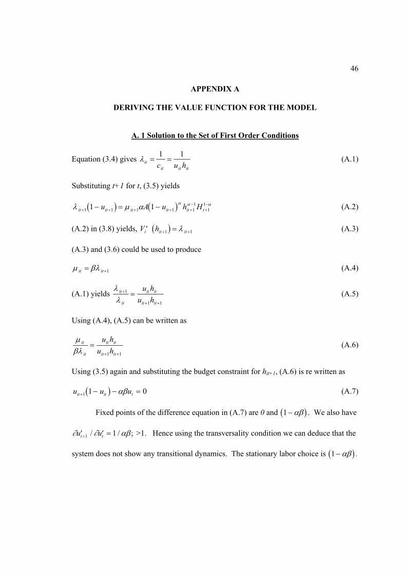
A. 1 Solution to the Set of First Order Conditions
Equation (3.4) gives ititit
it huc11
==λ (A.1)
Substituting t+1 for t, (3.5) yields
( ) ( )λ µ α α α αit it it it it tu A u h H+ + + + +
−+−− = −1 1 1 1 1
11
11 1 (A.2)
(A.2) in (3.8) yields, ( )′ =+ +V hi it it1 1λ (A.3)
(A.3) and (3.6) could be used to produce
µ βλit it= +1 (A.4)
(A.1) yields λλ
it
it
it it
it it
u hu h
+
+ +
=1
1 1
(A.5)
Using (A.4), (A.5) can be written as
µβλ
it
it
it it
it it
u hu h
=+ +1 1
(A.6)
Using (3.5) again and substituting the budget constraint for hit+1, (A.6) is re written as
( )u u uit it t+ − − =1 1 0αβ (A.7) Fixed points of the difference equation in (A.7) are 0 and ( )1− αβ . We also have
∂ ∂ αβ′ ′ =+u ut t1 1/ / ; >1. Hence using the transversality condition we can deduce that the
system does not show any transitional dynamics. The stationary labor choice is ( )1− αβ .

47
A.2. Human Capital Accumulation Process
Using the result in A1, the following process is derived. ( )h A h Hi i2 1 1
1= −αβα α α
( )
( ) ( )[ ] ( )
( )
h A h H
A A h H A h Hj
A h H h
i
j
j jj
13 2 21
11 11
11 11
1
211 1
11
12 2
=
−
− −
−
−
−
∑
∑
αβ
αβ αβ θ αβ
αβ θ
α α α
α α α αα α α α
α
α α α α
α
=
=
( )
( ) ( ) ( )
( )
h A h H
A A h H h A h H h
A h H h
i
j jj
j j j jjj
i j jj
14 3 31
211 1
11
1
21 1
11
1 1
31 1
11
1
2 2 2 2
3 3
=
−
−
−
−
− −
−
−
∑ ∑∑
∑
αβ
αβ αβ θ θ αβ θ
αβ θ
α α α
α α α α α
α α
α α α α
α α
α α α α
α
=
=
( )
( )
=
∑∑
∑ ∑
∑∏
− −
−
− −
−
−
α
α α
α α
α α α α
α
α
α
α α α α
α
θ θ
αβ θ θ
αβ θ
j j j jjj
i j jj
j jj
i j jj
h h
A h H h h
A h H hs
s
1 1
1 1
31 1
11
1
1
1
31 1
11
12
2
3 3 2
3 3
1
=
=
Hence
( )h A h hs
itt
i j jj
tt s
=
=∑∏
−−
11 1
11
0/α α α α
α
αβ θ (A.8)
A.3. Consumption Path
( ) ( )( )c u h A h H hs
it it it
t
i j jj
tt s
= = −
=−
−−
∑∏11
1 11
1
11
αβ αβ θα α α α
α
( ) ( ) = 10
1 1
114
−
=∑∏
−−
αβ αβ θα α α
α
A h hs
t ti j j
j
ts
(A.9)

48
A.4. Value Function
( ) ( )( )
V c
A h h
it
tit
t
t
t
j jjs
tt s
=
−
=
∞
=
∞ −
=
−
∑
∑ ∑∏
β
β αβ αβ θα α α
α
0
011 1
1
0
1
1
ln
ln =
( ) ( )( )= β αβ β αβ β β θα α α
α
t
t
t
t
tt
t
t
tj jj
js
t
A h ht s
=
∞
=
∞
=
∞
=
∞ −
=
−
∑ ∑ ∑ ∑ ∑∏− + + +
0 0 011
01
1
0
1
1ln ln ln ln
( ) ( ) ( ) ( )= β αβ β αβ αβ α β θα αt
t
t
t
t
ti
t
tj j
js
t
t A h hs
=
∞
=
∞
=
∞
=
∞
=
−
∑ ∑ ∑ ∑ ∑∑− + + + −
0 0 01
01
0
1
1 1ln . ln ln ln (A.10)
In order to further simplify (A.10), following results are used.
ββ
t∑ =−1
1 (A.11)
( )
β β β β
β β β β β β β
ββ
ββ
ββ
t t∑ = + + +
= + + + + + + +
=−
+
−
+ =
−
. ...
...
..
2 3
11
11 1
2 3
2 2 3 3 3 4
22
(A.12)
(A.11) and (A.12) in (A.10),
( )
( ) ( )( )
( )( )
V A h
h h
i i
j jj
t
tj j
j
t
=−−
+−
+−
− +−−
+
−−
∑ ∑ ∑
=
∞
ln( )( ) ( )
ln( )
ln
ln ln .
11 1
11
111
11
2 1
12
1
αββ
ββ
αβαβ
αα ββ
θαβ
β θ
α
α +
49
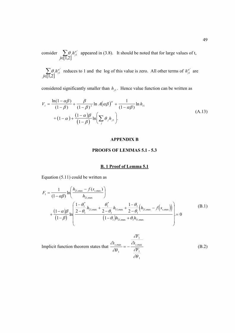
consider θ αj jh
j
t
11 2∈∑[ , ]
appeared in (3.8). It should be noted that for large values of t,
θ αj jh
j
t
11 2∈∑[ , ]
reduces to 1 and the log of this value is zero. All other terms of hjt
1α are
considered significantly smaller than hj1 . Hence value function can be written as
( )
( ) ( )( )
V A h
h
i i
j jj
=−−
+−
+−
− +−−
∑
ln( )( ) ( )
ln( )
ln
ln .
11 1
11
111
2 1
1
αββ
ββ
αβαβ
αα ββ
θ
α
+ (A.13)
APPENDIX B
PROOFS OF LEMMAS 5.1 - 5.3
B. 1 Proof of Lemma 5.1
Equation (5.11) could be written as
( )( )
( )( )( )
Fh f s
h
h h h f s
h h
s
s
121
21
1
121
1
111
1
121
1 21 1 11
11
11
12 2
12
10
=−
−
+−−
−−
+−
+−−
−
− +
=
( )ln
( )
ln .
,max ,max
,max
*
,max
*
,max ,max ,max
,max ,max
αβ
α ββ
θθ
θθ
θθ
θ θ
(B.1)
Implicit function theorem states that ∂∂θ
∂∂∂∂θ
sF
sF
s s,max ,max
1
1
1
1
= − (B.2)

50
Using the result ′f >0 discussed in Part1, ∂∂
Fss
1
,max
is <0 and ∂∂θ
F1
1
is >0. Hence we can
show that ∂∂θss,max
1
0> .
B.2. Proof of Lemma 5.2.
Equation (5.12) can be re-written as
( )( )
( )( ) ( ) ( )( )F
h f sh
h f s h f s
h
p
p p
211
11
1 11 1 21
11
11
11
10
=−
−
+−−
− + − −
=
( )ln
( )
ln .
,max ,max
,max
,max ,max ,max ,max
,max
αβ
α ββ
θ θ
(B.3)
Using result ′f >0, it is easy to show that ∂
∂F
sp
1
,max
<0. It can also be shown that ∂∂θ
F1
1
0< .
Hence the implicit function theorem derives the result.
B.3 Proof of Lemma 5.3
The proposition is proved by examining the functions F1 and F2 defined above.
Using F2 it is easy to show that when θ1 → 1, then sp,max → 0. Using F1 it could be
shown that when θ1 → 1, ss,max should remain non zero for F1 to hold. Hence when θ1 →
1, then sp,max < ss,max.
Consider θ1 → θ*1 .
Then F1 and F2 takes following forms.

51
( )
( )( )
( )( )( )
F sh f s
h
h h h f s
h h
ss
s
1 121
21
1
121
1
110
1
121
1 21 1 11
11
11
12 2
12
10
θαβ
α ββ
θθ
θθ
θθ
θ θ
*,max
,max ,max
,max
*
* ,max
*
* ,max
*
* ,max ,max
*,max
*,max
,( )
ln( )
ln .
=−
−
+−−
−−
+−
+−−
−
− +
=
(B.4)
and
( )
( )( )
( )( ) ( ) ( )( )F s
h f sh
h f s h f s
h
pp
io
p p
2 111
1 11 1 21
11
11
11
10
θαβ
α ββ
θ θ
*,max
,max ,max
,max
*,max ,max
*,max ,max
,max
,( )
ln( )
ln .
=−
−
+−−
− + − −
=
(B.5)
We wish to show that the root of ( )F ss1 1 0θ *,max, = , is smaller than the root of
( )F sp2 1 0θ *,max, = , In order to show this, we establish that on the F - s plane,
i. both ( )F ss1 1θ*
,max, and ( )F sp2 1θ*
,max, are concave downward, and
ii. ( )F sp2 1θ*
,max, lies above ( )F ss1 1θ*
,max, until ( )F ss1 1θ*
,max, approaches the
value zero.
Both functions can be proved concave downward by examining the first and
second derivatives. The strict convexity of cost functions of signaling (f1 and f2)
ensures the property (i) above.
In order to show the property (ii) above, consider the behavior of two functions at s=0.

52
Fh h
h2 11 21 1 11
110
11
1( , )
( )( )
ln( )
**
,max*
,max
,maxθ
α ββ
θ θ=
−−
− +
(B.7)
For . ( )F2 1 0θ * , > ( )F1 1 0θ * , , it should be the case that
( )( )( ) ( ) ( )
( )
*,max
*,max
,max
*,max
*,max
*,max
*,max
*,max
*
1 1 1
1 21 21 1 11
11
1 21 1 11 1 21
1 21 1 11 1
− +
>
− + + −
− + −
θ θ θ θ θ
θ θ θ
h hh
h h h
h h (B.8)
Define z=h20,max/h10,max. Then, (B.8) becomes,
( )( )θ θ
θ θ
θ θ θ1 1
1 1
1 1 1
12 1
1 2* *
* *
* * *( )
( )( )
+ − >− +
+ − −
zzz
re-arranging,
( ) ( )z z2 1
1
1
1
2 12 2
−−
−
>
−
( )*
*
*
*
θθ
θθ
( ) ( )z −
−−
>
−+
−−
=
−
12 2
12
1
21
1
2
1
1
1
1
2
1
2
θθ
θθ
θθ θ
* *
*
*
* *
z >−−
±−
12
12
1
1 1
θθ θ
*
* *
i. e. z >−−θθ1
12
*
* or 1 (B.9)
Since z>1, the inequality holds.
( )( )Fh h h
h h1 11 21 1 11 1 21
1 21 1 11 1
011
1 1
1 2( , )
( )( )
ln( ) ( )
( )*
*,max
*,max
*,max
*,max
*,max
*θ
α ββ
θ θ θ
θ θ θ=
−−
− + + −
− + −
(B.6)
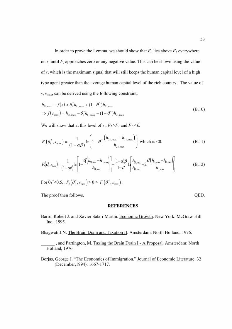
53
In order to prove the Lemma, we should show that F2 lies above F1 everywhere
on s, until F1 approaches zero or any negative value. This can be shown using the value
of s, which is the maximum signal that will still keeps the human capital level of a high
type agent greater than the average human capital level of the rich country. The value of
s, smax, can be derived using the following constraint.
( )
( )h f s h h
f s h h h21 1 11 1 21
21 1 11 1 21
1
1,max
*,max
*,max
max ,max*
,max*
,max
( )
( )
− > + −
⇒ = − − −
θ θ
θ θ (B.10)
We will show that at this level of s , F2 >F1 and F1 <0.
( ) ( )F s
h hh1 1 1
21 11
21
11
1θαβ
θ*max
* ,max ,max
,max
,( )
ln=−
−−
which is <0. (B.11)
( ) ( )( ) ( ) ( )
F sh h
hhh
h hh2 1
1 21 11
11
21
11
1 21 11
11
11
111
2θαβ
θ α ββ
θ*
max
*,max ,max
,max
,max
,max
*,max ,max
,max, ln ln=
−−
−
+
−−
−−
(B.12)
For θ1*<0.5, . ( )F s2 1θ
*max, > 0 > ( )F s1 1θ
*max, .
The proof then follows. QED.
REFERENCES
Barro, Robert J. and Xavier Sala-i-Martin. Economic Growth. New York: McGraw-Hill Inc., 1995.
Bhagwati J.N. The Brain Drain and Taxation II. Amsterdam: North Holland, 1976. ______ , and Partington, M. Taxing the Brain Drain I - A Proposal. Amsterdam: North
Holland, 1976. Borjas, George J. “The Economics of Immigration.” Journal of Economic Literature 32
(December,1994): 1667-1717.

54
Braun, Juan. “Essays on Economic Growth and Migration.”, Ph.D. Dissertation, Harvard University, 1993.
Cho, In-Koo and David M. Kreps. “Signaling Games and Stable Equilibria.” Quarterly
Journal of Economics CII Issue 2 (May 1987): 179-221. Cooper, Russell and Andrew John. “Coordinating Coordination Failures in Keynesian
Models.” Quarterly Journal of Economics CIII Issue 3 (August 1988): 441-463. Glomm, Gerhard. “A Model of Growth and Migration.” Canadian Journal of Economics
XXV (November, 1992): 901-922. Harris John R. and Michael P. Todaro. “Migration, Unemployment and Development: A
Two Sector Analysis.” American Economic Review VLX (March 1970): 126-142. Lucas, Robert E. Jr. “On the Mechanics of Economic Development.” Journal of
Monetary Economics 22 (July 1988): 3-42. Osborne M. J. and Ariel Rubinstein. A Course in Game Theory. Cambridge,
Massachusetts: The MIT Press, 1994. Quah D., “Increasingly Weightless Economies”, Bank of England Quarterly , Vol. 37,
No. 1, Bank of England, 1997 Smith, Adam, “That the Division of Labour is limited by the Extent of the Market”, An
Inquiry into the Nature And Causes of the Wealth of Nations, Chapter III, Adam Smith Institute, 1776
Spence , A. M. “Job Market Signaling.” Quarterly Journal of Economics 87 (1973): 557-
573. _____ . “Competitive and Optimal Responses to Signaling: An Analysis of Efficiency
and Distribution.” Journal of Economic Theory 8 (1974): 296-332. Tamura, Robert. "Income Convergence in an Endogenous Growth Model." Journal of
Political Economy (Dec. 1991): 522-540. _____ . "Regional Economies and Market Integration." Hoover Institute and University
of Iowa Working Paper, August 1994. Thenuwara, H. N., Interactions between Growth Economies, Migration and Trade, Ph. D.
Dissertation, University of Iowa, 1997

55
Todaro, Michael P. “A Model of Labor Migration and Urban Unemployment in Less Developed Countries.” American Economic Review 59 (1969): 138-48.
World Trade Organization Secretariat, Services Sector Classification List, WTO, Geneva,
1991, _____ GATS, Mode 4 and the Pattern of Commitments, WTO, Geneva, 2002