paper sas1991:2018 causal mediation analysis …...paper sas1991-2018 causal mediation analysis with...

Paper SAS1991-2018

Causal Mediation Analysis with the CAUSALMED Procedure

Yiu-Fai Yung, Michael Lamm, and Wei Zhang, SAS Institute Inc.

Abstract

Important policy and health care decisions often depend on understanding the direct and indirect (mediated) effects ofa treatment on an outcome. For example, does a youth program directly reduce juvenile delinquent behavior, or doesit indirectly reduce delinquent behavior by changing the moral and social values of teenagers? Or, for example, is aparticular gene directly responsible for causing lung cancer, or does it have an indirect (mediated) effect through itsinfluence on smoking behavior? Causal mediation analysis deals with the mechanisms of causal treatment effects,and it estimates direct and indirect effects. A treatment variable is assumed to have causal effects on an outcomevariable through two pathways: a direct pathway and a mediated (indirect) pathway through a mediator variable. Thispaper introduces the CAUSALMED procedure, new in SAS/STAT® 14.3, for estimating various causal mediationeffects from observational data in a counterfactual framework. The paper also defines these causal mediation andrelated effects in terms of counterfactual outcomes and describes the assumptions that are required for unbiasedestimation. Examples illustrate the ideas behind causal mediation analysis and the applications of the CAUSALMEDprocedure.

Introduction

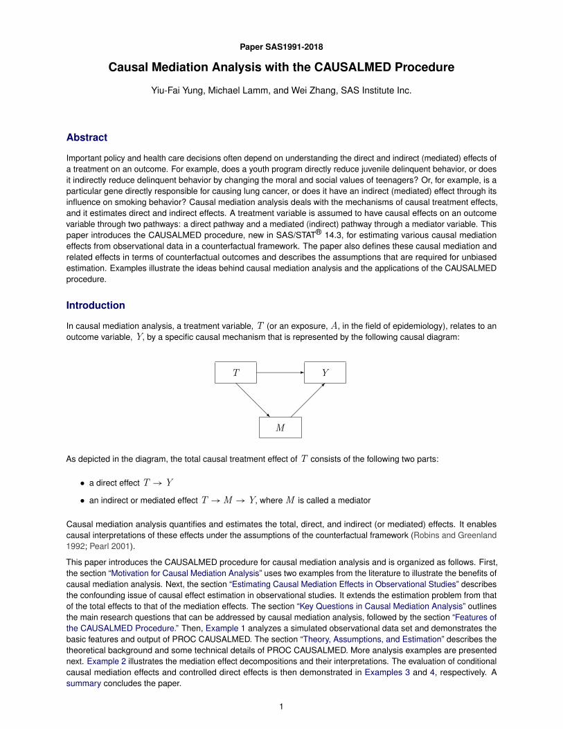
In causal mediation analysis, a treatment variable, T (or an exposure, A, in the field of epidemiology), relates to anoutcome variable, Y, by a specific causal mechanism that is represented by the following causal diagram:

T Y

M

As depicted in the diagram, the total causal treatment effect of T consists of the following two parts:

� a direct effect T ! Y

� an indirect or mediated effect T !M ! Y, where M is called a mediator

Causal mediation analysis quantifies and estimates the total, direct, and indirect (or mediated) effects. It enablescausal interpretations of these effects under the assumptions of the counterfactual framework (Robins and Greenland1992; Pearl 2001).

This paper introduces the CAUSALMED procedure for causal mediation analysis and is organized as follows. First,the section “Motivation for Causal Mediation Analysis” uses two examples from the literature to illustrate the benefits ofcausal mediation analysis. Next, the section “Estimating Causal Mediation Effects in Observational Studies” describesthe confounding issue of causal effect estimation in observational studies. It extends the estimation problem from thatof the total effects to that of the mediation effects. The section “Key Questions in Causal Mediation Analysis” outlinesthe main research questions that can be addressed by causal mediation analysis, followed by the section “Features ofthe CAUSALMED Procedure.” Then, Example 1 analyzes a simulated observational data set and demonstrates thebasic features and output of PROC CAUSALMED. The section “Theory, Assumptions, and Estimation” describes thetheoretical background and some technical details of PROC CAUSALMED. More analysis examples are presentednext. Example 2 illustrates the mediation effect decompositions and their interpretations. The evaluation of conditionalcausal mediation effects and controlled direct effects is then demonstrated in Examples 3 and 4, respectively. Asummary concludes the paper.

1

Motivation for Causal Mediation Analysis

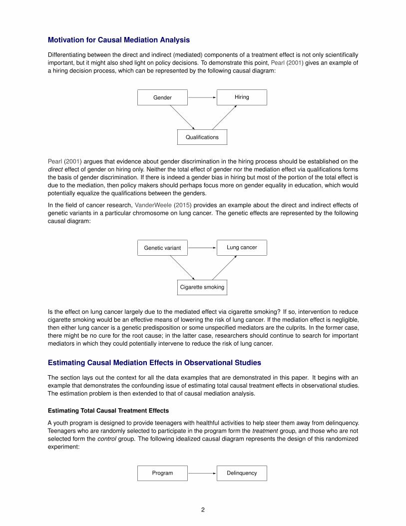
Differentiating between the direct and indirect (mediated) components of a treatment effect is not only scientificallyimportant, but it might also shed light on policy decisions. To demonstrate this point, Pearl (2001) gives an example ofa hiring decision process, which can be represented by the following causal diagram:

HiringGender

Qualifications

Pearl (2001) argues that evidence about gender discrimination in the hiring process should be established on thedirect effect of gender on hiring only. Neither the total effect of gender nor the mediation effect via qualifications formsthe basis of gender discrimination. If there is indeed a gender bias in hiring but most of the portion of the total effect isdue to the mediation, then policy makers should perhaps focus more on gender equality in education, which wouldpotentially equalize the qualifications between the genders.

In the field of cancer research, VanderWeele (2015) provides an example about the direct and indirect effects ofgenetic variants in a particular chromosome on lung cancer. The genetic effects are represented by the followingcausal diagram:

Lung cancerGenetic variant

Cigarette smoking

Is the effect on lung cancer largely due to the mediated effect via cigarette smoking? If so, intervention to reducecigarette smoking would be an effective means of lowering the risk of lung cancer. If the mediation effect is negligible,then either lung cancer is a genetic predisposition or some unspecified mediators are the culprits. In the former case,there might be no cure for the root cause; in the latter case, researchers should continue to search for importantmediators in which they could potentially intervene to reduce the risk of lung cancer.

Estimating Causal Mediation Effects in Observational Studies

The section lays out the context for all the data examples that are demonstrated in this paper. It begins with anexample that demonstrates the confounding issue of estimating total causal treatment effects in observational studies.The estimation problem is then extended to that of causal mediation analysis.

Estimating Total Causal Treatment Effects

A youth program is designed to provide teenagers with healthful activities to help steer them away from delinquency.Teenagers who are randomly selected to participate in the program form the treatment group, and those who are notselected form the control group. The following idealized causal diagram represents the design of this randomizedexperiment:

DelinquencyProgram

2

Because of the random assignment, all factors other than the youth program itself are supposed to be balancedbetween the treatment and control groups. As a result, the observed difference in delinquency between the treatmentand control groups has a valid causal interpretation; this total program effect is not confounded by other factors.

However, if assignments to the treatment and control groups are not random and the teenagers are instead allowed toparticipate in the youth program voluntarily, the study would become an observational study. The preceding causaldiagram is not accurate unless the confounding causes or factors are added (for example, confounding factors inobservational studies are often added to the diagram as common causes to the treatment (T ) and outcome (Y )variables). Confounding factors or variables induce extraneous associations between T and Y, so the observedmean difference between the treatment and control groups would be a biased estimate of the causal effect.

For example, if the youth program is costly or free transportation to the program activities is not provided, teenagersfrom lower socioeconomic classes might not be able to participate. Consequently, the treatment group would beoverrepresented by teenagers with higher socioeconomic status (SES), and the control group would be overrepre-sented by teenagers with lower SES. The observed relationship between T and Y is thus confounded by SES,making it difficult to determine whether the delinquent behavior is due to the true program effect, the different SESmakeups of the treatment and control groups, or both. In this case, you must somehow adjust for SES (which is calleda confounding variable or a confounder) when you estimate the causal effect of the youth program.

Generally, in observational studies where random assignments of participants are not made, there could be a lotof confounders that cloud the observed relationships between the treatment and outcome variables. In the currentexample, in addition to SES, pretreatment characteristics such as teenagers’ personality (extroversion/introversion),their degree of parental support, and their academic performance are also potential confounders that you might needto adjust for when you assess the causal effect of the youth program.

The CAUSALTRT and PSMATCH procedures in SAS/STAT software (SAS Institute Inc. 2017) provide statisticaladjustments for confounding pretreatment characteristics so that the total causal treatment effect can be estimatedwithout bias. For more information about these procedures as well as application examples, see Lamm and Yung(2017) and Yuan, Yung, and Stokes (2017). This paper extends beyond the estimation of total causal treatment effectsand discusses the decomposition of causal effects through causal mediation analysis by using the CAUSALMEDprocedure.

Mechanism of the Causal Process

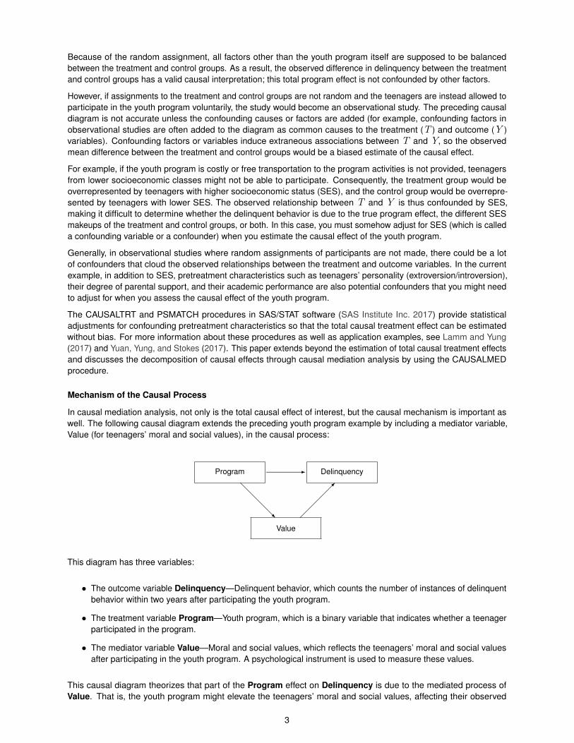
In causal mediation analysis, not only is the total causal effect of interest, but the causal mechanism is important aswell. The following causal diagram extends the preceding youth program example by including a mediator variable,Value (for teenagers’ moral and social values), in the causal process:

DelinquencyProgram

Value

This diagram has three variables:

� The outcome variable Delinquency—Delinquent behavior, which counts the number of instances of delinquentbehavior within two years after participating the youth program.

� The treatment variable Program—Youth program, which is a binary variable that indicates whether a teenagerparticipated in the program.

� The mediator variable Value—Moral and social values, which reflects the teenagers’ moral and social valuesafter participating in the youth program. A psychological instrument is used to measure these values.

This causal diagram theorizes that part of the Program effect on Delinquency is due to the mediated process ofValue. That is, the youth program might elevate the teenagers’ moral and social values, affecting their observed

3

Value level, which in turn reduces subsequent delinquent behavior. In addition, the direct pathway from Program toDelinquency represents the “residual” or direct treatment effect that is not due to the mediation process.

Causal mediation analysis enables you to understand the mechanism of the causal process. If the youth programdoes reduce subsequent delinquent behavior, is it largely due to the program’s intermediate effect in changing theteenagers’ moral and social values? If so, then the program administrator (or policy maker) might want to make certainthat future youth programs retain or even increase the educational elements for moral and social values. If not, thenthe program administrator might want to investigate what other mediating factors might have been important in theprocess and incorporate these factors into the design of future youth programs.

As in the case of estimating causal treatment effects (see Example 1), causal mediation analysis from observationalstudies is also subject to confounding. Even if treatment assignments have been randomized, causal interpretationsand estimation of mediation and related effects might still be subject to confounding because the mediator levelsare usually not randomized. Thus, you need to take confounding covariates into account when you estimate causalmediation effects. Example 1 demonstrates a basic analysis by using the CAUSALMED procedure.

Key Questions in Causal Mediation Analysis

To summarize, causal mediation analysis helps researchers find answers to the following key questions:

� Is part of the total causal treatment effect due to the specified mediation process?

� Is there an interaction effect between the treatment and the mediator on the outcome?

� What percentage of the total causal effect is due to the mediation, the interaction, or both?

� Can you intervene in the causal mediation process to achieve desirable outcomes?

To answer these questions, causal mediation analysis must deal with the following main issues:

� Definition—How can various causal mediation effects be defined appropriately in a general modeling situation?

� Interpretation—How do you properly interpret the various causal mediation effects and decompositions?

� Identification—Under what conditions can various causal mediation effects be estimated without bias?

� Estimation—How can various causal mediation effects be estimated?

The counterfactual framework (Robins and Greenland 1992; Pearl 2001) has been proposed to deal with the definition,interpretation, and identification issues of causal mediation analysis. Based on the counterfactual framework, theCAUSALMED procedure implements the regression adjustment method to estimate causal mediation effects (Valeriand VanderWeele 2013; VanderWeele 2014). For more information about the technical details of the counterfactualframework and the estimation methods of PROC CAUSALMED, see the section “Theory, Assumptions, and Estimation.”

Features of the CAUSALMED Procedure

The CAUSALMED procedure supports a limited set of generalized linear models for describing the relationshipsamong the outcome, treatment, mediator, and confounder variables. With this set of models, you can use PROCCAUSALMED to conduct causal mediation analysis on data of the following types:

� outcome variable Y : binary, continuous, or count

� treatment variable T : binary or continuous

� mediator variable M : binary or continuous

� covariates: categorical or continuous

4

The main features and output from PROC CAUSALMED include the following:

� estimates of total, controlled direct, natural direct, and natural indirect effects

� effects that are computed on the odds ratio scale and the excess relative risk scale for binary responses

� percentages of the total effect that are attributed to mediation and interaction, and the percentage of the totaleffect eliminated by controlling the mediator level

� various decompositions of total effects, including several two-, three-, and four-way decompositions

� flexible evaluation of controlled direct effects and conditional mediation effects

Other important features that you can optionally request from the procedure include these:

� analysis with case-control design

� bootstrap estimation of standard errors and confidence intervals

� output of outcome and mediator model estimates

Example 1. Basic Causal Mediation Analysis of the Youth Program Data

This section demonstrates how you can use the CAUSALMED procedure to perform causal mediation analysis ofobservational data. As described in Example 2, a youth program was designed to foster teenagers’ personal growthand thus reduce their delinquent behavior. The analysis also sought to determine whether any of the program effectwas due to the mediation of the teenagers’ moral and social values during their participation in the process.

A data set for an observational study was simulated. It contains 800 observations with the following variables:

� Delinquency, the frequency of delinquent behavior within two years after the outset of the youth program; thisis the outcome variable of interest.

� Program, the indicator of youth program participation (Yes or No); this is the treatment variable of interest.

� Value, the teenager’s score on a moral and social values scale one year after the outset of the youth program;this is the mediator variable of interest.

� Delinquency0, the frequency of delinquent behavior within two years before the outset of the youth program

� Gender, the gender of the teenager

� GPA, the teenager’s grade point average in school at the outset of the youth program

� Introversion, the indicator of self-described introversion (Yes or No)

� SES, the teenager’s socioeconomic status (Low, Medium, or High)

� Support, the degree of parental support on a four-point scale, which was assessed at the outset of the program

� Value0, the teenager’s score on a moral and social values scale at the outset of the youth program

The last seven variables are covariates that might have confounded the observed relationships among the outcome,treatment, and mediator variables.

The first 10 observations of the Youth data set are shown in Figure 1.

5

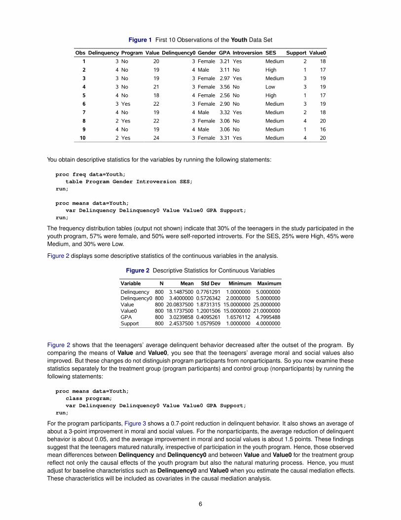
Figure 1 First 10 Observations of the Youth Data Set

Obs Delinquency Program Value Delinquency0 Gender GPA Introversion SES Support Value0

1 3 No 20 3 Female 3.21 Yes Medium 2 18

2 4 No 19 4 Male 3.11 No High 1 17

3 3 No 19 3 Female 2.97 Yes Medium 3 19

4 3 No 21 3 Female 3.56 No Low 3 19

5 4 No 18 4 Female 2.56 No High 1 17

6 3 Yes 22 3 Female 2.90 No Medium 3 19

7 4 No 19 4 Male 3.32 Yes Medium 2 18

8 2 Yes 22 3 Female 3.06 No Medium 4 20

9 4 No 19 4 Male 3.06 No Medium 1 16

10 2 Yes 24 3 Female 3.31 Yes Medium 4 20

You obtain descriptive statistics for the variables by running the following statements:

proc freq data=Youth;table Program Gender Introversion SES;

run;

proc means data=Youth;var Delinquency Delinquency0 Value Value0 GPA Support;

run;

The frequency distribution tables (output not shown) indicate that 30% of the teenagers in the study participated in theyouth program, 57% were female, and 50% were self-reported introverts. For the SES, 25% were High, 45% wereMedium, and 30% were Low.

Figure 2 displays some descriptive statistics of the continuous variables in the analysis.

Figure 2 Descriptive Statistics for Continuous Variables

Variable N Mean Std Dev Minimum Maximum

DelinquencyDelinquency0ValueValue0GPASupport

800800800800800800

3.14875003.400000020.083750018.17375003.02398582.4537500

0.77612910.57263421.87313151.20015060.40952611.0579509

1.00000002.000000015.000000015.00000001.65761121.0000000

5.00000005.000000025.000000021.00000004.79954884.0000000

Figure 2 shows that the teenagers’ average delinquent behavior decreased after the outset of the program. Bycomparing the means of Value and Value0, you see that the teenagers’ average moral and social values alsoimproved. But these changes do not distinguish program participants from nonparticipants. So you now examine thesestatistics separately for the treatment group (program participants) and control group (nonparticipants) by running thefollowing statements:

proc means data=Youth;class program;var Delinquency Delinquency0 Value Value0 GPA Support;

run;

For the program participants, Figure 3 shows a 0.7-point reduction in delinquent behavior. It also shows an average ofabout a 3-point improvement in moral and social values. For the nonparticipants, the average reduction of delinquentbehavior is about 0.05, and the average improvement in moral and social values is about 1.5 points. These findingssuggest that the teenagers matured naturally, irrespective of participation in the youth program. Hence, those observedmean differences between Delinquency and Delinquency0 and between Value and Value0 for the treatment groupreflect not only the causal effects of the youth program but also the natural maturing process. Hence, you mustadjust for baseline characteristics such as Delinquency0 and Value0 when you estimate the causal mediation effects.These characteristics will be included as covariates in the causal mediation analysis.

6

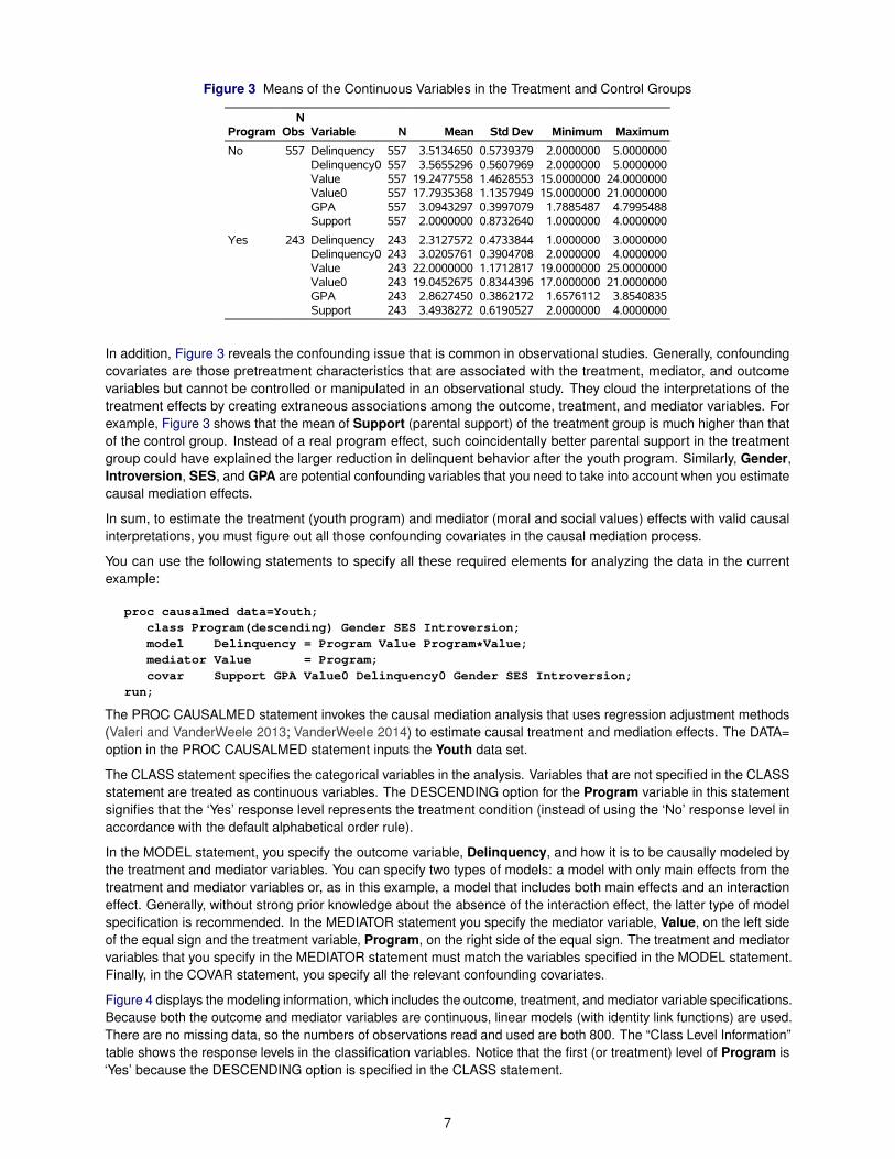
Figure 3 Means of the Continuous Variables in the Treatment and Control Groups

ProgramN

Obs Variable N Mean Std Dev Minimum Maximum

No 557 DelinquencyDelinquency0ValueValue0GPASupport

557557557557557557

3.51346503.565529619.247755817.79353683.09432972.0000000

0.57393790.56079691.46285531.13579490.39970790.8732640

2.00000002.000000015.000000015.00000001.78854871.0000000

5.00000005.000000024.000000021.00000004.79954884.0000000

Yes 243 DelinquencyDelinquency0ValueValue0GPASupport

243243243243243243

2.31275723.020576122.000000019.04526752.86274503.4938272

0.47338440.39047081.17128170.83443960.38621720.6190527

1.00000002.000000019.000000017.00000001.65761122.0000000

3.00000004.000000025.000000021.00000003.85408354.0000000

In addition, Figure 3 reveals the confounding issue that is common in observational studies. Generally, confoundingcovariates are those pretreatment characteristics that are associated with the treatment, mediator, and outcomevariables but cannot be controlled or manipulated in an observational study. They cloud the interpretations of thetreatment effects by creating extraneous associations among the outcome, treatment, and mediator variables. Forexample, Figure 3 shows that the mean of Support (parental support) of the treatment group is much higher than thatof the control group. Instead of a real program effect, such coincidentally better parental support in the treatmentgroup could have explained the larger reduction in delinquent behavior after the youth program. Similarly, Gender,Introversion, SES, and GPA are potential confounding variables that you need to take into account when you estimatecausal mediation effects.

In sum, to estimate the treatment (youth program) and mediator (moral and social values) effects with valid causalinterpretations, you must figure out all those confounding covariates in the causal mediation process.

You can use the following statements to specify all these required elements for analyzing the data in the currentexample:

proc causalmed data=Youth;class Program(descending) Gender SES Introversion;model Delinquency = Program Value Program*Value;mediator Value = Program;covar Support GPA Value0 Delinquency0 Gender SES Introversion;

run;

The PROC CAUSALMED statement invokes the causal mediation analysis that uses regression adjustment methods(Valeri and VanderWeele 2013; VanderWeele 2014) to estimate causal treatment and mediation effects. The DATA=option in the PROC CAUSALMED statement inputs the Youth data set.

The CLASS statement specifies the categorical variables in the analysis. Variables that are not specified in the CLASSstatement are treated as continuous variables. The DESCENDING option for the Program variable in this statementsignifies that the ‘Yes’ response level represents the treatment condition (instead of using the ‘No’ response level inaccordance with the default alphabetical order rule).

In the MODEL statement, you specify the outcome variable, Delinquency, and how it is to be causally modeled bythe treatment and mediator variables. You can specify two types of models: a model with only main effects from thetreatment and mediator variables or, as in this example, a model that includes both main effects and an interactioneffect. Generally, without strong prior knowledge about the absence of the interaction effect, the latter type of modelspecification is recommended. In the MEDIATOR statement you specify the mediator variable, Value, on the left sideof the equal sign and the treatment variable, Program, on the right side of the equal sign. The treatment and mediatorvariables that you specify in the MEDIATOR statement must match the variables specified in the MODEL statement.Finally, in the COVAR statement, you specify all the relevant confounding covariates.

Figure 4 displays the modeling information, which includes the outcome, treatment, and mediator variable specifications.Because both the outcome and mediator variables are continuous, linear models (with identity link functions) are used.There are no missing data, so the numbers of observations read and used are both 800. The “Class Level Information”table shows the response levels in the classification variables. Notice that the first (or treatment) level of Program is‘Yes’ because the DESCENDING option is specified in the CLASS statement.

7

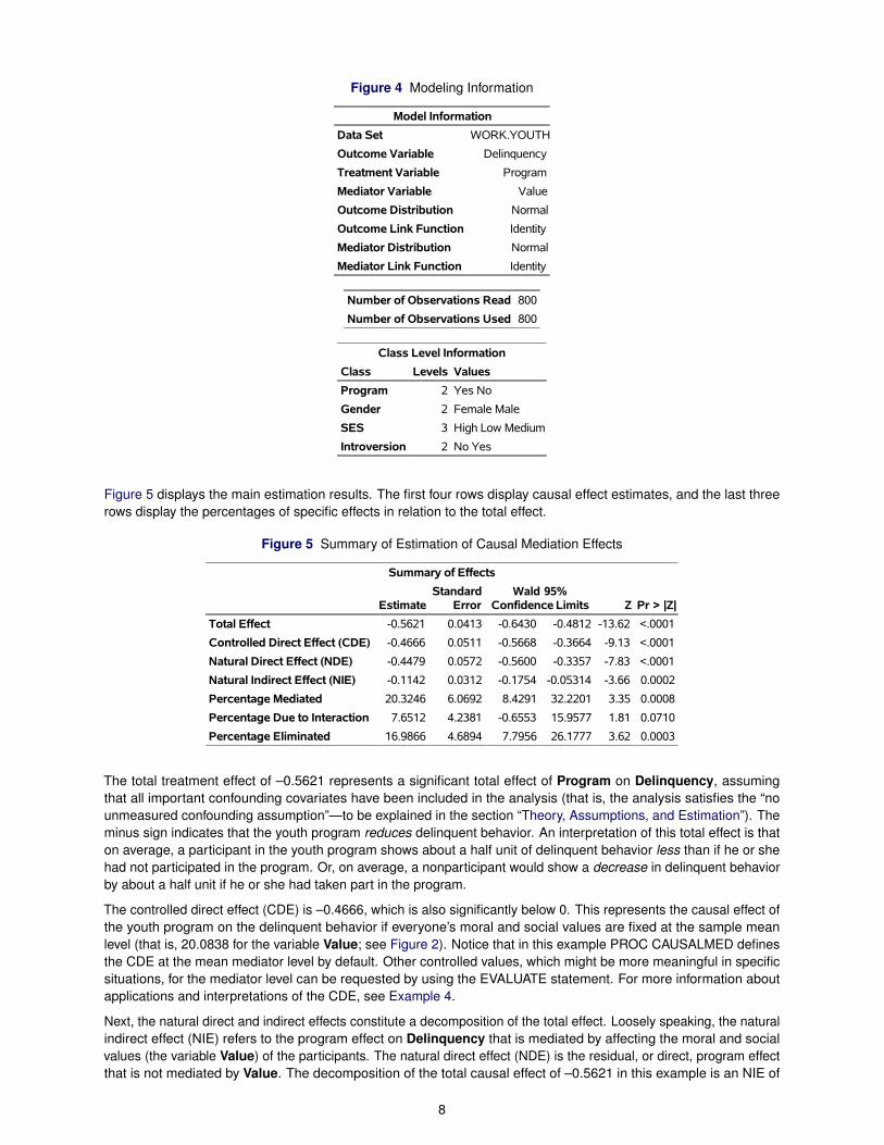
Figure 4 Modeling Information

Model Information

Data Set WORK.YOUTH

Outcome Variable Delinquency

Treatment Variable Program

Mediator Variable Value

Outcome Distribution Normal

Outcome Link Function Identity

Mediator Distribution Normal

Mediator Link Function Identity

Number of Observations Read 800

Number of Observations Used 800

Class Level Information

Class Levels Values

Program 2 Yes No

Gender 2 Female Male

SES 3 High Low Medium

Introversion 2 No Yes

Figure 5 displays the main estimation results. The first four rows display causal effect estimates, and the last threerows display the percentages of specific effects in relation to the total effect.

Figure 5 Summary of Estimation of Causal Mediation Effects

Summary of Effects

EstimateStandard

ErrorWald 95%

Confidence Limits Z Pr > |Z|

Total Effect -0.5621 0.0413 -0.6430 -0.4812 -13.62 <.0001

Controlled Direct Effect (CDE) -0.4666 0.0511 -0.5668 -0.3664 -9.13 <.0001

Natural Direct Effect (NDE) -0.4479 0.0572 -0.5600 -0.3357 -7.83 <.0001

Natural Indirect Effect (NIE) -0.1142 0.0312 -0.1754 -0.05314 -3.66 0.0002

Percentage Mediated 20.3246 6.0692 8.4291 32.2201 3.35 0.0008

Percentage Due to Interaction 7.6512 4.2381 -0.6553 15.9577 1.81 0.0710

Percentage Eliminated 16.9866 4.6894 7.7956 26.1777 3.62 0.0003

The total treatment effect of –0.5621 represents a significant total effect of Program on Delinquency, assumingthat all important confounding covariates have been included in the analysis (that is, the analysis satisfies the “nounmeasured confounding assumption”—to be explained in the section “Theory, Assumptions, and Estimation”). Theminus sign indicates that the youth program reduces delinquent behavior. An interpretation of this total effect is thaton average, a participant in the youth program shows about a half unit of delinquent behavior less than if he or shehad not participated in the program. Or, on average, a nonparticipant would show a decrease in delinquent behaviorby about a half unit if he or she had taken part in the program.

The controlled direct effect (CDE) is –0.4666, which is also significantly below 0. This represents the causal effect ofthe youth program on the delinquent behavior if everyone’s moral and social values are fixed at the sample meanlevel (that is, 20.0838 for the variable Value; see Figure 2). Notice that in this example PROC CAUSALMED definesthe CDE at the mean mediator level by default. Other controlled values, which might be more meaningful in specificsituations, for the mediator level can be requested by using the EVALUATE statement. For more information aboutapplications and interpretations of the CDE, see Example 4.

Next, the natural direct and indirect effects constitute a decomposition of the total effect. Loosely speaking, the naturalindirect effect (NIE) refers to the program effect on Delinquency that is mediated by affecting the moral and socialvalues (the variable Value) of the participants. The natural direct effect (NDE) is the residual, or direct, program effectthat is not mediated by Value. The decomposition of the total causal effect of –0.5621 in this example is an NIE of

8

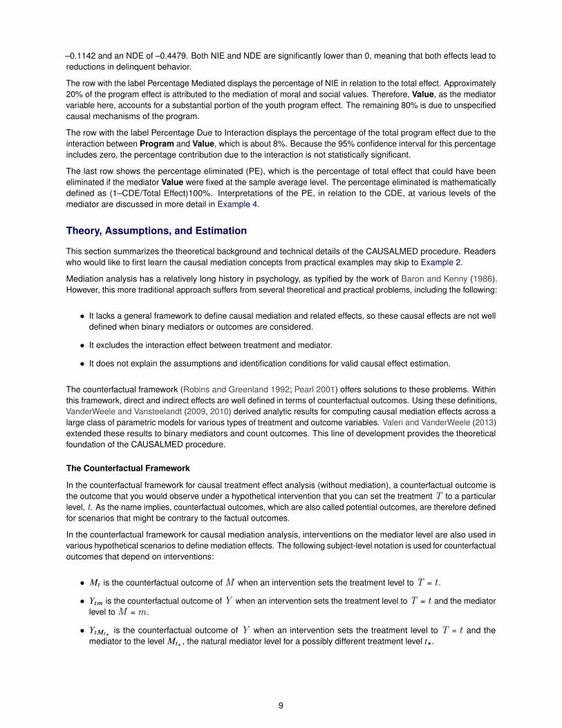
–0.1142 and an NDE of –0.4479. Both NIE and NDE are significantly lower than 0, meaning that both effects lead toreductions in delinquent behavior.

The row with the label Percentage Mediated displays the percentage of NIE in relation to the total effect. Approximately20% of the program effect is attributed to the mediation of moral and social values. Therefore, Value, as the mediatorvariable here, accounts for a substantial portion of the youth program effect. The remaining 80% is due to unspecifiedcausal mechanisms of the program.

The row with the label Percentage Due to Interaction displays the percentage of the total program effect due to theinteraction between Program and Value, which is about 8%. Because the 95% confidence interval for this percentageincludes zero, the percentage contribution due to the interaction is not statistically significant.

The last row shows the percentage eliminated (PE), which is the percentage of total effect that could have beeneliminated if the mediator Value were fixed at the sample average level. The percentage eliminated is mathematicallydefined as (1–CDE/Total Effect)100%. Interpretations of the PE, in relation to the CDE, at various levels of themediator are discussed in more detail in Example 4.

Theory, Assumptions, and Estimation

This section summarizes the theoretical background and technical details of the CAUSALMED procedure. Readerswho would like to first learn the causal mediation concepts from practical examples may skip to Example 2.

Mediation analysis has a relatively long history in psychology, as typified by the work of Baron and Kenny (1986).However, this more traditional approach suffers from several theoretical and practical problems, including the following:

� It lacks a general framework to define causal mediation and related effects, so these causal effects are not welldefined when binary mediators or outcomes are considered.

� It excludes the interaction effect between treatment and mediator.

� It does not explain the assumptions and identification conditions for valid causal effect estimation.

The counterfactual framework (Robins and Greenland 1992; Pearl 2001) offers solutions to these problems. Withinthis framework, direct and indirect effects are well defined in terms of counterfactual outcomes. Using these definitions,VanderWeele and Vansteelandt (2009, 2010) derived analytic results for computing causal mediation effects across alarge class of parametric models for various types of treatment and outcome variables. Valeri and VanderWeele (2013)extended these results to binary mediators and count outcomes. This line of development provides the theoreticalfoundation of the CAUSALMED procedure.

The Counterfactual Framework

In the counterfactual framework for causal treatment effect analysis (without mediation), a counterfactual outcome isthe outcome that you would observe under a hypothetical intervention that you can set the treatment T to a particularlevel, t. As the name implies, counterfactual outcomes, which are also called potential outcomes, are therefore definedfor scenarios that might be contrary to the factual outcomes.

In the counterfactual framework for causal mediation analysis, interventions on the mediator level are also used invarious hypothetical scenarios to define mediation effects. The following subject-level notation is used for counterfactualoutcomes that depend on interventions:

� Mt is the counterfactual outcome of M when an intervention sets the treatment level to T = t .

� Ytm is the counterfactual outcome of Y when an intervention sets the treatment level to T = t and the mediatorlevel to M = m .

� YtMt�is the counterfactual outcome of Y when an intervention sets the treatment level to T = t and the

mediator to the level Mt� , the natural mediator level for a possibly different treatment level t�.

9

This notation places no restriction on variable types. The variables Y, T, and M can be continuous or binary.

Suppose for the moment that the treatment is binary, so t is either 0 or 1, denoting the control (no treatment)and treatment conditions, respectively. The total effect (TE) for a subject is defined as the difference between thecounterfactual outcomes at the treatment and control levels:

TE D Y1M1� Y0M0

In this equation, the first subscript in the counterfactual outcomes denotes the level (at either 1 or 0) that is set for thetreatment, and the second subscript denotes the mediator value (either M1 or M0) that would follow from setting thetreatment to a specific level. Notice that M1 and M0 are not fixed values, so their realized values could be different fordifferent subjects. Because YiMi

in the TE definition has consistent treatment levels i, Yi is an equivalent notation forYiMi

and therefore TE can also be defined by Y1 � Y0.

The controlled direct effect (CDE) for a subject is defined as the difference between the counterfactual outcomes atthe two treatment levels when an intervention sets the mediator to a particular level, M = m. That is,

CDE.m/ D Y1m � Y0m

The natural direct effect (NDE) for a subject is defined as the difference between the counterfactual outcomes atthe two treatment levels when an intervention sets the mediator value to M = M0, which is the natural level of themediator when there is no treatment. That is,

NDE D Y1M0� Y0M0

The natural indirect effect (NIE) for a subject is defined as the difference between the counterfactual outcomes at thetwo mediator levels at M1 and M0 when an intervention sets the treatment to T = 1. That is,

NIE D Y1M1� Y1M0

If the treatment variable T is continuous, then the treatment levels must be defined according to the treatment andcontrol levels of interest. For example, if t1 and t0 are the treatment and control levels on a continuous scale andthey represent the levels of substantive interest, then they should replace the values 1 and 0, respectively, for thetreatment and control levels in the definitions. However, this more general notation is not used here because it wouldunnecessarily complicate the presentation.

So far, TE, CDE, NDE, and NIE have been defined at the subject level. The corresponding effects at the populationlevel are defined by the average or expectation of these effects—that is, EŒTE�, EŒCDE.m/�, EŒNDE�, and EŒNIE�,respectively. PROC CAUSALMED estimates these population-level effects, as illustrated in Example 1.

The counterfactual definitions of effects have two important properties. First, they yield the following well-knownformula of a two-way decomposition of the total effect (TE):

TE D NDEC NIE

Or, using the population notation, the two-way decomposition is of the form

EŒTE� D EŒNDE�CEŒNIE�

The percentage of total effect that is mediated (PM) is then computed as

PM D EŒNIE�=EŒTE� � 100%

Second, and more importantly, because these definitions are independent of the model for the outcome or mediator,you can apply them to a wide range of modeling situations. That is, these definitions of effects and the total effectdecomposition formulas are applicable to various variable types and linear or nonlinear models with or without aninteraction effect between T and M.

10

VanderWeele (2014) took a step further and introduced the following four-way decomposition of the total effect:

TE D CDEC IRFC IMDC PIE

The four component effects in this equation are characterized by how they represent the interaction and mediationeffects, as follows:

� CDE—controlled direct effect: the component that is not due to interaction or mediation

� IRF—reference interaction: the component that is due to interaction but not mediation

� IMD—mediated interaction: the component that is due to both interaction and mediation

� PIE—pure indirect effect: the component that is due to mediation but not interaction

In VanderWeele (2014), IRF is denoted as INTref and IMD is denoted as INTmed. These four component effectsare also defined in terms of counterfactual outcomes (see VanderWeele 2014). For an illustration of the four-waydecomposition, see Example 2.

Again, all the preceding effect notations for the four-way decomposition are defined at the subject level. Thecorresponding population parameters are obtained by taking expectations of the subject-level effects over the entirepopulation. The composite relationship still holds for the population component effects. That is,

EŒTE� D EŒCDE�CEŒIRF�CEŒIMD�CEŒPIE�

Dividing each of these population component effects by EŒTE� yields the corresponding proportion contributions ofthese components to the total effect. However, these contributions might not be interpretable when the componenteffects have mixed signs.

Two important relationships between the four-way decomposition and the preceding two-way decomposition areexpressed by the following equations:

NDE D CDEC IRF

NIE D PIEC IMD

The first equation expresses the natural direct effect (NDE) as the composite component of the controlled direct effectand reference interaction. The second equation expresses the mediation effect or natural indirect effect (NIE) as thecomposite component of the pure indirect effect and mediated interaction. Three-way decompositions of the totaleffect follow from substituting the expression for either the NDE or the NIE into the two-way total effect decomposition.

Another useful composite component is the “portion attributed to interaction” (PAI) between T and M, which is definedas

PAI D IRFC IMD

At the population level, the percentage of total effect that is due to the interaction is therefore computed as

EŒPAI�=EŒTE� � 100%

Finally, the portion eliminated (PE), which is defined as

EŒPE� D 1 �EŒCDE�=EŒTE�

is the portion of the total effect that is eliminated when an intervention sets the mediator variable to a particular level.Multiplying the right side of the PE formula by 100% yields the definition of “percentage eliminated.” For an illustrationof the use of the CDE and PE estimates, see Example 4 .

For further discussion of the various two-way and three-way decompositions and their relationships to the four-waydecomposition, see VanderWeele (2014). You can use the DECOMP option in the CAUSALMED procedure toobtain several two-way decompositions, several three-way decompositions, and the four-way decomposition. For anillustration and further discussion of the various decompositions, see Example 2.

When the outcome responses are binary, various mediation and related effects are defined on the odds ratio orexcess relative risk scale (Valeri and VanderWeele 2013; VanderWeele 2014). Parallel conceptions about effectcomponents and decompositions to those that have been discussed in this section are still applicable. See the PROCCAUSALMED documentation (SAS Institute Inc. 2017) for examples.

11

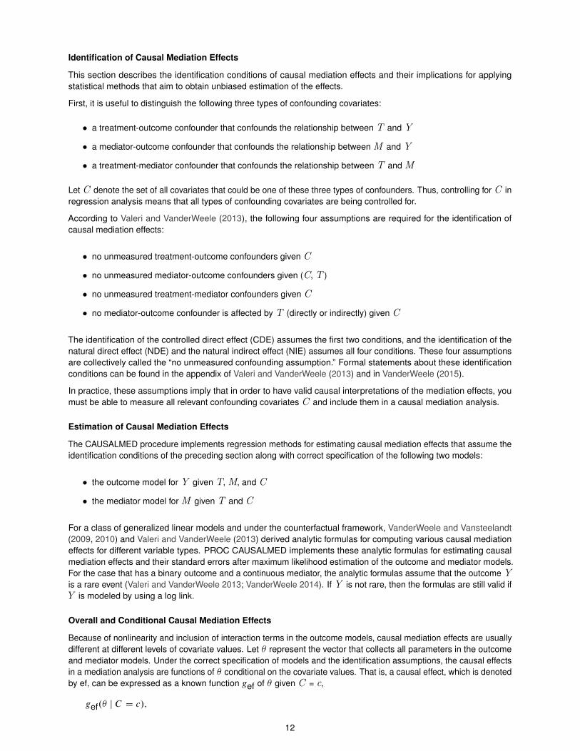
Identification of Causal Mediation Effects

This section describes the identification conditions of causal mediation effects and their implications for applyingstatistical methods that aim to obtain unbiased estimation of the effects.

First, it is useful to distinguish the following three types of confounding covariates:

� a treatment-outcome confounder that confounds the relationship between T and Y

� a mediator-outcome confounder that confounds the relationship between M and Y

� a treatment-mediator confounder that confounds the relationship between T and M

Let C denote the set of all covariates that could be one of these three types of confounders. Thus, controlling for C inregression analysis means that all types of confounding covariates are being controlled for.

According to Valeri and VanderWeele (2013), the following four assumptions are required for the identification ofcausal mediation effects:

� no unmeasured treatment-outcome confounders given C

� no unmeasured mediator-outcome confounders given (C, T )

� no unmeasured treatment-mediator confounders given C

� no mediator-outcome confounder is affected by T (directly or indirectly) given C

The identification of the controlled direct effect (CDE) assumes the first two conditions, and the identification of thenatural direct effect (NDE) and the natural indirect effect (NIE) assumes all four conditions. These four assumptionsare collectively called the “no unmeasured confounding assumption.” Formal statements about these identificationconditions can be found in the appendix of Valeri and VanderWeele (2013) and in VanderWeele (2015).

In practice, these assumptions imply that in order to have valid causal interpretations of the mediation effects, youmust be able to measure all relevant confounding covariates C and include them in a causal mediation analysis.

Estimation of Causal Mediation Effects

The CAUSALMED procedure implements regression methods for estimating causal mediation effects that assume theidentification conditions of the preceding section along with correct specification of the following two models:

� the outcome model for Y given T, M, and C

� the mediator model for M given T and C

For a class of generalized linear models and under the counterfactual framework, VanderWeele and Vansteelandt(2009, 2010) and Valeri and VanderWeele (2013) derived analytic formulas for computing various causal mediationeffects for different variable types. PROC CAUSALMED implements these analytic formulas for estimating causalmediation effects and their standard errors after maximum likelihood estimation of the outcome and mediator models.For the case that has a binary outcome and a continuous mediator, the analytic formulas assume that the outcome Yis a rare event (Valeri and VanderWeele 2013; VanderWeele 2014). If Y is not rare, then the formulas are still valid ifY is modeled by using a log link.

Overall and Conditional Causal Mediation Effects

Because of nonlinearity and inclusion of interaction terms in the outcome models, causal mediation effects are usuallydifferent at different levels of covariate values. Let � represent the vector that collects all parameters in the outcomeand mediator models. Under the correct specification of models and the identification assumptions, the causal effectsin a mediation analysis are functions of � conditional on the covariate values. That is, a causal effect, which is denotedby ef, can be expressed as a known function gef of � given C = c,

gef.� j C D c/;

12

where c represents some fixed values for covariates C. By default, PROC CAUSALMED computes gef.� j C D c/with c = c0, where c0 is the sample mean value of C. This default setting provides “overall” measures of variouscausal mediation effects. It is consistent with the treatment of the SAS® macros that are implemented by Valeri andVanderWeele (2013). If the outcome and mediator models are linear, then the overall effects are also marginal effects.For more information about the computation of c0, see the PROC CAUSALMED documentation (SAS Institute Inc.2017).

However, in some applications you might be interested in the conditional mediation effects instead of the overallcounterparts. Denote a conditional causal mediation effect at the covariate value ck as

gef.� j C D ck/

For example, a particular c1 value defines a highly motivated subpopulation and a particular c2 value defines a lessmotivated subpopulation. In this case, you want to compare gef.� j C D c1/ with gef.� j C D c2/ to see whether thespecific mediation effects would be the same for the subpopulations with different motivational levels. You can use theEVALUATE statement in the CAUSALMED procedure to estimate these conditional causal mediation effects. SeeExample 3 for an illustration.

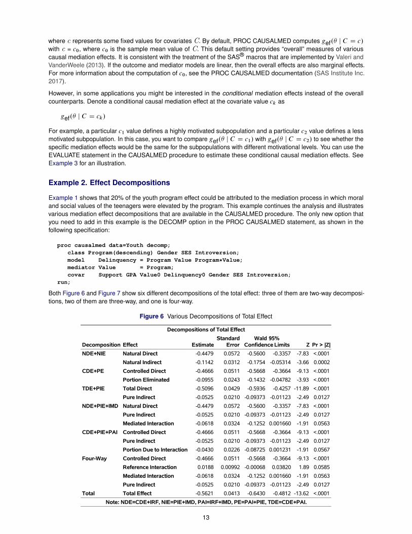
Example 2. Effect Decompositions

Example 1 shows that 20% of the youth program effect could be attributed to the mediation process in which moraland social values of the teenagers were elevated by the program. This example continues the analysis and illustratesvarious mediation effect decompositions that are available in the CAUSALMED procedure. The only new option thatyou need to add in this example is the DECOMP option in the PROC CAUSALMED statement, as shown in thefollowing specification:

proc causalmed data=Youth decomp;class Program(descending) Gender SES Introversion;model Delinquency = Program Value Program*Value;mediator Value = Program;covar Support GPA Value0 Delinquency0 Gender SES Introversion;

run;

Both Figure 6 and Figure 7 show six different decompositions of the total effect: three of them are two-way decomposi-tions, two of them are three-way, and one is four-way.

Figure 6 Various Decompositions of Total Effect

Decompositions of Total Effect

Decomposition Effect EstimateStandard

ErrorWald 95%


NDE+NIE Natural Direct -0.4479 0.0572 -0.5600 -0.3357 -7.83 <.0001

Natural Indirect -0.1142 0.0312 -0.1754 -0.05314 -3.66 0.0002

CDE+PE Controlled Direct -0.4666 0.0511 -0.5668 -0.3664 -9.13 <.0001

Portion Eliminated -0.0955 0.0243 -0.1432 -0.04782 -3.93 <.0001

TDE+PIE Total Direct -0.5096 0.0429 -0.5936 -0.4257 -11.89 <.0001

Pure Indirect -0.0525 0.0210 -0.09373 -0.01123 -2.49 0.0127

NDE+PIE+IMD Natural Direct -0.4479 0.0572 -0.5600 -0.3357 -7.83 <.0001

Pure Indirect -0.0525 0.0210 -0.09373 -0.01123 -2.49 0.0127

Mediated Interaction -0.0618 0.0324 -0.1252 0.001660 -1.91 0.0563

CDE+PIE+PAI Controlled Direct -0.4666 0.0511 -0.5668 -0.3664 -9.13 <.0001

Pure Indirect -0.0525 0.0210 -0.09373 -0.01123 -2.49 0.0127

Portion Due to Interaction -0.0430 0.0226 -0.08725 0.001231 -1.91 0.0567

Four-Way Controlled Direct -0.4666 0.0511 -0.5668 -0.3664 -9.13 <.0001

Reference Interaction 0.0188 0.00992 -0.00068 0.03820 1.89 0.0585

Mediated Interaction -0.0618 0.0324 -0.1252 0.001660 -1.91 0.0563

Pure Indirect -0.0525 0.0210 -0.09373 -0.01123 -2.49 0.0127

Total Total Effect -0.5621 0.0413 -0.6430 -0.4812 -13.62 <.0001

Note: NDE=CDE+IRF, NIE=PIE+IMD, PAI=IRF+IMD, PE=PAI+PIE, TDE=CDE+PAI.

13

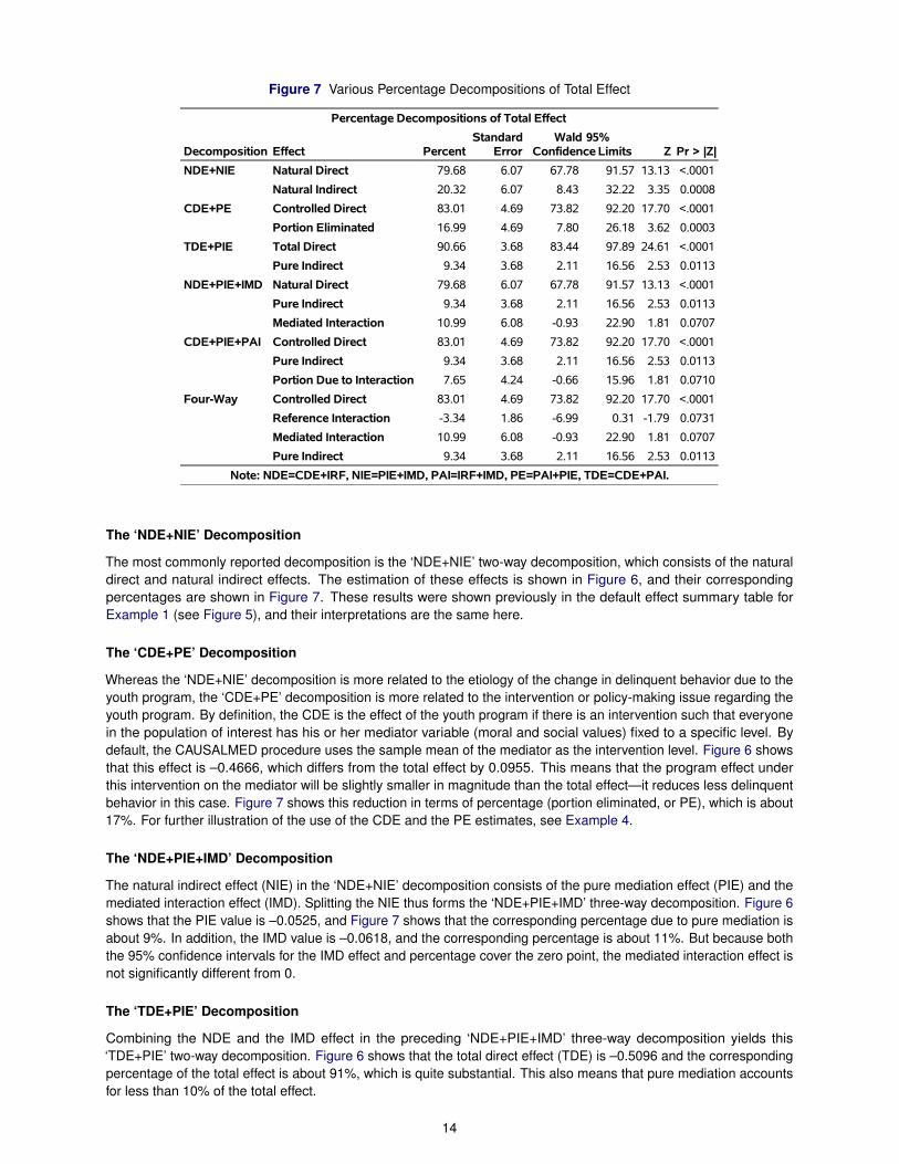
Figure 7 Various Percentage Decompositions of Total Effect

Percentage Decompositions of Total Effect

Decomposition Effect PercentStandard

ErrorWald 95%


NDE+NIE Natural Direct 79.68 6.07 67.78 91.57 13.13 <.0001

Natural Indirect 20.32 6.07 8.43 32.22 3.35 0.0008

CDE+PE Controlled Direct 83.01 4.69 73.82 92.20 17.70 <.0001

Portion Eliminated 16.99 4.69 7.80 26.18 3.62 0.0003

TDE+PIE Total Direct 90.66 3.68 83.44 97.89 24.61 <.0001

Pure Indirect 9.34 3.68 2.11 16.56 2.53 0.0113

NDE+PIE+IMD Natural Direct 79.68 6.07 67.78 91.57 13.13 <.0001

Pure Indirect 9.34 3.68 2.11 16.56 2.53 0.0113

Mediated Interaction 10.99 6.08 -0.93 22.90 1.81 0.0707

CDE+PIE+PAI Controlled Direct 83.01 4.69 73.82 92.20 17.70 <.0001

Pure Indirect 9.34 3.68 2.11 16.56 2.53 0.0113

Portion Due to Interaction 7.65 4.24 -0.66 15.96 1.81 0.0710

Four-Way Controlled Direct 83.01 4.69 73.82 92.20 17.70 <.0001

Reference Interaction -3.34 1.86 -6.99 0.31 -1.79 0.0731

Mediated Interaction 10.99 6.08 -0.93 22.90 1.81 0.0707

Pure Indirect 9.34 3.68 2.11 16.56 2.53 0.0113

Note: NDE=CDE+IRF, NIE=PIE+IMD, PAI=IRF+IMD, PE=PAI+PIE, TDE=CDE+PAI.

The ‘NDE+NIE’ Decomposition

The most commonly reported decomposition is the ‘NDE+NIE’ two-way decomposition, which consists of the naturaldirect and natural indirect effects. The estimation of these effects is shown in Figure 6, and their correspondingpercentages are shown in Figure 7. These results were shown previously in the default effect summary table forExample 1 (see Figure 5), and their interpretations are the same here.

The ‘CDE+PE’ Decomposition

Whereas the ‘NDE+NIE’ decomposition is more related to the etiology of the change in delinquent behavior due to theyouth program, the ‘CDE+PE’ decomposition is more related to the intervention or policy-making issue regarding theyouth program. By definition, the CDE is the effect of the youth program if there is an intervention such that everyonein the population of interest has his or her mediator variable (moral and social values) fixed to a specific level. Bydefault, the CAUSALMED procedure uses the sample mean of the mediator as the intervention level. Figure 6 showsthat this effect is –0.4666, which differs from the total effect by 0.0955. This means that the program effect underthis intervention on the mediator will be slightly smaller in magnitude than the total effect—it reduces less delinquentbehavior in this case. Figure 7 shows this reduction in terms of percentage (portion eliminated, or PE), which is about17%. For further illustration of the use of the CDE and the PE estimates, see Example 4.

The ‘NDE+PIE+IMD’ Decomposition

The natural indirect effect (NIE) in the ‘NDE+NIE’ decomposition consists of the pure mediation effect (PIE) and themediated interaction effect (IMD). Splitting the NIE thus forms the ‘NDE+PIE+IMD’ three-way decomposition. Figure 6shows that the PIE value is –0.0525, and Figure 7 shows that the corresponding percentage due to pure mediation isabout 9%. In addition, the IMD value is –0.0618, and the corresponding percentage is about 11%. But because boththe 95% confidence intervals for the IMD effect and percentage cover the zero point, the mediated interaction effect isnot significantly different from 0.

The ‘TDE+PIE’ Decomposition

Combining the NDE and the IMD effect in the preceding ‘NDE+PIE+IMD’ three-way decomposition yields this‘TDE+PIE’ two-way decomposition. Figure 6 shows that the total direct effect (TDE) is –0.5096 and the correspondingpercentage of the total effect is about 91%, which is quite substantial. This also means that pure mediation accountsfor less than 10% of the total effect.

14

The ‘CDE+PIE+PAI’ Decomposition

The most interesting effect in this three-way decomposition is perhaps the “portion attributed to interaction” (PAI)component, which pools the mediated interaction (IMD) and reference interaction (IRF) together. Because both the95% confidence intervals for PAI and its corresponding percentage cover the zero point, the interaction effect betweenthe youth program and the moral and social values is not evident.

The Four-Way Decomposition: ‘CDE+IRF+IMD+PIE’

Finally, Figure 6 and Figure 7 show the four-way decomposition (VanderWeele 2014) of the effects and theirpercentages. All four of these effects have been discussed previously in various decompositions. In fact, you canview all the lower-order decompositions as some particular collapsing of the component effects of the four-waydecomposition. The conceptual advantage of the four-way decomposition is that it delineates the contributions due tomediation but not interaction (PIE), interaction but not mediation (IRF), both mediation and interaction (IMD), andneither mediation nor interaction (CDE). In the current case, both IMD and IRF percentages are not statisticallysignificant.

Example 3. Conditional Causal Mediation Effects

By default, PROC CAUSALMED evaluates the causal mediation effects at the “averaged” sample covariate values.These overall effects are useful for a general assessment of the mediation effects and their percentages. However,researchers sometimes want to examine the conditional causal mediation effects, given particular levels of covariatesof interest. This example illustrates how you can use the EVALUATE statement to study conditional mediation effects.

Using the same data as in Examples 1 and 2, you want to examine whether the mediation patterns are the same fordifferent subpopulations (or subgroups). In the following statements, you specify the same outcome and mediatormodels as those in Examples 1 and 2, but you add four EVALUATE statements that define specific subpopulations forlater comparisons:

proc causalmed data=Youth;class Program(descending) Gender SES Introversion;model Delinquency = Program Value Program*Value;mediator Value = Program;covar Support GPA Value0 Delinquency0 Gender SES Introversion;evaluate 'Delinquency0=2' Delinquency0=2;evaluate 'Delinquency0=5' Delinquency0=5;evaluate 'Delinquency0=2 Support=4 Value0=21' Delinquency0=2 Support=4 Value0=21;evaluate 'Delinquency0=5 Support=1 Value0=15' Delinquency0=5 Support=1 Value0=15;

run;

The levels for the covariates that are specified in these EVALUATE statements allow for the following two comparisonsof causal mediation patterns:

� low versus high initial delinquency subpopulations

� low-risk versus high-risk subpopulations

For the first comparison, you define the low and high initial delinquency subpopulations by using the minimumand maximum sample values of Delinquency0 (see Figure 2). Hence, the first EVALUATE statement specifiesDelinquency0=2, and the second EVALUATE statement specifies Delinquency0=5. The quoted strings in thesestatements are used as labels in the output results.

For the second comparison, you define the low-risk and high-risk subpopulations of the teenagers according to thecovariate levels summarized in Table 1. The low and high levels for these covariates are defined by the maximum andminimum sample values, which are shown in Figure 2 and specified in the last two EVALUATE statements.

Table 1 Subpopulation Definitions

Covariate Low-Risk Subpopulation High-Risk Subpopulation

Delinquency0 (initial frequency of delinquent behavior) Low HighSupport (level of family support) High LowValue0 (initial moral and social values) High Low

15

Figure 8 and Figure 9 show the effect summary tables for the first comparison. It appears that the total effect, NDE,NIE, percentage mediated, and other statistics in these two figures are quite similar. Therefore, the causal mediationpatterns for the low and high initial delinquency subpopulations differ minimally.

Figure 8 Low Initial Delinquency

Summary of Effects: Delinquency0=2

EstimateStandard

ErrorWald 95%


Total Effect -0.5654 0.0410 -0.6458 -0.4850 -13.78 <.0001







Figure 9 High Initial Delinquency

Summary of Effects: Delinquency0=5

EstimateStandard

ErrorWald 95%


Total Effect -0.5613 0.0420 -0.6436 -0.4790 -13.37 <.0001







Figure 10 and Figure 11 show the conditional causal mediation results in the low-risk and high-risk subpopulations.Clearly, the total program effect for the low-risk subpopulation (–0.6645) is larger in magnitude than that of the high-risksubpopulation (–0.4510). The percentage of program effect that is mediated by the moral and social values in thelow-risk subpopulation (17%) is smaller than that of the high-risk subpopulation (25%). This is perhaps conceivablebecause on average the low-risk subpopulation already has a higher level of Value0, so the program effect is lesslikely to be mediated by further enhancing the level of Value.

Figure 10 Low-Risk Subpopulation

Summary of Effects: Delinquency0=2 Support=4 Value0=21

EstimateStandard

ErrorWald 95%


Total Effect -0.6645 0.0541 -0.7704 -0.5585 -12.29 <.0001




Percentage Mediated 17.1935 4.0870 9.1831 25.2040 4.21 <.0001

Percentage Due to Interaction 21.8778 10.1947 1.8965 41.8590 2.15 0.0319


16

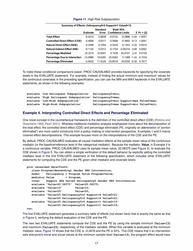
Figure 11 High-Risk Subpopulation

Summary of Effects: Delinquency0=5 Support=1 Value0=15

EstimateStandard

ErrorWald 95%


Total Effect -0.4510 0.0828 -0.6132 -0.2888 -5.45 <.0001


Natural Direct Effect (NDE) -0.3368 0.1054 -0.5434 -0.1302 -3.20 0.0014



Percentage Due to Interaction -15.0986 10.6265 -35.9262 5.7289 -1.42 0.1554

Percentage Eliminated -3.4635 11.4229 -25.8519 18.9250 -0.30 0.7617

To make these conditional comparisons easier, PROC CAUSALMED provides keywords for specifying the covariatelevels in the EVALUATE statement. For example, instead of finding the actual minimum and maximum values forthe continuous covariates in the preceding specification, you can use the MIN and MAX keywords in the EVALUATEstatements, as shown in the following examples:

evaluate 'Low Delinquent Subpopulation' Delinquency0=min;evaluate 'High Delinquent Subpopulation' Delinquency0=max;evaluate 'Low-Risk Subpopulation' Delinquency0=min Support=max Value0=max;evaluate 'High-Risk Subpopulation' Delinquency0=max Support=min Value0=min;

Example 4. Interpreting Controlled Direct Effects and Percentage Eliminated

One novel concept in the counterfactual framework is the definition of the controlled direct effect (CDE) (Robins andGreenland 1992; Pearl 2001). Whereas traditional mediation analysis emphasizes more about the decomposition ofthe total effect, the controlled direct effect (CDE) and percentage eliminated (PE, originally an abbreviation of “portioneliminated”) are more useful constructs from a policy-making or intervention perspective. Examples 1 and 2 mainlycovered effect decompositions. This example focuses more on the interpretations of the CDE and the PE.

By default, PROC CAUSALMED evaluates all causal mediation effects at the sample mean value of the continuousmediator (or the baseline/reference level of the categorical mediator). Because the mediator, Value, in Example 2 isa continuous variable, PROC CAUSALMED uses its sample mean value, 20.08375 (see Figure 2), to evaluate theCDE shown in Figure 5. You can obtain a simple verification of this default behavior by explicitly setting the controlledmediator level in the first EVALUATE statement of the following specification, which includes other EVALUATEstatements for computing the CDE and the PE given other mediator and covariate levels:

proc causalmed data=Youth;class Program(descending) Gender SES Introversion;model Delinquency = Program Value Program*Value;mediator Value = Program;covar Support GPA Value0 Delinquency0 Gender SES Introversion;evaluate 'Value=20.08375' Value=20.08375;evaluate 'Value=15' Value=15;evaluate 'Value=25' Value=25;evaluate 'Value=25 Delinquency0=2 Support=4 Value0=21'

Value=25 Delinquency0=2 Support=4 Value0=21;evaluate 'Value=25 Delinquency0=5 Support=1 Value0=15'

Value=25 Delinquency0=5 Support=1 Value0=15;run;

The first EVALUATE statement generates a summary table of effects (not shown here) that is exactly the same as thatin Figure 5, verifying the default evaluation of the CDE and the PE.

The next two EVALUATE statements compute the CDE and the PE by using the sample minimum (Value=15)and maximum (Value=25), respectively, of the mediator variable. When this variable is evaluated at the minimummediator value, Figure 12 shows that the CDE is –0.2678 and the PE is 52%. This CDE means that if an interventionsets everyone’s moral and social values at the minimum sample level (Value=15), the program effect would have

17

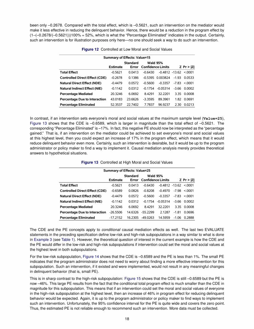
been only –0.2678. Compared with the total effect, which is –0.5621, such an intervention on the mediator wouldmake it less effective in reducing the delinquent behavior. Hence, there would be a reduction in the program effect by(1–(–0.2678/(–0.5621)))100% = 52%, which is what the “Percentage Eliminated” indicates in the output. Certainly,such an intervention is for illustration purposes only here—no one should seek a way to do such an intervention.

Figure 12 Controlled at Low Moral and Social Values

Summary of Effects: Value=15

EstimateStandard

ErrorWald 95%


Total Effect -0.5621 0.0413 -0.6430 -0.4812 -13.62 <.0001

Controlled Direct Effect (CDE) -0.2678 0.1386 -0.5395 0.003824 -1.93 0.0533






In contrast, if an intervention sets everyone’s moral and social values at the maximum sample level (Value=25),Figure 13 shows that the CDE is –0.6589, which is larger in magnitude than the total effect of –0.5621. Thecorresponding “Percentage Eliminated” is –17%. In fact, this negative PE should now be interpreted as the “percentagegained.” That is, if an intervention on the mediator could be achieved to set everyone’s moral and social valuesat this highest level, then you could expect an increase of 17% in the program effect, which means that it wouldreduce delinquent behavior even more. Certainly, such an intervention is desirable, but it would be up to the programadministrator or policy maker to find a way to implement it. Causal mediation analysis merely provides theoreticalanswers to hypothetical situations.

Figure 13 Controlled at High Moral and Social Values

Summary of Effects: Value=25

EstimateStandard

ErrorWald 95%


Total Effect -0.5621 0.0413 -0.6430 -0.4812 -13.62 <.0001







The CDE and the PE concepts apply to conditional causal mediation effects as well. The last two EVALUATEstatements in the preceding specification define low-risk and high-risk subpopulations in a way similar to what is donein Example 3 (see Table 1). However, the theoretical question of interest in the current example is how the CDE andthe PE would differ in the low-risk and high-risk subpopulations if intervention could set the moral and social values atthe highest level in both subpopulations.

For the low-risk subpopulation, Figure 14 shows that the CDE is –0.6589 and the PE is less than 1%. The small PEindicates that the program administrator does not need to worry about finding a more effective intervention for thissubpopulation. Such an intervention, if it existed and were implemented, would not result in any meaningful changesin delinquent behavior (that is, small PE).

This is in sharp contrast to the high-risk subpopulation: Figure 15 shows that the CDE is still –0.6589 but the PE isnow –46%. This large PE results from the fact that the conditional total program effect is much smaller than the CDE inmagnitude for this subpopulation. This means that if an intervention could set the moral and social values of everyonein the high-risk subpopulation at the highest level, then an increase of 46% in program effect for reducing delinquentbehavior would be expected. Again, it is up to the program administrator or policy maker to find ways to implementsuch an intervention. Unfortunately, the 95% confidence interval for the PE is quite wide and covers the zero point.Thus, the estimated PE is not reliable enough to recommend such an intervention. More data must be collected.

18

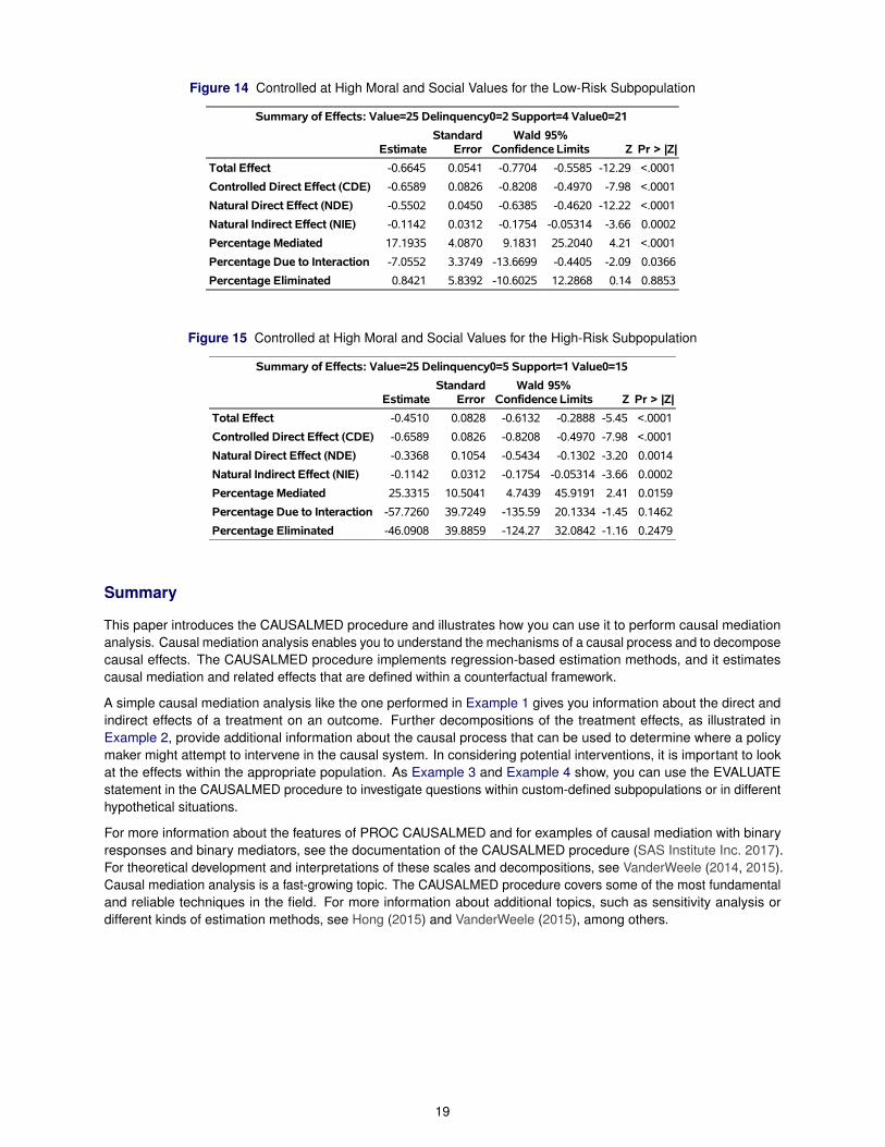
Figure 14 Controlled at High Moral and Social Values for the Low-Risk Subpopulation

Summary of Effects: Value=25 Delinquency0=2 Support=4 Value0=21

EstimateStandard

ErrorWald 95%


Total Effect -0.6645 0.0541 -0.7704 -0.5585 -12.29 <.0001




Percentage Mediated 17.1935 4.0870 9.1831 25.2040 4.21 <.0001

Percentage Due to Interaction -7.0552 3.3749 -13.6699 -0.4405 -2.09 0.0366

Percentage Eliminated 0.8421 5.8392 -10.6025 12.2868 0.14 0.8853

Figure 15 Controlled at High Moral and Social Values for the High-Risk Subpopulation

Summary of Effects: Value=25 Delinquency0=5 Support=1 Value0=15

EstimateStandard

ErrorWald 95%


Total Effect -0.4510 0.0828 -0.6132 -0.2888 -5.45 <.0001


Natural Direct Effect (NDE) -0.3368 0.1054 -0.5434 -0.1302 -3.20 0.0014





Summary

This paper introduces the CAUSALMED procedure and illustrates how you can use it to perform causal mediationanalysis. Causal mediation analysis enables you to understand the mechanisms of a causal process and to decomposecausal effects. The CAUSALMED procedure implements regression-based estimation methods, and it estimatescausal mediation and related effects that are defined within a counterfactual framework.

A simple causal mediation analysis like the one performed in Example 1 gives you information about the direct andindirect effects of a treatment on an outcome. Further decompositions of the treatment effects, as illustrated inExample 2, provide additional information about the causal process that can be used to determine where a policymaker might attempt to intervene in the causal system. In considering potential interventions, it is important to lookat the effects within the appropriate population. As Example 3 and Example 4 show, you can use the EVALUATEstatement in the CAUSALMED procedure to investigate questions within custom-defined subpopulations or in differenthypothetical situations.

For more information about the features of PROC CAUSALMED and for examples of causal mediation with binaryresponses and binary mediators, see the documentation of the CAUSALMED procedure (SAS Institute Inc. 2017).For theoretical development and interpretations of these scales and decompositions, see VanderWeele (2014, 2015).Causal mediation analysis is a fast-growing topic. The CAUSALMED procedure covers some of the most fundamentaland reliable techniques in the field. For more information about additional topics, such as sensitivity analysis ordifferent kinds of estimation methods, see Hong (2015) and VanderWeele (2015), among others.

19

REFERENCES

Baron, R. M., and Kenny, D. A. (1986). “The Moderator-Mediator Variable Distinction in Social Psychological Research:Conceptual, Strategic, and Statistical Considerations.” Journal of Personality and Social Psychology 51:1173–1182.

Hong, G. (2015). Causality in a Social World: Moderation, Mediation, and Spill-Over. New York: John Wiley & Sons.

Lamm, M., and Yung, Y.-F. (2017). “Estimating Causal Effects from Observational Data with the CAUSALTRTProcedure.” In Proceedings of the SAS Global Forum 2017 Conference. Cary, NC: SAS Institute Inc. http://support.sas.com/resources/papers/proceedings17/SAS0374-2017.pdf.

Pearl, J. (2001). “Direct and Indirect Effects.” In Proceedings of the Seventeenth Conference on Uncertainty in ArtificialIntelligence, edited by J. Breese, and D. Koller, 411–420. San Francisco: Morgan Kaufmann.

Robins, J. M., and Greenland, S. (1992). “Identifiability and Exchangeability for Direct and Indirect Effects.” Epidemiol-ogy 3:143–155.

SAS Institute Inc. (2017). SAS/STAT 14.3 User’s Guide. Cary, NC: SAS Institute Inc. http://go.documentation.sas.com/?docsetId=statug&docsetTarget=titlepage.htm&docsetVersion=14.3&locale=en.

Valeri, L., and VanderWeele, T. J. (2013). “Mediation Analysis Allowing for Exposure-Mediator Interactions and CausalInterpretation: Theoretical Assumptions and Implementation with SAS and SPSS Macros.” Psychological Methods18:137–150.

VanderWeele, T. J. (2014). “A Unification of Mediation and Interaction: A 4-Way Decomposition.” Epidemiology25:749–761.

VanderWeele, T. J. (2015). Explanation in Causal Inference: Methods for Mediation and Interaction. New York: OxfordUniversity Press.

VanderWeele, T. J., and Vansteelandt, S. (2009). “Conceptual Issues Concerning Mediation, Interventions andCompositions.” Statistics and Its Interface 2:457–468.

VanderWeele, T. J., and Vansteelandt, S. (2010). “Odds Ratios for Mediation Analysis for a Dichotomous Outcome.”American Journal of Epidemiology 172:1339–1348.

Yuan, Y., Yung, Y.-F., and Stokes, M. (2017). “Propensity Score Methods for Causal Inference with the PSMATCHProcedure.” In Proceedings of the SAS Global Forum 2017 Conference. Cary, NC: SAS Institute Inc. http://support.sas.com/resources/papers/proceedings17/SAS0332-2017.pdf.

ACKNOWLEDGMENTS

The authors are grateful to Bob Rodriguez, Clay Thompson, and Ed Huddleston of the Advanced Analytics Division atSAS for their valuable assistance in the preparation of this paper. The first author also thanks Dr. Linda Valeri and Dr.Tyler VanderWeele of Harvard University for their support and assistance in the development of the CAUSALMEDprocedure.

CONTACT INFORMATION

Your comments and questions are valued and encouraged. Contact the authors:

Yiu-Fai Yung Michael Lamm Wei ZhangSAS Institute Inc. SAS Institute Inc. SAS Institute Inc.SAS Campus Drive SAS Campus Drive SAS Campus DriveCary, NC 27513 Cary, NC 27513 Cary, NC [email protected] [email protected] [email protected]

SAS and all other SAS Institute Inc. product or service names are registered trademarks or trademarks of SASInstitute Inc. in the USA and other countries. ® indicates USA registration.

Other brand and product names are trademarks of their respective companies.

20

http://support.sas.com/resources/papers/proceedings17/SAS0374-2017.pdf


http://go.documentation.sas.com/?docsetId=statug&docsetTarget=titlepage.htm&docsetVersion=14.3&locale=en

http://go.documentation.sas.com/?docsetId=statug&docsetTarget=titlepage.htm&docsetVersion=14.3&locale=en



paper sas1991:2018 causal mediation analysis …...paper sas1991-2018 causal mediation analysis with...

Documents