paper - valuesignals · paper december 2010 mfie capital by philip vanstraceele & luc allaeys...

Paper

December 2010

MFIE Capital

By Philip Vanstraceele & Luc Allaeys

Systematic Value Investing ;

Does it really work ?

€ 0,00

€ 100,00

€ 200,00

€ 300,00

€ 400,00

€ 500,00

€ 600,00

€ 700,00

€ 800,00

2

[

G

e

e

f

d

e

t

i

t

e

l

v

a

n

h

e

t

d

o

c

u

m

e

n

t

o

p

]

|

1

-

9

-

2

0

1

0

S Y S T E M A T I C V A L U E I N V E S T I N G

“DOES I T REALLY WORK ” ?

-MFIE CAPITAL- WH I T E P A P E R - D E C E M B E R 2 0 1 0

INTRODUCTION

In our first paper “Studying different Value Investing Strategies”¹, we stated that when applying a bottom-up mechanical Value Investing system, you could beat the market over a number of years.

Still convinced and devoted value investors, or as Graham would put it”² ;”this involves

buying securities whose shares appear underpriced by some form(s) of fundamental analysis”, we wanted

to go a step further and build a framework to construct and back-test a small size, mid- & small cap investment fund.

For this study we changed the rules of the game to our own disadvantage and tried to get as close to the

“real thing” as possible. We did this by changing two capital items namely, by changing the benchmark and

by adding a minimum liquidity requirement on the purchased stocks, all the other most important constituents are left untouched.

Benchmark:

For this purpose, we constructed a new benchmark based on the weighted sum of the 250 biggest traded

companies in the Euro zone (for this we excluded banks and insurance companies, because in our

screeners we exclude them as well).

As you will remember, in our first paper we used the EUROSTOXX as the benchmark including banks and insurers, and we know what their performance was in the last few years.

To get the big picture of returns we also wanted our dividends reinvested, in both the Value portfolios and the benchmark.

Minimum Liquidity:

In our first paper, we worked with minimum market caps as an investment criteria. This is fine as long as you can actually buy or sell stock without influencing its price in a mayor way.

For this study, we worked with a minimum liquidity threshold varying for the different portfolios, so that in the end, the stock positions could be closed in 5 days.

http://en.wikipedia.org/wiki/Security_%28finance%29

http://en.wikipedia.org/wiki/Share_%28finance%29

http://en.wikipedia.org/wiki/Fundamental_analysis

3

SUMMARY

We will cover back-testing of portfolios of a size of €100.000, €500.000, €1.000.000 €10.000.000 and

€20.000.000 over an 11-year period from 13/06/1999 up to 13/06/2010.

The portfolios are formed by 9 value investing screeners (explained in the glossary part of this paper) and

tested against an index or market portfolio constructed specially for this study.

We also wondered if there is a benefit of financial analysis (in contrast with the efficient market hypothe-

sis), concentrated in small-and medium-sized firms, companies with low shares turnover (volume), and

firms with no analysts followings. Because as a small- and medium-size investor, we have an edge against

big institutional organisations, we do not have large sums of money to invest.

Our portfolio characteristics are as follows

Portfolios of €100.000, €500.000, €1.000.000 , €10.000.000 and €20.000.000. Portfolio’s of 30 and 50 stocks. Positions must be purchased within a maximum of 1 week (5 working days). Companies with a minimum market cap of €15.000.000 (of course, if we demand a higher

minimum trading volume, the market Cap will be higher also).

12 months buy and hold strategy.

Our market portfolio is a portfolio consisting of a weighted sum of the 250 most important stocks of the

total industrial market of companies in our databases (sorted descending by the trailing 30 days average

trading volume), with weights in the proportions of the trading volume of the individual stock. Each year, the

portfolio is reweighted based on their trading volume (based on the previous 30 days before 13/06)

Unlike our first paper, we use this benchmark instead of the EUROSTOXX, because in our analysis we want

to take into account the reinvestment of dividends paid by companies in the index and our value investing

portfolios, assuming that dividends are re-invested to purchase additional units of an equity at the closing

price applicable on the ex-dividend date.

It is also important to note that the EUROSTOXX contains many banks and insurers . The latter are not

included in our screener portfolios (we are not able to analyse them with our computer models), so it is

better to use an alternative benchmark.

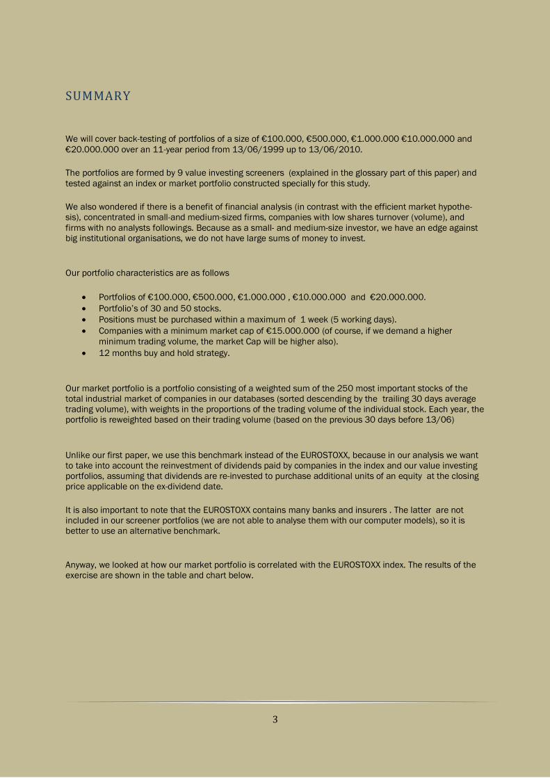
Anyway, we looked at how our market portfolio is correlated with the EUROSTOXX index. The results of the

exercise are shown in the table and chart below.

4

[

G

e

e

f

d

e

t

i

t

e

l

v

a

n

h

e

t

d

o

c

u

m

e

n

t

o

p

]

|

1

-

9

-

2

0

1

0

MFIE Index EUROSTOXX

Total Return 11,42% -21,21% Compound Annual Return 0,99% -2,14% Standard Deviation Return 22,28% 23,12%

Correlation with EUROSTOXX 0,9736 1 Beta 0,9384 1

Number of positive years 6 6 Number of negative years 5 5

Maximum peak-to-trough decline -63,39% -64,52%

With a correlation value of 0,9736 to the EUROSTOXX this is very clear.

Over an 11-year period (from 13/06/1999 until 13/06/2010), our Market portfolio has a total return

(dividends included and reinvested) of 11,42% (or 0,99% a year) vs. -21,21% (or - 2,14 % a year) for the

EUROSTOXX.

Evaluating these numbers, the least you could say is that the last decade was certainly not good for stocks

in general and that you were better off investing in bonds.

The different strategies will be back-tested and compared to our market portfolio. Risks and returns will be

examined, and the following items will be studied.

Average return of each value portfolio Standard deviation of the return Number of negative years of return of the different portfolios Number of years of underperformance agains the benchmark Maximum Peak-to-Trough Decline (worst case in the past)

Beta1

11

/06

/19

99

20

/10

/19

99

28

/02

/20

00

6/0

7/2

00

01

4/1

1/2

00

02

3/0

3/2

00

11

/08

/20

01

10

/12

/20

01

18

/04

/20

02

27

/08

/20

02

3/0

1/2

00

31

4/0

5/2

00

32

2/0

9/2

00

32

9/0

1/2

00

48

/06

/20

04

15

/10

/20

04

23

/02

/20

05

4/0

7/2

00

51

0/1

1/2

00

52

1/0

3/2

00

62

8/0

7/2

00

66

/12

/20

06

16

/04

/20

07

23

/08

/20

07

1/0

1/2

00

89

/05

/20

08

17

/09

/20

08

26

/01

/20

09

4/0

6/2

00

91

3/1

0/2

00

91

9/0

2/2

01

0

0

20

40

60

80

100

120

140

160

180

MFIE Index

EUROSTOXX

5

Academic theory states that higher-risk investments should have higher return long-term. Or in other words:

the greater the risk, the greater the expected return. But is this really true?

In his book "The new finance”2, Professor Robert Haugen claims that value stocks have higher returns than

growth stocks and that they are less risky!

In his book “Finding Alpha”, Eric Falkenstein even states that low beta stocks have higher returns “None-

theless, today it is a dirty little secret, something all good quants know, but it is rarely addressed directly”3

In our previous paper “Studying different Systematic Value Investing Strategies on the Euro zone

stockmarket”4 we have already stated that, a value based stock selection achieves a greater return than

the EUROSTOXX, but we have not really examined the risk of the value portfolios against a benchmark.

It is our intention to take a closer look at the “risk” of these value strategies.

But before we start the tests, we first have to consider one more thing. We will put a maximum clearing

time span on our portfolio formation, i.e. depending on the portfolio size and number of stocks in it, we will give ourselves a maximum of 5 days to settle the stocks in the different portfolios.

We can achieve this by putting a threshold on the liquidity of a stock before portfolio formation as follows;

[For a Minimum Market Cap. of €15.000.000]

Minimum Daily Volume

30 Stock Portfolio € 100.000 € 500.000 € 1.000.000 € 10.000.000 € 20.000.000

MF € 667 € 3.333 € 6.667 € 66.667 € 133.333

ERP5 € 667 € 3.333 € 6.667 € 66.667 € 133.333

Piotroski € 667 € 3.333 € 6.667 € 66.667 € 133.333

ERP/Piot € 667 € 3.333 € 6.667 € 66.667 € 133.333

MF/Piot € 667 € 3.333 € 6.667 € 66.667 € 133.333

5YeY/Piot € 667 € 3.333 € 6.667 € 66.667 € 133.333

TinyT € 667 € 3.333 € 6.667 € 66.667 € 133.333

PS/Piot € 667 € 3.333 € 6.667 € 66.667 € 133.333

ModERP € 667 € 3.333 € 6.667 € 66.667 € 133.333

50 Stock Portfolio € 100.000 € 500.000 € 1.000.000 € 10.000.000 € 20.000.000

MF € 400 € 2.000 € 4.000 € 40.000 € 80.000

ERP5 € 400 € 2.000 € 4.000 € 40.000 € 80.000

Piotroski € 400 € 2.000 € 4.000 € 40.000 € 80.000

ERP/Piot € 400 € 2.000 € 4.000 € 40.000 € 80.000

MF/Piot € 400 € 2.000 € 4.000 € 40.000 € 80.000

5YeY/Piot € 400 € 2.000 € 4.000 € 40.000 € 80.000

TinyT € 400 € 2.000 € 4.000 € 40.000 € 80.000

PS/Piot € 400 € 2.000 € 4.000 € 40.000 € 80.000

ModERP € 400 € 2.000 € 4.000 € 40.000 € 80.000

6

[

G

e

e

f

d

e

t

i

t

e

l

v

a

n

h

e

t

d

o

c

u

m

e

n

t

o

p

]

|

1

-

9

-

2

0

1

0

RESULTS

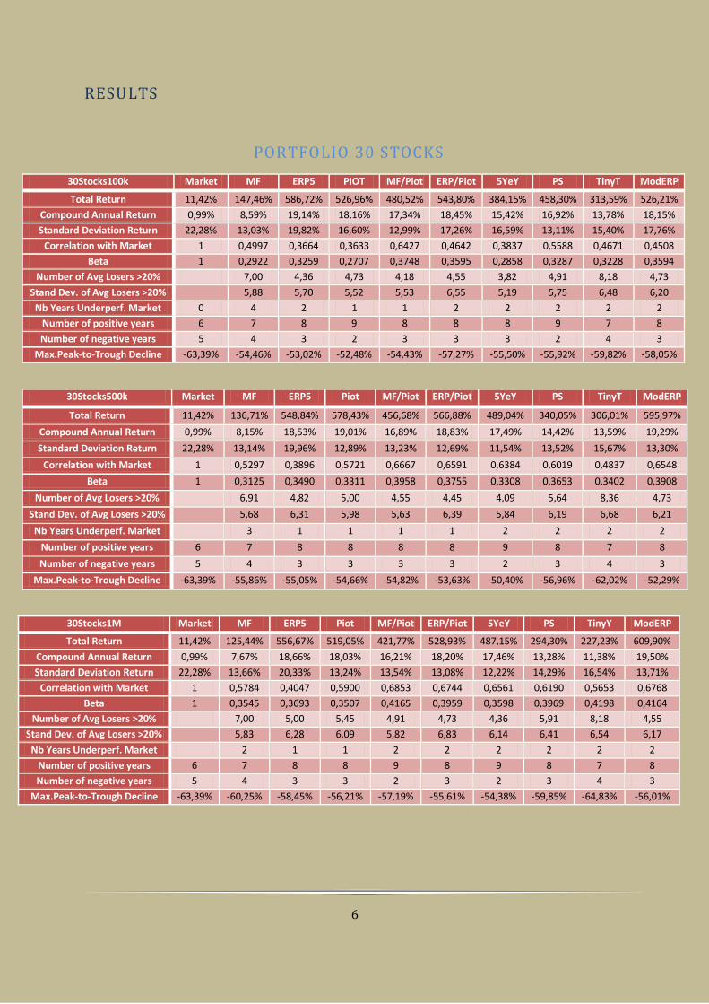
PORTFOLIO 30 STOCKS

30Stocks100k Market MF ERP5 PIOT MF/Piot ERP/Piot 5YeY PS TinyT ModERP

Total Return 11,42% 147,46% 586,72% 526,96% 480,52% 543,80% 384,15% 458,30% 313,59% 526,21%

Compound Annual Return 0,99% 8,59% 19,14% 18,16% 17,34% 18,45% 15,42% 16,92% 13,78% 18,15%

Standard Deviation Return 22,28% 13,03% 19,82% 16,60% 12,99% 17,26% 16,59% 13,11% 15,40% 17,76%

Correlation with Market 1 0,4997 0,3664 0,3633 0,6427 0,4642 0,3837 0,5588 0,4671 0,4508

Beta 1 0,2922 0,3259 0,2707 0,3748 0,3595 0,2858 0,3287 0,3228 0,3594

Number of Avg Losers >20% 7,00 4,36 4,73 4,18 4,55 3,82 4,91 8,18 4,73

Stand Dev. of Avg Losers >20% 5,88 5,70 5,52 5,53 6,55 5,19 5,75 6,48 6,20

Nb Years Underperf. Market 0 4 2 1 1 2 2 2 2 2

Number of positive years 6 7 8 9 8 8 8 9 7 8

Number of negative years 5 4 3 2 3 3 3 2 4 3

Max.Peak-to-Trough Decline -63,39% -54,46% -53,02% -52,48% -54,43% -57,27% -55,50% -55,92% -59,82% -58,05%

30Stocks500k Market MF ERP5 Piot MF/Piot ERP/Piot 5YeY PS TinyT ModERP

Total Return 11,42% 136,71% 548,84% 578,43% 456,68% 566,88% 489,04% 340,05% 306,01% 595,97%




Beta 1 0,3125 0,3490 0,3311 0,3958 0,3755 0,3308 0,3653 0,3402 0,3908



Nb Years Underperf. Market 3 1 1 1 1 2 2 2 2




30Stocks1M Market MF ERP5 Piot MF/Piot ERP/Piot 5YeY PS TinyY ModERP

Total Return 11,42% 125,44% 556,67% 519,05% 421,77% 528,93% 487,15% 294,30% 227,23% 609,90%




Beta 1 0,3545 0,3693 0,3507 0,4165 0,3959 0,3598 0,3969 0,4198 0,4164







7

30Stocks10M Market MF ERP Piot MF/Piot ERP/Piot 5YeY PS/Piot TinyT ModERP

Total Return 11,42% 147,87% 387,10% 466,99% 296,53% 425,49% 401,83% 521,24% 227,23% 460,35%




Beta 1 0,5114 0,5011 0,5024 0,5587 0,4933 0,4747 0,5214 0,4198 0,5293







30Stocks20M Market MFIE ERP5 Piot MF/Piot ERP/Piot 5YeY PS/Piot TinyT ModERP

Total Return 11,42% 177,36% 278,91% 401,83% 296,53% 372,06% 287,97% 243,77% 126,20% 367,98%




Beta 1 0,5460 0,5581 0,4747 0,5587 0,5484 0,5330 0,6002 0,4723 0,5899







8

[

G

e

e

f

d

e

t

i

t

e

l

v

a

n

h

e

t

d

o

c

u

m

e

n

t

o

p

]

|

1

-

9

-

2

0

1

0

PORTFOLIO 50 STOCKS


Total Return 11,42% 154,49% 504,63% 518,36% 336,37% 427,95% 396,54% 424,44% 248,44% 516,63%




Beta 1 0,3066 0,3282 0,2851 0,3786 0,3426 0,2913 0,3224 0,2761 0,3664








Total Return 11,42% 150,16% 427,38% 566,15% 312,64% 449,41% 408,30% 352,72% 244,87% 506,12%




Beta 1 0,3265 0,3448 0,3193 0,3873 0,3475 0,3202 0,3509 0,3030 0,3797







50Stocks1M Market MF ERP5 PIOT MF/Piot ERP/Piot 5YeY PS TinyT ModERP

Total Return 11,42% 137,20% 506,86% 624,27% 328,87% 471,47% 446,48% 347,34% 255,37% 503,43%




Beta 1 0,3422 0,3548 0,3441 0,4006 0,3670 0,3446 0,3761 0,3121 0,3973







9


Total Return 11,42% 149,24% 293,32% 470,72% 272,93% 343,10% 367,86% 266,35% 235,72% 364,99%




Beta 1 0,4542 0,4509 0,4520 0,4812 0,4742 0,4227 0,4967 0,3802 0,4938








Total Return 11,42% 133,62% 344,85% 373,76% 279,95% 376,52% 330,71% 352,75% 200,73% 327,20%




Beta 1 0,5091 0,5241 0,5169 0,5283 0,5206 0,4873 0,5571 0,4222 0,5364







10

[

G

e

e

f

d

e

t

i

t

e

l

v

a

n

h

e

t

d

o

c

u

m

e

n

t

o

p

]

|

1

-

9

-

2

0

1

0

WHY WE ARE NO BETA AFFECTIONADOS

The CAPM formula was developed in 1970 by William Sharpe and John Lintner and is based on the modern

portfolio theory (MPT) by Markowitz.

The CAPM redefines risk in terms of a security’s beta (β), which captures the non-diversifiable portion of

that stock’s (portfolio) risk relative to the market as a whole.

This eventually leads to a very convenient interpretation: a stock with a beta of 1,20 has a level of syste-

matic risk that is 20% greater than the average for the entire market, while a stock with a beta of 0,70 is

30% less risky than the market. By definition the market always has a beta of 1.

But there is something that bothers us, if we examine the back tests in each “value” portfolio we do beat

the market consistently.

In contradiction to the theory of efficient markets, this can only be explained through a higher risk or beta of

the portfolio ?

In fact, each and every “value” portfolio has a beta between min.0,2707 and max. 0,5899 ?

Like Newton’s law, or even Archimedes’s law, you should be able to compute the outcome to a certain de-

gree of accuracy.

With the CAPM, this is not the case, and we wonder what is wrong with it. Is it the formula, or the concept of

an efficient market?

We suspect the latter.

11

CONCLUSION

Although back testing is a purely academic exercise you can try to simulate reality by taking in account some basic rules with regard to the following issues;

1. Survival Bias:

Most studies don’t include companies that went bankrupt or that were taken over by others. In our test, these companies were not excluded.

2. Look ahead Bias:

When you are using data for your stock ranking that was not available at the moment of portfolio formation, your results will suffer from look-ahead bias. This bias results upwards.

We worked with accounting data from the previous fiscal year and waited 6 months to form our portfolios and actual trading.

Example:

Back-testing for 1999, we took the accounting data from the end of 1998 and formed the different portfo-lios on 13/06/1999. This ensured that all accounting data was available upon portfolio formation.

We formed our portfolios and waited 6 months before actually buying them. Then we held them until

13/06/2000 before again rebalancing the complete portfolio.

We back-tested for the period : 13/06/1999 and 13/06/2010

3. Bid-Asked bounce:

It is practically impossible to buy large positions in micro cap stocks (<25 million). If you do so, it will influ-

ence the price very negatively. The price will skyrocket. In our first paper we put a restriction of minimum 25

million on the market cap.

For this paper, we looked at this problem from a different angle.

On portfolio formation, we worked with the idea that you need a minimum liquidity for buying and selling the different stocks in the open market. The different positions need to be cleared within 5 working days.

Even by multiplying the minimum liquidity requirement by a factor 2, there was no significant decline in

overall return.

4. Data mining:

You can run your computer a thousand times and pick the best results to publish. We on the other hand used the same methodology over and over again through our study with the same constituents.

5. A Reliable Database :

Before we started this project, we examined different data providers. There are very good sources available

in today’s market but very few had the necessary data coverage with respect to Europeans stocks as

Thomson Reuters has.

So, we selected the Thomson DataStream application and it has worked great for us.

6. Small sample Bias :

You can have a strategy that does very well over a 5-year period or longer and that may then go horribly

wrong. We therefore tested the different strategies over an 11-year period. This should give the necessary time span we need to test the solidity and endurance of these strategies in detail.

All things considered, the last decade has been quite turbulent for the stock markets all over the globe. We had one bull market and two major crashes (a “luxury” for back-testers).

12

[

G

e

e

f

d

e

t

i

t

e

l

v

a

n

h

e

t

d

o

c

u

m

e

n

t

o

p

]

|

1

-

9

-

2

0

1

0

By joining the two screener selections of MF and Piotroski F_Score, you can increase your performance substantially.

Adding more stocks to your portfolio (30 stocks versus 50 stocks) does not improve the overall return: on

the contrary, you decrease it.

Nevertheless diversification is one of the cornerstones of safe investing, and it helps you to sleep well at

night.

We think that a portfolio of +/-30 ”value labelled” stocks should perform well as a long term buy and hold

strategy.

By using one of the screeners you limit your underperformance to the market to 2 years (over an 11-year

period) on average. You must realise that the “value” strategies can underperform the market for a num-

ber of years (this was the case in the dotcom period).

As discussed in our first paper, by applying a mechanical value screener, you minimise the emotional im-pact on your portfolio. As is often the case you are your own enemy with regards to investing.

You can use the screeners as a tool to invest in the top 30/50 companies that are selected for a given period or you can use it as a stock picking tool if you are better skilled than the average investor.

All investing periods are 1year buy and hold, the screeners are rebalanced at the same time over and over

again.

We advise you not to use the screeners as a guidance for shorting stocks, even though this seems theoreti-cally logical, because the factor time can seriously go against you.

A study made by James Montier1 in March 2006 showed that adding a factor quality (ROIC) to the Green-

blatt formula (It has a Price element EY and a Quality element ROIC) did not increase return in a major way, instead it reduced total return (on a 12 year basis) and added more volatility.

This is a similar result we got on our back testing results from the Magic Formula in comparison with all other screeners.

13

GLOSSARY

The 9 mechanical Value Investing techniques that were tested are explained in this chapter and [the codes

between parenthesis are the short codes used in the graphs in the paper].

1) Magic Formula as described in “The little book that beats the market” by

Joel Greenblatt [MF]

The Magic Formula stock strategy, developed by Joel Greenblatt in The Little Book That Beats the Market

earned nearly 31% ANNUAL returns over a 17 year period.

The formula start with the list of all the companies in a monetary zone (we have 4 zones available in our

screener databases, namely EURO, UK, USA and Japan). For example in the EURO zone we have +/- 2000

companies available in our list. The formula then applies a ranking to those companies, from 1 to 2000,

based on their Return Of Invested Capital (ROIC)¹. The company with the highest ROIC gets ranking 1, the

company with the lowest gets ranking 2000.

Next, the formula follows the same procedure, but this time the ranking is done using Earning Yield(EY)².

The company with the highest yield is ranking 1, and the company with the lowest earning yield receives

ranking 2000.

Finally, the formula combines the rankings. The formula is looking for the companies that have the best

combination of both two factors. So a company that is ranked 232nd best in ROIC and 153rd highest in EY,

gets a better combined ranking than a company that is ranked 1st in ROIC but only 1150th best in

EY,because the first company has a better combined rank of 385 (232 + 153= 385) than the second

company has (1 + 1150= 1151)

2) ERP5 [ERP5]

Finding stocks with a “considerable margin of safety” isn’t a stand alone feature. When it comes down to

investing in a stock, the investment needs to have a considerable earning power as well. So we thought of a

screening method (similar to the Greenblatt's Magic Formula ) that would cover the issue of cheapness and

earning power as well. We noticed in our back-testing, that the ratio Price to Book of a business gives a

good indication for finding value stocks. Instead of the 2-parameter model used by Greenblatt (EY & ROIC)

we will apply 4 parameters, but we are searching for a combination of cheapness and earning power.

We selected the following 4 variables:

Earning Yield : (EBIT/Enterprise Value) How much is a business earning compared to the enterprise value (purchase price) of the company.

ROIC : Last 12 months (Return On Invested Capital) How much capital is needed to conduct its business (earnings factor). The ROIC measure gives a sense of

how well a company is using its money to generate returns

Price to Book Value : How much “margin of safety” is there on the purchased price factor compared to the

company's book value? Considerable research documents the returns to a high book-to-market investment

strategy (e.g., Rosenberg, Reid-, and Lanstein 1984; Fama and French 1992; and Lakonishok, Shleifer, and

Vishny 1994 )

5 year trailing ROIC

http://www.amazon.com/gp/product/0471733067?ie=UTF8&tag=magicdi05-20&linkCode=as2&camp=1789&creative=9325&c

14

[

G

e

e

f

d

e

t

i

t

e

l

v

a

n

h

e

t

d

o

c

u

m

e

n

t

o

p

]

|

1

-

9

-

2

0

1

0

This indicates the development of earnings over a 5-year trailing period. A company could have had an

exceptional good year (or last 12 months), but did the company also obtain good returns on its investments

over a longer period (i.e. over the last 5-year business cycle)?

The formula is calculated the same way as the Magic Formula, but here we are combining the 4 rankings,

so we are looking for the best combination of all 4 factors.

3) Piotroski 's F-score for low price to book companies [Piot]

In a research paper3, written in 2000, Joseph Piotroski an accounting professor, from the University of Chi-

cago, developed and successfully tested a system where, with the use of a few simple accounting based

ratios, you can achieve substantial index beating investment performances. He wanted to see if he could

develop a system (using a simple 9-point scoring system) that could increase the returns of a strategy of

investing in low price to book value companies. Buying only those companies that scored highest (8 or 9)

on his 9-point scale, or F-Score as he called it, over the 20-year period from 1976 to 1996 led to an aver-

age outperformance over the market of 13.4% on USA stock exchanges.

How is the Piotroski or F-Score calculated?

Profitability

1. Return On Assets (ROA)

Net income before extraordinary items for the year divided by total assets at the beginning of the year.

Score 1 if positive, 0 if negative

2. Cash Flow Return On Assets (CFROA)

Net cash flow from operating activities (operating cash flow) divided by total assets at the beginning of the

year.

Score 1 if positive, 0 if negative

3. Change in return on assets

Compare this year’s return on assets (1) to last year’s return on assets.

Score 1 if it’s higher, 0 if it’s lower

4. Quality of earnings (accrual)

Compare Cash flow return on assets (2) to return on assets (1)

Score 1 if CFROA>ROA, 0 if CFROA<ROA

Funding

5. Change in gearing or leverage

Compare this year’s gearing (long-term debt divided by average total assets) to last year’s gearing.

Score 1 if gearing is lower, 0 if it’s higher.

6. Change in working capital (liquidity)

Compare this year’s current ratio (current assets divided by current liabilities) to last year’s current ratio.

Score 1 if this year’s current ratio is higher, 0 if it’s lower

7. Change in shares in issue

Compare the number of shares in issue this year, to the number in issue last year.

Score 1 if there are the same amount or fewer shares in issue this year. Score 0 if there are more shares in

issue.

Efficiency

15

8. Change in gross margin

Compare this year’s gross margin (gross profit divided by sales) to last year’s.

Score 1 if this year’s gross margin is higher, 0 if it’s lower

9. Change in asset turnover

Compare this year’s asset turnover (total sales divided by total assets at the beginning of the year) to last

year’s asset turnover ratio.

Score 1 if this year’s asset turnover ratio is higher, 0 if it’s lower

Evaluation

Piotroski or F-Score = 1 + 2 + 3 + 4 + 5 + 6 + 7 + 8 + 9

Good or high score = 8 or 9

Bad or low score = 0 or 1

We will backtest the F-score stand alone and in combination with other Value screeners (MF, ERP5 , Price

to Sales, Highest 5 year average Earning Yield). In our first paper we found out that the F-score may help

you to substantially increase your investment returns, irrespective of what investment strategy you may be

following.

4) ERP5 - highest F-score [ERP/Piot]

This is a combination of ERP5 and the F-score. We first take the best 20% ERP5 companies (instead of the

lowest Price to Book companies) and then we sort them in a descending order according to the F-score. The

best 30 or 50 companies are then selected.

5) Highest 5-year average Earning Yield - sorted by the highest F-score. [5YeY]

As value investors, we believe that buying bad companies at very low prices is also a perfectly viable

strategy, provided, of course, they don’t go bankrupt. One needs to separate the winners from the losers. As

we saw in our First Paper, the F score is the perfect tool for that purpose. The standard Piotroski analysis

works with low price to book stocks, but we can also look for cheap stocks by looking at their earning

power. We herefore use the 5 year average earning yield and select the highest 20 % of our database and

sort them next according to the F-score.

6) Price -to -sales -highest F-score [PS/Piot]

The price-to-sales ratio is called; “the king of the value factors” by O'Shaughnessy4. A price-to-sales ratio

(PSR) is similar to its price-to-earning ratio, but measures the price of the company against annual sales

instead of earning. We wanted to test this theory and combine PSR with the F-Score and the relative

strength.

7) Modified ERP5: (F-score between 7 and 9, and then sorted in ascending order

according to the ERP5 ranking) [ModERP]

With this screener, we first select all the companies with a F-score between 7 and 9. Next, we sort them in

ascending order according to their ERP5 ranking. We finally take the best 30 or 50 stocks.

8) Tiny Titans [TinyT]

The screen looks for companies with a market cap between €25 million and €250 million, a price to sales

of less than 1, and finally, ranks the top 25 based on the greatest relative strength over the past 52 weeks.

16

[

G

e

e

f

d

e

t

i

t

e

l

v

a

n

h

e

t

d

o

c

u

m

e

n

t

o

p

]

|

1

-

9

-

2

0

1

0

This creates a list of highly volatile and risky stocks according to O'Shaugnessy4. Since 1998 the screen

has produced in the USA cumulative results of over 2000%. However, since 2007, the screen has struggled

significantly along with the overall market.

9) Magic Formula - highest F-score [MF/Piot]

This screener sorts for the Magic Formula first and then selects the highest F-score.

REFERENCES

INTRODUCTION

¹http://www.value-investing.eu/articles/Paper1005_MFIE.pdf

² Value investing is an investment paradigm that derives from the ideas on investment and speculation that Ben Graham & David Dodd began teaching at Columbia Business School in 1928 and subsequently developed in their 1934 text Security Analysis.

SUMMARY

¹ The beta coefficient was born out of linear regression analysis. It is linked to a regression analysis of the returns of a portfolio (such as a stock index) (x-axis) in a specific period versus the returns of an individu-al asset (y-axis) in a specific year. An asset with a beta of 0 means that its price is not at all correlated with the market. A positive beta means that the asset generally follows the market. A negative beta shows that the asset inversely follows the market, the asset generally decreases in value if the market goes up and vice versa.

2Robert A.Haugen; The new finance; Pearson Education International.

3Eric Falkenstein; Finding Alpha; Wiley Finance.

4http://www.value-investing.eu/articles/Paper1005_MFIE.pdf

CONCLUSION

¹DrKW Macro research 9 March 2006 “The little note that beats the market” by James Montier

GLOSSARY

1 Return on Capital= EBIT/(Net Working Capital + Net Fixed Assets) 2 Earnings Yield= EBIT/Enterprise Value.

3 http://www.chicagobooth.edu/faculty/selectedpapers/sp84.pdf

4 James P.O’Shaughnessy; What works on Wall Street; Mc Graw-Hill.

http://www.value-investing.eu/articles/Paper1005_MFIE.pdf

http://en.wikipedia.org/wiki/Investment

http://en.wikipedia.org/wiki/Investor_profile

http://en.wikipedia.org/wiki/Speculation

http://en.wikipedia.org/wiki/Benjamin_Graham

http://en.wikipedia.org/wiki/David_Dodd

http://en.wikipedia.org/wiki/Columbia_Business_School

http://en.wikipedia.org/wiki/Security_Analysis_%28book%29

http://en.wikipedia.org/wiki/Linear_regression

http://www.value-investing.eu/articles/Paper1005_MFIE.pdf

http://www.chicagobooth.edu/faculty/selectedpapers/sp84.pdf

paper - valuesignals · paper december 2010 mfie capital by philip vanstraceele & luc allaeys...

Documents