paragon: parallel architecture-aware graph partition...

PARAGON: Parallel Architecture-Aware Graph PartitionRefinement Algorithm

Angen ZhengUniversity of Pittsburgh

Pittsburgh, PA, [email protected]

Alexandros LabrinidisUniversity of Pittsburgh


Patrick PisciuneriUniversity of Pittsburgh


Panos K. ChrysanthisUniversity of Pittsburgh


Peyman GiviUniversity of Pittsburgh


ABSTRACTWith the explosion of large, dynamic graph datasets from variousfields, graph partitioning and repartitioning are becoming more andmore critical to the performance of many graph-based Big Data ap-plications, such as social analysis, web search, and recommendersystems. However, well-studied graph (re)partitioners usually as-sume a homogeneous and contention-free computing environment,which contradicts the increasing communication heterogeneity andshared resource contention in modern, multicore high performancecomputing clusters. To bridge this gap, we introduce PARAGON,a parallel architecture-aware graph partition refinement algorithm,which mitigates the mismatch by modifying a given decompositionaccording to the nonuniform network communication costs and thecontentiousness of the underlying hardware topology. To furtherreduce the overhead of the refinement, we also make PARAGONitself architecture-aware.

Our experiments with a diverse collection of datasets showedthat on average PARAGON improved the quality of graph decom-positions computed by the de-facto standard (hashing partitioning)and two state-of-the-art streaming graph partitioning heuristics (de-terministic greedy and linear deterministic greedy) by 43%, 17%,and 36%, respectively. Furthermore, our experiments with an MPIimplementation of Breadth First Search and Single Source Short-est Path showed that, in comparison to the state-of-the-art stream-ing and multi-level graph (re)partitioners, PARAGON achieved up to5.9x speedups. Finally, we demonstrated the scalability of PARAGONby scaling it up to a graph with 3.6 billion edges using only 3 ma-chines (60 physical cores).

1. INTRODUCTIONIt is well-known that graph (re)partitioning has been extensively

studied in the area of scientific simulations [14, 34]. Yet, its impor-tance is continuously increasing due to the explosion of large graphdatasets from various fields, such as the World Wide Web, Pro-

c©2016, Copyright is with the authors. Published in Proc. 19th Inter-national Conference on Extending Database Technology (EDBT), March15-18, 2016 - Bordeaux, France: ISBN 978-3-89318-070-7, on OpenPro-ceedings.org. Distribution of this paper is permitted under the terms of theCreative Commons license CC-by-nc-nd 4.0

tein Interaction Networks, Social Networks, Financial Networks,and Transportation Networks. This has led to the development ofgraph-specialized parallel computing frameworks, e.g., Pregel [21],GraphLab [19], and PowerGraph [13].

Pregel, as a representative of these computing frameworks, em-braces a vertex-centric approach where the graph is partitioned acrossmultiple servers for parallel computation. Computations are oftendivided into a sequence of supersteps separated by a global syn-chronization barrier. During each superstep, a user-defined func-tion is computed against each vertex based on the messages it re-ceived from its neighbors in the previous step. The function canchange the state and outgoing edges of the vertex, send messagesto the neighbors of the vertex, or even add or remove vertices/edgesto the graph.

Traditional Graph Partitioners Clearly, the distribution of thegraph data across servers may impact the performance of target ap-plications significantly. Graph partitioning has been studied fordecades [14, 34], attempting to provide a good partitioning of thegraph data, whereby both the skewness and the communication(edge-cut) among partitions are minimized as much as possible,in order to minimize the total response time for the entire compu-tation. However, classic graph partitioners such as METIS [23] andChaco [7] do not scale well with large graphs.

Streaming Graph Partitioners Streaming graph partitioners (e.g.,DG/LDG [39], arXiv’13 [11], and Fennel [42]) have been proposedin order to overcome the scalability challenges of classic graphpartitioners, by examining the graph incrementally. One of themain shortcomings of these approaches is that they also assumeuniform network communication costs among partitions as classicgraph partitioners do. That is, they all assume that the communica-tion cost is proportional only to the amount of data communicatedamong partitions. This assumption is no longer valid in modernparallel architectures due to the increasing communication hetero-geneity [47, 8]. For example, on a 4 ∗ 4 ∗ 4 3D-torus interconnect,the distance to different nodes starting from a single node variesfrom 0 to 6 hops.

Architecture-Aware Graph Partitioners Architecture-aware graphpartitioners [24, 8, 46] have been proposed to improve the map-ping of the application’s communication patterns to the underlyinghardware topology. Chen et al. [8] (SoCC’12) took architecture-awareness a step further, by making the partitioning algorithm itselfpartially aware of the communication heterogeneity. However, both[8] and [24] (ICA3PP’08) are built on top of existing heavyweightgraph partitioners, namely, METIS [23] and PARMETIS [30], which

}} } }

Partitioners StreamingPartitioners

Re-Partitioners

Parallel Re-Partitioners

Performance

Feat

ures

(arc

hite

ctur

e-aw

are,

gra

ph d

ynam

ism

, w

eigh

ted

edge

/ver

tex,

ver

tex

size

)

most

leastworst best

Metis

PARAGON

ica3pp'08

chaco sheep

tkde'15

scotcharXiv'13

DG/LDG

socc'12

ARAGON

ParMetisZoltan

LogGP

catchW

Mizan

xdgp Hermes Fennel

Figure 1: Classification of all graph partitioners/re-partitioners ac-cording to their features vs performance profile.

are known to be the best graph partitioners and repartitioners interms of partitioning quality but have poor scalability. Finally, al-though Xu et al. [46] (TKDE’15) proposed a lightweight architecture-aware streaming graph partitioner, the partitioner may lead to sub-optimal performance for dynamic graphs [43].Traditional Graph Repartitioners Most real-world graphs areoften non-static, and continue to evolve over time. Because of thisgraph dynamism, both the quality of the initial partitioning and themapping of the application communication pattern to the underly-ing hardware topology will continuously degrade over time, lead-ing to (a potentially significant) load imbalance and additional com-munication overhead. Considering the sheer scale of real-worldgraphs, repartitioning the entire graph from scratch using [46, 8,24], even in parallel, is often impractical, either because of thelong partitioning time or the huge volume of data migration therepartitioning may introduce. To address this, several graph repar-titioning algorithms have been proposed, such as Zoltan [1, 6] andPARMETIS [30, 33]. Although they are able to greatly reduce thedata migration cost, they are all architecture-agnostic and do notscale well with massive graphs.Parallel/Lightweight Graph Repartitioners Parallel lightweightgraph repartitioners (e.g., CatchW [37], xdgp [43], Hermes [26],Mizan [17], arXiv’13 [11], and LogGP [45]) have been proposedto improve the performance and scalability of graph repartitioning.Instead of seeking an optimal partitioning at once, these algorithmsadapt the graph decomposition to changes efficiently by incremen-tally migrating vertices from one partition to another based on somelocal heuristics. However, they are all oblivious of the nonuniformnetwork communication costs among partitions.Limitations of the State-of-the-Art Despite the plethora of graphpartitioners and repartitioners (Figure 1), the current state-of-the-art is suffering from two main problems:• Graph (re)partitioners either consider architecture-awareness (for

CPU/network heterogeneity) or consider performance (i.e., par-allel/lightweight implementation), but never both. This is illus-trated in Figure 1, where the top-right corner is empty (exceptfor PARAGON, which is presented in this paper).• No existing graph (re)partitioner considers the issue of shared

resource contention in modern multicore high performance com-puting (HPC) clusters. Shared resource contention is a well-known issue in multicore systems and has received a lot of at-tention in system-level research [15, 41].

Our prior work We have previously presented an architecture-aware graph repartitioner, ARAGONLB [48]. Although ARAGONLBconsiders the communication heterogeneity for target applications,it disregards the issue of shared resource contention, and the repar-titioning itself is not architecture-aware. Moreover, the refinementalgorithm that ARAGONLB uses to improve the mapping of the ap-plication communication pattern to the underlying hardware topol-ogy requires the entire graph to be stored in memory by a singleserver, which is infeasible for large graphs. Furthermore, the re-finement algorithm is performed sequentially, which may becomea performance bottleneck. Finally, ARAGONLB assumes that com-pute nodes used for parallel computation have the same number ofcores and memory hierarchies, which may not always be true.Contributions In this paper, we present PARAGON, which over-comes both limitations of the current state-of-the-art graph reparti-tioners by extending ARAGONLB in the following aspects.1. We separate the refinement algorithm, ARAGON, from ARAGONLB

as an independent component, and develop a parallelized ver-sion of ARAGON, PARAGON, for large graphs (Section 3, 4, 5).We further reduce the overhead of PARAGON by making it awareof the nonuniform network communication costs (explained inSection 2.1).

2. We identify and consider the issue of shared resource contentionin modern HPC clusters for graph partitioning (Section 2.2 & 6).

3. We perform an extensive experimental study of PARAGON witha diverse set of 13 datasets and two real-world applications,demonstrating the effectiveness and scalability of PARAGON(Section 7).

2. MOTIVATIONIn this section we explain the importance of architecture-awareness

(i.e., communication heterogeneity and shared resource contention)for efficient graph (re)partitioners.

2.1 Communication HeterogeneityFor distributed graph computations on multicore systems, com-

munication can be either inter-node (i.e., among cores of differentcompute nodes) or intra-node (i.e., among cores of the same com-pute node). In general, intra-node communication is an order ofmagnitude faster than inter-node communication. This is becausein many modern parallel programming models like MPI [27, 25], apredominant messaging standard for HPC applications, intra-nodecommunication is implemented via shared memory/cache [16, 5],while inter-node communication needs to go through the networkinterface. Additionally, both inter-node and intra-node communi-cation are themselves nonuniform.Nonuniform Inter-Node Network Communication Modern par-allel architectures, like supercomputers, usually consist of a largenumber of compute nodes linked via a network. Consequently, thecommunication costs among compute nodes vary a lot because oftheir varying locations. For example, in the Gordon supercom-puter [28], the network topology is a 4x4x4 3D torus of switcheswith 16 compute nodes attached to each switch. As a result, the dis-tance to different compute nodes starting from a single node variesfrom 0 to 6 hops. Also, supercomputers often allow multiple jobsto concurrently run on different compute nodes and contend forthe shared network links, limiting the effective network bandwidthavailable for each job and thus amplifying the heterogeneity.Nonuniform Intra-Node Network Communication Communi-cation among cores of the same compute node is also nonuniformbecause of the complex memory hierarchy. Communication among

Memory Controller(Northbridge)

Memory

Socket 0 Socket 1

L2 L2FSB Interface

core core core core

L1 L1 L1 L1

FSB InterfaceL2 L2

FSB Interface

core core core core

L1 L1 L1 L1

FSB Interface

FSB FSB

(a) Uniform Memory Access (UMA) Architecture

core core core core

L2 L2 L2 L2L3

Memory Controller

Inter-socket Link Controller

Memory

Socket 1

core core core core

L1 L1 L1 L1L2 L2 L2 L2

L3

Memory Controller

Inter-socket Link Controller

Memory

Socket 0

QPI/HT

L1 L1 L1 L1

(b) Nonuniform Memory Access (NUMA) ArchitectureFigure 2: Example Architectures of Modern Compute Nodes

cores sharing more cache-levels can achieve lower latency and highereffective bandwidth than cores sharing fewer cache-levels. For ex-ample, in the architecture described by Figure 2a, communicationamong cores sharing L2 caches (e.g., between the first and secondcore of Socket 0) offers the highest performance, while commu-nication among cores of the same socket but not sharing any L2cache (e.g., between the first and third core of Socket 0) deliversthe next highest performance. Communication among cores of dif-ferent sockets performs the worst. Similarly, in Figure 2b, coresof the same socket (intra-socket communication) usually commu-nicate faster than cores residing on different sockets (inter-socketcommunication). This is because intra-socket communication canbe achieved via the shared caches, while inter-socket communica-tion has to go through the front-side bus and the off-chip memorycontroller (Figure 2a) or the inter-socket link controller (Figure 2b).Take-away To improve the performance of graph-based big-dataapplications, we should not only minimize the number of edgesacross different partitions (edge-cut), but also the number of edge-cuts among partitions having higher network communication costs(hop-cut). This is the major difference between architecture-agnosticsolutions (that only minimize edge-cut) and architecture-aware ones(that try to minimize both edge-cut and hop-cut).

2.2 Intra-Node Shared Resource ContentionAs mentioned above, MPI intra-node communication is imple-

mented via shared memory, which can either be user-space or kernel-based [16, 5]. Current MPI implementations often use the formerfor small messages and the latter for large messages. The user-space approach requires two memory copies. The sender first needsto load the send buffer into its cache and then write the data to theshared buffer (which may require loading the shared buffer blockinto the sender’s cache first). Then, the receiver reads the data fromthe shared memory (which may demand loading the shared mem-ory block and receiving buffer into the receiver’s cache first). Forkernel-based approaches, the receiver first loads the send buffer di-rectly to its cache with the help of the OS kernel. Then, the receiverwrites the data to the receiving buffer (which may require loadingthe receiving buffer into its cache first). Clearly, kernel-based ap-proaches reduce the number of memory copies to be one, mitigatingthe traffic on the memory subsystem. However, it demands a trapto the kernel on both the sender and receiver, making it inefficientfor small messages. As can be seen, intra-node communicationgenerates lots of memory traffic and cache pollution, which maysaturate the memory subsystem if we put too much communica-tion within each compute node. This issue is further amplified bythe increasing contentiousness of the shared resources in modernmulticore systems. Table 1 summarizes the resources that differentcores may have to compete for when they are communicating witheach other for the architectures presented in Figures 2a and 2b. The

Table 1: Intra-Node Shared Resource ContentionCores/Resources Sharing Contention

Core Groups Socket LLC LLC FSB/QPI(HT) Memory ControllerG1 X X X X X

UMA G2 X X XFig. 2a G3 X

NUMA G1 X X X XFig. 2b G2 X

summary is based on whether the cores are on the same socket andwhether they share the last level cache (LLC).Take-away Focusing solely on placing neighboring vertices as closeas possible is not sufficient to achieve superior performance. Infact, putting too much communication within each compute nodemay even hurt the performance due to the traffic congestion onmemory subsystems. Counter-intuitively, offloading a certain amountof intra-node communication across compute nodes may some-times achieve better performance. This is because inter-node com-munication is often implemented using Remote Direct MemoryAccess (RDMA) and rendezvous protocols [40], which allow acompute node to read data from the memory of another computenode without involving the processor, cache, or operating systemof either node, thus alleviating the traffic on memory subsystemsand cache pollution. Additionally, it is reported in [3] that modernRDMA-enabled networks can deliver comparable network band-width as that of memory channels. This requires us to examine theimpact of multi-core architecture on graph partitionings more care-fully, especially for small HPC clusters, since the network may nolonger be the bottleneck.

3. PROBLEM STATEMENTLet G = (V,E) be a graph, where V is the vertex set and E is

the edges set, and P be a partitioning of G with n partitions, where

P = {Pi : ∪ni=1Pi = V and Pi ∩ Pj = φ for any i 6= j} (1)

and let M be the current assignment of partitions to servers, wherePi is assigned to server M [i]. The server can be either a hardwarethread, a core, a socket, or a machine.Architecture-aware graph partition refinement aims to improvethe mapping of the application communication pattern to the un-derlying hardware topology by modifying the current partitioningof the graph, such that the communication cost of the target appli-cation, given the specific hardware topology, is minimized. Themodification usually involves migrating vertices from one partitionto another partition. Hence, in addition to the communication cost,the refinement should also minimize the data migration cost amongpartitions. Also, to ensure balanced load distribution in terms of thecomputation requirement, the refinement should keep the skewnessof the partitioning as small as possible.

h

ij a

d

bc

f

ge

P1(N1)P3(N3)

P2(N2)

Figure 3: Old Decomposition

h

ij

ad

b

c

f

geP2(N2)

P3(N3)P1(N1)

Figure 4: Better Decomposition

h

ij

a d

bc

f

geP2(N2)

P3(N3) P1(N1)

Figure 5: Best Decomposition

N1 N2 N3

N1 1 6N2 1 1N3 6 1

Figure 6: Relative NetworkCommunication Costs

We define the communication cost of a partitioning P as:

comm(G,P ) = α ∗∑

e=(u,v)∈Eand u∈Pi and v∈Pj and i6=j

w(e) ∗ c(Pi, Pj) (2)

where α specifies the relative importance between communicationand migration cost, which is usually set to be the number of su-persteps carried out between two consecutive refinement/reparti-tioning steps, w(e) is the edge weight, indicating the amount ofdata communicated along the edge per superstep, and c(Pi, Pj)can be either the relative network communication cost, the degreeof shared resource contentiousness between Pi and Pj or a hybridof both. Existing architecture-agnostic graph (re)partitioners usu-ally assume c(Pi, Pj) = 1.

The migration cost of the refinement is defined as:

mig(G,P, P ′) =∑v∈V

and v∈Pi and v∈P ′j and i 6=j

vs(v) ∗ c(Pi, P ′j) (3)

where vs(v) is the vertex size, reflecting the amount of applicationdata represented by v, and P ′ denotes the partitioning after beingrefined/repartitioned.

The skewness of a partitioning, P , is defined as:

skewness(G,P ) =max{w(P1), w(P2), · · · , w(Pn)}∑n

i=1 w(Pi)

n

(4)

wherew(Pi) =∑v∈Pi

w(v) withw(v) denoting the vertex weight(i.e., the computation requirement of the vertex).

Self Architecture-Awareness In fact, the refinement algorithm it-self should be architecture-aware (during its execution), since therefinement may also result in a lot of communication.

4. OUR PRIOR WORK: ARAGONARAGON is a serial, architecture-aware graph partition refine-

ment algorithm proposed by us in [48]. It is a variant of the Fiduccia-Mattheyses (FM) algorithm [12]. It tries to reduce the applicationcommunication cost by modifying the current decomposition ac-cording to the nonuniform network communication costs of the un-derlying hardware topology. Each time it takes as input two par-titions of the n-way decomposition and the relative network com-munication costs among partitions. For each input partition pair,it attempts to improve the mapping of the application communi-cation pattern to the underlying hardware topology by iterativelymoving vertices between them. During each iteration, it tries tofind a single vertex such that moving it from its current partitionto the alternative partition would lead to a maximal gain, where thegain is defined as the reduction in the communication and migrationcost. Upon each movement of a vertex, v, it also updates the gainof v’s neighbors of the partition pair. This process is repeated untilall vertices are moved once or the decomposition cannot be fur-ther improved after a certain number of vertex movements. Since

ARAGON can only refine one partition pair at a time, it is repeatedlyapplied to all partition pairs sequentially.

The gain of moving vertex v from its current partition, Pi, to itsrefinement partner, Pj , is defined as:

gi,j(v) = gi,jstd(v) + gi,jtopo(v) + gi,jmig(v) (5)

Here, gi,jstd(v) considers the impact of the movement on the com-munication between Pi and Pj , defined as:

gi,jstd(v) = α ∗ (dext(v, Pj)− dext(v, Pi)) ∗ c(Pi, Pj) (6)

where dext(v, Pi) denotes the amount of data v communicates withvertices of partition Pi, formally defined as

dext(v, Pi) =∑

e=(v,u)∈E and u∈Pi

w(e) (7)

The second term of Equation 5, gi,jtopo(v), considers the impact ofthe movement on the communication between v and its neighborsin other partitions in addition to Pi and Pj . We define it as:

gi,jtopo(v) = α∗n∑k=1

and k 6=i and k 6=j

dext(v, Pk)∗(c(Pi, Pk)−c(Pj , Pk))

(8)The third term of Equation 5, gi,jmig(v), considers the impact of themovement on migration cost, which is defined as:

gi,jmig(v) = vs(v) ∗ (c(Pi, Pk)− c(Pj , Pk)) (9)

where Pk is the owner of v in the original decomposition. Thecurrent owner of v, Pi, may be different from its original owner,Pk, due to the refinement.

Example In the decomposition shown in Figure 3, we have a graphwith unit weights and sizes and is initially distributed across 3 ma-chines: N1, N2, and N3. The relative network communicationcosts among partitions are shown in Figure 6. Clearly, the numberof edges among partitions goes from 4 in Figure 3, to 3 in Fig-ure 4. In fact, if we assume uniform network communication costsamong partitions, Figure 4 would be the optimal decomposition ofthe graph. However, if we consider the case where all networkcosts are not equal (as in Figure 6), then the decomposition in Fig-ure 4 can be further improved by moving vertex a to P2 (Figure 5).Even though moving vertex a from P1 to P2 increases the com-munication cost between P1 and P2 by 1, it actually reduces thecommunication cost between a and j by 5, since the relative net-work communication cost between P1 and P3 is 6, while that of P2

and P3 is 1. For the same reason, moving a to P2 also decreasesthe migration cost of a by 5, since vertex a was originally in P3.

5. PARAGONMotivation Clearly, one naive implementation of ARAGON couldbe as follows: server M [i] is responsible for the refinement of Piwith all its partners Pi+1, Pi+2, · · · , Pn, and server M [i + 1] can

not start its refinement for Pi+1 until server M [i] finishes its re-finement. One major issue of this approach is that it requires theentire graph to be sent across network n−1

2times. An advantage of

this approach is that each server only needs to hold two partitionsin memory at a time (one for its local partition and the other onefor the refinement partner). In our prior work [48], ARAGON goesfor another extreme, where all servers send their local partitions toa single server that is responsible for the refinement of all partitionpairs. By doing this, ARAGON only needs to send the entire graphover network once, significantly reducing the communication traf-fic. One drawback of this approach is that it requires the server tostore the entire graph in memory. Another issue is that the servercan easily become a performance and scalability bottleneck.

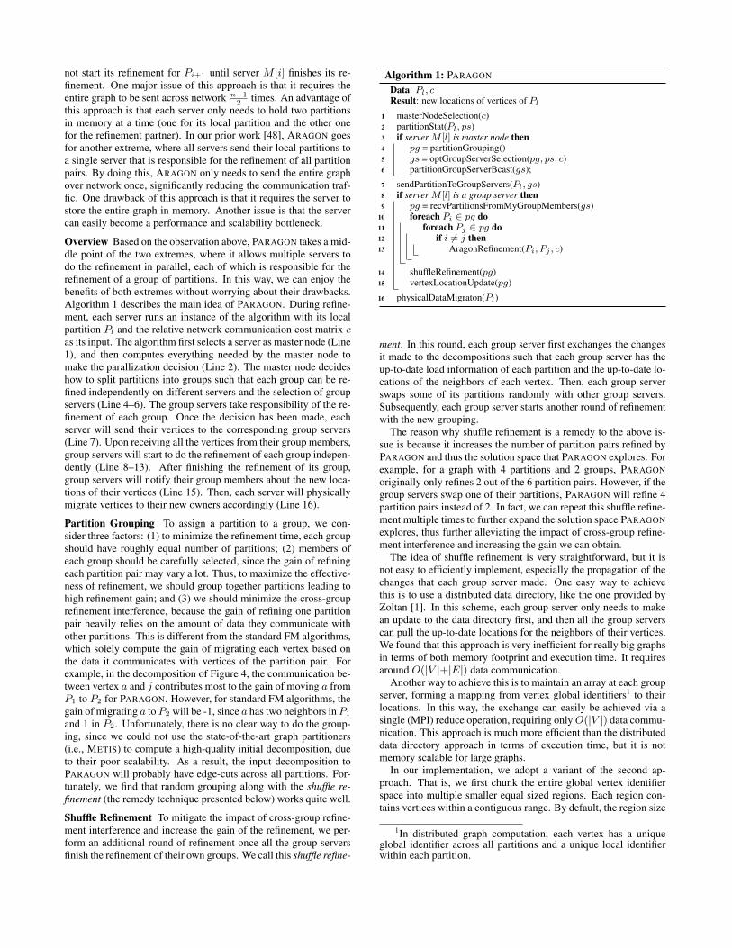
Overview Based on the observation above, PARAGON takes a mid-dle point of the two extremes, where it allows multiple servers todo the refinement in parallel, each of which is responsible for therefinement of a group of partitions. In this way, we can enjoy thebenefits of both extremes without worrying about their drawbacks.Algorithm 1 describes the main idea of PARAGON. During refine-ment, each server runs an instance of the algorithm with its localpartition Pl and the relative network communication cost matrix cas its input. The algorithm first selects a server as master node (Line1), and then computes everything needed by the master node tomake the parallization decision (Line 2). The master node decideshow to split partitions into groups such that each group can be re-fined independently on different servers and the selection of groupservers (Line 4–6). The group servers take responsibility of the re-finement of each group. Once the decision has been made, eachserver will send their vertices to the corresponding group servers(Line 7). Upon receiving all the vertices from their group members,group servers will start to do the refinement of each group indepen-dently (Line 8–13). After finishing the refinement of its group,group servers will notify their group members about the new loca-tions of their vertices (Line 15). Then, each server will physicallymigrate vertices to their new owners accordingly (Line 16).

Partition Grouping To assign a partition to a group, we con-sider three factors: (1) to minimize the refinement time, each groupshould have roughly equal number of partitions; (2) members ofeach group should be carefully selected, since the gain of refiningeach partition pair may vary a lot. Thus, to maximize the effective-ness of refinement, we should group together partitions leading tohigh refinement gain; and (3) we should minimize the cross-grouprefinement interference, because the gain of refining one partitionpair heavily relies on the amount of data they communicate withother partitions. This is different from the standard FM algorithms,which solely compute the gain of migrating each vertex based onthe data it communicates with vertices of the partition pair. Forexample, in the decomposition of Figure 4, the communication be-tween vertex a and j contributes most to the gain of moving a fromP1 to P2 for PARAGON. However, for standard FM algorithms, thegain of migrating a toP2 will be -1, since a has two neighbors inP1

and 1 in P2. Unfortunately, there is no clear way to do the group-ing, since we could not use the state-of-the-art graph partitioners(i.e., METIS) to compute a high-quality initial decomposition, dueto their poor scalability. As a result, the input decomposition toPARAGON will probably have edge-cuts across all partitions. For-tunately, we find that random grouping along with the shuffle re-finement (the remedy technique presented below) works quite well.

Shuffle Refinement To mitigate the impact of cross-group refine-ment interference and increase the gain of the refinement, we per-form an additional round of refinement once all the group serversfinish the refinement of their own groups. We call this shuffle refine-

Algorithm 1: PARAGON

Data: Pl, cResult: new locations of vertices of Pl

1 masterNodeSelection(c)2 partitionStat(Pl, ps)3 if server M [l] is master node then4 pg = partitionGrouping()5 gs = optGroupServerSelection(pg, ps, c)6 partitionGroupServerBcast(gs);

7 sendPartitionToGroupServers(Pl, gs)8 if server M [l] is a group server then9 pg = recvPartitionsFromMyGroupMembers(gs)

10 foreach Pi ∈ pg do11 foreach Pj ∈ pg do12 if i 6= j then13 AragonRefinement(Pi, Pj , c)

14 shuffleRefinement(pg)15 vertexLocationUpdate(pg)

16 physicalDataMigraton(Pl)

ment. In this round, each group server first exchanges the changesit made to the decompositions such that each group server has theup-to-date load information of each partition and the up-to-date lo-cations of the neighbors of each vertex. Then, each group serverswaps some of its partitions randomly with other group servers.Subsequently, each group server starts another round of refinementwith the new grouping.

The reason why shuffle refinement is a remedy to the above is-sue is because it increases the number of partition pairs refined byPARAGON and thus the solution space that PARAGON explores. Forexample, for a graph with 4 partitions and 2 groups, PARAGONoriginally only refines 2 out of the 6 partition pairs. However, if thegroup servers swap one of their partitions, PARAGON will refine 4partition pairs instead of 2. In fact, we can repeat this shuffle refine-ment multiple times to further expand the solution space PARAGONexplores, thus further alleviating the impact of cross-group refine-ment interference and increasing the gain we can obtain.

The idea of shuffle refinement is very straightforward, but it isnot easy to efficiently implement, especially the propagation of thechanges that each group server made. One easy way to achievethis is to use a distributed data directory, like the one provided byZoltan [1]. In this scheme, each group server only needs to makean update to the data directory first, and then all the group serverscan pull the up-to-date locations for the neighbors of their vertices.We found that this approach is very inefficient for really big graphsin terms of both memory footprint and execution time. It requiresaround O(|V |+|E|) data communication.

Another way to achieve this is to maintain an array at each groupserver, forming a mapping from vertex global identifiers1 to theirlocations. In this way, the exchange can easily be achieved via asingle (MPI) reduce operation, requiring onlyO(|V |) data commu-nication. This approach is much more efficient than the distributeddata directory approach in terms of execution time, but it is notmemory scalable for large graphs.

In our implementation, we adopt a variant of the second ap-proach. That is, we first chunk the entire global vertex identifierspace into multiple smaller equal sized regions. Each region con-tains vertices within a contiguous range. By default, the region size

1In distributed graph computation, each vertex has a uniqueglobal identifier across all partitions and a unique local identifierwithin each partition.

equals k = min{226, |V |}, where V is the vertex set of the entiregraph. Correspondingly, the exchange is split into multiple rounds.Each round only exchanges the locations of vertices of one region.With this scheme, we only need to maintain a smaller array at eachgroup sever and thus the amount of data communication remainsunchanged. Although this scheme requires scanning the edge listsof each partition multiple times, it is much more efficient than thedistributed data directory approach.

Degree of Refinement Parallelism Theoretically, the number ofgroups we can have can be any integer between 1 and n

2, where

n is the number of partitions of the graph. Clearly, if the numberof groups equals 1, PARAGON degrades to ARAGON, in which allservers will send their local partitions to a single group server forsequential refinement. The reason why there is an upper bound isbecause each group needs to have at least 2 partitions for the re-finement to proceed. Typically, the higher the number is, the fasterthe refinement will finish. However, there is a tradeoff between thedegree of parallelism and the quality of the resulting decomposi-tion we can have. This is because the higher the number is, thefewer partitions each group will have and thus the fewer partitionpairs will be refined. Given a graph with n partitions andm groups,PARAGON only refines n(n−m)

2mpartition pairs, while ARAGON re-

fines all n(n−1)2

partition pairs. In other words, ARAGON will even-tually select an optimal migration destination among all partitionsfor each vertex, whereas PARAGON only considers a subset of thepartitions for each vertex. This also explains the reason why the re-sulting decompositions computed by PARAGON are usually poorerthan those of ARAGON. Fortunately, the shuffle refinement tech-nique we proposed helps to address the issue.

Group Server Selection Once the master node finishes the group-ing process, it will select an optimal server for each group, suchthat the cost of sending partitions of the group to the group serveris minimized. For example, in case of Figure 4, where we assumethat P1, P2, and P3 are of one group, we should select server M [2]as the group server intuitively since c(P1, P2) = c(P2, P3) = 1while c(P1, P3) = 6. To achieve this, we define the cost of select-ing server M [s] as the group server for group g as:∑

Pi∈g

ps[i] ∗ c(Pi, Ps) ∗ (1 +σ(s)

drp) (10)

Here, ps[i] denotes the number of edges associated with verticesof Pi, which is a good approximation for the amount of data eachserver needs to send to their group servers. σ(s) is the number ofgroup servers that have been designated on the compute node thatserver M [s] belongs to. It should be noticed that server M [s] canbe a hardware thread, a core, a socket, or a machine. drp is thedegree of refinement parallelism (number of group servers). Thelast term (1 + σ(s)

drp) is the penalty that is added to avoid the con-

centration of multiple group servers into a single compute node,reducing the chance of memory exhaustion. Once all group serversare selected, the master node will broadcast the group servers of allgroups to all slave nodes. Then, each server will send its vertices(as well as their edge lists) to their corresponding group servers,after which the group servers will start to refine partitions of theirown groups independently.

Reducing Communication Volume Clearly, PARAGON with theshuffle refinement disabled requires the entire graph to be sent overthe network once, and PARAGON with the shuffle refinement en-abled demands more data communication. For really big graphs,the communication volume may get very high. Thus, we followthe same approach proposed in [35] to reduce the communication

volume. Specifically, instead of sending the entire partition to theirgroup servers, each server only needs to send vertices that can bereached by a breadth-first search from boundary vertices of eachpartition within k-hop traversal. Boundary vertices are vertices thathave neighbors in other partitions. The rationale behind this is thatif a vertex is very far from the boundary vertex, the chance that itget moved by PARAGON to another partition to improve the decom-position is very small. Surprisingly, we find that PARAGON is notsensitive to k in terms of the partitioning quality, and that a largerk does not always lead to partitionings of higher quality. However,it may increase the refinement time greatly. Thus, in our imple-mentation, we set k = 0 by default. In other words, we only sendboundary vertices of each partition to the group servers.

In fact, [35] has presented a solution to parallellize the standardFM algorithms [12]. However, it may require a graph with n parti-tions to be sent over the network n− 1 times in case the initial de-composition has edge-cuts across all partition pairs. Furthermore,the presence of communication heterogeneity complicates thingsgreatly. First, ARAGON has to be applied to all partition pairs,whereas standard FM algorithms, which assume uniform networkcommunication costs, only need to refine partition pairs that haveedge-cuts between them. Second, during each refinement iterationof a single partition pair, standard FM algorithms only need to con-sider migrating vertices of both partitions that have neighbors in thealternative partition. On the other hand, PARAGON has to considermigrating all boundary vertices.

Master Node Selection As presented so far, each server (slavenode) needs to send some auxiliary data (i.e., the number of ver-tices/neighbors) of their local partitions to the master node for theparallelization decision, and the master needs to broadcast the deci-sion it made to all slave nodes. To reduce the communication costbetween the master node and the slave nodes, we also select themaster node in an intelligent way using the following heuristic:

minm∈[1,n]

n∑i=1 and i 6=m

c(Pi, Pm) (11)

The heuristic tries to find a server M [m] that will result in minimalnetwork communication cost as the master node. For example, incase of Figure 4, we should select server M [2] as the master node.Clearly, the selection of master node can be made locally by eachserver without synchronizing with each other.

Physical Data Migration To support efficient distributed com-putation, we also provide a basic migration service for graph work-loads. Considering that physical data migration is highly application-dependent, the migration service only takes responsibility for theredistribution of the graph data itself. It is the users who are re-sponsible for the migration of any application data associated witheach vertex. That is, the users should save the application contextbefore using our migration service and restore the context after-wards. For example, in breadth first search, each vertex is usuallyassociated with a value indicating its current distance to the sourcevertex. Users need to keep track of the distance value of each vertexwhile migrating. For complicated workloads, users can exploit themigration service provided by Zoltan [1] to simplify the migration.

6. CONTENTION AWARENESSSo far, we have presented how we parallelize ARAGON. In this

section, we will cover how we make PARAGON aware of the issueof shared resource contention in multicore systems. We know that,guided by a given network communication cost matrix, PARAGONis able to gather neighboring vertices as close as possible, and that

the contention is caused by the fact that we put too much commu-nication within the compute nodes. Hence, to avoid serious intra-node shared resource contention, we can simply penalize intra-nodenetwork communication costs by a score. The score is computedbased on the degree of contentiousness between the communica-tion peers. By doing this, the amount of intra-node communicationwill decrease accordingly. In our implementation, we refine theintra-node communication costs as follows:

c(Pi, Pj) = c(Pi, Pj) + λ ∗ (s1 + s2) (12)

where Pi and Pj are two partitions collocated in a single computenode; λ is a value between 0 and 1, denoting the degree of con-tention; and s1 denotes the maximal inter-node network commu-nication cost, while s2 equals 0 if Pi and Pj reside on differentsockets and equals the maximal inter-socket network communica-tion cost otherwise. Clearly, if λ = 0, PARAGON will only considerthe communication heterogeneity, and λ = 1 means that intra-nodeshared resource contention is the biggest performance bottleneck,which should be prioritized over the communication heterogeneity.It should be noticed that PARAGON with any λ ∈ (0, 1] considersboth the contention and the communication heterogeneity. Consid-ering the impact of both resource contention and communicationheterogeneity is highly application- and hardware-dependent, userswill need to do simple profiling of the target applications on the ac-tual computing environment to determine the ideal λ for them.

7. EVALUATIONIn this section, we first evaluate the sensitivity of PARAGON to

varying input decompositions computed by different initial parti-tioners and the impact of its two important parameters: the degreeof parallelism and the number of shuffle refinement times (Sec-tion 7.1). We then validate the effectiveness of PARAGON using tworeal-world graph workloads: Breadth-First Search (BFS) [4] andSingle-Source Shortest Path (SSSP) [20], which we implementedusing MPI (Section 7.2). Finally, we demonstrate the scalability ofPARAGON via a billion-edge graph (Section 7.3).

Datasets Table 2 describes the datasets used. By default, thegraphs were (re)partitioned with vertex weights (i.e., computationalrequirement) set to be their vertex degree, with vertex sizes (i.e.,amount of the data of the vertex) set to be their vertex degree, andwith edge weights (i.e., amount of data communicated) set to 1.The degree of each vertex is often a good approximation of thecomputational requirement and the migration cost of each vertex,while a uniform edge weight of 1 is a close estimation of the com-munication pattern of many graph algorithms, like BFS and SSSP.Given the fact that communication cost is usually more impor-tant than migration cost, all the experiments were performed withα = 10 (Eq. 2). Unless explicitly specified, all the graphs wereinitially partitioned by DG (deterministic greedy heuristic), a state-of-the-art streaming graph partitioner [39], across cores of the com-pute node used (one partition per core). The partitionings were thenimproved by PARAGON. During the (re)partitioning, we allowedup to 2% load imbalance among partitions. For fairness, DG/LDGwere extended to support vertex- and edge-weighted graphs.

Platforms We evaluated PARAGON on two clusters: PittMPIClus-ter [32] and Gordon supercomputer [28]. PittMPICluster had a flatnetwork topology, with all 32 compute nodes connected to a sin-gle switch via 56Gbps FDR Infiniband. On the other hand, theGordon network topology was a 4x4x4 3D torus of switches con-nected via QDR Infiniband with 16 compute nodes attached to eachswitch (with 8Gbps link bandwidth). Table 3 depicts the computenode configuration of both clusters. The results presented were the

Table 2: Datasets used in our experimentsDataset |V | |E| Description

wave [38] 156,317 2,118,662 2D/3D FEMauto [38] 448,695 6,629,222 3D FEM

333SP [10] 3,712,815 22,217,266 2D FE Triangular MeshesCA-CondMat [2] 108,300 373,756 Collaboration Network

DBLP [18] 317,080 1,049,866 Collaboration NetworkEmail-Eron [2] 36,692 183,831 Communication Network

as-skitter [2] 1,696,415 22,190,596 Internet TopologyAmazon [2] 334,863 925,872 Product Network

USA-roadNet [9] 23,947,347 58,333,344 Road NetworkPA-roadNet [2] 1,090,919 6,167,592 Road NetworkYouTube [18] 3,223,589 24,447,548 Social Network

com-LiveJournal [2] 4,036,537 69,362,378 Social NetworkFriendster [2] 124,836,180 3,612,134,270 Social Network

Table 3: Cluster Compute Node ConfigurationNode Configuration PittMPICluster

(Intel Haswell Processor)Gordon

(Intel Sandy Bridge Processor)Sockets 2 2Cores 20 16

Clock Speed 2.6 GHz 2.6 GHzL3 Cache 25 MB 20 MB

Memory Capacity 128 GB 64 GBMemory Bandwidth 65 GB/s 85 GB/s

means of 5 runs, except the execution of SSSP on Gordon (Sec-tion 7.2) and the scalability test (Section 7.3).Network Communication Cost Modelling The relative networkcommunication costs among partitions (cores) were approximatedusing a variant of the osu_latency benchmark [29]. To ensure thecorrectness of the cost matrix, each MPI rank (process) was boundto a core using the mechanism provided by MVAPICH2 1.9 [25] onGordon and OpenMPI 1.8.6 [27] on PittMPICluster. MVAPICH2and OpenMPI were two different MPI implementations availableon the clusters.

7.1 MicroBenchmarks

7.1.1 Varying Degree of ParallelismConfiguration In this experiment, we examined the impact of thedegree of parallelism in terms of both the refinement time (i.e.,the time that the refinement took) and the refinement quality (i.e.,the communication cost of the resulting decomposition). Towardsthis, we first partitioned the com-lj dataset into 40 partitions usingDG across 2 compute nodes of PittMPICluster, and then appliedPARAGON to the decompositions with varying degree of refinementparallelism but with shuffle refinement disabled.Results (Figures 7a & 7b) Figure 7a plots the runtime of PARAGONon the com-lj dataset for various degrees of parallelism. As ex-pected, the higher the degree of parallelism, the faster the refine-ment would finish, and PARAGON significantly reduced the refine-ment time of ARAGON (PARAGON with degree of parallelism of 1).However, the speedup was achieved at the cost of higher communi-cation cost of the resulting decompositions (Figure 7b). The com-munication costs presented were normalized to that of the initialdecomposition computed by DG. However, in the end, PARAGONstill resulted in lower communication cost in all cases when com-pared to the initial decompositions.

7.1.2 Impact of Shuffle RefinementConfiguration In our second experiment, we were interested to seewhether the shuffle refinement technique could address the issue weidentified in the previous experiment. Towards this, we repeated thesame experiment but with a fixed degree of refinement parallelism(8) and varying number of shuffle refinement times (from 8 to 15).

0

5

10

15

20

25

30

35

1 2 4 6 8 10 12 14 16 18 20Refinement Time(s)

Degree of Refinement Parallelism

(a) Refinement time

0.0 0.1 0.2 0.3 0.4 0.5 0.6 0.7 0.8 0.9 1.0

1 2 4 6 8 10 12 14 16 18 20

Normalized Comm Cost

Degree of Refinement Parallelism

(b) Normalized communication cost of the resulting decompositionsFigure 7: Refinement time and communication costs of the com-lj decompositions after being refined with varying degree of refinementparallelism on two 20-core compute nodes. The communication costs presented were normalized to that of the initial decomposition.

0

0.2

0.4

0.6

0.8

1

1.2

1.4

0 2 4 6 8 10 12

Nor

mal

ized

Com

m C

ost

Refinement Time (s)

0 1 2 3 4 5 6 7 8 9 10111213 1415

Figure 8: Y-axis corresponds to the communication costs of thecom-lj decompositions after being refined with varying number ofshuffle refinement times on two 20-core compute nodes when theywere normalized to that of the decompositions refined by ARAGON;X-axis denotes the corresponding refinement time; the labels oneach data point were the number of refinement times.

Results (Figure 8) Figure 8 shows the corresponding refinementtime and the normalized communication costs of resulting decom-positions with the decompositions computed by ARAGON as thebaseline. As shown, PARAGON (with shuffle refinement enabled)not only produced decompositions of lower communication coststhan ARAGON (when the number of shuffle refinement times wasgreater than 11), but also completed the refinement faster (ARAGONtook around 33s to finish the refinement vs 8.12s by PARAGON with11 shuffle refinement times).

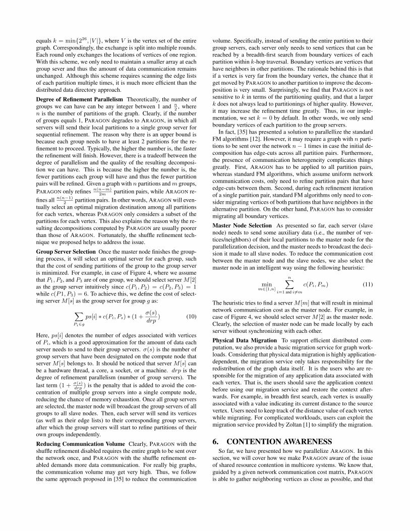
7.1.3 Impact of Initial PartitionersConfiguration This experiment examined the refinement overheadand the quality of the resulting decompositions, when PARAGONwas provided with decompositions computed by four different par-titioners: (a) HP, the default graph partitioner of many parallelgraph computing engines; (b) DG and LDG, two state-of-the-artstreaming graph partitioning heuristics [39]; and (c) METIS, a state-of-the-art multi-level graph partitioner [23]. The graphs were ini-tially partitioned across the same two machines used in our priorexperiments but with both the degree of refinement parallelism andthe number of shuffle refinement times set to 8.Quality of the Initial Decompositions (Figure 9) Figure 9 de-notes the communication cost of the initial decompositions com-puted by HP, DG, LDG, and METIS for a variety of graphs. Asanticipated, METIS performed the best and HP the worst. How-ever, METIS is a heavyweight serial graph partitioner, making it in-feasible for large-scale distributed graph computation either as aninitial partitioner or as an online repartitioner (repartitioning from

0

20

40

60

80

100

120

140

waveauto

333SP

roadNet−PA

USA−road−d

CA−CondMat

com−dblp

com−amazon

Email−Enron

YouTube

as−skitter

com−lj

Comm Cost (10^7)

HPDGLDGMETIS

Figure 9: Communication cost of the initial decompositions com-puted by HP, DG, LDG, and METIS across cores of two 20-corecompute nodes for a variety of graphs.

scratch). It was reported in prior work [42] that METIS took upto 8.5 hours to partition a graph with 1.46 billion edges. Unex-pectedly, DG outperformed LDG, the best streaming partitioningheuristic among the ones presented in [39]. This was probably be-cause the order in which the vertices were presented to the parti-tioner favored DG over LDG (the results of DG and LDG rely onthe order in which vertices are presented). This was also the reasonwhy we picked DG as the default initial partitioner for PARAGON.

Quality of the Resulting Decompositions (Figures 10a & 10b)Figures 10a and 10b show the corresponding communication costof the resulting decompositions and the improvement achieved byPARAGON in terms of the communication cost when compared tothe initial decompositions. As shown, the better the initial decom-position was, the better the resulting decomposition would be. Incomparison with the initial decompositions computed by HP, DG,and LDG, PARAGON reduced the communication cost of the de-compositions by up to 58% (43% on average), 29% (17% on aver-age), and 53% (36% on average), respectively. Although PARAGONdid not improve significantly the decompositions computed by METISfor easily partitioned FEM and road networks (left 7 datasets), itachieved an improvement of up to 4.5% for complex networks (right5 datasets). Given the size of the dataset, the improvement was stillnon-negligible. Fortunately, we found that PARAGON with DGas its initial partitioner can achieve even better performance thanMETIS on real-world workloads (Section 7.2).

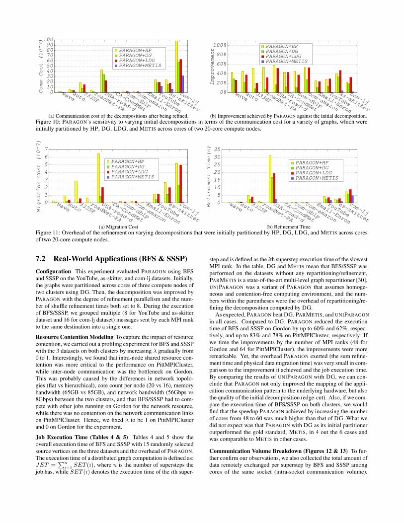
Refinement Overhead (Figures 11a & 11b) We also noticedthat the quality of the initial decomposition impacted the refine-ment overhead greatly. Figures 11a and 11b plot the migrationcost (Eq. 3) and the refinement time. Clearly, the poorer the initialdecomposition was, the higher the migration cost and the longerthe refinement time would be. Finally, for decompositions, whichPARAGON failed to make much improvement, PARAGON only ledto a very small amount of overhead.

0 10 20 30 40 50 60 70 80 90 100

waveauto

333SP

roadNet−PA

USA−road−d

CA−CondMat

com−dblp

com−amazon

Email−Enron

YouTube

as−skitter

com−lj

Comm Cost (10^7)

PARAGON+HPPARAGON+DGPARAGON+LDGPARAGON+METIS

(a) Communication cost of the decompositions after being refined.

0%

20%

40%

60%

80%

100%

waveauto

333SP

roadNet−PA

USA−road−d

CA−CondMat

com−dblp

com−amazon

Email−Enron

YouTube

as−skitter

com−lj

Improvement


(b) Improvement achieved by PARAGON against the initial decomposition.Figure 10: PARAGON’s sensitivity to varying initial decompositions in terms of the communication cost for a variety of graphs, which wereinitially partitioned by HP, DG, LDG, and METIS across cores of two 20-core compute nodes.

0

1

2

3

4

5

6

7

waveauto

333SP

roadNet−PA

USA−road−d

CA−CondMat

com−dblp

com−amazon

Email−Enron

YouTube

as−skitter

com−ljMigration Cost (10^7)


(a) Migration Cost

0

5

10

15

20

25

30

35

waveauto

333SP

roadNet−PA

USA−road−d

CA−CondMat

com−dblp

com−amazon

Email−Enron

YouTube

as−skitter

com−ljRefinement Time(s)


(b) Refinement TimeFigure 11: Overhead of the refinement on varying decompositions that were initially partitioned by HP, DG, LDG, and METIS across coresof two 20-core compute nodes.

7.2 Real-World Applications (BFS & SSSP)Configuration This experiment evaluated PARAGON using BFSand SSSP on the YouTube, as-skitter, and com-lj datasets. Initially,the graphs were partitioned across cores of three compute nodes oftwo clusters using DG. Then, the decomposition was improved byPARAGON with the degree of refinement parallelism and the num-ber of shuffle refinement times both set to 8. During the executionof BFS/SSSP, we grouped multiple (8 for YouTube and as-skitterdataset and 16 for com-lj dataset) messages sent by each MPI rankto the same destination into a single one.

Resource Contention Modeling To capture the impact of resourcecontention, we carried out a profiling experiment for BFS and SSSPwith the 3 datasets on both clusters by increasing λ gradually from0 to 1. Interestingly, we found that intra-node shared resource con-tention was more critical to the performance on PittMPICluster,while inter-node communication was the bottleneck on Gordon.This was probably caused by the differences in network topolo-gies (flat vs hierarchical), core count per node (20 vs 16), memorybandwidth (65GB vs 85GB), and network bandwidth (56Gbps vs8Gbps) between the two clusters, and that BFS/SSSP had to com-pete with other jobs running on Gordon for the network resource,while there was no contention on the network communication linkson PittMPICluster. Hence, we fixed λ to be 1 on PittMPIClusterand 0 on Gordon for the experiment.

Job Execution Time (Tables 4 & 5) Tables 4 and 5 show theoverall execution time of BFS and SSSP with 15 randomly selectedsource vertices on the three datasets and the overhead of PARAGON.The execution time of a distributed graph computation is defined as:JET =

∑ni=1 SET (i), where n is the number of supersteps the

job has, while SET (i) denotes the execution time of the ith super-

step and is defined as the ith superstep execution time of the slowestMPI rank. In the table, DG and METIS mean that BFS/SSSP wasperformed on the datasets without any repartitioning/refinement,PARMETIS is a state-of-the-art multi-level graph repartitioner [30],UNIPARAGON was a variant of PARAGON that assumes homoge-neous and contention-free computing environment, and the num-bers within the parentheses were the overhead of repartitioning/re-fining the decomposition computed by DG.

As expected, PARAGON beat DG, PARMETIS, and UNIPARAGONin all cases. Compared to DG, PARAGON reduced the executiontime of BFS and SSSP on Gordon by up to 60% and 62%, respec-tively, and up to 83% and 78% on PittMPICluster, respectively. Ifwe time the improvements by the number of MPI ranks (48 forGordon and 64 for PittMPICluster), the improvements were moreremarkable. Yet, the overhead PARAGON exerted (the sum refine-ment time and physical data migration time) was very small in com-parison to the improvement it achieved and the job execution time.By comparing the results of UNIPARAGON with DG, we can con-clude that PARAGON not only improved the mapping of the appli-cation communication pattern to the underlying hardware, but alsothe quality of the initial decomposition (edge-cut). Also, if we com-pare the execution time of BFS/SSSP on both clusters, we wouldfind that the speedup PARAGON achieved by increasing the numberof cores from 48 to 60 was much higher than that of DG. What wedid not expect was that PARAGON with DG as its initial partitioneroutperformed the gold standard, METIS, in 4 out the 6 cases andwas comparable to METIS in other cases.

Communication Volume Breakdown (Figures 12 & 13) To fur-ther confirm our observations, we also collected the total amount ofdata remotely exchanged per superstep by BFS and SSSP amongcores of the same socket (intra-socket communication volume),

Table 4: BFS Job Execution Time (s)Algorithm/Dataset YouTube as-skitter com-lj

PittMPIClusterDG 30 59 218

METIS 8.50 67 27PARMETIS 29 (21.00) 59 (9.65) 185 (4.71)

UNIPARAGON 25 (2.70) 27 (2.26) 159 (7.54)PARAGON 8 (4.00) 10 (3.31) 40 (10.00)

GordonDG 322 577 4319


Table 5: SSSP Job Execution Time (s)Algorithm/Dataset YouTube as-skitter com-lj

PittMPIClusterDG 2136 1823 5196

METIS 545 822 955PARMETIS 1842 (19.00) 582 (9.28) 3268 (4.50)


GordonDG 3436 7092 10732


0

500

1,000

1,500

2,000

2,500

DG METIS

PARMETIS

uniPARAGON

PARAGON

DG METIS

PARMETIS

uniPARAGON

PARAGON

DG METIS

PARMETIS

uniPARAGON

PARAGON

Comm Volume(MB)

YouTube as−skitter com−lj

Inter−NodeInter−SocketIntra−Socket

Figure 12: The breakdown of the accumulated communication volumeacross all supersteps for BFS on PittMPICluster.

0

500

1,000

1,500

2,000

2,500

DG uniPARAGON

PARAGON

DG uniPARAGON

PARAGON

DG uniPARAGON

PARAGON

Comm Volume(MB)

YouTube as−skitter com−lj

Inter−NodeInter−SocketIntra−Socket

Figure 13: The breakdown of the accumulated communication volumeacross all supersteps for BFS on Gordon.

among cores of the same compute node but belonging to differ-ent sockets (inter-socket communication volume), and among coresof different compute nodes (inter-node communication volume).Since we observed similar patterns for BFS and SSSP in all thecases, we only present the breakdown of the accumulated commu-nication volume across all supersteps for BFS here.

As shown in Figures 12 (for PittMPICluster) and 13 (for Gor-don), PARAGON and UNIPARAGON have much lower remote com-munication volume than DG in all cases, and PARAGON has thelowest inter-node communication volume and highest intra-node(inter-socket & intra-socket) communication volume on Gordon(vice versa on PittMPICluster), which was expected given our choicefor λ. It is worth mentioning that on PittMPICluster, intra-nodedata communication was the bottleneck. Another interesting thingwas that in spite of its higher total communication volume whencompared to METIS, PARMETIS, and UNIPARAGON, PARAGONstill outperformed them in most cases due to the reduced commu-nication on critical components.

Graph Dynamism (Figure 14) To further validate the effective-ness of PARAGON in the presence of graph dynamism, we split theYouTube dataset (a collection of YouTube users and their friend-ship connections over a period of 225 days) into 5 snapshots withan interval of 45 days. Thus, snapshot Si denotes the collectionof YouTube users and their friendship connections appearing dur-ing the first 45 ∗ i days. We then ran BFS on snapshot S1 acrossthree 20-core machines and injected vertices newly appeared ineach snapshot to the system using DG whenever BFS finished itscomputation for every 15 randomly selected vertices. The injec-tion also triggered the execution of PARAGON, UNIPARAGON, andPARMETIS on the decomposition.

Figure 14 plots the BFS execution time for 15 randomly selectedsource vertices on each snapshot. As shown, both architecture-awareness and the capability to cope with graph dynamism werecritical to achieve superior performance. This is especially true asthe graph changes a lot from its original version: at snapshot S5,PARAGON performed 90% better than DG, 85% better than METIS,73% better than PARMETIS, and 89% better than UNIPARAGON.

7.3 Billion-Edge Graph ScalingConfiguration In this experiment, we investigated the scalabil-ity of PARAGON as the graph scale increased. Towards this, wegenerated three additional datasets by sampling the edge list of thefriendster dataset (3.6 billion edges). We denote the datasets gen-erated as friendster-p, where p was the probability that each edgewas kept while sampling. Hence, friendster-p would have around3.6∗p billion edges. Interestingly, the number of vertices remainedalmost unchanged in spite of the sampling. We ran the experimenton three compute nodes of PittMPICluster with the degree of re-finement parallelism, the number of shuffle refinement times, andthe message grouping size set to 10, 10, and 256, respectively.Results (Figures 15 & 16) Figures 15 and 16 present the execu-tion time of BFS with 15 randomly selected source vertices andthe overhead of PARAGON at different graph scales. As shown,PARAGON not only led to lower job execution times, but also tolower speed in which the job execution time increased as the graphsize increased. It should be noticed that PARAGON reduced theexecution time of all machines (3*20 cores) not just one. Also,the refinement time increased at a much slower rate (from 140s, to236s, to 312s, and to 410s) than that of the graph size. The rea-son why we did not present the results of METIS or PARMETIShere was because they failed to (re)partition the graphs (even forthe first dataset, of 0.9 billion edges).

8. RELATED WORKGraph partitioning and repartitioning are receiving more and more

attention in recent years due to the proliferation of large graphdatasets. In this section, we categorize existing approaches of graph(re)partitioners into three types: (a) heavyweight, (b) lightweight,and (c) streaming, which are presented next.Heavyweight Graph (Re)Partitioning Graph partitioning and repar-titioning has been studied for decades (e.g., METIS [23], PARMETIS [30],Scotch [36], Chaco [7], and Zoltan [1]). These graph (re)partitionersare well-known for their capability of producing high-quality graphdecompositions. However, they usually require full knowledge ofthe entire graph for (re)partitioning, making them scale poorly against

0 20 40 60 80 100 120 140 160 180 200

S1 S2 S3 S4 S5

BFS JET(s)

Snapshots

DGMETISPARMETISuniPARAGONPARAGON

Figure 14: BFS JET with Graph Dynamism

2002500

5000

7500

10000

12500

15000

0 0.9 1.8 2.7 3.6

BFS JET(s

)

Approximate # of edges (billions)

DGPARAGON

Figure 15: BFS JET vs Graph Size

0

100

200

300

400

500

0 0.9 1.8 2.7 3.6Refin

em

ent

Tim

e(s

)

Approximate # of edges (billions)

PARAGON

Figure 16: Refinement Time vs Graph Size

large graphs even if performed in parallel. Furthermore, they areall architecture-agnostic. Although [24], a METIS variant, consid-ers the communication heterogeneity, it is a sequential static graphpartitioner, which is inapplicable for massive graphs or dynamicgraphs. Several recent works [48, 8] have been proposed to copewith the heterogeneity and dynamism. However, they are also tooheavyweight for massive graphs because of the high communica-tion volume they generate. As a consequence, they are not ap-propriate for online graph repartitioning in large-scale distributedgraph computation. Furthermore, they disregard the issue of re-source contention in multicore systems.

Lightweight Graph Repartitioning As a result of the shortcom-ings of heavyweight graph (re)partitioners, many lightweight graphrepartitioners [37, 43, 26, 17, 45] have been proposed. They ef-ficiently adapt the partitioning to changes by incrementally mi-grating vertices among partitions based on some heuristics (ratherthan repartitioning the entire graph). Nevertheless, they are notarchitecture-aware. Also, many of them assume uniform vertexweights and sizes, and some [43, 26] even assume uniform edgeweights, which may not always be true.

In fact, work [17] is a Pregel-like graph computing engine, whichmigrates vertices based on runtime characteristics of the workload(i.e., # of message sent/received by each vertex and response time)instead of the graph structure (i.e., the distribution of vertex neigh-bors, edge weights, and vertex sizes). Paper [45] also presentsa repartitioning system that migrates vertices on-the-fly based onsome runtime statistics (i.e., the average compute and communica-tion time of each superstep and the probability of a vertex becomingactive in the next superstep).

Recently, a novel distributed graph partitioner, Sheep [22], hasbeen proposed for large graphs. It is similar in spirit to METIS.That is, they both first reduce the original graph to a smaller tree ora sequence of smaller graphs, then do a partition of the tree or thesmallest graph, and finally map the partitioning back to the origi-nal graph. In terms of partitioning time, Sheep outperforms bothMETIS and streaming partitioners. For partitioning quality, Sheepis competitive with METIS for a small number of partitions and iscompetitive with streaming graph partitioners for larger numbersof partitions. However, Sheep is unable to deal with both weightedand dynamic graphs, and it is architecture-agnostic.

Streaming Graph Partitioning Recently, a new family of graphpartitioning heuristics, streaming graph partitioning [39, 11, 42],has been proposed for online graph partitioning. They are able toproduce partitionings comparable to the heavyweight graph par-titioner, METIS, within a relative short time. However, they arearchitecture-agnostic. Although [46] has presented a streaminggraph partitioner with awareness of both compute and communi-cation heterogeneity, it may lead to suboptimal performance in thepresence of graph dynamism.

Vertex-Cut Graph Partitioning Several vertex-cut graph parti-tioners [44, 31, 13] were also proposed to improve the performanceof distributed graph computation. Vertex-cut solutions partition

the graph by assigning edges of the graph across partitions in-stead of vertices. It has been shown that vertex-cut solutions re-duce the communications with respect to edge-cut ones, especiallyon power-law graphs. However, it also has to deal with the issueof communication heterogeneity and the issue of shared-resourcecontention, since vertices appearing in multiple partitions need tocommunicate with each other during the computation. Neverthe-less, its discussion is beyond the scope of this paper.

Overview of Related Work Table 6 visually classifies the state-of-the-art graph (re)partitioners according to algorithm and graphproperties. In terms of algorithm properties, we characterize eachapproach as to whether it (a) runs in parallel and (b) is architecture-aware (i.e., CPU heterogeneity, network cost non-uniformity, andresource contention). In terms of graph properties, we charac-terize each approach as to whether it can handle graphs with (a)dynamism, (b) weighted vertices (i.e., nonuniform computation),(c) weighted edges (i.e., nonuniform data communication), and (d)vertex sizes (i.e., nonuniform data sizes on each vertex).

9. CONCLUSIONSIn this paper, we presented PARAGON, a parallel architecture-

aware graph partition refinement algorithm that bridges the mis-match between the application communication pattern and the un-derlying hardware topology. PARAGON achieves this by modify-ing a given decomposition according to the nonuniform networkcommunication costs and consideration of the contentiousness ofthe underlying hardware. To further reduce its overhead, we madePARAGON itself architecture-aware. Compared to the state-of-the-art, PARAGON improved the quality of graph decompositions byup to 53%, achieved up to 5.9x speedups on real workloads, andsuccessfully scaled up to a 3.6 billion-edge graph.

10. ACKNOWLEDGMENTSWe would like to thank Jack Lange, Albert DeFusco, Kim Wong,

Mark Silvis, and the anonymous reviewers for their valuable helpon the paper. This work was funded in part by NSF awards CBET-1250171 and OIA-1028162.

11. REFERENCES[1] http://www.cs.sandia.gov/zoltan/.[2] http://snap.stanford.edu/data.[3] C. Binnig, U. Çetintemel, A. Crotty, A. Galakatos, T. Kraska,

E. Zamanian, and S. B. Zdonik. The End of Slow Networks: It’sTime for a Redesign. CoRR, 2015.

[4] A. Buluç and K. Madduri. Parallel Breadth-First Search onDistributed Memory Systems. CoRR, abs/1104.4518, 2011.

[5] D. Buntinas, B. Goglin, D. Goodell, G. Mercier, and S. Moreaud.Cache-efficient, intranode, large-message MPI communication withMPICH2-Nemesis. In ICPP, 2009.

[6] U. V. Catalyurek, E. G. Boman, K. D. Devine, D. Bozdag, R. T.Heaphy, and L. A. Riesen. A repartitioning hypergraph model fordynamic load balancing. J Parallel Distr Com, 2009.

[7] http://www.sandia.gov/~bahendr/chaco.html.

http://www.cs.sandia.gov/zoltan/

http://snap.stanford.edu/data

http://www.sandia.gov/~bahendr/chaco.html

Table 6: State-of-the-art Graph (Re)Partitioners

Name/ReferenceAlgorithm Properties Graph Properties

Parallel Architecture-Aware Dynamism Weighted Vertex SizeCPU Network Contention Vertex EdgeGraph Partitioners

METIS [23] X XICA3PP’08 [24] X X X X

Chaco [7] X XDG/LDG [39]/Fennel [42] Yes/No

arXiv’13 [11] XTKDE’15 [46] X X Yes/No X XSoCC’12 [8] X X XSheep [22] X

Graph RepartitionersPARMETIS [30] X X X X X

Zoltan [1] X X X X XScotch [36] X X X X

CatchW [37] X X X Xxdgp [43] X X X

Hermes [26] X X XMizan [17] X X X XLogGP [45] X X X X

ARAGON [48] X X X X X

PARAGON X X X X X X X

[8] R. Chen, M. Yang, X. Weng, B. Choi, B. He, and X. Li. Improvinglarge graph processing on partitioned graphs in the cloud. In SoCC,2012.

[9] http://www.dis.uniroma1.it/challenge9.[10] http://www.cc.gatech.edu/dimacs10/.[11] L. M. Erwan, L. Yizhong, and T. Gilles. (Re) partitioning for

stream-enabled computation. arXiv:1310.8211, 2013.[12] C. M. Fiduccia and R. M. Mattheyses. A linear-time heuristic for

improving network partitions. In DAC, 1982.[13] J. E. Gonzalez, Y. Low, H. Gu, D. Bickson, and C. Guestrin.

PowerGraph: Distributed Graph-Parallel Computation on NaturalGraphs. In OSDI, 2012.

[14] B. Hendrickson and T. G. Kolda. Graph partitioning models forparallel computing. Parallel computing, 2000.

[15] R. Hood, H. Jin, P. Mehrotra, J. Chang, J. Djomehri, S. Gavali,D. Jespersen, K. Taylor, and R. Biswas. Performance impact ofresource contention in multicore systems. In IPDPS, 2010.

[16] H.-W. Jin, S. Sur, L. Chai, and D. K. Panda. Limic: Support forhigh-performance mpi intra-node communication on linux cluster. InICPP, 2005.

[17] Z. Khayyat, K. Awara, A. Alonazi, H. Jamjoom, D. Williams, andP. Kalnis. Mizan: a system for dynamic load balancing in large-scalegraph processing. In EuroSys, 2013.

[18] http://konect.uni-koblenz.de/networks/.[19] Y. Low, J. E. Gonzalez, A. Kyrola, D. Bickson, C. E. Guestrin, and

J. Hellerstein. Graphlab: A new framework for parallel machinelearning. arXiv:1408.2041, 2014.

[20] Y. Lu, J. Cheng, D. Yan, and H. Wu. Large-scale distributed graphcomputing systems: An experimental evaluation. VLDB, 2014.

[21] G. Malewicz, M. H. Austern, A. J. Bik, J. C. Dehnert, I. Horn,N. Leiser, and G. Czajkowski. Pregel: a system for large-scale graphprocessing. In SIGMOD, 2010.

[22] D. Margo and M. Seltzer. A Scalable Distributed Graph Partitioner.VLDB, 2015.

[23] http://glaros.dtc.umn.edu/gkhome/metis/metis/overview.

[24] I. Moulitsas and G. Karypis. Architecture aware partitioningalgorithms. In ICA3PP, 2008.

[25] http://mvapich.cse.ohio-state.edu/.[26] D. Nicoara, S. Kamali, K. Daudjee, and L. Chen. Hermes: Dynamic

partitioning for distributed social network graph databases. In EDBT,2015.

[27] http://www.open-mpi.org/.[28] https://portal.xsede.org/sdsc-gordon.

[29] http://mvapich.cse.ohio-state.edu/benchmarks/.[30] http://glaros.dtc.umn.edu/gkhome/metis/

parmetis/overview.[31] F. Petroni, L. Querzoni, K. Daudjee, S. Kamali, and G. Iacoboni.

HDRF: Stream-Based Partitioning for Power-Law Graphs. 2015.[32] http://core.sam.pitt.edu/MPIcluster.[33] K. Schloegel, G. Karypis, and V. Kumar. A unified algorithm for

load-balancing adaptive scientific simulations. In SC, 2000.[34] K. Schloegel, G. Karypis, and V. Kumar. Graph partitioning for high

performance scientific simulations. AHPCRC, 2000.[35] C. Schulz. Scalable parallel refinement of graph partitions. PhD

thesis, Karlsruhe Institute of Technology, May 2009.[36] http://www.labri.u-bordeaux.fr/perso/pelegrin/

scotch/.[37] Z. Shang and J. X. Yu. Catch the wind: Graph workload balancing on

cloud. In ICDE, 2013.[38] http:

//staffweb.cms.gre.ac.uk/~wc06/partition/.[39] I. Stanton and G. Kliot. Streaming graph partitioning for large

distributed graphs. In SIGKDD, 2012.[40] S. Sur, H.-W. Jin, L. Chai, and D. K. Panda. RDMA read based

rendezvous protocol for MPI over InfiniBand: design alternatives andbenefits. In PPoPP, 2006.

[41] L. Tang, J. Mars, N. Vachharajani, R. Hundt, and M. L. Soffa. Theimpact of memory subsystem resource sharing on datacenterapplications. In ISCA, 2011.

[42] C. Tsourakakis, C. Gkantsidis, B. Radunovic, and M. Vojnovic.Fennel: Streaming graph partitioning for massive scale graphs. InWSDM, 2014.

[43] L. Vaquero, F. Cuadrado, D. Logothetis, and C. Martella. xdgp: Adynamic graph processing system with adaptive partitioning. CoRR,2013.

[44] C. Xie, L. Yan, W.-J. Li, and Z. Zhang. Distributed Power-law GraphComputing: Theoretical and Empirical Analysis. In NIPS. 2014.

[45] N. Xu, L. Chen, and B. Cui. LogGP: a log-based dynamic graphpartitioning method. VLDB, 2014.

[46] N. Xu, B. Cui, L.-n. Chen, Z. Huang, and Y. Shao. HeterogeneousEnvironment Aware Streaming Graph Partitioning. TKDE, 2015.

[47] C. Zhang, X. Yuan, and A. Srinivasan. Processor affinity and MPIperformance on SMP-CMP clusters. In IPDPSW, 2010.

[48] A. Zheng, A. Labrinidis, and P. K. Chrysanthis. Architecture-AwareGraph Repartitioning for Data-Intensive Scientific Computing. InBigGraphs, 2014.

http://www.dis.uniroma1.it/challenge9

http://www.cc.gatech.edu/dimacs10/

http://konect.uni-koblenz.de/networks/

http://glaros.dtc.umn.edu/gkhome/metis/metis/overview

http://glaros.dtc.umn.edu/gkhome/metis/metis/overview

http://mvapich.cse.ohio-state.edu/

http://www.open-mpi.org/

https://portal.xsede.org/sdsc-gordon

http://mvapich.cse.ohio-state.edu/benchmarks/

http://glaros.dtc.umn.edu/gkhome/metis/parmetis/overview

http://glaros.dtc.umn.edu/gkhome/metis/parmetis/overview

http://core.sam.pitt.edu/MPIcluster

http://www.labri.u-bordeaux.fr/perso/pelegrin/scotch/

http://www.labri.u-bordeaux.fr/perso/pelegrin/scotch/

http://staffweb.cms.gre.ac.uk/~wc06/partition/

http://staffweb.cms.gre.ac.uk/~wc06/partition/

paragon: parallel architecture-aware graph partition...

Documents