parallel contour path planning for complicated cavity part
TRANSCRIPT

Parallel Contour Path Planning for Complicated Cavity Part Fabrication using Voronoi-based Distance Map
Wang Xiangping*, Zhang Haiou*, Wang Guilan† * School of Mechanical Science and Engineering, Huazhong University of Science & Technology,
Wuhan 430074, P. R. China
† School of Materials Science and Engineering, Huazhong University of Science & Technology,
Wuhan 430074, P. R. China
Abstract
To generate parallel contour path for direct production of complicated cavity component, a novel path planning based on Voronoi-based distance map is presented in this paper. Firstly, the grid representation of polygonal slice is produced by hierarchical rasterization using graphics hardware acceleration and divided into Voronoi cells of contour by an exact EDT (Euclidean distance transformation). Then, each VCI (Voronoi cell of inner contour) is further subdivided into CLRI (closed loop region of inner contour) and OLRI (open loop region of inner contour). Closed paths for each CLRI and the block merging VCO (Voronoi cell of outer contour) and all OLRIs are generated by local and global isoline extraction, respectively. The final path ordered in circumferential and radial directions is obtained by sorting and connecting all individual paths. In comparison with conventional methods such as pair-wise intersection and Voronoi diagram, the proposed algorithm is numerically robust, can avoid null path and self-intersection because of the application of distance map and discrete Voronoi diagram. It is especially used for FGM (Functionally Graded Material) design and fabrication.
Keywords
Complicated Cavity Part; Discrete Voronoi diagram; Distance map; Path planning; Additive manufacturing;
Introduction
AM (Additive Manufacturing) is a short process fabrication technology integrating material designing, preparing and shaping. Different than conventional processes such as casting, forging, cutting and milling, part with complicated geometry and function can be fabricated easily and rapidly. It is reported that AM is the catalyst for the Third Industrial Revolution [1]. In past two decades, direct production of metal parts has been attracting attentions of many organizations and scholars, various types of processes have been brought. According to forms of energy source and raw material, the processes can be fall into three categories:
749

(1) Laser + Powder. LENS (Laser Engineered Net Shaping) [2], DMLS (Direct Metal Laser Sintering) [3], SLM (Selective Laser Melting) [4], DLF (Direct Light Fabrication) [5] and DMD (Direct Metal Deposition) [6] are in this category.
(2) Electron Beam + Powder. Typical process is EBM (Electron Beam Melting)[7] developed by Arcam Inc. It mainly serves for aerospace and medical implants because of high fabricating cost.
(3) Arc + Wire (Powder). Electric arcs include MIG (Metal Inert Gas Welding), TIG (Tungsten Inert Gas Welding) and PTA (Plasma Transferred Arc). SDM (Shape Deposition Manufacturing) [8], SMD (Shaped Metal Deposition) [9] and PDM (Plasma Deposition Manufacturing) [10] are in this category. PDM is a cost-efficient AM process for direct production of metal component.
Energy source is PTA and raw material is metal powder in early stage but metal wire now. It has wide deposition width, high efficiency and low material waste and cost. On the basis of PDM, HPDM (Hybrid Plasma Deposition and Milling) [11, 12] has been developed for precision fabrication. Deposition stair-stepping error and fabrication tolerance can be eliminated by milling. Recently PDM integrating with rolling is developing. It can flatten the weld bead, reduce height error, improve dimensional accuracy as well as refine grain, microstructure and mechanical properties.
It is hard to eliminate residual stress because of severe temperature change in metal deposition. Deformation and crack induced by residual stress will reduce shape and dimensional accuracy and increase part-reject rate. Using proper filling path can balance the distribution of thermal stress, reduce temperature gradient and deformation and improve manufacturing accuracy. Based on finite element numerical analysis, Dai [13] and Tian [14] contrasted outputs of thermal stress and deformation in different types of scanning patterns. Their results showed that the output is less in the case of parallel contour path. Yu and Lin [15] conducted an experiment to study the shaping accuracy and mechanical properties in various types of filling patterns. The patterns include raster, fractal, offset from the outside to the inside and offset from the inside to the outside. The result showed that the part fabricated by using offset from the inside to outside has superior accuracy and mechanical properties. Moreover, parallel contour path is capable to reduce the length and number of idle path and without need of switching energy source and adjusting feed rate frequently. The final part has good surface quality and mechanical properties. Therefore, it is a more desired scanning pattern for metal part fabrication.
Part is fabricated by raw material deposition layer upon layer using slices generated by slicing from 3D model data in AM process. STL (STereoLithography) representing 3D CAD model as a collection of unordered triangular planar facets has become the de facto data exchange standard for AM process [16]. The intersection between a given plane and a STL model consisting of a series of segments is called polygonal slice. Block is usually taken as a basic fabricating cell in deposition. There are one or more blocks in a slice. Each block has one or more polygonal contours described by ordered vertex list. Each contour includes properties: ID, outer/inner, parent ID and additional information. Outer/inner property is decided by the depth of
750

contour. The contour whose depth is odd is inner contour, otherwise it is outer contour. Outer contour must be parent contour and inner must be child contour. Each parent contour and its child contours form a block. If the number of child contours is not equal to 0, the block is multiply-connected; otherwise, it is simply-connected. Additional information comprises AABB (Axis-Aligned Bounding Box) and smallest enclosing circle. Fig.1 demonstrates a polygonal slice with four blocks: two simply-connected blocks and two multiply-connected blocks. Contour and its child contours: and make up a multiply-connected block with two holes. Contour has no child contour, so it forms a block by itself.
Fig.1 Polygonal slice
There are usually two approaches to generating parallel contour path for polygonal slice. One is pair-wise intersection and the other is Voronoi diagram. The former as described by Hansen [17] consists of three stages: (1) offset each segment to get offset element; (2) close gaps between offset elements by arcs to generate closed loop; (3) distinguish and eliminate invalid self-intersection loop. The third stage is very critical and attracts attentions of many scholars. Invalid self-intersection loop is discriminated by the direction of loop. When the direction of loop (CW) is opposite to the direction of contour (CCW), the loop is an invalid self-intersection loop. According to the number of self-intersection points, invalid self-intersection loop is divided into two categories: global with one point and local with two points. The method is intuitive and simple. However, there is numerical error in self-intersection point computation, such as near-circle singularity [18]. It results in that invalid loop is mistaken as a valid loop. Additionally, self-intersection point computation involving lots of intersection between offset line segments is a time-consuming procedure whose time complexity is where denotes the number of offset line segments. The latter approach is based upon Voronoi diagram of polygon. For a set of points, the efficient algorithms are divide-and-conquer algorithm [19] and Fortune’s sweep line algorithm [20]. In view of topology consistency, numerically robust incremental algorithm has been proposed by Sugih [22]. Inaga [21] extended the algorithm to line segments, chains and polygons. Although topology consistency is prior to numerical computation, there are still numerical errors. For convex polygons, Aggarwal [23] pointed out that Voronoi diagram can be gained in linear time. For simple polygons with concave, Lee [24] and Held [25] computed Voronoi diagram by using divide-and-conquer algorithm in time.
751

However, the computation involves representing and manipulating high-degree algebraic curves (parabola) and their intersections on the one hand and degenerate cases (such as four point-sites on the common circle) need special process which is usually numerical instability on the other hand. As a result, there is no efficient and numerically robust algorithm to compute Voronoi diagram of simple polygon.
In the past years, simply-connected slice has being a focus and multiply-connected slice was seldom studied. Path link is also an important issue. It is difficult to generate radial ordered path for multiply-connected slice because of more than one boundaries constraint. For part with complicated cavity, there must be multiply-connected slice. To directly fabricate this kind of part with less machining, a novel path planning for multiply-connected slice using distance map and discrete Voronoi diagram is proposed in this paper to avoid complex self-intersection and numerical instability.
Algorithm Overview
As shown in Fig.2, the input is polygonal slice and the output is corresponding parallel contour path. Polygonal slice deriving from slicing is simply-connected or multiply-connected. 1) grid representation of slice is produced by hierarchical rasterization using graphics hardware acceleration; 2) distance map and Voronoi diagram of contour are computed by exact EDT; 3) each VCI is divided into CLRI and OLRI according to mini-COD (critical offset distance). Equidistant offset paths for each CLRI and the block merging VCO and all OLRIs are generated by local and global isoline extraction, respectively; 4) the final path closed and ordered in circumferential and radial directions is obtained by sorting and connecting of individual paths.
Fig.2 Pipeline of the proposed algorithm
Hierarchical Rasterization
Rasterization is the process converting a polygonal slice into a grid. Basic element of 2D grid is usually called pixel. To improve efficiency, graphics hardware acceleration is employed. Firstly, normalize a slice into a unit box by translation and rotation transformation. Without loss of generality, two diagonal vertices of the unit box are 0,0 and 1,1 , respectively. Then, project normalized slice into a specific size window. The size of window is specified by user expected resolution. Finally, read pixels from frame buffer and distinguish them. When the pixel is opaque, it is an inner pixel; otherwise it is an outer pixel. Hierarchical rasterization consists of two
752

sequential stages: contour rasterization and interior rasterization. The former handles the slice contour by contour and the latter handles slices layer by layer. Taking boundary pixel as a special kind of inner pixel, the latter will not change the output of the former. Without extra post-process to distinguish boundary pixels, hierarchical rasterization directly generates three categories of pixels: inner, outer and boundary. Boundary pixel can also inherit extra information from polygonal contour such as ID and material. Therefore, hierarchical rasterization can serve for some specific applications such as FGM design. However, when polygonal contour overlaps edge of the unit box, portion of boundary pixels will miss. As shown in Fig.3(a), pixels of outer contour is disconnected. The phenomenon is called boundary effect and has unfavorable influence on the accuracy of grid representation. To avoid boundary-effect, the normalized slice must be strictly in unit box. An inflation prior to normalization is performed.
Fig.3 Boundary effect and inflation Projection is very important in rasterization. Different than contour rasterization, interior rasterization require filling the interior to guarantee the inner pixel is opaque. OpenGL as excellent graphics hardware programmable interface is adopted in our implementation. It can assure satisfactory precision as our experience. Unfortunately, OpenGL only supports convex polygon rendering. Thus, a pre-process for concave polygon rendering is necessary. A naive and simple solution is sweep lines. It usually appears in CPU rasterization algorithm. One of its disadvantages is that the distance between two adjacent sweep lines is closely related to the resolution of rasterization. The other is that the computation of sweep lines involves lots of intersection. An alternative approach is polygon triangulation. Mark [26] described an algorithm to triangulate a simple polygon in great detail. The polygonal slice is first partitioned into strict Y-monotone sub-polygons in time where denotes the number of vertices of slice. Then, each sub-polygon is triangulated in linear time. Fig.4 illustrates the results of sweep lines and triangulation. Test polygonal slice is Hubei administrative division map from National Fundamental Geographic Information System of China (http://nfgis.nsdi.gov.cn). Outer contour is its provincial boundary with 866 vertices. Three inner contours from right to left are municipal
753

boundaries of Wuhan with 451 vertices, Shiyan with 174 vertices and Yichang with 640 vertices, respectively. The computer is using ATI Radeon HD 4350 GPU and Intel® Core™2 Quad Q9500 2.83GHz CPU. Their efficiency comparison is shown in Fig.5. The computation time of sweep lines linearly increases with the increase of the resolution. Polygon triangulation is irrelevant to the resolution and finishes in const time. So polygon triangulation is superior to sweep lines.
(a) Sweep lines with resolution 256 (b) Triangulation with 2135 faces
Fig.4 Sweep lines filling and triangulation
Fig.5 Efficiency comparison Fig.6 Influence of resolution on DTVR
As shown in Fig.7, time of rasterization consists of normalization of contours, slice triangulation, DTRV (Data Transfer from RAM to VM (video memory)) for contour and interior and reverse DTVR (data transfer from VM to RAM). The previous three components are unrelated to the resolution and are const for a given polygonal slice. DTVR is the major factor affecting efficiency. Since test object has four contours and one contour is rasterized at a time, DTVRC is larger than DTVRI that handles one block at a time. Influence of the resolution on the efficiency of DTVR is investigated (see Fig.6). It takes 56.90, 1.04 and 76.54ms to get different resolution grids with 416, 418 and 480, respectively. It is clear that rasterization is significantly faster when the resolution is divisible by 64. Data type for data transfer is also studied. When the resolution is 512, transfer time of float (1.33ms) is far less than those of short and char (5.57ms). It may be depend on structure and design of VM and its access mechanism. Let ∆ , ∆ , and be translation vector and scale factor of normalization, and the resolution of rasterization, respectively. Pixel is represented by its center. Transformation from pixel coordinate to object coordinate is formulated by: · · · ′ (1)
754

where , , and are homogeneous transformation matrices:
1 0 0.50 1 0.50 0 1
,0 0
0 00 0 1
,0 0
0 00 0 1
,1 0 ∆0 1 ∆0 0 1
Let be the length in object coordinate system, the corresponding length in pixel coordinate system is expressed by: (2)
0 128 256 384 512 640 768 896
0
4
8
12
16
20
24
28
32
36
40
Resolution
CN
DTRVC
DTVRC
PT
DTRVI
DTVRI
TOT
CN: contour normalization
DTRVC: data transfer from RAM to VM for contour
PT: polygon triangulation
DTVRC: data transfer from VM to RAM for contour
DTVRI: data transfer from VM to RAM for interior
DTRVI: data transfer from RAM to VM for interior
TOT: total
Fig.7 Time of rasterization
Discrete Voronoi Diagram of Contour
As mentioned above, a slice maybe consists of more than one blocks and block is the basic fabrication cell. Let , , be a set of distinct contours of a block . Voronoi diagram of is the subdivision of into regions. Each region is called Voronoi cell. Let denote Voronoi cell corresponding to a site . For
, a point lies in with the property:
, , (3)
As shown in Fig.8, the block is subdivided into three Voronoi cells corresponding to its three contours, respectively. Voronoi cell of the inner contour is written as VCI for short. Voronoi cell of the outer contour is accordingly written as VCO. It is clear that each Voronoi cell is bounded and closed. One of its closed boundaries must be the corresponding contour site. The others are the loci of points equidistant from two contour sites. If , we define its contour property as ID of the site . Let , , be grid representation of the block , a set of pixels with the same contour property forms the discrete Voronoi cell . It can be expressed as: , , | , , (4)
It is important to decide the contour property of each pixel for computing discrete
755

Voronoi diagram of contour. Boundary pixels derived from the same contour have been assigned the same contour property in rasterization process. For an inner pixel, its contour property is determinated by its nearest boundary pixel. Taking boundary pixels as feature pixels, the nearest feature pixel of an inner pixel can be found by an EDT. A naïve and intuitive EDT algorithm is BF (brute-force) performing nested loops. Although it is exact, it needs operations. In fact, feature pixels are just a small proportion of the total pixels. BF can be improved by means of reducing the search region of feature pixels. But it requests additional memory blocks for feature pixels storage. Fortunately, there are some exact EDT linear algorithms such as Saito’s [27], Meijster’s [28] and Wang’s [29]. Fig.9 illustrates their comparison in the aspect of efficiency. The test object with resolution 256 is shown in Fig.10(a). It is clear that Wang’s algorithm is faster than others. Therefore, it is adopted.
iP V
Fig.8 Voronoi diagram of contour Fig.9 Efficiency comparison of exact EDT algorithms
Wang’s algorithm is an independent scanning algorithm. In our application, it includes four stages: 1) pixels initializing. Boundary pixel is set to 1 and inner pixel is 0; 2) column scanning. The square distance between a pixel and its nearest pixel in the same column is computed; 3) row scanning. The square distance between a pixel and its nearest pixel in the whole grid is computed by using the results of column scanning and nearest feature pixel of each pixel is determinated; 4) distance normalizing. The distance is mapped into the interval 0,1 where 1 represents the global maximum distance and 0 represents the contour. For an inner pixel , Let be its nearest feature pixel in the whole grid. has been given in the third stage (see details in ref. [29]). is computed by the following formulas:
(5)
(6) where -the relative square distance is given by the third stage, -the square distance in the same column is computed by the second stage.
From the observation of equation(5), there may be two feature pixels of an inner pixel. If two feature pixels have the same contour property, the inner pixel must be in the Voronoi cell. If their properties are different, the inner pixel must be on the Voronoi edge and is called skeleton pixel. Skeleton pixel is equidistant away from two contours and must be different from one of its edge-neighbours in the aspect of
756

contour property. Fig.10 illustrates the results of discrete Voronoi diagram generation and the intermediate processes. The previous three figures is in high resolution 256 and the last figure is in low resolution 128. The block is divided into four Voronoi cell corresponding to its four contours. Pixels of each Voronoi cell are divided into three categories: contour, skeleton and inner.
(a) Grid (b) Distance map
(c) Discrete Voronoi diagram in high resolution (d) Discrete Voronoi diagram in low resolution
Fig.10 Discrete Voronoi diagram generation procedures
Closed Loop Region and Open Loop Region
According to the attribute of the offset path (see Fig.11), each Voronoi cell can be
further divided into CLRs (Closed Loop Regions) where all offset paths are closed and OLRs (Open Loop Regions) where all offset paths are open. The interface between two adjacent CLR and OLR is defined as the critical closed offset contour written as COC. Its distance away from the original contour is called COD (critical offset distance). The CLR of the inner contour is written as CLRI for short. CLRO, OLRI and OLRO respectively represent the CLR of the outer contour, the OLR of the inner contour and the OLR of the outer contour.
When the contour and its Voronoi cell are convex, there is only one COC or no. In consideration of the concavity, there may be more than one COCs. Among them, the COC corresponding to minimum COD is called mini-COC. Taking mini-COD as the interface, Voronoi cell is divided into two pieces. One is the set of pixels less or equal than mini-COD still called CLR; the other is the set of pixels greater than mini-COD still called OLR. Different than the above description, there is at least one open offset contour in OLR. It is obvious that each contour pixel must be the CLR pixel. Mini-COD can be computed by bisection method: 1) determine the suspected interval by detecting the first open offset contour in an increasing order; 2) narrow the
757
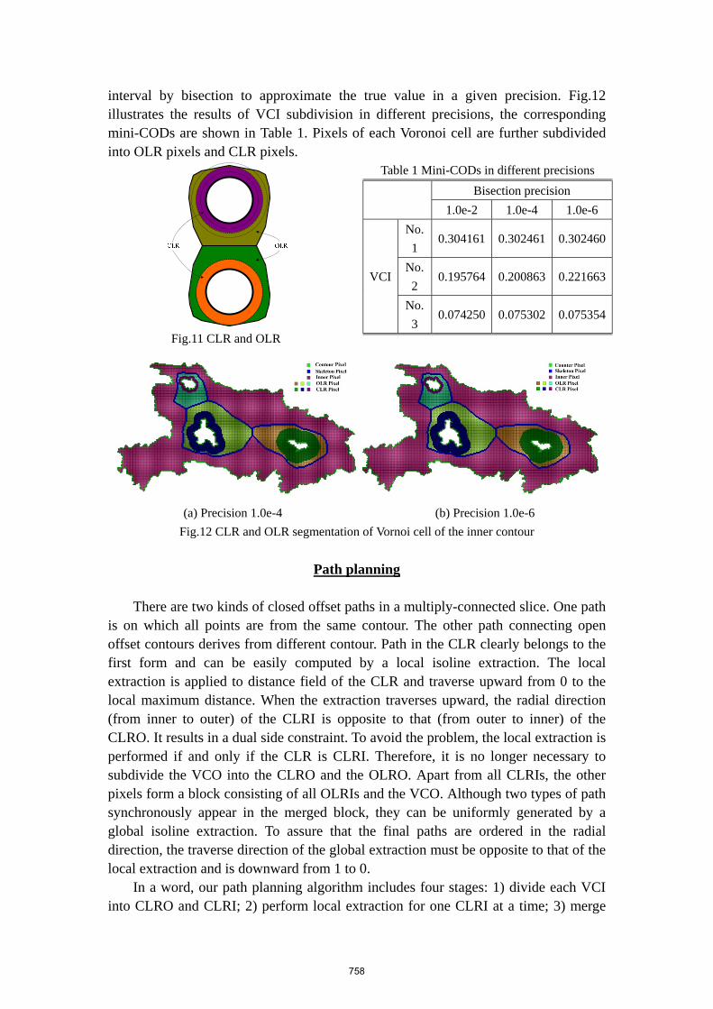
interval by bisection to approximate the true value in a given precision. Fig.12 illustrates the results of VCI subdivision in different precisions, the corresponding mini-CODs are shown in Table 1. Pixels of each Voronoi cell are further subdivided into OLR pixels and CLR pixels.
Fig.11 CLR and OLR
Table 1 Mini-CODs in different precisions
Bisection precision
1.0e-2 1.0e-4 1.0e-6
VCI
No.
1 0.304161 0.302461 0.302460
No.
2 0.195764 0.200863 0.221663
No.
3 0.074250 0.075302 0.075354
(a) Precision 1.0e-4 (b) Precision 1.0e-6
Fig.12 CLR and OLR segmentation of Vornoi cell of the inner contour
Path planning
There are two kinds of closed offset paths in a multiply-connected slice. One path
is on which all points are from the same contour. The other path connecting open offset contours derives from different contour. Path in the CLR clearly belongs to the first form and can be easily computed by a local isoline extraction. The local extraction is applied to distance field of the CLR and traverse upward from 0 to the local maximum distance. When the extraction traverses upward, the radial direction (from inner to outer) of the CLRI is opposite to that (from outer to inner) of the CLRO. It results in a dual side constraint. To avoid the problem, the local extraction is performed if and only if the CLR is CLRI. Therefore, it is no longer necessary to subdivide the VCO into the CLRO and the OLRO. Apart from all CLRIs, the other pixels form a block consisting of all OLRIs and the VCO. Although two types of path synchronously appear in the merged block, they can be uniformly generated by a global isoline extraction. To assure that the final paths are ordered in the radial direction, the traverse direction of the global extraction must be opposite to that of the local extraction and is downward from 1 to 0.
In a word, our path planning algorithm includes four stages: 1) divide each VCI into CLRO and CLRI; 2) perform local extraction for one CLRI at a time; 3) merge
758

all CLROs and VCO into a block; 4) perform global extraction for the merged block. In fact, the first and the second stages can be simultaneously performed. It is no need to exactly compute the mini-COD since equidistant offset is a discrete sampling process whose interval is the path space . The mini-COD is determined by the first open sampling path detection. Let be the detected distance, the mini-COD can be expressed as: (7)
Since the traverse direction of the CLRI is opposite to that of the merged block, there is still a dual side constraint. To overcome the problem, both the CLRI and the block must be relative to the same reference datum. Fig.14 (a) demonstrates the results of non-uniform datum application. The expected path space is 5mm, but the transition space between two kinds of paths is distinctly more than 5mm. In a normalized distance field, there are two alternative reference datums: 0 representing boundary constraint and 1 representing center constraint.
As shown in Fig.13(a), no closed path appears in the OLRI. Let and denote the distance between the skeleton and the maximum path in the CLRI and the merged block, respectively. The transition space can be written as . Although both and are related to , it is difficult to adapt the transition space to the path space. In this case, boundary constraint will result in a non-uniform transition as well. However, when closed path appears in the OLRI (Fig.13(b)), the transition space must be and non-uniform transition will disappear. Whether or not path appears in the OLRI can be determinated by the inequality: (8) where denotes the skeleton distance. There are three alternative distances in the skeleton pixels: maximum, minimum and mean. With statistical consideration, the mean distance is chosen:
∑ (9)
If inequality (8) is true, closed path will appear in the OLRI; otherwise, there will be no path. In comparison with center constraint, the gap between the original contour and offset contour can be effectively managed by using boundary constraint. Therefore, the reference datum is determined by: 1) if inequality (8) is true, boundary constraint is adopted; 2) if inequality(8) is false, center constraint is adopted. For boundary constraint, the local extraction starts from /2 and increases by , the global extraction starts from and decreases by . For center constraint, the global extraction starts from 1 /2 and decreases by ; the local extraction starts from and increases by . and are initialize by:
(10)
1 (11)
where denotes rounding off operation. Fig.14 illustrates the results of different reference datums. It is obvious that boundary constraint is better than center constraint in the gap management. The
759
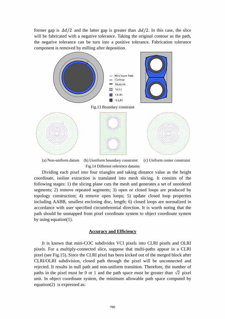
former gap is /2 and the latter gap is greater than /2. In this case, the slice will be fabricated with a negative tolerance. Taking the original contour as the path, the negative tolerance can be turn into a positive tolerance. Fabrication tolerance component is removed by milling after deposition.
δε
Fig.13 Boundary constraint
(a) Non-uniform datum (b) Uuniform boundary constraint (c) Uniform center constraint
Fig.14 Different reference datums
Dividing each pixel into four triangles and taking distance value as the height coordinate, isoline extraction is translated into mesh slicing. It consists of the following stages: 1) the slicing plane cuts the mesh and generates a set of unordered segments; 2) remove repeated segments; 3) open or closed loops are produced by topology construction; 4) remove open loops; 5) update closed loop properties including AABB, smallest enclosing disc, length; 6) closed loops are normalized in accordance with user specified circumferential direction. It is worth noting that the path should be unmapped from pixel coordinate system to object coordinate system by using equation(1).
Accuracy and Efficiency
It is known that mini-COC subdivides VCI pixels into CLRI pixels and OLRI pixels. For a multiply-connected slice, suppose that multi-paths appear in a CLRI pixel (see Fig.15). Since the CLRI pixel has been kicked out of the merged block after CLRI/OLRI subdivision, closed path through the pixel will be unconnected and rejected. It results in null path and non-uniform transition. Therefore, the number of paths in the pixel must be 0 or 1 and the path space must be greater than √2 pixel unit. In object coordinate system, the minimum allowable path space computed by equation(2) is expressed as:
760

Δd √2/rs (12)
Fig.15 Multi-paths through the CLRI pixel
As shown in Fig.16, the time is absolute in the first figure and is relative in the latter three figures. The relative time is the difference between absolute time in the actual case and in the case of no hole. Test hardware environment is: Intel® Core™2 Quad Q9500 2.83GHz CPU and 3.00 GB RAM. The computation time is in direct proportion to the resolution and the reciprocal of the path space. The influence of the number of the inner contours (holes) on the efficiency is also studied. Although the number of total pixels decreases with the increase of holes, the efficiency may reduce since it takes more time to perform VCI and CLRI/OLRI subdivision.
Tim
e (m
s)
128 256 384 512 640 768 896
0
100
200
300
400
500
600
700
800
Path space 0.10
Resolution
one hole two holes three holes
128 256 384 512 640 768 896
0
100
200
300
400
500
600
700
800
Path space 0.05
Resolution
one hole two holes three holes
Fig.16 Efficiency analysis for path planning
Examples
761

As shown in Fig.17, the grid is divided into three VCIs corresponding to their three inner contours in the above figure. The differences between min-COD and mean skeleton values: are 0.205073, 0.33460 and 0.232557 for three VCIs, respectively. The actual path space is 0.041527 and less than the previous three differences. So the inequality (8) is true and boundary constraint is applied. Each VCI is subdivided into CLRI and OLRI. The number of paths in the CLRI is determinated by ⁄ 0.5, so there are 7, 5 and 2 paths in the three CLRIs, respectively. There is the same analysis in the below figure. Two paths show that boundary constraint is capable to manage the gap and lead to fabricating in positive tolerance.
Fig.18 illustrates another important application of the proposed algorithm. It is used for FGM design and fabrication. The different colors represent the different volume percentages of two constituent materials. There is just one VCI corresponding to the inner contour. The difference is 0.020087 and less than the path space 0.086353, so the inequality (8) is false and center constraint is applied. The gap distinctly is greater than path space, so the original contour should be taken as the path for positive tolerance fabrication.
Fig.17 Parallel contour path for multiply-connected slice
Conclusion
An algorithm based on discrete Voronoi diagram and distance map for parallel contour path planning is introduced in this article. Its computation time is in direct proportion to the resolution and the reciprocal of the path space. The number of inner
762

contours has influence on the efficiency as well. Compared with pair-wise intersection and Voronoi diagram, it is numerically robust, avoids null path and self-intersection because of the application of distance map and discrete Voronoi diagram.
Without post-processes, hierarchical rasterization directly generate three types of pixel: inner, outer and boundary. The boundary pixel inherits boundary properties including ID and material from the original slice. It is especially used for multiply-connected and FGM slice. Rasterization using graphics hardware acceleration has high efficiency. Triangulation is the better strategy for interior rasterization of concave slice than sweep line. When the resolution is divisible by 64 and float data type is adopted, rasterization will be faster.
Contour property of the inner pixel is determined by that of the nearest boundary pixel. According to the contour property, a grid is easily divided into VCIs. Each VCI is subdivided into CLRI and OLRI in response to the actual path space. To eliminate non-uniform transition from paths in the CLRI to the merged block, uniform reference datum has been built. If no path appears in the OLRI, center constraint is applied; otherwise boundary constraint is adopted. Boundary constraint has better gap management than center constraint. To avoid null path in the transition area, the path space must be greater and equal than √2 pixel unit.
Fig.18 Parallel contour path for FGM slice
763

Acknowledgement
We gratefully acknowledgement the support of the National Natural Science Foua
tion of China (51175203) and National Aerospace Science Foundation of China (2011ZE79002).
References
1. Print Me a Stradivarius, The Economist, Feb. 10, 2011. 2. Atwood, C., Ensz, M., Greene, D., Griffith, M., et al. (1998). Laser engineered
net shaping (LENS (TM)): A tool for direct fabrication of metal parts (No. SAND98-2473C). Sandia National Laboratories, Albuquerque, NM, and Livermore, CA.
3. Simchi A, Petzoldt F, Pohl H. (2003). On the development of direct metal laser sintering for rapid tooling. Journal of Materials Processing Technology, 141(3), pp. 319-328.
4. Kruth J P, Froyen L, Van Vaerenbergh J, et al. (2004). Selective laser melting of iron-based powder. Journal of Materials Processing Technology, 149(1), pp. 616-622.
5. Lewis G K, Schlienger E. (2000). Practical considerations and capabilities for laser assisted direct metal deposition. Materials & Design, 2000, 21(4), pp. 417-423.
6. Mazumder J, Dutta D, Kikuchi N, et al. (2000). Closed loop direct metal deposition: art to part[J]. Optics and Lasers in Engineering, 34(4), pp. 397-414.
7. Parthasarathy J, Starly B, Raman S, et al. (2010). Mechanical evaluation of porous titanium (Ti6Al4V) structures with electron beam melting (EBM). Journal of the mechanical behavior of biomedical materials, 3(3), pp. 249-259.
8. Dollar A M, Howe R D. (2010). The highly adaptive SDM hand: Design and performance evaluation. The international journal of robotics research, 29(5), pp. 585-597.
9. Baufeld B, Biest O V, Gault R. (2010). Additive manufacturing of Ti–6Al–4V components by shaped metal deposition: Microstructure and mechanical properties. Materials & Design, 31, pp. S106-S111.
10. Zhang H, Xu J, Wang G. Fundamental study on plasma deposition manufacturing. (2002). Surface and Coatings Technology, 171(1), pp. 112-118.
11. Xinhong X, Haiou Z, Guilan W, et al. Hybrid plasma deposition and milling for an aeroengine double helix integral impeller made of superalloy. (2010). Robotics and Computer-Integrated Manufacturing, 26(4), pp. 291-295.
12. Xiong X, Zhang H, Wang G. Metal direct prototyping by using hybrid plasma deposition and milling. (2009). Journal of Materials Processing Technology, 209(1), pp.124-130.
13. K. Dai, L. Shaw. Distortion minimization of laser-processed components through control of laser scanning patterns. Rapid Prototyping Journal, 2002, 8(5),
764

pp.270-276. 14. X.Y. Tian, Bo Sun, J.G. Heinrich, et al. (2013). Scan pattern, stress and mechnical
strength of laser directly sintered ceramics. The International Journal of Advanced Manufacturing Technology,, 64(1-4), pp. 239-246
15. Jun Yu, Xin Lin, Liang Ma, et al. (2011). Influence of laser deposition patterns on part distortion, interior quality and mechanical properties by laser solid forming (LSF). Materials Science and Engineering A, 528(3), pp.1094-1104.
16. Munguía J, de Ciurana J, Riba C. (2008). Pursuing successful rapid manufacturing: a users' best-practices approach. Rapid Prototyping Journal, 14(3), pp. 173-179.
17. Hansen A, Arbab F. (1992). An algorithm for generating NC tool paths for arbitrarily shaped pockets with islands. ACM Transactions on Graphics (TOG), 11(2), pp.152-182.
18. Choi B K, Park S C. (1999). A pair-wise offset algorithm for 2D point-sequence curve. Computer-Aided Design, 31(12), pp. 735-745.
19. Sugihara, K. (1992). Voronoi diagrams in a river. International Journal of Computational Geometry & Applications, 2(01), pp.29-48.
20. Fortune S. A sweepline algorithm for Voronoi diagrams. (1987). Algorithmica, 2(1-4), pp.153-174.
21. Okabe A, Boots B, Sugihara K, et al. (2009). Spatial tessellations: concepts and applications of Voronoi diagrams. Wiley. com
22. Sugihara K, Iri M. (1992). Construction of the Voronoi diagram forone million'generators in single-precision arithmetic. Proceedings of the IEEE, 80(9), pp. 1471-1484.
23. Aggarwal A, Guibas L J, Saxe J, et al (1989). A linear-time algorithm for computing the Voronoi diagram of a convex polygon. Discrete & Computational Geometry, 4(1), pp. 591-604.
24. Srinivasan V, Nackman L R. (1987). Voronoi diagram for multiply-connected polygonal domains I: Algorithm. IBM Journal of Research and Development, 31(3), pp. 361-372.
25. Held M. (1998). Voronoi diagrams and offset curves of curvilinear polygons. Computer-Aided Design, 30(4), pp. 287-300.
26. De Berg M, Cheong O, Van Kreveld M. (2008). Computational geometry: algorithms and applications. Springer.
27. Saito T, Toriwaki J I. (1994). New algorithms for euclidean distance transformation of an n-dimensional digitized picture with applications. Pattern recognition, 27(11), pp.1551-1565.
28. Meijster A, Roerdink J B T M, Hesselink W H. (2002). A general algorithm for computing distance transforms in linear time. Mathematical Morphology and its applications to image and signal processing. Springer US, pp.331-340.
29. Wang, J., & Tan, Y. (2011, June). Efficient Euclidean distance transform using perpendicular bisector segmentation. In Computer Vision and Pattern Recognition (CVPR), 2011 IEEE Conference on (pp. 1625-1632). IEEE.
765