parallel gröbner basis algorithms over finite fieldsederc/download/3cing.pdf · parallel gröbner...
TRANSCRIPT
Parallel Gröbner Basis Algorithms over Finite Fields
Christian Eder and Jean-Charles Faugère
University of Kaiserslautern
October 14, 2016
1 / 50
Table of Contents
1. Gröbner Bases and Buchberger’s Algorithm
2. Faugère’s F4 Algorithm
3. Specialized Linear Algebra for Gröbner Basis Computation
4. GBLA – A Gröbner Basis Linear Algebra Library
5. GB – A Gröbner Basis Library
6. Some benchmarks
7. Outlook
2 / 50

Buchberger’s criterion
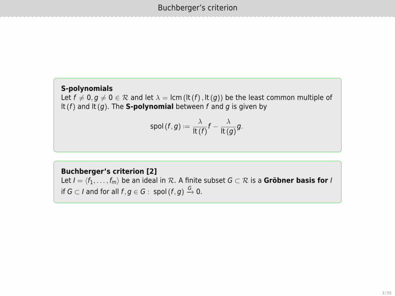
S-polynomialsLet f ̸= 0,g ̸= 0 ∈ R and let λ = lcm (lt (f) , lt (g)) be the least common multiple oflt (f) and lt (g). The S-polynomial between f and g is given by
spol (f ,g) ..=λ
lt (f) f −λ
lt (g)g.
Buchberger’s criterion [2]Let I = ⟨f1, . . . , fm⟩ be an ideal in R. A finite subset G ⊂ R is a Gröbner basis for Iif G ⊂ I and for all f ,g ∈ G : spol (f ,g) G−→ 0.
3 / 50
Buchberger’s criterion
S-polynomialsLet f ̸= 0,g ̸= 0 ∈ R and let λ = lcm (lt (f) , lt (g)) be the least common multiple oflt (f) and lt (g). The S-polynomial between f and g is given by
spol (f ,g) ..=λ
lt (f) f −λ
lt (g)g.
Buchberger’s criterion [2]Let I = ⟨f1, . . . , fm⟩ be an ideal in R. A finite subset G ⊂ R is a Gröbner basis for Iif G ⊂ I and for all f ,g ∈ G : spol (f ,g) G−→ 0.
3 / 50

Buchberger’s algorithm
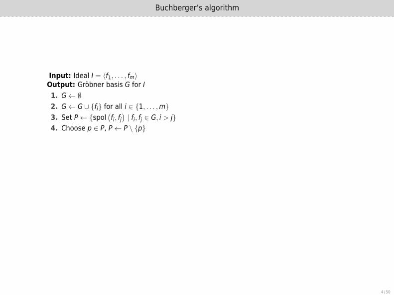
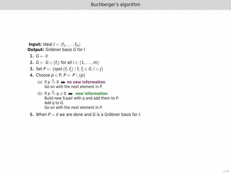
Input: Ideal I = ⟨f1, . . . , fm⟩Output: Gröbner basis G for I1. G← ∅2. G← G ∪ {fi} for all i ∈ {1, . . . ,m}3. Set P← {spol
(fi, fj
)| fi, fj ∈ G, i > j}
4. Choose p ∈ P, P← P \ {p}(a) If p G−→ 0 ▶▶ no new information
Go on with the next element in P.(b) If p G−→ q ̸= 0 ▶▶ new information
Build new S-pair with q and add them to P.Add q to G.Go on with the next element in P.
5. When P = ∅ we are done and G is a Gröbner basis for I.
4 / 50
Buchberger’s algorithm
Input: Ideal I = ⟨f1, . . . , fm⟩Output: Gröbner basis G for I1. G← ∅2. G← G ∪ {fi} for all i ∈ {1, . . . ,m}3. Set P← {spol
(fi, fj
)| fi, fj ∈ G, i > j}
4. Choose p ∈ P, P← P \ {p}
(a) If p G−→ 0 ▶▶ no new informationGo on with the next element in P.
(b) If p G−→ q ̸= 0 ▶▶ new informationBuild new S-pair with q and add them to P.Add q to G.Go on with the next element in P.
5. When P = ∅ we are done and G is a Gröbner basis for I.
4 / 50
Buchberger’s algorithm
Input: Ideal I = ⟨f1, . . . , fm⟩Output: Gröbner basis G for I1. G← ∅2. G← G ∪ {fi} for all i ∈ {1, . . . ,m}3. Set P← {spol
(fi, fj
)| fi, fj ∈ G, i > j}
4. Choose p ∈ P, P← P \ {p}(a) If p G−→ 0 ▶▶ no new information
Go on with the next element in P.(b) If p G−→ q ̸= 0 ▶▶ new information
Build new S-pair with q and add them to P.Add q to G.Go on with the next element in P.
5. When P = ∅ we are done and G is a Gröbner basis for I.
4 / 50
Faugère’s F4 algorithm

Faugère’s F4 algorithm
Input: Ideal I = ⟨f1, . . . , fm⟩Output: Gröbner basis G for I1. G← ∅2. G← G ∪ {fi} for all i ∈ {1, . . . ,m}3. Set P← {(af ,bg) | f ,g ∈ G}4. d← 05. while P ̸= ∅:
(a) d← d+ 1(b) Pd ← Select (P), P← P \ Pd(c) Ld ← {af ,bg | (af ,bg) ∈ Pd}(d) Ld ← Symbolic Preprocessing(Ld,G)(e) Fd ← Reduction(Ld,G)(f) for h ∈ Fd:
▶ If lt (h) /∈ L(G) (all other h are “useless”):▷ P← P ∪ {new pairs with h}▷ G← G ∪ {h}
6. Return G
6 / 50

Differences to Buchberger
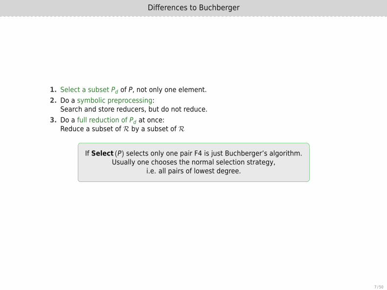
1. Select a subset Pd of P, not only one element.2. Do a symbolic preprocessing:
Search and store reducers, but do not reduce.3. Do a full reduction of Pd at once:
Reduce a subset of R by a subset of R
If Select (P) selects only one pair F4 is just Buchberger’s algorithm.Usually one chooses the normal selection strategy,
i.e. all pairs of lowest degree.
7 / 50
Differences to Buchberger
1. Select a subset Pd of P, not only one element.2. Do a symbolic preprocessing:
Search and store reducers, but do not reduce.3. Do a full reduction of Pd at once:
Reduce a subset of R by a subset of R
If Select (P) selects only one pair F4 is just Buchberger’s algorithm.Usually one chooses the normal selection strategy,
i.e. all pairs of lowest degree.
7 / 50

Symbolic preprocessing
Input: L,G finite subsets of ROutput: a finite subset of R1. F← L2. D← L(F) (S-pairs already reduce lead terms)3. while T(F) ̸= D:
(a) Choose m ∈ T(F) \ D, D← D ∪ {m}.(b) If m ∈ L(G) ⇒ ∃ g ∈ G and λ ∈ R such that λ lt (g) = m
▷ F← F ∪ {λg}
4. Return F
We optimize this soon!
8 / 50
Reduction
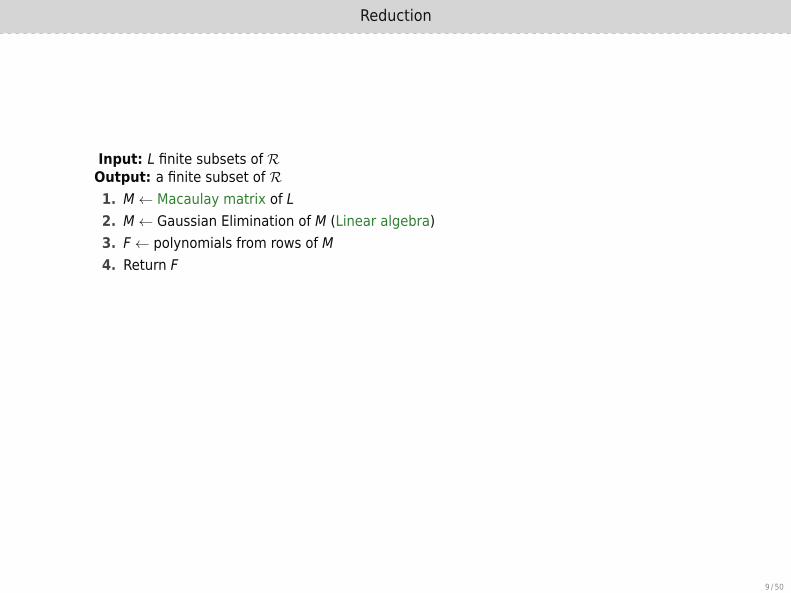
Input: L finite subsets of ROutput: a finite subset of R1. M← Macaulay matrix of L2. M← Gaussian Elimination of M (Linear algebra)3. F← polynomials from rows of M4. Return F
Macaulay matrix: columns =̂ monomials (sorted by monomial order <)rows =̂ coefficients of polynomials in L
9 / 50

Reduction
Input: L finite subsets of ROutput: a finite subset of R1. M← Macaulay matrix of L2. M← Gaussian Elimination of M (Linear algebra)3. F← polynomials from rows of M4. Return F
Macaulay matrix: columns =̂ monomials (sorted by monomial order <)rows =̂ coefficients of polynomials in L
9 / 50
Example: Cyclic-4
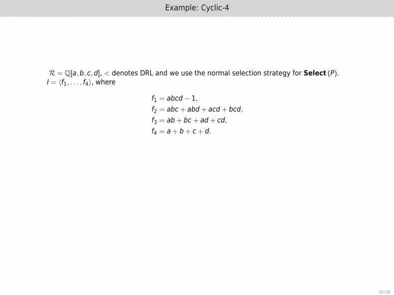
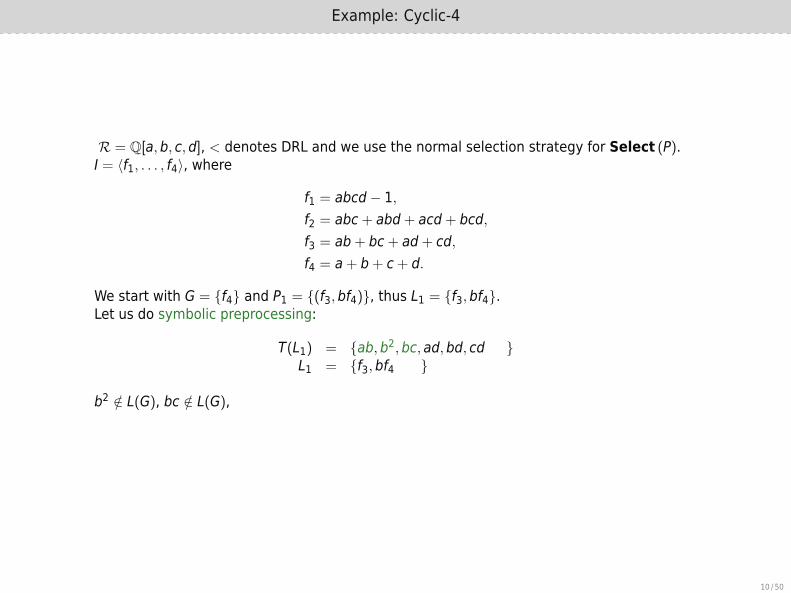
R = Q[a,b, c,d], < denotes DRL and we use the normal selection strategy for Select (P).I = ⟨f1, . . . , f4⟩, where
f1 = abcd− 1,f2 = abc+ abd+ acd+ bcd,f3 = ab+ bc+ ad+ cd,f4 = a+ b+ c+ d.
We start with G = {f4} and P1 = {(f3,bf4)}, thus L1 = {f3,bf4}.Let us do symbolic preprocessing:
T(L1) = {ab,b2,bc, ad,bd, cd
,d2
}L1 = {f3,bf4
,df4
}
b2 /∈ L(G), bc /∈ L(G), d lt (f4) = ad, all others also /∈ L(G),
10 / 50
Example: Cyclic-4
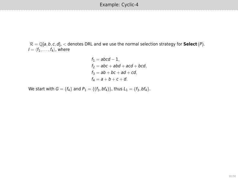
R = Q[a,b, c,d], < denotes DRL and we use the normal selection strategy for Select (P).I = ⟨f1, . . . , f4⟩, where
f1 = abcd− 1,f2 = abc+ abd+ acd+ bcd,f3 = ab+ bc+ ad+ cd,f4 = a+ b+ c+ d.
We start with G = {f4} and P1 = {(f3,bf4)}, thus L1 = {f3,bf4}.
Let us do symbolic preprocessing:
T(L1) = {ab,b2,bc, ad,bd, cd
,d2
}L1 = {f3,bf4
,df4
}
b2 /∈ L(G), bc /∈ L(G), d lt (f4) = ad, all others also /∈ L(G),
10 / 50
Example: Cyclic-4
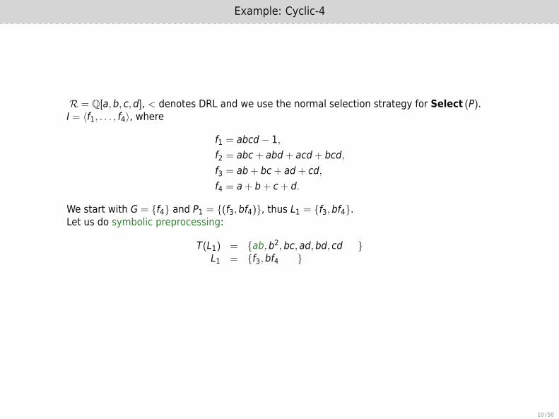
R = Q[a,b, c,d], < denotes DRL and we use the normal selection strategy for Select (P).I = ⟨f1, . . . , f4⟩, where
f1 = abcd− 1,f2 = abc+ abd+ acd+ bcd,f3 = ab+ bc+ ad+ cd,f4 = a+ b+ c+ d.
We start with G = {f4} and P1 = {(f3,bf4)}, thus L1 = {f3,bf4}.Let us do symbolic preprocessing:
T(L1) = {ab,b2,bc, ad,bd, cd
,d2
}L1 = {f3,bf4
,df4
}
b2 /∈ L(G), bc /∈ L(G), d lt (f4) = ad, all others also /∈ L(G),
10 / 50
Example: Cyclic-4
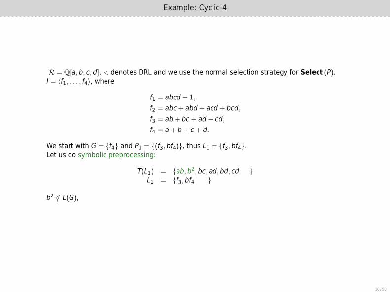
R = Q[a,b, c,d], < denotes DRL and we use the normal selection strategy for Select (P).I = ⟨f1, . . . , f4⟩, where
f1 = abcd− 1,f2 = abc+ abd+ acd+ bcd,f3 = ab+ bc+ ad+ cd,f4 = a+ b+ c+ d.
We start with G = {f4} and P1 = {(f3,bf4)}, thus L1 = {f3,bf4}.Let us do symbolic preprocessing:
T(L1) = {ab,b2,bc, ad,bd, cd
,d2
}L1 = {f3,bf4
,df4
}
b2 /∈ L(G),
bc /∈ L(G), d lt (f4) = ad, all others also /∈ L(G),
10 / 50
Example: Cyclic-4
R = Q[a,b, c,d], < denotes DRL and we use the normal selection strategy for Select (P).I = ⟨f1, . . . , f4⟩, where
f1 = abcd− 1,f2 = abc+ abd+ acd+ bcd,f3 = ab+ bc+ ad+ cd,f4 = a+ b+ c+ d.
We start with G = {f4} and P1 = {(f3,bf4)}, thus L1 = {f3,bf4}.Let us do symbolic preprocessing:
T(L1) = {ab,b2,bc, ad,bd, cd
,d2
}L1 = {f3,bf4
,df4
}
b2 /∈ L(G), bc /∈ L(G),
d lt (f4) = ad, all others also /∈ L(G),
10 / 50

Example: Cyclic-4
R = Q[a,b, c,d], < denotes DRL and we use the normal selection strategy for Select (P).I = ⟨f1, . . . , f4⟩, where
f1 = abcd− 1,f2 = abc+ abd+ acd+ bcd,f3 = ab+ bc+ ad+ cd,f4 = a+ b+ c+ d.
We start with G = {f4} and P1 = {(f3,bf4)}, thus L1 = {f3,bf4}.Let us do symbolic preprocessing:
T(L1) = {ab,b2,bc, ad,bd, cd,d2}L1 = {f3,bf4,df4}
b2 /∈ L(G), bc /∈ L(G), d lt (f4) = ad,
all others also /∈ L(G),
10 / 50

Example: Cyclic-4
R = Q[a,b, c,d], < denotes DRL and we use the normal selection strategy for Select (P).I = ⟨f1, . . . , f4⟩, where
f1 = abcd− 1,f2 = abc+ abd+ acd+ bcd,f3 = ab+ bc+ ad+ cd,f4 = a+ b+ c+ d.
We start with G = {f4} and P1 = {(f3,bf4)}, thus L1 = {f3,bf4}.Let us do symbolic preprocessing:
T(L1) = {ab,b2,bc, ad,bd, cd,d2}L1 = {f3,bf4,df4}
b2 /∈ L(G), bc /∈ L(G), d lt (f4) = ad, all others also /∈ L(G),
10 / 50

Example: Cyclic-4
Now reduction:Convert polynomial data L1 to Macaulay Matrix M1
0 0 0 1 1 1 1
1 0 1 1 0 1 0
1 1 1 0 1 0 0
ab b2 bc ad bd cd d2
df4f3
bf4
Gaussian Elimination of M1:
0 0 0 1 1 1 1
1 0 1 0 −1 0 −1
0 1 0 0 2 0 1
ab b2 bc ad bd cd d2
df4f3
bf4
11 / 50

Example: Cyclic-4
Now reduction:Convert polynomial data L1 to Macaulay Matrix M1
0 0 0 1 1 1 1
1 0 1 1 0 1 0
1 1 1 0 1 0 0
ab b2 bc ad bd cd d2
df4f3
bf4
Gaussian Elimination of M1:
0 0 0 1 1 1 1
1 0 1 0 −1 0 −1
0 1 0 0 2 0 1
ab b2 bc ad bd cd d2
df4f3
bf4
11 / 50

Example: Cyclic-4
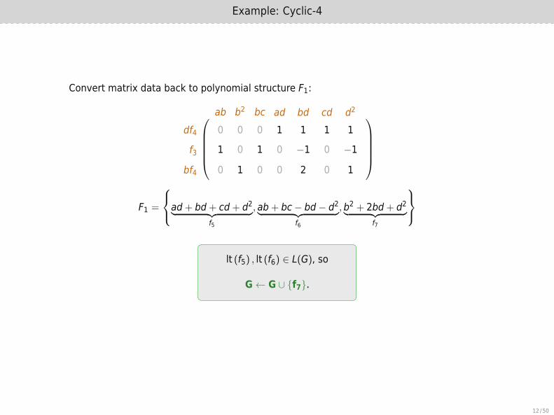
Convert matrix data back to polynomial structure F1:
0 0 0 1 1 1 1
1 0 1 0 −1 0 −1
0 1 0 0 2 0 1
ab b2 bc ad bd cd d2
df4f3
bf4
F1 =
ad+ bd+ cd+ d2︸ ︷︷ ︸f5
, ab+ bc− bd− d2︸ ︷︷ ︸f6
,b2 + 2bd+ d2︸ ︷︷ ︸f7
lt (f5) , lt (f6) ∈ L(G), so
G← G ∪ {f7}.
12 / 50
Example: Cyclic-4
Convert matrix data back to polynomial structure F1:
0 0 0 1 1 1 1
1 0 1 0 −1 0 −1
0 1 0 0 2 0 1
ab b2 bc ad bd cd d2
df4f3
bf4
F1 =
ad+ bd+ cd+ d2︸ ︷︷ ︸f5
, ab+ bc− bd− d2︸ ︷︷ ︸f6
,b2 + 2bd+ d2︸ ︷︷ ︸f7
lt (f5) , lt (f6) ∈ L(G), so
G← G ∪ {f7}.
12 / 50
Example: Cyclic-4
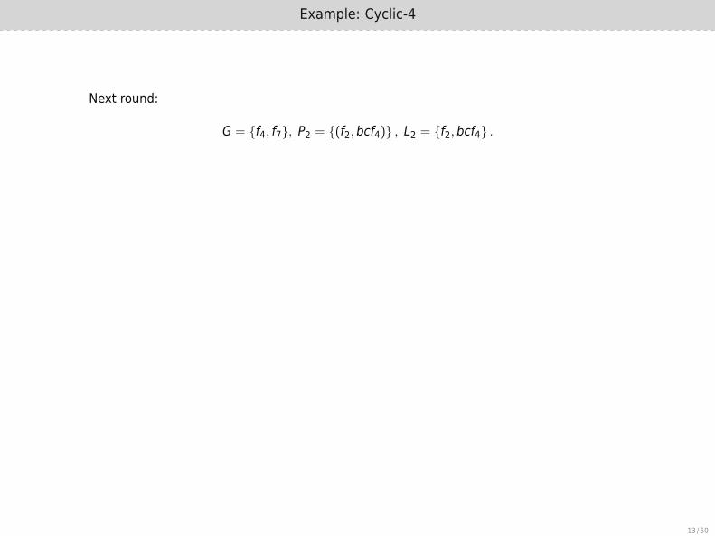
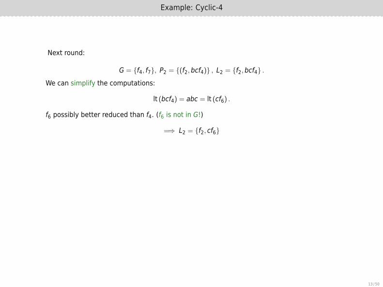
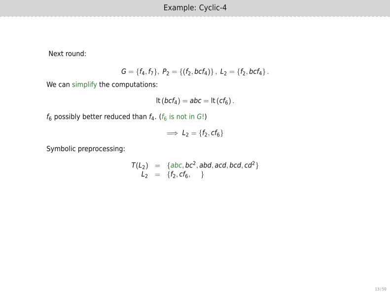
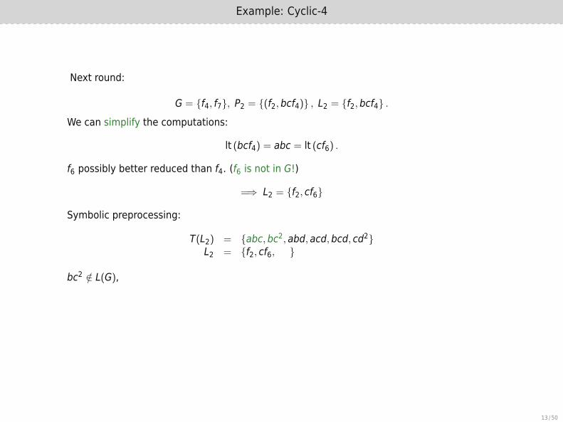
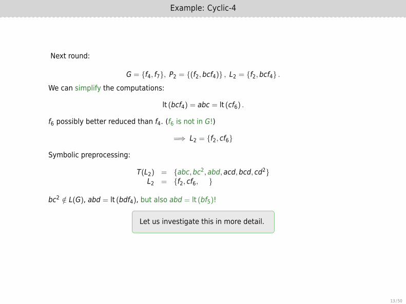
Next round:
G = {f4, f7}, P2 = {(f2,bcf4)} , L2 = {f2,bcf4} .
We can simplify the computations:
lt (bcf4) = abc = lt (cf6) .
f6 possibly better reduced than f4. (f6 is not in G!)
=⇒ L2 = {f2, cf6}
Symbolic preprocessing:
T(L2) = {abc,bc2, abd, acd,bcd, cd2}L2 = {f2, cf6, }
bc2 /∈ L(G), abd = lt (bdf4), but also abd = lt (bf5)!
Let us investigate this in more detail.
13 / 50
Example: Cyclic-4
Next round:
G = {f4, f7}, P2 = {(f2,bcf4)} , L2 = {f2,bcf4} .
We can simplify the computations:
lt (bcf4) = abc = lt (cf6) .
f6 possibly better reduced than f4. (f6 is not in G!)
=⇒ L2 = {f2, cf6}
Symbolic preprocessing:
T(L2) = {abc,bc2, abd, acd,bcd, cd2}L2 = {f2, cf6, }
bc2 /∈ L(G),
abd = lt (bdf4), but also abd = lt (bf5)!
Let us investigate this in more detail.
13 / 50

Example: Cyclic-4
Next round:
G = {f4, f7}, P2 = {(f2,bcf4)} , L2 = {f2,bcf4} .
We can simplify the computations:
lt (bcf4) = abc = lt (cf6) .
f6 possibly better reduced than f4. (f6 is not in G!)
=⇒ L2 = {f2, cf6}
Symbolic preprocessing:
T(L2) = {abc,bc2, abd, acd,bcd, cd2}L2 = {f2, cf6, }
bc2 /∈ L(G), abd = lt (bdf4), but also abd = lt (bf5)!
Let us investigate this in more detail.
13 / 50
Example: Cyclic-4
Next round:
G = {f4, f7}, P2 = {(f2,bcf4)} , L2 = {f2,bcf4} .
We can simplify the computations:
lt (bcf4) = abc = lt (cf6) .
f6 possibly better reduced than f4. (f6 is not in G!)
=⇒ L2 = {f2, cf6}
Symbolic preprocessing:
T(L2) = {abc,bc2, abd, acd,bcd, cd2}L2 = {f2, cf6, }
bc2 /∈ L(G), abd = lt (bdf4), but also abd = lt (bf5)!
Let us investigate this in more detail.
13 / 50

Interlude – Simplify
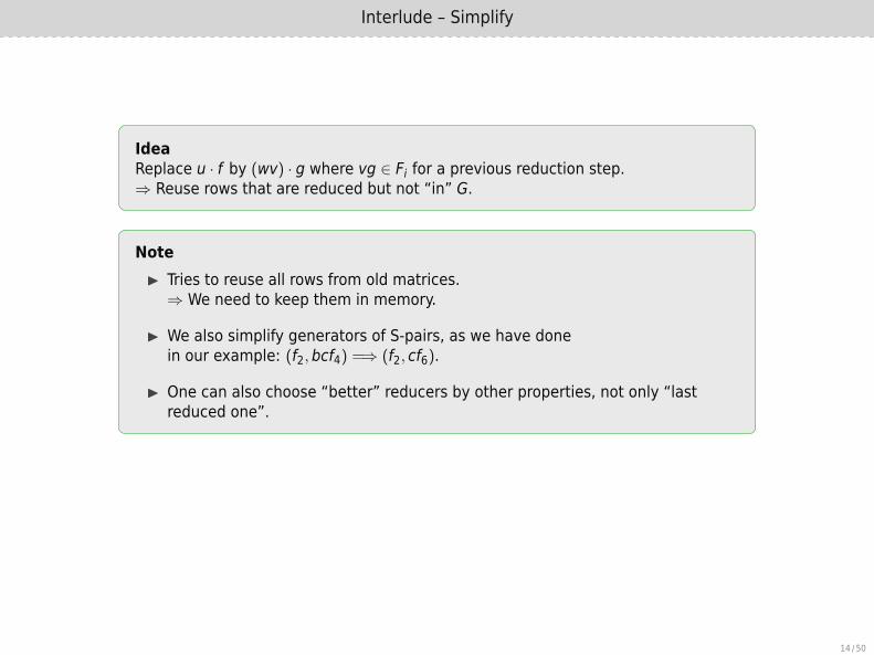
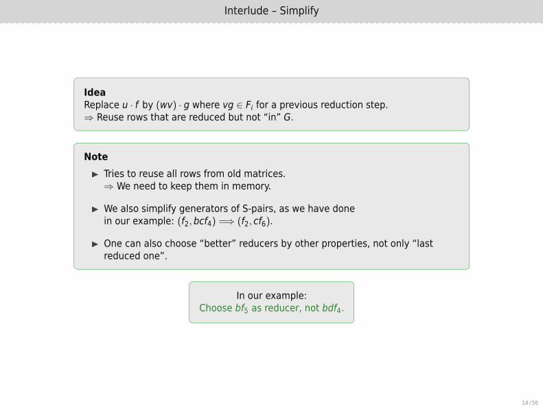
IdeaReplace u · f by (wv) · g where vg ∈ Fi for a previous reduction step.⇒ Reuse rows that are reduced but not “in” G.
Note▶ Tries to reuse all rows from old matrices.⇒ We need to keep them in memory.
▶ We also simplify generators of S-pairs, as we have donein our example: (f2,bcf4) =⇒ (f2, cf6).
▶ One can also choose “better” reducers by other properties, not only “lastreduced one”.
In our example:Choose bf5 as reducer, not bdf4.
14 / 50
Interlude – Simplify
IdeaReplace u · f by (wv) · g where vg ∈ Fi for a previous reduction step.⇒ Reuse rows that are reduced but not “in” G.
Note▶ Tries to reuse all rows from old matrices.⇒ We need to keep them in memory.
▶ We also simplify generators of S-pairs, as we have donein our example: (f2,bcf4) =⇒ (f2, cf6).
▶ One can also choose “better” reducers by other properties, not only “lastreduced one”.
In our example:Choose bf5 as reducer, not bdf4.
14 / 50
Example: Cyclic-4
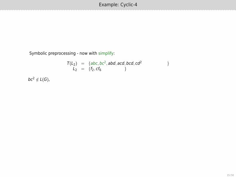
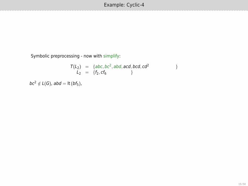
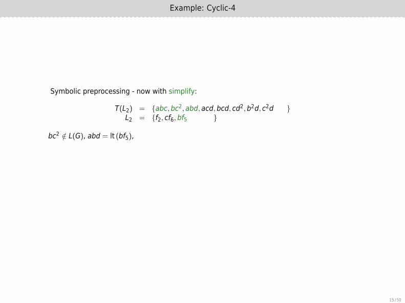
Symbolic preprocessing - now with simplify:
T(L2) = {abc,bc2, abd, acd,bcd, cd2
,b2d, c2d, . . .
}L2 = {f2, cf6
,bf5, cf5,df7
}
bc2 /∈ L(G),
abd = lt (bf5), and so on.
Now try to exploit the special structure of the Macaulay matrices.
15 / 50
Example: Cyclic-4
Symbolic preprocessing - now with simplify:
T(L2) = {abc,bc2, abd, acd,bcd, cd2
,b2d, c2d, . . .
}L2 = {f2, cf6
,bf5, cf5,df7
}
bc2 /∈ L(G), abd = lt (bf5),
and so on.
Now try to exploit the special structure of the Macaulay matrices.
15 / 50
Example: Cyclic-4
Symbolic preprocessing - now with simplify:
T(L2) = {abc,bc2, abd, acd,bcd, cd2,b2d, c2d
, . . .
}L2 = {f2, cf6,bf5
, cf5,df7
}
bc2 /∈ L(G), abd = lt (bf5),
and so on.
Now try to exploit the special structure of the Macaulay matrices.
15 / 50

Example: Cyclic-4
Symbolic preprocessing - now with simplify:
T(L2) = {abc,bc2, abd, acd,bcd, cd2,b2d, c2d, . . . }L2 = {f2, cf6,bf5, cf5,df7}
bc2 /∈ L(G), abd = lt (bf5), and so on.
Now try to exploit the special structure of the Macaulay matrices.
15 / 50

Example: Cyclic-4
Symbolic preprocessing - now with simplify:
T(L2) = {abc,bc2, abd, acd,bcd, cd2,b2d, c2d, . . . }L2 = {f2, cf6,bf5, cf5,df7}
bc2 /∈ L(G), abd = lt (bf5), and so on.
Now try to exploit the special structure of the Macaulay matrices.
15 / 50

Specialized Linear Algebra for Gröbner Basis Computation
Idea by Faugère & Lachartre
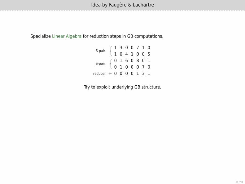
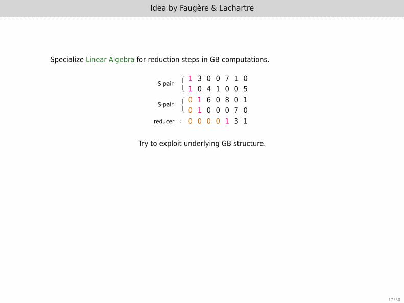
Specialize Linear Algebra for reduction steps in GB computations.
1 3 0 0 7 1 01 0 4 1 0 0 50 1 6 0 8 0 10 1 0 0 0 7 00 0 0 0 1 3 1
S-pair
S-pair
reducer
Try to exploit underlying GB structure.
Main ideaDo a static reordering before the Gaussian Elimination to achieve
a better initial shape. Invert the reordering afterwards.
17 / 50

Idea by Faugère & Lachartre
Specialize Linear Algebra for reduction steps in GB computations.
1 3 0 0 7 1 01 0 4 1 0 0 50 1 6 0 8 0 10 1 0 0 0 7 00 0 0 0 1 3 1
S-pair
S-pair
reducer
Try to exploit underlying GB structure.
Main ideaDo a static reordering before the Gaussian Elimination to achieve
a better initial shape. Invert the reordering afterwards.
17 / 50

Idea by Faugère & Lachartre
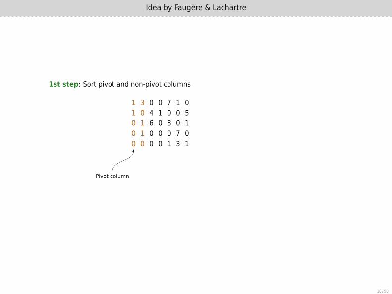
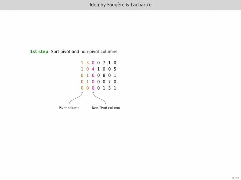
1st step: Sort pivot and non-pivot columns
1 3 0 0 7 1 01 0 4 1 0 0 50 1 6 0 8 0 10 1 0 0 0 7 00 0 0 0 1 3 1
Pivot column Non-Pivot column
1 3 7 0 0 1 01 0 0 4 1 0 50 1 8 6 0 0 90 1 0 0 0 7 00 0 1 0 0 3 1
18 / 50

Idea by Faugère & Lachartre
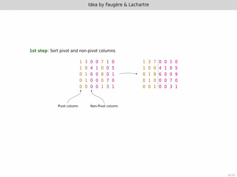
1st step: Sort pivot and non-pivot columns
1 3 0 0 7 1 01 0 4 1 0 0 50 1 6 0 8 0 10 1 0 0 0 7 00 0 0 0 1 3 1
Pivot column
Non-Pivot column
1 3 7 0 0 1 01 0 0 4 1 0 50 1 8 6 0 0 90 1 0 0 0 7 00 0 1 0 0 3 1
18 / 50
Idea by Faugère & Lachartre
1st step: Sort pivot and non-pivot columns
1 3 0 0 7 1 01 0 4 1 0 0 50 1 6 0 8 0 10 1 0 0 0 7 00 0 0 0 1 3 1
Pivot column
Non-Pivot column
1 3 7 0 0 1 01 0 0 4 1 0 50 1 8 6 0 0 90 1 0 0 0 7 00 0 1 0 0 3 1
18 / 50
Idea by Faugère & Lachartre
1st step: Sort pivot and non-pivot columns
1 3 0 0 7 1 01 0 4 1 0 0 50 1 6 0 8 0 10 1 0 0 0 7 00 0 0 0 1 3 1
Pivot column Non-Pivot column
1 3 7 0 0 1 01 0 0 4 1 0 50 1 8 6 0 0 90 1 0 0 0 7 00 0 1 0 0 3 1
18 / 50

Idea by Faugère & Lachartre
1st step: Sort pivot and non-pivot columns
1 3 0 0 7 1 01 0 4 1 0 0 50 1 6 0 8 0 10 1 0 0 0 7 00 0 0 0 1 3 1
Pivot column Non-Pivot column
1 3 7 0 0 1 01 0 0 4 1 0 50 1 8 6 0 0 90 1 0 0 0 7 00 0 1 0 0 3 1
18 / 50
Idea by Faugère & Lachartre
1st step: Sort pivot and non-pivot columns
1 3 0 0 7 1 01 0 4 1 0 0 50 1 6 0 8 0 10 1 0 0 0 7 00 0 0 0 1 3 1
Pivot column Non-Pivot column
1 3 7 0 0 1 01 0 0 4 1 0 50 1 8 6 0 0 90 1 0 0 0 7 00 0 1 0 0 3 1
18 / 50
Idea by Faugère & Lachartre
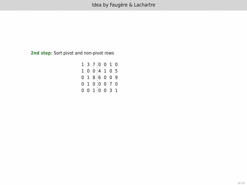
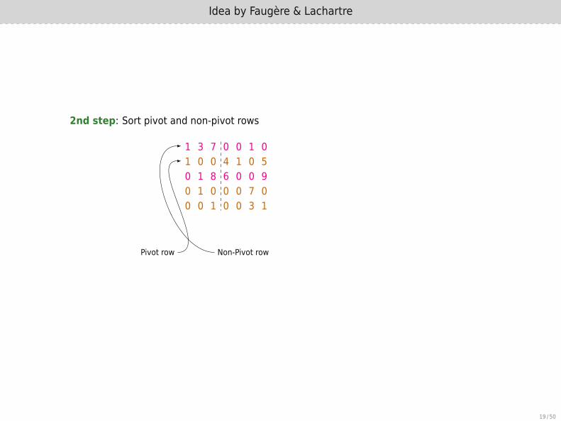
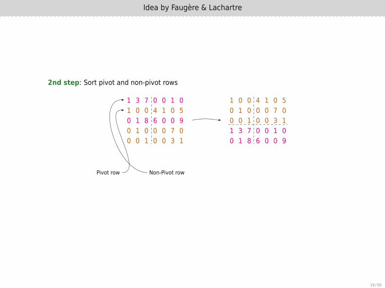
2nd step: Sort pivot and non-pivot rows
1 3 7 0 0 1 01 0 0 4 1 0 50 1 8 6 0 0 90 1 0 0 0 7 00 0 1 0 0 3 1
Pivot row Non-Pivot row
1 0 0 4 1 0 50 1 0 0 0 7 00 0 1 0 0 3 11 3 7 0 0 1 00 1 8 6 0 0 9
19 / 50

Idea by Faugère & Lachartre
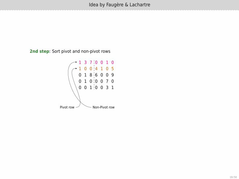
2nd step: Sort pivot and non-pivot rows
1 3 7 0 0 1 01 0 0 4 1 0 50 1 8 6 0 0 90 1 0 0 0 7 00 0 1 0 0 3 1
Pivot row
Non-Pivot row
1 0 0 4 1 0 50 1 0 0 0 7 00 0 1 0 0 3 11 3 7 0 0 1 00 1 8 6 0 0 9
19 / 50
Idea by Faugère & Lachartre
2nd step: Sort pivot and non-pivot rows
1 3 7 0 0 1 01 0 0 4 1 0 50 1 8 6 0 0 90 1 0 0 0 7 00 0 1 0 0 3 1
Pivot row Non-Pivot row
1 0 0 4 1 0 50 1 0 0 0 7 00 0 1 0 0 3 11 3 7 0 0 1 00 1 8 6 0 0 9
19 / 50
Idea by Faugère & Lachartre
2nd step: Sort pivot and non-pivot rows
1 3 7 0 0 1 01 0 0 4 1 0 50 1 8 6 0 0 90 1 0 0 0 7 00 0 1 0 0 3 1
Pivot row Non-Pivot row
1 0 0 4 1 0 50 1 0 0 0 7 00 0 1 0 0 3 11 3 7 0 0 1 00 1 8 6 0 0 9
19 / 50
Idea by Faugère & Lachartre
2nd step: Sort pivot and non-pivot rows
1 3 7 0 0 1 01 0 0 4 1 0 50 1 8 6 0 0 90 1 0 0 0 7 00 0 1 0 0 3 1
Pivot row Non-Pivot row
1 0 0 4 1 0 50 1 0 0 0 7 00 0 1 0 0 3 11 3 7 0 0 1 00 1 8 6 0 0 9
19 / 50

Idea by Faugère & Lachartre
3rd step: Reduce lower left part to zero
1 0 0 4 1 0 50 1 0 0 0 7 00 0 1 0 0 3 11 3 7 0 0 1 00 1 8 6 0 0 9
1 0 0 4 1 0 50 1 0 0 0 7 00 0 1 0 0 3 10 0 0 7 10 3 100 0 0 6 0 2 1
20 / 50

Idea by Faugère & Lachartre
3rd step: Reduce lower left part to zero
1 0 0 4 1 0 50 1 0 0 0 7 00 0 1 0 0 3 11 3 7 0 0 1 00 1 8 6 0 0 9
1 0 0 4 1 0 50 1 0 0 0 7 00 0 1 0 0 3 10 0 0 7 10 3 100 0 0 6 0 2 1
20 / 50

Idea by Faugère & Lachartre
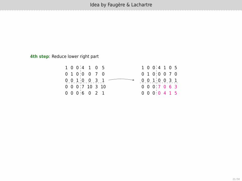
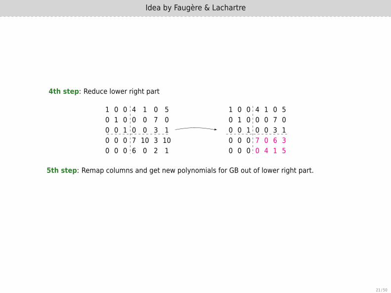
4th step: Reduce lower right part
1 0 0 4 1 0 50 1 0 0 0 7 00 0 1 0 0 3 10 0 0 7 10 3 100 0 0 6 0 2 1
1 0 0 4 1 0 50 1 0 0 0 7 00 0 1 0 0 3 10 0 0 7 0 6 30 0 0 0 4 1 5
5th step: Remap columns and get new polynomials for GB out of lower right part.
21 / 50
Idea by Faugère & Lachartre
4th step: Reduce lower right part
1 0 0 4 1 0 50 1 0 0 0 7 00 0 1 0 0 3 10 0 0 7 10 3 100 0 0 6 0 2 1
1 0 0 4 1 0 50 1 0 0 0 7 00 0 1 0 0 3 10 0 0 7 0 6 30 0 0 0 4 1 5
5th step: Remap columns and get new polynomials for GB out of lower right part.
21 / 50
Idea by Faugère & Lachartre
4th step: Reduce lower right part
1 0 0 4 1 0 50 1 0 0 0 7 00 0 1 0 0 3 10 0 0 7 10 3 100 0 0 6 0 2 1
1 0 0 4 1 0 50 1 0 0 0 7 00 0 1 0 0 3 10 0 0 7 0 6 30 0 0 0 4 1 5
5th step: Remap columns and get new polynomials for GB out of lower right part.
21 / 50

“Real world” matrices?
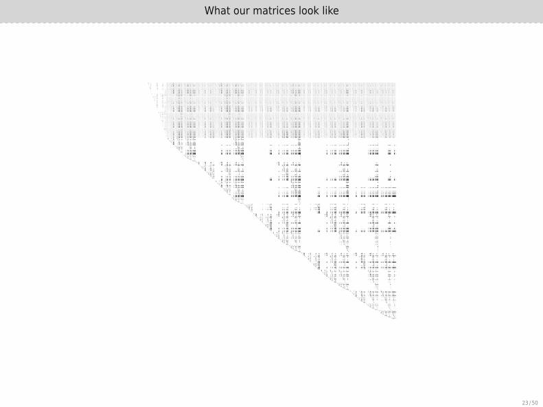
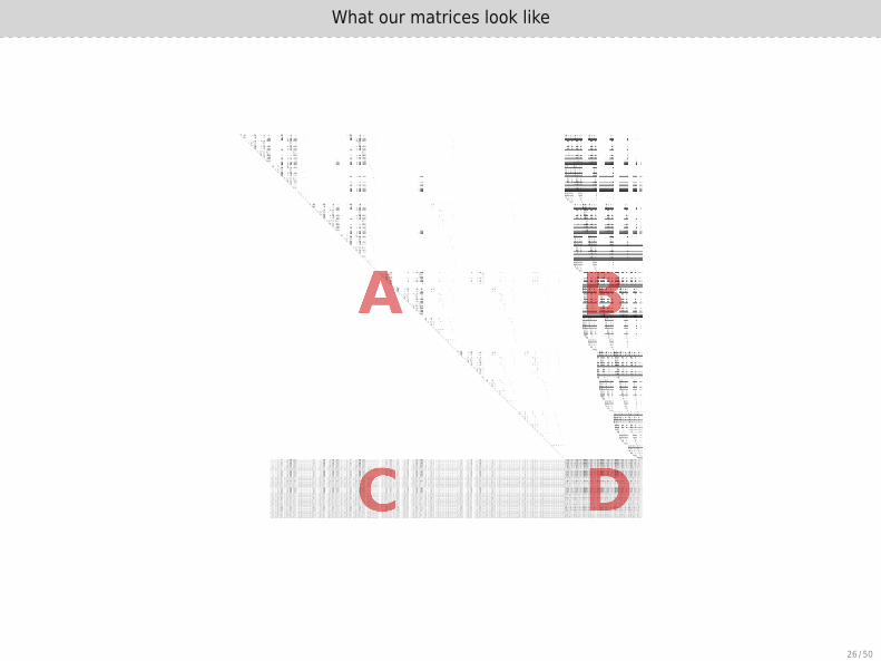
What our matrices look like
23 / 50
What our matrices look like
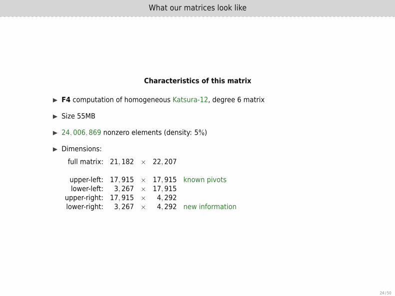
Characteristics of this matrix
▶ F4 computation of homogeneous Katsura-12, degree 6 matrix
▶ Size 55MB
▶ 24,006,869 nonzero elements (density: 5%)
▶ Dimensions:full matrix: 21,182 × 22,207
upper-left: 17,915 × 17,915 known pivotslower-left: 3,267 × 17,915
upper-right: 17,915 × 4,292lower-right: 3,267 × 4,292 new information
24 / 50
What our matrices look like
Characteristics of this matrix
▶ F4 computation of homogeneous Katsura-12, degree 6 matrix
▶ Size 55MB
▶ 24,006,869 nonzero elements (density: 5%)
▶ Dimensions:full matrix: 21,182 × 22,207
upper-left: 17,915 × 17,915 known pivotslower-left: 3,267 × 17,915
upper-right: 17,915 × 4,292lower-right: 3,267 × 4,292 new information
24 / 50

What our matrices look like
25 / 50
What our matrices look like
26 / 50

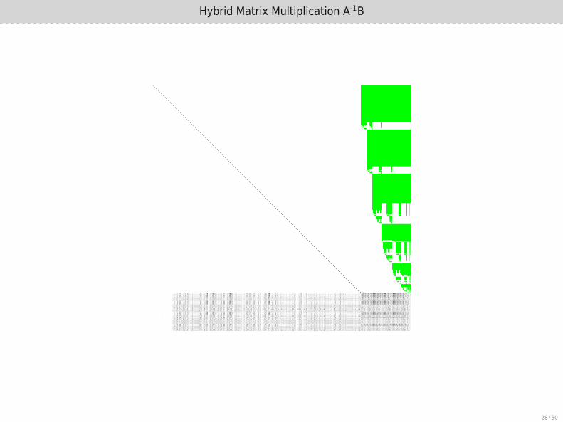
Hybrid Matrix Multiplication A-1B
27 / 50
Hybrid Matrix Multiplication A-1B
28 / 50
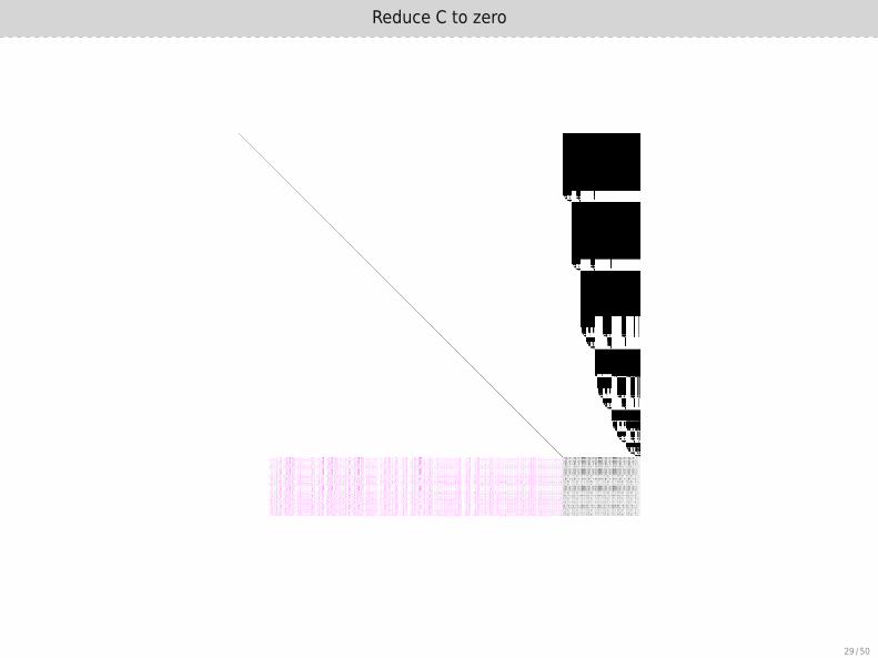
Reduce C to zero
29 / 50
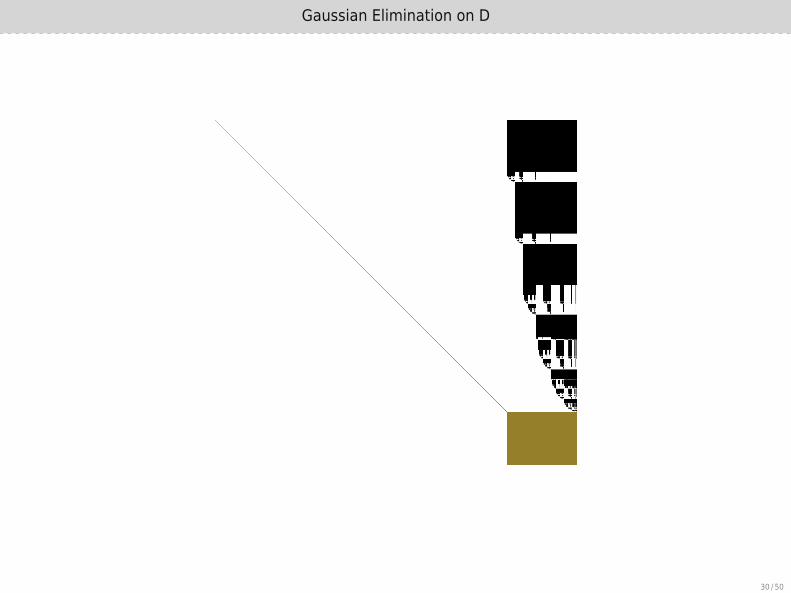
Gaussian Elimination on D
30 / 50
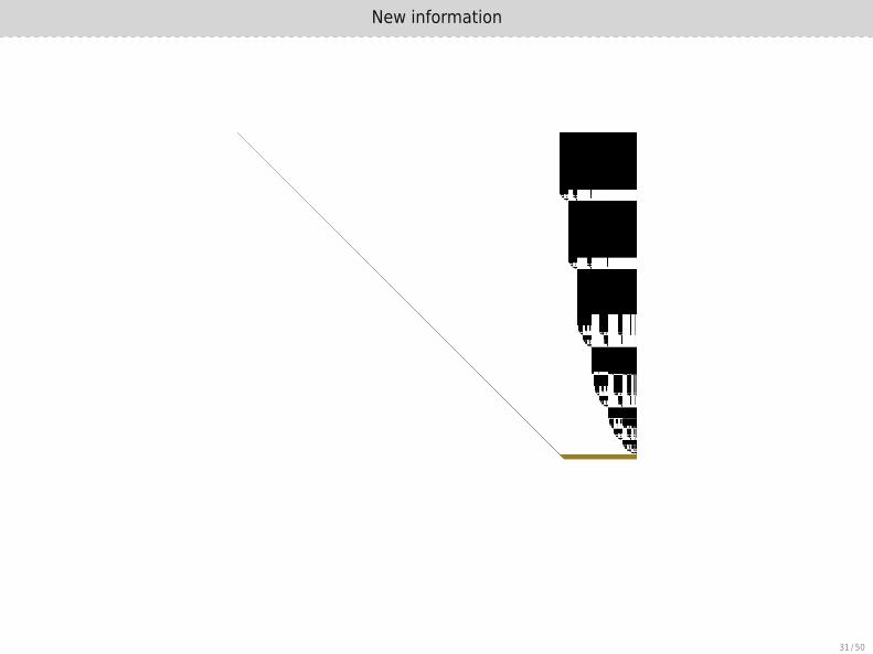
New information
31 / 50
GBLA – A Gröbner Basis Linear Algebra Library
Library Overview
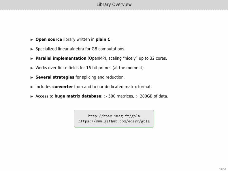
▶ Open source library written in plain C.
▶ Specialized linear algebra for GB computations.
▶ Parallel implementation (OpenMP), scaling “nicely” up to 32 cores.
▶ Works over finite fields for 16-bit primes (at the moment).
▶ Several strategies for splicing and reduction.
▶ Includes converter from and to our dedicated matrix format.
▶ Access to huge matrix database: > 500 matrices, > 280GB of data.
http://hpac.imag.fr/gbla
https://www.github.com/ederc/gbla
33 / 50
Library Overview
▶ Open source library written in plain C.
▶ Specialized linear algebra for GB computations.
▶ Parallel implementation (OpenMP), scaling “nicely” up to 32 cores.
▶ Works over finite fields for 16-bit primes (at the moment).
▶ Several strategies for splicing and reduction.
▶ Includes converter from and to our dedicated matrix format.
▶ Access to huge matrix database: > 500 matrices, > 280GB of data.
http://hpac.imag.fr/gbla
https://www.github.com/ederc/gbla
33 / 50
Exploiting block structures in GB matrices
34 / 50

Exploiting block structures in GB matrices
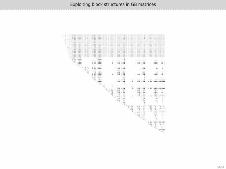
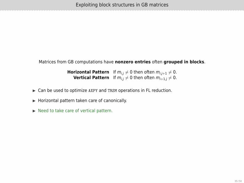
Matrices from GB computations have nonzero entries often grouped in blocks.
Horizontal Pattern If mi,j ̸= 0 then often mi,j+1 ̸= 0.
Vertical Pattern If mi,j ̸= 0 then often mi+1,j ̸= 0.
▶ Can be used to optimize AXPY and TRSM operations in FL reduction.
▶ Horizontal pattern taken care of canonically.
▶ Need to take care of vertical pattern.
35 / 50
Exploiting block structures in GB matrices
Matrices from GB computations have nonzero entries often grouped in blocks.
Horizontal Pattern If mi,j ̸= 0 then often mi,j+1 ̸= 0.Vertical Pattern If mi,j ̸= 0 then often mi+1,j ̸= 0.
▶ Can be used to optimize AXPY and TRSM operations in FL reduction.
▶ Horizontal pattern taken care of canonically.
▶ Need to take care of vertical pattern.
35 / 50

Exploiting block structures in GB matrices
. . . ......
......
......
1 · · · ∗ ∗ ∗ ∗1 · · · ai,j ai,j+1 ∗. . . ...
......
1 · · · ∗1 ∗
1
A......
......
......
...∗ ∗ · · · ∗ · · · ∗ ∗∗ ∗ · · · bi,k ∗ · · · ∗......
......
......
...∗ ∗ · · · bj,k ∗ · · · ∗∗ ∗ · · · bj+1,k ∗ · · · ∗∗ ∗ · · · ∗ · · · ∗ ∗
B
Exploiting horizontal and vertical patterns in the TRSM step.
36 / 50

Multiline data structure – an example
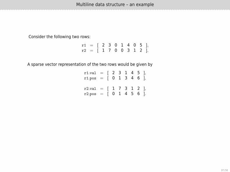
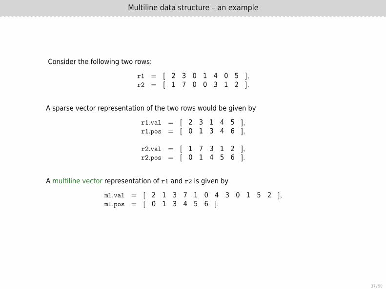
Consider the following two rows:
r1 = [ 2 3 0 1 4 0 5 ],r2 = [ 1 7 0 0 3 1 2 ].
A sparse vector representation of the two rows would be given by
r1.val = [ 2 3 1 4 5 ],r1.pos = [ 0 1 3 4 6 ],
r2.val = [ 1 7 3 1 2 ],r2.pos = [ 0 1 4 5 6 ].
A multiline vector representation of r1 and r2 is given by
ml.val = [ 2 1 3 7 1 0 4 3 0 1 5 2 ],ml.pos = [ 0 1 3 4 5 6 ].
37 / 50
Multiline data structure – an example
Consider the following two rows:
r1 = [ 2 3 0 1 4 0 5 ],r2 = [ 1 7 0 0 3 1 2 ].
A sparse vector representation of the two rows would be given by
r1.val = [ 2 3 1 4 5 ],r1.pos = [ 0 1 3 4 6 ],
r2.val = [ 1 7 3 1 2 ],r2.pos = [ 0 1 4 5 6 ].
A multiline vector representation of r1 and r2 is given by
ml.val = [ 2 1 3 7 1 0 4 3 0 1 5 2 ],ml.pos = [ 0 1 3 4 5 6 ].
37 / 50
New order of operations
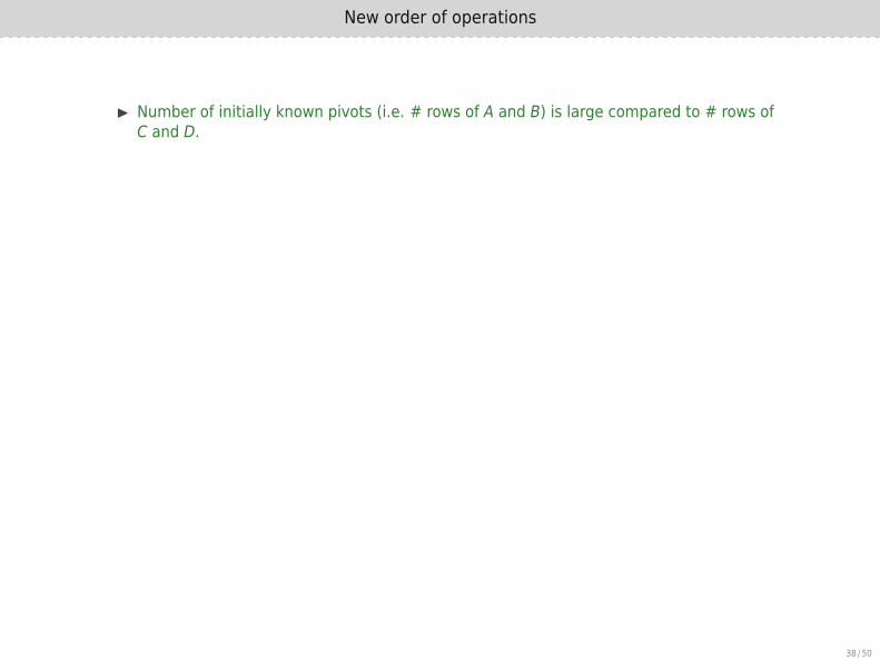
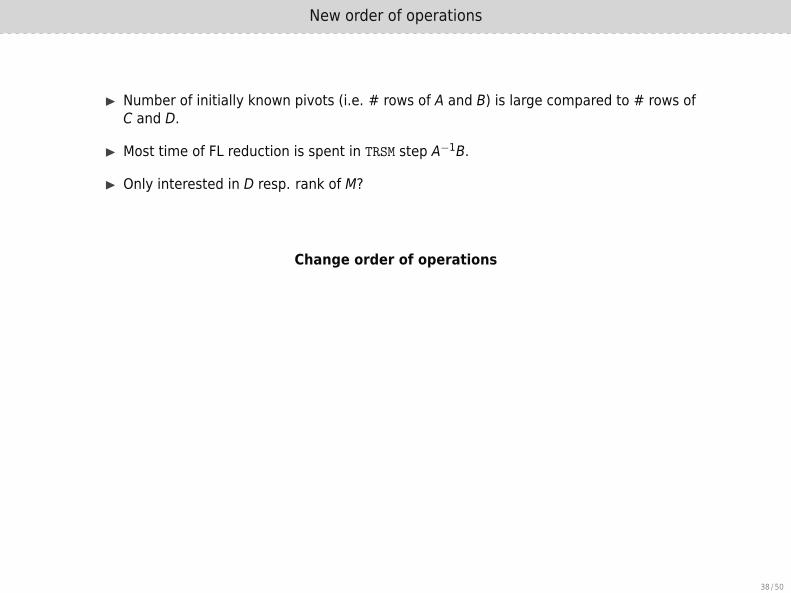
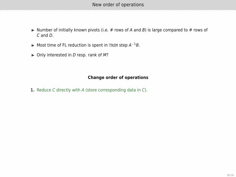
▶ Number of initially known pivots (i.e. # rows of A and B) is large compared to # rows ofC and D.
▶ Most time of FL reduction is spent in TRSM step A−1B.
▶ Only interested in D resp. rank of M?
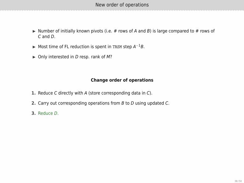
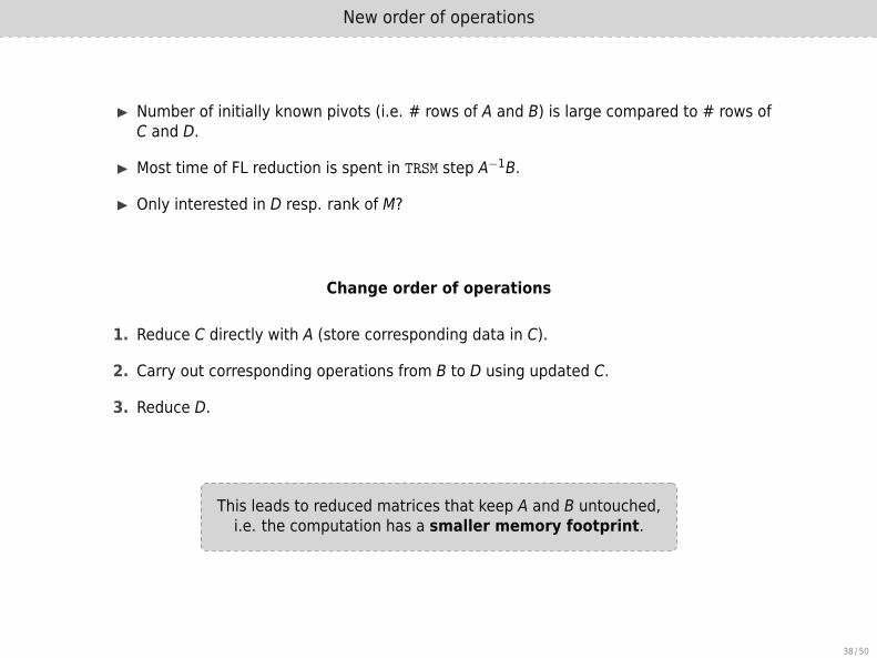
Change order of operations
1. Reduce C directly with A (store corresponding data in C).
2. Carry out corresponding operations from B to D using updated C.
3. Reduce D.
This leads to reduced matrices that keep A and B untouched,i.e. the computation has a smaller memory footprint.
38 / 50

New order of operations
▶ Number of initially known pivots (i.e. # rows of A and B) is large compared to # rows ofC and D.
▶ Most time of FL reduction is spent in TRSM step A−1B.
▶ Only interested in D resp. rank of M?
Change order of operations
1. Reduce C directly with A (store corresponding data in C).
2. Carry out corresponding operations from B to D using updated C.
3. Reduce D.
This leads to reduced matrices that keep A and B untouched,i.e. the computation has a smaller memory footprint.
38 / 50

GBLA Matrix formats
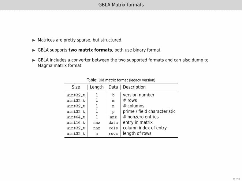
▶ Matrices are pretty sparse, but structured.
▶ GBLA supports two matrix formats, both use binary format.
▶ GBLA includes a converter between the two supported formats and can also dump toMagma matrix format.
Table: Old matrix format (legacy version)
Size Length Data Descriptionuint32_t 1 b version numberuint32_t 1 m # rowsuint32_t 1 n # columnsuint32_t 1 p prime / field characteristicuint64_t 1 nnz # nonzero entriesuint16_t nnz data entry in matrixuint32_t nnz cols column index of entryuint32_t m rows length of rows
39 / 50
GBLA Matrix formats
▶ Matrices are pretty sparse, but structured.
▶ GBLA supports two matrix formats, both use binary format.
▶ GBLA includes a converter between the two supported formats and can also dump toMagma matrix format.
Table: Old matrix format (legacy version)
Size Length Data Descriptionuint32_t 1 b version numberuint32_t 1 m # rowsuint32_t 1 n # columnsuint32_t 1 p prime / field characteristicuint64_t 1 nnz # nonzero entriesuint16_t nnz data entry in matrixuint32_t nnz cols column index of entryuint32_t m rows length of rows
39 / 50

GBLA Matrix formats
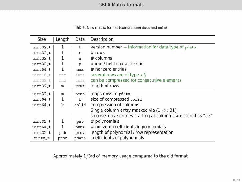
Table: New matrix format (compressing data and cols)
Size Length Data Descriptionuint32_t 1 b version number + information for data type of pdatauint32_t 1 m # rowsuint32_t 1 n # columnsuint32_t 1 p prime / field characteristicuint64_t 1 nnz # nonzero entriesuint16_t nnz data several rows are of type xifjuint32_t nnz cols can be compressed for consecutive elementsuint32_t m rows length of rowsuint32_t m pmap maps rows to pdata
uint64_t 1 k size of compressed colid
uint64_t k colid compression of columns:Single column entry masked via (1 << 31);s consecutive entries starting at column c are stored as “c s”
uint32_t 1 pnb # polynomialsuint64_t 1 pnnz # nonzero coefficients in polynomialsuint32_t pnb prow length of polynomial / row representationxinty_t pnnz pdata coefficients of polynomials
Approximately 1/3rd of memory usage compared to the old format.
40 / 50
GBLA Matrix formats
Table: New matrix format (compressing data and cols)
Size Length Data Descriptionuint32_t 1 b version number + information for data type of pdatauint32_t 1 m # rowsuint32_t 1 n # columnsuint32_t 1 p prime / field characteristicuint64_t 1 nnz # nonzero entriesuint16_t nnz data several rows are of type xifjuint32_t nnz cols can be compressed for consecutive elementsuint32_t m rows length of rowsuint32_t m pmap maps rows to pdata
uint64_t 1 k size of compressed colid
uint64_t k colid compression of columns:Single column entry masked via (1 << 31);s consecutive entries starting at column c are stored as “c s”
uint32_t 1 pnb # polynomialsuint64_t 1 pnnz # nonzero coefficients in polynomialsuint32_t pnb prow length of polynomial / row representationxinty_t pnnz pdata coefficients of polynomials
Approximately 1/3rd of memory usage compared to the old format.
40 / 50
GBLA Matrix formats – Comparison
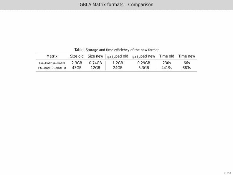
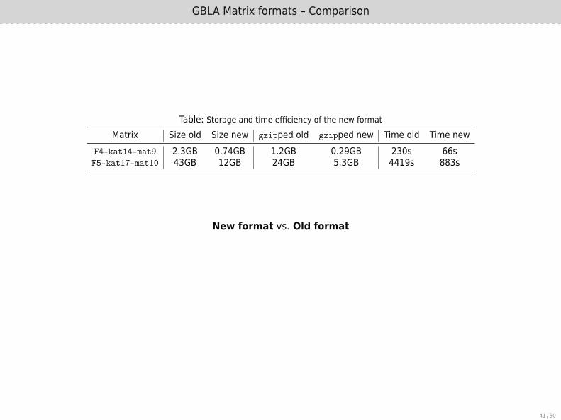
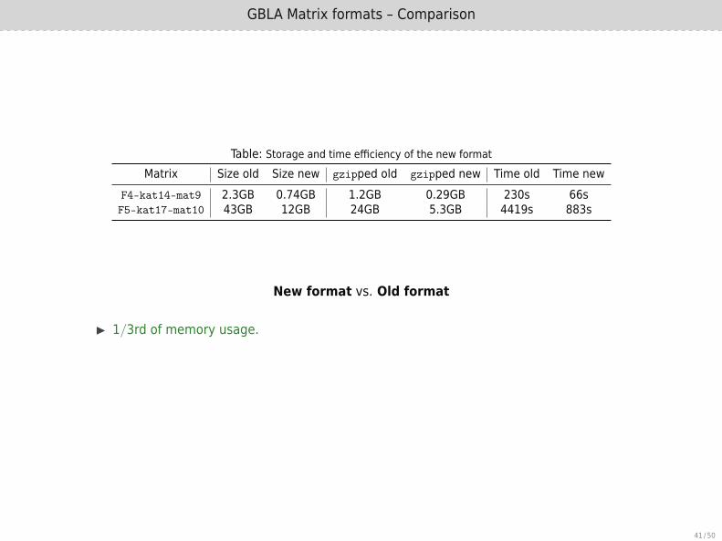
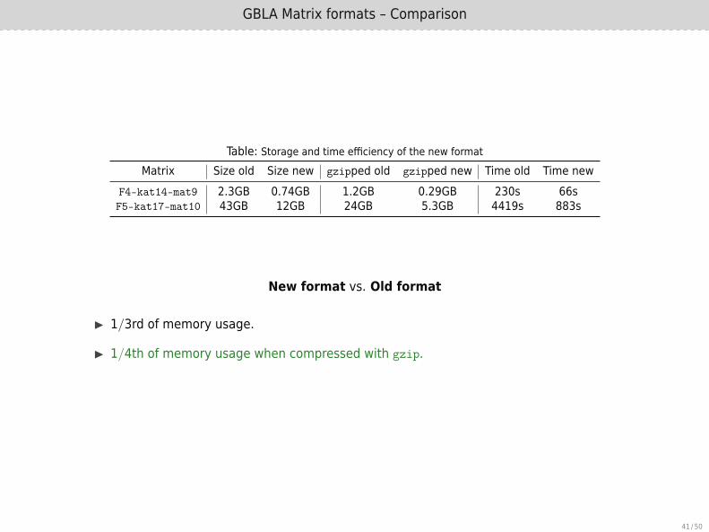
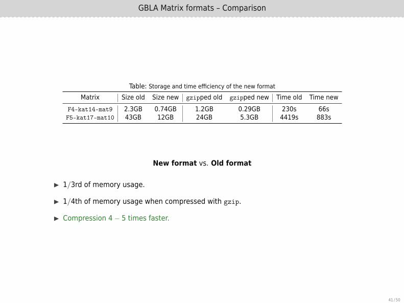
Table: Storage and time efficiency of the new formatMatrix Size old Size new gzipped old gzipped new Time old Time new
F4-kat14-mat9 2.3GB 0.74GB 1.2GB 0.29GB 230s 66sF5-kat17-mat10 43GB 12GB 24GB 5.3GB 4419s 883s
New format vs. Old format
▶ 1/3rd of memory usage.
▶ 1/4th of memory usage when compressed with gzip.
▶ Compression 4− 5 times faster.
41 / 50
GBLA Matrix formats – Comparison
Table: Storage and time efficiency of the new formatMatrix Size old Size new gzipped old gzipped new Time old Time new
F4-kat14-mat9 2.3GB 0.74GB 1.2GB 0.29GB 230s 66sF5-kat17-mat10 43GB 12GB 24GB 5.3GB 4419s 883s
New format vs. Old format
▶ 1/3rd of memory usage.
▶ 1/4th of memory usage when compressed with gzip.
▶ Compression 4− 5 times faster.
41 / 50

GB – A Gröbner Basis Library

Library Overview
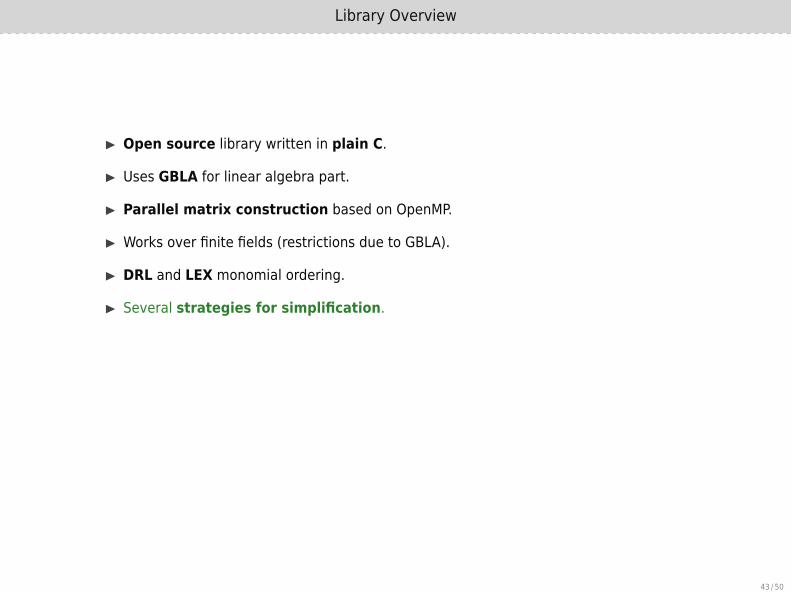
▶ Open source library written in plain C.
▶ Uses GBLA for linear algebra part.
▶ Parallel matrix construction based on OpenMP.
▶ Works over finite fields (restrictions due to GBLA).
▶ DRL and LEX monomial ordering.
▶ Several strategies for simplification.
▶ Available as alpha version in Singular after 4-0-3 release.
https://www.github.com/ederc/gb
43 / 50
Library Overview
▶ Open source library written in plain C.
▶ Uses GBLA for linear algebra part.
▶ Parallel matrix construction based on OpenMP.
▶ Works over finite fields (restrictions due to GBLA).
▶ DRL and LEX monomial ordering.
▶ Several strategies for simplification.
▶ Available as alpha version in Singular after 4-0-3 release.
https://www.github.com/ederc/gb
43 / 50
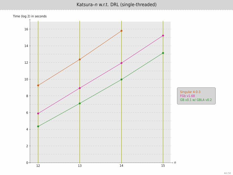
Katsura–n w.r.t. DRL (single-threaded)
n
Time (log 2) in seconds
12 13 14 150
2
4
6
8
10
12
14
16
Singular 4-0-3FGb v1.68GB v0.1 w/ GBLA v0.2
44 / 50
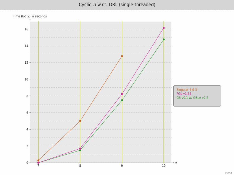
Cyclic–n w.r.t. DRL (single-threaded)
n
Time (log 2) in seconds
7 8 9 100
2
4
6
8
10
12
14
16
Singular 4-0-3FGb v1.68GB v0.1 w/ GBLA v0.2
Magma v2.21 / Maple 2016
45 / 50
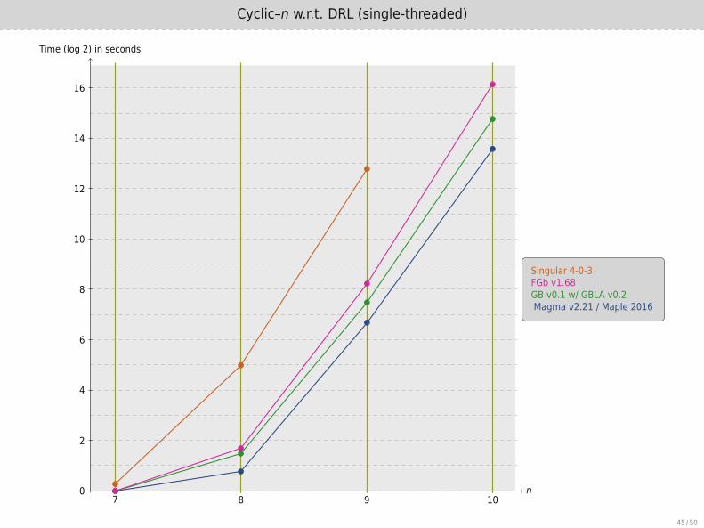
Cyclic–n w.r.t. DRL (single-threaded)
n
Time (log 2) in seconds
7 8 9 100
2
4
6
8
10
12
14
16
Singular 4-0-3FGb v1.68GB v0.1 w/ GBLA v0.2Magma v2.21 / Maple 2016
45 / 50
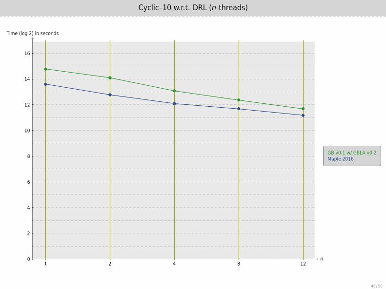
Cyclic–10 w.r.t. DRL (n-threads)
n
Time (log 2) in seconds
1 2 4 8 120
2
4
6
8
10
12
14
16
GB v0.1 w/ GBLA v0.2Maple 2016
46 / 50

Next steps
▶ v0.3 of GBLA.
▶ Optimizing GBLA for floating point and 32-bit unsigned int arithmetic.
▶ Multi-modular computation in GB.
▶ Parallel hashing in GB.
▶ Better handling of memory bounds in GB/GBLA.
▶ FGLM in GB for zero-dimensional system solving.
▶ First steps exploiting heterogeneous CPU/GPU platforms for GBLA.
▶ Deeper investigation on parallelization on networks.
47 / 50

References
[1] Boyer, B. and Eder, C. and Faugère, J.-C. and Lachartre, S. and Martani, F. GBLA -Gröbner Basis Linear Algebra Package, 2016. Proceedings of the 2016 InternationalSymposium on Symbolic and Algebraic Computation
[2] Buchberger, B. Ein Algorithmus zum Auffinden der Basiselemente desRestklassenringes nach einem nulldimensionalen Polynomideal, 1965. PhD thesis,Universtiy of Innsbruck, Austria
[3] Buchberger, B. A criterion for detecting unnecessary reductions in the construction ofGröbner bases, 1979. EUROSAM ’79, An International Symposium on Symbolic andAlgebraic Manipulation
[4] Buchberger, B. Gröbner Bases: An Algorithmic Method in Polynomial Ideal Theory,1985. Multidimensional Systems Theory, D. Reidel Publication Company
[5] Eder, C. and Faugère, J.-C. A survey on signature-based Gröbner basis algorithms,2016. Journal of Symbolic Computation
[6] Faugère, J.-C. A new efficient algorithm for computing Gröbner bases (F4), 1999.Journal of Pure and Applied Algebra
[7] Faugère, J.-C. A new efficient algorithm for computing Gröbner bases without reductionto zero (F5), 2002. Proceedings of the 2002 International Symposium on Symbolic andAlgebraic Computation
[8] Faugère, J.-C. and Lachartre, S. Parallel Gaussian Elimination for Gröbner basescomputations in finite fields, 2010. Proceedings of the 4th International Workshop onParallel and Symbolic Computation
[9] Gebauer, R. and Möller, H. M. On an installation of Buchberger’s algorithm, 1988.Journal of Symbolic Computation
48 / 50

Thank you!

Questions? Comments?