parallel optimisation - greycon parallel optimisation g r e y c o n version 1.2 18 january 2013 iii...

X-Trim

Parallel Optimisation

Document Version 1.2

GREYCON www.greycon.com

http://www.greycon.com/

X-Trim Parallel Optimisation

G R E Y C O N

Version 1.2 18 January 2013 ii

Table of Contents

1. BACKGROUND.......................................................................................................................... 1

1.1. INTRODUCTION ......................................................................................................................................... 1

1.1.1. Fine-Grained ...................................................................................................................................... 1

1.1.2. Coarse-Grained ............................................................................ Error! Bookmark not defined.

2. X-TRIM MODEL ........................................................................................................................ 2

2.1. PARAMETER SETS ......................................................................................................................................2

2.2. MULTI-OPT EXECUTION SCHEMA ............................................................................................................ 3

3. EXPERIMENTS AND RESULTS .................................................................................................. 5

3.1. INTRODUCTION .........................................................................................................................................5

3.2. EXAMPLES .................................................................................................................................................5

3.3. PRIMARY OPTIMISATION.......................................................................................................................... 6

3.4. SECONDARY OPTIMISATION .................................................................................................................... 8

4. HARDWARE & SCALABILITY ................................................................................................. 12

4.1. MULTI-CORE SCALABILITY ...................................................................................................................... 12

4.2. HYPERTHREADING ................................................................................................................................. 13

5. CONCLUSION ......................................................................................................................... 14

Version Control

No. Date Who Comments

1.0 8 August 2009 Leandro Gomez Initial version

1.1 26 June 2011 Constantine Goulimis Updated capabilities in the software

1.2 18 January 2012 Constantine Goulimis XPRESS maximum core count increased to 100

Terms

Term Definition

Speedup In parallel computing, speedup refers to how much faster a parallel algorithm is than the corresponding sequential algorithm.

In parallel computing speedup Speedup is defined as : Sp = T1 / Tp, where:

T1 is the elapsed time without using parallelism.

Tp is the elapsed time of the parallel version running in p processors.

http://en.wikipedia.org/wiki/Parallel_computing

http://en.wikipedia.org/wiki/Parallel_algorithm

http://en.wikipedia.org/wiki/Algorithm


G R E Y C O N

Version 1.2 18 January 2013 iii

Term Definition

HyperThreading Simultaneous multithreading (often abbreviated as SMT) is a technique for improving the overall efficiency of a superscalar CPU with hardware multithreading. In other words, it is a technique that simulates multiple processors within a single processor. A very well known implementation of simultaneous multithreading is Intel’s HyperThreading technology.

http://en.wikipedia.org/wiki/Superscalar

http://en.wikipedia.org/wiki/Central_processing_unit

http://en.wikipedia.org/wiki/Multithreading_%28computer_hardware%29

http://en.wikipedia.org/wiki/Multithreading_%28computer_hardware%29


G R E Y C O N

Version 1.2 18 January 2013 1

1. Background

1.1. Introduction

X-Trim supports two distinct kinds of parallelism: fine-grained and coarse-grained.

1.1.1. Fine-Grained

In fine-grained parallelism, a single algorithm exploits 2- and 4-core processors. This parallel processing capability supplies a speed advantage dependent on both the size of the problem and the algorithm used. However, while most algorithms employ fine-grained parallelism, the following currently do not:

Primary optimisation:

o PB algorithm

o Landau algorithm

Secondary optimisation:

o Knife Changes

o Extruder Order Spread

o Minimum Open Stacks

Prior to 7.6 (released November 2012), the third-party XPRESS integer programming library (used by Full Optimisation & KC primary and Pattern Reduction secondary algorithms) was limited to a maximum of 4 cores. There were two separately chargeable options for 2- and 4-core processors. With the advent of the 7.6 release, the standard XPRESS license allows up to 100 cores (although we not recommend numbers higher than 8) and this is part of the baseline package (i.e. no need for additional options).

1.1.2. Coarse-Grained

X-Trim 6.8 (released April 2009) introduced coarse-grained parallelism. Coarse-grained parallelism allows multiple parameter sets to be used simultaneously. A parameter set defines all the algorithm-related information necessary for solving a run. X-Trim 6.8 allows users to employ multiple optimisation algorithms/parameters in parallel and then to choose a solution from among all the results returned by all parameter sets. Multi-core processors are therefore fully exploited.

X-Trim 6.9 (released July 2009) enhances this functionality by adding secondary optimisation to the list of parallelised processes. Users are now able to apply secondary optimisation automatically and in parallel to all solutions returned by a parameter set.

Subsequent releases have extended the amount of parallelism that is available, e.g. the pattern generation in the Full Optimisation is now (from 7.2) is parallelised, extending the benefits of this important technology.

This article focuses primarily on coarse-grained parallelism, while still considering some examples of fine-grained parallelism.


G R E Y C O N


2. X-Trim Model

2.1. Parameter Sets

Parameter sets encapsulate almost all algorithm parameters. Using multiple parameter sets allows users to experiment with different configurations simultaneously. This is very useful, as configuring X-Trim can be require a lot of skill and experience – parameter sets therefore become a mechanism for encapsulating this knowledge and making it available to all users.

Parameters sets may or may not include secondary optimisation. This is configured with the Invoke secondary optimisation automatically flag. Secondary optimisation modifies the solutions returned by the primary algorithm. These secondary optimisations are not usually intended to modify a solution’s original waste, but may improve other solution characteristics such as knife changes, order spread, etc.

Parameter sets may also capture machine characteristics, such as machine widths.

Figure 2: Screenshot of list of parameter sets

Figure 1 : Screenshot of main parameter form


G R E Y C O N


2.2. Multi-Opt Execution Schema

Multi-Opt execution schema is depicted in figure 3. When the execution starts, all primary optimisations are executed in parallel, one for each parameter set. The maximum number of simultaneous parallel executions depends on the number of cores. Table 1 shows this relationship. However, users are still allowed to configure this internal parameter manually. This is shown in figure 4.

After the primary algorithm finishes for a given parameter set, every solution returned by the optimisation is processed. If the Invoke secondary

optimisation automatically flag is set, then the secondary optimisation is executed, in parallel, for each solution generated. If multiple secondary optimisation algorithms are specified, they execute sequentially on each solution.

Maximum number of processes

1 processor core 2

2 processor cores 3

3 processor cores 5

4 processor cores 6

More than 4 processor cores 1.25 × (Number of cores)

Table 1: Relationship between number of processors and maximum number of processes

Figure 3 : Multi-Opt execution schema


G R E Y C O N


The user may over-ride the default settings by using the configuration settings in the Greycon Administrator utility. This would typically be employed to avoid any one user taking up too many available resources in shared server environment:

Figure 4: Maximum number of parallel executions manual configuration


G R E Y C O N


3. Experiments and Results

3.1. Introduction

The following sections examine various experiments that focus on parallelism. All of them were run on an Intel Quad Core machine with the following characteristics:

CPU Model: Intel® Core™2 Quad CPU

Frequency: 2.40 GHz each processor

RAM: 3.5 GB

3.2. Examples

This section considers a practical example illustrating the usefulness of parallelism in common situations. This example shows all parallelism levels (coarse-grained and fine-grained) interacting simultaneously. Different levels of parallelism will be considered in the next sections’ experiments.

In experiment #1, sample run 124 is solved with five different parameter sets. Fine-grained parallelism is used in all algorithms that support it (4 threads in each primary algorithm). Coarse grained parallelism applies to each parameter set (in secondary optimisation) and between them.

Each parameter set configuration is shown below:

Parameter Set 1 –KC Algorithm

Parameter Set 2 -Full Optimisation – Normal

Parameter Set 3 -Full Optimisation - Allow over production

Parameter Set 4 -Full Optimisation – Allow under production

Parameter Set 5- H-Trim Algorithm

Figure 5: Screenshot of solving window


G R E Y C O N


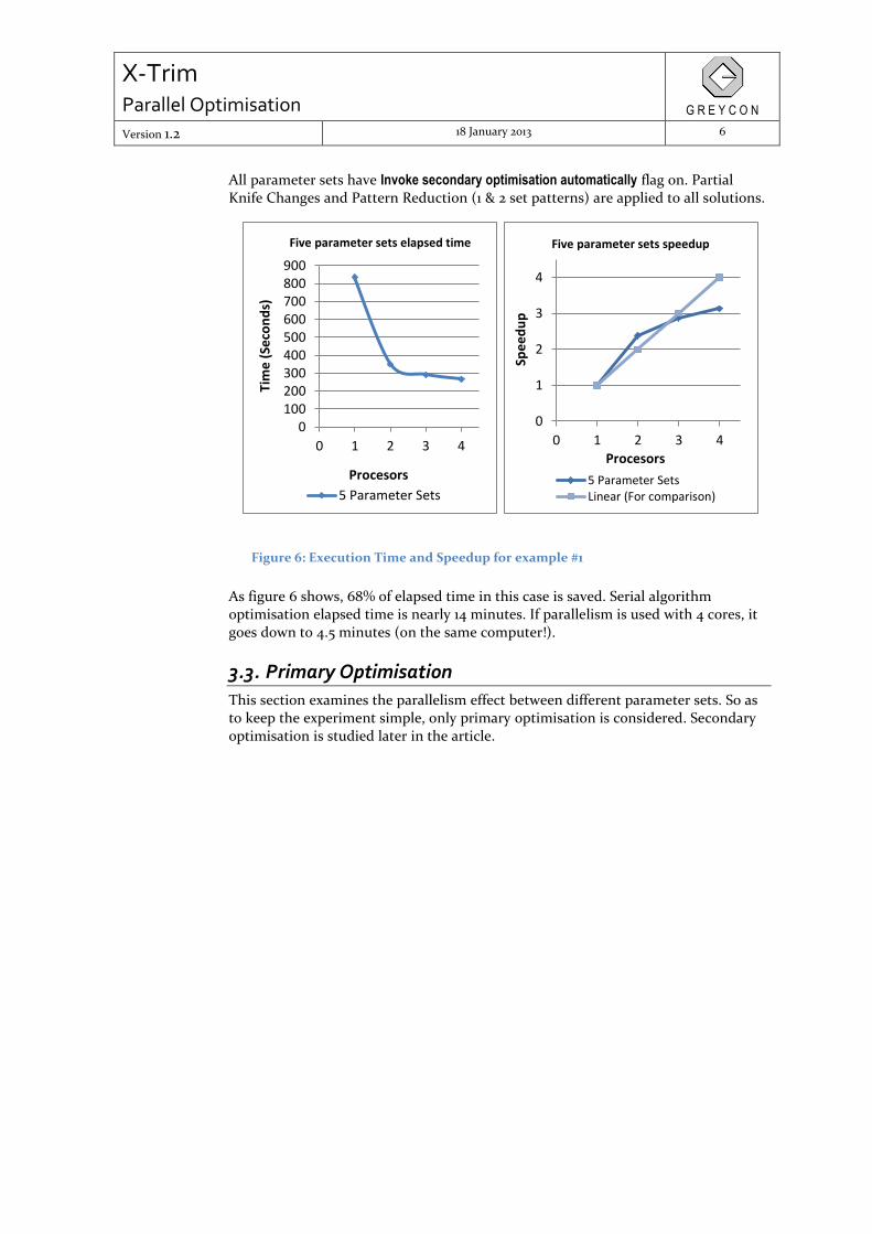
All parameter sets have Invoke secondary optimisation automatically flag on. Partial Knife Changes and Pattern Reduction (1 & 2 set patterns) are applied to all solutions.

As figure 6 shows, 68% of elapsed time in this case is saved. Serial algorithm optimisation elapsed time is nearly 14 minutes. If parallelism is used with 4 cores, it goes down to 4.5 minutes (on the same computer!).

3.3. Primary Optimisation

This section examines the parallelism effect between different parameter sets. So as to keep the experiment simple, only primary optimisation is considered. Secondary optimisation is studied later in the article.

Figure 6: Execution Time and Speedup for example #1

0100200300400500600700800900

0 1 2 3 4

Tim

e (

Seco

nd

s)

Procesors

Five parameter sets elapsed time

5 Parameter Sets

0

1

2

3

4

0 1 2 3 4

Spe

ed

up

Procesors

Five parameter sets speedup

5 Parameter SetsLinear (For comparison)


G R E Y C O N


In order to measure the parallelism effect in parameter sets, the problem presented in experiment #1 (section 3.2) is modified so that fine-grained parallelism and secondary optimisation are no longer used. Results are shown in figure 7:

Speedup values indicate a good utilisation of the available cores. The sub-linear shape of the speedup curve above occurs frequently in parallel applications.

The impact of parallelism is less noticeable when the time to solve the problem is short. That is because parallelisable work increases if the problem is hard to solve, while non-parallelisable work usually remains constant.

To show this, we have created different versions of run #124. “Reduced” versions were created by deleting some orders of a copy of run #124. An “extended” version was also created, which is a copy of run #124 in which each order was cloned one time. The same parameter sets of experiment #2 were tested in these “extended” and “reduced” versions, and speedup was measured. Results are shown in figure 8 (original run version is shown as a red marker in the chart).

Speedup may also improve if all the parameter sets are of similar complexity, and, conversely, speedup may be negatively affected in the opposite case (as parallelism cannot be fully exploited). This can also be observed in figure 8; 28 order version (“extended” version) shows less speedup, as the computational cost of each parameter set is more heterogeneous in this version than in the original one.

Figure 7: Speedup for experiment #2

0

1

2

3

4

0 1 2 3 4

Spe

ed

up

Procesors

Five parameters sets, only primary optimization

5 ParameterSets

Linear (Forcomparison)


G R E Y C O N


3.4. Secondary Optimisation

When secondary optimisation is enabled in a parameter set, the secondary algorithms will execute in parallel with other primary algorithms (recall that a primary algorithm may generate multiple solutions, each requiring secondary optimisation). This can be seen as another level of parallelism. The following

Figure 8: Experiment #3, speedup for different versions of run #124 (above). Independent algorithms executions on two different versions of run #124 (below).

0

0.5

1

1.5

2

2.5

0 5 10 15 20 25 30

Spe

ed

up

Order Count

Speedup on four processors vs order count with 5 parameter sets

0

10

20

30

40

50

60

70

80

90

Full Opt Full Opt.Allow Over

Prod.

Full Opt.AllowUnderProd.

KCAlgorithm

H-Trim

Elap

sed

Tim

e (

seco

nd

s)

Independent algorithms executions elapsed time

14 Orders (Original)

28 Orders


G R E Y C O N


experiments focus on the parallelism between secondary optimisation algorithms in a single parameter set.

Experiment #4 is straightforward: an independent secondary optimisation has been applied automatically to sample problem #148 (simple eight order problem). It generates 39 different solutions, so parallelism is high in secondary optimisation. Only secondary optimisation elapsed time is shown (primary optimisation elapsed time is subtracted from total elapsed time). Fine-grained optimisation is disabled.

The Pattern Reduction algorithm presents the best speedup curve. When Full Knife Changes or Minimum Open Stacks are applied, the elapsed time improves compared to the serial version, but it remains constant when more processors are used. This is due mainly to the algorithm’s optimisation of elapsed time for each solution. Pattern Reduction presents the highest speedup among the three secondary optimisation algorithms for that run.

Figure 9: Speedup for experiment #4

0

1

2

3

4

5

0 1 2 3 4 5

Spe

ed

up

Procesors

Speedup for independent secondary optimizations

Pattern Reduction (Physical Number)

Minimun Open Stacks

Full Knife Changes

Linear (For comparison)


G R E Y C O N


As figure 10 shows, the Pattern Reduction algorithm spent about 46 seconds on each solution (in its serial version), while Minimum Open Stacks and Full Knife Changes did so for nearly half a second.

Experiment #5 is designed to test how secondary optimisation performs when multiple secondary algorithms are applied simultaneously. Pattern Reduction and Full Knife Changes are applied simultaneously to the same problem.

As figure 11 shows, speedup is even better than before. The result is a super-lineal speedup curve, and is probably due to the fact that the serial algorithm cannot fully exploit a single core.

Figure 11 : Speedup for experiment #5

0

1

2

3

4

5

6

7

0 2 4 6

Spe

ed

up

Procesors

Multiple secondary optimizations applied simultaneously

Pattern Reduction& Full KnifeChanges


Figure 10: Secondary opt. time spent in experiment #4

0

200

400

600

800

1000

1200

1400

1600

1800

2000

0 1 2 3 4

Tim

e (

Seco

nd

s)

Procesors

Patern Reduction elapsed time

Pattern Reduction (Physical Number)

0

2

4

6

8

10

12

14

16

18

20

22

0 1 2 3 4Ti

me

(Se

con

ds)

Procesors

Full Knife Changes and Min. Open Stacks elapsed time

Minimun Open StacksFull Knife Changes


G R E Y C O N


So far, parallelism has been shown to be highly effective in reducing the elapsed time of secondary optimisation. However, is the effect of parallelism really significant in terms of the total elapsed time? Well, that is highly dependent on the individual problem on which we are working. Even so, upper bounds on this contribution can still be estimated.

The contribution of the secondary optimisation’s parallelism to the total elapsed time is high when:

The primary optimisation’s elapsed time is short.

The secondary optimisation’s elapsed time is long.

The primary optimisation returns a lot of solutions.

Experiment #6 tries to measure the upper bound of secondary optimisation’s parallelism contribution by designing a problem with those properties. The same problem as experiment #5 is used.

As table 2 shows, the elapsed time in primary optimisation execution is nearly 1% of the total elapsed time when a serial algorithm is used. If the parallel version is used with four processors, 83% of elapsed time is saved (this value can be improved further if more processors are used).

Serial algorithm 4 Cores

Primary Optimisation 15 seconds 15 seconds

Secondary optimisation 1863 seconds 310 seconds

Total Time 1878 seconds 325seconds

Table 2: Experiment #6, secondary optimisation parallelism contribution in execution time


G R E Y C O N


4. Hardware & Scalability

X-Trim parallel processing in traditional single core architectures may be worthwhile, as the serial X-Trim version may not fully exploit such architectures in certain situations. However, multi-core architectures will present much better results. This section focuses on multi-core architectures’ scalability. HyperThreading architectures are also reviewed.

4.1. Multi-Core Scalability

Speedup is not very appropriate for analyzing scalability (as it compares a parallel algorithm vs. a sequential algorithm).

Therefore, we will define “scalability” as T1 / Tp where:

T1 is the running time of the parallel version in one processor.

Tp is the running time of the parallel version running in p processors.

Experiment #7 focuses on the scalability of the problem presented in experiment #1 (section 3.2). The experiment was run in the same hardware that was used in section 3. Figure 12 shows the results. As scalability increases in a roughly linear fashion, we can extrapolate the results.

In this experiment, doubling the number of processors increases speed 1.5 times. As ever, the results may depend on the problem’s characteristics.

Figure 12: Scalability for experiment #7.

0

1

2

3

4

5

6

7

8

0 1 2 3 4 5 6 7 8

Scal

lab

ility

Procesors

Scalability for 5 parameter sets

5 ParameterSets


Trendline


G R E Y C O N


4.2. HyperThreading

HyperThreading technology is implemented in several Intel processors. In Experiment #8, X-Trim’s parallel processing was tested in a Intel Pentium 4 machine with the following characteristics:

Intel® Pentium® 4 CPU (Single CPU)

Frequency: 3.0 GHz

RAM: 3 GB

The same problem of experiment #1 was used. In a first stage, we run the problem without using HyperThreading (it was disabled in the BIOS setup). The test was then repeated using HyperThreading, which makes the operating system that there are 2 cores available. Results are shown in figure 13.

As figure 13 shows, using X-Trim Parallel Processing with Intel’s HyperThreading technology saves 36% of optimisation time. This means “speed” increases 1.5 times, exactly the same that is achieved by adding a new processor (see last section’s results).

Figure 13: Elapsed time for experiment #8 in a Intel HyperThreading architecture, enabling and disabling HyperThreading

0

200

400

600

800

1000

1200

Without HyperThreading Using HyperThreading

Tim

e (

Seco

nd

s)

Five parameter sets in a HyperThreading Architecture


G R E Y C O N


You can see in figure 14 that the system believes that there are two cores, even though there is only one physically present.

Figure 14: Task manager showing two virtual cores.

5. Conclusion

X-Trim 6.9 parallelism functionality can take advantage of multi-core and HyperThreading architectures. Moreover, X-Trim parallel processing is scalable in multi-core environments. For problems which take a significant time, the new parallel capabilities result in massively improved productivity. Investing in 2- or 4-core hardware is therefore strongly recommended in these situations.

parallel optimisation - greycon parallel optimisation g r e y c o n version 1.2 18 january 2013 iii...

Documents