parallel query processing for in-memory databasesparallel query processing for in-memory databases...

Aalto University

School of Science and Technology

Faculty of Information and Natural Sciences

Degree Programme of Computer Science and Engineering

Parallel query processing for in-memory

databases

Final project

Espoo, December 13, 2010

Supervisor: Eljas Soisalon-Soininen

Instructor: Antoni Wolski

Aalto University

School of Science and Technology

Faculty of Information and Natural Sciences

Degree Programme of Computer Science and

Engineering

ABSTRACT OF THE FINAL

PROJECT

Author: Carlos López Rodríguez

Title:Parallel query processing for in-memory databases

Number of pages: 70 Date: 13/12/2010 Language: English

Professorship: Eljas Soisalon-Soininen Code:

Supervisor: Eljas Soisalon-Soininen

Instructor(s): Antoni Wolski

Abstract:

In this final project, we present an approach for optimizing and parallelizing the query execution for in-memory database management systems.

Our study starts by explaining in detail a query optimizer and introducing the concept of in-memory database. Afterwards, we explain different approaches for achieving parallelism into the query execution.

Finally, we provide an experiment to demonstrate the performance improvements achieved with parallelism against the sequential execution.

Keywords: parallel query, main memory database, query optimization, operator tree

Table of contents

Table of contentsTable of contents.......................................................................................... v

1 Introduction...................................................................................................1

2 Query optimization methods....................................................................... 22.1 Introduction..................................................................................................... 22.2 Query Translation .......................................................................................... 52.2.1 SQL transformation...................................................................................... 52.2.2 Execution plan generation.......................................................................... 112.2.3 Cost model.................................................................................................16

2.3 Query Execution .......................................................................................... 17

3 In-memory databases ................................................................................ 183.1 Introduction................................................................................................... 183.2 In-memory against traditional databases...................................................... 183.2.1 Physical comparison.................................................................................. 193.2.2 Implementation differences........................................................................ 19

3.3 Making the choose between MMDB and DRDB...........................................223.3.1 Traditional database with a large cache .................................................... 233.3.2 Persistent and durable in-memory database..............................................23

4 Parallel query processing.......................................................................... 244.1 Introduction................................................................................................... 244.2 Parallelism operator types............................................................................ 284.2.1 Intra-operator parallelism........................................................................... 284.2.2 Pipelined inter-operator parallelism............................................................294.2.3 Independent inter-operator........................................................................ 30

4.3 Parallelism management.............................................................................. 314.3.1 Operator tree............................................................................................. 314.3.2 Decomposing the operator tree..................................................................354.3.3 Dependency graph.................................................................................... 374.3.4 Schedule process ..................................................................................... 38

4.4 An approach of parallel query for SMP systems........................................... 424.4.1 Introducing ASYNC operator......................................................................424.4.2 Applying Inter- and Intra-operator parallelism............................................434.4.3 Query optimizer implementation................................................................ 43

5 Experiment implementation....................................................................... 455.1 Overview...................................................................................................... 455.2 Test setup..................................................................................................... 46

6 Experiment results..................................................................................... 48

7 Conclusions................................................................................................ 51

A Glossary of terms and abbreviations........................................................... I

Bibliography................................................................................................. III

v

1 Introduction

1 Introduction

The present and future of database management systems resides on the realm of highly

parallel computers. The main reason is that parallel machines can be constructed at a low

cost without the need for any special hardware technology.

On the other hand, semiconductor memory becomes cheaper and chip densities increase

quickly, that causes that it is more feasible to store larger databases in memory than

before, making in-memory database management systems a real and attractive

alternative. Because data can be accessed directly in memory, these databases can

provide much better response time and transaction throughput than conventional

databases.

Those arguments confirm the importance of researching about parallelism on in-memory

databases.

First, we introduce our study explaining in detail a query optimization approach. Query

optimization process is responsible for planning statement executions with the purpose to

take advantage of the strengths of the database management system. Parallel query

optimization is only a part that belongs to this process. Hence, it is important to know the

whole scope of the query optimization process to be able to understand the context of

parallel query.

Second, we explain how in-memory database management works, exposing the

advantages and disadvantages against conventional databases.

Third, we expose two different approaches about how to apply parallelism into the query

optimization process. The first one is a trusted approach researched and highly discussed

during the last decade, whereas the second approach is relatively new and there are less

information about it.

Finally, we present an experiment applying parallel query into the commercial IBM

SolidDB product, analyzing its results and taking the respective conclusions.

1

2 Query optimization methods


In this section, we propose a theoretical structure to describe, step by step, the

process of query optimization. That structure is based on several papers that will be

referenced throughout the section.

2.1 Introduction

Structured Query Language (SQL [1]) is a declarative language designed for managing

data in a relational database management systems (RDBMS). As with any declarative

language, when users are writing a query in SQL, they just have to focus their attention in

the information that they want to obtain. The internal process that retrieve that information

is completely transparent to them.

That separation between query specification and execution is one of the main reasons for

the popularity of relational databases. The user, who usually does not have knowledge of

the system's details, specifies the query using a logic-based language.

For that reason, we need a layer between the SQL statement and the internal process of

the RDBMS. The goal of that layer is to transform the SQL to an understandable input for

the internal components of the RDBMS. There are a large number of ways to do it, having

a different cost. Selecting the best option for executing a query is the problem of query

optimization.

Query optimization is responsible for planning statement executions with the purpose to

take advantage of the strengths of the RDBMS. Thanks to that, the statements can

achieve a sufficient performance.

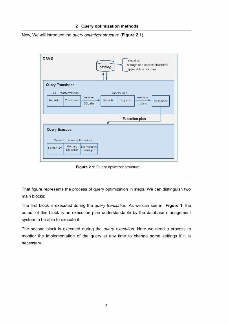
The query optimization belongs to two parts: Query translation and Query execution

(Figure 2.1). If we consider it as an integral object, we call it Query optimizer [5] [33].

The main goal of the query optimizer is to find the way to execute the query as quickly as

possible. Complex queries usually have too many ways to be solved, and because of that

it is a NP-hard problem for the query optimizer to find the best of those ways.

For that reason, the query optimizer is very important for the performance of a relational

database. It determines the best strategy for performing each query and it chooses, for

example, whether or not to use indexes for a given query, and which join techniques to

use when joining multiple tables. Those decisions have an important effect on SQL

performance.

2


During the optimization process, the query optimizer will make decisions among many

possible options. For instance, it must know what is the best access method for a table.

In the past, a ruled based method was the strategy used by the database management

system to be able to make those decisions. The goal of that method is just to apply rules

in order of preference. Imagine that we have a table and two different access methods to

access it. The first method will be called “AM1” and the second method will be called

“AM2”.

Each method has several preconditions. In that case, the query fulfill more preconditions

of AM1 than AM2. Hence, the system will choose the access method AM1 to access the

table.

There is another method of making decisions. This method uses mainly a cost-based

strategy instead of a ruled-based strategy. In a cost-based optimization strategy, multiple

plans are generated for a given query and then an estimated cost is computed for each

plan. The query optimizer chooses the plan with the lowest estimated cost. That is the

method used almost in all the contemporary database management systems. We will

explain it in more detail later.

3


Now, We will introduce the query optimizer structure (Figure 2.1).

That figure represents the process of query optimization in steps. We can distinguish two

main blocks:

The first block is executed during the query translation. As we can see in Figure 1, the

output of this block is an execution plan understandable by the database management

system to be able to execute it.

The second block is executed during the query execution. Here we need a process to

monitor the implementation of the query at any time to change some settings if it is

necessary.

4

Figure 2.1: Query optimizer structure


2.2 Query Translation

2.2.1 SQL transformation

There are many ways of writing the same query using the SQL language [35]. It is obvious

that all ways of expressing a query will not have the same performance; there will be

queries whose performance can be better than others.

Queries can be hand-written or machine-generated. It is almost certain that the query

produced by those methods will not be the most optimum possible.

On the one hand, queries generated by applications tend to follow some patterns and

rules [34], which produces queries that are too verbose: there are operations that could be

omitted.

On the other hand, although SQL is a declarative language, not implying any specific

query execution decision, most RDBMS provides optimization hints in the SQL language.

Moreover, there are often more than one way to write a query, and choosing one or

another may affect the performance. Unfortunately, a hand-written query usually is written

by users who do not know the best way to do it.

Because of these problems, the objective of the SQL transformations is to transform a

given SQL statement into a semantically equivalent sentence, which can provide better

performance.

Naturally, all changes must be completely transparent to the users. Most DBMS

implement a wide range of transformations, which can be divided into two categories:

heuristic query transformations and cost-based query transformations.

We will focus first on the heuristic query transformations. These transformations are

applied to the SQL statements as soon as possible. The transformations guarantee

performance equal or greater than the original statement.

5


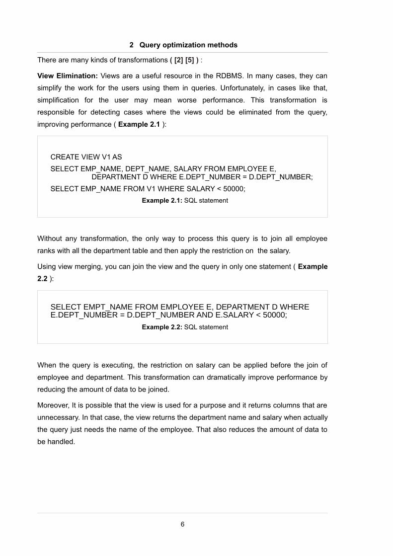
There are many kinds of transformations ( [2] [5] ) :

View Elimination: Views are a useful resource in the RDBMS. In many cases, they can

simplify the work for the users using them in queries. Unfortunately, in cases like that,

simplification for the user may mean worse performance. This transformation is

responsible for detecting cases where the views could be eliminated from the query,

improving performance ( Example 2.1 ):

Without any transformation, the only way to process this query is to join all employee

ranks with all the department table and then apply the restriction on the salary.

Using view merging, you can join the view and the query in only one statement ( Example

2.2 ):

When the query is executing, the restriction on salary can be applied before the join of

employee and department. This transformation can dramatically improve performance by

reducing the amount of data to be joined.

Moreover, It is possible that the view is used for a purpose and it returns columns that are

unnecessary. In that case, the view returns the department name and salary when actually

the query just needs the name of the employee. That also reduces the amount of data to

be handled.

6

CREATE VIEW V1 AS

SELECT EMP_NAME, DEPT_NAME, SALARY FROM EMPLOYEE E, DEPARTMENT D WHERE E.DEPT_NUMBER = D.DEPT_NUMBER;

SELECT EMP_NAME FROM V1 WHERE SALARY < 50000;

Example 2.1: SQL statement

SELECT EMPT_NAME FROM EMPLOYEE E, DEPARTMENT D WHERE E.DEPT_NUMBER = D.DEPT_NUMBER AND E.SALARY < 50000;



In reality, the elimination view method can be much more complex. There are cases

where it is difficult to detect if a view can be eliminated from the query or not. If the

RDBMS has an algorithm that doesn't detect many of those cases, the optimization will

not be optimal. For that reason, it is necessary to develop an algorithm to detect the

largest possible number of cases where views can be eliminated.

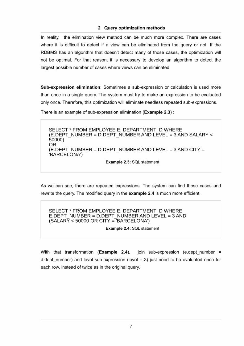
Sub-expression elimination: Sometimes a sub-expression or calculation is used more

than once in a single query. The system must try to make an expression to be evaluated

only once. Therefore, this optimization will eliminate needless repeated sub-expressions.

There is an example of sub-expression elimination (Example 2.3) :

As we can see, there are repeated expressions. The system can find those cases and

rewrite the query. The modified query in the example 2.4 is much more efficient.

With that transformation (Example 2.4), join sub-expression (e.dept_number =

d.dept_number) and level sub-expression (level = 3) just need to be evaluated once for

each row, instead of twice as in the original query.

7

SELECT * FROM EMPLOYEE E, DEPARTMENT D WHERE(E.DEPT_NUMBER = D.DEPT_NUMBER AND LEVEL = 3 AND SALARY < 50000)OR(E.DEPT_NUMBER = D.DEPT_NUMBER AND LEVEL = 3 AND CITY = 'BARCELONA')


SELECT * FROM EMPLOYEE E, DEPARTMENT D WHEREE.DEPT_NUMBER = D.DEPT_NUMBER AND LEVEL = 3 AND (SALARY < 50000 OR CITY = 'BARCELONA')



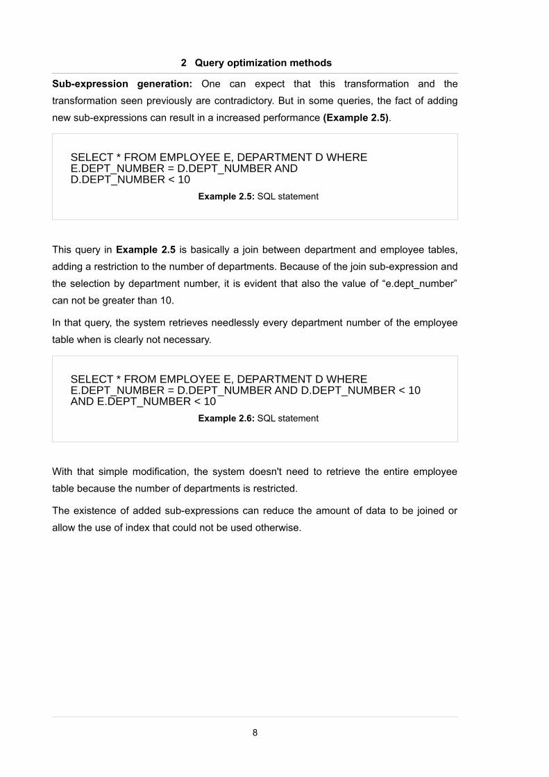
Sub-expression generation: One can expect that this transformation and the

transformation seen previously are contradictory. But in some queries, the fact of adding

new sub-expressions can result in a increased performance (Example 2.5).

This query in Example 2.5 is basically a join between department and employee tables,

adding a restriction to the number of departments. Because of the join sub-expression and

the selection by department number, it is evident that also the value of “e.dept_number”

can not be greater than 10.

In that query, the system retrieves needlessly every department number of the employee

table when is clearly not necessary.

With that simple modification, the system doesn't need to retrieve the entire employee

table because the number of departments is restricted.

The existence of added sub-expressions can reduce the amount of data to be joined or

allow the use of index that could not be used otherwise.

8

SELECT * FROM EMPLOYEE E, DEPARTMENT D WHEREE.DEPT_NUMBER = D.DEPT_NUMBER AND D.DEPT_NUMBER < 10


SELECT * FROM EMPLOYEE E, DEPARTMENT D WHEREE.DEPT_NUMBER = D.DEPT_NUMBER AND D.DEPT_NUMBER < 10AND E.DEPT_NUMBER < 10



Sub-expression moving: A complex query may contain multiple views and sub-queries

with many restrictions applied to them. A way to improve performance is to provide some

“flexibility” for those restrictions.

Following is a case with a single-table view (Example 2.7):

If the system realize that this view is used only in the following query:

The view could be simplified to process less data in the following manner:

First, instances are filtered by the number of departments and subsequently grouped.

That will reduce the amount of data to be grouped, because a small set of rows are

grouped.

9

CREATE VIEW DPT_SALARY AS SELECT

NUMBER_DEPARTMENT,AVG(SALARY) AS AVG_SALARYFROM EMPLOYEEGROUP BY NUMBER_DEPARMENT;


SELECT NUMBER_DEPARMENT, AVG_SALARY FROM DPT_SALARY WHERE NUMBER_DEPARMENT = 10;


CREATE VIEW DPT_SALARY AS SELECT

NUMBER_DEPARTMENT,AVG(SALARY) AS AVG_SALARYFROM EMPLOYEEWHERE NUMBER_DEPARMENT = 10GROUP BY NUMBER_DEPARMENT;



Until here, we have seen the heuristic query transformations. Now, we will focus in the

cost-based query transformation.

Unlike the transformations viewed previously, here you can not know at first glance if the

converted query performance is better than the original, for that reason the algorithm has

to evaluate estimating the costs of each option and choosing the most efficient.

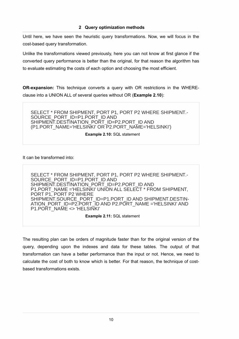
OR-expansion: This technique converts a query with OR restrictions in the WHERE-

clause into a UNION ALL of several queries without OR (Example 2.10):

It can be transformed into:

The resulting plan can be orders of magnitude faster than for the original version of the

query, depending upon the indexes and data for these tables. The output of that

transformation can have a better performance than the input or not. Hence, we need to

calculate the cost of both to know which is better. For that reason, the technique of cost-

based transformations exists.

10

SELECT * FROM SHIPMENT, PORT P1, PORT P2 WHERE SHIPMENT.-SOURCE_PORT_ID=P1.PORT_ID AND SHIPMENT.DESTINATION_PORT_ID=P2.PORT_ID AND (P1.PORT_NAME='HELSINKI' OR P2.PORT_NAME='HELSINKI')


SELECT * FROM SHIPMENT, PORT P1, PORT P2 WHERE SHIPMENT.-SOURCE_PORT_ID=P1.PORT_ID AND SHIPMENT.DESTINATION_PORT_ID=P2.PORT_ID AND P1.PORT_NAME ='HELSINKI' UNION ALL SELECT * FROM SHIPMENT, PORT P1, PORT P2 WHERE SHIPMENT.SOURCE_PORT_ID=P1.PORT_ID AND SHIPMENT.DESTIN-ATION_PORT_ID=P2.PORT_ID AND P2.PORT_NAME ='HELSINKI' AND P1.PORT_NAME <> 'HELSINKI'



2.2.2 Execution plan generation

The output of the previous step, which is an optimized rewritten SQL statement, will be the

input to the “Execution plan generation” step responsible for processing that input and

getting the most efficient execution plans.

As you can see in Figure 2.1, the step is comprised of two distinct parts. In the first part,

the syntactical tree is created and optimized. The second part is a method where the

physical optimization are applied and the best execution plans are generated.

The syntactic part consist of translating the sentence from SQL into a sequence of

algebraic operations. There are many possible methods for this algebraic process [4].

In this work, it will be explained from the perspective of a syntax tree [2].

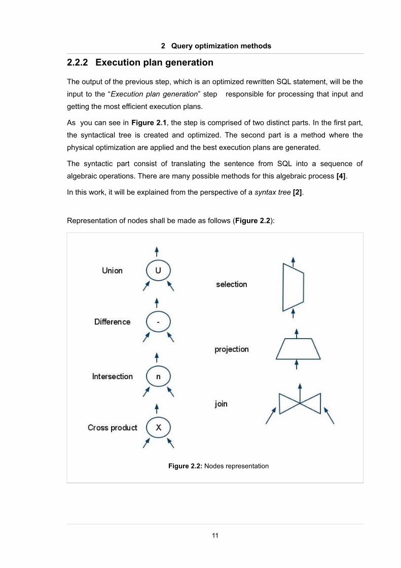
Representation of nodes shall be made as follows (Figure 2.2):

11

Figure 2.2: Nodes representation


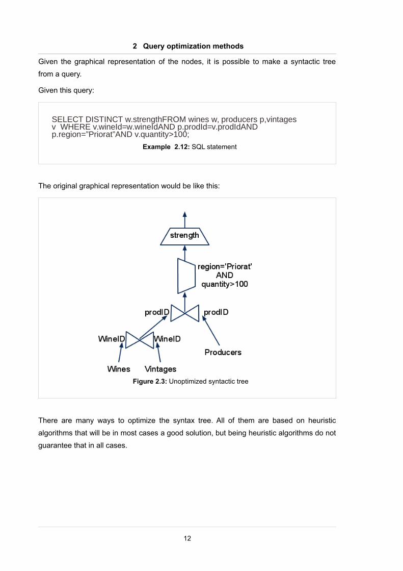
Given the graphical representation of the nodes, it is possible to make a syntactic tree

from a query.

Given this query:

The original graphical representation would be like this:

There are many ways to optimize the syntax tree. All of them are based on heuristic

algorithms that will be in most cases a good solution, but being heuristic algorithms do not

guarantee that in all cases.

12

SELECT DISTINCT w.strengthFROM wines w, producers p,vintages v WHERE v.wineId=w.wineIdAND p.prodId=v.prodIdAND p.region=”Priorat”AND v.quantity>100;


Figure 2.3: Unoptimized syntactic tree


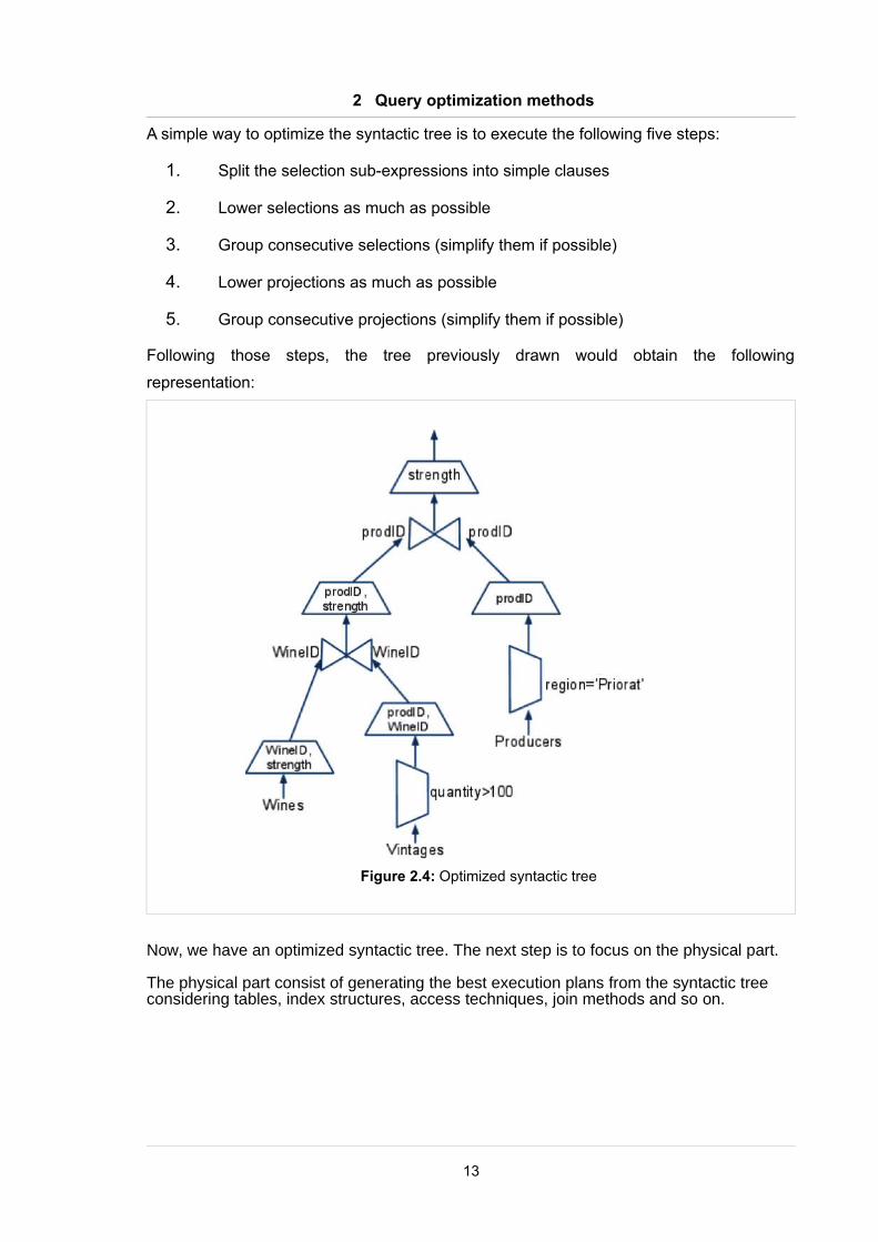
A simple way to optimize the syntactic tree is to execute the following five steps:

1. Split the selection sub-expressions into simple clauses

2. Lower selections as much as possible

3. Group consecutive selections (simplify them if possible)

4. Lower projections as much as possible

5. Group consecutive projections (simplify them if possible)

Following those steps, the tree previously drawn would obtain the following

representation:

Now, we have an optimized syntactic tree. The next step is to focus on the physical part.

The physical part consist of generating the best execution plans from the syntactic tree considering tables, index structures, access techniques, join methods and so on.

13

Figure 2.4: Optimized syntactic tree


Some of the most important processing techniques are explained below [5]:

Join Ordering

When joining a large number of tables, the space of all possible execution plans

can be extremely large and it would be impossible for the optimizer to explore all

the options. For example, a query joining 5 tables has 5! = 120 join order

permutations. After that, for each permutation there is even more possibilities

depending on different combination of indexes, access methods and so on.

Definitely, to analyze all the options with only 5 tables is quite time-consuming.

Considering that 5 tables is a little number, one can imagine the possibilities with

more than 10 tables. Therefore, it’s necessary for the optimizer to use an heuristic

method in the exploration of the possible execution plans rather than brute force

[6].

Access Path

In a single table or a join table, you need to calculate the costs of all the access

path methods that are available for the table and then choose the one with better

performance. More information in [7].

Materialization or not of intermediate result

Materialized results can provide improvements in query processing time, especially

for queries with high cost requirements. To realize this potential, the query

optimizer must know how and when to exploit materialized results. A bad decision

can cause a significant loss of performance. Some concepts about that are

explained in [8] [23].

14


Partition optimizations

By partitioning the data it is possible to access it more quickly because of exploring

smaller modules of information.

If the technique is not used properly, it could be counterproductive. Poor

management of partitions may cause access to too many partitions, causing poor

performance.

For example, consider a table of sales. This table is partitioned by month. If we

want to know the sales in the last two months, the most efficient way to access is

retrieving only the partitions for the last two months. With this solution, the data

retrieved is exactly the data that we want, no more. With other methods or with a

bad partition system, the system would retrieve no relevant information, and in the

worst case, all the data [9].

Sort elimination

Taking into account that sorting of a large amount of data is an operation with a

high cost, it´s very important to eliminate the unnecessary sorts that we can find in

a query.

Parallel execution

Parallel execution is the ability to apply multiple resources to the execution of a

single SQL statement. Parallelism is a fundamental capability for managing large

data sets.

15


2.2.3 Cost model

The cost model step takes multiple execution plan as input. The goal of it is to choose the

best and most efficient execution plan, calculating the cost of each one and choosing the

one that has lower cost. Certainly, it is difficult to know the real cost of an execution plan.

For that reason, it is very important to get a good cost model process [10].

The global cost of an execution plan is the sum of costs of each physical operation. The

cost of each physical operation is the sum of the cost of calculating the operation and the

cost of writing its result.

The most important factors to consider are:

• CPU

• Memory access time

• Disk access time (Number of disk page touches)

The cost model is a complex component. In addition to considering these factors, it is also

vital to consider the performance effects of caching, access times on memory and on disk,

parallelism and so on.

In addition, there is no single definition of costs. Consider that for certain applications the

most important thing is to show as quickly as possible the first rows, while for other

applications the most important thing is to get all rows as quickly as possible. This

difference in behavior must also be considered when calculating the cost, as is quite

possible that depending on this execution one must choose one plan or another.

16


2.3 Query Execution

The workload of a database changes over time. If the query optimization process is only in

query translation, it does not consider changes that may arise in the database at any time

and it is possible that the configuration chosen statically at a particular time is not the most

optimal at another time.

For that reason, it is very important to expand the query optimization process to the query

execution time to change the settings to the best possible if the database is in a different

state [11].

That optimizer is composed of many parts, but the most notable to the topic of this thesis

is the degree of run-time parallelism. By run-time parallelism we mean it is a dynamic

parallelism which could be change meanwhile query execution.

The method of parallelizing is useful to improve response time of a query in a

multiprocessor hardware. However, a big degree of parallelism can be counterproductive.

For example, if we assign to a operator more resources that it needs, we are wasting

resources that could be needed for other operations at the same time, decreasing the

performance in such operations.

Among other factors, the degree of parallelism is adjusted to the amount of resources

available to the system at that time. An estimated amount of parallelism can be statically

assigned, but it is important that it can vary dynamically during the execution

For example, we have a system with five resources. We use the term “resource” to refer

without distinction a software thread, physical thread, core, processor or node, avoiding by

this way the level of granularity.

In a particular moment, there are 3 resources busy and 2 resources free, therefore the

degree of parallelism is set to 2 because there are no more resources available.

If some resources are released in the execution time, to consider dynamic level of

parallelism could increase the degree of parallelism of the query to increase performance.

Without the dynamic optimizer would be wasting resources and having a poorer

performance.

17

3 In-memory databases


In this section, We will expose a brief description of in-memory databases. Moreover, it

will be compared against the traditional database management system. This information is

based on several papers that will be referenced throughout the section.

3.1 Introduction

The semiconductor memories are lowering their price constantly and increasing data

capacity. Therefore, it is an increasingly feasible option to have a database stored in main

memory. Moreover, memories are becoming faster. That causes the main memory

databases can be larger and more efficient.

The information in a in-memory database is accessible directly in main memory and it

provides a better response time compared to a traditional database. That is especially

important for real time applications where transactions must be completed almost

instantaneously [40].

Definitely, in-memory databases are a solution to take into account. For more information

about that kind of databases see [12]:

3.2 In-memory against traditional databases

In a traditional database management system (DRDBMS), the data is normally stored on

disk. But in that system, the data is also cached in main memory, in a shared page buffer

pool to access it faster. So, DRDBMS uses also main memory to improve its performance

[37].

In contrast, in a in-memory database management system (MMDBMS), the data is

normally stored in main memory. But that system also uses the disks to solve some

physical main memory problems. Basically, MMDBMS uses disk to keep a checkpointed

database and keep the logs.

Summarizing, main memory and disk are used in both management systems. Basically,

the difference is which is used as main storage and which as support storage.

18


3.2.1 Physical comparison

Main memory and magnetic disks have intrinsic physical differences. Those differences

cause also differences when we are designing and improving the performance of the

database system. The most important differences are exposed below [12]:

• The access time to main memory is orders of magnitude less than for disk storage.

• The main memory is usually volatile. The disk storage is persistent instead.

• The disks have a high fixed-cost access that do not depend on the amount of data

that is collected in those accesses. For that reason, disks are block-oriented while

the main memory is not it.

• Sequential access is not important in main memory, while on disk is a useful

strategy.

• The main memory is usually directly accessible by the processors. For that reason,

the data in main memory is more vulnerable than the data resident on disk.

Because a software error, not necessary related to the database, could affect to

memory address that we are using to retrieve data.

3.2.2 Implementation differences

We will explain here the more notables differences between DRDB and MMDB [13].

Concurrency Control

The access time in main memory is less than on disk. Therefore, transactions are

completed much more faster in a MMDB. Systems that are using lock-based

concurrency controls will be less time blocked, so the contentions will not be so

important.

Commit processing

To protect against failures, it is necessary to have a database checkpoints and

keep a log of transactions to allow recovery. That log must be kept in a stable

storage device.

The system must write the transaction in the log before the transaction is executed.

Taking into account that the log should be stored synchronously on disk, that

access could be a major bottleneck.

19


The best solution to that problem is to have a small amount of stable main memory

to store a portion of the log temporarily. So, when the transaction is ready to run,

the log is stored in this small stable memory and later, an auxiliary resource is

responsible for storing those pages in the corresponding log record on disk.

Access Methods

Index structures like B-trees have been designed for conventional databases.

Those structures for a main memory database becomes less efficient because of

the physical differences between main memory and disk. There is a wide variety of

index structures for main memory databases. Those include indexes based on

hashing and trees.

For example, the T-tree is a balanced tree structure used in MMDMS. It is an

evolution of AVL-tree and B-tree [13].

The AVL-tree was designed as an internal structure of data. Updates always affect

a leaf node, and may result in an unbalanced tree, so the tree is kept balanced by

rotation operations. However it has a big disadvantage: the poor data storage.

Each node keeps only one data item, so there are two pointers and control

information for each data item.

The T-tree is a binary tree with many elements per node. It has the AVL-tree

search engine behavior and, taking into account that T-node contains many

elements, the T-tree has a good update and storage system inherited from the B-

tree.

When we have an insertion or deletion of data, that modification could affect the

node structure and the tree could become unbalanced and inefficient ordered

because of this structure modification. For that reason, it is necessary to

redistribute the data of the tree in such operations. This redistribution of the data is

called “Rebalancing”, and it is done using rotations like in AVL-tree.

A common characteristic of the all main memory access data methods is that

values are not stored in the index itself, as if occurs with the b-tree structure,

because random access is much faster in main memory. Therefore, the index

should only store a pointer to memory instead of the data. That eliminates the

problems of different length fields and also it saves space because it normally

takes less space to keep the pointer than to keep the data.

20


Pointers

The use of pointers in a very important advantage in main memory databases. The

access methods that we have seen before are a good example of how important

they are. Furthermore, the use of pointers can save space because if a large value

appears multiple times in the database, it is only necessary to store the data once

and use pointers after that.

Query Processing

In the case of main memory databases, the query processors must have a different

behavior. In that case we have to focus on reducing the processing costs, whereas

in a conventional database most important thing is to reduce disk accesses.

A major difficulty for the query processors is to predict costs. It is even more

difficult in that case because it is more difficult to predict the cost of CPU

processing than the cost of disk accesses. Those costs can vary from one system

to another making it more difficult to develop optimization techniques that suits all

systems.

Performance

The performance of a main memory database is very dependent on processing

time and less of disk accesses. Instead, there are things you need to take greater

account than in a conventional system. One example is the creation of backups. In

a conventional system is not a important function to note, however in the MMDB,

being something that is done often , it should be borne in mind and try to optimize

it as much as possible [40] [41].

21


3.3 Making the choose between MMDB and DRDB

In the previous section, we realized that there are many differences between MMDB and

DRDB. Actually, there is no better than other, just different. For some cases it will be better

to use a MMDB, and for other cases it will be better to use a DRDB [39].

MMDB would be most useful in applications which require a very short response time.

Instead, DRDB would be most useful when the data volume is larger than the main

memory available.

There are many cases where an application has a lot of data but only a few items are

accessed frequently. For those cases, the right solvetion is to have a MMDB for frequently

accessed data and DRDB for the large volume of information that is accessed

infrequently.

The data handling between both DBMS could be a problem, because you have

databases belonging to DRDBMS and also different databases belonging to MMDBMS.

If you do not need to share data between MMDB and DRDB, the data would be

completely disjoint. In that case, there is no data communication between them and

managing them become easier.

Unfortunately, databases can also be partially integrated. It means that there are cases

that a MMDB should share some data with a DRDB. In that case, we have to take into

account the data handling between them. Note that this communication is a complicated

process if you want to have a system with a good performance.

The best way for understanding the combination between MMDB and DRDB is explaining

a brief example. A simple case might be a banking case.

The data relating to the account of customers, such as balance, are very frequently used

data. However, data such as the customer address are rarely used. In that case, It is a

good choice to keep the data frequently accessed in a MMDB and keep the data rarely

used in a DRDB.

There are solutions like SolidDB [38] that allows to configure which method (in-memory or

on disk) will be used for each table, giving more flexibility and avoiding the need of use

two DBMS.

Another solution is the mixed DBMS. Until now, we have seen two types of DBMS:

MMDBMS and DRDBMS. But we can modify the configuration of DRDBMS to be closer to

MMDBMS and vice versa. We will see two examples below:

22


3.3.1 Traditional database with a large cache

“Cache” is a component that transparently stores data so that future requests for that data

can be served faster [32].

If cache in a DRDBMS is large enough, data will reside in memory all the time, and

performance would be similarly to MMDBMS. However, without a well optimized system

for main memory, will not be taking full advantage of memory access [37].

For example, the index structures in a DRDBMS are designed for disk access, although

the data is in memory. Hence, the performance would be better with structures designed

specially for main memory.

3.3.2 Persistent and durable in-memory database

The main memory is a volatile memory that needs a constant voltage to retrieve the data,

if that voltage turns off we automatically lose all the data. Because of that, the global

probability of failure increases because we need to add the probability of failure of the

system which provides that voltage.

A hardware improvement could be to install a independent power supply system which

provides voltage to the memory, making sure that this system is providing voltage all the

time.

By that way, we could have a MMDBS with less probability of failure and higher durability.

23

4 Parallel query processing


In this section, we will expose a description of parallel query processing. That is the

main subject of this study. By “resource” we mean a processor, core or thread, without

distinction.

4.1 Introduction

Highly parallel computers are the present and the future of large and fast databases. The

reason is parallel machine can be constructed at a low cost without any specialized

technology. It means that we do not need to spend money in specialized and usually

expensive hardware because we can use generic computer technology and cheap

interconnection networks.

Parallelism has two great attributes in an ideal case. The first one is the linear speedup

where adding N resources reduces response time by a factor of N. The second one is the

linear scaleup where adding N times as many resources allows the system to run N times

bigger load in the same amount of time.

Unfortunately, that is in an ideal environment and in a real environment is not linear

because of two basic problems: unbalanced load [24] and contention.

Two architectures have emerged trying to solve these problems for achieving a linear

speedup and scaleup: shared-nothing and shared-everything. Those parallel system

architectures are completely opposites in terms of sharing information among resources.

There are also intermediate architectures such as shared-disk [22]. That one is also very

important architecture but we will focus the attention just in shared-nothing and shared-

everything [15] [20] [21].

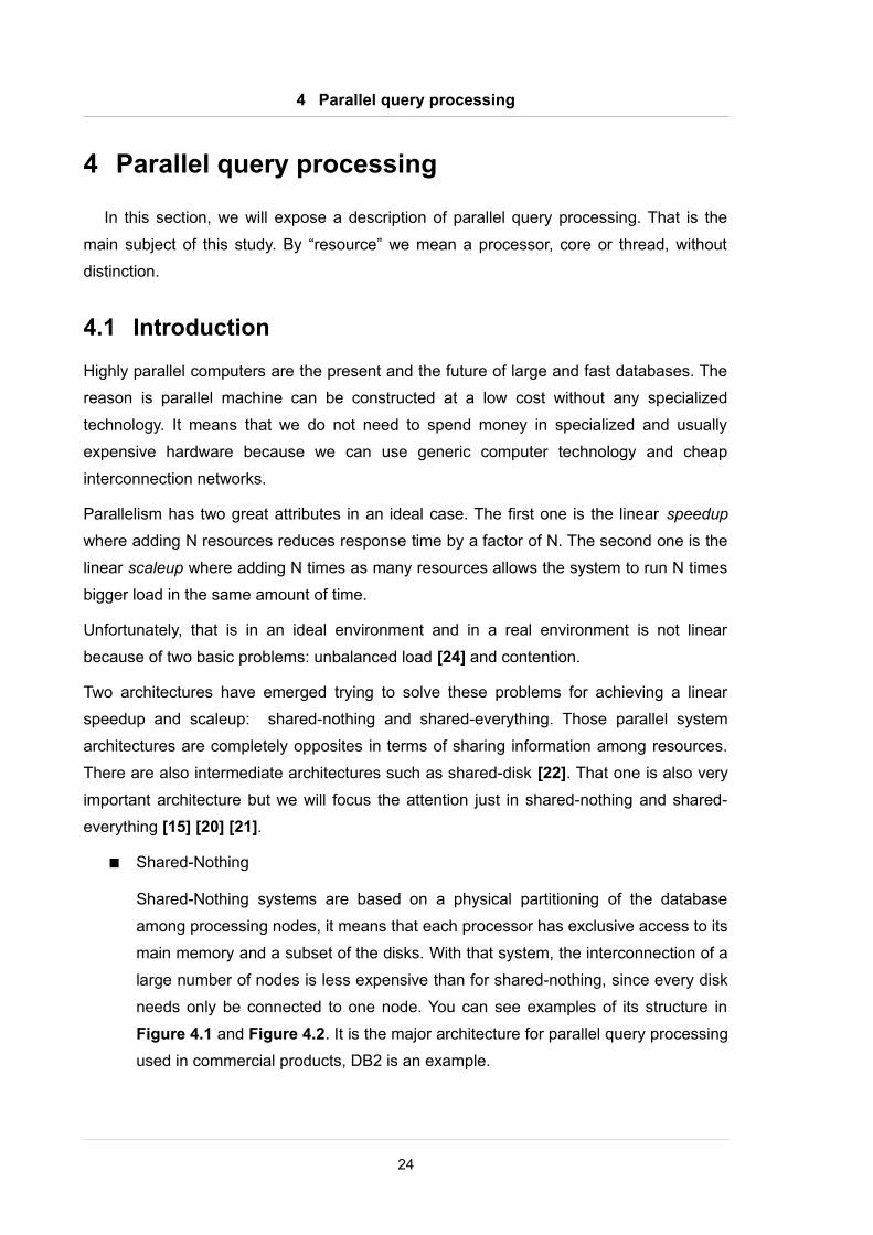
Shared-Nothing

Shared-Nothing systems are based on a physical partitioning of the database

among processing nodes, it means that each processor has exclusive access to its

main memory and a subset of the disks. With that system, the interconnection of a

large number of nodes is less expensive than for shared-nothing, since every disk

needs only be connected to one node. You can see examples of its structure in

Figure 4.1 and Figure 4.2. It is the major architecture for parallel query processing

used in commercial products, DB2 is an example.

24


The query execution in shared-nothing systems is distributed if the access to

different partitions is needed. Of course, the communication among partitions is

required.

Shared nothing architectures solve scalability and availability problems by reducing

interference among processors. Unfortunately, load balancing is harder in that

systems and find a efficient fragmentation and allocation is a challenge and it has

a profound impact on performance. Moreover, variations of the number of nodes

requires also a reallocation of the database.

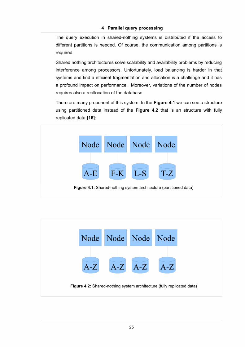
There are many proponent of this system. In the Figure 4.1 we can see a structure

using partitioned data instead of the Figure 4.2 that is an structure with fully

replicated data [16]:

25

Figure 4.1: Shared-nothing system architecture

Node Node Node Node

A-E F-K L-S T-Z

Figure 4.1: Shared-nothing system architecture (partitioned data)

Node Node Node Node

A-E F-K L-S T-Z

Figure 4.2: Shared-nothing system architecture (fully replicated data)

Node Node Node Node

A-Z A-Z A-Z A-Z


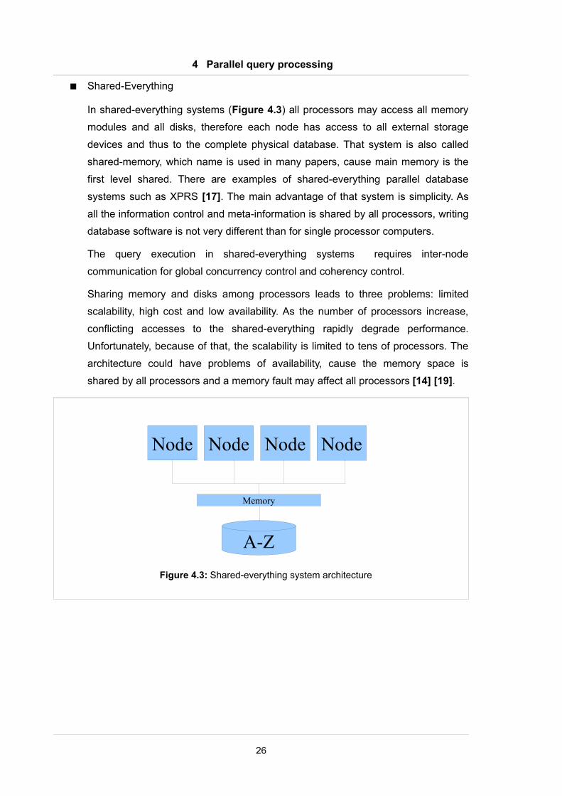
Shared-Everything

In shared-everything systems (Figure 4.3) all processors may access all memory

modules and all disks, therefore each node has access to all external storage

devices and thus to the complete physical database. That system is also called

shared-memory, which name is used in many papers, cause main memory is the

first level shared. There are examples of shared-everything parallel database

systems such as XPRS [17]. The main advantage of that system is simplicity. As

all the information control and meta-information is shared by all processors, writing

database software is not very different than for single processor computers.

The query execution in shared-everything systems requires inter-node

communication for global concurrency control and coherency control.

Sharing memory and disks among processors leads to three problems: limited

scalability, high cost and low availability. As the number of processors increase,

conflicting accesses to the shared-everything rapidly degrade performance.

Unfortunately, because of that, the scalability is limited to tens of processors. The

architecture could have problems of availability, cause the memory space is

shared by all processors and a memory fault may affect all processors [14] [19].

26

Figure 4.3: Shared-everything system architecture

Node Node Node Node

A-Z

Memory


In recent years, the computer industry have been developing hardware focusing on high

physical parallelism exposed in the form of multiple processors, cores or hardware

threads. Those systems are intrinsically shared-everything systems.

Many researchers consider Shared-Nothing as the major architecture for parallel query

processing. In my opinion, the best option would be an intermediate architecture with

different sharing levels, where the parallel threads in the same processor would share

everything, where processors in the same computer would share only disks and where

among computers would use a shared-nothing architecture.

Unfortunately, that system would be too complex and it is not clear that could have an

improved performance.

27


4.2 Parallelism operator types

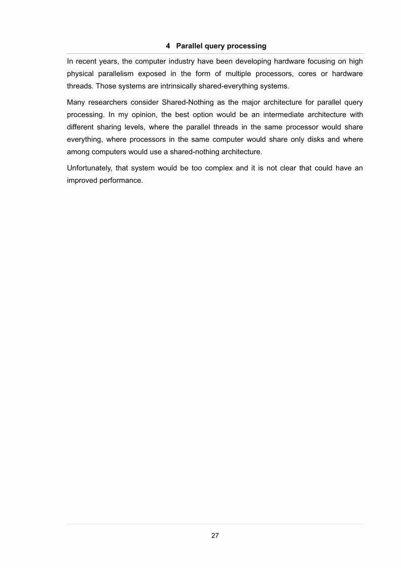
We can find two forms of parallelism: Intra-operator and Inter-operator.

By intra-operator parallelism we mean that an operation is parallelized over several

resources, and inter-operator parallelism is when several operations are executed

concurrently.

There are two forms of inter-operator parallelism: independent and pipelined. Independent

means that no dependencies exist between operations and pipelined refers to a producer-

consumer relationship between operators.

The three forms of parallelism are explained below in more detail.

4.2.1 Intra-operator parallelism

Intra-operator parallelism [31] is a well established technique to increase system

performance. This technique is about partitioning the data and storing it into different

memory spaces, and every partition of data can be processed by different resources.

Furthermore, it means that an operator is divided into many independent operators where

each one works with subset of the data (Figure 4.4).

However, it is a NP-hard problem how the intra-operator parallelism should be used in a

multi-query environment, where there is concurrence. Selecting low degrees of operator

parallelism can lead to underutilization of the system and reduced performance. On the

other hand, high degrees of parallelism can give too many resources to a single query and

28

Figure 4.4: Intra-operator

Scan A Scan B

Join

Result


lead to high resource contention. Therefore, we must know how to choose a good degree

in each case.

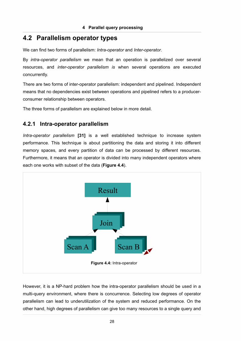
4.2.2 Pipelined inter-operator parallelism

We mean pipelined inter-operator parallelism when two operators execute as a producer-

consumer pair at the same time.

In the figure below (Figure 4.5), we can see two producers (Scan A and Scan B). For

applying a pipelined inter-operator in this case, Scan A, Scan B and Join operators have

to be executed in parallel at the same time [18].

If we want to use a pipelined parallelism, we need to choose in some step which

technique we want to use to communicate a producer-consumer relationship. We have

two options: materialization or pipelining.

The best option is to use pipelining to achieve a better performance. Unfortunately, we can

not use pipelining in all cases because of two problems.

The first one is the possibility of a unpredictable output from the producer. That could

happens for many reasons; for example, the producer could be running other process

during an interval of time, losing priority our task. This leads to irregular patterns of idle

time for the consumer.

The second problem is long pipeline chain of operations. Long chains can cause a

propagation delay from the first consumer to the last producer.

29

Figure 4.5: Pipelined inter-operator

Scan A Scan B

Join

Result


Furthermore, we need a good algorithm to try to find the best combination. The best

combination could be different depending what you need; whether you want a better

throughput or response of time.

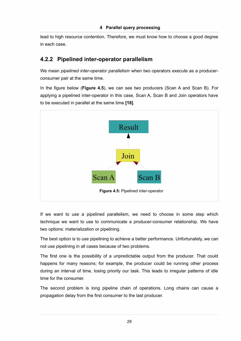
4.2.3 Independent inter-operator

The operations with no path between them usually can be executed on a set of resources

independent of each other. For example, in Figure 4.5, operations Scan A and Scan B can

be executed in parallel, whereas the join operation must await the completion of them

[18].

30

Figure 4.6: Independent inter-operator

Scan A Scan B

Join

Result


4.3 Parallelism management

This section is based on several papers [25] [26] [27] [28] [29]:

4.3.1 Operator tree

The execution plan is not an appropriate representation to manage parallelism because

we need a representation with higher granularity to be able to have more possibilities of

parallelism. For that reason, the first step in the parallelism process is to transform the

execution plan into a more basic form called operator tree.

The resource allocation methods proposed in several papers [26] [28] [29] uses that

method of tree decomposition to divide a the query operations in schedulable

components.

The first step is how to decompose the tree. One method is refining each node into a sub-

tree of physical operator nodes, each of these nodes will be an atomic component [26].

We can see some examples below:

• Scan: an operation that scans the entire table. It can use selections, projections,

etc.

• Sort: sorts the input

• Hash: Built a hash table from the input

• Probe: uses input to probe a hash table, hits are the output

• Merge: merges two sorted inputs

• Nested-Loops: Compares each row of one table against all rows in another table.

31


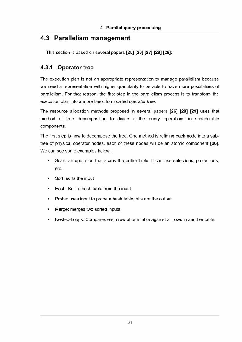
These components can be combined to form more complex operations. Combining these

operators is possible to achieve an operator tree equivalent to any execution plan. For

example, two sorts and a merge can be put together to create a sort-merge join (Figure

4.7):

These join of two tables would be also represented as:

“merge(sort(scan(T1)),sort(scan(T2)))”.

32

Figure 4.7: sort-merge join

scan

scan sort

sort

merge


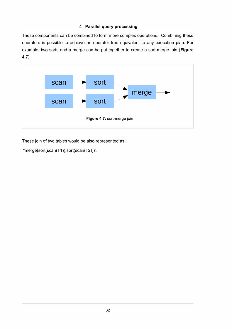
In the next figure (Figure 4.8), we have the execution plan of a query:

33

Figure 4.8: Execution plan

Hash-join

Merge-join


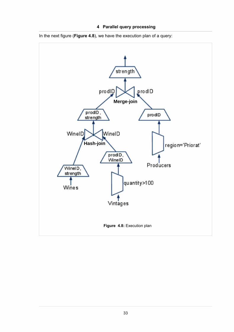
We can see the equivalent operator tree below (Figure 4.9):

The last step is this section is to calculate an approximate cost value for each operator in

the operator tree, determining its individual resource requirements using hardware

parameters, DBMS statistics and conventional optimizer cost models [26].

34

Figure 4.9: operator tree

scan

Wines

scan

Vintages

scan

Producers

hash

probe

scan

sortsort

merge


4.3.2 Decomposing the operator tree

An operator tree is composed by a set of operations. The operations are interconnected to

each other, sending information to the next operator and receiving information from one or

more child operators.

There are two ways to make possible the communication among operators:

materialization and pipelining [26] [28].

A materialized communication indicates that the child operator completes, and its entire

result is materialized before the parent operator begins. A pipelined communication means

that the two operators execute as a producer-consumer pair. That is exactly the pipelined

intra-operator that we have seen in the section 4.2.2.

In an operator tree (Figure 4.9), the pipelined communication is represented as a solid

edge between two operators and the materialized communication is represented as a

dashed edge between two operators.

In every situation, we would like to use pipelining communication, also called pipelined

inter-operator parallelism. Unfortunately, there are situations that is not possible to use it

and the only option is to use materialization.

Materialized communication is required when the input to an operation must be complete

prior to the start of the operation. For example, the hash table generated by a hash

operator has to be completely built before its utilization, therefore in this case is

compulsory to use materialization. We also need to use materialization in situations where

it is difficult to estimate the proper buffer size for the pipeline or when high variability

producers and consumers will require large amounts of memory to handle the worst case.

Once we know the type of communication used for every edge in the operator tree, we

can decompose the tree in a set of tasks. It is necessary to know the type of

communication between operators because the materialized edges will be the split points.

35


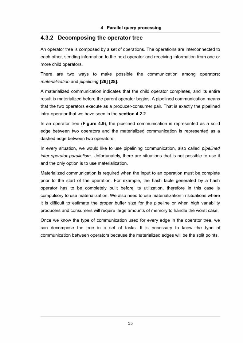
The operator tree is decomposed into a set of components by breaking it at each

materialized edge. Therefore, resulting components are a single operation or a pipelined

chain of operators. In the Figure 4.9, we saw an operator tree as sample. We can see that

operator tree decomposed in the next figure:

In the figure, tasks are numbered to be easier to reference them in the next sections.

36

Figure 4.10: operator tree decomposed

scan

Wines

scan

Vintages

scan

Producers

hash

probe

scan

sortsort

merge

1

2

4

3

5


4.3.3 Dependency graph

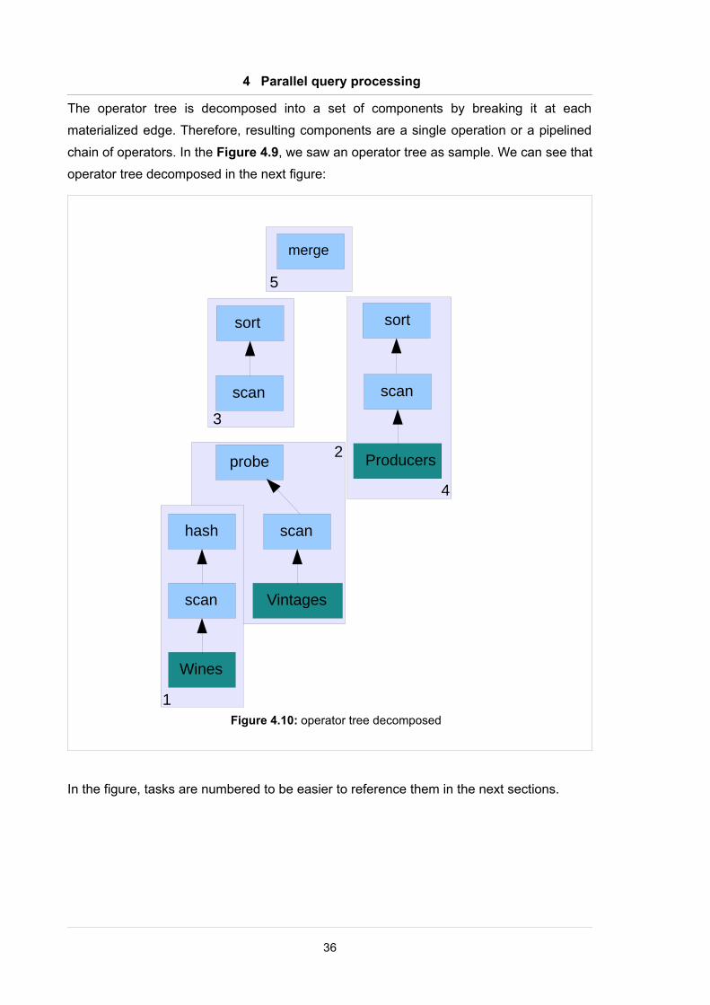
The goal in this section is to develop a high level schedulable structure from the operator

tree [26]. At this point, we have an operator tree decomposed into different parts, also

called schedulable tasks. Those tasks are connected with other parts using materialization

and the operators within a part are connected using pipelined parallelism.

As the operators inside a task are connected using pipelined parallelism, there are no

dependencies among them. Therefore, task will be the atomic object in the dependency

graph, because there are no dependencies inside of it.

The next figure contains the graph related to the operator tree that we have seen before:

37

Figure 4.11: dependency graph

1

2

4

3

5


4.3.4 Schedule process

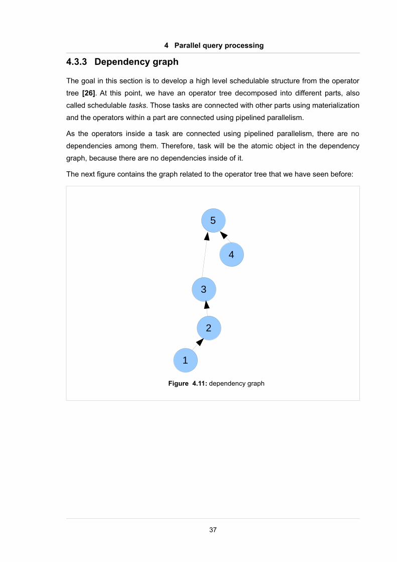
Since each task ends with a materialized edge, our rule is that the children of a task must

be finished prior to the task starting.

In order to schedule tasks, the first step is to assign a theoretic cost for each task. There

are many ways to calculate the cost of a task [26] [29].

This work estimate is based on the amount of work done by a single resource.

At this point, we have a graph with a cost assigned to each item. You can see an example

below:

38

Figure 4.12: dependency graph with costs

1

2

4

3

5

C1= 150

C2= 100

C3= 90

C4= 80

C5= 200


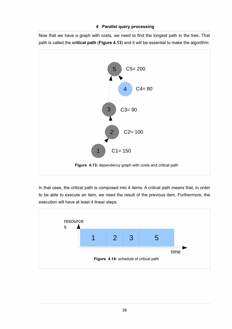
Now that we have a graph with costs, we need to find the longest path in the tree. That

path is called the critical path (Figure 4.13) and it will be essential to make the algorithm:

In that case, the critical path is composed into 4 items. A critical path means that, in order

to be able to execute an item, we need the result of the previous item. Furthermore, the

execution will have at least 4 linear steps.

39

Figure 4.13: dependency graph with costs and critical path

1

2

4

3

5

C1= 150

C2= 100

C3= 90

C4= 80

C5= 200

Figure 4.14: schedule of critical path

time

resources

1 2 3 5


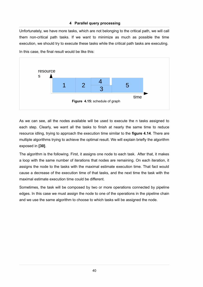
Unfortunately, we have more tasks, which are not belonging to the critical path, we will call

them non-critical path tasks. If we want to minimize as much as possible the time

execution, we should try to execute these tasks while the critical path tasks are executing.

In this case, the final result would be like this:

As we can see, all the nodes available will be used to execute the n tasks assigned to

each step. Clearly, we want all the tasks to finish at nearly the same time to reduce

resource idling, trying to approach the execution time similar to the figure 4.14. There are

multiple algorithms trying to achieve the optimal result. We will explain briefly the algorithm

exposed in [30].

The algorithm is the following. First, it assigns one node to each task. After that, it makes

a loop with the same number of iterations that nodes are remaining. On each iteration, it

assigns the node to the tasks with the maximal estimate execution time. That fact would

cause a decrease of the execution time of that tasks, and the next time the task with the

maximal estimate execution time could be different.

Sometimes, the task will be composed by two or more operations connected by pipeline

edges. In this case we must assign the node to one of the operations in the pipeline chain

and we use the same algorithm to choose to which tasks will be assigned the node.

40

Figure 4.15: schedule of graphtime

resources

1 23

54


To summarize, there are three types of parallel execution:

Intra-operator

When two or more nodes are assigned to a task with a single operator or to an

operator within a task with pipelined operators, we will apply the intra-operator

parallelism.

Pipelined Inter-operator

If we have enough nodes to assign at least one to every operator in a task with

pipelined operators, we are applying the pipelined inter-operator parallelism.

Independent inter-operator

The execution of two or more tasks in the same step is a parallel inter-operator

parallelism.

There are situations where we can achieve better performance using only one or two of

these three techniques. Fortunately, you can make a few changes in this algorithm to

achieve a reduced parallelism functionality.

For example, if we want to use only the inter-operator parallelism, including independent

and pipelined, we just need to do a small modification in the algorithm: An operator can

only have assigned one resource at most. With that limitation, we do not have intra-

operator parallelism because we need more than one resource per operator to use this

parallel technique.

We can reduce even more the parallelism using only the independent inter-operator. For

that, we only need to add another restriction: A task can only have assigned one resource

at most.

Unfortunately, there are other technique combinations that are not possible to achieve

with this algorithm. For example, we can not use only the intra-operator parallelism. For

that, we would need to use other algorithms mainly based on intra-operator [31].

41


4.4 An approach of parallel query for SMP systems

A different approach to apply parallelism in the query optimization is presented in [20].

That approach is especially focused in modern SMP systems, because it takes into

account the emerging technology changes produced by the newest hardware.

Fundamental concepts of task identification and resource scheduling needed to be revised

by a new approach. Because of that, the main goal of this method is to reduce the amount

of necessary synchronization among the execution threads and facilitate load balancing

among the resources.

4.4.1 Introducing ASYNC operator

In this approach, the parallelism is performed by a new operator called ASYNC, which

enables the communication between resources.

An ASYNC operator is a transparent method of parallelism. It means that it has no side-

effect compromising the functional integrity of the query execution plan. Because of that,

an ASYNC operator can be placed between any pair of operators without any problem,

facilitating multiple forms of parallelism. Moreover, we can use the existing operators,

explained in section 4.3.1, without any modification.

The data is transferred through an ASYNC operator from one resource to another.

Exchange of data over resources is done via a buffer that is encapsulated and operated

on by every ASYNC operator and access to this buffer is synchronized.

Unfortunately, the synchronized communication could produce an overhead between

consumer and producer. In order to minimize that problem, the buffer is not locked for

every row insertion, but it is divided equally into some partitions. Consumer and producer

need to be synchronized only when they acquire access to a new partition. By this way,

one resource can switch partitions without having to wait for other resource, because one

resource can write in one partition while other resource is reading another.

Experimental results have confirmed that partitioning into three parts is optimal for a

common database operations.

42


4.4.2 Applying Inter- and Intra-operator parallelism

Inter-operator parallelism can be easily modeled with this approach by simply inserting

ASYNC nodes into the operator tree. There are positions where the ASYNC node could

not be effective because of the dependencies among operators. Therefore, the algorithm

has to know where are the better positions to insert an ASYNC node.

Moreover, we need to manage the resources, which will be assigned to different tasks

along the operator tree execution. For that, the system maintains a pool of worker

resources. Resources from this pool can be assigned to all sorts of tasks. If the operation

is completed, the ASYNC operator is closed, the resource will return into the pool where it

can be reused for another task.

Intra-operator parallelism is modeled by identifying pipeline fragments in the operator tree

that are suitable for parallel execution. These fragments are enclosed by two ASYNC

nodes. Each of these fragments is logically replicated and its clone is executed in parallel

as a data pipeline. At each resource a partitioned buffer is installed.

The lower ASYNC node acts as data partitioner, it distributes its input data among the

pipelines output buffers. And the upper ASYNC will then arrange its output along this

sequence, thereby preserving the original order.

4.4.3 Query optimizer implementation

Similarly to the previous approach, you can apply both static and dynamic parallelism.

In the implementation, we need to take into account two factors:

The total size of memory available per ASYNC operator. Every ASYNC operator requires

a buffer for inter-thread communication. If this buffer is chosen too small, a lot of

synchronization has to be performed when large amounts of data are passed through it. It

the buffer is too large, memory might be wasted.

The maximum number of parallel pipeline fragments that should be active at any time. It is

actually desired to have many branches of the tree operator running in parallel, but some

precautions have to be taken in order to not overload the system, limiting the number of

ASYNC operators.

43


The main goal of the static part is to identify query execution plan fragments that can be

split off for asynchronous execution. To limit memory consumption, synchronization and

communication overhead, we take into account the parameters explained before.

After that, in the dynamic parallelism part the system resources must be constantly

reallocated to ensure optimal utilization of CPU and memory.

To read in detail the complete algorithm, see [20].

44

5 Experiment implementation


5.1 Overview

In the following, we present the experimental part of our investigation. In the study, we

use a commercial in-memory database management system IBM solidDB.

In this experiment, we want to prove that the DBMS could obtain a significant increase of

performance when we parallelize a query which contains an aggregator such as COUNT.

We are interested in measuring application-perceived performance, that is a rate of

executed queries per second by an application that has a fixed number of database

connections (sessions).

In all the database management systems, most operations that usually needs a high

computational cost are the aggregations. One of them is the COUNT function, whose goal

is to return the number of rows in a query result. The aggregate operations, especially the

count operation, are frequently used in several tasks. Thus, it becomes an important

challenge to improve the performance of these operations.

Parallel query execution can be expressed in two different manners:

The first one is based on dividing a query into multiple sub-queries and executing each of

them in a different parallel thread. Assume we have a query that processes N rows and

we want to parallelize it with a degree of parallelism equal to 4. It means that we should

divide the query into 4 queries and execute them in 4 parallel threads. To be effective,

every query has to process N/4 rows and then obtain a final result from the partial results

of the 4 queries.

In the specific case of this experiment, we have a query which counts the total number of

rows of a table. In this case, we should divide that query into multiple queries and then

sum up the 4 partial results to obtain the final result.

This type of parallelism can be called Intra-query parallelism, and we will use this name in

the next sections.

The second type of parallelism is executing several queries in different parallel threads.

This is a normal way any contemporary multi-threaded database server works. In this

experiment, we will execute many instances of the same query at the same time,

concurrently to enable that kind of parallelism. This type of parallelism can be called Inter-

query parallelism.

45


With this experiment, we expect a significant improved performance over sequential

execution. As we explain before, the increasing of performance are not directly

proportional to the increasing of parallel resources.

Thus, we expect to obtain an increased performance with a number of threads not

excessively high, because this number is closely related to the amount of available

resources. With more degree of parallelism, we expect problems resulting from the

overhead of managing resources.

5.2 Test setup

All measurements in the experiment are performed on a 8 CPU Intel Xeon E5504 at

2GHz, running Linux 2.6.18 as operative system. This machine has 16 GB of main

memory RAM and 4 MB of cache size.

We use Open Database Connectivity (ODBC) driver to allow the communication between

the test program and the DBMS. ODBC provides a standard software interface making it

independent of programming languages, database systems, and operative systems. This

driver is provided by the solidDB product.

The structure of this experiment is based on a test program called “ todbcmt”. This

program is commonly used in solidDB product testing, thus it is a stable and trusted

method to measure the performance.

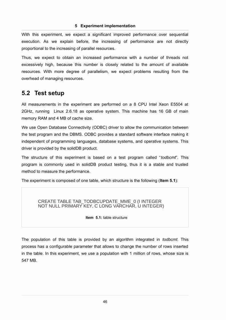
The experiment is composed of one table, which structure is the following (Item 5.1):

The population of this table is provided by an algorithm integrated in todbcmt. This

process has a configurable parameter that allows to change the number of rows inserted

in the table. In this experiment, we use a population with 1 million of rows, whose size is

547 MB.

46

CREATE TABLE TAB_TODBCUPDATE_MME_0 (I INTEGER NOT NULL PRIMARY KEY, C LONG VARCHAR, U INTEGER)

Item 5.1: table structure


The query used in the experiment is the following (Item 5.2):

For applying intra-query parallelism, we split this query (Item 5.2) in N number of sub-

queries, which have the following structure:

Although the table has three columns, we interact in the experiment only with the column

called “I”. Between-selector is used for dividing the total set of rows processed by the

original query in N number of disjoint subsets of rows.

We use that size of database because it is sufficient big to prove the difference of

performance between sequential and parallel execution and sufficient small to keep all

the database in main memory avoiding page swapping that would distort the results.

There are also two important parameters in the experiment related to the two forms of

parallelism that we mentioned in the previous section.

The first one is related to Inter-query parallelism. Basically, this parameter is the number

of threads that are executing separate queries in parallel. Depending on each particular

case, increasing the number of threads could affect significantly the performance of the

execution.

The other parameter to consider is the degree of parallelism of a operation, and it is

related to Intra-query parallelism. It is interesting to consider that the results obtained with

different values of this parameter could be altered when we also change the value of the

inter-query parallelism parameter. Thus, in this experiment we also want to unveil the

relation between those parameters.

47

SELECT COUNT(*) FROM TAB_TODBCUPDATE_MME_0

Item 5.2: query with aggregation count function

SELECT COUNT(*) FROM TAB_TODBCUPDATE_MME_0 WHERE I BETWEEN X AND Y

Item 5.2: query with aggregation count function

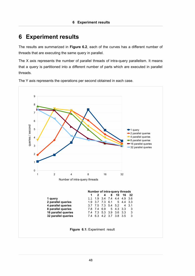
6 Experiment results


The results are summarized in Figure 6.2, each of the curves has a different number of

threads that are executing the same query in parallel.

The X axis represents the number of parallel threads of intra-query parallelism. It means

that a query is partitioned into a different number of parts which are executed in parallel

threads.

The Y axis represents the operations per second obtained in each case.

48

Figure 6.1: Experiment result

1 2 4 8 16 32

0

1

2

3

4

5

6

7

8

9

1 query2 parallel queries4 parallel queries8 parallel queries16 parallel queries32 parallel queries

Number of intra-query threads

quer

ies

/ sec

ond

Number of intra-query threads1 2 4 8 10 16 32

1 query 1.1 1.9 3.4 7.4 4.4 4.9 3.62 parallel queries 1.9 3.7 7.3 6.1 5 4.4 3.34 parallel queries 3.7 7.5 7.3 5.4 5.2 4 3.18 parallel queries 7.8 7.4 6.9 5 4.3 3.3 316 parallel queries 7.4 7.3 5.3 3.9 3.6 3.3 332 parallel queries 7.4 6.3 4.2 3.7 3.8 3.5 3


First, we focus on intra-query parallelism. In order to that, we analyze the curve with inter-

query parallelism equal to one (dark blue curve). In this case, we obtain 1.1

operations/second in the basic case with only 1 intra-query thread, whereas we obtain 7.4

operations/second using 8 parallel threads intra-query. Thus, we have an improvement

factor of performance 6.7, compared to the basic case. Unfortunately, from more than 8

threads the performance decreases dramatically.

Second, we focus on the inter-query parallelism. For that, we analyze the first column of

points in the chart, where the intra-query parallelism is equal to one. We can see the best

performance, starting from 8 threads on: 8, 16 and 32 threads obtain a similar result.

When combining intra-query parallelism and inter-query parallelism, we also obtain some

cases with a significant performance similar to the best one (7.5 operations/second).

One can realize that the best performances are obtained when the system uses 8 threads

in total. The reason is the test machine has 8 cores, allowing to execute 8 physical

threads in parallel. When we increase the number of total threads, the performance is not

increased because there are no more physical threads for executing in parallel.

In addition, there are an important difference between intra- and inter-query parallelism.

When intra-query parameter value is larger than 8, the performance is decreased

dramatically, whereas inter-query parameter do not decrease the performance with high

values.

In intra-query parallelism, the final result is obtained when the last query is finished.

Because of that, if we have more queries than physical threads, some of them will have to

wait for a free physical thread, thus causing a queue that reduces the performance

drastically.

In contrast, a query with inter-query parallelism does not have to wait for other queries

because they are independent, and that is the reason why a high parallelism does not

affect performance.

In conclusion, we should use intra-query parallelism when we want to achieve a significant

performance on a single query, whereas we should utilize inter-query parallelism when we

want a significant performance for all queries.

In a real environment, we can find situations where there are more physical threads than

concurrent queries. In that case, we can envisage an algorithm that would adjust the intra-

query parallelism to the level optimal for the situation.

50

7 Conclusions

7 Conclusions

In this study, we have addressed query processing issues and parallel query approaches

applicable to a main memory database management system. After that, we have exposed

a brief experiment to prove the advantage of having query parallelism execution in the

database management system.

From that experiment, we have attained encouraging results demonstrating the

application performance improvements that can be achieved by the parallelism. The

application performance is directly affected by query response times, and we were able to

significantly reduce that in the case where there have been unused parallel resources in

the system.

In addition, we have recognized the importance of having a hardware architecture with

high parallelism. In the experiment, we have used a system with 8 CPU cores and we

have achieved a significantly improved performance. In a production environment, we

could have had a hardware architecture with much higher physical parallelism, and

possibly obtaining much higher performance.

The parallel query implementation can vary in complexity, because, as we have explained

in the previous sections, we can implement many optimizations with the purpose to obtain

an improvement of performance.

But, as we have proved in this study, even with a simple parallel query implementation we

could obtain significant performance improvements in the execution of aggregate

functions that are often blamed for poor performance.

For the future work, It would be an appropriate challenge to implement one of the parallel

query approaches that we have exposed in this study.

51

Glossary of terms and abbreviations

A Glossary of terms and abbreviations

SQL

Structured Query Language

RDBMS

Relational Database Management System

DRDB

Disk Rigid Database

DRDBMS

Disk Rigid Database Management System.

MMDB

Main Memory Database

MMDBMS

Main Memory Database Management System

NP-Hard Problem

Non-deterministic Polynomial-time hard problem

SMP

Symmetric MultiProcessing

I

Bibliography

Bibliography

[1] Jim Melton and Alan R. Simon. SQL:1999 Understanding Relational Language

Components. Morgan Kaufmann, 2002.

[2] R. Ramakrishnan and J. Gehrke. Database Management Systems. McGraw-Hill, 3rd

Edition, 2003.

[4] Cliff Leung, Hamid Pirahesh, Praveen Seshadri, and Joseph Hellerstein. Query

rewrite optimization rules in IBM DB2 universal database. Readings in database systems

(3rd ed.), Morgan Kaufmann Series in Data Management Systems, Morgan Kaufmann,

1998.

[5] G. Lumpkin and H. Jakobsson. Query Optimization in Oracle Database 10g.

Redwood Shores (CA): Oracle Corporation, 2005.

[6] Aaron Swami. Optimization of large queries: Combining heuristics and combinatorial

techniques. In Proc. ACM SIGMOD International Conference on Management of Data

(SIGMOD 1989).

[7] P.P. Griffiths, M.M. Astrahan, D.D. Chamberlin, R.A. Lorie, and T.G. Price. Access path

selection in a relational database management system. In Proc. ACM SIGMOD

International Conference on Management of Data (SIGMOD 1979).

[8] Mathias Jarke and Jurgen Koch. Query optimization in Database Systems. In ACM

Comput. Surv. (1984) 16(2): 111-152.

[9] David Dewitt and Jim Gray. The future of high performance Database systems. In

Commun. ACM (1992) 35(6): 85-98.

[10] J Lewis. Cost-Based Oracle Fundamentals. Apress, 2005.

III

Bibliography

[11] Erhard Rahm and Robert Marek. Analysis of Dynamic Load Balancing Strategies for

parallel shared nothing database systems. In International Conference on Very large Data

Bases (VLDB 1993).

[12] Hector Garcia-Molina and Kenneth Salem. Main Memory Database Systems: An

Overview. In IEEE Trans. Knowl. Data Eng. (1992) 4(6): 509-516 .

[13] Tobin Lehman and Michal Carey. Query Processing in Main Memory Database

Management Systems. In Proc. ACM SIGMOD International Conference on Management

of Data (SIGMOD 1986).

[14] P. Valduriez. Parallel Database Systems: open problems and new issues. In

International Journal on Distributed and Parallel Databases (1993) 1(2): 137-165.

[15] Hasan, W. Florescu and P. Valduriez. Open issues in parallel query optimization. In

ACM SIGMOD Record (1996) 25(3): 28-33.

[16] M. Stonebraker. The case for shared nothing. In Database Engineering Bulletin.

(1986) 9(1).

[17] W. Hong and M. Stonebraker. Optimization of parallel query execution plans in

XPRS. In Proc. the First International Conference on Parallel and Distributed Information

Systems (1991).

[18] A. Hameurlain and F. Morvan. Exploiting Inter-operation Parallelism for SQL query

optimization. In Database and Expert Systems Applications (DEXA 1994). Lecture Notes

in Computer Science, Volume 856:759-768, Springer-Verlag, 1994.

[19] L. Bouganim, B. Dageville, and P. Valduriez. Adaptative parallel query execution in

DBS3. In Proc. International Conference on Extending Database Technology (EDBT

1996).

IV

https://intraweb.hel.fi.ibm.com/rd/dlib/mmdb/GMS92.pdf

https://intraweb.hel.fi.ibm.com/rd/dlib/mmdb/GMS92.pdf

Bibliography

[20] Ralph Acker, Christian Roth, and Rudolf Bayer. Parallel Query Processing in

Databases on Multicore Architectures. In Algorithms and architectures for parallel

Processing. Lecture Notes in Computer Science, Volume 5022: 2-13, Springer-Verlag,

2008.

[21] J. Zhou, J. Cieslewicz, K. A. Ross, and M. Shah. Improving database performance on

simultaneous multithreading processors. In Proc. the 31st international conference on

very large data bases (VLDB 2005): 49–60.

[22] E. Rahm. Parallel Query-Processing in Shared Disk Database Systems. In ACM

SIGMOD Record (1993) 22(4): 32-37.

[23] Jonathan Goldstein and Per-Åke Larson. Optimizing Queries Using Materialized

Views:A Practical, Scalable Solution. In Proc. ACM SIGMOD International Conference on

Management of Data (SIGMOD 2001).

[24] Erhard Rahm. Dynamic Load balancing in Parallel Database Systems. In Proc. Euro-

Par 96 Parallel Processing Conference (EURO-PAR 1996), Lecture Notes in Computer

Science, Volume 1123: 37-52, Springer-Verlag, 1996.

[25] S. Ganguly, W. Hasan, and R. Krishnamurthy. Query optimization for parallel

execution. In Proc. ACM SIGMOD International Conference on Management of Data

(SIGMOD 1996).

[26] Thomas M. Niccum. A tree-decomposition approach to parallel query optimization. In

Technical Report TR 93-016, 1993.

[27] Minos N. Garofalakis and Yannis E. Ionannidis. Parallel query scheduling and

optimization with time- and space-shared resources. In Proc. ACM SIGMOD International

Conference on Management of Data (SIGMOD 2002).

V

Bibliography

[28] Max Kremer and Jarek Gryz. A survey of query optimization in parallel databases. In

Technical Report CS-1999-04, November 1999.

[29] M. N. Garofalakis and Y. E. Ioannidis. Multi-dimensional resource scheduling for

parallel queries. In Proc. ACM SIGMOD International Conference on Management of Data

(SIGMOD 1996).

[30] J. Turek, J. Wolf, K. Pattipati, and P. Yu. Scheduling Parallelizable Tasks: Putting it all

on the Shelf . In Proc. the 1992 ACM SIGMETRICS joint international conference on

Measurement and modeling of computer systems (SIGMETRICS 1992/PERFORMANCE

1992).

[31] A. Hameurlain. Exploiting interoperation parallelism for SQL query optimization. In

Database and Expert Systems Applications (DEXA 1994), Lecture Notes in Computer

Science, Volume 856: 759-768, Springer-Verlag, 1994.

[32] Cache definition: http://en.wikipedia.org/wiki/Cache.

[33] Y. E. Ioannidis. Query optimization. In ACM Computing Surveys (CSUR 1996) 28(1):

121-123.

[34] G. Colliat. OLAP, relational, and multidimensional database systems. In ACM

SIGMOD Record. (1996) 25(3).

[35] Cliff Leung, Hamid Pirahesh, Joseph Hellerstein, and Praveen Seshadri. Query

rewrite optimization rules in IBM DB2 universal database. In Readings in database

systems. 3rd edition (1998): 153-168.

[37] Cui Bin. Indexing for efficient main memory processing. Ph.D. Thesis, National

University of Singapore, 2004.

[38] SolidDB: www.ibm.com/software/data/soliddb/.

VI

http://www.ibm.com/software/data/soliddb/

http://portal.acm.org/author_page.cfm?id=81100151533&coll=DL&dl=ACM&trk=0&cfid=112483650&cftoken=97378867




http://en.wikipedia.org/wiki/Cache

Bibliography

[39] Sang K. Cha, Sangyong Hwang, Kihong Kim, and Keunjoo Kwon. Cache-

Conscious Concurrency Control of Main-Memory Indexes on Shared-Memory

Multiprocessor Systems. In Proc. the 27th international conference on very large data

bases (VLDB 2001): 181-190.

[40] D. Bitton, M. B. Hanrahan, and C. Turbyfill. Performance of complex queries in main

memory database systems. In Proc. The third International Conference on Data

Engineering (ICDE 1987): 72-81.

[41] S. Manegold, P. Boncz, and M. Kersten. Optimizing main-memory join on modern

hardware. In Technical Report INS-R9912, CWI, Amsterdam, The Netherlands, October

1999.

VII

parallel query processing for in-memory databasesparallel query processing for in-memory databases...

Documents