parallelized deep neural networks for distributed intelligent systems

7/27/2019 Parallelized Deep Neural Networks for Distributed Intelligent Systems

http://slidepdf.com/reader/full/parallelized-deep-neural-networks-for-distributed-intelligent-systems 1/54

PARALLELIZED DEEP NEURAL NETWORKS

FOR DISTRIBUTED INTELLIGENT SYSTEMS

LANCE LEGEL

Bachelor of Arts in Physics, University of Florida, 2010

Thesis submitted to the Faculty of the Graduate School of the University of Colorado in partial fulfillment of the requirements for the degree of Master of Science from the

Interdisciplinary Telecommunications Program, 2013.



This thesis entitled:

Parallelized Deep Neural Networks for Distributed Intelligent Systems written by Lance Legel

has been approved for the Interdisciplinary Telecommunications Program

Committee Chair, Timothy X. Brown

Committee Member, Randall O’Reilly

Date

The final copy of this thesis has been examined by the signatories, and we

Find that both the content and the form meet acceptable presentation standards

Of scholarly work in the above mentioned discipline.



iii

Lance Legel (M.S., Interdisciplinary Telecommunications Program)

Parallelized Deep Neural Networks for Distributed Intelligent Systems

Thesis directed by Professors Timothy X. Brown, Randall O’Reilly, and Michael Mozer

ABSTRACT

We present rigorous analysis of distributed intelligent systems, particularly through work on large-scale deep neural networks. We show how networks represent functions, andexamine how all functions and physical systems can be learned by an infinite number of neural networks. Stressing dimensionality reduction as key to network optimization, westudy encoding, energy minimization, and topographic independent components analysis.We explain how networks can be parallelized along local receptive fields by asynchronousstochastic gradient descent, and how robustness can increase with adaptive subgradients.We show how communication latency across an InfiniBand cluster grows linearly with

number of computers, a positive result for large-scale parallelization of neural networks viamessage passing. We also present results of a topographic hierarchical network model of the human visual cortex on the NYU Object Recognition Benchmark.



iv

CONTENTS

1. Intelligence 1

1.1 Nature of Intelligence 1

1.1.1 Sensing 1

1.1.2 Learning 2

1.1.3 Actuation 4

1.2 Intelligent Systems 4

2. Deep Neural Networks 6

2.1 Hierarchical and Functional Architecture 6

2.1.1 Importance of Pre-Training 8

2.2 Data Dimensionality Reduction and Feature Invariance 10

2.2.1 Regularization: Normalization 102.2.2 Sparse Encoding 11

2.2.3 Energy Minimization: Boltzmann Machines 13

2.2.4 Topographic Independent Components Analysis 18

3. Parallel Distributed Computing 20

3.1 Single Model Parallelism 21

3.1.1 Parallelizing Columns of Local Receptive Fields 21

3.2 Multiple Model Parallelism 22

3.2.1 Asynchronous Stochastic Gradient Descent 22

3.2.2 Adaptive Subgradient Algorithm 25

4. Parallelizing and Optimizing Deep Neural Networks 27

4.1 Leabra Vision Model 27

4.2 Three-Dimensional Data Set for Invariance Testing 30

4.3 Message Passing Interface Benchmarks 31

4.4 Synaptic Firing Delay 34

4.5 Warmstarting 37

4.6 Experiments on NYU Object Recognition Benchmark dataset 40

References 42



1

CHAPTER 1: INTELLIGENCE

What is intelligence, how does it emerge, and how can it be engineered? These questions have

motivated ambitious research by cognitive and computer scientists for over half of a century.

Meanwhile, society has embraced the Internet. Systems for organizing, finding, and processing

information from millions of computers increasingly exceed in efficiency beyond imagination.

As a result, scientists can now increasingly find the best explanations on every topic instantly.

The scope of pursuing a generally applicable theory of intelligence remains extremely humbling.

But the opportunity to learn mathematical, statistical, physical, and computational principles that

may lead to its development is increasingly greater than ever before in history.

This thesis focuses on deep neural networks as one dynamic substrate for intelligence with

profound capabilities. It is a theoretical analysis of deep neural network foundations and

parallelization mechanics for large-scale computing; and a presentation of results of experiments

seeking to parallelize deep neural networks modeled after the human visual cortex. The overall

goal of this work is to establish foundations for research and development in intelligent systems

that can learn and control solutions to very complex and pervasive problems.

1.1 Nature of Intelligence

1.1.1 Sensing

To define the nature of intelligence, we briefly start where intelligence starts: sensing.

Organisms can sense through DNA encoding of organs that have evolved to provide information

about environmental physics. There seem to be few physical parameters not sensed by some

living organism [1]. Each sensory organ responds to one physical parameter – e.g. chemical,

mechanical, electromagnetic – within a finite space of elements. For example, Figure 1.1 shows



2

how the human eye evolved to detect and differentiate the most common photon wavelengths

generated by the Sun. This highlights the key function of sensing in intelligent systems:

statistical representation. Intelligent systems that sense more data can internally represent a more

accurate generative model for the data [2,3]. The human eye is thus a nearly optimal receptor for

photons emitted by the Sun.

Figure 1.1. Planck’s law of radiance for the Sun’s emissions of photons versus the range of

photons visible to the human eye.

1.1.2 Learning

Intelligence starts with sensing and follows with internal representation of phenomena [4,5,6].

This is considered as learning. Organisms without brains can use various means to learn about

their environment, like training oscillatory actuators in cells for optimal timing of action [7], and

Escherichia coli cultures that evolve genetically to predict systematic environmental danger [8].

Learning can mostly be explained in organisms with brains by changes in strength of synapses

among many neurons as functions of experience [9,10,11,12], while chemical neurotransmitters

like oxytocin and dopamine regulate learning in accordance with evolved instincts [13,14].



3

Weights of neural networks can encode “equations that evolve in time − dynamic problems”:

network parameters are matrices that may be solved by eigenspectra optimization [15,16,17,18].

The network parameters − e.g. neurons, synapses, layers, sparsity − functionally determine the

space of equations that may be represented [19]. This equivalence of functions and neural

network parameters leads to the following proposition, supported by mathematical derivations

from [20,21,22]:

Proposition 1.1. Any function can be learned by an infinite number of neural networksin an infinite dimensional space of parameter sets that define architecture.

If all physics can be explained as transformations of energy from one state to another, and thus as

systems of equations and statistical probability, then another proposition follows:

Proposition 1.2. Any physical system can be learned by a neural network to the extent

that data sensed about it completely represents its generative model.

These propositions suggest an infinite capacity of neural networks to encode useful information.

We will more formally address the foundations of these statements in the following chapter.

Whatever theoretical possibilities may exist for neural networks, it is also clear that there are

learning limitations of biological neural networks, as their architectural plasticity is constrained.

Humans develop 100 billion neurons in specialized regions of the brain with over 100 trillion

synapses continuously changing to learn new phenomena [23]. But in human brains the quantity

and location of neurons − and thus probability of synapses among them − are generally “hard

wired” by genetic encoding [24]. The absolute limits of the unaided human brain are best

revealed by physics that exhibit exponential complexity: e.g. we cannot possibly visualize the

interaction of 1023 molecules − less than the number of molecules in a cup of tea − while even



4

ten dynamic objects may be too hard to visualize. This obvious limitation is the inability of brain

architecture to selectively create and destroy neurons (not just synapses among a roughly finite

set of neurons); we cannot readily alter the “infrastructure” of our brains to represent greater

complexity than the existing one allows for. It should thus be clear that the common neural

network architecture providing for “common sense” among humans is just a local optimization

by genetic evolution to the limited patterns sensed on Earth throughout the evolution of life.

Indeed, genetic evolution of life may be considered as one massive learning process of nature.

Thus, evolution of data structures used for learning in intelligent systems seems essential to their

ability to adaptively learn in the context of radical changes in environment [25,26,27]. We willrevisit the relationship of architecture and functionality in the next chapter to conclude that a key

capacity for learning complex functions is “semantic integration” of several simple neural

networks each representing simple functions.

1.1.3 Actuation

Driven by goals, intelligent systems sense and learn to optimize interaction with environment.

Just as all physics can be sensed, all physics can be acted upon, potentially. The goals for action

may be dynamic in space, time, energy forms, etc., but generally are defined as the “realization”

(sensed expression) of a specific range of values within a finite space of physical dimensions.

The actions are based on what has already been learned, and the outcomes of the actions are

sensed in order to continue learning the best future actions for realizing goals. This optimization

of sensing, learning, and actuation toward goals is thus the nature of intelligence.

1.2 Intelligent Systems

The applications of intelligence vary widely in complexity and scope − e.g. industrial,

biomedical, social, scientific, ecological − but Proposition 1.1 and Proposition 1.2 from the prior



5

section would predict that neural networks can be structured to learn whatever physics intelligent

systems aim to sense and act about. The structures of neural networks most effective for

representing important problems has been an active area of research for several decades in many

domains. With no claim to completeness in this thesis on all types of structures for all types of

important problems that neural networks can represent, we can still focus on common

engineering challenges that all designers must overcome:

How do we acquire data that best represents the generative model of interest?

What is the best learning architecture for encoding the data structures?

How can we maximize the time and resource efficiency of learning implementations?

How can we optimize the interface between sensing, learning, and action?

Each of these questions is a difficult research thrust, while together they comprise the curriculum

of research into deep neural networks for intelligent systems. The theoretical and experimental

work of this thesis aims to provide an initial integrated response to these questions, especially

with regard to learning architectures and efficiency of learning implementations.



6

CHAPTER 2: DEEP NEURAL NETWORKS

With the motivations and introductory arguments for researching deep neural networks

established, we will now give a more rigorous analysis of their foundations. We will formally

examine the hierarchical and functional nature of neural networks, and provide an example for

clarifying this; along the way, we will show how pre-training is most likely essential to reaching

global optima; we will examine data dimensionality reduction techniques through autoencoders

and sparsity constraints; examine energy minimization through Boltzmann machines, which have

proven very successful in pre-training neural networks; and finally we will examine the

technique of topographic independent components analysis. Throughout this chapter and the

remainder of this thesis we will try to smash through diverse nomenclatures in favor of

understanding how different techniques may be doing similar or identical things.

2.1 Hierarchical and Functional Architecture

Inspired by Yoshua Bengio’s Learning Deep Architectures for AI [19], we will now examine

how neural networks, and graphical architectures more generally, can approximately and exactly

represent functions. We will first examine the concept of layers in a neural network. Let’s begin

with the simplest case of a directed acyclic graph where each node in the graph computes some

basic function on its inputs. The inputs of each node are the outputs of previous nodes, except

for the first input layer of the network, which receives inputs from environmental stimuli.

Remember, our network is designed to produce an overall desired target function, i.e. function of

the generative model for the environment to be learned. This target function is represented in the

network as a composition of a set of computational elements (e.g. multiplication, division), with

each node applying one computational element. So the depth of architecture refers to the largest



7

combination of computational elements that the graph instructs. In a neural network, depth

intuitively translates into the number of layers in question. The concept of depth as a

combination of computational elements, and the nature of how network architecture can encode

functions, will be best understood through example. Consider the equation for the Bekenstein –

Hawking entropy (S ) of a black hole, which depends on the area of the black hole ( A):

(2.1)

This equation is represented by the graph in Figure 2.1, with computational elements {×, /} and

input values {c, k ,

,

,

, 4}. The graph has a depth of 4 because the largest combination of

elements is 4 computations. Most revealing is how a seemingly complex equation breaks down

into simple paths of real number values through simple processing units.

Figure 2.1. Architecture of a neural network for a black hole’s entropy This architecture has adepth of 4 and uses only the computational elements {×, /}.



8

Yet, we see in Figure 2.1 that while the network for the equation of entropy of a black hole is

relatively simple, the choices of input values, connectivity, and computational element that each

node represents are very specific. This is the challenge for designers of deep neural networks:

how can we efficiently explore the infinite space of possible architectural choices?

2.1.1 Importance of Pre-Training

The values in Figure 2.1 are not the result of “random” chance, but are based on the product of

well-defined physical forces; they have been derived iteratively by hundreds of scientists over

centuries of fundamental physics experiments. This has an important lesson: we can

substantially reduce the dimensionality of possible configuration space, and thus increase the

likelihood of convergence to a global optimum configuration, by using pre-trained inputs, which

have already been determined to represent some aspect of the input space. Random iterative

search of network architectures is computationally intractable, but with highly constrained

guidance a configuration like Figure 2.1 can be reached. This is why pre-training, prior

knowledge, and culture are crucially important to the ability of neural networks to reach the best

configurations and overcome local optima [28,29,30,31,32,33].

The specificity of the architecture in Figure 2.1 could not likely be achieved by any engineered

intelligent system in existence today. But ultimately this is a core goal of researchers in

intelligence: develop systems that can reduce dimensionality of architecture space to be explored

by integrating simple component architectures, which collectively describe complex functions to

be learned. The physicists who developed the equation for the entropy of a black hole knew that

input values would need to be parameters relating to fundamental properties of gravity, quantum

and statistical mechanics, and energy. Deriving how these parameters (i.e. physical constants)

integrate is a long sequential process based on structural transformations: deriving a physics



9

equation requires an analysis of how systems of energy (equations) transform from state to state.

In mathematical and statistical terms, networks must be able to make transformations and

establish relationships about different dimensions of one multidimensional generative model.

Mammals on Earth have regions of their brains dedicated to analysis of space, time, and other

dimensions of inputs they sense. For example, humans have a region of the brain known as the

parietal lobe, which enables them to establish spatial relationships across visual, audial, and their

other senses. Like all other parts of the human brain, the mechanics of this region may be largely

described by the synaptic connections of neurons [34]. But this region does not accept inputs

from senses directly; rather, it is able to do geometric and abstract analysis of other neural

network regions, which we have argued here is essential to discovering a highly specific (and

thus relatively complex) generative model like the entropy of a black hole. Far from intuition

that deep neural networks are “black boxes” suffering from “credit assignment inability” [35,36],

we have established their concrete equality with functions. Functional analysis of neural

networks − especially with respect to physical dimensions − is thus a critical capacity for natural

and artificial intelligence development and pursuit of global optima. We may therefore venture

to establish another proposition:

Proposition 2.1. Representation of complex functions by deep neural networks requires

semantic integration of simple networks that represent simple functions.

For Proposition 2.1, we define “semantic integration” as the meaningful extraction and

combination of representations from network components. Among other regions of the brain

that achieve semantic integration in primates, the basal ganglia excel at this ability to parse

several discrete inputs of network signals, commonly considered as “executive control”. How it

does this exactly is a very active and promising area of research [37,38]. But as we will make



10

clear in the next chapter that discusses the human visual cortex, complex functions are typically

learned in a deep neural network as a hierarchy of increasing complexity.

2.2 Data Dimensionality Reduction and Feature Invariance

2.2.1 Regularization: Normalization

We have identified how dimensionality reduction of the configuration space for neural network

architectures is an important step in reaching global optima. It follows that reducing the

dimensionality of the data is equally important. The process of finding more general

representations of an input space from specific data is regularization. One powerful and popular

regularization method is -normalization in space [39,40,41]:

√

(2.2)

In (2.2), is the -normalization of vector of weights {, , ..., } that defines a

neural network. Minimizing the square root of the sum of squares is one way to pursue features

that are invariant to location, rotation, size, and other transformations.

2.2.2 Sparse Encoding

Another powerful form of regularization is sparse autoencoding. Autoencoding by itself is not

very useful unless the initial weights of the autoencoder are close to a good solution [42]. Thus,

after explaining how autoencoders work, we will describe an unsupervised statistical technique

that has been used to find approximate pre-training solutions: stacks of Boltzmann machines.

This approach is typical in that it restricts parameter space of exploration according to patterns

identified in data. After encoding the data into a lower dimensional space, standard supervised

learning techniques can provide state-of-the-art results in diverse domains [43,44,45].



11

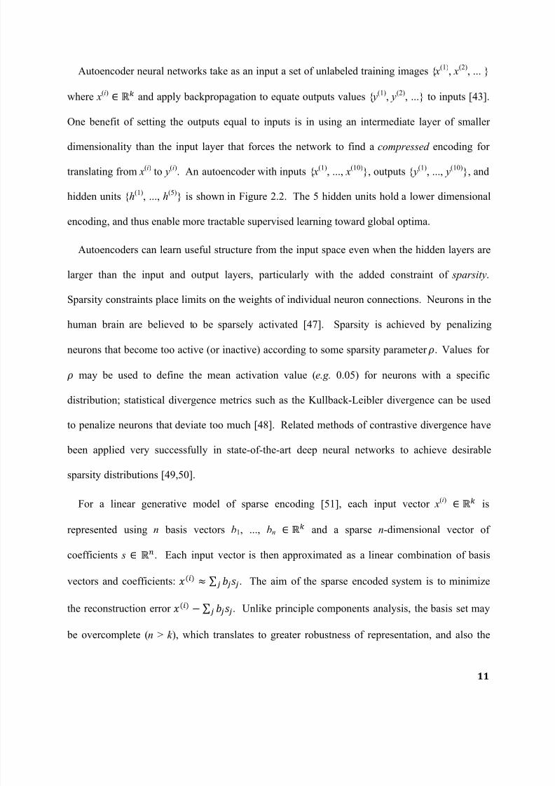
Autoencoder neural networks take as an input a set of unlabeled training images { x(1), x(2), ... }

where x(i) and apply backpropagation to equate outputs values { y(1), y

(2), ...} to inputs [43].

One benefit of setting the outputs equal to inputs is in using an intermediate layer of smaller

dimensionality than the input layer that forces the network to find a compressed encoding for

translating from x(i) to y

(i). An autoencoder with inputs { x(1), ..., x(10)}, outputs { y(1), ..., y(10)}, and

hidden units {h(1), ..., h

(5)} is shown in Figure 2.2. The 5 hidden units hold a lower dimensional

encoding, and thus enable more tractable supervised learning toward global optima.

Autoencoders can learn useful structure from the input space even when the hidden layers are

larger than the input and output layers, particularly with the added constraint of sparsity.

Sparsity constraints place limits on the weights of individual neuron connections. Neurons in the

human brain are believed to be sparsely activated [47]. Sparsity is achieved by penalizing

neurons that become too active (or inactive) according to some sparsity parameter . Values for

may be used to define the mean activation value (e.g. 0.05) for neurons with a specific

distribution; statistical divergence metrics such as the Kullback-Leibler divergence can be used

to penalize neurons that deviate too much [48]. Related methods of contrastive divergence have

been applied very successfully in state-of-the-art deep neural networks to achieve desirable

sparsity distributions [49,50].

For a linear generative model of sparse encoding [51], each input vector x(i) is

represented using n basis vectors b1, ..., bn and a sparse n-dimensional vector of

coefficients s . Each input vector is then approximated as a linear combination of basis

vectors and coefficients: ∑ . The aim of the sparse encoded system is to minimize

the reconstruction error ∑ . Unlike principle components analysis, the basis set may

be overcomplete (n > k ), which translates to greater robustness of representation, and also the



12

capacity for discovering deeper patterns from the data. Following we will go into depth about a

special type of sparse-encoded system that has proven very powerful: Boltzmann machines.

Figure 2.2. Autoencoder with 10 input and output units and 5 hidden units. This network sets

inputs equal to outputs to find a lower dimensional representation of the input space.

2.2.3 Energy Minimization: Boltzmann Machines

Because deep neural networks afford greater complexity in architecture configuration and

synaptic optimization space, as we have discussed, they are correlatively more difficult to train:

when weights are randomly initialized, deep networks will reach worse solutions than networks

with 1 or 2 hidden layers [19,52,53]. Additionally, it seems that supervised methods alone are

ineffective because the error gradient usually vanishes or blows up after propagating through

several non-linear layers [19,54,55]. Thus, deep neural networks require “pre-training” in a way

that is robust to many layers while still initializing the network roughly near a global optimum.

A good solution in this regard is the use of energy-based Boltzmann machines trained on each



13

layer in isolation [42]. We will examine the fundamentals of Boltzmann machines to understand

why they have proven so effective in pre-training deep neural networks.

Boltzmann machines learn large number of “weak” or “soft” constraints of input data, and

form an internal generative model that produces examples within the same probability

distribution as the examples it is shown [56]. The constraints may be violated but at a penalty;

the solution with the least violations is the best. Like a neural network, Boltzmann machines are

made of neurons that have links among them; however, in addition to weighted links, each node

has a binary on or off state probabilistically determined by the weights of its connections with

neighboring nodes, and their current state. Inspired by Hopfield [11], Hinton et al. introduced

notation for describing the global state of the Boltzmann machine by its energy E [56]:

(2.3)

In (2.3), is the weight between units i and j and and are 1 or 0 (on or off). Because the

connections are symmetric, we can determine the difference of the energy of the whole system

with and without the k th hypothesis, locally for the k th unit:

(2.4)

The objective of the Boltzmann machine is to minimize this energy function. Thus, we need to

determine for each unit whether it is better to be in the on or off state. Doing this best requires

“shaking” the system: enabling temporary jumps to higher energy to avoid local minima. We set

the probability of the k th unit to be on based on the energy difference in (2.4):

(2.5)



14

In thermal physics, a system of such probabilities will reach thermal equilibrium with a body of

different temperature that it is in contact with, and the probability of finding a system in any

global state will obey a Boltzmann distribution. In precisely the same way, Boltzmann machines

establish equilibrium with input stimuli, and the relative probability of two global states will

follow a Boltzmann distribution:

(2.6)

Relation (2.6) states that for a temperature of 1, the log probability difference of two global states

is precisely the difference in their energy. This is the foundation of information theory [56]:

information is a specific probability distribution of energy. The measure of energy state

differences is important to global optimization due to the following properties:

High T enables fast global search of states, i.e. discovery of regions near global optima

Low T enables slow local relaxation into states of lowest , i.e. local minima

Thus, starting with a high temperature and reducing to a low temperature enables the system to

roughly find global optima, and then precisely zero in on it. This was originally described as a

process of physical annealing in [57].

If the networks are only built from “clamping” visible units to input environmental stimuli,

then they cannot learn very interesting features. However, in a similar fashion that constructs

basis vectors as described in the prior section on sparse encoding, Boltzmann machines introduce

a second layer of “hidden” units that can learn deeper features. Minimizing the energy of this

two-layer network has been shown [56] to equal the minimization of information gain, G:

(2.7)



15

In (2.7), is the probability of the th state of visible units, which are “clamped” by the

inputs, and is the same but for the network that learns without clamping. The second

variable for learning without clamping is achieved by having two phases of learning: first a

“minus phase” where the two layers directly respond to input stimuli, and second a “ plus phase”

where the layers are updated independently according a rule like (2.4). In (2.7), G will be zero if

the distributions between the first phase and the second phase are identical, otherwise it will be

positive. Intuitively, we can think of this difference between the first and second phases as a

measure of how well the network has achieved “thermal equilibrium”. If the difference is very

small with an additional update even after seeing new environmental stimuli, then that means thenetwork does not feel like there is a much better state it can be in, and information gain is low.

The minimization of information gain G is executed by changing the weights between each i

and j node, proportional to a difference of probabilities that the first and second phases will have

units i and j both on ( ):

(2.8)

The above learning rule (2.8) has the appealing property that all weight changes require

information only about each neuron’s weights with local neighbors (i.e. changes do not emerge

from propagation of some “artificial value” across multiple layers); this is considered to be one

important principle of biological neural networks [58]. With G minimized the Boltzmann

machine has successfully captured regularities of the environment in as low of a dimensionalspace (lowest energy) as possible [56]. Beyond being a part of a class of energy minimization

methods, Boltzmann machines may be considered closely related to applications that minimize

contrastive divergence, since the contrast between two phases is minimized here.



16

The preceding explanation describes a single “restricted Boltzmann machine” (RBM), but

recent breakthroughs in deep neural networks that use Boltzmann-like methods to reduce

dimensionality take one step further in pre-training. They recognize that a single binary RBM

learns only “low level” features: edges, blobs, etc.. However, stacks of Boltzmann machines, as

seen in Figure 2.3, have the ability to detect high level features [49,42]. The basic technique is to

provide the output of one RBM as the input of another RBM, with each successive RBM

recognizing higher level features composed as combinations of low-level features. Each RBM is

trained iteratively in a greedy fashion completely ignorant of layers that it is not connected to; it

is therefore important to train the RBMs sequentially rather than in parallel or combination.Stacks of RBMs are a direct application of Proposition 2.1, which states that complex functions

are best learned as integration of several simpler functions. More generally, stacks of RBMs

reflect the common hierarchical learning strategy of deep neural networks, with invariance to

low-level transformations increasing at higher layers.

Boltzmann machines are a powerful means of pre-training an autoencoder to be near the

global optimum for an input space. After running stacks of RBMs to find high level features, we

may then “unfold” (i.e. decode) these stacks back to the original parameter size of the input

space, thus completing the autoencoder (see Figure 2.3). We may then use a supervised learning

algorithm to “fine-tune” the autoencoder according to whatever specific learning task is at hand.

Large systems of this type can do the vast majority of learning with unlabeled data, prior to

doing minor supervised learning to equate what has already been learned with labeled

information [49]. Figure 2.3 is a simple 9-6-3 autoencoder with two stacked RBMs, but most

successful deep neural networks recently reported use stacks of at least 3 RBM-like energy-

minimizers, each containing hundreds to thousands of neurons.



17

Figure 2.3. Autoencoder with two stacked restricted Boltzmann machines that are to be trained

sequentially, with the output of energy-minimized RBM 1 feeding into the input of RBM 2. The

output of RBM 2 encodes higher-level features from low-level features determined by RBM 1. After RBM 2 is energy-minimized, the stack is “unfolded”, such that the architecture inverts

itself with equal weights to the encoding. Finally, supervised learning may be applied in

traditional ways through error backpropagation across the entire autoencoder [42].



18

2.2.4 Topographic Independent Components Analysis

Humans can recognize objects observed with many rotations, scales, locations, shading, etc.

Such robustness to variance is clearly a desired quality in object recognition systems. There are

many methods that succeed in achieving greater invariance in neural networks. One technique

for achieving feature invariance is topographic independent components analysis (TICA) [59].

This technique was recently used to train deep neural network with one billion parameters; it is

scalable to distributed parallel computing [49]. The basic idea is to pool many “simple cells”

(i.e. early neurons that detect simple shapes) into “complex cells” that are invariant to various

configurations of the simple cells − hierarchically, precisely like stacks of Boltzmann machines.

This idea was inspired by the way that the natural visual cortex is organized, with location of

neurons following topography to minimize wiring distance [60]. It uses “local receptive fields”:

complex cells are only receptive to a local region of simple cells.

Like Boltzmann machines, TICA finds configurations of complex cells that minimize overall

dimensionality of the system, while finding high-level patterns invariant to low-level changes;

and they apply binary on or off states to each hidden node, such a neighborhood function

is 1 or 0 as a function of the proximity of features with indices i and j. The measure of proximity

of features is like convolutional networks, which pool subspaces according to proximity [61,62].

The function is 1 if the features are close enough, beyond a threshold. However, TICA

differs from convolutional networks in that not all weights are equal, and from Boltzmann

machines in that the “complex cells” (i.e. hidden nodes) are only locally connected. Thus, the

determination of the threshold in TICA is not based on energy as in Boltzmann machines,

but distance. For example, given an image of 200 by 200 pixels, TICA might check whether two

features map within the same two-dimensional space of 25 by 25 pixels. Components close to



19

each other in the topographic grid constructed have correlations of squares. An important

emergent property of TICA is that location, frequency, and orientation of input features comprise

the topographic grid purely from the statistical nature of the input space [59]. The grid is able to

achieve invariance to these parameters and pool objects that are actually the same without using

labels as in supervised learning. Because TICA is very close in structure to the visual cortex −

based on local receptive fields in at least two dimensions and pooling of similar features − it is an

attractive foundation for both computational neuroscience and large scale machine learning [49].



20

CHAPTER 3: PARALLEL DISTRIBUTED COMPUTING

Training neural networks with more data and more parameters encodes more descriptive

generative models [2,3,49,63,64], but the scale of computing needed to do so is a bottleneck: it

can take several days to train big networks. It follows that research in parallel computing of

network parameters across multiple cores and hardware implementations on a single computer,

and across multiple computers in large clusters, is an important frontier for general research and

applications of deep neural networks. Research in the natural manifestations and practical

engineering approaches to parallel distributed processing of neural networks has been active for

several decades. Rumelhart and McClelland organized a prescient set of research in “ Parallel

Distributed Processing: Explorations in the Microstructure of Cognition” (1986), which

provided benchmarks for a new generation of “connectionist” neural network models that aimed

to encode distributed representations of information and support parallelization [65]. Indeed the

human brain is one massive parallel system that computes independent and dependent

components in and across regions like the basal ganglia, visual, and auditory cortices [66,67,68].Yet it has been found that there are serial bottlenecks that coexist with parallelization,

particularly in executive decision making [69].

It follows that understanding how the brain integrates asynchronous parallel computation is

both a wonderful scientific endeavor and desiderata for designers of deep neural networks and

next-generation neuromorphic computing hardware. This venture has inspired commitments of

billions of dollars into research around large-scale deep neural networks in the United States via

the Brain Research through Advancing Innovative Neurotechnologies (BRAIN) Initiative [70],

and in the European Union via the Human Brain Project [71]. The U.S. project is led by the

National Institutes of Health, DARPA, and NSF. Its motivation is the integration of



21

breakthrough machine learning and computing capabilities with the potential for new neural

imaging systems that can map the “functional connectome” of the brain: it seeks to collect data

on individual firing activity of all of the billions of neurons in a single brain to precisely

understand how that translates into emergent behavior [72]. This research will lead the science

of parallelizing neural networks to become an increasingly important and rewarding focus, which

will be applied through development of intelligent systems that solve big problems for humanity.

3.1 Single Model Parallelism

3.1.1 Parallelizing Columns of Local Receptive Fields

One key enabler of single model parallelization in deep neural networks is local connectivity,

where computation is parallelized in vertical columns of local receptive fields, as in Figure 2.4.

The basic premise is that locally-connected networks have vertical cross-sections spanning

multiple layers, where the weights of certain regions are relatively independent from those of

other regions, and therefore those regions may be computed simultaneously. Figure 3.1 shows a

model with 3 layers that is parallelized on 4 machines; this approach was recently used to

parallelize a single model with 9 layers on 32 machines, with each machine using an average of

16 cores, before network communication costs dominated [73]. The killer for parallelization of

large networks is communication latency. To minimize communication across machines, it is

therefore important to send only one parameter update between machines with the minimum

required information at the smallest interval acceptable. In models where computation is not

well localized, this minimum possible communication may still be too high to make it possible

for the single model to be parallelized.



22

Figure 3.1. Neural network of 3 layers parallelized across 4 machines, with each machine

denoted by color: red, green, purple, or blue. Each of the 9 neurons in the 2

nd

layer has areceptive field of 4x4 neurons in the first layer; each of the 4 neurons in the 3rd

layer has a

receptive field of 2x2 neurons in the second layer. Local receptive fields enable independent

simultaneous computation of regions that do not depend on each other. Communication acrossmachines is minimized to single messages containing all relevant parameter updates needed

from one machine to another, sent at a periodic interval.

3.2 Multiple Model Parallelism

3.2.1 Asynchronous Stochastic Gradient Descent

Deep neural networks may also have multi-model parallelism, with several “model replicas”

(complete networks) trained in parallel. At regular intervals parameters from each of the

equivalent architectures are integrated into master parameters that are then used to “rewire” each

architecture. In [73] an “intelligent version” of asynchronous stochastic gradient descent is



23

introduced for training very large deep neural networks. It starts by dividing the training set into

r batches, where r equals the number of model replicas. Each replica then splits its one batch

into µ mini-batches, and updates its parameters with a central parameter server after each mini-

batch is finished. We set µ to ensure that updates occur frequently enough to avoid divergence

of multiple asynchronous models beyond some threshold. But since update frequency , we

set µ small enough so that models can achieve uniquely useful explorations of input space.

Because models may be so large that the computation of all combined model parameters in the

“central parameter server” cannot fit neatly into the fast input/output operations of a single

machine, we may also split the parameter server into separate asynchronous “shards” that are

spread across multiple machines.

This protocol, known as downpour stochastic gradient descent , is asynchronous in two ways:

model replicas run independently of each other, as do the central parameter shards [73]. Beyond

the fact that models will be computing with “out of date” global parameters at each moment,

there is also asynchrony in the central parameter shards as they compute with different update

speeds. Communication costs are minimized with minimization of synchronization, so studies of

probabilistic divergence of models are a key foundation for optimizing parallelization of multiple

instances of one neural network architecture. The approach described here features high

robustness to failure or slowness of individual models, because all other models continue

pushing and updating their parameters through the central parameter server, regardless of the

activity of other models; individual model(s) struggling need not force all other models to wait.

We can prevent systemically slower models with more outdated parameters from dragging the

global optimization led by faster models by devising and implementing a simple rule that we

may call slow exclusion, with pseudocode as follows in Figure 3.2.



24

Figure 3.2. Pseudocode for rule that ensures global parameters are only updated by models that

are not too outdated, i.e. not too slow. This rule prevents models that suddenly become slower

than a fine-tuned value max_delay from “drag ging ” the global parameter space back into older optima; and it makes sure that slower models that suddenly become faster can contribute again

by updating their model parameters to global parameters.

The algorithm in Figure 3.2 makes sure that only models that have been recently updated with

global parameters are allowed to contribute to global optimization. It assumes that the rate of

updating local and global parameters is the same, while this need not be true to implement the

core of the algorithm: exclusion of slow models.

The promise of parallelizing multiple models of the same architecture by integrating their

parameters iteratively depends on the extent that the architecture will follow optimization paths

of a well-constrained probability distribution. If for each iteration the architecture makes the

parameter space to be stochastically explored too large dimensionally, then the models will not

converge cooperatively, and the system will get stuck in local optima unique to the architecture’s

general evolutionary probability distribution, specified by the data. Proposition 3.1 thus follows.

Proposition 3.1. In asynchronous stochastic gradient descent, the marginal increase in

global optimization efficiency per new model is a function of the probability distribution

of evolutionary paths that model parameters may follow.



25

Consequently, methods like voting , perhaps by maximum entropy selection, have proven to be

one way to combat the implications of Proposition 3.1 for multi-model parallelism [74]. Further,

it is possible to measure convergence constraints of a network’s architecture [75], and to

guarantee minimum acceleration bounds from parallelizing additional model replicas [76].

3.2.2 Adaptive Subgradient Algorithm

As explained above, robustness of global optimization in the face of local asynchrony is the

greatest challenge of multi-model parallelism. One very potent technique used by [46,70] is

adaptive subgradient learning rates (“AdaGrad”) for each parameter, as opposed to a single

learning rate for all parameters [77]. The learning rate of the i-th parameter at the K -th

iteration is defined by its gradient as follows [70]:

(3.1)

The denominator in (3.1) is the normalization, defined by equation (2.2) in the prior chapter,

with the i-th parameter held constant in the summation from j = 1 to j = K . Further,

is a

constant scaling factor that is usually at least two times larger than the best learning rate used

without AdaGrad [78]. The use of AdaGrad is feasible in an asynchronous system with

parameters of a model distributed across several machines because only considers the i-th

parameter. This technique enables more model replicas r to differentially search global structure

of the input space in ways that are more sensitive to each parameter’s feature space. Two

conditions must be met for AdaGrad to lead to convergence of a solution [79,80]:

(a) is below a maximum scaling value

(b) regularization exceeds a minimum threshold



26

If (a) is not met, then the learning rate will be too large to explore smaller convex subspaces.

Conversely, if (b) is not met then the space of exploration will be too non-linear for parameters

to linearly settle into a global optimum. Thus, learning rate and dimensionality reduction need to

be tuned against representational accuracy of encoding. We can ensure γ is not too large through

custom learning rate schedules [79], and we can ensure our input space is made convex enough

through an adaptive regularization function derived directly from our loss function [81]. If (a)

and (b) are met, then the following condition holds:

(3.2)

The relation (3.2) indicates that the learning rate in a network that converges to an optimum will

change less and less as the number of iterations goes to infinity. This simply means that

AdaGrad will enable the system to reach an equilibrium.



27

CHAPTER 4: PARALLELIZING DEEP NEURAL NETWORKS

We organized parallelization experiments with computational models of the human visual cortex

in order to explore the principles explained in the previous chapters. In this chapter we will

review the mechanical and architectural foundations of a deep model for the human visual cortex

before presenting results of experiments to parallelize it. We will include a progressive outlook

on experiments testing message passing benchmarks, network tolerance of communication delay,

and “warmstarting” of networks to reduce likelihood of undesired asynchronous divergence.

Our model is statistically and mathematically very similar to the best deep neural networks

reported in literature in the following respects: adaptive learning rates, sparse encoding,

bidirectional connectivity across layers, integration of unsupervised and supervised learning, and

hierarchical architecture for topographically invariant high-level features of low-level features.

4.1 Leabra Vision Model

The first layer of neurons in our vision model, modeled as the primary visual cortex (V1),

receives energy from environmental stimuli (e.g. eyes) that, like Boltzmann machines,

propagates through deeper layers of the network. This propagation manifests through “firing”:

when each neuron’s membrane voltage potential exceeds an action potential threshold then

it sends energy to neighboring neurons. The threshold is smooth like a sigmoid function, and

due to added noise in our models, identical energy inputs near may or may not push the neuron

through the threshold. Firing in our networks is dynamically inhibited to enforce sparsity (andthus reduce data dimensionality, as previously described), and to maintain network sensitivity to

radical changes in input energy, e.g. be robust to large changes in lighting and size. The timing

of neuron firing has been shown to encode neural functionality, such as evolution of inhibitory



28

competition, receptive fields, and directionality of weight changes [82,83,84]. Yet our networks

do not directly model “spike timing dependent plasticity”. Instead they follow equations that

provide for “firing rate approximation” (i.e. average firing per unit time). But in practice, our

models do implement an adaptive exponential firing rate for each neuron (“AdEx”) [85], which

is strikingly similar to the AdaGrad algorithm described in the previous chapter. One constraint

of AdEx is that there is a single adaptation time constant while real neurons adapt at

various rates [86]. This constraint is partially addressed by customizations in our model that

change the activation value dynamically according to its convolution and prior

activation value :

(4.1)

Equation (4.1) enables our model’s neurons to exhibit gradual changes in firing rate over time as

a probabilistic function of excitatory net input [58].

The human primary visual cortex (V1) has on the order of 140 million neurons [87], while all

of the object recognition parallelization experiments contained herein model the V1 with onlyabout 3,600 neurons. Our full visual model is typically run with about 7,000 neurons connected

by local receptive fields across four layers: V1, V2/V4, IT, and Output. There are on average

about a few million synaptic connections to tune among all of the neurons in the vision model.

The limit on neurons, and thus tunable parameters, generally exists to reduce the computation

time and increase the simplicity of architecture design. Yet we have argued here that more

parameters leads to the capacity for representation of more complex functions (e.g. see

[49,63,64]); therefore, we hope that developments in deep neural network parallelization science,

along with large scale computing and processor efficiency, will lead to larger models with more

parameters. This would serve a harmonious dual purpose of potentially achieving better



29

generative representations of input spaces when built properly, and a more granular model of real

brain architecture.

The organization of neurons into networks in our model achieves a distributed sparse encoding

precisely as described in §2.2.2. Each layer affects all other layers above and below during each

exposure to input stimuli (i.e. each image trial), as opposed to simple supervised training of

neural networks where a single error signal is backpropagated down a network. Error-driven

learning in our model means minimizing the contrastive divergence between two phases −

“minus” during exposure to new stimuli, and “ plus” during a following adjustment − precisely

like the energy-minimizing Boltzmann machines described in §2.2.3. Additionally, our model is

close in mathematical nature to topographic independent components analysis as described in

§2.2.4, as it achieves topography in V1 and spatial invariance at higher layers. In addition to

error-driven learning, the model uses “self -organizing” (i.e. unsupervised) associative learning

rules based on chemical rate parameters from experiments of Urakubo et al. [88]. Our “self -

organizing” learning rule is a function

based on Hebbian learning, where weight change

is determined by the product of the activities of the sending neuron and receiving neuron (

over short (S ) and long ( L) periods of time:

⟨⟩ (4.2)

In (4.2), ⟨⟩ is the average activity of the receiving neuron over a long time. It acts as a

“floating threshold” to regulate weight increases and decreases. If

⟨

⟩is low then weights are

more likely to increase to a corresponding degree; if it is high then weights are more likely to

decrease to a corresponding degree. Determination of actual weight changes depends upon the

product of short term activities . If the product is very high, then it can still push weight

increases even if an already large ⟨⟩ would otherwise discourage it. Thus, the self-organizing



30

associative rule has the property of seeking “homeostasis”, where neurons are neither likely to

completely dominate nor to completely disappear from action [58]. It follows that the only

major difference between the error-driven and self-organizing learning elements of our network

is timescales: error-minimization enables faster weight changes according to short-term

activities, while unsupervised learning favors deeper and statistically richer features. The

combined weight change ultimately is parameterized by a weighted-average that is

tuned to make the best trade-offs from short, medium, and long-term learning:

(4.3)

It has been shown that the physical manifestation of a parameter like in the brain is regulated

by phasic bursts of neuromodulators like dopamine [89]: learning rate and focus change

dynamically each moment according to recognition of surprise, fear, and other emotions.

4.2 Three-Dimensional Data Set For Invariance Testing

Our data set for experiments presented here is the CU3D-100, which has 100 object classes, each

with about 10 different forms (“exemplars”) [90]; these objects are rotated in three dimensions,

rescaled, and subjected to lighting and shading changes in random ways to make object

recognition difficult. Our data set is similar to the NORB data set [91], which has become a

benchmark in machine learning tests of invariance [92,93,94], while our data is more complex:

CU3D-100 variations are applied randomly along a continuous spectrum (e.g. any number of

elevations of any value), while variations in NORB are deterministic and discrete (e.g. 9

elevations from 30 to 70 degrees with 5 degree intervals); additionally, CU3D-100 has size

changes, and over 20 times as many objects as NORB. Both data sets are similar in their purpose

of testing invariance to transformations and rotations.



31

4.3 Message Passing Interface Benchmarks

Our overall goal is to develop an asynchronous stochastic gradient descent protocol (as described

in §3.2.1) that uses a slow model exclusion rule like Figure 3.2 to ensure the fastest overall

parameter search by multiple models in parallel. To do this we acquired metrics with standard

Message Passing Interface (MPI) implementations in our local cluster. Our local computing

cluster has 26 nodes, each with two Intel Nehalem 2.53 GHz quad-core processors and 24 GB of

memory; all nodes are networked via an InfiniBand high-speed low-latency network. We needed

to determine the communication costs that would ultimately constrain the capacity for single

model parallelism as well as asynchrony tolerance in multiple models. In Figures 4.1 and 4.2 we

see our initial results using Qperf [90] for one-way latency between two nodes in TCP.

Figure 4.1. One-way latency in microseconds between two nodes in our computer cluster using TCP for message sizes ranging from 1 byte to 64 kilobytes. We see that latency is almost

negligible up to messages of 1kB, and stays at 0.3 milliseconds for messages between 4-16 kB.



32

Figure 4.2. Same measure as Figure 4.1 but in milliseconds versus kilobytes. We see that latency

is under 5 milliseconds up to 0.5 MB.

The results of Figure 4.1 and 4.2 were helpful but there was concern that they did not reflect the

time it takes for nodes to write new data delivered to it by the network, and that they were too

“low level” because they were not computed using MPI. To confirm these results we used

functionality from Intel’s MPI Benchmarks [91]. First we ran 100,000 tests of the latency for

each of nodes in a cluster to send a message of bytes to all other nodes. was tested

for 1 to 25 and for 32 kB, 64 kB, 128 kB. The message sizes tested are within the range of

actual neuron activation messages our networks send. In combination with the test results in

Figure 4.3, we wanted to be sure that the write time of saving new data from another node in an

MPI framework was carefully measured. Thus, we acquired the data on the parallel write time of

nodes in a cluster, where each node opens and saves a private file, for file sizes of bytes.

The node and byte size ranges are the same in Figure 4.3 and Figure 4.4.



33

Figure 4.3. Latency for all-to-all communications in a cluster with 1-25 computer nodes, as a

function of the number of cluster nodes communicating, tested for three different message sizes.

Figure 4.4. Parallel write time of separate files in MPI framework. We see basically no

correlation between file sizes and write time; and write time is weakly correlated with number of

nodes writing in parallel.



34

In Figure 4.3, we see that in the worst case scenario of 128 kB messages being simultaneously

sent and received by all 25 nodes, latency is 7 milliseconds. We also see that for clusters less

than 7 nodes latency costs for increasing message sizes is relatively negligible. But the drag from

larger message sizes becomes exponentially pronounced beyond clusters of 10 nodes. The all-to-

all test is an exaggeration of communications needed in a network like [73] where

communications are minimized between central parameter servers.

The results of Figures 4.3 and 4.4 indicate that in a network with 25 nodes we can expect in

the absolute worst case (all-to-all roundtrip communications rather than all-to-one one-way;

maximum write times rather than average) for a file size of 128 kB, the total latency adds up to

about 9 milliseconds. But there are many optimizations that apparently can decrease this latency

down to order of 3 milliseconds. The first is to implement a central parameter server instead of

having models communicate directly to each other. This would make the latencies more closely

resemble Figures 4.1 and 4.2 rather than Figure 4.3. The second is to decrease the message size

by removing “overhead” from the messages and decreasing the size of data types.

4.4 Synaptic Firing Delay

With an idea of the communication costs of parallelizing across machines, it is useful to consider

experiments that test the tolerance of communication delay. We used code that delays the firing

of neurons by number of cycles [92], where we tested for {1, ... , 5}. A cycle in our

network corresponds to weight changes that occur following a stimulus (i.e. image presentation);

many cycles take place until “settling” from a single image, e.g. 50-100. The question is how

robust the network may still train if it is effectively paralyzed in cycle computations. Figure 4.5

shows that the network can withstand a delay of one cycle per neuron with almost no cost to

learning efficiency, but for 2 or more cycles learning performance degrades, earlier and earlier.



35

Figure 4.5. Learning efficiency of networks that have been “paralyzed” by neuronal firing

ranging from 1 to 5 cycles. Networks can learn with one cycle of communication delay, but areincreasingly suppressed beyond that threshold: networks with 5 cycles of delay learn nothing.

When we examine the network guesses closely in Table 4.1, we see that 2-3 of 100 possible

objects completely dominate.

delay accuracy #1 choice (%) #2 choice (%) #3 choice (%)

0 cycles 93% - - -1 cycles 91% - - -

2 cycles 1% car (61%) helicopters (37%) -3 cycles 2% telephone (69%) person (26%) motorcycle (4%)4 cycles 2% airplane (49%) hotairballoon (46%) person (3%)5 cycles 2% telephone (56%) pliers (39%) -

Table 4.1. Training experiments show that networks with 2 or more cycles of delay are able to

learn only 2-3 objects among 100 possible objects supposedly introduced.



36

The results in Table 4.1 imply that 2 or more cycles of delay per neuron firing completely

paralyzes the ability of the network to learn more than a few objects, if those few objects are

even represented faithfully. This makes sense because of the fact that every single neuron is

forced to learn from increasingly old parameters as training continues. Asynchrony increasingly

emerges among all of the neurons as they try exploring paths that locally seem useful, but are

globally confused. It should also make sense then that parallelizing the firing delay of a single

model across multiple models does not affect learning efficiency, as demonstrated in Figure 4.6.

Figure 4.6. Parallelization of multiple models, all with neuron firing delay of 2 cycles.

Forthcoming experiments of single model communication tolerance should explore

communication delay only across regions of local receptive fields, as in Figure 3.1, so that we

can intelligently explore parallelization of a single model across multiple machines. In terms of

multiple model parallelization, future experiments should be done with the recognition that each

network does not need to be tolerant of delay within the network; even if we seek to exclude

slower models from dragging the global parameter search as explained by the rule in Figure 3.2,

we should recognize that each model should receive updates from at least some other models.



37

We should thus explore asynchrony tolerance of complete networks with relation to each other,

rather than all individual neurons in a single network, which amounts to paralyzing it.

4.5 Warmstarting

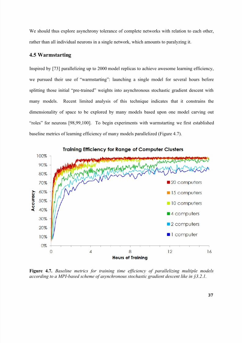
Inspired by [73] parallelizing up to 2000 model replicas to achieve awesome learning efficiency,

we pursued their use of “warmstarting”: launching a single model for several hours before

splitting those initial “pre-trained” weights into asynchronous stochastic gradient descent with

many models. Recent limited analysis of this technique indicates that it constrains the

dimensionality of space to be explored by many models based upon one model carving out

“roles” for neurons [98,99,100]. To begin experiments with warmstarting we first established

baseline metrics of learning efficiency of many models parallelized (Figure 4.7).

Figure 4.7. Baseline metrics for training time efficiency of parallelizing multiple models

according to a MPI-based scheme of asynchronous stochastic gradient descent like in §3.2.1.



38

We then explored several sequences of warmstarting experiments to identify if this technique can

provide a foundation for robustly scaling to larger clusters. Out of curiosity, we tested

transitions from one-to-many computers and many-to-one computers. Figure 4.8 shows that

surprisingly this technique did not prove useful for our networks, as presently constructed.

Figure 4.8. Results of warmstarting experiments. (1) The first type of experiment in green colors

is the transition from many-to-one computers. We see two of these transitions in green: (1.1) 20computers trained for 3 hours (hazel green), prior to 1 computer for 41 hours (bright green), and

(1.2) 20 computers for 12 hours (hazel green), prior to 1 computer for 32 hours (lime green).

The first transition at 3 hours merely slows down pace of learning, but does not disrupt it, whilethe second transition at 12 hours severely disorients the network optimization for several hours

before it begins to recover. (2) The second type of experiment in blue/purple colors is the one-to-

many transitions, which have better theoretical justification: 1 computer (light blue) is trained

for 32 hours, and then used to initialize (2.1) 10 computers (purple) and (2.2) 20 computers(dark blue). We do see small performance improvements relative to each other in this second

group, but we know from Figure 4.7 that this improvement is negligible.



39

Beyond the high-level trends in Figure 4.7, one may still ask: regardless of learning efficiency,

what about impact on reaching global optima? Figure 4.9 suggests that warmstarting does not

improve the search for global optima, either.

Figure 4.8. Count of the number of training epochs (500 trials per epoch) that recognize over

99% of training samples correctly for networks with and without warmstarting. The similar

distributions suggest that warmstarting does not improve global optimization in our networks.

Our results on warmstarting are all from training , while it is possible − however not implied −

that testing our network with objects held out from training could produce different results.

Additionally, we have considered and intend to explore in future experiments the possibility that

warmstarting defined by different parameters could yet prove useful, such as warmstarting as a

function of accuracy, trials, or learning rate schedules, instead of hours; and experimentation

with much larger cluster sizes such as those explored in [73].



40

4.6 Experiments on NYU Object Recognition Benchmark Dataset

We ran the Leabra Vision Model (LVis) on the NYU Object Recognition Benchmark (NORB)

dataset, which is a standard for measuring recognition that is invariant to transformations. Our

initial results follow in Figure 4.9.

Figure 4.9. Training accuracy of our model of the human visual cortex in recognizing objects

contained in the NYU Object Recognition Benchmark, using parameters published in [101].

After analyzing the above results and the configurations behind its implementations, we

concluded that our learning rate schedule was too slow for this dataset. The schedule details a

logarithmic decline in the magnitude of weight changes by some rate. After optimizing the rate,

we get the training results in Figure 4.10, slightly better than the 5% misclassification threshold.



41

Figure 4.10. Training accuracy on the NORB data with learning rate declines every 75 epochs.

These results show that our model can successfully learn complex datasets with above 95%

discriminative accuracy.

After running the weights from the above network on the NORB testing set, which is equally

large as the training set, and then doing a majority vote on 7 repeated presentations of the same

images, we receive a misclassification error rate of 16.5%. This is in comparison to 10.8%

achieved in 2012 by deep Boltzmann machines [102], as well as 18.4% by k-nearest neighbors

and 22.4% by logistic regression by LeCun in 2004 [103]. Further optimization of our network

on NORB will be presented in future publications.



42

REFERENCES

[1] Committee on Defining and Advancing the Conceptual Basis of Biological Sciences in the

21st Century, National Research Council. The Role of Theory in Advancing 21st-Century

Biology: Catalyzing Transformative Research. "What Determines How OrganismsBehave in Their Worlds?". Washington, DC: The National Academies Press, 2008.

[2] Halevy, Alon, Peter Norvig, and Fernando Pereira. "The Unreasonable Effectiveness of

Data." IEEE Intelligent Systems 24.2 (2009): 8-12.

[3] Banko, Michele, and Eric Brill. "Scaling to Very Very Large Corpora for Natural Language

Disambiguation." Association for Computational Linguistics 16 (2001): 26-33.

[4] He, Haibo. Self-adaptive Systems for Machine Intelligence. 3rd ed. Hoboken, NJ: Wiley-

Interscience, 2011.

[5] Holland, John H. Adaptation in Natural and Artificial Systems: An Introductory Analysis with

Applications to Biology, Control, and Artificial Intelligence. Cambridge, MA: MIT,

1992.

[6] Russell, Stuart J., and Peter Norvig. Artificial Intelligence: A Modern Approach. Upper

Saddle River: Prentice Hall, 2010.

[7] Bell-Pedersen, Deborah, Vincent M. Cassone, David J. Earnest, Susan S. Golden, Paul E.

Hardin, Terry L. Thomas, and Mark J. Zoran. "Circadian Rhythms from MultipleOscillators: Lessons from Diverse Organisms." Nature Reviews Genetics 6.7 (2005): 544-

56.

[8] Tagkopoulos, I., Y.-C. Liu, and S. Tavazoie. "Predictive Behavior Within Microbial Genetic

Networks." Science 320.5881 (2008): 1313-317.

[9] Legel, Lance. Synaptic Dynamics Encrypt Functional Memory. University of Florida

Biophysics Research, 2010. Web: http://bit.ly/synaptic-dynamics-encrypt-cognition

[10] Chklovskii, D. B., B. W. Mel, and K. Svoboda. "Cortical Rewiring and InformationStorage." Nature 431.7010 (2004): 782-88.

[11] Hopfield, J. J. "Neural Networks and Physical Systems with Emergent Collective

Computational Abilities." Proceedings of the National Academy of Sciences 79.8 (1982):

2554-558.



43

[12] Trachtenberg, Joshua T., Brian E. Chen, Graham W. Knott, Guoping Feng, Joshua R. Sanes,

Egbert Welker, and Karel Svoboda. "Long-term in Vivo Imaging of Experience-

dependent Synaptic Plasticity in Adult Cortex." Nature 420.6917 (2002): 788-94.

[13] De Oliveira, Lucas Fürstenau, Clarissa Camboim, Felipe Diehl, Angélica Rosat Consiglio,

and Jorge Alberto Quillfeldt. "Glucocorticoid-mediated Effects of Systemic Oxytocin

upon Memory Retrieval." Neurobiology of Learning and Memory 87.1 (2007): 67-71.

[14] Olvera-Cortés, María Esther, Patricia Anguiano-Rodríguez, Miguel Ángel López-Vázquez,

and José Miguel Cervantes Alfaro. "Serotonin/Dopamine Interaction in

Learning." Progress in Brain Research 172 (2008): 567-602.

[15] Strang, Gilbert. Linear Algebra and Its Applications. Vol. 4. Belmont, CA: Thomson,

Brooks/Cole, 2006.

[16] LeCun, Yann, Ido Kanter, and Sara A. Solla. "Eigenvalues of Covariance Matrices:

Application to Neural-Network Learning." Physical Review Letters 66.18 (1991): 2396-

399.

[17] Cichocki, A., and R. Unbehauen. "Neural Networks for Computing Eigenvalues and

Eigenvectors." Biological Cybernetics 68.2 (1991): 155-64.

[18] Zhou, Qingguo, Tao Jin, and Hong Zhao. "Correlations Between Eigenspectra and

Dynamics of Neural Networks." Neural Computation 21 (2009): 2931-941.

[19] Bengio, Yoshua. "Learning Deep Architectures for AI." Foundations and Trends in

Machine Learning 2.1 (2009): 1-127.

[20] Leshno, M., V. Lin, A. Pinkus, and S. Schocken. "Multilayer Feedforward Networks with a

Nonpolynomial Activation Function Can Approximate Any Function." Neural

Networks 6.6 (1993): 861-67.

[21] Cybenko, G. "Approximation by Superpositions of a Sigmoidal Function." Mathematics of

Control, Signals, and Systems 2.4 (1989): 303-14.

[22] Candès, E. "Harmonic Analysis of Neural Networks." Applied and Computational

Harmonic Analysis 6.2 (1999): 197-218.

[23] Herculano-Houzel, Suzana. "The Human Brain in Numbers: A Linearly Scaled-Up Primate

Brain." Frontiers in Human Neuroscience 3.31 (2009): 1-11.



44

[24] Stepanyants, A., and D. Chklovskii. "Neurogeometry and Potential Synaptic Connectivity."

Trends in Neurosciences 28.7 (2005): 387-94.

[25] Mitchell, Melanie. An Introduction to Genetic Algorithms. Cambridge, MA: MIT, 1996.

[26] Hornby, Gregory S., and Jordan B. Pollack. "Creating High-Level Components with aGenerative Representation for Body-Brain Evolution." Artificial Life 8.3 (2002): 223-46.

[27] De, Jong Kenneth A. Evolutionary Computation: A Unified Approach. Cambridge, MA:

MIT, 2006.

[28] Gulcehre, Caglar, and Yoshua Bengio. "Knowledge Matters: Importance of Prior

Information for Optimization." ArXiv E-prints 1301.4083 (2013): 1-17.

[29] Erhan, Dumitru, Yoshua Bengio, Aaron Courville, Pierre-Antoine Manzagol, and Pascal

Vincent. "Why Does Unsupervised Pre-training Help Deep Learning?" Journal of Machine Learning Research 11 (2010): 625-60.

[30] Bengio, Yoshua. "Evolving Culture vs Local Minima." ArXiv E-prints 1203.2990 (2012): 1-

28.

[31] Mozer, Michael C., Michael Jones, and Michael Shettel. "Context Effects in Category

Learning: An Investigation of Four Probabilistic Models." Advances in Neural

Information Processing Systems 19 (2007): 993-1000.

[32] Hinton, Geoffrey, Simon Osindero, and Yee-Whye Teh. "A Fast Learning Algorithm for Deep Belief Nets." Neural Computation 18.7 (2006): 1527-554.

[33] Weston, Jason, Frederic Ratale, and Ronan Collobert. "Deep Learning Via Semi-Supervised

Embedding." International Conference on Machine Learning 25 (2008): 1168-175.

[34] O'Reilly, Randall C., and Yuko Munakata. Computational Explorations in Cognitive

Neuroscience: Understanding the Mind by Simulating the Brain. Cambridge, MA: MIT,

2000.

[35] Minsky, M. and S. Papert. Perceptrons. Cambridge, MA: MIT, 1968.

[36] Rosenblatt, F. Principles of Neurodynamics: Perceptrons and the Theory of Brain

Mechanisms. Washington, D.C.: Spartan, 1968.

[37] Hazy, Thomas E., Michael J. Frank, and Randall C. O'Reilly. "Towards an Executive

without a Homunculus: Computational Models of the Prefrontal Cortex / Basal Ganglia



45

System." Philosophical Transactions of the Royal Society B: Biological

Sciences 362.1485 (2007): 1601-613.

[38] Stocco, A., C. Lebiere, R. O'Reilly, and J.R. Anderson. "Distinct Contributions of the

Caudate Nucleus, Rostral Prefrontal Cortex, and Parietal Cortex to the Execution of

Instructed Tasks." Cognitive, Affective, and Behavioral Neuroscience 12.4 (2012): 611-

28.

[39] Stein, Elias M., and Rami Shakarchi. Real Analysis: Measure Theory, Integration, and

Hilbert Spaces. Vol. 3. Princeton University Press, 2010.

[40] Köthe, Gottfried. Topological Vector Spaces. Vol. 462. Berlin-Heidelberg-New York:

Springer, 1969.

[41] Ng, Andrew "Feature Selection, L1 vs. L2 Regularization, and Rotational

Invariance." Proceedings of the Twenty-First International Conference on Machine

Learning (2004).

[42] Hinton, Geoffrey., and Ruslan Salakhutdinov. "Reducing the Dimensionality of Data with

Neural Networks." Science 313.5786 (2006): 504-07.

[43] Erhan, Dumitru, Yoshua Bengio, Aaron Courville, Pierre-Antoine Manzagol, Pascal

Vincent, and Samy Bengio. "Why Does Unsupervised Pre-Training Help Deep

Learning?." The Journal of Machine Learning Research 11 (2010): 625-60.

[44] Vincent, Pascal, Hugo Larochelle, Isabelle Lajoie, Yoshua Bengio, and Pierre-AntoineManzagol. "Stacked Denoising Autoencoders: Learning Useful Representations in a

Deep Network with a Local Denoising Criterion." The Journal of Machine Learning

Research 11 (2010): 3371-408.

[45] Nair, Vinod, and Geoffrey Hinton. "3D Object Recognition with Deep Belief Nets."

Advances in Neural Information Processing Systems 22 (2009): 1339-1347.

[46] Ng, Andrew. "Sparse Autoencoders." Artificial Intelligence Course Notes. Stanford

University Computer Science Department. Web.

[47] Quiroga, R. Quian, L. Reddy, G. Kreiman, C. Koch, and I. Fried. "Invariant Visual

Representation by Single Neurons in the Human Brain." Nature 435.7045 (2005): 1102-

107.

[48] Hinton, Geoffrey "Training Products of Experts by Minimizing Contrastive Divergence."

Neural Computation 14.8 (2002): 1771-800.



46

[49] Le, Quoc V., Marc'Aurelio Ranzato, Rajat Monga, Matthieu Devin, Kai Chen, Greg S.

Corrado, Jeff Dean, and Andrew Ng. "Building High-Level Features Using Large Scale

Unsupervised Learning." Proceedings of the 29th International Conference on Machine

Learning 29 (2012).

[50] Jarrett, Kevin, Koray Kavukcuoglu, Marc’Aurelio Ranzato, and Yann LeCun. "What is the

Best Multi-Stage Architecture for Object Recognition?" IEEE 12th International

Conference on Computer Vision 12 (2009): 2146-153.

[51] Lee, Honglak, et al. "Efficient Sparse Coding Algorithms." Advances in Neural Information

Processing Systems 19 (2007): 801.

[52] Bengio, Y., P. Lamblin, D. Popovici, and H. Larochelle, “Greedy Layer -Wise Training of

Deep Networks,” Advances in Neural Information Processing Systems 19 (2006): 153-60.

[53] Larochelle, H., Y. Bengio, J. Louradour, and P. Lamblin, “Exploring Strategies for Training

Deep Neural Networks,” Journal of Machine Learning Research, 10 (2009): 1-40.

[54] Bengio, Y., P. Simard, and P. Frasconi, “Learning Long-Term Dependencies with Gradient

Descent is Difficult,” IEEE Transactions on Neural Networks, 5:2 (1994): 157 – 66.

[55] Lin, T., B. G. Horne, P. Tino, and C. L. Giles, “Learning Long -Term Dependencies is Not

as Difficult with NARX Recurrent Neural Networks,” Technical Report UMICAS-TR-95-

78, Institute for Advanced Computer Studies, University of Maryland, (1995).

[56] Ackley, D. H., Geoffrey Hinton, and T. J. Sejnowski, “A Learning Algorithm for

Boltzmann Machines,” Cognitive Science, 9 (1985): 147 – 69.

[57] Kirkpatrick, S., C. D. Gelatt, M. P. Vecchi. “Optimization By Simulated Annealing”.

Science, 220 (1983): 671-80.

[58] O'Reilly, R. C., Munakata, Y., Frank, M. J., Hazy, T. E., and Contributors (2012).

Computational Cognitive Neuroscience. Wiki Book, 1st Edition. URL:

http:/ /ccnbook.colorado.edu

[59] Hyvärinen, Aapo, Jarmo Hurri, and Patrick O. Hoyer. Natural Image Statistics: A

Probabilistic Approach to Early Computational Vision. Vol. 39. Springer, 2009.

[60] Olshausen, Bruno A. "Emergence of simple-cell receptive field properties by learning a

sparse code for natural images." Nature 381.6583 (1996): 607-609.

[61] LeCun, Yann, Léon Bottou, Yoshua Bengio, and Patrick Haffner. "Gradient-based learning

applied to document recognition." Proceedings of the IEEE 86, 11 (1998): 2278-324.



47

[62] Lee, Honglak, Roger Grosse, Rajesh Ranganath, and Andrew Y. Ng. "Convolutional deep

belief networks for scalable unsupervised learning of hierarchical representations."

Proceedings of the 26th Annual International Conference on Machine Learning , 26

(2009): 609-16.

[63] Claudiu, Dan, Ciresan, Ueli Meier, Luca Maria Gambardella, Juergen Schmidhuber. “Deep

Big Simple Neural Nets Excel on Handwritten Digit Recognition.” Neural Computation,

22 (2010).

[64] Coates, Adam, Honglak Lee, and Andrew Ng. “An Analysis of Single-Layer Networks in

Unsupervised Feature Learning.” 14th

International Conference on Artificial Intelligence

and Statistics, 14 (2011).

[65] Rumelhart, David E., and James L. McClelland. Parallel Distributed Processing:

Explorations in the Microstructure of Cognition. Foundations. Vol. 1. MIT Press, 1987.

[66] Alexander, Garrett, and Michael Crutcher. "Functional Architecture of Basal Ganglia

Circuits: Neural Substrates of Parallel Processing." Trends in Neuroscience, 13 (1990):

266-71.

[67] Milner, A. David, Melvyn A. Goodale, and Algis J. Vingrys. The Visual Brain in Action.

Vol. 2. Oxford: Oxford University Press, 2006.

[68] Rauschecker, Josef P. "Parallel Processing in the Auditory Cortex of Primates." Audiology

and Neurotology 3.2-3 (1998): 86-103.[69] Sigman, Mariano, and Stanislas Dehaene. "Brain Mechanisms of Serial and Parallel

Processing During Dual-Task Performance." The Journal of Neuroscience 28 (2008):

7585-598.

[70] Collins, Francis, and Arati Prabhakar. "Brain Initiative Challenges Researchers to Unlock

Mysteries of Human Mind." The White House 2 Apr. 2013.

[71] HBP Preparatory Study Consortium. The Human Brain Project: Report to the European

Union. 2012.

[72] Alivisatos, A. Paul, Miyoung Chun, George M. Church, Ralph J. Greenspan, Michael L.

Roukes, and Rafael Yuste. "The Brain Activity Map Project and the Challenge of

Functional Connectomics." Neuron 74, 6 (2012): 970-74.

[73] Dean, Jeffrey, Greg Corrado, Rajat Monga, Kai Chen, Matthieu Devin, Quoc Le, Mark

Mao, Marc’Aurelio Ranzato, Andrew Senior, Paul Tucker, Ke Yang, and Andrew Ng.



48

“Large Scale Distributed Deep Networks.” Advances in Neural Information Processing

Systems 25 (2012).

[74] Mann, Gideon, Ryan McDonald, Mehryar Mohri, Nathan Silberman, and Dan Walker.

"Efficient Large-Scale Distributed Training of Conditional Maximum Entropy

Models." Advances in Neural Information Processing Systems 22 (2009): 1231-239.

[75] McDonald, Ryan, Keith Hall, and Gideon Mann. "Distributed training strategies for the

structured perceptron." Human Language Technologies: 2010 Annual Conference of the

North American Chapter of the Association for Computational Linguistics, Association

for Computational Linguistics (2010): 456-64.

[76] Duchi, John, Elad Hazan, and Yoram Singer. "Adaptive Subgradient Methods for Online

Learning and Stochastic Optimization." Journal of Machine Learning Research 12

(2010): 2121-159.

[77] Zinkevich, Martin, Markus Weimer, Alex Smola, and Lihong Li. "Parallelized Stochastic

Gradient Descent." Advances in Neural Information Processing Systems 23 (2010): 1-9.

[78] Bengio, Yoshua. "Deep Learning of Representations for Unsupervised and Transfer

Learning." Workshop on Unsupervised and Transfer Learning, International Conference

on Machine Learning (2011): 1-20.

[79] Bottou, Léon. "Large-Scale Machine Learning with Stochastic Gradient Descent."

Proceedings of the International Conference on Computational Statistics (2010): 177-86.[80] Dennis, John, and Robert Schnabel. Numerical Methods for Unconstrained Optimization

and Nonlinear Equations. Vol. 16. Society for Industrial and Applied Mathematics, 1987.

[81] McMahan, H. B., and M. Streeter. “Adaptive Bound Optimization for Online Convex

Optimization.” Proceedings of the 23rd Annual Conference on Learning Theory (2010).

[82] Song, Sen, Kenneth D. Miller, and Larry F. Abbott. "Competitive Hebbian Learning

Through Spike-Timing-Dependent Synaptic Plasticity." Nature Neuroscience 3, no. 9

(2000): 919-26.

[83] Meliza, C. Daniel, and Yang Dan. "Receptive-Field Modification in Rat Visual Cortex

Induced by Paired Visual Stimulation and Single-Cell Spiking." Neuron 49, no. 2 (2006):

183.



49

[84] Bi, Guo-qiang, and Mu-ming Poo. "Synaptic Modifications in Cultured Hippocampal

Neurons: Dependence on Spike Timing, Synaptic Strength, and Postsynaptic Cell

Type." The Journal of Neuroscience 18.24 (1998): 10464-72.

[85] Brette, Romain, and Wulfram Gerstner. "Adaptive Exponential Integrate-and-Fire Model as

an Effective Description of Neuronal Activity." Journal of Neurophysiology 94, no. 5

(2005): 3637-42.

[86] Gerstner, Wulfram and Romain Brette. “Adaptive Exponential Integrate-and-Fire Model.”

Scholarpedia, 4,6 (2009): 8427.

[87] Leuba, G., and R. Kraftsik. "Changes in Volume, Surface Estimate, Three-Dimensional

Shape and Total Number of Neurons of the Human Primary Visual Cortex From

Midgestation Until Old Age." Anatomy and Embryology 190, no. 4 (1994): 351-66.

[88] Urakubo, Hidetoshi, Minoru Honda, Robert C. Froemke, and Shinya Kuroda. "Requirementof an Allosteric Kinetics of NMDA Receptors for Spike Timing-Dependent

Plasticity." The Journal of Neuroscience 28, no. 13 (2008): 3310-23.

[89] O'Reilly, Randall C. "Biologically Based Computational Models of High-Level

Cognition." Science Signaling 314, no. 5796 (2006): 91.

[90] Wyatt, Dean et al . "CU3D-100 Object Recognition Data Set." Computational Cognitive

Neuroscience Wiki. Web: cu3d.colorado.edu/

[91] Y. LeCun, F.J. Huang, L. Bottou, “Learning Methods for Generic Object Recognition withInvariance to Pose and Lighting”. IEEE Computer Society Conference on Computer

Vision and Pattern Recognition (2004).

[92] Nair, Vinod, and Geoffrey Hinton. "3-D Object Recognition with Deep Belief Nets."

Advances in Neural Information Processing Systems 22 (2009): 1339-47.

[93] Glorot, Xavier, Antoine Bordes, and Yoshua Bengio. "Deep Sparse Rectifier Networks."

Proceedings of the 14th International Conference on Artificial Intelligence and Statistics.

JMLR W&CP 15 (2011): 315-23.

[94] Salakhutdinov, Ruslan, and Geoffrey Hinton. "Deep Boltzmann Machines." Proceedings of

the 12th

International Conference on Artificial Intelligence and Statistics, 5 (2009): 448-

55.

[95] George, Johann. "Qperf(1) - Linux Man Page." Qperf(1): Measure RDMA/IP Performance.

Web: http://linux.die.net/man/1/qperf



[96] Intel. "M.P.I Benchmarks: Users Guide and Methodology Description." Intel GmbH,

Germany 452 (2004).

[97] Emergent Neural Network Documentation. "SynDelaySpec Class Reference." Member and

Method Documentation. Web:

http://grey.colorado.edu/gendoc/emergent/SynDelaySpec.html

[98] Zinkevich, M. "Theoretical Analysis of a Warm Start Technique." Advances in Neural

Information Processing Systems: Parallel and Large-Scale Machine Learning Workshop

(2011).

[99] S. Boyd and L. Vandenberghe. Convex Optimization. Cambridge University Press, New

York, 2004.

[100] Colombo, M., J. Gondzio, and A. Grothey. "A Warm-Start Approach for Large-Scale

Stochastic Linear Programs." Mathematical Programming 127 (2011): 371-97.

[101] O’Reilly, Randall C., Dean Wyatte, Seth Herd, Brian Mingus, and David J. Jilk.

"Recurrent processing during object recognition." Frontiers in Psychology (2013).

[102] Salakhutdinov, R. and G. Hinton. "An Efficient Learning Procedure for Deep Boltzmann

Machines." Neural Computation 24 (2012): 1967-2006.

[103] LeCun, Y., Huang, F. J., & Bottou, L. “Learning methods for generic object recognition

with invariance to pose and lighting.” IEEE Proc. Computer Vision and Pattern

Recognition (2012): 97 – 104.

parallelized deep neural networks for distributed intelligent systems

Documents