parameter analysis of an adaptive, fault-tolerant attitude
TRANSCRIPT

Running head: ADAPTIVE, FAULT-TOLERANT ATTITUDE CONTROL
1
Parameter Analysis of an Adaptive, Fault-Tolerant
Attitude Control System Using Lazy Learning
Matthew Russell
A Senior Thesis submitted in partial fulfillment
of the requirements for graduation
in the Honors Program
Liberty University
Spring 2018
ADAPTIVE, FAULT-TOLERANT ATTITUDE CONTROL
2
Acceptance of Senior Honors Thesis
This Senior Honors Thesis is accepted in partial
fulfillment of the requirements for graduation from the
Honors Program of Liberty University.
______________________________
Kyung Bae, Ph.D.
Thesis Chair
______________________________
Frank Tuzi, Ph.D.
Committee Member
______________________________
David Wang, Ph.D.
Committee Member
______________________________
David Schweitzer, Ph.D.
Assistant Honors Director
______________________________
Date

ADAPTIVE, FAULT-TOLERANT ATTITUDE CONTROL
3
Abstract
Several key requirements would be met in an ideal fault-tolerant, adaptive spacecraft
attitude controller, all centered around increasing tolerance to actuator non-idealities and
other unknown quantities. This study seeks to better understand the application of lazy
local learning to attitude control by characterizing the effect of bandwidth and the
number of training points on the system’s performance. Using NASA’s 42 simulation
framework, the experiment determined that in nominal operating scenarios, the actuator
input/output relationship is linear. Once enough information is available to capture this
linearity, additional training data and differing bandwidths did not significantly affect the
system’s performance.
ADAPTIVE, FAULT-TOLERANT ATTITUDE CONTROL
4
Parameter Analysis of an Adaptive, Fault-Tolerant
Attitude Control System Using Lazy Learning
Since the first satellite was launched into space in 1958, both spacecraft and
mission complexity have increased dramatically. While early satellites might be able to
function effectively with limited, spin-stabilized attitude control, more recent missions
such as the Hubble Space Telescope, the upcoming James Webb Space Telescope, or the
International Space Station must dynamically manage their attitude to achieve the
mission objectives. Several active and passive methods have been developed to control
attitude. Mechanical reaction wheels leverage conservation of angular momentum to
exert torques on the spacecraft’s body. However, these wheels often fail or degrade over
time, leading to changes in the movement model of the satellite. Furthermore, the inertial
characteristics of the spacecraft could be unknown or varying. An adaptive, fault-tolerant
attitude control system could mitigate the effect of these factors on pointing accuracy and
overall mission success.
Background
Spacecraft Attitude Control
Almost all spacecraft require some level of pointing control to accomplish their
mission (Russell & Straub, 2017). Imaging satellites in Earth orbit must accurately
manage their attitude, or orientation, to produce photographs of desired regions, and the
necessary precision increases with the resolution of the imaging sensors. Deep space
probes rely on attitude control to maintain communication with NASA's Deep Space
Network (DSN) while those closer to the Sun must ensure the spacecraft is rotated to

ADAPTIVE, FAULT-TOLERANT ATTITUDE CONTROL
5
expose solar arrays to the maximum amount of light. The system responsible for
monitoring and adjusting the orientation of the spacecraft is the Attitude Determination
and Control System (ADCS). As this study focuses on control techniques, the discussion
of attitude determination falls outside the scope of this work.
Reference frames. The primary reference frame used in spacecraft attitude
dynamics is the Earth Centered Inertial (ECI) frame (Stoneking, 2014). The origin of ECI
is at the center of the earth, and the x-axis extends along the vernal equinox. The z-axis
runs through the north pole, and the y-axis lies on the equator and is orthogonal to both
the x and z axes (Hall, n.d.). According to Stoneking (2014) the attitude of a spacecraft is
defined as the rotation from the ECI frame to the body frame, which are the axes fixed
relative to the spacecraft’s structure (see Figure 1).
Figure 1. Spacecraft reference frames. The red n axes are the inertial axes, while the
green b axes are the body axes. The orientation or attitude of the spacecraft can be
specified as the rotation from the inertial axes to the body axes.

ADAPTIVE, FAULT-TOLERANT ATTITUDE CONTROL
6
Equations of motion. Wiesel (2010) describes rigid-body rotation as
𝝉 =𝑑
𝑑𝑡𝑯 (1)
where 𝑯 is the angular momentum, and 𝝉 is the net torque on the rigid body. The angular
momentum itself can be written in matrix form as
𝑯 = 𝑱𝝎 (2)
where 𝑯 ∈ ℝ3×1 is the angular momentum vector, 𝑱 ∈ ℝ3×3 is the moment of inertia
matrix, and 𝝎 ∈ ℝ3×1 is the angular velocity vector in the inertial frame. The moment of
inertia (MOI) matrix can be found using
𝑱 = [
∫ (𝑦2 + 𝑧2)𝑑𝑚 −∫ 𝑦𝑥 𝑑𝑚 −∫ 𝑧𝑥 𝑑𝑚
−∫ 𝑥𝑦 𝑑𝑚 ∫ (𝑥2 + 𝑧2)𝑑𝑚 −∫ 𝑧𝑦 𝑑𝑚
−∫ 𝑥𝑧 𝑑𝑚 −∫ 𝑦𝑧 𝑑𝑚 ∫ (𝑥2 + 𝑦2)𝑑𝑚
] (3)
where m is the mass of the spacecraft.
Passive attitude control. Attitude control can be either active or passive. Active
control allows the orientation to be arbitrarily set by the ADCS while passive control
relies on exploiting external forces for stabilization. Starin and Eterno (2011) state that
passive attitude control for Earth-orbiting satellites can be achieved via a permanent
magnet that pulls the satellite in line with the Earth’s magnetic field. Alternatively, the

ADAPTIVE, FAULT-TOLERANT ATTITUDE CONTROL
7
satellite could be provided an initial angular velocity when ejected from the launch
vehicle, relying on gyroscopic effects to constrain the orientation in a method known as
spin stabilization.
Thrusters. Instead of passive techniques, systems may use an active method or
combination of methods. Thrusters are one active approach suitable for coarse attitude
control. When a thruster produces a force vector that does not pass through the
spacecraft’s center of mass, it applies a torque to the rigid body (Starin & Eterno, 2011).
Wiesel (2010) notes that by adding a second thruster which applies an opposite torque,
the two torques can be used to point the spacecraft along one axis. Although allowing
rapid change of orientation, thruster-based systems suffer a few key disadvantages. A
limited supply of propellant means that attitude control will be lost when all the
propellant has been expended. Thrusters also cannot completely stop the rotation of the
spacecraft since they fire at discrete levels.
Magnetorquers. Magnetorquers utilize the Earth’s magnetic field to create a
torque on the spacecraft (Starin & Eterno, 2011). Using three-axis solenoids,
magnetorquers create a virtual magnetic dipole. The Earth’s magnetic field then acts on
this dipole just like it does on a compass needle, pulling the dipole parallel to the
magnetic field lines. Although magnetorquers do not require propellant, their
performance is restricted by the direction of local field lines; the desired torque may not
be possible given the field vector at a specific location. Combined with the small
magnitude of torque possible, magnetorquers are often used for small, long-duration
attitude maneuvers. One commonly-used maneuver is the B-dot algorithm, which seeks
ADAPTIVE, FAULT-TOLERANT ATTITUDE CONTROL
8
to prevent the buildup of angular momentum from external disturbances (e.g., gravity
gradient).
Reaction wheels, momentum wheels, and CMGs. Finer pointing can be
achieved using reaction wheels, momentum wheels, or control moment gyroscopes
(CMGs). All three of these techniques apply torque to the spacecraft through the
conservation of angular momentum, which states that the total angular momentum in a
closed system remains constant (Wiesel, 2010). The wheels generally consist of a
flywheel driven by an electric motor.
For reaction and momentum wheels, the angular momentum stored in the device
is varied by increasing or decreasing the spin rate of the flywheel whose axis coincides
with the desired axis of rotation (Wiesel, 2010). Since the overall angular momentum in
the system including the spacecraft and the flywheel must remain constant, changing the
angular momentum in the flywheel causes the angular momentum of the spacecraft to
change in the opposite direction. The rotational analog of Newton’s Second Law of
Motion states that torque is simply a change in momentum:
𝝉 = 𝑱𝜶 = 𝑱�̇� = �̇� (4)
where 𝝉 is the torque, 𝑱 is the moment of inertia, 𝜶 is the angular acceleration, �̇� is the
change in angular velocity, and �̇� is the change in angular momentum. Thus, changing
the wheel’s speed (and therefore momentum) applies a torque to the wheel. Since
momentum is conserved, the rotational analog of Newton's First Law of Motion states
ADAPTIVE, FAULT-TOLERANT ATTITUDE CONTROL
9
that an equal and opposite torque will be applied to the spacecraft. The conservation of
angular momentum can be described as
∑𝝉 = ∑�̇� = 0 (5)
i.e., the total change in momentum in the system must be zero. Thus, by precisely
controlling the spin rate of the flywheels, reaction and momentum wheels can apply a
variable torque to the spacecraft, allowing much finer attitude control than thrusters.
Reaction wheel modules can be controlled via torque commands (i.e., desired torque)
instead of raw motor current (Carrara & Kuga, 2013). Carrara, da Silva, and Kuga (2012)
and Carrara and Kuga (2013) point out that the presence of friction means that the
relationship between the current supplied to the reaction wheel motor and the resulting
speed is nonlinear.
Although only three reaction wheels (one for each axis) are required for full
attitude control, many spacecraft include four or more wheels. By using four wheels in a
tetrahedral structure, the ADCS will be able to maintain full three-axis control of the
spacecraft even with the complete failure of one of the wheels (Hacker, Ying, & Lai,
2015). For additional redundancy, six reaction wheels will be used to control attitude on
the forthcoming James Webb Space Telescope (Space Telescope Science Institute, n.d.).
CMGs operate on a slightly different principle. Instead of changing the spin rate
of the flywheel, the axis of the wheel is rotated (Wiesel, 2010). Conservation of angular
momentum causes a torque to be applied to the spacecraft. According to NASA (n.d.),

ADAPTIVE, FAULT-TOLERANT ATTITUDE CONTROL
10
International Space Station (ISS) uses four, 98-kilogram CMGs to stabilize the orbiting
laboratory.
Momentum dumping. Flywheel methods suffer from momentum saturation,
which occurs when the wheel has maximized the amount of momentum it can store (i.e.,
reached its maximum spin rate) (Starin & Eterno, 2011; Wiesel, 2010). The momentum
of the wheel cannot be increased, and it cannot provide any more torque in that direction.
If the spacecraft was truly a closed system, this situation could be avoided. However,
external torques act on the spacecraft through the Earth’s gravity gradient, its magnetic
field, solar pressure, initial spin from the launch vehicle, etc. Thus, as these external
torques affect the spacecraft, the wheels must be used to counteract the additional
momentum added to the system. In addition to introducing the possibility of momentum
saturation, this counteraction requires the wheels to spin continuously, negatively
affecting power consumption.
To mitigate this problem, most spacecraft use a process known as momentum
dumping or desaturation in which the excess momentum is shed from the system (Starin
& Eterno, 2011). Thrusters or magnetorquers are generally used in this process. Since
thrusters eject propellant and magnetorquers rely on external forces, these methods can
remove angular momentum from the system, allowing the speed of the reaction wheels to
be reduced. The James Web Space Telescope and the ISS both use thrusters for
momentum dumping (NASA, n.d.; Space Telescope Science Institute, n.d.).

ADAPTIVE, FAULT-TOLERANT ATTITUDE CONTROL
11
Adaptive, Fault-Tolerant Attitude Control
A standard proportional-integral-derivative (PID) controller can be used for three-
axis attitude control with reaction wheels (Li, Post, Wright, & Lee, 2013; Sahay et al.,
2017). The control algorithm can be summarized as
𝑀𝑖 = 𝐾𝑃𝑖(𝛽𝑖,err) + 𝐾𝐷𝑖
𝑑
𝑑𝑡(𝛽𝑖,err) + 𝐾𝐼𝑖 ∫ 𝛽𝑖,err
𝑡
0𝑑𝑡 (6)
where 𝑀𝑖 is the output torque command for the 𝑖th inertial axis, 𝛽𝑖,err is the angular
position error for the 𝑖th inertial axis, 𝐾𝑃𝑖 is the proportional gain, 𝐾𝐷𝑖
is the derivative
gain, and 𝐾𝐼𝑖 is the integral gain (Snider, 2010). All three gains may not be used; some
instances use a proportional-derivative (PD) controller and rely on Kalman filtering to
eliminate noise in the input parameters (Van Buijtenen, Schram, Babuska, & Verbruggen,
1998). In either case, Straub (2015) argues that the underlying dynamics model of the
satellite’s rotation is often assumed a priori. Since this dynamics model may change
during a spacecraft’s lifetime, due to propellant depletion or hardware failures, a PID
control system is not necessarily fault tolerant.
Need for adaptive fault-tolerant control. KrishnaKumar, Rickard, and
Bartholomew (1995) state that a spacecraft can benefit from using adaptive control
algorithms because of the unique operating environment and uncertainties of spaceflight.
They point out this need in the context of space station-class spacecraft, observing that
the incremental construction of the station and the docking and removal of visiting
vehicles significantly alters the rotational dynamics of the system. An adaptive controller

ADAPTIVE, FAULT-TOLERANT ATTITUDE CONTROL
12
could compensate for these variations. Although KrishnaKumar et al. (1995) focuses on
the application of adaptive neural network controllers to the space station problem, the
justifications for the study are equally valid for all spacecraft. These can be summarized
as follows: (a) environmental uncertainty, (b) flaws in the kinematics model, and (c)
system failure. As described by Hu, Xiao, and Friswell (2011), system failure includes
not only complete malfunction, but also the degradation of component performance. Cruz
and Bernstein (2013) support the position that adaptive controllers are beneficial when a
“sufficiently accurate” (p. 4832) kinematics model of the spacecraft is not known.
The mechanical nature of reaction wheels and CMGs makes them vulnerable to
degradation and failure over the life of the mission. High-profile examples include the
Hubble Space Telescope, the Kepler telescope, the ISS, the Dawn spacecraft, and the Far
Ultraviolet Spectroscopic Explorer (FUSE). FUSE was crippled and left with a single,
functioning reaction wheel (Burt & Loffi, 2003; Cowen, 2013; Rayman & Mase, 2014;
Sahnow et al., 2006; Space Telescope Science Institute, n.d.).
Some actuator failure can be linked to difficulties in maintaining proper
lubrication in a space-based system (Krishnan, Lee, Hsu, & Konchady, 2011). Control
algorithms must account for increasing friction in the wheel assemblies which introduces
high levels of nonlinearity into the system (Dinca, 2004). In the recent case of reaction
wheel failure on a Globalstar second generation satellite, Hacker et al. (2015) states that
“the bearing friction is considered the most effective data to monitor for early detection
of any hardware degradation” (p. 255). Furthermore, the study identified a sudden

ADAPTIVE, FAULT-TOLERANT ATTITUDE CONTROL
13
increase in calculated dry friction (i.e., reduced performance) as characteristic of
hardware failure.
Existing adaptive control work. Existing adaptive techniques examine ways to
initially adjust and tune the controller. Van Buijtenen et al. (1998) explores the usage of
reinforcement learning to constrain the limit cycle of an ADCS fuzzy logic controller
without a priori information about the spacecraft. Similarly, Shi, Allen, & Ulrich (2015)
and Tang (1995) discuss adaptive tuning of the controller but do not address the
possibility of deeper changes to the inertial model of the spacecraft.
Yoon and Tsiotras (2002) recognize the need for an adaptive controller capable of
reacting to changes in the spacecraft’s inertial model due to mission operations but
differentiate from existing literature by developing adaptive methods for systems using
variable speed single-gimbal control moment gyroscopes (VSCMGs), a hybrid of typical
CMGs and reaction wheels which can cause the inertial model to vary.
Straub (2015) and Yoon and Agrawal (2009) highlight that the problem of
actuator misalignment, in addition to performance degradation, has not been adequately
studied. Yoon and Agrawal (2009) describe this issue as follows:
Most (if not all) of the previous research, however, deals only with uncertainties
in the inertia, centripetal/Corilois [sic], and gravitational terms, assuming that an
exact model of the actuators is available. This assumption is rarely satisfied in
practice because the actuator parameters may also have uncertainties due to
installation error, aging and wearing out of the mechanical and electrical parts,
etc.
ADAPTIVE, FAULT-TOLERANT ATTITUDE CONTROL
14
Adaptive control with actuator uncertainty does not seem to have received
much attention in the literature, even though this uncertainty may result in a
significant degeneration of controller performance. (p. 900)
Yoon and Tsiotras (2008) attempt to address this problem but rely on many estimated
parameters and assume that the inertial model does not change. Cruz and Bernstein
(2013) study the application of retrospective cost adaptive control (RCAC) to adapt
without requiring information about the spacecraft’s inertial model and the actuator
momentums. Although actuator misalignment is considered, they assume the inertial
model is constant, which may not be the case for a variety of reasons, including
propellant depletion, hardware damage, or payload release (Yoon & Tsiotras, 2008).
Existing fault-tolerant control work. Previous fault-tolerant control (FTC)
studies have attempted approaches which autonomously detect and potentially mitigate
failures, including Hu et al. (2011) and Schreiner (2015). Active FTC systems use a two-
step process: detect the problem, and then use this knowledge to adjust the controller (Hu
et al., 2011). In contrast, passive FTC systems are structured such that component failure
does not introduce instability into the controller. According to Hu et al. (2011), the
system is stable, with “an acceptable degradation of performance” (p. 271). They point
out that passive FTC research has not targeted nonlinear systems such as those in
spacecraft and investigate the development of a control law that guarantees the stability
of the system based on Lyapunov functional analysis in situations of actuator degradation
and failure. They acknowledge the need for additional work to verify the new control law
in attitude tracking applications. Importantly, their work does not address variation in

ADAPTIVE, FAULT-TOLERANT ATTITUDE CONTROL
15
actuator alignment (i.e., change in actuator axis) and uses a second, separate control law
in the case of complete actuator failure when a redundant (e.g., fourth) actuator is
available. It is also unclear how the control law would respond to a dynamic, changing
inertia matrix.
Adaptive Control Using Lazy Learning
From the literature, several key requirements would be met in an ideal fault-
tolerant, adaptive attitude controller: (a) no requirement of a priori information regarding
the inertial model of the spacecraft or actuators, (b) a resilience to actuator misalignment,
(c) robustness against actuator degradation or complete failure, and (d) an ability to adapt
to a changing inertial model. Straub (2016) identified the potential application of an
expert system or systems that could be used to achieve these goals. Russell and Straub
(2017) extended this idea to include the use of lazy local learning to fully achieve the
desired system capabilities. Here the author includes a brief overview of locally weighted
learning and its advantages over neural networks in fault-tolerant ADCS applications.
Locally weighted learning. In lazy learning, a system stores a database of
training points from which the desired predictions can be found as needed (i.e., lazily)
instead of performing a priori training on the dataset. Atkeson, Moore, and Schaal (1997)
state that these “methods defer processing of training data until a query needs to be
answered. This usually involves storing the training data in memory, and finding relevant
data in the database to answer a particular query” (p. 11). Locally weighted learning
answers queries by weighting the data points surrounding the query point based on their
proximity (i.e., relevance) to the query.
ADAPTIVE, FAULT-TOLERANT ATTITUDE CONTROL
16
A key aspect of local learning is bandwidth. This bandwidth determines how
many training points or how far from the query point the algorithm should go to build the
local model (Atkeson et al., 1997). Several methods exist for finding optimal bandwidths
(e.g., fixed width, minimizing cross validation error, point-specific bandwidths, etc.). A
description of these methods is deferred to more detailed discussion by Atkeson et al.
(1997).
In addition to bandwidth, the amount of training data is another key parameter. By
only using training points in close proximity to the query, locally weighted learning can
be applied to nonlinear systems. However, the training database must contain enough
information to effectively characterize the nonlinearity. According to Atkeson et al.
(1997), the number of points needed can be “highly problem dependent” (p. 59), most
likely because the nature of the nonlinearities varies greatly from application to
application.
Several methods are presented in Atkeson et al. (1997) to achieve locally
weighted learning, including nearest neighbor, weighted averages, and locally weighted
regression. Local regression involves fitting linear models to data around the query point
and using these models to predict the query point result. Weighted regression uses a
distance function to increase the contribution of training points to the regression based on
their proximity to the query point, suppressing the effects of more distant points.
Bottou and Vapnik (1992) examine the use of neural networks in local learning.
Instead of training a neural network on an entire dataset, training examples similar to the
query are extracted from the database, and a local neural network is trained on just this

ADAPTIVE, FAULT-TOLERANT ATTITUDE CONTROL
17
subset. Although effective in improving recognition of handwritten digits over traditional
neural networks, this method is very slow since the network must be retrained for each
query.
Advantages over neural networks in adaptive, fault-tolerant controllers. In
theory, a multi-layer perceptron (MLP) artificial neural network (ANN) could be trained
on ADCS performance data (i.e., input/output relations) and used in an adaptive
controller. In this case, the controller would initially collect a large amount of training
data, and then train the ANN for future use. This method suffers in several ways: training
neural networks is slow, especially on embedded systems with limited computational
resources as is the case in many spacecraft; the ANN is not easily adapted after the initial
training (i.e., in the case of hardware failure); and the ANN is vulnerable to overtraining.
Atkeson et al. (1997) argues that lazy learning algorithms present themselves as a better-
suited adaptive algorithm because they avoid the overtraining problem found in neural
networks. Since the training data is not encoded in a complex network of weights, the
algorithm also allows for detection and removal of outlier training points that may skew
the predictions, as discussed in Straub (2015), opening the door for long term adaption
without the need to completely retrain the model.
Russell and Straub (2017) detail an initial implementation of a locally-weighted,
lazy learning ADCS control algorithm which collected training points (i.e., input/output
pairs) through a sequence of random reaction wheel torque commands. This training data
represents the correlation between torque commands supplied to the actuators and the
resulting angular acceleration output measured by the spacecraft. The preliminary

ADAPTIVE, FAULT-TOLERANT ATTITUDE CONTROL
18
simulations indicate the resilience of the algorithm to actuator misalignments.
Furthermore, the self-training aspect of the system allows the algorithm to meet the
adaptive, fault-tolerant requirements (a) and (b) described earlier in the Adaptive Control
Using Lazy Learning section. Tests also showed that the algorithm was robust against
drift of actuator alignment, partially satisfying (c). The implementation of an expert
system as described by Straub (2015) would achieve (d). Therefore, lazy local learning
appears well-suited to solving the adaptive, fault-tolerant control problem for attitude
control systems. Building off the results of Russell and Straub (2017), this study seeks to
better understand the algorithm and characterize the effect of bandwidth and the number
of training points on the system’s performance.
Methods
Algorithm Design
In Russell and Straub (2017), the role of the adaptive, fault-tolerant algorithm was
not clearly described in relation to standard ADCS control laws. No new control law is
proposed. Instead, the focus falls on developing an adaptive relationship that transforms
the desired responses generated by the control law (e.g., PID) into torque commands for a
set of four potentially non-ideal actuators, referred to as torque distribution (Princeton
Satellite Systems, 2000). To achieve these goals, the proposed algorithm leverages lazy
learning. Each item in the collection of training data stores the initial angular velocity
vector, the torque commands sent to the actuators, and the resulting body angular
acceleration vector. The initial angular velocity vector is included to account for
situations in which a torque along a single axis may induce rotation around a secondary

ADAPTIVE, FAULT-TOLERANT ATTITUDE CONTROL
19
axis if the initial angular velocity is non-zero. These training maneuvers are collected
through a series of random actuator torque commands.
This process achieves initial adaption of the ADCS without a priori knowledge of
the spacecraft’s inertial model and accounts for any actuator non-idealities existing
during the training period. Although outside the scope of this study, the addition of an
expert system as described by Straub (2015) would add active fault-tolerant control to the
algorithm, allowing it to continue to adapt outside the training period. The following
sections describe the lazy learning algorithm used in this study. It resembles the
algorithm from Straub & Russell (2017) with a few key revisions which are noted as they
are discussed.
Collecting the training points. The training points are collected through a
sequence of random actuator torque commands (see Figure 2). The torque commands are
generated uniformly and restricted to 10% of the maximum torque capability of the
actuator. Since the movements are random, this prevents a large accumulation of angular
momentum during the training period. After recording the initial angular velocity vector,
the random torque command is stored and then applied to the actuators. Following a brief
delay (i.e., 0.25 sec), the resulting angular velocity vector is measured, and the true body
torque vector components are calculated:
𝜏𝑖 =𝜔𝑖𝑓 − 𝜔𝑖0
Δ𝑡⋅ 𝐽𝑖 (7)

ADAPTIVE, FAULT-TOLERANT ATTITUDE CONTROL
20
In Equation 7, 𝜏𝑖 is the true body torque, 𝜔𝑖𝑓 is the final body angular velocity, 𝜔𝑖0 is the
initial angular velocity, Δ𝑡 is the maneuver duration, and 𝐽𝑖 is the spacecraft's moment of
inertia. The initial angular velocity state, torque command, and measured true body
torque are then hashed using a locality sensitive hashing (LSH) method which ensures
similar training points are grouped together. This algorithm is presented in more detail in
later sections.
Figure 2. Overview of the training process. The LSH algorithm ensures similar training
points are grouped together.
At this point, Equation 7 can be seen to incorrectly depend on the inertial
properties of the spacecraft. The correct implementation of Equation 7 would be
𝛼𝑖 =𝜔𝑖𝑓 − 𝜔𝑖0
Δ𝑡 (8)

ADAPTIVE, FAULT-TOLERANT ATTITUDE CONTROL
21
where 𝛼𝑖 is the resulting body angular acceleration. In the correct version, the database
stores data points relating the torque commands to the output angular acceleration, not the
output torque. This error was made in the implementation; however, it does not impact
the results of this study. In the method tested by this study, the PID algorithm generates
the desired body torques with which to query the lazy learning database. In the correct
method (which does not rely on a priori knowledge of the spacecraft), the PID algorithm
would generate the desired body angular accelerations with which to query the database.
That is, instead of querying with 𝑀𝑖, it would query with 𝛼𝑖 = Mi/𝐽𝑖, where 𝐽𝑖 can be
unknown. Adjusting the existing PID implementation to generate 𝛼𝑖 instead of 𝑀𝑖 is
simply a matter of adjusting the PID gain constants. Thus, even though the inclusion of 𝐽𝑖
appears to make the system dependent on knowing the spacecraft’s inertial
characteristics, it acts only as a scaling constant. The results of the correct
implementation would match the current implementation with the proper PID tuning.
With this knowledge, the remainder of this discussion will assume the correct
implementation.
PID control law. A PID control law generates the body axis torque commands
given the angular position vector and the target angular position vector:
𝑴 = 𝐾𝑃𝒆 + 𝐾𝐷
𝑑𝒆
𝑑𝑡+ 𝐾𝐼 ∫ 𝒆
𝑡
0
𝑑𝑡 (9)
In this study, the PID gain constants were experimentally set to 𝐾𝑃 = 5, 𝐾𝐼 = 0, and
𝐾𝐷 = 2. The PID angular acceleration commands and the current angular velocity vector
ADAPTIVE, FAULT-TOLERANT ATTITUDE CONTROL
22
are used to query the lazy learning training database. The algorithm returns the optimal
set of actuator torque commands to achieve the desired body acceleration vector
according to a user-defined mathematical heuristic function which numerically rates a
maneuver based on power consumption or other mission-critical factors. Since a four-
reaction-wheel system is over-actuated, the heuristic function provides a mechanism to
select an optimal solution from the solution space. In most applications, this heuristic
would be designed to minimize power consumption. The actuator torque commands are
then sent to the reaction wheels.
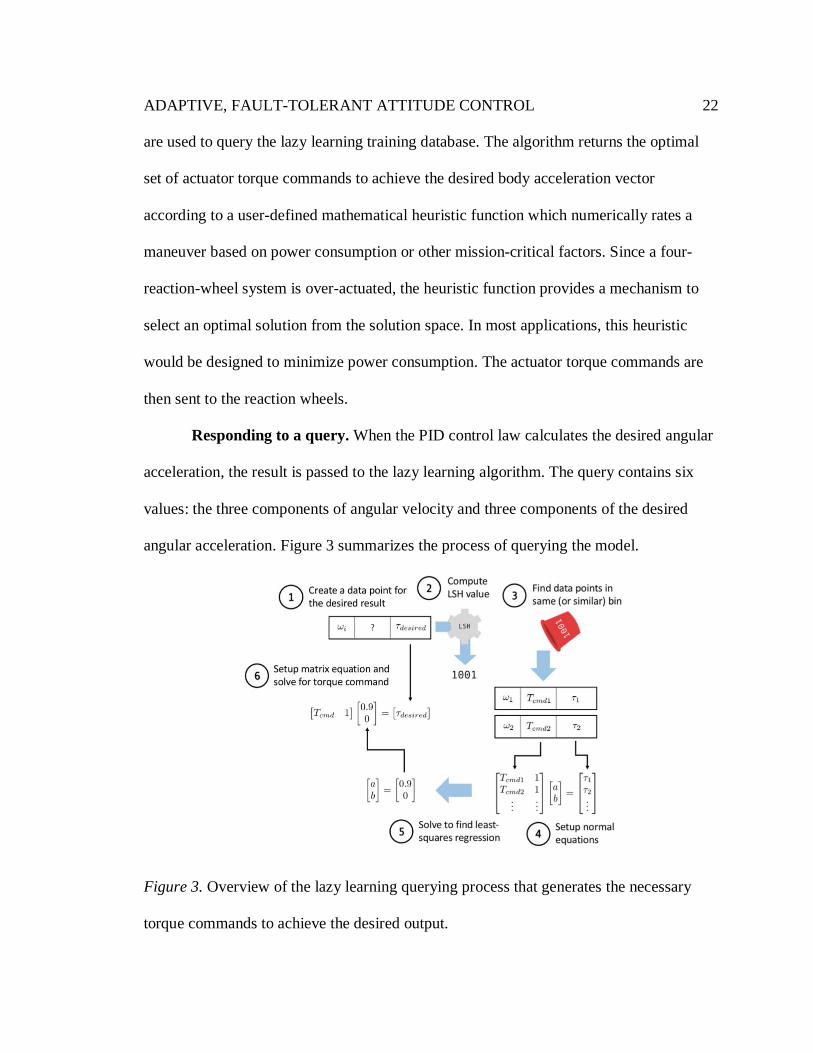
Responding to a query. When the PID control law calculates the desired angular
acceleration, the result is passed to the lazy learning algorithm. The query contains six
values: the three components of angular velocity and three components of the desired
angular acceleration. Figure 3 summarizes the process of querying the model.
Figure 3. Overview of the lazy learning querying process that generates the necessary
torque commands to achieve the desired output.
ADAPTIVE, FAULT-TOLERANT ATTITUDE CONTROL
23
Note that Figure 3 simplifies the algorithm to a single-dimensional angular
velocity state, desired torque output, and torque command. The full implementation uses
three-dimensional vectors for the angular velocity and torque output, while the torque
command has four components, one for each actuator.
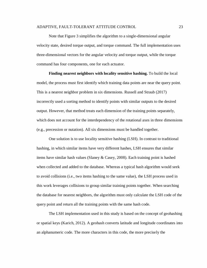
Finding nearest neighbors with locality sensitive hashing. To build the local
model, the process must first identify which training data points are near the query point.
This is a nearest neighbor problem in six dimensions. Russell and Straub (2017)
incorrectly used a sorting method to identify points with similar outputs to the desired
output. However, that method treats each dimension of the training points separately,
which does not account for the interdependency of the rotational axes in three dimensions
(e.g., precession or nutation). All six dimensions must be handled together.
One solution is to use locality sensitive hashing (LSH). In contrast to traditional
hashing, in which similar items have very different hashes, LSH ensures that similar
items have similar hash values (Slaney & Casey, 2008). Each training point is hashed
when collected and added to the database. Whereas a typical hash algorithm would seek
to avoid collisions (i.e., two items hashing to the same value), the LSH process used in
this work leverages collisions to group similar training points together. When searching
the database for nearest neighbors, the algorithm must only calculate the LSH code of the
query point and return all the training points with the same hash code.
The LSH implementation used in this study is based on the concept of geohashing
or spatial keys (Karich, 2012). A geohash converts latitude and longitude coordinates into
an alphanumeric code. The more characters in this code, the more precisely the

ADAPTIVE, FAULT-TOLERANT ATTITUDE CONTROL
24
coordinates are specified. When converted to binary, the even-indexed bits encode the
longitude, and the odd-indexed bits encode the latitude. Each code represents a binary
search algorithm. Given that latitude ranges from −90∘ to 90∘, each bit of the latitude
code indicates which half of the remaining range the true value falls within. For example,
let 𝑥 be the true latitude. Given the code 1011, the first bit indicates that 𝑥 ∈ [0∘, 90∘].
The second bit narrows the range to 𝑥 ∈ [0∘, 45∘), and the third narrows it further to 𝑥 ∈
[22.5∘, 45∘). Using the final bit, 𝑥 can be constrained to [34.75∘, 45∘). The same
algorithm can be repeated for the longitude. The two-bit sequences are interleaved so that
the latitude and longitude information are integrated together. The interleaved code
essentially identifies a region on the surface of the earth containing the original
coordinates. By removing bits from the end of the code, the binary search tree for both
the latitude and longitude is flattened, and the resulting geographic area is enlarged.
Importantly, if two pairs of coordinates fall in the same region, they will generate the
same geohash.
This concept can be extended into the six-dimensional space of the training data
points. Instead of encoding and interleaving two values (i.e., latitude and longitude), the
binary codes of six values are interleaved. The method of calculating each individual
code resembles geohashing. For the angular velocity values, the code represents the
binary search of the range (𝜔min, 𝜔max), where 𝜔min and 𝜔max are the minimum and
maximum expected angular velocities during the training period. The exact values of
these parameters do not appear to be critical as long as the region encloses the normal
operating space of the ADCS. This will ensure that all of the data points are placed into
ADAPTIVE, FAULT-TOLERANT ATTITUDE CONTROL
25
the most accurate LSH bins. If the range is set too small, more points will be placed in the
edge bins, while if the range is set too large, the points will be clustered toward the
middle bins. The results of this study, presented later, indicate that the LSH algorithm
does not play a significant role in the performance of the system.
In this study, a statistical analysis of the training sequence was used to estimate
appropriate values for the range. The training sequence can be modeled as a random walk
in which each step has a magnitude of
Δ𝜔 =𝜏
𝐽Δ𝑡 (10)
where 𝜏 ∈ [−𝜏max, 𝜏max) is randomly chosen uniform distribution, 𝜏max is the maximum
allowed torque magnitude of the actuators during the training phase, 𝐽 is the spacecraft
moment of inertia (MOI), and Δ𝑡 is the maneuver duration. As with a random walk, the
final parameter value after 𝑛 steps will be
𝑆𝑛 = ∑𝑋𝑛
𝑛
𝑖=1
(11)
where 𝑋𝑛 is the step size of the 𝑛th step (Taipale, n.d.). Therefore, the expected final
value will be
ADAPTIVE, FAULT-TOLERANT ATTITUDE CONTROL
26
𝐸(𝑆𝑛) = 𝐸 (∑ 𝑋𝑛
𝑛
𝑖=1
)
= ∑𝐸
𝑛
𝑖=1
(𝑋𝑛)
= 0
(12)
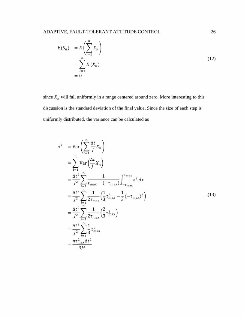
since 𝑋𝑛 will fall uniformly in a range centered around zero. More interesting to this
discussion is the standard deviation of the final value. Since the size of each step is
uniformly distributed, the variance can be calculated as
𝜎2 = Var (∑Δ𝑡
𝐽
𝑛
𝑖=1
𝑋𝑛)
= ∑Var
𝑛
𝑖=1
(Δ𝑡
𝐽𝑋𝑛)
=Δ𝑡2
𝐽2∑
1
𝜏max − (−𝜏max)
𝑛
𝑖=1
∫ 𝑥2𝜏max
−𝜏max
𝑑𝑥
=Δ𝑡2
𝐽2∑
1
2𝜏max
𝑛
𝑖=1
(1
3𝜏max
3 −1
3(−𝜏max)
3)
=Δ𝑡2
𝐽2∑
1
2𝜏max
𝑛
𝑖=1
(2
3𝜏max
3 )
=Δ𝑡2
𝐽2∑
1
3
𝑛
𝑖=1
𝜏max2
=𝑛𝜏max
2 Δ𝑡2
3𝐽2
(13)

ADAPTIVE, FAULT-TOLERANT ATTITUDE CONTROL
27
Therefore, the standard deviation is
𝜎 = √𝑛𝜏max
2 Δ𝑡2
3𝐽2
=𝜏maxΔ𝑡√3𝑛
3𝐽
(14)
Since the final value 𝑆𝑛 is normally distributed (Taipale, n.d.), no defined maximum or
minimum value exists, and the value of three standard deviations is used instead:
𝜔max = 3𝜎 =𝜏maxΔ𝑡√3𝑛
𝐽 (15)
Note that although 𝐽 and actuator characteristics (i.e., 𝜏max) appear in this derivation, they
are not required for the LSH algorithm. This limit does not have to be calculated from the
parameters but could be taken from the maximum angular velocity constraints of the
spacecraft. If the 𝜔max is too high, this only means that there may be many unused LSH
bins. Time constraints during this study forced the 𝜔max and 𝜏max to be determined from
the spacecraft’s characteristics; however, the results of the experiments indicated that the
LSH algorithm does not significantly affect the system’s performance.
Given 𝜔max and 𝜏max, the three angular acceleration components of the datapoint
can be encoded as
ADAPTIVE, FAULT-TOLERANT ATTITUDE CONTROL
28
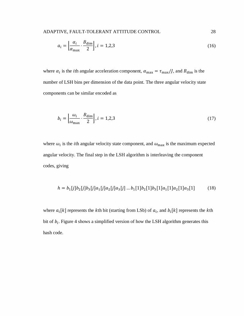
𝑎𝑖 = ⌊𝛼𝑖
𝛼max⋅𝐵dim
2⌋ , 𝑖 = 1,2,3 (16)
where 𝛼𝑖 is the 𝑖th angular acceleration component, 𝛼max = 𝜏max/𝐽, and 𝐵dim is the
number of LSH bins per dimension of the data point. The three angular velocity state
components can be similar encoded as
𝑏𝑖 = ⌊𝜔𝑖
𝜔max⋅𝐵dim
2⌋ , 𝑖 = 1,2,3 (17)
where 𝜔𝑖 is the 𝑖th angular velocity state component, and 𝜔max is the maximum expected
angular velocity. The final step in the LSH algorithm is interleaving the component
codes, giving
ℎ = 𝑏1[𝑗]𝑏2[𝑗]𝑏3[𝑗]𝑎1[𝑗]𝑎2[𝑗]𝑎3[𝑗] … 𝑏1[1]𝑏2[1]𝑏3[1]𝑎1[1]𝑎2[1]𝑎3[1] (18)
where 𝑎𝑖[𝑘] represents the 𝑘th bit (starting from LSb) of 𝑎𝑖, and 𝑏𝑖[𝑘] represents the 𝑘th
bit of 𝑏𝑖. Figure 4 shows a simplified version of how the LSH algorithm generates this
hash code.

ADAPTIVE, FAULT-TOLERANT ATTITUDE CONTROL
29
Figure 4. Simplified demonstration of the LSH algorithm with two, one-dimensional
quantities. In the implementation, both the initial angular velocity state and the output
torque were three-dimensional vectors, so the final, interleaved code was 12 bits long.
Although the figure uses output torque, the recommended implementation would use
angular acceleration per the discussion of the training point collection.
Notice that the angular acceleration values are used in the LSb of ℎ. In the event
that the query hash bin is empty during the nearest neighbor search, the LSH code can be
incremented to find neighboring bins from which to take the necessary points. Using
angular acceleration values as the LSb means that neighboring bins with similar angular
accelerations will be searched first. The bins are searched until enough points are found
to meet the bandwidth requirements (e.g., 10 points).
ADAPTIVE, FAULT-TOLERANT ATTITUDE CONTROL
30
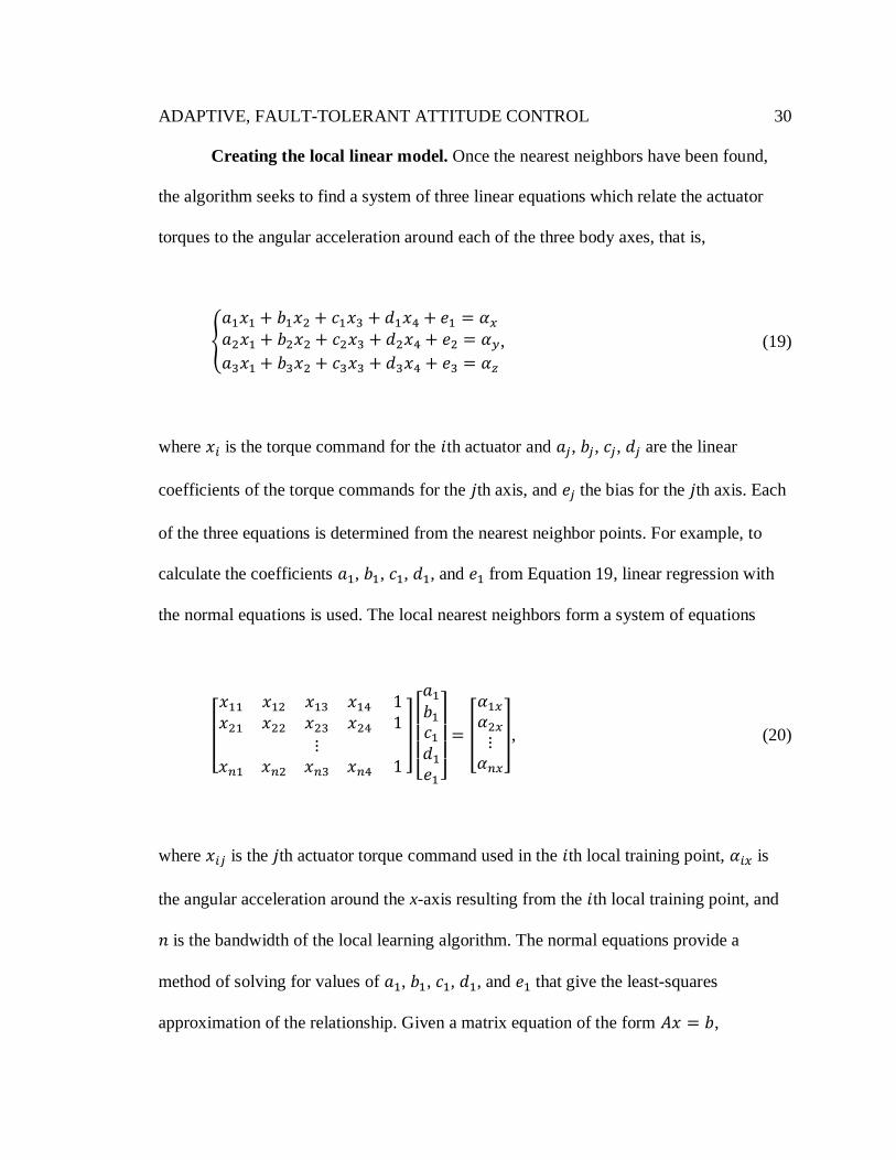
Creating the local linear model. Once the nearest neighbors have been found,
the algorithm seeks to find a system of three linear equations which relate the actuator
torques to the angular acceleration around each of the three body axes, that is,
{
𝑎1𝑥1 + 𝑏1𝑥2 + 𝑐1𝑥3 + 𝑑1𝑥4 + 𝑒1 = 𝛼𝑥
𝑎2𝑥1 + 𝑏2𝑥2 + 𝑐2𝑥3 + 𝑑2𝑥4 + 𝑒2 = 𝛼𝑦
𝑎3𝑥1 + 𝑏3𝑥2 + 𝑐3𝑥3 + 𝑑3𝑥4 + 𝑒3 = 𝛼𝑧
, (19)
where 𝑥𝑖 is the torque command for the 𝑖th actuator and 𝑎𝑗, 𝑏𝑗, 𝑐𝑗, 𝑑𝑗 are the linear
coefficients of the torque commands for the 𝑗th axis, and 𝑒𝑗 the bias for the 𝑗th axis. Each
of the three equations is determined from the nearest neighbor points. For example, to
calculate the coefficients 𝑎1, 𝑏1, 𝑐1, 𝑑1, and 𝑒1 from Equation 19, linear regression with
the normal equations is used. The local nearest neighbors form a system of equations
[
𝑥11 𝑥12 𝑥13 𝑥14 1𝑥21 𝑥22 𝑥23 𝑥24 1
⋮𝑥𝑛1 𝑥𝑛2 𝑥𝑛3 𝑥𝑛4 1
]
[ 𝑎1
𝑏1
𝑐1
𝑑1
𝑒1 ]
= [
𝛼1𝑥
𝛼2𝑥
⋮𝛼𝑛𝑥
], (20)
where 𝑥𝑖𝑗 is the 𝑗th actuator torque command used in the 𝑖th local training point, 𝛼𝑖𝑥 is
the angular acceleration around the x-axis resulting from the 𝑖th local training point, and
𝑛 is the bandwidth of the local learning algorithm. The normal equations provide a
method of solving for values of 𝑎1, 𝑏1, 𝑐1, 𝑑1, and 𝑒1 that give the least-squares
approximation of the relationship. Given a matrix equation of the form 𝐴𝑥 = 𝑏,
ADAPTIVE, FAULT-TOLERANT ATTITUDE CONTROL
31
the normal equations become 𝐴𝑇𝐴𝑥 = 𝐴𝑇𝑏, where 𝐴𝑇𝐴 is known as the normal matrix.
Solving this matrix equation for 𝑥 gives the values of the coefficients of the least-squares
regression. Using this process, 𝑎1, 𝑏1, 𝑐1, 𝑑1, and 𝑒1 from Equation 20 can be found. By
repeating this process, the algorithm can solve for 𝑎𝑗, 𝑏𝑗, 𝑐𝑗, 𝑑𝑗, and 𝑒𝑗 for each axis.
Once all three equations have been found, the coefficients can be substituted in
Equation 19 and 𝛼𝑥, 𝛼𝑦, and 𝛼𝑧 are set to the desired angular accelerations generated by
the PID control law.
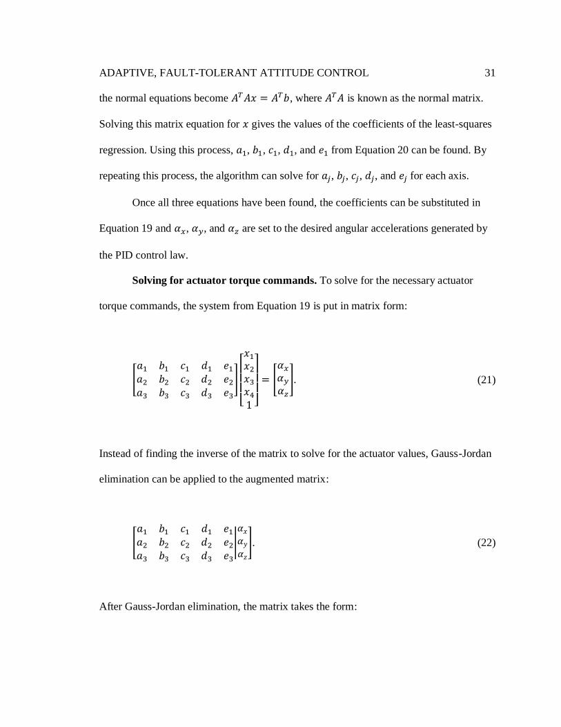
Solving for actuator torque commands. To solve for the necessary actuator
torque commands, the system from Equation 19 is put in matrix form:
[
𝑎1 𝑏1 𝑐1 𝑑1 𝑒1
𝑎2 𝑏2 𝑐2 𝑑2 𝑒2
𝑎3 𝑏3 𝑐3 𝑑3 𝑒3
]
[ 𝑥1
𝑥2
𝑥3
𝑥4
1 ]
= [
𝛼𝑥
𝛼𝑦
𝛼𝑧
]. (21)
Instead of finding the inverse of the matrix to solve for the actuator values, Gauss-Jordan
elimination can be applied to the augmented matrix:
[
𝑎1 𝑏1 𝑐1 𝑑1 𝑒1
𝑎2 𝑏2 𝑐2 𝑑2 𝑒2
𝑎3 𝑏3 𝑐3 𝑑3 𝑒3
|
𝛼𝑥
𝛼𝑦
𝛼𝑧
]. (22)
After Gauss-Jordan elimination, the matrix takes the form:

ADAPTIVE, FAULT-TOLERANT ATTITUDE CONTROL
32
[
1 0 0 𝑑1′ 𝑒1
′
0 1 0 𝑑2′ 𝑒2
′
0 0 1 𝑑3′ 𝑒3
′|
𝛼𝑥′
𝛼𝑦′
𝛼𝑧′
]. (23)
This represents the following system:
{
𝑥1 + 𝑑1′𝑥4 + 𝑒1
′ = 𝛼𝑥′
𝑥2 + 𝑑2′ 𝑥4 + 𝑒2
′ = 𝛼𝑦′
𝑥3 + 𝑑3′ 𝑥4 + 𝑒3
′ = 𝛼𝑧′
. (24)
If only three actuators were used, the system would be determined, and there will be a
single solution. However, four or more actuators will create an overdetermined system.
This study investigates a four-actuator system, but the results can be extended to any
number of actuators.
Handling overdetermined equations. An overdetermined system means that
three of the actuator commands are dependent on the fourth command and the constant
term. The fourth actuator command is a free variable and can take on any value within
the actuator’s operating range. This solution space can be searched for the optimal set of
actuator commands. Rearranging Equation 24 gives
{
𝑥1 = 𝛼𝑥′ − (𝑑1′𝑥4 + 𝑒1′)
𝑥2 = 𝛼𝑦′ − (𝑑2′𝑥4 + 𝑒2′)
𝑥3 = 𝛼𝑧′ − (𝑑3′𝑥4 + 𝑒3′)
(27)
Returning Equation 27 to matrix form allows easy calculation of the solution space.

ADAPTIVE, FAULT-TOLERANT ATTITUDE CONTROL
33
[
𝑥1
𝑥2
𝑥3
] = [
𝛼𝑥′
𝛼𝑦′
𝛼𝑧′
] − [
𝑑1′ 𝑒1′
𝑑2′ 𝑒2′
𝑑3′ 𝑒3′
] [𝑥4
1] (28)
Expanding the matrix multiplication in Equation 28 confirms that it equals Equation 27.
Optimality is determined by a heuristic function. In this study, the heuristic was designed
to minimize the magnitude of torque applied to the spacecraft, i.e.,
ℎ(𝑥) = ∑𝑥𝑖2
4
i=1
(29)
where 𝑥 = [𝑥1, 𝑥2, 𝑥3, 𝑥4]T. By stepping through the solution space, the actuator
commands with the smallest heuristic value can be found. Once the optimal result has
been reached, the torque commands are applied to the reaction wheels.
Simulation Using NASA’s 42
In order to test the lazy learning algorithm, simulations were run using 42, an
open-source simulation software developed at NASA's Goddard Space Flight Center (see
Appendix A). Configuration files are used to specify aspects of the simulation, such as
which environmental effects to simulate, the spacecraft's 3D model and characteristics,
starting orbit and time, etc. (see Appendix B). The simulations in this study were run with
aerodynamic forces and torques, solar pressure forces and torques, gravity gradient
torques, gravity perturbation forces, and reaction wheel imbalance forces and torques. To
control the simulated spacecraft, users develop a custom flight software (FSW) function
ADAPTIVE, FAULT-TOLERANT ATTITUDE CONTROL
34
in C that is called at each step of the simulation and implements custom control
algorithms.
C Software Architecture
The implementation of the algorithm was developed in C. The code can be
divided into three primary sections: (a) matrix operations, (b) ADCS functions, and (c)
main flight software loop (see Appendix C).
Matrix operations. It is advantageous to create a set of matrix manipulation
functions to facilitate building the lazy learning model. Although existing C/C++ libraries
for matrix operations exist, the decision was made to create a custom lightweight
implementation that only included what was needed (Free Software Foundation, n.d.).
This library would be more practical than a complete library of numerical operations
when porting the code to an embedded target. The matrix content and dimensions are
stored in a structure which is modified by a set of matrix operation functions. The
datatype of the matrices is fixed to double. The matrix functions include initializing
matrices, getting and setting elements, matrix addition, matrix multiplication, scalar
multiplication, row multiplication, row addition, transposition, horizontal and vertical
concatenation, horizontal splitting, reduced row echelon form, duplication, deletion, and
debug printing.
ADCS functions. Building off of the matrix operations, a set of ADCS functions
provides locality sensitive hashing, manages the training sequence, and handles lazy
learning queries. Training data points are stored in a data structure that has fields for the
initial angular velocity state, the actuator commands, and the resulting angular

ADAPTIVE, FAULT-TOLERANT ATTITUDE CONTROL
35
acceleration. The lazy learning database is stored as a list of LSH bins. Each bin is
represented by a structure holding an array of data points, the size of the of bin, and the
number of points in the bin. An ADCS structure holds the LSH bins, a pointer to the
heuristic function, and the current state of the ADCS. The ADCS has four states: IDLE,
TRAIN, MOVE, and RESET.
Main flight software loop. The main flight software loop transitions the system
between the four ADCS states to test the performance of the algorithm. The program
flow is summarized in Figure 5.
Figure 5. Flowchart of the C flight software used in the simulations with NASA’s 42

ADAPTIVE, FAULT-TOLERANT ATTITUDE CONTROL
36
Training data collection. The flight software initializes by creating the ADCS
structure and starting in the TRAIN state. During training, the system performs four
actions: (a) initialize the training sequence, (b) generate a random torque command, (c)
wait for maneuver completion, and (d) store the results in the database. After storing the
result, the training loop returns to step (b) to gather another data point. Once all the data
points have collected, the ADCS state is changed from TRAIN to IDLE.
Return to initial orientation. Once reaching the IDLE state for the first time, the
flight software changes the state to RESET. This function seeks to use the newly acquired
training data to reset the spacecraft's orientation back to 𝜽𝟎 = ⟨0,0,0⟩. More importantly,
this phase allows the test maneuver that follows to be started from same position for all
the trials. Once the angular velocity and position are reset within the required thresholds,
the flight software advances the ADCS to the MOVE state.
Rotation to target orientation. In the MOVE state, the spacecraft attempts to
rotate to the target orientation of 𝜽𝒇 = ⟨𝜋/4 , 𝜋/4, 𝜋/4⟩. In quaternion form, this
orientation becomes 𝑞𝑓 = 0.462�̂� + 0.191�̂� + 0.462�̂� + 0.733. Using a PID control law
in combination with the lazy learning algorithm, the spacecraft applies torques to the four
actuators to reach the target attitude. During this movement, the angular position error for
each axis is written to a log file.
Test parameters. This study focuses on evaluating the effect of the lazy learning
database size and bandwidth on the performance of the ADCS as measured by the time
required to rotate from 𝜽𝟎 to 𝜽𝒇. Five different values were tested for each parameter,
and each test consisted of 100 trials. Since two configurations overlapped, nine total

ADAPTIVE, FAULT-TOLERANT ATTITUDE CONTROL
37
parameter combinations were tested. The training database size was tested with 10, 50,
100, 500, and 1000 points while the bandwidth was held constant at 10 points. Then, the
bandwidth was varied with values of 1, 5, 10, 15, and 20 points while the training
database size was held constant at 100 points.
Results
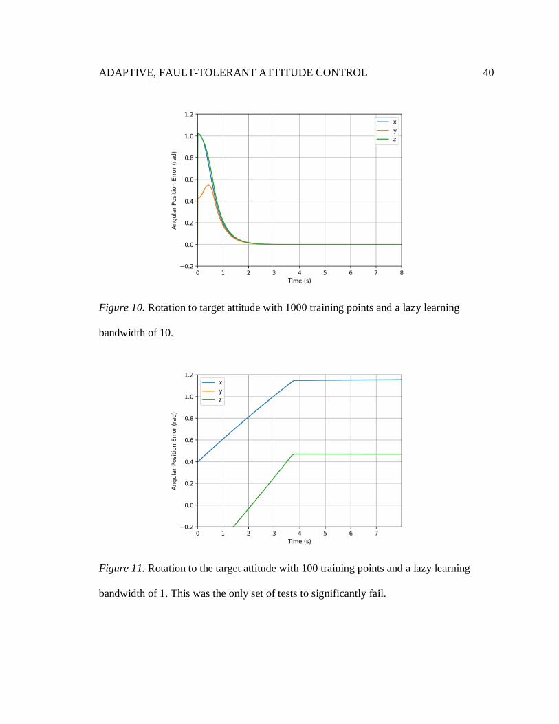
Figures 6 through 14 show representative samples of the rotation to the target
orientation for each of the nine parameter combinations. Figures 6 through 10 cover the
variation of the training point database size while Figures 11 through 14 show the
remaining results for the bandwidth tests. Table 1 contains the statistical results of the
simulations for each configuration.
Table 1
Summary of Statistical Results of 100 Trials for Nine Configurations
Test Training Points Bandwidth Avg. Time (sec) s (sec) Failures
1 10 10 3.8171 0.0095 0
2 50 10 3.8173 0.0145 0
3 100 10 3.8157 0.0188 0
4 500 10 3.8074 0.0294 0
5 1000 10 3.8025 0.0316 0
6 100 1 - - 100
7 100 5 3.8241 0.0952 2
8 100 15 3.8151 0.0138 0
9 100 20 3.8143 0.0135 0
Interestingly, once the bandwidth was at least five data points, the average time required
to rotate to the target remained largely the same across all the tests. Adding more points
to the database in an attempt to more precisely capture any nonlinearity or expanding the
bandwidth to smooth the lazy linear approximation did not impact the overall
performance of the algorithm. This seems to indicate that the relationship between

ADAPTIVE, FAULT-TOLERANT ATTITUDE CONTROL
38
actuator commands and resulting angular acceleration was linear. Once enough points
were used to capture this relationship, no additional points in either the training database
or the bandwidth were needed.
Figure 6. Rotation to target attitude with 10 training points and a lazy learning bandwidth
of 10.
Figure 7. Rotation to target attitude with 50 training points and a lazy learning bandwidth
of 10.

ADAPTIVE, FAULT-TOLERANT ATTITUDE CONTROL
39
Figure 8. Rotation to target attitude with 100 training points and a lazy learning
bandwidth of 10.
Figure 9. Rotation to target attitude with 500 training points and a lazy learning
bandwidth of 10.
ADAPTIVE, FAULT-TOLERANT ATTITUDE CONTROL
40
Figure 10. Rotation to target attitude with 1000 training points and a lazy learning
bandwidth of 10.
Figure 11. Rotation to the target attitude with 100 training points and a lazy learning
bandwidth of 1. This was the only set of tests to significantly fail.

ADAPTIVE, FAULT-TOLERANT ATTITUDE CONTROL
41
Figure 12. Rotation to the target attitude with 100 training points and a lazy learning
bandwidth of 5.
Figure 13. Rotation to the target attitude with 100 training points and a lazy learning
bandwidth of 15.

ADAPTIVE, FAULT-TOLERANT ATTITUDE CONTROL
42
Figure 14. Rotation to the target attitude with 100 training points and a lazy learning
bandwidth of 20.
The linearity present in the results was not expected based on the original
understanding of spacecraft attitude dynamics and control systems. This prodded a deeper
investigation into rotational dynamics and the architecture of attitude control systems to
see if this linearity could have been predicted. As described by both Snider (2010) and by
Princeton Satellite Systems (2000), satellite attitude dynamics are nonlinear due to the
interaction between the three separate axes.
To control this nonlinear plant, attitude control systems linearize the problem by
reducing the range around an operating point and apply a linear control law, such as PID
(Princeton Satellite Systems, 2000; Snider, 2010). Developed via control system theory,
these laws determine the stability of the system, and the previous adaptive studies
ADAPTIVE, FAULT-TOLERANT ATTITUDE CONTROL
43
discussed in the literature review have researched the stability of various control laws
when encountering partial or complete actuator failure.
The expectation that reaction wheels would have a nonlinear response to torque
commands, especially in the presence of friction, justified the exploration of using lazy
local learning to intelligently adapt the control system in the presence of changing
nonlinearity in the actuator’s response. The lazy learning algorithm described in this
study improves on Russell and Straub (2017) by using LSH instead of treating each axis
of the training point independently. LSH allows for the algorithm to account for the
interdependence of the rotation axes by including all six elements of the training point at
once in the hashing algorithm. In addition, using the normal equations for linear
regression allows the algorithm to use varying bandwidths (i.e., numbers of training
points) when constructing the local linear models, a flexibility that was not present in the
methods presented by Russell and Straub (2017). These modifications would increase the
flexibility of the lazy local learning algorithm in the presence of nonlinearities, such as
those expected in the actuators.
Although the relationship between electrical current and reaction wheel speed is
truly nonlinear, both Carrara and Kuga (2013) and Princeton Satellite Systems (2000)
note that when operated in speed control mode, reaction wheels have an internal feedback
loop which ensures they produce the required torque response, removing this
nonlinearity. Therefore, the nonlinearity of rotational dynamics is removed by linearizing
the system around an operating point, and the nonlinearity of actuator response is
removed via an internal feedback loop.
ADAPTIVE, FAULT-TOLERANT ATTITUDE CONTROL
44
With this improved knowledge, the system described in this study is better
understood as an adaptive torque distribution system. After the control law has calculated
the torques that should be applied to the system, the torques must be distributed among
the actual actuators located on the spacecraft (Princeton Satellite Systems, 2000). In
effect, the torque distribution process projects the desired torques from the body axes
onto the actuator axes. If the spacecraft has more than three actuators, their axes will not
be linearly independent (four axis vectors in three dimensions), and a cost function
similar to the heuristic within the lazy learning algorithm can be used to find an optimal
projection. Since the reaction wheel feedback control removes the nonlinearity from the
actuator response, this projection is linear, matching the results of this study. This means
that instead of searching the training database for relevant points and creating a local
linear model for each query, the linear torque distribution matrix could be calculated once
initially. A fault detection system could identify degradation and failure of actuators,
triggering a new linear distribution matrix to be calculated. Such a system would be
valuable since it would allow the distribution matrix to be calculated during mission
operations without previous knowledge of the spacecraft, mitigating actuator
misalignment and inertial issues.
If the reaction wheels used current control instead of speed control, the
nonlinearity of the wheels would emerge. In this scenario, the torque distribution process
would translate the desired torques from the control law into current levels to supply to
the wheels. A lazy local learning system could potentially be used in this application to
account for the nonlinearity.
ADAPTIVE, FAULT-TOLERANT ATTITUDE CONTROL
45
Conclusions
This study seeks to further investigate the application of lazy local learning to
adaptive, fault-tolerant attitude determination and control systems for spacecraft. The
results show that the input/output relationship for reaction wheels is predominately linear
in nominal operating scenarios and is not significantly impacted by the number of
training points or local learning bandwidth. This reflects the linear nature of the torque
distribution process. The expected nonlinearity of the rotational dynamics is limited by
the control law design, while the nonlinearity of the actuator response is removed by an
internal feedback control loop within the reaction wheels. From these results, the torque
distribution process can be simplified by removing the lazy learning aspect while
retaining the training process to account for actuator misalignments. Future work could
explore the application of the lazy local learning algorithm to current-controlled reaction
wheels or the continued adaptation of the linear torque distribution matrix in the presence
of actuator degradation and failure.

ADAPTIVE, FAULT-TOLERANT ATTITUDE CONTROL
46
References
Atkeson, C. G., Moore, A. W., & Schaal, S. (1997). Locally weighted learning. Artificial
Intelligence Review, 11, 11-73. doi:10.1023/A:1006559212014
Bottou, L., & Vapnik, V. (1992). Local learning algorithms. Neural Computation, 4(6),
888-900. doi:10.1162/neco.1992.4.6.888
Burt, R. R., & Loffi, R. W. (2003). Failure analysis of International Space Station control
moment gyro. Proceedings of the 10th European Space Mechanisms and
Tribology Symposium, San Sebastian, Spain (pp. 13-25).
Carrara, V., & Kuga, H. K. (2013). Estimating friction parameters in reaction wheels for
attitude control. Mathematical Problems in Engineering, 2013, 1-8.
doi:10.1155/2013/249674
Carrara, V., da Silva, A. G., & Kuga, H. K. (2012). A dynamic friction model for reaction
wheels. Advances in the Astronautical Sciences, 145, 343-352. San Diego:
Univelt.
Cowen, R. (2013, May 23). The wheels come off Kepler. Nature, 497, 417-418.
doi:10.1038/497417a
Cruz, G., & Bernstein, D. S. (2013). Adaptive spacecraft attitude control with reaction
wheel actuation. American Control Conference, 2013, Washington, D.C. (pp.
4832-4837). doi:10.1109/ACC.2013.6580586

ADAPTIVE, FAULT-TOLERANT ATTITUDE CONTROL
47
Dinca, D. (2004). Satellite momentum wheel speed control with dry rolling friction
compensation (Master’s thesis). Retrieved from
https://www.csuohio.edu/engineering/sites/
csuohio.edu.engineering/files/media/ece/documents/DragosDinca.pdf
Free Software Foundation. (n.d.). GSL - GNU scientific library. Retrieved from
https://www.gnu.org/software/gsl/
Hacker, J. M., Ying, J., & Lai, P. C. (2015). Reaction wheel friction telemetry data
processing methodology and on-orbit experience. Journal of Astronautical
Sciences, 62(3), 254-269. doi:10.1007/s40295-015-0076-7
Hall, C. (n.d.). Reference frames for spacecraft dynamics and control. Retrieved from
http://www.dept.aoe.vt.edu/~cdhall/courses/aoe4140/refframes.pdf
Hu, Q., Xiao, B., & Friswell, M. I. (2011). Robust fault-tolerant control for spacecraft
attitude stabilisation subject to input saturation. IET Control Theory and
Applications, 5(2), 271-282. doi:10.1049/iet-cta.2009.0628
Karich, P. (2012). Spatial keys – Memory efficient geohashes. Retrieved from
https://karussell.wordpress.com/2012/05/23/spatial-keys-memory-efficient-
geohashes/
KrishnaKumar, K., Rickard, S., & Bartholomew, S. (1995). Adaptive neuro-control for
spacecraft attitude control. Neurocomputing, 9, 131-148.
doi:10.1109/CCA.1994.381353

ADAPTIVE, FAULT-TOLERANT ATTITUDE CONTROL
48
Krishnan, S., Lee, S.-H., Hsu, H.-Y., & Konchady, G. (2011). Lubrication of attitude
control systems. In J. Hall (Ed.), Advances in Spacecraft Technologies (pp. 75-
98). http://doi.org/10.5772/13354
Li, J., Post, M., Wright, T., & Lee, R. (2013). Design of attitude control systems for
CubeSat-class nanosatellite. Journal of Control Science and Engineering, 2013,
1-15. doi:10.1155/2013/657182
NASA. (n.d.). International Space Station guide: Systems. Retrieved from
https://www.nasa.gov/pdf/167129main_Systems.pdf
Princeton Satellite Systems, Inc. (2000). Attitude and orbit control using the spacecraft
control toolbox v4.6. Retrieved from http://www.cs.cmu.edu/afs/cs.cmu.edu/
user/cjp/matlab/SC_doc/ACSTheory.pdf
Rayman, M. D., & Mase, R. A. (2014). Dawn’s operations in cruise from Vesta to Ceres.
Acta Astronautica, 103, 113-118.
Russell, M., & Straub, J. (2017). Characterization of command software for an
autonomous attitude determination and control system for spacecraft.
International Journal of Computers and Applications, 4, 198-209.
doi:10.1080/1206212X.2017.1329261
Sahay, D., Tejaswini, G. S., Santosh, K., Yuvaraj, S., Rakshit, S., Sandya, S., & Kannan,
T. (2017). Reaction wheel control, testing and failure analysis for STUDSAT-2.
Proceedings of the 2017 Aerospace Conference, Big Sky, Montana (pp. 1-11)
doi:10.1109/AERO.2017.7943707

ADAPTIVE, FAULT-TOLERANT ATTITUDE CONTROL
49
Sahnow, D. J., Kruk, J. W., Ake, T. B., Andersson, B.-G., Berman, A., Blair, W. P., . . .
Roberts, B. A. (2006). Operations with the new FUSE observatory: Three-axis
control with one reaction wheel. Proceedings of SPIE 6266, Space Telescopes
and Instrumentation II: Ultraviolet to Gamma Ray, Orlando (pp. 1-11).
doi:10.1117/12.673408
Schreiner, J. N. (2015). A neural network approach to fault detection in spacecraft
attitude determination and control systems (Master’s thesis). Retrieved from
http://digitalcommons.usu.edu/etd
Shi, J.-F., Allen, A., & Ulrich, S. (2015). Spacecraft adaptive attitude control with
application to space station free-flyer robotic capture. Paper presented at AIAA
Guidance, Navigation, and Control Conference, Kissimmee, FL.
doi:10.2514/6.2015-1780
Slaney, M., & Casey, M. (2008). Locality-sensitive hashing for finding nearest neighbors.
IEEE Signal Processing Magazine, 25(2), 128-131.
doi:10.1109/MSP.2007.914237
Snider, R. E. (2010, March). Attitude control of a satellite simulator using reaction
wheels and a PID controller (Master’s thesis). Retrieved from
http://www.dtic.mil/dtic/tr/fulltext/u2/a516856.pdf
Space Telescope Science Institute. (n.d.). Pointing and guiding. Retrieved from NASA’s
James Webb Space Telescope: https://jwst.stsci.edu/instrumentation/telescope-
and-pointing/pointing-and-guiding

ADAPTIVE, FAULT-TOLERANT ATTITUDE CONTROL
50
Space Telescope Science Institute. (n.d.). Team Hubble: Servicing missions. Retrieved
from HUBBLESITE:
http://hubblesite.org/the_telescope/team_hubble/servicing_missions.php
Starin, S. R., & Eterno, J. (2011, January 1). Attitude determination and control systems.
Retrieved from NASA Technical Reports Server:
http://hdl.handle.net/2060/20110007876
Stoneking, E. (2014). 42: A general-purpose, multi-body, multi-spacecraft simulation.
Straub, J. (2015). An intelligent attitude determination and control system concept for a
CubeSat class spacecraft. 2015 AIAA Space and Astronautics Forum and
Exposition.
Taipale, K. (n.d.). Chapter 7: Random walks. Mathematical Preparation for Finance.
Retrieved from
https://www.softcover.io/read/bf34ea25/math_for_finance/random_walks
Tang, C. (1995). Adaptive nonlinear attitude control of spacecraft (Doctoral dissertation).
Retrieved from https://lib.dr.iastate.edu/rtd/
Van Buijtenen, W. M., Schram, G., Babuska, R., & Verbruggen, H. B. (1998). Adaptive
fuzzy control of satellite attitude by reinforcement learning. IEEE Transactions
on Fuzzy Systems, 6(2), 185-194. doi:10.1109/91.669012
Wiesel, W. E. (2010). Spaceflight dynamics. Beavercreek, OH: Aphelion Press.
ADAPTIVE, FAULT-TOLERANT ATTITUDE CONTROL
51
Yoon, H. & Agarwal, B. N. (2009). Adaptive control of uncertain Hamiltonian multi-
input multi-output systems: with application to spacecraft control. IEEE
Transactions on Control Systems Technology, 17(4), 900-906.
doi:10.1109/ACC.2008.4586947
Yoon, H., & Tsiotras, P. (2008). Adaptive spacecraft attitude tracking control with
actuator uncertainties. Journal of the Astronautical Sciences, 56(2), 251-268.
doi:10.1007/BF03256551
Yoon, H., & Tsiotras, P. (2002). Spacecraft adaptive attitude and power tracking with
variable speed control moment gyroscopes. Journal of Guidance, Control, and
Dynamics, 25(6), 1081-1090. doi:10.2514/2.4987

ADAPTIVE, FAULT-TOLERANT ATTITUDE CONTROL
52
Appendix A
Getting Started with NASA’s 42 Simulation Framework on a UNIX-based Machine
1. Download the 42 archive from the official Sourceforge page:
https://sourceforge.net/projects/fortytwospacecraftsimulation/
2. Unzip the archive and navigate to the folder from the command line (e.g., “cd
Downloads/42”)
3. Edit the Makefile to ensure that the proper build platform is selected. 42 will attempt
to auto-detect the platform, but the manual backup should be set to the correct value
in case the auto-detect fails. The default is Linux. Find the AUTOPLATFORM lines
at the top of the Makefile, uncomment the line corresponding to the current platform,
and comment out the lines for the other platforms (see bolded text in the Makefile in
Appendix B). The Makefile from Appendix B is configured for macOS.
4. Build the executable by running “make” in the 42 folder from the command line. If
linker errors are encountered while trying to build the executable, use “make clean” to
clean the output folders.
5. Test the build by running the executable (“./42”). Several windows should open
including a 3D view of the spacecraft and a ground track. If using the Inp_Sim.txt
from Appendix B, change the time mode to REAL and the graphics front-end to
TRUE to see these windows appear.
6. This study added additional source files to the framework (see Appendix C). A folder
named “adcs” with “src” and “build” subfolders was created in the main 42 directory.

ADAPTIVE, FAULT-TOLERANT ATTITUDE CONTROL
53
The Makefile was changed to add these source files to the build process (see bolded
text in the Makefile in Appendix B).
Additional documentation can be found in the Docs folder of the 42 main directory or
within the configuration files themselves.

ADAPTIVE, FAULT-TOLERANT ATTITUDE CONTROL
54
Appendix B
42 Simulator Configuration Files
Inp_Sim.txt
<<<<<<<<<<<<<<<<< 42: The Mostly Harmless Simulator >>>>>>>>>>>>>>>>>
************************** Simulation Control **************************
FAST ! Time Mode (FAST, REAL, or EXTERNAL)
300.0 0.001 ! Sim Duration, Step Size [sec]
0.01 ! File Output Interval [sec]
FALSE ! Graphics Front End?
Inp_Cmd.txt ! Command Script File Name
************************** Reference Orbits **************************
1 ! Number of Reference Orbits
TRUE Orb_LEO.txt ! Input file name for Orb 0
***************************** Spacecraft *****************************
1 ! Number of Spacecraft
TRUE 0 SC_CubeSat1U_Custom.txt ! Existence, RefOrb, Input file for SC 0
***************************** Environment *****************************
07 09 2017 ! Date (Month, Day, Year)
00 00 00.00 ! Greenwich Mean Time (Hr,Min,Sec)
0.0 ! Time Offset (sec)
USER_DEFINED ! Model Date Interpolation for Solar Flux and AP
values?(TWOSIGMA_KP, NOMINAL or USER_DEFINED)
230.0 ! If USER_DEFINED, enter desired F10.7 value
100.0 ! If USER_DEFINED, enter desired AP value
IGRF ! Magfield (NONE,DIPOLE,IGRF)
8 8 ! IGRF Degree and Order (<=10)
2 0 ! Earth Gravity Model N and M (<=18)
2 0 ! Mars Gravity Model N and M (<=18)
2 0 ! Luna Gravity Model N and M (<=18)
TRUE ! Aerodynamic Forces & Torques
TRUE ! Gravity Gradient Torques
TRUE ! Solar Pressure Forces & Torques
TRUE ! Gravity Perturbation Forces
FALSE ! Passive Joint Forces & Torques
FALSE ! Thruster Plume Forces & Torques
TRUE ! RWA Imbalance Forces and Torques
TRUE ! Contact Forces and Torques
FALSE ! CFD Slosh Forces and Torques
FALSE ! Output Environmental Torques to Files
********************* Celestial Bodies of Interest *********************
FALSE ! Mercury
FALSE ! Venus
TRUE ! Earth and Luna
FALSE ! Mars and its moons
FALSE ! Jupiter and its moons
FALSE ! Saturn and its moons
FALSE ! Uranus and its moons
FALSE ! Neptune and its moons
FALSE ! Pluto and its moons
FALSE ! Asteroids and Comets
***************** Lagrange Point Systems of Interest ******************
FALSE ! Earth-Moon
FALSE ! Sun-Earth
FALSE ! Sun-Jupiter
************************* Ground Stations ***************************
5 ! Number of Ground Stations
TRUE EARTH -77.0 37.0 "GSFC" ! Exists, World, Lng, Lat, Label
TRUE EARTH -155.6 19.0 "South Point" ! Exists, World, Lng, Lat, Label
TRUE EARTH 115.4 -29.0 "Dongara" ! Exists, World, Lng, Lat, Label
TRUE EARTH -71.0 -33.0 "Santiago" ! Exists, World, Lng, Lat, Label
TRUE LUNA 45.0 45.0 "Moon Base Alpha" ! Exists, World, Lng, Lat, Label

ADAPTIVE, FAULT-TOLERANT ATTITUDE CONTROL
55
SC_CubeSat1U_Custom.txt
<<<<<<<<<<<<<<<<< 42: Spacecraft Description File >>>>>>>>>>>>>>>>>
1-U Cubesat ! Description
"Cube 1" ! Label
GenScSpriteAlpha.ppm ! Sprite File Name
AD_HOC_FSW ! Flight Software Identifier
************************* Orbit Parameters ****************************
ENCKE ! Orbit Prop FIXED, EULER_HILL, or ENCKE
CM ! Pos of CM or ORIGIN, wrt F
0.00000 0.00000 2.50000 ! Pos wrt F
0.00566 0.00283 -0.00000 ! Vel wrt F
*************************** Initial Attitude ***************************
NAN ! Ang Vel wrt [NL], Att [QA] wrt [NLF]
0.0 0.0 0.0 ! Ang Vel (deg/sec)
0.0 0.0 0.0 1.0 ! Quaternion
0.0 0.0 0.0 123 ! Angles (deg) & Euler Sequence
*************************** Dynamics Flags ***************************
KIN_JOINT ! Rotation STEADY, KIN_JOINT, or DYN_JOINT
TRUE ! Assume constant mass properties
FALSE ! Passive Joint Forces and Torques Enabled
FALSE ! Compute Constraint Forces and Torques
REFPT_CM ! Mass Props referenced to REFPT_CM or REFPT_JOINT
FALSE ! Flex Active
FALSE ! Include 2nd Order Flex Terms
2.0 ! Drag Coefficient
************************************************************************
************************* Body Parameters ******************************
************************************************************************
1 ! Number of Bodies
================================ Body 0 ================================
1.0 ! Mass (kg)
0.0017 0.0017 0.0017 ! Moments of Inertia (kg-m^2)
0.0 0.0 0.0 ! Products of Inertia (xy,xz,yz)
0.0 0.0 0.0 ! Location of mass center, m
0.0 0.0 0.0 ! Constant Embedded Momentum (Nms)
Cubesat_1U.obj ! Geometry Input File Name
NONE ! Flex File Name
************************************************************************
*************************** Joint Parameters ***************************
************************************************************************
(Number of Joints is Number of Bodies minus one)
============================== Joint 0 ================================
0 1 ! Inner, outer body indices
1 213 GIMBAL ! RotDOF, Seq, GIMBAL or SPHERICAL
0 123 ! TrnDOF, Seq
FALSE FALSE FALSE ! RotDOF Locked
FALSE FALSE FALSE ! TrnDOF Locked
0.0 0.0 0.0 ! Initial Angles [deg]
0.0 0.0 0.0 ! Initial Rates, deg/sec
0.0 0.0 0.0 ! Initial Displacements [m]
0.0 0.0 0.0 ! Initial Displacement Rates, m/sec
0.0 0.0 0.0 312 ! Bi to Gi Static Angles [deg] & Seq
0.0 0.0 0.0 312 ! Go to Bo Static Angles [deg] & Seq
0.0 0.0 0.0 ! Position wrt inner body origin, m
0.0 0.0 0.0 ! Position wrt outer body origin, m
0.0 0.0 0.0 ! Rot Passive Spring Coefficients (Nm/rad)
0.0 0.0 0.0 ! Rot Passive Damping Coefficients (Nms/rad)
0.0 0.0 0.0 ! Trn Passive Spring Coefficients (N/m)
0.0 0.0 0.0 ! Trn Passive Damping Coefficients (Ns/m)
*************************** Wheel Parameters ***************************
4 ! Number of wheels
============================= Wheel 0 ================================
0.0 ! Initial Momentum, N-m-sec
0.5 0.5 0.5 ! Wheel Axis Components, [X, Y, Z]
0.004 0.015 ! Max Torque (N-m), Momentum (N-m-sec)
(http://bluecanyontech.com/wp-content/uploads/2017/03/DataSheet_RW_06.pdf)

ADAPTIVE, FAULT-TOLERANT ATTITUDE CONTROL
56
0.00003 ! Wheel Rotor Inertia, kg-m^2 (estimated)
0.12 ! Static Imbalance, g-cm0
0.20 ! Dynamic Imbalance, g-cm^2
0 ! Flex Node Index
============================= Wheel 1 ================================
0.0 ! Initial Momentum, N-m-sec
-0.5 -0.5 0.5 ! Wheel Axis Components, [X, Y, Z]
0.004 0.015 ! Max Torque (N-m), Momentum (N-m-sec)
0.00003 ! Wheel Rotor Inertia, kg-m^2 (estimated)
0.12 ! Static Imbalance, g-cm
0.20 ! Dynamic Imbalance, g-cm^2
0 ! Flex Node Index
============================= Wheel 2 ================================
0.0 ! Initial Momentum, N-m-sec
0.5 -0.5 -0.5 ! Wheel Axis Components, [X, Y, Z]
0.004 0.015 ! Max Torque (N-m), Momentum (N-m-sec)
0.00003 ! Wheel Rotor Inertia, kg-m^2 (estimated)
0.12 ! Static Imbalance, g-cm
0.20 ! Dynamic Imbalance, g-cm^2
0 ! Flex Node Index
============================= Wheel 3 ================================
0.0 ! Initial Momentum, N-m-sec
-0.5 0.5 -0.5 ! Wheel Axis Components, [X, Y, Z]
0.004 0.015 ! Max Torque (N-m), Momentum (N-m-sec)
0.00003 ! Wheel Rotor Inertia, kg-m^2 (estimated)
0.12 ! Static Imbalance, g-cm
0.20 ! Dynamic Imbalance, g-cm^2
0 ! Flex Node Index
**************************** MTB Parameters ****************************
3 ! Number of MTBs
============================== MTB 0 =================================
180.0 ! Saturation (A-m^2)
1.0 0.0 0.0 ! MTB Axis Components, [X, Y, Z]
============================== MTB 1 =================================
180.0 ! Saturation (A-m^2)
0.0 1.0 0.0 ! MTB Axis Components, [X, Y, Z]
============================== MTB 2 =================================
180.0 ! Saturation (A-m^2)
0.0 0.0 1.0 ! MTB Axis Components, [X, Y, Z]
************************* Thruster Parameters **************************
0 ! Number of Thrusters
============================== Thr 0 =================================
1.0 ! Thrust Force (N)
-1.0 0.0 0.0 ! Thrust Axis
1.0 1.0 1.0 ! Location in B0, m
**************************** CMG Parameters ****************************
0 ! Number of CMGs
=============================== CMG 0 ================================
1 ! CMG DOF (typically 1 or 2)
0.0 0.0 0.0 123 ! Initial Gimbal Angles [deg] and Seq
0.0 0.0 0.0 ! Initial Gimbal Angle Rates, deg/sec
-90.0 0.0 -54.74 123 ! Static Mounting Angles [deg] and Seq
0.12 ! Rotor Inertia, kg-m^2
75.0 ! Momentum, Nms
1.0 0.0 0.0 ! Max Gimbal Angle Rates, deg/sec
Makefile
########################## Macro Definitions ############################
# Let's try to auto-detect what platform we're on.
# If this fails, set 42PLATFORM manually in the else block.
AUTOPLATFORM = Failed
ifeq ($(PLATFORM),apple)
AUTOPLATFORM = Succeeded
42PLATFORM = __APPLE__
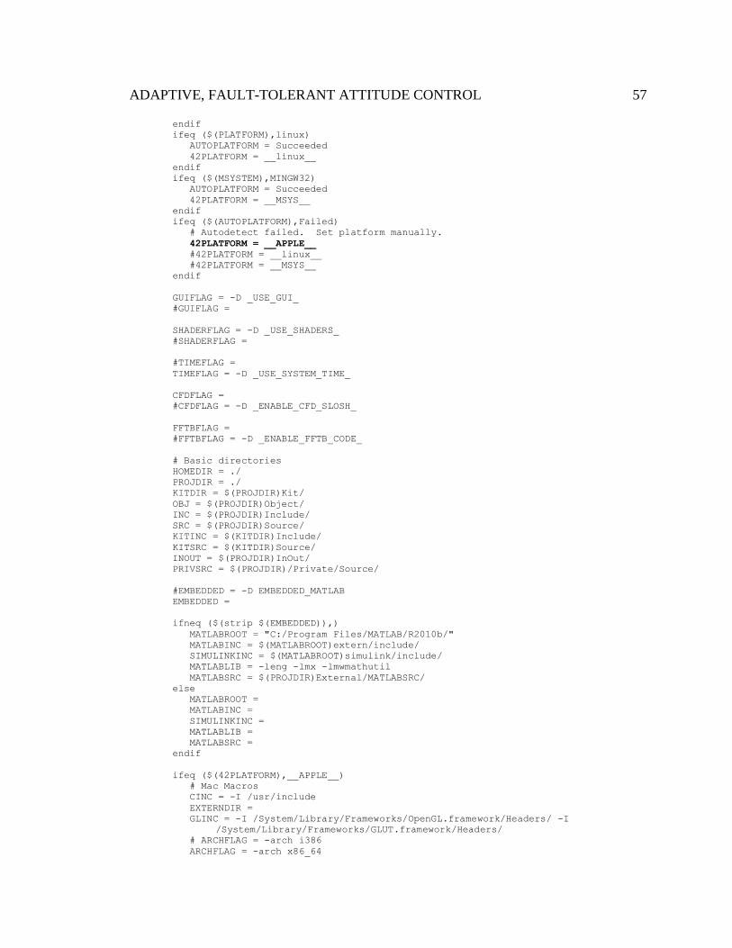
ADAPTIVE, FAULT-TOLERANT ATTITUDE CONTROL
57
endif
ifeq ($(PLATFORM),linux)
AUTOPLATFORM = Succeeded
42PLATFORM = __linux__
endif
ifeq ($(MSYSTEM),MINGW32)
AUTOPLATFORM = Succeeded
42PLATFORM = __MSYS__
endif
ifeq ($(AUTOPLATFORM),Failed)
# Autodetect failed. Set platform manually.
42PLATFORM = __APPLE__
#42PLATFORM = __linux__
#42PLATFORM = __MSYS__
endif
GUIFLAG = -D _USE_GUI_
#GUIFLAG =
SHADERFLAG = -D _USE_SHADERS_
#SHADERFLAG =
#TIMEFLAG =
TIMEFLAG = -D _USE_SYSTEM_TIME_
CFDFLAG =
#CFDFLAG = -D _ENABLE_CFD_SLOSH_
FFTBFLAG =
#FFTBFLAG = -D _ENABLE_FFTB_CODE_
# Basic directories
HOMEDIR = ./
PROJDIR = ./
KITDIR = $(PROJDIR)Kit/
OBJ = $(PROJDIR)Object/
INC = $(PROJDIR)Include/
SRC = $(PROJDIR)Source/
KITINC = $(KITDIR)Include/
KITSRC = $(KITDIR)Source/
INOUT = $(PROJDIR)InOut/
PRIVSRC = $(PROJDIR)/Private/Source/
#EMBEDDED = -D EMBEDDED_MATLAB
EMBEDDED =
ifneq ($(strip $(EMBEDDED)),)
MATLABROOT = "C:/Program Files/MATLAB/R2010b/"
MATLABINC = $(MATLABROOT)extern/include/
SIMULINKINC = $(MATLABROOT)simulink/include/
MATLABLIB = -leng -lmx -lmwmathutil
MATLABSRC = $(PROJDIR)External/MATLABSRC/
else
MATLABROOT =
MATLABINC =
SIMULINKINC =
MATLABLIB =
MATLABSRC =
endif
ifeq ($(42PLATFORM),__APPLE__)
# Mac Macros
CINC = -I /usr/include
EXTERNDIR =
GLINC = -I /System/Library/Frameworks/OpenGL.framework/Headers/ -I
/System/Library/Frameworks/GLUT.framework/Headers/
# ARCHFLAG = -arch i386
ARCHFLAG = -arch x86_64

ADAPTIVE, FAULT-TOLERANT ATTITUDE CONTROL
58
#SOCKETFLAG =
SOCKETFLAG = -D _ENABLE_SOCKETS_
ifneq ($(strip $(EMBEDDED)),)
LFLAGS = -bind_at_load -m64 -L$(MATLABROOT)bin/maci64
LIBS = -framework System -framework Carbon -framework OpenGL -framework GLUT
$(MATLABLIB)
else
LFLAGS = -bind_at_load
LIBS = -framework System -framework Carbon -framework OpenGL -framework GLUT
endif
GUIOBJ = $(OBJ)42GlutGui.o $(OBJ)glkit.o
EXENAME = 42
CC = gcc
endif
ifeq ($(42PLATFORM),__linux__)
# Linux Macros
CINC =
EXTERNDIR =
#SOCKETFLAG =
SOCKETFLAG = -D _ENABLE_SOCKETS_
ifneq ($(strip $(GUIFLAG)),)
GUIOBJ = $(OBJ)42GlutGui.o $(OBJ)glkit.o
#GLINC = -I /usr/include/
GLINC = -I $(KITDIR)/include/GL/
LIBS = -lglut -lGLU -lGL
LFLAGS = -L $(KITDIR)/GL/lib/
ARCHFLAG =
else
GUIOBJ =
GLINC =
LIBS =
LFLAGS =
ARCHFLAG =
endif
EXENAME = 42
CC = g++
endif
ifeq ($(42PLATFORM),__MSYS__)
CINC =
EXTERNDIR = /c/42ExternalSupport/
#SOCKETFLAG =
SOCKETFLAG = -D _ENABLE_SOCKETS_
ifneq ($(strip $(GUIFLAG)),)
GLEW = $(EXTERNDIR)GLEW/
GLUT = $(EXTERNDIR)freeglut/
LIBS = -lopengl32 -lglu32 -lfreeglut -lws2_32 -lglew32
LFLAGS = -L $(GLUT)lib/ -L $(GLEW)lib/
GUIOBJ = $(OBJ)42GlutGui.o $(OBJ)glkit.o
GLINC = -I $(GLEW)include/GL/ -I $(GLUT)include/GL/
ARCHFLAG = -D GLUT_NO_LIB_PRAGMA -D GLUT_NO_WARNING_DISABLE -D
GLUT_DISABLE_ATEXIT_HACK
else
GUIOBJ =
GLINC =
LIBS =
LFLAGS =
ARCHFLAG =
endif
ifneq ($(strip $(EMBEDDED)),)
LFLAGS = -L $(GLUT)lib/ -m64 -L$(MATLABROOT)bin/win32

ADAPTIVE, FAULT-TOLERANT ATTITUDE CONTROL
59
LIBS = -lopengl32 -lglu32 -lfreeglut $(MATLABLIB)
endif
EXENAME = 42.exe
CC = gcc
endif
# If not using GUI, don't compile GUI-related files
ifeq ($(strip $(GUIFLAG)),)
GUIOBJ =
endif
# If not using IPC, don't compile IPC-related files
ifneq ($(strip $(SOCKETFLAG)),)
IPCOBJ = $(OBJ)42ipc.o
else
IPCOBJ =
endif
# If not in FFTB, don't compile FFTB-related files
ifneq ($(strip $(FFTBFLAG)),)
FFTBOBJ = $(OBJ)42fftb.o
else
FFTBOBJ =
endif
CFLAGS = -Wall -Wshadow -Wno-deprecated -g $(GLINC) $(CINC) -I $(INC) -I
$(KITINC) -I $(KITSRC) -I $(MATLABSRC) -I $(MATLABINC) -I $(SIMULINKINC) -
O0 $(ARCHFLAG) $(GUIFLAG) $(SHADERFLAG) $(TIMEFLAG) $(SOCKETFLAG)
$(EMBEDDED) $(CFDFLAG) $(FFTBFLAG)
42OBJ = $(OBJ)42main.o $(OBJ)42exec.o $(OBJ)42actuators.o $(OBJ)42cmd.o \
$(OBJ)42dynam.o $(OBJ)42environs.o $(OBJ)42ephem.o $(OBJ)42fsw.o \
$(OBJ)42init.o $(OBJ)42perturb.o $(OBJ)42report.o \
$(OBJ)42sensors.o
ifneq ($(strip $(CFDFLAG)),)
SLOSHOBJ = $(OBJ)42CfdSlosh.o
else
SLOSHOBJ =
endif
KITOBJ = $(OBJ)dcmkit.o $(OBJ)envkit.o $(OBJ)fswkit.o $(OBJ)geomkit.o \
$(OBJ)iokit.o $(OBJ)mathkit.o $(OBJ)nrlmsise00kit.o $(OBJ)msis86kit.o
$(OBJ)orbkit.o $(OBJ)sigkit.o $(OBJ)sphkit.o $(OBJ)timekit.o
ifneq ($(strip $(EMBEDDED)),)
MATLABOBJ = $(OBJ)DetectorFSW.o $(OBJ)OpticsFSW.o
else
MATLABOBJ =
endif
# custom ADCS
ADCSOBJ = ./adcs/build/ADCS_main.o ./adcs/build/Matrix.o
########################## Rules to link 42 #############################
42 : $(42OBJ) $(GUIOBJ) $(IPCOBJ) $(FFTBOBJ) $(SLOSHOBJ) $(KITOBJ) $(MATLABOBJ)
$(ADCSOBJ)
$(CC) $(LFLAGS) -o $(EXENAME) $(42OBJ) $(GUIOBJ) $(IPCOBJ) $(FFTBOBJ)
$(SLOSHOBJ) $(KITOBJ) $(MATLABOBJ) $(ADCSOBJ) $(LIBS)
#################### Rules to compile objects ###########################
$(OBJ)42main.o : $(SRC)42main.c
$(CC) $(CFLAGS) -c $(SRC)42main.c -o $(OBJ)42main.o
$(OBJ)42exec.o : $(SRC)42exec.c $(INC)42.h
$(CC) $(CFLAGS) -c $(SRC)42exec.c -o $(OBJ)42exec.o

ADAPTIVE, FAULT-TOLERANT ATTITUDE CONTROL
60
$(OBJ)42actuators.o : $(SRC)42actuators.c $(INC)42.h $(INC)42fsw.h
$(INC)fswdefines.h $(INC)fswtypes.h
$(CC) $(CFLAGS) -c $(SRC)42actuators.c -o $(OBJ)42actuators.o
$(OBJ)42cmd.o : $(SRC)42cmd.c $(INC)42.h $(INC)42fsw.h $(INC)fswdefines.h
$(INC)fswtypes.h
$(CC) $(CFLAGS) -c $(SRC)42cmd.c -o $(OBJ)42cmd.o
$(OBJ)42dynam.o : $(SRC)42dynam.c $(INC)42.h
$(CC) $(CFLAGS) -c $(SRC)42dynam.c -o $(OBJ)42dynam.o
$(OBJ)42environs.o : $(SRC)42environs.c $(INC)42.h
$(CC) $(CFLAGS) -c $(SRC)42environs.c -o $(OBJ)42environs.o
$(OBJ)42ephem.o : $(SRC)42ephem.c $(INC)42.h
$(CC) $(CFLAGS) -c $(SRC)42ephem.c -o $(OBJ)42ephem.o
$(OBJ)42fsw.o : $(SRC)42fsw.c $(INC)42fsw.h $(INC)fswdefines.h
$(INC)fswtypes.h
$(CC) $(CFLAGS) -c $(SRC)42fsw.c -o $(OBJ)42fsw.o
$(OBJ)42GlutGui.o : $(SRC)42GlutGui.c $(INC)42.h $(INC)42GlutGui.h
$(KITSRC)CamShaders.glsl $(KITSRC)MapShaders.glsl
$(CC) $(CFLAGS) -c $(SRC)42GlutGui.c -o $(OBJ)42GlutGui.o
$(OBJ)42init.o : $(SRC)42init.c $(INC)42.h
$(CC) $(CFLAGS) -c $(SRC)42init.c -o $(OBJ)42init.o
$(OBJ)42ipc.o : $(SRC)42ipc.c $(INC)42.h
$(CC) $(CFLAGS) -c $(SRC)42ipc.c -o $(OBJ)42ipc.o
$(OBJ)42perturb.o : $(SRC)42perturb.c $(INC)42.h
$(CC) $(CFLAGS) -c $(SRC)42perturb.c -o $(OBJ)42perturb.o
$(OBJ)42report.o : $(SRC)42report.c $(INC)42.h
$(CC) $(CFLAGS) -c $(SRC)42report.c -o $(OBJ)42report.o
$(OBJ)42sensors.o : $(SRC)42sensors.c $(INC)42.h $(INC)42fsw.h
$(INC)fswdefines.h $(INC)fswtypes.h
$(CC) $(CFLAGS) -c $(SRC)42sensors.c -o $(OBJ)42sensors.o
$(OBJ)dcmkit.o : $(KITSRC)dcmkit.c
$(CC) $(CFLAGS) -c $(KITSRC)dcmkit.c -o $(OBJ)dcmkit.o
$(OBJ)envkit.o : $(KITSRC)envkit.c
$(CC) $(CFLAGS) -c $(KITSRC)envkit.c -o $(OBJ)envkit.o
$(OBJ)fswkit.o : $(KITSRC)fswkit.c
$(CC) $(CFLAGS) -c $(KITSRC)fswkit.c -o $(OBJ)fswkit.o
$(OBJ)glkit.o : $(KITSRC)glkit.c $(KITINC)glkit.h
$(CC) $(CFLAGS) -c $(KITSRC)glkit.c -o $(OBJ)glkit.o
$(OBJ)geomkit.o : $(KITSRC)geomkit.c $(KITINC)geomkit.h
$(CC) $(CFLAGS) -c $(KITSRC)geomkit.c -o $(OBJ)geomkit.o
$(OBJ)iokit.o : $(KITSRC)iokit.c
$(CC) $(CFLAGS) -c $(KITSRC)iokit.c -o $(OBJ)iokit.o
$(OBJ)mathkit.o : $(KITSRC)mathkit.c
$(CC) $(CFLAGS) -c $(KITSRC)mathkit.c -o $(OBJ)mathkit.o
$(OBJ)nrlmsise00kit.o : $(KITSRC)nrlmsise00kit.c
$(CC) $(CFLAGS) -c $(KITSRC)nrlmsise00kit.c -o $(OBJ)nrlmsise00kit.o
$(OBJ)msis86kit.o : $(KITSRC)msis86kit.c $(KITINC)msis86kit.h
$(CC) $(CFLAGS) -c $(KITSRC)msis86kit.c -o $(OBJ)msis86kit.o

ADAPTIVE, FAULT-TOLERANT ATTITUDE CONTROL
61
$(OBJ)orbkit.o : $(KITSRC)orbkit.c
$(CC) $(CFLAGS) -c $(KITSRC)orbkit.c -o $(OBJ)orbkit.o
$(OBJ)sigkit.o : $(KITSRC)sigkit.c
$(CC) $(CFLAGS) -c $(KITSRC)sigkit.c -o $(OBJ)sigkit.o
$(OBJ)sphkit.o : $(KITSRC)sphkit.c
$(CC) $(CFLAGS) -c $(KITSRC)sphkit.c -o $(OBJ)sphkit.o
$(OBJ)timekit.o : $(KITSRC)timekit.c
$(CC) $(CFLAGS) -c $(KITSRC)timekit.c -o $(OBJ)timekit.o
$(OBJ)DetectorFSW.o : $(MATLABSRC)DetectorFSW.c
$(CC) $(CFLAGS) -c $(MATLABSRC)DetectorFSW.c -o $(OBJ)DetectorFSW.o
$(OBJ)OpticsFSW.o : $(MATLABSRC)OpticsFSW.c
$(CC) $(CFLAGS) -c $(MATLABSRC)OpticsFSW.c -o $(OBJ)OpticsFSW.o
$(OBJ)42CfdSlosh.o : $(PRIVSRC)42CfdSlosh.c $(INC)42.h
$(CC) $(CFLAGS) -c $(PRIVSRC)42CfdSlosh.c -o $(OBJ)42CfdSlosh.o
$(OBJ)42fftb.o : $(PRIVSRC)42fftb.c $(INC)42.h
$(CC) $(CFLAGS) -c $(PRIVSRC)42fftb.c -o $(OBJ)42fftb.o
# Build Custom ADCS
./adcs/build/ADCS_main.o: ./adcs/src/ADCS_main.c ./adcs/src/ADCS_main.h
$(CC) $(CFLAGS) -c ./adcs/src/ADCS_main.c -o ./adcs/build/ADCS_main.o
./adcs/build/Matrix.o: ./adcs/src/Matrix.c ./adcs/src/Matrix.h
$(CC) $(CFLAGS) -c ./adcs/src/Matrix.c -o ./adcs/build/Matrix.o
######################## Miscellaneous Rules ############################
clean :
ifeq ($(42PLATFORM),_WIN32)
del .\Object\*.o .\$(EXENAME) .\InOut\*.42
else ifeq ($(42PLATFORM),_WIN64)
del .\Object\*.o .\$(EXENAME) .\InOut\*.42
else
rm $(OBJ)*.o ./$(EXENAME) $(INOUT)*.42 ./Demo/*.42 ./Rx/*.42 ./Tx/*.42
./adcs/build/*.o
endif

ADAPTIVE, FAULT-TOLERANT ATTITUDE CONTROL
62
Appendix C
Matrix.h
/** @addtogroup Matrix
* @{ */
/**
* @file Matrix.h
* Header file for custom Matrix operations code
*
*/
#ifndef __MATRIX_H__
#define __MATRIX_H__
#include <stdint.h>
#define MATRIX_SUCCESS 0
#define MATRIX_DIMMISMATCH 1
#define MATRIX_ERROR 1
typedef struct
{
uint32_t rows; /**< Number of rows in matrix */
uint32_t cols; /**< Number of cols in matrix */
double *data; /**< Contents of matrix */
} Matrix_t;
/**
* @brief Set the value of a matrix entry
*
* @param m: Matrix to edit
* @param row: Row of entry to change
* @param col: Column of entry to change
* @param value: New value of location
* @returns result: Matrix with (row, col) set to value
* @returns iStatus
*/
uint32_t Matrix_Set(Matrix_t* m, uint32_t row, uint32_t col, double value);
/**
* @brief Get the value of a matrix entry
*
* @param m: Matrix to get value from
* @param row: Row of entry
* @param col: Column of entry
* @returns value: Value of entry in the matrix
*/
double Matrix_Get(Matrix_t* m, uint32_t row, uint32_t col);
/**
* @brief Add two matrices
*
* @param m: First matrix
* @param n: Second matrix
* @returns result: m + n
* @returns iStatus
*/
uint32_t Matrix_Add(Matrix_t *m, Matrix_t *n, Matrix_t *result);
/**
* @brief Multiply a matrix by a scalar
*
* @param m: Matrix to multiply
* @param scalar: Scalar value
* @returns iStatus
*/
uint32_t Matrix_ScalarMult(Matrix_t *m, double scalar);

ADAPTIVE, FAULT-TOLERANT ATTITUDE CONTROL
63
/**
* @brief Multiply two matrices
*
* The columns of m must equal the rows of n.
*
* @param m: First matrix
* @param n: Second matrix
* @returns result: m * n
* @returns iStatus
*/
uint32_t Matrix_Mult(Matrix_t *m, Matrix_t *n, Matrix_t *result);
/**
* @brief Multiply a row of the matrix by a scalar
*
* @param m: Matrix to operate on
* @param row: Row to operate on
* @param scalar: Scalar to multiply the row by.
* @returns iStatus
*/
uint32_t Matrix_RowMult(Matrix_t *m, uint32_t row, double scalar);
/**
* @brief Add row1 of the matrix to row2
*
* @param m: Matrix to operate on
* @param row1: The source row
* @param row2: The destination row to be added to
* @param scale: Coefficient of row1 when adding to row2
* @returns iStatus
*/
uint32_t Matrix_RowAdd(Matrix_t *m, uint32_t row1, uint32_t row2, double scale);
/**
* @brief Find the reduced row echelon form of the matrix
*
* @param m: The matrix to be RREFed
* @returns iStatus
*/
uint32_t Matrix_RREF(Matrix_t *m);
/**
* @brief Transpose the Matrix
*
* @param m: The matrix to be transposed
* @returns iStatus
*/
uint32_t Matrix_Transpose(Matrix_t* m);
/**
* @brief Concatenate matrices horizontally
*
* @param m: Left-hand matrix
* @param n: Right-hand matrix
* @returns result: The concatenated matrix
* @returns iStatus
*/
uint32_t Matrix_hcat(Matrix_t *m, Matrix_t *n, Matrix_t *result);
/**
* @brief Concatenate matrices vertically
*
* @param m: Top matrix
* @param n: Bottom matrix
* @returns result: The concatenated matrix
* @returns iStatus
*/
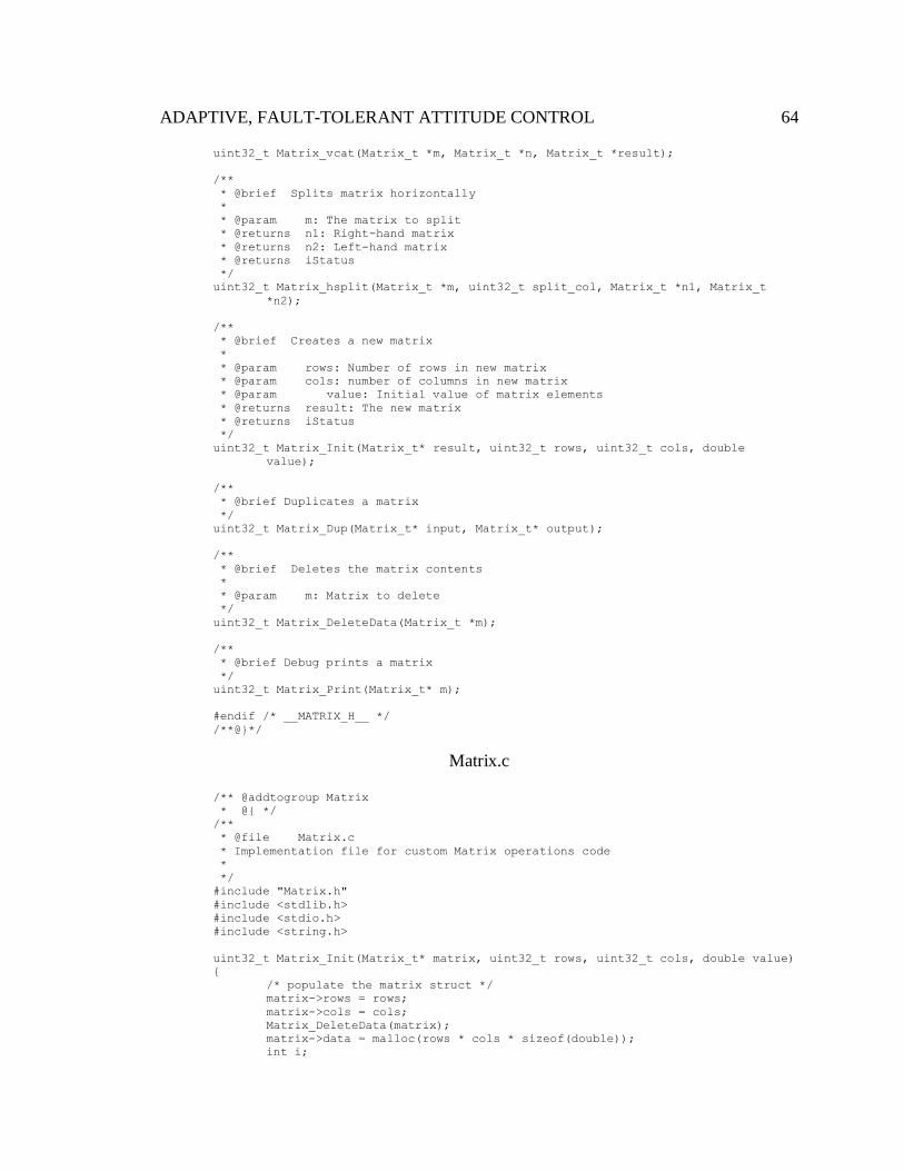
ADAPTIVE, FAULT-TOLERANT ATTITUDE CONTROL
64
uint32_t Matrix_vcat(Matrix_t *m, Matrix_t *n, Matrix_t *result);
/**
* @brief Splits matrix horizontally
*
* @param m: The matrix to split
* @returns n1: Right-hand matrix
* @returns n2: Left-hand matrix
* @returns iStatus
*/
uint32_t Matrix_hsplit(Matrix_t *m, uint32_t split_col, Matrix_t *n1, Matrix_t
*n2);
/**
* @brief Creates a new matrix
*
* @param rows: Number of rows in new matrix
* @param cols: number of columns in new matrix
* @param value: Initial value of matrix elements
* @returns result: The new matrix
* @returns iStatus
*/
uint32_t Matrix_Init(Matrix_t* result, uint32_t rows, uint32_t cols, double
value);
/**
* @brief Duplicates a matrix
*/
uint32_t Matrix_Dup(Matrix_t* input, Matrix_t* output);
/**
* @brief Deletes the matrix contents
*
* @param m: Matrix to delete
*/
uint32_t Matrix_DeleteData(Matrix_t *m);
/**
* @brief Debug prints a matrix
*/
uint32_t Matrix_Print(Matrix_t* m);
#endif /* __MATRIX_H__ */
/**@}*/
Matrix.c
/** @addtogroup Matrix
* @{ */
/**
* @file Matrix.c
* Implementation file for custom Matrix operations code
*
*/
#include "Matrix.h"
#include <stdlib.h>
#include <stdio.h>
#include <string.h>
uint32_t Matrix_Init(Matrix_t* matrix, uint32_t rows, uint32_t cols, double value)
{
/* populate the matrix struct */
matrix->rows = rows;
matrix->cols = cols;
Matrix_DeleteData(matrix);
matrix->data = malloc(rows * cols * sizeof(double));
int i;
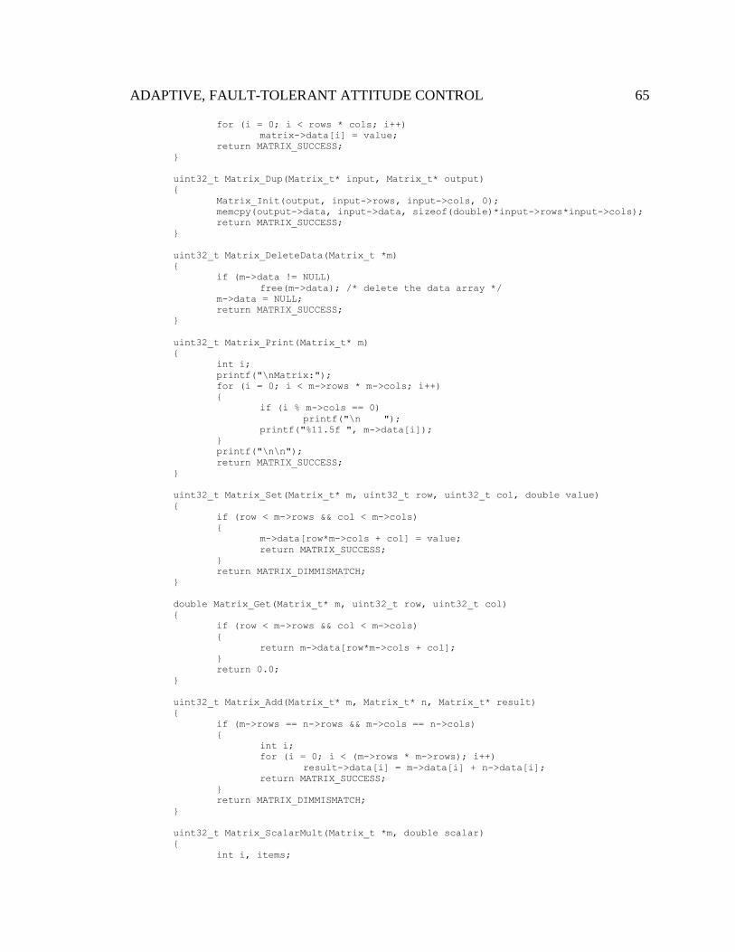
ADAPTIVE, FAULT-TOLERANT ATTITUDE CONTROL
65
for (i = 0; i < rows * cols; i++)
matrix->data[i] = value;
return MATRIX_SUCCESS;
}
uint32_t Matrix_Dup(Matrix_t* input, Matrix_t* output)
{
Matrix_Init(output, input->rows, input->cols, 0);
memcpy(output->data, input->data, sizeof(double)*input->rows*input->cols);
return MATRIX_SUCCESS;
}
uint32_t Matrix_DeleteData(Matrix_t *m)
{
if (m->data != NULL)
free(m->data); /* delete the data array */
m->data = NULL;
return MATRIX_SUCCESS;
}
uint32_t Matrix_Print(Matrix_t* m)
{
int i;
printf("\nMatrix:");
for (i = 0; i < m->rows * m->cols; i++)
{
if (i % m->cols == 0)
printf("\n ");
printf("%11.5f ", m->data[i]);
}
printf("\n\n");
return MATRIX_SUCCESS;
}
uint32_t Matrix_Set(Matrix_t* m, uint32_t row, uint32_t col, double value)
{
if (row < m->rows && col < m->cols)
{
m->data[row*m->cols + col] = value;
return MATRIX_SUCCESS;
}
return MATRIX_DIMMISMATCH;
}
double Matrix_Get(Matrix_t* m, uint32_t row, uint32_t col)
{
if (row < m->rows && col < m->cols)
{
return m->data[row*m->cols + col];
}
return 0.0;
}
uint32_t Matrix_Add(Matrix_t* m, Matrix_t* n, Matrix_t* result)
{
if (m->rows == n->rows && m->cols == n->cols)
{
int i;
for (i = 0; i < (m->rows * m->rows); i++)
result->data[i] = m->data[i] + n->data[i];
return MATRIX_SUCCESS;
}
return MATRIX_DIMMISMATCH;
}
uint32_t Matrix_ScalarMult(Matrix_t *m, double scalar)
{
int i, items;

ADAPTIVE, FAULT-TOLERANT ATTITUDE CONTROL
66
items = m->rows*m->cols;
for (i = 0; i < items; i++)
{
m->data[i] *= scalar;
}
return MATRIX_SUCCESS;
}
uint32_t Matrix_Mult(Matrix_t* m, Matrix_t* n, Matrix_t* result)
{
// check for correct dimensions
if (m->cols != n->rows)
{
// illegal dimensions for multiplication
return MATRIX_DIMMISMATCH;
}
// initialize the result
Matrix_DeleteData(result);
Matrix_Init(result, m->rows, n->cols, 0.0);
int i, j, k, index;
for (i = 0; i < m->rows; i++)
{
for (j = 0; j < n->cols; j++)
{
index = i*n->cols + j;
result->data[index] = 0.0;
for (k = 0; k < m->cols; k++)
{
result->data[index] += m->data[i*m->cols + k] * n-
>data[k*n->cols + j];
}
}
}
return MATRIX_SUCCESS;
}
uint32_t Matrix_RowMult(Matrix_t *m, uint32_t row, double scalar)
{
if (row >= m->rows)
return MATRIX_DIMMISMATCH;
int i;
for (i = 0; i < m->cols; i++)
m->data[row*m->cols + i] *= scalar;
return MATRIX_SUCCESS;
}
uint32_t Matrix_RowAdd(Matrix_t *m, uint32_t row1, uint32_t row2, double scale)
{
if (row1 >= m->rows || row2 >= m->rows)
return MATRIX_DIMMISMATCH;
int i;
for (i = 0; i < m->cols; i++)
m->data[row2*m->cols + i] += m->data[row1*m->cols + i]*scale;
return MATRIX_SUCCESS;
}
uint32_t Matrix_Transpose(Matrix_t* m)
{
Matrix_t* transposed = malloc(sizeof(Matrix_t));
memset(transposed, 0x0, sizeof(Matrix_t));
Matrix_Init(transposed, m->cols, m->rows, 0);
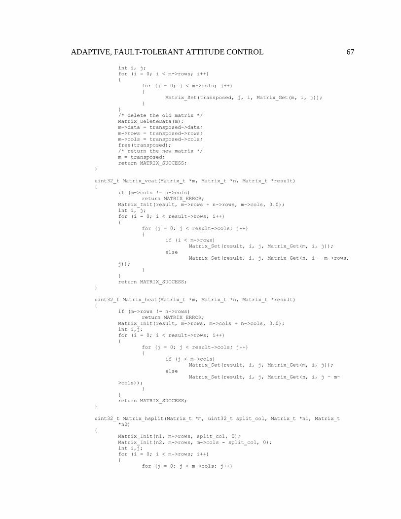
ADAPTIVE, FAULT-TOLERANT ATTITUDE CONTROL
67
int i, j;
for (i = 0; i < m->rows; i++)
{
for (j = 0; j < m->cols; j++)
{
Matrix_Set(transposed, j, i, Matrix_Get(m, i, j));
}
}
/* delete the old matrix */
Matrix_DeleteData(m);
m->data = transposed->data;
m->rows = transposed->rows;
m->cols = transposed->cols;
free(transposed);
/* return the new matrix */
m = transposed;
return MATRIX_SUCCESS;
}
uint32_t Matrix_vcat(Matrix_t *m, Matrix_t *n, Matrix_t *result)
{
if (m->cols != n->cols)
return MATRIX_ERROR;
Matrix_Init(result, m->rows + n->rows, m->cols, 0.0);
int i, j;
for (i = 0; i < result->rows; i++)
{
for (j = 0; j < result->cols; j++)
{
if (i < m->rows)
Matrix_Set(result, i, j, Matrix_Get(m, i, j));
else
Matrix_Set(result, i, j, Matrix_Get(n, i - m->rows,
j));
}
}
return MATRIX_SUCCESS;
}
uint32_t Matrix_hcat(Matrix_t *m, Matrix_t *n, Matrix_t *result)
{
if (m->rows != n->rows)
return MATRIX_ERROR;
Matrix_Init(result, m->rows, m->cols + n->cols, 0.0);
int i,j;
for (i = 0; i < result->rows; i++)
{
for (j = 0; j < result->cols; j++)
{
if (j < m->cols)
Matrix_Set(result, i, j, Matrix_Get(m, i, j));
else
Matrix_Set(result, i, j, Matrix_Get(n, i, j - m-
>cols));
}
}
return MATRIX_SUCCESS;
}
uint32_t Matrix_hsplit(Matrix_t *m, uint32_t split_col, Matrix_t *n1, Matrix_t
*n2)
{
Matrix_Init(n1, m->rows, split_col, 0);
Matrix_Init(n2, m->rows, m->cols - split_col, 0);
int i,j;
for (i = 0; i < m->rows; i++)
{
for (j = 0; j < m->cols; j++)

ADAPTIVE, FAULT-TOLERANT ATTITUDE CONTROL
68
{
if (j < split_col)
Matrix_Set(n1, i, j, Matrix_Get(m, i, j));
else
Matrix_Set(n2, i, j-split_col, Matrix_Get(m, i, j));
}
}
return MATRIX_SUCCESS;
}
uint32_t Matrix_RREF(Matrix_t *m)
{
int row = 0;
int row2 = 0;
// first we go down...
for (row = 0; row < m->rows-1; row++)
{
// normalize the row
Matrix_RowMult(m, row, 1.0 / Matrix_Get(m, row, row));
// remove the leading value from each lower row
for (row2 = row+1; row2 < m->rows; row2++)
{
Matrix_RowAdd(m, row, row2, -Matrix_Get(m, row2, row));
}
}
// normalize the last row
row = m->rows-1;
Matrix_RowMult(m, row, 1.0 / Matrix_Get(m, row, row));
// now go back up!
for (row = m->rows-1; row > 0; row--)
{
// add to rows above
for (row2 = row-1; row2 >= 0; row2--)
{
Matrix_RowAdd(m, row, row2, -Matrix_Get(m, row2, row));
}
}
// should be done...
return MATRIX_SUCCESS;
}
/**@}*/
ADCS_main.h
/** @addtogroup ADCS_main
* @{ */
/**
* @file ADCS_main.h
* Header file for custom ADCS code
*
*/
#ifndef __ADCS_MAIN_H__
#define __ADCS_MAIN_H__
#include <stdint.h>
#include "42types.h"
#include "Matrix.h"
#define ADCS_TRAINING_POINTS 100 /**< Maximum mumber of training points */
#define ADCS_SQRT_TRAINING_POINTS 10
#define ADCS_BANDWIDTH 20 /**< Model bandwidth */
#define ADCS_ACT_CNT 4 /**< Number of actuators */

ADAPTIVE, FAULT-TOLERANT ATTITUDE CONTROL
69
#define ADCS_MAX_TCMD 0.004 /**< Maximum torque cmd for the reaction wheel (N-
m)*/
#define ADCS_TRAINING_TORQUE_SCALE 0.1
#define ADCS_TRAINING_MOVE_DURATION 0.25
#define ADCS_RESET_TOLERANCE 0.001
/* Error Codes */
#define ADCS_SUCCESS 0 /**< Generic success return code */
#define ADCS_ERROR 1 /**< Generic error return code */
#define ADCS_NOT_ENOUGH_POINTS 2 /**< Not enough points similar to the desired
output */
#define ADCS_SOLVE_SUCCESS 0 /**< Indicates successful solution */
#define ADCS_SOLVE_OVERDEFINED 1 /**< Indicates error due to overdefinition */
#define ADCS_LSH_MAX_GYRO
(ADCS_SQRT_TRAINING_POINTS*3.1373*ADCS_TRAINING_MOVE_DURATION) /**< 3x std
dev for angular rotation amplitude (rad/s) */
#define ADCS_LSH_MAX_TORQUE 0.0092 /**< Max torque around a body axis (N-m)
*/
#define ADCS_LSH_HASH_BITS_PER_DIM 2 /**< bits per dimension */
#define ADCS_LSH_BINS_PER_DIM 4 /**< number of bins per dim = 2^(bits per
dim) */
#define ADCS_LSH_TOTAL_NUM_OF_BINS 4096 /**< total bins = (bins per dim)^6 */
#define ADCS_SEARCH_STEP_SIZE 0.002
/** Lazy Learning Point structure */
typedef struct
{
double state[3]; /**< Stores initial rotation state */
double inputs[ADCS_ACT_CNT]; /**< Stores input torque cmds to actuators */
double outputs[3]; /**< Stores output rotation on XYZ body axes */
} ADCS_Point_t;
/** Typedef for heuristic function pointer */
typedef double (*HEURISTIC_PTR)(ADCS_Point_t*);
typedef struct
{
ADCS_Point_t* points;
uint32_t size;
uint32_t nextPoint;
} ADCS_LSH_Bin_t;
typedef enum
{
IDLE,
TRAIN,
MOVE,
RESET
} ADCS_State_t;
/** ADCS Data structure */
typedef struct
{
uint8_t actuatorCount; /**< Number of actuators */
uint8_t numPoints; /**< Number of training points */
ADCS_LSH_Bin_t lshBins[ADCS_LSH_TOTAL_NUM_OF_BINS]; /**< Array of LSH bins.
Each bin is an array of points */
HEURISTIC_PTR heuristic; /**< Function pointer to heuristic used to select
* the "best" movement option */
ADCS_State_t state; /**< Current ADCS state */
} ADCS_Data_t;
/**
* @brief Initialize the ADCS model
*
* This function initializes the contents of the ADCS_Data_t structure
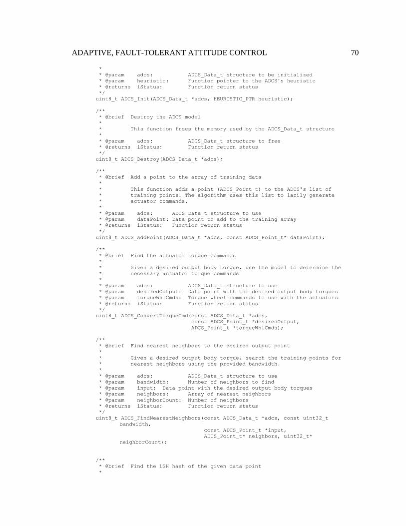
ADAPTIVE, FAULT-TOLERANT ATTITUDE CONTROL
70
*
* @param adcs: ADCS_Data_t structure to be initialized
* @param heuristic: Function pointer to the ADCS's heuristic
* @returns iStatus: Function return status
*/
uint8_t ADCS_Init(ADCS_Data_t *adcs, HEURISTIC_PTR heuristic);
/**
* @brief Destroy the ADCS model
*
* This function frees the memory used by the ADCS_Data_t structure
*
* @param adcs: ADCS_Data_t structure to free
* @returns iStatus: Function return status
*/
uint8_t ADCS_Destroy(ADCS_Data_t *adcs);
/**
* @brief Add a point to the array of training data
*
* This function adds a point (ADCS_Point_t) to the ADCS's list of
* training points. The algorithm uses this list to lazily generate
* actuator commands.
*
* @param adcs: ADCS_Data_t structure to use
* @param dataPoint: Data point to add to the training array
* @returns iStatus: Function return status
*/
uint8_t ADCS_AddPoint(ADCS_Data_t *adcs, const ADCS_Point_t* dataPoint);
/**
* @brief Find the actuator torque commands
*
* Given a desired output body torque, use the model to determine the
* necessary actuator torque commands
*
* @param adcs: ADCS_Data_t structure to use
* @param desiredOutput: Data point with the desired output body torques
* @param torqueWhlCmds: Torque wheel commands to use with the actuators
* @returns iStatus: Function return status
*/
uint8_t ADCS_ConvertTorqueCmd(const ADCS_Data_t *adcs,
const ADCS_Point_t *desiredOutput,
ADCS_Point_t *torqueWhlCmds);
/**
* @brief Find nearest neighbors to the desired output point
*
* Given a desired output body torque, search the training points for
* nearest neighbors using the provided bandwidth.
*
* @param adcs: ADCS_Data_t structure to use
* @param bandwidth: Number of neighbors to find
* @param input: Data point with the desired output body torques
* @param neighbors: Array of nearest neighbors
* @param neighborCount: Number of neighbors
* @returns iStatus: Function return status
*/
uint8_t ADCS_FindNearestNeighbors(const ADCS_Data_t *adcs, const uint32_t
bandwidth,
const ADCS_Point_t *input,
ADCS_Point_t* neighbors, uint32_t*
neighborCount);
/**
* @brief Find the LSH hash of the given data point
*

ADAPTIVE, FAULT-TOLERANT ATTITUDE CONTROL
71
*
* @param point: ADCS_Point_t structure to hash
* @param hash: Hash value
*/
uint32_t ADCS_LSH_Hash(const ADCS_Point_t *point);
/**
* @brief Heuristic function for finding "best" solution
*
* @param point: ADCS_Point_t structure to use as input
* @returns value: Heuristic value for point
*/
double ADCS_Heuristic(ADCS_Point_t* point);
/**
* @brief Main loop function of custom ADCS flight software
*
* This function contains the code that gets called each time through
* the simulation loop. This is the primary interface point between the
* custom code and the 42 simulation.
*
* @param Spacecraft - The 42 SCType structure representing the spacecraft
* @return None
*/
void ADCS_FSW(struct SCType *Spacecraft);
#endif /* __ADCS_MAIN_H__ */
/**@}*/
ADCS_main.c
/** @addtogroup ADCS_main
* @{ */
/**
* @file ADCS_main.c
* Implementation file for custom ADCS code
*
*/
#include "ADCS_main.h"
#include <string.h>
#include "42.h"
#include <math.h>
#include <float.h>
#include <time.h>
uint8_t ADCS_Init(ADCS_Data_t *adcs, HEURISTIC_PTR heuristic)
{
adcs->actuatorCount = ADCS_ACT_CNT;
adcs->numPoints = 0;
adcs->heuristic = heuristic;
/* initialize the LSH bins */
memset(adcs->lshBins, 0x00,
sizeof(ADCS_LSH_Bin_t)*ADCS_LSH_TOTAL_NUM_OF_BINS);
uint32_t i;
for (i = 0; i < ADCS_LSH_TOTAL_NUM_OF_BINS; i++)
{
adcs->lshBins[i].points = malloc(sizeof(ADCS_Point_t)*8); // start with 8
point size
adcs->lshBins[i].size = 8;
memset(adcs->lshBins[i].points, 0x00, sizeof(ADCS_Point_t)*8);
}
return ADCS_SUCCESS;
}
uint8_t ADCS_Destroy(ADCS_Data_t *adcs)

ADAPTIVE, FAULT-TOLERANT ATTITUDE CONTROL
72
{
int i;
for (i = 0; i < ADCS_LSH_TOTAL_NUM_OF_BINS; i++)
{
free(adcs->lshBins[i].points); // free the bin
}
return ADCS_SUCCESS;
}
uint8_t ADCS_AddPoint(ADCS_Data_t *adcs, const ADCS_Point_t* dataPoint)
{
uint32_t hash;
/* store the data point */
/* calculate the hash */
hash = ADCS_LSH_Hash(dataPoint);
if (hash > ADCS_LSH_TOTAL_NUM_OF_BINS-1)
hash = ADCS_LSH_TOTAL_NUM_OF_BINS-1;
if (adcs->lshBins[hash].nextPoint >= adcs->lshBins[hash].size / 2)
{
/* need to expand the array. double the capacity */
/* create a new array */
ADCS_Point_t* newArray = malloc(2*adcs-
>lshBins[hash].size*sizeof(ADCS_Point_t));
memset(newArray, 0x0, 2*adcs->lshBins[hash].size*sizeof(ADCS_Point_t));
/*copy data to new array*/
memcpy(newArray, adcs->lshBins[hash].points, adcs-
>lshBins[hash].size*sizeof(ADCS_Point_t));
/* free the old array */
free(adcs->lshBins[hash].points);
/* use the new array */
adcs->lshBins[hash].points = newArray;
/* update to the new size */
adcs->lshBins[hash].size *= 2;
}
/* add the new point */
adcs->lshBins[hash].points[adcs->lshBins[hash].nextPoint++] = *dataPoint;
//adcs->points[adcs->numPoints] = *dataPoint;
/* increment the end of the list index */
adcs->numPoints++;
return ADCS_SUCCESS;
}
uint32_t ADCS_LSH_Hash(const ADCS_Point_t *point)
{
/* hash the point! */
char values[6]; /* 3 dimensions for initial state, 3 for output state */
int i;
/* copy the values to the array */
/* quantize as we go to avoid needing another loop */
for (i = 0; i < 3; i++)
{
values[i] = (char)(floor(point->outputs[i] / ADCS_LSH_MAX_TORQUE *
ADCS_LSH_BINS_PER_DIM/2)); // convert the torque to integer
values[i+3] = (char)(floor(point->state[i] / ADCS_LSH_MAX_GYRO *
ADCS_LSH_BINS_PER_DIM/2)); // convert the state input to integer
}
// calculate the hash
uint32_t hash = 0;
/* loop through each bit of the hash from MSb to LSb */
/* Example: 01 10 01 11 00 10 */
/*
* 0: hash + 0b1 = 0b1
* 1: hash + 0b00 = 0b01
* 2: hash + 0b100 = 0b101

ADAPTIVE, FAULT-TOLERANT ATTITUDE CONTROL
73
* 3: hash + 0b1000 = 0b1101
* 4: hash + 0b00000 = 0b01101
* 5: hash + 0b000000 = 0b001101
* 6: hash + 0b0000000 = 0b0001101
* 7: hash + 0b10000000 = 0b10001101
* 8: hash + 0b000000000 = 0b010001101
* 9: hash + 0b1000000000 = 0b1010001101
* 10: hash + 0b00000000000 = 0b01010001101
* 11: hash + 0b100000000000 = 0b101010001101
* final hash value is 0xA8D
*/
for (i = 0; i < 6*ADCS_LSH_HASH_BITS_PER_DIM-1; i++)
{
if (i >= 6*(ADCS_LSH_HASH_BITS_PER_DIM-1))
{
/* here we want the sign bits */
hash += ((values[i % 6] >> 8) & 0x1) << i;
}
else
{
hash += ((values[i % 6] >> (i / 6)) & 0x1) << i;
}
}
return hash;
}
uint8_t ADCS_FindNearestNeighbors(const ADCS_Data_t *adcs, uint32_t bandwidth,
const ADCS_Point_t *input,
ADCS_Point_t* neighbors, uint32_t*
neighborCount)
{
uint32_t hash, binNum;
ADCS_LSH_Bin_t bin;
hash = ADCS_LSH_Hash(input);
if (hash > ADCS_LSH_TOTAL_NUM_OF_BINS-1)
hash = ADCS_LSH_TOTAL_NUM_OF_BINS-1;
binNum = hash;
/* use a moving pointer to add points from bins */
ADCS_Point_t* nextBinPoints = neighbors;
/* reset the neighbor count */
*neighborCount = 0;
while (bandwidth > 0)
{
bin = adcs->lshBins[binNum];
/* copy up to bandwidth points into the array */
if (bin.nextPoint < bandwidth)
{
/* copy the whole bin */
memcpy(nextBinPoints, bin.points, sizeof(ADCS_Point_t)*bin.nextPoint);
/* update the neighbors pointer */
nextBinPoints += bin.nextPoint;
/* update the number of neighbors found */
*neighborCount += bin.nextPoint;
/* decrement the number of neighbors left */
bandwidth -= bin.nextPoint;
}
else
{
/* copy just the points we need */
memcpy(nextBinPoints, bin.points, sizeof(ADCS_Point_t)*bandwidth);
nextBinPoints += bandwidth;

ADAPTIVE, FAULT-TOLERANT ATTITUDE CONTROL
74
*neighborCount += bandwidth;
bandwidth = 0;
}
if (bandwidth > 0)
{
/* if more points are needed, move to the next bin */
binNum++;
/* if next bin is too high, move to first bin */
if (binNum >= ADCS_LSH_TOTAL_NUM_OF_BINS)
binNum = 0;
/* if next bin is the original bin, we are out of points */
if (binNum == hash)
break;
}
}
if (bandwidth > 0)
return ADCS_NOT_ENOUGH_POINTS;
return ADCS_SUCCESS;
}
double ADCS_Heuristic(ADCS_Point_t* point)
{
/* shoot for smallest overall change in wheel speed */
/* not the best option */
int i;
double result = 0;
for (i = 0; i < ADCS_ACT_CNT; i++)
{
result += point->inputs[i]*point->inputs[i];
}
return result;
}
uint8_t ADCS_ConvertTorqueCmd(const ADCS_Data_t *adcs,
const ADCS_Point_t *desiredOutput,
ADCS_Point_t *torqueWhlCmds)
{
/* find similar points */
ADCS_Point_t neighbors[ADCS_BANDWIDTH];
uint32_t neighborCount;
ADCS_FindNearestNeighbors(adcs, ADCS_BANDWIDTH, desiredOutput, neighbors,
&neighborCount);
/* put the information into linear equations */
Matrix_t modelEquations, augmentedModelEquations;
memset(&modelEquations, 0x0, sizeof(Matrix_t));
memset(&augmentedModelEquations, 0x0, sizeof(Matrix_t));
Matrix_Init(&modelEquations, 3, ADCS_ACT_CNT, 0.0);
Matrix_t inputMatrix; /**< Matrix A */
Matrix_t inputMatrixTranspose; /**< Matrix A' */
Matrix_t normalMatrix; /**< Normal matrix = A'A */
memset(&inputMatrix, 0x0, sizeof(Matrix_t));
memset(&inputMatrixTranspose, 0x0, sizeof(Matrix_t));
memset(&normalMatrix, 0x0, sizeof(Matrix_t));
Matrix_Init(&inputMatrix, neighborCount, ADCS_ACT_CNT+1, 0.0);
int i,j;
for (i = 0; i < neighborCount; i++)
{
for (j = 0; j < ADCS_ACT_CNT; j++)
{
Matrix_Set(&inputMatrix, i, j, neighbors[i].inputs[j]);
}
Matrix_Set(&inputMatrix, i, ADCS_ACT_CNT, 1.0);
}
Matrix_Dup(&inputMatrix, &inputMatrixTranspose);
Matrix_Transpose(&inputMatrixTranspose);
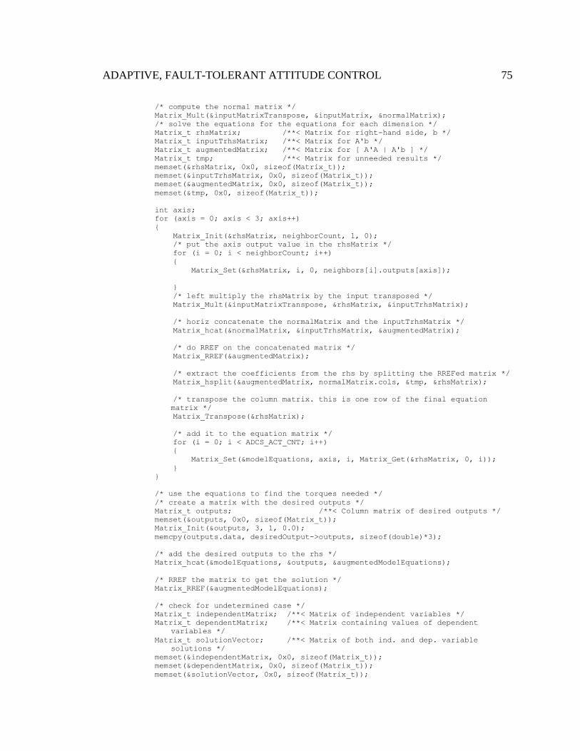
ADAPTIVE, FAULT-TOLERANT ATTITUDE CONTROL
75
/* compute the normal matrix */
Matrix_Mult(&inputMatrixTranspose, &inputMatrix, &normalMatrix);
/* solve the equations for the equations for each dimension */
Matrix_t rhsMatrix; /**< Matrix for right-hand side, b */
Matrix_t inputTrhsMatrix; /**< Matrix for A'b */
Matrix_t augmentedMatrix; /**< Matrix for [ A'A | A'b ] */
Matrix_t tmp; /**< Matrix for unneeded results */
memset(&rhsMatrix, 0x0, sizeof(Matrix_t));
memset(&inputTrhsMatrix, 0x0, sizeof(Matrix_t));
memset(&augmentedMatrix, 0x0, sizeof(Matrix_t));
memset(&tmp, 0x0, sizeof(Matrix_t));
int axis;
for (axis = 0; axis < 3; axis++)
{
Matrix_Init(&rhsMatrix, neighborCount, 1, 0);
/* put the axis output value in the rhsMatrix */
for (i = 0; i < neighborCount; i++)
{
Matrix_Set(&rhsMatrix, i, 0, neighbors[i].outputs[axis]);
}
/* left multiply the rhsMatrix by the input transposed */
Matrix_Mult(&inputMatrixTranspose, &rhsMatrix, &inputTrhsMatrix);
/* horiz concatenate the normalMatrix and the inputTrhsMatrix */
Matrix_hcat(&normalMatrix, &inputTrhsMatrix, &augmentedMatrix);
/* do RREF on the concatenated matrix */
Matrix_RREF(&augmentedMatrix);
/* extract the coefficients from the rhs by splitting the RREFed matrix */
Matrix_hsplit(&augmentedMatrix, normalMatrix.cols, &tmp, &rhsMatrix);
/* transpose the column matrix. this is one row of the final equation
matrix */
Matrix_Transpose(&rhsMatrix);
/* add it to the equation matrix */
for (i = 0; i < ADCS_ACT_CNT; i++)
{
Matrix_Set(&modelEquations, axis, i, Matrix_Get(&rhsMatrix, 0, i));
}
}
/* use the equations to find the torques needed */
/* create a matrix with the desired outputs */
Matrix_t outputs; /**< Column matrix of desired outputs */
memset(&outputs, 0x0, sizeof(Matrix_t));
Matrix_Init(&outputs, 3, 1, 0.0);
memcpy(outputs.data, desiredOutput->outputs, sizeof(double)*3);
/* add the desired outputs to the rhs */
Matrix_hcat(&modelEquations, &outputs, &augmentedModelEquations);
/* RREF the matrix to get the solution */
Matrix_RREF(&augmentedModelEquations);
/* check for undetermined case */
Matrix_t independentMatrix; /**< Matrix of independent variables */
Matrix_t dependentMatrix; /**< Matrix containing values of dependent
variables */
Matrix_t solutionVector; /**< Matrix of both ind. and dep. variable
solutions */
memset(&independentMatrix, 0x0, sizeof(Matrix_t));
memset(&dependentMatrix, 0x0, sizeof(Matrix_t));
memset(&solutionVector, 0x0, sizeof(Matrix_t));
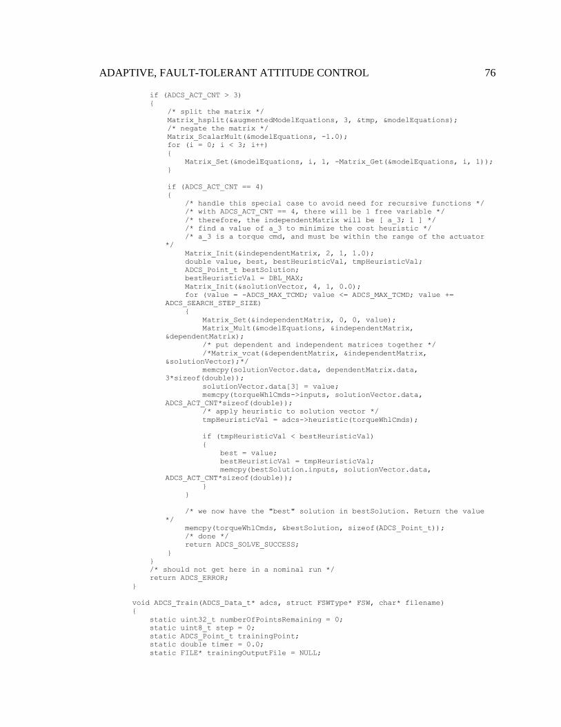
ADAPTIVE, FAULT-TOLERANT ATTITUDE CONTROL
76
if (ADCS_ACT_CNT > 3)
{
/* split the matrix */
Matrix_hsplit(&augmentedModelEquations, 3, &tmp, &modelEquations);
/* negate the matrix */
Matrix_ScalarMult(&modelEquations, -1.0);
for (i = 0; i < 3; i++)
{
Matrix_Set(&modelEquations, i, 1, -Matrix_Get(&modelEquations, i, 1));
}
if (ADCS_ACT_CNT == 4)
{
/* handle this special case to avoid need for recursive functions */
/* with ADCS_ACT_CNT == 4, there will be 1 free variable */
/* therefore, the independentMatrix will be [ a_3; 1 ] */
/* find a value of a_3 to minimize the cost heuristic */
/* a_3 is a torque cmd, and must be within the range of the actuator
*/
Matrix_Init(&independentMatrix, 2, 1, 1.0);
double value, best, bestHeuristicVal, tmpHeuristicVal;
ADCS_Point_t bestSolution;
bestHeuristicVal = DBL_MAX;
Matrix_Init(&solutionVector, 4, 1, 0.0);
for (value = -ADCS_MAX_TCMD; value <= ADCS_MAX_TCMD; value +=
ADCS_SEARCH_STEP_SIZE)
{
Matrix_Set(&independentMatrix, 0, 0, value);
Matrix_Mult(&modelEquations, &independentMatrix,
&dependentMatrix);
/* put dependent and independent matrices together */
/*Matrix_vcat(&dependentMatrix, &independentMatrix,
&solutionVector);*/
memcpy(solutionVector.data, dependentMatrix.data,
3*sizeof(double));
solutionVector.data[3] = value;
memcpy(torqueWhlCmds->inputs, solutionVector.data,
ADCS_ACT_CNT*sizeof(double));
/* apply heuristic to solution vector */
tmpHeuristicVal = adcs->heuristic(torqueWhlCmds);
if (tmpHeuristicVal < bestHeuristicVal)
{
best = value;
bestHeuristicVal = tmpHeuristicVal;
memcpy(bestSolution.inputs, solutionVector.data,
ADCS_ACT_CNT*sizeof(double));
}
}
/* we now have the "best" solution in bestSolution. Return the value
*/
memcpy(torqueWhlCmds, &bestSolution, sizeof(ADCS_Point_t));
/* done */
return ADCS_SOLVE_SUCCESS;
}
}
/* should not get here in a nominal run */
return ADCS_ERROR;
}
void ADCS_Train(ADCS_Data_t* adcs, struct FSWType* FSW, char* filename)
{
static uint32_t numberOfPointsRemaining = 0;
static uint8_t step = 0;
static ADCS_Point_t trainingPoint;
static double timer = 0.0;
static FILE* trainingOutputFile = NULL;

ADAPTIVE, FAULT-TOLERANT ATTITUDE CONTROL
77
/* set the state */
adcs->state = TRAIN;
if (step == 0)
{
trainingOutputFile = fopen(filename, "w");
numberOfPointsRemaining = ADCS_TRAINING_POINTS;
step++;
}
else if (step == 1)
{
/* compute the torque cmd */
memset(&trainingPoint, 0x0, sizeof(ADCS_Point_t));
int i;
for (i = 0; i < ADCS_ACT_CNT; i++)
trainingPoint.inputs[i] = ADCS_TRAINING_TORQUE_SCALE*(-ADCS_MAX_TCMD +
((double)rand()/((double)RAND_MAX))*(2*ADCS_MAX_TCMD));
memcpy(trainingPoint.state, FSW->wbn, sizeof(double)*3);
memcpy(FSW->Twhlcmd, trainingPoint.inputs, sizeof(double)*ADCS_ACT_CNT);
numberOfPointsRemaining--;
step++;
timer = 0.0;
}
else if (step == 2)
{
/* wait for delay */
timer += FSW->DT;
if (timer >= ADCS_TRAINING_MOVE_DURATION)
{
step++;
}
}
else if (step == 3)
{
/* save the point data */
/* calculate the torque */
int i;
for (i = 0; i < 3; i++)
/* calculate torque: \tau = I * \alpha = I * (\omega_f - \omega_i) /
(\Delta t) */
trainingPoint.outputs[i] = (FSW->wbn[i] - trainingPoint.state[i]) /
timer * FSW->MOI[i];
fprintf(trainingOutputFile, "%5.4f, %5.4f, %5.4f, %5.4f, %5.4f, %5.4f,
%5.4f, %5.4f, %5.4f, %5.4f, %5.4f, %5.4f, %5.4f\n",
trainingPoint.state[0],
trainingPoint.state[1],
trainingPoint.state[2],
trainingPoint.inputs[0],
trainingPoint.inputs[1],
trainingPoint.inputs[2],
trainingPoint.inputs[3],
FSW->wbn[0],
FSW->wbn[1],
FSW->wbn[2],
trainingPoint.outputs[0],
trainingPoint.outputs[1],
trainingPoint.outputs[2]);
/* add the training point to the database */
ADCS_AddPoint(adcs, &trainingPoint);
if (numberOfPointsRemaining > 0)
{
/* go back to add another point */
step = 1;
}
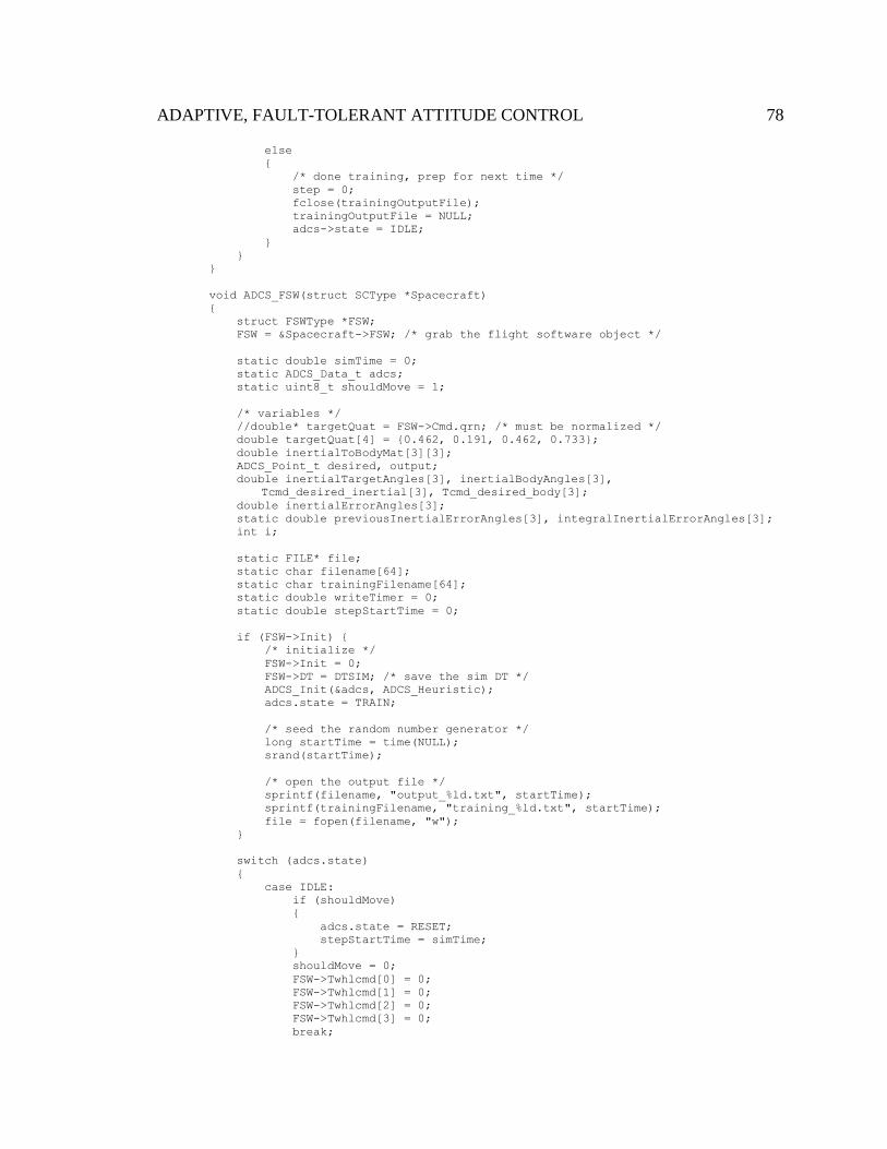
ADAPTIVE, FAULT-TOLERANT ATTITUDE CONTROL
78
else
{
/* done training, prep for next time */
step = 0;
fclose(trainingOutputFile);
trainingOutputFile = NULL;
adcs->state = IDLE;
}
}
}
void ADCS_FSW(struct SCType *Spacecraft)
{
struct FSWType *FSW;
FSW = &Spacecraft->FSW; /* grab the flight software object */
static double simTime = 0;
static ADCS_Data_t adcs;
static uint8_t shouldMove = 1;
/* variables */
//double* targetQuat = FSW->Cmd.qrn; /* must be normalized */
double targetQuat[4] = {0.462, 0.191, 0.462, 0.733};
double inertialToBodyMat[3][3];
ADCS_Point_t desired, output;
double inertialTargetAngles[3], inertialBodyAngles[3],
Tcmd_desired_inertial[3], Tcmd_desired_body[3];
double inertialErrorAngles[3];
static double previousInertialErrorAngles[3], integralInertialErrorAngles[3];
int i;
static FILE* file;
static char filename[64];
static char trainingFilename[64];
static double writeTimer = 0;
static double stepStartTime = 0;
if (FSW->Init) {
/* initialize */
FSW->Init = 0;
FSW->DT = DTSIM; /* save the sim DT */
ADCS_Init(&adcs, ADCS_Heuristic);
adcs.state = TRAIN;
/* seed the random number generator */
long startTime = time(NULL);
srand(startTime);
/* open the output file */
sprintf(filename, "output_%ld.txt", startTime);
sprintf(trainingFilename, "training_%ld.txt", startTime);
file = fopen(filename, "w");
}
switch (adcs.state)
{
case IDLE:
if (shouldMove)
{
adcs.state = RESET;
stepStartTime = simTime;
}
shouldMove = 0;
FSW->Twhlcmd[0] = 0;
FSW->Twhlcmd[1] = 0;
FSW->Twhlcmd[2] = 0;
FSW->Twhlcmd[3] = 0;
break;

ADAPTIVE, FAULT-TOLERANT ATTITUDE CONTROL
79
case TRAIN:
ADCS_Train(&adcs, FSW, trainingFilename);
break;
case RESET:
targetQuat[0] = 0;
targetQuat[1] = 0;
targetQuat[2] = 0;
targetQuat[3] = 1.0;
Q2AngleVec(FSW->qbn, inertialBodyAngles);
double bodyError = 0.0;
double omegaError = 0.0;
for (i = 0; i < 3; i++)
bodyError += inertialBodyAngles[i]*inertialBodyAngles[i];
for (i = 0; i < 3; i++)
omegaError += (FSW->wbn[i]*FSW->wbn[i]);
if (bodyError < ADCS_RESET_TOLERANCE && omegaError <
ADCS_RESET_TOLERANCE)
{
adcs.state = MOVE;
stepStartTime = simTime;
printf("MOVE\n");
}
case MOVE:
/* some MOI data from
https://www.hindawi.com/journals/jcse/2013/657182/ */
/* convert target to euler angles */
Q2AngleVec(targetQuat, inertialTargetAngles);
/* convert body quat to euler angles */
Q2AngleVec(FSW->qbn, inertialBodyAngles);
for (i = 0; i < 3; i++)
{
inertialErrorAngles[i] = inertialTargetAngles[i] -
inertialBodyAngles[i];
integralInertialErrorAngles[i] += inertialErrorAngles[i]*FSW->DT;
}
for (i = 0; i < 3; i++)
{
Tcmd_desired_inertial[i] = 5*inertialErrorAngles[i] +
2*(inertialErrorAngles[i] -
previousInertialErrorAngles[i])/FSW->DT +
0*(integralInertialErrorAngles[i]);
/* save for next loop */
previousInertialErrorAngles[i] = inertialErrorAngles[i];
}
/* convert inertial to body torque command */
Q2C(FSW->qbn, inertialToBodyMat);
/* transform the Tcmd */
MxV(inertialToBodyMat, Tcmd_desired_inertial, Tcmd_desired_body);
writeTimer += FSW->DT;
if (writeTimer > 0.01 && file != NULL)
{
fprintf(file, "%10.4f, %10.4f, %10.4f, %10.4f\n", simTime,
inertialErrorAngles[0], inertialErrorAngles[1], inertialErrorAngles[2]);
writeTimer = 0;
}
if (simTime - stepStartTime > 8.0 && file != NULL)
{
fclose(file);
file = NULL;
exit(0);
}

ADAPTIVE, FAULT-TOLERANT ATTITUDE CONTROL
80
memset(&desired, 0x0, sizeof(ADCS_Point_t));
/* copy current state */
memcpy(&desired.state, FSW->wbn, sizeof(double)*3);
memcpy(&desired.outputs, &Tcmd_desired_body, sizeof(double)*3);
/* use new algorithm */
ADCS_ConvertTorqueCmd(&adcs, &desired, &output);
FSW->Twhlcmd[0] = output.inputs[0];
FSW->Twhlcmd[1] = output.inputs[1];
FSW->Twhlcmd[2] = output.inputs[2];
FSW->Twhlcmd[3] = output.inputs[3];
break;
default:
break;
}
simTime += FSW->DT;
}
/**@}*/