parameterized algorithmics: a graph-theoretic approachfernau/papers/habil.pdf · parameterized...
TRANSCRIPT

Parameterized Algorithmics:
A Graph-Theoretic Approach
Henning Fernau
Universitat Tubingen, WSI fur Informatik, Sand 13,72076 Tubingen, Germany
University of Newcastle, School of Electr. Eng. & Computer Sci.,University Drive, Callaghan, NSW 2308, Australia
April 20, 2005

2
Contents
Contents 3
1 Prologue 91.1 Why practitioners may wish to continue reading . . . . . . . . 91.2 Standard notations . . . . . . . . . . . . . . . . . . . . . . . . 111.3 What mathematicians can find . . . . . . . . . . . . . . . . . . 121.4 Messages to algorithm developers . . . . . . . . . . . . . . . . 141.5 Acknowledgments . . . . . . . . . . . . . . . . . . . . . . . . . 151.6 Keeping up to date . . . . . . . . . . . . . . . . . . . . . . . . 15
2 Introduction 172.1 The parameterized landscape . . . . . . . . . . . . . . . . . . 17
2.1.1 The world of parameterized algorithmics: definitions . 172.1.2 The world of parameterized algorithmics: methodologies 25
2.2 Is parameterized algorithmics the solution to “everything”? . . 272.3 A primer in graph theory . . . . . . . . . . . . . . . . . . . . . 302.4 Some favorite graph problems . . . . . . . . . . . . . . . . . . 362.5 The power of data reduction . . . . . . . . . . . . . . . . . . . 43
3 Parameterizations 513.1 Internal and external parameters . . . . . . . . . . . . . . . . 52
3.1.1 A classification scheme . . . . . . . . . . . . . . . . . . 523.1.2 Different classifications in games . . . . . . . . . . . . . 53
3.2 Standard parameters . . . . . . . . . . . . . . . . . . . . . . . 573.2.1 Minimization problems . . . . . . . . . . . . . . . . . . 573.2.2 Maximization problems . . . . . . . . . . . . . . . . . . 593.2.3 Philosophical remarks, inspired by linear arrange-
ment . . . . . . . . . . . . . . . . . . . . . . . . . . . 623.3 Alternative parameterizations . . . . . . . . . . . . . . . . . . 743.4 Multiple parameters . . . . . . . . . . . . . . . . . . . . . . . 793.5 Dual parameters . . . . . . . . . . . . . . . . . . . . . . . . . 84
3

4 CONTENTS
4 Kernels 914.1 Reduction rules . . . . . . . . . . . . . . . . . . . . . . . . . . 934.2 Greedy approaches . . . . . . . . . . . . . . . . . . . . . . . . 944.3 Large is no good (or too good)?! . . . . . . . . . . . . . . . . . 964.4 The mathematical way . . . . . . . . . . . . . . . . . . . . . . 102
4.4.1 Colorful kernelizations . . . . . . . . . . . . . . . . . . 1024.4.2 nonblocker set . . . . . . . . . . . . . . . . . . . . 1064.4.3 Dominating Queens . . . . . . . . . . . . . . . . . . . . 113
4.5 vertex cover: our old friend again . . . . . . . . . . . . . . 1154.5.1 The result of Nemhauser and Trotter . . . . . . . . . . 1164.5.2 Crown reductions: another way to a small kernel . . . 1194.5.3 A generalization of vertex cover . . . . . . . . . . . 122
4.6 planar dominating set: a tricky example . . . . . . . . . . 1234.7 Kernelization schemes . . . . . . . . . . . . . . . . . . . . . . 1314.8 Compilability and kernels . . . . . . . . . . . . . . . . . . . . 133
5 Search trees 1375.1 Cover problems . . . . . . . . . . . . . . . . . . . . . . . . . . 139
5.1.1 vertex cover . . . . . . . . . . . . . . . . . . . . . . 1395.1.2 The time analysis of search tree algorithms . . . . . . . 1485.1.3 weighted vertex cover . . . . . . . . . . . . . . . 1535.1.4 constraint bipartite vertex cover . . . . . . . . 154
5.2 Improved branching: a bottom-up approach . . . . . . . . . . 1585.3 Improved branching: simple algorithms . . . . . . . . . . . . . 168
5.3.1 planar independent set . . . . . . . . . . . . . . . 1685.3.2 planar dominating set . . . . . . . . . . . . . . . . 1725.3.3 hitting set . . . . . . . . . . . . . . . . . . . . . . . 1805.3.4 face cover . . . . . . . . . . . . . . . . . . . . . . . 196
6 Case studies 2076.1 matrix row column merging . . . . . . . . . . . . . . . . 207
6.1.1 Problem definition . . . . . . . . . . . . . . . . . . . . 2076.1.2 The database background . . . . . . . . . . . . . . . . 2086.1.3 Some examples . . . . . . . . . . . . . . . . . . . . . . 2116.1.4 Complexity results . . . . . . . . . . . . . . . . . . . . 2136.1.5 Revisiting our example . . . . . . . . . . . . . . . . . . 220
6.2 Problems related to hitting set . . . . . . . . . . . . . . . . 2226.2.1 Problems from computational biology . . . . . . . . . . 2226.2.2 Call control problems . . . . . . . . . . . . . . . . . . . 224
6.3 Graph modification problems . . . . . . . . . . . . . . . . . . 2356.3.1 A maximization graph modification problem . . . . . . 235

CONTENTS 5
6.3.2 Graph modification problems related to HS . . . . . . 237
6.3.3 clique complement cover: an easy problem? . . . 239
6.4 Graph drawing problems . . . . . . . . . . . . . . . . . . . . . 243
6.4.1 linear arrangement again. . . . . . . . . . . . . . . 243
6.4.2 one-sided crossing minimization . . . . . . . . . . 251
6.4.3 Biplanarization problems . . . . . . . . . . . . . . . . . 264
6.4.4 More related problems . . . . . . . . . . . . . . . . . . 281
6.5 Summary . . . . . . . . . . . . . . . . . . . . . . . . . . . . . 296
7 Graph parameters 299
7.1 Treewidth . . . . . . . . . . . . . . . . . . . . . . . . . . . . . 301
7.2 Dynamic programming . . . . . . . . . . . . . . . . . . . . . . 309
7.3 Planar graphs and their structure . . . . . . . . . . . . . . . . 321
7.3.1 Outerplanarity: the definition . . . . . . . . . . . . . . 323
7.3.2 Outerplanarity versus treewidth . . . . . . . . . . . . . 325
7.3.3 Outerplanarity and other graph parameters . . . . . . 330
7.4 Domination number versus treewidth . . . . . . . . . . . . . . 332
7.4.1 Separators and treewidth . . . . . . . . . . . . . . . . . 332
7.4.2 Finding separators layerwisely . . . . . . . . . . . . . . 334
7.4.3 An upper bound for the size of the separators . . . . . 338
7.4.4 A treewidth-based algorithm for planar dominatingset . . . . . . . . . . . . . . . . . . . . . . . . . . . . . 340
7.5 The beauty of small kernels: separator theorems . . . . . . . . 342
7.5.1 Classical separator theorems . . . . . . . . . . . . . . . 343
7.5.2 Select&verify problems and glueability . . . . . . . . . 347
7.5.3 Fixed-parameter divide-and-conquer algorithms . . . . 354
7.6 The beauty of small kernels: layerwise separation . . . . . . . 359
7.6.1 Phase 1: Layerwise separation . . . . . . . . . . . . . . 361
7.6.2 Phase 2:Algorithms on layerwisely separated graphs . . . . . . 365
7.6.3 The approach of Fomin and Thilikos . . . . . . . . . . 376
7.7 Further improvements for planar dominating set . . . . . 377
7.8 planar red-blue dominating set and related problems . 383
7.9 Other related graph classes . . . . . . . . . . . . . . . . . . . . 387
8 Further approaches 391
8.1 Dynamic programming on subsets . . . . . . . . . . . . . . . . 391
8.2 Parameterized Enumeration . . . . . . . . . . . . . . . . . . . 398
8.2.1 General notions and motivation . . . . . . . . . . . . . 3988.2.2 Enumerating hitting sets . . . . . . . . . . . . . . . . . 399
6 CONTENTS
8.2.3 Multiple parameters for constraint bipartite ver-tex cover . . . . . . . . . . . . . . . . . . . . . . . . 408
8.2.4 edge dominating set . . . . . . . . . . . . . . . . . 4128.2.5 More parameterized enumeration problems . . . . . . . 420
8.3 Parameterized Counting . . . . . . . . . . . . . . . . . . . . . 4218.3.1 Classical graph parameters in view of counting: VC . . 4228.3.2 Back to the Queens . . . . . . . . . . . . . . . . . . . . 424
8.4 Other techniques for FPT algorithms . . . . . . . . . . . . . 4288.5 Implementations . . . . . . . . . . . . . . . . . . . . . . . . . 428
8.5.1 Implementations of sequential algorithms . . . . . . . . 4298.5.2 Parallel implementations . . . . . . . . . . . . . . . . . 429
9 Limitations to parameterized algorithmics 4319.1 Parameterized intractability . . . . . . . . . . . . . . . . . . . 431
9.1.1 W[1] . . . . . . . . . . . . . . . . . . . . . . . . . . . . 4329.1.2 W[2] . . . . . . . . . . . . . . . . . . . . . . . . . . . . 4349.1.3 Beyond W[2] . . . . . . . . . . . . . . . . . . . . . . . 4409.1.4 More downsides . . . . . . . . . . . . . . . . . . . . . . 442
9.2 How small can kernels get ? . . . . . . . . . . . . . . . . . . . 443
10 The non-parameterized view 44910.1 Dealing with dominating set . . . . . . . . . . . . . . . . . 451
10.1.1 Looking for dominating sets in vertex cover sets . . . . 45110.1.2 Some remarks on bipartite graphs . . . . . . . . . . . . 45210.1.3 Edge domination revisited . . . . . . . . . . . . . . . . 45310.1.4 Back to nonblocker set . . . . . . . . . . . . . . . . 454
10.2 A nonparameterized view on 3-hitting set . . . . . . . . . . 45610.2.1 Connections to Logic . . . . . . . . . . . . . . . . . . . 45710.2.2 Back to 3-hitting set . . . . . . . . . . . . . . . . . . 459
10.3 A dual approach to eliminate a parameter . . . . . . . . . . . 462
11 The WWW repository 467
12 Problems 47112.1 Cover problems and their relatives . . . . . . . . . . . . . . . . 47112.2 Dominating problems and their relatives . . . . . . . . . . . . 47412.3 Graph modification problems . . . . . . . . . . . . . . . . . . 47712.4 Further graph-theoretic problems . . . . . . . . . . . . . . . . 48012.5 Graph drawing problems . . . . . . . . . . . . . . . . . . . . . 48212.6 Hypergraph problems . . . . . . . . . . . . . . . . . . . . . . . 48512.7 Network problems . . . . . . . . . . . . . . . . . . . . . . . . . 486
CONTENTS 7
12.8 Automata problems . . . . . . . . . . . . . . . . . . . . . . . . 48712.9 Logical problems . . . . . . . . . . . . . . . . . . . . . . . . . 48812.10Miscellaneous and applications . . . . . . . . . . . . . . . . . . 489
Bibliography 493
Index 528

8 CONTENTS

Chapter 1
Prologue
This Habilitationsschrift can be read in various ways by different people.
• People working in the area of parameterized complexity can hopefullyfind main ideas leading to efficient parameterized algorithms presentedin a new way. This may spark new research, hopefully leading to moreand more useful examples of parameterized algorithms.
• Practitioners having to cope with computationally hard problems willfind an exposition how they can cast their everyday heuristic method-ologies into the framework of parameterized algorithmics. They willbe hopefully able to write up their own parameterized analysis of theirheuristics, and working in this somewhat more abstract framework willthen help them introduce improvements in their algorithms.
By addressing two audiences, we also express the hope that both “worlds”may come together to share their experiences. Especially, we are convincedthat if more and more heuristic ideas are made public (often enough, wefear that such “straightforward ideas” are considered not to be publishable)in order to spike their mathematical in-depth analysis in the parameterizedframework. This way, mathematicians and algorithm theorists can help ex-plain why in many cases simple heuristics do work well on concrete instancesof computationally hard problems.
1.1 Why practitioners may wish to continue
reading
First, I should at least try to describe what “practitioner” may mean in thiscontext. In fact, there are different possible interpretations:
9

10 CHAPTER 1. PROLOGUE
• A programmer should benefit from the fact that this Habilitations-schrift pays special attention to presenting algorithms in a unifyingway by means of pseudo-code. Those program fragments should berelatively easily translatable into real programs.
The reason for being that explicit in the presentation of the algorithms(and this also contrasts with many other research papers and mono-graphs on algorithmics) is that we are often under the impression thatthe typical implicit presentation of algorithms, cast within the schemeof a proof, often only indicating “other similar cases” along the mathe-matical argument, is not helpful for the propagation of the often cleveralgorithmic ideas. We hope that this style of the Habilitationsschrifthelps proliferate the ideas of parameterized algorithmics into real-worldprograms, a step that is mostly still lacking (as is the fate also for manyclever algorithmic ideas according to our experience and according totalks with people that write “everyday pieces” of software).
• A user might get some insights what is currently possible in terms ofalgorithm development.
By giving appropriate feedback, software companies might use moreand more of the techniques presented in this Habilitationsschrift (andalso other books on algorithmics) to improve their products.
• A manager might have found himself / herself a couple of times in thesituation sketched in [199, page 3], where some of his employees excusethemselves by pointing to the fact that
“I can’t find an efficient algorithm, but neither can all thesefamous people.”
This Habilitationsschrift shows that sometimes there might be a wayout (without relying on possibly better known techniques like approx-imation, randomization or pure heuristics) if one has to cope with acombinatorially hard problem: namely parameterized algorithmics.
If any practitioner finds that his / her area of interest in underrepresentedin this Habilitationsschrift, please bear two things in mind:
• the graph theoretical problems we chose to tackle can be often find indisguise in applications (sometimes, this will be hinted at throughoutthe Habilitationsschrift);

1.2. STANDARD NOTATIONS 11
• the concrete applications that we describe are due to personal expe-rience based on personal contacts; different contacts and backgroundswould have probably led to different case studies.
However, I would warmly welcome any concrete pointers to problemclasses that might be suitable to the presented approach.
1.2 Standard notations
Although we do present all necessary notions in this Habilitationsschrift, letus utter a cautious caveat: standard notions from elementary set theory andlogic will be used without further explanation; however, their explanationshould be obtainable from practically any textbook on elementary mathe-matics. Since some denotations sometimes vary in different books, we reviewthem in what follows:
• N denotes the set of natural numbers, including zero. finally check forconsistent use• R denotes the set of real numbers.
R≥1 = x ∈ R | x ≥ 1.R>0 = x ∈ R | x > 0.
Of crucial importance for the understanding of the running time estimatesgiven in this Habilitationsschrift are the following (again rather standard)notations.
We write “an algorithm A has running time O(f(n))” if
• a and b are constants independent of n,
• n is a (specified) way of measuring the size of an input instance,
• f : N → R>0,
• I is an arbitrary input of size n, and
• A uses t ≤ af(n) + b time steps on a standard random access machine(RAM) when given input I.
We will not actually specify what a RAM is; a definition can be found in anystandard text in algorithmic complexity. For most purposes, it is enough toenvisage a RAM as being your favorite desktop or laptop computer. Tech-nology will only influence the constants a and b.
This is the core of the well-known concept of O-notation in algorithmics.Observe that the constants a and b suppressed in this notation may play twodifferent roles:

12 CHAPTER 1. PROLOGUE
• They may hide specifics of the hardware technology; this hiding iswanted in order to be able to compare different algorithms (ratherthan different hardware technologies).
• They may also hide peculiar points of the algorithmics. In the algo-rithms that are described in this Habilitationsschrift, this second pointwill not be important, either. However, notice that there are some ele-ments in the development of exact algorithms for hard problems wherethese constants do play a big role. This is true in particular for algo-rithms directly taken from the graph minor approach.1 From a practicalpoint of view, large constants due to the algorithms themselves are kindof malicious, so they should not be hidden by the O-notation.
From time to time we will also use the related Ω(·)− and o(·)−notations.Since they are not at the core of this Habilitationsschrift, we refrain fromgiving detailed definitions here.
For exact algorithms of hard problems (that seemingly inherently havesuperpolynomial running times), a different notation has been established.
We write “an algorithm A has running time O∗(f(n))” if
• p is a polynomial dependent on n,
• f : N → R>0 is a superpolynomial function (usually, an exponentialfunction), and
• A has running time O(f(n)p(n)).
Observe that the O∗-notation not only hides additive and multiplicativeconstants, but also polynomials. The reason is that within exponential-time algorithmics, finally the exponential functions that estimate the runningtimes of the algorithms will dominate any polynomial. However, the caveatformulated above is even stronger in this context: Large-degree polynomialsmight dominate exponential functions for all practically relevant input values.The astute reader will notice that the polynomials that are suppressed inthe formulation of the run time estimates of our algorithms (when given inO∗-notation) are all of low degree, which justifies the use of this shorthandnotation.
1.3 What mathematicians can find
Well, it depends what kind of mathematician you are. Let me offer you atleast some possible answers.
1We won’t give details of this approach here but rather refer to [134].

1.3. WHAT MATHEMATICIANS CAN FIND 13
• Throughout the Habilitationsschrift, you will find many examples of no-tions that were originally developed for good theoretical reasons, butlater also revealed their usefulness for the development of efficient algo-rithms. This should give a good stimulus for theoreticians to continuedeveloping mathematically nice and elegant notions, although even thepurest theoretical ideas often run the risk of getting applied sooner orlater. In the area of graph theory (where most examples of this Habili-tationsschrift are drawn from), particular such examples are the notionsof treewidth and pathwidth, which originated in the deep mathemati-cal theory of graph minors, as primarily developed by Robertson andSeymour.
• Besides developing good definitions, proving good theorems is of coursewhat mathematics is after. Again, there are numerous examples of deeptheorems that are used as kind of subroutines in this Habilitations-schrift. Some of them are well known as the Four Color Theorem forplanar graphs established by Appel and Haken, other less well known(in fact, we use a couple of coloring-type theorems at various places).Funny enough, the co-author of one of these theorems complained tous that they did not get properly published their result, since refereesthought it would not be of too much interest. . .
Again, this should be a stimulus for mathematicians to continue provingnice theorems.
• In fact, although for some of the pure mathematicians this might bea sort of detour, it would be also nice if some emphasis could be puton computability aspects of mathematical proofs. Often, proofs can beactually read as algorithms, but I suspect that programmers would havehard times deciphering these algorithms. Putting some more effort inthis direction would surely also increase the impact of certain papers,especially if possible applications are sketched or at least mentioned.
• Finally, and not in the least, mathematicians are and should be prob-lem solvers by profession. You will find lots of examples to pursue yourresearch upon reading this Habilitationsschrift. Please report your so-lutions to concrete problems or results inspired by this text to me; Iwould be really interested in such results.
14 CHAPTER 1. PROLOGUE
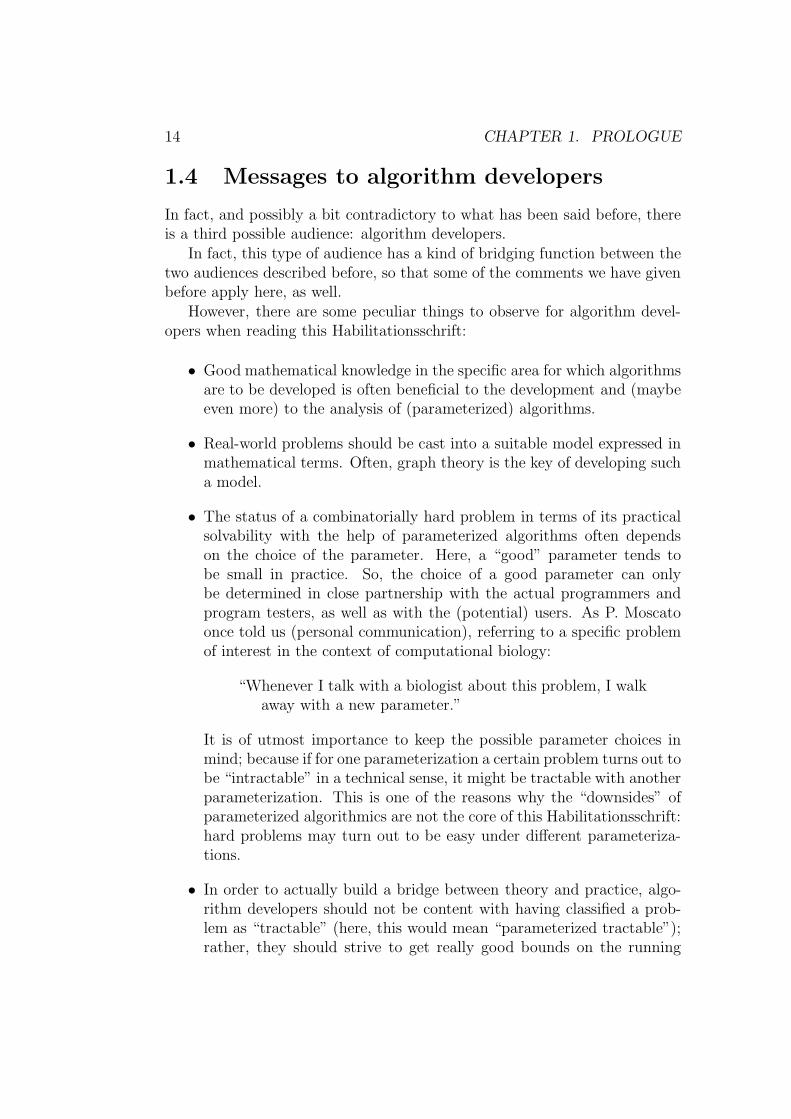
1.4 Messages to algorithm developers
In fact, and possibly a bit contradictory to what has been said before, thereis a third possible audience: algorithm developers.
In fact, this type of audience has a kind of bridging function between thetwo audiences described before, so that some of the comments we have givenbefore apply here, as well.
However, there are some peculiar things to observe for algorithm devel-opers when reading this Habilitationsschrift:
• Good mathematical knowledge in the specific area for which algorithmsare to be developed is often beneficial to the development and (maybeeven more) to the analysis of (parameterized) algorithms.
• Real-world problems should be cast into a suitable model expressed inmathematical terms. Often, graph theory is the key of developing sucha model.
• The status of a combinatorially hard problem in terms of its practicalsolvability with the help of parameterized algorithms often dependson the choice of the parameter. Here, a “good” parameter tends tobe small in practice. So, the choice of a good parameter can onlybe determined in close partnership with the actual programmers andprogram testers, as well as with the (potential) users. As P. Moscatoonce told us (personal communication), referring to a specific problemof interest in the context of computational biology:
“Whenever I talk with a biologist about this problem, I walkaway with a new parameter.”
It is of utmost importance to keep the possible parameter choices inmind; because if for one parameterization a certain problem turns out tobe “intractable” in a technical sense, it might be tractable with anotherparameterization. This is one of the reasons why the “downsides” ofparameterized algorithmics are not the core of this Habilitationsschrift:hard problems may turn out to be easy under different parameteriza-tions.
• In order to actually build a bridge between theory and practice, algo-rithm developers should not be content with having classified a prob-lem as “tractable” (here, this would mean “parameterized tractable”);rather, they should strive to get really good bounds on the running

1.5. ACKNOWLEDGMENTS 15
times of their algorithms. The better the running times of the algo-rithms, the more useful are the proposed algorithms. This is true inparticular for the development of exact algorithms for computationallyhard problems: the difference between an O∗(2k) algorithm and anO∗(1.3k) algorithm is tremendous.
• Conversely, it does not make much sense to strive for smaller andsmaller bases of the exponential terms if this comes at the cost of veryintricate algorithms; rather, one should see if there are actually simplealgorithms which are easy to implement and clearly structured and thatstill have good running times. This would surely help proliferate ideasin the area of exact algorithmics in general, and in the fixed-parameterarea in particular.
1.5 Acknowledgments
This Habilitationsschrift would not have come into “life” without the steadysupport from my family, friends and colleagues.
In particular, I like to mention (and thank in this way) for many scientificdiscussions the following people (in alphabetical order):
Faisal Abu-Khzam, Jochen Alber, Regina Barretta, Hans Bodlaender,Oleg Borodin, Ljiljana Brankovic, David Bryant, Frank Dehne, FredericDorn, Vida Dujmovic, Mike Fellows, Jens Gramm, Jiong Guo, Torben Hagerup,Falk Huffner, David Juedes, Iyad Kanj, Michael Kaufmann, Ton Kloks,Klaus-Jorn Lange, Mike Langston, Margaret Mitchell, Pablo Moscato, RolfNiedermeier, Naomi Nishimura, Ljubomir Perkovic, Elena Prieto-Rodriguez,Prabhakar Ragde, Klaus Reinhardt, Frances Rosamond, Peter Shaw, Chris-tian Sloper, Ulrike Stege, Matthew Suderman, Bjarne Toft, Magnus Wahlstrom,Sue Whitesides, and Gerhard Woeginger.
Apologies to everybody whom I forgot to mention in that list.
1.6 Keeping up to date
In a fast-growing field as the one of parameterized algorithmics, or moregenerally speaking, parameterized complexity and algorithms to denote thewhole area, it is close to impossible to keep up to date with recent develop-ments. So, our apologies to to everybody whose work is underrepresented ifnot completely missed out in this Habilitationsschrift.
The interested reader is advised to follow up overview articles that seemto appear every second month on this area. We list the survey papers we
16 CHAPTER 1. PROLOGUE
came across that only appeared in the second half of 2004:
• R. Niedermeier gave an invited talk at MFCS in August [307]. In thiscontext, his Habilitationsschrift [306] is also worth mentioning.
• J. Flum and M. Grohe gave a nice overview on recent developmentsof parameterized complexity in the complexity theory column of theBulletin of the EATCS (October issue), see [185].
• R. Downey and C. McCartin had an invited talk at DLT in Decem-ber [138].
We therefore recommend trying to keep up to date by following up recentconferences and to simply search the internet with appropriate catchwordsfrom time to time. The special chapter 11 collecting web addresses can beseen as a starting point for such a research.
The internet is also a good place to look for sources on algorithmics, forlooking up definitions etc., see Site [Chapter 11, Site 1].
However, one should not completely disregard “older” overview articles.For example, the papers [137, 136] still contain lots of programmatic materialthat hasn’t been properly dealt with in the last couple of years.

Chapter 2
Introduction
This introductory chapter is meant to introduce the basic notions used inthis Habilitationsschrift:
• Sec. 2.1 will acquaint the reader with the basic notions of parameterizedcomplexity and algorithmics, since this is the basic framework for ourwork.
• Sec. 2.3 provides a primer in graph theory, since most problems weapproach in this Habilitationsschrift are drawn from that area (or canbe conveniently expressed in those terms).
• Then, in Sec. 2.4 we make this more concrete by exhibiting some of ourfavorite combinatorial graph problems.
• Sec. 2.5 is meant to be an appetizer to show one of the main techniquesof this area: that of data reduction.
2.1 The parameterized landscape
Parameterized complexity has nowadays become a standard way of dealingwith computationally hard problems.
2.1.1 The world of parameterized algorithmics: defini-tions
In this section, we are going to provide the basic definitions of parameterizedalgorithmics.
17

18 CHAPTER 2. INTRODUCTION
Definition 2.1 (parameterized problem) A parameterized problem P isa usual decision problem together with a special entity called parameter.Formally, this means that the language of YES-instances of P, written L(P),is a subset of Σ∗×N. An instance of a parameterized problem P is thereforea pair (I, k) ∈ Σ∗ × N.
If P is a parameterized problem with L(P) ⊆ Σ∗ × N and a, b ⊆ Σ,then Lc(P) = Iabk | (I, k) ∈ L(P) is the classical language associated toP. So, we can also speak about NP-hardness of a parameterized problem.
As classical complexity theory, it helps classify problems as “nice,” ormore technically speaking, as tractable, or as “bad,” or intractable, althoughthese notions may be misleading to a practical approach, since intractabledoes not imply that such problems cannot be solved in practice. It rathermeans that there are really bad instances that can be constructed on whichany conceivable algorithm would badly perform. It might also indicate thatthe current choice of parameter is not the “right” one.
Since this Habilitationsschrift is focusing on the algorithmic aspects, let usin the first place define the class of problems that we consider to be tractablefrom a parameterized perspective.
Another thing that is worth mentioning is the way how the complexityof an algorithm is mentioned. In general, we assume a suitable underlyingRAM model. Since the technical details are not really crucial in our setting,we deliberately refrain from giving more details here, as they are containedin any textbook on classical complexity theory or algorithmics. Rather, weassume an intuitive understanding of what an algorithm is and how thecomplexity of an algorithm is measured. Hence, we will give all algorithmsin a high-level pseudo-code notation.
When measuring the complexity of an algorithm, it is crucial against whatwe measure, i.e., how we measure the size of the input. We already discussedthis issue for “number parameters.” In most cases, a rather intuitive under-standing of size is sufficient, assuming a suitable encoding of the instanceas a binary encoded string and taking the length of this string as the sizeof the instance. Given I, |I| should denote this size measure. However, insome cases, other size functions make sense, as well. For examples, graphsare usually measured in terms of the number of edges or in terms of the num-ber of vertices. In classical complexity, this does not really matter as longas we only distinguish between say polynomial time and exponential time.However, these things may become crucial for algorithmics that deals withalgorithms that run in exponential time. Therefore, at some times we will bemore picky and explicitly refer to a size function size(·) to measure the sizesize(I) of the instance I. More details are discussed in Chapter 3. Some of

2.1. THE PARAMETERIZED LANDSCAPE 19
the following definitions already make use of this function. At this point, it issufficient to always think about size(·) as referring to | · |, i.e., the length of abinary string encoding the instance, where a “reasonable encoding” functionis assumed.
Definition 2.2 (parameterized tractability) A parameterized problemP is called fixed-parameter tractable if there exists a solving algorithm forP running in time O(f(k)p(|I|)) on instance (I, k) for some function f andsome polynomial p, i.e., the question if (I, k) ∈ L(P) or not can be decidedin time O(f(k)p(|I|)).
The class of problems collecting all fixed-parameter tractable parameter-ized problems is called FPT .
A parameter can, in principle, be nearly everything, as detailed in Chap-ter 3. However, in most examples we consider, the parameter will be anumber. From a theoretical point of view, it does not matter whether such anumber is given in unary or in binary to classify a problem in FPT . However,this would of course matter for the algorithmics, since the size of a numberconsiderably differs depending on the encoding. Therefore, let us fix here thatnumbers that appear as parameters will be considered as unary-encoded ifnot stated otherwise. Hence, the size of the number would correspond to itsnumerical value. This can be justified, since in most cases (say for graphproblems) the parameter (say the size of a selection of vertices) is upper-bounded by the size of a list of items that is explicitly part of the input. Ascan be seen above, we already tailored our definitions to the unary encodingof the “number parameter.”
Assuming some basic knowledge of graph theory on side of the reader(who might otherwise first wish to browse through Sec. 2.3), we illustratethe notions with shortly discussing one example in this section:
Problem name: vertex cover (VC)Given: A graph G = (V,E)Parameter: a positive integer kOutput: Is there a vertex cover C ⊆ V with |C| ≤ k?
Definition 2.3 (Kernelization) Let P be a parameterized problem. Akernelization is a function K that is computable in polynomial time andmaps an instance (I, k) of P onto an instance (I ′, k′) of P such that
• (I, k) is a YES-instance of P if and only if (I ′, k′) is a YES-instance ofP
• size(I ′) ≤ f(k), and

20 CHAPTER 2. INTRODUCTION
• k′ ≤ g(k) for some arbitrary functions f and g.
To underpin the algorithmic nature of a kernelization, K may be referredto as a kernelization reduction. (I ′, k′) is also called the kernel (of I), andsize(I ′) the kernel size. Of special interest are polynomial-size kernels andlinear-size kernels, where f is a polynomial or a linear function, respectively.
A kernelization is a proper kernelization if g(k) ≤ k.
A parameterized problem that admits a kernelization is also called ker-nelizable.
Of course, of uttermost importance are proper kernelizations yieldinglinear-size kernels. In fact, this is the best we can hope for when dealingwith hard problems, since sub-linear kernels for NP-hard problems wouldmean that P equals NP, see Lemma 9.11.
With one exception, all kernelization reduction that are presented in thisHabilitationsschrift are proper.
Once a kernelization is found, membership of the corresponding problemin FPT is easy to see:
Algorithm 1 A brute force FPT algorithm from kernelization
Input(s): kernelization function K, a brute-force solving algorithm A forP, instance (I, k) of P
Output(s): solve (I, k) in FPT -time
Compute kernel (I ′, k′) = K(I, k)Solve (I ′, k′) by brute force, i.e., return A(I ′, k′).
Interestingly, the converse is also true: each problem in FPT is ker-nelizable. The corresponding construction is contained in [134] and is notreproduced, since it is not of any algorithmic interest.
Theorem 2.4 A parameterized problem is in FPT iff it is kernelizable.
In the rest of this Habilitationsschrift, we are mostly sloppy when it comesto the issue of defining kernelizations. The issue of reduction rules and howthey lead to kernelizations is discussed in Sec. 4.1.
Secondly, we will also accept algorithms as valid kernelizations if theyactually completely solve or even reject the given instance. In our algorithms,we denote this behavior by, e.g.,
if . . . then YES
2.1. THE PARAMETERIZED LANDSCAPE 21
Formally, an algorithm that contains such statements can be interpreted as akernelization function by first choosing some small YES- (or NO-) instances inthe beginning and outputting them whenever the algorithm detects that thegiven (or transformed) instance can be trivially solved or rejected. Particularexamples for such forms of reductions can be found by (ab)using (non-trivial)theorems combinatorics, as listed in Sec. 4.4.
Finally, and possibly even more sloppy, we write down reduction rules inthe form:
Let (I, k) be an instance of problem P . If conditions . . . are met,then reduce the instance to (I ′, k′) with k′ < k.
What we sweep under the carpet is that it might be that k′ might have avalue that is not permitted; e.g., often the parameter is a positive integer,and therefore k′ < 0 would not be permitted. So, whenever a reductionrule application would yield an instance that has a parameter which is notpermitted, we would implicitly return NO, in the sense described in theprevious paragraph.
Let us state two simple reduction rules for vertex cover (as the runningexample not only of this section) that are usually attributed to S. Buss: 1
Reduction rule 1 Delete isolated vertices (and leave the parameter un-changed).
Reduction rule 2 (Buss’ rule) If v is a vertex of degree greater than kin the given graph instance (G, k), then delete v from the instance and reducethe parameter by one, i.e., produce the instance (G− v, k − 1).2
The soundness of these rules can be “easily” seen by the following obser-vations.
• If v is a vertex with no neighbors, v can be removed from the graph,since v will not be part of any minimum vertex cover.
1Let us mention the following historical aside: Although the two reduction rules (inparticular, the second one) listed in the following are generally attributed to a personalcommunication of Sam Buss, in particular [64], there is a reference of Evans [158] thatconsiderably predates the Buss reference. Admittedly, Evans considers a special variantof vertex cover (namely, the constraint bipartite vertex coverproblem discussed indetail in Chap. 5) which arises in connection with VLSI reconfiguration, but the reductionrules are basically the same.
2G− v denotes the graph that is obtained from G = (V,E) by removing v from V andby removing all edges that contain v. If V` is a vertex set V` = v1, . . . , v`, G − V` isinductively defined: G− V1 = G− v1, G− Vi = (G− Vi−1) − vi for i > 1.

22 CHAPTER 2. INTRODUCTION
• If v is a vertex of degree greater than k, v must be in any vertexcover, since otherwise all neighbors would be in the cover, which isnot feasible, because we are looking for vertex covers with at most kvertices. Hence, we can remove v from the graph.
More precisely, to actually prove the soundness of the reduction rules, thefollowing has to be shown (since the polynomial-time computability of therules is trivial to see):
Lemma 2.5 Let (G, k) be an instance of vertex cover that contains iso-lated vertices I. Then, (G, k) is a YES-instance of VC iff (G − I, k) is aYES-instance of VC.
Lemma 2.6 Let (G, k) be an instance of vertex cover that contains avertex v of degree larger than k. Then, (G, k) is a YES-instance of VC iff(G− v, k − 1) is a YES-instance of VC.
To get acquainted with the proof strategy involved in this kind of reason-ing, let us formally prove the soundness of Buss’ rule:
Proof. If (G, k) is a YES-instance of vertex cover that contains avertex v of degree larger than k, then v must be part of any solution; hence,(G− v, k − 1) is a YES-instance of VC.
Conversely, if C ′ is a cover verifying that (G− v, k− 1) is a YES-instanceof VC, then C = C ′ ∪ v shows that (G, k) is also a YES-instance of VC;this is true irrespectively of the degree of v.
The very idea of kernelization (as detailed in Chap. 4) now means toapply the available reduction rules to a given problem instance as long aspossible. This leaves us finally with a reduced instance, as discussed in thefollowing theorem.
Theorem 2.7 A YES-instance (G, k), with G = (V,E), of vertex coverto which neither Rule 1 nor Rule 2 is applicable, satisfies |E| ≤ k2 and|V | < k2.
Proof. Due to Rule 2, every vertex has degree bounded by k. Since (G, k)is a YES-instance, there is a selection of k vertices that cover all edges E.But each vertex can cover at most k edges, so that |E| ≤ k2 follows. SinceRule 1 is not applicable, the number of vertices of G is basically bounded bythe number of edges of the graph.
Theorem 2.7 allows to state the following kernelization rule in the form ofa little program 2; observe that the ELSIF-branch codifies a third reduction

2.1. THE PARAMETERIZED LANDSCAPE 23
rule whose correctness follows from the preceding theorem. Theorem 2.7 thenalso shows the kernel size that is claimed in Alg. 2.
Algorithm 2 A kernelization algorithm for vertex cover, called Buss-kernelInput(s): A vertex cover instance (G, k)Output(s): an instance (G′, k′) with k′ ≤ k, |E(G′)|, |V (G′)| ≤ (k′)2, such
that (G, k) is a YES-instance of VC iff (G′, k′) is a YES-instance
if possible thenApply Rule 1 or Rule 2; producing instance (G′, k′).return Buss-kernel(G′, k′).
else if |E(G)| > k2 thenreturn ((x, y, x, y), 0) encoding NO
elsereturn (G, k)
end if
To explicitly show that vertex cover belongs to FPT , we can considerAlg. 3. This allows us to state:
Algorithm 3 A kernelization algorithm for vertex cover, called VC-kernelization-basedInput(s): A vertex cover instance (G, k)Output(s): YES iff (G, k) is a YES-instance of VC.
Let (G′, k′):=Buss-kernel(G, k). Let G′ = (V,E).if k′ ≤ 0 then
return (k′ = 0 AND E = ∅)else
for all C ⊆ V , |C| = k doif C is a vertex cover of G′ then
return YES
end ifend forreturn NO
end if
Theorem 2.8 V C ∈ FPT . More specifically, given an instance (G, k) ofvertex cover, the question “(G, k) ∈ L(V C) ?” can be answered in time
24 CHAPTER 2. INTRODUCTION
O(f(k) + |V (G)|), where
f(k) =
(k2
k
)∈ O(2k
2
).
Proof. The correctness is immediate by Theorem 2.7. That theorem alsoshows the claimed bound on the running time. Observe that the reductionrules themselves can be efficiently implemented.
After having introduced the essential concepts of this Habilitationsschrift,let us formulate a warning when it comes to interpreting results that arestated without explicit reference to the “world” of parameterized complexity.For example, the following can be found in a recent paper dedicated to specificaspects of graph theory [360, page 338]:
Garey and Johnson [199] proved that testing CR(G) ≤ k is NP-complete, . . . Testing planarity, and therefore testing CR(G) ≤k for any fixed k can be done in polynomial time—introduceat most k new vertices for crossing points in all possible waysand test planarity.
More specifically, CR(G) is the crossing number of a graph G, i.e., the num-ber of edge crossing necessarily incurred when embedding G into the Eu-clidean plane;3 it is however not necessary to understand the exact defini-tion of this notion for the warning that we like to express. Namely, whensuperficially read, the quoted sentence could be interpreted as showing fixed-parameter tractability of the following problem:
Problem name: crossing number (CRN)Given: A graph G = (V,E)Parameter: a positive integer kOutput: Is CR(G) ≤ k?
However, this is not a correct interpretation. Namely, how would you in-terpret or even implement the algorithm sketch in more concrete terms? Ourinterpretation of the quoted lines would be as detailed in Alg. 4. However,the complexity of this algorithm is roughly O(|G|k), and hence this algo-rithm does not show that crossing number is fixed-parameter tractable.
3There seem to be some intricate problems with the exact definition of what is meantby a crossing number; papers on this topic should be read with careful scrutiny to seewhat definitions the authors adhere to. This is detailed in the paper of Szekely [360], aswell as in [317]. In fact, the interpretation we detail on the quoted algorithm sketch forcrossing number is referring to the so-called pairwise crossing number.

2.1. THE PARAMETERIZED LANDSCAPE 25
Algorithm 4 Determining pairwise crossing numbers
Input(s): Graph G = (V,E), parameter kOutput(s): Is CR(G) ≤ k?
for all sets of k pairs of edges P = e1, e′1, . . . , ek, e′k do
Initialize G′ = (V ′, E ′) as G.for i = 1, . . . , k do
Into G′, we introduce one new vertex xi and new edges fi, gi, f′i , g
′i
that contain xi as one endpoint and that satisfy |fi ∩ ei| = |gi ∩ ei| =|f ′i ∩ e′i| = |g′i ∩ e′i| = 1.
Mark ei and e′i.end forRemove all marked edges from G′.if G′ can be drawn without crossings into the plane (planarity test)then
return YES
end ifend forreturn NO.
In fact, to our knowledge, it is open if crossing number is parameterizedtractable. Only if the input is restricted to graphs of maximum degree three,membership in FPT has been established, see [134, page 444].
Conversely, this caveat does not mean that—albeit it has become sort ofstandard to refer to parameterized complexity when stating exact algorithms—all results that do not reference the parameterized paradigm are necessarilynot interpretable as results in parameterized algorithmics. A good (positive)and recent example is the tree editing problems investigated in [198], whichshow that these problems are in FPT when parameterized by the numberof admissible edit operations (which is also the standard parameter followingthe terminology introduced in Chap. 3).
2.1.2 The world of parameterized algorithmics: method-
ologies
A whole toolbox for developing these algorithms has been developed. Marx(in his recent talk at CCC 2004) compared these tools with a Swiss armyknife, see [Chapter 11, Site 12].
Those tools are, in particular (according to the mentioned slides):
1. well-quasi-orderings;
26 CHAPTER 2. INTRODUCTION
2. graph minor theorems;
3. color-coding;
4. tree-width, branch-width etc.;
5. kernelization rules;
6. bounded search tree.
This list is probably not exhaustive but gives some good impression ofthe available techniques. This list is ordered by “increasing applicability,” aswill be explained in the following.
The first two methods are the most abstract tools. In a certain sense,they are useful to classify problems as being tractable by the parameterizedmethodology, but (as far as we know) they never led to algorithms that canbe really termed useful from a practical point of view. Once a problem hasbeen classified as tractable, a good research direction is to try to improve thecorresponding algorithms by using the more “practical” methods.
Color coding is a methodology that is helpful for getting randomized pa-rameterized algorithms. Since this is not the primary interest of this Habili-tationsschrift, we will neglect this methodology, as well.
The last three methods are of definite practical interest. They comprisethe methods which yielded the best parameterized algorithms in nearly allcases. They will be in the focus of the exposition of this Habilitationsschrift.To each of these three methodologies, a chapter of the Habilitationsschriftwill be devoted.
More specifically, treewidth and branchwidth are typical examples ofstructural parameters for graphs that are particularly helpful in the sensethat once it is known that a graph has a small treewidth, then problems thatare NP-hard for general graphs can be solved in polynomial, often even inlinear time. We will give details in Chapter 7.
Kernelization rules can be viewed as a method of analyzing data reductionrules. These have been always successfully used in practice for solving hugedata instances, but parameterized algorithmics offers now a way to tell whythese rules actually work that well. Further introductory remarks can alreadybe found in this chapter. Note that the very first theorem of this Habili-tationsschrift, which is Thm. 2.4, says that the basic algorithmic class weare dealing with can be characterized by algorithms that use kernelizationrules (although the rules leading to that theorem are admittedly of artificialnature). A worked-out example of this technique is contained in Sec. 2.5.Further details on this technique are collected in Chapter 4.

2.2. IS PARAMETERIZED ALGORITHMICS THE SOLUTION TO “EVERYTHING”?27
Finally, exact algorithms for computationally hard problems are often ifnot mostly based on a clever search through the space of all possibilities.This naturally leads to the notion of a search tree, and the art of developingsearch tree algorithms can be seen as devising clever rules how to work one’sway through the search space. Chapter 5 collects many ideas how to findand how to improve on search tree algorithms. More examples can be foundthroughout the whole Habilitationsschrift.
We deliberately ignored some techniques that others would find essentialto parameterized algorithmics, notably including techniques related to logic.However, at several places, the reader will find hints to further reading.
2.2 Is parameterized algorithmics the solu-
tion to “everything”?
Such a bold question cannot be possibly answered affirmatively. So, what canwe find on the downside, the parameterized complexity theory? Let us hereonly briefly mention that there does exist a whole area dealing with this. Wewill explore more of this in Chapter 9. The reader who is primarily interestedin complexity theory should be warned, however, that this is not the focusof the present Habilitationsschrift. Rather, (s)he could take Chapter 9 as acollection of pointers to further reading.
From an algorithmic point of view, the most important notion of param-eterized complexity is that of a parameterized reduction, since it makes itpossible to link seemingly different problems in a way that algorithms forone problem can be used to solve another one. Even if the idea to constructsuch a simple reduction fails, it often gives us good hints at how to use ideasfrom a “solved” problem to tackle a new problem.
Definition 2.9 (Parameterized reduction) Let P and P ′ be parameter-ized problems. Let g : N → N be some arbitrary function.
A parameterized reduction is a function r that is computable in timeO(g(k)p(size(I))) for some polynomial p and maps an instance (I, k) of Ponto an instance r(I, k) = (I ′, k′) of P ′ such that
• (I, k) is a YES-instance of P if and only if (I ′, k′) is a YES-instance ofP ′ and
• k′ ≤ g(k).
We also say that P reduces to P ′.

28 CHAPTER 2. INTRODUCTION
Note that we defined a sort of many-one reduction. More generally speak-ing, it is also possible to define Turing reductions, see [134, 185]. The corre-sponding details won’t matter in the remainder of this Habilitationsschrift.
Observe that the kernelization reduction introduced above is a sort of“self-reduction” and fits into the concept of a parameterized reduction.
Unfortunately, most classical reductions between NP-hard problems turnout not to be reductions in the parameterized sense, although there are alsosome exceptions, as contained in [98, 282].
Let us discuss some simple examples (drawn from graph theory; the readerwho is not so familiar with the corresponding concepts might first wish toconsult the primer contained in Sec. 2.3):
Problem name: clique (CQ)Given: A graph G = (V,E)Parameter: a positive integer kOutput: Is there a clique C ⊆ V with |C| ≥ k?
Alternatively, we may focus on the edges:
Problem name: clique (CQE)Given: A graph G = (V,E)Parameter: a positive integer kOutput: Is there a edge-induced clique C ⊆ E with |C| ≥ k?
Lemma 2.10 clique and clique (edge-induced) are parameterized in-terreducible.
This simple result is also mentioned in [232] (without reference to param-eterized complexity); however, since this gives a nice example for an easyparameterized reduction, we provide a proof in what follows.
Proof. Let G = (V,E) be a graph. For some k, let (G, k) be an instance ofclique. If (G, k) is a YES-instance, then (G, k(k − 1)/2) is a YES-instancefor clique (edge-induced) and vice versa.
Conversely, consider an instance (G, k) of clique (edge-induced). If(G, k) is a YES-instance, then consider integers k′, k′′ such that
(k′ − 1)(k′ − 2)/2 < k ≤ k′(k′ − 1)/2 =: k′′.
Obviously, (G, k′′) is a YES-instance of clique (edge-induced), as well.Moreover, if (G, k) is a NO-instance, then (G, k′′) is a NO-instance of clique(edge-induced), as well.

2.2. IS PARAMETERIZED ALGORITHMICS THE SOLUTION TO “EVERYTHING”?29
Hence, (G, k) is a YES-instance of CQE iff (G, k′′) is a YES-instance ofCQE iff (G, k′) is a YES-instance of CQ.
In Chapter 9, we will be more explicit about the complexity classes (i.e.,the classes of problems) that are not amenable to the parameterized ap-proach. At this stage, it is sufficient to know that the lowest complexityclass thought to surpass FPT is called W[1] (according to the expositionin the monograph [134]). All those classes are closed under parameterizedreductions.
Since it is well-known that clique is W[1]-complete, we may deduce:
Corollary 2.11 clique (edge-induced) is W[1]-complete.
Of course, taking the NP-completeness of clique for granted, the proofof Lemma 2.10 also shows that clique (edge-induced) is NP-complete.
Now, consider the following two related problems:
Problem name: vertex clique complement cover (VCCC)Given: A graph G = (V,E)Parameter: a positive integer kOutput: Is there a vertex clique complement cover C ⊆ V with|C| ≤ k?
Here, C ⊆ V is a vertex clique complement cover in G = (V,E) iffV −C induces a complete graph (i.e., a clique). Similarly, C ⊆ E is a cliquecomplement cover in G = (V,E) iff E − C induces a complete graph.
Problem name: clique complement cover (CCC)Given: A graph G = (V,E)Parameter: a positive integer kOutput: Is there a clique complement cover C ⊆ E with |C| ≤ k?
The latter problem has been studied in [34] under the viewpoint of ap-proximation; in actual fact, a weighted version was examined in that paper.
The following is an easy consequence from the definition (also see [232]:
Lemma 2.12 • C is a vertex clique complement cover of G = (V,E) iffV \ C induces a clique in G iff C is a vertex cover of Gc.
• C is a clique complement cover of G = (V,E) iff E \C induces a cliquein G.

30 CHAPTER 2. INTRODUCTION
However, the induced translation from say clique to vertex cliquecomplement cover or from clique (edge-induced) to clique com-plement cover (or vice versa) is not a parameterized reduction; in fact,the status of the problems is quite different: while vertex clique com-plement cover (and clique complement cover, as we will later see4)is in FPT (combining Lemma 2.12 with Theorem 2.8), CQ and CQE areW[1]-complete and hence not believed to lie in FPT .
2.3 A primer in graph theory
Most examples in this Habilitationsschrift will be basically graph theoreticquestions, although not all problems (at first glance) are of graph theoreticnature. The reason is that graph theory offers a very nice framework ofstating combinatorial problems of any kind.5 Therefore, in this section, webriefly introduce some basic notions related to graphs (and hypergraphs).Reader familiar with graph theory may skip this section and return to itwhenever some possibly non-familiar notions are used throughout the text;the index will help find the appropriate place of definition.
A graph G can be described by a pair (V,E), where V is the vertex setand E is the edge set of G. Abstractly speaking, E is a relation on V . If thisrelation is symmetric, then G is an undirected graph, otherwise (and moregeneral) we also speak of a directed graph. A loop is an edge of the form (x, x).If an undirected graph contains no loops, its edge set can be also specifiedby a set of 2-element subsets of V . We therefore often use set notation todenote edges. Specifically, this is true for hypergraphs as defined below, sothat undirected graphs (even those containing loops) become special cases ofhypergraphs.
If not stated otherwise, graphs in this Habilitationsschrift will be undi-rected and without loops. Edges are then alternatively denoted as (x, y),x, y or simply xy, whatever is more convenient in the concrete example.
As mentioned, undirected graphs can be generalized to hypergraphs. Ahypergraph G is specified by a pair (V,E), where V is the vertex set and Eis the hyperedge set, i.e., a set of subsets of V . If e is a hyperedge, |e| isits hyperedge size. For convenience, we often refer to hyperedges simply asedges. To underline the duality of vertices and hyperedges in hypergraphs,
4Bar-Yehuda and Hochbaum [34, 232] indicate that clique complement cover hasa direct connection to vertex cover; however, we believe that this is not true, as we willdetail in Sec. 6.3.
5A nice selection of such “applied problems” modeled by graphs can be found in [283],although that book rather focuses on Graph Drawing than on Graph Theory as such.

2.3. A PRIMER IN GRAPH THEORY 31
we sometime also refer to the hyperedge size as hyperedge degree.The following notions mostly apply both to (undirected) graphs and to
hypergraphs:
• V (G) denotes the set of vertices of G.
• E(G) denotes the set of edges of G.
• P (G) denotes the set of paths of G, where a path is a sequence of edgesp = e1e2 . . . ek with ei∩ei+1 6= ∅ for i = 1, 2, . . . , k−1; k is also referredto as the length of the path. A path p = e1e2 . . . ek is called a simplepath if ei ∩ ei+1 ∩ ej 6= ∅ iff j = i or j = i + 1 for i = 1, 2, . . . , k − 1,and j = 1, 2, . . . , k. Two vertices x, y are connected iff there is a pathbetween them. A connected component, or simple said a component, isa set of vertices C in a graph such that each pair of vertices x, y ∈ C isconnected. A graph is called connected if it contains only one connectedcomponent.
A simple path p = e1e2 . . . ek is a cycle iff e1 ∩ ek 6= ∅; k is also referredto as the length of the cycle.
A cycle of length k is usually abbreviated as Ck. A simple path oflength k that is not a cycle is usually abbreviated as Pk.
• If G is a (hyper-)graph, then (V ′, E ′) is called a subgraph of G iffV ′ ⊆ V (G) and E ′ ⊆ E(G).
A graph is called cycle-free or acyclic if it does not contain a cycle asa subgraph.
A subgraph (V ′, E ′) of G = (V,E) is vertex-induced (by V ′) iff
∀e ∈ E : e ⊆ V ′ ⇐⇒ e ∈ E ′.
In other words, E ′ contains all edges between vertices in V ′ that arementioned in G. We also write G[V ′] to denote G′. A subgraph (V ′, E ′)of G = (V,E) is edge-induced (by E ′) iff V ′ =
⋃e∈E′ e. We also write
G[E ′] to denote G′.
• N(v) collects all vertices of v that are neighbors of v, i.e., N(v) = u |∃e ∈ E(G) : u, v ⊆ e. N(v) is also called the open neighborhood ofv, while N [v] := N(v) ∪ v is the closed neighborhood of v. deg(v)denotes the degree of vertex v, i.e., deg(v) = |N(v)|. If X ⊆ V , we canalso use N(X) =
⋃x∈X N(x) and N [X] = N(X) ∪X.
• If G is a (hyper-)graph, then a vertex set I is an independent set iffI ∩N(I) 6= ∅. A set D ⊆ V is a dominating set iff N [D] = V .

32 CHAPTER 2. INTRODUCTION
• If G is a (hyper-)graph, then a mapping c : V → C is a coloring iff, forall a ∈ C, c1(a) is an independent set. A graph is k-colorable iff thereis a coloring c : V → C with |C| = k. A 2-colorable graph is also calledbipartite. Note that a graph is bipartite iff it does not contain a cycleof even length as a subgraph.
It is sometimes convenient to link graphs and (binary) matrices.
• If G = (V,E) is a (directed) graph, then A(G) is a binary two-dimen-sional matrix (called adjacency matrix of G) whose rows and columnsare indexed (for simplicity) by V . Then, A[x, y] = 1 iff (x, y) ∈ E.Put it in another way, A(G) is the relation matrix associated to theadjacency matrix. Observe that A(G) is symmetric iff G is undirected.A(G) contains ones on the main diagonal iff G contains loops.
• If G = (V,E) is a hypergraph, then I(G) is a binary two-dimensionalmatrix (called incidence matrix of G) whose rows are indexed by Vand whose columns are indexed by E. Then, I[x, e] = 1 iff x ∈ e.Conversely, every binary matrix M can be interpreted as the incidencematrix of some hypergraph G(M). Observe that undirected loop-freegraphs have incidence matrices with the special property that, in eachcolumn, there are exactly two entries that equal one.
• If G = (V,E) is a bipartite undirected graph with bipartization V =V1 ∪ V2, A(G) has the special form that the submatrices indexed byV1 × V1 and by V2 × V2 only contain zeros. Moreover, since the graphis supposed to be symmetric, the submatrix indexed by V1 × V2 is thetransposal of the submatrix indexed by V2×V1. Hence, the informationcontained in A(G) can be compressed and stored in a binary matrixAB(G) which is the submatrix of A(G) indexed by V1 × V2. AB(G) isalso called bipartite adjacency matrix of G. Observe that any binarymatrix M can be interpreted as the bipartite adjacency matrix of somebipartite undirected graph B(M).
The definitions we gave up to now also provide some good hints how torepresent graphs on computers; either as edge lists (where to each vertex, alist of incident edges is attached) or as matrices of different types. Althoughwe are dealing with algorithms on graphs, we won’t we in general too specificabout the actual data structures we use for graphs. All the data structures wementioned (and many other conceivable “reasonable” ones) are polynomiallyrelated, so that for the exponential-time algorithms we mostly look at, itdoes not so much matter which representation we actually choose.

2.3. A PRIMER IN GRAPH THEORY 33
Of particular importance are certain (undirected) graph classes in whatfollows.6 The possibly simplest non-trivial graph is a tree, i.e., a connectedgraph without cycles. A graph that consists of a collection of componentseach of which is a tree is known as a forest. A vertex of degree one in a tree(and more generally, in a graph) are also called a leaf, and any other vertex iscalled an inner node. Here, we see another convention followed in this text:a vertex in a tree is often referred to as a node.
For example, a graph G = (V,E) is cycle-free iff V induces a forest in Gor, in other words, if G is a forest. Then, a tree can be characterized as aconnected forest.
More generally speaking, if G is a class of graphs, then a graph G isa forest of G iff G = (V,E) can be decomposed into G1 = (V1, E1), . . . ,Gk = (Vk, Ek), with Vi ∩ Vj = ∅ iff i 6= j and
⋃ki=1 Vi = V , such that all
Gi ∈ G.
Figure 2.1: An example graph with 12 vertices
Example 2.13 Let us view at a particular example to explain most of thenotions introduces so far. Here and in the following, we consider the graphwith 12 vertices as depicted in Fig. 2.1. This graph has edges that are(as usually) graphically represented as line segments or (in one case) moregenerally as a polygon. The vertices of the graph are represented as circularblobs.
The following table gives an adjacency matrix of this graph:
6For a nearly complete overview on various graph classes, we refer to [Chapter 11,Site 8].

34 CHAPTER 2. INTRODUCTION
0 1 0 0 1 0 0 0 0 0 0 01 0 0 0 0 1 0 0 0 0 0 00 0 0 1 0 1 1 0 0 0 0 00 0 1 0 0 0 1 0 0 0 0 01 0 0 0 1 0 0 0 0 0 0 00 1 0 1 0 1 0 0 0 0 0 00 0 1 1 0 1 0 0 0 0 0 00 0 0 0 0 0 0 0 0 0 0 10 0 0 0 0 0 0 0 0 1 0 00 0 0 0 0 0 0 0 1 0 1 10 0 0 0 0 0 0 0 0 1 0 00 0 0 0 0 0 0 1 0 1 0 0
This table should be read as follows: the vertices (used as indices of thatbinary matrix) are read row by row from the picture (observe that in thepicture there are three rows of vertices, each one containing four vertices),and in each row, from left to right. Therefore, the fifth column of the matrixcontains the adjacency of the vertex depicted in the leftmost place of thesecond row.
We leave it as a small exercise to the reader to write up the incidencematrix of this graph.
Let us look more closely at the graph to explain some more of the notionsintroduced so far. The graph has two connected components, depicted redand blue in Fig. 2.2(a). The blue component is a tree. Therefore, the graphinduced by the green edges in Fig. 2.2(b) is also induced by the vertices ofthat component. Moreover, that component is bipartite.
Since the red component contains a triangle, it is not bipartite.
Similarly, also the graph induced by the red edges in Fig. 2.2(b) is vertex-induced. More specifically, that subgraph is a cycle of length four. However,the cycle of length for as given by the outermost four blue edges in Fig. 2.2(b)is not vertex-induced, since in the corresponding vertex-induced subgraph, afifth edge is contained (also colored blue).
One can also define simple operations on graphs.
• If G = (V,E) is a graph, its graph complement is the graph Gc =(V,Ec), where xy ∈ Ec iff xy /∈ E.
• If G1 = (V1, E1) and G2 = (V2, E2) are graphs, their graph union is thegraph (V1 ∪ V2, E1 ∪ E2), assuming (in general) V1 ∩ V2 = ∅.

2.3. A PRIMER IN GRAPH THEORY 35
(a) Two components: red andblue.
(b) Induced graphs.
Figure 2.2: Basic graph notions
• If G = (V,E) is a graph and x, y ∈ V , then
G[x = y] = ((V ∪ [x, y]) \ x, y, E ′)
denotes the vertex merge between x and y, where
E ′ = u, v | u, v ∈ V \x, y∪u, [x, y] | u, x, u, y∩E 6= ∅.
(If e = x, y ∈ E, this operation is also known as the contraction ofe.)
For example, a graph is a forest iff it can be expressed as the union oftrees (hence its name).
We have already encountered some important graph classes like paths,cycles and trees. Of particular importance are also graphs that can be nicelydrawn; planar graphs (as defined below) furthermore enjoy the fact that theyare often encountered in practical circumstances, when graphs are to modelphenomena “down on earth.”
A graph G = (V,E) is called a planar graph if it can be drawn in the planewithout crossings between edges. To be more specific, this means that thereexists an embedding of G into the Euclidean plane R2, which is a mappingthat associates to every vertex v a unique point φ(v) ∈ R2 and to every edgeu, v it associates a simple path (Jordan curve) φ((u, v)) that connects φ(u)and φ(v), such that two paths have more than one common points only iftheir endpoints are identical. Recall that a simple path refers to a continuouscurve in the plane that has no loops, i.e., every point in the plane is visited atmost once, in accordance with the purely graph-theoretic notion of a simplepath.
If a planar graph is given together with its embedding, we also speak ofa plane graph.
36 CHAPTER 2. INTRODUCTION
Observe that an embedded graph partitions the surface on which it isembedded into open regions that are called faces.
2.4 Some favorite graph problems
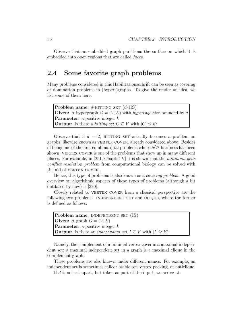
Many problems considered in this Habilitationsschrift can be seen as coveringor domination problems in (hyper-)graphs. To give the reader an idea, welist some of them here.
Problem name: d-hitting set (d-HS)Given: A hypergraph G = (V,E) with hyperedge size bounded by dParameter: a positive integer kOutput: Is there a hitting set C ⊆ V with |C| ≤ k?
Observe that if d = 2, hitting set actually becomes a problem ongraphs, likewise known as vertex cover, already considered above. Besidesof being one of the first combinatorial problems whose NP-hardness has beenshown, vertex cover is one of the problems that show up in many differentplaces. For example, in [251, Chapter V] it is shown that the minimum geneconflict resolution problem from computational biology can be solved withthe aid of vertex cover.
Hence, this type of problems is also known as a covering problem. A goodoverview on algorithmic aspects of these types of problems (although a bitoutdated by now) is [320].
Closely related to vertex cover from a classical perspective are thefollowing two problems: independent set and clique, where the formeris defined as follows:
Problem name: independent set (IS)Given: A graph G = (V,E)Parameter: a positive integer kOutput: Is there an independent set I ⊆ V with |I| ≥ k?
Namely, the complement of a minimal vertex cover is a maximal indepen-dent set; a maximal independent set in a graph is a maximal clique in thecomplement graph.
These problems are also known under different names. For example, anindependent set is sometimes called: stable set, vertex packing, or anticlique.
If d is not set apart, but taken as part of the input, we arrive at:

2.4. SOME FAVORITE GRAPH PROBLEMS 37
Problem name: hitting set (HS)Given: A hypergraph G = (V,E)Parameter: a positive integer kOutput: Is there a hitting set C ⊆ V with |C| ≤ k?
Interestingly, hitting set can be also equivalently represented as a dom-inating set problem on graphs:
Problem name: red-blue dominating set (RBDS)Given: A graph G = (V,E) with V partitioned as Vred ∪ Vblue
Parameter: a positive integer kOutput: Is there a red-blue dominating set D ⊆ Vred with |D| ≤ k,i.e., Vblue ⊆ N(D)?
An instance G = (V,E) of hitting set would be translated into aninstance G′ = (V ′, E ′) of red-blue dominating set as follows.
• The vertices of G would be interpreted as the red vertices of G′.
• The edges of G would be interpreted as the blue vertices of G′.
• An edge in G′ between x ∈ V and e ∈ E means that x ∈ e (in G).
More specifically, the bound d on the size of the hyperedges would have beenreflected by a bound d on the degree of vertices in Vblue; let us call thisrestricted version of red-blue dominating set d-RBDS.
The translation also works backwards, if we note that edges in a graphbeing an instance of red-blue dominating set that connect vertices of thesame color are superfluous and can be deleted. Namely, an edge connectingtwo red vertices is useless, since red vertices only dominate blue vertices andnot red vertices; likewise, an edge between two blue vertices is useless, sinceblue vertices can be only dominated by red vertices. This observation alsogives an example of reduction rules for this problem:
Reduction rule 3 If e is an edge in a RBDS instance that connects verticesof the same color, then delete e.
The exhaustive application of this reduction rule transfers each instance ofred-blue dominating set into a bipartite graph, where the bipartizationof the vertex set is just given by the red and blue vertices.
Let us explicitly state this connection in the following lemma:
Lemma 2.14 red-blue dominating set and red-blue dominatingset, restricted to bipartite graphs are parameterized interreducible.

38 CHAPTER 2. INTRODUCTION
Then, it is easy to read the translation we gave above (working from HSinto RBDS) in a backward manner.
Observe that this also gives an example of two (easy) parameterized re-ductions between these two problems. More specifically, we can state:
Lemma 2.15 hitting set and red-blue dominating set are parame-terized interreducible. Moreover, assuming a bound d on the degree of theblue vertices and likewise a bound d on the size of the hyperedges, d-HS andd-RBDS are again parameterized interreducible.
Essentially, the transformation between RBDS and HS can be also ex-pressed as follows: ifG is a hypergraph (as an instance for HS), then B(A(G))is the corresponding RBDS instance, and if G is a bipartite graph (as a re-duced instance for RBDS with respect to the rule 3), then G(I(G)) is thecorresponding HS instance.
In fact, there is a third formulation of hitting set that can be found inthe literature:
Problem name: set cover (SC)Given: A groundset X, a collection T of subsets of XParameter: a positive integer kOutput: Is there a set cover C ⊆ T with |C| ≤ k, i.e., every elementin X belongs to at least one member of C?
The translation works here as follows:
• The groundset X of the SC instance corresponds to the set of hyper-edges in a HS instance.
• The collection of subsets T corresponds to the set of vertices in a HSinstance, where for a subset t ∈ T , x ∈ t means that the vertex tbelongs to the hyperedge x.
From a practical point of view, HS and SC only formalize two kind of dualrepresentations of hypergraphs:
• HS corresponds to represent hypergraphs by hyperedge sets, each ofthem being a list of incident vertices;
• SC means to represent hypergraphs by vertex sets, each of them beinga list of incident hyperedges.

2.4. SOME FAVORITE GRAPH PROBLEMS 39
For the (in the sense explained above) equivalent problems hitting setand set cover, there exists a vast amount of literature. We only men-tion the (already a bit out-dated) annotated bibliography [73] for furtherreference.
The basic domination problem is not RBDS but the following one:
Problem name: dominating set (DS)Given: A graph G = (V,E)Parameter: a positive integer kOutput: Is there a dominating set D ⊆ V with |D| ≤ k?
Important variants are independent dominating set and connecteddominating set:
Problem name: independent dominating set (IDS)Given: A graph G = (V,E)Parameter: a positive integer kOutput: Is there an independent dominating set D ⊆ V with |D| ≤k?
This problem can be equivalently expressed as a bicriteria problem—andthe reader may wish to check this equivalence— (a proof can be found in[314, Sec. 13]), without explicit reference to the domination property:
Problem name: minimum maximal independent set (MMIS)Given: A graph G = (V,E)Parameter: a positive integer kOutput: Does there exist a maximal independent set of cardinality≤ k ?
Also the other mentioned problem can be equivalently expressed withoutexplicit reference to the domination property:
Problem name: connected dominating set (CDS)Given: A graph G = (V,E)Parameter: a positive integer kOutput: Is there a connected dominating set D ⊆ V with |D| ≤ k,i.e., D is both a connected set and a dominating set?
Problem name: minimum inner node spanning tree(MinINST)Given: A (simple) graph G = (V,E)Parameter: a positive integer kOutput: Is there a spanning tree of G with at most k inner nodes?
40 CHAPTER 2. INTRODUCTION
The importance of domination problems is underlined by the fact thatalready around 1988 there have been about 300 papers dedicated towardsthis topic, see [230].7
Let us explain our favorite graph problems by continuing our examplefrom Ex. 2.13.
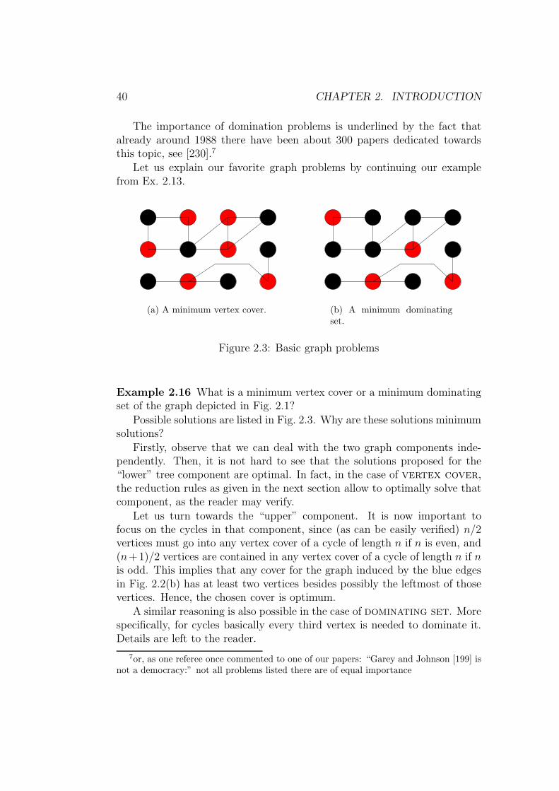
(a) A minimum vertex cover. (b) A minimum dominatingset.
Figure 2.3: Basic graph problems
Example 2.16 What is a minimum vertex cover or a minimum dominatingset of the graph depicted in Fig. 2.1?
Possible solutions are listed in Fig. 2.3. Why are these solutions minimumsolutions?
Firstly, observe that we can deal with the two graph components inde-pendently. Then, it is not hard to see that the solutions proposed for the“lower” tree component are optimal. In fact, in the case of vertex cover,the reduction rules as given in the next section allow to optimally solve thatcomponent, as the reader may verify.
Let us turn towards the “upper” component. It is now important tofocus on the cycles in that component, since (as can be easily verified) n/2vertices must go into any vertex cover of a cycle of length n if n is even, and(n+1)/2 vertices are contained in any vertex cover of a cycle of length n if nis odd. This implies that any cover for the graph induced by the blue edgesin Fig. 2.2(b) has at least two vertices besides possibly the leftmost of thosevertices. Hence, the chosen cover is optimum.
A similar reasoning is also possible in the case of dominating set. Morespecifically, for cycles basically every third vertex is needed to dominate it.Details are left to the reader.
7or, as one referee once commented to one of our papers: “Garey and Johnson [199] isnot a democracy:” not all problems listed there are of equal importance

2.4. SOME FAVORITE GRAPH PROBLEMS 41
Moreover, observe that the dominating set in Fig. 2.3(b) is neither con-nected nor independent. The reader may wish to prove that there is indeedan independent dominating set of cardinality four of that graph, but no con-nected dominating set of that cardinality.
Let us mention here that covering and domination problems often appearin disguise, for example, in various puzzle questions.
Example 2.17 One instance is the so-called Five Queens Problem on thechessboard:8 it is required to place five queens on the board in such positionsthat they dominate each square. This task corresponds to dominating setas follows: the squares are the vertices of a graph; there is an edge betweentwo such vertices x, y iff a queen placed on one square that corresponds to xcan directly move to y (assuming the board were empty otherwise). In otherwords, the edge relation models the way a queen may move on a chess board.
According to [97], the general version played on a (general) n× n boardis also known as the Queen Domination Problem. The task is to find theminimum number of queens that can be placed on a general chessboard sothat each square contains a queen or is attacked by one. Recent bounds onthe corresponding domination number can be found in [62, 63, 100, 315]. Itappears to be that the queen domination number is “approximately” n/2,but only few exact values have been found up to today. By way of contrast,observe that on the n× n square beehive, the queen domination number hasbeen established to be b(2n+ 1)/3c, see [366].
As special classes of graphs (like planar graphs) will become importantin later chapters of this Habilitationsschrift, let us mention that, althoughthe structure we started with, namely the chessboard, is of course a planarstructure, the corresponding graph model we used is not a planar graph: inparticular, all vertices that correspond to one line on the chessboard form aclique, i.e., the family of chessboard queen graphs contains arbitrary cliques,quite impossible for planar graphs by Kuratowski’s theorem.
Following Ore [314, Sec. 13], one solution to the Five Queens Problem isas follows:
8The terminology in this area is a bit awkward: as can be seen, the Five QueensProblem is not a special case of the n-Queens problem introduced below. We will ratherdistinguish these problems by referring to them as the Queen domination problem and theQueen independence problem later on.

42 CHAPTER 2. INTRODUCTION
It is clear that similar domination-type problems may be created from otherchess pieces as rooks, bishops, or knights (or even artificial chess pieces),see [202] as an example.
Also the variant that only certain (predetermined) squares need to bedominated has been considered. For example, the n × n Rook DominationProblem is trivially solvable by choosing one main diagonal and putting nrooks on this diagonal. By pidgeon-hole, any trial to dominate all squares byfewer than n rooks must fail. However, if only a certain number of predeter-mined squares need to be dominated by placing a minimum number of rookson one of those predetermined squares, we arrive at a problem also knownas matrix domination set; this is treated in more detail in Sec. 8.2.
Further variants of the Queen domination problem are discussed in [100].
Example 2.18 A related problem on the chessboard is the following one,originally introduced in 1850 by Carl Friedrich Gauß:9
The n-Queens Problem may be stated as follows: find a placement of nqueens on an n × n chessboard, such that no queen can be taken by anyother, see [333]. Again, this problem can be also considered for other chesspieces and modified boards, see (e.g.) [52] as a recent reference.
We can use the same translation as sketched in Ex. 2.17 to translate thechessboard into a (non-planar) graph that reflects reachability by movementsof a queen.
If (for the moment) we “forget” about the well-known property that infact a solution exists to the n-Queens Problem for each n, then the n-QueensProblem corresponds to the task of solving maximum independent set onthe chess-board graph (with n2 vertices).
In fact, this approach was taken in [270], where an integer linear pro-gramming formulation was presented. The example for n = 10 of Fig. 2.4was taken from that paper.
9This solution is contained in a letter to H. C. Schuhmacher dating from Sept. 12th,reprinted on pp. 19–21 in [204]; this was a sort of reply to a problem that was posed two

2.5. THE POWER OF DATA REDUCTION 43
Figure 2.4: A sample solution of the n-Queens Problem for n = 10.
More information on Mathematical Games and their solutions can befound in [Chapter 11, Site 9]. Regarding mathematical chess, we recommend[Chapter 11, Site 4].
2.5 The power of data reduction
As we will see in the following chapters, data reduction is (in practice) thebasic trick to efficiently solve computationally hard problems. In the fol-lowing, we show this potential of data reduction rules with the example ofhitting set.
Data reduction rules for hitting set
Reduction rule 4 (hyper)edge domination: A hyperedge e is dominated byanother hyperedge f if f ⊂ e. In such a situation, delete e.
Reduction rule 5 tiny edges: Delete all hyperedges of degree one, place thecorresponding vertices into the hitting set.
Reduction rule 6 vertex domination: A vertex x is dominated by a vertexy if, whenever x belongs to some hyperedge e, then y belongs to e, as well.In such a situation, delete x.
Lemma 2.19 The three reduction rules are sound.
years earlier in the magazine of the “Berliner Schachgesellschaft.”
44 CHAPTER 2. INTRODUCTION
Although the reduction rules were elsewhere mentioned, we are not awareof any formal correctness proof. Since the soundness of the reductions isessential to the correctness of the overall algorithm, we provide the corre-sponding soundness proofs right here. This also gives examples of how toactually prove the correctness (usually called soundness) of reduction rules.
Proof. We have to show that, whenever S is a solution to an instance(G, k), then there is a solution S ′ to the instance (G′, k′), where (G′, k′) isobtained from (G, k) by applying any of the reduction rules. We must alsoshow the converse direction.
1. (hyper)edge domination: Let e and f be hyperedges in G such that f ⊂e. If S is a solution to (G, k), then trivially S is also a solution to theinstance (G′, k) obtained from (G, k) by applying the edge dominationrule to the situation f ⊂ e. Conversely, if S ′ is a solution to (G′, k),then in particular S ′ ∩ f 6= ∅, which means that S ′ ∩ e 6= ∅, so that S ′
is a solution to (G, k), as well.
2. tiny edges: Hyperedges of degree one can only be covered by the ver-tices they contain.
3. vertex domination: Let x and y be vertices in G such that x is dom-inated by y. If S is a solution to (G, k) which does not contain x,then S is also a solution to the instance (G′, k) obtained from (G, k)by applying the vertex domination rule triggered by the domination ofx by y. If S is a solution to (G, k) which contains x, then because x isdominated by y, (S \ x)∪y is also a solution to (G, k) and, by thepreceding sentence, this is a solution to the reduced instance (G′, k), aswell. Conversely, if S ′ is a solution to (G′, k), S ′ is a solution to (G, k),since no edges are deleted when forming G′.
The rules themselves are not new: the last two are also used by Nie-dermeier and Rossmanith in [308] and all of them are used by Wahlstomin [373]. Actually, the rules seem to be “around” since many years. Theoldest reference (which was found by Regina Barretta, Newcastle) is to ourknowledge [201, Chapter 8]. They are also known for related problems as,e.g., the Path Cover Problem, see [375].
Reduction rules are often valuable to produce problem instances that havespecific properties. More precisely, if R is a set of reduction rules and I is aproblem instance to which none of the rule in R applies, then I is also calledan R-reduced instance or an R-irreducible instance. If R is clear from thecontext, then R will be also suppressed. Hence, we can formulate:

2.5. THE POWER OF DATA REDUCTION 45
Lemma 2.20 In a reduced hitting set instance with at least two vertices,no vertex has degree less than two.
Proof. In the reduced instance, there are no vertices of degree zero, sincethis would trigger the vertex domination rule, because there are at least twovertices. The vertex domination rule would also get rid of vertices of degreeone that are connected to other vertices. Vertices of degree one that are notconnected to other vertices are coped with by the tiny edge rule.
Figure 2.5: A sample hitting set instance
Example 2.21 To see how these reduction rules work, consider the exampledepicted in Fig. 2.5. The different black circles indicate different vertices, andthe regions that include certain vertices denote the corresponding hyperedges.Observe that the size of the hyperedges is bounded by three in this example,but this does not matter regarding the applicability of the reduction rules.
In Fig. 2.6(a), two locations are indicated (by coloring them) to which thevertex domination rule is applicable in the given HS instance. More precisely,in each of the two hyperedges whose boundaries are colored blue, the vertexcolored red is dominated by the vertex colored green. The rule tells us toremove those dominated vertices, which leads to Fig. 2.6(b). What happensnext is indicated by coloring one vertex and one hyperedge (boundary) redand one hyperedge blue; actually, there are two ways of explaining the sameoutcome:
1. The red-colored hyperedge dominates the “surrounding hyperedge” col-ored blue. Hence, the edge domination rule is triggered. Then, the tinyedge rule puts the red vertex into the hitting set, and the red hyperedgeis covered and hence removed.
2. The tiny edge rule puts the red vertex into the hitting set, and both thered hyperedge and the blue hyperedge are covered and hence removed.

46 CHAPTER 2. INTRODUCTION
Anyways, the picture from Fig. 2.6(c) is produced. Again, the vertices coloredred in that picture are dominated by green vertices.
The next Figure 2.6(d) is obtained by applying the vertex dominationrule twice (as described) to Fig. 2.6(c). In Fig. 2.6(d), the tiny edge rules(and edge domination rules) are applicable to the two hyperedges coloredred, incidentally also destroying the blue hyperedges (similar to the situationin Fig. 2.6(b)).
Applications of the mentioned rules lead to the situation depicted inFig. 2.6(e). Finally, the vertex domination rule applies twice in that sit-uation (as indicated by the by now familiar color coding).
Hence, we can conclude that the reduction rules 4, 5 and 6 allow to com-pletely resolve the original HS instance. A solution is indicated by coloringthe hitting set vertices blue in Fig. 2.6(f).
Let us add some more remarks in this place:
Remark 2.22 The three rules we listed for hitting set have the specificproperty that they are formulated without explicit reference to the (change ofthe) parameter by applying the reduction rules. This indicates that the rulesare also true for the minimization variant minimum hitting set, as wellas for different parameterizations.
However, the proof of the soundness of the rules given in Lemma 2.19 isbased on the standard parameter.10 Hence, the soundness proof is also validfor minimum hitting set, but not necessarily for other parameterizations.Nonetheless, we leave it as an—easy—exercise to the reader to prove thesoundness of the rules with respect to the following (natural) parameters,that will be also considered in this Habilitationsschrift:
• parameterization by the number of vertices, and
• parameterization by the number of hyperedges.
Remark 2.23 Reduction rules have always been used by practitioners tosolve hard problems. Parameterized algorithmics makes use of this idea in atleast three different places:
• for devising kernelization algorithms,
• for developing search tree algorithms, and
• for the final tuning of search tree algorithms, trading off space for time.
10These notions are formally explained in the next chapter.

2.5. THE POWER OF DATA REDUCTION 47
The reduction rules we discussed for hitting set has not (yet) turned outto be fruitful to develop kernelization algorithms for hitting set. However,as we will explain in Chapter 5, they are the key for the development of thefastest known parameterized algorithms for 3-HS (and variants thereof).
As to the third point, note that Lemma 2.20 is the key observation to afinal tuning of parameterized algorithms for vertex cover that use bothexponential time and exponential space, see [77].11
Finally, a reader might ask for an example on which the given reductionrules don’t work so smoothly, i.e., an example of an irreducible instance. Infact, this can be obtained by a slight modification of Fig. 2.5, as depicted inFig. 2.7; the only edge that is added is colored blue. By observing that thevertex domination rule is the only rule applicable to Fig. 2.5, and the onlyplaces to which it could be applied are the ones indicated in Fig. 2.6(a), itcan be seen that Fig. 2.7 is indeed a reduced instance of hitting set.
11This trick is not new and is also exhibited in [77, 306, 342, 373] to mention only a fewreferences. However, we think that still exponential time is “more affordable” than expo-nential space, not only from the presumed difference between time and space classes withthe same resource bounds, but also from purely practical considerations, since abundantuse of storage will first lead to paging and finally kill any application. Therefore, we didnot expand on this “trick” in this Habilitationsschrift.

48 CHAPTER 2. INTRODUCTION
(a) First applying the vertex domi-nation rule to Fig. 2.5, . . .
(b) . . . then applying the tinyedges & edge domination rules,. . .
(c) . . . then again applying thevertex domination rule, . . .
(d) . . . and the tiny edges & edgedomination rules.
(e) The vertex dominationrule resolves the problem.
(f) A mimimum hitting set producedby reduction rules.
Figure 2.6: How the reduction rules completely resolve the hitting setinstance given in Fig. 2.5

2.5. THE POWER OF DATA REDUCTION 49
Figure 2.7: A sample hitting set instance that is reduced

50 CHAPTER 2. INTRODUCTION
Chapter 3
Parameterizations
In this chapter, we are going to develop ideas what can serve as a param-eter for the parameterized approach. This question looks funny, at firstglance, but is an issue, indeed. Problems may be hard from a parameter-ized viewpoint with a certain parameterization, but tractable with anotherparameterization. In fact, this statement is true in a very general sense:since in principal anything could be the parameter, especially the overall sizeof the problem instance could be taken as the parameter of that instance.Under such a parameterization, any computable problem becomes parame-terized tractable. Of course, this is rather a gambler’s trick, but it shows thedramatic effect that a change of the parameterization can have. However,the basic techniques presented in this Habilitationsschrift also apply to thisrather non-parameterized setting; more about this in Chapter 10.
This chapter is structured as follows: In Sec. 3.1, we are introducingand discussing a simple conceptual scheme to classify different choices of pa-rameters. This should also make clear that a problem might have differentreasonable parameterizations, as exemplified by exploring the well-knowngame Rush Hour. However, it has become common in the parameterizedcomplexity community to view the entity to be optimized as a standard pa-rameter for problems that are usually formulated as optimization problems.This issue is critically discussed in the following section. Moreover, lineararrangement and facility location problems are introduced and investigatedto illustrate the ideas. In Sec. 3.3, alternative parameterization strategies arediscussed and illustrated with various examples. Up to this point, a problemused to have only one distinguished parameter. This need not be the case, inparticular in several application areas, where several entities might be identi-fied that turn out to be small and hence useful as a parameter. This issue isdetailed in Sec. 3.4. Finally, Sec. 3.5 discusses the issue of parameter duality,which can be also viewed as discussing two possible parameterizations of a
51

52 CHAPTER 3. PARAMETERIZATIONS
classical optimization problem from two seemingly equivalent angles: maxi-mizing the profit is kind of equivalent to minimizing the costs, but from thepoint of view of parameterized algorithmics, it might make a huge differenceif we choose a bound either on the profit or on the cost as parameter. Inthis context, it turns out to be important to formalize the size of an instanceformally, an issue that will be also important in other chapters.
3.1 Internal and external parameters
Let us begin our considerations on parameterizations with a simple classifi-cation of parameters.
3.1.1 A classification scheme
Parameters classify as explicit internal parameters if they explicitly show upin the specification list of an instance of the problem under consideration.For example, in vertex cover, entities that qualify as explicit internalparameters are:
• The bound k on the cover size. This is also the standard parameter,see Sec. 3.2.
• The number n of vertices of the graph.
• The number m of edges of the graph.
Since n and m are naturally polynomially related to the overall size of theinput, they are usually not regarded as proper parameterizations, but ratherconsidered to be the corresponding non-parameterized problem, see Chap-ter 10. By way of contrast, observe that a valid vertex cover might be arbi-trarily small in comparison to the overall number of vertices: consider a stargraph as an example.
Another form of internal parameters are implicit internal parameters.Here, we only require that the parameter is bounded by a polynomial inthe overall size of the instance (counted without the parameter). A typicalexample of an internal parameter that is implicit is the treewidth of a graph,see Chapter 7 for the definitions; of course, every graph G = (V,E) can berepresented by a tree decomposition with |V | vertices in just one bag.
Finally, there are parameters that are not bounded by a polynomial in theoverall size of the instance (counted without the parameter). For that case,we are only aware of natural examples that qualify themselves as countingor enumeration problems, if we take the number of items to be counted or

3.1. INTERNAL AND EXTERNAL PARAMETERS 53
enumerated as a parameter, as a sort of parameterization that measuresthe output-sensitivity. This specific type of problems are usually differentlyparameterized. Therefore, we omit a further classification here and refer toChapter 8.
Finally, there are external parameters that are not bounded at all by theinput specification, measured without taking the parameter into account.Typically, external parameters are stemming from dynamical aspects of aproblem. For example, when considering Turing machines, the number ofpossible moves till the machine halts or the number of visited squares aretypical external parameters.
Unfortunately, usually external parameterizations lead to problems thatare not parameterized tractable. This is particularly the case of (most) Tur-ing machine computation variants (along the lines previously sketched; morecan be found in Chapter 9). However, already in the next subsection, we willencounter an FPT result with an external parameterization.
3.1.2 Different classifications in games
Let us elucidate the choice of different parameters with the discussion of an(abstract) game, namely rush hour, see [178] for more details.
We consider the parameterized complexity of a generalized version of thegame Rush Hour 1, which is a puzzle requiring the player to find a sequenceof moves by vehicles to enable a special target vehicle to escape from a grid-shaped game board that may contain obstacles. Although the problem isPSPACE -complete [184], we demonstrate algorithms that work in polyno-mial time when either the total number of vehicles or the total number ofmoves is bounded by a constant.
The goal of the Rush Hour puzzle is to remove a target vehicle (that iscolored red in the original version of Rush Hour) from a grid by moving it andother vehicles until eventually it reaches an exit on the perimeter of the grid.So, in Fig. 3.1, the task is to move out the red car to leave the parking at theexit that is located at the right side of the parking site. Each vehicle can moveeither horizontally or vertically, but cannot change its initial orientation (noteven in successive moves; hence, it cannot make turns), and a vehicle can bemoved from one position to another only when all intervening grid positionsare empty. The grid may also contain obstacles that do not move; we usethe generic term “car” to denote a vehicle or an obstacle. Fig. 3.1 containsno obstacles. The original puzzle consists of a 6 × 6 grid with a single fixed
1The name “Rush Hour” is a trademark of Binary Arts, Inc.; more info on the currentstatus of Rush Hour can be found on the Web, see [Chapter 11, Site 19].

54 CHAPTER 3. PARAMETERIZATIONS
Figure 3.1: A sample instance of the classical rush hour puzzle.
exit and vehicles of width one and length two or three; a sample instance isdepicted in Fig. 3.1.
The Rush Hour puzzle is one of many games and puzzles determined tobe computationally difficult to solve [111]; such problems include the (n2−1)-puzzle [327] and Atomix [235, 244], related to a variant of Rush Hour in whichall cars are squares of shape 1 × 1. The original Rush Hour problem wasgeneralized by Flake and Baum to allow arbitrary grid sizes and placementsof the exit and shown to be PSPACE -complete [184].
We extend the generalization formulated by Flake and Baum [184]. Inour generalization, the game board is an infinite plane, cars are arbitraryaxes-parallel rectangles, and each vehicle must reach one of a set of goalpositions in the plane.
The PSPACE -completeness result of Flake and Baum indicates thatthere is not much hope of finding a solution to a given Rush Hour instancein polynomial time. However, we show that when the number of cars or thenumber of moves allowed is small, the problem can be solved in polynomialtime. Observe that the number of cars is an (explicit) internal parameter,while the number of moves is an external parameter.
In still greater generality, an instance of rush hour can be formalizedas a tuple (C, S, p0, d, Z), where C is a finite set (of cars) and the remainingcomponents are functions mapping C to 2R2
, R2, R2 and 2R, respectively.For each c ∈ C, S(c) is the car shape of c, p0(c) is its initial position, d(c)

3.1. INTERNAL AND EXTERNAL PARAMETERS 55
is its directional vector, and Z(c) is the set of its RH goals.2 A car c is anobstacle iff d(c) = (0, 0). A car c initially covers the points p0(c) + S(c) inthe plane, and it can be moved to positions of the form p0(c) + ud(c), foru ∈ R, where it will cover the points (p0(c)+ud(c))+S(c). Correspondingly,the RH position of car c (at a certain moment in time) can be described bya number u(c) ∈ R, and the set of goals available to a car can be describedby a set of goal intervals.
The object of the game is to move each car to one of its goal positions. Bydefining trivially achievable goal intervals, the original version of the gamecan be seen to be a special case of our definition.
A RH configuration is a function u : C → R, and it is a legal configurationif
(p0(c) + u(c)d(c) + S(c)) ∩ (p0(c′) + u(c′)d(c′) + S(c′)) = ∅for all c, c′ ∈ C with c 6= c′. A RH move is an operation that adds to (orsubtracts from) the position of a car a multiple of its directional vector; it isa legal move if the initial and final configurations as well as all intermediateconfigurations are legal, that is, no other car blocks the passage. A RHsolution to an instance is a sequence of legal configurations such that thefirst consists of the cars in their initial positions, the last consists of the carsin goal positions, and each pair of successive configurations is connected viaa legal move.
Most of our work focuses on a special case of the general problem inwhich all cars are axes-parallel rectangles and the only directional vectorsallowed are (1, 0), (0, 1) and (0, 0). An APR instance satisfies the additionalconstraints that for all c ∈ C, d(c) ∈ (1, 0), (0, 1), (0, 0) and S(c) is an openrectangle contained in the first quadrant of the plane and with the origin as acorner. In this case, a car c is called a horizontal car if d(c) ∈ (1, 0), (0, 0)and a vertical car if d(c) ∈ (0, 1), (0, 0). Flake and Baum’s version is aspecial case of APR rush hour.
Problem name: rush hour, parameterized by cars (RH(cars))Given: A RH tuple (C, S, p0, d, Z) of an APR instanceParameter: a positive integer k, upperbounding |C|Output: Is there a sequence of legal moves that solves the given RHinstance?
By observing that, for each car, there is only a certain number of so-called discretized positions in which it may be, i.e., other positions are in
2Here and in the following, we add “RH” to some notions that have a special meaningfor rush hour.
56 CHAPTER 3. PARAMETERIZATIONS
a way equivalent to one of the discretized positions, and by upperboundingthe number of discretized positions by a function in k, in [178] it is shownthat rush hour, parameterized by cars is parameterized tractable,since then there are at most (2k3)k discretized configurations. To limit theconstruction of the space of discretized configurations, we assume that allcars are initially in an n× n square. Thus, we can state:
Theorem 3.1 rush hour, parameterized by cars can be solved in timeO((2k3)2kp(n)), where p is a polynomial.
We omit to list the corresponding algorithm here, but only emphasizeonce more its two basic steps:
• Generate (at least implicitly) the search space of discretized configura-tions.
• Exhaustively search through that space by first testing if there is aone-step transition between each pair of states and then looking for apath from the initial configuration to some goal configuration.
Observe that the parameterization of rush hour in terms of the num-ber of cars is an obvious explicit internal parameterization. However, thefollowing alternative parameterization is obviously external, and due to theclassical complexity of the problem [235], it was even a bit surprising to seehere a parameterized tractability result according to our comments in theprevious subsection.
Problem name: rush hour, parameterized by moves (RH(moves))Given: A RH tuple (C, S, p0, d, Z) of an APR instanceParameter: a positive integer mOutput: Is there a sequence of at most m legal moves that solvesthe given RH instance?
To handle the case where the number of moves m is bounded, we computea set of cars with the property that if all other cars are removed, we arecertain that for every t ≤ m this will not change an instance without a t-stepsolution into one that has a t-step solution. In other words, the computedset should contain all cars that might be relevant. It may contain additionalspurious cars that, in actual fact, do not make any difference, but we boundthe number of relevant cars by 3m. Then we apply an algorithm similarto the one previoustly sketched which leads to a running time of the form2O(m2·3m)p(n).
3.2. STANDARD PARAMETERS 57
The main point that might be applicable to other situations, as well,is that we can make use of an FPT algorithm for one parameterization todevise an FPT for a different, seemingly more complicated parameterization.
3.2 Standard parameters
3.2.1 Minimization problems
For minimization problems, it is kind of standard approach to consider theentity to be minimized as the parameter. This is in accordance with theobservation that, as long as minimization problems aim at minimizing somesort of cost function, it is desirable to have these costs as small as possi-ble. Even “worse:” if a minimal solution incurs tremendous costs, then itwould not be worthwhile considering them at all in practical terms. Let uspoint the reader here especially to the examples drawn from VLSI fabrication(discussed in the next section) and from graph drawing, see Sec. 6.4.
Let us be more specific with a certain number of examples:
• A good selection of problems where parameterized algorihms have beendeveloped for are cover problems. The most notable examples are ver-tex cover and, more generally, hitting set.
• A whole lot of minimization problems stem from (technical) failuremodels. Since typically failures can be repaired in multiple ways, thecorresponding minimization task is to determine a minimum set ofrepair operations that can cope with all failures.
Conversely, by assuming the principle of Occam’s razor, a theory ofdiagnosis has been developed [331]. Here, the task is to analyze agiven set of failure symptoms to explore the reasons of failure. Thishas been set up rather in the context of diagnosis in medicine thanin the context of analysis of technical failures, but the ideas are ofcourse transferrable. Occam’s razor implies that the best diagnosis isshowing the least complicated explanation for all observed symptoms.More mathematically speaking, but adhering to the medical context,this is about finding the smallest set of deseases that can explain allsymptoms. Having found this set, the “repair” (e.g., the choice ofadequate medication) is relatively easy.
Both related setting often quite easily translate into cover problems.In fact, Reiter [331] based his theory of diagnosis on a clever searchalong so-called hitting set trees, using standard methods from ArtificialIntelligence.

58 CHAPTER 3. PARAMETERIZATIONS
In fact, this motivates why cover problems play a central role in thisHabilitationsschrift. More explanations on Reiter’s approach can befound in Chapter 8.2.
• Many examples of optimization problems have a cost function thatdetermines the value of a valid solution. Naturally, a solution incur-ring minimum cost is used. In the graph-theoretic terminology, suchproblems often correspond to weighted versions of graph minimizationproblems. Then, weights (costs) are associated to vertices, edges, etc.
As a more “natural” problem (providing an example for the last men-tioned category of minimization problems based on cost functions), let usconsider facility location.
Problem name: facility location (FL)Given: A bipartite graph B = (F ] C,E), consisting of a set F ofpotential facility locations, a set C of customers, and an edge relationE, where f, c ∈ E indicates that c can be served from the facility(at) f ; and a weight functions wF : F → N and wE : E → N (bothcalled w if no confusion may arise)Parameter: k ∈ NOutput: Is there a set F ′ ⊆ F of facility locations and a set E ′ ⊆ Eof ways to serve customers such that (1) E ′∩F = F ′, (2) E ′∩C = C,and (3)
∑f∈F ′ wF (f) +
∑e∈E′ wE(e) ≤ k?
Alternatively, and sometimes more convenient, this problem can be for-mulated in terms of a “matrix problem:”
Problem name: Facility Location (matrix formulation)Given: A matrix M ∈ N(n+1)×m, indexed as M [0 . . . n][1 . . .m].Parameter: k ∈ NOutput: Is there a set C ⊆ 1, . . . , m of columns and a functions : 1, . . . , n → C such that
∑f∈C(M [0, f ] +
∑c:s(c)=f M [c, f ]) ≤ k?
In the matrix formulation, the columns play the role of the potentialfacility locations and the rows represent the customers to be served. Since“missing edges” in the bipartite graph formulation can be expressed as edgeswhich have “infinite weight” (corresponding in turn to a weight larger than kin the decision problem formulation), we can assume that the graph is indeeda complete graph. Then, the matrix M [1 . . . n][1 . . .m] contains the weightsof the edges, while M [0][1 . . . m] stores the weights associated to potentialfacility locations.

3.2. STANDARD PARAMETERS 59
Whenever we return to this example in the following, we will use termi-nology from both formulations interchangeably, whatever seems to be moreconvenient. Notice that the matrix representation is related to the adjacencymatrix of a bipartite graph.
Summararizing what we said above, when facing a minimization problem,the standard parameterization (for minimization problems) is that the entityto be minimized is the parameter.
3.2.2 Maximization problems
Also with maximization problems, it has turned out to be fruitful to considerthe entity to be maximized as the parameter. We will also refer to this settingas the standard parameterization (for maximization problems).
Both forms of standard parameterizations are called parameterized ver-sions of an optimization problem in [84]. However, in the case of maxi-mization problems, there are some philosophical arguments against usingthe standard parameterization as a “standard.”
• A natural counterpart to covering problems are packing problems; herethe aim is to fit in as many items as possible into a given boundaryor framework. The probably best-known of such “packing problems”is maximum knapsack, although this particular problem can be alsoviewed as a profit problem as discussed below. In graph-theoreticalterms, maximum independent set can be viewed as a packing prob-lem, as well: the task is to place as many pebbles as possible ontovertices of a graph that serves as the specified framework. The restric-tion is that no two pebbles may be placed on neighboring vertices.
As will be explicitly discussed below in the next section, the “dual-ity” of covering and packing problems can be formally expressed inthe framework of parameterized algorithms. Let us only state herethat if we assume, as argued above, that the entity to be minimized(in the standard parameterization of a covering problem) is “small”(when compared to the overall size of the instance, measured withoutthe parameter), then its dual packing problem cannot enjoy the sameproperty (namely, that the standard parameter is small), unless theoverall instance is small, anyhow.
So, expecting a small standard parameter for packing problems seemto be hard to justify on these philosophical grounds.
However, there might be situations where certain graph parametersthat are to be maximized (to keep within this rather general model)

60 CHAPTER 3. PARAMETERIZATIONS
are known to be small compared to the overall instance size. Then, itwould make perfect sense to consider the entity to be maximized as aparameter.
• The natural maximization correspondence to minimize the cost is tomaximize the profit of an enterprise. This leads to profit problems. Aswell as the expectation can be justified that costs should be small, onewants profits to be large. Again, this counteracts the basic underlyingassumption of parameterized algorithms that the parameter (values)are small. maximum knapsack is probably the best known amongsuch profit problems:
Problem name: maximum knapsack (KS)Given: n items x1, . . . , xn with sizes si and profits pi, the knapsackcapacity b, and the profit threshold k. All numbers are natural numbers
encoded in binary.
Parameter: kOutput: Is there a subset of items which yield a profit larger thank and has an overall size of less than b?
Profit variants of graph problems have been also discussed, see [354]for a variant of vertex cover that is defined as follows:
Problem name: profit vertex cover (PrVC)Given: A graph G = (V,E)Parameter: a positive integer pOutput: Is there a profit vertex cover C ⊆ V with |E| − |E(G[V \C])| − |C| ≥ p?
Intuitively speaking, the profit of a cover is the gain of the cover, i.e.,the size of the edge set the is covered that can be expressed as |E| −|E(G[V \ C])|, minus the cost of the cover, i.e., its size |C|. In [354], aO(p|V (G)| + 1.151p)-algorithm is reported.
As ways out of the dilemma with maximization problems (especially ifit is expected that the values of the standard parameterization of the maxi-mization problem are known to be large), we might think of the following:
• Consider the parameterized dual of the problem, which will always be aminimization problem in case we started with a maximization problem,and when we expect that the values of the standard parameterization

3.2. STANDARD PARAMETERS 61
of the maximization problem are “big,” then the values of the standardparameterization of the dual minimization problem are “small.” Thistechnique is discussed in detail in Sec. 3.5.
• If the optimization problem can be expressed as an integer linear pro-gram (ILP), then we can translate its so-called relaxation into an“equivalent” dual problem (where dual is meant in terms of linear pro-gramming; we won’t give details here). Since the dual program of amaximization problem is a minimization problem, we might use thisas an idea for the definition of parameters for the problem in questionthat are meant to be small.
For example, an instance maximum knapsack can be expressed asfollows as ILP:
max
n∑
i=1
pixi
subject ton∑
i=1
sixi ≤ b,
where xi ∈ 0, 1 is the integrality condition. When we ignore theintegrality condition, we arrive at a linear program.
The corresponding dual minimization problem could give us the ideaof the following reparameterization of KS:
Problem name: maximum knapsack, minimum weight(KSMW)Given: n items x1, . . . , xn with sizes si and profits pi, the knap-sack capacity b, and the profit threshold k. All numbers are natural
numbers encoded in binary.
Parameter: bOutput: Is there a subset of items which yield a profit larger thank and has an overall size of less than b?
• Finally, if it is known that the value of any solution to a maximizationproblem must be above a certain threshold, then it is useful to considerre-parameterization according to the strategy of parameterizing aboveguaranteed values, as detailed in the next section.

62 CHAPTER 3. PARAMETERIZATIONS
Except from Sec. 4.3, we will not further the study of problems relatedto maximum knapsack in the following. However, let us notify that allthese problems are typically in FPT . More precisely, Chen et al. [84, Theo-rem 1] have shown that so-called scalable optimization problems have a fullypolynomial-time approximation scheme (FPTAS) iff they are in a certainsubclass of FPT they called efficient-FPT . Since maximum knapsackand many similar problems are scalable and known to possess an FPTAS(see [30]), it is clear that all these optimization problems (with the standardparameterization) are in FPT . In fact, this already follows from [68, The-orem 3.2]. More precisely, if the FPTAS allows to solve the optimizationproblem in time p(|x|, 1/ε) (where x is the input and ε is the approxima-tion factor to be attained), then the standard parameter k yields a probleminstance (x, k) that can be solved in time O(p(|x|, 2k)).
3.2.3 Philosophical remarks, inspired by linear ar-
rangement
It is finally worth mentioning that the standard parameterization is not al-ways very meaningful even for minimization problems. For example, considerthe following problem that is number GT 42 in [199]; also refer to [200]:
Problem name: linear arrangement (LA)Given: A graph G = (V,E)Parameter: a positive integer kOutput: Is there a one-to-one mapping σ : V → 1, . . . , |V | suchthat ∑
u,v∈E|σ(u) − σ(v)| ≤ k ?
In actual fact, this problem is given in the reference as defined above,i.e., including the bound k, and not as a minimization problem (to which itis naturally related). linear arrangement is only one amongst a hugenumber of so-called arrangement or (more generally) layout problems. Someof them will be discussed in this Habilitationsschrift. A recent survey by J.Dıaz, J. Petit and M. Serna has been published in [126]. Let us briefly reviewthe literature on this problem first. The most comprehensive study on thisproblem appears to be the PhD thesis of S. B. Horton [239]. Surprisingly fewgraph classes are known on which linear arrangement can be efficientlysolved:
• trees [5, 99, 352],

3.2. STANDARD PARAMETERS 63
• a subclass of Halin graphs [150, 239],
• outerplanar graphs [194], . . .
Of interest are of course also variations of this scheme; for example, thefitting of a graph into a two-dimenional grid was discussed in [239]. Also, therather geometric problem of fitting a k-point polyline seems to be related,see [28], although in general these more geometric problems tend to be easier,see [268]. Some literature is also reviewed at [Chapter 11, Site 10].
To see the flavor of this problem, look at a simple example:
Figure 3.2: Two ways of mapping C4
Example 3.2 As can be easily seen, the circle C4 cannot be mapped onto aline in a way that preserves edge lengths, i.e., not every edge corresponds toan interval of length one. In Fig. 3.2, we used color coding to visualize twomappings. The one to the left is optimal: all but one edge correspond to aninterval of unit length; this arrangement then “costs” 6 length units. Theone to the right shows a different mapping that costs 8 length units (and istherefore worse than the other one).
Since the distance even between the σ-images of two vertices that aremapped on neighboring points is at least one, for connected graphs one canimmediately derive for the linear arrangement number
λ(G) =∑
u,v∈E|σ∗(u) − σ∗(v)|
for a minimum arrangement σ∗:3
Proposition 3.3 If G = (V,E) is a connected graph, then λ(G) ≥ |V | − 1.
Hence, for connected graphs, the following rule is sound:
3The result of Prop. 3.3 is also mentioned in [239, page 34]. Further bounds basedon cuts and on eigenvalues of the Laplacian of a given graph do not seem to help for thekernelization we have in mind; they can be found in [239], as well; also compare [249, 241].
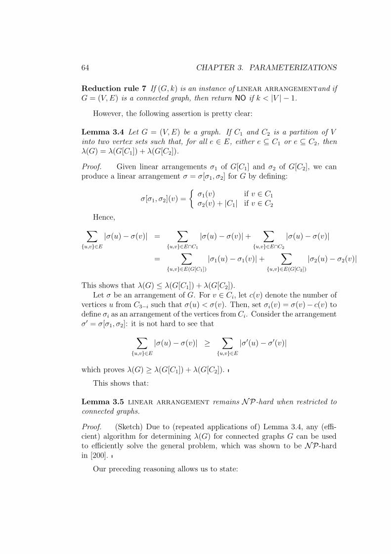
64 CHAPTER 3. PARAMETERIZATIONS
Reduction rule 7 If (G, k) is an instance of linear arrangementand ifG = (V,E) is a connected graph, then return NO if k < |V | − 1.
However, the following assertion is pretty clear:
Lemma 3.4 Let G = (V,E) be a graph. If C1 and C2 is a partition of Vinto two vertex sets such that, for all e ∈ E, either e ⊆ C1 or e ⊆ C2, thenλ(G) = λ(G[C1]) + λ(G[C2]).
Proof. Given linear arrangements σ1 of G[C1] and σ2 of G[C2], we canproduce a linear arrangement σ = σ[σ1, σ2] for G by defining:
σ[σ1, σ2](v) =
σ1(v) if v ∈ C1
σ2(v) + |C1| if v ∈ C2
Hence,
∑
u,v∈E|σ(u) − σ(v)| =
∑
u,v∈E∩C1
|σ(u) − σ(v)| +∑
u,v∈E∩C2
|σ(u) − σ(v)|
=∑
u,v∈E(G[C1])
|σ1(u) − σ1(v)| +∑
u,v∈E(G[C2])
|σ2(u) − σ2(v)|
This shows that λ(G) ≤ λ(G[C1]) + λ(G[C2]).Let σ be an arrangement of G. For v ∈ Ci, let c(v) denote the number of
vertices u from C3−i such that σ(u) < σ(v). Then, set σi(v) = σ(v)− c(v) todefine σi as an arrangement of the vertices from Ci. Consider the arrangementσ′ = σ[σ1, σ2]: it is not hard to see that
∑
u,v∈E|σ(u) − σ(v)| ≥
∑
u,v∈E|σ′(u) − σ′(v)|
which proves λ(G) ≥ λ(G[C1]) + λ(G[C2]).
This shows that:
Lemma 3.5 linear arrangement remains NP-hard when restricted toconnected graphs.
Proof. (Sketch) Due to (repeated applications of) Lemma 3.4, any (effi-cient) algorithm for determining λ(G) for connected graphs G can be usedto efficiently solve the general problem, which was shown to be NP-hardin [200].
Our preceding reasoning allows us to state:

3.2. STANDARD PARAMETERS 65
Theorem 3.6 linear arrangement, restricted to connected graphs, isNP-complete but belongs to FPT .
Proof. We already argued for the NP-hardness. Membership in NPis of course trivially inherited from LA. Membership in FPT can be seenas follows: after applying rule 7, we will have an instance ((V,E), k) with|V | ≤ k + 1 (unless already solved). Hence, that rule is a kernelization rule,so that Theorem 2.4 applies.
We mention this restricted problem here, since it is a problem where onecan actually argue that the standard parameterization is not very natural:the reduction rule we employed is simply answering that there cannot be anysolution if the parameter size is small (related to the number of vertices in thegraph). So, small parameter values do not exist. This is a bit different in thegeneral setting of linear arrangement which is treated in more details inChap. 4. However, the basic criticism regarding the standard parameteriza-tion is valid there, as well, since it is based on the following proposition andan according reduction rule that generalize Prop. 3.3. Put in another way:due to the lower bounds expressed in the propositions, it might make moresense to consider a parameterization via the number of vertices or by thenumber of edges instead of taking the entity to be minimized as the parame-ter. However, this kind of parameterization would generally be not regardedas belonging to the realm of parameterized algorithmics, but rather to exactalgorithmics (for hard problems) in a broader sense, see Chap. 10.
Proposition 3.7 If G = (V,E) is a graph, then λ(G) ≥ |E|.
Proof. According to the formula how to compute the linear arrangementcost, each edge contributes at least a cost of one, since the mapping σ thatassociates vertices and natural numbers is one-to-one and the graphs weconsider have no loops.
Reduction rule 8 If (G, k) is an instance of linear arrangement, thenreturn NO if k < |E|.
Other lower bounds on the size of the linear arrangement number of agraph are discussed in [321] from a very practical perspective. Other (theo-retical) bounds are obtained in [5, 277]. In [321], it is also mentioned thatlinear arrangement is only known to be approximable within a logarith-mic factor (and even that algorithm is pretty impractical for sufficiently largegraph instances, since it involves solving a linear program with an exponentialnumber of variables), although the related problem of crossing minimization
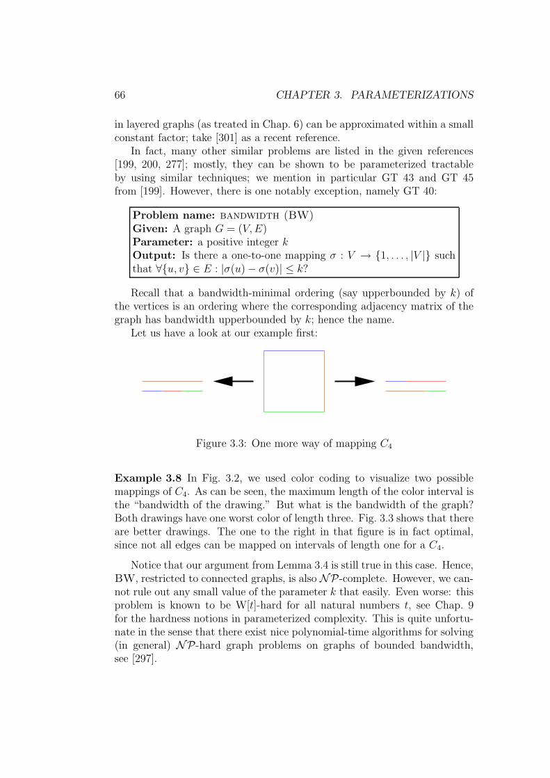
66 CHAPTER 3. PARAMETERIZATIONS
in layered graphs (as treated in Chap. 6) can be approximated within a smallconstant factor; take [301] as a recent reference.
In fact, many other similar problems are listed in the given references[199, 200, 277]; mostly, they can be shown to be parameterized tractableby using similar techniques; we mention in particular GT 43 and GT 45from [199]. However, there is one notably exception, namely GT 40:
Problem name: bandwidth (BW)Given: A graph G = (V,E)Parameter: a positive integer kOutput: Is there a one-to-one mapping σ : V → 1, . . . , |V | suchthat ∀u, v ∈ E : |σ(u) − σ(v)| ≤ k?
Recall that a bandwidth-minimal ordering (say upperbounded by k) ofthe vertices is an ordering where the corresponding adjacency matrix of thegraph has bandwidth upperbounded by k; hence the name.
Let us have a look at our example first:
Figure 3.3: One more way of mapping C4
Example 3.8 In Fig. 3.2, we used color coding to visualize two possiblemappings of C4. As can be seen, the maximum length of the color interval isthe “bandwidth of the drawing.” But what is the bandwidth of the graph?Both drawings have one worst color of length three. Fig. 3.3 shows that thereare better drawings. The one to the right in that figure is in fact optimal,since not all edges can be mapped on intervals of length one for a C4.
Notice that our argument from Lemma 3.4 is still true in this case. Hence,BW, restricted to connected graphs, is also NP-complete. However, we can-not rule out any small value of the parameter k that easily. Even worse: thisproblem is known to be W[t]-hard for all natural numbers t, see Chap. 9for the hardness notions in parameterized complexity. This is quite unfortu-nate in the sense that there exist nice polynomial-time algorithms for solving(in general) NP-hard graph problems on graphs of bounded bandwidth,see [297].

3.2. STANDARD PARAMETERS 67
The similarity between linear arrangement and bandwidth canbe best seen if one considers the following generalization, based on a givenvector norm ‖ · ‖ on vectors of numbers; to this end, we extend a mappingσ : V → 1, . . . , |V | to a mapping σE : E → 0, . . . , |V | − 1 by settingσE(u, v) = |σ(u)−σ(v)|. If we now assume an arbitrary but fixed orderingof the edges, i.e., E = e1, . . . , em, then we can associate to σ a vector, alsowritten σE for brevity, defined as:
σE = (σE(e1), . . . , σE(em)).
Problem name: linear arrangement (generalized to avector norm ‖ · ‖)Given: A graph G = (V,E), E = e1, . . . , emParameter: a positive integer kOutput: Is there a one-to-one mapping σ : V → 1, . . . , |V | suchthat ‖ σE ‖≤ k?
Observe that both linear arrangement and bandwidth are specialcases by choosing ‖ · ‖ to be the sum norm ‖ · ‖1 and the maximum norm‖ · ‖∞, respectively. What about the usual “intermediate norms” ‖ · ‖p fornatural numbers 1 < p <∞? Recall that
‖ (x1, . . . , xn) ‖p= p
√√√√p∑
i=1
|xi|p.
These problems are also known as minimum p-sum problems.To continue with our example, let us focus on p = 2:
Example 3.9 The arrangement on the left-hand side of Fig. 3.2 yields a2-sum of √
12 + 12 + 12 + 32 =√
12.
On the right-hand side of that figure, the arrangement has a 2-sum of
√22 + 12 + 22 + 32 =
√18.
The arrangement on the right-hand side of Fig. 3.3 however has a 2-sum of
√22 + 12 + 22 + 12 =
√10.
The reader might wish to see if there are arrangements with smaller 2-sumnumbers.

68 CHAPTER 3. PARAMETERIZATIONS
For the corresponding linear arrangement numbers λp, the following gen-eralizations of earlier results are easy to obtain:
Proposition 3.10 If G = (V,E) is a graph, then λp(G) ≥ p√
|E|.
Reduction rule 9 If (G, k) is an instance of linear arrangement (gen-eralized to a vector norm ‖ · ‖p), then return NO if k < p
√|E|.
Hence, we can state the following result:
Theorem 3.11 For each fixed natural number p, the generalized lineararrangement problem (based on norm ‖ · ‖p), lies in FPT .
Proof. Reduction rule 9 provides a kernel of size |k|p for the generalizedproblem, which is showing FPT -membership when p is assumed to be afixed constant; here, the problem size is measured in terms of the number ofedges of the input graph.
Remark 3.12 According to [239], the (classical) complexity status of thegeneralized linear arrangement problem (in actual fact, this is a familyof problems indexed by p) is open if p /∈ 1,∞.
However, for a different set of problems (namely scheduling problems), thequestion of finding approximation algorithms that are good with respect todifferent norms has been recently addressed in [31], so that a closer scrutinyto this type of problem is not too artificial, keeping in mind that for practicalpurposes different metrics might indeed exhibit different behaviors.
Some of the problems (for p /∈ 1,∞) were addressed in [51, 249, 277].From a parameterized perspective, it would make also sense to consider thenatural number p as part of the input; the proof of Theorem 3.11 only workswhen p is not part of the input. Hence, the parameterized status of thisproblem is open. Of course, if p = ∞ is also allowed as input, then it isclear that such a problem would be at least as hard as bandwidth, so thatmembership in FPT would be very unlikely.
Two further generalizations (motivated from practical applications) arementioned in [5, 277]:
• Edges could be given integer weights ≥ 1 to model the possibility ofmultiple connections between points or of different flow capacities.
• Instead of edges, hyperedges could be considered. Given an arrange-ment σ, the cost of drawing a hyperedge h would then be measuredas
σE(h) = maxx∈h
σ(x) − miny∈h
σ(y).

3.2. STANDARD PARAMETERS 69
The cost of a drawing (generalizing the LA problem) would then be
∑
h∈EσE(h)
for a given hypergraph G = (V,E) where, for all h ∈ E, |h| ≥ 2,since smaller hyperedges can be removed from a given instance with-out changing the parameter (in other words, we have found a reductionrule). As can be easily seen, all kernelization results stated above trans-fer to this case, as well.
We can therefore conclude:
Corollary 3.13 linear arrangement, generalized to the (integer-)weightedcase or to the case allowing hyperedges (also in combination), lends to prob-lems in FPT , even if we generalize the allowed vector norms as in Thm. 3.11.
Let us describe one of the practical motivations to consider generalizationsof linear arrangement a bit more in detail, since this also gives a goodexample how to derive graph-theoretical formalizations from problems thatwere originally not stemming from graph theory itself.
Example 3.14 Consider the following placement problem occurring in VLSI,inspired from [277]: we are given a set of modules and a wiring prescriptiontelling us which modules are to be connected; this information can even comeas a kind of wiring proposal, see Fig. 3.4. In that picture, the modules aredrawn as boxes labeled A through E. The wires are drawn as straight-linesegments. For better readability of the further solutions, they have differentcolors. The connection points are drawn as filled circles. The question is ifthe proposed arrangement of modules is best. In other words, is it possibleto reorder the modules to improve the arrangent given in the proposal?
What is our criterion of optimality? It could be at least three things:
1. The total wire length should be minimal.
Such an optimality might help save fabrication costs. Moreover, keepin mind that long wires mean long run times of signals on these wires.
2. The wire length between any two points connected by a wire should beminimal.
The overall run-time behavior of a manufactured chip is determined byits weakest spot, i.e., the length of the longest point-to-point intercon-nection.

70 CHAPTER 3. PARAMETERIZATIONS
1 2 3 4 5 6 7
B
C
D
E
A
Figure 3.4: A wiring proposal for some modules
3. Observe that we used one column for each wire in Fig. 3.4. From theviewpoint of fabrication, it would be however desirable to use as few ofthese columns (usually called tracks in these context) as possible.
How do these VLSI problems relate to the graph problems we consideredso far? Let us see this with the first of the mentioned problems, that can beformalized as follows:
Problem name: module placement problem (MPP)Given: a set of modules M , a set of wires W connecting modules,i.e., each wire w ∈ W is a subset of MParameter: a positive integer kOutput: Is it possible to find a mapping σ : M → 1, . . . , |M | suchthat the overall wire length is less than or equal to k?
If we measure the overall length of the wires by∑
w∈W(maxx∈w
σ(x) − miny∈w
σ(y)),
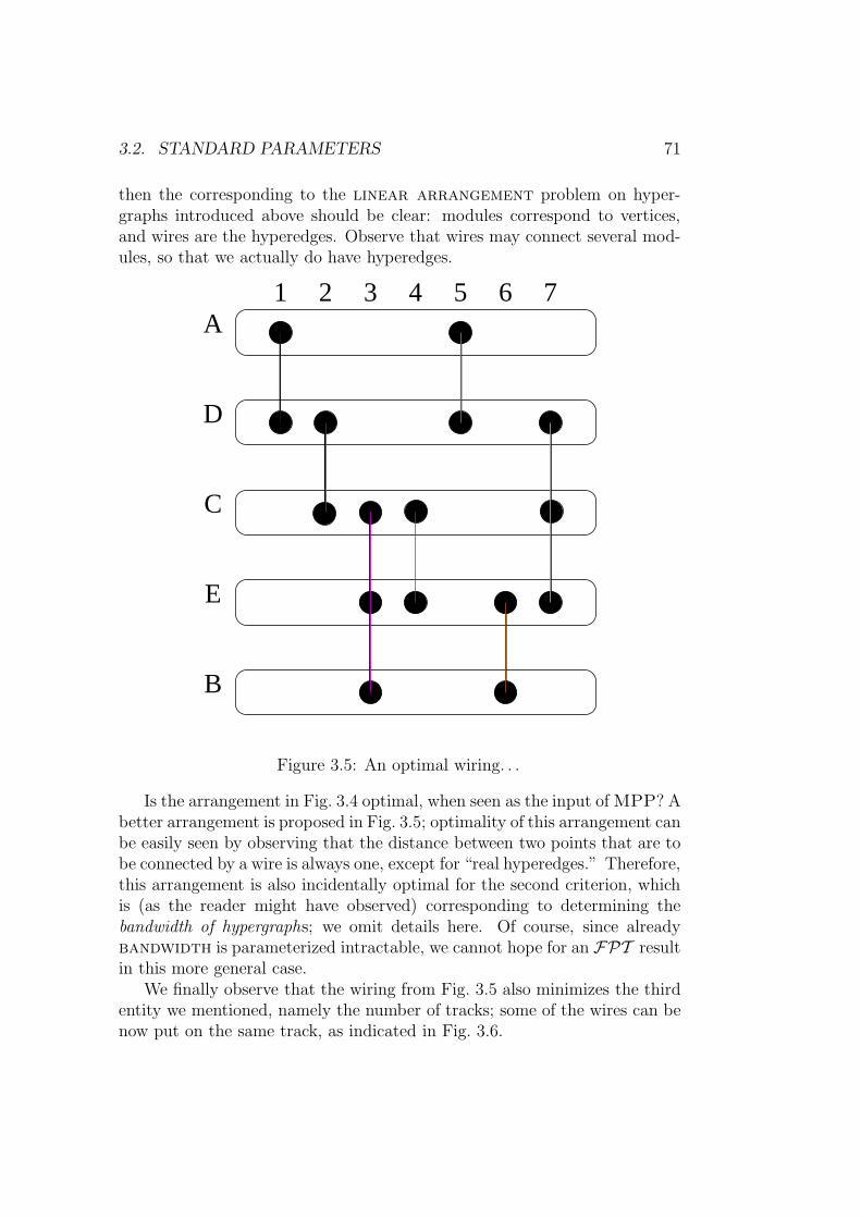
3.2. STANDARD PARAMETERS 71
then the corresponding to the linear arrangement problem on hyper-graphs introduced above should be clear: modules correspond to vertices,and wires are the hyperedges. Observe that wires may connect several mod-ules, so that we actually do have hyperedges.
1 2 3 4 5 6 7
E
B
A
D
C
Figure 3.5: An optimal wiring. . .
Is the arrangement in Fig. 3.4 optimal, when seen as the input of MPP? Abetter arrangement is proposed in Fig. 3.5; optimality of this arrangement canbe easily seen by observing that the distance between two points that are tobe connected by a wire is always one, except for “real hyperedges.” Therefore,this arrangement is also incidentally optimal for the second criterion, whichis (as the reader might have observed) corresponding to determining thebandwidth of hypergraphs; we omit details here. Of course, since alreadybandwidth is parameterized intractable, we cannot hope for an FPT resultin this more general case.
We finally observe that the wiring from Fig. 3.5 also minimizes the thirdentity we mentioned, namely the number of tracks; some of the wires can benow put on the same track, as indicated in Fig. 3.6.
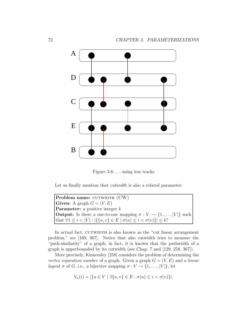
72 CHAPTER 3. PARAMETERIZATIONS
E
B
A
D
C
Figure 3.6: . . . using less tracks
Let us finally mention that cutwidth is also a related parameter:
Problem name: cutwidth (CW)Given: A graph G = (V,E)Parameter: a positive integer kOutput: Is there a one-to-one mapping σ : V → 1, . . . , |V | suchthat ∀1 ≤ i < |V | : |u, v ∈ E | σ(u) ≤ i < σ(v)| ≤ k?
In actual fact, cutwidth is also known as the “cut linear arrangementproblem,” see [169, 367]. Notice that also cutwidth tries to measure the“path-similarity” of a graph; in fact, it is known that the pathwidth of agraph is upperbounded by its cutwidth (see Chap. 7 and [129, 258, 367]).
More precisely, Kinnersley [258] considers the problem of determining thevertex separation number of a graph. Given a graph G = (V,E) and a linearlayout σ of G, i.e., a bijective mapping σ : V → 1, . . . , |V |, let
Vσ(i) = |u ∈ V | ∃u, v ∈ E : σ(u) ≤ i < σ(v)|.

3.2. STANDARD PARAMETERS 73
The vertex separation number of the linear layout σ of G is then
vsσ(G) = max1≤i<|V |
Vσ(i),
and the vertex separation number of G is
vs(G) = minvsσ(G) | σ is a linear layout of G.
Kinnersley has shown that the vertex separation number of a graph equalsits pathwidth (as defined in Chap. 7). Conversely, the cutwidth of a graphG = (V,E) could be described as follows: Let
Eσ(i) = |u, v ∈ E | σ(u) ≤ i < σ(v)|.
Then definecwσ(G) = max
1≤i<|V |Eσ(i),
and the cutwidth of G is
cw(G) = mincwσ(G) | σ is a linear layout of G.
Since for all layouts and all positions
Vσ(i) ≤ Eσ(i),
vs(G) ≤ cw(G)
follows.With the standard parameterization, the cutwidth problem is known
to be in FPT , see [134, 169].Let us have a look at some examples to better understand these concepts:
Example 3.15 In Fig. 3.3, we used color coding to visualize two possiblemappings of C4. For better readability, the intervals that correspond to edgesare drawn in different “bands.” As can be seen, the number of necessarybands for such drawings is just the cutwidth of the layout, which happensto be the same in both cases. Both are in fact optimal arrangements withrespect to cutwidth.
Incidentally, also the vertex separation number of both layouts is two.
Example 3.16 Consider the family of star graphs Sn with vertices 1, . . . , nand edges 1, i for i = 2, . . . , n. Imagine 1 to be drawn in the center and ifor i 6= 1 being the rays of the star.
74 CHAPTER 3. PARAMETERIZATIONS
The identity then provides a layout with vertex separation number one.However, the cutwidth of that layout is n−1. A better layout (with respect tocutwidth) can be produced by mapping 1 in the center of the image, placinghalf of the ray vertices to the left and the other one (arbitrarily) to the rightof the center vertex; the cutwidth of this layout (which is now equal to thevertex separation number of the layout) is then bn/2c. This also gives theoptimal arrangement for star graphs when considering them as inputs forlinear arrangement, see [277, Cor. 2.4].
Let us briefly re-examine Ex. 3.14 from the point of view of cutwidth;at first glance, it might appear that the third mentioned goal in the moduleplacement scenario would correspond to something like cutwidth in hy-pergraphs. However, if this were the case, then the second and third tracks(where the wires actually only have two connection points each, so that theyactually correspond to edges) in Fig. 3.6 could be merged; this is not the case(for easily seen physical reasons). Hence, we would have as optimization goalto minimize (in the formulation of module placement problem):
max1≤i≤|M |
|w ∈ W | minm∈w
σ(m) ≤ i ≤ maxm∈w
σ(m)|.
3.3 Alternative parameterizations
As we have seen above, the standard parameterization is not the only wayto parameterize problem, even though they might be given as optimizationproblems; it is clear that decicision problems that don’t correspond to or stemfrom optimization problems have no standard parameterization, so that theideas we present here will apply in that scenario, as well.
Let us first discuss one of our favourite problems, again: vertex cover.Mohar [294] had shown that k-vertex cover restricted to (planar)graphs of maximum degree three is NP-hard. This result is as closeas NP-hardness could go with respect to the degree bound: for graphs ofmaximum degree two, the problem becomes easily solvable.4
In [220], another idea of parameterization is advocated which they calleddistance from triviality. In this context, the number ` of vertices of degreethree or more could be such a distance measure. If this parameter is small,testing all 2` possible assignments of 0 and 1 to the vertices of degree threeor more (interpreted as “not going into the cover” or “going into the cover”)would allow solving the minimum vertex cover problem in time O(2`|G|)for each graph G with at most ` vertices of degree three or more. Morespecifically, this shows FPT -membership of the following problem:
4Even the more general problem edge cover is solvable in polynomial time, see [311].
3.3. ALTERNATIVE PARAMETERIZATIONS 75
Problem name: vertex cover, parameterized by numberof vertices of degree three or larger (VCdeg)Given: A graph G = (V,E)Parameter: a positive integer ` that equals the number of verticesin G of degree three or largerOutput: What is the size of a minimum vertex cover C ⊆ V ?
As another example from the literature (that can be seen as a reparam-eterization of set cover and hence of hitting set) we quote [344], wheretriviality is measured in terms of the so-called (almost) consecutive onesproperty. Observe that the referenced paper does not explicitly mention pa-rameterized complexity in any way, yet the results can be interpreted thisway.
As seen in the previous section (and also in Chap. 4), linear arrange-ment and dominating set of queens can be viewed as problems that havetrivial kernels if viewed from the perspective of the standard parameteriza-tion. This motivates the idea of parameterizing above guaranteed values: forthe mentioned two problems, this might mean the following:
Problem name: linear arrangement (LA), parameterizedabove guaranteed valueGiven: A graph G = (V,E)Parameter: a positive integer kOutput: Is there a one-to-one mapping σ : V → 1, . . . , |V | suchthat ∑
u,v∈E|σ(u) − σ(v)| ≤ k + |E|?
Problem name: dominating set of queens (QDS), parame-terized above guaranteed valueGiven: An n× n chessboard CParameter: a positive integer kOutput: Is it possible to place n/2 + k queens on C such that allsquares are dominated ?
To our knowledge, the status of the two mentioned re-parameterizationsis currently unknown.
The idea of parameterizing above guaranteed values was actually “born”in the context of maximization problems. More specifically, Mahajan andRaman [285] showed that the following two problems are parameterizedtractable by (again) a kind of mathematical “cheating” argument:

76 CHAPTER 3. PARAMETERIZATIONS
Problem name: maximum satisfiability (MAXSAT)Given: A Boolean formula F in conjunctive normal form (CNF),with variables XParameter: a positive integer kOutput: Is there an assignment α : X → 0, 1 such that at least kclauses in F evaluate to 1 (true) under α?
and
Problem name: maximum cut (MAXCUT)Given: A graph G = (V,E)Parameter: a positive integer kOutput: Is there a cut set C ⊆ E with |C| ≥ k, i.e., (V, V \ C) is abipartite graph?
Namely, the following reduction rule is easily seen to be sound for MAXSAT:
Reduction rule 10 Let F be a CNF formula containing m = |F | clauses,over the set of variables X. If k < m/2, then YES.
Why? Simply pick an arbitrary assignment α. If α evaluates more thanhalf of the formulae to be true, then the YES of the reduction rule is justifiedby α. Otherwise, consider the assignment α that assigns α(x) = 1 − α(x),i.e., always the opposite of what α assigns. Then, exactly those clauses thatused to be unsatisfied via α are now satisfied with respect to α. Hence, therule is justified in this case, as well.
So, we can trivially conclude:
Corollary 3.17 maximum satisfiability has a problem kernel of size 2k(where the problem size is measured in the number of clauses).
Due to the trivial nature of this “reduction,” Mahajan and Raman sug-gested parameterizing above guaranteed values, that is, in this case, theystudied the following problem variant:
Problem name: maximum satisfiability (MAXSAT), param-eterized above guaranteed valueGiven: A Boolean formula F in conjunctive normal form (CNF),with variables XParameter: a positive integer kOutput: Is there an assignment α : X → 0, 1 such that at leastm/2 + k clauses in F evaluate to 1 (true) under α?
3.3. ALTERNATIVE PARAMETERIZATIONS 77
Mahajan and Raman showed that also this modified problem is fixed-parameter tractable; in fact, their algorithms (in final form based on search-trees and not merely on kernelization) were later improved in [212]. It isworthwhile mentioning that J. Gramm et al. also considered different pa-rameterizations (for restricted problems like maximum satisfiability onformulae whose clauses all contain at most two literals), namely a param-eterization by the number of clauses (or also the number of clauses thatcontain exactly two literals); however, this could be also considered as beinga treatment within the nonparameterized setting, see Chap. 10.
For maximum cut, Mahajan and Raman gave a similar argument forproving the soundness of the following reduction rule:
Reduction rule 11 Let G be a graph containing m = |E| edges. If k <m/2, then YES.
Corollary 3.18 maximum cut has a problem kernel of size 2k (measuredin terms of number of edges).
Again, the question of parameterizing above guaranteed values was dis-cussed, and the following problem was placed into FPT :
Problem name: maximum cut (MAXCUT), parameterizedabove guaranteed valueGiven: A graph G = (V,E)Parameter: a positive integer kOutput: Is there a cut set C ⊆ E with |C| ≥ |E|/2+k, i.e., (V, V \C)is a bipartite graph?
These questions are more recently discussed in [323, 322].A further example of parameterizing above guaranteed values (nonblocker
set) will be discussed in Chap. 4.We already discussed different parameterizations of optimization prob-
lems in the preceding section and will return to the topic in the context ofdual parameterizations below.
One might finally ask how one can actually obtain a “good” parameteri-zation for a given problem? From a practical perspective, when facing a con-crete problem, it is surely worthwhile analysing which part of the input canbe usually considered as small. Observe that this can be very application-dependent, even for the seemingly identical problem. From a theoreticalstandpoint, bear in mind that anything may serve as a parameter. Of par-ticular interest might be parameters that are hidden in the structure of theproblem instance. What this could mean, we will discuss for graph problems

78 CHAPTER 3. PARAMETERIZATIONS
in Chap. 7. However, all good intentions for choosing a parameter mightalso fail if the problem (under the chosen parameterizations) turns out to beparameterized intractable. This possibility is not stressed in this Habilita-tionsschrift, but it should be kept in mind if trials to find fixed-parameteralgorithms fail.
From a philosophical point of view, we might quote Gomes [208], whowrote:
The ability to capture and exploit problem structure is of centralimportance, a way of taming computational complexity.
Our tool of taming, i.e., our whip, is the choice of a good parameter. Thequality of this choice is highly dependent on our understanding of the prob-lem. Conversely, if a particular choice of a parameter turned out to work verywell or very bad, this could also add to our understanding of the structureof the problem at hand. As a guideline for choosing a good parameter, letus once more stress the idea of distance from triviality; in fact, this has beenused in various areas without explicit notice of the connection with param-eterized algorithmics, partly because the methodologies we mention now domuch predate the advent of parameterized algorithmics.
In her recommendable survey, Gomes [208] compares the methodologiesemployed by the Operations Research (OR) and Artificial Intelligence (AI)communities for solving computationally hard problems. She mentions threemain veins to find tractable (sub-)instance of a problem, where tractabilityrefers to polynomial-time computability:
• Linear Programming,
• Network Flow, and
• Horn clause formulations.
What happens, for example, if an OR problem cannot be “completelysolved” with linear programming techniques due to additional integralityconstraints? Usually, one first ignores these integrality constraints. If theso-called relaxation gives an optimal solution that already complies with theintegrality constraints, the problem is solved. If not, then if the number ofvariables that do not comply with the integrality constraints is small, usuallya search tree is started, where in each node of the search tree new LinearPrograms are solved by fixing one of the variables with non-integer solutionsby rounding the non-integer solutions either up or down (two cases, i.e., twochildren per internal node of the search tree). If the integrality constraintsare not just leaving the choices 0 and 1 (as it is often the case), this idea

3.4. MULTIPLE PARAMETERS 79
more generally leads to the cutting planes approach, where, e.g., a solutionwith xi = 3.5 is excluded by introducing the constraints xi ≤ 3 and xi ≥ 4 inthe two branches. From the point of view of parameterized complexity, thisapproach can be seen as a practical implementation of the idea of parame-terizing by the distance from triviality, especially, if the choices of a variableare just 0 and 1, since then the described branching actually decrements theparameter value in each branch. We are not aware of similar approaches inthe other two cases, although it seems to be that here is a largely unexploredbut promising area of research for people working in parameterized algorith-mics. An illuminating worked-out example comparing different approachesto solve a particular problem both by OR and by AI methods can be foundin [236].
3.4 Multiple parameters
Sometimes, not only one parameter appears to be natural, but it seems to bereasonable to consider multiple parameters, i.e., several parameters that arethought of being “the” parameter at the same time. Abstractly, this posesno problems at all, since a parameter list 〈k1, . . . , k`〉 can be also read asencoding a single (number) parameter.
We shall see, in what follows, a couple of examples showing that multipleparameters do show up in many applications and are hence nothing oneshould consider to be artificial.
Let us start with examples stemming from VLSI manufacturing. Kuoand Fuchs [267] provide a fundamental study of the spare allocation problem.Put concisely, this “most widely used approach to reconfigurable VLSI” usesspare rows and columns to tolerate failures in rectangular arrays of identicalcomputational elements, which may be as simple as memory cells or as com-plex as processor units (see [267] for details). If a faulty cell is detected, theentire row or column is replaced by a spare one.
This problem can be formally formulated as follows:
Problem name: spare allocation (SAP)Given: A n × m binary matrix A representing an erroneous chipwith A[r, c] = 1 iff the chip is faulty at position [r, c]Parameter: positive integers k1, k2
Output: Is there a reconfiguration strategy that repairs all faults anduses at most k1 spare rows and at most k2 spare columns?
With reconfiguration strategy, we mean a prescription which rows andcolumns from A have to be replaced by spares.

80 CHAPTER 3. PARAMETERIZATIONS
1 2 3 4 5 6 7 8 91 ? ? ?23 ?4 ? ? ?567 ? ?
4
7
3 3
4
7
9
1 1
Figure 3.7: A 7 × 9 array with faults “?” and the bipartite graph model
By considering A as the bipartite adjacency matrix of a graph, spareallocation can be easily seen to be parameterized interreducible with thefollowing problem:
Problem name: constraint bipartite vertex cover(CBVC)Given: A bipartite graph G = (V1, V2, E)Parameter: positive integers k1, k2
Output: Is there a vertex cover C ⊆ V1 ∪ V2 with |C ∩ Vi| ≤ ki fori = 1, 2?
Consider the following example of a reconfigurable array of size 7×9 with2 spare rows and 3 spare columns in Fig. 3.7, where faulty cells are markedwith a “?”, together with its corresponding bipartite graph, where, e.g., anedge between 3 and 1 indicates the faulty cell in row 3 and column 1. Herein,we omit isolated vertices.5 Obviously, the array is repairable using one sparerow (replacing row 4) and 3 spare columns (replacing columns 1, 4, 9). Thiscorresponds to a solution of the CBVC problem with k1 = 1 and k2 = 3, asone can easily see. This also reflects the reduction mentioned above.
Typical examples in [267] are arrays with up to 1024 rows and 1024columns (nowadays possibly even more) and with up to 20 additional sparerows and columns each time (cf. their Table 1), making this problem a nat-ural candidate for a fixed parameter approach, Kuo and Fuchs obtained thefollowing results. First, they showed NP-completeness for constraint bi-partite vertex cover by reducing clique to it. Then they present two
5Alternatively, this can be seen as a reduction rule.

3.4. MULTIPLE PARAMETERS 81
heuristic algorithms, first a branch-and-bound approach which always deliv-ers optimal results, but is only “efficient for arrays with a moderate numberof faulty cells” [267, page 29]. The second one is a polynomial time approx-imation algorithm. By way of contrast, our FPT -approach always deliversoptimal results. Furthermore, its complexity basically depends on the num-ber of available spare rows and columns. More details will be given in laterchapters.
It should be noted here that people developing algorithms for VLSI designactually discovered the FPT concept in the analysis of their algorithms,coming up with O(2k1+k2k1k2 + (k1 + k2)|G|) algorithms in [222, 278]. Theyobserved that “if k1 and k2 are small, for instance O(log(|G|)), then thismay be adequate.” [222, p. 157]. It was in the context of this problem thatEvans [158] basically discovered Buss’ rule to prove a problem kernel forconstraint bipartite vertex cover. Kuo and Fuchs called this stepquite illustratively the “must-repair-analysis.” The reader is encouraged toformulate the necessary reduction rules to prove the following assertion:
Lemma 3.19 constraint bipartite vertex cover has a problem ker-nel of size 2k1k2.
constraint bipartite vertex cover (in the disguise of spare allo-cation) has important applications especially in the fabrication of high-endVLSI chips: With increasing integration in chip technology, a fault-free chipfabrication can no longer be assumed. So, fault-tolerance has to be taken intoconsideration within the very fabrication process to obtain reasonable pro-duction yields [1, 78]. These ideas are already quite old, see [348] for an earlytreatment of the topic, but have continued to persist into the most recentdevelopments in VLSI technology. Interestingly, the most challenging (partsof) high-end processors are the seemingly simplest of all possible VLSI chips,namely memories due to their rapidly expanding needs; moreover, e.g., theyaccount for approximately 44% of transistors of the UltraSparc processor, sothat they are used as technology and yield drivers [271, 384]. One commonsolution to increase yield in memory fabrication is to supply a few sparerows and columns to each memory array. These can be used in an internal(on-chip) or external reconfiguration phase (using lasers to “program” fuses)where faulty array rows or columns are replaced by spare ones, cf. some re-ports on DEC Alpha and UltraSparc processor manufacturing [46, 271, 384].
As pointed out in, e.g., [222], there are several points due to which theproblem formulated above is not a completely adequate model:
1. In the manufacturing process, the cost of repairing a chip by usingvertical movements of the repair laser may be different from that of

82 CHAPTER 3. PARAMETERIZATIONS
Figure 3.8: Sharing repair resources
horizontal movements. This leads to a sort of weighted variant of con-straint bipartite vertex cover. The according (pair of standard)parameters would then be budgets for the costs of vertical and hori-zontal laser movements, again denoted k1 and k2.
2. As indicated in Fig. 3.8, a huge memory chip may be split into smallerblocks, each of them possibly having its own spare rows and columns.For reasons of economy, other designs are preferred in this case, e.g.,each spare row depicted inbetween two memory blocks can be individ-ually used to reconfigure either the block above or the block below it.In other words, in such complex designs, spares may be shared spares.These can be seen in Fig. 3.8 schematically drawn inbetween differentblocks. Moreover, there may be spare rows or columns which are linkedspares, which means that such a spare can only be used to reconfigureone certain row or column in several blocks. (Linked spares are notshown in the Figure.) Usually, linked spares are not shared, althoughthis could be the case, as well. Obviously, the idea is here to reducethe costs of chip repair.
This more general scenario introduces a further natural third parame-ter: the number k3 of blocks of the array. The parameters k1 and k2
should then be understood as the available resources per block. Thisallows us to formulate constraint bipartite vertex cover with

3.4. MULTIPLE PARAMETERS 83
shared spares.
Finally, we could create the problem constraint bipartite vertexcover with shared spares and links with five natural parame-ters, incorporating furthermore the numbers k4 and k5 that upperboundthe linked spare rows and the linked spare columns, resp., on the wholeboard.
This example should have made clear that it is quite imaginable that awhole lot of parameters show up in a “real problem” in a fairly natural way.Observe that the basic assumptions concerning parameter values being smallin practice is pretty clear in this example, as well, for all five parameters.
Further examples for multi-parameter problems can be found in manyapplication areas. Let us now turn to a more abstract view on this topic.
Typical examples are also delivered by bicriteria problems.6 For example,the following problem that generalizes the usual vertex cover problem istackled in [234] from the viewpoint of approximation:
Problem name: t-vertex cover (tVC)Given: A graph G = (V,E)Parameter: positive integers k and tOutput: Is there a t-vertex cover C ⊆ V with |C| ≤ k, i.e., |e ∈E | C ∩ e 6= ∅| = |E| − |E(G[V \ C])| ≥ t?
Of course, choosing t = |E| yields the usual VC problem, where t is thenot considered as a parameter. However, although the approximability oftVC is as good as the one of VC, its parameterized complexity status isopen (to our knowledge). Observe that this problem is related to profitvertex cover discussed above, since the profit is the difference of the gain(lowerbounded by t) and the cost (upperbounded by k) of the cover. Fur-thermore, notice that t-vertex cover is also naturally related to vertexcover from the point of view of the integer linear program (ILP) related tovertex coverwhich is
minn∑
i=1
xi
subject to
xi + xj ≤ 1, for all vivj ∈ E
6Such problems are also sometimes called MAX-MIN problems, see [42].

84 CHAPTER 3. PARAMETERIZATIONS
where xi ∈ 0, 1 is the integrality condition. When we ignore the inte-grality condition, we arrive at a linear program. The corresponding dualmaximization problem would be
maxm∑
j=1
yj
subject to ∑
e incident with v
y(e) ≥ 1 for all v ∈ V,
where y(e) is the variable y that corresponds to edge e. So, k and t boundthe primal and the dual entity to be optimized in a rather natural fashion.This also shows a general technique how to obtain two-parameter versionsout of problems that can be formulated as ILP. A similar technique (how toobtain alternative parameterizations by ILP dualization) has been discussedabove.
Further rather natural examples from graph theory also concern hittingset: namely, as we will see, for each d, d-hitting set is fixed-parametertractable (parameterized by the standard parameter). But, if we consider d tobe a parameter, as well, this statement can be extended to this two-parameterversion of hitting set, giving a more uniform view on this problem. Thisis discussed more deeply with a related problem motivated from networks inSec. 6.2.2.
3.5 Dual parameters
To formally specify what we mean by the dual of a parameterized problem,we explicitly need a proper notion of a size function.
Definition 3.20 (Size function) A mapping size : Σ∗ ×N → N is called asize function
• if 0 ≤ k ≤ size(I, k),7
• if size(I, k) ≤ |I| (where |I| denotes the length of the string I) and
• if size(I, k) = size(I, k′) for all appropriate k, k′ (independence).
7We deliberately ignore instances with k > size(I, k) in this way, assuming that theirsolution is trivial. Moreover, it is hard to come up with a reasonable notion of “duality”if larger parameters are to be considered.

3.5. DUAL PARAMETERS 85
“Natural size functions” (in graphs, for example, these are entities as the“number of vertices” or the “number of edges”) are independent. We canthen also write size(I).8
For clarity, we denote a problem P together with its size function sizeas (P, size). To the dual problem Pd then corresponds the language of YES-instances L(Pd) = (I, size(I) − k) | (I, k) ∈ L(P). The dual of the dual ofa problem with size function is again the original problem. Sometimes, wewill call P the primal problem (distinguishing it from Pd). Then, k is theprimal parameter and kd is the dual parameter.
Let us discuss a couple of examples to explain these notions.
Example 3.21 We first return to d-hitting set. The special case d = 2 isknown as VC in undirected graphs. Let L(d − HS) denote the language ofYES-instances of d-hitting set. Taking as size function size(G) = |V (G)|,it is clear that the dual problem obeys (G, kd) ∈ L(d − HSd) iff G has anindependent set of cardinality kd.
More precisely, if C is a hitting set of size at most |V |−kd in G = (V,E),then V \C has at least kd many vertices and is independent, i.e., for all edgese ∈ E, |(V \ C) ∩ e| < |e|.
Example 3.22 In Sec. 2.2, we discussed clique together with some vari-ants.
• When taking the size function size(G) = |V (G)|, clique and ver-tex clique complement cover become parameterized duals ofeach other.
• When taking the size function size(G) = |E(G)|, clique (edge-induced) and clique complement cover become parameterizedduals of each other.
Example 3.23 Let us turn to dominating set. Taking as size functionsize(G) = |V |, it is clear that the dual problem obeys (G, kd) ∈ L(DSd) iff Ghas a nonblocker set N of cardinality kd, where a set N is a nonblocker setif, for each v ∈ N , we can find a u /∈ N such that u, v ∈ E(G).
So, more precisely, we deal with the following problem:
Problem name: nonblocker set (NB)Given: A graph G = (V,E)Parameter: a positive integer kdOutput: Is there a nonblocker set N ⊆ V with |N | ≥ kd?
8Observe that Chen and Flum [91] are using a less restrictive notion of size functionwhen discussing the parameterized complexity of so-called miniaturized problems.
86 CHAPTER 3. PARAMETERIZATIONS
Example 3.24 A cover problem related to vertex cover is the followingone:
Problem name: feedback vertex set (FVS)Given: A (simple) graph G = (V,E)Parameter: a positive integer kOutput: Is there a feedback vertex set of size at most k, i.e.,
∃F ⊆ V, |F | ≤ k, ∀c ∈ C(G)(F ∩ c 6= ∅)?
Here, C(G) denotes the set of cycles of G, where a cycle is a sequenceof vertices (also interpreted as a set of vertices) v0, v1, . . . , v` such thatvi, v(i+1) mod ` ∈ E for i = 0, . . . , `− 1.
This problem is (again) a vertex selection problem. Hence, we naturallytake size(G) = |V | as the size function. Then, the dual problem can bedescribed as follows.
Problem name: vertex induced forest (ViF)Given: a (simple) graph G = (V,E)Parameter: a positive integer kdOutput: Is there a vertex-induced forest of size at least kd, i.e.,
∃F ⊆ V, |F | ≥ kd, C(G[F ]) = ∅?
In a similar fashion, one can define the problem feedback edge set,where we ask if it is possible to turn a graph into a forest by deleting atmost k edges. Being an edge selection problem, the natural size function isnow size(G) = |E|. The dual problem can be hence called edge inducedforest.
Moreover, notice that both FVS and FES can be seen as graph mod-ification problems: namely, the task is to find a set of vertices (or edges)whose removal makes the graph cycle-free. The complexity status of theseproblems different, however: FVS is known to be in FPT ; only recently,independently two groups of researchers have found O∗(ck) algorithms forFVS for some constant c.9
9J. Gramm and F. Rosamond, independent personal communications; the work aboutwhich we were informed by F. Rosamond will appear in the Proceedings of COCOON2005.

3.5. DUAL PARAMETERS 87
feedback edge set can be solved in polynomial time: finding an edge-induced forest will be done by any spanning forest algorithm. Hence, edgeinduced forest is a trivial problem, as well.
By way of contrast, vertex induced forest is parameterized intractablesee [257], also cf. Chap. 9.
A somewhat related problem is the following one:
Example 3.25 Above, we already discussed the problem maximum cut.There, the task (seen as a maximization problem that is parameterized inthe standard way) is to partition the vertices of a graph G = (V,E) into twosets V1 and V2 so that the number of edges in
v1, v2 ∈ E | vi ∈ Vi for i = 1, 2
is maximized. The natural dual problem (as also discussed in [347]) wouldtherefore be:
Problem name: bipartization, edge variant (BPedge)Given: A graph G = (V,E)Parameter: a positive integer kOutput: Is there a bipartization set C ⊆ E with |C| ≤ k whoseremoval produces a bipartite graph?
Example 3.26 It is known that the following problem is in FPT , see [57] forthe currently best algorithm; the “history” of this problem is best describedin [164].
Problem name: maximum leaf spanning tree (MaxLST)Given: A (simple) graph G = (V,E)Parameter: a positive integer kdOutput: Is there a spanning tree of G with at least kd leaves?
Being a vertex selection problem, the natural size function is the numberof vertices of G, i.e., size(G) = |V |. Hence, the dual problem can be describedas follows.
Problem name: minimum inner node spanning tree(MinINST)Given: A (simple) graph G = (V,E)Parameter: a positive integer kOutput: Is there a spanning tree of G with at most k inner nodes?

88 CHAPTER 3. PARAMETERIZATIONS
In terms of decision problems, the latter problem can be equivalentlyreformulated as follows, when observing that any set of inner nodes of aspanning tree in a graph G forms a connected dominating set of G, and—conversely—any spanning tree of the graph induced by a connected domi-nating set D of G can be transformed into a spanning tree T of G with D asthe set of inner nodes of T :
Problem name: connected dominating set (CDS)Given: A graph G = (V,E)Parameter: a positive integer kOutput: Is there a connected dominating set D ⊆ V with |D| ≤ k,i.e., D is both a connected set and a dominating set?
Without the observations of the preceding paragraph, it is not imme-diately apparent that maximum leaf spanning tree and connecteddominating set are parameterized duals. M. Fellows mentions in [164] thatit is unlikely that connected dominating set is parameterized tractable;more specifically, he mentions a W[2]-hardness result, see Chap. 9.
Generally speaking, it is easy to “correctly” define the dual of a problemfor selection problems as formalized in [14].
Particularly easy cases (with respect to “correctly” defining the duals)are also bicriteria problems; the following example is of course also a vertexselection problem:
Example 3.27 As seen in Chapter 2, independent dominating set canbe equivalently expressed as the problem minimum maximal independentset. Hence, the dual problem can be described as follows:
Problem name: maximum minimal vertex cover (MMVC)Given: A graph G = (V,E)Parameter: a positive integer kOutput: Does there exist a minimal vertex cover set of cardinality≥ k ?
As detailed in Chap. 9, primal and dual problems often show differ-ent behavior when examined from a parameterized perspective, also see[163, 257, 324], although this is not alway the case, as we will see in this Ha-bilitationsschrift. The first observation in this direction was probable madein [285]: they observed that the parameterized dual of maximum satisfia-bility is W[2]-hard (as problem size measure of a given CNF input formula,the number of clauses is taken). This paper also contains an example where

3.5. DUAL PARAMETERS 89
(at that time) the parameterized status of the primal problem was settled(containment within FPT ), while the dual seemed to be open, namely max-imum cut; here the problem size is measured in terms of the number ofedges of the graph. Observe that the dual can be seen as an “edge-version”of bipartization discussed in Chap. 8. There, we also explain how recentalgorithmic developments actually also place the dual of maximum cut intoFPT , see Cor. 8.5.
In fact, it might be that it is possible to find parameterizations so thatboth primal and dual problems show the same quality from a parameterizedperspective, namely FPT -membership: the typical phase transition scenario(as described in [295], also see [208]) might be paraphrased as follows: ifthere are very few (even relatively few) clauses in a 3-SAT instance, thenthe corresponding instance is almost certainly satisfiable, and a satisfyingassignment can be rapidly found; conversely, if there are very many clausesin a 3-SAT instance, then such an instance tends to be unsatisfiable, andthis can be quickly shown, too. This observation may be a fruitful futureresearch branch.
As an aside, we mention that in [295] it is also discussed for 3-SAT(clause) how the fraction of clauses that have three literals influences thehardness of typical instances. This might motivate the following problem:
Problem name: satisfiability problem with clauses of sizethree (clause parameterization) (3-SAT)Given: A Boolean formula F in conjunctive normal form (CNF),with variables X, each clause having at most three literalsParameter: a positive integer k, upperbounding the number ofclauses of size threeOutput: Is there a satisfying assignment α : X → 0, 1 for F ?
In fact, this problem can be also seen as a further example of the distancefrom triviality approach to parameterizing problems. If one could find atheoretical justification of the observation that, if the fraction of clauses withthree variables is less than .4 when compared with the number of all clauses ina given satisfiability problem with clauses of size three (clauseparameterization) instance, then the instance can be quickly solved, thenone might even think about re-parameterizing the problem satisfiabilityproblem with clauses of size three (clause parameterization),by taking as parameter only the number of clauses that excess the mentionedfraction of “large clauses” that can be still tolerated; this would surely makesense from a practical point of view.

90 CHAPTER 3. PARAMETERIZATIONS
Remark 3.28 We also like to mention that basically the notion of dualityhas been also developed in the area of approximation algorithms under thename of differential approximation.
Recall that, in the case of minimization problems like minimum vertexcover, the quality of a solution mA found by algorithm A is usually mea-sured against the value m∗ of an optimal solution by the performance ratiomA(I)/m∗(I) for an instance I. So, in the case of minimum vertex cover,(rather trivial) algorithms A provide a performance ratio that is upperboundedby two, i.e., mA(I)/m∗(I) ≤ 2 for all graph instances I. Differential approx-imation offers an alternative way to measure the quality of a solution. Letω(I) denote the value of the worst feasible solution of instance I. In the caseof minimum vertex cover, for a graph instance G = (V,E), the value ofa worst feasible solution is |V |. Then, the differential approximation ratioδA is measured as follows:
δA(I) =|ω(I) −mA(I)||ω(I) −m∗(I)|
In the case of minimum vertex cover, observe that A could be easilyturned into an algorithm A′ for maximum independent set, if instead ofsolution C, the complement V \ C is returned. Clearly, the size of V \ C isexactly |V \ C| = |V | − |C|. In other words, the differential approximationratio of A is nothing else than the (inverse of the) performance ratio of A′
(the inversion is due to the “inversed definition” of performance ratio formaximization problems). Results on (the more general) minimum hittingset can be found in [39], where also pointers to the relevant literature can beseen.
From a parameterized perspective, this means that measuring the differen-tial approximation ratio instead of the performance ratio means to considerthe dual of the standard parameterization.
This also gives an idea how to properly define the dual of a weightedproblem, as weighted vertex cover: the dual parameter would be kd =∑
v∈V ω(v)− k, where ω is now the vertex weight function. In fact, the valueof a maximum independent set of instance (G = (V,E), ω) is then again theweight of the complement of a minimum vertex cover of that instance.
We would finally like to point once more to [208], as well as to [236], wherethe concept of duality is discussed in a very broad sense; this might indeedgive additional insights how to find suitable parameterizations for concreteproblems.

Chapter 4
Kernels
In [134], the idea to get small problem kernels is somehow depreciated bycalling it an ad hoc method. Although in some respects this idea still deservesthis title (there is still no standard way of arriving at small kernels, but rathera collection of ways to get there), it could be also called the core methodologyfor arriving at parameterized algorithms.1
Mathematically, this is justified by Theorem 2.4: a problem is parame-terized tractable if and only if it can be kernelized. So, while other methods,especially the search tree method as detailed in Chapter 5, might fail to pro-duce parameterized algorithms for problems in FPT , we can be sure thatthe kernelization technique will always work, at least in principle. Unfor-tunately, the proof of Theorem 2.4 does not provide efficient kernelizations,i.e., the resulting kernels could be rather huge.
From a practical point of view, kernelization could be also called the coremethodology, although in a different sense: most (efficient) kernelizations arebased on simple data reduction rules, i.e., local heuristics meant to simplifythe problem. This can also open up a potentially fruitful dialog between prac-titioners and mathematicians, since kernelization may be a way to explainwhy certain heuristics do work so well in practice. This actually justifies theassertion “Eureka, you shrink” by Woeginger [378].
How do we measure the quality of a kernelization algorithm? Formally,this depends on the choice of the function “size” with which we measure thesize of an instance. In this chapter, we mostly prefer to give this function inan implicit form. However, if we think ambiguities might arise, we will bemore precise.
How can we turn a kernelization algorithm into an FPT algorithm? Usu-
1Notice, however, that in particular for maximization problems that are parameter-ized in the standard way, ideas from extremal combinatorics do now provide a certainmethodological approach for getting small kernels, as exhibited in [323].
91

92 CHAPTER 4. KERNELS
ally, after the kernelization phase, there will be an exhaustive search phase.This exhaustive phase can be either based on (often quite elaborated) searchtree techniques (as detailed in the following Chapter 5) or on brute force.Brute force means in our case (i.e., mostly dealing with graph problems thatare either vertex or edge selection problems) to try all possible subsets of sizek of vertices or of edges. Here, the following combinatorial lemma comes inquite handy. More precisely, for algorithms derived from linear kernels, thefollowing lemma (based on Stirling’s formula) is quite handy and often givesa considerably smaller bound than the “naive” 2ak:
Lemma 4.1 For any a > 1,
(akk
)≈ ak
(a
a− 1
)(a−1)k
≤ (ea)k
Proof.(akk
)=
(ak)!
k!((a− 1)k)!
≈√
2πak√2πk
√2π(a− 1)k
·(ak
e
)ak·( ek
)k·(
e
(a− 1)k
)(a−1)k
=
√a√
2π(a− 1)kak(
a
a− 1
)(a−1)k
≤ ak(
a
a− 1
)(a−1)k
≤ (ea)k
for large enough k. (If a is not an integer, we can use general binomialcoefficients based on the Gamma function.)
A nice exposition of the current state of the art with many examples canbe found in the recent PhD thesis of E. Prieto [323].
In the rest of this Habilitationsschrift, we are mostly sloppy when it comesto the issue of defining kernelizations. The issue of reduction rules and howthey lead to kernelizations is discussed in Sec. 4.1. How to actually obtainreduction rules is shown in various examples in the following sections. One ofthe simplest heuristic strategies is based on greedy approaches. Sometimes,this strategy also works to devise reduction rules, as explained in Sec. 4.2.Another idea to obtain reductions is to look if certain entities are particularlybig or small. This is discussed in Sec. 4.3, in particular referring to facil-ity location and to maximum knapsack, minimum weight. Sec. 4.4

4.1. REDUCTION RULES 93
describes how to use (rather) deep mathematical results to obtain small ker-nels, mainly based on variants of coloring theorems. We will also discuss twoproblems related to dominating set: nonblocker set and dominat-ing set of queens. Sec. 4.5 revisits again kernelization rules for vertexcover. In Sec. 4.6, we discuss a kernelization example that is far from triv-ial: planar dominating set. Sec. 4.7 discusses a novel, still tentativeidea in kernelization algorithmics that might be fruitful for future research:kernelization schemes. We conclude this chapter with Sec. 4.8, where we dis-cuss the differences of the approach to preprocessing taken by parameterizedalgorithmics to the one favored by the theory of compilability.
4.1 Reduction rules
In fact, it will be quite an exception if the kernelization function is explic-itly given. This is due to the fact that kernelizations are usually given by acollection R of so-called reduction rules. Reduction rules are usually simpleprocessing rules that somehow simplify the given instance by local modifica-tions; usually, they can be computed even in linear time. A reduction rule Rtakes the following form, when applied to the instance (I, k): if I satisfiessome conditions cR(I, k), then modify (I, k), yielding (I ′, k′) = R(I, k). Wealso say that R is an applicable rule if cR(I, k) is true.
An instance to which none of the reduction rules from R is applicable isalso called a reduced instance (with respect to R).
Given such a collection R, these rules implicitly define a kernelization bya procedure similar to the one listed in Alg. 5.
Algorithm 5 A generic kernelization algorithm from reduction rules
Input(s): a collection R of reduction rulesOutput(s): kernelization function K[R]
Let (I ′, k′) = (I, k).while ∃R ∈ R : cR(I ′, k′) is true do
Choose some R ∈ R such that cR(I ′, k′) is trueUpdate (I ′, k′) := R(I, k)
end whilereturn (I ′, k′)
Let us call a reduction R a proper reduction if, for all instances (I, k) onwhich R is applicable, the resulting instance (I ′, k′) = R(I, k) satisfies
• size(I ′) < size(I) and k′ = k, or
94 CHAPTER 4. KERNELS
• size(I ′) = size(I) and k′ < k.
For collections R of proper reductions, it is clear that the kernelization K[R]can be computed in polynomial time. It can be also seen that in that case,only proper kernelizations will be produced.
Actually, we can relax the condition on R a bit, still getting polynomialtime computable kernelizations K[R]: we only have to ensure that reductionrules that are not proper will be only applied at most some predefined fixednumber of times.
Let us make the point that it is crucial that, given a set R of reductionrules, a successful application of one reduction rule may enable the applica-tion of another reduction rule. A good example for this mutual triggeringof reduction rules is given in Ex. 2.21 for hitting set. This possibility isthe reason why special care has to be taken when proving the correctnessof reduction rules. Related to hitting set, we mention from the litera-ture that the original algorithm for simplifying so-called Hitting Set trees asintroduced by Reiter [331] turned out to be flawed [214], since the possibleinteraction between the proposed reduction rules was not properly taken intoconsideration.
4.2 Greedy approaches
In the case of a standard parameterization (for maximization problems),greedy algorithms have turned out to be quite useful.
As a very simple example, let us consider the following problem. Recallthat an independent set I ⊆ V of a graph G = (V,E) satisfies:
∀u, v ∈ I : u, v /∈ E.
Problem name: planar independent set (PIS)Given: A planar graph G = (V,E)Parameter: a positive integer kOutput: Is there an independent set I ⊆ V with |I| ≥ k?
Furthermore, recall that each planar graph has at least one vertex ofdegree at most five (this is a consequence of Euler’s formula, see [Chapter 11,Site 6]).
Therefore, the following algorithm either finds a sufficiently large inde-pendent set or the scanned graph has no more than 6k − 6 vertices.
The loop invariant [+] can be easily proved by induction, so that thecorrectness of the algorithm is clear.

4.2. GREEDY APPROACHES 95
Algorithm 6 Greedy kernelization for planar independent set
Input(s): planar graph G = (V,E), positive integer kOutput(s): either independent set I with |I| = k or |V | ≤ 6(k − 1)
G′ := Gi := 0I := ∅while V (G′) 6= ∅ and i < k do
5: pick vertex v ∈ V (G′) of smallest degreeG′ := (G′ −N [v]) |N [v]| ≤ 6 (∗)i := i+ 1I := I ∪ vI is an independent set of size i in G. [+]
10: end whileif i = k thenI is an independent set of size k in G.
else V (G′) = ∅ and i < kDue to (∗), no more than 6(k − 1) have been taken out before “ex-hausting” V .
15: end if
Without giving explicit formulations of the algorithms, we mention thata couple of maximization problems, when restricted on planar graphs andparameterized in the standard way, can be solved by greedy kernelization,amongst them maximum minimal vertex cover and maximum minimaldominating set, a problem defined as follows:
Problem name: maximum minimal dominating set (MMDS)Given: A graph G = (V,E)Parameter: a positive integer kOutput: Does there exist a minimal dominating set of cardinality≥ k ?
Observe that, in the case of MMDS, we do not need a “small degree guar-antee” on so-called black-white graphs that are treated in detail in Sec. 5.3.2.Rather, Alg. 6 could be literally seen as a kernelization algorithm for max-imum minimal vertex cover and for MMDS, as well. Namely, if thatalgorithm (run on graph G) comes up with an independent set I after k steps,then this set can be greedily augmented to give a minimal vertex cover ora minimal dominating set. The only crucial observation is that I does notcontain a proper subset already dominating G[I], since E(G[I]) = ∅. Hence,

96 CHAPTER 4. KERNELS
the answer YES can be justified in that case. In the other case, we have seenthat there are less than 6k vertices in G.
More uses of the greedy idea can be found in the literature; more specifi-cally, it has been successfully applied, e.g., in [110], to show certain propertiesof a problem kernel by means of arguments based on so-called greedy local-ization.
4.3 Large is no good (or too good)?!
In fact, the previous section could also take this headline, because there, formaximization problems, a problem that is too large meant it was a trivialYES-instance. (We will more examples along these lines below.) In the caseof minimization problems, we rather have a local kernelization rule; then,something must happen in order to prevent the instance becoming a NO-instance.
In this spirit, we can also reconsider vertex cover: Buss’ rule can beseen as implementing a local version of the idea of tackling “large instances.”Namely, here a local version of the idea of looking at large instances applies;a vertex is “large” if its degree is larger than k; such vertices must belong toany k-vertex cover (if such a small cover exists at all). Due to the simplicityof this idea, the same rule basically also applies to enumeration and countingversions of vertex cover, as discussed in Chap. 8. Interestingly, this rule isalso valid for different problems, as for the (parametric) dual of the maximumirredundant set problem, see [135] for details. It is also instructive toobserve how Buss’ rule is changed for the maximization version maximumminimal vertex cover: whenever we encounter a vertex v of degree atleast k, we now know we have a YES-instance of MMVC, since putting N(v)(but not v) into the cover C (and then greedily supplementing C to actuallybecome a valid vertex cover) will justify this answer. However, the small-degree rule would stay the same, since putting an isolated vertex into a coverwould render it non-minimal. We summarize our observations below:
Reduction rule 12 Delete isolated vertices (and leave the parameter un-changed).
Reduction rule 13 If v is a vertex of degree greater than k in the givengraph instance (G, k), then answer YES.
Theorem 4.2 maximum minimal vertex cover admits a kernel of sizek2 (measured in terms of number of vertices).
4.3. LARGE IS NO GOOD (OR TOO GOOD)?! 97
As an aside, let us mention that this puts maximum minimal vertexcover into FPT , while it is known [134, page 464] that its parameterizeddual independent dominating set is W[2]-complete, i.e., most likely notin FPT .
The possibly simplest example for this principle for obtaining kernels isgiven by:
Problem name: minimum partition (PART)Given: A finite set X = x1, . . . , xn, a weight function w : X →R≥1
Parameter: k ∈ NOutput: Is there a set Y ⊂ X such that
max∑
y∈Yw(y),
∑
z /∈Yw(y) ≤ k ?
The problem is therefore to partition the set X into two bins Y , X \ Ysuch that the accumulated weights in both bins is as close to one half of theoverall weight
w(X) =∑
x∈Xw(x)
as possible. Note that we are using the standard parameterization of theminimization problem minimum partition.
Now, consider the following rule designed after the principle of looking atlarge instances:
Reduction rule 14 If k < w(X)/2, then NO.
The correctness of this rule is easily seen: if it would be possible to putfractions of items into the bins, then it would be possible to put equal weightsin both bins, i.e., w(X)/2 weight in each bin. If fractions are disallowed (asaccording to the problem definition), then the obtained values
max∑
y∈Yw(y),
∑
z /∈Yw(y) ≤ k
could not decrease.
Lemma 4.3 If (X,w, k) is an instance of minimum partition that is re-duced according to Rule 14, then |X| ≤ 2k and w(X) ≤ 2k. Hence, there isa small problem kernel for PART.

98 CHAPTER 4. KERNELS
Let us now reconsider now facility location, using the matrix notationintroduced in Sec. 3.2.2 The following observation is easy but crucial:
Reduction rule 15 (FL-R0) If a given instance (M, k) with M ∈ N(n+1)×m
obeys n > k, then NO.
Lemma 4.4 Rule 15 is sound.
Proof. Each customer must be served. Since edges have positive integerweights, each customer thus incurs “serving costs” of at least one unit. Hence,no more than k customers can be served.
Lemma 4.5 After having exhaustively applied Rule 15, the reduced instance(M, k) will have no more than k rows.
Proof. By the definition of the problem, each customer has to be served,and serving some customer will cost at least one “unit.” Hence, a budget ofk units helps serve at most k customers.
A facility location f is described by the vector vf = M [0 . . . n][f ]. Thesevectors can be componentwisely compared.
Reduction rule 16 (FL-R1) If for two facility locations f and g, vf ≤ vg,then delete g; the parameter stays the same.
Lemma 4.6 Rule 16 is sound.
Proof. Obviously, a solution to the FL-R1-reduced instance is also asolution to the original instance. If we had a solution S to the originallygiven instance which contains a facility g and there is another facility f suchthat vf ≤ vg, then a solution S ′ obtained from S by choosing facility f insteadof g (and choosing to serve any customer served by f in S to be served by gin S ′) will also be a valid solution which comes at no greater cost. This way,we can gradually transform S into a solution which is also a valid solutionto the FL-R1-reduced instance and has no larger costs than S.
Central to the complexity class FPT is the concept of kernelization, sinceit characterizes FPT . We first provide a “quick classification” of facilitylocation in FPT based on well-quasi-orderings.
Theorem 4.7 facility location is fixed-parameter tractable.
2What follows is part of unpublished work with M. Fellows.

4.3. LARGE IS NO GOOD (OR TOO GOOD)?! 99
Proof. We show that, after having exhaustively applied FL-R0 and FL-R1,we are left with a problem of size f(k). Let (M, k) be a (FL-R0,FL-R1)-reduced instance. By Lemma 4.5, we know that M contains no more than krows, since (M, k) is FL-R0-reduced. Each facility is therefore characterizedby a (k + 1)-dimensional vector. Since (M, k) is FL-R1-reduced, all thesevectors are pairwise uncomparable. According to Dickson’s Lemma [127]these could be only finitely many, upperbounded by some function g(k).Hence, M is a matrix with no more than (k + 1)g(k) entries.
The function f(k) derived for the kernel size in the previous theorem ishuge, yet it provides the required classification. So, we would not claim thatwe actually arrived at an efficient algorithm for FL.
To obtain a better algorithm, observe that a solution can be viewed as apartition of the set of all customers into groups such that customers withinthe same group get served by the same facility. In actual fact, a solutionspecified by the selected facilities and selected serving connections can bereadily transformed into this sort of partition. Also the converse is true:given a partition of the set of customers, we can compute in polynomial timewhich the cheapest way to serve this group by a certain facility is, so that anoptimal solution (given the mentioned partition) in the sense of specifyingthe selected facilities and the chosen serving connections can be obtained.
This model immediately allows to derive the following result:
Lemma 4.8 facility location can be solved in time O(kkp(g(k)) + |M |)(where p is some polynomial and g(k) bounds the number of facilities) givensome instance (M, k).
Proof. The kernelization rules FL-R0 and FL-R1 can be applied in timeO(|M |). Then, we have to check all partitions (there are actually o(kk) manyof them; more precisely, this is described by Bell’s number whose asymptoticsis due to de Brujn (1958), see [Chapter 11, Site 2]) and for each partition, wehave to compute its cost incurred by the assumption that each group in thepartition is served by one facility. Hence, per partition p(g(k)) computationshave to be performed.
Still, this algorithm is practically useless due to the huge constants. Letus now develop a better algorithm.
Let us first focus on kernelization.
Reduction rule 17 (FL-R2) If in an instance (M, k) there is a customersuch that the total cost for serving this customer c (given by the sum ofinstallation cost of a particular facility f and the serving cost of c via f) islarger than k, no matter which facility is picked, then NO.

100 CHAPTER 4. KERNELS
The following is obvious.
Lemma 4.9 FL-R2 is sound.
Lemma 4.10 An instance (M, k) of facility location that is reducedaccording to FL-R0, FL-R1, and RL-R2 obeys |M | ≤ k3k+1.
Proof. Let (M, k) be an instance reduced according to FL-R0, FL-R1and FL-R2. Each customer can assign, from its personal perspective, a two-dimensional vector to each facility, consisting of the costs of the facility andthe costs of the corresponding service connection. The sum of both costsis bounded by k due to FL-R2. In the view of a particular customer, twofacilities are indistinguishable if they incur the same vector. There are nomore than k3 many of these vectors. Therefore, k3k many groups of facilitiesmay occur, such that two facilities in each group are indistinguishable by anyof the customers. Since (M, k) is FL-R1-reduced, each such group containsat most one facility. Hence, M has no more than k3k+1 many entries.
Let us now turn our attention to one of the two variants of maximumknapsack discussed in Chap. 3:
Problem name: maximum knapsack, minimum weight(KSMW)Given: n items x1, . . . , xn with sizes si and profits pi, the knap-sack capacity b, and the profit threshold k. All numbers are natural
numbers encoded in binary.
Parameter: bOutput: Is there a subset of items which yield a profit larger thank and has an overall size of less than b?
We show by elaborating on maximum knapsack, minimum weighthow some relatively simple combinatorial observations can be used to obtaina kernel. Notice that, along with the combinatorics, we will develop somereduction rules of the form:
if a certain entity is too big thenNO
end if
We will not specify these rules in explicit form.First of all, one can get rid of all items whose size is larger than b, because
they will never belong to any feasible solution.Then, there can be at most one item of size b, one item of size b− 1, . . . ,
and at most one item of size d(b+1)/2e. Moreover, there can be at most two
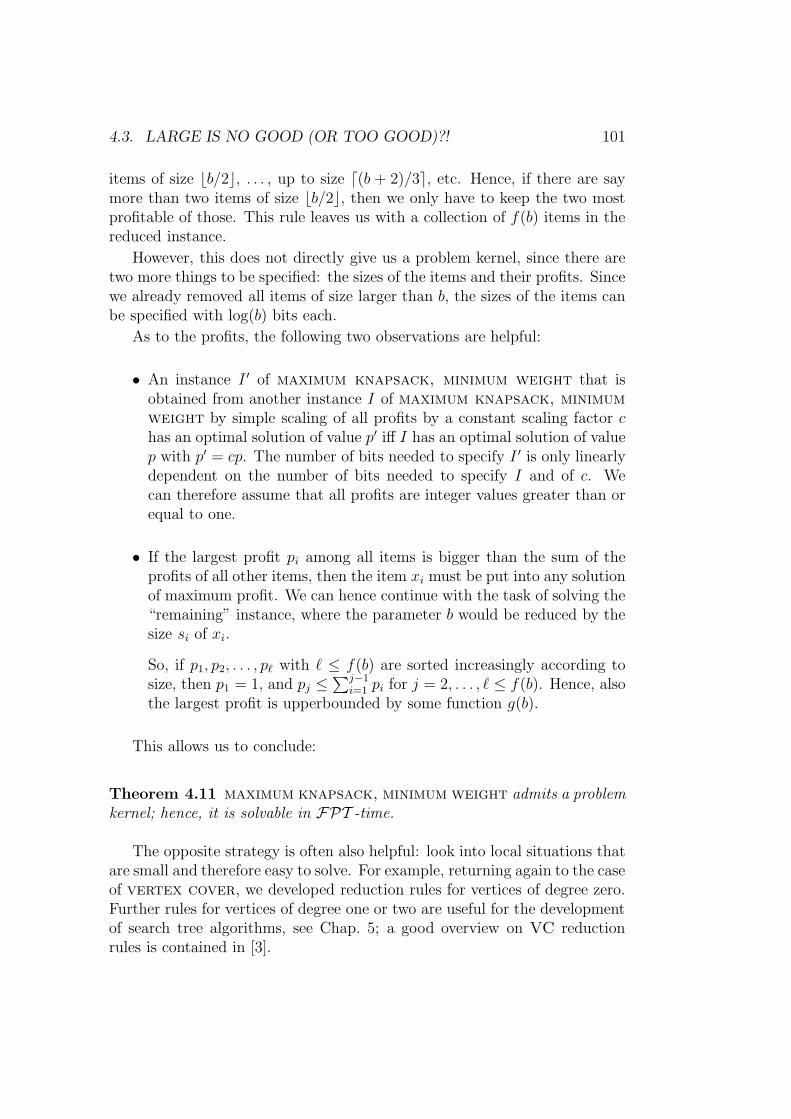
4.3. LARGE IS NO GOOD (OR TOO GOOD)?! 101
items of size bb/2c, . . . , up to size d(b + 2)/3e, etc. Hence, if there are saymore than two items of size bb/2c, then we only have to keep the two mostprofitable of those. This rule leaves us with a collection of f(b) items in thereduced instance.
However, this does not directly give us a problem kernel, since there aretwo more things to be specified: the sizes of the items and their profits. Sincewe already removed all items of size larger than b, the sizes of the items canbe specified with log(b) bits each.
As to the profits, the following two observations are helpful:
• An instance I ′ of maximum knapsack, minimum weight that isobtained from another instance I of maximum knapsack, minimumweight by simple scaling of all profits by a constant scaling factor chas an optimal solution of value p′ iff I has an optimal solution of valuep with p′ = cp. The number of bits needed to specify I ′ is only linearlydependent on the number of bits needed to specify I and of c. Wecan therefore assume that all profits are integer values greater than orequal to one.
• If the largest profit pi among all items is bigger than the sum of theprofits of all other items, then the item xi must be put into any solutionof maximum profit. We can hence continue with the task of solving the“remaining” instance, where the parameter b would be reduced by thesize si of xi.
So, if p1, p2, . . . , p` with ` ≤ f(b) are sorted increasingly according tosize, then p1 = 1, and pj ≤
∑j−1i=1 pi for j = 2, . . . , ` ≤ f(b). Hence, also
the largest profit is upperbounded by some function g(b).
This allows us to conclude:
Theorem 4.11 maximum knapsack, minimum weight admits a problemkernel; hence, it is solvable in FPT -time.
The opposite strategy is often also helpful: look into local situations thatare small and therefore easy to solve. For example, returning again to the caseof vertex cover, we developed reduction rules for vertices of degree zero.Further rules for vertices of degree one or two are useful for the developmentof search tree algorithms, see Chap. 5; a good overview on VC reductionrules is contained in [3].
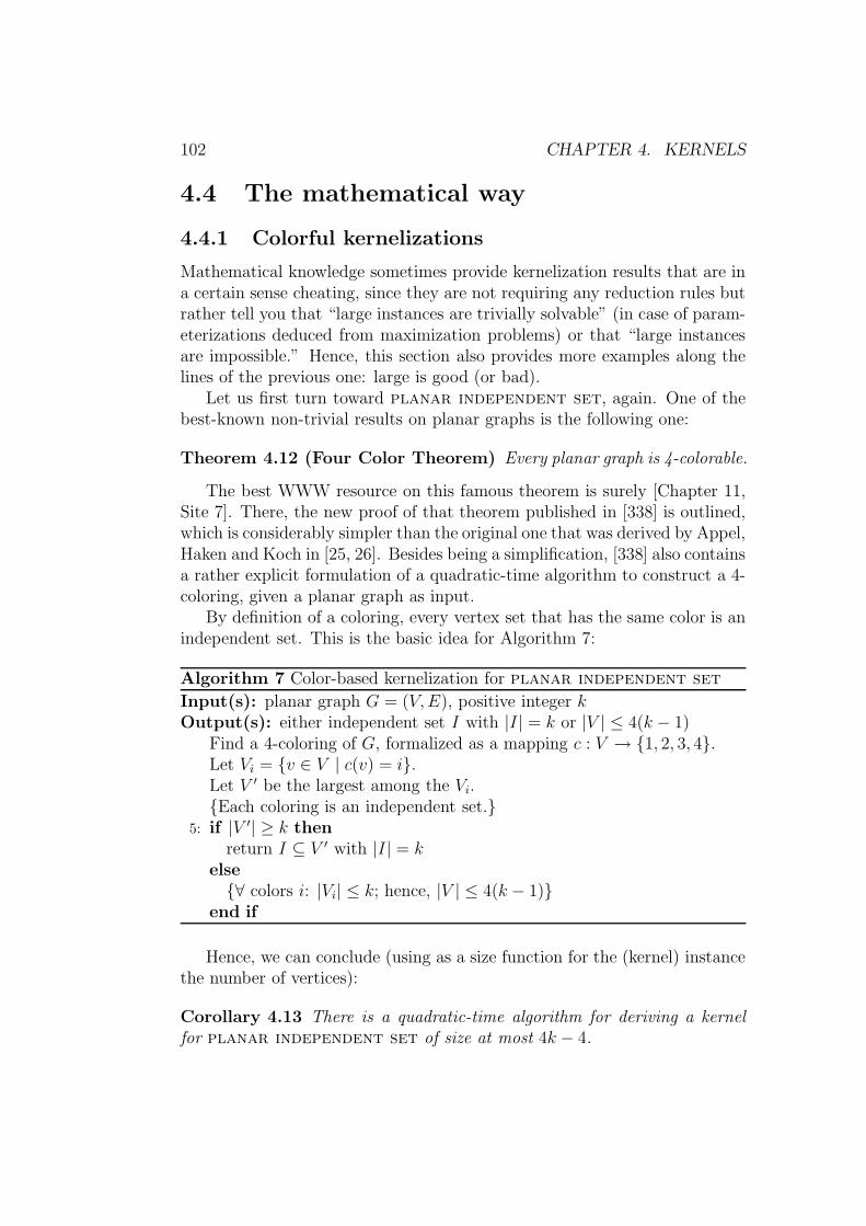
102 CHAPTER 4. KERNELS
4.4 The mathematical way
4.4.1 Colorful kernelizations
Mathematical knowledge sometimes provide kernelization results that are ina certain sense cheating, since they are not requiring any reduction rules butrather tell you that “large instances are trivially solvable” (in case of param-eterizations deduced from maximization problems) or that “large instancesare impossible.” Hence, this section also provides more examples along thelines of the previous one: large is good (or bad).
Let us first turn toward planar independent set, again. One of thebest-known non-trivial results on planar graphs is the following one:
Theorem 4.12 (Four Color Theorem) Every planar graph is 4-colorable.
The best WWW resource on this famous theorem is surely [Chapter 11,Site 7]. There, the new proof of that theorem published in [338] is outlined,which is considerably simpler than the original one that was derived by Appel,Haken and Koch in [25, 26]. Besides being a simplification, [338] also containsa rather explicit formulation of a quadratic-time algorithm to construct a 4-coloring, given a planar graph as input.
By definition of a coloring, every vertex set that has the same color is anindependent set. This is the basic idea for Algorithm 7:
Algorithm 7 Color-based kernelization for planar independent set
Input(s): planar graph G = (V,E), positive integer kOutput(s): either independent set I with |I| = k or |V | ≤ 4(k − 1)
Find a 4-coloring of G, formalized as a mapping c : V → 1, 2, 3, 4.Let Vi = v ∈ V | c(v) = i.Let V ′ be the largest among the Vi.Each coloring is an independent set.
5: if |V ′| ≥ k thenreturn I ⊆ V ′ with |I| = k
else∀ colors i: |Vi| ≤ k; hence, |V | ≤ 4(k − 1)
end if
Hence, we can conclude (using as a size function for the (kernel) instancethe number of vertices):
Corollary 4.13 There is a quadratic-time algorithm for deriving a kernelfor planar independent set of size at most 4k − 4.

4.4. THE MATHEMATICAL WAY 103
Proof. Algorithm 7 satisfies the claim. In particular, since we would choosethe biggest amongst the colorings, |V | ≤ 4(k − 1) whenever the algorithmdoes not already produce a sufficiently large independent set.
Observe the either-or structure of the kernelization algorithm 7:
• either: there is a large enough coloring which we can return as a solutionto our problem,
• or: all colorings are small, which means that there are only a fewvertices in the graph.
Notice one special feature of this kernelization: if we only aim at a thedecision version of planar independent set (as according to the definitionof the problem), we can substitute Alg. 7 by the following rule:
Reduction rule 18 If (G, k) is an instance of planar independent setand if |V (G)| > 4k, then YES.
This shows that the fact that there is an efficient algorithm for getting afour-coloring is not important to this problem, so that the kernel (as such)can be even derived in linear time.
Observe that Alg. 7 (or the reduction rule just discussed) can again bealso read as a 4k-kernelization algorithm both for maximum minimal ver-tex cover and for maximum minimal dominating set, following thereasoning given above. More precisely, the idea would be (say for MMVC)to greedily extend the largest color class C to a minimal vertex cover (if|C| ≥ k, where k is the parameter of the MMVC instance).
Corollary 4.14 There is a quadratic-time algorithm for deriving a kernelfor maximum minimal vertex cover, restricted to planar instances, ofsize at most 4k − 4.
Observe that Theorem 4.2 only delivered a quadratic kernel for generalgraph instances.
Corollary 4.15 There is a quadratic-time algorithm for deriving a kernelfor maximum minimal dominating set, restricted to planar instances, ofsize at most 4k − 4.
Other coloring theorems can be used to derive similar results. For exam-ple, 3 Ringel [335] considered graphs that corresponds to maps embedded on
3This notion is different from so-called map graphs that have been made popular bythe papers [92, 93].

104 CHAPTER 4. KERNELS
a sphere that are defined as follows: the vertices of these graphs correspondto either regions or points that do not belong to the open edges separatingto regions. Two regions or points are neighbored if they share an edge; andthis gives the edge relation of the corresponding graph.
Theorem 4.16 Graphs that are derived from maps in the way describedabove can be colored with at most seven colors.
In fact, Ringel showed a stronger result by allowing certain crossingsin the drawing of the map. We omit details here. Anyhow, Alg. 7 can beeasily modified to get a 7k kernel for independent set, restricted to graphsderived from maps as described by Ringel.
Ringel (and later Kronk and Mitchem [265]) also considered a differentkind of graph derivable from maps on the sphere, where also edge (bound-aries) are considered as vertices of the derived graph; again, a coloring theo-rem is derived.
This schematics is typical for kernelization algorithms based on theoremsknown from combinatorics. We will encounter more examples along theselines in what follows.
A similar, color-based linear kernel can be shown for vertex inducedforest, which is:
Problem name: vertex induced forest in planar graphs(PViF)Given: a (simple) planar graph G = (V,E)Parameter: a positive integer kdOutput: Is there a vertex-induced forest of size at least kd, i.e.,
∃F ⊆ V, |F | ≥ kd, C(G[F ]) = ∅?
Namely, Borodin [59] managed to prove the following (former) conjectureof Grunbaum:
Theorem 4.17 [Borodin] Every planar graph is acyclically 5-colorable.
To properly understand this theorem, let us introduce the following notionaccording to Borodin:
Definition 4.18 A coloring of a graph is called an acyclic coloring, if everybichromatic subgraph that is induced by this coloring is a forest (i.e., anacyclic graph).
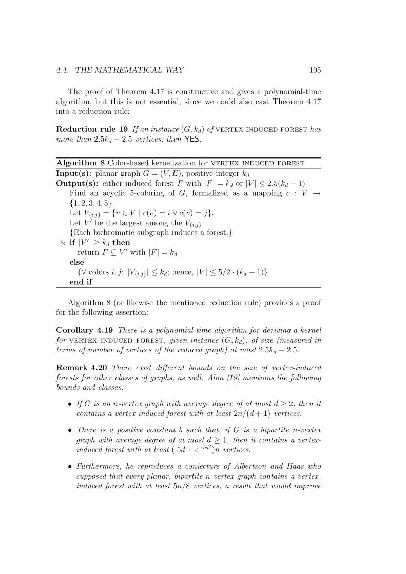
4.4. THE MATHEMATICAL WAY 105
The proof of Theorem 4.17 is constructive and gives a polynomial-timealgorithm, but this is not essential, since we could also cast Theorem 4.17into a reduction rule:
Reduction rule 19 If an instance (G, kd) of vertex induced forest hasmore than 2.5kd − 2.5 vertices, then YES.
Algorithm 8 Color-based kernelization for vertex induced forest
Input(s): planar graph G = (V,E), positive integer kdOutput(s): either induced forest F with |F | = kd or |V | ≤ 2.5(kd − 1)
Find an acyclic 5-coloring of G, formalized as a mapping c : V →1, 2, 3, 4, 5.Let Vi,j = v ∈ V | c(v) = i ∨ c(v) = j.Let V ′ be the largest among the Vi,j.Each bichromatic subgraph induces a forest.
5: if |V ′| ≥ kd thenreturn F ⊆ V ′ with |F | = kd
else∀ colors i, j: |Vi,j| ≤ kd; hence, |V | ≤ 5/2 · (kd − 1)
end if
Algorithm 8 (or likewise the mentioned reduction rule) provides a prooffor the following assertion:
Corollary 4.19 There is a polynomial-time algorithm for deriving a kernelfor vertex induced forest, given instance (G, kd), of size (measured interms of number of vertices of the reduced graph) at most 2.5kd − 2.5.
Remark 4.20 There exist different bounds on the size of vertex-inducedforests for other classes of graphs, as well. Alon [19] mentions the followingbounds and classes:
• If G is an n-vertex graph with average degree of at most d ≥ 2, then itcontains a vertex-induced forest with at least 2n/(d+ 1) vertices.
• There is a positive constant b such that, if G is a bipartite n-vertexgraph with average degree of at most d ≥ 1, then it contains a vertex-induced forest with at least (.5d+ e−bd
2)n vertices.
• Furthermore, he reproduces a conjecture of Albertson and Haas whosupposed that every planar, bipartite n-vertex graph contains a vertex-induced forest with at least 5n/8 vertices, a result that would improve
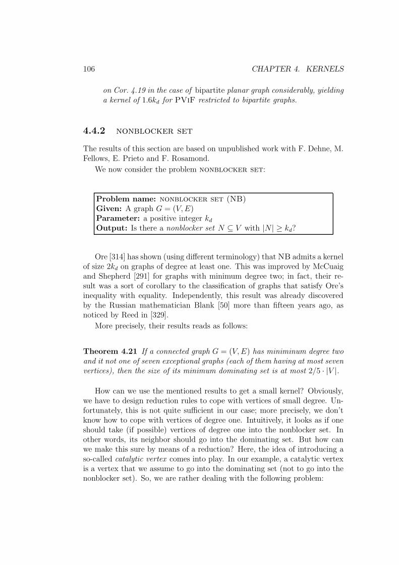
106 CHAPTER 4. KERNELS
on Cor. 4.19 in the case of bipartite planar graph considerably, yieldinga kernel of 1.6kd for PViF restricted to bipartite graphs.
4.4.2 nonblocker set
The results of this section are based on unpublished work with F. Dehne, M.Fellows, E. Prieto and F. Rosamond.
We now consider the problem nonblocker set:
Problem name: nonblocker set (NB)Given: A graph G = (V,E)Parameter: a positive integer kdOutput: Is there a nonblocker set N ⊆ V with |N | ≥ kd?
Ore [314] has shown (using different terminology) that NB admits a kernelof size 2kd on graphs of degree at least one. This was improved by McCuaigand Shepherd [291] for graphs with minimum degree two; in fact, their re-sult was a sort of corollary to the classification of graphs that satisfy Ore’sinequality with equality. Independently, this result was already discoveredby the Russian mathematician Blank [50] more than fifteen years ago, asnoticed by Reed in [329].
More precisely, their results reads as follows:
Theorem 4.21 If a connected graph G = (V,E) has miniminum degree twoand it not one of seven exceptional graphs (each of them having at most sevenvertices), then the size of its minimum dominating set is at most 2/5 · |V |.
How can we use the mentioned results to get a small kernel? Obviously,we have to design reduction rules to cope with vertices of small degree. Un-fortunately, this is not quite sufficient in our case; more precisely, we don’tknow how to cope with vertices of degree one. Intuitively, it looks as if oneshould take (if possible) vertices of degree one into the nonblocker set. Inother words, its neighbor should go into the dominating set. But how canwe make this sure by means of a reduction? Here, the idea of introducing aso-called catalytic vertex comes into play. In our example, a catalytic vertexis a vertex that we assume to go into the dominating set (not to go into thenonblocker set). So, we are rather dealing with the following problem:

4.4. THE MATHEMATICAL WAY 107
Problem name: nonblocker set with catalytic vertex(NBcat)Given: A graph G = (V,E), a catalytic vertex cParameter: a positive integer kdOutput: Is there a nonblocker set N ⊆ V with |N | ≥ kd such thatc /∈ N?
We now propose the following reduction rules:
Reduction rule 20 Let (G, c, kd) be an instance of nonblocker set withcatalytic vertex. If C is a complete graph component of G that does notcontain c, then reduce to (G− C, c, kd − (|C| − 1)).
Observe that the previous rule is in particular applicable to isolated ver-tices. It also applies to instances that don’t contain a catalytic vertex. Thesoundness of the rule is easy to see; a formal proof is contained in [323].Notice that this rule alone gives a 2kd kernel for general graphs with thementioned result of Ore (details are shown below).
Reduction rule 21 Let (G, c, kd) be an instance of nonblocker set withcatalytic vertex. Whenever you have a vertex x ∈ V (G) whose neigh-borhood contains a non-empty subset U ⊆ N(x) such that N(U) ⊆ U ∪ xand c /∈ U , then you can merge x with the catalytic vertex c and delete U(and reduce the parameter by |U |).
This rule is a bit more tricky, but the basic idea that c is used to annotatea vertex of the dominating set should be clear: it simply makes no sense toput any of the vertices from U into the (minimum) dominating set (that weimplicitly construct when building up a (maximum) nonblocker set), sincex will dominate at least those vertices as any of the vertices from U woulddo. In fact, we shouldn’t apply that rule for very large neighborhoods, sinceit might be quite time-consuming to test all subsets as required (in orderto make sure that the rule is no longer applicable). However, only smallneighborhoods will suffice for our analytic purposes, as we will see.
We have actually found a reduction rule that can also cope with twoconsecutive vertices of degree two and hence eliminate all exceptional graphsof Theorem 4.21 (since all of them have this property).
However, from the point of view of systematics, it is more interestinghow to first of all introduce a catalytic vertex (to produce a genuine NBcatinstance from the original nonblocker set instance) and then to get ridof the catalysts again (to be able to apply Theorem 4.21:

108 CHAPTER 4. KERNELS
catalyzation rule If (G, kd) is an instance of nonblocker set with G =(V,E), then (G′, c, kd) is an equivalent instance of nonblocker setwith catalytic vertex, where c /∈ V is a new vertex, and G′ =(V ∪ c, E).
decatalyzation rule Let (G, c, kd) be an instance of nonblocker setwith catalytic vertex. Then, perform the following surgery toget a new instance (G′, k′d) of nonblocker set:
Connect the catalytic vertex c to three new vertices u, v, and w byedges; moreover, introduce new edges uv and vw. All other verticesand edge relations in G stay the same. This describes the new graphG′. Set k′d = kd + 3. You may then forget about the special role of thecatalyst. The surgery is described in Fig. 4.1.
k
u wv
catalytic vertex
c
k’=k+3
Figure 4.1:
The overall kernelization algorithm for a given nonblocker set instance(G, kd) is then the procedure listed in Alg. 9.
Without further discussion, we only mention those reduction rules thatcan be used to get rid of all consecutive degree-2-vertices in a graph:
Reduction rule 22 Let (G, c, kd) be an instance of NBcat. Let u, v be twovertices of degree two in G such that u ∈ N(v) and |N(u) ∪ N(v)| = 4, i.e.,N(u) = u′, v and N(v) = v′, u for some u′ 6= v′. If c /∈ u, v, thenmerge u′ and v′ and delete u and v to get a new instance (G′, c′, kd − 2). Ifu′ or v′ happens to be c, then c′ is the merger of u′ and v′; otherwise, c′ = c.
Reduction rule 23 Let (G, c, kd) be an instance of NBcat, where G =(V,E). Assume that c has degree two and a neighboring vertex v of degreetwo, i.e., N(v) = v′, c. Then, delete the edge vv′. Hence, we get the newinstance ((V,E \ vv′), c, kd).

4.4. THE MATHEMATICAL WAY 109
Algorithm 9 A kernelization algorithm for nonblocker set
Input(s): an instance (G, kd) of nonblocker setOutput(s): an equivalent instance (G′, k′d) of nonblocker set withV (G′) ⊆ V (G), |V (G′)| ≤ 5/3 · k′d and k′d ≤ kd OR YES
if G has more than seven vertices thenApply the catalyzation rule.Exhaustively apply Rules 20 and 21 for neighborhoods U up to size two.Apply the decatalyzation rule.This leaves us with a reduced instance (G′, k′d).if |V (G′)| > 5/3 · k′d then
return YES
elsereturn (G′, k′d)
end ifelse
Solve by table look-up and answer accordingly.end if
Notice that really all cases of two subsequent vertices u, v of degree twoare covered in this way:
• If u or v is the catalytic vertex, then Rule 23 applies.
• Otherwise, if u and v have a common neighbor x, then Rule 21 isapplicable; x will be merged with the catalytic vertex.
• Otherwise, Rule 22 will apply.
Let us finally mention that the kernelization rules we developed for non-blocker set are rather independent of the parameter, so that they can bealso applied when solving maximum nonblocker set or even minimumdominating set. Hence, they can be read as important practical heuristicsfor minimum dominating set algorithms, although we cannot expect FPTresults for dominating set in the general case, see Chap. 9.
Corollary 4.22 Alg. 9 provides a kernel of size at most 5/3 · kd for a giveninstance (G, kd) of nonblocker set, where the problem size is measured interms of the number of vertices.
Let us do our computations a bit more generally, as a plug-in. Assumewe have a theorem telling us that all graphs in a graph class G obey thatthe domination number γ(G) satisfies γ(G) ≤ c|V (G)| for all G ∈ G. Then,
110 CHAPTER 4. KERNELS
given a graph G from our class and a parameter k, we can answer YES to thequestion if G has a dominating set of size at most k whenever k > c|V (G)|.Hence, given G from our class and a parameter kd, we can answer YES to thequestion if G has a nonblocker set of size at least kd whenever (|V (G)|−kd) >c|V (G)|, or if kd < (1− c)|V (G)|. Otherwise, we don’t know the answer, butwe know that kd/(1 − c) ≥ |V (G)|. So, we have a kernel size of kd/(1 − c),measured in terms of the number of vertices ofG. With the result of McCuaigand Shepherd, we have c = 2/5, so that the corollary follows.
Together with Lemma 4.1, we can conclude:
Corollary 4.23 By testing all subsets of size kd of a reduced instance (G, kd)of nonblocker set, this problem can be solved in time O∗(3.0701kd).
A slightly improved running time analysis will be presented in Chap. 10.
From an algorithmic perspective, the fact that the domination numberof a graph without isolated vertices is bounded by its edge independencenumber [372, Theorem 1] could be also useful to get a smaller kernel fornonblocker set; observe that the edge independence number is just thesize of a maximum matching which can be computed in polynomial time.
Observe that Rule 21 may destroy planarity, since merging vertices fromdifferent parts of a graph may create a K5 or a K3,3 as a substructure thathas not been there before. Therefore, we cannot rely anymore on Cor. 4.22if we insist on having a planar reduced graph. However, as the reader mayverify, all other rules for nonblocker set do preserve planarity. As alreadymentioned above, Ore proved in [314, Theorem 13.1.3] c=.5 for graphs ofminimum degree one. Of course, we can deal with vertices of degree zero bya reduction rule that does not affect planarity, namely Rule 20. Hence, wecan conclude:
Corollary 4.24 nonblocker set, restricted to the planar case, admits aplanar kernel graph with at most 2kd vertices.
Ore’s construction is quite instructive and can be found in Alg. 10. Webelieve that spanning tree techniques can be used in other kernelization prob-lems, as well. We mention one more application in the following: maximumminimal vertex cover. Observe that we have already treated this prob-lem for the special case of planar graph inputs. Hence, the kernelization basedon spanning trees is yielding not only smaller kernels (as we will see) but alsomore general results regarding the FPT membership of these problems.
We basically have to see how to treat isolated vertices.

4.4. THE MATHEMATICAL WAY 111
Algorithm 10 A kernelization algorithm for nonblocker set, also appli-cable to the planar case
Input(s): an instance (G, kd) of nonblocker setOutput(s): an equivalent instance (G′, k′d) of nonblocker set withV (G′) ⊆ V (G), |V (G′)| ≤ 2k′d and k′d ≤ kd OR YES; in the latter case,also a solution A is constructed.
Exhaustively apply reduction rule 20. Call the resulting instance G again.Compute a minimum spanning tree for each component of G.for all component C do
Pick an arbitrary root rC of the spanning tree TC belonging to C.Collect in LiC all vertices of TC having distance i from rC , where thedistance is measured in TC .Define, for j = 0, 1: Aj =
⋃i≥0 L
2i+jC .
Choose the larger of the two and call it ANB(C), where ties are brokenarbitrarily.
end forForm A =
⋃ANB(C) | C is component of G.if |A| > kd then
return YES
elseG is the returned instance.
end if
Reduction rule 24 Let (G, k) be an instance of maximum minimal ver-tex cover. If C is a complete graph component of G, then reduce to(G− C, k − (|C| − 1)).
The soundness of the rulecan be easily seen: A vertex cover of a completegraph C needs |C| − 1 vertices, and putting all vertices in the cover wouldrender it non-minimal.
If Alg. 10 returns YES, it implicitly selects either of two disjoint vertexsets A0 and A1 (basically, every second level of the spanning tree). However,A0 or A1 need not be vertex cover sets. Notice that both A0 and A1 areminimal in the sense that none of them contains a closed neighborhood ofany vertex. Then, we would have to supplement say the larger of the twoto get a valid minimal vertex cover. Hence, answering YES in the indicatedcase is o.k., so that we conclude:
Corollary 4.25 maximum minimal vertex cover admits a kernel graphwith at most 2k vertices.
112 CHAPTER 4. KERNELS
Let us once more return to nonblocker set: Unfortunately, we werenot able to use the stronger result provided by B. Reed [329] for the kernel-ization algorithm, upperbounding the domination number of a graph thathas minimum degree of three. More precisely, he showed c = 3/8, whichgives a kernel of size 1.6kd for graphs of minimum degree two. This graphclass appears to be a bit strange, admittedly, but we simply don’t know howto get rid of all vertices of degree up to two by reduction rules.4 There isanother result due to Matheson and Tarjan [288]. We can conclude fromtheir reasoning that graphs G = (V,E) that possess a triangulated planar
subgraph G′ = (V,E ′) have a dominating set with at most |V |3
vertices. Thisgives a kernel of 1.5kd for this graph class for nonblocker set.
Coming back to the “cheating argument” of the introductory paragraphof this section, let us reconsider nonblocker set: In a certain sense, thetheorems we used to provide small kernels are in fact telling us that, wheneverwe assume the existence of a small nonblocker set, then the graph cannot bebig. This may mean that in actual fact the parameterization we chose isnot appropriate. Similar to the suggestion in [307], this might imply weshould reparameterize. One such reparameterization was already discussedin [284] for a logical problem. Transferred to nonblocker set, we mightask questions like:
Problem name: δ-nonblocker set (δ-NB)Given: A graph G = (V,E)Parameter: a positive integer kdOutput: Is there a nonblocker set N ⊆ V with |N | ≥ δ|V | + kd?
Here, δ ∈ (0, 1) is a constant that steers the reparameterization. It isnot part of the input, but rather essential for creating a whole family ofparameterized problems.
Theorem 4.26 If δ < 3/5, then δ-nonblocker set is in FPT .
Proof. We are going to show that δ-NB has a problem kernel, see Theo-rem 2.4.
Let G be a graph instance and kd the parameter. We exhaustively applythe same reduction rules as developed before for nonblocker set to get areduced graph G′ with parameter k′d. G′ = (V,E) has minimum degree of
4It might be worthwhile noting that there is a kind of complementary result for graphswith maximum degree three by Fisher, Fraughnaugh and Seager [182]; however, the cor-responding bound also includes the number of vertices in the graph, so that the kernelsize bound looks a bit strange; for cubic graphs, however, the result of Reed is exactlymatched.

4.4. THE MATHEMATICAL WAY 113
two, and therefore it has a minimum dominating set of size at most 2/5 · |V |.Hence, |V | − |N | ≤ 2/5 · |V | for a maximum nonblocker set N , i.e., |N | ≥3/5 · |V |. If we ask for an N that is smaller than this, we can safely answerYES, see Alg. 9. Hence, given the question if |N | ≥ δ|V |+ kd, we can answerYES if δ|V | + kd ≤ 3/5 · |V |, i.e., if kd ≤ (3/5 − δ)|V |. Otherwise, we havearrived at a kernel of size |V | ≤ (3/5 − δ)−1kd.
Observe that similar reparameterizations can be performed (while keepingFPT -membership) for problems like vertex induced forest, planarindependent set, etc.
4.4.3 Dominating Queens
Finally, let us reconsider the following variant of a domination problem al-ready introduced in the introduction:
Problem name: dominating set of queens (QDS)Given: An n× n chessboard CParameter: a positive integer kOutput: Is it possible to place k queens on C such that all squaresare dominated ?
Theorem 4.27 QDS has a problem kernel of size (2k + 1)2.
Proof. Indeed, we are going to verify the following “cheating” reductionrule:
Reduction rule 25 If C is an n × n board and k a parameter with n >2k + 1, then NO.
A proof of this result is shown in [100, Theorem 3]; however, that proof con-tains a non-trivial “hole,” and therefore we produce a proof in what follows.5
Given an n×n board C, fix a dominating set of k queens, where k is min-imal. The rule is surely o.k. for n = 1, 2, since there is no fitting parametervalue. If n > 2, we can show k ≤ n−2, since placing n−2 queens on the maindiagonal of the chessboard, leaving free the first and last square in that diag-onal, will dominate the whole chessboard. Therefore, the following rows andcolumns exist: Let column a (b, resp.) be the leftmost (rightmost, respec-tively) column that is not occupied by any queen in our minimum dominating
5Thanks to my class in approximation algorithms (Tubingen in 2004/2005), in partic-ular to Bernd Lutz, who pointed this hole to me.

114 CHAPTER 4. KERNELS
set. Correspondingly, let row c (d, resp.) be the topmost (bottom-most, re-spectively) unoccupied row. Let δ1 = b− a and δ2 = d− c. By symmetry ofthe argument, we can assume that δ1 ≥ δ2.
Let Sa (Sb, resp.) be the set of squares in column a (b, resp.) that liebetween rows c and d′ := minn, c+ δ1 inclusive. Set S := Sa ∪ Sb.Claim 0: Any queen can diagonally dominate at most two squares of S.Proof of Claim. Since δ1 ≥ δ2, no diagonal intersects both Sa and Sb. Hence,every queen can dominate at most one square of S on a southwest-northeastdiagonal and one square of S on a northwest-southeast diagonal. ♦
Claim 1: Any queen placed in the first c− 1 rows or in the last n − d′ rowscan only dominate at most two squares of S.Proof of Claim. By definition, no queen that is placed on the mentionedsquares can dominate any squares from S by row or column. The precedingclaim hence proves Claim 1. ♦
Claim 2: Any queen can only dominate at most four squares of S.Proof of Claim. Due to the preceding claim, we consider a queen that isplaced on the rows c through d′ (inclusive). By definition of S, such a queencannot dominate any squares of S by column. It can obviously dominate atmost two squares of S by row. Hence, Claim 0 finishes this proof. ♦
Let o be the number of “occupied” rows to which Claim 1 applies, i.e.,o = c− 1 + n− d′. Summarizing our claims, we can state:
• At least o queens dominate at most two squares of S.
• At most k − o queens dominate at most four squares of S.
Hence, the k queens together dominate at most 2o + 4(k − o) = 4k − 2osquares of S.
We now distinguish two subcases:
• If o ≥ c (or, equivalently, if c+ δ1 ≤ n, i.e., d′ = c+ δ1), then |S| = 2δ1,since δ1 is the number of rows that is pertaining to S. Moreover,Claim 1 applies to the remaining o = n − (δ1 + 1) many rows. Thisgives the following inequality, since we are discussing how to dominateall squares in S:
4k − 2n+ 2δ1 + 2 ≥ 2δ1 2k + 1 ≥ n.
• If o = c − 1 (or, equivalently, if c + δ1 > n, i.e., d′ = n), then |S| =2(n− (c− 1)) = 2n− 2o. Hence,
4k − 2o ≥ 2n− 2o 2k ≥ n.
4.5. VERTEX COVER: OUR OLD FRIEND AGAIN 115
Since we don’t know which of the two cases applies, we have to take the lessstricter bound in our theorem.
So, on the one hand, this shows membership of dominating set ofqueens in FPT , but on the other hand, it is also sort of questionable if theparameterization is appropriate.
4.5 vertex cover: our old friend again
The reason for having an own section on vertex cover in the context ofkernelization are manifold:
• In the introduction, we already saw how to design data reduction rulesthat provide a quadratic kernel for vertex cover.
• There exist by now two (at first glance) completely different ways ofobtaining a small linear kernel for vertex cover, one being based onnice structural properties of vertex covers, as discovered by Nemhauserand Trotter [304]; the other one being based on generalizing Rule 1 forisolated vertices to a so-called crown rule [110, 164]. Having two waysto obtain the same result is in fact an interesting situation on its own.Computer experiments indicate, however, that the kernelization basedon crown reduction rules is better, not only in terms of running time(see [3]).
• Finally, we will discuss a generalization of vertex cover and see howwe can build up a set of data reduction rules that can be read eitheras a reduction to the formerly treated case of vertex cover or asenabling to read reduction rules for vertex cover as being valid forthe more general case, as well, and hence enabling us to state a smallkernel result for this case, too.
As indicated above, the first part of this section will be devoted to dis-cussing the following result:
Theorem 4.28 vertex cover has a kernel of size upperbounded by 2k.
Remark 4.29 Can we possibly hope for a smaller kernel? The difficulty ofgetting a smaller kernel for vertex cover seems to be related with the (old)problem of getting approximation algorithms that provide a quality ratio es-sentially better than two. More precisely, the best known approximation [255]gives a ratio of
2 − Θ(1√
logn).
116 CHAPTER 4. KERNELS
More precisely, although not formally required by the definition of kerneliza-tion, it seems likely that the development of a kernelization algorithm thatgives a kernel of say 1.7k would also mean that we get a 1.7 approximationfor vertex cover, by simply taking all kernel vertices (plus possibly somethat are provided by the reduction itself) into the (approximate) cover.
Similar comments also apply to the vertex cover problem on hyper-graphs, likewise known as d-hitting set, where the trivial d-approximationalgorithm is hard to beat. Regarding positive approximability results in someparticular cases, we refer to the recent papers of Halperin and Okun [226,313]. However, in that case no linear kernel is known, see [310], which initself can be regarded as an interesting research topic.
4.5.1 The result of Nemhauser and Trotter
Let us first state the theorem of Nemhauser and Trotter according to theformulation given in [35] and in [320]; the original formulation of Nemhauserand Trotter [304] uses connections with Integer Linear Programming thatare not central to this Habilitationsschrift. A concise proof of the result iscontained in [35].
If G = (V,E) is a graph, let GBP = (V × 1, 2, EBP ) be its bipartitegraph variant, where
EBP = (u, 1), (v, 2) | u, v ∈ E .
Given a vertex set CBP of GBP , let
CANDBP (G) = v ∈ V | (v, 1) ∈ C ∧ (v, 2) ∈ C ,
CXORBP (G) =
v ∈ V \ CAND
BP (G) | (v, 1) ∈ C ∨ (v, 2) ∈ C.
One point of Alg. 11 needs further clarification: how can we efficientlycompute a vertex cover in bipartite graphs? The key to this lies in thefollowing theorem, due to Konig and Egervary (see [264]):
Theorem 4.30 If G is a bipartite graph, then the size of a minimum vertexcover of G equals the size of a maximum matching of G.
It is worth noting that one direction of that theorem is close to trivial;let us state it in a weakened form:
Lemma 4.31 If M is a matching in a graph G, then G has no vertex coverof size less than |M |.

4.5. VERTEX COVER: OUR OLD FRIEND AGAIN 117
Algorithm 11 A kernelization algorithm for vertex cover, called VCNT
Input(s): an instance (G, k) of vertex coverOutput(s): an equivalent instance (G′, k′) of vertex cover with V (G′) ⊆
V (G), |V (G′)| ≤ 2k′ and k′ ≤ k, as well as a set C ⊆ V (G) that mustappear in any vertex cover for G (and that is not accounted into thebudget k′).
Create GBP from G.Compute a minimum vertex cover CBP of GBP .Compute C := CAND
BP (G) and CXORBP (G).
Let k′ := k − |C|.5: if k′ < 0 then
Pick an edge e = u, v from G.Define G′ = (u, v, e) and k′ = 0.Let C := ∅.
else10: Let G′ = G[CXOR
BP (G)].end ifreturn (G′, k′) as well as C.
Proof. All edges of M need to be covered. Each edge can be covered byeither of its endpoints. Covering e ∈ M this way will not cover any otheredge from M , since M is a matching. Hence, we need |M | vertices to coverM , so that we need (at least) |M | vertices to cover G.
From an algorithmic point of view, two things are worth mentioning:
• A maximum matching M ⊆ E of a graph G = (V,E) can be computedin time O(|E|
√|V |; such an algorithm is usually based on the notion of
alternating paths and can be found in any introductory standard texton algorithms.
• From M , one can efficiently construct a vertex cover C ⊆ V if G isbipartite. Such a construction can be based on an alternating pathsconstruction, as they are already used in the standard constructionshowing that maximum matchings can be found in polynomial time,see [Chapter 11, Site 13]. An alternative way using Dinic’s algorithmis explained in [3].
Nemhauser and Trotter then showed the following properties:
Theorem 4.32 Let G = (V,E) be a graph.

118 CHAPTER 4. KERNELS
1. Let C ′ be a cover of G[CXORBP (G)]. Then C := C ′ ∪CAND
BP (G) is a coverof G.
2. There is a minimum cover C∗(G) of G that contains CANDBP (G).
3. |CXORBP (G)| ≤ 2|C∗(G)|, where C∗(G) is a minimum cover of G.
From the mentioned results, the following was observed in [86, 251]:
Corollary 4.33 To each vertex cover instance (G, k), Alg. 11 computes
a kernel (G′, k′) with |V (G′)| ≤ 2k′ and k′ ≤ k in time O(|E(G)|
√|V (G)|
).
Remark 4.34 Hochbaum [233] used the result of Nemhauser and Trotter togive a factor-2 approximation algorithm for minimum vertex cover: thisalgorithm would output
CORBP (G) = CAND
BP (G) ∪ CXORBP (G)
for an input graph G (using the abbreviation introduced above).
Remark 4.35 By first kernelizing according to Buss’ rule (see Chap. 2) andthen according to Alg. 11 (in fact, all these rules could and should be appliedto exhaustion before starting the search-tree part as explained in the nextchapter), the overall complexity for the kernelization phase could be reducedto O(nk + k3).
Remark 4.36 A similar algorithm works for the kernelization of the weightedversion of vertex cover, i.e., of weighted vertex cover. Then, how-ever, the computation of the kernel would be based on maximum flow compu-tations, which are slower than the maximum matching computations in theunweighted case.
When the input graph is planar, the kernelization computations could beconsiderably sped up. All these complexities are detailed in [35].
We also mention the following properties of a decomposition of the vertexset V of a graph G = (V,E) according to Theorem 4.32 that are lists in [320,Sec. 5.1]:
1. CNORBP (G) = V \ (CXOR
BP (G)∪CANDBP (G)) forms an independent set in G.
2. All neighbors of CNORBP (G) are in CAND
BP (G).
Remark 4.37 In [96, 95], the theorem of Nemhauser & Trotter got sharp-ened so that, for all minimum vertex covers of G, they are contained inCANDBP (G).

4.5. VERTEX COVER: OUR OLD FRIEND AGAIN 119
It is finally worthwhile noticing that the kernelization due to the Nemhauser-Trotter theorem can be called global in contrast to all other kernelization pro-cedures we have seen up to now; this is also the reason for its comparativelyhuge complexity.
4.5.2 Crown reductions: another way to a small kernel
We follow the definition of a crown as given in [95] for the more generalweighted case. Otherwise, this section is mostly based on [3, 110, 247].
Definition 4.38 Let G = (V,E) be a graph. An independent set I in G iscalled a crown if, for all nonempty sets U ⊆ N(I), |U | ≤ |N(U) ∩ I|.That definition is equivalent to the one given in [3, 110, 164] due to Hall’smarriage theorem (apart from the requirement that I 6= ∅ according to thosedefinitions) that can be found in any textbook on graph theory. Hence, acrown I has the following property:
• H := N(I) is matched into I. (H is usually referred to as the head ofthe crown.)
In other words, the bipartite graph with vertex set H ∪ I and edge set uv |u ∈ Hv ∈ I has a upper perfect matching.
Observe that a decomposition a la Nemhauser and Trotter is “nearly” acrown (more precisely, the set CNOR
BP (G)).M. Chlebık and J. Chlebıkova [95] have shown that there is always a
specific Nemhauser-Trotter decomposition that is actually a crown.Fellows has introduced the following reduction rule:
Reduction rule 26 If (G = (V,E), k) a vertex cover instance and I ⊆V a crown with head H = N(I), then reduce to (G− (I ∪H), k − |H|).
The question is then how to find crowns. Juedes6 devised Alg. 12 tothis purpose. How can we use this algorithm to get a small kernel for ver-tex cover? In fact, the kernelization algorithm has several ways to usethe information collected in Alg. 12; therefore, we state the correspondingkernelization algorithm in an explicit form in Alg. 13.
Lemma 4.39 Alg. 13 combined with Rule 26, when run on input (G, k),either correctly answers NO or yields a reduced instance (G′, k′) of vertexcover such that |V (G′)| ≤ 3k.
6personal communication in Oct. 2002; this idea can be found in [3, 247]
120 CHAPTER 4. KERNELS
Algorithm 12 An efficient algorithm to find a crown in a graph, calledGETCROWNInput(s): an graph GOutput(s): a crown I ⊆ V (G)
Greedily find a maximal matching M1 of G.Let O (outsiders) be the set of vertices fromG that are not in the matching.if O 6= ∅ then
Let I ′ := ∅.Find a maximum matching M2 in the bipartite graph B with vertex setO ∪N(O) and edge set uv | u ∈ O ∧ v ∈ N(O).Let I collect all vertices in O that are not matched by M2.while I ′ 6= I do
Let I ′ := I.Let H := N(I).Let I := I ∪ u ∈ O | ∃v ∈ H(uv ∈ M2).
end whileelseI := ∅.
end if
The proof of this lemma is based on the following observations:
• If we find a matching M (i.e., M1 or M2) in G such that |M | > k, then(G, k) is a NO-instance due to Lemma 4.31.
• If M1 and M2 contain no more than k edges, the graph induced byM1∪M2 has at most 3k vertices. Has, after applying Rule 26 followingthe execution of Alg. 13, the remaining graph has at most 3k vertices.
Abu-Khzwam et al. have demonstrated [3] that a kernelization based onAlg. 13 runs much faster than directly using Alg. 11. This is probably due tothe fact that the Nemhauser-Trotter reduction has to compute a maximummatching in a relatively large graph, while the crown-based reduction onlycomputes a maximal matching in a large graph and then maximum match-ings in much smaller graphs. More precisely, it is shown in [247] that thisalgorithm runs in time O(|V |+ |E|) on an input graph G = (V,E) by lookingagain into how maximum matching algorithms work in our case.
However, it is clear that one could certainly afford running Alg. 11 afterhaving obtained a 3k kernel with Alg. 13. The experiments reported in [3]also indicate that this might not actually lead to a smaller kernel (as couldbe expected due to theory).

4.5. VERTEX COVER: OUR OLD FRIEND AGAIN 121
Algorithm 13 Using crowns for kernels in the case of vertex cover; thealgorithm is called kernelfromcrown
Input(s): an instance (G, k) of vertex coverOutput(s): NO if the vertex cover instance has no solution OR a crownI ⊆ V (G) such that |V (G−N [I])| ≤ 3k
Greedily find a maximal matching M1 of G.if |M1| > k then
return NO
elseLet O (outsiders) be the set of vertices from G that are not in M1.if O 6= ∅ then
Find a maximum matching M2 in the bipartite graph B with vertexset O ∪N(O) and edge set uv | u ∈ O ∧ v ∈ N(O).if |M2| > k then
return NO
elseLet I ′ := ∅.Let I collect all vertices in O that are not matched by M2.while I ′ 6= I do
Let I ′ := I.Let H := N(I).Let I := I ∪ u ∈ O | ∃v ∈ H(uv ∈M2).
end whileend if
elseI := ∅.
end ifreturn I
end if
There is alternative way of obtaining a kernel of size 2k, known as iterativecompression, see [110]. However, getting the kernel that small comes at aprice: one has to optimally solve k (smaller) instances of vertex cover,so that the overall kernelization does not need polynomial time anymore(as required by the kernelization definition) but rather in FPT -time. Wetherefore omit details here.
The idea of crown reductions have been successfully applied to othercircumstances, as well. We only mention the following papers: [110, 166,247, 289, 324, 325].
122 CHAPTER 4. KERNELS
4.5.3 A generalization of vertex cover
Let us now consider the following generalization of VC:
Problem name: generalized vertex cover (VCgen)Given: A graph G = (V,E), a subset V ′ of verticesParameter: a positive integer kOutput: Is there a vertex cover C ⊆ V ′ with |C| ≤ k?
It is clear that this is actually a generalization of VC, since it is possibleto have V ′ = V . Therefore, NP-hardness of VCgen is trivially concluded.
We propose the following reduction rules for this problem. In these rules,let (G = (V,E), V ′, k) be an instance of VCgen.
Reduction rule 27 If there is an edge in G[V \ V ′], then NO.
Reduction rule 28 If there is an edge u, v with u ∈ V ′ and v ∈ V \ V ′,then put u into the cover, i.e., reduce to (G− u, V ′, k − 1).
The soundness of both rules is clear, since we are still aiming at a cover.Hence, edges between vertices from V \ V ′ cannot be covered at all (leadingto a NO-instance), and edges that contain exactly one vertex u from V ′ canonly be covered by taking that vertex u into the cover.
After having exhaustively applied these two reduction rules, in the casethat we did not already discover that the given instance was not solvable atall, we are left with an instance that contains only vertices from V \ V ′ thatare isolates. Since such isolates would not be put into a cover even if theywere belonging to V ′, we can conclude:
Lemma 4.40 If (G = (V,E), V ′, k) is an instance of generalized vertexcover that is reduced with respect to Rules 27 and 28. Then, (G, V ′, k) is aYES-instance of VCgen iff (G, V, k) is a YES-instance of VCgen iff (G, k)is a YES-instance of VC.
This means that we have reduced VCgen to VC. In view of the trivialreduction for the converse direction, we may conclude:
Corollary 4.41 generalized vertex cover and vertex cover are pa-rameterized interreducible.
However, we can also interpret this reducibility as providing a completeset of data reduction rules for generalized vertex cover that have tobe applied in a certain order to get an overall kernelization algorithm that

4.6. PLANAR DOMINATING SET: A TRICKY EXAMPLE 123
Algorithm 14 A kernelization algorithm for generalized vertex cover,called VCgen-kern
Input(s): an instance (G, V ′, k) of generalized vertex coverOutput(s): YES iff the given instance has a solution
if Reduction rule R out of rules 27 and 28 is applicable thenreturn VCgen-kern(R(G, V ′, k))
else if V (G) 6= V ′ thenThis can only happen if G[V (G) \ V ′] contains no edges.return VCgen-kern(G, V (G), k)
elseApply your favorite vertex cover-reduction rules to get a 2k-kernel,interpreted as rules for generalized vertex cover.
end if
deviates a bit from the usual scheme (see Alg. 5) for kernelization algorithms,so that we explicitly state it in Alg. 4.5.3. The indicated interpretation ofVC-rules as VCgen-rules is very straightforward: a VC instance (G, k) issimply understood as VCgen instance (G, V (G), k). Since (according tothe case distinction in Alg. 4.5.3), we are only left with VCgen instances(G, V ′, k) such that V ′ = V (G), this translation gives a sound reduction rulefor generalized vertex cover. Hence, we can conclude:
Theorem 4.42 generalized vertex cover has a 2k problem kernel.
4.6 planar dominating set: a tricky example
In the following, we present results on planar dominating set; this is anexample of quite complex kernelization rules derived in [12, 82].
Let us first state the problem.
Problem name: planar dominating set (PDS)Given: A planar graph G = (V,E)Parameter: a positive integer kOutput: Is there a dominating set D ⊆ V with |D| ≤ k?
For a graph G, we denote by γ(G) the size of a minimum dominating setin G. We will color the vertices of the graph G with two colors: black andwhite. Initially, all vertices are colored black. Informally speaking, whitevertices will be those vertices that we know for sure when we color them that

124 CHAPTER 4. KERNELS
there exists a minimum dominating set for the graph excluding all of them.The black vertices are all other vertices.7
For a vertex v in G, we partition its set of neighbors N(v) into three sets:
1. N1(v) = u ∈ N(v) | N(u) \N [v] 6= ∅;
2. N2(v) = u ∈ N(v) \N1(v) | N(u) ∩N1(v) 6= ∅; and
3. N3(v) = N(v) \ (N1(v) ∪N2(v)).
To understand these notions, have a look at the following example:
Figure 4.2: Explaining the division of the neighborhood of v.
Example 4.43 Have a look at the red vertex v in Fig. 4.2. Its neighbor-hood is colored in three different colors. For the convenience of the reader,we repeat the definitions of the various divisions of the neighborhood inthe following, using matching colorings with respect to the example graph.N1(v) = u ∈ N(v) | N(u) \N [v] 6= ∅N2(v) = u ∈ N(v) \N1(v) | N(u) ∩N1(v) 6= ∅N3(v) = N(v) \ (N1(v) ∪N2(v))
For two vertices v and w we define N(v, w) = N(v)∪N(w) and N [v, w] =N [v] ∪N [w]. Similarly, we partition N(v, w) into three sets:
7In Chap. 5, we will present a search tree algorithm for planar dominating set thatis also using a black and white graph: note that the colors there have different semanticsfrom the usage here.

4.6. PLANAR DOMINATING SET: A TRICKY EXAMPLE 125
1. N1(v, w) = u ∈ N(v, w) | N(u) \N [v, w] 6= ∅;
2. N2(v, w) = u ∈ N(v, w) \N1(v, w) | N(u) ∩N1(v, w) 6= ∅; and
3. N3(v, w) = N(v, w) \ (N1(v, w) ∪N2(v, w)).
Definition 4.44 Let G = (V,E) be a plane graph. A region R(v, w) be-tween two vertices v and w is a closed subset of the plane with the followingproperties:
1. The boundary of R(v, w) is formed by two simple paths P1 and P2 inV which connect v and w, and the length of each path is at most three.
2. All vertices that are strictly inside (i.e., not on the boundary) the regionR(v, w) are from N(v, w).
For a region R = R(v, w), let V [R] denote the vertices in R, i.e.,
V [R] := u ∈ V | u sits inside or on the boundary of R.
Let V (R) = V [R] − v, w.
Definition 4.45 A region R = R(v, w) between two vertices v and w iscalled a simple region if all vertices in V (R) are common neighbors of bothv and w, that is, V (R) ⊆ N(v) ∩N(w).
We introduce the following definitions.
Definition 4.46 A region R = R(v, w) between two vertices v and w iscalled a quasi-simple region if V [R] = V [R′] ∪ R+, where R′ = R′(v, w) is asimple region between v and w, and R+ is a set of white vertices satisfyingthe following conditions:
1. Every vertex of R+ sits strictly inside R′.
2. Every vertex of R+ is connected to v and not connected to w, andis also connected to at least one vertex on the boundary of R′ otherthan v.
A vertex in V (R) is called a simple vertex, if it is connected to both vand w, otherwise it is called a non-simple vertex. The set of vertices R+,which consists of the non-simple vertices in V (R), will be referred to asR+(v, w).
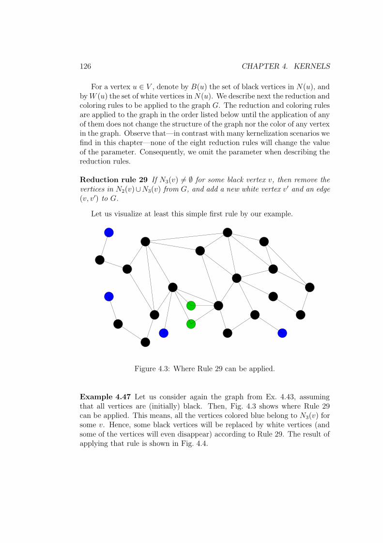
126 CHAPTER 4. KERNELS
For a vertex u ∈ V , denote by B(u) the set of black vertices in N(u), andbyW (u) the set of white vertices inN(u). We describe next the reduction andcoloring rules to be applied to the graph G. The reduction and coloring rulesare applied to the graph in the order listed below until the application of anyof them does not change the structure of the graph nor the color of any vertexin the graph. Observe that—in contrast with many kernelization scenarios wefind in this chapter—none of the eight reduction rules will change the valueof the parameter. Consequently, we omit the parameter when describing thereduction rules.
Reduction rule 29 If N3(v) 6= ∅ for some black vertex v, then remove thevertices in N2(v)∪N3(v) from G, and add a new white vertex v ′ and an edge(v, v′) to G.
Let us visualize at least this simple first rule by our example.
Figure 4.3: Where Rule 29 can be applied.
Example 4.47 Let us consider again the graph from Ex. 4.43, assumingthat all vertices are (initially) black. Then, Fig. 4.3 shows where Rule 29can be applied. This means, all the vertices colored blue belong to N3(v) forsome v. Hence, some black vertices will be replaced by white vertices (andsome of the vertices will even disappear) according to Rule 29. The result ofapplying that rule is shown in Fig. 4.4.

4.6. PLANAR DOMINATING SET: A TRICKY EXAMPLE 127
Figure 4.4: Some vertices are white now.
Reduction rule 30 If N3(v, w) 6= ∅ for two black vertices v, w, and ifN3(v, w) cannot be dominated by a single vertex in N2(v, w)∪N3(v, w), thenwe distinguish the following two cases.
Case 1. If N3(v, w) can be dominated by a single vertex in v, w then:
(1.1) if N3(v, w) ⊆ N(v) and N3(v, w) ⊆ N(w), remove N3(v, w) andN2(v, w) ∩ N(v) ∩ N(w) from G and add two new white vertices z,z′ and the edges (v, z), (w, z), (v, z′), (w, z′) to G;
(1.2) if N3(v, w) ⊆ N(v) and N3(v, w) 6⊆ N(w), remove N3(v, w) andN2(v, w) ∩ N(v) from G and add a new white vertex v ′ and the edge(v, v′) to G; and
(1.3) if N3(v, w) ⊆ N(w) and N3(v, w) 6⊆ N(v), remove N3(v, w) andN2(v, w) ∩ N(w) from G and add a new white vertex w′ and the edge(w,w′) to G.
Case 2. If N3(v, w) cannot be dominated by a single vertex in v, w, thenremove N2(v, w) ∪ N3(v, w) from G and add two new white vertices v ′, w′
and the edges (v, v′), (w,w′) to G.
Reduction rule 31 For each black vertex v in G, if there exists a blackvertex x ∈ N2(v)∪N3(v), color x white, and remove the edges between x andall other white vertices in G.
128 CHAPTER 4. KERNELS
Reduction rule 32 For every two black vertices v and w, if N3(v, w) 6= ∅,then for every black vertex x ∈ N2(v, w) ∪ N3(v, w) that does not dominateall vertices in N3(v, w), color x white and remove all the edges between x andthe other white vertices in G.
Reduction rule 33 For every quasi-simple region R = R(v, w) between twovertices v and w, if v is black, then for every black vertex x ∈ N2(v, w) ∪N3(v, w) strictly inside R that does not dominate all vertices in N2(v, w) ∪N3(v, w) strictly inside R, color x white and remove all the edges between xand the other white vertices in G.
Reduction rule 34 For every two white vertices u and v, if N(u) ⊆ N(v),and u ∈ N2(w) ∪N3(w) for some black vertex w, then remove v.
Reduction rule 35 For every black vertex v, if every vertex u ∈ W (v) isconnected to all the vertices in B(v), then remove all the vertices in W (v)from G.
Reduction rule 36 For every two black vertices v and w, let W (v, w) =W (v) ∩W (w). If |W (v, w)| ≥ 2 and there is a degree-2 vertex u ∈ W (v, w),then remove all vertices in W (v, w) except u, add a new degree-2 white vertexu′, and connect u′ to both v and w.
Theorem 4.48 Let G be a graph with n vertices. Then in time O(n3) wecan construct a graph G′ from G such that:
1. G′ is reduced,
2. γ(G′) = γ(G),
3. there exists a minimum dominating set for G′ that excludes all whitevertices of G′, and
4. from a minimum dominating set for G′, a minimum dominating set forG can be constructed in linear time.
Given any dominating set D in a graph G, a D-region decomposition of G isa set < of regions between pairs of vertices in D such that:
1. For any region R = R(v, w) in <, no vertex in D is in V (R). That is,a vertex in D can only be an endpoint of a region in <.
2. No two distinct regions R1, R2 ∈ < intersect. However, they may toucheach other by having common boundaries.
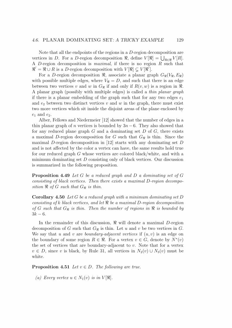
4.6. PLANAR DOMINATING SET: A TRICKY EXAMPLE 129
Note that all the endpoints of the regions in a D-region decomposition arevertices in D. For a D-region decomposition <, define V [<] =
⋃R∈< V [R].
A D-region decomposition is maximal, if there is no region R such that<′
= < ∪R is a D-region decomposition with V [<] ( V [<′].
For a D-region decomposition <, associate a planar graph G<(V<, E<)with possible multiple edges, where V< = D, and such that there is an edgebetween two vertices v and w in G< if and only if R(v, w) is a region in <.A planar graph (possibly with multiple edges) is called a thin planar graphif there is a planar embedding of the graph such that for any two edges e1
and e2 between two distinct vertices v and w in the graph, there must existtwo more vertices which sit inside the disjoint areas of the plane enclosed bye1 and e2.
Alber, Fellows and Niedermeier [12] showed that the number of edges in athin planar graph of n vertices is bounded by 3n− 6. They also showed thatfor any reduced plane graph G and a dominating set D of G, there existsa maximal D-region decomposition for G such that G< is thin. Since themaximal D-region decomposition in [12] starts with any dominating set Dand is not affected by the color a vertex can have, the same results hold truefor our reduced graph G whose vertices are colored black/white, and with aminimum dominating set D consisting only of black vertices. Our discussionis summarized in the following proposition.
Proposition 4.49 Let G be a reduced graph and D a dominating set of Gconsisting of black vertices. Then there exists a maximal D-region decompo-sition < of G such that G< is thin.
Corollary 4.50 Let G be a reduced graph with a minimum dominating set Dconsisting of k black vertices, and let < be a maximal D-region decompositionof G such that G< is thin. Then the number of regions in < is bounded by3k − 6.
In the remainder of this discussion, < will denote a maximal D-regiondecomposition of G such that G< is thin. Let u and v be two vertices in G.We say that u and v are boundary-adjacent vertices if (u, v) is an edge onthe boundary of some region R ∈ <. For a vertex v ∈ G, denote by N ∗(v)the set of vertices that are boundary-adjacent to v. Note that for a vertexv ∈ D, since v is black, by Rule 31, all vertices in N2(v) ∪ N3(v) must bewhite.
Proposition 4.51 Let v ∈ D. The following are true.
(a) Every vertex u ∈ N1(v) is in V [<].
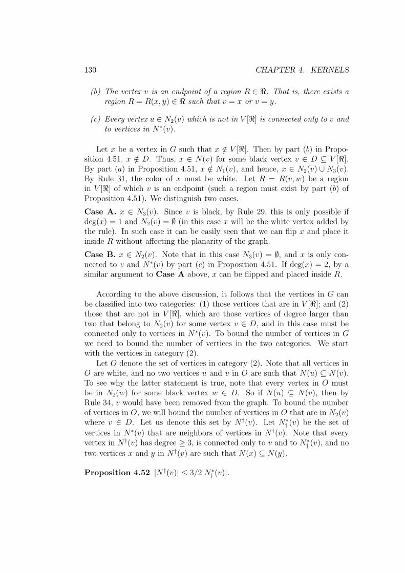
130 CHAPTER 4. KERNELS
(b) The vertex v is an endpoint of a region R ∈ <. That is, there exists aregion R = R(x, y) ∈ < such that v = x or v = y.
(c) Every vertex u ∈ N2(v) which is not in V [<] is connected only to v andto vertices in N ∗(v).
Let x be a vertex in G such that x /∈ V [<]. Then by part (b) in Propo-sition 4.51, x /∈ D. Thus, x ∈ N(v) for some black vertex v ∈ D ⊆ V [<].By part (a) in Proposition 4.51, x /∈ N1(v), and hence, x ∈ N2(v) ∪ N3(v).By Rule 31, the color of x must be white. Let R = R(v, w) be a regionin V [<] of which v is an endpoint (such a region must exist by part (b) ofProposition 4.51). We distinguish two cases.
Case A. x ∈ N3(v). Since v is black, by Rule 29, this is only possible ifdeg(x) = 1 and N2(v) = ∅ (in this case x will be the white vertex added bythe rule). In such case it can be easily seen that we can flip x and place itinside R without affecting the planarity of the graph.
Case B. x ∈ N2(v). Note that in this case N3(v) = ∅, and x is only con-nected to v and N ∗(v) by part (c) in Proposition 4.51. If deg(x) = 2, by asimilar argument to Case A above, x can be flipped and placed inside R.
According to the above discussion, it follows that the vertices in G canbe classified into two categories: (1) those vertices that are in V [<]; and (2)those that are not in V [<], which are those vertices of degree larger thantwo that belong to N2(v) for some vertex v ∈ D, and in this case must beconnected only to vertices in N ∗(v). To bound the number of vertices in Gwe need to bound the number of vertices in the two categories. We startwith the vertices in category (2).
Let O denote the set of vertices in category (2). Note that all vertices inO are white, and no two vertices u and v in O are such that N(u) ⊆ N(v).To see why the latter statement is true, note that every vertex in O mustbe in N2(w) for some black vertex w ∈ D. So if N(u) ⊆ N(v), then byRule 34, v would have been removed from the graph. To bound the numberof vertices in O, we will bound the number of vertices in O that are in N2(v)where v ∈ D. Let us denote this set by N †(v). Let N∗
† (v) be the set of
vertices in N ∗(v) that are neighbors of vertices in N †(v). Note that everyvertex in N †(v) has degree ≥ 3, is connected only to v and to N ∗
† (v), and no
two vertices x and y in N †(v) are such that N(x) ⊆ N(y).
Proposition 4.52 |N †(v)| ≤ 3/2|N ∗† (v)|.
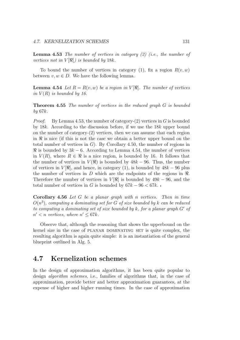
4.7. KERNELIZATION SCHEMES 131
Lemma 4.53 The number of vertices in category (2) (i.e., the number ofvertices not in V [<]) is bounded by 18k.
To bound the number of vertices in category (1), fix a region R(v, w)between v, w ∈ D. We have the following lemma.
Lemma 4.54 Let R = R(v, w) be a region in V [<]. The number of verticesin V (R) is bounded by 16.
Theorem 4.55 The number of vertices in the reduced graph G is boundedby 67k.
Proof. By Lemma 4.53, the number of category-(2) vertices inG is boundedby 18k. According to the discussion before, if we use the 18k upper boundon the number of category-(2) vertices, then we can assume that each regionin < is nice (if this is not the case we obtain a better upper bound on thetotal number of vertices in G). By Corollary 4.50, the number of regions in< is bounded by 3k − 6. According to Lemma 4.54, the number of verticesin V (R), where R ∈ < is a nice region, is bounded by 16. It follows thatthe number of vertices in V (<) is bounded by 48k − 96. Thus, the numberof vertices in V [<], and hence, in category (1), is bounded by 48k − 96 plusthe number of vertices in D which are the endpoints of the regions in <.Therefore the number of vertices in V [<] is bounded by 49k − 96, and thetotal number of vertices in G is bounded by 67k − 96 < 67k.
Corollary 4.56 Let G be a planar graph with n vertices. Then in timeO(n3), computing a dominating set for G of size bounded by k can be reducedto computing a dominating set of size bounded by k, for a planar graph G′ ofn′ < n vertices, where n′ ≤ 67k.
Observe that, although the reasoning that shows the upperbound on thekernel size in the case of planar dominating set is quite complex, theresulting algorithm is again quite simple: it is an instantiation of the generalblueprint outlined in Alg. 5.
4.7 Kernelization schemes
In the design of approximation algorithms, it has been quite popular todesign algorithm schemes, i.e., families of algorithms that, in the case ofapproximation, provide better and better approximation guarantees, at theexpense of higher and higher running times. In the case of approximation

132 CHAPTER 4. KERNELS
algorithms, such schemes were called approximation schemes. Is it possibleto translate this idea into the realm of parameterized algorithmics?
To this end, let us return to a problem that we already discussed inChap. 3: linear arrangement. We have already seen through Theo-rem 3.11 that linear arrangement is fixed parameter tractable. How-ever, observe that we also considered the problem linear arrangementrestricted to connected graphs and showed FPT -membership by providinga kernel with at most k + 1 vertices (the more general kernel was measuredin terms of edges).
We have also observed that components can be treated separately. Ob-viously, a component of size one or two (measured in terms of number ofvertices) can be trivially solved at the end of the algorithm:
Reduction rule 37 If G has two or less vertices, then construct an arbi-trary arrangement onto neighbored numbers.
In combination with Lemma 3.4, this shows the following:
Proposition 4.57 A reduced instance of LA has at most 1.5k vertices.
Proof. Since the instance is reduced and since each component can betreated separately, the number of vertices n in a reduced instance is the sumof the vertices nc in the components c. Each nc can be upperbounded bykc+1, where kc is the proportion of the parameter that is spent on componentc. Hence:
n =∑
c
nc ≤∑
c
(kc + 1) =∑
c
kc + #c = k + #c
where #c denotes the number of components of the instance. However, sincewe are dealing with a reduced instance, there are at most n/3 components inthe instance: namely, each component has at least three vertices. Therefore:
k ≥ n− n
3=
2
3n.
This shows the claim.
In fact, our reduction rule can be generalized: optimal arrangements forall graphs up to q − 1 vertices may be precomputed (taking exponentialtime, measured against q); this shows that each component then has at leastq vertices. After formulating an appropriate reduction rule, we may deduce:
Proposition 4.58 For each fixed q, a reduced instance of LA has at mostqq−1
k vertices.

4.8. COMPILABILITY AND KERNELS 133
This certainly has the flavor of an algorithmic scheme: at the expense oflarger and larger running times, we may get smaller and smaller kernels (letq grow).
In fact, we have already seen a similar example before: Rule 21 is a kernel-ization scheme, since we would have to test larger and larger neighborhoods,although for our analysis of the kernel size for nonblocker set, we canonly exploit the rule for neighborhoods up to size two. Similarly, a naivesearch for crowns can be viewed as a kernelization scheme, since again largerand larger (potential) crowns should be examined.
In Chap. 6, we will encounter further such examples.
4.8 Compilability and kernels
The idea of using preprocessing rules is not new but has been around in theheuristics community for years: it is in fact a very natural approach to solvehard problems by making them as small as possible to be able to attack them.The main interesting thing of parameterized algorithmics is that it allows amathematical analysis of this heuristic approach and hence somehow explainsthe success of preprocessing in practice.
In fact, there exists an alternative way of mathematically analyzing pre-processing rules, mainly developed by P. Liberatore and his colleagues: theyterm the preprocessing compilation and analyze the compilability of intract-able problems. This approach is based on the following observation: fastalgorithms can be realized when part of the input data (called fixed inputpart) is known long before the rest of the input (called varying input part).Then, it makes sense to spend some (more) computation time to analyzethe fixed part to speed up the solution when the varying part arrives. Moretechnically speaking, a problem is compilable if the fixed input part x canbe transformed (by arbitrarily complex preprocessing computations) into apart x′ such that the size |x′| is upperbounded by a polynomial in |x| andthere is a polynomial-time algorithm that solves the overall problem in timemeasured in |x′| and the varying input part size |y|. To a certain extent,this approach also allows to separate an on-line behavior from an off-linebehavior.
However, this idea is a bit contradicting the basic idea of parameterizedalgorithmics in the sense that in many concrete applications, the fixed inputpart is in fact large while the varying input part is rather small. This mightbe the main intuitive reason why results on compilability do significantlydiffer from results in computational complexity.
As an example, consider the following problem taken from [272]:
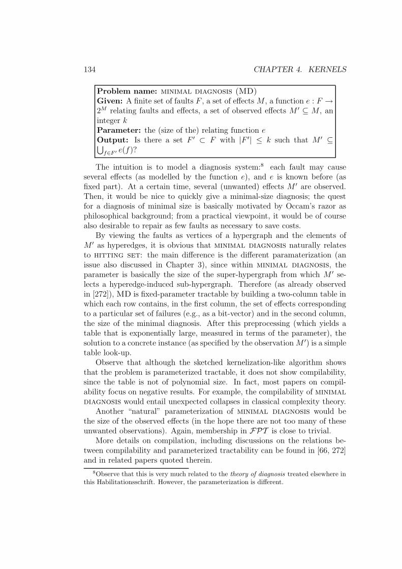
134 CHAPTER 4. KERNELS
Problem name: minimal diagnosis (MD)Given: A finite set of faults F , a set of effects M , a function e : F →2M relating faults and effects, a set of observed effects M ′ ⊆ M , aninteger kParameter: the (size of the) relating function eOutput: Is there a set F ′ ⊂ F with |F ′| ≤ k such that M ′ ⊆⋃f∈F ′ e(f)?
The intuition is to model a diagnosis system:8 each fault may causeseveral effects (as modelled by the function e), and e is known before (asfixed part). At a certain time, several (unwanted) effects M ′ are observed.Then, it would be nice to quickly give a minimal-size diagnosis; the questfor a diagnosis of minimal size is basically motivated by Occam’s razor asphilosophical background; from a practical viewpoint, it would be of coursealso desirable to repair as few faults as necessary to save costs.
By viewing the faults as vertices of a hypergraph and the elements ofM ′ as hyperedges, it is obvious that minimal diagnosis naturally relatesto hitting set: the main difference is the different paramaterization (anissue also discussed in Chapter 3), since within minimal diagnosis, theparameter is basically the size of the super-hypergraph from which M ′ se-lects a hyperedge-induced sub-hypergraph. Therefore (as already observedin [272]), MD is fixed-parameter tractable by building a two-column table inwhich each row contains, in the first column, the set of effects correspondingto a particular set of failures (e.g., as a bit-vector) and in the second column,the size of the minimal diagnosis. After this preprocessing (which yields atable that is exponentially large, measured in terms of the parameter), thesolution to a concrete instance (as specified by the observation M ′) is a simpletable look-up.
Observe that although the sketched kernelization-like algorithm showsthat the problem is parameterized tractable, it does not show compilability,since the table is not of polynomial size. In fact, most papers on compil-ability focus on negative results. For example, the compilability of minimaldiagnosis would entail unexpected collapses in classical complexity theory.
Another “natural” parameterization of minimal diagnosis would bethe size of the observed effects (in the hope there are not too many of theseunwanted observations). Again, membership in FPT is close to trivial.
More details on compilation, including discussions on the relations be-tween compilability and parameterized tractability can be found in [66, 272]and in related papers quoted therein.
8Observe that this is very much related to the theory of diagnosis treated elsewhere inthis Habilitationsschrift. However, the parameterization is different.
4.8. COMPILABILITY AND KERNELS 135
Unfortunately, there are only few natural examples of compilable prob-lems around (as far as we observed). In the context of paramaterized al-gorithmics, the revised knowledge base problems from [65] seem to be quiteinteresting, since M. Cadoli et al. showed that, under many forms of “be-lief revisions,” given a set of beliefs T and some additional (possibly con-tradictory) information P , a “revised belief” T ′ can be computed in timepolynomial in |T | but exponential in |P |. This gives an FPT algorithm ifthe problem is parameterized by the size of the additional information |P |.Note that this parameterization is different from the viewpoint of compilabil-ity, which would allow large computations in terms of |T |. Therefore, theseresults are listed under the headline of bounded revision. However, these ex-amples do perfectly fit into the landscape of parameterized algorithmics, sincein practice the size of the background knowledge database, i.e., |T |, wouldbe rather large, while the additional information P would be comparativelysmall.
It would not be surprising if the future shows more fruitful dialog betweencompilability and parameterized tractability.

136 CHAPTER 4. KERNELS
Chapter 5
Search trees
Again, R. Downey and M. R. Fellows [134] classify the search tree method weare going to exhibit in this section as an ad hoc method. And again, they areright. However, besides kernelization this is the other standard methodologyto get efficient parameterized algorithms. The downside is here that we knowof no guarantee that actually all problems in FPT admit some sort of searchtree algorithm —if we rule out the fact that the kernel that can be alwaysobtained according to Theorem 2.4 may be “searched” by brute force; thisdoes not yield the kind of search trees we are after.
From a practical point of view, this approach has lots of similarities tobranch-and-cut algorithms and similar paradigms, so that again parameter-ized algorithmics might turn out as a way of mathematically analyzing andjustifying (pruning) heuristics applied by practitioners anyhow to solve com-binatorially hard problems.
As such, search tree algorithms are nothing new. They have been alongsince a long time. Robson’s work [342] on maximum independent set andFomin, Kratsch and Woeginger’s recent work [187] on minimum dominatingset are examples showing that the techniques we present here likewise applyto the non-parameterized setting. More can be found in Chap. 10.
For logical (satisfiability) type problems, many variants of search tree al-gorithms have been also proposed. A very elaborate example of this approachcan be found in [266], albeit the earlier mentioned (more “parameterized”)papers [212, 285] also follow the same basic methodology, which is a searchtree that is build along ideas stemming from Davis-Putnam algorithms fordealing with satisfiability problems.
As a warm-up to this chapter, let us therefore reconsider the problemsatisfiability problem with clauses of size three (clause pa-rameterization) as introduced in the end of Chap. 3.
Observe that the number of clauses of size three decreases in both re-
137
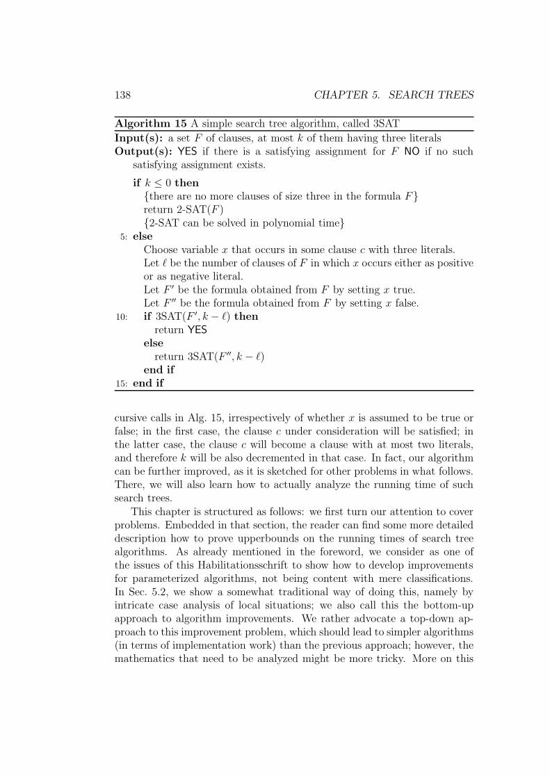
138 CHAPTER 5. SEARCH TREES
Algorithm 15 A simple search tree algorithm, called 3SAT
Input(s): a set F of clauses, at most k of them having three literalsOutput(s): YES if there is a satisfying assignment for F NO if no such
satisfying assignment exists.
if k ≤ 0 thenthere are no more clauses of size three in the formula Freturn 2-SAT(F )2-SAT can be solved in polynomial time
5: elseChoose variable x that occurs in some clause c with three literals.Let ` be the number of clauses of F in which x occurs either as positiveor as negative literal.Let F ′ be the formula obtained from F by setting x true.Let F ′′ be the formula obtained from F by setting x false.
10: if 3SAT(F ′, k − `) thenreturn YES
elsereturn 3SAT(F ′′, k − `)
end if15: end if
cursive calls in Alg. 15, irrespectively of whether x is assumed to be true orfalse; in the first case, the clause c under consideration will be satisfied; inthe latter case, the clause c will become a clause with at most two literals,and therefore k will be also decremented in that case. In fact, our algorithmcan be further improved, as it is sketched for other problems in what follows.There, we will also learn how to actually analyze the running time of suchsearch trees.
This chapter is structured as follows: we first turn our attention to coverproblems. Embedded in that section, the reader can find some more detaileddescription how to prove upperbounds on the running times of search treealgorithms. As already mentioned in the foreword, we consider as one ofthe issues of this Habilitationsschrift to show how to develop improvementsfor parameterized algorithms, not being content with mere classifications.In Sec. 5.2, we show a somewhat traditional way of doing this, namely byintricate case analysis of local situations; we also call this the bottom-upapproach to algorithm improvements. We rather advocate a top-down ap-proach to this improvement problem, which should lead to simpler algorithms(in terms of implementation work) than the previous approach; however, themathematics that need to be analyzed might be more tricky. More on this
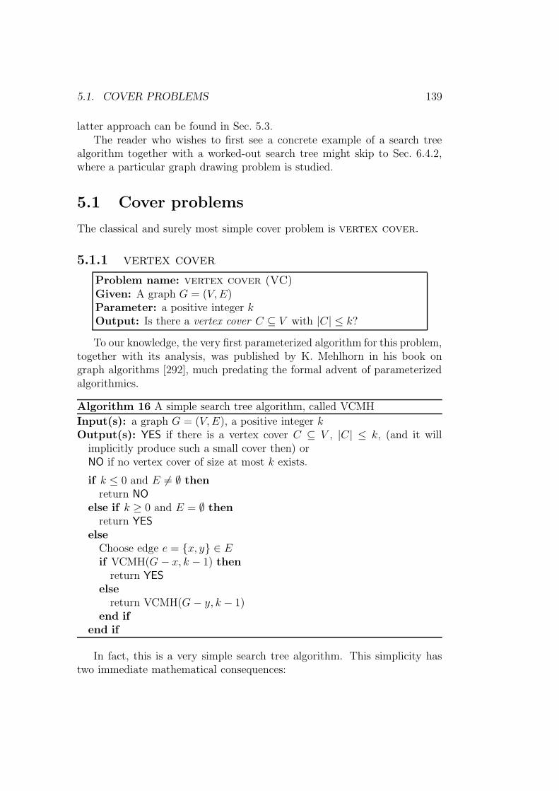
5.1. COVER PROBLEMS 139
latter approach can be found in Sec. 5.3.The reader who wishes to first see a concrete example of a search tree
algorithm together with a worked-out search tree might skip to Sec. 6.4.2,where a particular graph drawing problem is studied.
5.1 Cover problems
The classical and surely most simple cover problem is vertex cover.
5.1.1 vertex cover
Problem name: vertex cover (VC)Given: A graph G = (V,E)Parameter: a positive integer kOutput: Is there a vertex cover C ⊆ V with |C| ≤ k?
To our knowledge, the very first parameterized algorithm for this problem,together with its analysis, was published by K. Mehlhorn in his book ongraph algorithms [292], much predating the formal advent of parameterizedalgorithmics.
Algorithm 16 A simple search tree algorithm, called VCMH
Input(s): a graph G = (V,E), a positive integer kOutput(s): YES if there is a vertex cover C ⊆ V , |C| ≤ k, (and it will
implicitly produce such a small cover then) orNO if no vertex cover of size at most k exists.
if k ≤ 0 and E 6= ∅ thenreturn NO
else if k ≥ 0 and E = ∅ thenreturn YES
elseChoose edge e = x, y ∈ Eif VCMH(G − x, k − 1) then
return YES
elsereturn VCMH(G− y, k − 1)
end ifend if
In fact, this is a very simple search tree algorithm. This simplicity hastwo immediate mathematical consequences:

140 CHAPTER 5. SEARCH TREES
• The correctness of the algorithm can be verified in a nearly trivial yetformal manner.
• The running time can also be easily estimated.
Due to the simplicity of this algorithm, we will perform both analyses inthe following.
Let us remark that the way this search tree algorithm was obtained can beseen as a specific technique for designing search tree algorithms: the choice ofan appropriate, provably small candidate set ; in each branching step, simplyall possible candidates are considered one after the other. The correctnessof a search tree algorithm based on candidate set branching can be basicallyseen by showing that, in every solution (or at least in every solution that isobeying the constraint imposed by the given parameter value), at least oneof the elements in the candidate set has to show up.
The correctness of Mehlhorn’s algorithm:Let us consider the following variant VCMH-C of Mehlhorn’s algorithm (thepseudocode is listed in Alg. 17) that actually produces a cover if possible. Ina certain sense, this algorithm can be seen as an extension of the previousalgorithm, making the produced cover explicit.
This is indeed a fairly generally applicable technique to transform searchtree algorithms for pure decision problems into search tree algorithms thatactually produce the desired solution. In order to keep our algorithm presen-tation as simple as possible, we will refrain from actually constructing thesolutions if ever possible, but the reader should be able to do this simpletransformation on her/his own.
The proof of the correctness of this algorithm can be formally seen byinduction on the number of edges in G.
First observe that, if k ≤ 0 but E(G) 6= ∅, there cannot be any validcover for G.
If E(G) = ∅, then the algorithm correctly returns ∅ as minimum coverset.
Otherwise, the algorithm chooses an arbitrary candidate edge e = x, yand then branches according to which of the two incident vertices goes intothe cover. This is valid, since any edge must be covered by a feasible solution.In other words, an edge is a valid candidate set. In the recursion call, thegraph is modified by deleting, e.g., x and its incident edges from G (whichare the edges that are covered by taking x into the cover), i.e., the procedureis called with arguments G − x and k − 1, since obviously the “budget” ofvertices that can still go into a cover is decremented by putting x into thecover.
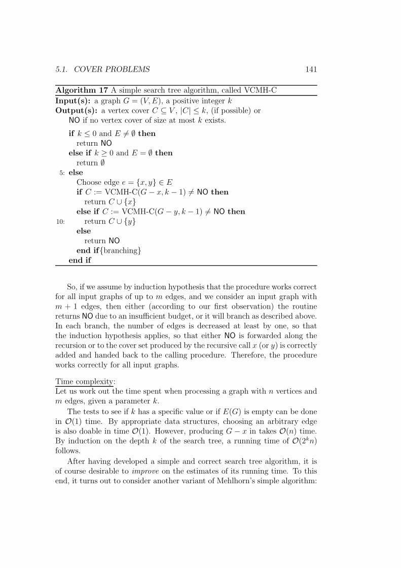
5.1. COVER PROBLEMS 141
Algorithm 17 A simple search tree algorithm, called VCMH-C
Input(s): a graph G = (V,E), a positive integer kOutput(s): a vertex cover C ⊆ V , |C| ≤ k, (if possible) or
NO if no vertex cover of size at most k exists.
if k ≤ 0 and E 6= ∅ thenreturn NO
else if k ≥ 0 and E = ∅ thenreturn ∅
5: elseChoose edge e = x, y ∈ Eif C := VCMH-C(G− x, k − 1) 6= NO then
return C ∪ xelse if C := VCMH-C(G− y, k − 1) 6= NO then
10: return C ∪ yelse
return NO
end ifbranchingend if
So, if we assume by induction hypothesis that the procedure works correctfor all input graphs of up to m edges, and we consider an input graph withm + 1 edges, then either (according to our first observation) the routinereturns NO due to an insufficient budget, or it will branch as described above.In each branch, the number of edges is decreased at least by one, so thatthe induction hypothesis applies, so that either NO is forwarded along therecursion or to the cover set produced by the recursive call x (or y) is correctlyadded and handed back to the calling procedure. Therefore, the procedureworks correctly for all input graphs.
Time complexity:Let us work out the time spent when processing a graph with n vertices andm edges, given a parameter k.
The tests to see if k has a specific value or if E(G) is empty can be donein O(1) time. By appropriate data structures, choosing an arbitrary edgeis also doable in time O(1). However, producing G − x in takes O(n) time.By induction on the depth k of the search tree, a running time of O(2kn)follows.
After having developed a simple and correct search tree algorithm, it isof course desirable to improve on the estimates of its running time. To thisend, it turns out to consider another variant of Mehlhorn’s simple algorithm:
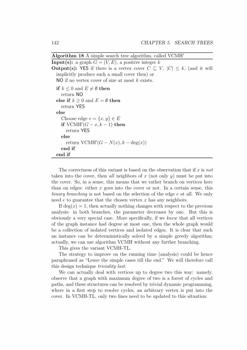
142 CHAPTER 5. SEARCH TREES
Algorithm 18 A simple search tree algorithm, called VCMH′
Input(s): a graph G = (V,E), a positive integer kOutput(s): YES if there is a vertex cover C ⊆ V , |C| ≤ k, (and it will
implicitly produce such a small cover then) orNO if no vertex cover of size at most k exists.
if k ≤ 0 and E 6= ∅ thenreturn NO
else if k ≥ 0 and E = ∅ thenreturn YES
elseChoose edge e = x, y ∈ Eif VCMH′(G− x, k − 1) then
return YES
elsereturn VCMH′(G−N(x), k − deg(x))
end ifend if
The correctness of this variant is based on the observation that if x is nottaken into the cover, then all neighbors of x (not only y) must be put intothe cover. So, in a sense, this means that we rather branch on vertices herethan on edges: either x goes into the cover or not. In a certain sense, thisbinary branching is not based on the selection of the edge e at all. We onlyneed e to guarantee that the chosen vertex x has any neighbors.
If deg(x) = 1, then actually nothing changes with respect to the previousanalysis: in both branches, the parameter decreases by one. But this isobviously a very special case. More specifically, if we knew that all verticesof the graph instance had degree at most one, then the whole graph wouldbe a collection of isolated vertices and isolated edges. It is clear that suchan instance can be deterministically solved by a simple greedy algorithm;actually, we can use algorithm VCMH without any further branching.
This gives the variant VCMH-TL.The strategy to improve on the running time (analysis) could be hence
paraphrased as “Leave the simple cases till the end.” We will therefore callthis design technique triviality last.
We can actually deal with vertices up to degree two this way: namely,observe that a graph with maximum degree of two is a forest of cycles andpaths, and these structures can be resolved by trivial dynamic programming,where in a first step to resolve cycles, an arbitrary vertex is put into thecover. In VCMH-TL, only two lines need to be updated to this situation:

5.1. COVER PROBLEMS 143
Algorithm 19 A still simple search tree algorithm, called VCMH-TL
Input(s): a graph G = (V,E), a positive integer kOutput(s): YES if there is a vertex cover C ⊆ V , |C| ≤ k, (and it will
implicitly produce such a small cover then) orNO if no vertex cover of size at most k exists.
if k ≤ 0 and E 6= ∅ thenreturn NO
else if k ≥ 0 and E = ∅ thenreturn YES
5: else if possible thenChoose vertex x ∈ V such that deg(x) ≥ 2.if VCMH-TL(G− x, k − 1) then
return YES
else10: return VCMH-TL(G−N(x), k − deg(x))
end ifelsevertex selection not possible maximum degree is 1resolve deterministically
15: end if
• line 6 becomes “Choose vertex x ∈ V such that deg(x) ≥ 3” and
• line 13 becomes “ . . .maximum degree is 2 .”
Hence, we observe the following branching behavior:
1. If x is put into the cover, the parameter is reduced by one.
2. If x is not put into the cover, the parameter is reduced by at least three.
Therefore, the recurrence for the number of leaves in the search tree ofthe worst case (when deg(x) = 3) can be expressed as follows:
T (k) = O(1) for k < 3
T (k) = T (k − 1) + T (k − 3) for k ≥ 3
Solving this recurrence with the ansatz T (k) = ck gives: T (k) ≤ 1.4656k.In terms of parameterized algorithm analysis, this is indeed a huge progresswhen compared to the earlier analysis leading to the estimate 2k.

144 CHAPTER 5. SEARCH TREES
Lemma 5.1 The modified Algorithm 19 solves k-vertex cover in timeO(1.4656kn) on an instance with n vertices.
Further improvements on vertex cover will be reported in the followingsections.
Let us remark that also the simple improvement we observed (in com-parison with Mehlhorn’s original algorithm) is only possible if we assume (asit is the usual case with graph algorithms) that the whole graph instanceis input to the algorithm at the very beginning. In other words, we nearlyexclusively tackle the problem of developing off-line algorithms in the param-eterized framework. If, in this example, the graph would be given edge afteredge and decisions on how the specific edge is going to be covered are to beimmediately made, then we would face the task of developing a parameter-ized off-line algorithm. This area has only be superficially scratched in [23],as it will be explained in Sec. 6.2.2. In the specific case of vertex cover,where edges are given one after the other, the algorithm of Mehlhorn can beused to obtain a 2k branching behavior, and the example of k disjoint copiesof K1,1 shows that there is no way to avoid this 2k branching, since at nostage it is known that all vertices have indeed a degree of only one.
We have just described how to improve on search tree algorithms withthe triviality last principle. This name alone indicates that we can also thinkabout the opposite strategy, namely triviality first. In this approach, webasically make use of reduction rules, again. More specifically, consider thefollowing two rules for vertex cover:
Reduction rule 38 (Rule 1) If deg(x) = 0, then remove x.
Reduction rule 39 If deg(x) = 1, then place N(x) into the vertex coverset and remove N [x].
It is clear that both rules are sound:
• An isolated vertex cannot cover any edge by definition, and thereforeit is not useful to put it into any small vertex cover set.
• A vertex of degree one only covers one edge by definition, so that takingthe other endpoint of that edge would never be worse. However, bydoing so we could possibly cover other edges, as well.
Observe that both rules can be seen as special cases of Rule 26.This leads us to the following algorithm VCMH-TF, which is rather
generic, since there is no specific implementation of what is meant by “re-duction rules.” Of course, to be able to conclude with a reasonable timeanalysis, at least the mentioned two reduction rules are addressed.
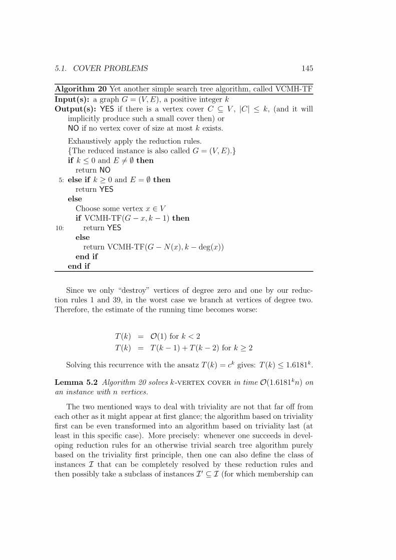
5.1. COVER PROBLEMS 145
Algorithm 20 Yet another simple search tree algorithm, called VCMH-TF
Input(s): a graph G = (V,E), a positive integer kOutput(s): YES if there is a vertex cover C ⊆ V , |C| ≤ k, (and it will
implicitly produce such a small cover then) orNO if no vertex cover of size at most k exists.
Exhaustively apply the reduction rules.The reduced instance is also called G = (V,E).if k ≤ 0 and E 6= ∅ then
return NO
5: else if k ≥ 0 and E = ∅ thenreturn YES
elseChoose some vertex x ∈ Vif VCMH-TF(G− x, k − 1) then
10: return YES
elsereturn VCMH-TF(G−N(x), k − deg(x))
end ifend if
Since we only “destroy” vertices of degree zero and one by our reduc-tion rules 1 and 39, in the worst case we branch at vertices of degree two.Therefore, the estimate of the running time becomes worse:
T (k) = O(1) for k < 2
T (k) = T (k − 1) + T (k − 2) for k ≥ 2
Solving this recurrence with the ansatz T (k) = ck gives: T (k) ≤ 1.6181k.
Lemma 5.2 Algorithm 20 solves k-vertex cover in time O(1.6181kn) onan instance with n vertices.
The two mentioned ways to deal with triviality are not that far off fromeach other as it might appear at first glance; the algorithm based on trivialityfirst can be even transformed into an algorithm based on triviality last (atleast in this specific case). More precisely: whenever one succeeds in devel-oping reduction rules for an otherwise trivial search tree algorithm purelybased on the triviality first principle, then one can also define the class ofinstances I that can be completely resolved by these reduction rules andthen possibly take a subclass of instances I ′ ⊆ I (for which membership can

146 CHAPTER 5. SEARCH TREES
be easily detected for a given instance), so that the trivial branching is onlydone as long as the instance under consideration is not in I ′. This way, oneobtains an algorithm based on the triviality last principle.
In our concrete example of the reduction rules 1 and 39, the class of graphsimmediately recognizable as being completely resolvable by these rule is theclass of graphs with maximum degree one. Let us remark here that the tworeduction rules—together with a trivial commitment (i.e., one branching) ofone vertex per cycle component—can be actually used to completely resolveall graphs of maximum degree two.
However, it is in general not possible to describe a sufficiently large class ofinstances of the class of instances that can be efficiently resolved (and hencetaken as a base for a simple search tree algorithm based on the triviality lastprinciple) merely by reduction rules, so that a conversion into a simple searchtree algorithm suitable for a triviality first approach is not always possible.In our example of vertex cover, it is not clear how to always deal withvertices of degree two, at least not at first glance. However, in this example,Chen, Kanj and Jia [86] (also see [251]) found a reduction rule that dealswith vertices of degree two:
Reduction rule 40 Let (G, k) be an instance of vertex cover. Let v ∈V (G) such that N(v) = u, w, i.e., deg(v) = 2.
• Assume that u /∈ N(w). Construct the graph G′ = G[u = w]−v. Then,the reduced instance is (G′, k − 1).
• If u ∈ N(w), then put u, w into the vertex cover and reduce to (G −(u, v, w), k− 2).
In fact, only the first part of Rule 40 is known as folding rule. The secondpart can be actually generalized as follows:
Reduction rule 41 If C ⊆ V (G) is a clique in a graph instance (G, k) ofVC such that C contains a vertex v with N [v] ⊆ C, then reduce to (G −C, k − (|C| − 1)).
Observe that Rule 41 can be again seen as a kind of kernelization schemerule, since the running time for detecting large cliques scales up exponentiallywith the size of the clique, although we do not know of an exploit for thisrule (in terms of analysis) if |C| > 3.
In other words, also Alg. 20 can be improved to run in time O(1.4656kn).The difference between the two approaches will become more transparent
when we do more involved subcase analysis in the following section. There, itmakes a difference whether certain vertices have been actually removed from

5.1. COVER PROBLEMS 147
the graph instance with the help of reduction rules, i.e., with the trivial-firstapproach, or whether these vertices are still around and may interact withother vertices in the graph.
Put in another way: while the triviality last approach is suitable forquickly developing search tree algorithms with reasonable running times, itis not easy (and actually, we don’t know of any such example) to furtherimprove on such search tree algorithms by any form of “clever branching.”By way of contrast, the triviality first approach (where the trivial cases areusually resolved by reduction rules) tends to lead to running times that areworse than the ones from the triviality last approach. However, they mightbe improvable by clever branching, as seen below in many instances.
At this stage, let us mention that it is also possible to combine both ap-proaches, leading to the following, typical general scheme detailed in Alg. 21that first applies reduction rules and then only branches at non-trivial cases:
Algorithm 21 A simple search tree algorithm, called VCMH-TD
Input(s): a graph G = (V,E), a positive integer kOutput(s): YES if there is a vertex cover C ⊆ V , |C| ≤ k, (and it will
implicitly produce such a small cover then) orNO if no vertex cover of size at most k exists.
Exhaustively apply the reduction rules.The reduced instance is also called G = (V,E).if Gis trivial then
resolve G deterministically in polynomial time5: else
Choose some vertex x ∈ Vif VCMH-TD(G− x, k − 1) then
return YES
else10: return VCMH-TD(G−N(x), k − deg(x))
end ifend if
As within algorithm VCMH-TL (see Alg. 20), triviality basically meansto have maximum degree two. Observe that we now could subsume the othertrivial cases (basically, when there are no edges left over) under this headline.The analysis of VCMH-TL basically transfers, so that the exponential partof the running time can be estimated as T (k) ≤ 1.4656k.
Lemma 5.3 Algorithm 21 solves k-vertex cover in time O(1.4656kn) onan instance with n vertices.
148 CHAPTER 5. SEARCH TREES
This scheme is typical for the top-down approaches discussed in Sec. 5.3.The point is that the branching part itself is still rather trivial, where thispart becomes really tricky with algorithms developed by a rather bottom-up approach. We will see a couple of examples for this from the followingsubsection on.
One peculiar important property shared by all three algorithms VCMH-TL, VCMH-TF and VCMH-TD is that their correctness immediately trans-fers from the correctness of the basic algorithm VCMH as long as
• the reduction rules are sound and
• the algorithms for solving the trivial cases are correct and properlycalled from the main algorithm.
This is different from the bottom-up approach we present in the next sub-section(s), where the correctness of the over-all algorithm must be proven, inaddition.
Let us finally mention that it is actually hard to pin down the sourcesof this subsection: vertex cover is simply the standard example for pa-rameterized algorithmics. What might be new, however, is the stress of thestrategies (triviality first versus triviality last) how to improve on parame-terized search tree algorithms.
5.1.2 The time analysis of search tree algorithms
In this section, we will first try to generalize our observations on how toanalyze the running time of search tree algorithms and then apply our resultsto the analysis of satisfiability problem with clauses of size three(clause parameterization) algorithms.
In the cases we have seen so far, it was not hard to obtain recurrences ofthe form:
T (k) ≤ α1T (k − 1) + α2T (k − 2) + · · ·+ α`T (k − `) (5.1)
for the size T (k) of the search tree (which can be measured in terms of thenumber of leaves of the search tree, since that number basically determinesthe running time of a search tree based algorithm).
More specifically, αi is a natural number that indicates that in αi of the∑j αj overall branches of the algorithm, the parameter value k got decreased
by i. Notice that, whenever ` = 1, it is quite easy to find an estimate forT (k), namely αk1. But how can we deal with the more general case? A recipeis contained in Alg. 22.
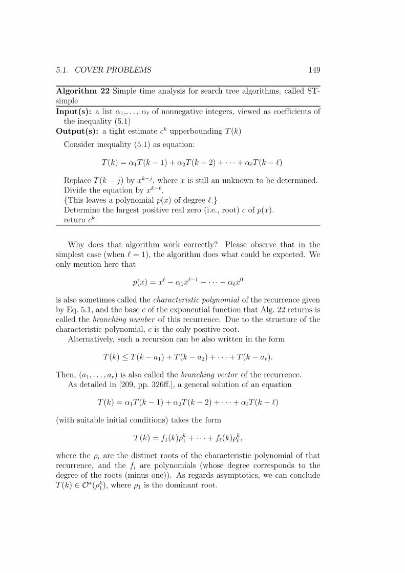
5.1. COVER PROBLEMS 149
Algorithm 22 Simple time analysis for search tree algorithms, called ST-simple
Input(s): a list α1,. . . , α` of nonnegative integers, viewed as coefficients ofthe inequality (5.1)
Output(s): a tight estimate ck upperbounding T (k)
Consider inequality (5.1) as equation:
T (k) = α1T (k − 1) + α2T (k − 2) + · · · + α`T (k − `)
Replace T (k − j) by xk−j, where x is still an unknown to be determined.Divide the equation by xk−`.This leaves a polynomial p(x) of degree `.Determine the largest positive real zero (i.e., root) c of p(x).return ck.
Why does that algorithm work correctly? Please observe that in thesimplest case (when ` = 1), the algorithm does what could be expected. Weonly mention here that
p(x) = x` − α1x`−1 − · · · − α`x
0
is also sometimes called the characteristic polynomial of the recurrence givenby Eq. 5.1, and the base c of the exponential function that Alg. 22 returns iscalled the branching number of this recurrence. Due to the structure of thecharacteristic polynomial, c is the only positive root.
Alternatively, such a recursion can be also written in the form
T (k) ≤ T (k − a1) + T (k − a2) + · · · + T (k − ar).
Then, (a1, . . . , ar) is also called the branching vector of the recurrence.As detailed in [209, pp. 326ff.], a general solution of an equation
T (k) = α1T (k − 1) + α2T (k − 2) + · · · + α`T (k − `)
(with suitable initial conditions) takes the form
T (k) = f1(k)ρk1 + · · · + f`(k)ρ
k` ,
where the ρi are the distinct roots of the characteristic polynomial of thatrecurrence, and the fi are polynomials (whose degree corresponds to thedegree of the roots (minus one)). As regards asymptotics, we can concludeT (k) ∈ O∗(ρk1), where ρ1 is the dominant root.

150 CHAPTER 5. SEARCH TREES
The exact mathematical reasons can be found in the theory of polynomialroots, as detailed in [209, 183, 210, 266]. It is of course also possible to checkthe validity of the approach by showing that T (k) ≤ ρk for the obtainedsolution ρ by a simple mathematical induction argument.
There are two more general settings which we will encounter in this Ha-bilitationsschrift:
• Due to case distinctions that will play a key role for designing refinedsearch tree algorithms, the recurrences will then take the form
T (k) ≤ maxf1(k), . . . , fr(k),where each of the fi(k) is of the form
fi(k) = αi,1T (k − 1) + αi,2T (k − 2) + · · ·+ αi,`T (k − `).
Such a recurrence can be solved by r invocations of Alg. 22, each timesolving T (k) ≤ fi(k). This way, we get r upperbounds T (k) ≤ cki .Choosing c = maxc1, . . . , cr is then a suitable upperbound.
• We might have systems of equations. In its most general form, thesewill again include maximum operators that can be treated as explainedin the previous point. Then, we are left with solving systems like
T `(k) ≤r∑
i=1
f `i (k),
where each of the f `i (k) is of the form
f `i (k) = αi,`,1Ti(k − 1) + αi,`,2T
i(k − 2) + · · ·+ αi,`,q`Ti(k − q`),
where 1 ≤ i, ` ≤ r. We shall follow the approach of first transformingthis set of mutual recurrences into a single recurrence for the maincomponent (usually T 1) only, by treating all involved inequalities asequalities. Then, we again apply Alg. 22.
We should like to remark that this is not the only way of dealing withsets of linear recurrence equations that involve an auxiliary parame-ter `. For instance, Kullmann and Wahlstrom included this auxiliaryparameter by deriving a single recurrence equation from a set of re-currence equations in their algorithm analysis [266, 373], trading off `against k, so to speak. Sometimes, even more involved methods tai-lored to the specific analysis of a certain algorithm may be worthwhilepursuing, as can be seen with the algorithm analysis of Monien andSpeckenmeyer, see [296]. A more general and abstract approach calledquasiconvex method was recently exhibited by Eppstein [155].

5.1. COVER PROBLEMS 151
Let us finally return to satisfiability problem with clauses ofsize three (clause parameterization), the warm-up problem of thischapter. By the techniques developed so far for VC, the following result canbe easily seen:
Theorem 5.4 Alg. 15 solves a satisfiability problem with clausesof size three (clause parameterization) instance (F,X, k) in timeO∗(2k).
We already mentioned that there are simple strategies to improve onthis running time. One simple observation relies on the fact that, whenevera particular variable x always only occurs as say a positive literal in theformula F , then we can set x to true (without any further need to branch),this way simplifying the formula (possibly decreasing the number of clauseswith three variables). This motivates the following reduction rule:
Reduction rule 42 Let (F,X, k) be an instance of satisfiability prob-lem with clauses of size three (clause parameterization) andx ∈ X.
• If x only appears as a positive literal in the formula F , then set x totrue, remove all clauses in which x appears from F , remove x from Xand reduce the parameter by the number of clauses of size three in Fin which x appeared.
• If x only appears as a negative literal in the formula F , then set x tofalse, remove all clauses in which x appears from F , remove x from Xand reduce the parameter by the number of clauses of size three in Fin which x appeared.
Similarly, the following observation is helpful (although it will not di-rectly affect the analysis of the modified search tree algorithm for 3-SAT(clause)):
Reduction rule 43 Let (F,X, k) be an instance of satisfiability prob-lem with clauses of size three (clause parameterization) andx ∈ X. If C is a clause that contains only the variable x, then do one of thefollowing things:
• If x and x are contained in C, then remove C from F (only affectingthe parameter if C contained three literals).
• If only x is contained in C, then set x to true, remove C from F andx from X (only affecting the parameter if C contained three literals).

152 CHAPTER 5. SEARCH TREES
• If only x is contained in C, then set x to false, remove C from F andx from X (only affecting the parameter if C contained three literals).
In fact, the first case of the previous rule can be formulated more generallyas follows:
Reduction rule 44 Let (F,X, k) be an instance of satisfiability prob-lem with clauses of size three (clause parameterization) andx ∈ X. Assume that Rule 43 does not apply. If x and x are containedin C, then remove x and x from C, this way modifying F . Decrement theparameter (by one).
The rules themselves are not new but can be found in basically any al-gorithm dealing with satisfiability problems. The correctness of the pro-posed modified search tree procedure for satisfiability problem withclauses of size three (clause parameterization) relies on the sound-ness of the reduction rules. The proof of the following lemma is left to thereader.
Lemma 5.5 Let (F,X, k) be an instance of satisfiability problem withclauses of size three (clause parameterization). Let (F ′, X ′, k′)be obtained from (F,X, k) by applying either of the rules 42 or 43 or 44 to(F,X, k). Then, (F,X, k) is satisfiable if and only if (F ′, X ′, k′) is satisfiable.
If we now modify Alg. 15 by adding inbetween lines 5 and 6 of thatprocedure the following line of code:
Exhaustively apply rules 42, 43 and 44;the resulting instance is also named (F, k).1
then we arrive at an algorithm for which we can prove:
Theorem 5.6 The modified version of Alg. 15 solves a satisfiability prob-lem with clauses of size three (clause parameterization) instance(F,X, k) in time O∗(1.6182k).
Proof. (Sketch) The correctness of the procedure directly follows from thecorrectness of Alg. 15 and the soundness of the reduction rules.
Before branching, the instance (F, k) is reduced. In particular, this meansthat the variable x we choose is contained both as a positive and a negativeliteral; more precisely, there is one clause C in which x occurs as a positiveliteral and one clause C ′ in which x occurs as a negative literal x (otherwise,one of the reduction rules would trigger).
1Observe that in the search tree algorithm, we do not explicitly specify the set ofvariables X as an argument, since this can be implicitly deduced from the set of clauses.

5.1. COVER PROBLEMS 153
Now, we consider two cases:
• The two clauses C and C ′ mentioned above both contain three vari-ables. Then, we will arrive at the following recursion for limiting thesize of the search tree:
T (k) ≤ 2T (k − 2).
Namely, irrespectively of whether we set x to true or false, at least twoclauses of size three will vanish.
• W.l.o.g., consider the case that C contains three variables but C ′ con-tains two variables. Now, in the branch that x is set to true, C ′ = x∨ `can only be satisfied by setting the variable y of ` accordingly. Accord-ing to the reduction rules, y will appear in another clause Cy; moreprecisely, if ` = y, y will show up in Cy, and if ` = y, y will showup in Cy. If Cy contains only one other literal z, the argument willrepeat, since the fixing of y will also fix z: possibly, the whole instancewill be resolved this way. If not, finally a clause C ′′ will be reached inthis sequence (in the simplest case, this is already Cy) that containsthree literals. This clause C ′′ will be turned into a clause with only twoliterals.
In the branch that x is set to false, nothing is gained. Altogether, thisbranch leads to the following recursion for limiting the size of the searchtree:
T (k) ≤ T (k − 1) + T (k − 2).
Due to T (k− 1) ≥ T (k− 2), the worst case is obviously given by the secondrecursion, which gives the claimed result.
5.1.3 weighted vertex cover
Problem name: weighted vertex cover (WVC)Given: A graph G = (V,E) with vertex weights ω : V → R≥1
Parameter: a positive integer kOutput: Is there a vertex cover C ⊆ V with ω(C) ≤ k?
In the following, the weight function ω will also be used for sets of verticesas argument.
The interesting thing of this weighted version of vertex cover—andin contrast with the unweighted case—is that of the two simple reductionrules for VC we listed above, only the rule 1 for isolates is still valid. The

154 CHAPTER 5. SEARCH TREES
problem with the degree-1 rule 39 is that there may be degree-1 vertices ofrelatively small weight whose inclusion in the vertex cover is actually betterthan taking its heavy-weight neighbor.
Yet, the simple VCMH algorithm is also valid in this case, since stilleach edge needs to be covered. Moreover, even the more sophisticated Algo-rithm 19, called VCMH-TL, based on the triviality last principle, togetherwith the analysis is still valid, although a little care has to be applied to thetrivial cases, i.e., the graph with maximum degree of two. Now, for pathsactually some little dynamic programming must be performed (due to theinavailability of the second reduction rule for the weighted case as explainedabove), starting from one end of the path, working through towards theother. The according easily derived algorithm is left as an exercise, see [309].Similarly, we can also develop an analogue to Alg. 21: again, the proof ofthe correctness of the algorithm itself and its running time upperbounds areeasy to obtain.
Lemma 5.7 Variants of Algorithm 19 and Algorithm 21 solve k-weightedvertex cover in time O(1.4656kn) on an instance with n vertices.
However, the triviality first principle is harder to apply, since only Rule 1is valid in the weighted case. Nonetheless, by using a bottom-up approach,the currently best exact algorithm for weighted vertex cover was de-veloped in [309], the variant of which that uses polynomial space is explicitlyshown in Alg. 26 and the subsequently listed subroutines.
5.1.4 constraint bipartite vertex cover
Let us reconsider the problem constraint bipartite vertex cover in-troduced in Chap. 3. We already mentioned that an O(2k1+k2k1k2 + (k1 +k2)|G|) has been developed by people working in that area, much predat-ing the systematic development of FPT algorithms. This algorithm—as thestated running time indicates, was a combination of a kernelization and asearch tree algorithm. Let us focus here on the search tree part.
In fact, it is not hard to see how to obtain a O∗(2k1+k2) algorithm: thebasic observation for the development of Alg. 16 was that every edge u, vneeded to be covered, so branching into the to cases “u comes into the cover”or “v comes into the cover” is a complete case distinction. The same obser-vation is also true for constraint bipartite vertex cover. Since ineither branch, k1 or k2 is decreased, the claimed running time follows.
How can this simple algorithm be improved? Let us (again) try thetriviality last approach. To this end, we need to be able to deal with simple

5.1. COVER PROBLEMS 155
cases, where “simple” means graphs with a low maximum degree. If thesesimple cases can be dealt with in polynomial time, then it is clear that thesimple branching strategy exhibited in Alg. 20 transfers to this case, as well.
Lemma 5.8 constraint bipartite vertex cover can be solved in poly-nomial time on forests of cycle and path components.
Proof. (Sketch) First observe that this assertion is not completely trivialin this two-parameter vertex cover variant. For example, a cycle C8 oflength eight would need every second vertex to be put into the cover, seen asan instance of vertex cover. Hence, 4 vertices would need to be put intoa cover. But this would not be possible if say k1 = k2 = 2. Hence, if k1 < 4and k2 < 4, three vertices of one kind and two of the other would need to beput into a cover for C8.
This is more generally true: if the parameter values k1 and k2 shouldsuffice to cover a cycle component Cm, then if m ≤ 2k1 or m ≤ 2k2, the cyclecan be optimally covered (as if it were a vertex cover instance); otherwise,if m−2 ≤ 2(k1+k2), then such a cover can be constructed for Cm (as CBVCinstance), and how this “change” between taking one sort of vertices or theother one is performed is arbitrary (where only “using” at least two verticesfrom each sort makes sense). Finally, if m−2 > 2(k1+k2), then no solution ispossible. This gives the following strategy for solving forests of cycles (withcurrent parameter (k1, k2):
Select a cycle C of smallest length m.Let k` be the smaller among k1 and k2.if m ≤ 2k` then
Cover C by taking m/2 vertices from C from vertex set V`.else if m− 2 ≤ 2(k1 + k2) then
Use k` vertices from V` and (m+ 1)/2− k` from the other sort to coverC.
elseThe instance has NO solution.
end if
Why did we choose to first treat small cycles? As we argued above, whenit is not possible to cover a cycle by vertices from one type, we would need(overall) one more vertex to cover that cycle. This observation is independentof the size of the cycles. Hence, leaving the large cycles for the end is betterthan the converse strategy. Moreover, it shows that at most one cycle willbe covered non-optimally.
Similar considerations can be made for paths, although here the situationis slightly more intricate: there are basically three types of paths that need

156 CHAPTER 5. SEARCH TREES
different considerations: (1) paths of odd length, (2) paths of even lengththat begin and end with vertices from V1, and (3) paths of even length thatbegin and end with vertices from V2. The additional problem is that pathsof even length can be covered optimally (as a VC instance) by taking everysecond vertex into the cover, starting with the second vertex on a path; fora path of length m, m/2 vertices are needed this way. If there are, however,not “sufficiently” many vertices of a particular kind available (in the bipartitecase), one more vertex will be needed in the cover. The situation is differentwith paths of odd length: there, the additional constraints put within theCBVC problem (in contrast with VC) do not incur additional costs; moreprecisely, a path of odd length as a vertex cover of size k if and only if it issolvable as part of a constraint bipartite vertex cover instance, withany parameter values k1 and k2 that satisfy k1 + k2 = k.
To get a really efficient algorithm, we would therefore stick to the follow-ing strategy:
1. Solve all paths of even length, first solving short path components.
2. Solve cycles, first solving short cycles (see details above).
3. Solve paths of odd length.
Details are left to the reader. The claimed polynomial running time is thenobvious. In fact, the polynomial is pretty small; assuming that the compo-nents are already sorted by size, it is even linear.
This gives us the Algorithm listed in Alg. 23. We can conclude:
Theorem 5.9 constraint bipartite vertex cover can be solved intime O∗(1.4656k1+k2).
By a much more involved case analysis, a search tree algorithm wasdeveloped for constraint bipartite vertex cover that runs in timeO∗(1.3999k), see [180]. We omit stating the rather complicated algorithmhere. However, let us mention that it would be another perfect example ofthe bottom-up approach illustrated in the next section.
When it comes to the analysis of search tree algorithms, there is one ingre-dient of [180] that is worth mentioning, since it might be applicable to othersearch tree algorithms, as well, the so-called bonus point trick. Namely, thesearch tree algorithm is basically an intricate implementation of the triviality-last principle, combined with a sophisticated analysis of many different localsituations. In this sophisticated analysis, from time to time it happens thatcomponents consisting of at least two vertices, each of degree at most two,

5.1. COVER PROBLEMS 157
Algorithm 23 A still simple search tree algorithm for CBVC, called CBVC-TLInput(s): a bipartite graph G = (V1, V2;E), positive integers k1 and k2
Output(s): YES iff there is a vertex cover (C1, C2) ⊆ V1×V2, |C1| ≤ k1 and|C2| ≤ k2
if k1 + k2 ≤ 0 and E 6= ∅ thenreturn NO
else if k1 + k2 ≥ 0 and E = ∅ thenreturn YES
5: else if possible thenChoose vertex x ∈ V1 ∪ V2 such that deg(x) ≥ 3.if x ∈ V1 thend = (1, 0)
else10: d = (0, 1)
end ifif CBVC-TL(G− x, (k1, k2) − d) then
return YES
else15: return CBVC-TL(G−N(x), (k1, k2) − deg(x)((1, 1) − d))
end ifelsevertex selection not possible maximum degree is 2resolve deterministically according to Lemma 5.8
20: end if
are split off. When this happens, we can (already) reduce the parameter byone, since we might (as well) already at that point completely resolve thatcomponent, and we would need at least one vertex to come into the cover forsuch a solution. Hence, we can count this as a “bonus point,” although wewill only later actually “use up” this bonus point for covering that compo-nent. Hence, formally the concrete parameter value no longer corresponds tothe number of vertices put into the (partial) cover (implicitly) constructedso far on some branching path.
If one further requires that a solution to constraint bipartite ver-tex cover is only accepted if it is also a minimum vertex cover (an assump-tion accepted in [279] to get a better solving strategy (heuristic) based onthe Dulmage-Mendelsohn decomposition for bipartite graphs), then even anO∗(1.26k) algorithm was derived [85] (their algorithm also makes use of theDulmage-Mendelsohn decomposition); however, it appears to be question-
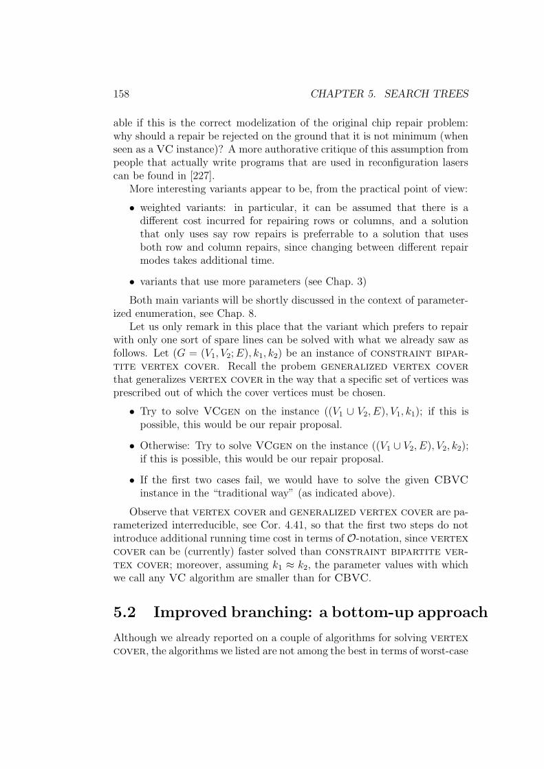
158 CHAPTER 5. SEARCH TREES
able if this is the correct modelization of the original chip repair problem:why should a repair be rejected on the ground that it is not minimum (whenseen as a VC instance)? A more authorative critique of this assumption frompeople that actually write programs that are used in reconfiguration laserscan be found in [227].
More interesting variants appear to be, from the practical point of view:
• weighted variants: in particular, it can be assumed that there is adifferent cost incurred for repairing rows or columns, and a solutionthat only uses say row repairs is preferrable to a solution that usesboth row and column repairs, since changing between different repairmodes takes additional time.
• variants that use more parameters (see Chap. 3)
Both main variants will be shortly discussed in the context of parameter-ized enumeration, see Chap. 8.
Let us only remark in this place that the variant which prefers to repairwith only one sort of spare lines can be solved with what we already saw asfollows. Let (G = (V1, V2;E), k1, k2) be an instance of constraint bipar-tite vertex cover. Recall the probem generalized vertex coverthat generalizes vertex cover in the way that a specific set of vertices wasprescribed out of which the cover vertices must be chosen.
• Try to solve VCgen on the instance ((V1 ∪ V2, E), V1, k1); if this ispossible, this would be our repair proposal.
• Otherwise: Try to solve VCgen on the instance ((V1 ∪ V2, E), V2, k2);if this is possible, this would be our repair proposal.
• If the first two cases fail, we would have to solve the given CBVCinstance in the “traditional way” (as indicated above).
Observe that vertex cover and generalized vertex cover are pa-rameterized interreducible, see Cor. 4.41, so that the first two steps do notintroduce additional running time cost in terms of O-notation, since vertexcover can be (currently) faster solved than constraint bipartite ver-tex cover; moreover, assuming k1 ≈ k2, the parameter values with whichwe call any VC algorithm are smaller than for CBVC.
5.2 Improved branching: a bottom-up approach
Although we already reported on a couple of algorithms for solving vertexcover, the algorithms we listed are not among the best in terms of worst-case

5.2. IMPROVED BRANCHING: A BOTTOM-UP APPROACH 159
running times. Still, VCMH-TL and VCMH-TD are significantly better thanthe first improved branching algorithms, as reported, e.g., in [33, Theorem 1].Note that it was the mentioned algorithm of Balasubramanian, Fellows andRaman that was chosen in the parallel implementation of vertex coveralgorithms as described in [80] in the dispatching phase, also see Sec. 8.5.2.
Let us now first present the second algorithm introduced in [33] as a kindof random example of the bottom-up approach, see Alg. 24.
The correctness of this algorithm must be argued on a case-by-case basis.For example, in lines 5 through 21, the case that x has degree two is discussed.In the corresponding subcases that lead to different branching scenarios, thesubcase that y and z are both having no neighbor besides x is not mentioned.Nonetheless, the case distinction is complete, since this evidently means thatbot y and z have degree one, and this case got treated in the very first casedistinction. Observe that we could replace basically the first 21 lines of codeby referring to the reduction rules we presented for getting rid of vertices ofdegree of at most two in the case of vertex cover.
However, it is clear that in contrast to the simple algorithms we consideredup to now, a formal correctness proof is pretty tedious. Moreover, observethat not all details of the algorithm have been given; rather, the lines ofpseudo-code should give an impression of how complicated algorithms tendto be that are optimized according to the bottom-up approach.
The algorithm we presented here is not the one for which the smallestupper bound has been shown. When restricting oneself on algorithms thatonly use polynomial space, the currently best algorithm (that needs onlypolynomial space) is published in [86] (also see Kanj’s PhD Thesis [251])and runs in time O∗(1.2852k). However, if exponential space is allowed,running times down to O∗(1.2745k) are possible [77]. Those algorithms arenot conceptually (and not from the point of view of implementing them)simpler than the one we listed to some detail. Moreover, it can be doubtedif the exponential space requirement (of course, in the area of parameterizedalgorithmics, exponential space rather means “parameterized space”) of thetheoretically best algorithm pays off in practice, since time may be eaten upby page swapping.
As a second example of this approach (that is still prominent in theliterature) we reconsider weighted vertex cover. By using a complicatedalgorithm, Niedermeier and Rossmanith were able to prove the followingtheorem:
Theorem 5.10 weighted vertex cover can be solved in time O(1.3954k+kn).

160 CHAPTER 5. SEARCH TREES
Algorithm 24 An involved search tree algorithm, called VCBFR
Input(s): a graph G = (V,E), a positive integer kOutput(s): YES if there is a vertex cover C ⊆ V , |C| ≤ k, (and it will
implicitly produce such a small cover then) orNO if no vertex cover of size at most k exists.
if there is a vertex x of degree zero thenreturn VCBFR(G− x, k)
else if there is a vertex x of degree one thenreturn VCBFR(G−N [x], k − 1)
5: else if there is a vertex x of degree two thenLet y and z be the two neighbors.if y and z are neighbors theny and z can go into vertex cover.return VCBFR(G− x, y, z, k − 2)
10: else if |(N(y) ∪N(z)) \ x| ≥ 2 thenEither y, z are part of the cover or N(y, z).if VCBFR(G− x, y, z, k − 2) then
return YES
else15: return VCBFR(G−N [x, y], k − 3)
end ifelsey and z have one other neighbor a besides x.x and a can go into vertex cover.
20: return VCBFR(G−N [x, y], k − 2)end if
else if there is a vertex x ∈ V with deg(x) ≥ 5 thenif VCBFR(G− x, k − 1) then
return YES
25: elsereturn VCBFR(G−N [x], k − deg(x))
end ifelse if there is a vertex x ∈ V with deg(x) = 3 thenLet x1, x2, x3 be the neighbors of x.
30: See next algorithm.elseThere is a vertex x ∈ V with deg(x) = 4.This case is similar and hence omitted.
end if
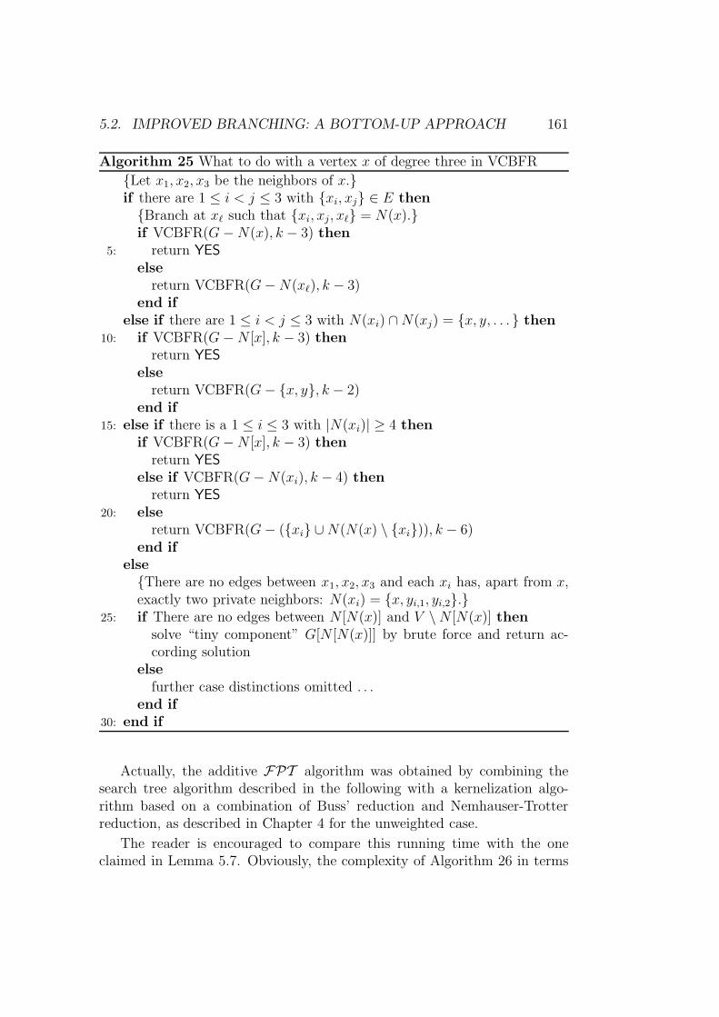
5.2. IMPROVED BRANCHING: A BOTTOM-UP APPROACH 161
Algorithm 25 What to do with a vertex x of degree three in VCBFR
Let x1, x2, x3 be the neighbors of x.if there are 1 ≤ i < j ≤ 3 with xi, xj ∈ E thenBranch at x` such that xi, xj, x` = N(x).if VCBFR(G−N(x), k − 3) then
5: return YES
elsereturn VCBFR(G−N(x`), k − 3)
end ifelse if there are 1 ≤ i < j ≤ 3 with N(xi) ∩N(xj) = x, y, . . . then
10: if VCBFR(G−N [x], k − 3) thenreturn YES
elsereturn VCBFR(G− x, y, k − 2)
end if15: else if there is a 1 ≤ i ≤ 3 with |N(xi)| ≥ 4 then
if VCBFR(G−N [x], k − 3) thenreturn YES
else if VCBFR(G−N(xi), k − 4) thenreturn YES
20: elsereturn VCBFR(G− (xi ∪N(N(x) \ xi)), k − 6)
end ifelseThere are no edges between x1, x2, x3 and each xi has, apart from x,exactly two private neighbors: N(xi) = x, yi,1, yi,2.
25: if There are no edges between N [N(x)] and V \N [N(x)] thensolve “tiny component” G[N [N(x)]] by brute force and return ac-cording solution
elsefurther case distinctions omitted . . .
end if30: end if
Actually, the additive FPT algorithm was obtained by combining thesearch tree algorithm described in the following with a kernelization algo-rithm based on a combination of Buss’ reduction and Nemhauser-Trotterreduction, as described in Chapter 4 for the unweighted case.
The reader is encouraged to compare this running time with the oneclaimed in Lemma 5.7. Obviously, the complexity of Algorithm 26 in terms

162 CHAPTER 5. SEARCH TREES
of
• proving the correctness of the algorithm,
• proving the running time of the algorithm and
• implementing the algorithm (without introducing any errors)
is much higher. It could be even questioned if the running time would bemuch better (compared to Algorithms 19 and 21) in practice, since muchmore work has to be done in each node of the search tree.
To simplify the notations when stating the algorithm of Niedermeier andRossmanith, we write
WVC-NR-branch at x
to abbreviate:
if WVC-NR(G− x, k − ω(x)) thenreturn YES
elsereturn WVC-NR(G−N(x), k − ω(N(x)))
end if
The reader is encouraged to actually prove the correctness of the listedalgorithm. Especially, this means that one has to argue why the many casedistinctions are actually capturing all cases. Also, the quality of the branch-ings would have to be considered. The worst case branching can be describedby the recurrence
T (k) ≤ 2T (k − 3) + T (k − 4),
which gives the claimed upper bound on the running time.Let us finally report on interesting automatic approaches that were re-
cently developed to analyze local branching scenarios, see [211].

5.2. IMPROVED BRANCHING: A BOTTOM-UP APPROACH 163
Algorithm 26 An elaborated search tree algorithm, called WVC-NR
Input(s): a graph G = (V,E) with real vertex weights ω : V → R withminω(V ) ≥ 1, a positive real k
Output(s): YES if there is a vertex cover C ⊆ V , ω(C) ≤ k, (and it willimplicitly produce such a small cover then) orNO if no vertex cover of weight at most k exists.
Resolve all graph components of maximum degree two in polynomialtime. (∗)Resolve all graph components with no more than six vertices in constanttime.The new (reduced) instance is also called G = (V,E).if k ≤ 0 and E 6= ∅ then
5: return NO
else if k ≥ 0 and E = ∅ thenreturn YES
else if possible thenChoose some vertex x ∈ V with deg(x) ≥ 4
10: WVC-NR-branch at xelse if possible then
Choose some vertex x ∈ V with deg(x) = 1.Let a denote the unique neighbor of x.return WVC-NR-deg1(G, x, a, k)
15: else if possible thenChoose some triangle a, b, c ∈ Vreturn WVC-NR-triangle(G, a, b, c, k)
elsereturn WVC-NR-notriangles(G, k)
20: end if

164 CHAPTER 5. SEARCH TREES
Algorithm 27 A subroutine for WVC-NR, called WVC-NR-deg1
Input(s): a graph G = (V,E) with real vertex weights ω : V → R withminω(V ) ≥ 1 of maximum degree three without “easy components”, adegree one vertex x with neighbor a, a positive real k
Output(s): YES if there is a vertex cover C ⊆ V , ω(C) ≤ k, (and it willimplicitly produce such a small cover then) orNO if no vertex cover of weight at most k exists.
if ω(x) ≥ ω(a) thenreturn WVC-NR(G− a, k − ω(a))
else if deg(a) = 2 thenLet y denote the first vertex on the path starting with x, a, . . . withdeg(y) 6= 2; due to step (∗), deg(y) > 2.
5: WVC-NR-branch at yelsedeg(a) = 3if at least one of a’s neighbors (say y) has degree three then
WVC-NR-branch at y10: else if a’s other neighbors y and y′ have degree two then
Let N(y) = a, z and N(y′) = a, z′.if ω(a) ≥ 2 OR ω(y) ≥ ω(z) OR ω(y′) ≥ ω(z′) then
WVC-NR-branch at aelse
15: ω(y) < ω(z) AND ω(y′) < ω(z′)WVC-NR-branch at x
end ifelseOne of a’s other neighbors, say y, has degree two and one, say y ′,has degree one. This case is similar to deg(a) = 2 and is henceomitted.
20: end ifend if

5.2. IMPROVED BRANCHING: A BOTTOM-UP APPROACH 165
Algorithm 28 A subroutine for WVC-NR, called WVC-NR-triangle
Input(s): a graph G = (V,E) with real vertex weights ω : V → R withminω(V ) ≥ 1 of maximum degree three without “easy components”,with a triangle a, b, c, a positive real k
Output(s): YES if there is a vertex cover C ⊆ V , ω(C) ≤ k, (and it willimplicitly produce such a small cover then) orNO if no vertex cover of weight at most k exists.
Let (w.l.o.g.) deg(a) ≤ deg(b) ≤ deg(c) = 3.if deg(b) = 2 thenone vertex in the triangle has degree threeif ω(a) ≤ ω(b) then
5: return WVC-NR(G−N(a), k − ω(N(a)))else
return WVC-NR(G−N(b), k − ω(N(b)))end if
else if deg(a) = 2 then10: two vertices in the triangle have degree two
WVC-NR-branch at belseall vertices in the triangle have degree twoassume, w.l.o.g., ω(a) ≤ ω(b) ≤ ω(c)
15: WVC-NR-branch at aend if

166 CHAPTER 5. SEARCH TREES
Algorithm 29 A subroutine for WVC-NR, called WVC-NR-notriangles
Input(s): a graph G = (V,E) with real vertex weights ω : V → R withminω(V ) ≥ 1 of maximum degree three without “easy components”,without triangles, a positive real k
Output(s): YES if there is a vertex cover C ⊆ V , ω(C) ≤ k, (and it willimplicitly produce such a small cover then) orNO if no vertex cover of weight at most k exists.
if possible thenChoose some vertex x with ω(x) ≥ 2.if deg(x) = 3 then
WVC-NR-branch at x5: else
deg(x) = 2; let N(x) = y, y′ with deg(y) ≤ deg(y′)WVC-NR-branch at y′
end ifelse
10: All vertices have weight less than two.if possible then
Choose two neighbors a and b with deg(a) = deg(b) = 2.Let x and y be the two endpoints of a path a and b are part of suchthat deg(x), deg(y) ≥ 3if x ∈ N [y] then
15: WVC-NR-branch at xelse
if WVC-NR(G− x, y, k − ω(x, y)) thenreturn YES
else if WVC-NR(G− (x ∪N(y)), k − ω(x ∪N(y))) then20: return YES
elsereturn WVC-NR(G−N(x), k − ω(N(x)))
end ifend if
25: end ifreturn WVC-NR-notriangles-ctd(G, k)
end if

5.2. IMPROVED BRANCHING: A BOTTOM-UP APPROACH 167
Algorithm 30 A subroutine for WVC-NR-notriangles, called WVC-NR-notriangles-ctd
if possible then
Choose three vertices x, y, z with deg(x) = deg(y) = deg(z) = 3 and two verticesa, b with N(a) = x, z and N(b) = y, z.if WVC-NR(G − x, y, z, k− ω(x, y, z)) then
return YES
5: else if WVC-NR(G− (x ∪N(y)), k − ω(x ∪N(y))) then
return YES
else
return WVC-NR(G−N(x), k − ω(N(x)))end if
10: else if possible then
Choose a vertex x with deg(x) = 3 and a vertex a ∈ N(x) with deg(a) = 2 andω(a) ≥ ω(x).WVC-NR-branch at x
else
We can find the following situation in G: vertices x, y, z with deg(x) = deg(y) =deg(z) = 3 and y ∈ N(z), a vertex a with N(a) = x, z and N(z) = a, b, y.
15: if deg(b) = 2 then
Let N(b) = c, z.if c = x then
if y ∈ N(x) then
WVC-NR-branch at y20: else
if WVC-NR(G − x, y, k − ω(x, y)) then
return YES
else if WVC-NR(G− (y ∪N(x)), k − ω(y ∪N(x))) then
return YES
25: else
return WVC-NR(G−N(y), k − ω(N(y)))end if
end if
else
30: if WVC-NR(G − x, y, z, c, k− ω(x, y, z, c)) then
return YES
else if WVC-NR(G− (N(y)), k − ω(N(y))) then
return YES
else
35: return WVC-NR(G−N(z), k − ω(N(z)))end if
end if
else
if WVC-NR(G − a, b, y, k− ω(a, b, y)) then
40: return YES
else if WVC-NR(G− (b ∪N(y)), k − ω(b ∪N(y))) then
return YES
else
return WVC-NR(G−N(b), k − ω(N(b)))45: end if
end if
end if

168 CHAPTER 5. SEARCH TREES
5.3 Improved branching: simple algorithms
The aim of this section is to develop very simple search tree algorithms. Dueto their simplicity, these algorithms are easily seen to be working correctly.Their time analysis, however, often involves either some thorough mathemat-ical background knowledge or a possible tough mathematical analysis.
If an involved time analysis is necessary, the algorithm development oftenproceeds in a top-down rather than bottom-up manner. This means that thecase analysis is guided by the need of the time analysis rather than by acollection of observations concerning local situations.
However, sometimes improved time analysis and actually slightly chang-ing (tuning) algorithms goes hand in hand. This is the actual topic of ourfirst example.
5.3.1 planar independent set
Recall that the greedy kernelization algorithm 6 was based on the well-knownfact that each planar graph has at least one vertex of degree at most five.This result can be also used to create a very simple search tree algorithm forplanar independent set, see Alg. 31.
The mentioned result on planar graphs shows that for any v that is pickedby the algorithm, |N [v]| ≤ 6, so that we can state:
Proposition 5.11 Alg. 31 solves planar independent set in time O(6k|G|).
Fortunately, some mathematicians gave a deeper analysis of the structureof planar graphs regarding vertices of small degree. In [6, Theorem 2], theauthors have shown the following result:
Theorem 5.12 Every connected plane graph with at least two vertices has
1. two vertices with degree sum at most 5, or
2. two vertices of distance at most two and with degree sum at most 7, or
3. a triangular face with two incident vertices with degree sum at most 9,or
4. two triangular faces neighbored via an edge u, v where the sum of thedegrees of u and v is at most 11.
Based on that theorem, we propose Algorithm 32:

5.3. IMPROVED BRANCHING: SIMPLE ALGORITHMS 169
Algorithm 31 A simple search tree algorithm for planar independentset, called PIS-ST-simple
Input(s): planar graph G = (V,E), positive integer kOutput(s): YES if G has an independent set I with |I| = k; NO otherwise
if k ≤ 0 thenreturn YES
else if V = ∅ thenreturn NO
5: elseLet v be a vertex of lowest degree in G.One vertex from N [v] will be in any maximal independent set.for all x ∈ N [v] doV ′ := N [x]
10: if PIS-ST-simple(G[V \ V ′], k − 1) thenreturn YES
end ifend forAll trials have failed.
15: return NO
end if
The correctness of the algorithm immediately follows from the quotedtheorem. The running time T of the new algorithm, measured in terms ofthe number of leaves of the search tree, satisfies
T (k) ≤ 4T (k − 1) + 6T (k − 2).
This recurrence can be solved, showing T (k) ≤ 5.1623k as claimed.This shows Proposition 5.13.
Proposition 5.13 Alg. 32 solves planar independent set within timeO(5.1623k|G|).
Unfortunately, we have to remark in this place that this is not the best al-gorithm for planar independent set that we are aware of. As mentionedbelow in Chap. 10, there are very cute algorithms for solving (general) max-imum independent set that run in time approximately O(1.2n). Since ncan be limited to 4k (see Alg. 7), a combination of these algorithms wouldoutperform the (admittedly still simple) algorithm that we presented here.However, note that even the full-fledged Alg. 32 is still close to trivial in com-parison with the quite sophisticated algorithms that should be implementedto enjoy the better running times.

170 CHAPTER 5. SEARCH TREES
Algorithm 32 A more advanced search tree algorithm for planar inde-pendent set, called PIS-ST
Input(s): planar graph G = (V,E), positive integer kOutput(s): YES if G has an independent set I with |I| = k; NO otherwise
if k ≤ 0 thenreturn YES
else if V = ∅ thenreturn NO
5: elseLet v be a vertex of lowest degree in G.One vertex from N [v] will be in any maximal independent set.if deg(v) ≤ 4 then
for all x ∈ N [v] do10: V ′ := N [x]
if PIS-ST(G[V \ V ′], k − 1) thenreturn YES
end ifend for
15: elseThe fourth case of Theorem 5.12 applies.Hence: N(v) = x, y, u, v1, v2such that N(u) = x, y, v, u1, u2, u3if PIS-ST(G[V \N [v]], k − 1) thenBranch 1: v in IS ?
20: return YES;else if PIS-ST(G[V \N [u]], k − 1) thenBranch 2: v is not in IS, but u ?return YES;
else if PIS-ST(G[V \N [x]], k − 1) then25: Branch 3: v, u is not in IS, but x ?
return YES;else if PIS-ST(G[V \N [y]], k − 1) thenBranch 4: v, u, x is not in IS, but y ?return YES;
30: elseNow v, u, x, y is not in IS, so one of the vi and one of the uj mustbe in a maximal independent set.for all i = 1, 2; j = 1, 2, 3 do
if PIS-ST(G[V \ (N [vi] ∪N [uj])], k − 2) thenreturn YES
35: end ifend forreturn NO
end ifend if
40: end if

5.3. IMPROVED BRANCHING: SIMPLE ALGORITHMS 171
The next subsection is devoted to planar dominating set. However,there is one kind of intermediate problem, namely planar independentdominating set:
Problem name: planar independent dominating set (PIDS)Given: A planar graph G = (V,E)Parameter: a positive integer kOutput: Is there a independent dominating set D ⊆ V with |D| ≤ k?
Clearly, this problem can be likewise called minimum maximal inde-pendent set, restricted to planar graphs. Now, observe that the searchtree algorithms we presented for planar independent set never actuallyrely on the fact that we actually look for a maximum independent set, sinceall branchings are based on the idea of finding a maximal independent set.We can therefore conclude:
Proposition 5.14 planar independent dominating set can be solvedin time O(5.1623k|G|).
Proof. Alg. 32 would have to be modified: the first four lines of the codeshould be replaced by the following four lines:
if k < 0 thenreturn NO
else if V = ∅ thenreturn YES
else. . .
end if
where the . . . contains the actual branching program. k < 0 means thatthere is no small independent dominating set. If k ≥ 0 and V = ∅, we havefound an independent dominating set. Otherwise, there exists a vertex onwhich we can branch.
This bound on the running time is actually better than the one of thealternative algorithm that looks amongst the dominating sets produced withthe algorithm presented in the next subsection for a dominating set thathappens to be independent. Moreover, the previous comments on producingbetter algorithms by relying on exact algorithms for maximum indepen-dent set do not apply here.
Special graph classes that allow polynomial-time algorithms for indepen-dent dominating set are considered in [55].

172 CHAPTER 5. SEARCH TREES
5.3.2 planar dominating set
The following exposition follows [11].In the case of dominating set, the situation seems more intricate than
with independent set or independent dominating set, where we couldsimply branch at a low-degree vertex u (as existing in planar graphs). Clearly,again, either u or one of its neighbors can be chosen to be in an optimaldominating set. However, removing u from the graph leaves all its neighborsbeing already dominated, but still also being suitable candidates for an opti-mal dominating set. This consideration leads us to formulate our search treeprocedure in a more general setting, where there are two kinds of vertices inour graph.
We stress this fact by partitioning the vertex set V of G into two disjointsets B and W of black and white vertices, respectively, i.e., V = B ] W ,where ] denotes disjoint set union. We will also call this kind of graph ablack and white graph.
Problem name: annotated dominating set (ADS)Given: A black and white graph G = (B ]W,E)Parameter: a positive integer kOutput: Is there a choice of at most k vertices V ′ ⊆ V = B ]Wsuch that, for every vertex u ∈ B, there is a vertex u′ ∈ N [u] ∩ V ′?In other words, is there a set of at most k vertices (which may beeither black or white) that dominates the set of black vertices?
In each step of the search tree, we would like to branch according to a lowdegree black vertex. This would work fine if we deal with a graph class, sothat we can guarantee the existence of a vertex u ∈ B ]W with deg(u) ≤ d.However, as long as not all vertices have degree bounded by d (as, e.g., thecase for graphs of bounded genus g, where only the existence of a vertex ofdegree at most dg is known), this vertex need not necessarily be black.
We consider the following reduction rules for simplifying annotateddominating set the on planar graphs. In developing the search tree, wewill always assume that we are branching from a “reduced instance;” thus,we are constantly simplifying the instance according to the reduction rulesgiven below (the details will be explained later). When a vertex u is placedin the dominating set D by a reduction rule, then the target size k for D isreduced to k − 1 and the neighbors of u are whitened.
(R1) Delete an edge between white vertices.
(R2) Delete a pendant white vertex, i.e., a vertex of degree one.
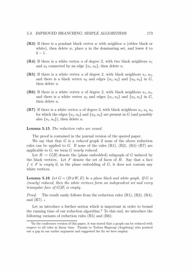
5.3. IMPROVED BRANCHING: SIMPLE ALGORITHMS 173
(R3) If there is a pendant black vertex w with neighbor u (either black orwhite), then delete w, place u in the dominating set, and lower k tok − 1.
(R4) If there is a white vertex u of degree 2, with two black neighbors u1
and u2 connected by an edge u1, u2, then delete u.
(R5) If there is a white vertex u of degree 2, with black neighbors u1, u3,and there is a black vertex u2 and edges u1, u2 and u2, u3 in G,then delete u.
(R6) If there is a white vertex u of degree 2, with black neighbors u1, u3,and there is a white vertex u2 and edges u1, u2 and u2, u3 in G,then delete u.
(R7) If there is a white vertex u of degree 3, with black neighbors u1, u2, u3
for which the edges u1, u2 and u2, u3 are present in G (and possiblyalso u1, u3), then delete u.
Lemma 5.15 The reduction rules are sound.
The proof is contained in the journal version of the quoted paper.We say that that G is a reduced graph if none of the above reduction
rules can be applied to G. If none of the rules (R1), (R2), (R4)–(R7) areapplicable to G, we term G nearly reduced.
Let H := G[B] denote the (plane embedded) subgraph of G induced bythe black vertices. Let F denote the set of faces of H. Say that a facef ∈ F is empty if, in the plane embedding of G, it does not contain anywhite vertices.
Lemma 5.16 Let G = (B ]W,E) be a plane black and white graph. If G is(nearly) reduced, then the white vertices form an independent set and everytriangular face of G[B] is empty.
Proof. The result easily follows from the reduction rules (R1), (R2), (R4),and (R7).
Let us introduce a further notion which is important in order to boundthe running time of our reduction algorithm.2 To this end, we introduce thefollowing variants of reduction rules (R5) and (R6):
2In the conference version of this paper, it was stated that a graph can be reduced withrespect to all rules in linear time. Thanks to Torben Hagerup (Augsburg) who pointedout a gap in our earlier argument and suggested the fix we here employ.

174 CHAPTER 5. SEARCH TREES
(R5′) If there is a white vertex u of degree 2, with black neighbors u1, u3
such that u1 has at most seven neighbors that have degree at least 4,and there exists a black vertex u2 and edges u1, u2 and u2, u3 inG, then delete u.
(R6′) If there is a white vertex u of degree 2, with black neighbors u1, u3
such that u1 has at most seven neighbors that have degree at least 4,and there exists a white vertex u2 and edges u1, u2 and u2, u3 inG, then delete u.
We say that thatG is a cautiously reduced graph if (R1), (R2), (R4), (R5′),(R6′), and (R7) cannot be applied anymore to G. Observe that Lemma 5.16is also valid for cautiously reduced graphs.
Lemma 5.17 Applying reduction rules (R1), (R2), (R4), (R5′), (R6′), and(R7), a given planar black and white graph G = (B]W,E) can be transformedinto a cautiously reduced graph G′ = (B′ ]W ′, E ′) in time O(n), where n isthe number of vertices in G.
Again, we skip details of the proof and refer to the journal version.The main theorem for proving the correctness and running time of the
simple branching algorithm 33 is the following one.
Theorem 5.18 If G = (B ]W,E) is a planar black and white graph that isnearly reduced, then there exists a black vertex u ∈ B with degG(u) ≤ 7.
Since the proof of Theorem 5.18 is very technical, we will omit mostparts of it and basically only give an overview of it. In Lemma 5.19, wespecialize Euler’s well-known formula for planar graphs to planar black andwhite graphs. This is a core tool within the proof of Theorem 5.18, whichis done by contradiction. Lemma 5.20 sets up some additional informationused in the proof of Theorem 5.18. For the involved technical details, werefer to our (journal) paper on the material.
The following technical lemma, based on an “Euler argument,” will beneeded.
Lemma 5.19 Suppose G = (B]W,E) is a connected plane black and whitegraph with b black vertices, w white vertices, and e edges. Let the subgraphinduced by the black vertices be denoted H = G[B]. Let cH denote the numberof connected components of H and let fH denote the number of faces of H.Let
z =(3(b+ w) − 6
)− e (5.2)

5.3. IMPROVED BRANCHING: SIMPLE ALGORITHMS 175
measure the extent to which G fails to be a triangulation of the plane. If thecriterion
3w − 4b− z + fH − cH < 7 (5.3)
is satisfied, then there exists a black vertex u ∈ B with degG(u) ≤ 7.
Proof. Let the (total) numbers of vertices, edges, and faces of G be denotedv, e, f , respectively. Let ebw be the number of edges in G between black andwhite, and let ebb denote the number of edges between black and black. Withthis notation, we have the following relationships.
v − e + f = 2 (Euler formula for G) (5.4)
v = b+ w (5.5)
e = ebb + ebw (5.6)
b− ebb + fH = 1 + cH ((extended) Euler formula for H) (5.7)
2v − 4 − z = f (by Eq. (5.2), (5.4), and (5.5)) (5.8)
If the lemma were false, then the minimum degree would be at least eight.Hence, we would have, using (5.6),
8b ≤ 2ebb + ebw = ebb + e. (5.9)
We will assume this and derive a contradiction. The following inequalityholds:
3 + cH = v + b− (ebb + e) + f + fH (by (5.4) and (5.7))≤ v + b− 8b+ f + fH (by (5.9))= 3v − 7b+ fH − 4 − z (by (5.8))= 3w − 4b+ fH − 4 − z. (by (5.5))
This yields a contradiction to (5.3).
We will prove Theorem 5.18 by contradiction. The reduction rules give usadditional helpful properties of an assumed counterexample. This is statedin the following lemma.
Lemma 5.20 If there is any counterexample to Theorem 5.18, then there isa connected counterexample where degG(u) ≥ 3 for all u ∈ W .
In order to be able to conclude our stated running times, we in fact needa corollary of Theorem 5.18 first:
Corollary 5.21 Let G be a cautiously reduced planar black and white graph.Then, G contains a black vertex of degree at most 7.

176 CHAPTER 5. SEARCH TREES
Proof. Let G′ be the graph obtained when reducing G further with respectto all reduction rules (R1)–(R7). In particular, each connected componentofG′ is nearly reduced. Hence, there exists a black vertex v with degG′(v) ≤ 7(in one such component). The only difference between G′ and G is that Gmay contain white vertices of degree two where both neighbors have morethan seven neighbors that are of degree at least 4. We argue that degG(v) ≤ 7.If this were not the case, then v must have additional neighbors which arenot present in G′. By the above observation an additional neighbor mustbe a white vertex u of degree two where both neighbors (in particular, theneighbor v) have more than seven neighbors that are of degree at least 4.Hence, there exist vertices v1, . . . , v` ∈ NG(v) (` ≥ 8) which are of degree atleast 4. Since these vertices are not removed by any of the reduction rules, itfollows that v1, . . . , v` ∈ NG′(v) which implies degG′(v) > 7, a contradiction.
Theorem 5.22 annotated dominating set on planar graphs can be solvedin O(8kn) time.
Proof. Use Corollary 5.21 for the construction of a search tree as sketchedin the beginning of the subsection. Algorithm 33 is initiated with the callPDS-ST(V, ∅, E, k), where ((V,E), k) is the given planar graph instance.
Note that performing the reduction in each node of the search tree, byLemma 5.17, can be done in time O(n). Moreover, it would be also possibleto incorporate reduction rule (R3) to avoid further recursive calls; the timeanalysis is valid in this case, as well.
Alternatively, using a reduction to a linear size problem kernel for planardominating set shown in [12, 82] (also see Chap. 4, we obtain the followingresult.
Theorem 5.23 planar dominating set can be solved in O(8kk + n3)time.
Let us also remark that, albeit this result generalizes to graphs of boundedgenus [154], further generalizations are unlikely, as examined in [87].
Let us now briefly discuss the following variant of dominating set,namely Roman domination, restricted to planar graphs:
Problem name: planar Roman domination (pROMAN)Given: A planar graph G = (V,E)Parameter: a positive integer kOutput: Is there a Roman domination function R such that∑
x∈V R(x) ≤ k?

5.3. IMPROVED BRANCHING: SIMPLE ALGORITHMS 177
Algorithm 33 A simple search tree algorithm for planar dominatingset, called PDS-ST
Input(s): planar black and white graph G = (B,W,E), positive integer kOutput(s): YES if G has a dominating set D with |D| ≤ k; NO otherwise
Exhaustively apply “cautious reduction rules” to (B,W, k);if k < 0 then
return NO
else if k = 0 then5: return B = ∅
elsek > 0pick some black vertex v of minimum degree;B′ := B ∩N [v];
10: W ′ := W ∩N [v];for all v′ ∈ B′ doE ′ := u, v′ | u ∈ B ∪W;if PDS-ST(B \N [v′],W ∪N(v′), E \E ′, k − 1) then
return YES
15: end ifend forfor all v′ ∈ W ′ doE ′ := u, v′ | u ∈ B ∪W;if PDS-ST(B \N(v′), (W \ v′) ∪N(v′), E \ E ′, k − 1) then
20: return YES
end ifend forreturn NO
end if
Here, a Roman domination of a graph G = (V,E) is a function R : V →0, 1, 2 such that
∀v ∈ V : R(v) = 0 ⇒ ∃x ∈ N(v) : R(x) = 2.
DR = R−1(1, 2) is then the Roman domination set. The minimum∑
x∈V R(x) =∑x∈DR
R(x) =: R(V ) over all valid Roman domination functions is alsocalled the Roman domination number of a given graph.
This problem comes with an interesting history dating back to the loca-tion of armies in the times of Emperor Constantine. This is nicely explainedin [Chapter 11, Site 17]; the journal version being [334]. This problem becamepopular by a note published in the Scientific American [356].

178 CHAPTER 5. SEARCH TREES
A nice overview on problems related to Roman domination can be foundin [41, 141]. We assume that solving algorithms similar to the ones presentedin this Habilitationsschrift can be also found for most of these variants, inparticular regarding multi-attack variants [231].
We show how to solve planar Roman domination with our reasoningabout dominating set. Namely, a specific vertex x of low degree (as wouldbe picked by Alg. 33) could be dominated in the following ways:
• The Roman domination function assigns 2 to y ∈ N [x]. This case istreated completely analogous to the case that puts y into the dominat-ing set in the problem planar dominating set described above.
• The Roman domination function (that is constructed along the searchtree) assigns 1 to x. Then, x (together with its incident vertices) isdeleted in the next recursive call.
This is a complete case distinction that leads to Alg. 34.There is one point that still needs justification: are the reduction rules
still sound for this modified problem? As the reader can observe, this is infact the case for all rules but (R3), since the basic argument for showingcorrectness of deleting that particular white vertex always is that it is neverworse to put another black (in one case also white) vertex into the dominatingset (i.e., in this case, assign 2 to that vertex via the Roman dominationfunction). In fact, deleting black vertices is not that easy, since it mightbe cheaper to put one army onto that vertex instead of putting two armiesonto the neighboring vertex. Fortunately, observe that we actually don’t userule (R3) in the analysis for planar dominating set. Consequently, the“Roman domination rules” exclude (R3). This justifies the (nice) branchingthat can be found in Alg. 34.
Let us analyze the running time of Alg. 34. Domination of a particularchosen vertex v can be accomplished in two ways:
• either the implicitly constructed Roman domination function R showsR(v) = 1; then the parameter is reduced by one,
• or R shows R(u) = 2 for some u ∈ N [v]; this branching reduces theparameter by two for each u; according to Thm. 5.18, N [v] contains atmost eight vertices.
Solving the corresponding recurrence T (k) ≤ T (k−1)+8T (k−2) for thesize of the search tree shows the following assertion:
Theorem 5.24 Alg. 34 solves planar Roman domination in O(3.3723kk+n3) time.

5.3. IMPROVED BRANCHING: SIMPLE ALGORITHMS 179
Algorithm 34 A simple search tree algorithm for planar Roman domi-nation, called pROMAN-ST
Input(s): planar black and white graph G = (B,W,E), positive integer kOutput(s): YES if G has a Roman domination function R with |R(B ∪
W )| ≤ k; NO otherwise
Exhaustively apply “Roman domination reduction rules” to (B,W, k);the resulting instance is also called (B,W, k).if k < 0 then
return NO
else if k = 0 then5: return B = ∅
elsek > 0if there is a pendant black vertex v with neighbor u (either black orwhite) then
if pROMAN-ST(B \ v,W,E \ e ∈ E | v ∈ e, k − 1) then10: return YES
elsereturn pROMAN-ST(B \v, u, (W \u)∪ (N(u)\v), E \e ∈E | v ∈ e, k − 2)
end ifend if
15: Now, the instance is reduced w.r.t. all cautious reduction rules knownfor PDS.pick some black vertex v of minimum degree;if pROMAN-ST(B \ v,W,E \ e ∈ E | v ∈ e, k − 1) then
return YES
end if20: B′ := B ∩N [v];
W ′ := W ∩N [v];for all v′ ∈ B′ doE ′ := u, v′ | u ∈ B ∪W;if pROMAN-ST(B \N [v′],W ∪N(v′), E \ E ′, k − 2) then
25: return YES
end ifend forfor all v′ ∈ W ′ doE ′ := u, v′ | u ∈ B ∪W;
30: if pROMAN-ST(B \N(v′), (W \ v′) ∪N(v′), E \E ′, k− 2) thenreturn YES
end ifend forreturn NO
35: end if

180 CHAPTER 5. SEARCH TREES
Regarding running time, in the same spirit as discussed above with pla-nar dominating set, one should again replace (R5) and (R6) by their“cautious counterparts.” We leave the obvious modifications to the reader.
5.3.3 hitting set
As observed in various places throughout this Habilitationsschrift, hittingset is a very important example, showing both the possibilities and limita-tions of the parameterized approach. Here, we focus on a top-down approachto develop search tree algorithms for d-hitting set, where d is fixed. Theresults presented in this section are based on mostly unpublished works, alsosee [175].
We are improving on Niedermeier and Rossmanith’s results for d-hittingset, in particular for small d. Basically, we are doing a better analysis of asimple search tree algorithm with the guide of improved heuristic prioritiesand the use of data reduction rules within the search tree algorithm (analy-sis). In actual fact, the reduction rules we use have been already introducedin Chap. 2. The better analysis is based on the introduction of a secondauxiliary parameter, a technique which can be useful in other analyses ofparameterized algorithms, as we believe.
More precisely, we get the following table:
d 3 4 5 6 10 100T (k) 2.18k 3.12k 4.08k 5.05k 9.02k 99.0002k
which favorably compares to the one obtained in [308], who obtained thefollowing values:
d 3 4 5 6 10 100T (k) 2.42k 3.31k 4.24k 5.20k 9.11k 99.0101k
The general formula is
O
(d− 1
2
(1 +
√1 +
4
(d− 1)2
))k
+ n
,
since Niedermeier and Rossmanith also presented a simple linear-time kernel-ization, i.e., a preprocessing step typical for parameterized algorithms whichleaves us with an instance of size f(k) (instead of n). A smaller kernel wasrecently described in [310]. As can be seen, the exponential base tends tod− 1 with growing d.

5.3. IMPROVED BRANCHING: SIMPLE ALGORITHMS 181
By an intricate case analysis of a comparatively complicated algorithm,they were able to arrive at an O(2.270k + n) algorithm for 3-hitting set.This was improved in [175] to about O(2.179k + n). We will also sketch thisresult below.
For the special case of 2-hitting set, likewise known as vertex cover,in a kind of race (using more and more intricate case analysis) an O(1.285k+n)-algorithm [86] has been obtained. Our approach is not suitable to tacklethat case.
Interestingly, a similar sort of analysis has been performed independentlyof the present work by Wahlstrom for the non-parameterized minimum 3-hitting set problem [373]. Or if we like to put it into the parameterizedframework, we can say that he used a different parameterization, namely bythe number of vertices of the given minimum 3-hitting set instance. Moreprecisely, he basically used
• the same set of reduction rules and
• the same auxiliary parameter, but
• the mathematical way how to analyze the algorithms is different: whileWahlstrom is combining the auxiliary parameter with the ordinary pa-rameter to get specific numbers as labels of the search tree (and hencethe branching numbers), we will here derive explicit sets of recurrenceequations.
We present a simplified version of his work in Chap. 10.
Simple algorithmics
Since each hyperedge must be covered, there exists a trivial O∗(dk) algorithmfor d-hitting set. The procedure HS-simple listed in Alg. 35 is initiallycalled with arguments (G, k, ∅), where (G, k) is the d-hitting set instanceto be solved. The procedure returns a valid hitting set S of size at most k iff(G, k) is a YES-instance; otherwise, the procedure returns NO.
Obviously, the base of the exponential running time of this algorithmheavily depends on the necessary amount of branching. Observe that accord-ing to the problem specification, in a d-hitting set instance, there mightbe edges of degree up to d; in particular, there might be edges of smallerdegree in the very beginning. “Small degree edges” may also be introducedlater during the run of the algorithm, since the removal of a certain vertex xwill reduce the edge degree of all edges incident with x. A natural heuristicwould therefore first branch according to edges of small degree. We wouldtherefore refine:

182 CHAPTER 5. SEARCH TREES
Algorithm 35 A simple search tree algorithm for d-HS, called HS-simple
Input(s): G, k: input instance,S: partial solution constructed so far along the branch
Output(s): a valid hitting set S of size at most k iff (G, k) is a YES-instance;otherwise, the procedure returns NO.
if k > 0 AND G has some edges thenchoose some edge e; to be refinedS ′ := ∅; solution to be constructedfor all x ∈ e doG′ := (V \ x, e ∈ E | x /∈ e);S ′ := HS-simple(G′, k − 1, S ∪ x)if S ′ 6= NO then
return S ′
end ifend forreturn NO
else if G has no edges and k ≥ 0 thenreturn S
elsereturn NO
end if
HS-simple-heuristic(G, k, S):if k > 0 AND G has some edges then
choose some edge e of smallest degree;. . . as before
end if
In fact, as a further technical detail, we shall use the following binaryversion of the latter algorithm; details of what is meant by reduction rulesare explained in Chap. 2; all heuristic priorities are later exhibited, one ofthem—preferring small edges—has been already shown.
Lemma 5.25 If the reduction rules and the procedure solving simple in-stances are correct, then HS-binary(G, k, ∅) either returns a correct solutionto the instance (G, k) or it returns NO, i.e., (G, k) has no solution.
Proof. Formally, the proof is done by induction on the number of verticesof the graph. The base is solved by rules for simple instances. Assumethat the correctness of the algorithm has been shown for all graphs up to n

5.3. IMPROVED BRANCHING: SIMPLE ALGORITHMS 183
Algorithm 36 A refined binary search tree algorithm for d-HS, called HS-binary
Input(s): G, k: input instance,S: partial solution constructed so far along the branch
Output(s): a valid hitting set S of size at most k iff (G, k) is a YES-instance;otherwise, the procedure returns NO.
Exhaustively apply the reduction rules.call the resulting instance (G, k) and the intermediate solution Sif (G, k) is a simple instance then
solve in polynomial time and return solution accordinglyelse
choose some edge e and some x ∈ e according to heuristic prioritiesS ′ := ∅; solution to be constructedG′ := (V \ x, e ∈ E | x /∈ e);S ′ := HS-binary(G′, k − 1, S ∪ x);if S ′ = NO thentry x not in solutionG′ = (V \ x, e \ x | e ∈ E);S ′ := HS-binary(G′, k, S)
end ifreturn S ′
end if
vertices. Consider now an instance (G, k) where G has n+1 vertices. If afterapplying the reduction rules, G has n vertices, the correctness follows by theinduction hypothesis. Otherwise, let us call the resulting instance (G, k), aswell. Possibly, (G, k) can be correctly solved by rules for simple instances. Ifnot, we encounter a binary branching, covering two mutually exclusive casesfor some chosen vertex x:
1. If x is taken into the hitting set, then in the recursive call the followinginstance is created:
• x is removed from the vertex set; hence, the induction hypothesisis applicable to the created instance.
• The parameter k is accordingly decremented.
• x is put into the hitting set S which is going to be recursivelyconstructed.
• All hyperedges to which x belongs are covered and hence deleted.
184 CHAPTER 5. SEARCH TREES
2. If x is not put into the hitting set, then in the recursive call the followinginstance is created:
• x is removed from the vertex set; hence, the induction hypothesisis applicable to the created instance.
• The hitting set S which is going to be recursively constructed isnot changed.
• The parameter k is not changed.
• From all hyperedges to which x belongs, x is removed.
The second branch is only executed when the first branch returns the emptyset. This is correct, since x will be in each correct cover that is returned inthe first case, and hence if the empty set is returned, this clearly signals thatthe corresponding branch shows no solution.
Since the described actions are obviously correct, the correctness of thealgorithm follows by induction.
Remark 5.26 We haven’t been specific about what we mean by “simple in-stances” in our search tree algorithm. Notice that although our reductionrules (as listed in Chap. 2) already guarantee that all vertices in a reducedinstance have minimum degree of two (see Lemma 2.20), we could even sup-pose more: hitting set in hypergraphs of degree upperbounded by two isobviously equivalent to edge cover (which is the natural edge-analog tovertex cover in graphs). edge cover was probably first observed to becomputable in polynomial time by Norman and Rabin [311]. Already there,the connection to matching techniques was drawn. Hence, hitting set,restricted to hypergraphs of vertex degree of at most two, can be efficientlysolved. Therefore, we can even assume that all instance that we ever branchon will have minimum degree of three. We will only exploit this when actuallyanalyzing 3-hitting set in more details below.
Heuristic priorities
We will base the analysis on several heuristic priorities. Let G = (V,E) bea reduced instance of d-hitting set.
P1 Prefer small edges. More formally, let δ0 = min|e| | e ∈ E and
V0 = v ∈ V | ∃e ∈ E : (v ∈ e) ∧ (|e| = δ0).
P2 Choose some x ∈ V0 of maximum degree in G[V0].

5.3. IMPROVED BRANCHING: SIMPLE ALGORITHMS 185
P3 Resolve possible nondeterminism in P2 by choosing among the verticesof maximum degree in G[V0] a vertex x that has minimum degree inG[V1], where
V1 = v ∈ V | ∃e ∈ E : (v ∈ e) ∧ (|e| < d).
How to analyze the our d-hitting set algorithm
The idea of making favorable branches first has also another bearing, thistime on the way we are going to analyze our algorithm.
Let T `d(k), ` ≥ 0 denote the size (more precisely, the number of leaves)of the search tree when assuming that exactly ` edges in the given instance(with parameter k) have a degree of (at most) d − 1. So, ` is the auxiliaryparameter in our analysis. Sometimes, we will shortcut our discussions byusing T≥`
d (k), denoting the situation of a search tree assuming that at least` edges in the given instance (with parameter k) have a degree of (at most)(d − 1). The intuition is that, e.g., in the case of 3-Hitting Set, T 4
3 (k)would describe a situation which is “more like” 2-Hitting Set than T 3
3 (k).Therefore, we can conclude: T≥`
d (k) ≤ T `d(k). Regarding an upperboundon the size Td(k) of the search tree of the whole problem, we can estimateTd(k) ≤ T 0
d (k), since the worst case is that we have no edges of low degree.In the following, we are exhibiting mutually recursive relationships betweendifferent T `d(k); solving these recursions will yield the bounds on the size ofthe search tree and hence on the running time.
Lemma 5.27 T 0d (k) ≤ T 0
d (k − 1) + T 2d (k).
Proof. Due to Lemma 2.20, the instance G contains (immediately beforethe branching) a vertex x of degree 2 (or larger). One branch is that x is putinto the cover. Otherwise, two or more edges of degree (d− 1) are created.
Lemma 5.28 T 1d (k) ≤ T 0
d (k−1)+T 1d (k−1)+T 2
d (k−1)+ · · ·+T d−2d (k−1).
Proof. Due to Lemma 2.20, all vertices have degree at least two. If thechosen x ∈ e is not put into the cover, then at least one new edge of degree(d− 1) is created besides the edge e′ = e \ x of degree (d− 2). Accordingto the heuristic priorities, we would continue branching at some vertex frome′. The argument then repeats, yielding the formula as claimed, since everytime a new edge of degree (d− 1) is created: otherwise, the reduction ruleswould trigger and reduce the number of branches, enabling an even betteranalysis in that case.

186 CHAPTER 5. SEARCH TREES
When plugging in T `d ≤ T 1d for ` ≥ 1, we obtain the following recurrences:
T 0d (k) ≤ T 0
d (k − 1) + (d− 1)T 1d (k − 1)
T 1d (k) ≤ T 0
d (k − 1) + (d− 2)T 1d (k − 1)
These are exactly the recurrences derived in [308], which immediately entailsthat we can only beat their results with our analysis. Observe that up tothis point the degree heuristics P2 and P3 did not come into play.
An analysis of T 2d
In the following discussion, let e1 and e2 be two edges of degree d− 1. More-over, since we are only analyzing situations up to T 2
d , Lemma 5.28 impliesthe following relation:
T 1d (k) ≤ T 0
d (k − 1) + T 1d (k − 1) + (d− 3)T 2
d (k − 1) (5.10)
Case e1 ∩ e2 = ∅:
Lemma 5.29 If e1 ∩ e2 = ∅, then we can estimate
T 2d (k) ≤ T 1
d (k − 1) + (d− 2)T 2d (k − 1).
Proof. By edge domination, each small edge that is created along the waywhen branching on say e1 is in fact new.
In the following analysis, as justified in [175], we will treat all derived in-equalities as if they were equations. Lemma 5.29 then provides an expressionfor T 1
d in terms of T 0d and T 2
d , and Lemma 5.27 allows to express T 2d in terms
of T 0d , so that Eq. (5.10) gives, after some algebra, the following equation
that T 0d should satisfy:
0 = T 0d (k + 1) − dT 0
d (k) + (d− 1)T 0d (k − 1) − T 0
d (k − 2).
Exact solutions to such recurrence relations would entail sums of exponentialfunctions. Since we are only interested in the growth rate, we can solve suchequations by the ansatz T 0
d (k) ≈ ckd. Some computations give the followingtable:
d 3 4 5 6 10 100
T 0d (k) ≈ 2.3248k 3.1479k 4.0780k 5.0490k 9.0139k 99.0002k
(5.11)

5.3. IMPROVED BRANCHING: SIMPLE ALGORITHMS 187
Comparing with the figures listed above, we already see some considerableimprovements for this case, so that a further analysis seems worthwhile doing.However, in the case d = 3, this approach is not matching the values obtainedby Niedermeier and Rossmanith with their (intricate) algorithm; how toobtain a significantly better algorithm is detailed in [175] and some ideaswill be given below.
Case e1 ∩ e2 = x:
Hence, ei = x, x1i , . . . , x
d−2i .
Lemma 5.30 If e1 ∩ e2 = x and if d ≥ 4, then we can estimate
T 2d (k) ≤ T 0
d (k − 1) + T 0d (k − 2) + (d− 1)T 1
d (k − 2) + (d2 − 5d+ 4)T 2d (k − 2).
Proof. Due to P2, we will branch at x. Taking x into the cover is aT 0d (k − 1)-branch. Now, notice that at the start of every branch, we are
dealing with a reduced instance. Hence, the following properties are alwayssatisfied for all xji ∈ ei. There is a further edge e(xji ) incident to xji thatverifies:3
• e(xji ) is different from ei (vertex domination);
• e(xji ) is different from (e3−i \ x) ∪ xji (edge domination);
• e(xji ) is different from all other e(xj′
i ) we chose (vertex domination).
Otherwise, some reduction rules will trigger and simplify the instance, so thatthe corresponding branching would become only better and hence negligiblein the following analysis.
Let us assume that in the case that x is not taken into the cover, theheuristic priorities yield a branch at x1
1. If x11 is going into the cover, another
smallish edge, e2 \x remains. A rather trivial branch (due to edge domina-tion) on that edge overall gives one T 0
d (k − 2)-branch, one T 1d (k − 2) branch
and (for simplicity) (d− 4) T 2d (k − 2)-branches.
If x11 is not taken into the cover, P1 would force us to continue branching
on e1 \ x, x11, choosing say x2
1. Moreover, we have “gained” a new smalledge e(x1
1). According to the second observations listed above, there is avertex y ∈ e2 \ x that is not contained in e(x1
1). We continue branchingat such a y according to P3. However, in the case that we don’t take y intothe cover, we might fail to find a y′ ∈ e2 \ x, y that is not contained in
3or, there are several edges each of which caters for one of the listed conditions; thismore general case offers a better branching, since vertices of higher degree are involved

188 CHAPTER 5. SEARCH TREES
e(x11). Therefore, we get two T 1
d (k− 2) branches and (for simplicity) (d− 4)T 2d (k − 2)-branches.
If neither x11 nor x2
1 go into the cover, we have gained (at least) two smalledges e(x1
1) and e(x21). According to the second observations listed above,
there is a vertex y ∈ e2 \ x that is not contained in e(x11) (but possibly
in e(x21)). Altogether, we get one T 1
d (k − 2) branch and (d − 3) T 2d (k − 2)-
branches, since when y is not put into the cover, we will find a y ′ in e2\x, ythat is neither contained in e(x2
1) nor in e(y).This argument continues, yielding the formula as listed.
Some algebraic and numerical computations then allows us to infer thefollowing table:
d 4 5 6 10 100
T 0d (k) ≈ 3.0974k 3.8993k 4.7899k 8.6304k 98.5091k
(5.12)
Case e1 ∩ e2 = x, y:
Hence, ei = x, y, x1i , . . . , x
d−3i . A reasoning along the lines of Lemma 5.30
shows:
Lemma 5.31 If e1 ∩ e2 = x, y and if d ≥ 4, then we can estimate
T 2d (k) ≤ T 0
d (k− 1) + T 1d (k− 1) + (d− 3)T 1
d (k− 2) + (d2 − 7d+ 12)T 2d (k− 2).
To simplify the algebra, we used a slightly worse bound, namely
T 2d (k) ≤ T 0
d (k− 1) + T 1d (k− 1) + (d− 3)T 0
d (k− 2) + (d2 − 7d+ 12)T 2d (k− 2),
to derive the following table:
d 4 5 6 10 100
T 0d (k) ≈ 3.1150k 3.7984k 4.6020k 8.2848k 98.0207k
(5.13)
Now, we covered all cases for d = 4, deriving an O∗(3.1479k) bound.
Case |e1 ∩ e2| = j ≥ 3:
Now, observe that vertex domination entails that each vertex in e1 ∩ e2has degree at least three. Therefore, without any further scrutiny, the edgedomination rule (again only applied to the vertices from e1 ∩ e2) yields:

5.3. IMPROVED BRANCHING: SIMPLE ALGORITHMS 189
Lemma 5.32 If |e1 ∩ e2| = j, j ≥ 3 and if d ≥ j + 2, then we can estimate
T 2d (k) ≤ T 0
d (k − 1) + T 1d (k − 1) + (j − 2)T 2
d (k − 1) + (d− 1 − j)T 0d (k − 2).
After some algebra, we get: 0 = T 0d (k + 1) − (j + 1)T 0
d (k) − (d2 − (2j +1)d+ j2 + 1)T 0
d (k − 1) + (d2 − (2j + 1)d+ j2 + j)T 0d (k − 2).
Some numerical computations entail:
d 5 6 7 10 100
j = 3, T 0d (k) ≈ 3.8662k 4.5869k 5.4339k 8.2371k 98.0156k
j = 4, T 0d (k) ≈ −−− 4.6964k 5.3511k 7.9283k 97.5250k
j = 5, T 0d (k) ≈ −−− −−− 5.5771k 7.7344k 97.0371k
j = 8, T 0d (k) ≈ −−−− −−−− −−− 8.3745k 95.5916k
j = 98, T 0d (k) ≈ −−−− −−−− −−− −−− 98.0308k
(5.14)
We finally observe that the actual worst case situations are always foundwithin the seemingly simplest situation, when e1 ∩ e2 = ∅.
More tweaking for 4-hitting set
In order to improve on the constants of 4-hitting set, we are going to derivea special analysis for the T 1
4 -estimate, since this immediately comes into playtogether with the T 2
4 -estimate in the worst case situation e1 ∩ e2 = ∅.
Lemma 5.33
T 14 (k) ≤ maxT 0
4 (k−1)+2T 24 (k−1), T 0
4 (k−1)+2T 04 (k−2)+T 1
4 (k−1). (5.15)
Proof. Let e = x, y, z be an edge of degree three we chose to branch onaccording to priority P1. According to Lemma 2.20, in particular all verticesin e have degree two or larger.
Let x be the vertex of maximum degree in e to start branching at accord-ing to P2. Taking x into the cover means a T 0
4 (k − 1)-branch. If we don’ttake x into the cover, an edge ex of degree three is created.
We now consider two main cases.
• deg(x) = 2. Hence, deg(y) = deg(z) = 2. y ∈ ex or z ∈ ex are excludeddue to vertex domination.
Let ey and ez be other edges (besides e) such that y is contained iney and z is contained in ez. Due to vertex domination, ey 6= ez. Ifwe take y into the cover, ex would remain a small edge, and z wouldbecome dominated by any other vertex in ez, so that e′z = ez \ z is

190 CHAPTER 5. SEARCH TREES
produced as another small edge. Hence, this is a T 24 (k − 1)-branch. If
y does not go into the cover, then ey \ y would become another smalledge. Moreover, z must go into the cover to hit e. Therefore, we haveanother T 2
4 (k − 1)-branch.
Summarizing, we arrived at the following inequality:
T 14 (k) ≤ T 0
4 (k − 1) + 2T 24 (k − 1). (5.16)
• deg(x) ≥ 3. Hence, in the case that x does not go into the cover, wegain (at least) two new small edges e1
x and e2x.
If |y, z ∩ (e1x ∪ e2x)| ≤ 1, we arrive at Eq. (5.16): first, P1 would let
us branch at x, and then (if x does not go into the cover), P3 wouldcause a branch at say y with y /∈ (e1
x ∪ e2x). If y is not put into thecover, then z goes; possibly, e1
x or e2x gets destroyed, but there must bea new small edge ey that is created in this case, so that this is also aT 2
4 (k − 1)-branch.
Now, assume that z ∈ e1x. Then, we can assume that z /∈ e2
x due tovertex domination. By edge domination with respect to e and to e1
x,y /∈ e1
x. Due to the case analysis of the previous paragraph, we couldhowever assume that y ∈ e2
x. W.l.o.g., let us assume that we branch aty according to P3. Since y ∈ e2
x, taking y into the cover will destroye2x. Hence, this is a T 1
4 (k − 1)-branch. Not putting y into the coverwould cause the edge e2
x shrinking to size two. Hence, in the case thatz goes into the cover, we know by P1 that we can continue branchingon e2x \ y. Therefore, we get two T 0
4 (k − 2)-branches.
Altogether, we derived for this case:
T 14 (k) ≤ T 0
4 (k − 1) + 2T 04 (k − 2) + T 1
4 (k − 1).
For the case e1 ∩ e2 = ∅, we therefore get the following estimate:
T 24 (k) ≤ maxT 1
4 (k − 1) + 2T 24 (k − 1), T 1
4 (k − 1) + 2T 14 (k − 2) + T 2
4 (k − 1).
Some algebra then shows that our algorithm solves 4-hitting set intime O∗(3.1150k), one of the worst cases being met via Lemma 5.33.

5.3. IMPROVED BRANCHING: SIMPLE ALGORITHMS 191
More tweaking for 3-hitting set
We will now explain some more details about how to further improve on therunning time analysis in the case of 3-HS. The first lemma in fact is moregenerally applicable.
In what follows, we use #dE to count the number of edges (or vertices)of the edge set E which have size d. Moreover, for a vertex x, degd(x) is thenumber of hyperedges of degree d that contain x.
Lemma 5.34 If e is an edge in a hypergraph G = (V,E) (as an instance ofd-hitting set) to which the edge domination rule is not applicable, then inthe branch where x ∈ e is not taken into the cover, the instance G′ = (V ′, E ′)with V ′ = V \ x and E ′ = e \ x | e ∈ E will have
#d−1E + degd(x) − degd−1(x) (5.17)
many edges of degree (d− 1).
Proof. Not taking x into the cover means that, in order to cover edgese ∈ E with x ∈ e, some z ∈ e \ x must go into the cover. Therefore, the“next instance” is G′. The question is if e \ x ∈ E for any e with x ∈ e,because then less than degd(x) edges of degree (d−1) would be created. Butthis is ruled out by the edge domination rule. Since degd−1(x) edges of degree(d− 1) are “destroyed” in G′, the formula is valid.
The point is that we will have to extent our analysis to search trees oftype T 3
d , i.e, situation where we have at least three small edges. Rem. 5.26shows:
Lemma 5.35 T 0d (k) ≤ T 0
d (k − 1) + T 3d (k).
Heuristics for 3-Hitting Set
We us the following heuristic priorities. P2′ is motivated by Lemma 5.34.
P1 Prefer small edges. More formally, let E0 = e ∈ E | |e| = 2. If E0 = ∅,set E0 = E.
P2′ Maximize Eq. (5.17), i.e., let V1 = x ∈ ⋃e∈E0| deg3(x) − deg2(x) is
maximum.
P3 Choose some x ∈ V1 of maximum degree.
In the next lemma, we show a first step into a strategy which will finallygive us better branching behaviors. Namely, we try to exploit the effect ofreduction rules triggered in different sub-cases.

192 CHAPTER 5. SEARCH TREES
Lemma 5.36 T 13 (k) ≤ max2k, T 0
3 (k − 1) + T 23 (k − 1).
Proof. The instance G has an edge e = x, y of degree two. Assumethat deg(x) ≥ deg(y), so that we branch at x. By Lemma 2.20, deg(x) ≥deg(y) ≥ 2. We distinguish now two cases:
1. deg(y) = 2. If we take x into the cover, then y will become of degreeone and hence will get deleted by the reduction rules (see Lemma 2.20),producing one new edge e′ of degree at most two with e′ 6= e due toedge domination. So this gives a T 1
3 (k − 1)-branch. Not taking x intothe cover means to take y into the cover by the tiny edge rule, andat least one other edge of degree two (from the ones which have beenincident to x) is created. This gives another T 1
3 (k − 1)-branch. Thecorresponding recurrence can be solved by 2k as claimed.
2. deg(y) > 2. The worst case is that deg(y) = deg(x) = 3. If x goes intothe cover, we only get a T 0
3 (k−1)-branch. If x is not put into the cover,y will be in the cover. Moreover, at least two new edges of degree twoare created, yielding a T 2
3 (k − 1)-branch in this subcase.
Lemma 5.37 Assuming two edges of degree two, we get the following bound:
T 23 (k) ≤ maxT 1
3 (k−1)+T 23 (k−1), T 0
3 (k−2)+T 13 (k−1), T 0
3 (k−1)+T 23 (k−2).
Proof. We consider first the situation that the two edges e1 and e2 ofdegree two are disjoint. Then, basically the analysis of the previous lemmaapplies, showing that
T 23 (k) ≤ max2k, T 1
3 (k − 1) + T 33 (k − 1) ≤ T 1
3 (k − 1) + T 23 (k − 1). (5.18)
Otherwise, let e1 = x, y and e2 = x, z. Then, deg(y) ≥ 2 and deg(z) ≥ 2according to Lemma 2.20, because when branching, we always have reducedinstances. We again make some case distinctions:
1. If deg(x) = 2, then (since deg3(x) = 0 and deg3(y) > 0, deg3(z) > 0)we can assume we branch (w.l.o.g.) at y. If y is put into the cover, thenx will be removed from the vertex set by the reduction rules (since itthen has degree one) and z will be put into the cover, as well, giving aT 0
3 (k − 2)-branch. If y is not put into the cover, x will be by the tinyedge rule, covering both e1 and e2. Moreover, since deg3(y) > 0, at leastone new edge ey of degree two is created. Since the edge domination

5.3. IMPROVED BRANCHING: SIMPLE ALGORITHMS 193
rule was not applicable to the instance under consideration, x /∈ ey,because otherwise e1 ⊂ ey∪y. This branch is of type T 1
3 (k−1). Thisyields:
T 23 (k) ≤ T 0
3 (k − 2) + T 13 (k − 1). (5.19)
2. If deg(x) = 3 and say deg(y) = 2, assume we branch at x (due toheuristic priority P3). If x goes into the cover, then the vertex dom-ination rule eliminates y, producing a new edge of degree two. Thisgives a T 1
3 (k − 1)-branch. Otherwise, both y and z must go into thecover, and deg3(x) = 1 gives us a new edge of degree two (due to edgedomination). This yields a T 1
3 (k − 2)-branch. In conclusion, we have:
T 23 (k) ≤ T 1
3 (k − 1) + T 13 (k − 2).
This is always better than Eq. (5.19) and won’t be considered anyfurther.
3. If deg(x) ≥ 3 and deg(y) ≥ 3, assume we branch at y (due to heuristicpriority P2′). A simple analysis yields (cf. Eq. (5.18))
T 23 (k) ≤ T 1
3 (k − 1) + T 23 (k − 1).
4. If deg(x) ≥ 4, then assume that we branch at x. When x is not putinto the cover, then we gain two new small edges. Therefore,
T 23 (k) ≤ T 0
3 (k − 1) + T 23 (k − 2).
Estimating running times: As has been successfully done in other search-tree analyses, we will focus in the the following on analyzing “pure” cases,where we assume that we fix the possible branching scenarios for T 1
3 andfor T 2
3 , assuming that the worst case will show up in these pure cases. Ofcourse, in practice, “mixed cases” will happen, where in the same search-treedifferent branching cases occur. This restriction to the worst-case analysis ofpure branching scenarios brings along another benefit: looking closely at theanalysis given in Lemma 5.37, one can notice that the worst case is alwayshappening if the inequalities are satisfied with equality. Hence, we have todeal with the following set of recursions.
T 03 (k) = T 0
3 (k − 1) + T 23 (k)
T 13 (k) = T 0
3 (k − 1) + T 23 (k − 1)
(1) T 23 (k) = T 1
3 (k − 1) + T 23 (k − 1)
(2) T 23 (k) = T 0
3 (k − 2) + T 13 (k − 1)
(3) T 23 (k) = T 0
3 (k − 1) + T 23 (k − 2)
194 CHAPTER 5. SEARCH TREES
We are looking for a solution ci such that T 03 (k) = cki for i = 1, 2, 3,
corresponding to case (i) in the list of equations above. Note that we left outthe cases where obviously T j3 (k) ≤ 2k can be shown; this is justified by thefollowing analysis which always gives worse branchings.
1. In this case, we have to tackle the following equations:
T 03 (k) = T 0
3 (k − 1) + T 23 (k)
T 13 (k) = T 0
3 (k − 1) + T 23 (k − 1)
T 23 (k) = T 1
3 (k − 1) + T 23 (k − 1) = T 0
3 (k − 2) + T 23 (k − 1) + T 2
3 (k − 2)
The first equation gives T 23 (k) = T 0
3 (k)−T 03 (k− 1); plugged in the last
relation, we get:
(T 03 (k)−T 0
3 (k−1)) = (T 03 (k−1)−T 0
3 (k−2))+T 03 (k−2)+(T 0
3 (k−2)−T 03 (k−3))
This simplifies as follows:
T 03 (k) = 2T 0
3 (k − 1) + T 03 (k − 2) − T 0
3 (k − 3)
which implies that T 03 (k) = ck1 with c1 ≤ 2.2470 .
2.
T 03 (k) = T 0
3 (k − 1) + T 23 (k)
T 13 (k) = T 0
3 (k − 1) + T 23 (k − 1)
T 23 (k) = T 0
3 (k − 2) + T 13 (k − 1)
Hence, T 23 (k) = 2T 0
3 (k − 2) + T 23 (k − 2) which implies
T 03 (k) − T 0
3 (k − 1) = 3T 03 (k − 2) − T 0
3 (k − 3),
meaning that T 03 (k) ≤ 2.1701k.
3.
T 03 (k) = T 0
3 (k − 1) + T 23 (k)
T 23 (k) = T 0
3 (k − 1) + T 23 (k − 2)
By using the first equation, we get:
(T 03 (k) − T 0
3 (k − 1)) = T 03 (k − 1) + (T 0
3 (k − 2) − T 03 (k − 3))
which yields
T 03 (k) = 2T 0
3 (k − 1) + T 03 (k − 2) − T 0
3 (k − 3)
Therefore T 03 (k) = ck3 ≤ 2.2470 k.

5.3. IMPROVED BRANCHING: SIMPLE ALGORITHMS 195
In other words, even with the two worst-case cases (highlighted by puttingframes around them) we arrive at a better branching behavior than Nieder-meier and Rossmanith did with their more intricate “bottom-up” approach.
By a more involved but similar analysis (based on slightly different heuris-tic priorities and two more reduction rules), together with the kernelizationas explained by Niedermeier and Rossmanith, we can show:
Theorem 5.38 3-Hitting Set can be solved in O(2.1788k + n) time.
Instead of giving the complete analysis, we will only mention the algo-rithmically relevant details in what follows.
In order to be able to better handle the situation that some of the smalledges don’t intersect, we refine our heuristic priorities as follows. Note thatthe additional heuristic rule we introduce does not affect the analysis of T `
3
for ` < 3.
P1 Prefer small edges. More formally, let degEmin = min|e| | e ∈ E and letE0 = e ∈ E | |e| = degEmin.
P1′ Prefer small lonely edges If degEmin = 2, then if there is an edge e′ ∈ E0
such that ∀e ∈ E0 \ e′(e ∩ e′ = ∅) then set E0 = e′.
P2′ Maximize Eq. (5.17), i.e., let V1 = x ∈ ⋃e∈E0| deg3(x) − deg2(x) is
maximum.
P3 Choose some x ∈ V1 of maximum degree.
Moreover, we employ the following two special case reduction rules, spe-cific to the case of 3-hitting set:
Reduction rule 45 path reduction Let G = (V,E) contain the small edgese1 = x, y, e2 = y, z and e2 = u, x, u 6= z. Assume that deg(x) =deg(y) = 2. If z is dominated by u in G− e2 = (V,E \ e2), then delete z,i.e., reduce G to G′ = (V \ z, e \ z | e ∈ E) without changing the valueof the parameter.
Reduction rule 46 triangle reduction Consider the instance (G, k), whereG = (V,E) contains the small edges e1 = x, y, e2 = y, z and e3 = x, zwith deg(x) = 2. Then, put y into the cover, i.e., reduce to (G′, k − 1) withG′ = (V ′, E ′), E ′ = e ∈ E | y /∈ e and V ′ = v ∈ V | ∃e ∈ E ′(v ∈ e).
These rules can be seen as a variant of the vertex domination rule; smallpictures can be found in Fig. 5.1(a) and Fig. 5.1(c), respectively.

196 CHAPTER 5. SEARCH TREES
x y z
u
(a) path
x y z
u
(b) star
x y z
(c) triangle
Figure 5.1: Three situations for arranging three edges.
5.3.4 face cover
In this section, we consider the following problem on plane graphs:
Problem name: face cover (FC)Given: A plane graph G = (V,E) with face set FParameter: a positive integer kOutput: Is there a face cover set C ⊆ F with |C| ≤ k?
Here, a face cover set is a set of faces whose boundaries contain all verticesof the given plane graph.
The material of this section is based on [2] and yet unpublished commonwork with F. Abu-Khzam and M. Langston.
Consider a plane graph G = (V,E) with face set F . If we consider avertex v to be given as a set F (v) of those faces on whose boundary v lies,then a face cover set C ⊆ F corresponds to a hitting set of a hypergraphH = (F,EH), where the vertex set of F is the face set of G, and
EH = F (v) | v ∈ V .
Basically, Abu-Khzam and Langston have shown that a traditional hit-ting set algorithm can then be translated into a face cover algorithm,

5.3. IMPROVED BRANCHING: SIMPLE ALGORITHMS 197
where rather than deleting vertices or faces, they are marked. Vertices thatare not yet marked are called active. Initially, all vertices and all faces areactive. So, more formally, we are dealing with an annotated version of facecover in the course of the algorithm, i.e.:
Problem name: annotated face cover (FCann)Given: A plane graph G = (V,E) with face set F , a function µV :V → active,marked and a function µF : F → active,markedParameter: a positive integer kOutput: Is there a set C ⊆ f ∈ F | µF (f) = active with |C| ≤ kand ∀v : µV (v) = active ⇒ Fa(v) ∩ C 6= ∅?
In addition, marked vertices are shortcut by a sort of triangulation op-eration. This geometrical surgery allows to finally use the fact that eachplanar graph possesses a vertex of degree at most five to branch at (also cf.Site [Chapter 11, Site 6]). Let us explain this idea in more details. In orderto do this, let us first translate the reduction rules we derived for hittingset in Chap. 2. In extension of the notation introduced above, let
• Fa(v) collect all active faces incident to vertex v; dega(v) = |Fa(v)| bethe face degree of v;
• Va(f) collect all active vertices on the boundary of face f ; dega(f) =|Va(f)| be the face size of f .
Rule 4 translates to:
Reduction rule 47 Let Fa(u) ⊆ Fa(v) for some active vertices u, v. Then,mark v.
Rule 5 becomes:
Reduction rule 48 If dega(v) = 1 and v is active, then put the uniqueactive incident face f (i.e., Fa(v) = f) into the face cover and mark bothv and f .
Rule 6 now reads as follows:
Reduction rule 49 If Va(f) ⊆ Va(f′) for some active faces f, f ′, then
mark f .
As shown in [2], we have to be cautious with simply deleting vertices andfaces, so that we only mark them with the above rules. However, it is indeedpossible to simplify the obtained graph with a couple of surgery rules.
198 CHAPTER 5. SEARCH TREES
Reduction rule 50 If u and v are two marked vertices with u ∈ N(v), thenmerge u and v. (This way, our graph may get multiple edges or loops.)
Reduction rule 51 If u is a marked vertex with two active neighbors v, wsuch that u, v, w are all incident to an active face f , then partition f intotwo faces by introducing a new edge between v and w, and that edge has to bedrawn inside of f . (This way, our graph may get multiple edges.) The newtriangular face bordered by u, v, w is marked, while the other part of what wasformerly the face f will be active.
Reduction rule 52 If deg(v) = 1 and if v is marked, then delete v.
Reduction rule 53 If dega(v) = 0 and if v is marked, then delete v. Thenew face that will replace all the marked faces that formerly surrounded vwill be marked, as well.
Reduction rule 54 If f is a marked face with only one vertex or with twovertices on its boundary, then choose one edge e on the boundary of f anddelete e. This will destroy f .
Reduction rule 55 If e is an edge with two incident marked faces f, f ′, thendelete e, i.e., merge f and f ′; the resulting new face will be also marked.
Without proof, we state:
Lemma 5.39 The reduction rules for face cover are sound.
We can now prove the following fact:
Lemma 5.40 If G = (V,E) is an annotated plane graph with face set F(seen as an instance of annotated face cover with parameter k) that isreduced according to the face cover reduction rules listed above, then nomarked vertex will exist in G.
Proof. Assume there is a marked vertex v in G. deg(v) > 1, since otherwiseRules 53 or 52 would have been applicable. Hence, v has two neighbors u andw. If one of them would be marked, Rule 50 would have applied. Therefore,all neighbors of v must be active. To avoid application of Rule 53, we canassume that dega(v) > 0. Then, Rule 51 applies dega(v) many times. Thenew triangular-shaped faces that would be introduced by that rule plus thealready previously marked faces incident to v would be in fact all faces thatare incident to v, and all of them are marked. Hence, Rule 53 (in possiblecooperation with Rule 55) applies and deletes v.
5.3. IMPROVED BRANCHING: SIMPLE ALGORITHMS 199
As mentioned within the reduction rules, it might occur that we createdegenerated faces (i.e., faces with only one or two incident vertices) in thecourse of the application of the reduction rules.
Lemma 5.41 If G = (V,E) is an annotated plane graph with face set F(seen as instance of annotated face cover with parameter k) that isreduced according to the face cover reduction rules listed above, then theonly degenerated faces that might exist are active faces f with two incidentvertices. Moreover, the two faces that are neighbored with such a degeneratedface f via common edges are both marked.
Proof. Let f be a degenerated face. If f has only one vertex v on itsboundary, the following will happen:
• If f and v are active and dega(v) = 1, then Rule 48 applies and putsf into the face cover. Moreover, f and v will become marked. Hence,Rule 52 applies and deletes v, so that also f will be replaced by aprobably larger face.
• If f and v are active and dega(v) > 1, then Rule 49 applies and rendersf marked.
• If f is active but v is marked, then Va(f) = ∅, so that Rule 49 vacuouslyapplies and renders f marked.
• If f is marked, then Rule 54 applies and removes f .
Hence, in the end a degenerated face with only one vertex on its boundarycannot exist in a reduced instance.
Consider now a degenerated face f with two vertices u and v on itsboundary. If f is marked, then Rule 54 applies and removes f . Otherwise, fis active. Let f ′ be one of the faces with which f shares one edge. If f ′ wereactive, then Rule 49 would render f marked (see previous case). Hence, allfaces that share edges with f are marked in a reduced instance.
We are now going to analyze Alg. 37.
Theorem 5.42 (Abu-Khzam, Langston) Alg. 37 solves annotated facecover in time O∗(5k).
Proof. We have to show that, in an annotated (multi-)graph G, there isalways a vertex with face degree at most five. Having found such a vertex v,the heuristic priority of choosing a face incident to the vertex of lowest facedegree (as formulated in Alg. 37, line 8) would let the subsequent branchesbe made at faces also neighboring v, so that the claim then follows.

200 CHAPTER 5. SEARCH TREES
Algorithm 37 A simple search tree algorithm for annotated face cover,called FC-STInput(s): an annotated plane graphG = (V,E) with face set F and marking
functions µV and µF , a positive integer kOutput(s): YES if G has an annotated face cover set C ⊆ F with |C| ≤ k;
NO otherwise
Exhaustively apply the reduction rules.The resulting instance will be also called G (etc.) as before.if k < 0 then
return NO
5: else if Va = ∅ thenreturn YES
elseLet v be a vertex of lowest face degree in G.One incident face of v must be used to cover v.
10: Choose f ∈ Fa such that f is incident to v.Mark f and all vertices that are on the boundary of f .Call the resulting marking functions µ′
V and µ′F .
if FC-ST(G,F, µ′V , µ
′F , k − 1) then
return YES
15: elseMark f , i.e., return FC-ST(G,F, µV , µ
′F , k)
end ifend if
The (non-annotated) simple graph G′ = (V,E ′) obtained from the an-notated (multi-)graph G = (V,E) by putting one edge between u and vwhenever there is some edge between u and v in G is planar; therefore, wecan find a vertex v of degree at most five in G′.
However, back in G, an edge uv in G′ might correspond to two edgesconnecting u and v, i.e., there might be up to ten faces neighboring v in G.4
Lemma 5.41 shows that at most five of these faces can be active.
Can we improve on the running time of the algorithm? Yes, we can againuse Theorem 5.12. Of course, as long as in the auxiliary graph G′ constructedaccording to the previous proof we find a vertex of degree four, we find a 4k
branching behavior and are happy with it. So, the only situation that needsto be analyzed is the following one (in G′): there are two triangular faces
4This was the basic concern when stating the O∗(10k) (actually, even worse) algorithmfor face cover in [134].

5.3. IMPROVED BRANCHING: SIMPLE ALGORITHMS 201
neighbored via an edge u, v where the sum of the degrees of u and v isat most 11. Since we want to analyze the worst case in the sequel, we canassume that deg(u) = 5 and deg(v) = 6.
We now discuss some possibilities for vertex u (which we would choose tobranch at according to our heuristic priority, see line 8):
1. If some of the edges incident to u in G′ represent degenerated faces in Gand some correspond to (simple) edges in G, then Lemma 5.41 impliesthat the face degree of u in G is less than five, so that we automaticallyget a favorable branching.
2. If all edges incident to u in G′ represent degenerated faces in G, thenthis is true in particular for the edge uv in G′. In order to achievedega(v) = deg(v)(= 6), all edges incident to v must also representdegenerated faces in G (otherwise, the branching would be only better,see Lemma 5.41).5
We are dealing with the case that the edge u, v is neighboring themarked triangular faces uwv and uzv (in G′). So, we have the followingalternatives for covering u and v; as usual, we consider first all cases ofcovering the small-degree vertex u.
• Take the degenerated face u, w into the cover. Then, both facesv, w and u, v will get marked by the dominated face rule,so that for branching at v, only four further cases need to beconsidered. This is hence yielding four T (k − 2)-branches.
• Quite analogously, the case when we take u, z into the cover canbe treated, leading to another four T (k − 2)-branches.
• Otherwise, three possibilities remain to cover u, leading us to threeT (k − 1)-branches.
Analyzing this branching scenario gives us: T k ≤ 4.7016k.
3. If all edges incident to u (in G′) correspond to simple edges in G, thenwe can assume (according to our previous reasonings) that also all edgesincident to v (in G′) correspond to simple edges in G.
5More precisely, if dega(v) = 5 and deg(v) = 6, this can only be if only four out ofthe six faces incident to v are non-degenerated. Branching first on the degenerated faceuv and then (in the case that uv is not taken into the face cover) on all remaining fourpossibilities to cover u times four possibilities to cover v gives the recursion
T (k) ≤ T (k − 1) + 16T (k − 2) ≤ 4.5312k.

202 CHAPTER 5. SEARCH TREES
Then, we would propose the following branching:
• Start branching at the active triangular faces uwv and uzv (inG′). This gives two T (k − 1)-branches.
• Then, branch at the remaining three active faces surrounding u,followed (each time) by branches according to the remaining fouractive faces surrounding v; overall, this gives 12 T (k−2)-branches.
Analyzing this branching scenario gives us: T k ≤ 4.6056k.
To further improve on our analysis, let us look a bit closer at the casethat all edges incident with u and v represent degenerated faces. Let N(u) =u1, u2, v, w, z be the neighbors of u and similarlyN(v) = v1, v2, v3, u, w, z.
• If the the degenerated face u, w is put into the cover, then bothfaces v, w and u, v will get marked by the dominated face rule,so that for branching at v, four further cases need to be considered.Moreover, notice that our reduction rules will produce the followingsituation thereafter:6
– u and v will be deleted.
– All faces formerly neighboring u or v will be merged into one largemarked face f .
– On the boundary of f , w will be marked together with one vertexout of v1, v2, v3, z.
• If the the degenerated face u, z is put into the cover, then a similaranalysis applies. This means that (according to the previous reasoning)we are left with the following situations:
– u and v will be deleted.
– All faces formerly neighboring u or v will be merged into one largemarked face f .
– On the boundary of f , z will be marked together with one vertexout of v1, v2, v3, w.
Now, observe that the situation that marks z together with w (on theboundary of f) has already been found before. Hence, we only need toconsider three T (k − 2)-branches here.
6In fact, the marked vertices will again disappear by further application of reductionrules, but this will be neglected in the following argument.

5.3. IMPROVED BRANCHING: SIMPLE ALGORITHMS 203
• The other cases are treated as before, giving three more T (k − 1)-branches.
Altogether, we get as a recurrence for the search tree size:
T (k) ≤ 3T (k − 1) + 7T (k − 2)
which gives the estimate T (k) ≤ 4.5414k.This lets us conclude:
Algorithm 38 The code of FC-ST-case-1
Let G′ = G \ u, v and mark the face to which (formally) u, v belonged;modify F, µV , µF accordingly, yielding F ′, µ′
V and µ′F .
if FC-ST-advanced(G′, F ′, µ′V , µ
′F , k − 1) then
return YES
else5: for all unordered vertex pairs x, y such that x ∈ N(u) \ v and
y ∈ N(v) \ x, u doModify µ′
V so that x and y are the only vertices of (N(u) ∪N(v)) \u, v that are marked.if FC-ST-advanced(G′, F ′, µ′
V , µ′F , k − 2) then
return YES
end if10: end for
return NO
end if
Theorem 5.43 face cover can be solved in time O∗(4.6056k).
The pseudo-code of such an efficient algorithm for face cover is shownin Alg. 41. For better readability, we grouped out three code fragments asmacros that deal with the three special cases we had analyzed.
Using more sophisticated algorithms (based on structural corollaries ofTheorem 5.12), Abu-Khzam, Fernau and Langston were able to further lowerthe base of the exponential algorithm to about 4.5.7
We conclude with two final remarks:
1. Bienstock and Monma [47] considered a variant of face cover wheresome preselected vertices need not be covered. This variant can besolved by our algorithm, as well, since it evidently gives a restrictionof annotated face cover.
7unpublished note

204 CHAPTER 5. SEARCH TREES
Algorithm 39 The code of FC-ST-case-2
Let G′ = G \ u, v and mark the face to which (formally) u, v belonged;modify F, µV , µF accordingly, yielding F ′, µ′
V and µ′F .
for all vertices x ∈ w, z doModify µ′
V so that x is the only vertex of (N(u) ∪N(v)) \ u, v thatis marked.if FC-ST-advanced(G′, F ′, µ′
V , µ′F , k − 1) then
5: return YES
end ifend forfor all vertices x ∈ u1, u2 and y ∈ v1, v2, v3 do
Modify µ′V so that x and y are the only vertices of (N(u)∪N(v))\u, v
that are marked.10: if FC-ST-advanced(G′, F ′, µ′
V , µ′F , k − 2) then
return YES
end ifend forreturn NO
Algorithm 40 The code of FC-ST-case-3
for all faces f ∈ Fa(u), g ∈ Fa(v) doMark f and g and all vertices in Va(f)∪Va(g); call the modified markingfunctions µ′
V and µ′F .
if FC-ST-advanced(G′, F, µ′V , µ
′F , k − |f, g|) then
return YES
5: end ifend forreturn NO
2. red-blue dominating set (restricted to planar instances) can bealso solved with our algorithm. Formally, we only must (after arbitrar-ily embedding the given red-blue graph into the plane)
• mark all faces of the graph
• attach to each red vertex an active loop
• inflate a loop attached to the red vertex v along the edges thatconnect v with its blue neighbors until the loop (seen as a regionin the plane) touches all these neighbors; then, we can finallyremove v.

5.3. IMPROVED BRANCHING: SIMPLE ALGORITHMS 205
Algorithm 41 An advanced search tree algorithm for annotated facecover, called FC-ST-advanced
Input(s): an annotated plane graphG = (V,E) with face set F and markingfunctions µV and µF , a positive integer k
Output(s): YES if G has an annotated face cover set C ⊆ F with |C| ≤ k;NO otherwise
Exhaustively apply the reduction rules.The resulting instance will be also called G (etc.) as before.if k < 0 then
return NO
5: else if Va = ∅ thenreturn YES
elseLet u be a vertex of lowest face degree in G.One incident face of u must be used to cover u.
10: if dega(u) ≤ 4 thenChoose f ∈ Fa such that f is incident to u.Mark f and all vertices that are on the boundary of f .Call the resulting marking functions µ′
V and µ′F .
if FC-ST-advanced(G,F, µ′V , µ
′F , k − 1) then
15: return YES
elseMark f , i.e., return FC-ST-advanced(G,F, µV , µ
′F , k)
end ifelse
20: Let N(u) = u1, u2, v, w, z be the neighbors of u and similarlyN(v) = v1, v2, v3, u, w, z.if all active faces incident with v are degenerated then
execute FC-ST-case-1else if no active faces incident with v are degenerated then
execute FC-ST-case-225: else
all active faces incident with u are degenerated; only one activeface incident with v is degeneratedexecute FC-ST-case-3
end ifend if
30: end if

206 CHAPTER 5. SEARCH TREES
Chapter 6
Case studies
We are going to explore the applicability of the parameterized approachto algorithmics by working out examples from different areas. This showsthe applicability of the various techniques we have seen so far to obtainparameterized algorithms.
In Sec. 6.1, we develop an efficient search tree algorithm for a problem thatarises in the area of statistical databases (we will describe the background ofthe problem, too). Sec. 6.2 is devoted to the study of various problems thatare intimately related to hitting set; in fact, many other problems that wemeet in this chapter can be also viewed from this perspective. The applicationareas we draw our examples from are quite diverse: computational biologyand communication networks; in further sections, we will also learn examplesfrom graph drawing and Artificial Intelligence. Section 6.3 is devoted to thestudy of various graph modification problems, which again are often relatedto (or can be formulated as) hitting set problems. In Sec. 6.4, we willencounter different graph drawing problems, studied from a parameterizedpoint of view. In particular, we will work again on linear arrangementand its variants. Finally, Section 6.5 reviews again the techniques we haveseen so far for developing efficient parameterized algorithms.
6.1 matrix row column merging
The material of this section is taken from [60, 172].
6.1.1 Problem definition
L. Brankovic communicated to us the following abstract problem arising inthe theory of statistical databases, stated below in an abstract and simplified
207

208 CHAPTER 6. CASE STUDIES
version:
Problem name: matrix row column merging (MRCM)Given: a n×m 0, 1-matrix MParameter: a positive integer kOutput: Is it possible to get the all-zeros-matrix by merging at mostk neighboring rows or columns?
Here, merging means to perform a component-wise logical AND. Forshort, we will also call this a k-mergible matrix. In order to simplify ourformulations, a line of a matrix is either a row or a column of that matrix.Hence, a matrix is k-mergible iff the all-zeros-matrix can be obtained bymerging at most k neighboring lines. A line can be of type row or column.We also say that rows and columns are opposite types.
6.1.2 The database background
Let us explain a bit more the background from statistical databases.Statistical security is an area of data security that focuses on the protec-
tion of individual values used for statistical purposes. This problem becameapparent in the seventies [125] and was revived in recent years due to themassive data collection and growing social awareness of individual privacy.This problem is different from most other security problems which typicallyoccur when an unauthorized user obtains an access to data, or when an au-thorized user obtains an access to data for which he/she is not authorized.The latter is referred to as unauthorized access by an authorized user. Notethat both these problems can be solved by cryptographic and access controltechniques. However, these techniques cannot solve statistical security prob-lem, as the access to confidential individual values is not obtained directlybut rather indirectly through a combination of legitimate statistical queries.Thus we have a case of a security breach by an authorized user obtainingauthorized access to data.
The techniques used for preventing statistical disclosure fall into two cat-egories: noise addition, where all users’ queries are answered but the answersare only approximate rather than exact, and query restriction, where thesystem only accepts those queries that are considered safe. In either case,a technique is evaluated by measuring both the information loss and theachieved level of privacy. In the case of a noise addition technique, the in-formation loss is measured by deterioration in data quality, in terms of bias(the difference between unperturbed statistics and the expected value of itsperturbed estimate), precision (variance of an estimator) and consistency

6.1. MATRIX ROW COLUMN MERGING 209
(absence of contradictions and paradoxes) [4]. For query restriction tech-niques, information loss is measured by the decrease in the usability, thatis, the percentage of queries that can be answered without database com-promise. Obviously, the goal of statistical data protection is to maximizethe security while minimizing the information loss. In order to evaluate aparticular technique it is important to find the theoretical lower bound onthe information loss necessary to achieve a given level of privacy.
Here, we focus on query restriction in a database that contains a singleconfidential attribute and only allows so-called range sum queries on thatattribute, such that it is impossible for an intruder to disclose any confidentialindividual value. Range queries are those that are based on records thathave all attribute values within the prescribed ranges. For example, in adatabase with attributes “age”, “education” and “years of experience” withthe domains [18, 70], [HighSchool, TradeCertificate, Bachelor, Master, PhD]and [0,55], respectively, and a confidential attribute “salary”, the followingare range sum queries:
SUM(age > 50, education > bachelor; salary)
SUM(age < 35, experience < 10; salary)
Note that all the attributes are numerical or enumeration types, that is,all of them have a natural ordering of their values.
Databases that only allow range queries can be represented as multidi-mensional matrices where range queries are contiguous sub-matrices [237].Each entry in the matrix denotes how many records with that particularcombination of attribute values exist in the database. This representationis essentially the same as the data cube in OLAP (On-line Analytical Pro-cessing) [157], where the range queries are typically referred to as multi-dimensional range (MDR) queries and are widely used for exploring patternsin data warehouses. As an illustration, consider a database given in Table 6.1and its data cube representation in Table 6.2.
Another representation often used for release of statistical data is the so-called tabular model, in which the entries represent the number of recordswith attribute values falling within specified ranges. Note that the tabularmodel contains less information than the data cube and thus these two modelsare not equivalent. Table 6.3 shows a possible tabular representation of ourSample Database from Table 6.1.
We now consider m-dimensional matrices in which all entries are greaterthan 0, that is, in which there exists at least one record for each combina-tion of attribute values. It was shown in [237] that for such m-dimensional

210 CHAPTER 6. CASE STUDIES
Age Salary21 2500021 2700021 2800022 2600022 2700022 2800024 2600024 2700024 2800025 26000
Table 6.1: Sample Database
25000 26000 27000 2800021 1 0 1 122 0 1 1 123 0 0 0 024 0 1 1 125 0 1 0 0
Table 6.2: Sample Database—data cube representation
25000–26000 27000–2800021–22 2 423–24 1 2
25 1 0
Table 6.3: Sample Database—tabular representation
matrices the fraction of queries that can be answered without exact disclo-sure of any individual value is bounded from below by (2m − 1)/2m. Theminimum is achieved in the case where there is precisely one record for eachcombination of attribute values, that is, when a database matrix containsonly ones. A precise formula for the usability of one-dimensional databaseswith arbitrary elements in the database matrix is given in [61], and databaseswith 0 entries (holes) were considered in [374].
Here, we restrict the problem to two dimensions and tackle it from adifferent angle. The main idea is simple: if the database is dense, that

6.1. MATRIX ROW COLUMN MERGING 211
is, if the database matrix does not contain too many zeros, and if zerosare spread across the matrix, then it is worth partitioning the domains ofthe attributes into intervals, and disallowing all the queries whose attributeranges cannot be expressed as unions of these intervals. This effectivelycorresponds to a transition from a data cube to a tabular model where theranges are not necessarily equal but all the entries are greater than 0. Inother words, this corresponds to merging neighboring rows and columns ina database matrix in order to eliminate all 0’s in the matrix. Once thisis achieved, we know from [237] that we can keep the data secure whileachieving very high usability by allowing only “even” range queries, thatis, those queries that are represented by contiguous sub-matrices with evennumber of elements. Clearly, our goal is to minimize the number of rowor column mergings necessary for eliminating all 0’s in the matrix. If weapply this to our Sample Database in Table 6.2, we arrive at the tabularmodel presented in Table 6.4. The advantages of this representation overthe representation in Table 6.3 are obvious: there are more entries than inTable 6.3 and the set of all contiguous sub-matrices containing even numberof cells is compromise free.
25000-26000 27000 2800021 1 1 1
22-23 1 1 124-25 2 1 1
Table 6.4: Sample Database—tabular representation that minimizes thenumber of mergings, while ensuring that all entries are greater than 0
Note that in the mathematical formulation of the preceding subsection,zeros in the database matrix are represented by 1 while positive integers arerepresented by 0.
6.1.3 Some examples
Let us first discuss a simple example. In this way, we will introduce a bitmore notation.
Example 6.1 Let us consider the following matrix instance M (where onlythe 1-entries are shown, all other entries are implicitly 0-entries):

212 CHAPTER 6. CASE STUDIES
1 2 3 4 5 6 7 8 91 1 1 123 14 1 1 1567 1 1
Can we eliminate the ones by merging at most k ≤ 3 neighboring rowsor columns? For example, merging rows 1 and 2, 4 and 3, as well as 6 and 7leaves us with:
1 2 3 4 5 6 7 8 91/23/45
6/7
Observe that the merged rows are written as a list of row numbers. Thisnotation is convenient, since it allows us to talk about, e.g., merging rows 4and 5 later on (of course, this is not necessary in our example), referring to theoriginal row numbers. Alternatively, we would have to re-number the linesafter each merge operation, but this appears to be too awkward to explainexamples, although it is quite natural when thinking about implementingsolving algorithms. That is why we will later deviate from this convention.A second point we gain by our convention is that the order in which we applymerge operations does not matter at all. In our example, we could describeour solution as RM(1, 2),RM(3, 4),RM(6, 7). Similarly, we can indicatecolumn mergers by writing CM(i, j). To simplify our notation, we will alsosay that the operation RM(·, ·) is of the type row, and the operation CM(·, ·)is of the type column.
In other words, the given instance is 3-mergible. Is it possible to fix theinstance by using only two merging operations? Let us look at the first row.It contains three ones. If all the ones were “fixed” by column mergers, thiswould need at least three merging operations. Hence, we must fix these onesby merging row 1 with row 2. A similar argument applies to row 4. But nowwe have used two (enforced) mergers but did not fix the matrix successfully.Hence, the instance is not 2-mergible.

6.1. MATRIX ROW COLUMN MERGING 213
6.1.4 Complexity results
In [172], we have shown the following result that actually makes the probleminteresting to be tackled by a parameterized approach:
Theorem 6.2 matrix row column merging is NP-complete.
In fact, all results we list in the following can be found in [172] if notnoted otherwise.
Let us first try to find a simple way of proving membership of MRCM inFPT : observe that a one at location (i, j) in the instance matrix M can onlybe fixed by merging it row-wise or column-wise with a neighboring line. Intotal, this gives a four-element candidate set for fixing M(i, j), see Alg. 42.
It is clear that the running time of Alg. 42 is O∗(4k), since each of thefour branches reduces the parameter by one, i.e., the (exponential part ofthe) running time is bounded by the recursion T (k) ≤ 4T (k − 1).
Can we improve on this running time? Firstly, observe that the worstcase can only happen if we are not able to find a one in some row or columnin M that is a borderline of M . Otherwise, one of the branches cannot hap-pen, so that we immediately get a O∗(3k) behavior. What does it mean ifsay the first row contains only zeros? Obviously, we don’t need any columnmergers to repair that row. Consider the row merging RM(1, 2). The result-ing matrix M ′ coincides with the given one M , assuming that the secondrow got deleted. However, if we did, instead of RM(1, 2), merge rows 2 and3, then the resulting matrix M ′′ would contain, as would M ′, a first rowcontaining only zeros and a second row that has, compared to the secondrow of M ′, at most ones in places in which M ′ has ones, as well. In all otherrows, M ′ and M ′′ coincide. Hence, if we compare the matrices M ′ and M ′′
componentwisely, M ′′ ≤M ′.
Proposition 6.3 If (M1, k) is a YES-instance of matrix row columnmerging and if M2 is a 0, 1-matrix with the same dimensions as M1, suchthat M2 ≤ M1 by componentwise comparison, then (M2, k) is a YES-instanceof MRCM, as well.
Due to Prop. 6.3, the preceding argument shows that we do not have toconsider the operation RM(1, 2) at all in our branchings, since RM(2, 3)would do no worse, and RM(2, 3) will be considered in one of the laterbranches anyhow. The only exception to this observation is when there is nothird row at all, so that RM(1, 2) is the only possible row merging operation.
This is the basic idea to show the soundness of the following reductionrule.

214 CHAPTER 6. CASE STUDIES
Algorithm 42 A simple search tree algorithm for matrix row columnmerging, called MRCM-simple
Input(s): a binary n×m matrix M , a positive integer kOutput(s): YES if there is sequence of line merges of length at most k that
turns M into a matrix that only contains zeros orNO, otherwise.
if M contains no ones thenreturn YES
else if k > 0 thenpick some index (i, j) such that M [i, j] = 1;
5: branch according to the four fixing possibilitiesif i > 1 then
if MRCM-simple(RM(i− 1, i)(M), k − 1)=YES thenreturn YES
end if10: end if
if i < n thenif MRCM-simple(RM(i, i + 1)(M), k − 1)=YES then
return YES
end if15: end if
if j > 1 thenif MRCM-simple(CM(j − 1, j)(M), k − 1)=YES then
return YES
end if20: end if
if j < m thenreturn MRCM-simple(CM(j, j + 1)(M), k − 1)
elsereturn NO
25: end ifelse
return NO
end if
Reduction rule 56 0-borderline-rule: If (M, k) is an instance of matrixrow column merging whose first and last row are completely consistingof zeros, then (M, k) can be reduced to (M ′, k), where M is obtained from Mby deleting the first row.
A similar rule can be stated for columns.
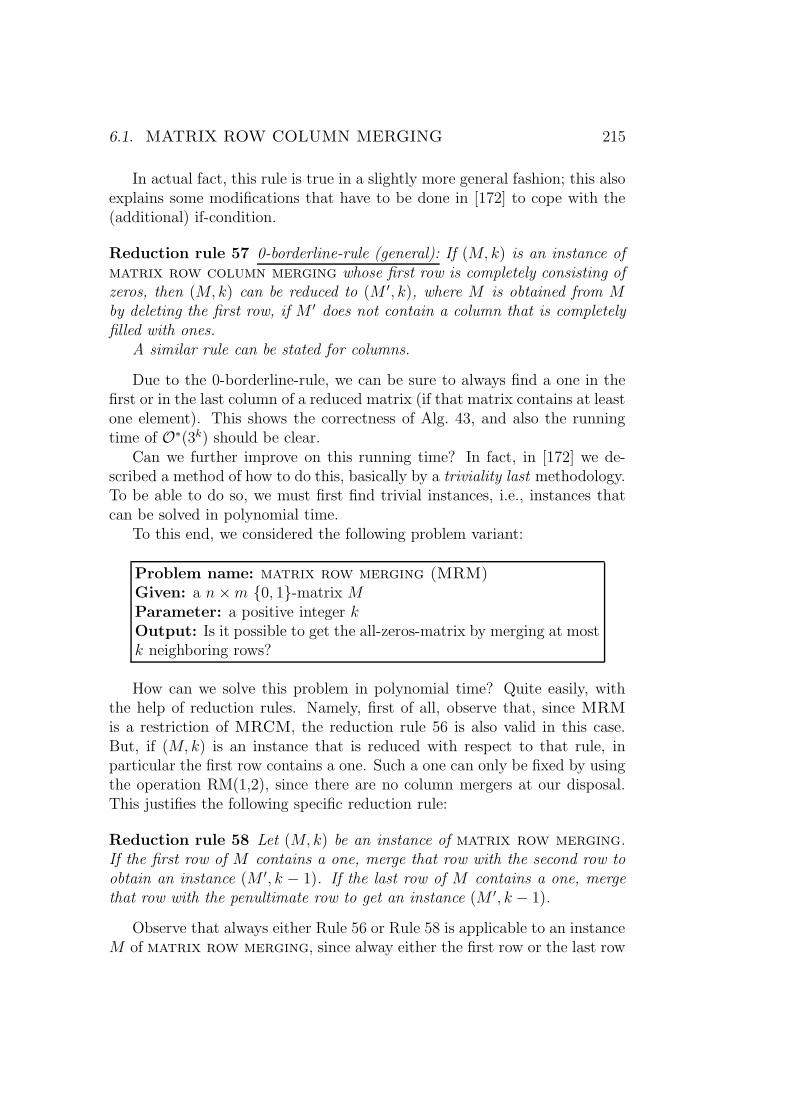
6.1. MATRIX ROW COLUMN MERGING 215
In actual fact, this rule is true in a slightly more general fashion; this alsoexplains some modifications that have to be done in [172] to cope with the(additional) if-condition.
Reduction rule 57 0-borderline-rule (general): If (M, k) is an instance ofmatrix row column merging whose first row is completely consisting ofzeros, then (M, k) can be reduced to (M ′, k), where M is obtained from Mby deleting the first row, if M ′ does not contain a column that is completelyfilled with ones.
A similar rule can be stated for columns.
Due to the 0-borderline-rule, we can be sure to always find a one in thefirst or in the last column of a reduced matrix (if that matrix contains at leastone element). This shows the correctness of Alg. 43, and also the runningtime of O∗(3k) should be clear.
Can we further improve on this running time? In fact, in [172] we de-scribed a method of how to do this, basically by a triviality last methodology.To be able to do so, we must first find trivial instances, i.e., instances thatcan be solved in polynomial time.
To this end, we considered the following problem variant:
Problem name: matrix row merging (MRM)Given: a n×m 0, 1-matrix MParameter: a positive integer kOutput: Is it possible to get the all-zeros-matrix by merging at mostk neighboring rows?
How can we solve this problem in polynomial time? Quite easily, withthe help of reduction rules. Namely, first of all, observe that, since MRMis a restriction of MRCM, the reduction rule 56 is also valid in this case.But, if (M, k) is an instance that is reduced with respect to that rule, inparticular the first row contains a one. Such a one can only be fixed by usingthe operation RM(1,2), since there are no column mergers at our disposal.This justifies the following specific reduction rule:
Reduction rule 58 Let (M, k) be an instance of matrix row merging.If the first row of M contains a one, merge that row with the second row toobtain an instance (M ′, k − 1). If the last row of M contains a one, mergethat row with the penultimate row to get an instance (M ′, k − 1).
Observe that always either Rule 56 or Rule 58 is applicable to an instanceM of matrix row merging, since alway either the first row or the last row
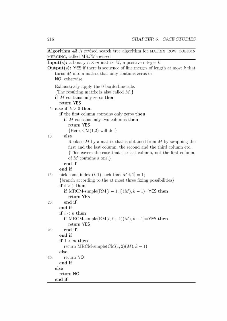
216 CHAPTER 6. CASE STUDIES
Algorithm 43 A revised search tree algorithm for matrix row columnmerging, called MRCM-revised
Input(s): a binary n×m matrix M , a positive integer kOutput(s): YES if there is sequence of line merges of length at most k that
turns M into a matrix that only contains zeros orNO, otherwise.
Exhaustively apply the 0-borderline-rule.The resulting matrix is also called M .if M contains only zeros then
return YES
5: else if k > 0 thenif the first column contains only zeros then
if M contains only two columns thenreturn YES
Here, CM(1,2) will do.10: else
Replace M by a matrix that is obtained from M by swapping thefirst and the last column, the second and the third column etc.This covers the case that the last column, not the first column,of M contains a one.
end ifend if
15: pick some index (i, 1) such that M [i, 1] = 1;branch according to the at most three fixing possibilitiesif i > 1 then
if MRCM-simple(RM(i− 1, i)(M), k − 1)=YES thenreturn YES
20: end ifend ifif i < n then
if MRCM-simple(RM(i, i + 1)(M), k − 1)=YES thenreturn YES
25: end ifend ifif 1 < m then
return MRCM-simple(CM(1, 2)(M), k − 1)else
30: return NO
end ifelse
return NO
end if

6.1. MATRIX ROW COLUMN MERGING 217
of M contains a one or both the first and the last row of M contain onlyzeros.
It is obvious that an instance (M, k) that is reduced both according toboth Rules 56 and 58 is either a matrix with zero or with one row; in thefirst case, the instance is solvable, while in the second case, it is not. Observethat, according to the last remarks in Sec. 2.1.1, it is well possible that aninstance is detected as non-solvable when trying to apply the reduction rules,namely if the budget k that was originally provided was too small.
As detailed in [172], the sketched polynomial time solving algorithm formatrix row merging is interesting on its own right since it also yields asimple solving algorithm for vertex cover on so-called interval graphs.
Having found this simple solution for row (or column) mergers only, wecan now formulate an algorithm for which we can show a further improvedrunning time, called MRCM-final, see Alg. 44. This procedure is used asdescribed in the following:
Let (M, k) be the given MRCM instance.A is an initially all-zero auxiliary matrix with the same dimensions as M .Call S :=MRCM-final(M, k, ∅, 0, k, A, 1, 0).if M contains a one and S = ∅ then
(M, k) is a NO-instance.else
(M, k) is a YES-instance, solved by S.end if
The idea of this algorithm is pretty simple and similar to the previouscase: a one in the first column can be either solved by a column merger or bysome row mergers. The trick is that we defer solving by row mergers till thevery end, which is possible since the merging operations are commutative(in a certain sense: namely, when considered on the original matrix lineindexing). Observe that λ ≥ 1 due to the fact that M contains at least oneone in the first column.
Observe that the line marked with (*) in Alg. 44 is needs some modifica-tions along the lines of Alg. 43 to cover the cases in which the 0-borderline-rule is not applicable; since the corresponding swapping of indices introducessome technicalities that are tedious but don’t add to the understanding ofthe overall procedure. The necessary modifications should be doable by thereader.
We allow ourselves to override some ones in M by twos, namely, if wedecide that the corresponding row containing that one should be resolved bya row merger. Then, we should not consider the possibility of repairing acolumn containing only zeros and twos by column mergings (at all). Rather,
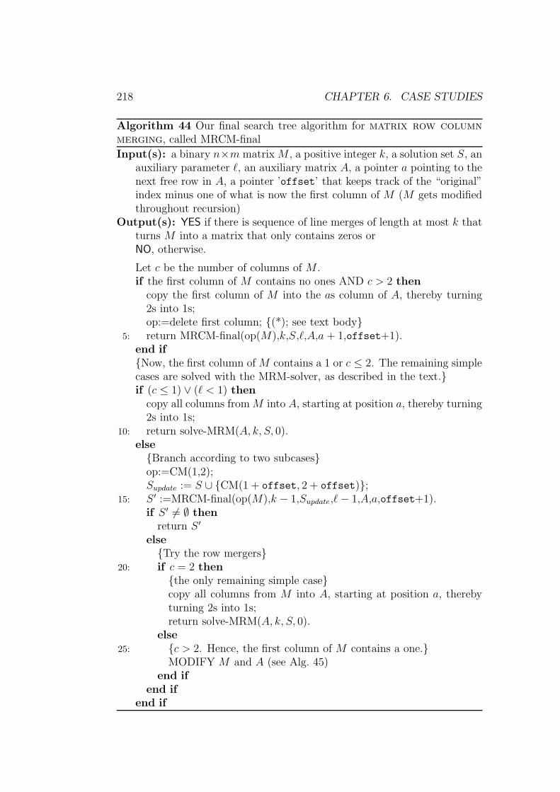
218 CHAPTER 6. CASE STUDIES
Algorithm 44 Our final search tree algorithm for matrix row columnmerging, called MRCM-final
Input(s): a binary n×m matrix M , a positive integer k, a solution set S, anauxiliary parameter `, an auxiliary matrix A, a pointer a pointing to thenext free row in A, a pointer ’offset’ that keeps track of the “original”index minus one of what is now the first column of M (M gets modifiedthroughout recursion)
Output(s): YES if there is sequence of line merges of length at most k thatturns M into a matrix that only contains zeros orNO, otherwise.
Let c be the number of columns of M .if the first column of M contains no ones AND c > 2 then
copy the first column of M into the as column of A, thereby turning2s into 1s;op:=delete first column; (*); see text body
5: return MRCM-final(op(M),k,S,`,A,a + 1,offset+1).end ifNow, the first column of M contains a 1 or c ≤ 2. The remaining simplecases are solved with the MRM-solver, as described in the text.if (c ≤ 1) ∨ (` < 1) then
copy all columns fromM into A, starting at position a, thereby turning2s into 1s;
10: return solve-MRM(A, k, S, 0).elseBranch according to two subcasesop:=CM(1,2);Supdate := S ∪ CM(1 + offset, 2 + offset);
15: S ′ :=MRCM-final(op(M),k − 1,Supdate,`− 1,A,a,offset+1).if S ′ 6= ∅ then
return S ′
elseTry the row mergers
20: if c = 2 thenthe only remaining simple casecopy all columns from M into A, starting at position a, therebyturning 2s into 1s;return solve-MRM(A, k, S, 0).
else25: c > 2. Hence, the first column of M contains a one.
MODIFY M and A (see Alg. 45)end if
end ifend if

6.1. MATRIX ROW COLUMN MERGING 219
Algorithm 45 The macro MODIFY as used in Alg. 44.
λ := 0;set the ath column of A to be the all-zero-vector;for all rows i in the first column of M with M [i, 1] = 1 doλ := λ+ 1;for all columns j > 1 of M with M [i, j] = 1 doM [i, j] := 2;
end forend forfor all rows i in the first column of M with M [i, 1] 6= 0 doA[i, a] := 1;
end forop:=delete first column;return MRCM-final(op(M),k,S,` − λ/2,A,a+ 1,offset+1).
in this sense a two would be treated as a zero by the 0-borderline-rule withinM , deferring the solution to the polynomial-time phase with solve-MRM.This justifies the initial part of the algorithm. Still, if we decide to mergethe first column with the second which may contain a two, then this two istreated as if it were a one. More precisely, merging within M is then doneaccording to the following algebraic laws:
• 0 AND X = 0 for X = 0, 1, 2;
• X AND X = X for X = 0, 1, 2.
Note that we will never merge a one with a two, since all ones in a row willbe turned into twos (when we assume that that row is fixed by row merging)or not, see the macro described in Alg. 45 for details. Hence, the given rulescover all cases that may occur.
The idea behind the new variable ` is that for each row which we decideto be resolved by row mergers only, we can be sure to put aside at least onehalf of a parameter value, since one row merger can completely resolve atmost two rows to be fixed by row mergers only. This “book-keeping trick”(which might be in fact wider applicable: use simple approximation boundsto account for cases to be resolved later in a deterministic, polynomial-timefashion) gives us the following recursion:
T (`) ≤ T (`− 1) + T (`− 1/2) +O(1)
Assuming T (`) = c` yields c = (3 +√
5)/2 ≈ 2.6181. Alternatively, c = φ2 =φ+ 1, where φ ≈ 1.6181 is the number of the golden ratio.
Hence, we may state as our final version:

220 CHAPTER 6. CASE STUDIES
Theorem 6.4 matrix row column merging can be solved in time O(2.6181kmn),given an n×m matrix M and a parameter k.
6.1.5 Revisiting our example
Let us follow the work of this algorithm by having another look at the firstexample, solving it as instance (M, 3). For clarity, we put the value of theoffset variable into each table.
offset = 0 1 2 3 4 5 6 7 8 91 1 1 123 14 1 1 1567 1 1
The first branch would take CM(1,2), and one application of the 0-borderline-rule (in its general form) leaves us with a new instance (M1, 2),using curly brackets to denote the different subcases:
offset = 2 1 2 3 4 5 6 71 1 1234 1 1 1567 1 1
Alternatively, the second branch would copy the first column of M into Aand color some 1s into 2s, arriving at the following matrix instance (M2, 2),after one application of the 0-borderline-rule (in its general form):
offset = 2 1 2 3 4 5 6 71 2 2234 1 1 1567 1 1
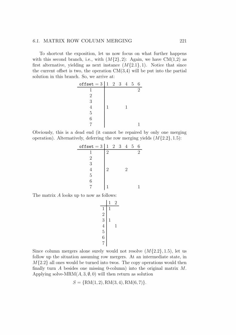
6.1. MATRIX ROW COLUMN MERGING 221
To shortcut the exposition, let us now focus on what further happenswith this second branch, i.e., with (M2, 2): Again, we have CM(1,2) asfirst alternative, yielding as next instance (M2.1, 1). Notice that sincethe current offset is two, the operation CM(3,4) will be put into the partialsolution in this branch. So, we arrive at:
offset = 3 1 2 3 4 5 61 2234 1 1567 1
Obviously, this is a dead end (it cannot be repaired by only one mergingoperation). Alternatively, deferring the row merging yields (M2.2, 1.5):
offset = 3 1 2 3 4 5 61 2 2234 2 2567 1 1
The matrix A looks up to now as follows:
1 21 123 14 1567
Since column mergers alone surely would not resolve (M2.2, 1.5), let usfollow up the situation assuming row mergers. At an intermediate state, inM2.2 all ones would be turned into twos. The copy operations would thenfinally turn A besides one missing 0-column) into the original matrix M .Applying solve-MRM(A, 3, ∅, 0) will then return as solution
S = RM(1, 2),RM(3, 4),RM(6, 7).

222 CHAPTER 6. CASE STUDIES
6.2 Problems related to hitting set
In this section, we will show how a whole variety of problems can be solvedwith the help (or at least taking ideas from) hitting set algorithms asdeveloped in Chap. 5. In fact, we already started with such type of problemsin the preceding section, since we sketched the connections between 4-HSand matrix row column merging. However, in that example, we usedfurther techniques that are specific to MRCM to get better running times.Presumably, it would be also possible to improve on the running times ofsome of the algorithms described below by exploiting more problem-specificproperties (if it is not clear that the problems are not exactly described byHS).
More specifically, we will encounter in this sections hitting set-likeproblems from the areas of computational biology and of network algorithms.Later in this chapter, further related problems will be discussed.
6.2.1 Problems from computational biology
Let us first mention here the following two problems arising in computa-tional biology that can be effectively solved with the help of 3-hitting set,see [17, 45, 137]: maximum agreement subtree and maximum compat-ible tree.
To formulate these problems, we need some more terminology: a phy-logeny is a rooted tree T whose leaf set L(T ) is in bijection with a labelset (with which it can be hence identified). Within maximum agreementsubtree, the rooted tree is always binary, i.e., all inner nodes but the roothave degree three; the root has degree two.1 To maintain this property, weassume that label deletion may propagate in the following sense:
• Assume that x is an inner node with children y and z, where z is a leafthat is going to be deleted.
• Upon deleting z, x would have a degree that is too small. Therefore, xis deleted as well. Two subcases arise:
– x is the root of the tree. Then, y will be the root of the tree thatis produced.
– x is not the root of the tree. Then, x is the child of another nodex′, and an edge between x′ and y is added in the tree that isproduced to maintain it connected.
1We disregard trees with two or fewer nodes in this discussion to avoid messy formula-tions.

6.2. PROBLEMS RELATED TO HITTING SET 223
Let T \λ the tree obtained after deleting label λ from L(T ). We can extendthis operation to sets of labels, arriving at the notation T \ Λ for a set oflabels Λ.
Problem name: maximum agreement subtree (MAST)Given: A set T1, . . . , Tn of binary rooted trees with equal label setL = L(T1) = · · · = L(Tn)Parameter: a positive integer kOutput: Is there a set of labels L′ ⊆ L, |Λ| ≤ k, such that all treesTi \ Λ are isomorphic?
maximum agreement subtree can be basically solved with the helpof 3-hitting set by creating a hyperedge between three labels `1, `2, `3 ifin one tree Ti the least common ancestor of `1 and `2 is closer to the rootthan the least common ancestor of `1 and `3, while in another tree Tj, theopposite is true: the least common ancestor of `1 and `3 is closer to the rootthan the least common ancestor of `1 and `2. The operation of deleting alabel corresponds to putting the corresponding label into the hitting set.
The problem maximum compatible tree is more general, since it al-lows inner nodes of degree larger than three for a phylogeny. However, it isshown in [45] that this problem is still solvable with the help of 3-hittingset.
From the point of view of applications, also other, related problems seemto be of interest. For example, Berman, DasGupta and Sontag [43] consideredthe following problem (which we already rephrased in terms of hitting set)that was motivated by applications to reverse engineering of protein and genenetworks:
Problem name: multi-hitting set (HSmulti)Given: A hypergraph G = (V,E)Parameter: positive integers k, `Output: Is there a multi-hitting set C ⊆ V with |C| ≤ k, i.e., Csatisfies ∀e ∈ E∃c ⊆ e(|c| ≥ ` ∧ c ⊆ C)?
Again, if we restrict the size of the hyperedges to d, we can expect FPTresults. More specifically, it is then sufficient to branch on all
(d`
)possibil-
ities to cover a chosen hyperedge e (candidate set method). This immediately
gives an O∗
((d`
)k/`)= O∗(dk) algorithm for d-HSmulti.
Better results can be expected in certain circumstances. For example, if` = d − 1, then we can simulate the fact that d − 1 out of the d elements

224 CHAPTER 6. CASE STUDIES
of a hyperedge must be covered by the multi-hitting set by replacing thathyperedge by a clique (in the classical graph theoretic sense) on these dvertices and considering the translated graph as a vertex cover instance.More specifically, we would use the program fragment listed as Alg. 46.
Algorithm 46 How to turn a special multi-hitting set instance into anequivalent vertex cover instance
Input(s): G = (V,E): the input hypergraph with parameter kOutput(s): G′ = (V ′, E ′): the output graph with parameter k′ (the equiv-
alent VC instance).
Let V ′ := E ′ := ∅for all e ∈ E according to increasing size do
if |e| < d− 1 or k < d− 1 thenLet E ′ = vv′ for arbitrary v, v′ ∈ V .Let k′ = 0.return (G′, k′).
else if |e| = d− 1 thenRemove all vertices from e from V and from E.Remove empty hyperedges from E.Decrease k by d− 1.
elseAdd the vertices in e to V ′.Make these vertices a clique in V ′ by accordingly updating E ′.Remove e from E.
end ifend forreturn (G′, k).
This shows that also reductions can be sometimes used to solve a specificproblem in particular with the help of hitting set programs.
6.2.2 Call control problems
Th. Erlebach and his co-authors investigated variants of call admission con-trol problems. In such a setting, we are given a set of connection requestsin a communication network and have to determe which of the requests canbe accepted without exceeding the capacity of the network. The goal is tomaximize the number of accepted requests or, equivalently, to minimize thenumber of rejected requests. We follow the terminology as introduced in [23]in this section. In fact, most results are obtained in the quoted paper; how-

6.2. PROBLEMS RELATED TO HITTING SET 225
ever, we think this setting allows for even a certain number of nice exampleswhere hitting set techniques can be fruitfully applied.
We restrict our discussion here to communication networks that can bedescribed by undirected graphs. In [23], also networks that can be modeledby directed or (as a special case) bidirected graphs are treated. So, here acommunication network is represented by an undirected graph G = (V,E)with edge capacities c : E → N. A communication request is a pair ofvertices. If a request (u, v) is an accepted request, then a unit of bandwidth isreserved on all edges along a path p((u, v)) from u to v. Naturally, this meansthe remaining capacity decreases by one for each edge involved in p((u, v)),once this path has been chosen to satisfy request (u, v). Accordingly, a setof paths is a feasible path set if no edge e ∈ E is contained in more than c(e)paths. For a given set P of paths in a graph with edge capacities, an edge eis called a violated edge if the number of paths in P that contain e is greaterthan c(e). In this setting, we can now formulate the basic call admissionproblem.
Problem name: CallControlGiven: A communication network represented by an undirectedgraph G = (V,E) with edge capacities c : E → N, a set R ⊆ V × Vof communication requestsParameter: a positive integer kOutput: Is there a subset A ⊂ R and a corresponding feasible pathset p(A) resulting from assigning to each request r ∈ A some pathp(r) such that p(A) is feasible and the set of rejected requests R \ Acontains no more than k elements?
(Recall that P (G) collects all paths of G.) Unfortunately, there is no realhope to find efficient parameterized algorithms, since CallControl is NP-hard, even for k = 0 and when we only consider unit capacities and when theinput graphs are restricted to series-parallel graphs (a usually very “easy”class of graphs, where many graph problems that are NP-hard in generalcan be efficiently solved). The basic reason is that, in the formulation of thepreceding problem, we have an additional degree of freedom (in comparisonto other similar parameterized problems), namely the choice of the pathp((u, v)) to satisfy the request (u, v). This path assignment problem itself isclosely related to the problem of finding disjoint paths and can therefore notefficiently solved.
Moreover, in some applications, this path is actually predetermined by apath assigning function. We can therefore formulate the following variant:

226 CHAPTER 6. CASE STUDIES
Problem name: CallControl-PreGiven: A communication network represented by an undirectedgraph G = (V,E) with edge capacities c : E → N, a set R ⊆ V × Vof communication requests, a path assigning function p : R → P (G)Parameter: a positive integer kOutput: Is there a subset A ⊂ R such that p(A) is feasible and theset of rejected requests R \ A contains no more than k elements?
Now, the (in principle) unbounded edge capacities actually make theproblem hard in the parameterized sense. More technically speaking, in [23],showed that that problem is W[2]-hard, even when restricted to series-parallelgraphs.
The picture changes if we further restrict the problem to instances withbounded edge capacities, i.e., assume there is a constant d such that, for all e,c(e) ≤ d. We denote the problem as d-CallControl-Pre (to be specifiedformally below).
Now, there is a simple candidate set in each step of a simple search tree:namely, if there happen to be more request then capacity for a certain edgee, then take an arbitrary selection of c(e)+1 ≤ d+1 paths through e. One ofthese paths (or better said one of the corresponding calls) must be rejected.This motivates Alg. 47 for solving d-CallControl-Pre.
Interestingly enough, the Alg. 47 (that is implicitly presented in [23])assumes a sort of online generation of the candidate sets. Alternatively,one could think of trying to generate all possible candidate sets in the verybeginning. Then, we would have all violating candidate sets at hand in thevery beginning of the branching process. In fact, we would have produced aspecial instance of (d+1)-hitting set in this way. Then, we could take thebest known parameterized off-line algorithm for hitting set, see Sec. 5.3.3.This would of course improve on the presented on-line algorithm which has aworst-case running time of O((d+1)kn). Note that although the overall size ofthe produced d-hitting set instance is (alternatively) bounded by O(nd)and is hence polynomial for any predetermined fixed d, this many (trial)conflict edges may be generated if we consider d really as fixed. However, aswe already remarked in Sec. 3.4, it is usually the case in d-HS algorithmsthat they might work uniformly in the sense that both d and k can be viewedas parameters of the problem. If we like to get a similar behavior for this callcontrol problem, we cannot afford spending so much time on the generationof the instance. So, formally we attack the following problem:
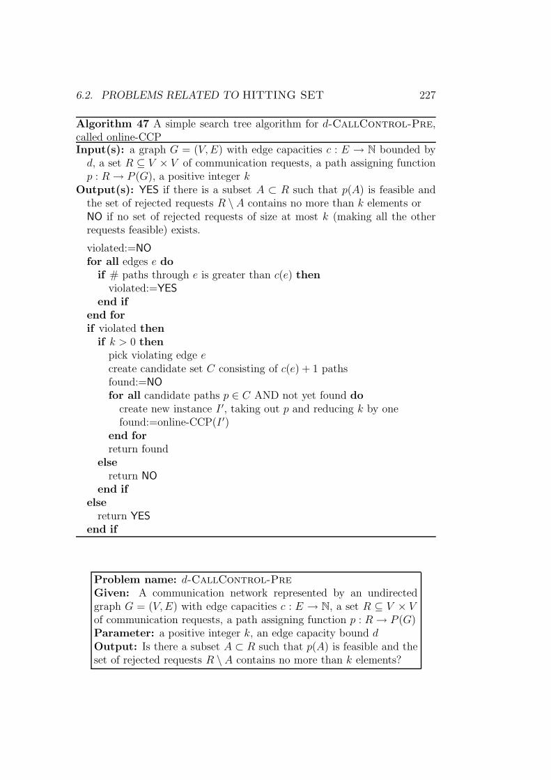
6.2. PROBLEMS RELATED TO HITTING SET 227
Algorithm 47 A simple search tree algorithm for d-CallControl-Pre,called online-CCPInput(s): a graph G = (V,E) with edge capacities c : E → N bounded byd, a set R ⊆ V × V of communication requests, a path assigning functionp : R → P (G), a positive integer k
Output(s): YES if there is a subset A ⊂ R such that p(A) is feasible andthe set of rejected requests R \ A contains no more than k elements orNO if no set of rejected requests of size at most k (making all the otherrequests feasible) exists.
violated:=NO
for all edges e doif # paths through e is greater than c(e) then
violated:=YES
end ifend forif violated then
if k > 0 thenpick violating edge ecreate candidate set C consisting of c(e) + 1 pathsfound:=NO
for all candidate paths p ∈ C AND not yet found docreate new instance I ′, taking out p and reducing k by onefound:=online-CCP(I ′)
end forreturn found
elsereturn NO
end ifelse
return YES
end if
Problem name: d-CallControl-PreGiven: A communication network represented by an undirectedgraph G = (V,E) with edge capacities c : E → N, a set R ⊆ V × Vof communication requests, a path assigning function p : R → P (G)Parameter: a positive integer k, an edge capacity bound dOutput: Is there a subset A ⊂ R such that p(A) is feasible and theset of rejected requests R \ A contains no more than k elements?

228 CHAPTER 6. CASE STUDIES
Let us therefore analyze our situation more carefully.For example, it could well be that an edge has a demand p(e) (measured
in terms of the number of paths that want to use e) that is “much” largerthan the capacity c(e). This automatically means (by pigeon hole principle)that at least p(e) − c(e) paths have to be removed. Therefore, the followingreduction rule is safe:
Reduction rule 59 If p(e) − c(e) > k, we can immediately reply NO.
In terms of HS, such a situation corresponds to a sort of hyperclique.Observe that otherwise, each of the paths (that correspond to the vertices inthe instance of hitting set) has “degree” p(e).
To see if the solutions that can be found when solving CallControl-Pre or HS, let us be a bit more formal. We study how the information thatcertain paths are removed (i.e., vertices are put into the hitting set) is prop-agated in the branching process. Consider a CallControl-Pre instanceI and the “corresponding” HS instance HS(I), where the translation fromI to HS(I) can be described as follows:
• IF G = (V,E) is the underlying network graph of I, then P (G) is thevertex set of HS(I).
• If e ∈ E with p(e) − c(e) > 0, then let P (e) ⊆ P (G) be the paths thatcontain e and put all (c(e) + 1)-element subsets of P (e) as hyperedgesinto HS(I). All hyperedges in HS(I) are described this way.
• If k is the parameter of I, then k is also the parameter of HS(I).
We have to show that if C is a path set whose removal resolves all conflictsin I, then C is a hitting set in HS(I) and vice versa.
On the other hand, the instance that would have to be generated couldbe rather big, so that in the end the on-line variant could have an edge overthe off-line variant. Namely, consider an edge e with p(e) − c(e) = k manypaths to be removed. This means that in HS(I), e would “generate”
(p(e)
c(e) + 1
)=
(c(e) + kc(e) + 1
)∈ O((c(e) + 1)k)
many hyperedges, which are “too many” from a parameterized perspective.More precisely, since we consider c(e) ≤ d for all edges, and since we
translate a d-CallControl-Pre instance I into a (d + 1)-HS instanceHS(I), this generated instance could be as large as O((d + 1)k) (even if weassume that we don’t translate instances I that contain edges with p(e) −
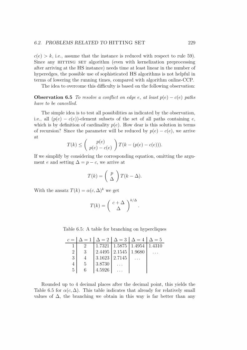
6.2. PROBLEMS RELATED TO HITTING SET 229
c(e) > k, i.e., assume that the instance is reduced with respect to rule 59).Since any hitting set algorithm (even with kernelization preprocessingafter arriving at the HS instance) needs time at least linear in the number ofhyperedges, the possible use of sophisticated HS algorithms is not helpful interms of lowering the running times, compared with algorithm online-CCP.
The idea to overcome this difficulty is based on the following observation:
Observation 6.5 To resolve a conflict on edge e, at least p(e) − c(e) pathshave to be cancelled.
The simple idea is to test all possibilities as indicated by the observation,i.e., all (p(e) − c(e))-element subsets of the set of all paths containing e,which is by definition of cardinality p(e). How dear is this solution in termsof recursion? Since the parameter will be reduced by p(e) − c(e), we arriveat
T (k) ≤(
p(e)p(e) − c(e)
)T (k − (p(e) − c(e))).
If we simplify by considering the corresponding equation, omitting the argu-ment e and setting ∆ = p− c, we arrive at
T (k) =
(p∆
)T (k − ∆).
With the ansatz T (k) = α(c,∆)k we get
T (k) =
(c+ ∆
∆
)k/∆.
Table 6.5: A table for branching on hypercliques
c = ∆ = 1 ∆ = 2 ∆ = 3 ∆ = 4 ∆ = 51 2 1.7321 1.5875 1.4954 1.43102 3 2.4495 2.1545 1.9680 . . .3 4 3.1623 2.7145 . . .4 5 3.8730 . . .5 6 4.5926 . . .
Rounded up to 4 decimal places after the decimal point, this yields theTable 6.5 for α(c,∆). This table indicates that already for relatively smallvalues of ∆, the branching we obtain in this way is far better than any

230 CHAPTER 6. CASE STUDIES
branching numbers we earlier obtained for hitting set. We replaced severalnumbers by dots because of the following monotonicity property, which alsoexplains that “sooner or later” also in the case c = 1 (which correspondsto vertex cover), this approach will beat any sophicated algorithm forVC. More precisely, for c = 1 and ∆ = 9, we have a branching numberα(1, 9) ≤ 1.2916, for ∆ = 10, we get α(1, 10) ≤ 1.2710, and for ∆ = 20,α(1, 20) ≤ 1.1645.
Proposition 6.6 For every fixed c, the sequence
((c+ ∆
∆
)1/∆)
∆=1,2,3,...
is strictly decreasing and converges to one.
Proof. Combine
(c+ ∆
∆
)∈ O(∆c) with lim∆→∞
∆√
∆ = 1.
Therefore, we can propose the off-line counterpart outlined in Alg. 48,whose running time (in terms of O∗) coincides with that of the best cor-responding algorithm for hitting set, since the size of the generated HSinstance is only dependent on the capacity bound d (times k). In Alg. 48,the constant εd has to be chosen large enough to ensure that the first branch-ings are not worse than the ones incurred by the chosen (d + 1)-hittingset algorithms. We have therefore demonstrated the following result thatstrengthens the observations from [23].
Theorem 6.7 d-CallControl-Pre can be solved in the same time boundsas the best corresponding algorithm for d-hitting set. In particular, thisproblem is in FPT .
Anand et al. describe some more FPT algorithms for call control prob-lems. Let us mention two particular cases:
Problem name: CallControl in trees of ringsGiven: A communication network represented by an undirectedgraph G = (V,E) that is a tree of rings with unit edge capacities, aset R ⊆ V × V of communication requestsParameter: a positive integer kOutput: Is there a subset A ⊂ R and a path assigning functionp : R → P (G) such that p(A) is feasible and the set of rejectedrequests R \ A contains no more than k elements?

6.2. PROBLEMS RELATED TO HITTING SET 231
Algorithm 48 A still simple search tree algorithm for CallControl-Pre,called offline-CCPInput(s): a graph G = (V,E) with edge capacities c : E → N bounded byd, a set R ⊆ V × V of communication requests, a path assigning functionp : R → P (G), a positive integer k
Output(s): YES if there is a subset A ⊂ R such that p(A) is feasible andthe set of rejected requests R \ A contains no more than k elements orNO if no set of rejected requests of size at most k (making all the otherrequests feasible) exists.
found:=NO
for all edges e and not yet found doif # paths p(e) through e is greater than c(e) + εd then
if p(e) − c(e) > k thenreturn NO
else∆ = p(e) − c(e)for all path sets P of size ∆ that contain e AND not yet found do
create new instance I ′, taking out P and reducing k by ∆found:=offline-CCP(I ′)
end forend if
end ifend forTransform the given instance I into HS(I).Let (d+ 1)-HS be the hitting set algorithm of your choice.return (d+ 1)-HS(HS(I))
The problem on bidirected trees of rings can be similarly treated, see [23].We omit those details here.
It is shown in [23] that at most three rejection candidates can be found ateach level of the recursion. This again “smells” like 3-hitting set. Let us seeif we can again reduce this problem completely to 3-HS. To this end, we needto introduce some more notation (similar to [23]) to study CallControlin trees of rings in more depth.
• For any request (u, v) in a tree of rings, all undirected paths from uto v contain edges of the same rings.
• Hence, in any ring a path from u to v passes through, the vertex atwhich the path enters the ring (or begins) and the vertex at which thepath leaves the ring (or terminates) is uniquely determined by u and v.

232 CHAPTER 6. CASE STUDIES
Hence, a path request in a tree of rings can be equivalently representedby a set of subrequests in all rings that the path passes through. Let ustherefore study the problem in rings first.
Let R be a ring, drawn as a circle in the plane. Represent a subrequest(u, v) between two vertices on R as a straight line segment (called chord)joining u and v. Two chords are parallel chords if they intersect at most inpoints on R or if they are identical. A cut is a pair of edges of the graph onthe ring. A request crosses a cut if each of the two possible paths connectingthe endpoints of the request contains exactly one of the edges in the cut.In [23], the following characterization of routeability in rings is shown:
Lemma 6.8 Given a ring R and a set of requests S in R, the requests in Scan be routed along edge-disjoint paths iff
• all chords of the requests in S are pairwisely parallel and
• no cut is crossed by three (or more) requests.
More precisely, Algorithm 49 can be used to find all routes if the condi-tions of the lemma apply. This algorithm can be read off the proof of thepreceding lemma.
Algorithm 49 can be adapted to get an overall algorithm for the problemeven in the presence of conflicts. More precisely, the first lines of Alg. 49reflects the preprocessing that allows us to restrict our attention to subrequeston each ring.
According to Lemma 6.8, there are two reasons why a set of requests isnot routeable in a ring:
1. There are two chords that are not parallel.
In that case, one of the two corresponding requests must be deleted.Checking all possibilities gives hence a trivial O∗(2k) running time forthis part of the algorithm.
2. All chords in all rings are parallel, but there are rings that contain cutswhich are crossed by three requests.
As proposed by Anand et al., there is a trivial O∗(3k) algorithm fortesting all possible request deletion for each violating cut. Since therecannot be more than O(n3) many conflict sets in a ring that bears nsubrequests, this part of the overall algorithm can be sped up by usingthe best available 3-hitting set algorithm.

6.2. PROBLEMS RELATED TO HITTING SET 233
Algorithm 49 A greedy algorithm for CallControl in trees of rings(assuming no conflicts), called greedy-CCTR
Input(s): a tree of rings G = (V,E), a set R ⊆ V × V of communicationrequests
Output(s): a feasible routing of all requests
The overall routing can be reconstructed from the routings of the sub-requests.for all rings R do
create list L or parallel chords (corresponding to subrequests)L could contain multiple occurrences of the same subrequest, origi-nating from different requests.
5: while |L| > 1 dochoose two parallel chords c and c′ from L corresponding to subre-quests u and v, as well as u′ and v′
if c = c′ thenroute the corresponding subrequests arbitrarily
else10: route c and c′ in a unique fashion
end ifremove c and c′ from L
end whileif L is not empty then
15: route r ∈ L arbitrarilyend if
end for
In the leaves of the search tree, a postprocessing that actually finds routesin the now conflict-free case can be made (according to Alg. 49, lines 3–16).It is important to note that this postprocessing won’t make any changes tothe parameter value.
We can therefore state:
Theorem 6.9 CallControl in trees of rings can be solved in timeO(2.1788kp(n)), where p is some polynomial.
Observe that it is important that in the first phase of the search tree, theseeming 2-hitting set instance is not solved by the best available algorithmfor vertex cover, since the complexity of the subsequent 3-HS instance(to be solved in the second phase of the search tree processing) depends onthe changes incidentally obtained by choosing one solution or other to the
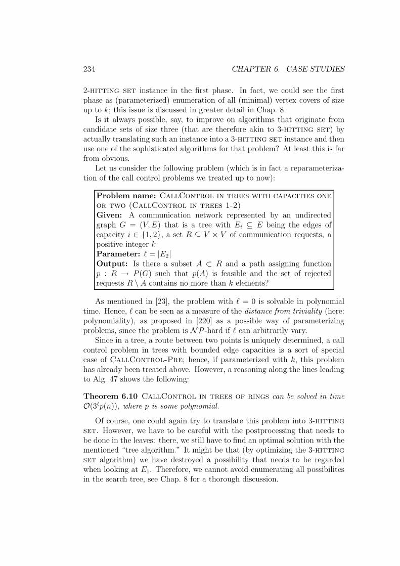
234 CHAPTER 6. CASE STUDIES
2-hitting set instance in the first phase. In fact, we could see the firstphase as (parameterized) enumeration of all (minimal) vertex covers of sizeup to k; this issue is discussed in greater detail in Chap. 8.
Is it always possible, say, to improve on algorithms that originate fromcandidate sets of size three (that are therefore akin to 3-hitting set) byactually translating such an instance into a 3-hitting set instance and thenuse one of the sophisticated algorithms for that problem? At least this is farfrom obvious.
Let us consider the following problem (which is in fact a reparameteriza-tion of the call control problems we treated up to now):
Problem name: CallControl in trees with capacities oneor two (CallControl in trees 1-2)Given: A communication network represented by an undirectedgraph G = (V,E) that is a tree with Ei ⊆ E being the edges ofcapacity i ∈ 1, 2, a set R ⊆ V × V of communication requests, apositive integer kParameter: ` = |E2|Output: Is there a subset A ⊂ R and a path assigning functionp : R → P (G) such that p(A) is feasible and the set of rejectedrequests R \ A contains no more than k elements?
As mentioned in [23], the problem with ` = 0 is solvable in polynomialtime. Hence, ` can be seen as a measure of the distance from triviality (here:polynomiality), as proposed in [220] as a possible way of parameterizingproblems, since the problem is NP-hard if ` can arbitrarily vary.
Since in a tree, a route between two points is uniquely determined, a callcontrol problem in trees with bounded edge capacities is a sort of specialcase of CallControl-Pre; hence, if parameterized with k, this problemhas already been treated above. However, a reasoning along the lines leadingto Alg. 47 shows the following:
Theorem 6.10 CallControl in trees of rings can be solved in timeO(3`p(n)), where p is some polynomial.
Of course, one could again try to translate this problem into 3-hittingset. However, we have to be careful with the postprocessing that needs tobe done in the leaves: there, we still have to find an optimal solution with thementioned “tree algorithm.” It might be that (by optimizing the 3-hittingset algorithm) we have destroyed a possibility that needs to be regardedwhen looking at E1. Therefore, we cannot avoid enumerating all possibilitesin the search tree, see Chap. 8 for a thorough discussion.

6.3. GRAPH MODIFICATION PROBLEMS 235
6.3 Graph modification problems
Graph modification problems are abundant and turn up in many disguises.The main idea is if it is possible to change a given graph by a number k ofcertain allowed graph edit operations like vertex deletion, edge deletion, oredge adding into a graph of a prescribed type.
For example, vertex cover can be viewed as a graph modificationproblem, the task being to find a set of at most k vertices whose removalturns the given graph G into a graph without any edges.
With adding certain constraints, also maximization problems can be cre-ated that may be viewed as graph modification problems. Typically, thequestion is then if at least k edit operations suffice to get a graph of aprescribed type, where the constraints restrict the way in which the editoperations may be performed.
6.3.1 A maximization graph modification problem
Consider for example the following problem:2
Problem name: maximum minimal vertex cover (MMVC)Given: A graph G = (V,E)Parameter: a positive integer kOutput: Does there exist a minimal vertex cover set of cardinality≥ k ?
The additional constraint is here the minimality of the considered vertexcovers. This problem can therefore be equivalently formulated as follows:Given a graph G = (V,E) and an integer k, is it possible to find a vertex setM , |M | ≥ k, whose removal produces a graph G[V \M ] with empty edgeset, such that for all x ∈ M there is a y ∈ V \M with x, y ∈ E?
In fact, it is pretty easy to design an FPT algorithm for maximumminimal vertex cover, based on the simple first search tree algorithm wepresented for vertex cover, since still we are looking for a vertex cover, i.e.,every edge must be covered. The only difference is how we treat the leavesof the search tree. After having put k vertices in the cover along a recursionpath, we have to check if possibly some vertices could be added to producea minimal vertex cover; so the point is to check the minimality assumptionrather than the cover property at this point. The corresponding algorithmis listed in Alg. 50. Initially, the algorithm is called with the parameters(G, k, ∅), where (G, k) is the instance of MMVC under scrutiny.
2We are not aware of any publication of the results of this subsection elsewhere.

236 CHAPTER 6. CASE STUDIES
Algorithm 50 A simple search tree algorithm, called MMVC-simple
Input(s): a graphG = (V,E), a positive integer k, a partial solutionM ⊆ VOutput(s): YES if there is a minimal vertex cover C ⊆ V , |C| ≥ k, M ⊆ C
orNO if no vertex cover of size at least k exists.
if k ≤ 0 thenif M can be enlarged to get a minimal vertex cover then
return YES
elsereturn NO
end ifelse if E = ∅ then
return NO
elseChoose edge e = x, y ∈ Eif MMVC-simple(G − x, k − 1,M ∪ x) then
return YES
elsereturn MMVC-simple(G −N [x], k − deg(x),M ∪N(x))
end ifend if
Can we further improve on that algorithm? This might be done, indeed,by providing proper data structures to simply detect non-minimality “on theway” of the branching process itself. To this end, we may start with a setcollection C = N [v] | v ∈ V . This collection should always maintain theproperty that, whenever ∅ ∈ C shows up in one branch, we can stop thebranching process, since we can no longer obtain a minimal cover on thisbranch. Hence, if we take a vertex v into the vertex cover, we would deletev from every set S ∈ C, and in the branch that don’t takes v into the coverbut its neighbors, we would first delete all sets S ∈ C that contain v (becauseall these sets have now a member that is not in the cover, hence ensuringminimality), and then we would delete every x ∈ N(v) from every set S ∈ C.The leaves of the corresponding search tree would never correspond to partialcovers that cannot be extended to minimal vertex covers of the whole graph.However, we were not able to prove better running times for a search treealgorithm using such additional information, even at some stage the graphcontains only vertices of degree one. The problem is that still vertices mightdepend on one another due to the collection C.

6.3. GRAPH MODIFICATION PROBLEMS 237
Recall that we have derived a small kernel for maximum minimal ver-tex cover in Chap. 4, so that we can state:
Theorem 6.11 maximum minimal vertex cover can be solved in timeO(2k + p(n)), where p is some polynomial.
6.3.2 Graph modification problems related to HS
In this section, we discuss several graph modification problems mentionedin [211]. In [211, Sec. 4.1.3], the following problem is mentioned:
Problem name: triangle edge deletion (TED)Given: A graph G = (V,E)Parameter: a positive integer kOutput: Is there an edge set C ⊆ E with |C| ≤ k whose removalproduces a graph without triangles as vertex-induced subgraphs?
Observe that three vertices x, y, z are a triangle subgraph iff the graphinduced by these three vertices is a triangle, while in general terms there isa difference between subgraphs and vertex-induced subgraphs.
A triangle edge deletion instance G = (V,E) can be transformedinto an 3-hitting set instance G′ as follows:
• Interpret the edges E as vertices of G′.
• A hyperedge h = e1, e2, e3 is contained in G′ iff, for some x, y, z ∈ V ,e1 = x, y, e2 = y, z and e3 = x, z, and h ⊆ E.
It is straightforward to see that the removal of C ⊆ E produces a graphG−C that does not contain any vertex-induced triangle iff C is a hitting setof G′.
Moreover, the currently best algorithms are based on 3-hitting set,so that the algorithm presented in Section 5.3.3 automatically improves theconstants as presented in [211].
Corollary 6.12 triangle edge deletion can be solved in time O(|E(G)|3+2.1788k), given an instance G.
Proof. According to what we earlier observed, we only have to transform Ginto a 3-hitting set instance. This transformation takes time O(|V (G)|),since we have to cycle through all triples of vertices that might form a triangle.Then we can run a 3-hitting set algorithm to get the claimed running time.

238 CHAPTER 6. CASE STUDIES
There are three more vertex deletion problems mentioned in [211] thatwe incidentally improve on:
Problem name: triangle vertex deletion (TVD)Given: A graph G = (V,E)Parameter: a positive integer kOutput: Is there an vertex set C ⊆ V with |C| ≤ k whose removalproduces a graph without triangles as vertex-induced subgraphs?
Corollary 6.13 triangle vertex deletion can be solved in time O(|V (G)|3+2.1788k), given an instance G.
Problem name: cluster vertex deletion (CVD)Given: A graph G = (V,E)Parameter: a positive integer kOutput: Is there an vertex set C ⊆ V with |C| ≤ k whose removalproduces a graph being a union of vertex-induced cliques?
Here, it might not be immediately clear how to apply the proposedmethodology. However, we have the following forbidden subgraph charac-terization also mentioned in [351]:
Theorem 6.14 A graph G is a cluster graph, i.e., a forest of cliques, iff noselection of three vertices from G induces a path of length two in G.
We can hence conclude:
Corollary 6.15 cluster vertex deletion can be solved in time O(|V (G)|3+2.1788k), given an instance G.
Observe, however, that we cannot (completely) use the methodoloy ofreducing to hitting set problems for the edge deletion analogue of clustervertex deletion, since the deletion of edges might also create inducedpaths of length two. Hence, we would need a problem-specific analysis toimprove over the trivial O∗(2k) search tree for that problem (where, for eachinduced path of length two, one of the two involved edges is deleted in eachbranch); this has been done in [211] to obtain a rather complicated O∗(1.53k)search tree algorithm. A similar effect is encountered in the edge deletionproblem clique complement cover discussed below.
To understand the following problem from [211], we need some moreterminology.
A cograph (or complement-reducible graph) is a graph defined by the threecriteria:
6.3. GRAPH MODIFICATION PROBLEMS 239
1. K1 (i.e., a graph having only one vertex) is a cograph,
2. If G is a cograph, then so is its graph complement Gc, and
3. If G and G′ are cographs, then so is their graph union.
According to the entry http://mathworld.wolfram.com/Cograph.html
in Mathworld (see [Chapter 11, Site 14]), there is one criterion characterizingcographs that is especially interesting to us:
Theorem 6.16 G is a cograph iff G does not contain any set of four verticesthat induce a path.
Another interesting property of these types of graphs is that some hardproblems can be efficiently solved when restricted to cographs. But let usnow formulate the graph modification problem:
Problem name: cograph vertex deletion (CoVD)Given: A graph G = (V,E)Parameter: a positive integer kOutput: Is there an vertex set C ⊆ V with |C| ≤ k whose removalproduces a cograph ?
We can hence conclude:
Corollary 6.17 cograph vertex deletion can be solved in time O(|V (G)|3+3.1150k), given an instance G.
6.3.3 clique complement cover: an easy problem?
The idea of relating graph modification problems with hitting set is oftenhelpful, but not always leading to the applicability of the best known hittingset algorithms. This will be exemplified by the next two problemwe consider:clique complement cover. Let us first recall CCC from Chap. 2:3
Problem name: clique complement cover (CCC)Given: A graph G = (V,E)Parameter: a positive integer kOutput: Is there a clique complement cover C ⊆ E with |C| ≤ k?
3The results of this subsections were not published elsewhere.
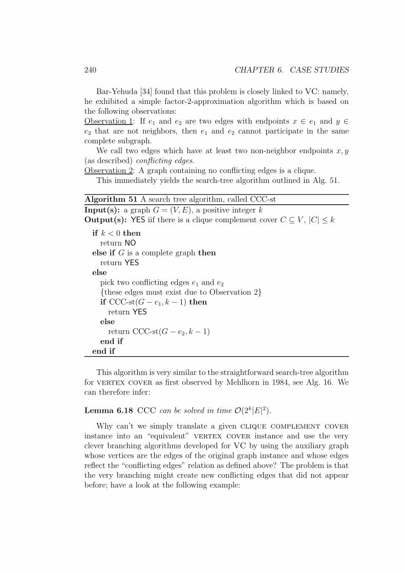
240 CHAPTER 6. CASE STUDIES
Bar-Yehuda [34] found that this problem is closely linked to VC: namely,he exhibited a simple factor-2-approximation algorithm which is based onthe following observations:Observation 1: If e1 and e2 are two edges with endpoints x ∈ e1 and y ∈e2 that are not neighbors, then e1 and e2 cannot participate in the samecomplete subgraph.
We call two edges which have at least two non-neighbor endpoints x, y(as described) conflicting edges.Observation 2: A graph containing no conflicting edges is a clique.
This immediately yields the search-tree algorithm outlined in Alg. 51.
Algorithm 51 A search tree algorithm, called CCC-st
Input(s): a graph G = (V,E), a positive integer kOutput(s): YES iif there is a clique complement cover C ⊆ V , |C| ≤ k
if k < 0 thenreturn NO
else if G is a complete graph thenreturn YES
elsepick two conflicting edges e1 and e2these edges must exist due to Observation 2if CCC-st(G− e1, k − 1) then
return YES
elsereturn CCC-st(G − e2, k − 1)
end ifend if
This algorithm is very similar to the straightforward search-tree algorithmfor vertex cover as first observed by Mehlhorn in 1984, see Alg. 16. Wecan therefore infer:
Lemma 6.18 CCC can be solved in time O(2k|E|2).Why can’t we simply translate a given clique complement cover
instance into an “equivalent” vertex cover instance and use the veryclever branching algorithms developed for VC by using the auxiliary graphwhose vertices are the edges of the original graph instance and whose edgesreflect the “conflicting edges” relation as defined above? The problem is thatthe very branching might create new conflicting edges that did not appearbefore; have a look at the following example:

6.3. GRAPH MODIFICATION PROBLEMS 241
Figure 6.1: The left-hand side shows a small clique complement coverinstance, with the corresponding conflict graph depicted on the right-handside.
Example 6.19 In Fig. 6.1, an instance of clique complement cover isshown with four vertices and four edges. Obviously, an optimal solution isto take away the red edge. However, our search tree algorithm would al-ternatively test the possibility to take out the blue edge; this is also to beseen on the right-hand side of the figure where the conflict graph is drawn.However, if the blue edge is taken out, this would of course also solve theconflict graph, but this would be no valid solution of the original cliquecomplement cover instance. In fact, the branching algorithm would pos-sibly continue on that branch if the branching actually started with the blueedge and the parameter budget would be high enough.
We have not bothered to further lower the constants in the search treealgorithm nor with providing a kernelization. However, observe that Buss’rule can be applied to the conflict graphs that can be constructed in eachstep of the branching process. We can also transfer the rules that get ridof vertices of degree zero and one to CCC. The main observation here toshow the validity of such reduction rules is the following: destroying a notnecessarily induced K1 or K2 in the conflict graph corresponds to possiblydestroying a particularK1 orK2 as “target clique” in the original graph; thesecan be easily replaced by other tiny cliques if necessary. Observe that wecannot claim to actually have found a small kernel for the original problem.However, this can be shown with some additional effort. Actually finding asmall kernel is left to the reader in this case.
As a specific rule for clique complement cover, we may use the factthat vertices of degree larger than k must all belong to the clique that shouldremain, since it is too dear to separate them from the rest. Hence, wheneverthe set
v ∈ V | deg(v) > k

242 CHAPTER 6. CASE STUDIES
does not induce a clique in the given instance G, then we can answer NO.Hence, an O(1.6182k+ p(n)) algorithm is attainable by the triviality first
principle.Let us finally remark that Bar-Yehuda (as well as Hochbaum) consider [34,
36, 232] also weighted versions of clique complement cover (and of othersimilar problems that can actually be treated by similar techniques); weightedversions formed in analogy to weighted vertex cover can be also solvedin time O∗(2k). Note that the quoted reference mostly deal with findingapproximation algorithms. In the case of clique complement cover,the approximation algorithm also bears some similarity with the well-knownapproximation algorithms for vertex cover. However, it is noteworthythat the simplest 2-approximation algorithm for vertex cover (that doesnot transfer to the weighted case) that simply takes both vertices incidentto a “current” edge into the cover (while the search tree algorithm 16 weconsidered would branch on the two possibilities) does not transfer to cliquecomplement cover due to the effect described in our example: deletingboth the red and blue edge would be no valid solution to the problem instance.
Let us mention finally that there are also other graph operations thatqualify as graph modifications. For example, consider the following problemthat is mentioned in [347]:
Problem name: bipartization, replacing edges by 2-pathsvariant (BPedgevar)Given: A graph G = (V,E)Parameter: a positive integer kOutput: Is there a bipartization set C ⊆ E with |C| ≤ k such thatreplacing each edge in C by a path of length two produces a bipartitegraph?
In fact, it is not hard to see that BPedgevar is equivalent to biparti-zation, edge variant in the following strong sense:
Lemma 6.20 (G, k) is a YES instance of BPedgevar iff (G, k) is a YES
instance of bipartization, edge variant.
How to actually solve bipartization, edge variant in FPT time will beexplained in Chap. 8.
It should have been made clear by now that many graph modificationproblems are indeed in FPT . This is true in quite general terms as long as afinite forbidden subgraph characterization is available. In general terms, thishas been addressed by Cai [67], also see [134, Sec. 3.2.2]. More candidateproblems can be found in [302], where the question of FPT -membership of

6.4. GRAPH DRAWING PROBLEMS 243
these problems is explicitly raised. The list of references given there alsoprovides a good starting point for further studies.
6.4 Graph drawing problems
The problems that we shall study in this section can be paraphrased asfollows:
Given a graph G, try to draw G in the plane in a specific waysuch the drawing looks as good as possible.
The quality of a drawing is usually measured by estimating the distancebetween a specific drawing and the case of a “perfect drawing” (amongst allgraphs, disregarding the specific input graph); at least, it is expected thata perfect drawing of some graph has a minimal measure amongst all graphsthat have the same number of edges or vertices (depending on the concreteproblem).
For more background to the problems under study, we can generally referto [283, Chapter 5], a chapter written by O. Bastert and C. Matuszewskiwith the title “Layered Drawings of Digraphs.”
6.4.1 linear arrangement again. . .
In this context, let us revisit two problems we already came across in earlierchapters:4
Problem name: linear arrangement (LA)Given: A graph G = (V,E)Parameter: a positive integer kOutput: Is there a one-to-one mapping σ : V → 1, . . . , |V | suchthat ∑
u,v∈E|σ(u) − σ(v)| ≤ k ?
4The contents of this subsection did not yet appear elsewhere but has been acceptedfor presentation at CTW 2005.

244 CHAPTER 6. CASE STUDIES
Problem name: linear arrangement (LA), parameterizedabove guaranteed valueGiven: A graph G = (V,E)Parameter: a positive integer kOutput: Is there a one-to-one mapping σ : V → 1, . . . , |V | suchthat ∑
u,v∈E|σ(u) − σ(v)| ≤ k + |E|?
Observe that the expression
∑
u,v∈E|σ(u) − σ(v)|
can be seen as measuring the distance between the linear drawability ofG = (V,E) and that of the graph G = (V, ∅) (where the measure wouldbecome 0); again, the modified problem (parameterizing about guaranteedvalues) is a bit more meaningful, since
∑
u,v∈E(|σ(u) − σ(v)| − 1)
becomes zero for all graphs that are collection of paths (and only for those),so that that expression can be viewed as measuring the distance of an inputgraph G from a forest of paths. As we have already seen, the path-similaritycan be alternatively measured in terms of pathwidth and bandwidth. An-other related problem is the following graph modification problem:
Problem name: linear arrangement by deleting edges(LADE)Given: A graph G = (V,E)Parameter: a positive integer kOutput: Is there an edge set E ′ with |E ′| ≤ k and a one-to-onemapping σ : V → 1, . . . , |V | such that
∑
u,v∈E\E′
|σ(u) − σ(v)| = |E \ E ′| ?
So, the task is to find a minimum number of edges whose removal turnsthe given graph into a forest of paths.
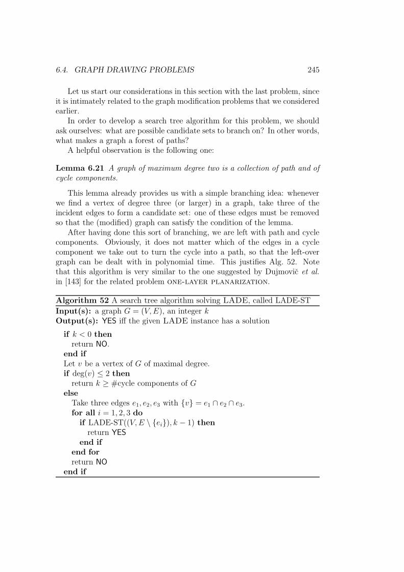
6.4. GRAPH DRAWING PROBLEMS 245
Let us start our considerations in this section with the last problem, sinceit is intimately related to the graph modification problems that we consideredearlier.
In order to develop a search tree algorithm for this problem, we shouldask ourselves: what are possible candidate sets to branch on? In other words,what makes a graph a forest of paths?
A helpful observation is the following one:
Lemma 6.21 A graph of maximum degree two is a collection of path and ofcycle components.
This lemma already provides us with a simple branching idea: wheneverwe find a vertex of degree three (or larger) in a graph, take three of theincident edges to form a candidate set: one of these edges must be removedso that the (modified) graph can satisfy the condition of the lemma.
After having done this sort of branching, we are left with path and cyclecomponents. Obviously, it does not matter which of the edges in a cyclecomponent we take out to turn the cycle into a path, so that the left-overgraph can be dealt with in polynomial time. This justifies Alg. 52. Notethat this algorithm is very similar to the one suggested by Dujmovic et al.in [143] for the related problem one-layer planarization.
Algorithm 52 A search tree algorithm solving LADE, called LADE-ST
Input(s): a graph G = (V,E), an integer kOutput(s): YES iff the given LADE instance has a solution
if k < 0 thenreturn NO.
end ifLet v be a vertex of G of maximal degree.if deg(v) ≤ 2 then
return k ≥ #cycle components of Gelse
Take three edges e1, e2, e3 with v = e1 ∩ e2 ∩ e3.for all i = 1, 2, 3 do
if LADE-ST((V,E \ ei), k − 1) thenreturn YES
end ifend forreturn NO
end if
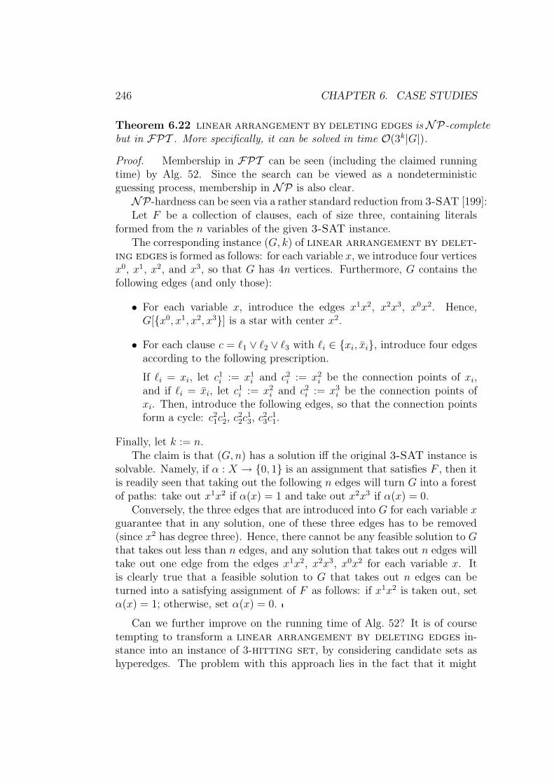
246 CHAPTER 6. CASE STUDIES
Theorem 6.22 linear arrangement by deleting edges is NP-completebut in FPT . More specifically, it can be solved in time O(3k|G|).
Proof. Membership in FPT can be seen (including the claimed runningtime) by Alg. 52. Since the search can be viewed as a nondeterministicguessing process, membership in NP is also clear.
NP-hardness can be seen via a rather standard reduction from 3-SAT [199]:Let F be a collection of clauses, each of size three, containing literals
formed from the n variables of the given 3-SAT instance.The corresponding instance (G, k) of linear arrangement by delet-
ing edges is formed as follows: for each variable x, we introduce four verticesx0, x1, x2, and x3, so that G has 4n vertices. Furthermore, G contains thefollowing edges (and only those):
• For each variable x, introduce the edges x1x2, x2x3, x0x2. Hence,G[x0, x1, x2, x3] is a star with center x2.
• For each clause c = `1 ∨ `2 ∨ `3 with `i ∈ xi, xi, introduce four edgesaccording to the following prescription.
If `i = xi, let c1i := x1i and c2i := x2
i be the connection points of xi,and if `i = xi, let c1i := x2
i and c2i := x3i be the connection points of
xi. Then, introduce the following edges, so that the connection pointsform a cycle: c21c
12, c
22c
13, c
23c
11.
Finally, let k := n.The claim is that (G, n) has a solution iff the original 3-SAT instance is
solvable. Namely, if α : X → 0, 1 is an assignment that satisfies F , then itis readily seen that taking out the following n edges will turn G into a forestof paths: take out x1x2 if α(x) = 1 and take out x2x3 if α(x) = 0.
Conversely, the three edges that are introduced into G for each variable xguarantee that in any solution, one of these three edges has to be removed(since x2 has degree three). Hence, there cannot be any feasible solution to Gthat takes out less than n edges, and any solution that takes out n edges willtake out one edge from the edges x1x2, x2x3, x0x2 for each variable x. Itis clearly true that a feasible solution to G that takes out n edges can beturned into a satisfying assignment of F as follows: if x1x2 is taken out, setα(x) = 1; otherwise, set α(x) = 0.
Can we further improve on the running time of Alg. 52? It is of coursetempting to transform a linear arrangement by deleting edges in-stance into an instance of 3-hitting set, by considering candidate sets ashyperedges. The problem with this approach lies in the fact that it might
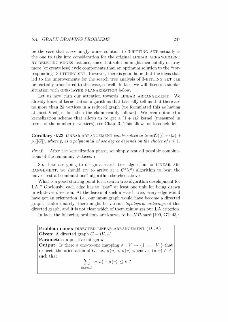
6.4. GRAPH DRAWING PROBLEMS 247
be the case that a seemingly worse solution to 3-hitting set actually isthe one to take into consideration for the original linear arrangementby deleting edges instance, since that solution might incidentally destroymore (or create less) cycle components than an optimum solution to the “cor-responding” 3-hitting set. However, there is good hope that the ideas thatled to the improvements for the search tree analysis of 3-hitting set canbe partially transferred to this case, as well. In fact, we will discuss a similarsituation with one-layer planarization below.
Let us now turn our attention towards linear arrangement. Wealready know of kernelization algorithms that basically tell us that there areno more than 2k vertices in a reduced graph (we formulated this as havingat most k edges, but then the claim readily follows). We even obtained akernelization scheme that allows us to get a (1 + ε)k kernel (measured interms of the number of vertices), see Chap. 3. This allows us to conclude:
Corollary 6.23 linear arrangement can be solved in time O(((1+ε)k)!+pε(|G|), where pε is a polynomial whose degree depends on the choice of ε ≤ 1.
Proof. After the kernelization phase, we simply test all possible combina-tions of the remaining vertices.
So, if we are going to design a search tree algorithm for linear ar-rangement, we should try to arrive at a O∗(ck) algorithm to beat thenaive “test-all-combinations” algorithm sketched above.
What is a good starting point for a search tree algorithm development forLA ? Obviously, each edge has to “pay” at least one unit for being drawnin whatever direction. At the leaves of such a search tree, every edge wouldhave got an orientation, i.e., our input graph would have become a directedgraph. Unfortunately, there might be various topological orderings of thisdirected graph, and it is not clear which of them minimizes our LA criterion.
In fact, the following problems are known to be NP-hard [199, GT 43]:
Problem name: directed linear arrangement (DLA)Given: A directed graph G = (V,A)Parameter: a positive integer kOutput: Is there a one-to-one mapping σ : V → 1, . . . , |V | thatrespects the orientation of G, i.e., σ(u) < σ(v) whenever (u, v) ∈ A,such that ∑
(u,v)∈A|σ(u) − σ(v)| ≤ k ?

248 CHAPTER 6. CASE STUDIES
Problem name: directed linear arrangement (DLA), pa-rameterized above guaranteed valueGiven: A directed graph G = (V,A)Parameter: a positive integer kOutput: Is there a one-to-one mapping σ : V → 1, . . . , |V | thatrespects the orientation of G such that
∑
(u,v)∈A|σ(u) − σ(v)| ≤ k + |A| ?
More specifically, the sketched search tree algorithm for linear ar-rangement has (as of yet) reduced the original instance to an instance(G, k,≺) that can be viewed as an instance of directed linear arrange-ment, parameterized above guaranteed value, see Alg. 53. The procedureLA-ST is called with (G, k, ∅) at the beginning, where (G, k) is the instanceof linear arrangement we like to investigate.
Algorithm 53 A search tree algorithm solving LA, called LA-ST
Input(s): a graph G = (V,E), an integer k, a partial ordering ≺ on VOutput(s): YES iff the given LA instance has a solution
Determine the edges that are settled by transitivity and adjust ≺ and kaccordingly.if k < 0 or ≺ contains both (x, y) and (y, x) then
return NO.else if ∃x, y ∈ E : neither x ≺ y nor y ≺ x is settled then
if LA-ST(G, k − 1,≺ ∪ (x, y)) thenreturn YES
elsereturn LA-ST(G, k − 1,≺ ∪ (y, x))
end ifelse
return DLAgv-ST((V,≺), k, ∅)end if
In Alg. 53, (G,≺) should denote the directed acyclic graph that corre-sponds to G, when the arcs of (G,≺) are oriented so that they respect theordering ≺.
Lemma 6.24 Alg. 54 correctly solves directed linear arrangement,parameterized above guaranteed value.
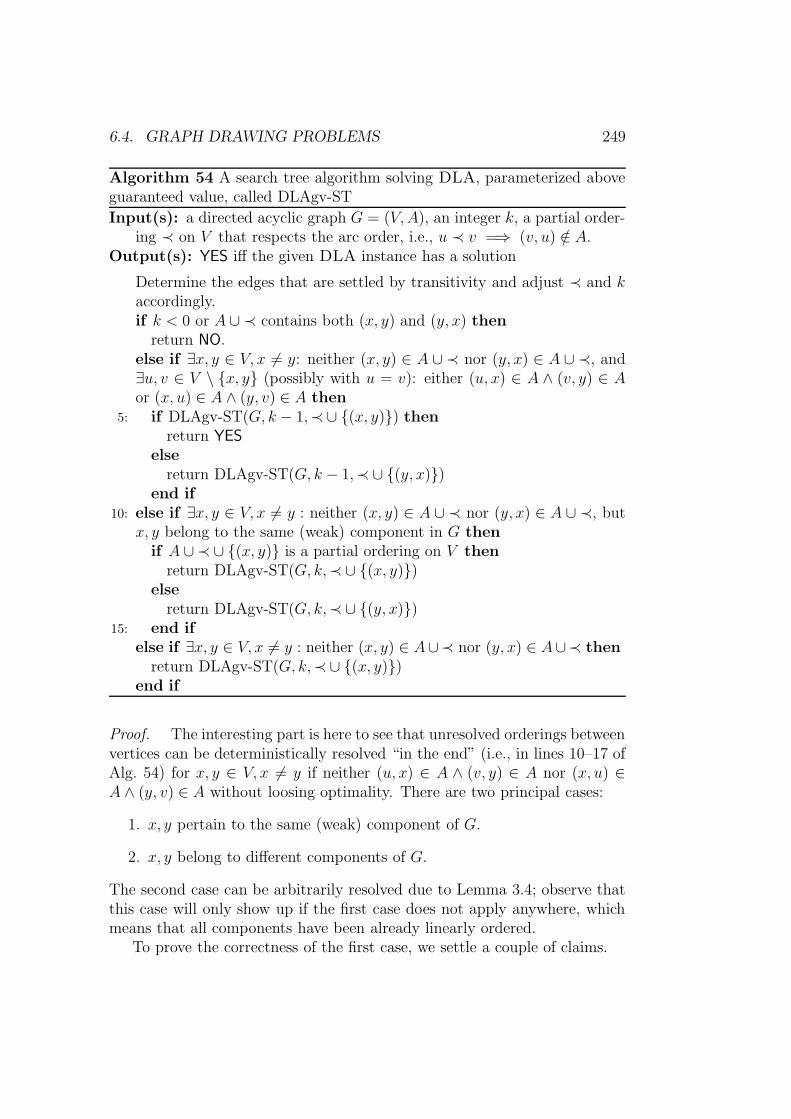
6.4. GRAPH DRAWING PROBLEMS 249
Algorithm 54 A search tree algorithm solving DLA, parameterized aboveguaranteed value, called DLAgv-ST
Input(s): a directed acyclic graph G = (V,A), an integer k, a partial order-ing ≺ on V that respects the arc order, i.e., u ≺ v =⇒ (v, u) /∈ A.
Output(s): YES iff the given DLA instance has a solution
Determine the edges that are settled by transitivity and adjust ≺ and kaccordingly.if k < 0 or A ∪ ≺ contains both (x, y) and (y, x) then
return NO.else if ∃x, y ∈ V, x 6= y: neither (x, y) ∈ A ∪ ≺ nor (y, x) ∈ A ∪ ≺, and∃u, v ∈ V \ x, y (possibly with u = v): either (u, x) ∈ A ∧ (v, y) ∈ Aor (x, u) ∈ A ∧ (y, v) ∈ A then
5: if DLAgv-ST(G, k − 1,≺ ∪ (x, y)) thenreturn YES
elsereturn DLAgv-ST(G, k − 1,≺ ∪ (y, x))
end if10: else if ∃x, y ∈ V, x 6= y : neither (x, y) ∈ A ∪ ≺ nor (y, x) ∈ A ∪ ≺, but
x, y belong to the same (weak) component in G thenif A ∪ ≺ ∪ (x, y) is a partial ordering on V then
return DLAgv-ST(G, k,≺ ∪ (x, y))else
return DLAgv-ST(G, k,≺ ∪ (y, x))15: end if
else if ∃x, y ∈ V, x 6= y : neither (x, y) ∈ A∪≺ nor (y, x) ∈ A∪≺ thenreturn DLAgv-ST(G, k,≺ ∪ (x, y))
end if
Proof. The interesting part is here to see that unresolved orderings betweenvertices can be deterministically resolved “in the end” (i.e., in lines 10–17 ofAlg. 54) for x, y ∈ V, x 6= y if neither (u, x) ∈ A ∧ (v, y) ∈ A nor (x, u) ∈A ∧ (y, v) ∈ A without loosing optimality. There are two principal cases:
1. x, y pertain to the same (weak) component of G.
2. x, y belong to different components of G.
The second case can be arbitrarily resolved due to Lemma 3.4; observe thatthis case will only show up if the first case does not apply anywhere, whichmeans that all components have been already linearly ordered.
To prove the correctness of the first case, we settle a couple of claims.

250 CHAPTER 6. CASE STUDIES
Claim 0: There exists u, v ∈ V \ x, y (possibly u = v) such that u isconnected by an arc to x and v is connected by an arc to y.Proof of Claim. Since there is no arc connecting x and y but both belongin the same weak component, the claim is true. ♦
In the following, let us fix such u, v ∈ V according to Claim 0. Since theprevious If-branch is not applicable, we have either (x, u) ∈ A and (v, y) ∈ A,or (u, x) ∈ A and (y, v) ∈ A. For reasons of symmetry, we only discuss thefirst of these possibilities in what follows.
Claim 1: Either (x, v) ∈ A or (v, x) ∈ A.Proof of Claim. Otherwise, the previous If-branch would have been appli-cable, since we have neither (x, v) ∈ A nor (v, x) ∈ A but (x, u) ∈ A and(v, y) ∈ A. ♦
Symmetrically, one can show:Claim 1’: Either (y, u) ∈ A or (u, y) ∈ A.
This leaves us with the following possibilities:
1. (x, u) ∈ A, (v, y) ∈ A, (x, v) ∈ A, (the relation between y and u isarbitrary): the underlined relations imply (y, x) ∈ ≺, and this has beenfound by the transitivity check at the very beginning of the routine, sothat this case cannot occur at this stage.
2. (x, u) ∈ A, (v, y) ∈ A, (v, x) ∈ A, (y, u) ∈ A:
There are no arcs leading into x and no arcs emanating from y, sinceotherwise the previous If-branch would have been applicable. Hence,there is only one way of ordering x and y without (locally) incurringadditional costs, and this ordering y ≺ x does not interfere with otherconnections due to the previous sentence.
3. (x, u) ∈ A, (v, y) ∈ A, (v, x) ∈ A, (u, y) ∈ A: the underlined relationsimply (x, y) ∈ ≺, so that this case cannot occur at this stage.
Observe that Alg. 54 can be also used to solve the problem when parame-terized in the standard way. Namely, one could call DLAgv-ST(G, k−|A|, ∅),when (G = (V,A), k) is the given DLA instance.
Theorem 6.25 The problems linear arrangement, directed lineararrangement (the latter parameterized either in the standard way or aboveguaranteed value) are solvable in time O(2k|G|).
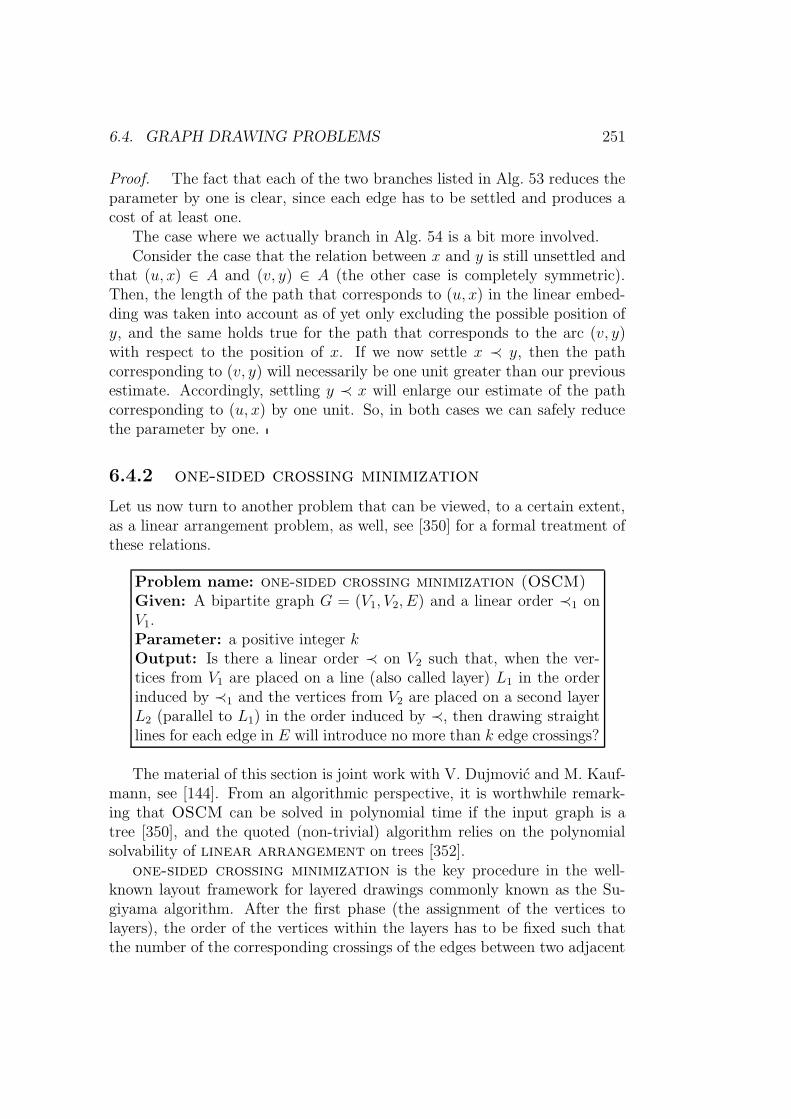
6.4. GRAPH DRAWING PROBLEMS 251
Proof. The fact that each of the two branches listed in Alg. 53 reduces theparameter by one is clear, since each edge has to be settled and produces acost of at least one.
The case where we actually branch in Alg. 54 is a bit more involved.Consider the case that the relation between x and y is still unsettled and
that (u, x) ∈ A and (v, y) ∈ A (the other case is completely symmetric).Then, the length of the path that corresponds to (u, x) in the linear embed-ding was taken into account as of yet only excluding the possible position ofy, and the same holds true for the path that corresponds to the arc (v, y)with respect to the position of x. If we now settle x ≺ y, then the pathcorresponding to (v, y) will necessarily be one unit greater than our previousestimate. Accordingly, settling y ≺ x will enlarge our estimate of the pathcorresponding to (u, x) by one unit. So, in both cases we can safely reducethe parameter by one.
6.4.2 one-sided crossing minimization
Let us now turn to another problem that can be viewed, to a certain extent,as a linear arrangement problem, as well, see [350] for a formal treatment ofthese relations.
Problem name: one-sided crossing minimization (OSCM)Given: A bipartite graph G = (V1, V2, E) and a linear order ≺1 onV1.Parameter: a positive integer kOutput: Is there a linear order ≺ on V2 such that, when the ver-tices from V1 are placed on a line (also called layer) L1 in the orderinduced by ≺1 and the vertices from V2 are placed on a second layerL2 (parallel to L1) in the order induced by ≺, then drawing straightlines for each edge in E will introduce no more than k edge crossings?
The material of this section is joint work with V. Dujmovic and M. Kauf-mann, see [144]. From an algorithmic perspective, it is worthwhile remark-ing that OSCM can be solved in polynomial time if the input graph is atree [350], and the quoted (non-trivial) algorithm relies on the polynomialsolvability of linear arrangement on trees [352].
one-sided crossing minimization is the key procedure in the well-known layout framework for layered drawings commonly known as the Su-giyama algorithm. After the first phase (the assignment of the vertices tolayers), the order of the vertices within the layers has to be fixed such thatthe number of the corresponding crossings of the edges between two adjacent
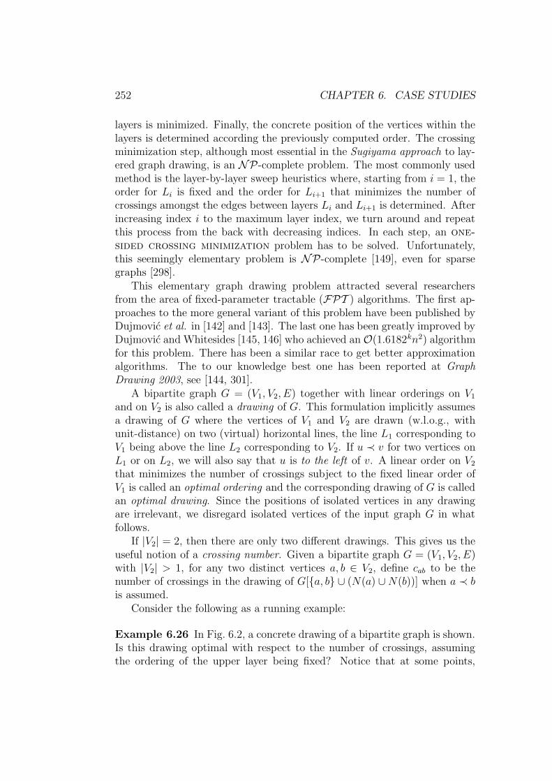
252 CHAPTER 6. CASE STUDIES
layers is minimized. Finally, the concrete position of the vertices within thelayers is determined according the previously computed order. The crossingminimization step, although most essential in the Sugiyama approach to lay-ered graph drawing, is an NP-complete problem. The most commonly usedmethod is the layer-by-layer sweep heuristics where, starting from i = 1, theorder for Li is fixed and the order for Li+1 that minimizes the number ofcrossings amongst the edges between layers Li and Li+1 is determined. Afterincreasing index i to the maximum layer index, we turn around and repeatthis process from the back with decreasing indices. In each step, an one-sided crossing minimization problem has to be solved. Unfortunately,this seemingly elementary problem is NP-complete [149], even for sparsegraphs [298].
This elementary graph drawing problem attracted several researchersfrom the area of fixed-parameter tractable (FPT ) algorithms. The first ap-proaches to the more general variant of this problem have been published byDujmovic et al. in [142] and [143]. The last one has been greatly improved byDujmovic and Whitesides [145, 146] who achieved an O(1.6182kn2) algorithmfor this problem. There has been a similar race to get better approximationalgorithms. The to our knowledge best one has been reported at GraphDrawing 2003, see [144, 301].
A bipartite graph G = (V1, V2, E) together with linear orderings on V1
and on V2 is also called a drawing of G. This formulation implicitly assumesa drawing of G where the vertices of V1 and V2 are drawn (w.l.o.g., withunit-distance) on two (virtual) horizontal lines, the line L1 corresponding toV1 being above the line L2 corresponding to V2. If u ≺ v for two vertices onL1 or on L2, we will also say that u is to the left of v. A linear order on V2
that minimizes the number of crossings subject to the fixed linear order ofV1 is called an optimal ordering and the corresponding drawing of G is calledan optimal drawing. Since the positions of isolated vertices in any drawingare irrelevant, we disregard isolated vertices of the input graph G in whatfollows.
If |V2| = 2, then there are only two different drawings. This gives us theuseful notion of a crossing number. Given a bipartite graph G = (V1, V2, E)with |V2| > 1, for any two distinct vertices a, b ∈ V2, define cab to be thenumber of crossings in the drawing of G[a, b ∪ (N(a) ∪N(b))] when a ≺ bis assumed.
Consider the following as a running example:
Example 6.26 In Fig. 6.2, a concrete drawing of a bipartite graph is shown.Is this drawing optimal with respect to the number of crossings, assumingthe ordering of the upper layer being fixed? Notice that at some points,

6.4. GRAPH DRAWING PROBLEMS 253
c
3 4 5 6
d e
1 2
a b
3
3
Figure 6.2: Our running example for one-sided crossing minimization
more than two edges cross. How often such a crossing actually counts whencomputing the overall crossing number is shown at the side of a correspondingbox that emphasizes the crossing point.
Let us now compute the crossing numbers cuv for this graph.
cuv a b c d ea − 4 5 0 1b 1 − 1 0 0c 3 3 − 0 1d 3 2 3 − 1e 2 3 2 0 −
The number of crossings in the given drawing can be hence computed as
cab + cac + cad + cae + cbc + cbd + cbe + ccd + cce + cde
= 4 + 5 + 0 + 1 + 1 + 0 + 0 + 0 + 1 + 1
= 13.
Furthermore, for any u ∈ V2 with deg(u) > 0, let lu be the leftmostneighbor of u on L1, and ru be the rightmost neighbor of u. We call twovertices u, v ∈ V2 interfering or unsuited if there exists some x ∈ N(u) withlv ≺ x ≺ rv, or there exists some x ∈ N(v) with lu ≺ x ≺ ru. Otherwise,they are called suited. Observe that, for u, v suited, cuv ·cvu = 0. Dujmovicand Whitesides have shown:

254 CHAPTER 6. CASE STUDIES
Lemma 6.27 Let G = (V1, V2, E) be an instance of one-sided crossingminimization, where the ordering of V1 is fixed. In any optimal ordering ≺of the vertices of V2, we find u ≺ v if ru ≤ lv.
This means that all suited pairs appear in their natural ordering.
This already allows us to formulate a first parameterized algorithm forone-sided crossing minimization, which is a simple search tree algo-rithm. In the course of this algorithm, we will gradually construct a suit-able ordering ≺ on V2; when settling the ordering between u and v on V2,we also say that we commit u ≺ v or v ≺ u. A generalized instance ofone-sided crossing minimization therefore contains, besides the bipar-tite graph G = (V1, V2, E), a partial ordering on V2. A vertex v ∈ V2 is fullycommitted if, for all u ∈ V2 \ u, v, u, v is committed.
Lemma 6.27 allows us to state the following rule:
Reduction rule 60 For every pair of vertices u, v from V2 with cuv = 0,commit u ≺ v.
Algorithm 55 A search tree algorithm solving OSCM, called OSCM-ST-simple
Input(s): a bipartite graph G = (V1, V2, E), an integer k, a linear ordering≺1 on V1, a partial ordering ≺2 on V2
Output(s): YES iff the given OSCM instance has a solution
repeatExhaustively apply the reduction rules, adjusting ≺2 and k accordingly.Determine the vertices whose order is settled by transitivity and adjust≺2 and k accordingly.
until there are no more changes to ≺2 and to k5: if k < 0 or ≺2 contains both (x, y) and (y, x) then
return NO.else if ∃x, y ⊆ V2 : neither x ≺2 y nor y ≺2 x is settled then
if OSCM-ST-simple(G, k − 1,≺1,≺2 ∪ (x, y)) thenreturn YES
10: elsereturn OSCM-ST-simple(G, k − 1,≺1,≺2 ∪ (y, x))
end ifelse
return YES
15: end if
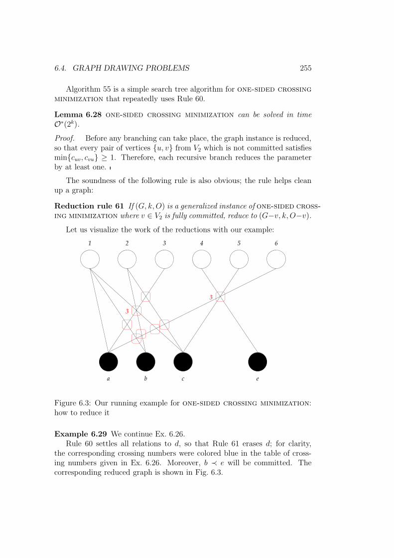
6.4. GRAPH DRAWING PROBLEMS 255
Algorithm 55 is a simple search tree algorithm for one-sided crossingminimization that repeatedly uses Rule 60.
Lemma 6.28 one-sided crossing minimization can be solved in timeO∗(2k).
Proof. Before any branching can take place, the graph instance is reduced,so that every pair of vertices u, v from V2 which is not committed satisfiesmincuv, cvu ≥ 1. Therefore, each recursive branch reduces the parameterby at least one.
The soundness of the following rule is also obvious; the rule helps cleanup a graph:
Reduction rule 61 If (G, k,O) is a generalized instance of one-sided cross-ing minimization where v ∈ V2 is fully committed, reduce to (G−v, k, O−v).
Let us visualize the work of the reductions with our example:
c
3 4 5 6
e
1 2
a b
3
3
Figure 6.3: Our running example for one-sided crossing minimization:how to reduce it
Example 6.29 We continue Ex. 6.26.Rule 60 settles all relations to d, so that Rule 61 erases d; for clarity,
the corresponding crossing numbers were colored blue in the table of cross-ing numbers given in Ex. 6.26. Moreover, b ≺ e will be committed. Thecorresponding reduced graph is shown in Fig. 6.3.

256 CHAPTER 6. CASE STUDIES
Our usual question is if and how to improve on the very simple searchtree algorithm. Our first observation is that it is not necessary to branchat x, y ⊂ V2 with cxy = cyx. This means to modifications to our Alg. 55,following the triviality last principle:
• Line 5 should exclude cxy = cyx.
• Line 12 should arbitrary commit some x, y ⊂ V2 that are not yetcommitted and recurse; only if all x, y ⊂ V2 are committed, YES isto be returned.
These modifications immediately yield an O∗(1.6182k) algorithm for one-sided crossing minimization. This is also the core of the algorithm pro-posed by Dujmovic and Whitesides [146]. There, more details are discussed,as, for example:
• How to efficiently calculate all the crossing numbers cxy in a prepro-cessing phase.
• How to integrate branch and cut elements in the algorithm that aresurely helpful from a practical perspective.
• How to generalize the algorithm for instances that allow integer weightson the edges (multiple edges).
Further improvements are possible if one gives a deeper analysis of lo-cal patterns x, y ∈ V2 such that cxycyx ≤ 2. This way, we were able toprove [144] that one-sided crossing minimization can be solved in timeO∗(1.4656k).
Instead of actually presenting that algorithm, let us point to another re-markable fact that is already present in Alg. 55 (and that alone indicates thatthat algorithm is far from optimal): we never actually used the propertiesof OSCM as a graph drawing problem; we only relied on dealing with thecrossing numbers. So, we basically presented an algorithm that solves thefollowing problem (in the spirit inspired by Junger and Mutzel [248]).

6.4. GRAPH DRAWING PROBLEMS 257
Problem name: positive weighted completion of an or-dering (PCO)Given: An ordered digraph P = (V,A) and a cost function c map-ping A(D([U(P )]c)) into the positive integers; by setting c to zero forarcs in A(D(U(P ))), we can interpret the domain of c as V (P )×V (P ).Parameter: a positive integer k.Output: Is there a selection A′ of arcs from A(D([U(P )]c)) such thatthe transitive closure (A′ ∪ A(P ))+ is a linear order and
∑c(a) | a ∈ (A′ ∪ A(P ))+ ≤ k ?
To understand this problem, we need to explain some more notions. Wecall a digraph an ordered digraph if its arc relation complies with the axiomsof a partial order. A directed graph obtained from an undirected graph Gby replacing every edge u, v by the two arcs (u, v) and (v, u) is denoted byD(G). The undirected graph obtained from a digraph G by putting an edgeu, v whenever there is an arc (u, v) in G is denoted by U(G). The set ofarcs of a digraph G is denoted by A(G).
It is quite obvious that one-sided crossing minimization can besolved with the help of positive weighted completion of an order-ing; the linear order which is aimed at is the permutation of the vertices onthe second layer which minimizes the number of crossings involved, so thatthe crossing number cab is the cost of the arc (a, b) in the digraph model. Dueto the validity of reduction rule 60, all crossing numbers can be assumed to begreater than or equal to one. Since it is easy to see that positive weightedcompletion of an ordering is nondeterministically solvable in polyno-mial time, and since Eades and Wormald [149] have shown that one-sidedcrossing minimization is NP-hard, we can immediately deduce:
Lemma 6.30 positive weighted completion of an ordering is NP-complete.
This makes positive weighted completion of an ordering an in-teresting problem to study. In addition to being used as a tool in solvingk-one-sided crossing minimization, this problem, as a variant of thelinear ordering problem, is of independent interest. The linear or-dering problem, defined as positive weighted completion of anordering where A = ∅ (but without the constraint that all arc costsare necessarily positive), is a well-known NP-hard combinatorial optimiza-tion problem. This problem has large number of applications in such diverse
258 CHAPTER 6. CASE STUDIES
fields as economy, sociology, graph theory, archaeology, and task scheduling.Applications of the linear ordering problem include the triangulationof input-output matrices in economy, minimizing total weighted completiontime in one-machine scheduling and the aggregation of individual preferencesin the social sciences. For a good overview on this problem, the reader is re-ferred to the corresponding book of Reinelt [332]. In fact, the famous branchand cut methods was first formulated for and successfully applied to the lin-ear ordering problem by Grotschel et al. [218], and these resemble inspirit and methodology the search tree methods we will present below.
Keeping in mind what we said above, Alg. 55 can be read as an algorithmsolving positive weighted completion of an ordering. Hence, weimmediately get:
Lemma 6.31 positive weighted completion of an ordering is inFPT .
However, we like to improve on the running time of our algorithm in whatfollows in two ways:
1. We provide a small kernel for PCO.
2. We give a better search tree algorithm for PCO.
Note that this (on the fly) also solves the corresponding problems for OSCM,albeit the search tree algorithm we shall present has worse running time thatwhat was claimed above for OSCM.
In fact, we can even observe a kernelization scheme for positive weightedcompletion of an ordering:
Reduction rule 62 [RRLOq] For any fixed q > 1 do:For each connected component C ⊆ V of [U(P )]c with |C| ≤ q, solve PCOoptimally on P [C].
The reduced instance will see the orderings between all pairs of verticesfrom C settled, and the parameter will be reduced accordingly. Note thatthis implies that all the vertices of C are isolated in the reduced [U(P )]c andcan thus be deleted by Rule 61 that is also valid for positive weightedcompletion of an ordering.
This new set of rules yields a kernel of size k q+1q
, since after exhaustive
application of this rule and Rule 61, each connected component of [U(P )]c
has at least (q+1) vertices and thus at least q edges. Correspondingly, at leastq arcs with a weight of at least one per arc have to be added per component,therefore there are at most k/q components. In other words, a kernel size of

6.4. GRAPH DRAWING PROBLEMS 259
k (where the kernel size is measured in terms of the number of vertices of thecorresponding order graph) can be “approximated” with arbitrary precision,at the expense of higher running times (the connected components of size upto q have to be solved), the typical behavior of a kernelization scheme. Still,arbitrary constants q or q = log k are possible choices for polynomial-timekernelization algorithms.
Lemma 6.32 The kernelization scheme is sound.
Proof. Assume that C is a connected component of [U(P )]c. Consider avertex x 6∈ C. Since C is a connected component in [U(P )]c, x is comparablewith each y ∈ C (otherwise, y and x would be connected in the complementgraph). Hence, C can be portioned into C` = y ∈ C | y ≺ x and Cr =y ∈ C | x ≺ y. Since C` ≺ x ≺ Cr, either C` = ∅ or Cr = ∅; otherwise,there would be no connection between vertices of C` and vertices of Cr in thecomplement graph. Hence, x will never be ordered “in-between” two verticesfrom C.
Therefore, the reduction rule RRLOq is sound and we can conclude:
Theorem 6.33 Fix some 1 < α ≤ 1.5. Then, each instance of positiveweighted completion of an ordering admits a problem kernel of sizeαk.
Corollary 6.34 Fix some 1 < α ≤ 1.5. Then, each instance of one-sidedcrossing minimization can be reduced to an instance (P = (V2, A), k) ofpositive weighted completion of an ordering, with |V2| ≤ αk.
This has not yet given us a problem kernel for the original problem, since|V1| (and hence |E|) has not yet been bounded by a function of k. Withthat aim, consider the following simple reduction rule, akin to Buss’s rule forvertex cover:
Reduction rule 63 If cab > k then do: if cba ≤ k then commit b ≺ a elsereturn NO.
This is clearly a sound rule. Moreover notice, that if a vertex a ∈ V2
has deg(a) ≥ 2k + 1, then for every vertex b ∈ V2, cab > k or cba > k aretrue. Therefore, after exhaustively performing Rule 63 in combination withRule 61, all the vertices of V2 of degree larger than 2k will have been removedfrom the one-sided crossing minimization instance. This yields:
Theorem 6.35 For some 1 < α ≤ 1.5, OSCM admits a problem kernelG = (V1, V2, E) with |V1| ≤ 2k|V2|(≤ 3k2), |V2| ≤ αk, and |E| ≤ 2k|V2|.

260 CHAPTER 6. CASE STUDIES
Now, we come to improving the search tree algorithm.
Theorem 6.36 positive weighted completion of an ordering canbe solved in time O(1.5175k + kn2), where n is the number of vertices in theaccompanying ordered digraph.
To describe the algorithm for positive weighted completion of anordering we will need the following definitions.
A pair of vertices a, b ∈ V is transitive in an ordered digraph P = (V,A)if there exists a vertex c ∈ V such that a, b is transitive with respect to c.We say that a pair of vertices a, b is strongly dependent with respect to avertex c if a, b is dependent but not transitive with respect to c.
a, b ∈ V form a i/j pattern in a given PCO instance if c((a, b)) = i andc((b, a)) = j. Furthermore, if a, c or b, c form 2/1 pattern, we say thata, b is strongly 2/1 dependent with respect to vertex c. We are now readyto give the algorithm for PCO.
Let us mention once more that it is possible to interleave other (more com-plicated) instances of the family of reduction rules RRLOq with the searchtree algorithm to further compress the instances as far as affordable. Thispresents a general way of how to actually implement kernelization schemes(the overall algorithm is exponential anyway).Proof. It is clear that the algorithm is correct if the step (*) is valid. Beforeshowing that the step is indeed valid, we prove the claimed running time byanalyzing its exponential part, that is we analyze the size of the search tree.
A node of the search tree branches with three conditions:
1. There is a dependent i/j pattern a, b such that i+ j ≥ 4.
2. There is a 2/1 pattern a, b that is transitive.
3. There is 2/1 pattern a, b strongly 2/1 dependent w.r.t. c.
The smallest branching vectors that may arise in the first case are (3, 1) and(2, 2). These are also the smallest branching vectors arising in the secondcase, since a, b is a transitive 2/1 pattern; thus, committing a ≺ b or b ≺ acommits by transitivity at least one other pair.
Consider now the branching vectors arising in the last case. Since thepair a, b is strongly 2/1 dependent with respect to vertex c, we know thatat least one of the four costs c(a, c), c(c, a), c(b, c), and c(c, b) is equal to2 units, the worst case being then that all the other costs are one. Thissituation is then best analyzed by considering all possible arc directions whenc((a, b)) = α ∈ 1, 2, c((b, a)) = 3−α, c((b, c)) = β ∈ 1, 2, c((c, b)) = 3−β,c((a, c)) = c((c, a)) = 1. The different arc directions according to which webranch are then:

6.4. GRAPH DRAWING PROBLEMS 261
Algorithm 56 A parameterized algorithm solving positive weightedcompletion of an ordering, called PCO
Input(s): an ordered digraph graph G = (V,A), an integer k, a cost func-tion c
Output(s): YES iff the given PCO instance has a solution
repeatExhaustively apply the reduction rules, adjusting G, c, and k accord-ingly.Determine the vertices whose order is settled by transitivity and adjustaccordingly.
until there are no more changes5: if k < 0 then
return NO.else if (there is a dependent i/j pattern a, b such that i + j ≥ 4) or(there is a 2/1 pattern a, b that is transitive) then
Set c((a, b)) = c((b, a)) = 0.if PCO(G ∪ (a, b), k − 1, c) then
10: return YES
elsereturn PCO(G ∪ (b, a), k − 1, c)
end ifelse if there is 2/1 pattern a, b strongly 2/1 dependent w.r.t. c then
15: Set c((a, b)) = c((a, b)) = c((b, c)) = c((c, b)) = 0.for all orderings O between a, b and b, c do
set k′ as updated kif PCO(G ∪O, k′, c) then
return YES
20: end ifend for
elseresolve each remaining 2/1 pattern in favor of the cheaper orderingand update G and k accordingly; (*)resolve all remaining 1/1 patterns arbitrarily and update G and kaccordingly;
25: return k ≥ 0.end if
1. (a, b) and (b, c): by transitivity, this commits (a, c), so that this selec-tion costs α + β + 1;

262 CHAPTER 6. CASE STUDIES
2. (a, b) and (c, b), costing α + (3 − β),
3. (b, a) and (b, c), costing (3 − α) + β; and
4. (b, a) and (c, b), where transitivity establishes a cost of (3 − α) + (3 −β) + 1.
Going through all choices of α and β leaves us with the branching vectors(2, 4, 4, 4) (for α 6= β) and (3, 3, 3, 5) (for α = β). Thus overall in the abovealgorithm the worst case branching is (2, 4, 4, 4) and (3, 3, 3, 5) resulting inthe search tree having the size 1.5175k in the worst case.
We now prove that step (*) of the algorithm is valid. Let a time counter beequal to zero right before step (*) starts. First observe that, at that time thereare no two incomparable pairs a, b and a, c both forming a 2/1 pattern,as otherwise a, b would have been committed in the preceding cases. Nowconsider committing, one by one, each of the remaining 2/1 patterns by theircheaper ordering. In that process, whenever a pair of vertices is committed(either directly or by transitivity) we increase the time by one and assignthe current time to the pair being committed. We will now prove that nopair is committed by transitivity. We first show that no 1/1 pattern getscommitted (by transitivity) at any time step. Assume the contrary and let idenote the time step when the first 1/1 pattern c, d gets committed. Sincewe only commit directly 2/1 patterns, the pair a, b committed at time i−1forms a 2/1 pattern. Therefore, without loss of generality, committing a ≺ bat time i − 1 commits by transitivity c ≺ d at time i. That further impliesthat at time i − 1, we have c ≺ a and b ≺ d (note that we may also havec = a and b ≺ d or c ≺ a and b = d). In either case, at least one of these twopairs, c, a or b, d, say a, c, is incomparable at step 0 as otherwise a, bwould have been committed at a previous step of the algorithm. Thus, a, cforms either a 2/1 or a 1/1 pattern. Since a, b forms a 2/1 pattern then bythe above observation a, c cannot form a 2/1 pattern. Furthermore, a, ccannot stem from a 1/1 pattern since the pair is incomparable at time 0 andis comparable at time i− 1 > 0 thus contradicting the fact that c, d is the1/1 pattern that is assigned the smallest time stamp. Hence, no 1/1 patterngets committed (by transitivity) at any time step.
Assume now that some 2/1 pattern g, h gets committed by transitivityat some time j. Since no 1/1 pattern gets committed at any time step, thepair e, f committed at time j − 1 forms a 2/1 pattern. Therefore, withoutloss of generality, committing e ≺ f at time j − 1 commits by transitivityg ≺ h at time j. Since e, f and g, h form 2/1 patterns, e 6= g 6= h andf 6= g 6= h. Furthermore, at time j − 1 we know that g ≺ e and f ≺ hand at least one of these two pairs, say e, g, is incomparable at time 0, as

6.4. GRAPH DRAWING PROBLEMS 263
otherwise g, h would have been already committed earlier in the course ofthe algorithm. Since the pair e, g is incomparable at time 0 and the pairg, h forms a 2/1 pattern, by the above observation the pair e, g mustform 1/1 pattern. However, by the above demonstration, it is not possiblethat a 1/1 pattern incomparable at time 0 gets committed at any later time.
7
2 4
−2 0
<0
−2 3
0
<0 0
<0
c<aa<c
a<b
b<cc<b
b<ab<c
b<aa<b
c<b
2
0
e<a(b<e)
c<ea<e
Figure 6.4: A search tree example for one-sided crossing minimization.
We can actually apply this algorithm to our Example (in fact, the morecomplicated cases would not trigger); this gives the search tree of Fig. 6.4.This graphic is to be read as follows:
• Nodes contain the parameter value.
• Edges are labeled with the committed orders; blue labels indicate theorders committed by transitivity.
We start with displaying the reduced generalized graph instance (and thecorresponding table), assuming we started with the instance (G, 7). The(minimum) solution found this way is shown in Fig. 6.5.

264 CHAPTER 6. CASE STUDIES
3 4 5 61 2
e dc ab
Figure 6.5: An optimal solution to our instance.
As a possible line of future research, we mention a variant of one-sidedcrossing minimization (crossing minimization of two-layered graphs withvertex pairs) that was discussed in [381, 382] with a bio-informatics motiva-tion (visualizing genetic networks to improve the understanding of interac-tions between genes). It might be that some of our methods apply to thatproblem, as well, which is interesting since good approximation algorithmsare known for one-sided crossing minimization (see [380]) but not forthe two-layered crossing minimization problem with vertex pairs.
6.4.3 Biplanarization problems
A graph modification variant of one-sided crossing minimization wasalso considered, one-layer planarization, see [300]. To define this prob-lem properly, we need another notion: A bipartite graph G = (V1, V2;E)is biplanar if the vertices can be placed on two parallel lines L1 and L2 inthe plane (where the vertices from Vi are placed on Li) such that there areno edge crossings when edges are drawn as straight-line segments. A graphG = (V,E) is biplanar if there is a bipartition V = V1 ∪ V2 of its edge set(i.e., G[V1] = G[V2] = ∅) such that (V1, V2;E) is biplanar.
The biplanarization problem was discussed in two variants in [142, 148,176, 177]:

6.4. GRAPH DRAWING PROBLEMS 265
Problem name: two-layer planarization (TLP)Given: A graph G = (V,E)Parameter: a positive integer kOutput: Is there a set C ⊆ E, |C| ≤ k, whose removal makes thegraph biplanar?
Problem name: one-layer planarization (OLP)Given: A bipartite graph G = (V1, V2, E), a linear ordering < on V1
Parameter: a positive integer kOutput: Is there a set C ⊆ E, |C| ≤ k, whose removal allows abiplanar drawing of the graph that respects < on V1?
In fact, the latter problem is intimately related to one-sided crossingminimization: the only difference is the way in which a non-biplanar draw-ing is penalized; while within OSCM, the number of crossings is counted,within OLP, the number of edges that has to be removed to make the graphdrawable without crossings is measured. Hence, a procedure for solving OLPcan be also seen as a sub-routine within the Sugiyama approach to layereddrawings. Again, the tree case is solvable in polynomial time, see [350].
Let us first study TLP. Dujmovic et al. mentioned a nice characterizationof biplanar graphs in terms of forbidden subgraphs:
Theorem 6.37 A graph G is biplanar iff it is acyclic and does not containa 2-claw.
(a) The smallest four forbidden cycles. (b) The 2-claw.
Figure 6.6: Two classes of forbidden substructures for biplanar graphs.
Fig. 6.6 contain (some of) these forbidden structures and explains thenotion of a 2-claw. More precisely, there are two slightly different reasonswhy cycles are forbidden substructures: cycles of odd length (colored red)are forbidden, since biplanarity obviously implies bipartiteness by definition.Cycles of even length cannot be drawn without crossings, in whatever way wemight arrange the vertices on the two layers. This is indicated in Fig. 6.6(a):

266 CHAPTER 6. CASE STUDIES
a drawing is shown with (implicit) layers for C4 and C6, indicating that eras-ing one edge is sufficient to make this structure drawable; observe that dueto symmetry, it does not matter which edge we take out. Finally, Fig. 6.6(b)explains the notion of a 2-claw. More formally, a 2-claw is a graph consist-ing of one degree-3 vertex, the center, which is adjacent to three degree-2vertices, each of which is adjacent to the center and one leaf. The 2-claw iscomposed of three fingers, one of them colored red in Fig. 6.6(b) to show theimpossibility to biplanarily draw this graphs: when the finger-tip edge of thered finger is removed, however, this graph becomes biplanar.
The basic algorithmic idea would be to regard the edge sets of forbid-den substructures as candidate sets and branch on the different possibilitiesto destroy these structures. The problem is that there are infinitely manyforbidden structures, and hence there is no bound on the size of the hyper-edges in any hitting set instance one tends to form (where the forbiddensubstructures correspond, as usual, to the candidate sets).
To get a search tree algorithm that runs in FPT time, the following two(rather easy to check) results from [143] are crucial; to understand them, weneed some more notions first.
The non-leaf degree of a vertex v in graph G is the number of non-leafedges at v in G, and is denoted by deg′
G(v).A graph is a caterpillar (wreath, respectively) if deleting all the leaves
produces a (possibly empty) path (cycle, respectively). These graphs are vi-sualized in Fig. 6.7. Graphs composed of caterpillar and wreath componentsare exactly the graphs whose non-leaf degree is bounded by two.
Figure 6.7: Graphs without a vertex of non-leaf degree three or larger.
Lemma 6.38 If there exists a vertex v in a graph G such that deg′G(v) ≥ 3,then G has a 2-claw or a 3- or 4-cycle containing v as a subgraph.

6.4. GRAPH DRAWING PROBLEMS 267
Lemma 6.39 For graphs G with deg′G(v) ≤ 2 for all vertices v, G consistsof a forest of wreaths and caterpillars. Hence, a minimum biplanarizing setof G consists of one cycle edge from each component wreath.
These two lemmas lead themselves to Alg. 57. There, we use the notationfC to refer to the edge set of the forbidden structure C, since we are dealingwith an edge-deleting problem.
Algorithm 57 A search tree algorithm solving two-layer planariza-tion, called TLP-st-simple
Input(s): a graph G = (V,E), a positive integer kOutput(s): YES iff there is a biplanarization set B ⊆ E, |B| ≤ k
if ∃v ∈ V : deg′G(v) ≥ 3 and k ≥ 0 thenDetermine 2-claw, 3-cycle or 4-cycle C containing v.for all edges e ∈ fC do
if TLP-st-simple(G − e, k − 1) thenreturn YES
end ifend forreturn NO
elsereturn (k ≥ # wreath components)
end if
Example 6.40 Let us return to the example graph from Fig. 6.2, this timeseen as an TLP instance. There are two forbidden structures to be found inthis graph. In Fig. 6.8, we used color coding to emphasize them: three out ofthe four edges of a C4 we colored red and the fourth edge green. There is alsoa 2-claw with center at vertex labeled 1, the edges of which that don’t (also)participate in the 4-cycle we colored blue. The green edge is one of the edgesthat participate in both forbidden structures. Hence, if we remove that edge,we turn the graph into a biplanar graph. Fig. 6.9 shows how the verticescould be reordered so that we obtain a biplanar drawing of the modifiedgraph. In that drawing, we kept the color-coding of the edges, as well as thegreen edge (that is of course destroying biplanarity of the drawing) to clarifythe reordering.
How can we improve on this obvious O∗(6k) algorithm? A direct trans-lation into 6-hitting set is not possible due to the “postprocessing” of thesearch tree in the line colored red. However, how would such a translationlook like?

268 CHAPTER 6. CASE STUDIES
c
3 4 5 6
d e
1 2
a b
Figure 6.8: Forbidden subgraphs of our sample graph.
b
1 5 4
c e
6 3
a
2
d
Figure 6.9: Reordering: if the green edge is deleted, the graph drawingbecomes biplanar.
• Edges in the original instance correspond to the vertices of the relatedhypergraph.

6.4. GRAPH DRAWING PROBLEMS 269
• Hyperedges in the hypergraph correspond to the edge sets of the for-bidden structures as derived according to Lemma 6.38.
This allows to translate back the reduction rules we used for obtainingbetter algorithms for hitting set. Due to the mentioned postprocessing,we cannot actually delete edges along the search tree. Instead, we will markthem virtual ;5 the non-virtual edges of a forbidden structure f are denotedc(f), and the size of a forbidden structure is measured by s(f) = |c(f)|.Even more, also the edge domination rule that allows to delete hyperedgeshas to be considered with care.
When reconsidering the correctness proofs of the rules, one observes thatthe only rule that causes trouble is the vertex domination rule. However,without this rule, we cannot actually gain anything against the simple O∗(6k)algorithm.
Nonetheless, we obtain the following reduction rules:
1. structure domination: A forbidden structure f is dominated by anotherstructure f ′ if c(f ′) ⊂ c(f). Then, mark f as dominated.
2. small structures: If s(f) = 1, put the only non-virtual edge into thesolution that is constructed.
3a isolates: If e is an edge of degree zero, then mark e virtual.
Due to the relation with hitting set, let us call the number of non-dominated forbidden structures to which a specific edge e belongs is thedegree of e.
Can we also handle non-virtual edges of degree one (to a certain extent)by reduction rules? We will discuss this point later on.
Let C = c, w1, w2, w3, x1, x2, x3 be a 2-claw centered at c, such thatwi is neighbored (at least) to c and xi for i = 1, 2, 3. We will call Fi =cwi, wixi also a finger of C, so that the forbidden structure fC = F1∪F2∪F3
corresponding to C is partitioned into three disjoint fingers. A 2-claw whereone or more edges are virtual is called injured. Clearly, in an injured 2-clawwith five edges, only one of the fingers actually got injured and two fingersare still pretty fingers. In an injured 2-claw with four edges, we still have atleast one pretty finger left over.
The second ingredient in the approach to hitting set problems describedin Chap. 5 are so-called heuristic priorities. More specifically, we use the
5This idea is similar to the marking procedure we used for our face cover search treealgorithm; note that that problem also relates to hitting set, as it is basically red-bluedominating set on planar graphs.

270 CHAPTER 6. CASE STUDIES
following rules to select forbidden structures and edges to branch at in caseof multiple possibilities:
1. Select a forbidden structure f of smallest size that if possible corre-sponds to a short cycle.
2. If s(f) ≤ 5 and if there is another forbidden structure f ′ with c(f) ∩c(f ′) 6= ∅ and s(f ′) ≤ 5, modify f := c(f) ∩ c(f ′).
3. Select an edge e of maximal degree within f , if possible incident to thecenter of the 2-claw f , such that e belongs to a pretty finger.
In the following analysis, assume that we have already branched on allcycles up to length five (see the first heuristic priority). Then, we can applythe following reduction rule for (injured) 2-claws:
3b (injured) 2-claws: If e is an edge of degree one in a non-dominatedforbidden structure of size four, five or six corresponding to an (injured)2-claw, and if e is incident to the center of the corresponding 2-claw,then mark e virtual.
This allows us to state the whole procedure in Alg. 58, where branch at emeans the following:
if TLP-st(G− e, k − 1,M,DF ) thenreturn YES
else if G[M ∪ e] is acyclic thenAvoid deleting the last edge in a cyclereturn TLP-st(G, k,M ∪ e, DF )
elsereturn NO.
end if
In [176], we have shown the following result:
Theorem 6.41 Given a graph G and an integer parameter k, Alg. 58 whencalled with TLP-st(G, k, ∅, ∅), returns YES iff there is a biplanarization setB ⊆ E, |B| ≤ k.
The running time can be estimated as shown in Chap. 5 for the case ofHS; we only sketch the basic steps in what follows. Details can be foundin [176] (also cf. [177]).
Let (again) T `(k) denote the size of a search tree assuming that at least` forbidden structures in the given instance (with parameter k) have sizefive. Then, we can prove the recurrences listed in Fig. 6.10. Let us brieflycomment on these recurrences:

6.4. GRAPH DRAWING PROBLEMS 271
Algorithm 58 A search tree algorithm for TLP, called TLP-st
Input(s): a graph G = (V,E), a positive integer k, a set of virtual edgesM , a list of dominated forbidden structures DF
Output(s): YES if there is a biplanarization set B ⊆ E, |B| ≤ k (and itwill implicitly produce such a small biplanarization set then) orNO if no such set exists.
Exhaustively apply the reduction rules 1., 2., and 3a.; the resulting instanceis also called (G, k,M,DF ).if ∃ v ∈ V such that deg′G[E\M ](v) ≥ 3 then
if possible thenFind a non-dominated cycle C of length at most 5Select an edge e from C and branch at e
elseExhaustively apply all reduction rulesSelect 2-claw C and edge e from C according to heuristic prioritiesBranch at e
end ifelse
return (k ≥ # component wreaths of G[E \M ])end if
• The recurrence for T 0(k) is due to simple binary branching. In thecase that an edge e is not taken into the biplanarization set, one has toobserve that two small forbidden structures are created, i.e., structuresof size at most five: due to reduction rule 3b., we will branch at somee whose degree is at least two.
• The recurrence for T 1(k) is the most difficult to prove; its correctnessagain relies on reduction rule 3b.
• The seemingly complicated recurrences for T 2(k) are in fact trivial;they correspond to all possibilities for i such that two small forbiddenstructures f1 and f2 satisfy i = |c(f1) ∩ c(f2)|.
With the methods that were earlier explained, we can show:
Theorem 6.42 Given a graph G and an integer k, Alg. 58 determines if Gcan be made biplanar by deleting ≤ k edges in O(k2 · 5.1926k + |G|) time,when applied to the problem kernel derived in [143].
Let us now turn towards the case where the order of the vertices on onelayer is fixed, i.e., towards one-layer planarization. In contrast to what

272 CHAPTER 6. CASE STUDIES
T 0(k) ≤ T 0(k − 1) + T 2(k)
T 1(k) ≤ 2T 0(k − 1) + 2T 1(k − 1) + T 2(k − 1)
T 2(k) ≤ max
2T 1(k − 1) + 3T 2(k − 1),T 0(k − 1) + 16T 0(k − 2),2T 0(k − 1) + 9T 0(k − 2),3T 0(k − 1) + 4T 0(k − 2),4T 0(k − 1) + T 0(k − 2)
Figure 6.10: Upperbounding the size of the search tree of Alg. 58.
we presented for TLP, we will focus here mainly on the development of akernelization algorithm. Again, the similarities to hitting set problems ishelpful but distinctive features have to be observed.
The next two results from [143] give important properties for π-biplanargraphs.
Lemma 6.43 A bipartite graph G = (A,B;E) with a fixed permutation πof A is π-biplanar if and only if G is acyclic and the following condition holds.
For every path (x, v, y) of G with x, y ∈ A, and for every vertexu ∈ A between x and y in π, the only edge incident to u (if any) isuv.
(?)
Figure 6.11: A new forbidden substructure for OLP
This means that the 5-vertex graph depicted in Fig. 6.11 (where the upperlayer, i.e., the layer that contains three vertices, is fixed with respect of theordering of the vertices) is a forbidden structure. It is not hard to verify thatall cycles but cycles of length four and also 2-claws contain this forbidden

6.4. GRAPH DRAWING PROBLEMS 273
substructure, in whatever way we assign the vertices to the layer. This im-mediately shows that one-layer planarization is indeed “simpler” thantwo-layer planarization from a parameterized algorithmics standpoint.
Let G = (A,B;E) be a bipartite graph with a fixed permutation of Athat satisfies condition (?). Let H = K2,p be a complete bipartite subgraphof G with V (H) ∩ A = x, y, and V (H) ∩ B = v ∈ B : vx ∈ E, vy ∈E, degG(v) = 2, and |V (H)∩B| = p. Then H is called a p-diamond. Everycycle of G is in some p-diamond with p ≥ 2.
Lemma 6.44 If G = (A,B;E) is a bipartite graph and π is a permutation ofA satisfying condition (?) then the biplanarization number, given π, satisfies:
bpr(G, π) =∑
maximal p-diamonds of G
(p− 1) .
We are now going to derive a kernelization algorithm for OLP. Let ussay that an edge e of a bipartite graph G potentially violates condition (?)if, using the notation of condition (?), e = ei for i = 1, 2, 3, where e1 = xv ore2 = vy or e3 = uz for some u strictly between x and y in π such that z 6= v.We will also say that e1, e2, e3 (together) violate condition (?).
According to Lemma 6.43 (as well as the proof of Lemma 6.44 for thelast two rules), the following reduction rules are sound, given an instance(G = (A,B;E), π, k) of OLP. Analogues to the first three rules are well-known from Hitting Set problems, see Chap. 5.
Reduction rule 64 If e ∈ E does not participate in any cycle and does notpotentially violate condition (?), then remove e from the instance (keepingthe same parameter k).
Reduction rule 65 If v ∈ A ∪ B has degree zero, then remove v from theinstance and modify π appropriately (keeping the same parameter k).
Reduction rule 66 If e ∈ E participates in more than k2 situations thatpotentially violate condition (?), then put e into the biplanarization set andmodify the instance appropriately (also decreasing the parameter).
Let E? ⊆ E be all edges that potentially violate condition (?). Let E ⊆ Ebe all edges that participate in cycles. Let G4c be generated from those edgesfrom E? \ E? that participate in 4-cycles. By construction, G4c satisfies (?).Lemma 6.44 shows that the next reduction rule can be applied in polynomialtime:
Reduction rule 67 If bpr(G4c, π) > k, then NO.

274 CHAPTER 6. CASE STUDIES
Lemma 6.45 Let G = (A,B;E) be a bipartite graph and let π be a permu-tation of A. Let v ∈ B. Then, there is at most one edge e incident to v thatdoes not potentially violate condition (?) and participates in cycles of length> 4.
Theorem 6.46 Let G = (A,B;E) be a bipartite graph, π be a permutationof A and k ≥ 0. Assume that none of the reduction rules applies to the OLPinstance (G, π, k). Then, |E| ≤ k3. Hence, |V | < k3. The kernel can befound in time O(|G|2).6
Proof. Now consider E? as vertex set V ′ of a hypergraph G′ = (V ′, E ′) andput e1, e2, e3 into E ′ iff e1, e2, e3 together violate condition (?). A subset ofedges from E whose removal converts (A,B;E) into a bipartite graph whichsatisfies condition (?) is in obvious one-to-one correspondence with a hittingset of the hypergraph G′. Niedermeier and Rossmanith have shown [308,Proposition 1] a cubic kernel for 3-hitting set, so that at most k3 edgesare in E? (else NO). Their reduction rules correspond to our rules 64 and 66.
If e = xy ∈ E \ E? with y ∈ B does not belong to a 4-cycle, thenLemma 6.45 shows that there is no other edge zy ∈ E \ E?. But sincexy ∈ E, there must be some “continuing edge” zy on the long circle xybelongs to, so that zy ∈ E? follows. We can take zy as a witness for xy. ByLemma 6.45, zy can witness for at most one edge from E \E? incident to yand not participating in a 4-cycle.
This allows us to partition E into three disjoint subsets: (a) E∩E?, (b)E4c = e ∈ E \ E? | e participates in a 4-cycle : there can be at most 4ksuch edges according to rule 67 and Lemma 6.44, and (c) E \E4c: accordingto our preceding reasoning, there are at most |E?| many of these edges.
Rule 65 allows to conclude the bound on the number of vertices.
Theorem 6.47 (Dujmovic et al. [143]) Given a bipartite graph G = (A,B;E),a fixed permutation π of A, and integer k, there is an algorithm that deter-mines if bpr(G, π) ≤ k in O(3k · |G|) time.
Can we further improve on this algorithm? Firstly, it is clear that we cancombine the search tree algorithm with the kernelization algorithm describedabove. But furthermore, observe that the search tree algorithm basicallybranches on all members of E?, trying to destroy the corresponding triples ofedges violating condition (?). This means that we again take ideas stemmingfrom solutions of the naturally corresponding instance of 3-hitting set.
6More recently, a quadratic kernel for 3-hitting set was derived [310] based on the2k-kernel for vertex cover, see Chap. 4. Translating the corresponding reduction rulesshows that |E?| and hence |E| is in fact upperbounded by O(k2).

6.4. GRAPH DRAWING PROBLEMS 275
Unfortunately again, we cannot simply “copy” the currently best search treealgorithm for 3-hitting set, see Chap. 5, since destroying triples of edgesviolating condition (?) might incidentally also destroy more or less of the4-cycles. As explained in the TLP case, the problem is again the vertexdomination rule. In order to gain anything against the previously sketchedalgorithm, we must somehow at least avoid branching on vertices of degreeone contained in hyperedges of size three.
Firstly, we can prove a lemma that shows that, whenever we have branchedon all hyperedges of size three in the 3-hitting set instance (that corre-spond to situations violating condition (?) in the original OLP instance)that contain vertices of degree at least two, then we have already destroyedall “large” cycles. Then, we investigate the possible interaction between acycle of length four and a structure violating (?), after having “destroyed”all “mutually interacting” structures violating (?).
Lemma 6.48 Let G = (A,B;E) be a bipartite graph and π be a fixed per-mutation of A. Assume that if h = e1, e2, e3 and h′ = e′1, e′2, e′3 are twosituations violating (?), then h∩h′ = ∅. Let C = ab, bc, cd, da be a sequenceof edges forming a 4-cycle. Then, there is at most one hyperedge h—amongthe hyperedges modeling situations violating (?)—such that C ∩ h 6= ∅.
Hence, after the indicated branching, for each 4-cycle, at most one hyper-edge of size three remains such that the corresponding edge sets have non-empty intersection. Since we have to destroy every 4-cycle, the best we thencan obviously do is to take out an edge that takes part in the “accompanying”situation violating (?). This can be done completely deterministically due tothe preceding lemma. Finally, the only remaining situations correspond topossibly interacting 4-cycles. These can be solved with Lemma 6.44.
In the algorithm depicted in Alg. 59, we again use a set of virtual edgesM to mark edges which (according to our previous branching) we shall notput into the biplanarization set. This part of the input is therefore initial-ized with ∅ at the very beginning. The notation bpr(G, π,M) is accordinglyunderstood.
As a subroutine, we have singled out the situation exclusively dealingwith the T 0-branching. Note that the branching in the T 2-case can be alsoviewed as “branching at e” followed by the application of the small structurerule (which is also valid in this case, since it is derived from the 3-hittingset reduction rules).
Theorem 6.49 OLP can be solved in O(k3 · 2.5616k + |G|2) time.
Proof. We only have to analyze the running time in the following. As said

276 CHAPTER 6. CASE STUDIES
Algorithm 59 A search tree algorithm for one-layer planarization,called OLPInput(s): a bipartite graph G = (A,B;E), a permutation π of A, a positive
integer k, a set of virtual edges MOutput(s): NO if bpr(G, π,M) > k; otherwise, YES (and it will implicitly
produce such a small biplanarization set then)
Exhaustively apply the reduction rules; the resulting instance is also called(G, π, k,M).if (?) fails for some path (x, v, y) and edge ab with x ≺ a ≺ y then
if k = 0 thenreturn NO
else if possible thenchoose (x, v, y) and ab such that xv, vy, ab ∩M 6= ∅if possible then
choose (x′, v′, y′) and a′b′ such that x′v′, v′y′, a′b′ ∩M 6= ∅ ande = xv, vy, ab ∩ x′v′, v′y′, a′b′ ∩ (E \M)This is a T 2-branchif OLP(G− e,π, k − 1, M)=’YES’ then
return YES
elseLet e, f = xv, vy, ab ∩ (E \M).Let e, f ′ = x′v′, v′y′, a′b′ ∩ (E \M).return OLP(G− f, f ′,π, k − 2, M ∪ e)
end ifelseonly “isolated” forbidden structures of size two (also T 1)Let e, f = xv, vy, ab ∩ (E \M).if OLP(G− e,π, k − 1, M)=’YES’ then
return YES
elsereturn OLP(G− f,π, k − 1, M)
end ifend if
elseT 0-branchreturn OLP-T0(G, π, k,M)
end ifelse
return k ≥∑
maximal p-diamonds of G
(p− 1)
end if

6.4. GRAPH DRAWING PROBLEMS 277
Algorithm 60 A subroutine for OLP, called OLP-T0
Input(s): a bipartite graph G = (A,B;E), a permutation π of A, a positiveinteger k, a set of virtual edges M ; it has been tested that no reductionrules apply and that no T `-branching with ` > 0 is possible
Output(s): NO if bpr(G, π,M) > k; otherwise, YES (and it will implicitlyproduce such a small biplanarization set then)
if possible thenchoose (x, v, y) and ab such that there are (x′, v′, y′) and a′b′ such thate ∈ xv, vy, ab ∩ x′v′, v′y′, a′b′if OLP(G− e,π, k − 1, M) = ’YES’ then
return YES
elsereturn OLP(G,π, k, M ∪ e)
end ifelseonly “isolated conflicts”if h = xv, vy, ab intersects with some 4-cycle C then
Let e be a common edge of h and C.else
Choose some e ∈ h.end ifreturn OLP(G− e,π, k − 1, M)
end if
before, branching only actually takes place when we “solve” the correspond-ing 3-hitting set instance. During these recursions, we always assumethat, whenever we branch at forbidden structures of size three, there is someelement contained in that forbidden structure which actually participates inat least two forbidden structures.
More distinctly, let T `(k) denote the situation of a search tree assumingthat at least ` forbidden structures in the given instance (with parameter k)have a size of (at most) 2. Of course, T (k) ≤ T 0(k). We again analyze therecurrences for T 0, T 1 and T 2, and we use the notions of core and size of aforbidden structure similar to the TLP case.
For T 0, we obtain as in the case of 3-hitting set:
T 0(k) ≤ T 0(k − 1) + T 2(k).
For T 1, we cannot claim to “gain” any new forbidden structures of size two.Therefore, a trivial branching gives:
T 1(k) ≤ 2T 0(k − 1).

278 CHAPTER 6. CASE STUDIES
For T 2, we distinguish two sub-cases, considering two forbidden structuresf1, f2 of size two:
1. c(f1) ∩ c(f2) = ∅. Then, trivial branching gives:
T 2(k) ≤ 2T 1(k − 1) ≤ 4T 0(k − 2).
2. ∃e ∈ c(f1) ∩ c(f2). Branching at e (which our algorithm will do) thenyields:
T 2(k) ≤ T 0(k − 1) + T 0(k − 2).
The first sub-case leads to:
T 0(k) ≤ T 0(k − 1) + 4T 0(k − 2) ≤ 2.5616k.
The second sub-case gives:
T 0(k) ≤ T 0(k − 1) + (T 0(k − 1) + T 0(k − 2)) ≤ 2.4143k.
So, the first sub-case yields the worst case.
c
3 4 5 6
d e
1 2
a b
Figure 6.12: Our running example, this time for one-layer planarization
Example 6.50 Let us have another look at Fig. 6.2 and study the behaviorof our search tree algorithm.

6.4. GRAPH DRAWING PROBLEMS 279
c
3 4 5 6
d e
1 2
a b
(a) The branch that takes out anedge.
c
3 4 5 6
d e
1 2
a b
(b) The branch that makes anedge virtual.
Figure 6.13: Two possible first branches at edges of “high degree”.
c
3 4 5 6
d e
1 2
a b
(a) A second-level branch.
c
3 4 5 6
d e
1 2
a b
(b) A third-level branch.
Figure 6.14: Two further branching levels, only listing the case when a spe-cific edge is deleted.
We can find two classes of forbidden structures, marked with colors inFig. 6.12: one of them having two edges (colored in light and dark blue)incident with vertex a and one of them having two edges (colored in redfor the two possible left branches and colored in magenta for the right arm)incident with c. The remaining colored edges create forbidden structurestogether with the mentioned edges.
Let us pick one edge that participates in many forbidden structures, asdepicted in Fig. 6.13: the edge 1, c. Let us further follow what happens inthe first branch. We might then select 4, e for branching; in the case wetake out this edge, we arrive at Fig. 6.14(a). We follow this branch further,next considering edge 2, b. After having deleted that (third) edge, we cancolor the edge 1, a black again, since all forbidden structures this edge did

280 CHAPTER 6. CASE STUDIES
c
3 4 5 6
d e
1 2
a b
Figure 6.15: One solution to our problem.
a
3 4 5 6
d e
1 2
c b
Figure 6.16: One solution to our problem, when rearranged.
participate in have been already hit; formally, this means that the edge 1, ais removed (by rule 64). This is all shown in Fig. 6.14.
Finally, taking out edge 5, c resolves our problem completely, as canbe seen in Fig. 6.15: it is obviously possible to reorder the second layer (byswapping b and c to the left) so that the graph be be drawn without crossings.This can be best seen in Fig. 6.16; the edges that were taken out are drawnas dashed lines, keeping their original colors.
We should mention in this place that there is a natural generalization ofTLP (and also of crossing minimization problems): namely, one could allow
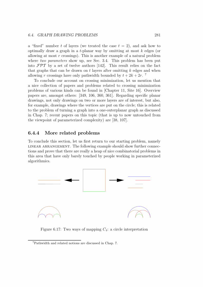
6.4. GRAPH DRAWING PROBLEMS 281
a “fixed” number t of layers (we treated the case t = 2), and ask how tooptimally draw a graph in a t-planar way by omitting at most k edges (orallowing at most r crossings). This is another example of a natural problemwhere two parameters show up, see Sec. 3.4. This problem has been putinto FPT by a set of twelve authors [142]. This result relies on the factthat graphs that can be drawn on t layers after omitting k edges and whenallowing r crossings have only pathwidth bounded by t+ 2k + 2r. 7
To conclude our account on crossing minimization, let us mention thata nice collection of papers and problems related to crossing minimizationproblems of various kinds can be found in [Chapter 11, Site 16]. Overviewpapers are, amongst others: [349, 106, 360, 361]. Regarding specific planardrawings, not only drawings on two or more layers are of interest, but also,for example, drawings where the vertices are put on the circle; this is relatedto the problem of turning a graph into a one-outerplanar graph as discussedin Chap. 7; recent papers on this topic (that is up to now untouched fromthe viewpoint of parameterized complexity) are [38, 107].
6.4.4 More related problems
To conclude this section, let us first return to our starting problem, namelylinear arrangement. The following example should show further connec-tions and prove that there are really a heap of nice combinatorial problems inthis area that have only barely touched by people working in parameterizedalgorithmics.
Figure 6.17: Two ways of mapping C4: a circle interpretation
7Pathwidth and related notions are discussed in Chap. 7.

282 CHAPTER 6. CASE STUDIES
Example 6.51 We studied mappings of C4 in Ex. 3.2. Here, we give a con-crete “drawing interpretation” of such a mapping (different from the “bandinterpretation” given in Ex. 3.15): namely, if we draw each interval on whichan edge is mapped as a half-circle (where all half-circles are drawn to oneside of the basic “interval line”), then the mapping shown on the left-handside incurs no crossing, while the mapping on the right-hand side producesone crossing. This is shown in Fig. 6.17.
Now, as discussed with the bilayer drawings, different criteria for opti-mality could be investigated: minimize the number of crossings, the numberof half-circles that should be removed to ensure drawability.
Observe that the task to remove the fewest number of edges to ensurehalf-circle drawability is different from the problem linear arrangementby deleting edges discussed above. For example, a star graph Sn withvertices 1, . . . , n and edges 1, i for i = 2, . . . , n can be drawn with half-circles without crossings, while n − 3 edges (out of the n − 1 edges of Sn)have to be removed to produce a forest of paths.
These problems are also related to the notion of book embedding, also see[44, 287, 305].
Note that the considerations on linear arrangements might also influenceideas to introduce parameters that could be meaningfully optimized in 2-layer-drawings. For example, one might wish to minimize the “overall length”of all straight lines involved in such a drawing (assuming that the points aredrawn equidistantly on the two lines and that the two lines of the layers havea certain fixed distance; the ratio between the distance between neighbors ona layer and the distance between the two layer lines influences which drawingis preferable); again, different norms could be considered. It is possible toargue that drawings enjoying short overall length of all straight lines arebetter readable.
Quite recently,8 we considered the following problem that is motivated byapplications that compare two trees with each other,9 formalizing a methodthat is particularly popular in bio-informatics:
Problem name: two-tree crossing minimization (TTCM)Given: A two-tree (T1, T2) with leaf labels ΛParameter: a positive integer kOutput: Can (T1, T2) be drawn with at most k crossings ?
Here, a two-tree simply denotes a pair of rooted binary trees with perfectmatching between corresponding leaves of the two trees, where the corre-
8in yet unpublished joint work with M. Kaufmann and M. Poths9A nice overview on tree comparison methods can be found in [49].

6.4. GRAPH DRAWING PROBLEMS 283
(a) Two balanced trees
(b) Two unbalanced trees
Figure 6.18: The two types of contradicting quadruple two-trees.
spondence is given by an appropriate labeling such that only leaves with thesame label are matched. Alternatively, we can visualize the matching by as-signing labels (colors) to the leaves such that leaves that are matched get thesame labels. We discuss only drawings of the following form: The given twounordered binary trees with the same number of leaves have to be embeddedlayerwise in the plane such that the leaves are aligned in two adjacent layers.Our goal is hence to find two planar embeddings of the two trees such thatthe crossings of the matching edges are minimized. Two particularly simpleexamples of two-trees that cannot be drawn without crossings are shown inFig. 6.18. They are referred to as quadruple trees since each of the trees hasfour leaves.

284 CHAPTER 6. CASE STUDIES
It is hopefully clear that also two-tree crossing minimization isbasically a restricted reordering problem: namely, the task is to order theleaves in a way that the drawing of the matching edges between correspondingvertices incurs the least number of crossings. The restriction is given bythe two trees. Namely, observe that in the case of a binary tree with nleaves, there are exactly 2n−1 different permutations of the leaves which areimplied the different ordering of the subtrees. This is in contrast to the n!permutations which are possible in general.
We have achieved the following results:
Theorem 6.52 two-tree crossing minimization is NP-complete.
Theorem 6.53 two-tree crossing minimization is in FPT . Moreprecisely, the problem can be solved in time O∗(ck) for some constant c.
The algorithm that shows FPT -membership is interesting insofar thatthe proof of its correctness basically also solves the following related problem(that can be seen as the natural graph modification variant of TTCM):
Problem name: two-tree drawing by deleting edges(TTDE)Given: A two-tree (T1, T2) with leaf labels ΛParameter: a positive integer kOutput: Is there a label set L ⊆ Λ with |L| ≤ k such that thetwo-tree (T1 〈Λ \ L〉 , T2 〈Λ \ L〉) can be drawn without crossings ?
More specifically, we need the following structural result:
Theorem 6.54 In each two-tree crossing minimization instance (T1, T2)that is not embeddable without crossings, there exists a quadruple a, b, c, dof leaf labels such that (T1 〈a, b, c, d〉 , T2 〈a, b, c, d〉) is also not embeddablewithout crossings.
Here, we use the notation T 〈L〉 to denote the “binary subtree” of T thatcontains only the leaves from L and as inner nodes those nodes which areleast common ancestors of the L-leaves in T .
We will present a recursive algorithm which either finds such an quadru-ple, or it provides a crossing-free embedding (drawing) of the two-trees. Thisalgorithm will not only prove this structural result that gives a character-ization of drawable two-trees in terms of forbidden substructures, but alsoprovides the backbone of two FPT algorithms that are presented in thefollowing.

6.4. GRAPH DRAWING PROBLEMS 285
Proof. Let (T1, T2) be the two-trees. Let T1 be the top one and T2 be theone on the bottom. Without loss of generality, we assume that the set Λ oflabels associated to the leaves of T1 and T2 has more than one element.
We assume that each inner node provides links to its two children and inaddition permanent and temporary information attached to each such link.The permanent information p(`) attached to link ` is either L,R or ∗. Thesemantics is as follows:
L This link leads to the left child.
R This link leads to the right child.
∗ It is not yet determined if this link leads to the left or to the right child.
In the initialization phase of our algorithm, we (arbitrarily) set p(`1) = Land p(`2) = R for the two links emanating from the root of T2. All otherpermanent information is set to ∗. This defines the function p (that we useboth for T1 and for T2). Thus initiated, we call embed(T1, T2, p).
As can be seen from how the permanent information is initiated andupdated, the following is always true:Claim 1: Let n be an inner node with emanating links `1 and `2. Then, oneof the following cases is true:
• p(`1) = L and p(`2) = R;
• p(`1) = R and p(`2) = L; or
• p(`1) = ∗ and p(`2) = ∗.
The temporary information t(`) attached to link ` is either L,R or M .The semantics is as follows:
L All links below (i.e., in direction to the leaves) are marked L.
R All links below are marked R.
M Mixed case: some links below are marked L and some are marked R.
The temporary information is processed in a bottom-up fashion from theleaves to the root as follows:
1. As described in the main algorithm, the links leading to the leaves ofthe tree to be processed are assigned either L or R.

286 CHAPTER 6. CASE STUDIES
2. Let n be an inner node where to both links `1 and `2 emanating to itstwo children, the temporary information has been assigned. If t(`1) =t(`2) = M , then we have found a quadruple situation corresponding tothe balanced tree case in Fig. 6.18. Hence, there is no way of finding acrossing-free embedding of the two-trees, and we can abort here.
3. Let n be an inner node (besides the root) where to both links `1 and`2 emanating to its two children, the temporary information has beenassigned, such that the previous situation does not apply. Then, to thelink ` that leads to n we assign t(`) according to the following table:
t(`1) L L L R R R M M Mt(`2) L R M L R M L R Mt(`) L M M M R M M M E
Here, E signals the error case we discussed in the previous point.
Interestingly, we can also update the permanent information of two siblings.Let n be an inner node where to both links `1 and `2 emanating to its twochildren, the temporary information has been assigned. We update p(`1) andp(`2) according to the following table:
t(`1) L L L L L L L L Lt(`2) L L L R R R M M Mp(`1) L R ∗ L R ∗ L R ∗p(`2) R L ∗ R L ∗ R L ∗p(`1) L R ∗ L E L L E Lp(`2) R L ∗ R E R R E R
Observe that there are more cases with the roles of `1 and `2 being inter-changed. Furthermore, notice that the list of cases of assignments to `1 and`2 is complete because of Claim 1. The table should be read as follows: thefirst four lines give the current values of t and p on the two links. The lasttwo lines give the updated values of p. Here, an E signals that we founda contradictory situation; more specifically (as we will see below), we havefound a quadruple situation corresponding to the unbalanced tree case inFig. 6.18 (as will be explained below). Hence, there is no way of finding acrossing-free embedding of the two-trees, and we can abort here.Claim 2: Observe that the graph that is induced by the edges (links) to whichnon-∗ permanent information has been attached to is a tree before and aftereach complete bottom-up tree processing (as described above). Moreover, ifthis induced tree is non-empty, then it also contains the root.

6.4. GRAPH DRAWING PROBLEMS 287
How to actually use these bottom-up processing of the temporary andpermanent information is explained in Alg. 61. We will make use of thefollowing property of our algorithm:Claim 3: Each time that it is again say the upper tree’s turn to get newtemporary labels, the former root of that tree (and possibly more nodes) willno longer be taken into consideration.
We still have to show that the two aborts (error cases) described aboveare indeed based on finding a contradictory quadruple two-tree as explainedin Fig. 6.18. The proofs below of the following claims show the details of thisconstruction.Claim 4: Whenever an error occurs within the temporary label informationupdate, we can exhibit a balanced quadruple two-tree.Claim 5: Whenever a contradiction is found between the temporary labelinformation and the already existent permanent label information, we canexhibit an unbalanced quadruple two-tree.
We still have to show that the two aborts (error cases) described aboveare indeed based on finding a contradictory quadruple two-tree.
Finding a pair of balanced trees. According to Alg. 61, we have speci-fied a left and right sub-tree say in the lower tree of the two-tree. Thecorresponding L and R information is propagated as temporary infor-mation in the upper tree of the two-tree as described above, up to thepoint that we encountered two sibling links `1 and `2 to which we haveattached M as temporary information. Hence, in the upper tree wefind four leaf links (that we might identify with the leaf labels) a, b, c, dsuch that a, b (c, d, resp.) are in the sub-tree emanating from `1 (`2,resp.) with t(a) = t(c) = L and t(b) = t(d) = R. However, in the lowertree, the leaves with labels a and b are both in the left subtree, and theleaves with labels c, d both in the right subtree. So, both in the lowerand in the upper tree, the subtree that is induced by the labels a, b, c, dis a balanced quadruple tree, and the shape of both quadruple trees iscontradictory as explained in Fig. 6.18.
Finding a pair of unbalanced trees. A conflict occurs here if there aretwo sibling links `1 and `2 emanating from an inner node such thatthe bottom-up algorithm infers from the temporary information anorder of the links that is different from what was already stored in thepermanent information.
Without loss of generality, let us assume that `1 and `2 belong to theupper tree and that p(`1) = L and p(`2) = R and that t(`1) = R andt(`2) = L. Let x be the node where both `1 and `2 emanate. Assume
288 CHAPTER 6. CASE STUDIES
we observed a conflict say at the t1th level of the recursion. Theremust have been a point of time (i.e., level) in the recursion that forthe first time fixed p(`1) = L and p(`2) = R. This point could not bethe initialization due to Claim 3. Since we did not observe a conflictat level t0 = t1 − 2 of the recursion, we either fixed at time t0 for thefirst time the permanent information that is at t1 leading to a conflictor it got at least confirmed when processing level t0. This fixing (orconfirming) was obtained by using the temporary link information (attime t0). So, at time t0, there was a leaf labeled a reachable from `1that then was also a label of a leaf in the left subtree of the lower tree.Let us now furthermore assume (again without loss of generality bycompletely symmetric arguments in the other case) that the recursionbranch where our observed conflict occurs is along recursing on the rightsubtree T `R of the lower tree and on the left subtree T uL of the uppertree (where these subtrees were considered at level t = t0 + 1 = t1 − 1of the recursion).
Consider some leaf labeled d in the right subtree T uR of the upper treeat level t. Naturally, d is found as a leaf label in the right subtree T `Rof the lower tree (referring to level t0), since otherwise we would haveobserved non-drawability at an earlier stage. Let y be the root of T `
R.The position of d also permanently fixes the order of children links ofy. Now, if the labels of the leaf descendants of the right child of y areonly belonging to the label set of the leaves in T uR, then we won’t geta contradiction at level t1 as presumed. Hence, upon further recursingon T uL in step t1, we will find both left and right descendants of y thatcarry labels that can be also found in T uL .
Let us further discuss the node x in the upper tree in what follows.There must be a descendant z of x (along `1) where one of the branchesstarting at z leads to a (and in fact we may assume all other leaves thatcan be reached from that branch carry labels that are in T `L) and theother branch leads to some leaf with label c that can be also found asleaf label in the right tree at level t1 of the recursion (since t(`1) = Rat level t1). Moreover, that descendant z is no longer “visible” at levelt1, since the “left descendants” of z do not find their counterparts inT `R. Hence, x 6= z.
Moreover, by assumption on the temporary information of `2, theremust be a leaf node labeled b that is reachable from `2; a leaf labeledb can be also reached in the lower tree from the left child of y.
This proves that the labels a, b, c, d as constructed above present a

6.4. GRAPH DRAWING PROBLEMS 289
contradictory quadruple two-tree.
This theorem motivates the study of quadruple trees.
Lemma 6.55 There are only two types of contradicting quadruple trees, theones depicted in Fig. 6.18.
Since we have now identified small forbidden structures, we can translateany two-tree drawing by deleting edges instance into 4-hittingset as follows: simply cycle through all O(n4) possible quadruple two-trees(given a concrete two-tree (T1, T2) with n leaves): If a quadruple two-tree iscontradictory, then it corresponds to a hyperedge with four vertices, the leaflabels forming that quadruple. All n leaf labels together are the vertices ofthe hypergraph.
With the help of known parameterized algorithms for 4-hitting set asderived in Chap. 5, we can thus show:
Corollary 6.56 two-tree drawing by deleting edges is in FPT .More precisely, it can be solved in O∗(3.115k) time.
Upon solving two-tree crossing minimization, the additional com-plication arises to guarantee that each branch in the search tree (that is per-formed again with the small contradicting substructures), we actually “gain”one crossing. However, these difficulties can be overcome, as we sketch in thefollowing, this way proving Theorem 6.53.
More precisely, we will sketch a parameterized algorithm that brancheson small contradicting structures (primarily, at contradicting quadruples) aslong as these incur new crossings. In a second phase, we attempt at drawingthe remaining two-tree with using a variant of the algorithm embed, possiblyfinding new small contradicting structures. The validity of this approachrelies on the fact that we are able to separate contradicting structures fromthe rest of the two-trees by attachment links that are described as follows.
Let u be a node in a tree T . The parent link p(u) is the unique edgeleading to u in T ; if u is the root, then there is no parent link to u. Let Gbe a subgraph of T . The set of parent links of G, written P(G), is the set ofall attachment links of pairs of vertices u ∈ V (G), i.e., P(G) = p(u) | u ∈V (G).
Let u, v be nodes in a tree T . The attachment link of u and v, writtena(u, v), is the unique edge leading to the least common ancestor (lca) of uand v, i.e., a(u, v) = p(lca(u, v)); if the least common ancestor of u, v is theroot, then there is no attachment link to u and v.

290 CHAPTER 6. CASE STUDIES
Algorithm 61 Procedure “embed-TT”.
Input(s): A two-tree (T1, T2) and a permanent link information function p.Output(s): YES iff a crossing-free drawing of (T1, T2) respecting p can be
obtained. Moreover, either (implicitly) a crossing-free drawing of (T1, T2)respecting p is found or a contradictory quadruple two-tree is produced.
Let r be the root of T2.if (T1, T2) has at most four leaves then
return answer by table look-upelse if r has only one child then
5: Delete r to produce T ′2.
Modify p accordingly, yielding p′.embed-TT(T1, T
′2, p
′);elseLet `1 and `2 be the two links emanating from the root x of T2.
10: if p(`1) = ∗ thenp(`1) := L and p(`2) := R.
end ifLet TL2 be the subtree of T2 that is emanating from `L with t(`L) = L;similarly, TR2 is defined.Let ΛL := Λ(TL) and ΛR := Λ(TR).
15: Initialize the bottom-up computation of new temporary informationand (eventually) also permanent information t and p within T1:
• by setting t(`) = L for each link leading to a leaf in T1 with alabel in ΛL;
• by setting t(`) = R for each link leading to a leaf in T1 with alabel in ΛR.
• by setting t(`) = ∗ for each link leading not to a leaf in T1.
Update the temporary and permanent information within T1 as de-scribed in the proof.if contradiction is reached then
Report contradictory quadruple two-tree (obtainable as described inthe proof).return NO
20: elseLet TL1 = T1 〈ΛL〉; TR1 = T1 〈ΛR〉;Let pL be the permanent information p updated to cover the two-tree(TL1 , T
L2 ); pR is accordingly understood.
return embed-TT(T L2 , TL1 , pL) AND embed-TT(TR2 , T
R1 , pR)
end if25: end if
6.4. GRAPH DRAWING PROBLEMS 291
Let G be a subgraph of T . The set of attachment links of G, writtenA(G), is the set of all attachment links of pairs of vertices u, v ∈ V (G), i.e.,A(G) = a(u, v) | u, v ∈ V (G).
As above, we work with the permanent information p(`) attached to anedge `, initialized with p = ∗ and later gradually updated to either L or R.Sometimes, it is more convenient to think of this labeling information beingattached to the inner nodes in the sense that a bit (called flip) is associatedwith each inner node that tells, when defined, which child is to the left andwhich is to the right.
A connection link is either a parent link or an attachment link; the corre-sponding set is denoted by C(G) = P(G) ∪ A(G). Given a two-tree (T1, T2),our algorithm will basically branch on all possible settings of p to either L orR on the connection links C(Gi) (that do not contradict earlier settings 6= ∗)for the subgraphs Gi = Ti〈Q〉 of Ti for all possible contradicting quadruplesQ. Observe that whenever a parent link of some node is assigned L, then theparent link of its sibling will be assigned R for reasons of consistency (andvice versa).
The problem we are facing is that we have to ensure that the naturalparameter of this problem, i.e., the given budget k of tolerable crossings,is decremented in each branching step. So, our strategy will be to onlybranch at contradicting structures if this gives us a gain in each branch. Tosimplify matters, we assume that only those leaves that participated in thosecontradicting structures we earlier branched on have been accounted for inthe branching process.
To fully understand Alg. 62, we still have to explain what to do whenthere are no longer contradicting quadruples or pairs to be found (line 10):we will then start a procedure very similar to embed-TT. The only differenceis that it will not find any of the contradictions described in the proof ofTheorem 6.54 (since there are no contradicting quadruples). The only con-tradiction that could arise is that a temporary labeling would contradict thealready established permanent labeling. In that case, the permanent labelingwould already exist upon first calling embed-TT′, so that we face the situ-ation depicted in Fig. 6.19. This figure is understood as follows: the greeninner node indicates a flip that has been previously determined. As the labelsL and R indicate, this flip would go the other way round according to thetemporary link information propagation. The L,R-labeling must have a rea-son (otherwise, we could just interchange the meaning of L and R): namely,there must be a third leaf (the golden label) that is residing somewhere inthe “right branch” of the upper tree but in the “left branch” in the lower tree(on a previous level of recursion). Hence, we also get a crossing if we drawthe left part of lower tree coherently with the “green flip.” Upon finding such

292 CHAPTER 6. CASE STUDIES
Algorithm 62 Procedure “TTCM”: embed a two-tree with minimum num-ber of crossings.
Input(s): A two-tree (T1, T2) and a permanent link information function p.A parameter k. Let L be the set of labels that have been already treatedand k′ be the original parameter.
Output(s): YES iff a drawing of (T1, T2) with at most k crossings respectingp can be obtained.
if k < 0 thenreturn NO
else if k = 0 thenreturn embed-TT(T1, T2, p)
5: elseif there is a small contradicting structure S then
branch on all possible flips for C(Ti〈S〉) with recursive calls onTTCM, where S is deleted from the new created instances and pand L are accordingly modified.To actually compute the new parameter value, k′ and the crossingsin the two-tree (T1〈L〉, T1〈L〉) may be used.
else10: return embed-TT′(T1, T2, p, L, k, k
′)L, k, k′ are only needed if embed-TT′ recursively calls TTCM.
end ifend if
an erroneous situation, we would consider the leaves labeled red, blue andgolden as a contradicting structure and branch on all connection points asbefore, recursively calling TTCM again.
Unfortunately, the constant c in Theorem 6.53 is still quite astronomicdue to the many flips that have to be tested according to our approach. Wecan see our result therefore as a preliminary one, producing a classificationof the problem but not a really good algorithm.
As in the case of two-sided crossing minimization or two-layerplanarization, it also makes sense to consider the case when the orderingon one layer is fixed:
Problem name: one-tree crossing minimization (OTCM)Given: A two-tree (T1, T2) with leaf labels Λ, where the ordering ofthe vertices of T1 is fixedParameter: a positive integer kOutput: Can (T1, T2) be drawn with at most k crossings ?

6.4. GRAPH DRAWING PROBLEMS 293
LR
L R
Figure 6.19: A further contradiction for embed-TT′.
We can show the following result:
Theorem 6.57 In time O(n log2 n), we can solve the one-tree crossingminimization problem with n-leaf-trees.
This improves on an earlier result of Dwyer and Schreiber [147].
Problem name: one-tree drawing by deleting edges(OTDE)Given: A binary tree T1 with leaf labels Λ, a linear ordering ≺ on ΛParameter: a positive integer kOutput: Is there a label set L ⊆ Λ with |L| ≤ k such that the treeT1 〈Λ \ L〉 can be drawn without crossings in the plane, so that theleaves in Λ \ L are arranged according to the ordering ≺ on someline ?
Let us now turn to the corresponding graph-modification variant:Some straightforward case analysis shows:
Lemma 6.58 When the order of the leaf labels is fixed, then there is only onepossible contradictory situation in a tree with three leaves, and this situationis shown in Fig. 6.20.

294 CHAPTER 6. CASE STUDIES
Figure 6.20: The contradicting triple tree.
In the following theorem formulation, we simply assume that only theordering ≺ induced by the fixed tree on one side is given.
Theorem 6.59 In each one-tree drawing by deleting edges instance(T,≺) that is not embeddable without crossings, there exists a triple a, b, cof leaf labels which is, with its induced tree structure T 〈a, b, c〉 also notembeddable without crossings (when respecting ≺).
Again, we find small forbidden substructures (here: triple trees) thatallows to transfer the problem to hitting set:
Corollary 6.60 one-tree drawing by deleting edges is in FPT .More precisely, it can be solved in O∗(2.179k) time.
Interestingly, we do not know if two-tree drawing by deletingedges or one-tree drawing by deleting edges are NP-hard. In view

6.4. GRAPH DRAWING PROBLEMS 295
of our FPT -results and due to the interest in these problems from bioinfor-maticians, this is a nice open problem in classical complexity theory.

296 CHAPTER 6. CASE STUDIES
6.5 Summary
We conclude this chapter by summarizing the methodology we explored upto now to obtain parameterized algorithms.
As a first step, to get acquainted with the problem, it is always useful tocollect a couple of reduction rules and prove their correctness (soundness).The search for these rules can be guided by a couple of meta-heuristics. Letk be (as usual) the parameter.
• Think big : What happens if an instance if very big?
If dealing with a graph problem, this could mean:
– The instance is globally big. For example, this means that theinstance has many vertices (compared to k).
– The instance is locally big. For example, this means that theinstance has vertices of high degree (compared to k).
Then, one can often conclude that some properties must be true, say,certain vertices must go into a cover set we are going to construct.Conversely, if an instance is not big (in whatever sense), this oftengives at least a hint how to proceed to actually find a set of rules thatprovides a kernelization. For example, in the case of vertex cover,Buss’ rule is a simple result of the idea of thinking (locally) big. Observethat Buss’ rule on its own does not provide a complete kernelization,as there could be lots of isolate vertices left over. Here, the next ideacomes into play (and is kind of complimenting):
• Think small : What happens if an instance is very small?
– If the instance is globally small? Well, this is a rephrasement ofthe idea of kernelization itself, so usually then an instance can besolved by brute force.
– The instance is locally small. For example, this means that theinstance has vertices of low degree (compared to k).
The consideration of locally small instances often gives particularlyeasy if not trivial reduction rules. For example, in the case of vertexcover, we can state a rule that simply deletes isolates.
Having thought both big and small, it is often possible to obtain akernelization lemma of the following form:
6.5. SUMMARY 297
Lemma 6.61 (schematic kernelization lemma) If a problem instanceis neither (locally) small nor locally big, it is globally small, i.e., of sizelimited by f(k).
For instance, Buss’ rule and the isolates rule provide a quadratic kernelfor vertex cover.
In general especially the idea of thinking locally small or big turnsout to be possibly surprisingly fruitful, so let us classify this idea abit further. The general idea can be phrased as finding a small set ofelements C such that one of the following possibilities is true:
1. All (optimal) solutions are containing C.
Such rules can be useful for purposes of enumeration or counting(see Section 8.2).
A typical example here is again Buss’ reduction rule: if v is avertex of degree deg(v) > k, then v must go into any vertex coverof size at most k.
2. Some (optimal) solutions are containing C.
An example of this type can be also found with vertex cover,namely the crown rule: it might well be that there are minimalvertex covers that contain vertices from the crown, but at leastone minimum vertex cover does not contain any crown vertices atall.
From the point of view of the classification we are discussing here, theVC reduction rule formed according the often quoted Theorem of Nemhauserand Trotter has undergone a kind of metamorphosis: in its original form(see Thm. 4.32), it was only clear that some minimum cover contains C =CANDBP (G) (in the notation of that theorem), while only recently that theorem
got sharpened: all minimum covers contain C, see Remark 4.37.Usually, C actually forms a problem kernel, but this need not be the case;
for what we said above, it would be sufficient to have the set C singled out;it might still be useful to keep some other parts of the instance for checkingpurposes.
In this more general form, the search tree development technique knownas forming candidate sets C is quite similar. What is the decisive property ofa candidate set (for a decision problem)? It should be the case that there issome (optimal) solution that contains at least one of the candidates. For thepurposes of enumeration or counting (discussed in Chap. 8), we would need astronger form of candidate set: all (optimal) solutions should contain at least
298 CHAPTER 6. CASE STUDIES
one of the candidates. Whenever we found such a candidate set and whenthis set is small (in the sense that its size only depends on the parameter or,even better, is only bounded by a constant), then we can “afford” branchingaccording to all possibilites. Notice that some of our most demanding resultsare in fact theorems that bound the size of a (natural) candidate set.
In the next phase of algorithm design, one should look for improvementsof the current algorithm. This could
• either be done by a computer-aided approach to look for further im-provements on the search tree part, as developed in [211, 161],
• or it is “manually” done. We have seen several examples of the lattermethodology in this Habilitationsschrift.
We have in passing discussed another classification of search tree devel-opment in the preceding two chapters:
• In what we called the bottom-up approach to search trees, the branch-ing on candidate sets is refined by looking more deeply into local situ-ations. The complicated thing is then to prove the correctness of theresulting algorithm, i.e.: are still all cases covered by the suggestedbranching? The computer-aided approach mentioned above tries tomechanize the search for better branchings according to this method-ology.
• In a suitably tweaked top-down analysis, we try to keep the algorithmstructure simple, but we add further reduction rules and branch ac-cording to heuristic priorities (notice that the sequence of branchingson candidate sets bears a potential source of nondeterminism). Thetricky part is then to prove the claimed bounds on the search tree size.

Chapter 7
Graph parameters
In this chapter, we discuss parameterizations that qualify, as discussed inChap. 3, as implicit internal namely, parameters like treewidth, branchwidth,etc. as defined for graphs. However, they are of utmost interest for thedevelopment of efficient parameterized algorithms:
1. When parameterized with say the treewidth of a graph, problems ongraphs tend to be (to say the least) parameterized tractable by meansof dynamic programming techniques. We will refer to such algorithms(e.g.) as treewidth-based algorithms.
2. Often, relations between the actual entity of a graph we are interestedin and the (tree)width of a graph can be shown, and this relation canbe turned into an algorithm that uses the treewidth-based algorithmmentioned in 1.
3. Sometimes, practice shows that certain graphs simply are of boundedtreewidth, which might even lead to problems that are efficiently solv-able in the classical, non-parameterized sense. A nice example can befound in [369], where the treewidth of graphs induced by structuredprograms is investigated.
4. Another “non-standard application” is exhibited in [195, 215, 217],where M. Grohe and his coauthors showed (amongst others) that cer-tain model-checking and database problems become tractable whenviewed from the angle of treewidth. Connection to logical problemsare also discussed in [179, 286].
It is also worthwhile mentioning that recently structural connections be-tween the treewidth of a graph and certain properties of the so-called Sherali-Adams reformulation procedure for 0/1 integer programs was obtained [48];
299

300 CHAPTER 7. GRAPH PARAMETERS
such insights might help link treewidth-based algorithms with another, prac-tically very successful technique for solving hard problems, namely (integer)linear programming (ILP).
In order to keep this exposition short, we will mainly focus on one ofthe mentioned graph parameters, namely treewidth. Similar techniques andcomments apply to other parameters, as well. More details on further pa-rameters can be found in the following papers:
branchwidth The use of branchwidth (as opposed to treewidth) for ob-taining parameterized algorithms was initiated by Fomin and Thilikos[192, 189]. Admittedly, the most efficient parameterized algorithms forvertex cover and for dominating set on planar graphs are actu-ally based on branchwidth. However, we still assume that treewidth isa better known and (arguably) easier understandable notion, so thatwe focus on that parameter here.
local treewidth The notion of treewidth has be generalized towards a localvariant (which basically means that bounded treewidth should holdin any neighborhood). This notion has been under extensive studyfrom the parameterized algorithmics community in recent years, see[121, 122, 112, 191, 216].
cliquewidth The notion of cliquewidth also allows for efficient algorithms;however, besides being a natural implicit internal parameter, we don’tknow of any applications that use cliquewidth (replacing treewidth orbranchwidth) to obtain parameterized algorithms for problems that areparameterized in the “usual way.” The corresponding body of literatureis also quite impressive; the foundations were laid by Courcelle withhis series of (now 16) papers starting with “The monadic second-orderlogic of graphs” see [102, 103] for the latest published entries. Furtherrather recent works that may serve for a start are: [55, 104, 105]. One ofthe drawbacks is probably that there is no known efficient recognitionalgorithm for graphs of bounded cliquewidth. 1
For a nice source on graphs of bounded cliquewidth, see [Chapter 11,Site 5]. The notions of treewidth, of bandwidth, and of cliquewidthhave been recently linked for some special graph classes in [280].
1There seems to be a recent break-through in [316] where an algorithm is presented thateither shows that the given graph does not have cliquewidth k or it gives a decompositionthat shows that the graph has at most cliquewidth 2O(k). This might make cliquewidthamenable to the parameterized approach.

7.1. TREEWIDTH 301
outerplanarity Due to the deep connections between outerplanarity andtreewidth (as explained below), we won’t elaborate on specific dynamicprogramming algorithms; details on such dynamic programming forvertex cover can be found in the seminal work of Baker [32]. Fordominating set, a specific algorithm (supplementing the paper ofBaker) has been designed [253] that is useful for better parameterizedalgorithms for planar dominating set.
Let us furthermore two concepts that are very much related to what weare presenting in this chapter.
bidimensionality The recent sequence of papers of Demaine, Fomin andtheir coauthors have provided solid grounds to see bidimensionality asa further basic technique in this area. We can only refer the interestedreader to these papers here [112, 117, 120, 118, 191].
non-planar graphs We will mostly consider planar graphs in what follows.However, there are many related graph classes that can be treatedalike, as has been exposed in many recent papers. The following list isprobably far from exhaustive: [121, 117, 113, 115, 120, 119].
This chapter is organized as follows: In Section 7.1, we explain the notionof treewidth. How this can be used to obtain fixed-parameter results isexhibited in Sec. 7.2. We then show in Sec. 7.3 how treewidth relates to thestructural properties of planar graphs. Section 7.4 contains a more concreteexample, a(nother) parameterized algorithm for planar dominating set.The next two sections, Sec. 7.5 and 7.6, show more general techniques howthe ideas presented so far can be used to obtain parameterized algorithmsof the form O∗(c
√k). In Sec. 7.7, we once more return to PDS, exhibiting
how the involved (huge) constants can be significantly lowered. Section 7.8explains how these techniques can be used for related problems like red-bluedominating set and face cover. We conclude with a section shortlydiscussing FPT results for graph classes different from planar graphs.
A nice presentation of most results that are exhibited in this chapter isalso contained in J. Albers PhD dissertation [7].
7.1 Treewidth
We are now going to study the basic notions of a tree decomposition, andbased thereupon, of the treewidth of a graph. These notions were originallyintroduced by Robertson and Seymour along their way of developing graph

302 CHAPTER 7. GRAPH PARAMETERS
minor theory, see [340, 341], although basically the same notions have beenindependently developed by others under the name of partial k-trees [27, 363,364, 365] and algorithms for recursive graph classes [58]. More recent surveysinclude [54, 53, 261].
Most of the results of this section (and the subsequent ones) are, moreconcretely, from [8, 14, 15, 179].
Definition 7.1 Let G = (V,E) be a graph. A tree decomposition of G is apair 〈Xi | i ∈ I, T 〉, where each Xi is a subset of V , called a bag, and T isa tree with the elements of I as nodes. The following three properties musthold:
1.⋃i∈I Xi = V ;
2. for every edge u, v ∈ E, there is an i ∈ I such that u, v ⊆ Xi;
3. for all i, j, k ∈ I, if j lies on the path between i and k in T , thenXi ∩Xk ⊆ Xj.
The width of the tree decomposition 〈Xi | i ∈ I, T 〉 equals
max|Xi| | i ∈ I − 1.
The treewidth of G is the minimum k such that G has a tree decompositionof width k, also written tw(G) for short.
A tree decomposition with a particularly simple structure is given by thefollowing definition.
Definition 7.2 A tree decomposition 〈Xi | i ∈ I, T 〉 with a distinguishedroot node r is called a nice tree decomposition if the following conditions aresatisfied:
1. Every node of the tree T has at most 2 children.
2. If a node n has two children n′ and n′′, then Xn = Xn′ = Xn′′ (in thiscase n is called a join node).
3. If a node n has one child n′, then either
(a) |Xn| = |Xn′| + 1 and Xn′ ⊂ Xn (in this case n is called an insertnode or an introduce node), or
(b) |Xn| = |Xn′| − 1 and Xn ⊂ Xn′ (in this case n is called a forgetnode).

7.1. TREEWIDTH 303
Observe that each node in a nice tree decomposition is either a join node,an insert node, a forget node, or a leaf node. In [54], it is—in addition—required for a nice tree decomposition that each leaf node has a bag of sizeone associated to it; from the point of view of presentation of algorithms, thismight further simplify the exposition, since the initialization action in leafnodes would become completely trivial. More precisely, the leaf node actionrequired by our somewhat broader definition in a leaf node with bag X canbe replaced by a sequence of at most |X| nodes, one of them (the new leaf)having a bag containing only one element and the other nodes being insertnodes. Conversely, one could also require that the bag that is associated tothe root is empty. Then, the final value of the computation can be triviallylooked up from the table of the root.
It is not hard to transform a given tree decomposition into a nice treedecomposition. More precisely, the following result holds (see [261, Lemma13.1.3])
Lemma 7.3 Given a tree decomposition of a graph G that has width k andO(n) nodes, where n is the number of vertices of G. Then, we can find anice tree decomposition of G that has also width k and O(kn) nodes in timeO(kn).
Related to the notion of a tree decomposition is the following one:
Definition 7.4 Let G = (V,E) be a graph. A path decomposition of G isa pair 〈Xi | i ∈ I, T 〉 such that 〈Xi | i ∈ I, T 〉 is a tree decompositionof G where T is a path.
Accordingly, the pathwidth of G is the minimum k such that G has a pathdecomposition of width k.
Quite recently, an alternative notion—persistence— was coined [139]; how-ever, recognition of graphs of persistence pathwidth bounded by k is param-eterized intractable (in contrast to what we know about the correspondingnotions based on treewidth), so that we do not elaborate on this notion here,although it might actually better capture the intuition of path-similarity thatis behind the notion of pathwidth (as also discussed in other places in thisbook).
Let us exemplify these notions with some examples:
Example 7.5 Let us consider the n × n grid graph. Formally, this graphGn = (Vn, En) can be defined as follows:
• Vn = (i, j) | 1 ≤ i, j ≤ n. Vn can be viewed as indices of a square-likegrid.

304 CHAPTER 7. GRAPH PARAMETERS
(a) The grid graph G4. (b) Indicating a path decom-position of G4.
Figure 7.1: Grids: graphs with pathwidth O(√
|V |).
• En 3 (i, j), (i′, j ′) if one of the following condition is true:
– i′ = i+ 1 and i < n and j ′ = j, OR
– j ′ = j + 1 and j < n and i′ = i.
There are no other edges in En than the ones described.
The graph G4 is shown in Fig. 7.1(a).How does a tree decomposition of G4 look like? In actual fact, we are
going to describe a path decomposition of that graph in what follows. We willuse O(|Vn|) = O(n2) many bags. We “walk” along our graph in a column-wise fashion, starting with the first column, and within each column, in arow-wise manner, starting with the first row. This way, we visit the verticesof the graph in the following way:
(1, 1), (2, 1), . . . , (n, 1), (1, 2), (2, 2), . . . , (n, 1), (n, 2), . . . , (n, n).
Hence, we can speak about the ith vertex xi that we visit; for instance, (2, 2)is the (n + 2)nd visited vertex. Let now Xi, 1 ≤ i ≤ n2 − n collect allvertices that are visited in steps i, . . . , i + n. Considering the path P givenby X1, X2, . . . , Xn2−n in that order, the reader may verify that
⟨Xi | 1 ≤ i ≤ n2 − n, P
⟩
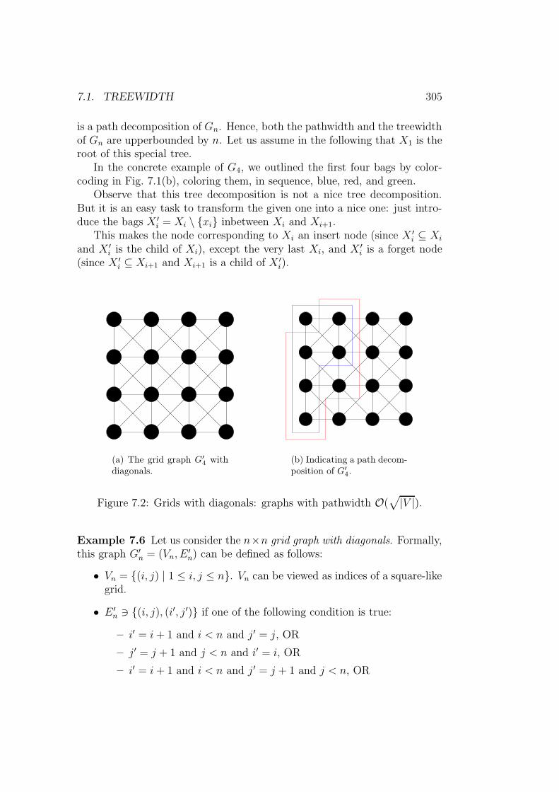
7.1. TREEWIDTH 305
is a path decomposition of Gn. Hence, both the pathwidth and the treewidthof Gn are upperbounded by n. Let us assume in the following that X1 is theroot of this special tree.
In the concrete example of G4, we outlined the first four bags by color-coding in Fig. 7.1(b), coloring them, in sequence, blue, red, and green.
Observe that this tree decomposition is not a nice tree decomposition.But it is an easy task to transform the given one into a nice one: just intro-duce the bags X ′
i = Xi \ xi inbetween Xi and Xi+1.This makes the node corresponding to Xi an insert node (since X ′
i ⊆ Xi
and X ′i is the child of Xi), except the very last Xi, and X ′
i is a forget node(since X ′
i ⊆ Xi+1 and Xi+1 is a child of X ′i).
(a) The grid graph G′
4 withdiagonals.
(b) Indicating a path decom-position of G′
4.
Figure 7.2: Grids with diagonals: graphs with pathwidth O(√|V |).
Example 7.6 Let us consider the n×n grid graph with diagonals. Formally,this graph G′
n = (Vn, E′n) can be defined as follows:
• Vn = (i, j) | 1 ≤ i, j ≤ n. Vn can be viewed as indices of a square-likegrid.
• E ′n 3 (i, j), (i′, j ′) if one of the following condition is true:
– i′ = i + 1 and i < n and j ′ = j, OR
– j ′ = j + 1 and j < n and i′ = i, OR
– i′ = i + 1 and i < n and j ′ = j + 1 and j < n, OR
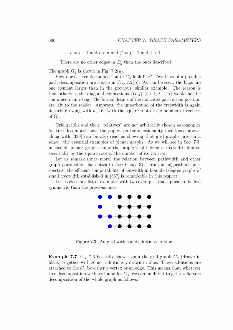
306 CHAPTER 7. GRAPH PARAMETERS
– i′ = i+ 1 and i < n and j ′ = j − 1 and j > 1.
There are no other edges in E ′n than the ones described.
The graph G′4 is shown in Fig. 7.2(a).
How does a tree decomposition of G′4 look like? Two bags of a possible
path decomposition are shown in Fig. 7.2(b). As can be seen, the bags areone element larger than in the previous, similar example. The reason isthat otherwise the diagonal connections (i, j), (i + 1, j + 1) would not becontained in any bag. The formal details of the indicated path decompositionare left to the reader. Anyways, the upperbound of the treewidth is againlinearly growing with n, i.e., with the square root of the number of verticesof G′
n.
Grid graphs and their “relatives” are not arbitrarily chosen as examplesfor tree decompositions; the papers on bidimensionality mentioned above,along with [339] can be also read as showing that grid graphs are—in asense—the essential examples of planar graphs. As we will see in Sec. 7.3,in fact all planar graphs enjoy the property of having a treewidth limitedessentially by the square root of the number of its vertices.
Let us remark (once more) the relation between pathwidth and othergraph parameters like cutwidth (see Chap. 3). From an algorithmic per-spective, the efficient computability of cutwidth in bounded degree graphs ofsmall treewidth established in [367] is remarkable in this respect.
Let us close our list of examples with two examples that appear to be lesssymmetric than the previous ones:
Figure 7.3: An grid with some additions in blue.
Example 7.7 Fig. 7.3 basically shows again the grid graph G4 (drawn inblack) together with some “additions”, drawn in blue. These additions areattached to the G4 by either a vertex or an edge. This means that, whatevertree decomposition we have found for G4, we can modify it to get a valid treedecomposition of the whole graph as follows:

7.1. TREEWIDTH 307
• Find a bag that contains the attachment vertex or the attachment edge.
• Connect this bag to a bag that only contains the attachment vertex oredge.
• From this starting point, attach a tree decomposition of the two partsof the blue addition.
It is an easy exercise to see that the overall width of the tree decompositionis not increased by the chosen attachments. Observe that we actually get atree decomposition this way, not (again) a path decomposition.
Finally, let us turn to the concrete problem to find a nice tree decompo-sition.
Figure 7.4: A modified grid.
Example 7.8 Let us have a look at Fig. 7.4. It shows a graph G whosevertices can be addressed, similar to the grid G4, by pairs of numbers (i, j),with 1 ≤ i, j ≤ 4. It is actually a simplification of the graph considered inthe previous example.
How would a nice tree decomposition of width two look like? The twoleaf nodes would correspond to bags drawn in blue and in yellow in Fig. 7.4.For example, the “blue leaf” would contain the bag with the vertices (1, 1),(1, 2), and (2, 1) of G. The sequence of ancestor nodes could contain thefollowing vertices in their corresponding bags:
• (1, 1), (1, 2);
• (1, 1), (1, 2), (1, 3);
• (1, 2), (1, 3);

308 CHAPTER 7. GRAPH PARAMETERS
• (1, 2), (1, 3), (1, 4);
• (1, 3), (1, 4);
• (1, 3), (1, 4), (2, 3);
• (1, 4), (2, 3);
• (1, 4), (2, 3), (2, 4);
• (2, 3), (2, 4);
• (2, 3), (2, 4), (3, 4).
The last mentioned bag is colored green in the figure. The “yellow leaf” wouldcontain the bag with the vertices (3, 1), (3, 2), and (4, 2) of G. The sequenceof ancestor nodes could contain the following vertices in their correspondingbags:
• (3, 2), (4, 2);
• (3, 2), (4, 2), (3, 3);
• (4, 2), (3, 3);
• (4, 2), (3, 3), (4, 3);
• (3, 3), (4, 3);
• (3, 3), (4, 3), (4, 4);
• (3, 3), (4, 4);
• (3, 3), (4, 4), (3, 4);
• (3, 3), (3, 4);
• (3, 3), (3, 4), (2, 3);
• (3, 4), (2, 3);
• (2, 3), (2, 4), (3, 4).
In our case, the tree decomposition can be either interpreted as a path decom-position or as a “true” tree decomposition, where a possible root is coloredgreen.

7.2. DYNAMIC PROGRAMMING 309
7.2 Dynamic programming
Let us show how to devise dynamic programming algorithms for graphs thatare given together with a suitable tree decomposition. More general scenariosfor developing treewidth-based algorithms are exposed in [27, 134, 225, 364,363, 365].
We shall focus on the following four problems:
1. vertex cover: In fact, since we are not putting emphasis on the stan-dard parameter, basically the same dynamic programming approachsolves independent set and clique, as well.
2. dominating set: While the dynamic programming solution of ver-tex cover is close to trivial, this is no longer the case with domi-nating set; in fact, the constants claimed in [9] were flawed due toa misreading of earlier published results, and the corrections (as ex-plained below) published in the journal version [8] of that extendedabstract contain ideas that were used in other dynamic programmingscenarios, as well [193].
3. Roman domination: We consider this problem, since it is—first ofall—one of the seemingly uncountable number of variations of domi-nation problems. Secondly, it has a nice story coming with it; namely,it should reflect the idea of how to secure the Roman Empire by po-sitioning the armies (legions) on the various parts of the Empire in away that either a specific region r is also the location of at least onearmy or one neighboring region r′ has two armies, so that it can affordsending one army to the region r without an army (in case of an at-tack) without loosing the capability to defend itself (since the secondarmy located in r′ will stay there). Thirdly, the dynamic programmingalgorithm previously published in [318] appears to be incorrect.
4. dominating set of queens: Here, we will see how we can alsoestablish an efficient solution to the original problem (i.e., not a problemthat is “re-parameterized” by treewidth) through a treewidth-basedalgorithm.
We have seen all the problems in further sections; let us briefly remindthe possibly least known of these problems, Roman domination:

310 CHAPTER 7. GRAPH PARAMETERS
Problem name: Roman domination (ROMAN)Given: A graph G = (V,E)Parameter: a positive integer kOutput: Is there a Roman domination function R such that∑
x∈V R(x) ≤ k?
Let us first link Roman domination with dominating set:
Lemma 7.9 If D ⊆ V is a Roman domination set for G = (V,E) (withrespect to a Roman domination function R, i.e., D = DR), then D is also adominating set. Moreover, if
∑x∈DR
R(x) ≤ k, then |D| ≤ k.
Of course, in the context of this chapter, we will be also interested in analternative parameterization, namely a parameterization by the treewidth ofthe underlying graph.
More specifically, a typical problem of interest would be the following one:
Problem name: vertex cover, parameterized bytreewidth (VCTW)Given: A graph G = (V,E) together with some tree decompositionParameter: a positive integer k that equals the width of the treedecompositionOutput: What is the size of a minimum vertex cover C ⊆ V ?
Theorem 7.10 An instance G = (V,E) of vertex cover, parameter-ized by treewidth can be solved in time O(2tw(G)|V |).
Proof. Recall that we can assume that the graph G is given by a nice treedecomposition with underlying tree T . Arbitrarily, we select a root r in T .
We will maintain a table for each node n in this decomposition. The rowsof this table can be viewed as corresponding to mappings α : X → 0, 1,where X is the bag that is associated to the node n. The value
∑x∈X α(x)
can interpreted as being the number of vertices that go into the vertex coverfrom bag X, assuming the particular assignment α. In other words, eachvertex x can carry two values, 1 and 0, reflecting that x is going into thevertex cover (if α(x) = 1) or not (if α(x) = 0).
Let T [n] be the subtree of T that contains n and all nodes in T thatbelong to the component of T − n to which r does not belong. Moreover,G 〈n〉 is the subgraph of G that is induced by the union of all bags thatcorrespond to nodes of T [n].
In the table for n, we store

7.2. DYNAMIC PROGRAMMING 311
Algorithm 63 A schematics for algorithms based on a given tree decompo-sition.Input(s): a graph G, together with a tree decompositionOutput(s): Whatever to be solved. . .
Find a nice tree decomposition TD = 〈Xi | i ∈ I, T 〉 of G.Perform a depth-first search along T , choosing an arbitrary root r for Tas starting point; i.e., call: dfs(G, TD, r).Read off a solution from the table that belongs to r.
subroutine dfs(G, TD, n)if current node n is a leaf then
perform leaf node actions and return corresponding tableelse if current node n has one child n′ then
tablen′ :=dfs(G, TD, n′)if n is forget node then
perform forget node actions and return corresponding table, based ontablen′
elseperform insert node actions and return corresponding table, based ontablen′
end ifelseCurrent node n has two children n′ and n′′tablen′ :=dfs(G, TD, n′)tablen′′ :=dfs(G, TD, n′′)perform join node actions and return corresponding table, based ontablen′ and on tablen′′
end if
• either the number that corresponds to the size of a minimum vertexcover of G 〈n〉 that is consistent with a particular assignment α on thebag X associated to n,
• or we store ∞ in the case that there is no way to construct a validvertex cover assuming the assignment α.
Formally, the fact that the tables constructed as described below verify theseproperties can be easily shown by tree induction following the algorithmdetails that follow; the leaf node description would correspond to the induc-tion basis, and the other three cases cover the induction step. Finally, thisthen implies that we can determine the size of a minimum vertex cover of

312 CHAPTER 7. GRAPH PARAMETERS
G = G 〈r〉 by one final sweep through the table that has been computed forthe root node r.
In a nice tree decomposition, we have to specify how to deal with thefollowing four situations:
leaf nodes At a leaf node with bag X, we build up a table that stores,for all mappings α : X → 0, 1, the value
∑x∈X α(x), interpreted as
being the number of vertices that go into the vertex cover, assumingthe particular assignment α. In the case that a particular α assigns 0 toto neighboring vertices x, y ∈ X, ∞ will be stored in the correspondingtable entry.
forget nodes We have two bags: the parent bag X we currently work on,and an already processed child node with associated bag Y with acorresponding table tableY . By definition, Y ∪ x = X. Consider aspecific mapping α : X → 0, 1. The value αY of the restriction of αto Y can be looked up in tableY . If α(x) = 0, the value of α in tableXis αY iff, for all vertices z ∈ N [x] ∩X, α(z) = 1; otherwise, the valueof α would be ∞. If α(x) = 1, the value of α in tableX is αY plusone. Observe that a table entry ∞ in tableX is possible for a specificmapping α if either tableY (αY ) = ∞ or α assigns zero to all verticesfrom N [x] ∩X.
insert nodes We have again two bags: the parent bag X we currently workon, and an already processed child node with associated bag Y with acorresponding table tableY . By definition, X ∪ x = Y . Consider aspecific mapping α : X → 0, 1. α can be extended in two ways to amapping on Y : αx=i is identical to α on X and defines αx=i(x) = i fori = 0, 1. The value of α that should be put into tableX is then
mintableY (αx=0), tableY (αx=1)
join nodes We have now three nodes: the parent node n and the two chil-dren nodes n′ and n′′. To all these nodes, the same bag X is associated.
Since the validity of the assignments was already tested in the childrennodes, we can compute the table entry tablen for assignment α : X →0, 1 from the corresponding tables tablen′ and tablen′′ for the sameassignment as follows:
tablen(α) = tablen′(α) + tablen′′(α) −∑
x∈Xα(x).

7.2. DYNAMIC PROGRAMMING 313
Observe that if α is invalid for one of the children n or n′, then at leastone of the table entries tablen′(α) or tablen′′(α) is ∞, and this will beinherited to tablen(α) by the usual computation rules.
How to combine these ingredients within a general schematics for solving treedecomposition based algorithms is shown in Alg. 63. The claimed runningtime for vertex cover, parameterized by treewidth follows from thefact that there are only O(|V |) many tree nodes to be processed accordingto Lemma 7.3 and that for each node, each of the at most 2tw(G) many tableentries incurs only a constant processing time (assuming sufficiently quickaccess to the table entries in the children nodes’ tables).
Let us illustrate this algorithm for computing a minimum vertex cover bycontinuing with Example 7.8.
Example 7.11 Let us start with listing a small table that contains all pos-sible choices for the leaf node whose bag is colored blue in Fig. 7.4:
(1, 1) (1, 2) (2, 1) table0 0 0 ∞0 0 1 ∞0 1 0 ∞0 1 1 21 0 0 ∞1 0 1 21 1 0 21 1 1 3
Its parent node is a forget node and contains the bag with the vertices (1, 1)and (1, 2). The accordingly smaller table looks as follows:
(1, 1) (1, 2) table0 0 ∞0 1 21 0 21 1 2
This table was obtained from the previous one basically by minimizing overtwo neighboring rows. The next parent node to be processed has the bagwith the vertices (1, 1), (1, 2), and (1, 3) and is hence an insert node, followedby another forget node.

314 CHAPTER 7. GRAPH PARAMETERS
(1, 1) (1, 2) (1, 3) table0 0 0 ∞0 0 1 ∞0 1 0 20 1 1 31 0 0 ∞1 0 1 31 1 0 21 1 1 3
(1, 2) (1, 3) table0 0 ∞0 1 31 0 21 1 3
Adding (1, 4) gives us again first an insert and then a forget node:
(1, 2) (1, 3) (1, 4) table0 0 0 ∞0 0 1 ∞0 1 0 30 1 1 41 0 0 ∞1 0 1 31 1 0 31 1 1 4
(1, 3) (1, 4) table0 0 ∞0 1 31 0 31 1 4
Adding (2, 3) gives us again first an insert and then a forget node; not to loosesight of the optimal solutions, we start adding them in one extra column:
(1, 3) (1, 4) (2, 3) table0 0 0 ∞0 0 1 ∞0 1 0 ∞0 1 1 41 0 0 31 0 1 41 1 0 41 1 1 5
(1, 4) (2, 3) table a corresponding solution0 0 3 (1, 1), (1, 2), (1, 3)0 1 4 (1, 1), (1, 2), (1, 3), (2, 3)1 0 4 (1, 1), (1, 2), (1, 3), (1, 4)1 1 4 (1, 1), (1, 2), (2, 3), (1, 4)
The final change in this branch is dealing with adding (2, 4) and then (3, 4)to our considerations:
(1, 4) (2, 3) (2, 4) table0 0 0 ∞0 0 1 40 1 0 ∞0 1 1 51 0 0 ∞1 0 1 51 1 0 41 1 1 5
(2, 3) (2, 4) table0 0 ∞0 1 41 0 41 1 5
(2, 3) (2, 4) (3, 4) table0 0 0 ∞0 0 1 ∞0 1 0 40 1 1 51 0 0 ∞1 0 1 51 1 0 51 1 1 6
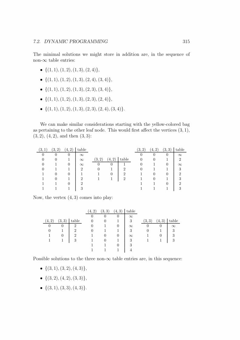
7.2. DYNAMIC PROGRAMMING 315
The minimal solutions we might store in addition are, in the sequence ofnon-∞ table entries:
• (1, 1), (1, 2), (1, 3), (2, 4),
• (1, 1), (1, 2), (1, 3), (2, 4), (3, 4),
• (1, 1), (1, 2), (1, 3), (2, 3), (3, 4),
• (1, 1), (1, 2), (1, 3), (2, 3), (2, 4),
• (1, 1), (1, 2), (1, 3), (2, 3), (2, 4), (3, 4).
We can make similar considerations starting with the yellow-colored bagas pertaining to the other leaf node. This would first affect the vertices (3, 1),(3, 2), (4, 2), and then (3, 3):
(3, 1) (3, 2) (4, 2) table0 0 0 ∞0 0 1 ∞0 1 0 ∞0 1 1 21 0 0 11 0 1 21 1 0 21 1 1 3
(3, 2) (4, 2) table0 0 10 1 21 0 21 1 2
(3, 2) (4, 2) (3, 3) table0 0 0 ∞0 0 1 20 1 0 ∞0 1 1 31 0 0 21 0 1 31 1 0 21 1 1 3
Now, the vertex (4, 3) comes into play:
(4, 2) (3, 3) table0 0 20 1 21 0 21 1 3
(4, 2) (3, 3) (4, 3) table0 0 0 ∞0 0 1 30 1 0 ∞0 1 1 31 0 0 ∞1 0 1 31 1 0 31 1 1 4
(3, 3) (4, 3) table0 0 ∞0 1 31 0 31 1 3
Possible solutions to the three non-∞ table entries are, in this sequence:
• (3, 1), (3, 2), (4, 3),
• (3, 2), (4, 2), (3, 3),
• (3, 1), (3, 3), (4, 3).

316 CHAPTER 7. GRAPH PARAMETERS
Then, vertices (4, 4) and (3, 4) are treated:
(3, 3) (4, 3) (4, 4) table0 0 0 ∞0 0 1 ∞0 1 0 30 1 1 41 0 0 ∞1 0 1 41 1 0 31 1 1 4
(3, 3) (4, 4) table0 0 30 1 41 0 31 1 4
(3, 3) (4, 4) (3, 4) table0 0 0 ∞0 0 1 40 1 0 ∞0 1 1 51 0 0 ∞1 0 1 41 1 0 41 1 1 5
The non-∞ entries of the following table correspond to minimal solutions aslisted below:
• (3, 1), (3, 2), (4, 3), (3, 4),
• (3, 1), (3, 2), (4, 3), (4, 4),
• (3, 1), (3, 2), (4, 3), (3, 4), (4, 4).
Then, we have to integrate (2, 3):
(3, 3) (3, 4) table0 0 ∞0 1 41 0 41 1 5
(3, 3) (3, 4) (2, 3) table0 0 0 ∞0 0 1 ∞0 1 0 ∞0 1 1 51 0 0 41 0 1 51 1 0 51 1 1 6
(3, 4) (2, 3) table0 0 40 1 51 0 51 1 5
Possible solutions to the table entries are, in this sequence:
• (3, 1), (3, 3), (4, 3), (4, 4),
• (3, 1), (3, 3), (4, 3), (4, 4), (2, 3),
• (3, 1), (3, 3), (4, 3), (4, 4), (3, 4),
• (3, 1), (3, 2), (4, 3), (3, 4), (2, 3).
Adding (2, 4) gives the following table, to which side we put the tablevalues that we obtained in the other branch, as well as the final values ofthe root of this tree decomposition; we use color-coding to denote these

7.2. DYNAMIC PROGRAMMING 317
Figure 7.5: An optimal vertex cover of the modified grid.
branches. Therefore, we get as optimal size for a vertex cover: eight, andthere are obvious various different solutions attaining this value.
(2, 3) (2, 4) (3, 4) table table table a possible minimal solution
0 0 0 ∞ ∞ ∞ —0 0 1 ∞ ∞ ∞ —0 1 0 5 4 8 L1
0 1 1 6 5 9 —1 0 0 ∞ ∞ ∞ —1 0 1 5 5 8 L2
1 1 0 6 5 9 —1 1 1 6 6 9 —
A possible optimal solution can be seen in Fig. 7.5; the red vertices form avertex cover. From the table, we can in fact read off two alternative minimumsolutions:
L1 = (1, 1), (1, 2), (1, 3), (3, 1), (3, 3), (4, 3), (4, 4), (2, 4)L2 = (1, 1), (1, 2), (1, 4), (2, 3), (3, 4), (3, 1), (3, 2), (4, 3)
Observe that the solution given in Fig. 7.5 is different from the oneswhose computation is sketched in the tables. The reason is that in thetable computations, sometimes minimal solutions are “forgotten” if thereare other minimal solutions that are no worse when looked at them from theperspective of the corresponding “interface bag.”
Let us now turn to dominating set: is it (again) sufficient to onlystore two possible “states” per graph vertex, i.e., being in the dominating

318 CHAPTER 7. GRAPH PARAMETERS
set or not? Unfortunately, this is not the case, since along the course of atreewidth-based algorithm, we may encounter vertices in a bag that are not inthe dominating set according to the specific assignment under considerationin the present bag, nor they are dominated; however, they might be already“happy” since they have already been dominated according to a previousassignment (that has been already “forgotten” within the present bag) orthey are still “unhappy”, i.e., they still have to be dominated by verticesthat are not yet visible in the current bag. This basically means that thereare now three states, say 1, 0, 0, where the assignment of 0 means thatthe vertex is already dominated at the current stage of the algorithm, and 0means that, at the current stage of the algorithm, we still ask for a dominationof this vertex.2 We ask the reader to fill in the details for the four differentsituations of a treewidth-based algorithm.
Let us only point to the following additional complication when dealingwith join nodes: if we update an assignment that maps vertex x onto 0, itis not necessary that both children assign 0 to x; it is sufficient that one ofthe two branches does, while the other assigns 0. So, while it is clear that inthe initialization phase and when processing insert or forget nodes, O(3tw(G))time is needed to perform the other node actions, a direct implementation ofwhat we said in the previous sentence would amount in spending O(9tw(G))time for the join node processing. How this could be sped up to O(4tw(G))is explained in [8]. However, observe that in any case here a small pathdecomposition offers an edge over a tree decomposition of the same size,since then no join nodes would have to be processed.
Let us explain the mentioned O(4tw(G)) complexity for the join nodes abit more in detail, deviating in our explanation from [8] in some details. Thebasic trick can be boiled down to the reinterpretation of the assignment of 0to vertex x: we assume that we don’t know if x has already been dominatedat the current stage of the algorithm. This means that, whenever we have toassignments α and α′ such that we can obtain α from α′ by replacing some0 by 0, then the table value (this time denoting the number of vertices thathave been put into the dominating set at this stage of the algorithm) of αis greater than or equal to the table value of α′. Therefore, we only needto distinguish two cases whenever we have a 0 assignment for some vertexx in the parent node: either the left child assigns 0 to x and the right childassigns 0 to x, or left child assigns 0 to x and the right child assigns 0 to x.Hence, we can compute the number of all necessary checks for assignments to
2This necessity of two states for a vertex not being in the dominating set has beenoverlooked in [318], so that the running times that are claimed in that paper for Romandomination are better than ours as explained below.
7.2. DYNAMIC PROGRAMMING 319
k vertices (in the parent node) by the following recursion, where we assumeto have chosen a specific vertex x:
• either 1 or 0 is assigned to x; then, the same assignment must havebeen made in the two children;
• or 0 is assigned to x; then, we have two possible assignments in thechild nodes: 0 to x in the left child and 0 to x in the right child or viceversa.
In each case, we can now assume we have k−1 vertices to which values mustbe assigned. All in all, for the number T (k) of situations we have to check tocompute the values in a parent node with k vertices, we have obtained therecursion T (k) = 4T (k − 1), where naturally T (0) = 1 ends the recursion.Hence, T (k) = 4k as claimed.
Theorem 7.12 minimum dominating set, parameterized by the treewidthtw(G) of the input graph G, can be solved in time O(4tw(G)|V (G)|).
A graph-structural reason for dominating set being more difficult thanvertex cover3 can be found in the fact that, whenever a graph G canbe covered by k vertices, then any subgraph can be covered by at most kvertices; yet, there may be subgraphs of a graph G that can be dominatedby k vertices that need more vertices for domination; such phenomena wererecently studied in detail in [229].
In the case of Roman domination, a similar problem occurs withinthe join nodes. Moreover, notice that we now have two different states fora vertex that is in the dominating set, depending on whether it hosts oneor two armies. Again, we leave details to the reader; however, the naiveO(16tw(G)) algorithm should be in principle clear from what we said. Noticeagain that this algorithm can be substantially improved by the techniqueswe just mentioned. Namely, assume that we assign one out of 0, 0, 1, 2to each vertex in a bag. The semantics of 0 an 0 is not changed. Theassignments 1 and 2 count the number of armies put on the correspondingvertex. Observe that a vertex can be only dominated by a neighbor vertexto which we assigned a 2. Using the same tricks as explained in the previouscase, we get the following recursion for the number T (k) of situations wehave to check to compute the values in a parent node with k vertices:
3an observation that cannot be only seen in the more complex dynamic programmingfor the treewidth-bounded case, but also in the fact that on general graphs dominatingset is parameterized intractable, yet vertex cover is in FPT , vertex cover enjoysa smaller kernel than planar dominating set etc.

320 CHAPTER 7. GRAPH PARAMETERS
• We get three T (k− 1)-branches for assigning 0, 1, 2 to the parent node,since the child nodes must assign the same values to the chosen vertex.
• We get two more T (k− 1)-branches for assigning 0 to the parent node.
All in all, we have T (k) = 5k. Since the other node updates can be even donein time O(4k), we can conclude:
Theorem 7.13 minimum Roman domination, parameterized by the treewidthtw(G) of the input graph G, can be solved in time O(5tw(G)|V (G)|).
Finally, we turn towards the Queen Domination Problem that is definedas follows:
Problem name: dominating set of queens (QDS)Given: An n× n chessboard CParameter: a positive integer kOutput: Is it possible to place k queens on C such that all squaresare dominated ?
However, we do not start, at this point, from the Queen chessboard graph,but rather with the n × n planar grid with diagonals that corresponds to achessboard in a straightforward interpretation. As mentioned, this graphhas pathwidth n+ 1 (see Ex. 7.6). For our dynamic programming algorithm(solving the problem in time O(cn) for a c to be determined), we endow eachvertex of this graph (i.e., each square on the chessboard) with the followinginformation: for each of the at most four directions (neighbors) of that aspecific square might still “influence” in the future of the algorithm (namely,if we take the way of passing through a grid that was indicated in Ex. 7.6,then these possible influence directions are: the upper right, right, lower rightand lower directions), we keep track if the present square is dominated (andwill hence enable domination of squares in the indicated direction, includingthe possibility that the square is hosting a queen) or if it still has to bedominated (and if so, from which direction). Excluding the possibility thata vertex (square) is not dominated at all, this leads to 24 − 1 = 15 different“states” of a square. Notice again that we are now talking about a pathdecomposition based algorithm, i.e., there are no join nodes that need to beprocessed. Hence, we can conclude:
Theorem 7.14 minimum dominating set of queens, parameterized bythe treewidth tw(G) of the input graph G, can be solved in time O(15tw(G)|V (G)|) =O(15nn2), given an n× n chessboard.

7.3. PLANAR GRAPHS AND THEIR STRUCTURE 321
Note that this also directly leads to a solution to the original parame-terized problem. We have already seen in Theorem 4.27 that QDS has asmall kernel. Of course, this shows that dominating set of queens isin FPT . More precisely, we would have a direct O(2(2k+1)2 + n) algorithmfor dominating set of queens by testing all placements of queens on the(2k + 1) × (2k + 1) chessboard. We could do better along the lines of ourprevious reasoning, however:
Theorem 7.15 dominating set of queens can be solved in time O(152k+n).
Proof. First, apply the reduction rule 25, see Theorem 4.27. Then, n ≤2k + 1. Hence, the dynamic programming algorithm we sketched above canbe assessed to run in the claimed time.
Having seen the previous examples, it might appear that all graph prob-lems, at least those graph problems that are easy to solve on trees, should beeasily solvable on graphs with a bounded treewidth. In fact, finding efficienttree algorithms say for dominating set often predates their solution ongraphs of bounded treewidth, see [101, 303] for algorithms solving minimumdominating set on trees in linear time. Let us remind, however, that thereare some problems that, albeit efficiently solvable on trees, it is unknown ifthere are efficient treewidth-based algorithms. One particular example is thelinear arrangement problem, see [5, 99, 352] for efficient algorithms ontrees, and the discussion in [239, 240] for the obvious problems of findingefficient treewidth-based algorithms for this problem.
7.3 Planar graphs and their structure
Let us first improve our understanding of planar graphs. First, observe thatthere can be many ways in which a graph can be embedded into the plane.
Example 7.16 Let us continue with Example 7.5. More precisely, let ushave another look at the grid graph G4 that has been drawn as a planargraph already in Fig. 7.1(a). Namely, Fig. 7.6(a) shows another way ofembedding G4: it is basically turned inside-out.
Interestingly, different embeddings, i.e., finally different drawings, do havetheir bearing at the way we see graphs. For example, recall the strategywith which we constructed a tree decomposition of G4: we took the leftmost“column” plus the “next” vertex to the upmost right into the first bag, sothat we could forget about the leftmost top vertex in the next bag, and soforth. If we apply the same strategy to this alternative embedding, we might

322 CHAPTER 7. GRAPH PARAMETERS
(a) Another embedding ofthe grid graph G4.
(b) Indicating another path decompo-sition of G4.
Figure 7.6: Grids: graphs with pathwidth O(√
|V |).
get another tree decomposition of G4, as indicated in Fig. 7.6(b). In thatpicture, the first bag is colored blue, then comes the red one; this is graduallychanged into the green bag, as indicated by the red arrows. Further changeslet us finally arrive at the pink bag. Observe that the biggest bag is thegreen one, and this determines the width of the tree decomposition, whichis four (as above). In contrast to the previously described decomposition,this decomposition appears to be fairly asymmetric, in fact, along the linesof the sketch, a decomposition is obtainable such that only one of the bags(namely, the green one) contains five vertices.
Planar graphs are interesting in our context, since most NP-hard graphproblems remain NP-hard when restricted to planar graphs (a notable ex-ception being maximum cut, see [223]). However, from a parameterizedperspective, one can sometimes observe that problems that are W[1]-hardfor general graphs fall into FPT when restricted to planar graphs; examplesbeing independent set and dominating set, as well as their variants.In fact, the derivation of the according FPT algorithms is somewhat thecore of this chapter. In a certain sense, these problems are even easier thansay vertex cover on general graphs, since they allow for algorithms with arunning time of O∗(c
√k), which is improbable for problems on general graphs,
see [69].

7.3. PLANAR GRAPHS AND THEIR STRUCTURE 323
7.3.1 Outerplanarity: the definition
Definition 7.17 A crossing-free embedding of a graph G in the plane iscalled outerplanar embedding if each vertex lies on the boundary of the outerface. A graph G is called an outerplanar graph if it admits an outerplanarembedding in the plane.
The following generalization of the notion of outerplanarity was intro-duced by Baker [32].
Definition 7.18 A crossing-free embedding of a graph G in the plane iscalled r-outerplanar if:
• for r = 1, the embedding is outerplanar, and,
• for r > 1—inductively—when removing all vertices on the boundary ofthe outer face and their incident edges, the embedding of the remainingsubgraph is (r − 1)-outerplanar.
A graph G is called r-outerplanar if it admits an r-outerplanar embedding.The smallest number r, such that G is r-outerplanar is called the outerpla-narity (number).
In this way, we may speak of the layers L1, . . . , Lr of an embedding of anr-outerplanar graph:
Definition 7.19 For a given r-outerplanar embedding of a graphG = (V,E),we define the ith layer Li inductively as follows. Layer L1 consists of thevertices on the boundary of the outer face, and, for i > 1, the layer Li is theset of vertices that lie on the boundary of the outer face in the embedding ofthe subgraph G− (L1 ∪ . . . ∪ Li−1).
Let us look at grid graphs again to see the general flavor of these notions.
Example 7.20 What about our favorite graph, the grid graph G4, in termsof outerplanarity? Starting with the embedding from Fig. 7.1, Fig. 7.7 showsthe two layers of G4 by coloring them red and blue. It is not too hardto see in this case that there is no embedding that might display smallerouterplanarity.
In general terms, the grid graph Gn has outerplanarity dn/2e. Hence, theouterplanarity grows linearly with the square root of the number of verticesof Gn.

324 CHAPTER 7. GRAPH PARAMETERS
Figure 7.7: An example graph of outerplanarity two.
To understand the techniques used in the following sections, it is helpful toconsider the concept of a layer decomposition of an r-outerplanar embeddingof graph G. A layer decomposition of an r-outerplanar embedding of graphG is a forest of height r − 1. The nodes of the forest correspond to differentconnected components of the subgraphs of G induced by a layer. For eachlayer with vertex set Li, suppose the connected components of the subgraphof G induced by Li have vertex sets Ci,1, . . . , Ci,`i, i.e., Li =
⋃`ij=1Ci,j. Then,
we have `i nodes that represent the nodes of layer Li, one for each suchconnected component. Such a set Ci,j will be called a layer component. Eachlayer component node C1,j will be the root of a tree in the forest, so wewill have one tree per connected component of G, representing the exteriorvertices of the component. Two layer component nodes will be adjacent ifthey contain vertices that share a common face. This means that a layercomponent node Ci,j can only be adjacent to layer component nodes of theform Ci−1,j′ or Ci+1,j′′; if Ci,j is adjacent to Ci−1,j′, then the vertices of Ci,jlie within the area formed by the subgraph induced by Ci−1,j′. Note thatthe layer component nodes on the i’th level of the forest correspond to thelayer components of the form Ci,j. One easily observes that the planarity ofG implies that the layer decomposition must indeed be a forest.
We need some further notation for the construction in the next sections.
A layer component Ci,j of layer Li is called a non-vacuous layer if thereare vertices from layer Li+1 in the interior of Ci,j (i.e., in the region enclosedby the subgraph induced by Ci,j). In other words, Li is non-vacuous iff thecorresponding component node in the layer decomposition has a child.
Lemma 7.21 Let ∅ 6= C ⊆ Ci,j be a subset of a non-vacuous layer compo-nent Ci,j of layer i, where i ≥ 2. Then, there exists a unique smallest (in

7.3. PLANAR GRAPHS AND THEIR STRUCTURE 325
number of vertices) cycle B(C) in layer Li−1, such that C is contained in theregion enclosed by B(C). No other vertex of layer Li−1 is contained in thisregion.
Definition 7.22 For each non-empty subset C of a non-vacuous layer com-ponent of layer i (i ≥ 2), the set B(C) as given in Lemma 7.21 is called theboundary cycle of C (which we will also call ring of C.
A ring decomposition of an r-outerplanar graph G is a directed forestFG of height r − 1 which is described as follows: the nodes of the trees arerings of vertices of G and the different trees (may) correspond to differentcomponents of G. If B′ and B′′ are boundary cycles, then B ′′ is a childof B′ iff B(x) = B′ for any x ∈ B′′. The ith layer of FG consists of ciboundary cycles B(i, 1), . . . , B(i, ci) from the ith layer Li of G, and someinterconnection pattern Ji = Li \Bi with Bi =
⋃cij=1B(i, j).
Since different components of a graph can be processed separately in thealgorithms presented below, we can assume that FG is in fact a (directed)tree. Notationally, we stress this by writing TG instead of FG. If TG happensto be a path, we will call G simple r-outerplanar. The tree F ′
G is obtainedfrom FG by attaching a child to any leaf B(i, j) of FG.
With respect to the “history” of the papers that deal with hard problemson planar graphs, first the notion of layer decomposition was used, but thatwas later (more precisely, in [179]) replaced by the obviously related notion ofa ring decomposition, since that one allowed arguments of a more geometricflavor.
Let us finally stress the fact that a ring decomposition may be differentfrom the so-called layer decomposition introduced in [8]; e.g., two rings mayshare an edge, see Fig. 7.8.
The reader who wishes a concrete visualization of ring structures mightwish to have a look at Fig. 7.9. The idea given by onion rings is very wellreflecting the ring structure of a planar graph. We will return to this issuelater on.
7.3.2 Outerplanarity versus treewidth
We provide now a constructive proof of how to upperbound the treewidth ofa planar graph by its outerplanarity. The proof is based upon the proof in[54, Theorem 83]. To be more precise, we show:
Theorem 7.23 Let an r-outerplanar graph G = (V,E) be given togetherwith an r-outerplanar embedding. A tree decomposition 〈Xi | i ∈ I, T 〉, ofwidth at most 3r− 1 and with |I| = O(n) of G, can be found in O(rn) time.
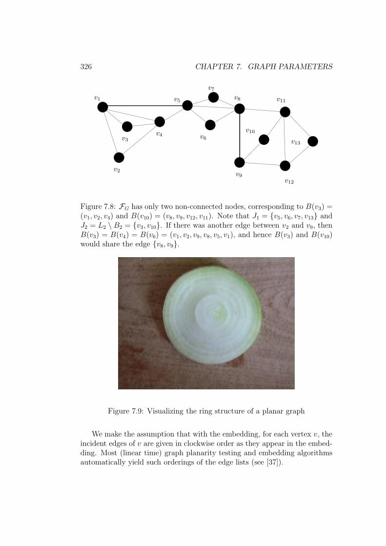
326 CHAPTER 7. GRAPH PARAMETERS
v1
v2
v3
v4
v5
v6
v7
v9
v10
v12
v8 v11
v13
Figure 7.8: FG has only two non-connected nodes, corresponding to B(v3) =(v1, v2, v4) and B(v10) = (v8, v9, v12, v11). Note that J1 = v5, v6, v7, v13 andJ2 = L2 \ B2 = v3, v10. If there was another edge between v2 and v9, thenB(v3) = B(v4) = B(v6) = (v1, v2, v9, v8, v5, v1), and hence B(v3) and B(v10)would share the edge v8, v9.
Figure 7.9: Visualizing the ring structure of a planar graph
We make the assumption that with the embedding, for each vertex v, theincident edges of v are given in clockwise order as they appear in the embed-ding. Most (linear time) graph planarity testing and embedding algorithmsautomatically yield such orderings of the edge lists (see [37]).

7.3. PLANAR GRAPHS AND THEIR STRUCTURE 327
Now, we discuss the proof of Theorem 7.23. For the construction of thedesired tree decomposition we proceed in several steps, see Alg. 64.
Algorithm 64 Construct a tree decomposition for an r-outerplanar graph
Input(s): an r-outerplanar graph GOutput(s): a tree decomposition of G of width at most 3k − 1
1: Determine the layers of the given graph G.2: Embed G into a graph H, whose degree is bounded by 3 and whose
outerplanarity number doesn’t exceed the one of G.3: Construct a suitable maximal spanning forest for H.
This step is done inductively proceeding along the different layers of H in a
way that the so-called “edge and vertex remember numbers” are kept small.
4: Using this spanning tree, determine a tree decomposition of H.5: Turn this tree decomposition into a tree decomposition of G.
The details of the steps in Alg. 64 are discussed in the following.
Determining the layers of the embedded graph. Without loss of gen-erality, we assume G is connected. Suppose G is given with an r-outerplanarembedding with, for every vertex, a clockwise ordering of its adjacent edges.With the help of these orderings, one can build, in O(|V |) time, the dualgraph G∗,4 with pointers from edges of G to the two adjacent faces in thedual. We can first partition the set of faces into ‘layers’: put a face f in layerL∗i+1 if the distance of this face in the dual graph to the exterior face is i.
This distance can be determined in linear time using breadth-first search onthe dual graph.
Now, a vertex v of G belongs to layer Li for the smallest i such that vis adjacent to a face fv in L∗
i . Note that faces can belong to layer L∗r+1, but
not to layers L∗s with s > r + 1.
Embedding G in a graph H of degree three. The next step is toconstruct an r′-outerplanar (where r′ ≤ r) graph H = (VH , EH) of degree atmost three that contains G as a minor, i.e., G can be obtained from H by aseries of vertex deletions, edge deletions, and edge contractions.
4Given a plane graph G, its dual G∗ is formed by considering the faces of G as thevertices of G∗ and by putting an edge between two “face-vertices” iff there is a commonboundary edge of the two faces in G. Please note that G∗ depends on the given embeddingof G; moreover, G∗ is often seen as a multigraph (e.g., loops may occur if there are edgesin G that lead to leaf vertices within a face; double edges may be due to faces that areneighbored via two different edges). For our purpose, the simple graph that correspondsto such a multigraph is sufficient.

328 CHAPTER 7. GRAPH PARAMETERS
v
w1 w2 w3 wd−1 wd w1 w2 w3 wd−1 wd
v1 v2 vd−2
Figure 7.10: Replacing a vertex by a path with vertices of degree 3.
In order to do this, every vertex with degree d ≥ 4 is replaced by a pathof d − 2 vertices of degree 3, as shown in Fig. 7.10. This is done in such away that the graph stays r′-outerplanar. More precisely, for each vertex v oflayer Li we determine the face fv in L∗
i as described above. We then find twosuccessive edges x, v, v, y that are border to fv. Now, let x take the roleof w1 and y take the role of wd in Fig. 7.10. Observe that, in this manner,all vertices vi on the newly formed path are adjacent to face fv ∈ L∗
i . Let Hbe the graph obtained after replacing all vertices of degree at least four inthis manner.
Note that H has the same set of faces as G (i.e., H∗ and G∗ share thesame set of vertices) and that faces adjacent in G are still adjacent in H (i.e.,G∗ is a subgraph of H∗). Hence, H∗ can be obtained from G∗ by possiblyadding some further edges. Clearly, the minimum distance of a vertex in H∗
to the exterior face vertex may only decrease (not increase) compared to thecorresponding distance in G∗. Since the layer to which a vertex belongs isexactly one more than the minimum distance of the adjacent faces to theexterior face, the outerplanarity number r′ of H is bounded by r.
Constructing a suitable maximal spanning forest for H. At this point,we have an r′-outerplanar graph H = (VH , EH) of maximum degree 3. Wenow construct a maximal spanning forest T for H that yields small so-called“edge and vertex remember numbers.” This step is done inductively alongthe different layers proceeding from inside towards the exterior.
Observe that, when removing all edges on the exterior face of an s-outer-planar graph of maximum degree three, we obtain an (s − 1)-outerplanargraph when s > 1; we obtain a forest when s = 1.
Thus, we can partition the edges into r′ + 1 sets E1, . . . , Er′+1, with E1
the edges on the exterior face, and Ei the edges on the exterior face when alledges in E1 ∪ . . . ∪ Ei−1 are removed. Again, using the dual, this partitioncan be computed in O(n) time.
Now, we form a sequence of forests. We start with forest Tr′+1, whichconsists of all edges in Er′+1. (Note that these are the interior edges of an

7.3. PLANAR GRAPHS AND THEIR STRUCTURE 329
outerplanar graph of maximum degree 3, so Tr′+1 is acyclic.)When we have Ti, 1 < i ≤ r′ + 1, we form Ti−1 in the following way:
add a maximal set of edges from Ei−1 to Ti such that no cycles are formed.Note that in this way, each Ti is a maximal spanning forest of the subgraphformed by the edges in Ei ∪ . . . ∪ Er′+1; we call this subgraph Hi. As usual,maximality is meant with respect to set inclusion; a maximal spanning forestof an arbitrary graph hence can be found in O(n) time using a standarddepth first search approach, but here we need such a forest constructed in aspecific way.
It is not hard to see that one such step can be done in O(n) time; as wedo at most r such steps, the time to build T1 becomes O(rn).
Definition 7.24 For a graph G = (V,E), and a forest T = (V, F ) that isa subgraph of G, define the edge remember number er(G, T, e) of an edgee ∈ F (with respect to G and T ) as the number of edges v, w ∈ E \F suchthat there is a simple path in T from v to w that uses e. The edge remembernumber of T (with respect to G) is er(G, T ) = maxe∈F er(G, T, e).
The vertex remember number vr(G, T, v) of a vertex v ∈ V (with respectto G and T ) is the number of edges v, w ∈ E \F such that there is a simplepath in T from v to w that uses v. The vertex remember number of T (withrespect to G) is vr(G, T ) = maxv∈V vr(G, T, v).
One may observe that the construction of the trees Ti is the one used inthe proofs given in [54, Section 13]. The following result is proved in [54,Lemma 80]. Note that in order to obtain this result it is essential that thedegree of H is bounded by 3:
Lemma 7.25 (i) For every i, 1 ≤ i ≤ r′ + 1, er(Hi, Ti) ≤ 2(r′ + 1 − i).(ii) For every i, 1 ≤ i ≤ r′, vr(Hi, Ti) ≤ 3(r′ + 1 − i) − 1.
Without loss of generality, we can suppose that G and, therefore, H isconnected and, hence, we have a spanning tree T1 of H with er(H, T1) ≤ 2r′
and vr(H, T1) ≤ 3r′ − 1.
Deriving a tree decomposition from the spanning forest. We nowapply the following result of [54, Theorem 71] to the graph H and the span-ning forest T1 in order to obtain a tree decomposition in time O(rn) of widthbounded by
max(vr(H, T1), er(H, T1) + 1) ≤ 3r′ − 1 ≤ 3r − 1.
For the sake of completeness of the whole construction, we outline the easyproof.

330 CHAPTER 7. GRAPH PARAMETERS
Theorem 7.26 Let T = (V, F ) be a maximal spanning forest for the graphG = (V,E). Then, a tree decomposition with width smaller than or equalto maxvr(G, T ), er(G, T ) + 1 and with O(n) nodes can be determined inO(vr(G, T ) · n) time.
Proof. Our aim is to construct a tree decomposition 〈Xi | i ∈ I, T ′〉of G. Let T ′ = (V ∪ F, F ′) with
F ′ = v, e | v ∈ V, e ∈ F, ∃w ∈ V : e = v, wbe the tree obtained by subdividing every edge of T . The bags Xi for i ∈I := V ∪F are obtained as follows. For every v ∈ V , add v to Xv. For everye = v, w ∈ F , add v and w to Xe. Now, for every edge e = v, w in Ebut not in F , add v to all sets Xu and Xe, with u ∈ V or e ∈ F on the pathfrom v to w in T .
Using standard graph algorithmic techniques, the path between two ver-tices in a tree can be found in time proportional to the length of that path;since each vertex in T can contribute to at most vr(G, T ) such paths, therunning time is bounded by O(vr(G, T ) · n).
It is easy to check that this yields a tree decomposition. Its bags have size|Xv| ≤ 1 + vr(G, T ) (for all v ∈ V ) and |Xe| ≤ 2 + er(G, T ) (for all e ∈ E).Hence, the resulting treewidth is at most max(vr(G, T ), er(G, T ) + 1).
Undoing the minor operations. Finally, the tree decomposition of Hcan be turned into a tree decomposition of G of equal or smaller width byreplacing every occurrence of a vertex vi in a bag Xi by an occurrence ofthe corresponding vertex v (see e.g., [54, Lemma 16].) This again costs timelinear in the size of all bags Xi in the tree decomposition, i.e., O(rn) time.
Altogether this establishes the correctness of Theorem 7.23.
7.3.3 Outerplanarity and other graph parameters
The concept of outerplanarity is quite useful for showing that particularproblems are in FPT . Let us clarify this with a number of examples. Theycomprise rather folklore results.
Proposition 7.27 A plane graph with a dominating set of size of at most kis r-outerplanar with r ≤ 3k.
Proof. By definition of outerplanarity, each vertex in a dominating set canonly dominate vertices from at most three layers, so that there cannot bemore than 3k layers in any YES-instance of planar dominating set.
From what we have seen in the preceding subsection, we may deduce:

7.3. PLANAR GRAPHS AND THEIR STRUCTURE 331
Corollary 7.28 If a planar graph G = (V,E) has a k-dominating set, thenits treewidth is bounded by 9k − 1.
We will give a considerably stronger bound later.
Corollary 7.29 planar dominating set is in FPT .
Let us remark that, from an algorithmic point of view, the followingobservation might be even more useful, although it delivers the same worst-case bound in the case of simple r-outerplanar graphs.
Lemma 7.30 A plane graph G with a dominating set of size of at most khas a ring decomposition FG with a dominating set of size of at most k.
The proof for this result can be taken as a blueprint for similar statementsbelow. It is explicitly contained in Alg. 65.
Algorithm 65 An FPT algorithm for planar dominating set
Input(s): a planar graph G, a positive integer kOutput(s): YES if G has a dominating set of size at most k and NO, oth-
erwise
Find an arbitrary planar embedding of G.Determine the outerplanarity out of that embedding.if out > 3k then
return NO
elseDetermine minimum dominating set D of G with the help of anouterplanarity-based algorithm.return |D| ≤ k
end if
For specific types of domination problems, the bounds can be better:
Proposition 7.31 A plane graph with a connected dominating set of size ofat most k is r-outerplanar with r ≤ k + 2.
Corollary 7.32 planar connected dominating set is in FPT .
Similarly, one can show:
Proposition 7.33 A plane graph with a maximal matching of size of at mostk is r-outerplanar with r ≤ 2k.
332 CHAPTER 7. GRAPH PARAMETERS
Proof. Consider two subsequent layers L1, L2 in one connected componentof a plane graph. If none of the edges within the layer (i.e., both endpointsare within either L1 or L2) are in the matching, then at least one of the edgesinterconnecting the layers (i.e., one endpoint is in L1 and the other one is inL2) is in the matching by maximality.
Therefore, we get an FPT -classification of the determination of a mini-mum maximal matching (standard parameterization) in a plane graph.
In the following, we are aiming at improved relations between graphparameters (like domination number) and treewidth in the case of planargraphs.
7.4 Domination number versus treewidth
In this section, we explain in details the strategy used in [8] to obtain an
O∗(c√k) algorithm for planar dominating set. In particular, we show
that a planar graph with domination number k has treewidth of at mostO(
√k). This improves Corollary 7.28 considerably. In the next section, we
will show how this new result can be turned into a constructive algorithm.Combining the results of this section with the treewidth-based algorithmswe saw above, we can present an algorithm having time complexity 4O(
√k)n.
This obviously gives an asymptotic improvement of the O(8kn) search treealgorithm, see Chap. 5.
This section is organized as follows. In a first subsection, we make somegeneral observations on how to construct tree decompositions using sepa-rators. The following two subsections show that, in a planar graph whichadmits a k-dominating set, we can find small separators layerwisely. Finally,the results are pieced together to prove our main result in this section.
7.4.1 Separators and treewidth
Here, the main idea is to find small separators of the graph and to merge thetree decompositions of the resulting subgraphs.
To simplify notation, we write A]B for the disjoint union of two sets Aand B. Graph separators are defined as follows.
Definition 7.34 Let G = (V,E) be an undirected graph. A separatorS ⊆ V of G divides V into two parts (or chunks) A1 ⊆ V and A2 ⊆ V suchthat5
5In general, of course, A1, A2 and S will be non-empty. In order to cover boundarycases in some considerations below, we did not put this into the separator definition.
7.4. DOMINATION NUMBER VERSUS TREEWIDTH 333
• A1 ] S ] A2 = V , and
• no edge joins vertices in A1 and A2.
Later, we will write δA1 (or δA2) as shorthand for A1 ]S (or A2 ]S, respec-tively). The triple (A1, S, A2) is also called a separation of G.
Clearly, this definition can be generalized to the case where a separator par-titions the vertex set into ` subsets instead of only two. We refer to suchseparators simply by `-separator ; ` = 2 then is the separator in Defini-tion 7.34.
For any given separator splitting a graph into different components, weobtain a simple upper bound for the treewidth of this graph which dependson the size of the separator and the treewidth of the resulting components.
Proposition 7.35 If a connected graph can be decomposed into componentsof treewidth of at most t by means of a separator of size s, then the wholegraph has treewidth of at most t+ s.
Proof. The separator splits the graph into different components. Supposewe are given the tree decompositions of these components of width at mostt. The goal is to construct a tree decomposition for the original graph. Thiscan be achieved by firstly merging the separator to every bag in each of thesegiven tree decompositions. In a second step, add some arbitrary connectionspreserving acyclicity between the trees corresponding to the components. Itis straightforward to check that this forms a tree decomposition of the wholegraph of width at most t+ s.
For plane graphs, there is an iterated version of this observation can besimilarly shown.
Proposition 7.36 Let G be a plane graph with layers Li, (i = 1, . . . , r). Fori = 1, . . . , `, let Li be a set of consecutive layers, i.e.,
Li = Lji , Lji+1, . . . , Lji+ni,
such that Li ∩ Li′ = ∅ for all i 6= i′. Moreover, suppose G can be decom-posed into components, each of treewidth of at most t, by means of sepa-rators S1, . . . , S`, where Si ⊆ ⋃
L∈LiL for all i = 1, . . . , `. Then, G has
treewidth of at most t+ 2s, where s = maxi=1,...,` |Si|.

334 CHAPTER 7. GRAPH PARAMETERS
7.4.2 Finding separators layerwisely
In the following, we assume that our graph G has a fixed plane embed-ding with r layers. We show that the treewidth cannot exceed O(
√k) if
a dominating set of size k exists. This implies that if we have an optimaltree-decomposition we can find the domination number fast using standarddynamic programming techniques (as explained above).
Let the layers be L1, L2, . . . , LT , with L1 being the outer layer.We assume that we have a dominating set D of size at most k. Let ki
be the number of vertices of Di = D ∩ Li. Hence,∑r
i=1 ki = k. In order toavoid case analysis, we set k0 = kr+1 = kr+2 = 0. Moreover, let ci denote thenumber of non-vacuous layer components of layer Li.
Our approach is based on finding small separators in G layerwisely. Moreprecisely, for each i = 1, . . . , r−2, we want to construct a set Si ⊆ Li−1∪Li∪Li+1 separating layer Li−1 from layer Li+2 in such a way that the total size ofthese sets can be bounded by some linear term in k. The key idea for provingthat Si separates layers Li−1 from Li+2 relies on a close investigation of thepaths leaving layer Li−1 to the interior of the graph. Each such path passes a“first” vertex in layer Li. This particular vertex can be dominated by verticesfrom Di−1, Di, or Di+1. It turns out that, in order to cut this particular path,the set Si has to contain the vertices of the sets Di−1, Di, and Di+1 plus somesuitably chosen pairs of neighbors of any of these vertices. This results inletting Si be the union of so-called “upper,” “lower,” and “middle” triples.We will carry out the to some extent technically complicated step in whatfollows.
Upper triples. An upper triple for layer Li is associated to a non-vacuous6
layer component Ci+1,j of layer Li+1 and a vertex x ∈ Di−1 that has aneighbor on the boundary cycle B(Ci+1,j) (see Fig. 7.11). Then, clearly,x ∈ B(B(Ci+1,j)), by definition of a boundary cycle. Let x1 and x2 be theneighbors of x on the boundary cycle B(B(Ci+1,j)). Starting from x1, wego around x up to x2 so that we visit all neighbors of x in layer Li. Wenote the neighbors of x on the boundary cycle B(Ci+1,j). Going around givestwo outermost neighbors y and z on this boundary cycle. The triple, then,is the three-element set x, y, z. In case x has only a single neighbor y inB(Ci+1,j), the “triple” consists of only x, y (let, by default, z = y).
Definition 7.37 For each non-vacuous layer component Ci+1,j of Li+1 and
6Note that here, as well as in the definitions of middle and upper triples, all vacuouscomponents of layer Li+1 are of no interest to us, since we want to find a set of verticesseparating levels Li−1 from Li+2.
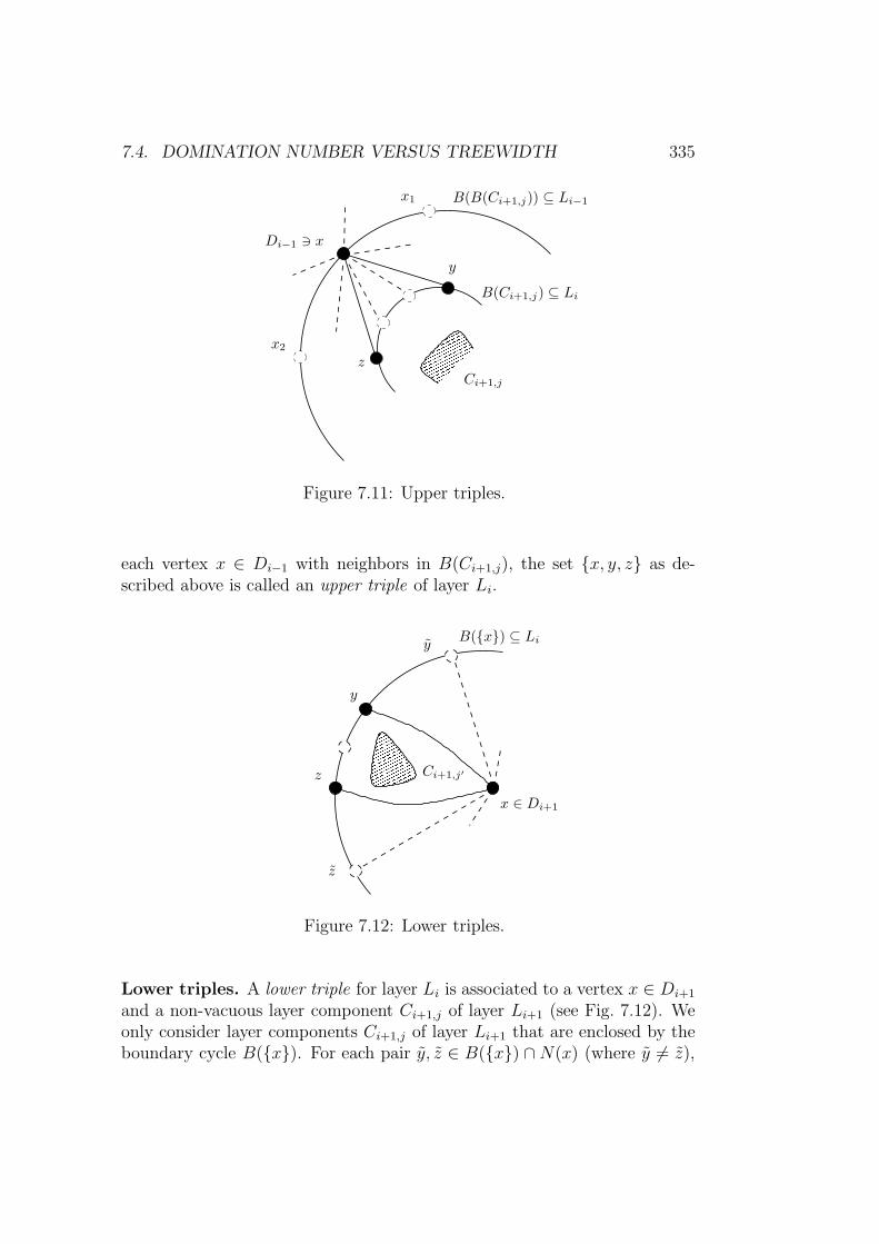
7.4. DOMINATION NUMBER VERSUS TREEWIDTH 335
Ci+1,j
B(Ci+1,j) ⊆ Li
z
y
x2
x1
Di−1 3 x
B(B(Ci+1,j)) ⊆ Li−1
Figure 7.11: Upper triples.
each vertex x ∈ Di−1 with neighbors in B(Ci+1,j), the set x, y, z as de-scribed above is called an upper triple of layer Li.
y
z
yB(x) ⊆ Li
x ∈ Di+1
z
Ci+1,j′
Figure 7.12: Lower triples.
Lower triples. A lower triple for layer Li is associated to a vertex x ∈ Di+1
and a non-vacuous layer component Ci+1,j of layer Li+1 (see Fig. 7.12). Weonly consider layer components Ci+1,j of layer Li+1 that are enclosed by theboundary cycle B(x). For each pair y, z ∈ B(x) ∩ N(x) (where y 6= z),

336 CHAPTER 7. GRAPH PARAMETERS
we consider the path Py,z from y to z along the cycle B(x), taking thedirection such that the region enclosed by z, x, x, y, and Py,z containsthe layer component Ci+1,j. Let y, z ⊆ B(x) ∩ N(x) be the pair suchthat the corresponding path Py,z is shortest. The triple, then, is the three-element set x, y, z. If x has no or only a single neighbor y in B(x), thenthe “triple” consists only of x, or x, y (by default, in these cases, we letx = y = z, or y = z, respectively).
Definition 7.38 For each vertex x ∈ Ci+1,j of Di+1 and each non-vacuouslayer component Ci+1,j that is enclosed by B(x), the set x, y, z as de-scribed above is called a lower triple of layer Li.
Ci+1,j
Case 1:
Ci+1,j
Case 2:
x ∈ Diy
x ∈ Di
zyz
B(Ci+1,j) ⊆ Li B(Ci+1,j) ⊆ Li
Figure 7.13: Middle triples.
Middle triples. A middle triple for layer Li is associated to a non-vacuouslayer component Ci+1,j and a vertex x ∈ Di that has a neighbor in B(Ci+1,j)(see Fig. 7.13). Note that, due to the layer model, it is easy to see that avertex x ∈ Di can have at most two neighbors y, z in B(Ci+1,j). Dependingon whether x itself lies on the cycle B(Ci+1,j) or not, we obtain two differentcases which are both illustrated in Fig. 7.13. In either of these cases, themiddle triple is defined as the set x, y, z. Again, if x has none or onlya single neighbor y in B(Ci+1,j), then the “triple” consists only of x, orx, y, respectively (by default, in these cases, we let x = y = z, or y = z,respectively).
Definition 7.39 For each non-vacuous layer component Ci+1,j and each ver-tex x ∈ Di, the set x, y, z as described above is called a middle triple forlayer Li.

7.4. DOMINATION NUMBER VERSUS TREEWIDTH 337
x
Ci+1,j B(Ci+1,j)
B(B(Ci+1,j ))
d1
d13
y2
z
d23
d2
y1
d3
Figure 7.14: Si separates Li−1 and Li+2.
Definition 7.40 We define the set Si as the union of all upper triples, lowertriples and middle triples of layer Li.
In the following, we will show that Si is a separator of the graph. Notethat the upper bounds on the size of Si, which are derived afterwards, arecrucial for the upper bound on the treewidth derived later on.
Proposition 7.41 The set Si separates vertices of layers Li−1 and Li+2.
Proof. Suppose there is a path P (with no repeated vertices) from layerLi+2 to layer Li−1 that avoids Si. This clearly implies that there exists apath P ′ from a vertex x in a non-vacuous layer component Ci+1,j of layerLi+1 to a vertex z ∈ B(B(Ci+1,j)) in layer Li−1 which has the following twoproperties:
• P ′ ∩ Si = ∅.
• All vertices inbetween x and z belong to layer Li or to vacuous layercomponents of layer Li+1.
This can be achieved by simply taking a suitable sub-path P ′ of P . Let y1
(and y2, respectively) be the first (last) vertex along the path P ′ from x to zthat lies on the boundary cycle B(Ci+1,j) ⊆ Li (see Fig. 7.14).

338 CHAPTER 7. GRAPH PARAMETERS
Obviously, y2 cannot be an element of D since, then, it would appear in amiddle triple of layer Li and, hence, in Si. We now consider the vertex thatdominates y2. This vertex can lie in layer Li−1, Li, or Li+1.
Suppose first that y2 is dominated by a vertex d1 ∈ Li−1. Then, d1 isin B(B(Ci+1,j)), simply by definition of the boundary cycle (see Fig. 7.14).Since G is planar, this implies that y2 must be an “outermost” neighbor of d1
among all elements in N(d1)∩B(Ci+1,j). If this were not the case, then therewould be an edge from d1 to a vertex on B(Ci+1,j) that leaves the closedregion bounded by d1, y2, the path from y2 to z, and the correspondingpath from z to d1 along B(B(Ci+1,j)). Hence, y2 would be in the upper tripleof layer Li which is associated to the layer component Ci+1,j and d1. Thiscontradicts the assumption that P ′ avoids Si.
Now, suppose that y2 is dominated by a vertex d2 ∈ Di (see Fig. 7.14).By definition of the middle triples, this clearly implies that y2 is in themiddle triple associated to Ci+1,j and d2. Again, this contradicts the factthat P ′ ∩ Si = ∅.
Consequently, the dominating vertex d3 of y2 has to lie in layer Li+1. Letd3, d
13, d
23, where d1
3, d23 ∈ N(d3) ∩ B(Ci+1,j), be the lower triple associated
to layer component Ci+1,j and d3 (see Fig. 7.14). By definition, Ci+1,j iscontained in the region enclosed by d1
3, d3, d3, d23, and the path from d2
3
to d13 along B(Ci+1,j), which—assuming that y2 /∈ d3, d
13, d
23—does not hit
y2 (see Fig. 7.14). We now observe that, whenever the path from y1 to y2
leaves the cycle B(Ci+1,j) to its exterior, say at a vertex q, then it has toreturn to B(Ci+1,j) at a vertex q′ ∈ N(q) ∩ B(Ci+1,j). Otherwise, we wouldviolate the fact that, by definition, B(Ci+1,j) ⊆ Li. This, however, showsthat the path P ′ has to hit either d1
3 or d23 on its way from y1 to y2. Since
d13, d
23 ∈ Si, this case also contradicts the fact that P ′ ∩ Si = ∅.
7.4.3 An upper bound for the size of the separators
In this subsection, we want to show that the sum of the cardinalities of allseparators can be bounded by some linear term in k.
Lemma 7.42 |Si| ≤ 5(ki−1 + ki + ki+1) + 12ci+1.
A proof of this assertion can be found in [8].
For the number ci of non-vacuous components in layer i, we have thefollowing estimate.
Lemma 7.43 ci ≤ ki + ki+1 + ki+2.

7.4. DOMINATION NUMBER VERSUS TREEWIDTH 339
Proof. By definition, ci refers to only non-vacuous layer components inlayer Li, i.e., there is at least one vertex of layer Li+1 contained within eachsuch layer component. Such a vertex can only be dominated by a vertex fromlayer Li, Li+1, or Li+2. In this way, we get the claimed upper bound.
Combining the two previous results yields the bound claimed at the be-ginning of this subsection.
Proposition 7.44∑r
i=1 |Si| ≤ 51k, where r is the number of layers of thegraph.
Proof. This follows directly when we combine the previous two lemmas,noting that
∑ri=1 ki = k.
We are now ready to state the main result from [8] relating the dominationnumber and the treewidth of a planar graph. Note that the following theoremgives a decisive asymptotic improvement of Corollary 7.28.
Theorem 7.45 A planar graph with domination number k has treewidth ofat most 6
√34√k + 8.
Proof. Using the separators Si as found in the previous subsections, weconsider the following three sets of vertices: S1 = S1 ∪ S4 ∪ S7 ∪ . . ., S2 =S2 ∪ S5 ∪ S8 ∪ . . ., and S3 = S3 ∪ S6 ∪ S9 ∪ . . .. Since, by Proposition 7.44,|S1| + |S2| + |S3| ≤ 51k, one of these sets has size at most 51
3k, say Sδ (with
δ ∈ 1, 2, 3).Let δ and Sδ be obtained as above. Let d := 3
2
√34. We now go through
the sequence S1+δ, S4+δ, S7+δ, . . . and look for separators of size at mosts(k) := d
√k. Due to the estimate on the size of Sδ, such separators of
size at most s(k) must appear within each n(k) := 513· 1d√k· k = 1
3
√34√k
sets in the sequence. In this manner, we obtain a set of disjoint separatorsof size at most s(k) each, such that any two consecutive separators from thisset are at most 3n(k) layers apart. Clearly, the separators chosen in this wayfulfill the requirements in Proposition 7.36.
Observe that the components cut out in this way each have at most3(n(k) + 1) layers and, hence, their treewidth is bounded by 9(n(k) + 1)− 1due to Prop. 7.27.
Using Proposition 7.36, we can compute an upper bound on the treewidthtw(k) of the originally given graph with domination number k:
tw(k) ≤ 2s(k) + 9(n(k) + 1) − 1
= 2(3
2
√34√k) + 9(
1
3
√34√k) + 8
= 6√
34√k + 8.

340 CHAPTER 7. GRAPH PARAMETERS
This proves our claim.
How did we come to the constants? We simply computed the minimumof 2s(k) + 9(n(k) + 1) − 1 (the upper bound on the treewidth) given thebound s(k)n(k) ≤ 51
3k. This suggests s(k) = d
√k, and d is optimal when
2s(k) = 9n(k) = 9 · 513· k · s(k)−1, so, 2d = 153
d, i.e., d = 3
2
√34.
Observe that the tree structure of the tree decomposition obtained inthe preceding proof corresponds to the structure of the layer decompositionforest.
Remark 7.46 Up to constant factors, the relation exhibited in Theorem 7.45is optimal. This can be seen, for example, by considering a complete gridgraph G` of size `× `, i.e., with `2 vertices. It is known that tw(G`) ≥ ` (see[54, Corollary 89]) and the domination number γ(·) obeys γ(G`) ∈ Θ(`2), see[228, Theorem 2.39]. Therefore, there is an infinite family of planar graphsGki
with domination number ki such that Gkihas treewidth of Ω(
√ki).
7.4.4 A treewidth-based algorithm for planar domi-
nating set
In this section, we outline our fixed parameter algorithm for solving planardominating set constructively. The input instance to the algorithm con-sists of a planar graph G = (V,E) and a positive integer k. The algorithmdetermines whether G admits a dominating set of size at most k, and, if so,constructs such a set. The running time for the algorithm will be 4O(
√k)n,
where n = |V |.
The key idea for our algorithm is to construct a tree decomposition ofthe stated width. However, Theorem 7.45 is a pure existence theorem whichcannot be made constructive directly. There is one point that needs specificattention. As we do not start with the dominating set given, we cannot con-struct the upper, middle, and lower triples. Instead, we have to compute theminimum size separator Si between Li−1 and Li+2 directly, and use that setinstead of Si as defined in the proof of Subsection 7.4.2. Such a minimum sizeseparator can be computed with well known techniques based on maximumflow (see, e.g., [250]).
Our algorithm proceeds in the following steps:
1. Embed the planar graph G = (V,E) crossing-free into the plane. De-termine the outerplanarity number r of this embedding and all layersL1, . . . , Lr. By default, we set Li = ∅ for all i < 0 and i > r.

7.4. DOMINATION NUMBER VERSUS TREEWIDTH 341
2. If r > 3k then exit (there exists no k-dominating set). This step ofthe algorithm is justified by Proposition 7.27.
3. For δ = 1, 2, 3 and i = 0, . . . , b r3c−1, find the minimum separator S3i+δ,
separating layers L(3i+δ)−1 and L(3i+δ)+2. Let s3i+δ = |S3i+δ|.
4. Check whether there exists a δ ∈ 1, 2, 3 and an increasing sequence(ij)j=1,...,t of indices in 0, . . . , b r
3c − 1, such that
s3ij+δ ≤ s(k) :=3
2
√34√k for all j = 1, . . . , t and
|ij+1 − ij| ≤ n(k) :=1
3
√34√k for all j = 1, . . . , t− 1.
If the answer is “no,” then exit (there exists no k-dominating set).This step of the algorithm is justified by the considerations in the proofof Theorem 7.45.
5. Consider the separators Sj := S3ij+δ for j = 1, . . . , t (by default, Sj = ∅for all other j) and, for each j = 0, . . . , t, let Gj be the subgraph cutout by the separators Sj and Sj+1 or, more precisely, let
Gj := G−( (3i(j+1)+δ)+1⋃
`=(3ij+δ)−1
L` \ (Sj ∪ Sj+1)).
Note that Gj is at most 3(n(k) + 1)-outerplanar.
6. Construct tree decompositions Xj for Gj (j = 0, . . . , t) with O(n) nodeseach. For this step, we refer to Theorem 7.23.
7. Construct a tree decomposition X of G with O(n) nodes using theseparators S1, . . . ,St and the tree decompositions Xj by the separatormerging technique described in the proof of Proposition 7.36.
8. Solve the minimum dominating set problem for G with tree decom-position X as described in Sec. 7.2.
Details on implementing Step 1 can be found in [8].As to Step 3 of the algorithm, we want to remark that such a minimum
size separator can be computed with well known techniques based on max-imum flow (see, e.g., [250]) as follows: For given values of i and δ, we first,build the graph G′, induced by the vertices in L3i+δ−1 ∪ L3i+δ ∪ L3i+δ+1 ∪L3i+δ+2. Then, we contract all vertices in L3i+δ−1 to one vertex s, and all

342 CHAPTER 7. GRAPH PARAMETERS
vertices in L3i+δ+2 to one vertex t. We look for a minimum s-t-separator inthe resulting graph but, if this separator has size more than s(k), then wejust note that no separator of size at most s(k) exists (compare with Step 4).Finding the separator or determining that no small enough separator existscan be done with the following standard method. Build a directed graph G′′
in the following way. Every vertex v in the graph is replaced by two verticesv− and v+, with an edge from v− to v+, and an edge v, w is replaced bytwo edges (v+, w−), (w+, v−). As explained in [292, Lemma 11, page 83],the minimum s-t separator in G′ can be found by applying a maximum flowalgorithm in G′′. To keep the running time in the stated bounds, we use theFord-Fulkerson maximum flow algorithm, but stop as soon as a flow valueof more than s(k) is used since, in such a case, we can conclude that nos-t-separator of size at most s(k) exists. As each flow augmentation stepcosts time linear in the number of vertices and edges of G′′ and increasesthe flow value by one, the time used by this procedure is O(n′ · s(k)), withn′ = |L3i+δ−1 ∪ L3i+δ ∪ L3i+δ+1 ∪ L3i+δ+2|.
As for every vertex in G, there are at most four combinations of δ and iin Step 3 such that it belongs to L3i+δ−1 ∪ L3i+δ ∪ L3i+δ+1 ∪ L3i+δ+2 and thetotal time of step 3 is bounded by O(n · s(k)) = O(n
√k).
The correctness of the algorithm above follows from our considerations inthe previous sections.
Steps 1-7 allow us to construct a tree decomposition of width 6√
34√k+8
of G in O(√kn) time. The running time for the last step in the algorithm is
O(46√
34√kn).
Summarizing these observations, we obtain the following theorem.
Theorem 7.47 planar dominating set can be solved in time O(c√kn),
where c = 46√
34. Moreover, if the domination number obeys γ(G) ≤ k, aminimum size dominating set can be constructed within the same time.
The constant c above is 46√
34, which is rather large. However, a morerefined analysis can help reduce this constant, as we will see below.
7.5 The beauty of small kernels: separator
theorems
The strategy explained in the previous section appears to be pretty specialto planar dominating set. Can we obtain similar results say for vertex

7.5. THE BEAUTY OF SMALL KERNELS: SEPARATOR THEOREMS343
cover on planar graphs? In this and the following section, we are going toexplain the more general ideas how to exploit small kernels from [14, 15, 190].More specifically, in this section we exhibit how to use classical separatortheorems plus nice kernelization results to get parameterized algorithms withrunning times of the form O∗(c
√k). The next section will use strategies
inspired from the notion of outerplanarity that we showed above. This way,better running times are achievable.
7.5.1 Classical separator theorems
One of the most useful algorithmic techniques for solving computational prob-lems is divide and conquer. In the case of planar graph problems, the famousplanar separator theorem of Lipton and Tarjan [275, 276] laid the basis forthe divide and conquer approach. The techniques we develop here all arebased on the existence of “small” graph separators, which means that theseparator size |S| is bounded by o(|V |). It is well-known that, for generalgraphs, small separators need not exist; consider, for example, the completegraph Kn, which does not possess small separators. It is of key importancefor our purpose that, in particular, planar graphs do have small separators.Therefore, it is not only of pure mathematical importance to study graphclasses which are guaranteed to have small generators.
Definition 7.48 According to Lipton and Tarjan [275], an f(·)-separatortheorem (with constants α < 1, β > 0) for a class G of graphs which is closedunder taking vertex-induced subgraphs is a theorem of the following form:If G is any n-vertex graph in G, then there is a separation (A1, S, A2) of Gsuch that
• neither A1 nor A2 contains more than αn vertices, and
• S contains no more than βf(n) vertices.
Again, this definition easily generalizes to `-separators with ` > 2.Stated in this framework, the planar separator theorem due to Lipton
and Tarjan [275] is a√·-separator theorem with constants α = 2/3 and
β = 2√
2 ≈ 2.83. The current record for α = 2/3 is β =√
2/3+√
4/3 ≈ 1.97[128]. Djidjev has also shown a lower bound of β ≈ 1.55 for α = 2/3 [130].For α = 1/2, the “record” is β = 2
√6 ≈ 4.90 [18, 54]. A lower bound of
β ≈ 1.65 is known in this case [353]. For α = 3/4, the best known value for
β is√
2π/√
3 · (1 +√
3)/√
8 ≈ 1.84 with a known lower bound of β ≈ 1.42,
see [353]. The results are summarized in Table 7.1.
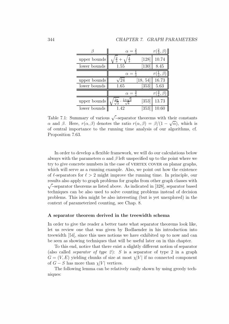
344 CHAPTER 7. GRAPH PARAMETERS
β α = 23
r(23, β)
upper bounds√
23
+√
43
[128] 10.74
lower bounds 1.55 [130] 8.45
α = 12
r(12, β)
upper bounds√
24 [18, 54] 16.73lower bounds 1.65 [353] 5.63
α = 34
r(34, β)
upper bounds√
2π√3· 1+
√3√
8[353] 13.73
lower bounds 1.42 [353] 10.60
Table 7.1: Summary of various√·-separator theorems with their constants
α and β. Here, r(α, β) denotes the ratio r(α, β) = β/(1 − √α), which is
of central importance to the running time analysis of our algorithms, cf.Proposition 7.63.
In order to develop a flexible framework, we will do our calculations belowalways with the parameters α and β left unspecified up to the point where wetry to give concrete numbers in the case of vertex cover on planar graphs,which will serve as a running example. Also, we point out how the existenceof `-separators for ` > 2 might improve the running time. In principle, ourresults also apply to graph problems for graphs from other graph classes with√·-separator theorems as listed above. As indicated in [328], separator basedtechniques can be also used to solve counting problems instead of decisionproblems. This idea might be also interesting (but is yet unexplored) in thecontext of parameterized counting, see Chap. 8.
A separator theorem derived in the treewidth schema
In order to give the reader a better taste what separator theorems look like,let us review one that was given by Bodlaender in his introduction intotreewidth [54], since this uses notions we have exhibited up to now and canbe seen as showing techniques that will be useful later on in this chapter.
To this end, notice that there exist a slightly different notion of separator(also called separator of type 2 ): S is a separator of type 2 in a graphG = (V,E) yielding chunks of size at most χ|V | if no connected componentof G− S has more than χ|V | vertices.
The following lemma can be relatively easily shown by using greedy tech-niques:

7.5. THE BEAUTY OF SMALL KERNELS: SEPARATOR THEOREMS345
Lemma 7.49 If G = (V,E) has a separator S of type 2, yielding chunks ofsize at most 1/2 · |V |, then G has a separation (A1, S
′, A2) such that neitherA1 nor A2 have more than 2/3 · |V | elements.
The first theorem we need is the following one that relates treewidth andseparators of type 2 (see [54, Theorem 19]):
Theorem 7.50 If tw(G) ≤ k, then there is a type-2 separator S, |S| ≤ k+1,in G that yields chunks of size at most 1/2 · (|V | − k).
Namely, observe that in a graph of treewidth at most k, a suitably chosenbag may serve as a separator of type 2.
Algorithm 66 An algorithm for determining a small separator in a planegraph
Input(s): a plane n-vertex graph GOutput(s): a type-2 separator S, |S| ≤ 2
√6n of type 2, yielding chunks of
size at most 1/2 · |V |.Let c = 1/2 · √n.Let L1, . . . , Lr be the layer decomposition of the plane graph G.Determine s be such that |⋃i<s Li| ≤ 1/2·|V | and that |⋃i>s Li| ≤ 1/2·|V |.if |Ls| ≤ c
√n then
output Lselse if |Li| > c
√n for all 1 ≤ i ≤ r then
r ≤ 1/c · √n (since there are only n vertices in the graph)tw(G) ≤ 3r − 1 ≤ 3/c
√n− 1
Thm. 7.50 guarantees the existence of a sufficiently small separator S oftype 2 which the algorithm returns.
elseLet s1 < s be maximal with the property that |Ls1| ≤ c
√n.
Let s2 > s be minimal with the property that |Ls2| ≤ c√n.
Let L =⋃s1<i<s2
Li.Find small separator S of type 2 in G[L] according to Thm. 7.50.Notice that out(G[L]) ≤ s2 − s1 − 1 ≤ 1/c · √n, hence tw(G[L]) ≤3/c
√n− 1.
return Ls1 ∪ Ls2 ∪ Send if
Theorem 7.51 Alg. 66 produces to every plane n-vertex graph G a type-2separator of size 2
√6n, yielding chunks of size at most 1/2 · n.

346 CHAPTER 7. GRAPH PARAMETERS
With Lemma 7.49, we may conclude:
Corollary 7.52 Planar graphs admit an√n-separator theorem with con-
stants α = 2/3 and β ≈ 4.90.
Variants of separator theorems
Cycle separators. In the literature, there are many separator theoremsfor planar graphs which guarantee that all the vertices of the separator lieon a simple cycle, provided that the given graph is biconnected or even tri-angulated. In fact, the current “record holder” in the case of α = 2/3 yieldsa cycle separator, see [128]. From an algorithmic perspective, as explainedbelow, the requirements of having biconnected or triangulated graphs arerarely met: even if the original graph was biconnected or triangulated, sub-graphs which are obtained by recursive applications of separator theorems toa larger graph are not biconnected or triangulated in general. Therefore, weconsider the following definition appropriate for our purposes:
Definition 7.53 We will call a separator S of a planar graph G cycle sepa-rator if there exists a triangulation G of G such that S forms a simple cyclein G.
Note: some triangulation of a given planar graph can be computed in lineartime.
Remark 7.54 It will turn out that it is of special value (concerning thedesign of divide and conquer algorithms) to have separators that form simplecycles (within some triangulation of the given graph G), since then the Jordancurve theorem applies (for planar graphs), which basically means that theseparator S splits G into an “inside”-part A1 and an “outside”-part A2. If Gis a subgraph of a larger planar graph G, then this implies that each vertex vof G that has neighbors in A1 has no neighbors in A2 and vice versa. Thisobservation is important, since it means that a local property pertaining tovertex v of G (like: v belongs to a dominating set or not) can only influencevertices in δA1 or vertices in δA2.
Weighted separation. It is also possible to incorporate weights in mostseparator theorems. For our purposes, weights are nonnegative reals as-signed to the vertices in a graph such that the sum of all weights in a graphis bounded by one. For weighted graphs, an f(·)-separator theorem with con-stants α and β for graph class G guarantees, for any n-vertex graph G ∈ G,the existence of a separation (A1, S, A2) of G such that

7.5. THE BEAUTY OF SMALL KERNELS: SEPARATOR THEOREMS347
• neither A1 nor A2 has weight more than α, and
• S contains no more than βf(n) vertices.
Other graph classes with separator theorems. Similar to the case ofplanar graphs,
√·-separator theorems are also known for other graph classes,e.g., for the class of graphs of bounded genus, see [131]. More generally,Alon, Seymour and Thomas proved a
√·-separator theorem for graph classeswith an excluded complete graph minor [20, 21]. There are also interestinggraph classes which are not minor closed for which
√·-separator theorems areknown, as, e.g., the classes of `-map graphs, see [92, 93].7 Many commentsof this paper apply to these more general situations, too.
7.5.2 Select&verify problems and glueability
For the approach outlined in this section, we want to describe necessaryproperties for graph problems that allow for separator based algorithms.
Select&verify graph problems
Definition 7.55 A set G of tuples (G, k), G an undirected graph with vertexset V = v1, . . . , vn and k a positive real number, is called a select&verify(graph) problem if there exists a pair (P·, opt) with opt ∈ min,max, suchthat P· is a function that assigns to G a polynomial time computable functionof the form PG = P sel
G + P verG , where P sel
G : 0, 1n → R≥0, PverG : 0, 1n →
0,±∞, and
(G, k) ∈ G ⇔
opt~x∈0,1n PG(~x) ≤ k if opt = minopt~x∈0,1n PG(~x) ≥ k if opt = max .
For ~x = (x1, . . . , xn) ∈ 0, 1n with PG(~x) ≤ k if opt = min and withPG(~x) ≥ k if opt = max, the vertex set selected by ~x and verified by PG isvi ∈ V | xi = 1, 1 ≤ i ≤ n. A vector ~x is called admissible if P ver
G (~x) = 0.
The intuition behind the term P· = P sel· + P ver
· is that the “selectingfunction” P sel
· counts the size of the selected set of vertices and the “verifyingfunction” P ver
· verifies whether this choice of vertices is an admissible solution.
Observe that every select&verify graph problem that additionally admitsa problem kernel of size p(k) is solvable in time O(2p(k)p(k) + TK(n, k)).
7The ` basically refers to the maximal size of a complete subgraph of a map graph.

348 CHAPTER 7. GRAPH PARAMETERS
Example 7.56 We now give some examples for select&verify problems byspecifying the function PG = P sel
G + P verG . In all cases below, the “selecting
function” PG for a graph G = (V,E) will be
P selG =
∑
vi∈Vxi.
Also, we use the convention that 0 · (±∞) = 0.
1. In the case of vertex cover, we have opt = min and choose
P verG (~x) =
∑
vi,vj∈E∞ · (1 − xi)(1 − xj),
where this sum brings PG(~x) to infinity whenever there is an uncoverededge. In addition, PG(~x) ≤ k then guarantees a vertex cover set of sizeat most k. Clearly, PG is polynomial time computable.
2. Similarly, in the case of independent set, let opt = max and choose
P verG (~x) =
∑
vi,vj∈E(−∞) · xi · xj.
3. dominating set is another example for a select&verify graph problem.Here, for G = (V,E), we have
P verG (~x) =
∑
vi∈V(∞ · (1 − xi) ·
∏
vi,vj∈E(1 − xj)),
where this sum brings PG(~x) to infinity whenever there is a non-dominatedvertex which is not in the selected dominating set. In addition, PG(~x) ≤k then guarantees a dominating set of size at most k.
4. Similar observations do hold for many other graph problems and, inparticular, weighted variants of these.8 As a source of problems, con-sider the variants of dominating set listed in [140, 228, 364].
Moreover, graph problems where a small (or large) edge set is sought for canoften be reformulated into vertex set optimization problems by introducingan additional artificial vertex on each edge of the original graph. In this way,edge dominating set can be handled. Similarly, planar graph problems
8In the weighted case, one typically chooses a “selecting function” of the form P selG =∑
vi∈V αixi, where αi is the weight of the vertex vi.
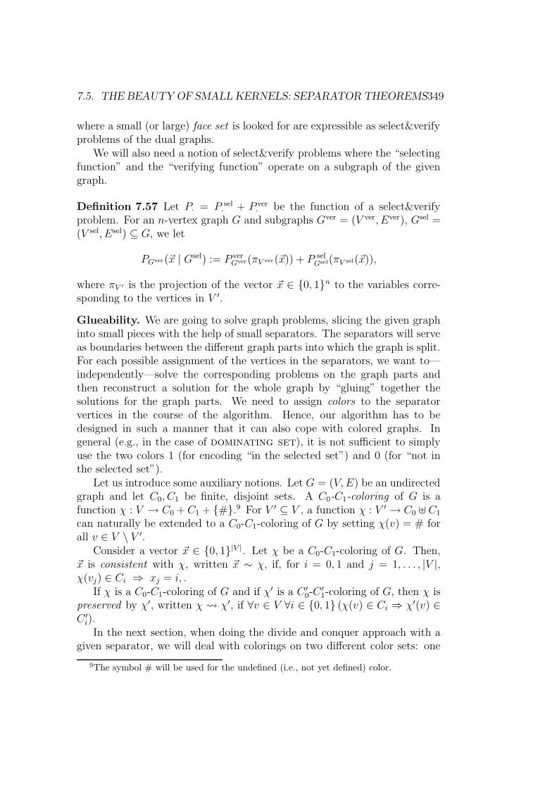
7.5. THE BEAUTY OF SMALL KERNELS: SEPARATOR THEOREMS349
where a small (or large) face set is looked for are expressible as select&verifyproblems of the dual graphs.
We will also need a notion of select&verify problems where the “selectingfunction” and the “verifying function” operate on a subgraph of the givengraph.
Definition 7.57 Let P· = P sel· + P ver
· be the function of a select&verifyproblem. For an n-vertex graph G and subgraphs Gver = (V ver, Ever), Gsel =(V sel, Esel) ⊆ G, we let
PGver(~x | Gsel) := P verGver(πV ver(~x)) + P sel
Gsel(πV sel(~x)),
where πV ′ is the projection of the vector ~x ∈ 0, 1n to the variables corre-sponding to the vertices in V ′.
Glueability. We are going to solve graph problems, slicing the given graphinto small pieces with the help of small separators. The separators will serveas boundaries between the different graph parts into which the graph is split.For each possible assignment of the vertices in the separators, we want to—independently—solve the corresponding problems on the graph parts andthen reconstruct a solution for the whole graph by “gluing” together thesolutions for the graph parts. We need to assign colors to the separatorvertices in the course of the algorithm. Hence, our algorithm has to bedesigned in such a manner that it can also cope with colored graphs. Ingeneral (e.g., in the case of dominating set), it is not sufficient to simplyuse the two colors 1 (for encoding “in the selected set”) and 0 (for “not inthe selected set”).
Let us introduce some auxiliary notions. Let G = (V,E) be an undirectedgraph and let C0, C1 be finite, disjoint sets. A C0-C1-coloring of G is afunction χ : V → C0 +C1 + #.9 For V ′ ⊆ V , a function χ : V ′ → C0 ] C1
can naturally be extended to a C0-C1-coloring of G by setting χ(v) = # forall v ∈ V \ V ′.
Consider a vector ~x ∈ 0, 1|V |. Let χ be a C0-C1-coloring of G. Then,~x is consistent with χ, written ~x ∼ χ, if, for i = 0, 1 and j = 1, . . . , |V |,χ(vj) ∈ Ci ⇒ xj = i, .
If χ is a C0-C1-coloring of G and if χ′ is a C ′0-C
′1-coloring of G, then χ is
preserved by χ′, written χ χ′, if ∀v ∈ V ∀i ∈ 0, 1 (χ(v) ∈ Ci ⇒ χ′(v) ∈C ′i).
In the next section, when doing the divide and conquer approach with agiven separator, we will deal with colorings on two different color sets: one
9The symbol # will be used for the undefined (i.e., not yet defined) color.
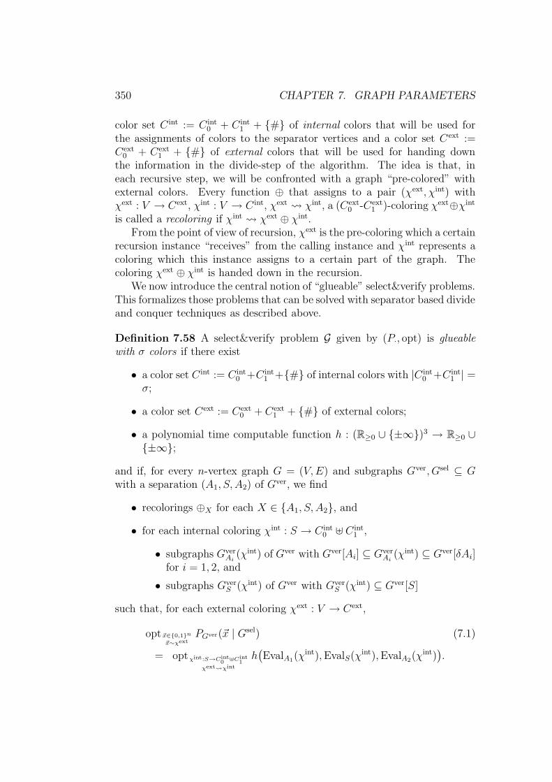
350 CHAPTER 7. GRAPH PARAMETERS
color set C int := C int0 + C int
1 + # of internal colors that will be used forthe assignments of colors to the separator vertices and a color set C ext :=Cext
0 + Cext1 + # of external colors that will be used for handing down
the information in the divide-step of the algorithm. The idea is that, ineach recursive step, we will be confronted with a graph “pre-colored” withexternal colors. Every function ⊕ that assigns to a pair (χext, χint) withχext : V → Cext, χint : V → C int, χext χint, a (Cext
0 -Cext1 )-coloring χext⊕χint
is called a recoloring if χint χext ⊕ χint.From the point of view of recursion, χext is the pre-coloring which a certain
recursion instance “receives” from the calling instance and χint represents acoloring which this instance assigns to a certain part of the graph. Thecoloring χext ⊕ χint is handed down in the recursion.
We now introduce the central notion of “glueable” select&verify problems.This formalizes those problems that can be solved with separator based divideand conquer techniques as described above.
Definition 7.58 A select&verify problem G given by (P·, opt) is glueablewith σ colors if there exist
• a color set C int := C int0 +C int
1 +# of internal colors with |C int0 +C int
1 | =σ;
• a color set Cext := Cext0 + Cext
1 + # of external colors;
• a polynomial time computable function h : (R≥0 ∪ ±∞)3 → R≥0 ∪±∞;
and if, for every n-vertex graph G = (V,E) and subgraphs Gver, Gsel ⊆ Gwith a separation (A1, S, A2) of Gver, we find
• recolorings ⊕X for each X ∈ A1, S, A2, and
• for each internal coloring χint : S → C int0 ] C int
1 ,
• subgraphs GverAi
(χint) of Gver with Gver[Ai] ⊆ GverAi
(χint) ⊆ Gver[δAi]for i = 1, 2, and
• subgraphs GverS (χint) of Gver with Gver
S (χint) ⊆ Gver[S]
such that, for each external coloring χext : V → Cext,
opt~x∈0,1n
~x∼χextPGver(~x | Gsel) (7.1)
= optχint:S→Cint0
]Cint1
χext χint
h(EvalA1(χ
int),EvalS(χint),EvalA2(χ
int)).

7.5. THE BEAUTY OF SMALL KERNELS: SEPARATOR THEOREMS351
Here, EvalX(·) for X ∈ A1, S, A2 is of the form
EvalX(χint) = opt ~x∈0,1n
~x∼(χext⊕Xχint)
PGverX (χint)(~x | Gver[X] ∩Gsel). (7.2)
Lemma 7.59 vertex cover and independent set are glueable with2 colors and dominating set is glueable with 4 colors.
Proof. For vertex cover(see Example 7.56.1), we use the color sets C `i :=
i` for ` ∈ int, ext and i = 0, 1. The function h is h(x, y, z) = x + y + z.The subgraphs Gver
X (χint) for X ∈ A1, S, A2 and χint : S → C int0 ] C int
1
are GverX (χint) := Gver[X]. In this way, the subroutine EvalS(χ
int) checkswhether the coloring χint yields a vertex cover on Gver[S] and the subroutinesEvalAi
(χint) compute the minimum size vertex cover on Gver[Ai]. However,we still need to make sure that all edges going from Ai to S are covered. If avertex in S is assigned a 1int by χint, the incident edges are already covered.In the case of a 0int-assignment for a vertex v ∈ S, we can color all neighborsin N(v) ∩ Ai to belong to the vertex cover. This is done by the followingrecolorings ⊕Ai
. Define
(χext ⊕Aiχint)(v) =
0ext if χint(v) = 0int,1ext if χint(v) = 1int or
if ∃w ∈ N(v) with χint(w) = 0int,#, otherwise.
By this recoloring definition, an edge between a separator vertex and avertex in Ai which is not covered by the separator vertex (due to the currentlyconsidered internal covering) will be covered by the vertex in Ai. Our abovereasoning shows that—with these settings—Equation (7.1) in Definition 7.58is satisfied.
independent set (see Example 7.56.2)) is shown to be glueable with2 colors by a similar idea.
To show that dominating set (see Example 7.56.3)) is glueable with4 colors, we use the following color sets
C int0 := 0int
A1, 0int
A2, 0int
S , C int1 := 1int,
Cext0 := 0ext, Cext
1 := 1ext.
The semantics of these colors is as follows. Assigning the color 0intX , for
X ∈ A1, A2, S, to vertices in a current separation V = A1 ] S ]A2 meansthat the vertex is not in the dominating set and will be dominated by a vertexin X. Clearly, 1int will mean that the vertex belongs to the dominating set.The external colors simply hand down the information whether a vertex

352 CHAPTER 7. GRAPH PARAMETERS
belongs to the dominating set, represented by 1ext, or whether it is not inthe dominating set and still needs to be dominated, represented by 0ext.10
The function h simply is addition, i.e., h(x, y, z) = x+ y+ z. When handingdown the information to the subproblems, for a given internal coloring χint :S → C int
0 ] C int1 , we define
GverAi
(χint) := Gver[Ai ∪ (χint)−1(1int, 0intAi)] and
GverS (χint) := Gver[(χint)−1(1int, 0int
S )].
The recolorings ⊕X for X ∈ A1, S, A2 are chosen to be
(χext ⊕X χint)(v) =
0ext if χint(v) ∈ C int0 ,
1ext if χint(v) = 1int,#, otherwise.
Let us explain in a few lines why—with these settings—Equation (7.1) inDefinition 7.58 is satisfied. If an internal coloring χint assigns color 0int
X
(X ∈ A1, S, A2) to a vertex in S, then this vertex needs to be domi-nated by a neighbor in X. This will be checked in EvalX(χint) using thegraph Gver
X (χint). To this end, vertices assigned the color 0intX (i.e., the set
(χint)−1(0intX )) are included in Gver
X (χint). The vertices assigned color 1int
(i.e., (χint)−1(1int)) also need to be handed down to the subroutines, sincesuch a vertex may already dominate vertices in X. The recolorings mergethe given external coloring χext with the current internal coloring χint in away that already assigned colors from C int
i or Cexti (i = 0, 1) become iext. The
terms EvalAi(χint) then compute (for each internal coloring χint) the size of a
minimum dominating set in Ai under the constraint that some vertices in δAi
still need to be dominated (namely, the vertices in δAi∩(χext⊕Aiχint)−1(0ext))
and some vertices in δAi can already be assumed to be in the dominating set(namely, the vertices in δAi ∩ (χext ⊕Ai
χint)−1(1ext)). The term EvalS(χint)
checks the correctness of the internal coloring χint of S.
Note that, from the point of view of divide-and-conquer algorithms, threecolors are enough for dominating set, since the color 1int already deter-mines the color 0int
S .We illustrate the ideas of the dominating set algorithm by using an example.
Example 7.60 Consider dominating set for the separated graph in Fig. 7.15.Beginning with the external coloring χext ≡ # and Gver = Gsel = G, we need
10A vertex that is not in the dominating set but is already guaranteed to be dominated,e.g., by a vertex in the current separator, will never be handed down, since these verticesare of no use in the sequel of the recursion.

7.5. THE BEAUTY OF SMALL KERNELS: SEPARATOR THEOREMS353
Figure 7.15: A partitioned graph.
to go over all 42 = 16 internal colorings χint : S → 0intA1, 0int
S , 0intA2, 1int (which
trivially satisfy χext χint). As an example, we choose χint with v5 7→ 0intA1
,v6 7→ 0int
A2. In this case, we get Gver
A1[χint] = Gver[v1, . . . , v5], Gver
S [χint] = ∅,and Gver
A2[χint] = Gver[v6, . . . , v11]. Recursively, we will use these graphs for
the verifying function and the graphs Gver[A1], Gver[S], and Gver[A2] for the
selecting function. The external colorings that will be handed down to thesubproblems after the recoloring look as follows: On the graph Gver
A1[χint], we
have χ1(vi) := (χext ⊕A1 χint)(vi) = # for i = 1, . . . , 4, and χ1(v5) = 0ext.
On the graph GverA2
[χint], we have χ2(vi) := (χext ⊕A2 χint)(vi) = # for
i = 7, . . . , 11, and χ2(v6) = 0ext. Clearly,
EvalA1(χint) = 2, EvalS(χ
int) = 0, and EvalA2(χint) = 2.
The minimum in Equation (7.2) of Definition 7.58 for X = A1 is obtained,e.g., by choosing the vertices v1 and v2 (note that the latter needs to bechosen, since χ1(v5) = 0ext, meaning that v5 is forced to be dominated in thisterm). The minimum for A2 is obtained, e.g., by choosing the vertices v8 andv10 (again, χ2(v6) = 0ext forces either v8 or v9 to be in the dominating set).Hence,
h(EvalA1(χint),EvalS(χ
int),EvalA2(χint)) = 2 + 0 + 2 = 4.
We obtain an optimal result, e.g., for the choice of the internal color-ing χint with χint(v5) = χint(v6) = 0int
A2. Here, we get EvalA1(χ
int) = 1,EvalS(χ
int) = 0, and EvalA2(χint) = 2, for the possible choices of v3, v8, v10 as
dominating set vertices.
Remark 7.61 In the case that recurrences are based on separator theoremsyielding `-separators, let us call a problem `-glueable with σ` colors if σ`colors are to be distinguished in the recursion. For example, an extensionof our previous lemma shows that dominating set is `-glueable with ` + 2

354 CHAPTER 7. GRAPH PARAMETERS
colors, where |C int0 | = ` + 1. There need not be, however, a dependence of
the number of colors on the number of graph parts: both vertex cover andindependent set are `-glueable with two colors.
Besides the problems stated in the preceding Lemma 7.59, many moreselect&verify problems are glueable, for example, those which are listed in[363, 364, 365]. In particular, weighted versions and variations of the prob-lems discussed in Lemma 7.59 are glueable.
7.5.3 Fixed-parameter divide-and-conquer algorithms
In this section, we provide the basic framework for deriving fixed-parameteralgorithms based on the concepts we introduced so far.
Using glueability for divide-and-conquer
Fix a graph class G for which a√·-separator theorem with constants α and
β (cf. Definition 7.48) is known. We consider a glueable select&verify graphproblem G defined by (P·, opt). The evaluation of the term opt~x∈0,1n PG(~x)(cf. Definition 7.55) can be done recursively according to the following strat-egy.
The sizes of the subproblems, i.e., the sizes of the graphs GverAi
(χint) whichare used in the recursion, play a crucial role in the analysis of the runningtime of this algorithm. A particularly nice situation is given by the followingproblems.
Definition 7.62 A glueable select&verify problem is called a slim problemif the subgraphs Gver
Ai(χint) are only by a constant number of vertices larger
than Gver[Ai], i.e., if there exists an η ≥ 0 such that |V (GverAi
(χint))| ≤ |Ai|+ηfor all internal colorings χint : S → C int.
Note that the proof of Lemma 7.59 shows that both vertex cover andindependent set are slim with η = 0, whereas dominating set is not.
The following proposition gives the running time of the above algorithm interms of the parameters of the separator theorem used and the select&verifyproblem considered. In order to assess the time required for the above givendivide-and-conquer algorithm, we use the following abbreviations for the run-ning times of certain subroutines:
• TS(n) denotes the time to find a “sufficiently small” separator in ann-vertex graph from class G.

7.5. THE BEAUTY OF SMALL KERNELS: SEPARATOR THEOREMS355
1. Start the computation by evaluating
opt~x∈0,1n PG(~x) = opt~x∈0,1n, ~x∼χext0PGver(~x | Gsel),
where “χext0 ≡ #” is the everywhere undefined external coloring and
Gver = Gsel = G (also cf. Definition 7.57).
2. When opt~x∈0,1n, ~x∼χext PGver(~x | Gsel) needs to be calculated for some
subgraphs Gsel, Gver ⊆ G, and an external coloring χext : V (G) →Cext
0 ] Cext1 ] #, we do the following:
(a) If Gver has size greater than some constant c, then find a√·-
separator S for Gver with V (Gver) = A1 ] S ] A2.
(b) Define Φ := χint : S → C int0 ] C int
1 | χext χint.For all internal colorings χint ∈ Φ do:
i. Determine EvalAi(χint) recursively for i = 1, 2.
ii. Determine EvalS(χint).
(c) Return optχint∈Φ h(EvalA1(χint),EvalS(χ
int),EvalA2(χint)).
• TM(n) denotes the time to construct the modified graphs GverX (χint) ∈ G
and the modified colorings (χext⊕X χint) (for X ∈ A1, S, A2 and each
internal coloring χint ∈ Φ from an n-vertex graph from class G.
• TE(m) is the time to evaluate EvalS(χint) for any χint ∈ Φ in a separa-
tor S of size m.
• TG(n) is the time for gluing the results obtained by two sub-problemseach of size O(n).
In the following, we assume that all these functions are polynomials.
Proposition 7.63 Let G be a graph class for which a√·-separator theo-
rem with constants α and β is known and let G be a select&verify problemdefined by (P·, opt) that is glueable with σ colors. Then, for every G ∈ G,opt~x∈0,1n PG(~x) can be computed in time
c(α′, β, σ)√nq(n), where c(α′, β, σ) = σβ/(1−
√α′).
Here, α′ = α + ε for any ε ∈ (0, 1 − α) and q(·) is some polynomial; therunning time analysis only holds for n ≥ n0(ε).

356 CHAPTER 7. GRAPH PARAMETERS
If, however, G is slim or the√·-separator theorem yields cycle separa-
tors (and G is the class of planar graphs), then the running time for thecomputation is c(α, β, σ)
√nq(n), which then holds for all n.
The (rather lengthy) proof is contained in [14].
Remark 7.64 A similar proposition holds for graph classes on which an `-separator theorem is known with constants α and β. It might turn out thatsuch separator theorems have better ratio β/(1−√
α), which, in turn, woulddirectly improve the running time in Proposition 7.63.
How (linear) problem kernels help
If the considered parameterized problem has a problem kernel of size dk,we can use the considerations we have made up to this point in order toobtain fixed-parameter algorithms whose exponential term is of the form c
√k
for some constant c. More generally, a problem kernel of size p(k) yields
exponential terms of the form c√p(k).
Theorem 7.65 Assume the following:
• Let G be a graph class for which a√·-separator theorem with con-
stants α and β is known,
• let G be a select&verify problem defined by (P·, opt) glueable with σcolors, and
• suppose that G admits a problem kernel of polynomial size p(k) on Gcomputable in time TK(n, k).
Then, there is an algorithm to decide (G, k) ∈ G, for a graph G ∈ G, in time
c(α′, β, σ)√p(k)q(k) + TK(n, k), where c(α′, β, σ) = σβ/(1−
√α′), (7.3)
and α′ = α+ ε for any ε ∈ (0, 1 − α), holding only for k ≥ k0(ε), where q(·)is some polynomial.
If, however, G is slim or the√·-separator theorem yields cycle separators
(on the class G of planar graphs), then the running time for the computationis
c(α, β, σ)√p(k)q(k) + TK(n, k),
which then holds for all k.

7.5. THE BEAUTY OF SMALL KERNELS: SEPARATOR THEOREMS357
In particular, Theorem 7.65 means that, for glueable select&verify prob-lems for planar graphs that admit a linear problem kernel of size dk, we canget an algorithm of running time
O(c(α, β, σ, d)
√kq(k) + TK(n, k)
), where c(α, β, σ, d) = σ
√dβ/(1−√
α).
Obviously, the choice of the separator theorem has a decisive impact onthe constants of the corresponding algorithms. In particular, our runningtime analysis shows that the ratio r(α, β) := β/(1 − √
α) has a direct andsignificant influence on the running time. In Table 7.1, this ratio is computedfor the various
√·-separator theorems. In the following example we use theseratios explicitly.
Example 7.66 In the case of Vertex Cover on planar graphs, we can taked = 2, α = 2/3, and β =
√2/3 =
√4/3 (see [128]) with the ratio r(α, β) ≈
10.74. In this way, we obtain an algorithm with running time O(2√
2·10.74·√k+
nk). Neglecting polynomial terms, we have such obtained a c√k-algorithm
with c ≈ 215.19 ≈ 37381. By way of contrast, taking d = 2, α = 3/4, and
β =√
2π/√
3 · (1 +√
3)/√
8 ≈ 1.84 (see [353]) with r(α, β) ≈ 13.73, we get
an algorithm with running time O(2√
2·13.73·√k + nk). This means, we have a
c√k-algorithm with c ≈ 219.42 ≈ 701459.
The constants obtained by this first approach are admittedly bad. How-ever, by a careful analysis of how separator theorems are obtained in theliterature, we can show in [14]:
Theorem 7.67 Let G be a select&verify problem on planar graphs defined by(P·, opt) which is glueable with σ colors, and suppose that G admits a problemkernel of polynomial size p(k) computable in time TK(n, k).
Then, there is an algorithm to decide (G, k) ∈ G, for an n-vertex planargraph G, in time
c(α′, σ)√p(k)q(k) + TK(n, k), where c(α′, σ) ≈ σ1.80665/(1−
√α′),
and α′ = 2/3 + ε for any ε ∈ (0, 1/3), holding only for k ≥ k0(ε), where q(·)is some polynomial.
If G is slim, then the running time for the computation is
c(2/3, σ)√p(k)q(k) + TK(n, k),
which then holds for all k.
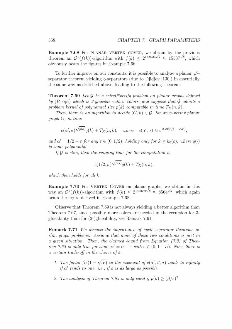
358 CHAPTER 7. GRAPH PARAMETERS
Example 7.68 For planar vertex cover, we obtain by the previoustheorem an O∗(f(k))-algorithm with f(k) ≤ 213.9234
√k ≈ 15537
√k, which
obviously beats the figures in Example 7.66.
To further improve on our constants, it is possible to analyze a planar√·-
separator theorem yielding 3-separators (due to Djidjev [130]) in essentiallythe same way as sketched above, leading to the following theorem:
Theorem 7.69 Let G be a select&verify problem on planar graphs definedby (P·, opt) which is 3-glueable with σ colors, and suppose that G admits aproblem kernel of polynomial size p(k) computable in time TK(n, k).
Then, there is an algorithm to decide (G, k) ∈ G, for an n-vertex planargraph G, in time
c(α′, σ)√p(k)q(k) + TK(n, k), where c(α′, σ) ≈ σ2.7056/(1−
√α′),
and α′ = 1/2 + ε for any ε ∈ (0, 1/2), holding only for k ≥ k0(ε), where q(·)is some polynomial.
If G is slim, then the running time for the computation is
c(1/2, σ)√p(k)q(k) + TK(n, k),
which then holds for all k.
Example 7.70 For Vertex Cover on planar graphs, we obtain in thisway an O∗(f(k))-algorithm with f(k) ≤ 213.0639
√k ≈ 8564
√k, which again
beats the figure derived in Example 7.68.
Observe that Theorem 7.69 is not always yielding a better algorithm thanTheorem 7.67, since possibly more colors are needed in the recursion for 3-glueability than for (2-)glueability, see Remark 7.61.
Remark 7.71 We discuss the importance of cycle separator theorems orslim graph problems. Assume that none of these two conditions is met ina given situation. Then, the claimed bound from Equation (7.3) of Theo-rem 7.65 is only true for some α′ = α + ε with ε ∈ (0, 1 − α). Now, there isa certain trade-off in the choice of ε:
1. The factor β/(1 −√α′) in the exponent of c(α′, β, σ) tends to infinity
if α′ tends to one, i.e., if ε is as large as possible.
2. The analysis of Theorem 7.65 is only valid if p(k) ≥ (β/ε)2.

7.6. THE BEAUTY OF SMALL KERNELS: LAYERWISE SEPARATION359
Keeping in mind that typical values of p(k) are not very large in practicalcases, the second point means that, since β is fixed, ε should be comparativelylarge, otherwise, β/ε would be greater than
√p(k). This gives us very bad
constants in the analysis due to the first point.
As explained in the following example, Theorem 7.65 is not only interest-ing in the case of planar graph problems.
Example 7.72 Since Vertex Cover is a slim problem which has a linearsize kernel, Theorem 7.65 yields a c
√gk-algorithm for Gg, where Gg denotes
the class of graphs of genus bounded by g; see [131], where the existence ofa separator of size O(
√gn) for n-vertex graphs from Gg was proven. For the
same reason, we get a c√gk-algorithm for Independent Set on Gg. Simi-
larly, for the class of `-map graphs, we obtain c√`k-algorithms for Vertex
Cover and for Independent Set based on [92].
Note that these are the first examples of fixed-parameter algorithms withsublinear exponents for bounded genus graphs and for `-map graphs. In thissense, the techniques discussed in this paper apply to a wider range of graphscompared to the approach discussed in the next section. The “LayerwiseSeparation Property” we provide there makes sense for planar graphs only,although it might be extensible to map graphs.
7.6 The beauty of small kernels: layerwise
separation
This approach differs strongly from research directions, where running timesof algorithms are improved in a very problem-specific manner (e.g., by ex-tremely sophisticated case-distinctions). For example, once one can showthat a problem has the so-called “Layerwise Separation Property,” one canrun a general algorithm which quickly computes a tree decomposition ofguaranteed small width (independent of the concrete problem). In summary,the heart of our approach can roughly be sketched as follows: If...
1. ...one can show that a graph problem carries some nice properties (e.g.,the Layerwise Separation Property) and
2. ...one can determine some corresponding “problem-parameters” for theseproperties (e.g., the width and the size-factor of the Layerwise Separa-tion Property);

360 CHAPTER 7. GRAPH PARAMETERS
kernel
size: dk
linear problem
problem-specific
max(out(Gi)) ≤√dk/ψ + w # of colors: λ
bounded outerplanarity
algorithm for
CONSTRAINT Gtree-decomposition
Layerwise Separation Property
bounded outerplanarity
approach
(dynamic programming)
tree decomposition
algorithm for Gσtw(G) · n
size-factor: d
(LSP)
max |S| ≤ ψ√dk
Partial Separation S(ψ)
τout(G) · n
tw(G) ≤ 2√
3d√k + (3w − 1)
O( 2θ1(σ,d)√k · n )
θ2(λ, τ, d) = 2√
d log(λ) log(τ)O( 2θ2(λ,τ,d)
√k · n )
weakly glueable
θ1(σ, d) = 2 log(σ)√
3d
width: w
Figure 7.16: Road map of our methodology for planar graph problems.
then one gets an algorithm of running time O(c√knO(1)), where we give con-
crete formulas on how to evaluate the constant c as a function of theseproblem-parameters.
In a first phase, one separates the graph in a particular way (“layerwise”).The key property of a graph problem to allow such an approach will be the so-called “Layerwise Separation Property.” The details herefore are presentedin Section 7.6.1. It will be shown that such a property holds for quite a largeclass of graph problems including those which admit a linear problem kernel.This property assures that the planar graph can be separated nicely.
In a second phase, the problem is solved on the layerwisely separatedgraph. We present two independent ways to achieve this in Section 7.6.2.Either, using the separators to set up a tree decomposition of width O(
√k)
and solving the problem using this tree decomposition; or using a combina-tion of a trivial approach on the separators and some algorithms working ongraphs of bounded outerplanarity (see [32]) for the partitioned rest graphs.Figure 7.16 gives a general overview of our methodology presented in thefollowing two sections. As noted before, in the second phase (Section 7.6.2)we will describe two independent ways to solve the underlying graph problemon the layerwisely separated graph. Both the tree decomposition as well asthe bounded outerplanarity approach do have their pros and cons, which iswhy we present both of them. As to the tree decomposition approach, its ad-vantage is its greater generality (up to the tree decomposition it is the samefor all graph problems). In particular, it is definitely easier to implement in
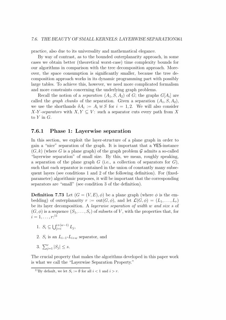
7.6. THE BEAUTY OF SMALL KERNELS: LAYERWISE SEPARATION361
practice, also due to its universality and mathematical elegance.By way of contrast, as to the bounded outerplanarity approach, in some
cases we obtain better (theoretical worst-case) time complexity bounds forour algorithms in comparison with the tree decomposition approach. More-over, the space consumption is significantly smaller, because the tree de-composition approach works in its dynamic programming part with possiblylarge tables. To achieve this, however, we need more complicated formalismand more constraints concerning the underlying graph problems.
Recall the notion of a separation (A1, S, A2) of G; the graphs G[Ai] arecalled the graph chunks of the separation. Given a separation (A1, S, A2),we use the shorthands δAi := Ai ] S for i = 1, 2. We will also considerX-Y -separators with X, Y ⊆ V : such a separator cuts every path from Xto Y in G.
7.6.1 Phase 1: Layerwise separation
In this section, we exploit the layer-structure of a plane graph in order togain a “nice” separation of the graph. It is important that a YES-instance(G, k) (where G is a plane graph) of the graph problem G admits a so-called“layerwise separation” of small size. By this, we mean, roughly speaking,a separation of the plane graph G (i.e., a collection of separators for G),such that each separator is contained in the union of constantly many subse-quent layers (see conditions 1 and 2 of the following definition). For (fixed-parameter) algorithmic purposes, it will be important that the correspondingseparators are “small” (see condition 3 of the definition).
Definition 7.73 Let (G = (V,E), φ) be a plane graph (where φ is the em-bedding) of outerplanarity r := out(G, φ), and let L(G, φ) = (L1, . . . , Lr)be its layer decomposition. A layerwise separation of width w and size s of(G, φ) is a sequence (S1, . . . , Sr) of subsets of V , with the properties that, fori = 1, . . . , r:11
1. Si ⊆⋃i+(w−1)j=i Lj,
2. Si is an Li−1-Li+w separator, and
3.∑r
j=1 |Sj| ≤ s.
The crucial property that makes the algorithms developed in this paper workis what we call the “Layerwise Separation Property.”
11By default, we let Si := ∅ for all i < 1 and i > r.

362 CHAPTER 7. GRAPH PARAMETERS
Definition 7.74 A parameterized problem G for planar graphs is said tohave the Layerwise Separation Property (abbreviated by: LSP) of separationwidth w and size-factor d if for each (G, k) ∈ G and every planar embedding φof G, the plane graph (G, φ) admits a layerwise separation of width w andsize dk.
How can layerwise separations be obtained?
The LSP can be shown directly for many parameterized graph problems.
Example 7.75 1. Consider planar vertex cover. Here, we get con-stants w = 2 and d = 2. In fact, for (G, k) ∈ vertex cover (andany planar embedding φ of G) with a “witnessing” vertex cover V ′ ofsize k, the sets Si := (Li∪Li+1)∩V ′ form a layerwise separation, giventhe layer decomposition L(G, φ) = (L1, . . . , Lr).
2. We have already seen how the non-trivial fact is proven that for planardominating set this property holds, yielding constants w = 3 andd = 51.
Fenau and Juedes ([179], also described below) have shown that all prob-lems describable by formulas from Planar T MIN 1 (as defined in [256]) sat-isfy LSP. This class includes planar red-blue dominating set, facecover, and planar edge dominating set.
A large class of parameterized graph problems for which the LSP holdsis given whenever there exists a reduction to a linear problem kernel.
Lemma 7.76 Let G be a parameterized problem for planar graphs that ad-mits a problem kernel of size dk. Then, the parameterized problem G ′ whereeach instance is replaced by its problem kernel has the LSP of width 1 andsize-factor d.
Proof. Let (G′, k′) ∈ G ′ with k′ ≤ dk be the problem kernel of (G, k) ∈ G,and let L(G′, φ′) = (L′
1, . . . , L′r′) be the layer decomposition of (G′, φ′) (where
φ′ is any embedding). Let r′ = out(G′, φ′). Observe that r′ ≤ dk3
since eachlayer has to consist of at least 3 vertices. Then, the sequence Si := L′
i fori = 1, . . . , r′ is a layerwise separation of width 1 and size dk of (G′, φ′).
Chap. 4 gives us therefore already a collection of problems that satisfyLSP. In particular, we have:
Example 7.77 1. planar vertex cover has the LSP of width 1 andsize-factor 2 (which is even better than what was shown in Exam-ple 7.75).

7.6. THE BEAUTY OF SMALL KERNELS: LAYERWISE SEPARATION363
2. planar independent set has the LSP of width 1 and size-factor 4on the set of reduced instances.
3. planar dominating sethas the LSP of width 1 and size-factor 67.Observe that these bounds are worse than the one mentioned in Exam-ple 7.75, since it is the size-factor that mainly influences the runningtime of our algorithms.
What are layerwise separations good for?
From a layerwise separation of small size (say bounded by O(k)), we areable to choose a set of separators such that their size is bounded by O(
√k)
and—at the same time—the subgraphs into which these separators cut theoriginal graph have outerplanarity bounded by O(
√k). In order to formalize
such a choice of separators from a layerwise separation, we give the followingdefinition.
Definition 7.78 Let (G = (V,E), φ) be a plane graph with layer decompo-sition L(G, φ) = (L1, . . . , Lr). A partial layerwise separation of width w is asequence S = (S1, . . . , Sq) such that there exist i0 = 1 < i1 < . . . < iq < r =iq+1 such that for i = 1, . . . , q:12
1. Sj ⊆⋃ij+(w−1)`=ij
L`,
2. ij + w ≤ ij+1 (so, the sets in S are pairwise disjoint) and
3. Sj is a Lij−1-Lij+w separator.
The sequence CS = (G0, . . . , Gq) with
Gj := G[(
ij+1+(w−1)⋃
`=ij
L`) − (Sj ∪ Sj+1)], j = 0, . . . , q,
is called the sequence of graph chunks obtained by S.
With this definition at hand, we can state the key result needed to establishthe algorithms that will be presented in Section 7.6.2. The proof techniquesapplied show some similarity to Baker [32].
Proposition 7.79 Let (G = (V,E), φ) be a plane graph that admits a lay-erwise separation of width w and size dk. Then, for every ψ ∈ R≥0, thereexists a partial layerwise separation S(ψ) of width w such that
1.∑
S∈S(ψ) |S| ≤ ψ√dk and13
12Again, by default, we set Si := ∅ for i < 1 and i > q.13Taking
∑instead of max here is a proposal of Kanj and Perkovic, compare [15, 252].

364 CHAPTER 7. GRAPH PARAMETERS
2. out(H) ≤√dkψ
+ w for each graph chunk H in CS(ψ).
Moreover, there is an algorithm with running time O(√kn) which, for a
given ψ,
• recognizes whether (G, φ) admits a layerwise separation of width w andsize dk and, if so, computes S(ψ);
• computes a partial layerwise separation of width w that fulfills the con-ditions above.
Proof. For m = 1, . . . , w, consider the integer sequences Im = (m +
jw)br/wc−1j=0 and the corresponding sequences of separators Sm = (Si)i∈Im.
Note that each Sm is a sequence of pairwise disjoint separators. Since(S1, . . . , Sr) is a layerwise separation of size dk, this implies that there existsa 1 ≤ m′ ≤ w with ∑
i∈Im′
|Si| ≤dk
w. (7.4)
For a given ψ, let s := ψ√dk. Define S(ψ) to be the subsequence of Sm′ such
that |S| ≤ s for all S ∈ S(ψ), and |S| > s for all S ∈ Sm′ −S(ψ). This yieldscondition 1. As to condition 2, suppose that S(ψ) = (Si1 , . . . , Siq). Howmany layers are two separators Sij and Sij+1
apart? Herefore, note that thenumber of separators in Sm′ that appear between Sij and Sij+1
is (ij+1−ij)/w.Since all of these separators have size greater than s, their number has to bebounded by dk/ws, see Equation (7.4). Therefore, we get ij+1 − ij ≤
√dk/ψ
for all j = 1, . . . , q − 1. Hence, the chunks G[(⋃ij+1+w−1`=ij
L`) − (Sij ∪ Sij+1)]
have outerplanarity at most√dk/ψ + w.
The algorithm that computes a partial layerwise separation S proceedsas follows: For given ψ, compute s := ψ
√dk. Then, for j = 1, . . . , r − w,
one checks whether the graph Gj(vs, vt) admits a vs-vt–separator Sj of size at
most s. Here, Gj(vs, vt) is the graph G[⋃j+(w−1)`=j L`] with two further vertices
vs and vt and edges from vs to all vertices in Lj and from vt to all vertices inLj+w−1. The separator Sj can be computed in time O(s ·n) using techniquesbased on maximum flow (see [250] for details).
Let S = (S1, . . . , Sq) be the sequence of all separators of size at most s
found in this manner.14 Suppose that Sj ⊆ ⋃ij+(w−1)`=ij
L` for some indices1 ≤ i1 < . . . < iq ≤ r. Note that, by the arguments given above, no two
14Possibly, the separators Sj in S found by the algorithm may differ from the separatorsin S(ψ).
7.6. THE BEAUTY OF SMALL KERNELS: LAYERWISE SEPARATION365
such separators can be more than√dk/ψ layers apart. Hence, if there was
a j0 such that ij0+1 − ij0 >√dk/ψ, the algorithms exits and returns “no.”
Otherwise, S is a partial layerwise separation of width w.
In what follows, the positive real number ψ of Proposition 7.79 is alsocalled trade-off parameter. This is because it allows us to optimize the trade-off between outerplanarity and separator size.
Proposition 7.79 will help construct a tree decomposition of treewidthtw(G) = O(
√k), assuming that a layerwise separation of some constant
width and size dk exists. Hence, for graph problems fulfilling this assump-tion and, moreover, allowing a σtw(G)n time algorithm for constant σ whenthe graph is given together with a tree decomposition, we obtain a solvingalgorithm with running time c
√kn. This aspect will be outlined in Subsec-
tion 7.6.2.
7.6.2 Phase 2:
Algorithms on layerwisely separated graphs
After Phase 1, we are left with a set of disjoint (layerwise) separators of sizeO(
√k) separating the graph in components, each of which having outerpla-
narity bounded by O(√k). We now present two different ways how to obtain,
in a second phase, a c√k-algorithm that makes use of this separation. In both
cases, there is the trade-off parameter ψ from Proposition 7.79 that can beused to optimize the running time of the resulting algorithms.
Using tree decompositions
We use the concept of tree decompositions as described above. We show howthe existence of a layerwise separation of small size helps to constructivelyobtain a tree decomposition of small width.
Theorem 7.80 Let (G, φ) be a plane graph that admits a layerwise separa-tion of width w and size dk. Then, we have tw(G) ≤ 2
√3dk + (3w − 1).
Such a tree decomposition can be computed in time O(k3/2n).
Proof. By Proposition 7.79, for each ψ ∈ R≥0, there exists a partiallayerwise separation S(ψ) = (S1, . . . , Sq) of width w with corresponding
graph chunks CS(ψ) = (G0, . . . , Gq), such that∑
S∈S(ψ) |S| ≤ ψ√dk and
out(Gi) ≤√dkψ
+ w for all i = 0, . . . , q. The algorithm that constructs atree decomposition Xψ is given as follows:
• Construct a tree decomposition Xi of width at most 3 out(Gi) − 1 foreach of the graphs Gi (using the algorithm from Theorem 7.23).

366 CHAPTER 7. GRAPH PARAMETERS
• Add Si and Si+1 to every bag in Xi (i = 0, . . . , q).
• Let Ti be the tree of Xi. Then, successively add an arbitrary connectionbetween the trees Ti and Ti+1 in order to obtain a tree T .
Using Proposition 7.35, we see that the tree T , together with the constructedbags, gives a tree decomposition of G. Clearly, its width tw(Xψ) is upper-bounded by
tw(Xψ) ≤∑
S∈S(ψ)
|S| + maxi=0,...,q
tw(Gi)
≤∑
S∈S(ψ)
|S| + 3( maxi=0,...,q
out(Gi)) − 1
≤ (ψ + 3/ψ)√dk + (3w − 1).
This upper bound is minimized for ψ =√
3.
By [20, Proposition 4.5], a graph G that has no Kh-minor has treewidthbounded by h3/2
√n. In particular, this implies that a planar graph has
treewidth bounded by 11.2√n. In the case of the existence of linear problem
kernels for a given graph problem G, this method might be used in orderto obtain c
√k-algorithms. From our results, we can derive upper bounds of
the treewidth of a planar graph in terms of several graph specific numbers.As the reader may verify, these problem-specific treewidth bounds tend tooutperform the numbers obtainable via [20, Proposition 4.5]. For example,Theorem 7.80 and Example 7.75 imply the following inequalities for a planargraph G, relating the treewidth with the vertex cover and dominating setnumber:
tw(G) ≤ 2√
6 vc(G) + 5, and
tw(G) ≤ 6√
17 ds(G) + 8.
Note that for general graphs, no relation of the form
tw(G) ≤ f(ds(G)) (7.5)
(for any function f) holds; consider, e.g., the clique Kn with n vertices, wheretw(Kn) = n − 1, but ds(Kn) = 1. Fomin and Thilikos have recently shown[191] that Eq. (7.5) holds for a graph G iff G has bounded local treewidth.For VC, only the linear relation
tw(G) ≤ vc(G)
7.6. THE BEAUTY OF SMALL KERNELS: LAYERWISE SEPARATION367
can be easily shown: Note that the complement of a vertex cover set Cforms an independent set I in G. Hence, we can easily construct even apath decomposition by choosing |I| bags and making each bag consist ofall vertices of C and exactly one element from I each time. This estimateis sharp (which becomes clear by, again, considering the graph Kn, wherevc(Kn) = n− 1).
Theorem 7.80 yields a c√k-algorithm for certain graph problems:
Theorem 7.81 Let G be a parameterized problem for planar graphs. Supposethat
1. G has the LSP of width w and size-factor d, and
2. there exists a time σ`n algorithm that decides (G, k) ∈ G, if G is giventogether with a tree decomposition of width `.
Then, there is an algorithm to decide (G, k) ∈ G in time O(σ3w−1·2θ1(σ,d)√kn),
where θ1(σ, d) = 2(log σ)√
3d.
Proof. Given an instance (G, k), in linear time we can compute someplanar embedding φ of G (for details see [94]). In time O(
√kn) (see Propo-
sition 7.79), we can check whether the plane graph (G, φ) admits a layerwiseseparation of width w and size dk.
If so, the algorithm of Theorem 7.80 computes a tree decomposition ofwidth at most 2
√3dk+ (3w− 1), and we can decide (G, k) ∈ G by using the
given tree decomposition algorithm in time O(σ2√
3dk+(3w−1)n).If (G, φ) does not admit such a layerwise separation, we know that (G, k) /∈
G, by definition of the LSP.
Example 7.82 Going back to our running examples, it is well-known thatvertex cover and independent setadmit such a tree decompositionbased algorithm with σ = 2 and, in the case of dominating set, withσ = 4, as detailed above.
1. For planar vertex cover, by Example 7.77.1 Theorem 7.81 guar-antees an O(22
√6kn) algorithm for this problem.
2. For planar independent set, Example 7.77.2 and Theorem 7.81yield an O(24
√3kn) algorithm.
3. By Example 7.75.2, Theorem 7.81 improves on the result from [8] (that
are reproduced above; there, we got an O(46√
34kn) ≈ O(269.98√kn)
algorithm), namely, getting an O(46√
17kn) ≈ O(249.48√kn) algorithm
for planar dominating set.
368 CHAPTER 7. GRAPH PARAMETERS
In this subsection, we have seen that, for plane graphs, the notion ofthe LSP gives us a sufficient condition to upperbound the treewidth of theYES-instance graphs of a problem. Moreover, this property led to fast com-putations of the corresponding tree decompositions. All in all, we came upwith algorithms of running time O(c
√kn) for a wide class of problems.
The next subsection aims to show similar results in a different context.
Using bounded outerplanarity
We now turn our attention to certain parameterized graph problems for whichwe know that a solving algorithm of linear running time on the class ofgraphs of bounded outerplanarity exists. This issue was addressed in [32];several examples can be found therein. In this subsection, examine how, inthis context, the notion of select&verify problems and the LSP will lead toc√k-algorithms. Since this will be a purely separator-based approach, we
will restrict ourselves to parameterized graph problems that can be solvedeasily on separated graphs. We will introduce the notion of weakly glueableselect&verify problems in a first paragraph and present the design of c
√k-
algorithms for these problems afterwards (see Paragraph 7.6.2).
Weakly glueable graph problemsThe notion of weak glueability that is introduced here is much related tothe notion of glueability we introduced in the previous section. We need onemore auxiliary notion for colorings.
Definition 7.83 For two 0-1-colorings χ1, χ2 : V → 0, 1,#with χ−11 (0, 1)∩
χ−12 (0, 1) = ∅, the sum χ1 + χ2 is defined by
(χ1 + χ2)(v) =
χ1(v) if χ1(v) 6= #,χ2(v) if χ2(v) 6= #,# otherwise.
Definition 7.84 A select&verify problem G given by (P·, opt) is weakly glue-able with λ colors if there exist
• a color set C := C0 + C1 + # with |C0 + C1| = λ, and
• a polynomial time computable function h : (R≥0 ∪ ±∞)3 → R≥0 ∪±∞;
and, for every n-vertex graph G = (V,E) and subgraphs G sel, Gver ⊆ G witha separation (A1, S, A2) of Gver, we find, for each coloring χint : S → C0]C1,

7.6. THE BEAUTY OF SMALL KERNELS: LAYERWISE SEPARATION369
• subgraphs G(Ai, χint) of Gver with Gver[Ai] ⊆ G(Ai, χ
int) ⊆ Gver[δAi]for i = 1, 2,
• subgraphs G(S, χint) of Gver with G(S, χint) ⊆ Gver[S]
such that, for each 0-1-coloring χext : V → 0, 1,# with χext |S≡ #, wehave
opt~x∈0,1n
~x∼χextPGver(~x | G sel) (7.6)
= optχint:S→C0]C1h(EvalA1(χ
int),EvalS(χint),EvalA2(χ
int)).
Here, EvalX(·) for X ∈ A1, S, A2 is of the form
EvalX(χint) = opt ~x∈0,1n
~x∼(χext+ˆ
χint)
PG(X,χint)(~x | G[X] ∩G sel).
Example 7.85 We give some examples of weakly glueable problems, where—for the time being—we restrict ourselves to the case where Gver = G sel =G. The subtlety of allowing different subgraphs Gver, G sel in the definitionabove is due to technical reasons that become clear later. All examplesgeneralize in a straight-forward way to this case.
1. vertex cover is weakly glueable with λ = 2 colors. We use the colorsets Ci := i for i = 0, 1. The function h is h(x, y, z) = x+ y+ z. Thesubgraphs G(X,χint) for X ∈ A1, S, A2 and χint : S → C0 ] C1 are
G(Ai, χint) := G[Ai ∪ χint−1
(0)] for i = 1, 2, and
G(S, χint) := G[S].
The subroutine EvalS(χint) checks if the coloring χint yields a vertex
cover on G[S] and the subroutines EvalAi(χint) compute the minimum
size vertex cover on G[Ai] under the constraint that all neighbors in
Ai of a vertex in χint−1(0) are covered. Obviously, Eq. (7.6) is thus
satisfied.
2. Similarly, independent set is weakly glueable with 2 colors.
3. dominating set is weakly glueable with λ = 4 colors, using C0 :=0A1, 0A2, 0S and C1 := 1. The semantics of these colors is as follows.Assigning the color 0X , for X ∈ A1, S, A2, to vertices in a separation(A1, S, A2) means that the vertex is not in the dominating set and willbe dominated by a vertex from X. Color 1 means that the vertex

370 CHAPTER 7. GRAPH PARAMETERS
belongs to the dominating set. We set h(x, y, z) = x + y + z. For agiven coloring χint : S → C0 ] C1, we define
G(Ai, χint) := G[Ai ∪ χint−1
(1, 0Ai)]
G(S, χint) := G[χint−1(1, 0S)].
In this way, color information is passed to the subproblems. EvalS(χint)
checks whether the assignments of the color 0S are correct (i.e., whetherall vertices assigned 0S are dominated by a vertex from S). Also,EvalAi
returns the size of a minimum dominating set in Ai under theconstraint that some vertices in δAi still need to be dominated (namely,
the vertices in χint−1(0Ai
)) and some vertices in δAi can already be
assumed to be in the dominating set (namely, the vertices in χint−1(1)).
With these settings, Eq. (7.6) is satisfied.
We want to mention in passing that—besides the problems given here—manymore select&verify problems are weakly glueable. In particular this is truefor the weighted versions and variations of the above mentioned problems.
The algorithm
Similar to Theorem 7.81, which is based on tree decompositions, we constructa partial layerwise separation S(ψ) with optimally adapted trade-off param-eter ψ to guarantee an efficient dynamic programming algorithm. However,for our purposes here, we need to be able to deal with “precolored” graphs.
Definition 7.86 Let G be a select&verify graph problem defined by (P·, opt).The problem constraint G then is to determine, for an n-vertex graph G =(V,E), two subgraphs G sel, Gver ⊆ G, and a given 0-1-coloring χ : V →0, 1,#, the value
opt~x∈0,1n
~x∼χ
PGver(~x | G sel).
Theorem 7.87 Let G be a select&verify problem for planar graphs. Supposethat
1. G has the LSP of width w and size-factor d,
2. G is weakly glueable with λ colors, and
3. there exists an algorithm that solves the problem constraint G for agiven graph G in time τ out(G)n.
Then, there is an algorithm to decide (G, k) ∈ G in time O(τw · 2θ2(λ,τ,d)√kn),
where θ2(λ, τ, d) = 2√d log(λ) log(τ).

7.6. THE BEAUTY OF SMALL KERNELS: LAYERWISE SEPARATION371
! #" "
$%&('*) ',+-/.*02143 ! 65
$%7&8'9)':+;-/.902143 <=5
"
> <
Figure 7.17: Dynamic programming on layerwisely separated graph.
Proof. Let us first sketch the overall structure of the algorithm.
1. Compute some planar embedding φ of G, and find a “suitable” partiallayerwise separation (S1, . . . , Sq) for the plane graph (G, φ). A coarsesketch of the such obtained graph structure is depicted in Figure 7.17.
2. By using dynamic programming techniques, an optimal solution isfound by sweeping over the graph from left to right, as illustrated inFigure 7.17. More detailed, we do the following:
(a) For all possible “colorings” of S1, find an optimal solution of con-straint G on G0 (plus suitably chosen precolored vertices fromS1); store the obtained optima in a (large) table belonging to S1.
(b) For j := 2 to q do:
• For all possible “colorings” of Sj−1 and of Sj, find an opti-mal solution of constraint G on Gj−1 (plus suitably chosenprecolored vertices from Sj−1 as well as of Sj).
• Store the obtained optima (for the subgraph ofG with verticesfrom G0 through Gj−1 and S1 through Sj) in a table belongingto Sj.
• (For reasons of space efficiency, you might now forget aboutthe table belonging to Sj−1.)
(c) For all possible “colorings” of Sq, find an optimal solution of con-straint G on Gq (plus suitably chosen precolored vertices fromSq); store the obtained optima in a (large) table belonging to Sq.
(d) From the table pertaining to Sq, the desired optimum is found.

372 CHAPTER 7. GRAPH PARAMETERS
We are now giving formal details of the sketched algorithms, thereby provingits correctness. Suppose G is defined by (P·, opt).
Step 1: Given an instance (G, k), in linear time we can compute some planarembedding φ of G (see [94]). Compute a partial layerwise separation S(ψ)(ψ will be determined later) for (G, φ), using Proposition 7.79 and the as-sumption 1 (LSP). Suppose S(ψ) = (S1, . . . , Sq) and let CS(ψ) = (G0, . . . , Gq)denote the corresponding graph-chunks cut out by S(ψ).
For every separator Si, we get a separation of the form
(A(i)out, Si, A
(i)in ),
where A(i)out, and A
(i)in , respectively, are the vertices of the graph chunks of
lower order layers, and higher order layers, respectively. By default, welet S0 = Sq+1 = ∅ such that the corresponding separations are (∅, S0, V )and (V, Sq+1, ∅), respectively. The layerwise separation and the separations
(A(i)out, Si, A
(i)in ) are illustrated in Figure 7.17.
Step 2: Determine the value
opt~x∈0,1n PG(~x).
This can be done by a dynamic programming approach that makes use ofthe weak glueability of G as follows.
We successively compute, for i = 1, . . . , q + 1, the values
M (i)(µ(i)) := opt~x∼dµ(i) PHver
i (µ(i))(~x | H seli ) (7.7)
for all C0-C1-colorings µ(i) : Si → C0 + C1, where
Hveri (µ(i)) := G(A
(i)out, µ
(i)) and H seli := G[A
(i)out].
Note that we have
opt~x∈0,1n PG(~x) = M (q+1)(µ),
for the empty map µ : Sq+1 = ∅ → C0 + C1, because H selq+1 = G[A
(q+1)out ] =
G[V ] = G and Hverq+1(µ) = G (since H sel
q+1 ⊆ Hverq+1(µ)).
The computation of M (i)(µ(i)) as defined in (7.7) can be done iteratively.To do so, note that Hver
i (µ(i)) is separated by Si−1 in
(B(i−1)out , Si−1, B
(i−1)in ),

7.6. THE BEAUTY OF SMALL KERNELS: LAYERWISE SEPARATION373
where B(i−1)out = A
(i−1)out and B
(i−1)in = A
(i−1)in ∩ V (Hver
i (µ(i))). Hence, by defini-tion of weak glueability we have
M (i)(µ(i)) = optµ(i−1):Si−1→C0+C1
h(EvalB
(i−1)out
(µ(i−1)),EvalSi−1(µ(i−1)),Eval
B(i−1)in
(µ(i−1))),(7.8)
where
EvalX(µ(i−1)) = opt~x∼(µ(i−1)+dµ(i))
PG(X,µ(i−1))(~x | G[X] ∩H seli ). (7.9)
for X ∈ B(i−1)out , Si−1, B
(i−1)in . Here, recall that µ(i) denotes the 0-1-coloring
corresponding to µ(i). In particular, for the different choices of X, we get thefollowing.
• For X = B(i−1)out , equation (7.9) becomes
EvalB
(i−1)out
(µ(i−1)) = opt~x∼(µ(i−1)+dµ(i))
PHveri−1(µ(i−1))(~x | H sel
i−1 ∩H seli )
= M (i−1)(µ(i−1)), (7.10)
where the last equation holds, since H seli−1 ⊆ H sel
i and since µ(i) ≡ #
restricted to G(B(i−1)out , µ(i−1)) = Hver
i−1(µ(i−1)).
Hence, the value of EvalB
(i−1)out
(µ(i−1)) is given by the previous step of
the iteration.
• For X = Si−1, equation (7.9) becomes
EvalSi−1(µ(i−1)) = opt
~x∼µ(i−1)PG(Si−1,µ(i−1))(~x | G[Si−1])
= PG(Si−1,µ(i−1))(~xµ(i−1)| G[Si−1]), , (7.11)
where ~xµ(i−1)
∈ 0, 1n is an arbitrary vector such that ~xµ(i−1)
∼ µ(i−1).
The first equation above holds, since G(Si−1, µ(i−1)) ⊆ G[Si−1] ⊆ H sel
i
and µ(i) ≡ # restricted to G(Si−1, µ(i−1)). The second equation is true
since the 0-1-coloring µ(i−1) assigns color 0 or color 1 to all vertices inSi−1, and since G(Si−1, µ
(i−1)) ⊆ G[Si−1].
Hence, the value EvalSi−1(µ(i−1)) can be computed by a simple evalua-
tion of the function P for the given vector ~xµ(i−1)
.
• For X = B(i−1)in , equation (7.9) becomes
EvalB
(i−1)in
(µ(i−1)) = opt~x∼(µ(i−1)+dµ(i))
PG(B
(i−1)in ,µ(i−1))
(~x | G[B(i−1)in ] ∩H sel
i )
= opt~x∼(µ(i−1)+dµ(i))
PG(µ(i),µ(i−1))(~x | Gi−1), (7.12)

374 CHAPTER 7. GRAPH PARAMETERS
!" !#$%
Figure 7.18: The graph G(µ(i), µ(i−1)).
where G(µ(i), µ(i−1)) := G(A(i−1)in , µ(i−1)) ∩ G(A
(i)out, µ
(i)). This graphis illustrated in Figure 7.18. In the evaluation above we used thatG[B
(i−1)in ] ∩H sel
i = Gi−1 and that G(B(i−1)in , µ(i−1)) = G(µ(i), µ(i−1)).
Hence, the value EvalB
(i−1)in
(µ(i−1)) can be computed using the τ out(G)
time algorithm for constraint G.
Hence, plugging formulas (7.10), (7.11), and (7.12) in expression (7.8), weobtain
M (i)(µ(i)) = optµ(i−1):Si−1→C0+C1h
M (i−1)(µ(i−1))PG(Si−1,µ(i−1))(~xµ(i−1)
| G[Si−1])
opt~x∼
µ(i−1)+dµ(i)PG(µ(i),µ(i−1))(~x | Gi−1)
.
(7.13)This evaluation is done successively for all i = 1, . . . , q+1. By induction,
one sees thatopt~x∈0,1n PG(~x) = M (q+1)(µ)
can be computed in this way.
Computation time: For fixed coloring µ(i), computing M (i)(µ(i)) accordingto equation (7.13) costs time
λ|Si−1| · τ out(G[Si−1∪VGi−1∪Si]).
The first factor reflects the cost of computing the opt over all µ(i−1) : Si−1 →C0+C1. The second factor arises by the evaluations on the graphsG(Si−1, µ
(i−1)),G(µ(i−1), µ(i)) ⊆ G[Si−1 ∪ V (Gi−1) ∪ Si], where we use assumption 3 of thetheorem. Thus, the running time for evaluating M (i)(µ(i)) for all µ(i) : Si →C0 + C1 is bounded by
λ|Si| · λ|Si−1| · τ out(G[Si−1∪VGi−1∪Si]).

7.6. THE BEAUTY OF SMALL KERNELS: LAYERWISE SEPARATION375
Hence, the total running time of the algorithm is bounded by 2θ(ψ)n, where
θ(ψ) ≤ log(λ)∑
i=1,...,q
|Si| + log(τ) maxi=0,...,q
out(G[Si ∪ VGi∪ Si+1])
≤ log(λ)ψ√dk + log(τ)(
√dk
ψ+ w)
= (log(λ)ψ +log τ
ψ)√dk + log(τ)w
This upper bound is minimized for ψ =√
log(τ)/ log(λ), which gives us the
claimed value θ2(λ, τ, d) = 2√d log(λ) log(τ) and the constant τw.
It remains to say for which problems there exists a solving algorithm ofthe problem constraint G for a given graph G in time τ out(G)n.
In the case of planar vertex cover, as well as in the case of planarindependent set, it is quite simple to handle a “precoloring” χext : V →0, 1,# for a graph G = (V,E).
More formally, given an admissible15 coloring χext, one likes to transforman instance (G, k) to an instance (G′, k′), such that (G, k) ∈ G for somewitnessing vector ~x with ~x ∼ χext iff (G′, k′) ∈ G for some witnessing vector~x′ (without any constraint).
For planar vertex cover, this can, e.g., be achieved by the followingtransformation:
G′ = G[V − (C ∪N(χext−1(0)))] and
k′ = k − |χext−1(1)| − |v ∈ V − C | ∃u ∈ χext−1
(0) ∩N(v)|,
here C := χext−1(0, 1) denotes the vertices that are already assigned a
color. A vertex v ∈ C, which is—by the coloring χext— assigned not to be inthe vertex cover, i.e., χext(v) = 0, forces its neighbors to be in a vertex cover.Hence, the set N(χext−1
(0)) needs to be in any vertex cover (given by ~x)that fulfills the constraint ~x ∼ χext. This justifies the definition of G′. Theparameter k becomes smaller by the number of vertices which are alreadyassigned to be in the vertex cover, i.e., χext−1
(1), and the number of verticesthat are forced to be in the vertex cover by χext, i.e., by the number of verticesin V −C that have a neighbor in χext−1
(0). We can apply the non-constraintalgorithm to (G′, k′), with out(G′) ≤ out(G). A similar observation helpsdeal with planar independent set.
15Here, admissible means that there exists a vector ~x ∈ 0, 1n with ~x ∼ χext, such thatP ver
G (~x) = 0.

376 CHAPTER 7. GRAPH PARAMETERS
Example 7.88 1. For planar vertex cover, we have d = 2, w = 1(see Example 7.77.1), λ = 2 (see Example 7.85.1), and τ = 8 (see theresult of Baker [32] which can be adapted to the constraint case by theconsiderations above) and, hence, the approach in Theorem 7.87 yields
an O(22√
6kn) time algorithm.
2. Similarly, Examples 7.77.2, and 7.85.2 give d = 4, w = 1 and λ = 2 forplanar independent set. Since τ = 8 (see [32] and our considera-
tions for the constraint case), we obtain a O(24√
3kn) time algorithm.
3. Kanj and Perkovic have recently shown [253] that constraint domi-nating set can be solved in O(27out(G)n) time, this way improving onExample 7.82. Together with Example 7.75.1, Theorem 7.87 gives anO(36
√17kn) ≈ O(239.21
√kn) time algorithm for planar dominating
set.
Which of the two approaches (presented in Subsections 7.6.2 and 7.6.2,respectively) for the algorithms on layerwisely separated graphs should bepreferred? This question is discussed in details in [15]. The bottom-lineis that it mainly depends whether there are particular outerplanarity-basedalgorithms that are superior to the treewidth-based algorithms (when usingthe r ≤ 3k bound described above that relates a graph of outerplanarity rwith its treewidth k).
7.6.3 The approach of Fomin and Thilikos
In a very deep paper, Fomin and Thilikos [190] (see [193] for the reportversion) were able to prove the following result:
Theorem 7.89 Every planar n-vertex graph has treewidth at most 3.182√n.
The drawback of that approach is currently that the way how to actuallyobtain a tree decomposition for a planar graph with n vertices is not veryclear from [190], so that it is not that easy to implement.
However, observe that also the approach we detailed above (using treewidthinstead of branchwidth), yields a result analogous to Thm. 7.89, althoughwith somewhat weaker constants. More precisely, Theorem 7.80 can be used,since we can basically set k = n and d = w = 1. With this observation,we obtain a bound of 2
√3n ≤ 3.4642
√n on the treewidth for any planar
n-vertex graph.Theorem 7.89 immediately entails O∗(c
√k)-algorithms for many planar
problems where we know of linear problem kernels. For example, we would

7.7. FURTHER IMPROVEMENTS FOR PLANAR DOMINATING SET377
get an O(22·3.182√
67k) = O∗(252.092√k)-algorithm for planar dominating
set.
7.7 Further improvements for planar domi-
nating set
First of all, let us summarize the preprocessing observations that we havemade up to this point on planar dominating set in Alg. 67. This algo-rithm prelude can be performed in linear time.
Algorithm 67 Algorithmic Prelude
Input(s): A plane graph G and parameter k ∈ N.
Compute the ring decomposition FG.Compute a minimum dominating set D of FG (see Lemma 7.30).if |D| > k then
return NO
elsecontinue
end if
As it is well-known, given some planar graph G, we could also build anembedding of G in the plane in linear time. The planar embedding algorithmcould also be included as part of the prelude, if necessary.
After executing the prelude, algorithms for planar dominating setproceed as follows. If G has a dominating set of size k, then Proposition 7.27tells us that G is ≤ 3k outerplanar. So, assume that G is ≤ 3k outerplanar.
In the following, we will show how to obtain a sequence S—called alayerwise separator—of “small” separators S3, . . . , Sr−2, where Si containsvertices from Li−1, Li and Li+1 that separate layer Li−1 from Li+2, such that
‖ S ‖= |S3| + · · · + |Sr−2| ≤ h(k)
for some linear-bounded function h. This was also the basic trick in whatwe explained when referring to [8]. Once we have such a “small” layerwiseseparator we can essentially split G into disconnected components, each ofwhich is O(
√k)-outerplanar.
Notice that it must be the case that one of the families
Fi =⋃
j=i mod 3,3≤j≤r−2
Sj,

378 CHAPTER 7. GRAPH PARAMETERS
i = 1, 2, 3 satisfies |Fi| ≤ h(k)/3. Without loss of generality, assume that|F1| ≤ h(k)/3. Now, F1 can be partitioned into g(k) mutually disjoint sub-families
Fm1 =
⋃
ji=1+m+ig(k)
Sji,
m = 0, . . . , g(k) − 1, i = 0, . . . , br/g(k)c. At least one Fm1 satisfies |Fm
1 | ≤h(k)/(3g(k)). Notice that the separator Sm = Fm
1 splits the graph intocomponents that are at most 3g(k) + 3 outerplanar.
As detailed above, to find the minimum dominating set in G, it suffices tosearch through all possible three possible domination choices for each vertexv in the partial layerwise separator Sm = (Sj0 , . . . , Sjq). Schematically, wecan think of the “rest” of the vertices of G being “inbetween” some Sji andSji+1
. The possible domination choices are “v is in the dominating set,” “v isdominated by component to the left,” or “v is dominated by a vertex u ∈ Smor a component to the right.” Since |Sm| ≤ h(k)/3g(k), there are 3h(k)/3g(k)
possible domination choices for Sm. Using a setting of domination choices forSm, it is possible to split the graph into ≤ 3g(k)+5-outerplanar componentsthat are precolored with the colors free, already dominated, not dominated.(These components may contain contain vertices from Sm.) Making use ofTheorem 7.23, we can solve the “precolored” planar dominating setproblem on the remaining graph components in time O(49g(k)) time. Kanjand Perkovic [253] described a dynamic programming algorithm for precol-ored planar dominating set on r-outerplanar graphs running in timeO(27r). This allows us to compute the size of the minimum dominating setin time O(39g(k)) for each precolored component. Using the notation intro-duced so far, we arrive at the following result.
Lemma 7.90 planar dominating set can be solved in time
O(h(k)/g(k)3h(k)/(3g(k))+9g(k) + n3),
where k upperbounds the number of vertices in the dominating set.
More details are described in Algorithm 68.
Since h(k), as determined in the next section, will be bounded by dk forsome d, g(k) would then be best chosen as c
√k such that dk/(3c
√k) = 9c
√k,
i.e., c =√d/(3
√3), because 3dk/(3c
√k) is the asymptotics of the time spent to
test all possible separator settings, and 33∗3c√k is the time to solve the prob-
lem on the remaining graph chunks. Hence, 9c√k = 9
√dk/(3
√3) =
√3dk.
This gives us an O(√k32
√3dk + n3) = O(
√k22 log2(3)
√3dk + n3) algorithm.

7.7. FURTHER IMPROVEMENTS FOR PLANAR DOMINATING SET379
Algorithm 68 A Generic Subexponential Algorithm for Planar DS
Input(s): A plane graph G and a parameter k ∈ NOutput(s): YES iff G has a dominating set of size ≤ k
Perform Algorithm 67 and kernelization (see Chap. 4)Try to find a “small” partial layerwise separator Sm with |Sm| ≤h(k)/(3g(k)).if such a small separator cannot be found then
return NO
end iffor all 3h(k)/3g(k) settings of domination choices for the vertices in Sm do
for all precolored graph chunks of G doCompute a minimal dominating set for the precolored graph chunk
end forif minimum dominating set of G using this choice is ≤ k then
return YES
end ifend forreturn NO
For convenience, we list a table for different values of f(d) = 2 log2(3)√
3dkrounded up, which we use in the following sections.
d = 9 15 16 20 39 45 51f(d) = 16.48 21.27 21.97 24.56 34.29 36.84 39.21
These numbers correspond to the constant factor in the exponent of therunning times for different estimates of h(k). Observe that the last columncorresponds to the h(k)-bound worked out in [8], combined with the outer-planarity algorithm from [253].
To allow for some “geometric arguments” when tweaking the analysis ofbasically Alg. 68, we need to slightly adapt our earlier notions.
If C is an embedded cycle and x ∈ C some vertex, then we can speakabout the left and right neighbor of x on C, if we imagine ourselves to beplaced in the center of the cycle. Similarly, if y is some point outside ofC which is connected by edges to vertices x0, . . . , xm−1 (and no others)on C (in that order from left to right, when “standing” in the center of C,viewing in direction of y), then there uniquely exists some j such that theregion described by the edges y, xj, y, x(j+1) mod m and the left-to-rightpath from x(j+1) mod m to xj contains all edges from y to any xi on C. Wecall y, xj, x(j+1) mod m the upper triple associated to y and C (also in theboundary case when m = 0 and m = 1, when the triple will be y and

380 CHAPTER 7. GRAPH PARAMETERS
y, x0, respectively). Likewise, if y is a point in the interior of C and z isanother reference “point” within C, then there are points x, x′ on C adjacentto y such that all other vertices x′′ on C which are adjacent to y are on onlyone of the two sub-paths into which C is cut by x and x′, while z is containedin the other “half.” We will call y, x, x′ the lower triple associated to yand z.
As we will understand below, it is possible to restrict oneself to the con-sideration of simple r-outerplanar graphs.
Our aim is to obtain a set of vertices Si from layers Li−1, Li and Li+1 thatseparate the vertices of Li−1 from the vertices of Li+2. In a fashion similar to[8], we achieve this by deleting “upper”, “lower”, and also kind of “middle”triples of vertices in D ∩Bi and D ∩ Ji. Let bi = |D ∩Bi| and ji = |D ∩ Ji|.
Lemma 7.91 There exists a set Si that separates Li−1 from Li+2 of size|Si| ≤ 3bi−1 + 3ji + 3bi + 3ji+1 + 3bi+1.
This lemma is proven quite analogous to the reasoning we detailed above.Since
∑r−2i=3 |Si| ≤ 9k = h(k), for simple r-outerplanar graphs, we get an
216.4715√k-algorithm (which is of course much better than what we obtained
above). This is appears to be a lower bound on the running-time that wecan obtain by the current approach.
Let us try to transfer our reasoning to the general case. Recall the notionsB(i, j) introduced along the definition of a ring decomposition.
As a first preparatory step for layer Li, let us think about how muchit would “cost” to actually separate each B(i, j) from the other B(i, j ′) suchthat we can be sure that any (remaining) dominating set vertex on B(i, j) orin the interior of B(i, j) only dominates vertices on B(i, j) or in the interiorof B(i, j) or from Ji. Furthermore, “indirect” influences of different ringsby interconnection patterns will be ruled out. Moreover, this reasoning willimply that later on we can safely speak about dominating vertices “private”to B(i, j). The vertices “taken out” in this preparatory step will be put intothe separator we are going to construct.
For the general case, we will need to sufficiently separate the boundarycycles in each layer so that we can employ the previous arguments for simpler-outerplanar graphs. In particular, we say that a set S i properly separatesLi according to D if each x ∈ (D ∩ Li) \ Si dominates only vertices in oneB(i, j) \ Si for some 1 ≤ j ≤ ci. The following results are crucial to ourconstruction of Si.
Lemma 7.92 If x ∈ Li \B(i, j) and P1 and P2 are two paths leading from xto some points z1 and z2 on B(i, j), using only vertices from Ji on the way,then either z1 = z2 or z1 and z2 are neighbors.

7.7. FURTHER IMPROVEMENTS FOR PLANAR DOMINATING SET381
Lemma 7.93 It suffices to take out at most four vertices to separate twolinked rings of the same layer.
As we show next, we can construct such an S i by applying the previ-ous two lemmas, using only 4ci vertices. The proof and construction arecontained in the journal version of [179].
Lemma 7.94 There exists an Si with |Si| ≤ 4ci that properly separates Liaccording to any dominating D.
In the example of Fig. 7.8, we would have to take out v1, v4 and v8 toprevent B(v3) from influencing B(v10), and if we assume that there is an edgebetween v2 and v9, then these two vertices would be taken out.
We now describe a second preparatory step for layer Li, sketchedin the following lemma, which will simplify the “triple” arguments in whatfollows.
Lemma 7.95 Having performed the first preparatory step for layer Li, thereare at most 2ci vertices on Bi−1 ∪Bi whose removal leaves a graph such thatany path from any x ∈ Bi−1 down-to Bi must get to some ring B(i, j) specificto x, i.e., there is a partial mapping x 7→ j.
The proof of Lemma 7.95 is omitted here (we refer to the yet unpublishedjournal version of [179]); however, we give some intuition concerning theapproach. By removing Si from G, we partition Li into regions that canonly reach a single B(i, j). The planarity of G forces an ordering of theseregions w.r.t. Bi−1. Hence, it is possible to delete at most 2 shared fringevertices from Bi−1 per B(i, j) to force all paths starting at x ∈ Bi−1 to go toB(i, j).
We now assume that we have performed both preparatory steps for layersLi and Li+1. This way, we take out at most 6ci + 6ci+1 vertices.
After these preparatory steps, the graph will look “locally” like a simpler-outerplanar graph. Therefore, the analysis of that previously consideredcase basically transfers. Altogether, |Si| ≤ 3bi−1+3ji+3bi+3di+1+6ci+6ci+1.
Theorem 7.96 If G is a plane graph with a dominating set of size at mostk, then the overall sum of the sizes of the layerwise separators can be upper-bounded by h(k) = 9k + 12c(k), where c(k) upperbounds
∑ri=1 ci.
We can now adapt some trade-off computations of Kanj and Perkovic [252]that show that c(k) is negligibly small; in other words, the case of simple r-outerplanar graphs is the “dominating case.”

382 CHAPTER 7. GRAPH PARAMETERS
Kanj and Perkovic made the following observation: There is no need tocut off branches in T ′
G starting in a node n whose distance δ(n) to its farestdescendant is only δ(n) ≤ D(k) = O(
√k), since, in the worst case, only D(k)
layers would be added to each graph chunk.Using some simplified arguments, we show that their computations carry
over to our new analysis, as well. Actually, the above analysis was “tuned”in order to exploit their technique best possible.
For a given bounding function D, call a node n in T ′G deep, medium,
and shallow, respectively, if δ(n) > D(k), δ(n) = D(k), or δ(n) < D(k),respectively.
Let µ denote the number of medium nodes in T ′G. Any medium node n
contains D(k) layers in int(n) and therefore at least D(k)/3 vertices fromthe dominating set D. Given medium nodes n and n′ in TG (and hencerings in G), then int(n) ∩ int(n′) = ∅. If µ > 3k/D(k), then the number ofdominating set vertices in
⋃int(n) : n is medium would exceed k. Hence,µ ≤ 3k/D(k).
A node is called m-complex if it has at least m non-shallow children.Considering the number of inner nodes in m-ary trees with µ leaves, it isreadily seen that there are no more than b(µ− 1)/(m− 1)c many m-complexnodes. Denoting the number of non-shallow children of of n by c(n), itfollows that the sum of all c(n), taken over complex nodes, is no larger thanbm(µ− 1)/(m− 1)c.
In the following, let us specialize towards m = 2.16 Terming a non-2-complex node simple generalizes the earlier introduced terminology of simpler-outerplanar graphs. Our reasoning entails:
Lemma 7.97∑c(n) | n is complex ≤ 2µ ≤ 6k/D(k).
Let us now reconsider the considerations of the previous section underthe observation that we only try to separate deep nodes (rings). This leadsimmediately to our main theorem.
Theorem 7.98 The planar dominating set problem can be solved intime
O(√k36
√3k+o(
√k) + n3) ≈ O(
√k26 log2(3)
√3k + n3) ≈ O(216.4715
√k + n3).
Observe that similar improvements can be obtained for the other domination-type problems mentioned in [8]. More specifically, for planar independentdominating set, we get the same constants as stated in Theorem 7.98, sincethe treewidth- and outerplanarity-based algorithms have the same running
16In [252], the case m = 3 was considered instead.

7.8. PLANAR RED-BLUE DOMINATING SET AND RELATED PROBLEMS383
times. But, if we like to treat say the problem of finding a total dominatingset, i.e., a set D, |D| ≤ k, such that each vertex x is dominated by some othervertex y ∈ D, then the constants get worse, since the treewidth-based algo-rithm as outlined in [8] is worse, and similar changes have to be implementedin the outerplanarity-based algorithm of Kanj and Perkovic [253].
Moreover, our results also improve on the constants derived in [123] fordominating set on K3,3-minor-free or K5-minor-free graphs. Here, thefollowing theorem is important.
Theorem 7.99 If G is a planar graph which has a dominating set of size k,then G has treewidth of at most 6
√3k + o(
√k) = O(10.40
√k).
Observe that this largely improves the upperbound 6√
34k proved in [8]and also nearly matches the treewidth bound 9.55 ≈ (4.5)1.5 derived in [192]via completely different arguments.
Corollary 7.100 If the n-vertex graph G is K3,3-minor-free or K5-minor-
free, then in time O(49.55√kn) it can be determined if G has a dominating set
of size at most k or not.
Observe that the strategy outlined in the last two sections is not onlyapplicable to dominating set, but rather to any planar graph problem wherethe sum of the sizes of the layerwise separators can be estimated as a linearfunction in k and in the number of rings. For many problems, we can reallyrestrict our attention to the case of simple r-outerplanar graphs, since theestimates involving the number of rings and the optimization computationsdo not rely on the structure of the concrete problem in any way. We exemplifythis approach in the next section.
Let us briefly mention that also related problems can be solved as sketchedabove. Recall Roman domination for a moment. From Lemma 7.9 and thetreewidth bound of Fomin and Thilikos [193] we can immediately conclude:
Corollary 7.101 planar Roman domination can be solved in time
O∗(59.55√k) = O∗(222.165
√k).
7.8 planar red-blue dominating set and re-
lated problems
The techniques outlined in the previous sections apply to other problems onplanar graphs. For planar red-blue dominating set, it suffices to buildan appropriate separator Si to separate layers Li−1 from layer Li+3.

384 CHAPTER 7. GRAPH PARAMETERS
Lemma 7.102 There exists a separator Si that separates layer Li−1 fromlayer Li+3 in G of size
|Si| ≤ 3bi−1 + 3ji + 7bi + 4ji+1 + 5bi+1 + 5ji+2 + 5bi+2 + 6ci + 6ci+1 + 6ci+2.
Proof. (Sketch) Let us sketch how to prevent an “adversary path” fromlayer Li−1 to sneak through to layer Li+3 in this case. Observe that the “ge-ometrical arguments” used up to now basically transfer to this case, as well,while the “domination-type” arguments needs to be adapted. The construc-tion and more detailed proof can be found in the journal version of [179].
Our aim is again to construct a separator Si which contains the followingingredients, basically combining two “neighbored” separators as constructedin the usual dominating set problem:
1. Do the two “preparatory steps” for layers Li, Li+1 and Li+2. This totalsup to at most 6ci + 6ci+1 + 6ci+2 vertices going into Si.
2. Both on the rings of Li and of Li+1, remove all dominating set verticesand their two neighbors, putting at most 3bi + 3bi+1 vertices into Si.
3. For each d ∈ D ∩ (Bi−1 ∪ Ji), take out the “upper triples.” This addsanother at most 3bi−1 + 3ji vertices into Si.
4. For each d ∈ D ∩ Ji+1, take out the (at most) four vertices which cutoff the region R(d); namely, there are (according to Lemma 7.92 atmost two “connection points” of R(d) on Bi+1 and there are at mosttwo “outermost” connection points of R(d) on Bi (by the definition ofR(d) and due to previous surgery). This adds 4ji+1 vertices to Si.
5. For each d ∈ D ∩ Bi+1: if d has no neighbors in Ji but neighborson Bi, cut out the “lower triple” associated to this situation; if d hasa neighbor x in Ji, cutting out the “quadruple” as described in theprevious step is what we do. In each case, due to step 2, only at mosttwo vertices have to be removed additionally, giving another (at most)2bi+1 vertices into Si.
6. For each d ∈ D∩Bi: go “to the left” of d on Bi (and symmetrically, go“to the right”) looking for red vertices on Bi which share a blue vertexin Li+1 with d. Geometrically, this gives us a series of nested triangles.We take out the endpoints of the “largest” (on both sides). Due to step2, this adds at most 4bi vertices into Si.

7.8. PLANAR RED-BLUE DOMINATING SET AND RELATED PROBLEMS385
7. For each d ∈ D ∩ (Ji+2 ∪Bi+2), first remove the lower triple d, z1, z2associated to d and some (other) z on Bi+2. This lower triple describesa region enclosed by the edges d, z1 and d, z2 as well as a path Pon Bi+1 between z1 and z2 such that z is not enclosed in this region.Let y1 and y2 be the two neighbors of z1 and z2, respectively, which arenot contained in the region. Let u1 and u2 denote the two “outermost”vertices on Bi such that there is a path from P to ui using only inter-mediate vertices from Ji (if any). Then, put d, z1, z2, u2, u2 into Si,given another 5ji+1 + 5bi+1 vertices.
This totals up to
|Si| ≤ (3bi−1 +3ji)+(7bi+4ji+1)+(5bi+1 +5ji+2)+5bi+2 +6ci+6ci+1 +6ci+2
Adapting the notion of “partial layerwise separator” to allow for consid-ering only every fourth layer, there exist a partial layerwise separator S with||S|| ≤ h(k) = 20k + 18c(k). Since the trade-off computations only involvecombinatorics on ring decomposition trees, they readily carry over to thiscase, basically making the term c(k) disappear when it comes to the runningtime of algorithms.
Taking either the 27ln-algorithm (l denoting the number of layers of thegraph, i.e., its outerplanarity) as given in [253] or the 3tw-algorithm (twdenotes the treewidth of the graph; observe that tw < 3out) exhibited in [8]and finding a c such that the overall size of the partial layerwise separators20k/(4c
√k) matches the treewidth of the remaining graph chunks 12c
√k,
i.e., c =√
5√12
=√
52√
3. This gives the following result.
Theorem 7.103 planar red-blue dominating set can be solved intime
O(32·10·
√3√5+o(
√k)n) = O(224.551
√kn).
Moreover, a planar graph which has a k-red/blue dominating set has treewidth
of at most 20√
3√5
+ o(√k) ≈ 15.5
√k.
Using the results of [123], this readily transfers to the case of K3,3-minor-free graphs and of K5-minor-free graphs.
Theorem 7.103 has several important applications, as we show next.Our results concerning planar red-blue dominating set can be used
to show that each problem in a subset of the class Planar T MIN has ac√k parameterized algorithm. Planar T MIN is a syntactic class that was

386 CHAPTER 7. GRAPH PARAMETERS
defined by Khanna and Motwani [256], along with two other classes, to char-acterize those problem that admit PTAS. The precise definition of PlanarT MIN and it subclasses requires a brief explanation.
Given a collection of variables X, a minterm is simply a conjunction(AND) of literals over X. A literal l is negative if it is the negation of somevariable xi ∈ X, i.e., l = ¬xi. Otherwise, a literal is positive. A minterm mis positive if all of the literals in m are positive. Likewise, a minterm m isnegative if all of the literals in m are negative. A first order formula (FOF)is a disjunction (OR) of minterms. A FOF is positive if all of its mintermsare positive. Similarly, A FOF is negative if all of its minterms are negative.The width of a FOF is the number of minterms in the formula. The size ofa minterm is the number of literals in the minterm.
The class T MIN [256] is the class of all NP-optimization problemsthat can be written (rewritten) as follows. Given a collection C of positiveFOFs over n variables, find a minimum weighted truth assignment T thatsatisfies all FOFs in C. Given a collection C of FOFs over n variables X, theincidence graph of C is the bipartite graph GC with edges between FOFs inC and the set of variables X such that there is an edge between a formulaand a variable if and only the variable appears in a minterm in the formula.The class Planar T MIN is the class T MIN restricted to problems withplanar incidence graphs.
Cai, Fellows, Juedes and Rosamond (unpublished) have shown that thereexist problems in Planar T MIN that are W[1]-hard, and hence not allproblems in Planar T MIN have parameterized tractable algorithms unlessFPT = W [1]. In contrast, we show here that all the problems in subclassof Planar T MIN , known as Planar T MIN 1, have fast parameterized al-gorithms.
Planar T MIN 1 is the subclass of Planar T MIN where all mintermsare restricted to be of size 1. It is easy to see that planar vertex coveris in Planar T MIN 1 since the minimum vertex cover in a planar graph Gcan be described as the minimum weighted truth assignment satisfying
∧
(u,v)∈E(xu ∨ xv).
Notice that each term xu ∨ xv is FOF, and the the incidence graph of thiscollection of FOFs is planar.
Theorem 7.103 leads immediately to the following result.
Theorem 7.104 Each problem Π in Planar T MIN 1 can be solved in timeO(2O(
√k)p(n)) for some polynomial p(·).

7.9. OTHER RELATED GRAPH CLASSES 387
The main application of this general result is that faster algorithms forplanar red-blue dominating set can be used to achieve faster algo-rithms for a variety of problems in Planar T MIN 1. In particular, this leadsto the fastest-known parameterized algorithms for face cover.
Corollary 7.105 face cover can be solved in time O(224.551√kn).
Proof. Place variables on each face and formulae describing the face-incidence at each vertex of the given graph.
This largely improves the best-known algorithm running in time O(336√
34kn)according to [8]. Moreover, Alber et al. discuss the related disk dimensionproblem. The disk dimension problem treated by Bienstock and Monma[47] generalizes face cover in two ways: firstly, they do not start with afixed embedding of the planar input graph and, secondly, they have an addi-tional input of their problem, namely a set D of designated vertices, whereonly these need to be covered. In [8], it is admitted that “both of these gener-alizations seem to be hard to treat within our framework.” As regarding thefirst generalization that basically involves minimizing over all planar embed-dings, we don’t know how to tackle this with the present approach, either.However, having a set D of designated vertices in the input is amenable toour approach, since it would only change the set of blue (formulae) vertices inthe translation into Planar T MIN 1. Recall our discussion of face coverand annotated face cover from Chap. 5.
Corollary 7.106 The planar edge dominating set problem can be solvedin time O(224.551
√kn).
Proof. Place variables on each edge and formulae describing edge-adjacenciesat each vertex of the given plane graph.
7.9 Other related graph classes
Up to now, we focused on algorithms for planar graphs. There are, how-ever, related graph classes that have been also investigated from the point ofview of parameterized algorithmics. We shortly report on these results here.Details can be found in the mentioned papers.
Disk graphs. Disk graphs are a subclass of intersection graphs describedby disks in the plane, i.e., the vertices of the corresponding graph are thedisks, and an edge between two vertices indicates that the corresponding disks

388 CHAPTER 7. GRAPH PARAMETERS
overlap. A collection D of disks is λ-precision if all centers are pairwisely atleast λ apart.
Alber and Fiala [16] consider the following parameterized problem, whetherfor a given set D of n disks (of bounded radius ratio, i.e., the maximum radiusamong all disks divided by the minimum radius among all disks is boundedby some α) in the Euclidean plane there exists a set of k non-intersectingdisks.
For this problem, they expose an algorithm running in time nO(√k). For
λ-precision disk graphs of bounded radius ratio, they show that the problemis fixed parameter tractable with a running time O(c
√k + p(n)) for some
constant c and a polynomial p. The results are based on problem kerneliza-tion (also see Section 9.2) and a new “geometric (-separator) theorem” whichholds for all disk graphs of bounded radius ratio.
So, more precisely, they showed membership in FPT for the followingproblem, where the considered graph class is predetermined by the choice ofα and λ:
Problem name: independent set on disks graphs (DIS)Given: A disk graph G = (V,E) whose disk model has radii between1 and α and is λ-precisionParameter: a positive integer kOutput: Is there an independent set I ⊆ V with |I| ≥ k?
Bounded genus graphs. The notion of bounded genus generalizes thenotion of a planar graph in a straightforward manner: no longer graphs thatare embeddable on a sphere are looked at (this corresponds to graphs ofgenus zero) but graphs that are embeddable on the surface of a sphere thatis decorated with γ handles; this graph parameter γ upperbounds the genusof the graph under consideration.
We already mentioned in Sec. 7.5 that for these graph classes, FPT -algorithms of running time O∗(c
√k
γ ) can be constructed. Alternatively, Ellis,Fan and Fellows have shown in [154] that dominating set on boundedgenus graphs can be solved in time O((4γ + 40)kn2) by a search treealgorithm.
There is also an algorithmic theory for solving basically all problemsmentioned in this chapter (amongst others) in time O∗(c
√k) that was recently
developed by Demaine, Fomin, Hajiaghayi and Thilikos [116].
H-minor free graphs. The theory we mentioned [116] also applies to H-minor free graphs. Related recent papers include [112, 121, 122, 216, 185].

7.9. OTHER RELATED GRAPH CLASSES 389
For the particular case of K3,3 and K5 as forbidden minors, we mentionedspecial results in the previous section.

390 CHAPTER 7. GRAPH PARAMETERS

Chapter 8
Further approaches
In this chapter, we discuss further approaches to the phenomenon of param-eterized problems, including some non-standard applications. Moreover, thischapter can be seen as containing some ideas how to further develop areasin which the parameterized paradigm can be applied.
In Section 8.1, we present one approach that has been proven to be use-ful to develop efficient parameterized algorithms: dynamic programming onsubsets. We proceed with a section (Sec. 8.2) on enumeration, a techniquethat is also useful for a “rapid prototyping” approach to decision problems.Related to enumerating all solutions is the issue of counting them, which isdealt with in Section 8.3.
Section 8.4 briefly reviews some other techniques that are useful for prov-ing FPT results.
Another issue is of course how to practically employ the methodologiespresented in this Habilitationsschrift. A short section is devoted to this issue,dealing both with sequential and parallel computations.
8.1 Dynamic programming on subsets
Fomin, Kratsch and Woeginger [187] recently came up with an efficient pa-rameterized algorithm for the following problem, which is in fact an alterna-tive parameterization of hitting set:
Problem name: minimum hitting set, parameterized by #edges (HSE)Given: A hypergraph G = (V,E)Parameter: |E|Output: Find a minimum hitting set C ⊆ V
391

392 CHAPTER 8. FURTHER APPROACHES
The algorithm uses a technique known as dynamic programming on sub-sets. To this end, given a hypergraph G = (V,E) with V = v1, . . . , vn,the algorithm maintains a 2-dimensional array F that contains, for E ′ ⊆ Eand for j = 1, . . . , n, in F [E ′, j] the minimum cardinality of a subset C ofVj := v1, . . . , vj that covers E ′ (C is also called a hitting set for E ′ (relativeto Vj)); if no such cover exists, set F [E ′, j] = ∞. More details on how toconstruct the entries for F are contained in Alg. 69. There, also the basicreasoning for the inductive step in the correctness proof of that algorithm isgiven.
Let us mention that the famous Dreyfus-Wagner algorithm for solvingthe Steiner tree in graphs problem is based on a similar recursion andexhibits basically the same running time, see [326]. This is not completelysurprising, given the relatively close connections between red-blue domi-nating set and Steiner tree in graphs.
Algorithm 69 A dynamic programming algorithm for minimum hittingset, parameterized by # edges, called HSE
Input(s): a hypergraph G = (V,E), V = v1, . . . , vnOutput(s): a hitting set C ⊂ V of minimal cardinality
for all E ′ ⊆ E doF [E ′, 1] := 1for all e ∈ E ′ do
if v1 /∈ e thenF [E ′, 1] := ∞
end ifend for
end forfor j = 2, . . . , n do
for all E ′ ⊆ E doLet E ′′ := e ∈ E ′ | vj ∈ e.F [E ′, j] := minF [E ′, j − 1], F [E ′ \ E ′′, j − 1] + 1Two cases arise: either vj is not belonging to a minimum hittingset for E ′, then, F [E ′, j] = F [E ′, j − 1]; or vj belongs to a minimumhitting set C for E ′, but then, C \ vj is a minimum hitting set forE ′ \ E ′′ relative to Vj−1, so that F [E ′, j] = F [E ′ \ E ′′, j − 1] + 1.
end forend for
Theorem 8.1 minimum hitting set, parameterized by # edges canbe solved in time O∗(2|E|) for a hypergraph instance G = (V,E).

8.1. DYNAMIC PROGRAMMING ON SUBSETS 393
When dealing with sets, it is however often sufficient to do a much simplerthing, namely to test all possible assignments of certain numerical values tothe set under scrutiny. A nice non-trivial application of this simple idea wasrecently published by B. Reed, K. Smith and A. Vetta [330]: they consideredthe following problem:
Problem name: bipartization (BP)Given: A graph G = (V,E)Parameter: a positive integer kOutput: Is there a bipartization set C ⊆ V with |C| ≤ k whoseremoval produces a bipartite graph?
It was open for more than 10 years if this problem belongs to FPT ornot. Their algorithm is based on a couple of nice ideas that might be usefulfor similar situations, as well. The importance of the result for the area ofparameterized algorithmics is also described in [243]. But let us first presentthe algorithm in Alg. 70.
The main point to the correctness of this greedy algorithm is of coursethe subroutine BP-improve presented in Alg. 71 that contains the exponentialpart of the overall algorithm. To describe this algorithm, we introduce thefollowing additional auxiliary notations.
Given a set X ⊂ Y , denote by X[i] the set xi | x ∈ X, where we assumethat X[i] ∩ Y 6= ∅.
If G = (V,E) is a graph with bipartization set C ⊆ V , then G−C has (bydefinition) two independent sets S1, S2 such that S1 ∪S2 = V \C. BP (G,C)denotes the bipartization variant of G with respect to C, where the graphBP (G,C) = (V ′, E ′) is given as follows:
• V ′ = (V \ C) ∪ C[1] ∪ C[2].
• E ′ contains the following edges:
1. all edges from G− C;
2. if e ∈ E joins some y ∈ Si to some c ∈ C, then we put a corre-sponding edge e′ into E ′ that joins y to c3−i;
3. if e ∈ E joins two vertices x, y ∈ C, then we put a correspondingedge e′ into E ′ that either joins x1 to y2 or that joins x2 to y1.
Given v′ ∈ V ′, call v corresponding to v′ if either v′ ∈ V \ C and v = v′
or v ∈ C and v′ = vi ∈ C[i] for i = 1, 2.The bipartization variant BP (G,C) in indeed bipartite, since S1 ∪ C[1]
and S2 ∪ C[2] are both independent sets.

394 CHAPTER 8. FURTHER APPROACHES
Algorithm 70 A greedy algorithm for bipartization, called GBP
Input(s): a graph G = (V,E), a positive integer kOutput(s): if possible: a subset C ⊂ V , |C| ≤ k whose removal produces a
bipartite graph orNO if no such set exists.
if V = 0 AND k ≥ 0 thenreturn ∅
elsepick a vertex vC := GBP(G− v, k)if C =NO then
return NO
else if |C| < k thenreturn C ∪ v
elseC := BP-improve(G,C ∪ v, k)if C =NO then
return NO
elsereturn C
end ifend if
end if
Given a subset Y ⊂ C, a partition of Y [1]∪Y [2] into two sets YA and YBis a valid partition if, for all y ∈ Y , either y1 ∈ YA and y2 ∈ YB or y1 ∈ YBand y2 ∈ YA.
The correctness of Alg. 71 relies on a characterization of minimum bipar-tization sets in terms of valid partitions that is contained in [330]; we referthe interested reader to that paper. Note that (as stated in Alg. 71), thebipartization improvement subroutine can be implemented to run in timeO∗(3k), which is slightly better than claimed in the paper [330]. 1
So, we can state the following results:
Theorem 8.2 bipartization improvement can be solved in time O(3kmn),where n and m are the number of vertices and edges, respectively, of the inputgraph.
1This improvement was (to our knowledge) first announced in the invited talk R. Nie-dermeier gave at MFCS’04.

8.1. DYNAMIC PROGRAMMING ON SUBSETS 395
Algorithm 71 A search algorithm to improve solutions for bipartization,called improve-BP
Input(s): a graph G = (V,E), a bipartization set C, a positive integer ksuch that |C| = k + 1
Output(s): if possible: a subset C ⊂ V , |C| ≤ k whose removal produces abipartite set orNO if no such set exists.
Let G′ = (V ′, E ′) = BP (G,C).found:=NO
for all mappings α : C → 0, 1, 2 AND not found doLet Y := c ∈ C | α(c) 6= 0.Let YA := ci | c ∈ C, α(c) = i.Let YB := ci | c ∈ C, α(c) = 3 − i.Let NOT(C) := C[1] ∪ C[2] \ (YA ∪ YB).By construction, YA and YB form a valid partition.if there are less than |Y | vertex disjoint paths from YA to YB in G′′ :=G′ − NOT(C) then
found:=YES
Let W ′ be a cutset that separates YA from YB in G′′, with |W ′| < |Y |.Let W be the set of vertices in G that correspond to vertices in W ′.By definition, |W | ≤ |W ′|.W ∪ (C \ Y ) is a bipartization set of G
end ifend forif found then
return Welse
return NO
end if
Corollary 8.3 bipartization can be solved in time O(3kmn), where n andm are the number of vertices and edges, respectively, of the input graph.
We explain the work of this algorithm by a small example.
Example 8.4 Let G = (V,E) with V = 1, 2, 3, 4, 5. G consists of twotriangles: (1, 2, 3, 1) and (1, 4, 5, 1). We want to know if there exists a bipar-tization set of size 1. Assume that the ith recursion of the main algorithm,GBP is called with the graph G[1, . . . , i]. For example, GBP(G[1, 2, 1)returns the empty set. Therefore, GBP(G[1, 2, 3, 1) returns 3. Simi-larly, GBP(G[1, 2, 3, 4, 1) returns 3. Hence, GBP(G[1, 2, 3, 4, 5, 1) first

396 CHAPTER 8. FURTHER APPROACHES
constructs 3, 5 as bipartization set. The subroutine BP-improve will how-ever find that this is not a minimum bipartization set. For example, withYA = 31, 52 and YB = 32, 51, 1 appears to be a small cutset in G′′.Hence, 1 is a smaller bipartization set in G′.
Let us summarize some of the ideas that might turn out to be fruitful inother circumstances, as well.
• The actual recursion in the main routine is “trivial” and does not makeany branches at all.
More precisely: The recursion will produce a solution either of size k or of
size k + 1 or it returns that no solution exists. If a solution of size k is
returned, this is o.k. If the size is k+1, a subroutine is triggered that checks
if the solution is minimal. If the solution is minimal, the overall procedure
returns that no solution exists. If the solution is not minimal, a smaller
solution is generated and is used in the further recursion.
The parameterized complexity behavior is hidden in the subroutine.
• The general idea is therefore to produce a solution that might be slightlylarger than wanted but then verify minimality.
• The mentioned subroutine works by trivial assignment of three valuesto the set under scrutiny and testing all possibilities. This also imme-diately gives the claimed time bound.
• Reed et al.’s algorithm seem to be the first example of an improvementproblem to be observed in FPT . More precisely, it can be seen thatAlg. 71 puts the following problem in FPT :
Problem name: bipartization improvementGiven: A graph G = (V,E), a bipartization set C ⊆ V with |C| =k + 1Parameter: a positive integer kOutput: Is there a bipartization set C ′ ⊆ V with |C ′| ≤ k ?
It is clear that corresponding problems can be also studied in othercircumstances. While it is trivial that, whenever the “original version”of a problem is in FPT , then its “improvement version” is in FPT , aswell, Reed et al.’s algorithm is—to our knowledge—the first example ofhow to use a converse relation. It would be interesting to see examplesof W[1]-hard problems whose improvement version lies in FPT .

8.1. DYNAMIC PROGRAMMING ON SUBSETS 397
The problems bipartization and bipartization, edge variant areknown to be interrelated. Choi, Nakajima and Rim showed [98] that theproblems are equivalent if the degree of the input graphs is limited to three.More generally, S. Wernicke [376, Theorem 6.7] provided a parameterizedreduction that shows how to solve bipartization, edge variant with thehelp of bipartization. That reduction transforms an instance (G, k) ofbipartization, edge variant into an instance (G′, k′) of bipartizationsuch that k′ = k, i.e., it is even parameter-preserving. We can therefore stateas a corollary:
Corollary 8.5 bipartization, edge variant is in FPT . More specifi-cally, an instance (G, k) of bipartization, edge variant can be solved intime O∗(3k).
Lemma 6.20 allows us then to state:
Corollary 8.6 bipartization, replacing edges by 2-paths variantis in FPT .
Note, however, that the links between BP and BPedge are not perfect:while BP, restricted to planar graphs, is still NP-hard, see [98], BPedge(or equivalently maximum cut) then becomes solvable in polynomial time,see [223].
Let us return again to facility location, which we have previouslylooked into in Chap. 4.2 The idea of dynamic programming on subsets givesus a better overall running time.
Theorem 8.7 facility location can be solved in time O(k3k+12k+ |M |).Proof. We start by kernelization as described in Lemma 4.10. In a pre-processing phase, we compute the cost incurred by a certain set of customerswhen being served by a single facility, storing the results in a table “one-serve” with 2k entries. Since there are at most k3k many facilities and kcustomers, we get a running time of O(k3k2k). Then, we can compute theminimal costs of serving a certain group of customers by some facilities bydynamic programming, combining two subsets at a time. If we have storedthe results of the preprocessing in table “one-serve”, each step in the dynamicprogramming will take only constant time, so that we arrive at the followingformula for dynamic programming:
c(A) = min min∅6=B(A
c(B) + c(A \B), one-serve(A)
2What follows is part of unpublished work with M. Fellows.
398 CHAPTER 8. FURTHER APPROACHES
Disregarding preprocessing time, this amounts in O(4k) operations; the pre-processing actually worsens this in the way explained.
Remark 8.8 If we neglect the kernelization, we arrive at an O(4k|M |) al-gorithm for facility location.
We like to remark that facility location shows up in really manyplaces. For example, in a project called XTRACT, M. Garofalakis et al. [203]proposed to apply the Mimimum Description Length (MDL) principle toselect the most appropriate Document Type Definition (DTD) for a specificelement of an XML document with unknown or insufficiently known DTD.Since the related combinatorial problem seems to be hard,3 they proposedtaking approximation algorithms for facility location to practically solvethe involved MDL-based optimization step. Their straightforward translationcan be also read as a parameterized reduction, so that in principle also ourexact algorithm could be incorporated in that project.
Fellows et al. also used dynamic programming on subsets to obtain bet-ter running times for algorithms dealing with packings and matchings ofgeometric objects and graphs [168].
8.2 Parameterized Enumeration
8.2.1 General notions and motivation
The problem of enumerating all minimal hitting sets is an important examplein the area of Artificial Intelligence, where this problem is known as thetransversal hypergraph problem, see [151, 152, 153, 331]. Further referencesand links to problems in computational biology can be found in [108]. Infact, we already saw a couple of applications of this technique in Chap. 6.The following exposition, however, rather follows the ideas from [171], thenotions being slightly modified, to reconciliate them with [108].
We call an optimization problem fixed-parameter enumerable iff all opti-mal solutions of size k can be listed in time O(f(k)p(n)).
In [171], we rather studied the following problems from a parameterizedstandpoint for an optimization problem:
• generate all feasible solutions of size k,
• generate all optimum solutions of size k, and
• generate representative solutions.
3In fact, we recently showed NP-hardness of that problem [173].

8.2. PARAMETERIZED ENUMERATION 399
Then—in contrast what we define here—, the first of these versions wascalled fixed-parameter enumerable. In [171], an example was given for ver-tex cover that shows that even this “simple” problem is not enumerable inthis sense: the graph with n vertices and no edges has O(nk) many covers ofsize k. For minimization problems, the tasks of listing all minimal solutionsof size k and of listing all minimum solutions of size k are parameterizedinterreducible, as one easily sees.
We will return to what is meant be the third enumeration task (to gen-erate representative solutions), later in this section.
8.2.2 Enumerating hitting sets
It is rather straightforward to devise a variant of Mehlhorn’s simple searchtree algorithm(s) to list all minimal vertex covers up to a size of k, see Alg. 72.
Algorithm 72 A simple enumerating search tree algorithm, called VC-enum
Input(s): a graph G = (V,E), a positive integer k, a subset C containingthe vertices already assumed to be in the cover; furthermore, global readaccess to the original graph and write access to a global list L of covers(to be constructed) is required.
Output(s): if possible, returns a minimal vertex cover C ⊆ V , |C| ≤ k (andputs it onto a global list L), orNO if no vertex cover of size at most k exists.
if k ≤ 0 and E 6= ∅ thenreturn NO
else if k ≥ 0 and E = ∅ thenfor all x ∈ C do
if C \ x is a cover of the original graph thenreturn NO
end ifend forC is a minimal vertex cover with no more vertices than required by theoriginal boundput C onto the list L and return
elseChoose edge e = x, y ∈ EVC-enum(G − x, k − 1, C ∪ x)VC-enum(G −N(x), k − deg(x), C ∪N(x))
end if
The correctness of Alg. 72 is based on the following characterization of

400 CHAPTER 8. FURTHER APPROACHES
minimal vertex covers:
Lemma 8.9 C is a minimal vertex cover of a graph G = (V,E) if and onlyif
• C is a cover of G, and
• for each x ∈ V , N [x] is not completely contained in C.
Proof. If C is a vertex cover of G that is not minimal, then there is astrict subset C ′ of C that is already a cover of G. Assume (w.l.o.g.) thatC = C ′ ∪ x. Since x can be deleted from C without destroying the coverproperty, all neighbors of x must be in C. Hence, N [x] ⊆ C.
Conversely, if C is a vertex cover of G with some vertex x ∈ C such thatN [x] ⊆ C, then C \ x is also a cover of G, so that C is not minimal.
By providing read access to the original instance (G, k) and by initializinga list L of covers by the empty list, Alg. 72 can be used to list all minimalvertex covers, thanks to the following proposition.4
Proposition 8.10 Alg. 72 lists all minimal vertex covers of size up to kwithin the list L.
Proof. Due to the minimality test in Alg. 72, it is clear that Alg. 72 onlylists minimal vertex covers of size up to k within the list L.
The question is if it is possible not to list some minimal vertex covers byignoring non-minimal covers. Let C be such a non-minimal cover. Due toLemma 8.9, there is a vertex x such that N [x] ⊆ C. How is is possible thatx together with all its neighbors is put into a cover along the constructionperformed by the algorithm?
Assume first that during the course of the algorithm we branch at x.In the branch that x is not put into the cover, N(x) is put into the cover.
This implicitly makes x an isolated vertex, since all edges incident with xare covered and can be hence removed. Therefore, x will never be consideredanymore by the algorithm, since only edges are picked for branching. There-fore, in this branch, x will never be put into the cover, so that N [x] won’t becompletely contained in any cover produced this way. So, the non-minimalcover C can not turn up this way.
In the branch that puts x into the cover, it might happen that later on allneighbors of x are put into the cover. Hence, with hindsight, having put x
4P. Damaschke proposes a similar algorithm for listing all minimal vertex covers in [108].Prop. 8.10 basically justifies his statement “One easily verifies that any minimal vertexcover appears. . . ”.

8.2. PARAMETERIZED ENUMERATION 401
into the cover turns out to be superfluous. But the case that all neighbors of xare put into the cover is also treated by the algorithm, see the considerationsin the preceding paragraph. Hence, it is sound not to further consider C (asdone by the algorithm).
Finally, we have to discuss the possibility that N [x] is put into C withoutever branching on x. Since we are considering all uncovered edges within thecourse of the algorithm, this means that at least for one edge x, y we havebranched on y.
In the branch that does not put y into the cover, we cannot have put all ofN [x] into C by a reasoning similar to the one above when we considered thecase the x is not put into the cover during branching. So, the only interestingremaining case is that we put y into the cover. This reasoning is true for allneighbors y′ of x, so that “at worst” finally all neighbors of x are put intothe cover. But then, all edges incident with x are covered, so that x won’tbe considered any more, and hence N [x] won’t be completely contained inC.
From the previous proposition and due to the trivial binary branching inthe search tree, we can deduce:
Theorem 8.11 Alg. 72 lists all minimal vertex covers of size up to k in timeO∗(2k).
In fact, if we knew how to deal with small-degree vertices, then Alg. 72could actually run faster. Unfortunately, for the mere task of listing allminimal vertex covers, we can do no better, as seen by the following example.
Remark 8.12 Essentially, there is no better minimal vertex cover enumer-ation algorithm than the one given in Alg. 72, since the graph
(1, . . . , k × 1, 2, (i, 1), (i, 2) | 1 ≤ i ≤ k)
has 2k many different minimum (!) vertex covers.This simple example is interesting, since it shows, in addition, that there
is no minimal vertex cover enumeration algorithm for planar vertex coverhaving running time of the form c
√kn, as it has been found for the decision
problem for example in [15].
Remark 8.13 We only mention that the reduction rules 1 and 2 presentedfor vertex cover in Chap. 2 are also valid for the purpose of parameterizedenumeration; this idea is detailed in [108]. More precisely, if C1 is the setof vertices put into any vertex cover (of size at most k) due to Rule 2, theneach minimal solution C2 that is found by the search-tree method explained

402 CHAPTER 8. FURTHER APPROACHES
above (when applied to the kernel) can be transformed into a minimal solutionC1 ∪ C2 of the original graph instance. Details are left to the reader.
Note that also (variants of) the Nemhauser-Trotter theorem can be used tofind sets of vertices C ′
1 that must be contained in any minimum vertex cover,see Rem. 4.37. In practice, these can be used as well to further restrict thesize of the search space if looking for an enumeration of all minimum vertexcovers up to a given size, see [96, 95] for more details. Observe that thiscorresponds to the kind of enumeration problem proposed in [171].
There is one more idea from [108] we like to mention here: the idea ofenumerating compact representations of vertex cover solutions. Then, theexample from Rem. 8.12 could be easily dealt with when allowing specialrepresentations for matchings. Damaschke developed a rather intricate al-gorithm to enumerate compact representations of all minimal vertex coversup to size k. If we relax this task a bit and allow possible enumerations ofadditional minimal vertex covers of size larger than k in some situations, wecan actually find an easier algorithm with better running time, if we under-stand the following as a compact representation;5 observe that a compactrepresentation formally represents a collection of covers:
1. ∅ is an expression denoting a compact representation that denotes nosets at all, i.e., C(∅) = ∅.
2. If a is a vertex, then a is an (atomic) compact representation of thecover collection C(a) only containing the cover a, i.e., C(a) = a.
3. If a is a vertex, then a is an (atomic) compact representation of thecover collection C(a) only containing the covers a and N1(a), whereN1(a) collects all neighbors of a of degree one, i.e., C(a) = a, N1(a).
4. If A and B are compact representations that represent cover collectionsC(A) and C(B), resp., then A+B represents the cover collections
C(A+B) = X ∪ Y | X ∈ C(A), Y ∈ C(B).
In the special case that A = ∅, then A+B = B.In the special case that B = ∅, then A+B = A.
5. If A and B are compact representations that represent cover collectionsC(A) and C(B), then A∪B represents the cover collection C(A∪B) =C(A) ∪ C(B).
5The following results haven’t appeared elsewhere.

8.2. PARAMETERIZED ENUMERATION 403
6. Nothing else are compact representations.
Example 8.14 For example, the minimal vertex covers of the graph
(1, . . . , k × 1, 2, (i, 1), (i, 2) | 1 ≤ i ≤ k)
can be written as(1, 1) + (2, 1) + · · · + (k, 1).
For instance, if k = 3,
(1, 1) + (2, 1) + (3, 1)
= (1, 1), (1, 2)+ (2, 1), (2, 2)+ (3, 1), (3, 2)= (1, i), (2, j), (3, `) | 1 ≤ i, j, ` ≤ 2
In the course of Alg. 73, we will construct a compact representation C ofminimal vertex covers of the input graph. Accompanying a graphG = (V,E),we have a representation function ρ that maps a vertex x either onto x oronto x. Initially, ρ will map each vertex x onto x. Similarly, the initial covercollection C will equal ∅.
Then, we will use modified reduction rules:
Reduction rule 68 If (G, k) is the graph instance with representation func-tion ρ and C the compact representation of the partial covers found so farand if x is an isolated vertex, then delete x from G. If ρ(x) = x, then modifyC := C + ρ(x) and decrement k.
Reduction rule 69 Let x be a vertex in G of degree one. If N1(x) 6= ∅,then delete N1(x) from G and modify ρ such that ρ(x) = x.
Let us illustrate the work of the reduction rules with the help of Exam-ple 8.14:
Example 8.15 We continue considering Example 8.14 with k = 3. Initially,ρ((i, j)) = (i, j), and C = ∅.
Let Rule 69 apply to (1, 1), i.e., now ρ((1, 1)) = (1, 1), and N1((1, 1)) =(1, 2) got deleted from the instance. Then, Rule 68 may trigger with re-
spect to (1, 1), which is now an isolate. Since ρ((1, 1)) = (1, 1), the previously
initiated C = ∅ is modified to become C + (1, 1) = (1, 1), (1, 2).Then, Rule 69, followed by Rule 68, might apply to (1, 1), further modi-
fying C to become
C + (1, 2) = (1, 1), (2, 1), (1, 1), (2, 2), (1, 2), (2, 1), (1, 2), (2, 2).

404 CHAPTER 8. FURTHER APPROACHES
Another sequence of applications of the reduction rules, this time to (3, 2)(e.g.), leaves us with the correct 8-element minimal cover collection, as al-ready computed in Example 8.14.
Note that (as can be seen by the example), x will be interpreted withrespect to the original graph, not the one modified due to Rule 69.
Algorithm 73 A search tree algorithm for enumerating compact represen-tations of vertex covers, called VC-enum-compact
Input(s): a graph G = (V,E), a representation function ρ, a positive integerk, a compact representation C of the partial cover found so far.
Output(s): If possible: Collects into C compact representations of all min-imal vertex covers of size up to k.
Apply reduction rules 68 and 69, this way possibly modifying the instance.if k ≤ 0 and E 6= ∅ then
return NO
else if k ≥ 0 and E = ∅ thenChoose a vertex x of maximum degree in Gdeg(x) ≥ 2 due to the reduction rulesFor simplicity, ρ also denotes the appropriate restriction of ρ to a certainnew vertex set.C1 :=VC-enum-compact(G − x, ρ, k − 1, C + x)C2 :=VC-enum-compact(G−N(x), ρ, k−deg(x), C+x1+· · ·+xr), whereN(x) = x1, . . . , xr.if C1 = NO then
return C2
else if C2 = NO thenreturn C1
elsereturn C1 ∪ C2
end ifend if
Theorem 8.16 Alg. 73 lists representations of all minimal vertex covers ofsize up to k (and possible some more minimal cover representations) in timeO∗(1.6182k).
We will leave detailed proofs for the correctness of this algorithm to thereader. Observe, however, that the representation function ρ only comes intoplay via the reduction rules. The purpose of this function is to ensure thatactually only minimal vertex covers are created. The problem shows up if,

8.2. PARAMETERIZED ENUMERATION 405
one after the other, the neighbors of a certain vertex x are considered to beput into a partial cover. This will first turn x into a vertex of degree oneand then into an isolate. In the decision version of vertex cover, we couldsimply discard x in that case. However, if x happened to have a neighborof degree one in former stages of the algorithm, ρ(x) = x. Then, either xor that neighbor should be in a minimal vertex cover set, provided all otherneighbors of x are already in the cover. To ensure that no non-minimal coversare created, it must be prevented that x together with all of its neighborscomes into any cover that is described.
As regards running time, it is crucial to observe that any maximum degreevertex ever selected for branching will be at least two. Namely, assume agraph having maximum degree of one. Then, N1(x) 6= ∅ is satisfied for anyvertex of degree one (assuming simple input graphs as we usually do). Hence,Rule 69, followed by Rule 68, will trigger, finally eliminating all vertices fromthe instance.
It is relatively straightforward to generalize the above algorithm for enu-merating all minimal vertex covers to an algorithm that enumerates all hit-ting sets; if the size of the hyperedges of the given hypergraph is bounded bysome constant d, such an algorithm would run in time O∗(dk), cf. [108]. Apossible application of such an algorithm in the context of plan generationis discussed in Sec. 6.3.
In actual fact, the task of enumerating all minimal hitting sets has beenalready undertaken by Reiter [331] (also refer to the corrections in [214] andfurther discussions concerning the applicability of the diagnosis approachin [259]; the work of de Kleer and Williams is also pretty much related [260]).Since the mentioned papers sketch a nice application scenario of computingall minimal hitting sets (and also for the variant of finding one particularminimum hitting set), let us present this application scenario in the following.
Reiter’s general starting point is the notion of a system, that is seen as apair (SD,COMPONENTS), where SD is the system description and COM-PONENTS is the finite set of system components. The system descriptionshould use some logical language and may use the distinguished unary predi-cate AB(·), interpreted as abnormal. It takes any component as an argument.The system description is intended to describe the normal behavior of thecomponents. For example, a sentence like “Normally, an adult human’s heartrate is between 70 and 90 beats per minute.” could be expressed as followsin some logical language:
ADULT(x) ∧HEART-OF(x, h)∧ ¬AB(h) =⇒ rate(h) ≥ 70∧ rate(h) ≤ 90.
Then, Reiter introduces the notion of an observation, which is a finiteset OBS of first-order sentences describing the actual behavior of a concrete

406 CHAPTER 8. FURTHER APPROACHES
system. Then, a system (SD,c1, . . . , cn) is faulty if
SD ∪ ¬AB(c1), . . . ,¬AB(cn) ∪ OBS
is inconsistent. Then, appealing to the principle of parsimony (akin toOccam’s razor), Reiter calls a set ∆ ⊆ COMPONENTS a diagnosis for(SD,COMPONENTS,OBS) if ∆ is a minimal set of components such that
SD ∪ AB(c) | c ∈ ∆ ∪ ¬AB(c) | c ∈ COMPONENTS \ ∆ ∪ OBS
is consistent. Conversely, a conflict set for (SD,COMPONENTS,OBS) is aset C ⊆ COMPONENTS such that
SD ∪ ¬AB(c) | c ∈ C ∪ OBS
is inconsistent. The connection between these notions is obtained by thefollowing theorem of Reiter:
Theorem 8.17 ∆ ⊆ COMPONENTS is a diagnosis for
(SD,COMPONENTS,OBS)
iff ∆ is a minimal hitting set for the collection of (minimal) conflict sets for(SD,COMPONENTS,OBS), where conflict sets are interpreted as hyperedgesof a hypergraph with vertex set COMPONENTS.
Example 8.18 For example, consider the system depicted in Fig. 8.1. Com-ponents of this system could be: the aerial antenna, the satellite dish, thetwo surveying cameras, the switch between different scenes, the TV set, acouple of wires and cables, etc. Now, we won’t try to specify in any formalway a system description.
What could be the cause if we cannot observe any picture on the TVscreen? In principle, the failure of any of the mentioned components mightresult in such an observation. So, in order to make a better diagnosis, weshould be more specific about this observation, or we might wish to addmore observations. For example, if we can express that we only observe nopicture if the switch tries to transmit a signal from the aerial, this prettymuch restricts the possible set of causes. More specifically, the surveyingcameras would no longer be in a minimal conflict set.
Observe that the possible restriction to minimal conflict sets in the for-mulation of Theorem 8.17 (as also observed by Reiter) is valid through the

8.2. PARAMETERIZED ENUMERATION 407
Figure 8.1: A sample system.
soundness of reduction rule 4 (edge domination) also in the case of the enu-meration version of hitting set.
In Reiter’s scenario, it makes also perfect sense to look for a minimumhitting set (resp., to enumerate all minimum hitting sets), and since a specificdiagnosis also incurs a specific cost, the weighted hitting set problem showsup here, as well.
We basically left open the problem how to actually obtain a hitting setspecification out of a system description (plus the observations). In practice,theorem provers are used as an intermediate step. This problem is explicitlyaddressed in [224]. In fact, explicitly Reiter does not restrict the logic tobe used in the specification of the system. For example, in [355], the use oforder-sorted logic is described; more details can be found in [196]. This canalso include probabilistic reasoning, see [109, 263].
Let us again mention that Reiter suggests further pruning rules to im-prove on the computation of a hitting set tree (that basically representsall minimal hitting sets); in fact, there exists a whole sequence of paper thatdeals with this subject; in chronological order [333, 214, 379, 273]. It is worthmentioning that the first papers on the computation of hitting set trees usebranching on edges, while [273] suggest the use of binary branching, as wealso advocated in Chap. 5 for the decision problem variant. Also, alternativesto hitting set trees for computing all minimal hitting sets have been discussedin the diagnosis literature. For example, Lin and Jiang [273] report on goodresults using a translation of a hitting set instance into a propositional logic

408 CHAPTER 8. FURTHER APPROACHES
formula. Fijany et al. [181] propose the use of satisfiability and 0/1 integerprogramming techniques for this problem. They also describe a very goodapplication for using a computer-assisted diagnosis approach, namely thatof spacecrafts that should be able to autonomously diagnose faults. Theyalso report on the alternative of using expert knowledge (for creating a goodinference base) in this setting: the development of such a self-monitoring ex-pert system took 20 work years for the Cassini spacecraft, and this is indeeda barely tolerable amount of time in a rapidly developing area of technology.
As a further example, observe that the theory of model-based diagnosishas also been used to solve the diagnosis problem in configuration knowledgebases, see [162]. The reader who likes to see a very concrete applicationmight wish to study the RAPPER project [197], where the use of model-based diagnosis in photocopier service is studied.
Reiter’s theory of model-based diagnosis has not only found applicationin the analysis (in the sense of diagnosis) of (faulty) technical systems. Forexample, Obst reports in [312] how model-based diagnosis can be used in spa-tial reasoning tasks as they show up in the Robocup (robot soccer) scenario,where in fact hypotheses about the environment (instead of a diagnosis of afaulty system) have to be generated. Further generalizations can be foundin [24], where not also the diagnosis of a system but also its reliability isstudied in a probabilistic framework. The relevance of model-based reason-ing within the area of Artificial Intelligence can be also seen from Site [Chap-ter 11, Site 15].
8.2.3 Multiple parameters for constraint bipartite
vertex cover
We studied constraint bipartite vertex cover in various places through-out this Habilitationsschrift. Let us here focus on using the technique ofenumeration to place multi-parameter versions of CBVC within FPT .
We first need some more notions for the 2-parameter version of con-straint bipartite vertex cover:
Let (S1, S2) be a pair of cover sets for our CBVC. By its signature we sim-ply understand (|S1|, |S2|). A signature (|S1|, |S2|) (and the solution (S1, S2))is called minimal if there is no solution (S ′
1, S′2) for our CBVC with |S ′
1| ≤ |S1|and |S ′
2| < |S2| or |S ′1| < |S1| and |S ′
2| ≤ |S2|.
Lemma 8.19 If we consider k1 and k2 as fixed, then there are at mostmink1, k2 +1 pairwise uncomparable (minimal) signatures.
This allows to state how to deal with graphs containing only vertices of

8.2. PARAMETERIZED ENUMERATION 409
degree at most two in a different way:
Lemma 8.20 Let G = (V1, V2, E) be a connected undirected bipartite graphwith maximum vertex degree 2 and let ` = |E| be the number of edges in G.
1. If G is a cycle, then for `′ := `/2 we have the minimal signatures (0, `′),(`′, 0) as well as (2, `′ − 1), (3, `′ − 2), . . . , (`′ − 1, 2) if ` > 4.
2. Let G be a path.
(a) If ` is odd, then for `′ := (`+1)/2 we have the minimal signatures(0, `′), (1, `′ − 1), . . . , (`′ − 1, 1), (`′, 0).
(b) If ` is even, then for `′ := `/2 + 1 we have the minimal signa-tures (0, `′ − 1), (2, `′ − 2), . . . , (`′ − 1, 1), (`′, 0) if |V1| > |V2| and(0, `′), (1, `′ − 1), . . . , (`′ − 2, 2), (`′ − 1, 0) if |V1| < |V2|.
Upon recalling the multi-parameter versions of constraint bipartitevertex cover, it appears to be reasonable to think about separately solv-ing the different blocks; however, if spares are shared, then it is not clearthat a solution of the first block that has signature say (2, 2) is better than asolution with signature (1, 6), since saving one (shared) spare row for anotherblock might be crucial to the solvability of the reconfiguration problem for thewhole chip. Hence, we naturally arrive at the problem of enumerating repre-sentative solutions for constraint bipartite vertex cover: namely, foreach signature (x, y) with x + y = k, we store one minimal solution (whereminimality is now a two-dimensional notion relating to the comparability ofsignature vectors) whose signature is smaller than or equal to (x, y).
In [180], a parameterized algorithm running in time less than O(1.4k1+k2n)was developed for this decision problem. In fact, by analyzing the decisionprocedure developed in that paper one easily derives:
Corollary 8.21 For the CBVC problem, generating one representative so-lution for each minimal signature can be done in time
O(1.3999k1+k2k1k2 + (k1 + k2)n),
where n is the number of vertices of the input graph and k1 and k2 are thetwo parameters.
Theorem 8.22 Given a chip board with n elementary cells which is splitinto k3 blocks each of which has at most k1 neighboring spare rows and k2

410 CHAPTER 8. FURTHER APPROACHES
neighboring spare columns, then a reconfiguration strategy can be found intime
O(k3(1.3999k1+k2k1k2 + (k1 + k2)n) + k3(mink1, k2 + 1)√k3+1)
if it exists.
Proof. (Sketch) At first, we run the representative enumeration proce-dure from Corollary 8.21 for each block. Then, all possible combinations ofsignatures for all blocks are examined to see whether the decision problemis solvable. This second step can be implemented more efficiently by usingdynamic programming techniques in a sweep-line fashion. From a graph-theoretic point of view, we exploit the fact that a grid graph (representingthe local dependencies between the blocks on the chip) with k vertices hastreewidth of at most
√k + 1, see [54] and also Chap. 7.
In other words, the parameterized enumeration of representative solutionscan be used in order to show that another (related) decision problem is fixedparameter tractable, considering k1, k2 and k3 as parameters of the problem.
The third mentioned variation which is also incorporating linked sparesseems to be harder, since knowing only one representative solution per signa-ture is of not much help here. Even worse, also the generation of all minimalsolutions (which can be done as in the case of vertex cover elaborated above)would not help, since possibly non-optimal solutions (considered “locally”for each block) would be a better choice. For example, consider the followingchip with two blocks each containing three rows:
1 2 3 4 5 6 7 8 91 ? ?23 ?4 ?5 ? ? ?6 ? ?
For each of the two blocks, we have one spare row and, furthermore, there aretwo linked spare columns. If we use the linked spare columns in order to repaircolumns number 1 and 4, the array can be repaired by using the remainingtwo spare rows for row number 3 and row number 5. Only considering the firstblock, this solution is not minimal, since its signature (1, 2) is outperformedby taking, e.g., a spare row for row number 1 and one of the two linked sparecolumns for column number 2. However, then the second block would be notrepairable with the remaining spares (one spare row and one spare column).

8.2. PARAMETERIZED ENUMERATION 411
Only at the expense of a considerable exponential blow-up, we can showthe following fixed parameter tractability result:
Theorem 8.23 Given a chip board with n elementary cells which is splitinto k3 blocks each of which has at most k1 neighboring spare rows and k2
neighboring spare columns and assuming that there are, furthermore, at mostk4 linked spare rows and k5 linked spare columns on the whole board, then areconfiguration strategy can be found in time
O(k3((k1 + k2 + k4 + k5)n+(k3(k1 + k4)
k4
)(k3(k2 + k5)
k5
)[1.3999k1+k2k1k2 + (mink1, k2 + 1)
√k3+1]))
if it exists.
Proof. Such a board can be reconfigured as follows:
1. Kernelize each block assuming that there are at most k1+k4 spare rowsand at most k2 + k5 spare columns per block. The size of the problemkernel such obtained is k3(k1 + k4)(k2 + k5).
2. Consider all possible assignments of the k4 linked spare rows to one ofthe k3(k1 + k4) possibly faulty rows and all assignments of linked sparecolumns to possibly faulty columns and apply the algorithm sketched inthe proof of the preceding theorem to each of the remaining “boards”.
Of course, the algorithm obtained in the previous theorem is only man-ageable for very small values of k3, k4 and k5. Again, one might think abouta weighted variant of the last considered problem (which is again solvableby considering the signatures as detailed above), since a solution using onelinked spare is probably to be preferred over a solution using ≈ √
k3 manyindividual spares.
Remark 8.24 The example shown in this section proves that, from the pointof view of applications, it might make perfect sense to consider problemswith a certain number of parameters. Note that the philosophy behind thedevelopment of fixed parameter algorithms is that the involved parametersshould be small in practice, and this is exactly what we expect for all fiveparameters occurring in Theorem 8.23.
To conclude our discussion on variants of constraint bipartite ver-tex cover, let us mention another issue discussed in [227]: namely, withinour formalization of the reconfiguration problem, we assumed up to now that

412 CHAPTER 8. FURTHER APPROACHES
the k1 spare rows and k2 spare columns that are supplied on a chip are notfaulty. Assuming some errors in the fabrication process, this assumption isof course not realistic.
In fact, the current state-of-the-art seem to be even more complicated (atfirst glance): Namely, if a row r and a column c are replaced by spare lines riand cj, respectively, the question might arise what happens with the “centralelement” that is seemingly both replaced by ri and cj? To avoid dependencieson the sequence of replace operations (and also for technological reasons), itis assumed that this central element is replaced by the so-called limbo elementthat seemingly both belonged to ri and to cj (before reconfiguration). Theproblem now is that (in contrast to what we have seen before) we cannotanymore take any two of the spare rows (if two were required under thefaultless spares assumption), since some of these spare might themselves befaulty, and even the limbo elements might be faulty, so that we have, inaddition, to specify which of the spare rows we take. For a naive algorithm,this should mean that the trivial 2k1+k2 branching we saw before is nowreplaced by some (k1 + k2)
k1+k2-branching. Luckily, the situation is not sobad. Handa and Haruki proved the following theorem:
A chip (array) M with k1 spare rows and k2 spare columns isreconfigurable (assuming that the spares themselves might befaulty) if and only if there is an associated chip array M ′
with k1 spare rows and k2 spare columns that is reconfigurable(assuming that the spares themselves are not faulty).
Hence, we can use the algorithms we developed so far in this scenario, aswell.
8.2.4 edge dominating set
In this part, we show how to use the parameterized enumeration approachto solve some parameterized decision problems. These results haven’t beenpublished elsewhere.
Recall that an edge dominating set of a graph is a subset D of edges suchthat each edge is either in D or incident to an edge in D.
Problem name: edge dominating set (EDS)Given: A graph G = (V,E)Parameter: a positive integer kOutput: Is there an edge dominating set D ⊆ E with |D| ≤ k?
According to [70], a graph has a minimum edge dominating set that isalso a maximal matching.
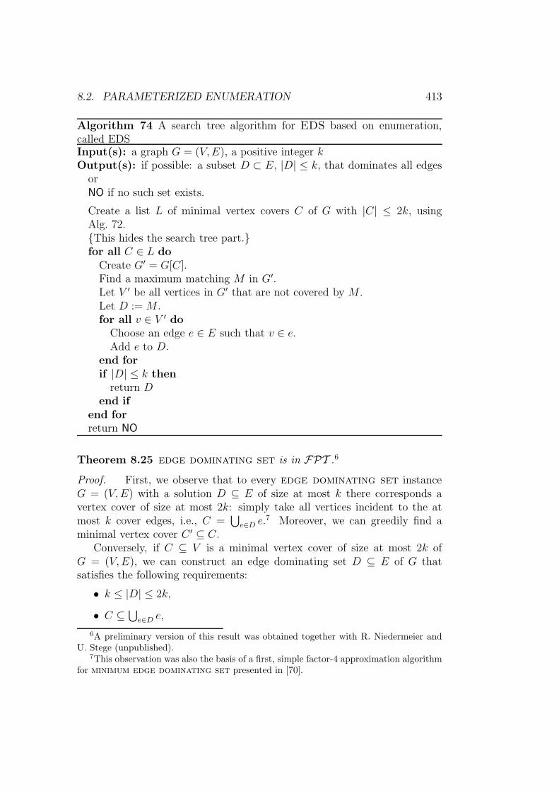
8.2. PARAMETERIZED ENUMERATION 413
Algorithm 74 A search tree algorithm for EDS based on enumeration,called EDSInput(s): a graph G = (V,E), a positive integer kOutput(s): if possible: a subset D ⊂ E, |D| ≤ k, that dominates all edges
orNO if no such set exists.
Create a list L of minimal vertex covers C of G with |C| ≤ 2k, usingAlg. 72.This hides the search tree part.for all C ∈ L do
Create G′ = G[C].Find a maximum matching M in G′.Let V ′ be all vertices in G′ that are not covered by M .Let D := M .for all v ∈ V ′ do
Choose an edge e ∈ E such that v ∈ e.Add e to D.
end forif |D| ≤ k then
return Dend if
end forreturn NO
Theorem 8.25 edge dominating set is in FPT .6
Proof. First, we observe that to every edge dominating set instanceG = (V,E) with a solution D ⊆ E of size at most k there corresponds avertex cover of size at most 2k: simply take all vertices incident to the atmost k cover edges, i.e., C =
⋃e∈D e.
7 Moreover, we can greedily find aminimal vertex cover C ′ ⊆ C.
Conversely, if C ⊆ V is a minimal vertex cover of size at most 2k ofG = (V,E), we can construct an edge dominating set D ⊆ E of G thatsatisfies the following requirements:
• k ≤ |D| ≤ 2k,
• C ⊆ ⋃e∈D e,
6A preliminary version of this result was obtained together with R. Niedermeier andU. Stege (unpublished).
7This observation was also the basis of a first, simple factor-4 approximation algorithmfor minimum edge dominating set presented in [70].

414 CHAPTER 8. FURTHER APPROACHES
• D is a minimum set satisfying the first two requirements.
Consider first the isolates in G[C]: by minimality of C, each isolate x isnecessary to cover (at least) one of the edges, so that x must be simulatedby one (arbitrary) edge ex with x ∈ ex, and since x is an isolate, y /∈ ex foreach y ∈ C \ x. Hence, all the requirements are satisfied when restrictingone’s attention to isolates in G[C].
If K is a (non-trivial) connected component of G[C], let M ⊆ E(K) bea maximum matching of K. Put M into D and treat V (K) \
(⋃e∈M e
)as
isolates (see above).Why is the set D that is finally obtained in the way described minimum
with respect to the first two requirements? A possible violation of minimalitycan only be caused by the treatment of non-trivial connected components. IfD′ is a minimal set satisfying the first two requirements, consider how it lookson a connected component K. Such a restriction D′
K collecting all edges inD′ incident with vertices in K is again minimum. The incidence of an edgefrom D′
K with a vertex from K can be caused in two different ways: either(1) e ∈ D′
K is an edge in E(K) ⊆ E(G[C]) or (2) not. By minimality of D′K,
the collection M of all edges in D′K that are edges in E(K) is a maximal
matching. If M were not a maximum matching, there would be (by the well-known algorithms for maximum matching) an augmenting alternating pathin K on which M could be increased to M ′. This means that there are twovertices x, y in K that did not belong to any edge from M but do belongto edges from M ′. These two vertices are covered in D′
K by edges ex andey. ex and ey do not contain other vertices than x and y from C. Hence, ifwe make the following changes to D′
K (and hence to D′), we get an edgedominating set D′′ satisfying the two requirements but being smaller thanD′, contradicting the third requirement:
• Remove M from D′K and replace it by M ′. This increases the edge
dominating set by one.
• Delete ex and ey from D′K. This decreases the edge dominating set
by two.
Therefore, we will reduce the size of D′K by the two operations. We can do
this as long as we can find such augmenting alternating paths. Hence, a Dsatisfying all three requirements must be caused by maximum matchings asdescribed.
This shows the correctness of the procedure described in Alg. 74.
Observe that in the proof of the preceding theorem, we basically showedhow to compute a minimum edge cover for G[C].

8.2. PARAMETERIZED ENUMERATION 415
Let us add some further comments on Alg. 74.
Remark 8.26 Alg. 74, as listed, needs exponential space. It is however easyto interleave the enumeration algorithm Alg. 72 in a way that only one min-imal vertex cover is delivered at a time. Hence, Alg. 74 can be implementedto run in polynomial space.
In the formulation of Theorem 8.25, we were not very specific about therunning time of our algorithm. But since the running time is mainly deter-mined by the enumeration algorithm, and since the time spent on each min-imal vertex cover is polynomial (especially, the involved maximum matchingalgorithm), we may conclude:
Remark 8.27 Alg. 74 runs in time O∗(4k).
What about the weighted variant(s) of edge dominating set? Moreprecisely, let us consider—motivated by the introduction in [70]:
Problem name: weighted edge dominating set (WEDS)Given: A graph G = (V,E) with edge weights ω : E → R≥1
Parameter: a positive integer kOutput: Is there an edge dominating set D ⊆ E with ω(D) ≤ k?
Corollary 8.28 Alg. 74 can be modified to work for weighted edge dom-inating set and then runs in time O∗(4k) (and may only use polynomialspace).
Proof. First observe that, by our constraints on the edge weight functionω, any edge dominating set D with ω(D) ≥ k obeys |D| ≥ k. Hence, wecan use the (non-weighted) listing of all minimal vertex covers C of size upto 2k as before. However, when constructing the corresponding weightededge dominating sets, we have to use a weighted variant of maximum match-ing. Hence, we have to compute a minimum edge cover for G[C], seen as aweighted graph. The analogous details are left to the reader.
The fact that the algorithm for weighted variant of edge dominatingset basically has the same running time as the non-weighted variant shouldmake us a bit suspicious, recalling experiences from vertex cover. Infact, as regards the approximability of these problems [70], the unweightedvariant has an (easy) 2-approximation (via some maximal matching), whilethe weighted variant only enjoys a 2.1-approximation due to some reasoningabout integer linear programs.
Can we design any reduction rules that deal with small vertex degrees?If so, it might be sufficient to only list minimal vertex covers in a way that

416 CHAPTER 8. FURTHER APPROACHES
the branching x vs. N(x) has a branching vector of (1, 2) or better. Let ustry to follow these thoughts.
Incidentally, we have to use some coloring on vertices. More precisely, avertex x is colored red to denote that one of the edges incident to x muststill go into the edge dominating set. In a certain sense, we hence generalizethe original problem towards the following one:
Problem name: generalized edge dominating set (GEDS)Given: A graph G = (V,E), a set R ⊆ V of red verticesParameter: a positive integer kOutput: Is there an edge dominating set D ⊆ E with |D| ≤ k suchthat all vertices from R are covered by D?
Obviously, any edge dominating set instance can be also interpretedas a generalized edge dominating set instance by considering an emptyset of red vertices.
Reduction rule 70 Delete isolated vertices that are not red. If an isolatedred vertex is found, answer NO.
Reduction rule 71 If x is a vertex of degree one, incident to e = x, y,then do:
1. If deg(y) = 1 or if x is red, put e into the edge dominating set weconstruct.
2. Otherwise, delete x and color y red.
Observe that reduction rule 71 is not true for the weighted case, similarlyto what we found with weighted vertex cover, since it might be cheaperto actually put edges into the dominated set that would have been eraseddue to Rule 71 (or some variant of it).
Lemma 8.29 The reduction rules 70 and 71 are sound.
Proof. If we have a red isolated vertex, then there cannot be any solution tothis instance of generalized edge dominating set. By way of contrast,an isolated vertex that is not red need not be covered, so we can simply eraseit from the instance.
A red vertex must be covered, and if it is of degree one, we have to putits incident edge into the edge dominating set.
A vertex x of degree one that is not red need not be covered. However, ifits only adjacent vertex is denoted by y, the connecting edge e need only be
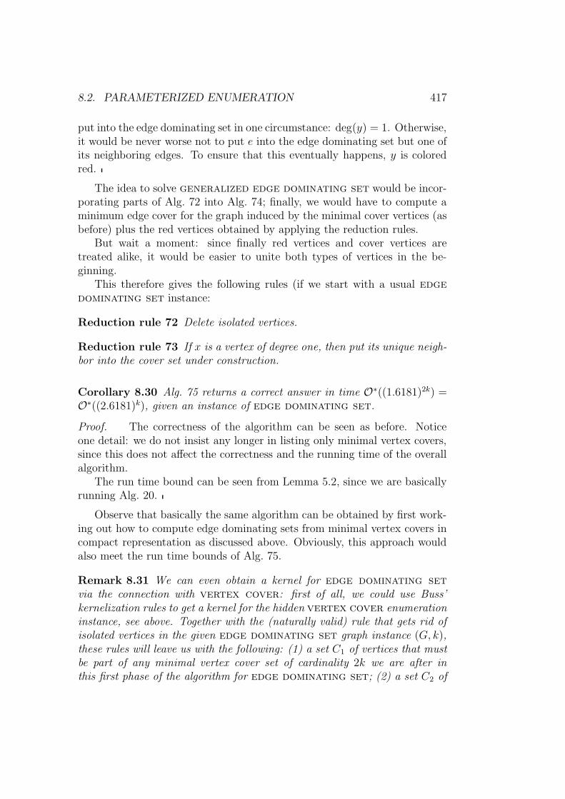
8.2. PARAMETERIZED ENUMERATION 417
put into the edge dominating set in one circumstance: deg(y) = 1. Otherwise,it would be never worse not to put e into the edge dominating set but one ofits neighboring edges. To ensure that this eventually happens, y is coloredred.
The idea to solve generalized edge dominating set would be incor-porating parts of Alg. 72 into Alg. 74; finally, we would have to compute aminimum edge cover for the graph induced by the minimal cover vertices (asbefore) plus the red vertices obtained by applying the reduction rules.
But wait a moment: since finally red vertices and cover vertices aretreated alike, it would be easier to unite both types of vertices in the be-ginning.
This therefore gives the following rules (if we start with a usual edgedominating set instance:
Reduction rule 72 Delete isolated vertices.
Reduction rule 73 If x is a vertex of degree one, then put its unique neigh-bor into the cover set under construction.
Corollary 8.30 Alg. 75 returns a correct answer in time O∗((1.6181)2k) =O∗((2.6181)k), given an instance of edge dominating set.
Proof. The correctness of the algorithm can be seen as before. Noticeone detail: we do not insist any longer in listing only minimal vertex covers,since this does not affect the correctness and the running time of the overallalgorithm.
The run time bound can be seen from Lemma 5.2, since we are basicallyrunning Alg. 20.
Observe that basically the same algorithm can be obtained by first work-ing out how to compute edge dominating sets from minimal vertex covers incompact representation as discussed above. Obviously, this approach wouldalso meet the run time bounds of Alg. 75.
Remark 8.31 We can even obtain a kernel for edge dominating setvia the connection with vertex cover: first of all, we could use Buss’kernelization rules to get a kernel for the hidden vertex cover enumerationinstance, see above. Together with the (naturally valid) rule that gets rid ofisolated vertices in the given edge dominating set graph instance (G, k),these rules will leave us with the following: (1) a set C1 of vertices that mustbe part of any minimal vertex cover set of cardinality 2k we are after inthis first phase of the algorithm for edge dominating set; (2) a set C2 of

418 CHAPTER 8. FURTHER APPROACHES
Algorithm 75 A search tree algorithm for EDS, called EDS-fast
Input(s): a graph G = (V,E), a positive integer k, a set C of cover verticesfrom H, global read access to the original graph H
Output(s): YES if there is a subset D ⊂ E, |D| ≤ k, that dominates alledges of H orNO if no such set exists.
Exhaustively, apply the reduction rules 72 and 73. The resulting instanceis called as the original one.if k ≤ 0 AND E 6= ∅ then
return NO
else if k ≥ 0 AND E = ∅ thenCreate H ′ = H[C].Find a maximum matching M in H ′.Let V ′ be all vertices in H ′ that are not covered by M .Let D := M .for all v ∈ V ′ do
Choose an edge e ∈ E(H) such that v ∈ e.Add e to D.
end forreturn |D| ≤ k.
elsePick a vertex x.By the reduction rules, deg(x) ≥ 2.if EDS-fast(G− x, k − 1/2, C ∪ x) then
return YES
elsereturn EDS-fast(G−N(x), k − deg(x)/2, C ∪N(x))
end ifend if
vertices from which we still have to select cover vertices (in order to coverG[C2]). Now, it is rather straightforward to observe that G′ = G[C1∪C2] has(similar to G[C2]) O(k2) edges and vertices. It can then be shown that it issufficient to look for a solution to (G, k) by solving (G′, k).
Moreover, since edge dominating sets for graphs with maximum degreetwo (even for trees and more general graph structures, see [238, 383]) can beeasily solved in polynomial time, we might get further improvements by ap-plying the triviality last principle, when we restrict the branching to verticesof degree at least three.

8.2. PARAMETERIZED ENUMERATION 419
Remark 8.32 Relation to approximation: A parameterized factor-2 approx-imation of edge dominating set (even weighted) can be obtained withthe help of parameterized vertex cover- or weighted vertex cover-algorithms, see [70].
Let us finally consider a related problem, also mentioned in [383]:
Problem name: matrix domination set (MDS)Given: A n× n matrix with entries from 0, 1, positive integer kParameter: kOutput: Is there a set D of one-entries in the matrix, where |D| ≤ k,such that every other one-entry has at least one row or one columnin common with some one-entry from D?
Observe that this problem can be also seen as a chess piece dominationproblem: interpret the matrix as a chessboard showing places where it isallowed to place a rook or where not (by having a one- or a zero-entry in thecorresponding position).
Lemma 8.33 (Yannakakis/Gavril) matrix domination set can be re-duced (via FPT reduction) to edge dominating set.
The corresponding reduction is formulated in Alg. 76.
Algorithm 76 Reducing matrix domination set to edge dominatingset.Input(s): a matrix instance (M, k) of matrix domination set.Output(s): a graph instance (G, k) of edge dominating set such that
(M, k) is a YES-instance iff (G, k) is a YES-instance.
Let C be the set of columns of M .Let R be the set of rows of M .Form the vertex set V = C ∪ R of G = (V,E).for all i ∈ R, j ∈ C do
Put i, j ∈ E iff entry (i, j) of M is one.end for
Put in different words, matrix domination set is in one-to-one cor-respondence to EDS, restricted to bipartite graphs. Since our solution ofedge dominating set is based on vertex cover, and the latter (in itsdecision version!) is known to be easier on bipartite graph, the followingcorollary might see some improvements; however, we did not manage to getimprovements in a straightforward manner, since we are rather relying onthe enumeration than on the decision version of VC.

420 CHAPTER 8. FURTHER APPROACHES
Corollary 8.34 matrix domination set can be solved in time O∗((2.6181)k).
In [134, Exercise 3.2.9], solving matrix domination set by means ofa kernelization and search tree based algorithm is proposed as an exercise.However, to our knowledge there is no published solution for this problem.
In the literature, several other variants of edge dominating set havebeen considered that can be attacked with similar methods; one recent paperis [281].
8.2.5 More parameterized enumeration problems
Let us finally mention that also the topic of enumeration is not new in itself:in the literature, also many “parameterized” results can be found, althoughthey tend to be stated not as explicit parameterized problems.
As an example, let us rephrase the main results of a paper of A. Kanevsky [250],who considered the following problem:
Problem name: separating vertex sets enumeration (SVS)Given: A graph G = (V,E)Parameter: a positive integer kOutput: Enumerate all minimum size separating vertex sets of sizeat most k.
Theorem 8.35 (Kanevsky) SVS can be solved in time O(2k|V (G)|) for agiven graph G. Using O(4k(|V (G)|/k2)) processors (in the PRAM model),we can get down to a running time of O(k logn).
The last statement of the quoted theorem is insofar interesting, as it mayshow a way of establishing a parameterized theory of parallel computing, atopic nearly untouched up to now.
Without giving further explicit definitions, we quote a theorem due toKaplan et al. [254] that is also a parameterized enumeration result:
Theorem 8.36 All minimal k-triangulations of a graph G can be found inO(16k|E(G)|) time.8
That paper contains two more parameterized graph modification enumer-ation problems. It would be interesting to see if the pure decision versions ofthe mentioned three problem of Kaplan et al. would allow for better FPTalgorithms.
8The decision version of this problem is also known as Minimum Fill-In.
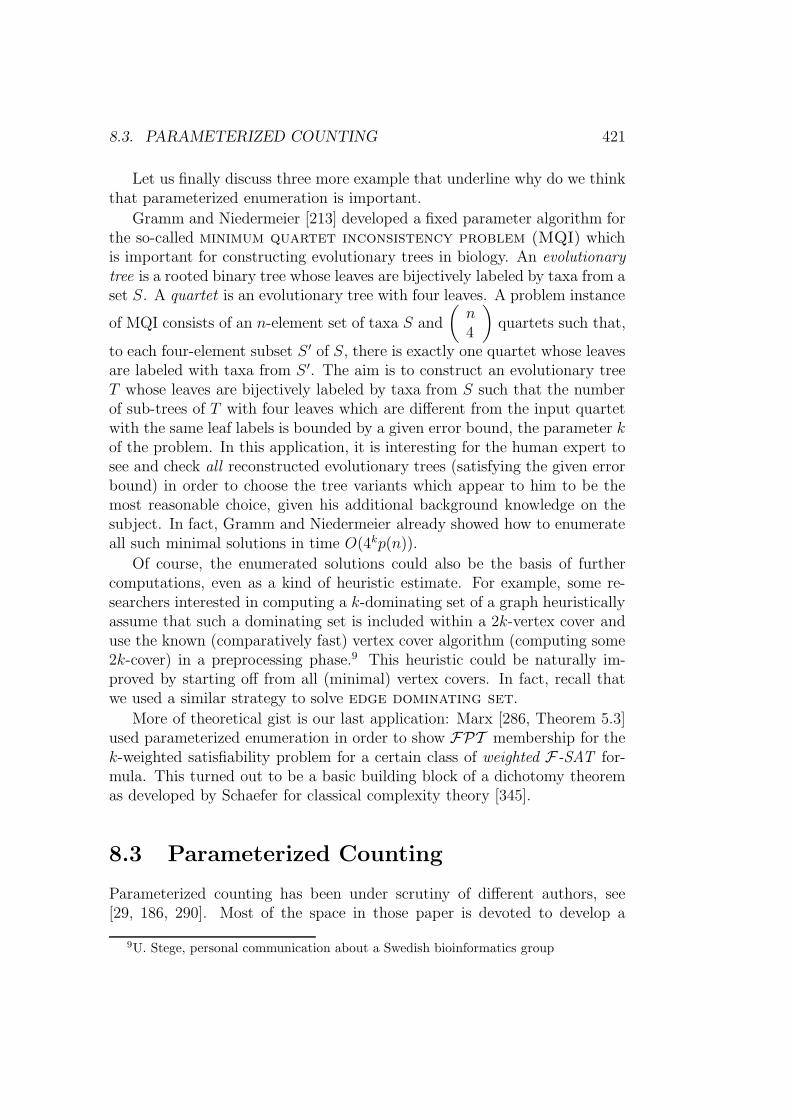
8.3. PARAMETERIZED COUNTING 421
Let us finally discuss three more example that underline why do we thinkthat parameterized enumeration is important.
Gramm and Niedermeier [213] developed a fixed parameter algorithm forthe so-called minimum quartet inconsistency problem (MQI) whichis important for constructing evolutionary trees in biology. An evolutionarytree is a rooted binary tree whose leaves are bijectively labeled by taxa from aset S. A quartet is an evolutionary tree with four leaves. A problem instance
of MQI consists of an n-element set of taxa S and
(n4
)quartets such that,
to each four-element subset S ′ of S, there is exactly one quartet whose leavesare labeled with taxa from S ′. The aim is to construct an evolutionary treeT whose leaves are bijectively labeled by taxa from S such that the numberof sub-trees of T with four leaves which are different from the input quartetwith the same leaf labels is bounded by a given error bound, the parameter kof the problem. In this application, it is interesting for the human expert tosee and check all reconstructed evolutionary trees (satisfying the given errorbound) in order to choose the tree variants which appear to him to be themost reasonable choice, given his additional background knowledge on thesubject. In fact, Gramm and Niedermeier already showed how to enumerateall such minimal solutions in time O(4kp(n)).
Of course, the enumerated solutions could also be the basis of furthercomputations, even as a kind of heuristic estimate. For example, some re-searchers interested in computing a k-dominating set of a graph heuristicallyassume that such a dominating set is included within a 2k-vertex cover anduse the known (comparatively fast) vertex cover algorithm (computing some2k-cover) in a preprocessing phase.9 This heuristic could be naturally im-proved by starting off from all (minimal) vertex covers. In fact, recall thatwe used a similar strategy to solve edge dominating set.
More of theoretical gist is our last application: Marx [286, Theorem 5.3]used parameterized enumeration in order to show FPT membership for thek-weighted satisfiability problem for a certain class of weighted F-SAT for-mula. This turned out to be a basic building block of a dichotomy theoremas developed by Schaefer for classical complexity theory [345].
8.3 Parameterized Counting
Parameterized counting has been under scrutiny of different authors, see[29, 186, 290]. Most of the space in those paper is devoted to develop a
9U. Stege, personal communication about a Swedish bioinformatics group

422 CHAPTER 8. FURTHER APPROACHES
hardness theory for parameterized counting. Since the present Habilitations-schrift is rather devoted to presenting parameterized algorithmics, let us alsohere only report on the positive results, as especially outlined in [186].
We first give two interpretations of what is meant by “counting” along thelines of the preceding section, this way a bit deviating from the mentionedpapers:
For our favorite problem vertex cover, this yields the following twoalternative counting problems:
1. count all vertex covers of size (exactly) k
2. count all minimal vertex covers of size (exactly) k
Observe that one could also define variants where we replace “(exactly)”in the sentences above by “(at most)”. However, it is not hard to see that, ata polynomial-time expense, the corresponding problems can be solved withthe help of each other.
8.3.1 Classical graph parameters in view of counting:
VC
In [186, p.868], an algorithm was presented to solve the first of the mentionedtasks, and this algorithm is basically (again) a variant of Mehlhorn’s searchtree algorithm 16. It relies on listing all minimal vertex covers of size atmost k (of the given graph G = (V,E)) in a cover collection C of G andthen computing the number of all vertex covers of size exactly k by applyingthe inclusion-exclusion principle from combinatorics (see, e.g., [274, Chap-ter 10]), relying on the fact that the number of all vertex covers of size exactlyk equals
|X ⊆ V | ∃C ∈ C : C ⊆ X ∧ |X| = k|.Besides recurring to combinatorics, we could also directly work on Mehlhorn’ssearch tree algorithm 16, or better, its binary branching variant, Alg. 18. Letus briefly follow this idea in Alg. 77.
Why is Alg. 77 correctly working ? Obviously, we have to avoid double-counting. So, whenever we branch into the case “take x into the cover”, wedo not exclude the possibility of taking all neighbors of x into the cover, too.Moreover, in that branch only vertex covers that do contain x are counted.However, in the other branch, x is added to the list of excluded vertices E, sothat we will never account for any vertex cover that contains x in this branch.Whenever the parameter was decreased to zero, all possibilities of addingvertices to the cover obtained to that point are taken into consideration that

8.3. PARAMETERIZED COUNTING 423
Algorithm 77 A simple search tree based counting algorithm, called VC-countInput(s): a graph G = (V,E), a positive integer k; the original number of
vertices n and a set E of excluded vertices.Output(s): the number of vertex covers of G of size exactly k
if k ≤ 0 and E 6= ∅ thenreturn 0
else if k ≥ 0 and E = ∅ then
return
(n− |E|k
)
elseChoose edge e = x, y ∈ ELet ` :=VC-count(G − x, k − 1, n,E ∪ x).return `+VC-count(G−N [x], k − deg(x), n,E ∪N [x])
end if
respect the list of excluded vertices (that also includes all vertices that aretaken into the cover along that particular search tree branch).
Can we do better?
Notice that counting of vertex covers has also been treated from a non-parameterized perspective. More precisely, Goldberg, Spencer and Berquehave developed [207] an intricate algorithm that counts all vertex coversof size k in an n-vertex graph in time O∗(2.325n). For graphs of degree atmost three, they even come up with a counting algorithm running in timeO∗(2.2292n). Observe that this latter result also (incidentally) improves onthe counting algorithm we presented:
Corollary 8.37 All vertex covers of size k in an n-vertex graph G of degreeat most three can be counted in time O(1.8880kk).
Proof. Since G has maximum degree of three, k vertices can cover at most3k edges. Hence, G has at most 4k vertices.
Alternatively, note that we may also apply the inclusion-exclusion princi-ple to the enumeration algorithms for minimal vertex covers in some sort ofcompact form. We won’t pursue this venue here. Rather, let us return oncemore to Alg. 77. Do we need to branch all the way down through the graph ?No, rather we could stop branching say at vertices of degree two (actually, bydoing some sort of dynamic programming, we could even stop with branchingat vertices of degree three). Then, we are left with a forest of matching edges.If there are say r edges left, there are obviously 2r possibilities to cover them.
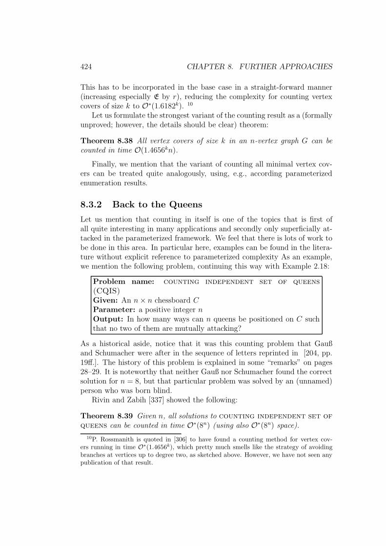
424 CHAPTER 8. FURTHER APPROACHES
This has to be incorporated in the base case in a straight-forward manner(increasing especially E by r), reducing the complexity for counting vertexcovers of size k to O∗(1.6182k). 10
Let us formulate the strongest variant of the counting result as a (formallyunproved; however, the details should be clear) theorem:
Theorem 8.38 All vertex covers of size k in an n-vertex graph G can becounted in time O(1.4656kn).
Finally, we mention that the variant of counting all minimal vertex cov-ers can be treated quite analogously, using, e.g., according parameterizedenumeration results.
8.3.2 Back to the Queens
Let us mention that counting in itself is one of the topics that is first ofall quite interesting in many applications and secondly only superficially at-tacked in the parameterized framework. We feel that there is lots of work tobe done in this area. In particular here, examples can be found in the litera-ture without explicit reference to parameterized complexity As an example,we mention the following problem, continuing this way with Example 2.18:
Problem name: counting independent set of queens(CQIS)Given: An n× n chessboard CParameter: a positive integer nOutput: In how many ways can n queens be positioned on C suchthat no two of them are mutually attacking?
As a historical aside, notice that it was this counting problem that Gaußand Schumacher were after in the sequence of letters reprinted in [204, pp.19ff.]. The history of this problem is explained in some “remarks” on pages28–29. It is noteworthy that neither Gauß nor Schumacher found the correctsolution for n = 8, but that particular problem was solved by an (unnamed)person who was born blind.
Rivin and Zabih [337] showed the following:
Theorem 8.39 Given n, all solutions to counting independent set ofqueens can be counted in time O∗(8n) (using also O∗(8n) space).
10P. Rossmanith is quoted in [306] to have found a counting method for vertex cov-ers running in time O∗(1.4656k), which pretty much smells like the strategy of avoidingbranches at vertices up to degree two, as sketched above. However, we have not seen anypublication of that result.

8.3. PARAMETERIZED COUNTING 425
They actually derived basically the same result for the n-Queens problemon a toroidal chessboard, i.e., on a chessboard with wrap-around connections,so that every line (on a chessboard), i.e., a row, a column, or a diagonal, hasn squares.
Algorithm 78 A dynamic programming algorithm for CQIS
Input(s): a positive integer nOutput(s): the number Q(n) of ways in which n queens can be placed on
an n× n board without attacking themselves
Set Q to (∅, 1).Q should be organized as a directed acyclic graph GQ reflecting the in-clusion relation of the first components; the “root” of GQ is always (∅, 1).A directed spanning tree of GQ is used to investigate GQ in the secondFOR-loop.for all squares s of the chessboard do
Let T be the set of (at most six) lines that contain s.for all (S, i) ∈ Q doStart the search through GQ at the rootif S ∩ T = ∅ thena queen can be placed on s without attacking any of the lines thatare already dominatedLook for some (S ∪ T, j) in Q using GQ.if found then
Replace (S ∪ T, j) by (S ∪ T, j + i)else
Add (S ∪ T, i) to Q (maintaining GQ)end if
elseWe can skip all successors of (S, i) in GQ.
end ifend for
end forLet M be the set of 2n lines that are either rows or columns.Initiate Q(n) := 0.for all (S, i) in Q do
if M ⊆ S thenQ(n) := Q(n) + i
end ifend for

426 CHAPTER 8. FURTHER APPROACHES
Algorithm 78 reproduces a preliminary version of Rivin and Zabih’s al-gorithm running in time O∗(64n).11 It is based on dynamic programming(although this time written up in an iterative rather than in a recursiveform) and uses as the basic data structure a queue Q containing pairs (S, i).Here, S is a set of lines (i.e., either rows, columns, or diagonals) each of thosehas been already become a closed line, i.e., a queen has been put on one of thesquares of it. The integer i tells us in how many ways it is possible to placequeens on a chessboard that do not attack themselves mutually but dominateexactly the lines in S. So, at the start, Q contains only the pair (∅, 1), sincethere is only one way to place no queens on the chessboard. The correctnessand the claimed running time is based on the following observations:
• A chessboard has 6n− 2 lines.
• For each set of lines S, there will be never two items (S, i) and (S, i′)in the queue.
• Hence, there will never be more than 26n−2 elements in the queue.
• The second FOR-loop visits each element of the queue at most a poly-nomial number of times (namely, notice that the set T used for updatingS ∪ T contains at most 6 elements).
• A valid solution must put one queen in each row and in each column.
In essence, this counting algorithm is based on the idea of putting possiblecandidate solutions into the same equivalence class if the set of closed lines isthe same. The improvements of the algorithm are then based on putting evenmore solutions into the same equivalence class. Moreover, the order in whichall squares of the chessboard are scanned is fixed, namely to row-major, sothat, whenever one row r has been completely scanned, all (S, i) with r /∈ Sare deleted from S, since a valid solution must place a queen in every row.
It has been conjectured in [336] that the number of solutions Q(n) tothe n-Queens Problem, divided by n logn, converges to some constant β.If this conjecture were true, then Algorithm 78 would be superior to anybacktracking algorithm that actually constructs (enumerates) all solutions.However, the values of Q(n) listed in [336] were obtained by such a backtrack-ing algorithm due to the (at that time) seemingly unsurmountable usage ofmemory of Algorithm 78 (even in its improved form). To such backtrackingalgorithms, “intelligence” is usually added that exploits certain patterns forcreating solutions, see [156, 159, 331].
11In actual fact, a naive direct implementation of their algorithm Queens containedin [337] has (contrary to what is claimed) a running time of O∗(642n).

8.3. PARAMETERIZED COUNTING 427
Can we use the ideas from Algorithm 78 to solve similar problems, aswell? Let us try to do so with dominating set of queens, i.e., a decisionproblem (rather than a counting problem).
Algorithm 79 A dynamic programming algorithm for QDS
Input(s): positive integer n and kOutput(s): Is it possible to place k queens on an n× n board to dominate
all squares?
Set Q to (∅, 0).Q should be organized as a directed acyclic graph GQ reflecting the in-clusion relation of the first components; the “root” of GQ is always (∅, 0).A directed spanning tree of GQ is used to investigate GQ in the secondFOR-loop.for all squares s of the chessboard do
Let T be the set of (at most six) lines that contain s.for all (S, i) ∈ Q doStart the search through GQ at the rootif NOT T ⊆ S thenputting a queen on s would dominate new linesLook for some (S ∪ T, j) in Q using GQ.if found then
Replace (S ∪ T, j) by (S ∪ T,minj, i+ 1)else
Add (S ∪ T, i + 1) to Q (maintaining GQ)end if
end ifend for
end forLet M be the set of all possible lines.Find (M, j) in Q.return k ≤ j
In Alg. 79, we again maintain a queue that contains information in theform of pairs (S, i); however, this time partial solutions are encoded. Morespecifically, S is a set of already dominated lines, and i shows how manyqueens are needed to dominate S. Hence, the initialization is different: theempty set is dominated by zero queens.
What is the running time of Alg. 79? Again, since for each S, at most oneelement (S, i) will be present in the queue, there are at most 26n elementsever showing up in the queue at the same time. Clearly, each subset of lines

428 CHAPTER 8. FURTHER APPROACHES
S will be modified at most O(|S|6) times (choose a subset T of at most sixlines from S that, together with S \ T , might cause an update). Keeping inmind Theorem 4.27, we may hence conclude:
Theorem 8.40 Alg. 79, when started upon a reduced kernel according toTheorem 4.27, solves a dominating set of queens instance in time O∗(212k).
Observe that this is worse than what we got by the treewidth-based ap-proach in Theorem 7.15. However, there might be ways to improve the cur-rent estimate of Alg. 79 or even combine this methodology with the treewidth-based approach.
8.4 Other techniques for FPT algorithms
In this section, we briefly review other techniques for obtaining FPT results.Alon, Yuster and Zwick [22] introduced the idea of using color coding into
the domain of FPT algorithm design. In recent papers, there has been arevival of those ideas. We only mention two of them:
• Fellows et al. used this technique in [168] to get improved FPT results(all of type O∗(ck)) for geometric packing and matching problems.
• Marx [286] used color coding to show FPT results for certain types ofconstraint satisfaction problems.
As already mentioned in Chap. 2, there does also exist “machinery” fromgraph minor theory, and more general, from well-quasi-orderings. With theexceptions reported in Chap. 7, this machinery is well suited for derivingclassification results, but usually the running times of these algorithms areworse than what can be obtained by other methods. One particular exam-ple shown in this Habilitationsschrift is Theorem 4.7 that got substantiallyimproved in terms of running time in this chapter. 12
Other techniques based on logical characterizations of problems could alsobe (again) mentioned here, although the concrete solving strategy does relyon algorithmic techniques as explained throughout this Habilitationsschrift.
8.5 Implementations
Unfortunately, reports on practical experiences with parameterized algo-rithms are relatively scarce throughout the literature. Nonetheless, we will
12Actually, we refrained from giving an exact running time bound in Theorem 4.7; theinvolved constants are simply astronomically huge.

8.5. IMPLEMENTATIONS 429
try to underline the validity of the parameterized approach by reporting onsome of the relevant aspects. This should also inspire people working onthe more practical parts of algorithmics to constantly report their results.In fact, the ultimate goal in this area might be to compile a repository ofprograms that implement basic parameterized algorithms. Since this Habi-litationsschrift is focusing on graph-theoretic problems, an incorporation ofsuch a repository in LEDA, see [293] and [Chapter 11, Site 11].
8.5.1 Implementations of sequential algorithms
According to our observation, most of the implementation work done so faris focusing on treewidth-based algorithms, the quotations [10, 124, 132, 133]being only a (possibly random) selection of corresponding works.
The (partly dramatic) effect of data reduction rules has been describedin [7]. Of course, also the paper of Weihe [375] deserves to be mentioned inthis place, although it is not directly referring to parameterized algorithmics.In Sec. 4, we also mentioned the experiments of [3] when considering crownreductions for vertex cover.
Recently, Huffner reported [243] about an implementation of the bipar-tization algorithm we also presented in Alg. alg-GBP. He also relates thatalgorithm with the iterative compression idea briefly mentioned in Chap. 4.
As regards search tree algorithms, the reported experiments we are awareof [210, 357] mostly show that the worst case running time estimates that weretheoretically derived for the according algorithms are rarely met in practice;the algorithms tend to behave far better than “expected” both on artificialand on real data. Of course, this might mean that the derived estimates aresimply not good enough. Alternatively, it could mean that the worst casescenario that could be drawn from the theoretical analysis rarely shows up inpractice. This might also encourage research on the average case complexityof exact, exponential-time algorithms, an area that is (to our knowledge) noteven attempted at up to now.
8.5.2 Parallel implementations
Works on the parallelization of search tree algorithms have been reportedin b[80]. More precisely, the algorithm they implemented for vertex coverhas two phases:
1. The first phase is basically executed to obtain instances that can beeasily dispatched on different processors on a predetermined level of theoverall search tree. This technique requires that the search tree is quite

430 CHAPTER 8. FURTHER APPROACHES
regular. Therefore, in [80] even a worse than best-known sequentialalgorithm is chosen in this phase, based on [33, Theorem 1].
2. In the second phase, a rather up-to-date search tree algorithm (basedon [33, Theorem 2]) is chose to be executed on each processor to workon the subproblems originating from the dispatcher phase one.
Such a coarse-grained parallelization of a search tree algorithm is a quitenatural idea. In our context, it is interesting that the authors of [80] chosetwo different algorithms for the two processing phases, since they needed asimple branching behavior in the first phase. This is interesting, since thetop-down approach to search tree algorithms we advocate yields particularlysimple algorithms, so that for example in the case of hitting set, it wouldnot be necessary to twice encode the same algorithm to be run on the differentphases. The fact that in the binary branching of our hitting set algorithms,some branches will (nearly) keep the parameter value should not matter toomuch, since the seemingly more work-intensive jobs can be dispatched first,leaving the dispatching processor finally with the instance with the largestparameter. This strategy should help balance the overall workload.
In the case of vertex cover, this would mean that we propose to usealgorithm VCMH-BU as described in Sec. 5.1.1.
In [79], the authors report on how to solve vertex cover instancesthrough the addition of parallelism, thereby allowing even larger problem in-stances to be solved in practice. They implemented a parallel FPT methodfor vertex cover using C and the MPI communication library, and testedit on a PC cluster. This has been the first experimental examination of par-allel FPT techniques. The authors tested this method on protein sequencesobtained from the National Center for Biotechnology Information. As partof the experiments, they solved larger instances of VC than in any previ-ously reported implementations. For example, it is mentioned that probleminstances with k ≥ 400 in less than 1.5 hours can be exactly solved. Sincethe parallel FPT algorithm requires only very little communication betweenprocessors, it is expected that the method to also perform well on grids.

Chapter 9
Limitations to parameterizedalgorithmics
In this chapter, we rather briefly discuss limitations to parameterized algo-rithmics.
1. We will see that parameterizing problems does not always help over-come the P versus NP problem. More specifically, we will introduce(some aspects of) the parameterized hardness theory developed to showthat—most likely—certain parameterized problems are not parameter-ized tractable.
2. We will show that for dualizable parameterized problems with linearkernels, the kernel sizes could not be “arbitrarily small.”
We will also encounter many of the problems we have seen before on thisway.
9.1 Parameterized intractability
In actual fact, there are now a certain number of ways to formalize the notionof parameterized intractability.
Since we believe that Turing machines—albeit being amongst the firstformulations of computability—are still one of the models many computerscientists are most familiar with, we are going to present the most importantclasses of parameterized intractability “in the Turing way,” following [74].Some results in this direction can also be found in [90]. In [74], it is alsoshown that this approach is very useful and natural to prove that certainproblems are belonging to a specific complexity class.
431

432CHAPTER 9. LIMITATIONS TO PARAMETERIZED ALGORITHMICS
In this way, we will describe the basic levels of the W-hierarchy
FPT ⊆ W[1] ⊆ W[2] ⊆ · · · ⊆ W[SAT] ⊆ W[P].
The examples from this section have not yet appeared anywhere else,although some of the results have been at least known for a long time.
9.1.1 W[1]
W[1] can be characterized by the following problem on Turing machines:
Problem name: short nondeterministic Turing machinecomputation (SNTMC)Given: A (single-tape) nondeterministic Turing machine M , an in-put string xParameter: a positive integer kOutput: Is there an accepting computation of M on input x thatreaches a final accepting state in at most k steps?
Formally, we can state:
Definition 9.1 A parameterized problem P with parameter k is in W[1] iffthere is a function f and, for every instance I of P , a nondeterministic Turingmachine TP,I such that TP,I halts within f(k) steps, writing a one onto itstape, iff (I, k) is a YES-instance of P .
This means that you can prove both hardness (with respect to W[1]) andcontainment within W[1] by finding according parameterized reductions.
The question whether FPT equals W[1] has therefore the same philo-sophical backing as the question whether P equals NP: it seems to beimpossible to deterministically simulate a nondeterministic Turing machinethat uses k steps within f(k) steps on a deterministic Turing machine.
To illustrate this approach, let us show the following lemma:
Lemma 9.2 independent set is in W[1].
Proof. Let G = (V,E) be an instance of independent set. We have totransform it into an instance (T, k′) of short nondeterministic Turingmachine computation. We also assume that k > 0 (k = 0 is a trivialinstance).
Let T have V as its set of non-blank tape symbols.In a first phase, T guesses exactly k different symbols from V and writes
them onto its tape. This can be done as follows: In a preliminary sub-phase,

9.1. PARAMETERIZED INTRACTABILITY 433
T guesses k symbols from V and writes them onto its tape, using k steps. Letus now assume an ordering on V being fixed. Then, T can run a bubble-sortalgorithm, needing b(k) steps, where in the end the head of T is scanning thefirst blank symbol to the right of the k symbols from V . By another sweepto the left, T can verify in k more steps that actually all guessed symbols aredifferent.
In a second phase, T will once more scan the guessed symbols and nowsee if they are independent. More specifically, T will perform, upon scanninga symbol v, perform the following steps:
• Memorize v in finite memory and erase v on the tape.
• Move to the right until you find the first blank symbol. On the way,check if any u ∈ N(v) has been found. If such a u ∈ N(v) is found,reject.
If and only if the guessed vertex set was an independent set, no rejection casecan be found. Hence, the Turing machine can then accept. Assuming thatthis second phase takes c(k) time, we can estimate the overall running timeof T (assuming a correct guess) to be t(k) = 2k+ b(k) + c(k) ∈ O(k2). Moreprecisely, the guessed vertex set is an independent set of size k iff T halts (inan accepting state) after having run t(k) steps.
The reader will have noticed that the Turing machine described in thepreceding proof could have been designed to be more efficient. For example,we could get rid of all sub-phases but the guessing phase in the first phaseif we checked if u ∈ N [v] can be found during the second phase. However,we think that the present description is more illuminating since it clearlyseparates the two steps that are typical for Turing machines that shouldshow membership in W[1]:
• In a first phase, a possible solution is guessed.
• In a second phase, this guess is checked; here, it is crucial to know thatthe instance of the original problem (as such) could be hard-wired intothe Turing machine table that is constructed.
As an aside, let us mention that the necessity of this hard-wiring is es-sential for the questions if certain problems are in W[1] or rather (already)in FPT .
Remark 9.3 Another problem whose membership in W[1] can be seen in asimilar fashion is vertex induced forest. We only indicate the necessarymodifications in what follows. After having guessed the k would-be forest
434CHAPTER 9. LIMITATIONS TO PARAMETERIZED ALGORITHMICS
vertices, only acyclicity has to be tested, i.e., for each pair of forest vertices,it has to be examined if there is at most one path between them (in the graphinduced by the guessed vertices). This can be done in time O(k3).
Let us now consider the following variant of SNTMC:
Problem name: short nondeterministic small Turing ma-chine computation (SNSTMC)Given: A (single-tape) nondeterministic Turing machine M whosesize is bounded by f(k), an input string xParameter: a positive integer kOutput: Is there an accepting computation of M on input x thatreaches a final accepting state in at most k steps?
More precisely, Thm. 2.4 can be re-interpreted in the present context inthe following way:
Corollary 9.4 A problem P is in FPT if and only if it can be solved withthe help of short nondeterministic small Turing machine compu-tation, for some memory delimiting function f .
This is the basic content of [75, Corollary 6].
9.1.2 W[2]
W[2] can be characterized by the following problem on Turing machines:
Problem name: short multi-tape nondeterministic Turingmachine computation (SMNTMC)Given: A multi-tape nondeterministic Turing machine M , an inputstring xParameter: a positive integer kOutput: Is there an accepting computation of M on input x thatreaches a final accepting state in at most k steps?
This means that you can prove both hardness (with respect to W[2]) andcontainment within W[2] by finding according reductions.
To show these ideas, let us present one simple construction that showsthat red-blue dominating set (and hence related problems like hittingset) belong to W[2].
Lemma 9.5 red-blue dominating set belongs to W[2].

9.1. PARAMETERIZED INTRACTABILITY 435
Proof. Let (G = (Vred∪Vblue, E), k) be an instance of red-blue dominat-ing set. We have to transform it into an instance of short multi-tapenondeterministic Turing machine computation.
In fact, we won’t give a completely formal description of the Turing ma-chine but rather describe the ideas. Details of the construction can be foundin [74, p.664ff.] in a slightly different setting (namely, Steiner tree ingraphs). We also assume that k > 0 (k = 0 is a trivial instance).
The corresponding Turing machine T has |Vblue| + 1 tapes; let they beindexed by 0∪Vblue. As tape symbols, we will use Vred on tape 0. The edgerelation of G is “hard-wired” into the transition function of T as describedbelow.
T will first nondeterministically guess the red-blue dominating set andwrite it on tape 0 using the letters from Vred. Since T need not worry aboutguessing the same vertex more than once (this would only mean that thecorresponding red-blue dominating set has less than k elements, whichis fine), this guessing phase takes k steps.
In a second phase, T has to verify that the guess is correct. To this end,upon reading symbol v ∈ Vred on tape 0, T
• will move the heads corresponding to tapes addressed by vertices fromN(v) one step to the right, and
• will move the head on tape 0 one step to the right.
Upon reading the blank symbol on tape 0, T will move all heads one step tothe left; only if this is possible for all of the heads, T will accept.
The second phase will take another k + 1 steps.It is now easy to see that G has a red-blue dominating set of size at most
k iff T has an accepting computation within 2k+1 steps, so that we actuallydescribed a parameterized reduction.
So, the basic idea to show that a certain problem is in W[2] is to find away in which a nondeterministic multi-tape Turing machine can solve it bymaking use of its many tapes, where the actual (original) problem instance(I, k) is usually stored within the finite memory of the Turing machine, andthen only f(k) steps may be performed by the Turing machine. The onlything that always needs some caution is that the Turing machine table canbe written up in a succinct way, i.e., polynomial in I.
In the preceding proof, the only delicate thing to note here is that, in thesecond phase, all but the tape labeled 0 will contain a blank symbol undertheir heads, so that there is actually only one transition per symbol in Vredthat has to put into the Turing table (plus one transition for the final step).

436CHAPTER 9. LIMITATIONS TO PARAMETERIZED ALGORITHMICS
So, to be more specific, the Turing machine constructed in the precedingproof will contain (k − 1)|Vred| transitions for phase one (it has to count upto k within its finite memory), plus |Vred| + 1 transitions for phase two.
More generally speaking, the mentioned condition will be met if all but afixed number of tapes are only worked by using the head positions for count-ing, or if it is at least clear what symbols to expect under the correspondingheads. Otherwise, the corresponding Turing tables might be of size Ω(2|I|).
A similar but slightly more complicated proof for showing that dominat-ing set is contained in W[2] is given in [75, Theorem 6], following basicallythe same ideas; simplifications are contained [90, Cor. 1]. We mention in pass-ing that also variants like independent dominating set can be treatedthis way. Similarly, the problem of finding a digraph kernel as examined in[221] can be shown to lie in W[2] by very closely following these lines. Notethat membership in W[2] of that problem was left open in [221].
Let us give one more example of this technique:
Lemma 9.6 Roman domination is in W[2].
The proof is actually pretty similar to the preceding one.
Proof. Let G = (V,E) be an instance of Roman domination. We haveto transform it into an instance of short multi-tape nondeterministicTuring machine computation. We also assume that k > 0 (k = 0 is atrivial instance).
The corresponding Turing machine T has |V |+1 tapes; let they be indexedby 0 ∪ V . As tape symbols, we will use (V × 1, 2) on tape 0. The edgerelation of G is “hard-wired” into the transition function of T as describedbelow.
T will first nondeterministically guess the Roman domination function Rand write it on tape 0 using the letters from V ×1, 2 as follows: wheneverR(v) = 1, it will write (v, 1), and if R(v) = 2, then it will write (v, 2). Thevalues R(v) = 0 are implicitly stored (by having no (v, i) written on the tape0).
If we look a bit more closely how the second phase works (described be-low), we will see that if it happens that by these nondeterministic guessesboth (v, 1) and (v, 2) are written onto tape 0, we will see that such a nota-tion is interpreted as two (v, 2) write-ups would be. Hence, T need not worryabout picking some vertex v more than once for writing either (v, 1) or (v, 2)onto tape 0 (this would only mean that the corresponding red-blue dom-inating set has less than k elements, which is fine). However, the Turingmachine should care about whether (or not) the second components of theelements stored on tape 0 sum up to a number that is at most k. This check

9.1. PARAMETERIZED INTRACTABILITY 437
can be done “in parallel” with the guessing itself, storing intermediate sumsin finite memory. Therefore, this guessing phase takes k steps and uses up apolynomial number of transitions in the Turing table.
In a second phase, T has to verify that the guess is correct. To this end,upon reading symbol (v, 1) on tape 0, T
• will move the head on the tape addressed by v one step to the right,and
• will move the head on tape 0 one step to the right.
Upon reading (v, 2), T
• will move the heads on to tapes addressed by vertices from N [v] onestep to the right, and
• will move the head on tape 0 one step to the right.
Upon reading the blank symbol on tape 0, T will move all heads one step tothe left; only if this is possible for all of the heads, T will accept.
The second phase will take another k + 1 steps.
It is now easy to see that (G, k) is a YES-instance to Roman dominationiff T has an accepting computation within 2k + 1 steps, so that we actuallydescribed a parameterized reduction.
More discussion on hardness of decision problems related to Turing ma-chines can be found in [75]. In particular, note that if we allow multiple headsin addition or instead of multiple tapes for a Turing machine, we get a prob-lem similar to short multi-tape nondeterministic Turing machinecomputation that is also W[2]-complete.1
Let us give one example of a hardness proof within the W-hierarchy, basedon the fact (see [134]) that red-blue dominating set is W[2]-complete(with no bound on the degrees of the blue vertices).
To prove the hardness result, we need one fact about the Roman domi-nation of complete graphs.
Lemma 9.7 For the complete graph Kn on n vertices, the Roman domina-tion number is two iff n ≥ 2.
1More precisely, the theorems from [75] only give hardness of these problems. In orderto prove that the corresponding problem(s) are in W[2], a technique similar to the oneapplied in the proof of [74, Theorem 3] can be used.

438CHAPTER 9. LIMITATIONS TO PARAMETERIZED ALGORITHMICS
Proof. The mapping that assigns two to an arbitrary vertex of Kn andzero to all other vertices is obviously a valid Roman domination function.
If one is assigned to any vertex by some Roman domination function forKn, this function can only meet the claimed Roman domination number oftwo if n = 2, since then to the other vertex, one could be assigned, as well.Otherwise, to one further vertex the value of two would have to be assigned,so that this Roman domination function would be worse than the one givenin the first paragraph.
Theorem 9.8 Roman domination is W[2]-complete.
Proof. Due to Lemma 9.6, we already know that Roman dominationlies in W[2].
Assume that G = (V,E) is an instance of red-blue dominating set,restricted to bipartite graphs (see Lemma 2.14), i.e., V = Vred]Vblue.
Without loss of generality, we can assume that |Vred| > 1, since otherwisean optimal solution to the given RBDS instance can be found in polynomialtime and can be accordingly translated into an equivalent Roman domina-tion instance.
In the simulating Roman domination instance, we construct a graphG′ = (V ′, E ′), where
V ′ = (Vred ∪ 1, . . . , 2k + 1) × 1, . . . , k ∪ Vblue,
and E ′ contains the following edges (and no others):
1. G′[Vred × i] is a complete graph for each i ∈ 1, . . . , k.
2. For all i ∈ 1, . . . , k and x ∈ Vred, y ∈ Vblue, x, y ∈ E iff [x, i], y ∈E ′.
3. For all i ∈ 1, . . . , k, j ∈ 1, . . . , 2k + 1 and x ∈ Vred: [x, i], [j, i] ∈E ′.
We are going to show the following claim: G has a red-blue dominating setD of size k iff G′ has a Roman domination function R with
∑x∈DR
R(x) = 2k.If G has a red-blue dominating set D = d1, . . . , dk of size k, then
consider the following function R : V ′ → 0, 1, 2: R assigns zero to allvertices but to d′i = [di, i], to which R assigns two. Since di is connected toall vertices in (Vred ∪ 1, . . . , 2k + 1) × i, the vertices in V ′ \ V are alldominated by this assignment. Moreover, since D is a red-blue dominatingset of G, all vertices in Vblue are dominated in G′, as well.

9.1. PARAMETERIZED INTRACTABILITY 439
Now consider a Roman domination function R for G′ with∑
x∈DRR(x) =
2k. Due to Lemma 9.7 and according to the first condition on edges, the Ro-man domination number of each induced graph G′[Vred×i] is two, assuming|Vred| > 1. Since G′[Vred×1, . . . , k] can be decomposed into k components,the Roman domination number of G′[Vred × 1, . . . , k] is 2k. More specifi-cally, to achieve that bound, the domination function would have to assigntwo to one vertex from Vred × i for each i and zero to all other vertices.Observe that such an assignment would be also a valid Roman dominationfunction R′ for G′[(Vred ∪ 1, . . . , 2k + 1) × 1, . . . , k] if we assign zero toall vertices from 1, . . . , 2k + 1 × 1, . . . , k.
Since there are “too many” vertices in 1, . . . , 2k + 1 × 1, . . . , k, wecannot simply replace one or more vertices to which R′ assigns two by verticesfrom 1, . . . , 2k + 1 × 1, . . . , k to which R′ (as constructed) had assignedzero.
Observe that we have left over yet some degrees of freedom for finallyconstructing a valid Roman domination function R from R′; namely, we havenot been specific about how to choose a vertex from Vred × i (for each i)to which we assign two. However, if we find k assignments of two to verticesfrom Vred × 1, . . . , k such that also all vertices from Vblue are dominated,i.e., DR = [d1, 1], . . . , [dk, k] = R−1(2), then D = d1, . . . , dk is a validdominating set of G.
Since there are no connections between vertices from 1, . . . , 2k + 1 ×1, . . . , k and Vblue, there is no way of replacing some of the vertices selectedfrom (Vred ∪ 1, . . . , 2k+ 1)×1, . . . , k (by assigning two to them) by ver-tices from Vblue, so that there cannot be a Roman domination function Rthat assigns one or two to any of the vertices from Vblue without violating thecondition
∑x∈DR
R(x) = 2k. Hence, the Roman domination function (ten-tatively) constructed above is the only possibility; that construction works ifand only if G has a dominating set of size k.
Let us finally mention one further problem, also taken from [318]; in fact,some more (and similar) problems can be found there and treated alike.
Problem name: dominating rearrangement (DR)Given: A graph G = (V,E), a subset S ⊆ VParameter: a positive integer k = |S|Output: Is there a dominating rearrangement r : S → N [S], s 7→r(s) ∈ N [s] such that r(S) ⊆ V is a dominating set?
Again, this problem can be viewed from a military perspective: S is theset of locations where currently armies are placed on, and the question isif by a one-step rearrangement of each army (if necessary) a situation can

440CHAPTER 9. LIMITATIONS TO PARAMETERIZED ALGORITHMICS
be created in which each region (modeled by graph vertices) is sheltered byeither a defending army in the region itself or in a neighboring region.
This problem is interesting for at least two reasons from a parameterizedperspective:
• The parameterization is not standard. Actually, there is no obviousoptimization problem hidden here, although the variant that only kout of the vertices from S may be actually rearranged gives anotherobviously W[2]-complete problem.
• It is a specific example of a problem where the problem is if a given“solution” can be improved in order to satisfy a certain property, here:being a dominating set. Such type of problems can show up in manydisguises in practice, we are sure.
Theorem 9.9 dominating rearrangement is W[2]-complete.
Proof. Membership in W[2] can be seen by a guess-and-verify strategy asseen before. We don’t give details but only mention that it appears to bebest to take S × V as the alphabet on tape 0, where (s, v) is indicating thatan army on vertex s has been moved to v.
For the hardness, take again an instance (G = (V = Vred ∪ Vblue, E), k)of red-blue dominating set. Let S = 1, . . . , k be disjoint from V ,and consider the graph G′ = (V ′, E ′) with V ′ = V ∪ E and E ′ = E ∪ (S ×Vred). Hence, G′[S ∪ Vred] forms a complete bipartite graph. This gives theinstance (G′, S) of dominating rearrangement. Obviously, D ⊆ Vred isa dominating set of size (at most) k iff (G′, S) can be solved by moving |D|of the armies in S onto the vertices from D.
9.1.3 Beyond W[2]
In [74], also a Turing machine characterization for the natural upperboundW[P] of the W-hierarchy was obtained. Cesati used the following problem,which actually uses a different parameterization for nondeterministic Turingmachines:
Problem name: bounded nondeterminism Turing machinecomputation (BNTMC)Given: A (single-tape) nondeterministic Turing machine M , an in-put string x, an integer n coded in unaryParameter: a positive integer kOutput: Is there an accepting computation of M on input x thatreaches a final accepting state in at most n steps and uses at most knondeterministic steps?

9.1. PARAMETERIZED INTRACTABILITY 441
A Turing machine problem for W[SAT] was obtained in [76]. They con-sidered the following problem:
Problem name: compact deterministic Turing machinecomputation (CDTMC)Given: A deterministic Turing machine M , an input string xParameter: a positive integer kOutput: Is there an accepting computation of M on input x thatvisits at most k squares?
They showed that compact deterministic Turing machine com-putation is W[SAT]-hard. Whether or not it is belonging to W[SAT] seemsto be open. Nonetheless, this problem appears to be interesting, since it isa natural parameterized analogue to the classical complexity class PSPACEcollecting all problems that can be solved on a deterministic Turing ma-chine using only polynomial space. So, in a sense the question if compactdeterministic Turing machine computation belongs to W[1] is theparameterized analogue to whether P coincides with PSPACE .
In fact, this intuitive relation was used to translate a PSPACE -hardnessproof of a motion planning problem into a W[SAT]-hardness result for thatproblem. Details can be found in [76]. In this context, it might be interestingto observe that for other motion planning problems, membership in FPThad been shown [178], also confer Sec. 3.1.2.
We refrain from giving the (rather complicated circuit) definition of eachlevel of the W-hierarchy here but refer to the book [134]. For the pur-pose of this Habilitationsschrift—putting specific emphasis on parameterizedalgorithmics—it should be enough to know the downsides of parameterizedcomplexity as presented.
Let us briefly mention that there does exist a machine characterizationof each level W[t] of the W-hierarchy in terms of machines, based on so-called W-RAMs. The interested reader is referred to [90]. There, it is shownthat each level W[t] can be characterized by t alternations in (alternating)W-RAMs.
An alternative to the W-hierarchy was suggested by M. Grohe, the so-called A-hierarchy based on model checking [215]. It is still an open questionsif both hierarchies coincide. Observe that a characterization of all levels ofthe W-hierarchy (corresponding to the W-RAM characterization mentionedabove) by alternating Turing machines is open. More specifically, Chen andFlum defined in [90] a complexity class L[t] basically corresponding to alter-nating Turing machines with t alternations. It is known that W[t] ⊆ L[t] ⊆A[t].

442CHAPTER 9. LIMITATIONS TO PARAMETERIZED ALGORITHMICS
9.1.4 More downsides
In fact, the whole area of intractability in the parameterized sense is still ina developing state. Recent advances include (and this is not meant to be acomplete account):
• M. Fellows [165, 164] and his co-authors developed a hardness theorythat can be seen as an alternative to the W-hierarchy that we presentedabove. The basic class, called MINI-1 or M[1], is based upon theminiaturization version of some classical problem. The following is anexample of an M[1]-hard problem:
Problem name: miniaturized vertex cover (VCmini)Given: A graph G = (V,E)Parameter: a positive integer kOutput: Is there a vertex cover C ⊆ V with |C| ≤ k log(|V |)?
It is known that FPT ⊆ M[1] ⊆ W[1].
Showing M[1]-hardness is often simpler than proving W[1]-hardness,although the basic message is almost the same: it it commonly notbelieved that FPT equals M[1] due to the following result.
Theorem 9.10 (Cai and Juedes [69]) FPT =M[1] iff n-variable3-SAT instances can be solved in time 2o(n).
The theory of miniaturization was further developed by Chen andFlum [91] who exhibited a whole hierarchy of “miniaturized complex-ity classes” between FPT and W[1]. They also accordingly generalizedTheorem 9.10.
• Let us mention the work of J. Chen, X. Huang, I. A. Kanj, and G.Xia [83] who developed new techniques for deriving very strong compu-tational lower bounds for a class of well-known NP-hard problems, in-cluding weighted satisfiability, dominating set, hitting set,clique, and independent set. For example, although a trivial enu-meration can easily test in time O(nk) if a given graph of n vertices hasa clique of size k, they prove that unless an unlikely collapse occurs inparameterized complexity theory, the problem is not solvable in timef(k)no(k) for any function f , even if we restrict the parameter value k tobe bounded by an arbitrarily small function of n. Similar results havebeen reported in [81]. In particular, it is shown that any problem in the

9.2. HOW SMALL CAN KERNELS GET ? 443
syntactic complexity class SNP as defined in [319] (that class includesoptimization problems like vertex cover and independent set)can be solved in time no(k) if clique can be solved in time no(k).
• In a similar spirit, Cai and Juedes [69] excluded the possibility of
O(2o(√k))-algorithms for planar vertex cover, planar dominat-
ing set and many other problems on planar graphs, since this wouldentails that MAXSNP-complete problems are all solvable in timeO(2o(k)p(n)).
• We already mentioned the relations of FPT and approximability asdescribed in [84]; of course, we can also read these connections in away that non-approximability results imply non-FPT -results.
9.2 How small can kernels get ?
In previous chapters, we have often seen some sort of races to get better andbetter parameterized algorithms. Is there a particular “end” to this kindof races? Unfortunately, we actually do not know any way to limit theseraces in the area of search tree based algorithms. It has been even indicatedin [211] that by more and more (computer-assisted) sophisticated analysis, itwould be possible to continually improve on search tree algorithms (and onthe bases of the estimates that delimited the exponential parts of the runningtimes of such algorithms).
Another point here may be the approach of Weyer [377] that introducesmore fine-sliced complexity classes to look into FPT from a structural per-spective; however, even then it is unclear how to rule out say an O(1.3kp(n))algorithm once an O(2kp(n)) algorithm is known for a certain problem, andit is this kind of race that is usually going on in parameterized algorithmics.The only thing that has been successfully shown (see the previous section) is
that certain problems cannot have O∗(co(k)) or O∗(co(√k)) algorithms, provid-
ing reasonable complexity assumptions. This is surely a good starting pointfor future research.
In the area of devising kernelization algorithms, the situation is different.In a recent paper [174], whose content relevant to this chapter also appearedin [82], we were able to derive lower bounds on kernel sizes. We will sketchthis approach in the following.
In a certain sense, kernels are the essential ingredient of parameterizedalgorithmics, since a problem is fixed-parameter tractable iff it admits aproblem kernel, see Thm. 2.4. The smaller the problem kernel, the “moretractable” is the corresponding problem. As we will see in this section, we

444CHAPTER 9. LIMITATIONS TO PARAMETERIZED ALGORITHMICS
cannot hope for arbitrarily small kernels for NP-hard problems (unless P =NP), especially if both primal and dual problem (as discussed in Sec. 3.5, asection the reader might to revise) are fixed-parameter tractable.
Lemma 9.11 If (P, size()) is a parameterized problem with size function andif P admits a kernelization K such that size(K(I, k)) ≤ αk for some α < 1,then P is in P.
Proof. By assumption, size(I ′, k′) ≥ k′ for each instance (I ′, k′) accordingto our definition of a size function. This is in particular true for the parame-ter k′ of the problem kernel instance I ′ = r(I, k). So, k′ ≤ αk for some α < 1.Repeatedly kernelizing, we arrive at a problem with arbitrary small parame-ter and hence of arbitrarily small size. Basically, we need O(log k) many suchkernelizations, each of them requiring polynomial time. Hence, the classicallanguage Lc(P) (as defined in Sec. 2.1) can be decided in polynomial time.
Remark 9.12 The assumption size(I, k) ≥ k is crucial here. As a concrete“counterexample,” consider the decision tree problem, specified by nobjects X = x1, . . . , xn, t boolean tests T = t1, . . . , Tt and a parameter k.In this setting, a decision tree is a binary tree B whose leaves are (uniquely)labeled with objects and whose inner nodes are labeled with tests such that onthe path from the root to the leaf labeled xi tests are performed that uniquelydistinguish xi from all other objects. As cost function, the overall length ofall paths from the root to each leaf is usually considered. The question is ifthere exists a decision tree with cost bounded by k. This problem is known tobe NP-complete, see [245].
If say n = 2`, the decision tree with optimal cost is surely the completebinary tree (possibly not attainable with the given set of tests), since it isoptimally balanced. Hence, k > n log2 n (else, an algorithm can simply an-swer NO); this can be seen as a trivial kernelization algorithm. Therefore,n ∈ o(k). Conversely, this can be interpreted as giving the (to our knowledge)first natural parameterized problem having a sub-linear kernel.2 On the otherhand, this relation also implies that size(I, k) < k is true here, so that theprevious lemma does not lead to a contradiction with the known NP-hardnessresult.
More specifically, the problem here is the seemingly innocuous choice ofthe size function as being n = |X|. Observe that any “reasonable” encodingof an instance would rather use n logn bits, since each element of X wouldneed to get a name. This way, the seeming problem would disappear.
2Also confer our discussions of kernelization schemes.

9.2. HOW SMALL CAN KERNELS GET ? 445
We now discuss the case when both the primal and the dual version of aproblem admits a linear kernel.
Theorem 9.13 Let P be an NP-hard parameterized problem with size func-tion. If P admits an αk-size kernel and its dual Pd admits an αdkd-size kernel(α, αd ≥ 1), then
(α− 1)(αd − 1) ≥ 1
unless P equals NP.
Proof. Let r(·) denote the assumed linear kernelization reduction for P.Similarly, rd(·) is the linear kernelization for Pd. Consider Alg. 80 for areduction R, given an instance (I, k) of P:
Algorithm 80 A reduction R based on combining the kernelizations r(·)and rd(·).
if k ≤ αd
α+αdsize(I) then
compute r(I, k)else
compute rd(I, size(I) − k)end if
For the size of the R-reduced instance I ′, we can compute:
• If k ≤ αd
α+αdsize(I), then size(I ′) ≤ αk ≤ ααd
α+αdsize(I).
• Otherwise,
size(I ′) ≤ αdkd
= αd(size(I) − k)
< αd
(size(I) − αd
α + αdsize(I)
)
=ααdα + αd
size(I)
By repeatedly applying R, the problem P is solvable in polynomial time, ifααd
α+αd< 1. (Details are very similar to Lemma 9.11.)
Remark 9.14 For the following examples, it is handy to rewrite the conclu-sion of Theorem 9.13 as
α ≥ αdαd − 1
.

446CHAPTER 9. LIMITATIONS TO PARAMETERIZED ALGORITHMICS
From the previous theorem, we can immediately deduce a couple of corol-laries, always assuming that P is not equal to NP.
Corollary 9.15 For any ε > 0, there is no (4/3 − ε)k kernel for planarvertex cover.
Proof. Recall that planar independent set has a 4kd kernel due to thefour-color theorem, see Chap. 4.
This “negative result” immediately transfers to more general graph classesin the following manner: If there is any way to produce a kernel smallerthan 4/3k for vertex cover on general graphs, then the correspondingreduction rules must “somehow” possibly introduce K3,3 or K5 as subgraphs(or as minors) into the reduced instance.
Namely, assume that there were a kernelization algorithm which does notintroduce K3,3 or K5 as subgraphs (or as minors) into the reduced instances.Then, this would also be a kernelization algorithm for planar k-vertexcover, since it would be planarity preserving due to Kuratowski’s theorem.Therefore, Cor. 9.15 applies.
Unfortunately, we cannot conclude that there is no (4/3k − ε)-kernel forthe general vertex cover problem.
Corollary 9.16 For any ε > 0, there is no (2 − ε)kd kernel for planarindependent set.
Likewise, there is no (2−ε)kd kernel for kd-independent set on graphsof maximum degree bounded by three.
This is even true for the combination problem (which is still NP-hard):There is no (2− ε)kd kernel for kd-independent set on planar graphsof maximum degree bounded by three.
Proof. The general k-vertex cover has a 2k kernel based on a Theoremdue to Nemhauser and Trotter [86, 304], see Chap. 5. For our purposes, itis enough to know that that rule identifies a subset of vertices V ′, |V ′| ≤ 2kof the given graph instance G = (V,E) and a parameter k′ ≤ k such that Ghas a k-vertex cover iff the induced subgraph in G[V ′] has a k′-vertex cover.Since the class of planar graphs, as well as the class of graphs of a specifiedbounded degree, are closed under taking induced subgraphs, the claims aretrue by Theorem 9.13.
Based on a theorem due to Grotzsch (which can be turned into a polynomial-time coloring algorithm; see [72, 219]) it is known that planar triangle-freegraphs are 3-colorable. This implies:

9.2. HOW SMALL CAN KERNELS GET ? 447
Lemma 9.17 kd-independent set, restricted to planar triangle-free graphs,has a 3kd kernel.
Corollary 9.18 For any ε > 0, there is no (1.5 − ε)k kernel for k-vertexcover restricted to triangle-free planar graphs.
Observe that the Nemhauser/Trotter kernelization preserves planarityand triangle-freeness, so that we actually know of a 2k kernel for this partic-ular restriction of vertex cover.
This last corollary interesting due to the following result that can befound in even more restricted form in [371, Chapter 7].
Lemma 9.19 k-vertex cover restricted to triangle-free planargraphs is NP-hard.
Remark 9.20 Since “Euler-type” theorems exist for graphs of arbitrary genus g,it can be shown that there is a constant cg such that each graph of genus gis cg-colorable. Hence, according lower bounds for kernel sizes of k-vertexcover on graphs of genus g can be derived. For triangle-free graphsof genus g, Thomassen has shown that the corresponding constant c′g is in
O(g1/3(log g)−2/3), see [205, 368].
Remark 9.21 Alber and Fiala have provided a linear kernel for indepen-dent set on disks graphs, where the concrete factor determining the ker-nel size depends on the entities α and λ that—strictly speaking—determinethe class of disk graphs under consideration. More precicely, the kernel size(measured in terms of number of vertices of the graph) is upperbounded by
• 36(α/λ)2kd if λ ≤ 2 and by
• 9α2kd if λ > 2.
In other words, if α is close to 1 and λ = 2, their approach nearly yields a9kd-kernel for independent set on disks graphs, which can be opposedto the 2k-kernel for vertex cover.
Corollary 9.22 There is no (67/66−ε)kd kernel for planar kd-nonblockerfor any choice of ε > 0.
Proof. A 67k kernel for planar dominating set is sketched in Chapter 4.Hence, the lower bound follows.
Corollary 9.23 For any ε > 0, there is no (2 − ε)k kernel for planardominating set.

448CHAPTER 9. LIMITATIONS TO PARAMETERIZED ALGORITHMICS
This is also true when further restricting the graph class to planar graphsof maximum degree three (due to the known NP-hardness of that problem).For a proof, we can simply refer to Cor. 4.24.
Remark 9.24 Recently, Fomin and Thilikos [189] were able to extend thelinear kernel result for dominating set to graphs on surfaces of arbitrarygenus. Therefore, our lower bound result extend to these more general graphclasses, as well.
The presented results open up a completely new line of research:
• Can we find examples of problems such that the derived kernel sizesare optimal (unless P equals NP)?
• If not, can we close the gaps more and more? According to our previousdiscussion, planar vertex cover on triangle-free graphs isour “best match:” we know how to derive a kernel of size 2k (due toNemhauser & Trotter), and (assuming P 6= NP) we know that nokernel smaller than 1.5k is possible.
• Are there other, possibly more sophisticated arguments for showinglower bounds on kernel sizes? Especially, it would be interesting tohave arguments ruling out say the existence of a kernel of size o(k3) ina situation when a kernel of size O(k3) has been obtained. The kind ofalgebra we used in the proof of Theorem 9.13 does not extend.
• Although we are only able to derive results for problems where both theprimal and the dual parameterization allow for linear size kernels, thismight already give a good starting point, especially for graph problems.Observe that many NP-hard graph problems are still NP-hard whenrestricted to the class of planar graphs. However, in the planar case,our general impression is that linear bounds can be obtained due tothe known linear relationships amongst the numbers of edges, facesand vertices.

Chapter 10
The non-parameterized view
The idea to exactly solve computationally hard problems rather than touse approximation or (meta-)heuristic algorithms is not particularly new.However, there seems to be a revived interest in this area in recent times, asexemplified by the survey papers of Schoning and of Woeginger [378, 346].
A classical example is the maximum independent set algorithm(s)due to Robson [342, 343] which are the last in a series of papers dealingwith improving on the complexity of search-tree algorithms for maximumindependent set, see [246, 362] amongst others. We refrain from givingany details here, but be assured that the corresponding algorithms are farfrom trivial, also see Site [Chapter 11, Site 18].
Let us merely state the currently best result [343]; to list the correspond-ing algorithm in reasonable space is close to impossible, since the wholereport [343] is basically a description of just this one algorithm.
Theorem 10.1 maximum independent set can be solved in time O∗(1.1893n)for n-vertex graphs.
In this context, also the enumeration version—how to efficiently generateall maximal independent sets—deserves to be mentioned, see [269, 370]. Agood overview on (not only exact) algorithms handling maximum cliqueand hence also maximum independent set can be found in [56]. Forrestricted graph classes, better algorithms are known. For instance, in thecase of graphs whose degree is bounded by three, Chen et al. obtained onO∗(1.152n) algorithm [89].
Why are these problems interesting in the context of parameterized algo-rithmics? There are indeed a couple of reasons for dealing with them in thisHabilitationsschrift.
• If one looks at how the results in non-parameterized exact algorithmics
449

450 CHAPTER 10. THE NON-PARAMETERIZED VIEW
are stated, they can be directly interpreted as parameterized results,as well. For example, already the title of Jian’s paper on maximumindependent set shows that the complexity is examined with respectto the number of vertices of the graph. This is indeed a valid graphparameter: at least for graphs with relatively many edges it makesa thorough difference whether one aims at an O(cn1 ) algorithm or atan O(cm2 ) = O(cn
2
2 ) algorithm. We also refer to the discussion onparameterizations in Chapter 3.
• The techniques used to develop non-parameterized algorithms are quitesimilar to the usual parameterized approach. In particular, both reduc-tion rules and search tree techniques are employed.
• Sometimes, parameterized algorithms can be used to speed up non-parameterized algorithms (as subroutines) or non-parameterized algo-rithms may speed up parameterized algorithms. Examples treated inthis Habilitationsschrift are: minimum 3-hitting set (treated below)and nonblocker set.
• The technique with which lower bounds on kernel sizes were derived inSection 9.2 can be also interpreted as a way to develop non-parameterizedalgorithms from parameterized ones. This will be explained below.
Examples for non-parameterized exact algorithms for hard problems fallin different categories: since we mostly focus on graph-theoretic questions,we give a (surely incomplete) list of such papers in the following:
• 3-coloring: Is a given graph colorable with three colors? [40]
• maximum independent set, as discussed above. Due to the intimaterelationship with maximum clique, also the corresponding exact al-gorithms for that problem are worth mentioning here [71].
• minimum dominating set, see [187].
• minimum 3-hitting set, see [373].
• maximum cut, see [160].
• minimum feedback vertex set, see [188].
Lot of work on exact algorithmics is also devoted to logic (satisfiability);we already mentioned the “parameterization” by the number of clauses for

10.1. DEALING WITH DOMINATING SET 451
maximum satisfiability in the work of Gramm, Hirsch, Niedermeier andRossmanith [212] in Chap. 3.
Although all exact algorithms for hard problems that can be found inthe literature can be somehow interpreted as parameterized results, we willpay special focus in this chapter on the interplay between the parameterizedand the nonparameterized view on problems. Observe that we have alreadyfound this idea in some places throughout this Habilitationsschrift, e.g., inChap. 8 when discussing parameterized counting.
10.1 Dealing with dominating set
10.1.1 Looking for dominating sets in vertex cover sets
To underline the connections to parameterized algorithmics, let us mentionone of the results from [187] in more details here. They consider (amongstothers) the following problem:
Problem name: dominating set, given vertex cover num-ber (DSvc)Given: A graph G = (V,E)Parameter: a positive integer k such that G has a vertex cover ofsize kOutput: Is there a minimum dominating set D ⊆ V ?
Fomin, Kratsch and Woeginger were able to derive the following result:
Theorem 10.2 dominating set, given vertex cover number can besolved in time O∗(3k), where k upperbounds the size of a vertex cover for thegiven graph instance.
The corresponding algorithm is presented in Alg. 81. Regarding its run-ning time, the computing of a minimum vertex cover set is comparativelynegligible. Observe that one call of Alg. 69 costs O∗(2k−|X|), so that theoverall running time can be estimated by
k∑
i=1
(ki
)O∗(2k−|X|) = O∗(3k).
This result is particularly interesting from the viewpoint of graph param-eters as discussed in Chapter 7, since it also links the domination numberand the vertex cover number of a graph. This appears to be a particularlyinteresting form of alternative parameterization, see Chapter 3.

452 CHAPTER 10. THE NON-PARAMETERIZED VIEW
Algorithm 81 How to solve dominating set, given vertex covernumber, a procedure called DSwithVC
Input(s): a graph G = (V,E), an upperbound k on the size of the minimumvertex cover for G
Output(s): a minimum dominating set D for G
Find a minimum vertex cover C of G, by using one of the algorithmspresented in Chapter 5.D := Vfor all X ⊆ C doY := V \ (C ∪N(X));Z := N [X] ∩ (V \ C);C ′ := C \ (N [X] ∪N [Y ]);Compute a vertex set Z ′ ⊆ Z of minimum cardinality subject to C ′ ⊆N [Z ′] with the help of Alg. 69.More specifically, the hypergraph H is derived as follows: the set ofhyperedges corresponds to C ′, and there are at most |C −X| ≤ k− |X|many of them; the vertices of the hypergraph are N [X] ∩ (V \ C); ahyperedge h (as element of C ′) “collects” all vertices that are neighborsto h in G.D′ := X ∪ Y ∪ Z ′
if |D′| < |D| thenD := D′
end ifend for
10.1.2 Some remarks on bipartite graphs
Theorem 10.2 has the following nice consequence for non-parameterized al-gorithmics, since every bipartite n-vertex graph has a vertex cover of size atmost n/2.
Corollary 10.3 dominating set can be solved in time O∗((√
3)k) on bi-partite graphs.
This corollary is interesting, since it shows the difference between bipar-tite and general graphs from a parameterized perspective. Namely, recall thefollowing facts:1
• vertex cover is NP-complete but in FPT on general graphs.
1For the results on VC, we also refer to Chapter 5.
10.1. DEALING WITH DOMINATING SET 453
• vertex cover can be solved in polynomial time on bipartite graphsby matching techniques.
• The two-parameter version constraint bipartite vertex cover(on bipartite graphs) is NP-complete but in FPT .
This somehow contrasts with the corresponding results for dominatingset. To formally state this summary, let us first formally introduce thefollowing problem:
Problem name: constraint bipartite dominating set(CBDS)Given: A bipartite graph G = (V1, V2, E)Parameter: positive integers k1, k2
Output: Is there a dominating set D ⊆ V1 ∪ V2 with |D ∩ Vi| ≤ kifor i = 1, 2?
As an addendum to Chapter 9, let us demonstrate the following fact:
Lemma 10.4 constraint bipartite dominating set is W[2]-hard.
Proof. It is easy to solve red-blue dominating set with the help ofconstraint bipartite dominating set by setting one of the parametersto zero.
• dominating set is NP-complete and W[2]-complete on general graphs.
• dominating set on bipartite graphs is in FPT .
• The two-parameter version constraint bipartite dominating set(on bipartite graphs) is W[2]-hard.
10.1.3 Edge domination revisited
However, it need not be always the case that bipartiteness helps alleviate thecomplexity of graph problems. For example, reconsider the problem edgedominating set. Observe that the construction of Lemma 8.33 can be kindof reversed if the edge dominating set instance is bipartite. More pre-cisely, the matrix of the matrix domination set instance will correspondto the (bipartite) adjacency matrix AB(G) of the (bipartite) edge domi-nating set instance G. As derived in Sec. 8.2.4, both EDS and MDS arein FPT (and both problems are NP-hard). However, a solution to matrixdomination set was obtained by relating it to edge dominating set, so
454 CHAPTER 10. THE NON-PARAMETERIZED VIEW
that it it quite imaginable that we could get better algorithms for matrixdomination set as a problem on its own right, i.e., it might be that finallythe parameterized algorithmics for the bipartite case is better than for thegeneral case. Let us finally mention that a “two-parameter version” (as de-fined for vertex cover and for dominating set above) is not meaningfulfor edge dominating set, since it is not vertices that are constrained.
Another issue, however, deserves mentioning here: recall that a line graphis a graph L(G) whose edge relation comes from another graph G = (V,E)by interpreting E as a vertex set and putting an edge (in L(G)) betweene1 and e2 iff e1 and e2 share a vertex in G. It has been observed in manyoccasions that problems that are hard on general graphs may become easieron line graphs. For example, vertex cover in line graphs is better knownas edge cover and hence solvable in polynomial time. This is also truefor dominating set, since DS on line graphs is nothing else than edgedominating set in disguise.
10.1.4 Back to nonblocker set
In this section, we show how to use the exact results of Fomin, Kratschand Woeginger [187] to improve parameterized algorithms, in our case non-blocker set that was tackled in Chap. 4.
More precisely, let us first recall the result of [187] on general graphs:
Theorem 10.5 minimum dominating set can be solved in time O∗(1.9379n)on arbitrary n-vertex graphs.
Due to the 5/3 · kd-kernel for nonblocker set—see Cor. 4.22, we con-clude:
Corollary 10.6 By applying the algorithm of Fomin, Kratsch and Woegin-ger [187] to solve minimum dominating set to a reduced instance (G, kd)of nonblocker set, this problem can be solved in time O∗(3.0121kd).
Can we also use Cor. 10.3 for bipartite graphs? We must be careful here,since our reduction rules for nonblocker set do not preserve bipartitenessas stated. The problem is that the catalytic vertex would be merged witheither type of vertices from the bipartition. Hence, the solution consists inputting up separate catalytic vertices for each bipartition and accordinglymodified reduction rules. We leave the details to the reader. However, it isclear that we can apply the result of Blank, McCuaig, and Shepherd [50, 291]to conclude:

10.1. DEALING WITH DOMINATING SET 455
Corollary 10.7 By applying the algorithm of Fomin, Kratsch and Woeg-inger [187] to solve minimum dominating set on bipartite graphs to areduced instance (G, kd) of nonblocker set, restricted to bipartite graphs,this problem can be solved in time O∗(2.4932kd).
Let us finally mention that due to the fact that the kernel we got fornonblocker set is really small, it might be actually worthwhile lookinginto an algorithm that uses exponential space, as explained in details in [77,306] in the case of vertex cover. The basic algorithm would then beAlg. 82. It is rather straightforward to compute the cut-off value α: namely,one has to balance the time spent to compute the entries of OPT againstthe savings of the actual search-tree part. If c is the exponential base of thealgorithm of Fomin, Kratsch and Woeginger, then the initialization needs
αkd∑
j=1
cj(
5/3 · kdαkd
)≈ cαkd+1
(5/3 · kdαkd
)
time. Letting ` = αkd, Lemma 4.1 gives
(5/(3α) · `
`
)≈ (5/(3α))`
(5/(3α)
5/(3α) − 1
)(5/(3α)−1)`
.
Since we stop the branching of the “usual” search-tree algorithm when thegraph has αkd vertices or less, the corresponding time has shrunk down toO∗(c(5/3−α)·kd). Depending on c (whether or not we solve the problem onbipartite graphs, general graphs, . . . ) we get different cut-off values that arecomputed by equating:
(5/(3α))αkd
(5/(3α)
5/(3α) − 1
)(5/(3α)−1)αkd
= c(5/3−2α)·kd .
The important thing that must be satisfied when applying this techniqueis that the search-tree algorithm that is used does only create subinstancesthat are vertex-induced subgraphs. Otherwise, the preprocessing on smallinstances would not work.
Let us take a first shot at this equation. Guessing α = 1/6, we compute1.7192kd as an estimate for the left-hand side (roughly the preprocessing cost)of the equation, while we get 2.4161kd for the right-hand side. We observe twothings: first of all, this approach may be worthwhile doing in terms of timecomplexity, since even the worse of both expressions is well below the 3. . . .kd
(more precisely, we get an O∗(2.6978kd) estimate for the running time ofthat algorithm) we obtained when restricting ourselves to polynomial space.

456 CHAPTER 10. THE NON-PARAMETERIZED VIEW
However, both sides of the equation are still some way apart. More precisely,we spend much more time in the main processing than in the preprocessing.Therefore, we might afford further raising the fraction α.
With α ≈ 0.2724, we can conclude:
Corollary 10.8 By using exponential space, nonblocker set can be solvedin time (and space) O∗(2.5154kd).
Similar computations can be performed for the bipartite case.
Algorithm 82 A sketch of an exponential-space algorithm for nonblockersetInput(s): a graph G = (V,E), kd giving the size of the nonblocker set we
are afterOutput(s): YES iff G has a nonblocker set of size kd
Kernelize according to Alg. 9.Let kd be also the new parameter value and G = (V,E) the graph.Determine cut-off value α.for all X ⊆ V of size at most αkd do
Determine maximum nonblocker set with the algorithm of Fomin,Kratsch, and Woeginger. Put its size in a table OPT(X).
end forDo the branching with the algorithm of Fomin, Kratsch, and Woegingerup to graphs with at most αkd many vertices.For small graphs, look the solution up within OPT.
10.2 A nonparameterized view on 3-hitting
set
When ignoring the specific role of the parameter k in 3-hitting set, wecould of course use the algorithm(s) sketched in Sec. 5.3.3. Measured interms of the number of vertices n, this would hence yield a straightforwardestimate of roughly O∗(2.2n) in order to find a minimum 3-hitting set, sincek ≤ n.
However, it is immediately clear that we can do better by simply testingall O∗(2n) possible hitting sets by brute force. Wahlstrom came up with anice algorithm that considerably improves on the two algorithms sketchedso far; interestingly enough, it does rely on having a fast algorithm for the(standardly) parameterized problem.

10.2. A NONPARAMETERIZED VIEW ON 3-HITTING SET 457
10.2.1 Connections to Logic
Let us (before actually reviewing Wahlstrom’s algorithm) point to the con-nections to a problem from logic:
Problem name: satisfiability problem with clauses of sizethree (variable parameterization) (3-SAT (variable))Given: A Boolean formula F in conjunctive normal form (CNF),with variables X, each clause having at most three literalsParameter: |X|Output: Is there a satisfying assignment α : X → 0, 1 for F ?
Monien and Speckenmeyer [296] have developed an exact algorithm for3-SAT (variable) that runs in time O(1.619n), where n is the numberof variables of the given formula. One first step (as explained in [266, 346])towards their algorithm that already breaks the trivial O(2n) algorithm is ex-plained in Alg. 83. In that algorithm, F [x = 1] denotes the formula obtainedfrom F by setting the variable x to 1 (true) and simplifying F accordingly,i.e., deleting clauses that are satisfied through this assignment of x and bydeleting the negation of x from all (other) clauses. Similarly, F [x = 0] isunderstood.
The recurrence that describes the corresponding search tree size is:
T (n) ≤ T (n− 1) + T (n− 2) + T (n− 3) ≤ 1.8393n.
Hence, we are already improving on the naive O(2n) estimate. The reasonfor this improvement is basically the “binary variable branching” that thealgorithm does. There are obviously simple reduction rules dealing withvariables that only occur once in the whole formula:
Reduction rule 74 If F is a formula in which x occurs only once, thenreduce to F [x = 1] if the literal that contains x is positive, and reduce toF [x = 0] if the literal that contains x is negative.
This means that in a reduced formula each variable occurs at least once.This is true in particular for the x we choose in F according to Alg. 83.Hence, in the case F [x = 1 − `x], we have at least two clauses that onlycontain two variables. A straightforward (binary) branching according tothe settings of the involved four variables yields the following search tree sizeestimate:
T (n) ≤ T (n− 1) + T (n− 3) + 2T (n− 4) + T (n− 5) ≤ 1.7944n.

458 CHAPTER 10. THE NON-PARAMETERIZED VIEW
Algorithm 83 A simple search tree algorithm for 3-SAT (variable), calledDSATv-simple
Input(s): a Boolean formula F in conjunctive normal form (CNF), withvariables X, each clause having at most three literals
Output(s): YES iff a satisfying assignment for F exists
if F is trivial thenreturn according solution
elseChoose some clause C containing the variables x, y, z.Possibly, C contains less variables; this only makes the branching bet-ter.Let `x = 1 if the literal that contains x (in C) is positive and `x = 0 ifthe literal is negative; similarly, `y and `z are understood.if DSATv-simple(F [x = `x]) then
return YES
else if DSATv-simple(F [x = 1 − `x][y = `y]) thenreturn YES
elsereturn DSATv-simple(F [x = 1 − `x][y = 1 − `y][z = `z])
end ifend if
Further improvements (in particular according to the autarkness princi-ple) are rather specific to satisfiability problem with clauses of sizethree (variable parameterization) and hence omitted here. The inter-ested reader is referred to [296, 266]. We only mention that already Monienand Speckenmeyer’s analysis uses a sort of auxiliary “parameter” analysis(preferring branches on small clauses) which is however quite special-purposeand rather intricate in itself. Refinement of these techniques has led to anO(1.5045n) algorithm for 3-SAT (variable) in [266]. Let us also mentionthat there have been also truly parameterized approaches to satisfiability andsimilar problems. We only mention two groups of papers here:
• Szeider [358] has parameterized satisfiability by the so-called maxi-mum deficiency of a formula. More precisely, if the maximum deficiencyover all subsets of a formula F is at most k, then one can decide intime O(2kn3) whether F is satisfiable or not. Here, the deficiency ofa propositional formula F in CNF with n variables and m clauses isdefined as m− n. He also compares this parameterization with graphparameters (e.g., treewidth) that are belonging to (hyper-)graphs re-
10.2. A NONPARAMETERIZED VIEW ON 3-HITTING SET 459
lated to SAT (as it is also explained in this section), also see [359]. Thistreewidth approach is also investigated in [167] for a different kind ofsatisfiability problem.
• Marx [286] has extended Schaefer’s dichotomy theorem from classicalto parameterized complexity; in this context, he investigated whichBoolean constraints put the weighted satisfiability problem inFPT , where the weight of an assignment is the number of variablesthat are set to true.
10.2.2 Back to 3-hitting set
But let us return to satisfiability problem with clauses of sizethree (variable parameterization). What has this problem to do withour problem 3-hitting set ? In fact, in the explanations and rules used upto now we barely ever used the actual “logical” properties of satisfiabilityproblem with clauses of size three (clause parameterization);rather, we were looking for an assignment that “hits” all clauses. Hence, itis easy to convert (even the improved variant of) Alg. 83 into a 3-hittingset algorithm; a pseudocode for this algorithm can be found in Alg. 84. Thereduction rule we are referring to (and that is substituting Rule 74) is:
Reduction rule 75 Let G = (V,E) be an instance of 3-HS. If x is a vertexof degree one, then reduce to G− x = (V \ x, e \ x | e ∈ E \ ∅).
Algorithm 84 A simple search tree algorithm for 3-hitting set, calledTHS-simple
Input(s): a hypergraph G = (V,E), each edge having at most three verticesOutput(s): the size k of a minimum hitting set C ⊂ V of G.
Reduce G; the reduced instance is also called G.if G is trivial then
return according solutionelse
Choose some edge e with the least number of vertices, containing thevertices x, y (and possibly z).k1:=THS-simple(G − x);k2:=THS-simple((V \ x, E \ e ∈ E | x ∈ e);return min(k1, k2 + 1)
end if

460 CHAPTER 10. THE NON-PARAMETERIZED VIEW
Observe that once the binary branching was performed at an edge withthree vertices, then the two subsequent branches on each search tree pathwill be at edges of size two; further vertices might be treated with Rule 75.Hence, we may state:
Lemma 10.9 Alg. 84 solves 3-hitting set in time O(1.7944n).
Wahlstrom then used more reduction rules (actually basically the sameas we presented in Chap. 2 for the parameterized version of the problem) andrefined heuristic priorities to further lower the base of the run time estimate.Moreover, he used another mathematical property that we like to presentin the following, since it shows how parameterized algorithms can be usedto improve on non-parameterized algorithms, which is indeed an interestingapplication of parameterized algorithmics.
Theorem 10.10 (Wahlstrom) Let G = (V,E) be a hypergraph where eachedge has size (exactly) three. Assume that |E| ≤ δn, where n = |V |. Then,the size of a minimum hitting set for G is upperbounded by
⌈6δ + 1 −
√12δ + 1
6δn
⌉.
For example, if each vertex has degree of at most three, then there cannotbe more than n edges in a hypergraph where each edge has size (exactly)three. Hence, the size of a minimum hitting set is upperbounded by
d7 −√
13
6ne ≤ 0.5658n.
We can therefore use our earlier derived parameterized algorithm for 3-hitting set, parameterized by k = d0.5658ne, to improve on the runningtime of our non-parameterized algorithm for 3-HS by introducing the follow-ing heuristic priorities:
H0-THS Select a vertex of degree at least four for branching.
H1-THS Among the vertices of degree four, choose one that is contained in anedge of size two (if possible).
If it is not possible to find a high-degree vertex according to H0-THS, then wewould use the parameterized 3-hitting set algorithm. What is the overallrunning time of such an algorithm?
• For the cases that are solved with the parameterized algorithm, we finda search tree size of roughly O(2.1788.5658n) = O(1.5537n).

10.2. A NONPARAMETERIZED VIEW ON 3-HITTING SET 461
• Otherwise, we get the following formula for the search tree size:
T (n) ≤ T (n− 1) +4∑
`=0
(4`
)T (n− 5 − `)
Hence,
T (n) ≤ T (n− 1) + T (n− 5) + 4T (n− 6) +
6T (n− 7) + 4T (n− 8) + T (n− 9)
≤ 1.7184n.
This gives an obvious improvement over the bound we have derived be-fore. Since the two estimates for the two cases are still some way apart,we can make the same reasoning for hypergraphs of degree upperbounded byfour: then, δ = 4/3. Hence, the parameterized algorithm would be run fork = .6097n, giving a time of O(1.6078n). Similarly, hypergraphs of degreeupperbounded by five yield δ = 5/3. Hence, we run the parameterized algo-rithm for k = .6418, giving a time of O(1.6485n). Conversely, the estimatefor the running time of the non-parameterized algorithm (part) will furtherdrop, assuming a minimum degree of six:
T (n) ≤ T (n− 1) +6∑
`=0
(6`
)T (n− 7 − `)
Hence,
T (n) ≤ T (n− 1) + T (n− 7) + 6T (n− 8) + 15T (n− 9)
+20T (n− 10) + 15T (n− 11) + 6T (n− 12) + T (n− 13)
≤ 1.6919n.
We stop here our analysis but only quote the following theorem of Wahlstromthat is based on a more sophisticated use of heuristic priorities and reductionrules:
Theorem 10.11 (Wahlstrom) 3-hitting set can be solved in time O(1.6538n).
Observe that that algorithm is relying on the parameterized 3-hitting setalgorithm of Niedermeier and Rossmanith; taking ours instead (see the dis-cussion in Chap. 5) improves the running time further down to O(1.617n).2
2personal communication of M. Wahlstrom

462 CHAPTER 10. THE NON-PARAMETERIZED VIEW
10.3 A dual approach to eliminate a param-
eter
It is natural that algorithms developed in the parameterized framework canalso be used to solve the “non-parameterized” versions of the problem, inmany cases simply by possibly testing all parameter values. As shown inthe case of solving the independent set problem on graphs of max-imum degree three, sometimes upper bounds on the possible parame-ter values are known. In the mentioned example, the size of a minimumvertex cover is upperbounded by 2/3n for connected graphs, where n hereand in the following is the number of vertices of the graph instance. Chen,Kanj and Xia [88] used this result to turn their O(1.194k + kn) algorithmfor k-vertex cover on graphs of maximum degree three into anO(1.1942n/3) = O(1.1254n) algorithm for independent set problem ongraphs of maximum degree three. So, knowing bounds on the possi-ble parameter values helps considerably reduce the bounds on the comput-ing time. In a similar spirit, the four-color theorem teaches us that eachn-vertex planar graph has a minimum vertex cover of size at most 3/4n. Theknown O(1.29k + kn) algorithm for k-vertex cover this way implies anO(1.2853n/4) = O(1.207n) algorithm for planar independent set, whichis slightly better than Robson’s published algorithm [342] (for general graphs)needing O(1.211n) time. However, we already mentioned that Robson laterimproved that algorithm considerably, and that algorithm not only appliesto graphs of maximum degree three.
With problems having both FPT algorithms for their primal and for theirdual parameterizations, we have the possibility of converting both algorithmsinto one non-parameterized algorithm, kind of attacking the problem fromtwo sides. This means that we can use either of the two FPT algorithms.
Theorem 10.12 Let (P, s) be a parameterized problem with size functionand Pd its dual. Assume that both P and Pd are in FPT . Let f be somemonotone function. Assume that there is an algorithm A for solving P oninstance (I, k), having running time O(f(βk)p(s(I))) for some polynomialp, and that Ad is an algorithm for solving Pd on instance (I, kd) running intime O(f(βdkd)pd(s(I))) for a polynomial pd.
Then, there is an algorithm A′ for solving the non-parameterized probleminstance I running in time
O(f(ββdβ + βd
s(I))p′(s(I)))
for some polynomial p′.
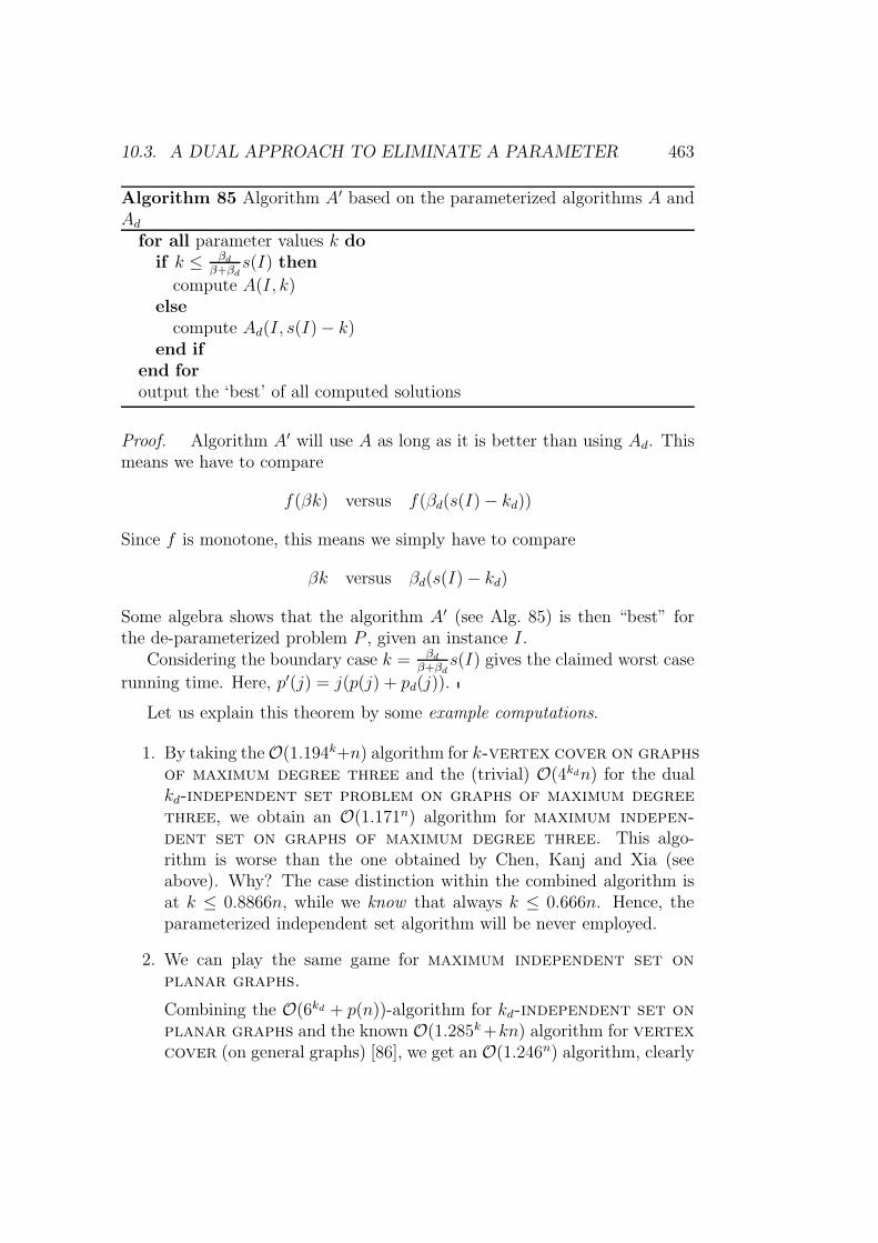
10.3. A DUAL APPROACH TO ELIMINATE A PARAMETER 463
Algorithm 85 Algorithm A′ based on the parameterized algorithms A andAd
for all parameter values k doif k ≤ βd
β+βds(I) then
compute A(I, k)else
compute Ad(I, s(I) − k)end if
end foroutput the ‘best’ of all computed solutions
Proof. Algorithm A′ will use A as long as it is better than using Ad. Thismeans we have to compare
f(βk) versus f(βd(s(I) − kd))
Since f is monotone, this means we simply have to compare
βk versus βd(s(I) − kd)
Some algebra shows that the algorithm A′ (see Alg. 85) is then “best” forthe de-parameterized problem P , given an instance I.
Considering the boundary case k = βd
β+βds(I) gives the claimed worst case
running time. Here, p′(j) = j(p(j) + pd(j)).
Let us explain this theorem by some example computations.
1. By taking the O(1.194k+n) algorithm for k-vertex cover on graphsof maximum degree three and the (trivial) O(4kdn) for the dualkd-independent set problem on graphs of maximum degreethree, we obtain an O(1.171n) algorithm for maximum indepen-dent set on graphs of maximum degree three. This algo-rithm is worse than the one obtained by Chen, Kanj and Xia (seeabove). Why? The case distinction within the combined algorithm isat k ≤ 0.8866n, while we know that always k ≤ 0.666n. Hence, theparameterized independent set algorithm will be never employed.
2. We can play the same game for maximum independent set onplanar graphs.
Combining the O(6kd + p(n))-algorithm for kd-independent set onplanar graphs and the known O(1.285k+kn) algorithm for vertexcover (on general graphs) [86], we get an O(1.246n) algorithm, clearly
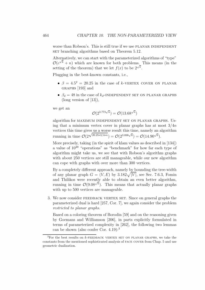
464 CHAPTER 10. THE NON-PARAMETERIZED VIEW
worse than Robson’s. This is still true if we use planar independentset branching algorithms based on Theorem 5.12.
Alternatively, we can start with the parameterized algorithms of “type”O(c
√k + n) which are known for both problems. This means (in the
setting of the theorem) that we let f(x) to be 2√x.
Plugging in the best-known constants, i.e.,
• β = 4.52 = 20.25 in the case of k-vertex cover on planargraphs [193] and
• βd = 48 in the case of kd-independent set on planar graphs(long version of [13]),
we get anO(23.773
√n) = O(13.68
√n)
algorithm for maximum independent set on planar graphs. Us-ing that a minimum vertex cover in planar graphs has at most 3/4nvertices this time gives us a worse result this time, namely an algorithm
running in time O(2√
20.25∗3/4∗n) = O(23.898√n) = O(14.90
√n).
More precisely, taking (in the spirit of klam values as described in [134])a value of 1020 “operations” as “benchmark” for how far each type ofalgorithm might take us, we see that with Robson’s algorithm graphswith about 250 vertices are still manageable, while our new algorithmcan cope with graphs with over more than 300 vertices.
By a completely different approach, namely by bounding the tree-widthof any planar graph G = (V,E) by 3.182
√|V |, see Sec. 7.6.3, Fomin
and Thilikos were recently able to obtain an even better algorithm,running in time O(9.08
√n). This means that actually planar graphs
with up to 500 vertices are manageable.
3. We now consider feedback vertex set. Since on general graphs theparameterized dual is hard [257, Cor. 7], we again consider the problemrestricted to planar graphs.
Based on a coloring theorem of Borodin [59] and on the reasoning givenby Goemans and Williamson [206], in parts explicitly formulated interms of parameterized complexity in [262], the following two lemmascan be shown (also confer Cor. 4.19):3
3For the best results on k-feedback vertex set on planar graphs, we take theconstants from the mentioned sophisticated analysis of face cover from Chap. 5 and usegeometric dualization.
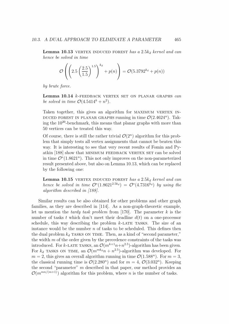
10.3. A DUAL APPROACH TO ELIMINATE A PARAMETER 465
Lemma 10.13 vertex induced forest has a 2.5kd kernel and canhence be solved in time
O
(
2.5
(2.5
1.5
)1.5)kd
+ p(n)
= O(5.3792kd + p(n))
by brute force.
Lemma 10.14 k-feedback vertex set on planar graphs canbe solved in time O(4.5414k + n2).
Taken together, this gives an algorithm for maximum vertex in-duced forest in planar graphs running in time O(2.4624n). Tak-ing the 1020-benchmark, this means that planar graphs with more than50 vertices can be treated this way.
Of course, there is still the rather trivial O(2n) algorithm for this prob-lem that simply tests all vertex assignments that cannot be beaten thisway. It is interesting to see that very recent results of Fomin and Py-atkin [188] show that minimum feedback vertex set can be solvedin time O∗(1.8621n). This not only improves on the non-parameterizedresult presented above, but also on Lemma 10.13, which can be replacedby the following one:
Lemma 10.15 vertex induced forest has a 2.5kd kernel and canhence be solved in time O∗(1.86212.5kd) = O∗(4.7316kd) by using thealgorithm described in [188].
Similar results can be also obtained for other problems and other graphfamilies, as they are described in [114]. As a non-graph-theoretic example,let us mention the tardy task problem from [170]. The parameter k is thenumber of tasks t which don’t meet their deadline d(t) on a one-processorschedule, this way describing the problem k-late tasks. The size of aninstance would be the number n of tasks to be scheduled. This defines thenthe dual problem kd tasks on time. Then, as a kind of “second parameter,”the width m of the order given by the precedence constraints of the tasks wasintroduced. For k-late tasks, an O(mk+1n+n2.5)-algorithm has been given.For kd tasks on time, an O(mmkdn + n2.5)-algorithm was developed. Form = 2, this gives an overall algorithm running in time O(1.588n). For m = 3,the classical running time is O(2.280n) and for m = 4, O(3.032n). Keepingthe second “parameter” m described in that paper, our method provides anO(mmn/(m+1)) algorithm for this problem, where n is the number of tasks.

466 CHAPTER 10. THE NON-PARAMETERIZED VIEW
Chapter 11
The WWW repository
In the following, we present a list of sites on the WWW where papers, talksetc. on parameterized complexity and algorithmics can be found. Of course,this list is neither meant to be exhaustive nor can it be guaranteed thatall items still “work” when you try to follow them up. This is one of theunfortunate consequences of the dynamic nature of the World Wide Web.Nonetheless, the list may give useful hints where to find more about thisarea.
1. The web resources on algorithmics are very impressive nowadays. Forthe contents of this books, in particular http://www.nist.gov/dads/is of interest, a rather recently built “Dictionary of Algorithms andData Structures.”
2. A good account on Bell’s number can be found in http://mathworld.
wolfram.com/BellNumber.html. In fact, Wolfram’s page contains acollection of many useful mathematical facts.
3. The Compendium of Parameterized Problems compiled and updatedby M. Cesati can be found at http://bravo.ce.uniroma2.it/home/cesati/research/compendium.pdf.
4. A general coverage of chess puzzles, in particular of the queens prob-lems discussed in the introductory chapter, are contained in http:
//mathworld.wolfram.com/Chess.html and in http://www.dsitri.
de/wiki.php?page=NQP. A good animation for the n×n Queens Prob-lem can be found at http://www.math.utah.edu/~alfeld/queens/
queens.html. Further hints on chess-related puzzles can be found inVelucchi’s page http://anduin.eldar.org/~problemi/papers.html.
467
468 CHAPTER 11. THE WWW REPOSITORY
5. Cliquewidth of special classes of graphs are listed in http://www.
laria.u-picardie.fr/~vanherpe/cwd/cwd.html; unfortunately, thelinks given in that page are usually out of date. The most autho-rative list of publications on the topic is surely the one by Courcellehimself: http://www.labri.fr/Perso/~courcell/ActSci.html. Re-garding “older” publications http://www.labri.fr/Perso/~courcell/Textes/BiblioReecritureGraphes%281995%29.pdf contains a rathercomprehensive survey with the title “Reecriture de graphes: orientationbibliographique.”
6. http://www.ics.uci.edu/~eppstein/junkyard/euler/ contains aninteresting collection of 17 different proofs for Euler’s formula that saysthat, for any connected plane graph G = (V,E),
|V | − |E| + |F | = 2,
where F is the set of faces of G. Nice 3D-visualizations for vari-ous embeddings onto the “sphere” (this is how these drawings canbe interpreted) can be found in http://www.math.ohio-state.edu/
~fiedorow/math655/Euler.html. A simple deduction of the fact thateach planar graph has (at least one) vertex of degree at most five can befound in http://www-math.mit.edu/18.310/planarity_coloring.
html.
The other entries in Eppstein’s “junkard” are also recommendable, sogive it a try!
7. http://www.math.gatech.edu/~thomas/FC/fourcolor.html gives abrief summary of a new proof of the Four Color Theorem and a four-coloring algorithm found by Neil Robertson, Daniel P. Sanders, PaulSeymour and Robin Thomas.
8. http://wwwteo.informatik.uni-rostock.de/isgci contains a nicecollection of graph classes and their interrelations.
9. Many nice examples of Mathematical Games that can be formulated asinteger linear programs or as graph problems can be found at http://ite.informs.org. This site (and the corresponding electronic journal)is devoted to the presentation of Operations Research techniques in ed-ucation. Nice and recommendable is also the site http://www.chlond.demon.co.uk/academic/puzzles.html called “Integer Programmingin Recreational Mathematics.”

469
10. http://tracer.lsi.upc.es/minla/minla_info.php seems to be aplace where up-to-date information on linear arrangement is kept.
11. http://www.algorithmic-solutions.com/enledabeschreibung.htm
contains a description of the (formerly public domain) software packageLEDA. To quote from that websited: LEDA provides algorithmic in-depth knowledge in the field of graph- and network problems, geometriccomputations, combinatorial opimization and other.
12. The slides of the talk of D. Marx at CCC / Freiburg can be foundat http://www.cs.bme.hu/~dmarx/papers/marx-freiburg-slides.pdf. The picture of the mentioned Swiss army knife is on page 6.
13. Searching through the internet for notions like matching will give youmany hits, including good slides etc. One example is http://www.cs.rpi.edu/~goldberg/05-AAH/matching.pdf which also shows a nice il-lustration of a proof of Theorem 4.30. Nice applications of Hall’s The-orem can be found in the coursenotes http://www.stat.uchicago.
edu/~lalley/Courses/388/Matching.pdf.
14. http://mathworld.wolfram.com is a very nice, easily accessible internet-based mathematical dictionary.
15. There are research groups dedicated to model-based reasoning through-out the world. A European example is http://www.cs.ru.nl/~peterl/mbr.html, where further pointers can be found.
16. The site http://parc.lboro.ac.uk/research/projects/parseqgd/
not only contains a good project description of a recent project dedi-cated to graph drawing, in particular, to crossing minimization prob-lems, but also some nice overview papers, e.g., [106].
17. The background on Roman domination is nicely described in theonline John Hopkins Magazine, more specifically, look into http://
www.jhu.edu/~jhumag/0497web/locate3.html. Interestingly, a smallexercise in connection with that problem is posed, whose solution ispresented in http://www.jhu.edu/~jhumag/0697web/revelle.html.
18. http://dept-info.labri.u-bordeaux.fr/~robson/mis/techrep.html
contains a HTML version of the currently best algorithm for maximumindependent set, see [343]. Also, the mathematical background ex-plaining the analysis of the memorization part of the algorithm can befound in that directory.

470 CHAPTER 11. THE WWW REPOSITORY
19. We simply quote from the Homepage of Thinkfun: http://www.puzzles.com/products/rushhour.htm: “Rush Hour is a genuine puzzle phe-nomenon with legions of fans. There are some great places on the Webdedicated to this most successful sliding block puzzle of these years.We’d like to introduce here some of them. Good Luck!” As can beseen, there are numerous links on Rush Hour to be found at that site.

Chapter 12
Problems
In this chapter, we collect all definitions of problems encountered in thisbook. In a certain way, this collection also complements the correspondingappendix in [134]. However, since we are mostly dealing with graph problemsin this book, we will rather have a finer grained classification of those graphproblem lists; problems from other areas will we rather scarce.
12.1 Cover problems and their relatives
Problem name: vertex cover (VC)Given: A graph G = (V,E)Parameter: a positive integer kOutput: Is there a vertex cover C ⊆ V with |C| ≤ k?
From the viewpoint of classical complexity, the following two problems areeqivalent to vertex cover.
Problem name: clique (CQ)Given: A graph G = (V,E)Parameter: a positive integer kOutput: Is there a clique C ⊆ V with |C| ≥ k?
Problem name: independent set (IS)
471

472 CHAPTER 12. PROBLEMS
Given: A graph G = (V,E)Parameter: a positive integer kOutput: Is there an independent set I ⊆ V with |I| ≥ k?
Also variants of this problem can be considered. In this text, we looked at:
Problem name: generalized vertex cover (VCgen)Given: A graph G = (V,E), a subset V ′ of verticesParameter: a positive integer kOutput: Is there a vertex cover C ⊆ V ′ with |C| ≤ k?
Problem name: clique (CQE)Given: A graph G = (V,E)Parameter: a positive integer kOutput: Is there a edge-induced clique C ⊆ E with |C| ≥ k?
Problem name: profit vertex cover (PrVC)Given: A graph G = (V,E)Parameter: a positive integer pOutput: Is there a profit vertex cover C ⊆ V with |E|−|E(G[V \C])|−|C| ≥p?
Problem name: t-vertex cover (tVC)Given: A graph G = (V,E)Parameter: positive integers k and tOutput: Is there a t-vertex cover C ⊆ V with |C| ≤ k, i.e., |e ∈ E |C ∩ e 6= ∅| = |E| − |E(G[V \ C])| ≥ t?
Problem name: miniaturized vertex cover (VCmini)Given: A graph G = (V,E)Parameter: a positive integer kOutput: Is there a vertex cover C ⊆ V with |C| ≤ k log(|V |)?
Problem name: clique complement cover (CCC)

12.1. COVER PROBLEMS AND THEIR RELATIVES 473
Given: A graph G = (V,E)Parameter: a positive integer kOutput: Is there a clique complement cover C ⊆ E with |C| ≤ k?
Problem name: vertex clique complement cover (VCCC)Given: A graph G = (V,E)Parameter: a positive integer kOutput: Is there a vertex clique complement cover C ⊆ V with |C| ≤ k?
Problem name: planar independent set (PIS)Given: A planar graph G = (V,E)Parameter: a positive integer kOutput: Is there an independent set I ⊆ V with |I| ≥ k?
Problem name: independent set on disks graphs (DIS)Given: A disk graph G = (V,E) whose disk model has radii between 1 andα and is λ-precisionParameter: a positive integer kOutput: Is there an independent set I ⊆ V with |I| ≥ k?
Problem name: weighted vertex cover (WVC)Given: A graph G = (V,E) with vertex weights ω : V → R≥1
Parameter: a positive integer kOutput: Is there a vertex cover C ⊆ V with ω(C) ≤ k?
Problem name: constraint bipartite vertex cover (CBVC)Given: A bipartite graph G = (V1, V2, E)Parameter: positive integers k1, k2
Output: Is there a vertex cover C ⊆ V1 ∪ V2 with |C ∩ Vi| ≤ ki for i = 1, 2?
Problem name: vertex cover, parameterized by number of ver-tices of degree three or larger (VCdeg)Given: A graph G = (V,E)Parameter: a positive integer ` that equals the number of vertices in G ofdegree three or larger

474 CHAPTER 12. PROBLEMS
Output: What is the size of a minimum vertex cover C ⊆ V ?
Problem name: vertex cover, parameterized by treewidth (VCTW)Given: A graph G = (V,E) together with some tree decompositionParameter: a positive integer k that equals the width of the tree decompo-sitionOutput: What is the size of a minimum vertex cover C ⊆ V ?
Problem name: counting independent set of queens (CQIS)Given: An n× n chessboard CParameter: a positive integer nOutput: In how many ways can n queens be positioned on C such that notwo of them are mutually attacking?
12.2 Dominating problems and their relatives
Another important graph-theoretic problem is:
Problem name: dominating set (DS)Given: A graph G = (V,E)Parameter: a positive integer kOutput: Is there a dominating set D ⊆ V with |D| ≤ k?
Again, variants can be considered:
Problem name: planar dominating set (PDS)Given: A planar graph G = (V,E)Parameter: a positive integer kOutput: Is there a dominating set D ⊆ V with |D| ≤ k?
Problem name: dominating set on bounded genus graphsGiven: A graph G = (V,E) of genus bounded by γ

12.2. DOMINATING PROBLEMS AND THEIR RELATIVES 475
Parameter: a positive integer kOutput: Is there a dominating set D ⊆ V with |D| ≤ k?
Problem name: red-blue dominating set (RBDS)Given: A graph G = (V,E) with V partitioned as Vred ∪ Vblue
Parameter: a positive integer kOutput: Is there a red-blue dominating set D ⊆ Vred with |D| ≤ k, i.e.,Vblue ⊆ N(D)?
Problem name: Roman domination (ROMAN)Given: A graph G = (V,E)Parameter: a positive integer kOutput: Is there a Roman domination function R such that
∑x∈V R(x) ≤
k?
Problem name: planar Roman domination (pROMAN)Given: A planar graph G = (V,E)Parameter: a positive integer kOutput: Is there a Roman domination function R such that
∑x∈V R(x) ≤
k?
Problem name: dominating rearrangement (DR)Given: A graph G = (V,E), a subset S ⊆ VParameter: a positive integer k = |S|Output: Is there a dominating rearrangement r : S → N [S], s 7→ r(s) ∈N [s] such that r(S) ⊆ V is a dominating set?
Problem name: dominating set, given vertex cover number (DSvc)Given: A graph G = (V,E)Parameter: a positive integer k such that G has a vertex cover of size kOutput: Is there a minimum dominating set D ⊆ V ?
Problem name: constraint bipartite dominating set (CBDS)Given: A bipartite graph G = (V1, V2, E)Parameter: positive integers k1, k2

476 CHAPTER 12. PROBLEMS
Output: Is there a dominating set D ⊆ V1 ∪ V2 with |D ∩ Vi| ≤ ki fori = 1, 2?
Problem name: independent dominating set (IDS)Given: A graph G = (V,E)Parameter: a positive integer kOutput: Is there an independent dominating set D ⊆ V with |D| ≤ k?
Problem name: planar independent dominating set (PIDS)Given: A planar graph G = (V,E)Parameter: a positive integer kOutput: Is there a independent dominating set D ⊆ V with |D| ≤ k?
Problem name: connected dominating set (CDS)Given: A graph G = (V,E)Parameter: a positive integer kOutput: Is there a connected dominating set D ⊆ V with |D| ≤ k, i.e., Dis both a connected set and a dominating set?
Problem name: nonblocker set (NB)Given: A graph G = (V,E)Parameter: a positive integer kdOutput: Is there a nonblocker set N ⊆ V with |N | ≥ kd?
Problem name: nonblocker set with catalytic vertex (NBcat)Given: A graph G = (V,E), a catalytic vertex cParameter: a positive integer kdOutput: Is there a nonblocker set N ⊆ V with |N | ≥ kd such that c /∈ N?
Problem name: dominating set of queens (QDS)Given: An n× n chessboard CParameter: a positive integer kOutput: Is it possible to place k queens on C such that all squares aredominated ?

12.3. GRAPH MODIFICATION PROBLEMS 477
Problem name: dominating set of queens (QDS), parameterizedabove guaranteed valueGiven: An n× n chessboard CParameter: a positive integer kOutput: Is it possible to place n/2 + k queens on C such that all squaresare dominated ?
Likewise, edges or faces may be in the focus of domination:
Problem name: edge dominating set (EDS)Given: A graph G = (V,E)Parameter: a positive integer kOutput: Is there an edge dominating set D ⊆ E with |D| ≤ k?
Problem name: generalized edge dominating set (GEDS)Given: A graph G = (V,E), a set R ⊆ V of red verticesParameter: a positive integer kOutput: Is there an edge dominating set D ⊆ E with |D| ≤ k such that allvertices from R are covered by D?
Problem name: weighted edge dominating set (WEDS)Given: A graph G = (V,E) with edge weights ω : E → R≥1
Parameter: a positive integer kOutput: Is there an edge dominating set D ⊆ E with ω(D) ≤ k?
12.3 Graph modification problems
Graph modification problems deliver a wealth of hard problems that tend toclassify in FPT . The examples contained here are:
Problem name: triangle edge deletion (TED)Given: A graph G = (V,E)

478 CHAPTER 12. PROBLEMS
Parameter: a positive integer kOutput: Is there an edge set C ⊆ E with |C| ≤ k whose removal producesa graph without triangles as vertex-induced subgraphs?
Problem name: triangle vertex deletion (TVD)Given: A graph G = (V,E)Parameter: a positive integer kOutput: Is there an vertex set C ⊆ V with |C| ≤ k whose removal producesa graph without triangles as vertex-induced subgraphs?
Problem name: cluster vertex deletion (CVD)Given: A graph G = (V,E)Parameter: a positive integer kOutput: Is there an vertex set C ⊆ V with |C| ≤ k whose removal producesa graph being a union of vertex-induced cliques?
Problem name: cograph vertex deletion (CoVD)Given: A graph G = (V,E)Parameter: a positive integer kOutput: Is there an vertex set C ⊆ V with |C| ≤ k whose removal producesa cograph ?
Problem name: bipartization (BP)Given: A graph G = (V,E)Parameter: a positive integer kOutput: Is there a bipartization set C ⊆ V with |C| ≤ k whose removalproduces a bipartite graph?
Problem name: bipartization improvementGiven: A graph G = (V,E), a bipartization set C ⊆ V with |C| = k + 1Parameter: a positive integer kOutput: Is there a bipartization set C ′ ⊆ V with |C ′| ≤ k ?
Problem name: bipartization, edge variant (BPedge)Given: A graph G = (V,E)

12.3. GRAPH MODIFICATION PROBLEMS 479
Parameter: a positive integer kOutput: Is there a bipartization set C ⊆ E with |C| ≤ k whose removalproduces a bipartite graph?
Also, cover-like problems can be viewed as graph modification problems.Examples discussed in the text are:
Problem name: feedback vertex set (FVS)Given: A (simple) graph G = (V,E)Parameter: a positive integer kOutput: Is there a feedback vertex set of size at most k, i.e.,
∃F ⊆ V, |F | ≤ k, ∀c ∈ C(G)(F ∩ c 6= ∅)?
Here, C(G) denotes the set of cycles of G, where a cycle is a sequence of ver-tices (also interpreted as a set of vertices) v0, v1, . . . , v` such that vi, v(i+1) mod ` ∈E for i = 0, . . . , `− 1.
Problem name: feedback edge set (FES)Given: A (simple) graph G = (V,E)Parameter: a positive integer kOutput: Is there a feedback edge set of size at most k, i.e.,
∃F ⊆ E, |F | ≤ k, ∀c ∈ C(G)(F ∩ c 6= ∅)?
Here, C(G) denotes the set of cycles of G, where a cycle is a sequence of ver-tices (also interpreted as a set of edges) v0, v1, . . . , v` such that vi, v(i+1) mod ` ∈E for i = 0, . . . , `− 1.
as well as their duals:
Problem name: vertex induced forest (ViF)Given: a (simple) graph G = (V,E)Parameter: a positive integer kdOutput: Is there a vertex-induced forest of size at least kd, i.e.,
∃F ⊆ V, |F | ≥ kd, C(G[F ]) = ∅?

480 CHAPTER 12. PROBLEMS
Problem name: edge induced forest (EiF)Given: a (simple) graph G = (V,E)Parameter: a positive integer kdOutput: Is there a edge-induced forest of size at least kd, i.e.,
∃F ⊆ E, |F | ≥ kd, C(G[E]) = ∅?
On planar graphs, corresponding problems are:
Problem name: face cover (FC)Given: A plane graph G = (V,E) with face set FParameter: a positive integer kOutput: Is there a face cover set C ⊆ F with |C| ≤ k?
Problem name: vertex induced forest in planar graphs (PViF)Given: a (simple) planar graph G = (V,E)Parameter: a positive integer kdOutput: Is there a vertex-induced forest of size at least kd, i.e.,
∃F ⊆ V, |F | ≥ kd, C(G[F ]) = ∅?
12.4 Further graph-theoretic problems
Further graph-theoretic problems discussed in the text include:
Problem name: maximum leaf spanning tree (MaxLST)Given: A (simple) graph G = (V,E)Parameter: a positive integer kd

12.4. FURTHER GRAPH-THEORETIC PROBLEMS 481
Output: Is there a spanning tree of G with at least kd leaves?
Problem name: minimum inner node spanning tree (MinINST)Given: A (simple) graph G = (V,E)Parameter: a positive integer kOutput: Is there a spanning tree of G with at most k inner nodes?
Problem name: minimum maximal independent set (MMIS)Given: A graph G = (V,E)Parameter: a positive integer kOutput: Does there exist a maximal independent set of cardinality ≤ k ?
Problem name: maximum minimal vertex cover (MMVC)Given: A graph G = (V,E)Parameter: a positive integer kOutput: Does there exist a minimal vertex cover set of cardinality ≥ k ?
Problem name: maximum minimal dominating set (MMDS)Given: A graph G = (V,E)Parameter: a positive integer kOutput: Does there exist a minimal dominating set of cardinality ≥ k ?
Problem name: maximum cut (MAXCUT)Given: A graph G = (V,E)Parameter: a positive integer kOutput: Is there a cut set C ⊆ E with |C| ≥ k, i.e., (V, V \C) is a bipartitegraph?
Problem name: separating vertex sets enumeration (SVS)Given: A graph G = (V,E)Parameter: a positive integer kOutput: Enumerate all minimum size separating vertex sets of size at mostk.

482 CHAPTER 12. PROBLEMS
12.5 Graph drawing problems
The following problems can be considered as graph drawing problems.
Problem name: crossing number (CRN)Given: A graph G = (V,E)Parameter: a positive integer kOutput: Is CR(G) ≤ k?
Problem name: bandwidth (BW)Given: A graph G = (V,E)Parameter: a positive integer kOutput: Is there a one-to-one mapping σ : V → 1, . . . , |V | such that∀u, v ∈ E : |σ(u) − σ(v)| ≤ k?
Problem name: cutwidth (CW)Given: A graph G = (V,E)Parameter: a positive integer kOutput: Is there a one-to-one mapping σ : V → 1, . . . , |V | such that∀1 ≤ i < |V | : |u, v ∈ E | σ(u) ≤ i < σ(v)| ≤ k?
Problem name: linear arrangement (LA)Given: A graph G = (V,E)Parameter: a positive integer kOutput: Is there a one-to-one mapping σ : V → 1, . . . , |V | such that
∑
u,v∈E|σ(u) − σ(v)| ≤ k ?
Problem name: linear arrangement (LA), parameterized aboveguaranteed valueGiven: A graph G = (V,E)Parameter: a positive integer k

12.5. GRAPH DRAWING PROBLEMS 483
Output: Is there a one-to-one mapping σ : V → 1, . . . , |V | such that
∑
u,v∈E|σ(u) − σ(v)| ≤ k + |E|?
Problem name: directed linear arrangement (DLA)Given: A directed graph G = (V,A)Parameter: a positive integer kOutput: Is there a one-to-one mapping σ : V → 1, . . . , |V | that respectsthe orientation of G, i.e., σ(u) < σ(v) whenever (u, v) ∈ A, such that
∑
(u,v)∈A|σ(u) − σ(v)| ≤ k ?
Problem name: directed linear arrangement (DLA), parame-terized above guaranteed valueGiven: A directed graph G = (V,A)Parameter: a positive integer kOutput: Is there a one-to-one mapping σ : V → 1, . . . , |V | that respectsthe orientation of G such that
∑
(u,v)∈A|σ(u) − σ(v)| ≤ k + |A| ?
Problem name: linear arrangement by deleting edges (LADE)Given: A graph G = (V,E)Parameter: a positive integer kOutput: Is there an edge set E ′ with |E ′| ≤ k and a one-to-one mappingσ : V → 1, . . . , |V | such that
∑
u,v∈E\E′
|σ(u) − σ(v)| = |E \ E ′| ?

484 CHAPTER 12. PROBLEMS
Problem name: one-sided crossing minimization (OSCM)Given: A bipartite graph G = (V1, V2, E) and a linear order ≺1 on V1.Parameter: a positive integer kOutput: Is there a linear order ≺ on V2 such that, when the vertices from V1
are placed on a line (also called layer) L1 in the order induced by ≺1 and thevertices from V2 are placed on a second layer L2 (parallel to L1) in the orderinduced by ≺, then drawing straight lines for each edge in E will introduceno more than k edge crossings?
Problem name: two-layer planarization (TLP)Given: A graph G = (V,E)Parameter: a positive integer kOutput: Is there a set C ⊆ E, |C| ≤ k, whose removal makes the graphbiplanar?
Problem name: one-layer planarization (OLP)Given: A bipartite graph G = (V1, V2, E), a linear ordering < on V1
Parameter: a positive integer kOutput: Is there a set C ⊆ E, |C| ≤ k, whose removal allows a biplanardrawing of the graph that respects < on V1?
Problem name: two-tree crossing minimization (TTCM)Given: A two-tree (T1, T2) with leaf labels ΛParameter: a positive integer kOutput: Can (T1, T2) be drawn with at most k crossings ?
Problem name: one-tree crossing minimization (OTCM)Given: A two-tree (T1, T2) with leaf labels Λ, where the ordering of thevertices of T1 is fixedParameter: a positive integer kOutput: Can (T1, T2) be drawn with at most k crossings ?
Problem name: two-tree drawing by deleting edges (TTDE)Given: A two-tree (T1, T2) with leaf labels ΛParameter: a positive integer kOutput: Is there a label set L ⊆ Λ with |L| ≤ k such that the two-tree
12.6. HYPERGRAPH PROBLEMS 485
(T1 〈Λ \ L〉 , T2 〈Λ \ L〉) can be drawn without crossings ?
Problem name: one-tree drawing by deleting edges (OTDE)Given: A binary tree T1 with leaf labels Λ, a linear ordering ≺ on ΛParameter: a positive integer kOutput: Is there a label set L ⊆ Λ with |L| ≤ k such that the tree T1 〈Λ \ L〉can be drawn without crossings in the plane, so that the leaves in Λ \ L arearranged according to the ordering ≺ on some line ?
12.6 Hypergraph problems
Problem name: d-hitting set (d-HS)Given: A hypergraph G = (V,E) with hyperedge size bounded by dParameter: a positive integer kOutput: Is there a hitting set C ⊆ V with |C| ≤ k?
Problem name: minimum hitting set, parameterized by # edges(HSE)Given: A hypergraph G = (V,E)Parameter: |E|Output: Find a minimum hitting set C ⊆ V
Problem name: set cover (SC)Given: A groundset X, a collection T of subsets of XParameter: a positive integer kOutput: Is there a set cover C ⊆ T with |C| ≤ k, i.e., every element in Xbelongs to at least one member of C?
Problem name: multi-hitting set (HSmulti)Given: A hypergraph G = (V,E)Parameter: positive integers k, `Output: Is there a multi-hitting set C ⊆ V with |C| ≤ k, i.e., C satisfies
486 CHAPTER 12. PROBLEMS
∀e ∈ E∃c ⊆ e(|c| ≥ ` ∧ c ⊆ C)?
12.7 Network problems
Problem name: CallControlGiven: A communication network represented by an undirected graph G =(V,E) with edge capacities c : E → N, a set R ⊆ V × V of communicationrequestsParameter: a positive integer kOutput: Is there a subset A ⊂ R and a corresponding feasible path setp(A) resulting from assigning to each request r ∈ A some path p(r) suchthat p(A) is feasible and the set of rejected requests R \ A contains no morethan k elements?
Problem name: CallControl-PreGiven: A communication network represented by an undirected graph G =(V,E) with edge capacities c : E → N, a set R ⊆ V × V of communicationrequests, a path assigning function p : R → P (G)Parameter: a positive integer kOutput: Is there a subset A ⊂ R such that p(A) is feasible and the set ofrejected requests R \ A contains no more than k elements?
Problem name: d-CallControl-PreGiven: A communication network represented by an undirected graph G =(V,E) with edge capacities c : E → N, a set R ⊆ V × V of communicationrequests, a path assigning function p : R → P (G)Parameter: a positive integer k, an edge capacity bound dOutput: Is there a subset A ⊂ R such that p(A) is feasible and the set ofrejected requests R \ A contains no more than k elements?
Problem name: CallControl in trees of ringsGiven: A communication network represented by an undirected graph G =(V,E) that is a tree of rings with unit edge capacities, a set R ⊆ V × V of

12.8. AUTOMATA PROBLEMS 487
communication requestsParameter: a positive integer kOutput: Is there a subset A ⊂ R and a path assigning function p : R →P (G) such that p(A) is feasible and the set of rejected requests R\A containsno more than k elements?
Problem name: CallControl in trees with capacities one ortwo (CallControl in trees 1-2)Given: A communication network represented by an undirected graph G =(V,E) that is a tree with Ei ⊆ E being the edges of capacity i ∈ 1, 2, aset R ⊆ V × V of communication requests, a positive integer kParameter: ` = |E2|Output: Is there a subset A ⊂ R and a path assigning function p : R →P (G) such that p(A) is feasible and the set of rejected requests R\A containsno more than k elements?
12.8 Automata problems
Problem name: short nondeterministic small Turing machinecomputation (SNSTMC)Given: A (single-tape) nondeterministic Turing machine M whose size isbounded by f(k), an input string xParameter: a positive integer kOutput: Is there an accepting computation of M on input x that reaches afinal accepting state in at most k steps?
Problem name: short nondeterministic Turing machine compu-tation (SNTMC)Given: A (single-tape) nondeterministic Turing machine M , an input stringxParameter: a positive integer kOutput: Is there an accepting computation of M on input x that reaches afinal accepting state in at most k steps?

488 CHAPTER 12. PROBLEMS
Problem name: short multi-tape nondeterministic Turing ma-chine computation (SMNTMC)Given: A multi-tape nondeterministic Turing machine M , an input stringxParameter: a positive integer kOutput: Is there an accepting computation of M on input x that reaches afinal accepting state in at most k steps?
Problem name: bounded nondeterminism Turing machine compu-tation (BNTMC)Given: A (single-tape) nondeterministic Turing machine M , an input stringx, an integer n coded in unaryParameter: a positive integer kOutput: Is there an accepting computation of M on input x that reaches afinal accepting state in at most n steps and uses at most k nondeterministicsteps?
Problem name: compact deterministic Turing machine computa-tion (CDTMC)Given: A deterministic Turing machine M , an input string xParameter: a positive integer kOutput: Is there an accepting computation of M on input x that visits atmost k squares?
12.9 Logical problems
Logical problems might have deserved more attention in this book. Here area few of them, anyways:Problem name: maximum satisfiability (MAXSAT)Given: A Boolean formula F in conjunctive normal form (CNF), with vari-ables XParameter: a positive integer kOutput: Is there an assignment α : X → 0, 1 such that at least k clausesin F evaluate to 1 (true) under α?

12.10. MISCELLANEOUS AND APPLICATIONS 489
Problem name: maximum satisfiability (MAXSAT), parameter-ized above guaranteed valueGiven: A Boolean formula F in conjunctive normal form (CNF), with vari-ables XParameter: a positive integer kOutput: Is there an assignment α : X → 0, 1 such that at least m/2 + kclauses in F evaluate to 1 (true) under α?
Problem name: satisfiability problem with clauses of size three(clause parameterization) (3-SAT)Given: A Boolean formula F in conjunctive normal form (CNF), with vari-ables X, each clause having at most three literalsParameter: a positive integer k, upperbounding the number of clauses ofsize threeOutput: Is there a satisfying assignment α : X → 0, 1 for F ?
Problem name: satisfiability problem with clauses of size three(variable parameterization) (3-SAT (variable))Given: A Boolean formula F in conjunctive normal form (CNF), with vari-ables X, each clause having at most three literalsParameter: |X|Output: Is there a satisfying assignment α : X → 0, 1 for F ?
12.10 Miscellaneous and applications
Some problems don’t fit into the categories listed above. They are collectedhere.
Problem name: maximum agreement subtree (MAST)Given: A set T1, . . . , Tn of binary rooted trees with equal label set L =L(T1) = · · · = L(Tn)Parameter: a positive integer kOutput: Is there a set of labels L′ ⊆ L, |Λ| ≤ k, such that all trees Ti \ Λare isomorphic?

490 CHAPTER 12. PROBLEMS
Problem name: spare allocation (SAP)Given: A n × m binary matrix A representing an erroneous chip withA[r, c] = 1 iff the chip is faulty at position [r, c]Parameter: positive integers k1, k2
Output: Is there a reconfiguration strategy that repairs all faults and usesat most k1 spare rows and at most k2 spare columns?
Problem name: minimal diagnosis (MD)Given: A finite set of faults F , a set of effects M , a function e : F → 2M
relating faults and effects, a set of observed effects M ′ ⊆M , an integer kParameter: the (size of the) relating function eOutput: Is there a set F ′ ⊂ F with |F ′| ≤ k such that M ′ ⊆ ⋃f∈F ′ e(f)?
Problem name: matrix domination set (MDS)Given: A n× n matrix with entries from 0, 1, positive integer kParameter: kOutput: Is there a set D of one-entries in the matrix, where |D| ≤ k, suchthat every other one-entry has at least one row or one column in commonwith some one-entry from D?
Problem name: matrix row column merging (MRCM)Given: a n×m 0, 1-matrix MParameter: a positive integer kOutput: Is it possible to get the all-zeros-matrix by merging at most kneighboring rows or columns?
Problem name: module placement problem (MPP)Given: a set of modules M , a set of wires W connecting modules, i.e., eachwire w ∈ W is a subset of MParameter: a positive integer kOutput: Is it possible to find a mapping σ : M → 1, . . . , |M | such thatthe overall wire length is less than or equal to k?
Problem name: positive weighted completion of an ordering

12.10. MISCELLANEOUS AND APPLICATIONS 491
(PCO)Given: An ordered digraph P = (V,A) and a cost function c mappingA(D([U(P )]c)) into the positive integers; by setting c to zero for arcs inA(D(U(P ))), we can interpret the domain of c as V (P ) × V (P ).Parameter: a positive integer k.Output: Is there a selection A′ of arcs from A(D([U(P )]c)) such that thetransitive closure (A′ ∪ A(P ))+ is a linear order and
∑c(a) | a ∈ (A′ ∪ A(P ))+ ≤ k ?
Problem name: facility location (FL)Given: A bipartite graph B = (F ] C,E), consisting of a set F of poten-tial facility locations, a set C of customers, and an edge relation E, wheref, c ∈ E indicates that c can be served from the facility (at) f ; and aweight functions wF : F → N and wE : E → N (both called w if no confusionmay arise)Parameter: k ∈ NOutput: Is there a set F ′ ⊆ F of facility locations and a set E ′ ⊆ E ofways to serve customers such that (1) E ′ ∩ F = F ′, (2) E ′ ∩ C = C, and (3)∑
f∈F ′ wF (f) +∑
e∈E′ wE(e) ≤ k?
Problem name: minimum partition (PART)Given: A finite set X = x1, . . . , xn, a weight function w : X → R≥1
Parameter: k ∈ NOutput: Is there a set Y ⊂ X such that
max∑
y∈Yw(y),
∑
z /∈Yw(y) ≤ k ?
Problem name: maximum knapsack (KS)Given: n items x1, . . . , xn with sizes si and profits pi, the knapsack ca-pacity b, and the profit threshold k. All numbers are natural numbers encoded
in binary.
Parameter: kOutput: Is there a subset of items which yield a profit larger than k and

492 CHAPTER 12. PROBLEMS
has an overall size of less than b?
Problem name: maximum knapsack, minimum weight (KSMW)Given: n items x1, . . . , xn with sizes si and profits pi, the knapsack ca-pacity b, and the profit threshold k. All numbers are natural numbers encoded
in binary.
Parameter: bOutput: Is there a subset of items which yield a profit larger than k andhas an overall size of less than b?
In Chapter 3, we discussed several algorithmic problems related to rushhour. For the rather specific definitions surrounding rush hour, we referto that section.
Problem name: rush hour, parameterized by cars (RH (cars))Given: A RH tuple (C, S, p0, d, Z) of an APR instanceParameter: a positive integer k, upperbounding |C|Output: Is there a sequence of legal moves that solves the given RH in-stance?
Problem name: rush hour, parameterized by moves (RH (moves))Given: A RH tuple (C, S, p0, d, Z) of an APR instanceParameter: a positive integer mOutput: Is there a sequence of at most m legal moves that solves the givenRH instance?
Bibliography
[1] J. A. Abraham et al. Fault tolerance techniques for systolic arrays.IEEE Computer, pages 65–75, July 1987.
[2] F. Abu-Khzam and M. Langston. A direct algorithm for the parame-terized face cover problem. In R. Downey, M. Fellows, and F. Dehne,editors, International Workshop on Parameterized and Exact Compu-tation IWPEC 2004, volume 3162 of LNCS, pages 213–222. Springer,2004.
[3] F. N. Abu-Khzam, R. L. Collins, M. R. Fellows, M. A. Langston, W. H.Sutters, and C. T. Symons. Kernelization algorithms for the vertexcover problem: Theory and experiments. In L. Arge, G. F. Italiano, andR. Sedgewick, editors, Proceedings of the Sixth Workshop on AlgorithmEngineering and Experiments and the First Workshop on Analytic Al-gorithmics and Combinatorics, New Orleans, LA, USA, January 10,2004, pages 62–69. SIAM, 2004.
[4] N. Adam and J. Wortmann. Security-control methods for statisticaldatabases: A comparative study. ACM Computing Surveys, 21:515–556, 1989.
[5] D. Adolphson and T. C. Hu. Optimal linear orderings. SIAM J[ournalof] Appl[ied] Math[ematics], 25:403–423, 1973.
[6] V. A. Aksionov, O. V. Borodin, L. S. Mel’nikov, G. Sabidussi, M. Stieb-itz, and B. Toft. Deeply asymmetric planar graphs. Technical ReportPP–2000–14, University of Southern Denmark, IMADA, Odense, Den-mark, September 2000.
[7] J. Alber. Exact Algorithms for NP-hard Problems on Networks: Design,Analysis, and Implementation. Dissertation, Universitat Tubingen,2002.
493

494 BIBLIOGRAPHY
[8] J. Alber, H. L. Bodlaender, H. Fernau, T. Kloks, and R. Niedermeier.Fixed parameter algorithms for dominating set and related problemson planar graphs. Algorithmica, 33:461–493, 2002.
[9] J. Alber, H. L. Bodlaender, H. Fernau, and R. Niedermeier. Fixedparameter algorithms for planar dominating set and related problems.In M. M. Halldorsson, editor, 7th Scandinavian Workshop on AlgorithmTheory SWAT 2000, volume 1851 of LNCS, pages 97–110, 2000.
[10] J. Alber, F. Dorn, and R. Niedermeier. Experimental evaluation of atree decomposition based algorithm for vertex cover on planar graphs.Discrete Applied Mathematics, 145:219–231, 2005.
[11] J. Alber, H. Fan, M. R. Fellows, H. Fernau, R. Niedermeier, F. Rosa-mond, and U. Stege. Refined search tree techniques for the planardominating set problem. In J. Sgall, A. Pultr, and P. Kolman, ed-itors, Mathematical Foundations of Computer Science (MFCS 2001),volume 2136 of LNCS, pages 111–122. Springer, 2001. Long version toappear in Journal of Computer and System Sciences.
[12] J. Alber, M. R. Fellows, and R. Niedermeier. Polynomial-time datareduction for dominating set. Journal of the ACM, 51(3), 2004.
[13] J. Alber, H. Fernau, and R. Niedermeier. Parameterized complex-ity: exponential speedup for planar graph problems. In F. Orejas,P. G. Spirakis, and J. v. Leeuwen, editors, International Colloquiumon Automata, Languages and Programming ICALP’01, volume 2076 ofLNCS, pages 261–272. Springer, 2001.
[14] J. Alber, H. Fernau, and R. Niedermeier. Graph separators: a param-eterized view. Journal of Computer and System Sciences, 67:808–832,2003.
[15] J. Alber, H. Fernau, and R. Niedermeier. Parameterized complexity:exponential speedup for planar graph problems. Journal of Algorithms,52:26–56, 2004.
[16] J. Alber and J. Fiala. Geometric separation and exact solutions forthe parameterized independent set problem on disk graphs. Journal ofAlgorithms, 52:134–151, 2004.
[17] J. Alber, J. Gramm, and R. Niedermeier. Faster exact algorithms forhard problems: a parameterized point of view. Discrete Mathematics,229(1):3–27, 2001.

BIBLIOGRAPHY 495
[18] L. G. Aleksandrov and H. N. Djidjev. Linear algorithms for partition-ing embedded graphs of bounded genus. SIAM J[ournal of] DiscreteMath[ematics], 9:129–150, 1996.
[19] N. Alon. Problems and results in extremal combinatorics—I. DiscreteMathematics, 273:31–53, 2003.
[20] N. Alon, P. D. Seymour, and R. Thomas. A separator theorem forgraphs with an excluded minor and its applications. In Proc. 22ndSymp. Theory of Computing, pages 293–299. Assoc. Comput. Mach.,1990.
[21] N. Alon, P. D. Seymour, and R. Thomas. A separator theorem fornonplanar graphs. Journal of the AMS, 3:801–808, 1990.
[22] N. Alon, R. Yuster, and U. Zwick. Color-coding. Journal of the ACM,42(4):844–856, 1995.
[23] R. S. Anand, T. Erlebach, A. Hall, and S. Stefanakos. Call control withk rejections. Journal of Computer and System Sciences, 67:707–722,2003.
[24] B. Anrig and J. Kohlas. Model-based reliability and diagnostic: Acommon framework for reliability and diagnostics. Int. J. of Intell.Systems, 18(10):1001–1033, 2003.
[25] K. Appel and W. Haken. Every planar map is four colorable. Part I.Discharging. Illinois Journal of Mathematics, 21:429–490, 1977.
[26] K. Appel, W. Haken, and J. Koch. Every planar map is four col-orable. Part II. Reducibility. Illinois Journal of Mathematics, 21:491–567, 1977.
[27] S. Arnborg, J. Lagergren, and D. Seese. Easy problems for tree-decomposable graphs. Journal of Algorithms, 12:308–340, 1991.
[28] B. Aronov, T. Asano, N. Katoh, K. Mehlhorn, and T. Tokuyama. Poly-line fitting of planar points under min-sum criteria. In R. Fleischer andG. Trippen, editors, Algorithms and Computation: 15th InternationalSymposium ISAAC 2004, volume 3341 of LNCS, pages 77–88. Springer,2004.
496 BIBLIOGRAPHY
[29] V. Arvind and V. Raman. Approximation algorithms for some param-eterized counting problems. In P. Bose and P. Morin, editors, Algo-rithms and Computation, 13th International Symposium, ISAAC 2002,volume 2518 of LNCS, pages 453–464. Springer, 2002.
[30] G. Ausiello, P. Creczenzi, G. Gambosi, V. Kann, A. Marchetti-Spaccamela, and M. Protasi. Complexity and Approximation; Combi-natorial Optimization Problems and Their Approximability Properties.Springer, 1999.
[31] Y. Azar, L. Epstein, Y. Richter, and G. J. Woeginger. All-norm ap-proximation algorithms. Journal of Algorithms, 52:120–133, 2004.
[32] B. Baker. Approximation algorithms for NP-complete problems onplanar graphs. Journal of the ACM, 41:153–180, 1994.
[33] R. Balasubramanian, M. R. Fellows, and V. Raman. An improved fixedparameter algorithm for vertex cover. Information Processing Letters,65(3):163–168, 1998.
[34] R. Bar-Yehuda. A linear time 2-approximation algorithm for the minclique-complement problem. Technical Report CS0933, Technion, 1998.
[35] R. Bar-Yehuda and S. Even. A local-ratio theorem for approximatingthe weighted vertex cover problem. Annals of Discrete Mathematics,25:27–45, 1985.
[36] R. Bar-Yehuda and D. Rawitz. Approximating element-weighted ver-tex deletion problems for the complete k-partite property. Journal ofAlgorithms, 42(1):20–40, 2002.
[37] G. Di Battista, P. Eades, R. Tamassia, and I.G. Tollis. Graph Drawing;Algorithms for the Visualization of Graphs. Prentice Hall, 1999.
[38] M. Baur and U. Brandes. Crossing minimization in circular layouts.In Hromkovic et al. [242], pages 332–343.
[39] C. Bazgan, J. Monnot, V. Th. Paschos, and F. Serriere. Greedy dif-ferential approximations for min set cover. In P. Vojtas, M. Bielikova,B. Charron-Bost, and O. Sykora, editors, SOFSEM, volume 3381 ofLNCS, pages 62–71. Springer, 2005.
[40] R. Beigel and D. Eppstein. 3-coloring in time O(1.3446n): a no-MISalgorithm. Technical Report TR95-033, ECCC, Trier, 1995.

BIBLIOGRAPHY 497
[41] S. Benecke. Higher order domination of graphs. Master’s the-sis, Department of Applied Mathematics of the University ofStellebosch, South Africa, http://dip.sun.ac.za/~vuuren/Theses/Benecke.pdf, 2004.
[42] P. Berman, B. DasGupta, and S. Muthukrishnan. Approximation algo-rithms for MAX-MIN tiling. Journal of Algorithms, 47:122–134, 2003.
[43] P. Berman, B. DasGupta, and E. Sontag. Randomized approximationalgorithms for set multicover problems with applications to reverse en-gineering of protein and gene networks. In K. Jansen, S. Khanna,J. D. P. Rolim, and D. Ron, editors, Approximation, Randomization,and Combinatorial Optimization, Algorithms and Techniques, 7th In-ternational Workshop on Approximation Algorithms for CombinatorialOptimization Problems, APPROX 2004, and 8th International Work-shop on Randomization and Computation, RANDOM 2004, Proceed-ings, volume 3122 of LNCS, pages 39–50. Springer, 2004.
[44] F. Bernhart and P. Kainen. The book thickness of a graph. Journal ofCombinatorial Theory, Series B, 27:320–331, 1979.
[45] V. Berry and F. Nicolas. Maximum agreement and compatible su-pertrees. In 15th Ann. Combinatorial Pattern Matching Symposium(CPM), volume 3109 of LNCS, pages 205–219. Springer, 2004.
[46] D. K. Bhavsar and J. H. Edmondson. Alpha 21164 testability strategy.IEEE Design and Test, 14(1):25–33, 1997.
[47] D. Bienstock and C.L. Monma. On the complexity of embedding planargraphs to minimize certain distance measures. Algorithmica, 5:93–109,1990.
[48] D. Bienstock and N. Ozbay. Tree-width and the Sherali-Adams oper-ator. Discrete Optimization, 1:13–21, 2004.
[49] P. Bille. Tree edit distance, alignment distance and inclusion. TechnicalReport TR-2003-23, The IT University of Copenhagen, 2003.
[50] M. Blank. An estimate of the external stability number of a graph with-out suspended vertices (in Russian). Prikl. Math. i ProgrammirovanieVyp., 10:3–11, 1973.
[51] J. P. Blanks. Near-optimal quadratic-based placement for a class ofIC layout problems. IEEE Circuits and Devices, ??:31–37, September1985.
498 BIBLIOGRAPHY
[52] J.-P. Bode and H. Harborth. Independence for knights on hexagon andtriangle boards. Discrete Mathematics, 272:27–35, 2003.
[53] H. Bodlaender. Discovering treewidth. In P. Vojtas, M. Bielikova,B. Charron-Bost, and O. Sykora, editors, SOFSEM, volume 3381 ofLNCS, pages 1–16. Springer, 2005.
[54] H. L. Bodlaender. A partial k-arboretum of graphs with boundedtreewidth. Theoretical Computer Science, 209:1–45, 1998.
[55] R. Boliac and V. V. Lozin. Independent domination in finitely definedclasses of graphs. Theoretical Computer Science, 301:271–284, 2003.
[56] I. Bomze, M. Budinich, P. Pardalos, and M. Pelillo. The maximumclique problem. In D.-Z. Du and P. M. Pardalos, editors, Handbook ofCombinatorial Optimization, volume 4. Kluwer Academic Publishers,Boston, MA, 1999.
[57] P. S. Bonsma, T. Brueggemann, and G. J. Woeginger. A faster FPTalgorithm for finding spanning trees with many leaves. In B. Rovanand P. Vojtas, editors, Mathematical Foundations of Computer Science2003, volume 2747 of LNCS, pages 259–268. Springer, 2003.
[58] R. B. Borie, R. G. Parker, and C. A. Tovey. Deterministic de-composition of recursive graph classes. SIAM J[ournal of] DiscreteMath[ematics], 4:481–501, 1991.
[59] O. Borodin. On acyclic colorings of planar graphs. Discrete Mathemat-ics, 25:211–236, 1979.
[60] L. Brankovic and H. Fernau. Approximability of a 0, 1-matrix prob-lem. Presented at ACCMCC in Auckland, NZ, 2004.
[61] L. Brankovic, P. Horak, and M. Miller. An optimization problem instatistical databases. SIAM Journal on Discrete Mathematics, 13:346–353, 2000.
[62] A. P. Burger and C. M. Mynhardt. An upper bound for the minimumnumber of queens covering the n × n chessboard. Discrete AppliedMathematics, 121:51–60, 2002.
[63] A. P. Burger and C. M. Mynhardt. An improved upper bound forqueens domination numbers. Discrete Mathematics, 266:119–131, 2003.

BIBLIOGRAPHY 499
[64] J. F. Buss and J. Goldsmith. Nondeterminism within P. SIAM JournalComput., 22(3):560–572, 1993.
[65] M. Cadoli, F. M. Donini, P. Liberatore, and M. Schaerf. The sizeof a revised knowledge base. In Proceedings of the Fourteenth ACMSIGACT SIGMOD SIGART Symposium on Principles of DatabaseSystems PODS’95, pages 151–162, 1995.
[66] M. Cadoli, F. M. Donini, P. Liberatore, and M. Schaerf. Preprocessingof intractable problems. Information and Computation, 176:89–120,2002.
[67] L. Cai. Fixed-parameter tractability of graph modification problemsfor hereditary properties. Information Processing Letters, 58:171–176,1996.
[68] L. Cai and J. Chen. On fixed-parameter tractability and approxima-bility of NP optimization problems. Journal of Computer and SystemSciences, 54:465–474, 1997.
[69] L. Cai and D. Juedes. On the existence of subexponential parameter-ized algorithms. Journal of Computer and System Sciences, 67:789–807, 2003.
[70] R. Carr, T. Fujito, G. Konjevod, and O. Parekh. A 2 1/10 approxi-mation algorithm for a generalization of the weighted edge-dominatingset problem. Journal of Combinatorial Optimization, 5:317–326, 2001.
[71] R. Carraghan and P. M. Pardalos. An exact algorithm for the maximumclique problem. Operations Research Letters, 9:375–382, 1990.
[72] N. de Castro, F. J. Cobos, J. C. Dana, A. Marquez, and M. Noy.Triangle-free planar graphs as segment intersection graphs. Journal ofGraph Algorithms and Applications, 6:7–26, 2002.
[73] S. Ceria, P. Nobili, and A. Sassano. Set covering problems. In An-notated Bibliographies in Combinatorial Optimization, pages 415–428.Wiley, 1997.
[74] M. Cesati. The Turing way to parameterized complexity. Journal ofComputer and System Sciences, 67:654–685, 2003.
[75] M. Cesati and M. Di Ianni. Computation models for parameterizedcomplexity. Mathematical Logic Quarterly, 43:179–202, 1997.
500 BIBLIOGRAPHY
[76] M. Cesati and H. T. Wareham. Parameterized complexity analysis ofrobot motion planning. In Proc. 25th IEEE Int. Conf. on Systems,Man and Cybernetics, 1995.
[77] L. Sunil Chandran and F. Grandoni. Refined memorization for ver-tex cover. In R. Downey, M. Fellows, and F. Dehne, editors, Inter-national Workshop on Parameterized and Exact Computation IWPEC2004, volume 3162 of LNCS, pages 61–70. Springer, 2004.
[78] M. Chean and J. A. B. Fortes. A taxonomy of reconfiguration tech-niques for fault-tolerant processor arrays. IEEE Computer, pages 55–69, January 1990.
[79] J. Cheetham, F. Dehne, A. Rau-Chaplin, U. Stege, and P. J. Taillon. Aparallel FPT application for clusters. In CCGRID, pages 70–77. IEEEComputer Society, 2003.
[80] J. Cheetham, F. Dehne, A. Rau-Chaplin, U. Stege, and P. J. Tail-lon. Solving large FPT problems on coarse-grained parallel machines.Journal of Computer and System Sciences, 67:691–706, 2003.
[81] J. Chen, B. Chor, M. Fellows, X. Huang, D. W. Juedes, I. Kanj, andG. Xia. Tight lower bounds for certain parameterized NP-hard prob-lems. In Proc. 19th Annual IEEE Conference on Computational Com-plexity CCC, pages 150–160, 2004.
[82] J. Chen, H. Fernau, I. A. Kanj, and Ge Xia. Parametric duality andkernelization: Lower bounds and upper bounds on kernel size. InV. Diekert and B. Durand, editors, Symposium on Theoretical Aspectsof Computer Science STACS 2005, volume 3404 of LNCS, pages 269–280. Springer, 2005.
[83] J. Chen, X. Huang, I. A. Kanj, and G. Xia. Linear FPT reduc-tions and computational lower bounds. In Proceedings of the 36th An-nual ACM Symposium on Theory of Computing STOC, pages 212–221.ACM Press, 2004.
[84] J. Chen, X. Huang, I. A. Kanj, and G. Xia. Polynomial time ap-proximation schemes and parameterized complexity. In MathematicalFoundations of Computer Science MFCS 2004, volume 3153 of LNCS,pages 500–512. Springer, 2004.

BIBLIOGRAPHY 501
[85] J. Chen and I. A. Kanj. Constrained minimum vertex cover in bipar-tite graphs: complexity and parameterized algorithmics. Journal ofComputer and System Sciences, 67:833–847, 2003.
[86] J. Chen, I. A. Kanj, and W. Jia. Vertex cover: further observationsand further improvements. Journal of Algorithms, 41:280–301, 2001.
[87] J. Chen, I. A. Kanj, L. Perkovic, E. Sedgwick, and G. Xia. Genuscharacterizes the complexity of graph problems: Some tight results. InICALP 2003, volume 2719 of LNCS, pages 845–856, 2003.
[88] J. Chen, I. A. Kanj, and G. Xia. Labeled search trees and amortizedanalysis: improved upper bounds for NP-hard problems. In T. Ibaraki,N. Katoh, and H. Ono, editors, Proc. 14th Annual International Sym-posium on Algorithms and Computation, volume 2906 of LNCS, pages148–157, 2003.
[89] J. Chen, L. Liu, and W. Jia. Improvement for vertex cover onlow-degree graphs. Networks, 35:253–259, 2000.
[90] Y. Chen and J. Flum. Machine characterization of the classes of the W-hierarchy. In M. Baaz and J. A. Makowsky, editors, Computer ScienceLogic, 17th International Workshop, CSL 2003, volume 2803 of LNCS,pages 114–127. Springer, 2003.
[91] Y. Chen and J. Flum. On miniaturized problems in parameterizedcomplexity theory. In R. Downey, M. Fellows, and F. Dehne, editors,International Workshop on Parameterized and Exact Computation IW-PEC 2004, volume 3162 of LNCS, pages 108–120. Springer, 2004.
[92] Z.-Z. Chen. Approximation algorithms for independent sets in mapgraphs. Journal of Algorithms, 41:20–40, 2001.
[93] Z.-Z. Chen, M. Grigni, and C. H. Papadimitriou. Map graphs. Journalof the ACM, 49(2):127–138, 2002.
[94] N. Chiba, T. Nishizeki, S. Abe, and T. Ozawa. A linear algorithmfor embedding planar graphs using pq-trees. Journal of Computer andSystem Sciences, 30:54–76, 1985.
[95] M. Chlebık and J. Chlebıkova. Crown reductions for the minimumweighted vertex cover problem. Technical Report TR04-101, ElectronicColloquium on Computational Complexity ECCC Trier, 2004.
502 BIBLIOGRAPHY
[96] M. Chlebık and J. Chlebıkova. Improvement of Nemhauser-Trotter the-orem and its applications in parametrized complexity. In T. Hagerupand J. Katajainen, editors, Algorithm Theory—SWAT 2004: 9th Scan-dinavian Workshop on Algorithm Theory, volume 3111 of LNCS, pages174–186. Springer, 2004.
[97] M. J. Chlond. IP modeling of chessboard placements and related puz-zles. INFORMS Transactions on Education, 2(2):56–57, 2002.
[98] H.-A. Choi, K. Nakajima, and C. S. Rim. Graph bipartization and viaminimization. SIAM J[ournal of] Discrete Math[ematics], 2(1):38–47,1989.
[99] F. R. K. Chung. On optimal linear arrangements of trees. Comp MathsAppl (Comp. & Maths with Appls.), 10:43–60, 1984.
[100] E. J. Cockayne. Chessboard domination problems. Discrete Mathe-matics, 86:13–20, 1990.
[101] E. J. Cockayne, S. E. Goodman, and S. T. Hedetniemi. A linear al-gorithm for the domination number of a tree. Information ProcessingLetters, 4:41–44, 1975.
[102] B. Courcelle. The monadic second-order logic of graphs XIV: Uniformlysparse graphs and edge set quantifications. Theoretical Computer Sci-ence, 299:1–36, 2003.
[103] B. Courcelle. The monadic second-order logic of graphs XV: On aconjecture by D. Seese. To appear in Journal of Applied Logic, 2005.
[104] B. Courcelle, J. Makowsky, and U. Rotics. Linear time solvable op-timization problems on certain structured graph families. Theory ofComputing Systems, 2000.
[105] B. Courcelle and S. Olariu. Upper bounds to the clique-width of graphs.Discrete Applied Mathematics, 101:77–104, 2000.
[106] E. Czabarka, O. Sykora, L.Szekely, and I. Vr´to. Biplanar crossingnumbers i: A survey of results and problems. year unknown.
[107] E. Czabarka, O. Sykora, L. A. Szkely, and I Vrt’o. Outerplanar cross-ing numbers, the circular arrangement problem and isoperimetric func-tions. The Electronic Journal of Combinatorics, 11:R81, November2004.

BIBLIOGRAPHY 503
[108] P. Damaschke. Parameterized enumeration, transversals, and imperfectphylogeny reconstruction. In R. Downey, M. Fellows, and F. Dehne,editors, International Workshop on Parameterized and Exact Compu-tation IWPEC 2004, volume 3162 of LNCS, pages 1–12. Springer, 2004.
[109] A. Darwiche. Model-based diagnosis using structured system descrip-tions. Journal of Artificial Intelligence Research, 1998.
[110] F. Dehne, M. Fellows, F. Rosamond, and P. Shaw. Greedy localiza-tion, iterative compression and modeled crown reductions: New FPTtechniques, an improved algorithm for set splitting and a novel 2k ker-nelization for vertex cover. In R. Downey, M. Fellows, and F. Dehne,editors, International Workshop on Parameterized and Exact Compu-tation IWPEC 2004, volume 3162 of LNCS, pages 271–280. Springer,2004.
[111] E. D. Demaine. Playing games with algorithms: algorithmic combi-natorial game theory. In J. Sgall, A. Pultr, and P. Kolman, editors,Mathematical Foundations of Computer Science (MFCS 2001), volume2136 of LNCS, pages 18–32. Springer, 2001.
[112] E. D. Demaine, F. V. Fomin, M. Hajiaghayi, and D. M. Thilikos. Bidi-mensional parameters and local treewidth. Technical Report 257, De-partment of Informatics, University of Bergen (Norway), 2003. Toappear in Proc. LATIN 2004.
[113] E. D. Demaine, F. V. Fomin, M. Hajiaghayi, and D. M. Thilikos.Fixed-parameter algorithms for the (k, r)-center in planar graphs andmap graphs. In International Colloquium on Automata, Languages andProgramming ICALP, volume 2719 of LNCS, pages 829–844. Springer,2003.
[114] E. D. Demaine, F. V. Fomin, M. Hajiaghayi, and D. M. Thilikos.Subexponential parameterized algorithms on graphs of bounded genusand H-minor-free graphs. Technical Report 251, Department of In-formatics, University of Bergen (Norway), 2003. To appear in Proc.SODA 2004.
[115] E. D. Demaine, F. V. Fomin, M. Hajiaghayi, and D. M. Thilikos. Bidi-mensional parameters and local treewidth. SIAM J[ournal of] DiscreteMath[ematics], 18:501–511, 2004.
[116] E. D. Demaine, F. V. Fomin, M. T. Hajiaghayi, and D. M. Thi-likos. Subexponential parameterized algorithms on graphs of bounded
504 BIBLIOGRAPHY
genus and H-minor-free graphs. In Symposium on Discrete AlgorithmsSODA, pages 823–832. ACM, 2004.
[117] E. D. Demaine and M. Hajiaghayi. Fast algorithms for hard problems:bidimensionality, minors, and local treewidth. In Graph Drawing GD,volume 3383 of LNCS, pages 517–533. Springer, 2004.
[118] E. D. Demaine and M. Hajiaghayi. Bidimensionality: new connec-tions between FPT algorithms and PTASs. In Symposium on DiscreteAlgorithms SODA, pages 590–601. ACM Press, 2005.
[119] E. D. Demaine and M. Hajiaghayi. Graphs excluding a fixed minorhave grids as large as treewidth. In Symposium on Discrete AlgorithmsSODA, pages 682–689. ACM Press, 2005.
[120] E. D. Demaine, M. Hajiaghayi, and D. M. Thilikos. The bidimensionaltheory of bounded-genus graphs. In Mathematical Foundations of Com-puter Science MFCS, volume 3153 of LNCS, pages 191–203. Springer,2004.
[121] E. D. Demaine and M. T. Hajiaghayi. Diameter and treewidth inminor-closed graph families, revisited. Algorithmica, 40:211–215, 2004.
[122] E. D. Demaine and M. T. Hajiaghayi. Equivalence of local treewidthand linear local treewidth and its algorithmic applications. In Sympo-sium on Discrete Algorithms SODA, pages 833–842. ACM, 2004.
[123] E. D. Demaine, M. T. Hajiaghayi, and D. Thilikos. Exponentialspeedup of fixed parameter algorithms on k3,3-minor-free or k5-minor-free graphs. Technical Report MIT-LCS-TR-838, MIT, March 2002.Abstract version in P. Bose and P. Morin (editors): 13th Annual Inter-national Symposium on Algorithms and Computation, ISAAC 2002,volume 2518 of LNCS, pp. 262–273. Springer-Verlag, 2002.
[124] Z. Deng. Exploiting parse trees for graphs of bounded treewidth. Mas-ter’s thesis, University of Auckland, 2001.
[125] D. Denning. Cryptography and Data Security. Addison-Wesley, 1982.
[126] J. Dıaz, J. Petit, and M. Serna. A survey on graph layout problems.ACM Computing Surveys, 34:313–356, 2002.
[127] L. E. Dickson. Finiteness of the odd perfect and primitive abundantnumbers with r distinct prime factors. Amer. Journal Math., 35:413–422, 1913.
BIBLIOGRAPHY 505
[128] H. Djidjev and S. Venkatesan. Reduced constants for simple cycle graphseparation. Acta Informatica, 34:231–243, 1997.
[129] H. Djidjev and I. Vrt´o. Crossing numbers and cutwidths. Journal ofGraph Algorithms and Applications, 7:245–251, 2003.
[130] H. N. Djidjev. On the problem of partitioning planar graphs. SIAM J.Algebraic Discrete Methods, 3(2):229–240, 1982.
[131] H. N. Djidjev. A separator theorem for graphs of fixed genus. Serdica,11:319–329, 1985.
[132] F. Dorn. Tuning algorithms for hard planar graph problems. Master’sthesis, Universitat Tubingen, January 2003.
[133] F. Dorn. Special branch decomposition: A natural link between treedecompositions and branch decompositions. Diplomarbeit, UniversitatTubingen, April 2004.
[134] R. G. Downey and M. R. Fellows. Parameterized Complexity. Springer,1999.
[135] R. G. Downey, M. R. Fellows, and V. Raman. The complexity ofirredundant set parameterized by size. Discrete Applied Mathematics,100:155–167, 2000.
[136] R. G. Downey, M. R. Fellows, and U. Stege. Computational tractabil-ity: the view from Mars. EATCS Bulletin, 69:49–99, 1999.
[137] R. G. Downey, M. R. Fellows, and U. Stege. Parameterized complexity:A framework for systematically confronting computational intractabil-ity. In Contemporary Trends in Discrete Mathematics: From DIMACSand DIMATIA to the Future, volume 49 of DIMACS Series in DiscreteMathematics and Theoretical Computer Science, pages 49–99. 1999.
[138] R. G. Downey and C. McCartin. Some new directions and questionsin parameterized complexity. In C. S. Calude, E. Calude, and M. J.Dinneen, editors, Developments in Language Theory: 8th InternationalConference, DLT 2004, volume 3340 of LNCS, pages 12–26. Springer,2004.
[139] R. G. Downey and C. McCartin. Bounded persistence pathwidth. InM. Atkinson and F. Dehne, editors, Eleventh Computing: The Aus-tralasian Theory Symposium (CATS2005), volume 41 of CRPIT, pages

506 BIBLIOGRAPHY
51–56, Newcastle, Australia, 2005. ACS (Australian Computer Soci-ety).
[140] F. Drewes. Tree-based picture generation. Theoretical Computer Sci-ence, 246:1–51, 2000.
[141] P. A. Dreyer. Applications and Variations of Domination in Graphs.PhD thesis, Rutgers University, New Jersey, USA, PhD Thesis, 2000.
[142] V. Dujmovic, M. Fellows, M. Hallett, M. Kitching, G. Liotta,C. McCartin, N. Nishimura, P. Ragde, F. Rosamond, M. Suderman,S. Whitesides, and D. R. Wood. On the parameterized complexity oflayered graph drawing. In F. Meyer auf der Heide, editor, 9th AnnualEuropean Symposium on Algorithms ESA, volume 2161 of LNCS, pages488–499. Springer, 2001.
[143] V. Dujmovic, M. Fellows, M. Hallett, M. Kitching, G. Liotta,C. McCartin, N. Nishimura, P. Ragde, F. Rosamond, M. Suderman,S. Whitesides, and D. R. Wood. A fixed-parameter approach to two-layer planarization. In Mutzel et al. [299], pages 1–15.
[144] V. Dujmovic, H. Fernau, and M. Kaufmann. Fixed parameter algo-rithms for one-sided crossing minimization revisited. In G. Liotta, ed-itor, Graph Drawing, 11th International Symposium GD 2003, volume2912 of LNCS, pages 332–344. Springer, 2004.
[145] V. Dujmovic and S. Whitesides. An efficient fixed parameter tractablealgorithm for 1-sided crossing minimization. In M. T. Goodrich andS. G. Kobourov, editors, Graph Drawing GD 2002, volume 2528 ofLNCS, pages 118–129. Springer, 2002.
[146] V. Dujmovic and S. Whitesides. An efficient fixed parameter tractablealgorithm for 1-sided crossing minimization. Algorithmica, 40:15–32,2004.
[147] T. Dwyer and F. Schreiber. Optimal leaf ordering for two and a half di-mensional phylogenetic tree visualisation. In Proc. Australasian Symp.on Information Visualisation (InVis.au 2004), volume 35 of CPRIT,pages 109–115, 2004.
[148] P. Eades and S. Whitesides. Drawing graphs in two layers. TheoreticalComputer Science, 13:361–374, 1994.

BIBLIOGRAPHY 507
[149] P. Eades and N. C. Wormald. Edge crossings in drawings of bipartitegraphs. Algorithmica, 11:379–403, 1994.
[150] T. Easton, S. B. Horton, and R. G. Parker. A solvable case of theoptimal linear arrangement problem on halin graphs. Congressus Nu-merantium (Utilitas mathematica), 119:3–17, 1996.
[151] T. Eiter. Exact transversal hypergraphs and application to booleanµ-functions. Journal of Symbolic Computation, 17(3):215–225, 1994.
[152] T. Eiter and G. Gottlob. Identifying the minimal transversals ofa hypergraph and related problems. SIAM Journal on Computing,24(6):1278–1304, 1995.
[153] T. Eiter and G. Gottlob. Hypergraph transversal computation andrelated problems in logic and ai. In Proc. 8th European Conference onLogics in Artificial Intelligence JELIA, volume 2424 of LNCS, pages549–564. Springer, 2002.
[154] J. Ellis, H. Fan, and M. Fellows. The dominating set problem is fixedparameter tractable for graphs of bounded genus. Journal of Algo-rithms, 52:152–168, 2004.
[155] D. Eppstein. Quasiconvex analysis of backtracking algorithms. InProc. 15th Symp. Discrete Algorithms SODA, pages 781–790. ACMand SIAM, January 2004.
[156] C. Erbas, M. M. Tanik, and Z. Aliyazicioglu. Linear conguence equa-tions for the solutions of the n-queens problem. Information ProcessingLetters, 41:301–306, 1992.
[157] V. Estivill-Castro and L. Brankovic. Data swapping: balancing privacyagainst precision in mining for logic rules. In Data Warehousing andKnowledge Discovery DaWaK’99, volume 1676 of LNCS, pages 389–398. Springer, 1999.
[158] R. C. Evans. Testing repairable RAMs and mostly good memories. InProceedings of the IEEE Int’l Test Conf., pages 49–55, 1981.
[159] B.-J. Falkowski and L. Schmitz. A note on the queens’ problem. In-formation Processing Letters, 23:39–46, 1986.
[160] S. Fedin and A. Kulikov. A 2|E|/4 algorithm for MAXCUT. ZapiskiNauchnov Seminarov POMI; English translation to appear in: Journalof Mathematical Sciences, 293:129–138, 2002.

508 BIBLIOGRAPHY
[161] S. S. Fedin and A. S. Kulikov. Automated proofs of upper bounds onthe running time of splitting algorithms. In R. Downey, M. Fellows,and F. Dehne, editors, International Workshop on Parameterized andExact Computation IWPEC 2004, volume 3162 of LNCS, pages 248–259. Springer, 2004.
[162] A. Felfernig, G. E. Friedrich, D. Janach, and M. Stumptner.Consistency-based diagnosis of configuration knowledge bases. In Proc.14th European Conf. on Artif. Intell. ECAI 2000, pages 146–150. IOSPress, 2000.
[163] M. Fellows. Parameterized complexity: the main ideas and connectionsto practical computing. Electronic Notes in Theoretical Computer Sci-ence, 61, 2002.
[164] M. Fellows. Blow-ups, win/win’s, and crown rules: some new directionsin FPT. In H. L. Bodlaender, editor, WG 2003, volume 2880 of LNCS,pages 1–12, 2003.
[165] M. Fellows. New directions and new challenges in algorithm designand complexity, parameterized. In F. Dehne, J. R. Sack, and M. Smid,editors, Algorithms and Data Structures, 8th International Workshop,WADS 2003, volume 2748 of LNCS, pages 505–520. Springer, 2003.
[166] M. Fellows, P. Heggernes, F. Rosamond, C. Sloper, and J. A. Telle.Exact algorithms for finding k disjoint triangles in an arbitrary graph.In Hromkovic et al. [242], pages 235–244.
[167] M. Fellows, S. Szeider, and G. Wrightson. On finding short resolutionrefutations and small unsatisfiable subsets. In R. Downey, M. Fellows,and F. Dehne, editors, International Workshop on Parameterized andExact Computation IWPEC 2004, volume 3162 of LNCS, pages 223–234. Springer, 2004.
[168] M. R. Fellows, C. Knauer, N. Nishimura, P. Ragde, F. A. Rosamond,U. Stege, D. M. Thilikos, and S. Whitesides. Faster fixed-parametertractable algorithms for matching and packing problems. In S. Albersand T. Radzik, editors, ESA, volume 3221 of LNCS, pages 311–322.Springer, 2004.
[169] M. R. Fellows and M. A. Langston. On well-partial-order theory and itsapplications to combinatorial problems in VLSI design. SIAM J[ournalof] Discrete Math[ematics], 5(1):117–126, 1992.
BIBLIOGRAPHY 509
[170] M. R. Fellows and C. McCartin. On the parametric complexity of sched-ules to minimize tardy tasks. Theoretical Computer Science, 298:317–324, 2003.
[171] H. Fernau. On parameterized enumeration. In O. H. Ibarra andL. Zhang, editors, Computing and Combinatorics, Proceedings CO-COON 2002, volume 2383 of LNCS, pages 564–573. Springer, 2002.
[172] H. Fernau. Complexity of a 0, 1-matrix problem. The AustralasianJournal of Combinatorics, 29:273–300, 2004.
[173] H. Fernau. Extracting minimum length Document Type Definitionsin NP-hard. In G. Paliouras and Y. Sakakibara, editors, GrammaticalInference: Algorithms and Applications; 7th International ColloquiumICGI, volume 3264 of LNCS/LNAI, pages 277–278. Springer, 2004.
[174] H. Fernau. Parametric duality: Kernel sizes and algorithmics. Techni-cal Report TR04-027, Electronic Colloquium on Computational Com-plexity ECCC, 2004.
[175] H. Fernau. A top-down approach to search-trees: Improved algorith-mics for 3-Hitting Set. Technical Report TR04-073, Electronic Collo-quium on Computational Complexity ECCC, 2004.
[176] H. Fernau. Two-layer planarization: Improving on parameterized algo-rithmics. Technical Report TR04-078, Electronic Colloquium on Com-putational Complexity ECCC, 2004.
[177] H. Fernau. Two-layer planarization: Improving on parameterized algo-rithmics. In P. Vojtas, M. Bielikova, B. Charron-Bost, and O. Sykora,editors, SOFSEM, volume 3381 of LNCS, pages 137–146. Springer,2005.
[178] H. Fernau, T. Hagerup, N. Nishimura, P. Ragde, and K. Reinhardt.On the parameterized complexity of a generalized rush hour puzzle. InCanadian Conference on Computational Geometry, CCCG 2003, pages6–9, 2003.
[179] H. Fernau and D. Juedes. A geometric approach to parameterizedalgorithms for domination problems on planar graphs. In MathematicalFoundations of Computer Science MFCS 2004, volume 3153 of LNCS,pages 488–499. Springer, 2004.

510 BIBLIOGRAPHY
[180] H. Fernau and R. Niedermeier. An efficient exact algorithm for con-straint bipartite vertex cover. Journal of Algorithms, 38(2):374–410,2001.
[181] A. Fijany, F. Vatan, A. Barrett, and R. Mackey. New approaches forsolving the diagnosis problem. Technical Report IPN Progress Report42–149, Jet Propulsion Laboratory, California Institute of Technology,May 2002.
[182] D. C. Fisher, K. Fraughnaugh, and S. M. Seager. Domination of graphswith maximum degree three. Technical Report UCD-CCM-090, 1,1996.
[183] P. Flajolet and Sedgewick. Analytic combinatorics, chapters i-ix. to ob-tain from http://algo.inria.fr/flajolet/Publications/books.
html, November 2004.
[184] G. W. Flake and E. B. Baum. Rush hour is PSPACE-complete, or“why you should generously tip parking lot attendants”. Availableat http://www.neci.nj.nec.com/homepages/flake/rushhour.ps,2001.
[185] J. Flum and M. Grohe. Parameterized complexity and subexponentialtime. EATCS Bulletin, 84:71–100, 2004.
[186] J. Flum and M. Grohe. The parameterized complexity of countingproblems. SIAM Journal Comput., 33:892–922, 2004.
[187] F. Fomin, D. Kratsch, and G. Woeginger. Exact (exponential) algo-rithms for the dominating set problem. In Hromkovic et al. [242], pages245–256.
[188] F. V. Fomin and A. V. Pyatkin. Finding minimum feedback vertex setin bipartite graph. Technical Report 291, Department of Informatics,University of Bergen (Norway), February 2005.
[189] F. V. Fomin and D. Thilikos. Fast parameterized algorithms for graphson surfaces: Linear kernel and exponential speed-up. In ICALP, volume3142 of Lecture Notes in Computer Science, pages 581–592. Springer,2004.
[190] F. V. Fomin and D. Thilikos. A simple and fast approach for solvingproblems on planar graphs. In V. Diekert and M. Habib, editors, Sym-posium on Theoretical Aspects of Computer Science STACS, LNCS,pages 56–67. Springer, 2004.

BIBLIOGRAPHY 511
[191] F. V. Fomin and D. M. Thilikos. Dominating sets and local treewidth.In Proceedings of the 11th Annual European Symposium on Algorithms,ESA 2003, LNCS. Springer, 2003.
[192] F. V. Fomin and D. M. Thilikos. Dominating sets in planar graphs:branch-width and exponential speed-up. In Proceedings of the Four-teenth Annual ACM-SIAM Symposium on Discrete Algorithms, SODA2003, pages 168–177, 2003.
[193] F. V. Fomin and D. M. Thilikos. A simple and fast approach forsolving problems on planar graphs. Technical Report 258, Departmentof Informatics, University of Bergen (Norway), 2003. To appear inProc. STACS 2004.
[194] G. N. Frederickson and S. E. Hambrusch. Planar linear arrangementsof outerplanar graphs. IEEE Trans. Circuits Syst., 35:323–332, 1988.
[195] M. Frick and M. Grohe. Deciding first-order properties of locally tree-decomposable structures. In 26th ICALP’99, volume 1644, pages 331–340, 1999.
[196] P. Frohlich. DRUM-II: Efficient Model-Based Diagnosis of TechnicalSystems. Phd thesis, Universitat Hannover, 1998.
[197] M. P.J. Fromherz and M. H. Shirley. Supporting service technicians:Model-based diagnosis in context. In Workshop on AI in Service andSupport at AAAI’93, 1993.
[198] D. Fukagawa and T. Akutsu. Fast algorithms for comparison of similarunordered trees. In R. Fleischer and G. Trippen, editors, Algorithmsand Computation: 15th International Symposium ISAAC 2004, volume3341 of LNCS, pages 452–463. Springer, 2004.
[199] M. R. Garey and D. S. Johnson. Computers and Intractability. NewYork: Freeman, 1979.
[200] M. R. Garey, D. S. Johnson, and L. Stockmeyer. Some simplified NP-complete graph problems. Theoretical Computer Science, 1:237–267,1976.
[201] R. S. Garfinkel and G. L. Nemhauser. Integer Programming. JohnWiley & Sons, 1972.

512 BIBLIOGRAPHY
[202] D. K. Garnick and N. A. Nieuwejaar. Total domination of the m × nchessboard by kings, crosses, and knights. Ars Combinatoria, 41:45–56,1995.
[203] M. Garofalakis, A. Gionis, R. Rastogi, S. Seshadri, and K. Shim.XTRACT: learning document type descriptors from XML documentcollections. Data Mining and Knowledge Discovery, 7:23–56, 2003.
[204] C. F. Gauß. Werke, volume 12. Berlin: Julius Springer, 1929.
[205] J. Gimbel and C. Thomassen. Coloring triangle-free graphs with fixedsize. Discrete Mathematics, 219:275–277, 2000.
[206] M. X. Goemans and D. P. Williamson. Primal-dual approximationalgorithms for feedback problems in planar graphs. Combinatorica,18(1):37–59, 1998.
[207] M. K. Goldberg, T. H. Spencer, and D. A. Berque. A low-exponentialalgorithm for counting vertex covers. Graph Theory, Combinatorics,Algorithms, and Applications, 1:431–444, 1995.
[208] C. P. Gomes. Structure, duality, and randomization — common themesin ai and or. invited talk (invited plenary talk). In Proceedings of theSeventeenth National Conference on Artificial Intelligence (AAAI-00),2000.
[209] R. Graham, D. E. Knuth, and O. Patashnik. Concrete Mathematics.Reading, MA: Addison-Wesley, 3. edition, 1989.
[210] J. Gramm. Fixed-Parameter Algorithms for the Consensus Analysisof Genomic Data. Dissertation, Wilhelm-Schickard-Institut fur Infor-matik, UniversitaT Tubingen, 2003.
[211] J. Gramm, J. Guo, F. Huffner, and R. Niedermeier. Automated gener-ation of search tree algorithms for hard graph modification problems.Algorithmica, 39:321–347, 2004.
[212] J. Gramm, E. A. Hirsch, R. Niedermeier, and P. Rossmanith. Worst-case upper bounds for MAX-2-SAT with an application to MAX-CUT.Discrete Applied Mathematics, 130:139–155, 2003.
[213] J. Gramm and R. Niedermeier. Quartet inconsistency is fixed param-eter tractable. In A. Amir and G. M. Landau, editors, Proceedings ofthe 12th Annual Symposium on Combinatorial Pattern Matching (CPM2001), volume 2089 of LNCS, pages 241–256. Springer, 2001.

BIBLIOGRAPHY 513
[214] R. Greiner, B. A. Smith, and R. W. Wilkerson. A correction to thealgorithm in Reiter’s theory of diagnosis. Artificial Intelligence, 41:79–88, 1989.
[215] M. Grohe. Descriptive and parameterized complexity. In J. Flumand M. Rodriguez-Artalejo, editors, Computer Science Logic CSL’99,volume 1683 of LNCS, pages 14–31. Springer, 1999.
[216] M. Grohe. Local tree-width, excluded minors, and approximation al-gorithms. Combinatorica, To appear, 2001.
[217] M. Grohe and J. Marino. Definability and descriptive complexity ondatabases with bounded tree-width. In Beeri and Bunemann, editors,Proc. 7th International Conference on Database Theory, volume 1540of LNCS, pages 70–82, 1999.
[218] M. Grotschel, M. Junger, and G. Reinelt. A cutting plane algorithm forthe linear ordering problem. Operations Reseach, 32:1195–1220, 1984.
[219] H. Grotzsch. Ein Dreifarbensatz fur dreikreisfreie Netze auf der Kugel.Wiss. Zeitschrift der Martin-Luther-Univ. Halle-Wittenberg, Math.-Naturwiss. Reihe, 8:109–120, 1959.
[220] J. Guo, F. Huffner, and R. Niedermeier. A structural view on parame-terizing problems: distance from triviality. In R. Downey, M. Fellows,and F. Dehne, editors, International Workshop on Parameterized andExact Computation IWPEC 2004, volume 3162 of LNCS, pages 162–173. Springer, 2004.
[221] G. Gutin, T. Kloks, and C. Lee. Kernels in planar digraphs. Techni-cal report, Optimization Online, Mathematical Programming Society,Philadelphia, 2001.
[222] R. W. Haddad, A. T. Dahbura, and A. B. Sharma. Increased through-put for the testing and repair of RAMs with redundancy. IEEE Trans-actions on Computers, 40(2):154–166, February 1991.
[223] F. Hadlock. Finding a maximum cut in a planar graph in polynomialtime. SIAM Journal Comput., 4:221–225, 1975.
[224] R. Haenni. Generating diagnosis from conflict sets. Technical report,www.aaai.org, 1997.

514 BIBLIOGRAPHY
[225] T. Hagerup. Dynamic algorithms for graphs of bounded treewidth.In P. Degano, R. Gorrieri, and A. Marchetti-Spaccamela, editors, Au-tomata, Languages and Programming, Proc. 24th ICALP, volume 1256of LNCS, pages 292–302, 1997.
[226] E. Halperin. Improved approximation algorithms for the vertex coverproblem in graphs and hypergraphs. SIAM Journal Comput., 31:1608–1623, 2002.
[227] K. Handa and K. Haruki. A reconfiguration algorithm for memoryarrays containing faulty spares. IEICE Trans. Fundamentals, E83-A(6):1123–1130, 2000.
[228] T. W. Haynes, S. T. Hedetniemi, and P. J. Slater. Fundamentals ofDomination in Graphs, volume 208 of Monographs and Textbooks inPure and Applied Mathematics. Marcel Dekker, 1998.
[229] T. W. Haynes and M. A. Henning. Changing and unchanging domina-tion: a classification. Discrete Mathematics, 272:65–79, 2003.
[230] S. T. Hedetniemi and R. C. Laskar. Bibliography on domination ingraphs and some basic definitions of domination parameters. DiscreteMathematics, 86:257–277, 1990.
[231] M. A. Henning. Defending the Roman Empire from multiple attacks.Discrete Applied Mathematics, 271:101–115, 2003.
[232] D. Hochbaum. Approximating clique and biclique problems. Journalof Algorithms, 29:174–200, 1998.
[233] D. S. Hochbaum. Approximation algorithms for the set covering andvertex cover problems. SIAM Journal Comput., 11(3):555–556, 1982.
[234] D. S. Hochbaum. The t-vertex cover problem: Extending the half in-tegrality framework with budget constraints. In K. Jansen and D. S.Hochbaum, editors, Approximation Algorithms for Combinatorial Op-timization, International Workshop, Proceedings of APPROX’98, vol-ume 1444 of LNCS, pages 111–122. Springer, 1998.
[235] M. Holzer and S. Schwoon. Assembling molecules in atomix is hard.Theoretical Computer Science, 303(3):447–462, 2004.
[236] J. N. Hooker, G. Ottosson, E. S. Thorsteinsson, and H.-J. Kim. Ascheme for unifying optimization and constraint satisfaction methods.

BIBLIOGRAPHY 515
Knowledge Engineering Review, special issue on AI/OR, 15(1):11–30,2000.
[237] P. Horak, L. Brankovic, and M. Miller. A combinatorial problem indatabase security. Discrete Applied Mathematics, 91:119–126, 1999.
[238] J. Horton and K. Kilakos. Minimum edge dominating sets. SIAMJ[ournal of] Discrete Math[ematics], 6:375–387, 1993.
[239] S. B. Horton. The optimal linear arrangement problem: algorithms andapproximation. Phd thesis, School of Industrial and System Engineer-ing, Georgia Institute of Technology, Atlanta, GA, USA, 1997.
[240] S. B. Horton, T. Easton, and R. G. Parker. The linear arrangementproblem on recursively constructed graphs. Networks, 42(3):165–168,2003.
[241] S. B. Horton, R. G. Parker, and R. B. Borie. On minimum cuts and thelinear arrangement problem. Discrete Applied Mathematics, 103:127–139, 2000.
[242] J. Hromkovic et al., editors. 30th International Workshop on Graph-Theoretic Concepts in Computer Science WG 2004, volume 3353 ofLNCS. Springer, 2004.
[243] F. Huffner. Algorithm engineering for optimal graph bipartization. InWorkshop on Algorithm Engineering WEA, LNCS, page To appear,2005.
[244] F. Huffner, S. Edelkamp, H. Fernau, and R. Niedermeier. Findingoptimal solutions to atomix. In F. Baader, G. Brewka, and T. Eiter,editors, KI 2001: Advances in Artificial Intelligence, volume 2174 ofLNCS/LNAI, pages 229–243. Springer, 2001.
[245] R. Hyafil and R. L. Rivest. Constructing optimal binary trees is NP-complete. Information Processing Letters, 5:15–17, 1976.
[246] T. Jian. An O(20.304n)-algorithm for solving maximum independent setproblem. IEEE Transactions on Computers, C-35(9):847–851, 1986.
[247] D. Juedes, B. Chor, and M. Fellows. Linear kernels in linear time, orhow to save k colors in O(n2) steps. In Hromkovic et al. [242], pages257–269.

516 BIBLIOGRAPHY
[248] M. Junger and P. Mutzel. 2-layer straightline crossing minimization:Performance of exact and heuristic algorithms. Journal of Graph Al-gorithms and Applications, 1:1–25, 1997.
[249] M. Juvan and B. Mohar. Optimal linear labelings and eigenvalues ofgraphs. Discrete Applied Mathematics, 36:153–168, 1992.
[250] A. Kanevsky. Finding all mimimum-size separating vertex sets in agraph. Networks, 23:533–541, 1993.
[251] I. Kanj. Vertex Cover: Exact and Approximation Algorithms and Ap-plications. Phd thesis, Texas A& M University, 2001.
[252] I. A. Kanj and L. Perkovic. Improved parameterized algorithms forplanar dominating set. In K. Diks and W. Rytter, editors, Mathemati-cal Foundations of Computer Science 2002, 27th International Sympo-sium, MFCS 2002, Warsaw, Poland, August 26-30, 2002, Proceedings,volume 2420 of LNCS, pages 399–410. Springer, 2002.
[253] I. A. Kanj and L. Perkovic. A note on Baker’s algorithm. TechnicalReport 04-006, DePaul University, November 2004.
[254] H. Kaplan, R. Shamir, and R. E. Tarjan. Tractability of parameterizedcompletion problems on chordal, strongly chordal, and proper intervalgraphs. SIAM Journal Comput., 28(5):1906–1922, October 1999.
[255] G. Karakostas. A better approximation ratio for the vertex cover prob-lem. Technical Report ECCC Report TR04-084, ECCC Trier, 2004.
[256] S. Khanna and R. Motwani. Towards a syntactic characterization ofPTAS. In Proc. 28th ACM Symp. Theory of Computing, pages 329–337,1996.
[257] S. Khot and V. Raman. Parameterized complexity of finding subgraphswith hereditary properties. Theoretical Computer Science, 289:997–1008, 2002.
[258] N. Kinnersley. The vertex separation number of a graph equals itspathwidth. Information Processing Letters, 142:345–350, 1992.
[259] J. de Kleer, A. K. Mackworth, and R. Reiter. Characterizing diagnosesand systems. Artificial Intelligence, 56:197–222, 1992.
[260] J. de Kleer and B. C. Williams. Diagnosing multiple faults. ArtificialIntelligence, 32:97–129, 1987.

BIBLIOGRAPHY 517
[261] T. Kloks. Treewidth. Computations and Approximations, volume 842of LNCS. Springer, 1994.
[262] T. Kloks, C. M. Lee, and J. Liu. New algorithms for k-face cover, k-feedback vertex set, and k-disjoint cycles on plane and planar graphs.In L. Kucera, editor, Graph-Theoretic Concepts in Computer ScienceWG 2002, volume 2537 of LNCS, pages 282–295. Springer, 2002.
[263] J. Kohlas, D. Berzati, and R. Haenni. Probabilistic argumentation sys-tems and abduction. Annals of Mathematics and Artificial Intelligence,Special Issue (AMAI), 34:177–195, 2002.
[264] D. Konig. Uber Graphen und Matrizen. Matematikai es Fizikai Lapok,38:116–119, 1931.
[265] H. Kronk and J. Mitchem. A seven-color theorem on the sphere. Dis-crete Mathematics, 5:255–260, 1973.
[266] O. Kullmann. New methods for 3-SAT decision and worst-case analysis.Theoretical Computer Science, 223:1–72, 1999.
[267] S.-Y. Kuo and W.K. Fuchs. Efficient spare allocation for reconfigurablearrays. IEEE Design and Test, 4:24–31, February 1987.
[268] S. Langerman and W. Steiger. Optimization in arrangements. In H. Altand M. Habib, editors, STACS 2003: 20th Annual Symposium on The-oretical Aspects of Computer Science, volume 2607 of LNCS, pages50–61. Springer, 2003.
[269] E. Lawler, J. K. Lenstra, and A. H. G. Rinnooy Kan. Generatingall maximal independent sets: NP-hardness and polynomial-time algo-rithms. SIAM Journal Comput., 9:558–565, 1980.
[270] C. Letavec and J. Ruggiero. The n-queens problem. INFORMS Trans-actions on Education, 2(3):101–103, 2002.
[271] M. E. Levitt. Designing UltraSparc for testability. IEEE Design andTest, 14(1):10–17, 1997.
[272] P. Liberatore. Monotonic reductions, representative equivalence, andcompilation of intractable problems. Journal of the ACM, 48:1091–1125, 2001.
[273] L. Lin and Y. Jiang. The computation of hitting sets: review and newalgorithms. Information Processing Letters, 86:177–184, 2003.
518 BIBLIOGRAPHY
[274] J. H. van Lint and R. M. Wilson. A Course in Combinatorics. Cam-bridge University Press, 1992.
[275] R. J. Lipton and R. E. Tarjan. A separator theorem for planar graphs.SIAM J[ournal of] Appl[ied] Math[ematics], 36(2):177–189, 1979.
[276] R. J. Lipton and R. E. Tarjan. Applications of a planar separatortheorem. SIAM Journal Comput., 9(3):615–627, 1980.
[277] W. Liu and A. Vannelli. Generating lower bounds for the linear ar-rangement problems. Discrete Applied Mathematics, 59:137–151, 1995.
[278] F. Lombardi and W. K. Huang. Approaches to the repair of VLSI/WSIPRAMs by row/column deletion. In International Symposium on Fault-Tolerant Computing (FTCS ’88), pages 342–347, Washington, D.C.,USA, June 1988. IEEE Computer Society Press.
[279] C. P. Low and H. W. Leong. A new class of efficient algorithms forreconfiguration of memory arrays. IEEE Transactions on Computers,45(5):614–618, 1996.
[280] V.V. Lozin and D. Rautenbach. On the band-, tree- and clique-widthof graphs with bounded vertex degree. SIAM J[ournal of] DiscreteMath[ematics], 18:195–206, 2004.
[281] C. L. Lu, M.-T. Ko, and C. Y. Tang. Perfect edge domination andefficient edge domination in graphs. Discrete Applied Mathematics,119(3):227–250, 2002.
[282] A. Lubiw. The boolean basis problem and how to cover some polygonsby rectangles. SIAM J[ournal of] Discrete Math[ematics], 3:98–115,1990.
[283] D. Wagner M. Kaufmann. Drawing Graphs, Methods and Models, vol-ume 2025 of LNCS. Springer, 2001.
[284] M. Mahajan and V. Raman. Parameterizing above guaranteed values:MaxSat and MaxCut. Technical Report TR97-033, ECCC Trier, 1997.
[285] M. Mahajan and V. Raman. Parameterizing above guaranteed values:MaxSat and MaxCut. Journal of Algorithms, 31(2):335–354, 1999.
[286] D. Marx. Parameterized complexity of constraint satisfaction prob-lems. In 19th IEEE Annual Conference on Computational Complexity(CCC’04), pages 139–149. IEEE, 2004.

BIBLIOGRAPHY 519
[287] S. Masuda, K. Nakajima, T. Kashiwabara, and T. Fujisawa. Crossingminimization in linear embeddings of graphs. IEEE Transactions onComputers, 39:124–127, 1990.
[288] L. R. Matheson and R. E. Tarjan. Dominating sets in planar graphs.European Journal of Combinatorics, 17:565–568, 1996.
[289] L. Mathieson, E. Prieto, and C. Sloper. Packing edge-disjoint trian-gles: a paramaterized view. In R. Downey, M. Fellows, and F. Dehne,editors, International Workshop on Parameterized and Exact Compu-tation IWPEC 2004, volume 3162 of LNCS, pages 127–137. Springer,2004.
[290] C. McCartin. Parameterized counting problems. In K. Diks andW. Rytter, editors, Mathematical Foundations of Computer Science2002, 27th International Symposium, MFCS 2002, volume 2420 ofLNCS, pages 556–567. Springer, 2002.
[291] B. McCuaig and B. Shepherd. Domination in graphs of minimum de-gree two. Journal of Graph Theory, 13:749–762, 1989.
[292] K. Mehlhorn. Graph algorithms and NP-completeness. Heidelberg:Springer, 1984.
[293] K. Mehlhorn and S. Naher. LEDA: A Platform of Combinatorial andGeometric Computing. Cambridge University Press, Cambridge, Eng-land, 1999.
[294] B. Mohar. Face cover and the genus problem for apex graphs. Journalof Combinatorial Theory, Series B, 82:102–117, 2001.
[295] R. Monasson, R. Zecchina, S. Kirkpatrick, B. Selman, and L. Troyan-sky. Determining computational complexity from characteristic ‘phasetransitions’. Nature, 400:133–137, 1999.
[296] B. Monien and E. Speckenmeyer. Solving satisfiability in less than 2n
steps. Discrete Applied Mathematics, 10:287–295, 1985.
[297] B. Monien and I. H. Sudborough. Bandwidth constrained NP-completeproblems. In Proc. 13th Ann. Symp. Theory of Computing STOC,pages 207–217. ACM Press, 1981.
[298] X. Munoz, W. Unger, and I. Vrt’o. One sided crossing minimization isNP-hard for sparse graphs. In Mutzel et al. [299], pages 115–123.

520 BIBLIOGRAPHY
[299] P. Mutzel, M. Junger, and S. Leipert, editors. 9th International Symp.on Graph Drawing GD’01, volume 2265 of LNCS. Springer, 2002.
[300] Petra Mutzel. An alternative method to crossing minimization on hier-archical graphs. In Stephen C. North, editor, Graph Drawing, volume1190 of LNCS, pages 318–333, 1997.
[301] H. Nagamochi. An improved approximation to the one-sided bilayerdrawing. In G. Liotta, editor, Graph Drawing, 11th International Sym-posium GD 2003, volume 2912 of LNCS, pages 406–418. Springer, 2004.
[302] A. Natanzon, R. Shamir, and R. Sharan. Complexity classificationof some edge modification problems. Discrete Applied Mathematics,113(1):109–128, 2001.
[303] K. S. Natarajan and L. J. White. Optimum domination in weightedtrees. Information Processing Letters, 7:261–265, 1978.
[304] G. L. Nemhauser and Jr. L. E. Trotter. Vertex packing: structuralproperties and algorithms. Mathematical Programming, 8:232–248,1975.
[305] T. A. J. Nicholson. Permutation procedure for minimizing the numberof crossings in a network. Proc IEE, 115:21–26, 1968.
[306] R. Niedermeier. Invitation to Fixed-Parameter Algorithms. Habili-tationsschrift, Wilhelm-Schickard-Institut fur Informatik, UniversitatTubingen, Germany, October 2002.
[307] R. Niedermeier. Ubiquitous parameterization—invitation to fixed-parameter algorithms. In Mathematical Foundations of Computer Sci-ence MFCS 2004, volume 3153 of LNCS, pages 84–103. Springer, 2004.
[308] R. Niedermeier and P. Rossmanith. An efficient fixed-parameter al-gorithm for 3-Hitting Set. Journal of Discrete Algorithms, 1:89–102,2003.
[309] R. Niedermeier and P. Rossmanith. On efficient fixed parameter al-gorithms for weighted vertex cover. Journal of Algorithms, 47:63–77,2003.
[310] N. Nishimura, P. Ragde, and D. Thilikos. Smaller kernels for hitting setproblems of constant arity. In R. Downey, M. Fellows, and F. Dehne,

BIBLIOGRAPHY 521
editors, International Workshop on Parameterized and Exact Compu-tation IWPEC 2004, volume 3162 of LNCS, pages 121–126. Springer,2004.
[311] R. Z. Norman and M. O. Rabin. An algorithm for a minimum cover of agraph. Proceedings of the American Mathematical Society, 10:315–319,1959.
[312] O. Obst. Using model-based diagnosis to build hypotheses about spa-tial environments. Technical Report Fachberichte Informatik Nr. 5,Universitat Koblenz-Landau, 19.
[313] M. Okun. On approximation of the vertex cover problem in hyper-graphs. Discrete Optimization, 2:101–111, 2005.
[314] O. Ore. Theory of Graphs, volume XXXVIII of Colloquium Publica-tions. American Mathematical Society, 1962.
[315] P. R. J. Ostergard and W. D. Weakley. Values of domination numbersof the queen’s graph. Electronic J. Combin., 8:#R29, 19pp., 2001.
[316] S.-I. Oum and P. Seymour. Approximating clique-width and branch-width. see http://www.math.princeton.edu/~sangil/rwdfpt.pdf,2005.
[317] J. Pach and G. Toth. Which crossing number is it anyway? Journalof Combinatorial Theory, Series B, 80:225–246, 2000.
[318] A. Pagourtzis, P. Penna, K. Schlude, K. Steinhofel, D. S. Taylor, andP. Widmayer. Server placements, Roman domination and other domi-nating set variants. In R. A. Baeza-Yates, U. Montanari, and N. San-toro, editors, Foundations of Information Technology in the Era of Net-
working and Mobile Computing, IFIP 17th World Computer Congress
— TC1 Stream / 2nd IFIP International Conference on TheoreticalComputer Science IFIP TCS, pages 280–291. Kluwer, 2002. Also avail-able as Technical Report 365, ETH Zurich, Institute of TheoreticalComputer Science, 10/2001.
[319] C. H. Papadimitriou and M. Yannakakis. Optimization, approximation,and complexity classes. Journal of Computer and System Sciences,43:425–440, 1991.
[320] V. T. Paschos. A survey of approximately optimal solutions to somecovering and packing problems. ACM Computing Surveys, 29(2):171–209, 1997.
522 BIBLIOGRAPHY
[321] J. Petit. Experiments on the minimum linear arrangement problem. J.Exp. Algorithmics, 8, 2003.
[322] E. Prieto. The method of extremal structure on the k-maximum cutproblem. In M. Atkinson and F. Dehne, editors, Eleventh Comput-ing: The Australasian Theory Symposium (CATS2005), volume 41 ofCRPIT, pages 119–126, Newcastle, Australia, 2005. ACS (AustralianComputer Society).
[323] E. Prieto. Systematic Kernelization in FPT Algorithm Design. PhDthesis, The University of Newcastle, Australia, 2005.
[324] E. Prieto and C. Sloper. Either/or: Using vertex cover structure indesigning FPT-algorithms—the case of k-internal spanning tree. InProceedings of WADS 2003, Workshop on Algorithms and Data Struc-tures, volume 2748 of LNCS, pages 465–483. Springer, 2003.
[325] E. Prieto and C. Sloper. Looking at the stars. In R. Downey, M. Fel-lows, and F. Dehne, editors, International Workshop on Parameterizedand Exact Computation IWPEC 2004, volume 3162 of LNCS, pages138–148. Springer, 2004.
[326] H. J. Promel and A. Steger. The Steiner Tree Problem; a Tour throughGraphs, Algorithms, and Complexity. Vieweg, 2002.
[327] D. Ratner and M. K. Warmuth. The (n2 − 1)-puzzle and related relo-cation problems. Journal of Symbolic Computation, 10:111–137, 1990.
[328] S. S. Ravi and H. B. Hunt. An application of the planar separator the-orem to counting problems. Information Processing Letters, 25(6):317–322, 1987.
[329] B. Reed. Paths, stars, and the number three. Combinatorics, Proba-bility and Computing, 5:277–295, 1996.
[330] B. Reed, K. Smith, and A. Vetta. Finding odd cycle transversals.Operations Research Letters, 32:299–301, 2004.
[331] M. Reichling. A simplified solution of the n queens’ problem. Infor-mation Processing Letters, 25:253–255, 1987.
[332] G. Reinelt. The Linear Ordering Problem: Algorithms and Applica-tions. Heldermann, 1985.

BIBLIOGRAPHY 523
[333] R. Reiter. A theory of diagnosis from first principles. Artificial Intel-ligence, 32:57–95, 1987.
[334] C. S. ReVelle and K. E. Rosing. Defendens imperium Romanum:A classical problem in military strategy. American MathematicalMonthly, 107:585–594, 2000.
[335] G. Ringel. Ein Sechsfarbenproblem auf der Kugel. Abhandlungen desMathematischen Seminars der Universitat Hamburg, 29:107–117, 1965.
[336] I. Rivin, I. Vardi, and P. Zimmerman. The n-queens problem. AmericanMathematical Monthly, 101(7):629–639, 1994.
[337] I. Rivin and R. Zabih. A dynamic programming solution to the n-queens problem. Information Processing Letters, 41:253–256, 1992.
[338] N. Robertson, D. P. Sanders, P. D. Seymour, and R. Thomas. The fourcolour theorem. Journal of Combinatorial Theory, Series B, 70:2–44,1997.
[339] N. Robertson, P. Seymour, and R. Thomas. Quickly excluding a planargraph. Journal of Combinatorial Theory, Series B, 62:323–348, 1994.
[340] N. Robertson and P. D. Seymour. Graph minors. II. Algorithmic as-pects of tree-width. Journal of Algorithms, 7:309–322, 1986.
[341] N. Robertson and P. D. Seymour. Graph minors IV: tree-widthand well-quasi-ordering. Journal of Combinatorial Theory, Series B,48:227–254, 1990.
[342] J. M. Robson. Algorithms for maximum independent sets. Journal ofAlgorithms, 7(3):425–440, September 1986.
[343] J. M. Robson. Finding a maximum independent set in time O(2n/4).Technical report, LaBRI, Universite Bordeaux I, Talence, January2001.
[344] N. Ruf and A. Schobel. Set covering with almost consecutive onesproperty. Discrete Optimization, 1:215–228, 2004.
[345] T. J. Schaefer. The complexity of satisfiability problems. In Proc. 10thAnn. ACM Symp. Theory of Computing STOC, pages 216–226. ACMPress, 1978.

524 BIBLIOGRAPHY
[346] U. Schoning. Algorithms in exponential time. In V. Diekert and B. Du-rand, editors, Symposium on Theoretical Aspects of Computer ScienceSTACS 2005, volume 3404 of LNCS, pages 36–43. Springer, 2005.
[347] H. Schroder, A. E. May, I. Vr´to, and O. Sykora. Approximation algo-rithms for the vertex bipartization problem. In SOFSEM ’97: Proceed-ings of the 24th Seminar on Current Trends in Theory and Practice ofInformatics, volume 1338 of LNCS, pages 547–554. Springer, 1997.
[348] S. E. Schuster. Multiple word/bit line redundancy for semiconductormemories. IEEE J. Solid-State Circuits, 13(5):698–703, 1978.
[349] F. Shahrokhi, O. Sykora, L. Szekely, and I. Vrto. Crossing numbers:bounds and applications, 1997.
[350] F. Shahrokhi, O. Sykora, L. A. Szekely, and I. Vr´to. On bipartitedrawings and the linear arrangement problem. SIAM Journal Comput.,30(6):1773–1789, 2001.
[351] R. Shamir, R. Sharan, and D. Tsur. Cluster graph modification prob-lems. In L. Kucera, editor, Graph-Theoretic Concepts in ComputerScience WG 2002, volume 2573 of LNCS, pages 379–390. Springer,2002.
[352] Y. Shiloach. A minimum linear arrangement algorithm for undirectedtrees. SIAM Journal Comput., 8:15–32, 1979.
[353] D. A. Spielman and S.-H. Teng. Disk packings and planar separators. InSCG 96: 12th Annual ACM Symposium on Computational Geometry,pages 349–358, 1996.
[354] U. Stege, I. van Rooij, A. Hertel, and P. Hertel. An O(pn + 1.151p)-algorithm for p-profit cover and its practical implications for vertexcover. In P. Bose and P. Morin, editors, Algorithms and Computation,13th International Symposium, ISAAC 2002, volume 2518 of LNCS,pages 249–261. Springer, 2002.
[355] F. Steimann, P. Frohlich, and W. Nejdl. Model-based diagnosis foropen systems fault management. AI Communications, 12:5–17, 1999.
[356] I. Stewart. Defend the Roman Empire. Scientific American, pages136,137,139, December 1999.

BIBLIOGRAPHY 525
[357] M. Suderman and S. Whitesides. Experiments with the fixed-parameterapproach for two-layer planarization. In G. Liotta, editor, Graph Draw-ing GD, volume 2912 of LNCS, pages 345–356. Springer, 2003.
[358] S. Szeider. Minimal unsatisfiable formulas with bounded clause-variable difference are fixed-parameter tractable. Journal of Computerand System Sciences, 69:656–674, 2004.
[359] S. Szeider. On fixed-parameter tractable parameterizations of sat. InE. Giunchiglia and A. Tacchella, editors, SAT, volume 2919 of LNCS,pages 188–202. Springer, 2004.
[360] L. A. Szekely. A successful concept for measuring non-planarity ofgraphs: the crossing number. Discrete Mathematics, 276:331–352,2004.
[361] L. A. Szekely. Progress on crossing number problems. In P. Vojtas,M. Bielikova, B. Charron-Bost, and O. Sykora, editors, SOFSEM, vol-ume 3381 of LNCS, pages 53–61. Springer, 2005.
[362] R. E. Tarjan and A. E. Trojanowski. Finding a maximum independentset. SIAM Journal Comput., 6:537–546, 1977.
[363] J. A. Telle. Complexity of domination-type problems in graphs. NordicJ. of Comp., 1:157–171, 1994.
[364] J. A. Telle and A. Proskurowski. Practical algorithms on partial k-treeswith an application to domination-like problems. In F. Dehne et al.,editors, Algorithms and Data Structures, Proc. 3rd WADS’93, volume709 of LNCS, pages 610–621, 1993.
[365] J. A. Telle and A. Proskurowski. Algorithms for vertex partitioningproblems on partial k-trees. SIAM J[ournal of] Discrete Math[ematics],10(4):529–550, 1997.
[366] W. F. D. Theron and G. Geldenhuys. Domination by queens on asquare beehive. Discrete Mathematics, 178:213–220, 1998.
[367] D. M. Thilikos, M. J. Serna, and H. L. Bodlaender. A polynomialtime algorithm for the cutwidth of bounded degree graphs with smalltreewidth. In F. Meyer auf der Heide, editor, 9th Annual EuropeanSymposium on Algorithms ESA, volume 2161 of LNCS, pages 380–390,2001.
526 BIBLIOGRAPHY
[368] C. Thomassen. Grotzsch’s 3-color theorem and its counterparts forthe torus and the projective plane. Journal of Combinatorial Theory,Series B, 62:268–279, 1994.
[369] M. Thorup. Structured programs have small tree-width and good reg-ister allocation. In R. Mohring, editor, Proc. 23rd Intern. WorkshopGraph-Theor. Concepts in Comp. Sci. WG’97, volume 1335 of LNCS,pages 318–332, 1997.
[370] S. Tsukiyama, H. Ariuoshi, and I. Shirakawa. A new algorithm forgenerating all the maximal independent sets. SIAM Journal Comput.,16:505–517, 1977.
[371] R. Uehara. Probabilistic Algorithms and Complexity Classes. PhDthesis, Department of Computer Science and Information Mathematics,The University of Electro-Communications, Japan, March 1998.
[372] L. Volkmann. On graphs with equal domination and edge independencenumbers. Ars Combinatoria, 41:45–56, 1995.
[373] M. Wahlstrom. Exact algorithms for finding minimum transversals inrank-3 hypergraphs. Journal of Algorithms, 51:107–121, 2004.
[374] L. Wang, Y. Li, D. Wijesekera, and S. Jajodia. Precisely answeringmulti-dimensional range queries without privacy breaches. In ComputerSecurity — European Symposium on Research in Computer SecurityESORICS 2003, volume 2808 of LNCS, pages 100–115. Springer, 2003.
[375] K. Weihe. Covering trains by stations or the power ofdata reduction. In R. Battiti and A. A. Bertossi, edi-tors, Algorithms and Experiments ALEX 98, pages 1–8.http://rtm.science.unitn.it/alex98/proceedings.html, 1998.
[376] S. Wernicke. On the algorithmic tractability of single nucleotidepolymorphism (SNP) analysis and related problems. Diplomar-beit, Wilhelm-Schickard-Institut fur Informatik, Universitat Tubingen,September 2003.
[377] M. Weyer. Bounded fixed-parameter tractability: the case 2poly(k). InR. Downey, M. Fellows, and F. Dehne, editors, International Workshopon Parameterized and Exact Computation IWPEC 2004, volume 3162of LNCS, pages 49–60. Springer, 2004.

BIBLIOGRAPHY 527
[378] G. J. Woeginger. Exact algorithms for NP-hard problems: A survey. InM. Juenger, G. Reinelt, and G. Rinaldi, editors, Combinatorial Opti-mization - Eureka! You shrink!, volume 2570 of LNCS, pages 185–207.Springer, 2003.
[379] F. Wotawa. A variant of Reiter’s hitting set algorithm. InformationProcessing Letters, 79:45–51, 2001.
[380] A. Yamaguchi and A. Sugimoto. An approximation algorithm for thetwo-layered graph drawing problem. In T. Asano et al., editors, Proc.COCOON’99, volume 1627 of LNCS, pages 81–91, 1999. A journal ver-sion appeared in Japanese in the Journal of the Information ProcessingSociety of Japan, vol. 40, no. 10.
[381] A. Yamaguchi and H. Toh. Visualization of genetic networks: edgecrossing minimization of a graph drawing with vertex pairs. GenomeInformatics, 11:245–246, 2000.
[382] A. Yamaguchi and H. Toh. Two-layered genetic network drawings withminimum edge crossings. Genome Informatics, 12:456–457, 2001.
[383] M. Yannakakis and F. Gavril. Edge dominating sets in graphs. SIAMJournal on Applied Mathematics, 38(3):364–372, June 1980.
[384] L. Youngs and S. Paramanandam. Mapping and repairing embedded-memory defects. IEEE Design and Test, 14(1):18–24, 1997.

Index
A(G), 32AB(G), 32
B(M), 32C0-C1-coloring, 349Ck, 31
E(G), 31G(M), 32G− v, 21
G[E ′], 31G[V ′], 31I(G), 32
N(v), 31P (G), 31Pk, 31V (G), 31
X-Y -separators, 361`-separator, 333γ(G), 123
γ(·), 340λ-precision, 388deg(v), 31
f(·)-separator theorem (with constants α <1, β > 0), 343
k-mergible matrix, 208
m-complex, 382n-Queens Problem, 42r-outerplanar, 323, 323
t-vertex cover, 83, 83, 472YES-instance, 18O-notation, 11O∗-notation, 12
δ-nonblocker set (δ-NB), 112
d-CallControl-Pre, 227, 486
d-hitting set (d-HS), 36, 485
t-vertex cover (tVC), 83, 472
CallControl in trees of rings, 230,486
CallControl in trees with capac-ities one or two (CallCon-trol in trees 1-2), 234, 487
CallControl-Pre, 226, 486
CallControl, 225, 486
Facility Location (matrix formu-lation), 58
Roman domination (ROMAN), 310,475
annotated dominating set (ADS),172
annotated face cover (FCann), 197
bandwidth (BW), 66, 482
bipartization improvement, 396, 478
bipartization, edge variant (BPedge),87, 478
bipartization, replacing edges by2-paths variant (BPedgevar),242
bipartization (BP), 393, 478
bounded nondeterminism Turing ma-chine computation (BNTMC),440, 488
clique complement cover (CCC), 29,239, 472
528

INDEX 529
clique (CQ), 28, 471clique (CQE), 28, 472cluster vertex deletion (CVD), 238,
478cograph vertex deletion (CoVD),
239, 478compact deterministic Turing ma-
chine computation (CDTMC),441, 488
connected dominating set (CDS),39, 88, 476
constraint bipartite dominating set(CBDS), 453, 475
constraint bipartite vertex cover(CBVC), 80, 473
counting independent set of queens(CQIS), 424, 474
crossing number (CRN), 24, 482cutwidth (CW), 72, 482directed linear arrangement (DLA),
parameterized above guar-anteed value, 248, 483
directed linear arrangement (DLA),247, 483
dominating rearrangement (DR), 439,475
dominating set of queens (QDS),parameterized above guar-anteed value, 75, 477
dominating set of queens (QDS),113, 320, 476
dominating set on bounded genusgraphs, 474
dominating set, given vertex covernumber (DSvc), 451, 475
dominating set (DS), 39, 474edge dominating set (EDS), 412, 477edge induced forest (EiF), 480face cover (FC), 196, 480facility location (FL), 58, 491feedback edge set (FES), 479
feedback vertex set (FVS), 86, 479generalized edge dominating set (GEDS),
416, 477generalized vertex cover (VCgen),
122, 472hitting set (HS), 37independent dominating set (IDS),
39, 476independent set on disks graphs (DIS),
388, 473independent set (IS), 36, 471linear arrangement by deleting edges
(LADE), 244, 483linear arrangement (LA), param-
eterized above guaranteedvalue, 75, 244, 482
linear arrangement (LA), 62, 243,482
linear arrangement (generalizedto a vector norm ‖ · ‖), 67
matrix domination set (MDS), 419,490
matrix row column merging (MRCM),208, 490
matrix row merging (MRM), 215maximum agreement subtree (MAST),
223, 489maximum cut (MAXCUT), parame-
terized above guaranteed value,77
maximum cut (MAXCUT), 76, 481maximum knapsack, minimum weight
(KSMW), 61, 100, 492maximum knapsack (KS), 60, 491maximum leaf spanning tree (MaxLST),
87, 480maximum minimal dominating set (MMDS),
95, 481maximum minimal vertex cover (MMVC),
88, 235, 481maximum satisfiability (MAXSAT),

530 INDEX
parameterized above guar-anteed value, 76, 489
maximum satisfiability (MAXSAT),76, 488
miniaturized vertex cover (VCmini),442, 472
minimal diagnosis (MD), 134, 490minimum hitting set, parameterized
by # edges (HSE), 391, 485minimum inner node spanning tree
(MinINST), 39, 87, 481minimum maximal independent set
(MMIS), 39, 481minimum partition (PART), 97, 491module placement problem (MPP),
70, 490multi-hitting set (HSmulti), 223, 485nonblocker set with catalytic ver-
tex (NBcat), 107, 476nonblocker set (NB), 85, 106, 476one-layer planarization (OLP), 265,
484one-sided crossing minimization (OSCM),
251, 484one-tree crossing minimization (OTCM),
292, 484one-tree drawing by deleting edges
(OTDE), 293, 485planar Roman domination (pROMAN),
176, 475planar dominating set (PDS), 123,
474planar independent dominating set
(PIDS), 171, 476planar independent set (PIS), 94,
473positive weighted completion of an
ordering (PCO), 257, 491profit vertex cover (PrVC), 60, 472red-blue dominating set (RBDS), 37,
475
rush hour, parameterized by cars(RH (cars)), 55, 492
rush hour, parameterized by moves(RH (moves)), 56, 492
satisfiability problem with clausesof size three (clause param-eterization) (3-SAT), 89, 489
satisfiability problem with clausesof size three (variable pa-rameterization) (3-SAT (vari-able)), 457, 489
separating vertex sets enumeration(SVS), 420, 481
set cover (SC), 38, 485short multi-tape nondeterministic
Turing machine computation(SMNTMC), 434, 488
short nondeterministic Turing ma-chine computation (SNTMC),432, 487
short nondeterministic small Tur-ing machine computation (SNSTMC),434, 487
spare allocation (SAP), 79, 490triangle edge deletion (TED), 237,
477triangle vertex deletion (TVD),
238, 478two-layer planarization (TLP), 265,
484two-tree crossing minimization (TTCM),
282, 484two-tree drawing by deleting edges
(TTDE), 284, 484vertex clique complement cover (VCCC),
29, 473vertex cover, parameterized by num-
ber of vertices of degree threeor larger (VCdeg), 75, 473
vertex cover, parameterized by treewidth(VCTW), 310, 474

INDEX 531
vertex cover (VC), 19, 139, 471vertex induced forest in planar graphs
(PViF), 104, 480vertex induced forest (ViF), 86, 479weighted edge dominating set (WEDS),
415, 477weighted vertex cover (WVC), 153,
473minimum quartet inconsistency prob-
lem, 4212-claw, 265, 2663-SAT, 89, 246, 442
A-hierarchy, 441abnormal, 405accepted request, 225acyclic, 31acyclic coloring, 104adjacency matrix, 32admissible, 375algorithm schemes, 131alternating paths, 117annotated dominating set, 172, 176annotated face cover, 198–200, 203, 205,
387anticlique, 36applicable rule, 93approximation schemes, 132APR instance, 55Artificial Intelligence, 57, 78, 398attachment link, 289autarkness principle, 458auxiliary parameter, 150auxiliary parameter,, 180axes-parallel rectangles, 55
bag, 302bandwidth, 66–68, 71, 244bandwidth of hypergraph, 71beehive, 41Bell’s number, 467
bicriteria problem, 39, 83, 88bidimensionality, 301bipartite, 32bipartite adjacency matrix, 32, 80bipartite graph variant, 116bipartization, 89, 394, 395, 397bipartization improvement, 394bipartization set, 87, 242, 393, 396, 478,
479bipartization variant, 393bipartization, edge variant, 242, 397bipartization, replacing edges by 2-paths
variant, 242, 397biplanar, 264, 264biplanarization number, 273biplanarization problem, 264black and white graph, 172bonus point trick, 156book embedding, 282boolean test, 444boundary cycle, 325boundary-adjacent vertices, 129bounded edge capacities, 226bounded revision, 135branching number, 149branching vector, 149brute force, 92Buss’ rule, 21, 81, 96
call admission, 225call admission control problem, 224CallControl, 225CallControl in trees of rings, 231, 233CallControl in trees with capacities one
or two, 234CallControl-Pre, 226–228, 230, 231, 234candidate set, 140, 140, 213, 223, 226candidate sets, 266car, 54car shape, 54catalytic vertex, 106

532 INDEX
caterpillar, 266characteristic polynomial, 149chess puzzles, 467chessboard, 42chord, 232classical language, 18clique, 28–30, 36, 80, 85, 309, 442, 443,
471clique (edge-induced), 28–30, 85clique complement cover, 29, 29, 30, 85,
238–242, 473cliquewidth, 300, 468closed line, 426closed neighborhood, 31cluster graph, 238cluster vertex deletion, 238CNF, 458cograph, 238, 239, 478cograph vertex deletion, 239color coding, 428colorable, 32coloring, 32commit, 254communication network, 225communication request, 225compact deterministic Turing machine com-
putation, 441compact representations, 402Compendium of Parameterized Problems,
467compilability, 133compilable, 133compilation, 133complement graph, 36complement-reducible graph, 238component, 31conflict set, 406conflicting edges, 240connected, 31connected component, 31
connected dominating set, 39, 39, 88, 88,476
connected dominating set on planar graphs,331
connection link, 291consecutive ones property, 75constraint bipartite dominating set, 453constraint bipartite vertex cover, 21, 80–
83, 154–158, 408, 409, 411, 453contraction, 35cost function, 58counting independent set of queens, 424,
425cover problem, 138cover problems, 57, 58covering problem, 36cross, 232crossing number, 24, 25, 252crown, 119crown rule, 115customer, 58, 491cut, 232cut set, 76, 77, 481cutting planes, 79cutwidth, 72, 73, 73, 74cycle, 31, 86, 479cycle-free, 31, 86
data reduction, 43, 91data reduction rules, 180Davis-Putnam algorithm, 137decision tree problem, 444deficiency, 458degenerated face, 199degree, 31demand, 228diagnosis, 406dichotomy theorem, 421differential approximation, 90differential approximation ratio, 90digraph kernel, 436

INDEX 533
directed graph, 30directed linear arrangement, 248–250directional vector, 55discretized configurations, 56discretized positions, 55distance from triviality, 74, 78, 89, 234Document Type Definition (DTD), 398dominating rearrangement, 439, 440, 475dominating set, 31, 39–41, 85, 93, 109,
123, 172, 176, 178, 300, 301, 309,310, 317, 319, 321, 322, 348, 349,351–354, 367, 369, 383, 384, 436,442, 451–454, 474–476
dominating set of queens, 75, 93, 113, 115,309, 321, 427, 428
dominating set on bounded genus graphs,388
dominating set, given vertex cover num-ber, 451, 452
dominating set on planar graphs, 93, 123,124, 131, 171, 172, 176–180, 301,319, 330–332, 340, 342, 362, 363,367, 376–378, 382, 443, 447
domination number, 340domination problem, 39drawing, 252dual graph, 327dual parameter, 85dual problem, 85Dulmage-Mendelsohn decomposition, 157dynamic programming, 426dynamic programming on subsets, 392,
397
edge, 30edge adding, 235edge deletion, 235edge dominating set, 348, 362, 387, 412,
412, 413–421, 453, 454, 477edge domination, 43edge domination rule, 269
edge induced forest, 86, 87edge list, 32edge remember number, 329edge-induced, 31edge-induced clique, 28, 472either-or structure, 103embedding, 35Euclidean plane, 35Euler’s formula, 94, 468evolutionary tree, 421exhaustive search, 92explicit internal parameter, 52external parameter, 53
face, 36face cover, 196–200, 203, 269, 301, 362,
387, 464face cover set, 196, 196, 480face degree, 197face size, 197facility location, 51, 58, 58, 92, 98–100,
397, 398, 491failure models, 57faulty, 406feasible path set, 225feedback edge set, 86, 87, 479feedback vertex set, 86, 86, 464, 479finger, 269Five Queens Problem, 41fixed input part, 133fixed-parameter enumerable, 398folding rule, 146forest, 33forest of paths, 244forget node, 302Four Color Theorem, 468fully committed, 254fully polynomial-time approximation scheme
(FPTAS), 62
generalized edge dominating set, 416, 417

534 INDEX
generalized instance, 254generalized vertex cover, 122, 123, 158genus, 388goal intervals, 55graph, 30graph chunk, 332graph chunks, 361graph classes, 468graph complement, 34graph drawing, 57graph edit operation, 235graph modification problem, 86, 244graph union, 34greedy algorithms, 94greedy localization, 96grid graph, 303, 321grid graph with diagonals, 305groundset, 38
Hall’s marriage theorem, 119head, 119heuristic priorities, 180, 269hitting set, 36–39, 43, 45–49, 57, 75, 84,
85, 94, 116, 134, 180–185, 189–191, 195–197, 207, 222–226, 228–234, 237–239, 246, 247, 266, 267,269, 270, 272, 274, 275, 277, 289,294, 391, 392, 407, 430, 434, 442,456, 459–461, 485
hitting set for, 392Hitting Set trees, 94hitting set trees, 57horizontal car, 55Horn clause, 78hyperedge, 30hyperedge degree, 31hyperedge size, 30, 36, 485hypergraph, 30
implicit internal, 299, 300implicit internal parameter, 52
improvement problem, 396incidence matrix, 32inclusion-exclusion principle, 422independent dominating set, 39, 88, 97,
171, 172, 436, 476independent dominating set on planar graphs,
171, 382independent set, 31, 36, 85, 94, 94, 104,
172, 309, 322, 348, 351, 354, 367,369, 388, 432, 442, 443, 472, 473
independent set on disk graphs, 447independent set on planar graphs, 95, 102,
103, 113, 168–171, 363, 367, 375,376, 446, 462, 464
initial position, 54injured, 269inner node, 33insert node, 302instance, 18integer linear program (ILP), 61, 83, 300interconnection pattern, 325interfering, 253internal parameter, 52interval graph, 217intractable, 18introduce node, 302irreducible instance, 44iterative compression, 121, 429
join node, 302Jordan curve, 35
kernel, 20kernel size, 20kernelizable, 20kernelization, 19kernelization reduction, 20kernelization scheme, 258, 259, 444
label deletion, 222layer, 323layer component, 324

INDEX 535
layer decomposition, 324Layerwise Separation Property, 362layerwise separator, 377leaf, 33legal configuration, 55legal move, 55length of the cycle, 31length of the path, 31limbo, 412line (on a chessboard), 425line graph, 454linear arrangement, 51, 62, 64, 65, 67–69,
71, 74, 75, 132, 207, 243, 247, 248,250, 251, 281, 321, 469
linear arrangement by deleting edges, 245–247, 282
linear arrangement number, 63linear layout, 72linear ordering problem, 257Linear Programming, 78linear-size kernels, 20linked spares, 82, 410local treewidth, 366loop, 30lower triple, 335, 336, 380
M[1], 442many-one reduction, 28map graph, 103matching, 469Mathematical Games, 468matrix domination set, 42, 419, 420, 453,
454matrix row column merging, 207, 213–
216, 218, 220, 222matrix row merging, 215, 217maximal matching, 120maximization problems, 59maximum agreement subtree, 222, 223maximum compatible tree, 222, 223maximum cut, 77, 87, 89, 322, 397, 450
maximum irredundant set, 96maximum knapsack, 59–62, 100maximum knapsack, minimum weight, 92,
100, 101maximum leaf spanning tree, 88maximum minimal vertex cover, 95–97,
103, 110, 111, 235, 237maximum satisfiability, 76, 77, 88, 451middle triple, 336, 336Mimimum Description Length (MDL), 398MINI-1, 442minimal diagnosis, 134minimization problems, 57minimum p-sum problems, 67minimum gene conflict resolution prob-
lem, 36minimum maximal independent set, 88,
171minimum maximal matching, 332minimum partition, 97minor, 327, 330, 347, 366, 383, 385, 388model-based reasoning, 469module placement problem, 71, 74multi-hitting set, 223, 224, 485
natural ordering, 254neighbor, 31Network Flow, 78nice tree decomposition, 302node, 33non-leaf degree, 266non-parameterized problem, 52non-simple vertex, 125non-vacuous layer, 324nonblocker set, 77, 85, 85, 93, 106–112,
133, 450, 454–456, 476nonblocker set with catalytic vertex, 107,
108
observation, 405Occam’s razor, 57, 406

536 INDEX
off-line algorithm, 144, 226off-line behavior, 133on-line algorithm, 226on-line behavior, 133one-layer planarization, 245, 247, 264, 265,
271–278one-sided crossing minimization, 251–259,
263–265one-tree crossing minimization, 293one-tree drawing by deleting edges, 294open neighborhood, 31Operations Research, 78, 468ordered digraph, 257outerplanar embedding, 323outerplanar graph, 281, 323outerplanarity, 323output-sensitivity, 53outsiders, 120, 121
pairwise crossing number, 24parallel chords, 232parameter, 18parameterized complexity, 27parameterized dual, 60parameterized intractability, 431parameterized problem, 18parameterized reduction, 27parameterized versions, 59parameterizing above guaranteed values,
61, 75, 75, 76partial k-tree, 302partial order, 257path, 31path assigning function, 225path decomposition, 303pathwidth, 72, 244, 303performance ratio, 90persistence, 303phase transition, 89phylogeny, 222planar graph, 35
planar Roman domination, 178, 179, 383plane graph, 35polynomial-size kernels, 20positive weighted completion of an order-
ing, 257–261pretty finger, 269primal parameter, 85primal problem, 85principle of parsimony, 406profit, 83profit of a cover, 60profit problem, 60profit vertex cover, 60, 83, 472proper kernelization, 20, 94proper parameterization, 52proper reduction, 93
quadruple tree, 283quartet, 421quasi-simple region, 125quasiconvex method, 150Queen Domination Problem, 41, 320
random access machine (RAM), 11range sum queries, 209re-parameterization, 61reconfiguration strategy, 79, 490recursive graph, 302red-blue dominating set, 37–39, 204, 269,
301, 362, 383, 385, 387, 392, 434–438, 440, 453, 475
reduced instance, 22, 44, 93reduces to, 27reduction rule, 20, 92, 93, 93, 144region, 125region decomposition, 128rejected request, 225, 226, 227, 230, 234,
486, 486, 487relaxation, 61, 78reparameterize, 112represent graphs on computers, 32

INDEX 537
representative solutions, 409revised knowledge base, 135RH configuration, 55RH goals, 55RH move, 55RH position, 55RH solution, 55ring, 325ring decomposition, 325Roman domination, 176, 177, 309, 310,
318, 319, 383, 436–438, 469, 475Roman domination number, 177, 437Roman domination set, 177Rook Domination Problem, 42Rush Hour, 51, 53rush hour, 53–56, 492rush hour, parameterized by cars, 56
satisfiability problem with clauses of sizethree (clause parameterization), 89,137, 148, 151, 152, 459
satisfiability problem with clauses of sizethree (variable parameterization),457–459
scalable, 62schematic kernelization lemma, 297search tree, 27search tree method, 137select&verify (graph) problem, 347separating vertex sets enumeration, 420separation, 333separation width, 362separator, 332separator of type 2, 344series-parallel graph, 225set cover, 38, 39, 75, 485set of edges, 31set of paths, 31set of vertices, 31shared spares, 82, 409Sherali-Adams, 299
short multi-tape nondeterministic Turingmachine computation, 435–437
short nondeterministic small Turing ma-chine computation, 434
short nondeterministic Turing machine com-putation, 432, 434
simple r-outerplanar, 325simple path, 31, 35simple region, 125simple vertex, 125size, 18size function, 18, 84, 85size-factor, 362slim problem, 354soundness, 44spanning tree, 87, 481spare allocation, 80, 81stable set, 36standard parameter, 46, 51, 52standard parameterization (for maximiza-
tion problems), 59, 94standard parameterization (for minimiza-
tion problems), 59star graph, 52, 73Steiner tree in graphs, 392, 435strongly dependent, 260subgraph, 31subrequests, 232Sugiyama approach, 252, 265suited, 253system, 405system description, 405
tardy task problem, 465theory of diagnosis, 57, 134thin planar graph, 129Think big, 296Think small, 296Thinkfun, 470tiny edges, 43top-down approach, 430

538 INDEX
topological ordering, 247toroidal chessboard, 425tractable, 18transitive, 260transversal hypergraph problem, 398tree, 33tree decomposition, 302treewidth, 52, 302treewidth-based algorithms, 299triangle edge deletion, 237triangle vertex deletion, 238triangulation, 420trivial kernel, 75triviality first, 144, 145–147, 154triviality last, 142, 144, 146, 147, 154,
215, 256triviality last approach, 154Turing reduction, 28two-layer planarization, 265, 267, 271–273,
275, 277, 280, 292two-sided crossing minimization, 292two-tree, 282two-tree crossing minimization, 284, 289two-tree drawing by deleting edges, 289,
294
undirected graph, 30upper perfect matching, 119upper triple, 334, 335, 379
valid partition, 394varying input part, 133vector norm, 67vertex, 30vertex clique complement cover, 29, 29,
30, 85, 473vertex cover, 19, 21–23, 30, 36, 40, 47, 52,
57, 60, 74, 75, 80, 83, 85, 86, 93,96, 101, 115–119, 121–123, 139,144–148, 151, 153, 155, 156, 158,159, 181, 184, 217, 224, 230, 233,
235, 240, 242, 259, 274, 296, 297,300, 301, 309, 310, 319, 322, 343,344, 348, 351, 354, 358, 362, 366,367, 369, 375, 376, 386, 399, 401,405, 415, 417, 419, 422, 429, 430,442, 443, 446, 447, 451–455, 471–475
vertex cover, parameterized by treewidth,310, 313
vertex deletion, 235vertex domination, 43vertex domination rule, 269vertex induced forest, 87, 104–106, 113,
433, 465vertex merge, 35vertex packing, 36vertex remember number, 329vertex separation number, 72vertex-induced, 31vertical car, 55violated edge, 225virtual, 269VLSI, 69
W-hierarchy, 432W-RAMs, 441W[1], 29weakly glueable, 368weight, 459weighted F -SAT, 421weighted edge dominating set, 415weighted vertex cover, 90, 118, 153, 154,
159, 242, 416, 419well-quasi-ordering, 98width of the tree decomposition, 302wreath, 266
XML, 398