parameters of and measurement procedures on …€¦ · rep. itu-r sm.2125 1 report itu-r sm.2125...

Rep. ITU-R SM.2125 1

REPORT ITU-R SM.2125

Parameters of and measurement procedures on H/V/UHF monitoring receivers and stations

(2007)

Executive summary This Report describes the measurement procedures to determine the technical parameters of monitoring receivers and monitoring systems. This Report does not describe all possible solutions and also not automatically always the best solution for determining a parameter.

The Report describes in one section the verification of the key parameters of a monitoring receiver and in another section the verification of the technical parameters of monitoring stations and other integrated systems like direction finders. Both sections can show an overlap in contents and even bear the same name. However these items should be treated as different parameters.

The reason for splitting the specifications in key parameters and station parameters is the fact that monitoring receivers can be bought either as separate devices, or as an integrated system where the separate receiver parameters sometimes cannot be determined.

2 Rep. ITU-R SM.2125

TABLE OF CONTENTS

Page

1 Introduction .................................................................................................................... 2

2 Key receiver parameters ................................................................................................. 2

2.1 IP2/IP3 ................................................................................................................. 2

2.2 Sensitivity ........................................................................................................... 4

2.3 Receiver noise figure .......................................................................................... 4

2.4 IF filter characteristics ........................................................................................ 4

2.5 Receiver scanning speed..................................................................................... 6

2.6 Key parameters for DF receivers ........................................................................ 6

3 Monitoring and DF station parameter measurement procedures ................................... 6

3.1 Monitoring and DF station IP2/IP3 measurement ............................................... 7

3.2 Monitoring and DF station sensitivity measurement.......................................... 9

3.3 Key parameters for DF stations .......................................................................... 18

1 Introduction The ITU-R Handbook – Spectrum Monitoring (Edition 2002) contains typical specifications of monitoring receivers and direction-finder (DF)/monitoring stations but does not specify the measurement procedures to determine these specifications. The Handbook also does not take into account the specifications of complex systems like a complete monitoring/DF station built around the monitoring receiver. NOTE 1 – The ITU-R Handbook – Spectrum Monitoring is not to set a standard but to try to give guidance on all aspects of spectrum monitoring.

The present Report states the relevant key receiver parameters and the station parameters. The discussed parameters can be determined either by the manufacturer or by the end user.

2 Key receiver parameters

2.1 IP2/IP3 Monitoring receivers operate in an environment where strong and weak signals are present at the same time. An important property of a receiver therefore is its capability to handle those signals at the same time without distortion. This property is referred to as the linearity of the receiver and a way to quantify this linearity is by the IP2 and IP3 values.


Although the front-end of the receiver contributes most to the IP2 and IP3 the IF amplifier filters in the case of a digital monitoring receiver and any other amplifiers influence the IP2 and IP3. All these components therefore should be taken into account when an IP2 and IP3 measurement is performed. IP2 and IP3 measurements are performed by injecting two signals in the receiver input and measuring the response of the receiver. In the case of non-linearity, products of the two injected signals are generated, and the level of these products is a measure for the non-linearity of the receiver. Besides the linearity of the receiver component itself, the measured IP2 and IP3 values also depend on the following parameters: – the difference in frequency and level between the two test signals applied, – the selected test frequencies.

2.1.1 Principle of second order intermodulation product calculation Two test signals of the same r.m.s. power (Pin) at frequencies f1 and f2 (f1 < f2) are inserted into the antenna input of the monitoring receiver. Due to non-linearities, two intermodulation products at frequencies f3 and f4 may appear:

f3 = f2 – f1 and f4 = f2 + f1

These frequencies can also be written using the ∆f parameter (frequency difference). ∆f depends on the type of measurement:

f1 = f3 + ∆f and f2 = 2 × f3 + ∆f, with ∆f = 2 × f1 – f2

The input second order intermodulation product shall then be calculated:

IP2 = Pin + a

with: IP2: second order intermodulation product at the input to the monitoring receiver

under test Pin: r.m.s. power (dBm) of the two inserted test signals a: difference (dB) between the level of the test signals and the level of the highest

intermodulation product at the input.

2.1.2 Principle of third order intermodulation product calculation Two test signals of the same r.m.s. power (Pin) at frequencies F1 and F2 (F1 < F2) are inserted into the antenna input of the monitoring receiver. Due to non-linearities, two intermodulation products at frequencies F3 and F4 may appear:

f3 = [(2 × f1) – f2] and f4 = [(2 × f2) – f1].

These frequencies can also be written using the ∆f parameter (frequency difference), ∆f depends on the type of measurement

f1 = f3 + ∆f and f2= f3 + 2 × ∆f, with ∆f = f2 – f1

The third order intermodulation products shall then be calculated:

IP3 = Pin + a/2


with: IP3: third order intermodulation product at the input to the monitoring receiver

under test Pin: r.m.s. power (dBm) of the two inserted test signals a: difference (dB) between the level of the inserted test signals and the level of

the highest intermodulation products at the input.

2.2 Sensitivity The sensitivity of a spectrum monitoring receiver is defined as the minimum signal voltage (µV) at the input of the monitoring receiver that allows demodulation and audible listening of the received signal.

The minimum audible signal level can be determined using a signal-to-interference ratio including noise and distortion (SINAD) measurement.

2.3 Receiver noise figure The noise figure is one of the main specifications of a monitoring receiver. The noise figure is closely tied to the sensitivity of the monitoring receiver. The noise figure of a monitoring receiver is the factor by which the noise power delivered by the monitoring receiver increases when a reference noise is applied to it; the noise figure is measured on the input of the monitoring receiver.

The noise figure of a monitoring receiver can be measured by several methods: – gain method; – “Y-factor” method (noise diode method); – sensitivity method.

2.4 IF filter characteristics For most monitoring and measurement applications both the shape, the bandwidth and the quality of the various IF filters are important. Basically four parameters are used to describe the IF filter characteristics.

2.4.1 IF bandwidth This is the bandwidth specified as the distance between the −3 dB and −6 dB points of the IF filter of the receiver.

2.4.2 IF filter passband ripple and asymmetry The way ripple in the passband is specified depends on the manufacturer. Mainly there are two ways, and each has its advantage for either digital or analogue filtering. For analogue filters the peak-to-peak value is used because no notches are present and the distribution of ripples is not uniform. For digital filters a peak-to-average value is used because of the notches present and the uniform distribution of ripples (see Fig. 1).

FIGURE 1 Examples of filter passband ripple

Rap 2125-01Example of ripple of digital filter Example of ripple of analogue filter


2.4.3 IF filter passband curve and out-of-band suppression Out-of-band suppression is the suppression of signals far from the edges of the filter specified on a certain distance from the centre of the filter. Dependent on the construction of the filter but also on its mounting and termination, different values can be found for various receivers offered. This parameter is especially important for receivers with digital filters where out-of-band suppression is dependent on the used A-D converters. This suppression can be dependent on the actual measurement distance from the centre frequency of the filter because of anomalies caused by improper termination of the filter.

2.4.4 IF filter shape factor The shape factor is defined as the ratio between the n dB bandwidth and the −6 dB bandwidth. The factor n has to be specified, e.g. n = 60 dB or n = 50 dB. It should be specified for each filter (see Fig. 2).

FIGURE 2 Some IF filter parameters

Rap 2125-02

Bandwidth

3 levels of out of band suppression

Passbandripple

Anomalies caused by improper termination of the filter

2.4.5 IF filter group delay Group delay is the mutual difference in time it takes for a number of signals to travel through the IF filter of a receiver.

In an ideal filter all signals applied at different frequency positions inside the IF filter travel with the same delay, so the phase difference between the signals at the input is the same as the phase difference between the signals at the output of the filter. Group delay can also be called phase linearity of the filter.

A high group delay exhibits itself mainly near the edges of the passband of the filter, but in high order filters is also prominent inside the passband. As a rule of thumb, we can say that narrow filters and filters with a low shape factor (steep filter edges) have a higher group delay yielding lower performance. In this aspect there is basically no difference between digital and analogue filters.

What does this mean for the user of a monitoring receiver? These wideband steep-edged filters are used in receivers for demodulating digital signals and particularly phase demodulators suffer in performance if filter group delay is too high. Also aural monitoring can be a tiring exercise if the


group delay of the filter is very high. The signals sound distorted and noisy. In a general-purpose monitoring receiver filter group delay should be within certain limits for each IF filter.

A way to measure filter group delay is to use a network analyser and sweep through the passband of the filter, and record the changes in phase/frequency behaviour. Group delay is expressed in time (microseconds, nanoseconds).

2.5 Receiver scanning speed Scanning speed (sometimes called sweep speed) is a measure of how quickly a receiver can provide signal level values on a number of frequencies within a given frequency band. It is measured in MHz per second.

Scanning speed shall include the effect of any band switching time, end-of-sweep retrace time, local oscillator settling time and any computation time. In other words, the scanning speed parameter can be used to compute the revisit period. Optionally, the individual elements that affect scanning speed can be listed separately, so users can determine the revisit time for any arbitrary frequency range.

2.6 Key parameters for DF receivers Depending on the parameters to be measured, the DF receiver shall be considered as a monitoring receiver or a DF station reception chain, and the corresponding parameters measurement shall apply.

3 Monitoring and DF station parameter measurement procedures The typical block diagram of a spectrum-monitoring station (as well as a direction-finding station) is given in Fig. 3.

Several measurements points can be defined to characterize the antenna (P1), the reception chain (P2) or the receiver (P3).

FIGURE 3 Block diagram of an H/V/UHF monitoring/direction finding station

Rap 2125-03

P2 = «Reception chain» m easurement

P1 = Antenna measurement

D.F.

Measurement

Antenna(active/passive)

Antennaswitch Receiver Processing

P3 = Receiver measurement

The antenna is generally made up of a number of elementary antennas (dipoles or other). These elementary antennas can contain switchable amplifiers, adaptation cells, etc. These components shall be integral parts of the antenna if they are associated with a single elementary antenna.

On the other hand, the antenna switches used to select several elementary antennas (direction-finding or monitoring) shall not be considered as an integral parts of the antenna but as the reception chain antenna switch. Similarly, amplifiers, filters common to several elementary antennas, as well as frequency change or transposition components shall not be considered as part of the antenna, but as part of the receiving chain.


This section describes the antenna (P1) and receiving chain (P2) measurements; monitoring receiver (P3) measurements are described in § 2.

The cables implementing the station (and the reception chain) shall be representative an operational station: – for a mobile station, the cables used for the tests shall be 10 m; – for a fixed station, the cables used for the tests shall be 20 m.

3.1 Monitoring and DF station IP2/IP3 measurement Intermodulation measurements are dependent on the conditions in which they are made. So that end customers can compare monitoring receivers and spectrum monitoring and DF stations performances it is therefore important to specify the procedures for measuring second order (IP2) and third order (IP3) intermodulation products.

Second and third order intermodulation products are generated at all the levels of a spectrum-monitoring or DF station: at the antennas (direction-finding and/or listening antennas), at the antenna switches and cables, at the receiver.

In order to be able to understand the phenomena resulting from the intermodulation it is therefore necessary to know the intermodulation generated by the complete monitoring station.

In the example graphically given in Fig. 4, the IP3 of the receiver is 20 dBm, but the same IP3 measured at the antenna output is reduced to 7.5 dBm. This example shows that the performance of the receiver does not necessary reflect the performance of the station.

FIGURE 4 Example of a station IP3 measurement

Rap 2125-04

Cable ReceiverAntenna switch

Gain = 20 dBIP3 = 31 dBm

IP3 = 7.5 dBm

Antenna Cable

Gain = – 10 dB IP3 = 20 dBm

Antennas can generate intermodulation products that must be characterized. These non-linearities are produced by the active elements and/or the matching transformers. A measurement will therefore give the value of the IP2s and IP3s output from the antennas (P1).

The reception chain IP2s and IP3s values shall be measured on the complete station without its antenna and shall be given at the input to the receiving chain (P2).

The monitoring receiver IP2s and IP3s measurements are described in § 2.1.

3.1.1 Antenna IP2 and IP3 measurement The test signals are applied by a transmission antenna.

The main difference to the receiver procedure is that the measurement reference is the output of the antenna, so formulas are slightly different:

The second order intermodulation product at the output of the antenna shall then be calculated:

IP2s = Pout + a


with: IP2s: second order intermodulation product at the output of the antenna Pout: r.m.s. power (dBm) of the two inserted test signals measured at the output of

the antenna a: difference (dB) between the level of the inserted test signals and the level of

the highest intermodulation products at the output.

The third order intermodulation product at the output of the antenna shall then be calculated:

IP3s = Pout + a/2

with: IP3s: third order intermodulation product at the output of the antenna Pout: r.m.s. power (dBm) of the two inserted test signals measured at the output of

the antenna a: difference (dB) between the level of the inserted test signals and the level of

the highest intermodulation products at the output.

The signals at the output of the antenna shall be available for measurement. If this signal is not available because of integration constraints, the measurements shall be made on an identical reference antenna to that on which the output signal is made available.

The measurement setup as proposed in Fig. 5 (including the transmission antenna) shall have a higher performance than the measured monitoring receiver. The intermodulation products of the measurement setup shall be 10 dB above the intermodulation products being measured.

FIGURE 5 Antenna IP2/IP3 measurement setup

Rap 2125-05

G1 generator

G2 generator

10 dBattenuator

3 dB powerspliter

30 dBlinear

amplifier

Transmissionantenna

Spectrumanalyser

Stationantenna under

test

10 dBattenuator

20 dBattenuator

30 dBlinear

amplifier

The level measurement should be done with an accuracy better than 1 dB.

3.1.2 Reception chain IP2 and IP3 measurement The same principle as for the monitoring receiver measurement described in § 2.1 shall be applied.

This principle shall be applied either for monitoring stations or DF stations. If several channels are present, one may be used for the test.


This measurement is defined for both monitoring stations and DF stations. A proposed setup for this measurement is given in Fig. 6.

FIGURE 6 Reception chain IP2/IP3 measurement setup

Rap 2125-06

10 dBattenuator

3 dB powerspliter

30 dBlinear

amplifier

ReceiverSpectrumanalyser

Antennasswitch

20 dBattenuator

G1 generator

G2 generator30 dBlinear

amplifier10 dB

attenuator

Receiving chain under test

The level measurement should be done with an accuracy better than 1 dB.

3.2 Monitoring and DF station sensitivity measurement When performing measurements at the level of a monitoring or direction-finding station, the radioelectric environment may influence the measurement. When receiving a weak signal, near the limit of sensitivity of the station, reflections from nearby obstacles, ambient noise, and other radio signals may interfere with the measurement.

Errors which result from the propagation medium, multipath effects and interference should not be included in the sensitivity measurement of the station. It is then difficult to perform sensitivity measurements using an uncontrolled site.

Two test environments are then proposed: – measurement on a platform using defined frequencies. – measurements at an open air test site (OATS) using restricted frequencies where no

reflections from nearby obstacles, ambient noise, and other radio signals may interfere with the measurement.

Results from measurement on a platform shall be published by the manufacturers. Measurements at an OATS shall be used to confirm the platform measurements for restricted frequencies.

VLF/LF/HF station sensitivity measurements at an OATS shall not be done for the following reasons: – VLF/LF/HF signal wavelengths impose large transmitter/receiver distances; – interference by atmospheric noise is difficult to control (depends on sunspot activity, on the

time of day, etc.).

Only platform measurements shall therefore be done for VLF/LF/HF station sensitivity measurements (from 9 kHz to 30 MHz). Both platform and OATS measurements shall be done for V/UHF station sensitivity measurements.

3.2.1 Sensitivity measurement principle in platform In order to characterize the sensitivity of a monitoring station, three main measurements should be made: – characterization of the antenna factor (refer to Fig. 3 – P1 measurement point); – characterization of the antenna noise floor (refer to Fig. 3 – P1 measurement point); – characterization of the receiving chain sensitivity (refer to Fig. 3 – P2 measurement point).


The platform sensitivity measurement is then split into: – measurement of the antenna factor, in order to be able to give the power delivered by the

antenna as a function of the received field. This measurement is described in § 3.2.1.1. – measurement of the antenna noise floor, which characterizes the contribution of the antenna

to the noise of the station. This measurement is described in § 3.2.1.2. – reception chain sensitivity measurement. This measurement is described in § 3.2.1.3 for the

monitoring station and in § 3.2.1.4 for the direction-finding station.

To compute the station sensitivity with the antenna factor, the antenna noise floor and the reception chain sensitivity, two steps are required.

The first step is the contribution of the antenna to the station noise:

NFrcNFaNFrcNfloor

−⎥⎥

⎦

⎤

⎢⎢

⎣

⎡−+×=

⎟⎠⎞

⎜⎝⎛

⎟⎠⎞

⎜⎝⎛ +

11010log10 1010174

where: NFa: contribution of the antenna to the noise of the station (dB) NFrc: noise factor for the station receiving chain (dB) Nfloor: antenna noise floor in dBm/Hz (measured – see § 3.2.1.2).

The noise factor measurement procedure for the receiving chain (Fig. 3 – P2 measurement point ) is exactly the same way as the receiver noise factor measurement.

The second step is the computation of the sensitivity:

S = AF + Src + NFa

where: S: station sensitivity (dBµV/m) AF: antenna factor (dBµV/m) (measured – see § 3.2.1.1) Src: sensitivity limit of the station receiving chain (dBm) (see § 3.2.1.3 and 3.2.1.4) NFa: contribution of the antenna to the noise of the station (dB), computed above. NOTE 1 – If the antenna or the sub-band antenna is passive, noise contribution of the antenna can be considered as null. The station sensitivity is then:

S = AF + Src

3.2.1.1 Antenna factor The definition of the antenna factor is given in § 4.3.1.1.1 of the ITU-R Hadbook – Spectrum Monitoring (Edition 2002). The antenna factor of a receive antenna is the electric field of the plane wave divided by the electrical voltage (V0) of the antenna connected to its nominal load (usually 50 Ω):

AF = E – V0


where: AF: antenna factor (dB/m) E: electric field (dBµV/m) V0: output voltage into 50 Ω (dBµV)

The antenna factor measurement is made in two steps: – measurement of the field received by a reference antenna; – measurement of the voltage delivered by the antenna being tested (monitoring or direction

finding antenna).

The measurement principle is to produce a known homogeneous field at the level of the measurement antenna and measure the antenna output voltage. A proposed setup for this measurement is given in Fig. 7.

FIGURE 7 Antenna factor measurement setup

Rap 2125-07

Switch

Generator

Control PC

Spectrumanalyser

Rotating mast

Transmission antenna Reference antenna or antenna undertest (monitoring or DF)

Antenna

For antennas where the phase centre is unknown (like log periodic structures), and where short test distances are used (anechoic chamber) it is advisable to use a network analyser to determine the exact phase centre. The phase centre of the reference antenna and antenna under test should be the same.

The calculation of the antenna factor is independent of the type of antenna:

refantrefant LevLevAFAF −+=

where: antAF : antenna factor of the direction-finding or monitoring antenna (dB/m)

refAF : antenna factor of the reference antenna (dB/m)

antLev : output voltage of the direction-finding antenna into 50 Ω (dBµV)

refLev : output voltage of the reference antenna (dBµV).


The reference antenna shall be selected as follows: – the number of antennas shall depend on the frequency range to be covered. The frequency

range of the antenna being tested shall be fully covered by the antennas; – the “reference” antenna shall have known antenna factors with corresponding accuracy.

The antenna factor or gain shall be traceable to a national or international standard.

The losses in the cables are not included in the calculation, but they must be the same for the measurements of the reference antenna as for the measurements of the antennas being tested.

Case of DF antenna A direction-finding antenna is made up of N elementary antennas. Each elementary antenna has an aperture angle of 360°/N. The measurement shall be done over this aperture angle for one elementary antenna.

For example, in the case of an antenna having five elementary dipoles as given in Fig. 8, the measurement shall be done over 72°.

FIGURE 8 Level measurement for a direction-finding antenna

Rap 2125-08

A

DF Antenna

A

Elementary antenna

Measurementelementary antenna

360°/5 = 72°

Emission direction

DF antenna

Make 10 level measurements distributed over an angle from −(360°/N)/2 to +(360°/N)/2.

Calculate the received signal for each measurement frequency:

10

)(∑= mesant

NLev

NOTE 1 – For Watson-Watt based DFs or Doppler based DFs this method is not suitable because the accuracy is dependent on the dimension of the total antenna array. NOTE 2 – The cables and the measuring device (spectrum analyser or measurement station) must be the same for the measurement on the reference antenna as for the measurement on the direction-finding antenna.

3.2.1.2 Antenna noise floor Active antennas are made up of elements powered by a direct voltage or current. They are transistor-based amplifiers, switches, or matching elements. The active components generate a noise power density that degrades the sensitivity of the system.


The noise floor measurement shall be made in a Faraday cage as given in Fig. 9. The noise floor (dBm/Hz) shall be measured directly on the output of the antenna, using a spectrum analyser.

The antenna shall be placed in an electrically quiet environment away from any structure which might affect its impedance or gain. In practice a screened room (like a Faraday cage) is relevant.

FIGURE 9 Antenna noise power density measurement setup

Rap 2125-09

Spectrumanalyser

Faraday cage

Antennaunder test

The spectrum analyser shall have a 10 dB better noise floor than the noise density delivered by the antenna under test. A low-noise amplifier may be needed.

3.2.1.3 Monitoring station reception chain sensitivity definition The sensitivity of a spectrum monitoring reception chain (Src) is defined as the minimum signal voltage (µV) at the input of the receiving chain that allows suite demodulation and audio listening of the received signal.

The measurement is the same as monitoring receivers parameters. A proposed setup for this measurement is given in Fig. 10.

The minimum audible signal level shall be determined by a SINAD measurement.

The generator is used to apply the signals with the desired amplitudes to the reception chain.

FIGURE 10 Receiving chain sensitivity measurement setup for a monitoring station

Rap 2125-010

Receiver Audio analyzerGeneratorAF

outputAntennas switch


3.2.1.4 Direction finding station reception chain sensitivity definition An improved sensitivity extends the coverage of a direction-finder or preserve the necessary accuracy in case of weak signals. The sensitivity measurement is based on the degradation of direction-finding accuracy when the receiving signal level is reduced. A proposed setup for this measurement is given in Fig. 11.

The generator shall be used to apply the signals with the desired amplitudes and phases to the reception chain. For that purpose, an arrival angle simulator shall be connected to the receiving chain.

FIGURE 11 Reception chain sensitivity measurement setup for a direction-finding station

Rap 2125-011

With N measurements associated to a strong signal, compute the angle of arrival (it must be stable):

N

Nn∑θ

=θ0

Reducing the signal level up to reach the azimuth error:

N

mes∑ θ−θ=δ

20 )(

where: δ: RMS error between the measurement at the sensitivity limit and the

measurement with strong signal (degrees) θ0: azimuth measured with strong signal (degrees) θmes: azimuth measured for each level of the generator (degrees) N: number of readings of the azimuth for each level of the generator.

The sensitivity limit is reached when: – either δ is greater than +2° RMS, – or the direction-finder no longer yields a result.

If the acceptable azimuth error δ is different than 2° RMS in some frequency sub-ranges, this azimuth error shall be reported together with the sensitivity specification.


The measurements shall be made using the following parameters: – an integration time value close to 1 s shall be chosen. – the bandwidth selected shall be as close as possible to 1 kHz.

3.2.2 Sensitivity measurement principle in OATS Another method for sensitivity measurement is explained in this paragraph.

A free-space site or OATS is a site specialized for antenna measurements (gain, radiation pattern).

A station sensitivity measurement at a free-space site or OATS is made on the complete station. A proposed setup for this measurement is given in Fig. 12.

The transmit antenna shall be directional to be directed to the receive antenna. It shall be chosen to be able to transmit sufficient power without causing intermodulation or radiating spurious signals at the measurement frequencies.

The receive antenna must be placed on a rotating mast that allows precise positioning of the antenna.

In case of direction-finder sensitivity measurement, the field received by the antenna should be homogeneous thus have the same phase over the whole antenna structure. The distance between the transmit antenna and the receive antenna shall be at least equal to the wavelength of the signal to be measured, or a distance should be chosen in such a way that the phase difference over the whole antenna structure is less than 5° for a DF error less than 0.5°.

The environment of the site shall be selected to ensure that reflections from nearby obstacles, ambient noise, and other radio signals shall not interfere with the measurement.

The selected site shall: – be clear of buildings; – have no metallic surfaces nearby; – have no roads nearby that might lead to interference from vehicles; – be at a sufficient distance from any interfering transmitter (broadcast, mobile telephony,

airport, etc.); – be at a sufficient distance from noise sources such as high-voltage power lines, telephone

lines, etc.

The distance between receiving and transmitting antenna shall be larger than the antenna size.

The frequencies shall be chosen within frequency bands without interference.

A survey of occupied frequency bands shall be done. Frequencies that might result in degradation of the measurements shall be rejected. A proposed setup for this measurement is given in Fig. 13.


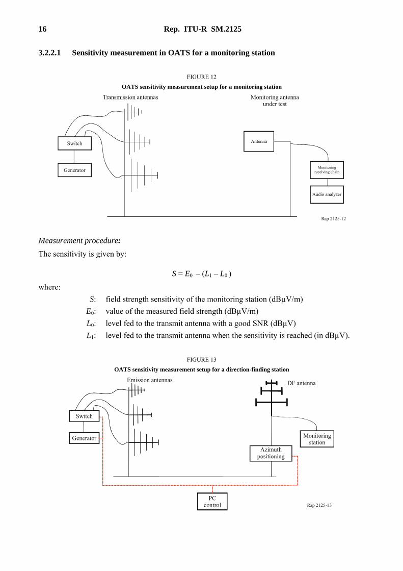
3.2.2.1 Sensitivity measurement in OATS for a monitoring station

FIGURE 12 OATS sensitivity measurement setup for a monitoring station

Rap 2125-12

Switch

Generator

Audio analyzer

Monitoringreceiving chain

Transmission antennas Monitoring antennaunder test

Antenna

Measurement procedure: The sensitivity is given by:

S = E0 – (L1 – L0 )

where: S: field strength sensitivity of the monitoring station (dBµV/m) E0: value of the measured field strength (dBµV/m) L0: level fed to the transmit antenna with a good SNR (dBµV) L1: level fed to the transmit antenna when the sensitivity is reached (in dBµV).

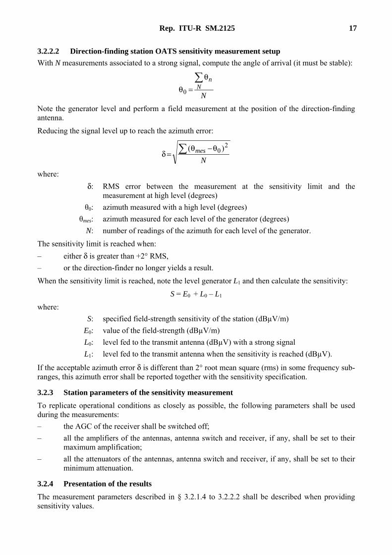
FIGURE 13 OATS sensitivity measurement setup for a direction-finding station

Rap 2125-13

Switch

Generator

Emission antennas DF antenna

Switch

Generator

PCcontrol

Monitoringstation

Azimuthpositioning


3.2.2.2 Direction-finding station OATS sensitivity measurement setup With N measurements associated to a strong signal, compute the angle of arrival (it must be stable):

N

Nn∑θ

=θ0

Note the generator level and perform a field measurement at the position of the direction-finding antenna.

Reducing the signal level up to reach the azimuth error:

N

mes∑ θ−θ=δ

20 )(

where: δ: RMS error between the measurement at the sensitivity limit and the

measurement at high level (degrees) θ0: azimuth measured with a high level (degrees) θmes: azimuth measured for each level of the generator (degrees) N: number of readings of the azimuth for each level of the generator.

The sensitivity limit is reached when: – either δ is greater than +2° RMS, – or the direction-finder no longer yields a result.

When the sensitivity limit is reached, note the level generator L1 and then calculate the sensitivity:

S = E0 + L0 – L1

where: S: specified field-strength sensitivity of the station (dBµV/m) E0: value of the field-strength (dBµV/m) L0: level fed to the transmit antenna (dBµV) with a strong signal L1: level fed to the transmit antenna when the sensitivity is reached (dBµV).

If the acceptable azimuth error δ is different than 2° root mean square (rms) in some frequency sub-ranges, this azimuth error shall be reported together with the sensitivity specification.

3.2.3 Station parameters of the sensitivity measurement To replicate operational conditions as closely as possible, the following parameters shall be used during the measurements: – the AGC of the receiver shall be switched off; – all the amplifiers of the antennas, antenna switch and receiver, if any, shall be set to their

maximum amplification; – all the attenuators of the antennas, antenna switch and receiver, if any, shall be set to their

minimum attenuation.

3.2.4 Presentation of the results The measurement parameters described in § 3.2.1.4 to 3.2.2.2 shall be described when providing sensitivity values.


These sensitivity values shall be guaranteed over the whole frequency band or by sub-band specified by the manufacturer. A mean or typical value may be given by the manufacturer.

The manufacturer shall state the conditions of calculation of this mean or typical value.

The values stated by the manufacturer shall be: – the field sensitivity of the monitoring station (dBµV/m) with the following parameters:

– type of modulation (A3E or F3E); – bandwidth of the analysis filter (kHz); – modulation index or frequency deviation; – SINAD used (dB).

– the field sensitivity of the direction-finding station (dBµV/m) with the following parameters: – integration time (s); – bandwidth of the analysis filter (kHz).

3.3 Key parameters for DF stations

3.3.1 DF accuracy (angular): System accuracy The procedures of measurement of the DF accuracy are not specified in the ITU-R Handbook – Spectrum Monitoring (Edition 2002). The Handbook describes only the classes of bearings (Classes A, B, C and D) with regard to Recommendation ITU-R SM.854 but not the characterization of the DF receivers.

The DF system accuracy is the effective or rms value of the difference between the true azimuth and the display bearing.

Three methods can be applied for DF accuracy measurement: – a test in a real environment which represents the final operational environment; – measurements at an OATS using restricted frequencies where no reflections from nearby

obstacles, ambient noise, and other radio signals may interfere with the measurement; – measurements on a platform: the DF station without its antenna is connected to a simulator

and a generator.

The first test is mainly used to determine system accuracy or the practical accuracy for a typical use of the system. The other two methods are used to determine instrument accuracy and can be used for example for calibration purposes.

3.3.1.1 DF accuracy tests in a real environment

Introduction to real environment testing The accuracy of a radio direction finding system, including stand-alone radio direction finders as well as direction finding functionality that is integrated with and part of a spectrum monitoring system, can be measured in a variety of ways. A system can be tested without its antennas in a laboratory, by connecting a signal generator to a device (such as a power divider and RF cables of appropriate lengths) that simulates voltages and phases incident on the antennas, and connecting this simulator to the DF system without its antennas. A system can be placed inside an anechoic chamber and test signals can be generated and used to measure accuracy of the system. A system can be placed on a test bed or test range, in an electromagnetically clean environment without reflections or structures that could provide scattering, resonances or re-radiation, and tested with strong signals. In such clean environments, most direction finding systems have excellent


performance, and such measurements serve to determine the “instrument accuracy” of the system. Performance measurements under such conditions do not allow discrimination among direction finding systems, however, as there are not the actual operational “real world” conditions which a high performance system can handle and which a lower performance system cannot handle as well. An administration might procure a system that performs well in laboratory tests, only to find that it does not work when actually deployed.

In order to give an accurate measure of the performance of a direction finding system, tests must be done under actual operational conditions, similar to those in which the system will actually be used, and such measurements serve to determine the “system accuracy” of the system. The remainder of this section outlines the recommended procedure for determining “system accuracy”; i.e. for testing direction finding systems in actual operational conditions with a variety of modulations and using signals of the minimum signal to noise ratio specified by the manufacturer of the system. Sections 3.3.1.3 and 3.3.1.4 describe procedures for determining “instrument accuracy;” i.e. for testing direction finding systems in the laboratory or in a test range using strong signals.

Definition of measurement procedure The DF system should be tested in actual operational conditions, preferably at typical locations where the system will be used by the procuring administration. “Factory operational tests” are an acceptable alternative, but should be done under conditions that are as close to the expected conditions where the system will actually be deployed as possible.

Prior to performing DF accuracy tests, an analysis should be performed to determine the coverage area from test transmitters which will be deployed for purposes of the tests, and from existing known broadcast stations and other transmitters (termed “targets of opportunity”). This analysis will aid in locating test transmitters and selecting targets of opportunity which should be received by the direction finder with a signal strength that will give a minimum signal-to-noise ratio at least that specified by the manufacturer of the system.

Test equipment should be prepared for the tests. This equipment includes test transmitters and modulation generators to allow all modulation types, both analog and digital modulations, of a variety of bandwidths, including narrow bandwidth and wide bandwidth signals. For digital modulations, pulses should be as narrow as 0.5 ms, of randomized pulse length. This equipment should be placed in a vehicle with a global positioning system and with appropriate power source; the vehicle will drive to randomly selected locations along roads in the calculated coverage area, to obtain at least 36 well-distributed azimuth values.

Signal level of the test transmitter should be adjusted to produce a signal at the DF system that meets the signal to noise ratio value specified by the manufacturer for the system under test. Targets of opportunity should be chosen which meet the specified signal to noise ratio, while avoiding signals which produce signal to noise ratios greater than 20 dB above the specified signal to noise ratio.

For each measurement performed, the bearing error is calculated as the difference between the true azimuth (angle of the transmitter’s test antenna) and the displayed bearing on the DF equipment.

During the tests data should be recorded on measurements for at least 36 azimuth values well distributed within 360°. Specifically, there should be a significantly large number of test locations that cover the entire 360° range with various (randomized) azimuth spacings that yield measurements down to 10° resolution, but not exactly every 10° and not every 10°. The measurement points should be spaced at a minimum of 6° and a maximum of 14°, with an average spacing of 10°, to provide flexibility is selecting suitable measurement locations in the field.


For example, a “suitable” measurement set may consist of 36 test locations at the following bearings relative to the DF antenna:

1°, 8°, 14°, 27°, 39°, 46°, 60°, 72°, 85°, 92°, 104°, 118°, 131°, 144°, 156°, 165°, 172°, 179°, 189°,

198°, 206°, 215°, 222°, 235°, 247°, 258°, 268°, 276°, 286°, 299°, 310°, 319°, 327°, 334°, 346°, 354°

This set has a minimum increment of 6° (8° to 14°) and a maximum increment of 14° (46° to 60°; 104° to 118°), and with 36 measurements, an “average” increment of 10°.

The bearing error should be measured for at least nine frequencies per decade well distributed within the frequency range of the direction finder, including the beginning and the end of the scale, and with at least five frequencies within the operational range when it does not comprise a full decade.

Data should be gathered for each azimuth and frequency, and for many cases of modulations at each azimuth and frequency, including analog and digital, narrowband and wideband modulations. Individual DF measurements may be averaged to produce a composite DF result for each case of azimuth, frequency and modulation, discarding at most 10% of the individual DF measurements as “wild data”. The resultant DF result is then compared with the known angle of arrival and the error, or ∆, is computed and entered in a test data table.

Most DF systems use vertically polarized antennas for reception, because horizontally polarized antennas for reception add to the cost and complexity of a DF system, and because signals of interest are generally either vertically polarized or because of imperfect polarization or propagation effects can be received with a vertically polarized antenna. Specifically: a) HF skywaves undergo polarization rotation in the ionosphere, so an antenna of one

polarization, generally vertical, suffices to receive HF signals that originate as either vertically or horizontally polarized. HF groundwaves propagate as vertically polarized signals, because horizontally polarized signals cannot propagate as groundwaves.

b) Most VHF/UHF signals (other than some TV signals) are usually vertical (or at least dual polarization like many FM broadcast signals), so the most important measurement is vertical. The few signals that are horizontal only (like some TV broadcasts) are usually of well-known location and therefore accurate DF of these signals is not necessary. Due to the simplicity of construction of vertical VHF/UHF antennas, especially for mobile platforms, most transmitters of interest use vertical antennas, and this is the most important need for DF.

c) Some technologies at UHF use signals that might have horizontal polarization, or whose polarization might vary depending on the momentary orientation of the transmitting antenna (such as mobile cellular), and it may be of interest to characterize the DF system performance against signals transmitted with horizontal polarization.

Therefore, most DF testing is typically done with vertical polarization. However, DF tests may be done with signals transmitted with horizontal in addition to vertical polarization. The polarization of test signals should be noted in a test data table.

Table 1 is an example of such a test data table; one such table is used for each analog modulation and for each digital modulation that is tested.


TABLE 1

Sample test data table

Signal modulation _______________Signal polarization ________

True Frequency 1 Frequency 2 Frequency 3 Frequency 4 Frequency M Index Azimuth DF ∆ DF ∆ DF ∆ DF ∆ DF ∆

1 1° 2 8° 3 14°

36 354°

In the table, DF stands for the measured azimuth and ∆ stands for the difference between the measured and the true azimuth.

In performing the tests, the vehicle should drive to the first location. The global positioning system should be used to determine precise location, from which the bearing from the DF system to the test transmitter is determined. Then the azimuth should be entered into all of the data tables for the different modulations, and the tests should be performed for the different frequencies and modulations, and data recorded in the data tables. After all measurements at one location have been completed, the vehicle should move to a location which is a randomized increment approximately 10° greater than the previous bearing, and the measurement procedure should be repeated. This procedure should be repeated until measurements have been made at all of the required azimuths.

The effective or RMS (root mean square) value of the bearing error is calculated as:

∑=

∆=∆N

iiRMS N 1

21

where: N: count of measurement.

During the international review of this draft, alternatives to RMS computation of error should be considered. For example, a cumulative distribution function of the error might be considered, where one determines the percentage of total measurements that fall within a certain azimuth error. As an example, for a given system, one might determine: Percentage of measurements Azimuth error 50% < 0.1° 67% < 1.7° 90% < 5.5°

Using the 90 percentile as the benchmark would give in this case, an error specification of < 5.5° for this system.

In order to ensure the reliability of results, the following requirements should be observed: a) The transmitter azimuth in relation to the DF station (true azimuth) should be established

with an accuracy of at least 0.1º RMS or a tenth of the estimated DF accuracy, whichever alternative is more restrictive, considering a confidence level of 95.45%.


b) Up to 10% of the locations in the coverage area (azimuth angles) may be discarded to account for siting, coverage and other operational problems, provided that a suitable process or procedure is developed for discard of such data.

c) The declared accuracy of the DF system should be the computed RMS of all data points other than those discarded.

Considering, for example, a DF system operating with two sets of antennas, one could define the following test points as a minimum test consistent with this standard: a) Antenna in the range of 80 MHz to 1 300 MHz.

– 36 azimuth points, well distributed within 360º. – 13 frequency points, 2 points on the first decade of the operational range (80 MHz and

90 MHz), 9 points on the second decade (from 100 MHz to 900 MHz) plus 2 points to complete the range on the third decade (1 000 MHz and 1 300 MHz).

– Total N = 36 × 13 = 468 test points for each of several analog and for each of several digital modulations.

b) Antenna in the range of 1 300 MHz to 3 000 MHz. – 36 azimuth points, well distributed within 360º. – 5 frequency points as the minimum since the range does not comprise full logarithmic

decade (1 300, 1 640, 1 980, 2 320, 2 660, 3 000 MHz). – Total N = 36 × 5 = 180 test points for each of several analogue and for each of several

digital modulations.

3.3.1.2 Additional considerations for HF DF measurements The measurement of the HF DF accuracy faces some further constraints: – HF signal wavelength impose important distances between transmitters and receivers, – the variations of the atmospheric noises are not easily controllable (depends on the solar

activity, the day or the night, and other variables.)

Measurements of HF DF accuracy shall then be the same as for VHF/UHF DF accuracy, except that: – the transmitter shall be real broadcast transmitter with known characteristics (azimuth,

level), or – an HF transmitter vehicle at a known position.

Example for a specification in a data sheet: DF accuracy: ≤ 2.5° RMS (80 MHz to 1 300 MHz, based on operational tests) (to relevant ITU-R SM Recommendation).

DF accuracy: ≤ 2.0° RMS (1 300 MHz to 3 000 MHz, based on operational tests) (to relevant ITU-R SM Recommendation).

3.3.1.3 Definition of DF accuracy test procedure on an OATS A system can be tested without its antennas in a laboratory, by connecting a signal generator to an antenna simulator and connecting it to the DF system without its antennas. A system can be placed on an OATS, in an electromagnetically clean environment without reflections or structures that could provide scattering, resonances or re-radiation, and tested with strong signals. See Fig. 14. Measurements in such a clean environment serve to determine the “instrument accuracy” of the system. The instrument accuracy is usually not that good a measure of how a DF system will


perform in actual operational conditions, because most DF systems perform well in the controlled environment of a laboratory or test bed when strong test signals are used.

For this test the DF accuracy of the direction finder is measured by using a test transmitter located in the surroundings of the DF antenna, in a reflection free environment. The test arrangement must permit changing the azimuth of the transmitter’s test antenna in defined steps to cover the full bearing range of 360°.

The frequencies for which propagation medium or multipath effects lead to DF errors should be rejected.

FIGURE 14 DF accuracy measurement setup for a direction finding station on oats

Rap 2125-14

Switch

Generator

Transmission antenna DF antenna

Switch

Generator

Command PC

DF receivingchain

Rotatingmast

Calculate the measured azimuth error :

)θ–θ(θ ),( theomesF =θ

where: θmes: angle measured at the frequency and the selected azimuth (degrees) θtheo: theoretical angle with the selected azimuth (degrees)

Compute the result of DF accuracy by calculating a quadratic average of all the values to the frequencies and the selected azimuths:

N

FF∑∑ θ

θ=

2),(θ

θ

θ: measurement of azimuth (degrees rms) θ(F,θ): angle measured at the frequency and the azimuth selected (degrees) N: the number of points of measurements.

It is possible to compensate for the error due to installation bias of the DF antenna taking into account the average bias from all measurements as follows:

N

FF∑∑

θ=θ),(θ

–θθ


The measurement of the HF DF accuracy faces some further constraints: – HF signal wavelength impose important distances between transmitters and receivers; – the variations of the atmospheric noises are not easily controllable (depends on the solar

activity, the day or the night…).

Measurements of HF DF accuracy shall then be the same as for VHF/UHF DF accuracy, except that: – the transmitter shall be real broadcast transmitter with known characteristics (azimuth,

level); – or an HF transmitter vehicle at a known position.

Distribution of the points of measurements To allow an equitable distribution of the frequencies on the totality of the band, the frequencies will have to be selected as follows: – the distribution will be made by octave; – the number of measurement per sub-band will be fixed and be equal to or higher than 1; – the points of measurements will be selected in a random way.

For measurements in site in open space, the azimuths of measurements will be selected as follow: – the number of azimuths of measurement will be fixed and be equal to or higher than 2; – the azimuths of measurements will be selected in a random way on 360°.

The DF accuracy shall be guaranteed. The published DF accuracy shall be valid over the entire rated temperature range indicated in the data sheet.

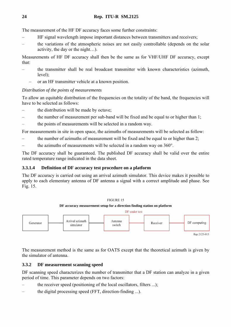
3.3.1.4 Definition of DF accuracy test procedure on a platform The DF accuracy is carried out using an arrival azimuth simulator. This device makes it possible to apply to each elementary antenna of DF antenna a signal with a correct amplitude and phase. See Fig. 15.

FIGURE 15 DF accuracy measurement setup for a direction finding station on platform

Rap 2125-015

The measurement method is the same as for OATS except that the theoretical azimuth is given by the simulator of antenna.

3.3.2 DF measurement scanning speed DF scanning speed characterizes the number of transmitter that a DF station can analyze in a given period of time. This parameter depends on two factors: – the receiver speed (positioning of the local oscillators, filters ...); – the digital processing speed (FFT, direction-finding ...).


The scanning speed is the capability of the direction finder to measure valid DF detection rate of the incoming signals in a given frequency band between Fmin and Fmax. The scanning speed performance is given in MHz/s.

The DF scanning speed is independent of the antenna used, so the measurement shall be made without the antenna. The measure scanning speed shall be the direction finding station receiving chain scanning speed as defined in Fig. 10.

The performance is guaranteed by two measurements: – valid azimuth calculation of one burst which proves the speed at which the band is scanned; – valid azimuth calculation of several simultaneous bursts with no impact on the speed at

which the band is scanned.

Only valid azimuth measurements shall be taken into account for scanning speed measurement.

Presentation of the results The DF scanning speed value shall be guaranteed.

The published scanning speed shall be valid over the entire rated temperature range indicated in the data sheet.

3.3.3 DF minimum signal duration

Principle of measurement The minimum signal duration characterizes the minimum time that a signal should be present to be detected and measured by the direction finder.

This time depends on: – the digital processing speed (FFT, direction-finding ...); – the selected IF filter.

The principle of the measurement is to generate a pulse equal in time to the minimum signal duration and to compute the probability of detection. This one should be higher than 95%.

Presentation of the results The minimum signal duration value shall be guaranteed.

The published minimum signal duration shall be valid over the entire rated temperature range indicated in the data sheet.

parameters of and measurement procedures on …€¦ · rep. itu-r sm.2125 1 report itu-r sm.2125...

Documents