parametric and nonparametric sequential change detection ... · jss journalofstatisticalsoftware...

JSS Journal of Statistical SoftwareAugust 2015, Volume 66, Issue 3. http://www.jstatsoft.org/

Parametric and Nonparametric Sequential Change

Detection in R: The cpm Package

Gordon J. RossUniversity College London

Abstract

The change point model framework introduced in Hawkins, Qiu, and Kang (2003) andHawkins and Zamba (2005a) provides an effective and computationally efficient methodfor detecting multiple mean or variance change points in sequences of Gaussian randomvariables, when no prior information is available regarding the parameters of the distri-bution in the various segments. It has since been extended in various ways by Hawkinsand Deng (2010), Ross, Tasoulis, and Adams (2011), Ross and Adams (2012) to allow forfully nonparametric change detection in non-Gaussian sequences, when no knowledge isavailable regarding even the distributional form of the sequence. Another extension comesfrom Ross and Adams (2011) and Ross (2014) which allows change detection in streamsof Bernoulli and Exponential random variables respectively, again when the values of theparameters are unknown.

This paper describes the R package cpm, which provides a fast implementation of allthe above change point models in both batch (Phase I) and sequential (Phase II) settings,where the sequences may contain either a single or multiple change points.

Keywords: change detection, sequential analysis, R.

1. Introduction

Many statistical problems require change points to be identified in sequences of data. Inthe usual setting, a sequence of observations x1, x2, . . . is drawn from the random variablesX1, X2, . . . and undergoes one or more abrupt changes in distribution at the unknown changepoints τ1, τ2, . . .. It is usually assumed that the observations are independent and identicallydistributed between every pair of change points, so that the distribution of the sequence canbe written as:

http://www.jstatsoft.org/

2 cpm: Sequential Change Detection in R

t

x

0 50 100 150

−2

−1

01

23

45

(a) Mean change.

t

x

0 50 100 150

−6

−4

−2

02

46

(b) Variance change.

Figure 1: Basic examples of changes to a univariate stream, with the time of the change pointsuperimposed.

Xi ∼

F0 if i ≤ τ1F1 if τ1 < i ≤ τ2F2 if τ2 < i ≤ τ3,. . .

(1)

where the Fis represent the distribution in each segment. Some simple examples are given inFigure 1, which shows two sequences of Gaussian random variables that undergo changes intheir mean and variance respectively.

Although requiring independence between change-points seems a restrictive assumption, thisis not the case since dependence can typically be handled by first modeling any underlyingdynamics or autocorrelation, and then performing change detection on either the model resid-uals or one-step ahead prediction errors, both of which should give i.i.d. sequences, providedthat the model has been correctly fit. For more information on this topic, see Gustafsson(2000). In the remainder of this paper apart from the example in Section 4.2, it is assumedthat such modeling has already been carried out, giving sequences of observations which arei.i.d. conditional on the change points.

Change detection problems differ based on what is assumed to be known about the Fi distri-butions. In most practical situations the parameters of these distributions will be unknown,and in many cases there may not even be information available about their distributionalform. Recently the change point model (CPM) framework has been developed for changedetection in situations where the available information about the Fi distributions is verylimited. Several different CPMs have been developed, which incorporate different test statis-tics to enable changes to be detected in a wide variety of sequences, using both parametricand nonparametric techniques (Hawkins et al. 2003; Hawkins and Zamba 2005a; Zhou, Zou,Zhang, and Wang 2009; Hawkins and Deng 2010; Ross et al. 2011; Ross and Adams 2011,2012).

The purpose of this paper is to describe the cpm package (Ross 2015), which is written in R(R Core Team 2014) and implements most of these published CPMs for detecting changes inthe distribution of discrete-time sequences of univariate random variables. Unlike existing Rpackages related to change detection, such as bcp (Erdman and Emerson 2007), strucchange(Zeileis, Leisch, Hornik, and Kleiber 2002) and changepoint (Killick and Eckley 2014), the

Journal of Statistical Software 3

cpm package allows sequential Phase II analysis when the parameters and, perhaps, thedistributional form of the observations are unknown.

Section 2 gives a more detailed overview of the sequential change detection problem. Section 3provides a general overview of the CPM framework. Finally, the cpm package is introducedin Section 4 and an overview of its capabilities is given, along with many examples of usage.This package can be obtained from the Comprehensive R Archive Network (CRAN) at http://CRAN.R-project.org/package=cpm.

2. Background information

The change detection problem described by Equation 1 in the previous section has been alively area of research since the 1950s. Because of the very general nature of the problem, theliterature is diverse and spans many fields. In particular, many popular methods have theirorigin in the quality control community, where the goal is to monitor the output of industrialmanufacturing processes and detect faults as quickly as possible (Lai 1995). However there aremany other situations where change detection techniques are important, such as identifyingcopy number variation in genomic data (Efron and Zhang 2011), detecting intrusions incomputer networks (Tartakovsky, Rozovskii, Blazek, and Kim 2006), and fitting multipleregime models which are popular in economics and finance (Ross 2012).

There are two main types of change detection problems, batch and sequential. In the qualitycontrol literature, these are respectively known as Phase I and Phase II detection:

1. Batch detection (Phase I): In this case, there is a fixed length sequence consisting ofn observations from the random variables X1, . . . , Xn, and it is required to test whetherthis sequence contains any change points. This type of change detection is retrospective,meaning that the decision whether a change has occurred at a particular point in thesequence is made using all the available observations, including those which occur laterin the sequence. These batch methods work well when there are only a small numberof change points, but can be computationally infeasible when larger numbers of changepoints are present, unless heuristics are used (Inclan and Tiao 1994; Hawkins 2001).

2. Sequential detection (Phase II): In this case, the sequence does not have a fixedlength. Instead, observations are received and processed sequentially over time. Wheneach observation has been received, a decision is made about whether a change has oc-curred based only on the observations which have been received so far. If no change isflagged, then the next observation in the sequence is processed. The sequential formula-tion allows sequences containing multiple change points to be easily handled; whenevera change point is detected, the change detector is simply restarted from the followingobservation in the sequence.

Traditionally, the tools used for both of these problems were quite different. For batch de-tection, the most commonly used approaches are some form of likelihood ratio testing (Hink-ley and Hinkley 1970) or Bayesian inference (Stephens 1994), while the sequential detectionproblem uses control charts such as the CUSUM (Page 1954), Exponential weighted mov-ing averages (Roberts 1959), or sequential Bayesian methods (Chib 1998; Fearnhead and Liu2007).

http://CRAN.R-project.org/package=cpm



Recent years have seen the emergence of the CPM framework, which extends the use oflikelihood-based batch detection methods to the problem of sequential monitoring. The orig-inal work on the CPM was presented by Hawkins et al. (2003) which focuses on the problemof sequentially detecting a change in the mean of a sequence of Gaussian random variables.This has since been extended in many directions to allow more complex types of changes to bedetected, including those in streams where the underlying distribution is unknown (Hawkinsand Zamba 2005a; Zou and Tsung 2010; Ross et al. 2011).

The R package cpm contains an implementation of several different CPMs, both parametricand nonparametric, for use on univariate streams in both the Phase I and Phase II setting.Specifically, it implements the CPM framework using the Student-t, Bartlett, GLR, Fisher’sexact test, Exponential, Mann-Whitney, Mood, Lepage, Kolmogorov-Smirnov, and Cramer-von-Mises statistics. The first three are intended for detecting changes in sequences which areknown to be Gaussian, the fourth is used for Bernoulli sequences, the fifth for Exponential se-quences, while the remainder statistics are nonparametric and can be deployed on any streamof continuous random variables without requiring any prior knowledge of their distribution.The package is implemented in R and provides a small number of customizable high-levelfunctions which allow the user to easily detect changes in a given stream, along with a moreflexible S4 object system based representation of CPM objects which allow for greater controlover the change detection procedure.

3. The CPM

The CPM extends techniques for batch detection to the sequential case. We first review thebatch scenario, and then describe the sequential extension.

3.1. Batch change detection (Phase I)

In the batch scenario, there is a fixed length sequence containing the n observations x1, . . . , xnwhich may or may not contain a change point. For ease of exposition, assume that at mostone change point can be present. If no change point exists, the observations are independentand identically distributed according to some distribution F0. If a change point exists at sometime τ , then the observations have a distribution F0 prior to this point, and a distribution F1

afterwards, where F0 6= F1.

First consider the problem of testing whether a change occurs immediately after some specificobservation k. This leads to choosing between the following two hypotheses:

H0 : Xi ∼ F0(x; θ0), i = 1, . . . , n,

H1 : Xi ∼{F0(x; θ0) i = 1, 2, . . . , k,F1(x; θ1) i = k + 1, k + 2, . . . , n,

where θi represent the potentially unknown parameters of each distribution.

This is a standard problem which can be solved using a two-sample hypothesis test, wherethe choice of test statistic depends on what is assumed to be known about the distributionof the observations, and the type of change which they may undergo. For example, if theobservations are assumed to be Gaussian, then it would be appropriate to use a two-sampleStudent-t test to detect a mean shift, and an F test to detect a scale shift. To avoid making


such distributional assumptions, a nonparametric test can be used, such as the Mann-Whitneytest for location shifts, the Mood test for scale shifts, and the Lepage, Kolmogorov-Smirnov,and Cramer-von-Mises tests for more general changes.

After choosing a two-sample test statistic Dk,n, its value can be computed and if Dk,n ex-ceeds some appropriately chosen threshold hk,n then the null hypothesis that the two sampleshave identical distributions is rejected, and we conclude that a change point has occurredimmediately following observation xk.

Since it is not known in advance where the change point occurs, we do not know which valueof k should be used for testing. Therefore, Dk,n is evaluated at every value 1 < k < n, andthe maximum value is used. In other words, every possible way of splitting the data into twocontiguous subsequences is considered, with a two-sample test applied at every split point.The test statistic is then:

Dn = maxk=2,...,n−1

Dk,n = maxk=2,...,n−1

∣∣∣∣∣ D̃k,n − µD̃k,n

σD̃k,n

∣∣∣∣∣ .The Dk,n statistics are obtained by standardizing D̃k,n to have mean 0 and variance 1 bysubtracting their means µD̃k,n

and dividing by their standard deviations σD̃k,nand taking the

absolute value. Note that the modulus should be taken to allow for two-sided change detectionwhen using a statistic where both very low and very high values indicate a difference betweenthe samples (e.g., being able to detect both increases and decreases in the mean and/orvariance).

The null hypothesis of no change is then rejected if Dn > hn for some appropriately chosenthreshold hn. This threshold is chosen to bound the Type 1 error rate as is standard instatistical hypothesis testing. Suppose α is an acceptable level for the proportion of falsepositives, i.e., the probability of falsely declaring that a change has occurred if in fact nochange has occurred. Then, hn should be chosen as the upper α quantile of the distributionof Dn under the null hypothesis.

However, this requires computing the distribution of Dn, which generally does not have ananalytic finite-sample form. For some choices of the test statistics Dk,n the asymptotic dis-tribution of Dn can be written; for example, Hawkins (1977) derives the distribution whenDk,n is the test statistic associated with the Student-t test, Pettitt (1979) does provide similarresults for the Mann-Whitney statistics, and a general procedure for asymptotically boundingDn for other classes of test statistics is given by Worsley (1982). However, these asymptoticdistributions may not be accurate when considering finite length sequences, and so numericalsimulation may be required in order to estimate the distribution. The latter approach is usedin the cpm package.

Finally, the best estimate of the change point location will be immediately following the valueof k which maximized Dn:

τ̂ = arg maxk

Dk,n. (2)

3.2. Sequential change detection (Phase II)

The two-sample hypothesis testing approach used in the batch case can be extended to se-quential change detection where new observations are received over time, and multiple change


points may be present. Let xt denote the tth observation that has been received, wheret ∈ {1, 2, . . .}.Whenever a new observation xt is received, the CPM approach treats x1, . . . , xt as being afixed length sequence and computes Dt using the above batch methodology, where we areusing the notation Dt rather than Dn to highlight the sequential nature of the procedure.A change is then flagged if Dt > ht for some appropriately chosen threshold. If no changeis detected, the next observation xt+1 is received, then Dt+1 is computed and compared toht+1, and so on. The procedure therefore consists of a repeated sequence of hypothesis tests.In general, the Dk,n statistics will have properties which allow Dt+1 to be computed fromDt without incurring too much computational overhead; see Hawkins et al. (2003) and Rosset al. (2011) for specific examples of this.

In the sequential setting, ht is chosen so that the probability of incurring a Type 1 error isconstant over time, so that under the null hypothesis of no change:

P (D1 > h1) = α

P (Dt > ht|Dt−1 ≤ ht−1, . . . , D1 ≤ h1) = α, t > 1.(3)

In this case, assuming that no change occurs, the average number of observations receivedbefore a false positive detection occurs is equal to 1/α. This quantity is referred to as theaverage run length, or ARL0. In general, the conditional distribution in Equation 3 is an-alytically intractable, and Monte Carlo simulation is used in order to compute the requiredsequences of ht values corresponding to a given choice of α. This is a computationally expen-sive procedure but it only needs to be carried out a single time, and the values can then bestored in a look-up table. The cpm package contains pre-computed sequences of thresholdswhich correspond to a variety of choices of α.

4. Package overview

The cpm package contains implementations of the CPM framework, for detecting changes ineither a batch of data containing at most one change point (Phase I), or a sequential contextwith data which may contain multiple change points (Phase II). The package supports thefollowing CPMs:

� The Student-t, Bartlett and GLR statistics for detecting changes in a Gaussian sequenceof random variables. The first two monitor for changes in either the mean or variancerespectively, while the latter can detect changes in both (Hawkins et al. 2003; Hawkinsand Zamba 2005a,b).

� The Exponential statistic for detecting a parameter change in a sequence of Exponen-tially random variables (Ross 2014).

� The GLRAdjusted and ExponentialAdjusted statistics which are identical to the GLRand Exponential statistics, except for using the finite sample correction described inRoss (2014) which can lead to more powerful change detection.

� The Fisher’s exact test (FET) statistic for detecting a change in a sequence of Bernoullirandom variables (Ross and Adams 2011).


� The Mann-Whitney and Mood statistics for detecting location and scale changes re-spectively in sequences of random variables, where no assumptions are made about thedistribution (Hawkins and Deng 2010; Ross et al. 2011).

� The Lepage, Kolmogorov-Smirnov, and Cramer-von-Mises statistics for detecting moregeneral distributional changes where again no assumptions are made about the sequencedistribution (Ross and Adams 2012).

These CPMs are implemented in C++ in order to provide fast computation. The R interfacein the package wraps around this code, and has two parts, which are:

1. A set of utility functions allowing the user to easily detect changes in a sequence of obser-vations. The core functions here are detectChangePointBatch and detectChangePoint

which perform Phase I and Phase II detection respectively for sequences containing atmost one change point, and processStream which can detect multiple change points ina sequence, by repeatedly restarting the Phase II CPM procedure whenever a change isdetected.

2. While the above functions will be sufficient for many basic change detection tasks,many streaming Phase II applications will require more nuanced control of the CPMprocedure. The cpm package therefore provides functions which allow CPM objectsto be represented as S4 objects in R and thus allowing for greater flexibility. Here,the function makeChangePointModel is used to create a CPM object and the functionprocessObservation allows observations to be processed individually, with the CPMstatistics being made available to the user after every observation.

All of these functions allow any of the above test statistics to be used in conjunction with anyCPM, and also allow a variety of different values for the ARL0 to be specified. We will firstdescribe in Section 4.1 how the utility functions in the package can be used to detect singlechange points in a sequence, and then focus on the multiple change point case in Section 4.2.Finally, we discuss the S4 section of the package in Section 4.3 which allows greater flexibilityin situations where this is required.

4.1. Detecting a single change point

We begin by describing how to perform Phase I analysis, and then focus on Phase II.

Phase I

The detectChangePointBatch function is used to test for a single change point in a sequenceof observations, and estimate its location. In keeping with Phase I analysis, the data isprocessed in one batch rather than sequentially. The use of this function can be illustratedusing a simple example of a Gaussian stream which undergoes a change in mean from 0 to0.5, occurring after 200 observations while the variance remains unchanged. Parametric andnonparametric change detection can be performed by using the CPM based on the Student-tand Mann-Whitney test statistics respectively:

R> set.seed(0)

R> x <- c(rnorm(200, 0, 1), rnorm(200, 0.5, 1))


0 100 200 300 400

−2

−1

01

23

4

Observation

x

(a) Observations with detected change point.

0 100 200 300 400

01

23

45

Observation

Dt

(b) Dk,n statistics.

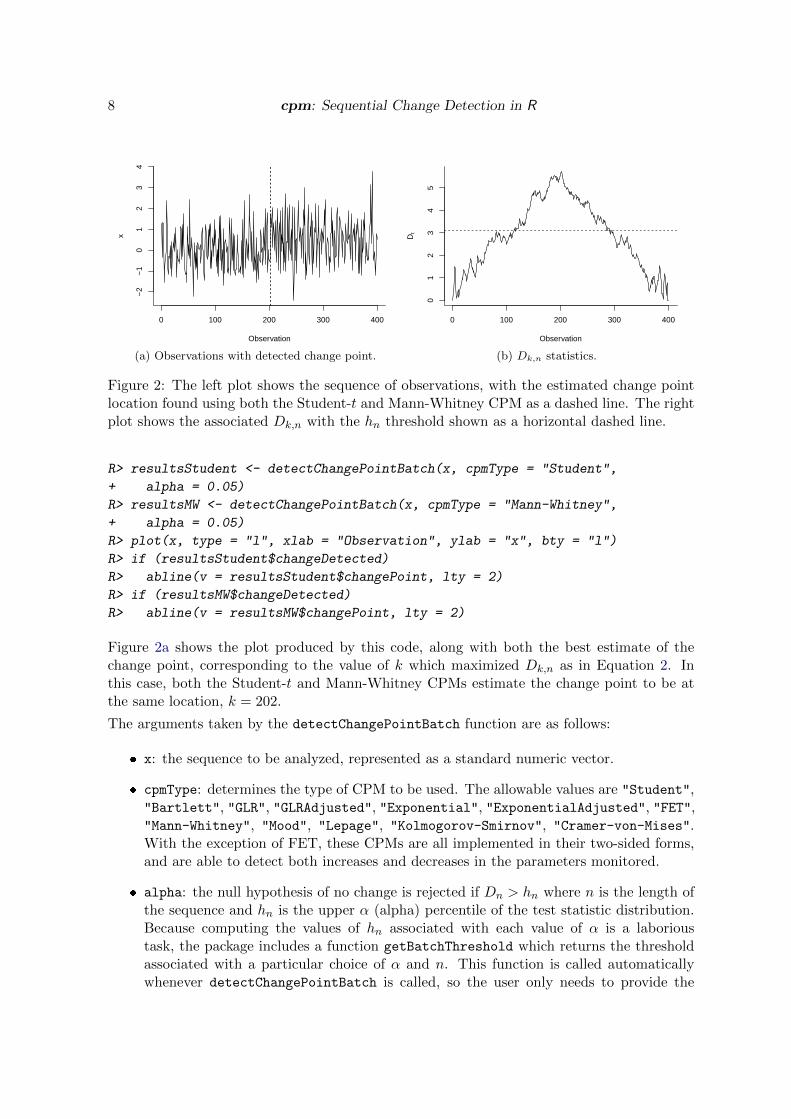
Figure 2: The left plot shows the sequence of observations, with the estimated change pointlocation found using both the Student-t and Mann-Whitney CPM as a dashed line. The rightplot shows the associated Dk,n with the hn threshold shown as a horizontal dashed line.

R> resultsStudent <- detectChangePointBatch(x, cpmType = "Student",

+ alpha = 0.05)

R> resultsMW <- detectChangePointBatch(x, cpmType = "Mann-Whitney",

+ alpha = 0.05)

R> plot(x, type = "l", xlab = "Observation", ylab = "x", bty = "l")

R> if (resultsStudent$changeDetected)

R> abline(v = resultsStudent$changePoint, lty = 2)

R> if (resultsMW$changeDetected)

R> abline(v = resultsMW$changePoint, lty = 2)

Figure 2a shows the plot produced by this code, along with both the best estimate of thechange point, corresponding to the value of k which maximized Dk,n as in Equation 2. Inthis case, both the Student-t and Mann-Whitney CPMs estimate the change point to be atthe same location, k = 202.

The arguments taken by the detectChangePointBatch function are as follows:

� x: the sequence to be analyzed, represented as a standard numeric vector.

� cpmType: determines the type of CPM to be used. The allowable values are "Student","Bartlett", "GLR", "GLRAdjusted", "Exponential", "ExponentialAdjusted", "FET","Mann-Whitney", "Mood", "Lepage", "Kolmogorov-Smirnov", "Cramer-von-Mises".With the exception of FET, these CPMs are all implemented in their two-sided forms,and are able to detect both increases and decreases in the parameters monitored.

� alpha: the null hypothesis of no change is rejected if Dn > hn where n is the length ofthe sequence and hn is the upper α (alpha) percentile of the test statistic distribution.Because computing the values of hn associated with each value of α is a laborioustask, the package includes a function getBatchThreshold which returns the thresholdassociated with a particular choice of α and n. This function is called automaticallywhenever detectChangePointBatch is called, so the user only needs to provide the


desired value of α. The allowable values for this argument are 0.05, 0.01, 0.005, 0.001.If a different value is required then the user will need to compute it manually.

� lambda: specifies the amount of smoothing to be used when using the FET CPM,as described in Ross and Adams (2011). This parameter is not used with any of theother CPM types. The only allowable values for this parameter are 0.1 and 0.3; moreinformation on this is provided later in this section.

The detectChangePointBatch function returns the following arguments:

� changeDetected: TRUE if Dn exceeds the value of hn associated with α, otherwise FALSE.

� changePoint: assuming a change was detected, this stores the most likely location ofthe change point, defined as the value of k which maximized Dk,n. If no change isdetected, this is set to 0.

� Ds: the sequence of test statistics Dk,n.

� threshold: the value of hn which corresponds to the specified α.

The Dk,n statistics returned by this function can be used for diagnostics. The following codeplots the values of the Dk,n statistics which were computed in the above example, along withthe hn threshold corresponding to α = 0.05.

R> plot(resultsMW$Ds, type = "l", xlab = "Observation",

+ ylab = expression(D[t]), bty = "l")

R> abline(h = resultsMW$threshold, lty = 2)

The resulting plot is shown in Figure 2b. It can be seen that the test statistics start to peakaround the 200th observation where the change occurs, as expected.

Phase II

The detectChangePoint function allows Phase II analysis to be performed, where the ob-servations are processed sequentially rather than in batch. In this case the goal is usually todetect the change point as soon after it occurs as possible. The arguments to this functionare similar to those of the detectChangeBatch function in the previous section and are:

� cpmType: as before.

� ARL0: denotes which ARL0 the CPM should have. As discussed in Section 3.2, comput-ing the thresholds associated with a specific choice of ARL0 can take a large amount ofcomputation time. Therefore, the package includes pre-computed values for a selectionof ARL0’s. Specifically, the allowable values for the argument ARL0 are: {370, 500, 600,700, . . . , 1000, 2000, 3000, . . . , 10000, 20000, . . . , 50000}. If this argument is missing thenno change detection will occur, and the Dt statistics will be computed and returned forthe whole sequence.

� startup: determines how many observations are used for the initialization period. Ifstartup = 20, then no change detection will be performed until after the first 20 ob-servations have been received. This is usually necessary since the statistical tests willhave low power for small sample sizes.


� lambda: as before.

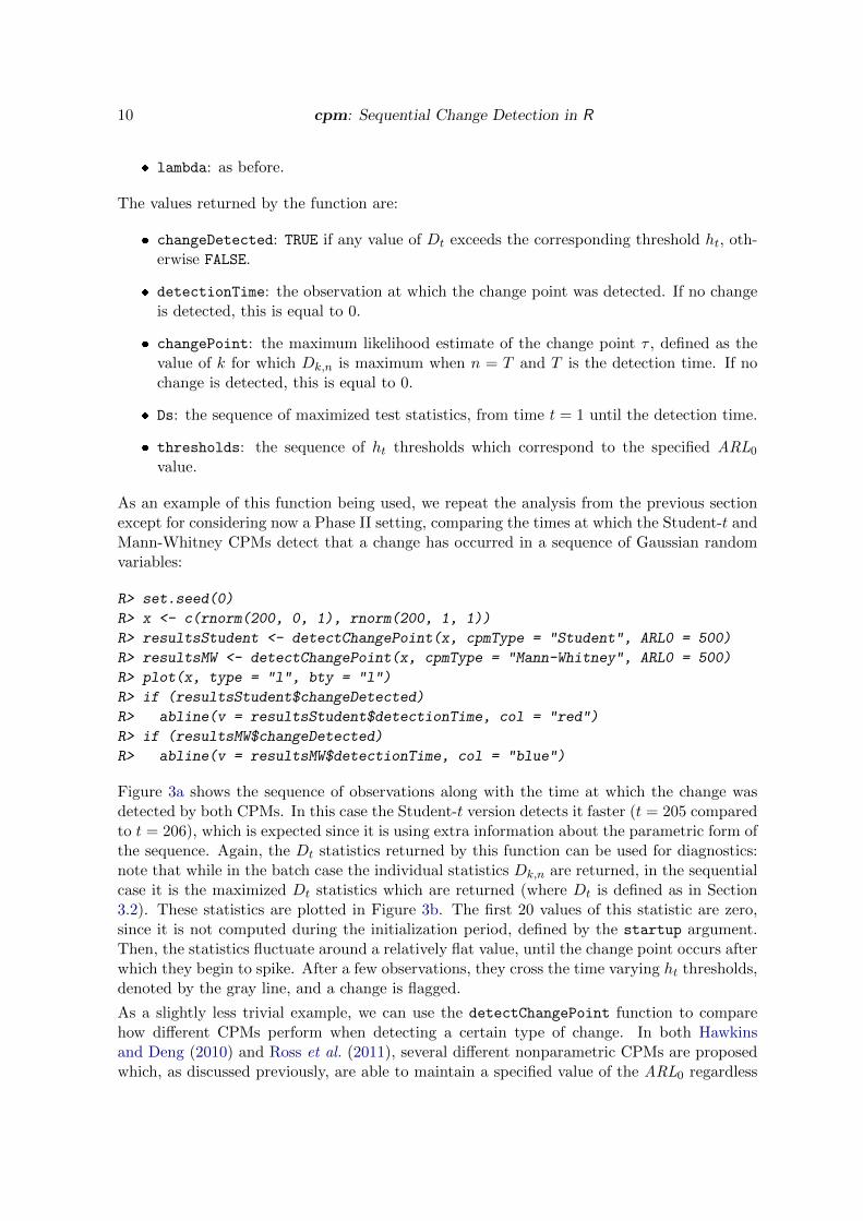
The values returned by the function are:

� changeDetected: TRUE if any value of Dt exceeds the corresponding threshold ht, oth-erwise FALSE.

� detectionTime: the observation at which the change point was detected. If no changeis detected, this is equal to 0.

� changePoint: the maximum likelihood estimate of the change point τ , defined as thevalue of k for which Dk,n is maximum when n = T and T is the detection time. If nochange is detected, this is equal to 0.

� Ds: the sequence of maximized test statistics, from time t = 1 until the detection time.

� thresholds: the sequence of ht thresholds which correspond to the specified ARL0

value.

As an example of this function being used, we repeat the analysis from the previous sectionexcept for considering now a Phase II setting, comparing the times at which the Student-t andMann-Whitney CPMs detect that a change has occurred in a sequence of Gaussian randomvariables:

R> set.seed(0)

R> x <- c(rnorm(200, 0, 1), rnorm(200, 1, 1))

R> resultsStudent <- detectChangePoint(x, cpmType = "Student", ARL0 = 500)

R> resultsMW <- detectChangePoint(x, cpmType = "Mann-Whitney", ARL0 = 500)

R> plot(x, type = "l", bty = "l")

R> if (resultsStudent$changeDetected)

R> abline(v = resultsStudent$detectionTime, col = "red")

R> if (resultsMW$changeDetected)

R> abline(v = resultsMW$detectionTime, col = "blue")

Figure 3a shows the sequence of observations along with the time at which the change wasdetected by both CPMs. In this case the Student-t version detects it faster (t = 205 comparedto t = 206), which is expected since it is using extra information about the parametric form ofthe sequence. Again, the Dt statistics returned by this function can be used for diagnostics:note that while in the batch case the individual statistics Dk,n are returned, in the sequentialcase it is the maximized Dt statistics which are returned (where Dt is defined as in Section3.2). These statistics are plotted in Figure 3b. The first 20 values of this statistic are zero,since it is not computed during the initialization period, defined by the startup argument.Then, the statistics fluctuate around a relatively flat value, until the change point occurs afterwhich they begin to spike. After a few observations, they cross the time varying ht thresholds,denoted by the gray line, and a change is flagged.

As a slightly less trivial example, we can use the detectChangePoint function to comparehow different CPMs perform when detecting a certain type of change. In both Hawkinsand Deng (2010) and Ross et al. (2011), several different nonparametric CPMs are proposedwhich, as discussed previously, are able to maintain a specified value of the ARL0 regardless


0 100 200 300 400

−2

−1

01

23

4

Index

x

(a) Observations with detected change point.

0 50 100 150 200

0.0

0.5

1.0

1.5

2.0

2.5

3.0

Observation

Dt

(b) Dt statistics.

Figure 3: The left plot shows the sequence of observations, with the point where the changewas detected using both the Student-t and Mann-Whitney CPMs as a red and blue linerespectively. The right plot shows the values of the Dt statistics from the Mann-WhitneyCPM up until the change is detected, with the thresholds ht shown as a red line.

of the true stream distribution. While this is a useful feature, the trade-off is that they willusually be slower to detect changes on any particular stream than a parametric CPM that hasbeen designed with knowledge of the true data distribution, as was the case in the previousexample where the Mann-Whitney CPM was slower to detect the Gaussian mean shift than theStudent-t CPM. In the above-mentioned papers, many simulations were performed in orderto measure how close the performance of the nonparametric detectors is to their parametriccounterparts.

To show how such a comparison can be performed using the cpm package, we compare theperformance of the parametric CPM which uses the Bartlett test for detecting a change inthe variance of a Gaussian stream, to several different nonparametric methods. Specificallywe look at the Mood CPM which is a nonparametric test for changes in scale, and the LepageCPM which is intended to detect more general types of distributional change.

For a fixed value of the ARL0, the two main factors which affect how long a change takes to bedetected are the size of the change, and the number of observations which are available fromthe pre-change distribution. We can investigate the impact of these by considering differentsets of values: specifically we consider the case where the distribution of the stream changesfrom N(0, 1) to N(0, δ) for δ ∈ {1.5, 2.0, 3.0, 0.5, 0.3} and where the change occurs at timesτ ∈ {50, 300}.The supplementary material contains the R code used to perform this analysis and Table 1shows the results, averaged over 100 simulations (note that we have kept the number of sim-ulations low for computational reasons; more accurate results will be obtained with a highernumber of simulations, but the qualitative results in the table do not change). It can be seenthat, as expected, large changes are easier to detect than smaller changes, and changes whichoccur after the 300th observation are easier to detect than those occurring after the 50th,since the sample size is larger. In general, the parametric CPM outperforms the nonpara-metric CPMs, which is understandable since it incorporates knowledge that the observationsare Gaussian. Interestingly, for changes with smaller magnitudes, the nonparametric CPMs


τ δ Bartlett Mood Lepage

τ = 50

1.5 140.2 (249.3) 93.5 (179.0) 142.1 (240.4)2.0 16.0 (17.5) 18.0 (20.5) 26.5 (44.4)3.0 5.5 (3.9) 7.8 (5.4) 9.4 (6.8)0.5 20.1 (16.4) 37.9 (70.5) 61.4 (109.1)0.3 8.7 (3.1) 13.8 (4.8) 18.9 (6.0)

τ = 300

1.5 30.7 (23.5) 27.8 (24.4) 35.3 (32.0)2.0 10.7 (7.3) 11.5 (8.3) 14.0 (10.1)3.0 4.6 (3.0) 6.2 (3.7) 7.5 (4.4)0.5 16.5 (7.5) 22.5 (8.7) 31.9 (10.6)0.3 8.4 (2.7) 12.2 (2.7) 17.4 (3.1)

Table 1: Average time taken to detect shifts of magnitude δ in the mean and standarddeviation of a Gaussian N(0, 1) stream, for various change times τ . Standard deviations aregiven in brackets.

actually outperform this parametric version. This surprising phenomena is discussed in moredetail in both Hawkins and Deng (2010) and Ross et al. (2011)

As a final example, we investigate the impact that different choices of the ARL0 have on per-formance. Choosing an appropriate value for the ARL0 depends on the particular applicationbeing considered; low values typically result in less delay until change points are detected, atthe cost of incurring a greater number of false positives. We illustrate this by using the FETCPM to detect a change of a fixed magnitude in a Bernoulli sequence, for different choices ofthe ARL0.

Note that the FET CPM differs slightly from the other CPMs implemented in the pack-age. As described in Ross and Adams (2011), the test statistics when using the FET arehighly discrete, even more so than the other statistics considered. Therefore, a smoothingparameter λ is used to smooth the Dk,t statistics and make them less discrete. Both thedetectChangePointBatch and detectChangePoint functions implement this by allowing aparameter lambda to be passed to control the degree of smoothing. Because each choice ofparameter value requires a different sequences of ht thresholds to be used, we have only in-cluded threshold sequences for λ = 0.1 and λ = 0.3, which are the two values used in Rossand Adams (2011). Note that the authors show that performance is not particularly sensitiveto the choice of λ, and 0.1 can generally be used for all sequences. The option to use 0.3is provided only for completeness. Finally, for reasons discussed in Ross and Adams (2011)the test statistic discreteness means that the FET CPM is conservative when the pre-changeproportion θ0 is less than 0.1, and so the achieved ARL0 may exceed the desired ARL0 forsmall values of θ0.

The supplementary material contains code that can be used to calculate the performance FETCPM when detecting a change from θ0 = 0.4 to θ1 = 0.6, occurring after 100 observations,again using 100 simulations. Table 2 shows the average delay until the change is detected forseveral choices of the ARL0, along with the proportion of times a change was flagged beforethe change occurs at the 100th, corresponding to a false positive. As expected, a lower valueof the ARL0 results in faster change detection, at the cost of higher false positives. Againin practice the user should typically decide what sort of false positive rate is acceptable, andchoose the ARL0 appropriately.


ARL0 Delay False positives

100 18.48 0.54500 42.84 0.15

1000 61.09 0.08

Table 2: Average time to detect a change from 0.4 to 0.6 in a Bernoulli parameter occurringafter 100 observations, for various choices of ARL0. The proportion of times a false positivewas signaled is also given.

4.2. Sequences containing multiple change points

In many applications, the stream of observations may contain multiple change points. TheprocessStream function can be used to detect these. The basic idea behind this function isto run the CPM as described above, processing each observation one-by-one. Suppose thata change is detected at time T1, with the corresponding change point estimate being τ̂1. Inorder to detect further change points, all the observations from before the detected changepoint are discarded, and a new CPM is run, beginning with the (τ̂1 + 1)th observation. Thisis repeated until all the observations have been processed.

Figure 4 gives an illustration of this. Here, the stream consists of Student-t(5) randomvariables which undergo an increase in mean after the 50th observation, followed by a decreasein mean after the 100th. Since this is not a Gaussian stream, one of the nonparametric CPMsshould be used to detect these changes.

When the CPM using the Mann-Whitney statistic is deployed on this stream, a change is de-tected immediately following the 53rd observation. The corresponding change point estimateis τ̂1 = 49. After this change point has been detected, a new CPM is created and monitoringbegins from the 49 + 1 = 50th observation. A second change point is then detected at timet = 105, with the corresponding change point estimate being τ̂2 = 100.

The parameters of the processStream function are identical to those for the detectChange

function in the previous section. This function returns the following list of values:

� detectionTimes: the observation times at which the changes were detected. If multiplechange points are detected then this will be a vector. If no change points are detectedthen it will be a vector of length zero.

� changePoints: the maximum likelihood estimate of the change points τi, defined as thevalues of k which maximize Dk,Ti

, where Ti is the detection time. Again, this will be avector if multiple change points are detected, and an empty vector if no change pointsare detected.

Figure 4 can hence be reproduced by the following code:

R> set.seed(0)

R> x <- c(rt(50, 5), rt(50, 5) + 3, rt(50, 5))

R> res <- processStream(x, cpmType = "Mann-Whitney", ARL0 = 500,

+ startup = 20)

R> plot(x, type = "l", xlab = "Observation", ylab = "", bty = "l")

R> abline(v = res$detectionTimes)

R> abline(v = res$changePoints, lty = 2)


0 50 100 150

−2

02

46

8

Observation

Figure 4: A sequence of Student-t(5) random variables which undergoes a change in meanafter the 50th and 100th observations. The solid black lines show the points when the changewas detected, and the dashed black lines show the estimated change point locations.

As a less trivial example of how the processStream function can be used for multiple changepoint detection, we analyze a real sequence of foreign exchange data. This example alsoshows how the CPM framework can be applied to sequences of observations which are notindependent between the change points, by first applying a suitable transformation.

The data consists of a historical sequence of the exchange rates between the Swiss Franc(CHF) and the British Pound (GBP). The maximum value of the exchange rate was recordedat three hour intervals running from October 21st 2002 to May 15th 2007. In total, 9273observations xt were made and we treat them as being a data stream where observations arereceived and processed sequentially. Although the analysis of financial data is often quitesophisticated, we provide this example to demonstrate the capabilities of our algorithm in asimplified setting.

This data set is included in the cpm package, and can be loaded with the following command:

R> data("ForexData", package = "cpm")

The third column of this matrix contains the logarithm of the maximum value of the exchangerate for each period. This can be selected using:

R> x <- ForexData[, 3]

R> plot(x, type = "l", xlab = "Observation", ylab = "log(Exchange Rates)",

+ bty = "l")

This produces a plot of the financial sequence, as shown in Figure 5a. From this, it is apparentthat there is a high degree of autocorrelation. This is problematic for the CPM framework,which assumes that observations are independent between change points. In order to deploythe CPM, the correlation between the observations should be removed. In general, thismay require modeling the time series and deploying the CPM on the residuals rather thanthe original data. With this financial data, we make a simple transformation and insteadconsider the first differences of the logarithm of the data, defined as ∆xt = xt − xt−1. This


0 2000 4000 6000 8000

1.2

1.3

1.4

1.5

Observation

log(

Exc

hang

e R

ates

)

(a) Original sequence.

0 2000 4000 6000 8000

−0.

015

−0.

005

0.00

50.

015

Observation

Diff

eren

ces

(b) First differences.

0 2000 4000 6000 8000

0e+

004e

−06

8e−

06

Observation

(c) EWMA estimate of variance.

Figure 5: The foreign exchange data, its first differences, and the EWMA of the squared firstdifferences, all with the detected scale change points superimposed.

transformation is typical when working with financial data, and the resulting sequence isplotted in Figure 5b, and appears stationary with mean 0. However, these first differenceshave very heavy tails, and this high kurtosis suggests that the data is non-Gaussian. Anonparametric change detector hence seems an appropriate tool to use for analysis.

A typical goal when analyzing financial data is to detect changes in the variance (volatility) ofthe first differences. We use the Mood CPM for this purpose. Due to the length of the data,the ARL0 was set to 5000 in order to avoid a large number of false alarms being generated.Because this stream is likely to contain multiple change points, the processStream functionis used, with the CPM being restarted whenever a change is detected. The following codeperforms the analysis:

R> results <- processStream(diffs, cpmType = "Mood", ARL0 = 5000,

+ startup = 20)

This CPM detects a total of 11 change points. We have superimposed these change points onFigure 5b. It is not obvious from this plot whether the discovered change points correspondto true scale shifts, so to investigate further, we compute the exponentially weighted averageof the stream variance, defined as EWMAt = λEWMAt−1 +(1−λ)(∆xt)

2. This allows a local


estimate of the variance to be formed. This EWMA is plotted in Figure 5c, with λ = 0.995.It can be seen that the variance is undergoing gradual drift, and that the discovered changepoints seem to correspond to abrupt changes in the variance. The following code reproducesthis EWMA analysis:

R> ewma <- numeric(length(diffs))

R> ewma[1] <- diffs[1]^2

R> lambda <- 0.995

R> for (i in 2:length(ewma))

+ ewma[i] <- lambda * ewma[i - 1] + (1 - lambda) * diffs[i]^2

R> plot(ewma, type = "l", xlab = "Observation", ylab = "", bty = "l")

R> abline(v = results$changePoints, lty = 2)

4.3. Manipulating CPMs as S4 objects

The detectChangePoint and processStream functions provide a convenient wrapper aroundthe internals of the CPM implementation, and will hopefully be sufficient for most problems.However in some situations more control may be required over how sequences are processed –for example, the user may wish to inspect the individual Dk,t statistics after each observation,or the user may wish to be able to halt processing part of the way through the sequence inorder to perform some further analysis.

To facilitate this, we have also implemented the CPMs as S4 objects within the cpm package.After a CPM object is created, it can be passed observations individually for processing. Theobject maintains its internal state consisting of all the observations which it has seen so far.At any point, it can be queried in order to find whether a change has been detected, or toobtain the latest set of Dk,t statistics.

The makeChangePointModel function is used to create a CPM object. It takes exactly thesame arguments as the detectChangePoint function above. After this has been created,the processObservation function can be used to process a sequence of one observation at atime, with state being maintained after each one is processed. At any point, the CPM can bequeried by using the changeDetected function to test whether a change has been detected,or the getStatistics function to gain access to the underlying Dk,t statistics.

To illustrate this, we provide code which replicates the financial data example from the pre-vious section. First, the data is loaded and two arrays are created to contain the detectiontimes and change points:

R> detectiontimes <- numeric()

R> changepoints <- numeric()

Next, a Lepage CPM is created, and the observations are iterated over one by one:

R> cpm <- makeChangePointModel(cpmType = "Mood", ARL0 = 5000, startup = 20)

R> i <- 0


R> while (i < length(diffs)) {

+ i <- i + 1

+ cpm <- processObservation(cpm, diffs[i])

+ if (changeDetected(cpm)) {

+ cat(sprintf("Change detected at observation %d\n", i))

+ detectiontimes <- c(detectiontimes, i)

+ Ds <- getStatistics(cpm)

+ tau <- which.max(Ds)

+ if (length(changepoints) > 0)

+ tau <- tau + changepoints[length(changepoints)]

+ changepoints <- c(changepoints, tau)

+ cpm <- cpmReset(cpm)

+ i <- tau

+ }

+ }

After the CPM object has been created, the loop iterates over the sequence of one observationat a time. For each observation, the processObservation function is used to update theCPM. After this has been done, the changeDetected function is used to test whether therehas been a change point. This function returns TRUE if the Dt statistic used in the CPM hasexceeded the ht threshold sequence at any point since monitoring began.

If a change point has been flagged, the getStatistics function is used to return the vector ofDk,n statistics where n is equal to the index of the last observation processed (i.e., if 100 ob-servations have been processed, then getStatistics will return the values D1,1, . . . , D1,100).From Equation 2, the best estimate of the change point location is the maximum value ofDk,n, and this can be found by using the built-in R function which.max.

After the change location has been estimated, the cpmReset function is used to clear the stateof the CPM. When this is called, a new CPM is essentially created from scratch. Finally, theloop index i is set to the observation immediately following the detected change point, andthe monitoring continues.

The estimated change points are as follows:

R> changepoints

[1] 764 796 2414 2843 3584 4034 6620 7089 7452 8007 8338

which match the values returned by the processStream function in the previous section.Note as a slight subtlety that since the CPM is completely reset after each change point, theCPM only stores the observations which occurred after the previous change point. Therefore,the following line:

R> tau <- tau + changepoints[length(changepoints)]

was included in the above loop to convert the change point location index to an index overthe whole sequence.


References

Chib S (1998). “Estimation and Comparison of Multiple Change-Point Models.” Journal ofEconometrics, 86(2), 221–241.

Efron B, Zhang NR (2011). “False Discovery Rates and Copy Number Variation.” Biometrika,98(2), 251–271.

Erdman C, Emerson JW (2007). “bcp: An R Package for Performing a Bayesian Analysisof Change Point Problems.” Journal of Statistical Software, 23(3), 1–13. URL http:

//www.jstatsoft.org/v23/i03/.

Fearnhead P, Liu Z (2007). “On-line Inference for Multiple Changepoint Problems.” Journalof the Royal Statistical Society B, 69(4), 589–605.

Gustafsson F (2000). Adaptive Filtering and Change Detection. John Wiley & Sons, Hoboken.

Hawkins DM (1977). “Testing a Sequence of Observations for a Shift in Location.” Journalof the American Statistical Association, 72(357), 180–186.

Hawkins DM (2001). “Fitting Multiple Change-Point Models to Data.” Computational Statis-tics & Data Analysis, 37(3), 323–341.

Hawkins DM, Deng Q (2010). “A Nonparametric Change-Point Control Chart.” Journal ofQuality Technology, 42(2), 165–173.

Hawkins DM, Qiu PH, Kang CW (2003). “The Changepoint Model for Statistical ProcessControl.” Journal of Quality Technology, 35(4), 355–366.

Hawkins DM, Zamba KD (2005a). “A Change-Point Model for a Shift in Variance.” Journalof Quality Technology, 37(1), 21–31.

Hawkins DM, Zamba KD (2005b). “Statistical Process Control for Shifts in Mean or VarianceUsing a Changepoint Formulation.” Technometrics, 47(2), 164–173.

Hinkley DV, Hinkley EA (1970). “Inference about Change-Point in a Sequence of BinomialVariables.” Biometrika, 57(3), 477–488.

Inclan C, Tiao GC (1994). “Use of Cumulative Sums of Squares for Retrospective Detection ofChanges of Variance.” Journal of the American Statistical Association, 89(427), 913–923.

Killick R, Eckley IA (2014). changepoint: An R Package for Changepoint Analysis. URLhttp://www.jstatsoft.org/v58/i03/.

Lai TL (1995). “Sequential Changepoint Detection in Quality Control and Dynamical Sys-tems.” Journal of the Royal Statistical Society B, 57(4), 613–658.

Page ES (1954). “Continuous Inspection Schemes.” Biometrika, 41(1/2), 100–115.

Pettitt AN (1979). “A Non-Parametric Approach to the Change-Point Problem.” Journal ofthe Royal Statistical Society C, 28(2), 126–135.

http://www.jstatsoft.org/v23/i03/




R Core Team (2014). R: A Language and Environment for Statistical Computing. R Founda-tion for Statistical Computing, Vienna, Austria. URL http://www.R-project.org/.

Roberts SW (1959). “Control Chart Tests Based on Geometric Moving Averages.” Techno-metrics, 42(1), 97–101.

Ross GJ (2012). “Modelling Financial Volatility in the Presence of Abrupt Changes.” PhysicaA: Statistical Mechanics and Its Applications, 392(2), 350–360.

Ross GJ (2014). “Sequential Change Detection in the Presence of Unknown Parameters.”Statistics and Computing, 24(6), 1017–1030.

Ross GJ (2015). cpm: Sequential Parametric and Nonparametric Change Detection. Rpackage version 2.2, URL http://CRAN.R-project.org/package=cpm.

Ross GJ, Adams NM (2011). “Sequential Monitoring of a Bernoulli Sequence When thePre-Change Parameter is Unknown.” Computational Statistics, 28(2), 463–479.

Ross GJ, Adams NM (2012). “Two Nonparametric Control Charts for Detecting ArbitraryDistribution Changes.” Journal of Quality Technology, 44(12), 102–116.

Ross GJ, Tasoulis DK, Adams NM (2011). “Nonparametric Monitoring of Data Streams forChanges in Location and Scale.” Technometrics, 53(4), 379–389.

Stephens DA (1994). “Bayesian Retrospective Multiple-Changepoint Identification.” Journalof the Royal Statistical Society C, 43(1), 159–178.

Tartakovsky AG, Rozovskii BL, Blazek RB, Kim H (2006). “A Novel Approach to Detectionof Intrusions in Computer Networks via Adaptive Sequential and Batch-Sequential Change-Point Detection Methods.” IEEE Transactions on Signal Processing, 54(9), 3372–3382.

Worsley KJ (1982). “An Improved Bonferroni Inequality and Applications.” Biometrika,69(2), 297–302.

Zeileis A, Leisch F, Hornik K, Kleiber C (2002). “strucchange: An R Package for Testingfor Structural Change in Linear Regression Models.” Journal of Statistical Software, 7(2),1–38. URL http://www.jstatsoft.org/v07/i02.

Zhou C, Zou C, Zhang Y, Wang Z (2009). “Nonparametric Control Chart Based on Change-Point Model.” Statistical Papers, 50(1), 13–28.

Zou C, Tsung F (2010). “Likelihood Ratio-Based Distribution-Free EWMA Control Charts.”Journal of Quality Technology, 42(2), 174–196.

http://www.R-project.org/


http://www.jstatsoft.org/v07/i02


Affiliation:

Gordon J. RossDepartment of StatisticsUniversity College London1-19 Torrington PlaceLondon, WC1E 7JE, United KingdomE-mail: [email protected]: http://gordonjross.co.uk/

Journal of Statistical Software http://www.jstatsoft.org/

published by the American Statistical Association http://www.amstat.org/

Volume 66, Issue 3 Submitted: 2012-01-31August 2015 Accepted: 2013-06-27

mailto:[email protected]

http://gordonjross.co.uk/

http://www.jstatsoft.org/

http://www.amstat.org/

parametric and nonparametric sequential change detection ... · jss journalofstatisticalsoftware...

Documents