parametric and sensitivity analysis of a vibratory
TRANSCRIPT
Louisiana State UniversityLSU Digital Commons
LSU Master's Theses Graduate School
2002
Parametric and sensitivity analysis of a vibratoryautomobile modelKanika Nicole VesselLouisiana State University and Agricultural and Mechanical College, [email protected]
Follow this and additional works at: https://digitalcommons.lsu.edu/gradschool_theses
Part of the Mechanical Engineering Commons
This Thesis is brought to you for free and open access by the Graduate School at LSU Digital Commons. It has been accepted for inclusion in LSUMaster's Theses by an authorized graduate school editor of LSU Digital Commons. For more information, please contact [email protected].
Recommended CitationVessel, Kanika Nicole, "Parametric and sensitivity analysis of a vibratory automobile model" (2002). LSU Master's Theses. 1802.https://digitalcommons.lsu.edu/gradschool_theses/1802

PARAMETRIC AND SENSITIVITY ANALYSIS OF A VIBRATORY AUTOMOBILE MODEL
A Thesis
Submitted to the Graduate Faculty of the Louisiana State University and
Agricultural and Mechanical College in partial fulfillment of the
requirements for the degree of Master of Science in Mechanical Engineering
in
The Department of Mechanical Engineering
by
Kanika Nicole Vessel B.S. in Mechanical Engineering
Southern University and A & M College, 1999
May 2002

ii
DEDICATION
To my husband Bradley D. Vessel, my parents Theophilus and Nordica Mixon, Jr., my
grandparents Robert and Mary Pierce, my uncle Eddie Pierce, my aunty Debra Morgan, and my
siblings, LaKenya, Keesha, Damon, Tecarai, and Eric

iii
ACKNOWLEDGMENTS
First and foremost I would like to give thanks and all honor to God. Without Him I
would not be where I am today.
I would like to acknowledge my major professor Dr. Su-Seng Pang for his continued
guidance and support while making sure I stay focused. Thanks also go to Dr. Yitshak
M. Ram and Dr. Lynn Lamotte for serving on the graduate committee and evaluating my
thesis. Thanks to Dr. Yitshak M. Ram for serving as co-advisor on my graduate
committee. Furthermore, I would like to thank Dr. Michael A. Stubblefield for his advise
and support during this advanced degree program.
Thanks to my colleagues Akshay Nareshraj Singh and Kumar Vicram Singh for their
intellectual input. Also, thanks to Salvador Cupe-Beecha, Mr. Ed Martin and Jim Layton,
Jr. for their assistance in constructing the lab experiment.
Thanks to my friends Shani Allison, Caroline Stampley, Tameka Williamson,
Kristian Johnson, Phaedra Bell, Shari Jones, and Thereza Shanklin for their continued
support when times were tough. Thanks to the Pierce, Carter, Mixon and Williams
family for their continued support.
My gratitude goes to my uncle Eddie Pierce for being like a father to me and to my
aunty Debra Morgan who has always been there for me. Special thanks to my mom
Nordica Mixon for her faith, guidance, love, support, strength as single parent, and for
being one of my very best friends as well. Thanks to my dad Theophilus Mixon, Jr. for
being stern when I needed discipline, but also for being my friend when I needed one.
Last but certainly not least, my husband. Thanks for all your love, support, strength and
faith when I needed it.

iv
Thanks to NSF/Interactive Graduate Education Research Training and
NASA/LaSpace for their financial support to make this possible.

v
TABLE OF CONTENTS
DEDICATION… … … … … … … … … … … … … … … … … … … … … … … .… … … … ..… ii ACKNOWLEDGMENTS… … … … … … … … … … … … … … … … … … … … … … ....… iii LIST OF TABLES… … … … … … … … … … … … … … … … … … … … … ...… … … … … vii LIST OF FIGURES… … … … … … … … … … … ...… … … … … … … .… … … … … … … viii ABSTRACT… … … … … … … … … … … … … … … … … … … … … … … … … ...… … … … xi CHAPTER 1: INTRODUCTION… … … … … … … … … … … … … … … … … … .… … … 1 1.1 General Introduction… … … … … … … … … … … … … … … … … … … … … ..1 1.1.1 Vibration in Automotive Industry… … … … … … … … … … … … … ...… 2 1.1.2 Basis of this Research… … … … … .… … … … … … … … … … … … … ....3 1.2 Organization and Content of the Thesis… … … … … … … … … … … … … … .5 CHAPTER 2: LITERATURE REVIEW… … … … … … … … … … … … … … … … … … 7 2.1 Introduction… … … … … … … … … … … … … … … … … … … … … … … … … 7 2.2 Vehicle System Modeling… … … … … … … … … … … … … … … … … … … ..7 2.3 Vehicle Structure Modes… … … … … … … … … … … … … … … … … … … ..11 2.4 Tire Properties… … … … … … … … … … … … … … … … … … … … … … … ..13 2.5 Vehicle Handling… … … … … … … … … … … … … … … … … … … … … … ..16 CHAPTER 3: VIBRATION, PARAMETRIC
AND SENSITIVITY ANALYSIS… … … … … … … … … … … … … … .18 3.1 Introduction… … … … … … … … … … … … … … … … … … … … … … … … ..18 3.2 Vibration Analysis… … … … … … … … … … … … … … … … … … … … … … 18 3.2.1 Free Vibration… … … … … … … … … … … … … … … … … … … … … ...18 3.2.2 Forced Vibration (Harmonic Excitation)… … … … … … … … … … .… .25 3.3 Parametric Analysis… … … … … … … … … … … … … … … … … … … … … ..30 3.4 Sensitivity Analysis… … … … … … … … … … … … … … … … … … … … … ..41 3.4.1 Equations of Sensitivity… … … … … … … … … … … … … … … … … ....41 3.4.2 Sensitivity of Vibration… … … … … … … … … … … … … … … … … … .45 CHAPTER 4: EXPERIMENTAL VERIFICATION… … … … … … … … … … … … ...55 4.1 Introduction… … … … … … … … … … … … … … … … … … … … … … … … ..55 4.2 Experimental Determination… … … … … ...… … … … … … … … … … … … .55 4.2.1 Equipment… … … .… … … … … … … … … … … … … … … … … … … … 55 4.2.2 Setup… … … … … … … … … … … … … … … … … … … … … … … … … ..56 4.2.3 Procedure… … … … … … … … … … … … … … … … … … … … … … … ..57 4.2.4 Results… … … … … … … … … … … … … … … … … … … … … … … … ...61 4.3 Analytical Determination… .… … … … … … … … … … … … … … … … … … 67 4.3.1 Vibration Analysis.… … … … … … … … … … … … … … … … … … .… ..68 4.3.2 Parametric Analysis… … … … … … … … … … … … … … … … … … .… .68
vi
4.3.3 Sensitivity Analysis..… … … … … … … … … … … … … … … … … ..… ...70 CHAPTER 5: CONCLUSION AND RECOMMENDATIONS… … … … … … … … ..74 5.1 Conclusion… … … … … … … … … … … … … … … … … … … … … … … … … 74 5.2 Recommendations for Future Research… … … … … … … … … … … … … ...75 REFERENCES… … … … … … … … … … … … … … … … … … … … … … … … … … … … .76 APPENDIX: MATLAB PROGRAMS… … … … … … … … … … … … … … … … … … ...78 VITA… … … … … … … … … … … … … … … … … … … … … … … … … … … … … .....… … 96

vii
LIST OF TABLES
Table 3.1: Poles of the system… … … … … … … … … … … … … … … … … … … … … … ...22
Table 3.2: Eigenvectors of the system… … … … … … … … … … … … … … … … … … … ...23
Table 3.3: Ranges for each parameter for parametric analysis… … … … … … … … … … ..31
Table 3.4: Sensitivity analysis for J∂∂ /1λ … … … … … … … … … … ..… … … … … … … .47
Table 3.5: Sensitivity analysis for J∂∂ /2λ … … … … ...… … … … … … … … … … … … … 47
Table 4.1: Experimental and analytical parametric analysis results...… … … … … … … ...70
Table 4.2: Experimental and analytical sensitivity analysis results… … … … … … … … ...73

viii
LIST OF FIGURES
Figure 1.1: Bounce and pitch modes of vibration… … … … … … … … … … … … … … … … 5
Figure 3.1: 2-degree of freedom system… … … … … … … … … … … … … … … … … … … 19
Figure 3.2: Poles of the system for free vibration… … … … … … … … … … … … … … … ..22
Figure 3.3: First mode shape (absolute, real and imaginary part)… … .… … … … … … … 23
Figure 3.4: Second mode shape (absolute, real and imaginary part)… .… … … … … … … 24
Figure 3.5: Third mode shape (absolute, real and imaginary part)… … .… … … … … … ...24
Figure 3.6: Fourth mode shape (absolute, real and imaginary part)… … .… … … … … … .25
Figure 3.7: 2-degree of freedom system with external force… … … … … … … … … … … .27
Figure 3.8: Magnitude in bounce mode for forced vibration… … … … ..… … … … … … ...28
Figure 3.9: Phase function in bounce mode for forced vibration… … … .… … … … … … .28
Figure 3.10: Magnitude in pitch mode for forced vibration… .… … … … … … … … … … .29
Figure 3.11: Phase function in pitch mode for forced vibration… ..… … … … … … … … ..29
Figure 3.12: Parametric analysis for J-magnitude in bounce mode… … .… … … … … … ..31
Figure 3.13: Parametric analysis for J-phase function in bounce mode… ..… … … … … ..32
Figure 3.14: Parametric analysis for J-magnitude in pitch mode… … … … … … … … … ..32
Figure 3.15: Parametric analysis for J-phase function in pitch mode… … ..… … … … ..… 33
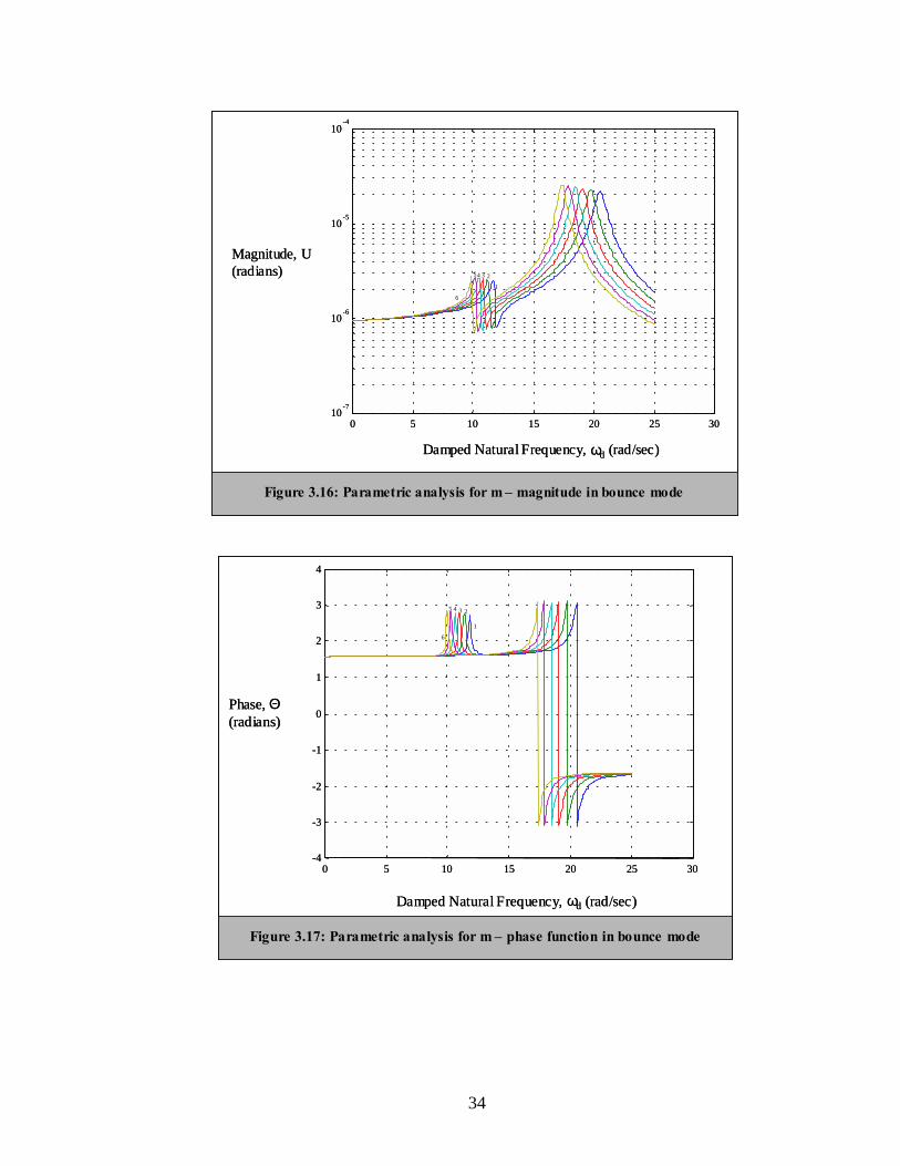
Figure 3.16: Parametric analysis for m-magnitude in bounce mode… … … … … … … … .34
Figure 3.17: Parametric analysis for m-phase function in bounce mode… ..… … … … … .34
Figure 3.18: Parametric analysis for m-magnitude in pitch mode… … … … … … … … … .35
Figure 3.19: Parametric analysis for m-phase function in pitch mode… … … .… … … .....35
Figure 3.20: Parametric analysis for 1k -magnitude in bounce mode… … … … … … … … 36
Figure 3.21: Parametric analysis for 1k -phase function in bounce mode… … … … … … ..37

ix
Figure 3.22: Parametric analysis for 1k -magnitude in pitch mode… … … … … … … … … 38
Figure 3.23: Parametric analysis for 1k -phase function in pitch mode… .… … … … … ....38
Figure 3.24: Parametric analysis for 1c -magnitude in bounce mode… … … … … … … … 39
Figure 3.25: Parametric analysis for 1c -phase function in bounce mode… … ..… … … ....40
Figure 3.26: Parametric analysis for 1c -magnitude in pitch mode… … … … … … … … … 40
Figure 3.27: Parametric analysis for 1c -phase function in pitch mode… … .… … … … ....41
Figure 3.28: Real part of sensitivity of the eigenvalues for both DOF ( )J … … … .… .… ..48
Figure 3.29: Imaginary part of sensitivity of the eigenvalues for both DOF ( )J … … … ...48
Figure 3.30: Real part of sensitivity of the eigenvalues for both DOF ( )m … … … … … ...50
Figure 3.31: Imaginary part of sensitivity of the eigenvalues for both DOF ( )m … … … ..50
Figure 3.32: Real part of sensitivity of the eigenvalues for both DOF ( )1k … … … … ...… 51
Figure 3.33: Imaginary part of sensitivity of the eigenvalues for both DOF ( )1k … … … ..52
Figure 3.34: Real part of sensitivity of the eigenvalues for both DOF ( )1c … … … … … ...53
Figure 3.35: Imaginary part of sensitivity of the eigenvalues for both DOF ( )1c … … … ..53
Figure 4.1: Complete experimental setup… … … … .… … … … … … … … … … … … … … .57
Figure 4.2: 2-DOF mass-spring system… … … … … … … … … … … … … … … … … … … .58
Figure 4.3: 2-DOF mass-spring system with added mass… … … … … … … … … … … … .59
Figure 4.4: 2-DOF mass-spring system with stiffness modification...… … … … … … … ..60
Figure 4.5: Close-up of mass-spring system modification.… … ..… … .… … … … … … … 60
Figure 4.6: Results for mass-spring system… … … … ...… … … … … … … … … … … … … 62
Figure 4.7: Snap shot results for added mass, m1=0.063 kg… … … … … … … .… … … … .63
Figure 4.8: Snap shot results for added mass, m2=0.122 kg… … … .… … … … … … … … .64

x
Figure 4.9: Snap shot results for mass-spring system, k3=910.7 N/m… … .… … … … … ..65
Figure 4.10: Snap shot results for mass-spring system, k3=1313 N/m… ..… … … .… … ...66
Figure 4.11: Experiment-imaginary part of sensitivity for both DOF (mass)… … … … ...71
Figure 4.12: Experiment-imaginary part of sensitivity for both DOF (k3)… .… … … … ...72

xi
ABSTRACT
Vibration response is an important aspect of any engineering problem. This thesis
deals with developing a method to obtain the vibration, parametric and sensitivity of an
automobile analyzed as a 2-DOF rigid body system with damping. The focus of the
vibration analysis is to obtain the poles, eigenvectors, and natural frequencies of the
system. The parametric analysis gave information on how the natural frequency is
affected when one of the parameters is perturbed. Information about how much the
system is affected by the change in one parameter is what is obtained from the sensitivity
analysis. The theoretical solution contained in this report uses the parameters of a 2002
Honda CR-V to give a general idea of how an automobile should respond when analyzed
as a two degree of freedom rigid body.
An experiment was designed to implement the theory in practical applications.
Modal testing was applied to extract the natural frequencies in order to characterize the
system. From the experiment, the parametric analysis produced results that resulted in
error of 5.8-10.8%. This error is small and it may seem the experiment is a good design,
but that error caused an even greater amount of error in the sensitivity results. In that
analysis, the stiffness produced the best results, resulting in 0% error. However, the error
for the sensitivity on the mass resulted in 28.09-54.0% for the first eigenvalue and 18.94-
24.76% for the second eigenvalue. This high error could be due to the fact that the mass
is a sensitive parameter. For the most part, fairly accurate results have been produced
from the developed theory. Some work still needs to be done with the sensitivity to get
better results. These results also prove that this theory can serve as a vital tool in
developing practical solutions to vibration control problems.

1
CHAPTER 1: INTRODUCTION
1.1 General Introduction
Vibration, which occurs in most machines, structures, and mechanical components,
can be desirable and undesirable. Vibrations on the strings of a harp are desirable
because it produces a beautiful sound. However, vibration in a vehicle is very
undesirable because it can cause discomfort to the passengers in the vehicle. Vibration is
undesirable, not only because of the unpleasant motion, the noise and the dynamic
stresses, which may lead to fatigue and failure of the structure, but also because of the
energy losses and the reduction in performance which accompany the vibrations.
Vibration analysis should be carried out as an inherent part of the design because of the
devastating effects, which unwanted vibrations could have on machines and structures.
Modifications can most easily be made in an effort to eliminate vibration, when necessary
or to reduce it as much as possible.
There are several classifications of vibration, free and forced, undamped and
damped, and linear and nonlinear vibration. Free vibration is when a system, after an
initial disturbance, is left to vibrate on its own. No external force acts on the system. If a
system is subjected to an external force, the resulting vibration is known as forced
vibration. If the frequency of the external force coincides with one of the natural
frequencies of the system, a condition known as resonance occurs, and the system
undergoes dangerously large oscillations. Undamped vibration is when no energy is lost
or dissipated in friction or other resistance during oscillations. On the other hand, when
energy is lost in this way, it is known as damped vibration. Linear vibration is when all
the variable forces are directly proportional to the displacement, or to the derivatives of

2
the displacement, with respect to time. On the other hand, if any of the variable forces
are not directly proportional to the displacement, or to its derivatives with respect to time
nonlinear vibration occurs.
In vibration, a number of simplifying assumptions have to be made to model any real
system. For example, a distributed mass may be considered as a lumped mass, or the
effect of damping in the system may be neglected particularly if only resonant
frequencies are sought, or a non-linear spring may be considered linear, or certain
elements may be neglected altogether if their effect is likely to be small. Furthermore,
the directions of motion of the mass elements are usually restrained to those of immediate
interest to the analyst.
1.1.1 Vibration in Automotive Industry
An automobile is made up of many components. These components include
suspension, engine and its components, chassis, transmission, braking, etc. and represent
the many subsystems in a multi-degree of freedom analysis. Yet, for many of the more
elementary analyses applied to it, all components move together. The type of analysis
used depends on what component is being investigated. For example, under braking, the
entire vehicle slows down as a unit; thus it can be represented as one lumped mass
located at its center of gravity with appropriate mass and inertia properties. One mass is
sufficient for acceleration, braking, and most turning analyses. For ride analysis, it is
often necessary to treat the wheels as separate lumped masses. In that case, the lumped
mass representing the body is the sprung mass, and the wheels are denoted as unsprung
masses. The vehicle is treated as a mass concentrated at its center of gravity for single
mass representation. The point mass at the center of gravity, with appropriate rotational

3
moments of inertia, is dynamically equivalent to the vehicle itself for all motions in
which it is reasonable to assume the vehicle to be rigid.
1.1.2 Basis of this Research
Engineering students often understand the theories and principles concerning
vibration by doing homework assignments or performing lab experiments. However, it is
not simple to design an experiment to implement these simple principles. A simple thing
as determining the spring force of a spring or the natural frequency of a simple system
can be a difficult experiment to perform. With homework assignments it is easy to use
the known equations and given information to solve the problem without much thought.
The same goes for lab experiments, the setup is given and the procedure is followed
without much thought as to why certain components are chosen.
All mechanical systems have natural frequencies. When analyzing these systems
engineers sometimes apply rigid body dynamics. Rigid body dynamics has been used in
many industries such as automotive, agricultural and aerospace. In industry, multi-degree
of freedom (DOF) systems is used to obtain measurements and simulate movement under
certain conditions. The purpose of a multi-DOF system is to represent the subsystems of
the body. When simplifying a mechanical system in terms of a rigid body, it is necessary
to determine the best method to do that. Take for instance the research of Chrstos in [1].
He was interested in vehicle parameters required for vehicle dynamics simulation and
determined there are three categories used to develop the vehicle dynamics simulation.
The three categories are low DOF linear models, nonlinear lumped parameter models,
and multi-body dynamic models.

4
The sophistication of simulation developed has ranged from 2-DOF linear models
used to study low severity vehicle behavior to complex multi-body formulations used to
investigate limit handling performance and vehicle rollover. The usage of the 2-DOF
models is only a technique to extract meaningful parameters from measured data.
Evaluation methods using an unreasonable number of parameters have no purpose for the
development of new cars or for comparison of similar cars since drivers’ preference vary
widely in various handling characteristics. Mimuro et al. showed this in their research in
[2]. He was interested in parameter evaluation of vehicle dynamic performance. These
engineers developed a Four Parameter Evaluation Method. The lateral transient response
data was curve fitted with a 2-DOF model and the parameters are extracted. The four
parameters were expressed in a rhombus to help recognize vehicle performance
intuitively. “The area of the rhombus denotes vehicle handling potential, and the
distortion denotes handling tendency. The key point of this method was making it
possible to see the parameters that contradict each other at a glance [2]”.
The use of rigid body dynamics in system analysis can assist in any objective the
engineer is trying to obtain, it is like a stepping-stone in system analysis. The parameters
of focus for this experiment are mass ( )m , stiffness ( )k , damping ( )c , and moment of
inertia ( )J . Two types of vibration will be investigated, free and forced. For both types
of vibration, the theoretical results will be compared to the experimental results. The
automobile body or sprung mass has two vibrations that are of interest for this
experiment, vertical (bounce) and pitch. Figure 1.1 shows these two modes of vibration.
Bounce is the translational component of ride vibrations of the sprung mass in the
direction of the vehicle z-axis. Pitch is the angular component of ride vibration of the

5
sprung mass about the vehicle y-axis. Therefore, the automobile will be investigated as a
rigid body 2-DOF system with damping. In addition to the vibration analysis, a
parametric and sensitivity analysis will be performed as well. The parametric analysis
will look at how perturbations in one parameter affect the natural frequency. The
sensitivity analysis will look at how sensitive a parameter is to change in one or several
other parameters.
1.2 Organization and Content of the Thesis
This thesis is divided into five sections, the structure and content of which are
described below:
Section 1: Introduction (Chapter 1)
This section is a general introduction to the subject of vibration, parametric and
sensitivity analysis, followed by a description of the organization and content of the
thesis.
x
y
z
Bounce
Pitch
Figure 1.1: Bounce and pitch modes of vibration
x
y
z
Bounce
Pitch
x
y
z
x
y
z
x
y
z
Bounce
Pitch
Figure 1.1: Bounce and pitch modes of vibration

6
Section 2: Literature Review (Chapter 2)
This section is a literature review to investigate the effect of vibration on the
automobile. This section reviews laboratory studies, which have investigated the effect
of various parameters on automotive vibration. This section also consists of reviews that
have investigated vibration on certain components of the automobile, as well as
considering the automobile with certain degrees of freedom.
Section 3: Vibration, Parametric and Sensitivity Analysis (Chapter 3)
This section describes the theory for modeling free and forced vibration for a 2-DOF
system with damping. Also included are the contributions of this experiment, which have
not been previously investigated. The contributions are the parametric and sensitivity
analysis for each parameter.
Section 4: Experimental Verification (Chapter 4)
Chapter 4 discusses the measurement process and the measurement instrument used
for our experiment, as well as the experimental setup and results of the experiment.
Section 5: Conclusion and Recommendations (Chapter 5)
This section contains a summary of the principle conclusions reached on the basis of
the literature review and subsequent experimental work. Included in this Chapter are
recommendations for the direction of future research relating to vibration, parametric and
sensitivity analysis.

7
CHAPTER 2: LITERATURE REVIEW
2.1 Introduction
The literature reviews that follow are to support the use of rigid body dynamic
analysis. Using a 2-DOF model cannot only be used to see the frequencies of the system,
but also to look at the effects of the suspension or the tires. Although only the bounce
and pitch modes are being investigated, the automobile has other modes that can be
investigated with a 2-DOF or a multi-DOF system. The literature on the tires is to show
that using the stiffness, k , is justifiable in representing the tires. This chapter is divided
into 4 sections: Vehicle System Modeling, Vehicle Structure Modes, Tire Properties and
Vehicle Handling.
2.2 Vehicle System Modeling
Hovarth was interested in vehicle system modeling in order to provide a method
of obtaining the dynamic response of the full vehicle when the dynamic characteristics of
each component are known in [3]. A comparison was made between a Finite Element
(FE) Approach and Modal Modeling. In the FE Approach, the mass and stiffness
properties of the elements are representative of the properties of the real structure at the
same location. The Modal Modeling method was based upon the fact that a structural
component can be mathematically represented by its modal characteristic as well as by
distributed mass and stiffness. In other words, modal models can be used as building
blocks and coupled to mathematical models of the vehicle’s other subsystems to simulate
the behavior of the complete vehicle system. To obtain the best results for modal

8
modeling, the vehicle was divided into 4 subsystems. The modal modeling technique
with 4-subsystem division was the best analysis technique because each subsystem
assured the simplest approach necessary to obtain the required results. Therefore, the
modal modeling technique could dramatically reduce the problem size and cost with no
reduction in accuracy when compared to the FE approach.
Davis further investigated modal modeling by fitting the model to measure
frequency responses in [4]. The foundation of modal modeling is the following principle:
Vibrational response of any structure can be considered to be the sum of the responses of
a set of coupled modes. The following 4 vehicle structure modes were examined:
bounce, pitch, and 2 beaming modes. He concluded that the dynamic behavior of any
structure can be completely simulated by a modal model. It is extremely important to
predict how the vehicle structure interacts with its subsystems in order to obtain the total
vehicle system. This is why modal models have become so useful.
Speckhart developed a 14-DOF mathematical model to analyze and predict the
handling dynamics of a 4-wheel vehicle in [5]. There was no allowance for the deflection
of any member; therefore, the vehicle was treated as an assembly of rigid masses when
deriving the equations of motion. This study determined that small changes in the
suspension design could make a noticeable difference in handling. The greatest sources
of error in predicting the dynamic response were attributed to the uncertainty in
determining the exact vehicle parameter and the performance of tires.
Simic and Petronijevic focused on the car body as an elastic structure in [6]. The
modal vector, driving force, frequency and vibration characteristics of the elastic
automobile structure determine the frequency response. They measured the vibrational

9
characteristics of the automobile body under the harmonic excitation forces at 5 points.
The car body tested was freely supported on four springs. They realized the input signals
could determine the actual vibration condition of a particular area of a car body. Possible
helpful tools in the process of designing and developing the car body are information
about the location of neutral lines and the shape of vibration modes.
Daberkow and Kreuzer investigated the integration of Solid Modeling Computer
Aided Design (CAD) systems within a dynamic simulation environment in [7]. The
modeling of a mechanical system by means of a multi-body system is based on the
composition of rigid bodies, interconnected by joints, springs, dampers and actuators.
The applied forces and torques on the rigid bodies are the force elements, which include
springs, dampers and actuators acting in discrete attachment points. Joints with different
kinematic properties have several effects on a mechanical system. They constrain the
motion of the bodies of the system, determine the DOF of the multi-body system, and
result in constraint forces and torques. In order to investigate a system without
considering the geometric model, modeling method and the solid model construction of
the CAD system in use, certain basic parameters are needed. The basic parameters
needed for system dynamics investigations are mass, center of gravity and moments of
inertia. The object-oriented classes and operations of this new approach are implemented
in a system-independent multi-body modeling kernel library.
Huang and Chao used a quarter-car 2-DOF system to design and construct the
concept of a four-wheel independent suspension to simulate the actions of an active
vehicle suspension system in [8]. “A model-free fuzzy logic control algorithm is
employed to design a controller for achieving vibration isolation [8]”. To satisfy the

10
expectations of customers the requirements of ride comfort and driving performance are
major development objectives of modern vehicles. The suspension system is an
important factor to the ride comfort and driving capability. The active suspension
consists of a spring, damper and actuator between the unsprung mass and sprung mass,
where the sprung mass is considered as a rigid body. The fuzzy logic control algorithm
suppressed the sprung mass vibration amplitude due to road variation. The vehicle
suspension served to suppress the vibration amplitude of the vehicle body. This
prevented the tire bouncing from the road surface owing to excessive tire deformation. In
order to obtain ride comfort the spring and damping forces acting on the body must be
compensated for. The control was used to compensate for these forces acting on the
body. The experimental results showed that this control strategy has successfully
reduced the oscillation amplitude of the vehicle body and improved the ride comfort.
Varadi et al. focused on a three-dimensional, computationally inexpensive
vehicular model in [9]. In the past the vehicle’s sprung mass is modeled as a rigid body,
but in this research it is modeled as a nonlinearly deformable body. The theory of a
Cosserat point was introduced to model three-dimensional deformable bodies with large
deformations. When the theory of a Cosserat point is applied to vehicle dynamics, it is
assumed that the sprung mass is deformable. “When applied to the sprung mass of a
vehicle, it results in a mathematical model with relatively few degrees of freedom whose
deformation can be used to explain the vents arising during a collision [9]”. The methods
used for rigid body models can be applied to the modeling of the unsprung mass of the
vehicle and the tire/road interaction.
11
Zhang et al. investigated how two beam elements suspension/suspension models
with rigid vehicle body representation and finite element tires were studied under proving
ground conditions in [10]. The only difference between the two models was that one
used flexible beam elements and the other used rigid beams. One of the obvious
advantages of conducting rigid body dynamics analysis is timing. The main purpose was
to show how suspension/suspension component flexibility and the consequence of small
deformations in these components could affect the nonlinear dynamic analysis results.
All the compliance/stiffness study results showed that there were differences between a
suspension/suspension model with deformable components and one with only rigid body
representation. In conclusion, the vehicle dynamic analysis results can be greatly
affected by the type of suspension/suspension sub-system representation being used. The
rigid vehicle body structure representation used in the present study had definitely some
influence on the vehicle’s dynamic characteristics and the simulation results.
2.3 Vehicle Structure Modes
Kawagoe et al. were interested in the influence of roll behavior on drivers
evaluating handling performance in [11]. Prototype cars were used for the experiment.
In the past, roll behavior of performance has been difficult to predict. In the past, indices
for evaluating roll behavior has not correlated well with subjective evaluations. To
improve roll behavior, the suspension properties of prototype cars had to be adjusted.
The results suggested that vehicle pitch motion is closely related to the sensation of roll.
In conclusion, pitch motion is an effective evaluation index for vehicle roll behavior and
it correlates well with subjective evaluation results. Controlling pitch motion during roll
to a lower mode at the front end relative to the rear is extremely important. This is the

12
key to acceptable roll behavior. Controlling of the pitch motion can be achieved by
designing suitable roll center characteristics, nonlinear load changes and damping force
coefficients.
Mehrabi et al. presented a parametric study of automated vehicles using the
sensitivity theory in [12]. A sixth order dynamic model of an axisymmetric vehicle was
developed to represent its 3-DOF motion in the lateral, yaw and roll modes. Important
parameters of the vehicle are grouped into three separate vectors, inertia, stiffness and
damping, and geometric-kinematic parameter, respectively. They investigated the effects
of various parameters of automated vehicles on their dynamic performance. The results
are useful for the design of both the mechanical structure of a vehicle and the its steering
controller. Simulation results show that an increase in the mass of the vehicle
significantly decreases the steady-state lateral velocity of the vehicle. Sprung mass and
roll moment of inertia affect the roll transient response. Both transient and steady state
responses of lateral velocity and yaw rate of the vehicle are sensitive to the cornering
stiffness of the front tires. Stiffness and damping parameters had virtually no effect on
the steady-state value of roll motion. Any increase in the forward vehicle speed increases
the yaw rate considerably because it is the most sensitive state. In general, the vehicle
parameters directly related to roll motion did not contribute significantly to the yaw and
lateral motion. The most significant parameter affecting all the motion of the vehicle,
especially yaw rate, was the forward speed of the vehicle. “The geometric-kinematic
parameters were the most influential on the performance of the vehicle, especially the
yaw rate [12]”. Inertia parameters were the most influential when it came to the transient
parts of the various responses.

13
El-Demerdash was interested in the performance of hydro-pneumatic limited
bandwidth active suspension system using a half car model in [13]. The bounce and pitch
motions for the sprung mass and 2 vertical DOF for the unsprung mass are considered.
With the passive suspension systems it is difficult to achieve the conflicting
requirements. This was because the principle vehicle dynamic modes: bounce, pitch and
roll, ride comfort and maneuverability modes, must have different natural frequencies
and damping for optimum suspension design. The half vehicle model is more convenient
to study their influence on the interactions between the body bounce and pitch motions
and to design the passive as well as the active suspension systems. The results showed
that the system with wheelbase correlation provides 20% improvement in pitch
acceleration and 18% reduction in the body vertical acceleration at the rear suspension
connection compared with uncorrelated system. In comparison with passive system,
there is 44% reduction in the pitch acceleration and 29% improvement in the body
vertical acceleration at the rear suspension connection. This reduction in the pitch
acceleration was useful to improve the ride comfort in the longitudinal direction. The
advantage of the proposed suspension system was that its hydraulic components are
standard and commercially available in the market.
2.4 Tire Properties
Loeb et al. examined on the relaxation length of a tire in [14]. The mechanical
characteristics of the pneumatic tire have a large influence on the vehicle handling
performance and directional response. “Kinematic properties are those that occur when
the tire is rolling on a surface. The mechanical properties consist of spring-like
properties measured with the tire in a stationary condition [14]”. The spring rate of the

14
tire is tested using a Firestone mechanical spring rate test rig. An increasing load is
applied to the tire and the resulting deflections are recorded and then plotted. The lateral
stiffness is determined by calculating the initial slope of this plot. Performing a least-
squares curve fit on the measured data and evaluating the derivative of the resultant
equation at zero deflection can find the slope. They concluded that the cornering
stiffness and lateral stiffness of a tire might be used to estimate the relaxation length.
Chiesa and Rinonapli looked at a new mathematical model developed to account
for nonlinearities between vehicles and tires in [15]. Lateral and vertical stiffness have
basic influences on the behavior of the car in sudden and severe maneuvers; therefore,
these two properties of the tire were investigated. They examined the behavior of the car
in various types of maneuvers at a constant speed. The vertical flexibility of the tires is
not constant and tends to reduce with the lateral force between the tire and the road.
They increased the number of DOF of the model to include the roll of the unsuspended
masses and the consequent increase in body roll in order to take account in a rigorous
manner of this flexibility. The increase in DOF occurs because the roll is not opposed by
the rigidity of the suspension alone but by a lower rigidity. The lower rigidity is due to
the effect of the flexibility of the tires being in series with that of the suspensions. The
mathematical model is a system of seven differential equations. Three of the equations
involve lateral, yaw, and roll movements of the car and the other four of the equations
involve the relative movements between the tread of the tires and the wheel due to lateral
flexibility of the tires. An increase in the lateral reaction for equivalent values of tire slip
angle and vertical load generally produces considerable improvements on the behavior of
the vehicle. The negative side to this is that the frequency of oscillations to which the

15
vehicle is subjected in the final part of each test is in fact noticeably increased. A
positive effect was the increase in the lateral elastic rigidity because it produced effects of
more modest dimensions. Clearly, the lateral elastic rigidity was seen to be a factor that
damps the oscillations of the vehicle. The task of the driver in holding the car on its path
is increased if the oscillation of the car were numerous. By balancing the increase in the
cornering stiffness with a simultaneous increase in the lateral elastic stiffness the designer
has the possibility of eliminating or reducing this trouble. “The calculating procedure
and the mathematical model adopted assist in general to forecasting the effects of any
modification on the parameters of the car or of the tires without actually building the
vehicle [15]”. They concluded the evaluation of handling characteristics of a vehicle
must consider the total dynamic system of the vehicle, which is, the sprung and unsprung
masses, the suspension system, and the tires.
Taylor et al. investigated the vertical stiffness measured for a radial ply
agricultural drive tire using five methods: Load-deflection, non-rolling vertical free
vibration, non-rolling equilibrium load-deflection, rolling vertical free vibration, and
rolling equilibrium load-deflection in [16]. At all inflation pressures, non-rolling free
vibration resulted in the highest stiffness, and load-deflection and non-rolling equilibrium
load deflection results were similar. “The natural frequency was measured by timing the
small oscillations of each frame while they were suspended from the pivot point.
Oscillations were initiated by pushing the frame, which was then allowed to move freely
[16]”. The range of motion for the tire increased when the vertical load on the tire was
increased. The natural frequency, the mass moment of inertia of the frame assembly, and
the distance from the pivot point of the frame to the axle were required to determine the

16
vertical stiffness for a given condition. The measurement method impacts the results
because of the noticeable differences in vertical stiffness, leading the authors to believe
the five methods caused bias in the results.
2.5 Vehicle Handling
Salaani et al. combined multi-body dynamics with subsystem models to provide
state-of-the-art high fidelity vehicle handling dynamics for real-time simulation in [17].
The particular formulation chosen to represent the vehicle as closely as possible depends
heavily on how the parameters are obtained from the physical system. The vehicle
response effects to be modeled must be specified in the multi-body approach. The multi-
body formalism in conjunction with other subsystems is needed to simulate a complete
vehicle model. The multi-body recursive formulations can be used to model rigid-body
nonlinear motions. They discovered that the vehicle subsystems have become the
fundamentals to complement vehicle dynamics simulation. The vehicle subsystem
models are as important as rigid body dynamics.
Nalecz and Bindemann focused on the development of four-wheel steering
systems for passenger vehicles in order to enhance their handling properties in [18].
Previous research on this subject is usually based on analysis of the classic 2-DOF linear
bicycle model; however, by using the 2-DOF bicycle model important effects such as
suspension kinematics, lateral weight transfer and chassis roll are ignored. Therefore, a
non-linear 3-DOF vehicle model was used to represent each suspension as a three
dimensional mechanism. They also used spatial kinematics to simulate suspension
motion, giving the simulation the ability to determine the change in wheel steer and
camber angles caused by chassis roll. These two men neglected aerodynamics. By doing

17
this, the only forces and moments, which act on the vehicle, are gravity, and those
produced by the tires at the four contact patches. “The model is a 3-DOF, three mass
model that consists of a sprung mass and the unsprung masses of front and rear
suspension systems, which are connected to the sprung mass through the vehicle roll axis.
The 3-DOF used for the vehicle model is lateral displacement, vehicle yaw and the
sprung mass roll angle [18]”. They determined that suspension kinematics, bump and
roll steer influence vehicle response. The results showed that suspension and steering
systems should be designed to either minimize the effects of bump and roll steer, or use
these effects to enhance vehicle stability and response.
Mousseau et al. focused on the advent of multi-body system simulations (MSS)
programs in [19]. MSS was effective in predicting the handling performance of vehicles;
but not as successful in predicting the vehicle response at frequencies that are of interest
in ride harshness and durability applications. For instance, when traveling on flat
surfaces a rigid body vehicle model may prove adequate for predicting the handling
response. On the other hand, a rigid body vehicle may prove inadequate for simulating a
vehicle traveling over irregular terrain, since high-frequency modes may be excited in the
vehicle and tire structure. They simulated the vehicle with a MSS program. The tires
were simulated with nonlinear FE programs. A simple 2-DOF-vehicle dynamics model
and a single-tire FE model were used for this approach. They assume that rigid bodies
can adequately represent components with significant masses. “The results of this study
indicate that this approach is a viable technique for simulating vehicle dynamic response
on rough roads [19]”.

18
CHAPTER 3: VIBRATION, PARAMETRIC AND SENSITIVITY ANALYSIS
3.1 Introduction
This chapter deals with the theoretical analysis for free and forced vibration. The
results will also include cases for parametric and sensitivity analysis. The purpose of the
theoretical analysis using realistic values is to show what happens under real conditions.
3.2 Vibration Analysis
3.2.1 Free Vibration
Systems that require two independent coordinates to describe their motion are
called two DOF systems. Consider the system shown in Figure 3.1, in which a mass m
is supported on two springs. Assuming that the mass is constrained to move in a vertical
plane, the position of the mass, m , at any time can be specified by a linear coordinate
( )tu , indicating the vertical displacement of the center of gravity of the mass, and an
angular coordinate ( )tθ , denoting the rotation of the mass m about its center of gravity.
Thus, the system has two degrees of freedom. It is important to note that in this case the
mass m is not treated as a point mass, but as a rigid body having two possible types of
motion. There are two equations of motion for a two DOF system and are generally in
the form of coupled differential equations; that is, each equation involves all the
coordinates.

19
From the Free Body Diagram in Figure 3.1, the equations of motion can be
obtained. With the positive values of the motion variables as indicated, the force
equilibrium equation in the vertical direction can be written as
∑ = uu maF
+−
−−
+−
−−= θθθθ &&&&&&
2222 2121luclucluklukum (3.1)
or equivalently,
( ) ( ) ( ) ( ) 022 21212121 =−−++−−++ θθ kklukkccluccum &&&& . (3.2)
The moment equation about the C.G. can be expressed as
∑ = αGG IM
022222222
2121 =
+−
−+
+−
−= θθθθθ &&&&&& lulclulclulklulkIG (3.3)
or equivalently,
( ) ( ) ( ) ( ) 04242 21
2
2121
2
21 =++−−++−− θθθ kklukklcclucclIG&&&& . (3.4)
k2k1
θ
u
l
Figure 3.1: 2-degree of freedom system
c1 c2 k2k1
θ
u
l
Figure 3.1: 2-degree of freedom system
c1 c2

20
Equations (3.2) and (3.4) can be rearranged and written in matrix form as
( )
( ) ( )
( ) ( )
( ) ( )
=
+−−
−−++
+−−
−−++
00
42
2
42
20
0
21
2
21
212
21
2
21
2121
θ
θθ
u
kklkkl
kklkk
u
cclccl
cclccuI
m
G&
&
&&
&&
. (3.5)
During free vibration at one of the natural frequencies, the amplitudes of the two DOF
(coordinates) are related in a specific manner and the configuration is called a normal
mode, principal mode, or natural mode of vibration. The system has damped natural
frequencies instead of natural frequencies because there is damping in the system. The
damped natural frequency is essentially, 21 ζωω −= nd , where ζ is the damping ratio.
Thus a two DOF system has two normal modes of vibration corresponding to the two
damped natural frequencies.
Now the equations of motion can be used to obtain the poles (eigenvalues) and
modes shapes (eigenvectors) for free vibration. A published article on tire parameters
states that for a single tire, the tire spring and damping rates usually fall into the ranges of
175 to 300 kN/m and 0.35-0.70 kN-s/m, respectively [20]. The values for ,, 1lm and l
are taken from the 2002 Honda CR-V model. The values for ,,, 121 ckk and 2c are picked
arbitrarily from the published ranges given previously. Hence, the values for the
parameters are the following:
mskNcmskNcmkNkmkNkmlmlkgm
/2.1,/`1,/600,/450,95.2,53.2,2519
21
211
−=−======

21
where m is the mass in kilograms, 1l is the distance from the mass center to end of rigid
body, l is the distance between front spring to rear spring, 1c and 1k are the spring and
damping rate for both front tires, and 2c and 2k are the spring and damping rate for both
rear tires. Note in the pages remaining, matrices are represented in bold capital letters
and vectors are represented as bold lowercase letters.
For free vibration, the general equations of motion are of the form
0KuuCuM =++ &&& . (3.6)
A first order realization of Equation (3.6) is
=
−
− 0
0uu
MC0I
uu
0KI0
&&
&
& (3.7)
where
−
=0KI0
A , (3.8)
=
MC0I
B (3.9)
and
=
uu
z&
. (3.10)
This leads to
0zBAz =− & . (3.11)
The response of this system takes the form
( ) tet λvz = (3.12)
where v is a constant vector. Substituting (3.12) in (3.11) leads to the eigenvalue
problem

22
( ) 0vBA =− λ . (3.13)
In this context the vector v is called the eigenvector and λ are the eigenvalues. Further
results are done using MATLAB. The simulation results are shown in Table 3.1 and
Figures 3.2-3.6. The system is stable when the real part of all poles is negative as
indicated in Figure 3.2. In Table 3.2, V1 and V2 are a complex conjugate pair and V3
and V4 are also a complex conjugate pair of vectors. With complex numbers in
vibration, the real part is associated with the damping in the system and the imaginary
part is associated with the frequency in the system.
Table 3.1: Poles of the system
Poles Values11
s22
s33
s44
-0.43796 +20.51711i
-0.14714 +11.71941i
-0.43796 -20.51711i
-0.14714 -11.71941i
Table 3.1: Poles of the systemTable 3.1: Poles of the system
Poles Values11
s22
s33
s44
-0.43796 +20.51711i
-0.14714 +11.71941i
-0.43796 -20.51711i
-0.14714 -11.71941i
Figure 3.2: Poles of the system for free vibration
-0.4 -0.3 -0.2 -0.1 0 0.1 0.2 0.3 0.4-25
-20
-15
-10
-5
0
5
10
15
20
25 Im
Re
Figure 3.2: Poles of the system for free vibration
-0.4 -0.3 -0.2 -0.1 0 0.1 0.2 0.3 0.4-25
-20
-15
-10
-5
0
5
10
15
20
25
-0.4 -0.3 -0.2 -0.1 0 0.1 0.2 0.3 0.4-25
-20
-15
-10
-5
0
5
10
15
20
25 Im
Re

23
Table 3.2: Eigenvectors of the system
V1 V2 V4V3
0.0486 - 0.0004i 0.0486+0.0004i -0.0031+0.0253i -0.0031-0.0253i
-0.0124-0.9975i-0.0124+0.9975i -0.296-0.0401i
0.0106+0.0804i0.0024+0.0001i0.0024 - 0.0001i 0.0106-0.0804i
-0.296+0.0401i
0.0001 + 0.0490i 0.0001-0.0490i 0.9408+0.1357i 0.9408-0.1357i
Table 3.2: Eigenvectors of the system
V1 V2 V4V3
0.0486 - 0.0004i 0.0486+0.0004i -0.0031+0.0253i -0.0031-0.0253i
-0.0124-0.9975i-0.0124+0.9975i -0.296-0.0401i
0.0106+0.0804i0.0024+0.0001i0.0024 - 0.0001i 0.0106-0.0804i
-0.296+0.0401i
0.0001 + 0.0490i 0.0001-0.0490i 0.9408+0.1357i 0.9408-0.1357i
Figure 3.3: First mode shape (absolute, real and imaginary part)
Index of points
Mode
Shape
1 2 3 4-0.2
0
0.2
0.4
0.6
0.8
1
1.2
Abs
Imag Real
Figure 3.3: First mode shape (absolute, real and imaginary part)
Index of points
Mode
Shape
1 2 3 4-0.2
0
0.2
0.4
0.6
0.8
1
1.2
Abs
Imag Real

24
Figure 3.4: Second Mode (absolute, real and imaginary part)
Index of points
Mode
Shape
1 2 3 4-1
-0.8
-0.6
-0.4
-0.2
0
0.2
0.4
0.6
0.8
1
Real
Imag
Abs
Figure 3.4: Second Mode (absolute, real and imaginary part)
Index of points
Mode
Shape
1 2 3 4-1
-0.8
-0.6
-0.4
-0.2
0
0.2
0.4
0.6
0.8
1
Real
Imag
Abs
Figure 3.5: Third Mode (absolute, real and imaginary part)
1 2 3 4-0.4
-0.2
0
0.2
0.4
0.6
0.8
1
Index of points
Mode
ShapeAbs
Imag
Real
Figure 3.5: Third Mode (absolute, real and imaginary part)
1 2 3 4-0.4
-0.2
0
0.2
0.4
0.6
0.8
1
Index of points
Mode
ShapeAbs
Imag
Real

25
3.2.2 Forced Vibration (Harmonic Excitation)
In general, the dynamic of a harmonically excited n degree-of-freedom system is
governed by the equations
tt ωω cossin hgKuuCuM +=++ &&& (3.14)
( ) ( ) 00 vuxu == 0,0 & (3.15)
where 0xhg ,, and 0v are constant vectors. The solution of the problem can be obtained
by solving two simpler problems. The first associated with the homogeneous solution,
the other with the particular solution, and then superimposing the results. This means,
( ) ( ) ( )ttt HP uuu += (3.16)
where Pu is the particular solution of
tt ωω cossin hgKuuCuM PPP +=++ &&& . (3.17)
Figure 3.6: Fourth Mode (absolute, real and imaginary part)
Index of points
Mode
Shape
1 2 3 4-0.4
-0.2
0
0.2
0.4
0.6
0.8
1
Real
Imag
Abs
Figure 3.6: Fourth Mode (absolute, real and imaginary part)
Index of points
Mode
Shape
1 2 3 4-0.4
-0.2
0
0.2
0.4
0.6
0.8
1
Real
Imag
Abs

26
Trying a solution of the form
( ) tttp ωω sincos qpu += (3.18)
leads to the matrix
=
−−
−gh
qp
MKCCMK
2
2
ωωωω
(3.19)
which determines p and q giving the solution ( )tpu .
The general solution, Hu , which depends on an arbitrary combination of n2
linearly independent functions, of the homogeneous problem
0=++ HHH KuuCuM &&& . (3.20)
Trying a solution of the form
stH eru = (3.21)
where s is the eigenvalues and r is the eigenvector. A more general solution of Equation
(3.20) is
∑=
=n
j
tsjjH
jea2
1
ru (3.22)
and is expressed as a combination of n2 linearly independent functions where ja are
constants. The step-by-step formulation to obtain the eigenvalue problem for the
homogenous solution is already given in Equations (3.6)-(3.13).
The homogeneous solution is what was covered in Section 3.2.1; therefore the
particular solution is of more interest. The equations of motion for forced vibration for
the system in Figure 3.7, where 0h = , are as follows,

27
( )
( ) ( )
( ) ( )
( ) ( )
=
+−−
−−++
+−−
−−++
0sin
42
2
42
20
0
21
2
21
212
21
2
21
2121
t
kklkkl
kklkk
cclccl
cclcc
Im
G
ωgθu
θu
θu
&
&
&&
&&
. (3.23)
The solution for Equation (3.23) can also be written in the form
( ) ( )ΘUu −= tt ωsin (3.24)
where U is the magnitude and Θ is the phase function. Equation (3.23) is the governing
equation and computer simulations will be used for further results. The results are shown
in Figures 3.8 to 3.11.
k2k1
θ
u
l
Figure 3.7: 2-degree of freedom system with external force
c1 c2
g sin ωt
k2k1
θ
u
l
Figure 3.7: 2-degree of freedom system with external force
c1 c2
g sin ωt

28
0 5 10 15 20 25 3010-7
10-6
10-5
10-4
Damped Natural Frequency, ωd (rad/sec)
Magnitude, U
(radians)
Figure 3.8: Magnitude in bounce mode for forced vibration
0 5 10 15 20 25 3010-7
10-6
10-5
10-4
Damped Natural Frequency, ωd (rad/sec)
Magnitude, U
(radians)
Figure 3.8: Magnitude in bounce mode for forced vibration
Figure 3.9: Phase function in bounce mode for forced vibration
0 5 10 15 20 25 30-4
-3
-2
-1
0
1
2
3
4
Damped Natural Frequency, ωd (rad/sec)
Phase, Θ
(radians)
Figure 3.9: Phase function in bounce mode for forced vibration
0 5 10 15 20 25 30-4
-3
-2
-1
0
1
2
3
4
-4
-3
-2
-1
0
1
2
3
4
Damped Natural Frequency, ωd (rad/sec)
Phase, Θ
(radians)

29
By not specifying a specific value for the frequency of the external force allows
for a parametric analysis to see when large amplitude of vibration occurs. Figure 3.8 to
Figure 3.11: Phase function in pitch mode for forced vibration
0 5 10 15 20 25 30-4
-3
-2
-1
0
1
2
3
4
Damped Natural Frequency, ωd (rad/sec)
Phase, Θ
(radians)
Figure 3.11: Phase function in pitch mode for forced vibration
0 5 10 15 20 25 30-4
-3
-2
-1
0
1
2
3
4
Damped Natural Frequency, ωd (rad/sec)
Phase, Θ
(radians)
0 5 10 15 20 25 3010
-8
10-7
10-6
10-5
Damped Natural Frequency, ωd (rad/sec)
Magnitude, U
(radians)
Figure 3.10: Magnitude in pitch mode for forced vibration
0 5 10 15 20 25 3010
-8
10-7
10-6
10-5
Damped Natural Frequency, ωd (rad/sec)
Magnitude, U
(radians)
Figure 3.10: Magnitude in pitch mode for forced vibration

30
3.11 show what happens when large amplitude of vibration occurs. Large amplitude
vibration is when the frequency of the external force coincides with one of the damped
natural frequencies of the system, and the system undergoes dangerously large
oscillations.
3.3 Parametric Analysis
Parametric studies of dynamical systems are an important task in all major
engineering design. This is especially true in the design of control systems, when the
focus is for low sensitivity to parameter variations. It is important to know when one
parameter is changed, how that affects the system; if the system becomes unstable, do the
natural frequencies change, etc. These are things to consider when attempting building a
system.
In the analyses below, all parameters are held constant except one. Table 3.3
shows the initial value, 0∆ , of each parameter as well as the new value after the ith
incremental change, i∆ . The increments for each parameter are chosen arbitrarily at
equal intervals. However, each parameter was not to exceed a certain limit. For
example, m was not to exceed the maximum load carried by the vehicle, 1l was not to
exceed the total length of the vehicle, 1k and 1c were not to exceed published ranges for
stiffness and damping of a vehicle. Hence, on each of the graphs following, there will be
six curves to represent the initial value and five incremental changes to the parameter.

31
The first parametric analysis is on the mass moment of inertia, J . It is possible to
change J without changing the mass by changing 1l . The simulation results are shown in
Figures 3.12-3.15.
2519m (kg)
l1 (m)
k1 (kN/m)
c1 (kN-s/m)
2719 2919 3119 3319
2.53 2.63 2.73 2.83 2.93 3.03
3519
450 454 458 462 466 470
1000 1020 1040 1060 1080 1100
∆5∆4∆3∆2∆1∆0
Table 3.3: Ranges for each parameter for parametric analysis
2519m (kg)
l1 (m)
k1 (kN/m)
c1 (kN-s/m)
2719 2919 3119 3319
2.53 2.63 2.73 2.83 2.93 3.03
3519
450 454 458 462 466 470
1000 1020 1040 1060 1080 1100
∆5∆4∆3∆2∆1∆0
Table 3.3: Ranges for each parameter for parametric analysis
0 5 10 15 20 25 3010
-7
10-6
10-5
10-4
6
5 4 3 2
1
Damped Natural Frequency, ωd (rad/sec)
Magnitude, U(radians)
Figure 3.12: Parametric analysis for J-magnitude in bounce mode
0 5 10 15 20 25 3010
-7
10-6
10-5
10-4
6
5 4 3 2
1
Damped Natural Frequency, ωd (rad/sec)
Magnitude, U(radians)
Figure 3.12: Parametric analysis for J-magnitude in bounce mode

32
0 5 10 15 20 25 30-4
-3
-2
-1
0
1
2
3
4
Damped Natural Frequency, ωd (rad/sec)
Phase, Θ(radians)
Figure 3.13: Parametric analysis for J � phase function in bounce mode
1
2345
6
0 5 10 15 20 25 30-4
-3
-2
-1
0
1
2
3
4
Damped Natural Frequency, ωd (rad/sec)
Phase, Θ(radians)
Figure 3.13: Parametric analysis for J � phase function in bounce mode
1
2345
6
0 5 10 15 20 25 3010-8
10-7
10-6
10-5
1
2345
6
Damped Natural Frequency, ωd (rad/sec)
Magnitude, U(radians)
Figure 3.14: Parametric analysis for J � magnitude in pitch mode
0 5 10 15 20 25 3010-8
10-7
10-6
10-5
1
2345
6
Damped Natural Frequency, ωd (rad/sec)
Magnitude, U(radians)
Figure 3.14: Parametric analysis for J � magnitude in pitch mode

33
In Figures 3.12 and 3.14 it shows that when J is increased, the first damped
natural frequency decreases from approximately 11.65 to 9.75 and decreases in
magnitude slightly. The corresponding phase function for each increase is shown in
Figures 3.13 and 3.15. For the first mode of vibration, as shown in Figures 3.12 and 3.13,
J does not have any effect on the second damped natural frequency. In the pitch mode,
the second damped natural frequency changes in magnitude only, whereas the first
damped natural frequency decreases as shown in Figures 3.14 and 3.15.
The second parametric analysis is on the mass. Changing the mass also means the
mass moment of inertia is affected as well. However, the effect that changing the mass
will have on the system will still be seen. The simulation results are shown in Figures
3.16-3.19.
0 5 10 15 20 25 30-4
-3
-2
-1
0
1
2
3
4
1
2
3
4
56
Damped Natural Frequency, ωd (rad/sec)
Phase, Θ(radians)
Figure 3.15: Parametric analysis for J � phase function in pitch mode
0 5 10 15 20 25 30-4
-3
-2
-1
0
1
2
3
4
1
2
3
4
56
Damped Natural Frequency, ωd (rad/sec)
Phase, Θ(radians)
Figure 3.15: Parametric analysis for J � phase function in pitch mode
34
0 5 10 15 20 25 3010
-7
10-6
10-5
10-4
1
2345
6
Damped Natural Frequency, ωd (rad/sec)
Magnitude, U(radians)
Figure 3.16: Parametric analysis for m � magnitude in bounce mode
0 5 10 15 20 25 3010
-7
10-6
10-5
10-4
1
2345
6
Damped Natural Frequency, ωd (rad/sec)
Magnitude, U(radians)
Figure 3.16: Parametric analysis for m � magnitude in bounce mode
0 5 10 15 20 25 30-4
-3
-2
-1
0
1
2
3
4
1
6
5 4 3 2
Damped Natural Frequency, ωd (rad/sec)
Phase, Θ(radians)
Figure 3.17: Parametric analysis for m � phase function in bounce mode
0 5 10 15 20 25 30-4
-3
-2
-1
0
1
2
3
4
1
6
5 4 3 2
Damped Natural Frequency, ωd (rad/sec)
Phase, Θ(radians)
Figure 3.17: Parametric analysis for m � phase function in bounce mode

35
0 5 10 15 20 25 3010
-8
10-7
10-6
10-5
1
2345
6
Damped Natural Frequency, ωd (rad/sec)
Magnitude, U(radians)
Figure 3.18: Parametric analysis for m � magnitude in pitch mode
0 5 10 15 20 25 3010
-8
10-7
10-6
10-5
1
2345
6
Damped Natural Frequency, ωd (rad/sec)
Magnitude, U(radians)
Figure 3.18: Parametric analysis for m � magnitude in pitch mode
0 5 10 15 20 25 30-4
-3
-2
-1
0
1
2
3
4
1
2345
6
Damped Natural Frequency, ωd (rad/sec)
Phase, Θ(radians)
Figure 3.19: Parametric analysis for m � phase function in pitch mode
0 5 10 15 20 25 30-4
-3
-2
-1
0
1
2
3
4
1
2345
6
Damped Natural Frequency, ωd (rad/sec)
Phase, Θ(radians)
Figure 3.19: Parametric analysis for m � phase function in pitch mode

36
When the mass is changed, both damped natural frequencies decrease but their
magnitude increases. Figures 3.16-3.19 show these changes. The damped natural
frequency depends on the natural frequency; therefore, it follows from the parametric
analysis that the damped natural frequency decreases as the mass increases. This is what
should happen since mkn /=ω .
The third parametric analysis is on the stiffness for the front tires, 1k . The
simulation results are shown in Figures 3.20-3.23.
0 5 10 15 20 25 3010
-7
10-6
10-5
10-4
Damped Natural Frequency, ωd (rad/sec)
Magnitude, U(radians)
Figure 3.20: Parametric analysis for k1 � magnitude in bounce mode
0 5 10 15 20 25 3010
-7
10-6
10-5
10-4
Damped Natural Frequency, ωd (rad/sec)
Magnitude, U(radians)
Figure 3.20: Parametric analysis for k1 � magnitude in bounce mode

37
0 5 10 15 20 25 30-4
-3
-2
-1
0
1
2
3
4
Damped Natural Frequency, ωd (rad/sec)
Phase, Θ(radians)
Figure 3.21: Parametric analysis for k1 � phase function in bounce mode
0 5 10 15 20 25 30-4
-3
-2
-1
0
1
2
3
4
Damped Natural Frequency, ωd (rad/sec)
Phase, Θ(radians)
Figure 3.21: Parametric analysis for k1 � phase function in bounce mode

38
0 5 10 15 20 25 3010
-8
10-7
10-6
10-5
Damped Natural Frequency, ωd (rad/sec)
Magnitude, U(radians)
Figure 3.22: Parametric analysis for k1 � magnitude in pitch mode
0 5 10 15 20 25 3010
-8
10-7
10-6
10-5
Damped Natural Frequency, ωd (rad/sec)
Magnitude, U(radians)
Figure 3.22: Parametric analysis for k1 � magnitude in pitch mode
0 5 10 15 20 25 30-4
-3
-2
-1
0
1
2
3
4
Damped Natural Frequency, ωd (rad/sec)
Phase, Θ(radians)
Figure 3.23: Parametric analysis for k1 � phase function in pitch mode
0 5 10 15 20 25 30-4
-3
-2
-1
0
1
2
3
4
Damped Natural Frequency, ωd (rad/sec)
Phase, Θ(radians)
Figure 3.23: Parametric analysis for k1 � phase function in pitch mode

39
There is a small effect of increasing 1k . Figure 3.20 shows the first damped
natural frequency decreases very slightly, almost not noticeable by the human eye.
Figures 3.21-3.23 show that both damped natural frequencies change positions slightly.
The increase in the damped natural frequencies is what should happen, but the effect
could be small because 1k was increased by a small amount, trying not to exceed 2k at the
same time. This small effect is noticed in Figures 3.20-3.23 because at some points all
the curves coincide. Although 1k is only shown, the same thing happens when a
parametric analysis is performed on 2k .
The fourth parametric analysis is on the damping for the front tires, 1c . The
simulation results are shown in Figures 3.24-3.27.
0 5 10 15 20 25 3010
-7
10-6
10-5
10-4
Damped Natural Frequency, ωd (rad/sec)
Magnitude, U(radians)
Figure 3.24: Parametric analysis for c1 � magnitude in bounce mode
0 5 10 15 20 25 3010
-7
10-6
10-5
10-4
Damped Natural Frequency, ωd (rad/sec)
Magnitude, U(radians)
Figure 3.24: Parametric analysis for c1 � magnitude in bounce mode

40
0 5 10 15 20 25 30-4
-3
-2
-1
0
1
2
3
4
Damped Natural Frequency, ωd (rad/sec)
Phase, Θ(radians)
Figure 3.25: Parametric analysis for c1 � phase function in bounce mode
0 5 10 15 20 25 30-4
-3
-2
-1
0
1
2
3
4
Damped Natural Frequency, ωd (rad/sec)
Phase, Θ(radians)
Figure 3.25: Parametric analysis for c1 � phase function in bounce mode
0 5 10 15 20 25 3010
-8
10-7
10-6
10-5
Damped Natural Frequency, ωd (rad/sec)
Magnitude, U(radians)
Figure 3.26: Parametric analysis for c1 � magnitude in pitch mode
0 5 10 15 20 25 3010
-8
10-7
10-6
10-5
Damped Natural Frequency, ωd (rad/sec)
Magnitude, U(radians)
Figure 3.26: Parametric analysis for c1 � magnitude in pitch mode

41
Figures 3.24-3.27 show that the damping has no effect on the damped natural
frequency. This indicates that ζ , the damping ratio, is very small such that nd ωω ≅ .
Although 1c is only shown, the same follows for 2c .
3.4 Sensitivity Analysis
3.4.1 Equations of Sensitivity
When performing a parametric analysis, it is necessary to consider the sensitivity
of the system to perturbations. This study involves the problem of determining how
sensitive is a parameter to a change in one or several other parameters. In general, it is
important when designing a system to not have parameters, which are extremely sensitive
to changes in the operating conditions. In dealing with vibration, the main concern is
with the sensitivity of the natural frequencies, or the eigenvalues of the system.
0 5 10 15 20 25 30-4
-3
-2
-1
0
1
2
3
4
Damped Natural Frequency, ωd (rad/sec)
Phase, Θ(radians)
Figure 3.27: Parametric analysis for c1 � phase function in pitch mode
0 5 10 15 20 25 30-4
-3
-2
-1
0
1
2
3
4
Damped Natural Frequency, ωd (rad/sec)
Phase, Θ(radians)
Figure 3.27: Parametric analysis for c1 � phase function in pitch mode

42
Consider a linear time invariant system is governed by the set of differential
equations
Azz =& , (3.25)
where nn 22 ×ℜ∈A , and n2ℜ∈z . The response of this system takes the form
( ) tet λxz = , (3.26)
where x is a constant vector. Substituting (3.26) in (3.25) leads to the eigenvalue
problem
( ) oxIA =− λ . (3.27)
In this context the vector x is called a right eigenvector of A . Generally, there
are n2 eigenvalues iλ , and n2 right eigenvectors ix , ni 2,...,2,1= . When A is not
symmetric, it is useful to investigate the auxiliary eigenvalue problem associated with
TA , namely
( ) oyIA =− λT . (3.28)
The vector y is called a left eigenvector of A . In general, there are n2
eigenvalues iλ to the problem in Equation (3.28), which are the same as that of the
problem in Equation (3.27), and n2 left eigenvectors iy , ni 2,...,2,1= . Obviously, if A
is symmetric then ii yx = , since in this case the eigenvalue problems in Equation (3.27)
and (3.28) are identical.
In many occasions, the matrix A is a function of a parameter, or several
parameters ia , i.e.
),...,2,1,( piai == AA .

43
The sensitivity of the eigenvalue iλ to incremental change in the parameter ka is given
in [21]
iTi
ik
Ti
k
i aa xy
xAy∂∂
=∂∂λ
ni 2,...,2,1= , pk ,...,2,1= (3.29)
where ka∂
∂A is the partial derivative of A with respect to ka .
The right and left eigenvectors can be assembled in modal matrices as follows:
[ ]n221 xxxX L= ,
and
[ ]n221 yyyY L= .
Then the relation between X and Y is
( ) 1−= TXY . (3.30)
Example
Let A be a 33× matrix depending on two parameters, 1a and 2a ,
−−=
1
22
1
437375
123
aaa
aA .
Differentiation with respect to 1a and 2a yields:
=
∂∂
400000003
1aA
and

44
=
∂∂
000370000
2aA
.
The right and left eigenvectors of IA λ− are:
−−−−
−=
0947.08506.08807.09928.05140.04520.0
0728.01109.01415.0X ,
and
−−−−−−−
=5506.07770.03258.09771.02274.03247.03060.01104.40026.4
Y .
In the neighborhood of 5.21 =a and 52 =a , the sensitivity functions for the eigenvalues
are
( )
( )
8466.2
8807.04520.01415.0
3258.03247.00026.4
8807.04520.01415.0
400000003
3258.03247.00026.4
1
1 =
−−
−
−
=∂∂aλ
1694.02
1 =∂∂aλ
0116.41
2 =∂∂
aλ
2380.02
2 −=∂∂aλ
1417.01
3 =∂∂aλ

45
0686.72
3 =∂∂aλ
.
In order to confirm the results, the parameters were slightly perturbed and the associated
change in the eigenvalues was inspected. For 11 5.2 aa ∆+= , where 001.01 =∆a ,
=∆ 1λ 0.002847. Hence, 847.2001.0
002847.0
1
1 ==∆∆
aλ
, which is a good approximation to the
exact sensitivity obtained from Equation (3.29).
3.4.2 Sensitivity of vibrations
In vibration the equations of motion are usually expressed in a second order form
oKuuCuM =++ &&& . (3.31)
A first order realization of (3.31) is
−−
=
uu
CKI0
uu
M00I
&&&
& (3.32)
so that
−−
=
− u
uCKI0
M00I
uu
&&&
&1 (3.33)
or
−−
=
−− u
uCMKM
I0uu
&&&
&11 . (3.34)
Denoting
=
uu
z&
(3.35)
and
−−
= −− CMKMI0
A 11 , (3.36)

46
Equation (3.34) takes the form of (3.25), and the sensitivity of the eigenvalues to the
parameters can be determined by (3.29).
The sensitivity analysis process is completed in detail for J . The only matrix that
contains J is Μ . The matrix 1−Μ takes the form
=
−
−−
1
11
00
Jm
Μ . (3.37)
Hence by (3.36)
( ) ( ) ( ) ( )
( ) ( ) ( ) ( )
+−+−
−+−+=
Jccl
Jccl
Jkkl
Jkkl
mccl
mccl
mkkl
mkkl
4242
2222
10000100
212
12212
12
12211221A . (3.38)
Therefore,
( ) ( ) ( ) ( )
+−+−=
∂∂
221
2
212
221
2
212
4242
000000000000
Jccl
Jccl
Jkkl
JkklJ
A. (3.39)
Using MATLAB, J∂
∂ 1λ and
J∂∂ 2λ
were determined. Once J∂
∂ 1λ and
J∂∂ 2λ
are obtained it is
necessary to make sure that the results are correct. In order for this theory to apply,
pp
i daa
≈∂∂λ
for small a∆ , where assda p ∆
−= 01 . 1s is the new eigenvalue after
incremental change, a∆ , and 0s is the original eigenvalue. So for small a∆ , p
i
a∂∂λ
should converge to pda . Tables 3.4 and 3.5 show the theoretical and approximated
sensitivities to the first and second eigenvalues, with 001.0=∆J .

47
It is evident that both J∂
∂ 1λ and
J∂∂ 2λ
converge to pda . The real and imaginary
part converges to five decimal places, which is a good approximation. The simulation
results are in Figures 3.28 and 3.29.
(0.00908 + 0.35784i) (0.00908 + 0.35784i)
(0.00779 + 0.31940i) (0.00779 + 0.31940i)
(0.00671 + 0.28619i) (0.00671 + 0.28619i)
(0.00582 + 0.25736i) (0.00582 + 0.25736i)
(0.00507 + 0.23224i) (0.00507 + 0.23224i)
(0.00443 + 0.21025i) (0.00443 + 0.21025i)
∆J=0.001
dJ∂λ1/∂Jl1
2.53
2.63
2.73
2.83
2.93
3.03
∆J
Table 3.4: Sensitivity Analysis for ∂λ∂λ∂λ∂λ 1 / ∂∂∂∂J
310−×
310−×
310−×
310−×
310−×
310−×
310−×
310−×
310−×
310−×
310−×
310−×
∆J=0.001
dJ∂λ2/∂Jl1
2.53
2.63
2.73
2.83
2.93
3.03
∆J
Table 3.5: Sensitivity Analysis for ∂λ ∂λ ∂λ ∂λ2 / ∂∂∂∂J
(0.01240 – 0.96686i) (0.01240 – 0.96686i)
(0.00978 – 0.77239i) (0.00978 – 0.77239i)
(0.00785 – 0.62636i) (0.00785 – 0.62636i)
(0.00639 – 0.51456i) (0.00639 – 0.51456i)
(0.00528 – 0.42754i) (0.00528 – 0.42754i)
(0.00440 – 0.35879i) (0.00440 – 0.35879i)
510−×
510−×
510−×
510−×
510−×
510−×
510−×
510−×
510−×
510−×
510−×
510−×

48
J, moment of inertia in kg-m2
Sensitivity, Real(∂λ/∂J)
(rad / (m2-kg-s))
Figure 3.28: Real part of sensitivity of the eigenvalues for both DOF (J)
2.41.6 1.7 1.8 1.9 2 2.1 2.2 2.3
x 104
-5
0
5
10x 10
-6
Real(∂λ1/∂J)
Real(∂λ2/∂J)
J, moment of inertia in kg-m2
Sensitivity, Real(∂λ/∂J)
(rad / (m2-kg-s))
Figure 3.28: Real part of sensitivity of the eigenvalues for both DOF (J)
2.41.6 1.7 1.8 1.9 2 2.1 2.2 2.3
x 104
-5
0
5
10x 10
-6
1.6 1.7 1.8 1.9 2 2.1 2.2 2.3
x 104
-5
0
5
10x 10
-6
Real(∂λ1/∂J)
Real(∂λ2/∂J)
J, moment of inertia in kg m2
Sensitivity,Imag(∂λ/∂J)
(rad/(m2-kg-s))
Figure 3.29: Imaginary part of sensitivity of the eigenvalues for both DOF (J)
1.6 1.7 1.8 1.9 2 2.1 2.2 2.3 2.4
x 104
-0.5
0
0.5
1
1.5
2
2.5
3
3.5
4x 10
-4
Imag(∂λ1/∂J)
Imag(∂λ2/∂J)
J, moment of inertia in kg m2
Sensitivity,Imag(∂λ/∂J)
(rad/(m2-kg-s))
Figure 3.29: Imaginary part of sensitivity of the eigenvalues for both DOF (J)
1.6 1.7 1.8 1.9 2 2.1 2.2 2.3 2.4
x 104
-0.5
0
0.5
1
1.5
2
2.5
3
3.5
4x 10
-4
Imag(∂λ1/∂J)
Imag(∂λ2/∂J)
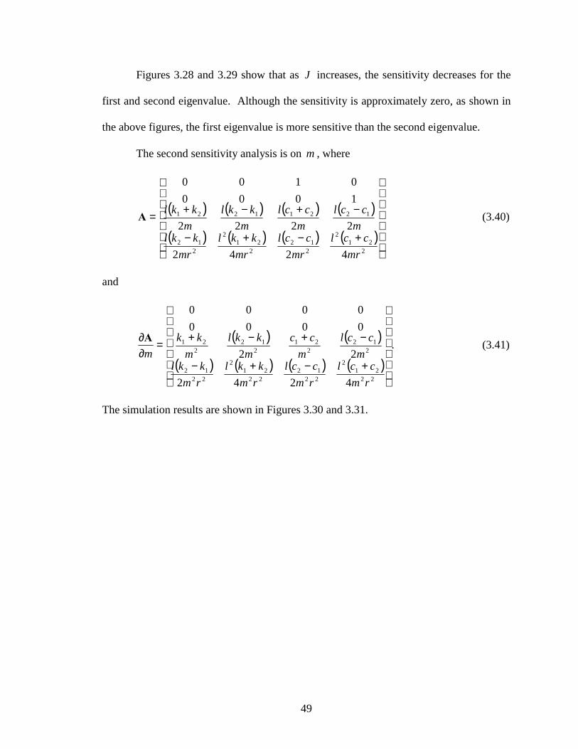
49
Figures 3.28 and 3.29 show that as J increases, the sensitivity decreases for the
first and second eigenvalue. Although the sensitivity is approximately zero, as shown in
the above figures, the first eigenvalue is more sensitive than the second eigenvalue.
The second sensitivity analysis is on m , where
( ) ( ) ( ) ( )
( ) ( ) ( ) ( )
+−+−
−+−+=
221
2
212
221
2
212
12211221
4242
2222
10000100
mrccl
mrccl
mrkkl
mrkkl
mccl
mccl
mkkl
mkklA (3.40)
and
( ) ( )
( ) ( ) ( ) ( )
+−+−
−+−+=∂∂
2221
2
2212
2221
2
2212
212
221
212
221
4242
22
00000000
rmccl
rmccl
rmkkl
rmkkl
mccl
mcc
mkkl
mkk
mA
. (3.41)
The simulation results are shown in Figures 3.30 and 3.31.

50
Mass, in kilograms
Sensitivity, Real(∂λ/∂m)
(rad/(kg-s))
Figure 3.30: Real part of sensitivity of the eigenvalues for both DOF (m)
2400 2600 2800 3000 3200 3400 36000.2
0.4
0.6
0.8
1
1.2
1.4
1.6
1.8x 10
-4
Real(∂λ1/∂m)
Real(∂λ2/∂m)
Mass, in kilograms
Sensitivity, Real(∂λ/∂m)
(rad/(kg-s))
Figure 3.30: Real part of sensitivity of the eigenvalues for both DOF (m)
2400 2600 2800 3000 3200 3400 36000.2
0.4
0.6
0.8
1
1.2
1.4
1.6
1.8x 10
-4
Real(∂λ1/∂m)
Real(∂λ2/∂m)
Mass, in kilograms
Sensitivity, Imag(∂λ/∂m)
(rad/(kg-s))
Figure 3.31: Imaginary part of sensitivity of the eigenvalues for both DOF (m)
2400 2600 2800 3000 3200 3400 36001
1.5
2
2.5
3
3.5
4
4.5
5x 10 -3
Imag(∂λ1/∂m)
Imag(∂λ2/∂m)
Mass, in kilograms
Sensitivity, Imag(∂λ/∂m)
(rad/(kg-s))
Figure 3.31: Imaginary part of sensitivity of the eigenvalues for both DOF (m)
2400 2600 2800 3000 3200 3400 36001
1.5
2
2.5
3
3.5
4
4.5
5x 10 -3
Imag(∂λ1/∂m)
Imag(∂λ2/∂m)

51
As the mass increases, the sensitivity of both eigenvalues decreases as in the
sensitivity analysis on J . However, although the sensitivity is once again approximately
zero, the second eigenvalue is more sensitive than the first eigenvalue.
The third sensitivity analysis is on 1k , where from Equation (3.40)
−−
=∂∂
−−
−−
0025.05.0005.000000000
121
111
mllmlmmk
A. (3.42)
The simulation results are shown in Figures 3.32 and 3.33.
Stiffness, in N/m
Sensitivity, Real(∂λ/∂k1)
(rad-m)/(N-s)
Figure 3.32: Real part of sensitivity of the eigenvalues for both DOF (k1)
4.5 4.52 4.54 4.56 4.58 4.6 4.62 4.64 4.66 4.68 4.7
x 10 5
-2.5
-2
-1.5
-1
-0.5
0
0.5
1
1.5
2
2.5x 10
-8
Real(∂λ1/∂k1)
Real(∂λ2/∂k1)
Stiffness, in N/m
Sensitivity, Real(∂λ/∂k1)
(rad-m)/(N-s)
Figure 3.32: Real part of sensitivity of the eigenvalues for both DOF (k1)
4.5 4.52 4.54 4.56 4.58 4.6 4.62 4.64 4.66 4.68 4.7
x 10 5
-2.5
-2
-1.5
-1
-0.5
0
0.5
1
1.5
2
2.5x 10
-8
Real(∂λ1/∂k1)
Real(∂λ2/∂k1)

52
Figures 3.32 and 3.33 indicate that small perturbations in the stiffness have the
slightest effect on the sensitivity of the eigenvalues. The simulation results follow for 2k ,
so it is not necessary to duplicate the graphs.
The fourth sensitivity analysis is on 1c , where
−−
=∂∂
−−
−−
121
111
25.05.0005.00000000000
mllmlmmc
A. (3.43)
The simulation results are shown in Figures 3.34 and 3.35.
Stiffness, in N/m
Sensitivity, Imag(∂λ/∂k1)
(rad-m)/(N-s)
Figure 3.33: Imaginary part of sensitivity of the eigenvalues for both DOF (k1)
4.5 4.52 4.54 4.56 4.58 4.6 4.62 4.64 4.66 4.68 4.7
x 105
-8.4
-8.3
-8.2
-8.1
-8
-7.9
-7.8x 10
-6
Imag(∂λ1/∂k1)
Imag(∂λ2/∂k1)
Stiffness, in N/m
Sensitivity, Imag(∂λ/∂k1)
(rad-m)/(N-s)
Figure 3.33: Imaginary part of sensitivity of the eigenvalues for both DOF (k1)
4.5 4.52 4.54 4.56 4.58 4.6 4.62 4.64 4.66 4.68 4.7
x 105
-8.4
-8.3
-8.2
-8.1
-8
-7.9
-7.8x 10
-6
Imag(∂λ1/∂k1)
Imag(∂λ2/∂k1)

53
Damping, in N-s/m
Sensitivity,
Real(∂λ/∂c1)
(rad-m)/N
Figure 3.34: Real part of sensitivity of the eigenvalues for both DOF (c1)
1000 1010 1020 1030 1040 1050 1060 1070 1080 1090 1100-1.7
-1.6
-1.5
-1.4
-1.3
-1.2
-1.1
-1
-0.9
-0.8x 10
-4
Real(∂λ1/∂c1)
Real(∂λ2/∂c1)
Damping, in N-s/m
Sensitivity,
Real(∂λ/∂c1)
(rad-m)/N
Figure 3.34: Real part of sensitivity of the eigenvalues for both DOF (c1)
1000 1010 1020 1030 1040 1050 1060 1070 1080 1090 1100-1.7
-1.6
-1.5
-1.4
-1.3
-1.2
-1.1
-1
-0.9
-0.8x 10
-4
Real(∂λ1/∂c1)
Real(∂λ2/∂c1)
Damping, in N-s/m
Sensitivity, Imag(∂λ/∂c1)
(rad-m)/N
Figure 3.35: Imaginary part of sensitivity of the eigenvalues for both DOF (c1)
1000 1010 1020 1030 1040 1050 1060 1070 1080 1090 11000.5
1
1.5
2
2.5
3
3.5
4
4.5
5x 10 -6
Imag(∂λ1/∂c1)
Imag(∂λ2/∂c1)
Damping, in N-s/m
Sensitivity, Imag(∂λ/∂c1)
(rad-m)/N
Figure 3.35: Imaginary part of sensitivity of the eigenvalues for both DOF (c1)
1000 1010 1020 1030 1040 1050 1060 1070 1080 1090 11000.5
1
1.5
2
2.5
3
3.5
4
4.5
5x 10 -6
Imag(∂λ1/∂c1)
Imag(∂λ2/∂c1)

54
Figure 3.34 shows that as the damping increases, it has no effect on the real part
of the sensitivity of the eigenvalue. Figure 3.35 shows that an increase in the damping
has a slight effect on the imaginary part of the sensitivity of the eigenvalues, but is still
approximately zero. The results follow for 2c so it is not necessary to duplicate the
graphs.
Figures 3.28-3.35 reflect the parametric results in Section 3.3. Recall that the real
part of the complex numbers deals with damping and the imaginary part deals with the
natural frequencies. The real part of the sensitivity for ,,, 1kmJ and 1c is approximately
zero indicating the increase in damping has no effect on the system. The imaginary part
of the sensitivity, although very small, reflects the increase or decrease in the two damped
natural frequencies in Section 3.3. The mass seems to be the most sensitive of all the
parameters, although it is extremely small. Recall the parametric analysis on the mass,
J was also affected, so it makes sense that the mass would be more sensitive than the
other parameters.
55
CHAPTER 4: EXPERIMENTAL VERIFICATION
4.1 Introduction
The objective here is to be able to implement the theory in practical applications.
This chapter deals with a laboratory experiment, imitating the configuration in Figure 3.1,
carried out in order to validate the method developed and results derived. However, the
experiment is a free vibration experiment and excludes damping. There will be two parts
to the experimental validation. The first will be results based on the experimental setup.
The second part of this chapter is based on the analytical results and then both of these
results will be compared.
4.2 Experimental Determination
Modal testing is used to obtain the natural frequencies for the experimental setup.
Modal testing is a test where the structure or component is vibrated with a known
excitation, most times out of its normal service environment, which includes both the
data acquisition, and its subsequent analysis. Below is a description of the equipment,
setup, procedure for each test and results.
4.2.1 Equipment
A quartz shear ICP accelerometer, Model 353B33, from PCB Piezotronic is used
in the experimental setup. The accelerometer has a frequency range of 2 Hz to 4000 Hz.
An Impact Hammer, Model 291M78-086C05 made by PCB Piezotronics, causes the
impact during the experiment. The striking end of the hammerhead consists of an
integral ICP quartz force sensor. The frequency range for this sensor is 5 kHz and the

56
hammer range is 22000N. The ICP power to the accelerometer and the hammer are
supplied by the BNC 2140 from National Instruments. The BNC 2140 connects the
accelerometer and hammer to the computer by way of a data collection system. The data
collection system used consisted of a NI 4551 PCI-based Dynamic Signal Analyzer
(DSA) Instrument and the software Virtual Work Bench by National Instruments. The
NI 4551 is specifically designed to make high-accuracy measurements. With the Virtual
Work Bench DSA software, many measurements can be performed such as the power
spectrum, cross power spectrum, and frequency response. This software has several
views, simultaneous displays, and averaging methods that can be used when measuring
the vibration in a system.
4.2.2 Setup
The complete setup is shown in Figure 4.1. When designing this experiment,
there were several issues to consider. (1) System must be rigid. (2) When springs
deform, they must deform linearly. (3) Mass should be heavy enough to cause
deformation. (4) Best to design system in such a way that each parameter can be
perturbed without much complication. (4) Make sure setup has a firm base to prevent
movement during testing. (5) Mount accelerometer securely to the structure to avoid
relative motion between the accelerometer and the structure. (6) Carefully consider the
placement of the accelerometer to obtain the best results. (7) Make sure that the impact
of the hammer is quick and sharp.
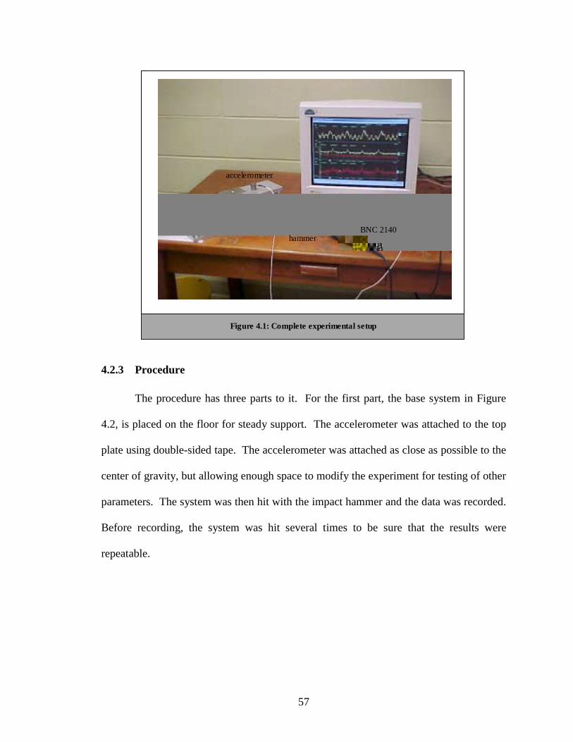
57
4.2.3 Procedure
The procedure has three parts to it. For the first part, the base system in Figure
4.2, is placed on the floor for steady support. The accelerometer was attached to the top
plate using double-sided tape. The accelerometer was attached as close as possible to the
center of gravity, but allowing enough space to modify the experiment for testing of other
parameters. The system was then hit with the impact hammer and the data was recorded.
Before recording, the system was hit several times to be sure that the results were
repeatable.
hammer
accelerometer
Figure 4.1: Complete experimental setup
BNC 2140hammer
accelerometer
Figure 4.1: Complete experimental setup
BNC 2140

58
For Part two of this procedure, two masses were used in this part of the
experiment. The first small mass was attached to the base system at the center of gravity
as in Figure 4.3. The system was hit several times with the impact hammer to make sure
the data was repeatable and then the data was recorded. The first mass was removed and
then the second mass was added. The system was hit again several times and then the
data was recorded.
Figure 4.2: 2-DOF mass-spring systemFigure 4.2: 2-DOF mass-spring system

59
For Part 3 of this procedure, all pieces added to the base system in the previous
testing were removed. Two springs were used in this part of the experiment. The first
was attached at the center of gravity by using a rod and knob as shown in Figures 4.4 and
4.5. The knob compresses the top plate down to the height of the center spring. The
system was then tested as in the previous experiments and the data was recorded. The
second spring was then tested and the data was recorded. All results are seen in the next
section.
Figure 4.3: 2-DOF mass-spring system with added massFigure 4.3: 2-DOF mass-spring system with added mass

60
Figure 4.4: 2-DOF mass-spring system with stiffness modificationFigure 4.4: 2-DOF mass-spring system with stiffness modification
Figure 4.5: Close-up of mass-spring system modificationFigure 4.5: Close-up of mass-spring system modification

61
4.2.4 Results
This section displays the results obtained from using the described equipment in
Section 4.2.1. Figure 4.6 is a snap shot of the results for the system in Figure 4.2. The
first display is the time waveform of the accelerometer and the hammer, the second
display is the amplitude spectrum, and the third display is the transfer function. The data
in yellow (top waveform in display 2) represents the output of the accelerometer and the
data in red (bottom waveform in display 2) represents the output of the hammer. The
peaks seen in the second display represent the natural frequencies of the system. The first
natural frequency is at 12.06 Hz and the second natural frequency is at 24.06 Hz. These
results are fairly close to what was predicted earlier in the analytical determination.
However, there are more than two natural frequencies seen in this figure. This means
that although only 2-DOF are represented in the mathematical model, the actual setup has
more DOF than what is being investigated.

62
For Figure 4.3, when kgm 063.01 = , the experimental results are shown in Figure
4.7. The first natural frequency is at 11.87 Hz and the second natural frequency is at
23.54 Hz.
Figure 4.6: Results for mass-spring systemFigure 4.6: Results for mass-spring system
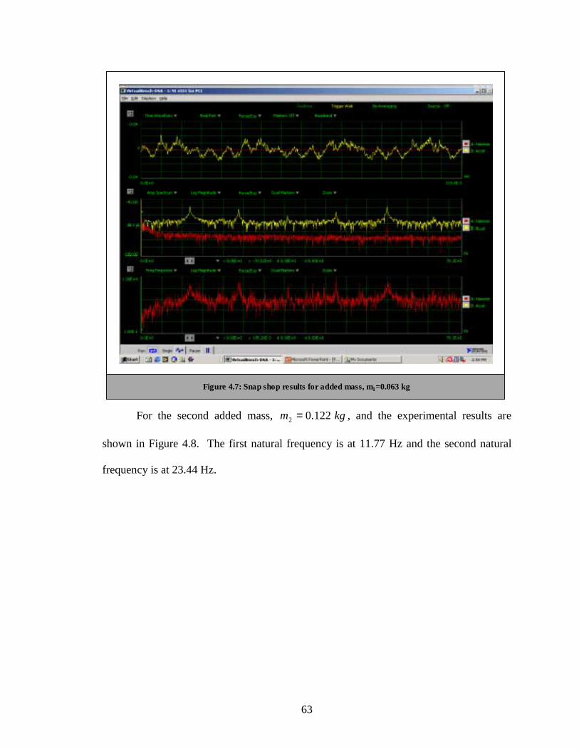
63
For the second added mass, kgm 122.02 = , and the experimental results are
shown in Figure 4.8. The first natural frequency is at 11.77 Hz and the second natural
frequency is at 23.44 Hz.
Figure 4.7: Snap shop results for added mass, m1=0.063 kgFigure 4.7: Snap shop results for added mass, m1=0.063 kg

64
For Figure 4.4 and 4.5, when mNk 7.9103 = the experimental results are shown in
Figure 4.9. In display two, the first natural frequency is at 12.06 Hz and the second
natural frequency is at 24.06 Hz.
Figure 4.8: Snap shot results for added mass, m2=0.122 kgFigure 4.8: Snap shot results for added mass, m2=0.122 kg

65
When mNk 13133 = the results are shown in Figure 4.10. In display two, the first
natural frequency is at 12.06 Hz and the second natural frequency is at 24.06 Hz.
Figure 4.9: Snap shot results for mass-spring system, k3=910.7 N/mFigure 4.9: Snap shot results for mass-spring system, k3=910.7 N/m

66
The experimental sensitivity of the eigenvalues can be determined by the
following formula:
nkniak
i ...,,2,1...,,2,12 ==×∆∆ π
ω, (4.1)
where ka is any parameter of the system and i represents the number of frequencies in
the system. The same two parameters investigated for the parametric analysis will be
investigated here as well. The first parameter that will be looked at is the mass. For
kgm 063.01 = , Equation (4.1) becomes
s
kgradm
−−=×−=∆∆
949.182063.0
06.1287.11
1
1 πω (4.2)
and
Figure 4.10: Snap shot results for mass-spring system, k3=1313 N/mFigure 4.10: Snap shot results for mass-spring system, k3=1313 N/m

67
s
kgradm
−−=×−=∆∆
861.512063.0
06.2454.23
1
2 πω. (4.3)
For kgm 122.02 = , Equation (4.1) becomes
skgrad
m−−=×−=
∆∆
935.142122.0
06.1277.11
2
1 πω (4.4)
and
skgrad
m−−=×−=
∆∆
931.312122.0
06.2444.23
2
2 πω (4.5)
The second parameter that was looked at was the stiffness. For mNk /7.9103 = ,
Equation (4.1) becomes
sNmrad
k −−=×−=
∆∆
0.027.910
06.1206.12
3
1 πω (4.6)
and
sNmrad
k −−=×−=
∆∆
0.027.910
06.2406.24
3
2 πω. (4.7)
For mNk /13133 = , Equation (4.1) becomes
sNmrad
k −−=×−=
∆∆
0.021313
06.1206.12
3
1 πω (4.8)
and
sNmrad
k −−=×−=
∆∆
0.021313
06.2406.24
3
2 πω (4.9)
4.3 Analytical Determination
The analytical determination consists of the vibration, parametric and sensitivity
analysis based on the theory.
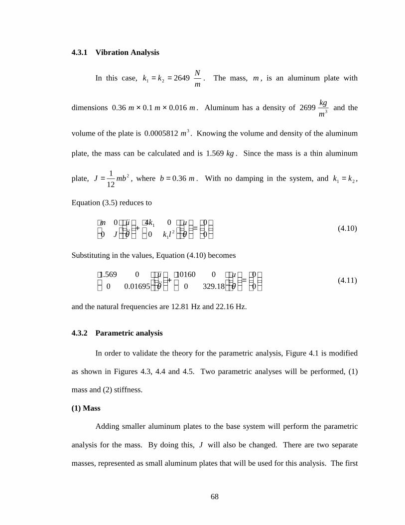
68
4.3.1 Vibration Analysis
In this case, mNkk 264921 == . The mass, m , is an aluminum plate with
dimensions mmm 016.01.036.0 ×× . Aluminum has a density of 32699mkg
and the
volume of the plate is 30005812.0 m . Knowing the volume and density of the aluminum
plate, the mass can be calculated and is kg569.1 . Since the mass is a thin aluminum
plate, 2
121 mbJ = , where mb 36.0= . With no damping in the system, and 21 kk = ,
Equation (3.5) reduces to
=
+
00
004
00
21
1
θθu
lkku
Jm
&&
&& (4.10)
Substituting in the values, Equation (4.10) becomes
=
+
00
18.3290010160
01695.000569.1
θθuu
&&&&
(4.11)
and the natural frequencies are 12.81 Hz and 22.16 Hz.
4.3.2 Parametric analysis
In order to validate the theory for the parametric analysis, Figure 4.1 is modified
as shown in Figures 4.3, 4.4 and 4.5. Two parametric analyses will be performed, (1)
mass and (2) stiffness.
(1) Mass
Adding smaller aluminum plates to the base system will perform the parametric
analysis for the mass. By doing this, J will also be changed. There are two separate
masses, represented as small aluminum plates that will be used for this analysis. The first

69
plate has dimensions mmm 01.004.007.0 ×× , giving it a mass, 1m , of kg063.0 . The
moment of inertia of this plate is 2000023.0 mkg − . The second plate has dimensions
mmm 01.005.008.0 ×× , giving it a mass, 2m , of kg122.0 . The moment of inertia of
this plate is 2000064.0 mkg − . For 1m , Equation (4.10) becomes
=
+
00
18.3290010160
01763.000632.1
θθuu
&&&&
(4.12)
and the natural frequencies are 12.56 Hz and 21.75 Hz. For 2m , Equation (4.10)
becomes
=
+
00
18.3290010160
01826.000691.1
θθuu
&&&&
(4.13)
and the natural frequencies are 12.35 Hz and 21.37 Hz.
(2) Stiffness
The parametric analysis on the stiffness, 1k , will be performed by changing the
stiffness parameter, 3k shown in Figure 4.4 and 4.5. The values for 3k are 910.7 mN
and
1313 mN
. For mNk 7.9103 = , Equation (4.10) becomes
=
+
00
18.3290066.11070
01698.000569.1
θθuu
&&&&
(4.14)
and the natural frequencies are 13.37 Hz and 22.16 Hz. For mNk 13133 = , Equation
(4.10) becomes
=
+
00
18.3290045.11473
01698.000569.1
θθuu
&&
&& (4.15)
and the natural frequencies are 13.61 hz and 22.16 hz.

70
Table 4.1 shows a comparison between the experimental and analytical
parametric analysis.
From Table 4.1, the mass-spring system design seemed to be a good way to verify
the theory because there was a minimum error of 4.9% and a maximum error of 12.9%.
However, just how good these results are will be better determined from the sensitivity
analysis.
4.3.3 Sensitivity Analysis
Following from the parametric analysis, the sensitivity of the parameters to
perturbations can be determined. Two sensitivity analyses will be performed, (1) mass
and (2) stiffness.
(1) Mass
Following the sensitivity analysis from Section 3.4.2, Equation (3.36) becomes
=
−
−
00000010000100
11
11
kJkm
A (4.16)
therefore,
13.61
22.1624.06
12.06
22.16
13.37
24.06
12.06
21.37
12.35
23.44
11.77
21.75
12.56
23.54
11.87
22.16
12.81
24.06
12.061
2
ExpExpExpExpExp AnalyAnalyAnalyAnalyAnalyωn
m2=0.063 kg k3=910.66 N/mBase system k3=1313.45 N/mm1=0.122 kg
Table 4.1: Experimental and analytical parametric analysis results
13.61
22.1624.06
12.06
22.16
13.37
24.06
12.06
21.37
12.35
23.44
11.77
21.75
12.56
23.54
11.87
22.16
12.81
24.06
12.061
2
ExpExpExpExpExp AnalyAnalyAnalyAnalyAnalyωn
m2=0.063 kg k3=910.66 N/mBase system k3=1313.45 N/mm1=0.122 kg
Table 4.1: Experimental and analytical parametric analysis results

71
( )
−−
=∂∂
−
−
0012000000000000
2
21
mbmkm
A (4.17)
Using MATLAB, m∂
∂ 1λ and
m∂∂ 2λ
were determined. The results are shown in Figures
4.11. Only the imaginary part of the sensitivity is shown because the real part is zero
indicating there is no damping in the system.
1.62 1.63 1.64 1.65 1.66 1.67 1.68 1.69 1.7-45
-40
-35
-30
-25
-20
Mass, in kilograms
Sensitivity,
Imag(∂λ/∂m)
(rad/(kg-s))
Figure 4.11: Experiment-imaginary part of sensitivity for both DOF (mass)
Imag(∂λ1∂m)
Imag(∂λ2∂m)
1.62 1.63 1.64 1.65 1.66 1.67 1.68 1.69 1.7-45
-40
-35
-30
-25
-20
Mass, in kilograms
Sensitivity,
Imag(∂λ/∂m)
(rad/(kg-s))
Figure 4.11: Experiment-imaginary part of sensitivity for both DOF (mass)
Imag(∂λ1∂m)
Imag(∂λ2∂m)

72
(2) Stiffness
Following the sensitivity analysis from Section 3.4.2, Equation (3.36) becomes
=∂∂
−
−
00000000000000
1
11
Jmk
A. (4.18)
Using MATLAB, 1
1
k∂∂λ
and 1
2
k∂∂λ
were determined. The results are shown in Figure 4.12.
Only the imaginary part of the sensitivity of the first eigenvalue is seen because the
second eigenvalue is zero.
Table 4.2 shows comparison between the experimental and sensitivity analysis
results.
900 950 1000 1050 1100 1150 1200 1250 1300 1350-4
-3.5
-3
-2.5
-2
-1.5
-1
-0.5
0x 10
-3
Stiffness, in N/m
Sensitivity,
Imag(∂λ/∂k3)
(rad-m)/(N-s)
Imag(∂λ1/∂k3)
Figure 4.12: Experiment-imaginary part of sensitivity for both DOF (k3)
900 950 1000 1050 1100 1150 1200 1250 1300 1350-4
-3.5
-3
-2.5
-2
-1.5
-1
-0.5
0x 10
-3
Stiffness, in N/m
Sensitivity,
Imag(∂λ/∂k3)
(rad-m)/(N-s)
Imag(∂λ1/∂k3)
Figure 4.12: Experiment-imaginary part of sensitivity for both DOF (k3)

73
Table 4.2 shows that the error ranges from 28.09-54.0% and 18.94-24.76% for the
sensitivities on the first and second eigenvalue, respectively, with mass incremental
changes. This error is high because the mass in this case is a very sensitive parameter, so
the slightest change affects it drastically. The Virtual Work Bench software used in this
experiment has cursors that aid in helping to find the value of the peaks or natural
frequencies, as in Figures 4.6-4.10. For example, if
skgrad
m−−=×−=
∆∆
91.132122.0
06.1278.11
2
1 πω
or
skgrad
m−−=×−=
∆∆
24.252122.0
06.1257.11
2
1 πω,
the error in sensitivity can increase to 65.35% or decrease to 8.87% from the original
54.0%. Therefore, this high error is due to error in experimental measurements that are
not seen by the human eye. It is evident that the best results were obtained for the
stiffness for the first and second eigenvalue.
-0.0037i
00
0
0
-0.0038i
0
0
-39.8383i
-23.0006i
-31.931i
-14.935i
-42.0392
-24.2713i
-51.861i
-18.949i1
2
ExpExpExpExp AnalyAnalyAnalyAnaly∂λ/∂ai
m2=0.122 kg k3=910.7 N/m k3=1313 N/mm1=0.063 kg
Table 4.2: Experimental and analytical sensitivity analysis results
-0.0037i
00
0
0
-0.0038i
0
0
-39.8383i
-23.0006i
-31.931i
-14.935i
-42.0392
-24.2713i
-51.861i
-18.949i1
2
ExpExpExpExp AnalyAnalyAnalyAnaly∂λ/∂ai
m2=0.122 kg k3=910.7 N/m k3=1313 N/mm1=0.063 kg
Table 4.2: Experimental and analytical sensitivity analysis results

74
CONCLUSION AND RECOMMENDATIONS
5.1 Conclusion
Vibration analysis is an inherent part of the design of any mechanical system.
The work done in this thesis was to develop a parametric and sensitivity methodology for
the effects of vibration in an automobile. Several supporting articles were given which
cover several techniques that others have proposed and implemented, in order to reduce
the vibration response of the system. This is essential because an increase in vibration
causes an undesirable effect for the driver.
A literature survey of past work was provided in developing a mathematical
model to best determine the vibration response in vehicle system modeling, vehicle
structure modes, tire properties and vehicle handling. The fundamental theory for free
and forced vibration for a damped system and the parametric and sensitivity analyses
have been provided. From the parametric analysis, J had an effect on the first damped
natural frequency only in the bounce mode; but in the pitch mode, J had an effect on
magnitude and position of the first damped natural frequency and an effect on the
magnitude for the second damped natural frequency. The mass had an effect on both the
position and magnitude of both damped natural frequencies in the bounce and pitch
mode. Surprisingly, 1k did not have much of an effect on either of the damped natural
frequencies in the bounce or pitch mode. This could be due to the fact that 1k may not
have had a high enough perturbation when compared to 2k . Another reason could be that
it was excessively large when compared to the mass, which with a slight change in
stiffness and the mass is constant; there was not much difference. The results for 1c

75
concluded that the damping had no effect on the system because the damping ratio was
very close to zero; therefore, nd ωω ≅ and nω depends only on m and k . For the
sensitivity analysis, the mass is the most sensitive parameter. This is mostly evident
because when m is changed J is changed as well. The opposite is not true because J
can be changed without changing m by changing the dimensions.
The equipment used for the experiment consisted of a quartz shear ICP
accelerometer, an impact hammer, DSA Instrument, and the software Virtual Work
Bench by National Instruments. This equipment proved successful in the experiment
because it allowed for different types of data collection without complication. The
natural frequencies obtained from the experiment were fairly close to the natural
frequencies obtained analytical. However, although the experimental sensitivities for the
most part were close in numbers to the analytical sensitivities, they were not close
enough because the error ranged from 0-54%. This large range of error was due to the
incremental change in the mass. The larger errors were due the sensitivity on the second
eigenvalue. This could be due to the fact that the mass is a sensitive parameter, which
was established in the parametric results. Therefore, the mass parameter must be handled
with special attention.
5.2 Recommendations for Future Research
There are several issues to consider for further investigation. (1) Investigating the
roll mode of the vehicle. (2) Analyzing the system as a lumped mass system, 1-mass and
1-spring. (3) Extend to a realistic automobile by adding more DOF. (4) Include
damping in the experiment. (5) Include a harmonic excitation force. (6) Include a
vibration absorber in the experiment.

76
REFERENCES
1. Chrstos, Jeffrey P., “A Simplified Method for the Measurement of Composite Suspension Parameters”, SAE Paper 910232, presented at International Congress and Exposition, Detroit, MI, February 25-March 1. 1991.
2. Mimuro, Tetsushi, Masayoshi Ohsaki, Hiromichi Yasunaga and Kohji Satoh, “Four
Parameter Evaluation Method of Lateral Transient Response”, SAE Paper 901734, presented at Passenger Car Meeting and Exposition, Dearborn, MI, September 17-20, 1990.
3. Hovarth, Jack K., “Structural and System Models”, SAE Paper 750135, 1975.
4. Davis, James C., “Modal Modeling Techniques for Vehicle Shake Analysis”, SAE Paper 720045, Presented at the Automobile Engineering Congress, Detroit, MI, January 10-14, 1972.
5. Speckhart, Frank H., “A Computer Simulation for Three-Dimensional Vehicle
Dynamics”, SAE Paper 730526, 1973. 6. Simic, Dusan P. and Zika Petronijevic, “Experimental Analysis of Automobile Body
Vibration Characteristics”, SAE Paper 861261, presented at the International Off-Highway Powerplant Congress and Exposition, Milwaukee, Wisconsin, September 8-11, 1986.
7. Daberkow, A. and E.J. Kreuzer, “An Integrated Approach for Computer Aided Design
in Multibody System Dynamics”, Engineering with Computers, Vol 15, No 2, 1999.
8. Huang, S.J. and H.C. Chao, “Fuzzy Logic Controller for a Vehicle Active Suspension
System”, presented at the Proceedings of the Institution of Mechanical Engineers, Part D; Journal of Automobile Engineering, Vol 214, No D1, 2000, pp1-12.
9. Varadi, Peter C., Gwo-Jeng Lo, Oliver M. O’Reilly and Panayiotis Papadopoulos, “A
Novel Approach to Vehicle Dynamics Using the Theory of a Cosserat Point and Its Application to Collision Analyses of Platooning Vehicles”, Vehicles System Dynamics, Vol 32, No 1, July 1999, 99 85-108.
10. Zhang, Yuan, Paul Xiao, Tim Palmer and Akbar Faraham, “Vehicle
Chassis/Suspension Dynamics Analysis-Finite Element Model vs. Rigid Body Model”, SAE Paper 980900, 1998, pp 113-126.
11. Kawagoe, Kenji, Kenji Suma and Masayuki Watanabe, “Evaluation and Improvement
of Vehicle Roll Behavior”, SAE Paper 970093 Presented at International Congress and Exposition, Detroit, MI, February 24-27, 1997.

77
12. Mehrabi, M.G., R.M.H. Cheng and A. Hemami, “Parametric Study and Sensitivity Analysis of Automated Vehicles”, Robotica, Vol 13, September –October 1995, pp 469-475.
13. El-Demerdash, S.M., “Performance of Limited Bandwith Active Suspension Based
on a Half Car Model”, SAE Paper 981119, pp 177-186, Developments in Tire, Wheel, Steering and Suspension Technology, SP-1338, 1998.
14. Loeb, Jeff S., Dennis A Guenther, Hung-Hsu Fred Chen and John R. Ellis, “Lateral
Stiffness, Cornering Stiffness and Relaxation Length of the Pneumatic Tire”, SAE Paper 900129, 1990.
15. Chiesa, A. and L. Rinonapoli, “Vehicle Stability Studied with a Non-Linear Seven
Degree Model”, pp 1708-1724. 16. Taylor, R.K., L.L. Bashford and M.D. Schrock, “Methods for Measuring Vertical
Tire Stiffness”, Transactions of the ASME, ASME, Vol 43, No 6, November-December 2000, pp 1415-1419.
17. Salaani, Mohamed Kamel, Jeffrey P. Chrstos and Dennis A. Guenther, “Parameter
Measurement and Development of a NADSdyna Validation Data Set for a 1994 Ford Taurus”, SAE Paper 970564, presented at International Congress and Exposition, Detroit, MI, February 24-27, 1997.
18. Nalecz, Andrej G. and Alan C. Bindemann, “Handling Properties of Four Wheel
Steering Vehicles”, SAE Paper 890080, 1989. 19. Mousseau, C.W., T.A. Laursen, M. Lidberg and R.L. Taylor, “Vehicle Dynamics
Simulations with Coupled Multibody and Finite Element Methods”, Finite Elements in Analysis and Design, Vol 31, No 4, 1999, pp 295-315.
20. Sekula, P.J., G.L. Hall, G.R. Potts and F.S. Conant, “Dynamic Indoor Tire Testing
and Fourier Transform Analysis”, Tire Science and Technology, Vol 4, No 2, May 1976, pp 66-85.
21. Elbay, S. and Y.M. Ram, “An Affine Inverse Eigenvalue Problem”, 2002 (to appear).

78
APPENDIX: MATLAB PROGRAMS
1. Program to determine the poles and eigenvectors of a mass-spring-damper system for free vibration.
clear all kf=225000; in N/m kr=300000; in N/m cf=500; in N-s/m cr=600; in N-s/m m=2519; in kilograms l1=2.53; in meters ig=m*l1^2; l=2.95; in meters k1=2*kf; total spring rate for both front tires k2=2*kr; total spring rate for both rear tires c1=2*cf; total damping rate for both front tires c2=2*cr; total damping rate for both rear tires
Formulation of M, C, K, A, and B matrices M=[m 0;0 ig]; K=[k1+k2 l/2*(k2-k1);l/2*(k2-k1) l^2/4*(k1+k2)]; C=[c1+c2 l/2*(c2-c1);l/2*(c2-c1) l^2/4*(c1+c2)]; A=[zeros(2,2) eye(2);-K zeros(2,2)]; B=[eye(2) zeros(2,2);C M];
Determination and plot of poles and eigenvectors [v,s]=eig(A,B) figure(1) plot(s,'.') v1=v(:,1); v2=v(:,3); v3=v(:,2); v4=v(:,4); figure(2) plot(real(v1),'bo-') hold on; plot(imag(v1),'k*-') plot(abs(v1),'rx-') grid on;

79
figure(3) plot(real(v2),'bo-') hold on; plot(imag(v2),'k*-') plot(abs(v2),'rx-') grid on; figure(4) plot(real(v3),'bo-') hold on; plot(imag(v3),'k*-') plot(abs(v3),'rx-') grid on; figure(5) plot(real(v4),'bo-') hold on; plot(imag(v4),'k*-') plot(abs(v4),'rx-') grid on;
2. Program to determine poles and eigenvectors of a mass-spring-damper system with an external force.
clear all kf=225000; kr=300000; cf=500; cr=600; m=2519; l1=2.53; ig=m*l1^2; l=2.95; k1=2*kf; k2=2*kr; c1=2*cf; c2=2*cr;
Formulation of M, C, K matrices M=[m 0;0 ig]; K=[k1+k2 l/2*(k2-k1);l/2*(k2-k1) l^2/4*(k1+k2)]; C=[c1+c2 l/2*(c2-c1);l/2*(c2-c1) l^2/4*(c1+c2)]; n=100; n represents the maximum time interval in 100th of a second dw=1/n; dw represents the increment for the natural frequency interval w=[0:dw:30]';

80
[zzz,dum]=size(w); f=[1;0];
Determination of frequency response and phase function for i=1:zzz, A=[K-w(i)^2*M w(i)*C;-w(i)*C K-w(i)^2*M]; B=[zeros(2,1);f]; sol=inv(A)*B; p=sol(1:2,1); q=sol(3:4,1); X1(i,1)=sqrt(p(1,1)^2+q(1,1)^2); F1(i,1)=atan2(q(1,1),p(1,1)); X2(i,1)=sqrt(p(2,1)^2+q(2,1)^2); F2(i,1)=atan2(q(2,1),p(2,1)); end
Plot of frequency response and phase function figure(1); semilogy(w,X1); grid on; figure(2); plot(w,F1); grid on; figure(3); semilogy(w,X2); grid on; figure(4); plot(w,F2); grid on;
3. Program to determine the natural frequencies when the parameter J is perturbed.
clear all for ii=1:6, l1=2.53+(ii-1)*0.1; kf=225000; kr=300000; cf=500; cr=600; m=2519;

81
ig=m*l1^2; l=2.95; k1=2*kf; k2=2*kr; c1=2*cf; c2=2*cr;
Formulation of M, C, and K matrices M=[m 0;0 ig]; K=[k1+k2 l/2*(k2-k1);l/2*(k2-k1) l^2/4*(k1+k2)]; C=[c1+c2 l/2*(c2-c1);l/2*(c2-c1) l^2/4*(c1+c2)]; n=1001; dw=0.025; w=[0:dw:n*dw]'; [zzz,dum]=size(w); f=[1;0];
Determination of frequency response and phase function for i=1:zzz, A=[K-w(i)^2*M w(i)*C;-w(i)*C K-w(i)^2*M]; B=[zeros(2,1);f]; sol=inv(A)*B; p=sol(1:2,1); q=sol(3:4,1); X1(i,ii)=sqrt(p(1,1)^2+q(1,1)^2); F1(i,ii)=atan2(q(1,1),p(1,1)); X2(i,ii)=sqrt(p(2,1)^2+q(2,1)^2); F2(i,ii)=atan2(q(2,1),p(2,1)); end end
Plot of frequency response and phase function figure(1); semilogy(w,X1); grid on; figure(2); plot(w,F1); grid on; figure(3); semilogy(w,X2); grid on;

82
figure(4); plot(w,F2); grid on;
4. Program to determine the natural frequencies when the parameter m is perturbed.
clear all for ii=1:6, l1=2.53; kf=225000; kr=300000; cf=500; cr=600; m=2519+(ii-1)*200; ig=m*l1^2; l=2.95; k1=2*kf; k2=2*kr; c1=2*cf; c2=2*cr;
Formulation of M, C, and K matrices M=[m 0;0 ig]; K=[k1+k2 l/2*(k2-k1);l/2*(k2-k1) l^2/4*(k1+k2)]; C=[c1+c2 l/2*(c2-c1);l/2*(c2-c1) l^2/4*(c1+c2)]; n=1001; dw=0.025; w=[0:dw:n*dw]'; [zzz,dum]=size(w); f=[1;0];
Determination of frequency response and phase function for i=1:zzz, A=[K-w(i)^2*M w(i)*C;-w(i)*C K-w(i)^2*M]; B=[zeros(2,1);f]; sol=inv(A)*B; p=sol(1:2,1); q=sol(3:4,1); X1(i,ii)=sqrt(p(1,1)^2+q(1,1)^2); F1(i,ii)=atan2(q(1,1),p(1,1)); X2(i,ii)=sqrt(p(2,1)^2+q(2,1)^2); F2(i,ii)=atan2(q(2,1),p(2,1));

83
end end
Plot of frequency response and phase function figure(1); semilogy(w,X1); grid on; figure(2); plot(w,F1); grid on; figure(3); semilogy(w,X2); grid on; figure(4); plot(w,F2); grid on;
5. Program to determine the natural frequencies when the parameter k1 is perturbed.
clear all for ii=1:6, l1=2.53; kf= 225000+(ii-1)*2000; kr=300000; cf=500; cr=600; m=2519; ig=m*l1^2; l=2.95; k1=2*kf; k2=2*kr; c1=2*cf; c2=2*cr;
Formulation of M, C, and K matrices M=[m 0;0 ig]; K=[k1+k2 l/2*(k2-k1);l/2*(k2-k1) l^2/4*(k1+k2)]; C=[c1+c2 l/2*(c2-c1);l/2*(c2-c1) l^2/4*(c1+c2)]; n=1001;

84
dw=0.025; w=[0:dw:n*dw]'; [zzz,dum]=size(w); f=[1;0];
Determination of frequency response and phase function for i=1:zzz, A=[K-w(i)^2*M w(i)*C;-w(i)*C K-w(i)^2*M]; B=[zeros(2,1);f]; sol=inv(A)*B; p=sol(1:2,1); q=sol(3:4,1); X1(i,ii)=sqrt(p(1,1)^2+q(1,1)^2); F1(i,ii)=atan2(q(1,1),p(1,1)); X2(i,ii)=sqrt(p(2,1)^2+q(2,1)^2); F2(i,ii)=atan2(q(2,1),p(2,1)); end end
Plot of frequency response and phase function figure(1); semilogy(w,X1); grid on; figure(2); plot(w,F1); grid on; figure(3); semilogy(w,X2); grid on; figure(4); plot(w,F2); grid on;
6. Program to determine the natural frequencies when the parameter c1 is perturbed.
clear all for ii=1:6, l1=2.53; kf=225000;

85
kr=300000; cf= 500+(ii-1)*10; cr=600; m=2519; ig=m*l1^2; l=2.95; k1=2*kf; k2=2*kr; c1=2*cf; c2=2*cr;
Formulation of M, C, and K matrices M=[m 0;0 ig]; K=[k1+k2 l/2*(k2-k1);l/2*(k2-k1) l^2/4*(k1+k2)]; C=[c1+c2 l/2*(c2-c1);l/2*(c2-c1) l^2/4*(c1+c2)]; n=1001; dw=0.025; w=[0:dw:n*dw]'; [zzz,dum]=size(w); f=[1;0];
Determination of frequency response and phase function for i=1:zzz, A=[K-w(i)^2*M w(i)*C;-w(i)*C K-w(i)^2*M]; B=[zeros(2,1);f]; sol=inv(A)*B; p=sol(1:2,1); q=sol(3:4,1); X1(i,ii)=sqrt(p(1,1)^2+q(1,1)^2); F1(i,ii)=atan2(q(1,1),p(1,1)); X2(i,ii)=sqrt(p(2,1)^2+q(2,1)^2); F2(i,ii)=atan2(q(2,1),p(2,1)); end end
Plot of frequency response and phase function figure(1); semilogy(w,X1); grid on; figure(2); plot(w,F1); grid on;

86
figure(3); semilogy(w,X2); grid on; figure(4); plot(w,F2); grid on;
7. Program to perform the sensitivity analysis on J for the perturbations in the parametric analysis.
clear all; for ii=1:6, l1=2.53+(ii-1)*0.1; kf=225000; kr=300000; cf=500; cr=600; m=2519; ig(ii)=m*l1^2; J=ig(ii); l=2.95; k1=2*kf; k2=2*kr; c1=2*cf; c2=2*cr;
Formulation of M, C, and K matrices M=[m 0;0 J]; K=[k1+k2 l/2*(k2-k1);l/2*(k2-k1) l^2/4*(k1+k2)]; C=[c1+c2 l/2*(c2-c1);l/2*(c2-c1) l^2/4*(c1+c2)]; A=[zeros(2,2) eye(2);-inv(M)*K -inv(M)*C]; [U,S]=eig(A); [s,ind]=sort(diag(S)); U=U(:,ind); V=inv(U');
ds1/dJ dA_dJ=[zeros(2,4);-[0 0;0 -1/J^2]*K -[0 0;0 -1/J^2]*C]; y1=V(:,1); x1=U(:,1); ds1_dJ(ii,1)=y1'*dA_dJ*x1/(y1'*x1);

87
check for s
dJ=0.1; M1=[m 0;0 J+dJ]; A1=[zeros(2,2) eye(2);-inv(M1)*K -inv(M1)*C]; [U1,S1]=eig(A1); [s1,ind]=sort(diag(S1)); U1=U1(:,ind); zz1(ii,1)=(s1(1)-s(1))/dJ;
ds2/dJ y2=V(:,3); x2=U(:,3); ds2_dJ(ii,1)=y2'*dA_dJ*x2/(y2'*x2);
check for s zz2(ii,1)=(s1(3)-s(3))/dJ; end [ds1_dJ zz1] [ds2_dJ zz2] figure(1) plot(ig,[real(ds1_dJ),real(ds2_dJ)]) grid on; figure(2) plot(ig,[imag(ds1_dJ),imag(ds2_dJ)]) grid on;
8. Program to perform the sensitivity analysis on m for the perturbations in the parametric analysis.
clear all; for ii=1:6, l1=2.53; kf=225000; kr=300000; cf=500; cr=600; m= 2519+(ii-1)*200; ig(ii)=m*l1^2; J=ig(ii); l=2.95; k1=2*kf;

88
k2=2*kr; c1=2*cf; c2=2*cr;
Formulation of M, C, and K matrices M=[m 0;0 J]; K=[k1+k2 l/2*(k2-k1);l/2*(k2-k1) l^2/4*(k1+k2)]; C=[c1+c2 l/2*(c2-c1);l/2*(c2-c1) l^2/4*(c1+c2)]; A=[zeros(2,2) eye(2);-inv(M)*K -inv(M)*C]; [U,S]=eig(A); [s,ind]=sort(diag(S)); U=U(:,ind); V=inv(U');
ds1/dJ dA_dm=[zeros(2,4);-[-1/m^2 0;0 -r^2/J^2]*K -[-1/m^2 0;0 -r^2/J^2]*C]; y1=V(:,1); x1=U(:,1); ds1_dm(ii,1)=y1'*dA_dm*x1/(y1'*x1);
check for s dm=0.1; M1=[m+dm 0;0 (m+dm)*l1^2]; A1=[zeros(2,2) eye(2);-inv(M1)*K -inv(M1)*C]; [U1,S1]=eig(A1); [s1,ind]=sort(diag(S1)); U1=U1(:,ind); zz1(ii,1)=(s1(1)-s(1))/dm;
ds2/dJ y2=V(:,3); x2=U(:,3); ds2_dm(ii,1)=y2'*dA_dm*x2/(y2'*x2);
check for s zz2(ii,1)=(s1(3)-s(3))/dm; end [ds1_dm zz1] [ds2_dm zz2] figure(1)

89
plot(ig,[real(ds1_dm),real(ds2_dm)]) grid on; figure(2) plot(ig,[imag(ds1_dm),imag(ds2_dm)]) grid on;
9. Program to perform the sensitivity analysis on k1 for the perturbations in the parametric analysis.
clear all; for ii=1:6, l1=2.53; kf= 225000+(ii-1)*2000; kr=300000; cf=500; cr=600; m=2519; ig(ii)=m*l1^2; J=ig(ii); l=2.95; k1=2*kf; k2=2*kr; c1=2*cf; c2=2*cr;
Formulation of M, C, and K matrices M=[m 0;0 J]; K=[k1+k2 l/2*(k2-k1);l/2*(k2-k1) l^2/4*(k1+k2)]; C=[c1+c2 l/2*(c2-c1);l/2*(c2-c1) l^2/4*(c1+c2)]; A=[zeros(2,2) eye(2);-inv(M)*K -inv(M)*C]; [U,S]=eig(A); [s,ind]=sort(diag(S)); U=U(:,ind); V=inv(U');
ds1/dk1: dA_dk1=[zeros(2,4);-inv(M)*[1 -l/2;-l/2 l^2/4] zeros(2,2)]; y1=V(:,1); x1=U(:,1); ds1_dk1(ii,1)=y1'*dA_dk1*x1/(y1'*x1);
check for s

90
dk1=0.1; K1=[k1+k2+dk1 l/2*(k2-k1-dk1);l/2*(k2-k1-dk1) l^2/4*(k1+k2+dk1)]; A1=[zeros(2,2) eye(2);-inv(M)*K1 -inv(M)*C]; [U1,S1]=eig(A1); [s1,ind]=sort(diag(S1)); U1=U1(:,ind); zz1(ii,1)=(s1(1)-s(1))/dk1;
ds2/dk1 y2=V(:,3); x2=U(:,3); ds2_dk1(ii,1)=y2'*dA_dk1*x2/(y2'*x2);
check for s zz2(ii,1)=(s1(3)-s(3))/dk1; end [ds1_dk1 zz1] [ds2_dk1 zz2] figure(1) plot(ig,[real(ds1_dk1),real(ds2_dk1)]) grid on; figure(2) plot(ig,[imag(ds1_dk1),imag(ds2_dk1)]) grid on;
10. Program to perform the sensitivity analysis on c1 for the perturbations in the parametric analysis.
clear all; for ii=1:6, l1=2.53; kf=225000; kr=300000; cf=500 500+(ii-1)*10; cr=600; m=2519; damp(ii)=c1; J=ig(ii); l=2.95; k1=2*kf; k2=2*kr; c1=2*cf;

91
c2=2*cr;
Formulation of M, C, and K matrices M=[m 0;0 J]; K=[k1+k2 l/2*(k2-k1);l/2*(k2-k1) l^2/4*(k1+k2)]; C=[c1+c2 l/2*(c2-c1);l/2*(c2-c1) l^2/4*(c1+c2)]; A=[zeros(2,2) eye(2);-inv(M)*K -inv(M)*C]; [U,S]=eig(A); [s,ind]=sort(diag(S)); U=U(:,ind); V=inv(U');
ds1/dc1 dA_dc1=[zeros(2,4);zeros(2,2) -inv(M)*[1 -l/2;-l/2 l^2/4]]; y1=V(:,1); x1=U(:,1); ds1_dc1(ii,1)=y1'*dA_dc1*x1/(y1'*x1);
check for s dc1=0.1; C1=[c1+c2+dc1 l/2*(c2-c1-dc1);l/2*(c2-c1-dc1) l^2/4*(c1+c2+dc1)]; A1=[zeros(2,2) eye(2);-inv(M)*K -inv(M)*C1]; [U1,S1]=eig(A1); [s1,ind]=sort(diag(S1)); U1=U1(:,ind); zz1(ii,1)=(s1(1)-s(1))/dc1;
ds2/dJ: Sensitivity on J y2=V(:,3); x2=U(:,3); ds2_dc1(ii,1)=y2'*dA_dJ*x2/(y2'*x2);
check for s zz2(ii,1)=(s1(3)-s(3))/dc1; end [ds1_dc1 zz1] [ds2_dc1 zz2] figure(1) plot(ig,[real(ds1_dc1),real(ds2_dc1)]) grid on;

92
figure(2) plot(ig,[imag(ds1_dc1),imag(ds2_dc1)]) grid on;
11. Program to calculate natural frequencies for free vibration for experiment- base system.
clear all b=0.36; k1=2540; m=1.569; J=1/12*m*b^2; l=b; M=[m 0;0 J]; K=[4*k1 0;0 l^2*k1]; [v,s]=eig(K,M)
12 Program to calculate natural frequencies for free vibration for experiment with added mass.
clear all m1=[0.063;0.122]; for ii=1:2, b=0.36; k1=2540; m=1.569+m1(ii); J=1/12*m*b^2; l=b; M=[m 0;0 J]; K=[4*k1+k3(ii) 0;0 l^2*k1]; [v,s]=eig(K,M) end
13. Program to calculate natural frequencies for free vibration for experiment with center spring.
clear all k3=[910.7;1313]; for ii=1:2, b=0.36; k1=2540; m=1.569; J=1/12*m*b^2;

93
l=b; M=[m 0;0 J]; K=[4*k1+k3(ii) 0;0 l^2*k1]; [v,s]=eig(K,M) end
14. Program to calculate the sensitivity analysis for mass perturbations for experimental setup.
clear all mm=[0.063;0.122]; for ii=1:2, b=0.36; k1=2540; m=1.569+mm(ii); J=1/12*m*b^2; l=b;% in meters M=[m 0;0 J]; K=[4*k1 0;0 l^2*k1]; C=[0 0;0 0]; mass(ii)=m; A=[zeros(2,2) eye(2);-inv(M)*K -inv(M)*C]; [U,S]=eig(A); [s,ind]=sort(diag(S)); U=U(:,ind); V=inv(U');
∂s1/∂m dA_dm=[zeros(2,4);[-1/m^2 0;0 -12/(m^2*b^2)]*K zeros(2,2)]; y1=V(:,1); x1=U(:,1); ds1_dm(ii,1)=y1'*dA_dm*x1/(y1'*x1);
check for s dm=0.001; M1=[m+dm 0;0 (m+dm)*b^2/12]; A1=[zeros(2,2) eye(2);-inv(M1)*K -inv(M)*C]; [U1,S1]=eig(A1); [s1,ind]=sort(diag(S1)); U1=U1(:,ind); zz1(ii,1)=(s(1)-s1(1))/dm;

94
∂s2/∂m y2=V(:,3); x2=U(:,3); ds2_dm(ii,1)=y2'*dA_dm*x2/(y2'*x2);
check for s zz2(ii,1)=(s(3)-s1(3))/dm; end [ds1_dm zz1] [ds2_dm zz2] figure(1) plot(mass,[real(ds1_dm),real(ds2_dm)]) grid on; figure(2) plot(mass,[imag(ds1_dm),imag(ds2_dm)]) grid on;
15 Program to calculate the sensitivity for the perturbations in the stiffness for the free vibration.
clear all k3=[910.7;1313]; for ii=1:2, b=0.36; k1=2540; m=1.569; J=1/12*m*b^2; l=b; M=[m 0;0 J]; K=[4*k1+k3(ii) 0;0 l^2*k1]; C=[0 0;0 0]; stiff(ii)=k3(ii); A=[zeros(2,2) eye(2);-inv(M)*K -inv(M)*C]; [U,S]=eig(A); [s,ind]=sort(diag(S)); U=U(:,ind); V=inv(U');
∂s1/∂k1 dA_dk1=[zeros(2,4);-inv(M)*[1 0;0 0] zeros(2,2)]; y1=V(:,1);

95
x1=U(:,1); ds1_dk1(ii,1)=y1'*dA_dk1*x1/(y1'*x1);
check for s dk3=0.1; K1=[4*k1+k3(ii)+dk3 0;0 l^2*k1]; A1=[zeros(2,2) eye(2);-inv(M)*K1 -inv(M)*C]; [U1,S1]=eig(A1); [s1,ind]=sort(diag(S1)); U1=U1(:,ind); zz1(ii,1)=(s1(1)-s(1))/dk3;
∂s2/∂k3 y2=V(:,3); x2=U(:,3); ds2_dk1(ii,1)=y2'*dA_dk1*x2/(y2'*x2);
check for s zz2(ii,1)=(s1(3)-s(3))/dk3; end [ds1_dk1 zz1] [ds2_dk1 zz2] figure(1) plot(stiff,[real(ds1_dk1),real(ds2_dk1)]) grid on; figure(2) plot(stiff,[imag(ds1_dk1),imag(ds2_dk1)]) grid on;

96
VITA
Kanika Nicole Vessel was born on March 7, 1977, in Detroit, Michigan, to
Theophilus and Nordica Mixon, Jr. She went to high school in Detroit, Michigan at
Martin Luther King, Jr. High School. She obtained a Bachelor of Science in Mechanical
Engineering from Southern University and A & M College in Baton Rouge, Louisiana.
Following graduation, she decided to pursue a graduate degree in mechanical engineering
at Louisiana State University-Baton Rouge, Louisiana, with specialization in mechanical
systems and vibration. She successfully defended her thesis on Friday, April 12, 2002,
and will be graduating with a Master of Science degree in Mechanical Engineering in
May 2002. She will continue to pursue a doctoral degree in engineering science at
Louisiana State University-Baton Rouge, Louisiana. Currently, she is taking classes that
will fulfill part of her requirements to obtain a Doctor of Philosophy degree.