parametric representation of the primary hurricane vortex

Parametric Representation of the Primary Hurricane Vortex.Part II: A New Family of Sectionally Continuous Profiles

H. E. WILLOUGHBY

International Hurricane Research Center, Florida International University, Miami, Florida

R. W. R. DARLING

National Security Agency, Fort George G. Meade, Maryland

M. E. RAHN*

NOAA/AOML/Hurricane Research Division, Miami, Florida

(Manuscript received 5 January 2005, in final form 20 July 2005)

ABSTRACT

For applications such as windstorm underwriting or storm-surge forecasting, hurricane wind profiles areoften approximated by continuous functions that are zero at the vortex center, increase to a maximum inthe eyewall, and then decrease asymptotically to zero far from the center. Comparisons between the mostcommonly used functions and aircraft observations reveal systematic errors. Although winds near the peakare too strong, they decrease too rapidly with distance away from the peak. Pressure–wind relations forthese profiles typically overestimate maximum winds.

A promising alternative is a family of sectionally continuous profiles in which the wind increases as apower of radius inside the eye and decays exponentially outside the eye after a smooth polynomial tran-sition across the eyewall. Based upon a sample of 493 observed profiles, the mean exponent for the powerlaw is 0.79 and the mean decay length is 243 km. The database actually contains 606 aircraft sorties, but 113of these failed quality-control screening. Hurricanes stronger than Saffir–Simpson category 2 often requiretwo exponentials to match the observed rapid decrease of wind with radius just outside the eye and slowerdecrease farther away. Experimentation showed that a fixed value of 25 km was satisfactory for the fasterdecay length. The mean value of the slower decay length was 295 km. The mean contribution of the fasterexponential to the outer profile was 0.10, but for the most intense hurricanes it sometimes exceeded 0.5. Thepower-law exponent and proportion of the faster decay length increased with maximum wind speed anddecreased with latitude, whereas the slower decay length decreased with intensity and increased withlatitude, consistent with the qualitative observation that more intense hurricanes in lower latitudes usuallyhave more sharply peaked wind profiles.

1. Introduction

In the first paper of this series (Willoughby and Rahn2004, hereafter Part I), we showed that the most com-monly used analytical representation of hurricanewinds’ radial structure (Holland 1980) suffers from sys-tematic errors. Comparisons between statistically fitted

profiles and nearly 500 tropical cyclones observed byaircraft demonstrated that, although the analytical pro-files overestimate the width of the eyewall wind maxi-mum, the wind decreases too rapidly with distance fromthe maximum both inside and outside the eye. Sincevariants of Holland’s profile are fundamental to appli-cations such as modeling storm surge (Jelesnianski1967) or windstorm risk (e.g., Vickery and Twisdale1995), these shortcomings highlight the need for a morerealistic alternative.

Tropical cyclones are nearly circular vortices withdamaging winds concentrated in and around the eye-wall. The geometric center of the clear eye or the stag-nation point inside the eye defines a vortex center that

* Deceased.

Corresponding author address: H. E. Willoughby, InternationalHurricane Research Center, Florida International University, 360MARC Building, University Park Campus, Miami, FL 33199.E-mail: [email protected]

1102 M O N T H L Y W E A T H E R R E V I E W VOLUME 134

© 2006 American Meteorological Society

MWR3106

can be tracked objectively. Thus, the center positionand intensity, measured in terms of maximum wind orminimum sea level pressure, provide a first-order char-acterization of tropical cyclones. Indeed, the HURDATfile (Jarvinen et al. 1984), which constitutes the authori-tative long-term hurricane climatology, contains exactlythat information. The role of “parametric” profiles is toconvert position and intensity into a geographical dis-tribution of winds. The Holland profile employs threeparameters: maximum wind, radius of maximum wind,and B, an exponent that sets the sharpness of the eye-wall wind maximum. A key result of Part I was that,even for an optimally chosen B, the magnitude of thesecond derivative of the wind with respect to radius istoo small near the radius of maximum wind where theprofile is concave downward and too large away fromthe maximum where the profile is concave upward.Here we propose a new family of parametric profilesthat do not suffer from these limitations. The profilewind is proportional to a power of radius inside the eyeand decays exponentially outside the eye with a smoothtransition across the eyewall. Least squares fits of theseprofiles to the same sample of aircraft observationsused in Part I validate them and provide statistical es-timates of their parameters. Section 2 of this paper for-mulates the new family of profiles and describes theleast squares fitting procedure. Subsequent sectionspresent profiles with a single outer exponential decaylength, and with a superposition of two outer exponen-tials. Section 5 considers alternative profile formula-tions and addresses hydrodynamic stability of the fittedvortices. Section 6 summarizes results and draws con-clusions.

2. Analysis

a. Profile formulation

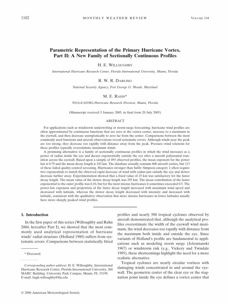
Piecewise continuous wind profiles (e.g., Willoughby1995) show promise as an alternative to the Hollandmodel. They are composed of analytical segmentspatched smoothly together (Fig. 1). Inside the eye thewind increases in proportion to a power of radius. Out-side the eye, the wind decays exponentially with a ra-dial e-folding distance that changes from storm tostorm. The transition across the radius of maximumwind from the inner to outer profiles is accomplished witha smooth, radially varying polynomial ramp function:

V�r� � Vi � Vmax� r

Rmax�n

, �0 � r � R1�, �1a�

V�r� � Vi�1 � w� � Vow, �R1 � r � R2�, �1b�

V�r� � Vo � Vmax exp��r � Rmax

X1�, �R2 � r�, �1c�

where Vi and Vo are the tangential wind component inthe eye and beyond the transition zone, which lies be-tween r � R1 and r � R2; Vmax and Rmax are the maxi-mum wind and radius at which the maximum wind oc-curs; X1 is the exponential decay length in the outervortex; and n is the exponent for the power law insidethe eye. Note that both Vi and Vo are defined through-out the transition zone and that both are equal to Vmax

at r � Rmax.The weighting function, w, is expressed in terms of a

nondimensional argument � � (r � R1)/(R2 � R1).When � � 0, w � 0; when � � 1, w � 1. In the subdo-main 0 � � � 1, the weighting is defined as the poly-nomial

w�� 126�5 � 420�6 � 540�7 � 315�8 � 70�9, �2�

which ramps up smoothly from zero to one between R1

and R2. As described in the appendix, the weightingfunction is derived by integration of a bell-shaped poly-nomial curve given by C[�(1 � �)]k when (0 � � � 1)

FIG. 1. (a) Schematic illustration of a sectionally continuousùhurricane wind profile (shading) constructed by joining an innerprofile with swirling wind proportional to a power of radius andan outer profile with swirling wind decaying exponentially withdistance outside the radius of maximum wind (darker curves). (b)In a zone spanning the radius of maximum wind, a polynomialramp weighting function is used to create a smooth transitionbetween the inner and outer profiles.

APRIL 2006 W I L L O U G H B Y E T A L . 1103

and zero elsewhere. The coefficient C is chosen to makew(1) � 1, and the exponent k is the “order” of the belland ramp curves, even though the resulting polynomi-als are of order 2k and 2k � 1, respectively. We havecoined the term “bellramp” functions to denote thisfamily of polynomials. Since the shapes of fitted pro-files are insensitive to the order of the polynomials, weselected fourth-order ramp functions for smoothnessand differentiability.

Based upon parameters Rmax, Vmax, X1, and n, thefull wind profile is constructed as follows. First, thewidth of the transition R1 � R2 is specified a priori at avalue between 10 and 25 km. Then, the location of thetransition zone is determined by requiring the radialderivative of (1b) to vanish at r � Rmax, recognizingthat Vi(Rmax) � Vo(Rmax) � Vmax. This condition yieldsthe value of w at the wind maximum:

w�Rmax � R1

R2 � R1� �

�Vi

�r

�Vi

�r�

�Vo

�r

�nX1

nX1 � Rmax, �3�

which may be solved for R1 through numerical inver-sion of (2).

As shown subsequently, in many situations the pro-file described by (1a)–(1c) suffers from the problemthat vexed the Holland profile in Part I. Relatively largevalues of X1 chosen to generate profiles that match theouter part of the vortex may fail to capture the rapiddecrease of wind just outside the eyewall; conversely,smaller values of X1 generate profiles that match thesteep gradient outside the eyewall and decrease toorapidly farther from the center. Often there is no inter-mediate value that can fit the observations in both partsof the domain. Although this difficulty is less pro-nounced than for the Holland profile, it is still prob-lematic. A remedy entails replacement of the singleexponential with the sum of two exponentials with e-folding lengths X1 and X2:

Vo � Vmax��1 � A� exp��r � Rmax

X1�

� A exp��r � Rmax

X2��, �R1 � r�, �4)

where the parameter A sets the proportion of the twoexponentials in the profile, and the rightmost expres-sion in (3) becomes n[(1 � A)X1 � AX2]/{n[(1 � A)X1

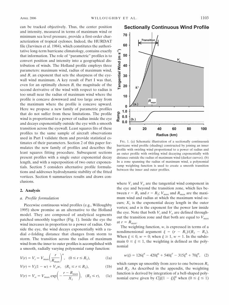
� AX2] � Rmax}. Figure 2 illustrates application of (4)to Hurricane Diana of 1984. Clearly, the dual-exponential profile captures the profile’s sharpness atthe radius of maximum wind as well as the more

gradual decrease of wind at radii farther from the eye-wall. There is an issue of nonuniqueness in this formu-lation. Several different combinations of X1, X2, and Acan often fit a given set of observations equally well.This situation complicates statistical estimation of theprofile parameters, so that we generally fit A and onevariable decay length, keeping the other decay length,usually the shorter one, fixed. Thus, most of this paperwill deal with either single-exponential profiles or dual-exponential profiles with one predetermined decaylength.

In this formulation, unlike the Holland profile, thereis no closed-form relation for the gradient-balance geo-potential height in terms of the vortex parameters.Thus, the geopotential height is computed through out-ward numerical integration of the gradient wind accel-eration from the observed height at the vortex center ofthe standard isobaric surface nearest flight level,

Z�r� � Zc �1g �

0

r

�V2�r��

r�� fV�r�� dr�, �5�

where Z(r) is the height of the specified surface, Zc isZ(0), and g is the acceleration of gravity. Setting theupper bound on the integral to infinity in (5) producesa gradient balance estimate of the undisturbed geopo-tential around the storm, Ze � Z(r → �). Based uponthis integral it is possible to relate Vmax to Ze � Zc inorder to devise height–wind relations for the single-exponential and dual-exponential profiles. A key ad-

FIG. 2. A dual-exponential profile used to approximate the ob-served wind in Hurricane Diana on 11 Sep 1984. Here and sub-sequent shading indicates observed winds, and the darker curvesindicate the fitted profiles.


vantage of using exponential functions to describe theouter profile is that it guarantees a well-behavedheight–wind relationship as well as finite values for vor-tex total relative angular momentum and kinetic en-ergy.

b. Profile fitting

Single-exponential profiles have four parametersRmax, Vmax, X1, and n. Dual-exponential profiles withone predetermined decay length have five parameters(Rmax, Vmax, X1, A, and n), and dual-exponential pro-files with both decay lengths free have six parameters(Rmax, Vmax, X1, X2, A, and n). As in Part I, Vmax andRmax are determined by scanning each profile for thestrongest reported wind and its radial position. Thisprocedure leaves the single-exponential, constraineddual-exponential, and free dual-exponential profiles,respectively, with two, three, and four parameters thatrequire least squares fitting to the data. The cost func-tion is the same as that used in Part I,

S2 � �k�1

K

vo�rk� � vg�rk, n, X1, . . .�2

� gzo�rk� � z�rk, n, X1, . . .�2Lz�1. �6�

It is the summed squares of the differences between theprofile and observed tangential wind and between thecomputed geopotential height (5) and the observedheight of the isobaric surface nearest the aircraft flightlevel. Since the parameter space has relatively few di-mensions and the cost function is essentially a parabola,we use the simplex algorithm (Nelder and Mead 1965;Press et al. 1986) to find the minimum value of S2. HereLz is a Lagrange multiplier that sets the strength of thegradient balance constraint and also makes (6) dimen-sionally homogeneous with units of velocity squared;we set Lz � 1 km, the same value used in Part I.

Ranges of the fitted parameters are constrained withLagrange multipliers, for example, 0.4 � n � 2.4 or 0 �

A � 1, to prevent the algorithm from wandering intophysically unrealistic parts of the parameter space.Typical minimum values of S2 are a few hundred to afew thousand m2 s�2, and the penalties imposed outsidethe preferred subdomain by the Lagrangian constraintsare 2–5 � 103 m2 s�2. The constraints generally havelimited effect on the fitted parameters inasmuch as thesimplex algorithm almost always finds values within thepreferred subdomain. Two exceptions to this generalityare A � 0 or 1, which characterize profiles where X1 orX2 can represent the shape of the “dual exponential”outer profile completely. The constraint on the mini-mum decay lengths generally is set for values greater

than 50–100 km, but the minimization algorithm sel-dom selects values that small. By contrast, the upperbound on decay lengths does exert significant controlover the fitted profiles. In some tropical cyclones wherethe wind remains fairly constant from just outside theeyewall to the sampling domain boundary, the uncon-strained algorithm will seek decay lengths �1000 km.Since the values of Ze that result from integration of (5)in these situations may be greater than Za, the height ofthe isobaric surface in climatologically representativesoundings (Jordan 1958; Sheets 1969), we generally setan upper bound of a few hundred kilometers on thelonger decay length. Tuning of this constraint is dis-cussed extensively in the next two sections, since it isimportant to obtaining realistic fits.

The data for the least squares fits are the same asthose used in Part I. They contain 606 logical sortiesinto Atlantic and eastern Pacific tropical storms andhurricanes flown by National Oceanic and AtmosphericAdministration (NOAA) and Air Force Reserve air-craft between 1977 and 2000 and are representative interms of geographical and seasonal distribution. Theyare divided into “logical sorties,” each a series of suc-cessive transects across the tropical cyclone center atfixed altitude, usually flown by one aircraft during thecourse of a few hours. Although there are a few sortieswith 300-km domains, most extend to �150 km. Thevariables are expressed in a cylindrical coordinate sys-tem that moves along the objectively determined cy-clone track. The observed dynamic and kinematic vari-ables are transformed into vortex-centered coordinatesand averaged azimuthally around the vortex to producea profile composite (PCMP) file for each sortie. Theleast squares fits use the PCMP files. Predominantflight levels were 850 and 700 hPa (1.5 and 3 km), butsome missions (generally in weaker storms) were flownas low as 950 hPa (500 m) and as high as 400 hPa (7km). Although depressions and weak tropical stormsare underrepresented, the sample is reasonably repre-sentative in terms of cyclone intensity. Of the originalsample, 113 failed quality-control (QC) criteria thatscreened out profiles where the radius of maximumwind was more than half the sampling domain or wherethe data fail to describe a well-defined dynamic centerinside the eye. The 493 PCMP files that met the QCcriteria are homogeneous with the sample used inPart I.

3. Single-exponential profile

The single-exponential profile is the simplest of thenew functional forms. Since the Lagrange multiplierconstraint on the maximum value of X1 is the only tun-


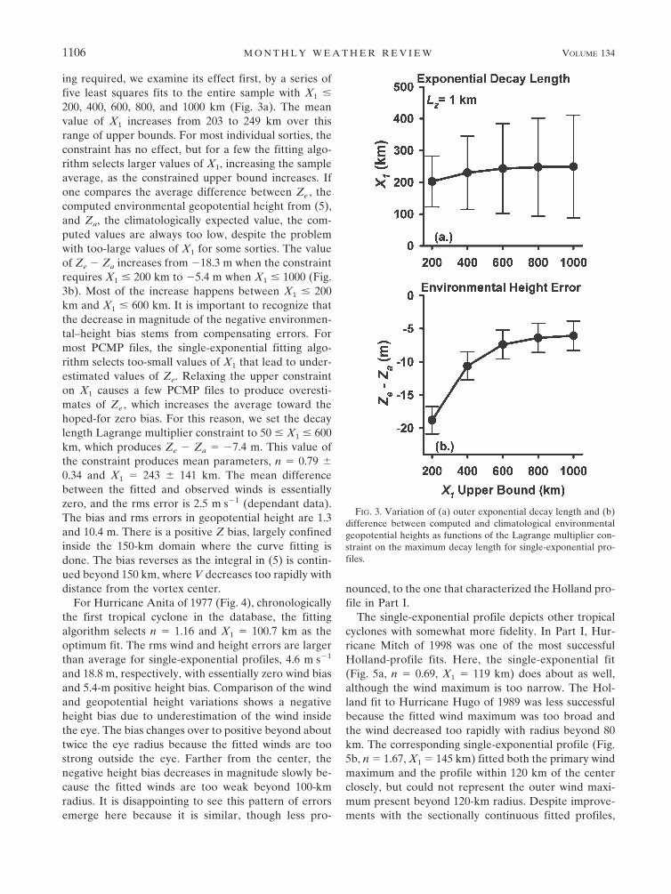
ing required, we examine its effect first, by a series offive least squares fits to the entire sample with X1 �

200, 400, 600, 800, and 1000 km (Fig. 3a). The meanvalue of X1 increases from 203 to 249 km over thisrange of upper bounds. For most individual sorties, theconstraint has no effect, but for a few the fitting algo-rithm selects larger values of X1, increasing the sampleaverage, as the constrained upper bound increases. Ifone compares the average difference between Ze , thecomputed environmental geopotential height from (5),and Za, the climatologically expected value, the com-puted values are always too low, despite the problemwith too-large values of X1 for some sorties. The valueof Ze � Za increases from �18.3 m when the constraintrequires X1 � 200 km to �5.4 m when X1 � 1000 (Fig.3b). Most of the increase happens between X1 � 200km and X1 � 600 km. It is important to recognize thatthe decrease in magnitude of the negative environmen-tal–height bias stems from compensating errors. Formost PCMP files, the single-exponential fitting algo-rithm selects too-small values of X1 that lead to under-estimated values of Ze. Relaxing the upper constrainton X1 causes a few PCMP files to produce overesti-mates of Ze , which increases the average toward thehoped-for zero bias. For this reason, we set the decaylength Lagrange multiplier constraint to 50 � X1 � 600km, which produces Ze � Za � �7.4 m. This value ofthe constraint produces mean parameters, n � 0.79 �0.34 and X1 � 243 � 141 km. The mean differencebetween the fitted and observed winds is essentiallyzero, and the rms error is 2.5 m s�1 (dependant data).The bias and rms errors in geopotential height are 1.3and 10.4 m. There is a positive Z bias, largely confinedinside the 150-km domain where the curve fitting isdone. The bias reverses as the integral in (5) is contin-ued beyond 150 km, where V decreases too rapidly withdistance from the vortex center.

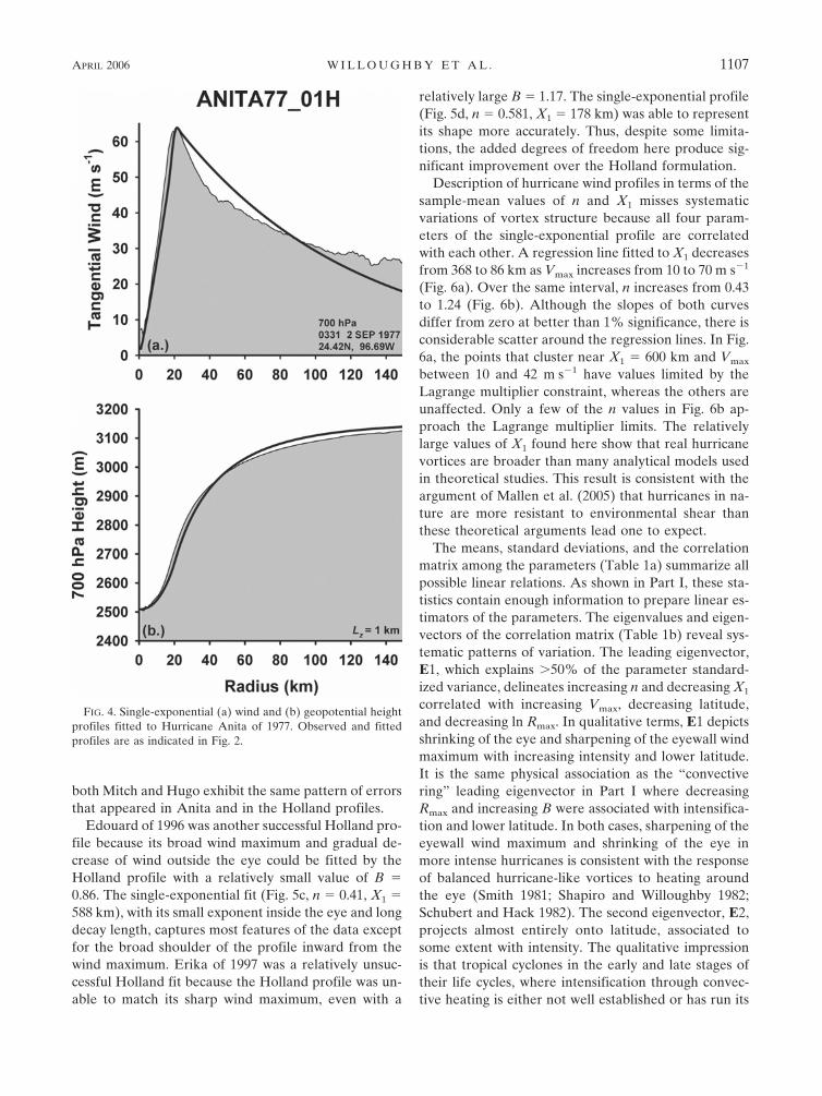
For Hurricane Anita of 1977 (Fig. 4), chronologicallythe first tropical cyclone in the database, the fittingalgorithm selects n � 1.16 and X1 � 100.7 km as theoptimum fit. The rms wind and height errors are largerthan average for single-exponential profiles, 4.6 m s�1

and 18.8 m, respectively, with essentially zero wind biasand 5.4-m positive height bias. Comparison of the windand geopotential height variations shows a negativeheight bias due to underestimation of the wind insidethe eye. The bias changes over to positive beyond abouttwice the eye radius because the fitted winds are toostrong outside the eye. Farther from the center, thenegative height bias decreases in magnitude slowly be-cause the fitted winds are too weak beyond 100-kmradius. It is disappointing to see this pattern of errorsemerge here because it is similar, though less pro-

nounced, to the one that characterized the Holland pro-file in Part I.

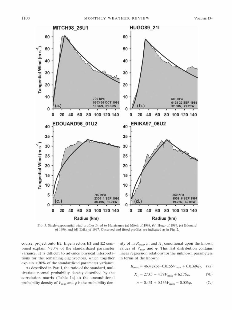
The single-exponential profile depicts other tropicalcyclones with somewhat more fidelity. In Part I, Hur-ricane Mitch of 1998 was one of the most successfulHolland-profile fits. Here, the single-exponential fit(Fig. 5a, n � 0.69, X1 � 119 km) does about as well,although the wind maximum is too narrow. The Hol-land fit to Hurricane Hugo of 1989 was less successfulbecause the fitted wind maximum was too broad andthe wind decreased too rapidly with radius beyond 80km. The corresponding single-exponential profile (Fig.5b, n � 1.67, X1 � 145 km) fitted both the primary windmaximum and the profile within 120 km of the centerclosely, but could not represent the outer wind maxi-mum present beyond 120-km radius. Despite improve-ments with the sectionally continuous fitted profiles,

FIG. 3. Variation of (a) outer exponential decay length and (b)difference between computed and climatological environmentalgeopotential heights as functions of the Lagrange multiplier con-straint on the maximum decay length for single-exponential pro-files.


both Mitch and Hugo exhibit the same pattern of errorsthat appeared in Anita and in the Holland profiles.

Edouard of 1996 was another successful Holland pro-file because its broad wind maximum and gradual de-crease of wind outside the eye could be fitted by theHolland profile with a relatively small value of B �0.86. The single-exponential fit (Fig. 5c, n � 0.41, X1 �588 km), with its small exponent inside the eye and longdecay length, captures most features of the data exceptfor the broad shoulder of the profile inward from thewind maximum. Erika of 1997 was a relatively unsuc-cessful Holland fit because the Holland profile was un-able to match its sharp wind maximum, even with a

relatively large B � 1.17. The single-exponential profile(Fig. 5d, n � 0.581, X1 � 178 km) was able to representits shape more accurately. Thus, despite some limita-tions, the added degrees of freedom here produce sig-nificant improvement over the Holland formulation.

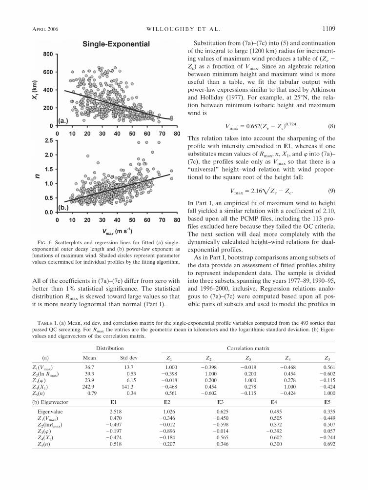
Description of hurricane wind profiles in terms of thesample-mean values of n and X1 misses systematicvariations of vortex structure because all four param-eters of the single-exponential profile are correlatedwith each other. A regression line fitted to X1 decreasesfrom 368 to 86 km as Vmax increases from 10 to 70 m s�1

(Fig. 6a). Over the same interval, n increases from 0.43to 1.24 (Fig. 6b). Although the slopes of both curvesdiffer from zero at better than 1% significance, there isconsiderable scatter around the regression lines. In Fig.6a, the points that cluster near X1 � 600 km and Vmax

between 10 and 42 m s�1 have values limited by theLagrange multiplier constraint, whereas the others areunaffected. Only a few of the n values in Fig. 6b ap-proach the Lagrange multiplier limits. The relativelylarge values of X1 found here show that real hurricanevortices are broader than many analytical models usedin theoretical studies. This result is consistent with theargument of Mallen et al. (2005) that hurricanes in na-ture are more resistant to environmental shear thanthese theoretical arguments lead one to expect.

The means, standard deviations, and the correlationmatrix among the parameters (Table 1a) summarize allpossible linear relations. As shown in Part I, these sta-tistics contain enough information to prepare linear es-timators of the parameters. The eigenvalues and eigen-vectors of the correlation matrix (Table 1b) reveal sys-tematic patterns of variation. The leading eigenvector,E1, which explains 50% of the parameter standard-ized variance, delineates increasing n and decreasing X1

correlated with increasing Vmax, decreasing latitude,and decreasing ln Rmax. In qualitative terms, E1 depictsshrinking of the eye and sharpening of the eyewall windmaximum with increasing intensity and lower latitude.It is the same physical association as the “convectivering” leading eigenvector in Part I where decreasingRmax and increasing B were associated with intensifica-tion and lower latitude. In both cases, sharpening of theeyewall wind maximum and shrinking of the eye inmore intense hurricanes is consistent with the responseof balanced hurricane-like vortices to heating aroundthe eye (Smith 1981; Shapiro and Willoughby 1982;Schubert and Hack 1982). The second eigenvector, E2,projects almost entirely onto latitude, associated tosome extent with intensity. The qualitative impressionis that tropical cyclones in the early and late stages oftheir life cycles, where intensification through convec-tive heating is either not well established or has run its

FIG. 4. Single-exponential (a) wind and (b) geopotential heightprofiles fitted to Hurricane Anita of 1977. Observed and fittedprofiles are as indicated in Fig. 2.


course, project onto E2. Eigenvectors E1 and E2 com-bined explain 70% of the standardized parametervariance. It is difficult to advance physical interpreta-tions for the remaining eigenvectors, which togetherexplain �30% of the standardized parameter variance.

As described in Part I, the ratio of the standard, mul-tivariate normal probability density described by thecorrelation matrix (Table 1a) to the unconditionalprobability density of Vmax and � is the probability den-

sity of ln Rmax, n, and X1 conditional upon the knownvalues of Vmax and �. This last distribution containslinear regression relations for the unknown parametersin terms of the known:

Rmax � 46.4 exp��0.0155Vmax � 0.0169��, �7a�

X1 � 270.5 � 4.78Vmax � 6.176�, �7b�

n � 0.431 � 0.136Vmax � 0.006�. �7c�

FIG. 5. Single-exponential wind profiles fitted to Hurricanes (a) Mitch of 1998, (b) Hugo of 1989, (c) Edouardof 1996, and (d) Erika of 1997. Observed and fitted profiles are indicated as in Fig. 2.


All of the coefficients in (7a)–(7c) differ from zero withbetter than 1% statistical significance. The statisticaldistribution Rmax is skewed toward large values so thatit is more nearly lognormal than normal (Part I).

Substitution from (7a)–(7c) into (5) and continuationof the integral to large (1200 km) radius for increment-ing values of maximum wind produces a table of (Ze �Zc) as a function of Vmax. Since an algebraic relationbetween minimum height and maximum wind is moreuseful than a table, we fit the tabular output withpower-law expressions similar to that used by Atkinsonand Holliday (1977). For example, at 25°N, the rela-tion between minimum isobaric height and maximumwind is

Vmax � 0.652�Ze � Zc�0.724. �8�

This relation takes into account the sharpening of theprofile with intensity embodied in E1, whereas if onesubstitutes mean values of Rmax, n, X1, and � into (7a)–(7c), the profiles scale only as Vmax so that there is a“universal” height–wind relation with wind propor-tional to the square root of the height fall:

Vmax � 2.16�Ze � Zc. �9�

In Part I, an empirical fit of maximum wind to heightfall yielded a similar relation with a coefficient of 2.10,based upon all the PCMP files, including the 113 pro-files excluded here because they failed the QC criteria.The next section will deal more completely with thedynamically calculated height–wind relations for dual-exponential profiles.

As in Part I, bootstrap comparisons among subsets ofthe data provide an assessment of fitted profiles abilityto represent independent data. The sample is dividedinto three subsets, spanning the years 1977–89, 1990–95,and 1996–2000, inclusive. Regression relations analo-gous to (7a)–(7c) were computed based upon all pos-sible pairs of subsets and used to model the profiles in

FIG. 6. Scatterplots and regression lines for fitted (a) single-exponential outer decay length and (b) power-law exponent asfunctions of maximum wind. Shaded circles represent parametervalues determined for individual profiles by the fitting algorithm.

TABLE 1. (a) Mean, std dev, and correlation matrix for the single-exponential profile variables computed from the 493 sorties thatpassed QC screening. For Rmax the entries are the geometric mean in kilometers and the logarithmic standard deviation. (b) Eigen-values and eigenvectors of the correlation matrix.

(a)

Distribution Correlation matrix

Mean Std dev Z1 Z2 Z3 Z4 Z5

Z1(Vmax) 36.7 13.7 1.000 �0.398 �0.018 �0.468 0.561Z2(ln Rmax) 39.3 0.53 �0.398 1.000 0.200 0.454 �0.602Z3(� ) 23.9 6.15 �0.018 0.200 1.000 0.278 �0.115Z4(X1) 242.9 141.3 �0.468 0.454 0.278 1.000 �0.424Z5(n) 0.79 0.34 0.561 �0.602 �0.115 �0.424 1.000

(b) Eigenvector E1 E2 E3 E4 E5

Eigenvalue 2.518 1.026 0.625 0.495 0.335Z1(Vmax) 0.470 �0.346 �0.450 0.505 �0.449Z2(lnRmax) �0.497 �0.012 �0.598 0.372 0.507Z3(� ) �0.197 �0.896 �0.014 �0.392 0.057Z4(X1) �0.474 �0.184 0.565 0.602 �0.244Z5(n) 0.518 �0.207 0.346 0.300 0.692


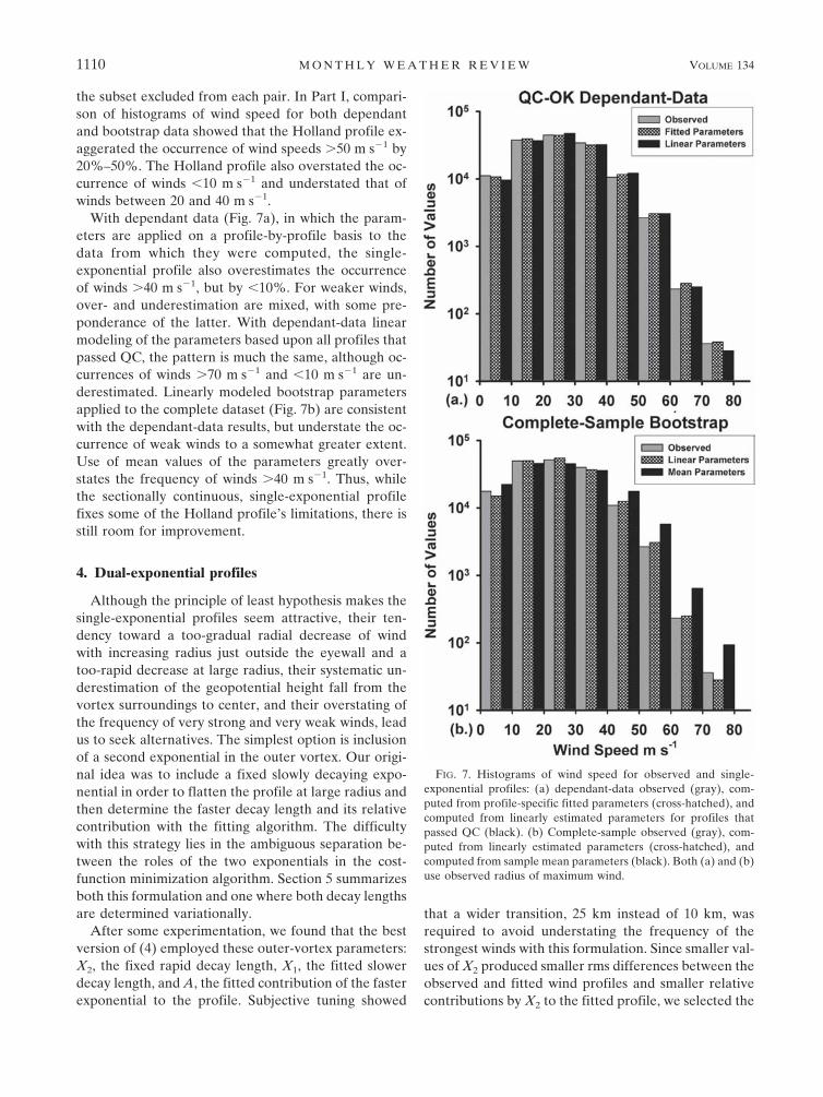
the subset excluded from each pair. In Part I, compari-son of histograms of wind speed for both dependantand bootstrap data showed that the Holland profile ex-aggerated the occurrence of wind speeds 50 m s�1 by20%–50%. The Holland profile also overstated the oc-currence of winds �10 m s�1 and understated that ofwinds between 20 and 40 m s�1.

With dependant data (Fig. 7a), in which the param-eters are applied on a profile-by-profile basis to thedata from which they were computed, the single-exponential profile also overestimates the occurrenceof winds 40 m s�1, but by �10%. For weaker winds,over- and underestimation are mixed, with some pre-ponderance of the latter. With dependant-data linearmodeling of the parameters based upon all profiles thatpassed QC, the pattern is much the same, although oc-currences of winds 70 m s�1 and �10 m s�1 are un-derestimated. Linearly modeled bootstrap parametersapplied to the complete dataset (Fig. 7b) are consistentwith the dependant-data results, but understate the oc-currence of weak winds to a somewhat greater extent.Use of mean values of the parameters greatly over-states the frequency of winds 40 m s�1. Thus, whilethe sectionally continuous, single-exponential profilefixes some of the Holland profile’s limitations, there isstill room for improvement.

4. Dual-exponential profiles

Although the principle of least hypothesis makes thesingle-exponential profiles seem attractive, their ten-dency toward a too-gradual radial decrease of windwith increasing radius just outside the eyewall and atoo-rapid decrease at large radius, their systematic un-derestimation of the geopotential height fall from thevortex surroundings to center, and their overstating ofthe frequency of very strong and very weak winds, leadus to seek alternatives. The simplest option is inclusionof a second exponential in the outer vortex. Our origi-nal idea was to include a fixed slowly decaying expo-nential in order to flatten the profile at large radius andthen determine the faster decay length and its relativecontribution with the fitting algorithm. The difficultywith this strategy lies in the ambiguous separation be-tween the roles of the two exponentials in the cost-function minimization algorithm. Section 5 summarizesboth this formulation and one where both decay lengthsare determined variationally.

After some experimentation, we found that the bestversion of (4) employed these outer-vortex parameters:X2, the fixed rapid decay length, X1, the fitted slowerdecay length, and A, the fitted contribution of the fasterexponential to the profile. Subjective tuning showed

that a wider transition, 25 km instead of 10 km, wasrequired to avoid understating the frequency of thestrongest winds with this formulation. Since smaller val-ues of X2 produced smaller rms differences between theobserved and fitted wind profiles and smaller relativecontributions by X2 to the fitted profile, we selected the

FIG. 7. Histograms of wind speed for observed and single-exponential profiles: (a) dependant-data observed (gray), com-puted from profile-specific fitted parameters (cross-hatched), andcomputed from linearly estimated parameters for profiles thatpassed QC (black). (b) Complete-sample observed (gray), com-puted from linearly estimated parameters (cross-hatched), andcomputed from sample mean parameters (black). Both (a) and (b)use observed radius of maximum wind.


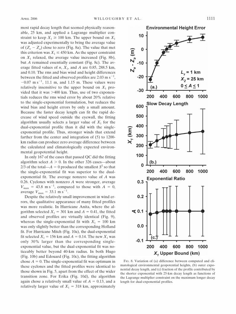
most rapid decay length that seemed physically reason-able, 25 km, and applied a Lagrange multiplier con-straint to keep X1 � 100 km. The upper bound on X1

was adjusted experimentally to bring the average valueof (Ze � Za) close to zero (Fig. 8a). The value that metthis criterion was X1 � 450 km. As the upper constrainton X1 relaxed, the average value increased (Fig. 8b),but A remained essentially constant (Fig. 8c). The av-erage fitted values of n, X1, and A are 0.85, 288.5 km,and 0.10. The rms and bias wind and height differencesbetween the fitted and observed profiles are 2.03 m s�1,�0.07 m s�1, 11.1 m, and 1.15 m. These values wererelatively insensitive to the upper bound on X1 pro-vided that it was 400 km. Thus, use of two exponen-tials reduces the rms wind error by about 20% relativeto the single-exponential formulation, but reduces thewind bias and height errors by only a small amount.Because the faster decay length can fit the rapid de-crease of wind speed outside the eyewall, the fittingalgorithm usually selects a larger value of X1 for thedual-exponential profile than it did with the single-exponential profile. Thus, stronger winds that extendfarther from the center and integration of (5) to 1200-km radius can produce zero average difference betweenthe calculated and climatologically expected environ-mental geopotential height.

In only 167 of the cases that passed QC did the fittingalgorithm select A 0. In the other 326 cases—about2/3 of the total—A � 0 produced the smallest S2 so thatthe single-exponential fit was superior to the dual-exponential fit. The average nonzero value of A was0.26. Cyclones with nonzero A were stronger, averageVmax � 43.8 m s�1, compared to those with A � 0,average Vmax � 33.1 m s�1.

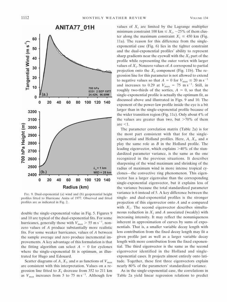
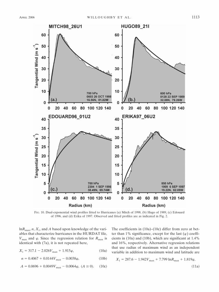
Despite the relatively small improvement in wind er-rors, the qualitative appearance of many fitted profileswas more realistic. In Hurricane Anita, where the al-gorithm selected X1 � 301 km and A � 0.41, the fittedand observed profiles are virtually identical (Fig. 9),whereas the single-exponential fit with X1 � 100 kmwas only slightly better than the corresponding Hollandfit. For Hurricane Mitch (Fig. 10a), the dual-exponentialfit selected X1 � 156 km and A � 0.14. The new X1 wasonly 30% larger than the corresponding single-exponential value, but the dual-exponential fit was no-ticeably better beyond 40-km radius. In both Hugo(Fig. 10b) and Edouard (Fig. 10c), the fitting algorithmchose A � 0. The single-exponential fit was optimum inthese cyclones and the fitted profiles were identical tothose shown in Fig. 5, apart from the effect of the widertransition zone. For Erika (Fig. 10d), the algorithmagain chose a relatively small value of A � 0.13, and arelatively larger value of X1 � 318 km, approximately

FIG. 8. Variation of (a) difference between computed and cli-matological environmental geopotential heights, (b) outer expo-nential decay length, and (c) fraction of the profile contributed bythe shorter exponential with 25-km decay length as functions ofthe Lagrange multiplier constraint on the maximum longer decaylength for dual-exponential profiles.


double the single-exponential value in Fig. 5. Figures 9and 10 are typical of the dual-exponential fits. For somehurricanes, generally those with Vmax 55 m s�1, non-zero values of A produce substantially more realisticfits. For some weaker hurricanes, values of A betweenthe sample average and zero produce incremental im-provements. A key advantage of this formulation is thatthe fitting algorithm can select A � 0 for cycloneswhere the single-exponential fit is optimum, as illus-trated for Hugo and Edouard.

Scatter diagrams of A, X1, and n as functions of Vmax

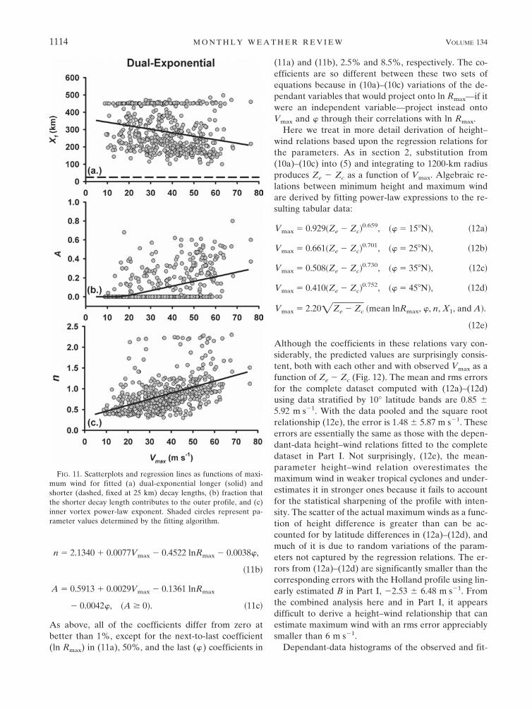
are consistent with this interpretation. Values on a re-gression line fitted to X1 decrease from 352 to 211 kmas Vmax increases from 5 to 75 m s�1. Although few

values of X1 are limited by the Lagrange multiplierminimum constraint 100 km � X1, �25% of them clus-ter along the maximum constraint X1 � 450 km (Fig.11a). The reason for this difference from the single-exponential case (Fig. 6) lies in the tighter constraintand the dual-exponential profiles’ ability to representsharp gradients near the eyewall with the X2 part of theprofile while representing the outer vortex with largervalues of X1. Nonzero values of A correspond to partialprojection onto the X2 component (Fig. 11b). The re-gression line for this parameter is not allowed to extendto negative values so that A � 0 for Vmax � 20 m s�1

and increases to 0.29 at Vmax � 75 m s�1. Still, inroughly two-thirds of the sorties, A � 0, so that thesingle-exponential profile is actually the optimum fit, asdiscussed above and illustrated in Figs. 9 and 10. Theexponent of the power-law profile inside the eye is a bitlarger than in the single-exponential profile because ofthe wider transition region (Fig. 11c). Only about 4% ofthe values are greater than two, but 70% of themare �1.

The parameter correlation matrix (Table 2a) is forthe most part consistent with that for the single-exponential and Holland profiles. Here, A, X1, and nplay the same role as B in the Holland profile. Theleading eigenvector, which explains 40% of the stan-dardized parameter variance, is the same as the onerecognized in the previous situations. It describessharpening of the wind maximum and shrinking of theradius of maximum wind in more intense tropical cy-clones—the convective ring phenomenon. This eigen-vector has a larger eigenvalue than the correspondingsingle-exponential eigenvector, but it explains less ofthe variance because the total standardized parametervariance is 6 instead of 5. A key difference between thesingle- and dual-exponential profiles is the strongerprojection of this eigenvector onto A and n comparedwith X1. The second eigenvector describes simulta-neous reduction in X1 and A associated (weakly) withincreasing intensity. It may reflect the nonuniquenessinherent in approximation of curves by sums of expo-nentials. That is, a smaller variable decay length withless contribution from the fixed decay length may fit agiven profile just as well as a larger variable decaylength with more contribution from the fixed exponen-tial. The third eigenvector is the same as the secondeigenvector identified in the Holland and single-exponential cases. It projects almost entirely onto lati-tude. Together, these first three eigenvectors explainnearly 80% of the parameters’ standardized variance.

As in the single-exponential case, the correlations inTable 2a yield linear regression relations to predict

FIG. 9. Dual-exponential (a) wind and (b) geopotential heightprofiles fitted to Hurricane Anita of 1977. Observed and fittedprofiles are as indicated in Fig. 2.


lnRmax, n, X1, and A based upon knowledge of the vari-ables that characterize hurricanes in the HURDAT file,Vmax and �. Since the regression relation for Rmax isidentical with (7a), it is not repeated here,

X1 � 317.1 � 2.026Vmax � 1.915�, �10a�

n � 0.4067 � 0.0144Vmax � 0.0038�, �10b�

A � 0.0696 � 0.0049Vmax � 0.0064�, �A � 0�. �10c�

The coefficients in (10a)–(10c) differ from zero at bet-ter than 1% significance, except for the last (�) coeffi-cients in (10a) and (10b), which are significant at 1.4%and 16%, respectively. Alternative regression relationsthat use radius of maximum wind as an independentvariable in addition to maximum wind and latitude are

X1 � 287.6 � 1.942Vmax � 7.799 lnRmax � 1.819�,

�11a�

FIG. 10. Dual-exponential wind profiles fitted to Hurricanes (a) Mitch of 1998, (b) Hugo of 1989, (c) Edouardof 1996, and (d) Erika of 1997. Observed and fitted profiles are as indicated in Fig. 2.


n � 2.1340 � 0.0077Vmax � 0.4522 lnRmax � 0.0038�,

�11b�

A � 0.5913 � 0.0029Vmax � 0.1361 lnRmax

� 0.0042�, �A � 0�. �11c�

As above, all of the coefficients differ from zero atbetter than 1%, except for the next-to-last coefficient(ln Rmax) in (11a), 50%, and the last (�) coefficients in

(11a) and (11b), 2.5% and 8.5%, respectively. The co-efficients are so different between these two sets ofequations because in (10a)–(10c) variations of the de-pendant variables that would project onto ln Rmax—if itwere an independent variable—project instead ontoVmax and � through their correlations with ln Rmax.

Here we treat in more detail derivation of height–wind relations based upon the regression relations forthe parameters. As in section 2, substitution from(10a)–(10c) into (5) and integrating to 1200-km radiusproduces Ze � Zc as a function of Vmax. Algebraic re-lations between minimum height and maximum windare derived by fitting power-law expressions to the re-sulting tabular data:

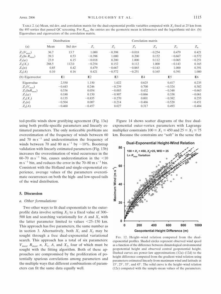
Vmax � 0.929�Ze � Zc�0.659, �� 15�N�, �12a�

Vmax � 0.661�Ze � Zc�0.701, �� 25�N�, �12b�

Vmax � 0.508�Ze � Zc�0.730, �� 35�N�, �12c�

Vmax � 0.410�Ze � Zc�0.752, �� 45�N�, �12d�

Vmax � 2.20�Ze � Zc �mean lnRmax, �, n, X1, and A�.

�12e�

Although the coefficients in these relations vary con-siderably, the predicted values are surprisingly consis-tent, both with each other and with observed Vmax as afunction of Ze � Zc (Fig. 12). The mean and rms errorsfor the complete dataset computed with (12a)–(12d)using data stratified by 10° latitude bands are 0.85 �5.92 m s�1. With the data pooled and the square rootrelationship (12e), the error is 1.48 � 5.87 m s�1. Theseerrors are essentially the same as those with the depen-dant-data height–wind relations fitted to the completedataset in Part I. Not surprisingly, (12e), the mean-parameter height–wind relation overestimates themaximum wind in weaker tropical cyclones and under-estimates it in stronger ones because it fails to accountfor the statistical sharpening of the profile with inten-sity. The scatter of the actual maximum winds as a func-tion of height difference is greater than can be ac-counted for by latitude differences in (12a)–(12d), andmuch of it is due to random variations of the param-eters not captured by the regression relations. The er-rors from (12a)–(12d) are significantly smaller than thecorresponding errors with the Holland profile using lin-early estimated B in Part I, �2.53 � 6.48 m s�1. Fromthe combined analysis here and in Part I, it appearsdifficult to derive a height–wind relationship that canestimate maximum wind with an rms error appreciablysmaller than 6 m s�1.

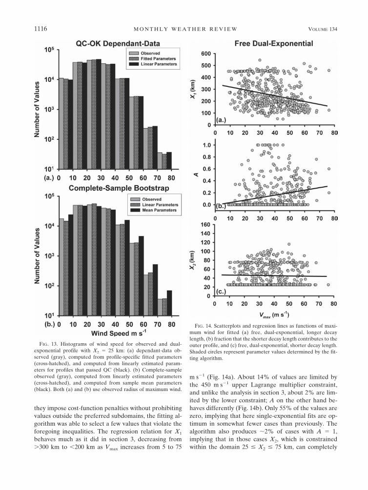
Dependant-data histograms of the observed and fit-

FIG. 11. Scatterplots and regression lines as functions of maxi-mum wind for fitted (a) dual-exponential longer (solid) andshorter (dashed, fixed at 25 km) decay lengths, (b) fraction thatthe shorter decay length contributes to the outer profile, and (c)inner vortex power-law exponent. Shaded circles represent pa-rameter values determined by the fitting algorithm.


ted-profile winds show gratifying agreement (Fig. 13a)using both profile-specific parameters and linearly es-timated parameters. The only noticeable problems areoverestimation of the frequency of winds between 60and 70 m s�1 and underestimation the frequency ofwinds between 70 and 80 m s�1 by �10%. Bootstrapvalidation with linearly estimated parameters (Fig. 13b)increases the overestimation of wind occurrence in the60–70 m s�1 bin, causes underestimation in the �10m s�1 bin, and reduces the error in the 70–80 m s�1 bin.Consistent with the Holland and single-exponential ex-perience, average values of the parameters overesti-mate occurrences on both the high- and low-speed tailsof the wind distribution.

5. Discussion

a. Other formulations

Two other ways to fit dual exponentials to the outer-profile data involve setting X2 to a fixed value of 300–500 km and searching variationally for A and X1 withthe latter parameter limited to values �25–150 km.This approach has five parameters, the same number asin section 3. Alternatively, both X1 and X2 may besought through a free dual-exponential variationalsearch. This approach has a total of six parameters:Vmax, Rmax, n, X1, A, and X2, four of which must besought with the fitting algorithm. Both of these ap-proaches are compromised by the proliferation of po-tentially spurious correlations among parameters andthe multiple ways that different combinations of param-eters can fit the same data equally well.

Figure 14 shows scatter diagrams of the free dual-exponential outer-vortex parameters with Lagrangemultiplier constraints 100 � X1 � 450 and 25 � X2 � 75km. Because the constrains are “soft” in the sense that

FIG. 12. Height–wind relation computed from the dual-exponential profiles. Shaded circles represent observed wind speedas a function of the difference between climatological environmentalgeopotential height and observed central geopotential height.Dashed curves are power-law approximations (12a)–(12d) to theheight difference computed from the gradient-wind relation usingparameters estimated linearly from maximum wind and latitude at15°, 25°, 35°, and 45°. The solid curve is the height–wind relation(12e) computed with the sample-mean values of the parameters.

TABLE 2. (a) Mean, std dev, and correlation matrix for the dual-exponential profile variables computed with X2 fixed at 25 km fromthe 493 sorties that passed QC screening. For Rmax the entries are the geometric mean in kilometers and the logarithmic std dev. (b)Eigenvalues and eigenvectors of the correlation matrix.

(a)

Distribution Correlation matrix

Mean Std dev Z1 Z2 Z3 Z4 Z5 Z6

Z1(Vmax) 36.7 13.7 1.000 �0.398 �0.018 �0.254 0.479 0.421Z2(ln Rmax) 39.3 0.53 �0.398 1.000 0.200 0.152 �0.667 �0.572Z3(� ) 23.9 6.15 �0.018 0.200 1.000 0.112 �0.065 �0.251Z4(X1) 288.5 112.0 �0.254 0.152 0.112 1.000 �0.143 0.165Z5(n) 0.85 0.42 0.479 �0.667 �0.065 �0.143 1.000 0.391Z6(A) 0.10 0.16 0.421 �0.572 �0.251 0.165 0.391 1.000

(b) Eigenvector E1 E2 E3 E4 E5 E6

Eigenvalue 2.550 1.150 1.022 0.625 0.417 0.235Z1(Vmax) �0.443 0.246 �0.239 0.700 �0.324 0.302Z2(lnRmax) 0.536 0.054 �0.003 0.432 �0.348 �0.663Z3(� ) 0.180 0.150 �0.907 �0.066 0.338 �0.061Z4(X1) 0.135 �0.835 �0.270 0.001 �0.382 0.255Z5(n) �0.504 0.087 �0.214 �0.466 �0.520 �0.451Z6(A) �0.460 �0.457 0.027 0.317 0.493 �0.484


they impose cost-function penalties without prohibitingvalues outside the preferred subdomains, the fitting al-gorithm was able to select a few values that violate theforegoing inequalities. The regression relation for X1

behaves much as it did in section 3, decreasing from 300 km to �200 km as Vmax increases from 5 to 75

m s�1 (Fig. 14a). About 14% of values are limited bythe 450 m s�1 upper Lagrange multiplier constraint,and unlike the analysis in section 3, about 2% are lim-ited by the lower constraint; A on the other hand be-haves differently (Fig. 14b). Only 55% of the values arezero, implying that here single-exponential fits are op-timum in somewhat fewer cases than previously. Thealgorithm also produces �2% of cases with A � 1,implying that in those cases X2, which is constrainedwithin the domain 25 � X2 � 75 km, can completely

FIG. 13. Histograms of wind speed for observed and dual-exponential profile with X2 � 25 km: (a) dependant-data ob-served (gray), computed from profile-specific fitted parameters(cross-hatched), and computed from linearly estimated param-eters for profiles that passed QC (black). (b) Complete-sampleobserved (gray), computed from linearly estimated parameters(cross-hatched), and computed from sample mean parameters(black). Both (a) and (b) use observed radius of maximum wind.

FIG. 14. Scatterplots and regression lines as functions of maxi-mum wind for fitted (a) free, dual-exponential, longer decaylength, (b) fraction that the shorter decay length contributes to theouter profile, and (c) free, dual-exponential, shorter decay length.Shaded circles represent parameter values determined by the fit-ting algorithm.


describe the vortex outside the eye. Despite the lack ofa consistent pattern in the dual-exponential fit, its re-gression relation for A is similar to that for the dual-exponential fit with fixed X2 � 25 km, but without theidentically zero values when the previous regressionline was negative for Vmax � 20 m s�1. The X2 scatterdiagram shows erratic variation. About 47% of the X2

values are at the lower Lagrange multiplier limit, 25km, so that the fits to these profiles are the same as insection 3. Another 18% of the X2 values are 75 kmwhere they are significantly penalized by the upper X2

constraint. These instances reflect ambiguity as theroles of the longer and shorter decay lengths overlap.

As a consequence, the regression line describes X2 asa constant value of �45 km, independent of Vmax. De-spite the additional degrees of freedom, the free dual-exponential fit has larger rms wind and height errors,2.81 m s�1 and 12.20 m, compared with 2.03 m s�1 and11.06 m with X2 fixed at 25 m s�1. A similarly vexingambiguity arises with the shorter decay length whenone attempts to fit it, A, and a fixed longer decaylength. The reason for these problems lies in localminima of the cost function that are distinct from theglobal minimum. Perhaps insightful application of dif-ferent constraints and a more sophisticated minimiza-tion algorithm can resolve these issues, but for now, thedual exponential profile with a fixed shorter decaylength seems to be the simplest representation of thedata.

b. Vortex stability

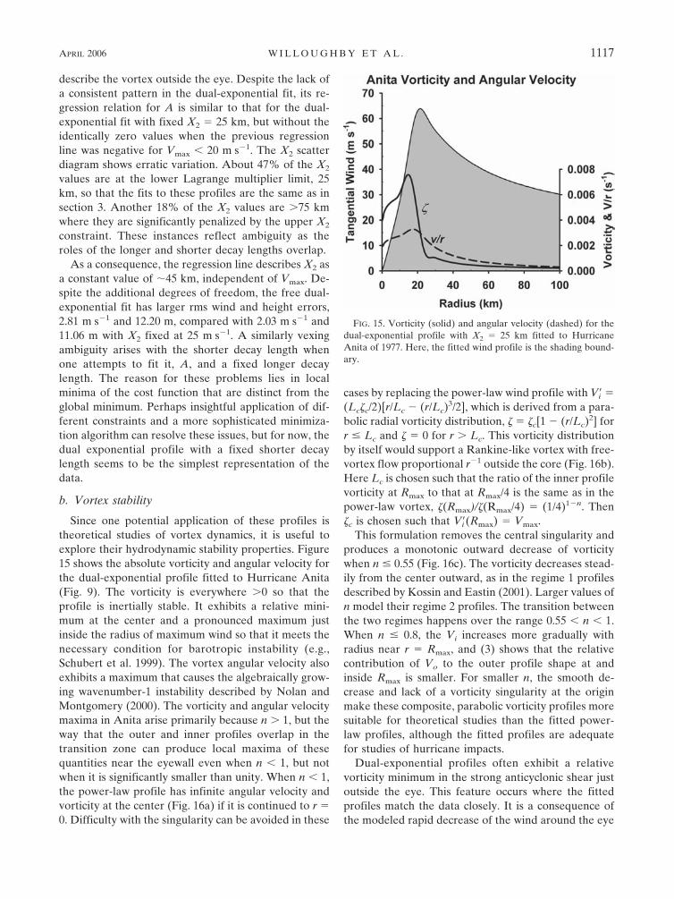
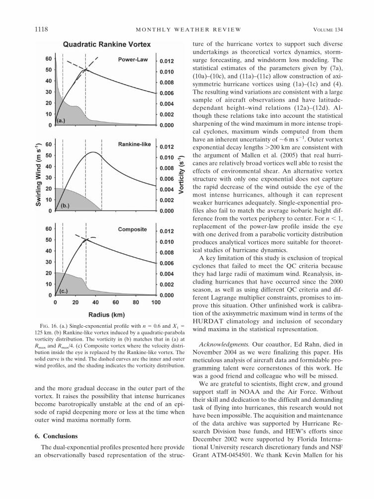
Since one potential application of these profiles istheoretical studies of vortex dynamics, it is useful toexplore their hydrodynamic stability properties. Figure15 shows the absolute vorticity and angular velocity forthe dual-exponential profile fitted to Hurricane Anita(Fig. 9). The vorticity is everywhere 0 so that theprofile is inertially stable. It exhibits a relative mini-mum at the center and a pronounced maximum justinside the radius of maximum wind so that it meets thenecessary condition for barotropic instability (e.g.,Schubert et al. 1999). The vortex angular velocity alsoexhibits a maximum that causes the algebraically grow-ing wavenumber-1 instability described by Nolan andMontgomery (2000). The vorticity and angular velocitymaxima in Anita arise primarily because n 1, but theway that the outer and inner profiles overlap in thetransition zone can produce local maxima of thesequantities near the eyewall even when n � 1, but notwhen it is significantly smaller than unity. When n � 1,the power-law profile has infinite angular velocity andvorticity at the center (Fig. 16a) if it is continued to r �0. Difficulty with the singularity can be avoided in these

cases by replacing the power-law wind profile with V�i �(Lc�c/2)[r/Lc � (r/Lc)

3/2], which is derived from a para-bolic radial vorticity distribution, � � �c[1 � (r/Lc)

2] forr � Lc and � � 0 for r Lc. This vorticity distributionby itself would support a Rankine-like vortex with free-vortex flow proportional r�1 outside the core (Fig. 16b).Here Lc is chosen such that the ratio of the inner profilevorticity at Rmax to that at Rmax/4 is the same as in thepower-law vortex, �(Rmax)/�(Rmax/4) � (1/4)1�n. Then�c is chosen such that V�i (Rmax) � Vmax.

This formulation removes the central singularity andproduces a monotonic outward decrease of vorticitywhen n � 0.55 (Fig. 16c). The vorticity decreases stead-ily from the center outward, as in the regime 1 profilesdescribed by Kossin and Eastin (2001). Larger values ofn model their regime 2 profiles. The transition betweenthe two regimes happens over the range 0.55 � n � 1.When n � 0.8, the Vi increases more gradually withradius near r � Rmax, and (3) shows that the relativecontribution of Vo to the outer profile shape at andinside Rmax is smaller. For smaller n, the smooth de-crease and lack of a vorticity singularity at the originmake these composite, parabolic vorticity profiles moresuitable for theoretical studies than the fitted power-law profiles, although the fitted profiles are adequatefor studies of hurricane impacts.

Dual-exponential profiles often exhibit a relativevorticity minimum in the strong anticyclonic shear justoutside the eye. This feature occurs where the fittedprofiles match the data closely. It is a consequence ofthe modeled rapid decrease of the wind around the eye

FIG. 15. Vorticity (solid) and angular velocity (dashed) for thedual-exponential profile with X2 � 25 km fitted to HurricaneAnita of 1977. Here, the fitted wind profile is the shading bound-ary.


and the more gradual decease in the outer part of thevortex. It raises the possibility that intense hurricanesbecome barotropically unstable at the end of an epi-sode of rapid deepening more or less at the time whenouter wind maxima normally form.

6. Conclusions

The dual-exponential profiles presented here providean observationally based representation of the struc-

ture of the hurricane vortex to support such diverseundertakings as theoretical vortex dynamics, storm-surge forecasting, and windstorm loss modeling. Thestatistical estimates of the parameters given by (7a),(10a)–(10c), and (11a)–(11c) allow construction of axi-symmetric hurricane vortices using (1a)–(1c) and (4).The resulting wind variations are consistent with a largesample of aircraft observations and have latitude-dependant height–wind relations (12a)–(12d). Al-though these relations take into account the statisticalsharpening of the wind maximum in more intense tropi-cal cyclones, maximum winds computed from themhave an inherent uncertainty of �6 m s�1. Outer vortexexponential decay lengths 200 km are consistent withthe argument of Mallen et al. (2005) that real hurri-canes are relatively broad vortices well able to resist theeffects of environmental shear. An alternative vortexstructure with only one exponential does not capturethe rapid decrease of the wind outside the eye of themost intense hurricanes, although it can representweaker hurricanes adequately. Single-exponential pro-files also fail to match the average isobaric height dif-ference from the vortex periphery to center. For n � 1,replacement of the power-law profile inside the eyewith one derived from a parabolic vorticity distributionproduces analytical vortices more suitable for theoret-ical studies of hurricane dynamics.

A key limitation of this study is exclusion of tropicalcyclones that failed to meet the QC criteria becausethey had large radii of maximum wind. Reanalysis, in-cluding hurricanes that have occurred since the 2000season, as well as using different QC criteria and dif-ferent Lagrange multiplier constraints, promises to im-prove this situation. Other unfinished work is calibra-tion of the axisymmetric maximum wind in terms of theHURDAT climatology and inclusion of secondarywind maxima in the statistical representation.

Acknowledgments. Our coauthor, Ed Rahn, died inNovember 2004 as we were finalizing this paper. Hismeticulous analysis of aircraft data and formidable pro-gramming talent were cornerstones of this work. Hewas a good friend and colleague who will be missed.

We are grateful to scientists, flight crew, and groundsupport staff in NOAA and the Air Force. Withouttheir skill and dedication to the difficult and demandingtask of flying into hurricanes, this research would nothave been impossible. The acquisition and maintenanceof the data archive was supported by Hurricane Re-search Division base funds, and HEW’s efforts sinceDecember 2002 were supported by Florida Interna-tional University research discretionary funds and NSFGrant ATM-0454501. We thank Kevin Mallen for his

FIG. 16. (a.) Single-exponential profile with n � 0.6 and X1 �125 km. (b) Rankine-like vortex induced by a quadratic-parabolavorticity distribution. The vorticity in (b) matches that in (a) atRmax and Rmax/4. (c) Composite vortex where the velocity distri-bution inside the eye is replaced by the Rankine-like vortex. Thesolid curve is the wind. The dashed curves are the inner and outerwind profiles, and the shading indicates the vorticity distribution.


insightful comments and Sneh Gulati for statistical ad-vice.

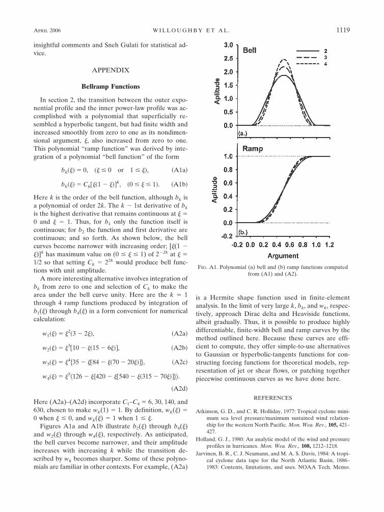
APPENDIX

Bellramp Functions

In section 2, the transition between the outer expo-nential profile and the inner power-law profile was ac-complished with a polynomial that superficially re-sembled a hyperbolic tangent, but had finite width andincreased smoothly from zero to one as its nondimen-sional argument, �, also increased from zero to one.This polynomial “ramp function” was derived by inte-gration of a polynomial “bell function” of the form

bk�� 0, �� 0 or 1 � ��, �A1a�

bk�� Ck��1 � ��k, �0 � � � 1�. �A1b�

Here k is the order of the bell function, although bk isa polynomial of order 2k. The k � 1st derivative of bk

is the highest derivative that remains continuous at � �0 and � � 1. Thus, for b1 only the function itself iscontinuous; for b2 the function and first derivative arecontinuous; and so forth. As shown below, the bellcurves become narrower with increasing order; [�(1 ��)]k has maximum value on (0 � � � 1) of 2�2k at � �1/2 so that setting Ck � 22k would produce bell func-tions with unit amplitude.

A more interesting alternative involves integration ofbk from zero to one and selection of Ck to make thearea under the bell curve unity. Here are the k � 1through 4 ramp functions produced by integration ofb1(�) through b4(�) in a form convenient for numericalcalculation:

w1�� 2�3 � 2��, �A2a�

w2�� 310 � ��15 � 6��, �A2b�

w3�� 4�35 � �84 � ��70 � 20��, �A2c�

w4�� 5�126 � ��420 � �540 � ��315 � 70��.

�A2d�

Here (A2a)–(A2d) incorporate C1–C4 � 6, 30, 140, and630, chosen to make wk(1) � 1. By definition, wk(�) �0 when � � 0, and wk(�) � 1 when 1 � �.

Figures A1a and A1b illustrate b2(�) through b4(�)and w2(�) through w4(�), respectively. As anticipated,the bell curves become narrower, and their amplitudeincreases with increasing k while the transition de-scribed by wk becomes sharper. Some of these polyno-mials are familiar in other contexts. For example, (A2a)

is a Hermite shape function used in finite-elementanalysis. In the limit of very large k, bk, and wk, respec-tively, approach Dirac delta and Heaviside functions,albeit gradually. Thus, it is possible to produce highlydifferentiable, finite-width bell and ramp curves by themethod outlined here. Because these curves are effi-cient to compute, they offer simple-to-use alternativesto Gaussian or hyperbolic-tangents functions for con-structing forcing functions for theoretical models, rep-resentation of jet or shear flows, or patching togetherpiecewise continuous curves as we have done here.

REFERENCES

Atkinson, G. D., and C. R. Holliday, 1977: Tropical cyclone mini-mum sea level pressure/maximum sustained wind relation-ship for the western North Pacific. Mon. Wea. Rev., 105, 421–427.

Holland, G. J., 1980: An analytic model of the wind and pressureprofiles in hurricanes. Mon. Wea. Rev., 108, 1212–1218.

Jarvinen, B. R., C. J. Neumann, and M. A. S. Davis, 1984: A tropi-cal cyclone data tape for the North Atlantic Basin, 1886–1983: Contents, limitations, and uses. NOAA Tech. Memo.

FIG. A1. Polynomial (a) bell and (b) ramp functions computedfrom (A1) and (A2).


NWS NHC 22, Coral Gables, FL, 21 pp. [Available online athttp://www.nhc.noaa.gov/pastall.shtml.]

Jelesnianski, C. P., 1967: Numerical computation of storm surgeswith bottom stress. Mon. Wea. Rev., 95, 740–756.

Jordan, C. L., 1958: Mean soundings for the West Indies area. J.Meteor., 15, 91–97.

Kossin, J. P., and M. D. Eastin, 2001: Two distinct regimes in thekinematic and thermodynamic structure of the hurricane eyeand eyewall. J. Atmos. Sci., 58, 1079–1090.

Mallen, K. J., M. T. Montgomery, and B. Wang, 2005: Reexamin-ing the near-core radial structure of the tropical cyclone pri-mary circulation: Implications for vortex resiliency. J. Atmos.Sci., 62, 408–425.

Nelder, J. A., and R. Mead, 1965: A simplex method for functionminimization. Comput. J., 7, 308–313.

Nolan, D. S., and M. T. Montgomery, 2000: The algebraic growthof wavenumber-1 disturbances in hurricane-like vortices. J.Atmos. Sci., 57, 3514–3538.

Press, W. H., B. P. Flannery, S. A. Teukolsky, and W. T. Vetter-ing, 1986: 10.4 Downhill simplex method in multidimensions.Numerical Recipes: The Art of Scientific Computing, Cam-bridge University Press, 289–293.

Schubert, W. H., and J. J. Hack, 1982: Inertial stability and tropi-cal cyclone development. J. Atmos. Sci., 39, 1687–1697.

——, M. T. Montgomery, R. K. Taft, T. A. Guinn, S. R. Fulton,J. P. Kossin, and J. P. Edwards, 1999: Polygonal eyewalls,asymmetric eye contraction and potential vorticity mixing inhurricanes. J. Atmos. Sci., 56, 1197–1223.

Shapiro, L. J., and H. E. Willoughby, 1982: The response of bal-anced hurricanes to local sources of heat and momentum. J.Atmos. Sci., 39, 378–394.

Sheets, R. C., 1969: Some mean hurricane soundings. J. Appl.Meteor., 8, 134–146.

Smith, R. K., 1981: The cyclostrophic adjustment of vorticies withapplication to tropical cyclone modification. J. Atmos. Sci.,38, 2021–2030.

Vickery, P. J., and L. A. Twisdale, 1995: Prediction of hurricanewind speeds in the United States. J. Struct. Eng., 121, 1691–1699.

Willoughby, H. E., 1995: Normal-mode initialization of barotropicvortex motion models. J. Atmos. Sci., 52, 4501–4514.

——, and M. E. Rahn, 2004: Parametric representation of theprimary hurricane vortex. Part I: Observations and evalua-tion of the Holland (1980) model. Mon. Wea. Rev., 132, 3033–3048.


parametric representation of the primary hurricane vortex

Documents