parrallel connecting component labeling
TRANSCRIPT


Parrallel Connecting Component LabelingHugo Bantignies
We built an optimized binarization to generate a binary image using intrasecs function in C.
Converting a pixel image to a binary image depending on a threshold.
Binarization
Connecting Component Labeling
Connecting Component Labeling ( CCL ) :Assigning a label to each connected component -blob- of a binary image.
Algorithm Comparizon
CCL Algorithm is already implemented. For example, NVIDIA,built the algorithm with CUDA.
We wanted to compare ourimplementation idea with them,about the execution time.
Labeling execution time of 2048x2048 on GPU, CUDA
References
[1] HAL, A new direct CCL and CCA Algorithms for GPUs,Arthur Hennequin and Lionel Lacassagne
[2] How to speed CCL up with SIMDRLE algorithms,Florian Lemaitre, Arthur Hannqeuin, Lionel Lacassagne
Parallel and Multithreading
To optimize the execution, we have to use parallelization and threads.That is why, for the horizontal propagation, each line of the image is associated to a thread.
This allows us the entire scanning of the image in a short time. The horizontal propagation is done at the same time.
Each line is runned by a different thread (t1,t2,t3)
Propagation
Root and Terminaison
During the CCL, there are two propagation : Horizontal and Vertical.Horizontal is the first propagation. During this step, each thread will create an array of label for his line and the next line. Each label will be connected to another label. At the end, we have got a horizontal propagation stored in arrays.
The second propagation is the Vertical.An array of root was built during the horizontal propagation. Our goal is to propagate each root, from the bottom to the top, throw the arrays built during the first step.
This array represents the first pixel line
A root is the start of a component -blob-, it will be stocked into an array during the first step of the algorithm.
A terminaison is the end of the component -blob-.
The root is the green run
The terminaison is the red run
Vertical propagation of the red root

Extended Abstract : Parallel Connecting Component Labelling Algorithm on
Multi-Core CPU
Hugo Bantignies
Supervised by: Dominique Houzet
I understand what plagiarism entails and I declare that this reportis my own, original work.Name, date and signature: Bantignies Hugo, 29/08/2020
Abstract
This document is an extended abstract of ”Paral-lel Connecting Component Labeling Algorithm onMulti-Core CPU”.
1 Introduction
Currently, in image processing, the direct Connecting Com-
ponent Labeling algorithm (CCL) was recently implementedin parallel. We wanted to submit our own version of the algo-rithm -a parallel version- to the OpenCV library and compareit with other implementations already existing on GPU -likeNVIDIA with CUDA- as a bibliographic review. Before that,we wanted a Multi-core CPU version of our code in C pro-gramming language.CCL is an algorithm consisting in providing a unique label toeach connected component of a binary image used primarilyin image detection. This algorithm can be enhanced in Con-
necting Component Analysis (CCA) to get more informationabout the image.
2 Binarization
The CCL algorithm needs a binary image. For this reason,we implemented our version of an optimized binarization bythresholding. This is an algorithm to convert a pixelized im-age into a binary image. We used intrinsics functions fromthe instruction set Streaming SIMD Extensions 2 (SSE2) tooptimize it. To read and stock the image, the m128i typeand his logical operations is an example. Also, we applied abyte compression to recreate the binary image.
3 New Parallel CCL Algorithm
3.1 Definitions
There are some terms to know about the algorithm :• run : A sequence of ”1” in a row in a line of the binary
image.• root : The first run encounter of a connected component
during the reading direction. It is the start of the compo-nent.
• ending : The last run encounter of a connected compo-nent during the reading direction. It is the end of thecomponent.
• 4-connectivity : A pixel is only connected -or not- withhis top, right, left and bottom neighbors.
3.2 Label Propagation
Propagation will detect and keep in table every connectionsbetween different run, to find every connected component atthe end. There are two propagations during the execution ofour CCL version : horizontal and vertical.
Horizontal Propagation
To have an optimized propagation we used multithreading.Each line of the binary image is associated to a thread. Eachthread explores his current line and the next one, to have acommon line with the next thread.Every run in a binary line is identified by a unique label. Thethread will explore his two lines switching when the end ofa run is farther than the other one on the other line. Twotables -A and B- will keep all run connections following 4-connectivity. A root table is filled during this propagation.
Vertical Propagation
Every root stocked in the table, will be propagated through Aand B tables generated by threads during the horizontal prop-agation. The root propagation will be stopped on a endingrun. There is a particular situation called a conflict, when aroot, during his propagation, arrives on an update run by aprevious root propagation. A conflict notified will be savedin an equivalence table like that : (updated root, new root)which means that every run updated by the previous root orby the current one are in the same component.
3.3 Equivalence table
At the end of propagation, all missing root labels inside theequivalence table are a unique label of a connected compo-nent. Otherwise, for each equivalent root, the connected com-ponent has several equivalent roots but one single label -theminus one-.

Validation of Presburger Sets operations
How to extract the formula defining an ISL set S in order to store it in Z3 format ?
How are ISL Sets stored and defined ?
Objective of the internship: test ISL operations between Presburger sets using Z3 SMT-Solver
How to create an ISL set defined with a Z3 formula and how to testOperations between and within sets ?
During the internship, ISL and Z3 were used in their python version

Abstract
The Validation of Presburger Sets operations willbe printed from electronic manuscripts submittedby the authors. The electronic manuscript will alsobe included in the online version of the proceed-ings. This paper provides the style instructions.
1 Introduction
1.1 ISL
Integer Set Library (ISL) is a C library used for storing sets
of vectors of integers, and computing different operations
such as union, intersection and projection on these sets.
1.2 Presburger Set definition
A set can be defined with a logical formula, i.e. , if an object
satisfies the formula, then it belongs to the set.
In ISL, these formulas are defined with the Presburger arith-
metic language.
1.3 Main objective
The main objective of the internship was to validate the
main operations offered by ISL, using an SMT solver (Z3).
During the internship, the python libraries ISLpy and Z3py
were used in order to facilitate the task.
1.4 Main issues
After a projection operation, in many cases the formula ends
up having an existential quantifier. The main problem is that
Z3 may induce an infinite loop when checking the satisfia-
bility of this kind of formula. This is why Cooper’s method
of quantifier elimination had to be implemented. This allows
to find a finite set, in which if the formula is satisfied, then
the original formula is also satisfied.
The “Set” data structure of the ISL library had to be under-
stood in order to program robust tests.
2. Testing the operations
2.1 Creation of Z3 random polyhedra
The first objective of the internship was to create a function
creating a random polyhedron, i.e, an array containing for-
mulas of the form : a1 x1 + … + an xn + an+1 ≥ 0 with every ai
created randomly . The formulas are objects of the class
“Expression” declared in the Z3 library, allowing to keep in
memory operations with variables.
2.2 Creation of ISL sets
Once the polyhedron is created, the conjunction of these in-
equalities is computed. In order to create an ISL set defined
by this formula, it suffices to give as a parameter to the ini-
tializer Set(), the string: “ { [ x1 , … , xn ] : Conjunction( P ) }
”, assuming “Conjunction( P )” computes the conjunction of
the inequalities forming the array P.
2.3 Computing Union and Intersection of ISL sets
Let A = { x : P(x) } and B = { x : Q(x) } . In set theory, the
intersection of A and B corresponds to :
A ∩ B = { x : P(x) and Q(x) }. The ISL operation A.inter-
sect(B) is supposed to keep in memory the simplification of
“P(x) and Q(x)”. The tests consist in seeing if in fact, the
simplification is equal to the expected formula. Idem for the
union of sets (A.union(B)).
2.4 Main idea for the tests
With two sets A and B created with two Z3 random polyhe-
dra PA and PB, the intersection or the union is computed.
Then the simplification of the formula F, defining the result-
ing set is extracted as a Z3 expression. Z3, being a SMT-
Solver allows to prove if two formulas are equivalent :
If Xor ( F , PA and PB ) is unsatisfiable, then the formulas
“F” and “PA and PB” are equivalent. The expected result to
consider that the operation works, is that for each randomly
created PA and PB, its conjunction has to be equivalent to the
resulting F if the tested operation is the intersection, and its
disjunction has to be equivalent to F if the tested operation
is the union.
Validation of Presburger Sets operations
Nicolas BessonUGA and VerimagGrenoble, France

2.5 Results
As expected, in every tested case (with 10 000 tests), the re-
sult was what was expected. In order to conclude that the
operations always work, the code of the operations has to be
mathematically proven ( which was not the point of the in-
ternship ).
References
[Aaron Bradley, Zohar Manna, 2007] The Calculus of Com-putation: Decision Procedures with Application to Veri-fication

Effective implementations of Information-Set Decoding algorithmsDorian Biichle supervized by Pierre Karpman
Team CASC @ Laboratoire Jean Kuntzmann, University of Grenoble-Alpes
IntroductionInformation-Set Decoding forms a class ofexponential probabilistic algorithms whose goal isto find a low-weight codeword in a given randomlinear code.
ISD Algorithms
‘ These algorithms operates on either the gen-erator or the parity-check matrix of the linearcode.
‘ By manipulating the matrix and checking itsrows, they try to find a codeword (a vector) witha weight as close as possible to a theoreticalminimum bound.
‘ Two main algorithms have been implemented:Prange [1] and Stern [3]. Prange idea is to an-alyze rows of the generator matrix in systematicform (when the left part of the generator matrixis the identity), while Stern is an improvement ofPrange using a time-memory trade-off.
‘ Two implementation of Stern have been done;a first one using only Canteaut and Chabaudimprovements [2], and a second one addingoptimizations and recommended parameters ofBernstein, Lange and Peters [4]
Implementations‘ Implementations have been tailored to solve
[1280, 640] binary codes. Thus, many opti-mizations rely on the fixed size of the code’sparameters to get faster.
‘ These algorithms have been implemented tomake the most of the AVX-512 instructions set.Hence, the implementations have been donein C, using AVX-512 intrinsics.
‘ Some linear algebra operations are done us-ing the M4RI library, which is specialized in fastarithmethic operations over F2.
ResultsEvaluating performances
‘ Solving the low-weight codeword problem inpractice has implications in cryptography assome cryptosystems rely on its hardness.
‘ In fact, our implementations have been testedagainst decoding-challenge.org’s chal-lenges, where the goal is to find a codewordwith the smallest weight possible for the giveninstance of a random linear binary code.
‘ The purpose of the website is to assert the prac-tical hardness of the problem, with real-worldcryptographic parameters.
‘ The code has been launched on one of GRI-CAD’s cluster, Dahu (dahu110 & dahu111nodes, 2x8 cores Intel(R) Xeon(R) Gold 6244CPU 3.60GHz).
‘ As ISD algorithms are probabilistic, the problemis embarassingly parallel, which means one canrun 16 instances of the program simultaneouslyon 16 cores without much effort.
Results in numbers
Prange Stern Stern 248h runs/core done 16 61 96evaluated codewords/s 58 400 000 9 800 000 15 295 500Av. smallest codeword/run 228.4 227.3 225Smallest codeword found 224 222 219
Figure: Overall stats for each implementations
After many runs, the best codeword found has aweight of 219 (theoretical minimum bound is 144for the given instances).
Figure: Average minimum weight found over time for eachimplementation
Figure: decoding-challenge.org’s scoreboard
That was close but not enough to get intodecoding-challenge.org’s scoreboard.‘ The code is accessible on github at
github.com/Antoxyde/isd.
ReferencesPrange, E. The use of information sets in decoding cyclic codes IRETransactions IT-8(1962) S5–S9
Canteaut, A., Chabaud,F A new algorithm for finding
minimum-weight words in a linear code: Application to McEliece’s
cryptosystem and to narrow-sense BCH codes of length 511. EEETransactions on Information Theory44(1) (January 1998) 367–378
Stern, J. A method for finding codewords of small weight Codingtheory and applications, volume 388 of Lecture Notes in ComputerScience, 1989.
Bernstein, DJ., Lange, T., Peters, C. Attacking and defending the
McEliece cryptosystem 2008

Effective implementations of information-set decoding algorithms
Dorian Biichle, supervised by Pierre KarpmanTeam CASC, Laboratoire Jean Kuntzmann, University of Grenoble-Alpes
1 IntroductionISD (Information-Set Decoding) is a class of probabilisticalgorithms whose goal is to find a low-weight codeword ina random linear code. This problem is considered hard, asthese algorithms all have an exponential complexity. Somecryptosystems rely on this hardness. The goal of this work isto ensure the practical hardness of the low-weight codewordproblem with real-world cryptographic parameters againstISD algorithms.
1.1 Linear codesA random linear [n, k] code is a linear subspace C ⇢ Fn
qof dimension k. We will only consider the binary case, ieq = 2. C can be characterized by a k ⇥ n generator matrixG, whose rows forms a basis of C. This matrix is said to bein systematic form if its in the form G = [Ik|R], where R isa random k ⇥ (n� k) matrix.
An information set of G is a subset of length k of {1, .., n},corresponding to indexes of linearly independant columns ofG.
The Gilbert-Varshamov bound on linear codes tells us thatthere exist on average a unique codeword of a certain givenweight. By ”low-weight codeword”, we thus means a code-word whose weight is as close as possible to that bound.
2 ISD algorithmsThe first algorithm implemented is Prange [3]. It aims to findlow-weight codewords by using a generator matrix in system-atic form. It uses the fact the rows have a maximum weightof n� k + 1 (and expected n�k
2 + 1).The second algorithm implemented is Stern [4]. The idea
is the same as Prange, but using a time-memory trade-off. Itstrives to lower the weight of analysed codewords by findinglinear combinations having the same value on a specific win-dow. The maximum weight of analysed codewords is thusn � k � ` + 2p (and expected n�k�l
2 + 2p), where p is thenumber of rows in the linear combinations, and ` the size ofthe window.
2.1 ImprovementsOver the years, researchers have found several improvementsto these algorithms. We implemented some of their ideas:
• Canteaut and Chabaud [1], who lowered the complexityof Stern algorithm by making single steps of the Gaus-sian elimination algorithm, instead of all the steps.
• Bernstein, Lange and Peters [2], who gives interestingoptimizations, for instance forcing several windows tozero in one iteration of the Stern algorithm, instead ofonly one.
3 ImplementationsImplementations were tailored to decoding-challenge.org’schallenges, which are [1280, 640] binary codes. That meansthat the code heavily rely on the fact that these parameters arefixed. We strove to make full use of the AVX-512 instructionsset, as the codewords are 1280 bits long. An optimizationmade consist of storing only the redundant part of the genera-tor matrix, meaning storing a single row takes 640 bits, so 512bits and 128 bits vectors. Some of the linear algebra opera-tions are done using the M4RI library, which is specialised inarithmetic over F2. The whole code is accessible on a githubrepository at github.com/Antoxyde/isd
4 ResultsThe code has been launched on one of the GRICAD’s clus-ter, Dahu (specifically on the dahu110 & dahu111 nodes, 2x8cores Intel(R) Xeon(R) Gold 6244CPU 3.60GHz).
Figure 1: Average min. weight found over 48h runsThe G-V bound for [1280, 640] binary codes is 144, and af-
ter running our Stern implementation for approximately 192core-days, the best codewords we obtained has a weight of219.

References[1] F. Chabaud A. Canteaut. “A new algorithm for find-
ing minimum-weight words in a linear code: Applica-tion to McEliece’s cryptosystem and to narrow-senseBCH codes of length 511”. In: IEEE Transactions onIn-formation Theory44 (1998), pp. 367–368.
[2] C. Peters D. J. Bernstein T. Lange. “Attacking and de-fending the McEliece cryptosystem”. In: (2008).
[3] E. Prange. “The use of information sets in decodingcyclic code”. In: IRE Transactions IT-8 (1962).
[4] J. Stern. “A method for finding codewords of smallweight”. In: Coding theory and applications 388 (1989).
Lattice based resolution for the Hidden Number Problem
Gaspard Anthoine1 and Pierre Karpman1
Abstract— We are interested in the problem of finding an
unknown value in an interval [0, p � 1] for a prime p given
a small number of relations of the form yi + Aiy0 + Bi ⌘ 0mod p only partially known and according to a uniform law.
Where Ai and Bi are uniformly random public values and yiare either well unknown according to a non-uniform law, or
only partially known and according to a uniform law.
I. INTRODUCTION
In cryptography digital signatures are used for verifyingauthenticity of a message, a document. They are in realitywidely used for software distribution, financial transactions,cryptocurrencies, website certificates. Digital signatures re-lies on asymmetric cryptography, the DSA standard wasproposed by NIST and adopted in 1994. This scheme is basedon modular exponentiation and a discrete logarithm problem.There is now some new scheme for digital signature forexample based on elliptic curves named ECDSA. Attackingtheses signatures algorithms when a certain amount of bitsleaks can be linked to what is called the Hidden NumberProblem. There are two principals methods used to solvethis problem, the first is called Bleichenbacher [1]. TheBleichenbacher’s method permits to attack leaks with a smallnumber of bits but requires a lot of signatures. The methodwe will study in this paper will be based on lattices. The HNPcan be solved via lattice as shown by Boneh and Venkatesan[2]. Howgrave-Graham & Smart [3] showed in 2001 howto attack DSA using lattice and building an appropriatebasis. The main concern of this work was to replicate theresults of Howgrave-Graham and Smart and to see if therecent progress of Albrecht et al. [4] for short vector searchin a lattice could improve the parameters (signature sizeand number of leaking bits). The advantage of the latticeapproach compared to the Bleichenbacher one is that fewersignatures are needed but in return more bits have to leak.
II. RELATED WORKS
Lattice based attacks on electronic signature have beenfirst introduced by Howgrave-Graham & Smart [3] in 2001.In 2002 Nguyen & Shparlinski [5] improved the results ofHowgrave-Graham & Smart by recovering the private keyon a 160 bits signature with only 3 bit of leaked nonce.Lattice based attacks have then shown to have real worldapplication. For example Benger & all [6] showed in 2014how to attack OpenSSL ECDSA with a side channel on cache(FLUSH+RELOAD) and lattice based attack to recover theprivate key. In 2019 Breitner & Heninger [7] show how
*This work was not supported by any organization1 Laboratoire Jean kuntzmann
to attack cryptocurrencies using transactions signature withbiased nonce and à lattice based private key recovery.
III. PRELIMINARIES
A. LatticesDefinition 1: A lattice is a discrete subgroup of space,
with a finite rank n. Let v1, . . . , vn 2 m be n linearlyindependents vectors. A lattice spanned by {v1, . . . , vn} isthe set of all linear combination of v1, . . . , vn such that :
L =
(nX
i=1
aivi, ai 2)
{v1, . . . , vn} will be called the basis of L. When m = n wecan construct a matrix of the basis by the vectors down rowby row.
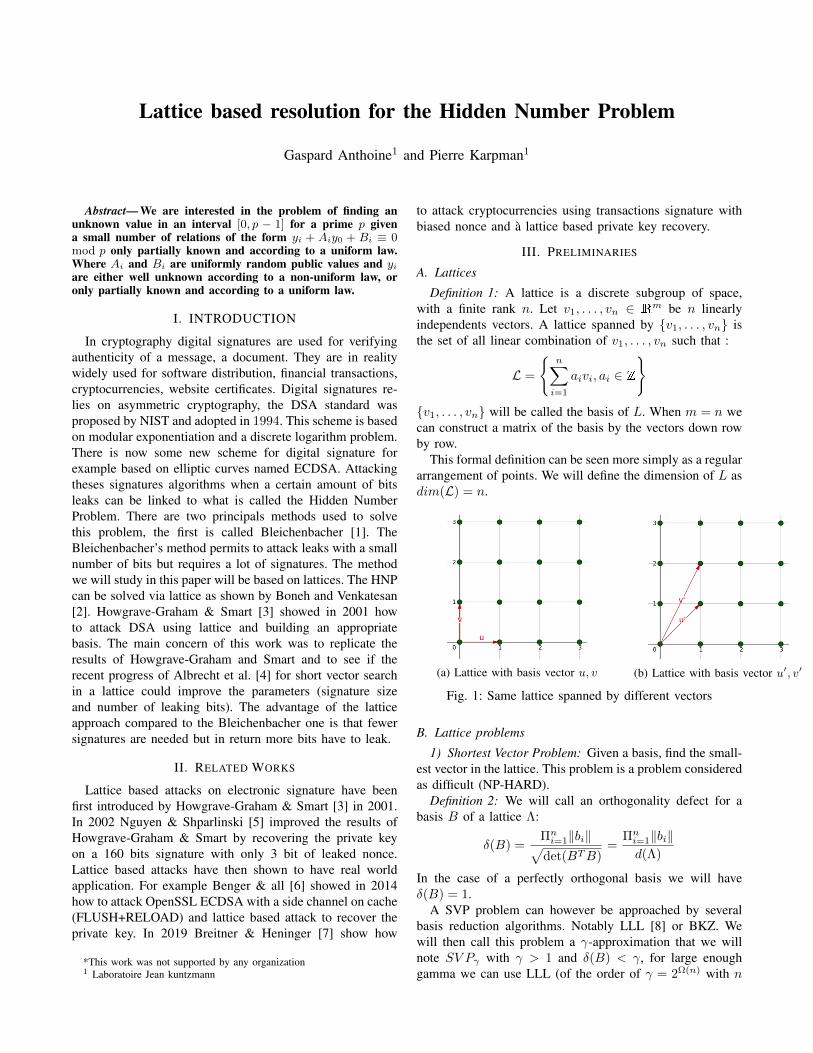
This formal definition can be seen more simply as a regulararrangement of points. We will define the dimension of L asdim(L) = n.
(a) Lattice with basis vector u, v (b) Lattice with basis vector u0, v0
Fig. 1: Same lattice spanned by different vectors
B. Lattice problems1) Shortest Vector Problem: Given a basis, find the small-
est vector in the lattice. This problem is a problem consideredas difficult (NP-HARD).
Definition 2: We will call an orthogonality defect for abasis B of a lattice ⇤:
�(B) =⇧n
i=1kbikpdet(BTB)
=⇧n
i=1kbikd(⇤)
In the case of a perfectly orthogonal basis we will have�(B) = 1.
A SVP problem can however be approached by severalbasis reduction algorithms. Notably LLL [8] or BKZ. Wewill then call this problem a �-approximation that we willnote SV P� with � > 1 and �(B) < �, for large enoughgamma we can use LLL (of the order of � = 2⌦(n) with n

the size of the lattice). If you want a better reduction youwill have to use BKZ (or even HKZ [4]) but the reductionwill then be slower (will depend on some parameters). If youuse LLL you will have a bad approximation ratio (( 2p
3)n)
but the algorithm will be polynomial.
Fig. 2: Example of basis reduction
As you can see in figure 2 the vector of the basis areshorter and more orthogonal (closer to the orthogonalitydefect) after the reduction.
2) Closest Vector Problem: Given a lattice, find the clos-est lattice’s vector to a given vector which does not belongto the lattice. We can define given a target vector t 2 n
and a lattice L ⇢ n :
dist(L, t)x2L
= kx� tk
The hardness of this problem is known to be NP-complete(first proved by Emde Boas [9]) and highly related tohardness of SVP. There is an approximation problem called�-CVP for any gamma > 1 approximation factor, t 2 n,a lattice L ⇢ R
n, the goal is to output x 2 L with :
kx� tk � · dist(L, t)
This problem is also known to be NP-complete for any� > n
c/ log logn for some constant c [10]. This problem canbe solved easily if one has a good base of the lattice withBabai’s algorithm [11] and the quality of the vector we foundwill depend on the quality of the reduction basis.
3) Closest Vector Problem reduction to Shortest VectorProblem: It’s possible to reduce à CVP problem to an SVPby building a new lattice with a particular basis :
B0 =
✓B 0u n
◆
Where B is the basis of the lattice for the CVP problem withvector u which where not in the lattice and B
0 is a basis foran SVP problem. Applying a basis reduction algorithm to B
will give you �-CVP solution with gamma depending on thequality of the reduction. In figure 3 you can see an example
of CVP for a lattice L with basis B =
✓1 00 1
◆and a vector
t =
✓3.14.9
◆. The solution vector is x =
✓35
◆.
(a) Vector t 62 L (b) vector x 2 L
Fig. 3: Example of CVP
C. Hidden Number Problem
Definition 3: The hidden problem number can be de-scribed as follows : considering T = (t1, . . . , tn), ti 2 p,↵ 2 Fp, and MSBl(↵ti) the l most significant bits of↵ti. Having T and (MSBl(↵t1 mod p), . . . ,MSBl(↵tnmod p)) can we found ↵ ?This model is a generalisation of some attack problems onDSA (digital signature Algorithm). This problem can besolved via a lattice as shown by Boneh and Venkatesan [2]or by Bleichenbacher’s method [1]. The complexity of theHidden Number Problem depends on several parameters :
• Time complexity : the runtime of an algorithm to solvean instance of the problem.
• Data complexity : the number of samples that will berequired to solve an instance.
In this paper we will only study solving HNP with lattice,this requires less sample than a Bleichenbacher’s method butwill only work for more bits leaking (the parameter l of theproblem).
D. Digital Signature Algorithm
DSA or Digital Signature Algorithm is an algorithmproposed by NIST and adopted in 1994 as a standard fordigital signatures. The algorithm is in three parts :
1) Alice publish a group of cardinal p (prime) and agenerator g 2 . Alice get a random x and publishh = g
x. We imagine there is a bijective functionf : ! /p that everybody knows. x will be theprivate key of Alice that she has to keep secret.
2) If Alice wants to sign a message m 2 Z/p shecomputes r = f(gy) and s such that :
m ⌘ sy � xr mod p
for some randomly chosen y 22 Z/p .3) Alice can now send (m, r, s)to Bob.
To verify the signature Bob can compute f(gms�1
hrs�1
) =r.
IV. ATTACKING DSA WITH LATTICE
It’s possible to translate an HNP instance into equationsmodulo a prime p. You can write MSBl(↵ti mod p) as :
↵ti � bi ⌘ yi mod p

with bi the least significant bits of ↵ti.If we got h signatures of the form :
mi � siyi + xri ⌘ 0 mod p
With x and yi unknown we can write :
yi +Aix+Bi ⌘ O mod p
With Ai = (�si)�1 · ri and Bi = (�si)�1 ·mi. If we knowsome of the most significant bits of the yi we now have aHNP instance : MSBl(�yi � Bi mod p) = MSBl(Aix
mod p) and thus recover x. We can build the basis B for àlattice L as follows :
B =
0
BBBBB@
p⇥ 2l+1 0 0 . . . 0 00 p⇥ 2l+1 0 . . . 0 0...
. . .0 . . . . . . . . . p⇥ 2l+1 0
A1 ⇥ 2l+1A2 ⇥ 2l+1
. . . An ⇥ 2l+1 1 0
1
CCCCCA
And applying Babai algorithm with a vector t = (MSB(↵⇥A1)⇥2l+1
, . . . ,MSB(↵⇥An)⇥2l+1) which is outside thelattice will give with good probability a vector y = (. . . ,↵).As we have seen before we can transform this instance ofa closest vector problem into a shortest vector problem bybuilding this basis :
B0 =
0
BBBBBBB@
p⇥ 2l+1 0 0 . . . 0 00 p⇥ 2l+1 0 . . . 0 0...
. . .0 . . . . . . . . . p⇥ 2l+1 0
A1 ⇥ 2l+1A2 ⇥ 2l+1
. . . An ⇥ 2l+1 1 0t1 ⇥ 2l+1
t2 ⇥ 2l+1. . . tn ⇥ 2l+1 0 p
1
CCCCCCCA
If we apply a basis reduction algorithm on B0 we get a
good probability to find y0 = (y,�p) as one of the vectors
of the basis.It’s also possible to slightly improve the dimension of the
matrix by rearranging the diffrents yi +Aix+Bi as follow:
• x ⌘ �A�1n yn �A
�1n Bn mod p
• so we have yi + Ciy0 + Di ⌘ 0 mod p with Ci =�A
�1n ·Ai, Di = �A
�1n Bn +Bi and y0 = yn
At the end we have n � 1 equations so this reduce thedimension of the lattice.
V. RESULTS
This results are the bests results we got using 100 signa-tures samples.
Nombre de bits CVP LLL CVP BKZ SVP160 6 5 4192 6 5 5
For the 4 bits of nonce leak and a 160 bits signature wegot à 50% success.For the 5 bits of nonce leak and a 192bits signature we got à 100% success.
VI. CONCLUSIONSTo conclude we we managed to get better results than
Howgrave-Graham & Smart [3] but not as good as Nguyen& Shparlinski [5] who managed to have 100% success on a4 bits leak for a 160 bits signature and even some successfor 3 bits leak. Maybe we could try to understand more howthe scaling factor is working in the basis (2l+1). We got alsoanother idea would be to use the knowledge about hn withthe last optimisation to get a bigger advantage. Further workshould be done to understand how the different factors workswith the algorithm.
REFERENCES
[1] D. Bleichenbacher, “Chosen ciphertext attacks against protocols basedon the rsa encryption standard pkcs #1,” in Advances in Cryptology— CRYPTO ’98 (H. Krawczyk, ed.), (Berlin, Heidelberg), pp. 1–12,Springer Berlin Heidelberg, 1998.
[2] D. Boneh and R. Venkatesan, “Hardness of computing the mostsignificant bits of secret keys in diffie-hellman and related schemes,”in Advances in Cryptology — CRYPTO ’96 (N. Koblitz, ed.), (Berlin,Heidelberg), pp. 129–142, Springer Berlin Heidelberg, 1996.
[3] N. A. Howgrave-graham and N. P. Smart, “Lattice attacks on digi-tal signature schemes,” Designs, Codes and Cryptography, vol. 23,pp. 283–290, 1999.
[4] M. R. Albrecht, L. Ducas, G. Herold, E. Kirshanova, E. W. Postleth-waite, and M. Stevens, “The general sieve kernel and new records inlattice reduction,” in Advances in Cryptology - EUROCRYPT 2019 -38th Annual International Conference on the Theory and Applicationsof Cryptographic Techniques, Darmstadt, Germany, May 19-23, 2019,Proceedings, Part II (Y. Ishai and V. Rijmen, eds.), vol. 11477 ofLecture Notes in Computer Science, pp. 717–746, Springer, 2019.
[5] P. Q. Nguyen and I. E. Shparlinski, “The insecurity of the digital sig-nature algorithm with partially known nonces,” Journal of Cryptology,vol. 15, pp. 151–176, 2000.
[6] N. Benger, J. van de Pol, N. P. Smart, and Y. Yarom, “"ooh aah... justa little bit" : A small amount of side channel can go a long way,” inCHES, pp. 75–92, Springer, 2014.
[7] J. Breitner and N. Heninger, “Biased nonce sense: Lattice attacksagainst weak ecdsa signatures in cryptocurrencies.” Cryptology ePrintArchive, Report 2019/023, 2019. https://eprint.iacr.org/2019/023.
[8] A. K. Lenstra, H. W. Lenstra, and L. Lovasz, “Factoring polynomialswith rational coefficients,” MATH. ANN, vol. 261, pp. 515–534, 1982.
[9] P. Boas, “Another np-complete problem and the complexity of com-puting short vectors in a lattice,” 1981.
[10] I. Dinur, G. Kindler, R. Raz, and S. Safra, “Approximating cvp towithin almost-polynomial factors is np-hard,” Combinatorica, vol. 23,p. 205–243, Apr. 2003.
[11] L. Babai, “On lovász’ lattice reduction and the nearest lattice pointproblem,” in STACS 85 (K. Mehlhorn, ed.), (Berlin, Heidelberg),pp. 13–20, Springer Berlin Heidelberg, 1985.

Curve-based stylization of 3D animations⇤
FARHAT Amine
Under the supervision ofVERGNE Romain • THOLLOT Joelle
I understand what plagiarism entails and I declare that this reportis my own, original work.Name, date and signature:
Abstract
Expressive rendering can be done in multiple ways.One of them involves the repetition of a simple 2Dmark. The usage of a map of 3D positions as an in-put allows for a placement of these marks that fol-lows the geometry of the objects, and stays coher-ent with their deformations as well as with the posi-tion of the camera. This aspect makes this methodextremely effective for the stylization of 3D anima-tions. In this project, these marks are procedurallygenerated in order to follow the shape of a curvedpath, which facilitates the reproduction of brush-based or line-based art styles. The path is computedfrom a series of points and directions sampled fromthe tangent map of the scene. This computationis done by fitting a quadratic function. Since thesampled point are determined by the geometry, thepath remains coherent with the movements of theobjects, while still maintaining a 2D painted aspect.
1 Introduction
When it comes to rendering images on a computer, one mightseek to stray away from the usual pursuit of photo-realism,aiming instead for a stylized appearance. In computer graph-ics, the process of stylization usually consists in taking a pho-tograph and applying a series of filters – that can be imple-mented as programmable shaders – in order to recreate thedesired art style. The past two decades have witnessed anever-increasing mainstream usage of these stylization algo-rithms, notably in real time photo manipulation.
While most of these methods yield more than satisfyingresults, their main limitation manifests itself when being ap-plied to animated scenes. Since the stylization process is gen-erally applied to one frame at a time, this can lead to impor-tant discrepancies between two consecutive images. For ex-ample, an oil-paint filter might represent an object with hori-zontal strokes in one frames and vertical strokes in the next,
⇤These match the formatting instructions of IJCAI-07. The sup-port of IJCAI, Inc. is acknowledged.
which leads to a noticeable increase in popping. This issuewas formalized as the temporal coherence by Benard et al.[4].
According to Benard, a stylization method can be ap-praised on three distinct factors : Flatness, Motion coherenceand Temporal continuity. But since these three factors are un-elikely to be achieved at the same time, each method has tosettle on a compromise [figure 1].
Figure 1: Visual representation of the Temporal coherenceproblem.
Last year, during my internship, I briefly contributed to the

development of a new stylization method, the groundwork ofwhich was laid down by my supervisors.
Our method ensures motion coherence by taking 3D scenesas an input instead of 2D images. Since the input is a 3Dscene, it can provide more information on what is to be rep-resented on the canvas, including but not restricted to the ob-jects on the scene, their positions, the orientation of their sur-faces, the textures and colors of their materials, etc. This datais stored in a stack of images, referred to as G-buffers: In anormal rendered image, each pixel is a projection of a sectionof a 3D scene onto the 2D screen. Usually, the pixel takes thecolor of the object it is representing, such as to be understoodby the human brain. However, it is also possible to store otherkinds of information in that pixel, such as the orientation ofthe corresponding point in the 3D space.
In broad terms, this process will procedurally create a 3Dcloud of “anchor” points, generated within the volume of theobjects on the scene. These anchor points are thus coherentwith the transformations of the objects, since they are gener-ated from the information gathered from the G-buffers. Then,the image is recreated by exclusively “pasting” a simple im-age on the canvas, depending on the position of the anchorpoints on the screen. These images, henceforth referred to as”splats”, can vary in terms of shape, size, color, and texture.These parameters are the defining factors of the type of artstyle that is going to be outputted.
This information can also be used throughout the styl-ization pipeline to obtain different results depending on theuser’s will. This allows for an extremely wide scope of artstyles, ranging from pointillism to watercolor.
However, the splats themselves are limited to 2D squareimages, which can be too restrictive in certain scenarios: Forexample, when representing a moving object, some artistsrely on motion lines - an artistic abstraction of motion blur- to better express the trajectory of the object. Additionally,many styles rely on long, uninterrupted strokes that bend andtwists depending on the geometry of the object.
By building on this method, it is possible to allow the splatsto be molded by a curved path, the shape of which could bedetermined by a number of factors based on the characteris-tics of the object. And since the splats are placed on the can-vas depending on the geometrical properties of the objects,we can ensure a satisfying level of motion coherence.
2 Related Work
The field of non-photorealistic rendering offers a goodamount of attempts at curve-based stylization methods. Ren-dering algorithms, and according to Benard’s survey[4], theycan be divided in two categories: texture and mark based.
When it comes to mark based approaches, we will focuson two papers with comparable process. Hertzmann et al.proposed an algorithm where the brush strokes are gener-ated in a path that follows the directions with the least colordifference[1] on a blurred version of the input. Huang et al.[2] had a similar approach, where the strokes are instead gen-erated by a grid of features. The cells of this grid have vari-able sizes, and each one of them regroups small clusters ofpixels with similar values. The stroke once again follows the
neighboring paths with the least color difference. In both ofthese methods, the shape of the strokes can thus only be de-fined by the colors on the input 2D image. However, sincethe splatting method is always based on a 3D scene, we havea wider range of data to choose from. One possible solutionwould be to use the tangent information on each pixel. In thatway, the brush strokes would follow the general shape of theobject - the principal curvature of the object - which might beclose to the painting process of a human artist.
Figure 2: The sampling process with a high and a low densityvalue
Schmid et al. [3] proposed a groundbreaking techniqueto draw paint-looking brushes in 3D space, by allowing theartists to draw 3D curves directly on the 3D geometry. Thesecurves are transformed into stripes of polygons, which arethen used to map the texture of the brush. The resultingmeshes can then be rendered as any classic textured object.

However, the process is not automated, since every strokesneeds to be hand drawn. Which means that the result cannotbe easily animated. Additionally the curves are oriented in3D space, which can limit the movements of the camera, andnegatively impacts the flatness of the result
3 Method
The objective of our method is to recreate the scene usinga set of brush strokes on a 2D canvas. Each brush strokefollows a path that represents the shape of an object on thescreen. As such, these curves are constructed from points thatare sampled from the surface of these objects. The process isdone in for steps. First, for each anchor point given as aninput, we need to sample a number of points in the 3D spacethat follow the general shape of the geometry. Second, thesepoints are projected onto a 2D canvas, and transformed into acurve. Thirdly, we generate a stripe that follows the shape ofthe curve. Finally, we can map the input splat onto the shapein order to obtain the final render.
3.1 Point sampling
The sampling process is the first and most important step ofour stylization method. In order to draw a curve, one mustfirst determine the points it is going to follow. We must en-sure that these points are coherent with the geometry, and re-main coherent when the object moves or when the camera isanimated. Additionally, since each anchor point is going togenerate a curve, we must ensure that the silhouette cases -the cases where a curve cannot be fully drawn, if at all - aretaken into consideration.
Description
Sampling is done in three steps: First, the 2D coordinates ofthe anchor point on the screen is projected onto the surface ofthe 3D object using the world position map. The resulting 3Dcoordinate corresponds to the point on the geometry of theobject that appears on the position of the anchor point to theviewer. This point also carries the value of the tangent of thesurface at that position. This tangent is then used to performa ”step” in the 3D space in that direction, with an offset ddetermined by the user [figure 4]. The resulting 3D step isthen reprojected onto the 2D canvas. Since the whole processstarted with a 2D coordinate, we can re-iterate using that lastpoint, and keep drawing the rest of the curve. A single stepcan be described with the following formula:
V0 = Vanchor
Vx = Mmvp ⇤ (M�1mvp ⇤ Vx�1 + T (Vx+1) ⇤ d)
where Vx is the xth sampled point, Vanchor is the 2D po-sition of the anchor on the screen, T () the function that re-turns the value of the tangent map at a given 2D position, andMmvp the projection matrix.
Once the process is complete, a series of 2D points is ob-tained, one that follows the geometry of the object in a curve-like pattern [figure 3].
Tangent map
The use of a tangent map was mentioned in the previous para-graph. The tangent map is a G-buffer that stores, for eachpixel on the map, the tangent on the surface of the corre-sponding point in the 3D scene. These tangent vectors canbe painted by the artist himself directly on the geometry, orglobally computed from the normal map and a direction vec-tor.
Fidelity and precision
The steps are performed using a user-defined offset. Thisoffset determines how spaced out are the sampling points in3D space. The density of the sampling points directly affectsthe shape of the curve [figure 3]: The higher the density, thecloser the curve is to the actual geometry of the object. Thereason for such a phenomenon arises from the re-projectionstep. Indeed, when projecting a 2D point into 3D coordinatesand vice-versa, the projection is done on a vector that orig-inates from the camera. [figure 4] The error gets higher themore the object’s surface is curved, i.e the higher the differ-ence between the normals of the origin point and the arrivingpoint. The camera position is also critical in determining theintensity of the error. However, a high precision may nega-tively impact the flatness of the result. This is why this factoris left to the user’s discretion, as these sampling errors mightbe desirable.
Figure 3: The sampling process with a high and a low densityvalue
3.2 Curve fitting
Once the sampling parameters are satisfactory, the pointsneed to be processed in order to obtain a continuous path.Note that there is no single method for processing a series ofpoints into a path. The following methods are simply threedifferent approaches with their own advantages and draw-backs. They have been chosen mainly for exploratory pur-poses, and alternative methods can always be proposed.
Polyline interpolation
This is one of the simplest ways to convert a series of pointsinto a continuous line. The path is a compound of straightsegments linking every two consecutive points. This fittingmethod offers the highest fidelity possible, since the path goesthrough every single point available.

Figure 4: A 2D explanation of the sampling error on a cross-section of a spherical object.
Since the polyline has a high fidelity to the input data, theresult is more satisfying with a high number of points, thatare close to each other on the 2D space. Lowering the numberof points can lead to apparent straight lines, which might beinteresting only for a handful of art-styles.
3.3 Spline iterpolation
This time, the path is no longer a series of lines, but a seriesof cubic splines linking the points. There are many ways ofobtaining a spline interpolation of a series of points, one ofwhich is centripetal Catmull-Rom interpolation. The result isa continuous path where each point is an anchor point to twoconsecutive splines. Even though the splines are different,the formula ensures that the transition from one to the other isconsistent, thanks to the usage of the previous anchor point asa control point. However, it is interesting to note that, by op-position to the polyline interpolation, the spline interpolationdoes not benefit from a high number of input points. Sinceeach segment can result in the formation of one to two bumps,having to many points may lead to a path with a jagged ap-pearance. Instead, it is wiser to reduce the number of inputpoints, as well as spacing them out. On the other hand, wedemonstrated in the previous section that increasing the dis-tance between the sampling points may lead to an increasederror factor. Thus, the correct way to proceed is to simplifythe input data, by using a curve decimation algorithm such asthe Ramer-Douglas-Peucker algorithm (see Algorithm 1).
This way, we ensure that the remaining points are still onthe geometry. The number of iterations of the algorithm andthe intensity of the decimation is once again left to the user[figure 6].
Polynomial curve fitting
Another way to proceed would be to rely on an approximatefunction instead of an interpolation. The main difference isthat, contrary to an interpolation, an approximation does not
Algorithm 1: Ramer–Douglas–Peucker algorithmResult: A decimation of the input set of pointsdmax = 0;index = 0;end = length(PointList);for i = 2 to (end - 1) do
d = perpendicularDistance(PointList[i],Line(PointList[1], PointList[end]));
if d >dmax then
index = i;dmax = d;
end
ResultList[] = empty; // If max distance is greaterthan epsilon, recursively simplify;
if dmax >epsilon then
// Recursive call;recResults1[] =DouglasPeucker(PointList[1...index],epsilon);
recResults2[] =DouglasPeucker(PointList[index...end],epsilon);
// Build the result list;ResultList[] =recResults1[1...length(recResults1) - 1],recResults2[1...length(recResults2)];
else
ResultList[] = PointList[1], PointList[end];end
// Return the result return ResultList[]end
necessarily pass by all the points. Its shape is instead definedby the rough distribution of the available data.
3.4 Splat aspect
Parametrization
The final step is to find a satisfying parametrization of thepath in order to map a 2D texture on it. While there are manyapproaches to this problem, the objective is always to gener-ate a 2D map where each pixel corresponds to a position onthe final render.
The parametrization process is always roughly the same,and can be sumarized in the following formula:
↵x =x
Nsegments⇤Npoints
Vx = Pb↵xc + '(Cb↵xc, {↵x})where Ns the number of segments, Np the number of poly-
gons, Px the xth sampled point,and '() a local parametriza-tion function that depends on the nature of the chosen fitting.For example, 'polyline() is a simple linear equation, while'spline() is a cubic curve parametrization function.
Splat Mesh
We use the parametrization function to build a mesh that fol-lows the path previously computed.

Figure 5: The resulting three sampling points after a Ramer-Douglas-Peucker decimation compared to the same 3 pointsobtained after a basic sampling
Figure 6: Fitting attempts with curves of different degrees
The number of polygons can be determined by the user,and affects the performances of the algorithm and the smooth-ness of the end result.
Mapping
Each vertex in the generated mesh has an UV value, thatmaps it to a point in the 2D texture of the splat. From that,many mapping options are available. The first and mostbasic method would be the simple mapping. It stretches thesplat on the mesh with no further processing. This mappingis extremely cost efficient but may lead to the formation ofundesirable artifacts due to the low resolution of the splatimage. One other way to proceed would be to use the basicstamp. [ref] The idea is to keep the aspect ratio of the inputimage, and recreate the shape of the mesh by continuouslyrepeating it and blending the consecutive sprites with oneanother. This technique is most commonly used in digitalpainting software.
The whole brush construction pipeline is summarizedin [figure 2].
4 Implementation
The whole stylization process runs entirely on the GPU, usingOpenGL 4.3 in the node-based compositing system ”Gratin”[[5]]. The generation of the anchor points is done on a com-pute shader. The anchor points are stored in an array whichis then passed to a vertex shader. In my implementation, thevertex shader serves no purpose beside liking an anchor pointto a single vertex and fetching its attributes. This attributelist can contain the position of the anchor point in 3D and 2Dspaces, its color, depth, opacity, and so on. These vertices arethen passed as primitives to a geometry shader. The geometryshader is tasked with creating a mesh for each anchor pointon the screen, which means that every step from the samplingto the parametrization is done in the geometry shader. Thegeometry shader will also assign, to each vector, a uv coor-dinate. Since these coordinates are interpolated between thevertices, we can directly call the fragment shader and map thesplat with ease.
5 Limitation
Although the process is done in interactive time, it still suffersfrom performance issues that prevents it from running in realtime. The use of a geometry buffer forces the shader to relyheavily on polygons, the number of which is set to an upperlimit by the GPU. Moreover, since all the inputs are in 2Dspace, some of the spacial information is ineluctably lost, ei-ther because the corresponding points are hidden behind otherobjects or outside the view space.
Silhouette cases
Some of the anchor points are generated near the silhou-ettes of the objects they are attached to. In most mark-basedstylization methods, this is one of the main causes of pop-ping. Popping is an umbrella term describing any sudden ap-pearance, disappearance or jittery movement that a mark canmake from one frame to another. A stylization process with alot of popping can be considered to have a low motion coher-ence, since the movements of the marks lack in fluidity, or areno longer characteristic of the movement they are supposed tobe describing.
Our method is not immune to this issue. Since the numberof sampled points is defined by the used offset as the precisionfactor, the sampler will often find itself in a situation whereno spacial value is available, since the projected tangent landson a pixel outside of the object’s silhouette. When such a casearises, it is once again left to the user whether or not the linesshould stop at the silhouette, or overshoot the boundaries ofthe object.
Another issue that arises with our sampling method is quitesimilar to the silhouette cases. Since the sampling is done ona 2D image, it is possible that the projected tangent lands ona pixel that does have a value, but that represents a differentobject than the one the anchor point originated from. Further-more, two sampled points might land on the same object, butwith depth or color discontinuities that are too significant tobe painted on the with the same brush stroke.
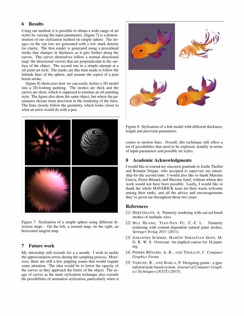
6 Results
Using our method, it is possible to obtain a wide range of artstyles by varying the input parameters. [figure 7] is a demon-stration of our stylization method on simple sphere. The im-ages on the top row are generated with a low mark densityfor clarity. The first render is generated using a proceduralstroke that changes in thickness as it gets further along thecurves. The curves themselves follow a normal directionalmap: the directional vectors that are perpendicular to the sur-face of the object. The second one in a simple attempt at aoil-paint art style. The marks are this time made to follow thelatitude lines of the sphere, and assume the aspect of a painbrush stroke.
[figure 8] showcases how we can easily stylize a 3D modelinto a 2D-looking painting. The strokes are thick and thecurves are short, which is supposed to emulate an oil-paintingstyle. The figure also show the same object, but where the pa-rameters dictate more precision in the rendering of the lines.The lines closely follow the geometry, which looks closer towhat an artist would do with a pen.
Figure 7: Stylization of a simple sphere using different di-rection maps : On the left, a normal map, on the right, anhorizontal tangent map.
7 Future work
My internship still extends for a a month. I wish to tacklethe approximation errors during the sampling process. More-over, there are still a few popping issues that would requiresome attention. The idea would be to lower the opacity ofthe curves as they approach the limits of the object. The us-age of curves as the main stylization technique also extendsthe possibilities of animation stylization, particularly when it
Figure 8: Stylization of a fish model with different thickness,length and precision parameters
comes to motion lines. Overall, this technique still offers alot of possibilities that need to be explored, notably in termsof input parameters and possible art styles.
8 Academic Acknowledgments
I would like to extend my sincerest gratitude to Joelle Thollotand Romain Vergne, who accepted to supervise my intern-ship for the second time. I would also like to thank MaximeGarcia, Pierre Benard, and Maxime Isnel, without whom thiswork would not have been possible. Lastly, I would like tothank the whole MAVERICK team for their warm welcomeamong their ranks, and all the advice and encouragementsthey’ve given me throughout these two years.
References
[1] HERTZMANN, A. Painterly rendering with curved brushstrokes of multiple sizes.
[2] HUA HUANG, TIAN-NAN FU, C.-F. L. Painterlyrendering with content-dependent natural paint strokes.Springer-Verlag 2011 (2011).
[3] JOHANNES SCHMID, MARTIN SEBASTIAN SENN, M.G. R. W. S. Overcoat: An implicit canvas for 3d paint-ing.
[4] PIERRE BENARD, A. B., AND THOLLOT, J. ComputerGraphics Forum.
[5] VERGNE, R., AND BARLA, P. Designing gratin - a gpu-tailored node-based system. Journal of Computer Graph-ics Techniques (JCGT) (2015).
Relationships between Scheduling and AutonomicComputing Techniques Applied to Parallel Computing
Resource Management
Manal BENAISSAMaster 2 MOSIG Data Infrastructure
Université Grenoble Alpes
Supervisors: Raphaël BLEUSE and Eric RUTTENTeam CTRL-A
This Masters research project will be defended before a jury composed of:Bruno RAFFIN (President of the jury)
Martin HEUSSE (Examiner)Olivier RICHARD (External Expert)
Raphaël BLEUSE (Supervisor)
AbstractThe scheduling field regroups various methods by which workis distributed across available computational resources. Con-sidering the complexity of modern infrastructures, particu-larly in Cloud and HPC computing, schedulers might facedi�culties to propose an e�cient scheduling while fitting tothe system reality and it implied uncertainties. The auto-nomic computing field suggests a more practical approach,by controlling constantly a system and adjusting taken deci-sions at runtime, via feedback loops. Applying this strategyin the scheduling context bring a less complex model witha more modular structure. Likewise, scheduling communitymay bring a new vision of autonomic computing challenges.This work presents some possible models, from the most ba-sic scheduling algorithm, to the most complex Cloud infras-tructures.
***
Le domaine de l’ordonnancement regroupe diverses meth-odes, ou le travail est distribue a travers les di↵erentes unitesde calcul disponibles. En considerant la complexite des in-frastructures actuelles, particulierement dans le domaine duCloud et du HPC, les ordonnanceurs peuvent rencontrer desdi�cultes a concilier la proposition d’ordonnancements ef-ficaces et les incertitudes liees a la realite du systeme. Ledomaine de l’informatique autonome propose une approche
ACM ISBN 978-1-4503-2138-9.
DOI: 10.1145/1235
plus pratique, en controlant regulierement un systeme et enajustant les decisions prises durant l’execution, par l’intermediairede boucles de retroaction. Appliquer cette strategie dans lecontexte de l’ordonnancement apporte un modele moins com-plexe et une structure plus modulaire. De meme, la com-munaute de l’ordonnancement pourrait apporter un regardnouveau sur les problemes que rencontre la communaute del’informatique autonome. Ce travail presente quelques mod-eles possibles, du plus basique algorithme d’ordonnancementaux plus complexes infrastructures Cloud.
1. CONTEXTCloud and HPC computing are both based on a complex
infrastructure composed of servers, data storage units, net-work connections and even software, dedicated to users. Thesystem o↵er platform access as a service, for personal orprofessional purpose in Cloud computing, and mainly forscientific purpose in HPC context. More and more tech-nologies in these fields need complex and time-consumingcomputations, which require to parallelize several tasks inhighly complex infrastructures. Using classical schedulingalgorithms that only take in account the amount of workand the number of compute units is not realistic in suchsystems. In fact, many other parameters like the cost ofcommunications, dependencies between tasks or elasticity ofthe infrastructure bring complications in the search of opti-mal scheduling. Typically, Cloud infrastructure is generallycomposed of tens of data-centers scattered around the worldand inter-connected by wide area networks (WAN). Everydays, each data-center has to process some data, and exe-cute many jobs. Most of the time, these jobs are dependentof each others, and need data from a far away data-center.Scheduler function is to distribute these jobs across di↵erentresources, taking into account Quality of Service and infras-tructure constraints.
In 2000s, IBM proposed the autonomic computing ap-

proach to address such challenges. A controller is addedto monitor the system and adjust decision when this one isno more adapted. This implies a constant checking of thesystem state and the computation of an adapted responseof a non desired evolution, forming a feedback loop. Evenif this strategy exists in Cloud computing, it is not alwaysclearly defined. Most of the time, a static analysis is done,despite uncertainties due to the overall architecture. Never-theless, the control loop concept can even be found in HPCsystems, where the adopted approach is based on a moretheoretical performance analysis. In this work, after a briefdefinition of each community politic, some possible strate-gies that promote collaboration between scheduling and au-tonomic community will be explored.
2. STATE OF THE ART: SCHEDULINGMore and more computer science fields require to solve
complex and time-consuming problems in short time, andthe idea of dividing these kinds of problems in small blocksdistributed across several compute units came quite intu-itively. However, the parallelization of algorithms impliesother problems like dependencies between these blocks, dis-tribution between all available compute units, time and re-source constraints and so on. R.L Graham [1] was the first toformalize scheduling constraints and to propose an approachin 1966 with the List Scheduling. After that, many strategieswere explored, particularly in operational research, HPC andCloud computing.
2.1 Scheduling problemScheduling problems are a part of constrained optimiza-
tion problems, widely known in operational research field.Scheduling regroups methods by which work is distributedacross available computational resources. Infrastructure isconsidered by following a model where work can be a task(block of code in program) or a job (an entire program). Thiswork can be distributed across physical nodes like CPU, ma-chines or even clusters, or logical nodes like threads.
Hence this notation allows to formalize the associatedproblem, by considering three aspects:
↵ the state of the system where parallelism is applied: Num-ber of compute units, and whether all of them are iden-tical.
� constraints on work: Number of task/job, dependenciesbetween them, and processing time.
� desired objective: minimizing execution time over all tasks,maximizing the total amount of work per time unit, orlimiting lateness when a deadline is defined for exam-ple.
Graham gathered all these constraints in a notation system,the Graham notation [2]. In this work, only the main cri-teria will be described. SchedulingZoo [3] gathers a morecomplete description about this notation. Here, < ↵|�|� >is chosen depending of the criteria described in Table 1 (thistable is only an extract of the Graham notation).For example, to describe a scheduling problem that min-
imizes the execution time and work on n identical parallelnodes, with k jobs linked by precedence constraints, we willwrite:
Machine environment ↵1 Single node2 Two nodesm m nodesP All nodes are identical, aka execution time is the
same, no matter the chosen nodeR Nodes are unrelated, which means execution time
is not the sameConstraints �prec Dependencies exist between tasks, which means
task T1 has to be finished before starting taskT2, if T2 is dependent of T1.
pj = p Each task has the same processing time p.pmtn Allows preemption, tasks can be suspended and
continued later, possibly by an other node.Objective function �Cmax Makespan, the total execution time between the
start of the first job and the end of the last job.
Table 1: Criteria in Graham notation [2].
< Pn|prec|Cmax >
A way to visualize this problem is to consider n identicalnodes Pi, 1 i n and m tasks Tj , 1 j m with de-pendencies. These dependencies are specified with � orderrelation: Ti � Tj if Tj is dependent of Ti, which means thatTj can not start its execution if Ti is not finished. Each taskneeds a certain amount of time to be executed, given by thefunction µ. With this data, we obtain a dependency graphG(�, µ), where each vertex indicates a task and its process-ing time, and each edge gives existing dependency betweentwo tasks.
Figure 1: Dependency graph example [1]
For such a problem where the set of tasks and executiontime are given, solutions exists and they are well known.Given a dependency graph G(�, µ),a certain number of com-puting nodes n and possibly some other elements, a Ganttdiagram ⇠ can be obtained (cf Figure 2). This diagramwill depend on the following algorithm, and must respectall specified constraints.
Online Scheduling
In online scheduling, the scheduler receives jobs that arriveover time, and generally must schedule the jobs withoutany knowledge of the future. The lack of knowledge of thefuture precludes the scheduler from guaranteeing optimalschedules[4]. The easiest way to understand scheduling is toimagine a finite set of tasks where we know duration of eachtasks. These problems where all constraints are fixed arewell known. However, many systems don’t know in advance

Figure 2: A possible Gantt diagram[1] of the dependencygraph in the Figure 1, for n = 3
neither the number of tasks, nor their duration. In Cloudcontext for example, each client request come as a job, andthey might arrive one by one as an input stream. On topof that, we distinguish non-clairvoyant problems which jobcomputation time is not known. Despite this lack of informa-tion, solution exists and they are based on o✏ine algorithmapproximation. More precisely, we compare an online algo-rithm A to an optimal o✏ine algorithm OPT that knowsthe entire input in advance.
Clairvoyant.
Clairvoyant scheduling constitutes a part of online schedul-ing, where processing requirement of each job is specified,but existence of jobs stay unknown until a certain releasetime.The jobs characteristics are not known until they ar-rive, restricting the scheduler to schedule jobs only with cur-rent information. However, once these ones are released, thejob size (µ function) is known.
Non-Clairvoyant.
In more realistic models, the processing requirement ofeach job is also unknown, and can only be determined byprocessing the job and observing its execution time.
2.2 Scheduling algorithms
2.2.1 Offline scheduling
In the o✏ine scheduling context, the List Scheduling is themost intuitive solution, particularly for the< Pn|prec|Cmax >problem described in section 2.1. Given a dependency graphG(�, µ), a certain number of processing nodes n, and an or-dered list L, an optimal scheduling can be obtained by fol-lowing some rules. We consider that a task Tj is available,and can be executed by a node if:
• It is not taken by an other node.
• It is not dependent of an other task.
• It is dependent, but all preceding tasks are alreadyexecuted and finished.
The processing node Pi takes the first available task Tj inthe list L. If no task is available in L, Pj become idle, byexecuting an empty task 'k. This task ends when an othertask finishes in an other node. We obtains the followingGantt diagram in the figure 3.
Figure 3: Gantt diagram[1] of the dependency graph in theFigure 1, for n = 4 and L = [T1, T2, T3, T4, T5]
FIFO scheduling is the most used algorithm in Cloud com-puting. It’s a variant of the List Scheduling, where the or-dered list L is fixed: tasks are treated with the order theyarrive. They are ordered in L by they release date, and thefirst task to be executed is the one with the earliest releasetime.
2.2.2 Online clairvoyant scheduling
To adapt o✏ine solutions to an online model, Schmoysdescribed in 1995 a method to converts algorithms that needcomplete knowledge of the input data into ones that needless knowledge. The idea is to use an o✏ine algorithm (suchas List Scheduling) to schedule a subset of jobs, releasedat each time interval. The system is defined by a set ofcomputing nodes and a waiting queue for arriving jobs.At time t = 0, a certain number S0 of jobs was queued inthe system queue. At t = 0, a snapshot of the queue stateis taken by the scheduler. Since we are in a clairvoyantscheduling, we know the execution time of each jobs, andthen we can estimate Cmax of the S0 scheduling. The o✏inescheduler schedules only these S0 jobs in the queue, untilthis queue is considered empty by the snapshot view. In thesame time, some jobs arrive in the queue and wait until S0
schedule ends. These waiting jobs compose S1 session. Sowhen S0 schedule ends (i.e at t = Cmax(S0)), S1 jobs arecaptured in an other snapshot and they are scheduled whileS2 jobs arrive in system queue. In the Figure 4, the releaseof S0, S1 etc (in red) corresponds to the moment when thesnapshot is taken by the scheduler. Only jobs taken in eachsnapshot are scheduled (in green), the other arriving jobswait until the next session.
2.3 Resources and Jobs Management SystemResources and Jobs Management Systems (RJMSs) [6] [7]
are specific software specialized in distribution of computingpower to user jobs within a parallel computing infrastruc-ture. RJMS has a key role in HPC infrastructures: it collectsall requests from users and scheduling them, while managingall resources of the system. An application (or executable) isgrouped with some data like an estimation of the computa-tion time and needed resources. All applications are queuedto be scheduled next. The RJMS must manage these twopart, to satisfy users demands for computation on one hand,
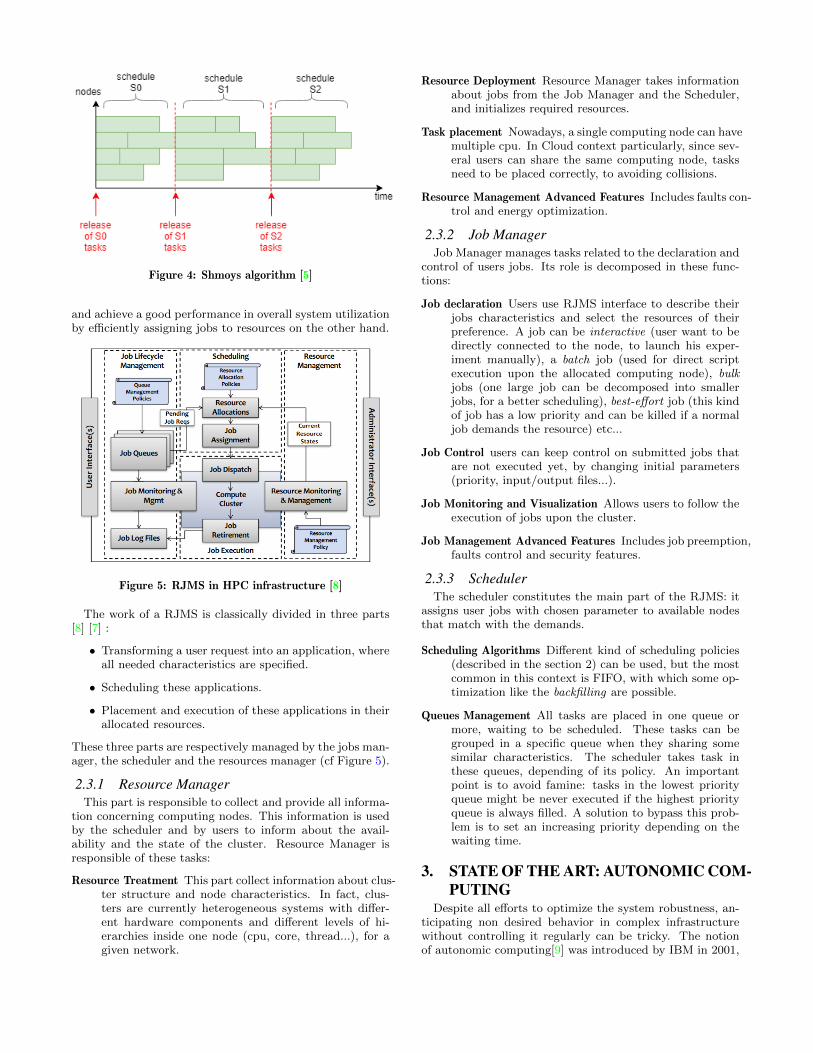
Figure 4: Shmoys algorithm [5]
and achieve a good performance in overall system utilizationby e�ciently assigning jobs to resources on the other hand.
Figure 5: RJMS in HPC infrastructure [8]
The work of a RJMS is classically divided in three parts[8] [7] :
• Transforming a user request into an application, whereall needed characteristics are specified.
• Scheduling these applications.
• Placement and execution of these applications in theirallocated resources.
These three parts are respectively managed by the jobs man-ager, the scheduler and the resources manager (cf Figure 5).
2.3.1 Resource Manager
This part is responsible to collect and provide all informa-tion concerning computing nodes. This information is usedby the scheduler and by users to inform about the avail-ability and the state of the cluster. Resource Manager isresponsible of these tasks:
Resource Treatment This part collect information about clus-ter structure and node characteristics. In fact, clus-ters are currently heterogeneous systems with di↵er-ent hardware components and di↵erent levels of hi-erarchies inside one node (cpu, core, thread...), for agiven network.
Resource Deployment Resource Manager takes informationabout jobs from the Job Manager and the Scheduler,and initializes required resources.
Task placement Nowadays, a single computing node can havemultiple cpu. In Cloud context particularly, since sev-eral users can share the same computing node, tasksneed to be placed correctly, to avoiding collisions.
Resource Management Advanced Features Includes faults con-trol and energy optimization.
2.3.2 Job Manager
Job Manager manages tasks related to the declaration andcontrol of users jobs. Its role is decomposed in these func-tions:
Job declaration Users use RJMS interface to describe theirjobs characteristics and select the resources of theirpreference. A job can be interactive (user want to bedirectly connected to the node, to launch his exper-iment manually), a batch job (used for direct scriptexecution upon the allocated computing node), bulkjobs (one large job can be decomposed into smallerjobs, for a better scheduling), best-e↵ort job (this kindof job has a low priority and can be killed if a normaljob demands the resource) etc...
Job Control users can keep control on submitted jobs thatare not executed yet, by changing initial parameters(priority, input/output files...).
Job Monitoring and Visualization Allows users to follow theexecution of jobs upon the cluster.
Job Management Advanced Features Includes job preemption,faults control and security features.
2.3.3 Scheduler
The scheduler constitutes the main part of the RJMS: itassigns user jobs with chosen parameter to available nodesthat match with the demands.
Scheduling Algorithms Di↵erent kind of scheduling policies(described in the section 2) can be used, but the mostcommon in this context is FIFO, with which some op-timization like the backfilling are possible.
Queues Management All tasks are placed in one queue ormore, waiting to be scheduled. These tasks can begrouped in a specific queue when they sharing somesimilar characteristics. The scheduler takes task inthese queues, depending of its policy. An importantpoint is to avoid famine: tasks in the lowest priorityqueue might be never executed if the highest priorityqueue is always filled. A solution to bypass this prob-lem is to set an increasing priority depending on thewaiting time.
3. STATE OF THE ART: AUTONOMIC COM-PUTING
Despite all e↵orts to optimize the system robustness, an-ticipating non desired behavior in complex infrastructurewithout controlling it regularly can be tricky. The notionof autonomic computing[9] was introduced by IBM in 2001,
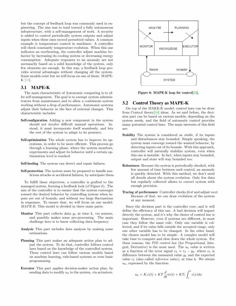
but the concept of feedback loop was commonly used in en-gineering. The aim was to tend toward a fully autonomousinfrastructure, with a self-management of work. A securityis added to control periodically system outputs and adjustinputs when these ones exceed permitted values. A commonexample is temperature control in machines: A controllerwill check constantly temperature evolution. When this oneindicates an overheating, the controller adjust machine be-havior by increasing its cooling system or decreasing energyconsumption. Adequate responses to an anomaly are notnecessarily based on a solid knowledge of the system, onlyfew elements are enough. In this way, a feedback loop pro-vides several advantages without changing all the system.Some models exist but we will focus on one of them: MAPE-K [10].
3.1 MAPE-KThe main characteristic of Autonomic computing is to of-
fer self-management. The goal is to exempt system adminis-trators from maintenance and to allow a continuous systemworking without a drop of performance. Autonomic systemsadjust their behavior in the face of external changes. Thischaracteristic includes:
Self-configuration Adding a new component in the systemshould not involve di�cult manual operations. In-stead, it must incorporate itself seamlessly, and letsthe rest of the system to adapt to its presence.
Self-optimization The whole system has to improve its op-erations, in order to be more e�cient. This process gothrough a learning phase, where the system monitors,experiments and adjust its behavior until a certain op-timization level is reached.
Self-healing The system can detect and repair failures.
Self-protection The system must be prepared to handle ma-licious attacks or accidental failures, by anticipate them.
To fulfill these objectives, a controller is grafted to themanaged system, forming a feedback look (cf Figure 6). Theaim of the controller is to ensure that the system convergestoward the desired behavior by controlling system when in-puts are out of bounds, and without too large fluctuationsin responses. To ensure that, we will focus on one model:MAPE-K. This model is divided in three main parts:
Monitor This part collects data yk at time k, via sensors,and possibly makes some pre-processing. The mainchallenge here is to know collecting data frequency.
Analysis This part includes data analysis by making someestimations.
Planning This part makes an adequate action plan to ad-just the system. To do that, controller follows controllaws based on the knowledge of the controlled system.These control laws can follow various models basedon machine learning, rule-based systems or even basicprogramming.
Executor This part applies decision-maker action plan, bysending data to modify uk to the system, via actuators.
Figure 6: MAPE-K loop for control[10].
3.2 Control Theory as MAPE-KOn top of the MAKE-K model, control laws can be draw
from Control theory[10] ideas. As we said before, the deci-sion part can be based on various models, depending on thesystem needs, and the field of automatic control providesmany potential control laws. The main interests of this fieldare:
Stability The system is considered as stable, if its inputsand disturbances stay bounded. Simply speaking, thesystem must converge toward the wanted behavior, bydetecting inputs out of its bounds. With this approach,controller will naturally stabilize system, even whenthis one is instable. In fact, when inputs stay bounded,output and state will stay bounded too.
Robustness Because the system is periodically checked, withfew amount of time between each control, an anomalyis quickly detected. With this method, we don’t needall details about the system evolution. Only few databut regularly collected allows to correct system withenough precision.
Tracing of performance Controller checks first and adjust next.Because of that, we can draw evolution of the systemat any moment.
Since the decision part is the controller core, and it willdefine the e�ciency of this one. A bad decision will impactdirectly the system, and it’s why the choice of control law isimportant. However, even if systems are di↵erent, in mostcase they follow the same rule: Only one variable is col-lected, and if its value falls outside the accepted range, onlyone other variable has to be changed. In the other hand,the chosen model has to be simple. A complex model willtake time to compute and slow down the whole system. Forthese reasons, the PID control law (for Proportional, Inte-gral, Derivative) is the most used. The uk value is writtenas a function of the error signal ek = rk � yk, where ek isdi↵erence between the measured value yk and the expectedvalue rk (also called reference value), at time k. We obtainuk, expressed by the function:
uk = K.e(t) +KTddt
te(t) +KTi
Z 0
t
e(x)dx

In this function, we can identifies three terms:
Proportional term K.e(t) where K controls the the risingtime.
Derivative term KTddt
te(t): this part, based on change fre-
quency, absorbs the oscillations and overshoots.
Integral term KTi
R 0
te(x)dx: this part ”memorizes” old val-
ues, to nullifies the static errors.
All factors (like K) are chosen depending on the system,by testing di↵erent values and estimate the most adaptedones. In many simplest models, only the proportional termis used and completed by derivative and integral term whenit’s required. Of course, PID model is not always su�cient,particularly if system behavior cannot be expressed by linearmodels.
4. PROBLEM STATEMENTScheduling computing field gathers many optimization meth-
ods to distribute work across all resources. As we saw inGraham notation, a precise representation of the systemshould be relevant (number and characteristics of computingnodes, description of the work...). But this representationreflects partially the reality of the system, despite a worsecase analysis. Dues to this partial capture of the reality,the representation implies uncertainties. This variability,mainly explained by the architecture, can be captured withan online approach. Autonomic computing community sug-gests a more practical strategy, by adapting to the system.It gives a compromise between a more simple model butlacks of performance and stability guarantees.
In this way, autonomic computing and scheduling comput-ing stay two distinct fields in computer science. However,scheduling community would benefit from control loop con-cept, autonomic computing community can use schedulingtechniques as decision-maker in controller, and the merge ofthese two domains deserves further consideration. Schedul-ing community uses worst case analysis to evaluate a schedul-ing method, but these worst case can be avoided with a con-trol loop. Some scheduling system already includes feedbackloops in the structure, but in an implicit way. Highlightingthese control loop in such a system will allow to fully ex-ploit autonomic computing methods and formalize properlythis kind of approach. In this way, autonomic computingcommunity can bring a better expertise in scheduling com-puting field. In this paper, we will present some case wherewe can bring out a feedback loop in a scheduling system, byidentifying each part of the potential MAPE-K pattern.
5. COMBINING SCHEDULING AND AUTO-NOMIC MANAGEMENT
The intersection between scheduling and autonomic com-puting field can be seen in di↵erent ways. In this part, westudy existing cases and re-interpret them through the prismof autonomic computing. Each example will focus on a cer-tain abstraction level, from the fine grain at the schedulerlevel to the Cloud infrastructure.
5.1 Feedback loop in a scheduling algorithmcontext
A first approach in the merge of these two domains is toreinterpret an online scheduler as a controller with MAPE-K pattern and scheduling policies as control laws. To dothat, we will use Shmoys[5] technique seen previously: Thismethod consists to use an o✏ine scheduler at each cycle,defined by the state of system queue at a certain time. Thecontrolled system is defined by a set of computing nodesand a waiting queue of jobs. In the clairvoyant context,released jobs and their execution times are known. Let usconsider sensors that capture queue snapshots described inthe section 2.2.2, allowing a monitoring of the queue state.An execution time Cmax can be estimated (in the analysispart) and a decision (the scheduling process itself) can bemade. This decision is injected directly on the nodes setvia implicit actuators, thus closing the loop (cf Figure 7).MAPE-K pattern is clearly defined here, where the chosencontrol law is an o✏ine scheduling algorithm.
Figure 7: Online scheduler as a controller. Dotted arrowscorresponds to possible additional monitoring. Plain arrowsconstitute the main control loop.
This approach can be adapted to pure online algorithms,by considering a sensor in the system queue and actuatorsthat apply scheduler decisions. Capture frequency can beadjusted, depending on the computing cost of the schedul-ing algorithm and the jobs themselves. In the case above,capturing a snapshot not at each Cmax but earlier may endup in a better result. It also may interesting to capturemore information during monitoring, like the state of eachnode (green dotted arrow in the Figure 7). Knowing if somenodes crashed, or if they are overloaded may lead to a fineranalysis, and thus to a better decision.
5.2 Feedback loop in a RJMS contextA scheduler can be interpreted as a closed loop, as shown
in the previous section. It is therefore natural to considerfeedback loops at the RJMS level, not only in the schedul-ing part itself but at the jobs and resources managementlevel too. This approach was adopted in the HPC context,to exploit unused resources in a cluster. Grid5000[11] is agrid for computing experiments with more than 5000 coresdispatched in 11 sites, mainly in France. OAR[12] is its as-sociated RJMS, highly configurable and based on a batch

scheduler. Like many RJMS, OAR can use many queuesto place user tasks, depending on the characteristic and thepriority of the submitted task. This strategy allows to re-spect QoS constraints, while exploiting the maximum of theclusters capacity. However, some resources can remain un-used despite these e↵orts. It’s why CiGri was implementedin top of OAR.
Figure 8: Overview of Grid5000 RJMS[13].
Each OAR scheduler is configured with a dedicated queuefor CiGri. When a user submit a task, this task can beplaced directly in OAR priority queue, to be executed inthe best conditions possible. Otherwise, it can be placed inthe CiGri queue, particularly if the task is small and it hasa low priority. In this way, CiGri can place these numer-ous small tasks on the remaining resources. At each cycle,CiGri submits a number of tasks called rate to the clusters,and wait the end of the execution of all these tasks. Then,in the next cycle, Cigri submits an other number of tasks,with an higher rate, and wait. This rate increases at eachcycle, depending on clusters availability. This method canbe seen as a tasks flow, where CiGri is the tap. This flow isnevertheless mismanaged:
• CiGri submits tasks to OAR scheduler only if OARpriority queue is empty. Therefore, resources mightremain unused while tasks in CiGri queue are still wait-ing (cf red dotted arrow in Figure 10).
• Clusters (or the storage system) are overloaded be-cause too many tasks are submitted by CiGri.
To avoid these problems, a feedback loop was implemented(in green in Figure 9). This control loop reuses all MAPE-Kand control theory concepts by monitoring the load in clus-ters queues and controlling the number of tasks submittedby CiGri. We recognize all parts of the MAPE-K pattern,with:
Monitoring The number of tasks yk in clusters queues ismeasured.
Analysis The gap ek between yk and the expected value rkis computed, giving the idea of CiGri behavior.
Planning Depending on ek, more or less tasks will be sub-mitted by CiGri. To know how many tasks uk CiGrishould submit, the controller use PI control law.
Executing At the end, the final decision is injected to CiGri.
These decisions are drawn on system knowledge that givethe controller sensibility and responsiveness. This knowl-edge is mainly based on experimentation. Adding a con-troller in the system permitted to gain 8% in clusters usage,and increase e�ciency of resources management.
Figure 9: Feedback loop in CiGri cluster[13].
Another way to see this infrastructure is to consider CiGrias a single controller, and OAR as a basic RJMS. The con-troller seen previously becomes a integral part of CiGri: Thenumber of tasks in clusters queues is monitored as before,but here, the number of submitted jobs in OAR low prior-ity queue is directly monitored (cf. Figure 10).The systemknowledge of this version is not static anymore, as long asthe number of jobs in CiGri queue changes. However, wesaw in the previous section that a scheduler can be seenas a controller too. Similarly, OAR can be interpreted as afeedback loop, where jobs and resources are monitored to in-fluence scheduling decision. So here, the overall system canbe viewed as the cooperation of the OAR controller and theCiGri controller. The OAR controller manages high priorityjobs that they can not be preempted (i.e they can not beinterrupted to be continued later by a possible other com-puting node). CiGri controller injects small preemptive jobsto maximize the resource usage without a↵ecting QoS con-straints. It’s important to note that a feedback loop alreadyexisted before adding the controller: CiGri controls clustersand OAR state and injects more or less jobs in OAR lowpriority queue, depending on this information. This loopcan be viewed in Figure 10 (with the red plain arrows).
As we said previously, more sensors can be added, to cap-ture more information about OAR state. CiGri already con-trols the OAR high priority queue, but the only thing cap-tured here is if this queue is empty or not. Rather thanmonitoring only that, CiGri may check the queue content:maybe some low priority jobs can be placed if this placementwill not disrupt the execution of the future high priority jobs.The scheduling strategy adopted by OAR can be monitoredtoo: we assume that this strategy don’t change dynamically,depending on the arriving jobs. If this point changes, check-ing OAR behavior may be relevant, to adapt CiGri to eachnew strategy.
5.3 Feedback loop in the Cloud contextIn previous sections, we saw that control loop can be rep-
resented at the scheduler level and it can be well used in

Figure 10: CiGri as an unique controller. Red plain arrowsrepresent the CiGri control loop (even without the addedintern controller). The red dotted arrow is additional infor-mation. Nothing excludes the possibility of monitoring moreinformation.
the HPC context. Finding this control mechanism will bequite easy in a Cloud context in that autonomic comput-ing was pretty popular in this kind of infrastructure. How-ever, the previous section showed us two feedback loopsthat cooperate but stay independents. We will try to showin this section how control loops can cooperate e�ciently.Cloud infrastructure benefits from the same RJMS model asHPC infrastructure: A job manager, the scheduler and a re-source manager that communicate each other, forming twoloops (see Figure 5). To show a possible finer interactionbetween these two loops, the model described by HadrienCROUBOIS[7] in 2019 will be adopted. In his paper, theauthor suggests a modular structure for a fully autonomousworkflow manager, with three main modules:
Static Analysis This module is in charge of the o✏ine op-timization of workflows. This part is the equivalentof the job manager seen in the RJMS section, apartfrom the fact that a workflow is a set of tasks withdependencies, and it can be viewed like an unique job.The objective is to precompute meta-data that willlater help in the placement and execution of the rela-tive workflows on the shared platform. In this part, alltasks will be grouped, depending on the dependenciesand data locality, to optimize the execution.
Dynamic scheduling This module is based on the previousmodule meta-data, to suggest a scheduling while tak-ing into account system elasticity.
Autonomic platform management This module is in chargeof balancing the number of available machines to meetusers demand. It will therefore control periodicallystate of the system and the workflows queue.
Figure 11: Overview of the system described in the paper[14].
One of the critical points is data-locality, which can beimproved by placing tasks in the same location as their datadependencies, or by duplicating tasks that produce largedatasets. The challenge here is to find a e�cient placementto reduce communication cost, while preserving workflowstructure. During the static analysis, tasks are grouped intoclusters, correspondingly to their dependencies with dataand other tasks: The aim is to execute one cluster in onesingle machine to achieve good data locality. After the map-ping of the clusters onto the nodes has been performed, thenodes will be in charge of the scheduling of the tasks inthe clusters they were assigned. We distinguish two kindof schedulers here: The core scheduler which assigns clus-ters to machine, and the node scheduler (in each machine)which assigns each tasks from the same cluster across all cpuof the said machine. As we said before, each scheduler canbe viewed as a control loop.
On top of that, resources must be managed despite thecomplexity of the work structure. An other control loop isneeded to manages all these resources in the highest level(core scheduler level). The estimation of a cluster neededresources is compared to the number of available resources.When a node is unused, it turn o↵ itself. A single loop maybe enough, but a finer approach was chosen here: The corescheduler is already aware of the resources state and theworkload distribution across the platform. Since it has aglobal view of the system, information about machines canbe reused. Binding the scheduler control loop with the re-source management loop seems to be a better strategy. Inthe other hand, when more resource is needed, we shouldallocate new nodes, this part is managed by a dedicatedcontrol loop.
To keep it simple: the scheduler loop manage the work dis-tribution and shut down useless nodes. The resource man-ager loop allocates new nodes, according to the informationgiven by the core scheduler. In this way, these two loopsshare the responsibility of managing the platform resources.
However, this configuration stays complex, and many loopshave to collaborate each other, adding more challenges. Ratherthan distribute decisions across all nodes, maybe a more cen-tralized approach may be more e�cient. Here, the decisionof activating or not a node is made by two loops. Mergingthese two loops in one single loop may simplify the overallstructure.
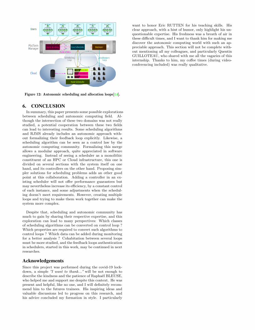
Figure 12: Autonomic scheduling and allocation loops[14].
6. CONCLUSIONIn summary, this paper presents some possible explorations
between scheduling and autonomic computing field. Al-though the intersection of these two domains was not reallystudied, a potential cooperation between these two fieldscan lead to interesting results. Some scheduling algorithmsand RJMS already includes an autonomic approach with-out formalizing their feedback loop explicitly. Likewise, ascheduling algorithm can be seen as a control law by theautonomic computing community. Formalizing this mergeallows a modular approach, quite appreciated in softwareengineering. Instead of seeing a scheduler as a monolithicconstituent of an HPC or Cloud infrastructure, this one isdivided on several sections with the system itself on onehand, and its controllers on the other hand. Proposing sim-pler solutions for scheduling problems adds an other goodpoint at this collaboration. Adding a controller in an ex-isting scheduler will not o↵er performance guarantees butmay nevertheless increase its e�ciency, by a constant controlof each instance, and some adjustments when the schedul-ing doesn’t meet requirements. However, creating multipleloops and trying to make them work together can make thesystem more complex.
Despite that, scheduling and autonomic community hasmuch to gain by sharing their respective expertise, and thisexploration can lead to many perspectives: Which classesof scheduling algorithms can be converted on control loop ?Which properties are required to convert such algorithms tocontrol loops ? Which data can be added during monitoringfor a better analysis ? Cohabitation between several loopsmust be more studied, and the feedback loops authenticationin schedulers, started in this work, may be continued in nextresearches.
AcknowledgementsSince this project was performed during the covid-19 lock-down, a simple ”I want to thank...” will be not enough todescribe the kindness and the patience of Raphael BLEUSE,who helped me and support me despite this context. He waspresent and helpful, like no one, and I will definitely recom-mend him to the futures trainees. His inspiring ideas andvaluable discussions led to progress on this research, andhis advice concluded my formation in style. I particularly
want to honor Eric RUTTEN for his teaching skills. Hisclear approach, with a hint of humor, only highlight his un-questionable expertise. His freshness was a breath of air inthese di�cult times, and I want to thank him for making mediscover the autonomic computing world with such an ap-preciable approach. This section will not be complete with-out mentioning all my colleagues, and particularly QuentinGUILLOTEAU, who shared with me all the vagaries of thisinternship. Thanks to him, my co↵ee times (during video-conferencing included) was really qualitative.

References[1] Ronald Lewis Graham. “Bounds for Certain Multi-
processing Anomalies”. In: Bell System Technical Jour-nal (1966).
[2] Ronald LewisGraham, Eugene Leighton Lawler, JanKarel Lenstra, and Alexander Hendrik George Rin-
nooy Kan. “Optimization and Approximation in De-terministic Sequencing and Scheduling: a Survey”. In:Annals of Discrete Mathematics 5.2 (1979), pp. 287–326. doi: 10.1016/S0167-5060(08)70356-X.
[3] Christoph Durr, Sigrid Knust, Damien Prot, andOscar C. Vasquez. The Scheduling Zoo. url: http ://schedulingzoo.lip6.fr (visited on 2019-06-07).
[4] Joseph Y.-T. Leung, ed. Handbook of Scheduling. Al-gorithms, Models, and Performance Analysis. Chap-man and Hall CRC, Apr. 2004. doi: 10.1201/9780203489802.
[5] David B. Shmoys, JoelWein, and David P.Williamson.“Scheduling Parallel Machines On-Line”. In: SIAM J.Comput. 24.6 (Dec. 1995), pp. 1313–1331. doi: 10 .1137/S0097539793248317.
[6] RaphaelBleuse.“Apprehending heterogeneity at (very)large scale. (Apprehender l’heterogeneitea (tres) grandeechelle)”. PhD thesis. Grenoble Alpes University, France,2017. url: https : / / tel . archives - ouvertes . fr / tel -01722991.
[7] Yiannis Georgiou. “Contributions for Resource andJob Management in High Performance Computing. (Con-tributions a la Gestion de Ressources et de Tachespour le Calcul de Haute Performance)”. PhD thesis.Grenoble Alpes University, France, 2010. url: https://tel.archives-ouvertes.fr/tel-01499598.
[8] Albert Reuther et al. “Scalable system scheduling forHPC and big data”. In: J. Parallel Distributed Comput.111 (2018), pp. 76–92.
[9] Je↵rey O. Kephart and David M. Chess. “The Visionof Autonomic Computing”. In: IEEE Computer 36.1(2003), pp. 41–50. doi: 10.1109/MC.2003.1160055.
[10] Eric Rutten, Nicolas Marchand, and Daniel Simon.“Feedback Control as MAPE-K Loop in AutonomicComputing”. In: Software Engineering for Self-AdaptiveSystems III. Assurances - International Seminar, DagstuhlCastle, Germany, December 15-19, 2013, Revised Se-lected and Invited Papers. Ed. by Rogerio de Lemos,DavidGarlan, CarloGhezzi, and HolgerGiese. Vol. 9640.Lecture Notes in Computer Science. Springer, 2013,pp. 349–373. doi: 10.1007/978-3-319-74183-3\ 12.
[11] Daniel Balouek et al. “Adding Virtualization Capa-bilities to the Grid’5000 Testbed”. In: Cloud Com-puting and Services Science. Ed. by Ivan I. Ivanov,Marten van Sinderen, Frank Leymann, and TonyShan. Vol. 367. Communications in Computer and In-formation Science. Springer International Publishing,2013, pp. 3–20. doi: 10.1007/978-3-319-04519-1\ 1.
[12] N. Capit, G.Da Costa, Y.Georgiou, G. Huard, C.Martin, G. Mounie, P. Neyron, and O. Richard.“A batch scheduler with high level components”. In:CCGrid 2005. IEEE International Symposium on Clus-ter Computing and the Grid, 2005. Vol. 2. 2005, 776–783 Vol. 2.
[13] Emmanuel Stahl, Agustın GabrielYabo, OlivierRichard,Bruno Bzeznik, Bogdan Robu, and Eric Rutten.“Towards a control-theory approach for minimizing un-used grid resources”. In: Proceedings of the 1st Inter-national Workshop on Autonomous Infrastructure forScience, AI-Science@HPDC 2018, Tempe, AZ, USA,June 11, 2018. ACM, 2018, 4:1–4:8. doi: 10 . 1145 /3217197 . 3217201. url: https : / / doi . org / 10 . 1145 /3217197.3217201.
[14] Hadrien Croubois. “Toward an autonomic engine forscientific workflows and elastic Cloud infrastructure.(Etude et conception d’un systeme de gestion de work-flow autonomique)”. PhD thesis. University of Lyon,France, 2018. url: https://tel.archives- ouvertes.fr/tel-01988995.

